PULS ON WARP PLATFORM - DETAILED INVESTIGATION OF REAL-TIME

SCHEDULING PERFORMANCE

A Thesis

by

VICTOR HAMILTON LIN

Submitted to the Office of Graduate and Professional Studies ofTexas A&M University

in partial fulfillment of the requirements for the degree of

MASTER OF SCIENCE

Chair of Committee, I-Hong HouCo-Chair of Committee, Srinivas ShakkottaiCommittee Member, Riccardo BettatiHead of Department, Miroslav M. Begovic

December 2018

Major Subject: Computer Engineering

Copyright 2018 Victor Hamilton Lin

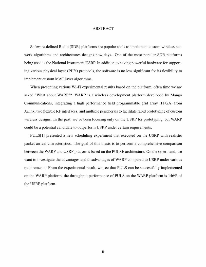
ABSTRACT

Software-defined Radio (SDR) platforms are popular tools to implement custom wireless net-

work algorithms and architectures designs now-days. One of the most popular SDR platforms

being used is the National Instrument USRP. In addition to having powerful hardware for support-

ing various physical layer (PHY) protocols, the software is no less significant for its flexibility to

implement custom MAC layer algorithms.

When presenting various Wi-Fi experimental results based on the platform, often time we are

asked "What about WARP"? WARP is a wireless development platform developed by Mango

Communications, integrating a high performance field programmable grid array (FPGA) from

Xilinx, two flexible RF interfaces, and multiple peripherals to facilitate rapid prototyping of custom

wireless designs. In the past, we’ve been focusing only on the USRP for prototyping, but WARP

could be a potential candidate to outperform USRP under certain requirements.

PULS[1] presented a new scheduling experiment that executed on the USRP with realistic

packet arrival characteristics. The goal of this thesis is to perform a comprehensive comparison

between the WARP and USRP platforms based on the PULSE architecture. On the other hand, we

want to investigate the advantages and disadvantages of WARP compared to USRP under various

requirements. From the experimental result, we see that PULS can be successfully implemented

on the WARP platform, the throughput performance of PULS on the WARP platform is 146% of

the USRP platform.

ii

ACKNOWLEDGMENTS

I’d like to thank Dr. I-Hong Hou for being my advisor and providing me the opportunity to

perform research on this topic. This adventurous journey is only possible because of you.

I’d also like to thank Yue Yang, Rajarshi Bhattacharyya, and Dr. Siomon Yau for their support

along my path of research.

I want to especially thank Dr. Ping-Chun Hsieh for his dedicated help when I need extra help,

and his tremendous support along my journey. I couldn’t have done it without you.

Last, but not the least, I want to thank Dr. Srinivas Shakkottai and Dr. Riccardo Bettati for

serving as my committee members.

iii

CONTRIBUTORS AND FUNDING SOURCES

Contributors

This work was supported by a thesis committee consisting of Professor I-Hong Hou and Dr.

Srinivas Shakkottai of the Department of Electrical and Computer Engineering and Professor Dr.

Riccardo Bettati of the Department of Computer Science and Engineering.

USRP data analyzed for Chapter 5 was provided by Dr. Ping-Chun Hsieh, Dr. Simon You, and

Rajarshi Bhattacharyya.

All other work conducted for the thesis was completed by the student independently.

Funding Sources

Graduate study was supported by a scholarship from Texas A&M University.

iv

NOMENCLATURE

PULS Processor-supported Ultra-low Latency Scheduling

USRP National Instrument USRP Software Defined Radio Device

WARP Mango Communications Software Defined Radio Device

MAC Medium Access Control

CPU Central Processing Unit

Wi-Fi Wireless local area network based on IEEE 802.11 standard

AP Access Point

ACK Acknowledge packet. We are referring to the MAC layerACK specifically

FPGA Field Programmable Grid Array

VR Virtual Reality

IIoT Industrial Internet-of-Things

SDR Software-Defined Radio

TX Packet transmission

RX Packet reception

reTX Packet re-transmission

DMA Direct Memory Access

ms Millisecond

µs Microsecond

ns Nanosecond

RR Round-Robin Scheduling Policy

LDF Lowest Deficit First Scheduling Policy

v

LQF Longest Queue First Scheduling Policy

KRT Number of packets generated for real-time flows

KNRT Number of packets generated for non-real-time flows

vi

TABLE OF CONTENTS

Page

ABSTRACT . . . . . . . . . . . . . . . . . . . . . . . . . . . . . . . . . . . . . . . . . . . . . . . . . . . . . . . . . . . . . . . . . . . . . . . . . . . . . . . . . . . . . . . . . ii

ACKNOWLEDGMENTS . . . . . . . . . . . . . . . . . . . . . . . . . . . . . . . . . . . . . . . . . . . . . . . . . . . . . . . . . . . . . . . . . . . . . . . . . . iii

CONTRIBUTORS AND FUNDING SOURCES . . . . . . . . . . . . . . . . . . . . . . . . . . . . . . . . . . . . . . . . . . . . . . . . . iv

NOMENCLATURE . . . . . . . . . . . . . . . . . . . . . . . . . . . . . . . . . . . . . . . . . . . . . . . . . . . . . . . . . . . . . . . . . . . . . . . . . . . . . . . . . v

TABLE OF CONTENTS . . . . . . . . . . . . . . . . . . . . . . . . . . . . . . . . . . . . . . . . . . . . . . . . . . . . . . . . . . . . . . . . . . . . . . . . . . . vii

LIST OF FIGURES . . . . . . . . . . . . . . . . . . . . . . . . . . . . . . . . . . . . . . . . . . . . . . . . . . . . . . . . . . . . . . . . . . . . . . . . . . . . . . . . . ix

LIST OF TABLES. . . . . . . . . . . . . . . . . . . . . . . . . . . . . . . . . . . . . . . . . . . . . . . . . . . . . . . . . . . . . . . . . . . . . . . . . . . . . . . . . . . xi

1. INTRODUCTION. . . . . . . . . . . . . . . . . . . . . . . . . . . . . . . . . . . . . . . . . . . . . . . . . . . . . . . . . . . . . . . . . . . . . . . . . . . . . . . 1

1.1 Motivation . . . . . . . . . . . . . . . . . . . . . . . . . . . . . . . . . . . . . . . . . . . . . . . . . . . . . . . . . . . . . . . . . . . . . . . . . . . . . . . . . 11.2 Goal . . . . . . . . . . . . . . . . . . . . . . . . . . . . . . . . . . . . . . . . . . . . . . . . . . . . . . . . . . . . . . . . . . . . . . . . . . . . . . . . . . . . . . . . 2

2. RELATED WORKS . . . . . . . . . . . . . . . . . . . . . . . . . . . . . . . . . . . . . . . . . . . . . . . . . . . . . . . . . . . . . . . . . . . . . . . . . . . . 4

3. MAC OVERVIEW .. . . . . . . . . . . . . . . . . . . . . . . . . . . . . . . . . . . . . . . . . . . . . . . . . . . . . . . . . . . . . . . . . . . . . . . . . . . . . 5

3.1 MAC Implementation on USRP. . . . . . . . . . . . . . . . . . . . . . . . . . . . . . . . . . . . . . . . . . . . . . . . . . . . . . . . . . 63.2 MAC Implementation on WARP . . . . . . . . . . . . . . . . . . . . . . . . . . . . . . . . . . . . . . . . . . . . . . . . . . . . . . . . . 6

4. DESIGN AND IMPLEMENTATION OF PULS . . . . . . . . . . . . . . . . . . . . . . . . . . . . . . . . . . . . . . . . . . . . . . 12

4.1 Overview . . . . . . . . . . . . . . . . . . . . . . . . . . . . . . . . . . . . . . . . . . . . . . . . . . . . . . . . . . . . . . . . . . . . . . . . . . . . . . . . . . 124.2 Architecture . . . . . . . . . . . . . . . . . . . . . . . . . . . . . . . . . . . . . . . . . . . . . . . . . . . . . . . . . . . . . . . . . . . . . . . . . . . . . . . 12

4.2.1 Packet Preparation . . . . . . . . . . . . . . . . . . . . . . . . . . . . . . . . . . . . . . . . . . . . . . . . . . . . . . . . . . . . . . . . 134.2.2 Packet Queues . . . . . . . . . . . . . . . . . . . . . . . . . . . . . . . . . . . . . . . . . . . . . . . . . . . . . . . . . . . . . . . . . . . . 144.2.3 Scheduling, Transmission, and Re-transmission . . . . . . . . . . . . . . . . . . . . . . . . . . . . . . . . 14

4.3 PULS on USRP Platform vs PULS on WARP Platform . . . . . . . . . . . . . . . . . . . . . . . . . . . . . . . . 154.4 Implementing PULS on WARP . . . . . . . . . . . . . . . . . . . . . . . . . . . . . . . . . . . . . . . . . . . . . . . . . . . . . . . . . . 16

5. EXPERIMENTAL RESULTS COMPARISON . . . . . . . . . . . . . . . . . . . . . . . . . . . . . . . . . . . . . . . . . . . . . . . 19

5.1 Non-saturated Traffic Measurement . . . . . . . . . . . . . . . . . . . . . . . . . . . . . . . . . . . . . . . . . . . . . . . . . . . . . . 205.1.1 Latency Measurement Timestamps . . . . . . . . . . . . . . . . . . . . . . . . . . . . . . . . . . . . . . . . . . . . . . 205.1.2 Latency: Policy-Mechanism . . . . . . . . . . . . . . . . . . . . . . . . . . . . . . . . . . . . . . . . . . . . . . . . . . . . . 20

vii

5.1.3 Latency: Round Trip Time . . . . . . . . . . . . . . . . . . . . . . . . . . . . . . . . . . . . . . . . . . . . . . . . . . . . . . . 225.1.4 Latency: Host PC to WARP . . . . . . . . . . . . . . . . . . . . . . . . . . . . . . . . . . . . . . . . . . . . . . . . . . . . . 24

5.2 Saturated Traffic Measurement . . . . . . . . . . . . . . . . . . . . . . . . . . . . . . . . . . . . . . . . . . . . . . . . . . . . . . . . . . . 265.2.1 Capacity Region . . . . . . . . . . . . . . . . . . . . . . . . . . . . . . . . . . . . . . . . . . . . . . . . . . . . . . . . . . . . . . . . . . 275.2.2 Capacity Region Throughput Performance . . . . . . . . . . . . . . . . . . . . . . . . . . . . . . . . . . . . . 285.2.3 Latency: ACK-to-ACK. . . . . . . . . . . . . . . . . . . . . . . . . . . . . . . . . . . . . . . . . . . . . . . . . . . . . . . . . . . 285.2.4 The Throughput Dip on LDF When Approaching Maximum KRT . . . . . . . . . . . . 28

6. ADVANTAGES AND DISADVANTAGES FROM OTHER PERSPECTIVES . . . . . . . . . . . . . 34

6.1 Software Features . . . . . . . . . . . . . . . . . . . . . . . . . . . . . . . . . . . . . . . . . . . . . . . . . . . . . . . . . . . . . . . . . . . . . . . . . 346.1.1 RAM Usage. . . . . . . . . . . . . . . . . . . . . . . . . . . . . . . . . . . . . . . . . . . . . . . . . . . . . . . . . . . . . . . . . . . . . . . 346.1.2 Data Retrieval Mechanism . . . . . . . . . . . . . . . . . . . . . . . . . . . . . . . . . . . . . . . . . . . . . . . . . . . . . . . 356.1.3 Ease of Programming on Platform. . . . . . . . . . . . . . . . . . . . . . . . . . . . . . . . . . . . . . . . . . . . . . . 356.1.4 Host PC Influence . . . . . . . . . . . . . . . . . . . . . . . . . . . . . . . . . . . . . . . . . . . . . . . . . . . . . . . . . . . . . . . . 36

6.2 Hardware Features . . . . . . . . . . . . . . . . . . . . . . . . . . . . . . . . . . . . . . . . . . . . . . . . . . . . . . . . . . . . . . . . . . . . . . . . 376.2.1 Radio Frequency. . . . . . . . . . . . . . . . . . . . . . . . . . . . . . . . . . . . . . . . . . . . . . . . . . . . . . . . . . . . . . . . . . 376.2.2 IEEE802.11 Standards . . . . . . . . . . . . . . . . . . . . . . . . . . . . . . . . . . . . . . . . . . . . . . . . . . . . . . . . . . . 376.2.3 Physical Host PC to Platform Connection . . . . . . . . . . . . . . . . . . . . . . . . . . . . . . . . . . . . . . 37

6.3 Pricing . . . . . . . . . . . . . . . . . . . . . . . . . . . . . . . . . . . . . . . . . . . . . . . . . . . . . . . . . . . . . . . . . . . . . . . . . . . . . . . . . . . . . 386.4 Picking the Right Platform for the Right Task . . . . . . . . . . . . . . . . . . . . . . . . . . . . . . . . . . . . . . . . . . . 38

7. CONCLUSION . . . . . . . . . . . . . . . . . . . . . . . . . . . . . . . . . . . . . . . . . . . . . . . . . . . . . . . . . . . . . . . . . . . . . . . . . . . . . . . . . 39

REFERENCES . . . . . . . . . . . . . . . . . . . . . . . . . . . . . . . . . . . . . . . . . . . . . . . . . . . . . . . . . . . . . . . . . . . . . . . . . . . . . . . . . . . . . . 40

viii

LIST OF FIGURES

FIGURE Page

3.1 Architecture of MAC layer on the WARP FPGA. . . . . . . . . . . . . . . . . . . . . . . . . . . . . . . . . . . . . . . . 7

3.2 High Level Architectural Comparison between USRP and WARP by functionalblocks, along with physical locations of these functional blocks and the communi-cation method between two physical locations on either platform. . . . . . . . . . . . . . . . . . . . . . 11

4.1 Architecture of PULS, grouped by functional blocks. The left side with Policy-Mechanism separation is implmeneted on the AP, where the the right side is thenormal STA without modification. . . . . . . . . . . . . . . . . . . . . . . . . . . . . . . . . . . . . . . . . . . . . . . . . . . . . . . . 13

4.2 High level abstraction of policy-mechanism separation in USRP and WARP plat-forms. On USRP platform, the physical interfacing method between policy andmechanism is the PCIe cable, while the physical interfacing method between pol-icy and mechanism on the WARP platform is Mailbox and Mutex. . . . . . . . . . . . . . . . . . . . . 15

5.1 Timeline of low traffic scenario in PULS. The top portion represent medium ac-tivity. The center portion shows various timestamps. The lower portion shows thePULS activity. The bottom time intervals show how various latency values aremeasured based on timestamps. . . . . . . . . . . . . . . . . . . . . . . . . . . . . . . . . . . . . . . . . . . . . . . . . . . . . . . . . . . 21

5.2 Empirical CDF of Policy-Mechanism interfacing latency for various payload sizeson both USRP and WARP platforms. Note the graph is on a logarithmic scale.. . . . . . . 22

5.3 Empirical CDF of Policy-Mechanism interfacing latency for various payload sizeson both USRP and WARP platforms. Note the graph is on a logarithmic scale.. . . . . . . 23

5.4 Timeline of PC to WARP latency measurement. The number packets transmittedbetween packets can be changed. The more packets there are, the more accuratethe average latency is. . . . . . . . . . . . . . . . . . . . . . . . . . . . . . . . . . . . . . . . . . . . . . . . . . . . . . . . . . . . . . . . . . . . . . 25

5.5 Plotting of Table 5.7 showing the average latency for each given number of packetsbetween timestamp measurement. . . . . . . . . . . . . . . . . . . . . . . . . . . . . . . . . . . . . . . . . . . . . . . . . . . . . . . . . 27

5.6 Capacity Region for different Policies with 5ms deadline and 0.99 delivery ratio.Circular points indicate region achievable by both USRP and WARP, where astriangular points indicate region achievable on by WARP . . . . . . . . . . . . . . . . . . . . . . . . . . . . . . 29

5.7 Throughput corresponding to margin of Capacity Region for different Policies with5ms deadline and 0.99 delivery ratio. . . . . . . . . . . . . . . . . . . . . . . . . . . . . . . . . . . . . . . . . . . . . . . . . . . . . 30

ix

5.8 Timeline of high traffic scenario in PULS. The top portion represent medium ac-tivity. The center portion shows various timestamps. The lower portion shows thePULS activity. The bottom time intervals show how various latency values aremeasured based on timestamps. With ACK-to-ACK is highlighted. . . . . . . . . . . . . . . . . . . . 31

5.9 Policy-Mechanism interfacing latency for RT flows, with KRT = 15 and KNRT =1. The x-axis is the packet in order of transmission, with the first packet startingfrom number 0. . . . . . . . . . . . . . . . . . . . . . . . . . . . . . . . . . . . . . . . . . . . . . . . . . . . . . . . . . . . . . . . . . . . . . . . . . . . . 32

5.10 Policy-Mechanism interfacing latency for RT flows, with KRT = 15 and KNRT =15. The x-axis is the packet in order of transmission, with the first packet startingfrom number 0. . . . . . . . . . . . . . . . . . . . . . . . . . . . . . . . . . . . . . . . . . . . . . . . . . . . . . . . . . . . . . . . . . . . . . . . . . . . . 33

x

LIST OF TABLES

TABLE Page

5.1 Policy to Mechanism latency on USRP . . . . . . . . . . . . . . . . . . . . . . . . . . . . . . . . . . . . . . . . . . . . . . . . . . 21

5.2 Policy to Mechanism latency on WARP . . . . . . . . . . . . . . . . . . . . . . . . . . . . . . . . . . . . . . . . . . . . . . . . . 22

5.3 Round Trip Time on USRP . . . . . . . . . . . . . . . . . . . . . . . . . . . . . . . . . . . . . . . . . . . . . . . . . . . . . . . . . . . . . . . 23

5.4 Round Trip Time on WARP . . . . . . . . . . . . . . . . . . . . . . . . . . . . . . . . . . . . . . . . . . . . . . . . . . . . . . . . . . . . . . 23

5.5 RTT, Interfacing Latency, and Mechanism RTT for both USRP and WARP. . . . . . . . . . . 24

5.6 PC to WARP Latency in µs for UDP Packet size 1460 Bytes . . . . . . . . . . . . . . . . . . . . . . . . . . 26

5.7 Latency comparison between WARP and USRP in µs . . . . . . . . . . . . . . . . . . . . . . . . . . . . . . . . . . 26

6.1 Comparison of memory usage by memory section between vanilla and PULS onthe WARP platform . . . . . . . . . . . . . . . . . . . . . . . . . . . . . . . . . . . . . . . . . . . . . . . . . . . . . . . . . . . . . . . . . . . . . . . 35

xi

1. INTRODUCTION

The paper PULS: Processor-Supported ultra-low latency scheduling[1] by Hou et al. proposed

a downlink implementation experiment with Policy-Mechanism separation that meets various tim-

ing requirements while maintaining realistic throughputs. PULS aims to bridge the gap between

theoretical scheduling algorithms and real-world usage. This experiment focuses on the concept of

Policy-Mechanism separation used in [2], where Policy refers to specification on how a particular

scheduling protocol should be performed, and Mechanism refers to functions needed to handle

traffic over the networking medium. As discussed in the PULS paper, strict latency requirements

are critical for various real-time applications, such as virtual reality (VR) [3], industrial Internet-of-

Things (IIoT), and tactile Internet [4]. PULS presented a ultra-low-latency scheduling framework

to enable the foundation of implementation on real hardware. From the experiment of the PULS

paper, we knew that the USRP platform from National Instrument was able to perform well with

the given various traffic loads and packet deadlines. The experiment enabled 4 different scheduling

policies for both real-time (RT) and non-real-time (non-RT) data streams in the MAC layer, while

meeting ultra-low latency timing requirements from given individual packets. The experiment was

able to demonstrate a loss ratio of less than 1%, compared to other protocol loss experiencing loss

ration of up to 65%.

1.1 Motivation

While USRP shows a promising result, we are in fact interested in the performance of a differ-

ent software-defined radio platform called WARP [5]. WARP is a very popular research platform,

providing programmable resources at every layer of the networking stack and enabling fully cus-

tom wireless designs. With over 468 papers throughout 92 academic institutions as of October

2018 [6] all based on the platform, it is not surprising when people ask for any MAC layer ex-

periment result specifically for this platform. With some initial idea of the architecture of the

platform based on data sheet specification, we think this platform is able to achieve the same

1

goal as in PULS. WARP features a similar architecture as in USRP with the separation of timing-

critical CSMA/CA from scheduling algorithms, but most MAC layer implementation is done in

the software domain with onboard general purpose CPUs. We suspected that there could be some

throughput performance increase due to the following reasons:

1. Fully implemented MAC layer on the platform: WARP features a fully implemented

MAC layer on the platform without the involvement of host PC to run any application.

Given that PULS is a MAC layer implementation, we want to investigate whether PULS

is achievable on WAPR or not. What are some of the limitations if we use this platform?

2. Policy-Mechanism latency reduction: The USRP platform uses a physical cable connec-

tion the host PC to the FPGA platform that generates latency in 100µs scale, which is sig-

nificant enough to affect throughput performance, as wireless transmissions operate in the

similar time frame. On the other hand, since WARP has the whole MAC layer implemented

onboard, we expect this latency to be reduced by a significant amount due to the whole

MAC layer being implemented on the same platform, with components with close proximity

to each other. PULS architecture is especially sensitive to such latency since the amount

of latency determines how much time the transceiver needs to wait until a packet can be

transmitted.

3. Programming language usage: USRP utilizes a custom GUI-based programming language

LabView running on the host PC, whereas WARP uses the more popular C language as

it’s the programming language of choice. C is much faster than many other programming

languages in many cases.

1.2 Goal

The goal of of this paper is to realize the implementation of PULS on WARP, and perform a

comprehensive comparison between the two platforms based on experimental results and known

facts. With the detailed investigation, we aim to identify factors that can determine which platform

is ideal for real-world applications that have similar characteristics as the PULS configuration.

2

The rest of the paper is organized as follows. Chapter 2 looks at existing works in the field

of ultra-low latency networks. Chapter 3 provides an overview of the MAC layer protocol in

IEEE802.11 standard and explains how the architecture of USRP and WARP platforms realize

this protocol. Chapter 4 reviews the PULS architecture presented previously, and describes how

USRP and WARP implements PULS in details. Chapter 5 provides experimental results. Chapter

6 investigate the 2 platforms from various aspects. We then conclude in chapter 7.

3

2. RELATED WORKS

As there are more connected devices nowadays than ever, especially IoT devices, it’s very

important to schedule packets based on criticalness of individual packet in order to achieve max-

imum efficiency. [7] studied the trade-off between latency and bandwidth on OFDM based 5G

network. [8] demonstrated a implementation that achieves millisecond latency for round-trip with

measurement for the target platform, but doesn’t consider scheduling. IEEE802.11e has an exist-

ing specification of changing DCF timing based on packet priorities, but it does not enforce packet

deadlines.

On the WARP platform, several low-latency architecture were proposed in order to improve

the current IEEE802.11 MAC layer architecture. Here we name a few of them. [9] addressed

the issue of "bufferbloat" due to over-buffering in the MAC layer, and aims to reduce queuing

latency by using a buffer management system based on reinforcement learning. [10] proposed

a modified version of token-passing protocol for providing better packet delivery than traditional

CSMA. [11] developed a new protocol based on modifying the DCF in the PHY in order to shorten

contention windows in the current CSMA/CA framework. Out of all the publications on the WARP

platform, perhaps the one that grabs the most attention is [12], which enabled full-duplex for

wireless network.

While all these paper proposed different ideas for supporting low-latency packet transmission

on the WARP platform, none of them addressed the potential issue of platform latency when a

packet traverses throughout the MAC layer when using such platform. With the existing PULS

architecture, we aim to provide the foundation of evaluating a platform’s latency by using various

metrics.

4

3. MAC OVERVIEW

MAC, or Medium-Access-Control, is a layer in the networking stack in charge of packet

scheduling and ensures packet delivery. MAC, together with the Logical Link Contrl (LLC), forms

the Data Link Layer in the OSI model. During typical transmission, MAC receives packets from

higher layers and decides when to transmit via PHY, or the physical layer. In a wireless envi-

ronment, MAC uses the Carrier Sensing Multiple Access and Collision Avoidance (CSMA/CA)

techniques according to In IEEE802.11 specification to avoid collision. CSMA detects how busy

the medium is and decides whether to transmit or to wait for a specified amount of time before retry.

CA uses the Distributed Coordination Function (DCF) to schedule backoffs before a transmission.

A successful transmission would expect an acknowledge packet (ACK) from the destination device

before transmitting the next packet. If ACK is not received within the deadline, a re-transmission

of the same packet will initiate instead of delivering the next packet.

IEEE802.11 also specifies the MAC being responsible for maintaining multiple connections

with other devices. The most common wireless connection structure in IEEE802.11 standard is

the AP-STA relationship, forming the wireless LAN (WLAN) network. The device, or node, in

WLAN in charge of maintaining multiple connections is called Wireless Access Point, or AP in

short, and devices that connect to an AP in the same WLAN network are called stations, or STAs.

STAs can communicate directly to their connected AP, and STAs can communicate to each other

through the AP. There exists another wireless connection type that allows communication between

2 devices without the need of an AP called Ad-Hoc, but it’s not in the primary focus today. In

wireless LAN, AP and a STA need to go though the handshaking process before a connection

is established for data transmission, and AP needs to send packets to their destined STAs while

ensuring packet delivery.

Due to the amount tasks handled and their corresponding complexity, the MAC layer needs

to have some computational power to handle multiple streams with high volume of traffic while

meeting timing requirements according to IEEE802.11 specification. Here we are exploring 2

5

different software defined radio platforms, namely USRP and WARP, that can perform such tasks

in the area of research.

3.1 MAC Implementation on USRP

The USRP Software Defined Radio Device is a tunable radio-frequency (RF) transceivers plat-

form for prototyping wireless communication systems developed by National Instrument (NI). The

USRP device allows advanced wireless applications to be created with the GUI-based LabVIEW

programming language. It features an onboard Field Programmable Grid Array (FPGA) for proto-

typing high performance wireless application that isn’t typically available in commercial WLAN

devices.

To enable WLAN, NI provides the 802.11 Application Framework software suite based on

the same IEEE802.11 standard. The Application Framework is a host PC application along with

hardware description language (HDL) implementation running on the FPGA. During program ex-

ecution, the Application Framework communicates with the USRP device through a PCI-Express

(PCIe) cable. In short, we’ll refer to USRP device and 802.11 Application Framework together

as the USRP platform in this Thesis. The architecture of USRP platform has a split MAC layer

implemented in the Host Application and the onboard FPGA in the device:

• Host Application: The software running on a host PC that handles non-timing-critical tasks

in general. Communication with higher layer protocols such as TCP and UDP, AP-STA

implementation, handshakes, scheduling, pseudo traffic generator, and data recording for

analysis are all part of the host application.

• FPGA: The FPGA hardware is mainly in charge of CSMA/CA, along with constructing

MAC frames since packets sent from the host application have a custom format.

3.2 MAC Implementation on WARP

WARP is an RF platform developed by Mango Communication, integrating an FPGA, two

programmable RF interfaces and a variety of peripherals. WARP’s onboard FPGA includes all

6

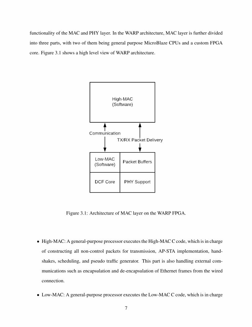
functionality of the MAC and PHY layer. In the WARP architecture, MAC layer is further divided

into three parts, with two of them being general purpose MicroBlaze CPUs and a custom FPGA

core. Figure 3.1 shows a high level view of WARP architecture.

Figure 3.1: Architecture of MAC layer on the WARP FPGA.

• High-MAC: A general-purpose processor executes the High-MAC C code, which is in charge

of constructing all non-control packets for transmission, AP-STA implementation, hand-

shakes, scheduling, and pseudo traffic generator. This part is also handling external com-

munications such as encapsulation and de-encapsulation of Ethernet frames from the wired

connection.

• Low-MAC: A general-purpose processor executes the Low-MAC C code, which is in charge

7

of more timing-critical tasks. CSMA/CA controller, MAC frame transmission and reception,

RTS/CTS frames, and re-transmission upon failed transmission are all part of the CPU Low.

Minimal state is maintained at this level. Only the contention window and station retry

counters are stored across packet transmission events. Communication between High-MAC

and Low-MAC is through the Mailbox and Mutex system.

• DCF Core: This custom FPGA core doesn’t handle packets. Instead, it is responsible for

timers being used for DCF in Low-MAC, and state machines for monitoring the medium.

This core is in fact being controlled from the Low-MAC C code. The state machines notifies

Low-MAC if the medium is clear and can start sending packets to PHY based on the status

and signal feedback from PHY.

• PHY Support: They are responsible for OFDM transceiver. PHY cores directly access

TX/RX buffers.

From the perspective of a packet traversal in the system, the High-MAC writes a ready-to-

be-transmitted packet to a TX buffer located in the onboard memory space, accessible by High-

MAC, Low-MAC, and can be directly transmitted via PHY core transceiver. Unlike the MAC

implementation in USRP, a packet isn’t being copied from one memory space (the Host PC’s

memory) to another memory space (the FPGA memory space). A packet is instead being written

in a buffer space for direct access by all 3 components mentioned above. In order to notify the

Low-MAC with the buffer being ready or not, the architecture incorporates a Mailbox & Mutex

System that can be used for status exchange between the 2 cores. Once the Low-MAC is notified

with the buffer being ready through the Mailbox & Mutex System, the DCF scheduling algorithm

starts with the aid of MAC DCF Core. The MAC DCF Core monitors the medium and notifies

the Low-MAC when it’s free to transmit. When this happens, Low-MAC initiates transmission by

sending commands to the PHY core. The PHY core transmits with content directly from the TX

buffer.

In fact, it may be easier to understand by virtually combining the CPU low and MAC DCF Core

8

together since the Low-MAC code relies on MAC DCF Core to perform DCF. Various Low-MAC

operations and decisions are based on the status of the MAC DCF Core.

As one may have noticed, the two platforms do have similar architecture. In fact, they both

feature a split MAC architecture, separating the timing-critical part from non-timing-critical in

general. However, it does not indicate that WARP platform has the same architecture as the USRP

plaform. We cannot possibly point out every subtle difference between the two platforms as they

are implemented separately by different companies with different architecture in mind, and ana-

lyzing such difference is not the goal of this Thesis. We therefore abstract many details into blocks

based on their functional similarities. Here we list several of them that are closely related to PULS

architecture:

• Communication to Higher Layer: In the network stack, packets to be transmitted are deliv-

ered from higher layers to MAC layer. This functional block is in charge of encapsulating

and de-encapsulating higher layer packets.

• Traffic Generator: Rather than getting packets from higher layers, software-defined radio

devices such as USRP and WARP have the ability to generate pseudo-random packets locally

in the MAC layer for throughput testing.

• WLAN Handshake: The process of establishing a relationship between two WLAN devices

before data exchange is the handshake. In a typical AP-STA relationship, the hanshake

process needs to go through a series of packet exchanges such as probe requests/responses,

authentication requests/responses, and association requests/responses.

• AP-STA Implementation: In a typical AP-STA relationship, the AP needs to maintain mul-

tiple connections to all connected STAs. Various mechanisms are implemented in the AP in

order to ensure packet delivery to designated STAs.

• MAC Frame Construction: With detailed specification of IEEE802.11 MAC frame, this

functional block needs to generate appropriate packets, along with frame header contents.

9

• Scheduling: The scheduling of packets for transmission.

• ACK: During a packet transmission flow, TX device expects an ACK from the RX device

right after data packet transmission. This functional block implements mechanisms for ACK

TX and RX.

• reTX: Upon a failed transmission, a re-transmission of the same packet is scheduled for

delivery.

• CSMA/CA: Carrier sensing and collision avoidance together is the core of IEEE802.11 spec-

ification in terms of ensuring packet delivery.

Figure 3.2 visualizes functional blocks and their corresponding placements in the two plat-

forms. Notice that some functionality are missing from the USRP platform as they are not sup-

ported with the Applcation Framework 1.1 used in the PULS paper.

10

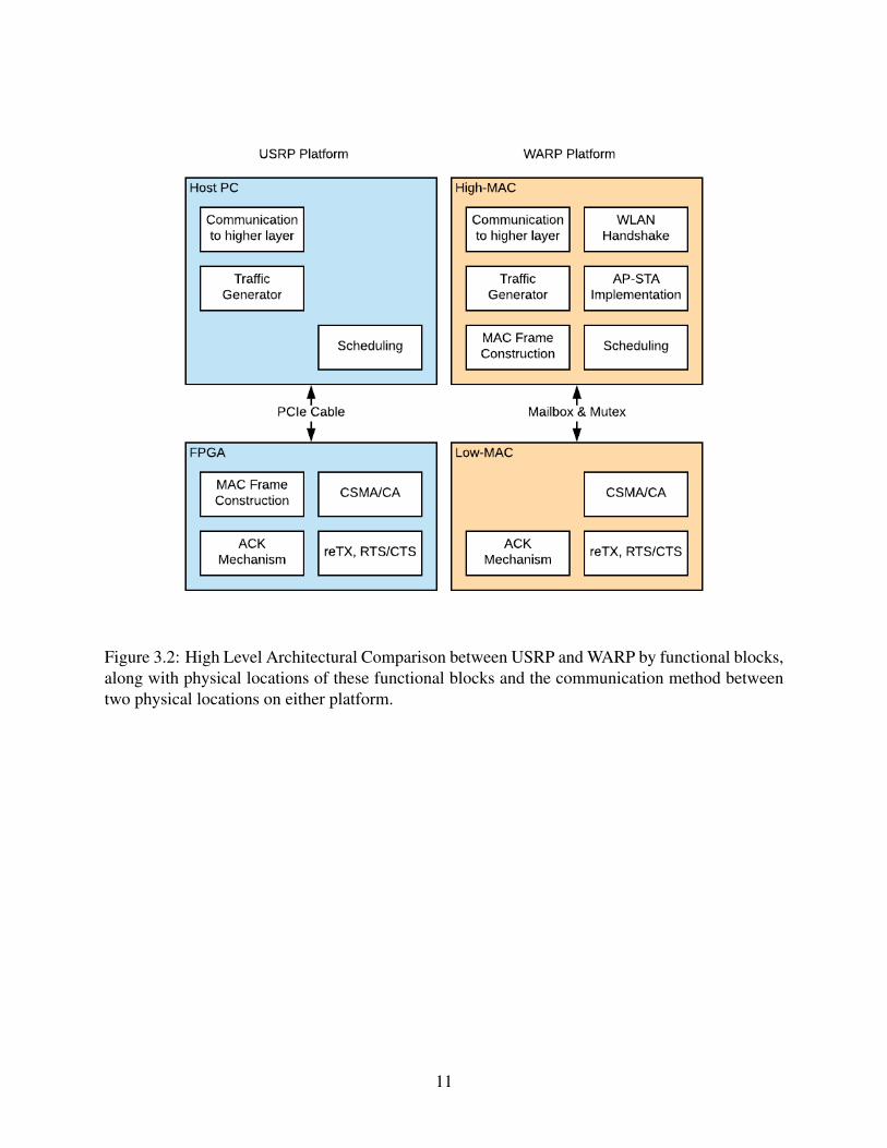
Figure 3.2: High Level Architectural Comparison between USRP and WARP by functional blocks,along with physical locations of these functional blocks and the communication method betweentwo physical locations on either platform.

11

4. DESIGN AND IMPLEMENTATION OF PULS

4.1 Overview

Proposed by Yau et al. [1], PULS, or processor-supported ultra low latency scheduling, is a

downlink implementation on the NI USRP platform that meets IEEE802.11 timing requirement

and maintains realistic throughputs with Policy-Mechanism separation (proposed by [2]). PULS

focuses on enforced packet deadline that is not currently available in commercial WLAN prod-

ucts. During packet generation, packets are categorized as either real-time (RT) or non-real-time

(non-RT) packets. With assigned per-packet deadline, each RT packet is checked after applying a

specific scheduling algorithm before entering the mechanism part for transmission, and it will be

dropped if such packet is past-due.

The goal of PULS is to bridge the gap between theory and implementation for heterogeneous

wireless networks supporting flows with strict per-packet latency constraints (real-time flows), as

well as flows that have no latency constraints (non-real-time flows), while maintaining high overall

system throughput.

In the concept of Policy-Mechanism separation, mechanism refers to a set of actions, or func-

tional blocks, required in order to operate packet transmission over a given medium, while pol-

icy refers to high-level specification of the protocol itself. In the context of WLAN, mechanism

refers to functional blocks such as radio frequency, modulation, channel, transmission bandwidth,

CSMA/CA, etc., while Policy refers to procedures such as AP-STA handshake process, scheduling

algorithms, packet queuing, etc.

4.2 Architecture

The architecture of PULS can be summarized in Figure 4.1. Implementation details can be

grouped into blocks based on their respective functionality. There are 5 main functional blocks in

the Policy that represent the core idea of PULS: packet generation, RT and non-RT queues, core

scheduler, reTX mechanism, and deficit calculation for LDF.

12

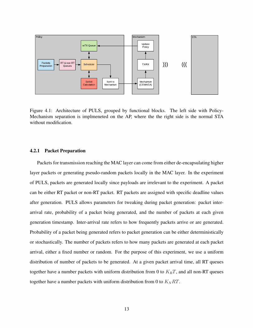
Figure 4.1: Architecture of PULS, grouped by functional blocks. The left side with Policy-Mechanism separation is implmeneted on the AP, where the the right side is the normal STAwithout modification.

4.2.1 Packet Preparation

Packets for transmission reaching the MAC layer can come from either de-encapsulating higher

layer packets or generating pseudo-random packets locally in the MAC layer. In the experiment

of PULS, packets are generated locally since payloads are irrelevant to the experiment. A packet

can be either RT packet or non-RT packet. RT packets are assigned with specific deadline values

after generation. PULS allows parameters for tweaking during packet generation: packet inter-

arrival rate, probability of a packet being generated, and the number of packets at each given

generation timestamp. Inter-arrival rate refers to how frequently packets arrive or are generated.

Probability of a packet being generated refers to packet generation can be either deterministically

or stochastically. The number of packets refers to how many packets are generated at each packet

arrival, either a fixed number or random. For the purpose of this experiment, we use a uniform

distribution of number of packets to be generated. At a given packet arrival time, all RT queues

together have a number packets with uniform distribution from 0 to KRT , and all non-RT queues

together have a number packets with uniform distribution from 0 to KNRT .

13

4.2.2 Packet Queues

Once a packet is generated during the generation process, it is being queued for scheduling.

The PULS implemented AP has 1 RT queue and 1 non-RT queue for each connected STA. PULS

presents a use case of 2 connected devices, resulting in 2 RT queues and 2 non-RT queues, resulting

in a total of 4 queues. All 4 queues are then being scheduled by a specified scheduling policy.

4.2.3 Scheduling, Transmission, and Re-transmission

4 different scheduling algorithm policies were given: Largest Deficit First (LDF) [13], Longest

Queue First (LQF), Round Robin (RR), and Random. Based on the definition of deficit introduced

in [13], LDF schedules the real-time flows with the largest deficit and selects non-real-time flows

with the largest queue length if the real-time flows are empty. Ties are broken randomly. LQF

schedules the flow with the longest queue. Ties, again, are broken randomly. RR schedules flows

in the following order: real-time flow for client 1, real-time flow for client 2, non-real-time flow for

client 1, and then non-real-time flow for client 2. Random policy simply selects a flow to schedule

among non-empty queues. If any of the queues are empty, the scheduler will pick the next queue.

Once a packet is selected for delivery, while non-RT packets proceed directly to mechanism

delivery, RT packets have to go through the extra process of deadline checking. As mentioned in

the Packet Generation process, each RT packet is given a deadline during generation. Here the

scheduler checks if the retrieved packet from queue has expired or not. If the packet is expired,

we discard the packet and repeat the scheduling process, otherwise proceed to mechanism deliv-

ery. Note that we assume the order of the packets in a RT queue is always earliest-deadline-first.

For cases otherwise, the PULS paper provided a solution with sorting the queue during packet

transmission.

Prior to delivering a packet to Mechanism for transmission, we duplicate the packet and store

the duplicated in a temporary location in case transmission fails (e.g. ACK is not received). In

this case, re-transmission (reTX) of such packet will be processed instead of scheduling for the

next packet from the queues. In the case of a successful transmission, the duplicated packet is

14

dropped and the scheduler schedules the next packet from queues. Again, in the case of RT packet,

deadline of packet needs to be checked again in the scheduler to ensure such packet is still valid

for transmission.

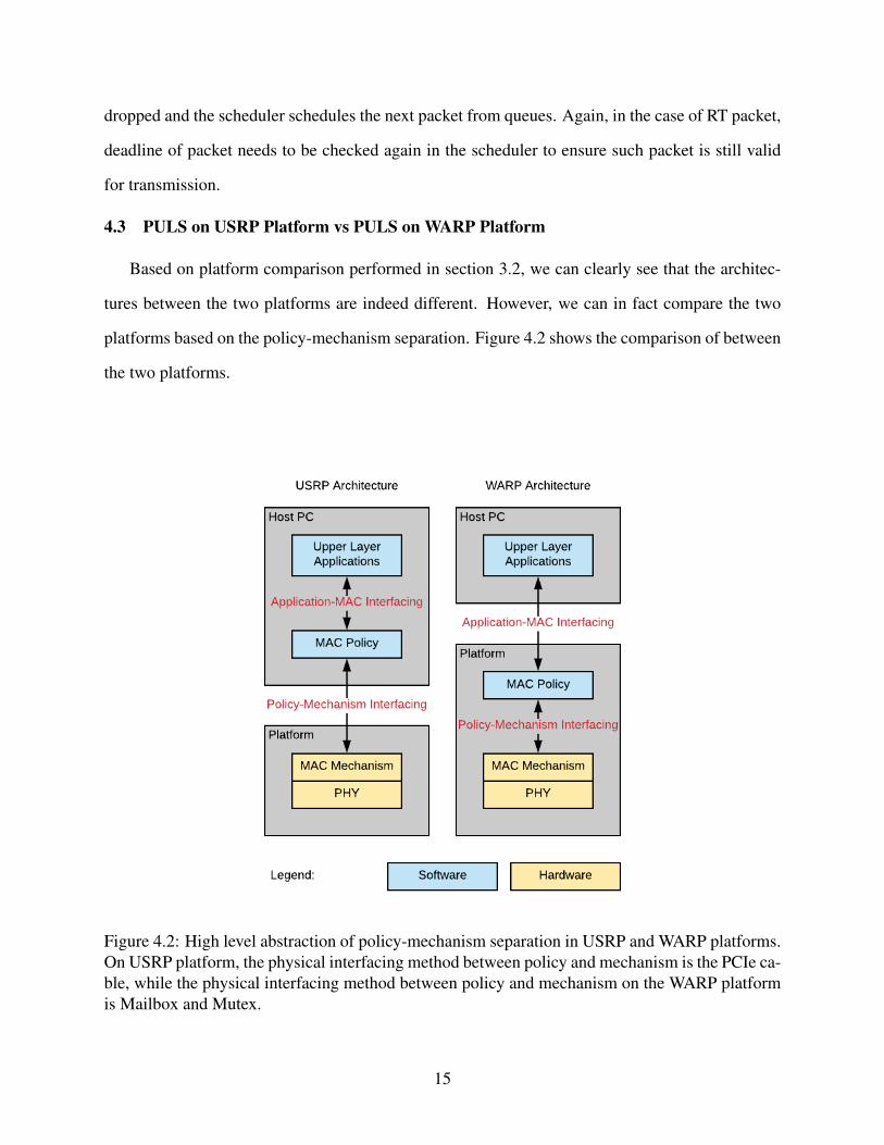
4.3 PULS on USRP Platform vs PULS on WARP Platform

Based on platform comparison performed in section 3.2, we can clearly see that the architec-

tures between the two platforms are indeed different. However, we can in fact compare the two

platforms based on the policy-mechanism separation. Figure 4.2 shows the comparison of between

the two platforms.

Figure 4.2: High level abstraction of policy-mechanism separation in USRP and WARP platforms.On USRP platform, the physical interfacing method between policy and mechanism is the PCIe ca-ble, while the physical interfacing method between policy and mechanism on the WARP platformis Mailbox and Mutex.

15

With the MAC layer fully implemented on the platform and on the same FPGA die in WARP

platform, the Policy-Mechanism separation is quite different from that of USRP. Policy deliver

packets to mechanism by writing to a buffer space on the WARP platform, where as Policy de-

liver packets to mechanism by traversing the PCIe cable on the USRP platform. On the other

hand, the interfacing between upper layer and the MAC layer is also structured differently between

USRP and PULS platforms. In the USRP platform, upper layers can communicate with the Policy

of MAC layer through software implementation directly. However, upper layer communication

with WARP platform isn’t trivial. With the upper layer application being located on the host PC

and the MAC layer located on the device, WARP requires Ethernet cable for packet transmis-

sion and reception between the two ends. The is done by using Ethernet frame encapsulation and

de-encapsulation. To summarize, we’ve identified two interfaces on each platform:

• Policy-Mechanism Interfacing: the connection between Policy and Mechanism in MAC

layer.

• Application-MAC Interfacing: the connection between upper layer applications and MAC

layer,

In the next chapter 5, we will investigate the calculation of the two latency values and provide

experimental result.

4.4 Implementing PULS on WARP

In order to make the result numbers comparable between the two platforms, we need to adjust

some settings on WARP to match the conditions used by USRP in PULS. All detailed setup can be

summarized as follows:

• Disabling default reTX: In vanilla setup, WARP has the re-transmission implemented in the

Low-MAC that will keep retrying until 1) an ACK is received or 2) the maximum number of

retry is reached. We disabled this mechanism as PULS requires reTX to be integrated with

scheduling algorithms in the High-MAC. In addition, we’ve enabled the ACK feedback from

16

Low-MAC to High-MAC as the original design didn’t require High-MAC to process ACK

packets.

• Disabled RTS/CTS: RTS and CTS packets are automatically initiated once packet payload

size exceeds a specified threshold. We’ve increased this threshold to be 2000 bytes to ensure

RTS and CTS packets are not delivered, as RTS and CTS packets are not used in PULS.

• 2 devices with wired connection: In the USRP setup, a total of 3 devices were used, with

2 of them having the vanilla setup for downlink clients and 1 having the PULS implemented

being the AP. This is to simulate the use case of an AP with packets to transmit to 2 STAs.

The setup has all devices with close proximity to each other in a fairly clean medium (close

to a chamber environment) as the goal is to measure throughput without contention. In

the meanwhile, only 2 WARP platforms are used for experiment in this Thesis with 60dB

attenuation RF cable connecting to each other. The reason for using 2 devices instead of 3

as used in USRP setup is simply due to the fact that the number of downlink clients used in

a chamber environment does not affect performance. The AP is the only device with data

packets to transmit, and a downlink client will not respond to the AP with ACK packet unless

the packet is designated for the specific client.

• 4 Flows: Even the number of downlink clients is reduced to just 1, we still implement the

AP to support 4 flows as implemented on USRP.

• Packet inter-arrival with uniform distribution: For generating traffic locally with pseudo-

random payload, WARP uses a local traffic generator (LTG) system. The specification allows

tweaking parameters such as packet size and the frequency of packet arrival. However, in or-

der to support uniform random distribution of packet arrival with the LTG, we implemented

a routine that throws dices for KRT and KNRT values at each given x inter-arrival time.

• Radio: IEEE802.11a with MCS7 data rate is the radio configuration used. The PHY layer

throughput for MCS7 is 54Mbps.

17

• Payload: Unless specifically mentioned, 1500 bytes packet payload size is the primary con-

figuration for all experimental configurations.

While the PULS implementation is through Xilinx SDK with C code, many platform specific

settings can be done with WARP provided framework using Python. In fact, we were able to

manually define parameters for sending custom python commands to the platform for setup. For

retrieving real-time platform status data such as the length of all queues, deficit values, and reTX

count, we came up with the polling method with 250ms data retrieval interval so that, during an

execution of a specific task, we are able to monitor these data without affecting overall platform

performance. While WARP does offer an UART interface to print out information directly on the

console window, such procedure is too processor-consuming and we’ve observed significant per-

formance decrease with this method. Even though the polling method is less than ideal comparing

to fast real-time monitoring as in the USRP, this is sufficient for our experimental purpose.

18

5. EXPERIMENTAL RESULTS COMPARISON

As stated in the PULS paper, the goal is to implement the scheduling policy while maintain-

ing reasonable overall throughput. In the vanilla architecture, or the original architecture without

PULS implementation, the throughput of USRP under IEEE802.11a specification is 31.8Mbps.

With the implementation of PULS, the maximum achievable throughput with any scheduling al-

gorithm became 24Mbps, which is still a reasonable number for real world applications. The loss

of throughput performance was mostly due to the interfacing latency between the host PC and

the USRP platform, measured at 192.2µs for 1500 bytes payload size. On the other hand, the

round-trip latency was also measured to indicate the minimum achievable per-packet deadline.

Round-trip latency is defined as the time elapsed between packet arrival at the MAC layer and the

reception of ACK for the packet, measured at 536.9µs with the same payload size of 1500 bytes.

In the following sections, we exam the following areas that support our intuition of WARP

throughput performance being better than that of USRP. The experiment can be categorized into

2 major categories: Unsaturated traffic measurement and saturated traffic measurement. In the

unsaturated traffic, the goal is to find the 3 latency values: Policy-Mechanism interfacing latency,

round trip time (RTT), and application-MAC interfacing latency. As mentioned at the beginning

of this chapter, throughput can be greatly affected by latency occurred over a series of actions. The

measurement of various latency values is critical in determining whether PULS with reasonable

throughput is achievable on a given platform or not. During exploration of architectures of the two

platforms from the last chapter, we know that both platforms incorporate the concept of Policy-

Mechanism separation. The latency between the separated parts can therefore be measured. RTT

is measured to show the lifetime of a packet inside the system. In the WARP platform, we addi-

tionally evaluate the interfacing latency between the Host PC and the platform as real world use

cases have packets come from higher layers instead of being locally generated. On the other hand,

the saturated traffic measurement contains two measurements: capacity region and ACK-to-ACK

latency. With RT and non-RT flows coexisting in the system, it’s important to understand how well

19

system performs under the maximum capacity. Capacity region refers to the achievable combina-

tion of KRT and KNRT for a given scheduling policy. ACK-to-ACK latency is the measurement

of time between previously received ACK and the currently received ACK. With a known packet

size, ACK-to-ACK directly translates to throughput. With these different latency metrics, we have

a solid evidence of source of performance difference between the two platforms.

5.1 Non-saturated Traffic Measurement

5.1.1 Latency Measurement Timestamps

During a packet transmission, a packet goes through a series of actions before it gets delivered

to the target device, and latency are bound to occur between each action. In this section, we are

explaining how we’re measuring different latency values with with regards to their timestamps.

When a packet gets generated by the system in the Policy, we give it a timestamp, denoted by

th. The packet is then queued and waiting to be scheduled by the scheduler. Once the packet

is delivered by Policy and received by Mechanism, we record the timestamp, denoted by tf . A

successful transmission would expect an ACK packet from the STA, and the reception of such

ACK packet at the AP is recorded with a timestamp, denoted by tr.

5.1.2 Latency: Policy-Mechanism

Policy-Mechanism Latency is measured by the difference of time-stamps between when a

packet arrives at the Policy and when a packet is received by the Mechanism. We can represent

this time different as ∆(tf − th). This measurement is done in a low-traffic environment in a way

that, at a given time, there’s only one packet in all given queues. This is to eliminate the measure-

ment of queuing time as the goal is to find how long does it take for a packet to be delivered from

Policy to Mechanism. We assume the PULS scheduler is optimized so that it has minimum latency

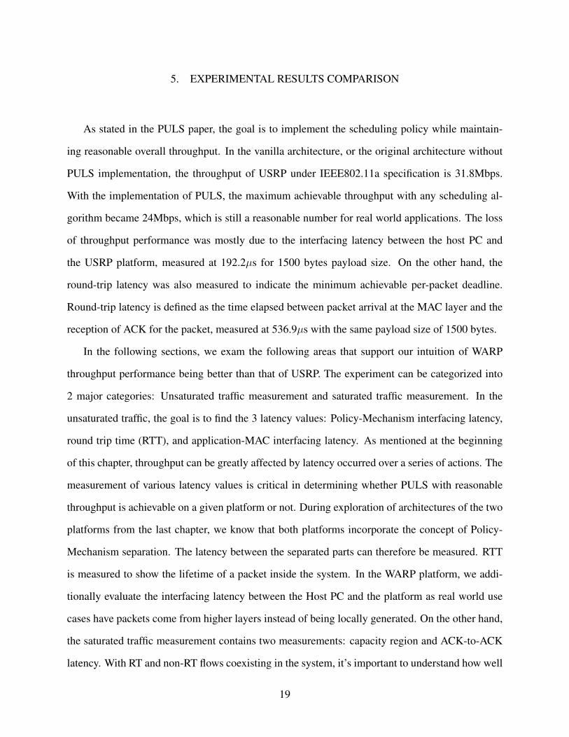
impact on the system. Figure 5.1 shows the timeline of a typical PULS transmission, along with

timestamps, instantaneous status of the medium (air), and corresponding status of the platform.

From the PULS paper, we knew that the average Policy-Mechanism interfacing latency for

1500Bytes payload size on the USRP platform is 192.2µs. USRP data is gathered with 50000

20

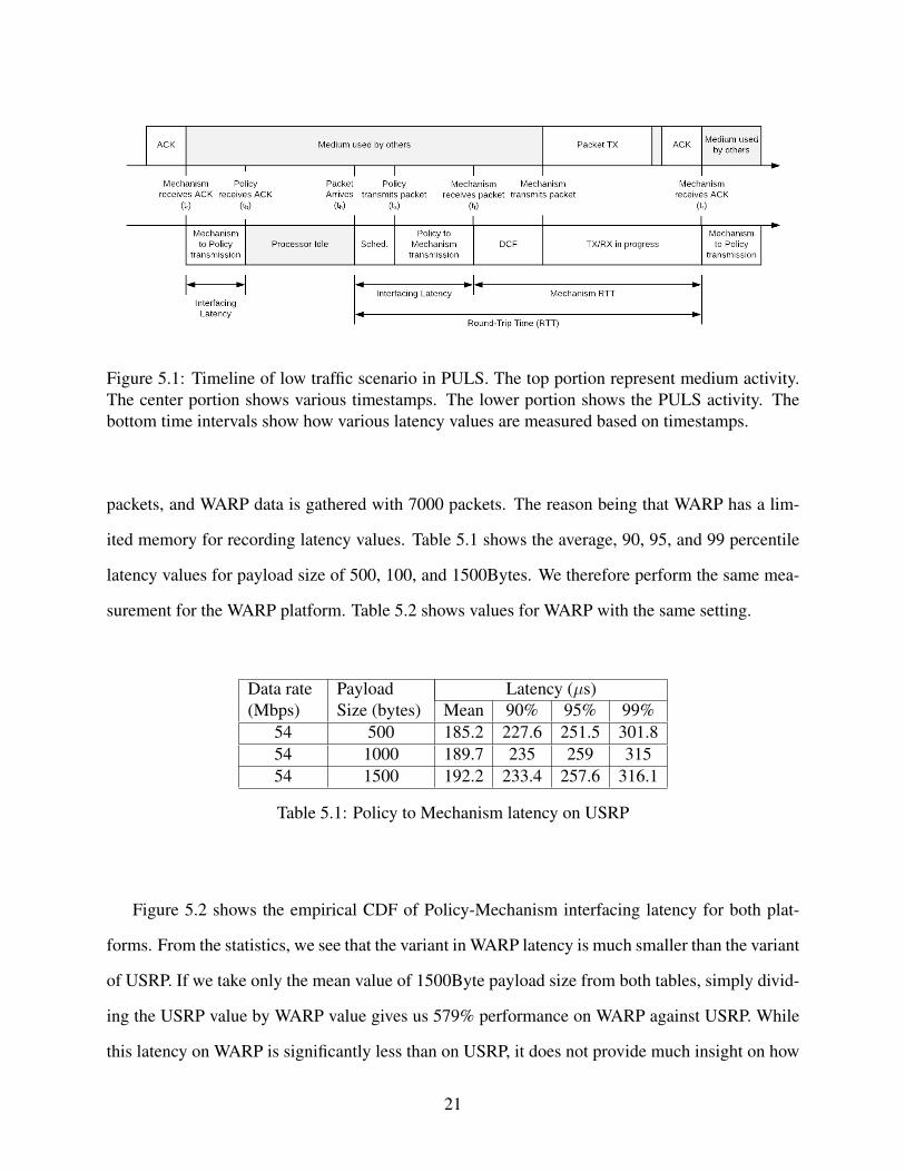
Figure 5.1: Timeline of low traffic scenario in PULS. The top portion represent medium activity.The center portion shows various timestamps. The lower portion shows the PULS activity. Thebottom time intervals show how various latency values are measured based on timestamps.

packets, and WARP data is gathered with 7000 packets. The reason being that WARP has a lim-

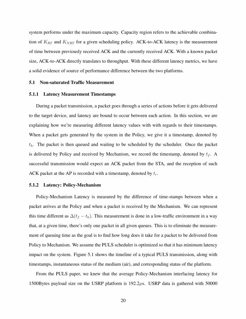
ited memory for recording latency values. Table 5.1 shows the average, 90, 95, and 99 percentile

latency values for payload size of 500, 100, and 1500Bytes. We therefore perform the same mea-

surement for the WARP platform. Table 5.2 shows values for WARP with the same setting.

Data rate(Mbps)

PayloadSize (bytes)

Latency (µs)Mean 90% 95% 99%

54 500 185.2 227.6 251.5 301.854 1000 189.7 235 259 31554 1500 192.2 233.4 257.6 316.1

Table 5.1: Policy to Mechanism latency on USRP

Figure 5.2 shows the empirical CDF of Policy-Mechanism interfacing latency for both plat-

forms. From the statistics, we see that the variant in WARP latency is much smaller than the variant

of USRP. If we take only the mean value of 1500Byte payload size from both tables, simply divid-

ing the USRP value by WARP value gives us 579% performance on WARP against USRP. While

this latency on WARP is significantly less than on USRP, it does not provide much insight on how

21

Data rate(Mbps)

PayloadSize (bytes)

Latency (µs)Mean 90% 95% 99%

54 500 32.44 33 33 3354 1000 32.91 34 34 3454 1500 33.20 34 34 34

Table 5.2: Policy to Mechanism latency on WARP

Figure 5.2: Empirical CDF of Policy-Mechanism interfacing latency for various payload sizes onboth USRP and WARP platforms. Note the graph is on a logarithmic scale.

the overall throughput performance is affected by this value, which brings us to the measurement

of round trip latency.

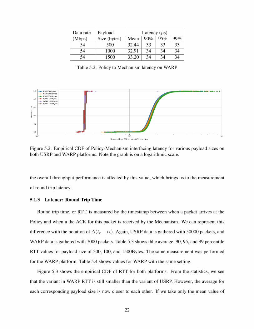
5.1.3 Latency: Round Trip Time

Round trip time, or RTT, is measured by the timestamp between when a packet arrives at the

Policy and when a the ACK for this packet is received by the Mechanism. We can represent this

difference with the notation of ∆(tr − th). Again, USRP data is gathered with 50000 packets, and

WARP data is gathered with 7000 packets. Table 5.3 shows thhe average, 90, 95, and 99 percentile

RTT values for payload size of 500, 100, and 1500Bytes. The same measurement was performed

for the WARP platform. Table 5.4 shows values for WARP with the same setting.

Figure 5.3 shows the empirical CDF of RTT for both platforms. From the statistics, we see

that the variant in WARP RTT is still smaller than the variant of USRP. However, the average for

each corresponding payload size is now closer to each other. If we take only the mean value of

22

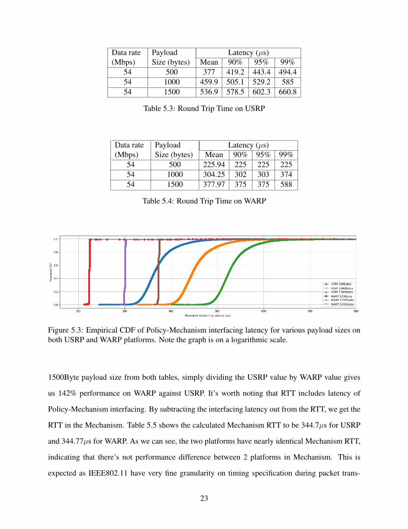
Data rate(Mbps)

PayloadSize (bytes)

Latency (µs)Mean 90% 95% 99%

54 500 377 419.2 443.4 494.454 1000 459.9 505.1 529.2 58554 1500 536.9 578.5 602.3 660.8

Table 5.3: Round Trip Time on USRP

Data rate(Mbps)

PayloadSize (bytes)

Latency (µs)Mean 90% 95% 99%

54 500 225.94 225 225 22554 1000 304.25 302 303 37454 1500 377.97 375 375 588

Table 5.4: Round Trip Time on WARP

Figure 5.3: Empirical CDF of Policy-Mechanism interfacing latency for various payload sizes onboth USRP and WARP platforms. Note the graph is on a logarithmic scale.

1500Byte payload size from both tables, simply dividing the USRP value by WARP value gives

us 142% performance on WARP against USRP. It’s worth noting that RTT includes latency of

Policy-Mechanism interfacing. By subtracting the interfacing latency out from the RTT, we get the

RTT in the Mechanism. Table 5.5 shows the calculated Mechanism RTT to be 344.7µs for USRP

and 344.77µs for WARP. As we can see, the two platforms have nearly identical Mechanism RTT,

indicating that there’s not performance difference between 2 platforms in Mechanism. This is

expected as IEEE802.11 have very fine granularity on timing specification during packet trans-

23

mission. Therefore, interfacing latency is the only contributing factor to RTT difference. Since

throughput performance highly depends on how much time RTT requires, the interfacing latency

becomes the sole factor affecting throughput performance.

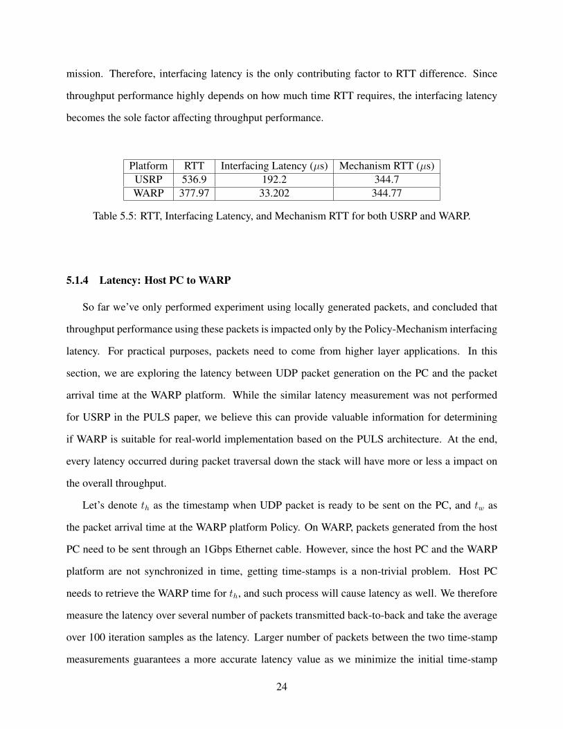
Platform RTT Interfacing Latency (µs) Mechanism RTT (µs)USRP 536.9 192.2 344.7WARP 377.97 33.202 344.77

Table 5.5: RTT, Interfacing Latency, and Mechanism RTT for both USRP and WARP.

5.1.4 Latency: Host PC to WARP

So far we’ve only performed experiment using locally generated packets, and concluded that

throughput performance using these packets is impacted only by the Policy-Mechanism interfacing

latency. For practical purposes, packets need to come from higher layer applications. In this

section, we are exploring the latency between UDP packet generation on the PC and the packet

arrival time at the WARP platform. While the similar latency measurement was not performed

for USRP in the PULS paper, we believe this can provide valuable information for determining

if WARP is suitable for real-world implementation based on the PULS architecture. At the end,

every latency occurred during packet traversal down the stack will have more or less a impact on

the overall throughput.

Let’s denote th as the timestamp when UDP packet is ready to be sent on the PC, and tw as

the packet arrival time at the WARP platform Policy. On WARP, packets generated from the host

PC need to be sent through an 1Gbps Ethernet cable. However, since the host PC and the WARP

platform are not synchronized in time, getting time-stamps is a non-trivial problem. Host PC

needs to retrieve the WARP time for th, and such process will cause latency as well. We therefore

measure the latency over several number of packets transmitted back-to-back and take the average

over 100 iteration samples as the latency. Larger number of packets between the two time-stamp

measurements guarantees a more accurate latency value as we minimize the initial time-stamp

24

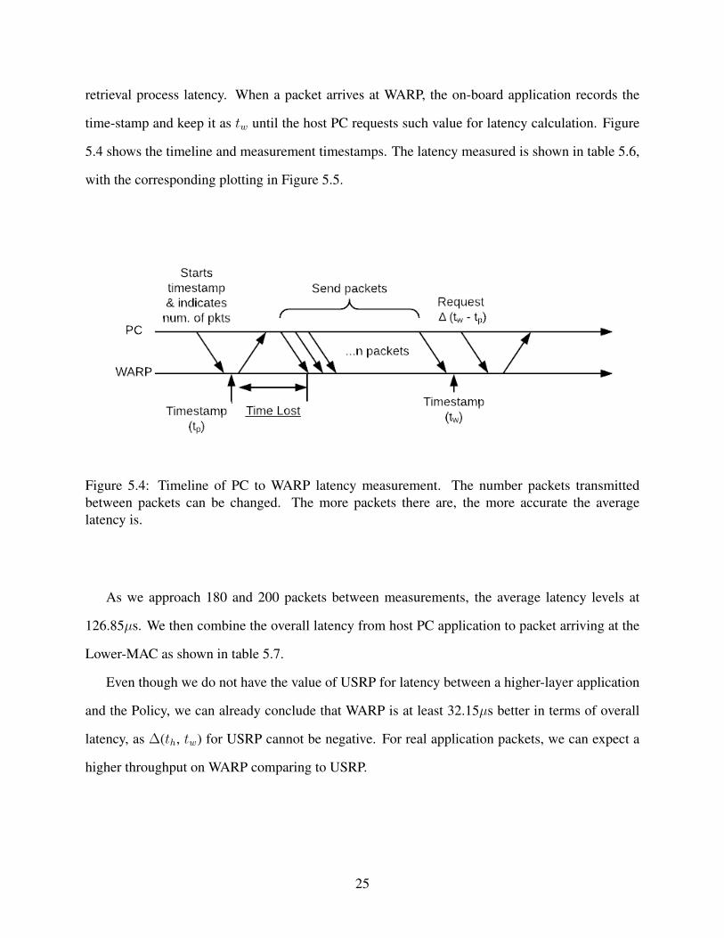
retrieval process latency. When a packet arrives at WARP, the on-board application records the

time-stamp and keep it as tw until the host PC requests such value for latency calculation. Figure

5.4 shows the timeline and measurement timestamps. The latency measured is shown in table 5.6,

with the corresponding plotting in Figure 5.5.

Figure 5.4: Timeline of PC to WARP latency measurement. The number packets transmittedbetween packets can be changed. The more packets there are, the more accurate the averagelatency is.

As we approach 180 and 200 packets between measurements, the average latency levels at

126.85µs. We then combine the overall latency from host PC application to packet arriving at the

Lower-MAC as shown in table 5.7.

Even though we do not have the value of USRP for latency between a higher-layer application

and the Policy, we can already conclude that WARP is at least 32.15µs better in terms of overall

latency, as ∆(th, tw) for USRP cannot be negative. For real application packets, we can expect a

higher throughput on WARP comparing to USRP.

25

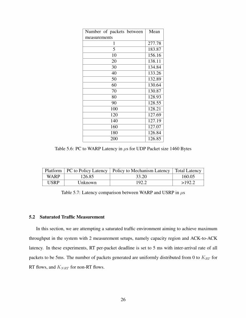
Number of packets betweenmeasurements

Mean

1 277.785 183.87

10 156.1620 138.1130 134.8440 133.2650 132.8960 130.6470 130.8780 128.9390 128.55

100 128.21120 127.69140 127.19160 127.07180 126.84200 126.85

Table 5.6: PC to WARP Latency in µs for UDP Packet size 1460 Bytes

Platform PC to Policy Latency Policy to Mechanism Latency Total LatencyWARP 126.85 33.20 160.05USRP Unknown 192.2 >192.2

Table 5.7: Latency comparison between WARP and USRP in µs

5.2 Saturated Traffic Measurement

In this section, we are attempting a saturated traffic environment aiming to achieve maximum

throughput in the system with 2 measurement setups, namely capacity region and ACK-to-ACK

latency. In these experiments, RT per-packet deadline is set to 5 ms with inter-arrival rate of all

packets to be 5ms. The number of packets generated are uniformly distributed from 0 to KRT for

RT flows, and KNRT for non-RT flows.

26

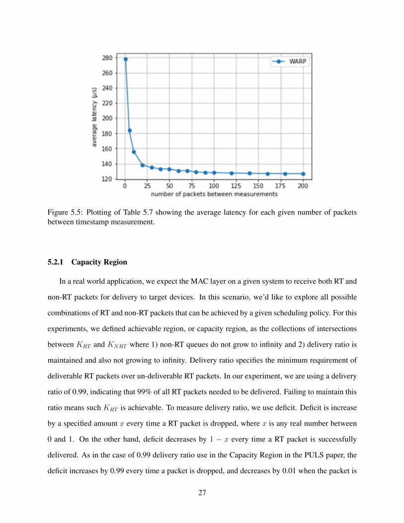
Figure 5.5: Plotting of Table 5.7 showing the average latency for each given number of packetsbetween timestamp measurement.

5.2.1 Capacity Region

In a real world application, we expect the MAC layer on a given system to receive both RT and

non-RT packets for delivery to target devices. In this scenario, we’d like to explore all possible

combinations of RT and non-RT packets that can be achieved by a given scheduling policy. For this

experiments, we defined achievable region, or capacity region, as the collections of intersections

between KRT and KNRT where 1) non-RT queues do not grow to infinity and 2) delivery ratio is

maintained and also not growing to infinity. Delivery ratio specifies the minimum requirement of

deliverable RT packets over un-deliverable RT packets. In our experiment, we are using a delivery

ratio of 0.99, indicating that 99% of all RT packets needed to be delivered. Failing to maintain this

ratio means such KRT is achievable. To measure delivery ratio, we use deficit. Deficit is increase

by a specified amount x every time a RT packet is dropped, where x is any real number between

0 and 1. On the other hand, deficit decreases by 1 − x every time a RT packet is successfully

delivered. As in the case of 0.99 delivery ratio use in the Capacity Region in the PULS paper, the

deficit increases by 0.99 every time a packet is dropped, and decreases by 0.01 when the packet is

27

successfully delivered. In other words, if we require 99% of real-time packets to arrive in 5 ms,

we say the policy can achieve that for any incoming packet rate where the deficits do not grow to

infinity. With this in mind, we compiled the capacity region for both platforms using the given 4

scheduling policies (Round-Robin, Random, LQF, and LDF) as shown in Figure 5.6.

5.2.2 Capacity Region Throughput Performance

It is clear to see that WARP is already performing better for any combination of KRT and

KNRT with any given scheduling policy. While USRP can only achieve at most 11 for KRT or 20

for KNRT , WARP is able to achieve at most 15 for KRT or 31 for KNRT . For any given scheduling

policy, the overall region covered by WARP is significantly more than that of USRP. If we plot

out the throughput value at a given marginal intersection for WARP for all 4 Capacity Region, we

get Figure 5.7. We can see that throughput is much better than that of USRP, thanks to the low

Policy-Mechanism interfacing delay. In fact, when we use the setting KRT = 0 and KNRT = 31

under the LQF policy, we see the throughput performance is 29.26Mbps, which is extremely close

to the 30Mbps value with vanilla WARP setup. The throughput performance on WARP is 146% of

USRP, which is 20Mbps achieved under the same configuration of KRT = 0.

5.2.3 Latency: ACK-to-ACK

In the last section, we measure the ACK-to-ACK latency, which is the time elapsed from the

timestamp of previously received ACK to the timestamp of currently received ACK. Figure 5.8

shows the detailed measurement timestamps and ACK-to-ACK interval. With saturated traffic at

really high KNRT value, we can identify how long much time does a complete cycle of packet

transmission takes. From the experiment, we see that the average of ACK-to-ACK latency is

441.17µs. Along with fixed packet size of 1500 bytes, we can calculate the throughput to be

roughly 27.90Mbps, which is almost the same as the measured 29.26Mbps.

5.2.4 The Throughput Dip on LDF When Approaching Maximum KRT

As you may have noticed in the Capacity Region measurement with plotted throughput graph,

LDF scheduling policy on the WARP platform experienced a significant performance loss as KRT

28

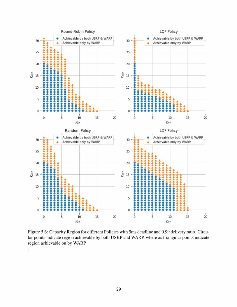
Figure 5.6: Capacity Region for different Policies with 5ms deadline and 0.99 delivery ratio. Circu-lar points indicate region achievable by both USRP and WARP, where as triangular points indicateregion achievable on by WARP.

29

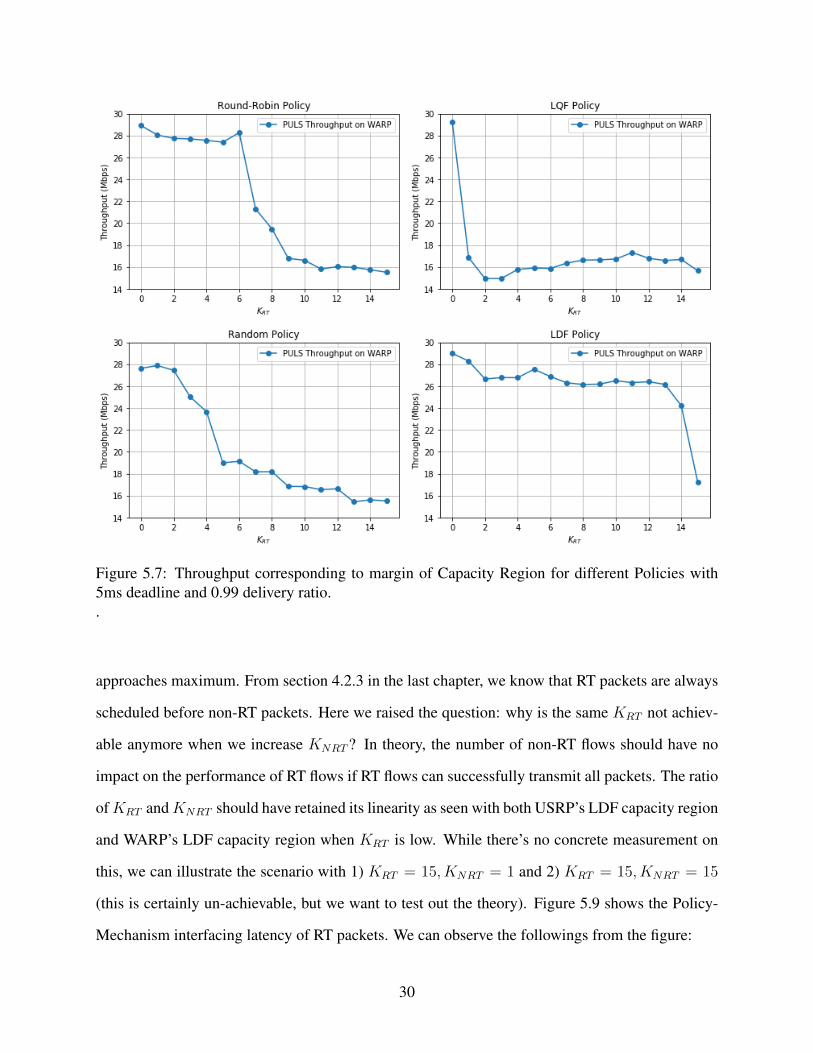
Figure 5.7: Throughput corresponding to margin of Capacity Region for different Policies with5ms deadline and 0.99 delivery ratio..

approaches maximum. From section 4.2.3 in the last chapter, we know that RT packets are always

scheduled before non-RT packets. Here we raised the question: why is the same KRT not achiev-

able anymore when we increase KNRT ? In theory, the number of non-RT flows should have no

impact on the performance of RT flows if RT flows can successfully transmit all packets. The ratio

ofKRT andKNRT should have retained its linearity as seen with both USRP’s LDF capacity region

and WARP’s LDF capacity region when KRT is low. While there’s no concrete measurement on

this, we can illustrate the scenario with 1) KRT = 15, KNRT = 1 and 2) KRT = 15, KNRT = 15

(this is certainly un-achievable, but we want to test out the theory). Figure 5.9 shows the Policy-

Mechanism interfacing latency of RT packets. We can observe the followings from the figure:

30

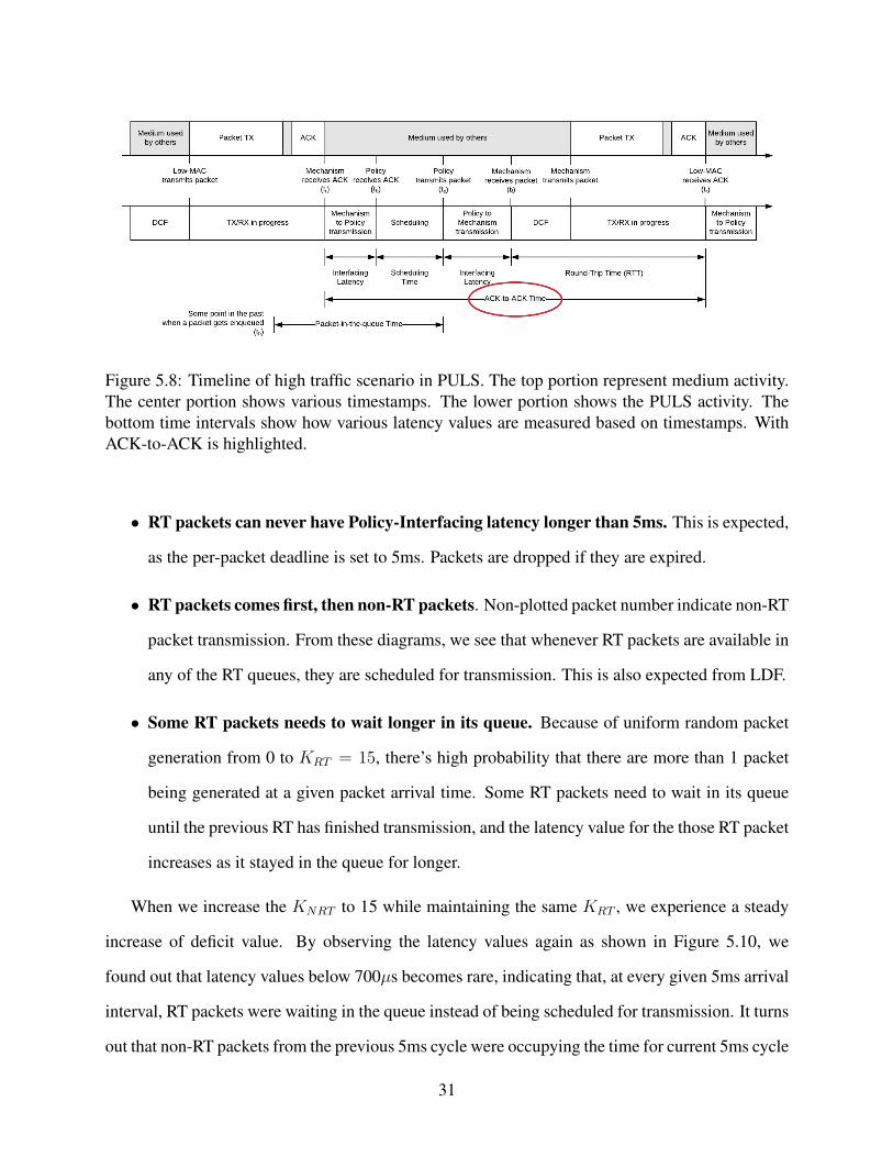
Figure 5.8: Timeline of high traffic scenario in PULS. The top portion represent medium activity.The center portion shows various timestamps. The lower portion shows the PULS activity. Thebottom time intervals show how various latency values are measured based on timestamps. WithACK-to-ACK is highlighted.

• RT packets can never have Policy-Interfacing latency longer than 5ms. This is expected,

as the per-packet deadline is set to 5ms. Packets are dropped if they are expired.

• RT packets comes first, then non-RT packets. Non-plotted packet number indicate non-RT

packet transmission. From these diagrams, we see that whenever RT packets are available in

any of the RT queues, they are scheduled for transmission. This is also expected from LDF.

• Some RT packets needs to wait longer in its queue. Because of uniform random packet

generation from 0 to KRT = 15, there’s high probability that there are more than 1 packet

being generated at a given packet arrival time. Some RT packets need to wait in its queue

until the previous RT has finished transmission, and the latency value for the those RT packet

increases as it stayed in the queue for longer.

When we increase the KNRT to 15 while maintaining the same KRT , we experience a steady

increase of deficit value. By observing the latency values again as shown in Figure 5.10, we

found out that latency values below 700µs becomes rare, indicating that, at every given 5ms arrival

interval, RT packets were waiting in the queue instead of being scheduled for transmission. It turns

out that non-RT packets from the previous 5ms cycle were occupying the time for current 5ms cycle

31

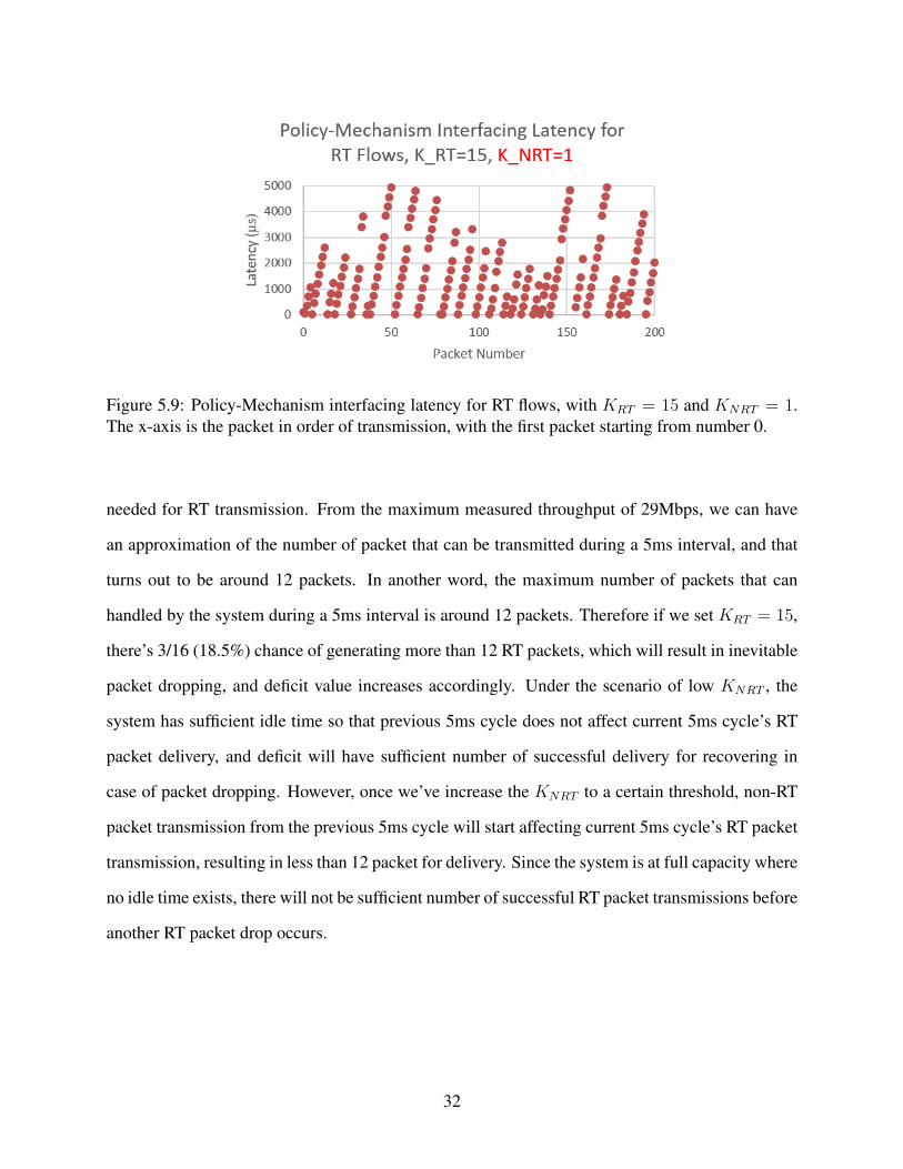
Figure 5.9: Policy-Mechanism interfacing latency for RT flows, with KRT = 15 and KNRT = 1.The x-axis is the packet in order of transmission, with the first packet starting from number 0.

needed for RT transmission. From the maximum measured throughput of 29Mbps, we can have

an approximation of the number of packet that can be transmitted during a 5ms interval, and that

turns out to be around 12 packets. In another word, the maximum number of packets that can

handled by the system during a 5ms interval is around 12 packets. Therefore if we set KRT = 15,

there’s 3/16 (18.5%) chance of generating more than 12 RT packets, which will result in inevitable

packet dropping, and deficit value increases accordingly. Under the scenario of low KNRT , the

system has sufficient idle time so that previous 5ms cycle does not affect current 5ms cycle’s RT

packet delivery, and deficit will have sufficient number of successful delivery for recovering in

case of packet dropping. However, once we’ve increase the KNRT to a certain threshold, non-RT

packet transmission from the previous 5ms cycle will start affecting current 5ms cycle’s RT packet

transmission, resulting in less than 12 packet for delivery. Since the system is at full capacity where

no idle time exists, there will not be sufficient number of successful RT packet transmissions before

another RT packet drop occurs.

32

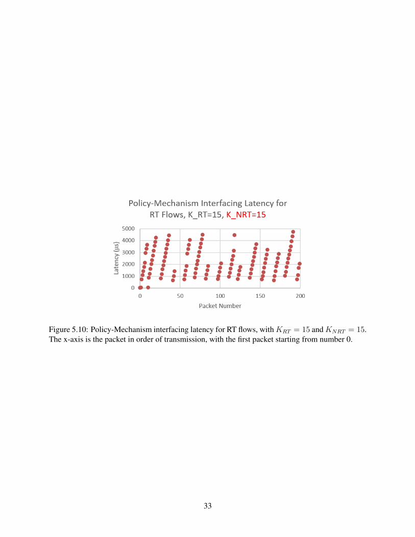
Figure 5.10: Policy-Mechanism interfacing latency for RT flows, withKRT = 15 andKNRT = 15.The x-axis is the packet in order of transmission, with the first packet starting from number 0.

33

6. ADVANTAGES AND DISADVANTAGES FROM OTHER PERSPECTIVES

While WARP appears to dominate USRP in terms of PULS performance, it’d be naive to

conclude that WARP is better than USRP. Here we will look at the details of the 2 platforms

and compare each specific aspect. These aspects can be divided into 2 major categories - software

and hardware - along with an additional side note of pricing.

6.1 Software Features

Software is the backbone of policy in PULS. It defines how algorithms should be processed, it

makes decision on what to do with a given packet, and it records all experimental values used in

this Thesis. Here we are investigating advantages and disadvantages of software portion in PULS

in both platforms.

6.1.1 RAM Usage

Application requires Random Access Memory (RAM) for various purposes. Application code

(TEXT), application stack (STACK), dynamic memory allocation (HEAP), and initialized/uninitialized

data segments (BSS) are all required parts in a C application memory layout in RAM. in the USRP

architecture for PLUS, the host PC has virtually no memory limit due to the fact that this portion

is running on the host PC. It all comes down to how much memory is installed and much much

memory is assigned to the application by the operating system. WARP, on the other hand, has

the High-MAC with onboard RAM usage strictly limited to 256KB based on the architecture. In

the vanilla version of the 802.11 WARP application, the application memory has the configuration

of 204.31KB for TEXT, pre-allocated 4KB for STACK, and pre-allocated 8KB for HEAP. With

PULS incorporated, even though the TEXT size only grows to 206.09KB, pre-allocated HEAP

has grown significantly to 38.7KB due to recording of up to 7000 sets of Policy-Mechanism and

RTT latency values. Pre-allocated space for STACK, in the meanwhile, has to shrink to 2.86KB

since our application doesn’t require all the default 4KB of space. Those extra space were used

for HEAP allocation. Table 6.1 shows comparison of memory usage by memory section between

34

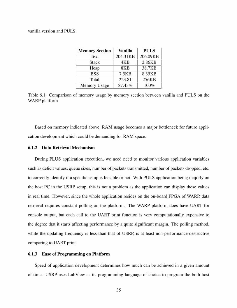
vanilla version and PULS.

Memory Section Vanilla PULSText 204.31KB 206.09KBStack 4KB 2.86KBHeap 8KB 38.7KBBSS 7.5KB 8.35KBTotal 223.81 256KB

Memory Usage 87.43% 100%

Table 6.1: Comparison of memory usage by memory section between vanilla and PULS on theWARP platform

Based on memory indicated above, RAM usage becomes a major bottleneck for future appli-

cation development which could be demanding for RAM space.

6.1.2 Data Retrieval Mechanism

During PLUS application execution, we need need to monitor various application variables

such as deficit values, queue sizes, number of packets transmitted, number of packets dropped, etc.

to correctly identify if a specific setup is feasible or not. With PULS application being majorly on

the host PC in the USRP setup, this is not a problem as the application can display these values

in real time. However, since the whole application resides on the on-board FPGA of WARP, data

retrieval requires constant polling on the platform. The WARP platform does have UART for

console output, but each call to the UART print function is very computationally expensive to

the degree that it starts affecting performance by a quite significant margin. The polling method,

while the updating frequency is less than that of USRP, is at least non-performance-destructive

comparing to UART print.

6.1.3 Ease of Programming on Platform

Speed of application development determines how much can be achieved in a given amount

of time. USRP uses LabView as its programming language of choice to program the both host

35

PC and FPGA logic, whereas WARP uses the more common C language to run on the general-

purpose processors. One could debate the development speed of HDL versus software is based

on a developer’s area of expertise, but it’s generally accepted that software programming is faster

and easier to understand than HDL programming. The other aspect to consider when choosing

LabView is the usability with version control software. Version control is a management of changes

to a collection of files. It is very critical in 2 areas:

• Maintaining traces of historical implementation for future references.

• Team collaboration on the same piece of code.

Mainstream programming languages such as C, C++, Python, Java, etc. are all text based, which

is very well integrated with popular version control protocols such as Git and SVN. LabView is

a graphical programming language with its source codes being saved as binary files instead of

text files. Version control on LabView code becomes a non-trivial process since we no longer can

quickly identify differences between revisions. Merging becomes a particularly complex problem

since traditional version control software suites do not provide functionality to aid graphical pro-

gramming language. While National Instrument does have it’s own version control software that

can provide graphical comparison between 2 versions of code, it is far from intuitive comparing to

traditional version control with line-by-line comparison.

6.1.4 Host PC Influence

Throughput performance heavily depends on how quickly the Policy can process information

and makes decision on what packet to transmit next. On WARP, the upper bound of High-MAC

processor time executing non-PULS process can be mathematically computed due to it’s simplicity.

However, defining such upper bound on the host PC program with the USRP platform is a non-

trivial problem. Host PC has a general purpose operating system running on a general purpose

CPU. Any process that got preempted with a higher priority value will take over PULS processing

time, resulting in a unpredictable result. Experimental results will vary depending on the hardware

configuration of the host PC as well. During experiment, we observed that even opening a browser

36

application on the host PC affected PULS performance on the USRP setup.

6.2 Hardware Features

While both platforms have hardware supporting the setup used for PULS, it does not indicate

potential expansion of PULS is suitable for both platforms. In this section, we are exploring some

hardware aspects that differentiates the two platforms.

6.2.1 Radio Frequency

Depending on the model, the USRP is able to handle frequency ranging from 10MHz to 6GHz

(USRP-2953R can do 1.2GHz - 6GHz), whereas the single-variation WARP is designed to only

support 2.4GHz and 5GHz bands. The wide range of radio frequency on USRP enables support for

LTE, spectrum monitoring, signals intelligence, military communications, radar, and many other

RF communication protocols other than IEEE802.11.

6.2.2 IEEE802.11 Standards

The RF hardware differences as discussed above are quite significant, but, in PULS, we are

particularly interested in the IEEE802.11 standard. According to the USRP 802.11 Application

Framework, the platform is able to transmit with IEEE802.11a/ac standards with 20/40/80Mhz

bandwidths. On the other hand, WARP is designed to support IEEE802.11a/g/n with 10/20/40Mhz

bandwidths.

6.2.3 Physical Host PC to Platform Connection

Host PC requires a medium to communicate with the target platform. In the case WARP,

programming is done through a USB-to-JTAG cable, console output through a micro-USB cable,

Python commands through a Gigabit Ethernet cable, and data packets through a second Gigabit

Ethernet cable. On USRP, all of these connections are simplified with a single proprietary cable

based on PCE-Express (PCIe for short) x4 channel. Nevertheless, the single cable solution of

USRP also has a drawback where a cable disconnection requires a reboot of the host PC before

connection can be re-established.

37

6.3 Pricing

Unlike commercial wireless products, wireless development platforms often come with much

higher price tags. The WARP v3 Kit used in this experiment is $4,900 for academic usage, and

$6,900 for commercial usage. The price range for USRP varies even greater with a range from

$6,945 to $12,787, depending on the model. The particular model used in PULS USRP-2953R,

priced at $8,381. All prices listed above are in USD, extracted from their official websites as of

October 2nd, 2018.

6.4 Picking the Right Platform for the Right Task

To summarize, we see that the WARP platform is a more suitable candidate for further PULS

development. However, if we start considering all possible aspects, WARP is a better choice when:

• Running a scheduling algorithm that doesn’t rely on heavy memory usage.

• Implementation that needs time sensitive criteria.

• The project requires fast development process.

• The project is a budgeted research.

On the other hand, USRP is a better candidate when:

• The area of research requires a large quantity of data for analysis.

• The project needs real-time status monitoring.

• The project requires high throughput, or involves RF development that’s not IEEE802.11

standard.

38

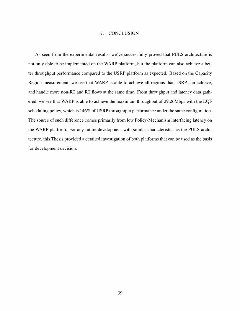
7. CONCLUSION

As seen from the experimental results, we’ve successfully proved that PULS architecture is

not only able to be implemented on the WARP platform, but the platform can also achieve a bet-

ter throughput performance compared to the USRP platform as expected. Based on the Capacity

Region measurement, we see that WARP is able to achieve all regions that USRP can achieve,

and handle more non-RT and RT flows at the same time. From throughput and latency data gath-

ered, we see that WARP is able to achieve the maximum throughput of 29.26Mbps with the LQF

scheduling policy, which is 146% of USRP throughtput performance under the same configuration.

The source of such difference comes primarily from low Policy-Mechanism interfacing latency on

the WARP platform. For any future development with similar characteristics as the PULS archi-

tecture, this Thesis provided a detailed investigation of both platforms that can be used as the basis

for development decision.

39

REFERENCES

[1] S. Yau, P.-C. Hsieh, R. Bhattacharyya, K. Bhargav, S. Shakkottai, I. Hou, P. Kumar, et al.,

“Puls: Processor-supported ultra-low latency scheduling,” in Proceedings of the Eighteenth

ACM International Symposium on Mobile Ad Hoc Networking and Computing, pp. 261–270,

ACM, 2018.

[2] S. Yau, L. Ge, P.-C. Hsieh, I.-H. Hou, S. Cui, P. Kumar, A. Ekbal, and N. Kundargi, “Wimac:

Rapid implementation platform for user definable mac protocols through separation,” in Pro-

ceedings of the 2015 ACM Conference on Special Interest Group on Data Communication,

SIGCOMM ’15, (New York, NY, USA), pp. 109–110, ACM, 2015.

[3] “Nsf workshop on ultra-low latency wireless networks,” tech. rep., USA, 2015.

[4] “The tactile internet,” tech. rep., 2014.

[5] “Warp project.”

[6] “Warp papers & presentations,” oct 2018.

[7] O. N. C. Yilmaz, Y. . E. Wang, N. A. Johansson, N. Brahmi, S. A. Ashraf, and J. Sachs, “Anal-

ysis of ultra-reliable and low-latency 5g communication for a factory automation use case,” in

2015 IEEE International Conference on Communication Workshop (ICCW), pp. 1190–1195,

June 2015.

[8] J. Pilz, M. Mehlhose, T. Wirth, D. Wieruch, B. Holfeld, and T. Haustein, “A tactile internet

demonstration: 1ms ultra low delay for wireless communications towards 5g,” in 2016 IEEE

Conference on Computer Communications Workshops (INFOCOM WKSHPS), pp. 862–863,

April 2016.

[9] N. Bouacida, Towards Controlling Latency in Wireless Networks. PhD thesis, 2017.

40

[10] C. Dombrowski and J. Gross, “Echoring: A low-latency, reliable token-passing mac protocol

for wireless industrial networks,” in Proceedings of European Wireless 2015; 21th European

Wireless Conference, pp. 1–8, May 2015.

[11] C. Hunter, P. Murphy, and A. Sabharwal, “Real-time testbed implementation of a distributed

cooperative mac and phy,” 2010.

[12] M. Jain, J. I. Choi, T. Kim, D. Bharadia, S. Seth, K. Srinivasan, P. Levis, S. Katti, and P. Sinha,

“Practical, real-time, full duplex wireless,” in Proceedings of the 17th Annual International

Conference on Mobile Computing and Networking, MobiCom ’11, (New York, NY, USA),

pp. 301–312, ACM, 2011.

[13] I. Hou, V. Borkar, and P. R. Kumar, “A theory of qos for wireless,” in IEEE INFOCOM 2009,

pp. 486–494, April 2009.

41