This research was sponsored by the Joint Highway Research Advisory Council (JHRAC) of the University of Connecticut and the Connecticut Department of Transportation and was performed through the Connecticut Transportation Institute of the University of Connecticut. The contents of this report reflect the views of the authors who are responsible for the facts and accuracy of the data presented herein. The contents do not necessarily reflect the official views or policies of the University of Connecticut or the Connecticut Department of Transportation. This report does not constitute a standard, specification, or regulation.

DETAILED MODAL ANALYSIS OF PARTICULATE EMISSIONS FROM

CONNECTICUT TRANSIT BUSES FOR LOCAL EMISSIONS MODELING

December 2008

Britt A. Holmén Eric D. Jackson

Darrell B. Sonntag H. Oliver Gao

JHR 08-316 Project 05-9

ii

Technical Report Documentation Page 1 Report No. JHR 08-316

2. Government Accession No. N/A

3. Recipient’s Catalog No.

5. Report Date December 2008

4. Title and Subtitle Detailed Modal Analysis of Particulate Emissions from Connecticut Transit Buses for Local Emissions Modeling

6. Performing Organization Code N/A

7. Authors Britt A. Holmén Eric D. Jackson Darrell B. Sonntag H. Oliver Gao

8. Performing Organization Report No. JHR 08-316

10. Work Unit No (TRAIS) N/A

9. Performing Organization Name and Address University of Connecticut Connecticut Transportation Institute Storrs, CT 06269

11. Contract or Grant No. N/A

13. Type of Report and Period Covered FINAL

12. Sponsoring Agency name and Address Connecticut Department of Transportation 280 West Street Rocky Hill, CT 06067-0207

14. Sponsoring Agency Code N/A

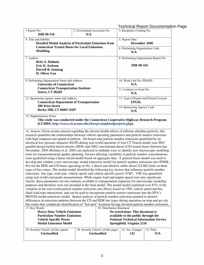
15. Supplementary Notes This study was conducted under the Connecticut Cooperative Highway Research Program (CCHRP, http://www.cti.uconn.edu/chwrp/completedprojects.php). 16. Abstract. Given recent concern regarding the adverse health effects of airborne ultrafine particles, this research quantifies the relationships between vehicle operating parameters and particle number emissions with high temporal and spatial resolution. On-board total particle number emissions quantified by an electrical low pressure impactor (ELPI) during real-world operation of four CT Transit model year 2003 parallel-design hybrid diesel-electric (HDE) and 2002 conventional diesel (CD) transit buses between Jan-November, 2004 (Holmén et al, 2005) are analyzed in multiple ways to identify new microscopic modeling tools for transportation/air quality planning. Factors affecting variability in particle number concentrations were quantified using a linear mixed model based on aggregate data. A general linear model was used to develop and validate a new microscopic modal emissions model for particle number emissions rate (PNER, #/s) for the HDE and CD buses operating on No. 1 diesel and ultralow sulfur diesel (ULSD) fuels on three types of bus routes. The modal model identified the following key factors that influence particle number emissions: bus type, road type, vehicle speed, and vehicle specific power (VSP). VSP was quantified using real-world road grade measurements. While engine load and engine speed were also significant factors, these parameters are not routinely available to transportation engineers for microscopic modeling purposes and therefore were not included in the final model. The modal model explained over 87% of the variation in the real-world particle number emissions rate (#/sec) based on VSP, vehicle speed and bus /fuel/ road type interactions, and can be used to incorporate particle number emissions into the EPA’s MOVES modal emissions model. Spatial analysis of particle number emissions pointed to distinct differences in emissions patterns between the CD and HDE bus types during operation on stop-and-go city bus routes that complicate identification of “hot-spot” locations having elevated particle number emissions. 17. Key Words: Heavy-Duty Vehicle Emissions Particulate Number Emissions Vehicle Specific Power Modal Emissions Model

18. Distribution Statement No restrictions. This document is available to the public through the

National Technical Information Service Springfield, Virginia 2216

19. Security Classif. (of this report) Unclassified

20. Security Classif. (of this page) Unclassified

21. No. of pages 132

22. Price N/A

iii

iv

Table of Contents

LIST OF FIGURES .............................................................................................................. VI

LIST OF FIGURES .............................................................................................................. VI

LIST OF TABLES .............................................................................................................VIII

ABSTRACT........................................................................................................................... IX

1.0 INTRODUCTION..............................................................................................................1 1.2 LITERATURE REVIEW....................................................................................................................................... 2

1.2.1 Particle Number Emissions from Transit Buses...................................................................................... 2 1.2.2 Uncertainty and Variability in Particle Number Emissions................................................................... 3 1.2.3 Operating Parameters Important for Modeling Diesel Particle Number Emissions ............................. 7 1.2.4 Emission Models for Heavy-duty Diesel Particulate Mass Emissions .................................................... 8 1.2.5 Modal Emissions Models ........................................................................................................................ 9

2.0 RESEARCH OBJECTIVES...........................................................................................11

3.0 RESEARCH METHODS................................................................................................12 3.1 VEHICLES AND ON-BOARD INSTRUMENTATION............................................................................................. 12

3.1.1 Vehicles ................................................................................................................................................. 12 3.1.2 Particle Number Emissions Instrumentation......................................................................................... 12 3.1.3 Horiba Exhaust Emissions System ........................................................................................................ 14 3.1.4 Global Positioning System (GPS) and Time Synchronization............................................................... 14 3.1.5 Engine Diagnostic Scan Tool................................................................................................................ 15 3.1.6 Data Collection Test Route Nomenclature............................................................................................ 15

3.2 DATABASE DEVELOPMENT ............................................................................................................................ 18 3.2.1 Temporal Alignment of Instrument Data............................................................................................... 18 3.2.2 Emissions Rate Calculation .................................................................................................................. 19 3.2.3 Route Definitions and Road Grade ....................................................................................................... 20 3.2.4 Vehicle Specific Power.......................................................................................................................... 21

3.3 DATABASE QUALITY ASSURANCE ................................................................................................................. 21 3.4 DATA ANALYSIS AND MODELING.................................................................................................................. 22

3.4.1 Evaluating Sources of Variability in Onboard Particle Number Concentrations................................. 22 3.4.2 Evaluation of Spatial Relationships ..................................................................................................... 25

4.0 RESULTS AND DISCUSSION ......................................................................................26 4.1 VARIABILITY IN PARTICLE NUMBER CONCENTRATIONS................................................................................ 27

4.1.1 Summary of Variability Analysis........................................................................................................... 36 4.2 VEHICLE OPERATION BY BUS TECHNOLOGY ................................................................................................ 38 4.3 PARTICLE NUMBER EMISSIONS RATE BY VEHICLE TYPE............................................................................... 41 4.4 BUS OPERATION BY ROUTE ........................................................................................................................... 43

4.4.1 Enfield Route Operation ....................................................................................................................... 43 4.4.2 Avon Route Operation........................................................................................................................... 47 4.4.3 Farmington Route Operation ................................................................................................................ 50

4.5 PARTICLE NUMBER EMISSIONS RATE BY ROUTE ........................................................................................... 55 4.6 RELATING PARTICLE EMISSIONS RATES TO OPERATING MODE..................................................................... 58

4.6.1 Vehicle Specific Power and Number Emissions.................................................................................... 59 4.6.2 Vehicle Speed and Number Emissions .................................................................................................. 61 4.6.3 Vehicle Acceleration and Number Emissions........................................................................................ 62

4.7 MODELING PARTICLE EMISSIONS .................................................................................................................. 63 4.8 SPATIAL ANALYSIS OF LAND-USE/TRANSPORTATION/EMISSIONS RATE RELATIONSHIPS.............................. 70 4.9 VALIDATION OF PARTICLE NUMBER EMISSIONS RATE MODAL MODEL........................................................ 75

v

5.0 STUDY SUMMARY AND RECOMMENDATIONS ..................................................77

6.0 REFERENCES CITED...................................................................................................79

7.0 APPENDICES..................................................................................................................85 APPENDIX A. ADDITIONAL INFORMATION ON FIELD DATA COLLECTION..................................... 86

APPENDIX B. TRANSIT BUS SPECIFICATIONS ......................................................................................... 88

APPENDIX C. TIME LAG ESTIMATES COMPARISON .............................................................................. 89

APPENDIX D. DATA DICTIONARY FOR DATASET PARAMETERS ....................................................... 94

APPENDIX E. MIXED MODEL PARAMETERS FROM VARIABILITY ANALYSIS............................... 107

APPENDIX F. MODAL EMISSIONS MODELING RESULTS AND PARAMETER ESTIMATES ........... 109

vi

List of Figures Figure 3.1. ELPI setup in transit bus for real-time particle number distributions (left) and Dekati schematic of ELPI operation (right, from

http://www.dekati.com/brochures/ELPI_esite_engl_pictorion.pdf) ..................................... 13 Figure 3.2. Test Route – Enfield Section (Test Route in Blue) .................................................... 16 Figure 3.3. Test Route – Downtown Farmington Ave Section (Test Route in Blue).................. 17 Figure 3.4. Test Route - Steep Grade and Suburban Avon Section (Test Route in Blue)........... 17 Figure 3.5. Comparison of Average Particle Concentrations and Average Particle Number

Emissions Rate by Vehicle Type from April 16th to September 21st.................................... 24 Figure 4.1. Interaction between Bus Technology and Fuel Type. ............................................... 28 Figure 4.2. Interaction Plot between Bus Technology and Aftertreatment ................................. 28 Figure 4.3. Interaction between Route and Bus Technology........................................................ 29 Figure 4.4. Interaction between Bus Driver and Route. ............................................................... 29 Figure 4.5. Interaction between Temperature and Aftertreatment............................................... 30 Figure 4.6. Interaction between Aftertreatment and Route........................................................... 30 Figure 4.7. Particle Number Concentration Variability (#/cc) according to each Model Factor for the DOC-equipped buses................................................................................................. 33 Figure 4.8. Particle Number Concentration Variability (#/cc) according to each Model Factor for the DPF-equipped buses.................................................................................................. 34 Figure 4.9. VSP Histograms by Bus Type and Route: April through November Data. 16 bins at 1kW intervals (i.e. bin 7= 6.5 kW to 7.5kW) ................................................................... 38 Figure 4.10. Engine Speed (RPM) Histograms for CD and HDE Bus Types by Route: April

through November Data........................................................................................................ 39 Figure 4.11. Engine Load Histograms for CD and HDE Bus Types by Route: April through

November Data ..................................................................................................................... 40 Figure 4.12. Particle Number Emissions Rate (PNER) for CD (top) and HDE (bottom) Bus

Types: All Routes, April through November Data ............................................................... 41 Figure 4.13. Log Transform PNER Histograms for CD (top) and HDE (bottom) Bus Types: All Routes, April through November Data ........................................................................... 42 Figure 4.14. Enfield Route Speed Acceleration Frequency Plot: CD Buses ............................... 44 Figure 4.15. Enfield Route Speed Acceleration Frequency Plot: HDE Buses ........................... 44 Figure 4.16. Enfield Route Speed, Acceleration and Engine Load Plot: CD Bus Type.............. 45 Figure 4.17. Enfield Route Speed, Acceleration and Engine Load Plot: HDE Bus Type ........... 45 Figure 4.18. Enfield Route Speed, Acceleration and Engine RPM Plot: CD Bus Type ............. 46 Figure 4.19. Enfield Route Speed, Acceleration and Engine RPM Plot: HDE Bus Type........... 47 Figure 4.20. Avon Route Speed Acceleration Frequency Plot: CD Bus Type ............................ 48 Figure 4.21. Avon Route Speed Acceleration Frequency Plot: HDE Bus Type ......................... 48 Figure 4.22. Avon Route Speed Acceleration Engine Load Plot: CD Bus Type ........................ 49 Figure 4.23. Avon Route Speed Acceleration Engine Load Plot: HDE Bus Type....................... 49 Figure 4.24. Avon Route Speed, Acceleration and Engine RPM Plot: CD Bus Type ................. 50 Figure 4.25. Avon Route Speed, Acceleration and Engine RPM Plot: HDE Bus Type............... 50 Figure 4.26. Farmington Route Speed Acceleration Frequency Plot: CD Bus Type .................. 51 Figure 4.27. Farmington Route Speed Acceleration Frequency Plot: HDE Bus Type................ 52 Figure 4.28. Farmington Route Speed Acceleration Engine Load Plot: CD Bus Type............... 53 Figure 4.29. Farmington Route Speed Acceleration Engine Load Plot: HDE Bus Type............ 53

vii

Figure 4.30. Farmington Route Speed, Acceleration and Engine RPM Plot: CD Bus Type....... 54 Figure 4.31. Farmington Route Speed, Acceleration and Engine RPM Plot: HDE Bus ............. 54 Figure 4.32. Mean Particle Number Emissions Rate (PNER) by Route and Bus Type. ............. 56 Figure 4.33. MOVES VSP Binning Relationship to PN Emissions Rate by Bus Type (CD top,

HDE bottom)......................................................................................................................... 60 Figure 4.34. VSP Binning Relationship to PN Emissions Rate by Bus Type (CD top, HDE

bottom).................................................................................................................................. 61 Figure 4.35. Vehicle Speed Relationship to PN Emissions Rate by Bus Type (CD top, HDE

bottom).................................................................................................................................. 62 Figure 4.36. Acceleration Relationship to PN Emissions Rate by Bus Type (CD top, HDE

bottom).................................................................................................................................. 63 Figure 4.37 Road grade on westbound Farmington Avenue Used for Microscopic Analysis ..... 70 Figure 4.38. Farmington Ave PNER & Acceleration Spatial plots: CD Buses........................... 71 Figure 4.39. Farmington Ave PNER &Acceleration Spatial plots: HDE Buses ......................... 72 Figure 4.40. Spatial Plot of PNER Coefficient of Variation by Route and Bus Type................. 73 Figure 4.41. Microscopic Analysis of Coefficient of Variation .................................................. 74 Figure 4.42. Spatial Differences in CV by Bus Type .................................................................. 75 Figure 4.43. Predicted vs. Actual LN(PNER) (left) and PNER (right) ...................................... 76 Figure 4.44. Spatial Plot of Model Residuals .............................................................................. 77 Figure A-1. On-Board Emissions Sampling Setup for Particle Number Measurements............ 87

viii

List of Tables Table 1-1. Valid Number of Test Days for Fuel, Aftertreatment and Bus Configurations ............ 2 Table 1-2. Summary of Previous Research on Transit Bus Particle Number Emissions .............. 4 Table 1-3. EPA MOVES Activity Binning Definitions (EPA, 2007) .......................................... 10 Table 3-1. ELPI Lower Aerodynamic Diameter Cuts (Dp) and Geometric Mean Diameters (Di)

for 30 L/min Sample Flowrate when Operating with Filter Stage........................................ 14 Table 3-2. Vehicle Scan Tool Hardware and Software ............................................................... 15 Table 3-3. Median Travel Times for Variability Analysis Subroute/Sections (6 Jan-10 Nov.

2004) ..................................................................................................................................... 23 Table 3-4. Linear Mixed Model Formulation to Evaluate Sources of Variability....................... 25 Table 4-1. Type 3 Tests of Fixed Effects of Linear Mixed Model .............................................. 27 Table 4-2. Random Effects .......................................................................................................... 31 Table 4-3. PNC Variability definitions for DOC-equipped buses................................................ 32 Table 4-4. PNC Variability definitions for DPF-equipped buses ................................................. 33 Table 4-5. Particle Number Emissions Rates (PNER) by Vehicle Type...................................... 43 Table 4-6. Conventional Diesel (CD) PNER Waller Grouping................................................... 56 Table 4-7. Hybrid Diesel-Electric (HDE) PNER Waller Grouping ............................................ 57 Table 4-8. HDE and CD Bus Types PNER Waller Grouping ..................................................... 58 Table 4-9. Road Type Model Fit Statistics .................................................................................. 64 Table 4-10. Road Type Model Parameter Estimates for Ln(PNER) ........................................... 64 Table 4-11. Route Model Fit Statistics ........................................................................................ 65 Table 4-12. Route Model Parameter Estimates ........................................................................... 65 Table 4-13. Route Direction Model Fit Statistics ........................................................................ 66 Table 4-14. Route Direction Model Parameter Estimates for Ln(PNER) ................................... 66 Table 4-15. Model Fit Statistics................................................................................................... 68 Table 4-16. Significant Variables and Parameter Estimates........................................................ 69 Table A-1. Detailed Summary of Testing Days Used in Statistical Analysis .............................. 86 Table B-1. Specifications of the Vehicles Tested*....................................................................... 88 Table C-1. Conventional Diesel Lags Applied ............................................................................. 89 Table C-2. Hybrid Vehicle Lags Applied .................................................................................... 91 Table D-1. Variable Descriptions for Conventional Diesel Buses .............................................. 95 Table D-2. Dilution Ratios for Diluter A by Route Segment* ................................................... 100 Table D-3. ELPI lower aerodynamic diameter cuts (Dp) and geometric mean diameters (Di) for 30 L/min sample flow rate when operating with Filter Stage ** .................................. 101 Table D-4. Variable Descriptions for Hybrid Diesel-Electric Buses......................................... 102 Table E-1. Fixed Effect Parameters (Including Interaction Effects) according to baseline case of: CD bus, ULSD fuel, DOC aftertreatment, Post-April Driver, and Farmington Route . 107

ix

Abstract Given recent concern regarding the adverse health effects of airborne ultrafine particles, this research quantifies the relationships between vehicle operating parameters and particle number emissions with high temporal and spatial resolution. On-board total particle number emissions quantified by an electrical low pressure impactor (ELPI) during real-world operation of four CT Transit model year 2003 parallel-design hybrid diesel-electric (HDE) and 2002 conventional diesel (CD) transit buses between Jan-November, 2004 (Holmén et al, 2005) are analyzed in multiple ways to identify new microscopic modeling tools for transportation/air quality planning. Factors affecting variability in particle number concentrations were quantified using a linear mixed model based on aggregate data. A general linear model was used to develop and validate a new microscopic modal emissions model for particle number emissions rate (PNER, #/s) for the HDE and CD buses operating on No. 1 diesel and ultralow sulfur diesel (ULSD) fuels on three types of bus routes. The modal model identified the following key factors that influence particle number emissions: bus type, road type, vehicle speed, and vehicle specific power (VSP). VSP was quantified using real-world road grade measurements. While engine load and engine speed were also significant factors, these parameters are not routinely available to transportation engineers for microscopic modeling purposes and therefore were not included in the final model. The modal model explained over 87% of the variation in the real-world particle number emissions rate (#/sec) based on VSP, vehicle speed and bus /fuel/ road type interactions and can be used to incorporate particle number emissions into the EPA’s MOVES modal emissions model. Spatial analysis of particle number emissions pointed to distinct differences in emissions patterns between the CD and HDE bus types during operation on stop-and-go city bus routes that complicate identification of “hot-spot” locations having elevated particle number emissions.

1

DETAILED MODAL ANALYSIS OF PARTICULATE EMISSIONS FROM CONNECTICUT TRANSIT BUSES FOR LOCAL EMISSIONS MODELING

1.0 Introduction Transit buses are significant sources of particulate matter (PM) and oxides of nitrogen (NOx) emissions in urban areas. Recent studies have shown that the number of airborne particles may be a more significant determinant of adverse respiratory and cardiovascular health effects than the total mass of particles emitted, the basis for current state and federal ambient and emissions standards. Because ultrafine (diameter < 100 nm) particles have recently been linked to more adverse human health effects than larger particles of identical composition, future regulatory changes will likely follow those recently promulgated in Europe to include not only the PM mass emissions criteria but also a criterion for the number of particles as a function of particle size. While particulate number emissions are therefore of primary concern for protecting human health, the relationships between real-world transient vehicle operation and particle number emissions (which are chiefly due to ultrafine particles) are not well known, especially for alternative bus technologies such as compressed natural gas (CNG), “clean” diesel buses equipped with diesel particulate filters (DPFs) and hybrid diesel-electric buses. In Connecticut, transit fleet turnover to new low-emitting vehicles in the coming decade has important implications for revision of the motor vehicle emissions budget of the State Implementation Plan (SIP). The mobile source emission budget is calculated using the U.S. EPA’s mobile source emissions model, MOBILE, in conjunction with travel activity data collected by the Department of Transportation. The results of the research presented here broadly address the shortcomings in the ability of MOBILE to accurately quantify real-world, on-road vehicle emissions, especially for new heavy-duty vehicle technologies. Specifically, the disaggregate particulate number emissions between conventional diesel and hybrid diesel-electric transit buses are modeled as a function of spatial and temporal vehicle and road parameters. Connecticut Transit (CT Transit) previously investigated the cost-effectiveness and emissions benefits of two parallel-drive hybrid diesel-electric transit buses in a field-testing program. One part of the previous effort, partially supported by the Connecticut Cooperative Highway Research Program (JHR 03-8, Holmén = PI), focused on particulate matter emissions, an area that has received relatively little attention relative to gas exhaust emissions. The real-world field measurements conducted under JHR 03-8 using an on-board emissions testing program generated a unique real-world emissions database. The field measurements were conducted from January - November 2004 on two diesel and two hybrid diesel-electric transit buses in the CT Transit fleet using two fuel types (No. 1 diesel and ultra-low sulfur diesel, ULSD). Tests were also conducted using ULSD and diesel particle filters (DPFs). During a single testing day, the buses drove three transit bus routes—a freeway commuter route (Enfield), city stop-and-go (Farmington Ave., Hartford) and suburban arterial with a steep grade section (Avon). Table 1-1 summarizes the number of valid test days of data collected for each of the three phases of the field sampling program. Note that for the No.1 diesel and ULSD phases, these model year 2002 and 2003 buses had diesel oxidation catalyst (DOC) aftertreatment.

2

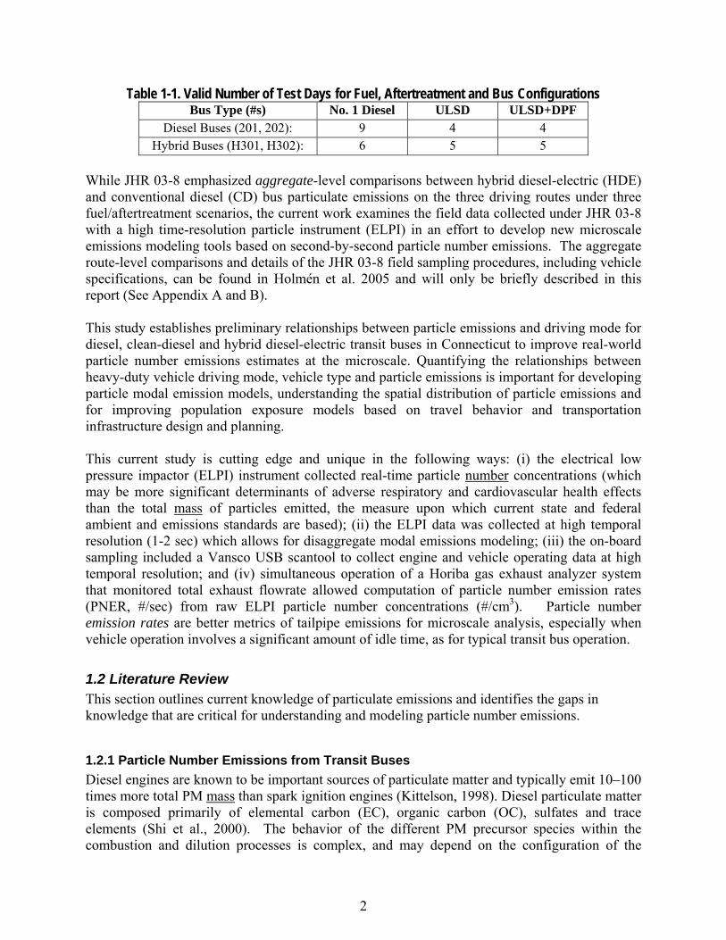
Table 1-1. Valid Number of Test Days for Fuel, Aftertreatment and Bus Configurations Bus Type (#s) No. 1 Diesel ULSD ULSD+DPF

Diesel Buses (201, 202): 9 4 4 Hybrid Buses (H301, H302): 6 5 5

While JHR 03-8 emphasized aggregate-level comparisons between hybrid diesel-electric (HDE) and conventional diesel (CD) bus particulate emissions on the three driving routes under three fuel/aftertreatment scenarios, the current work examines the field data collected under JHR 03-8 with a high time-resolution particle instrument (ELPI) in an effort to develop new microscale emissions modeling tools based on second-by-second particle number emissions. The aggregate route-level comparisons and details of the JHR 03-8 field sampling procedures, including vehicle specifications, can be found in Holmén et al. 2005 and will only be briefly described in this report (See Appendix A and B). This study establishes preliminary relationships between particle emissions and driving mode for diesel, clean-diesel and hybrid diesel-electric transit buses in Connecticut to improve real-world particle number emissions estimates at the microscale. Quantifying the relationships between heavy-duty vehicle driving mode, vehicle type and particle emissions is important for developing particle modal emission models, understanding the spatial distribution of particle emissions and for improving population exposure models based on travel behavior and transportation infrastructure design and planning. This current study is cutting edge and unique in the following ways: (i) the electrical low pressure impactor (ELPI) instrument collected real-time particle number concentrations (which may be more significant determinants of adverse respiratory and cardiovascular health effects than the total mass of particles emitted, the measure upon which current state and federal ambient and emissions standards are based); (ii) the ELPI data was collected at high temporal resolution (1-2 sec) which allows for disaggregate modal emissions modeling; (iii) the on-board sampling included a Vansco USB scantool to collect engine and vehicle operating data at high temporal resolution; and (iv) simultaneous operation of a Horiba gas exhaust analyzer system that monitored total exhaust flowrate allowed computation of particle number emission rates (PNER, #/sec) from raw ELPI particle number concentrations (#/cm3). Particle number emission rates are better metrics of tailpipe emissions for microscale analysis, especially when vehicle operation involves a significant amount of idle time, as for typical transit bus operation.

1.2 Literature Review This section outlines current knowledge of particulate emissions and identifies the gaps in knowledge that are critical for understanding and modeling particle number emissions. 1.2.1 Particle Number Emissions from Transit Buses Diesel engines are known to be important sources of particulate matter and typically emit 10–100 times more total PM mass than spark ignition engines (Kittelson, 1998). Diesel particulate matter is composed primarily of elemental carbon (EC), organic carbon (OC), sulfates and trace elements (Shi et al., 2000). The behavior of the different PM precursor species within the combustion and dilution processes is complex, and may depend on the configuration of the

3

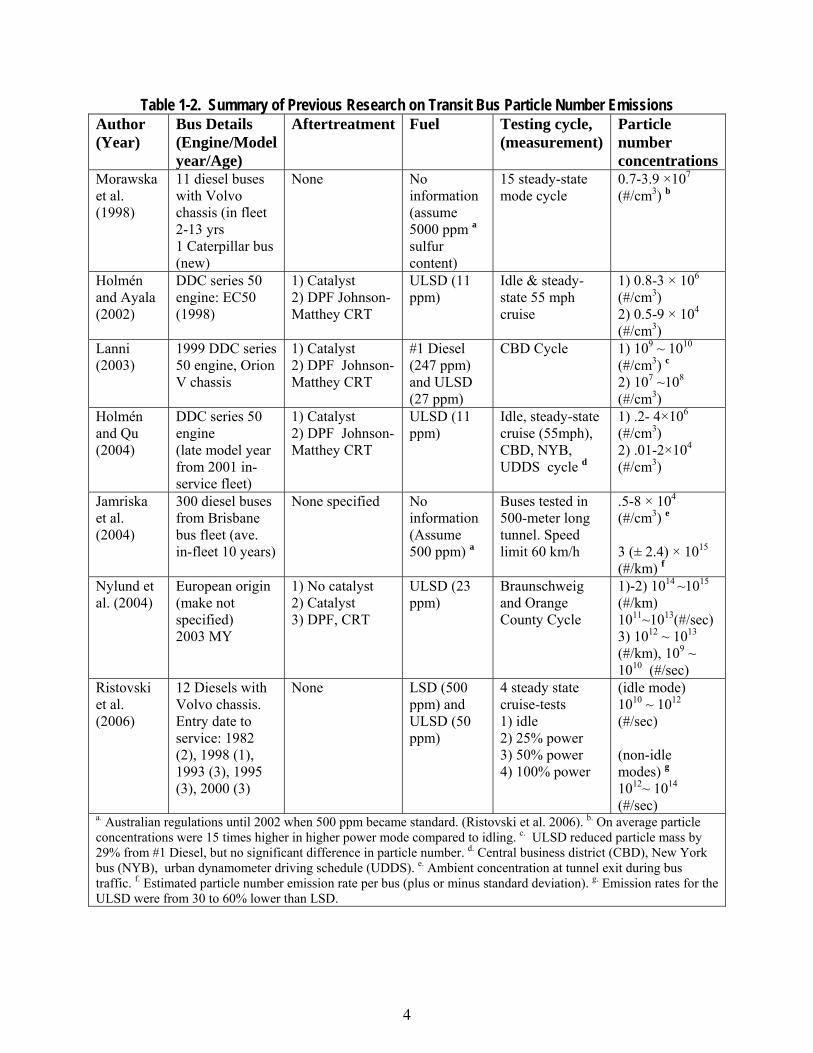
engine. Research is ongoing to better understand the engine, fuel and sampling parameters that determine the composition, size-distribution and concentration of diesel particulate matter emissions. The collection of particulate matter (PM) mass emissions is now a relatively mature science, while vehicle emissions research is currently focused on understanding particle number emissions. Current vehicle emissions models do not estimate the number of particles emitted, but as the regulatory environment shifts from mass to number, development of such number-based particle emissions models is warranted. Research on exposure to PM suggests long-term exposure to particulate matter is associated with inflammatory effects on the airways of even non-asthmatic subjects, increased risk of heart attacks and stroke as well as elevated risk of premature mortality in adults, including both respiratory and cardiovascular diseases (Holgate et al., 2003; Brook et al., 2002; Dockery, 2001). Furthermore, ultrafine particles, defined as having diameters less than 100nm, are a major component of diesel exhaust and have the most adverse health impacts (Kittelson, 1998; Utell, 2000; Nemmar et al., 2002). The EPA also reported that changes in peak expiratory flow (lung function) are more closely associated with ultrafine particles (particle number) than mass (EPA, 2004). Research on particle number emissions remains limited and there have been only a handful of studies that focus on particle number emissions from transit buses. The general results of these studies are summarized in Table 1-2. The results from previous studies highlight the fact that particulate sampling conditions (i.e., dilution rate and ratio, relative humidity and temperature of dilution air) affect measured number concentrations more than mass concentrations. Previous research efforts have investigated the impacts of fuel, engine type, aftertreatment devices, and engine load on particle number emissions (Table 1-2). Although the absolute magnitude of particle concentrations may depend on the dilution and sampling conditions (i.e. different dilution ratios), the relative effects of particle number emissions appears to be similar. For example, the use of a DPF appears to reduce particle number concentrations by two orders of magnitude (~99%) in all of the studies where DPF was evaluated (Holmén and Ayala, 2002 ; Lanni, 2003; Holmén and Qu, 2004; Nylund et al., 2004).

1.2.2 Uncertainty and Variability in Particle Number Emissions On-road vehicle emissions are known to vary according to many traffic, vehicle, fuel, ambient environment and driver behavior variables as well as emissions measurement technique. Furthermore, the factors that influence vehicle particle number emissions are especially difficult to establish because the variability observed in particle number emission tests can make it difficult to distinguish between true emission processes and random artifacts of the data. Even in laboratory testing, where the driving cycle and ambient conditions are strictly controlled, the between-test variability of particle number emission tests can be substantial (Zervas et al., 2004). For on-road testing, additional variability is added, due to changes in meteorological conditions, day-to-day setup of testing equipment on the test vehicles and changes in traffic conditions and driving behavior. Potential factors that can influence variability in the particle number emissions from transit buses evaluated in this study are discussed in the following paragraphs.

4

Table 1-2. Summary of Previous Research on Transit Bus Particle Number Emissions Author (Year)

Bus Details (Engine/Model year/Age)

Aftertreatment Fuel Testing cycle, (measurement)

Particle number concentrations

Morawska et al. (1998)

11 diesel buses with Volvo chassis (in fleet 2-13 yrs 1 Caterpillar bus (new)

None No information (assume 5000 ppm a sulfur content)

15 steady-state mode cycle

0.7-3.9 ×107 (#/cm3) b

Holmén and Ayala (2002)

DDC series 50 engine: EC50 (1998)

1) Catalyst 2) DPF Johnson-Matthey CRT

ULSD (11 ppm)

Idle & steady-state 55 mph cruise

1) 0.8-3 × 106 (#/cm3) 2) 0.5-9 × 104 (#/cm3)

Lanni (2003)

1999 DDC series 50 engine, Orion V chassis

1) Catalyst 2) DPF Johnson- Matthey CRT

#1 Diesel (247 ppm) and ULSD (27 ppm)

CBD Cycle

1) 109 ~ 1010 (#/cm3) c 2) 107 ~108 (#/cm3)

Holmén and Qu (2004)

DDC series 50 engine (late model year from 2001 in-service fleet)

1) Catalyst 2) DPF Johnson- Matthey CRT

ULSD (11 ppm)

Idle, steady-state cruise (55mph), CBD, NYB, UDDS cycle d

1) .2- 4×106 (#/cm3) 2) .01-2×104 (#/cm3)

Jamriska et al. (2004)

300 diesel buses from Brisbane bus fleet (ave. in-fleet 10 years)

None specified No information (Assume 500 ppm) a

Buses tested in 500-meter long tunnel. Speed limit 60 km/h

.5-8 × 104 (#/cm3) e 3 (± 2.4) × 1015

(#/km) f Nylund et al. (2004)

European origin (make not specified) 2003 MY

1) No catalyst 2) Catalyst 3) DPF, CRT

ULSD (23 ppm)

Braunschweig and Orange County Cycle

1)-2) 1014 ~1015 (#/km) 1011~1013(#/sec) 3) 1012 ~ 1013 (#/km), 109 ~ 1010 (#/sec)

Ristovski et al. (2006)

12 Diesels with Volvo chassis. Entry date to service: 1982 (2), 1998 (1), 1993 (3), 1995 (3), 2000 (3)

None LSD (500 ppm) and ULSD (50 ppm)

4 steady state cruise-tests 1) idle 2) 25% power 3) 50% power 4) 100% power

(idle mode) 1010 ~ 1012

(#/sec) (non-idle modes) g 1012~ 1014

(#/sec) a. Australian regulations until 2002 when 500 ppm became standard. (Ristovski et al. 2006). b. On average particle concentrations were 15 times higher in higher power mode compared to idling. c. ULSD reduced particle mass by 29% from #1 Diesel, but no significant difference in particle number. d. Central business district (CBD), New York bus (NYB), urban dynamometer driving schedule (UDDS). e. Ambient concentration at tunnel exit during bus traffic. f. Estimated particle number emission rate per bus (plus or minus standard deviation). g. Emission rates for the ULSD were from 30 to 60% lower than LSD.

5

Aftertreatment Devices. Diesel particulate filters have been shown to be a promising aftertreatment device to reduce both particle mass and particle number emissions from diesel engines (Burtscher, 2005). Diesel particulate filters (DPF) have been shown to significantly reduce the number of particles emitted from transit buses (Van Ling et al., 2003; Holmén and Qu., 2004; Vikara and Holmén, 2006; Hammond, 2007). Studies have shown that over 99% reduction in particle number emissions can occur when using a diesel particulate filter (Zervas et al., 2004; Burscher, 2005), including for diesel transit buses equipped with Detroit Diesel Series 50 engines operating in New York City (Lanni, 2003). Furthermore, Hammond et al. (2007) indicated retrofitting older school buses with particulate filters would reduce the in-vehicle particle number concentrations by a factor of two and reduce the in-vehicle particle number concentrations to levels consistent with new “Clean Diesel” buses. However, Van Ling et al. (2003) found DPF significantly reduced the number of particles in the accumulation mode (>50 nm) but resulted in a sharp increase for the portion of the particles in the nucleation mode below 40 nm diameter. This increase in <40nm particle numbers exceeded the engine-out numbers before the DPF was in place and was explained by sulfates forming in the oxidation catalyst of the DPF generating new particles via nucleation, even when using ultralow sulfur fuel.

In addition to significantly reducing the particle number emissions, diesel particulate filters may contribute to the relative increase in variability at the lower particle number counts (Holmén and Qu 2004; Mathis et al., 2005; Zervas et al. 2004). The variability has been attributed to volatile particle precursor species absorbing onto solid particles trapped within the DPF, and desorbing at high speeds or during DPF regeneration events (Zervas et al. 2004, Mathis et al. 2005). Studies have also investigated the impacts of aftertreatment devices on buses fueled by compressed natural gas (CNG). Holmén and Qu (2004) reported particle number emissions for CNG buses equipped with particulate filters/traps were consistently 2 orders of magnitude lower than diesel buses equipped only with oxidation catalysts and operating on ultralow sulfur fuel.

Vehicle Type. Emissions can also vary significantly between different vehicles types within the same vehicle class. Particle number emission rates have been observed to vary by a factor of 10 for transit buses in Brisbane, Australia (Jamriska et al. 2004). Significant variability of particulate emissions can also occur between different vehicles of the same vehicle type. Variability of particle mass emissions from similar NYC transit buses was attributed to differences in vehicle age, engine model, and maintenance (Canagaratna, 2004). The two buses within each bus vehicle type (conventional diesel and hybrid diesel-electric) in this study are similar in model year and engine type. Differences between the emissions of the two bus types will be evaluated, along with intra-vehicle type variability due to the effects of driving history and maintenance factors. Fuel Composition. The majority of past studies have investigated the effects of fuel type on particle emissions in an effort to determine which fuels produce the lowest particle number emissions. Ultralow sulfur fuels have been studied in this respect, but results vary with vehicle type, aftertreatment, operating conditions and particle size examined. Ristovski et al. (2006) observed a 30-60% reduction in particle number emissions in diesel buses with no aftertreatment devices. Other studies comparing particle number emissions from catalyst-equipped diesel buses indicate there may be slight impacts on nanoparticles emissions due to low sulfur fuel, but an overall reduction in particle number emissions was not detected (Van Ling et al. 2003, Lanni,

6

2003). Van Ling et al. (2003) indicated while sulfur content has an influence on the number of secondary nanoparticles generated, ultimately only zero sulfur fuel with light hydrocarbon fractions will produce low numbers of primary nanoparticle emissions. Thus, previous studies have shown mixed results (significant or insignificant differences) for the sulfur content effect of diesel fuel on particle number emissions. The effect of the two fuel types evaluated in the CT Transit emissions study (No. 1 Diesel and ULSD) will be evaluated for their influence on particle number emissions. Studies have also investigated buses fueled by compressed natural gas (CNG). Holmén and Ayala (2002) reported particle number concentrations (particles/cm3) of 0.8 to 3x106 for a 1998 oxidation catalyst-equipped diesel bus operating on ultralow sulfur fuel, from 0.5 to 9 x 104 for the diesel bus equipped with a DPF, and from 1 to 8 x 104 for a CNG bus without an oxidation catalyst. In addition, Nylund et al. (2004) found a two-fold decrease in particle number emissions when comparing CNG vehicles without a particle trap and diesel bus emissions without a catalyst. Nylund et al. (2004) also concluded there was no difference between the CNG and baseline diesel bus when a catalyst was used on the diesel bus.

Operating Conditions. Vehicle emission rates are highly dependent on the operating conditions of both the engine and the vehicle. Studies that have examined the operation effects of heavy-duty diesel engines and vehicles on particulate mass and number emissions are reviewed in Section 1.2.3 below. Driving Behavior. Previous studies have shown significant variation of CO and NOx emissions in light-duty vehicles due to driving behavior (Holmén and Niemeier, 1998, Frey et al., 2008). The effect of two primary bus drivers on the variability in particle number concentrations from the CT Transit diesel transit buses will be evaluated in this study (see results Section 4.1 below). Ambient Conditions. Lower ambient air temperature has been observed to increase particle number emissions when the diesel exhaust dilutes directly into the atmosphere from on-road (Kittleson et al. 2004) and roadside (Zhu et al. 2006) studies. Studies have shown mixed results with humidity, with both significant and insignificant effects on particle number emissions (Kittelson and Watts, 2002). Sampling Equipment. Comparisons of vehicle exhaust particle number concentration measurements between studies depends on the type of particle instrument (operating principle, rate of sampling, etc.) particle size range quantified and exhaust dilution system conditions. Uncertainties and variability are known to be associated with measuring particle number concentration using the Dekati electrical low pressure impactor (ELPI) employed in this study. Variability is associated with challenges in consistent zeroing the ELPI before each test run, electrometer drift during testing, and temporal alignment of the ELPI data with vehicle operation data (Holmén and Qu, 2004). Dilution System Properties. In laboratory dilution studies, much of the variability between tests is attributed to the deposition of particles on the surface of the dilution and exhaust system in previous tests, and subsequent release of particles in later runs, particularly at high temperatures and exhaust flow rates (Zervas et al., 2004). However, small changes in the dilution environment

7

(temperature, humidity) can have a tremendous impact on particle number emissions (Burtscher, 2005). Tests of heavy-duty diesel engines in the laboratory have concluded that increases in the dilution ratio, humidity of dilution air, and residence dilution time favor nucleation and condensation processes causing higher particle number concentrations (Shi and Harrison, 1999). At lower dilution air temperatures, more organic species condense and nucleate to form particles in the nucleation mode (Shi et al., 2000). For the CT Transit emissions study, daily setup of the on-board dilution system on the different transit buses and different operating conditions may have had an influence on the particle number emission measurements. Biasness of emission measurements. Although one focus of this study is to examine the variability of particle number measurements, it is important to recognize that systematic biasness may exist due to due to the ELPI sampling equipment which may cause inflated counts for small particle size bins (Maricq et al., 2000), or dilution systems which may suppress particle formation (Kittleson et al., 2004). 1.2.3 Operating Parameters Important for Modeling Diesel Particle Number Emissions To date, little research has been conducted on identifying the engine and vehicle operating parameters to model vehicle particle number emissions. This section provides a brief review of the engine and vehicle (vehicle speed, driving mode, etc.) parameters observed to affect particle number emissions. Engine operating parameters. The fuel-air equivalence ratio is an important determinant of particle number emissions as shown from engine dynamometer tests (Kittleson, 1998). The fuel-air equivalence ratio increases with engine load as additional fuel is added. High total particle number emissions can occur at both high and low equivalence ratios. At low equivalence ratios, the combustion temperature is lower and less of the fuel and oil is completely oxidized, leaving gas-phase volatile organic precursors to form small nucleation mode particles upon dilution. At higher equivalence ratios (and engine load) the organic fraction of particles decreases, but the number of solid particles increases due to incomplete combustion occurring in locally fuel-rich regions (Kittleson, 1998). Kweon et. al (2002) and Shi et al. (2000) also demonstrated, with a laboratory diesel engine, that engine load (or equivalence ratio) is an important indicator of the organic carbon (OC) to elemental carbon (EC) ratio. At low loads, the majority of the PM mass was organic carbon and the nucleation mode particle concentration was highest, while at high loads, diesel PM was composed primarily of elemental carbon. Shi et al. (2000) showed that OC fraction (by mass) ranged from 20 to 48% depending on engine speed and load, while the EC fraction ranged from 26% to 52%. Researchers have found that measurements of accumulation mode particles are more repeatable at a given engine load than nucleation mode particles (Kittelson and Watts, 2002, Shi et al. 2000). In order to produce more repeatable measurements, some studies have purposely prevented the volatile species from nucleating, to measure only the solid particles in the accumulation mode (Burtscher, 2005).

8

Vehicle Operating Parameters. Limited research has been conducted on identifying the vehicle operating parameters that affect particle number emissions. Jones and Harrison (2006) showed that vehicle particle number emissions rates estimated from roadway ambient air measurements are weakly correlated with average roadway speed. However, using only the average roadway speed is inadequate to distinguish different driving patterns and engine loads, as small increases in speed can cause doubling of horsepower for heavy-duty diesel vehicles (Yanowitz et al., 2002). A Swiss emission study showed that heavy-duty diesel vehicles had the highest ultrafine particle number emissions under stop-and-go driving conditions, compared to free-flowing high speed conditions (Imhof et al., 2005). In contrast, an Australian study of diesel transit buses showed that the particle emission rates were significantly higher on a high speed route compared to stop-and-go traffic (Morwaska et al., 2005). While useful for establishing the actual exposure levels of traffic-source particle emissions, the emission rates from the cited ambient studies can only be used to classify general traffic conditions. From chassis dynamometer testing of 12 diesel buses without aftertreatments, Morawska et al. (1998), observed particle number concentrations were on average 15 times higher in higher power modes compared to idling. Ristovski et al. (2006) observed a roughly two-orders of magnitude increase in particle number emissions from non-idle modes compared to idling modes on a similar set of diesel buses. Holmen and Qu (2004) performed chassis dynamometer testing of a catalyst-equipped diesel bus. Their results indicate that total particle number emissions were higher during acceleration modes and cruising modes than decelerating and idling modes. The particle number emissions also tended to increase within a driving mode as the average vehicle speed increased. For a diesel bus equipped with a diesel particulate filter, a less detectable relationship existed between driving mode and particle number emissions. 1.2.4 Emission Models for Heavy-duty Diesel Particulate Mass Emissions In the absence of particle number emission models, a brief overview of the current models used for mobile source pollutant mass emission rates follows. The two regulatory emission models used in the U.S., EMFAC and MOBILE, give mass-based PM emission factors for heavy-duty diesel vehicles (> 8,500 lbs). EMFAC, developed by the California Air Resource Board (CARB), has trip-based heavy-duty diesel PM emission factors based on data collected on chassis dynamometer tests using specified driving cycles. By using speed correction factors developed by fitting average speed of the driving cycles to PM mass emission rates, EMFAC calculates trip-based PM emission rates for user specified average speed (Kear and Niemeier 2006). MOBILE, developed by the US Environmental Protection Agency, estimates link-based PM emission rates based on diesel engine emissions certification data (Kear and Niemeier 2006). Gram-per-mile emission rates are estimated from measured gram-per-brake-horsepower-hour emissions using estimated conversion factors (Browning 1998), however these emission rates do not adjust to driving conditions, such as average speed. (Kear and Niemeier 2006). EPA recognizes that particulate mass emission rates are a better function of transient operating events and not engine load, but EPA continues to use the current methodology due to data constraints (Browning 1998).

9

More accurate link-level PM emission rates, have been developed by using a function of transient operating behavior. Kear and Niemeier (2006) use a property they term “intensity”, which they calculate by summing the product of all positive occurrences of horsepower and acceleration along the driving cycle. Yanowitz et al. (2002) modeled PM using “severity”, defined as the sum of all positive changes in horsepower over a driving cycle, to capture the relationship between the rate of fuel use and PM emission rates. Both methods are shown to work well to model PM mass emission rates from chassis dynamometer tests. Other emission models have been developed that use more time-resolved activity data. Clark et al. (2003) developed a model to predict HDD PM emissions, by binning second-by-second PM emissions according to speed and acceleration data. EPA’s upcoming MOVES model is also using a more resolved approach, by modeling emissions according to operating mode defined by vehicle specific power, as discussed in more detail below in Section 1.2.5. 1.2.5 Modal Emissions Models In response to the limitations of average speed based modeling methods such as MOBILE, the EPA has made significant changes to the methods used to estimate vehicle emissions. One major effort is development of a new mode-based emissions model called the Motor Vehicle Emission Simulator (MOVES). Once approved for use, MOVES will replace the EPA’s current mobile source emission model, MOBILE, and their NONROAD model (Beardsley, 2004; Koupal et al., 2002). According to Nam (2003), the MOVES model is essentially an effort to simplify, improve and implement the Comprehensive Modal Emissions Model (CMEM) developed at University of California, Riverside on a fleet wide-basis (Barth et al. 2000). CMEM. Development of the Comprehensive Modal Emissions Model (CMEM) began in the late 1990’s with the support of the National Cooperative Highway Research Program (NCHRP) and the U.S. Environmental Protection Agency (EPA). CMEM was developed to address the air quality impacts of changes and improvements to the transportation network. Therefore, CMEM was designed as a microscopic emissions model to predict second-by-second tailpipe emissions and fuel consumption based on individual vehicle activity (Barth et al., 2004). The required inputs for CMEM include vehicle activity (second-by-second speed trace, at a minimum) and the fleet composition of the traffic being modeled.

The initial version of CMEM was focused on gas-phase pollutant (CO, HC, NOx and CO2) emissions for light-duty vehicles and contained 23 light-duty gasoline vehicle categories. With the continued support by the U.S. EPA, CMEM has been maintained and updated. Most notably, CMEM has been expanded to include heavy-duty diesel vehicles. The current version of CMEM (version 3.0, 2005) includes 28 light-duty vehicle/technology categories and 3 heavy-duty vehicle/technology categories (Scora and Barth, 2006). Barth et al. (2004) describe the equations and development of the heavy-duty power demand, engine speed, fuel rate and emissions out models developed for the latest version of CMEM. Furthermore, in 2005 particulate matter mass emissions estimates were added to the CMEM model using the same power demand approach that CMEM uses for gas-phase pollutants (Scora and Barth, 2006).

MOVES. Recognizing the limitations of its existing mobile source emissions model, MOBILE, the U.S. Environmental Protection Agency is developing a new multi-scale modeling approach

10

that will enable quantifying emissions with temporal and spatial resolution (Koupal et al., 2002). These estimates are needed for understanding how proposed transportation improvements will affect emissions; evaluating potential “hot-spots” for transportation conformity and improving the mobile source inventory for State Implementation Plans (SIPs). The new model, Motor Vehicle Emission Simulator (MOVES), arose out of National Research Council recommendations for improving MOBILE (NRC, 2000) that included:

• Ability to model a range of spatial and temporal scales; • Include all mobile sources and all pollutants; • Include uncertainty estimates; • Ability to interface with other models, such as traffic simulation models.

With MOVES, the EPA is moving away from the average speed-based approach used in their MOBILE line of emissions models and adopting a mode-based emissions model similar to the one developed in CMEM. The MOVES model was initially developed to quantify energy consumption and greenhouse gas emissions based on vehicle activity (EPA, 2007). To produce emissions and fuel consumption estimates MOVES operates by estimating two fundamental quantities; total vehicle activity and the subdivision of that activity into modes (EPA, 2008). Total activity refers to the total amount of fleet based vehicle activity in the location and time of interest. The total activity is then subdivided into operating modes which produce unique energy consumption and emission rates (EPA, 2008). A significant on-going part of this effort is generation of new emission factors as a function of vehicle operating conditions for different vehicle types. The MOVES model implements a binning approach to classify second-by-second vehicle activity. Vehicle activity is binned based on vehicle specific power (VSP1) and vehicle instantaneous speed into 30 different activity bins (Table 1-3) that each has an associated emissions rate based on a multitude of factors (i.e. vehicle type, ambient weather conditions, fuel type, etc.) (EPA, 2007). MOVES depends on operating mode to provide multi-scale analysis capabilities.

Table 1-3. EPA MOVES Activity Binning Definitions (EPA, 2007)

Braking (Bin 0) Idle (Bin 1)

VSP/Instantaneous Speed 0-25 mph 25-50 mph >50 mph <0 kW/tonne Bin 11 Bin 21

0 to 3 Bin 12 Bin 22 3 to 6 Bin 13 Bin 23 6 to 9 Bin 14 Bin 24

9 to 12 Bin 15 Bin 25 12 and greater Bin 16

12 to 18 Bin 27 Bin 37 18 to 24 Bin 28 Bin 38 24 to 30 Bin 29 Bin 39

30 and greater Bin 30 Bin 40 6 to 12 Bin 35

<6 Bin 33 1 VPS is a calculated variable used to estimate power demand on an engine based on velocity, acceleration and road grade.

11

The development of MOVES has occurred in stages: a demo version was released in May 2007 and a draft version of the full on-road model is scheduled for release in 2008. The development, approval and widespread use of a modal emissions model will increase our ability to estimate the impacts of the transportation system on local air quality. However, the MOVES model still has many limitations. For particulate emissions, the major limitation is that MOVES only reports PM emissions in terms of mass and not number. MOVES outputs mass-based emissions estimates for three different classes of primary PM2.5 emissions (organic carbon, elemental carbon and sulfate). PM2.5 refers to the mass of particulate matter smaller than 2.5 microns in aerodynamic diameter. Furthermore, “primary” refers to particles emitted directly from the vehicle, and does not account for subsequent atmospheric chemical reactions that cause particles to transform. This research focuses on primary particle number emissions from heavy-duty transit bus vehicles to aid in removing limitations from future emissions models and allowing for more accurate microscale modeling of vehicle emissions. In particular, the VSP/speed-based binning definitions used in MOVES shown in Table 1-3 were applied to the data collected for this research to characterize particle number emission rates in these activity bins for the CT Transit diesel and hybrid bus test routes.

Following an overview of the research objectives in Section 2.0 below, the data processing and analysis procedures are outlined in Section 3.0 and Section 4.0 of this report presents research results.

2.0 Research Objectives This research aims to provide new understanding on time-resolved particle number emissions from diesel transit buses with different transmission, fuel and aftertreatment configurations. Specifically, the relationships between tailpipe emissions and vehicle/engine operating parameters are investigated to develop and evaluate new tools for estimating vehicle particle number emissions with high temporal and spatial resolution for use in microscale models such as MOVES. The study uses disaggregate analysis of the unique CT Transit on-road transit bus emissions and operations dataset collected in 2004 to examine (a) the magnitude of emissions as a function of vehicle operating conditions; and uses an aggregate approach to analyze the (b) the variability or level of uncertainty in these emissions. The research is based on detailed analysis of the tailpipe particle number emissions data collected with the electrical low pressure impactor (ELPI). Specific research objectives are to:

(1) Delineate the range of second-by-second operating conditions (speeds, acceleration rates, frequency and duration of acceleration/deceleration events) experienced by transit buses during operation on real-world bus routes and compare these conditions to driving cycles and databases used for emissions modeling. The field data on vehicle activity is compared in terms of previous work on “vehicle operating mode” to assess the differences in operation experienced by the conventional diesel and the parallel hybrid diesel-electric buses over the same driving routes.

12

(2) Quantify number-based total ultrafine particle emissions in exhaust from conventional diesel and hybrid diesel-electric transit buses as a function of the data-driven second-by-second “vehicle operating mode” categories defined in (1). Identify differences in emissions-operating mode relationships as a function of vehicle transmission, fuel sulfur content, and aftertreatment with a diesel particulate filter.

(3) Develop quantitative relationships between measured particle number emissions and

transportation network variables—facility type, distance from intersections, route grade, and level of congestion.

(4) Quantify uncertainty in emissions levels under real-world driving conditions.

3.0 Research Methods 3.1 Vehicles and On-Board Instrumentation This section briefly describes the vehicles and instrumentation used to generate the database used in this research. Some summary information on field sampling procedures appears in Appendices A and B of this report. More detailed information on the field data collection effort can be found in Holmén et al. (2005). 3.1.1 Vehicles A total of four transit buses from the in-service Connecticut Transit (CT Transit) fleet were tested in 2004. The buses all had identical 40-foot low-floor New Flyer chassis and engines with similar peak torque and power ratings:

• two of the buses (fleet numbers 201 and 202) were conventional diesel (CD) buses equipped with model year 2002 Detroit Diesel Corporation Series 40 engines; and

• two of the buses (fleet numbers H301 and H302) were hybrid diesel-electric (HDE) equipped with model year 2003 Cummins ISL 280 engines and the Allison Ep 40 electric drive parallel hybrid transmission.

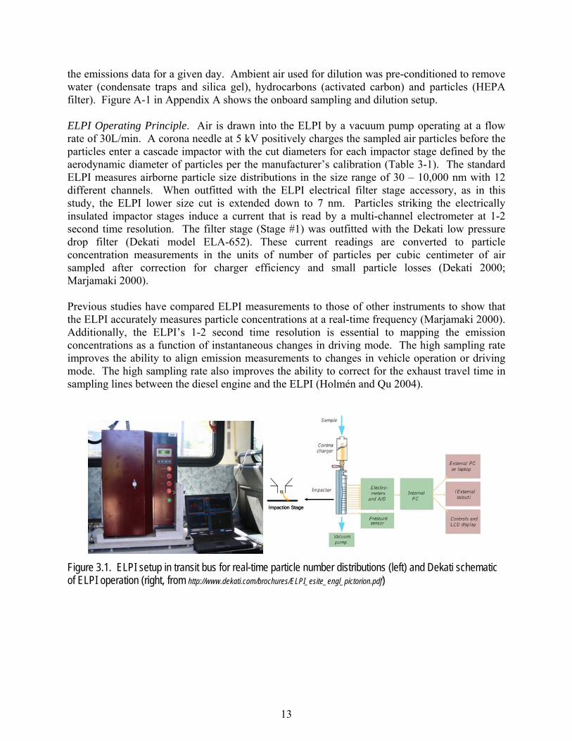
During all emissions sampling, the bus air conditioning was off and all instrumentation was powered from an external generator so there was no additional load on the vehicles. Detailed specifications on both vehicle types, including aftertreatment devices, are tabulated in Appendix B. 3.1.2 Particle Number Emissions Instrumentation Particle number concentrations analyzed in this study were measured using a Dekati, Ltd. (Finland) Electrical Low Pressure Impactor (ELPI) operating at 30 Lpm and outfitted with an electrical filter stage (Figure 3.1). The ELPI quantifies particle concentration in 12 size bins in real-time at 1-2 sec resolution over a particle aerodynamic diameter range of 7 – 8000 nm. Prior to entering the ELPI, bus exhaust was diluted with a Dekati ejector-diluter single-stage mini-dilution system operating at nominal dilution ratios of 22 to 35, (mean = 27). Under field sampling conditions, the flow rates of sample exhaust and dilution air were continuously recorded to compute dilution ratios. Because there was no significant difference in dilution ratio between driving routes for a given sampling day, a daily dilution ratio value was applied to all

13

the emissions data for a given day. Ambient air used for dilution was pre-conditioned to remove water (condensate traps and silica gel), hydrocarbons (activated carbon) and particles (HEPA filter). Figure A-1 in Appendix A shows the onboard sampling and dilution setup. ELPI Operating Principle. Air is drawn into the ELPI by a vacuum pump operating at a flow rate of 30L/min. A corona needle at 5 kV positively charges the sampled air particles before the particles enter a cascade impactor with the cut diameters for each impactor stage defined by the aerodynamic diameter of particles per the manufacturer’s calibration (Table 3-1). The standard ELPI measures airborne particle size distributions in the size range of 30 – 10,000 nm with 12 different channels. When outfitted with the ELPI electrical filter stage accessory, as in this study, the ELPI lower size cut is extended down to 7 nm. Particles striking the electrically insulated impactor stages induce a current that is read by a multi-channel electrometer at 1-2 second time resolution. The filter stage (Stage #1) was outfitted with the Dekati low pressure drop filter (Dekati model ELA-652). These current readings are converted to particle concentration measurements in the units of number of particles per cubic centimeter of air sampled after correction for charger efficiency and small particle losses (Dekati 2000; Marjamaki 2000). Previous studies have compared ELPI measurements to those of other instruments to show that the ELPI accurately measures particle concentrations at a real-time frequency (Marjamaki 2000). Additionally, the ELPI’s 1-2 second time resolution is essential to mapping the emission concentrations as a function of instantaneous changes in driving mode. The high sampling rate improves the ability to align emission measurements to changes in vehicle operation or driving mode. The high sampling rate also improves the ability to correct for the exhaust travel time in sampling lines between the diesel engine and the ELPI (Holmén and Qu 2004).

Impaction StageImpaction Stage

Figure 3.1. ELPI setup in transit bus for real-time particle number distributions (left) and Dekati schematic of ELPI operation (right, from http://www.dekati.com/brochures/ELPI_esite_engl_pictorion.pdf)

14

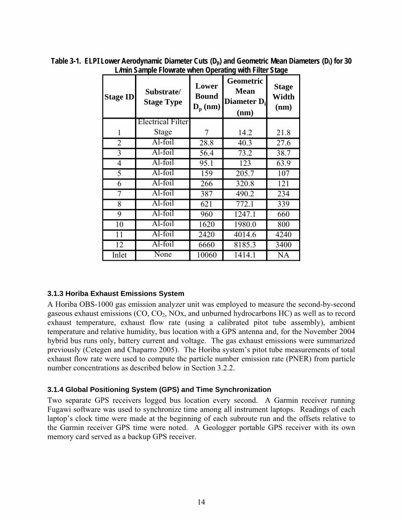
Table 3-1. ELPI Lower Aerodynamic Diameter Cuts (Dp) and Geometric Mean Diameters (Di) for 30

L/min Sample Flowrate when Operating with Filter Stage

Stage ID Substrate/ Stage Type

Lower Bound

Dp (nm)

Geometric Mean

Diameter Di

(nm)

Stage Width (nm)

1Electrical Filter

Stage 7 14.2 21.82 Al-foil 28.8 40.3 27.63 Al-foil 56.4 73.2 38.74 Al-foil 95.1 123 63.95 Al-foil 159 205.7 1076 Al-foil 266 320.8 1217 Al-foil 387 490.2 2348 Al-foil 621 772.1 3399 Al-foil 960 1247.1 66010 Al-foil 1620 1980.0 80011 Al-foil 2420 4014.6 424012 Al-foil 6660 8185.3 3400

Inlet None 10060 1414.1 NA 3.1.3 Horiba Exhaust Emissions System A Horiba OBS-1000 gas emission analyzer unit was employed to measure the second-by-second gaseous exhaust emissions (CO, CO2, NOx, and unburned hydrocarbons HC) as well as to record exhaust temperature, exhaust flow rate (using a calibrated pitot tube assembly), ambient temperature and relative humidity, bus location with a GPS antenna and, for the November 2004 hybrid bus runs only, battery current and voltage. The gas exhaust emissions were summarized previously (Cetegen and Chaparro 2005). The Horiba system’s pitot tube measurements of total exhaust flow rate were used to compute the particle number emission rate (PNER) from particle number concentrations as described below in Section 3.2.2. 3.1.4 Global Positioning System (GPS) and Time Synchronization Two separate GPS receivers logged bus location every second. A Garmin receiver running Fugawi software was used to synchronize time among all instrument laptops. Readings of each laptop’s clock time were made at the beginning of each subroute run and the offsets relative to the Garmin receiver GPS time were noted. A Geologger portable GPS receiver with its own memory card served as a backup GPS receiver.

15

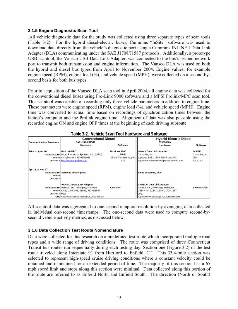
3.1.5 Engine Diagnostic Scan Tool All vehicle diagnostic data for the study was collected using three separate types of scan tools (Table 3-2). For the hybrid diesel-electric buses, Cummins “InSite” software was used to download data directly from the vehicle’s diagnostic port using a Cummins INLINE I Data Link Adapter (DLA) communicating under the SAE J1708/J1587 protocols. Additionally, a prototype USB scantool, the Vansco USB Data Link Adapter, was connected to the bus’s second network port to transmit both transmission and engine information. The Vansco DLA was used on both the hybrid and diesel bus types from April to November 2004. Engine values, for example engine speed (RPM), engine load (%), and vehicle speed (MPH), were collected on a second-by-second basis for both bus types. Prior to acquisition of the Vansco DLA scan tool in April 2004, all engine data was collected for the conventional diesel buses using Pro-Link 9000 software and a MPSI Prolink/MPC scan tool. This scantool was capable of recording only three vehicle parameters in addition to engine time. These parameters were engine speed (RPM), engine load (%), and vehicle speed (MPH). Engine time was converted to actual time based on recordings of synchronization times between the laptop’s computer and the Prolink engine time. Alignment of data was also possible using the recorded engine ON and engine OFF times at the beginning of each driving subroute.

Table 3-2. Vehicle Scan Tool Hardware and Software Communication Protocols: SAE J1708/J1587 J1939/CAN

Hardware Software Hardware Software

Prior to April 16: ProLink/MPC Pro-Link 9000 Inline 1 Data Link Adapter INSITEmanufacturer Micro Processor Systems, Inc. (MPSI) MPSI Cummins, Inc. Cummins, Inc.

model complies with J1708/J1939 Virtual Terminal Applic. supports SAE J1708/J1587 data link Liteversion # http://www.mpsilink.com 1.01 http://inline.cummins.com/products/inline1.html 6.2.224.0

Apr 16 to Nov 17:manufacturer Same as above, plus: Same as above, plus:

modelversion #

VANSCO Data Link Adapter VANSCO Data Link Adaptermanufacturer Vansco, Inc., Winnipeg, Manitoba CANsniff Vansco, Inc., Winnipeg, Manitoba SIMGAUGES

model USB; CAN 2.0B, J1939, J1708/1587 USB; CAN 2.0B, J1939, J1708/1587version # beta beta

URL http://www.vansco.ca/pdf/DLA_brochure.pdf http://www.vansco.ca/pdf/DLA_brochure.pdf

Conventional Diesel Hybrid-Electric Diesel

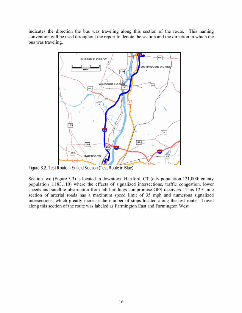
All scantool data was aggregated to one-second temporal resolution by averaging data collected in individual one-second timestamps. The one-second data were used to compute second-by-second vehicle activity metrics, as discussed below. 3.1.6 Data Collection Test Route Nomenclature Data were collected for this research on a predefined test route which incorporated multiple road types and a wide range of driving conditions. The route was comprised of three Connecticut Transit bus routes run sequentially during each testing day. Section one (Figure 3.2) of the test route traveled along Interstate 91 from Hartford to Enfield, CT. This 33.4-mile section was selected to represent high-speed cruise driving conditions where a constant velocity could be obtained and maintained for an extended period of time. The majority of this section has a 65 mph speed limit and stops along this section were minimal. Data collected along this portion of the route are referred to as Enfield North and Enfield South. The direction (North or South)

16

indicates the direction the bus was traveling along this section of the route. This naming convention will be used throughout the report to denote the section and the direction in which the bus was traveling.

Figure 3.2. Test Route – Enfield Section (Test Route in Blue)

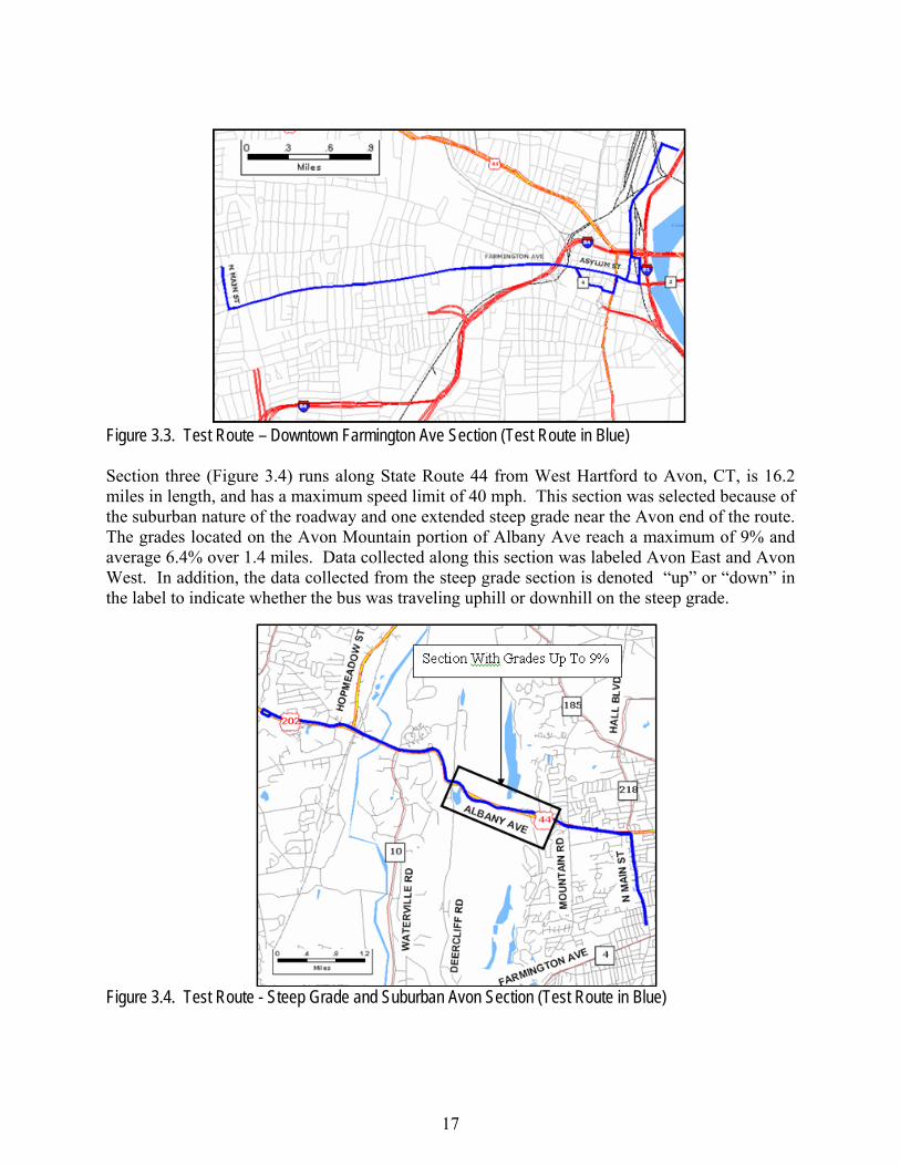
Section two (Figure 3.3) is located in downtown Hartford, CT (city population 121,000; county population 1,183,110) where the effects of signalized intersections, traffic congestion, lower speeds and satellite obstruction from tall buildings compromise GPS receivers. This 12.3-mile section of arterial roads has a maximum speed limit of 35 mph and numerous signalized intersections, which greatly increase the number of stops located along the test route. Travel along this section of the route was labeled as Farmington East and Farmington West.

17

Figure 3.3. Test Route – Downtown Farmington Ave Section (Test Route in Blue)

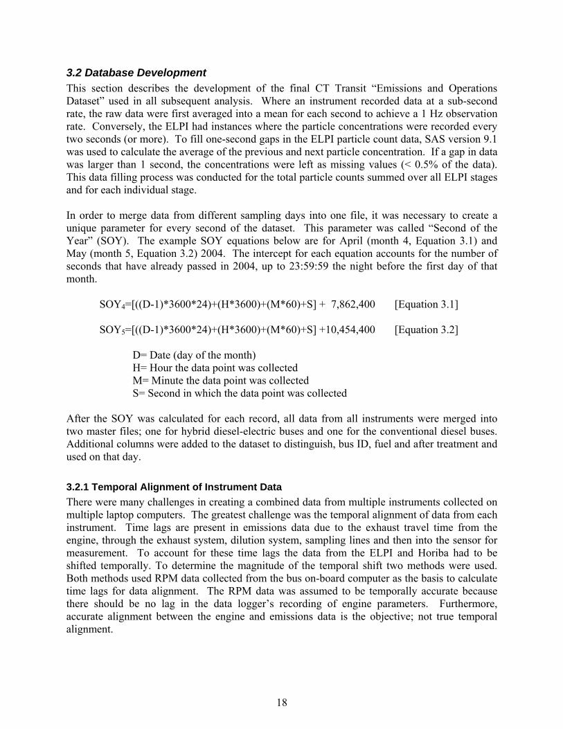
Section three (Figure 3.4) runs along State Route 44 from West Hartford to Avon, CT, is 16.2 miles in length, and has a maximum speed limit of 40 mph. This section was selected because of the suburban nature of the roadway and one extended steep grade near the Avon end of the route. The grades located on the Avon Mountain portion of Albany Ave reach a maximum of 9% and average 6.4% over 1.4 miles. Data collected along this section was labeled Avon East and Avon West. In addition, the data collected from the steep grade section is denoted “up” or “down” in the label to indicate whether the bus was traveling uphill or downhill on the steep grade.

Figure 3.4. Test Route - Steep Grade and Suburban Avon Section (Test Route in Blue)

18

3.2 Database Development This section describes the development of the final CT Transit “Emissions and Operations Dataset” used in all subsequent analysis. Where an instrument recorded data at a sub-second rate, the raw data were first averaged into a mean for each second to achieve a 1 Hz observation rate. Conversely, the ELPI had instances where the particle concentrations were recorded every two seconds (or more). To fill one-second gaps in the ELPI particle count data, SAS version 9.1 was used to calculate the average of the previous and next particle concentration. If a gap in data was larger than 1 second, the concentrations were left as missing values (< 0.5% of the data). This data filling process was conducted for the total particle counts summed over all ELPI stages and for each individual stage.

In order to merge data from different sampling days into one file, it was necessary to create a unique parameter for every second of the dataset. This parameter was called “Second of the Year” (SOY). The example SOY equations below are for April (month 4, Equation 3.1) and May (month 5, Equation 3.2) 2004. The intercept for each equation accounts for the number of seconds that have already passed in 2004, up to 23:59:59 the night before the first day of that month.

SOY4=[((D-1)*3600*24)+(H*3600)+(M*60)+S] + 7,862,400 [Equation 3.1]

SOY5=[((D-1)*3600*24)+(H*3600)+(M*60)+S] +10,454,400 [Equation 3.2] D= Date (day of the month) H= Hour the data point was collected M= Minute the data point was collected S= Second in which the data point was collected

After the SOY was calculated for each record, all data from all instruments were merged into two master files; one for hybrid diesel-electric buses and one for the conventional diesel buses. Additional columns were added to the dataset to distinguish, bus ID, fuel and after treatment and used on that day. 3.2.1 Temporal Alignment of Instrument Data There were many challenges in creating a combined data from multiple instruments collected on multiple laptop computers. The greatest challenge was the temporal alignment of data from each instrument. Time lags are present in emissions data due to the exhaust travel time from the engine, through the exhaust system, dilution system, sampling lines and then into the sensor for measurement. To account for these time lags the data from the ELPI and Horiba had to be shifted temporally. To determine the magnitude of the temporal shift two methods were used. Both methods used RPM data collected from the bus on-board computer as the basis to calculate time lags for data alignment. The RPM data was assumed to be temporally accurate because there should be no lag in the data logger’s recording of engine parameters. Furthermore, accurate alignment between the engine and emissions data is the objective; not true temporal alignment.

19

The first lag estimation method involved the calculation of the cross-correlation coefficient. By definition, a correlation coefficient indicates the strength and direction of a linear relationship between two random variables. Engine speed (RPM) is highly correlated with exhaust flow rate because the faster an engine runs the more exhaust it displaces. Therefore, an estimate of the appropriate time lag between engine parameters and the Horiba measurements (at the tailpipe) was determined based on the magnitude of temporal shift that produced the best correlation between RPM (recorded by the scantool) and exhaust flow rate (measured by the Horiba). SAS was used to calculate the cross- correlation coefficient for exhaust flow rate shifted ±150 seconds for each section of the test route for each day. The time lag with the highest correlation coefficient was assumed to be the appropriate time lag for the Horiba data. These estimated time lags can be found in Appendix C. The cross correlation method was also used to estimate the time lag between the engine parameters and the ELPI particle count data. For this analysis, RPM and particle number (PN) concentrations were hypothesized to be correlated with each other. Similar to engine flow data PN concentration data were shifted ±150 seconds for each section of the test route for each day. The time lag with the highest correlation coefficient was assumed to be the appropriate time lag for the ELPI data. The second method was a manually observed lag estimate. This method compared the instance in time when the engine was started (RPM increased significantly from zero) and when there was a significant change from a baseline flow rate or PN count value. The bus was stopped at the end of each test route section for instrument zeroing. This provided an “engine start” at the beginning of each test section to allow a manual estimate of the time lag for that section of the test route. These estimated time lags are comparable to the cross-correlation method. Selection of the final time lag applied to the ELPI and Horiba data was based on a combination of the cross-correlation method and the manual check. The cross-correlation method is the preferred time lag since it estimates the time lag over the entire length of the test section. In other words, true temporal lags vary second-by-second based on engine speed (RPM) and because the cross-correlation coefficient method uses data from the entire route segment, the time lag estimated using this method is hypothesized to be more accurate. The engine start method only approximates the lag at the instant the engine was started and does not consider how the time lag may change over the entire test section. It should be noted, however, that the cross-correlation method is not fool proof – there were instances where the correlation coefficient was high but the temporal lag was not realistic. To reduce the possibility of applying an inaccurate temporal lag, the results of the two methods were compared side-by-side to determine if there were large discrepancies in estimated lag. If discrepancies existed, the data was reexamined and the manual check was repeated. If accurate, then the manual estimate method was used to generate the applied temporal lag for that section. Appendix C contains this comparison and shows the applied temporal lag to each instrument.

3.2.2 Emissions Rate Calculation Once all the data were temporally aligned an emissions rate (in particles per second) could be calculated. The ELPI reports the concentration of particles (#/cm3). Concentrations are not as useful when trying to model vehicle emissions since a high exhaust flow rate could make low

20

concentration hazardous, or a low flow rate could reduce the ambient air impact of a high concentration. Therefore, exhaust flow rate (Horiba pitot tube measurement), PN concentration (ELPI) and the measured dilution ratio were used to calculate the particle number emissions rate (PNER, Equation 3.3). Emissions rate was calculated for the sum of particles across each stage, as well as for each individual ELPI stage.

Emissions_ Rate = PNER = P *Q* DR [Equation 3.3] P = ELPI Particle number concentration (#/cm3) Q = Flow rate (cm3/s calculated from Horiba pitot tube data) DR = Dilution Ratio = [Vdil + Vexh]/[Vexh]

Where Vdil is the measured volume of dilution air and Vexh is the measured exhaust sample volume.

3.2.3 Route Definitions and Road Grade Using the GPS data collected by the Horiba unit the data for each bus type were spatially plotted in ArcGIS (Version 9.1). The test route was then assigned three new attributes based on the bus spatial location on the test route. The first attribute was a basic route identifier. The second attribute identified the direction the bus was traveling along that section of the route. Because the bus traveled along sections of the route in both directions it was necessary to delineate which direct the bus was traveling to ensure proper accounting for road grade. Furthermore, the Avon section of the route has steep grades (up to 9%). This section of the test route was assigned a direction of travel and whether the bus was on an up-grade or down-grade. The final attribute added to the dataset was the road type on which the bus was traveling (i.e. rural arterial, urban arterial, divided highway, on-ramp, off-ramp). Using ArcGIS, segments of the route were selected and the road type attributes were added to the selected section. Personal knowledge of the transportation system and surrounding land development and access were used to assign a road type to each link of the network. The road type classifications were based on the Federal Highway Administration’s (FHWA) road classification system (US FHWA, 1989). Once the route definitions were assigned, road grade was assigned to each second of the dataset. Road grade data were collected along the test route by the Connecticut Department of Transportation’s (ConnDOT) Automatic Road Analyzer (ARAN) photologging van. The ARAN van was able to provide road grade (in %, at survey level accuracy) every 10 meters along the test route. Using ArcGIS, the ARAN road grade dataset and the CT Transit Emissions and Operations Dataset were overlaid and spatially joined. Effectively every record in the CT Transit Emissions and Operations Dataset was assigned a road grade based on the grade data point that was closest to it in spatial proximity. One of the challenges with this data join is that the buses traveled both directions on the same segment of the test route. Therefore, one direction the grade would be positive and then when traveling in the opposite direction the grade would be negative. To account for this situation, the route direction attribute was used to select the appropriate grade value from the ARAN dataset to ensure the bus and ARAN van were traveling the same direction.

21

3.2.4 Vehicle Specific Power The addition of second-by-second grade observation allows for a level of detailed modal emissions analysis that was previously not available. Vehicle Specific Power (VSP) is a measure of engine power demand that is calculated from velocity, acceleration and road grade. The joining of second-by-second road grade to the dataset allows for a detailed calculation of VSP where previous efforts had to ignore or estimate grade for the calculation of VSP. Previous research on vehicle emissions suggests VSP is highly correlated to increased concentrations of gas-phase exhaust emissions (Huai et al., 2005; Jimenez, 1999; Kuhns, 2004; Pokharel, 2001). VSP for each second of data was calculated (see Equation 3.4) using an expression derived from the United States Environmental Protection Agency’s (EPA) Motor Vehicle Emission Simulator (MOVES) manual (EPA, 2004b). The equation for VSP used here was tailored to a heavy-duty vehicle using coefficients outlined on pages 55-58 of EPA 2004b. The resulting VSP equation would be the same expression as the one used in MOVES to model modal emissions from “buses and motor homes”.

VSPbus= v * [a*g*sin (u) + 0.064] + [0.000265*v3] [Equation 3.4] A= vehicle acceleration (meters/s2) u= road grade (as decimal fraction, not percent) g= acceleration due to gravity, 9.81 m/s2 v= vehicle velocity (meters/s)

Appendix D contains a data dictionary summarizing each of the parameters found in the final CT Transit Emissions and Operations Dataset.

3.3 Database Quality Assurance The final CT transit Emissions and Operations dataset includes time-resolved (second-by-second) particle number emissions rates spatially aligned to the driving routes, and temporally aligned to the operation parameters. The dataset will form the basis of the microscopic emissions analysis in later sections of this report. Due to the importance for accuracy in the final dataset, the CT Transit Emissions and Operations Dataset was independently evaluated by another researcher before data analysis was performed. The following tasks were performed to: (a) ensure that the database was merged correctly, (b) assure that the correct data were uploaded to the final merged database, and (c) verify that all calculations were performed correctly.

a) The manually observed lags between the engine scantool, ELPI, and Horiba datasets were revaluated for the bus data collected from April 16 to September 21. The revaluated observed lags were compared to those obtained previously. The manually obtained lags coincided well between the two researchers. The comparison helped identify several runs where an incorrect lag was previously selected. These corrections were made and updated in the new dataset.

b) The second task assured that the measurement data recorded from the ELPI, Horiba Exhaust Emissions System, and Vansco Engine scantool were correctly uploaded into the final CT Transit Emissions and Operations Dataset by sub-route and day. The graphical tools within the SAS interactive data analysis function were used to visually examine the number of observations located within each dataset, along with mean values of key parameters from each measurement device. By so doing, several sub-routes were

22

identified as having missing data caused by either programming errors or errors in the SOY assignment of the unmerged datafiles. Additionally, discrepancies were detected in the geographical definitions of the basic route identifier. This led to the final route assignment methodology discussed in Section 3.2.3 based the second-by-second GPS data, to assure that the route definitions were consistent throughout the study.

c) For the third task, the calculations for VSP and PNER (using Equations 3.3 and 3.4 above) were independently performed to verify they were calculated correctly. All calculations were found to be correct in the final CT Transit Emissions and Operations Dataset.

3.4 Data Analysis and Modeling 3.4.1 Evaluating Sources of Variability in Onboard Particle Number Concentrations Dataset Used for Variability Analysis. The emissions variability analysis was performed prior to the creation of the final CT Transit Emissions and Operations Dataset. The major methodological differences between the data used for the variability analysis and the microscopic analysis were: 1) The particle number concentration (particle/cm3) was analyzed for variability instead of the particle number emission rates (particles/sec) that were used for microscopic analysis. (This difference occurred because careful alignment of the particle concentration data with the exhaust flowrate data was not complete yet so accurate particle number emission rates could not be calculated). Subsequently, it was confirmed that use of raw particle number concentration instead of particle number emissions rate to assess emissions variability had no effect on the outcome of the variability analysis. 2) The variability analysis evaluated data from the entire study (January 6 to November 10, 2004), not the more restricted April-November study dates used for the microscopic analysis. The CT Transit Emissions and Operations Data set did not include the pre-April testing dates because the exhaust flow rate, which is required to compute the emission rate, was incorrectly calibrated by Horiba and was not deemed sufficiently accurate to compute particle number emission rates for the pre-April days. To assure accuracy in exhaust flow measurement starting with the April testing days, the pitot tube that recorded exhaust flow rate was re-calibrated, and an exhaust pipe extension was added to prevent backflow (Holmén et al., 2005). By using the data collected from the entire study, the variability analysis was able to assess variation due to different bus drivers and a larger range of meteorological conditions. 3) The variability analysis evaluated particle number concentrations averaged over an entire route or section of a route, instead of the emissions at the second-by-second level. This approach was taken to quantify the aggregate differences between factors that influenced the particle number concentration between runs conducted each day, and between each day, instead of variation that occurred within a run. The average particle concentrations of the Enfield North, Enfield South, Farmington West and Farmington East routes were evaluated. Instead of

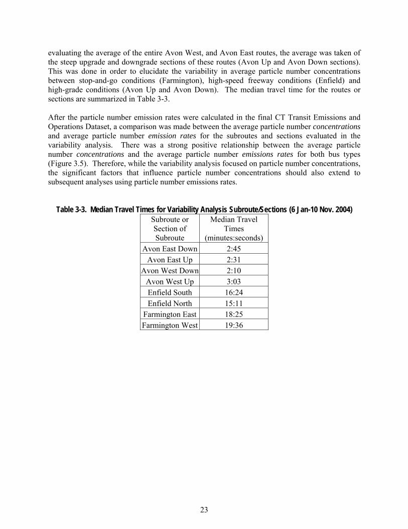
23

evaluating the average of the entire Avon West, and Avon East routes, the average was taken of the steep upgrade and downgrade sections of these routes (Avon Up and Avon Down sections). This was done in order to elucidate the variability in average particle number concentrations between stop-and-go conditions (Farmington), high-speed freeway conditions (Enfield) and high-grade conditions (Avon Up and Avon Down). The median travel time for the routes or sections are summarized in Table 3-3. After the particle number emission rates were calculated in the final CT Transit Emissions and Operations Dataset, a comparison was made between the average particle number concentrations and average particle number emission rates for the subroutes and sections evaluated in the variability analysis. There was a strong positive relationship between the average particle number concentrations and the average particle number emissions rates for both bus types (Figure 3.5). Therefore, while the variability analysis focused on particle number concentrations, the significant factors that influence particle number concentrations should also extend to subsequent analyses using particle number emissions rates.

Table 3-3. Median Travel Times for Variability Analysis Subroute/Sections (6 Jan-10 Nov. 2004)

Subroute or Section of Subroute

Median Travel Times

(minutes:seconds) Avon East Down 2:45

Avon East Up 2:31 Avon West Down 2:10

Avon West Up 3:03 Enfield South 16:24 Enfield North 15:11

Farmington East 18:25 Farmington West 19:36

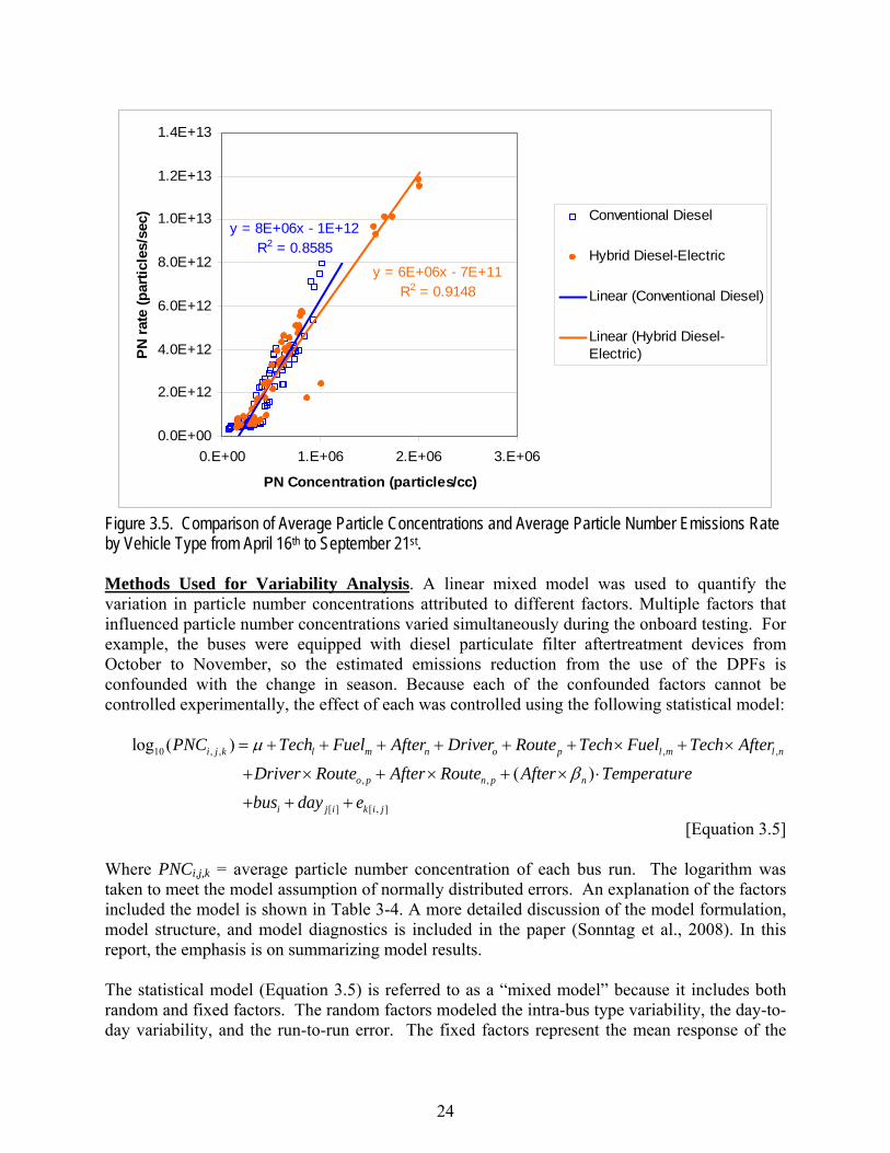
24

y = 8E+06x - 1E+12R2 = 0.8585

y = 6E+06x - 7E+11R2 = 0.9148

0.0E+00

2.0E+12

4.0E+12

6.0E+12

8.0E+12

1.0E+13

1.2E+13

1.4E+13

0.E+00 1.E+06 2.E+06 3.E+06

PN Concentration (particles/cc)

PN

rate

(par

ticle

s/se

c) Conventional Diesel

Hybrid Diesel-Electric

Linear (Conventional Diesel)

Linear (Hybrid Diesel-Electric)

Figure 3.5. Comparison of Average Particle Concentrations and Average Particle Number Emissions Rate by Vehicle Type from April 16th to September 21st.

Methods Used for Variability Analysis. A linear mixed model was used to quantify the variation in particle number concentrations attributed to different factors. Multiple factors that influenced particle number concentrations varied simultaneously during the onboard testing. For example, the buses were equipped with diesel particulate filter aftertreatment devices from October to November, so the estimated emissions reduction from the use of the DPFs is confounded with the change in season. Because each of the confounded factors cannot be controlled experimentally, the effect of each was controlled using the following statistical model:

10 , , , ,

, ,

[ ] [ , ]

log ( )

( )i j k l m n o p l m l n

o p n p n

i j i k i j

PNC Tech Fuel After Driver Route Tech Fuel Tech After

Driver Route After Route After Temperature

bus day e

μ

β

= + + + + + + × + ×

+ × + × + × ⋅

+ + +

[Equation 3.5] Where PNCi,j,k = average particle number concentration of each bus run. The logarithm was taken to meet the model assumption of normally distributed errors. An explanation of the factors included the model is shown in Table 3-4. A more detailed discussion of the model formulation, model structure, and model diagnostics is included in the paper (Sonntag et al., 2008). In this report, the emphasis is on summarizing model results. The statistical model (Equation 3.5) is referred to as a “mixed model” because it includes both random and fixed factors. The random factors modeled the intra-bus type variability, the day-to-day variability, and the run-to-run error. The fixed factors represent the mean response of the

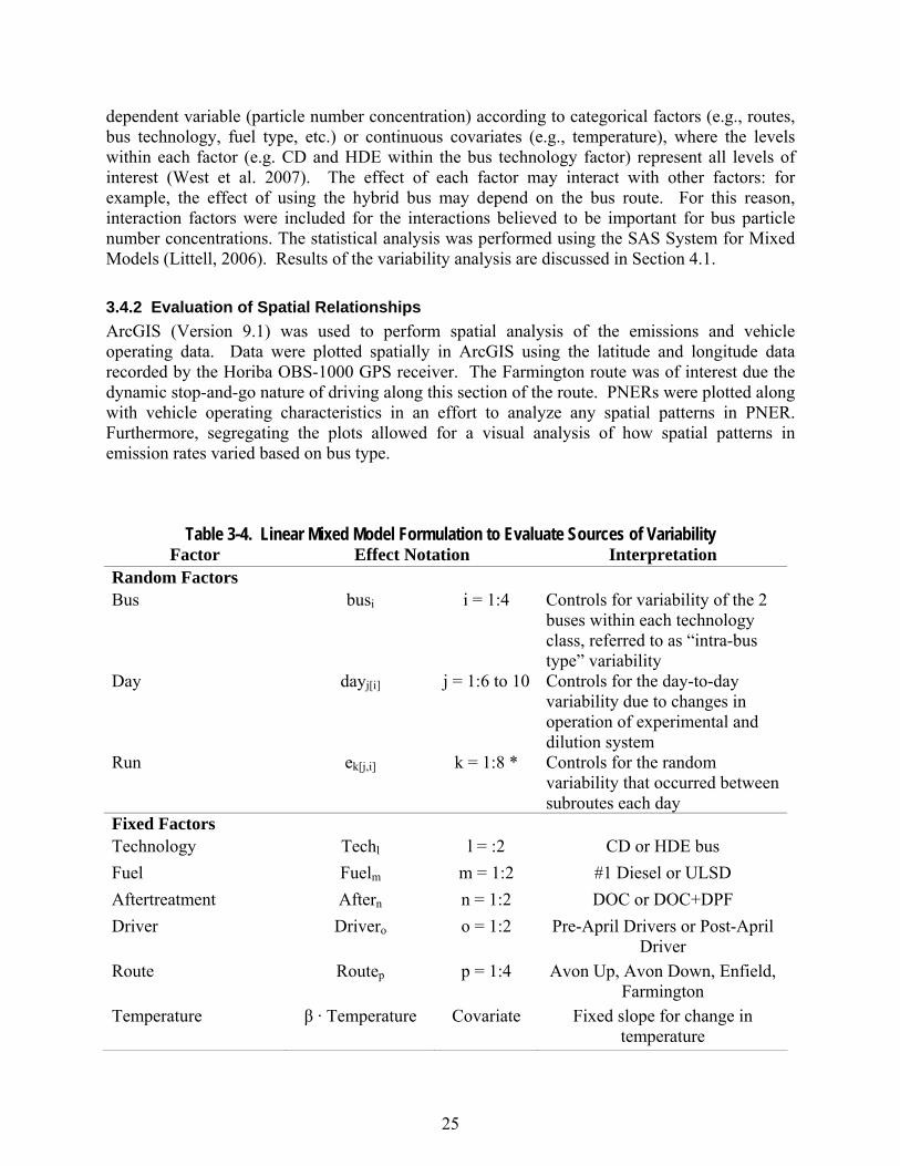
25

dependent variable (particle number concentration) according to categorical factors (e.g., routes, bus technology, fuel type, etc.) or continuous covariates (e.g., temperature), where the levels within each factor (e.g. CD and HDE within the bus technology factor) represent all levels of interest (West et al. 2007). The effect of each factor may interact with other factors: for example, the effect of using the hybrid bus may depend on the bus route. For this reason, interaction factors were included for the interactions believed to be important for bus particle number concentrations. The statistical analysis was performed using the SAS System for Mixed Models (Littell, 2006). Results of the variability analysis are discussed in Section 4.1. 3.4.2 Evaluation of Spatial Relationships ArcGIS (Version 9.1) was used to perform spatial analysis of the emissions and vehicle operating data. Data were plotted spatially in ArcGIS using the latitude and longitude data recorded by the Horiba OBS-1000 GPS receiver. The Farmington route was of interest due the dynamic stop-and-go nature of driving along this section of the route. PNERs were plotted along with vehicle operating characteristics in an effort to analyze any spatial patterns in PNER. Furthermore, segregating the plots allowed for a visual analysis of how spatial patterns in emission rates varied based on bus type.

Table 3-4. Linear Mixed Model Formulation to Evaluate Sources of Variability Factor Effect Notation Interpretation

Random Factors

Bus busi i = 1:4 Controls for variability of the 2 buses within each technology class, referred to as “intra-bus type” variability

Day dayj[i] j = 1:6 to 10 Controls for the day-to-day variability due to changes in operation of experimental and dilution system

Run ek[j,i] k = 1:8 * Controls for the random variability that occurred between subroutes each day

Fixed Factors Technology Techl l = :2 CD or HDE bus Fuel Fuelm m = 1:2 #1 Diesel or ULSD Aftertreatment Aftern n = 1:2 DOC or DOC+DPF Driver Drivero o = 1:2 Pre-April Drivers or Post-April

Driver Route Routep p = 1:4 Avon Up, Avon Down, Enfield,

Farmington Temperature β · Temperature Covariate Fixed slope for change in

temperature

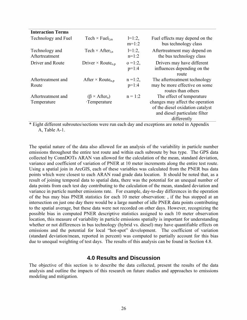
26

Interaction Terms

Technology and Fuel Tech × Fuell,m l=1:2, m=1:2

Fuel effects may depend on the bus technology class

Technology and Aftertreatment

Tech × Afterl,n l=1:2, n=1:2

Aftertreatment may depend on the bus technology class

Driver and Route Driver × Routeo,p o =1:2, p=1:4

Drivers may have different influences depending on the

route Aftertreatment and Route

After × Routen,p n =1:2, p=1:4

The aftertreatment technology may be more effective on some

routes than others Aftertreatment and Temperature

(β × Aftern) ·Temperature

n = 1:2 The effect of temperature changes may affect the operation

of the diesel oxidation catalyst and diesel particulate filter

differently * Eight different subroutes/sections were run each day and exceptions are noted in Appendix

A, Table A-1. The spatial nature of the data also allowed for an analysis of the variability in particle number emissions throughout the entire test route and within each subroute by bus type. The GPS data collected by ConnDOTs ARAN van allowed for the calculation of the mean, standard deviation, variance and coefficient of variation of PNER at 10 meter increments along the entire test route. Using a spatial join in ArcGIS, each of these variables was calculated from the PNER bus data points which were closest to each ARAN road grade data location. It should be noted that, as a result of joining temporal data to spatial data, there was the potential for an unequal number of data points from each test day contributing to the calculation of the mean, standard deviation and variance in particle number emissions rate. For example, day-to-day differences in the operation of the bus may bias PNER statistics for each 10 meter observation: , if the bus stopped at an intersection on just one day there would be a large number of idle PNER data points contributing to the spatial average, but these data were not recorded on other days. However, recognizing the possible bias in computed PNER descriptive statistics assigned to each 10 meter observation location, this measure of variability in particle emissions spatially is important for understanding whether or not differences in bus technology (hybrid vs. diesel) may have quantifiable effects on emissions and the potential for local “hot-spot” development. The coefficient of variation (standard deviation/mean, reported in percent) was computed to partially account for this bias due to unequal weighting of test days. The results of this analysis can be found in Section 4.8.

4.0 Results and Discussion The objective of this section is to describe the data collected, present the results of the data analysis and outline the impacts of this research on future studies and approaches to emissions modeling and mitigation.

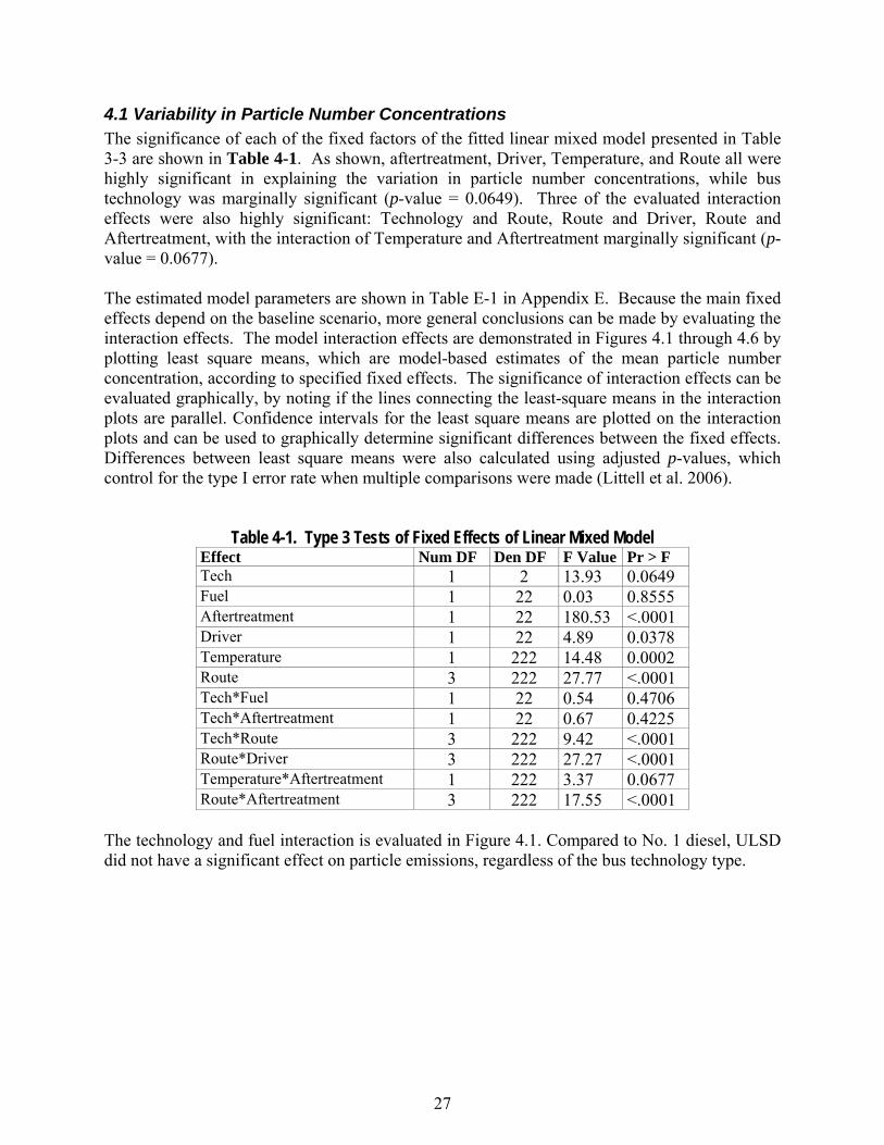
27

4.1 Variability in Particle Number Concentrations The significance of each of the fixed factors of the fitted linear mixed model presented in Table 3-3 are shown in Table 4-1. As shown, aftertreatment, Driver, Temperature, and Route all were highly significant in explaining the variation in particle number concentrations, while bus technology was marginally significant (p-value = 0.0649). Three of the evaluated interaction effects were also highly significant: Technology and Route, Route and Driver, Route and Aftertreatment, with the interaction of Temperature and Aftertreatment marginally significant (p-value = 0.0677). The estimated model parameters are shown in Table E-1 in Appendix E. Because the main fixed effects depend on the baseline scenario, more general conclusions can be made by evaluating the interaction effects. The model interaction effects are demonstrated in Figures 4.1 through 4.6 by plotting least square means, which are model-based estimates of the mean particle number concentration, according to specified fixed effects. The significance of interaction effects can be evaluated graphically, by noting if the lines connecting the least-square means in the interaction plots are parallel. Confidence intervals for the least square means are plotted on the interaction plots and can be used to graphically determine significant differences between the fixed effects. Differences between least square means were also calculated using adjusted p-values, which control for the type I error rate when multiple comparisons were made (Littell et al. 2006).

Table 4-1. Type 3 Tests of Fixed Effects of Linear Mixed Model

Effect Num DF Den DF F Value Pr > F Tech 1 2 13.93 0.0649 Fuel 1 22 0.03 0.8555 Aftertreatment 1 22 180.53 <.0001 Driver 1 22 4.89 0.0378 Temperature 1 222 14.48 0.0002 Route 3 222 27.77 <.0001 Tech*Fuel 1 22 0.54 0.4706 Tech*Aftertreatment 1 22 0.67 0.4225 Tech*Route 3 222 9.42 <.0001 Route*Driver 3 222 27.27 <.0001 Temperature*Aftertreatment 1 222 3.37 0.0677 Route*Aftertreatment 3 222 17.55 <.0001

The technology and fuel interaction is evaluated in Figure 4.1. Compared to No. 1 diesel, ULSD did not have a significant effect on particle emissions, regardless of the bus technology type.

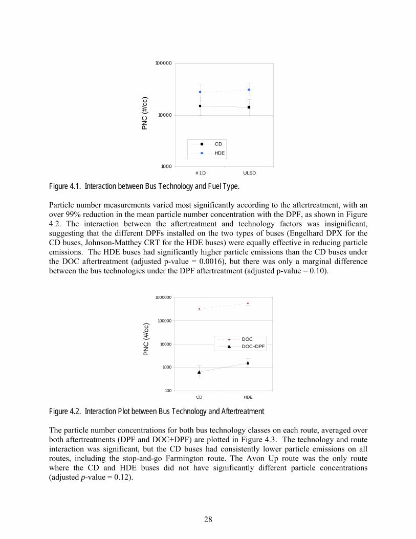
28

1000

10000

100000

# 1 D ULSD

CD

HDE

PNC

(#/c

c)

Figure 4.1. Interaction between Bus Technology and Fuel Type. Particle number measurements varied most significantly according to the aftertreatment, with an over 99% reduction in the mean particle number concentration with the DPF, as shown in Figure 4.2. The interaction between the aftertreatment and technology factors was insignificant, suggesting that the different DPFs installed on the two types of buses (Engelhard DPX for the CD buses, Johnson-Matthey CRT for the HDE buses) were equally effective in reducing particle emissions. The HDE buses had significantly higher particle emissions than the CD buses under the DOC aftertreatment (adjusted p-value = 0.0016), but there was only a marginal difference between the bus technologies under the DPF aftertreatment (adjusted p-value = 0.10).

100

1000

10000

100000

1000000

CD HDE

DOCDOC+DPF

PNC

(#/c

c)

Figure 4.2. Interaction Plot between Bus Technology and Aftertreatment The particle number concentrations for both bus technology classes on each route, averaged over both aftertreatments (DPF and DOC+DPF) are plotted in Figure 4.3. The technology and route interaction was significant, but the CD buses had consistently lower particle emissions on all routes, including the stop-and-go Farmington route. The Avon Up route was the only route where the CD and HDE buses did not have significantly different particle concentrations (adjusted p-value = 0.12).

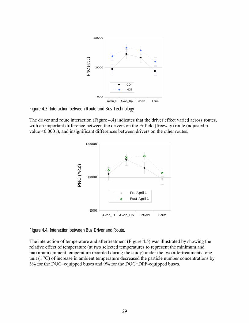
29

1000

10000

100000

Avon_D Avon_Up Enfield Farm

CD

HDE

8PNC

(#/c

c)

Figure 4.3. Interaction between Route and Bus Technology The driver and route interaction (Figure 4.4) indicates that the driver effect varied across routes, with an important difference between the drivers on the Enfield (freeway) route (adjusted p-value <0.0001), and insignificant differences between drivers on the other routes.

1000

10000

100000

Avon_D Avon_Up Enf ield Farm

Pre-April 1

Post-April 1

PNC

(#/c

c)

Figure 4.4. Interaction between Bus Driver and Route. The interaction of temperature and aftertreatment (Figure 4.5) was illustrated by showing the relative effect of temperature (at two selected temperatures to represent the minimum and maximum ambient temperature recorded during the study) under the two aftertreatments: one unit (1 oC) of increase in ambient temperature decreased the particle number concentrations by 3% for the DOC–equipped buses and 9% for the DOC+DPF-equipped buses.

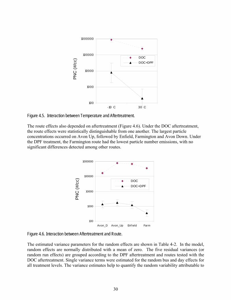
30

100

1000

10000

100000

1000000

-10 C 30 C

DOCDOC+DPF

PNC

(#/c

c)

Figure 4.5. Interaction between Temperature and Aftertreatment. The route effects also depended on aftertreatment (Figure 4.6). Under the DOC aftertreatment, the route effects were statistically distinguishable from one another. The largest particle concentrations occurred on Avon Up, followed by Enfield, Farmington and Avon Down. Under the DPF treatment, the Farmington route had the lowest particle number emissions, with no significant differences detected among other routes.

100

1000

10000

100000

1000000

Avon_D Avon_Up Enf ield Farm

DOCDOC+DPF

PNC

(#/c

c)

Figure 4.6. Interaction between Aftertreatment and Route. The estimated variance parameters for the random effects are shown in Table 4-2. In the model, random effects are normally distributed with a mean of zero. The five residual variances (or random run effects) are grouped according to the DPF aftertreatment and routes tested with the DOC aftertreatment. Single variance terms were estimated for the random bus and day effects for all treatment levels. The variance estimates help to quantify the random variability attributable to

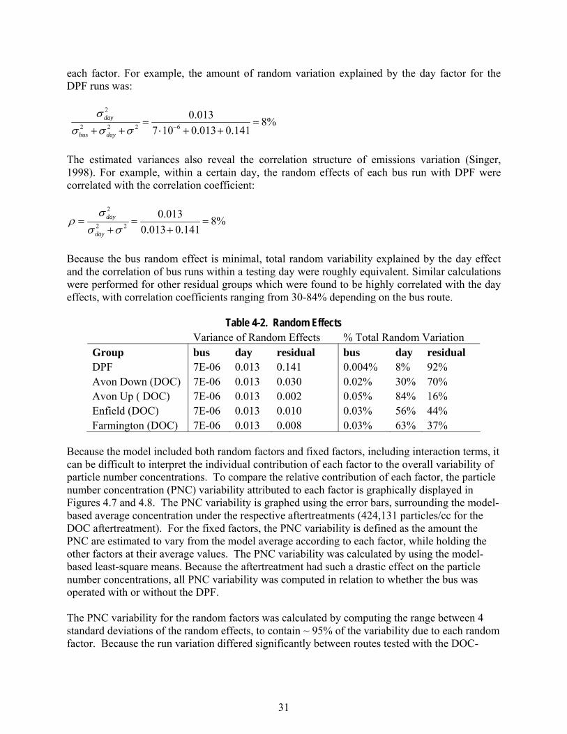
31

each factor. For example, the amount of random variation explained by the day factor for the DPF runs was:

2

2 2 2 6

0.013 8%7 10 0.013 0.141

day

bus day

σσ σ σ −= =

+ + ⋅ + +

The estimated variances also reveal the correlation structure of emissions variation (Singer, 1998). For example, within a certain day, the random effects of each bus run with DPF were correlated with the correlation coefficient:

2

2 2

0.013 8%0.013 0.141

day

day

σρ

σ σ= = =

+ +

Because the bus random effect is minimal, total random variability explained by the day effect and the correlation of bus runs within a testing day were roughly equivalent. Similar calculations were performed for other residual groups which were found to be highly correlated with the day effects, with correlation coefficients ranging from 30-84% depending on the bus route.

Table 4-2. Random Effects Variance of Random Effects % Total Random Variation Group bus day residual bus day residual DPF 7E-06 0.013 0.141 0.004% 8% 92% Avon Down (DOC) 7E-06 0.013 0.030 0.02% 30% 70% Avon Up ( DOC) 7E-06 0.013 0.002 0.05% 84% 16% Enfield (DOC) 7E-06 0.013 0.010 0.03% 56% 44% Farmington (DOC) 7E-06 0.013 0.008 0.03% 63% 37%

Because the model included both random factors and fixed factors, including interaction terms, it can be difficult to interpret the individual contribution of each factor to the overall variability of particle number concentrations. To compare the relative contribution of each factor, the particle number concentration (PNC) variability attributed to each factor is graphically displayed in Figures 4.7 and 4.8. The PNC variability is graphed using the error bars, surrounding the model-based average concentration under the respective aftertreatments (424,131 particles/cc for the DOC aftertreatment). For the fixed factors, the PNC variability is defined as the amount the PNC are estimated to vary from the model average according to each factor, while holding the other factors at their average values. The PNC variability was calculated by using the model-based least-square means. Because the aftertreatment had such a drastic effect on the particle number concentrations, all PNC variability was computed in relation to whether the bus was operated with or without the DPF. The PNC variability for the random factors was calculated by computing the range between 4 standard deviations of the random effects, to contain ~ 95% of the variability due to each random factor. Because the run variation differed significantly between routes tested with the DOC-

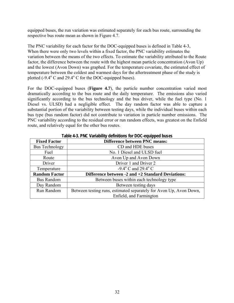
32

equipped buses, the run variation was estimated separately for each bus route, surrounding the respective bus route mean as shown in Figure 4.7. The PNC variability for each factor for the DOC-equipped buses is defined in Table 4-3, When there were only two levels within a fixed factor, the PNC variability estimates the variation between the means of the two effects. To estimate the variability attributed to the Route factor, the difference between the route with the highest mean particle concentration (Avon Up) and the lowest (Avon Down) was graphed. For the temperature covariate, the estimated effect of temperature between the coldest and warmest days for the aftertreatment phase of the study is plotted (-9.4o C and 29.4o C for the DOC-equipped buses).

For the DOC-equipped buses (Figure 4.7), the particle number concentration varied most dramatically according to the bus route and the daily temperature. The emissions also varied significantly according to the bus technology and the bus driver, while the fuel type (No. 1 Diesel vs. ULSD) had a negligible effect. The day random factor was able to capture a substantial portion of the variability between testing days, while the individual buses within each bus type (bus random factor) did not contribute to variation in particle number emissions. The PNC variability according to the residual error or run random effects, was greatest on the Enfield route, and relatively equal for the other bus routes.

Table 4-3. PNC Variability definitions for DOC-equipped buses Fixed Factor Difference between PNC means:

Bus Technology CD and HDE buses Fuel No. 1 Diesel and ULSD fuel

Route Avon Up and Avon Down Driver Driver 1 and Driver 2

Temperature -9.4o C and 29.4o C Random Factor Difference between -2 and +2 Standard Deviations:

Bus Random Between buses within each technology type Day Random Between testing days Run Random Between testing runs, estimated separately for Avon Up, Avon Down,

Enfield, and Farmington

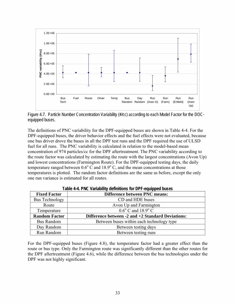
33

0.0E+00

2.0E+05

4.0E+05

6.0E+05

8.0E+05

1.0E+06

1.2E+06

BusTech

Fuel Route Driver Temp BusRandom

DayRandom

Run(Avon D)

Run(Farm)

Run(Enfield)

Run(AvonUp)

PNC

var

iabi

lity

(#/c

c)

Figure 4.7. Particle Number Concentration Variability (#/cc) according to each Model Factor for the DOC-equipped buses. The definitions of PNC variability for the DPF-equipped buses are shown in Table 4-4. For the DPF-equipped buses, the driver behavior effects and the fuel effects were not evaluated, because one bus driver drove the buses in all the DPF test runs and the DPF required the use of ULSD fuel for all runs. The PNC variability is calculated in relation to the model-based mean concentration of 974 particles/cc for the DPF aftertreatment. The PNC variability according to the route factor was calculated by estimating the route with the largest concentrations (Avon Up) and lowest concentrations (Farmington Route). For the DPF-equipped testing days, the daily temperature ranged between 0.6o C and 18.9o C, and the mean concentrations at those temperatures is plotted. The random factor definitions are the same as before, except the only one run variance is estimated for all routes.

Table 4-4. PNC Variability definitions for DPF-equipped buses

Fixed Factor Difference between PNC means: Bus Technology CD and HDE buses

Route Avon Up and Farmington Temperature 0.6o C and 18.9o C

Random Factor Difference between -2 and +2 Standard Deviations: Bus Random Between buses within each technology type Day Random Between testing days Run Random Between testing runs

For the DPF-equipped buses (Figure 4.8), the temperature factor had a greater effect than the route or bus type. Only the Farmington route was significantly different than the other routes for the DPF aftertreatment (Figure 4.6), while the difference between the bus technologies under the DPF was not highly significant.

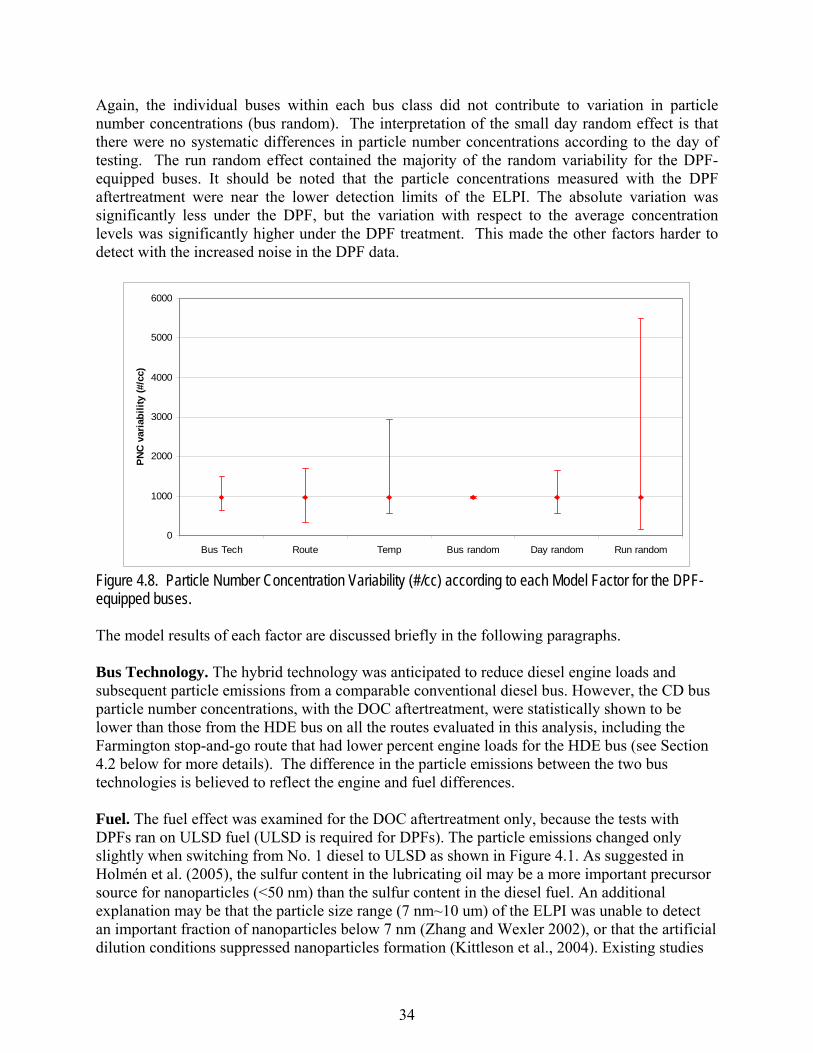
34

Again, the individual buses within each bus class did not contribute to variation in particle number concentrations (bus random). The interpretation of the small day random effect is that there were no systematic differences in particle number concentrations according to the day of testing. The run random effect contained the majority of the random variability for the DPF-equipped buses. It should be noted that the particle concentrations measured with the DPF aftertreatment were near the lower detection limits of the ELPI. The absolute variation was significantly less under the DPF, but the variation with respect to the average concentration levels was significantly higher under the DPF treatment. This made the other factors harder to detect with the increased noise in the DPF data.

0

1000

2000

3000

4000

5000

6000

Bus Tech Route Temp Bus random Day random Run random

PNC

varia

bilit

y (#

/cc)

Figure 4.8. Particle Number Concentration Variability (#/cc) according to each Model Factor for the DPF-equipped buses. The model results of each factor are discussed briefly in the following paragraphs. Bus Technology. The hybrid technology was anticipated to reduce diesel engine loads and subsequent particle emissions from a comparable conventional diesel bus. However, the CD bus particle number concentrations, with the DOC aftertreatment, were statistically shown to be lower than those from the HDE bus on all the routes evaluated in this analysis, including the Farmington stop-and-go route that had lower percent engine loads for the HDE bus (see Section 4.2 below for more details). The difference in the particle emissions between the two bus technologies is believed to reflect the engine and fuel differences. Fuel. The fuel effect was examined for the DOC aftertreatment only, because the tests with DPFs ran on ULSD fuel (ULSD is required for DPFs). The particle emissions changed only slightly when switching from No. 1 diesel to ULSD as shown in Figure 4.1. As suggested in Holmén et al. (2005), the sulfur content in the lubricating oil may be a more important precursor source for nanoparticles (<50 nm) than the sulfur content in the diesel fuel. An additional explanation may be that the particle size range (7 nm~10 um) of the ELPI was unable to detect an important fraction of nanoparticles below 7 nm (Zhang and Wexler 2002), or that the artificial dilution conditions suppressed nanoparticles formation (Kittleson et al., 2004). Existing studies

35

have shown mixed results (significant or insignificant differences) for the sulfur content effect of diesel fuel on particle number emissions from relatively newer (e.g., post-2002) diesel buses (Ristovski, 2006). Route Operating Conditions. The significant variation in particle number emissions among the bus routes tested under the DOC aftertreatment was attributed to the diverse operating conditions. The average particle emissions from each route followed the same trend as the average engine load, ascending in the following order: Avon Down, Farmington, Enfield, and Avon Up. However, the post-April driver had the highest particle number concentration on the Enfield route instead of the Avon up section. The runs were most variable on the Enfield route (Figure 4.2), which may be due to increased variation in the traffic conditions compared to other routes. (e.g. April 21st the HOV lane was closed on the southbound Enfield run). By reducing the emitted particle concentrations to near background levels, the DPF aftertreatment essentially removed all route differences, except for Farmington, which had significantly lower particle concentrations. The data was inconclusive regarding whether the low particle counts could be attributed to performances of the buses in stop-and-go driving conditions because the ELPI measurements were near the instrument’s lower detection limit for the DPF runs which could have reduced sensitivity. Also, other confounding variability sources (e.g. less vibration of the ELPI due to the slower speeds on the Farmington route) existed. Driving Behavior. Because only two primary bus drivers were evaluated in the study their influences on emissions were easier to control, but conclusions regarding multiple driving behaviors was limited. The results indicated that the post-April driver drove more aggressively on the freeway route, which significantly increased the measured PNCs. Otherwise, the difference between the two drivers was insignificant. Ambient Conditions. The daily temperature was included in the model as a surrogate variable to control for differing ambient conditions that occurred throughout data collection. Relative humidity was also tested in the model selection process, but had an insignificant relationship on particle number emissions and was removed. The model showed that the ambient daily temperature had a significant negative relationship with tailpipe particle number emission measurements as shown in Figure 4.8. A 1oC increase in ambient temperature decreased the particle emissions on average by 3% for the DOC–equipped buses and 9% on average for the DOC+DPF-equipped buses. The dilution air in this study was unheated, causing the dilution temperature to depend on the ambient temperature. At lower temperatures, a greater fraction of semi-volatile particle precursors nucleate to create higher particle counts in the 7nm~10um range recorded by the ELPI. Temperature had a larger relative effect under the DPF aftertreatment. A plausible explanation was that the DPF removed a higher fraction of the carbonaceous particles than the more volatile species. The volatile particle precursors would be more influenced by the dilution temperature, causing the relative temperature effect to be stronger under the DPF (Holmén and Qu, 2004).

36

Sampling Equipment. The ELPI sampling equipment was a potential source for both day-to-day and run-to-run variability, as represented by the day and run effects in the mixed model. At the beginning of each sampling day the ELPI was zeroed while placing a HEPA filter at the sampling inlet, though variation in zeroing could still occur and the ELPI measurements could drift during testing (Holmén and Qu, 2004). Another potential source of variation (both day and residual) for the onboard testing was vibration of the ELPI. The ELPI was placed on a plywood shock-absorbing module designed to isolate the bus vibration from the sampling equipment. On certain sampling days (November 16th and 17th) there was excessive vibration on the tested HDE bus due to a transmission problem. Because highly inflated counts were observed on these sampling days they were not included in the analysis, yet vibration between runs and days could still be an important source of variability for testing days. The lag between combustion emission and subsequent measurement of the ELPI could also contribute to the variation between runs. (The ELPI number concentration and scantool data were not aligned prior to analysis as for the particle number emission rate analysis). The temporal lag was estimated to be ~10 seconds using manual analysis of engine starts, although the exhaust residence time is anticipated to vary during operating of the bus due to changes in vehicle speed and exhaust flow rate. (Holmén et al. 2005) A misalignment of ~10 seconds should have a neglible effect on the average particle number concentrations from the longer Farmington and Enfield routes (travel time> 15 minutes), however it could affect the shorter Avon sections with travel time between 2~3 minutes (Table 3-3). Dilution System. The day random variation in particle emissions could also be influenced by the setup of the dilution system and changes in the equipment (e.g. fittings and environmental conditions) between testing days that would cause slight differences in the dilution environment (Holmén et al. 2005). In laboratory dilution studies, much of the variability between tests is attributed to the deposition of particles on the surface of the dilution and exhaust system in previous tests, and subsequent release of particles in later runs, particularly at high temperatures and exhaust flow rates (Zervas, 2004). This explanation seems consistent with the variation observed in our study, with the range of particle emissions between runs tested on the Avon Up and Enfield routes being the highest (Figure 4.7) for the DOC runs. Use of DPF aftertreatment resulted in large relative variability between testing runs that could not be explained by the fixed factors of the day-to-day random effect. Other studies have noticed a large variation in particle number emission tests with vehicles equipped with DPFs. The unexplained variation could be attributed to volatile particle precursor species absorbing onto solid carbonaceous particles within the DPF, and desorbing at high speeds or regeneration events (Zervas et al. 2004, Mathis et al. 2005). It must be noted that the increase in variation is in terms of the percentage change in particle concentration, because the absolute range of particle concentrations was much smaller for the DPF configuration. 4.1.1 Summary of Variability Analysis. The variability analysis used data aggregated over subroutes and sections to estimate the influence of factors that varied across days and routes on emissions. However, the study did not evaluate the factors that may influence particle number variability on a more resolved scale, such

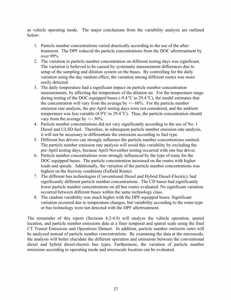
37

as vehicle operating mode. The major conclusions from the variability analysis are outlined below:

1. Particle number concentrations varied drastically according to the use of the after-treatment. The DPF reduced the particle concentrations from the DOC aftertreatment by over 99%.

2. The variation in particle number concentration on different testing days was significant. The variation is believed to be caused by systematic measurement differences due to setup of the sampling and dilution system on the buses. By controlling for the daily variation using the day random effect, the variation among different routes was more easily detected.

3. The daily temperature had a significant impact on particle number concentration measurements, by affecting the temperature of the dilution air. For the temperature range during testing of the DOC-equipped buses (-9.4 oC to 29.4 oC), the model estimates that the concentration will vary from the average by +/- 60%. For the particle number emission rate analysis, the pre-April testing days were not considered, and the ambient temperature was less variable (8.9oC to 29.4 oC). Thus, the particle concentration should vary from the average by +/- 30%.

4. Particle number concentrations did not vary significantly according to the use of No. 1 Diesel and ULSD fuel. Therefore, in subsequent particle number emission rate analysis, it will not be necessary to differentiate the emissions according to fuel type.

5. Different bus drivers can strongly influence the particle number concentrations emitted. The particle number emission rate analysis will avoid this variability by excluding the pre-April testing days, because April-November testing occurred with one bus driver.

6. Particle number concentrations were strongly influenced by the type of route for the DOC-equipped buses. The particle concentration increased on the routes with higher loads and speeds. Additionally, the variation of the particle number concentrations was highest on the freeway conditions (Enfield Route).

7. The different bus technologies (Conventional Diesel and Hybrid Diesel-Electric), had significantly different particle number concentrations. The CD buses had significantly lower particle number concentrations on all bus routes evaluated. No significant variation occurred between different buses within the same technology class.

8. The random variability was much higher with the DPF-equipped buses. Significant variation occurred due to temperature changes, but variability according to the route-type or bus technology were not detected with the DPF aftertreatment.

The remainder of this report (Sections 4.2-4.9) will analyze the vehicle operation, spatial location, and particle number emissions data at a finer temporal and spatial scale using the final CT Transit Emissions and Operations Dataset. In addition, particle number emission rates will be analyzed instead of particle number concentrations. By examining the data at the microscale, the analysis will better elucidate the different operation and emissions between the conventional diesel and hybrid diesel-electric bus types. Furthermore, the variation of particle number emissions according to operating mode and microscale location can be evaluated.

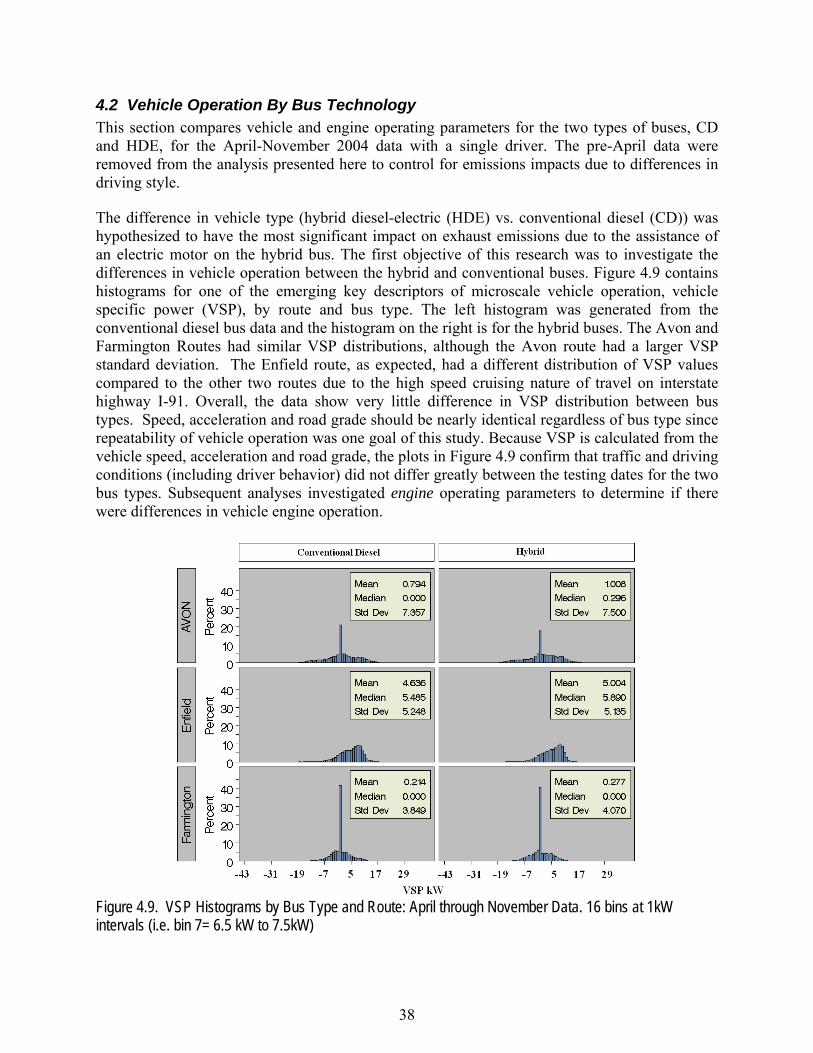
38

4.2 Vehicle Operation By Bus Technology This section compares vehicle and engine operating parameters for the two types of buses, CD and HDE, for the April-November 2004 data with a single driver. The pre-April data were removed from the analysis presented here to control for emissions impacts due to differences in driving style. The difference in vehicle type (hybrid diesel-electric (HDE) vs. conventional diesel (CD)) was hypothesized to have the most significant impact on exhaust emissions due to the assistance of an electric motor on the hybrid bus. The first objective of this research was to investigate the differences in vehicle operation between the hybrid and conventional buses. Figure 4.9 contains histograms for one of the emerging key descriptors of microscale vehicle operation, vehicle specific power (VSP), by route and bus type. The left histogram was generated from the conventional diesel bus data and the histogram on the right is for the hybrid buses. The Avon and Farmington Routes had similar VSP distributions, although the Avon route had a larger VSP standard deviation. The Enfield route, as expected, had a different distribution of VSP values compared to the other two routes due to the high speed cruising nature of travel on interstate highway I-91. Overall, the data show very little difference in VSP distribution between bus types. Speed, acceleration and road grade should be nearly identical regardless of bus type since repeatability of vehicle operation was one goal of this study. Because VSP is calculated from the vehicle speed, acceleration and road grade, the plots in Figure 4.9 confirm that traffic and driving conditions (including driver behavior) did not differ greatly between the testing dates for the two bus types. Subsequent analyses investigated engine operating parameters to determine if there were differences in vehicle engine operation.

Figure 4.9. VSP Histograms by Bus Type and Route: April through November Data. 16 bins at 1kW intervals (i.e. bin 7= 6.5 kW to 7.5kW)

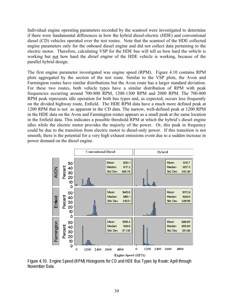
39

Individual engine operating parameters recorded by the scantool were investigated to determine if there were fundamental differences in how the hybrid diesel-electric (HDE) and conventional diesel (CD) vehicles operated over the test routes. Note that the scantool of the HDE collected engine parameters only for the onboard diesel engine and did not collect data pertaining to the electric motor. Therefore, calculating VSP for the HDE bus will tell us how hard the vehicle is working but not how hard the diesel engine of the HDE vehicle is working, because of the parallel hybrid design.

The first engine parameter investigated was engine speed (RPM). Figure 4.10 contains RPM plots aggregated by the section of the test route. Similar to the VSP plots, the Avon and Farmington routes have similar distributions but the Avon route has a larger standard deviation. For these two routes, both vehicle types have a similar distribution of RPM with peak frequencies occurring around 700-800 RPM, 1200-1300 RPM and 2000 RPM. The 700-800 RPM peak represents idle operation for both bus types and, as expected, occurs less frequently on the divided highway route, Enfield. The HDE RPM data have a much more defined peak at 1200 RPM that is not as apparent in the CD data. The narrow, well-defined peak at 1200 RPM in the HDE data on the Avon and Farmington routes appears as a small peak at the same location in the Enfield data. This indicates a possible threshold RPM at which the hybrid’s diesel engine idles while the electric motor provides the majority of the power. Or, this peak in frequency could be due to the transition from electric motor to diesel-only power. If this transition is not smooth, there is the potential for a very high exhaust emissions event due to a sudden increase in power demand on the diesel engine.

Figure 4.10. Engine Speed (RPM) Histograms for CD and HDE Bus Types by Route: April through November Data

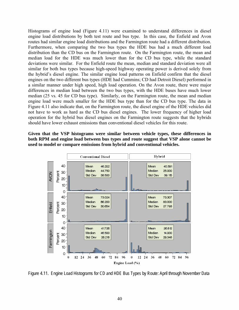
40

Histograms of engine load (Figure 4.11) were examined to understand differences in diesel engine load distributions by both test route and bus type. In this case, the Enfield and Avon routes had similar engine load distributions and the Farmington route had a different distribution. Furthermore, when comparing the two bus types the HDE bus had a much different load distribution than the CD bus on the Farmington route. On the Farmington route, the mean and median load for the HDE was much lower than for the CD bus type, while the standard deviations were similar. For the Enfield route the mean, median and standard deviation were all similar for both bus types because high-speed highway operating power is derived solely from the hybrid’s diesel engine. The similar engine load patterns on Enfield confirm that the diesel engines on the two different bus types (HDE had Cummins; CD had Detroit Diesel) performed in a similar manner under high speed, high load operation. On the Avon route, there were major differences in median load between the two bus types, with the HDE buses have much lower median (25 vs. 45 for CD bus type). Similarly, on the Farmington route, the mean and median engine load were much smaller for the HDE bus type than for the CD bus type. The data in Figure 4.11 also indicate that, on the Farmington route, the diesel engine of the HDE vehicles did not have to work as hard as the CD bus diesel engines. The lower frequency of higher load operation for the hybrid bus diesel engines on the Farmington route suggests that the hybrids should have lower exhaust emissions than conventional diesel vehicles for this route. Given that the VSP histograms were similar between vehicle types, these differences in both RPM and engine load between bus types and route suggest that VSP alone cannot be used to model or compare emissions from hybrid and conventional vehicles.

Figure 4.11. Engine Load Histograms for CD and HDE Bus Types by Route: April through November Data

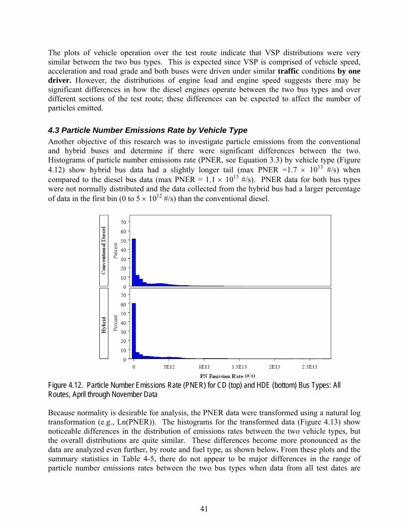
41

The plots of vehicle operation over the test route indicate that VSP distributions were very similar between the two bus types. This is expected since VSP is comprised of vehicle speed, acceleration and road grade and both buses were driven under similar traffic conditions by one driver. However, the distributions of engine load and engine speed suggests there may be significant differences in how the diesel engines operate between the two bus types and over different sections of the test route; these differences can be expected to affect the number of particles emitted.

4.3 Particle Number Emissions Rate by Vehicle Type Another objective of this research was to investigate particle emissions from the conventional and hybrid buses and determine if there were significant differences between the two. Histograms of particle number emissions rate (PNER, see Equation 3.3) by vehicle type (Figure 4.12) show hybrid bus data had a slightly longer tail (max PNER =1.7 × 1013 #/s) when compared to the diesel bus data (max PNER = 1.1 × 1013 #/s). PNER data for both bus types were not normally distributed and the data collected from the hybrid bus had a larger percentage of data in the first bin (0 to 5 × 1012 #/s) than the conventional diesel.

Figure 4.12. Particle Number Emissions Rate (PNER) for CD (top) and HDE (bottom) Bus Types: All Routes, April through November Data

Because normality is desirable for analysis, the PNER data were transformed using a natural log transformation (e.g., Ln(PNER)). The histograms for the transformed data (Figure 4.13) show noticeable differences in the distribution of emissions rates between the two vehicle types, but the overall distributions are quite similar. These differences become more pronounced as the data are analyzed even further, by route and fuel type, as shown below. From these plots and the summary statistics in Table 4-5, there do not appear to be major differences in the range of particle number emissions rates between the two bus types when data from all test dates are

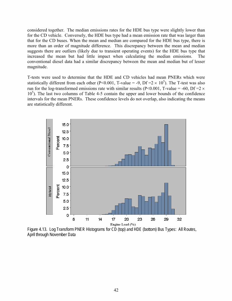
42

considered together. The median emissions rates for the HDE bus type were slightly lower than for the CD vehicle. Conversely, the HDE bus type had a mean emission rate that was larger than that for the CD buses. When the mean and median are compared for the HDE bus type, there is more than an order of magnitude difference. This discrepancy between the mean and median suggests there are outliers (likely due to transient operating events) for the HDE bus type that increased the mean but had little impact when calculating the median emissions. The conventional diesel data had a similar discrepancy between the mean and median but of lesser magnitude. T-tests were used to determine that the HDE and CD vehicles had mean PNERs which were statistically different from each other (P<0.001, T-value = -9, Df =2 × 105). The T-test was also run for the log-transformed emissions rate with similar results (P<0.001, T-value = -60, Df =2 × 105). The last two columns of Table 4-5 contain the upper and lower bounds of the confidence intervals for the mean PNERs. These confidence levels do not overlap, also indicating the means are statistically different.

Figure 4.13. Log Transform PNER Histograms for CD (top) and HDE (bottom) Bus Types: All Routes, April through November Data

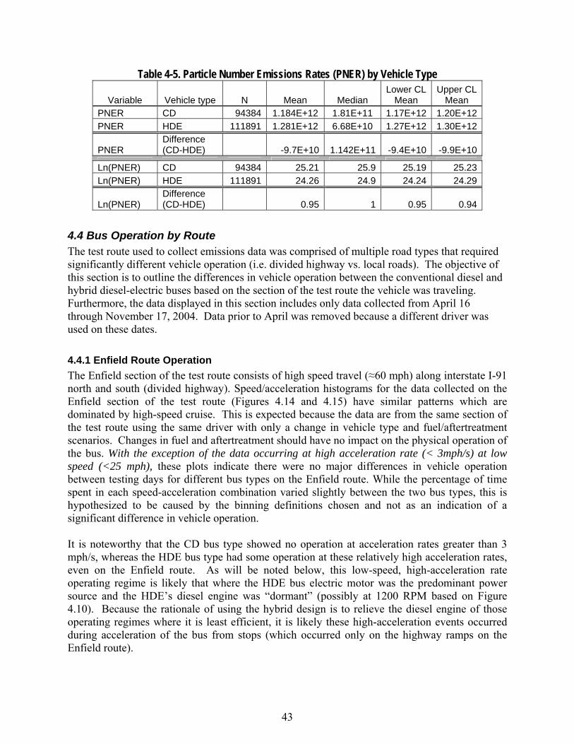
43

Table 4-5. Particle Number Emissions Rates (PNER) by Vehicle Type

Variable Vehicle type N Mean Median Lower CL

Mean Upper CL

Mean PNER CD 94384 1.184E+12 1.81E+11 1.17E+12 1.20E+12PNER HDE 111891 1.281E+12 6.68E+10 1.27E+12 1.30E+12

PNER Difference (CD-HDE) -9.7E+10 1.142E+11 -9.4E+10 -9.9E+10

Ln(PNER) CD 94384 25.21 25.9 25.19 25.23Ln(PNER) HDE 111891 24.26 24.9 24.24 24.29

Ln(PNER) Difference (CD-HDE) 0.95 1 0.95 0.94

4.4 Bus Operation by Route The test route used to collect emissions data was comprised of multiple road types that required significantly different vehicle operation (i.e. divided highway vs. local roads). The objective of this section is to outline the differences in vehicle operation between the conventional diesel and hybrid diesel-electric buses based on the section of the test route the vehicle was traveling. Furthermore, the data displayed in this section includes only data collected from April 16 through November 17, 2004. Data prior to April was removed because a different driver was used on these dates.

4.4.1 Enfield Route Operation The Enfield section of the test route consists of high speed travel (≈60 mph) along interstate I-91 north and south (divided highway). Speed/acceleration histograms for the data collected on the Enfield section of the test route (Figures 4.14 and 4.15) have similar patterns which are dominated by high-speed cruise. This is expected because the data are from the same section of the test route using the same driver with only a change in vehicle type and fuel/aftertreatment scenarios. Changes in fuel and aftertreatment should have no impact on the physical operation of the bus. With the exception of the data occurring at high acceleration rate (< 3mph/s) at low speed (<25 mph), these plots indicate there were no major differences in vehicle operation between testing days for different bus types on the Enfield route. While the percentage of time spent in each speed-acceleration combination varied slightly between the two bus types, this is hypothesized to be caused by the binning definitions chosen and not as an indication of a significant difference in vehicle operation. It is noteworthy that the CD bus type showed no operation at acceleration rates greater than 3 mph/s, whereas the HDE bus type had some operation at these relatively high acceleration rates, even on the Enfield route. As will be noted below, this low-speed, high-acceleration rate operating regime is likely that where the HDE bus electric motor was the predominant power source and the HDE’s diesel engine was “dormant” (possibly at 1200 RPM based on Figure 4.10). Because the rationale of using the hybrid design is to relieve the diesel engine of those operating regimes where it is least efficient, it is likely these high-acceleration events occurred during acceleration of the bus from stops (which occurred only on the highway ramps on the Enfield route).

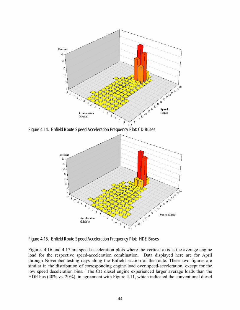
44

Figure 4.14. Enfield Route Speed Acceleration Frequency Plot: CD Buses

Figure 4.15. Enfield Route Speed Acceleration Frequency Plot: HDE Buses

Figures 4.16 and 4.17 are speed-acceleration plots where the vertical axis is the average engine load for the respective speed-acceleration combination. Data displayed here are for April through November testing days along the Enfield section of the route. These two figures are similar in the distribution of corresponding engine load over speed-acceleration, except for the low speed deceleration bins. The CD diesel engine experienced larger average loads than the HDE bus (40% vs. 20%), in agreement with Figure 4.11, which indicated the conventional diesel

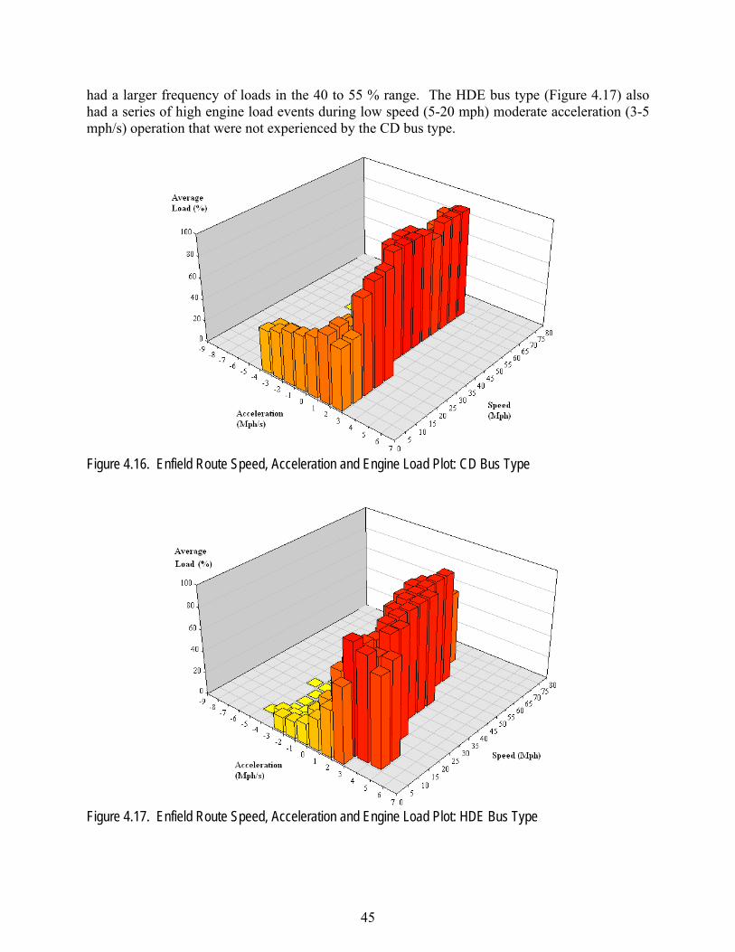
45

had a larger frequency of loads in the 40 to 55 % range. The HDE bus type (Figure 4.17) also had a series of high engine load events during low speed (5-20 mph) moderate acceleration (3-5 mph/s) operation that were not experienced by the CD bus type.

Figure 4.16. Enfield Route Speed, Acceleration and Engine Load Plot: CD Bus Type

Figure 4.17. Enfield Route Speed, Acceleration and Engine Load Plot: HDE Bus Type

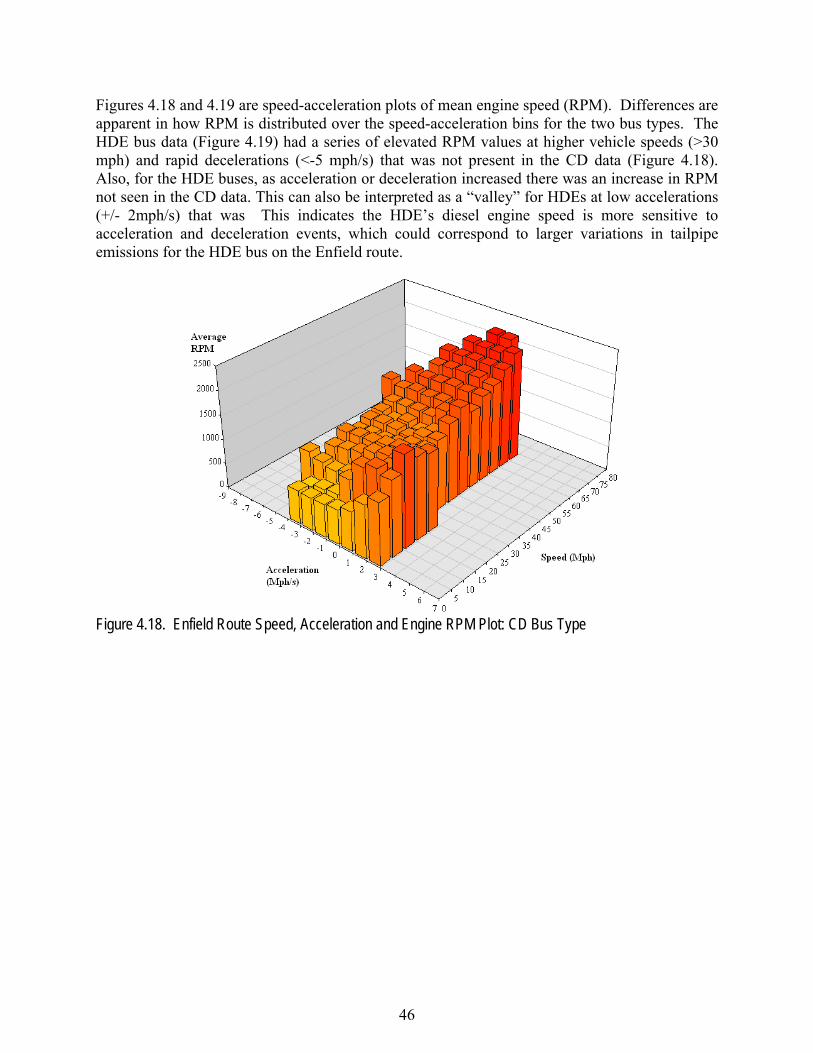
46

Figures 4.18 and 4.19 are speed-acceleration plots of mean engine speed (RPM). Differences are apparent in how RPM is distributed over the speed-acceleration bins for the two bus types. The HDE bus data (Figure 4.19) had a series of elevated RPM values at higher vehicle speeds (>30 mph) and rapid decelerations (<-5 mph/s) that was not present in the CD data (Figure 4.18). Also, for the HDE buses, as acceleration or deceleration increased there was an increase in RPM not seen in the CD data. This can also be interpreted as a “valley” for HDEs at low accelerations (+/- 2mph/s) that was This indicates the HDE’s diesel engine speed is more sensitive to acceleration and deceleration events, which could correspond to larger variations in tailpipe emissions for the HDE bus on the Enfield route.

Figure 4.18. Enfield Route Speed, Acceleration and Engine RPM Plot: CD Bus Type

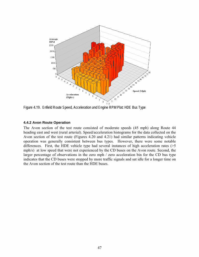
47

Figure 4.19. Enfield Route Speed, Acceleration and Engine RPM Plot: HDE Bus Type

4.4.2 Avon Route Operation The Avon section of the test route consisted of moderate speeds (45 mph) along Route 44 heading east and west (rural arterial). Speed/acceleration histograms for the data collected on the Avon section of the test route (Figures 4.20 and 4.21) had similar patterns indicating vehicle operation was generally consistent between bus types. However, there were some notable differences. First, the HDE vehicle type had several instances of high acceleration rates (>5 mph/s) at low speed that were not experienced by the CD buses on the Avon route. Second, the larger percentage of observations in the zero mph / zero acceleration bin for the CD bus type indicates that the CD buses were stopped by more traffic signals and sat idle for a longer time on the Avon section of the test route than the HDE buses.

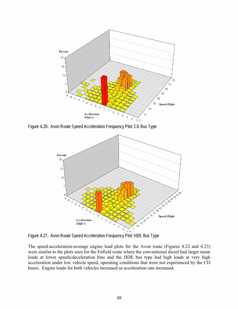
48

Figure 4.20. Avon Route Speed Acceleration Frequency Plot: CD Bus Type

Figure 4.21. Avon Route Speed Acceleration Frequency Plot: HDE Bus Type

The speed-acceleration-average engine load plots for the Avon route (Figures 4.22 and 4.23) were similar to the plots seen for the Enfield route where the conventional diesel had larger mean loads at lower speeds/deceleration bins and the HDE bus type had high loads at very high acceleration under low vehicle speed, operating conditions that were not experienced by the CD buses. Engine loads for both vehicles increased as acceleration rate increased.

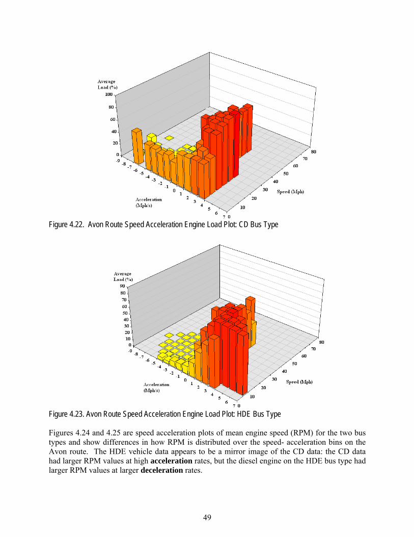
49

Figure 4.22. Avon Route Speed Acceleration Engine Load Plot: CD Bus Type

Figure 4.23. Avon Route Speed Acceleration Engine Load Plot: HDE Bus Type

Figures 4.24 and 4.25 are speed acceleration plots of mean engine speed (RPM) for the two bus types and show differences in how RPM is distributed over the speed- acceleration bins on the Avon route. The HDE vehicle data appears to be a mirror image of the CD data: the CD data had larger RPM values at high acceleration rates, but the diesel engine on the HDE bus type had larger RPM values at larger deceleration rates.

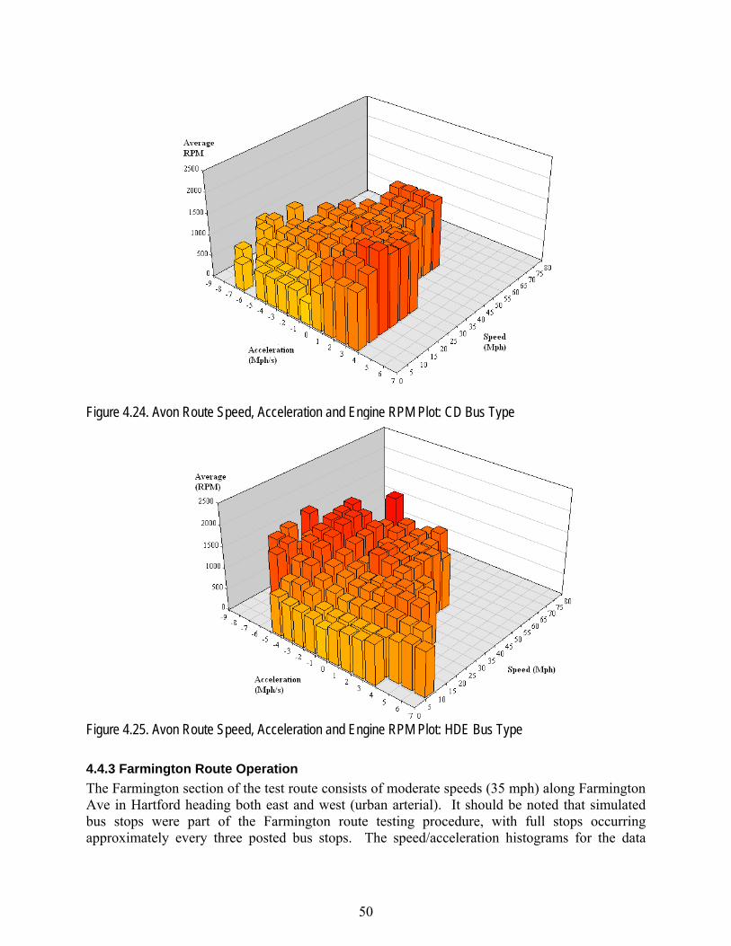
50

Figure 4.24. Avon Route Speed, Acceleration and Engine RPM Plot: CD Bus Type

Figure 4.25. Avon Route Speed, Acceleration and Engine RPM Plot: HDE Bus Type

4.4.3 Farmington Route Operation The Farmington section of the test route consists of moderate speeds (35 mph) along Farmington Ave in Hartford heading both east and west (urban arterial). It should be noted that simulated bus stops were part of the Farmington route testing procedure, with full stops occurring approximately every three posted bus stops. The speed/acceleration histograms for the data

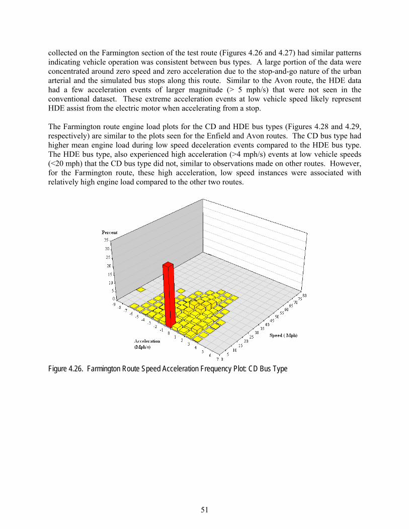
51

collected on the Farmington section of the test route (Figures 4.26 and 4.27) had similar patterns indicating vehicle operation was consistent between bus types. A large portion of the data were concentrated around zero speed and zero acceleration due to the stop-and-go nature of the urban arterial and the simulated bus stops along this route. Similar to the Avon route, the HDE data had a few acceleration events of larger magnitude (> 5 mph/s) that were not seen in the conventional dataset. These extreme acceleration events at low vehicle speed likely represent HDE assist from the electric motor when accelerating from a stop.

The Farmington route engine load plots for the CD and HDE bus types (Figures 4.28 and 4.29, respectively) are similar to the plots seen for the Enfield and Avon routes. The CD bus type had higher mean engine load during low speed deceleration events compared to the HDE bus type. The HDE bus type, also experienced high acceleration (>4 mph/s) events at low vehicle speeds (<20 mph) that the CD bus type did not, similar to observations made on other routes. However, for the Farmington route, these high acceleration, low speed instances were associated with relatively high engine load compared to the other two routes.

Figure 4.26. Farmington Route Speed Acceleration Frequency Plot: CD Bus Type

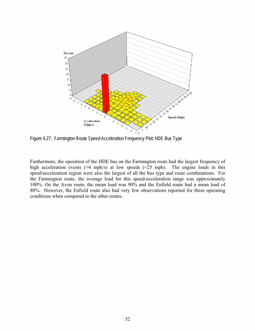
52

Figure 4.27. Farmington Route Speed Acceleration Frequency Plot: HDE Bus Type

Furthermore, the operation of the HDE bus on the Farmington route had the largest frequency of high acceleration events (>4 mph/s) at low speeds (<25 mph). The engine loads in this speed/acceleration region were also the largest of all the bus type and route combinations. For the Farmington route, the average load for this speed-acceleration range was approximately 100%. On the Avon route, the mean load was 90% and the Enfield route had a mean load of 80%. However, the Enfield route also had very few observations reported for these operating conditions when compared to the other routes.

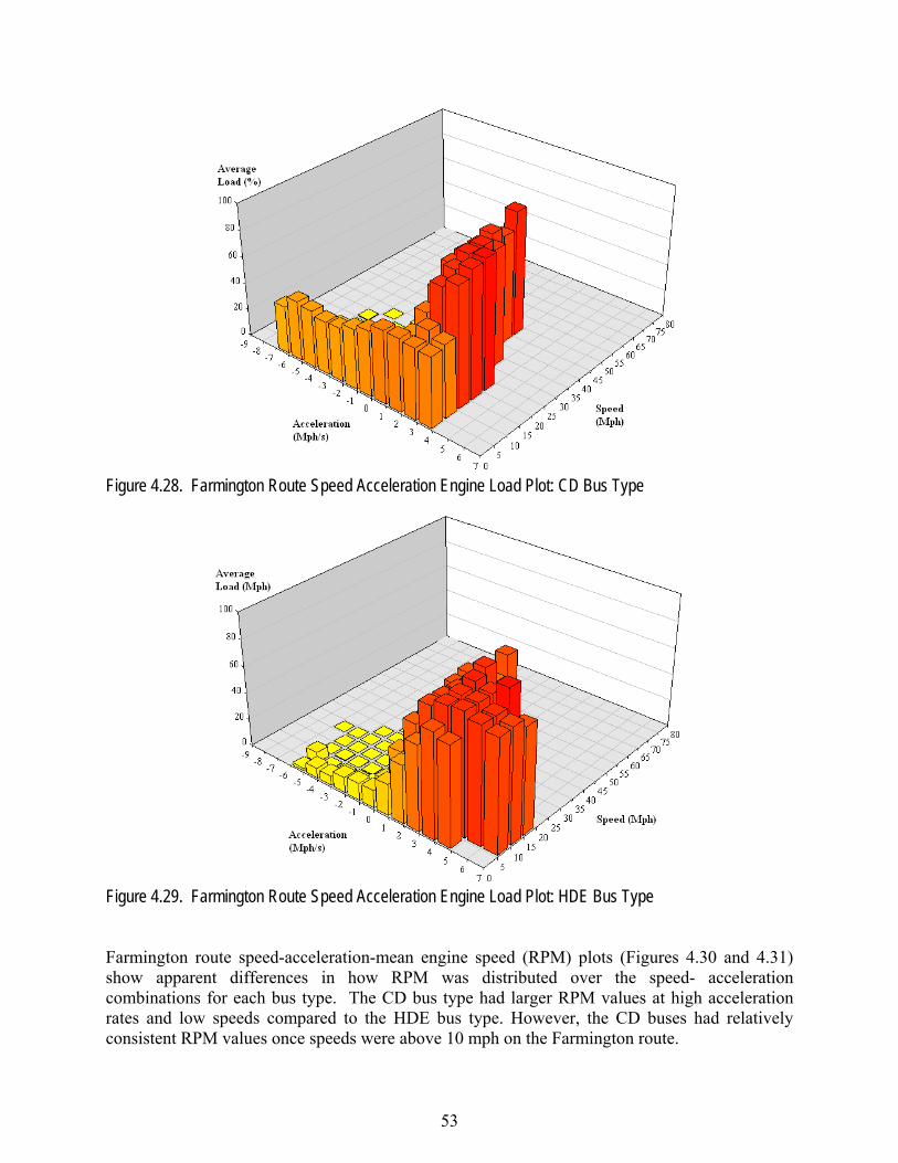
53

Figure 4.28. Farmington Route Speed Acceleration Engine Load Plot: CD Bus Type

Figure 4.29. Farmington Route Speed Acceleration Engine Load Plot: HDE Bus Type

Farmington route speed-acceleration-mean engine speed (RPM) plots (Figures 4.30 and 4.31) show apparent differences in how RPM was distributed over the speed- acceleration combinations for each bus type. The CD bus type had larger RPM values at high acceleration rates and low speeds compared to the HDE bus type. However, the CD buses had relatively consistent RPM values once speeds were above 10 mph on the Farmington route.

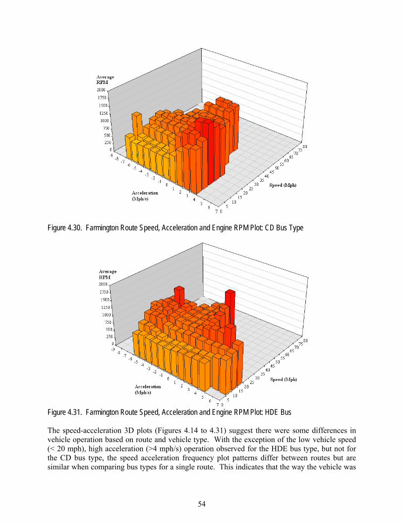
54

Figure 4.30. Farmington Route Speed, Acceleration and Engine RPM Plot: CD Bus Type

Figure 4.31. Farmington Route Speed, Acceleration and Engine RPM Plot: HDE Bus

The speed-acceleration 3D plots (Figures 4.14 to 4.31) suggest there were some differences in vehicle operation based on route and vehicle type. With the exception of the low vehicle speed (< 20 mph), high acceleration (>4 mph/s) operation observed for the HDE bus type, but not for the CD bus type, the speed acceleration frequency plot patterns differ between routes but are similar when comparing bus types for a single route. This indicates that the way the vehicle was

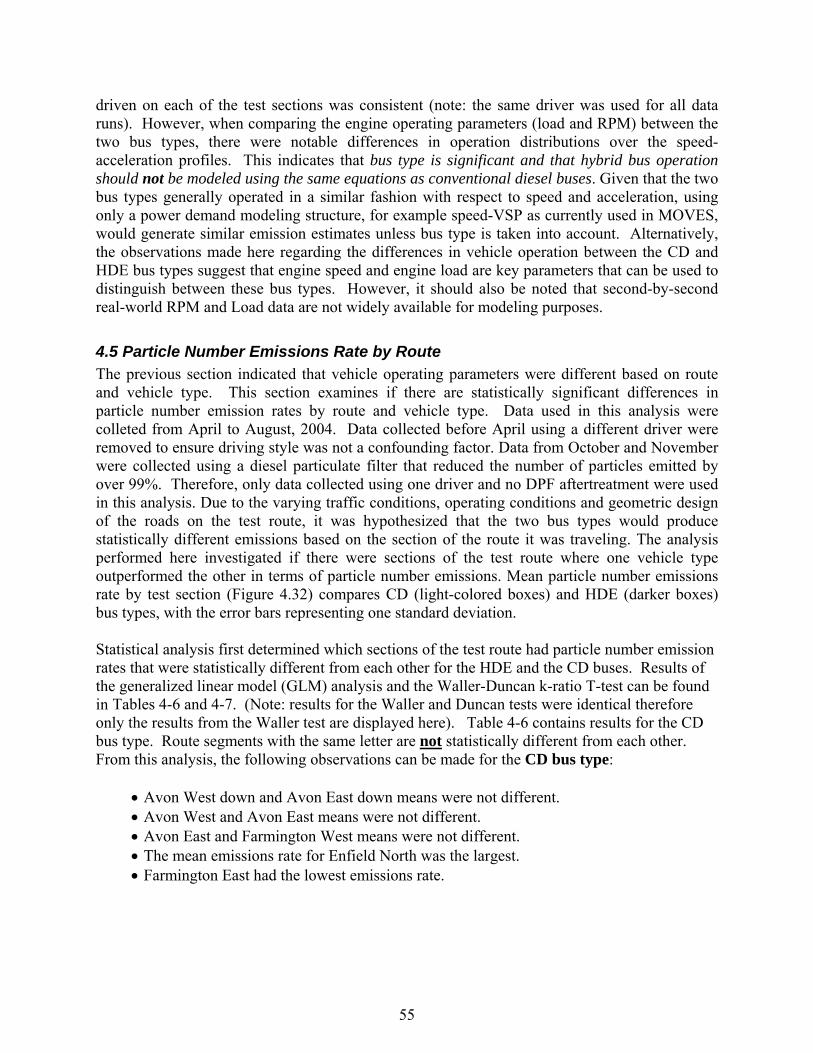
55

driven on each of the test sections was consistent (note: the same driver was used for all data runs). However, when comparing the engine operating parameters (load and RPM) between the two bus types, there were notable differences in operation distributions over the speed-acceleration profiles. This indicates that bus type is significant and that hybrid bus operation should not be modeled using the same equations as conventional diesel buses. Given that the two bus types generally operated in a similar fashion with respect to speed and acceleration, using only a power demand modeling structure, for example speed-VSP as currently used in MOVES, would generate similar emission estimates unless bus type is taken into account. Alternatively, the observations made here regarding the differences in vehicle operation between the CD and HDE bus types suggest that engine speed and engine load are key parameters that can be used to distinguish between these bus types. However, it should also be noted that second-by-second real-world RPM and Load data are not widely available for modeling purposes.

4.5 Particle Number Emissions Rate by Route The previous section indicated that vehicle operating parameters were different based on route and vehicle type. This section examines if there are statistically significant differences in particle number emission rates by route and vehicle type. Data used in this analysis were colleted from April to August, 2004. Data collected before April using a different driver were removed to ensure driving style was not a confounding factor. Data from October and November were collected using a diesel particulate filter that reduced the number of particles emitted by over 99%. Therefore, only data collected using one driver and no DPF aftertreatment were used in this analysis. Due to the varying traffic conditions, operating conditions and geometric design of the roads on the test route, it was hypothesized that the two bus types would produce statistically different emissions based on the section of the route it was traveling. The analysis performed here investigated if there were sections of the test route where one vehicle type outperformed the other in terms of particle number emissions. Mean particle number emissions rate by test section (Figure 4.32) compares CD (light-colored boxes) and HDE (darker boxes) bus types, with the error bars representing one standard deviation.

Statistical analysis first determined which sections of the test route had particle number emission rates that were statistically different from each other for the HDE and the CD buses. Results of the generalized linear model (GLM) analysis and the Waller-Duncan k-ratio T-test can be found in Tables 4-6 and 4-7. (Note: results for the Waller and Duncan tests were identical therefore only the results from the Waller test are displayed here). Table 4-6 contains results for the CD bus type. Route segments with the same letter are not statistically different from each other. From this analysis, the following observations can be made for the CD bus type:

• Avon West down and Avon East down means were not different. • Avon West and Avon East means were not different. • Avon East and Farmington West means were not different. • The mean emissions rate for Enfield North was the largest. • Farmington East had the lowest emissions rate.

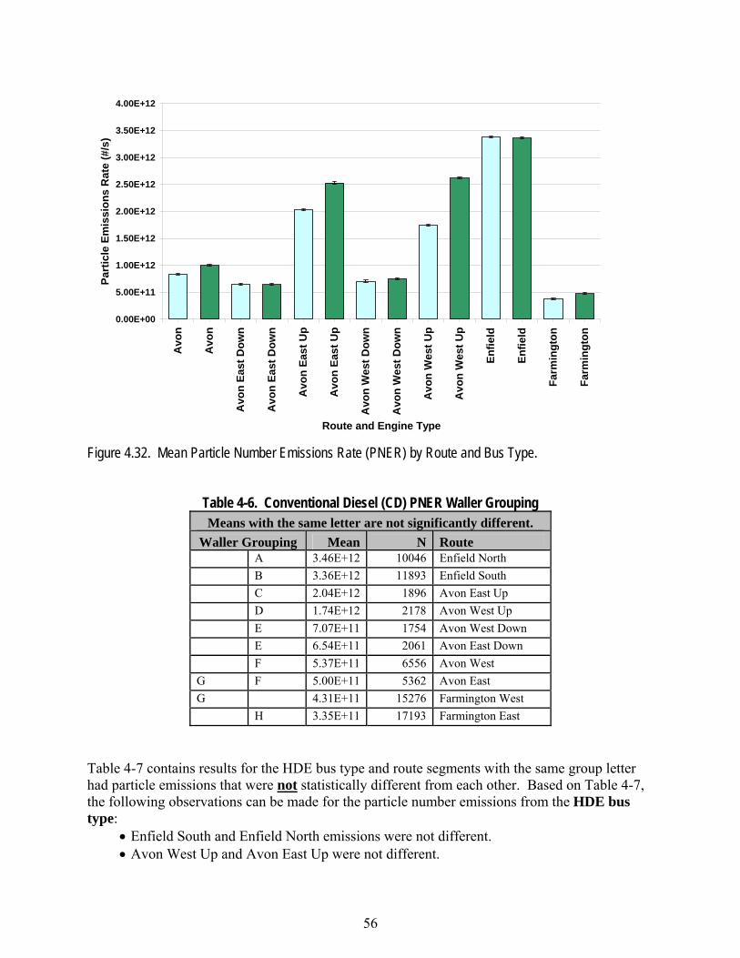
56

0.00E+00

5.00E+11

1.00E+12

1.50E+12

2.00E+12

2.50E+12

3.00E+12

3.50E+12

4.00E+12

Avo

n

Avo

n

Avo

n Ea

st D

own

Avo

n Ea

st D

own

Avo

n Ea

st U

p

Avo

n Ea

st U

p

Avo

n W

est D

own

Avo

n W

est D

own

Avo

n W

est U

p

Avo

n W

est U

p

Enfie

ld

Enfie

ld

Farm

ingt

on

Farm

ingt

on

Route and Engine Type

Part

icle

Em

issi

ons

Rat

e (#

/s)

Figure 4.32. Mean Particle Number Emissions Rate (PNER) by Route and Bus Type.

Table 4-6. Conventional Diesel (CD) PNER Waller Grouping Means with the same letter are not significantly different.

Waller Grouping Mean N Route A 3.46E+12 10046 Enfield North B 3.36E+12 11893 Enfield South C 2.04E+12 1896 Avon East Up D 1.74E+12 2178 Avon West Up E 7.07E+11 1754 Avon West Down E 6.54E+11 2061 Avon East Down F 5.37E+11 6556 Avon West G F 5.00E+11 5362 Avon East G 4.31E+11 15276 Farmington West H 3.35E+11 17193 Farmington East

Table 4-7 contains results for the HDE bus type and route segments with the same group letter had particle emissions that were not statistically different from each other. Based on Table 4-7, the following observations can be made for the particle number emissions from the HDE bus type:

• Enfield South and Enfield North emissions were not different. • Avon West Up and Avon East Up were not different.

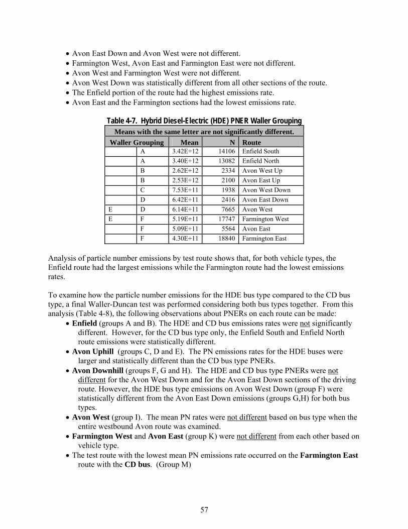
57

• Avon East Down and Avon West were not different. • Farmington West, Avon East and Farmington East were not different. • Avon West and Farmington West were not different. • Avon West Down was statistically different from all other sections of the route. • The Enfield portion of the route had the highest emissions rate. • Avon East and the Farmington sections had the lowest emissions rate.

Table 4-7. Hybrid Diesel-Electric (HDE) PNER Waller Grouping

Means with the same letter are not significantly different. Waller Grouping Mean N Route A 3.42E+12 14106 Enfield South A 3.40E+12 13082 Enfield North B 2.62E+12 2334 Avon West Up B 2.53E+12 2100 Avon East Up C 7.53E+11 1938 Avon West Down D 6.42E+11 2416 Avon East Down E D 6.14E+11 7665 Avon West E F 5.19E+11 17747 Farmington West F 5.09E+11 5564 Avon East F 4.30E+11 18840 Farmington East

Analysis of particle number emissions by test route shows that, for both vehicle types, the Enfield route had the largest emissions while the Farmington route had the lowest emissions rates. To examine how the particle number emissions for the HDE bus type compared to the CD bus type, a final Waller-Duncan test was performed considering both bus types together. From this analysis (Table 4-8), the following observations about PNERs on each route can be made:

• Enfield (groups A and B). The HDE and CD bus emissions rates were not significantly different. However, for the CD bus type only, the Enfield South and Enfield North route emissions were statistically different.

• Avon Uphill (groups C, D and E). The PN emissions rates for the HDE buses were larger and statistically different than the CD bus type PNERs.

• Avon Downhill (groups F, G and H). The HDE and CD bus type PNERs were not different for the Avon West Down and for the Avon East Down sections of the driving route. However, the HDE bus type emissions on Avon West Down (group F) were statistically different from the Avon East Down emissions (groups G,H) for both bus types.

• Avon West (group I). The mean PN rates were not different based on bus type when the entire westbound Avon route was examined.

• Farmington West and Avon East (group K) were not different from each other based on vehicle type.

• The test route with the lowest mean PN emissions rate occurred on the Farmington East route with the CD bus. (Group M)

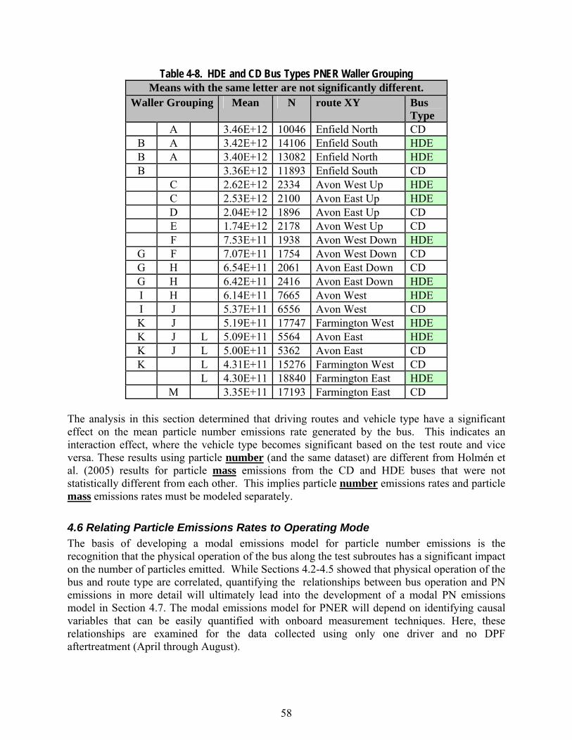
58

Table 4-8. HDE and CD Bus Types PNER Waller Grouping Means with the same letter are not significantly different.

Waller Grouping Mean N route XY Bus Type

A 3.46E+12 10046 Enfield North CD B A 3.42E+12 14106 Enfield South HDE B A 3.40E+12 13082 Enfield North HDE B 3.36E+12 11893 Enfield South CD C 2.62E+12 2334 Avon West Up HDE C 2.53E+12 2100 Avon East Up HDE D 2.04E+12 1896 Avon East Up CD E 1.74E+12 2178 Avon West Up CD F 7.53E+11 1938 Avon West Down HDE

G F 7.07E+11 1754 Avon West Down CD G H 6.54E+11 2061 Avon East Down CD G H 6.42E+11 2416 Avon East Down HDE I H 6.14E+11 7665 Avon West HDE I J 5.37E+11 6556 Avon West CD K J 5.19E+11 17747 Farmington West HDE K J L 5.09E+11 5564 Avon East HDE K J L 5.00E+11 5362 Avon East CD K L 4.31E+11 15276 Farmington West CD L 4.30E+11 18840 Farmington East HDE M 3.35E+11 17193 Farmington East CD

The analysis in this section determined that driving routes and vehicle type have a significant effect on the mean particle number emissions rate generated by the bus. This indicates an interaction effect, where the vehicle type becomes significant based on the test route and vice versa. These results using particle number (and the same dataset) are different from Holmén et al. (2005) results for particle mass emissions from the CD and HDE buses that were not statistically different from each other. This implies particle number emissions rates and particle mass emissions rates must be modeled separately.

4.6 Relating Particle Emissions Rates to Operating Mode The basis of developing a modal emissions model for particle number emissions is the recognition that the physical operation of the bus along the test subroutes has a significant impact on the number of particles emitted. While Sections 4.2-4.5 showed that physical operation of the bus and route type are correlated, quantifying the relationships between bus operation and PN emissions in more detail will ultimately lead into the development of a modal PN emissions model in Section 4.7. The modal emissions model for PNER will depend on identifying causal variables that can be easily quantified with onboard measurement techniques. Here, these relationships are examined for the data collected using only one driver and no DPF aftertreatment (April through August).

59

4.6.1 Vehicle Specific Power and Number Emissions As mentioned earlier, VSP incorporates speed, acceleration and road grade to estimate the power demand on a vehicle’s engine. This estimate of power demand can then be used to estimate tailpipe emissions and has been incorporated into MOVES for modal emissions estimates of the gaseous pollutants. However, the link between VSP and particle number emissions has not been previously established. Box plots (Figures 4.33 to 4.36) display the relationships between PNER and vehicle operating parameters by bus type over all routes. In these box plots, the median is represented by the horizontal line within the box, the mean is represented by a black cross and the upper and lower quartiles are represented by the extent of the boxed region. The whiskers on the box plot extend 1.5 times the inter-quartile range beyond the upper and lower quartiles and the outliers are represented by circles. Figure 4.33 contains box plots of PN emissions rate by MOVES VSP bin (see Table 1-3 for bin definitions) by bus type. Recall that bin 0 is deceleration, bin 1 is idle and the rest of the increasing bin numbers correspond to an increasing speed/VSP combination. From Figure 4.33 it is apparent that as the VSP bin number increased there was an increase in mean (and median) PNER. Furthermore, there was an increase in the variability of these emissions rates shown by the increasing height of the boxes. When comparing across bus types, the HDE bus had much more variability in PNER than the CD bus type (length of box and whiskers). Furthermore, at the high end of the MOVES VSP bins the HDE variability, mean and median in PNER were greater than for the CD bus type. Figure 4.34 shows the relationship between VSP for each bus type when binned solely by VSP value (i.e., bin 5 is comprised of VSPs from 2.5 to 7.5). While there is still a relationship between PNER and VSP it is not as clearly defined as the one seen when using the MOVES binning system. Therefore, the data confirm the importance of incorporating vehicle speed along with VSP in any models estimating particle number emission rate.

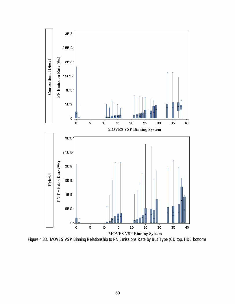
60

Figure 4.33. MOVES VSP Binning Relationship to PN Emissions Rate by Bus Type (CD top, HDE bottom)

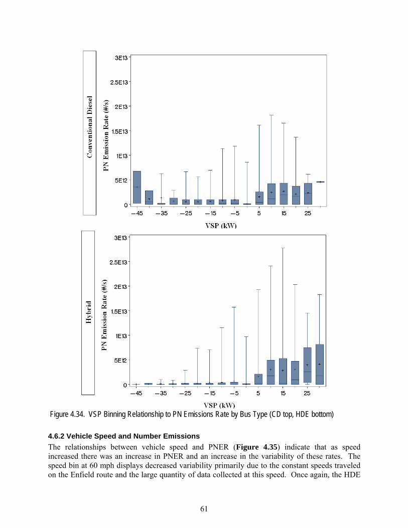
61

Figure 4.34. VSP Binning Relationship to PN Emissions Rate by Bus Type (CD top, HDE bottom) 4.6.2 Vehicle Speed and Number Emissions The relationships between vehicle speed and PNER (Figure 4.35) indicate that as speed increased there was an increase in PNER and an increase in the variability of these rates. The speed bin at 60 mph displays decreased variability primarily due to the constant speeds traveled on the Enfield route and the large quantity of data collected at this speed. Once again, the HDE

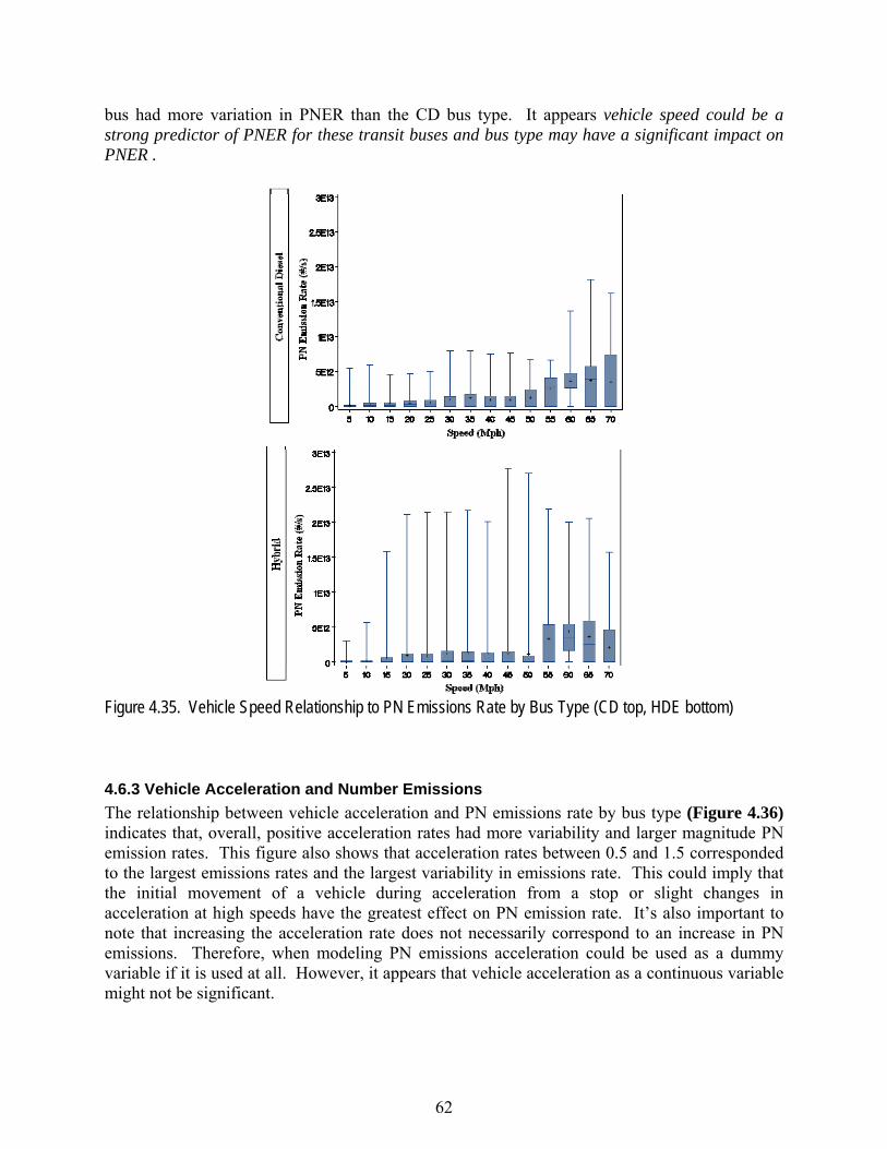
62

bus had more variation in PNER than the CD bus type. It appears vehicle speed could be a strong predictor of PNER for these transit buses and bus type may have a significant impact on PNER .

Figure 4.35. Vehicle Speed Relationship to PN Emissions Rate by Bus Type (CD top, HDE bottom) 4.6.3 Vehicle Acceleration and Number Emissions The relationship between vehicle acceleration and PN emissions rate by bus type (Figure 4.36) indicates that, overall, positive acceleration rates had more variability and larger magnitude PN emission rates. This figure also shows that acceleration rates between 0.5 and 1.5 corresponded to the largest emissions rates and the largest variability in emissions rate. This could imply that the initial movement of a vehicle during acceleration from a stop or slight changes in acceleration at high speeds have the greatest effect on PN emission rate. It’s also important to note that increasing the acceleration rate does not necessarily correspond to an increase in PN emissions. Therefore, when modeling PN emissions acceleration could be used as a dummy variable if it is used at all. However, it appears that vehicle acceleration as a continuous variable might not be significant.

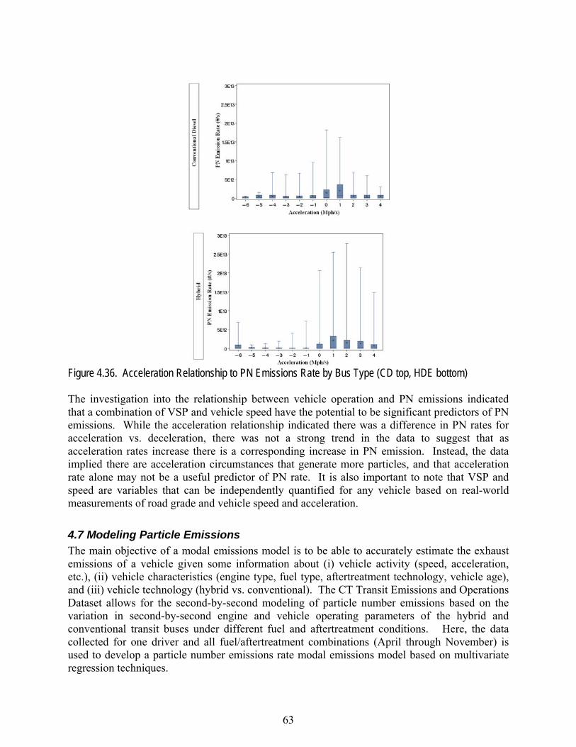
63

Figure 4.36. Acceleration Relationship to PN Emissions Rate by Bus Type (CD top, HDE bottom)

The investigation into the relationship between vehicle operation and PN emissions indicated that a combination of VSP and vehicle speed have the potential to be significant predictors of PN emissions. While the acceleration relationship indicated there was a difference in PN rates for acceleration vs. deceleration, there was not a strong trend in the data to suggest that as acceleration rates increase there is a corresponding increase in PN emission. Instead, the data implied there are acceleration circumstances that generate more particles, and that acceleration rate alone may not be a useful predictor of PN rate. It is also important to note that VSP and speed are variables that can be independently quantified for any vehicle based on real-world measurements of road grade and vehicle speed and acceleration.

4.7 Modeling Particle Emissions The main objective of a modal emissions model is to be able to accurately estimate the exhaust emissions of a vehicle given some information about (i) vehicle activity (speed, acceleration, etc.), (ii) vehicle characteristics (engine type, fuel type, aftertreatment technology, vehicle age), and (iii) vehicle technology (hybrid vs. conventional). The CT Transit Emissions and Operations Dataset allows for the second-by-second modeling of particle number emissions based on the variation in second-by-second engine and vehicle operating parameters of the hybrid and conventional transit buses under different fuel and aftertreatment conditions. Here, the data collected for one driver and all fuel/aftertreatment combinations (April through November) is used to develop a particle number emissions rate modal emissions model based on multivariate regression techniques.

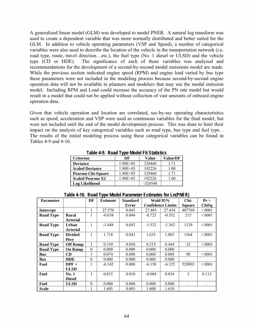
64

A generalized linear model (GLM) was developed to model PNER. A natural log transform was used to create a dependent variable that was more normally distributed and better suited for the GLM. In addition to vehicle operating parameters (VSP and Speed), a number of categorical variables were also used to describe the location of the vehicle in the transportation network (i.e. road type, route, travel direction…etc.), the fuel type (No. 1 diesel or ULSD) and the vehicle type (CD or HDE). The significance of each of these variables was analyzed and recommendations for the development of a second-by-second modal emissions model are made. While the previous section indicated engine speed (RPM) and engine load varied by bus type these parameters were not included in the modeling process because second-by-second engine operation data will not be available to planners and modelers that may use the modal emission model. Including RPM and Load could increase the accuracy of the PN rate model but would result in a model that could not be applied without collection of vast amounts of onboard engine operation data.

Given that vehicle operation and location are correlated, sec-by-sec operating characteristics such as speed, acceleration and VSP were used as continuous variables for the final model, but were not included until the end of the model development process. This was done to limit their impact on the analysis of key categorical variables such as road type, bus type and fuel type. . The results of the initial modeling process using these categorical variables can be found in Tables 4-9 and 4-10.

Table 4-9. Road Type Model Fit Statistics Criterion DF Value Value/DF Deviance 1.90E+05 329460 1.71 Scaled Deviance 1.90E+05 192226 1.00 Pearson Chi-Square 1.90E+05 329460 1.71 Scaled Pearson X2 1.90E+05 192226 1.00 Log Likelihood -324540

Table 4-10. Road Type Model Parameter Estimates for Ln(PNER)

Parameter DF Estimate Standard Error

Wald 95% Confidence Limits

Chi-Square

Pr > ChiSq

Intercept 1 27.570 0.043 27.485 27.654 407769 <.0001 Road Type Rural

Arterial 1 -0.638 0.044 -0.723 -0.552 215 <.0001

Road Type Urban Arterial

1 -1.448 0.043 -1.532 -1.363 1129 <.0001

Road Type Divided Hwy

1 1.718 0.043 1.633 1.803 1564 <.0001

Road Type Off Ramp 1 0.330 0.058 0.215 0.444 32 <.0001 Road Type On Ramp 0 0.000 0.000 0.000 0.000 . . Bus CD 1 0.074 0.008 0.060 0.089 98 <.0001 Bus HDE 0 0.000 0.000 0.000 0.000 . . Fuel DPF +

ULSD 1 -6.142 0.008 -6.158 -6.125 528903 <.0001

Fuel No. 1 Diesel

1 0.015 0.010 -0.004 0.034 3 0.113

Fuel ULSD 0 0.000 0.000 0.000 0.000 . . Scale 1 1.605 0.003 1.600 1.610

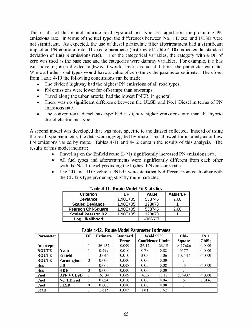
65

The results of this model indicate road type and bus type are significant for predicting PN emissions rate. In terms of the fuel type, the differences between No. 1 Diesel and ULSD were not significant. As expected, the use of diesel particulate filter aftertreatment had a significant impact on PN emission rate. The scale parameter (last row of Table 4-10) indicates the standard deviation of Ln(PN emissions rate). For the categorical variables, the category with a DF of zero was used as the base case and the categories were dummy variables. For example, if a bus was traveling on a divided highway it would have a value of 1 times the parameter estimate. While all other road types would have a value of zero times the parameter estimate. Therefore, from Table 4-10 the following conclusions can be made:

• The divided highway had the highest PN emissions of all road types. • PN emissions were lower for off-ramps than on-ramps. • Travel along the urban arterial had the lowest PNER, in general. • There was no significant difference between the ULSD and No.1 Diesel in terms of PN

emissions rate. • The conventional diesel bus type had a slightly higher emissions rate than the hybrid

diesel-electric bus type.

A second model was developed that was more specific to the dataset collected. Instead of using the road type parameter, the data were aggregated by route. This allowed for an analysis of how PN emissions varied by route. Tables 4-11 and 4-12 contain the results of this analysis. The results of this model indicate:

• Traveling on the Enfield route (I-91) significantly increased PN emissions rate. • All fuel types and aftertreatments were significantly different from each other

with the No. 1 diesel producing the highest PN emission rates. • The CD and HDE vehicle PNERs were statistically different from each other with

the CD bus type producing slightly more particles.

Table 4-11. Route Model Fit Statistics Criterion DF Value Value/DF Deviance 1.90E+05 503745 2.60

Scaled Deviance 1.90E+05 193073 1 Pearson Chi-Square 1.90E+05 503745 2.60 Scaled Pearson X2 1.90E+05 193073 1

Log Likelihood -366537

Table 4-12. Route Model Parameter Estimates Parameter DF Estimate Standard

Error Wald 95%

Confidence Limits Chi-

Square Pr >

ChiSq Intercept 1 26.132 0.009 26.12 26.15 9417686 <.0001 ROUTE Avon 1 0.799 0.010 0.78 0.82 6377 <.0001 ROUTE Enfield 1 3.046 0.010 3.03 3.06 102447 <.0001 ROUTE Farmington 0 0.000 0.000 0.00 0.00 . . Bus CD 1 0.065 0.008 0.05 0.08 75 <.0001 Bus HDE 0 0.000 0.000 0.00 0.00 . . Fuel DPF + ULSD 1 -6.134 0.009 -6.15 -6.12 520937 <.0001 Fuel No. 1 Diesel 1 0.024 0.010 0.00 0.04 6 0.0148 Fuel ULSD 0 0.000 0.000 0.00 0.00 . . Scale 1 1.615 0.003 1.61 1.62

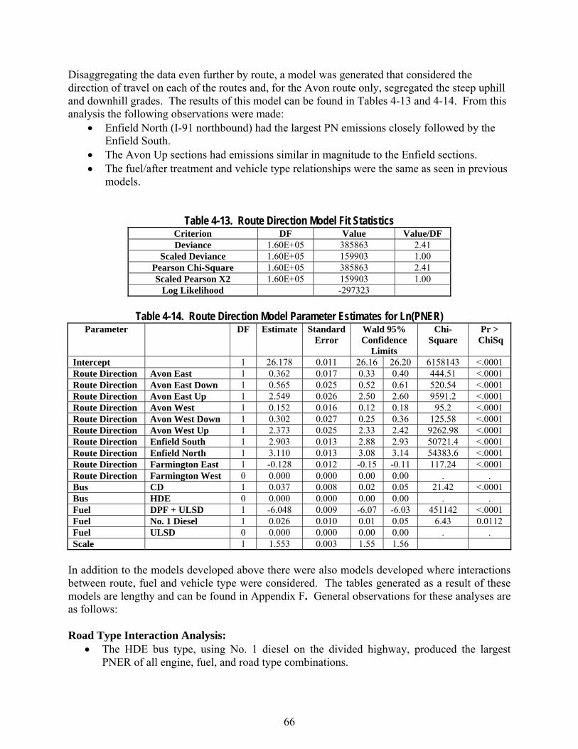
66

Disaggregating the data even further by route, a model was generated that considered the direction of travel on each of the routes and, for the Avon route only, segregated the steep uphill and downhill grades. The results of this model can be found in Tables 4-13 and 4-14. From this analysis the following observations were made:

• Enfield North (I-91 northbound) had the largest PN emissions closely followed by the Enfield South.

• The Avon Up sections had emissions similar in magnitude to the Enfield sections. • The fuel/after treatment and vehicle type relationships were the same as seen in previous

models.

Table 4-13. Route Direction Model Fit Statistics

Criterion DF Value Value/DF Deviance 1.60E+05 385863 2.41

Scaled Deviance 1.60E+05 159903 1.00 Pearson Chi-Square 1.60E+05 385863 2.41 Scaled Pearson X2 1.60E+05 159903 1.00

Log Likelihood -297323

Table 4-14. Route Direction Model Parameter Estimates for Ln(PNER) Parameter DF Estimate Standard

Error Wald 95% Confidence

Limits

Chi-Square

Pr > ChiSq

Intercept 1 26.178 0.011 26.16 26.20 6158143 <.0001 Route Direction Avon East 1 0.362 0.017 0.33 0.40 444.51 <.0001 Route Direction Avon East Down 1 0.565 0.025 0.52 0.61 520.54 <.0001 Route Direction Avon East Up 1 2.549 0.026 2.50 2.60 9591.2 <.0001 Route Direction Avon West 1 0.152 0.016 0.12 0.18 95.2 <.0001 Route Direction Avon West Down 1 0.302 0.027 0.25 0.36 125.58 <.0001 Route Direction Avon West Up 1 2.373 0.025 2.33 2.42 9262.98 <.0001 Route Direction Enfield South 1 2.903 0.013 2.88 2.93 50721.4 <.0001 Route Direction Enfield North 1 3.110 0.013 3.08 3.14 54383.6 <.0001 Route Direction Farmington East 1 -0.128 0.012 -0.15 -0.11 117.24 <.0001 Route Direction Farmington West 0 0.000 0.000 0.00 0.00 . . Bus CD 1 0.037 0.008 0.02 0.05 21.42 <.0001 Bus HDE 0 0.000 0.000 0.00 0.00 . . Fuel DPF + ULSD 1 -6.048 0.009 -6.07 -6.03 451142 <.0001 Fuel No. 1 Diesel 1 0.026 0.010 0.01 0.05 6.43 0.0112 Fuel ULSD 0 0.000 0.000 0.00 0.00 . . Scale 1 1.553 0.003 1.55 1.56

In addition to the models developed above there were also models developed where interactions between route, fuel and vehicle type were considered. The tables generated as a result of these models are lengthy and can be found in Appendix F. General observations for these analyses are as follows: Road Type Interaction Analysis:

• The HDE bus type, using No. 1 diesel on the divided highway, produced the largest PNER of all engine, fuel, and road type combinations.

67

• The CD bus type using ULSD produced higher PN emissions than when using No. 1 diesel on the divided highway.

• The interaction effects of fuel, engine, and road type suggest that the HDE bus had higher PN emissions for each road type than the CD bus type. However, for these HDE bus events with the largest PN emissions the fuel type varied between No. 1 diesel and ULSD. For example, on the rural arterial HDE/No. 1 diesel was the largest emitter but for the urban arterial HDE/ULSD was the largest emitter.

• The DPF aftertreatment reduced all emissions significantly regardless of vehicle type or route. The DPF was most effective on the HDE bus type when traveling on the urban arterial.

Route Interaction Analysis:

• For the Enfield and Avon routes, the HDE bus particle number emissions were higher than for the CD bus type regardless of fuel used.

• On the Farmington route, the HDE bus operating on ULSD had the highest PNER followed by the CD bus type on No. 1 diesel.

• Overall, it appears the DPF worked best on the HDE bus type, particularly in situations where there was stop-and-go traffic (i.e. downtown section and Farmington section).

Route Direction Interaction Analysis:

• For Enfield South and Enfield North the HDE bus operating on No.1 diesel resulted in the highest particle emissions rates.

• On the Avon Up sections, the HDE on ULSD was the largest emitter followed by the HDE on No.1 diesel.

• Once again, the DPF was most effective on the HDE under stop-and-go conditions (Farmington and Avon (excluding the high grade section) ).

The final model developed incorporated vehicle operation in terms of VSP and speed. Speed was included in this model because, as discussed previously, VSP alone is not sufficient when describing the operation of the vehicle. The EPA MOVES model also incorporates speed into its VSP binning system (Table 1-3) for this reason. Additional categorical variables were added such as road type, fuel and vehicle type due to their significance in PN emissions as shown above. The previous analysis indicated the interactions between fuel, vehicle type, and road type had a significant impact on PN emissions. Therefore, these interactions were incorporated into the final model. Also, because the route definitions are specific to the Hartford area, road type was selected over the routes names so the model may be applied to other regions. However, it should be noted that the data collected on these road types are not exhaustive or representative of all road types of the same classification. Therefore, broader application of this model without validation is limited and should not be considered accurate for all emissions analysis, just for the data described here. A more thorough and comprehensive data collection effort is necessary to develop a comprehensive model.

It should also be noted that this study benefited from the use of the Connecticut DOT’s ARAN van to collect the road grade information is necessary to compute vehicle specific power for real-world vehicle operation on the studied road network. Future studies of vehicle emissions using

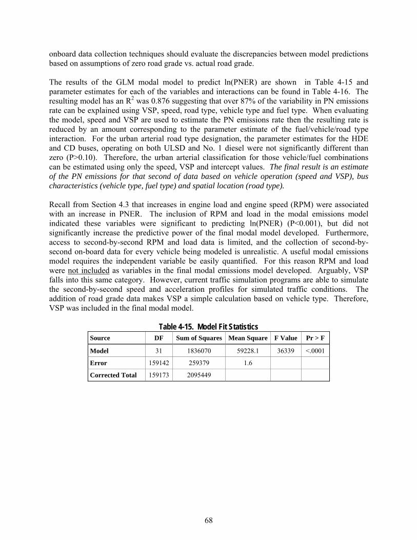
68

onboard data collection techniques should evaluate the discrepancies between model predictions based on assumptions of zero road grade vs. actual road grade.

The results of the GLM modal model to predict ln(PNER) are shown in Table 4-15 and parameter estimates for each of the variables and interactions can be found in Table 4-16. The resulting model has an R2 was 0.876 suggesting that over 87% of the variability in PN emissions rate can be explained using VSP, speed, road type, vehicle type and fuel type. When evaluating the model, speed and VSP are used to estimate the PN emissions rate then the resulting rate is reduced by an amount corresponding to the parameter estimate of the fuel/vehicle/road type interaction. For the urban arterial road type designation, the parameter estimates for the HDE and CD buses, operating on both ULSD and No. 1 diesel were not significantly different than zero (P>0.10). Therefore, the urban arterial classification for those vehicle/fuel combinations can be estimated using only the speed, VSP and intercept values. The final result is an estimate of the PN emissions for that second of data based on vehicle operation (speed and VSP), bus characteristics (vehicle type, fuel type) and spatial location (road type).

Recall from Section 4.3 that increases in engine load and engine speed (RPM) were associated with an increase in PNER. The inclusion of RPM and load in the modal emissions model indicated these variables were significant to predicting ln(PNER) (P<0.001), but did not significantly increase the predictive power of the final modal model developed. Furthermore, access to second-by-second RPM and load data is limited, and the collection of second-by-second on-board data for every vehicle being modeled is unrealistic. A useful modal emissions model requires the independent variable be easily quantified. For this reason RPM and load were not included as variables in the final modal emissions model developed. Arguably, VSP falls into this same category. However, current traffic simulation programs are able to simulate the second-by-second speed and acceleration profiles for simulated traffic conditions. The addition of road grade data makes VSP a simple calculation based on vehicle type. Therefore, VSP was included in the final modal model.

Table 4-15. Model Fit Statistics

Source DF Sum of Squares Mean Square F Value Pr > F

Model 31 1836070 59228.1 36339 <.0001

Error 159142 259379 1.6

Corrected Total 159173 2095449

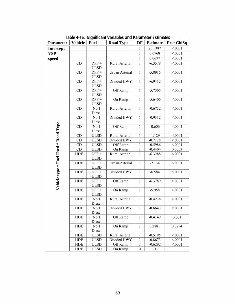
69

Table 4-16. Significant Variables and Parameter Estimates

Parameter Vehicle Fuel Road Type DF Estimate Pr > ChiSq Intercept 1 25.5387 <.0001 VSP 1 0.0768 <.0001 speed 1 0.0677 <.0001

CD DPF + ULSD

Rural Arterial 1 -6.3578 <.0001

CD DPF + ULSD

Urban Arterial 1 -5.8915 <.0001

CD DPF + ULSD

Divided HWY 1 -6.9412 <.0001

CD DPF + ULSD

Off Ramp 1 -5.7505 <.0001

CD DPF + ULSD

On Ramp 1 -5.6406 <.0001

CD No.1 Diesel

Rural Arterial 1 -0.6752 <.0001

CD No.1 Diesel

Divided HWY 1 -0.9312 <.0001

CD No.1 Diesel

Off Ramp 1 -0.606 <.0001

CD ULSD Rural Arterial 1 -1.129 <.0001 CD ULSD Divided HWY 1 -0.7128 <.0001 CD ULSD Off Ramp 1 -0.5986 <.0001 CD ULSD On Ramp 1 -0.4404 0.0003

HDE DPF + ULSD

Rural Arterial 1 -6.3288 <.0001

HDE DPF + ULSD

Urban Arterial 1 -7.134 <.0001

HDE DPF + ULSD

Divided HWY 1 -6.584 <.0001

HDE DPF + ULSD

Off Ramp 1 -6.3789 <.0001

HDE DPF + ULSD

On Ramp 1 -5.958 <.0001

HDE No.1 Diesel

Rural Arterial 1 -0.4238 <.0001

HDE No.1 Diesel

Divided HWY 1 -0.6643 <.0001

HDE No.1 Diesel

Off Ramp 1 -0.4149 0.001

HDE No.1 Diesel

On Ramp 1 0.2881 0.0294

HDE ULSD Rural Arterial 1 -0.5195 <.0001 HDE ULSD Divided HWY 1 -0.8673 <.0001 HDE ULSD Off Ramp 1 -0.6292 <.0001

Veh

icle

type

* F

uel U

sed

* R

oad

Typ

e

HDE ULSD On Ramp 0 0 .

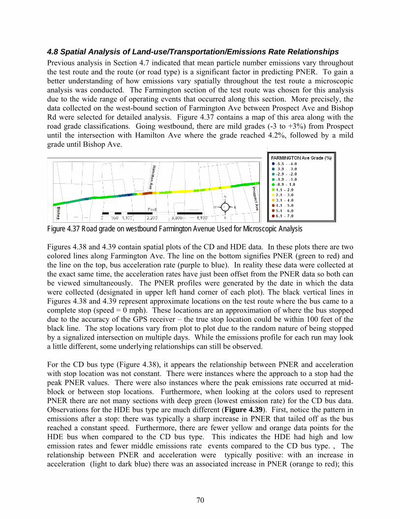
70

4.8 Spatial Analysis of Land-use/Transportation/Emissions Rate Relationships Previous analysis in Section 4.7 indicated that mean particle number emissions vary throughout the test route and the route (or road type) is a significant factor in predicting PNER. To gain a better understanding of how emissions vary spatially throughout the test route a microscopic analysis was conducted. The Farmington section of the test route was chosen for this analysis due to the wide range of operating events that occurred along this section. More precisely, the data collected on the west-bound section of Farmington Ave between Prospect Ave and Bishop Rd were selected for detailed analysis. Figure 4.37 contains a map of this area along with the road grade classifications. Going westbound, there are mild grades (-3 to +3%) from Prospect until the intersection with Hamilton Ave where the grade reached 4.2%, followed by a mild grade until Bishop Ave.

Figure 4.37 Road grade on westbound Farmington Avenue Used for Microscopic Analysis

Figures 4.38 and 4.39 contain spatial plots of the CD and HDE data. In these plots there are two colored lines along Farmington Ave. The line on the bottom signifies PNER (green to red) and the line on the top, bus acceleration rate (purple to blue). In reality these data were collected at the exact same time, the acceleration rates have just been offset from the PNER data so both can be viewed simultaneously. The PNER profiles were generated by the date in which the data were collected (designated in upper left hand corner of each plot). The black vertical lines in Figures 4.38 and 4.39 represent approximate locations on the test route where the bus came to a complete stop (speed = 0 mph). These locations are an approximation of where the bus stopped due to the accuracy of the GPS receiver – the true stop location could be within 100 feet of the black line. The stop locations vary from plot to plot due to the random nature of being stopped by a signalized intersection on multiple days. While the emissions profile for each run may look a little different, some underlying relationships can still be observed.

For the CD bus type (Figure 4.38), it appears the relationship between PNER and acceleration with stop location was not constant. There were instances where the approach to a stop had the peak PNER values. There were also instances where the peak emissions rate occurred at mid-block or between stop locations. Furthermore, when looking at the colors used to represent PNER there are not many sections with deep green (lowest emission rate) for the CD bus data. Observations for the HDE bus type are much different (Figure 4.39). First, notice the pattern in emissions after a stop: there was typically a sharp increase in PNER that tailed off as the bus reached a constant speed. Furthermore, there are fewer yellow and orange data points for the HDE bus when compared to the CD bus type. This indicates the HDE had high and low emission rates and fewer middle emissions rate events compared to the CD bus type. , The relationship between PNER and acceleration were typically positive: with an increase in acceleration (light to dark blue) there was an associated increase in PNER (orange to red); this

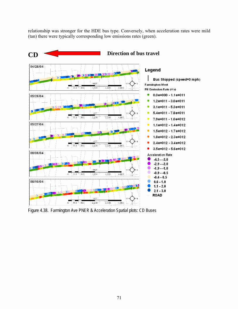
71

relationship was stronger for the HDE bus type. Conversely, when acceleration rates were mild (tan) there were typically corresponding low emissions rates (green).

CD

Figure 4.38. Farmington Ave PNER & Acceleration Spatial plots: CD Buses

Direction of bus travel

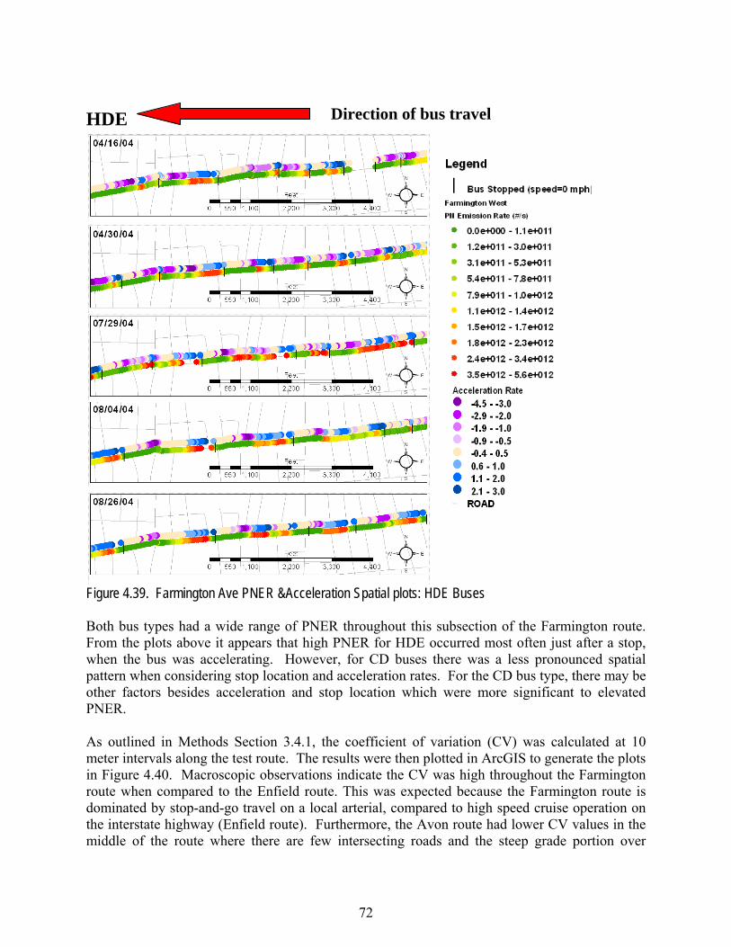
72

HDE

Figure 4.39. Farmington Ave PNER &Acceleration Spatial plots: HDE Buses

Both bus types had a wide range of PNER throughout this subsection of the Farmington route. From the plots above it appears that high PNER for HDE occurred most often just after a stop, when the bus was accelerating. However, for CD buses there was a less pronounced spatial pattern when considering stop location and acceleration rates. For the CD bus type, there may be other factors besides acceleration and stop location which were more significant to elevated PNER.

As outlined in Methods Section 3.4.1, the coefficient of variation (CV) was calculated at 10 meter intervals along the test route. The results were then plotted in ArcGIS to generate the plots in Figure 4.40. Macroscopic observations indicate the CV was high throughout the Farmington route when compared to the Enfield route. This was expected because the Farmington route is dominated by stop-and-go travel on a local arterial, compared to high speed cruise operation on the interstate highway (Enfield route). Furthermore, the Avon route had lower CV values in the middle of the route where there are few intersecting roads and the steep grade portion over

Direction of bus travel

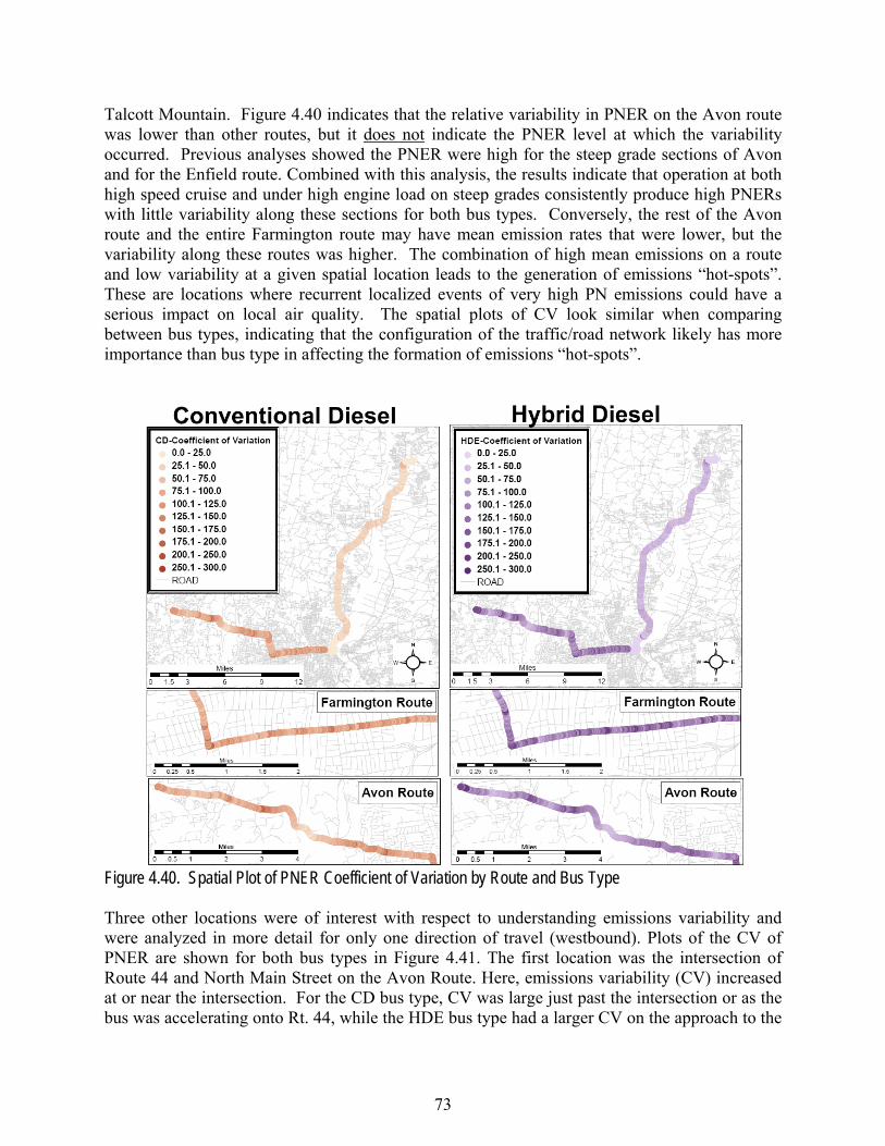
73

Talcott Mountain. Figure 4.40 indicates that the relative variability in PNER on the Avon route was lower than other routes, but it does not indicate the PNER level at which the variability occurred. Previous analyses showed the PNER were high for the steep grade sections of Avon and for the Enfield route. Combined with this analysis, the results indicate that operation at both high speed cruise and under high engine load on steep grades consistently produce high PNERs with little variability along these sections for both bus types. Conversely, the rest of the Avon route and the entire Farmington route may have mean emission rates that were lower, but the variability along these routes was higher. The combination of high mean emissions on a route and low variability at a given spatial location leads to the generation of emissions “hot-spots”. These are locations where recurrent localized events of very high PN emissions could have a serious impact on local air quality. The spatial plots of CV look similar when comparing between bus types, indicating that the configuration of the traffic/road network likely has more importance than bus type in affecting the formation of emissions “hot-spots”.

Figure 4.40. Spatial Plot of PNER Coefficient of Variation by Route and Bus Type

Three other locations were of interest with respect to understanding emissions variability and were analyzed in more detail for only one direction of travel (westbound). Plots of the CV of PNER are shown for both bus types in Figure 4.41. The first location was the intersection of Route 44 and North Main Street on the Avon Route. Here, emissions variability (CV) increased at or near the intersection. For the CD bus type, CV was large just past the intersection or as the bus was accelerating onto Rt. 44, while the HDE bus type had a larger CV on the approach to the

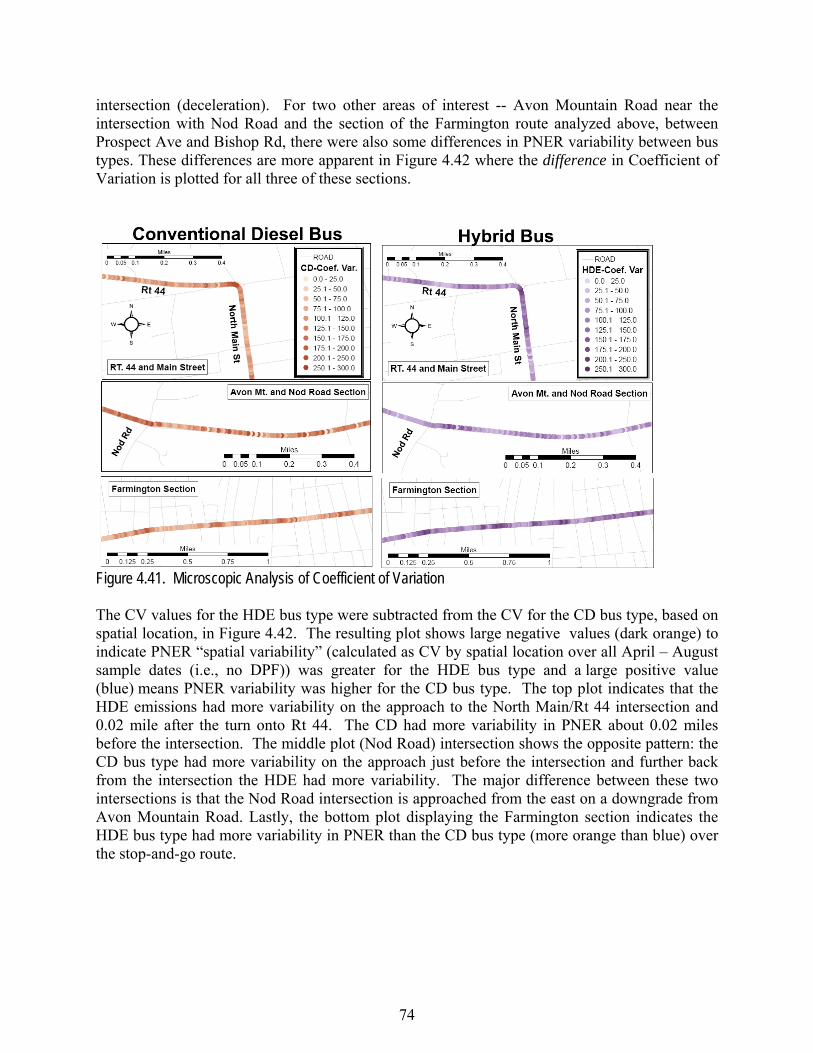
74

intersection (deceleration). For two other areas of interest -- Avon Mountain Road near the intersection with Nod Road and the section of the Farmington route analyzed above, between Prospect Ave and Bishop Rd, there were also some differences in PNER variability between bus types. These differences are more apparent in Figure 4.42 where the difference in Coefficient of Variation is plotted for all three of these sections.

Figure 4.41. Microscopic Analysis of Coefficient of Variation

The CV values for the HDE bus type were subtracted from the CV for the CD bus type, based on spatial location, in Figure 4.42. The resulting plot shows large negative values (dark orange) to indicate PNER “spatial variability” (calculated as CV by spatial location over all April – August sample dates (i.e., no DPF)) was greater for the HDE bus type and a large positive value (blue) means PNER variability was higher for the CD bus type. The top plot indicates that the HDE emissions had more variability on the approach to the North Main/Rt 44 intersection and 0.02 mile after the turn onto Rt 44. The CD had more variability in PNER about 0.02 miles before the intersection. The middle plot (Nod Road) intersection shows the opposite pattern: the CD bus type had more variability on the approach just before the intersection and further back from the intersection the HDE had more variability. The major difference between these two intersections is that the Nod Road intersection is approached from the east on a downgrade from Avon Mountain Road. Lastly, the bottom plot displaying the Farmington section indicates the HDE bus type had more variability in PNER than the CD bus type (more orange than blue) over the stop-and-go route.

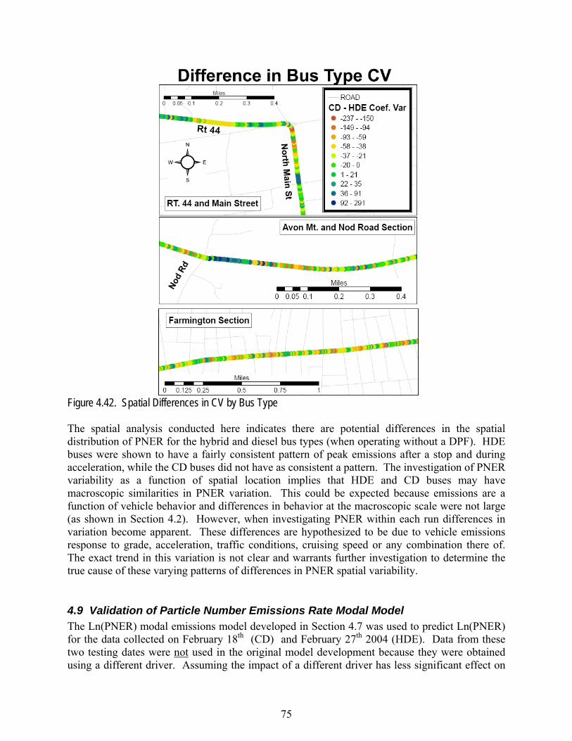
75

Figure 4.42. Spatial Differences in CV by Bus Type The spatial analysis conducted here indicates there are potential differences in the spatial distribution of PNER for the hybrid and diesel bus types (when operating without a DPF). HDE buses were shown to have a fairly consistent pattern of peak emissions after a stop and during acceleration, while the CD buses did not have as consistent a pattern. The investigation of PNER variability as a function of spatial location implies that HDE and CD buses may have macroscopic similarities in PNER variation. This could be expected because emissions are a function of vehicle behavior and differences in behavior at the macroscopic scale were not large (as shown in Section 4.2). However, when investigating PNER within each run differences in variation become apparent. These differences are hypothesized to be due to vehicle emissions response to grade, acceleration, traffic conditions, cruising speed or any combination there of. The exact trend in this variation is not clear and warrants further investigation to determine the true cause of these varying patterns of differences in PNER spatial variability.

4.9 Validation of Particle Number Emissions Rate Modal Model The Ln(PNER) modal emissions model developed in Section 4.7 was used to predict Ln(PNER) for the data collected on February 18th (CD) and February 27th 2004 (HDE). Data from these two testing dates were not used in the original model development because they were obtained using a different driver. Assuming the impact of a different driver has less significant effect on

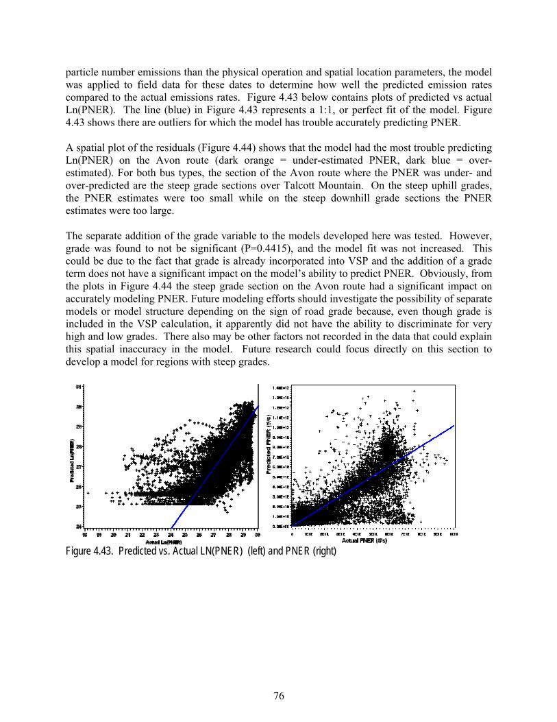
76

particle number emissions than the physical operation and spatial location parameters, the model was applied to field data for these dates to determine how well the predicted emission rates compared to the actual emissions rates. Figure 4.43 below contains plots of predicted vs actual Ln(PNER). The line (blue) in Figure 4.43 represents a 1:1, or perfect fit of the model. Figure 4.43 shows there are outliers for which the model has trouble accurately predicting PNER. A spatial plot of the residuals (Figure 4.44) shows that the model had the most trouble predicting Ln(PNER) on the Avon route (dark orange = under-estimated PNER, dark blue = over- estimated). For both bus types, the section of the Avon route where the PNER was under- and over-predicted are the steep grade sections over Talcott Mountain. On the steep uphill grades, the PNER estimates were too small while on the steep downhill grade sections the PNER estimates were too large. The separate addition of the grade variable to the models developed here was tested. However, grade was found to not be significant (P=0.4415), and the model fit was not increased. This could be due to the fact that grade is already incorporated into VSP and the addition of a grade term does not have a significant impact on the model’s ability to predict PNER. Obviously, from the plots in Figure 4.44 the steep grade section on the Avon route had a significant impact on accurately modeling PNER. Future modeling efforts should investigate the possibility of separate models or model structure depending on the sign of road grade because, even though grade is included in the VSP calculation, it apparently did not have the ability to discriminate for very high and low grades. There also may be other factors not recorded in the data that could explain this spatial inaccuracy in the model. Future research could focus directly on this section to develop a model for regions with steep grades.

Figure 4.43. Predicted vs. Actual LN(PNER) (left) and PNER (right)

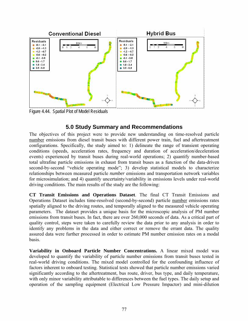
77

Figure 4.44. Spatial Plot of Model Residuals

5.0 Study Summary and Recommendations The objectives of this project were to provide new understanding on time-resolved particle number emissions from diesel transit buses with different power train, fuel and aftertreatment configurations. Specifically, the study aimed to: 1) delineate the range of transient operating conditions (speeds, acceleration rates, frequency and duration of acceleration/deceleration events) experienced by transit buses during real-world operations; 2) quantify number-based total ultrafine particle emissions in exhaust from transit buses as a function of the data-driven second-by-second “vehicle operating mode”; 3) develop statistical models to characterize relationships between measured particle number emissions and transportation network variables for microsimulation; and 4) quantify uncertainty/variability in emissions levels under real-world driving conditions. The main results of the study are the following: CT Transit Emissions and Operations Dataset. The final CT Transit Emissions and Operations Dataset includes time-resolved (second-by-second) particle number emissions rates spatially aligned to the driving routes, and temporally aligned to the measured vehicle operating parameters. The dataset provides a unique basis for the microscopic analysis of PM number emissions from transit buses. In fact, there are over 260,000 seconds of data. As a critical part of quality control, steps were taken to carefully review the data prior to any analysis in order to identify any problems in the data and either correct or remove the errant data. The quality assured data were further processed in order to estimate PM number emission rates on a modal basis. Variability in Onboard Particle Number Concentrations. A linear mixed model was developed to quantify the variability of particle number emissions from transit buses tested in real-world driving conditions. The mixed model controlled for the confounding influence of factors inherent to onboard testing. Statistical tests showed that particle number emissions varied significantly according to the aftertreatment, bus route, driver, bus type, and daily temperature, with only minor variability attributable to differences between the fuel types. The daily setup and operation of the sampling equipment (Electrical Low Pressure Impactor) and mini-dilution

78

system contributed to 30-84% of the total random variability of particle measurements among tests with only diesel oxidation catalyst aftertreatment. By controlling for the sampling day variability, the model better defined the differences in particle emissions among bus routes. In contrast, the low particle number emissions measured with diesel particle filter aftertreatment (decreased by over 99%) did not vary according to operating conditions or bus type, but did vary substantially with ambient temperature. Modal Particle Number Emissions Model. The CT Transit Emissions and Operations Dataset allows for the second-by-second modeling of particle number emissions based on the variation in second-by-second engine and vehicle operating parameters of the hybrid and conventional transit buses under different fuel and aftertreatment conditions. In this study, the data collected for one driver and all fuel/aftertreatment combinations (April through November) was used to develop a particle number emissions rate modal emissions model based on multivariate regression techniques and generalized linear models. In addition to vehicle operating parameters (VSP and Speed), a number of categorical variables were also used to describe the location of the vehicle in the transportation network (i.e. road type, route, travel direction…etc.), the fuel type (No. 1 diesel or ULSD) and the vehicle type (CD or HDE). The significance of each of these variables was analyzed and recommendations for the development of a second-by-second modal emissions model were made. Given that vehicle operation and location are correlated, sec-by-sec operating characteristics such as speed, acceleration and VSP were used as continuous variables for the final model. The EPA MOVES model also incorporates speed into its VSP binning system. The resulting model R2 was 0.876, suggesting that over 87% of the variability in PN emissions rate can be explained using VSP, speed, road type, vehicle type and fuel type. In terms of the fuel type, the differences between No. 1 Diesel and ULSD were not significant. Evaluation of Spatial Relationships. The spatial nature of the data also allowed for an analysis of the variability in particle number emissions throughout the entire test route and within each subroute by bus type. ArcGIS (Version 9.1) was used to perform spatial analysis of the emissions and vehicle operating data. PNERs were plotted along with vehicle operating characteristics in an effort to analyze any spatial patterns in PNER. The spatial analysis conducted here indicates there are potential differences in the spatial distribution of PNER for the hybrid and diesel bus types. HDE buses were shown to have a fairly consistent pattern of peak emissions after a stop and during acceleration, while the CD buses did not have as consistent a pattern. The investigation of PNER variability as a function of spatial location implies that HDE and CD buses may have macroscopic similarities in PNER variation. However, when investigating PNER within each run differences in variation became apparent. These differences are hypothesized to be due to vehicle emissions response to grade, acceleration, traffic conditions, cruising speed or any combination there of. The exact trend in this variation is not clear and warrants further investigation to determine the true cause of these varying patterns of differences in PNER variation. This study establishes preliminary relationships between particle number emissions and driving mode for diesel and hybrid diesel-electric transit buses in Connecticut to improve real-world particle number emissions estimates at the microscale. Quantifying the relationships between heavy-duty vehicle driving mode, vehicle type and particle emissions is important for improving population exposure models based on travel behavior and transportation infrastructure design

79

and planning. Overall, all of the key project objectives are satisfied based upon the findings of this study. The modal emissions model for PNER developed in Section 4.7 based on VSP, speed and bus/fuel/road type interactions can be used to incorporate particle number emissions into model’s such as EPA’s MOVES, which offer more flexibility in emissions modeling applications than the current MOBILE model. The success of this model for data collected using different onboard sampling techniques should be verified by future studies, but the validated results have identified the key parameters that can be used to estimate particle number emissions. Any study has some limitations that could motivate future work to expand the scope of the analysis or to apply improved methods. It should be noted that the data used in this study were collected on a small sample size of road types and buses, which are not exhaustive or representative of all road and bus types. Therefore, the models and relationships obtained in this study are somewhat limited and should not be considered as accurate for other emissions analysis. A more thorough and comprehensive data collection effort is necessary to develop a comprehensive model.

6.0 References Cited Barth, M., F. An, T. Younglove, G. Scora, and C. Levine (2000). "Development of a

Comprehensive Modal Emissions Model: Final Report." National Cooperative Highway Research Program (NCHRP Project 25-11), Washington, D.C.

Barth, M., G. Scora, and T. Younglove (2004) “Modal emissions model for heavy-duty diesel

vehicles.” Transportation Research Record: Journal of the Transportation Research Board, No. 1880, TRB, National Research Council, Washington, D.C., pp. 10-20.

Barth, M., T. Younglove, and G. Scora (2005). "Development of a Heavy-Duty Diesel Modal Emissions and Fuel Consumption Model ". California Partners for Advanced Transit and Highways (PATH). Research Reports: Paper UCB-ITS-PRR-2005-1. Beardsley, M (2004). “MOVES Model Update”, Proceedings of the 14th CRC On-Road Vehicle

Emissions Workshop, Hyatt Islandia, San Diego, California, March 29-31, 2004. Brook R.. J. Brook, B. Urch, R. Vincent, S. Rajagopalan, F. Silverman (2002). Fine particulate

air pollution and ozone inhalation causes acute arterial vasoconstriction in healthy adults. Journal of the American College of Cardiology. 39, Supplement 1, 219.

Browning, L (1998) “Update Heavy-Duty Engine Emissions Conversion Factors for MOBILE6: Analysis of BSFCs and Calculation of Heavy-Duty Engine Emission Conversion Factors; EPA. Brunekreef, B.and S. T Holgate (2002). Air Pollution and Health. Lancet. 360: 233-42.

80

Burtscher, H. (2005). Physical characterization of particulate emissions from diesel engines: a review. J. Aerosol Science. 36: 896-932. Canagaratna, M. R., J. T. Jayne, D. A. Ghertner, S. Herndon, Q. S. Jose, L. Jimenez, P. J. Silva, P. Williams, T. Lanni, F. Drewnick, K. L. Demerjian, C. E. Kolb, and D. R. Worsnop (2004). Chase Studies of Particulate Emissions from in-use New York City Vehicles. Aerosol Sci. Tech. 38: 555–573. Cetegen, B.M. and A. Chaparro (2005). CT Transit Hybrid and Conventional Bus Gas Emissions Measurement Test Report, Mechanical Engineering Department, University of Connecticut: 38 pp. Clark, N. N., P. Gajendran, and J. M. Kern (2003). A Predictive Tool for Emissions from Heavy-Duty Diesel Vehicles. Environ. Sci. Technol. 37: 7-15. Dekati (2000). ELPI Users Manual. Appendix A. Physical Operation. Dockery, D. (2001). Epidemiologic evidence of cardiovascular effects of particulate air

pollution. Environmental Health Perspectives, 109 (4), 483-486, EPA (2004). Air Quality Criteria for Particulate Matter, July 2004 draft, chapter 9, page 9-25. EPA (2004b). “MOVES2004 Highway Vehicle Population and Activity Data” EPA420-P-04-

020. Washington, D.C. December 2004 draft, page 55-58. EPA (2007). “Motor Vehicle Emission Simulator Highway Vehicle Implementation (MOVES-

HVI) Demonstration Version: Software Design and Reference Manual: Draft” Washington, D.C. EPA420-P-07-001. February, 2008.

EPA (2008). “MOVES2004 Software Design Reference Manual: DRAFT”

http://www.epa.gov/otaq/models/ngm/420p04017.pdf. Washington, D.C. Accessed: April, 22 2008.

FHWA (1989). “FHWA Functional Classification Guidelines.” US Federal Highway

Administration, Washington, DC http://www.fhwa.dot.gov/planning/fcsec2_1.htm Frey, C., K. Zhang and N. Rouphail (2008). Fuel Use and Emissions Comparisons for Alternative Routes, Time of Day, Road Grade, and Vehicles Based on In-Use Measurements, Environ. Sci.& Technol. 42: 2483-2489 Hammond, D., M. Lalor and S. Jones (2007). In-Vehicle Measurement of Particle Number

Concentrations on School Buses Equipped with Diesel Retrofits. Water, Air, and Soil Pollution, 179: Numbers 1-4, 217-225.

81

Holgate, Sandström, Frew, Stenfors, Nördenhall, Salvi, Blomberg, Helleday, and Söderberg. (2003). Health effects of acute exposures to air pollution. Part I. Healthy and asthmatic subjects exposed to diesel exhaust. Health Effects Institute, report 112, December 2003.

Holmén, B. A and D. A. Niemeier (1998). Characterizing the effects of driver variability on real- world vehicle emissions. Trans. Res. Rec., Part D 3 (2): 117-128. Holmén, B. A. and A. Ayala (2002). Ultrafine PM Emissions from Natural Gas, Oxidation- Catalyst Diesel, and Particle-Trap Diesel Heavy-Duty Transit Buses. Environ. Sci. Technol.36: 5041-5050. Holmén, B. A. and Y. Qu (2004). Uncertainty in Particle Number Modal Analysis during Transient Operation of Compressed Natural Gas, Diesel, and Trap-Equipped Diesel Transit Buses. Environ. Sci. Technol. 38: 2413-2423. Holmén, B. A.; Z. Chen, A. C. Davila, O. H. Gao, and D. M. Vikara (2005). Particulate Matter Emissions from Hybrid Diesel-Electric and Conventional Diesel Transit Buses: Fuel and Aftertreatment Effects. JHR 05-304, Project 03-8. Joint Highway Research Advisory Council. Huai, T., T. Durbin, T. Yunglove, G. Scora, M. Barth, and J. Norbeck. 2005. "Vehicle Specific

Power Approach to Estimating On-Road NH3 Emissions from Light-Duty Vehicles." Environmental Science and Technology. Vol. 39, No. 24, pg. 9595 -9600.

Imhof, D., E. Weingartner, C. Ordóñez, R. Gehrig, M. Hill, B. Buchmann, and U. Baltensperger (2005). U. Real-World Emission Factors of Fine and Ultrafine Aerosol Particles for Different Traffic Situations in Switzerland. Environ. Sci. Technol. 39: 8341-8350. Jamriska, M., L. Morawska, S. Thomas and C. He (2004). Diesel Bus Emissions Measured in a Tunnel Study. Environ. Sci. Technol. 38: 6701-6709. Jimenez, J.1999. "Understanding and Quantifying Motor Vehicle Emissions with Vehicle

Specific Power and TILDAS Remote Sensing." PhD Thesis. Massachusetts Institute of Technology.

Jones, A. and R. Harrison (2006). Estimation of the emission factors of particle number and mass fractions from a traffic at a site where mean vehicle speeds vary over short distances. Atmospheric Environ. 40: 7125-7137. Kear, T. and D. A. Niemeier (2006). On-Road Heavy-Duty Diesel Particulate Matter Emissions Modeled Using Chassis Dynameter Data. Environ. Sci. Technol, 40: 7828-7833. Kittleson, D (1998). Engines and Nanoparticles: A Review. Journal of Aerosol Science. 29:(5/6)

575-588.

82

Kittelson, D. B and W. F. Watts (2002). "Diesel Aerosol Sampling Methodology – CRC E-43: Final Report", University of Minnesota, Report for the Coordinating Research Council. Kittleson, D.B., W. F. Watts, and J. P. Johnson (2004). Nanoparticle emissions on Minnesota highways. Atmos. Environ. 38: 9-19. Koupal, J., M. Cumberworth, H. Michaels, M. Beardsley, D. Brzezinski (2002). “Draft Design

and Implementation Plan for EPA's Multi-Scale Motor Vehicle and Equipment Emission System (MOVES)”, U.S. EPA Technical Report #420-P-02-006, October 2002.

Kuhns, H., C. Mazzoleni, H. Moosmuller, D. Nikolic, R.Keislar, P. Barber, Z. Li, V. Etyemezian

and J. Watson. 2004. "Remote sensing of PM, NO, CO and HC emission factors for on-road gasoline and diesel engine vehicles in Las Vegas, NV" Science of the Total Environment, 322 (1-3), pp. 123-137.

Kweon, C, D. E. Foster, J. J. Schauer and S. Okada (2002). Detailed Chemical Composition and Particle Size Assessment of Diesel Engine Exhaust. SAE Technical Papers 2002-01- 2670. Lanni, T. (2003). Fine urban and precursor emissions control for diesel urban transit buses. Environmental Pollution. 2003, 123, 427-437. Littell, R. C.; G. A. Milliken, W.W. Stroup, R. D. Wolfinger and O. Schabenberger (2006). SAS® for Mixed Models, Second Edition; SAS Institue: Cary, NC. Maricq, M. M., D. H. Podsiadlik and R. E. Chase (2000). Size Distributions of Motor Vehicle Exhaust PM: A Comparison Between ELPI and SMPS Measurements. Aerosol Sci. Technol. 33: 239-260. Marjamaki, M., J. Keskinen, D. R. Chen, and Y. H. D. Pui (2000). Performance evaluation of the electrical low-pressure impactor (ELPI). J. Aerosol Science 31(2): 249-261. Mathis, U., M. Mohr, and A. Forss (2005). Comprehensive particle characterization of modern gasoline and diesel passenger cars at low ambient temperatures. Atmos. Environ. 39: 107-117. Morawska, L, N. D. Bofinger, L. Kocis, and A. Nwankwoala (1998). Submicrometer and Supermicrometer Particles from Diesel Vehicle Emissions. Environ. Sci. Technol. 32: 2033-2042. Morawska, L., M. Jamriska, S. Thomas, L. Ferreira, K. Mengersen, D. Wraith, and F. Mcgregor (2005). Quantification of Particle Number Emission Factors for Motor Vehicles from On- Road Measurements. Environ. Sci. Technol. 39: 9130-9139. Nam, E. (2003). “Proof of Concept Investigation for the Physical Emission Rate Estimator

(PERE) for MOVES” U.S. Environmental Protection Agency, 2003; EPA420-R-03-005.

83

Nemmar, A., Hoet, Vanquickenborne, Dinsdale, Thomeer, Hoylaerts, Vanbilloen, Mortelmans,

Nemery (2002). “Passage of Inhaled Particles Into the Blood Circulation in Humans.” Circulation. 2002; 105: 411-414.

Nylund, N.-O., K. Erkkilä, M. Lappi and M. Ikonen (2004). “Transit Bus Emission Study:

Comparison of Emissions from Diesel and Natural Gas Buses. VTT Technical Research Centre of Finland. Research Report. Project 3/P5150/04. November, 15 2004.

Pokharel, S., G.A. Bishop, and D.H. Stedman. 2001. "On-Road Remote Sensing of Automobile

Emissions in the Los Angeles Area: Year 2" Univ. of Denver final report to the Coordinating Research Council, Inc., available at www.crcao.com.

Ristovski, Z. D., E. R. Jayaratne, M. Lim, G. A. Ayoko, and L. Morawska (2006). Influence of Diesel Fuel Sulfur on Nanoparticle Emissions from City Buses. Environ. Sci. Technol. 40: 1314-1320. Scora, G. and Barth, M. (2006). "Comprehensive Modal Emissions Model (CMEM), version

3.01: User’s Guide." June 2006. University of California, Riverside, Center for Environmental Research and Technology.

Shi, J., D. Mark, and R. Harrison (2000). Characterization of Particles from a Current Technology Heavy-Duty Diesel Engine. Environ. Sci. Technol, 34: 748-755. Shi, J., R. Harrison, (1999) Investigation of Ultrafine Particle Formation during Diesel Exhaust Dilution. Environ. Sci. Technol. 33: 3730-3736. Singer, J. D. (1998) Using SAS PROC MIXED to Fit Multilevel Models, Hierarchical Models, and Individual Growth Models. J. Educ. Behav. Stat. 24(4): 323-355. Sonntag, D., H. O. Gao, and B. Holmén (2007). Modeling On-Road Particle Number Emissions

from a Hybrid Diesel–Electric Bus: Exploratory Econometric Analysis. Transportation Research Record. Issue number: 2011: 40-48.

Sonntag, D.B; Gao H. O; Holmén, B. A. (2008) Variability of Particle Number Emissions from Diesel and Hybrid Diesel-Electric Buses in Real Driving Conditions. Accepted for print Environ. Sci. Technol. Turrio-Baldassarri, L., C. Battistelli, L. Conti, R. Crebelli, B. De Berardis, A. Iamiceli, M.

Gambino, and S. Iannaccone (2004) Emission Comparison of Urban Bus Engine Fueled with Diesel Oil and `Biodiesel' Blend. Science of the Total Environment. 327, Issues 1-3: 147-162.

Utell M., and M. Frampton (2000). Acute health effects of ambient air pollution: the ultrafine

particle hypothesis. Journal of Aerosol Medicine. Winter; 13 (4):355-59.

84

Van Ling, J., R Van Helden, and I. Riemersma. (2003). “Comparison of Particle Size Distribution and Emissions from Heavy-duty Diesel Engines and Gas Engines for Urban Buses.” 12th International Scientific Symposium on Transport and Air Pollution, 16 – 18 June 2003, Avignon, France.

Vikara, D. and B. Holmén. (2006). “Ultrafine Particle Number Concentrations from Hybrid

Urban Transit Buses: Onboard Single-diameter Scanning Mobility Particle Sizer Measurements.” Transportation Research Record ISSN 0361-1981. pp. 54-61.

West, B. T, K. B. Welch, and A. T. Galecki (2007). Linear Mixed Models; Chapman & Hall/CRC: Boca Raton, FL. Yanowitz, J, M. S. Graboski and R. L. McCormick (2002). Prediction of In-Use Emissions of Heavy-Duty Diesel Vehicles from Engine Testing. Environ. Sci. Technol. 36: 270- 275. Zervas, E.; P. Dorlhène, R. Daviau and B. Dionnet (2004). Repeatability of fine particle measurement of diesel and gasoline vehicles exhaust gas. SAE Technical Paper Series 2004-01-1983. Zhang, K.M.; and A. S. Wexler (2002). A hypothesis for growth of fresh atmospheric nuclei. J. Geophys. Res. 107(D21): 4577. Zhu, Y.; T. Kuhn, P. Mayo and C. W. Hinds (2006). Comparison of Daytime and Nighttime Concentration Profiles and Size Distributions of Ultrafine Particles near a Major Highway. Environ. Sci. Technol. 40: 2531-2536

85

7.0 Appendices Appendix A. Additional information on field data collection...............................................86

Appendix B. Transit Bus Specifications................................................................................88

Appendix C. Time Lag Estimates Comparison .....................................................................89

Appendix D. Data Dictionary for Dataset Parameters ..........................................................94

Appendix E. Mixed Model Parameters From Variability Analysis .....................................107

Appendix F. Modal Emissions Modeling Results and Parameter Estimates ................... 109

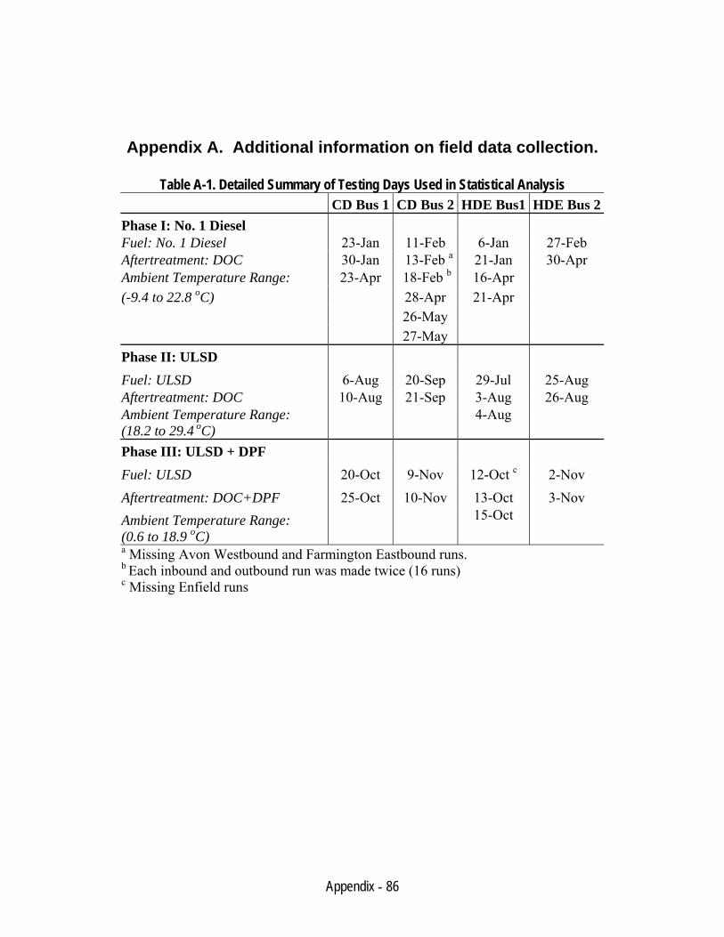
Appendix - 86

Appendix A. Additional information on field data collection.

Table A-1. Detailed Summary of Testing Days Used in Statistical Analysis CD Bus 1 CD Bus 2 HDE Bus1 HDE Bus 2

Phase I: No. 1 Diesel Fuel: No. 1 Diesel 23-Jan 11-Feb 6-Jan 27-Feb Aftertreatment: DOC 30-Jan 13-Feb a 21-Jan 30-Apr Ambient Temperature Range: 23-Apr 18-Feb b 16-Apr (-9.4 to 22.8 oC) 28-Apr 21-Apr

26-May 27-May

Phase II: ULSD Fuel: ULSD 6-Aug 20-Sep 29-Jul 25-Aug Aftertreatment: DOC 10-Aug 21-Sep 3-Aug 26-Aug Ambient Temperature Range: (18.2 to 29.4 oC)

4-Aug

Phase III: ULSD + DPF Fuel: ULSD 20-Oct 9-Nov 12-Oct c 2-Nov Aftertreatment: DOC+DPF 25-Oct 10-Nov 13-Oct 3-Nov Ambient Temperature Range: (0.6 to 18.9 oC)

15-Oct

a Missing Avon Westbound and Farmington Eastbound runs. b Each inbound and outbound run was made twice (16 runs) c Missing Enfield runs

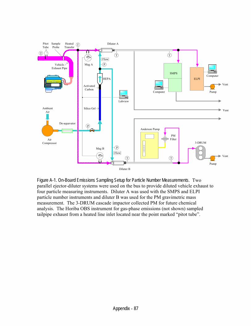
Appendix - 87

Figure A-1. On-Board Emissions Sampling Setup for Particle Number Measurements. Two parallel ejector-diluter systems were used on the bus to provide diluted vehicle exhaust to four particle measuring instruments. Diluter A was used with the SMPS and ELPI particle number instruments and diluter B was used for the PM gravimetric mass measurement. The 3-DRUM cascade impactor collected PM for future chemical analysis. The Horiba OBS instrument for gas-phase emissions (not shown) sampled tailpipe exhaust from a heated line inlet located near the point marked “pitot tube”.

Computer

Labview

Computer

Mag A

Mag B

Anderson Pump

ELPI

Pump

3-DRUM

Pump

PMFilter

Vent

Vent

T

Silica Gel

HEPA

Diluter A

Diluter B

VehicleExhaust Pipe

AirCompressor

Vent

Diesel EngineDiesel Engine

ActivatedCarbon

HeatedTransfer

SampleProbe

AmbientAir

De-aquavator

T

TT

P

P

T

P

PitotTube

SMPS

T

Flow

FlowdP

dP

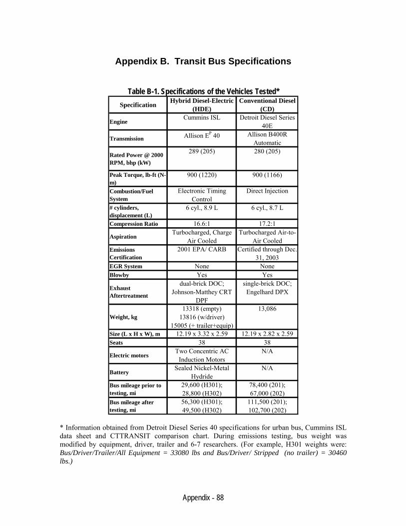
Appendix - 88

Appendix B. Transit Bus Specifications

Table B-1. Specifications of the Vehicles Tested* Specification Hybrid Diesel-Electric

(HDE)Conventional Diesel

(CD)

EngineCummins ISL Detroit Diesel Series

40E

Transmission Allison EP 40 Allison B400R Automatic

Rated Power @ 2000 RPM, bhp (kW)

289 (205) 280 (205)

Peak Torque, lb-ft (N-m)

900 (1220) 900 (1166)

Combustion/Fuel System

Electronic Timing Control

Direct Injection

# cylinders, displacement (L)

6 cyl., 8.9 L 6 cyl., 8.7 L

Compression Ratio 16.6:1 17.2:1

AspirationTurbocharged, Charge

Air CooledTurbocharged Air-to-

Air CooledEmissions Certification

2001 EPA/ CARB Certified through Dec. 31, 2003

EGR System None NoneBlowby Yes Yes

Exhaust Aftertreatment

dual-brick DOC; Johnson-Matthey CRT

DPF

single-brick DOC; Engelhard DPX

Weight, kg13318 (empty)

13816 (w/driver) 15005 (+ trailer+equip)

13,086

Size (L x H x W), m 12.19 x 3.32 x 2.59 12.19 x 2.82 x 2.59Seats 38 38

Electric motorsTwo Concentric AC

Induction MotorsN/A

BatterySealed Nickel-Metal

HydrideN/A

Bus mileage prior to testing, mi

29,600 (H301); 28,800 (H302)

78,400 (201); 67,000 (202)

Bus mileage after testing, mi

56,300 (H301); 49,500 (H302)

111,500 (201); 102,700 (202)

* Information obtained from Detroit Diesel Series 40 specifications for urban bus, Cummins ISL data sheet and CTTRANSIT comparison chart. During emissions testing, bus weight was modified by equipment, driver, trailer and 6-7 researchers. (For example, H301 weights were: Bus/Driver/Trailer/All Equipment = 33080 lbs and Bus/Driver/ Stripped (no trailer) = 30460 lbs.)

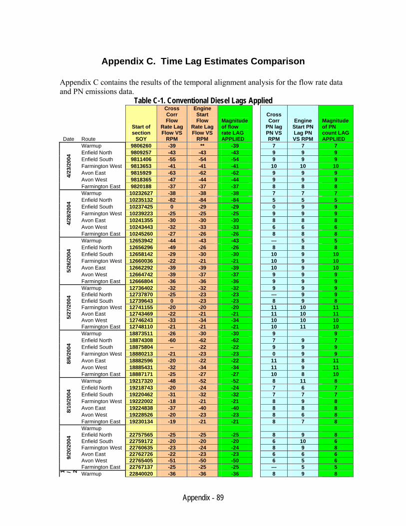
Appendix - 89

Appendix C. Time Lag Estimates Comparison Appendix C contains the results of the temporal alignment analysis for the flow rate data and PN emissions data.

Table C-1. Conventional Diesel Lags Applied

Date Route

Start of section

SOY

Cross Corr Flow

Rate Lag Flow VS

RPM

Engine Start Flow

Rate Lag Flow VS

RPM

Magnitude of flow rate LAG APPLIED

Cross Corr

PN lag PN VS RPM

Engine Start PN Lag PN VS RPM

Magnitude of PN count LAG APPLIED

Warmup 9806260 -39 ** -39 7 7 7 Enfield North 9809257 -43 -43 -43 9 9 9 Enfield South 9811406 -55 -54 -54 9 9 9 Farmington West 9813653 -41 -41 -41 10 10 10 Avon East 9815929 -63 -62 -62 9 9 9 Avon West 9818365 -47 -44 -44 9 9 9 4/

23/2

004

Farmington East 9820188 -37 -37 -37 8 8 8 Warmup 10232627 -38 -38 -38 7 7 7 Enfield North 10235132 -82 -84 -84 5 5 5 Enfield South 10237425 0 -29 -29 0 9 9 Farmington West 10239223 -25 -25 -25 9 9 9 Avon East 10241355 -30 -30 -30 8 8 8 Avon West 10243443 -32 -33 -33 6 6 6 4/

28/2

004

Farmington East 10245260 -27 -26 -26 8 8 8 Warmup 12653942 -44 -43 -43 --- 5 5 Enfield North 12656296 -49 -26 -26 8 8 8 Enfield South 12658142 -29 -30 -30 10 9 10 Farmington West 12660036 -22 -21 -21 10 9 10 Avon East 12662292 -39 -39 -39 10 9 10 Avon West 12664742 -39 -37 -37 9 9 9 5/

26/2

004

Farmington East 12666804 -36 -36 -36 9 9 9 Warmup 12736402 -32 -32 -32 9 9 9 Enfield North 12737870 -25 -23 -23 --- 9 9 Enfield South 12739643 0 -23 -23 8 9 8 Farmington West 12741155 -20 -20 -20 11 10 11 Avon East 12743469 -22 -21 -21 11 10 11 Avon West 12746243 -33 -34 -34 10 10 10 5/

27/2

004

Farmington East 12748110 -21 -21 -21 10 11 10 Warmup 18873511 -26 -30 -30 9 9 Enfield North 18874308 -60 -62 -62 7 9 7 Enfield South 18875804 -- -22 -22 9 9 9 Farmington West 18880213 -21 -23 -23 0 9 9 Avon East 18882596 -20 -22 -22 11 8 11 Avon West 18885431 -32 -34 -34 11 9 11

8/6/

2004

Farmington East 18887171 -25 -27 -27 10 8 10 Warmup 19217320 -48 -52 -52 8 11 8 Enfield North 19218743 -20 -24 -24 7 6 7 Enfield South 19220462 -31 -32 -32 7 7 7 Farmington West 19222002 -18 -21 -21 8 9 8 Avon East 19224838 -37 -40 -40 8 8 8 Avon West 19228526 -20 -23 -23 8 6 8 8/

10/2

004

Farmington East 19230134 -19 -21 -21 8 7 8 Warmup Enfield North 22757565 -25 -25 -25 8 9 8 Enfield South 22759172 -20 -20 -20 6 10 6 Farmington West 22760635 -23 -24 -24 8 9 8 Avon East 22762726 -22 -23 -23 6 6 6 Avon West 22765405 -51 -50 -50 6 5 6 9/

20/2

004

Farmington East 22767137 -25 -25 -25 --- 5 5

1 / 2 Warmup 22840020 -36 -36 -36 8 9 8

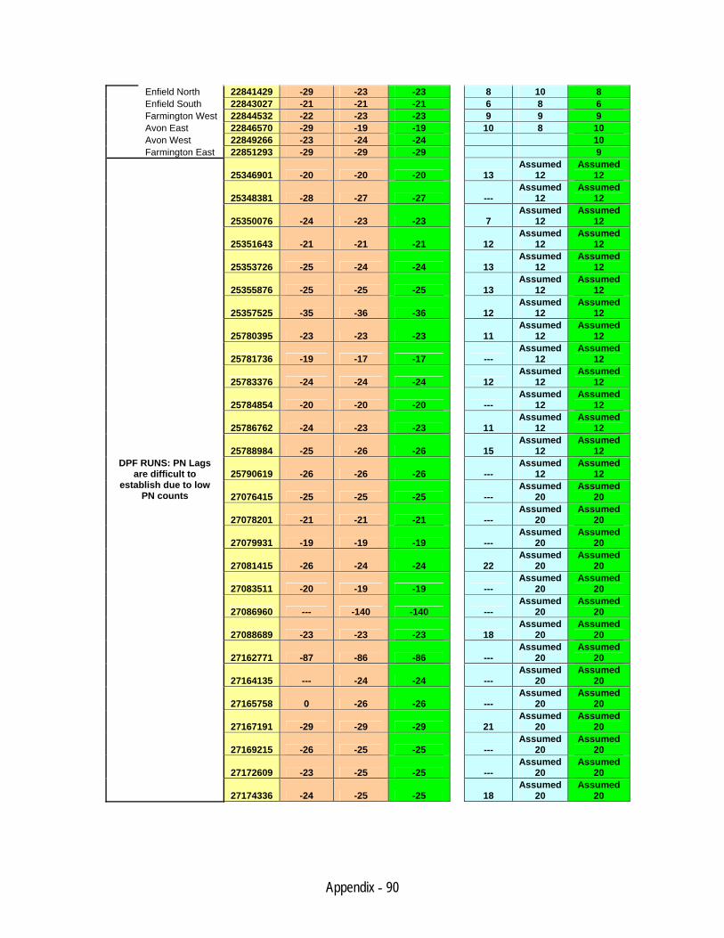
Appendix - 90

Enfield North 22841429 -29 -23 -23 8 10 8 Enfield South 22843027 -21 -21 -21 6 8 6 Farmington West 22844532 -22 -23 -23 9 9 9 Avon East 22846570 -29 -19 -19 10 8 10 Avon West 22849266 -23 -24 -24 10 Farmington East 22851293 -29 -29 -29 9

25346901 -20 -20 -20 13 Assumed

12 Assumed

12

25348381 -28 -27 -27 --- Assumed

12 Assumed

12

25350076 -24 -23 -23 7 Assumed

12 Assumed

12

25351643 -21 -21 -21 12 Assumed

12 Assumed

12

25353726 -25 -24 -24 13 Assumed

12 Assumed

12

25355876 -25 -25 -25 13 Assumed

12 Assumed

12

25357525 -35 -36 -36 12 Assumed

12 Assumed

12

25780395 -23 -23 -23 11 Assumed

12 Assumed

12

25781736 -19 -17 -17 --- Assumed

12 Assumed

12

25783376 -24 -24 -24 12 Assumed

12 Assumed

12

25784854 -20 -20 -20 --- Assumed

12 Assumed

12

25786762 -24 -23 -23 11 Assumed

12 Assumed

12

25788984 -25 -26 -26 15 Assumed

12 Assumed

12

25790619 -26 -26 -26 --- Assumed

12 Assumed

12

27076415 -25 -25 -25 --- Assumed

20 Assumed

20

27078201 -21 -21 -21 --- Assumed

20 Assumed

20

27079931 -19 -19 -19 --- Assumed

20 Assumed

20

27081415 -26 -24 -24 22 Assumed

20 Assumed

20

27083511 -20 -19 -19 --- Assumed

20 Assumed

20

27086960 --- -140 -140 --- Assumed

20 Assumed

20

27088689 -23 -23 -23 18 Assumed

20 Assumed

20

27162771 -87 -86 -86 --- Assumed

20 Assumed

20

27164135 --- -24 -24 --- Assumed

20 Assumed

20

27165758 0 -26 -26 --- Assumed

20 Assumed

20

27167191 -29 -29 -29 21 Assumed

20 Assumed

20

27169215 -26 -25 -25 --- Assumed

20 Assumed

20

27172609 -23 -25 -25 --- Assumed

20 Assumed

20

DPF RUNS: PN Lags are difficult to

establish due to low PN counts

27174336 -24 -25 -25 18 Assumed

20 Assumed

20

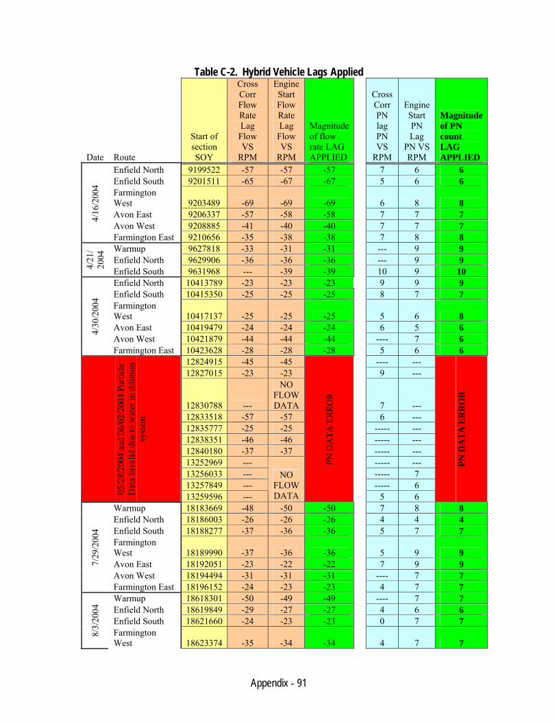
Appendix - 91

Table C-2. Hybrid Vehicle Lags Applied

Date Route

Start of section SOY

Cross Corr Flow Rate Lag Flow VS

RPM

Engine Start Flow Rate Lag

Flow VS

RPM

Magnitude of flow rate LAG APPLIED

Cross Corr PN lag PN VS

RPM

Engine Start PN Lag

PN VS RPM

Magnitude of PN count LAG APPLIED

Enfield North 9199522 -57 -57 -57 7 6 6 Enfield South 9201511 -65 -67 -67 5 6 6 Farmington West 9203489 -69 -69 -69 6 8 8 Avon East 9206337 -57 -58 -58 7 7 7 Avon West 9208885 -41 -40 -40 7 7 7

4/16

/200

4

Farmington East 9210656 -35 -38 -38 7 8 8 Warmup 9627818 -33 -31 -31 --- 9 9 Enfield North 9629906 -36 -36 -36 --- 9 9

4/21

/20

04

Enfield South 9631968 --- -39 -39 10 9 10 Enfield North 10413789 -23 -23 -23 9 9 9 Enfield South 10415350 -25 -25 -25 8 7 7 Farmington West 10417137 -25 -25 -25 5 6 8 Avon East 10419479 -24 -24 -24 6 5 6 Avon West 10421879 -44 -44 -44 ---- 7 6

4/30

/200

4

Farmington East 10423628 -28 -28 -28 5 6 6 12824915 -45 -45 ---- --- 12827015 -23 -23 9 ---

12830788 ---

NO FLOW DATA 7 ---

12833518 -57 -57 6 --- 12835777 -25 -25 ----- --- 12838351 -46 -46 ----- --- 12840180 -37 -37 ----- --- 13252969 --- ----- --- 13256033 --- ----- 7 13257849 --- ----- 6

05/2

8/20

04 a

nd 0

6/02

/200

4 Pa

rticl

e D

ata

Inva

lid d

ue to

wat

er in

dilu

tion

syst

em

13259596 ---

NO FLOW DATA

PN D

ATA

ER

RO

R

5 6

PN D

AT

A E

RR

OR

Warmup 18183669 -48 -50 -50 7 8 8 Enfield North 18186003 -26 -26 -26 4 4 4 Enfield South 18188277 -37 -36 -36 5 7 7 Farmington West 18189990 -37 -36 -36 5 9 9 Avon East 18192051 -23 -22 -22 7 9 9 Avon West 18194494 -31 -31 -31 ---- 7 7

7/29

/200

4

Farmington East 18196152 -24 -23 -23 4 7 7 Warmup 18618301 -50 -49 -49 ---- 7 7 Enfield North 18619849 -29 -27 -27 4 6 6 Enfield South 18621660 -24 -23 -23 0 7 7

8/3/

2004

Farmington West 18623374 -35 -34 -34 4 7 7

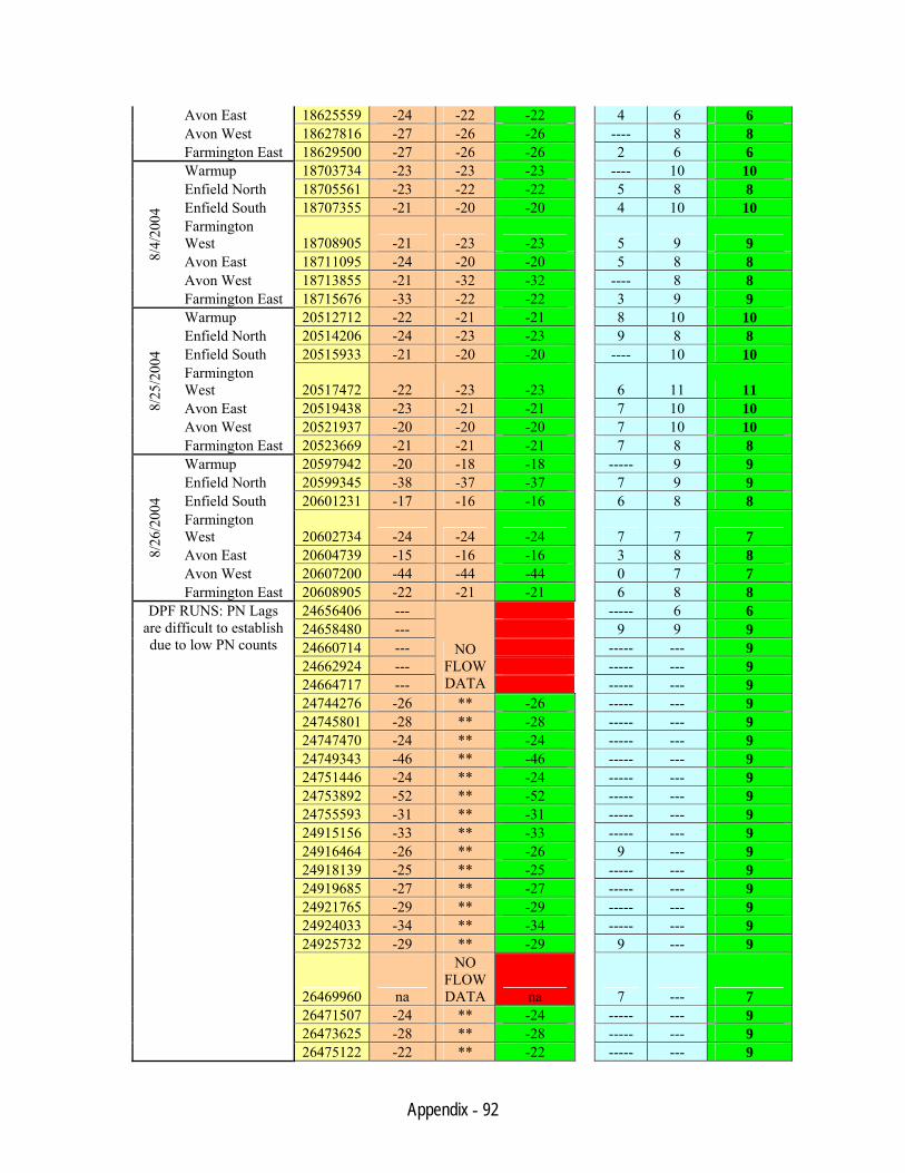
Appendix - 92

Avon East 18625559 -24 -22 -22 4 6 6 Avon West 18627816 -27 -26 -26 ---- 8 8 Farmington East 18629500 -27 -26 -26 2 6 6 Warmup 18703734 -23 -23 -23 ---- 10 10 Enfield North 18705561 -23 -22 -22 5 8 8 Enfield South 18707355 -21 -20 -20 4 10 10 Farmington West 18708905 -21 -23 -23 5 9 9 Avon East 18711095 -24 -20 -20 5 8 8 Avon West 18713855 -21 -32 -32 ---- 8 8

8/4/

2004

Farmington East 18715676 -33 -22 -22 3 9 9 Warmup 20512712 -22 -21 -21 8 10 10 Enfield North 20514206 -24 -23 -23 9 8 8 Enfield South 20515933 -21 -20 -20 ---- 10 10 Farmington West 20517472 -22 -23 -23 6 11 11 Avon East 20519438 -23 -21 -21 7 10 10 Avon West 20521937 -20 -20 -20 7 10 10

8/25

/200

4

Farmington East 20523669 -21 -21 -21 7 8 8 Warmup 20597942 -20 -18 -18 ----- 9 9 Enfield North 20599345 -38 -37 -37 7 9 9 Enfield South 20601231 -17 -16 -16 6 8 8 Farmington West 20602734 -24 -24 -24 7 7 7 Avon East 20604739 -15 -16 -16 3 8 8 Avon West 20607200 -44 -44 -44 0 7 7

8/26

/200

4

Farmington East 20608905 -22 -21 -21 6 8 8 24656406 --- ----- 6 6 24658480 --- 9 9 9 24660714 --- ----- --- 9 24662924 --- ----- --- 9 24664717 ---

NO FLOW DATA ----- --- 9

24744276 -26 ** -26 ----- --- 9 24745801 -28 ** -28 ----- --- 9 24747470 -24 ** -24 ----- --- 9 24749343 -46 ** -46 ----- --- 9 24751446 -24 ** -24 ----- --- 9 24753892 -52 ** -52 ----- --- 9 24755593 -31 ** -31 ----- --- 9 24915156 -33 ** -33 ----- --- 9 24916464 -26 ** -26 9 --- 9 24918139 -25 ** -25 ----- --- 9 24919685 -27 ** -27 ----- --- 9 24921765 -29 ** -29 ----- --- 9 24924033 -34 ** -34 ----- --- 9 24925732 -29 ** -29 9 --- 9

26469960 na

NO FLOW DATA na 7 --- 7

26471507 -24 ** -24 ----- --- 9 26473625 -28 ** -28 ----- --- 9

DPF RUNS: PN Lags are difficult to establish due to low PN counts

26475122 -22 ** -22 ----- --- 9

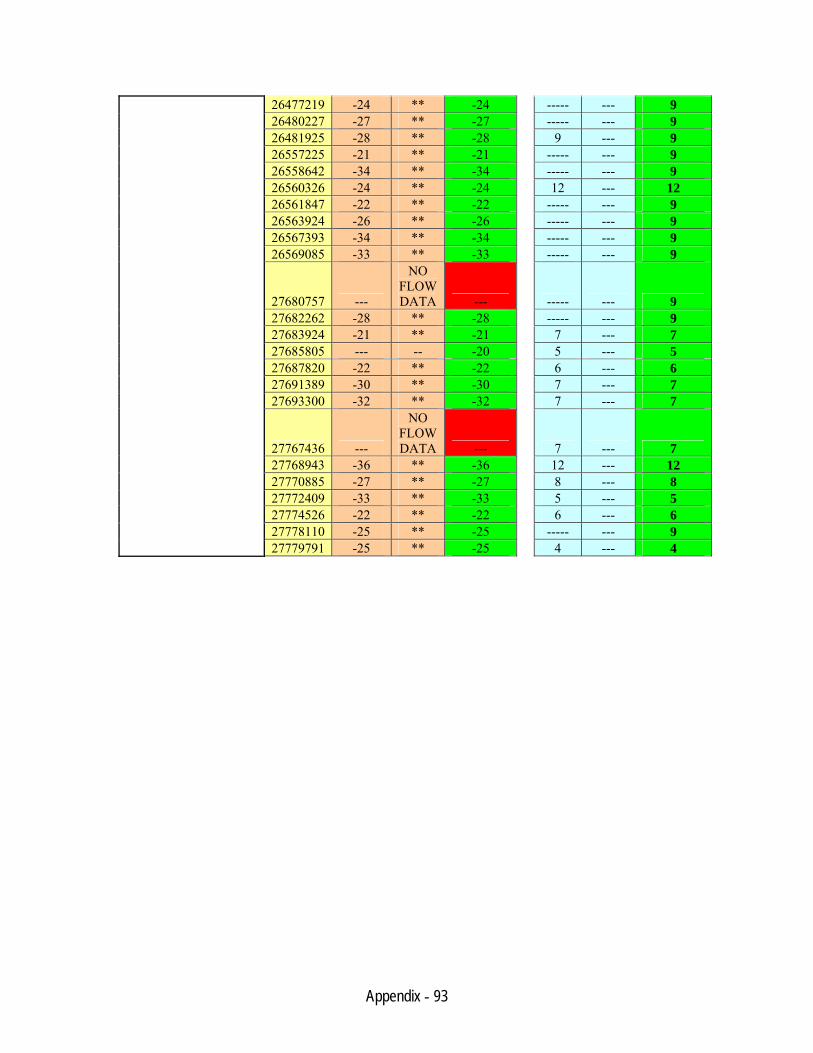
Appendix - 93

26477219 -24 ** -24 ----- --- 9 26480227 -27 ** -27 ----- --- 9 26481925 -28 ** -28 9 --- 9 26557225 -21 ** -21 ----- --- 9 26558642 -34 ** -34 ----- --- 9 26560326 -24 ** -24 12 --- 12 26561847 -22 ** -22 ----- --- 9 26563924 -26 ** -26 ----- --- 9 26567393 -34 ** -34 ----- --- 9 26569085 -33 ** -33 ----- --- 9

27680757 ---

NO FLOW DATA --- ----- --- 9

27682262 -28 ** -28 ----- --- 9 27683924 -21 ** -21 7 --- 7 27685805 --- -- -20 5 --- 5 27687820 -22 ** -22 6 --- 6 27691389 -30 ** -30 7 --- 7 27693300 -32 ** -32 7 --- 7

27767436 ---

NO FLOW DATA --- 7 --- 7

27768943 -36 ** -36 12 --- 12 27770885 -27 ** -27 8 --- 8 27772409 -33 ** -33 5 --- 5 27774526 -22 ** -22 6 --- 6 27778110 -25 ** -25 ----- --- 9 27779791 -25 ** -25 4 --- 4

Appendix - 94

Appendix D. Data Dictionary for Dataset Parameters

Appendix D contains a data dictionary summarizing each of the parameters found in the final CT Transit Emissions and Operations Dataset. The parameter lists for CD and HDE bus types are described separately here.

Data Dictionary: Conventional Diesel Bus Dataset

File Name: Conv_4_1_08.csv Organized By: Eric Jackson The dataset described in this document was compiled from the data collected in Project 03-8 as described in report JHR 05-304. A detailed data collection methodology and instrumentation description can be found in the final report from JHR 05-304 “PARTICULATE MATTER EMISSIONS FROM HYBRID DIESEL-ELECTRIC AND CONVENTIONAL DIESEL TRANSIT BUSES: FUEL AND AFTERTREATMENT EFFECTS” by Britt A. Holmén, Zhong Chen, Aura C. Davila, Oliver Gao and Derek M. Vikara. This report can be found at: www.ct.gov/dot/LIB/dot/documents/dresearch/CT_JHR_05-304_JH_03-8.pdf The original data were in multiple files based on the day of data collection and Dr. Eric Jackson compiled the multiple data files into one master file. The resulting master file was temporally aligned to ensure the emissions, vehicle operations and spatial data were all temporally accurate in terms of the time-stamp assigned as “seconds of year 2004” (SOY).

Segments of the test route were defined by the start and stop of the bus engine at predetermine locations along the test route. The temporal offset was then estimated for each segment of the test route. There were two methods used to estimate the temporal offset between instruments. The first method was to manually estimate the time lag between engine start and the response of the respective instrument. (i.e., the time when RPM increased from 0 compared to the instant Particle Number (PN) or exhaust flowrate increased dramatically).

The second method used a cross-correlation analysis to estimate the temporal offset between instruments. The temporal offset values obtained from the cross-correlation analysis were applied to the dataset. The cross-correlation analysis accounts for the temporal alignment over the entire test segment and not just the lag at the engine start like the manual engine start method. Both methods resulted in very similar estimates (within ± 2 seconds) of the temporal offset for each segment of the test route and therefore provided an accuracy check for temporal adjustment.

Table D-1 contains an explanation of each variable in the dataset and a brief description of that variable.

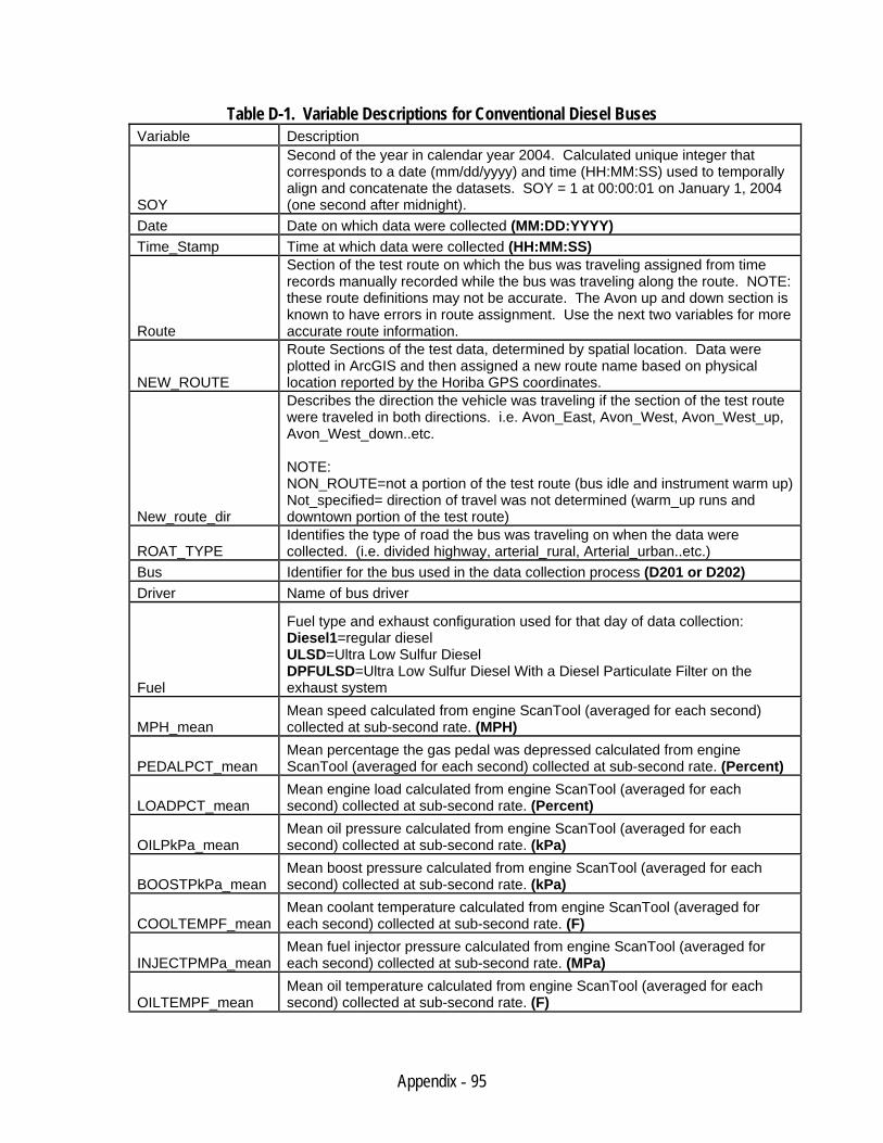
Appendix - 95

Table D-1. Variable Descriptions for Conventional Diesel Buses Variable Description

SOY

Second of the year in calendar year 2004. Calculated unique integer that corresponds to a date (mm/dd/yyyy) and time (HH:MM:SS) used to temporally align and concatenate the datasets. SOY = 1 at 00:00:01 on January 1, 2004 (one second after midnight).

Date Date on which data were collected (MM:DD:YYYY) Time_Stamp Time at which data were collected (HH:MM:SS)

Route

Section of the test route on which the bus was traveling assigned from time records manually recorded while the bus was traveling along the route. NOTE: these route definitions may not be accurate. The Avon up and down section is known to have errors in route assignment. Use the next two variables for more accurate route information.

NEW_ROUTE

Route Sections of the test data, determined by spatial location. Data were plotted in ArcGIS and then assigned a new route name based on physical location reported by the Horiba GPS coordinates.

New_route_dir

Describes the direction the vehicle was traveling if the section of the test route were traveled in both directions. i.e. Avon_East, Avon_West, Avon_West_up, Avon_West_down..etc. NOTE: NON_ROUTE=not a portion of the test route (bus idle and instrument warm up) Not_specified= direction of travel was not determined (warm_up runs and downtown portion of the test route)

ROAT_TYPE Identifies the type of road the bus was traveling on when the data were collected. (i.e. divided highway, arterial_rural, Arterial_urban..etc.)

Bus Identifier for the bus used in the data collection process (D201 or D202) Driver Name of bus driver

Fuel

Fuel type and exhaust configuration used for that day of data collection: Diesel1=regular diesel ULSD=Ultra Low Sulfur Diesel DPFULSD=Ultra Low Sulfur Diesel With a Diesel Particulate Filter on the exhaust system

MPH_mean Mean speed calculated from engine ScanTool (averaged for each second) collected at sub-second rate. (MPH)

PEDALPCT_mean Mean percentage the gas pedal was depressed calculated from engine ScanTool (averaged for each second) collected at sub-second rate. (Percent)

LOADPCT_mean Mean engine load calculated from engine ScanTool (averaged for each second) collected at sub-second rate. (Percent)

OILPkPa_mean Mean oil pressure calculated from engine ScanTool (averaged for each second) collected at sub-second rate. (kPa)

BOOSTPkPa_mean Mean boost pressure calculated from engine ScanTool (averaged for each second) collected at sub-second rate. (kPa)

COOLTEMPF_mean Mean coolant temperature calculated from engine ScanTool (averaged for each second) collected at sub-second rate. (F)

INJECTPMPa_mean Mean fuel injector pressure calculated from engine ScanTool (averaged for each second) collected at sub-second rate. (MPa)

OILTEMPF_mean Mean oil temperature calculated from engine ScanTool (averaged for each second) collected at sub-second rate. (F)

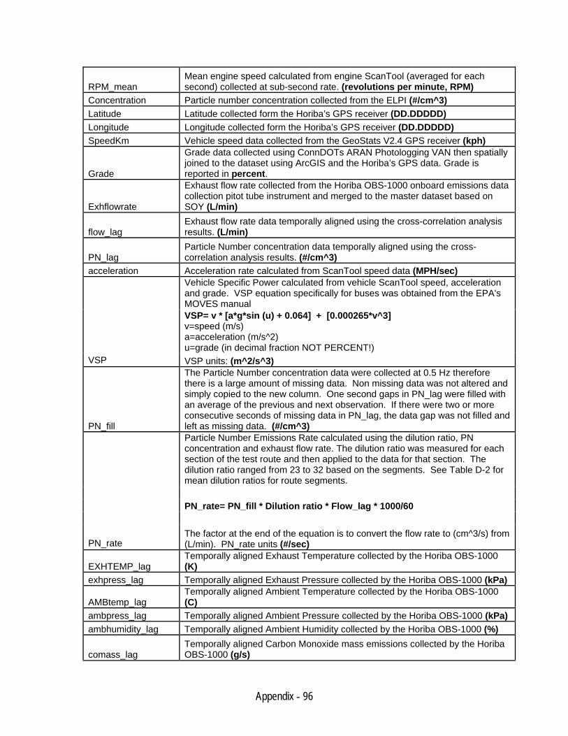
Appendix - 96

RPM_mean Mean engine speed calculated from engine ScanTool (averaged for each second) collected at sub-second rate. (revolutions per minute, RPM)

Concentration Particle number concentration collected from the ELPI (#/cm^3) Latitude Latitude collected form the Horiba’s GPS receiver (DD.DDDDD) Longitude Longitude collected form the Horiba’s GPS receiver (DD.DDDDD) SpeedKm Vehicle speed data collected from the GeoStats V2.4 GPS receiver (kph)

Grade

Grade data collected using ConnDOTs ARAN Photologging VAN then spatially joined to the dataset using ArcGIS and the Horiba’s GPS data. Grade is reported in percent.

Exhflowrate

Exhaust flow rate collected from the Horiba OBS-1000 onboard emissions data collection pitot tube instrument and merged to the master dataset based on SOY (L/min)

flow_lag Exhaust flow rate data temporally aligned using the cross-correlation analysis results. (L/min)

PN_lag Particle Number concentration data temporally aligned using the cross-correlation analysis results. (#/cm^3)

acceleration Acceleration rate calculated from ScanTool speed data (MPH/sec) Vehicle Specific Power calculated from vehicle ScanTool speed, acceleration and grade. VSP equation specifically for buses was obtained from the EPA's MOVES manual VSP= v * [a*g*sin (u) + 0.064] + [0.000265*v^3] v=speed (m/s) a=acceleration (m/s^2) u=grade (in decimal fraction NOT PERCENT!)

VSP VSP units: (m^2/s^3)

PN_fill

The Particle Number concentration data were collected at 0.5 Hz therefore there is a large amount of missing data. Non missing data was not altered and simply copied to the new column. One second gaps in PN_lag were filled with an average of the previous and next observation. If there were two or more consecutive seconds of missing data in PN_lag, the data gap was not filled and left as missing data. (#/cm^3) Particle Number Emissions Rate calculated using the dilution ratio, PN concentration and exhaust flow rate. The dilution ratio was measured for each section of the test route and then applied to the data for that section. The dilution ratio ranged from 23 to 32 based on the segments. See Table D-2 for mean dilution ratios for route segments. PN_rate= PN_fill * Dilution ratio * Flow_lag * 1000/60

PN_rate The factor at the end of the equation is to convert the flow rate to (cm^3/s) from (L/min). PN_rate units (#/sec)

EXHTEMP_lag Temporally aligned Exhaust Temperature collected by the Horiba OBS-1000 (K)

exhpress_lag Temporally aligned Exhaust Pressure collected by the Horiba OBS-1000 (kPa)

AMBtemp_lag Temporally aligned Ambient Temperature collected by the Horiba OBS-1000 (C)

ambpress_lag Temporally aligned Ambient Pressure collected by the Horiba OBS-1000 (kPa) ambhumidity_lag Temporally aligned Ambient Humidity collected by the Horiba OBS-1000 (%)

comass_lag Temporally aligned Carbon Monoxide mass emissions collected by the Horiba OBS-1000 (g/s)

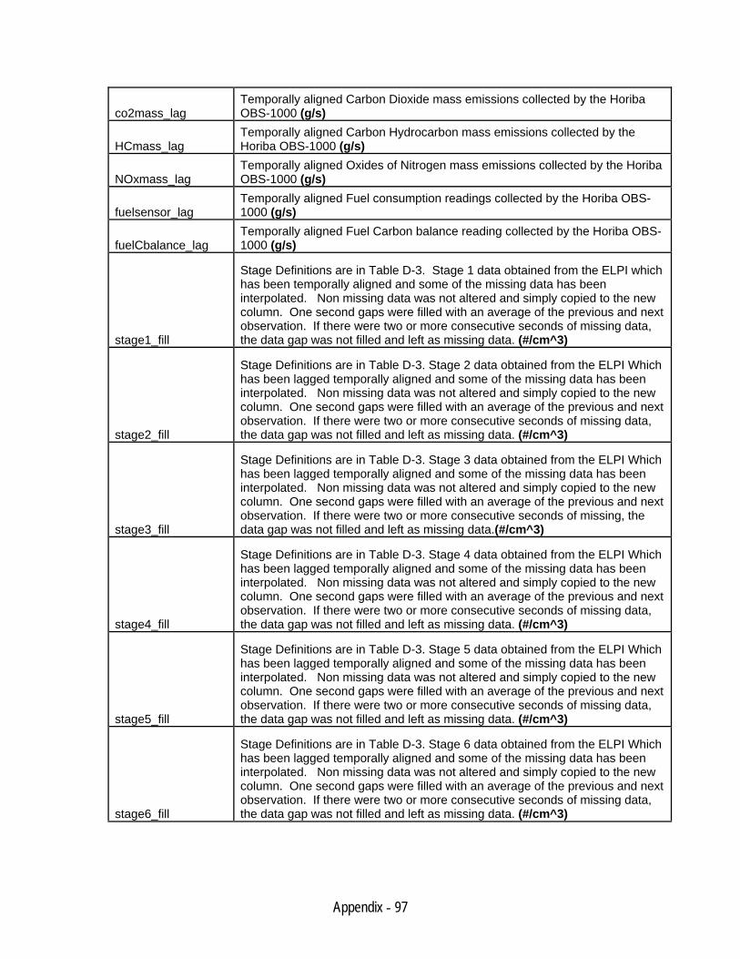
Appendix - 97

co2mass_lag Temporally aligned Carbon Dioxide mass emissions collected by the Horiba OBS-1000 (g/s)

HCmass_lag Temporally aligned Carbon Hydrocarbon mass emissions collected by the Horiba OBS-1000 (g/s)

NOxmass_lag Temporally aligned Oxides of Nitrogen mass emissions collected by the Horiba OBS-1000 (g/s)

fuelsensor_lag Temporally aligned Fuel consumption readings collected by the Horiba OBS-1000 (g/s)

fuelCbalance_lag Temporally aligned Fuel Carbon balance reading collected by the Horiba OBS-1000 (g/s)

stage1_fill

Stage Definitions are in Table D-3. Stage 1 data obtained from the ELPI which has been temporally aligned and some of the missing data has been interpolated. Non missing data was not altered and simply copied to the new column. One second gaps were filled with an average of the previous and next observation. If there were two or more consecutive seconds of missing data, the data gap was not filled and left as missing data. (#/cm^3)

stage2_fill

Stage Definitions are in Table D-3. Stage 2 data obtained from the ELPI Which has been lagged temporally aligned and some of the missing data has been interpolated. Non missing data was not altered and simply copied to the new column. One second gaps were filled with an average of the previous and next observation. If there were two or more consecutive seconds of missing data, the data gap was not filled and left as missing data. (#/cm^3)

stage3_fill

Stage Definitions are in Table D-3. Stage 3 data obtained from the ELPI Which has been lagged temporally aligned and some of the missing data has been interpolated. Non missing data was not altered and simply copied to the new column. One second gaps were filled with an average of the previous and next observation. If there were two or more consecutive seconds of missing, the data gap was not filled and left as missing data.(#/cm^3)

stage4_fill

Stage Definitions are in Table D-3. Stage 4 data obtained from the ELPI Which has been lagged temporally aligned and some of the missing data has been interpolated. Non missing data was not altered and simply copied to the new column. One second gaps were filled with an average of the previous and next observation. If there were two or more consecutive seconds of missing data, the data gap was not filled and left as missing data. (#/cm^3)

stage5_fill

Stage Definitions are in Table D-3. Stage 5 data obtained from the ELPI Which has been lagged temporally aligned and some of the missing data has been interpolated. Non missing data was not altered and simply copied to the new column. One second gaps were filled with an average of the previous and next observation. If there were two or more consecutive seconds of missing data, the data gap was not filled and left as missing data. (#/cm^3)

stage6_fill

Stage Definitions are in Table D-3. Stage 6 data obtained from the ELPI Which has been lagged temporally aligned and some of the missing data has been interpolated. Non missing data was not altered and simply copied to the new column. One second gaps were filled with an average of the previous and next observation. If there were two or more consecutive seconds of missing data, the data gap was not filled and left as missing data. (#/cm^3)

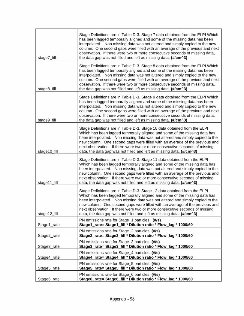
Appendix - 98

stage7_fill

Stage Definitions are in Table D-3. Stage 7 data obtained from the ELPI Which has been lagged temporally aligned and some of the missing data has been interpolated. Non missing data was not altered and simply copied to the new column. One second gaps were filled with an average of the previous and next observation. If there were two or more consecutive seconds of missing data, the data gap was not filled and left as missing data. (#/cm^3)

stage8_fill

Stage Definitions are in Table D-3. Stage 8 data obtained from the ELPI Which has been lagged temporally aligned and some of the missing data has been interpolated. Non missing data was not altered and simply copied to the new column. One second gaps were filled with an average of the previous and next observation. If there were two or more consecutive seconds of missing data, the data gap was not filled and left as missing data. (#/cm^3)

stage9_fill

Stage Definitions are in Table D-3. Stage 9 data obtained from the ELPI Which has been lagged temporally aligned and some of the missing data has been interpolated. Non missing data was not altered and simply copied to the new column. One second gaps were filled with an average of the previous and next observation. If there were two or more consecutive seconds of missing data, the data gap was not filled and left as missing data. (#/cm^3)

stage10_fill

Stage Definitions are in Table D-3. Stage 10 data obtained from the ELPI Which has been lagged temporally aligned and some of the missing data has been interpolated. Non missing data was not altered and simply copied to the new column. One second gaps were filled with an average of the previous and next observation. If there were two or more consecutive seconds of missing data, the data gap was not filled and left as missing data. (#/cm^3)

stage11_fill

Stage Definitions are in Table D-3. Stage 11 data obtained from the ELPI Which has been lagged temporally aligned and some of the missing data has been interpolated. Non missing data was not altered and simply copied to the new column. One second gaps were filled with an average of the previous and next observation. If there were two or more consecutive seconds of missing data, the data gap was not filled and left as missing data. (#/cm^3)

stage12_fill

Stage Definitions are in Table D-3. Stage 12 data obtained from the ELPI Which has been lagged temporally aligned and some of the missing data has been interpolated. Non missing data was not altered and simply copied to the new column. One second gaps were filled with an average of the previous and next observation. If there were two or more consecutive seconds of missing data, the data gap was not filled and left as missing data. (#/cm^3)

Stage1_rate PN emissions rate for Stage_1 particles. (#/s) Stage1_rate= Stage1_fill * Dilution ratio * Flow_lag * 1000/60

Stage2_rate PN emissions rate for Stage_2 particles. (#/s) Stage2_rate= Stage2_fill * Dilution ratio * Flow_lag * 1000/60

Stage3_rate PN emissions rate for Stage_3 particles. (#/s) Stage3_rate= Stage3_fill * Dilution ratio * Flow_lag * 1000/60

Stage4_rate PN emissions rate for Stage_4 particles. (#/s) Stage4_rate= Stage4_fill * Dilution ratio * Flow_lag * 1000/60

Stage5_rate PN emissions rate for Stage_5 particles. (#/s) Stage5_rate= Stage5_fill * Dilution ratio * Flow_lag * 1000/60

Stage6_rate PN emissions rate for Stage_6 particles. (#/s) Stage6_rate= Stage6_fill * Dilution ratio * Flow_lag * 1000/60

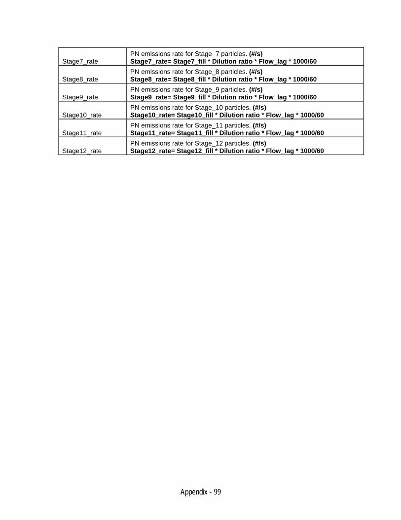
Appendix - 99

Stage7_rate PN emissions rate for Stage_7 particles. (#/s) Stage7_rate= Stage7_fill * Dilution ratio * Flow_lag * 1000/60

Stage8_rate PN emissions rate for Stage_8 particles. (#/s) Stage8_rate= Stage8_fill * Dilution ratio * Flow_lag * 1000/60

Stage9_rate PN emissions rate for Stage_9 particles. (#/s) Stage9_rate= Stage9_fill * Dilution ratio * Flow_lag * 1000/60

Stage10_rate PN emissions rate for Stage_10 particles. (#/s) Stage10_rate= Stage10_fill * Dilution ratio * Flow_lag * 1000/60

Stage11_rate PN emissions rate for Stage_11 particles. (#/s) Stage11_rate= Stage11_fill * Dilution ratio * Flow_lag * 1000/60

Stage12_rate PN emissions rate for Stage_12 particles. (#/s) Stage12_rate= Stage12_fill * Dilution ratio * Flow_lag * 1000/60

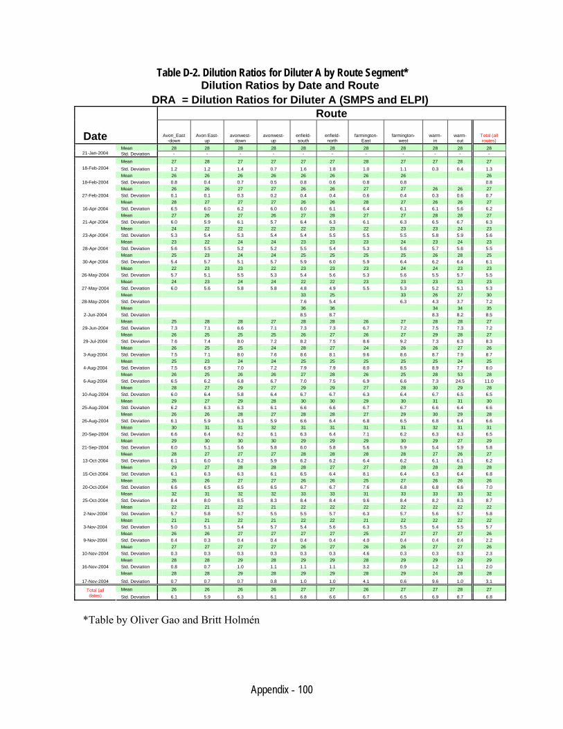
Appendix - 100

Table D-2. Dilution Ratios for Diluter A by Route Segment* Dilution Ratios by Date and Route

DRA = Dilution Ratios for Diluter A (SMPS and ELPI) Route

Date Avon_East

-down Avon East-

up avonwest-

down avonwest-

up enfield-south

enfield-north

farmington-East

farmington-west

warm-in

warm-out

Total (all routes)

Mean 28 28 28 28 28 28 28 28 28 28 28 21-Jan-2004 Std. Deviation - - - - - - - - - - -

Mean 27 28 27 27 27 27 28 27 27 28 27 18-Feb-2004 Std. Deviation 1.2 1.2 1.4 0.7 1.6 1.8 1.0 1.1 0.3 0.4 1.3

Mean 26 26 26 26 26 26 26 26 26 18-Feb-2004 Std. Deviation 0.8 0.4 0.7 0.5 0.8 0.6 0.8 0.8 0.8

Mean 26 26 27 27 26 26 27 27 26 26 27 27-Feb-2004 Std. Deviation 0.1 0.1 0.3 0.2 0.4 0.4 0.6 0.4 0.3 0.6 0.7

Mean 28 27 27 27 26 26 28 27 26 26 27 16-Apr-2004 Std. Deviation 6.5 6.0 6.2 6.0 6.0 6.1 6.4 6.1 6.1 5.6 6.2

Mean 27 26 27 26 27 28 27 27 28 28 27 21-Apr-2004 Std. Deviation 6.0 5.9 6.1 5.7 6.4 6.3 6.1 6.3 6.5 6.7 6.3

Mean 24 22 22 22 22 23 22 23 23 24 23 23-Apr-2004 Std. Deviation 5.3 5.4 5.3 5.4 5.4 5.5 5.5 5.5 5.8 5.9 5.6

Mean 23 22 24 24 23 23 23 24 23 24 23 28-Apr-2004 Std. Deviation 5.6 5.5 5.2 5.2 5.5 5.4 5.3 5.6 5.7 5.6 5.5

Mean 25 23 24 24 25 25 25 25 26 28 25 30-Apr-2004 Std. Deviation 5.4 5.7 5.1 5.7 5.9 6.0 5.9 6.4 6.2 6.4 6.1

Mean 22 23 23 22 23 23 23 24 24 23 23 26-May-2004 Std. Deviation 5.7 5.1 5.5 5.3 5.4 5.6 5.3 5.6 5.5 5.7 5.5

Mean 24 23 24 24 22 22 23 23 23 23 23 27-May-2004 Std. Deviation 6.0 5.6 5.8 5.8 4.8 4.9 5.5 5.3 5.2 5.1 5.3

Mean 33 25 33 26 27 30 28-May-2004 Std. Deviation 7.6 5.4 6.3 4.3 3.7 7.2

Mean 36 36 34 34 35 2-Jun-2004 Std. Deviation 8.5 8.7 8.3 8.2 8.5

Mean 25 28 28 27 28 28 26 27 28 28 27 29-Jun-2004 Std. Deviation 7.3 7.1 6.6 7.1 7.3 7.3 6.7 7.2 7.5 7.3 7.2

Mean 26 25 25 25 26 27 26 27 29 28 27 29-Jul-2004 Std. Deviation 7.6 7.4 8.0 7.2 8.2 7.5 8.6 9.2 7.3 6.3 8.3

Mean 26 25 25 24 28 27 24 26 26 27 26 3-Aug-2004 Std. Deviation 7.5 7.1 8.0 7.6 8.6 8.1 9.6 8.6 8.7 7.9 8.7

Mean 25 23 24 24 25 25 25 25 25 24 25 4-Aug-2004 Std. Deviation 7.5 6.9 7.0 7.2 7.9 7.9 8.0 8.5 8.9 7.7 8.0

Mean 26 25 26 26 27 28 26 25 28 53 28 6-Aug-2004 Std. Deviation 6.5 6.2 6.8 6.7 7.0 7.5 6.9 6.6 7.3 24.5 11.0

Mean 28 27 29 27 29 29 27 28 30 29 28 10-Aug-2004 Std. Deviation 6.0 6.4 5.8 6.4 6.7 6.7 6.3 6.4 6.7 6.5 6.5

Mean 29 27 29 28 30 30 29 30 31 31 30 25-Aug-2004 Std. Deviation 6.2 6.3 6.3 6.1 6.6 6.6 6.7 6.7 6.6 6.4 6.6

Mean 26 26 28 27 28 28 27 29 30 29 28 26-Aug-2004 Std. Deviation 6.1 5.9 6.3 5.9 6.6 6.4 6.8 6.5 6.8 6.4 6.6

Mean 30 31 31 32 31 31 31 31 32 31 31 20-Sep-2004 Std. Deviation 6.6 6.4 6.2 6.1 6.3 6.4 7.1 6.2 6.3 6.3 6.5

Mean 29 30 30 30 29 29 29 30 29 27 29 21-Sep-2004 Std. Deviation 6.0 5.1 5.6 5.8 6.0 5.8 5.6 5.9 5.4 5.9 5.8

Mean 28 27 27 27 28 28 28 28 27 26 27 13-Oct-2004 Std. Deviation 6.1 6.0 6.2 5.9 6.2 6.2 6.4 6.2 6.1 6.1 6.2

Mean 29 27 28 28 28 27 27 28 28 28 28 15-Oct-2004 Std. Deviation 6.1 6.3 6.3 6.1 6.5 6.4 8.1 6.4 6.3 6.4 6.8

Mean 26 26 27 27 26 26 25 27 26 26 26 20-Oct-2004 Std. Deviation 6.6 6.5 6.5 6.5 6.7 6.7 7.6 6.8 6.8 6.6 7.0

Mean 32 31 32 32 33 33 31 33 33 33 32 25-Oct-2004 Std. Deviation 8.4 8.0 8.5 8.3 8.4 8.4 9.6 8.4 8.2 8.3 8.7

Mean 22 21 22 21 22 22 22 22 22 22 22 2-Nov-2004 Std. Deviation 5.7 5.8 5.7 5.5 5.5 5.7 6.3 5.7 5.6 5.7 5.8

Mean 21 21 22 21 22 22 21 22 22 22 22 3-Nov-2004 Std. Deviation 5.0 5.1 5.4 5.7 5.4 5.6 6.3 5.5 5.4 5.5 5.7

Mean 26 26 27 27 27 27 25 27 27 27 26 9-Nov-2004 Std. Deviation 0.4 0.3 0.4 0.4 0.4 0.4 4.0 0.4 0.4 0.4 2.2

Mean 27 27 27 27 26 27 26 26 27 27 26 10-Nov-2004 Std. Deviation 0.3 0.3 0.3 0.3 0.3 0.3 4.6 0.3 0.3 0.3 2.3

Mean 28 28 29 28 29 29 28 29 29 29 29 16-Nov-2004 Std. Deviation 0.8 0.7 1.0 1.1 1.1 1.1 3.2 0.9 1.2 1.1 2.0

Mean 28 28 29 28 29 29 28 29 24 28 28

17-Nov-2004 Std. Deviation 0.7 0.7 0.7 0.8 1.0 1.0 4.1 0.6 9.6 1.0 3.1

Mean 26 26 26 26 27 27 26 27 27 28 27 Total (all dates) Std. Deviation 6.1 5.9 6.3 6.1 6.8 6.6 6.7 6.5 6.9 8.7 6.8

*Table by Oliver Gao and Britt Holmén

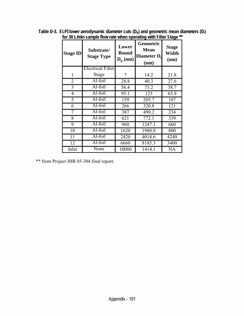
Appendix - 101

Table D-3. ELPI lower aerodynamic diameter cuts (Dp) and geometric mean diameters (Di) for 30 L/min sample flow rate when operating with Filter Stage **

Stage ID Substrate/ Stage Type

Lower Bound

Dp (nm)

Geometric Mean

Diameter Di

(nm)

Stage Width (nm)

1Electrical Filter

Stage 7 14.2 21.82 Al-foil 28.8 40.3 27.63 Al-foil 56.4 73.2 38.74 Al-foil 95.1 123 63.95 Al-foil 159 205.7 1076 Al-foil 266 320.8 1217 Al-foil 387 490.2 2348 Al-foil 621 772.1 3399 Al-foil 960 1247.1 66010 Al-foil 1620 1980.0 80011 Al-foil 2420 4014.6 424012 Al-foil 6660 8185.3 3400

Inlet None 10060 1414.1 NA

** from Project JHR 05-304 final report.

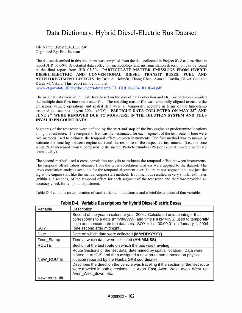
Appendix - 102

Data Dictionary: Hybrid Diesel-Electric Bus Dataset

File Name: Hybrid_4_1_08.csv Organized By: Eric Jackson The dataset described in this document was compiled from the data collected in Project 03-8 as described in report JHR 05-304. A detailed data collection methodology and instrumentation description can be found in the final report from JHR 05-304 “PARTICULATE MATTER EMISSIONS FROM HYBRID DIESEL-ELECTRIC AND CONVENTIONAL DIESEL TRANSIT BUSES: FUEL AND AFTERTREATMENT EFFECTS” by Britt A. Holmén, Zhong Chen, Aura C. Davila, Oliver Gao and Derek M. Vikara. This report can be found at: www.ct.gov/dot/LIB/dot/documents/dresearch/CT_JHR_05-304_JH_03-8.pdf The original data were in multiple files based on the day of data collection and Dr. Eric Jackson compiled the multiple data files into one master file. The resulting master file was temporally aligned to ensure the emissions, vehicle operations and spatial data were all temporally accurate in terms of the time-stamp assigned as “seconds of year 2004” (SOY). PARTICLE DATA COLLECTED ON MAY 28th AND JUNE 2nd WERE REMOVED DUE TO MOISTURE IN THE DILUTION SYSTEM AND THUS INVALID PN COUNT DATA.

Segments of the test route were defined by the start and stop of the bus engine at predetermine locations along the test route. The temporal offset was then estimated for each segment of the test route. There were two methods used to estimate the temporal offset between instruments. The first method was to manually estimate the time lag between engine start and the response of the respective instrument. (i.e., the time when RPM increased from 0 compared to the instant Particle Number (PN) or exhaust flowrate increased dramatically).

The second method used a cross-correlation analysis to estimate the temporal offset between instruments. The temporal offset values obtained from the cross-correlation analysis were applied to the dataset. The cross-correlation analysis accounts for the temporal alignment over the entire test segment and not just the lag at the engine start like the manual engine start method. Both methods resulted in very similar estimates (within ± 2 seconds) of the temporal offset for each segment of the test route and therefore provided an accuracy check for temporal adjustment.

Table D-4 contains an explanation of each variable in the dataset and a brief description of that variable.

Table D-4. Variable Descriptions for Hybrid Diesel-Electric Buses

Variable Description

SOY

Second of the year in calendar year 2004. Calculated unique integer that corresponds to a date (mm/dd/yyyy) and time (HH:MM:SS) used to temporally align and concatenate the datasets. SOY = 1 at 00:00:01 on January 1, 2004 (one second after midnight).

Date Date on which data were collected (MM:DD:YYYY) Time_Stamp Time at which data were collected (HH:MM:SS) ROUTE Section of the test route on which the bus was traveling

NEW_ROUTE

Route Sections of the test data, determined by spatial location. Data were plotted in ArcGIS and then assigned a new route name based on physical location reported by the Horiba GPS coordinates.

New_route_dir

Describes the direction the vehicle was traveling if the section of the test route were traveled in both directions. i.e. Avon_East, Avon_West, Avon_West_up, Avon_West_down..etc.

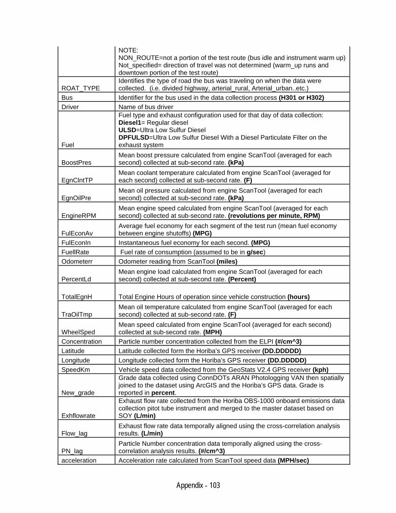
Appendix - 103

NOTE: NON_ROUTE=not a portion of the test route (bus idle and instrument warm up) Not_specified= direction of travel was not determined (warm_up runs and downtown portion of the test route)

ROAT_TYPE Identifies the type of road the bus was traveling on when the data were collected. (i.e. divided highway, arterial_rural, Arterial_urban..etc.)

Bus Identifier for the bus used in the data collection process (H301 or H302) Driver Name of bus driver

Fuel

Fuel type and exhaust configuration used for that day of data collection: Diesel1= Regular diesel ULSD=Ultra Low Sulfur Diesel DPFULSD=Ultra Low Sulfur Diesel With a Diesel Particulate Filter on the exhaust system

BoostPres Mean boost pressure calculated from engine ScanTool (averaged for each second) collected at sub-second rate. (kPa)

EgnClntTP Mean coolant temperature calculated from engine ScanTool (averaged for each second) collected at sub-second rate. (F)

EgnOilPre Mean oil pressure calculated from engine ScanTool (averaged for each second) collected at sub-second rate. (kPa)

EngineRPM Mean engine speed calculated from engine ScanTool (averaged for each second) collected at sub-second rate. (revolutions per minute, RPM)

FulEconAv Average fuel economy for each segment of the test run (mean fuel economy between engine shutoffs) (MPG)

FulEconIn Instantaneous fuel economy for each second. (MPG) FuellRate Fuel rate of consumption (assumed to be in g/sec) Odometerr Odometer reading from ScanTool (miles)

PercentLd Mean engine load calculated from engine ScanTool (averaged for each second) collected at sub-second rate. (Percent)

TotalEgnH Total Engine Hours of operation since vehicle construction (hours)

TraOilTmp Mean oil temperature calculated from engine ScanTool (averaged for each second) collected at sub-second rate. (F)

WheelSped Mean speed calculated from engine ScanTool (averaged for each second) collected at sub-second rate. (MPH)

Concentration Particle number concentration collected from the ELPI (#/cm^3) Latitude Latitude collected form the Horiba’s GPS receiver (DD.DDDDD) Longitude Longitude collected form the Horiba’s GPS receiver (DD.DDDDD) SpeedKm Vehicle speed data collected from the GeoStats V2.4 GPS receiver (kph)

New_grade

Grade data collected using ConnDOTs ARAN Photologging VAN then spatially joined to the dataset using ArcGIS and the Horiba’s GPS data. Grade is reported in percent.

Exhflowrate

Exhaust flow rate collected from the Horiba OBS-1000 onboard emissions data collection pitot tube instrument and merged to the master dataset based on SOY (L/min)

Flow_lag Exhaust flow rate data temporally aligned using the cross-correlation analysis results. (L/min)

PN_lag Particle Number concentration data temporally aligned using the cross-correlation analysis results. (#/cm^3)

acceleration Acceleration rate calculated from ScanTool speed data (MPH/sec)

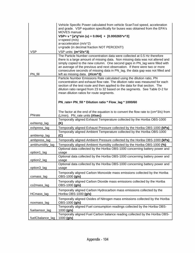
Appendix - 104

Vehicle Specific Power calculated from vehicle ScanTool speed, acceleration and grade. VSP equation specifically for buses was obtained from the EPA's MOVES manual VSP= v * [a*g*sin (u) + 0.064] + [0.000265*v^3] v=speed (m/s) a=acceleration (m/s^2) u=grade (in decimal fraction NOT PERCENT!)

VSP VSP units: (m^2/s^3)

PN_fill

The Particle Number concentration data were collected at 0.5 Hz therefore there is a large amount of missing data. Non missing data was not altered and simply copied to the new column. One second gaps in PN_lag were filled with an average of the previous and next observation. If there were two or more consecutive seconds of missing data in PN_lag, the data gap was not filled and left as missing data. (#/cm^3) Particle Number Emissions Rate calculated using the dilution ratio, PN concentration and exhaust flow rate. The dilution ratio was measured for each section of the test route and then applied to the data for that section. The dilution ratio ranged from 23 to 32 based on the segments. See Table D-2 for mean dilution ratios for route segments. PN_rate= PN_fill * Dilution ratio * Flow_lag * 1000/60

PNrate The factor at the end of the equation is to convert the flow rate to (cm^3/s) from (L/min). PN_rate units (#/sec)

exhtemp_lag Temporally aligned Exhaust Temperature collected by the Horiba OBS-1000 (K)

exhpress_lag Temporally aligned Exhaust Pressure collected by the Horiba OBS-1000 (kPa)

ambtemp_lag Temporally aligned Ambient Temperature collected by the Horiba OBS-1000 (C)

ambpress_lag Temporally aligned Ambient Pressure collected by the Horiba OBS-1000 (kPa) ambhumidity_lag Temporally aligned Ambient Humidity collected by the Horiba OBS-1000 (%)

option1_lag Optional data collected by the Horiba OBS-1000 concerning battery power and usage

option2_lag Optional data collected by the Horiba OBS-1000 concerning battery power and usage

option3_lag Optional data collected by the Horiba OBS-1000 concerning battery power and usage

comass_lag Temporally aligned Carbon Monoxide mass emissions collected by the Horiba OBS-1000 (g/s)

co2mass_lag Temporally aligned Carbon Dioxide mass emissions collected by the Horiba OBS-1000 (g/s)

HCmass_lag Temporally aligned Carbon Hydrocarbon mass emissions collected by the Horiba OBS-1000 (g/s)

noxmass_lag Temporally aligned Oxides of Nitrogen mass emissions collected by the Horiba OBS-1000 (g/s)

fuelsensor_lag Temporally aligned Fuel consumption readings collected by the Horiba OBS-1000 (g/s)

fuelCbalance_lag Temporally aligned Fuel Carbon balance reading collected by the Horiba OBS-1000 (g/s)

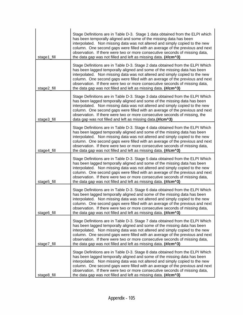
Appendix - 105

stage1_fill

Stage Definitions are in Table D-3. Stage 1 data obtained from the ELPI which has been temporally aligned and some of the missing data has been interpolated. Non missing data was not altered and simply copied to the new column. One second gaps were filled with an average of the previous and next observation. If there were two or more consecutive seconds of missing data, the data gap was not filled and left as missing data. (#/cm^3)

stage2_fill

Stage Definitions are in Table D-3. Stage 2 data obtained from the ELPI Which has been lagged temporally aligned and some of the missing data has been interpolated. Non missing data was not altered and simply copied to the new column. One second gaps were filled with an average of the previous and next observation. If there were two or more consecutive seconds of missing data, the data gap was not filled and left as missing data. (#/cm^3)

stage3_fill

Stage Definitions are in Table D-3. Stage 3 data obtained from the ELPI Which has been lagged temporally aligned and some of the missing data has been interpolated. Non missing data was not altered and simply copied to the new column. One second gaps were filled with an average of the previous and next observation. If there were two or more consecutive seconds of missing, the data gap was not filled and left as missing data.(#/cm^3)

stage4_fill

Stage Definitions are in Table D-3. Stage 4 data obtained from the ELPI Which has been lagged temporally aligned and some of the missing data has been interpolated. Non missing data was not altered and simply copied to the new column. One second gaps were filled with an average of the previous and next observation. If there were two or more consecutive seconds of missing data, the data gap was not filled and left as missing data. (#/cm^3)

stage5_fill

Stage Definitions are in Table D-3. Stage 5 data obtained from the ELPI Which has been lagged temporally aligned and some of the missing data has been interpolated. Non missing data was not altered and simply copied to the new column. One second gaps were filled with an average of the previous and next observation. If there were two or more consecutive seconds of missing data, the data gap was not filled and left as missing data. (#/cm^3)

stage6_fill

Stage Definitions are in Table D-3. Stage 6 data obtained from the ELPI Which has been lagged temporally aligned and some of the missing data has been interpolated. Non missing data was not altered and simply copied to the new column. One second gaps were filled with an average of the previous and next observation. If there were two or more consecutive seconds of missing data, the data gap was not filled and left as missing data. (#/cm^3)

stage7_fill

Stage Definitions are in Table D-3. Stage 7 data obtained from the ELPI Which has been lagged temporally aligned and some of the missing data has been interpolated. Non missing data was not altered and simply copied to the new column. One second gaps were filled with an average of the previous and next observation. If there were two or more consecutive seconds of missing data, the data gap was not filled and left as missing data. (#/cm^3)

stage8_fill

Stage Definitions are in Table D-3. Stage 8 data obtained from the ELPI Which has been lagged temporally aligned and some of the missing data has been interpolated. Non missing data was not altered and simply copied to the new column. One second gaps were filled with an average of the previous and next observation. If there were two or more consecutive seconds of missing data, the data gap was not filled and left as missing data. (#/cm^3)

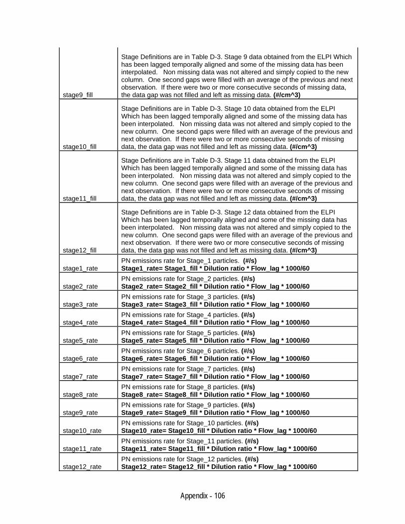
Appendix - 106

stage9_fill

Stage Definitions are in Table D-3. Stage 9 data obtained from the ELPI Which has been lagged temporally aligned and some of the missing data has been interpolated. Non missing data was not altered and simply copied to the new column. One second gaps were filled with an average of the previous and next observation. If there were two or more consecutive seconds of missing data, the data gap was not filled and left as missing data. (#/cm^3)

stage10_fill

Stage Definitions are in Table D-3. Stage 10 data obtained from the ELPI Which has been lagged temporally aligned and some of the missing data has been interpolated. Non missing data was not altered and simply copied to the new column. One second gaps were filled with an average of the previous and next observation. If there were two or more consecutive seconds of missing data, the data gap was not filled and left as missing data. (#/cm^3)

stage11_fill

Stage Definitions are in Table D-3. Stage 11 data obtained from the ELPI Which has been lagged temporally aligned and some of the missing data has been interpolated. Non missing data was not altered and simply copied to the new column. One second gaps were filled with an average of the previous and next observation. If there were two or more consecutive seconds of missing data, the data gap was not filled and left as missing data. (#/cm^3)

stage12_fill

Stage Definitions are in Table D-3. Stage 12 data obtained from the ELPI Which has been lagged temporally aligned and some of the missing data has been interpolated. Non missing data was not altered and simply copied to the new column. One second gaps were filled with an average of the previous and next observation. If there were two or more consecutive seconds of missing data, the data gap was not filled and left as missing data. (#/cm^3)

stage1_rate PN emissions rate for Stage_1 particles. (#/s) Stage1_rate= Stage1_fill * Dilution ratio * Flow_lag * 1000/60

stage2_rate PN emissions rate for Stage_2 particles. (#/s) Stage2_rate= Stage2_fill * Dilution ratio * Flow_lag * 1000/60

stage3_rate PN emissions rate for Stage_3 particles. (#/s) Stage3_rate= Stage3_fill * Dilution ratio * Flow_lag * 1000/60

stage4_rate PN emissions rate for Stage_4 particles. (#/s) Stage4_rate= Stage4_fill * Dilution ratio * Flow_lag * 1000/60

stage5_rate PN emissions rate for Stage_5 particles. (#/s) Stage5_rate= Stage5_fill * Dilution ratio * Flow_lag * 1000/60

stage6_rate PN emissions rate for Stage_6 particles. (#/s) Stage6_rate= Stage6_fill * Dilution ratio * Flow_lag * 1000/60

stage7_rate PN emissions rate for Stage_7 particles. (#/s) Stage7_rate= Stage7_fill * Dilution ratio * Flow_lag * 1000/60

stage8_rate PN emissions rate for Stage_8 particles. (#/s) Stage8_rate= Stage8_fill * Dilution ratio * Flow_lag * 1000/60

stage9_rate PN emissions rate for Stage_9 particles. (#/s) Stage9_rate= Stage9_fill * Dilution ratio * Flow_lag * 1000/60

stage10_rate PN emissions rate for Stage_10 particles. (#/s) Stage10_rate= Stage10_fill * Dilution ratio * Flow_lag * 1000/60

stage11_rate PN emissions rate for Stage_11 particles. (#/s) Stage11_rate= Stage11_fill * Dilution ratio * Flow_lag * 1000/60

stage12_rate PN emissions rate for Stage_12 particles. (#/s) Stage12_rate= Stage12_fill * Dilution ratio * Flow_lag * 1000/60

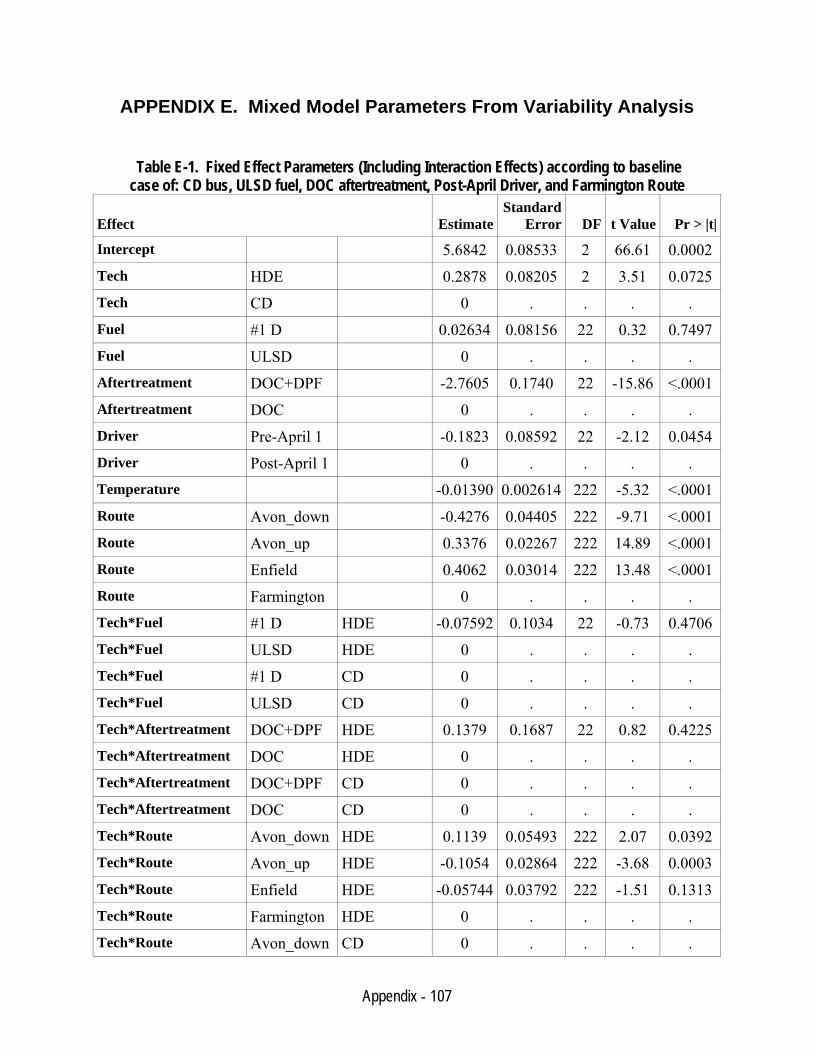
Appendix - 107

APPENDIX E. Mixed Model Parameters From Variability Analysis

Table E-1. Fixed Effect Parameters (Including Interaction Effects) according to baseline case of: CD bus, ULSD fuel, DOC aftertreatment, Post-April Driver, and Farmington Route

Effect EstimateStandard

Error DF t Value Pr > |t|

Intercept 5.6842 0.08533 2 66.61 0.0002 Tech HDE 0.2878 0.08205 2 3.51 0.0725 Tech CD 0 . . . . Fuel #1 D 0.02634 0.08156 22 0.32 0.7497 Fuel ULSD 0 . . . . Aftertreatment DOC+DPF -2.7605 0.1740 22 -15.86 <.0001Aftertreatment DOC 0 . . . . Driver Pre-April 1 -0.1823 0.08592 22 -2.12 0.0454 Driver Post-April 1 0 . . . . Temperature -0.01390 0.002614 222 -5.32 <.0001Route Avon_down -0.4276 0.04405 222 -9.71 <.0001Route Avon_up 0.3376 0.02267 222 14.89 <.0001Route Enfield 0.4062 0.03014 222 13.48 <.0001Route Farmington 0 . . . . Tech*Fuel #1 D HDE -0.07592 0.1034 22 -0.73 0.4706 Tech*Fuel ULSD HDE 0 . . . . Tech*Fuel #1 D CD 0 . . . . Tech*Fuel ULSD CD 0 . . . . Tech*Aftertreatment DOC+DPF HDE 0.1379 0.1687 22 0.82 0.4225 Tech*Aftertreatment DOC HDE 0 . . . . Tech*Aftertreatment DOC+DPF CD 0 . . . . Tech*Aftertreatment DOC CD 0 . . . . Tech*Route Avon_down HDE 0.1139 0.05493 222 2.07 0.0392 Tech*Route Avon_up HDE -0.1054 0.02864 222 -3.68 0.0003 Tech*Route Enfield HDE -0.05744 0.03792 222 -1.51 0.1313 Tech*Route Farmington HDE 0 . . . . Tech*Route Avon_down CD 0 . . . .

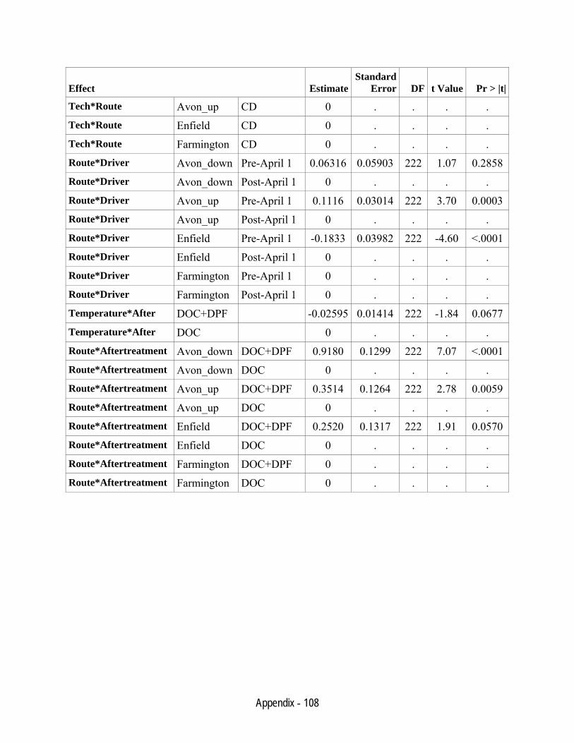
Appendix - 108

Effect EstimateStandard

Error DF t Value Pr > |t|

Tech*Route Avon_up CD 0 . . . . Tech*Route Enfield CD 0 . . . . Tech*Route Farmington CD 0 . . . . Route*Driver Avon_down Pre-April 1 0.06316 0.05903 222 1.07 0.2858 Route*Driver Avon_down Post-April 1 0 . . . . Route*Driver Avon_up Pre-April 1 0.1116 0.03014 222 3.70 0.0003 Route*Driver Avon_up Post-April 1 0 . . . . Route*Driver Enfield Pre-April 1 -0.1833 0.03982 222 -4.60 <.0001Route*Driver Enfield Post-April 1 0 . . . . Route*Driver Farmington Pre-April 1 0 . . . . Route*Driver Farmington Post-April 1 0 . . . . Temperature*After DOC+DPF -0.02595 0.01414 222 -1.84 0.0677 Temperature*After DOC 0 . . . . Route*Aftertreatment Avon_down DOC+DPF 0.9180 0.1299 222 7.07 <.0001Route*Aftertreatment Avon_down DOC 0 . . . . Route*Aftertreatment Avon_up DOC+DPF 0.3514 0.1264 222 2.78 0.0059 Route*Aftertreatment Avon_up DOC 0 . . . . Route*Aftertreatment Enfield DOC+DPF 0.2520 0.1317 222 1.91 0.0570 Route*Aftertreatment Enfield DOC 0 . . . . Route*Aftertreatment Farmington DOC+DPF 0 . . . . Route*Aftertreatment Farmington DOC 0 . . . .

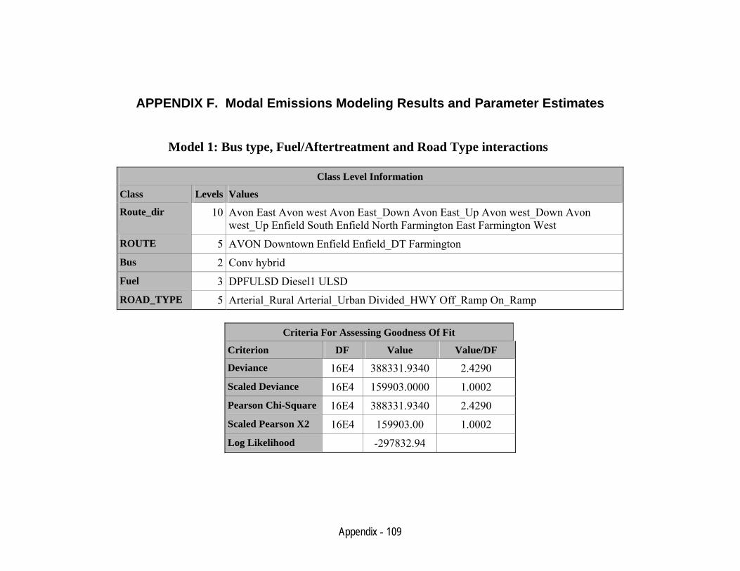
Appendix - 109

APPENDIX F. Modal Emissions Modeling Results and Parameter Estimates

Model 1: Bus type, Fuel/Aftertreatment and Road Type interactions

Class Level Information

Class Levels Values

Route_dir 10 Avon East Avon west Avon East_Down Avon East_Up Avon west_Down Avon west_Up Enfield South Enfield North Farmington East Farmington West

ROUTE 5 AVON Downtown Enfield Enfield_DT Farmington Bus 2 Conv hybrid Fuel 3 DPFULSD Diesel1 ULSD ROAD_TYPE 5 Arterial_Rural Arterial_Urban Divided_HWY Off_Ramp On_Ramp

Criteria For Assessing Goodness Of Fit

Criterion DF Value Value/DF

Deviance 16E4 388331.9340 2.4290 Scaled Deviance 16E4 159903.0000 1.0002 Pearson Chi-Square 16E4 388331.9340 2.4290 Scaled Pearson X2 16E4 159903.00 1.0002 Log Likelihood -297832.94

Appendix - 110

Analysis Of Parameter Estimates

Parameter DF EstimateStandard

Error

Wald 95% Confidence

Limits Chi-Square Pr > ChiSq

Intercept 1 27.6951 0.0984 27.5023

27.8879

79274.5 <.0001

Bus*Fuel*ROAD_TYP Conv DPFULSD Arterial_Rural

1 -6.4828 0.1003 -6.6794

-6.2862

4176.54 <.0001

Bus*Fuel*ROAD_TYP Conv DPFULSD Arterial_Urban

1 -7.1272 0.0996 -7.3223

-6.9320

5124.29 <.0001

Bus*Fuel*ROAD_TYP Conv DPFULSD Divided_HWY

1 -4.4565 0.1003 -4.6532

-4.2598

1972.45 <.0001

Bus*Fuel*ROAD_TYP Conv DPFULSD Off_Ramp

1 -5.3883 0.1445 -5.6714

-5.1052

1391.38 <.0001

Bus*Fuel*ROAD_TYP Conv DPFULSD On_Ramp 1 -5.6888 0.1479 -5.9787

-5.3989

1479.13 <.0001

Bus*Fuel*ROAD_TYP Conv Diesel1 Arterial_Rural

1 -0.9757 0.1001 -1.1720

-0.7794

94.92 <.0001

Bus*Fuel*ROAD_TYP Conv Diesel1 Arterial_Urban

1 -1.3152 0.0995 -1.5102

-1.1203

174.84 <.0001

Bus*Fuel*ROAD_TYP Conv Diesel1 Divided_HWY

1 1.2946 0.1001 1.0984 1.4908 167.31 <.0001

Bus*Fuel*ROAD_TYP Conv Diesel1 Off_Ramp

1 0.3377 0.1333 0.0764 0.5990 6.42 0.0113

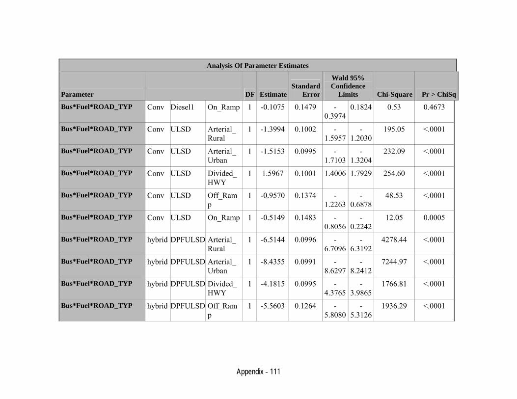
Appendix - 111

Analysis Of Parameter Estimates

Parameter DF EstimateStandard

Error

Wald 95% Confidence

Limits Chi-Square Pr > ChiSq

Bus*Fuel*ROAD_TYP Conv Diesel1 On_Ramp 1 -0.1075 0.1479 -0.3974

0.1824 0.53 0.4673

Bus*Fuel*ROAD_TYP Conv ULSD Arterial_Rural

1 -1.3994 0.1002 -1.5957

-1.2030

195.05 <.0001

Bus*Fuel*ROAD_TYP Conv ULSD Arterial_Urban

1 -1.5153 0.0995 -1.7103

-1.3204

232.09 <.0001

Bus*Fuel*ROAD_TYP Conv ULSD Divided_HWY

1 1.5967 0.1001 1.4006 1.7929 254.60 <.0001

Bus*Fuel*ROAD_TYP Conv ULSD Off_Ramp

1 -0.9570 0.1374 -1.2263

-0.6878

48.53 <.0001

Bus*Fuel*ROAD_TYP Conv ULSD On_Ramp 1 -0.5149 0.1483 -0.8056

-0.2242

12.05 0.0005

Bus*Fuel*ROAD_TYP hybrid DPFULSD Arterial_Rural

1 -6.5144 0.0996 -6.7096

-6.3192

4278.44 <.0001

Bus*Fuel*ROAD_TYP hybrid DPFULSD Arterial_Urban

1 -8.4355 0.0991 -8.6297

-8.2412

7244.97 <.0001

Bus*Fuel*ROAD_TYP hybrid DPFULSD Divided_HWY

1 -4.1815 0.0995 -4.3765

-3.9865

1766.81 <.0001

Bus*Fuel*ROAD_TYP hybrid DPFULSD Off_Ramp

1 -5.5603 0.1264 -5.8080

-5.3126

1936.29 <.0001

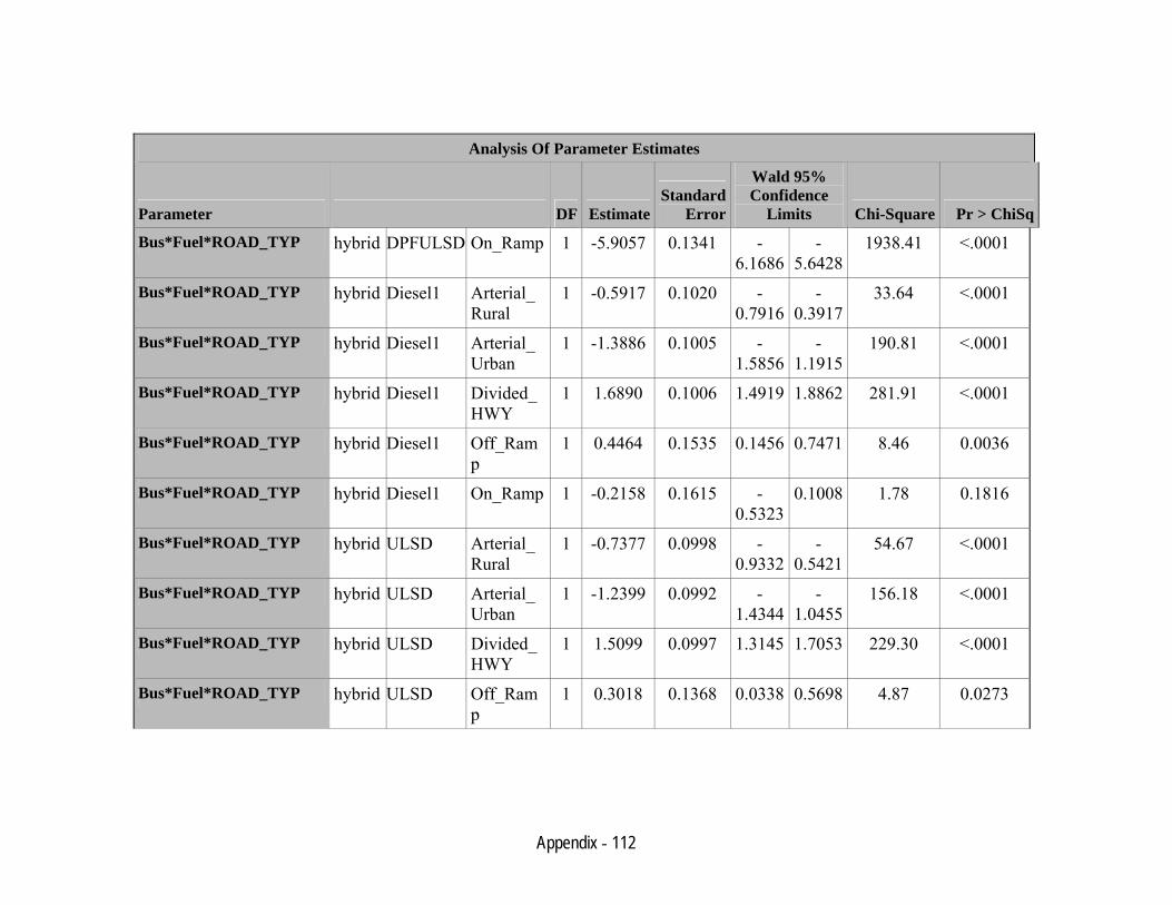
Appendix - 112

Analysis Of Parameter Estimates

Parameter DF EstimateStandard

Error

Wald 95% Confidence

Limits Chi-Square Pr > ChiSq

Bus*Fuel*ROAD_TYP hybrid DPFULSD On_Ramp 1 -5.9057 0.1341 -6.1686

-5.6428

1938.41 <.0001

Bus*Fuel*ROAD_TYP hybrid Diesel1 Arterial_Rural

1 -0.5917 0.1020 -0.7916

-0.3917

33.64 <.0001

Bus*Fuel*ROAD_TYP hybrid Diesel1 Arterial_Urban

1 -1.3886 0.1005 -1.5856

-1.1915

190.81 <.0001

Bus*Fuel*ROAD_TYP hybrid Diesel1 Divided_HWY

1 1.6890 0.1006 1.4919 1.8862 281.91 <.0001

Bus*Fuel*ROAD_TYP hybrid Diesel1 Off_Ramp

1 0.4464 0.1535 0.1456 0.7471 8.46 0.0036

Bus*Fuel*ROAD_TYP hybrid Diesel1 On_Ramp 1 -0.2158 0.1615 -0.5323

0.1008 1.78 0.1816

Bus*Fuel*ROAD_TYP hybrid ULSD Arterial_Rural

1 -0.7377 0.0998 -0.9332

-0.5421

54.67 <.0001

Bus*Fuel*ROAD_TYP hybrid ULSD Arterial_Urban

1 -1.2399 0.0992 -1.4344

-1.0455

156.18 <.0001

Bus*Fuel*ROAD_TYP hybrid ULSD Divided_HWY

1 1.5099 0.0997 1.3145 1.7053 229.30 <.0001

Bus*Fuel*ROAD_TYP hybrid ULSD Off_Ramp

1 0.3018 0.1368 0.0338 0.5698 4.87 0.0273

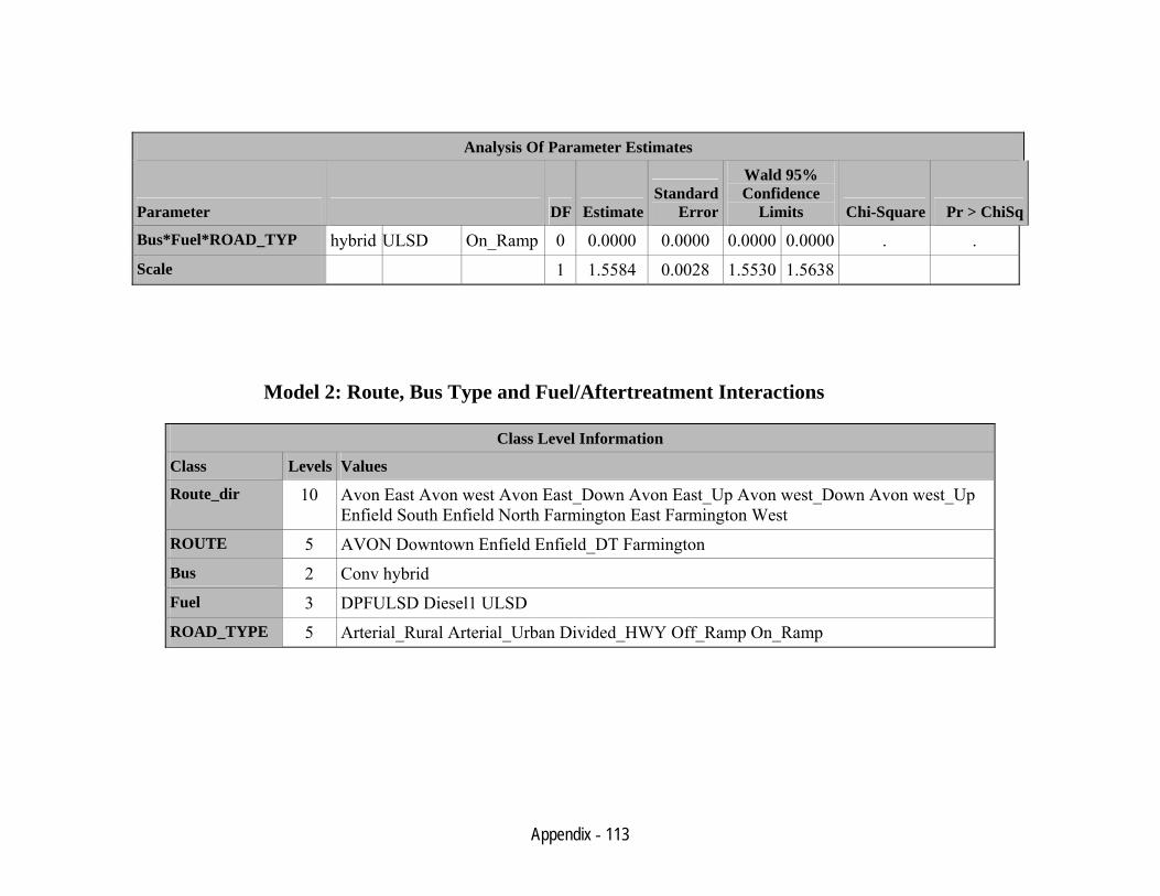
Appendix - 113

Analysis Of Parameter Estimates

Parameter DF EstimateStandard

Error

Wald 95% Confidence

Limits Chi-Square Pr > ChiSq

Bus*Fuel*ROAD_TYP hybrid ULSD On_Ramp 0 0.0000 0.0000 0.0000 0.0000 . . Scale 1 1.5584 0.0028 1.5530 1.5638

Model 2: Route, Bus Type and Fuel/Aftertreatment Interactions

Class Level Information

Class Levels Values

Route_dir 10 Avon East Avon west Avon East_Down Avon East_Up Avon west_Down Avon west_Up Enfield South Enfield North Farmington East Farmington West

ROUTE 5 AVON Downtown Enfield Enfield_DT Farmington Bus 2 Conv hybrid Fuel 3 DPFULSD Diesel1 ULSD ROAD_TYPE 5 Arterial_Rural Arterial_Urban Divided_HWY Off_Ramp On_Ramp

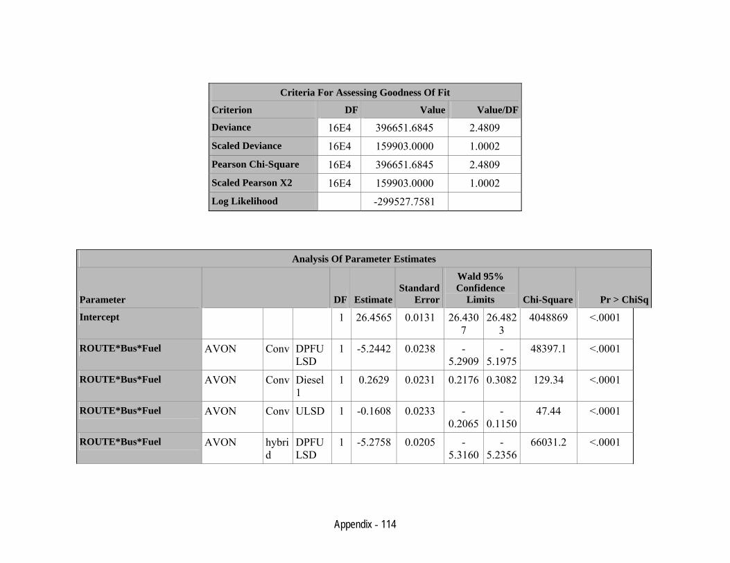
Appendix - 114

Criteria For Assessing Goodness Of Fit

Criterion DF Value Value/DF

Deviance 16E4 396651.6845 2.4809 Scaled Deviance 16E4 159903.0000 1.0002 Pearson Chi-Square 16E4 396651.6845 2.4809 Scaled Pearson X2 16E4 159903.0000 1.0002 Log Likelihood -299527.7581

Analysis Of Parameter Estimates

Parameter DF EstimateStandard

Error

Wald 95% Confidence

Limits Chi-Square Pr > ChiSq

Intercept 1 26.4565 0.0131 26.4307

26.4823

4048869 <.0001

ROUTE*Bus*Fuel AVON Conv DPFULSD

1 -5.2442 0.0238 -5.2909

-5.1975

48397.1 <.0001

ROUTE*Bus*Fuel AVON Conv Diesel1

1 0.2629 0.0231 0.2176 0.3082 129.34 <.0001

ROUTE*Bus*Fuel AVON Conv ULSD 1 -0.1608 0.0233 -0.2065

-0.1150

47.44 <.0001

ROUTE*Bus*Fuel AVON hybrid

DPFULSD

1 -5.2758 0.0205 -5.3160

-5.2356

66031.2 <.0001

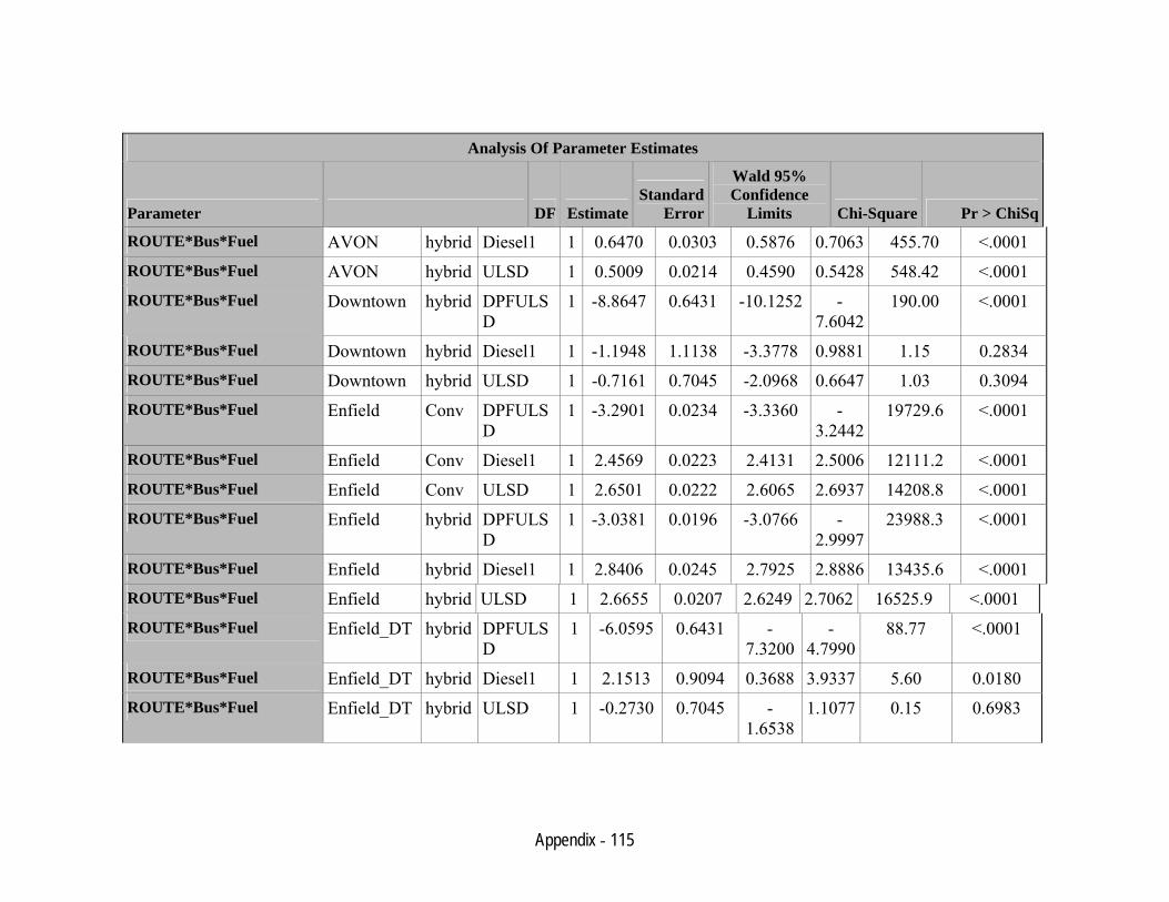
Appendix - 115

Analysis Of Parameter Estimates

Parameter DF EstimateStandard

Error

Wald 95% Confidence

Limits Chi-Square Pr > ChiSq

ROUTE*Bus*Fuel AVON hybrid Diesel1 1 0.6470 0.0303 0.5876 0.7063 455.70 <.0001 ROUTE*Bus*Fuel AVON hybrid ULSD 1 0.5009 0.0214 0.4590 0.5428 548.42 <.0001 ROUTE*Bus*Fuel Downtown hybrid DPFULS

D 1 -8.8647 0.6431 -10.1252 -

7.6042190.00 <.0001

ROUTE*Bus*Fuel Downtown hybrid Diesel1 1 -1.1948 1.1138 -3.3778 0.9881 1.15 0.2834 ROUTE*Bus*Fuel Downtown hybrid ULSD 1 -0.7161 0.7045 -2.0968 0.6647 1.03 0.3094 ROUTE*Bus*Fuel Enfield Conv DPFULS

D 1 -3.2901 0.0234 -3.3360 -

3.244219729.6 <.0001

ROUTE*Bus*Fuel Enfield Conv Diesel1 1 2.4569 0.0223 2.4131 2.5006 12111.2 <.0001 ROUTE*Bus*Fuel Enfield Conv ULSD 1 2.6501 0.0222 2.6065 2.6937 14208.8 <.0001 ROUTE*Bus*Fuel Enfield hybrid DPFULS

D 1 -3.0381 0.0196 -3.0766 -

2.999723988.3 <.0001

ROUTE*Bus*Fuel Enfield hybrid Diesel1 1 2.8406 0.0245 2.7925 2.8886 13435.6 <.0001 ROUTE*Bus*Fuel Enfield hybrid ULSD 1 2.6655 0.0207 2.6249 2.7062 16525.9 <.0001 ROUTE*Bus*Fuel Enfield_DT hybrid DPFULS

D 1 -6.0595 0.6431 -

7.3200-

4.799088.77 <.0001

ROUTE*Bus*Fuel Enfield_DT hybrid Diesel1 1 2.1513 0.9094 0.3688 3.9337 5.60 0.0180 ROUTE*Bus*Fuel Enfield_DT hybrid ULSD 1 -0.2730 0.7045 -

1.65381.1077 0.15 0.6983

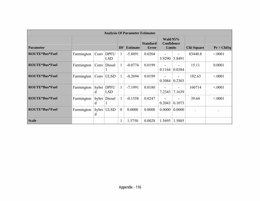
Appendix - 116

Analysis Of Parameter Estimates

Parameter DF EstimateStandard

Error

Wald 95% Confidence

Limits Chi-Square Pr > ChiSq

ROUTE*Bus*Fuel Farmington Conv DPFULSD

1 -5.8891 0.0204 -5.9290

-5.8491

83440.8 <.0001

ROUTE*Bus*Fuel Farmington Conv Diesel1

1 -0.0774 0.0199 -0.1164

-0.0384

15.11 0.0001

ROUTE*Bus*Fuel Farmington Conv ULSD 1 -0.2694 0.0199 -0.3084

-0.2303

182.63 <.0001

ROUTE*Bus*Fuel Farmington hybrid

DPFULSD

1 -7.1991 0.0180 -7.2343

-7.1639

160714 <.0001

ROUTE*Bus*Fuel Farmington hybrid

Diesel1

1 -0.1558 0.0247 -0.2043

-0.1073

39.64 <.0001

ROUTE*Bus*Fuel Farmington hybrid

ULSD 0 0.0000 0.0000 0.0000 0.0000 . .

Scale 1 1.5750 0.0028 1.5695 1.5805

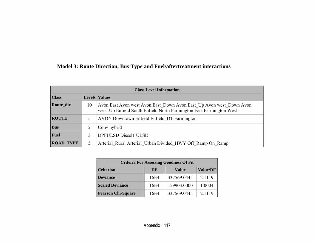
Appendix - 117

Model 3: Route Direction, Bus Type and Fuel/aftertreatment interactions

Class Level Information

Class Levels Values

Route_dir 10 Avon East Avon west Avon East_Down Avon East_Up Avon west_Down Avon west_Up Enfield South Enfield North Farmington East Farmington West

ROUTE 5 AVON Downtown Enfield Enfield_DT Farmington

Bus 2 Conv hybrid Fuel 3 DPFULSD Diesel1 ULSD ROAD_TYPE 5 Arterial_Rural Arterial_Urban Divided_HWY Off_Ramp On_Ramp

Criteria For Assessing Goodness Of Fit

Criterion DF Value Value/DF

Deviance 16E4 337569.0445 2.1119 Scaled Deviance 16E4 159903.0000 1.0004 Pearson Chi-Square 16E4 337569.0445 2.1119

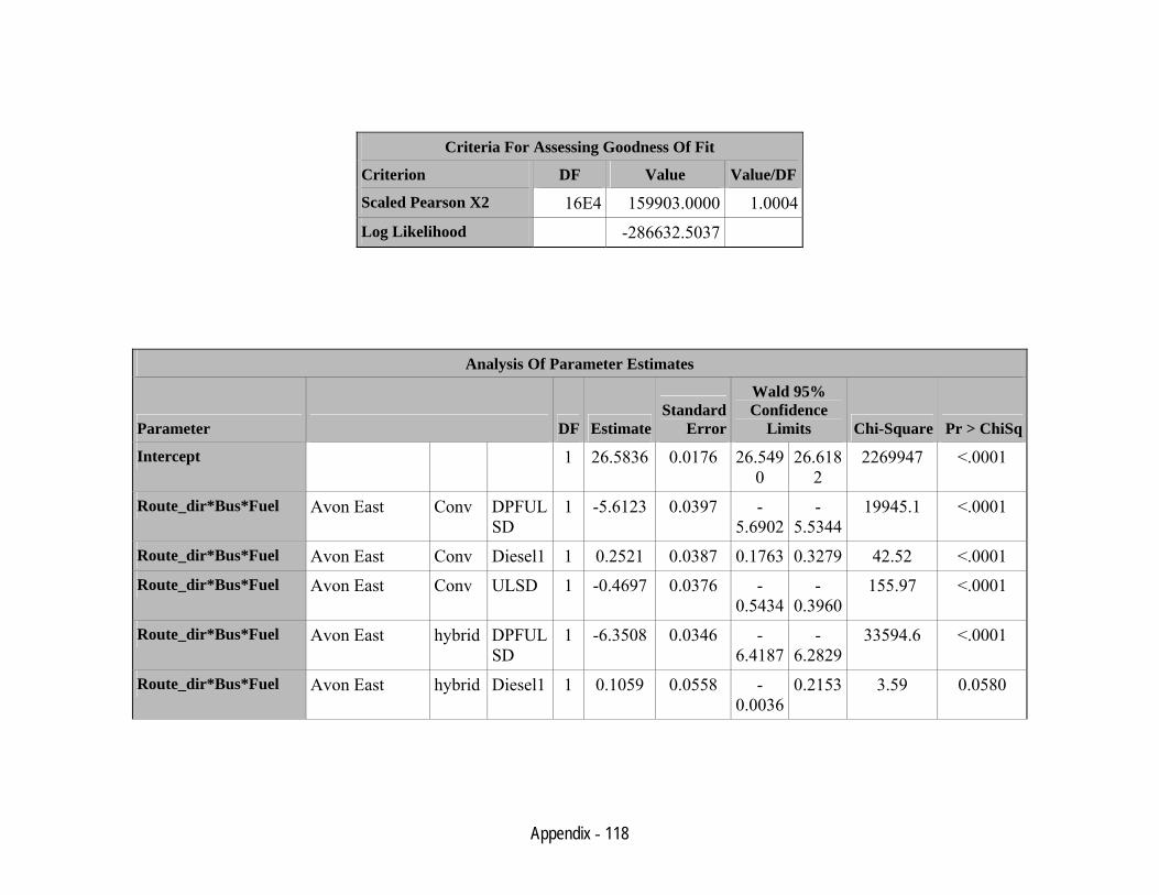
Appendix - 118

Criteria For Assessing Goodness Of Fit

Criterion DF Value Value/DF

Scaled Pearson X2 16E4 159903.0000 1.0004Log Likelihood -286632.5037

Analysis Of Parameter Estimates

Parameter DF EstimateStandard

Error

Wald 95% Confidence

Limits Chi-Square Pr > ChiSq

Intercept 1 26.5836 0.0176 26.5490

26.6182

2269947 <.0001

Route_dir*Bus*Fuel Avon East Conv DPFULSD

1 -5.6123 0.0397 -5.6902

-5.5344

19945.1 <.0001

Route_dir*Bus*Fuel Avon East Conv Diesel1 1 0.2521 0.0387 0.1763 0.3279 42.52 <.0001 Route_dir*Bus*Fuel Avon East Conv ULSD 1 -0.4697 0.0376 -

0.5434-

0.3960155.97 <.0001

Route_dir*Bus*Fuel Avon East hybrid DPFULSD

1 -6.3508 0.0346 -6.4187

-6.2829

33594.6 <.0001

Route_dir*Bus*Fuel Avon East hybrid Diesel1 1 0.1059 0.0558 -0.0036

0.2153 3.59 0.0580

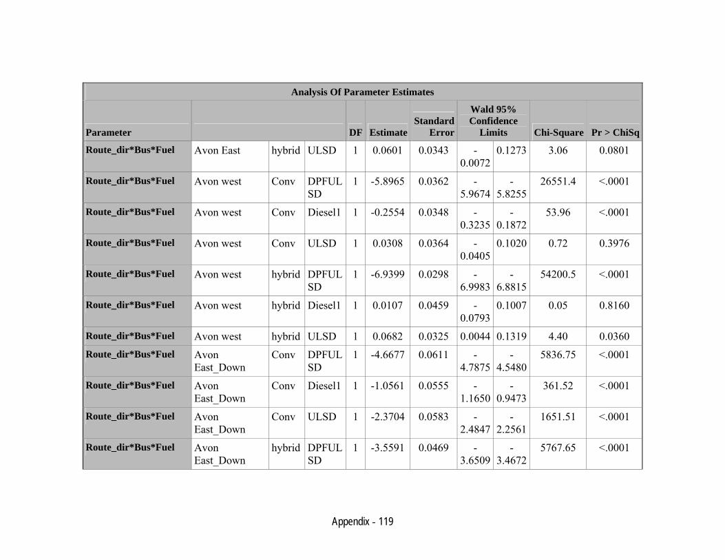
Appendix - 119

Analysis Of Parameter Estimates

Parameter DF EstimateStandard

Error

Wald 95% Confidence

Limits Chi-Square Pr > ChiSq

Route_dir*Bus*Fuel Avon East hybrid ULSD 1 0.0601 0.0343 -0.0072

0.1273 3.06 0.0801

Route_dir*Bus*Fuel Avon west Conv DPFULSD

1 -5.8965 0.0362 -5.9674

-5.8255

26551.4 <.0001

Route_dir*Bus*Fuel Avon west Conv Diesel1 1 -0.2554 0.0348 -0.3235

-0.1872

53.96 <.0001

Route_dir*Bus*Fuel Avon west Conv ULSD 1 0.0308 0.0364 -0.0405

0.1020 0.72 0.3976

Route_dir*Bus*Fuel Avon west hybrid DPFULSD

1 -6.9399 0.0298 -6.9983

-6.8815

54200.5 <.0001

Route_dir*Bus*Fuel Avon west hybrid Diesel1 1 0.0107 0.0459 -0.0793

0.1007 0.05 0.8160

Route_dir*Bus*Fuel Avon west hybrid ULSD 1 0.0682 0.0325 0.0044 0.1319 4.40 0.0360 Route_dir*Bus*Fuel Avon

East_Down Conv DPFUL

SD 1 -4.6677 0.0611 -

4.7875-

4.54805836.75 <.0001

Route_dir*Bus*Fuel Avon East_Down

Conv Diesel1 1 -1.0561 0.0555 -1.1650

-0.9473

361.52 <.0001

Route_dir*Bus*Fuel Avon East_Down

Conv ULSD 1 -2.3704 0.0583 -2.4847

-2.2561

1651.51 <.0001

Route_dir*Bus*Fuel Avon East_Down

hybrid DPFULSD

1 -3.5591 0.0469 -3.6509

-3.4672

5767.65 <.0001

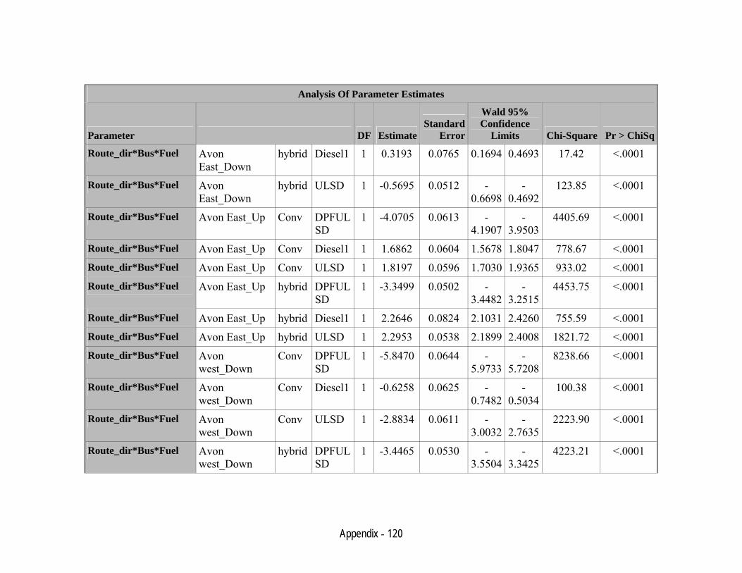
Appendix - 120

Analysis Of Parameter Estimates

Parameter DF EstimateStandard

Error

Wald 95% Confidence

Limits Chi-Square Pr > ChiSq

Route_dir*Bus*Fuel Avon East_Down

hybrid Diesel1 1 0.3193 0.0765 0.1694 0.4693 17.42 <.0001

Route_dir*Bus*Fuel Avon East_Down

hybrid ULSD 1 -0.5695 0.0512 -0.6698

-0.4692

123.85 <.0001

Route_dir*Bus*Fuel Avon East_Up Conv DPFULSD

1 -4.0705 0.0613 -4.1907

-3.9503

4405.69 <.0001

Route_dir*Bus*Fuel Avon East_Up Conv Diesel1 1 1.6862 0.0604 1.5678 1.8047 778.67 <.0001 Route_dir*Bus*Fuel Avon East_Up Conv ULSD 1 1.8197 0.0596 1.7030 1.9365 933.02 <.0001 Route_dir*Bus*Fuel Avon East_Up hybrid DPFUL

SD 1 -3.3499 0.0502 -

3.4482-

3.25154453.75 <.0001

Route_dir*Bus*Fuel Avon East_Up hybrid Diesel1 1 2.2646 0.0824 2.1031 2.4260 755.59 <.0001 Route_dir*Bus*Fuel Avon East_Up hybrid ULSD 1 2.2953 0.0538 2.1899 2.4008 1821.72 <.0001 Route_dir*Bus*Fuel Avon

west_Down Conv DPFUL

SD 1 -5.8470 0.0644 -

5.9733-

5.72088238.66 <.0001

Route_dir*Bus*Fuel Avon west_Down

Conv Diesel1 1 -0.6258 0.0625 -0.7482

-0.5034

100.38 <.0001

Route_dir*Bus*Fuel Avon west_Down

Conv ULSD 1 -2.8834 0.0611 -3.0032

-2.7635

2223.90 <.0001

Route_dir*Bus*Fuel Avon west_Down

hybrid DPFULSD

1 -3.4465 0.0530 -3.5504

-3.3425

4223.21 <.0001

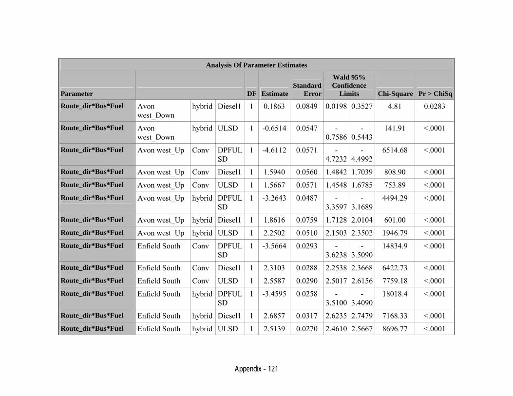
Appendix - 121

Analysis Of Parameter Estimates

Parameter DF EstimateStandard

Error

Wald 95% Confidence

Limits Chi-Square Pr > ChiSq

Route_dir*Bus*Fuel Avon west_Down

hybrid Diesel1 1 0.1863 0.0849 0.0198 0.3527 4.81 0.0283

Route_dir*Bus*Fuel Avon west_Down

hybrid ULSD 1 -0.6514 0.0547 -0.7586

-0.5443

141.91 <.0001

Route_dir*Bus*Fuel Avon west_Up Conv DPFULSD

1 -4.6112 0.0571 -4.7232

-4.4992

6514.68 <.0001

Route_dir*Bus*Fuel Avon west_Up Conv Diesel1 1 1.5940 0.0560 1.4842 1.7039 808.90 <.0001 Route_dir*Bus*Fuel Avon west_Up Conv ULSD 1 1.5667 0.0571 1.4548 1.6785 753.89 <.0001 Route_dir*Bus*Fuel Avon west_Up hybrid DPFUL

SD 1 -3.2643 0.0487 -

3.3597-

3.16894494.29 <.0001

Route_dir*Bus*Fuel Avon west_Up hybrid Diesel1 1 1.8616 0.0759 1.7128 2.0104 601.00 <.0001 Route_dir*Bus*Fuel Avon west_Up hybrid ULSD 1 2.2502 0.0510 2.1503 2.3502 1946.79 <.0001 Route_dir*Bus*Fuel Enfield South Conv DPFUL

SD 1 -3.5664 0.0293 -

3.6238-

3.509014834.9 <.0001

Route_dir*Bus*Fuel Enfield South Conv Diesel1 1 2.3103 0.0288 2.2538 2.3668 6422.73 <.0001 Route_dir*Bus*Fuel Enfield South Conv ULSD 1 2.5587 0.0290 2.5017 2.6156 7759.18 <.0001 Route_dir*Bus*Fuel Enfield South hybrid DPFUL

SD 1 -3.4595 0.0258 -

3.5100-

3.409018018.4 <.0001

Route_dir*Bus*Fuel Enfield South hybrid Diesel1 1 2.6857 0.0317 2.6235 2.7479 7168.33 <.0001 Route_dir*Bus*Fuel Enfield South hybrid ULSD 1 2.5139 0.0270 2.4610 2.5667 8696.77 <.0001

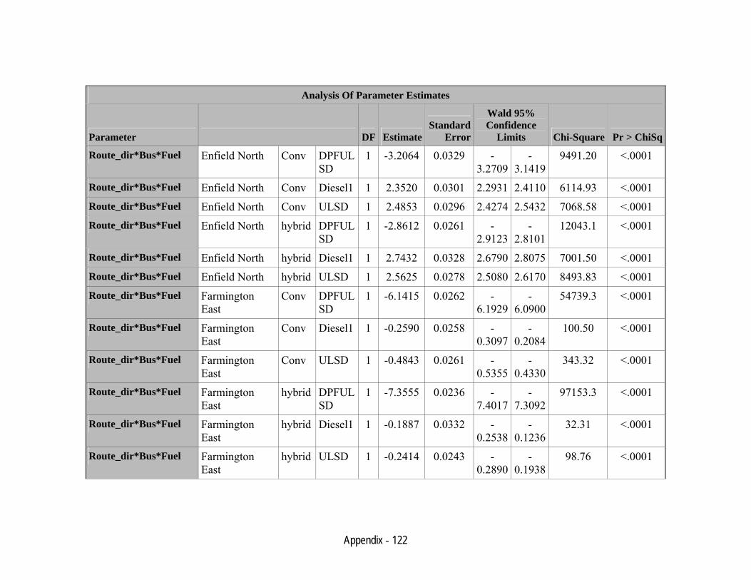
Appendix - 122

Analysis Of Parameter Estimates

Parameter DF EstimateStandard

Error

Wald 95% Confidence

Limits Chi-Square Pr > ChiSq

Route_dir*Bus*Fuel Enfield North Conv DPFULSD

1 -3.2064 0.0329 -3.2709

-3.1419

9491.20 <.0001

Route_dir*Bus*Fuel Enfield North Conv Diesel1 1 2.3520 0.0301 2.2931 2.4110 6114.93 <.0001 Route_dir*Bus*Fuel Enfield North Conv ULSD 1 2.4853 0.0296 2.4274 2.5432 7068.58 <.0001 Route_dir*Bus*Fuel Enfield North hybrid DPFUL

SD 1 -2.8612 0.0261 -

2.9123-

2.810112043.1 <.0001

Route_dir*Bus*Fuel Enfield North hybrid Diesel1 1 2.7432 0.0328 2.6790 2.8075 7001.50 <.0001 Route_dir*Bus*Fuel Enfield North hybrid ULSD 1 2.5625 0.0278 2.5080 2.6170 8493.83 <.0001 Route_dir*Bus*Fuel Farmington

East Conv DPFUL

SD 1 -6.1415 0.0262 -

6.1929-

6.090054739.3 <.0001

Route_dir*Bus*Fuel Farmington East

Conv Diesel1 1 -0.2590 0.0258 -0.3097

-0.2084

100.50 <.0001

Route_dir*Bus*Fuel Farmington East

Conv ULSD 1 -0.4843 0.0261 -0.5355

-0.4330

343.32 <.0001

Route_dir*Bus*Fuel Farmington East

hybrid DPFULSD

1 -7.3555 0.0236 -7.4017

-7.3092

97153.3 <.0001

Route_dir*Bus*Fuel Farmington East

hybrid Diesel1 1 -0.1887 0.0332 -0.2538

-0.1236

32.31 <.0001

Route_dir*Bus*Fuel Farmington East

hybrid ULSD 1 -0.2414 0.0243 -0.2890

-0.1938

98.76 <.0001

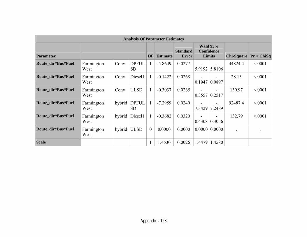
Appendix - 123

Analysis Of Parameter Estimates

Parameter DF EstimateStandard

Error

Wald 95% Confidence

Limits Chi-Square Pr > ChiSq

Route_dir*Bus*Fuel Farmington West

Conv DPFULSD

1 -5.8649 0.0277 -5.9192

-5.8106

44824.4 <.0001

Route_dir*Bus*Fuel Farmington West

Conv Diesel1 1 -0.1422 0.0268 -0.1947

-0.0897

28.15 <.0001

Route_dir*Bus*Fuel Farmington West

Conv ULSD 1 -0.3037 0.0265 -0.3557

-0.2517

130.97 <.0001

Route_dir*Bus*Fuel Farmington West

hybrid DPFULSD

1 -7.2959 0.0240 -7.3429

-7.2489

92487.4 <.0001

Route_dir*Bus*Fuel Farmington West

hybrid Diesel1 1 -0.3682 0.0320 -0.4308

-0.3056

132.79 <.0001

Route_dir*Bus*Fuel Farmington West

hybrid ULSD 0 0.0000 0.0000 0.0000 0.0000 . .

Scale 1 1.4530 0.0026 1.4479 1.4580