Deep-Sea Research II 58 (2011) 2135–2149

Contents lists available at ScienceDirect

Deep-Sea Research II

0967-06

doi:10.1

n Corr

E-m1 Ta

Hobart

journal homepage: www.elsevier.com/locate/dsr2

Protistan communities in the Australian sector of the Sub-Antarctic Zoneduring SAZ-Sense

Miguel F. de Salas 1, Ruth Eriksen, Andrew T. Davidson, Simon W. Wright n

Australian Antarctic Division, 203 Channel Hwy, Kingston, Tasmania 7050, Australia

a r t i c l e i n f o

Available online 30 May 2011

Keywords:

Southern Ocean

Marine protists

Phytoplankton

Protozoa

Pigments

CHEMTAX

Iron

Silica

45/$ - see front matter Crown Copyright & 2

016/j.dsr2.2011.05.032

esponding author. Tel.: þ61 3 62323338; fax

ail address: Simon.Wright@aad.gov.au (S.W. W

smanian Herbarium, Tasmanian Museum an

7001, Tasmania, Australia.

a b s t r a c t

Protistan species composition and abundance in the Sub-Antarctic Zone (SAZ) and Polar Front Zone (PFZ)

south of Tasmania were determined by microscopy and pigment analysis from samples collected during

the Sub-Antarctic Zone—Sensitivity of the sub-Antarctic Zone to Environmental Change (SAZ-Sense)

voyage, in January and February of 2007. A primary goal of this voyage was to determine the potential

effects of climate change-induced natural iron fertilisation of the SAZ on the protistan community by

exploring differences between communities in waters west of Tasmania, which are low in iron, and eastern

waters, which are fertilised by continental iron input and mixing across the subtropical front. The SAZ is a

sink for anthropogenic CO2 in spring, but the magnitude of this may vary depending on seasonal changes

in protistan abundance, composition and trophodynamics. Protistan species composition and abundance

in the western Sub-Antarctic Zone at process station 1 (P1) showed a community in which low carbon

biomass was dominated by a Thalassiosira sp., which was very weakly silicified under strong silica

limitation. Protistan cell carbon was dominated by diatoms and nano-picoflagellates at process station 2

(P2) in the Polar Front Zone (PFZ), while dinoflagellates dominated in the iron-enriched waters of eastern

SAZ at station 3 (P3). Iron enrichment enhanced production and favoured proliferation of small flagellates

during summer in the silica-depleted eastern SAZ rather than large diatoms, though the effect this may

have on the vertical export of particulate organic carbon (POC) is still unclear.

Crown Copyright & 2011 Published by Elsevier Ltd. All rights reserved.

1. Introduction

Marine protists play a vital role in sequestering CO2 to thedeep ocean (Trull et al., 2001a; Blain et al., 2007). The SouthernOcean, due to its cold water temperatures, turbulent environmentand deep mixed layer, removes up to 40% of anthropogenicatmospheric CO2 with much of the drawdown in the Sub-Antarctic Zone or SAZ (Metzl et al., 1999; McNeil et al., 2001;Sabine et al., 2004). Dissolved CO2 in the SAZ is then removed byboth physical (strong cooling which downwells CO2-rich water)and biological mechanisms (McNeil et al., 2007). Much of thisdissolved CO2 enters the biological pump in the strong seasonalcycle of biological production in the SAZ (Trull et al., 2001a).

Traditionally, various protist groups have been considered ashaving different effects on net carbon export, with the ultimatefate of this carbon depending on the taxonomic composition ofthe protistan biomass. For example large cell-size diatoms aretraditionally considered to be net exporters of carbon beyond thephotic zone, as they are silicified (heavy) and have a large particle

011 Published by Elsevier Ltd. All

: þ61 3 62323158.

right).

d Art Gallery, Private Bag 4,

size (Boyd and Newton, 1999). In contrast, small cell-size protists,such as autotrophic nanoflagellates and picoplankton, arepredated by both heterotrophic nanoflagellates and zooplankton,diverting carbon into the microbial loop, where it was thoughtto be quickly remineralised (Pearce et al., 2011). However,Richardson and Jackson (2007), working in the equatorial Pacificand the Arabian sea, have recently shown that picoplankton stillcontribute to carbon export proportionally to their net primaryproduction, despite their small size. Similarly, and of directrelevance to this study, Trull et al. (2001a) challenged the notionthat, given a similar biomass, large phytoplankton, particularlydiatoms, are significantly higher contributors to carbon export tothe deep ocean. They showed that the SAZ exported similar oreven higher amounts of POC than did the PFZ, despite the greaterproportion of diatoms in the production of the PFZ.

Much of the Southern Ocean, particularly the SAZ and PFZ, ischaracterised as high-nutrient, low chlorophyll (HNLC) waters,where iron limitation restricts use of other, abundant micro- andmacro-nutrients by phytoplankton (Martin et al., 1990; Martinez-Garcia et al., 2009). This results in paradoxically low algal biomass inan otherwise nutrient-rich environment (Boyd, 2008). Land bound-aries and bottom topography that create upwelling are almostnon-existent, thus making atmospheric dust a hypothesised mainsource of iron (Jickells et al., 2005;Cassar et al., 2007). However, in

rights reserved.

155°E150°E145°E140°E

40°S

45°S

50°S

55°S

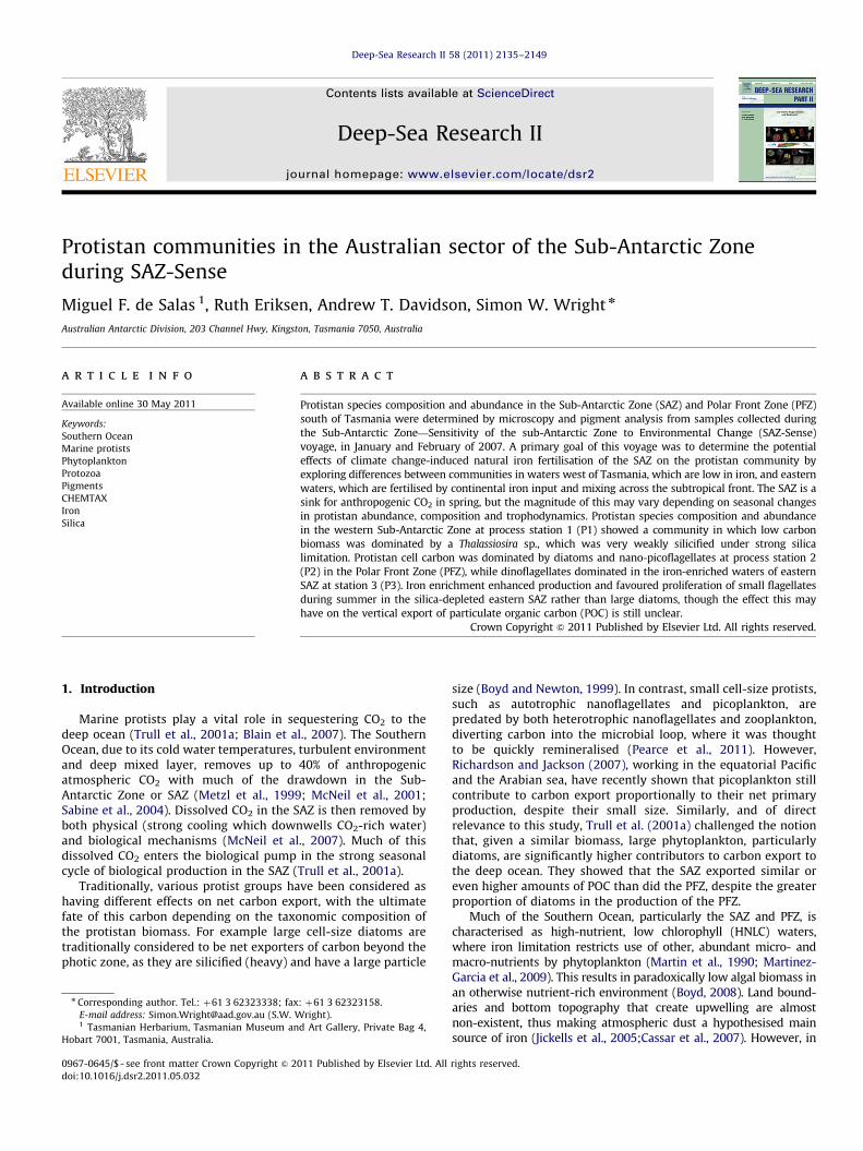
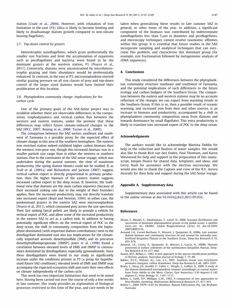
Fig. 1. Track of SAZ voyage showing the location of the three process stations used

in this study. Abbreviations: STZ¼subtropical zone; STF¼subtropical front;

SAZ-N¼northern SAZ; SAF-N¼north Sub-Antarctic front; SAZ-S¼southern

Sub-Antarctic zone; SAF-S¼south Sub-Antarctic front; PFZ¼polar front zone;

PF-N¼north polar front; IPFZ¼ inter-polar-frontal zone.

M.F. de Salas et al. / Deep-Sea Research II 58 (2011) 2135–21492136

the Southern Ocean, sources of dust are few (Prospero et al., 2002),and it has recently been proposed that input from the continentalshelf margins exceeds that from wind-blown dust (Tagliabue et al.,2009) or even that it is the principal source of iron in the SAZ (Bowieet al., 2009). Nutrient concentrations in the water bodies examinedin this study appear in Bowie et al. (2011).

Climate change is predicted to cause changes in atmosphericand oceanic circulation patterns, with diverse effects on the SAZ.Prevailing westerly winds may already be moving further south(Lovenduski et al., 2007, 2008) and are expected to push SouthernOcean frontal areas further south towards the Antarctic continent,logically resulting in a reduction of the ocean area that iscontained within the polar front. This reduction in surface areamay in itself have an effect on the Southern Ocean’s capacity toabsorb anthropogenic CO2 (Le Quere et al., 2007), as the areas ofocean with the highest wind turbulence and mixed layer arecontained within this region. The southwards shift of westerlywinds may also increase iron availability through severalmechanisms (Lyne and Rintoul, 2005). Warming trends may leadto a drier climate, and increased aridity may lead to a net result ofincreasing iron input to the Australian sector of the SAZ fromwindblown dust and other sources. In addition, subtropical watermay penetrate further south into the SAZ, increasing iron supplyto the northern SAZ. It has been suggested that penetration of lownutrient (but possibly higher iron) water from subtropical gyressuch as the East Australian Current (EAC) causes SAZ waters to theeast of Tasmania to be a proxy for a future, iron enriched SAZ(with increased dust input due to predicted warming and deser-tification), while those to the west of Tasmania are still typical ofthe present-day SAZ (Bowie et al., 2011; Westwood et al., 2011).In this light, comparison of waters west and east of Tasmania canprovide valuable insights into the effect of climate change onprotistan communities in the SAZ.

At present levels of iron limitation, diatoms dominate thebiomass in the Antarctic Zone, and remove much of the silicabefore surface waters are transported to lower latitudes (Alvainet al., 2008; Armand et al., 2008a, 2008b; Pike et al., 2008). TheSAZ is nitrate and phosphate rich, but both silica and irondepleted year-round. Results from previous research on ironenrichment in the Southern Ocean, such as KEOPS, SOFeX, SAGEand SOIREE surveys have produced mixed results, with somestimulating diatom growth and carbon export (KEOPS, SOFeX),and others (SOIREE) showing little effect (Bakker et al., 2001;Boyd and Law, 2001; Boyd et al., 2007; Blain et al., 2008). Not allof these results are necessarily applicable in the silica-limitedSAZ, and thus it is essential to quantify the effects of hypothesisedadditional iron sources due to climate change.

Two mechanisms are major contributors to carbon drawdownin the SAZ: downwelling of tropical waters that have cooled andtaken up CO2 during their southwards movement, and highbiological productivity in spite of nutrient limitations. Both ofthese mechanisms are vulnerable to change given anthropogenicperturbations to the global carbon cycle (McNeil et al., 2007).Thus in this paper we compare the protistan community of tworegions of the SAZ which have naturally different levels andsources of iron. We use two representative stations as proxiesfor current and future prevailing conditions in the SAZ, with lowiron supply to the southwest of Tasmania, and high iron supply tothe southeast. We also compare our results to a station in thenorthern PFZ, which like the SAZ is iron limited and seasonallylight limited, but unlike the SAZ, is only silica limited after thespring diatom bloom. By defining the community structure acrossthese three stations, we aim to link the structure of the food webto the efficiency of the biological pump given each site’s uniqueenvironment. Studies like this one are critical, as they allow us tolink environmental conditions, including nutrient conditions, to

the biological community structure, and assess subsequent poten-tial impacts of community change on carbon sequestration.

2. Materials and methods

2.1. Sample collection

Seawater samples were collected from 40 sites during theSAZ-Sense oceanographic cruise between 20 January and 16February 2007. Samples were collected from the three mainstations (Bowie et al., 2011), chosen to represent typical SAZ water(P1, approximately 461S 1401E), the polar front zone (P2, 541S1461E), and subtropical-water enriched SAZ (P3, 451S 1531E). Fig. 1shows the voyage track and location of each station. Repeatedsampling was carried out at several sites within each station. WhileP2 and P3 were representative of their respective water bodies, P1was highly stratified and exhibited vertical interleaving of waterfrom both sides of the subtropical front (Bowie et al., 2011). At eachsampling site, water was collected using 10 L Niskin bottlesattached to a CTD rosette (24 bottles). Samples of �960 ml werecollected into glass bottles, fixed with the addition of 1% Lugol’siodine solution and stored in the dark and under refrigeration, untilprocessed into permanent mounts.

2.2. HPMA slide preparation

Permanent mounts were prepared using a modification ofCrumpton’s (1981) HPMA (2-hydroxypropyl methacrylate)method (Davidson et al., 2010). Briefly, Lugol’s fixed sampleswere filtered onto 0.45 mm pore-size, 25 mm diameter cellulosefilters. The wet filters were placed upside down on a coverslip and

M.F. de Salas et al. / Deep-Sea Research II 58 (2011) 2135–2149 2137

coated with a few drops of HPMA, then polymerised and driedovernight at 60 1C. Each numbered coverslip was then attached toa labelled slide using a little more HPMA.

2.3. Microscopy

Protistan taxa were identified and counted in 20 randomlychosen Whipple-grid quadrats on each slide at 400� magnification,using a Zeiss Axioskop (Carl Zeiss, Gottingen, Germany) microscopeequipped with differential interference contrast illumination.Taxonomic identification was based primarily on descriptions inScott and Marchant (2005) and Thomas (1993, 1996).

Protistan taxa were identified to species level where possible.The constraints of light microscopy and HPMA permanent mountsmeant that many cells could only be identified to genus or evenclass level. Many diatom and armoured dinoflagellate species couldbe conclusively identified, but some Thalassiosira cells with delicatefrustules that did not withstand processing lacked diagnosticfeatures, and could only be placed into a genus. Other cryptic taxasuch as cryptophytes could only be identified to class level.

Lugol’s fixation of the samples meant it was not possible todetermine the trophic status of some dinoflagellates, especiallyunarmoured species. Some cells were clearly from heterotrophicgenera (Oxytoxum, Gyrodinium, Dinophysis) and others from auto-trophic or mixotrophic genera (Ceratium, Gonyaulax). Among theremainder of indeterminate dinoflagellate species, only a fewcontained Lugol’s-stained dark starch grains that clearly identifiedthem as autotrophic or at least mixotrophic. Many more speciesdid not contain starch and the trophic status of these cellsremained uncertain. In addition to the challenge of determiningthe trophic status of dinoflagellates, a distinct group of unidenti-fied coccoid or globular nanoflagellates in the size range of2–5 mm diameter, of indeterminate trophic status, was alsoidentified. These constituted a distinct grouping, too large in cellsize to be referred to as picoplankton, but distinct and abundantenough that they deserve a category of their own. We hence referto them as UNAN (for UNidentified NANoflagellate) throughoutthe rest of this study. Due to their extreme abundance in allsamples, cell number comparisons and discussion of other taxaexclude this group unless specifically stated in the text. Howevercell carbon biomass results and discussion include all taxa.

Many previous studies of protists in the Southern Ocean havedetermined protistan composition and abundance from samplesthat have been sedimented and viewed by inverted microscopy(Kopczynska et al., 2001, 2007; Fiala et al., 2004; Armand et al.,2008a; Beans et al., 2008). Using the HPMA method we foundlightly silicified pennate diatoms were especially difficult toresolve. Furthermore, other taxa may have been under- or over-estimated relative to studies using different methods. As a resultcaution should be exercised when comparing results in this studywith those using different methods.

2.4. Biomass calculations

Measurements of each taxon were obtained by microscopy(average of 20 individuals, or with reference to published litera-ture in the case of uncommon or rare taxa (Thomas, 1993, 1996;Scott and Marchant, 2005)) and their biovolume calculated usingthe formulae of Hillebrand et al. (1999) and Sun and Liu (2003).The biovolume was then used to calculate the carbon biomass ofeach taxon using the formulae of Menden-Deuer and Lessard(2000). Particle size distribution was plotted as a histogram ofcarbon biomass (in mg L�1 average across all CTDs in that station)into nine bins (in particle volumes expressed as mm3). The binsizes were selected to reflect the higher abundance of smallerbiovolume fractions in the biomass.

2.5. Statistical analysis

Exploratory data analyses were carried out using the multi-variate statistics package PATN v3.03 (Belbin, 2004). Differencesin protistan assemblages among sites were examined usingclassification and ordination techniques. Presence/absence datawere used for the floristic analysis (no transformation necessary)and the analysis was performed using the Two-Step measure ofassociation (Austin and Belbin, 1982). Three main groups and twosubgroups were discriminated at an arbitrary dissimilarity of 0.15that conveniently summarised differences amongst sample sites.

In contrast, taxon-specific biomass was analysed using the Bray–Curtis measure of association (Bray and Curtis, 1957) to calculatesimilarities due to the quantitative nature of the data and therelatively high frequency of 0 biomass caused by the absence of ataxon at a given site (Clarke and Warwick, 1994). Data was LOG10

(xþ1) transformed to reduce the influence of abundant taxa. Clusteranalysis was then performed using flexible hierarchical clustering byunweighted pair-group using arithmetic average (UPGMA) dendro-grams (Belbin et al., 1992). Three groups were identified at anarbitrary dissimilarity of 0.75 that conveniently summarised differ-ences amongst sampling sites. The ordination technique of Semi-Strong Hybrid multidimensional scaling (SSH MDS) was used toclassify samples in three dimensions, in order to assess protistancommunity structure. Analyses employed 500 random starts inorder to reduce the chances of the algorithm settling in false localoptima (Jongman et al., 1995). Environmental variables that had asignificant effect on the ordination were identified using PrincipalComponent Correlation (PCC, Faith and Norris, 1989), followed byMonte Carlo Attributes in Ordination (MCAO, Manly, 1991) to testthe statistical significance of correlation coefficients.

2.6. Pigment analysis

Pigments were collected and extracted as per Wright et al.(2010). Briefly, 1–2 L of seawater were filtered onto WhatmanGF/F filters in the dark. The blotted filters were frozen in liquidnitrogen for return to Australia and extracted by beadbeating(Mini-BeadBeater, Biospec Products, Bartlesville, OK, USA) in300 ml dimethylformamide plus 50 ml methanol (containing140 ng apo-80-carotenal (Fluka, Sigma-Aldrich, St. Louis, MO,USA) internal standard) using a modified method of Mock andHoch (2005). The extract was analysed by HPLC (Zapata et al.,2000). Pigment data were interpreted using CHEMTAX software(Mackey et al., 1996) performing 40 runs from randomized startson each depth bin (see supplementary information).

CHEMTAX categories are referred to in all-capitals to distin-guish them from protistan classes of the same name. Theyincluded CYANOBACTERIA, DIATOMS-A and DIATOMS-B (thosecontaining Chl c1þc2 or Chl c2þc3, respectively), DINOFLAGEL-LATES-A and DINOFLAGELLATES-B (those containing peridininor fucoxanthin plus 190-hexanoyloxyfucoxanthin, respectively),PRASINOPHYTES, CHLOROPHYTES, EUGLENOPHYTES, CRYPTO-PHYTES, and HAPTOPHYTES-8 (based on Phaeocystis sp.), all ofwhich were based on average pigment ratios for cultures, assummarised in Higgins et al. (in press), plus HAPTOPHYTES-6Aand HAPTOPHYTES-6B, based on Emiliania huxleyi morphotypesA and B/C, collected during the cruise (Cook et al., 2011). Choice ofcategories was based on microscopy and previous experience inthe area, but it must be noted that they represent pigmentcomposition categories rather than conventional taxa, and thereis considerable scope for overlap, particularly amongst categoriescontaining fucoxanthin and its derivatives, and amongst smallnanoplankton and picoplankton, which were unconstrained bymicroscopic data.

M.F. de Salas et al. / Deep-Sea Research II 58 (2011) 2135–21492138

3. Results and discussion

3.1. Overview

A total of 11 taxonomic classes and two unidentified groupswere observed during the course of the SAZ survey (Table 1). Theseincluded 197 taxa or discrete categories, the majority of which weredinoflagellates (87 taxa), closely followed by diatoms (78 taxa, ofwhich 40 were pennate and 38 centric). Of the three stationssampled, the southern station (P2) had the lowest number of taxa,and the eastern station (P3) had the highest, with the westernstation (P1) only possessing a few more species than P2 (Table 1).The number of taxa encountered per sample (single depth of a single

Table 1Total, arithmetic mean, median and standard deviation of number of taxa of each class p

across the whole study, and the next three groups individual process stations.

Total P1 (CTDs 10–28)

Total taxa

in study

Mean/

sample

Median/

sample

St.

dev.

Taxa in

this

station

Mean/

sample

Median/

sample

All taxa 197 25.9 25 6.42 92 23.7 23

Choanoflagellates 1 0.09 0 0.29 1 0.13 0

Cryptophytes 2 0.93 1 0.32 2 1.04 1

Diatoms (centric) 38 2.84 2 3 9 1.61 1

Diatoms

(pennate)

40 4.91 5 2.53 24 6.04 6

Dinoflagellates 87 10.9 9 6.39 37 8.04 8

Euglenoids 6 1.32 1 0.85 5 1.52 1

Haptophytes 3 0.3 0 0.5 2 0.17 0

Prasinophytes 1 0.3 0 0.46 1 0.35 0

Raphidophytes 1 0.07 0 0.26 1 0.09 0

Silicoflagellates 2 0.05 0 0.23 0 0 0

Other autotrophs 5 1.19 1 0.48 2 1.26 1

Ciliates 8 2.72 3 1.21 5 2.43 2

Unidentified 3 0.82 1 0.47 3 1.04 1

Table 2Taxa or discrete categories with contributions to cell numbers exceeding 1% of the subt

first for each station, the following data for other taxa is their relative contribution aft

within a taxon, the size range under consideration is given as +¼diameter or L¼ len

TCCC¼Total combined cell count average for all CTD samples in this station, in cells L

P1—TCCC¼6.56�105 P2—TCCC¼1.75�106

Species % of total Species

UNAN 94 UNAN

% of remaining cells excluding UNAN

Haptophytes 27 Dinoflagellates

Phaeocystis sp. (colonial) 27 Dinoflagellates o10 mm

Cryptophytes 12 Gyrodinium sp 10–20 mm

Diatoms 16 Gymnodinioids 10–20 mThalassiosira sp. 20–40 mm Ø 7 Dinoflagellates 10–20 mPseudo-nitzschia sp. 40–60 mm L 4 Diatoms

Euglenoids 6 Fragilariopsis kerguelens

Postgaardi sp. 3 Pseudo-nitzschia 40–60

Indet. Euglenoido20 mm L 2 Chaetoceros sp. indet 15

Prasinophytes 3 Chaetoceros dichaeta

Ciliates 5 Trichotoxon reinboldii

Strombidium 10–20 mm Ø 3 Membraneis challengeri

Dinoflagellates 31 Nitzschia cf. medioconst

Dinoflagellates o10 mm L 20 Pseuso-nitzschia 4100

Gymnodinioids 10–20 mm L 2 Cryptophytes

Gyrodinium sp. 10–20 mm L 2 Haptophytes

Gyrodinium sp. 20–50 mm L 1 Phaeocystis sp. (colonia

Indet. Cf. Haptophyte 8

Indeterminate

Hairy flap 20–50 mm Ø

Euglenoids

Euglenoido20 mm L

CTD) ranged from a minimum of 11 (P3, CTD 98, 30 m) to amaximum of 46 (P3, CTD 77, 25 m), with a mean of 26.5. Allstations were numerically dominated by nanoflagellates of less than5 mm in cell diameter (UNAN), which comprised 85–98% of all cellscounted per sample during SAZ-Sense, though only 6–23% of carbonbiomass, due to their small size (Table 2).

Protistan carbon biomass was comparatively low in the wes-tern station, and was dominated by a single diatom species(Table 3). The southern station had intermediate protistan carbonbiomass, which was dominated by cold-water diatoms comparedto the western station, with the east having the highest biomass,which in contrast to the other two stations, was dominated bydinoflagellates (Table 3).

resent, per process station. Please note the first group of columns denotes the total

P2 (CTDs 39–56) P3 (CTDs 77–103)

St.

dev.

Taxa in

this

station

Mean/

sample

Median/

sample

St.

dev.

Taxa in

this

station

Mean/

sample

Median/

sample

St.

dev.

4.7 84 25.6 25 5.41 129 29.5 31 8.81

0.34 0 0 0 0 1 0.09 0 0.29

0.21 1 0.91 1 0.3 1 0.83 1 0.39

1.08 23 7.64 8 3.41 13 1.78 1 1.48

2.18 22 6.45 6 1.37 20 3.04 3 2.12

2.65 21 5.36 6 2.54 69 16.3 17 6.26

0.9 4 0.82 1 0.6 5 1.35 1 0.83

0.39 2 0.73 1 0.65 2 0.22 0 0.42

0.49 1 0.27 0 0.47 1 0.26 0 0.45

0.29 0 0 0 0 1 0.09 0 0.29

0 1 0.09 0 0.3 2 0.09 0 0.29

0.45 2 1.09 1 0.3 4 1.17 1 0.58

0.66 6 1.64 2 0.92 8 3.52 4 1.24

0.37 1 0.64 1 0.5 2 0.7 1 0.47

otal (excluding UNAN). Please note that, although the percentage of UNAN is given

er UNAN are excluded from the count. (Where there were several size categories

gth, for cells that are approximately spherical, or irregular in shape, respectively.)�1.

P 3—TCCC¼7.20�105

% of total Species % of total

98 UNAN 85

24 Dinoflagellates 85L 17 Dinoflagellates o10 mm L 40

L 2 Gymnodinioids 10–20 mm L 11

m L 2 Oxytoxum cf. variabile 7

m L 2 Gyrodinium sp. 20–50 mm L 5

50 Gyrodinium sp 10–20 mm L 3

is 14 Oxytoxum cf. crassum 2

mm L 8 Oxytoxum cf. longum 2

mm L 5 Prorocentrum cf. balticum 2

3 Gymnodinium bullet 25 mm L 2

3 Prorocentrum rostratum 1

3 Katodinium sp. 15 mm L 1

ricta 3 Karenia sp 15–20 mm L 1

mm L 2 Cryptophytes 59 Euglenoids 38 Eutreptiella spo30 mm L 1

l) 7 Ciliates 3mm Ø 1 Strombidium 10–20 mm Ø 1

Tintinnid o30 um 1

3 Prasinophytes 131

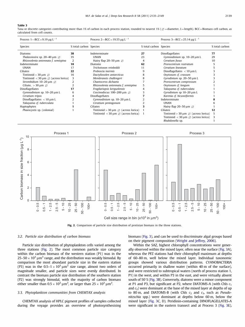
Table 3Taxa or discrete categories contributing more than 1% of carbon in each process station, rounded to nearest 1% (+¼diameter, L¼ length). BCC¼Biomass cell carbon, as

calculated from cell counts.

Process 1—BCC¼9.19 mg L�1 Process 2—BCC¼19.55 mg L�1 Process 3—BCC¼25.14 mg L�1

Species % total carbon Species % total carbon Species % total carbon

Diatoms 38 Indeterminate 27 Dinoflagellates 77Thalassiosira sp. 20–40 mm + 35 UNAN 23 Gymnodinium sp. 10–20 mm L 29

Rhizosolenia antennata f. semispina 2 Hairy flap 20–50 mm + 4 Ceratium fusus 10

Indeterminate 18 Diatoms 62 Prorocentrum rostratum 5

UNAN 17 Trichotoxon reinboldii 11 Ceratium lineatum 5

Ciliates 22 Proboscia inermis 9 Dinoflagellates o10 mm L 3

Tintinnid430 mm + 16 Dactyliosolen antarcticus 8 Oxytoxum cf. crassum 3

Tintinnid o30 mm + (across lorica) 3 Membraneis challengeri 8 Gyrodinium sp. 20–50 mm L 3

Strombidium 10–20 mm + 2 Chaetoceros dichaeta 7 Prorocentrum compressum 2

Ciliate, 430 mm + 2 Rhizosolenia antennata f. semispina 5 Oxytoxum cf. longum 1

Dinoflagellates 17 Fragilariopsis kerguelensis 4 Takayama cf. tuberculata 1

Gymnodinium sp. 10–20 mm L 6 Coscinodiscus 100–200 mm + 3 Gyrodinium sp 10–20 mm L 1

Ceratium tripos 4 Dinoflagellates 7 Karenia cf. bicuneiformis 1

Dinoflagellates o10 mm L 2 Gymnodinium sp. 10–20 mm L 2 Indeterminate 8Takayama cf. tuberculata 1 Ceratium pentagonum 2 UNAN 6

Haptophytes 1 Ciliates 3 Hairy flap 20–50 mm + 1

Phaeocystis sp. (colonial) 1 Tintinnid430 mm + (across lorica) 1 Ciliates 12Tintinnid o30 mm + (across lorica) 1 Tintinnid430 mm + (across lorica) 5

Tintinnid o30 mm + (across lorica) 3

Rhabdonella sp. 1

Process 1

0 - 0

.5

0.5

- 1

1 - 2

.5

2.5

- 5

5 - 1

0

10 -

25

25 -

50

50 -

100

100+

Car

bon

biom

ass

in s

ize

fract

ion

(µg

L-1)

0

2

4

6

8

10Process 2

Cell size range in bin (x103 in µm3)

0 - 0

.5

0.5

- 1

1 - 2

.5

2.5

- 5

5 - 1

0

10 -

25

25 -

50

50 -

100

100+

Process 3

0 - 0

.5

0.5

- 1

1 - 2

.5

2.5

- 5

5 - 1

0

10 -

25

25 -

50

50 -

100

100+

Fig. 2. Comparison of particle size distribution of protistan biomass in the three stations.

M.F. de Salas et al. / Deep-Sea Research II 58 (2011) 2135–2149 2139

3.2. Particle size distribution of carbon biomass

Particle size distribution of phytoplankton cells varied among thethree stations (Fig. 2). The most common particle size categorywithin the carbon biomass of the western station (P1) was in the25–50�103 mm3 range, and the distribution was weakly bimodal. Bycomparison the most abundant particle size in the eastern station(P3) was in the 0.5–1�103 mm3 size range, almost two orders ofmagnitude smaller, and particle sizes were evenly distributed. Incontrast the biomass particle size distribution of the southern station(P2) was strongly bimodal, with the majority of carbon biomasseither smaller than 0.5�103 mm3, or larger than 25�103 mm3.

3.3. Phytoplankton communities from CHEMTAX analysis

CHEMTAX analysis of HPLC pigment profiles of samples collectedduring the voyage provides an overview of photosynthesising

biomass (Fig. 3), and can be used to discriminate algal groups basedon their pigment composition (Wright and Jeffrey, 2006).

Within the SAZ, highest chlorophyll concentrations were gener-ally observed within the mixed layer, often near the surface (Fig. 3A),whereas the PFZ stations had their chlorophyll maximum at depthsof 60–80 m, well below the mixed layer. Individual taxonomicgroups showed various distribution patterns. CYANOBACTERIAoccurred primarily in shallow water (within 40 m of the surface),and were restricted to subtropical waters (north of process station 1,P1) in the west, and within P3 in the east, and were virtually absentsouth of 501S (Fig. 3B). Conversely, diatoms were a minor componentat P1 and P3, but significant at P2, where DIATOMS-A (with Chls c1

and c2) were dominant at the base of the mixed layer at depths of upto 80 m, and DIATOMS-B (with Chls c2 and c3, such as Pseudo-

nitzschia spp.) were dominant at depths below 60 m, below themixed layer (Fig. 3C, D). Peridinin-containing DINOFLAGELLATES-Awere significant in the eastern transect and at Process 3 (Fig. 3E),

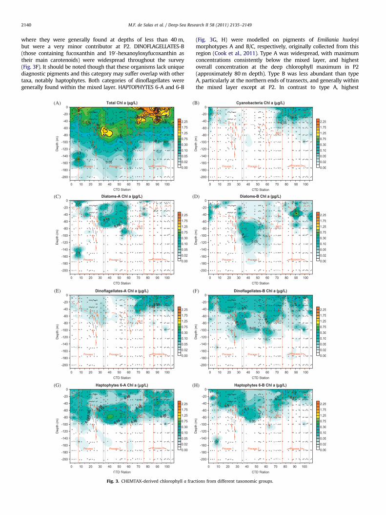
M.F. de Salas et al. / Deep-Sea Research II 58 (2011) 2135–21492140

where they were generally found at depths of less than 40 m,but were a very minor contributor at P2. DINOFLAGELLATES-B(those containing fucoxanthin and 190-hexanoyloxyfucoxanthin astheir main carotenoids) were widespread throughout the survey(Fig. 3F). It should be noted though that these organisms lack uniquediagnostic pigments and this category may suffer overlap with othertaxa, notably haptophytes. Both categories of dinoflagellates weregenerally found within the mixed layer. HAPTOPHYTES 6-A and 6-B

Fig. 3. CHEMTAX-derived chlorophyll a frac

(Fig. 3G, H) were modelled on pigments of Emiliania huxleyi

morphotypes A and B/C, respectively, originally collected from thisregion (Cook et al., 2011). Type A was widespread, with maximumconcentrations consistently below the mixed layer, and highestoverall concentration at the deep chlorophyll maximum in P2(approximately 80 m depth). Type B was less abundant than typeA, particularly at the northern ends of transects, and generally withinthe mixed layer except at P2. In contrast to type A, highest

tions from different taxonomic groups.

Fig. 3. (continued)

M.F. de Salas et al. / Deep-Sea Research II 58 (2011) 2135–2149 2141

abundances were observed within the SAZ and near the PF boundary.HAPTOPHYTES-8 (Fig. 3I, modelled on Phaeocystis spp.) were sig-nificant contributors at all process stations, particularly P3, and werevertically evenly distributed, to below 100 m depth in southernstations. The three green algal categories (PRASINOPHYTES, EUGLE-NOPHYTES, and CHLOROPHYTES, Fig. 3J, K, and L, respectively) wereall similarly distributed, with average populations at P1, very smallstocks at P2, and greatest concentrations at P3. CHLOROPHYTES weregenerally found above the base of the mixed layer, whereasEUGLENOPHYTES were generally found immediately below themixed layer, and PRASINOPHYTES appeared less constrained by themixed layer depth (MLD). Stocks of CRYPTOPHYTES were smallthroughout the study region, highest in subtropical water in bothtransects, but with a small deep population at P2.

3.4. Protistan community composition of stations

3.4.1. SAZ southwest of Tasmania

3.4.1.1. Abundance. The protistan composition at the westernstation (P1) was typical of the SAZ (DiTullio et al., 2003; Fiala et al.,2004). Species richness was intermediate between the two other

stations and composed mostly of flagellates rather than diatoms,reflecting the silica-poor nature of the water in this station (averagesilica was 0.29 mmol L�1, Bowie et al., 2011). The best representedclass in terms of biodiversity was the dinoflagellates. The majority ofdiatoms were lightly silicified pennate species rather than centrics(Table 1). In contrast to species richness, P1 had the lowest meancarbon biomass of all three stations (Fig. 3), and alsocontained the bottle sample with the lowest absolute phytoplanktoncarbon biomass in this study (CTD 21 at 15 m depth, which con-tained 0.16 mg L�1 carbon). This is supported by the pigment mea-surements, which show the lowest average Chl a concentrations inthe western station (Fig. 3). Although dinoflagellates dominated interms of species richness, the dominant carbon source was a diatom,Thalassiosira sp., which was so lightly silicified that frustule detailwas indistinguishable.

In total, ninety-two taxa were identified from the westernstation (P1, Table 1), and samples from this station had mean of23.7 taxa per sample. Excluding UNAN (nanoflagellates o5 mmdiameter, 6.19�105 cells L�1), the most common species werecolonial Phaeocystis spp. (1.02�104 cells L�1), dinoflagellateso10 mm long (7.52�103 cells L�1), and combined cryptophytes

Process StationP1

Car

bon

(µg

L-1)

0

5

10

15

20

25

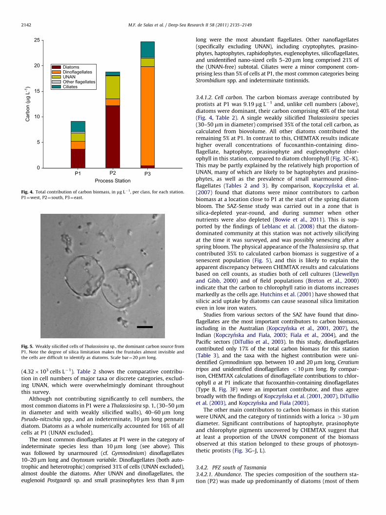
DiatomsDinoflagellatesUNANOther flagellatesCiliates

P2 P3

Fig. 4. Total contribution of carbon biomass, in mg L�1, per class, for each station.

P1¼west, P2¼south, P3¼east.

Fig. 5. Weakly silicified cells of Thalassiosira sp., the dominant carbon source from

P1. Note the degree of silica limitation makes the frustules almost invisible and

the cells are difficult to identify as diatoms. Scale bar¼20 mm long.

M.F. de Salas et al. / Deep-Sea Research II 58 (2011) 2135–21492142

(4.32�103 cells L�1). Table 2 shows the comparative contribu-tion in cell numbers of major taxa or discrete categories, exclud-ing UNAN, which were overwhelmingly dominant throughoutthis survey.

Although not contributing significantly to cell numbers, themost common diatoms in P1 were a Thalassiosira sp. 1, (30–50 mmin diameter and with weakly silicified walls), 40–60 mm longPseudo-nitzschia spp., and an indeterminate, 10 mm long pennatediatom. Diatoms as a whole numerically accounted for 16% of allcells at P1 (UNAN excluded).

The most common dinoflagellates at P1 were in the category ofindeterminate species less than 10 mm long (see above). Thiswas followed by unarmoured (cf. Gymnodinium) dinoflagellates10–20 mm long and Oxytoxum variabile. Dinoflagellates (both auto-trophic and heterotrophic) comprised 31% of cells (UNAN excluded),almost double the diatoms. After UNAN and dinoflagellates, theeuglenoid Postgaardi sp. and small prasinophytes less than 8 mm

long were the most abundant flagellates. Other nanoflagellates(specifically excluding UNAN), including cryptophytes, prasino-phytes, haptophytes, raphidophytes, euglenophytes, silicoflagellates,and unidentified nano-sized cells 5–20 mm long comprised 21% ofthe (UNAN-free) subtotal. Ciliates were a minor component com-prising less than 5% of cells at P1, the most common categories beingStrombidium spp. and indeterminate tintinnids.

3.4.1.2. Cell carbon. The carbon biomass average contributed byprotists at P1 was 9.19 mg L�1 and, unlike cell numbers (above),diatoms were dominant, their carbon comprising 40% of the total(Fig. 4, Table 2). A single weakly silicified Thalassiosira species(30–50 mm in diameter) comprised 35% of the total cell carbon, ascalculated from biovolume. All other diatoms contributed theremaining 5% at P1. In contrast to this, CHEMTAX results indicatehigher overall concentrations of fucoxanthin-containing dino-flagellate, haptophyte, prasinophyte and euglenophyte chlor-ophyll in this station, compared to diatom chlorophyll (Fig. 3C–K).This may be partly explained by the relatively high proportion ofUNAN, many of which are likely to be haptophytes and prasino-phytes, as well as the prevalence of small unarmoured dino-flagellates (Tables 2 and 3). By comparison, Kopczynska et al.(2007) found that diatoms were minor contributors to carbonbiomass at a location close to P1 at the start of the spring diatombloom. The SAZ-Sense study was carried out in a zone that issilica-depleted year-round, and during summer when othernutrients were also depleted (Bowie et al., 2011). This is sup-ported by the findings of Leblanc et al. (2008) that the diatom-dominated community at this station was not actively silicifyingat the time it was surveyed, and was possibly senescing after aspring bloom. The physical appearance of the Thalassiosira sp. thatcontributed 35% to calculated carbon biomass is suggestive of asenescent population (Fig. 5), and this is likely to explain theapparent discrepancy between CHEMTAX results and calculationsbased on cell counts, as studies both of cell cultures (Llewellynand Gibb, 2000) and of field populations (Breton et al., 2000)indicate that the carbon to chlorophyll ratio in diatoms increasesmarkedly as the cells age. Hutchins et al. (2001) have showed thatsilicic acid uptake by diatoms can cause seasonal silica limitationeven in low iron waters.

Studies from various sectors of the SAZ have found that dino-flagellates are the most important contributors to carbon biomass,including in the Australian (Kopczynska et al., 2001, 2007), theIndian (Kopczynska and Fiala, 2003; Fiala et al., 2004), and thePacific sectors (DiTullio et al., 2003). In this study, dinoflagellatescontributed only 17% of the total carbon biomass for this station(Table 3), and the taxa with the highest contribution were uni-dentified Gymnodinium spp. between 10 and 20 mm long, Ceratium

tripos and unidentified dinoflagellates o10 mm long. By compar-ison, CHEMTAX calculations of dinoflagellate contributions to chlor-ophyll a at P1 indicate that fucoxanthin-containing dinoflagellates(Type B, Fig. 3F) were an important contributor, and thus agreebroadly with the findings of Kopczynska et al. (2001, 2007), DiTullioet al. (2003), and Kopczynska and Fiala (2003).

The other main contributors to carbon biomass in this stationwere UNAN, and the category of tintinnids with a lorica 430 mmdiameter. Significant contributions of haptophyte, prasinophyteand chlorophyte pigments uncovered by CHEMTAX suggest thatat least a proportion of the UNAN component of the biomassobserved at this station belonged to these groups of photosyn-thetic protists (Fig. 3G–J, L).

3.4.2. PFZ south of Tasmania

3.4.2.1. Abundance. The species composition of the southern sta-tion (P2) was made up predominantly of diatoms (most of them

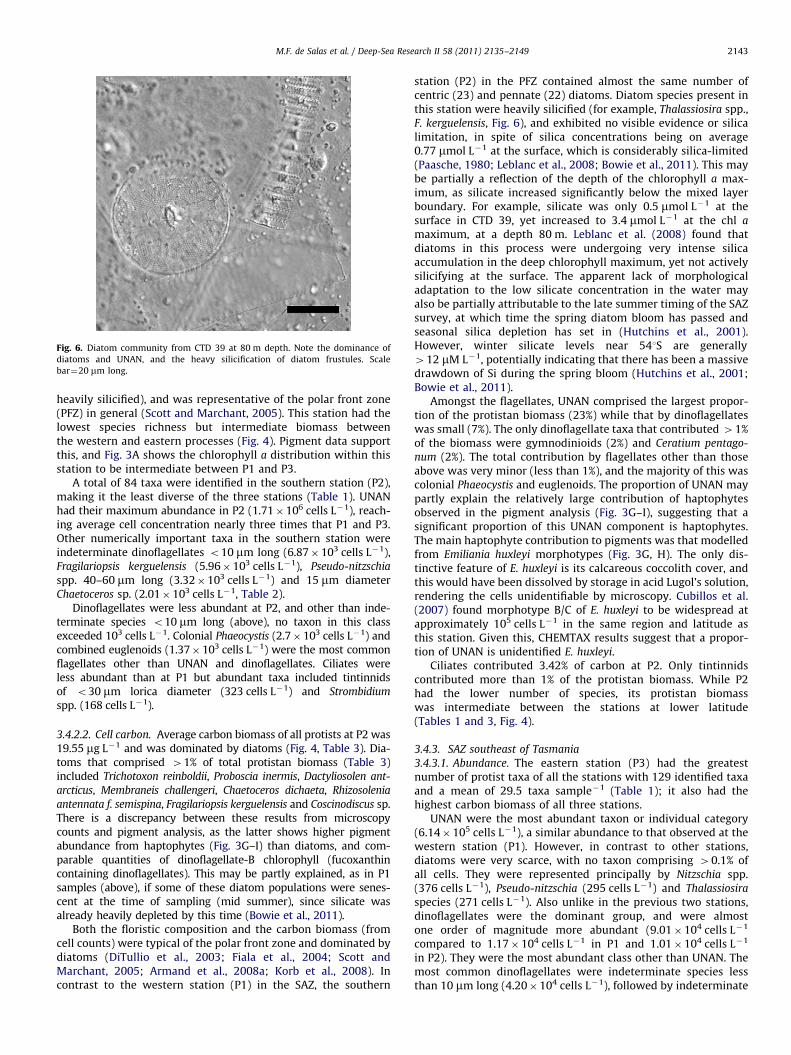
Fig. 6. Diatom community from CTD 39 at 80 m depth. Note the dominance of

diatoms and UNAN, and the heavy silicification of diatom frustules. Scale

bar¼20 mm long.

M.F. de Salas et al. / Deep-Sea Research II 58 (2011) 2135–2149 2143

heavily silicified), and was representative of the polar front zone(PFZ) in general (Scott and Marchant, 2005). This station had thelowest species richness but intermediate biomass betweenthe western and eastern processes (Fig. 4). Pigment data supportthis, and Fig. 3A shows the chlorophyll a distribution within thisstation to be intermediate between P1 and P3.

A total of 84 taxa were identified in the southern station (P2),making it the least diverse of the three stations (Table 1). UNANhad their maximum abundance in P2 (1.71�106 cells L�1), reach-ing average cell concentration nearly three times that P1 and P3.Other numerically important taxa in the southern station wereindeterminate dinoflagellates o10 mm long (6.87�103 cells L�1),Fragilariopsis kerguelensis (5.96�103 cells L�1), Pseudo-nitzschia

spp. 40–60 mm long (3.32�103 cells L�1) and 15 mm diameterChaetoceros sp. (2.01�103 cells L�1, Table 2).

Dinoflagellates were less abundant at P2, and other than inde-terminate species o10 mm long (above), no taxon in this classexceeded 103 cells L�1. Colonial Phaeocystis (2.7�103 cells L�1) andcombined euglenoids (1.37�103 cells L�1) were the most commonflagellates other than UNAN and dinoflagellates. Ciliates wereless abundant than at P1 but abundant taxa included tintinnidsof o30 mm lorica diameter (323 cells L�1) and Strombidium

spp. (168 cells L�1).

3.4.2.2. Cell carbon. Average carbon biomass of all protists at P2 was19.55 mg L�1 and was dominated by diatoms (Fig. 4, Table 3). Dia-toms that comprised 41% of total protistan biomass (Table 3)included Trichotoxon reinboldii, Proboscia inermis, Dactyliosolen ant-

arcticus, Membraneis challengeri, Chaetoceros dichaeta, Rhizosolenia

antennata f. semispina, Fragilariopsis kerguelensis and Coscinodiscus sp.There is a discrepancy between these results from microscopycounts and pigment analysis, as the latter shows higher pigmentabundance from haptophytes (Fig. 3G–I) than diatoms, and com-parable quantities of dinoflagellate-B chlorophyll (fucoxanthincontaining dinoflagellates). This may be partly explained, as in P1samples (above), if some of these diatom populations were senes-cent at the time of sampling (mid summer), since silicate wasalready heavily depleted by this time (Bowie et al., 2011).

Both the floristic composition and the carbon biomass (fromcell counts) were typical of the polar front zone and dominated bydiatoms (DiTullio et al., 2003; Fiala et al., 2004; Scott andMarchant, 2005; Armand et al., 2008a; Korb et al., 2008). Incontrast to the western station (P1) in the SAZ, the southern

station (P2) in the PFZ contained almost the same number ofcentric (23) and pennate (22) diatoms. Diatom species present inthis station were heavily silicified (for example, Thalassiosira spp.,F. kerguelensis, Fig. 6), and exhibited no visible evidence or silicalimitation, in spite of silica concentrations being on average0.77 mmol L�1 at the surface, which is considerably silica-limited(Paasche, 1980; Leblanc et al., 2008; Bowie et al., 2011). This maybe partially a reflection of the depth of the chlorophyll a max-imum, as silicate increased significantly below the mixed layerboundary. For example, silicate was only 0.5 mmol L�1 at thesurface in CTD 39, yet increased to 3.4 mmol L�1 at the chl a

maximum, at a depth 80 m. Leblanc et al. (2008) found thatdiatoms in this process were undergoing very intense silicaaccumulation in the deep chlorophyll maximum, yet not activelysilicifying at the surface. The apparent lack of morphologicaladaptation to the low silicate concentration in the water mayalso be partially attributable to the late summer timing of the SAZsurvey, at which time the spring diatom bloom has passed andseasonal silica depletion has set in (Hutchins et al., 2001).However, winter silicate levels near 541S are generally412 mM L�1, potentially indicating that there has been a massivedrawdown of Si during the spring bloom (Hutchins et al., 2001;Bowie et al., 2011).

Amongst the flagellates, UNAN comprised the largest propor-tion of the protistan biomass (23%) while that by dinoflagellateswas small (7%). The only dinoflagellate taxa that contributed 41%of the biomass were gymnodinioids (2%) and Ceratium pentago-

num (2%). The total contribution by flagellates other than thoseabove was very minor (less than 1%), and the majority of this wascolonial Phaeocystis and euglenoids. The proportion of UNAN maypartly explain the relatively large contribution of haptophytesobserved in the pigment analysis (Fig. 3G–I), suggesting that asignificant proportion of this UNAN component is haptophytes.The main haptophyte contribution to pigments was that modelledfrom Emiliania huxleyi morphotypes (Fig. 3G, H). The only dis-tinctive feature of E. huxleyi is its calcareous coccolith cover, andthis would have been dissolved by storage in acid Lugol’s solution,rendering the cells unidentifiable by microscopy. Cubillos et al.(2007) found morphotype B/C of E. huxleyi to be widespread atapproximately 105 cells L�1 in the same region and latitude asthis station. Given this, CHEMTAX results suggest that a propor-tion of UNAN is unidentified E. huxleyi.

Ciliates contributed 3.42% of carbon at P2. Only tintinnidscontributed more than 1% of the protistan biomass. While P2had the lower number of species, its protistan biomasswas intermediate between the stations at lower latitude(Tables 1 and 3, Fig. 4).

3.4.3. SAZ southeast of Tasmania

3.4.3.1. Abundance. The eastern station (P3) had the greatestnumber of protist taxa of all the stations with 129 identified taxaand a mean of 29.5 taxa sample�1 (Table 1); it also had thehighest carbon biomass of all three stations.

UNAN were the most abundant taxon or individual category(6.14�105 cells L�1), a similar abundance to that observed at thewestern station (P1). However, in contrast to other stations,diatoms were very scarce, with no taxon comprising 40.1% ofall cells. They were represented principally by Nitzschia spp.(376 cells L�1), Pseudo-nitzschia (295 cells L�1) and Thalassiosira

species (271 cells L�1). Also unlike in the previous two stations,dinoflagellates were the dominant group, and were almostone order of magnitude more abundant (9.01�104 cells L�1

compared to 1.17�104 cells L�1 in P1 and 1.01�104 cells L�1

in P2). They were the most abundant class other than UNAN. Themost common dinoflagellates were indeterminate species lessthan 10 mm long (4.20�104 cells L�1), followed by indeterminate

0.0380

0.1300

0.2219

0.3139

0.4058

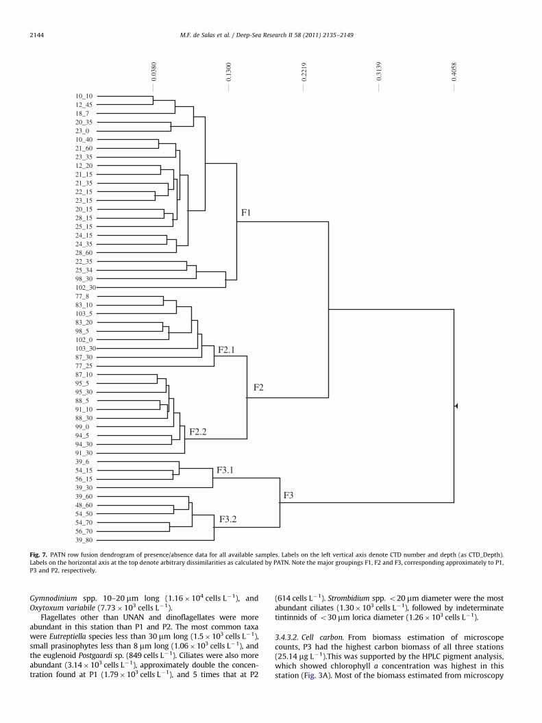
10_1012_4518_720_3523_010_4021_6023_3512_2021_1521_3522_1523_1520_1528_1525_1524_1524_3528_6022_3525_3498_30102_3077_883_10103_583_2098_5102_0103_3087_3077_2587_1095_595_3088_591_1088_3099_094_594_3091_3039_654_1556_1539_3039_6048_6054_5054_7056_7039_80

F1

F2

F3

F2.1

F2.2

F3.1

F3.2

Fig. 7. PATN row fusion dendrogram of presence/absence data for all available samples. Labels on the left vertical axis denote CTD number and depth (as CTD_Depth).

Labels on the horizontal axis at the top denote arbitrary dissimilarities as calculated by PATN. Note the major groupings F1, F2 and F3, corresponding approximately to P1,

P3 and P2, respectively.

M.F. de Salas et al. / Deep-Sea Research II 58 (2011) 2135–21492144

Gymnodinium spp. 10–20 mm long (1.16�104 cells L�1), andOxytoxum variabile (7.73�103 cells L�1).

Flagellates other than UNAN and dinoflagellates were moreabundant in this station than P1 and P2. The most common taxawere Eutreptiella species less than 30 mm long (1.5�103 cells L�1),small prasinophytes less than 8 mm long (1.06�103 cells L�1), andthe euglenoid Postgaardi sp. (849 cells L�1). Ciliates were also moreabundant (3.14�103 cells L�1), approximately double the concen-tration found at P1 (1.79�103 cells L�1), and 5 times that at P2

(614 cells L�1). Strombidium spp. o20 mm diameter were the mostabundant ciliates (1.30�103 cells L�1), followed by indeterminatetintinnids of o30 mm lorica diameter (1.26�103 cells L�1).

3.4.3.2. Cell carbon. From biomass estimation of microscopecounts, P3 had the highest carbon biomass of all three stations(25.14 mg L�1).This was supported by the HPLC pigment analysis,which showed chlorophyll a concentration was highest in thisstation (Fig. 3A). Most of the biomass estimated from microscopy

0.3213

0.4786

0.6358

0.7931

0.9503

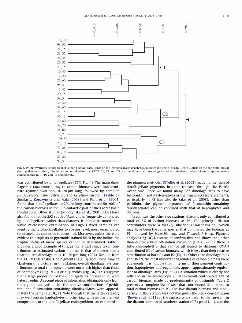
10_1098_3021_1521_3521_4520_3523_1510_4012_2021_6095_512_4520_1539_539_3039_6054_1556_1539_8054_7048_6018_7103_3077_1077_2583_1083_2098_5

C1

C2

C3

Fig. 8. PATN row fusion dendrogram of carbon biomass data. Labels on the left vertical axis denote CTD number and depth (as CTD_Depth). Labels on the horizontal axis at

the top denote arbitrary dissimilarities as calculated by PATN. C1, C2 and C3 are the three main groupings based on calculated carbon biomass, approximately

corresponding to P1, P2 and P3, respectively.

M.F. de Salas et al. / Deep-Sea Research II 58 (2011) 2135–2149 2145

was contributed by dinoflagellates (77%, Fig. 4). The main dino-flagellate taxa contributing to carbon biomass were indetermi-nate Gymnodinium spp. 10–20 mm long, followed by Ceratium

fusus, Prorocentrum rostratum, and Ceratium lineatum (Table 3).Similarly, Kopczynska and Fiala (2003) and Fiala et al. (2004)found that dinoflagellates o20 mm long contributed 50–90% ofthe carbon biomass in the Sub-Antarctic part of the Crozet Basinfrontal zone. Other studies (Kopczynska et al., 2001, 2007) havealso found that the SAZ south of Australia is frequently dominatedby dinoflagellates rather than diatoms. It should be noted that,while microscopic examination of Lugol’s fixed samples canidentify many dinoflagellates to species level, most unarmoureddinoflagellates cannot be so identified. Moreover, unless there areevident chloroplasts or pyrenoids stained black by the iodine, thetrophic status of many species cannot be determined. Table 3provides a good example of this, as the largest single taxon con-tribution to estimated carbon biomass is that of indeterminateunarmoured dinoflagellates 10–20 mm long (29%). Results fromthe CHEMTAX analysis of pigments (Fig. 3) goes some way toclarifying this picture: in this station, overall dinoflagellate con-tributions to total chlorophyll a were not much higher than thoseof haptophytes (Fig. 3G–I) or euglenoids (Fig. 3K). This suggeststhat a large proportion of the dinoflagellates present in P3 wereheterotrophic. A second piece of information obtainable only fromthe pigment analysis is that the relative contributions of peridi-nin- and fucoxanthin-containing dinoflagellates were approxi-mately the same (Fig. 3E, F). Note though that the latter categorymay well contain haptophytes or other taxa with similar pigmentcomposition to the dinoflagellate endosymbiont, as explained in

the pigment methods. DiTullio et al. (2003) made no mention ofdinoflagellate pigments in their transect through the PacificOcean SAZ. Since we found many SAZ dinoflagellates to havefucoxanthin and its derivatives as their main accessory pigments,particularly in P3 (see also de Salas et al., 2008), rather thanperidinin, the pigment signature of fucoxanthin-containingdinoflagellates can be confused with that of haptophytes anddiatoms.

In contrast the other two stations, diatoms only contributed atotal of 3% of carbon biomass at P3. The principal diatomcontributors were a weakly silicified Thalassiosira sp., whichmay have been the same species that dominated the biomass atP1, followed by Nitzschia spp. and Thalassiothrix sp. Pigmentanalysis (Fig. 3C, D) seems to confirm this, and shows that, otherthan during a brief off-station excursion (CTDs 87–95), there islittle chlorophyll a that can be attributed to diatoms. UNANcontributed 6% of carbon biomass, which is less than their relativecontribution at both P1 and P2 (Fig. 4). Other than dinoflagellatesand UNAN, the most important flagellates in carbon biomass wereeuglenoids. It is notable that, in terms of their pigment contribu-tion, haptophytes and euglenoids appear approximately equiva-lent to dinoflagellates (Fig. 3E–K), a situation which is clearly notreflected in the microscopy. Ciliates overall contributed 12% ofcarbon biomass, made up predominantly of tintinnids. Table 2presents a complete list of taxa that contributed 1% or more tototal carbon biomass in P3. The low diatom biomass and biodi-versity in this station was notable given the silica concentration(Bowie et al., 2011) at the surface was similar to that present inthe diatom-dominated southern station (0.71 mmol L�1), and the

M.F. de Salas et al. / Deep-Sea Research II 58 (2011) 2135–21492146

silica concentration was higher than that of the western station,where a diatom made the largest contribution to carbon biomass.Silica uptake rates of diatoms at this station showed that,although their biomass contribution was very small, they werean actively growing and silicifying community, in particularCylindrotheca, Rhizosolenia and Thalassiosira species (Leblancet al., 2008).

3.5. Exploratory data analysis

Multidimensional scaling (MDS) association and cluster ana-lysis of datasets containing both floristic composition (presence/absence) and carbon biomass showed three main clusters ofspecies (Figs. 7 and 8). In the floristic analysis (Fig. 7), PATNgroups F1, F2 and F3 corresponded well with samples from thestations in the west (P1), east (P3) and south (P2), respectively.The differences among the three sites were statistically signifi-cant, though not greatly so (ANOSIM real F¼1.12, randomisedf¼0, % randomised F¼0.02). PCC showed the main environmentalvariables with a reasonable correlation to the dataset to belatitude (R2

¼0.83), nitrate (R2¼0.68), longitude (R2

¼0.65) andtemperature (R2

¼0.58). Monte Carlo attributes in ordination(MCAO) results (0% permutated R2 values exceeded the actualR2 values) showed the correlation to these environmental vari-ables to the dataset to be statistically significant. Groups F1 andF2 were more similar to each other than either was to group F3,indicating that at the floristic level, P1 and P3 in the west andeast, respectively, shared a greater number of species betweenthem than either shared with P2 in the south. The floristicanalysis also separated samples from group F2 (eastern station)into two clearly defined subgroups. Subgroup F2.1 containedmostly collections from the start and end of sampling and withinP3, whereas group F2.2 represented mostly CTDs from an excur-sion to characterise a low chlorophyll, high salinity warm watermass to the north of P3 (Bowie et al., 2011). In a similar manner,group F3, which represented CTDs from PFZ water at the southernstation, was clearly split into two subgroups. In contrast to groupF2, subgroups F3.1 and F3.2 represented samples collected fromthe surface (F3.1) and at the chlorophyll maximum or intermedi-ate depths (F3.2).

Species that characterised PATN group F1 (representing thewestern station) included Cylindrotheca closterium, Ephemera sp.,and Nitzschia cf. sicula. Group F2 (eastern station) was the onlygroup to possess species such as Antinocyclus actinochilus, Chae-

toceros convolutus, Gyrosigma sp., Nitzschia acicularis, Ceratium

furca, Cochlodinium sp., Fragilidium sp., Gonyaulax digitale and G.

scrippsiae, Karenia spp., Karlodinium cf. conicum, Nematodinium sp.,Ebria sp., Mesodinium pulex, Dinophysis cf. norvegica, D. tripos,

Oxytoxum scolopax, O. caudatum, O. curvatum, O. curvicaudatum, O.

globosum, and Warnowia sp. A number of species were shared bythe eastern and western stations (which included the diatomsThalassiosira sp. (with weakly silicified walls, the main componentof biomass in P1), Planktoniella sol, and Pseudo-nitzschia subcur-

vata and dinoflagellates such as Ceratium fusus, C. lineatum,C. tripos, Prorocentrum balticum, P. minimum, P. rostratum andP. compressum, Oxytoxum crassum and O. longum, as well asDinophysis rotundata) and this supported the floristic analysisresults which showed groups F1 and F2 to be more similar to eachother than either of them was to F3.

Many species, particularly diatoms, were also characteristic ofP2, such as Azpeitia spp., Chaetoceros bulbosus, Dactyliosolen antarc-

ticus, Eucampia antarctica, Proboscia inermis, Trichotoxon reinboldii,

Ceratium pentagonum, Mesoporum perforatum, Prorocentrum antarc-

ticum, Dinophysis contracta and Protoperidinium deflectum.Cluster and MDS of the carbon biomass of protists classified

the sample sites into the same 3 groups as the floristic analysis

(Figs. 7 and 8). However, in contrast to the floristic analysis,samples from the western and southern stations (C1 and C2,respectively) were clustered closer to each other than either wasto the eastern station, and distances between terminal taxa weresuch that subgroups were not readily apparent as they were thefloristic analysis. In contrast to floristic analysis, PCC analysis ofcarbon biomass selected mixed layer depth (R2

¼0.76), latitude(R2¼0.72), temperature (R2

¼0.69), CTD transmittance (R2¼0.64)

and nitrate (R2¼0.59) as environmental variables with a good

correlation to the dataset. These correlations were all statisticallysignificant (MCAO of 0%). Notably, the level of dissimilaritybetween sample sites (within each station) in the carbon biomassanalysis (Fig. 8) was substantially higher than that between sitesin the floristic analysis (Fig. 7), although conversely, the level ofdissimilarity between stations was also higher in the carbonbiomass than the floristic analysis. This may reflect a large levelof variance in the order of the main few species contributing tocarbon biomass between sites, though the overall composition ofthe species that contribute to carbon stayed fairly constant.Indeed the carbon biomass analysis is not influenced significantlyby minor species, which have a large effect on the floristicanalysis.

3.6. Bottom-up control of phytoplankton populations

Several factors may explain why diatoms are dominant at thewestern station (P1) despite silica limitation, and why flagellatesoverwhelmingly dominate the community at eastern station (P3)despite extra nutrient availability and a similar degree of silicalimitation. Mixed layer depth was shallower in the eastern stationthan either P1 or P2. The shallowly stratified mixed layer is likelyto promote the growth of flagellates in favour of diatoms. Unlikediatoms, flagellates (especially dinoflagellates which dominatedat P3), are able to undergo diel vertical migration, therebyallowing them to optimise light and nutrient availability byswimming from surface waters during daylight hours to belowthe pycnocline during the night (Ji and Franks, 2007). Thus theextra availability of iron in the upper 100 m of P3 compared to P1and P2 (Bowie et al., 2009) may not have stimulated diatomgrowth in a mixed layer where concentrations of both silicate andnitrate were limiting (Bowie et al., 2011). At P2, the chlorophyllmaximum and highest diatom concentration was found at depthsbelow the mixed layer, where nutrient concentrations, includingsilicate, were higher than at the surface (Bowie et al., 2011). Thevertical distribution of nutrients is, in itself, not enough to explainthe absence of a deep chlorophyll maximum composed mostly ofdiatoms (as observed in P2). However, the polar front zone is onlyseasonally silica limited (Hiscock et al., 2003; Trull et al., 2001b),whereas the SAZ, which is less seasonally light limited, is a silicalimited environment year-round (Bowie et al., 2011), and thismay limit the seed source of diatoms able to capitalise on anyincreased availability of silica.

Hutchins and Bruland (1998) and Takeda (1998) showed thatiron limitation has a higher impact on nitrate than silica uptake,causing diatoms growing under iron enrichment conditions todeplete available silica more quickly, and those growing underiron stress to become more heavily silicified (therefore sinkingfaster). However, waters in the SAZ are silica-limited year-round,and this may be enough to prevent heavy uptake of silicic acid bydiatoms. Such silica limitation was demonstrated by the frustulesof the Thalassiosira sp. that dominated carbon biomass at P1, asthey were extremely weakly silicified (Fig. 5).

Iron is more limiting in the western than the eastern station(P3), which has iron inputs from land and the continental shelf(Bowie et al., 2009). In the presence of strict iron limitation,silicate is less likely to be a limiting nutrient, as in the western

M.F. de Salas et al. / Deep-Sea Research II 58 (2011) 2135–2149 2147

station (Coale et al., 2004). However, with relaxation of ironlimitation in the east (P3), silica is likely to become limiting andlikely to disadvantage diatom growth compared to non-silicatebearing flagellates.

3.7. Top-down control by grazers

Heterotrophic nanoflagellates, which graze preferentially thesmaller size fractions and limit the accumulation of organismssuch as picoflagellates and bacteria, were found to be thedominant grazers at the western station, P1 (Pearce et al.,2011). Conversely, diatoms were unconstrained by microhetero-trophic grazing and their abundance would be preferentiallyenhanced. In contrast, in the east at P3, microzooplankton exertedsimilar grazing pressure on all size classes of prey and top-downcontrol of the larger sized diatoms would have limited theirproliferation at this location.

3.8. Phytoplankton community change: implications for the

carbon cycle

One of the primary goals of the SAZ-Sense project was toestablish whether there are observable differences in the compo-sition, trophodynamics and vertical carbon flux between thewestern and eastern stations, under the premise that thesedifferences may reflect future climate-induced changes in theSAZ (IPCC, 2007; Boning et al., 2008; Turner et al., 2009).

The comparison between the SAZ sectors southeast and south-west of Tasmania is a possible proxy for the expected effect ofclimate change in this area of the southern hemisphere. The eastern,iron enriched station indeed exhibited higher carbon biomass thanthe western, iron-poor one, though this increased biomass was in asmaller particle size range than in either the western or southernstations. Due to the constraints of the SAZ-sense voyage, which wasundertaken during the austral summer, the time of maximumproductivity (the spring diatom bloom) could not be studied. If, asTrull et al. (2001a) and Richardson and Jackson (2007) suggest,vertical carbon export is directly proportional to primary produc-tion, then the higher biomass of the eastern station suggestsincreased carbon export to the deep ocean. If, however, the tradi-tional view that diatoms are the main carbon exporters (because oftheir increased sinking rate due to the weight of their frustules)applies, then the increased productivity may not directly translateinto increased export (Boyd and Newton, 1999). In either case, thepredominant grazers in the eastern SAZ were microzooplankton(Pearce et al., 2011), which consumed prey across the size spectrum.Their fast sinking faecal pellets are likely to provide a vehicle forvertical export of POC, and allow some of the increased productivityin the eastern SAZ to act as a carbon sink. In addition to havingpotentially significant effects on the vertical export of POC to thedeep ocean, the shift in community composition from the hapto-phyte-dominated (with important diatom contributions) west to thedinoflagellate dominated east also has implications for the climati-cally important aerosols dimethylsulfide (DMS) and its precursordimethylsulfoniopropionate (DMSP). Jones et al. (1998) found acorrelation between elevated levels of DMS and DMSP in commu-nities dominated by dinoflagellates, especially gymnodinioids. Sincethese dinoflagellates were found in our study to significantlyincrease under the conditions present in P3 (a proxy for hypothe-sised future SAZ conditions), elevated levels of DMS and DMSP mayaccompany the expected ecosystem shift and exert their own effectson climate independently of the carbon cycle.

This work has two important limitations that need to be notedhere. Having been carried out over the course of only a few weeksin late summer, this study provides an explanation of biologicalprocesses restricted to this time of the year, and care needs to be

taken when generalising these results to late summer SAZ ingeneral, or other times of the year. In addition, a significantcomponent of the biomass was contributed by indeterminatenanoflagellates less than 5 mm in diameter and picoflagellates,and microscopy techniques cannot resolve taxonomic affinitieswithin this group. It is essential that future studies in the SAZincorporate sampling and analytical techniques that can over-come this problem, and characterise this dominant group (forexample, size fractionation followed by metagenomic analysis ofrDNA sequences).

4. Conclusions

This study considered the differences between the phytoplank-ton community structure southeast and southwest of Tasmania,and the potential implications of such differences to the futureecology and carbon budgets of the Southern Ocean. The compar-ison between the eastern and western stations may be an accuratereflection of the changes we can expect from warming trends inthe Southern Ocean. If this is so, then a possible result of oceanicwarming, and increased iron from dust and other sources, is anincrease in biomass and productivity, accompanied by a shift inphytoplankton community composition away from diatoms andtowards dominance by small flagellates. This extra productivity islikely to translate into increased export of POC to the deep ocean.

Acknowledgments

The authors would like to acknowledge Martina Doblin forhelp in the collection and fixation of water samples. We wouldalso like to thank Rick van den Enden, Paul Thomson, and KarenWestwood for help and support in the preparation of this manu-script, Imojen Pearce for shared data, templates, and ideas, andGerry Nash for assistance with the electron microscopy. Wewould also like to thank the Captain and crew of the R.V. Aurora

Australis for their help and support during the SAZ-Sense voyage.

Appendix A. Supplementary data

Supplementary data associated with this article can be foundin the online version at doi:10.1016/j.dsr2.2011.05.032.

References

Alvain, S., Moulin, C., Dandonneau, Y., Loisel, H., 2008. Seasonal distribution andsuccession of dominant phytoplankton groups in the global ocean: a satelliteview—art. no. GB3001. Global Biogeochemical Cycles 22. doi:10.1029/2007GB003154.

Armand, L.K., Cornet-Barthaux, V., Mosseri, J., Queguiner, B., 2008a. Late summerdiatom biomass and community structure on and around the naturally iron-fertilised Kerguelen Plateau in the Southern Ocean. Deep-Sea Research II 55,653–676.

Armand, L.K., Crosta, X., Queguiner, B., Mosseri, J., Garcia, N., 2008b. Diatomspreserved in surface sediments of the northeastern Kerguelen Plateau. Deep-Sea Research II 55, 677–692.

Austin, M.P., Belbin, L., 1982. A new approach to the species classification problemin floristic analysis. Australian Journal of Ecology 7, 75–89.

Bakker, D.C.E., Watson, A.J., Law, C.S., 2001. Southern Ocean iron enrichmentpromotes inorganic carbon drawdown. Deep-Sea Research II 48, 2483–2507.

Beans, C., Hecq, J.H., Koubbi, P., Vallet, C., Wright, S., Goffart, A., 2008. A study ofthe diatom-dominated microplankton summer assemblages in coastal watersfrom Terre Adelie to the Mertz Glacier, East Antarctica (139 degrees E-145degrees E). Polar Biology 31, 1101–1117.

Belbin, L., Faith, D.P., Milligan, G.W., 1992. A comparison of two approaches tobeta-flexible clustering. Multivariate Behavioural Research 27, 417–433.

Belbin, L., 2004. PATN v3.03 for Windows. Blatant Fabrications Pty. Ltd, Brisbane,Australia.

M.F. de Salas et al. / Deep-Sea Research II 58 (2011) 2135–21492148

Blain, S., Queguiner, B., Armand, L., Belviso, S., Bombled, B., Bopp, L., Bowie, A.,Brunet, C., Brussaard, C., Carlotti, F., Christaki, U., Corbiere, A., Durand, I.,Ebersbach, F., Fuda, J.-L., Garcia, N., Gerringa, L., Griffiths, B., Guigue, C.,Guillerm, C., Jacquet, S., Jeandel, C., Laan, P., Lefevre, D., Lo Monaco, C., Malits,A., Mosseri, J., Obernosterer, I., Park, Y.-H., Picheral, M., Pondaven, P., Remenyi,T., Sandroni, V., Sarthou, G., Savoye, N., Scouarnec, L., Souhaut, M., Thuiller, D.,Timmermans, K., Trull, T., Uitz, J., van Beek, P., Veldhuis, M., Vincent, D.,Viollier, E., Vong, L., Wagener, T., 2007. Effect of natural iron fertilization oncarbon sequestration in the Southern Ocean. Nature 446, 1070–1074.

Blain, S., Queguiner, B., Trull, T., 2008. The natural iron fertilization experimentKEOPS (KErguelen Ocean and Plateau compared study): an overview. Deep-SeaResearch II 55, 559–565.

Boning, C.W., Dispert, A., Visbeck, M., Rintoul, S.R., Schwarzkopf, F.U., 2008. Theresponse of the Antarctic circumpolar current to recent climate change. NatureGeoscience 1, 864–869.

Bowie, A.R., Lannuzel, D., Remenyi, T.A., Wagener, T., Lam, P.J., Boyd, P.W., Guieu,C., Townsend, A.T., Trull, T.W., 2009. Biogeochemical iron budgets of theSouthern Ocean south of Australia: decoupling of iron and nutrient cycles inthe subantarctic zone by the summertime supply. Global BiogeochemicalCycles 23, GB4034. doi:10.1029/2009GB003500.

Bowie, A.R., Griffiths, F.B., Dehairs, F., Trull, T.W., 2011. Oceanography of thesubantarctic and polar frontal zones south of Australia during summer: settingfor the SAZ-Sense study. Deep-Sea Research II 58, 2059–2070.

Boyd, P.W., 2008. Implications of large-scale iron fertilization of the oceans—

introduction and synthesis. Marine Ecology Progress Series 364, 213–218.Boyd, P.W., Law, C.S., 2001. The Southern Ocean Iron RElease Experiment

(SOIREE)—introduction and summary. Deep-Sea Research II 48, 2425–2438.Boyd, P.W., Newton, P.P., 1999. Does planktonic community structure determine

downward particulate organic carbon flux in different oceanic provinces?Deep-Sea Research I 46, 63–91.

Boyd, P.W., Jickells, T., Law, C.S., Blain, S., Boyle, E.A., Buesseler, K.O., Coale, K.H.,Cullen, J.J., de Baar, H.J.W., Follows, M., Harvey, M., Lancelot, C., Levasseur, M.,Owens, N.P.J., Pollard, R., Rivkin, R.B., Sarmiento, J., Schoemann, V., Smetacek,V., Takeda, S., Tsuda, A., Turner, S., Watson, A.J., 2007. Mesoscale ironenrichment experiments 1993–2005: synthesis and future directions. Science315, 612–617. doi:10.1126/science.1131669.

Bray, J.R., Curtis, J.T., 1957. An ordination of the upland forest communities ofsouthern Wisconsin. Ecological Monographs 27, 325–349.

Breton, E., Brunet, C., Sautour, B., Brylinski, J.-M., 2000. Annual variations ofphytoplankton biomass in the Eastern English Channel: comparison bypigment signatures and microscopic counts. Journal of Plankton Research 22,1423–1440. doi:10.1093/plankt/22.8.1423.

Cassar, N., Bender, M.L., Barnett, B.A., Fan, S., Moxim, W.J., Levy II, H., Tilbrook, B.,2007. The Southern Ocean biological response to aeolian iron deposition.Science 317, 1067–1070. doi:10.1126/science.1144602.

Clarke, K., Warwick, R., 1994. Change in Marine Communities: An Approach toStatistical Analysis and Interpretation. Natural Environment Research Council,Plymouth, UK 172pp.

Coale, K.H., Johnson, K.S., Chavez, F.P., Buesseler, K.O., Barber, R.T., Brzezinski, M.A.,Cochlan, W.P., Millero, F.J., Falkowski, P.G., Bauer, J.E., Wanninkhof, R.H., Kudela,R.M., Altabet, M.A., Hales, B.E., Takahashi, T., Landry, M.R., Bidigare, R.R., Wang, X.,Chase, Z., Strutton, P.G., Friederich, G.E., Gorbunov, M.Y., Lance, V.P., Hilting, A.K.,Hiscock, M.R., Demarest, M., Hiscock, W.T., Sullivan, K.F., Tanner, S.J., Gordon,R.M., Hunter, C.N., Elrod, V.A., Fitzwater, S.E., Jones, J.L., Tozzi, S., Koblizek, M.,Roberts, A.E., Herndon, J., Brewster, J., Ladizinsky, N., Smith, G., Cooper, D.,Timothy, D., Brown, S.L., Selph, K.E., Sheridan, C.C., Twining, B.S., Johnson, Z.I.,2004. Southern Ocean iron enrichment experiment: carbon cycling in high- andlow-Si waters. Science 304, 408–414. doi:10.1126/science.1089778.

Cook, S.S., Whittock, L., Wright, S.W., Hallegraaf, G.M., 2011. Photosyntheticpigment and genetic differences between two Southern Ocean morphotypesof Emiliania huxleyi (Haptophyta). Journal of Phycology 47, 615–626.

Crumpton, W.G., 1981. A method for preparing permanent mounts of phytoplank-ton for critical microscopy and cell counting. Limnology and Oceanography 26,976–980.

Cubillos, J.C., Wright, S.W., Nash, G., de Salas, M.F., Griffiths, B., Tilbrook, B.,Poisson, A., Hallegraeff, G.M., 2007. Calcification morphotypes of the cocco-lithophorid Emiliania huxleyi in the Southern Ocean: changes in 2001 to 2006compared to historical data. Marine Ecology Progress Series 348, 47–54.

Davidson, A.T., Scott, F.J., Nash, G.V., Wright, S.W., Raymond, B., 2010. Physical andbiological control of protistan community composition, distribution andabundance in the seasonal ice zone of the Southern Ocean between 30 and801E. Deep-Sea Research II 57, 828–848.

de Salas, M.F., Laza-Martinez, A., Hallegraeff, G.M., 2008. Novel unarmoreddinoflagellates from the toxigenic family Kareniaceae (Gymnodiniales): fivenew species of Karlodinium and one new Takayama from the Australian sectorof the Southern Ocean. Journal of Phycology 44, 241–257.

DiTullio, G.R., Geesey, M.E., Jones, D.R., Daly, K.L., Campbell, L., Smith, W.O., 2003.Phytoplankton assemblage structure and primary productivity along 170degrees W in the South Pacific Ocean. Marine Ecology Progress Series 255,55–80.

Faith, D.P., Norris, R.H., 1989. Correlation of environmental variables with patternsof distribution and abundance of common and rare freshwater macroinverte-brates. Biological Conservation 50, 77–98.

Fiala, M., Kopczynska, E.E., Oriol, L., Machado, M.C., 2004. Phytoplankton varia-bility in the Crozet Basin frontal zone (Southwest Indian Ocean) during australsummer. Journal of Marine Systems 50, 243–261.

Higgins, H.W., Wright, S.W., Schluter, L.,Quantitative interpretation of chemotaxo-nomic pigment data. In: Roy, S., Llewellyn, C.A., Johnsen, G., Egeland, E.S. (Eds.),Phytoplankton Pigments in Oceanography. Cambridge University Press,Cambridge, UK, in press.

Hillebrand, H., Durselen, C.D., Kirschtel, D., Pollingher, U., Zohary, T., 1999.Biovolume calculation for pelagic and benthic microalgae. Journal of Phycol-ogy 35, 403–424.

Hiscock, M.R., Marra, J., Smith, W.O., Goericke, R., Measures, C., Vink, S., Olson, R.J.,Sosik, H.M., Barber, R.T., 2003. Primary productivity and its regulation in thePacific Sector of the Southern Ocean. Deep-Sea Research II 50, 533–558.

Hutchins, D.A., Bruland, K.W., 1998. Iron-limited diatom growth and Si:N uptakeratios in a coastal upwelling regime. Nature 393, 561–564.

Hutchins, D.A., DiTullio, G.R., Boyd, P.W., Queguiner, B., Crossley, A.C., Trull, T.W.,Sedwick, P.N., Griffiths, F.B., Rintoul, S.R., 2001. Control of phytoplanktongrowth by iron and silicic acid availability in the subantarctic Southern Ocean:experimental results from the SAZ Project. Journal of Geophysical Research106, 31559–31572. doi:10.1029/2000JC000333.

IPCC, 2007. Climate Change 2007: The Physical Science Basis. Contribution ofWorking Group I to the Fourth Assessment Report of the IntergovernmentalPanel on Climate Change. Cambridge University Press, Cambridge, UK 996pp.

Ji, R., Franks, P.J.S., 2007. Vertical migration of dinoflagellates: model analysis ofstrategies, growth, and vertical distribution patterns. Marine Ecology ProgressSeries 344, 49–61. doi:10.3354/meps06952.

Jickells, T.D., Andersen, Z.S., Baker, K.K., Bergametti, A.R., Brooks, G., Cao, N., Boyd,J.J., Duce, P.W., Hunter, R.A., Kawahata, K.A., Kubilay, H., laRoche, N., Liss, J.,Mahowald, P.S., Prospero, N., Ridgwell, J.M., Tegen, A.J., Torres, R., I., 2005.Global iron connections between desert dust, ocean biogeochemistry, andclimate. Science 308, 67–71. doi:10.1126/science.1105959.

Jones, G.B., Curran, M.A.J., Swan, H.B., Greene, R.M., Griffiths, F.B., Clementson, L.A.,1998. Influence of different water masses and biological activity on dimethyl-sulphide and dimethylfulphoniopropionate in the subantarctic zone of theSouthern Ocean during ACE 1. Journal of Geophysical Research 103,16691–16701.

Jongman, R.H.G., ter Braak, C.J.F., van Tongeren, O.F.R. (Eds.), 1995. Data Analysis inCommunity and Landscape Ecology. Cambridge University Press, Cambridge, UK.

Kopczynska, E.E., Dehairs, F., Elskens, M., Wright, S., 2001. Phytoplankton andmicrozooplankton variability between the Subtropical and Polar Fronts southof Australia: thriving under regenerative and new production in late summer.Journal of Geophysical Research 106, 31,597–31,609.

Kopczynska, E.E., Fiala, M., 2003. Surface phytoplankton composition and carbonbiomass distribution in the Crozet Basin during austral summer of 1999:variability across frontal zones. Polar Biology 27, 17–28.

Kopczynska, E., Savoye, N., Dehairs, F., Cardinal, D., Elskens, M., 2007. Springphytoplankton assemblages in the Southern Ocean between Australia andAntarctica. Polar Biology 31, 77–88.

Korb, R.E., Whitehouse, M.J., Atkinson, A., Thorpe, S.E., 2008. Magnitude andmaintenance of the phytoplankton bloom at South Georgia: a naturally iron-replete environment. Marine Ecology Progress Series 368, 75–91.

Le Quere, C., Rodenbeck, C., Buitenhuis, E.T., Conway, T.J., Langenfelds, R., Gomez,A., Labuschagne, C., Ramonet, M., Nakazawa, T., Metzl, N., Gillett, N., Heimann,M., 2007. Saturation of the Southern Ocean CO2 sink due to recent climatechange. Science 316, 1735–1738. doi:10.1126/science.1136188.

Leblanc, K., Cornet-Barthaux, V., Queguinier, B., Armand, L., Fripiat, F., Cardinal, D.,2008. Species-specific silicification rates using a new fluorescent probe(PMDPO) in the Subantarctic and Polar Front Zones (of the Southern Ocean).ASLO Ocean Sciences Meeting, Abstracts Volume. American Society of Limnol-ogy and Oceanography, Orlando, Florida, USA , p. 228.

Llewellyn, C.A., Gibb, S.W., 2000. Intra-class variability in the carbon, pigment andbiomineral content of prymnesiophytes and diatoms. Marine Ecology ProgressSeries 193, 33–44. doi:10.3354/meps193033.

Lovenduski, N.S., Gruber, N., Doney, S.C., Lima, I.D., 2007. Enhanced CO2 outgassingin the Southern Ocean from a positive phase of the Southern AnnularMode—art. no. GB2026. Global Biogeochem Cycles 21, B2026.

Lovenduski, N.S., Gruber, N., Doney, S.C., 2008. Toward a mechanistic under-standing of the decadal trends in the Southern Ocean carbon sink—art. no.GB3016. Global Biogeochem Cycles 22, B3016.

Lyne, V., Rintoul, R.T.S., 2005. Regional Impacts of Climate Change and Variabilityin South-East Australia. CSIRO Marine Research and CSIRO AtmosphericResearch, Hobart 39pp.

Mackey, M.D., Mackey, D.J., Higgins, H.W., Wright, S.W., 1996. CHEMTAX—a programfor estimating class abundances from chemical markers: application to HPLCmeasurements of phytoplankton. Marine Ecology Progress Series 144, 265–283.

Manly, B.F.J., 1991. Randomization and Monte Carlo Methods in Biology. Chapmanand Hall, London 281pp.

Martin, J.H., Gordon, R.M., Fitzwater, S.E., 1990. Iron in Antarctic Waters. Nature345, 156.

Martinez-Garcia, A., Rosell-Mele, A., Geibert, W., Gersonde, R., Masque, P., Gaspari,V., Barbante, C., 2009. Links between iron supply, marine productivity,sea surface temperature, and CO2 over the last 1.1 Ma—art. no. PA1207.Paleoceanography 24, A1207.

McNeil, B.I., Tilbrook, B., Matear, R.J., 2001. Accumulation and uptake of anthro-pogenic CO2 in the Southern Ocean, south of Australia between 1968 and1996. Journal of Geophysical Research 106, 31,431–31,445.

McNeil, B.I., Metzl, N., Key, R.M., Matear, R.J., Corbiere, A., 2007. An empiricalestimate of the Southern Ocean air–sea CO2 flux—art. no. GB3011. GlobalBiogeochem Cycles 21, B3011.

M.F. de Salas et al. / Deep-Sea Research II 58 (2011) 2135–2149 2149

Menden-Deuer, S., Lessard, E.J., 2000. Carbon to volume relationships for dino-flagellates, diatoms, and other protist plankton. Limnology and Oceanography45, 569–579.

Metzl, N., Tilbrook, B., Poisson, A., 1999. The annual fCO2 cycle and the air-sea CO2

flux in the sub-Antarctic Ocean. Tellus Series B 51, 849–861.Mock, T., Hoch, N., 2005. Long-term temperature acclimation of photosynthesis in

steady-state cultures of the polar diatom Fragilariopsis cylindrus. Photosynth-esis Research 85, 307–317.

Paasche, E., 1980. Silicon. In: Morris, I. (Ed.), The Physiological Ecology of Phyto-plankton. Studies in Ecology. University of California Press, Berkeley, pp. 259–284.

Pearce, I., Davidson, A.T., Thomson, P.G., Wright, S., van den Enden, R., 2011.Marine microbial ecology in the Sub-Antarctic Zone: rates of bacterial andphytoplankton growth and grazing by heterotrophic protists. Deep-SeaResearch II 58, 2248–2259.

Pike, J., Allen, C.S., Leventer, A., Stickley, C.E., Pudsey, C.J., 2008. Comparison ofcontemporary and fossil diatom assemblages from the western AntarcticPeninsula shelf. Marine Micropaleontology 67, 274–287.

Prospero, J.M., Ginoux, P., Torres, O., Nicholson, S.E., Gill, T.E., 2002. Environmentalcharacterization of global sources of atmospheric soil dust identified with theNimbus 7 Total Ozone Mapping Spectrometer (TOMS) absorbing aerosolproduct—art. no. 1002. Reviews in Geophysics 40, 1002.

Richardson, T.L., Jackson, G.A., 2007. Small phytoplankton and carbon export fromthe surface ocean. Science 315, 838–840.

Sabine, C.L., Feely, R.A., Gruber, N., Key, R.M., Lee, K., Bullister, J.L., Wanninkhof, R.,Wong, C.S., Wallace, D.W.R., Tilbrook, B., Millero, F.J., Peng, T.-H., Kozyr, A.,Ono, T., Rios, A.F., 2004. The oceanic sink for anthropogenic CO2. Science 305,367–371. doi:10.1126/science.1097403.

Scott, F.J., Marchant, H.J. (Eds.), 2005. Antarctic Marine Protists. ABRS, Canberra.Sun, J., Liu, D., 2003. Geometric models for calculating cell biovolume and surface

area for phytoplankton. Journal of Plankton Research 25 (11), 1331–1346.doi:10.1093/plankt/fbg096.

Tagliabue, A., Bopp, L., Aumont, O., 2009. Evaluating the importance of atmosphericand sedimentary iron sources to Southern Ocean biogeochemistry—art. no.L13601. Geophysical Research Letters 36, 13601.

Takeda, S., 1998. Influence of iron availability on nutrient consumption ratio ofdiatoms in oceanic waters. Nature 393, 774–777.

Thomas, C.R. (Ed.), 1993. Marine Phytoplankton: A Guide to Naked Flagellates andCoccolithophorids. Academic Press, Inc., San Diego.

Thomas, C.R. (Ed.), 1996. Identifying Marine Diatoms and Dinoflagellates.Academic Press, Inc., San Diego.

Trull, T.W., Bray, S.G., Manganini, S.J., Honjo, S., Franc-ois, R., 2001a. Mooredsediment trap measurements of carbon export in the Subantarctic and PolarFrontal Zones of the Southern Ocean, south of Australia. Journal of GeophysicalResearch 106, 31,489.

Trull, T., Rintoul, S.R., Hadfield, M., Abraham, E.R., 2001b. Circulation and seasonalevolution of polar waters south of Australia: implications for iron fertilizationof the Southern Ocean. Deep-Sea Research II 48, 2439–2466.

Turner, J., Bindschadler, R.A., Convey, P., Di Prisco, G., Fahrbach, E., Gutt, J.,Hodgson, D.A., Mayewski, P.A., Summerhayes, C.P. (Eds.), 2009. AntarcticClimate Change and the Environment. SCAR, Cambridge, UK.

Westwood, K.J., Griffiths, F.B., Webb, J., 2011. Primary production in the Sub-Antarctic and Polar Frontal zones south of Tasmania, Australia; SAZ-Sensesurvey, 2007. Deep-Sea Research II 58, 2162–2178.

Wright, S.W., Jeffrey, S.W., 2006. Pigment markers for phytoplankton production.In: Volkman, J.K. (Ed.), Maine Organic Matter: Biomarkers, isotopes and DNA.Springer-Verlag, Berlin, ISBN-10-3-540-28401-X, pp. 71–104.

Wright, S.W., van den Enden, R.L., Pearce, I., Davidson, A.T., Scott, F.J., Westwood,K.J., 2010. Phytoplankton community structure and stocks in the SouthernOcean (30–801E). Deep-Sea Research II 57, 758–778.

Zapata, M., Rodriguez, F., Garrido, J.L., 2000. Separation of chlorophylls andcarotenoids from marine phytoplankton: a new method using reversed-phaseC8 column and pyridine-containing mobile phases. Marine Ecology ProgressSeries 195, 29–45.