Embed Size (px)
Citation preview

Productivity Changes and Intangible Assets: Evidence
from French Plants
Corinne Autant-Bernard, Jean-Pascal Guironnet, Nadine Massard
To cite this version:
Corinne Autant-Bernard, Jean-Pascal Guironnet, Nadine Massard. Productivity Changesand Intangible Assets: Evidence from French Plants. Working Paper GATE 2010-05. 2010.<halshs-00489260>
HAL Id: halshs-00489260
https://halshs.archives-ouvertes.fr/halshs-00489260
Submitted on 4 Jun 2010
HAL is a multi-disciplinary open accessarchive for the deposit and dissemination of sci-entific research documents, whether they are pub-lished or not. The documents may come fromteaching and research institutions in France orabroad, or from public or private research centers.
L’archive ouverte pluridisciplinaire HAL, estdestinee au depot et a la diffusion de documentsscientifiques de niveau recherche, publies ou non,emanant des etablissements d’enseignement et derecherche francais ou etrangers, des laboratoirespublics ou prives.

GROUPED’ANALYSEETDETHÉORIEÉCONOMIQUELYON‐STÉTIENNE
WP1005
ProductivityChangesandIntangibleAssets:EvidencefromFrenchPlants
CorinneAutant‐Bernard,Jean‐PascalGuironnet,NadineMassard
Mars2010
Docum
entsdetravail|W
orkingPapers

GATEGrouped’AnalyseetdeThéorieÉconomiqueLyon‐StÉtienne93,chemindesMouilles69130Ecully–FranceTel.+33(0)472866060Fax+33(0)4728660906,rueBassedesRives42023Saint‐Etiennecedex02–FranceTel.+33(0)477421960Fax.+33(0)477421950Messagerieélectronique/Email:[email protected]éléchargement/Download:http://www.gate.cnrs.fr–Publications/WorkingPapers

PPrroodduuccttiivviittyy CChhaannggeess aanndd IInnttaannggiibbllee AAsssseettss:: EEvviiddeenncceess ffrroomm FFrreenncchh PPllaannttss
Corinne AUTANT-BERNARD*, Jean-Pascal GUIRONNET** and Nadine MASSARD***
Abstract: This paper investigates the effect of inter-firm and intra-firm spillovers on the
productivity of firms, using French data. The Luenberger Productivity Indicator (LPI) is used
to estimate the productivity and to break it down into several components (e.g. efficiency,
biased technical progress, scale effects, etc.). Using this approach, negative productivity
changes are found due to the unfavourable economic situation over 2000-2002. Intangible
assets underlying productivity change are then investigated through a Maximum Likelihood
Random Effect (MLRE) model. Spillover effects – influencing Total Factor Productivity
(TFP) and its correspondent components, technological and efficiency changes – are found.
Keywords: Productivity Change, Luenberger Indicator, Knowledge Externalities. JEL-Classification: C31, C23, R11, R12.
Acknowledgments:
This paper has benefited from the discussions and financial support associated to the
programme Intangible Assets and Regional Economic Growth. ECSC - ECSC RTD
Programme. FP7-SSH-2007-1 (216813). European Commission.
The authors are grateful for the useful comments of Nicolas Peypoch.
This study was conducted within the framework of the European IAREG (Intangible Assets and Regional Economic Growth) contract and therefore received European subsidies. * Université de Lyon, Université Jean Monnet, F - 42023 Saint-Etienne, France. CNRS, GATE Lyon-St Etienne, UMR n° 5824, 69130 Ecully, France e-mail: [email protected]. ** Université de Lyon, Université Jean Monnet, F - 42023 Saint-Etienne, France. CNRS, GATE Lyon-St Etienne, UMR n° 5824, 69130 Ecully, France e-mail: [email protected]. *** Université de Lyon, Université Jean Monnet, F - 42023 Saint-Etienne, France. CNRS, GATE Lyon-St Etienne, UMR n° 5824, 69130 Ecully, France e-mail: [email protected].
2
1. Introduction The purpose of this article is to measure productivity changes and to investigate the role of
intangible assets, in particular agglomeration forces and knowledge externalities, on the
productivity performances of plants, using a sample of French firms over the period 2000-
2002. As R&D has been considered an important engine of economic growth and welfare
(Romer, 1986), the measurement of the correspondent externalities is an interesting topic.
Even though this evidence has been recognised for a long time at the macro-economic level,
recent works investigate these intangible assets from a micro-economic viewpoint (e.g.
O’Mahony and Vecchi, 2009). In the same vein, the main contribution of this paper is to
analyse the impact of local spillover effects - in particular those due to R&D investments - on
plants’ performances. The paper then proposes to give some answers to the following
questions: Does the implementation of “high-performance” area ensure better plant
performances? Does regional knowledge accumulation produce positive externalities for
firms? Do firm intangible assets influence plant productivity?
Consequently, the first step of our study is an estimation of productivity. Plants’
performances are calculated with a Luenberger Productivity Indicator (LPI), which has a more
generalized form than the often-used Malmquist productivity index. Thus, LPI can be broken
down into several components: technological efficiency, scale effect, pure efficiency and
biased technological changes. Such an analysis is interesting as different forms of externalities
can be grasped within each of these components.
In a second step, spillover effects are investigated through a MLRE model. The
inclusion of spatial factors in our econometric estimations may show the productivity benefits
of clustering effects and not only those attributable to the hypothetical linear process directly
linking inputs to outputs (Yang et al. 2009). Finally, this framework improves upon previous
research in three ways: (i) by applying this approach to the spatial innovation topic, (ii) by
investigating “non-neutral” technological progress, (iii) by simultaneously assessing
“between” and “within” spillovers including both inter and intra-firm knowledge flows among
plants. Following this approach, we found that intra-firms spillovers are highly significant as
the human capital of the firms appears as a major determinant of each plant’s productivity.
Concerning inter-firms spillovers, we found that local R&D investments of other industries
improve technological component of productivity in “non-neutral” way whereas R&D

3
investments in the neighbouring departments have the opposite effect, thereby revealing
“shadow effects”.
This article is structured as follows. Section #2 briefly discusses the studies closely
related to this work. Section #3 presents the mathematical program used to estimate
productivity and the econometric model used to assess the role of intangible assets. Section #4
presents the data and variables while section #5 discusses the results. Section #6 provides the
concluding comments and policy implications derived from our results.
2. Related literature
Agglomeration forces were first investigated by Alfred Marshall (1980) who has identified
the main sources of agglomeration externalities. Among them, three types of externalities can
be distinguished: (i) forward-backward linkage externalities stemming from non-adequate
input prices; (ii) other pecuniary externalities issuing from the labour market and contributing
to higher productivity of workers within agglomerations. More recently the literature has
distinguished: Marshall-Arrow-Romer externalities resulting from a pool of specialized
workers (Romer, 1986) and Jacob externalities resulting from a pool of diversified workers
from various sectors of activity (Jacobs, 1969); (iii) knowledge externalities where industrial
clusters facilitate information exchanges (Arrow, 1962; Cohen and Levinthal, 1989) and
knowledge diffusion (via worker exchanges, for example). The two first are externalities
rising from production activities whereas the last one involves R&D activities.
Beyond the initial contribution of Marshall to the analysis of local externalities, new
perspectives have recently appeared which highlight the negative role of some new forms of
local externalities such as the congestion of transportation networks or pollution. In this
contribution however, we concentrate our analysis on the positive impact of agglomerating
activities knowing that this impact could sometimes be reduced by the existence of a negative
side of agglomeration.
Since the contribution of Marshall, some recent theoretical frameworks have also been
able to combine traditional agglomeration forces and knowledge externalities within location
and growth models (Martin and Ottaviano, 1999). It is true that whilst on the one hand
Krugman (1991) refers back to only two of the agglomeration forces suggested by Marshall:
pecuniary externalities linked to the forward-backward linkages within industries and the role
of labour market, ignoring the knowledge externalities which he considered to be
unmeasurable and therefore intangible, on the other hand the theories of endogenous growth

4
insist on the role of innovation and externality processes linked to the diffusion of knowledge
within growth dynamics.
Finally, the “economic geography-endogenous growth” synthesis approaches unite
these two perspectives giving a formalised framework for the analysis of localised growth
dynamics based on innovation.
From an empirical viewpoint, two types of interaction have been addressed: (i) the
effects of local industrial structures upon performances in terms of employment (e.g.
Henderson et al. 1995) or in terms of productivity (Henderson, 2003); (ii) the effect of
knowledge externalities upon innovative performances (e.g. Audretsch and Feldman, 1999).
By extension, our paper proposes to study simultaneously these two phenomena. Furthermore,
whereas most of this literature uses aggregated data at different geographical levels,
individual data at the plant level is used in this paper.
The present framework therefore, mainly investigates R&D externalities and
agglomeration forces across space. Jaffe was the first economist to estimate R&D spillovers
on innovation. Using a knowledge production function, an effect of “local” pooling of R&D
on the patent productivity of a firm was found: research efforts of other firms may allow a
given firm to achieve the same outputs with less research effort (Jaffe, 1986). Several studies
have explored this topic (e.g. Jaffe et al. 1993). In particular, some frameworks have revealed
a strongly positive relationship between a firm’s innovativeness and its regional location (e.g.
Beaudry and Breschi, 2003).
Our approach - estimating TFP as a first step and regressing it over spatial
characteristics as a second step - is quite similar to the study by Black and Lynch (2001) and
O’Mahonny and Vecchi (2009). In these papers however, TFP is computed from residuals of
a production function whereas in our case TFP is estimated by LPI which allows us to break
down the TFP into different components and take cyclical effects into account (see next
section). Only similar analyses have been used in another field: for example, energy (Nakano
and Managi, 2008) and ecologic economics (Jena and Managi, 2008). Our paper also extends
these previous researches by investigating “non-neutral” technical progress.

5
3. Models
In the following section, the mathematical program to compute LPI is first described and then
the estimated production function is discussed.
3.1. Measurement of Productivity
This study applies directional distance function which is the dual to the profit function1 and
the LPI. It does not require the choice of either input or output orientation (Chamber, 1996),
by opposition to the Malmquist index.
In this framework, we use a non parametric approach - inspired of Data Envelopment
Analysis (DEA) - with one output. Therefore, the production possibility set Tt represents all
feasible input (x=[x1,…, xn] n+ℜ∈ ) and output (y) vectors valid for a given time period t. It is
defined as follows:
{ }ttn
ttt yxyxT producecan :),( 1++ℜ∈= (1)
In the remainder, technology obeys the traditional axioms (e.g. no production with no input,
etc.).2
The proportional directional distance function – in a fixed direction ),( khg = - is
defined as follows (Chambers et al. 1998):
{ }
∞−
∈+−= tttttt TkyhxgyxD δδδ ,;sup);,( if
otherwiseRTkyhx ttt ∈∈+− δδδ ,);( (2)
where is the maximal amount that yt can be expanded and xt can be reduced simultaneously
given the technology Tt. Dt(.;g) is assumed concave and continuous on the interior 1++ℜn . The
directional distance function is a representation of the technology
.0);,(),( ≥⇔∈ gyxDTyx tttt
1 See Briec, et al. (2006) for an analysis in a temporal framework. 2 See Guironnet and Peypoch (2007) for a complete description.
6
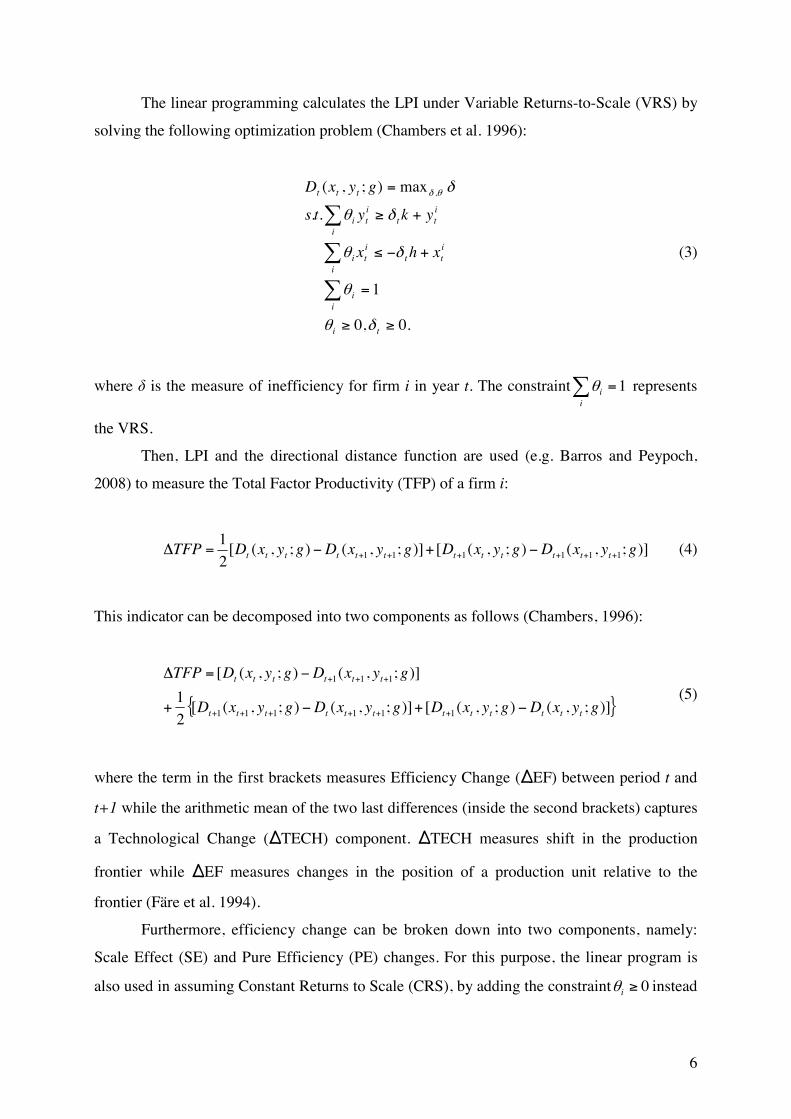
The linear programming calculates the LPI under Variable Returns-to-Scale (VRS) by
solving the following optimization problem (Chambers et al. 1996):
0.0,
1
..
max);,( ,
≥≥
=
+−≤
+≥
=
ti
ii
itt
i
iti
itt
i
iti
ttt
xhx
ykyts
gyxD
δθ
θ
δθ
δθ
δθδ
(3)
where is the measure of inefficiency for firm i in year t. The constraint =i
i 1θ represents
the VRS.
Then, LPI and the directional distance function are used (e.g. Barros and Peypoch,
2008) to measure the Total Factor Productivity (TFP) of a firm i:
)];,();,([)];,();,([21
111111 gyxDgyxDgyxDgyxDTFP tttttttttttt ++++++ −+−=Δ (4)
This indicator can be decomposed into two components as follows (Chambers, 1996):
{ })];,();,([)];,();,([21
)];,();,([
111111
111
gyxDgyxDgyxDgyxD
gyxDgyxDTFP
tttttttttttt
tttttt
−+−+
−=Δ
++++++
+++
(5)
where the term in the first brackets measures Efficiency Change (EF) between period t and
t+1 while the arithmetic mean of the two last differences (inside the second brackets) captures
a Technological Change (TECH) component. TECH measures shift in the production
frontier while EF measures changes in the position of a production unit relative to the
frontier (Färe et al. 1994).
Furthermore, efficiency change can be broken down into two components, namely:
Scale Effect (SE) and Pure Efficiency (PE) changes. For this purpose, the linear program is
also used in assuming Constant Returns to Scale (CRS), by adding the constraint 0≥iθ instead

7
of VRS (i.e. =i
i 1θ ). SE is then the difference between overall technical efficiency (under
CRS) and PE (under VRS).
Finally, input-neutral technical change as introduced by Briec et al. (2006) requires the
input set to be representable as a translation in the direction of h of an input set that is
independent of the state of technology. The Input Biased (IB) technical change is defined by:
{ })];,();,([)];,();,([21
1111 gyxDgyxDgyxDgyxDIB tttttttttttt ++++ −+−=Δ (6)
Holding the output vector constant at yt, IB is the arithmetic mean of the technical
change in a direction g with respect to xt+1 and xt. By opposition, Magnitude of Technological
(MT) change is defined by:
);,();,( 1 gyxDgyxDMT tttttt +−=Δ (7)
Technological decomposition can therefore be expressed by TECH = IB + MT.
Technology is Hicks neutral whenever the marginal rate of substitution between inputs is
unaffected by technological change, corresponding to “homothetic shift” in the isoquants.
Hence, biased technological change tends to influence the relative contribution of each input
to the production process. Thus, technological change is input parallel neutral only if
technology exhibits graph translation homotheticity (IB=0; Briec and Peypoch, 2007).
To calculate the resource directional distance functions, we define g = (h, k) = (x, y).
This measurement is thus linked with the proportional distance function (Briec, 1997). LPI is
applied to each industry, where each plant’s Added Value per worker (AV) is explained by its
own characteristics, i.e. the following four inputs: Capital per worker (K); Human Capital
indicator (HC), i.e. number of individuals employed in R&D divided by total number of
workers; R&D Investments per worker (RDI); Wage Means of the workers in the plant (WM).
WM can also be interpreted as a qualitative proxy of human capital (i.e. indicator of schooling
and learning by doing, etc.).

8
3.2. Measurement of Spillovers
This section presents econometric models for examining the relationship between intangible
assets and the productivity performances of plants. The estimation of spatial externalities is
based upon a production function (Griliches, 1979). The productivity change of a firm i is
represented by a Cobb-Douglas function:
PCit=(Ei,t-1)1(RDi,t-1)2 (8)
where PCit is the annual Productivity Change (such as the above defined TFP, TC, EC, SE,
PE, IB and MT) for a plant i at time t-1; Ei is a set of spatial variables which take pecuniary
externalities from industrial clustering into account (see table #1). Furthermore, in order to
introduce knowledge externalities, some other proxies are added at different spatial levels
(Acs et al. 1991; Autant-Bernard, 2001a; Bottazi and Peri, 2003), namely: RDi the change in
the research inputs within the area (see next section for more details on the construction of
variables).
One of the advantages of working on a first-difference model is to remove the unobserved
time-invariant firms, i.e. Fixed Effect (FE).3 Thus, a MLRE model can be estimated. In
addition, the previous year’s productivity change has an impact on the current year’s
productivity change, e.g. a higher efficiency at t-1 makes any further improvement of the
current efficiency more difficult (Simar and Wilson, 2007). To address this dynamic, the
lagged value of efficiency score in VRS is included in equation #8.
Furthermore, the estimations of a production function are mainly subject to the
simultaneity bias. Our approach however, in estimating productivity changes as a first step,
avoids this bias: cyclical effects impact plants’ performances (Olley and Pakes, 1996;
Levinsohn and Petrin, 2003) and our LPI estimations approximate these cyclical productivity
changes. Our dependent variable, in the production function, i.e. PCit, also includes
productivity change due to the economic situation and our final estimation is not subject to
simultaneity bias.
3 As LIP is an arithmetic mean index, the first-difference model (equation #8) can not be used in logarithms.

9
4. Data and Variables
In the first part of this section, we explain how the database was assembled. In the second
part, the plant selection is discussed and, finally, the used local variables are detailed.
4.1. Matching R&D and Firm Survey
The study relies on the cross-mapping of two national surveys: the French Annual Company
Survey (EAE) produced jointly by the Ministry of Industry and INSEE (the French Central
Statistical Office), and the R&D survey by the French Ministry of Research. The R&D survey
gives information on the R&D expenditure and R&D staff and the Company Survey records
general information such as sales, added-value, investments, total staff numbers, wages,
intermediate inputs, etc. This cross-mapping produced a panel of plants, observed from 2000
to 2002, with their added-value, workforce, wages, physical capital4, human capital5 and
internal R&D expenditure (IRDE) at plant level as well as at the Company level.
The added-value, workforce, wages and physical capital are observed at time t,
whereas R&D and human capital are respectively the combined IRDE and R&D staff figures
for t-1 and t-2. This procedure accounts for the cumulative feature of R&D and introduces a
lag between the date at which R&D is carried out and human resources introduced and the
date they impact on production. Scherer and Ravenscraft (1982) observe an average of about
4 or 6 years for this temporal lag between R&D and the increase of the firm profitability. This
temporal lag is reduced here to maximise the number of observations. We can consider that
this does not significantly affect the results (Hall, et al. 1984), since at the firm level the
correlation of R&D across time is very high.
Matching both surveys leads however to the exclusion of several firms carrying out
R&D. Indeed, over the 4500 observations recorded each year in the R&D survey, 2000 only
are also recorded in the Company survey. This is due to several reasons. Firstly, the sectoral
scope is different. The Company Survey in our possession neglects services and agriculture.
Thus, only industrial firms are considered in this study. Secondly, the Annual Company
Survey records only firms having more than 20 employees, whereas the R&D Survey takes
4 The physical capital variable has been computed as a sum of investments over 7 years (with a depreciation rate of 15% a year). 5 The human capital variable is given by the number of R&D workers (i.e. researchers and engineers).

10
into account all the firms employing at least one full time researcher, whatever their size.6 The
database which we have used contains 416 plants7, observed over three years, and regrouped
according to three aggregated sectors: Extractions (e.g. metal, salt, water, gas, etc.) composed
of 147 plants, Manufacturing Industries (MF, e.g. machine constructions) composed of 207
plants and Other Industries (OI, e.g. milk, textile) composed of 62 plants.8 These firms
represent 12.3% of French annual R&D expenditure and 4.5% of employment in industry.
This cross-mapping provides us with individual data, which is a progress particularly
for assessing the geographical dimension of externalities. Indeed, a major problem in most
studies in this field comes from the geographical level of observations. The unit is the
metropolitan area or county for the United States and the region (NUTS9 2 or 3) in Europe.
By focusing on an aggregated level, these studies are constrained by the administrative
segmentation of a geographical scale which is often quite large and fail to quantify the
spillovers enjoyed by each of these firms. Indeed they measure inter-agglomeration spillovers,
whereas the major facts lie undoubtedly in the relationship between the firm and the
agglomeration it belongs to (Lucas, 1988).
Furthermore, the use of plant data allows us to introduce, along with the plant level
inputs and local environmental variables, proxies accounting for intra-firm externalities. The
inputs provided at the global level of the firm, especially in terms of R&D, are likely to affect
the productivity of each distinct plant. If spillovers effects arise within firms, plants that
belong to firms carrying out R&D in their other plants would be more productive. In order to
assess this effect, the human capital available in the remainder of the firm is included in the
regression.
4.2. Analysis at Plant level and the problem of location
The Company survey is conducted both at plant and firm level, allowing an exact localisation.
The R&D survey however is conducted at the firm level and only a break down by
department is available (NUTS3). Indeed, each firm has to indicate the share of its R&D
activities carried out in each department. On this basis, the Ministry of Research provides a
dataset that recaps R&D employment and expenditure by firm in each department. Matching 6 We did not include research institutions situated in Corsica or the overseas departments as the analysis of proximity effects upon such was hardly relevant. 7 Which represent 328 firms. 8 The zeros in data represent a null investment in R&D and not missing values (Thompson et al. 1993). 9 NUTS: Nomenclature of Statistical Territorial Units; NUTS3 concerns units between 150,000 and 800,000 inhabitants.
11
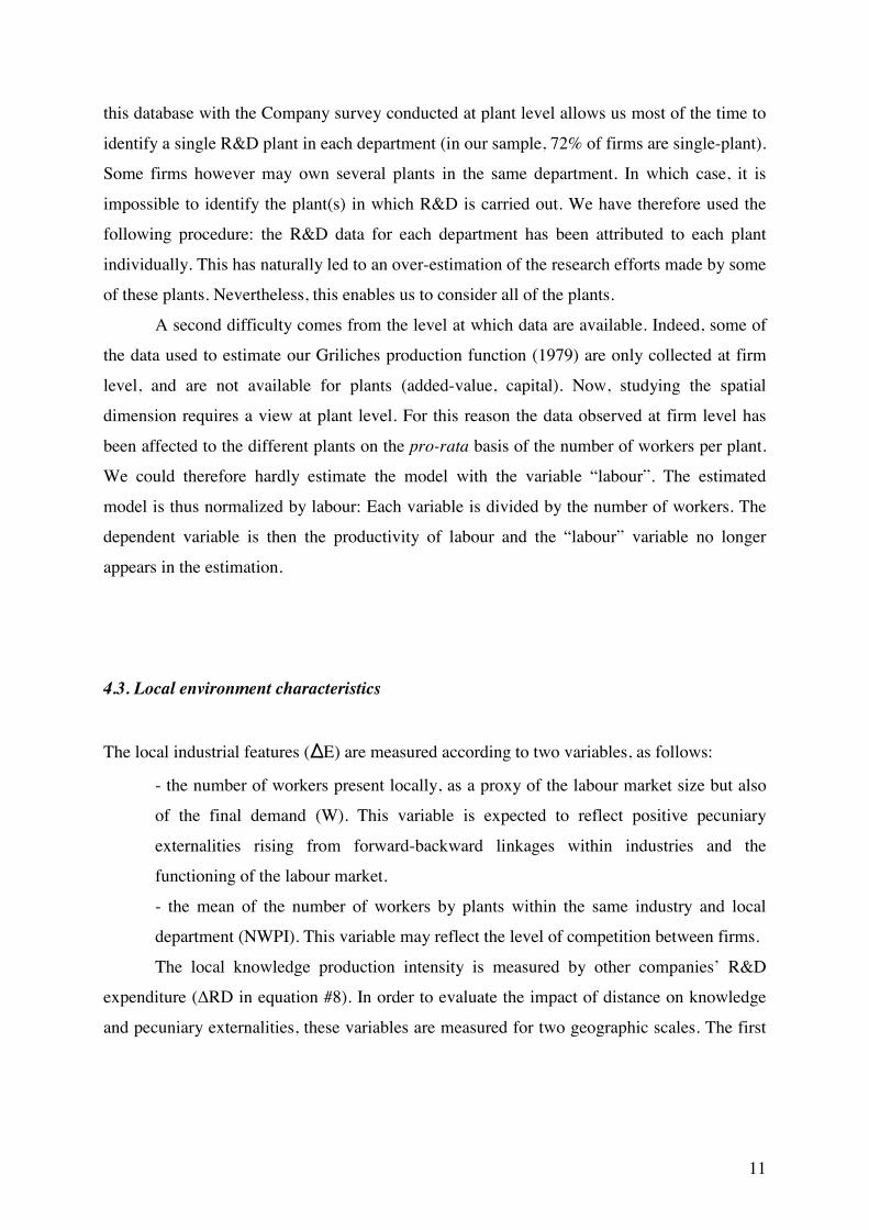
this database with the Company survey conducted at plant level allows us most of the time to
identify a single R&D plant in each department (in our sample, 72% of firms are single-plant).
Some firms however may own several plants in the same department. In which case, it is
impossible to identify the plant(s) in which R&D is carried out. We have therefore used the
following procedure: the R&D data for each department has been attributed to each plant
individually. This has naturally led to an over-estimation of the research efforts made by some
of these plants. Nevertheless, this enables us to consider all of the plants.
A second difficulty comes from the level at which data are available. Indeed, some of
the data used to estimate our Griliches production function (1979) are only collected at firm
level, and are not available for plants (added-value, capital). Now, studying the spatial
dimension requires a view at plant level. For this reason the data observed at firm level has
been affected to the different plants on the pro-rata basis of the number of workers per plant.
We could therefore hardly estimate the model with the variable “labour”. The estimated
model is thus normalized by labour: Each variable is divided by the number of workers. The
dependent variable is then the productivity of labour and the “labour” variable no longer
appears in the estimation.
4.3. Local environment characteristics
The local industrial features (E) are measured according to two variables, as follows:
- the number of workers present locally, as a proxy of the labour market size but also
of the final demand (W). This variable is expected to reflect positive pecuniary
externalities rising from forward-backward linkages within industries and the
functioning of the labour market.
- the mean of the number of workers by plants within the same industry and local
department (NWPI). This variable may reflect the level of competition between firms.
The local knowledge production intensity is measured by other companies’ R&D
expenditure (RD in equation #8). In order to evaluate the impact of distance on knowledge
and pecuniary externalities, these variables are measured for two geographic scales. The first

12
level is the ‘departement’ (NUTS 3), the second is given by the first and second order
bordering departments.10
The sectoral dimension is accounted for by distinguishing the environmental features
of the industry to which each plant belongs and the features of all the other industries. The full
set of variables used is summarised in table #1 below, together with the main descriptive
statistics.
Table 1. Variable Descriptions
Variables Description Mean Std-error Min. Max.
TFP Estimated by DEA-dependent variable -0.08 0.10 -0.95 0.51
TEt-1 Technical Efficiency in VRS 0.59 0.31 0.01 1.00
HCFt-1 Number of R&D workers in the firm -0.46 0.48 -2.23 0.11
NWPIt-1 Number of workers by plants from the same
industry. -0.14 22.89 -534.63 100.86
NWPIn,t-1 Number of workers by plants from the same
industry in the neighbouring area. 0.04 6.05 -38.65 24.20
WIt-1 Number of workers in the same industry within
the department. 95.246 736.80 -5842 10324
WOIt-1 Number of workers from other industries within
the department. 262.64 1849.29 -19112 3262
WIn,t-1 Number of workers in the same industry in the
neighbouring area. 759.77 3051.32 -8076 27726
WOIn,t-1 Number of workers from other industries in the
neighbouring area. 2027.20 5373.93 -29432 13022
WRDIt-1 R&D expenditure in the same industry within
the department. 31139.17 213228.69 -1268554.96 2178857.59
WDOIt-1 R&D expenditure in other industries within the
department. 285961.05 661008.15 -1660914.19 4066033.19
WRDIn,t-1 R&D expenditure in the same industry in the
neighbouring areas. 93316.47 392205.43 -1645006.08 3075880.59
WRDOIn,t-1 R&D expenditure from other industries in the
neighbouring areas. 2273715.96 1706815.08 -1102542.26 6743609.92
10 the contiguity matrix is standardized in row.

13
5. Results
In this section, the results of the DEA approach are presented first and those from the MLRE
model, second.
5.1. Productivity analysis
Table # 2 presents the arithmetic means of the LPI (Balk, 1998) estimated under the VRS
assumption.11
Table 2. LPI Results
Sectors PE SE EF IB MT TECH TFP
2000-2001
Other Industries 0.009 -0.004 0.005 -0.092 -0.021 -0.113 -0.108
Manufacturing 0.021 -0.004 0.017 -0.086 -0.026 -0.112 -0.095
Extractions -0.016 0.007 -0.009 -0.058 -0.012 -0.070 -0.079
Mean 0.006 8.10e(-5) 0.006 -0.077 -0.021 -0.098 -0.092
2001-2002
Other Industries 0.022 -0.021 0.001 -0.027 -0.008 -0.035 -0.034
Manufacturing -0.045 0.022 -0.023 -0.035 -0.007 -0.042 -0.065
Extractions -0.014 0.002 -0.012 -0.053 -0.008 -0.062 -0.074
Mean -0.023 0.008 -0.015 -0.040 -0.008 -0.048 -0.063
A first examination of table #2 shows a large decrease of the firms’ productivity
between 2000 and 2001 which then levels out over 2001-2002. The LPI, for example,
indicates that, on average and when compared to the whole of the industries resources,
manufacturing should have simultaneously contracted its inputs and increased its output by
9.5% in order to achieve a stable productivity. These results are in accordance with statistical
insights on French labour market (see INSEE): product demand seriously decreases from the
middle of 2000 until 2002 with a slight improvement at the end of 2002. Furthermore, a large
decrease in the employed labour force and of the rate of use of each firm productive capacity
is perceived over the same period.12 Thus, the better scores in 2001-2002 are mainly due to a
11 Following the section #3.1, TFP = TECH +EF, EF = PE + SE and TECH = IB + MAT. 12 See statistics of the French labour ministry.
14
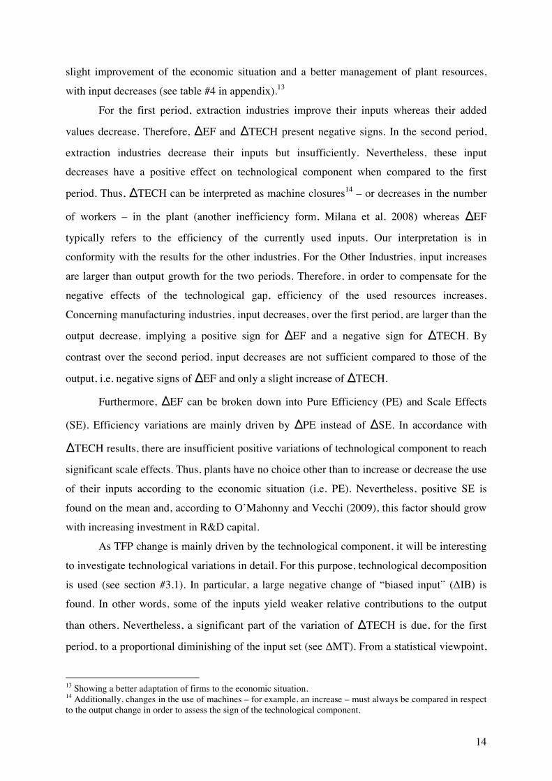
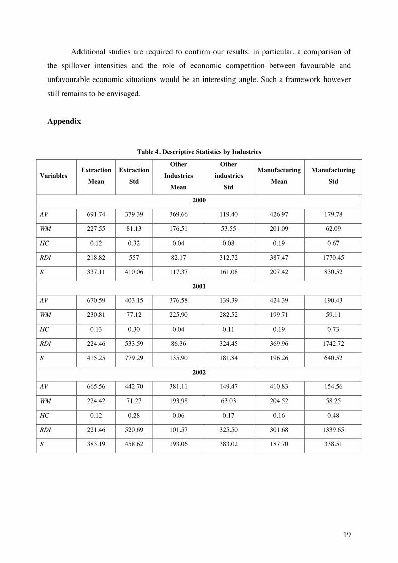
slight improvement of the economic situation and a better management of plant resources,
with input decreases (see table #4 in appendix).13
For the first period, extraction industries improve their inputs whereas their added
values decrease. Therefore, EF and TECH present negative signs. In the second period,
extraction industries decrease their inputs but insufficiently. Nevertheless, these input
decreases have a positive effect on technological component when compared to the first
period. Thus, TECH can be interpreted as machine closures14 – or decreases in the number
of workers – in the plant (another inefficiency form, Milana et al. 2008) whereas EF
typically refers to the efficiency of the currently used inputs. Our interpretation is in
conformity with the results for the other industries. For the Other Industries, input increases
are larger than output growth for the two periods. Therefore, in order to compensate for the
negative effects of the technological gap, efficiency of the used resources increases.
Concerning manufacturing industries, input decreases, over the first period, are larger than the
output decrease, implying a positive sign for EF and a negative sign for TECH. By
contrast over the second period, input decreases are not sufficient compared to those of the
output, i.e. negative signs of EF and only a slight increase of TECH.
Furthermore, EF can be broken down into Pure Efficiency (PE) and Scale Effects
(SE). Efficiency variations are mainly driven by PE instead of SE. In accordance with
TECH results, there are insufficient positive variations of technological component to reach
significant scale effects. Thus, plants have no choice other than to increase or decrease the use
of their inputs according to the economic situation (i.e. PE). Nevertheless, positive SE is
found on the mean and, according to O’Mahonny and Vecchi (2009), this factor should grow
with increasing investment in R&D capital.
As TFP change is mainly driven by the technological component, it will be interesting
to investigate technological variations in detail. For this purpose, technological decomposition
is used (see section #3.1). In particular, a large negative change of “biased input” (IB) is
found. In other words, some of the inputs yield weaker relative contributions to the output
than others. Nevertheless, a significant part of the variation of TECH is due, for the first
period, to a proportional diminishing of the input set (see MT). From a statistical viewpoint,
13 Showing a better adaptation of firms to the economic situation. 14 Additionally, changes in the use of machines – for example, an increase – must always be compared in respect to the output change in order to assess the sign of the technological component.
15
the labour force is rising while the output is decreasing over the same period (e.g. growth of
28% of wage mean in Other Industries). Therefore, this input has a weaker relative
contribution to the output in 2000-2001. This result is in conformity with technological
variations as the worker’s skills are less used. In the second period, firms better anticipated
the unfavourable economic situation and they have decreased their total inputs. Nevertheless,
firms have chosen not to decrease their inputs in the same way – or in the same
proportionality - as IB shows large negative coefficients. Statistically, firms have chosen to
decrease their investments in R&D in view of the decreasing demand (e.g. -22.6% in
manufacturing industries). Due to this similar trend of both output and R&D, the influence of
R&D on the output is more difficult to evaluate. Nevertheless, as the returns on R&D
investments are more uncertain and take longer to become visible, the R&D contribution to
the output is perceived by employers as less significant in an unfavourable economic
situation.
5.2. Econometric Results
An initial examination of the results15 presented in table #3 confirms the correlation
assumption between efficiency at t-1 and current TFP: a higher lagged efficiency score has a
large negative impact on the current TFP change. The higher the efficiency of a plant, the
more difficult it is to continue to approach the production frontier (Boussemart et al. 2006).
Even though the literature on agglomeration forces focuses on inter-firm effects, intra-firms
spillovers are also highly significant: human capital proxy of the firms is a major determinant
of their productivity. In particular, this intra-firm effect greatly improves the technological
component and decreases, by opposition, the efficiency of the used inputs. This result
supports some previous results concerning increasing returns associated with organizational
and geographical linkages among various functions of the firms. Kenney and Florida (1994)
point out that “transfer of employees between R&D and manufacturing and joint meetings are
judged as being the most important factors in ensuring the information transfer between the
two corporate functions.” In addition, the close location of R&D units and production units
would insure better knowledge creation and information transfer. Furthermore, the
technological decomposition shows that human capital homogeneously increases the relative
15 To improve the readability of this table each estimated coefficients have been multiplied by 106.
16
contribution of each input. In other words, human capital increases also the efficiency of
capital and, obviously, the R&D component.
Concerning the inter-firm effects and, more specifically, R&D investments within the
same industry in the department, the estimated coefficient presents the expected signs: plants
receive positive spillovers from the R&D investments of other plants which obviously
improve the technological component. R&D investments of the other industries in the
department however have no significant spillovers on the plant in question. This result
supports Marshall-Arrow-Romer externalities more than Jacobs externalities. It differs from
empirical evidence drawn from the French case using regional patent data as dependent
variable (Autant-Bernard and LeSage, 2009). Based on a knowledge production function,
Feldman and Audretsch (1999) found – in contrast with our result - that diversity would pay a
positive role on innovative firms, while more traditional activities would primarily benefit
from specialisation. Since only R&D firms are considered in this study, one would expect a
positive impact of diversity. Therefore, moving from a spatial knowledge production function
to a TFP function gives different results. This point would however deserve further attention
and could be addressed in further research.
For the local workers variables, the results may capture two opposite effects: first, a
positive effect of agglomeration spillovers, second, a pure productivity effect which implies
that a higher number of workers in the area, in an unfavourable economic situation, decreases
the productivity. Thus, the negative effects registered for worker variables show that negative
productivity effects exceed those positive from agglomeration. Furthermore, places which
favour a high employment rate are generally low-tech areas,16 explaining our negative impact
upon technological component by opposition to the results of the WRDI variable which
represents probably the high-tech areas. Then, higher positive externalities in “high-tech”
places (in comparison to the “low-tech” places) are found. By contrast, the number of workers
of the industries in the neighbouring area slightly improves a plant’s efficiency which could
be due to worker exchanges. Following the efficiency decomposition, this improvement of the
workers’ efficiency (i.e. PE) decreases SE. Furthermore, some relative input contributions
change in a “non neutral” way, in particular the one of labour force.17
16 Since our microeconomic data are essentially composed of manufacturing industries (Diaz and Quiros Tomas, 2002). 17 Estimations of the dependent variables - PE and MT – have been dropped, since they have respectively the opposite signs of SE and IB.

17
Table 3. Spillover Estimations by MLRE
Variables TFP TECH EF SE IB
Plant and Firm Features
TEt-1 -39103.50***
(8070.30)
-10418.30
(7228.20)
-28685.20***
(4638.50)
35092.40***
(5062.80)
-63777.60***
(8429.10)
HCFt-1 40844.80***
(6235.20)
62015.00***
(5584.60)
-21170.20***
(3583.80)
10554.20**
(3911.60)
-31724.40***
(6512.40)
Local Features
WRDIt-1 0.04**
(0.01)
0.03*
(0.01)
0.01
(0.01)
-0.01
(0.01)
0.02
(0.02)
WRDOIt-1 -0.01
(0.005)
-0.005
(0.004)
-0.002
(0.003)
-0.002
(0.003)
-0.001
(0.005)
WIt-1 -10.70*
(4.97)
-10.80*
(4.45)
0.15
(2.86)
0.23
(3.12)
-0.08
(5.20)
WOIt-1 -6.13**
(1.91)
-6.99***
(1.71)
0.86
(1.10)
-0.16
(1.20)
1.02
(1.99)
NWPIt-1 -11.80
(145.10)
10.40
(12.99)
-22.20
(83.40)
32.30
(91.00)
-54.50
(151.50)
Spatially Lagged Local Features
WRDIn,,t-1 -0.01
(0.01)
-0.02*
(0.007)
0.003
(0.005)
-0.001
(0.005)
0.004
(0.01)
WRDOIn,t-1 -0.01***
(0.002)
-0.01***
(0.001)
0.0002
(0.001)
-0.002*
(0.001)
0.003
(0.002)
WIn,t-1 0.44
(1.41)
-1.96
(1.27)
2.41**
(0.81)
-3.98***
(0.89)
6.38***
(1.48)
WOIn,t-1 -1.70*
(0.68)
-1.47*
(0.61)
-0.23
(0.39)
-0.68
(0.43)
0.44
(0.71)
NWPIn,t-1 906.90
(620.90)
308.90
(556.10)
598.10
(356.80)
114.50
(389.50)
483.60
(648.50)
Log-Likelihood 802.79 894.37 1262.99 1190.27 766.65
Note: * Significant at the 10% level, ** significant at the 5% level, *** significant at the 1% level.
In addition, R&D investments in the neighbouring area seem to have a negative impact
on TFP changes. These results can be explained by a “shadow effect” (Autant-Bernard,
2001b): high industrial clustering, in the neighbouring area, captures R&D investments and
consequently has a negative impact on the TFP of the considered plant. Hence, this
unfavourable effect is due to the negative impact of technological change – which represents
the fall in R&D investments – with negative estimated coefficients for WRDIn and WRDOIn

18
variables. Furthermore, this lack in R&D attractivity due to “shadow effects” decreases the
SE component.
Finally, the number of workers by plants in the neighbouring and local area has no
significant effect. This result is not surprising since the expected positive impact of economic
competition upon productivity is lower (due to higher financial pressure) during an
unfavourable economic situation (Nickell et al. 1997).
6. Conclusion
The results from our study can help us to paint a picture of policy recommendations. The
main result is that intra-firm spillovers across multiple locations have stronger influence than
inter-firm spillovers: the proxy of the human capital of the company largely and
homogeneously improves the technological component of the productivity and increases scale
effects. Improving knowledge flows within firms would generate more benefits than
spillovers stemming from outside the firm. This opens up an interesting area of research, in
order to better understand the role played by distance on this intra-firm knowledge flows.
These intra-firm externalities can give rise to spatial concentration phenomena. Economies of
localisation and urbanisation due to inter-firms spillovers would no longer be the only
determinant of agglomeration. This latter would also partly result from the internal strategies
of the firms: close proximity between the different plants of a single firm in order to reduce
the transport and transaction costs. Our empirical approach however, does not allow us to
address this question directly. Further analysis of the role played by distance on these intra-
firm knowledge flows would be required.
Nevertheless, some significant inter-firm effects are found: (i) benefits from the R&D
of the other firms within the same industry in the region for the technology used, (ii) “shadow
effects” which decrease the technological component, when a plant is established near an
industrial clustering, and prevent plants’ scale economies. Nevertheless, spillover intensities
must be discussed with caution as our estimations are based on a period during an
unfavourable economic situation.
For a given human capital of a firm, a feasible recommendation would be: in an
unfavourable economic situation, plants should be inside industrial clusters in order to benefit
from the knowledge externalities and avoid the “shadow effect” when locating outside. This
picture would improve the efficiency of plants and confirm the currently observed behaviour:
at national level, local-clustering is reinforced (Cantwell and Vertova, 2004).
19
Additional studies are required to confirm our results: in particular, a comparison of
the spillover intensities and the role of economic competition between favourable and
unfavourable economic situations would be an interesting angle. Such a framework however
still remains to be envisaged.
Appendix
Table 4. Descriptive Statistics by Industries
Variables Extraction
Mean
Extraction
Std
Other
Industries
Mean
Other
industries
Std
Manufacturing
Mean
Manufacturing
Std
2000
AV 691.74 379.39 369.66 119.40 426.97 179.78
WM 227.55 81.13 176.51 53.55 201.09 62.09
HC 0.12 0.32 0.04 0.08 0.19 0.67
RDI 218.82 557 82.17 312.72 387.47 1770.45
K 337.11 410.06 117.37 161.08 207.42 830.52
2001
AV 670.59 403.15 376.58 139.39 424.39 190.43
WM 230.81 77.12 225.90 282.52 199.71 59.11
HC 0.13 0.30 0.04 0.11 0.19 0.73
RDI 224.46 533.59 86.36 324.45 369.96 1742.72
K 415.25 779.29 135.90 181.84 196.26 640.52
2002
AV 665.56 442.70 381.11 149.47 410.83 154.56
WM 224.42 71.27 193.98 63.03 204.52 58.25
HC 0.12 0.28 0.06 0.17 0.16 0.48
RDI 221.46 520.69 101.57 325.50 301.68 1339.65
K 383.19 458.62 193.06 383.02 187.70 338.51
20
References Acs, Z.J., Audretsch, D.B., Feldman, M.P., 1991. Real Effects of Academic Research:
Comment. American Economic Review 82, 363-67. Arrow, K.J., 1962. Economic Welfare and the Allocation of Resources of invention. in Nelson
R.R. (ed.), The Rate and Direction of Inventive Activity: Economic and Social Factors, Princeton University Press, 609-26.
Audretsch, D.B., Feldman, M.P., 1999. Innovation in Cities: Science-Based Diversity, Specialization and Localized Competition. European Economic Review 43, 409-29.
Autant-Bernard, C., 2001a. The Geography of Knowledge Spillovers and Technological Proximity. Economics of Innovation and New Technology 10, 237-54.
Autant-Bernard, C., 2001b. Science and Knowledge Flows: Evidence from the French Case. Research Policy 30, 1069-78.
Autant-Bernard, C., LeSage, J., 2009. Quantifying Knowledge Spillovers using Spatial Econometric Models. CORE seminar, Catholic University of Louvain, 13 may.
Balk, B.M., 1998. Industrial Prices, Quantity, and Productivity Indices: The Micro-Economic Theory and an Application. Kluwer, Boston.
Barros, C.P., Peypoch, N., 2008. A Comparative Analysis of Productivity Change in Italian and Portuguese Airports. International Journal of Transport Economics 35, 243-54.
Black, S.E., Lynch, L.M., 2001. How to Compete: The Impact of Workplace Practices and information Technology on Productivity. Review of Economics and Statistics 83, 434-45.
Beaudry, C., Breschi, S., 2003. Are Firms in Clusters Really more Innovative?. Economics of Innovation and New Technology 12, 325-42.
Bottazzi, L., Peri, G., 2003. Innovation and Spillovers in Regions: Evidence from European Patent Data. European Economic Review 47, 687-710.
Boussemart, J-P., Briec, W., Cadoret, I., Tavéra, C., 2006. A Re-Examination of the Technological Catching-Up Hypothesis across OECD Industries. Economic Modelling 23, 967-77.
Briec, W., 1997. A Graph Type Extension of Farrell Technical Efficiency Measure. Journal of Productivity Analysis 8, 95-110.
Briec, W., Chambers, R.G., Färe, R., Peypoch, N., 2006. Parallel Neutrality. Journal of Economics 88, 285-305.
Briec, W., Comes, C., Kerstens, K. 2006. Temporal Technical and Profit Efficiency Measurement: Definitions, Duality and Aggregation Results. International Journal of Production Economics 103, 48-63.
Briec, W., Peypoch, N., 2007. Biased Technical Change and Parallel Neutrality. Journal of Economics 92, 281-92.
Cantwell, J., Vertova, G., 2004. Historical Evolution of Technological Diversification. Research Policy 33, 511-29.

21
Chambers, R.G., 1996. A New Look at Exact Input, Output, and Productivity Measurement. Working Paper 05, Department of Agricultural and Resources Economics, University of Maryland.
Chambers, R.G., Chung, Y., Färe, R., 1998. Profit, Directional Distance Functions, and Nerlovian Efficiency. Journal of Optimization Theory and Applications 98, 351-64.
Chambers, R.G., Färe, R., Grosskopf, S., 1996. Productivity Growth in APEC Countries. Pacific Economic Review 1, 181-90.
Cohen, W., Levinthal, D.A., 1989. Innovation and Learning: The Two Faces of R&D. Economic Journal 99, 569-96.
Diaz, M.S., Quiros Tomas, F.J., 2002. Technological Innovation and Employment: Data from a Decade in Spain. International Journal of Production Economics 75, 245-56.
Färe, R., Grosskopf, S., Norris, M., Zhang, Z., 1994. Productivity Growth, Technical Progress, and Efficiency Change in Industrialized Countries. American Economic Review 84, 66-83.
Feldman, M.P., Audretsch, D.B., 1999. Innovation and Cities: Science-based Diversity, Specialization, and Localized Competition. European Economic Review 43, 409-29.
Guironnet, JP., Peypoch, N., 2007. Human Capital Allocation and Overeducation: A Measure of French Productivity (1987, 1999). Economic Modelling 24, 398-410.
Griliches, Z., 1979. Issues in Assessing the Contribution of Research and Development to Productivity Growth. Bell Journal of Economics 10, 92-116.
Hausman, J., Hall, B., Griliches, Z., 1984. Economic Models for Count Data with an Application to the Patents R&D Relationship. Econometrica 52, 909-38.
Henderson, J.V., 2003. Marshal’s Scale Economies. Journal of Urban Economy 53, 1-28. Henderson, J.V., Kuncoro, A., Turner, M., 1995. Industrial Development in Cities. Journal of
Political Economy 103, 1067-90. Jacobs, J., 1969. The Economies of Cities. Random House. Jaffe, A.B., 1986. Technology Opportunity and Spillovers of R&D: Evidence from Firms’
Patents, Profits, Market Value. American Economic Review 76, 984-1001. Jaffe, A.B.Trajtenberg, M., Henderson, R., 1993. Geographic Localization of Knowledge
Spillovers as Evidenced by Patent Citation. Quarterly Journal of Economics 108, 577-98.
Kenney, M., Florida, R., 1994. The organization and geography of Japanese R&D: results from a survey of Japanese electronics and biotechnology firms. Research Policy 23, 305-23.
Levinsohn, J., Petrin, A., 2003. Estimating Production Functions Using Inputs to Control for Unobservables. Review of Economic Studies 70, 317-42.
Lucas, R.E., 1988. On the Mechanics of Economic Development. Journal of Monetary Economics 22, 3-42.
Luenberger, D.G., 1996. Welfare from a Benefit Viewpoint. Economic Theory 7, 445-62. Jena, P.R., Managi, S., 2008. Environmental Productivity and Kuznets Curve in India.
Ecological Economics, 432-40. Marshall, A., 1980. Principles of Economics. Macmillan, London.
22
Martin, P., Ottaviano, G., 1999. Growing Location: Industry Location in a Model of Endogenous Growth. European Economic Review 43, 281-302.
Milana, C., Leopoldo, N., Zeli, A., 2008. Changes in Multifactor Productivity in Italy from 1998-2004: Evidence from Firm-Level Data Using DEA. Working Paper 33, EU Klems.
Nakano, M., Managi, S., 2008. Regulatory Reforms and Productivity: An Empirical Analysis of the Japanese Electricity Industry. Energy Policy 36, 201-9.
Nickell, S., Nicolitsas, D., Dryden, N., 1997. What Makes Firms Perform Well?. European Economic Review 41, 783-96.
Olley, G.S., Pakes, A., 1996. The Dynamics of Productivity in the Telecommunications Equipment Industry. Econometrica 64, 1263-98.
O’Mahony, M., Vecchi, M., 2009. R&D, Knowledge Spillovers and Company Productivity Performance. Research Policy 38, 35-44.
Ravenscraft, D., Scherer, F.M., 1982. The Lag Structure of Returns to Research and Development. Applied Economics 14, 603-20.
Romer, P., 1986. Increasing Returns and Long Run Growth. Journal of Political Economy 94, 1002-37.
Simar, L., Wilson, P.W., 2007. Estimation and Inference in Two-Stage, Semi-Parametric Models of Production Processes. Journal of Econometrics 136, 31-64.
Thompson, R.G., Dharmapala, P.S., Thrall, R.M., 1993. Importance for DEA of Zeros in Data Multipliers, and Solutions. Journal of Productivity Analysis 4, 379-90.
Wooldridge, J.M., 1995. Selection Corrections for Panel Data Models under Conditional Mean Independence Assumptions. Journal of Econometrics 68, 115-32.
Yang, C-H., Motohashi, K., Chen, J-R., 2009. Are New Technology-Based Firms Located on Science Parks Really more Innovative? Evidence from Taiwan. Research Policy 38, 77-85.
Zhengfei, G., Oude Lansink, A., 2006. The Source of Productivity Growth in Dutch Agriculture: A Perspective from Finance. American Journal of Agricultural Economics 88, 644-56.


