international journal of

production economics

ELSEVIER Int. J. Production Economics 45 (1996) 489498

Product remanufacturing and disposal: A numerical comparison of alternative control strategies

Erwin van der Laan*, Rommert Dekker, Marc Salomon

Erasmus University Rotterdam, P.O. Box 1738, NL-3000 DR Rotterdam, Netherlands

Abstract

In this paper we consider a single-product, single-echelon production and inventory system with product returns, product remanufacturing, and product disposal. For this system we consider three different procurement and inventory control strategies, i.e., the (sp,Qp,sd,N) strategy, the (sp,Qp,sd) strategy, and the (sp, Q,,AJ) strategy. The control parameters in these strategies relate to the inventory position at which an outside procurement order is placed (sp), the inventory position at which returned products are disposed of (sd), the outside procurement order quantity (Q,), and the capacity of the remanufacturing facility (N). For each of the strategies we derive exact expressions of the total expected costs as functions of the control parameters. Main objective of this paper is to compare the performance of each of the alternative strategies with respect to costs, under different system conditions.

Keywords: Production planning and inventory control; Remanufacturing; Disposal; Re-order point and disposal point strategies for inventory control; Stochastic models; Markov chains

1. Introduction

Today, authorities force by means of environmental laws that manufacturers reduce the amount of waste generated by their products. Also, environmental conscientious consumers put pressure on manufacturers to start waste reduction programs. One option to reduce waste is to remanufacture. While remanufacturing, (components of) used products are returned from the market. Upon return, the used products are tested, cleaned, and repaired. Typical for remanufacturing is, that after these operations the product is suitable to be re-sold in the market of new products. This implies that remanufactured products need to satisfy the same quality standards as new products.

Although product remanufacturing influences almost all functional areas in business (see Cl]), we restrict ourselves in this paper to the operations management related consequences of remanufacturing. In particu- lar, we focus on production planning and inventory control strategies with remanufacturing.

* Corresponding author.

0925-5273/96/$15.00 Copyright 0 1996 Elsevier Science B.V. All rights reserved SSDI 0925..5273(95)00137-9

490 E. van der Lam et al. /ht. J. Production Economics 45 (1996) 489-498

In the past, most articles that appeared in the operations management literature dealt with inventory control of spare parts. Typical assumptions in models for spare-parts are, that, (i) demands for new products are generated by product failures (returns) only (implying perfect correlation between demands and returns), and (ii) the number of spare parts in the system is kept constant over time. This is why spare parts inventory control models are often indicated as ‘closed-loop’ models. Overviews on closed-loop models are found in Nahmias [2] and Cho and Parlar [3], among others.

Since recent, a growing interest for remanufacturing can be observed in the operations management literature. Specific for the situation with remanufacturing is, that assumptions (i) and (ii) do often not apply, i.e., in practice demand and returns are not perfectly correlated, and the number of products in the system may fluctuate over time. In addition, used products may still be disposed of after return from the market. This may be necessary due to a test outcome indicating that the product is (technically) inappropriate for remanufacturing, or it may be motivated by economical considerations. The latter might for instance be the case when a product is at the end of its life-cycle, where the average demand for new products is smaller than the average number of returned products. Remanufacturing all returned products would result in relatively high inventories, and consequently in high costs.

One of the first production planning and inventory control models which applies to the situation with remanufacturing was proposed by Muckstadt and Isaac [4]. In this model, it is assumed that demands and returns are independent Poisson processes, and outside procurement lead-times are constant. The re- manufacturing process is modelled by a multiple server queueing system, with stochastic remanufacturing

lead-times. The inventory position and the outside procurements are controlled by an (s,,, Q,) continuous review strategy, where sp is the outside procurement level, and Q, is the outside procurement quantity. The implementation of this strategy is as follows: whenever the inventory position drops below sp + 1, an outside procurement order of size Q, is placed. Muckstadt and Isaac present a numerical approximation procedure to calculate the control parameters, such that the sum of serviceable inventory holding costs, fixed outside procurement costs, and backordering costs is minimized. Disposal of used products is not allowed to occur in their model.

In an earlier paper, Heyman [S] presents a model which applies to the situation with disposal. However, remanufacturing lead-times, fixed outside procurement costs, and outside procurement lead- times are not taken into account. Heyman pointed out that under these conditions it is optimal to set the re-order level s,, = - 1 and the outside procurement quantity Q, = 1. The only remaining control

parameter is sd: the inventory level at which disposal becomes profitable. The strategy of the single

parameter model is as follows: as long as the inventory level exceeds or equals sd, every returned product is disposed of upon arrival. Heyman develops an exact expression to determine the parameter sd under which the sum of inventory holding costs, production costs, remanufacturing costs, and disposal costs is minimized.

Another interesting class of models in the context of remanufacturing are the so-called cash balancing models. In cash-balancing models, the amount of money in the cash (cash position) is controlled by an (sp,Sp,sd,Sd) strategy. This strategy is as follows: at the beginning of each period the cash position is inspected; whenever the cash position is at or below sp, money is ordered at the central bank, such that the cash position increases to S,. Furthermore, whenever the cash position exceeds sd, money is transferred to the central bank, such that the cash position reduces to Sd. Although these models consider both outside procurements (money orderings), and disposals (money transfers), practical applicability of these models for remanufacturing is limited to the rather uncommon situation were procurement lead-times, disposal lead-times, and remanufacturing lead-times are negligible. An overview of various cash-balancing models is given by Inderfurth [6].

Up to now, only two papers consider strategies in which decisions on outside procurements, remanufactur- ing, and disposals are considered simultaneously. As already mentioned, these combined strategies might be interesting from an economical point of view (see also [7]). In Salomon et al. [7], the (sp, Qp, sd) strategy is

E. van der Laan et al. /ht. J. Production Economics 45 (1996) 489-498 491

introduced and analyzed for a production-inventory system similar to the system considered by Muckstadt and Isaac [4]. In van der Laan et al. [S] an alternative disposal strategy is considered, i.e., the (sp, Qp, N) strategy. Under this strategy, remanufacturing and disposal are controlled by the queue length of returned products waiting to be remanufactured. The implementation of this strategy is as follows: whenever the number of products waiting in the queue in front of the remanufacturing facility equals N, every returned product is disposed of upon arrival.

The purpose of this paper is to present an operating strategy which generalizes the (sp, Qp,sd), the (sp, Qp, N), and the (sp, Q,) strategy and to perform a numerical comparison based on exact analysis. The generalized strategy consists of four control parameters, and is denoted by (sp, Qp, sd, N). Under this strategy, disposal of a returned item takes place in two cases, i.e., (i) whenever the inventory position equals sd, or (ii) whenever the number of products in the remanufacturing facility equals N. This operating strategy is further outlined in Section 2. Furthermore, in Section 2 an exact expression for the total expected costs under this operating strategy is derived. In Section 3 the performance of the three control strategies is compared with respect to expected minimal costs. To the latter end we report on the results of a numerical study. Conclusions and directions for further research are given in Section 4.

2. Inventory control under an (sp, Qp, sd, NJ strategy

The (sp, Qp, sd, N) strategy outlined here applies to the situation where a single-product is remanufactured and stocked at a single location. The other assumptions with respect to the production-inventory system are the following: l product demands and product returns are independent Poisson processes. The expected time between two

subsequent product demands (returns) equals l/A (l/r). Demand (return) quantities per demand (return) occurrence are equal to one unit,

l remanufacturing of product returns takes place in a remanufacturing facility.The remanufacturing facility consists of c identical parallel remanufacturing machines. Each machine has the capacity to remanufacture one returned unit at a time. The remanufacturing time at each machine is exponentially distributed, with expectation l/p. Remanufactured units enter the serviceable inventory,

l the queue in front of the remanufacturing facility consists of returned units waiting to be remanufactured. Units which have entered the queue are remanufactured as soon as a remanufacturing machine becomes available. The queueing discipline is FCFS. The maximum number of units of the remanufacturing facility equals N,

l whenever the inventory position drops below sp + 1 (sp 3 0), an outside procurement order of size Qp (Q, 3 1) is placed. The procurement lead-time equals z,

l returned units are either remanufactured or disposed of, depending on the inventory position and the number of units in the remanufacturing queue. The strategy with respect to remanufacturing and disposal is as follows: whenever the inventory position equals sd, or whenever the number of units in the remanufacturing facility equals N, returned units are disposed of upon arrival. Returned units that are not disposed of enter the remanufacturing facility,

l customer demand is fulfilled from serviceable inventory, or from outside procurements. If customer demand cannot be fulfilled immediately, demand is backordered,

l the costs consist of the following components: - fixed outside procurement costs of A per order, _ variable outside procurement costs of 6, per ordered unit of product, _ variable remanufacturing costs of 6, per remanufactured unit of product, _ variable disposal costs of dd per disposed unit of product, _ inventory holding costs of h, per time unit per unit of product in serviceable inventory,

492 E. van der Lam et al. /ht. J. Production Economics 45 (1996) 489-498

_ inventory holding costs of h, per time unit per product in the remanufacturing facility, ~ backordering costs of Sb per unit of product per time unit.

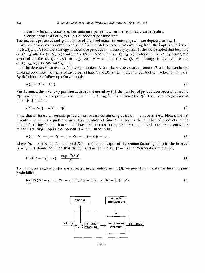
The relevant processes and goods-flows of the production-inventory system are depicted in Fig. 1. We will now derive an exact expression for the total expected costs resulting from the implementation of

the (s,,, Qp, sd, N) control strategy in the above productioninventory system. It should be noted that both the

(sp, Qp, sd) and the (s,,, Qp, N) strategy are special cases of the (sp, Qp, sd, N) strategy: the (sp, Q,,, sd) strategy is identical to the (sp, Qp,sd,N) strategy with N = CC, and the (sp, QP, N) strategy is identical to the (Sp, Q,,, sd, N) Strategy with &, = E.

In the derivation we use the following notation: N(t) is the net inventory at time t; O(t) is the number of on-hand products in serviceable inventory at time t, and B(t) is the number of products in backorder at time t. By definition the following relation holds,

N(t) = O(t) - B(t). (1)

Furthermore, the inventory position at time t is denoted by I(t), the number of products on order at time t by P(t), and the number of products in the remanufacturing facility at time t by R(t). The inventory position at

time t is defined as

l(t) = N(t) + R(t) + P(t). (2)

Note that at time t all outside procurement orders outstanding at time t - z have arrived. Hence, the net inventory at time t equals the inventory position at time t - z, minus the number of products in the remanufacturing shop at time t - T, minus the demands during the interval [t - 7, t], plus the output of the remanufacturing shop in the interval [t - z, t]. In formula,

N(t) = I(t - z) - R(t - z) + Z(t - T’, t) - D(t - z, t), (3)

where D(t - 7, t) is the demand, and Z(t - T, t) is the output of the remanufacturing shop in the interval [t - z, t]. It should be noted that the demand in the interval [t - z, t]

- Az(AT)d Pr{D(t-z,t)=d} =exp d, .

To obtain an expression for the expected net-inventory using (3) we probability,

lim Pr{Z(t - 7) = i, R(t - 7) = Y, Z(t - z, t) = 2, D(t - 7, t) = d}. f+m

- _ is Poisson distributed, i.e.,

(4)

need to calculate the limiting joint

(5)

1 serviceable -’ inventory

1 demands,

Fig. I

E. van der Laan et al. /ht. J. Production Economics 45 (1996) 489-498 493

Since I(t - r), R(t - r), and Z(t - z,t) are not mutually independent, it turns out to be complicated to evaluate the right-hand side of (5) directly. However, evaluation is simplified by rewriting (5) as,

(6)

where

rc,,, = f’m Pr{Z(t) = i, R(t) = r> (7)

and

P:lr,r = lim Pr{Z(t - z,t) = zlI(t - 5) = i, R(t - r) = r}. (8) fdol

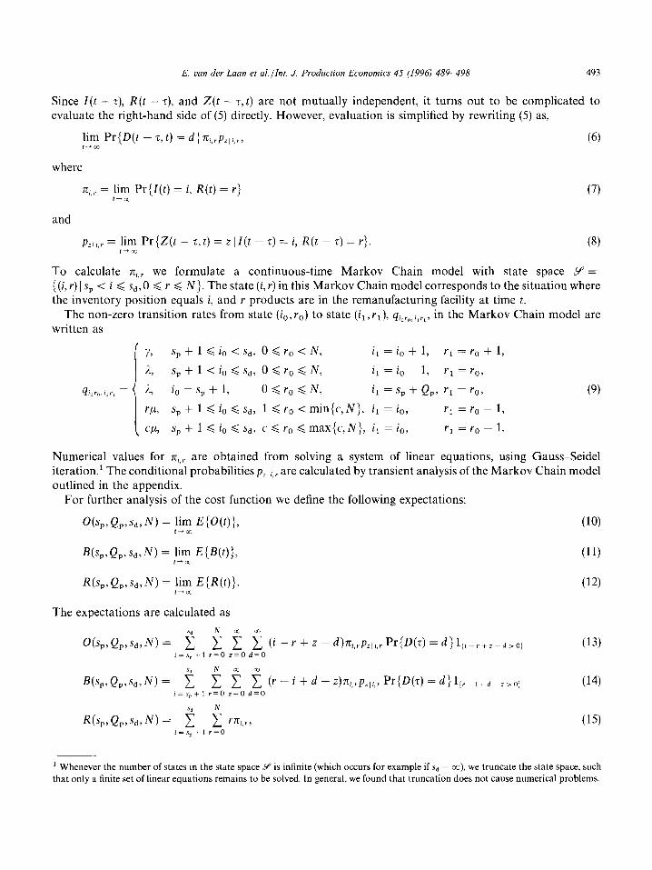
To calculate rr,,, we formulate a continuous-time Markov Chain model with state space Y = {(i, r) 1 sp < i 6 sd, 0 d r d N}. The state (i, r) in this Markov Chain model corresponds to the situation where the inventory position equals i, and r products are in the remanufacturing facility at time t.

The non-zero transition rates from state (io,ro) to state (il,rl), ql,r,,i,r,, in the Markov Chain model are written as

Numerical values for

sp + 1 < i. < sd, 0 < r. < N, il = io + 1, r1 = r. + 1,

sp + 1 < i. < sd, 0 < r. d N, il = i. - 1, rl = ro,

i. = sp + 1, 0 6 r. d N, il = sp + Qp, r1 = ro, (9)

sp + 1 d i. d sd, 1 d r. < min{c,N}, il = io, rl = r. - 1,

s,+ 1 diodsd, c < r. < max{c, N}, il = io, r1 = r. - 1.

n,,, are obtained from solving a system of linear equations, using Gauss-Seidel iteration.’ The conditional probabilities pII i,r are calculated by transient analysis of the Markov Chain model outlined in the appendix.

For further analysis of the cost function we define the following expectations:

O(s,>Q,,s,>N) = !im E{O(r)}, (10)

~(s,,Q,,%>N) = ,‘;t E{B(t))>

~b,,Q,,%,N) = f’; E{R(t)j.

The expectations are calculated as

(11)

(14

o(s,,Q,,Sd,N) = i -f f f (i-r + z -4q,p,~,,,Pr{W~) = d)lpr+z-d>O; ,=~,+l r=Oz=Od=O

(13)

Sd

B(sp,Qp,Sd,N)= 1 =f f -f (r--++--z)ni,,P,i,,,Pr{D(z)=d}li,~i+d-=>0}

i=s_+lr=Oz=Od=O (14)

R(s,,Q,,sd>N) = 2 ; rn,,,, !=$+I r=O

(15)

1 Whenever the number of states in the state space Y is infinite (which occurs for example ifs,, = CO), we truncate the state space, such that only a finite set of linear equations remains to be solved. In general, we. found that truncation does not cause numerical problems.

494 E. van der Lam et aLlInt. J. Production Economics 45 (1996) 489-498

where 1 ix , ,+ is the indicator function, which is defined as

1 i

1 if x > y,

‘X1” = 0 otherwise

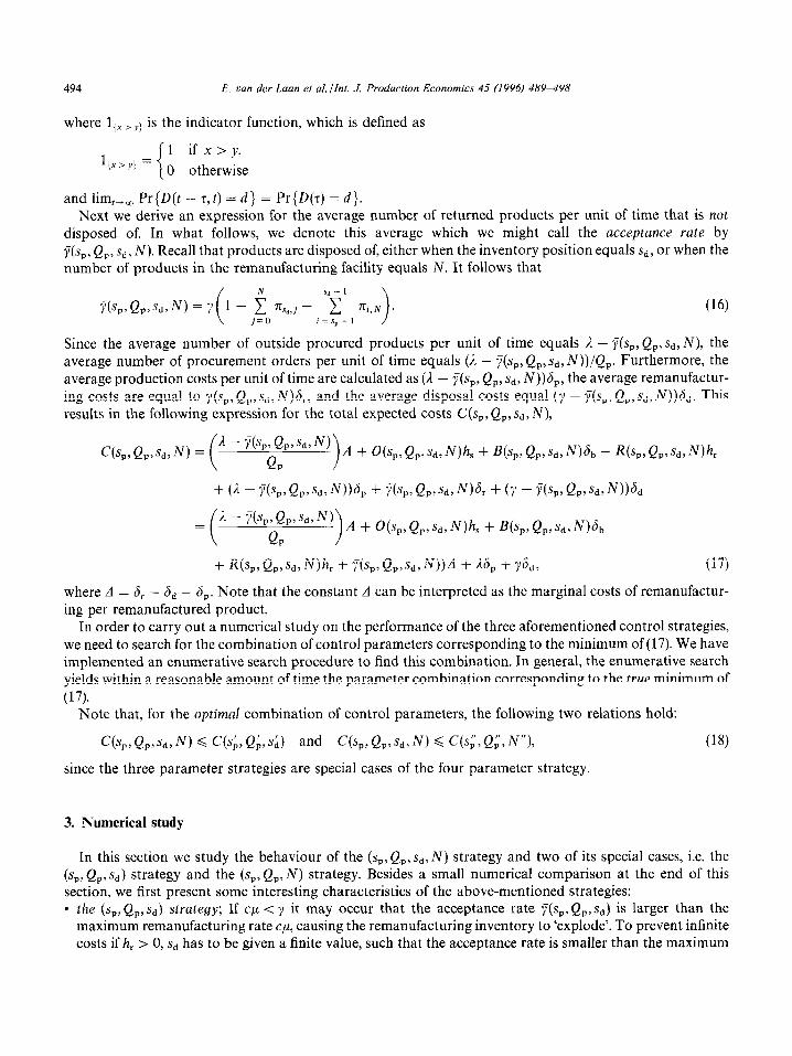
and lim,,, Pr{D(t - r, t) = d} = Pr{D(r) = d}. Next we derive an expression for the average number of returned products per unit of time that is not

disposed of. In what follows, we denote this average which we might call the acceptance rate by jJ(s,, Qp, sd, N). Recall that products are disposed of, either when the inventory position equals sd, or when the number of products in the remanufacturing facility equals N. It follows that

Since the average number of outside procured products per unit of time equals A - y(s,, Qp, sd, N), the average number of procurement orders per unit of time equals (A - y(s,, Qp,sdl N))/Q,. Furthermore, the average production costs per unit of time are calculated as (A - y(s,, Qp, sd, N))6,, the average remanufactur- ing costs are equal to Y(sp,Qp,sd,N)6,, and the average disposal costs equal (‘/ - ?/(s,, Qp,sd,N))bd. This results in the following expression for the total expected costs C(s,, Qp, sd, N),

+ ~(Sp,Qp,Sd,~h + ‘f(s,,Q,,Sd,~))~ + & + $d, (17)

where A = 6, - dd - 6,. Note that the constant A can be interpreted as the marginal costs of remanufactur-

ing per remanufactured product. In order to carry out a numerical study on the performance of the three aforementioned control strategies,

we need to search for the combination of control parameters corresponding to the minimum of (17). We have implemented an enumerative search procedure to find this combination. In general, the enumerative search yields within a reasonable amount of time the parameter combination corresponding to the true minimum of

(17). Note that, for the optimal combination of control parameters, the following two relations hold:

C(s,,Q,,sd,N) d C(sJ,,Q~,si) and Cb,,Q,,sd,N) G C(.$‘,Q~,W,

since the three parameter strategies are special cases of the four parameter strategy.

(18)

3. Numerical study

In this section we study the behaviour of the (sp, Qp, sd, N) strategy and two of its special cases, i.e. the (sp,Qp,sd) strategy and the (sp,Qp,N) strategy. Besides a small numerical comparison at the end of this section, we first present some interesting characteristics of the above-mentioned strategies: l the (s,,, QP,sd) strategy; If cp < y it may occur that the acceptance rate j+,,Qp,sd) iS larger than the

maximum remanufacturing rate cp, causing the remanufacturing inventory to ‘explode’. To prevent infinite costs if h, > 0, sd has to be given a finite value, such that the acceptance rate is smaller than the maximum

E. van der Laan et al. /lnt. J. Production Economics 45 (1996) 489-498 495

remanufacturing rate. Note that if y is large compared to cp, this may even lead to putting sd equal to s, + 1, which implies that all incoming products are disposed of. If cp is small compared to y we expect the number of items in the remanufacturing shop to be relatively large. Since we dispose on inventory position we do not directly control the (large) number of items in the remanufacturing shop so we expect this strategy to provide poorer control on disposals in case of small values of cc1 than for larger values of CF. the (sp,Qp,N) strategy; If y > i it may occur that the acceptance rate is larger than the demand rate, causing the serviceable inventory to ‘explode’. To prevent infinite costs if h, > 0, N has to be given a finite value, such that the acceptance rate is smaller than the demand rate. Note that if y is large compared to ;1, this may even lead to putting N equal to 0, which implies that all incoming products are disposed of.

If cp is large compared to y we expect this strategy to provide poor control on disposals. Since in this case there is almost no queueing, the only option besides accepting almost all incoming products (N > 0), is disposing all incoming products (N = 0). the (sp, Qp,sd, N) strategy; With respect to the cases cp < y and y > i the same remarks made for the (s,,, Qp, sd) and (sP, Qp, N) strategy hold. However, we expect this strategy to perform somewhat better than the other two since this strategy has finer disposal control capability. In our numerical study, we use a standard parameter set. The parameter I serves as a scale parameter and

is put at 1, whereas y, c and p are chosen such that y < 3, < cp, which implies that even if sd = cc or N = m, the inventory system will not ‘explode’. The number of remanufacturing machines is put at 1, so that the (sP, QP, N) strategy has maximum control on incoming products (less machines implies more queueing, which implies more control). The cost parameters are such that optimization results in nontrivial values of the decision variables. However, we found that the effects presented in the remainder of this section are very typical for a wide range of parameter settings.

We would like to note that the optimal values of the decision variables for all three disposal strategies do not so much depend on the individual values of 6,, 6,, and bd. It is the combination of the three, namely d = 6, - dd - 6,, which influences the optimal values of the decision variables. In other words, all combina- tions of 6,, 6,, and dd for which d = c, and c some predefined constant, will result in the same optimal values of the decision variables (optimal costs however may differ). We have chosen d = -2.00.

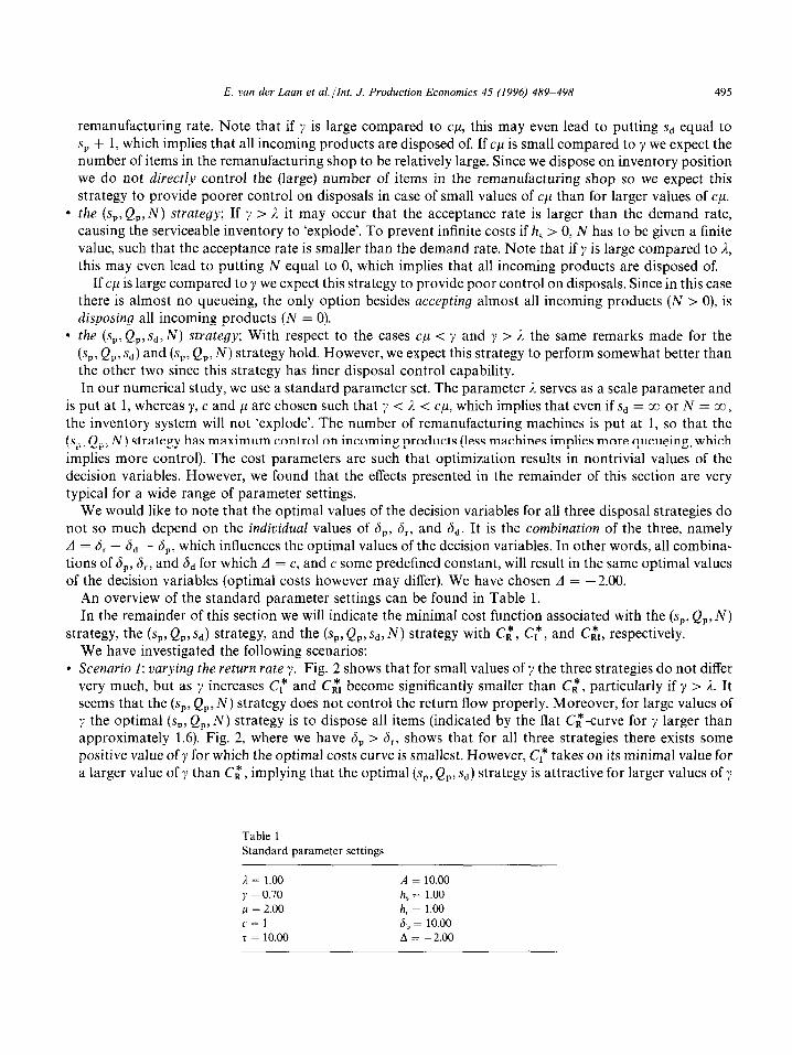
An overview of the standard parameter settings can be found in Table 1. In the remainder of this section we will indicate the minimal cost function associated with the (sP, Q,,, N)

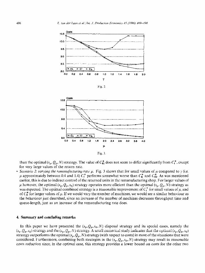
strategy, the (sP, Qp, sd) strategy, and the (sP, Qp, sd, N) strategy with C,*, C:, and C,*,, respectively. We have investigated the following scenarios: Scenario 1: varying the return rate y. Fig. 2 shows that for small values of y the three strategies do not differ very much, but as ‘/ increases CT and C,*, become significantly smaller than C,*, particularly if y > A. It seems that the (sP, Qp, N) strategy does not control the return flow properly. Moreover, for large values of y the optimal (sP, Qp, N) strategy is to dispose all items (indicated by the flat C,*-curve for y larger than approximately 1.6). Fig. 2, where we have 6, > 6,, shows that for all three strategies there exists some positive value of y for which the optimal costs curve is smallest. However, C,* takes on its minimal value for a larger value of y than C,*, implying that the optimal (sP, Qp, sd) strategy is attractive for larger values of y

Table 1

Standard parameter settings

i = 1.00

y = 0.70

p = 2.00 c=l

T = 10.00

A = 10.00

h, = 1.00

h, = 1.00 db = 10.00

A = -2.00

496 E, t’an der Laan et al. /ht. J. Production Economics 45 (1996) 489-498

Fig. 2

10.6 c0st9

10.2 .--- ..-.-. .-....... .._._..._............... _ _._ . . . . . . . .._.... _._ ___.___ _..._..__._ h i 9.6 I.... _ . . . . . . . ___~\.?i._._._ ._............ _ _ _ .._._._._....... _._._._ _I

9.4 .._. _._ _ . . .._................(_ _

9.0 I’ ‘Lc; +cc; ‘CL

0.0 0.4 0.8 1.2 1.6 2.0 2.4 2.8 3.2 56 4.0

P

Fig. 3

than the optimal (s,,, Qp, N) strategy. The value of C,*, does not seem to differ significantly from Cc, except for very large values of the return rate.

l Scenario 2: varying the remanufacturing rate p. Fig. 3 shows that for small values of ,u compared to y (i.e. p approximately between 0.4 and 1.4) C: performs somewhat worse than C,* and C,*,. As was mentioned earlier, this is due to indirect control of the returned units in the remanufacturing shop. For larger values of p however, the optimal (sP, Qp, s,J strategy operates more efficient than the optimal (sP, Qp, N) strategy as was expected. The optimal combined strategy is a reasonable improvement of C,* for small values of p, and of C,* for larger values of ,u. If we would vary the number of machines, we would see a similar behaviour as the behaviour just described, since an increase of the number of machines decreases throughput time and queue-length, just as an increase of the remanufacturing rate does.

4. Summary and concluding remarks

In this paper we have presented the (sP, QP, sd, N) disposal strategy and its special cases, namely the (sP, Qp, sd) strategy and the (sP, QP, N) strategy. A small numerical study indicates that the optimal (sP, Qp, sd) strategy outperforms the optimal (sP, Qp, N) strategy (with respect to costs) in most of the situations that were considered. Furthermore, combining both strategies in the (s,,, QP, sd, N) strategy may result in reasonable costs reduction since, in the optimal case, this strategy provides a lower bound on costs for the other two

E. uan der Lam et al. /ht. J. Production Economics 45 (1996) 489-498 497

strategies. The reader must note however that the computational burden involved with the optimization of these strategies, and the four parameter strategy in particular, is considerably large and probably not very practical. However, we think that this paper provides some insights in the effects of disposal strategies on inventory control which may be of help in constructing disposal strategies for more complex situations or in constructing fast approximative algorithms.

Other types of strategies may be worth while to consider as well, such as a strategy in which returned products are not immediately remanufactured or disposed but delayed for remanufacturing until they are really needed. This may be typical for the situation in which k, < k, or the situation in which we have nonzero setup costs for remanufacturing. This will be a topic for further study.

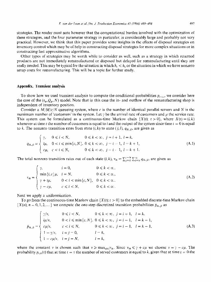
Appendix. Transient analysis

To show how we used transient analysis to compute the conditional probabilities pzIl,,, we consider here the case of the (sP, Qp, N) model. Note that in this case the in- and outflow of the remanufacturing shop is independent of inventory position.

Consider a M/M/c/N queueing system, where c is the number of identical parallel servers and N is the maximum number of ‘customers’ in the system. Let y be the arrival rate of customers and Jo the service rate. This system can be formulated as a continuous-time Markov chain {X(t); t > 0}, where X(t) = (i,k) whenever at time t the number of customers is equal to i and the output of the system since time t = 0 is equal to k. The nonzero transition rates from state (i, k) to state (j, I), qik,j[, are given as

I

Y> O<i<N, O<k<x, j=i+l, l=k,

qik,jl = 4, O<i<min{c,Nj, O<k<co, j=i-1, l=k+l,

cP> c<idN, O<k<m, j=i-1, l=k+l.

The total nonzero transition rates out of each state (i, k), Yik = ~~~~ I;“=, qik,j[, are given as

(A.1)

7, i = 0, O<k<co,

min(i,c}fi, i = N, Obk<co, Vik =

Y + ip, O<i<min{c,N}, Odk<ca,

1’ + cp, c<i<N, O<k<m.

(A.21

Next we apply a uniformization. To go from the continuous-time Markov chain {X(t); t > O> to the embedded discrete-time Markov chain

{X(n); n=0,1,2,...} we compute the one-step discretized transition probabilities Pik, jl as

( “ilv, Odi<N, Odk<co, j=i+l, 1=k,

W, O<ibmin{c,N}, O<k<m, j=i-1, l=k+l,

Pik,jl = ( CP/V, c<i<N, Odk<co, j=i-1, l=k+l,

1 - ‘i/v, i=j=O, 1 = k,

( 1 - cplv, i=j=N, 1 = k,

64.3)

where the constant v is chosen such that v > maxcikjvik. Since vik < y + cc1 we choose v = y + cp. The probability Pi,k(S) that at time t = T the number of served customers is equal to k, given that at time t = 0 the

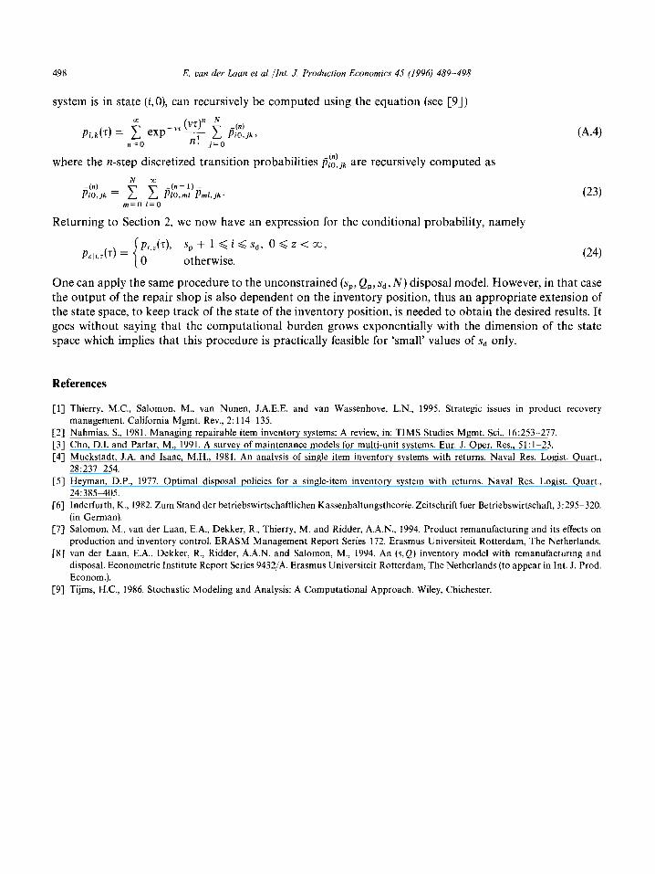
498 E. van der Laan et al. Jht. J. Production Economics 45 (1996) 489-498

system is in state (i,O), can recursively be computed using the equation (see [9])

~.~(r) = f exp_yiE ; P:lljk,

I,

n=O n! j=(J

where the n-step discretized transition probabilities P~~)jk are recursively computed as

(4.4)

Returning to Section 2, we now have an expression for the conditional probability, namely

PZ,i.r(r) = i

&(r), sp + 1 < i < sd, 0 d z < a,

0 otherwise.

One can apply the same procedure to the unconstrained (sr, QP, sd, N) disposal model. However, in that case the output of the repair shop is also dependent on the inventory position, thus an appropriate extension of the state space, to keep track of the state of the inventory position, is needed to obtain the desired results. It goes without saying that the computational burden grows exponentially with the dimension of the state space which implies that this procedure is practically feasible for ‘small’ values of sd only.

References

Cl1

PI c31 M

[Xl

Ccl

c71

PI

Thierry, M.C., Salomon, M., van Nunen, J.A.E.E. and van Wassenhove, L.N., 1995. Strategic issues in product recovery

management. California Mgmt. Rev., 2: 114-135.

Nahmias, S., 1981. Managing repairable item inventory systems: A review, in: TIMS Studies Mgmt. Sci., 16:253-277.

Cho, D.I. and Parlar, M., 1991. A survey of maintenance models for multi-unit systems. Eur. J. Oper. Res., 51: l-23.

Muckstadt, J.A. and Isaac, M.H., 1981. An analysis of single item inventory systems with returns. Naval Res. Logist. Quart.,

28:2377254.

Heyman, D.P., 1977. Optimal disposal policies for a single-item inventory system with returns. Naval Res. Logist. Quart.,

24:3855405.

Inderfurth, K., 1982. Zum Stand der betriebswirtschaftlichen Kassenhaltungstheorie. Zeitschrift fuer Betriebswirtschaft, 3:295-320.

(in German).

Salomon, M., van der Laan, E.A., Dekker, R., Thierry, M. and Ridder, A.A.N., 1994. Product remanufacturing and its effects on

production and inventory control. ERASM Management Report Series 172. Erasmus Universiteit Rotterdam, The Netherlands.

van der Laan, E.A., Dekker, R., Ridder, A.A.N. and Salomon, M., 1994. An (s,Q) inventory model with remanufacturing and

disposal. Econometric Institute Report Series 9432/A. Erasmus Universiteit Rotterdam, The Netherlands (to appear in Int. J. Prod.

Econom.).

c91 Tijms, H.C., 1986. Stochastic Modeling and Analysis: A Computational Approach. Wiley, Chichester.