Embed Size (px)
Citation preview
DRAFTPrinciples of Algorithmic Problem Solving
Johan Sannemo
2017

DRAFT
ii
This version of the book is a preliminary draft. Expect to findtypos and other mistakes. If you do, please report them [email protected]. Before reporting a bug, pleasecheck whether it still exists in the latest version of this draft,available at http://csc.kth.se/~jsannemo/slask/main.pdf.
DRAFTContents
Preface vii
Reading this Book ix
I Preliminaries 1
1 Algorithms and Problems 31.1 Computational Problems . . . . . . . . . . . . . . . . . . . . . . . . . . . 31.2 Algorithms . . . . . . . . . . . . . . . . . . . . . . . . . . . . . . . . . . . 5
1.2.1 Correctness . . . . . . . . . . . . . . . . . . . . . . . . . . . . . . 71.3 Programming Languages . . . . . . . . . . . . . . . . . . . . . . . . . . 81.4 Pseudo Code . . . . . . . . . . . . . . . . . . . . . . . . . . . . . . . . . . 91.5 The Kattis Online Judge . . . . . . . . . . . . . . . . . . . . . . . . . . . 101.6 Chapter Notes . . . . . . . . . . . . . . . . . . . . . . . . . . . . . . . . . 11
2 Programming in C++ 132.1 Development Environments . . . . . . . . . . . . . . . . . . . . . . . . . 142.2 Hello World! . . . . . . . . . . . . . . . . . . . . . . . . . . . . . . . . . . 142.3 Variables and Types . . . . . . . . . . . . . . . . . . . . . . . . . . . . . . 172.4 Input and Output . . . . . . . . . . . . . . . . . . . . . . . . . . . . . . . 212.5 Operators . . . . . . . . . . . . . . . . . . . . . . . . . . . . . . . . . . . 232.6 If Statements . . . . . . . . . . . . . . . . . . . . . . . . . . . . . . . . . . 252.7 For Loops . . . . . . . . . . . . . . . . . . . . . . . . . . . . . . . . . . . 272.8 While Loops . . . . . . . . . . . . . . . . . . . . . . . . . . . . . . . . . . 292.9 Functions . . . . . . . . . . . . . . . . . . . . . . . . . . . . . . . . . . . . 292.10 Structures . . . . . . . . . . . . . . . . . . . . . . . . . . . . . . . . . . . 322.11 Arrays . . . . . . . . . . . . . . . . . . . . . . . . . . . . . . . . . . . . . 352.12 The Preprocessor . . . . . . . . . . . . . . . . . . . . . . . . . . . . . . . 362.13 Template . . . . . . . . . . . . . . . . . . . . . . . . . . . . . . . . . . . . 372.14 Additional Exercises . . . . . . . . . . . . . . . . . . . . . . . . . . . . . 372.15 Chapter Notes . . . . . . . . . . . . . . . . . . . . . . . . . . . . . . . . . 38
iii
DRAFT
iv CONTENTS
3 Implementation Problems 393.1 Additional Exercises . . . . . . . . . . . . . . . . . . . . . . . . . . . . . 543.2 Chapter Notes . . . . . . . . . . . . . . . . . . . . . . . . . . . . . . . . . 54
4 Time Complexity 574.1 The Complexity of Insertion Sort . . . . . . . . . . . . . . . . . . . . . . 574.2 Asymptotic Notation . . . . . . . . . . . . . . . . . . . . . . . . . . . . . 604.3 NP-complete problems . . . . . . . . . . . . . . . . . . . . . . . . . . . . 624.4 Other Types of Complexities . . . . . . . . . . . . . . . . . . . . . . . . . 634.5 Exercises . . . . . . . . . . . . . . . . . . . . . . . . . . . . . . . . . . . . 634.6 Chapter Notes . . . . . . . . . . . . . . . . . . . . . . . . . . . . . . . . . 64
II Basics 65
5 Brute Force 675.1 Optimization Problems . . . . . . . . . . . . . . . . . . . . . . . . . . . . 675.2 Generate and Test . . . . . . . . . . . . . . . . . . . . . . . . . . . . . . . 685.3 Backtracking . . . . . . . . . . . . . . . . . . . . . . . . . . . . . . . . . . 715.4 Fixing Parameters . . . . . . . . . . . . . . . . . . . . . . . . . . . . . . . 775.5 Meet in the Middle . . . . . . . . . . . . . . . . . . . . . . . . . . . . . . 795.6 Chapter Notes . . . . . . . . . . . . . . . . . . . . . . . . . . . . . . . . . 81
6 Greedy Algorithms 836.1 Optimal Substructure . . . . . . . . . . . . . . . . . . . . . . . . . . . . . 836.2 Locally Optimal Choices . . . . . . . . . . . . . . . . . . . . . . . . . . . 856.3 Scheduling . . . . . . . . . . . . . . . . . . . . . . . . . . . . . . . . . . . 866.4 Chapter Notes . . . . . . . . . . . . . . . . . . . . . . . . . . . . . . . . . 89
7 Dynamic Programming 917.1 Best Path in a DAG . . . . . . . . . . . . . . . . . . . . . . . . . . . . . . 917.2 Dynamic Programming . . . . . . . . . . . . . . . . . . . . . . . . . . . 93
7.2.1 Bottom-Up Computation . . . . . . . . . . . . . . . . . . . . . . 947.2.2 Order of Computation and Memory Usage . . . . . . . . . . . . 95
7.3 Multidimensional DP . . . . . . . . . . . . . . . . . . . . . . . . . . . . . 967.4 Subset DP . . . . . . . . . . . . . . . . . . . . . . . . . . . . . . . . . . . 987.5 Digit DP . . . . . . . . . . . . . . . . . . . . . . . . . . . . . . . . . . . . 997.6 Standard Problems . . . . . . . . . . . . . . . . . . . . . . . . . . . . . . 101
7.6.1 Knapsack . . . . . . . . . . . . . . . . . . . . . . . . . . . . . . . 1027.6.2 Longest Common Subsequence . . . . . . . . . . . . . . . . . . . 1037.6.3 Set Cover . . . . . . . . . . . . . . . . . . . . . . . . . . . . . . . 104
7.7 Chapter Notes . . . . . . . . . . . . . . . . . . . . . . . . . . . . . . . . . 107
8 Divide and Conquer 109
DRAFT
CONTENTS v
8.1 Inductive Constructions . . . . . . . . . . . . . . . . . . . . . . . . . . . 1098.2 Merge Sort . . . . . . . . . . . . . . . . . . . . . . . . . . . . . . . . . . . 1168.3 Binary Search . . . . . . . . . . . . . . . . . . . . . . . . . . . . . . . . . 118
8.3.1 Optimization Problems . . . . . . . . . . . . . . . . . . . . . . . 1208.3.2 Searching in a Sorted Array . . . . . . . . . . . . . . . . . . . . . 1218.3.3 Generalized Binary Search . . . . . . . . . . . . . . . . . . . . . . 123
8.4 Karatsuba’s algorithm . . . . . . . . . . . . . . . . . . . . . . . . . . . . 1258.5 Chapter Notes . . . . . . . . . . . . . . . . . . . . . . . . . . . . . . . . . 126
9 Data Structures 1279.1 Disjoint Sets . . . . . . . . . . . . . . . . . . . . . . . . . . . . . . . . . . 1279.2 Range Queries . . . . . . . . . . . . . . . . . . . . . . . . . . . . . . . . . 130
9.2.1 Prefix Precomputation . . . . . . . . . . . . . . . . . . . . . . . . 1309.2.2 Sparse Tables . . . . . . . . . . . . . . . . . . . . . . . . . . . . . 1319.2.3 Segment Trees . . . . . . . . . . . . . . . . . . . . . . . . . . . . . 133
9.3 Chapter Notes . . . . . . . . . . . . . . . . . . . . . . . . . . . . . . . . . 136
10 Graph Algorithms 13710.1 Breadth-First Search . . . . . . . . . . . . . . . . . . . . . . . . . . . . . 13710.2 Depth-First Search . . . . . . . . . . . . . . . . . . . . . . . . . . . . . . 14210.3 Weighted Shortest Path . . . . . . . . . . . . . . . . . . . . . . . . . . . . 145
10.3.1 Dijkstra’s Algorithm . . . . . . . . . . . . . . . . . . . . . . . . . 14510.3.2 Bellman-Ford . . . . . . . . . . . . . . . . . . . . . . . . . . . . . 14510.3.3 Floyd-Warshall . . . . . . . . . . . . . . . . . . . . . . . . . . . . 147
10.4 Minimum Spanning Tree . . . . . . . . . . . . . . . . . . . . . . . . . . . 14810.5 Chapter Notes . . . . . . . . . . . . . . . . . . . . . . . . . . . . . . . . . 150
11 Maximum Flows 15111.1 Flow Networks . . . . . . . . . . . . . . . . . . . . . . . . . . . . . . . . 15111.2 Edmonds-Karp . . . . . . . . . . . . . . . . . . . . . . . . . . . . . . . . 153
11.2.1 Augmenting Paths . . . . . . . . . . . . . . . . . . . . . . . . . . 15411.2.2 Finding Augmenting Paths . . . . . . . . . . . . . . . . . . . . . 155
11.3 Applications of Flows . . . . . . . . . . . . . . . . . . . . . . . . . . . . 15611.4 Chapter Notes . . . . . . . . . . . . . . . . . . . . . . . . . . . . . . . . . 158
12 Strings 15912.1 Tries . . . . . . . . . . . . . . . . . . . . . . . . . . . . . . . . . . . . . . . 15912.2 String Matching . . . . . . . . . . . . . . . . . . . . . . . . . . . . . . . . 16412.3 Hashing . . . . . . . . . . . . . . . . . . . . . . . . . . . . . . . . . . . . 168
12.3.1 The Parameters of Polynomial Hashes . . . . . . . . . . . . . . . 17312.3.2 2D Polynomial Hashing . . . . . . . . . . . . . . . . . . . . . . . 175
12.4 Chapter Notes . . . . . . . . . . . . . . . . . . . . . . . . . . . . . . . . . 176
13 Combinatorics 177
DRAFT
vi CONTENTS
13.1 The Addition and Multiplication Principles . . . . . . . . . . . . . . . . 17713.2 Permutations . . . . . . . . . . . . . . . . . . . . . . . . . . . . . . . . . 180
13.2.1 Permutations as Bijections . . . . . . . . . . . . . . . . . . . . . . 18113.3 Ordered Subsets . . . . . . . . . . . . . . . . . . . . . . . . . . . . . . . . 18613.4 Binomial Coefficients . . . . . . . . . . . . . . . . . . . . . . . . . . . . . 186
13.4.1 Dyck Paths . . . . . . . . . . . . . . . . . . . . . . . . . . . . . . 19013.4.2 Catalan Numbers . . . . . . . . . . . . . . . . . . . . . . . . . . . 193
13.5 The Principle of Inclusion and Exclusion . . . . . . . . . . . . . . . . . . 19413.6 Invariants . . . . . . . . . . . . . . . . . . . . . . . . . . . . . . . . . . . 19613.7 Monovariants . . . . . . . . . . . . . . . . . . . . . . . . . . . . . . . . . 19813.8 Chapter Notes . . . . . . . . . . . . . . . . . . . . . . . . . . . . . . . . . 203
14 Number Theory 20514.1 Divisibility . . . . . . . . . . . . . . . . . . . . . . . . . . . . . . . . . . . 20514.2 Prime Numbers . . . . . . . . . . . . . . . . . . . . . . . . . . . . . . . . 20814.3 The Euclidean Algorithm . . . . . . . . . . . . . . . . . . . . . . . . . . 21214.4 Modular Arithmetic . . . . . . . . . . . . . . . . . . . . . . . . . . . . . . 21814.5 Chinese Remainder Theorem . . . . . . . . . . . . . . . . . . . . . . . . 22114.6 Euler’s totient function . . . . . . . . . . . . . . . . . . . . . . . . . . . . 22314.7 Chapter Notes . . . . . . . . . . . . . . . . . . . . . . . . . . . . . . . . . 227
15 Competitive Programming Strategy 22915.1 IOI . . . . . . . . . . . . . . . . . . . . . . . . . . . . . . . . . . . . . . . 229
15.1.1 Strategy . . . . . . . . . . . . . . . . . . . . . . . . . . . . . . . . 23015.1.2 Getting Better . . . . . . . . . . . . . . . . . . . . . . . . . . . . . 231
15.2 ICPC . . . . . . . . . . . . . . . . . . . . . . . . . . . . . . . . . . . . . . 23215.2.1 Strategy . . . . . . . . . . . . . . . . . . . . . . . . . . . . . . . . 23215.2.2 Getting Better . . . . . . . . . . . . . . . . . . . . . . . . . . . . . 234
A Mathematics 237A.1 Logic . . . . . . . . . . . . . . . . . . . . . . . . . . . . . . . . . . . . . . 237A.2 Sets and Sequences . . . . . . . . . . . . . . . . . . . . . . . . . . . . . . 240A.3 Sums and Products . . . . . . . . . . . . . . . . . . . . . . . . . . . . . . 242A.4 Graphs . . . . . . . . . . . . . . . . . . . . . . . . . . . . . . . . . . . . . 244A.5 Chapter Notes . . . . . . . . . . . . . . . . . . . . . . . . . . . . . . . . . 246
Bibliography 249
Index 251
DRAFTPreface
Algorithmic problem solving is the art of formulating efficient methods that solveproblems of a mathematical nature. From the many numerical algorithms developedby the ancient Babylonians to the founding of graph theory by Euler, algorithmicproblem solving has been a popular intellectual pursuit during the last few thousandyears. For a long time, it was a purely mathematical endeavor, with algorithmsmeant to be executed by hand. During the recent decades, algorithmic problemsolving has evolved. What was mainly a topic of research became a mind sportknown as competitive programming. As a sport, algorithmic problem solving rosein popularity, with the largest events attracting tens of thousands of programmers.While its mathematical counterpart has a rich literature, there are only a few bookson algorithms with a strong problem solving focus.
The purpose of this book is to contribute to the literature of algorithmic problemsolving in two ways. First of all, it tries to fill in some holes in existing books. Manytopics in algorithmic problem solving lack any treatment at all in the literature – atleast in English books. Instead, much of the content is documented only in blog postsand solutions to problems from various competitions. While this book attempts torectify this, it is not to detract from those sources. Many of the best treatments ofan algorithmic topic I have seen are as part of a well-written solution to a problem.However, there is value in completeness and coherence when treating such a largearea. Secondly, I hope to provide another way of learning the basics of algorithmicproblem solving, by helping the reader build an intuition for problem solving. A largepart of this book describes techniques using worked-through examples of problems.These examples attempt not only to describe the manner in which a problem is solved,but to give an insight into how a thought process might be guided to yield the insightsnecessary to arrive at a solution.
This book is different from pure programming books and most other algorithmtextbooks. Programming books are mostly either in-depth studies of a specific pro-gramming language, or describe various programming paradigms. In this book, asingle language is used – C++. The text on C++ exists for the sole purpose of enablingthose readers without prior programming experience to implement the solutions toalgorithm problems. Such a treatment is necessarily minimal, and will teach neither
vii
DRAFT
viii CONTENTS
good coding style nor advanced programming concepts. Algorithm textbooks teachprimarily algorithm analysis, basic algorithm design, and some standard algorithmsand data structures. They seldom include as much problem solving as this book does.Additionally, it falls somewhere between the practical nature of a programming bookand the heavy theory of algorithm textbooks. This is in part due to the book’s dualnature of being not only about algorithmic problem solving, but also competitiveprogramming, to an extent. As such, we will include more real code and efficient C++implementations of algorithms than you will see in most algorithm books.
Acknowledgments. First and foremost, thanks to Per Austrin, who provided muchvaluable advice and feedback during the writing of this book. Thanks to Simon andMårten, who have competed with me for several years as Omogen Heap. Finally,thanks to several others, who have read through drafts and caught numerous mistakesof my own.
DRAFTReading this Book
This book consists of two parts. The first part contains some preliminary background,such as algorithm analysis and programming in C++. With an undergraduate educa-tion in computer science, most of these chapters are probably familiar to you. It isrecommended that you at least skim through the first part, since the remainder of thebook assumes you know the contents of the preliminary chapters.
The second part makes up most of the material in the book. Some of it should befamiliar if you have taken a course in algorithms and data structures. The takeon those topics is a bit different compared to an algorithms course. Therefore, werecommend that you read through the parts even if you feel familiar with them –in particular those on the basic problem solving paradigms, i.e. brute force, greedyalgorithms, dynamic programming and divide & conquer. The chapters in this partare structured so that a chapter builds upon only the preliminaries and previouschapters to the largest extent possible.
At the end of the book, you can find a appendix with some mathematical back-ground.
This book can also be used to improve your competitive programming skills. Someparts are unique to competitive programming (in particular Chapter 15 on conteststrategy). This knowledge is extracted into competitive tips:
Competitive Tip
A competitive tip contains some information specific to competitive programming.These can be safely ignored if you are interested only in the problem solvingaspect and not the competitions.
The book often refers to exercises from the Kattis online judge. These are named KattisExercise, and give a problem name and ID.
Exercise 0.1 — Kattis Exercise
Problem Name – problemid
ix

DRAFT
x CONTENTS
The URL of such a problem is http://open.kattis.com/problem/problemid.
The C++ code in this book makes use of some preprocessor directives from a template.Even if you are familiar with C++, or does not wish to learn it, we still recommendthat you read through this template (Section 2.13) to better understand the C++ codein the book.

DRAFTPart I
Preliminaries
1

DRAFT
DRAFTChapter 1
Algorithms and Problems
The greatest technical invention of the last century was probably the digital, generalpurpose computer. It was the start of the revolution which provided us with theInternet, smartphones, tablets and the computerization of society.
To harness the power of computers, we use programming. Programming is the art ofdeveloping a solution to a computational problem, in the form of a set of instructions thata computer can execute. These instructions are what we call code, and the language inwhich they are written a programming language.
The abstract method that such code describes is what we call an algorithm. The aim ofalgorithmic problem solving is thus to, given a computational problem, devise an algo-rithm that solves it. One does not necessarily need to complete the full programmingprocess (i.e. writing code that implements the algorithm in a programming language)to enjoy solving algorithmic problems. However, it often provides more insight andtrains you at finding simpler algorithms to problems.
1.1 Computational Problems
A computational problem generally consists of two parts. First, it needs an inputdescription, such as “a sequence of integers”, “a string”, or some other kind ofmathematical object. Using this input, we have a goal which we wish to accomplishdefined by an output description. For example, a computational problem mightrequire us to sort a given sequence of integers. This particular problem is called theSorting Problem.
SortingYour task is to sort a sequence of integers in descending order, i.e. from the lowest
3
DRAFT
4 CHAPTER 1. ALGORITHMS AND PROBLEMS
to the highest.
InputThe input consists of a sequence of N integers a0, a1, ..., aN−1.
OutputThe output should contain a permutation a ′ of the sequence a, such that a ′0 ≤a ′1 ≤ ... ≤ a ′N−1.
A particular input to a computational problem is called an instance. To the sortingproblem, the sequence 3, 6, 1,−1, 2, 2 would be an instance. The correct output forthis particular problem would be −1, 1, 2, 2, 3, 6.
We will see some variations of this format later, such as problems without inputs, butin general this is what our problems will look like.
Competitive Tip
Sometimes, problem statements contain huge amounts of text. Skimming throughthe input and output sections before any other text in the problem can often giveyou a quick idea about its topic and difficulty, which helps determining whatproblems to solve first.
Exercise 1.1
What is the input and output for the following computational problems?
1) Compute the greatest common divisor of two numbers.
2) Find a root of a polynomial.
3) Multiply two numbers.
Exercise 1.2
Consider the following problem. I am thinking of an integer between 1 and 100.Your task is to find this number, by asking me questions of the form “is yournumber higher, lower or equal to x” for different numbers x.
This is an interactive, or online computational problem. How would you describethe input and output to it? Why do you think it is called interactive?
DRAFT
1.2. ALGORITHMS 5
1.2 Algorithms
Algorithms are the solutions to computational problems. They define a method whichuses the input to the problem to produce the correct output. A computational problemcan have many solutions. Algorithms to solve the sorting problem are a research areaby themselves! Let us look at one possible sorting algorithm as an example, calledselection sort.
Algorithm 1.1: Selection Sort
We construct the sorted sequence iteratively, one element at a time, starting withthe smallest.
Assume that we have chosen the K smallest elements of the original sequence, andhave sorted them. Then, the smallest element remaining in that sequence mustbe the (K+ 1)’st smallest element of the original sequence. Thus, by finding thesmallest element among those that remain, we know what the (K+ 1)’st elementof the sorted sequence is. Combining this with the first K sorted elements, we canfind the first K+ 1 elements of the output.
By repeating this processN times, the result will be theN numbers of the originalsequence, but sorted.
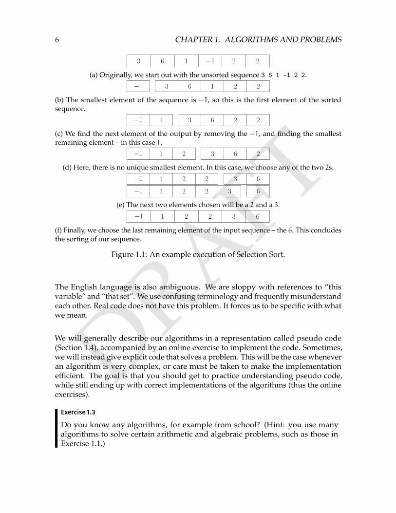
If you want to see this algorithm in practice, it is performed on our previous exampleinstance, the sequence 3, 6, 1,−1, 2, 2, in Figures 1.1a-1.1f.
So far, we have been vague about what exactly an algorithm is. Looking at our exam-ple (Algorithm 1.1) we do not have any particular structure or rigor in the descriptionof our method. There is nothing inherently wrong with describing algorithms thisway. It is easy to understand, and gives the writer an opportunity to provide contextas to why certain actions are performed, making the correctness of the algorithmmore obvious. The main downsides of such a description are the ambiguity and thelack of detail.
Until an algorithm is described in sufficient detail, it is possible to accidentally abstractaway operations we may not know how to perform behind a few English words. As asomewhat contrived example, our textual description of selection sort includes actionssuch as “choosing the smallest number of a sequence”. While such an operation mayseem very simple to us humans, algorithms are generally constructed with regardsto some kind of computer. Unfortunately, computers can not map such Englishexpressions to their code counterparts yet. Instructing a computer to execute analgorithm thus require us to formulate our algorithm in steps small enough that evena computer knows how to perform it. In this sense, a computer is rather stupid.
DRAFT
6 CHAPTER 1. ALGORITHMS AND PROBLEMS
3 6 1 −1 2 2
(a) Originally, we start out with the unsorted sequence 3 6 1 -1 2 2.
−1 3 6 1 2 2
(b) The smallest element of the sequence is −1, so this is the first element of the sortedsequence.
−1 1 3 6 2 2
(c) We find the next element of the output by removing the −1, and finding the smallestremaining element – in this case 1.
−1 1 2 3 6 2
(d) Here, there is no unique smallest element. In this case, we choose any of the two 2s.
−1 1 2 2 3 6
−1 1 2 2 3 6
(e) The next two elements chosen will be a 2 and a 3.
−1 1 2 2 3 6
(f) Finally, we choose the last remaining element of the input sequence – the 6. This concludesthe sorting of our sequence.
Figure 1.1: An example execution of Selection Sort.
The English language is also ambiguous. We are sloppy with references to “thisvariable” and “that set”. We use confusing terminology and frequently misunderstandeach other. Real code does not have this problem. It forces us to be specific with whatwe mean.
We will generally describe our algorithms in a representation called pseudo code(Section 1.4), accompanied by an online exercise to implement the code. Sometimes,we will instead give explicit code that solves a problem. This will be the case wheneveran algorithm is very complex, or care must be taken to make the implementationefficient. The goal is that you should get to practice understanding pseudo code,while still ending up with correct implementations of the algorithms (thus the onlineexercises).
Exercise 1.3
Do you know any algorithms, for example from school? (Hint: you use manyalgorithms to solve certain arithmetic and algebraic problems, such as those inExercise 1.1.)
DRAFT
1.2. ALGORITHMS 7
Exercise 1.4
Construct an algorithm which solves the guessing problem in exercise 1.2. Howmany questions does it use? The optimal number of questions is about log
2100 ≈ 7
questions. Can you achieve this?
1.2.1 Correctness
One subtle, albeit important point that we glossed over is what it means for analgorithm to actually be correct.
There are two common notions of correctness – partial correctness and total correct-ness. The first notion requires an algorithm to, upon termination, have produced anoutput that fulfill all the criteria laid out in the output description. Total correctnessadditionally require an algorithm to terminate within finite time. When we talkabout correctness of our algorithms later on, we will generally focus on the partialcorrectness. Termination will instead be proved implicitly, as we will consider moregranular measures of efficiency (called time complexity, Chapter 4) than just finitetermination. These measures will imply the termination of the algorithm, completingthe proof of total correctness.
Proving that the selection sort algorithm terminates in finite time is quite easy. Itperforms one iteration of the selection step for each element in the original sequence(which is finite). Furthermore, each such iteration can be performed in finite time byconsidering each remaining element of the selection when finding the smallest one.The remaining sequence is a subsequence of the original one, and is therefore alsofinite.
Proving that the algorithm produces the correct output is a bit more difficult to for-mally prove. The main idea behind a formal proof is contained within our descriptionof the algorithm itself.
Later on, we will compromise on both conditions. Generally, we are satisfied withan algorithm terminating in expected finite time, or answering correctly with, say,probability 0.75 for every input. Similarly, we are sometimes happy to find anapproximate solution to a problem. What this means more concretely will become clearin due time, when we study such algorithms.
Competitive Tip
Proving your algorithm correct is sometimes quite difficult. In a competition,a correct algorithm is correct even if you cannot prove it. If you have an ideayou think is correct, it may be worth testing. Unfortunately, this makes it evenharder to decide if an incorrect submission is due to an incorrect algorithm or an
DRAFT
8 CHAPTER 1. ALGORITHMS AND PROBLEMS
incorrect implementation.
Exercise 1.5
Prove the correctness of your algorithm to the guessing problem from Exercise 1.4.
Exercise 1.6
Why would an algorithm that is correct with e.g. probability 0.75 still be veryuseful to us?
Why is it important that such an algorithm is correct with probability 0.75 on everyproblem instance, instead of always being correct for 75% of all cases?
1.3 Programming Languages
The purpose of programming languages is to formulate methods at a level wherea computer can execute them. While we in textual descriptions of methods areoften satisfied with describing what we wish to do, programming languages requireconsiderably more constructive descriptions. Computers are quite basic creaturescompared to us humans. They only understand a very limited set of instructions,such as adding numbers, multiplying numbers, or moving data around within itsmemory. The syntax of programming languages are often a bit arcane at first, butthey grow on you with coding experience.
To complicate matters further, programming languages themselves define a spectrumof expressiveness. On the lowest level, programming deals with electrical current inyour processor, with current above or below a certain threshold denoting the digits0 and 1. Above these circuit-level electronics lie a processors own programming,often called microcode. Using this, a processor implements machine code, such asthe x86 instruction set. Machine code is often written using a higher-level syntaxcalled Assembly. While some code is written in this rather low-level language, wemostly abstract away details of them in high-level languages such as C++ (this book’slanguage of choice).
This knowledge is somewhat useless from a problem solving standpoint, but intimateknowledge of how a computer works is of high importance in software engineering,and is occasionally helpful in programming competitions. Therefore, you should notbe surprised about certain remarks relating to these low-level concepts.
These facts also provide some motivation for why we use what we call compilers.When programming in C++, we can not immediately tell a computer to run its code.
DRAFT
1.4. PSEUDO CODE 9
As you now know, C++ is at a higher level than what the processor of a computercan run. A compiler takes care of this problem, by translating our C++ code intomachine code, which a processor knows how to handle. It is a program of its own,that takes the code files we will write and produce executable files that we can run onthe computer. The process and purpose of a compiler is somewhat like what we doourselves when translating a method from English sentences or our own thoughtsinto the lower level language of C++.
1.4 Pseudo Code
Somewhere in between describing algorithms in English text and in a programminglanguage lie pseudo code. As hinted by its name, it is not quite actual code, in twoaspects. First of all, the instructions we write is not the programming language of anyparticular computer. The point of pseudo code is to be independent of what computerit is implemented on. Instead, it tries to convey the main points of an algorithm in adetailed manner such that it can easily be translated into any particular programminglanguage. Secondly, we sometimes fall back to the liberties of the English language.At some point, we may decide that “choose the smallest number of a sequence” isclear enough for our audience.
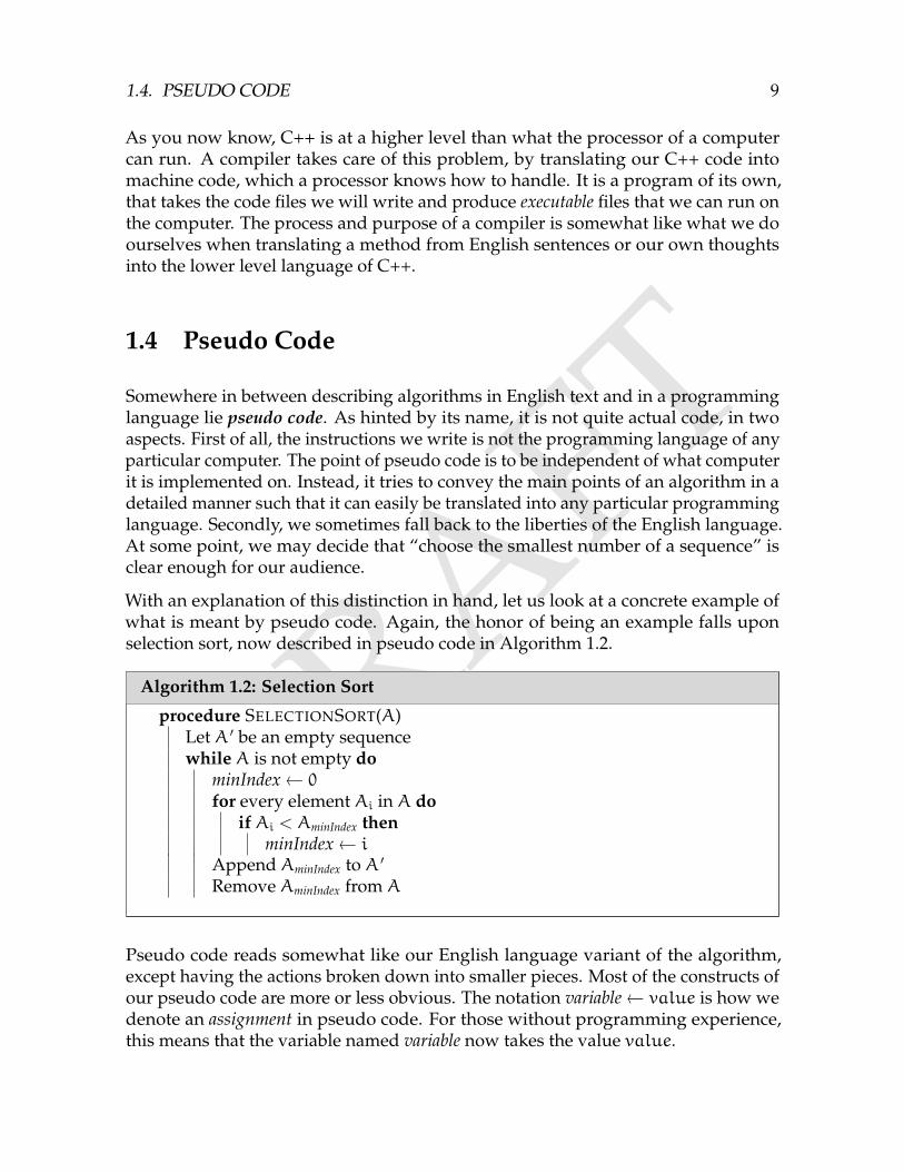
With an explanation of this distinction in hand, let us look at a concrete example ofwhat is meant by pseudo code. Again, the honor of being an example falls uponselection sort, now described in pseudo code in Algorithm 1.2.
Algorithm 1.2: Selection Sort
procedure SELECTIONSORT(A)Let A ′ be an empty sequencewhile A is not empty do
minIndex← 0
for every element Ai in A doif Ai < AminIndex then
minIndex← iAppend AminIndex to A ′
Remove AminIndex from A
Pseudo code reads somewhat like our English language variant of the algorithm,except having the actions broken down into smaller pieces. Most of the constructs ofour pseudo code are more or less obvious. The notation variable← value is how wedenote an assignment in pseudo code. For those without programming experience,this means that the variable named variable now takes the value value.
DRAFT
10 CHAPTER 1. ALGORITHMS AND PROBLEMS
Pseudo code will appear when we try to explain some part of a solution in greatdetail, but where programming language specific aspects would draw unnecessaryattention to themselves.
Competitive Tip
In team competitions where a team only have a single computer, a team will oftenhave solved problems waiting to be coded. Writing pseudo code of the solutionto one of these problems while waiting for computer time is an efficient way toparallelize your work. This can be practiced by writing pseudo code on papereven when you are solving problems by yourself.
Exercise 1.7
Write pseudo code for your algorithm to the guessing problem from Exercise 1.4.
1.5 The Kattis Online Judge
Most of the exercises in this book exist as problems on the Kattis web system. Youcan find the judge at https://open.kattis.com. Kattis is a so called online judge,which has been used in the university competitive programming world finals (theInternational Collegiate Programming Contest World Finals) for several years. Itcontains a large collection of computational problems, and allows you to submit aprogram you have written that purports to solve the problem. Kattis will then runyour program on a large number of predetermined instances of the problem.
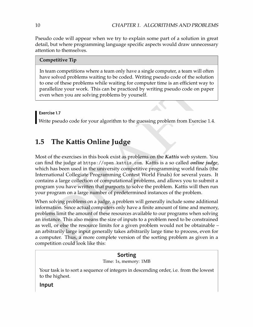
When solving problems on a judge, a problem will generally include some additionalinformation. Since actual computers only have a finite amount of time and memory,problems limit the amount of these resources available to our programs when solvingan instance. This also means the size of inputs to a problem need to be constrainedas well, or else the resource limits for a given problem would not be obtainable –an arbitrarily large input generally takes arbitrarily large time to process, even fora computer. Thus, a more complete version of the sorting problem as given in acompetition could look like this:
SortingTime: 1s, memory: 1MB
Your task is to sort a sequence of integers in descending order, i.e. from the lowestto the highest.
Input
DRAFT
1.6. CHAPTER NOTES 11
The input consists of a sequence of N integers (0 ≤ N ≤ 1000) a0, a1, ..., aN−1
(|ai| ≤ 109).OutputThe output should contain a permutation a ′ of the sequence a, such that a ′0 ≤a ′1 ≤ ... ≤ a ′N−1.
If your program exceeds the allowed resource limits (i.e. takes too much time ormemory), crashes, or gives an invalid output, Kattis will tell you so with a rejectedjudgment. Assuming your program passes all the instances, it will be be given theAccepted judgment.
Note that getting a program accepted by Kattis is not the same as having a correctprogram – it is a necessary but not sufficient criteria for correctness. This is also afact which is possible to exploit during competitions, which we will see later in thisbook.
We recommend that you get an account on Kattis, so that you can follow along withthe book’s exercises.
Exercise 1.8
Register an account on Kattis
Many other online judges exists, such as:
• Codeforces (http://codeforces.com)
• TopCoder (https://topcoder.com)
• HackerRank (https://hackerrank.com)
1.6 Chapter Notes
The introductions given in this chapter are very bare bones, mostly stripped down towhat you need to get by when solving algorithmic problems.
Many other books delve into the theoretical study of algorithms deeper than wewill, in particular regarding subjects not relevant to algorithmic problem solving.Introduction to Algorithms [5] is a rigorous introductory text book on algorithms, withboth depth and width.
For a gentle introduction to the technology that underlies computers, CODE [19] is awell-written journey from the basics of bits and bytes all the way to assembly codeand operating systems.

DRAFT
12 CHAPTER 1. ALGORITHMS AND PROBLEMS
DRAFTChapter 2
Programming in C++
We will learn some more practical matters – the basics of the C++ programminglanguage. This language is the most common programming language within thecompetitive programming community, for a few reasons (aside from C++ being apopular language in general). Programs coded in C++ are generally somewhat fasterthan most other competitive programming languages, and there are many routinesin the accompanying standard code libraries that are useful when implementingalgorithms.
Of course, no language is without downsides. C++ is a bit difficult to learn as abeginner’s programming language, to say the least. Its error management is un-forgiving, often causing erratic behavior in programs instead of crashing with anerror. Programming certain things become quite verbose, compared to many otherlanguages.
After bashing the difficulty of C++, you might ask if it really is the best languagein order to get started with algorithmic problem solving. While there certainly aresimpler languages, we believe the benefits of C++ weigh up for the disadvantagesin the long term even though it demands more from you as a reader. Either way, itis definitely the language we have the most experience of teaching problem solvingwith.
When you study this chapter, you will see a lot of example code. Type this codeand run it. We can not really stress this point enough. Learning programming fromscratch – in particular a complicated language such as C++ – is not possible unless youtry the concepts yourself. Additionally, we recommend that you do every exercise inthis chapter.
Finally, know that our treatment of C++ is minimal. We will not explain all thedetails behind the language, nor good coding style or general software engineeringprinciples. In fact, we will frequently make use of bad coding practices. If you want
13
DRAFT
14 CHAPTER 2. PROGRAMMING IN C++
to delve deeper, you can find more resources in the chapter notes.
2.1 Development Environments
Before we get to the juicy parts of C++, you first need to install a compiler for C++ and(optionally) a code editor. If you are running Windows, we recommend Code::Blocks,a code editor that also installs a compiler for you. You can download this from theCode::Blocks web site, http://www.codeblocks.org/downloads/26. Choose the filethat ends with mingw-setup.exe.
If you are using Mac OS, you can instead get a compiler by installing Xcode from theMac App Store. You can then either use Xcode to write your programs, or installCode::Blocks.
Running a Linux distribution (such as Ubuntu), you should be able to find the packageg++ in your favorite package manager. This installs the GCC compiler for you, whichis the most popular compiler for Linux systems. Possibly, codeblocks exists as apackage there as well.
Note that instructions like these tend to rot, with applications disappearing from theweb, operating systems changing names and so on. In this case, you are on your own,and will have to find instructions to by yourself.
In this chapter, we will assume you are using Code::Blocks. If you chose some othereditor or compiler, you will need to find instructions on how to compile and runprograms yourself.
2.2 Hello World!
Now that you have a compiler and editor ready, we will learn the basic structure of aC++ program. The classical example of a program when learning a new languageis to print the text Hello World!. We will also solve our first Kattis problem in thissection.
Start by opening Code::Blocks, and create a new file (by going to File ⇒ New ⇒Empty File). Save the file as hello.cpp in a new folder (such as Code).
Now, type the code from Listing 2.1 into your editor.
In Code::Blocks, You can save your program by typing Ctrl+S, and running it bypressing the F9 key. A window will appear, containing the text Hello World!. If nowindow appear, you probably mistyped the program.
DRAFT
2.2. HELLO WORLD! 15
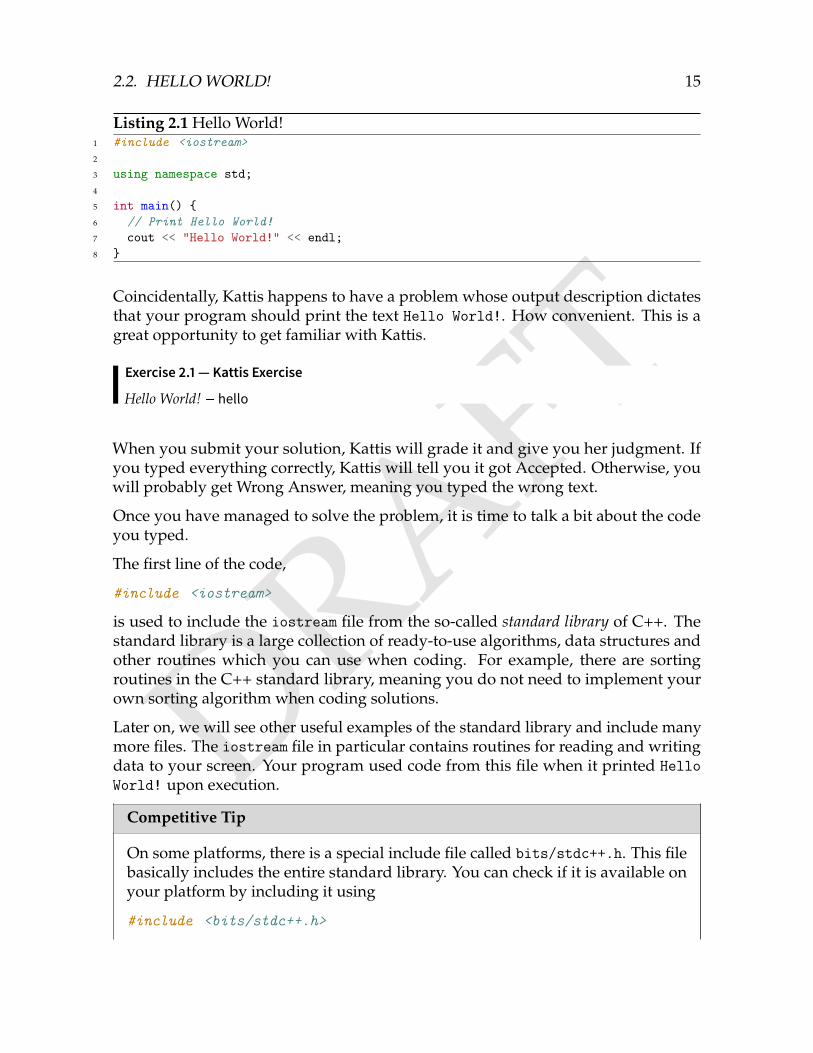
Listing 2.1 Hello World!1 #include <iostream>2
3 using namespace std;4
5 int main() 6 // Print Hello World!7 cout << "Hello World!" << endl;8
Coincidentally, Kattis happens to have a problem whose output description dictatesthat your program should print the text Hello World!. How convenient. This is agreat opportunity to get familiar with Kattis.
Exercise 2.1 — Kattis Exercise
Hello World! – hello
When you submit your solution, Kattis will grade it and give you her judgment. Ifyou typed everything correctly, Kattis will tell you it got Accepted. Otherwise, youwill probably get Wrong Answer, meaning you typed the wrong text.
Once you have managed to solve the problem, it is time to talk a bit about the codeyou typed.
The first line of the code,
#include <iostream>
is used to include the iostream file from the so-called standard library of C++. Thestandard library is a large collection of ready-to-use algorithms, data structures andother routines which you can use when coding. For example, there are sortingroutines in the C++ standard library, meaning you do not need to implement yourown sorting algorithm when coding solutions.
Later on, we will see other useful examples of the standard library and include manymore files. The iostream file in particular contains routines for reading and writingdata to your screen. Your program used code from this file when it printed HelloWorld! upon execution.
Competitive Tip
On some platforms, there is a special include file called bits/stdc++.h. This filebasically includes the entire standard library. You can check if it is available onyour platform by including it using
#include <bits/stdc++.h>
DRAFT
16 CHAPTER 2. PROGRAMMING IN C++
in the beginning of your code. If your program still compiles, you can use thisand not include anything else.
The third line,
using namespace std;
tells the compiler that we wish to use code from the standard library. If we did notuse it, we would have to specify this every time we used code from the standardlibrary later in our program.
The fifth line defines our main function. When we instruct the computer to run ourprogram, this is where it will start looking for code to execute. The first line of themain function is where the program will start to run, and then execute further linessequentially. We will later see how we can define additional functions, as a way ofstructuring our code.
Note that the code in a function – its body – must be enclosed by curly brackets.Without them, we would not know which lines belonged to the function.
On line 6, we wrote a comment
// Print Hello World!
Comments are explanatory lines which are not executed by the computer. Thepurpose of a comment is to explain what the code around it does, and why. Theybegin with two slashes // and continue until the end of the current line.
It is not until the seventh line that things start happening in the program. We usethe standard library utility cout to print text to the screen. This is done by writinge.g:
cout << "this is text you want to print. ";cout << "you can " << "also print " << "multiple things. ";cout << "to print a new line" << endl << "you print endl" << endl;cout << "without any quotes" << endl;
Lines that do things in C++ are called statements. Note the semi colon at the endof the line! Semi colons are used to specify the end of a statement, and are manda-tory.
Exercise 2.2
Must the main function be named main? What happens if you changed main tosomething else and try to run your program?
DRAFT
2.3. VARIABLES AND TYPES 17
Exercise 2.3
Play around with cout a bit, printing various things. For example, you can print apretty haiku.
2.3 Variables and Types
The Hello World! program is boring. It only prints text, which is seldom the onlynecessary component of an algorithm (aside from the Hello World! problem on Kattis).We now move on to a new but hopefully familiar concept.
When we solve mathematical problems, it often proves useful to introduce all kindsof names for known and unknown values. Math problems often deal with classesof N students, ice cream trucks with velocity vcar km/h and candy prices of pcandy$/kg.
This concept naturally translates into C++, but with a twist. In most programminglanguages, we first need to say what type a variable has! We do not bother with thisin mathematics. We say that “let x = 5”, and that is that. In C++, we need to be a bitmore verbose. We must write that “I want to introduce a variable x now. It is going tobe an integer – more specifically, 5”. Once we have decided what kind of value x willbe (in this case integer), it will always be an integer. We cannot just go ahead and say“oh, I’ve changed my mind. x = 2.5 now!” since 2.5 is of the wrong type (a decimalnumber rather than an integer).
Another major difference is that variables in C++ are not tied to a single value forthe entirety of its lifespan. Instead, we are able to modify the value which ourvariables take using something called assignment. Some languages does not permitthis, preferring their variables to be immutable.
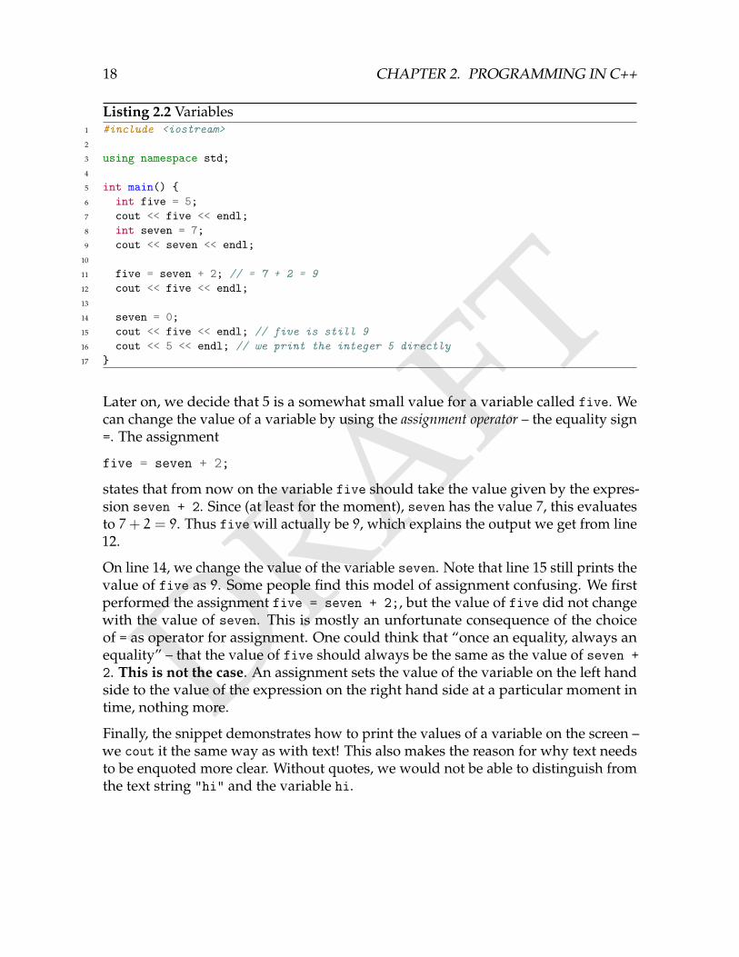
In Listing 2.2, we demonstrate how variables are used in C++. Type this program intoyour editor and run it. What is the output, and what did you expect the output tobe?
The first time we use a variable in C++, we need to decide what kind of values it maycontain. This is called declaring the variable of a certain type. For example
int five = 5;
declares an integer variable five, and assign the value 5 to it. The int part is C++ forinteger, and is what we call a type. After the type, we write the name of the variable –in this case 5. Finally, we may assign a value to the variable. Note that further use ofthe variable never include the int part. We declare the type of a variable once, andonly once.
DRAFT
18 CHAPTER 2. PROGRAMMING IN C++
Listing 2.2 Variables1 #include <iostream>2
3 using namespace std;4
5 int main() 6 int five = 5;7 cout << five << endl;8 int seven = 7;9 cout << seven << endl;
10
11 five = seven + 2; // = 7 + 2 = 912 cout << five << endl;13
14 seven = 0;15 cout << five << endl; // five is still 916 cout << 5 << endl; // we print the integer 5 directly17
Later on, we decide that 5 is a somewhat small value for a variable called five. Wecan change the value of a variable by using the assignment operator – the equality sign=. The assignment
five = seven + 2;
states that from now on the variable five should take the value given by the expres-sion seven + 2. Since (at least for the moment), seven has the value 7, this evaluatesto 7+ 2 = 9. Thus five will actually be 9, which explains the output we get from line12.
On line 14, we change the value of the variable seven. Note that line 15 still prints thevalue of five as 9. Some people find this model of assignment confusing. We firstperformed the assignment five = seven + 2;, but the value of five did not changewith the value of seven. This is mostly an unfortunate consequence of the choiceof = as operator for assignment. One could think that “once an equality, always anequality” – that the value of five should always be the same as the value of seven +2. This is not the case. An assignment sets the value of the variable on the left handside to the value of the expression on the right hand side at a particular moment intime, nothing more.
Finally, the snippet demonstrates how to print the values of a variable on the screen –we cout it the same way as with text! This also makes the reason for why text needsto be enquoted more clear. Without quotes, we would not be able to distinguish fromthe text string "hi" and the variable hi.
DRAFT
2.3. VARIABLES AND TYPES 19
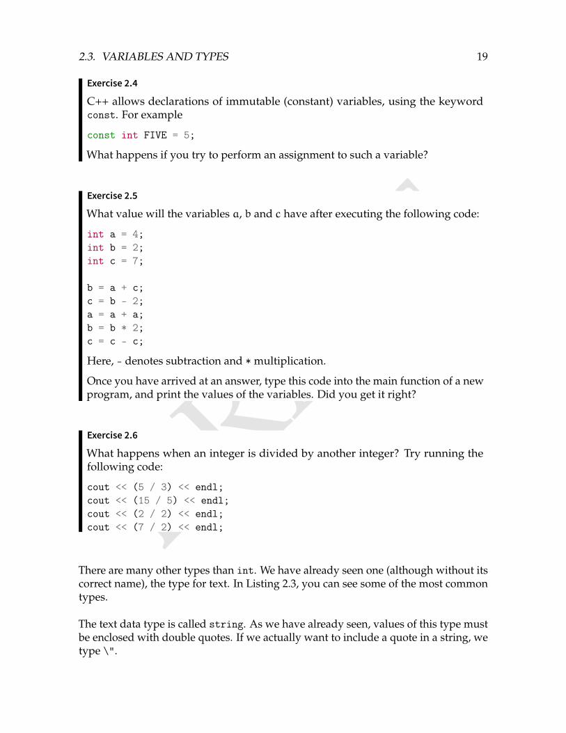
Exercise 2.4
C++ allows declarations of immutable (constant) variables, using the keywordconst. For example
const int FIVE = 5;
What happens if you try to perform an assignment to such a variable?
Exercise 2.5
What value will the variables a, b and c have after executing the following code:
int a = 4;int b = 2;int c = 7;
b = a + c;c = b - 2;a = a + a;b = b * 2;c = c - c;
Here, - denotes subtraction and * multiplication.
Once you have arrived at an answer, type this code into the main function of a newprogram, and print the values of the variables. Did you get it right?
Exercise 2.6
What happens when an integer is divided by another integer? Try running thefollowing code:
cout << (5 / 3) << endl;cout << (15 / 5) << endl;cout << (2 / 2) << endl;cout << (7 / 2) << endl;
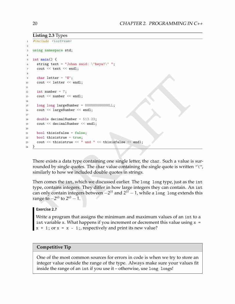
There are many other types than int. We have already seen one (although without itscorrect name), the type for text. In Listing 2.3, you can see some of the most commontypes.
The text data type is called string. As we have already seen, values of this type mustbe enclosed with double quotes. If we actually want to include a quote in a string, wetype \".
DRAFT
20 CHAPTER 2. PROGRAMMING IN C++
Listing 2.3 Types1 #include <iostream>2
3 using namespace std;4
5 int main() 6 string text = "Johan said: \"heya!\" ";7 cout << text << endl;8
9 char letter = ’@’;10 cout << letter << endl;11
12 int number = 7;13 cout << number << endl;14
15 long long largeNumber = 888888888888LL;16 cout << largeNumber << endl;17
18 double decimalNumber = 513.23;19 cout << decimalNumber << endl;20
21 bool thisisfalse = false;22 bool thisistrue = true;23 cout << thisistrue << " and " << thisisfalse << endl;24
There exists a data type containing one single letter, the char. Such a value is sur-rounded by single quotes. The char value containing the single quote is written ’\”,similarly to how we included double quotes in strings.
Then comes the int, which we discussed earlier. The long long type, just as the inttype, contains integers. They differ in how large integers they can contain. An intcan only contain integers between −231 and 231 − 1, while a long long extends thisrange to −263 to 263 − 1.
Exercise 2.7
Write a program that assigns the minimum and maximum values of an int to aint variable x. What happens if you increment or decrement this value using x =x + 1; or x = x - 1;, respectively and print its new value?
Competitive Tip
One of the most common sources for errors in code is when we try to store aninteger value outside the range of the type. Always make sure your values fitinside the range of an int if you use it – otherwise, use long longs!
DRAFT
2.4. INPUT AND OUTPUT 21
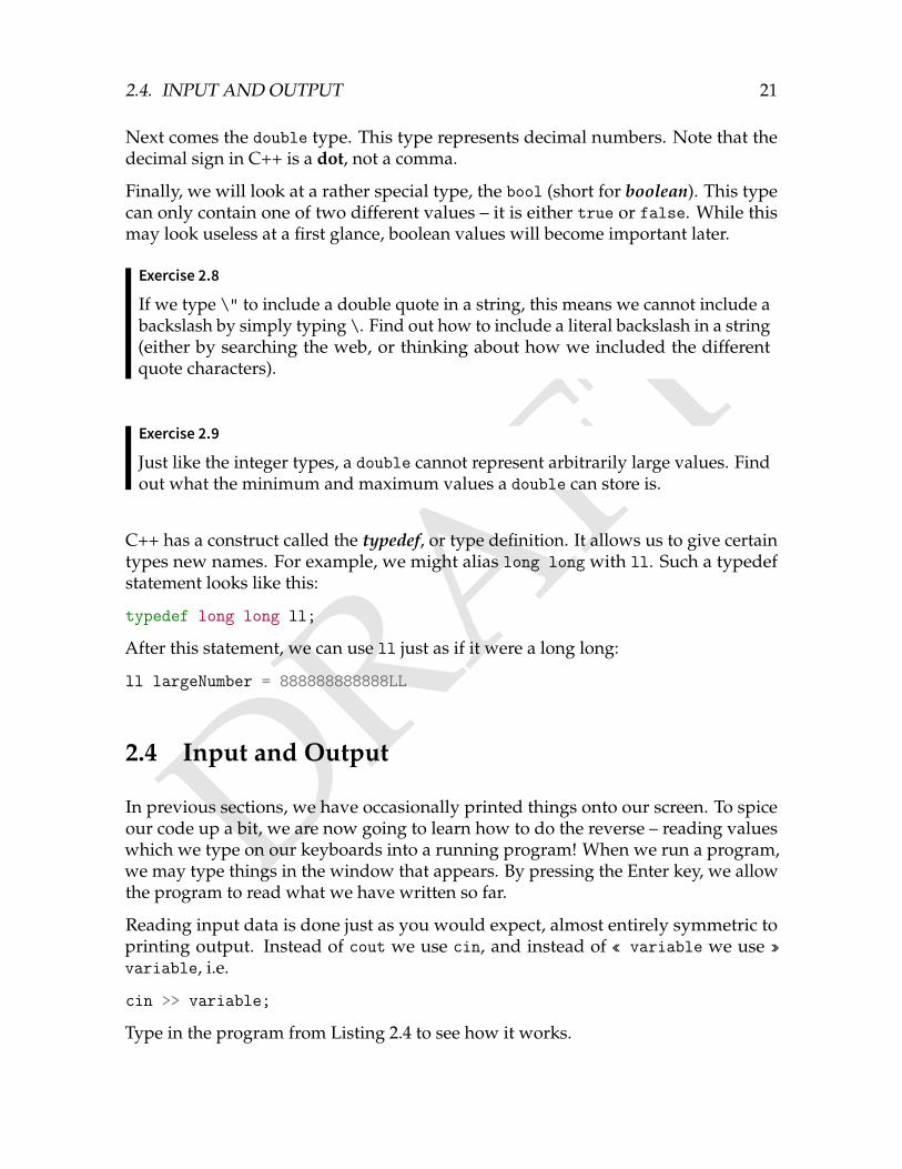
Next comes the double type. This type represents decimal numbers. Note that thedecimal sign in C++ is a dot, not a comma.
Finally, we will look at a rather special type, the bool (short for boolean). This typecan only contain one of two different values – it is either true or false. While thismay look useless at a first glance, boolean values will become important later.
Exercise 2.8
If we type \" to include a double quote in a string, this means we cannot include abackslash by simply typing \. Find out how to include a literal backslash in a string(either by searching the web, or thinking about how we included the differentquote characters).
Exercise 2.9
Just like the integer types, a double cannot represent arbitrarily large values. Findout what the minimum and maximum values a double can store is.
C++ has a construct called the typedef, or type definition. It allows us to give certaintypes new names. For example, we might alias long long with ll. Such a typedefstatement looks like this:
typedef long long ll;
After this statement, we can use ll just as if it were a long long:
ll largeNumber = 888888888888LL
2.4 Input and Output
In previous sections, we have occasionally printed things onto our screen. To spiceour code up a bit, we are now going to learn how to do the reverse – reading valueswhich we type on our keyboards into a running program! When we run a program,we may type things in the window that appears. By pressing the Enter key, we allowthe program to read what we have written so far.
Reading input data is done just as you would expect, almost entirely symmetric toprinting output. Instead of cout we use cin, and instead of « variable we use »variable, i.e.
cin >> variable;
Type in the program from Listing 2.4 to see how it works.
DRAFT
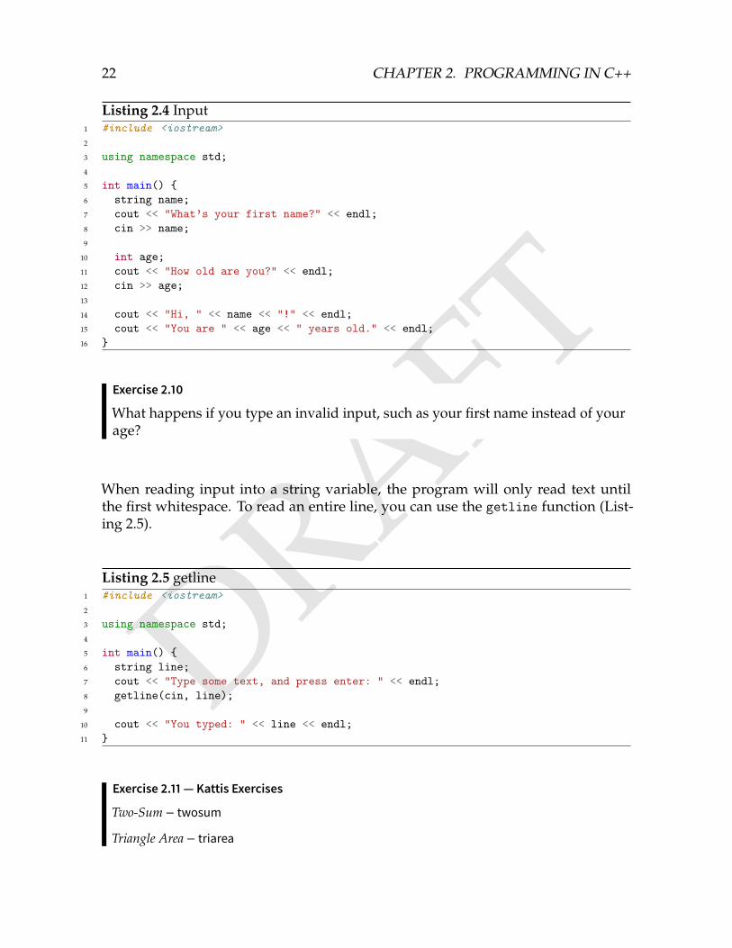
22 CHAPTER 2. PROGRAMMING IN C++
Listing 2.4 Input1 #include <iostream>2
3 using namespace std;4
5 int main() 6 string name;7 cout << "What’s your first name?" << endl;8 cin >> name;9
10 int age;11 cout << "How old are you?" << endl;12 cin >> age;13
14 cout << "Hi, " << name << "!" << endl;15 cout << "You are " << age << " years old." << endl;16
Exercise 2.10
What happens if you type an invalid input, such as your first name instead of yourage?
When reading input into a string variable, the program will only read text untilthe first whitespace. To read an entire line, you can use the getline function (List-ing 2.5).
Listing 2.5 getline1 #include <iostream>2
3 using namespace std;4
5 int main() 6 string line;7 cout << "Type some text, and press enter: " << endl;8 getline(cin, line);9
10 cout << "You typed: " << line << endl;11
Exercise 2.11 — Kattis Exercises
Two-Sum – twosum
Triangle Area – triarea

DRAFT
2.5. OPERATORS 23
2.5 Operators
We have already seen examples of what we call operators. Earlier we have usedthe assignment operator =, and the arithmetic operators + - * /, which stand foraddition, subtraction, multiplication and division. They work almost like they do inmathematics, and allows us to create code such as the one in Listing 2.6.
Listing 2.6 Operators1 #include <iostream>2
3 using namespace std;4
5 int main() 6 int a = 0;7 int b = 0;8
9 cin >> a >> b;10
11 cout << "Sum: " << (a + b) << endl;12 cout << "Difference: " << (a - b) << endl;13 cout << "Product: " << (a * b) << endl;14 cout << "Quotient: " << (a / b) << endl;15 cout << "Remainder: " << (a % b) << endl;16
Exercise 2.12
Type in Listing 2.6 and test it on a few different values. In particular, test:
• b = 0
• Negative values for a and/or b
• Values where the expected result is outside the valid range of an int
As you have probably noticed, the division operator of C++ performs so-called integerdivision, meaning it rounds the answer to an integer (towards 0). Hence 7 / 3 = 2,with remainder 1.
The snippet introduces the modulo operator, %. It computes the remainder of the firstoperand, when divided by the second. As an example, 7 % 3 = 1.
In case we wish the answer to be a decimal number instead of performing integerdivision, one of the operands must be a double (Listing 2.7).
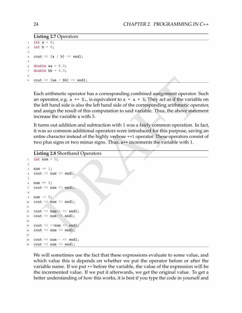
We end this section with some shorthand operators. Check out Listing 2.8 for someexamples.
DRAFT
24 CHAPTER 2. PROGRAMMING IN C++
Listing 2.7 Operators1 int a = 6;2 int b = 4;3
4 cout << (a / b) << endl;5
6 double aa = 6.0;7 double bb = 4.0;8
9 cout << (aa / bb) << endl;
Each arithmetic operator has a corresponding combined assignment operator. Suchan operator, e.g. a += 5;, is equivalent to a = a + 5; They act as if the variable onthe left hand side is also the left hand side of the corresponding arithmetic operator,and assign the result of this computation to said variable. Thus, the above statementincrease the variable a with 5.
It turns out addition and subtraction with 1 was a fairly common operation. In fact,it was so common additional operators were introduced for this purpose, saving anentire character instead of the highly verbose +=1 operator. These operators consist oftwo plus signs or two minus signs. Thus, a++ increments the variable with 1.
Listing 2.8 Shorthand Operators1 int num = 0;2
3 num += 1;4 cout << num << endl;5
6 num *= 2;7 cout << num << endl;8
9 num -= 3;10 cout << num << endl;11
12 cout << num++ << endl;13 cout << num << endl;14
15 cout << ++num << endl;16 cout << num << endl;17
18 cout << num-- << endl;19 cout << num << endl;
We will sometimes use the fact that these expressions evaluate to some value, andwhich value this is depends on whether we put the operator before or after thevariable name. If we put ++ before the variable, the value of the expression will bethe incremented value. If we put it afterwards, we get the original value. To get abetter understanding of how this works, it is best if you type the code in yourself and
DRAFT
2.6. IF STATEMENTS 25
analyze the results.
2.6 If Statements
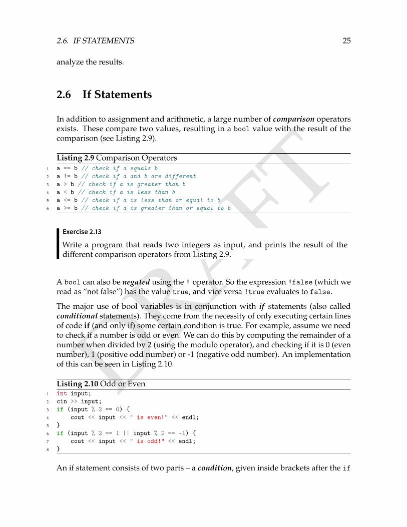
In addition to assignment and arithmetic, a large number of comparison operatorsexists. These compare two values, resulting in a bool value with the result of thecomparison (see Listing 2.9).
Listing 2.9 Comparison Operators1 a == b // check if a equals b2 a != b // check if a and b are different3 a > b // check if a is greater than b4 a < b // check if a is less than b5 a <= b // check if a is less than or equal to b6 a >= b // check if a is greater than or equal to b
Exercise 2.13
Write a program that reads two integers as input, and prints the result of thedifferent comparison operators from Listing 2.9.
A bool can also be negated using the ! operator. So the expression !false (which weread as “not false”) has the value true, and vice versa !true evaluates to false.
The major use of bool variables is in conjunction with if statements (also calledconditional statements). They come from the necessity of only executing certain linesof code if (and only if) some certain condition is true. For example, assume we needto check if a number is odd or even. We can do this by computing the remainder of anumber when divided by 2 (using the modulo operator), and checking if it is 0 (evennumber), 1 (positive odd number) or -1 (negative odd number). An implementationof this can be seen in Listing 2.10.
Listing 2.10 Odd or Even1 int input;2 cin >> input;3 if (input % 2 == 0) 4 cout << input << " is even!" << endl;5 6 if (input % 2 == 1 || input % 2 == -1) 7 cout << input << " is odd!" << endl;8
An if statement consists of two parts – a condition, given inside brackets after the if
DRAFT
26 CHAPTER 2. PROGRAMMING IN C++
keyword, followed by a body – some lines of code surrounded by curly brackets. Thecode inside the body will be executed in case the condition evaluates to true.
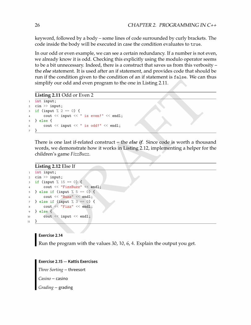
In our odd or even example, we can see a certain redundancy. If a number is not even,we already know it is odd. Checking this explicitly using the modulo operator seemsto be a bit unnecessary. Indeed, there is a construct that saves us from this verbosity –the else statement. It is used after an if statement, and provides code that should berun if the condition given to the condition of an if statement is false. We can thussimplify our odd and even program to the one in Listing 2.11.
Listing 2.11 Odd or Even 21 int input;2 cin >> input;3 if (input % 2 == 0) 4 cout << input << " is even!" << endl;5 else 6 cout << input << " is odd!" << endl;7
There is one last if-related construct – the else if. Since code is worth a thousandwords, we demonstrate how it works in Listing 2.12, implementing a helper for thechildren’s game FizzBuzz.
Listing 2.12 Else If1 int input;2 cin >> input;3 if (input % 15 == 0) 4 cout << "FizzBuzz" << endl;5 else if (input % 5 == 0) 6 cout << "Buzz" << endl;7 else if (input % 3 == 0) 8 cout << "Fizz" << endl;9 else
10 cout << input << endl;11
Exercise 2.14
Run the program with the values 30, 10, 6, 4. Explain the output you get.
Exercise 2.15 — Kattis Exercises
Three Sorting – threesort
Casino – casino
Grading – grading
DRAFT
2.7. FOR LOOPS 27
2.7 For Loops
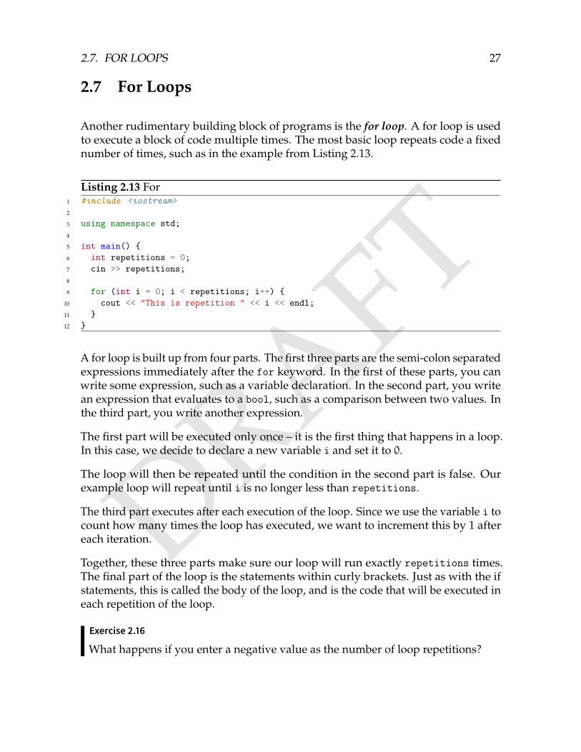
Another rudimentary building block of programs is the for loop. A for loop is usedto execute a block of code multiple times. The most basic loop repeats code a fixednumber of times, such as in the example from Listing 2.13.
Listing 2.13 For1 #include <iostream>2
3 using namespace std;4
5 int main() 6 int repetitions = 0;7 cin >> repetitions;8
9 for (int i = 0; i < repetitions; i++) 10 cout << "This is repetition " << i << endl;11 12
A for loop is built up from four parts. The first three parts are the semi-colon separatedexpressions immediately after the for keyword. In the first of these parts, you canwrite some expression, such as a variable declaration. In the second part, you writean expression that evaluates to a bool, such as a comparison between two values. Inthe third part, you write another expression.
The first part will be executed only once – it is the first thing that happens in a loop.In this case, we decide to declare a new variable i and set it to 0.
The loop will then be repeated until the condition in the second part is false. Ourexample loop will repeat until i is no longer less than repetitions.
The third part executes after each execution of the loop. Since we use the variable i tocount how many times the loop has executed, we want to increment this by 1 aftereach iteration.
Together, these three parts make sure our loop will run exactly repetitions times.The final part of the loop is the statements within curly brackets. Just as with the ifstatements, this is called the body of the loop, and is the code that will be executed ineach repetition of the loop.
Exercise 2.16
What happens if you enter a negative value as the number of loop repetitions?
DRAFT
28 CHAPTER 2. PROGRAMMING IN C++
Exercise 2.17
Design a loop that instead counts backwards, from repetitions − 1 to 0.
Exercise 2.18 — Kattis Exercises
N-sum – nsum
Cinema – cinema
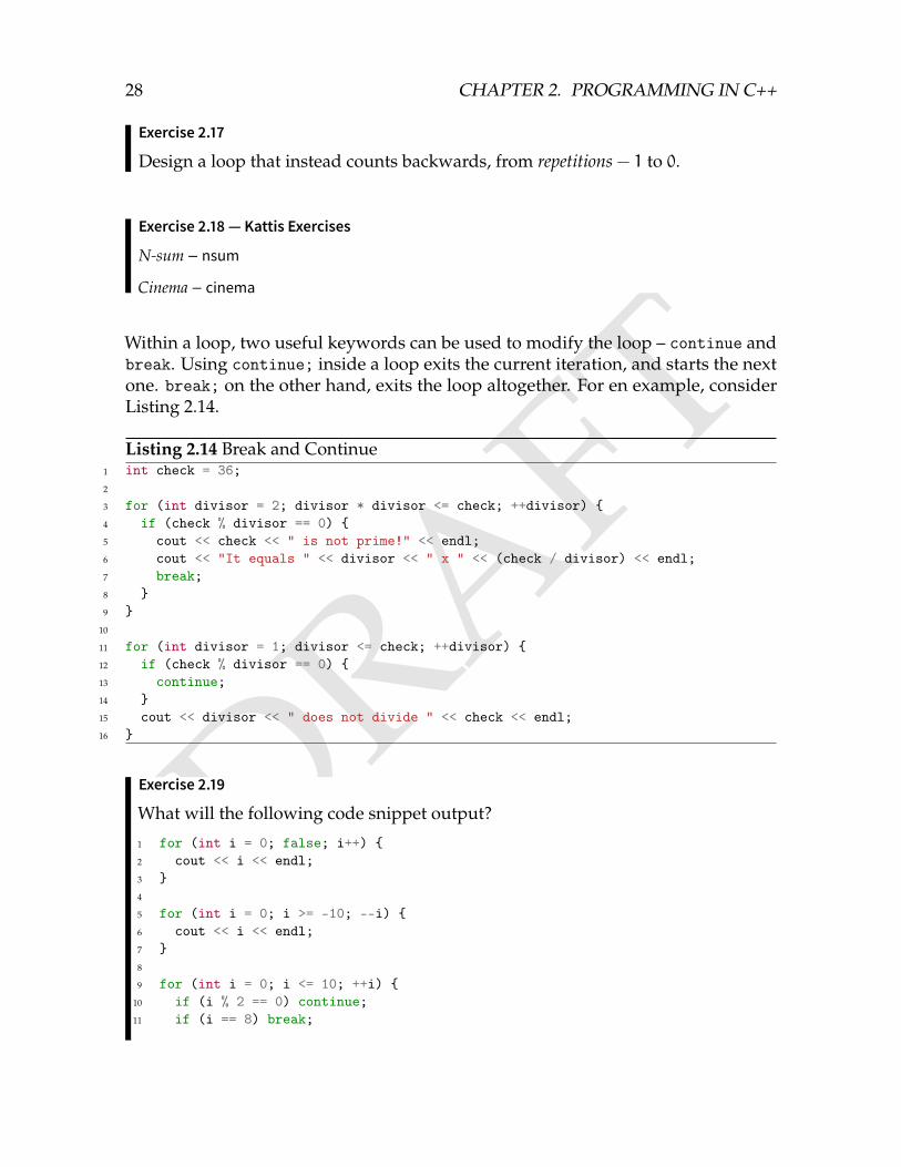
Within a loop, two useful keywords can be used to modify the loop – continue andbreak. Using continue; inside a loop exits the current iteration, and starts the nextone. break; on the other hand, exits the loop altogether. For en example, considerListing 2.14.
Listing 2.14 Break and Continue1 int check = 36;2
3 for (int divisor = 2; divisor * divisor <= check; ++divisor) 4 if (check % divisor == 0) 5 cout << check << " is not prime!" << endl;6 cout << "It equals " << divisor << " x " << (check / divisor) << endl;7 break;8 9
10
11 for (int divisor = 1; divisor <= check; ++divisor) 12 if (check % divisor == 0) 13 continue;14 15 cout << divisor << " does not divide " << check << endl;16
Exercise 2.19
What will the following code snippet output?
1 for (int i = 0; false; i++) 2 cout << i << endl;3 4
5 for (int i = 0; i >= -10; --i) 6 cout << i << endl;7 8
9 for (int i = 0; i <= 10; ++i) 10 if (i % 2 == 0) continue;11 if (i == 8) break;
DRAFT
2.8. WHILE LOOPS 29
12 cout << i << endl;13
Exercise 2.20 — Kattis Exercise
Cinema 2 – cinema2
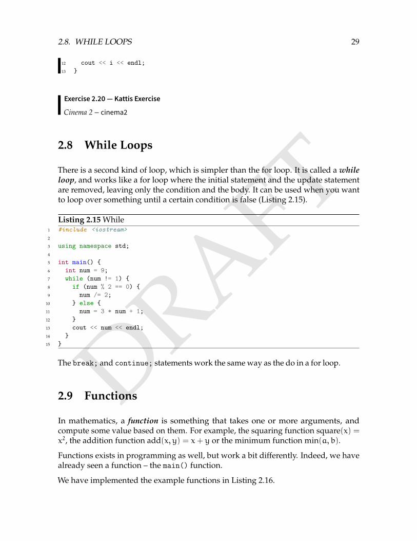
2.8 While Loops
There is a second kind of loop, which is simpler than the for loop. It is called a whileloop, and works like a for loop where the initial statement and the update statementare removed, leaving only the condition and the body. It can be used when you wantto loop over something until a certain condition is false (Listing 2.15).
Listing 2.15 While1 #include <iostream>2
3 using namespace std;4
5 int main() 6 int num = 9;7 while (num != 1) 8 if (num % 2 == 0) 9 num /= 2;
10 else 11 num = 3 * num + 1;12 13 cout << num << endl;14 15
The break; and continue; statements work the same way as the do in a for loop.
2.9 Functions
In mathematics, a function is something that takes one or more arguments, andcompute some value based on them. For example, the squaring function square(x) =x2, the addition function add(x, y) = x+ y or the minimum function min(a, b).
Functions exists in programming as well, but work a bit differently. Indeed, we havealready seen a function – the main() function.
We have implemented the example functions in Listing 2.16.

DRAFT
30 CHAPTER 2. PROGRAMMING IN C++
Listing 2.16 Functions1 #include <iostream>2
3 using namespace std;4
5 int square(int x) 6 return x * x;7 8
9 int min(int x, int y) 10 if (x < y) 11 return x;12 else 13 return y;14 15 16
17 int add(int x, int y) 18 return x + y;19 20
21 int main() 22 int x, y;23 cin >> x >> y;24 cout << x << "^2 = " << square(x) << endl;25 cout << x << " + " << y << " = " << add(x, y) << endl;26 cout << "min(" << x << ", " << y << ") = " << min(x, y) << endl;27
In the same way that a variable declaration starts by proclaiming what data type thevariable contains, a function declaration states what data type the function evaluatesto. Afterwards, we write the name of the function, followed by its arguments (whichis a comma-separated list of variable declarations). Finally, we give it a body of code,wrapped in curly brackets.
Unlike our main function, we see the return keyword in our functions. A returnstatement says “stop executing this function, and return the following value!”. Thus,when we call the squaring function by square(x), the function will compute thevalue x * x and make sure that square(x) evaluates to just that.
Why have we left a return statement out of the main function? In main(), the compilerinserts an implicit return 0; statement at the end of the function.
Exercise 2.21
What will the following function calls evaluate to?
square(5);
DRAFT
2.9. FUNCTIONS 31
add(square(3), 10);min(square(10), add(square(9), 23));
Exercise 2.22
In our code, we declared all of the new arithmetic functions above our mainfunction. Why did we do this? What happens if you move one below the mainfunction instead? (Hint: what happens if you try to use a variable before declaringit?)
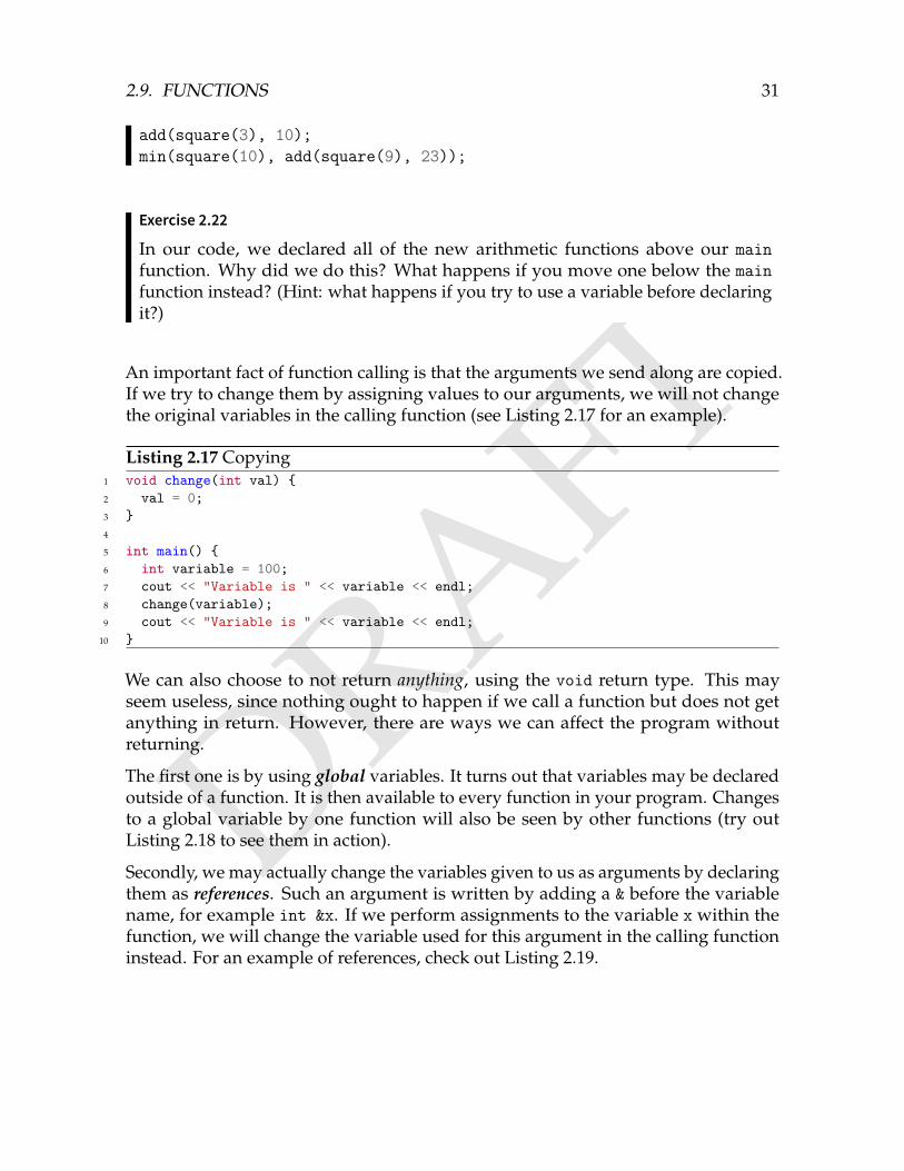
An important fact of function calling is that the arguments we send along are copied.If we try to change them by assigning values to our arguments, we will not changethe original variables in the calling function (see Listing 2.17 for an example).
Listing 2.17 Copying1 void change(int val) 2 val = 0;3 4
5 int main() 6 int variable = 100;7 cout << "Variable is " << variable << endl;8 change(variable);9 cout << "Variable is " << variable << endl;
10
We can also choose to not return anything, using the void return type. This mayseem useless, since nothing ought to happen if we call a function but does not getanything in return. However, there are ways we can affect the program withoutreturning.
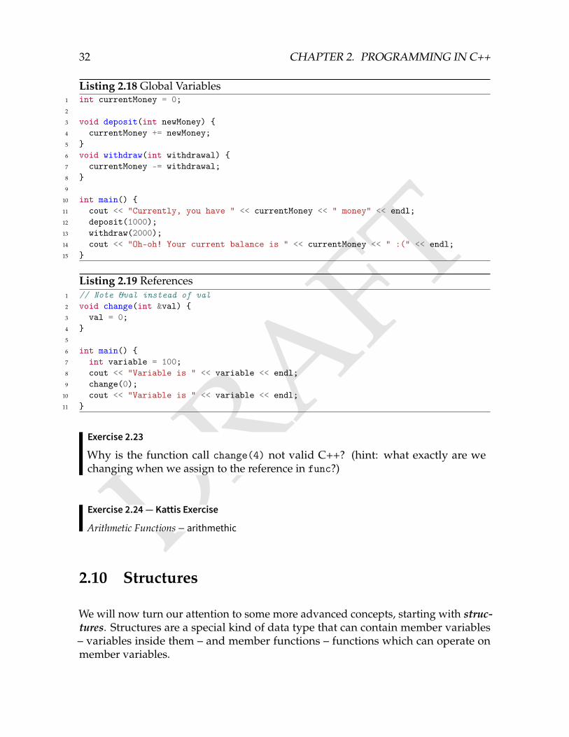
The first one is by using global variables. It turns out that variables may be declaredoutside of a function. It is then available to every function in your program. Changesto a global variable by one function will also be seen by other functions (try outListing 2.18 to see them in action).
Secondly, we may actually change the variables given to us as arguments by declaringthem as references. Such an argument is written by adding a & before the variablename, for example int &x. If we perform assignments to the variable x within thefunction, we will change the variable used for this argument in the calling functioninstead. For an example of references, check out Listing 2.19.
DRAFT
32 CHAPTER 2. PROGRAMMING IN C++
Listing 2.18 Global Variables1 int currentMoney = 0;2
3 void deposit(int newMoney) 4 currentMoney += newMoney;5 6 void withdraw(int withdrawal) 7 currentMoney -= withdrawal;8 9
10 int main() 11 cout << "Currently, you have " << currentMoney << " money" << endl;12 deposit(1000);13 withdraw(2000);14 cout << "Oh-oh! Your current balance is " << currentMoney << " :(" << endl;15
Listing 2.19 References1 // Note &val instead of val2 void change(int &val) 3 val = 0;4 5
6 int main() 7 int variable = 100;8 cout << "Variable is " << variable << endl;9 change(0);
10 cout << "Variable is " << variable << endl;11
Exercise 2.23
Why is the function call change(4) not valid C++? (hint: what exactly are wechanging when we assign to the reference in func?)
Exercise 2.24 — Kattis Exercise
Arithmetic Functions – arithmethic
2.10 Structures
We will now turn our attention to some more advanced concepts, starting with struc-tures. Structures are a special kind of data type that can contain member variables– variables inside them – and member functions – functions which can operate onmember variables.
DRAFT
2.10. STRUCTURES 33
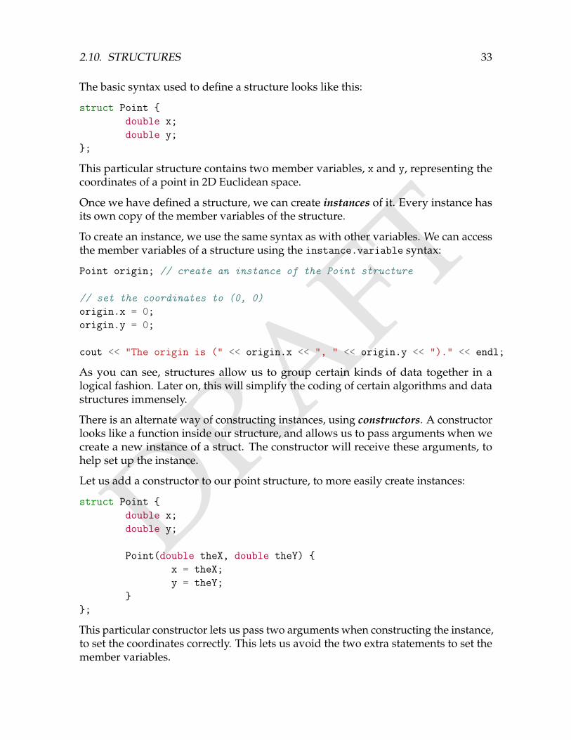
The basic syntax used to define a structure looks like this:
struct Point double x;double y;
;
This particular structure contains two member variables, x and y, representing thecoordinates of a point in 2D Euclidean space.
Once we have defined a structure, we can create instances of it. Every instance hasits own copy of the member variables of the structure.
To create an instance, we use the same syntax as with other variables. We can accessthe member variables of a structure using the instance.variable syntax:
Point origin; // create an instance of the Point structure
// set the coordinates to (0, 0)origin.x = 0;origin.y = 0;
cout << "The origin is (" << origin.x << ", " << origin.y << ")." << endl;
As you can see, structures allow us to group certain kinds of data together in alogical fashion. Later on, this will simplify the coding of certain algorithms and datastructures immensely.
There is an alternate way of constructing instances, using constructors. A constructorlooks like a function inside our structure, and allows us to pass arguments when wecreate a new instance of a struct. The constructor will receive these arguments, tohelp set up the instance.
Let us add a constructor to our point structure, to more easily create instances:
struct Point double x;double y;
Point(double theX, double theY) x = theX;y = theY;
;
This particular constructor lets us pass two arguments when constructing the instance,to set the coordinates correctly. This lets us avoid the two extra statements to set themember variables.
DRAFT
34 CHAPTER 2. PROGRAMMING IN C++
Point p(4, 2.1);cout << "The point is (" << p.x << ", " << p.y << ")." << endl;
We can also define functions inside the structure. These functions are as any otherfunctions, with the addition that they can access the member variables of the instancewhich the member function is called on. For example, we might want a convenientway to mirror a certain point in the x-axis. This could be accomplished by adding amember function:
struct Point double x;double y;
Point(double theX, double theY) x = theX;y = theY;
Point mirror() return Point(x, -y);
;
To call the member function mirror() on the point p, we write p.mirror().
Exercise 2.25
Add a translate member function to the point structure. It should take twodouble values x and y as arguments, returning a new point which is the instancepoint translated by (x, y).
In our mirror function, we are not modifying any of the internal state of the function.We can make this fact clearer by declaring the function to be const (similarly to aconst variable):
Point mirror() const return Point(x, -y);
This change ensures that our function will not be able to change any of the membervariables.
Exercise 2.26
What happens if we try to change a member variable in a const member function?
DRAFT
2.11. ARRAYS 35
Exercise 2.27
Write a struct which contains three variables of type Point called Triangle. Itshould have an area() member function which returns the area of the triangle.
Exercise 2.28
Fill in the remaining code to implement this structure:
struct Quotient int nominator;int denominator;
// Construct a new Quotient with the given nominator and denominatorQuotient(int n, int d)
...
// Return a new Quotient, this instance plus the "other" instanceQuotient add(const Quotient &other) const
...
// Return a new Quotient, this instance times the "other" instanceQuotient multiply(const Quotient &other) const
...
// Output the value on the screen in the format n/dvoid print() const
...
;
2.11 Arrays
An array is another special type of variable, which can contain a large number ofvariables of the same type. For example, it could be used to represent the recurringdata type “sequence of integers” from the Sorting Problem in Chapter 1. Whendeclaring an array, we specify the type of variable it should contain, its name and itssize using the syntax:
DRAFT
36 CHAPTER 2. PROGRAMMING IN C++
type name[size];
For example, an integer array of size 50 named seq would be declared using
int seq[50];
This creates 50 integer “variables”, which we can refer to using the syntax seq[index],starting from zero (they are zero-indexed). Thus we can use seq[0], seq[1], etc, allthe way up to seq[49].
Be aware that using an index outside the valid range for a particular array (i.e. below0 or above the size − 1 can cause erratic behavior in the program without crashingit.
Later on, we will transition from using arrays to using a structure from the standardlibrary which serve the same purpose – the vector.
Exercise 2.29 — Kattis Exercise
Reversing Strings – reverse
2.12 The Preprocessor
C++ has a powerful tool called the preprocessor. This utility is able to read andmodify your code using certain rules during compilation. For example, #include is apreprocessor directive that includes a certain file in your code.
Most commonly, we will use the #define directive. It allows us to replace certaintokens in our code with other ones. The most basic usage is
#define TOREPLACE REPLACEWITH
which replaces the token TOREPLACE in our program with REPLACEWITH. The truepower of the define comes when using define directives with parameters. These looksimilar to functions, and allows us to replace certain expressions with another one,additionally inserting certain values into it. We call these macros. For example themacro
#define rep(i,a,b) for (int i = a; i < b; i++)
means that the expression
rep(i,0,5) cout << i << endl;
is expanded to
DRAFT
2.13. TEMPLATE 37
for (int i = 0; i < 5; ++i) cout << i << endl;
You can probably get by without ever using macros in your code. The reason wediscuss them is because we are going to use them in code in the book, so it is a goodidea to at least be familiar with their meaning.
2.13 Template
In competitive programming, one often use a template, with some shorthand typedef’sand preprocessor directives. Here, we given an example of such a template, whichwill be used in some of the C++ code in this book.
#include <bits/stdc++.h>using namespace std;
#define rep(i, a, b) for(int i = a; i < (b); ++i)#define trav(a, x) for(auto& a : x)#define all(x) x.begin(), x.end()#define sz(x) (int)(x).size()typedef long long ll;typedef pair<int, int> pii;typedef vector<int> vi;
int main()
The trav(a, x) macro is used to iterate through all members of a data structure fromthe standard library. We will study such data structures in later chapters.
2.14 Additional ExercisesExercise 2.30 — Kattis Exercises
Solving for Carrots – carrots
Paul Eigon – pauleigon
Dice Game – dicegame
Reverse Binary – reversebinary
DRAFT
38 CHAPTER 2. PROGRAMMING IN C++
2.15 Chapter Notes
C++ was invented by Danish computer scientist Bjarne Stroustrup. Bjarne has alsopublished a book on the language, The C++ Programming Language[23] which containsa more in-depth treatment of the language. It is rather accessible to C++ beginners,but is better read by someone who have some prior programming experience (in anyprogramming language).
C++ is standardized by the International Organization for Standardization (ISO).These standards are the authoritative source on what C++ is. They final drafts ofthe standards can be downloaded at the homepage of the Standard C++ Founda-tion1.
There are many online references of the language and its standard library. The twowe use most are:
• http://en.cppreference.com/w/
• http://www.cplusplus.com/reference/
1https://isocpp.org/
DRAFTChapter 3
Implementation Problems
The “simplest” kind of problem we solve is those where the statement of a problemis so detailed that the difficult part is not to figure out the solution, but to imple-ment it in code. This kind of problem often comes in the form of performing somegiven calculation or simulating some process, based on a list of rules stated in theproblem.
The RecipeSwedish Olympiad in Informatics 2011, School Qualifiers
You have decided to cook some food. The dish you wish to make requires Ndifferent ingredients. For every ingredient, you know the amount you have athome, how much you need for the dish, and how much it costs to buy (per unit).
If you do not have a sufficient amount of some ingredient, you need to buythe remainder from the store. Your task is to compute the cost of buying theremaining ingredients.
InputThe first line of input is an integer N ≤ 10, the number of ingredients in the dish.
The next N lines contain the information about the ingredients, one per line. Aningredient is given by three space-separated integers 0 ≤ h,n, c ≤ 200 – theamount you have, the amount you need, and the cost per unit for this ingredient.
OutputOutput a single integer – the cost for purchasing the remaining ingredients neededto make the dish.
This problem is not particularly hard. For every ingredient, we first calculate theamount which we need to purchase. The only gotcha in the problem is the mistake ofcalculating this as n− h. The correct formula is max(0, n− h), required in case of the
39
DRAFT
40 CHAPTER 3. IMPLEMENTATION PROBLEMS
luxury problem of having more than we need. We then multiply this number by theingredient cost, and sum the costs up for all the ingredients.
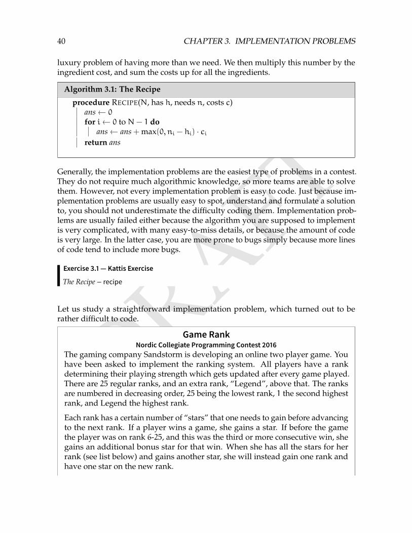
Algorithm 3.1: The Recipe
procedure RECIPE(N, has h, needs n, costs c)ans← 0
for i← 0 to N− 1 doans← ans + max(0, ni − hi) · ci
return ans
Generally, the implementation problems are the easiest type of problems in a contest.They do not require much algorithmic knowledge, so more teams are able to solvethem. However, not every implementation problem is easy to code. Just because im-plementation problems are usually easy to spot, understand and formulate a solutionto, you should not underestimate the difficulty coding them. Implementation prob-lems are usually failed either because the algorithm you are supposed to implementis very complicated, with many easy-to-miss details, or because the amount of codeis very large. In the latter case, you are more prone to bugs simply because more linesof code tend to include more bugs.
Exercise 3.1 — Kattis Exercise
The Recipe – recipe
Let us study a straightforward implementation problem, which turned out to berather difficult to code.
Game RankNordic Collegiate Programming Contest 2016
The gaming company Sandstorm is developing an online two player game. Youhave been asked to implement the ranking system. All players have a rankdetermining their playing strength which gets updated after every game played.There are 25 regular ranks, and an extra rank, “Legend”, above that. The ranksare numbered in decreasing order, 25 being the lowest rank, 1 the second highestrank, and Legend the highest rank.
Each rank has a certain number of “stars” that one needs to gain before advancingto the next rank. If a player wins a game, she gains a star. If before the gamethe player was on rank 6-25, and this was the third or more consecutive win, shegains an additional bonus star for that win. When she has all the stars for herrank (see list below) and gains another star, she will instead gain one rank andhave one star on the new rank.
DRAFT
41
For instance, if before a winning game the player had all the stars on her currentrank, she will after the game have gained one rank and have 1 or 2 stars (depend-ing on whether she got a bonus star) on the new rank. If on the other hand shehad all stars except one on a rank, and won a game that also gave her a bonusstar, she would gain one rank and have 1 star on the new rank.
If a player on rank 1-20 loses a game, she loses a star. If a player has zero stars ona rank and loses a star, she will lose a rank and have all stars minus one on therank below. However, one can never drop below rank 20 (losing a game at rank20with no stars will have no effect).
If a player reaches the Legend rank, she will stay legend no matter how manylosses she incurs afterwards.
The number of stars on each rank are as follows:
• Rank 25-21: 2 stars
• Rank 20-16: 3 stars
• Rank 15-11: 4 stars
• Rank 10-1: 5 stars
A player starts at rank 25 with no stars. Given the match history of a player, whatis her rank at the end of the sequence of matches?
InputThe input consists of a single line describing the sequence of matches. Eachcharacter corresponds to one game; ‘W’ represents a win and ‘L’ a loss. The lengthof the line is between 1 and 10 000 characters (inclusive).
OutputOutput a single line containing a rank after having played the given sequence ofgames; either an integer between 1 and 25 or “Legend”.
A very long problem statement! The first hurdle is finding the energy to read it fromstart to finish, without skipping any details. Not much creativity is needed here –indeed, the algorithm to implement is given in the statement. Despite this, it is not aseasy as one would think. At the contest where it was used, it was the second mostsolved problem, but also the one with the worst success ratio. On average, a teamneeded 3.59 attempts before getting a correct solution, compared to the runner-up at2.92 attempts. None of the top 6 teams in the contest got the problem accepted on theirfirst attempt. Failed attempts cost a lot. Not only in absolute time, but many forms ofcompetition include additional penalties for submitting incorrect solutions.
Implementation problems get much easier when you know your programming lan-guage well, and can use it to write good, structured code. Split code into functions,
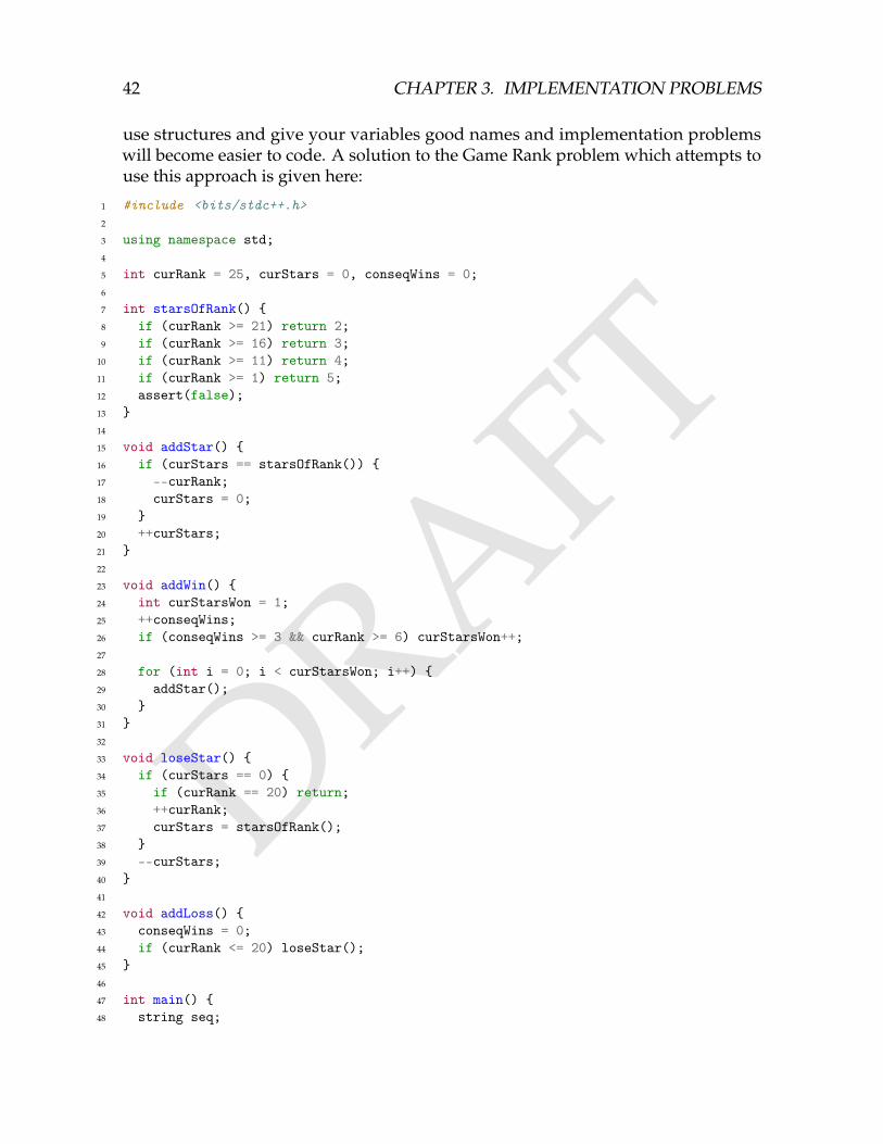
DRAFT
42 CHAPTER 3. IMPLEMENTATION PROBLEMS
use structures and give your variables good names and implementation problemswill become easier to code. A solution to the Game Rank problem which attempts touse this approach is given here:
1 #include <bits/stdc++.h>2
3 using namespace std;4
5 int curRank = 25, curStars = 0, conseqWins = 0;6
7 int starsOfRank() 8 if (curRank >= 21) return 2;9 if (curRank >= 16) return 3;
10 if (curRank >= 11) return 4;11 if (curRank >= 1) return 5;12 assert(false);13 14
15 void addStar() 16 if (curStars == starsOfRank()) 17 --curRank;18 curStars = 0;19 20 ++curStars;21 22
23 void addWin() 24 int curStarsWon = 1;25 ++conseqWins;26 if (conseqWins >= 3 && curRank >= 6) curStarsWon++;27
28 for (int i = 0; i < curStarsWon; i++) 29 addStar();30 31 32
33 void loseStar() 34 if (curStars == 0) 35 if (curRank == 20) return;36 ++curRank;37 curStars = starsOfRank();38 39 --curStars;40 41
42 void addLoss() 43 conseqWins = 0;44 if (curRank <= 20) loseStar();45 46
47 int main() 48 string seq;
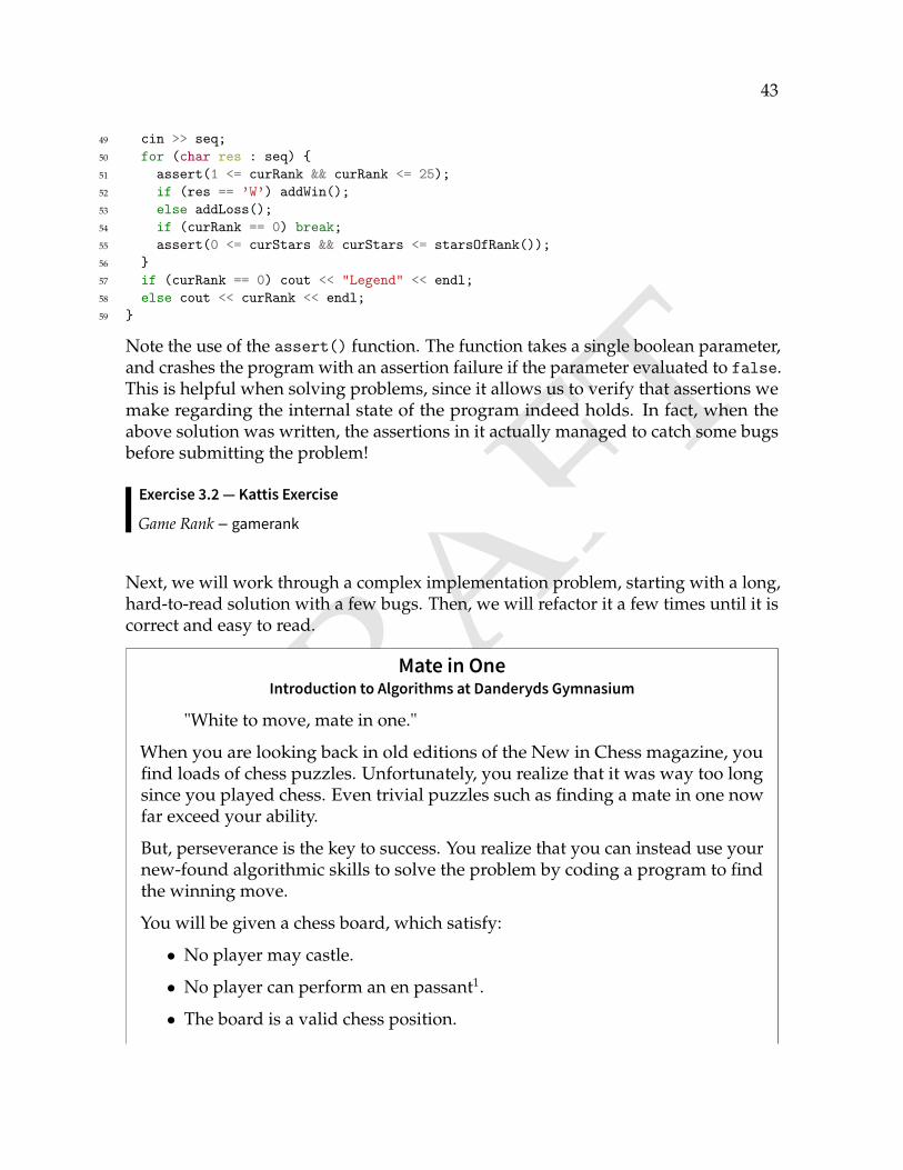
DRAFT
43
49 cin >> seq;50 for (char res : seq) 51 assert(1 <= curRank && curRank <= 25);52 if (res == ’W’) addWin();53 else addLoss();54 if (curRank == 0) break;55 assert(0 <= curStars && curStars <= starsOfRank());56 57 if (curRank == 0) cout << "Legend" << endl;58 else cout << curRank << endl;59
Note the use of the assert() function. The function takes a single boolean parameter,and crashes the program with an assertion failure if the parameter evaluated to false.This is helpful when solving problems, since it allows us to verify that assertions wemake regarding the internal state of the program indeed holds. In fact, when theabove solution was written, the assertions in it actually managed to catch some bugsbefore submitting the problem!
Exercise 3.2 — Kattis Exercise
Game Rank – gamerank
Next, we will work through a complex implementation problem, starting with a long,hard-to-read solution with a few bugs. Then, we will refactor it a few times until it iscorrect and easy to read.
Mate in OneIntroduction to Algorithms at Danderyds Gymnasium
"White to move, mate in one."
When you are looking back in old editions of the New in Chess magazine, youfind loads of chess puzzles. Unfortunately, you realize that it was way too longsince you played chess. Even trivial puzzles such as finding a mate in one nowfar exceed your ability.
But, perseverance is the key to success. You realize that you can instead use yournew-found algorithmic skills to solve the problem by coding a program to findthe winning move.
You will be given a chess board, which satisfy:
• No player may castle.
• No player can perform an en passant1.
• The board is a valid chess position.
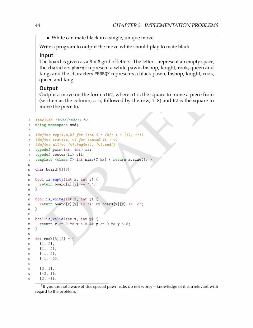
DRAFT
44 CHAPTER 3. IMPLEMENTATION PROBLEMS
• White can mate black in a single, unique move.
Write a program to output the move white should play to mate black.
InputThe board is given as a 8× 8 grid of letters. The letter . represent an empty space,the characters pbnrqk represent a white pawn, bishop, knight, rook, queen andking, and the characters PBNRQK represents a black pawn, bishop, knight, rook,queen and king.
OutputOutput a move on the form a1b2, where a1 is the square to move a piece from(written as the column, a-h, followed by the row, 1-8) and b2 is the square tomove the piece to.
1 #include <bits/stdc++.h>2 using namespace std;3
4 #define rep(i,a,b) for (int i = (a); i < (b); ++i)5 #define trav(it, v) for (auto& it : v)6 #define all(v) (v).begin(), (v).end()7 typedef pair<int, int> ii;8 typedef vector<ii> vii;9 template <class T> int size(T &x) return x.size();
10
11 char board[8][8];12
13 bool iz_empty(int x, int y) 14 return board[x][y] == ’.’;15 16
17 bool is_white(int x, int y) 18 return board[x][y] >= ’A’ && board[x][y] <= ’Z’;19 20
21 bool is_valid(int x, int y) 22 return x >= 0 && x < 8 && y >= 0 && y < 8;23 24
25 int rook[8][2] = 26 1, 2,27 1, -2,28 -1, 2,29 -1, -2,30
31 2, 1,32 -2, 1,33 2, -1,
1If you are not aware of this special pawn rule, do not worry – knowledge of it is irrelevant withregard to the problem.
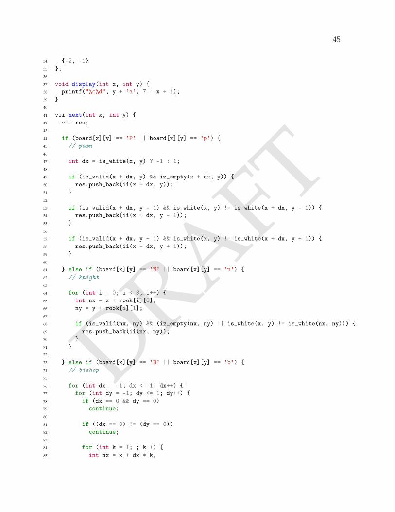
DRAFT
45
34 -2, -135 ;36
37 void display(int x, int y) 38 printf("%c%d", y + ’a’, 7 - x + 1);39 40
41 vii next(int x, int y) 42 vii res;43
44 if (board[x][y] == ’P’ || board[x][y] == ’p’) 45 // pawn46
47 int dx = is_white(x, y) ? -1 : 1;48
49 if (is_valid(x + dx, y) && iz_empty(x + dx, y)) 50 res.push_back(ii(x + dx, y));51 52
53 if (is_valid(x + dx, y - 1) && is_white(x, y) != is_white(x + dx, y - 1)) 54 res.push_back(ii(x + dx, y - 1));55 56
57 if (is_valid(x + dx, y + 1) && is_white(x, y) != is_white(x + dx, y + 1)) 58 res.push_back(ii(x + dx, y + 1));59 60
61 else if (board[x][y] == ’N’ || board[x][y] == ’n’) 62 // knight63
64 for (int i = 0; i < 8; i++) 65 int nx = x + rook[i][0],66 ny = y + rook[i][1];67
68 if (is_valid(nx, ny) && (iz_empty(nx, ny) || is_white(x, y) != is_white(nx, ny))) 69 res.push_back(ii(nx, ny));70 71 72
73 else if (board[x][y] == ’B’ || board[x][y] == ’b’) 74 // bishop75
76 for (int dx = -1; dx <= 1; dx++) 77 for (int dy = -1; dy <= 1; dy++) 78 if (dx == 0 && dy == 0)79 continue;80
81 if ((dx == 0) != (dy == 0))82 continue;83
84 for (int k = 1; ; k++) 85 int nx = x + dx * k,
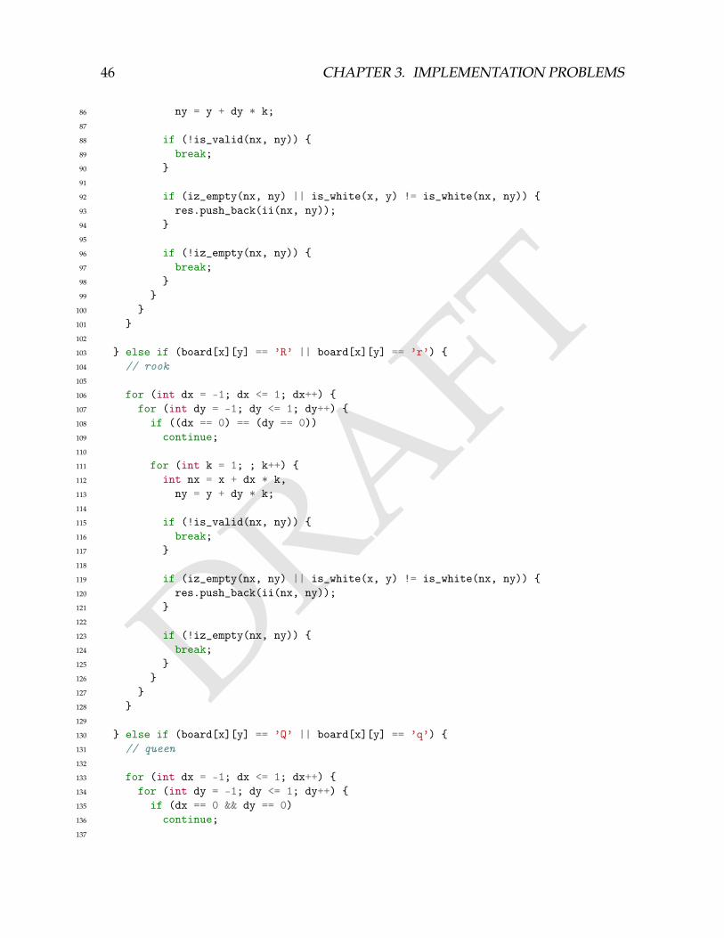
DRAFT
46 CHAPTER 3. IMPLEMENTATION PROBLEMS
86 ny = y + dy * k;87
88 if (!is_valid(nx, ny)) 89 break;90 91
92 if (iz_empty(nx, ny) || is_white(x, y) != is_white(nx, ny)) 93 res.push_back(ii(nx, ny));94 95
96 if (!iz_empty(nx, ny)) 97 break;98 99
100 101 102
103 else if (board[x][y] == ’R’ || board[x][y] == ’r’) 104 // rook105
106 for (int dx = -1; dx <= 1; dx++) 107 for (int dy = -1; dy <= 1; dy++) 108 if ((dx == 0) == (dy == 0))109 continue;110
111 for (int k = 1; ; k++) 112 int nx = x + dx * k,113 ny = y + dy * k;114
115 if (!is_valid(nx, ny)) 116 break;117 118
119 if (iz_empty(nx, ny) || is_white(x, y) != is_white(nx, ny)) 120 res.push_back(ii(nx, ny));121 122
123 if (!iz_empty(nx, ny)) 124 break;125 126 127 128 129
130 else if (board[x][y] == ’Q’ || board[x][y] == ’q’) 131 // queen132
133 for (int dx = -1; dx <= 1; dx++) 134 for (int dy = -1; dy <= 1; dy++) 135 if (dx == 0 && dy == 0)136 continue;137
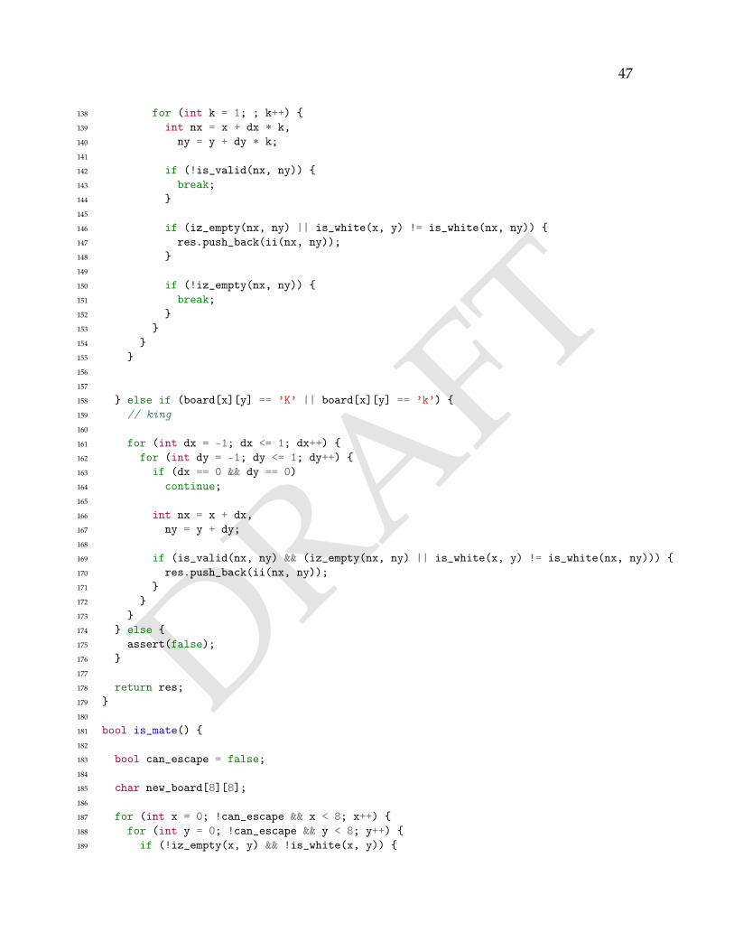
DRAFT
47
138 for (int k = 1; ; k++) 139 int nx = x + dx * k,140 ny = y + dy * k;141
142 if (!is_valid(nx, ny)) 143 break;144 145
146 if (iz_empty(nx, ny) || is_white(x, y) != is_white(nx, ny)) 147 res.push_back(ii(nx, ny));148 149
150 if (!iz_empty(nx, ny)) 151 break;152 153 154 155 156
157
158 else if (board[x][y] == ’K’ || board[x][y] == ’k’) 159 // king160
161 for (int dx = -1; dx <= 1; dx++) 162 for (int dy = -1; dy <= 1; dy++) 163 if (dx == 0 && dy == 0)164 continue;165
166 int nx = x + dx,167 ny = y + dy;168
169 if (is_valid(nx, ny) && (iz_empty(nx, ny) || is_white(x, y) != is_white(nx, ny))) 170 res.push_back(ii(nx, ny));171 172 173 174 else 175 assert(false);176 177
178 return res;179 180
181 bool is_mate() 182
183 bool can_escape = false;184
185 char new_board[8][8];186
187 for (int x = 0; !can_escape && x < 8; x++) 188 for (int y = 0; !can_escape && y < 8; y++) 189 if (!iz_empty(x, y) && !is_white(x, y))
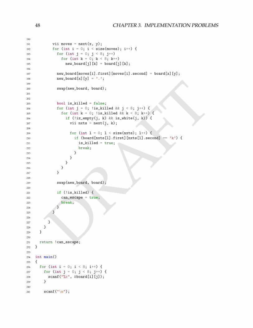
DRAFT
48 CHAPTER 3. IMPLEMENTATION PROBLEMS
190
191 vii moves = next(x, y);192 for (int i = 0; i < size(moves); i++) 193 for (int j = 0; j < 8; j++)194 for (int k = 0; k < 8; k++)195 new_board[j][k] = board[j][k];196
197 new_board[moves[i].first][moves[i].second] = board[x][y];198 new_board[x][y] = ’.’;199
200 swap(new_board, board);201
202
203 bool is_killed = false;204 for (int j = 0; !is_killed && j < 8; j++) 205 for (int k = 0; !is_killed && k < 8; k++) 206 if (!iz_empty(j, k) && is_white(j, k)) 207 vii nxts = next(j, k);208
209 for (int l = 0; l < size(nxts); l++) 210 if (board[nxts[l].first][nxts[l].second] == ’k’) 211 is_killed = true;212 break;213 214 215 216 217 218
219 swap(new_board, board);220
221 if (!is_killed) 222 can_escape = true;223 break;224 225 226
227 228 229 230
231 return !can_escape;232 233
234 int main()235 236 for (int i = 0; i < 8; i++) 237 for (int j = 0; j < 8; j++) 238 scanf("%c", &board[i][j]);239 240
241 scanf("\n");
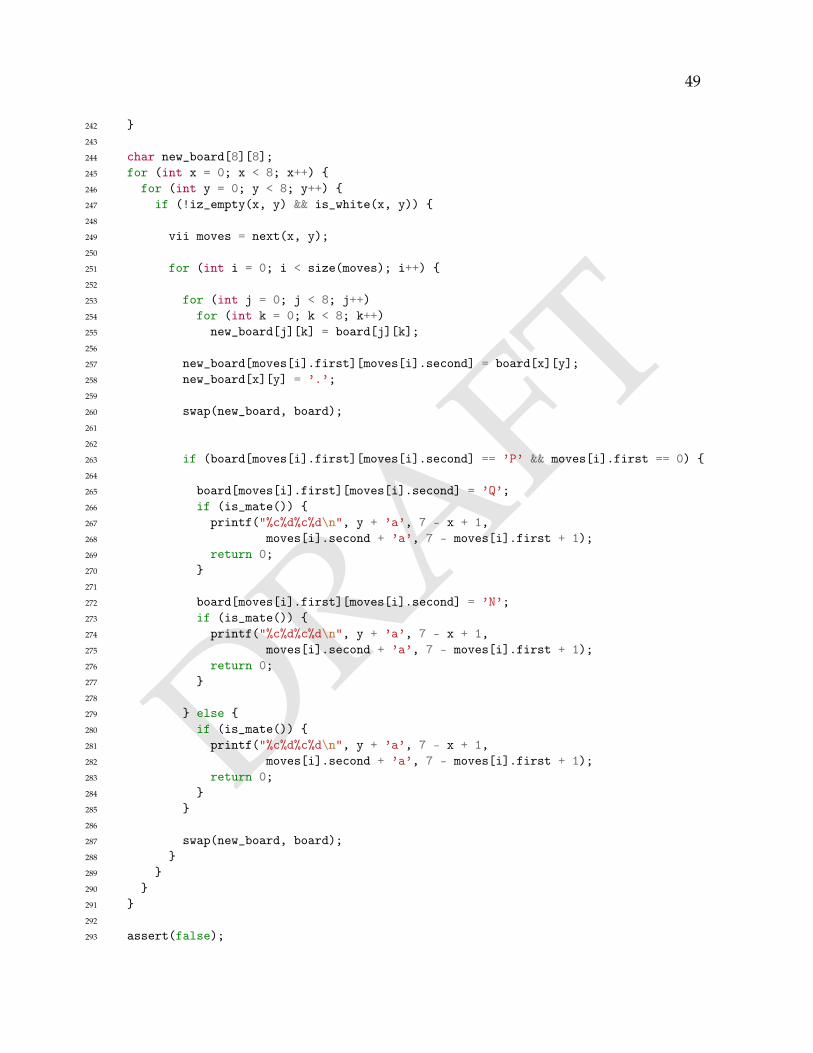
DRAFT
49
242 243
244 char new_board[8][8];245 for (int x = 0; x < 8; x++) 246 for (int y = 0; y < 8; y++) 247 if (!iz_empty(x, y) && is_white(x, y)) 248
249 vii moves = next(x, y);250
251 for (int i = 0; i < size(moves); i++) 252
253 for (int j = 0; j < 8; j++)254 for (int k = 0; k < 8; k++)255 new_board[j][k] = board[j][k];256
257 new_board[moves[i].first][moves[i].second] = board[x][y];258 new_board[x][y] = ’.’;259
260 swap(new_board, board);261
262
263 if (board[moves[i].first][moves[i].second] == ’P’ && moves[i].first == 0) 264
265 board[moves[i].first][moves[i].second] = ’Q’;266 if (is_mate()) 267 printf("%c%d%c%d\n", y + ’a’, 7 - x + 1,268 moves[i].second + ’a’, 7 - moves[i].first + 1);269 return 0;270 271
272 board[moves[i].first][moves[i].second] = ’N’;273 if (is_mate()) 274 printf("%c%d%c%d\n", y + ’a’, 7 - x + 1,275 moves[i].second + ’a’, 7 - moves[i].first + 1);276 return 0;277 278
279 else 280 if (is_mate()) 281 printf("%c%d%c%d\n", y + ’a’, 7 - x + 1,282 moves[i].second + ’a’, 7 - moves[i].first + 1);283 return 0;284 285 286
287 swap(new_board, board);288 289 290 291 292
293 assert(false);
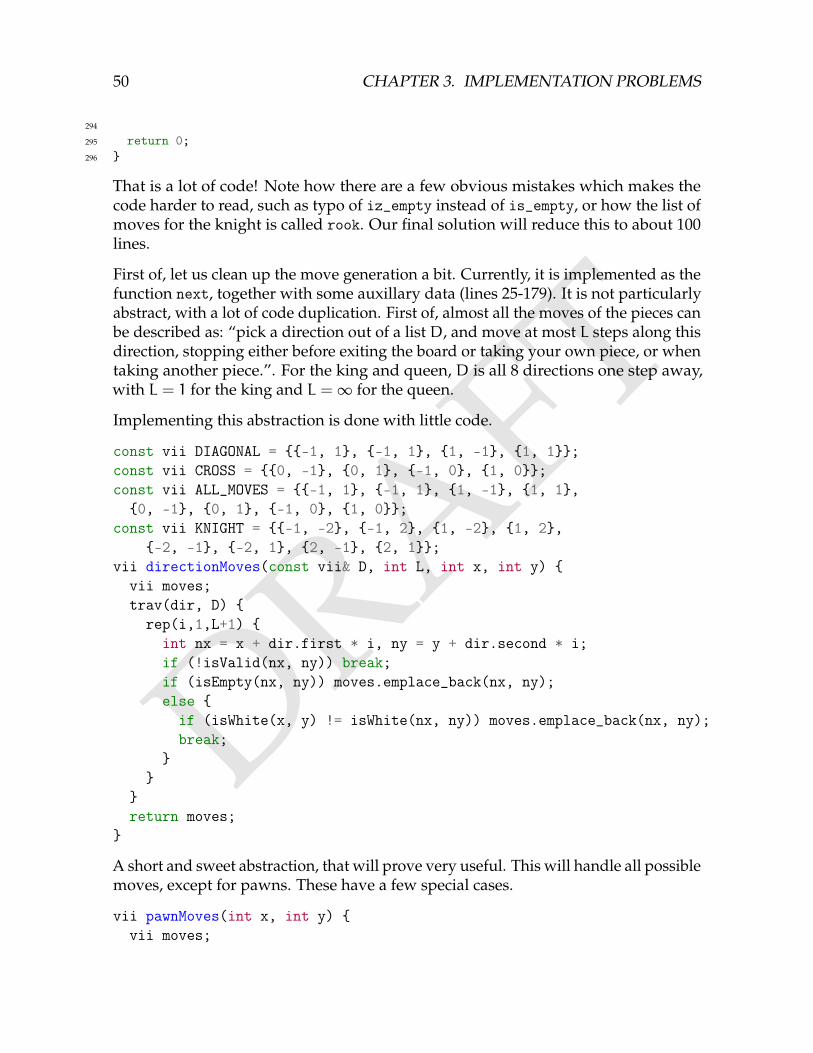
DRAFT
50 CHAPTER 3. IMPLEMENTATION PROBLEMS
294
295 return 0;296
That is a lot of code! Note how there are a few obvious mistakes which makes thecode harder to read, such as typo of iz_empty instead of is_empty, or how the list ofmoves for the knight is called rook. Our final solution will reduce this to about 100lines.
First of, let us clean up the move generation a bit. Currently, it is implemented as thefunction next, together with some auxillary data (lines 25-179). It is not particularlyabstract, with a lot of code duplication. First of, almost all the moves of the pieces canbe described as: “pick a direction out of a list D, and move at most L steps along thisdirection, stopping either before exiting the board or taking your own piece, or whentaking another piece.”. For the king and queen, D is all 8 directions one step away,with L = 1 for the king and L =∞ for the queen.
Implementing this abstraction is done with little code.
const vii DIAGONAL = -1, 1, -1, 1, 1, -1, 1, 1;const vii CROSS = 0, -1, 0, 1, -1, 0, 1, 0;const vii ALL_MOVES = -1, 1, -1, 1, 1, -1, 1, 1,0, -1, 0, 1, -1, 0, 1, 0;
const vii KNIGHT = -1, -2, -1, 2, 1, -2, 1, 2,-2, -1, -2, 1, 2, -1, 2, 1;
vii directionMoves(const vii& D, int L, int x, int y) vii moves;trav(dir, D) rep(i,1,L+1) int nx = x + dir.first * i, ny = y + dir.second * i;if (!isValid(nx, ny)) break;if (isEmpty(nx, ny)) moves.emplace_back(nx, ny);else if (isWhite(x, y) != isWhite(nx, ny)) moves.emplace_back(nx, ny);break;
return moves;
A short and sweet abstraction, that will prove very useful. This will handle all possiblemoves, except for pawns. These have a few special cases.
vii pawnMoves(int x, int y) vii moves;
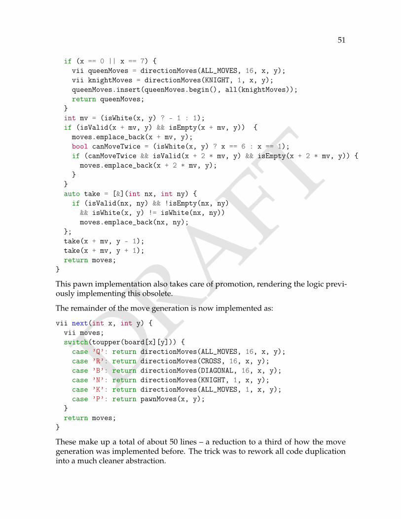
DRAFT
51
if (x == 0 || x == 7) vii queenMoves = directionMoves(ALL_MOVES, 16, x, y);vii knightMoves = directionMoves(KNIGHT, 1, x, y);queenMoves.insert(queenMoves.begin(), all(knightMoves));return queenMoves;
int mv = (isWhite(x, y) ? - 1 : 1);if (isValid(x + mv, y) && isEmpty(x + mv, y)) moves.emplace_back(x + mv, y);bool canMoveTwice = (isWhite(x, y) ? x == 6 : x == 1);if (canMoveTwice && isValid(x + 2 * mv, y) && isEmpty(x + 2 * mv, y)) moves.emplace_back(x + 2 * mv, y);
auto take = [&](int nx, int ny) if (isValid(nx, ny) && !isEmpty(nx, ny)&& isWhite(x, y) != isWhite(nx, ny))moves.emplace_back(nx, ny);
;take(x + mv, y - 1);take(x + mv, y + 1);return moves;
This pawn implementation also takes care of promotion, rendering the logic previ-ously implementing this obsolete.
The remainder of the move generation is now implemented as:
vii next(int x, int y) vii moves;switch(toupper(board[x][y])) case ’Q’: return directionMoves(ALL_MOVES, 16, x, y);case ’R’: return directionMoves(CROSS, 16, x, y);case ’B’: return directionMoves(DIAGONAL, 16, x, y);case ’N’: return directionMoves(KNIGHT, 1, x, y);case ’K’: return directionMoves(ALL_MOVES, 1, x, y);case ’P’: return pawnMoves(x, y);
return moves;
These make up a total of about 50 lines – a reduction to a third of how the movegeneration was implemented before. The trick was to rework all code duplicationinto a much cleaner abstraction.
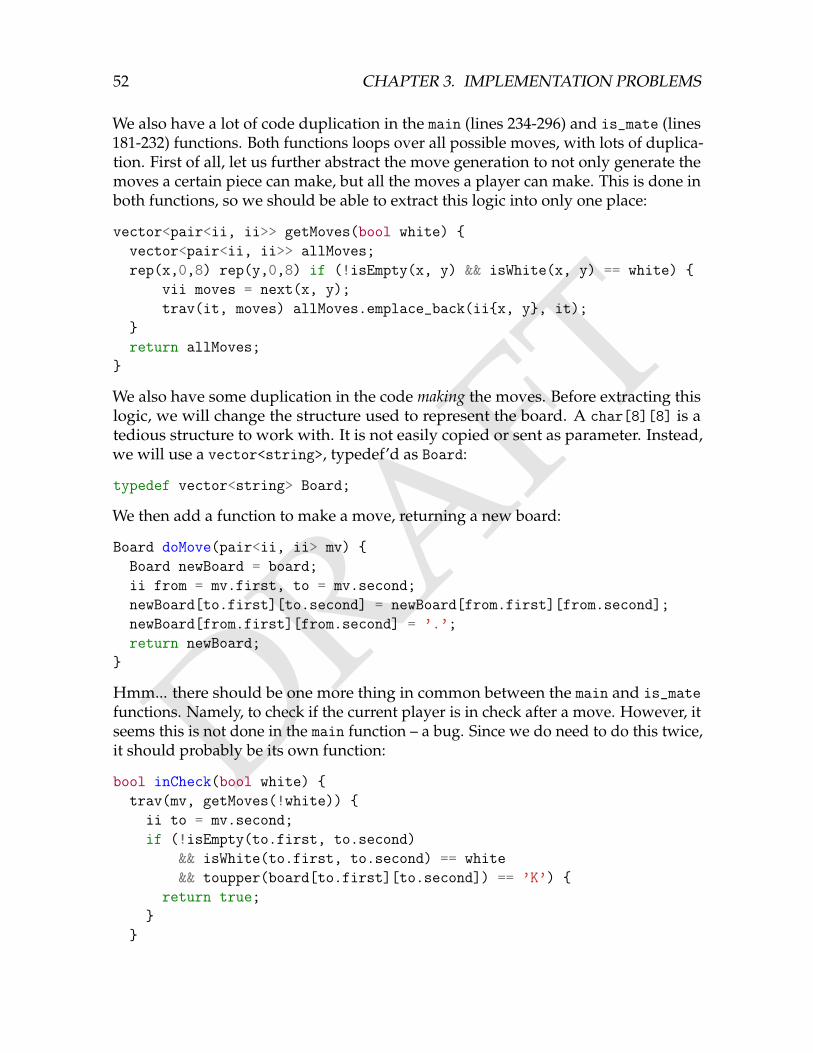
DRAFT
52 CHAPTER 3. IMPLEMENTATION PROBLEMS
We also have a lot of code duplication in the main (lines 234-296) and is_mate (lines181-232) functions. Both functions loops over all possible moves, with lots of duplica-tion. First of all, let us further abstract the move generation to not only generate themoves a certain piece can make, but all the moves a player can make. This is done inboth functions, so we should be able to extract this logic into only one place:
vector<pair<ii, ii>> getMoves(bool white) vector<pair<ii, ii>> allMoves;rep(x,0,8) rep(y,0,8) if (!isEmpty(x, y) && isWhite(x, y) == white)
vii moves = next(x, y);trav(it, moves) allMoves.emplace_back(iix, y, it);
return allMoves;
We also have some duplication in the code making the moves. Before extracting thislogic, we will change the structure used to represent the board. A char[8][8] is atedious structure to work with. It is not easily copied or sent as parameter. Instead,we will use a vector<string>, typedef’d as Board:
typedef vector<string> Board;
We then add a function to make a move, returning a new board:
Board doMove(pair<ii, ii> mv) Board newBoard = board;ii from = mv.first, to = mv.second;newBoard[to.first][to.second] = newBoard[from.first][from.second];newBoard[from.first][from.second] = ’.’;return newBoard;
Hmm... there should be one more thing in common between the main and is_matefunctions. Namely, to check if the current player is in check after a move. However, itseems this is not done in the main function – a bug. Since we do need to do this twice,it should probably be its own function:
bool inCheck(bool white) trav(mv, getMoves(!white)) ii to = mv.second;if (!isEmpty(to.first, to.second)
&& isWhite(to.first, to.second) == white&& toupper(board[to.first][to.second]) == ’K’)
return true;
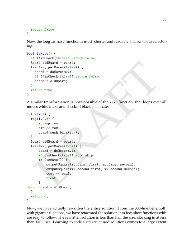
DRAFT
53
return false;
Now, the long is_mate function is much shorter and readable, thanks to our refactor-ing:
bool isMate() if (!inCheck(false)) return false;Board oldBoard = board;trav(mv, getMoves(false)) board = doMove(mv);if (!inCheck(false)) return false;board = oldBoard;
return true;
A similar transformation is now possible of the main function, that loops over allmoves white make and checks if black is in mate:
int main() rep(i,0,8)
string row;cin >> row;board.push_back(row);
Board oldBoard = board;trav(mv, getMoves(true))
board = doMove(mv);if (inCheck(true)) goto skip;if (isMate())
outputSquare(mv.first.first, mv.first.second);outputSquare(mv.second.first, mv.second.second);cout << endl;break;
skip: board = oldBoard;return 0;
Now, we have actually rewritten the entire solution. From the 300-line behemothwith gigantic functions, we have refactored the solution into few, short functions withare easy to follow. The rewritten solution is less than half the size, clocking in at lessthan 140 lines. Learning to code such structured solutions comes to a large extent

DRAFT
54 CHAPTER 3. IMPLEMENTATION PROBLEMS
from experience. During a competition, we might not spend time thinking about howto structure our solutions, instead focusing on getting it done as soon as possible.However, spending 1-2 minutes thinking about how to best implement a complexsolution could pay off not only in faster implementation times (such as halving thesize of the program), but also in being less buggy.
To sum up: implementation problems should not be underestimated in terms ofimplementation complexity. Work on your coding best practices and spend time prac-ticing coding complex solutions, and you will see your implementation performanceimprove.
3.1 Additional ExercisesExercise 3.3
Flexible Spaces – flexiblespaces
Sort of Sorting – sortofsorting
Permutation Encryption – permutationencryption
Jury Jeopardy – juryjeopardy
Fun House – funhouse
Settlers of Catan – settlers2
Cross – cross
Basic Interpreter – basicinterpreter
Cat Coat Colors – catcoat
3.2 Chapter Notes
Many good sources exist to become more proficient at writing readable, simple code.Clean Code[13] describes many principles that helps in writing better code. It includesgood walk-throughs on refactoring, and shows in a very tangible fashion how codingcleanly also makes coding easier.
Code Complete[14] is a huge tome on improving your programming skills. While muchof the content is not particularly relevant to coding algorithmic problems, chapters5-19 give many suggestions on coding style.
Different languages have different best practices. Some resources on improving yourskills in whatever language you code in are:

DRAFT
3.2. CHAPTER NOTES 55
C++ Effective C++[16], Effective Modern C++[17], Effective STL[15], by Scott Meyers,
Java Effective Java[3] by Joshua Bloch,
Python Effective Python[21] by Brett Slatkin, Python Cookbook[2] by David Beazley andBrian K. Jones.

DRAFT
56 CHAPTER 3. IMPLEMENTATION PROBLEMS
DRAFTChapter 4
Time Complexity
How do you know if your algorithm is fast enough before you have coded it? Inthis chapter, we will look at this question from the perspective of time complexity,a common tool of algorithm analysis to determine roughly how fast an algorithmis.
We will start our study of complexity by looking at a new sorting algorithm – insertionsort. Just like selection sort, which we studied in Chapter 1, insertion sort works byiteratively sorting the array.
4.1 The Complexity of Insertion Sort
The insertion sort algorithm works by ensuring that all of the first i elements of theinput sequence are sorted. First for i = 1, then for i = 2, etc, up to i = n, at whichpoint the entire sequence is sorted.
Algorithm 4.1: Insertion Sort
Assume we wish to sort the list a0, a1, ..., aN−1 of N integers. If we know that thefirst K elements a0, ..., aK−1 numbers are sorted, we can make the list a0, ..., aKsorted by taking the element aK and inserting it into the correct position of thealready-sorted prefix a0, ..., aK−1.
For example, we know that a list of a single element is always sorted, so we canuse that a0 is sorted as a base case. We can then sort a0, a1 by checking whethera1 should be to the left or to the right of a0. In the first case, we swap the twonumbers.
Once we have sorted a0, a1, we will insert a2 into the sorted list. If it is larger
57
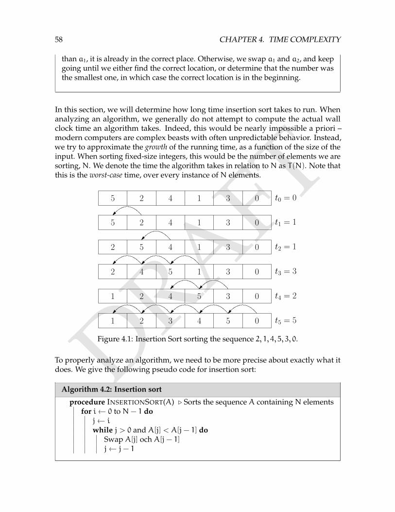
DRAFT
58 CHAPTER 4. TIME COMPLEXITY
than a1, it is already in the correct place. Otherwise, we swap a1 and a2, and keepgoing until we either find the correct location, or determine that the number wasthe smallest one, in which case the correct location is in the beginning.
In this section, we will determine how long time insertion sort takes to run. Whenanalyzing an algorithm, we generally do not attempt to compute the actual wallclock time an algorithm takes. Indeed, this would be nearly impossible a priori –modern computers are complex beasts with often unpredictable behavior. Instead,we try to approximate the growth of the running time, as a function of the size of theinput. When sorting fixed-size integers, this would be the number of elements we aresorting,N. We denote the time the algorithm takes in relation toN as T(N). Note thatthis is the worst-case time, over every instance of N elements.
5 2 4 1 3 0 t0 = 0
5 2 4 1 3 0 t1 = 1
2 5 4 1 3 0 t2 = 1
2 4 5 1 3 0 t3 = 3
1 2 4 5 3 0 t4 = 2
1 2 3 4 5 0 t5 = 5
Figure 4.1: Insertion Sort sorting the sequence 2, 1, 4, 5, 3, 0.
To properly analyze an algorithm, we need to be more precise about exactly what itdoes. We give the following pseudo code for insertion sort:
Algorithm 4.2: Insertion sort
procedure INSERTIONSORT(A) . Sorts the sequence A containing N elementsfor i← 0 to N− 1 doj← i
while j > 0 and A[j] < A[j− 1] doSwap A[j] och A[j− 1]j← j− 1
DRAFT
4.1. THE COMPLEXITY OF INSERTION SORT 59
To analyze the running time of the algorithm, we make the assumption that any“sufficiently small” operation takes the same amount of time – exactly 1 (of someundefined unit). We have to be careful in what assumptions we make regarding whata sufficiently small operation means. For example, sorting N numbers is not a smalloperation, while adding or multiplying two fixed-size numbers is. Multiplicationof integers of arbitrary size is not a small operation (see the Karatsuba algorithm,Chapter 8).
In our program, every line happens to represent a small operation. However, thetwo loops may cause some lines to execute more than once. The outer for loop willexecute N times. The number of times the inner loop runs depends on how the inputlooks. We will introduce the notation ti to mean the number of iterations the innerloop runs during the i’th iteration of the outer loop. These are included in figure 4.1for every iteration.
Let us take our pseudo code, and write how many times each line execute:
Algorithm 4.3: Insertion sort
1: procedure INSERTIONSORT(A). Sorts the sequence A containingN elements2: for i← 0 to N− 1 do . Runs N times, cost 13: j← i . Runs N times, cost 14: while j > 0 and A[j] < A[j− 1] do . Runs
∑N−1i=0 ti times, cost 1
5: Swap A[j] och A[j− 1] . Runs∑N−1
i=0 ti times, cost 16: j← j− 1 . Runs
∑N−1i=0 ti times, cost 1
We can now express T(N) as
T(N) = N+N+
(N−1∑i=0
ti
)+
(N−1∑i=0
ti
)+
(N−1∑i=0
ti
)
= 3
(N−1∑i=0
ti
)+ 2N
We still have some ti variables left, so we do not truly have a function of N. We caneliminate this by realizing that in the worst case, we have ti = i. This happens whenthe list we are sorting is in descending order. Then, each element must be moved tothe front, which requires i swaps.
This substitution gives us a way to simplify the expression:
T(N) = 3
(N−1∑i=0
i
)+ 2N
DRAFT
60 CHAPTER 4. TIME COMPLEXITY
= 3(N− 1)N
2+ 2N
=3
2(N2 −N) + 2N
=3
2N2 −
N
2
This function grows quadratically with the number of elements of N. Since we assignthe approximate growth of the time a function takes such importance, a notation wasdeveloped for it.
4.2 Asymptotic Notation
Most of the time when we express the running time of an algorithm, we use whatis called asymptotic notation. The notation captures the behavior of a function as itsarguments grow. For example, the function T(N) = 3
2N2 − N
2which described the
running time of insertion sort, is bounded by c ·N2 for large N, for some constant c.We write
T(N) = O(N2)
to state this fact.
Similarly, the linear function 2N+ 15 is bounded by c ·N for large N, with c = 3. Wealso have that 2N+ 15 = O(N2), since the asymptotic notation only concerns upperbounds. However, N2 is not bounded by c ·N for any constant c when N is large, sowe have that N2 6= O(N).
Definition 4.1 —O-notationLet f and g be non-negative functions from R≥0 to R≥0. If there exists positiveconstants n0 and c such that f(n) ≤ cg(n) whenever n ≥ n0, we say that f(n) =O(g(n)).
Intuitively, the notation means that f(n) grows slower than or as fast as g(n), within aconstant. Any quadratic function an2+bn+c = O(n2). Similarly, any linear functionan+ b = O(n2) as well. This definition implies that for two functions f and g whichare always within a constant of each other, we have that both f(n) = O(g(n)) andg(n) = O(f(n)).
We can use this definition to prove that the running time of insertion sort is boundedO(N2) in the worst case.
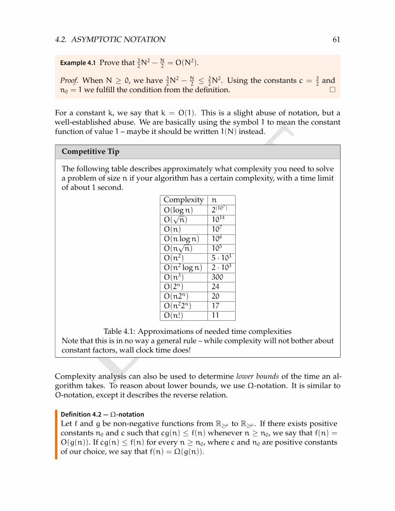
DRAFT
4.2. ASYMPTOTIC NOTATION 61
Example 4.1 Prove that 32N2 − N
2= O(N2).
Proof. When N ≥ 0, we have 32N2 − N
2≤ 3
2N2. Using the constants c = 3
2and
n0 = 1we fulfill the condition from the definition.
For a constant k, we say that k = O(1). This is a slight abuse of notation, but awell-established abuse. We are basically using the symbol 1 to mean the constantfunction of value 1 – maybe it should be written 1(N) instead.
Competitive Tip
The following table describes approximately what complexity you need to solvea problem of size n if your algorithm has a certain complexity, with a time limitof about 1 second.
Complexity n
O(logn) 2(107)
O(√n) 1014
O(n) 107
O(n logn) 106
O(n√n) 105
O(n2) 5 · 103O(n2 logn) 2 · 103O(n3) 300
O(2n) 24
O(n2n) 20
O(n22n) 17
O(n!) 11
Table 4.1: Approximations of needed time complexitiesNote that this is in no way a general rule – while complexity will not bother aboutconstant factors, wall clock time does!
Complexity analysis can also be used to determine lower bounds of the time an al-gorithm takes. To reason about lower bounds, we use Ω-notation. It is similar toO-notation, except it describes the reverse relation.
Definition 4.2 —Ω-notationLet f and g be non-negative functions from R≥0 to R≥0. If there exists positiveconstants n0 and c such that cg(n) ≤ f(n) whenever n ≥ n0, we say that f(n) =O(g(n)). If cg(n) ≤ f(n) for every n ≥ n0, where c and n0 are positive constantsof our choice, we say that f(n) = Ω(g(n)).
DRAFT
62 CHAPTER 4. TIME COMPLEXITY
We know that the complexity of insertion sort has an upper bound of O(N2) in theworst-case, but does it have a lower bound? In fact, it has the same lower bound, i.e.T(N) = Ω(N2).
Example 4.2 Prove that 32N2 − N
2= Ω(N2).
Proof. When N ≥ 1, we have 32N2 − N
2≥ N2 since N2 ≥ N. Using the constants
c = 1 and n0 = 1we fulfill the condition from the definition.
In this case, both the lower and the upper bound of the worst-case running time ofinsertion sort coincided (asymptotically). We have another notation for when this isthe case:
Definition 4.3 —Θ-notationIf f(n) = O(g(n)) and f(n) = Ω(g(n)), we say that f(n) = Θ(g(n)).
Thus, the worst-case running time for insertion sort is Θ(n2).
There are many ways of computing the time complexity of an algorithm. The mostcommon case is when a program has K nested loops, each of with performs O(M)iterations. The complexity of these loops are then O(MK · f(N)) if the inner-mostoperation takesO(f(N)) time. In Chapter 8, you will also see some ways of computingthe time complexity of a particular type of recursive solution, called Divide andConquer algorithms.
4.3 NP-complete problems
Of particular importance in computer science are the problems that can be solved algo-rithms running in polynomial time (often considered to be the “tractable” problems).There are a number of problems for which we do not yet know if there is an algorithmwhose time complexity is bounded by a polynomial. One particular class of theseare the NP-complete problems. They have the property that they are all reducibleto one another, in the sense that a polynomial-time algorithm to any one of themyields a polynomial-time algorithm to all the others. Many of these NP-completeproblems appear in algorithmic problem solving, so it is good to know that they existand that it is unlikely you will find a polynomial-time solution. During the courseof this book, you will occasionally see such problems, with their NP-completenessmentioned.
DRAFT
4.4. OTHER TYPES OF COMPLEXITIES 63
4.4 Other Types of Complexities
There are several other types of complexities aside from the time complexity. Forexample, the memory complexity of an algorithm measures the amount of memoryit uses. We use the same asymptotic notation when analyzing memory complexity.In most modern programming competitions, the allowed memory usage is highenough for the memory complexity not be a problem. However, it is still of interest incomputer science (and thus algorithmic problem solving) and computer engineeringin general.
Another common type of complexity is the query complexity. In some problems(like the Guessing Problem from chapter 1), we are given access to some kind ofexternal procedure (called an oracle) that computes some value given parametersthat we provide. Such a procedure call is called a query. The number of queries thatan algorithm makes to the oracle is called its query complexity. Problems wherethe algorithm is allowed access to an oracle often bound the number of queries thealgorithm may make. In these problems, the query complexity of the algorithm is ofinterest.
4.5 ExercisesExercise 4.1
Find a lower and an upper bound that coincide for the best-case running time forinsertion sort.
Exercise 4.2
Give an O(n) algorithm and an O(1) algorithm to compute the sum of the n firstintegers.
Exercise 4.3
Prove, using the definition, that 10n2 + 7n− 5+ log2 n = O(n2). What constantsc, n0 did you get?
Exercise 4.4
Prove that f(n) + g(n) = Θ(maxf(n), g(n)) for non-negative functions f and g.
DRAFT
64 CHAPTER 4. TIME COMPLEXITY
Exercise 4.5
Is 2n+1 = O(2n)? Is 22n = O(2n)?
Exercise 4.6
Prove that (n+ a)b = O(nb) for positive constants a, b > 0.
4.6 Chapter Notes
Advanced algorithm analysis sometimes use rather complicated discrete mathematics,such as number theoretical (as in Chapter 14) or combinatorial (as in Chapter 13)facts. Concrete Mathematics [7] by Donald Knuth, et al, does a thorough job on bothaccounts.
An Introduction to the Analysis of Algorithms [8] by Sedgewick and Flajolet has amore explicit focus on the analysis of algorithms, mainly discussing combinatorialanalysis.
The study of various kinds of complexities forms a research area called computationalcomplexity theory. Computational Complexity [18] by Papadimitriou is a classical intro-duction to computational complexity, although Computational Complexity: A ModernApproach [1] by Arora and Barak is a more modern textbook, with recent results thatthe book by Papadimitriou lack.
While complexity theory is mainly concerned about the limits of specific computa-tional models on problems that can be solved within those models, what can not bedone by computers is also interesting. This is somewhat out of scope for an algo-rithmic problem solving book (since we are interested in those problems which canbe solved), but is still of general interest. A book on e.g. automata theory (such asIntroduction to Automata Theory, Languages, and Computation [24] by Ullman et al) canbe a good compromise, mixing both some foundations of the theory of computationwith topics more applicable to algorithms (such as automatons and languages).

DRAFTPart II
Basics
65

DRAFT
DRAFTChapter 5
Brute Force
Many problems are solved by testing a large number of possibilities. For example,chess engines work by testing countless variations of moves and choosing the onesresulting in the “best” positions. This approach is called brute force. Brute forcealgorithms exploit that computers are fast, resulting in you having to be less smart.Just as with chess engines, brute force solutions might still require some ingenuity. Thesame brute force problem might have a simple algorithm which requires a computerto evaluate 240 options, while some deeper analysis might be able to reduce this to 220.This would be a huge reduction in running time. Different approaches to brute forcemay be the key factor in reaching the latter case instead of the former. In this chapter,we will study a few such techniques.
5.1 Optimization Problems
In an optimization problem, we have some solution set S and a value function f. Thegoal is to find an x ∈ Swhich maximize f(x), i.e., optimizing the function.
Optimization problems constitute a large class of the problems that we solve inalgorithmic problem solving, such as the Max Clique problem and the Buying Booksproblems we will study in this chapter. One of the most famous optimization problemsis the NP-complete Travelling Salesman Problem. The problem seeks the shortest cyclethat visits all vertices of a weighted graph. The practical applications of this problemare many. A logistics company that must perform a number of deliveries probablywant to minimize the distance traveled when visiting all the points of delivery. Whenplanning your backpacking vacation, you may prefer to minimize the cost of travellingbetween all your destinations. In this problem, the solution set S would consist of allcycles in the graph that visit all the vertices, with f(x) being the sum of all edges inthe cycle x.
67
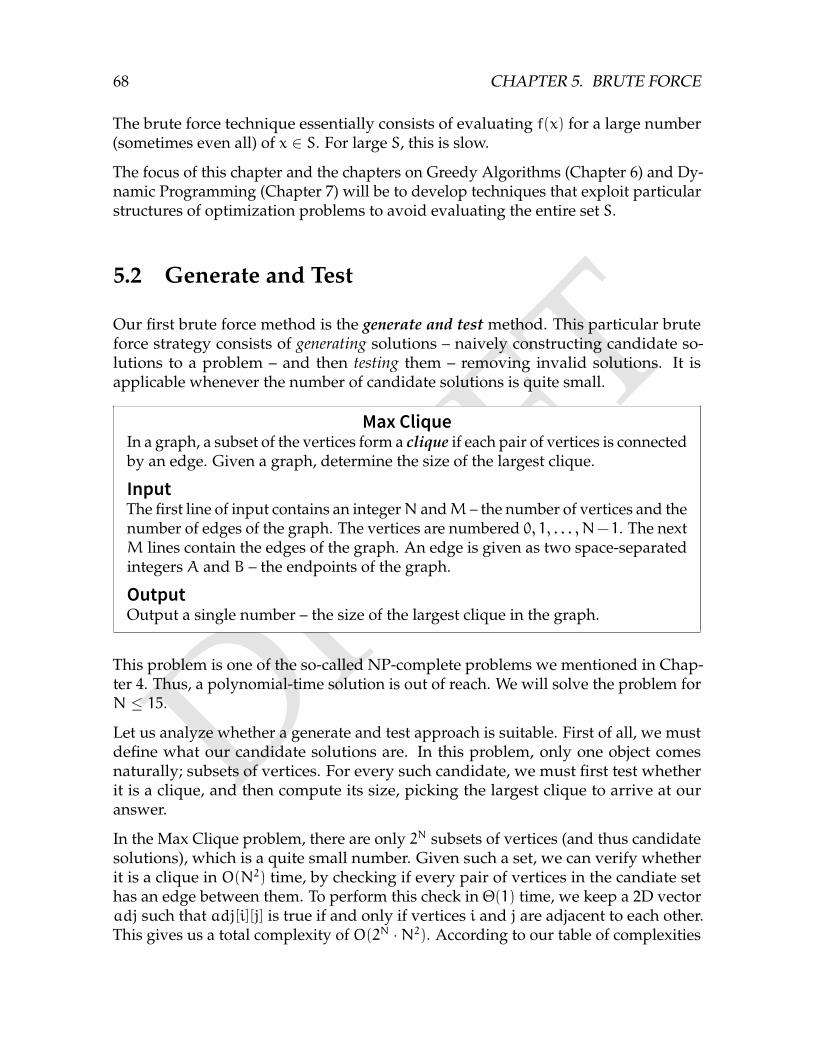
DRAFT
68 CHAPTER 5. BRUTE FORCE
The brute force technique essentially consists of evaluating f(x) for a large number(sometimes even all) of x ∈ S. For large S, this is slow.
The focus of this chapter and the chapters on Greedy Algorithms (Chapter 6) and Dy-namic Programming (Chapter 7) will be to develop techniques that exploit particularstructures of optimization problems to avoid evaluating the entire set S.
5.2 Generate and Test
Our first brute force method is the generate and test method. This particular bruteforce strategy consists of generating solutions – naively constructing candidate so-lutions to a problem – and then testing them – removing invalid solutions. It isapplicable whenever the number of candidate solutions is quite small.
Max CliqueIn a graph, a subset of the vertices form a clique if each pair of vertices is connectedby an edge. Given a graph, determine the size of the largest clique.
InputThe first line of input contains an integerN andM – the number of vertices and thenumber of edges of the graph. The vertices are numbered 0, 1, . . . ,N−1. The nextM lines contain the edges of the graph. An edge is given as two space-separatedintegers A and B – the endpoints of the graph.
OutputOutput a single number – the size of the largest clique in the graph.
This problem is one of the so-called NP-complete problems we mentioned in Chap-ter 4. Thus, a polynomial-time solution is out of reach. We will solve the problem forN ≤ 15.Let us analyze whether a generate and test approach is suitable. First of all, we mustdefine what our candidate solutions are. In this problem, only one object comesnaturally; subsets of vertices. For every such candidate, we must first test whetherit is a clique, and then compute its size, picking the largest clique to arrive at ouranswer.
In the Max Clique problem, there are only 2N subsets of vertices (and thus candidatesolutions), which is a quite small number. Given such a set, we can verify whetherit is a clique in O(N2) time, by checking if every pair of vertices in the candiate sethas an edge between them. To perform this check in Θ(1) time, we keep a 2D vectoradj such that adj[i][j] is true if and only if vertices i and j are adjacent to each other.This gives us a total complexity of O(2N ·N2). According to our table of complexities
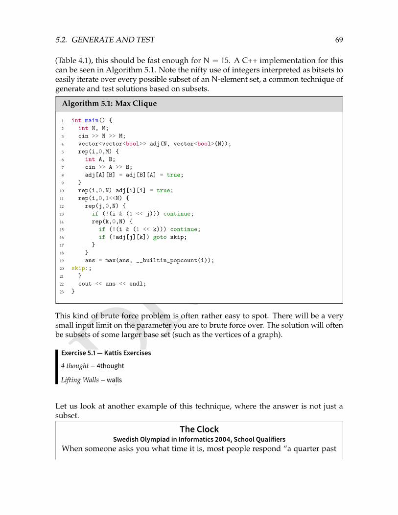
DRAFT
5.2. GENERATE AND TEST 69
(Table 4.1), this should be fast enough for N = 15. A C++ implementation for thiscan be seen in Algorithm 5.1. Note the nifty use of integers interpreted as bitsets toeasily iterate over every possible subset of an N-element set, a common technique ofgenerate and test solutions based on subsets.
Algorithm 5.1: Max Clique
1 int main() 2 int N, M;3 cin >> N >> M;4 vector<vector<bool>> adj(N, vector<bool>(N));5 rep(i,0,M) 6 int A, B;7 cin >> A >> B;8 adj[A][B] = adj[B][A] = true;9
10 rep(i,0,N) adj[i][i] = true;11 rep(i,0,1<<N) 12 rep(j,0,N) 13 if (!(i & (1 << j))) continue;14 rep(k,0,N) 15 if (!(i & (1 << k))) continue;16 if (!adj[j][k]) goto skip;17 18 19 ans = max(ans, __builtin_popcount(i));20 skip:;21 22 cout << ans << endl;23
This kind of brute force problem is often rather easy to spot. There will be a verysmall input limit on the parameter you are to brute force over. The solution will oftenbe subsets of some larger base set (such as the vertices of a graph).
Exercise 5.1 — Kattis Exercises
4 thought – 4thought
Lifting Walls – walls
Let us look at another example of this technique, where the answer is not just asubset.
The ClockSwedish Olympiad in Informatics 2004, School Qualifiers
When someone asks you what time it is, most people respond “a quarter past
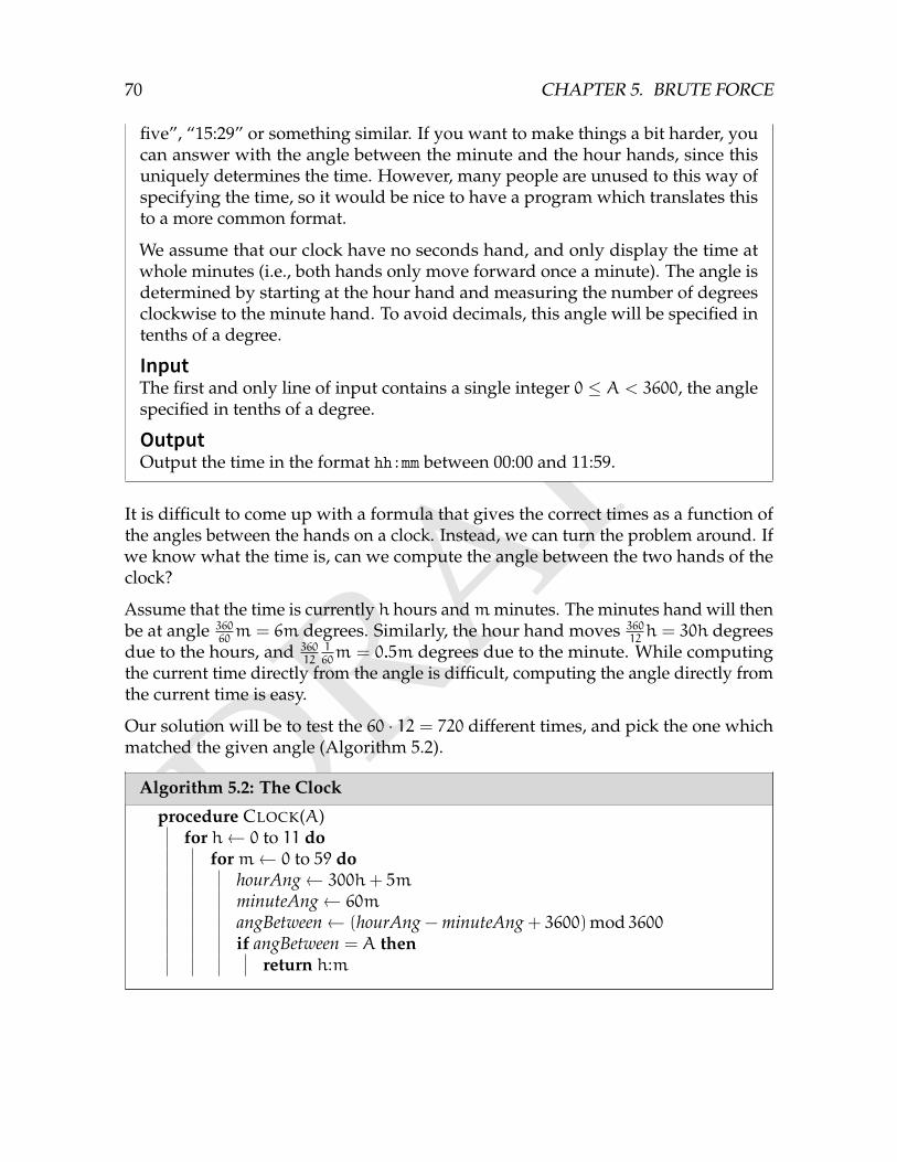
DRAFT
70 CHAPTER 5. BRUTE FORCE
five”, “15:29” or something similar. If you want to make things a bit harder, youcan answer with the angle between the minute and the hour hands, since thisuniquely determines the time. However, many people are unused to this way ofspecifying the time, so it would be nice to have a program which translates thisto a more common format.
We assume that our clock have no seconds hand, and only display the time atwhole minutes (i.e., both hands only move forward once a minute). The angle isdetermined by starting at the hour hand and measuring the number of degreesclockwise to the minute hand. To avoid decimals, this angle will be specified intenths of a degree.
InputThe first and only line of input contains a single integer 0 ≤ A < 3600, the anglespecified in tenths of a degree.
OutputOutput the time in the format hh:mm between 00:00 and 11:59.
It is difficult to come up with a formula that gives the correct times as a function ofthe angles between the hands on a clock. Instead, we can turn the problem around. Ifwe know what the time is, can we compute the angle between the two hands of theclock?
Assume that the time is currently h hours andmminutes. The minutes hand will thenbe at angle 360
60m = 6m degrees. Similarly, the hour hand moves 360
12h = 30h degrees
due to the hours, and 36012
160m = 0.5m degrees due to the minute. While computing
the current time directly from the angle is difficult, computing the angle directly fromthe current time is easy.
Our solution will be to test the 60 · 12 = 720 different times, and pick the one whichmatched the given angle (Algorithm 5.2).
Algorithm 5.2: The Clock
procedure CLOCK(A)for h← 0 to 11 do
form← 0 to 59 dohourAng← 300h+ 5mminuteAng← 60m
angBetween← (hourAng − minuteAng + 3600)mod 3600if angBetween = A then
return h:m
DRAFT
5.3. BACKTRACKING 71
Competitive Tip
Sometimes, competitions pose problems which are solvable quite fast, but a bruteforce algorithm will suffice as well. As a general rule, code the simplest correctsolution that is fast enough, even if you see a faster one.
Exercise 5.2 — Kattis Exercises
All about that base – allaboutthatbase
Natjecanje – natjecanje
Perket – perket
5.3 Backtracking
Backtracking is a variation of the generate and test method. Most of the time it isfaster, but it can sometimes be more difficult to code (in particular when the solutionsare subsets).
Let us return to the Max Clique problem. In the problem, we generated all thecandidate solutions (i.e., subsets of vertex) by using bitsets. In problems where thecandidate solutions are other objects than subsets, or the number of subsets is toolarge to iterate through, we need to construct the solutions in another way. Generally,we do this recursively. For example, when generating subsets, we would go throughevery element one at a time, and decide whether to include it. Backtracking extendsgenerate and test to not only testing all the candidate solutions, but also these partialcandidates. Thus, a backtracking approach can be faster than an iterative approach,by testing fewer candidate solutions.
For example, assume that two vertices a and b are not connected by an edge in thegraph. If we decide to include a in our solution, we already know that a candidatesolution can not include b. Thus, we have managed to reduce four choices – includingor excluding a and b – to three choices, by eliminating the inclusion of both vertices.Algorithm 5.3 contains a C++ implementation of this.
Algorithm 5.3: Max Clique, Recursive Variant
1 // excluded is a bit set containing the vertices with a chosen neighbour2 int best(int at, int excluded, int clique, const vector<int>& adjacent) 3 if (at == sz(adjacent)) return clique;4 // Case 1: Not including the current vertex5 int answer = best(at + 1, excluded, clique, adjacent);6 // Case 2: We can include the current vertex
DRAFT
72 CHAPTER 5. BRUTE FORCE
7 if (!((1 << at)&excluded)) 8 answer = max(answer,9 best(at + 1, excluded | ~adjacent[at], clique + 1, adjacent));
10 11 return answer;12 13
14 int main() 15 int N, M;16 cin >> N >> M;17 vector<int> adjacent(N);18 rep(i,0,M) 19 int A, B;20 cin >> A >> B;21 adjacent[A] |= 1 << B;22 adjacent[B] |= 1 << A;23 24 cout << best(0, 0, 0, adjacent) << endl;25
As written, this version has the same complexity as the generate-and-test version.Our improvement only generated fewer branches whenever the graph containededges. In the case where the graph consists of N vertices and no edges, this is not thecase. The recursion then degenerates to branching twiceN times, resulting in a Θ(2n)complexity.
Backtracking works whenever we can construct our solutions iteratively (as in con-structing it part by part), and quickly determine whether such a partial solution canpossibly be completed to an admissible solution.
Exercise 5.3 — Kattis Exercises
Class Picture – classpicure
Boggle – boggle
Geppetto – geppetto
Map Colouring – mapcolouring
Sudokunique – sudokunique
All Friends – friends
As a general principle, backtracking seems simple enough. Some backtracking solu-tions require a bit more ingenuity, as in the next problem.
DRAFT
5.3. BACKTRACKING 73
Basin City SurveillanceNordic Collegiate Programming Contest 2014 – Pål G. Drange and Markus S. Dregi
BASIN CITY is known for her incredibly high crime rates. The police see nooption but to tighten security. They want to install traffic drones at differentintersections to observe who’s running on a red light. If a car runs a red light,the drone will chase and stop the car to give the driver an appropriate ticket.The drones are quite stupid, however, and a drone will stop before it comes tothe next intersection as it might otherwise lose its way home, its home being thetraffic light to which it is assigned. The drones are not able to detect the presenceof other drones, so the police’s R&D department found out that if a drone wasplaced at some intersection, then it was best not to put any drones at any of theneighbouring intersections. As is usual in many cities, there are no intersectionsin Basin City with more than four other neighbouring intersections.
The drones are government funded, so the police force would like to buy as manydrones as they are allowed to. Being the programmer-go-to for the Basin CityPolice Department, they ask you to decide, for a given number of drones, whetherit is feasible to position exactly this number of drones.
InputThe first line contains an integer k (0 ≤ k ≤ 15), giving the number of dronesto position. Then follows one line with 1 ≤ n ≤ 100 000, the total number ofintersections in Basin City. Finally follow n lines describing consecutive intersec-tions. The i’th line describes the i’th intersection in the following format: Theline starts with one integer d (0 ≤ d ≤ 4) describing the number of intersectionsneighbouring the i’th one. Then follow d integers denoting the indices of theseneighbouring intersections. They will be all distinct and different from i. Theintersections are numbered from 1 to n.
OutputIf it is possible to position k drones such that no two neighbouring intersectionshave been assigned a drone, output a single line containing possible. Otherwise,output a single line containing impossible.
At a first glance, it is not even obvious whether the problem is a brute force problem,or if some smarter principle should be applied. After all, 100 000 vertices is a hugenumber of intersections! We can make the problem a bit more reasonable with ourfirst insight. If we have a large number of intersections, and every intersection isadjacent to very few other intersection, it is probably very easy to place the drones atappropriate intersections. To formalize this insight, consider what happens when weplace a drone at an intersection.
By placing a drone at the intersection marked in black in Figure 5.1, at most fiveintersections are affected – the intersection we placed the drone at, along with its
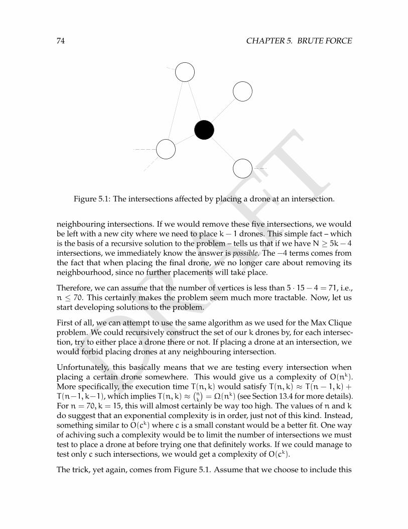
DRAFT
74 CHAPTER 5. BRUTE FORCE
Figure 5.1: The intersections affected by placing a drone at an intersection.
neighbouring intersections. If we would remove these five intersections, we wouldbe left with a new city where we need to place k− 1 drones. This simple fact – whichis the basis of a recursive solution to the problem – tells us that if we haveN ≥ 5k− 4intersections, we immediately know the answer is possible. The −4 terms comes fromthe fact that when placing the final drone, we no longer care about removing itsneighbourhood, since no further placements will take place.
Therefore, we can assume that the number of vertices is less than 5 · 15− 4 = 71, i.e.,n ≤ 70. This certainly makes the problem seem much more tractable. Now, let usstart developing solutions to the problem.
First of all, we can attempt to use the same algorithm as we used for the Max Cliqueproblem. We could recursively construct the set of our k drones by, for each intersec-tion, try to either place a drone there or not. If placing a drone at an intersection, wewould forbid placing drones at any neighbouring intersection.
Unfortunately, this basically means that we are testing every intersection whenplacing a certain drone somewhere. This would give us a complexity of O(nk).More specifically, the execution time T(n, k) would satisfy T(n, k) ≈ T(n − 1, k) +T(n−1, k−1), which implies T(n, k) ≈
(nk
)= Ω(nk) (see Section 13.4 for more details).
For n = 70, k = 15, this will almost certainly be way too high. The values of n and kdo suggest that an exponential complexity is in order, just not of this kind. Instead,something similar to O(ck) where c is a small constant would be a better fit. One wayof achiving such a complexity would be to limit the number of intersections we musttest to place a drone at before trying one that definitely works. If we could manage totest only c such intersections, we would get a complexity of O(ck).
The trick, yet again, comes from Figure 5.1. Assume that we choose to include this
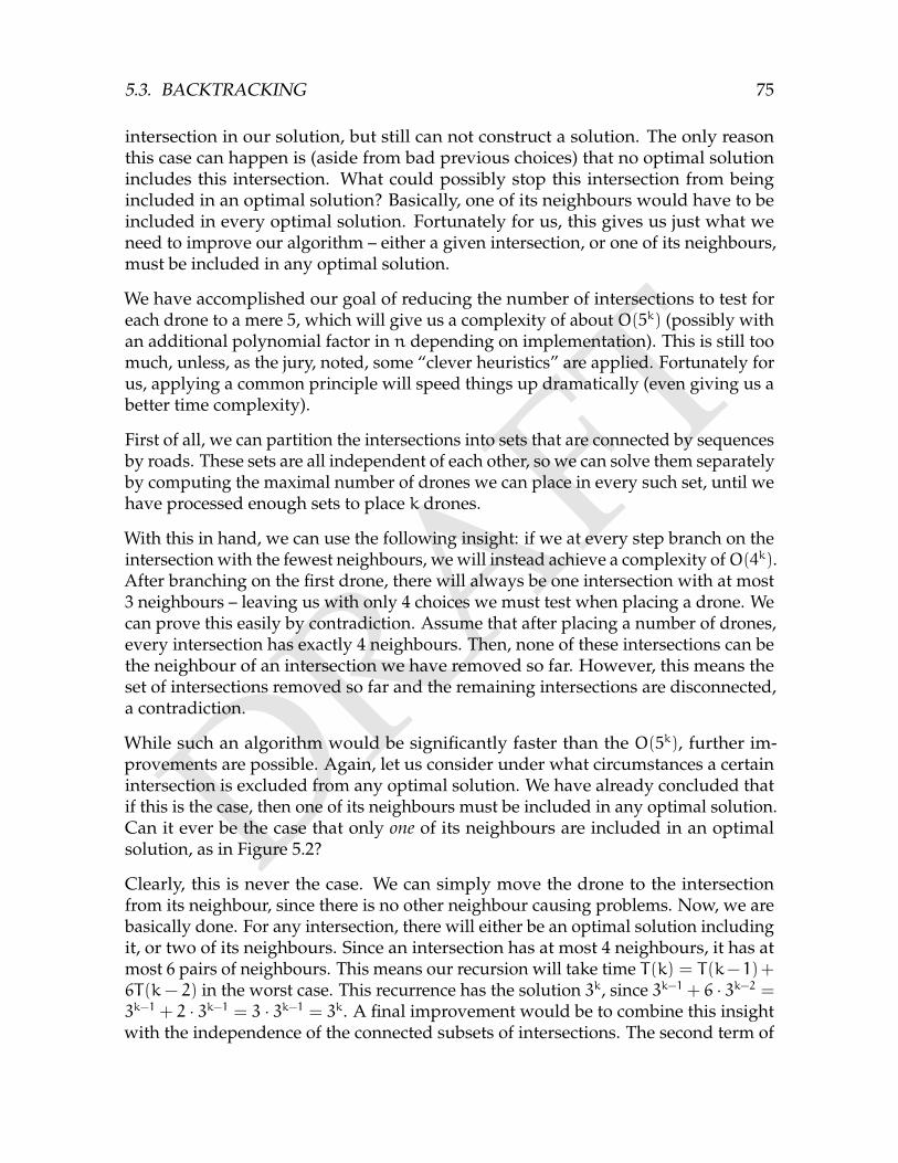
DRAFT
5.3. BACKTRACKING 75
intersection in our solution, but still can not construct a solution. The only reasonthis case can happen is (aside from bad previous choices) that no optimal solutionincludes this intersection. What could possibly stop this intersection from beingincluded in an optimal solution? Basically, one of its neighbours would have to beincluded in every optimal solution. Fortunately for us, this gives us just what weneed to improve our algorithm – either a given intersection, or one of its neighbours,must be included in any optimal solution.
We have accomplished our goal of reducing the number of intersections to test foreach drone to a mere 5, which will give us a complexity of about O(5k) (possibly withan additional polynomial factor in n depending on implementation). This is still toomuch, unless, as the jury, noted, some “clever heuristics” are applied. Fortunately forus, applying a common principle will speed things up dramatically (even giving us abetter time complexity).
First of all, we can partition the intersections into sets that are connected by sequencesby roads. These sets are all independent of each other, so we can solve them separatelyby computing the maximal number of drones we can place in every such set, until wehave processed enough sets to place k drones.
With this in hand, we can use the following insight: if we at every step branch on theintersection with the fewest neighbours, we will instead achieve a complexity ofO(4k).After branching on the first drone, there will always be one intersection with at most3 neighbours – leaving us with only 4 choices we must test when placing a drone. Wecan prove this easily by contradiction. Assume that after placing a number of drones,every intersection has exactly 4 neighbours. Then, none of these intersections can bethe neighbour of an intersection we have removed so far. However, this means theset of intersections removed so far and the remaining intersections are disconnected,a contradiction.
While such an algorithm would be significantly faster than the O(5k), further im-provements are possible. Again, let us consider under what circumstances a certainintersection is excluded from any optimal solution. We have already concluded thatif this is the case, then one of its neighbours must be included in any optimal solution.Can it ever be the case that only one of its neighbours are included in an optimalsolution, as in Figure 5.2?
Clearly, this is never the case. We can simply move the drone to the intersectionfrom its neighbour, since there is no other neighbour causing problems. Now, we arebasically done. For any intersection, there will either be an optimal solution includingit, or two of its neighbours. Since an intersection has at most 4 neighbours, it has atmost 6 pairs of neighbours. This means our recursion will take time T(k) = T(k−1)+6T(k− 2) in the worst case. This recurrence has the solution 3k, since 3k−1 + 6 · 3k−2 =3k−1 + 2 · 3k−1 = 3 · 3k−1 = 3k. A final improvement would be to combine this insightwith the independence of the connected subsets of intersections. The second term of
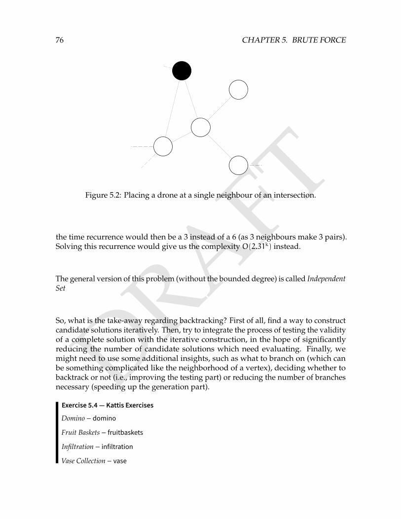
DRAFT
76 CHAPTER 5. BRUTE FORCE
Figure 5.2: Placing a drone at a single neighbour of an intersection.
the time recurrence would then be a 3 instead of a 6 (as 3 neighbours make 3 pairs).Solving this recurrence would give us the complexity O(2.31k) instead.
The general version of this problem (without the bounded degree) is called IndependentSet
So, what is the take-away regarding backtracking? First of all, find a way to constructcandidate solutions iteratively. Then, try to integrate the process of testing the validityof a complete solution with the iterative construction, in the hope of significantlyreducing the number of candidate solutions which need evaluating. Finally, wemight need to use some additional insights, such as what to branch on (which canbe something complicated like the neighborhood of a vertex), deciding whether tobacktrack or not (i.e., improving the testing part) or reducing the number of branchesnecessary (speeding up the generation part).
Exercise 5.4 — Kattis Exercises
Domino – domino
Fruit Baskets – fruitbaskets
Infiltration – infiltration
Vase Collection – vase
DRAFT
5.4. FIXING PARAMETERS 77
5.4 Fixing Parameters
The parameter fixing technique is also similar to the generate and test method, but isnot used to test the solution set itself. Instead, you perform brute force to fix someparameter in the problem by trying possible values they can assume. Hopefully,fixing the correct parameters allows you to solve the remaining problem easily. Theintuition is that while any particular choice of parameter may be wrong, testing everychoice allows us to assume that we at some point used the correct parameter.
Buying BooksSwedish Olympiad in Informatics 2010, Finals
You are going to buyN books, and are currently checking the different internetMbook shops for prices. Each book is sold by at least one book store, and can varyin prices between the different stores. Furthermore, if you order anything from acertain book store, you must pay for postage. Postage may vary between bookstores as well, but is the same no matter how many books you decide to order.You may order books from any number of book stores. Compute the smallestamount of money you need to pay for all the books.
InputThe first line contains two integers 1 ≤ N ≤ 100 – the number of books, and1 ≤M ≤ 15 – the number of book stores.
Then,M descriptions of the book stores follow. The description of the i’th storestarts with a line containing two integers 0 ≤ Pi ≤ 1 000 (the postage for thisbook store), and 1 ≤ Li ≤ N (the number of books this store sells). The nextL lines contains the books sold by the store. The j’th book is described by twointegers 0 ≤ Bi,j < N – the (zero-indexed) number of a book being sold here, and1 ≤ Ci,j ≤ 1000 – the price of this book at the current book store.
OutputOutput a single integer – the smallest amount of money you need to pay for thebooks.
If we performed naive generate and test on this problem, we would probably getsomething like 15100 solutions (testing every book shop for every book). This isinfeasible. So, why can we do better than this? There must be some hidden structurein the problem which makes testing all those possibilities unnecessary. To find thisstructure, we will analyze a particular candidate solution as given by the naivegenerate and test method. Can we find a simple criteria for when a solution obviouscannot be optimal?
It turns out that yes, we can. Assume that we, in a particular solution, bought a bookfrom some book store A, but it was available for a lower price at book store B. If thisis an optimal solution we must not have bought any books from B.
DRAFT
78 CHAPTER 5. BRUTE FORCE
When this happens, i.e., you notice very simple constraints which immediately dis-qualify many of the solution candidates from being optimal, it is a good sign you maybe able to restructure your brute force in order to avoid evaluating many of them. Inour case, this observation hints that making a choice for every book is not particularlygood.
We could decide to use this fact to turn our generate and test into a backtrackingalgorithm, by pruning away any solution where we have bought a book which isavailable at a cheaper price from another book store we also used. Unfortunately,this is easily defeated by giving most of the books equal prices at most of the bookstores.
Instead, let us use the observation differently. The entirety of the observation quiteplainly told us that we do not really have any choice in where we buy the books!Indeed, once we know what book stores we have bought from, we are forced to buythe book from the cheapest store that is used. At this point, we are basically done.We have reduced the amount of information we need to fix to solve the problem to“which book stores will we purchase from?”. This parameter has only 215 possibilities.After fixing it, we can compute the rest of the answer using the “cheapest store foreach book” rule. Since we test every possible such parameter, we must also includethe optimal one. The pseudo code for this solution is in Algorithm 5.4.
Algorithm 5.4: Buying Books
procedure BUYINGBOOKS(books N, storesM, costs C, postages P)answer←∞for every S ⊆ [M] do
cost← 0
for every s ∈ S docost← cost + Ps
for every b ∈ [N] docost← cost + mini∈SCi,b
answer← min(answer, cost)return answer
Alternatively, we could have come to the same insight by simply asking ourselves“can we bruteforce over the number of book shops?”. Whenever you have a parameterabout this size in such a problem, this is a question worth asking. However, theparameter to brute force over is not always this explicit, as in the following problem,which asks us to find all integer solutions to an equation in a certain interval.
Integer EquationCodeforces Round #262, Problem B
DRAFT
5.5. MEET IN THE MIDDLE 79
Find all integers 0 < x < 109 which satsify the equation
x = a · s(x)b + c
where a, b and c are given integers, and s(x) is the digit sum of x.
InputThe input contains the three integers a, b, and c such that
|a| ≤ 10 000
1 ≤ b ≤ 5|c| ≤ 10 000
OutputOutput a single integer – number of integer solutions x to the equation.
In this problem, the only explicit object we have is x. Unfortunately, 109 is a tad toomany possibilities. If we study the equation a bit closer, we see that s(x) also variesas a function of x. This is helpful, since s(x) has far fewer options than x. In fact, anumber bounded by 109 has at most 9 digits, meaning it has a maximum digit sum of9 · 9 = 81. Thus, we can solve the problem by looping over all the possibles valuesof s(x). This uniquely fixes our right hand side, which equals x. Given x, we verifythat s(x) has the correct value. Whenever we have such a function, i.e., one with alarge domain (like x in the problem) but a small image (like s(x) in the problem), thistechnique can be used by brute forcing over the image instead.
Exercise 5.5 — Kattis Exercises
Shopping Plan – shoppingplan
5.5 Meet in the Middle
The meet in the middle technique is essentially a special case of the parameter fixingtechnique. The general theme will be to fix half of the parameter space and build somefast structure such that when testing the other half of the parameter space, we canavoid explicitly re-testing the first half. It is a space-time tradeoff, in the sense that weimprove the time usage (testing half of the parameter space much faste much faster),by paying with increased memory usage (to save the pre-computed structures).
DRAFT
80 CHAPTER 5. BRUTE FORCE
Subset SumGiven a set of integers S, is there some subset A ⊆ Swith a sum equal to T?
InputThe first line contains an integer N, the size of S, and T . The next line containsN integers s1, s2, ..., sN , separated by spaces – the elements of S. It is guaranteedthat si 6= sj for i 6= j.OutputOutput possible if such a subset exists, and impossible otherwise.
In this problem, we have N parameters in our search space. For each element of S,we either choose to include it in A or not – a total of two choices for each parameter.This naive attempt at solving the problem (which amounts to computing the sum ofevery subset) gives us a complexity of O(2N). While sufficient for e.g. N = 20, we canmake an improvement that makes the problem tractable even for N = 40.
As it happens, our parameters are to a large extent independent. If we fix e.g. the N2
first parameters, the only constraint they place on the remaining N2
parameters is thesum of the integers in subset they decide. This latter constraint takes O(2
N2 ) time to
check for each choice of the first half of parameters if we use brute force. However,the computation performed is essentially the same, only differing in what sum wetry to find. We will instead trade away some memory in order to only computethis information once, by first computing all possible sums that the latter half of theelements can form. This information can be inserted into a hash set, which allowsus to determine if a sum can be formed by the elements in Θ(1) instead. Then, thecomplexity is instead Θ(N2
N2 ) in total.
Algorithm 5.5: Subset Sum
procedure SUBSETSUM(set S, target T )N← |S|
left← N2
right← N− leftLset← the left first elements of SRset← S \ LsetLsums← new set
for each L ⊆ Lset doLsums.insert(
∑l∈L l)
for each R ⊆ Rset dosum←∑r∈R r
if Lsums.contains(T − sum) thenoutput true
DRAFT
5.6. CHAPTER NOTES 81
returnoutput false
Exercise 5.6 — Kattis Exercises
Closest Sums – closestsums
Maximum Loot – maxloot
Celebrity Split – celebritysplit
Circuit Counting – countcircuits
Indoorienteering – indoorienteering
Key to Knowledge – keytoknowledge
Knights in Fen – knightsfen
Rubrik’s Revenge in ... 2D!? 3D? – rubriksrevenge
5.6 Chapter Notes
write chapternoteswrite chapternotes

DRAFT
82 CHAPTER 5. BRUTE FORCE
DRAFTChapter 6
Greedy Algorithms
In this chapter, we are going to look at another standard technique to solve somecategories of search and optimization problems faster than naive bruteforce, byexploiting properties of local optimality.
6.1 Optimal Substructure
Most optimization problems we study consist of making a series of sequential choices.They are often be of the following form: Given a weighted, directed acyclic graph(DAG) on N vertices, what is the “best” path from a vertex S to another vertex T?This graph is almost never be given explicitly. Instead, it hides behind the problem asa set of states (the vertices). At each state, we are to make some choice that takes usto another state (traversing an edge). If the path consists of edges e1, e2, . . . , ek, thefunction we are to maximize will be of the form
G(e1, e2, . . . , ek) = g(e1, g(e2, g(. . . , g(ek, 0))))
where g is a function from E× R to R. We will denote B(v) as the maximum value ofG(e1, e2, . . . , ek) over all paths from v to T . Often, g will be the negative sum of theedge weights, meaning we look for the shortest path from S to T . If g(e, x) is increasingin x, we say that problems exhibiting this property has optimal substructure.
One way to solve the problem would be to evaluate G for every path in the graph.Unfortunately, the number of paths in a general graph can be huge (growing expo-nentially with the number of vertices). However, the optimal substructure propertyallows us to make a simplification. Assume that S has neighbors v1, v2, ..., vm. Then bythe definition of B and g, B(s) = max(g(s, vi, B(vi)). Thus, we can solve the problemby first solving the same problem on all vertices vi instead.
83
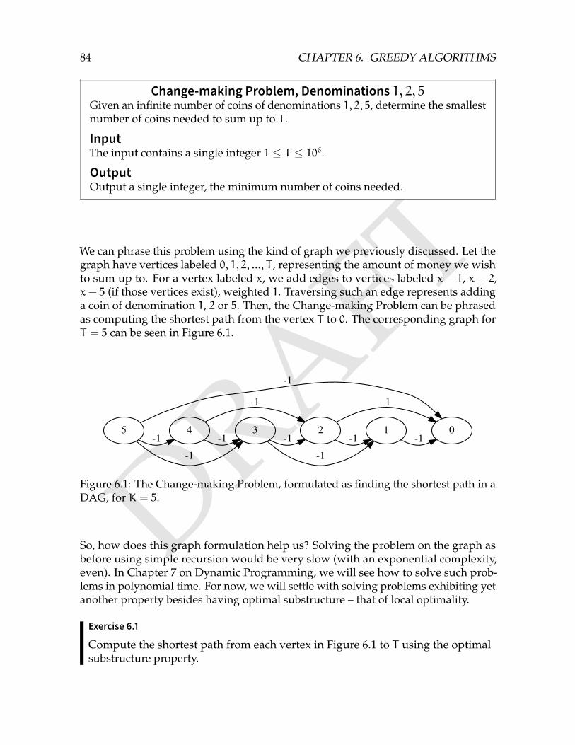
DRAFT
84 CHAPTER 6. GREEDY ALGORITHMS
Change-making Problem, Denominations 1, 2, 5Given an infinite number of coins of denominations 1, 2, 5, determine the smallestnumber of coins needed to sum up to T .
InputThe input contains a single integer 1 ≤ T ≤ 106.OutputOutput a single integer, the minimum number of coins needed.
We can phrase this problem using the kind of graph we previously discussed. Let thegraph have vertices labeled 0, 1, 2, ..., T , representing the amount of money we wishto sum up to. For a vertex labeled x, we add edges to vertices labeled x − 1, x − 2,x− 5 (if those vertices exist), weighted 1. Traversing such an edge represents addinga coin of denomination 1, 2 or 5. Then, the Change-making Problem can be phrasedas computing the shortest path from the vertex T to 0. The corresponding graph forT = 5 can be seen in Figure 6.1.
5 4-1
3
-1
0
-1
-12
-1
-11
-1
-1
-1
-1
Figure 6.1: The Change-making Problem, formulated as finding the shortest path in aDAG, for K = 5.
So, how does this graph formulation help us? Solving the problem on the graph asbefore using simple recursion would be very slow (with an exponential complexity,even). In Chapter 7 on Dynamic Programming, we will see how to solve such prob-lems in polynomial time. For now, we will settle with solving problems exhibiting yetanother property besides having optimal substructure – that of local optimality.
Exercise 6.1
Compute the shortest path from each vertex in Figure 6.1 to T using the optimalsubstructure property.
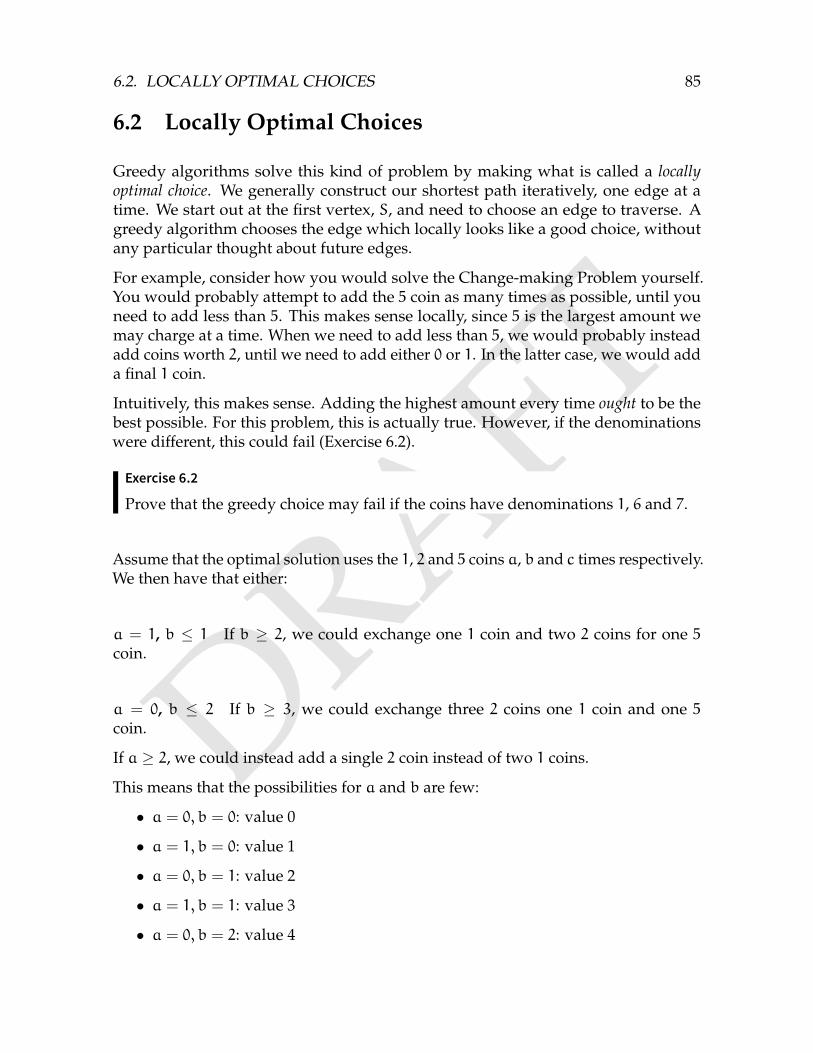
DRAFT
6.2. LOCALLY OPTIMAL CHOICES 85
6.2 Locally Optimal Choices
Greedy algorithms solve this kind of problem by making what is called a locallyoptimal choice. We generally construct our shortest path iteratively, one edge at atime. We start out at the first vertex, S, and need to choose an edge to traverse. Agreedy algorithm chooses the edge which locally looks like a good choice, withoutany particular thought about future edges.
For example, consider how you would solve the Change-making Problem yourself.You would probably attempt to add the 5 coin as many times as possible, until youneed to add less than 5. This makes sense locally, since 5 is the largest amount wemay charge at a time. When we need to add less than 5, we would probably insteadadd coins worth 2, until we need to add either 0 or 1. In the latter case, we would adda final 1 coin.
Intuitively, this makes sense. Adding the highest amount every time ought to be thebest possible. For this problem, this is actually true. However, if the denominationswere different, this could fail (Exercise 6.2).
Exercise 6.2
Prove that the greedy choice may fail if the coins have denominations 1, 6 and 7.
Assume that the optimal solution uses the 1, 2 and 5 coins a, b and c times respectively.We then have that either:
a = 1, b ≤ 1 If b ≥ 2, we could exchange one 1 coin and two 2 coins for one 5coin.
a = 0, b ≤ 2 If b ≥ 3, we could exchange three 2 coins one 1 coin and one 5coin.
If a ≥ 2, we could instead add a single 2 coin instead of two 1 coins.
This means that the possibilities for a and b are few:
• a = 0, b = 0: value 0
• a = 1, b = 0: value 1
• a = 0, b = 1: value 2
• a = 1, b = 1: value 3
• a = 0, b = 2: value 4
DRAFT
86 CHAPTER 6. GREEDY ALGORITHMS
Now, assume that we use exactly c coins of value 5, so that T = 5c + r. We knowthat 0 ≤ r < 5. Otherwise, we would be summing up to an amount larger than 4without using any 5 coins, but this is impossible based on the above list. This meansc must be as large as possible, i.e. it is optimal to add as many 5 coins as possible –which the greedy choice will. Then, only the cases 0, 1, 2, 3 and 4 remain. Lookingat the list of those cases, we see that their optimal solutions correspond to how thegreedy algorithm works. Thus, the greedy algorithm will always give the optimalanswer.
Competitive Tip
If you have the choice between a greedy algorithm and another algorithm (suchas one based on brute force or dynamic programming), use the other algorithmunless you are certain the greedy choice works.
Proving the correctness of a locally optimal choice is sometimes very cumbersome. Inthe remainder of the chapter, we are going to look at a few standard problems thatare solvable using a greedy algorithm. Take note of the kind of arguments we aregoing to use – there are a few common types of proofs which are often used in proofsof greedy algorithms.
6.3 Scheduling
Scheduling problems are a class of problems which deals with constructing largesubsets of non-overlapping intervals, from some given set of intervals.
The classical Scheduling Problem is the following.
Scheduling ProblemGiven is a set of half-open (being open on the right) intervals S. Determine thelargest subset A ⊆ S of non-overlapping intervals.
InputThe input contains the set of intervals S, where |S|.
OutputThe output should contain the subset A.
We will construct the solution iteratively, adding one interval at a time. When lookingfor greedy choices to perform, extremal cases are often the first ones you shouldconsider. Hopefully, one of these extremal cases can be proved to be included in anoptimal solution. For intervals, some extremal cases would be:
DRAFT
6.3. SCHEDULING 87
[ ) [ ) [ ) [ )
[ )
[ )
[ )
[ )
[ )
[ )
[ )
0 1 2 3 4 5 6 7 8
Figure 6.2: An instance of the scheduling problem, with the optimal solution at thebottom.
• a shortest interval,
• a longest interval,
• an interval overlapping as few other intervals as possible,
• an interval with the leftmost left endpoint (and symmetrically, the rightmostright endpoint),
• an interval with the leftmost right endpoint (and symmetrically, the rightmostleft endpoint).
As it turns out, we can always select an interval satisfying the fifth case. In theexample instance in Figure 6.2, this results in four intervals. First, the interval withthe leftmost right endpoint is the interval [1, 2). If we include this in the subset A,intervals [0, 3) and [1, 6) must be removed since they overlap [1, 2). Then, the interval[3, 4) would be the one with the leftmost right endpoint of the remaining intervals.This interval overlaps no other interval, so it should obviously be included. Next,we would choose [4, 6) (overlapping with [4, 7)), and finally [7, 8). Thus, the answer
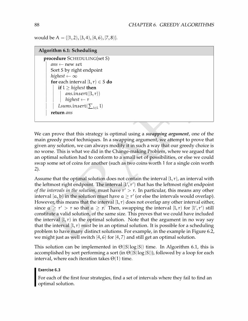
DRAFT
88 CHAPTER 6. GREEDY ALGORITHMS
would be A = [1, 2), [3, 4), [4, 6), [7, 8).
Algorithm 6.1: Scheduling
procedure SCHEDULING(set S)ans← new set
Sort S by right endpointhighest←∞for each interval [l, r) ∈ S do
if l ≥ highest thenans.insert([l, r))highest← r
Lsums.insert(∑
l∈L l)
return ans
We can prove that this strategy is optimal using a swapping argument, one of themain greedy proof techniques. In a swapping argument, we attempt to prove thatgiven any solution, we can always modify it in such a way that our greedy choice isno worse. This is what we did in the Change-making Problem, where we argued thatan optimal solution had to conform to a small set of possibilities, or else we couldswap some set of coins for another (such as two coins worth 1 for a single coin worth2).
Assume that the optimal solution does not contain the interval [l, r), an interval withthe leftmost right endpoint. The interval [l ′, r ′) that has the leftmost right endpointof the intervals in the solution, must have r ′ > r. In particular, this means any otherinterval [a, b) in the solution must have a ≥ r ′ (or else the intervals would overlap).However, this means that the interval [l, r) does not overlap any other interval either,since a ≥ r ′ > r so that a ≥ r. Then, swapping the interval [l, r) for [l ′, r ′) stillconstitute a valid solution, of the same size. This proves that we could have includedthe interval [l, r) in the optimal solution. Note that the argument in no way saythat the interval [l, r) must be in an optimal solution. It is possible for a schedulingproblem to have many distinct solutions. For example, in the example in Figure 6.2,we might just as well switch [4, 6) for [4, 7) and still get an optimal solution.
This solution can be implemented in Θ(|S| log |S|) time. In Algorithm 6.1, this isaccomplished by sort performing a sort (in Θ(|S| log |S|)), followed by a loop for eachinterval, where each iteration takes Θ(1) time.
Exercise 6.3
For each of the first four strategies, find a set of intervals where they fail to find anoptimal solution.
DRAFT
6.4. CHAPTER NOTES 89
We can extend the problem to choosing exactly K disjoint subsets of non-overlappingintervals instead, maximizing the sum of their sizes. The solution is similar to theoriginal problem, in that we always wish to include the interval with the leftmostright endpoint in one of the subsets if possible. The question is then, what subset?Intuitively, we wish to choose a subset there the addition of our new interval causes aslittle damage as possible. This subset is the one with the rightmost right endpoint thatwe can place the interval in. Proving this is similar to the argument we used whendeciding what interval to choose, and is a good exercise to practice the swappingargument.
Exercise 6.4
Prove that choosing to place the interval in the subset with the rightmost rightendpoint is optimal.
Exercise 6.5 — Kattis Exercises
Entertainment Box – entertainmentbox
Disastrous Downtime – downtime
6.4 Chapter Notes
Determining whether coins of denominations D can even be used to construct anamount T is an NP-complete problem in the general case[12]. It possible to determinewhat cases can be solved using the greedy algorithm described in polynomial timethough[4]. Such a set of denominations is called a canonical coin system.
Introduction to Algorithms[5] also treats the scheduling problem in its chapter in greedyalgorithms. It also brings up the connection between greedy problems and a conceptknown as matroids, which is well worth studying.

DRAFT
90 CHAPTER 6. GREEDY ALGORITHMS
DRAFTChapter 7
Dynamic Programming
This chapter will study a technique called dynamic programming (often abbreviatedDP). In one sense, it is simply a technique to solve the general case of the best pathin a directed acyclic graph problem (Section 6.1) in cases where the graph does notadmit locally optimal choices, in time approximately equal to the number of edges inthe graph. For graphs which are essentially trees with a unique path to each vertex,dynamic programming is no better than brute force. In more interconnected graphs,where many paths lead to the same vertex, the power of dynamic programmingshines through. It can also be seen as a way to speed up recursive functions (calledmemoization), which will be our first application.
First, we will see a familiar example – the Change-making problem, with a differentset of denominations. Then, we will discuss a little bit of theory, and finally round ofwith a few concrete examples and standard problems.
7.1 Best Path in a DAG
We promised a generalization that can find the best path in a DAG that exhibitoptimal substructure even when locally optimal choices does not lead to an optimalsolution. In fact, we already have such a problem – the Change-making Problem fromSection 6.1, but with certain other sets of denominations. Exercise 6.2 even asked youto prove that the case with coins worth 1, 6 and 7 could not be solved in the samegreedy fashion.
So, how can we adapt our solution to this case? The secret lies in the graph formulationof the problem which we constructed (Figure 6.1). For the greedy solution, weessentially performed a recursive search on this graph, except we always knew whichedge to pick. When we do not know, the solution ought to be obvious – let us test all
91
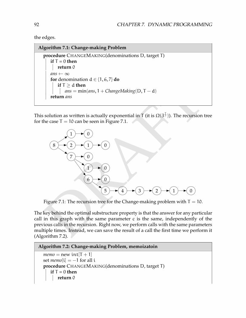
DRAFT
92 CHAPTER 7. DYNAMIC PROGRAMMING
the edges.
Algorithm 7.1: Change-making Problem
procedure CHANGEMAKING(denominations D, target T )if T = 0 then
return 0ans←∞for denomination d ∈ 1, 6, 7 do
if T ≥ d thenans = min(ans, 1+ ChangeMaking(D, T − d)
return ans
This solution as written is actually exponential in T (it isΩ(3T7 )). The recursion tree
for the case T = 10 can be seen in Figure 7.1.
8 1 02
1 0
7 0
1 0
6 0
5 4 3 2 1 0
Figure 7.1: The recursion tree for the Change-making problem with T = 10.
The key behind the optimal substructure property is that the answer for any particularcall in this graph with the same parameter c is the same, independently of theprevious calls in the recursion. Right now, we perform calls with the same parametersmultiple times. Instead, we can save the result of a call the first time we perform it(Algorithm 7.2).
Algorithm 7.2: Change-making Problem, memoizatoin
memo = new int[T + 1]set memo[i] = −1 for all iprocedure CHANGEMAKING(denominations D, target T )
if T = 0 thenreturn 0
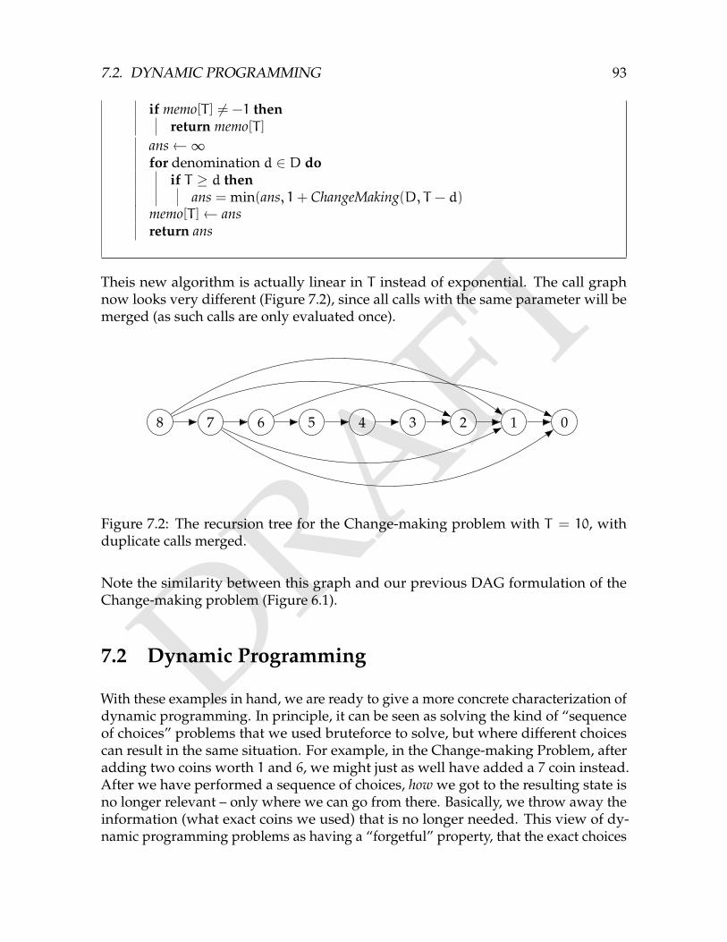
DRAFT
7.2. DYNAMIC PROGRAMMING 93
if memo[T ] 6= −1 thenreturn memo[T ]
ans←∞for denomination d ∈ D do
if T ≥ d thenans = min(ans, 1+ ChangeMaking(D, T − d)
memo[T ]← ansreturn ans
Theis new algorithm is actually linear in T instead of exponential. The call graphnow looks very different (Figure 7.2), since all calls with the same parameter will bemerged (as such calls are only evaluated once).
8 7 6 5 4 3 2 1 0
Figure 7.2: The recursion tree for the Change-making problem with T = 10, withduplicate calls merged.
Note the similarity between this graph and our previous DAG formulation of theChange-making problem (Figure 6.1).
7.2 Dynamic Programming
With these examples in hand, we are ready to give a more concrete characterization ofdynamic programming. In principle, it can be seen as solving the kind of “sequenceof choices” problems that we used bruteforce to solve, but where different choicescan result in the same situation. For example, in the Change-making Problem, afteradding two coins worth 1 and 6, we might just as well have added a 7 coin instead.After we have performed a sequence of choices, how we got to the resulting state isno longer relevant – only where we can go from there. Basically, we throw away theinformation (what exact coins we used) that is no longer needed. This view of dy-namic programming problems as having a “forgetful” property, that the exact choices
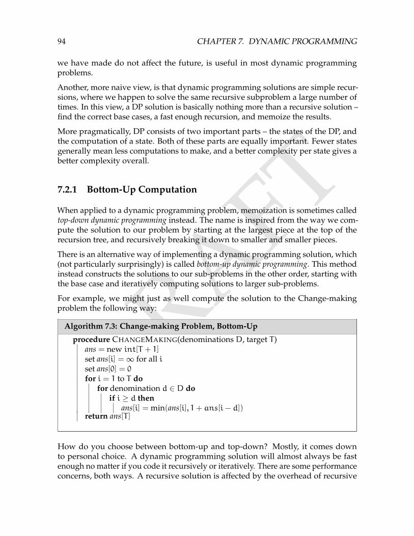
DRAFT
94 CHAPTER 7. DYNAMIC PROGRAMMING
we have made do not affect the future, is useful in most dynamic programmingproblems.
Another, more naive view, is that dynamic programming solutions are simple recur-sions, where we happen to solve the same recursive subproblem a large number oftimes. In this view, a DP solution is basically nothing more than a recursive solution –find the correct base cases, a fast enough recursion, and memoize the results.
More pragmatically, DP consists of two important parts – the states of the DP, andthe computation of a state. Both of these parts are equally important. Fewer statesgenerally mean less computations to make, and a better complexity per state gives abetter complexity overall.
7.2.1 Bottom-Up Computation
When applied to a dynamic programming problem, memoization is sometimes calledtop-down dynamic programming instead. The name is inspired from the way we com-pute the solution to our problem by starting at the largest piece at the top of therecursion tree, and recursively breaking it down to smaller and smaller pieces.
There is an alternative way of implementing a dynamic programming solution, which(not particularly surprisingly) is called bottom-up dynamic programming. This methodinstead constructs the solutions to our sub-problems in the other order, starting withthe base case and iteratively computing solutions to larger sub-problems.
For example, we might just as well compute the solution to the Change-makingproblem the following way:
Algorithm 7.3: Change-making Problem, Bottom-Up
procedure CHANGEMAKING(denominations D, target T )ans = new int[T + 1]set ans[i] =∞ for all iset ans[0] = 0for i = 1 to T do
for denomination d ∈ D doif i ≥ d then
ans[i] = min(ans[i], 1+ ans[i− d])return ans[T ]
How do you choose between bottom-up and top-down? Mostly, it comes downto personal choice. A dynamic programming solution will almost always be fastenough no matter if you code it recursively or iteratively. There are some performanceconcerns, both ways. A recursive solution is affected by the overhead of recursive
DRAFT
7.2. DYNAMIC PROGRAMMING 95
function calls. This problem is not as bad in C++ as in many other languages, but itis still noticeable. When you notice that the number of states in your DP solution isrunning a bit high, you might want to consider coding it iteratively. Top-down DP,on the other hand, has the upside that only the states reachable from the starting statewill be visited. In some DP solutions, the number of unreachable states which are stillin some sense “valid” enough to be computed bottom-up is significant enough thatexcluding them weighs up for the function call overhead. In extreme cases, it mightturn out that an entire parameter is uniquely given by other parameters (such as theFerry Loading problem in Section 7.3). While we probably would notice when this isthe case, the top-down DP saves us when we do not.
7.2.2 Order of Computation and Memory Usage
For top-down DP, the memory usage is often quite clear and unavoidable. If a DPsolution has N states, it will have anΩ(N) memory usage. For a bottom-up solution,the situation is quite different.
Firstly, let us consider one of the downsides of bottom-up DP. When coding a top-down DP, you do not need to bother with the structure of the graph you are solvingyour problem on. For a bottom-up DP, you need to ensure that whenever you solve asubproblem, you have already solved its subproblems too. This requires you to definean order of computation, such that if the subproblem a is used in solving subproblem b,a is computed before b.
In most cases, such an order is quite easy to find. Most parameters can simply beincreasing or decreasing, using a nested loop for each parameter. When a DP is doneover intervals, the order of computation is often over increasing or decreasing lengthof the interval. DP over trees usually require a post-order traversal of the tree. Interms of the recurring graph representation we often use for DP problems, the orderof computation must be a topological ordering of the graph.
While this order of computation business may seem to be nothing but a nuisancethat bottom-up users have to deal with, it is related to one of the perks of bottom-upcomputation. If the order of computation is chosen in a clever way, we need notsave every state during our computation. Consider e.g. the Change-making Problemagain, which had the following recursion:
change(n) =
0 if n = 0
min(change(n− 1), change(n− 6), change(n− 7)) if n > 0
It should be clear that using the order of computation 0, 1, 2, 3, ..., once we havecomputed e.g. change(k), the subproblems change(k− 7), change(k− 8), ... etc. arenever used again.
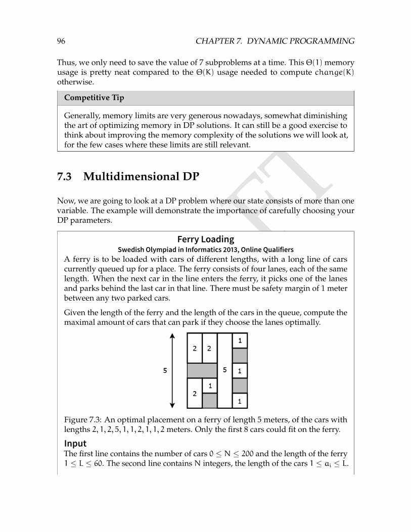
DRAFT
96 CHAPTER 7. DYNAMIC PROGRAMMING
Thus, we only need to save the value of 7 subproblems at a time. This Θ(1) memoryusage is pretty neat compared to the Θ(K) usage needed to compute change(K)otherwise.
Competitive Tip
Generally, memory limits are very generous nowadays, somewhat diminishingthe art of optimizing memory in DP solutions. It can still be a good exercise tothink about improving the memory complexity of the solutions we will look at,for the few cases where these limits are still relevant.
7.3 Multidimensional DP
Now, we are going to look at a DP problem where our state consists of more than onevariable. The example will demonstrate the importance of carefully choosing yourDP parameters.
Ferry LoadingSwedish Olympiad in Informatics 2013, Online Qualifiers
A ferry is to be loaded with cars of different lengths, with a long line of carscurrently queued up for a place. The ferry consists of four lanes, each of the samelength. When the next car in the line enters the ferry, it picks one of the lanesand parks behind the last car in that line. There must be safety margin of 1 meterbetween any two parked cars.
Given the length of the ferry and the length of the cars in the queue, compute themaximal amount of cars that can park if they choose the lanes optimally.
Figure 7.3: An optimal placement on a ferry of length 5meters, of the cars withlengths 2, 1, 2, 5, 1, 1, 2, 1, 1, 2meters. Only the first 8 cars could fit on the ferry.
InputThe first line contains the number of cars 0 ≤ N ≤ 200 and the length of the ferry1 ≤ L ≤ 60. The second line contains N integers, the length of the cars 1 ≤ ai ≤ L.
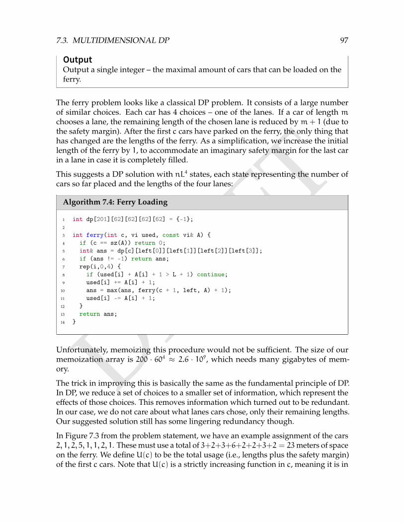
DRAFT
7.3. MULTIDIMENSIONAL DP 97
OutputOutput a single integer – the maximal amount of cars that can be loaded on theferry.
The ferry problem looks like a classical DP problem. It consists of a large numberof similar choices. Each car has 4 choices – one of the lanes. If a car of length mchooses a lane, the remaining length of the chosen lane is reduced bym+ 1 (due tothe safety margin). After the first c cars have parked on the ferry, the only thing thathas changed are the lengths of the ferry. As a simplification, we increase the initiallength of the ferry by 1, to accommodate an imaginary safety margin for the last carin a lane in case it is completely filled.
This suggests a DP solution with nL4 states, each state representing the number ofcars so far placed and the lengths of the four lanes:
Algorithm 7.4: Ferry Loading
1 int dp[201][62][62][62][62] = -1;2
3 int ferry(int c, vi used, const vi& A) 4 if (c == sz(A)) return 0;5 int& ans = dp[c][left[0]][left[1]][left[2]][left[3]];6 if (ans != -1) return ans;7 rep(i,0,4) 8 if (used[i] + A[i] + 1 > L + 1) continue;9 used[i] += A[i] + 1;
10 ans = max(ans, ferry(c + 1, left, A) + 1);11 used[i] -= A[i] + 1;12 13 return ans;14
Unfortunately, memoizing this procedure would not be sufficient. The size of ourmemoization array is 200 · 604 ≈ 2.6 · 109, which needs many gigabytes of mem-ory.
The trick in improving this is basically the same as the fundamental principle of DP.In DP, we reduce a set of choices to a smaller set of information, which represent theeffects of those choices. This removes information which turned out to be redundant.In our case, we do not care about what lanes cars chose, only their remaining lengths.Our suggested solution still has some lingering redundancy though.
In Figure 7.3 from the problem statement, we have an example assignment of the cars2, 1, 2, 5, 1, 1, 2, 1. These must use a total of 3+2+3+6+2+2+3+2 = 23meters of spaceon the ferry. We define U(c) to be the total usage (i.e., lengths plus the safety margin)of the first c cars. Note that U(c) is a strictly increasing function in c, meaning it is in
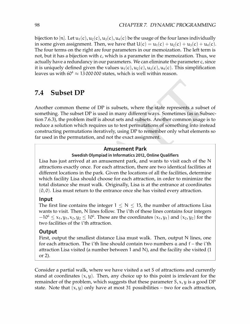
DRAFT
98 CHAPTER 7. DYNAMIC PROGRAMMING
bijection to [n]. Let u1(c), u2(c), u3(c), u4(c) be the usage of the four lanes individuallyin some given assignment. Then, we have that U(c) = u1(c) + u2(c) + u3(c) + u4(c).The four terms on the right are four parameters in our memoization. The left term isnot, but it has a bijection with c, which is a parameter in the memoization. Thus, weactually have a redundancy in our parameters. We can eliminate the parameter c, sinceit is uniquely defined given the values u1(c), u2(c), u3(c), u4(c). This simplificationleaves us with 604 ≈ 13 000 000 states, which is well within reason.
7.4 Subset DP
Another common theme of DP is subsets, where the state represents a subset ofsomething. The subset DP is used in many different ways. Sometimes (as in Subsec-tion 7.6.3), the problem itself is about sets and subsets. Another common usage is toreduce a solution which requires us to test permutations of something into insteadconstructing permutations iteratively, using DP to remember only what elements sofar used in the permutation, and not the exact assignment.
Amusement ParkSwedish Olympiad in Informatics 2012, Online Qualifiers
Lisa has just arrived at an amusement park, and wants to visit each of the Nattractions exactly once. For each attraction, there are two identical facilities atdifferent locations in the park. Given the locations of all the facilities, determinewhich facility Lisa should choose for each attraction, in order to minimize thetotal distance she must walk. Originally, Lisa is at the entrance at coordinates(0, 0). Lisa must return to the entrance once she has visited every attraction.
InputThe first line contains the integer 1 ≤ N ≤ 15, the number of attractions Lisawants to visit. Then, N lines follow. The i’th of these lines contains four integers−106 ≤ x1, y1, x2, y2 ≤ 106. These are the coordinates (x1, y1) and (x2, y2) for thetwo facilities of the i’th attraction.
OutputFirst, output the smallest distance Lisa must walk. Then, output N lines, onefor each attraction. The i’th line should contain two numbers a and f – the i’thattraction Lisa visited (a number between 1 and N), and the facility she visited (1or 2).
Consider a partial walk, where we have visited a set S of attractions and currentlystand at coordinates (x, y). Then, any choice up to this point is irrelevant for theremainder of the problem, which suggests that these parameter S, x, y is a good DPstate. Note that (x, y) only have at most 31 possibilities – two for each attraction,
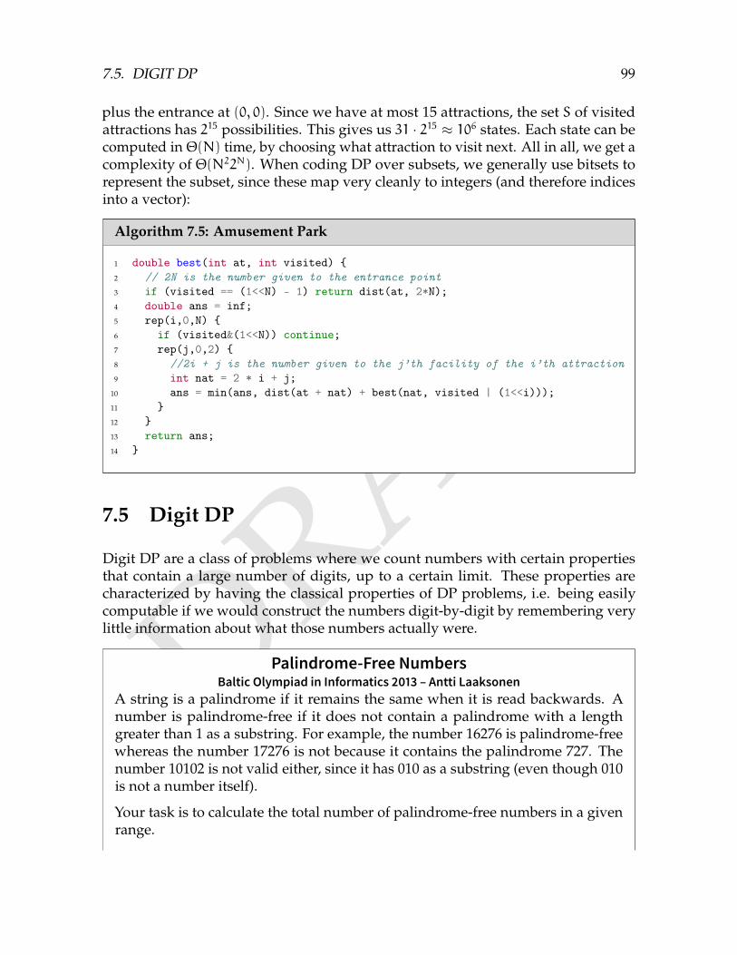
DRAFT
7.5. DIGIT DP 99
plus the entrance at (0, 0). Since we have at most 15 attractions, the set S of visitedattractions has 215 possibilities. This gives us 31 · 215 ≈ 106 states. Each state can becomputed in Θ(N) time, by choosing what attraction to visit next. All in all, we get acomplexity of Θ(N22N). When coding DP over subsets, we generally use bitsets torepresent the subset, since these map very cleanly to integers (and therefore indicesinto a vector):
Algorithm 7.5: Amusement Park
1 double best(int at, int visited) 2 // 2N is the number given to the entrance point3 if (visited == (1<<N) - 1) return dist(at, 2*N);4 double ans = inf;5 rep(i,0,N) 6 if (visited&(1<<N)) continue;7 rep(j,0,2) 8 //2i + j is the number given to the j’th facility of the i’th attraction9 int nat = 2 * i + j;
10 ans = min(ans, dist(at + nat) + best(nat, visited | (1<<i)));11 12 13 return ans;14
7.5 Digit DP
Digit DP are a class of problems where we count numbers with certain propertiesthat contain a large number of digits, up to a certain limit. These properties arecharacterized by having the classical properties of DP problems, i.e. being easilycomputable if we would construct the numbers digit-by-digit by remembering verylittle information about what those numbers actually were.
Palindrome-Free NumbersBaltic Olympiad in Informatics 2013 – Antti Laaksonen
A string is a palindrome if it remains the same when it is read backwards. Anumber is palindrome-free if it does not contain a palindrome with a lengthgreater than 1 as a substring. For example, the number 16276 is palindrome-freewhereas the number 17276 is not because it contains the palindrome 727. Thenumber 10102 is not valid either, since it has 010 as a substring (even though 010is not a number itself).
Your task is to calculate the total number of palindrome-free numbers in a givenrange.
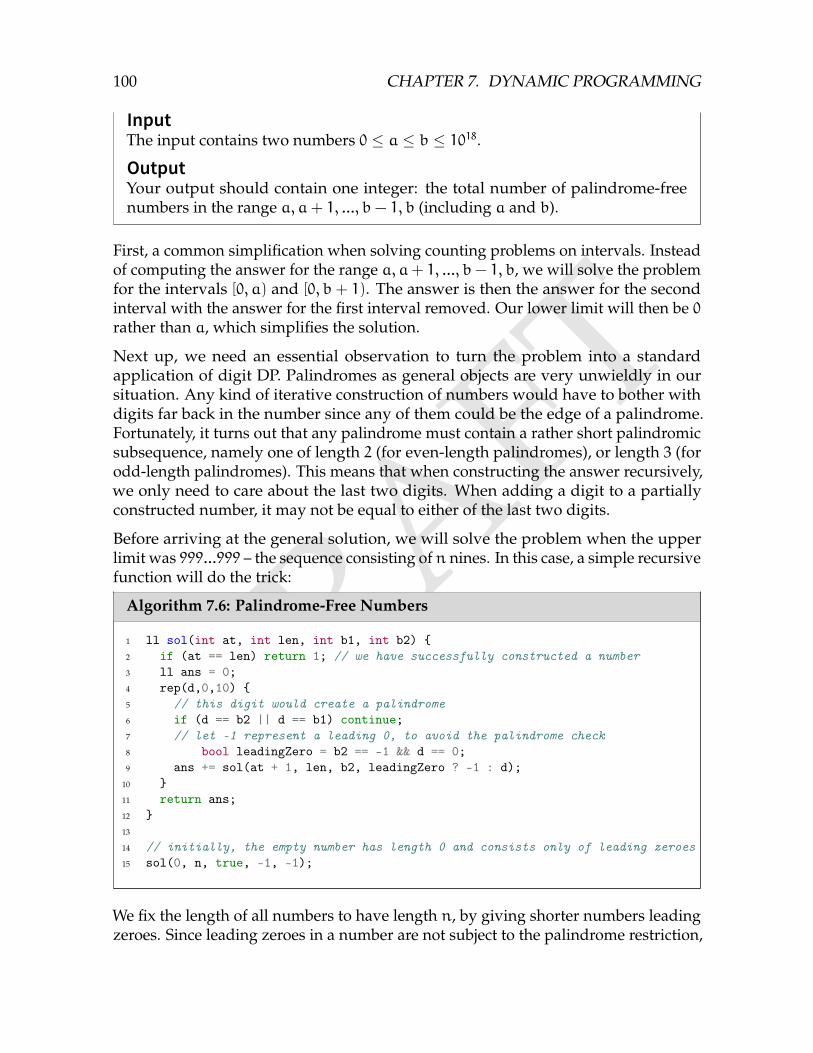
DRAFT
100 CHAPTER 7. DYNAMIC PROGRAMMING
InputThe input contains two numbers 0 ≤ a ≤ b ≤ 1018.OutputYour output should contain one integer: the total number of palindrome-freenumbers in the range a, a+ 1, ..., b− 1, b (including a and b).
First, a common simplification when solving counting problems on intervals. Insteadof computing the answer for the range a, a+ 1, ..., b− 1, b, we will solve the problemfor the intervals [0, a) and [0, b + 1). The answer is then the answer for the secondinterval with the answer for the first interval removed. Our lower limit will then be 0rather than a, which simplifies the solution.
Next up, we need an essential observation to turn the problem into a standardapplication of digit DP. Palindromes as general objects are very unwieldly in oursituation. Any kind of iterative construction of numbers would have to bother withdigits far back in the number since any of them could be the edge of a palindrome.Fortunately, it turns out that any palindrome must contain a rather short palindromicsubsequence, namely one of length 2 (for even-length palindromes), or length 3 (forodd-length palindromes). This means that when constructing the answer recursively,we only need to care about the last two digits. When adding a digit to a partiallyconstructed number, it may not be equal to either of the last two digits.
Before arriving at the general solution, we will solve the problem when the upperlimit was 999...999 – the sequence consisting of n nines. In this case, a simple recursivefunction will do the trick:
Algorithm 7.6: Palindrome-Free Numbers
1 ll sol(int at, int len, int b1, int b2) 2 if (at == len) return 1; // we have successfully constructed a number3 ll ans = 0;4 rep(d,0,10) 5 // this digit would create a palindrome6 if (d == b2 || d == b1) continue;7 // let -1 represent a leading 0, to avoid the palindrome check8 bool leadingZero = b2 == -1 && d == 0;9 ans += sol(at + 1, len, b2, leadingZero ? -1 : d);
10 11 return ans;12 13
14 // initially, the empty number has length 0 and consists only of leading zeroes15 sol(0, n, true, -1, -1);
We fix the length of all numbers to have length n, by giving shorter numbers leadingzeroes. Since leading zeroes in a number are not subject to the palindrome restriction,

DRAFT
7.6. STANDARD PROBLEMS 101
they must be treated differently. In our case, they are given the special digit −1instead, resulting in 11 possible “digits”. Once this function is memoized, it will haven · 2 · 11 · 11 different states, with each state using a loop iterating only 10 times. Thus,it uses on the order of 1000n operations. In our problem, the upper limit has at most19 digits. Thus, the solution only requires about 20 000 operations.
Once a solution has been formulated for this simple upper limit, extending it to ageneral upper limit is quite natural. First, we will save the upper limit as a sequenceof digits L. Then, we need to differentiate between two cases in our recursive function.The partially constructed number is either equal to the corresponding partial upperlimit, or it is less than the limit. In the first case, we are still constrained by the upperlimit – the next digit of our number can not exceed the next digit of the upper limit.In the other case, the the upper limit is no longer relevant. If a prefix of our numberis strictly lower than the prefix of the upper limit, our number can never exceed theupper limit.
This gives us our final solution:
Algorithm 7.7: Palindrome-Free Numbers, General Case
1 vector<int> L;2
3 ll sol(int at, int len, bool limEq, int b1, int b2) 4 if (at == len) return 1;5 ll ans = 0;6 // we may not exceed the limit for this digit if equal to the prefix of the limit7 rep(d,0,(limEq ? L[at] + 1 : 10)) 8 if (d == b2 || d == b1) continue;9 // the next step will be equal to the prefix if it was now,
10 // and our added digit was exactly the limit11 bool limEqNew = limEq && d == L[at];12 bool leadingZero = b2 == -1 && d == 0;13 ans += sol(at + 1, len, limEqNew, b2, leadingZero ? -1 : d);14 15 return ans;16 17
18 // initially, the number is equal to the prefix limit (both being the empty number)19 sol(0, n, true, true, -1, -1);
7.6 Standard Problems
Many problems are variations of known DP problems, or have them as parts of theirsolutions. This section will walk you through a few of them.
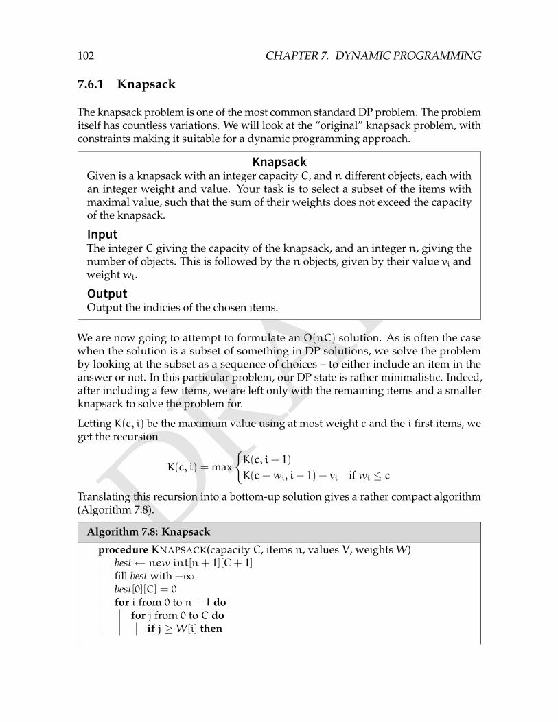
DRAFT
102 CHAPTER 7. DYNAMIC PROGRAMMING
7.6.1 Knapsack
The knapsack problem is one of the most common standard DP problem. The problemitself has countless variations. We will look at the “original” knapsack problem, withconstraints making it suitable for a dynamic programming approach.
KnapsackGiven is a knapsack with an integer capacity C, and n different objects, each withan integer weight and value. Your task is to select a subset of the items withmaximal value, such that the sum of their weights does not exceed the capacityof the knapsack.
InputThe integer C giving the capacity of the knapsack, and an integer n, giving thenumber of objects. This is followed by the n objects, given by their value vi andweight wi.
OutputOutput the indicies of the chosen items.
We are now going to attempt to formulate an O(nC) solution. As is often the casewhen the solution is a subset of something in DP solutions, we solve the problemby looking at the subset as a sequence of choices – to either include an item in theanswer or not. In this particular problem, our DP state is rather minimalistic. Indeed,after including a few items, we are left only with the remaining items and a smallerknapsack to solve the problem for.
Letting K(c, i) be the maximum value using at most weight c and the i first items, weget the recursion
K(c, i) = max
K(c, i− 1)
K(c−wi, i− 1) + vi if wi ≤ c
Translating this recursion into a bottom-up solution gives a rather compact algorithm(Algorithm 7.8).
Algorithm 7.8: Knapsack
procedure KNAPSACK(capacity C, items n, values V , weightsW)best← new int[n+ 1][C+ 1]fill best with −∞best[0][C] = 0for i from 0 to n− 1 do
for j from 0 to C doif j ≥W[i] then
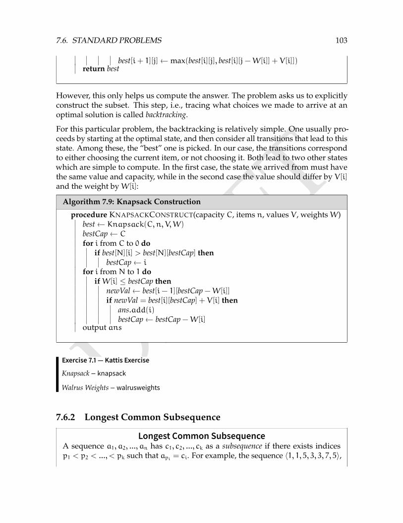
DRAFT
7.6. STANDARD PROBLEMS 103
best[i+ 1][j]← max(best[i][j], best[i][j−W[i]] + V[i]])return best
However, this only helps us compute the answer. The problem asks us to explicitlyconstruct the subset. This step, i.e., tracing what choices we made to arrive at anoptimal solution is called backtracking.
For this particular problem, the backtracking is relatively simple. One usually pro-ceeds by starting at the optimal state, and then consider all transitions that lead to thisstate. Among these, the “best” one is picked. In our case, the transitions correspondto either choosing the current item, or not choosing it. Both lead to two other stateswhich are simple to compute. In the first case, the state we arrived from must havethe same value and capacity, while in the second case the value should differ by V[i]and the weight byW[i]:
Algorithm 7.9: Knapsack Construction
procedure KNAPSACKCONSTRUCT(capacity C, items n, values V , weightsW)best← Knapsack(C,n, V,W)bestCap← C
for i from C to 0 doif best[N][i] > best[N][bestCap] then
bestCap← ifor i from N to 1 do
ifW[i] ≤ bestCap thennewVal← best[i− 1][bestCap −W[i]]if newVal = best[i][bestCap] + V[i] then
ans.add(i)bestCap← bestCap −W[i]
output ans
Exercise 7.1 — Kattis Exercise
Knapsack – knapsack
Walrus Weights – walrusweights
7.6.2 Longest Common Subsequence
Longest Common SubsequenceA sequence a1, a2, ..., an has c1, c2, ..., ck as a subsequence if there exists indicesp1 < p2 < ..., < pk such that api = ci. For example, the sequence 〈1, 1, 5, 3, 3, 7, 5〉,
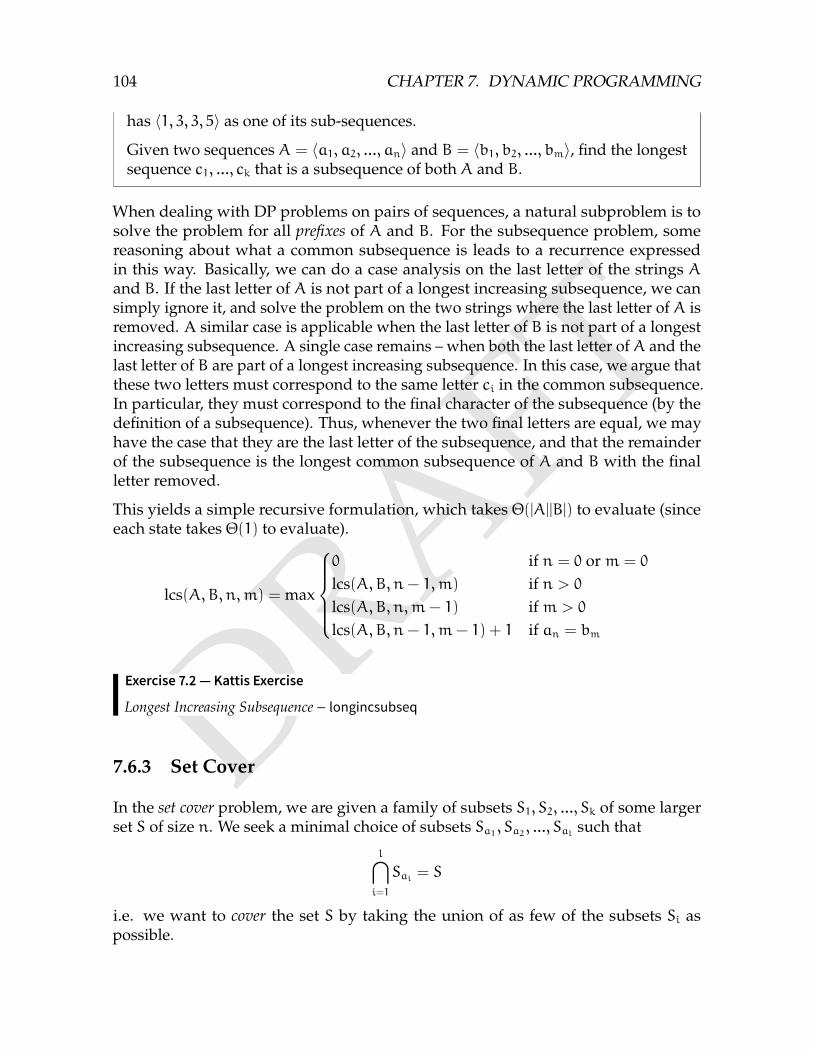
DRAFT
104 CHAPTER 7. DYNAMIC PROGRAMMING
has 〈1, 3, 3, 5〉 as one of its sub-sequences.
Given two sequences A = 〈a1, a2, ..., an〉 and B = 〈b1, b2, ..., bm〉, find the longestsequence c1, ..., ck that is a subsequence of both A and B.
When dealing with DP problems on pairs of sequences, a natural subproblem is tosolve the problem for all prefixes of A and B. For the subsequence problem, somereasoning about what a common subsequence is leads to a recurrence expressedin this way. Basically, we can do a case analysis on the last letter of the strings Aand B. If the last letter of A is not part of a longest increasing subsequence, we cansimply ignore it, and solve the problem on the two strings where the last letter of A isremoved. A similar case is applicable when the last letter of B is not part of a longestincreasing subsequence. A single case remains – when both the last letter ofA and thelast letter of B are part of a longest increasing subsequence. In this case, we argue thatthese two letters must correspond to the same letter ci in the common subsequence.In particular, they must correspond to the final character of the subsequence (by thedefinition of a subsequence). Thus, whenever the two final letters are equal, we mayhave the case that they are the last letter of the subsequence, and that the remainderof the subsequence is the longest common subsequence of A and B with the finalletter removed.
This yields a simple recursive formulation, which takes Θ(|A||B|) to evaluate (sinceeach state takes Θ(1) to evaluate).
lcs(A,B, n,m) = max
0 if n = 0 orm = 0
lcs(A,B, n− 1,m) if n > 0lcs(A,B, n,m− 1) ifm > 0
lcs(A,B, n− 1,m− 1) + 1 if an = bm
Exercise 7.2 — Kattis Exercise
Longest Increasing Subsequence – longincsubseq
7.6.3 Set Cover
In the set cover problem, we are given a family of subsets S1, S2, ..., Sk of some largerset S of size n. We seek a minimal choice of subsets Sa1 , Sa2 , ..., Sal such that
l⋂i=1
Sai = S
i.e. we want to cover the set S by taking the union of as few of the subsets Si aspossible.
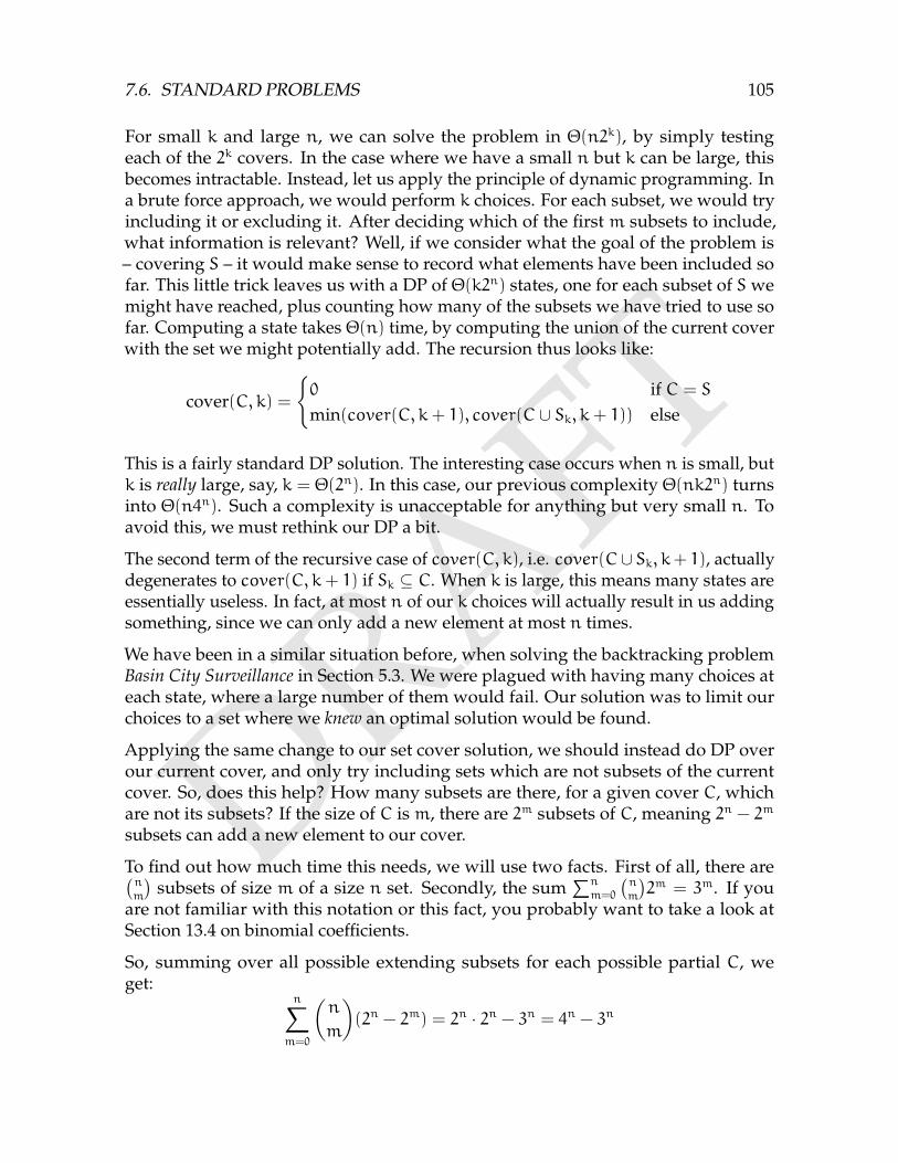
DRAFT
7.6. STANDARD PROBLEMS 105
For small k and large n, we can solve the problem in Θ(n2k), by simply testingeach of the 2k covers. In the case where we have a small n but k can be large, thisbecomes intractable. Instead, let us apply the principle of dynamic programming. Ina brute force approach, we would perform k choices. For each subset, we would tryincluding it or excluding it. After deciding which of the first m subsets to include,what information is relevant? Well, if we consider what the goal of the problem is– covering S – it would make sense to record what elements have been included sofar. This little trick leaves us with a DP of Θ(k2n) states, one for each subset of Swemight have reached, plus counting how many of the subsets we have tried to use sofar. Computing a state takes Θ(n) time, by computing the union of the current coverwith the set we might potentially add. The recursion thus looks like:
cover(C, k) =
0 if C = S
min(cover(C, k+ 1), cover(C ∪ Sk, k+ 1)) else
This is a fairly standard DP solution. The interesting case occurs when n is small, butk is really large, say, k = Θ(2n). In this case, our previous complexity Θ(nk2n) turnsinto Θ(n4n). Such a complexity is unacceptable for anything but very small n. Toavoid this, we must rethink our DP a bit.
The second term of the recursive case of cover(C, k), i.e. cover(C∪ Sk, k+ 1), actuallydegenerates to cover(C, k+ 1) if Sk ⊆ C. When k is large, this means many states areessentially useless. In fact, at most n of our k choices will actually result in us addingsomething, since we can only add a new element at most n times.
We have been in a similar situation before, when solving the backtracking problemBasin City Surveillance in Section 5.3. We were plagued with having many choices ateach state, where a large number of them would fail. Our solution was to limit ourchoices to a set where we knew an optimal solution would be found.
Applying the same change to our set cover solution, we should instead do DP overour current cover, and only try including sets which are not subsets of the currentcover. So, does this help? How many subsets are there, for a given cover C, whichare not its subsets? If the size of C is m, there are 2m subsets of C, meaning 2n − 2m
subsets can add a new element to our cover.
To find out how much time this needs, we will use two facts. First of all, there are(nm
)subsets of size m of a size n set. Secondly, the sum
∑nm=0
(nm
)2m = 3m. If you
are not familiar with this notation or this fact, you probably want to take a look atSection 13.4 on binomial coefficients.
So, summing over all possible extending subsets for each possible partial C, weget:
n∑m=0
(n
m
)(2n − 2m) = 2n · 2n − 3n = 4n − 3n
DRAFT
106 CHAPTER 7. DYNAMIC PROGRAMMING
Closer, but no cigar. Intuitively, we still have a large number of redundant choices.If our cover contains, say, n − 1 elements, there are 2n−1 sets which can extend ourcover, but they all extend it in the same way. This sounds wasteful, and avoiding itprobably the key to getting an asymptotic speedup.
It seems that we are missing some key function which can respond to the question:“is there some subset Si, that could extend our cover with some subset A ⊆ S?”. If wehad such a function, computing all possible extensions of a cover of size m wouldinstead take time 2n−m – the number of possible extensions to the cover. Last time wemanaged to extend a cover in time 2n − 2m, but this is exponentially better!
In fact, if we do our summing this time, we get:
n∑m=0
(n
m
)2n−m =
n∑m=0
(n
n−m
)2n−m
=
n∑m=0
(n
m
)2m
= 3n
It turns out our exponential speedup in extending a cover translated into an exponen-tial speedup of the entire DP.
We are not done yet – this entire algorithm depended on the assumption of ourmagical “can we extend a cover with a subset A?” function. Sometimes, this functionmay be quick to compute. For example, if S = 1, 2, ..., n and the family Si consists ofall sets whose sum is less than n, an extension is possible if and only if its sum is alsoless than n. In the general case, our Si are not this nice. Naively, one might think thatin the general case, an answer to this query would take Θ(nk) time to compute, bychecking if A is a subset of each of our k sets. Yet again, the same clever trick comesto the rescue.
If we have a set Si of size m available for use in our cover. just how many possibleextensions could this subset provide? Well, Si itself only have 2m subsets. Thus, if wefor each Si mark for each of its subsets that this is a possible extension to a cover, thisprecomputation only takes 3n time (by the same sum as above).
Since both steps are O(3n), this is also our final complexity.
Exercise 7.3 — Kattis Exercises
Square Fields (Easy) – squarefieldseasy
Square Fields (Hard) – squarefieldshard

DRAFT
7.7. CHAPTER NOTES 107
7.7 Chapter Notes
write chapternoteswrite chapternotes

DRAFT
108 CHAPTER 7. DYNAMIC PROGRAMMING
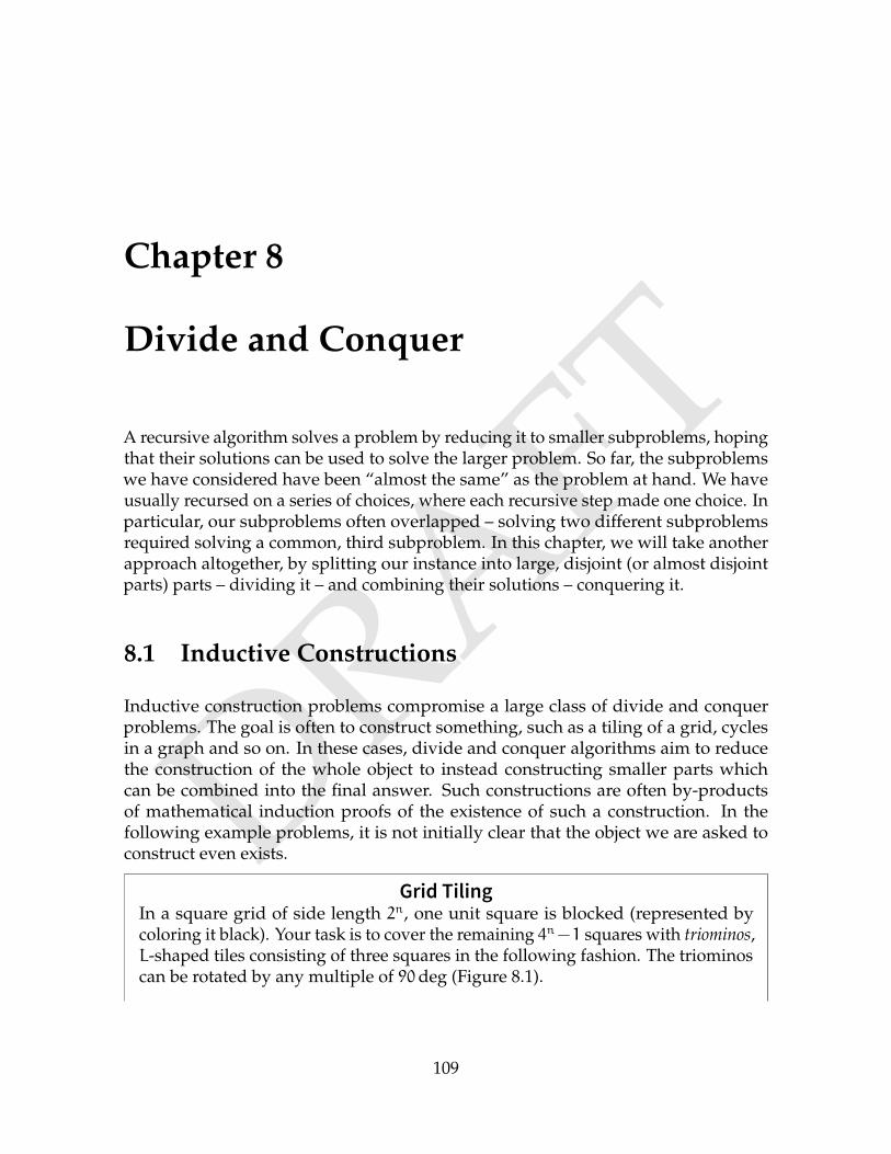
DRAFTChapter 8
Divide and Conquer
A recursive algorithm solves a problem by reducing it to smaller subproblems, hopingthat their solutions can be used to solve the larger problem. So far, the subproblemswe have considered have been “almost the same” as the problem at hand. We haveusually recursed on a series of choices, where each recursive step made one choice. Inparticular, our subproblems often overlapped – solving two different subproblemsrequired solving a common, third subproblem. In this chapter, we will take anotherapproach altogether, by splitting our instance into large, disjoint (or almost disjointparts) parts – dividing it – and combining their solutions – conquering it.
8.1 Inductive Constructions
Inductive construction problems compromise a large class of divide and conquerproblems. The goal is often to construct something, such as a tiling of a grid, cyclesin a graph and so on. In these cases, divide and conquer algorithms aim to reducethe construction of the whole object to instead constructing smaller parts whichcan be combined into the final answer. Such constructions are often by-productsof mathematical induction proofs of the existence of such a construction. In thefollowing example problems, it is not initially clear that the object we are asked toconstruct even exists.
Grid TilingIn a square grid of side length 2n, one unit square is blocked (represented bycoloring it black). Your task is to cover the remaining 4n−1 squares with triominos,L-shaped tiles consisting of three squares in the following fashion. The triominoscan be rotated by any multiple of 90deg (Figure 8.1).
109
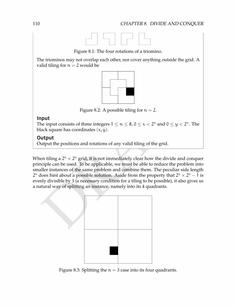
DRAFT
110 CHAPTER 8. DIVIDE AND CONQUER
Figure 8.1: The four rotations of a triomino.
The triominos may not overlap each other, nor cover anything outside the grid. Avalid tiling for n = 2would be
Figure 8.2: A possible tiling for n = 2.
InputThe input consists of three integers 1 ≤ n ≤ 8, 0 ≤ x < 2n and 0 ≤ y < 2n. Theblack square has coordinates (x, y).
OutputOutput the positions and rotations of any valid tiling of the grid.
When tiling a 2n × 2n grid, it is not immediately clear how the divide and conquerprinciple can be used. To be applicable, we must be able to reduce the problem intosmaller instances of the same problem and combine them. The peculiar side length2n does hint about a possible solution. Aside from the property that 2n × 2n − 1 isevenly divisible by 3 (a necessary condition for a tiling to be possible), it also gives usa natural way of splitting an instance, namely into its 4 quadrants.
Figure 8.3: Splitting the n = 3 case into its four quadrants.
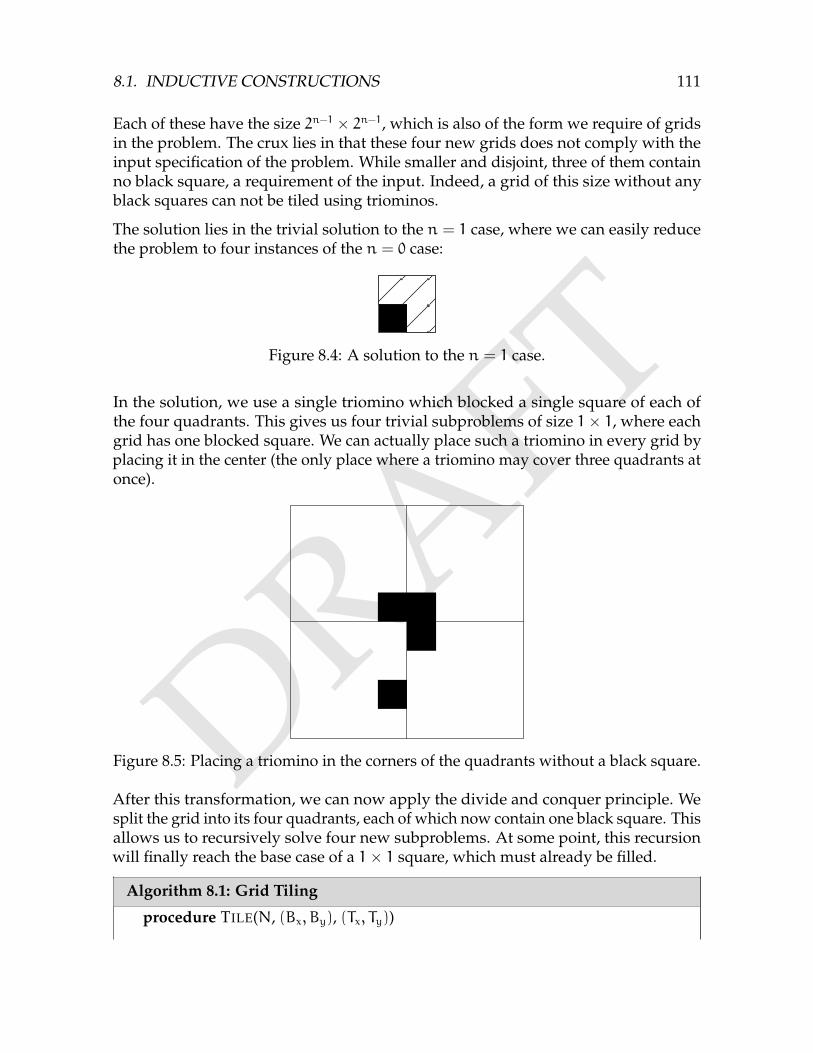
DRAFT
8.1. INDUCTIVE CONSTRUCTIONS 111
Each of these have the size 2n−1 × 2n−1, which is also of the form we require of gridsin the problem. The crux lies in that these four new grids does not comply with theinput specification of the problem. While smaller and disjoint, three of them containno black square, a requirement of the input. Indeed, a grid of this size without anyblack squares can not be tiled using triominos.
The solution lies in the trivial solution to the n = 1 case, where we can easily reducethe problem to four instances of the n = 0 case:
Figure 8.4: A solution to the n = 1 case.
In the solution, we use a single triomino which blocked a single square of each ofthe four quadrants. This gives us four trivial subproblems of size 1× 1, where eachgrid has one blocked square. We can actually place such a triomino in every grid byplacing it in the center (the only place where a triomino may cover three quadrants atonce).
Figure 8.5: Placing a triomino in the corners of the quadrants without a black square.
After this transformation, we can now apply the divide and conquer principle. Wesplit the grid into its four quadrants, each of which now contain one black square. Thisallows us to recursively solve four new subproblems. At some point, this recursionwill finally reach the base case of a 1× 1 square, which must already be filled.
Algorithm 8.1: Grid Tiling
procedure TILE(N, (Bx, By), (Tx, Ty))
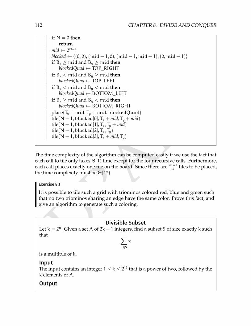
DRAFT
112 CHAPTER 8. DIVIDE AND CONQUER
if N = 0 thenreturn
mid← 2N−1
blocked← (0, 0), (mid− 1, 0), (mid− 1,mid− 1), (0,mid− 1)if Bx ≥ mid and By ≥ mid then
blockedQuad← TOP_RIGHTif Bx < mid and By ≥ mid then
blockedQuad← TOP_LEFTif Bx < mid and By < mid then
blockedQuad← BOTTOM_LEFTif Bx ≥ mid and By < mid then
blockedQuad← BOTTOM_RIGHTplace(Tx +mid, Ty +mid, blockedQuad)tile(N− 1, blocked[0], Tx + mid, Ty + mid)tile(N− 1, blocked[1], Tx, Ty + mid)tile(N− 1, blocked[2], Tx, Ty)tile(N− 1, blocked[3], Tx + mid, Ty)
The time complexity of the algorithm can be computed easily if we use the fact thateach call to tile only takes Θ(1) time except for the four recursive calls. Furthermore,each call places exactly one tile on the board. Since there are 4n−1
3tiles to be placed,
the time complexity must be Θ(4n).
Exercise 8.1
It is possible to tile such a grid with triominos colored red, blue and green suchthat no two triominos sharing an edge have the same color. Prove this fact, andgive an algorithm to generate such a coloring.
Divisible SubsetLet k = 2n. Given a set A of 2k− 1 integers, find a subset S of size exactly k suchthat ∑
x∈S
x
is a multiple of k.
InputThe input contains an integer 1 ≤ k ≤ 215 that is a power of two, followed by thek elements of A.
Output
DRAFT
8.1. INDUCTIVE CONSTRUCTIONS 113
Output the k elements of S.
When given a problem, it is often a good idea to solve a few small cases by hand.This applies especially to this kind of construction problems, where constructions forsmall inputs often shows some pattern or insight into how to solve larger instances.The case k = 1 is not particularly meaningful, since it is trivially true (any integer isa multiple of 1). When k = 2, we get an insight which might not seem particularlyinteresting, but is key to the problem. We are given 2 · 2− 1 = 3 numbers, and seektwo numbers whose sum is even. Given three numbers, it must have either twonumbers which both are even, or two odd numbers. Both of these cases yield a pairwith an even sum.
It turns out that this construction generalizes to larger instances. Generally, it is easierto do the “divide” part of a divide and conquer solution first, but in this problemwe will do it the other way around. The recursion will follow quite naturally afterwe attempt to find a way in combining solutions to the smaller instance to a largerone.
We will lay the the ground work for a reduction of the case 2k to k. First, assumethat we could solve the problem for a given k. The larger instance then contains2(2k− 1) = 4k− 1 numbers, of which we seek 2k numbers whose sum is a multipleof 2k. This situation is essentially the same as for the case k = 2, except everything isscaled up by k. Can we scale our solution up as well?
If we have three sets of k numbers whose respective sums are all multiples of k, wecan find two sets of k numbers whose total sum is divisible by 2k. This constructionessentially use the same argument as for k = 2. If the three subsets have sumsak, bk, ck and we wish to find two whose sum is a multiple of 2k, this is the sameas finding two numbers of a, b, c whose sum is a multiple of 2. This is possible,according to the case k = 2.
A beautiful generalization indeed, but we still have some remnants of wishful thinkingwe need to take care of. The construction assumes that, given 4k − 1 numbers, wecan find three sets of k numbers whose sum are divisible by k. We have now come tothe recursive aspect of the problem. By assumption, we could solve the problem fork. This means we can pick any 2k − 1 of our 4k − 1 numbers to get our first subset.The subset uses up k of our 4k − 1 numbers, leaving us with only 3k − 1 numbers.We keep going, and pick any 2k− 1 of these numbers and recursively get a secondsubset. After this, 2k− 1 numbers are left, exactly how many we need to constructour third subset.
The division of the problem was thus into four parts. Three subsets of k numbers, andone set of k− 1which we throw away. Coming up with such a division essentiallyrequired us to solve the combination part first with the generalizing of the casek = 2.
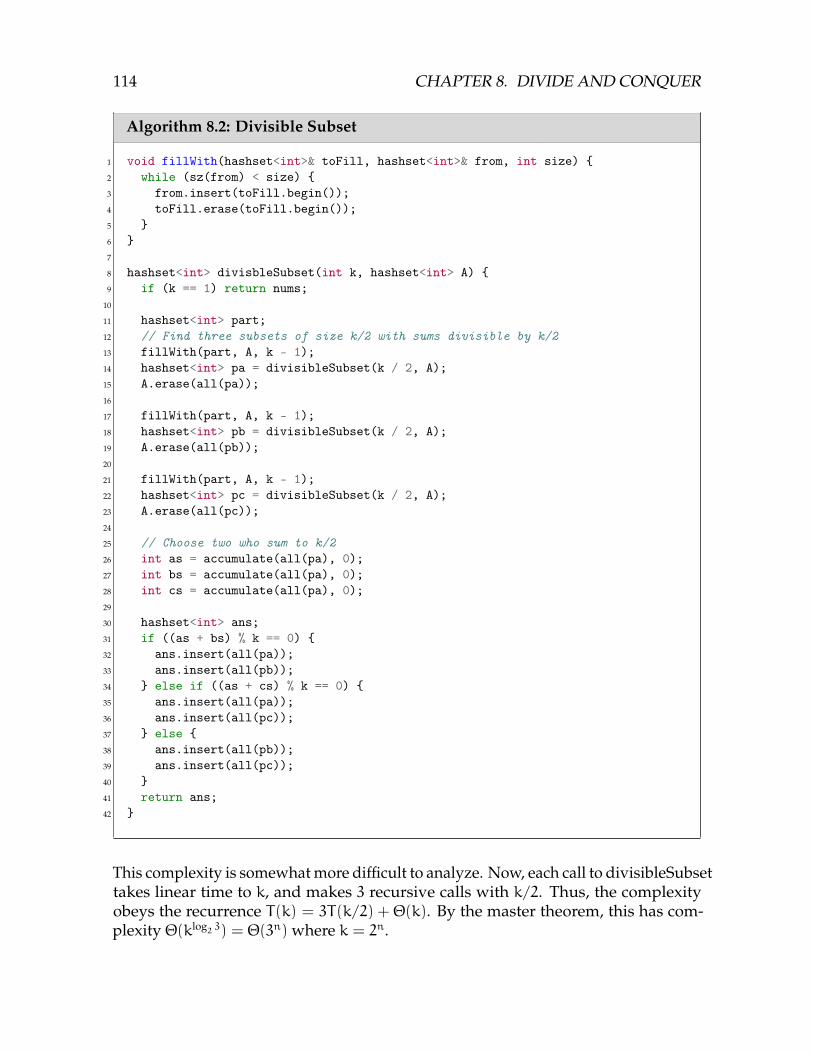
DRAFT
114 CHAPTER 8. DIVIDE AND CONQUER
Algorithm 8.2: Divisible Subset
1 void fillWith(hashset<int>& toFill, hashset<int>& from, int size) 2 while (sz(from) < size) 3 from.insert(toFill.begin());4 toFill.erase(toFill.begin());5 6 7
8 hashset<int> divisbleSubset(int k, hashset<int> A) 9 if (k == 1) return nums;
10
11 hashset<int> part;12 // Find three subsets of size k/2 with sums divisible by k/213 fillWith(part, A, k - 1);14 hashset<int> pa = divisibleSubset(k / 2, A);15 A.erase(all(pa));16
17 fillWith(part, A, k - 1);18 hashset<int> pb = divisibleSubset(k / 2, A);19 A.erase(all(pb));20
21 fillWith(part, A, k - 1);22 hashset<int> pc = divisibleSubset(k / 2, A);23 A.erase(all(pc));24
25 // Choose two who sum to k/226 int as = accumulate(all(pa), 0);27 int bs = accumulate(all(pa), 0);28 int cs = accumulate(all(pa), 0);29
30 hashset<int> ans;31 if ((as + bs) % k == 0) 32 ans.insert(all(pa));33 ans.insert(all(pb));34 else if ((as + cs) % k == 0) 35 ans.insert(all(pa));36 ans.insert(all(pc));37 else 38 ans.insert(all(pb));39 ans.insert(all(pc));40 41 return ans;42
This complexity is somewhat more difficult to analyze. Now, each call to divisibleSubsettakes linear time to k, and makes 3 recursive calls with k/2. Thus, the complexityobeys the recurrence T(k) = 3T(k/2) + Θ(k). By the master theorem, this has com-plexity Θ(klog2 3) = Θ(3n) where k = 2n.
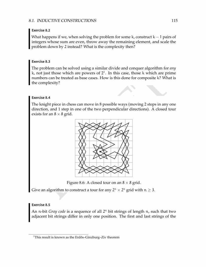
DRAFT
8.1. INDUCTIVE CONSTRUCTIONS 115
Exercise 8.2
What happens if we, when solving the problem for some k, construct k− 1 pairs ofintegers whose sum are even, throw away the remaining element, and scale theproblem down by 2 instead? What is the complexity then?
Exercise 8.3
The problem can be solved using a similar divide and conquer algorithm for anyk, not just those which are powers of 21. In this case, those k which are primenumbers can be treated as base cases. How is this done for composite k? What isthe complexity?
Exercise 8.4
The knight piece in chess can move in 8 possible ways (moving 2 steps in any onedirection, and 1 step in one of the two perpendicular directions). A closed tourexists for an 8× 8 grid.
Figure 8.6: A closed tour on an 8× 8 grid.
Give an algorithm to construct a tour for any 2n × 2n grid with n ≥ 3.
Exercise 8.5
An n-bit Gray code is a sequence of all 2n bit strings of length n, such that twoadjacent bit strings differ in only one position. The first and last strings of the
1This result is known as the Erdos–Ginzburg–Ziv theorem
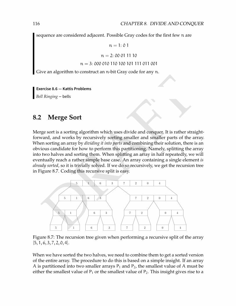
DRAFT
116 CHAPTER 8. DIVIDE AND CONQUER
sequence are considered adjacent. Possible Gray codes for the first few n are
n = 1: 0 1
n = 2: 00 01 11 10
n = 3: 000 010 110 100 101 111 011 001
Give an algorithm to construct an n-bit Gray code for any n.
Exercise 8.6 — Kattis Problems
Bell Ringing – bells
8.2 Merge Sort
Merge sort is a sorting algorithm which uses divide and conquer. It is rather straight-forward, and works by recursively sorting smaller and smaller parts of the array.When sorting an array by dividing it into parts and combining their solution, there is anobvious candidate for how to perform this partitioning. Namely, splitting the arrayinto two halves and sorting them. When splitting an array in half repeatedly, we willeventually reach a rather simple base case. An array containing a single element isalready sorted, so it is trivially solved. If we do so recursively, we get the recursion treein Figure 8.7. Coding this recursive split is easy.
5 1 6 3 7 2 0 4
5 1 6 3
5 1
5 1
6 3
6 3
7 2 0 4
7 2
7 2
0 4
0 4
Figure 8.7: The recursion tree given when performing a recursive split of the array[5, 1, 6, 3, 7, 2, 0, 4].
When we have sorted the two halves, we need to combine them to get a sorted versionof the entire array. The procedure to do this is based on a simple insight. If an arrayA is partitioned into two smaller arrays P1 and P2, the smallest value of A must beeither the smallest value of P1 or the smallest value of P2. This insight gives rise to a

DRAFT
8.2. MERGE SORT 117
simple iterative procedure, where we repeatedly compare the smallest values of P1and P2, extract the smaller one of them, and append it to our sorted array.
Algorithm 8.3: Merge Sort
1 void sortVector(vector<int>& a, int l, int r)2 int m = (l + r)/2;3 sortVector(a, l, m); // sort left half4 sortVector(a, m, r); // sort right half5
6 //combine the answers7 vector<int> answer;8 int x = l;9 int y = m;
10 while(x < m || y < r)11 if(x == m || (y < r && a[y] < a[x]))12 answer.push_back(a[y]);13 y++;14 else 15 answer.push_back(a[x]);16 x++;17 18 19 rep(i,l,r) a[i] = answer[i - l];20
To compute the complexity, consider the recursion tree in Figure 8.7. We make onecall with 8 elements, two calls with 4 elements, and so on. Further, the combiningprocedure takes Θ(l) time for a call with l elements. In the general case of n = 2k
elements, this means merge sort takes time
k∑i=0
2i ·Θ(2k−i) = Θ(k2k)
Since k = log2n, this means the complexity is Θ(n logn).
Exercise 8.7
Our complexity analysis assumed that the length of the array is a power of 2. Thecomplexity is the same in the general case. Prove this fact.
Exercise 8.8
Given an array A of size n, we call the pair i < j an inversion of A if A[i] > A[j].
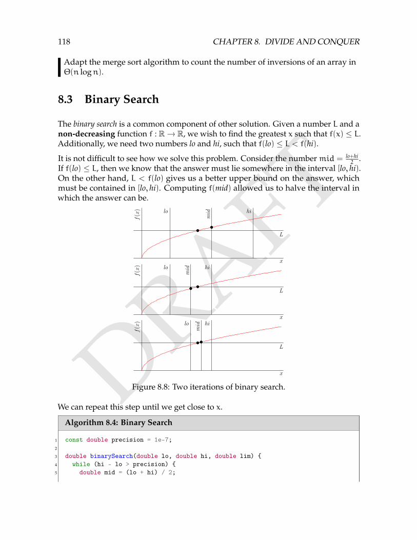
DRAFT
118 CHAPTER 8. DIVIDE AND CONQUER
Adapt the merge sort algorithm to count the number of inversions of an array inΘ(n logn).
8.3 Binary Search
The binary search is a common component of other solution. Given a number L and anon-decreasing function f : R→ R, we wish to find the greatest x such that f(x) ≤ L.Additionally, we need two numbers lo and hi, such that f(lo) ≤ L < f(hi).
It is not difficult to see how we solve this problem. Consider the numbermid = lo+hi2
.If f(lo) ≤ L, then we know that the answer must lie somewhere in the interval [lo, hi).On the other hand, L < f(lo) gives us a better upper bound on the answer, whichmust be contained in [lo, hi). Computing f(mid) allowed us to halve the interval inwhich the answer can be.
f(x)
x
lomid hi
L
f(x)
x
lo
mid hi
L
f(x)
x
lo
mid hi
L
Figure 8.8: Two iterations of binary search.
We can repeat this step until we get close to x.
Algorithm 8.4: Binary Search
1 const double precision = 1e-7;2
3 double binarySearch(double lo, double hi, double lim) 4 while (hi - lo > precision) 5 double mid = (lo + hi) / 2;
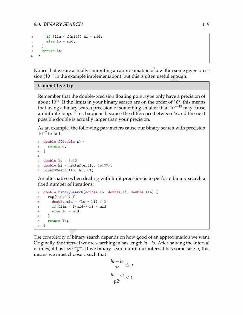
DRAFT
8.3. BINARY SEARCH 119
6 if (lim < f(mid)) hi = mid;7 else lo = mid;8 9 return lo;
10
Notice that we are actually computing an approximation of xwithin some given preci-sion (10−7 in the example implementation), but this is often useful enough.
Competitive Tip
Remember that the double-precision floating point type only have a precision ofabout 1015. If the limits in your binary search are on the order of 10x, this meansthat using a binary search precision of something smaller than 10x−15 may causean infinite loop. This happens because the difference between lo and the nextpossible double is actually larger than your precision.
As an example, the following parameters cause our binary search with precision10−7 to fail.
1 double f(double x) 2 return 0;3 4
5 double lo = 1e12;6 double hi = nextafter(lo, 1e100);7 binarySearch(lo, hi, 0);
An alternative when dealing with limit precision is to perform binary search afixed number of iterations:
1 double binarySearch(double lo, double hi, double lim) 2 rep(i,0,60) 3 double mid = (lo + hi) / 2;4 if (lim < f(mid)) hi = mid;5 else lo = mid;6 7 return lo;8
The complexity of binary search depends on how good of an approximation we want.Originally, the interval we are searching in has length hi−lo. After halving the intervalc times, it has size hi−lo
2c. If we binary search until our interval has some size p, this
means we must choose c such thathi − lo2c
≤ p
hi − lop2c
≤ 1
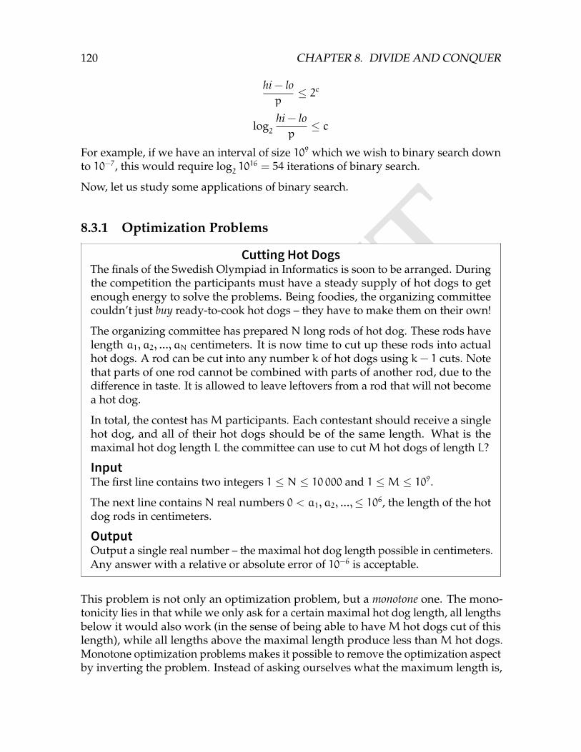
DRAFT
120 CHAPTER 8. DIVIDE AND CONQUER
hi − lop
≤ 2c
log2
hi − lop
≤ c
For example, if we have an interval of size 109 which we wish to binary search downto 10−7, this would require log
21016 = 54 iterations of binary search.
Now, let us study some applications of binary search.
8.3.1 Optimization Problems
Cutting Hot DogsThe finals of the Swedish Olympiad in Informatics is soon to be arranged. Duringthe competition the participants must have a steady supply of hot dogs to getenough energy to solve the problems. Being foodies, the organizing committeecouldn’t just buy ready-to-cook hot dogs – they have to make them on their own!
The organizing committee has prepared N long rods of hot dog. These rods havelength a1, a2, ..., aN centimeters. It is now time to cut up these rods into actualhot dogs. A rod can be cut into any number k of hot dogs using k− 1 cuts. Notethat parts of one rod cannot be combined with parts of another rod, due to thedifference in taste. It is allowed to leave leftovers from a rod that will not becomea hot dog.
In total, the contest hasM participants. Each contestant should receive a singlehot dog, and all of their hot dogs should be of the same length. What is themaximal hot dog length L the committee can use to cutM hot dogs of length L?
InputThe first line contains two integers 1 ≤ N ≤ 10 000 and 1 ≤M ≤ 109.The next line contains N real numbers 0 < a1, a2, ...,≤ 106, the length of the hotdog rods in centimeters.
OutputOutput a single real number – the maximal hot dog length possible in centimeters.Any answer with a relative or absolute error of 10−6 is acceptable.
This problem is not only an optimization problem, but a monotone one. The mono-tonicity lies in that while we only ask for a certain maximal hot dog length, all lengthsbelow it would also work (in the sense of being able to haveM hot dogs cut of thislength), while all lengths above the maximal length produce less than M hot dogs.Monotone optimization problems makes it possible to remove the optimization aspectby inverting the problem. Instead of asking ourselves what the maximum length is,
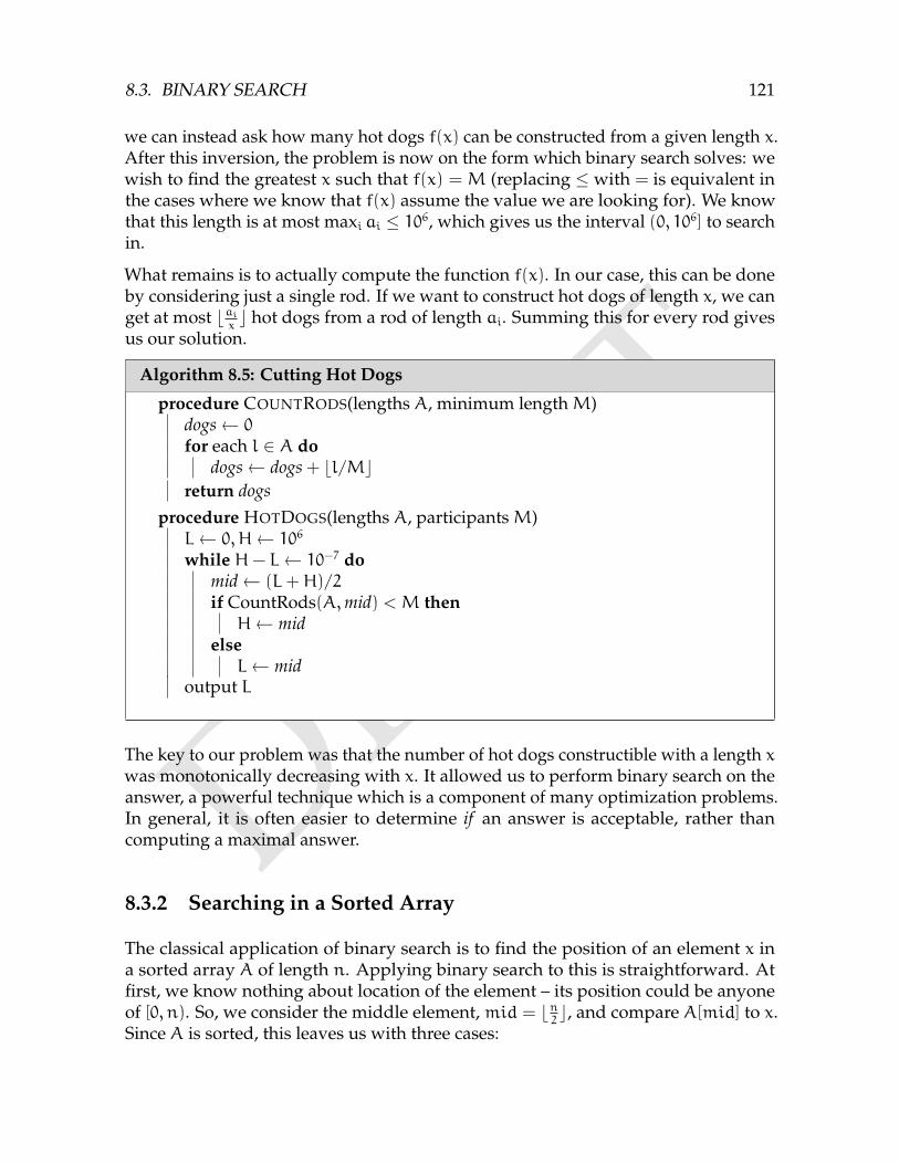
DRAFT
8.3. BINARY SEARCH 121
we can instead ask how many hot dogs f(x) can be constructed from a given length x.After this inversion, the problem is now on the form which binary search solves: wewish to find the greatest x such that f(x) = M (replacing ≤ with = is equivalent inthe cases where we know that f(x) assume the value we are looking for). We knowthat this length is at most maxi ai ≤ 106, which gives us the interval (0, 106] to searchin.
What remains is to actually compute the function f(x). In our case, this can be doneby considering just a single rod. If we want to construct hot dogs of length x, we canget at most bai
xc hot dogs from a rod of length ai. Summing this for every rod gives
us our solution.
Algorithm 8.5: Cutting Hot Dogs
procedure COUNTRODS(lengths A, minimum lengthM)dogs← 0
for each l ∈ A dodogs← dogs + bl/Mc
return dogsprocedure HOTDOGS(lengths A, participantsM)L← 0,H← 106
while H− L← 10−7 domid← (L+H)/2if CountRods(A,mid) < M thenH← mid
elseL← mid
output L
The key to our problem was that the number of hot dogs constructible with a length xwas monotonically decreasing with x. It allowed us to perform binary search on theanswer, a powerful technique which is a component of many optimization problems.In general, it is often easier to determine if an answer is acceptable, rather thancomputing a maximal answer.
8.3.2 Searching in a Sorted Array
The classical application of binary search is to find the position of an element x ina sorted array A of length n. Applying binary search to this is straightforward. Atfirst, we know nothing about location of the element – its position could be anyoneof [0, n). So, we consider the middle element,mid = bn
2c, and compare A[mid] to x.
Since A is sorted, this leaves us with three cases:
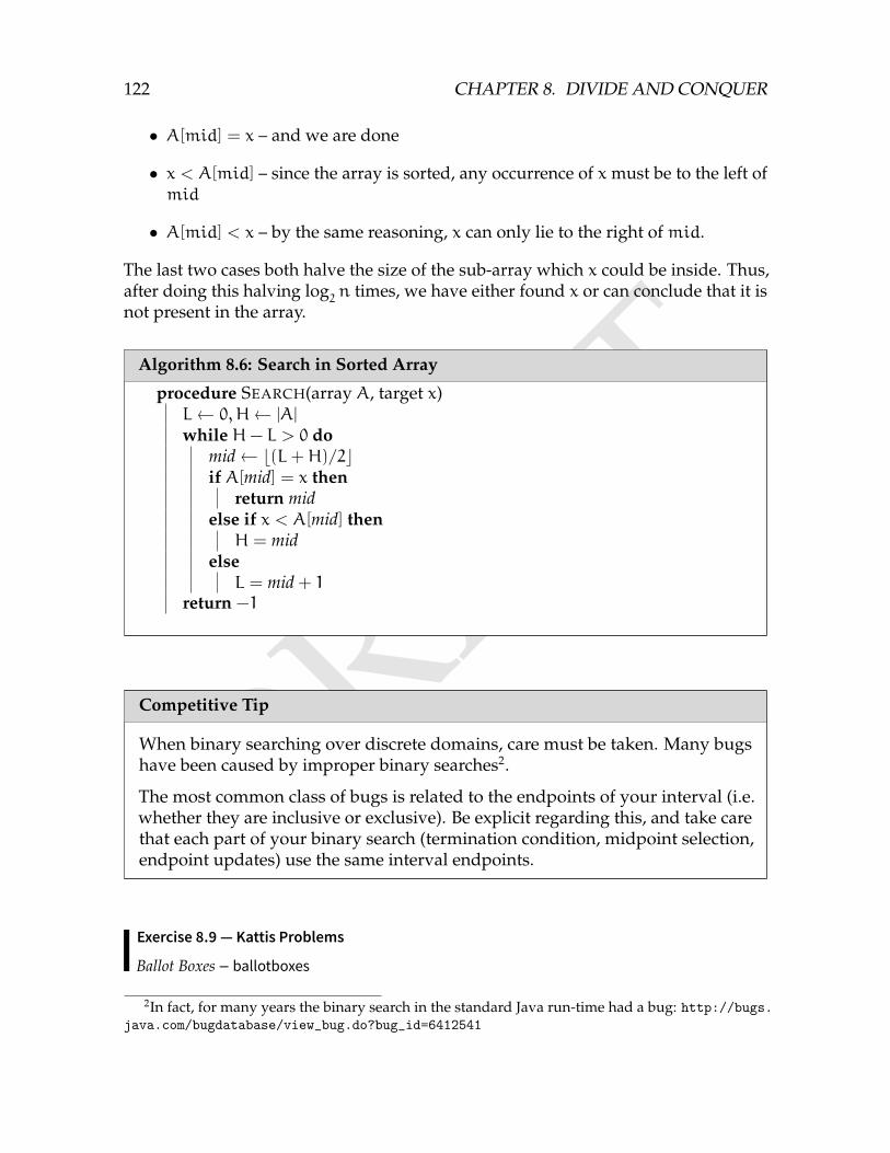
DRAFT
122 CHAPTER 8. DIVIDE AND CONQUER
• A[mid] = x – and we are done
• x < A[mid] – since the array is sorted, any occurrence of x must be to the left ofmid
• A[mid] < x – by the same reasoning, x can only lie to the right ofmid.
The last two cases both halve the size of the sub-array which x could be inside. Thus,after doing this halving log
2n times, we have either found x or can conclude that it is
not present in the array.
Algorithm 8.6: Search in Sorted Array
procedure SEARCH(array A, target x)L← 0,H← |A|
while H− L > 0 domid← b(L+H)/2cif A[mid] = x then
return midelse if x < A[mid] thenH = mid
elseL = mid + 1
return −1
Competitive Tip
When binary searching over discrete domains, care must be taken. Many bugshave been caused by improper binary searches2.
The most common class of bugs is related to the endpoints of your interval (i.e.whether they are inclusive or exclusive). Be explicit regarding this, and take carethat each part of your binary search (termination condition, midpoint selection,endpoint updates) use the same interval endpoints.
Exercise 8.9 — Kattis Problems
Ballot Boxes – ballotboxes
2In fact, for many years the binary search in the standard Java run-time had a bug: http://bugs.java.com/bugdatabase/view_bug.do?bug_id=6412541
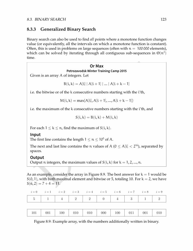
DRAFT
8.3. BINARY SEARCH 123
8.3.3 Generalized Binary Search
Binary search can also be used to find all points where a monotone function changesvalue (or equivalently, all the intervals on which a monotone function is constant).Often, this is used in problems on large sequences (often with n = 100 000 elements),which can be solved by iterating through all contiguous sub-sequences in Θ(n2)time.
Or MaxPetrozavodsk Winter Training Camp 2015
Given is an array A of integers. Let
B(i, k) = A[i] | A[i+ 1] | ... | A[i+ k− 1]
i.e. the bitwise or of the k consecutive numbers starting with the i’th,
M(i, k) = maxA[i], A[i+ 1], ..., A[i+ k− 1]
i.e. the maximum of the k consecutive numbers starting with the i’th, and
S(i, k) = B(i, k) +M(i, k)
For each 1 ≤ k ≤ n, find the maximum of S(i, k).
InputThe first line contains the length 1 ≤ n ≤ 105 of A.
The next and last line contains the n values of A (0 ≤ A[i] < 216), separated byspaces.
OutputOutput n integers, the maximum values of S(i, k) for k = 1, 2, ..., n.
As an example, consider the array in Figure 8.9. The best answer for k = 1 would beS(0, 1), with both maximal element and bitwise or 5, totaling 10. For k = 2, we haveS(6, 2) = 7+ 4 = 11.
i = 0 i = 1 i = 2 i = 3 i = 4 i = 5 i = 6 i = 7 i = 8 i = 9
5 1 4 2 2 0 4 3 1 2
101 001 100 010 010 000 100 011 001 010
Figure 8.9: Example array, with the numbers additionally written in binary.
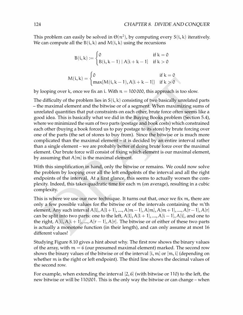
DRAFT
124 CHAPTER 8. DIVIDE AND CONQUER
This problem can easily be solved in Θ(n2), by computing every S(i, k) iteratively.We can compute all the B(i, k) andM(i, k) using the recursions
B(i, k) :=
0 if k = 0
B(i, k− 1) | A[i+ k− 1] if k > 0
M(i, k) =
0 if k = 0
maxM(i, k− 1), A[i+ k− 1] if k > 0
by looping over k, once we fix an i. With n = 100 000, this approach is too slow.
The difficulty of the problem lies in S(i, k) consisting of two basically unrelated parts– the maximal element and the bitwise or of a segment. When maximizing sums ofunrelated quantities that put constraints on each other, brute force often seems like agood idea. This is basically what we did in the Buying Books problem (Section 5.4),where we minimized the sum of two parts (postage and book costs) which constrainedeach other (buying a book forced us to pay postage to its store) by brute forcing overone of the parts (the set of stores to buy from). Since the bitwise or is much morecomplicated than the maximal element – it is decided by an entire interval ratherthan a single element – we are probably better of doing brute force over the maximalelement. Our brute force will consist of fixing which element is our maximal element,by assuming that A[m] is the maximal element.
With this simplification in hand, only the bitwise or remains. We could now solvethe problem by looping over all the left endpoints of the interval and all the rightendpoints of the interval. At a first glance, this seems to actually worsen the com-plexity. Indeed, this takes quadratic time for each m (on average), resulting in a cubiccomplexity.
This is where we use our new technique. It turns out that, once we fix m, there areonly a few possible values for the bitwise or of the intervals containing the m’thelement, Any such interval A[l], A[l+ 1], ..., A[m− 1], A[m], A[m+ 1], ..., A[r− 1], A[r]can be split into two parts: one to the left, A[l], A[l+ 1], ..., A[i− 1], A[i], and one tothe right, A[i], A[i + 1], ..., A[r − 1], A[r]. The bitwise or of either of these two partsis actually a monotone function (in their length), and can only assume at most 16different values!
Studying Figure 8.10 gives a hint about why. The first row shows the binary valuesof the array, withm = 6 (our presumed maximal element) marked. The second rowshows the binary values of the bitwise or of the interval [i,m] or [m, i] (depending onwhetherm is the right or left endpoint). The third line shows the decimal values ofthe second row.
For example, when extending the interval [2, 6] (with bitwise or 110) to the left, thenew bitwise or will be 110|001. This is the only way the bitwise or can change – when
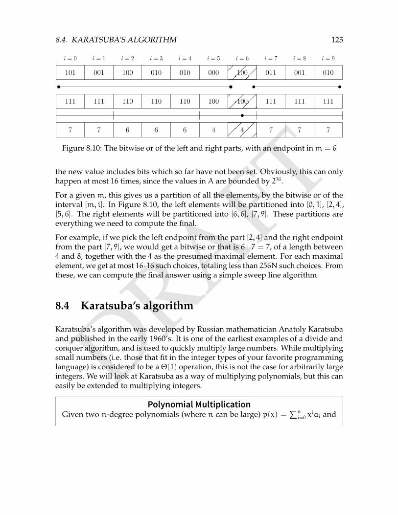
DRAFT
8.4. KARATSUBA’S ALGORITHM 125
i = 0 i = 1 i = 2 i = 3 i = 4 i = 5 i = 6 i = 7 i = 8 i = 9
101 001 100 010 010 000 100 011 001 010
111 111 110 110 110 100 100 111 111 111
7 7 6 6 6 4 4 7 7 7
Figure 8.10: The bitwise or of the left and right parts, with an endpoint inm = 6
the new value includes bits which so far have not been set. Obviously, this can onlyhappen at most 16 times, since the values in A are bounded by 216.
For a given m, this gives us a partition of all the elements, by the bitwise or of theinterval [m, i]. In Figure 8.10, the left elements will be partitioned into [0, 1], [2, 4],[5, 6]. The right elements will be partitioned into [6, 6], [7, 9]. These partitions areeverything we need to compute the final.
For example, if we pick the left endpoint from the part [2, 4] and the right endpointfrom the part [7, 9], we would get a bitwise or that is 6 | 7 = 7, of a length between4 and 8, together with the 4 as the presumed maximal element. For each maximalelement, we get at most 16·16 such choices, totaling less than 256N such choices. Fromthese, we can compute the final answer using a simple sweep line algorithm.
8.4 Karatsuba’s algorithm
Karatsuba’s algorithm was developed by Russian mathematician Anatoly Karatsubaand published in the early 1960’s. It is one of the earliest examples of a divide andconquer algorithm, and is used to quickly multiply large numbers. While multiplyingsmall numbers (i.e. those that fit in the integer types of your favorite programminglanguage) is considered to be a Θ(1) operation, this is not the case for arbitrarily largeintegers. We will look at Karatsuba as a way of multiplying polynomials, but this caneasily be extended to multiplying integers.
Polynomial MultiplicationGiven two n-degree polynomials (where n can be large) p(x) =
∑ni=0 x
iai and
DRAFT
126 CHAPTER 8. DIVIDE AND CONQUER
q(x) =∑n
i=0 xibi compute their product
(pq)(x) =
2n∑i=0
xi(
i∑j=0
ajbi−j)
The naive multiplication algorithm evaluates this using Θ(n2) multiplications (e.g. bytwo nested loops).
It turns out we can do this faster, using a recursive transformation. If we splitthe numbers p and q into their upper and lower k = n
2coefficients (if n is odd,
we pad the polynomials with a leading zero), so that p(x) = pl(x)xk + pr(x) and
q(x) = ql(x)xk + qr(x), their product is equal to
(pq)(x) = (pl(x)xk + pr(x))(ql(x)x
k + qr(x))
= pl(x)ql(x)xn + (pl(x)qr(x) + pr(x)ql(x))x
k + pr(x)qr(x)
This formula requires multiplying 4 pairs of k-degree polynomials instead, whichwe can recursively compute, resulting in the time complexity recurrence T(n) =4T(n
2) +Θ(n). Using the master theorem gives us the solution T(n) = Θ(n2), which
is no faster than the naive multiplication.
However, we can compute pl(x)qr(x) + pr(x)ql(x) using only one multiplicationinstead of two. Both of these terms are part of the expansion of pq, which is only onemultiplication. That particular multiplication is on n-degree polynomials, but it is notdifficult to see how we can reduce it to a single k-degree multiplication. We simplythrow away the multiplicative factors that makes plxk + pr and qlxk + qr an n-degreepolynomials:
(pl(x) + pr(x))(ql(x) + qr(x)) = pl(x)ql(x) + pl(x)qr(x) + pr(x)ql(x) + pr(x)qr(x)
so that
pl(x)qr(x) + pr(x)ql(x) = (pl(x) + pr(x))(ql(x) + pr(x)) − pl(x)ql(x) − pr(x)qr(x)
This means we only need to compute three k-degree multiplications: (pl(x)+pr(x))(ql(x)+qr(x)), pl(x)ql(x), pr(x), qr(x) Our time complexity recurrence is then reduced toT(n) = 3T(n
2) +O(n), which by the master theorem is Θ(nlog2 3) ≈ Θ(n1.585).
Exercise 8.10
Polynomial Multiplication 2 – polymul2
8.5 Chapter Notes

DRAFTChapter 9
Data Structures
Solutions to algorithmic problems consists of two constructs – algorithms and datastructures. Data structures are used to organize the data that the algorithms operateon. For example, the array is such an algorithm.
Many data structures has been developed to handle particular common operationswe need to perform on data quickly. In this chapter, we will study a few suchstructures.
9.1 Disjoint Sets
In the Connectivity Problem, we want to determine whether two vertices in the graphare in the same connected component. This problem can be solved using a Depth-FirstSearch (Section 10.2). For now, we will instead focus on an extension of this problemcalled the Dynamic Connectivity Problem, Additions only1, where we may also alter thegraph by adding edges.
Dynamic Connectivity, Additions OnlyGiven a graph G which initially consists of V disconnected vertices, you willreceive Q queries of two types:
1. take two vertices v and w, and add an edge between them
2. determine whether vertices v and w are currently in the same component
This problem can easily be solved in O(Q2), by after each query performing a DFSto partition the graph into its connected components. Since the graph has at most Q
1The Dynamic Connectivity problem where edges may also be removed can be solved by a datastructured called a Link-Cut tree, which is not discussed in this book.
127
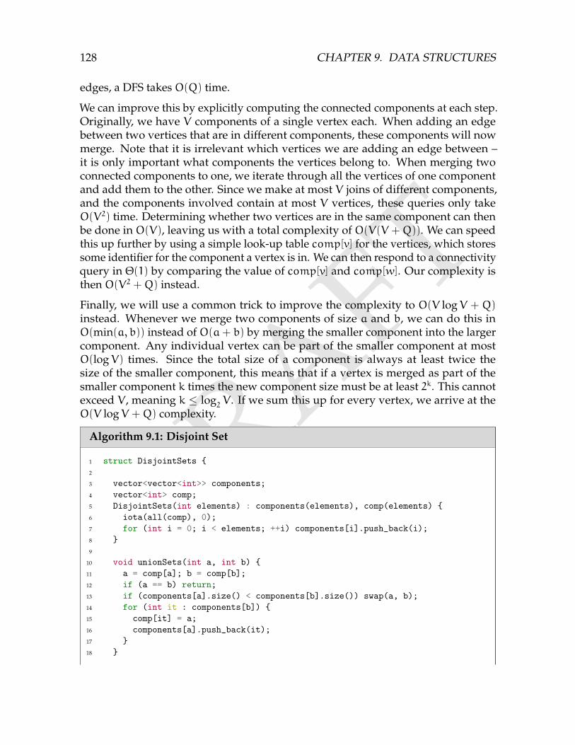
DRAFT
128 CHAPTER 9. DATA STRUCTURES
edges, a DFS takes O(Q) time.
We can improve this by explicitly computing the connected components at each step.Originally, we have V components of a single vertex each. When adding an edgebetween two vertices that are in different components, these components will nowmerge. Note that it is irrelevant which vertices we are adding an edge between –it is only important what components the vertices belong to. When merging twoconnected components to one, we iterate through all the vertices of one componentand add them to the other. Since we make at most V joins of different components,and the components involved contain at most V vertices, these queries only takeO(V2) time. Determining whether two vertices are in the same component can thenbe done in O(V), leaving us with a total complexity of O(V(V +Q)). We can speedthis up further by using a simple look-up table comp[v] for the vertices, which storessome identifier for the component a vertex is in. We can then respond to a connectivityquery in Θ(1) by comparing the value of comp[v] and comp[w]. Our complexity isthen O(V2 +Q) instead.
Finally, we will use a common trick to improve the complexity to O(V logV + Q)instead. Whenever we merge two components of size a and b, we can do this inO(min(a, b)) instead of O(a+ b) by merging the smaller component into the largercomponent. Any individual vertex can be part of the smaller component at mostO(logV) times. Since the total size of a component is always at least twice thesize of the smaller component, this means that if a vertex is merged as part of thesmaller component k times the new component size must be at least 2k. This cannotexceed V , meaning k ≤ log
2V . If we sum this up for every vertex, we arrive at the
O(V logV +Q) complexity.
Algorithm 9.1: Disjoint Set
1 struct DisjointSets 2
3 vector<vector<int>> components;4 vector<int> comp;5 DisjointSets(int elements) : components(elements), comp(elements) 6 iota(all(comp), 0);7 for (int i = 0; i < elements; ++i) components[i].push_back(i);8 9
10 void unionSets(int a, int b) 11 a = comp[a]; b = comp[b];12 if (a == b) return;13 if (components[a].size() < components[b].size()) swap(a, b);14 for (int it : components[b]) 15 comp[it] = a;16 components[a].push_back(it);17 18
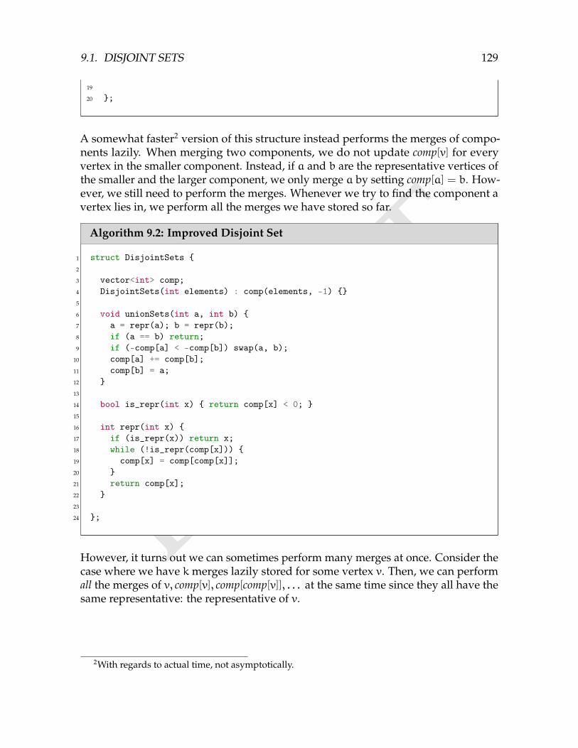
DRAFT
9.1. DISJOINT SETS 129
19
20 ;
A somewhat faster2 version of this structure instead performs the merges of compo-nents lazily. When merging two components, we do not update comp[v] for everyvertex in the smaller component. Instead, if a and b are the representative vertices ofthe smaller and the larger component, we only merge a by setting comp[a] = b. How-ever, we still need to perform the merges. Whenever we try to find the component avertex lies in, we perform all the merges we have stored so far.
Algorithm 9.2: Improved Disjoint Set
1 struct DisjointSets 2
3 vector<int> comp;4 DisjointSets(int elements) : comp(elements, -1) 5
6 void unionSets(int a, int b) 7 a = repr(a); b = repr(b);8 if (a == b) return;9 if (-comp[a] < -comp[b]) swap(a, b);
10 comp[a] += comp[b];11 comp[b] = a;12 13
14 bool is_repr(int x) return comp[x] < 0; 15
16 int repr(int x) 17 if (is_repr(x)) return x;18 while (!is_repr(comp[x])) 19 comp[x] = comp[comp[x]];20 21 return comp[x];22 23
24 ;
However, it turns out we can sometimes perform many merges at once. Consider thecase where we have kmerges lazily stored for some vertex v. Then, we can performall the merges of v, comp[v], comp[comp[v]], . . . at the same time since they all have thesame representative: the representative of v.
2With regards to actual time, not asymptotically.
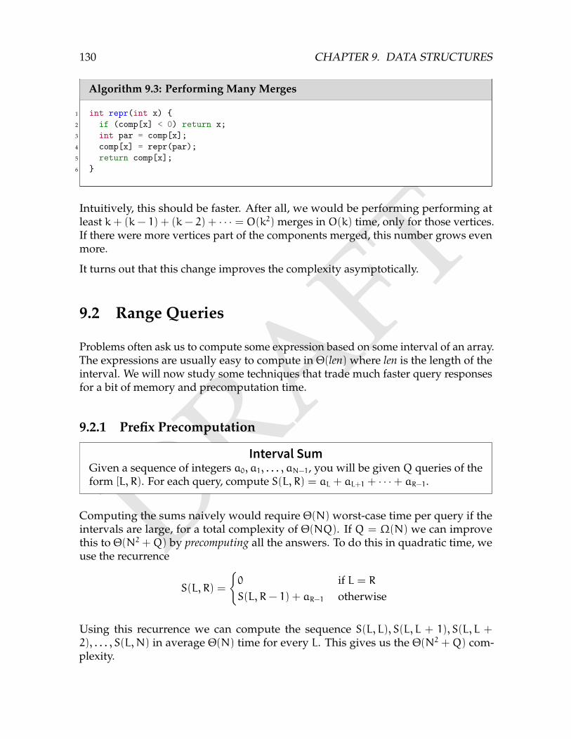
DRAFT
130 CHAPTER 9. DATA STRUCTURES
Algorithm 9.3: Performing Many Merges
1 int repr(int x) 2 if (comp[x] < 0) return x;3 int par = comp[x];4 comp[x] = repr(par);5 return comp[x];6
Intuitively, this should be faster. After all, we would be performing performing atleast k+ (k− 1) + (k− 2) + · · · = O(k2) merges in O(k) time, only for those vertices.If there were more vertices part of the components merged, this number grows evenmore.
It turns out that this change improves the complexity asymptotically.
9.2 Range Queries
Problems often ask us to compute some expression based on some interval of an array.The expressions are usually easy to compute in Θ(len) where len is the length of theinterval. We will now study some techniques that trade much faster query responsesfor a bit of memory and precomputation time.
9.2.1 Prefix Precomputation
Interval SumGiven a sequence of integers a0, a1, . . . , aN−1, you will be given Q queries of theform [L, R). For each query, compute S(L, R) = aL + aL+1 + · · ·+ aR−1.
Computing the sums naively would require Θ(N) worst-case time per query if theintervals are large, for a total complexity of Θ(NQ). If Q = Ω(N) we can improvethis to Θ(N2 +Q) by precomputing all the answers. To do this in quadratic time, weuse the recurrence
S(L, R) =
0 if L = R
S(L, R− 1) + aR−1 otherwise
Using this recurrence we can compute the sequence S(L, L), S(L, L + 1), S(L, L +2), . . . , S(L,N) in average Θ(N) time for every L. This gives us the Θ(N2 +Q) com-plexity.
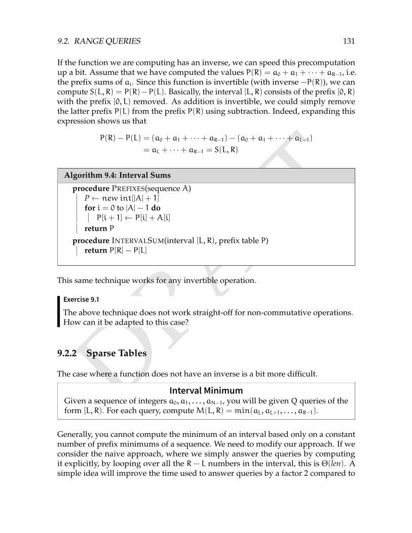
DRAFT
9.2. RANGE QUERIES 131
If the function we are computing has an inverse, we can speed this precomputationup a bit. Assume that we have computed the values P(R) = a0 + a1 + · · ·+ aR−1, i.e.the prefix sums of ai. Since this function is invertible (with inverse −P(R)), we cancompute S(L, R) = P(R)−P(L). Basically, the interval [L, R) consists of the prefix [0, R)with the prefix [0, L) removed. As addition is invertible, we could simply removethe latter prefix P(L) from the prefix P(R) using subtraction. Indeed, expanding thisexpression shows us that
P(R) − P(L) = (a0 + a1 + · · ·+ aR−1) − (a0 + a1 + · · ·+ aL−1)= aL + · · ·+ aR−1 = S(L, R)
Algorithm 9.4: Interval Sums
procedure PREFIXES(sequence A)P← new int[|A|+ 1]for i = 0 to |A|− 1 doP[i+ 1]← P[i] +A[i]
return Pprocedure INTERVALSUM(interval [L, R), prefix table P)
return P[R] − P[L]
This same technique works for any invertible operation.
Exercise 9.1
The above technique does not work straight-off for non-commutative operations.How can it be adapted to this case?
9.2.2 Sparse Tables
The case where a function does not have an inverse is a bit more difficult.
Interval MinimumGiven a sequence of integers a0, a1, . . . , aN−1, you will be given Q queries of theform [L, R). For each query, computeM(L, R) = min(aL, aL+1, . . . , aR−1).
Generally, you cannot compute the minimum of an interval based only on a constantnumber of prefix minimums of a sequence. We need to modify our approach. If weconsider the naive approach, where we simply answer the queries by computingit explicitly, by looping over all the R − L numbers in the interval, this is Θ(len). Asimple idea will improve the time used to answer queries by a factor 2 compared to
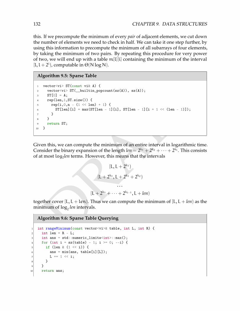
DRAFT
132 CHAPTER 9. DATA STRUCTURES
this. If we precompute the minimum of every pair of adjacent elements, we cut downthe number of elements we need to check in half. We can take it one step further, byusing this information to precompute the minimum of all subarrays of four elements,by taking the minimum of two pairs. By repeating this procedure for very powerof two, we will end up with a table m[l][i] containing the minimum of the interval[l, l+ 2i), computable in Θ(N logN).
Algorithm 9.5: Sparse Table
1 vector<vi> ST(const vi& A) 2 vector<vi> ST(__builtin_popcount(sz(A)), sz(A));3 ST[0] = A;4 rep(len,1,ST.size()) 5 rep(i,0,n - (1 << len) + 1) 6 ST[len][i] = max(ST[len - 1][i], ST[len - 1][i + 1 << (len - 1)]);7 8 9 return ST;
10
Given this, we can compute the minimum of an entire interval in logarithmic time.Consider the binary expansion of the length len = 2k1 + 2k2 + · · ·+ 2kl . This consistsof at most log2len terms. However, this means that the intervals
[L, L+ 2k1)
[L+ 2k1 , L+ 2k1 + 2k2)
. . .
[L+ 2k1 + · · ·+ 2kl−1 , L+ len)
together cover [L, L+ len). Thus we can compute the minimum of [L, L+ len) as theminimum of log
2len intervals.
Algorithm 9.6: Sparse Table Querying
1 int rangeMinimum(const vector<vi>& table, int L, int R) 2 int len = R - L;3 int ans = std::numeric_limits<int>::max();4 for (int i = sz(table) - 1; i >= 0; --i) 5 if (len & (1 << i)) 6 ans = min(ans, table[i][L]);7 L += 1 << i;8 9
10 return ans;
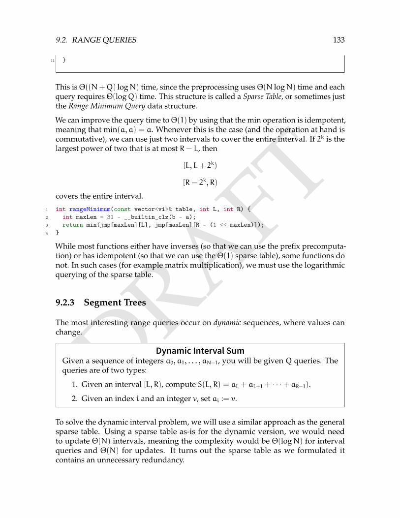
DRAFT
9.2. RANGE QUERIES 133
11
This is Θ((N+Q) logN) time, since the preprocessing uses Θ(N logN) time and eachquery requires Θ(logQ) time. This structure is called a Sparse Table, or sometimes justthe Range Minimum Query data structure.
We can improve the query time to Θ(1) by using that the min operation is idempotent,meaning that min(a, a) = a. Whenever this is the case (and the operation at hand iscommutative), we can use just two intervals to cover the entire interval. If 2k is thelargest power of two that is at most R− L, then
[L, L+ 2k)
[R− 2k, R)
covers the entire interval.
1 int rangeMinimum(const vector<vi>& table, int L, int R) 2 int maxLen = 31 - __builtin_clz(b - a);3 return min(jmp[maxLen][L], jmp[maxLen][R - (1 << maxLen)]);4
While most functions either have inverses (so that we can use the prefix precomputa-tion) or has idempotent (so that we can use the Θ(1) sparse table), some functions donot. In such cases (for example matrix multiplication), we must use the logarithmicquerying of the sparse table.
9.2.3 Segment Trees
The most interesting range queries occur on dynamic sequences, where values canchange.
Dynamic Interval SumGiven a sequence of integers a0, a1, . . . , aN−1, you will be given Q queries. Thequeries are of two types:
1. Given an interval [L, R), compute S(L, R) = aL + aL+1 + · · ·+ aR−1).2. Given an index i and an integer v, set ai := v.
To solve the dynamic interval problem, we will use a similar approach as the generalsparse table. Using a sparse table as-is for the dynamic version, we would needto update Θ(N) intervals, meaning the complexity would be Θ(logN) for intervalqueries and Θ(N) for updates. It turns out the sparse table as we formulated itcontains an unnecessary redundancy.
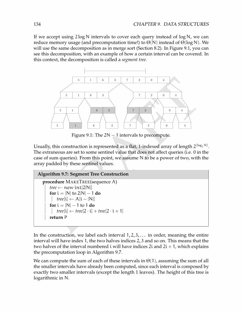
DRAFT
134 CHAPTER 9. DATA STRUCTURES
If we accept using 2 logN intervals to cover each query instead of logN, we canreduce memory usage (and precomputation time!) to Θ(N) instead of Θ(logN). Wewill use the same decomposition as in merge sort (Section 8.2). In Figure 9.1, you cansee this decomposition, with an example of how a certain interval can be covered. Inthis context, the decomposition is called a segment tree.
5 1 6 3 7 2 0 4
5 1 6 3
5 1
5 1
6 3
6 3
7 2 0 4
7 2
7 2
0 4
0 4
Figure 9.1: The 2N− 1 intervals to precompute.
Usually, this construction is represented as a flat, 1-indexed array of length 2dlog2Ne.The extraneous are set to some sentinel value that does not affect queries (i.e. 0 in thecase of sum queries). From this point, we assume N to be a power of two, with thearray padded by these sentinel values.
Algorithm 9.7: Segment Tree Construction
procedure MAKETREE(sequence A)tree← new int[2|N|]for i = |N| to 2|N|− 1 do
tree[i]← A[i− |N|]
for i = |N|− 1 to 1 dotree[i]← tree[2 · i] + tree[2 · i+ 1]
return P
In the construction, we label each interval 1, 2, 3, . . . in order, meaning the entireinterval will have index 1, the two halves indices 2, 3 and so on. This means that thetwo halves of the interval numbered i will have indices 2i and 2i+ 1, which explainsthe precomputation loop in Algorithm 9.7.
We can compute the sum of each of these intervals in Θ(1), assuming the sum of allthe smaller intervals have already been computed, since each interval is composed byexactly two smaller intervals (except the length 1 leaves). The height of this tree islogarithmic in N.
DRAFT
9.2. RANGE QUERIES 135
Note that any particular element of the array is included in logN intervals – one foreach size. This means that updating an element requires only logN intervals to beupdated, which means the update time is Θ(logN) instead of Θ(N) which was thecase for sparse tables.
Algorithm 9.8: Segment Tree Update
procedure UPDATETREE(tree T , index i, value v)index← i+Ntree[index]← v
while index 6= 0 doindex← index/2tree[index]← tree[2 · index] + tree[2 · index + 1]
It is more difficult to construct an appropriate cover if the interval we are to computethe sum of. A recursive rule can be used. We start at the interval [0,N). One of threecases must now apply:
• We are querying the entire interval [0,N)
• We are querying an interval that lies in either [0, N2) or [N
2, N)
• We are querying an interval that lies in both [0, N2) or [N
2, N)
In the first case, we are done (and respond with the sum of the current interval). Inthe second case, we perform a recursive call on the half of the interval that the querylies in. In the third case, we make the same recursive construction for both the leftand the right interval.
Since there is a possibility we perform two recursive calls, we might think that theworst-case complexity of this query would take Θ(logN) time. However, the callsthat the third call results in will have a very specific form – they will always haveone endpoint in common with the interval in the tree. In this case, the only time therecursion will branch is to one interval that is entirely contained in the query, andone that is not. The first call will not make any further calls. All in all, this meansthat there will me at most two branches of logarithmic height, so that queries areO(logN).
Algorithm 9.9: Segment Tree Query
procedure QUERYTREE(tree T , index i, query [L, R), tree interval [L ′, R ′))if R ≤ L ′ or L > R ′ then
return 0if L = L ′ and R = R ′ then
return T [i]

DRAFT
136 CHAPTER 9. DATA STRUCTURES
M = (L+ R)/2lsum = QueryTree(T, 2i, [L,min(R,M)), [L ′,M))rsum = QueryTree(T, 2i+ 1, [max(L,M), R), [M,R))return lsum + rsum
9.3 Chapter Notes
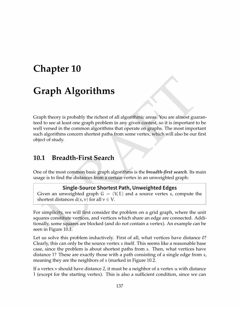
DRAFTChapter 10
Graph Algorithms
Graph theory is probably the richest of all algorithmic areas. You are almost guaran-teed to see at least one graph problem in any given contest, so it is important to bewell versed in the common algorithms that operate on graphs. The most importantsuch algorithms concern shortest paths from some vertex, which will also be our firstobject of study.
10.1 Breadth-First Search
One of the most common basic graph algorithms is the breadth-first search. Its mainusage is to find the distances from a certain vertex in an unweighted graph:
Single-Source Shortest Path, Unweighted EdgesGiven an unweighted graph G = (V, E) and a source vertex s, compute theshortest distances d(s, v) for all v ∈ V .
For simplicity, we will first consider the problem on a grid graph, where the unitsquares constitute vertices, and vertices which share an edge are connected. Addi-tionally, some squares are blocked (and do not contain a vertex). An example can beseen in Figure 10.1.
Let us solve this problem inductively. First of all, what vertices have distance 0?Clearly, this can only be the source vertex s itself. This seems like a reasonable basecase, since the problem is about shortest paths from s. Then, what vertices havedistance 1? These are exactly those with a path consisting of a single edge from s,meaning they are the neighbors of s (marked in Figure 10.2.
If a vertex v should have distance 2, it must be a neighbor of a vertex u with distance1 (except for the starting vertex). This is also a sufficient condition, since we can
137
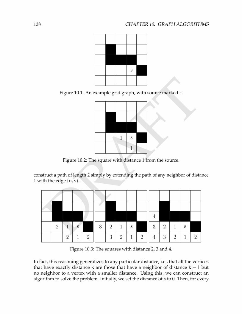
DRAFT
138 CHAPTER 10. GRAPH ALGORITHMS
s
Figure 10.1: An example grid graph, with source marked s.
s1
1
Figure 10.2: The square with distance 1 from the source.
construct a path of length 2 simply by extending the path of any neighbor of distance1with the edge (u, v).
s1
1
2
2 2
s1
1
2
2 2
3
3
s1
1
2
2 2
3
34
4
Figure 10.3: The squares with distance 2, 3 and 4.
In fact, this reasoning generalizes to any particular distance, i.e., that all the verticesthat have exactly distance k are those that have a neighbor of distance k − 1 butno neighbor to a vertex with a smaller distance. Using this, we can construct analgorithm to solve the problem. Initially, we set the distance of s to 0. Then, for every
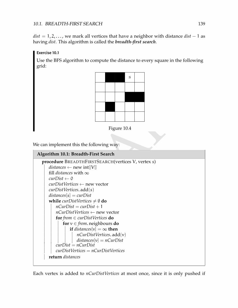
DRAFT
10.1. BREADTH-FIRST SEARCH 139
dist = 1, 2, . . . , we mark all vertices that have a neighbor with distance dist − 1 ashaving dist. This algorithm is called the breadth-first search.
Exercise 10.1
Use the BFS algorithm to compute the distance to every square in the followinggrid:
s
Figure 10.4
We can implement this the following way:
Algorithm 10.1: Breadth-First Search
procedure BREADTHFIRSTSEARCH(vertices V , vertex s)distances← new int[|V |]fill distances with∞curDist← 0
curDistVertices← new vectorcurDistVertices. add(s)distances[s] = curDistwhile curDistVertices 6= ∅ do
nCurDist = curDist + 1nCurDistVertices← new vectorfor from ∈ curDistVertices do
for v ∈ from.neighbours doif distances[v] =∞ then
nCurDistVertices. add(v)distances[v] = nCurDist
curDist = nCurDistcurDistVertices = nCurDistVertices
return distances
Each vertex is added to nCurDistVertices at most once, since it is only pushed if
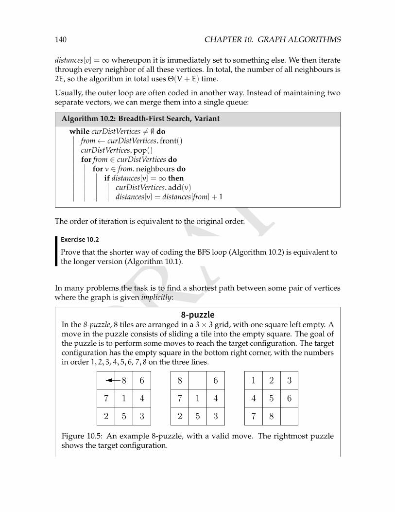
DRAFT
140 CHAPTER 10. GRAPH ALGORITHMS
distances[v] =∞whereupon it is immediately set to something else. We then iteratethrough every neighbor of all these vertices. In total, the number of all neighbours is2E, so the algorithm in total uses Θ(V + E) time.
Usually, the outer loop are often coded in another way. Instead of maintaining twoseparate vectors, we can merge them into a single queue:
Algorithm 10.2: Breadth-First Search, Variant
while curDistVertices 6= ∅ dofrom← curDistVertices. front()curDistVertices.pop()for from ∈ curDistVertices do
for v ∈ from.neighbours doif distances[v] =∞ then
curDistVertices. add(v)distances[v] = distances[from] + 1
The order of iteration is equivalent to the original order.
Exercise 10.2
Prove that the shorter way of coding the BFS loop (Algorithm 10.2) is equivalent tothe longer version (Algorithm 10.1).
In many problems the task is to find a shortest path between some pair of verticeswhere the graph is given implicitly:
8-puzzleIn the 8-puzzle, 8 tiles are arranged in a 3× 3 grid, with one square left empty. Amove in the puzzle consists of sliding a tile into the empty square. The goal ofthe puzzle is to perform some moves to reach the target configuration. The targetconfiguration has the empty square in the bottom right corner, with the numbersin order 1, 2, 3, 4, 5, 6, 7, 8 on the three lines.
2
7
5
1
8
3
4
6
2
7
5
1
8
3
4
6 1 2 3
4 5 6
7 8
Figure 10.5: An example 8-puzzle, with a valid move. The rightmost puzzleshows the target configuration.

DRAFT
10.1. BREADTH-FIRST SEARCH 141
Given a puzzle, determine how many moves are required to solve it, or if it cannotbe solved.
This is a typical BFS problem, characterized by a starting state (the initial puzzle),some transitions (the moves we can make), and the task of finding a short sequenceof such transitions to some goal state. We can model such problems using a graph.The vertices are then the possible arrangements of the tiles in the grid, and an edgeconnects two states if the differ by a single move. A sequence of moves from thestarting state to the target configuration then represents a path in this graph. Theminimum number of moves required is thus the same as the distance between thosevertices in the graph, meaning we can use a BFS.
In such a problem, most of the code is usually concerned with the representation of astate as a vertex, and generating the edges that a certain vertex is adjacent to. Whenan implicit graph is given, we generally do not compute the entire graph explicitly.Instead, we use the states from the problems as-is, and generate the edges of a vertexonly when it is being visited in the breadth-first search. In the 8-puzzle, we canrepresent each state as a 3× 3 2D-vector. The difficult part is generating all the statesthat we can reach from a certain state.
Algorithm 10.3: Generating 8-puzzle Moves
1 typedef vector<vi> Puzzle;2
3 vector<Puzzle> edges(const Puzzle& v) 4 int emptyRow, emptyCol;5 rep(row,0,3)6 rep(col,0,3)7 if (v[row][col] == 0) 8 emptyRow = row;9 emptyCol = col;
10 11 vector<Puzzle> possibleMoves;12 auto makeMove = [&](int rowMove, int colMove) 13 int newRow = row + rowMove;14 int newCol = col + colMove;15 if (newRow >= 0 && newCol >= 0 && newRow < 3 && newCol < 3) 16 Puzzle newPuzzle = v;17 swap(newPuzzle[emptyRow][emptyCol], newPuzzle[newRow][newCol]);18 possibleMoves.spush_back(newPuzzle);19 20 ;21 makeMove(-1, 0);22 makeMove(1, 0);23 makeMove(0, -1);24 makeMove(0, 1);
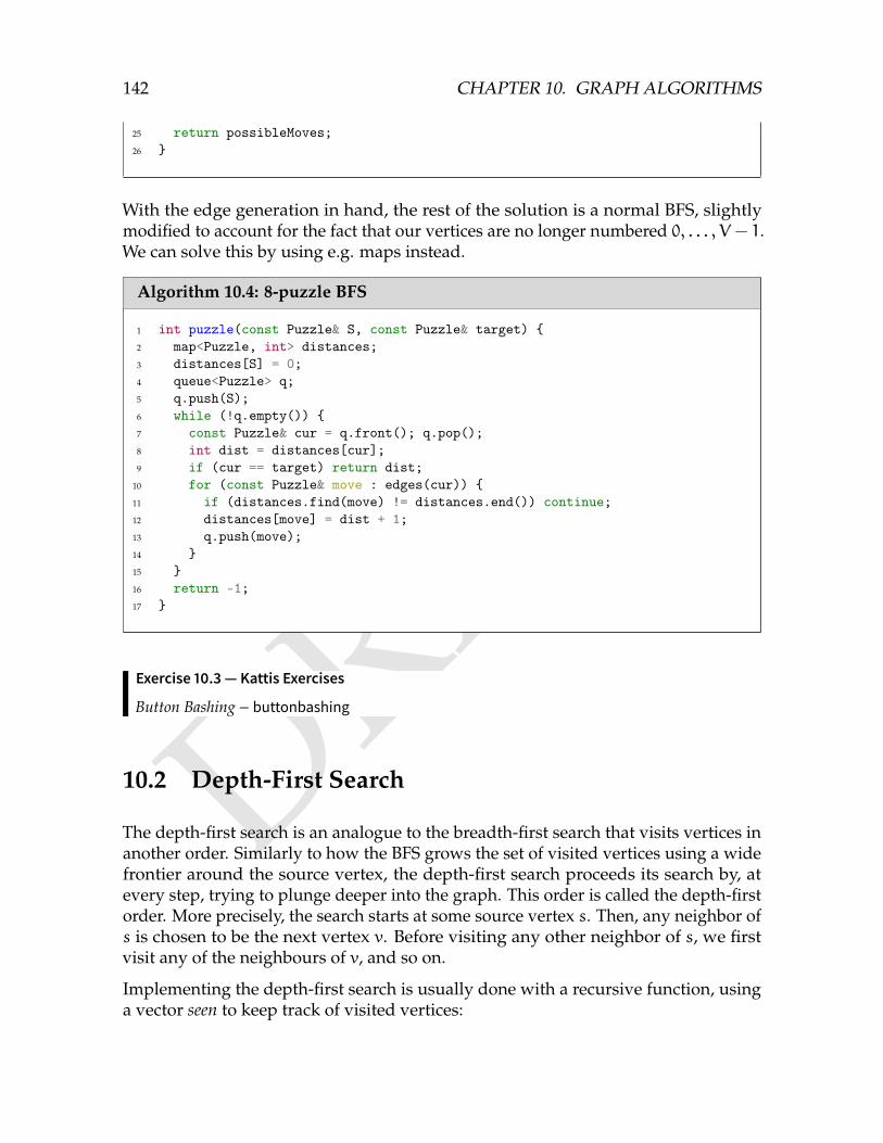
DRAFT
142 CHAPTER 10. GRAPH ALGORITHMS
25 return possibleMoves;26
With the edge generation in hand, the rest of the solution is a normal BFS, slightlymodified to account for the fact that our vertices are no longer numbered 0, . . . , V − 1.We can solve this by using e.g. maps instead.
Algorithm 10.4: 8-puzzle BFS
1 int puzzle(const Puzzle& S, const Puzzle& target) 2 map<Puzzle, int> distances;3 distances[S] = 0;4 queue<Puzzle> q;5 q.push(S);6 while (!q.empty()) 7 const Puzzle& cur = q.front(); q.pop();8 int dist = distances[cur];9 if (cur == target) return dist;
10 for (const Puzzle& move : edges(cur)) 11 if (distances.find(move) != distances.end()) continue;12 distances[move] = dist + 1;13 q.push(move);14 15 16 return -1;17
Exercise 10.3 — Kattis Exercises
Button Bashing – buttonbashing
10.2 Depth-First Search
The depth-first search is an analogue to the breadth-first search that visits vertices inanother order. Similarly to how the BFS grows the set of visited vertices using a widefrontier around the source vertex, the depth-first search proceeds its search by, atevery step, trying to plunge deeper into the graph. This order is called the depth-firstorder. More precisely, the search starts at some source vertex s. Then, any neighbor ofs is chosen to be the next vertex v. Before visiting any other neighbor of s, we firstvisit any of the neighbours of v, and so on.
Implementing the depth-first search is usually done with a recursive function, usinga vector seen to keep track of visited vertices:

DRAFT
10.2. DEPTH-FIRST SEARCH 143
Algorithm 10.5: Depth-First Search
procedure DEPTH-FIRST SEARCH(vertex at, adjacency list G)if seen[at] then
returnseen[at] = truefor neighbour ∈ G[at] do
dfs(neighbour, G)
In languages with limited stack space, it is possible to implement the DFS iterativelyusing a stack instead, keeping the vertices which are currently open in it.
Due to the simplicity of coding the DFS compared to a BFS, it is usually the algorithmof choice in problems where we want to visit all the vertices.
Coast LengthKTH Challenge 2011 – Ulf Lundström
The residents of Soteholm value their coast highly and therefore want to maximizeits total length. For them to be able to make an informed decision on their positionin the issue of global warming, you have to help them find out whether theircoastal line will shrink or expand if the sea level rises. From height maps theyhave figured out what parts of their islands will be covered by water, under thedifferent scenarios described in the latest IPCC report on climate change, but theyneed your help to calculate the length of the coastal lines.
You will be given a map of Soteholm as an N×M grid. Each square in the gridhas a side length of 1 km and is either water or land. Your goal is to compute thetotal length of sea coast of all islands. Sea coast is all borders between land andsea, and sea is any water connected to an edge of the map only through water.Two squares are connected if they share an edge. You may assume that the mapis surrounded by sea. Lakes and islands in lakes are not contributing to the seacoast.
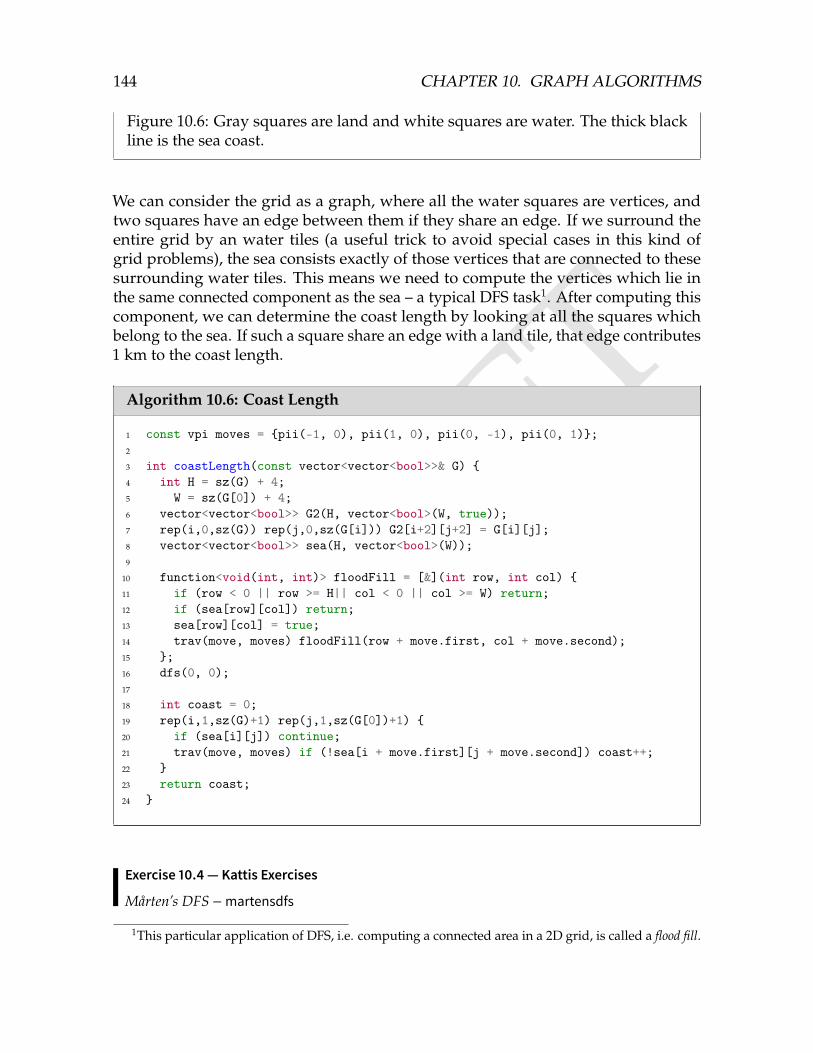
DRAFT
144 CHAPTER 10. GRAPH ALGORITHMS
Figure 10.6: Gray squares are land and white squares are water. The thick blackline is the sea coast.
We can consider the grid as a graph, where all the water squares are vertices, andtwo squares have an edge between them if they share an edge. If we surround theentire grid by an water tiles (a useful trick to avoid special cases in this kind ofgrid problems), the sea consists exactly of those vertices that are connected to thesesurrounding water tiles. This means we need to compute the vertices which lie inthe same connected component as the sea – a typical DFS task1. After computing thiscomponent, we can determine the coast length by looking at all the squares whichbelong to the sea. If such a square share an edge with a land tile, that edge contributes1 km to the coast length.
Algorithm 10.6: Coast Length
1 const vpi moves = pii(-1, 0), pii(1, 0), pii(0, -1), pii(0, 1);2
3 int coastLength(const vector<vector<bool>>& G) 4 int H = sz(G) + 4;5 W = sz(G[0]) + 4;6 vector<vector<bool>> G2(H, vector<bool>(W, true));7 rep(i,0,sz(G)) rep(j,0,sz(G[i])) G2[i+2][j+2] = G[i][j];8 vector<vector<bool>> sea(H, vector<bool>(W));9
10 function<void(int, int)> floodFill = [&](int row, int col) 11 if (row < 0 || row >= H|| col < 0 || col >= W) return;12 if (sea[row][col]) return;13 sea[row][col] = true;14 trav(move, moves) floodFill(row + move.first, col + move.second);15 ;16 dfs(0, 0);17
18 int coast = 0;19 rep(i,1,sz(G)+1) rep(j,1,sz(G[0])+1) 20 if (sea[i][j]) continue;21 trav(move, moves) if (!sea[i + move.first][j + move.second]) coast++;22 23 return coast;24
Exercise 10.4 — Kattis Exercises
Mårten’s DFS – martensdfs
1This particular application of DFS, i.e. computing a connected area in a 2D grid, is called a flood fill.
DRAFT
10.3. WEIGHTED SHORTEST PATH 145
10.3 Weighted Shortest Path
The theory of computing shortest paths in the case of weighted graphs is a bit morerich than the unweighted case. Which algorithm to use depends on three factors:
• The number of vertices.
• Whether edge weights are non-negative or not.
• If we seek shortest paths only from a single vertex or between all pairs ofvertices.
There are mainly three algorithms used: Dijkstra’s Algorithm, the Bellman-Ford algo-rithm, and the Floyd-Warshall algorithm.
10.3.1 Dijkstra’s Algorithm
Dijkstra’s Algorithm can be seen as an extension of the breadth-first search thatworks for weighted graphs as well.
Single-Source Shortest Path, non-negative weightsGiven a weighted graph G = (V, E) where all weights are non-negative and asource vertex s, compute the shortest distances d(s, v) for all v ∈ V(G).
It has a similar inductive approach, where we iteratively compute the shortest dis-tances to all vertices in ordered by distance. The difference lies in that we do notimmediately know when we have found the shortest path to a vertex. For example,the shortest path from a neighbour to the source vertex may now use several othervertices in its shortest path to s (Figure ??).
imageimage
However, can this be the case for every vertex adjacent to s? In particular, can theneighbour to s with the smallest edge weightW to s have a distance smaller than w?This is never the case in Figure ??, and actually holds in general. Assume that this isnot the case. In Figure ??, this hypothetical scenario is shown. Any such path muststill pass through some neighbour u of s. By assumption, the weight of the edge (s, u)must be larger than W (which was the minimal weight of the edges adjacent to s).This reasoning at least allows us to find the shortest distance to one other vertex.
10.3.2 Bellman-Ford
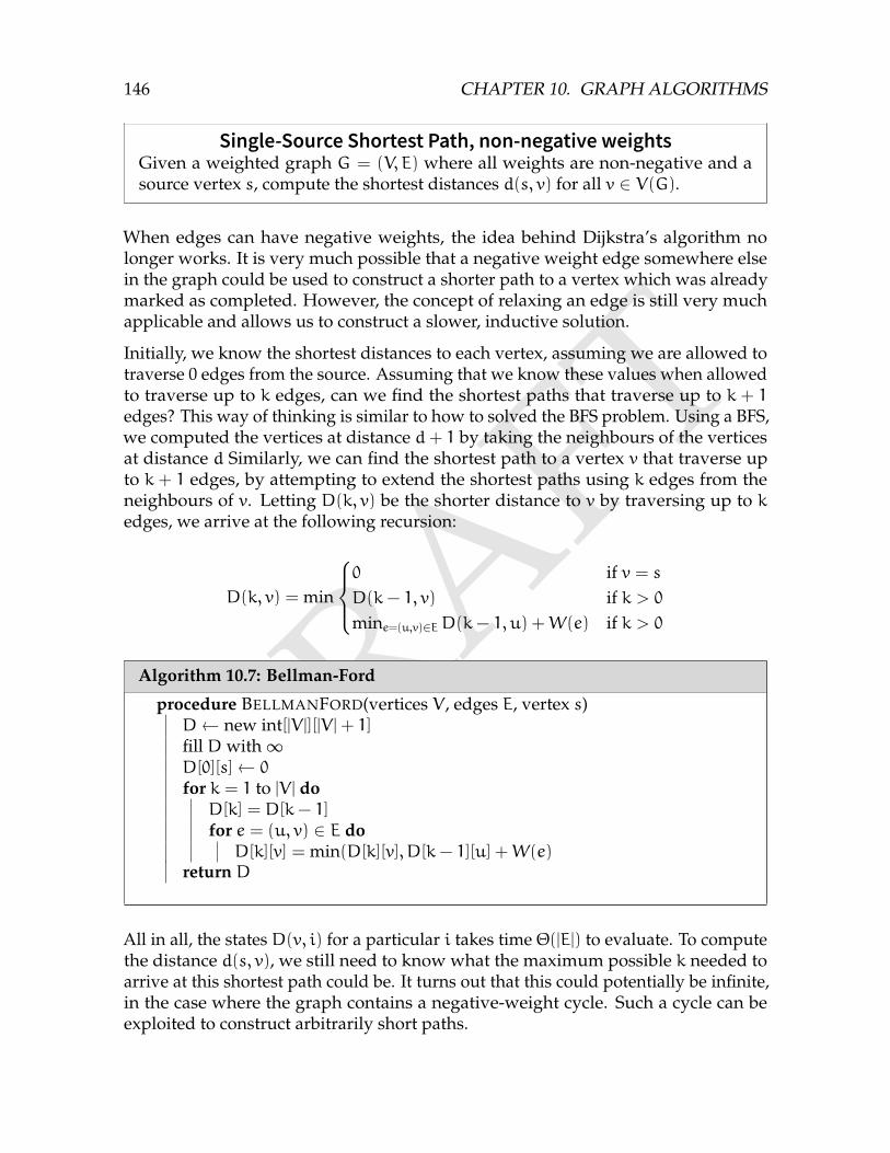
DRAFT
146 CHAPTER 10. GRAPH ALGORITHMS
Single-Source Shortest Path, non-negative weightsGiven a weighted graph G = (V, E) where all weights are non-negative and asource vertex s, compute the shortest distances d(s, v) for all v ∈ V(G).
When edges can have negative weights, the idea behind Dijkstra’s algorithm nolonger works. It is very much possible that a negative weight edge somewhere elsein the graph could be used to construct a shorter path to a vertex which was alreadymarked as completed. However, the concept of relaxing an edge is still very muchapplicable and allows us to construct a slower, inductive solution.
Initially, we know the shortest distances to each vertex, assuming we are allowed totraverse 0 edges from the source. Assuming that we know these values when allowedto traverse up to k edges, can we find the shortest paths that traverse up to k + 1edges? This way of thinking is similar to how to solved the BFS problem. Using a BFS,we computed the vertices at distance d+ 1 by taking the neighbours of the verticesat distance d Similarly, we can find the shortest path to a vertex v that traverse upto k + 1 edges, by attempting to extend the shortest paths using k edges from theneighbours of v. Letting D(k, v) be the shorter distance to v by traversing up to kedges, we arrive at the following recursion:
D(k, v) = min
0 if v = sD(k− 1, v) if k > 0mine=(u,v)∈ED(k− 1, u) +W(e) if k > 0
Algorithm 10.7: Bellman-Ford
procedure BELLMANFORD(vertices V , edges E, vertex s)D← new int[|V |][|V |+ 1]fill Dwith∞D[0][s]← 0
for k = 1 to |V | doD[k] = D[k− 1]for e = (u, v) ∈ E doD[k][v] = min(D[k][v], D[k− 1][u] +W(e)
return D
All in all, the states D(v, i) for a particular i takes time Θ(|E|) to evaluate. To computethe distance d(s, v), we still need to know what the maximum possible k needed toarrive at this shortest path could be. It turns out that this could potentially be infinite,in the case where the graph contains a negative-weight cycle. Such a cycle can beexploited to construct arbitrarily short paths.
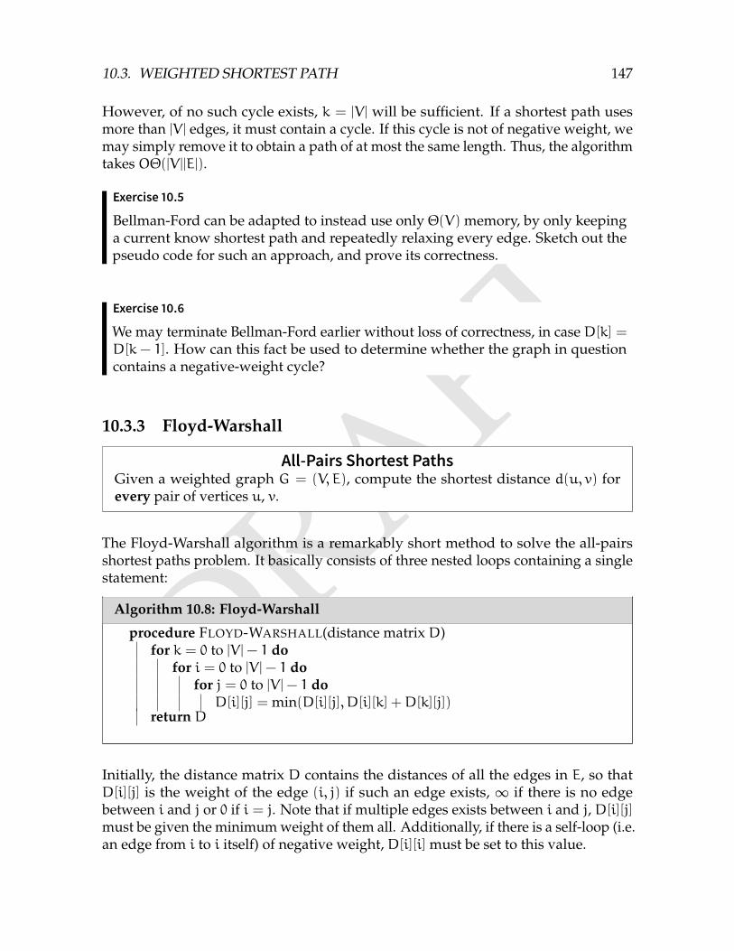
DRAFT
10.3. WEIGHTED SHORTEST PATH 147
However, of no such cycle exists, k = |V | will be sufficient. If a shortest path usesmore than |V | edges, it must contain a cycle. If this cycle is not of negative weight, wemay simply remove it to obtain a path of at most the same length. Thus, the algorithmtakes OΘ(|V ||E|).
Exercise 10.5
Bellman-Ford can be adapted to instead use only Θ(V) memory, by only keepinga current know shortest path and repeatedly relaxing every edge. Sketch out thepseudo code for such an approach, and prove its correctness.
Exercise 10.6
We may terminate Bellman-Ford earlier without loss of correctness, in case D[k] =D[k − 1]. How can this fact be used to determine whether the graph in questioncontains a negative-weight cycle?
10.3.3 Floyd-Warshall
All-Pairs Shortest PathsGiven a weighted graph G = (V, E), compute the shortest distance d(u, v) forevery pair of vertices u, v.
The Floyd-Warshall algorithm is a remarkably short method to solve the all-pairsshortest paths problem. It basically consists of three nested loops containing a singlestatement:
Algorithm 10.8: Floyd-Warshall
procedure FLOYD-WARSHALL(distance matrix D)for k = 0 to |V |− 1 do
for i = 0 to |V |− 1 dofor j = 0 to |V |− 1 doD[i][j] = min(D[i][j], D[i][k] +D[k][j])
return D
Initially, the distance matrix D contains the distances of all the edges in E, so thatD[i][j] is the weight of the edge (i, j) if such an edge exists, ∞ if there is no edgebetween i and j or 0 if i = j. Note that if multiple edges exists between i and j, D[i][j]must be given the minimum weight of them all. Additionally, if there is a self-loop (i.e.an edge from i to i itself) of negative weight, D[i][i] must be set to this value.
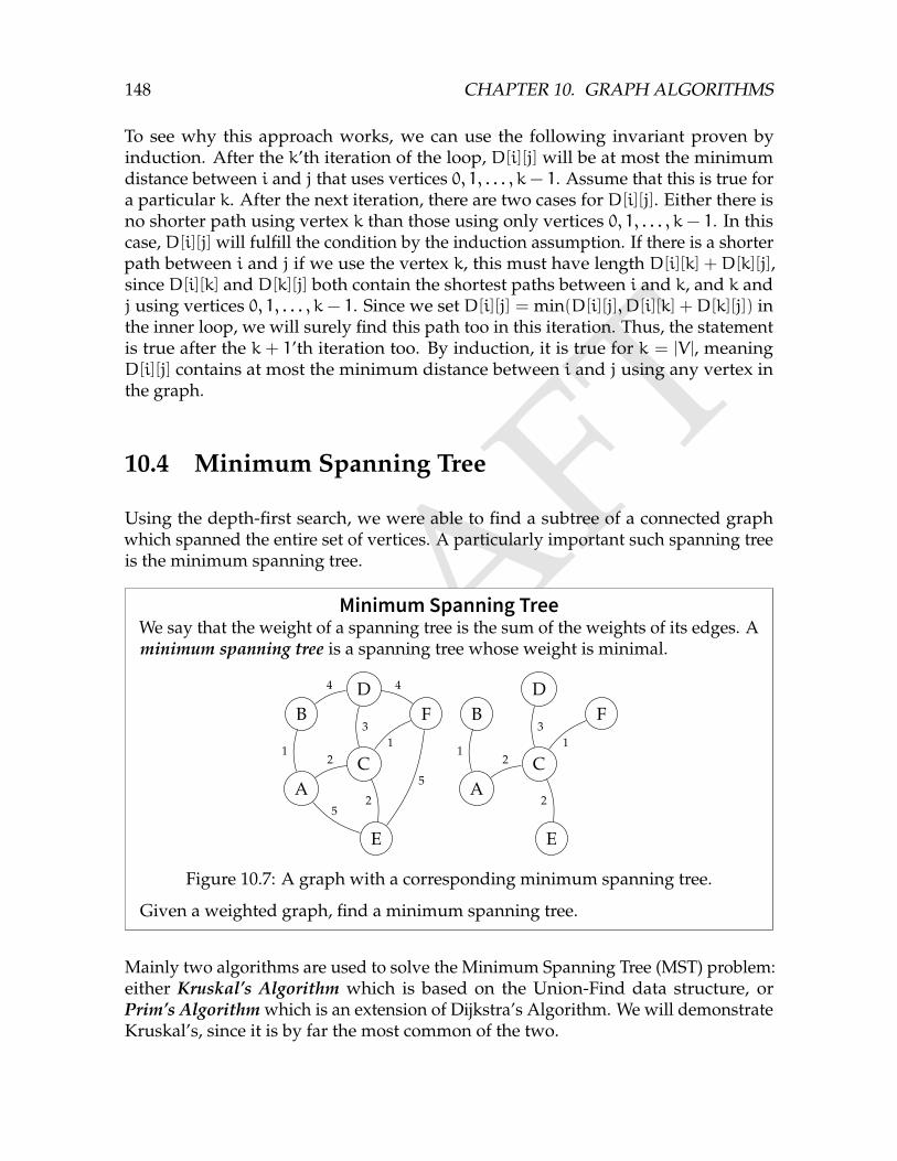
DRAFT
148 CHAPTER 10. GRAPH ALGORITHMS
To see why this approach works, we can use the following invariant proven byinduction. After the k’th iteration of the loop, D[i][j] will be at most the minimumdistance between i and j that uses vertices 0, 1, . . . , k− 1. Assume that this is true fora particular k. After the next iteration, there are two cases for D[i][j]. Either there isno shorter path using vertex k than those using only vertices 0, 1, . . . , k − 1. In thiscase, D[i][j] will fulfill the condition by the induction assumption. If there is a shorterpath between i and j if we use the vertex k, this must have length D[i][k] +D[k][j],since D[i][k] and D[k][j] both contain the shortest paths between i and k, and k andj using vertices 0, 1, . . . , k − 1. Since we set D[i][j] = min(D[i][j], D[i][k] +D[k][j]) inthe inner loop, we will surely find this path too in this iteration. Thus, the statementis true after the k + 1’th iteration too. By induction, it is true for k = |V |, meaningD[i][j] contains at most the minimum distance between i and j using any vertex inthe graph.
10.4 Minimum Spanning Tree
Using the depth-first search, we were able to find a subtree of a connected graphwhich spanned the entire set of vertices. A particularly important such spanning treeis the minimum spanning tree.
Minimum Spanning TreeWe say that the weight of a spanning tree is the sum of the weights of its edges. Aminimum spanning tree is a spanning tree whose weight is minimal.
A
B
C
D
E
F
1
4
2
3
52
1
4
5 A
B
C
D
E
F
12
3
2
1
Figure 10.7: A graph with a corresponding minimum spanning tree.
Given a weighted graph, find a minimum spanning tree.
Mainly two algorithms are used to solve the Minimum Spanning Tree (MST) problem:either Kruskal’s Algorithm which is based on the Union-Find data structure, orPrim’s Algorithm which is an extension of Dijkstra’s Algorithm. We will demonstrateKruskal’s, since it is by far the most common of the two.
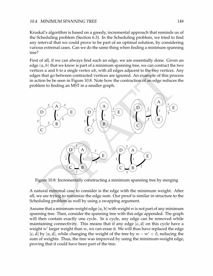
DRAFT
10.4. MINIMUM SPANNING TREE 149
Kruskal’s algorithm is based on a greedy, incremental approach that reminds us ofthe Scheduling problem (Section 6.3). In the Scheduling problem, we tried to findany interval that we could prove to be part of an optimal solution, by consideringvarious extremal cases. Can we do the same thing when finding a minimum spanningtree?
First of all, if we can always find such an edge, we are essentially done. Given anedge (a, b) that we know is part of a minimum spanning tree, we can contract the twovertices a and b to a single vertex ab, with all edges adjacent to the two vertices. Anyedges that go between contracted vertices are ignored. An example of this processin action be be seen in Figure 10.8. Note how the contraction of an edge reduces theproblem to finding an MST in a smaller graph.
C
D
B
AE
2
2
2
12
3
C
D
B
AE
2
2
2
12
3
C
D
B
AE
2
2
2
12
3
C
D
B
AE
2
2
2
12
3
C
D
B
AE
2
2
2
1
2
3
Figure 10.8: Incrementally constructing a minimum spanning tree by merging
A natural extremal case to consider is the edge with the minimum weight. Afterall, we are trying to minimize the edge sum. Our proof is similar in structure to theScheduling problem as well by using a swapping argument.
Assume that a minimum-weight edge a, b with weightw is not part of any minimumspanning tree. Then, consider the spanning tree with this edge appended. The graphwill then contain exactly one cycle. In a cycle, any edge can be removed whilemaintaining connectivity. This means that if any edge c, d on this cycle have aweight w ′ larger weight than w, we can erase it. We will thus have replaced the edgec, d by a, d, while changing the weight of the tree by w − w ′ < 0, reducing thesum of weights. Thus, the tree was improved by using the minimum-weight edge,proving that it could have been part of the tree.
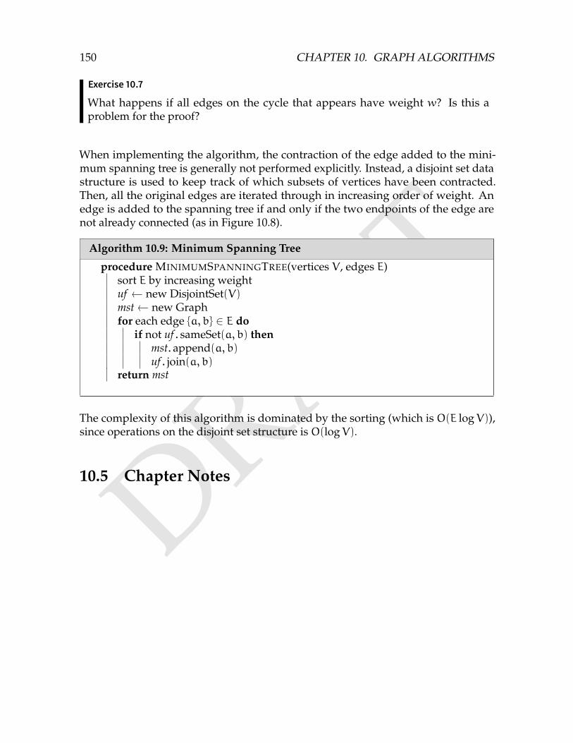
DRAFT
150 CHAPTER 10. GRAPH ALGORITHMS
Exercise 10.7
What happens if all edges on the cycle that appears have weight w? Is this aproblem for the proof?
When implementing the algorithm, the contraction of the edge added to the mini-mum spanning tree is generally not performed explicitly. Instead, a disjoint set datastructure is used to keep track of which subsets of vertices have been contracted.Then, all the original edges are iterated through in increasing order of weight. Anedge is added to the spanning tree if and only if the two endpoints of the edge arenot already connected (as in Figure 10.8).
Algorithm 10.9: Minimum Spanning Tree
procedure MINIMUMSPANNINGTREE(vertices V , edges E)sort E by increasing weightuf ← new DisjointSet(V)mst← new Graphfor each edge a, b ∈ E do
if not uf . sameSet(a, b) thenmst. append(a, b)uf . join(a, b)
return mst
The complexity of this algorithm is dominated by the sorting (which is O(E logV)),since operations on the disjoint set structure is O(logV).
10.5 Chapter Notes

DRAFTChapter 11
Maximum Flows
This chapter studies so called flow networks, and algorithms we use to solve the so-called maximum flow and minimum cut problems on such networks. Flow problemsare common algorithmic problems, particularly in ICPC competitions (while they areout-of-scope for IOI contests). They are often hidden behind statements which seemunrelated to graphs and flows, especially the minimum cut problem.
Finally, we will end with a specialization of maximum flow on the case of bipartitegraphs (called bipartite matching).
11.1 Flow Networks
Informally, a flow network is a directed graph that models any kind of network wherepaths have a fixed capacity, or throughput. For example, in a road network, each roadmight have a limited throughput, proportional to the number of lanes on the road. Acomputer network may have different speeds along different connections due to e.g.the type of material. These natural models are often use when describing a problemthat is related to flows. A more formal definition is the following.
Definition 11.1 — Flow NetworkA flow network is a special kind of directed graph (V, E, c), where each edge e isgiven a non-negative capacity c(e). Two vertices are designated the source andthe sink, which we will often abbreviate to S and T .
In Figure 11.1, you can see an example of a flow network.
In such a network, we can assign another value to each edge, that models the currentthroughput (which generally does not need to match the capacity). These values arewhat we call flows.
151
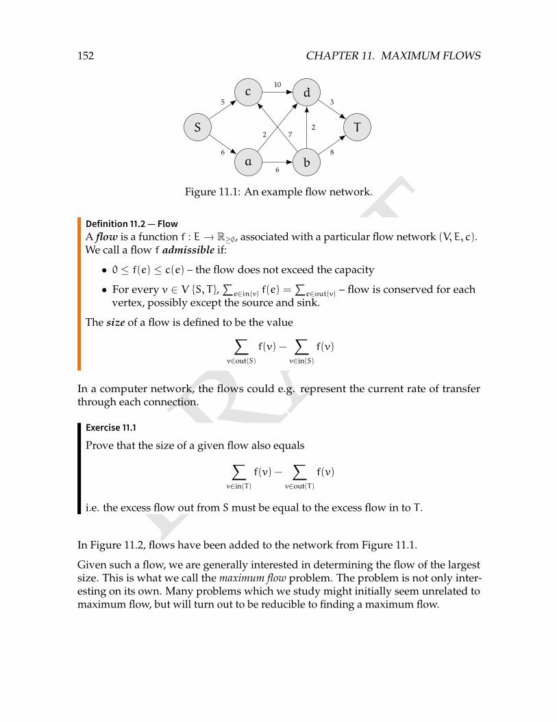
DRAFT
152 CHAPTER 11. MAXIMUM FLOWS
S
a b
c d
T
6
5
6
8
10
3
22 7
Figure 11.1: An example flow network.
Definition 11.2 — FlowA flow is a function f : E→ R≥0, associated with a particular flow network (V, E, c).We call a flow f admissible if:
• 0 ≤ f(e) ≤ c(e) – the flow does not exceed the capacity
• For every v ∈ V S, T ,∑
e∈in(v) f(e) =∑
e∈out(v) – flow is conserved for eachvertex, possibly except the source and sink.
The size of a flow is defined to be the value∑v∈out(S)
f(v) −∑v∈in(S)
f(v)
In a computer network, the flows could e.g. represent the current rate of transferthrough each connection.
Exercise 11.1
Prove that the size of a given flow also equals∑v∈in(T)
f(v) −∑
v∈out(T)
f(v)
i.e. the excess flow out from Smust be equal to the excess flow in to T .
In Figure 11.2, flows have been added to the network from Figure 11.1.
Given such a flow, we are generally interested in determining the flow of the largestsize. This is what we call the maximum flow problem. The problem is not only inter-esting on its own. Many problems which we study might initially seem unrelated tomaximum flow, but will turn out to be reducible to finding a maximum flow.
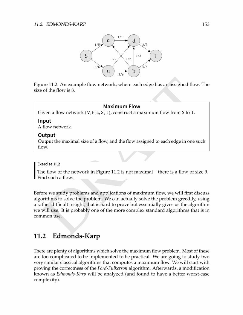
DRAFT
11.2. EDMONDS-KARP 153
S
a b
c d
T
6/6
1/5
5/6
5/8
1/10
3/3
1/21/2 0/7
Figure 11.2: An example flow network, where each edge has an assigned flow. Thesize of the flow is 8.
Maximum FlowGiven a flow network (V, E, c, S, T), construct a maximum flow from S to T .
InputA flow network.
OutputOutput the maximal size of a flow, and the flow assigned to each edge in one suchflow.
Exercise 11.2
The flow of the network in Figure 11.2 is not maximal – there is a flow of size 9.Find such a flow.
Before we study problems and applications of maximum flow, we will first discussalgorithms to solve the problem. We can actually solve the problem greedily, usinga rather difficult insight, that is hard to prove but essentially gives us the algorithmwe will use. It is probably one of the more complex standard algorithms that is incommon use.
11.2 Edmonds-Karp
There are plenty of algorithms which solve the maximum flow problem. Most of theseare too complicated to be implemented to be practical. We are going to study twovery similar classical algorithms that computes a maximum flow. We will start withproving the correctness of the Ford-Fulkerson algorithm. Afterwards, a modificationknown as Edmonds-Karp will be analyzed (and found to have a better worst-casecomplexity).
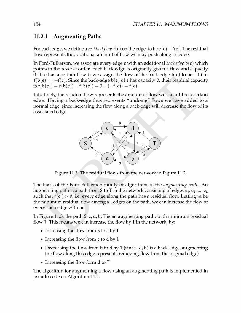
DRAFT
154 CHAPTER 11. MAXIMUM FLOWS
11.2.1 Augmenting Paths
For each edge, we define a residual flow r(e) on the edge, to be c(e)− f(e). The residualflow represents the additional amount of flow we may push along an edge.
In Ford-Fulkerson, we associate every edge e with an additional back edge b(e) whichpoints in the reverse order. Each back edge is originally given a flow and capacity0. If e has a certain flow f, we assign the flow of the back-edge b(e) to be −f (i.e.f(b(e)) = −f(e). Since the back-edge b(e) of e has capacity 0, their residual capacityis r(b(e)) = c(b(e)) − f(b(e)) = 0− (−f(e)) = f(e).
Intuitively, the residual flow represents the amount of flow we can add to a certainedge. Having a back-edge thus represents “undoing” flows we have added to anormal edge, since increasing the flow along a back-edge will decrease the flow of itsassociated edge.
S
a b
c d
T
6
4
1
1
5
3
5
9
1 3
1 11
1
7
Figure 11.3: The residual flows from the network in Figure 11.2.
The basis of the Ford-Fulkerson family of algorithms is the augmenting path. Anaugmenting path is a path from S to T in the network consisting of edges e1, e2, ..., el,such that r(ei) > 0, i.e. every edge along the path has a residual flow. Letting m bethe minimum residual flow among all edges on the path, we can increase the flow ofevery such edge withm.
In Figure 11.3, the path S, c, d, b, T is an augmenting path, with minimum residualflow 1. This means we can increase the flow by 1 in the network, by:
• Increasing the flow from S to c by 1
• Increasing the flow from c to d by 1
• Decreasing the flow from b to d by 1 (since (d, b) is a back-edge, augmentingthe flow along this edge represents removing flow from the original edge)
• Increasing the flow form d to T
The algorithm for augmenting a flow using an augmenting path is implemented inpseudo code on Algorithm 11.2.
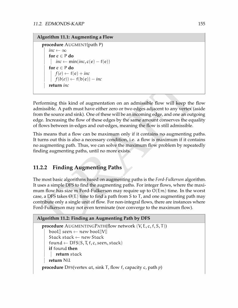
DRAFT
11.2. EDMONDS-KARP 155
Algorithm 11.1: Augmenting a Flow
procedure AUGMENT(path P)inc←∞for e ∈ P do
inc← min(inc, c(e) − f(e))for e ∈ P do
f (e)← f(e) + incf (b(e))← f(b(e)) − inc
return inc
Performing this kind of augmentation on an admissible flow will keep the flowadmissible. A path must have either zero or two edges adjacent to any vertex (asidefrom the source and sink). One of these will be an incoming edge, and one an outgoingedge. Increasing the flow of these edges by the same amount conserves the equalityof flows between in-edges and out-edges, meaning the flow is still admissible.
This means that a flow can be maximum only if it contains no augmenting paths.It turns out this is also a necessary condition, i.e. a flow is maximum if it containsno augmenting path. Thus, we can solve the maximum flow problem by repeatedlyfinding augmenting paths, until no more exists.
11.2.2 Finding Augmenting Paths
The most basic algorithms based on augmenting paths is the Ford-Fulkerson algorithm.It uses a simple DFS to find the augmenting paths. For integer flows, where the maxi-mum flow has size m Ford-Fulkerson may require up to O(Em) time. In the worstcase, a DFS takes Θ(E) time to find a path from S to T , and one augmenting path maycontribute only a single unit of flow. For non-integral flows, there are instances whereFord-Fulkerson may not even terminate (nor converge to the maximum flow).
Algorithm 11.2: Finding an Augmenting Path by DFS
procedure AUGMENTINGPATH(flow network (V, E, c, f, S, T))bool[] seen← new bool[|V |]Stack stack← new Stack
found← DFS(S, T, f, c, seen, stack)if found then
return stackreturn Nil
procedure DFS(vertex at, sink T , flow f, capacity c, path p)
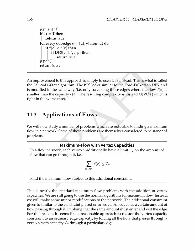
DRAFT
156 CHAPTER 11. MAXIMUM FLOWS
p.push(at)if at = T then
return truefor every out-edge e = (at, v) from at do
if f(e) < c(e) thenif DFS(v, T, f, c, p) then
return truep.pop()return false
An improvement to this approach is simply to use a BFS instead. This is what is calledthe Edmonds-Karp algorithm. The BFS looks similar to the Ford-Fulkerson DFS, andis modified in the same way (i.e. only traversing those edges where the flow f(e) issmaller than the capacity c(e). The resulting complexity is instead O(VE2) (which istight in the worst case).
11.3 Applications of Flows
We will now study a number of problems which are reducible to finding a maximumflow in a network. Some of these problems are themselves considered to be standardproblems.
Maximum-Flowwith Vertex CapacitiesIn a flow network, each vertex v additionally have a limit Cv on the amount offlow that can go through it, i.e. ∑
e∈in(v)
f(e) ≤ Cv
Find the maximum flow subject to this additional constraint.
This is nearly the standard maximum flow problem, with the addition of vertexcapacities. We are still going to use the normal algorithms for maximum flow. Instead,we will make some minor modifications to the network. The additional constraintgiven is similar to the constraint placed on an edge. An edge has a certain amount offlow passing through it, implying that the same amount must enter and exit the edge.For this reason, it seems like a reasonable approach to reduce the vertex capacityconstraint to an ordinary edge capacity, by forcing all the flow that passes through avertex vwith capacity Cv through a particular edge.
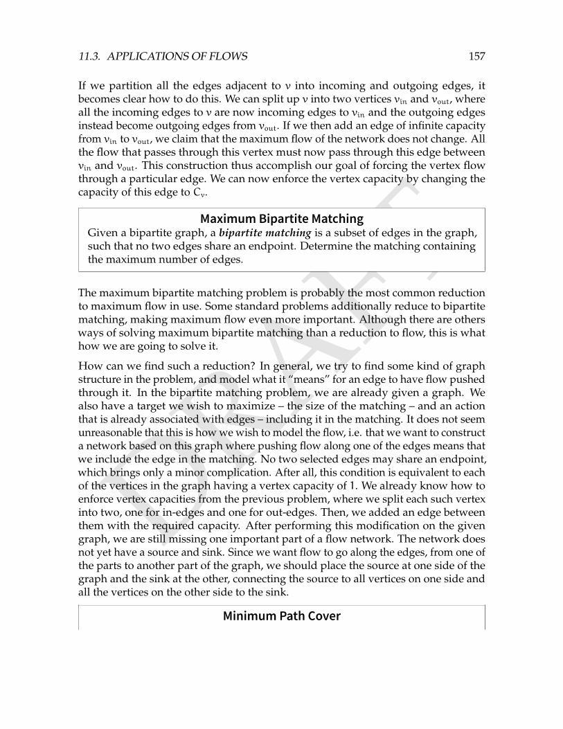
DRAFT
11.3. APPLICATIONS OF FLOWS 157
If we partition all the edges adjacent to v into incoming and outgoing edges, itbecomes clear how to do this. We can split up v into two vertices vin and vout, whereall the incoming edges to v are now incoming edges to vin and the outgoing edgesinstead become outgoing edges from vout. If we then add an edge of infinite capacityfrom vin to vout, we claim that the maximum flow of the network does not change. Allthe flow that passes through this vertex must now pass through this edge betweenvin and vout. This construction thus accomplish our goal of forcing the vertex flowthrough a particular edge. We can now enforce the vertex capacity by changing thecapacity of this edge to Cv.
Maximum Bipartite MatchingGiven a bipartite graph, a bipartite matching is a subset of edges in the graph,such that no two edges share an endpoint. Determine the matching containingthe maximum number of edges.
The maximum bipartite matching problem is probably the most common reductionto maximum flow in use. Some standard problems additionally reduce to bipartitematching, making maximum flow even more important. Although there are othersways of solving maximum bipartite matching than a reduction to flow, this is whathow we are going to solve it.
How can we find such a reduction? In general, we try to find some kind of graphstructure in the problem, and model what it “means” for an edge to have flow pushedthrough it. In the bipartite matching problem, we are already given a graph. Wealso have a target we wish to maximize – the size of the matching – and an actionthat is already associated with edges – including it in the matching. It does not seemunreasonable that this is how we wish to model the flow, i.e. that we want to constructa network based on this graph where pushing flow along one of the edges means thatwe include the edge in the matching. No two selected edges may share an endpoint,which brings only a minor complication. After all, this condition is equivalent to eachof the vertices in the graph having a vertex capacity of 1. We already know how toenforce vertex capacities from the previous problem, where we split each such vertexinto two, one for in-edges and one for out-edges. Then, we added an edge betweenthem with the required capacity. After performing this modification on the givengraph, we are still missing one important part of a flow network. The network doesnot yet have a source and sink. Since we want flow to go along the edges, from one ofthe parts to another part of the graph, we should place the source at one side of thegraph and the sink at the other, connecting the source to all vertices on one side andall the vertices on the other side to the sink.
Minimum Path Cover
DRAFT
158 CHAPTER 11. MAXIMUM FLOWS
In a directed, acyclic graph, find a minimum set of vertex-disjoint paths thatincludes every vertex.
This is a difficult problem to derive a flow reduction to. It is reduced to bipartitematching in a rather unnatural way. First of all, a common technique must be used toget introduce a bipartite structure into the graph. For each vertex, we split it into twovertices, one in-vertex and one out-vertex. Note that this graph still have the sameminimum path covers as the original graph.
Now, consider any path cover of this new graph, where we ignore the added edges.Each vertex is then adjacent to at most a single edge, since paths are vertex-disjoint.Additionally, the number of paths are equal to the number of in-edges that does notlie on any path in the cover (since these vertices are the origins of the paths). Thus, wewish to select a maximum subset of the original edges. Since the subgraph containingonly these edges is now bipartite, the problem reduces to bipartite matching.
Exercise 11.3
The minimum path cover reduction can be modified slightly to find a minimumcycle cover in a directed graph instead. Construct such a reduction.
11.4 Chapter Notes
The Edmonds-Karp algorithm was originally published in 1970 by Yefim Dinitz. Thereference topaperreference topaper paper by Edmonds and Karp
DRAFTChapter 12
Strings
In computing, much of the information we process is text. Therefore, it should notcome as a surprise that many common algorithms and problems focus concerns textstrings. In this chapter, we will study some of the common string algorithms and datastructures.
12.1 Tries
The trie (also called a prefix tree) is the most common string-related data structure. Itrepresents a set of words as a rooted tree, where every prefix of every word is a vertex,with children from a prefix P to all strings Pcwhich are also prefixes of a word. If twowords have a common prefix, the prefix only appears once as a vertex. The root ofthe tree is the empty prefix. The trie is very useful when we want to associate someinformation with prefixes of strings and quickly get the information from neighboringstrings.
The most basic operation of the trie is the insertion of strings, which may be imple-mented as follows.
Algorithm 12.1: Trie
1 struct Trie 2 map<char, Trie> children;3 bool isWord = false;4
5 void insert(const string& s, int pos) 6 if (pos != sz(s)) children[s[pos]].insert(s, pos + 1);7 else isWord = true;8 9
159
DRAFT
160 CHAPTER 12. STRINGS
10 ;
We mark those vertices which corresponds to the inserted word using a boolean flagisWord. Many problems essentially can be solved by very simple usage of a trie, suchas the following IOI problem.
Type PrinterInternational Olympiad in Informatics 2008
You need to print N words on a movable type printer. Movable type printers arethose old printers that require you to place small metal pieces (each containinga letter) in order to form words. A piece of paper is then pressed against themto print the word. The printer you have allows you to do any of the followingoperations:
• Add a letter to the end of the word currently in the printer.
• Remove the last letter from the end of the word currently in the printer.You are only allowed to do this if there is at least one letter currently in theprinter.
• Print the word currently in the printer.
Initially, the printer is empty; it contains no metal pieces with letters. At the endof printing, you are allowed to leave some letters in the printer. Also, you areallowed to print the words in any order you like. As every operation requirestime, you want to minimize the total number of operations.
Your task is to output a sequence of operations that prints all the words using theminimum number of operations needed.
InputThe first line contains the number of words 1 ≤ N ≤ 25 000. The next N linescontain the words to be printed, one per line. Each word is at most 20 letters longand consist only of lower case letters a-z. All words will be distinct
OutputOutput a sequence of operations that prints all the words. The operations shouldbe given in order, one per line, starting with the first. Adding a letter c is repre-sented by outputting c on a line. Removing the last letter of the current word isrepresented by a -. Printing the current word is done by outputting P.
Let us start by solving a variation of the problem, where we are not allowed to leaveletters in the printer at the end. First of all, are there actions that never make sense?For example, what sequences of letters will ever appear in the type writer during anoptimal sequence of operations? Clearly we never wish to input a sequence that is
DRAFT
12.1. TRIES 161
not a prefix of a word we wish to type. For example, if we input abcdef and this isnot a prefix of any word, we must at some point erase the last letter f, without havingprinted any words. But then we can erase the entire sequence of operations betweeninputting the f and erasing the f, without changing what words we print.
On the other hand, every prefix of a word we wish to print must at some point appearon the type writer. Otherwise, we would not be able to reach the word we wish toprint. Therefore, the partial words to ever appear on the type printer are exactly theprefixes of the words we wish to print – strongly hinting at a trie-based solution.
If we build the trie of all words we wish to print, it contains as vertices exactly thosestrings which will appear as partial words on the printer. Furthermore, the additionsand removals of letters form a sequence of vertices that are connected by edges in thistrie. We can move either from a prefix P to a prefix Pc, or from a prefix Pc to a prefixP, which are exactly the edges of a trie. The goal is then to construct the shortestpossible tour starting at the root of the trie and passing through all the vertices of thetrie.
Since a trie is a tree, any such trail must pass through every edge of the trie at leasttwice. If we only passed through an edge once, we can never get back to the rootsince every edge disconnects the root from the endpoint of the edge further awayfrom the root. It is actually possible to construct a trail which passes through everyedge exactly twice (which is not particularly difficult if you attempt this task byhand). As it happens, the depth-first search of a tree passes through an edge exactlytwice – once when first traversing the edge to an unvisited vertex, and once whenbacktracking.
The problem is subtly different once we are allowed to leave some letters in the printerat the end. Clearly, the only difference between an optimal sequence when lettersmay remain and an optimal sequence when we must leave the printer empty is thatwe are allowed to skip some trailing removal operations. If the last word we print isS, the difference will be exactly |S| “-” operations. An optimal solution will thereforeprint the longest word last, in order to “win” as many “-” operations as possible.We would like this last word to be the longest word of all the ones we print if possible.In fact, we can order our DFS such that this is possible. First of all, our DFS startsfrom the root and the longest word is s1s2 . . . sn. When selecting which order the DFSshould visit the children of the root in, we can select the child s1 last. Thus, all wordsstarting with the letter s1 will be printed last. When visiting s1, we use the same trickand visit the child s1s2 last of the children of s1, and so on. This guarantees S to be thelast word to be printed.
Note that the solution requires no additional data to be stored in the trie – the onlymodification to our basic trie is the DFS.
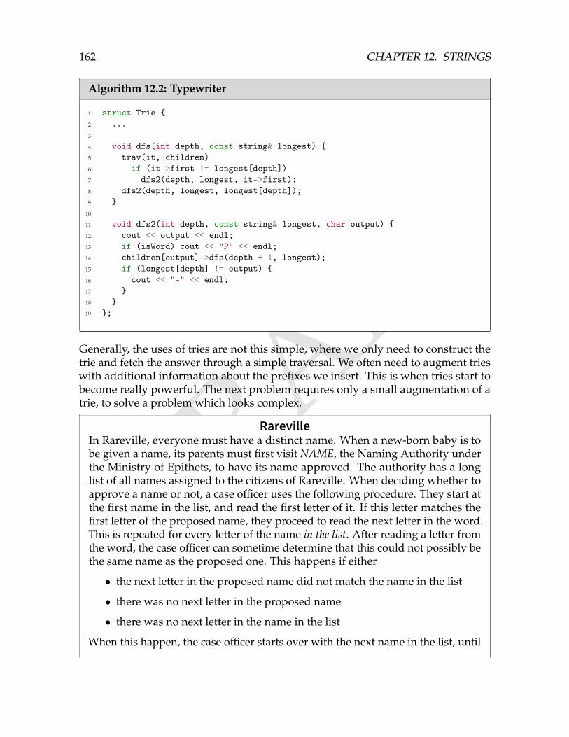
DRAFT
162 CHAPTER 12. STRINGS
Algorithm 12.2: Typewriter
1 struct Trie 2 ...3
4 void dfs(int depth, const string& longest) 5 trav(it, children)6 if (it->first != longest[depth])7 dfs2(depth, longest, it->first);8 dfs2(depth, longest, longest[depth]);9
10
11 void dfs2(int depth, const string& longest, char output) 12 cout << output << endl;13 if (isWord) cout << "P" << endl;14 children[output]->dfs(depth + 1, longest);15 if (longest[depth] != output) 16 cout << "-" << endl;17 18 19 ;
Generally, the uses of tries are not this simple, where we only need to construct thetrie and fetch the answer through a simple traversal. We often need to augment trieswith additional information about the prefixes we insert. This is when tries start tobecome really powerful. The next problem requires only a small augmentation of atrie, to solve a problem which looks complex.
RarevilleIn Rareville, everyone must have a distinct name. When a new-born baby is tobe given a name, its parents must first visit NAME, the Naming Authority underthe Ministry of Epithets, to have its name approved. The authority has a longlist of all names assigned to the citizens of Rareville. When deciding whether toapprove a name or not, a case officer uses the following procedure. They start atthe first name in the list, and read the first letter of it. If this letter matches thefirst letter of the proposed name, they proceed to read the next letter in the word.This is repeated for every letter of the name in the list. After reading a letter fromthe word, the case officer can sometime determine that this could not possibly bethe same name as the proposed one. This happens if either
• the next letter in the proposed name did not match the name in the list
• there was no next letter in the proposed name
• there was no next letter in the name in the list
When this happen, the case officer starts over with the next name in the list, until
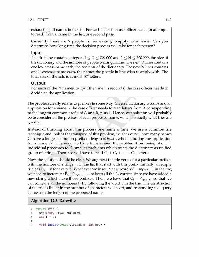
DRAFT
12.1. TRIES 163
exhausting all names in the list. For each letter the case officer reads (or attemptsto read) from a name in the list, one second pass.
Currently, there are N people in line waiting to apply for a name. Can youdetermine how long time the decision process will take for each person?
InputThe first line contains integers 1 ≤ D ≤ 200 000 and 1 ≤ N ≤ 200 000, the size ofthe dictionary and the number of people waiting in line. The nextD lines containsone lowercase name each, the contents of the dictionary. The nextN lines containsone lowercase name each, the names the people in line wish to apply with. Thetotal size of the lists is at most 106 letters.
OutputFor each of the N names, output the time (in seconds) the case officer needs todecide on the application.
The problem clearly relates to prefixes in some way. Given a dictionary wordA and anapplication for a name B, the case officer needs to read letters from A correspondingto the longest common prefix of A and B, plus 1. Hence, our solution will probablybe to consider all the prefixes of each proposed name, which is exactly what tries aregood at.
Instead of thinking about this process one name a time, we use a common trietechnique and look at the transpose of this problem, i.e. for every i, how many namesCi have a longest common prefix of length at least i when handling the applicationfor a name S? This way, we have transformed the problem from being about Dindividual processes to |S| smaller problems which treats the dictionary as unifiedgroup of strings. Then, we will have to read C0 + C1 + · · ·+ C|S| letters.
Now, the solution should be clear. We augment the trie vertex for a particular prefix pwith the number of strings Pp in the list that start with this prefix. Initially, an emptytrie has Pp = 0 for every p. Whenever we insert a new wordW = w1w2 . . . in the trie,we need to increment Pw1 , Pw1w2 , . . . , to keep all the Pp correct, since we have added anew string which have those prefixes. Then, we have that Ci = Ps1s2...si , so that wecan compute all the numbers Pi by following the word S in the trie. The constructionof the trie is linear in the number of characters we insert, and responding to a queryis linear in the length of the proposed name.
Algorithm 12.3: Rareville
1 struct Trie 2 map<char, Trie> children;3 int P = 0;4
5 void insert(const string& s, int pos)
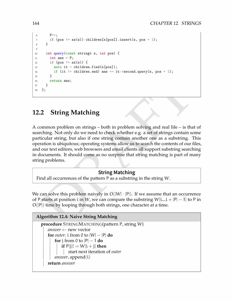
DRAFT
164 CHAPTER 12. STRINGS
6 P++;7 if (pos != sz(s)) children[s[pos]].insert(s, pos + 1);8 9
10 int query(const string& s, int pos) 11 int ans = P;12 if (pos != sz(s)) 13 auto it = children.find(s[pos]);14 if (it != children.end) ans += it->second.query(s, pos + 1);15 16 return ans;17 18 ;
12.2 String Matching
A common problem on strings – both in problem solving and real life – is that ofsearching. Not only do we need to check whether e.g. a set of strings contain someparticular string, but also if one string contain another one as a substring. Thisoperation is ubiquitous; operating systems allow us to search the contents of our files,and our text editors, web browsers and email clients all support substring searchingin documents. It should come as no surprise that string matching is part of manystring problems.
String MatchingFind all occurrences of the pattern P as a substring in the stringW.
We can solve this problem naively in O(|W| · |P|). If we assume that an occurrenceof P starts at position i inW, we can compare the substringW[i...i+ |P|− 1] to P inO(|P|) time by looping through both strings, one character at a time.
Algorithm 12.4: Naive String Matching
procedure STRINGMATCHING(pattern P, stringW)answer← new vectorfor outer: i from 0 to |W|− |P| do
for j from 0 to |P|− 1 doif P[j]! =W[i+ j] then
start next iteration of outeranswer. append(i)
return answer
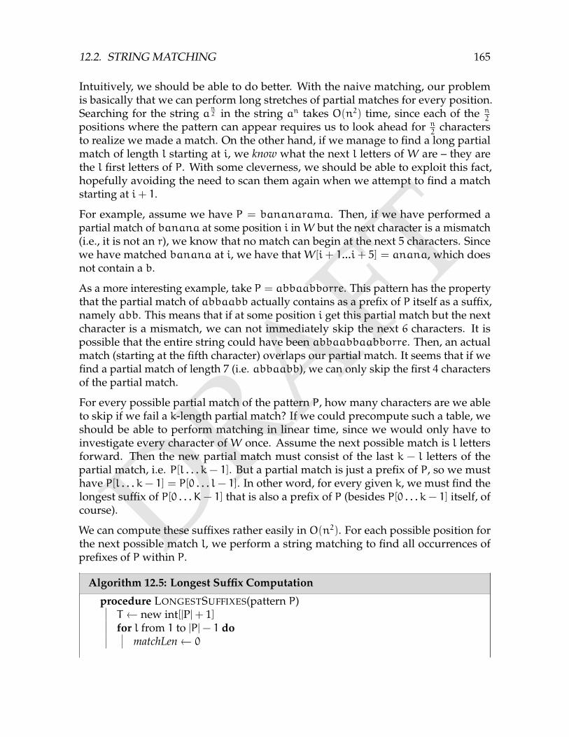
DRAFT
12.2. STRING MATCHING 165
Intuitively, we should be able to do better. With the naive matching, our problemis basically that we can perform long stretches of partial matches for every position.Searching for the string a
n2 in the string an takes O(n2) time, since each of the n
2
positions where the pattern can appear requires us to look ahead for n2
charactersto realize we made a match. On the other hand, if we manage to find a long partialmatch of length l starting at i, we know what the next l letters of W are – they arethe l first letters of P. With some cleverness, we should be able to exploit this fact,hopefully avoiding the need to scan them again when we attempt to find a matchstarting at i+ 1.
For example, assume we have P = bananarama. Then, if we have performed apartial match of banana at some position i inW but the next character is a mismatch(i.e., it is not an r), we know that no match can begin at the next 5 characters. Sincewe have matched banana at i, we have that W[i + 1...i + 5] = anana, which doesnot contain a b.
As a more interesting example, take P = abbaabborre. This pattern has the propertythat the partial match of abbaabb actually contains as a prefix of P itself as a suffix,namely abb. This means that if at some position i get this partial match but the nextcharacter is a mismatch, we can not immediately skip the next 6 characters. It ispossible that the entire string could have been abbaabbaabborre. Then, an actualmatch (starting at the fifth character) overlaps our partial match. It seems that if wefind a partial match of length 7 (i.e. abbaabb), we can only skip the first 4 charactersof the partial match.
For every possible partial match of the pattern P, how many characters are we ableto skip if we fail a k-length partial match? If we could precompute such a table, weshould be able to perform matching in linear time, since we would only have toinvestigate every character of W once. Assume the next possible match is l lettersforward. Then the new partial match must consist of the last k − l letters of thepartial match, i.e. P[l . . . k − 1]. But a partial match is just a prefix of P, so we musthave P[l . . . k− 1] = P[0 . . . l− 1]. In other word, for every given k, we must find thelongest suffix of P[0 . . . K− 1] that is also a prefix of P (besides P[0 . . . k− 1] itself, ofcourse).
We can compute these suffixes rather easily in O(n2). For each possible position forthe next possible match l, we perform a string matching to find all occurrences ofprefixes of P within P.
Algorithm 12.5: Longest Suffix Computation
procedure LONGESTSUFFIXES(pattern P)T ← new int[|P|+ 1]for l from 1 to |P|− 1 do
matchLen← 0
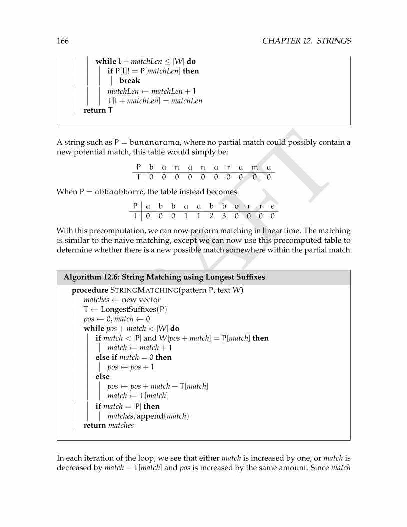
DRAFT
166 CHAPTER 12. STRINGS
while l+ matchLen ≤ |W| doif P[l]! = P[matchLen] then
breakmatchLen← matchLen + 1T [l+ matchLen] = matchLen
return T
A string such as P = bananarama, where no partial match could possibly contain anew potential match, this table would simply be:
P b a n a n a r a m a
T 0 0 0 0 0 0 0 0 0 0
When P = abbaabborre, the table instead becomes:
P a b b a a b b o r r e
T 0 0 0 1 1 2 3 0 0 0 0
With this precomputation, we can now perform matching in linear time. The matchingis similar to the naive matching, except we can now use this precomputed table todetermine whether there is a new possible match somewhere within the partial match.
Algorithm 12.6: String Matching using Longest Suffixes
procedure STRINGMATCHING(pattern P, textW)matches← new vectorT ← LongestSuffixes(P)pos← 0,match← 0
while pos + match < |W| doif match < |P| andW[pos + match] = P[match] then
match← match + 1else if match = 0 then
pos← pos + 1else
pos← pos + match − T [match]match← T [match]
if match = |P| thenmatches. append(match)
return matches
In each iteration of the loop, we see that either match is increased by one, or match isdecreased by match − T [match] and pos is increased by the same amount. Since match
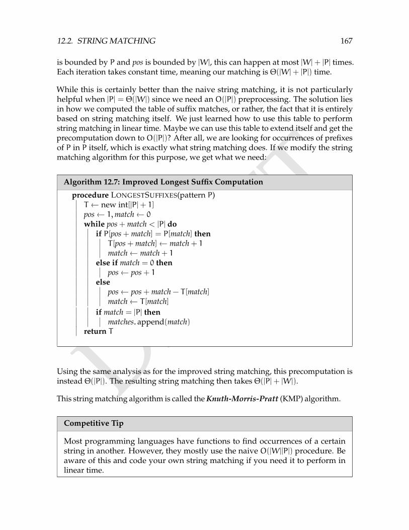
DRAFT
12.2. STRING MATCHING 167
is bounded by P and pos is bounded by |W|, this can happen at most |W|+ |P| times.Each iteration takes constant time, meaning our matching is Θ(|W|+ |P|) time.
While this is certainly better than the naive string matching, it is not particularlyhelpful when |P| = Θ(|W|) since we need an O(|P|) preprocessing. The solution liesin how we computed the table of suffix matches, or rather, the fact that it is entirelybased on string matching itself. We just learned how to use this table to performstring matching in linear time. Maybe we can use this table to extend itself and get theprecomputation down to O(|P|)? After all, we are looking for occurrences of prefixesof P in P itself, which is exactly what string matching does. If we modify the stringmatching algorithm for this purpose, we get what we need:
Algorithm 12.7: Improved Longest Suffix Computation
procedure LONGESTSUFFIXES(pattern P)T ← new int[|P|+ 1]pos← 1,match← 0
while pos + match < |P| doif P[pos + match] = P[match] thenT [pos + match]← match + 1match← match + 1
else if match = 0 thenpos← pos + 1
elsepos← pos + match − T [match]match← T [match]
if match = |P| thenmatches. append(match)
return T
Using the same analysis as for the improved string matching, this precomputation isinstead Θ(|P|). The resulting string matching then takes Θ(|P|+ |W|).
This string matching algorithm is called the Knuth-Morris-Pratt (KMP) algorithm.
Competitive Tip
Most programming languages have functions to find occurrences of a certainstring in another. However, they mostly use the naive O(|W||P|) procedure. Beaware of this and code your own string matching if you need it to perform inlinear time.
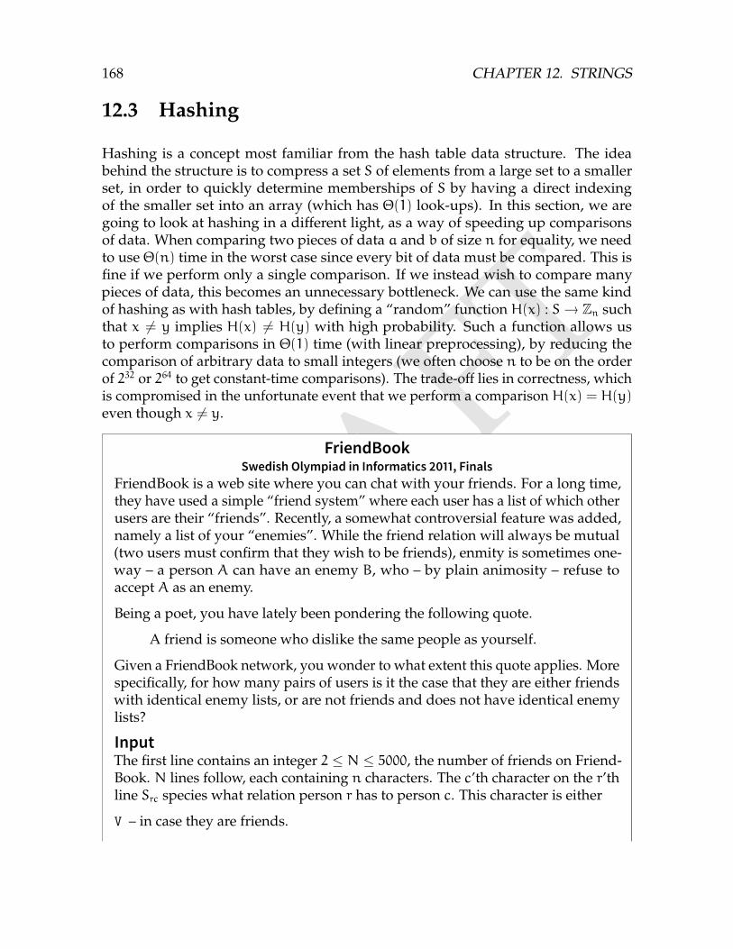
DRAFT
168 CHAPTER 12. STRINGS
12.3 Hashing
Hashing is a concept most familiar from the hash table data structure. The ideabehind the structure is to compress a set S of elements from a large set to a smallerset, in order to quickly determine memberships of S by having a direct indexingof the smaller set into an array (which has Θ(1) look-ups). In this section, we aregoing to look at hashing in a different light, as a way of speeding up comparisonsof data. When comparing two pieces of data a and b of size n for equality, we needto use Θ(n) time in the worst case since every bit of data must be compared. This isfine if we perform only a single comparison. If we instead wish to compare manypieces of data, this becomes an unnecessary bottleneck. We can use the same kindof hashing as with hash tables, by defining a “random” function H(x) : S→ Zn suchthat x 6= y implies H(x) 6= H(y) with high probability. Such a function allows usto perform comparisons in Θ(1) time (with linear preprocessing), by reducing thecomparison of arbitrary data to small integers (we often choose n to be on the orderof 232 or 264 to get constant-time comparisons). The trade-off lies in correctness, whichis compromised in the unfortunate event that we perform a comparison H(x) = H(y)even though x 6= y.
FriendBookSwedish Olympiad in Informatics 2011, Finals
FriendBook is a web site where you can chat with your friends. For a long time,they have used a simple “friend system” where each user has a list of which otherusers are their “friends”. Recently, a somewhat controversial feature was added,namely a list of your “enemies”. While the friend relation will always be mutual(two users must confirm that they wish to be friends), enmity is sometimes one-way – a person A can have an enemy B, who – by plain animosity – refuse toaccept A as an enemy.
Being a poet, you have lately been pondering the following quote.
A friend is someone who dislike the same people as yourself.
Given a FriendBook network, you wonder to what extent this quote applies. Morespecifically, for how many pairs of users is it the case that they are either friendswith identical enemy lists, or are not friends and does not have identical enemylists?
InputThe first line contains an integer 2 ≤ N ≤ 5000, the number of friends on Friend-Book. N lines follow, each containing n characters. The c’th character on the r’thline Src species what relation person r has to person c. This character is either
V – in case they are friends.
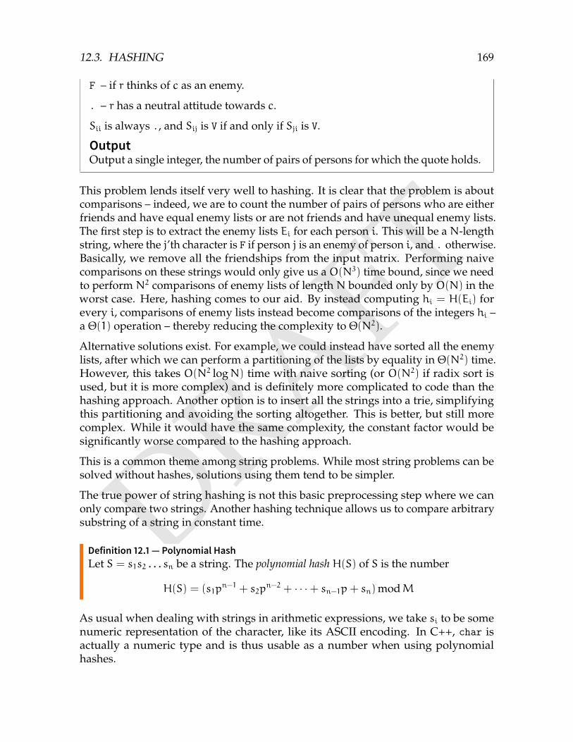
DRAFT
12.3. HASHING 169
F – if r thinks of c as an enemy.
. – r has a neutral attitude towards c.
Sii is always ., and Sij is V if and only if Sji is V.
OutputOutput a single integer, the number of pairs of persons for which the quote holds.
This problem lends itself very well to hashing. It is clear that the problem is aboutcomparisons – indeed, we are to count the number of pairs of persons who are eitherfriends and have equal enemy lists or are not friends and have unequal enemy lists.The first step is to extract the enemy lists Ei for each person i. This will be a N-lengthstring, where the j’th character is F if person j is an enemy of person i, and . otherwise.Basically, we remove all the friendships from the input matrix. Performing naivecomparisons on these strings would only give us a O(N3) time bound, since we needto perform N2 comparisons of enemy lists of length N bounded only by O(N) in theworst case. Here, hashing comes to our aid. By instead computing hi = H(Ei) forevery i, comparisons of enemy lists instead become comparisons of the integers hi –a Θ(1) operation – thereby reducing the complexity to Θ(N2).
Alternative solutions exist. For example, we could instead have sorted all the enemylists, after which we can perform a partitioning of the lists by equality in Θ(N2) time.However, this takes O(N2 logN) time with naive sorting (or O(N2) if radix sort isused, but it is more complex) and is definitely more complicated to code than thehashing approach. Another option is to insert all the strings into a trie, simplifyingthis partitioning and avoiding the sorting altogether. This is better, but still morecomplex. While it would have the same complexity, the constant factor would besignificantly worse compared to the hashing approach.
This is a common theme among string problems. While most string problems can besolved without hashes, solutions using them tend to be simpler.
The true power of string hashing is not this basic preprocessing step where we canonly compare two strings. Another hashing technique allows us to compare arbitrarysubstring of a string in constant time.
Definition 12.1 — Polynomial HashLet S = s1s2 . . . sn be a string. The polynomial hash H(S) of S is the number
H(S) = (s1pn−1 + s2p
n−2 + · · ·+ sn−1p+ sn)modM
As usual when dealing with strings in arithmetic expressions, we take si to be somenumeric representation of the character, like its ASCII encoding. In C++, char isactually a numeric type and is thus usable as a number when using polynomialhashes.
DRAFT
170 CHAPTER 12. STRINGS
Polynomial hashes have many useful properties.
Theorem 12.1 — Properties of the Polynomial HashIf S = s1 . . . sn is a string and c is a single character, we have that
1. H(S||c) = (pH(S) +H(c))modM
2. H(c||S) = (H(S) +H(c)pn)modM
3. H(s2 . . . sn) = (H(S) −H(s1)pn−1)modM
4. H(s1 . . . sn−1) = (H(S) −H(sn))p−1 modM
5. H(slsl+1 . . . sr−2sr−1) = (H(s1 . . . sR−1) −H(s1 − SL−1)pR−L)modM
Exercise 12.1
Prove the properties of Theorem 12.1
Exercise 12.2
How can we compute the hash of S||T in O(1) given the hashes of the strings S andT?
Properties 1-4 alone allow us to append and remove characters from the beginningand end of a hash in constant time. We refer to this property as polynomial hashesbeing rolling. This property allows us to String Matching problem with a singlepattern (Section 12.2) with the same complexity as KMP, by computing the hash ofthe pattern P and then rolling a |P|-length hash through the string we are searching in.This algorithm is called the Rabin-Karp algorithm.
Property 5 allows us to compute the hash of any substring of a string in constanttime, provided we have computed the hashes H(S1), H(s1s2), . . . , H(s1s2 . . . sn) first.Naively this computation would be Θ(n2), but property 1 allows us to compute themrecursively, resulting in Θ(n) precomputation.
Radio TransmissionBaltic Olympiad in Informatics 2009
Given is a string S. Find the shortest string L, such that S is a substring of theinfinite string T = . . . LLLLL . . . .
InputThe first and only line of the input contains the string S, with 1 ≤ |S| ≤ 106.
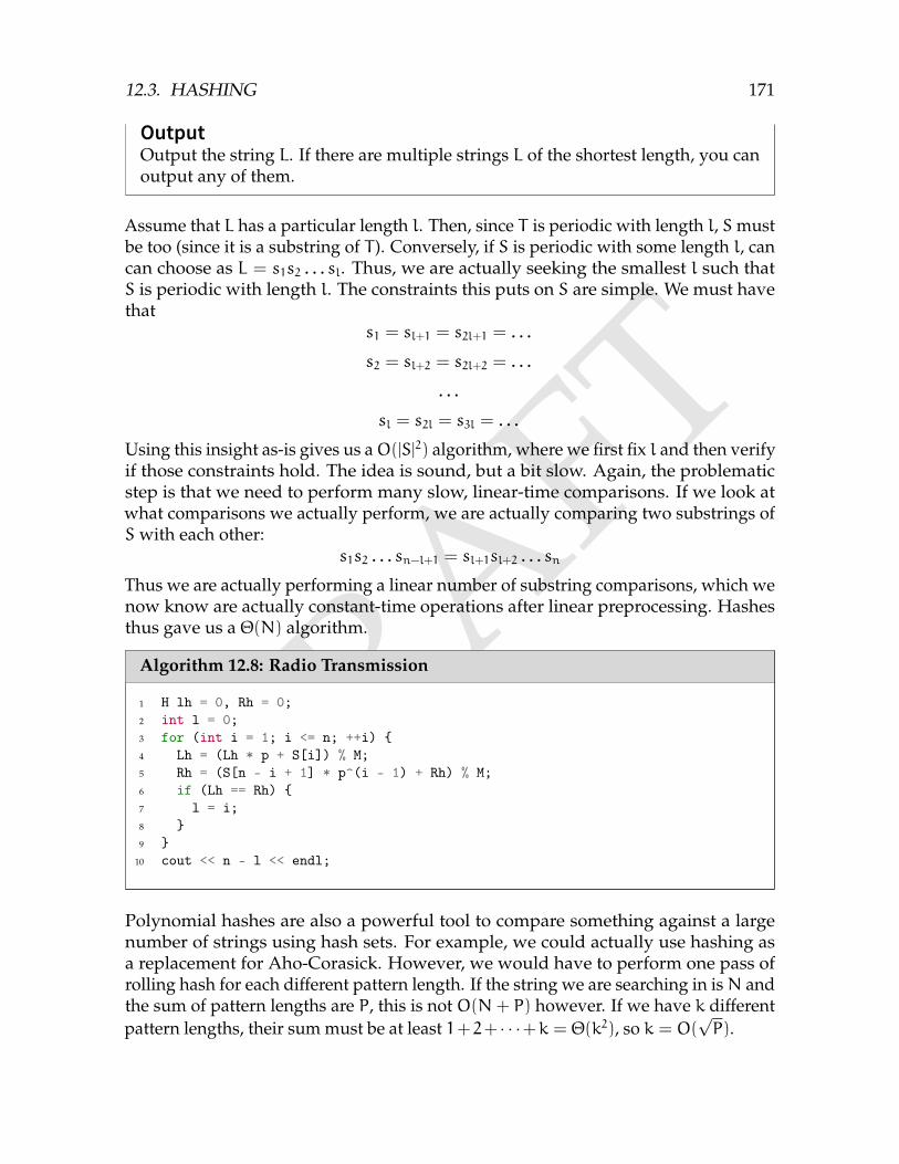
DRAFT
12.3. HASHING 171
OutputOutput the string L. If there are multiple strings L of the shortest length, you canoutput any of them.
Assume that L has a particular length l. Then, since T is periodic with length l, Smustbe too (since it is a substring of T ). Conversely, if S is periodic with some length l, cancan choose as L = s1s2 . . . sl. Thus, we are actually seeking the smallest l such thatS is periodic with length l. The constraints this puts on S are simple. We must havethat
s1 = sl+1 = s2l+1 = . . .
s2 = sl+2 = s2l+2 = . . .
. . .
sl = s2l = s3l = . . .
Using this insight as-is gives us aO(|S|2) algorithm, where we first fix l and then verifyif those constraints hold. The idea is sound, but a bit slow. Again, the problematicstep is that we need to perform many slow, linear-time comparisons. If we look atwhat comparisons we actually perform, we are actually comparing two substrings ofSwith each other:
s1s2 . . . sn−l+1 = sl+1sl+2 . . . sn
Thus we are actually performing a linear number of substring comparisons, which wenow know are actually constant-time operations after linear preprocessing. Hashesthus gave us a Θ(N) algorithm.
Algorithm 12.8: Radio Transmission
1 H lh = 0, Rh = 0;2 int l = 0;3 for (int i = 1; i <= n; ++i) 4 Lh = (Lh * p + S[i]) % M;5 Rh = (S[n - i + 1] * p^(i - 1) + Rh) % M;6 if (Lh == Rh) 7 l = i;8 9
10 cout << n - l << endl;
Polynomial hashes are also a powerful tool to compare something against a largenumber of strings using hash sets. For example, we could actually use hashing asa replacement for Aho-Corasick. However, we would have to perform one pass ofrolling hash for each different pattern length. If the string we are searching in isN andthe sum of pattern lengths are P, this is not O(N+ P) however. If we have k differentpattern lengths, their sum must be at least 1+2+ · · ·+k = Θ(k2), so k = O(
√P).
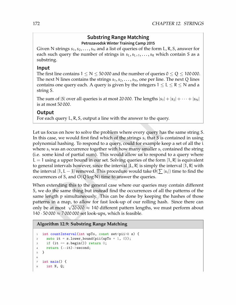
DRAFT
172 CHAPTER 12. STRINGS
Substring Range MatchingPetrozavodsk Winter Training Camp 2015
Given N strings s1, s2, . . . , sN and a list of queries of the form L, R, S, answer foreach such query the number of strings in sL, sL+1, . . . , sR which contain S as asubstring.
InputThe first line contains 1 ≤ N ≤ 50 000 and the number of queries 0 ≤ Q ≤ 100 000.The next N lines contains the strings s1, s2, . . . , sN, one per line. The next Q linescontains one query each. A query is given by the integers 1 ≤ L ≤ R ≤ N and astring S.
The sum of |S| over all queries is at most 20 000. The lengths |s1|+ |s2|+ · · ·+ |sN|
is at most 50 000.
OutputFor each query L, R, S, output a line with the answer to the query.
Let us focus on how to solve the problem where every query has the same string S.In this case, we would first find which of the strings si that S is contained in usingpolynomial hashing. To respond to a query, could for example keep a set of all the iwhere si was an occurrence together with how many smaller si contained the string(i.e. some kind of partial sum). This would allow us to respond to a query whereL = 1 using a upper bound in our set. Solving queries of the form [1, R] is equivalentto general intervals however, since the interval [L, R] is simply the interval [1, R] withthe interval [1, L− 1] removed. This procedure would take Θ(
∑|si|) time to find the
occurrences of S, and O(Q logN) time to answer the queries.
When extending this to the general case where our queries may contain differentS, we do the same thing but instead find the occurrences of all the patterns of thesame length p simultaneously. This can be done by keeping the hashes of thosepatterns in a map, to allow for fast look-up of our rolling hash. Since there canonly be at most
√20 000 ≈ 140 different pattern lengths, we must perform about
140 · 50 000 ≈ 7 000 000 set look-ups, which is feasible.
Algorithm 12.9: Substring Range Matching
1 int countInterval(int upTo, const set<pii>& s) 2 auto it = s.lower_bound(pii(upTo + 1, 0));3 if (it == s.begin()) return 0;4 return (--it)->second;5 6
7 int main() 8 int N, Q;
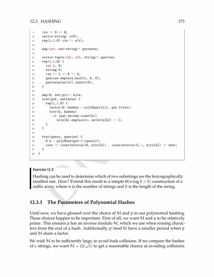
DRAFT
12.3. HASHING 173
9 cin >> N >> Q;10 vector<string> s(N);11 rep(i,0,N) cin >> s[i];12
13 map<int, set<string>> patterns;14
15 vector<tuple<int, int, string>> queries;16 rep(i,0,Q) 17 int L, R;18 string S;19 cin >> L >> R >> S;20 queries.emplace_back(L, R, S);21 patterns[sz(s)].insert(S);22 23
24 map<H, set<pii>> hits;25 trav(pat, patterns) 26 rep(i,0,N) 27 vector<H> hashes = rollHash(s[i], pat.first);28 trav(h, hashes)29 if (pat.second.count(h))30 hits[h].emplace(i, sz(hits[h]) + 1);31 32 33
34 trav(query, queries) 35 H h = polyHash(get<2>(query));36 cout << countInterval(R, hits[h]) - countInterval(L-1, hits[h]) << endl;37 38
Exercise 12.3
Hashing can be used to determine which of two substrings are the lexicographicallysmallest one. How? Extend this result to a simple Θ(n logS+ S) construction of asuffix array, where n is the number of strings and S is the length of the string.
12.3.1 The Parameters of Polynomial Hashes
Until now, we have glossed over the choice ofM and p in our polynomial hashing.These choices happen to be important. First of all, we wantM and p to be relativelyprime. This ensures p has an inverse moduloM, which we use when erasing charac-ters from the end of a hash. Additionally, pi modM have a smaller period when pandM share a factor.
We wishM to be sufficiently large, to avoid hash collisions. If we compare the hashesof c strings, we want M = Ω(
√c) to get a reasonable chance at avoiding collisions.
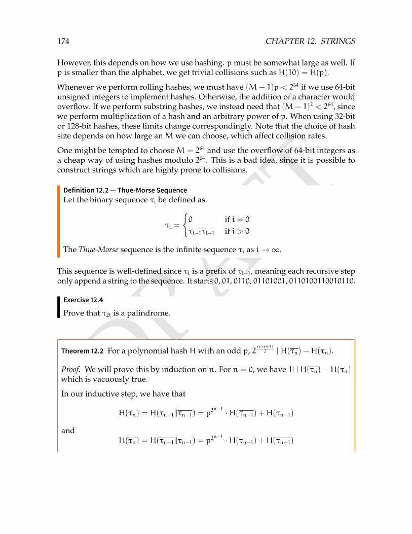
DRAFT
174 CHAPTER 12. STRINGS
However, this depends on how we use hashing. pmust be somewhat large as well. Ifp is smaller than the alphabet, we get trivial collisions such as H(10) = H(p).
Whenever we perform rolling hashes, we must have (M− 1)p < 264 if we use 64-bitunsigned integers to implement hashes. Otherwise, the addition of a character wouldoverflow. If we perform substring hashes, we instead need that (M− 1)2 < 264, sincewe perform multiplication of a hash and an arbitrary power of p. When using 32-bitor 128-bit hashes, these limits change correspondingly. Note that the choice of hashsize depends on how large anMwe can choose, which affect collision rates.
One might be tempted to chooseM = 264 and use the overflow of 64-bit integers asa cheap way of using hashes modulo 264. This is a bad idea, since it is possible toconstruct strings which are highly prone to collisions.
Definition 12.2 — Thue-Morse SequenceLet the binary sequence τi be defined as
τi =
0 if i = 0τi−1τi−1 if i > 0
The Thue-Morse sequence is the infinite sequence τi as i→∞.
This sequence is well-defined since τi is a prefix of τi−1, meaning each recursive steponly append a string to the sequence. It starts 0, 01, 0110, 01101001, 0110100110010110.
Exercise 12.4
Prove that τ2i is a palindrome.
Theorem 12.2 For a polynomial hash Hwith an odd p, 2n(n+1)2 | H(τn) −H(τn).
Proof. We will prove this by induction on n. For n = 0, we have 1| | H(τn) −H(τn)which is vacuously true.
In our inductive step, we have that
H(τn) = H(τn−1||τn−1) = p2n−1 ·H(τn−1) +H(τn−1)
andH(τn) = H(τn−1||τn−1) = p
2n−1 ·H(τn−1) +H(τn−1)
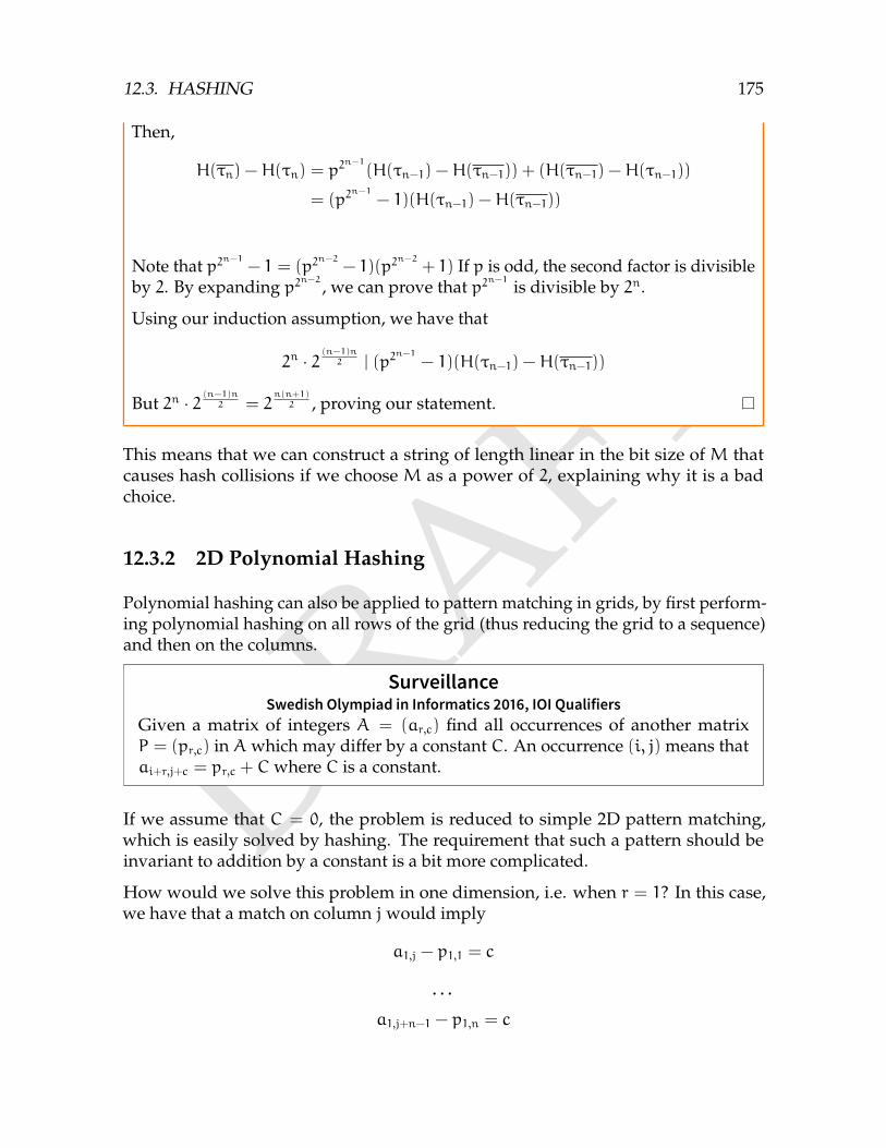
DRAFT
12.3. HASHING 175
Then,
H(τn) −H(τn) = p2n−1(H(τn−1) −H(τn−1)) + (H(τn−1) −H(τn−1))
= (p2n−1
− 1)(H(τn−1) −H(τn−1))
Note that p2n−1 − 1 = (p2n−2
− 1)(p2n−2
+ 1) If p is odd, the second factor is divisibleby 2. By expanding p2n−2 , we can prove that p2n−1 is divisible by 2n.
Using our induction assumption, we have that
2n · 2 (n−1)n2 | (p2
n−1
− 1)(H(τn−1) −H(τn−1))
But 2n · 2 (n−1)n2 = 2
n(n+1)2 , proving our statement.
This means that we can construct a string of length linear in the bit size of M thatcauses hash collisions if we choose M as a power of 2, explaining why it is a badchoice.
12.3.2 2D Polynomial Hashing
Polynomial hashing can also be applied to pattern matching in grids, by first perform-ing polynomial hashing on all rows of the grid (thus reducing the grid to a sequence)and then on the columns.
SurveillanceSwedish Olympiad in Informatics 2016, IOI Qualifiers
Given a matrix of integers A = (ar,c) find all occurrences of another matrixP = (pr,c) in A which may differ by a constant C. An occurrence (i, j) means thatai+r,j+c = pr,c + Cwhere C is a constant.
If we assume that C = 0, the problem is reduced to simple 2D pattern matching,which is easily solved by hashing. The requirement that such a pattern should beinvariant to addition by a constant is a bit more complicated.
How would we solve this problem in one dimension, i.e. when r = 1? In this case,we have that a match on column jwould imply
a1,j − p1,1 = c
. . .
a1,j+n−1 − p1,n = c
DRAFT
176 CHAPTER 12. STRINGS
Since c is arbitrary, this means the only condition is that
a1,j − p1,1 = · · · = a1,j+n−1 − p1,n = c
Rearranging this gives us that
a1,j − a1,j+1 = p1,1 − p1,2
a1,j+1 − a1,j+2 = p1,2 − p1,3
. . .
By computing these two sequences of the adjacent differences of elements a1,i and r1,j,we have reduced the problem to substring matching and can apply hashing. In 2D,we can do something similar. For a match (i, j), it is sufficient that this property holdsfor every line and every column in the match. We can then find matches using two2D hashes.
Exercise 12.5 — Kattis Exercise
Chasing Subs – chasingsubs
12.4 Chapter Notes
rabin karp paper
KMP
hashing
DRAFTChapter 13
Combinatorics
Combinatorics deals with various discrete structures, such as graphs and permuta-tions. In this chapter, we will mainly study the branch of combinatorics known asenumerative combinatorics – the art of counting. We will count the number of ways tochoose K different candies from N different candies, the number of distinct seatingarrangements around a circular table, the sum of sizes of all subsets of a set and manymore objects. Many combinatorial counting problems are based on a few standardtechniques which we will learn in this chapter.
13.1 The Addition and Multiplication Principles
The addition principle states that, given a finite collection of disjoint sets S1, S2, . . . , Sn,we can compute the size of the union of all sets by simply adding up the sizes of oursets, i.e.
|S1 ∪ S2 ∪ · · · ∪ Sn| = |S1|+ |S2|+ · · ·+ |Sn|
Example 13.1 Assume we have 5 different types of chocolate bars (the set C), 3different types of bubble gum (the set G), and 4 different types of lollipops (the setL). These form three disjoint sets, meaning we can compute the total number ofsnacks by summing up the number of snacks of the different types. Thus, we have|C|+ |G|+ |L| = 5+ 3+ 4 = 12 different snacks.
Later on, we will see a generalization of the addition principle that handles caseswhere our sets are not disjoint.
The multiplication principle, on the other hand, states that the size of the Cartesianproduct S1 × S2 × · · · × Sn equals the product of the individual sizes of these sets,
177
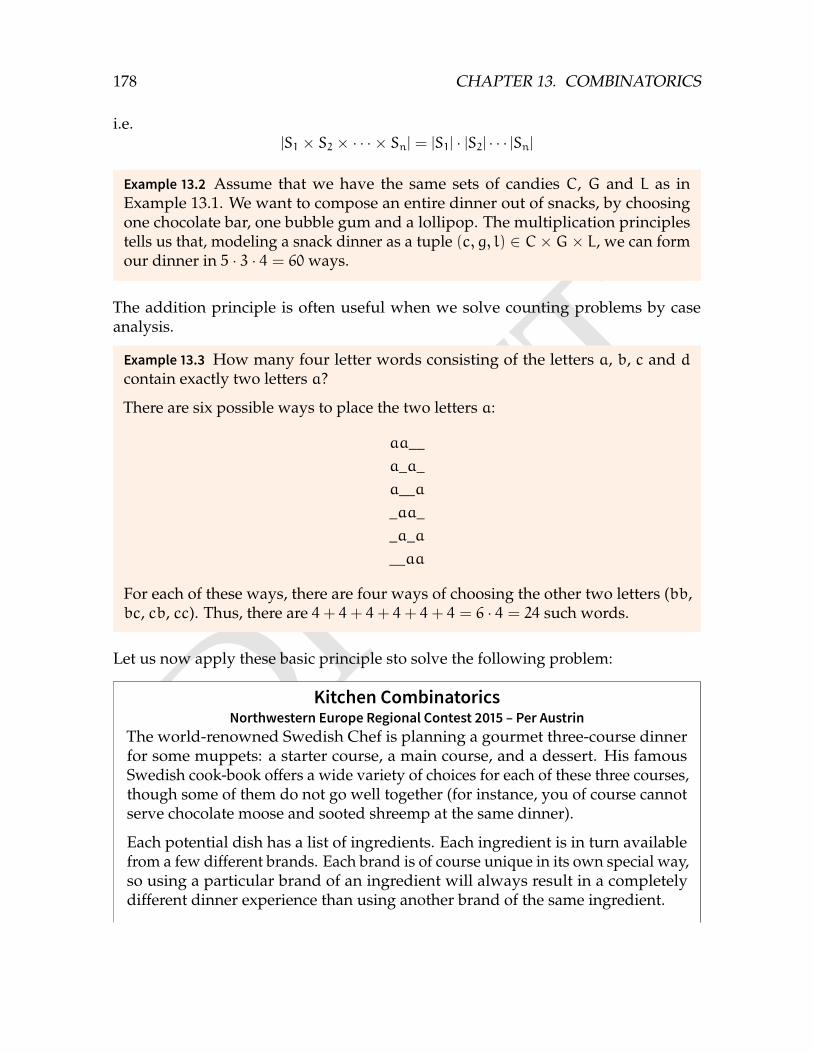
DRAFT
178 CHAPTER 13. COMBINATORICS
i.e.|S1 × S2 × · · · × Sn| = |S1| · |S2| · · · |Sn|
Example 13.2 Assume that we have the same sets of candies C, G and L as inExample 13.1. We want to compose an entire dinner out of snacks, by choosingone chocolate bar, one bubble gum and a lollipop. The multiplication principlestells us that, modeling a snack dinner as a tuple (c, g, l) ∈ C×G× L, we can formour dinner in 5 · 3 · 4 = 60ways.
The addition principle is often useful when we solve counting problems by caseanalysis.
Example 13.3 How many four letter words consisting of the letters a, b, c and dcontain exactly two letters a?
There are six possible ways to place the two letters a:
aa__a_a_a__a_aa__a_a__aa
For each of these ways, there are four ways of choosing the other two letters (bb,bc, cb, cc). Thus, there are 4+ 4+ 4+ 4+ 4+ 4 = 6 · 4 = 24 such words.
Let us now apply these basic principle sto solve the following problem:
Kitchen CombinatoricsNorthwestern Europe Regional Contest 2015 – Per Austrin
The world-renowned Swedish Chef is planning a gourmet three-course dinnerfor some muppets: a starter course, a main course, and a dessert. His famousSwedish cook-book offers a wide variety of choices for each of these three courses,though some of them do not go well together (for instance, you of course cannotserve chocolate moose and sooted shreemp at the same dinner).
Each potential dish has a list of ingredients. Each ingredient is in turn availablefrom a few different brands. Each brand is of course unique in its own special way,so using a particular brand of an ingredient will always result in a completelydifferent dinner experience than using another brand of the same ingredient.
DRAFT
13.1. THE ADDITION AND MULTIPLICATION PRINCIPLES 179
Some common ingredients such as pølårber may appear in two of the three chosendishes, or in all three of them. When an ingredient is used in more than one ofthe three selected dishes, Swedish Chef will use the same brand of the ingredientin all of them.
While waiting for the meecaroo, Swedish Chef starts wondering: how manydifferent dinner experiences are there that he could make, by different choices ofdishes and brands for the ingredients?
InputThe input consists of:
• five integers r, s, m, d, n, where 1 ≤ r ≤ 1 000 is the number of differentingredients that exist, 1 ≤ s,m, d ≤ 25 are the number of available starterdishes, main dishes, and desserts, respectively, and 0 ≤ n ≤ 2 000 is thenumber of pairs of dishes that do not go well together.
• r integers b1, . . . , br, where 1 ≤ bi ≤ 100 is the number of different brandsof ingredient i.
• s+m+ d dishes – the s starter dishes, then themmain dishes, then the ddesserts. Each dish starts with an integer 1 ≤ k ≤ 20 denoting the numberof ingredients of the dish, and is followed by k distinct integers i1, . . . , ik,where for each 1 ≤ j ≤ k, 1 ≤ ij ≤ r is an ingredient.
• n pairs of incompatible dishes.
OutputIf the number of different dinner experiences Swedish Chef can make is at most1018, then output that number. Otherwise, output “too many”.
The solution is a similar addition-multiplication principle combo as used in Exam-ple 13.3. First off, we can simplify the problem considerably by brute forcing over thecoarsest component of a dinner experience, namely the courses included. Since thereare at most 25 dishes of every type, we need to check up to 253 = 15 625 choices ofdishes. By the addition principle, we can compute the number of dinner experiencesfor each such three-course dinner, and then sum them up to get the answer. Somepairs of dishes do not go well together. At this stage in the process we exclude anytriple of dishes that include such a pair. We can perform this check in Θ(1) time if wesave the incompatible dishes in 2D boolean vectors, so that e.g. badStarterMain[i][j]determines if starter i is incompatible with main dish j.
For a given dinner course consisting of starter a, main dish b and dessert c, only theset of ingredients of three dishes matters since the chef will use the same brand foran ingredient even if it is part of two dishes. The next step is thus to compute thisset by taking the union of ingredients for the three included dishes. This step takesΘ(ka+kb+kc). Once this set is computed, the only remaining task is to choose a brand
DRAFT
180 CHAPTER 13. COMBINATORICS
for each ingredient. Assigning brands is an ordinary application of the multiplicationprinciple, where we multiply the number of brands available for each ingredienttogether.
13.2 Permutations
A permutation of a set S is an ordering of all the elements in the set. For example, theset 1, 2, 3 has 6 permutations:
123 132213 231312 321
Our first “real” combinatorial problem will be to count the number of permutations ofan n-element set S. When counting permutations, we use the multiplication principle.We will show a procedure that can be used to construct permutations one elementat a time. Assume that the permutation is the sequence 〈a1, a2, . . . , an〉. The firstelement of the permutation, a1, can be assigned any of the n elements of S. Oncethis assignment has been made, we have n − 1 elements we can choose to be a2(any element of S except a1). In general, when we are to select the (i + 1)’th valueai+1 of the permutation, i elements have already been included in the permutation,leaving n− i options for ai+1. Using this argument for all n elements of the sequence,we can construct a permutation in n · (n − 1) · · · 2 · 1 ways (by the multiplicationprinciple).
This number is so useful that it has its own name and notation.
Definition 13.1 — FactorialThe factorial of n, where n is a non-negative integer, denoted n!, is defined as theproduct of the first n positive integers, i.e.
n! = 1 · 2 · · ·n =
n∏i=1
i
For n = 0, we use the convention that the empty product is 1.
This sequence of numbers thus begin 1, 1, 2, 6, 24, 120, 720, 40 320, 362 880, 3 628 800,39 916 800 for n = 0, 1, 2, . . . , 11. It is good to know the magnitudes of these numbers,since they are frequent in time complexities when doing brute force over permutations.Asypmtotically, the grow as nΘ(n). More precisely, the well-used Stirling’s formula1
1Named after James Stirling (who have other important combinatorial objects named after him too),but stated already by his contemporary Abraham de Moivre.
DRAFT
13.2. PERMUTATIONS 181
gives the approximation
n! =√2πn
(ne
)n(1+O
(1
n
))
Exercise 13.1
In how many ways can 8 persons be seated around a round table, if we considercyclic rotations of a seating to be different? What if we consider cyclic rotations tobe equivalent?
Exercise 13.2 — Kattis Problems
n’th permutation – nthpermutation
Name That Permutation – namethatpermutation
13.2.1 Permutations as Bijections
The word permutation has roots in Latin, meaning “to change completely”. We are nowgoing look at permutations in a very different light, which gives some justification tothe etymology of the word.
Given a set such as [5], we can fix some ordering of its elements such as 〈1, 2, 3, 4, 5〉.A permutation π = 〈1, 3, 4, 5, 2〉 of this set can then be seen as a movement of theseelements. Of course, this same movement can be applied to any other 5-elementset with a fixed permutation, such as 〈a, b, c, d, e〉 being transformed to 〈a, c, d, e, b〉.This suggests that we can consider permutation as a “rule” which describes how tomove – permute – the elements.
Such a movement rule can also be described as a function π : [n] → [n], whereπ(i) describes what element should be placed at position i. Thus, the permutation〈1, 3, 4, 5, 2〉would have π(1) = 1, π(2) = 3, π(3) = 4, π(4) = 5, π(5) = 2.
i 1 2 3 4 5↓ ↓ ↓ ↓ ↓π(i) 1 3 4 5 2
Since each element is mapped to a different element, the function induced by apermutation is actually a bijection. By interpreting permutations as function, all thetheory from functions apply to permutations too.
We call 〈1, 2, 3, 4, . . . , n〉 the identity permutation, since the function given by the iden-tity permutation is actually the identity function. As a function, we can also consider
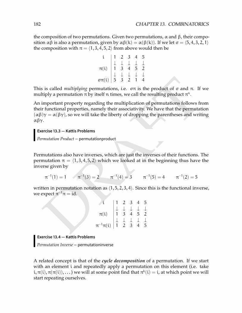
DRAFT
182 CHAPTER 13. COMBINATORICS
the composition of two permutations. Given two permutations, α and β, their compo-sition αβ is also a permutation, given by αβ(k) = α(β(k)). If we let σ = 〈5, 4, 3, 2, 1〉the composition with π = 〈1, 3, 4, 5, 2〉 from above would then be
i 1 2 3 4 5↓ ↓ ↓ ↓ ↓π(i) 1 3 4 5 2↓ ↓ ↓ ↓ ↓σπ(i) 5 3 2 1 4
This is called multiplying permutations, i.e. σπ is the product of σ and π. If wemultiply a permutation π by itself n times, we call the resulting product πn.
An important property regarding the multiplication of permutations follows fromtheir functional properties, namely their associativity. We have that the permutation(αβ)γ = α(βγ), so we will take the liberty of dropping the parentheses and writingαβγ.
Exercise 13.3 — Kattis Problems
Permutation Product – permutationproduct
Permutations also have inverses, which are just the inverses of their functions. Thepermutation π = 〈1, 3, 4, 5, 2〉 which we looked at in the beginning thus have theinverse given by
π−1(1) = 1 π−1(3) = 2 π−1(4) = 3 π−1(5) = 4 π−1(2) = 5
written in permutation notation as 〈1, 5, 2, 3, 4〉. Since this is the functional inverse,we expect π−1π = id.
i 1 2 3 4 5↓ ↓ ↓ ↓ ↓π(i) 1 3 4 5 2↓ ↓ ↓ ↓ ↓π−1π(i) 1 2 3 4 5
Exercise 13.4 — Kattis Problems
Permutation Inverse – permutationinverse
A related concept is that of the cycle decomposition of a permutation. If we startwith an element i and repeatedly apply a permutation on this element (i.e. takei, π(i), π(π(i)), . . . ) we will at some point find that πk(i) = i, at which point we willstart repeating ourselves.
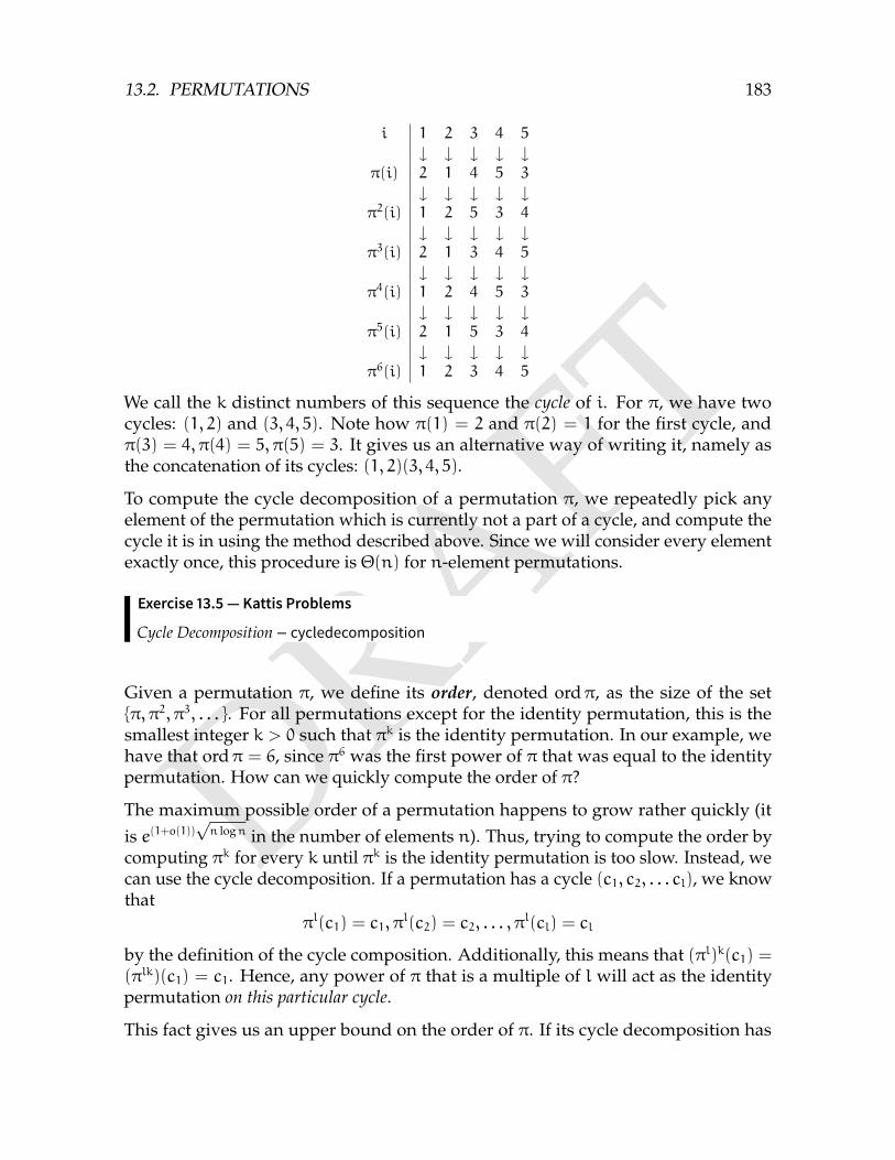
DRAFT
13.2. PERMUTATIONS 183
i 1 2 3 4 5↓ ↓ ↓ ↓ ↓π(i) 2 1 4 5 3↓ ↓ ↓ ↓ ↓π2(i) 1 2 5 3 4↓ ↓ ↓ ↓ ↓π3(i) 2 1 3 4 5↓ ↓ ↓ ↓ ↓π4(i) 1 2 4 5 3↓ ↓ ↓ ↓ ↓π5(i) 2 1 5 3 4↓ ↓ ↓ ↓ ↓π6(i) 1 2 3 4 5
We call the k distinct numbers of this sequence the cycle of i. For π, we have twocycles: (1, 2) and (3, 4, 5). Note how π(1) = 2 and π(2) = 1 for the first cycle, andπ(3) = 4, π(4) = 5, π(5) = 3. It gives us an alternative way of writing it, namely asthe concatenation of its cycles: (1, 2)(3, 4, 5).
To compute the cycle decomposition of a permutation π, we repeatedly pick anyelement of the permutation which is currently not a part of a cycle, and compute thecycle it is in using the method described above. Since we will consider every elementexactly once, this procedure is Θ(n) for n-element permutations.
Exercise 13.5 — Kattis Problems
Cycle Decomposition – cycledecomposition
Given a permutation π, we define its order, denoted ordπ, as the size of the setπ, π2, π3, . . . . For all permutations except for the identity permutation, this is thesmallest integer k > 0 such that πk is the identity permutation. In our example, wehave that ordπ = 6, since π6 was the first power of π that was equal to the identitypermutation. How can we quickly compute the order of π?
The maximum possible order of a permutation happens to grow rather quickly (itis e(1+o(1))
√n logn in the number of elements n). Thus, trying to compute the order by
computing πk for every k until πk is the identity permutation is too slow. Instead, wecan use the cycle decomposition. If a permutation has a cycle (c1, c2, . . . cl), we knowthat
πl(c1) = c1, πl(c2) = c2, . . . , π
l(cl) = cl
by the definition of the cycle composition. Additionally, this means that (πl)k(c1) =(πlk)(c1) = c1. Hence, any power of π that is a multiple of l will act as the identitypermutation on this particular cycle.
This fact gives us an upper bound on the order of π. If its cycle decomposition has
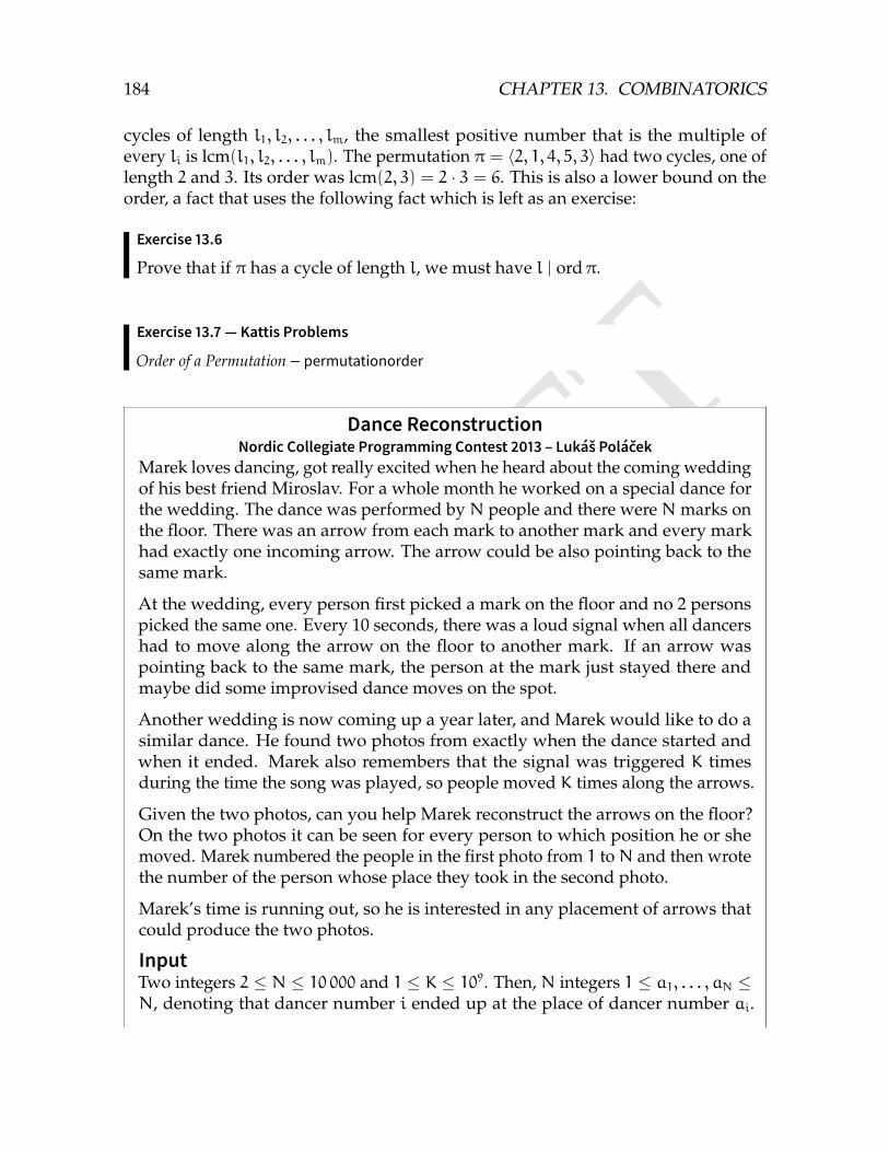
DRAFT
184 CHAPTER 13. COMBINATORICS
cycles of length l1, l2, . . . , lm, the smallest positive number that is the multiple ofevery li is lcm(l1, l2, . . . , lm). The permutation π = 〈2, 1, 4, 5, 3〉 had two cycles, one oflength 2 and 3. Its order was lcm(2, 3) = 2 · 3 = 6. This is also a lower bound on theorder, a fact that uses the following fact which is left as an exercise:
Exercise 13.6
Prove that if π has a cycle of length l, we must have l | ordπ.
Exercise 13.7 — Kattis Problems
Order of a Permutation – permutationorder
Dance ReconstructionNordic Collegiate Programming Contest 2013 – Lukáš Poláček
Marek loves dancing, got really excited when he heard about the coming weddingof his best friend Miroslav. For a whole month he worked on a special dance forthe wedding. The dance was performed by N people and there were N marks onthe floor. There was an arrow from each mark to another mark and every markhad exactly one incoming arrow. The arrow could be also pointing back to thesame mark.
At the wedding, every person first picked a mark on the floor and no 2 personspicked the same one. Every 10 seconds, there was a loud signal when all dancershad to move along the arrow on the floor to another mark. If an arrow waspointing back to the same mark, the person at the mark just stayed there andmaybe did some improvised dance moves on the spot.
Another wedding is now coming up a year later, and Marek would like to do asimilar dance. He found two photos from exactly when the dance started andwhen it ended. Marek also remembers that the signal was triggered K timesduring the time the song was played, so people moved K times along the arrows.
Given the two photos, can you help Marek reconstruct the arrows on the floor?On the two photos it can be seen for every person to which position he or shemoved. Marek numbered the people in the first photo from 1 toN and then wrotethe number of the person whose place they took in the second photo.
Marek’s time is running out, so he is interested in any placement of arrows thatcould produce the two photos.
InputTwo integers 2 ≤ N ≤ 10 000 and 1 ≤ K ≤ 109. Then, N integers 1 ≤ a1, . . . , aN ≤N, denoting that dancer number i ended up at the place of dancer number ai.
DRAFT
13.2. PERMUTATIONS 185
Every number between 1 and N appears exactly once in the sequence ai.
OutputIf it is impossible to find a placement of arrows such that the dance performedK times would produce the two photos, print “Impossible”. Otherwise print Nnumbers on a line, the i’th number denoting to which person the arrow leadsfrom person number i.
The problem can be rephrased in terms of permutations. First of all, the dancecorresponds so some permutation π of the dancers, given by where the arrows pointed.This is the permutation we seek in the problem. We are given the permutation a, sowe seek a permutation π such that πK = a.
When given permutation problems of this kind, we should probably attack it usingcycle decompositions in some way. Since the cycles of π are all independent of eachother under multiplication, it is a good guess that the decomposition can simplify theproblem. The important question is then how a cycle of π is affected when takingpowers. For example, a cycle of 10 elements in πwould decompose into two cycles oflength 5 in π2, and five cycles of length 2 in π5. The general case involves the divisorsof l and K:
Exercise 13.8
Prove that a cycle of length l in a permutation π decomposes into gcd(l, K) cyclesof length l
gcd(l,K) in πK.
This suggests our first simplification of the problem: to consider all cycles of πK
partitioned by their lengths. By Exercise 13.8, cycles of different lengths are completelyunrelated in the cycle decomposition of πK.
The result also gives us a way to “reverse” the decomposition that happens to thecycles of π. Given l
mcycles of lengthm in πK, we can combine them into a l-cycle in
π in the case where m · gcd(l, K) = l. By looping over every possible cycle length l(from 1 to N), we can then find all possible ways to combine cycles of πK into largercycles of π. This step takes Θ(N log(N+ K)) due to the GCD computation.
Given all the ways to combine cycles, a knapsack problem remains for each cyclelength of πK. If we have a cycles of length l in πK, we want to partition them into setsof certain sizes (given by by previous computation). This step takes Θ(a · c) ways, ifthere are cways to combine a-length cycles.
Once it has been decided what cycles are to be combined, only the act of computing acombination of them remains. This is not difficult on a conceptual level, but is a goodpractice to do on your own (the solution to Exercise 13.8 basically outlines the reverseprocedure).
DRAFT
186 CHAPTER 13. COMBINATORICS
13.3 Ordered Subsets
A variation of the permutation counting problem is to count the number of orderedsequences containing exactly k distinct elements, from a set of n. We can computethis by first consider the permutations of the entire set of n elements, and then grouptogether those whose k first elements are the same. Taking the set a, b, c, d as anexample, it has the permutations:
abcd bacd cabd dabcabdc badc cadb dacb
acbd bcad cbad dbacacdb bcda cbda dbca
adbc bdac cdab dcabadcb bdca cdba dcba
Once we have chosen the first k elements of a permutation, there are (n− k)! ways toorder the remaining n−k elements. Thus, we must have divided our n! permutationsinto one group for each ordered k-length sequence, with each group containing(n− k)! elements. To get the correct total, this means there must be n!
(n−k)!such groups
– and k-length sequences.
We call these objects ordered k-subsets of an n-element set, and denote the number ofsuch ordered sets by
P(n, k) =n!
(n− k)!
Note that this number can also be written as n · (n− 1) · · · (n− k+ 1), which hints atan alternative way of computing these numbers. We can perform the ordering andchoosing of elements at the same time. The first element of our sequence can be anyof the n elements of the set. The next element any but the first, leaving us with n− 1choices, and so on. The difference to the permutation is that we stop after choosingthe k’th element, which we can do in (n− k+ 1) ways.
13.4 Binomial Coefficients
Finally, we are going to do away with the “ordered” part of the ordered k-subsets,and count the number of subsets of size k of an n-element size. This number is calledthe binomial coefficient, and is probably the most important combinatorial numberthere is.
DRAFT
13.4. BINOMIAL COEFFICIENTS 187
To compute the number of k-subsets of a set of size n, we start with all the P(n, k)ordered subsets. Any particular unordered k-subset can be ordered in exactly k!different ways. Hence, there must be P(n,k)
k!unordered subsets, by the same grouping
argument we used when determining P(n, k) itself.
For example, consider again the ordered 2-subsets of the set a, b, c, d, of which thereare 12.
ab ba ca da
ac bc cb db
ad bd cd dc
The subset a, b can be ordered in 2! ways - the ordered subsets ab and ba. Sinceeach unordered subset is responsible for the same number of ordered subsets, weget the number of unordered subsets by dividing 12 with 2!, giving us the 6 different2-subsets of a, b, c, d.
ab
ac bc
ad bd cd
Definition 13.2 — Binomial CoeicientThe number of k-subsets of an n-set is called the binomial coefficient(
n
k
)=
n!
k!(n− k)!
This is generally read as “n choose k”.
Note that (n
k
)=
(n− k+ 1) · (n− k+ 2) · · · (n− 1) · n1 · 2 · · · (k− 1) · k
They are thus the product of k numbers, divided by another k numbers. With thisfact in mind, it does not seem unreasonable that they should be computable in O(k)time. Naively, one might try to compute them by first multiplying the k numbers inthe nominator, then the k numbers in the denominator, and finally divide them.
DRAFT
188 CHAPTER 13. COMBINATORICS
Unfortunately, both of these numbers grow quickly. Indeed, already at 21! we haveoutgrown a 64-bit integer. Instead, we will compute the binomial coefficient byalternating multiplications and divisions. We will start with storing 1 = 1
1. Then, we
multiply with n − r + 1 and divide with 1, leaving us with n−r+11
. In the next stepwe multiply with n− r+ 2 and divide with 2, having computed (n−r+1)·(n−r+2)
1·2 . Afterdoing this r times, we will be left with our binomial coefficient.
There is one big question mark from performing this procedure - why must ourintermediate result always be integer? This must be true if our procedure is correct, orwe will at some point perform an inexact integer division, leaving us with an incorrectintermediate quotient. If we study the partial results more closely, we see that theyare binomial coefficients themselves, namely
(n−r+11
),(n−r+22
), . . . ,
(n−1r−1
),(nr
). Certainly,
these numbers must be integers. As we just showed, the binomial coefficients countthings, and counting things tend to result in integers.
As a bonus, we discovered another useful identity in computing binomial coeffi-cients: (
n
r
)=n
r
(n− 1
r− 1
)
Exercise 13.9
Prove this identity combinatorially, by first multiplying both sides with r. (Hint:both sides count the number of ways to do the same two-choice process, but indifferent order.)
We have one more useful trick up our sleeves. Currently, if we want to computee.g.
(109
109−1
), we have to perform 109 − 1 operations. To avoid this, we exploit a
symmetry of the binomial coefficient. Assume we are working with subsets of somen-element set S. Then, we can define a bijection from the subsets of S onto itselfby taking complements. Since a subset T and its complement S \ T are disjoint, wehave |S \ T | = |S| − |T |. This means that every 0-subset is mapped bijectively toevery n-subset, every 1-subset to every (n− 1)-subset, and every r-subset to every(n− r)-subset.
However, if we can bijectively map r-subsets to (n− r)-subsets, there must be equallymany such subsets. Since there are
(nr
)subsets of the first kind and
(nn−r
)subsets of
the second kind, they must be equal:(n
r
)=
(n
n− r
)More intuitively, our reasoning is basically “choosing what r elements to include in aset is the same as choosing what n − r elements to exclude”. This is very useful in
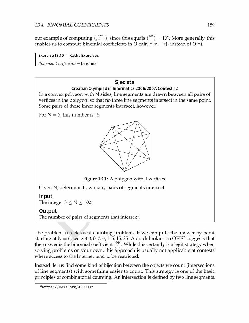
DRAFT
13.4. BINOMIAL COEFFICIENTS 189
our example of computing(109
109−1
), since this equals
(109
1
)= 109. More generally, this
enables us to compute binomial coefficients in O(min r, n− r) instead of O(r).
Exercise 13.10 — Kattis Exercises
Binomial Coefficients – binomial
SjecistaCroatian Olympiad in Informatics 2006/2007, Contest #2
In a convex polygon with N sides, line segments are drawn between all pairs ofvertices in the polygon, so that no three line segments intersect in the same point.Some pairs of these inner segments intersect, however.
For N = 6, this number is 15.
Figure 13.1: A polygon with 4 vertices.
Given N, determine how many pairs of segments intersect.
InputThe integer 3 ≤ N ≤ 100.OutputThe number of pairs of segments that intersect.
The problem is a classical counting problem. If we compute the answer by handstarting at N = 0, we get 0, 0, 0, 0, 1, 5, 15, 35. A quick lookup on OEIS2 suggests thatthe answer is the binomial coefficient
(N4
). While this certainly is a legit strategy when
solving problems on your own, this approach is usually not applicable at contestswhere access to the Internet tend to be restricted.
Instead, let us find some kind of bijection between the objects we count (intersectionsof line segments) with something easier to count. This strategy is one of the basicprinciples of combinatorial counting. An intersection is defined by two line segments,
2https://oeis.org/A000332
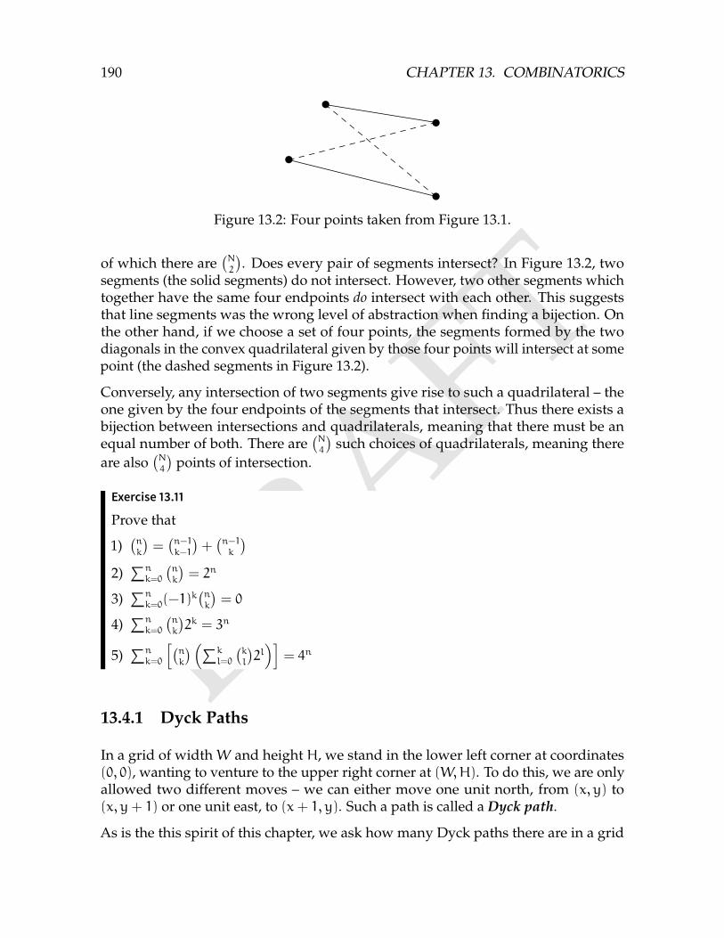
DRAFT
190 CHAPTER 13. COMBINATORICS
Figure 13.2: Four points taken from Figure 13.1.
of which there are(N2
). Does every pair of segments intersect? In Figure 13.2, two
segments (the solid segments) do not intersect. However, two other segments whichtogether have the same four endpoints do intersect with each other. This suggeststhat line segments was the wrong level of abstraction when finding a bijection. Onthe other hand, if we choose a set of four points, the segments formed by the twodiagonals in the convex quadrilateral given by those four points will intersect at somepoint (the dashed segments in Figure 13.2).
Conversely, any intersection of two segments give rise to such a quadrilateral – theone given by the four endpoints of the segments that intersect. Thus there exists abijection between intersections and quadrilaterals, meaning that there must be anequal number of both. There are
(N4
)such choices of quadrilaterals, meaning there
are also(N4
)points of intersection.
Exercise 13.11
Prove that
1)(nk
)=(n−1k−1
)+(n−1k
)2)∑n
k=0
(nk
)= 2n
3)∑n
k=0(−1)k(nk
)= 0
4)∑n
k=0
(nk
)2k = 3n
5)∑n
k=0
[(nk
) (∑kl=0
(kl
)2l)]
= 4n
13.4.1 Dyck Paths
In a grid of widthW and height H, we stand in the lower left corner at coordinates(0, 0), wanting to venture to the upper right corner at (W,H). To do this, we are onlyallowed two different moves – we can either move one unit north, from (x, y) to(x, y+ 1) or one unit east, to (x+ 1, y). Such a path is called a Dyck path.
As is the this spirit of this chapter, we ask how many Dyck paths there are in a grid
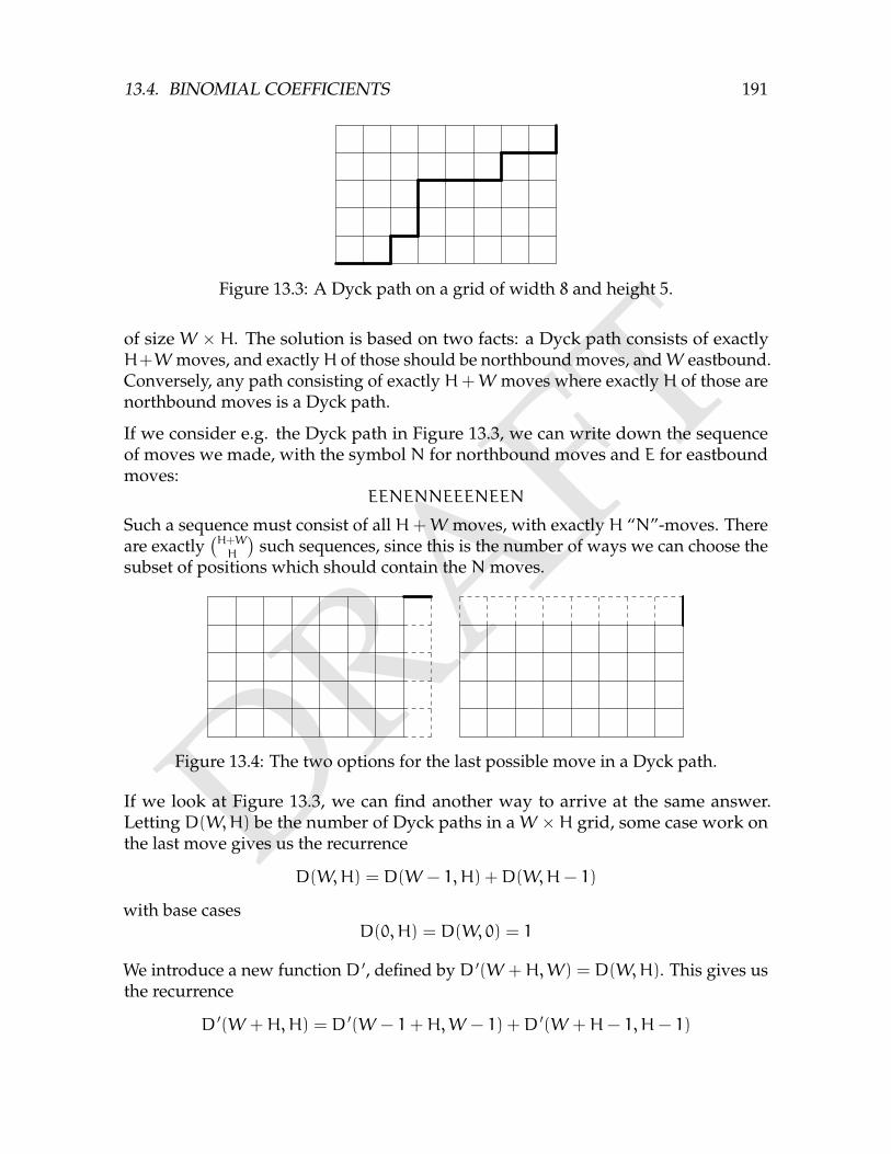
DRAFT
13.4. BINOMIAL COEFFICIENTS 191
Figure 13.3: A Dyck path on a grid of width 8 and height 5.
of size W × H. The solution is based on two facts: a Dyck path consists of exactlyH+W moves, and exactlyH of those should be northbound moves, andW eastbound.Conversely, any path consisting of exactly H+W moves where exactly H of those arenorthbound moves is a Dyck path.
If we consider e.g. the Dyck path in Figure 13.3, we can write down the sequenceof moves we made, with the symbolN for northbound moves and E for eastboundmoves:
EENENNEEENEEN
Such a sequence must consist of all H+W moves, with exactly H “N”-moves. Thereare exactly
(H+WH
)such sequences, since this is the number of ways we can choose the
subset of positions which should contain the Nmoves.
Figure 13.4: The two options for the last possible move in a Dyck path.
If we look at Figure 13.3, we can find another way to arrive at the same answer.Letting D(W,H) be the number of Dyck paths in a W ×H grid, some case work onthe last move gives us the recurrence
D(W,H) = D(W − 1,H) +D(W,H− 1)
with base casesD(0,H) = D(W,0) = 1
We introduce a new function D ′, defined by D ′(W +H,W) = D(W,H). This gives usthe recurrence
D ′(W +H,H) = D ′(W − 1+H,W − 1) +D ′(W +H− 1,H− 1)

DRAFT
192 CHAPTER 13. COMBINATORICS
with base casesD ′(0, 0) = D ′(H,H) = 0
These relations are satisfied by the binomial coefficients (Exercise 13.11).
Exercise 13.12
Prove that∑n
i=0
(ni
)(nn−i
)=(2nn
).
While Dyck paths sometimes do appear directly in problems, they are also a usefultool to find bijections to other objects.
SumsIn how many ways can the numbers 0 ≤ a1, a2, . . . , ak be chosen such that
k∑i=1
ai = n
InputThe integers 0 ≤ n ≤ 106 and 0 ≤ k ≤ 106.OutputOutput the number of ways modulo 109 + 7.
Given a Dyck path such as the one in Figure 13.3, what happens if we count thenumber of northbound steps we take at each x-coordinate? There are a total of W + 1coordinates and H northbound steps, so we except this to be a sum of W + 1 (non-negative) variables with a sum of H. This is indeed similar to what we are counting,and Figure 13.5 shows this connection explicitly.
a1 a2 a3 a4 a5 a6 a7 a8 a90 + 0 + 1 + 2 + 0 + 0 + 1 + 0 + 1 = 5
Figure 13.5: A nine-term sum as a Dyck path.
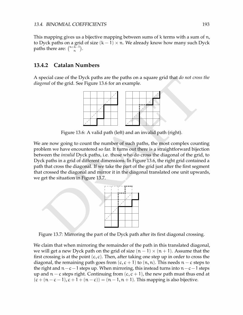
DRAFT
13.4. BINOMIAL COEFFICIENTS 193
This mapping gives us a bijective mapping between sums of k terms with a sum of n,to Dyck paths on a grid of size (k− 1)× n. We already know how many such Dyckpaths there are:
(n+k−1n
).
13.4.2 Catalan Numbers
A special case of the Dyck paths are the paths on a square grid that do not cross thediagonal of the grid. See Figure 13.6 for an example.
Figure 13.6: A valid path (left) and an invalid path (right).
We are now going to count the number of such paths, the most complex countingproblem we have encountered so far. It turns out there is a straightforward bijectionbetween the invalid Dyck paths, i.e. those who do cross the diagonal of the grid, toDyck paths in a grid of different dimensions. In Figure 13.6, the right grid contained apath that cross the diagonal. If we take the part of the grid just after the first segmentthat crossed the diagonal and mirror it in the diagonal translated one unit upwards,we get the situation in Figure 13.7.
Figure 13.7: Mirroring the part of the Dyck path after its first diagonal crossing.
We claim that when mirroring the remainder of the path in this translated diagonal,we will get a new Dyck path on the grid of size (n − 1)× (n + 1). Assume that thefirst crossing is at the point (c, c). Then, after taking one step up in order to cross thediagonal, the remaining path goes from (c, c+ 1) to (n,n). This needs n− c steps tothe right and n−c−1 steps up. When mirroring, this instead turns into n−c−1 stepsup and n− c steps right. Continuing from (c, c+ 1), the new path must thus end at(c+ (n− c− 1), c+ 1+ (n− c)) = (n− 1, n+ 1). This mapping is also bijective.
DRAFT
194 CHAPTER 13. COMBINATORICS
This bijection lets us count the number of paths that do cross the diagonal: they are(2nn+1
). The numbers of paths that does not cross the diagonal is then
(2nn
)−(2nn+1
).
Definition 13.3 — Catalan NumbersThe number of Dyck paths in an ×n grid is called the n’th Catalan number
Cn =
(2n
n
)−
(2n
n+ 1
)=
(2n
n
)−
n
n+ 1
(2n
n
)=
1
n+ 1
(2n
n
)
The first few Catalan numbers3 are 1, 1, 2, 5, 14, 42, 132, 429, 1430.
Exercise 13.13 — Kattis Exercises
Catalan Numbers – catalan
Catalan numbers count many other objects, most notably the number of balancedparentheses expressions. A balanced parentheses expression is a string of 2n characterss1s2 . . . s2n of letters ( and ), such that every prefix s1s2 . . . sk contain at least as manyletters ( as ). Given such a string, like (()())(()) we can interpret it as a Dyck path,where ( is a step to the right, and ) is a step upwards. Then, the condition that thestring is balanced is that, for every partial Dyck path, we have taken at least as manyright steps as we have taken up steps. This is equivalent to the Dyck path nevercrossing the diagonal, giving us a bijection between parentheses expressions andDyck paths. The number of such parentheses expressions are thus also Cn.
13.5 The Principle of Inclusion and Exclusion
Often, we wish to compute the size of the union of a collection of sets S1, S2, . . . , Sn,where these sets are not pairwise disjoint. For this, the principle of inclusion andexclusion was developed.
Let us consider the most basic case of the principle, using two sets A and B. If wewish to compute the size of their union |A∪B|, we at least need to count every elementin A and every set in B, i.e. |A|+ |B|. The problem with this formula is that wheneveran element is in both A and B, we count it twice. Fortunately, this is easily mitigated:the number of elements in both sets equals |A ∩ B| (Figure 13.8). Thus, we see that|A ∪ B| = |A|+ |B|− |A ∩ B|.Similarly, we can determine a formula for the union of three sets |A∪B∪C|. We beginby including every element: |A| + |B| + |C|. Again, we have included the pairwise
3https://oeis.org/A000108
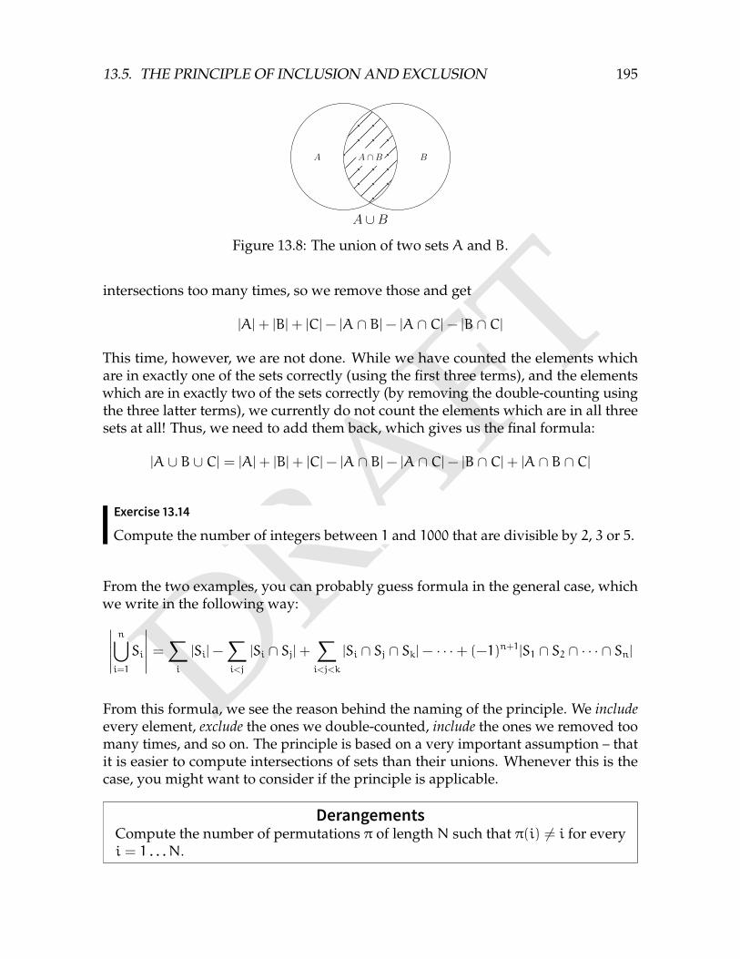
DRAFT
13.5. THE PRINCIPLE OF INCLUSION AND EXCLUSION 195
A BA ∩B
A ∪B
Figure 13.8: The union of two sets A and B.
intersections too many times, so we remove those and get
|A|+ |B|+ |C|− |A ∩ B|− |A ∩ C|− |B ∩ C|
This time, however, we are not done. While we have counted the elements whichare in exactly one of the sets correctly (using the first three terms), and the elementswhich are in exactly two of the sets correctly (by removing the double-counting usingthe three latter terms), we currently do not count the elements which are in all threesets at all! Thus, we need to add them back, which gives us the final formula:
|A ∪ B ∪ C| = |A|+ |B|+ |C|− |A ∩ B|− |A ∩ C|− |B ∩ C|+ |A ∩ B ∩ C|
Exercise 13.14
Compute the number of integers between 1 and 1000 that are divisible by 2, 3 or 5.
From the two examples, you can probably guess formula in the general case, whichwe write in the following way:∣∣∣∣∣
n⋃i=1
Si
∣∣∣∣∣ =∑i
|Si|−∑i<j
|Si ∩ Sj|+∑i<j<k
|Si ∩ Sj ∩ Sk|− · · ·+ (−1)n+1|S1 ∩ S2 ∩ · · · ∩ Sn|
From this formula, we see the reason behind the naming of the principle. We includeevery element, exclude the ones we double-counted, include the ones we removed toomany times, and so on. The principle is based on a very important assumption – thatit is easier to compute intersections of sets than their unions. Whenever this is thecase, you might want to consider if the principle is applicable.
DerangementsCompute the number of permutations π of length N such that π(i) 6= i for everyi = 1 . . .N.
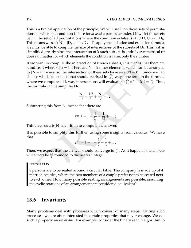
DRAFT
196 CHAPTER 13. COMBINATORICS
This is a typical application of the principle. We will use it on those sets of permuta-tions be where the condition is false for at least a particular index i If we let these setsbe Di, the set of all permutations where the condition is false is D1 ∪D2 ∪ · · · ∪DN.This means we seekN!− |D1∪· · ·∪DN|. To apply the inclusion and exclusion formula,we must be able to compute the size of intersections of the subsets of Di. This task issimplified greatly since the intersection of k such subsets is entirely symmetrical (itdoes not matter for which elements the condition is false, only the number).
If we want to compute the intersection of k such subsets, this means that there arek indices i where π(i) = i. There are N − k other elements, which can be arrangedin (N − k)! ways, so the intersection of these sets have size (N − k)!. Since we canchoose which k elements that should be fixed in
(Nk
)ways, the term in the formula
where we compute all k-way intersections will evaluate to(Nk
)(N − k)! = N!
k!. Thus,
the formula can be simplified to
N!
1!−N!
2!+N!
3!− . . .
Subtracting this from N! means that there are
N!(1− 1+1
2!−1
3!+ . . . )
This gives us a Θ(N) algorithm to compute the answer.
It is possible to simplify this further, using some insights from calculus. We havethat
e−1 = 1− 1+1
2−1
3+ . . .
Then, we expect that the answer should converge to N!e
. As it happens, the answerwill always be N!
erounded to the nearest integer.
Exercise 13.15
8 persons are to be seated around a circular table. The company is made up of 4married couples, where the two members of a couple prefer not to be seated nextto each other. How many possible seating arrangements are possible, assumingthe cyclic rotations of an arrangement are considered equivalent?
13.6 Invariants
Many problems deal with processes which consist of many steps. During suchprocesses, we are often interested in certain properties that never change. We callsuch a property an invariant. For example, consider the binary search algorithm to
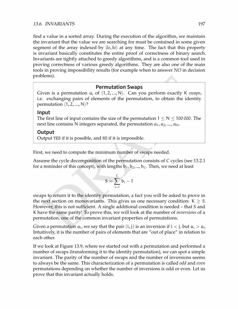
DRAFT
13.6. INVARIANTS 197
find a value in a sorted array. During the execution of the algorithm, we maintainthe invariant that the value we are searching for must be contained in some givensegment of the array indexed by [lo, hi) at any time. The fact that this propertyis invariant basically constitutes the entire proof of correctness of binary search.Invariants are tightly attached to greedy algorithms, and is a common tool used inproving correctness of various greedy algorithms. They are also one of the maintools in proving impossibility results (for example when to answer NO in decisionproblems).
Permutation SwapsGiven is a permutation ai of 〈1, 2, ...,N〉. Can you perform exactly K swaps,i.e. exchanging pairs of elements of the permutation, to obtain the identitypermutation 〈1, 2, ...,N〉?InputThe first line of input contains the size of the permutation 1 ≤ N ≤ 100 000. Thenext line contains N integers separated, the permutation a1, a2, ..., aN.
OutputOutput YES if it is possible, and NO if it is impossible.
First, we need to compute the minimum number of swaps needed.
Assume the cycle decomposition of the permutation consists of C cycles (see 13.2.1for a reminder of this concept), with lengths b1, b2, .., bC. Then, we need at least
S =
C∑i=1
bi − 1
swaps to return it to the identity permutation, a fact you will be asked to prove inthe next section on monovariants. This gives us one necessary condition: K ≥ S.However, this is not sufficient. A single additional condition is needed – that S andK have the same parity! To prove this, we will look at the number of inversions of apermutation, one of the common invariant properties of permutations.
Given a permutation ai, we say that the pair (i, j) is an inversion if i < j, but ai > aj.Intuitively, it is the number of pairs of elements that are “out of place” in relation toeach other.
If we look at Figure 13.9, where we started out with a permutation and performed anumber of swaps (transforming it to the identity permutation), we can spot a simpleinvariant. The parity of the number of swaps and the number of inversions seemsto always be the same. This characterization of a permutation is called odd and evenpermutations depending on whether the number of inversions is odd or even. Let usprove that this invariant actually holds.
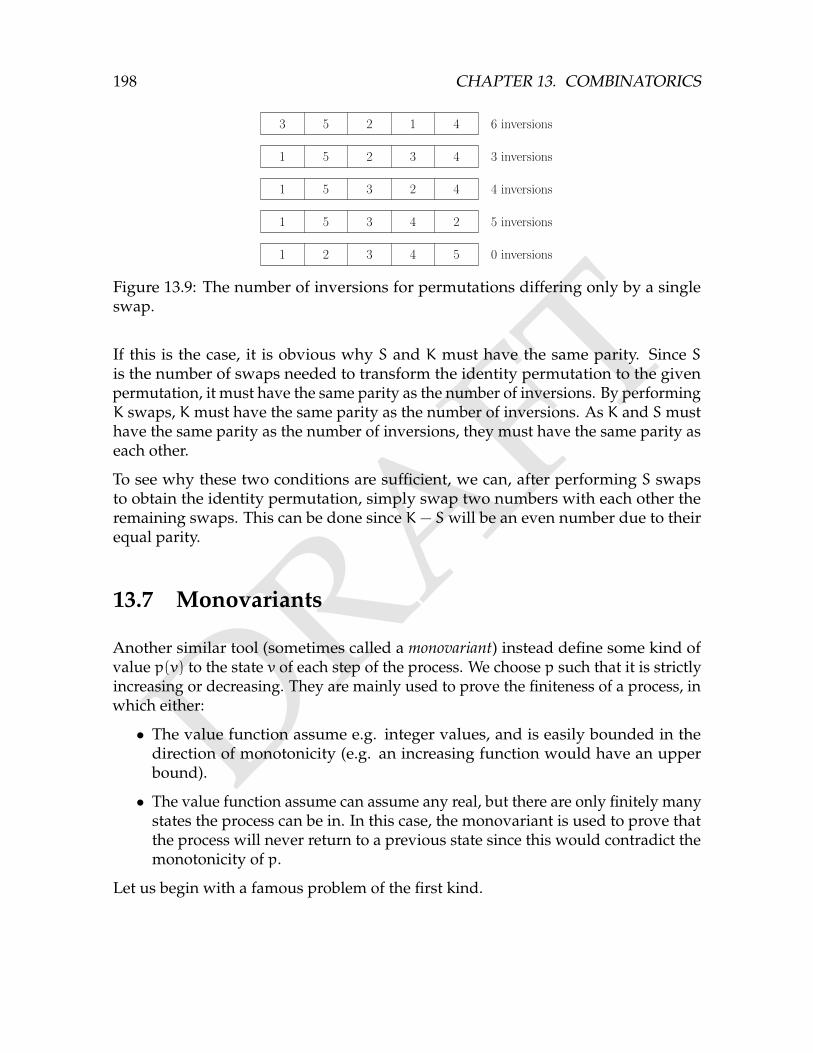
DRAFT
198 CHAPTER 13. COMBINATORICS
3 5 2 1 4 6 inversions
1 5 2 3 4 3 inversions
1 5 3 2 4 4 inversions
1 5 3 4 2 5 inversions
1 2 3 4 5 0 inversions
Figure 13.9: The number of inversions for permutations differing only by a singleswap.
If this is the case, it is obvious why S and K must have the same parity. Since Sis the number of swaps needed to transform the identity permutation to the givenpermutation, it must have the same parity as the number of inversions. By performingK swaps, K must have the same parity as the number of inversions. As K and S musthave the same parity as the number of inversions, they must have the same parity aseach other.
To see why these two conditions are sufficient, we can, after performing S swapsto obtain the identity permutation, simply swap two numbers with each other theremaining swaps. This can be done since K− Swill be an even number due to theirequal parity.
13.7 Monovariants
Another similar tool (sometimes called a monovariant) instead define some kind ofvalue p(v) to the state v of each step of the process. We choose p such that it is strictlyincreasing or decreasing. They are mainly used to prove the finiteness of a process, inwhich either:
• The value function assume e.g. integer values, and is easily bounded in thedirection of monotonicity (e.g. an increasing function would have an upperbound).
• The value function assume can assume any real, but there are only finitely manystates the process can be in. In this case, the monovariant is used to prove thatthe process will never return to a previous state since this would contradict themonotonicity of p.
Let us begin with a famous problem of the first kind.
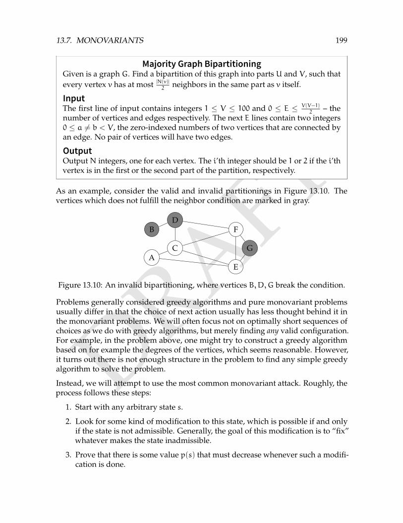
DRAFT
13.7. MONOVARIANTS 199
Majority Graph BipartitioningGiven is a graph G. Find a bipartition of this graph into parts U and V , such thatevery vertex v has at most |N(v)|
2neighbors in the same part as v itself.
InputThe first line of input contains integers 1 ≤ V ≤ 100 and 0 ≤ E ≤ V(V−1)
2– the
number of vertices and edges respectively. The next E lines contain two integers0 ≤ a 6= b < V , the zero-indexed numbers of two vertices that are connected byan edge. No pair of vertices will have two edges.
OutputOutputN integers, one for each vertex. The i’th integer should be 1 or 2 if the i’thvertex is in the first or the second part of the partition, respectively.
As an example, consider the valid and invalid partitionings in Figure 13.10. Thevertices which does not fulfill the neighbor condition are marked in gray.
A
B
C
D
E
F
G
Figure 13.10: An invalid bipartitioning, where vertices B,D,G break the condition.
Problems generally considered greedy algorithms and pure monovariant problemsusually differ in that the choice of next action usually has less thought behind it inthe monovariant problems. We will often focus not on optimally short sequences ofchoices as we do with greedy algorithms, but merely finding any valid configuration.For example, in the problem above, one might try to construct a greedy algorithmbased on for example the degrees of the vertices, which seems reasonable. However,it turns out there is not enough structure in the problem to find any simple greedyalgorithm to solve the problem.
Instead, we will attempt to use the most common monovariant attack. Roughly, theprocess follows these steps:
1. Start with any arbitrary state s.
2. Look for some kind of modification to this state, which is possible if and onlyif the state is not admissible. Generally, the goal of this modification is to “fix”whatever makes the state inadmissible.
3. Prove that there is some value p(s) that must decrease whenever such a modifi-cation is done.
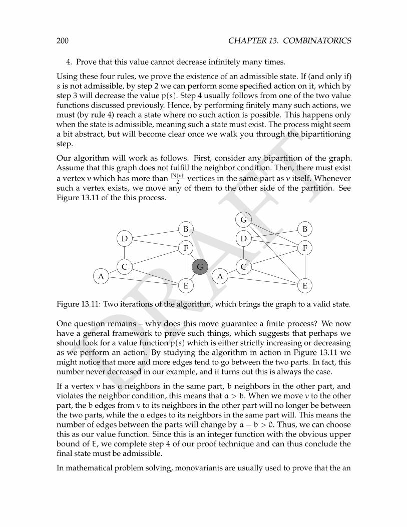
DRAFT
200 CHAPTER 13. COMBINATORICS
4. Prove that this value cannot decrease infinitely many times.
Using these four rules, we prove the existence of an admissible state. If (and only if)s is not admissible, by step 2 we can perform some specified action on it, which bystep 3 will decrease the value p(s). Step 4 usually follows from one of the two valuefunctions discussed previously. Hence, by performing finitely many such actions, wemust (by rule 4) reach a state where no such action is possible. This happens onlywhen the state is admissible, meaning such a state must exist. The process might seema bit abstract, but will become clear once we walk you through the bipartitioningstep.
Our algorithm will work as follows. First, consider any bipartition of the graph.Assume that this graph does not fulfill the neighbor condition. Then, there must exista vertex vwhich has more than |N(v)|
2vertices in the same part as v itself. Whenever
such a vertex exists, we move any of them to the other side of the partition. SeeFigure 13.11 of the this process.
A
B
C
D
E
F
GA
B
C
D
E
F
G
Figure 13.11: Two iterations of the algorithm, which brings the graph to a valid state.
One question remains – why does this move guarantee a finite process? We nowhave a general framework to prove such things, which suggests that perhaps weshould look for a value function p(s) which is either strictly increasing or decreasingas we perform an action. By studying the algorithm in action in Figure 13.11 wemight notice that more and more edges tend to go between the two parts. In fact, thisnumber never decreased in our example, and it turns out this is always the case.
If a vertex v has a neighbors in the same part, b neighbors in the other part, andviolates the neighbor condition, this means that a > b. When we move v to the otherpart, the b edges from v to its neighbors in the other part will no longer be betweenthe two parts, while the a edges to its neighbors in the same part will. This means thenumber of edges between the parts will change by a− b > 0. Thus, we can choosethis as our value function. Since this is an integer function with the obvious upperbound of E, we complete step 4 of our proof technique and can thus conclude thefinal state must be admissible.
In mathematical problem solving, monovariants are usually used to prove that the an
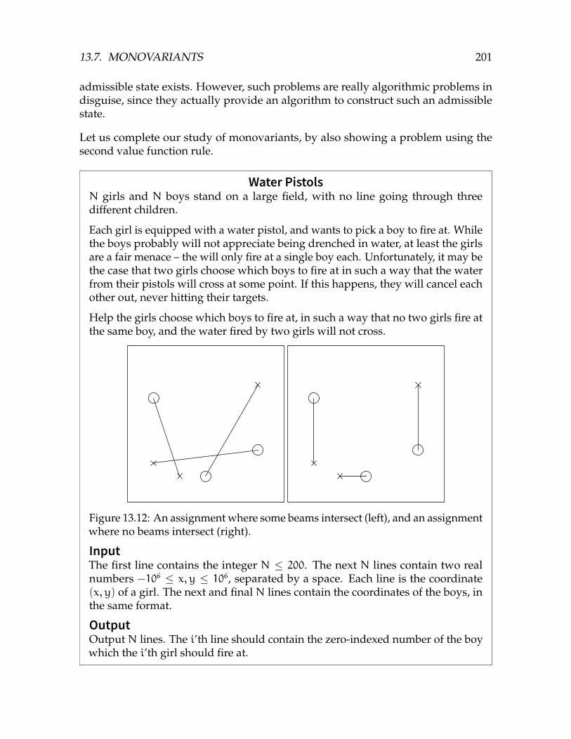
DRAFT
13.7. MONOVARIANTS 201
admissible state exists. However, such problems are really algorithmic problems indisguise, since they actually provide an algorithm to construct such an admissiblestate.
Let us complete our study of monovariants, by also showing a problem using thesecond value function rule.
Water PistolsN girls and N boys stand on a large field, with no line going through threedifferent children.
Each girl is equipped with a water pistol, and wants to pick a boy to fire at. Whilethe boys probably will not appreciate being drenched in water, at least the girlsare a fair menace – the will only fire at a single boy each. Unfortunately, it may bethe case that two girls choose which boys to fire at in such a way that the waterfrom their pistols will cross at some point. If this happens, they will cancel eachother out, never hitting their targets.
Help the girls choose which boys to fire at, in such a way that no two girls fire atthe same boy, and the water fired by two girls will not cross.
Figure 13.12: An assignment where some beams intersect (left), and an assignmentwhere no beams intersect (right).
InputThe first line contains the integer N ≤ 200. The next N lines contain two realnumbers −106 ≤ x, y ≤ 106, separated by a space. Each line is the coordinate(x, y) of a girl. The next and final N lines contain the coordinates of the boys, inthe same format.
OutputOutput N lines. The i’th line should contain the zero-indexed number of the boywhich the i’th girl should fire at.
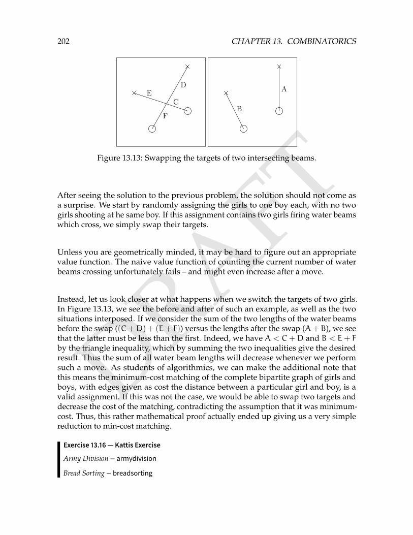
DRAFT
202 CHAPTER 13. COMBINATORICS
CE
F
DA
B
Figure 13.13: Swapping the targets of two intersecting beams.
After seeing the solution to the previous problem, the solution should not come asa surprise. We start by randomly assigning the girls to one boy each, with no twogirls shooting at he same boy. If this assignment contains two girls firing water beamswhich cross, we simply swap their targets.
Unless you are geometrically minded, it may be hard to figure out an appropriatevalue function. The naive value function of counting the current number of waterbeams crossing unfortunately fails – and might even increase after a move.
Instead, let us look closer at what happens when we switch the targets of two girls.In Figure 13.13, we see the before and after of such an example, as well as the twosituations interposed. If we consider the sum of the two lengths of the water beamsbefore the swap ((C+D) + (E+ F)) versus the lengths after the swap (A+ B), we seethat the latter must be less than the first. Indeed, we have A < C+D and B < E+ Fby the triangle inequality, which by summing the two inequalities give the desiredresult. Thus the sum of all water beam lengths will decrease whenever we performsuch a move. As students of algorithmics, we can make the additional note thatthis means the minimum-cost matching of the complete bipartite graph of girls andboys, with edges given as cost the distance between a particular girl and boy, is avalid assignment. If this was not the case, we would be able to swap two targets anddecrease the cost of the matching, contradicting the assumption that it was minimum-cost. Thus, this rather mathematical proof actually ended up giving us a very simplereduction to min-cost matching.
Exercise 13.16 — Kattis Exercise
Army Division – armydivision
Bread Sorting – breadsorting

DRAFT
13.8. CHAPTER NOTES 203
13.8 Chapter Notes

DRAFT
204 CHAPTER 13. COMBINATORICS
DRAFTChapter 14
Number Theory
Number theory is the study of certain properties of integers. It makes an occasionalappearance within algorithmic problem solving, in the form of its subfield computa-tional number theory. It is within number theory topics such as divisibility and primenumbers belong.
14.1 Divisibility
All of the number theory in this chapter relate to a single property of integers, divisi-bility.
Definition 14.1 — DivisibilityAn integer n is divisible by an integer d if there is another integer q such thatn = dq. We also say that d is a divisor of n.
We denote this fact with d | n.
Dividing both sides of the equality n = dq with d gives us an almost equivalentdefinition, namely that n
dis an integer. The difference is that the first definition admit
the divisibility by 0 with 0, while the second one does not (zero division is undefined).When we speak of the divisors of a number in most contexts (as in Example 14.1), wewill generally consider only the non-negative divisors. Since d is a divisor of n if andonly if −d is a divisor of n, this sloppiness lose little information.
Example 14.1 — Divisors of 12The number 12 has 6 divisors – 1 (1 · 12 = 12), 2 (2 · 6 = 12), 3, (3 · 4 = 12), 4(4 · 3 = 12), 6 (6 · 2 = 12) and 12 (12 · 1 = 12).
205
DRAFT
206 CHAPTER 14. NUMBER THEORY
12 is not divisible by e.g. 5 – we have 125= 2+ 2
5, which is clearly not an integer.
Exercise 14.1
Determine the divisors of 18.
The concept of divisibility raises many questions. First and foremost – how do wecheck if a number is divisible by another? This question has one short and onelong answer. For small numbers – those that fit inside the native integer types of alanguage – checking for divisibility is as simple as using the modulo operator (%) ofyour favorite programming language – n is divisible by d if and only if nmodd = 0.The situation is not as simple for large numbers. Some programming languages, suchas Java and Python, have built-in support for dealing with large integers, but e.g. C++does not. In Section 14.4 on modular arithmetic, we discuss the implementation ofthe modulo operator on large integers.
Secondly, how do we compute the divisors of a number? Every integer has at leasttwo particular divisors called the trivial divisors, namely 1 and n itself. If we excludethe divisor n, we get the proper divisors. To find the remaining divisors, we can usethe fact that any divisor d of n must satisfy |d| ≤ |n|. This means that we can limitourselves to testing whether the integers between 1 and n are divisors of n, a Θ(n)algorithm. We can do a bit better though.
Almost PerfectBaylor Competitive Learning course – David Sturgill
A positive integer p is called a perfect number if all the proper divisors of p sumto p exactly. Perfect numbers are rare; only 10 of them are known. Perhaps thedefinition of perfection is a little too strict. Instead, we will consider numbersthat we’ll call almost perfect. A positive integer p is almost perfect if the properdivisors of p sum to a value that differs from p by no more than two.
InputInput consists of a sequence of up to 500 integers, one per line. Each integer is inthe range 2 to 109 (inclusive).
OutputFor each input value, output the same value and then one of the following:“perfect” (if the number is perfect), “almost perfect” (if it is almost perfect but notperfect), or “not perfect” (otherwise).
In this problem, computing the divisors of the numbers of the input sequence wouldbe way too slow, requiring upwards of 1011 operations. Hidden in Example 14.1lies the key insight to speeding this up. It seems that whenever we had a divisor
DRAFT
14.1. DIVISIBILITY 207
d, we were immediately given another divisor q. For example, when claiming 3was a divisor of 12 since 3 · 4 = 12, we found another divisor, 4. This should notbe a surprise, since our definition of divisibility (Definition 14.1)– the existence ofthe integer q in n = dq – is symmetric in d and q, meaning divisors come in pairs(d, n
d).
Exercise 14.2
Prove that an integer has an odd number of divisors if and only if it is a perfectsquare (except 0, which has an infinite number of divisors).
Since divisors come in pairs, we can limit ourselves to finding one member of eachsuch pair. Furthermore, one of the elements in each such pair must be bounded by√n. Otherwise, we would have that n = d · n
d>√n · √n = n, a contradiction (again,
except for 0, which has 0d= 0). This limit helps us reduce the time it takes to find the
divisors of a number to Θ(√N), which allows us to solve the problem. You can see
the pseudo code for this in Algorithm 14.1
Algorithm 14.1: Almost Perfect
procedure DIVISORS(N)divisors← new list
for i from 1 up to i2 ≤ N doif Nmod i = 0 then
divisors.add(i)if i 6= N/i then
divisors.add(Ni)
return divisorsprocedure ALMOSTPERFECT(N)
divSum← 0
for d ∈ Divisors(N) doif d 6= N then
divSum← divSum + dif divSum = N then
output “perfect”else if |divSum −N| ≤ 2 then
output “almost perfect”else
output “not perfect”
This also happens to give us some help in answering our next question, regarding theplurality of divisors. The above result gives us an upper bound of 2
√n divisors of an
DRAFT
208 CHAPTER 14. NUMBER THEORY
integer n. We can do a little better, with O(n13 ) being a commonly used bound for the
number of divisors when dealing with integers which fit in the native integer types.1
For example, the maximal number of divisors of a number less than 103 is 32, 106 is240, 109 is 1 344, 1018 is 103 680.2
A bound we will find more useful when solving problems concerns the averagenumber of divisors of the integers between 1 and n.
Theorem 14.1 Let d(i) be the number of divisors of i. Then,
n∑i=1
d(i) ≈ n lnn
Proof. There are approximately ni
integers between 1 and n divisible by i, sinceevery i’th integer is divisible by i Thus, the number of divisors of all those integersis bounded by
n∑j=1
n
j= n
n∑j=1
1
j≈ n lnn
This proof also suggest a way to compute the divisors of all the integers 1, 2, ..., nin Θ(n lnn) time. For each integer i, we find all the numbers divisible by i (in Θ(n
i)
time), which are 0i, 1i, 2i, . . . dniei. This is an extension of the algorithm commonly
known as the Sieve of Eratosthenes, an algorithm to find the objects which are ournext topic of study – prime numbers.
Exercise 14.3 — Kattis Exercises
Dividing Sequence – sequence
14.2 Prime Numbers
From the concept of divisibility comes the building blocks of the integers, the famousprime numbers. With divisibility, we got factorizations. For example, given the number12, we could factor it as 2 · 6, or 3 · 4, or even 2 · 2 · 3. This last factorization is special,in that no matter how hard we try, it cannot be factored further. It consists only ofprime numbers.
1In reality, the maximal number of divisors of the interval [1, n] grows sub-polynomially, i.e., asO(nε) for every ε > 0.
2Sequence A066150 from OEIS: http://oeis.org/A066150.
DRAFT
14.2. PRIME NUMBERS 209
Definition 14.2 — Prime NumberAn integer p ≥ 2 is called a prime number if its only positive divisors are 1 and p.
The numbers that are not prime numbers are called composite numbers. There arean infinite number of primes. This be proven by a simple proof by contradiction.If p1, p2, ..., pq are the only primes, then P = p1p2 . . . pq + 1 is not divisible by anyprime number (and by extension has no divisors but the trivial ones), so it is notcomposite. However, P is larger than any prime, so it is not a prime number either, acontradiction.
Example 14.2 The first 10 prime numbers are 2, 3, 5, 7, 11, 13, 17, 19, 23, 29. Which isthe next one?
Since the prime numbers have no other divisors besides the trivial ones, a factorizationconsisting only of prime numbers is special.
Definition 14.3 — Prime FactorizationThe prime factorization of a positive integer n is a factorization of the form pe11 ·pe22 · · · · · pekk , where pi are all distinct primes. This factorization is unique, exceptfor a reordering of the pi.
Example 14.3 The prime factorization of 228 is 2 · 2 · 3 · 19.
A List GameSpotify Challenge 2010 – Per Austrin
You are playing the following simple game with a friend:
1. The first player picks a positive integer X.
2. The second player gives a list of k positive integers Y1, . . . , Yk such that
(Y1 + 1)(Y2 + 1) · · · (Yk + 1) = X
and gets k points.
Write a program that plays the second player.
InputThe input consists of a single integer X satisfying 103 ≤ X ≤ 109, giving thenumber picked by the first player.
OutputWrite a single integer k, giving the number of points obtained by the second
DRAFT
210 CHAPTER 14. NUMBER THEORY
player, assuming she plays as good as possible.
The problem seeks the factorization of X that contains the largest number of factors,where every factor is at least 2. This factorization must in fact be the prime factor-ization of X, which we will prove by contradiction. Assume that the optimal listof integers Y1, . . . , Yk contains a number Yi that is composite. In this case, it can befurther factored into Yi = ab with a, b > 1. Replacing Yi with the numbers a and bwill keep the product of the list invariant (since Yi = ab), but extend the length of thelist by 1, thus giving a higher-scoring sequence. The only case when this is impossibleis if all the Yi are primes, so the list we seek must indeed be the prime factorization ofX.
This begs the question, how do we compute the prime factorization of a number?Mainly two different algorithms are used when computing prime factorizations: trialdivision and the Sieve of Eratosthenes3. In computing the prime factorization of afew, large numbers, trial division is used. It runs in O(
√N) time, and use the same
insight we used in the improved algorithm to compute the divisors of an algorithm.Since any composite numberNmust have a divisor less than
√N, it must also have a
prime divisor less than√N. Implementing this is straightforward.
The other algorithm is used to factor every number in a large interval.
Product DivisorsGiven a sequence of integers a1, a2, . . . an, compute the number of divisors ofA =
∏ni=1 ai.
InputInput starts with an integer 0 ≤ n ≤ 1 000 000, the length of the sequence ai. Thenext line contains the numbers 1 ≤ a1, . . . , an ≤ 106.OutputOutput a single integer – the number of divisors of n. Since this number can bevery large, output it modulo 109 + 7.
Let A have the prime factorization A = pe11 · pe22 · · · · · pekk . A divisor of A must beof the form d = p
e ′11 · p
e ′22 · · · · · p
e ′kk , where 0 ≤ e ′i ≤ ei. This can be proven using the
uniqueness of the prime factorization, and the fact that A = dq for some integer q.More importantly, any number of this form is a divisor of A, by the same cancellationargument used when proving the uniqueness of the prime factorization.
With this in hand, we apply a simple combinatorial argument to count the number ofdivisors ofA. Each number e ′i can take any integer value between 0 and ei to fulfill the
3Many more exist, but are too complicated to be used in problem solving context, although they arevery much in use in real-life situations.
DRAFT
14.2. PRIME NUMBERS 211
conditions needed to make d a divisor ofA. This gives us ei+1 choices for the value ofe ′i. Since each e ′i is independent, there are a total of (e1+1)(e2+1) . . . (ek+1) numbersof this form, and thus divisors of A. We are left with the problem of determiningthe prime factorization of A. Essentially, this is tantamount to computing the primefactorization of every integer between 1 and 106. Once this is done, we can go throughthe sequence ai and tally up all primes in their factorization. Since an integer mhas at most log
2m prime factors, this step is bounded by approximately n log
2106
operations. This is implemented in Algorithm 14.2.
Algorithm 14.2: Product Divisors
procedure PRODUCTDIVISORS(sequence A)list of lists factorizations← factorInterval(106 + 1)map counts← new map
for each a in A dofor each p in factorizations[a] do
counts[p]← counts[p] + 1ans← 1
for each (key, value) in counts doans← (ans · (value+ 1))mod(109 + 7)
return ans
As of now, the crucial step of factoring all integers in [1..106] remains. This is thepurpose of the Sieve of Eratosthenes. We have already seen the basic idea whencomputing the divisors of all numbers in the interval [1...n] in Section 14.1. Extendingthis to factoring is only a matter of restricting the algorithm to finding prime divisors(Algorithm 14.3).
Algorithm 14.3: Sieve of Eratosthenes
procedure PRIMESIEVE(limit N)list nums← new list[N]for i from 1 to N− 1 do
nums[i]← i
list of lists factorizations← new list of lists[N]for i from 2 to i2 ≤ N do
if nums[i]! = i thenfor j ∈ i · i, i(i+ 1), i(i+ 2), ... up to N− 1 do
while nums[j]mod i = 0 dofactorizations[j].add(i)nums[j] = nums[j]/i
return factors
DRAFT
212 CHAPTER 14. NUMBER THEORY
The complexity of this procedure is a bit tricky to analyze. The important part of thesieve is the inner loop, which computes the actual factors. Let us count the number oftimes a prime p is pushed in this loop. First of all, every p’th integer is divisible by p,which totals n
piterations. However, every p2’th integer integer is divisible by p yet
again, contributing an additional np2
iterations, and so on. Summing this over every pwhich is used in the sieve gives us the bound
∑p≤√n
(n
p+n
p2+n
p3+ ...
)= n
∑p≤√n
(1
p+1
p2+1
p3+ ...
)
Using the formula for the sum of a geometric series ( 1p+ 1
p2+ ... = p
p−1) gives us the
simplification
n∑p≤√n
1
p− 1= Θ
n∑p≤√n
1
p
This last sum is out of reach to estimate with our current tools. It turns out that∑
p≤n1p= O(ln lnn). With this, the final complexity becomes a simpleO(n ln ln
√n) =
O(n ln lnn).
It is not uncommon for an algorithm to include in its complexity the number of primesup to a certain limit n. This function is known as π(n), the prime counting function.We have π(103) = 168, π(106) = 78 498, π(109) ≈ 51 000 000. In general, π(n) ≈ n
lnnfor large n.
Exercise 14.4 — Kattis Exercises
Prime Sieve – primesieve
Happy Happy Prime Prime – happyprime
Prime Path – primepathc
Perfect Pth Powers – perfectpowers
Factovisors – factovisors
Divisors – divisors
14.3 The Euclidean Algorithm
The Euclidean algorithm is one of the oldest known algorithms, dating back to Greekmathematician Euclid who wrote of it in his mathematical treatise Elements. It regardsthose numbers which are divisors two different integers, with an extension capable ofsolving integer equations of the form ax+ by = c.
DRAFT
14.3. THE EUCLIDEAN ALGORITHM 213
Definition 14.4 We call an integer d dividing both of the integers a and b a commondivisor of a and b.
The greatest such integer is called the greatest common divisor, or GCD of a andb. This number is denoted (a, b).
As always, we ask ourselves – how do we compute it?
Greatest Common DivisorGiven to integers a and b, compute (a, b).
We already know of anO(√a+√b) algorithm to compute (a, b), namely to enumerate
all divisors of a and b. Two simple identities are key to the much faster Euclideanalgorithm.
(a, 0) = |a| (14.1)
(a, b) = (a− b, b) (14.2)
Identity 14.1 is obvious. An integer a cannot have a larger divisor than |a|, and thisis certainly a divisor of a. Identity 14.2 needs a bit more work. We can prove theirequality by proving an even stronger result – that all common divisors of a and b arealso common divisors of a and b− a. Assume d is a common divisor of a and b, sothat a = da ′ and b = db ′ for integers a ′, b ′. Then b − a = db ′ − da ′ = d(b ′ − a ′),with b ′−a ′ being an integer, is sufficient for d also being a divisor of b−a. Hence thedivisors of a and b are also divisors of a and b−a. In particular, their largest commondivisor is the same. The application of these identities yield a recursive solution to theproblem. If we wish to compute (a, b) where a, b are positive and a > b, we reducethe problem to a smaller one by instead computing (a, b), we compute (a − b, b).This gives us a smaller problem, in the sense that a + b decrease. Since both a andb are non-negative, this means we must at some point arrive at the situation whereeither a or b are 0. In this case, we use the base case that is Identity 14.1.
One simple but important step remains before the algorithm is useful. Note howcomputing (109, 1) requires about 109 steps right now, since we will do the reductions(109 − 1, 1), (109 − 2, 1), (109 − 3, 1)... The fix is easy – the repeated application ofsubtraction of a number b from a while a > b is exactly the modulo operation,meaning
(a, b) = (amodb, b)
This last piece of our Euclidean puzzle complete our algorithm, and gives us aremarkably short algorithm, as seen in Algorithm 14.5.
DRAFT
214 CHAPTER 14. NUMBER THEORY
Algorithm 14.4: Greatest Common Divisor
procedure GCD(A, B)if B = 0 then
return Areturn GCD(B,AmodB)
Competitive Tip
The Euclidean algorithm exists as the built-in function __gcd(a, b) in C++.
Whenever dealing with divisors in a problem, the greatest common divisor maybe useful. This is the case in the next problem, from the Croatian high schoololympiad.
GranicaCroatian Open Competition in Informatics 2007/2008, Contest #6
Given integers a1, a2, ..., an, find all those numbers d such that upon division byd, all of the numbers ai leave the same remainder.
InputThe first line contains the integer 2 ≤ n ≤ 100, the length of the sequence ai. Thesecond line contains the integers n integers 1 ≤ a1, a2, . . . , an ≤ 109.OutputOutput all such integers d, separated by spaces.
What does it mean for two numbers ai and aj to have the same remainder whendividing by d? Letting this remainder be r we can write ai = dn+ r and aj = dm+ rfor integers n and m. Thus, ai − aj = d(n −m) so that d is divisor of ai − aj! Thisgives us a necessary condition for our numbers d. Is it sufficient? If ai = dn+ r andaj = dm + r ′, we have ai − aj = d(n −m) + (r − r ′). Since d is a divisor of ai − ajit must be a divisor of d(n−m) + (r− r ′) too, meaning r− r ′ = 0 so that r = r ′ andboth remainders were the same. The question then is how we compute
gcd1≤i<j≤n
ai − aj
which seek the greatest common divisor of many rather than just two numbers.
To our rescue comes the prime factor interpretation of divisors, namely that a divisorof a number
n = pe11 · · ·pekk
DRAFT
14.3. THE EUCLIDEAN ALGORITHM 215
is of the formd = p
e ′11 · · ·p
e ′kk
where 0 ≤ e ′i ≤ ei. Then, the requirement for d to be a common divisor of n andanother number
m = pf11 · · ·pf1kis that 0 ≤ e ′i ≤ min(fi, ei), with e ′i = min(fi, ei) giving us the GCD.
Using this interpretation of the GCD, we can extend the result can be extendedto finding the GCD d of a sequence b1, b2, . . . Consider any prime p, such thatpqi || bi. Then, we must have pmin(q1,q2,... ) || d. This suggests the recursion formulad = gcd(b1, b2, . . . ) = gcd(b1,gcd(b2, . . . )).
Algorithm 14.5: Greatest Common Divisor of Several Integers
procedure MULTIGCD(sequence A)gcd← 0
for each a ∈ A dogcd← GCD(gcd, a)
return gcd
We only need one more insight to solve the problem, namely that the common divisorsd of a and b are exactly the divisors of (a, b).
A related concept is given if we instead of taking the minimum of prime factors oftwo numbers take the maximum.
Definition 14.5 — Least CommonMultipleThe least common multiple of integers a and b is the smallest integerm such thata | m and b | m.
The computation of the LCM is basically the same as for the GCD.
A multiple d of an integer a of the form
a = pe11 · · ·pekk
must be of the formd = p
e ′11 · · ·p
e ′kk
where ei ≤ e ′i.Thus, if d is to be a common multiple of a and
b = pf11 · · ·pf1k
DRAFT
216 CHAPTER 14. NUMBER THEORY
it must be that max(fi, ei) ≤ e ′i, with e ′i = max(fi, ei) giving us the LCM. Sincemax(ei, fi) + min(ei, fi) = ei · +fi, we must have that lcm(a, b) · gcd(a, b) = ab.This gives us the formula lcm(a, b) = a
gcd(a,b)b to compute the LCM. The order ofoperations is chosen to avoid overflows in computing the product ab.
Since max is associative just like min, the LCM operation is too, meaning
lcm(a, b, c, . . . ) = lcm(a, lcm(b, lcm(c, . . . )))
Next up is the extended Euclidean algorithm.
Diophantine EquationGiven integers a, b, c, find an integer solution x, y to
ax+ by = (a, b)
First of all, it is not obvious such an integer solution exists. This is the case however,which we will prove constructively thus gaining an algorithm to find such a solutionat the same time. The trick lies in the exact same identities used when we formulatedthe Euclidean algorithm. Since (a, 0) = a, the case b = 0 gives us ax = (a, b) = a
with the obvious solution x = 1, y = 0. Furthermore, we have (a, b) = (b, a mod b).Assume we could compute a solution to bx + (a mod b)y = (b, amodb). Somerearrangement of this gives us
bx+ (amodb)y = (b, amodb)
bx+ (a− babcb)y = (b, amodb)
b(x− babcy) + ay = (b, amodb)
ay+ b(x− babcy)x = (b, amodb)
ay+ b(x− babcy)x = (a, b)
meaning (y, x− babcy) would be a solution to the equation we are actually interested
in.
Given the solution [x, y] to the equation with coefficients [b, amodb] we thus getthe solution [y, x− ba
bcy] to the equation with coefficients [a, b]. The transformation
[b, amodb]↔ [a, b] happen to be the key step in the Euclidean algorithm. This sug-gests a recursive solution, where we first perform the ordinary Euclidean algorithmto find (a, b) and obtain the solution [1, 0] to the equation (a, b)x + 0y = (a, b) andthen use the above trick to iteratively construct a solution to ax+ by = (a, b).
DRAFT
14.3. THE EUCLIDEAN ALGORITHM 217
Example 14.4 — Extended Euclidean algorithmConsider the equation 15x + 11y = 1. Performing the Euclidean algorithm onthese numbers we find that
(15, 11) = (11, 15mod 11) =
(11, 4) = (4, 11mod 4) =
(4, 3) = (3, 4mod 3) =
(3, 1) = (1, 3mod 1) =
(1, 0) = 1
Originally, we have the solution [1, 0] to the equation with coefficients [1, 0]:
1 · 1+ 0 · 0 = (1, 0)
Using the transformation we derived gives us the solution [0, 1− b 310c] = [0, 1] to
the equation with coefficients [3, 1]:
3 · 0+ 1 · 1 = (3, 1)
The next application gives us the solution [1, 0− b 43c1] = [1,−1] to [4, 3].
4 · 1+ 3 · (−1) = (4, 3)
[4, 3]→ [−1, 1− b 114c(−1)] = [−1, 3] which gives us
11 · (−1) + 4 · 3 = (11, 4)
Finally, [−1, 3]→ [3,−1− b 1511c3] = [3,−4], the solution we sought
15 · 3+ 11 · (−4) = (15, 11)
Exercise 14.5
Find an integer solution to the equation 24x+ 52y = 2.
This gives us a single solution, but can we find all solutions? First, assume a and bare co-prime. Then, given two solutions
ax1 + by1 = 1
ax2 + by2 = 1
DRAFT
218 CHAPTER 14. NUMBER THEORY
a simple subtraction gives us that
a(x1 − x2) + b(y1 − y2) = 0
a(x1 − x2) = b(y2 − y1)
Since a and b are co-prime, we have that
b | x1 − x2
Thus means x2 = x1 + kb for some k. Inserting this gives us
a(x1 − (x1 + kb)) = b(y2 − y1)
−akb = b(y2 − y1)
−ak = y2 − y1
y1 − ak = y2
Thus, any solution must be of the form
(x1 + kb, y1 − ka) for k ∈ Z
That these are indeed solutions to the original equation can be verified by substitutingx and y for these values. This result is called Bezout’s identity.
14.4 Modular Arithmetic
When first learning division, one is often introduced to the concept of remainders.For example, when diving 7 by 3, you would get “2 with a remainder of 1”. Ingeneral, when dividing a number a with a number n, you would get a quotientq and a remainder r. These numbers would satisfy the identity a = nq + r, with0 ≤ r < b.
Example 14.5 — Division with remaindersConsider division (with remainders) by 4 of the numbers 0, . . . , 6We have that
0
4= 0, remainder 0
1
4= 0, remainder 1
2
4= 0, remainder 2
3
4= 0, remainder 3
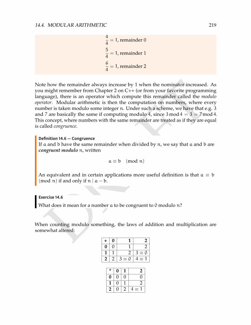
DRAFT
14.4. MODULAR ARITHMETIC 219
4
4= 1, remainder 0
5
4= 1, remainder 1
6
4= 1, remainder 2
Note how the remainder always increase by 1 when the nominator increased. Asyou might remember from Chapter 2 on C++ (or from your favorite programminglanguage), there is an operator which compute this remainder called the modulooperator. Modular arithmetic is then the computation on numbers, where everynumber is taken modulo some integer n. Under such a scheme, we have that e.g. 3and 7 are basically the same if computing modulo 4, since 3mod 4 = 3 = 7mod 4.This concept, where numbers with the same remainder are treated as if they are equalis called congruence.
Definition 14.6 — CongruenceIf a and b have the same remainder when divided by n, we say that a and b arecongruent modulo n, written
a ≡ b (mod n)
An equivalent and in certain applications more useful definition is that a ≡ b
(mod n) if and only if n | a− b.
Exercise 14.6
What does it mean for a number a to be congruent to 0modulo n?
When counting modulo something, the laws of addition and multiplication aresomewhat altered:
+ 0 1 20 0 1 21 1 2 3 ≡ 02 2 3 ≡ 0 4 ≡ 1
* 0 1 20 0 0 01 0 1 22 0 2 4 ≡ 1
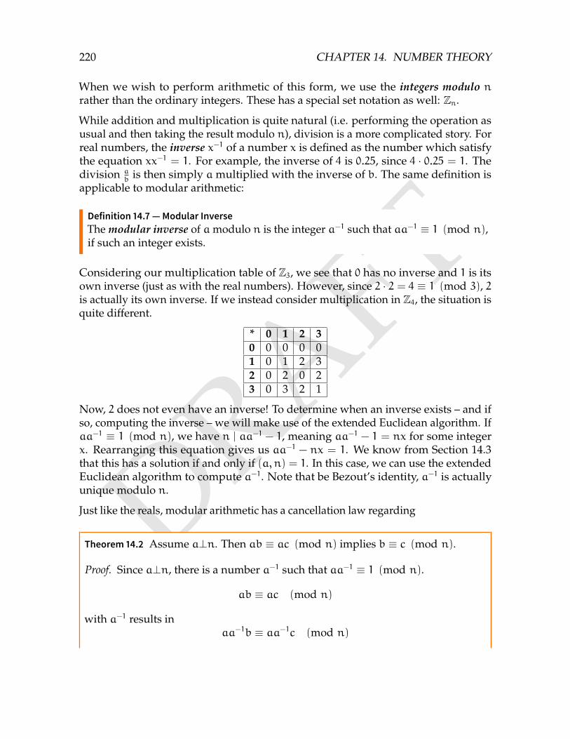
DRAFT
220 CHAPTER 14. NUMBER THEORY
When we wish to perform arithmetic of this form, we use the integers modulo nrather than the ordinary integers. These has a special set notation as well: Zn.
While addition and multiplication is quite natural (i.e. performing the operation asusual and then taking the result modulo n), division is a more complicated story. Forreal numbers, the inverse x−1 of a number x is defined as the number which satisfythe equation xx−1 = 1. For example, the inverse of 4 is 0.25, since 4 · 0.25 = 1. Thedivision a
bis then simply amultiplied with the inverse of b. The same definition is
applicable to modular arithmetic:
Definition 14.7 —Modular InverseThe modular inverse of amodulo n is the integer a−1 such that aa−1 ≡ 1 (mod n),if such an integer exists.
Considering our multiplication table of Z3, we see that 0 has no inverse and 1 is itsown inverse (just as with the real numbers). However, since 2 · 2 = 4 ≡ 1 (mod 3), 2is actually its own inverse. If we instead consider multiplication in Z4, the situation isquite different.
* 0 1 2 30 0 0 0 01 0 1 2 32 0 2 0 23 0 3 2 1
Now, 2 does not even have an inverse! To determine when an inverse exists – and ifso, computing the inverse – we will make use of the extended Euclidean algorithm. Ifaa−1 ≡ 1 (mod n), we have n | aa−1 − 1, meaning aa−1 − 1 = nx for some integerx. Rearranging this equation gives us aa−1 − nx = 1. We know from Section 14.3that this has a solution if and only if (a, n) = 1. In this case, we can use the extendedEuclidean algorithm to compute a−1. Note that be Bezout’s identity, a−1 is actuallyunique modulo n.
Just like the reals, modular arithmetic has a cancellation law regarding
Theorem 14.2 Assume a⊥n. Then ab ≡ ac (mod n) implies b ≡ c (mod n).
Proof. Since a⊥n, there is a number a−1 such that aa−1 ≡ 1 (mod n).
ab ≡ ac (mod n)
with a−1 results inaa−1b ≡ aa−1c (mod n)
DRAFT
14.5. CHINESE REMAINDER THEOREM 221
Simplifying aa−1 gives usb ≡ c (mod n)
Another common modular operation is exponentiation, i.e. computing am (mod n).While this can be computed easily in Θ(m), we can actually do better using a methodcalled exponentiation by squaring. It is essentially based on the recursion
am modn =
1modn if m = 0a · (am−1 modn)modn if m odd(a
m2 modn)2 modn if m even
This procedure is clearly Θ(log2m), since applying the recursive formula for even
numbers halve the m to be computed, while applying it an odd number will firstmake it even and then halve it in the next iteration. It is very important that a
m2 modn
is computed only once, even though it is squared! Computing it twice causes thecomplexity to degrade to Θ(m) again.
14.5 Chinese Remainder Theorem
The Chinese Remainder Theorem is probably the most useful theorem in algorith-mic problem solving. It gives us a way of solving certain systems of linear equa-tions.
Theorem 14.3 — Chinese Remainder TheoremGiven a system of equations
x ≡ a1 (mod m1)
x ≡ a2 (mod m2)
. . .
x ≡ am (mod mn)
where the numbers m1, . . . ,mn are pairwise relatively prime, there is a uniqueinteger x (mod
∏ni=1mi) that satisfy such a system.
Proof. We will prove the theorem inductively. The theorem is clearly true for n = 1,
DRAFT
222 CHAPTER 14. NUMBER THEORY
with the unique solution x = a1. Now, consider the two equations
x ≡ a1 (mod m1)
x ≡ a2 (mod m2)
Let x = a1 ·m2 · (m−12 modm1)+a2 ·m1 · (m−1
1 modm2), wherem−11 modm2 is taken
to be a modular inverse of m1 modulo m2. These inverses exist, since m1⊥m2 byassumption. We then have that x = a1 ·m2 ·(m−1
2 modm1)+a2 ·m1 ·(m−11 modm2) ≡
a1 ·m2 · (m−12 modm1) ≡ ai (mod m1).
Since a solution exist for every a1, a2, this solution must be unique by the pigeon-hole principle – there are m1 ·m2 possible values for a1, a2, and m1 ·m2 possiblevalues for x. Thus, the theorem is also true for n = 2.
Assume the theorem is true for k− 1 equations. Then, we can replace the equations
x ≡ a1 (mod m1)
x ≡ a2 (mod m2)
with another equationx ≡ x ∗ (mod m1m2)
where x∗ is the solution to the first two equations. We just proved those twoequations are equivalent with regards to x. This reduces the number of equationsto k − 1, which by assumption the theorem holds for. Thus, it also holds for kequations.
Note that the theorem used an explicit construction of the solution, allowing us tofind what the unique solution to such a system is.
RadarKTH Challenge 2014
We say that an integer z is within distance y of an integer xmodulo an integermif
z ≡ x+ t (mod m)
where |t| ≤ y.
Find the smallest non-negative integer z such that it is:
• within distance y1 of x1 modulom1
• within distance y2 of x2 modulom2
DRAFT
14.6. EULER’S TOTIENT FUNCTION 223
• within distance y3 of x3 modulom3
InputThe integers 0 ≤ m1,m2,m3 ≤ 106. The integers 0 ≤ x1, x2, x3 ≤ 106. The integers0 ≤ y1, y2, y3 ≤ 300.OutputThe integer z.
The problem gives rise to three linear equations of the form
z ≡ xi + ti (mod mi)
where −yi ≤ ti ≤ yi. If we fix all the variables ti, the problem reduces to solvingthe system of equations using CRT. We could then find all possible values of z,and choose the minimum one. This requires applying the CRT construction about2 · 6003 = 432 000 000 times. Since the modulo operation involved is quite expensive,this approach would use too much time. Instead, let us exploit a useful greedyprinciple in finding minimal solutions.
Assume that z is the minimal answer to an instance. There are only two situationswhere z− 1 cannot be a solution as well:
• z = 0 – since zmust be non-negative, this is the smallest possible answer
• z ≡ xi − yi – then, decreasing zwould violate one of the constraints
In the first case, we only need to verify whether z = 0 is a solution to the threeinequalities. In the second case, we managed to change an inequality to a linearequation. By testing which of the i this equation holds for, we only need to testthe values of ti for the two other equations. This reduce the number of times weneed to use the CRT to 6002 = 360 000 times, a modest amount well within the timelimit.
14.6 Euler’s totient function
Now that we have talked about modular arithmetic, we can give the numbers whichare not divisors to some integer n their well-deserved attention. This discussion willstart with the φ-function.
Definition 14.8 Two integers a and b are said to be relatively prime if their only (andthus greatest) common divisor is 1. If a and b are relatively prime, we write thata⊥b.
DRAFT
224 CHAPTER 14. NUMBER THEORY
Example 14.6 The numbers 74 and 22 are not relatively prime, since they are bothdivisible by 2.
The numbers 72 and 65 are relatively prime. The prime factorization of 72 is2 ·2 ·2 ·3 ·3, and the factorization of 65 is 5 ·13. Since these numbers have no primefactors in common, they have no divisors other than 1 in common.
Given an integer n, we ask ourselves how many of the integers 1, 2, . . . , n which arerelatively prime to n.
Definition 14.9 — Euler’s totient functionEuler’s totient function φ(n) is defined as the number if integers k ∈ [1, n] suchthat (k, n) = 1, i.e. those positive integers less than nwhich are co-prime to n.
Example 14.7 What is φ(12)? The numbers 2, 4, 6, 8, 10 all have the factor 2 incommon with 12 and the numbers 3, 6, 9 all have the factor 3 in common with 12.
This leaves us with the integers 1, 5, 7, 11which are relatively prime to 12. Thus,φ(12) = 4.
For prime powers,φ(pk) is easy to compute. The only integers which are not relativelyprime to φ(pk) are the multiples of p, which there are pk
p= pk−1 of, meaning
φ(pk) = pk − pk−1 = pk−1(p− 1)
It turns out φ(n) has a property which is highly useful in computing certain numbertheoretical functions – it is multiplicative, meaning
φ(ab) = φ(a)φ(b) if a⊥bFor multiplicative functions, we can reduce the problem of computing arbitrary valuesof the function to finding a formula only for prime powers. The reasoning behind themultiplicativity of φ is quite simple. Let a ′ = a − φ(a), i.e. the number of integerswhich do share a factor with a, and similarly b ′ = b− φ(b). Then, there will be ab ′
numbers between 1 and ab which share a factor with b. If x is one of the b ′ numberssharing a factor with b, then so are x, x + b, x + 2b, ..., x + (a − 1)b. Similarly, therewill be a ′b numbers between 1 and ab sharing a factor with a. However, there maybe some numbers sharing both a factor with a and b. Consider two such numbersx+ ib = y+ ja, which gives ib− ja = y− x. By Bezout’s identity, this have a singlesolution (i, j) modulo ab, meaning every number x+ ib equals exactly one numbery+ ja. Thus, there were a ′b ′ numbers sharing a factor with both a and b. This meansthere are ab ′ + a ′b− a ′b ′ numbers sharing a factor with either a and b, so
φ(ab) = ab− ab ′ − a ′b+ a ′b ′ = (a− a ′)(b− b ′) = φ(a)φ(b)
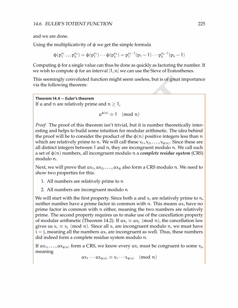
DRAFT
14.6. EULER’S TOTIENT FUNCTION 225
and we are done.
Using the multiplicativity of φwe get the simple formula
φ(pe11 . . . pekk ) = φ(pe11 ) · · ·φ(pekk ) = pe1−11 (p1 − 1) · · ·pek−1k (pk − 1)
Computingφ for a single value can thus be done as quickly as factoring the number. Ifwe wish to compute φ for an interval [1, n] we can use the Sieve of Eratosthenes.
This seemingly convoluted function might seem useless, but is of great importancevia the following theorem:
Theorem 14.4 — Euler’s theoremIf a and n are relatively prime and n ≥ 1,
aφ(n) ≡ 1 (mod n)
Proof. The proof of this theorem isn’t trivial, but it is number theoretically inter-esting and helps to build some intuition for modular arithmetic. The idea behindthe proof will be to consider the product of the φ(n) positive integers less than nwhich are relatively prime to n. We will call these x1, x2, . . . , xφ(n). Since these areall distinct integers between 1 and n, they are incongruent modulo n. We call sucha set of φ(n) numbers, all incongruent modulo n a complete residue system (CRS)modulo n.
Next, we will prove that ax1, ax2, . . . , axφ also form a CRS modulo n. We need toshow two properties for this:
1. All numbers are relatively prime to n
2. All numbers are incongruent modulo n
We will start with the first property. Since both a and xi are relatively prime to n,neither number have a prime factor in common with n. This means axi have noprime factor in common with n either, meaning the two numbers are relativelyprime. The second property requires us to make use of the cancellation propertyof modular arithmetic (Theorem 14.2). If axi ≡ axj (mod n), the cancellation lawgives us xi ≡ xj (mod n). Since all xi are incongruent modulo n, we must havei = j, meaning all the numbers axi are incongruent as well. Thus, these numbersdid indeed form a complete residue system modulo n.
If ax1, . . . , axφ(n) form a CRS, we know every axi must be congruent to some xj,meaning
ax1 · · ·axφ(n) ≡ x1 · · · xφ(n) (mod n)
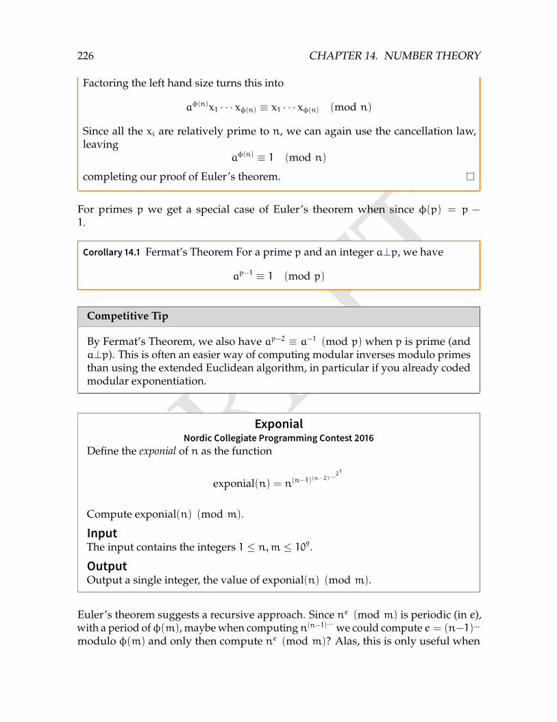
DRAFT
226 CHAPTER 14. NUMBER THEORY
Factoring the left hand size turns this into
aφ(n)x1 · · · xφ(n) ≡ x1 · · · xφ(n) (mod n)
Since all the xi are relatively prime to n, we can again use the cancellation law,leaving
aφ(n) ≡ 1 (mod n)
completing our proof of Euler’s theorem.
For primes p we get a special case of Euler’s theorem when since φ(p) = p −1.
Corollary 14.1 Fermat’s Theorem For a prime p and an integer a⊥p, we have
ap−1 ≡ 1 (mod p)
Competitive Tip
By Fermat’s Theorem, we also have ap−2 ≡ a−1 (mod p) when p is prime (anda⊥p). This is often an easier way of computing modular inverses modulo primesthan using the extended Euclidean algorithm, in particular if you already codedmodular exponentiation.
ExponialNordic Collegiate Programming Contest 2016
Define the exponial of n as the function
exponial(n) = n(n−1)(n−2)...21
Compute exponial(n) (mod m).
InputThe input contains the integers 1 ≤ n,m ≤ 109.OutputOutput a single integer, the value of exponial(n) (mod m).
Euler’s theorem suggests a recursive approach. Since ne (mod m) is periodic (in e),with a period ofφ(m), maybe when computingn(n−1)... we could compute e = (n−1)...
modulo φ(m) and only then compute ne (mod m)? Alas, this is only useful when
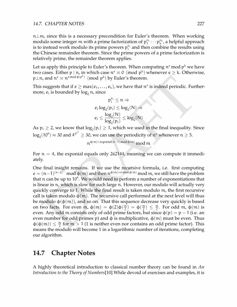
DRAFT
14.7. CHAPTER NOTES 227
n⊥m, since this is a necessary precondition for Euler’s theorem. When workingmodulo some integermwith a prime factorization of pe11 · · ·pekk , a helpful approachis to instead work modulo its prime powers peii and then combine the results usingthe Chinese remainder theorem. Since the prime powers of a prime factorization isrelatively prime, the remainder theorem applies.
Let us apply this principle to Euler’s theorem. When computing ne modpk we havetwo cases. Either p | n, in which case ne ≡ 0 (mod pk) whenever e ≥ k. Otherwise,p⊥n, and ne ≡ nemodφ(pk) (mod pk) by Euler’s theorem.
This suggests that if e ≥ max(e1, . . . , ek), we have that ne is indeed periodic. Further-more, ei is bounded by log
2n, since
peii ≤ n⇒ei log
2(pi) ≤ log
2(N)⇒
ei ≤log
2(N)
log2(pi)
≤ log2(N)
As pi ≥ 2, we know that log2(pi) ≥ 1, which we used in the final inequality. Since
log2(109) ≈ 30 and 432
1
≥ 30, we can use the periodicity of ne whenever n ≥ 5.nφ(m)+exponial(n−1)modφ(m) modm
For n = 4, the exponial equals only 262144, meaning we can compute it immedi-ately.
One final insight remains. If we use the recursive formula, i.e. first computinge = (n−1)(n−2)
... modφ(m) and then nφ(m)+emodφ(m) modm, we still have the problemthat n can be up to 109. We would need to perform a number of exponentiations thatis linear in n, which is slow for such large n. However, our modulo will actually veryquickly converge to 1. While the final result is taken modulo m, the first recursivecall is taken modulo φ(m). The recursive call performed at the next level will thusbe modulo φ(φ(m)), and so on. That this sequence decrease very quickly is basedon two facts. For even m, φ(m) = φ(2)φ(m
2) = φ(m
2) ≤ m
2. For odd m, φ(m) is
even. Any oddm consists only of odd prime factors, but since φ(p) = p− 1 (i.e. aneven number for odd primes p) and φ is multiplicative, φ(m) must be even. Thusφ(φ(m)) ≤ m
2for m > 1 (1 is neither even nor contains an odd prime factor). This
means the modulo will become 1 in a logarithmic number of iterations, completingour algorithm.
14.7 Chapter Notes
A highly theoretical introduction to classical number theory can be found in AnIntroduction to the Theory of Numbers[10] While devoid of exercises and examples, it is

DRAFT
228 CHAPTER 14. NUMBER THEORY
very comprehensive.
A Computational Introduction to Number Theory and Algebra[20] instead takes a moreapplied approach, and is freely available under a Creative Commons license at theauthors home page.4.
4http://www.shoup.net/ntb/
DRAFTChapter 15
Competitive Programming Strategy
Competitive programming is what we call the mind sport of solving algorithmicalproblems and coding their solutions, often under the pressure of time. Most program-ming competitions are performed online, at your own computer through some kindof online judge system. For students of either high school or university, there are twomain competitions. High school students compete in the International Olympiad in In-formatics (IOI), and university students go for the International Collegiate ProgrammingContest (ICPC).
Different competition styles have different difficulty, problem types and strategies. Inthis chapter, we will discuss some basic strategy of programming competitions, andgive tips on how to improve your competitive skills.
15.1 IOI
The IOI is an international event where a large number of countries send teams of upto 4 high school students to compete individually against each other during two daysof competition. Every participating country has its own national selection olympiadfirst.
During a standard IOI contest, contestants are given 5 hours to solve 3 problems, eachworth at most 100 points. These problems are not given in any particular order, andthe scores of the other contestants are hidden until the end of the contest. Generallynone of the problems are “easy” in the sense that it is immediately obvious how tosolve the problem in the same way the first 1-2 problems of most other competitionsare. This poses a large problem, in particular for the amateur. Without any trivialproblems nor guidance from other contestants on what problems to focus on, howdoes an IOI competitor prioritize? The problem is further exacerbated by problemsnot having a simple binary scoring, with a submission being either accepted or
229
DRAFT
230 CHAPTER 15. COMPETITIVE PROGRAMMING STRATEGY
rejected. Instead, IOI problems contain many so-called subtasks. These subtasks givepartial credit for the problem, and contain additional restrictions and limits on eitherinput or output. Some problems do not even use discrete subtasks. In these tasks,scoring is done on some scale which determines how “good” the output produced byyour program is.
15.1.1 Strategy
Very few contestants manage to solve every problem fully during an IOI contest.There is a very high probability you are not one of them, which leaves you with twooptions – you either skip a problem entirely, or you solve some of its subtasks. Atthe start of the competition, you should read through every problem and all of thesubtasks. In the IOI you do not get extra points for submitting faster. Thus, it doesnot matter if you read the problems at the beginning instead of rushing to solve thefirst problem you read. Once you have read all the subtasks, you will often see thesolutions to some of the subtasks immediately. Take note of the subtasks which youknow how to solve!
Deciding on which order you should solve subtasks in is probably one of the mostdifficult parts of the IOI for contestants at or below the silver medal level. In IOI 2016,the difference between receiving a gold medal and a silver medal was a mere 3 points.On one of the problems, with subtasks worth 11, 23, 30 and 36 points, the first silvermedalist solved the third subtask, worth 30 points (a submission that possibly was afailed attempt at 100 points). Most competitors instead solved the first two subtasks,together worth 34 points. If the contestant had solved the first two subtasks instead,he would have gotten a gold medal.
The problem basically boils down to the question when should I solve subtasks instead offocusing on a 100 point solution? There is no easy answer to this question, due to thelack of information about the other contestants’ performances. First of all, you needto get a good sense of how difficult a solution will be to implement correctly beforeyou attempt it. If you only have 30 minutes left of a competition, it might not be agreat idea to go for a 100 point solution on a very tricky problem. Instead, you mightwant to focus on some of the easier subtasks you have left on this or other problems.If you fail your 100 point solution which took over an hour to code, it is nice to knowyou did not have some easy subtasks worth 30-60 points which could have given youa medal.
Problems without discrete scoring (often called heuristic problems) are almost alwaysthe hardest ones to get a full score on. These problems tend to be very fun, and somecontestants often spend way too much time on these problems. They are treacherousin that it is often easy to increase your score by something. However, those 30 minutesyou spent to gain one additional point may have been better spent coding a 15 point
DRAFT
15.1. IOI 231
subtask on another problem. As a general rule, go for the heuristic problem lastduring a competition. This does not mean to skip the problem unless you completelysolve the other two, just to focus on them until you decide that the heuristic problemis worth more points if given the remaining time.
In IOI, you are allowed to submit solution attempts a large number of times, withoutany penalty. Use this opportunity! When submitting a solution, you will generally betold the results of your submission on each of the secret test cases. This provides youwith much details. For example, you can get a sense of how correct or wrong youralgorithm is. If you only fail 1-2 cases, you probably just have a minor bug, but youralgorithm in general is probably correct. You can also see if your algorithm is fastenough, since you will be told the execution time of your program on the test cases.Whenever you make a change to your code which you think affect correctness orspeed – submit it again! This gives you a sense of your progress, and also works as agood regression test. If your change introduced more problems, you will know.
Whenever your solution should pass a subtask, submit it. These subtask results willhelp you catch bugs earlier when you have less code to debug.
15.1.2 Getting Better
The IOI usually tend to have pretty hard problems. Some areas get rather littleattention. For example, there are basically no pure implementation tasks and verylittle geometry.
First and foremost, make sure you are familiar with all the content in the IOI syllabus1.This is an official document which details what areas are allowed in IOI tasks. Thisbook deals with most, if not all of the topics in the IOI syllabus.
In the Swedish IOI team, most of the top performers tend to also be good mathe-matical problem solvers (also getting IMO medals). Combinatorial problems frommathematical competitions tend to be somewhat similar to the algorithmic frame ofmind, and can be good practice for the difficult IOI problems.
When selecting problems to practice on, there are a large number of national olympiadswith great problems. The Croatian Open Competition in Informatics2 is a good source.Their competitions are generally a bit easier than solving IOI with full marks, butare good practice. Additionally, they have a final round (the Croatian Olympiad inInformatics) which are of high quality and difficulty. COCI publishes solutions for allof their contests. These solutions help a lot in training.
One step up in difficulty from COCI is the Polish Olympiad in Informatics3. This1https://people.ksp.sk/~misof/ioi-syllabus/2http://hsin.hr/coci/3http://main.edu.pl/en/archive/oi
DRAFT
232 CHAPTER 15. COMPETITIVE PROGRAMMING STRATEGY
is one of the most difficult European national olympiad published in English, butunfortunately they do not publish solutions in English for their competitions.
There are also many regional olympiads, such as the Baltic, Balkan, Central European,Asia-Pacific Olympiads in Informatics. Their difficulty is often higher than that ofnational olympiads, and of the same format as an IOI contest (3 problems, 5 hours).These, and old IOI problems, are probably the best sources of practice.
15.2 ICPC
In ICPC, you compete in teams of three to solve about 10-12 problems during 5hours. A twist in in the ICPC-style competitions is that the team shares a singlecomputer. This makes it a bit harder to prioritize tasks in ICPC competitions than inIOI competitions. You will often have multiple problems ready to be coded, and waitfor the computer. In ICPC, you see the progress of every other team as well, whichgives you some suggestions on what to solve. As a beginner or medium-level team,this means you will generally have a good idea on what to solve next, since manybetter teams will have prioritized tasks correctly for you.
ICPC scoring is based on two factors. First, teams are ranked by the number of solvedproblems. As a tie breaker, the penalty time of the teams are used. The penalty time ofa single problem is the number of minutes into the contest when your first successfulattempt was submitted, plus a 20 minute penalty for any rejected attempts. Your totalpenalty time is the sum of penalties for every problem.
15.2.1 Strategy
In general, teams will be subject to the penalty tie-breaking. In the 2016 ICPC WorldFinals, both the winners and the team in second place solved 11 problems. Theirpenalty time differed by a mere 7 minutes! While such a small penalty difference inthe very top is rather unusual, it shows the importance of taking your penalty intoaccount.
Minimizing penalties generally comes down to a few basic strategic points:
• Solving the problems in the right order.
• Solving each problem quickly.
• Minimizing the number of rejected attempts.
In the very beginning of an ICPC contest, the first few problems will be solved quickly.In 2016, the first accepted submissions to five of the problems came in after 11, 15, 18,
DRAFT
15.2. ICPC 233
32, 44 minutes. On the other hand, after 44 minutes no team had solved all of thoseproblems. Why does not every team solve the problems in the same order? Teams areof different skill in different areas, make different judgment calls regarding difficultyor (especially early in the contest) simply read the problem in a different order. Thebetter you get, the harder it is to distinguish between the “easy” problems of a contest– they are all “trivial” and will take less than 10-15 minutes to solve and code.
Unless you are a very good team or have very significant variations in skill amongdifferent areas (e.g., you are graph theory experts but do not know how to computethe area of a triangle), you should probably follow the order the other teams choosein solving the problems. In this case, you will generally always be a few problemsbehind the top teams.
The better you get, the harder it is to exploit the scoreboard. You will more often betied in the top with teams who have solved the exact same problems. The problemswhich teams above you have solved but you have not may only be solved by 1-2teams, which is not a particularly significant indicator in terms of difficulty. Teamswho are very strong at math might prioritize a hard maths problem before an easier(on average for most teams) dynamic programming problem. This can risk confusingyou into solving the wrong problems for the particular situation of your team.
The amount of cooperation during a contest is difficult to decide upon. The optimalamount varies a lot between different teams. In general, the amount of cooperationshould increase within a single contest from the start to the end. In the beginning,you should work in parallel as much as possible, to quickly read all the problems,pick out the easy-medium problems and start solving them. Once you have competedin a few contests, you will generally know the approximate difficulty of the simplesttasks, so you can skim the problem set for problems of this difficulty. Sometimes, youfind an even easier problem in the beginning than the one the team decided to startcoding.
If you run out of problems to code, you waste computer time. Generally, this shouldnot happen. If it does, you need to become faster at solving problems.
Towards the end of the contest, it is a common mistake to parallelize on several ofthe hard problems at the same time. This carries a risk of not solving any of theproblems in the end, due to none of the problems getting sufficient attention. Just aswith subtasks in IOI, this is the hardest part of prioritizing tasks. During the last hourof an ICPC contest, the previously public scoreboard becomes frozen. You can stillsee the number of attempts other teams make, but not whether they were successful.Hence, you can not really know how many problems you have to solve to get theposition that you want. Learning your own limits and practicing a lot as a team –especially on difficult contests – will help you get a feeling for how likely you are toget in all of your problems if you parallelize.
Read all the problems! You do not want to be in a situation where you run out of time
DRAFT
234 CHAPTER 15. COMPETITIVE PROGRAMMING STRATEGY
during a competition, just to discover there was some easy problem you knew howto solve but never read the statement of. ICPC contests are made more complex bythe fact that you are three different persons, with different skills and knowledge. Justbecause you can not solve a problem does not mean your team mates will not findthe problem trivial, have seen something similar before or are just better at solvingthis kind of problem.
The scoreboard also displays failed attempts. If you see a problem where many teamsrequire extra attempts, be more careful in your coding. Maybe you can performsome extra tests before submitting, or make a final read-through of the problem andsolution to make sure you did not miss any details.
If you get Wrong Answer, you may want to spend a few minutes to code up yourown test case generators. Prefer generators which create cases where you alreadyknow the answers. Learning e.g. Python for this helps, since it usually takes under aminute to code a reasonable complex input generator.
If you get Time Limit Exceeded, or even suspect time might be an issue – code a testcase generator. Losing a minute on testing your program on the worst case, versusa risk of losing 20 minutes to penalty is be a trade-off worth considering on someproblems.
You are allowed to ask questions to the judges about ambiguities in the problems.Do this the moment you think something is ambiguous (judges generally take a fewvaluable minutes in answering). Most of the time they give you a “No comment”response, in which case the perceived ambiguity probably was not one.
If neither you nor your team mates can find a bug in a rejected solution, considercoding it again from scratch. Often, this can be done rather quickly when you havealready coded a solution.
15.2.2 Getting Better
• Practice a lot with your team. Having a good team dynamic and learning whatproblems the other team members excel at can be the difference that helps youto solve an extra problem during a contest.
• Learn to debug on paper. Wasting computer time for debugging means notwriting code! Whenever you submit a problem, print the code. This can saveyou a few minutes in getting your print-outs when judging is slow (in case yoursubmission will need debugging). If your attempt was rejected, you can studyyour code on paper to find bugs. If you fail on the sample test cases and it takesmore than a few minutes to fix, add a few lines of debug output and print it aswell (or display it on half the computer screen).

DRAFT
15.2. ICPC 235
• Learn to write code on paper while waiting for the computer. In particular, trickysubroutines and formulas are great to hammer out on paper before occupyingvaluable computer time.
• Focus your practice on your weak areas. If you write buggy code, learn yourprogramming language better and code many complex solutions. If your team isbad at geometry, practice geometry problems. If you get stressed during contests,make sure you practice under time pressure. For example, Codeforceshas an http://
codeforces.comhttp://codeforces.comexcellent gym feature, where you can compete retroactively in a contest using
the same amount of time as in the original contest. The scoreboard will thenshow the corresponding scoreboard from the original contest during any giventime.

DRAFT
236 CHAPTER 15. COMPETITIVE PROGRAMMING STRATEGY
DRAFTAppendix A
Mathematics
This appendix reviews some basic mathematics. Without a good grasp on the foun-dations of mathematics, algorithmic problem solving is basically impossible. Whenwe analyze the efficiency of algorithms, we use sums, recurrence relations and a bitof algebra. One of the most common topics of algorithms is graph theory, an areawithin discrete mathematics. Without some basic topics, such as set theory, some ofthe proofs – and even problems – in this book will be hard to understand.
This mathematical preliminary touches lightly upon these topics and is meant tocomplement a high school education in mathematics in preparation for the remainingtext. While you can probably get by with the mathematics from this chapter, we highlyrecommend that you (at some point) delve deeper into discrete mathematics.
We do assume that you are familiar with basic proof techniques, such as proofs byinduction or contradiction, and mathematics that is part of a pre-calculus course(trigonometry, polynomials, etc). Some more mathematically advanced parts ofthis book will go beyond these assumptions, but this is only the case in very fewplaces.
A.1 Logic
In mathematics, we often deal with truths and falsehoods in the form of theorems,proofs, counter-examples and so on. Logic is a very exact discipline, and a preciselanguage has been developed to help us deal with logical statements.
For example, consider the statements
1. an integer is either odd or even,
2. programming is more fun than mathematics,
237
DRAFT
238 APPENDIX A. MATHEMATICS
3. if there exists an odd number divisible by 6, every integer is even,
4. x is negative if and only if x3 is negative,
5. every apple is blue,
6. there exists an integer.
The first statement uses the conjunction or. It connects two statements, and requiresonly one of them to be true in order for the whole statement to be true. Since anyinteger is either odd or even, the statement is true.
The second statement is not really a logical statement. While we might have a personalconviction regarding the entertainment value of such topics, it is hard to consider thestatements as having a truth value.
The third statement complicates matters by introducing an implication. It is a two-partstatement, which only makes a claim regarding the second part if the first part is true.Since no odd number divisible by 6 exists, it makes no statement about the evennessof every integer. Thus, this implication is true.
The fourth statement tells us that two statements are equivalent – one is true exactlywhen the other is. This is also a true statement.
The fifth statement concerns every object if some kind. It is a false statement, a factthat can be proved by exhibiting e.g., a green apple.
Finally, the last statement is true. It asks whether something exists, a statement wecan prove by presenting an integer such as 42.
To express such statements, a language has been developed where all these logicaloperations such as existence, implication and so on have symbols assigned to them.This enables us to remove the ambiguity inherent in the English language, which isof utmost importance when dealing with the exactness required by logic.
The disjunction (a is true or b is true) is a common logical connective. It is giventhe symbol ∨, so that the above statement is written as a ∨ b. The other commonconnective, the conjunction (a is true and b is true) is assigned the symbol ∧. Forexample, we write that a∧ b for the statement that both a and b are true.
An implication is a statement of the form “if a is true, then bmust also be true”. Thisis a statement on its own, which is true whenever a is false (meaning it does not sayanything of b), or when a is true and b is true. We use the symbol→ for this, writingthe statement as a→ b. The fourth statement would hence be written as
(∃p : p is prime ∧ p is divisible by 6)→ ∀ prime p : p is even
The next statement introduced the equivalence, a statement of the form “a is true if,and only if, b is true”. This is the same as a→ b (the only if part) and b→ a (the if
DRAFT
A.1. LOGIC 239
part). We use the symbol↔, which follows naturally for this reason. The statementwould then be written as
x < 0↔ x3 < 0
Logical also contains quantifiers. The fifth statement, that every apple is blue, actuallymakes a large number of statements – one for each apple. This concept is capturedusing the universal quantifier ∀, read as “for every”. For example, we could writethe statement as
∀ apple a : a is blue
In the final statement, another quantifier was used, which speaks of the existence ofsomething; the existential quantifier ∃, which we read as “there exists”. We wouldwrite the second statement as
∃x : x is an integer
The negation operator ¬ inverts a statement. The statement “no penguin can fly”would thus be written as
¬(∃ penguin p : p can fly)
or, equivalently∀ penguin p : ¬p can fly
Exercise A.1
Write the following statements using the logical symbols, and determine whetherthey are true or false:
1) If a and b are odd integers, a+ b is an even integer,
2) a and b are odd integers if and only if a+ b is an even integer,
3) Whenever it rains, the sun does not shine,
4) ab is 0 if and only if a or b is 0
Our treatment of logic ends here. Note that much is left unsaid – it is the mostrudimentary walk-through in this chapter. This section is mainly meant to give yousome familiarity with the basic symbols used in logic, since they will appear later. Ifyou wish to gain a better understanding of logic, you can follow the references in thechapter notes.
DRAFT
240 APPENDIX A. MATHEMATICS
A.2 Sets and Sequences
A set is an unordered collection of distinct objects, such as numbers, letters, other sets,and so on. The objects contained within a set are called its elements, or members. Setsare written as a comma-separated list of its elements, enclosed by curly brackets:
A = 2, 3, 5, 7
In this example, A contains four elements: the integers 2, 3, 5 and 7.
Because a set is unordered and only contains distinct objects, the set 1, 2, 2, 3 is theexact same set as 3, 2, 1, 1 and 1, 2, 3.
If x is an element in a set S, we write that x ∈ S. For example, we have that 2 ∈ A(referring to our example A above). Conversely, we use the notation x 6∈ Swhen theopposite holds. We have e.g., that 11 6∈ A.
Another way of describing the elements of a set uses the set builder notation, in whicha set is constructed by explaining what properties its elements should have. Thegeneral syntax is
element | properties that the element must have
To construct the set of all even integers, we would use the syntax
2i | i is an integer
which is read as “the set containing all numbers of the form 2iwhere i is an integer.To construct the set of all primes, we would write
p | p is prime
Certain sets are used often enough to be assigned their own symbols:
• Z – the set of integers . . . ,−2,−1, 0, 1, 2, . . . ,
• Z+ – the set of positive integers 1, 2, 3, . . . ,
• N – the set of non-negative integers 0, 1, 2, . . . ,
• Q – the set of all rational numbers pq| p, q integers where q 6= 0,
• R – the set of all real numbers,
• [n] – the set of the first n positive integers 1, 2, . . . , n,
• ∅ – the empty set.
DRAFT
A.2. SETS AND SEQUENCES 241
Exercise A.2
1) Use the set builder notation to describe the set of all odd integers.
2) Use the set builder notation to describe the set of all negative integers.
3) Compute the elements of the set k | k is prime and k2 ≤ 30.
A setA is a subset of a set S if, for every x ∈ A, we also have x ∈ S (i.e., every memberof A is a member of S). We denote this with A ⊆ B. For example
2, 3 ⊆ 2, 3, 5, 7
and 2
4, 2,
−1
7
⊆ Q
For any set S, we have that ∅ ⊆ S and S ⊆ S. Whenever a set A is not a subset ofanother set B, we write that A 6⊆ B. For example,
2, π 6⊆ Q
since π is not a rational number.
We say that sets A and B are equal whenever x ∈ A if and only if x ∈ B. This isequivalent to A ⊆ B and B ⊆ A. Sometimes, we will use the latter condition whenproving set equality, i.e., first proving that every element ofAmust also be an elementof B and then the other way round.
Exercise A.3
1) List all subsets of the set 1, 2, 3.
2) How many subsets does a set containing n elements have?
3) Determine which of the following sets are subsets of each other:
• ∅• Z
• Z+
• 2k | k ∈ Z
• 2, 16, 12
Sets also have many useful operations defined on them. The intersection A ∩ B oftwo sets A and B is the set containing all the elements which are members of bothsets, i.e.,
x ∈ A ∩ B⇔ x ∈ A∧ x ∈ B
DRAFT
242 APPENDIX A. MATHEMATICS
If the intersection of two sets is the empty set, we call the sets disjoint. A similarconcept is the union A ∪ B of A and B, defined as the set containing those elementswhich are members of either set.
Example A.1 Let
X = 1, 2, 3, 4, Y = 4, 5, 6, 7, Z = 1, 2, 6, 7
Then,X ∩ Y = 4
X ∩ Y ∩ Z = ∅X ∪ Y = 1, 2, 3, 4, 5, 6, 7
X ∪ Z = 1, 2, 3, 4, 6, 7
Exercise A.4
Compute the intersection and union of:
1) A = 1, 4, 2, B = 4, 5, 6
2) A = a, b, c, B = d, e, f
3) A = apple, orange, B = pear, orange
A sequence is an ordered collection of values (predominantly numbers) such a 1, 2, 1, 3, 1, 4, . . . .Sequences will mostly be a list of sub-scripted variables, such as a1, a2, . . . , an. Ashorthand for this is (ai)
ni=1, denoting the sequence of variables ai where i ranges
from 1 to n. An infinite sequence is given∞ as its upper bound: (ai)∞i=1
A.3 Sums and Products
The most common mathematical expressions we deal with are sums of sequences ofnumbers, such as 1+ 2+ · · ·+ n. Such sums often have a variable number of termsand complex summands, such as 1 · 3 · 5 + 3 · 5 · 7 + · · · + (2n + 1)(2n + 3)(2n + 5).In these cases, sums given in the form of a few leading and trailing terms, with theremaining part hidden by . . . is too imprecise. Instead, we use a special syntax forwriting sums in a formal way – the sum operator:
k∑i=j
ai
DRAFT
A.3. SUMS AND PRODUCTS 243
The symbol denotes the sum of the j− k+ 1 terms aj + aj+1 + aj+2 + · · ·+ ak, whichwe read as “the sum of ai from j to k”.
For example, we can express the sum 2+ 4+ 6+ · · ·+ 12 of the 6 first even numbersas
6∑i=1
2i
Exercise A.5
Compute the sum4∑
i=−2
2 · i− 1
Many useful sums have closed forms – expressions in which we do not need sums ofa variable number of terms.
Exercise A.6
Prove the following identities:
n∑i=1
c = cn
n∑i=1
i =n(n+ 1)
2
n∑i=1
i2 =n(n+ 1
2)(n+ 1)
3
n∑i=0
2i = 2n+1 − 1
The sum of the inverses of the first n natural numbers happen to have a very neatapproximation, which we will occasionally make use of later on:
n∑i=1
1
n≈ lnn
This is a reasonable approximation, since∫l11xdx = ln(l)
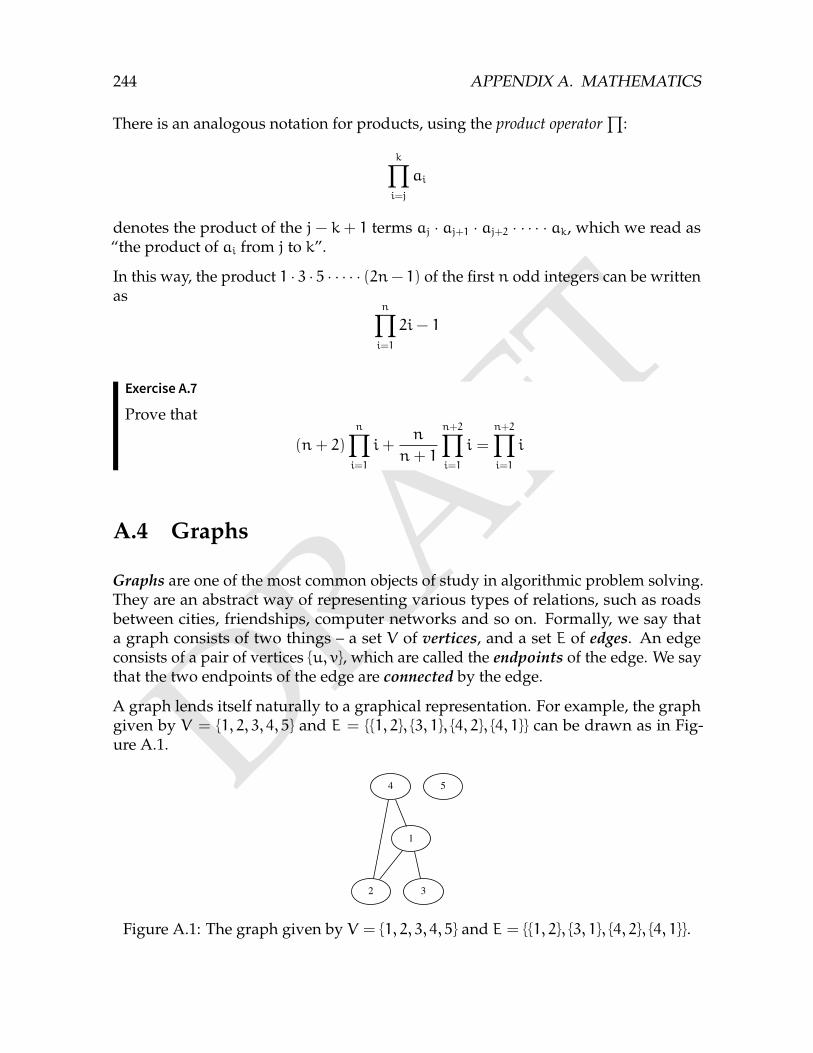
DRAFT
244 APPENDIX A. MATHEMATICS
There is an analogous notation for products, using the product operator∏
:
k∏i=j
ai
denotes the product of the j − k + 1 terms aj · aj+1 · aj+2 · · · · · ak, which we read as“the product of ai from j to k”.
In this way, the product 1 · 3 · 5 · · · · · (2n− 1) of the first n odd integers can be writtenas
n∏i=1
2i− 1
Exercise A.7
Prove that
(n+ 2)
n∏i=1
i+n
n+ 1
n+2∏i=1
i =
n+2∏i=1
i
A.4 Graphs
Graphs are one of the most common objects of study in algorithmic problem solving.They are an abstract way of representing various types of relations, such as roadsbetween cities, friendships, computer networks and so on. Formally, we say thata graph consists of two things – a set V of vertices, and a set E of edges. An edgeconsists of a pair of vertices u, v, which are called the endpoints of the edge. We saythat the two endpoints of the edge are connected by the edge.
A graph lends itself naturally to a graphical representation. For example, the graphgiven by V = 1, 2, 3, 4, 5 and E = 1, 2, 3, 1, 4, 2, 4, 1 can be drawn as in Fig-ure A.1.
1
2 3
4 5
Figure A.1: The graph given by V = 1, 2, 3, 4, 5 and E = 1, 2, 3, 1, 4, 2, 4, 1.
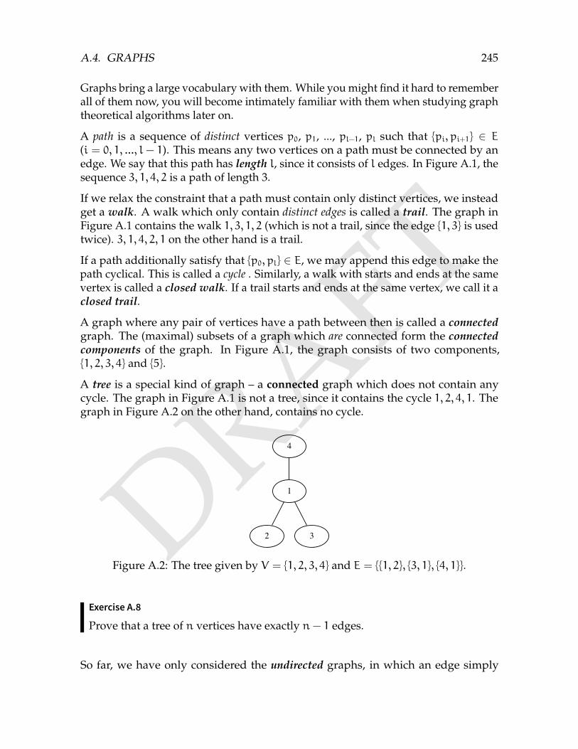
DRAFT
A.4. GRAPHS 245
Graphs bring a large vocabulary with them. While you might find it hard to rememberall of them now, you will become intimately familiar with them when studying graphtheoretical algorithms later on.
A path is a sequence of distinct vertices p0, p1, ..., pl−1, pl such that pi, pi+1 ∈ E(i = 0, 1, ..., l − 1). This means any two vertices on a path must be connected by anedge. We say that this path has length l, since it consists of l edges. In Figure A.1, thesequence 3, 1, 4, 2 is a path of length 3.
If we relax the constraint that a path must contain only distinct vertices, we insteadget a walk. A walk which only contain distinct edges is called a trail. The graph inFigure A.1 contains the walk 1, 3, 1, 2 (which is not a trail, since the edge 1, 3 is usedtwice). 3, 1, 4, 2, 1 on the other hand is a trail.
If a path additionally satisfy that p0, pl ∈ E, we may append this edge to make thepath cyclical. This is called a cycle . Similarly, a walk with starts and ends at the samevertex is called a closed walk. If a trail starts and ends at the same vertex, we call it aclosed trail.
A graph where any pair of vertices have a path between then is called a connectedgraph. The (maximal) subsets of a graph which are connected form the connectedcomponents of the graph. In Figure A.1, the graph consists of two components,1, 2, 3, 4 and 5.
A tree is a special kind of graph – a connected graph which does not contain anycycle. The graph in Figure A.1 is not a tree, since it contains the cycle 1, 2, 4, 1. Thegraph in Figure A.2 on the other hand, contains no cycle.
1
2 3
4
Figure A.2: The tree given by V = 1, 2, 3, 4 and E = 1, 2, 3, 1, 4, 1.
Exercise A.8
Prove that a tree of n vertices have exactly n− 1 edges.
So far, we have only considered the undirected graphs, in which an edge simply
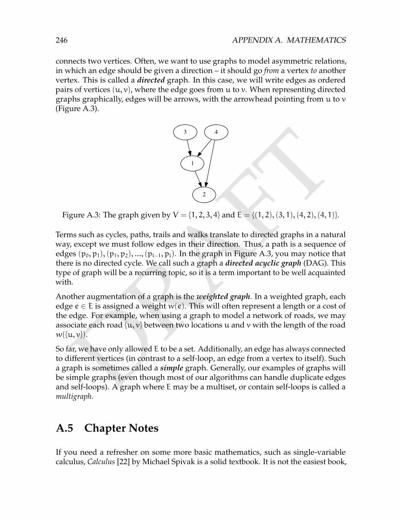
DRAFT
246 APPENDIX A. MATHEMATICS
connects two vertices. Often, we want to use graphs to model asymmetric relations,in which an edge should be given a direction – it should go from a vertex to anothervertex. This is called a directed graph. In this case, we will write edges as orderedpairs of vertices (u, v), where the edge goes from u to v. When representing directedgraphs graphically, edges will be arrows, with the arrowhead pointing from u to v(Figure A.3).
1
2
3 4
Figure A.3: The graph given by V = 1, 2, 3, 4 and E = (1, 2), (3, 1), (4, 2), (4, 1).
Terms such as cycles, paths, trails and walks translate to directed graphs in a naturalway, except we must follow edges in their direction. Thus, a path is a sequence ofedges (p0, p1), (p1, p2), ..., (pl−1, pl). In the graph in Figure A.3, you may notice thatthere is no directed cycle. We call such a graph a directed acyclic graph (DAG). Thistype of graph will be a recurring topic, so it is a term important to be well acquaintedwith.
Another augmentation of a graph is the weighted graph. In a weighted graph, eachedge e ∈ E is assigned a weight w(e). This will often represent a length or a cost ofthe edge. For example, when using a graph to model a network of roads, we mayassociate each road u, v between two locations u and vwith the length of the roadw(u, v).
So far, we have only allowed E to be a set. Additionally, an edge has always connectedto different vertices (in contrast to a self-loop, an edge from a vertex to itself). Sucha graph is sometimes called a simple graph. Generally, our examples of graphs willbe simple graphs (even though most of our algorithms can handle duplicate edgesand self-loops). A graph where Emay be a multiset, or contain self-loops is called amultigraph.
A.5 Chapter Notes
If you need a refresher on some more basic mathematics, such as single-variablecalculus, Calculus [22] by Michael Spivak is a solid textbook. It is not the easiest book,
DRAFT
A.5. CHAPTER NOTES 247
but one the best undergraduate text on single-variable calculus if you take the time towork it through.
Logic in computer science [11] is an introduction to formal logic, with many interestingcomputational applications. The first chapter on propositional logic is sufficient formost algorithmic problem solving, but the remaining chapters shows many non-obvious applications that makes logic relevant to computer science.
For a gentle introduction to discrete mathematics, Discrete and Combinatorial Math-ematics: An Applied Introduction [9] by Ralph Grimaldi is a nice book with a lot ofbreadth.
One of the best works on discrete mathematics ever produced for the aspiring algo-rithmic problem solver is Concrete Mathematics [7], co-authored by famous computerscientist Donald Knuth. It is rather heavy-weight, and probably serves better asa more in-depth study of the foundations of discrete mathematics rather than anintroductory text.
Graph Theory [6] by Reinhard Diestel is widely acknowledged as the go-to book onmore advanced graph theory concepts. The author is freely available for viewing atthe book’s home page1.
1http://diestel-graph-theory.com/

DRAFT
248 APPENDIX A. MATHEMATICS

DRAFTBibliography
[1] Sanjeev Arora and Boaz Barak. Computational Complexity: A Modern Approach.Cambridge University Press, 2009.
[2] David Beazley and Brian K. Jones. Python Cookbook. O’Reilly, 2013.
[3] Joshua Bloch. Effective Java. Pearson Education, 2008.
[4] Xuan Cai. Canonical coin systems for change-making problems. In 2009 NinthInternational Conference on Hybrid Intelligent Systems, volume 1, pages 499–504,Aug 2009.
[5] Thomas H. Cormen, Charles E. Leiserson, Ronald L. Rivest, and Clifford Stein.Introduction to Algorithms. The MIT Press, 3rd edition, 2009.
[6] Reinhard Diestel. Graph Theory. Springer, 2016.
[7] Oren Patashnik Donald E. Knuth and Ronald Graham. Concrete Mathematics: AFoundation for Computer Science. Addison-Wesley, 1994.
[8] Philippe Flajolet and Robert Sedgewick. An Introduction to the Analysis of Algo-rithms. Addison-Wesley, 2013.
[9] Ralph P. Grimaldi. Discrete and Combinatorial Mathematics: An Applied Introduction.Pearson Education, 2003.
[10] G.H Hardy and E.M Wright. An Introduction to the Theory of Numbers. OxfordUniversity Press, 2008.
[11] Michael Huth. Logic in Computer Science. Cambridge University Press, 2004.
[12] George S. Lueker. Two NP-complete Problems in Nonnegative Integer Programming.Princeton University. Department of Electrical Engineering, 1975.
[13] Robert C. Martin. Clean Code: A Handbook of Agile Software Craftsmanship. PearsonEducation, 2009.
[14] Steve McConnell. Code Complete: A Practical Handbook of Software Construction.Microsoft Press, 2004.
249
DRAFT
250 BIBLIOGRAPHY
[15] Scott Meyers. Effective STL. O’Reilly, 2001.
[16] Scott Meyers. Effective C++. O’Reilly, 2005.
[17] Scott Meyers. Effective Modern C++. O’Reilly, 2014.
[18] Christos Papadimitriou. Computational Complexity. Addison-Wesley, 1994.
[19] Charles Petzold. CODE. Microsoft Press, 2000.
[20] Victor Shoup. A Computational Introduction to Number Theory and Algebra. Cam-bridge University Press, 2008.
[21] Brett Slatkin. Effective Python. Addison-Wesley, 2015.
[22] Michael Spivak. Calculus. Springer, 1994.
[23] Bjarne Stroustrup. The C++ Programming Language. Addison-Wesley, 2013.
[24] Jeffrey Ullman and John Hopcroft. Introduction to Automata Theory, Languages,and Computation. Pearson Education, 2014.
DRAFTIndex
addition principle, 177algorithm, 5and, 238
BFS, 139bijection, 181binary search, 118binomial coefficient, 187bipartite matching, 157breadth-first search, 139
closed trail, 245closed walk, 245combinatorics, 177comment, 16compiler, 14component, 245composite number, 209computational problem, 3conjunction, 238connected, 244, 245connected component, 245correctness, 7cycle, 245cycle decomposition, 182
DAG, 246data structure, 127Dijkstra’s Algorithm, 145directed acyclic graph, 246directed graph, 246disjoint sets, 242disjunction, 238divide and conquer, 109divisibility, 205
divisor, 205Dyck path, 190
edge, 244element, 240endpoint, 244equivalence, 238existential quantifier, 239
factorial, 180flow network, 151
generate and test, 68graph, 244
identity permutation, 181implication, 238input description, 3insertion sort, 57instance, 4intersection
of sets, 241
judgment, 11
Kattis, 10KMP, 167Knuth-Morris-Pratt, 167
lengthof path, 245
logic, 237
main function, 16maximum matching, 157member, 240
251
DRAFT
252 INDEX
memory complexity, 63modular inverse, 220multiplication principle, 177
negation, 239NP-complete, 62
online judge, 10optimization problem, 67or, 238oracle, 63order
of a permutation, 183output description, 3
path, 245permutation, 180, 181
cycles, 182identity, 181inverse of, 182multiplication, 182order, 183
prime number, 209problem, 3product operator, 244programming language, 8pseudo code, 9
quantifier, 239query complexity, 63quotient, 218
Rabin-Karp, 170remainder, 218
sequence, 242set, 240Sieve of Eratosthenes, 208simple graph, 246subset, 241sum operator, 242
time complexity, 57trail, 245travelling salesman problem, 67
tree, 245
undirected graph, 245union, 242universal quantifier, 239
vertex, 244
walk, 245weighted graph, 246


