Embed Size (px)
Citation preview
Algorithmic Enhancements to Polynomial
Matrix Factorisations
PhD Thesis
Fraser Kenneth Coutts
Centre for Signal and Image Processing
Electronic and Electrical Engineering
University of Strathclyde, Glasgow
May 29, 2019
This thesis is the result of the author’s original research. It has been
composed by the author and has not been previously submitted for
examination which has led to the award of a degree.
The copyright of this thesis belongs to the author under the terms of the
United Kingdom Copyright Acts as qualified by University of Strathclyde
Regulation 3.50. Due acknowledgement must always be made of the use of
any material contained in, or derived from, this thesis.
Abstract
In broadband array processing applications, an extension of the eigenvalue decomposi-
tion (EVD) to parahermitian Laurent polynomial matrices — named the polynomial
matrix EVD (PEVD) — has proven to be a useful tool for the decomposition of space-
time covariance matrices and their associated cross-spectral density matrices. Existing
PEVD methods typically operate in the time domain and utilise iterative frameworks
established by the second-order sequential best rotation (SBR2) or sequential matrix
diagonalisation (SMD) algorithms. However, motivated by recent discoveries that es-
tablish the existence of an analytic PEVD — which is rarely recovered by SBR2 or
SMD — alternative algorithms that better meet analyticity by operating in the dis-
crete Fourier transform (DFT)-domain have received increasing attention.
While offering promising results in applications including broadband MIMO and
beamforming, the PEVD has seen limited deployment in hardware due to its high com-
putational complexity. If the PEVD is to be fully utilised, overcoming this bottleneck
is paramount. This thesis therefore seeks to reduce the computational cost of iterative
PEVD algorithms — with particular emphasis on SMD — through the development
of several novel algorithmic improvements. While these are effective, the complexity
of the optimised algorithms still grows rapidly with the spatial dimensions of the de-
composition. Steps are therefore taken to convert the sequential form of SMD to a
novel reduced dimensionality and partially parallelisable divide-and-conquer architec-
ture. The resulting algorithms are shown to converge an order of magnitude faster
than existing methods for large spatial dimensions, and are well-suited to application
scenarios with many sensors.
Further in this thesis, an investigation into DFT-based algorithms highlights their
potential to offer compact, analytic solutions to the PEVD. Subsequently, two novel
DFT-based algorithms improve upon an existing method by reducing decomposition
error and eliminating a priori knowledge requirements. Finally, an innovative strategy
is shown to be capable of extracting a minimum-order solution to the PEVD.
ii
Acknowledgements
I would like to begin by extending my sincere thanks to my supervisors, Professor
Stephan Weiss and Professor Stephen Marshall, who have kindly provided me with
their expert guidance, encouragement, and key insights throughout my time at the
University of Strathclyde. For their valuable advice and input to my research, I would
also like to thank Dr Keith Thompson, Professor Ian Proudler, Dr Jamie Corr, Dr
Jennifer Pestana, Professor John McWhirter, and Dr Paul Murray. I am also extremely
grateful to the Carnegie Trust, who funded my research.
Many thanks to Dr Louise Crockett and Dr Gaetano Di Caterina for trusting me
with their classes, and to Christine Bryson for her excellent administrative skills. For
their conversation and thoughts of the day, I would like to thank Dani, Kenny, Shawn,
Connor, Paul, David, Vianney, and the other Fraser.
I would like to extend my deepest gratitude to my parents, Karen and Kenny, for
always believing in me, for motivating me, and for being fantastic sources of inspira-
tion. At last, I’m no longer a student! Thanks should also go to Lauren, James, my
grandparents, and my extended family, for their encouragement.
For her invaluable support, input, and Oxford comma checking prowess during the
completion of this research, I would like to offer my profound gratitude to Elizabeth.
Merci beaucoup, ma cherie!
Fraser Kenneth Coutts
Glasgow, UK
May 29, 2019
iii
Contents
Abstract ii
Acknowledgements iii
Table of Contents iv
List of Figures x
List of Tables xiii
List of Publications xiv
Abbreviations and Mathematical Symbols xviii
1 Introduction 2
1.1 Polynomial Matrix Formulations . . . . . . . . . . . . . . . . . . . . . . 2
1.2 Objective of Research . . . . . . . . . . . . . . . . . . . . . . . . . . . . 4
1.3 Organisation of Thesis and Original Contributions . . . . . . . . . . . . 5
2 Background 7
2.1 Notations and Definitions . . . . . . . . . . . . . . . . . . . . . . . . . . 7
2.2 Polynomial Matrix Formulations in Broadband Signal Processing . . . 8
2.2.1 Introduction . . . . . . . . . . . . . . . . . . . . . . . . . . . . . 8
2.2.2 Space-Time Covariance and Cross-Spectral Density Matrices . . 9
2.3 Polynomial Matrix Eigenvalue Decomposition . . . . . . . . . . . . . . 11
2.3.1 Definition . . . . . . . . . . . . . . . . . . . . . . . . . . . . . . . 11
iv
2.3.2 Existing PEVD Algorithms . . . . . . . . . . . . . . . . . . . . . 12
2.3.3 Implementations of PEVD Algorithms . . . . . . . . . . . . . . . 15
2.4 Simulation Software and Hardware Platform . . . . . . . . . . . . . . . 16
3 Computational Advances for the Iterative PEVD 17
3.1 Introduction . . . . . . . . . . . . . . . . . . . . . . . . . . . . . . . . . . 17
3.2 Optimising Matrix Manipulations to Increase Algorithmic Efficiency . . 19
3.2.1 Product of a Matrix and Polynomial Matrix . . . . . . . . . . . 19
3.2.2 Product of Two Polynomial Matrices . . . . . . . . . . . . . . . 25
3.2.3 Implementation of Truncation Within PEVD Algorithms . . . . 28
3.2.4 Summary . . . . . . . . . . . . . . . . . . . . . . . . . . . . . . . 30
3.3 Parahermitian Matrix Symmetry and the Half-Matrix Approach . . . . 30
3.3.1 Half-Matrix Representation of a Parahermitian Matrix . . . . . 31
3.3.2 Half-Matrix Sequential Matrix Diagonalisation Algorithm . . . . 32
3.3.3 Modified Parameter Search in HSMD . . . . . . . . . . . . . . . 32
3.3.4 Modification of Shift Strategy in HSMD . . . . . . . . . . . . . 34
3.3.5 Complexity and Memory Reduction . . . . . . . . . . . . . . . . 36
3.3.6 Results and Discussion . . . . . . . . . . . . . . . . . . . . . . . 38
3.3.7 Summary . . . . . . . . . . . . . . . . . . . . . . . . . . . . . . . 39
3.4 Increasing Efficiency within Cyclic-by-Row PEVD Implementations . . 40
3.4.1 Cyclic-by-Row SMD Algorithm . . . . . . . . . . . . . . . . . . . 40
3.4.2 Concatenation of Rotations . . . . . . . . . . . . . . . . . . . . . 42
3.4.3 Thresholding of Rotations . . . . . . . . . . . . . . . . . . . . . 44
3.4.4 Results and Discussion . . . . . . . . . . . . . . . . . . . . . . . 44
3.4.5 Summary . . . . . . . . . . . . . . . . . . . . . . . . . . . . . . . 47
3.5 Restricting the Search Space of PEVD Algorithms . . . . . . . . . . . . 48
3.5.1 Limited Search Strategy . . . . . . . . . . . . . . . . . . . . . . 48
3.5.2 Results and Discussion . . . . . . . . . . . . . . . . . . . . . . . 49
3.5.3 Summary . . . . . . . . . . . . . . . . . . . . . . . . . . . . . . . 51
3.6 Restricting the Update Space of PEVD Algorithms . . . . . . . . . . . 53
3.6.1 Restricted Update SMD Algorithm . . . . . . . . . . . . . . . . 53
3.6.2 Restricted Update Step . . . . . . . . . . . . . . . . . . . . . . . 55
3.6.3 Complexity Reduction . . . . . . . . . . . . . . . . . . . . . . . 58
3.6.4 Results and Discussion . . . . . . . . . . . . . . . . . . . . . . . 59
3.6.5 Summary . . . . . . . . . . . . . . . . . . . . . . . . . . . . . . . 60
3.7 Multiple Shift Approach to the Polynomial Matrix QR Decomposition . 61
3.7.1 Multiple Shift Strategy . . . . . . . . . . . . . . . . . . . . . . . 62
3.7.2 Results and Discussion . . . . . . . . . . . . . . . . . . . . . . . 66
3.7.3 Summary . . . . . . . . . . . . . . . . . . . . . . . . . . . . . . . 67
3.8 Compensated Row-Shift Truncation of Paraunitary Matrices . . . . . . 68
3.8.1 Compensated Row-Shift Truncation Strategy . . . . . . . . . . . 68
3.8.2 Truncating After Algorithm Completion . . . . . . . . . . . . . 70
3.8.3 Truncating at Each Algorithm Iteration . . . . . . . . . . . . . . 73
3.8.4 Summary . . . . . . . . . . . . . . . . . . . . . . . . . . . . . . . 77
3.9 Conclusions . . . . . . . . . . . . . . . . . . . . . . . . . . . . . . . . . . 78
4 Divide-and-Conquer Strategy for PEVD Algorithms 80
4.1 Introduction . . . . . . . . . . . . . . . . . . . . . . . . . . . . . . . . . . 80
4.2 Divide-and-Conquer as a Methodology . . . . . . . . . . . . . . . . . . 81
4.3 Extending the Divide-and-Conquer Methodology to the PEVD . . . . . 82
4.3.1 Problem Formulation . . . . . . . . . . . . . . . . . . . . . . . . 82
4.3.2 Block Diagonalising a Parahermitian Matrix . . . . . . . . . . . 85
4.4 Sequential Matrix Segmentation Algorithm . . . . . . . . . . . . . . . . 87
4.4.1 Algorithm Overview . . . . . . . . . . . . . . . . . . . . . . . . . 88
4.4.2 Algorithm Convergence . . . . . . . . . . . . . . . . . . . . . . . 92
4.4.3 Algorithm Complexity . . . . . . . . . . . . . . . . . . . . . . . 95
4.4.4 Results and Discussion . . . . . . . . . . . . . . . . . . . . . . . 95
4.5 Divide-and-Conquer Sequential Matrix Diagonalisation Algorithm . . . 101
4.5.1 Algorithm Overview . . . . . . . . . . . . . . . . . . . . . . . . . 101
4.5.2 ‘Dividing’ the Parahermitian Matrix . . . . . . . . . . . . . . . . 102
4.5.3 ‘Conquering’ the Independent Matrices . . . . . . . . . . . . . . 103
4.5.4 Algorithm Convergence . . . . . . . . . . . . . . . . . . . . . . . 103
4.5.5 Impact of Algorithm Parameters on Decomposition Error . . . . 104
4.5.6 Algorithm Complexity . . . . . . . . . . . . . . . . . . . . . . . 105
4.6 Parallel-Sequential Matrix Diagonalisation PEVD Algorithm . . . . . . 106
4.6.1 Algorithm Overview . . . . . . . . . . . . . . . . . . . . . . . . . 107
4.6.2 ‘Dividing’ the Parahermitian Matrix . . . . . . . . . . . . . . . . 109
4.6.3 ‘Conquering’ the Independent Matrices . . . . . . . . . . . . . . 116
4.6.4 Algorithm Convergence . . . . . . . . . . . . . . . . . . . . . . . 118
4.6.5 Impact of Algorithm Parameters on Decomposition Error . . . . 118
4.6.6 Algorithm Complexity . . . . . . . . . . . . . . . . . . . . . . . 118
4.7 Simulations and Results . . . . . . . . . . . . . . . . . . . . . . . . . . . 119
4.7.1 Source Model Simulation Scenario 1 . . . . . . . . . . . . . . . . 120
4.7.2 Source Model Simulation Scenario 2 . . . . . . . . . . . . . . . . 126
4.7.3 Broadband Angle of Arrival Estimation Simulation Scenario . . 133
4.8 Conclusions . . . . . . . . . . . . . . . . . . . . . . . . . . . . . . . . . . 138
5 DFT-Based Alternatives for PEVD Algorithms 141
5.1 Introduction . . . . . . . . . . . . . . . . . . . . . . . . . . . . . . . . . 141
5.2 Comparison of Iterative and DFT-Based PEVDs . . . . . . . . . . . . . 145
5.2.1 Algorithm Complexities . . . . . . . . . . . . . . . . . . . . . . . 145
5.2.2 Approximation of Eigenvalues . . . . . . . . . . . . . . . . . . . 146
5.2.3 Paraunitarity of Polynomial Eigenvectors . . . . . . . . . . . . . 147
5.2.4 Model Examples and Results . . . . . . . . . . . . . . . . . . . . 148
5.2.5 Summary . . . . . . . . . . . . . . . . . . . . . . . . . . . . . . . 151
5.3 Development of a Novel DFT-Based PEVD Algorithm . . . . . . . . . . 152
5.3.1 Smoothness Metric . . . . . . . . . . . . . . . . . . . . . . . . . 152
5.3.2 Algorithm Overview . . . . . . . . . . . . . . . . . . . . . . . . . 155
5.3.3 Reordering the Eigenvectors and Eigenvalues . . . . . . . . . . . 155
5.3.4 Adjusting the Phase of the Eigenvectors . . . . . . . . . . . . . . 156
5.3.5 Algorithm Complexity . . . . . . . . . . . . . . . . . . . . . . . . 161
5.3.6 Source Model Simulation Scenarios and Results . . . . . . . . . 161
5.3.7 Model Example with Repeated Eigenvalues . . . . . . . . . . . . 163
5.3.8 Summary . . . . . . . . . . . . . . . . . . . . . . . . . . . . . . . 164
5.4 An Order-Iterated Novel DFT-Based PEVD Algorithm . . . . . . . . . 166
5.4.1 Algorithm Overview . . . . . . . . . . . . . . . . . . . . . . . . . 166
5.4.2 Algorithm Complexity . . . . . . . . . . . . . . . . . . . . . . . . 169
5.4.3 Simulation Scenarios . . . . . . . . . . . . . . . . . . . . . . . . 169
5.4.4 Results and Discussion . . . . . . . . . . . . . . . . . . . . . . . 171
5.4.5 Summary . . . . . . . . . . . . . . . . . . . . . . . . . . . . . . . 173
5.5 Eigenvector Ambiguity and Approximating a Minimum-Order Solution 174
5.5.1 Greatest Common Divisor of Multiple Polynomials . . . . . . . 176
5.5.2 Results and Discussion . . . . . . . . . . . . . . . . . . . . . . . 177
5.5.3 Summary . . . . . . . . . . . . . . . . . . . . . . . . . . . . . . . 180
5.6 Conclusions . . . . . . . . . . . . . . . . . . . . . . . . . . . . . . . . . . 180
6 Conclusions 183
6.1 Summary of Contributions . . . . . . . . . . . . . . . . . . . . . . . . . . 183
6.2 Future Work . . . . . . . . . . . . . . . . . . . . . . . . . . . . . . . . . 185
A Existing PEVD Algorithms and Performance Metrics 187
A.1 Sequential Matrix Diagonalisation PEVD Algorithm . . . . . . . . . . . 187
A.1.1 Algorithm Overview . . . . . . . . . . . . . . . . . . . . . . . . . 187
A.1.2 Algorithm Complexity . . . . . . . . . . . . . . . . . . . . . . . 190
A.2 Existing DFT-Based Approach to the PEVD . . . . . . . . . . . . . . . 191
A.2.1 Algorithm Overview . . . . . . . . . . . . . . . . . . . . . . . . . 191
A.2.2 Reordering the Eigenvectors and Eigenvalues . . . . . . . . . . . 193
A.2.3 Adjusting the Phase of the Eigenvectors . . . . . . . . . . . . . . 193
A.3 Performance Metrics . . . . . . . . . . . . . . . . . . . . . . . . . . . . . 195
A.3.1 Normalised Off-Diagonal Energy . . . . . . . . . . . . . . . . . . 195
A.3.2 Normalised Below-Diagonal Energy . . . . . . . . . . . . . . . . 196
A.3.3 Eigenvalue Resolution . . . . . . . . . . . . . . . . . . . . . . . . 196
A.3.4 Decomposition Mean Square Error . . . . . . . . . . . . . . . . . 197
A.3.5 Paraunitarity Error . . . . . . . . . . . . . . . . . . . . . . . . . 197
A.3.6 Paraunitary Filter Length . . . . . . . . . . . . . . . . . . . . . 197
B Broadband Randomised Source Model 198
C State-of-the-Art in Polynomial Matrix Truncation 199
D Spatio-Spectral MUSIC Algorithm 200
Bibliography 201
List of Figures
2.1 Visualisation of an M element broadband linear array . . . . . . . . . . 10
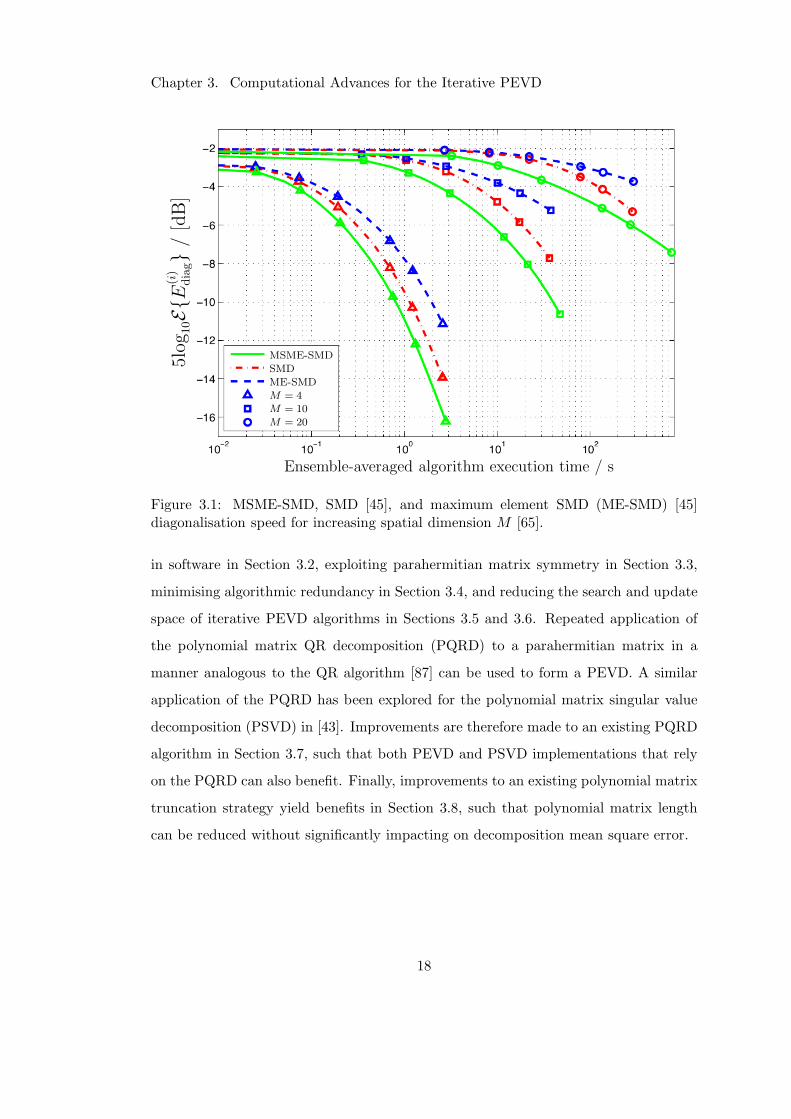
3.1 PEVD algorithm speed for high parahermitian matrix spatial dimension 18
3.2 Matrix multiplication speed comparison using SMD algorithm . . . . . . 23
3.3 Speed comparison of state-of-the-art iterative PEVD algorithms . . . . . 25
3.4 Impact of truncation on parahermitian matrix length . . . . . . . . . . . 29
3.5 Effect of novel placement of truncation on PEVD algorithm speed . . . 29
3.6 Half-matrix representation of a parahermitian matrix . . . . . . . . . . . 32
3.7 Half-matrix row shift example . . . . . . . . . . . . . . . . . . . . . . . . 35
3.8 Half-matrix column shift example . . . . . . . . . . . . . . . . . . . . . . 35
3.9 Performance increase due to half-matrix approach . . . . . . . . . . . . 39
3.10 Illustration of Jacobi sweep . . . . . . . . . . . . . . . . . . . . . . . . . 42
3.11 PEVD convergence unaffected when using cyclic-by-row improvements . 46
3.12 Performance increase due to cyclic-by-row improvements for M = 5 . . . 46
3.13 Performance increase due to cyclic-by-row improvements for M = 9 . . . 46
3.14 Impact of thresholding Jacobi rotations in SMDCbR . . . . . . . . . . . 47
3.15 Performance increase due to search space restriction . . . . . . . . . . . 51
3.16 Impact of restricted search approach on delay operations . . . . . . . . . 52
3.17 Impact of restricted search approach on parahermitian matrix length . . 52
3.18 Impact of restricted search approach on paraunitary matrix length . . . 52
3.19 Graphical demonstration of restricted update approach for the PEVD . 57
3.20 Algorithm complexity reduction due to restricted update approach . . . 60
3.21 Algorithm speed increase due to restricted update approach . . . . . . . 60
3.22 Triangularisation speed of developed PQRD algorithm . . . . . . . . . . 66
x
3.23 PQRD algorithm triangularisation speed for increasing M . . . . . . . . 67
3.24 Impact of CRST post completion on paraunitary matrix length . . . . . 71
3.25 Impact of CRST post completion on decomposition MSE . . . . . . . . 72
3.26 Impact of CRST post completion on paraunitarity error . . . . . . . . . 73
3.27 Impact of CRST post completion on parahermitian matrix length . . . . 73
3.28 Impact of CRST at each iteration on diagonalisation speed . . . . . . . 74
3.29 Impact of CRST at each iteration on paraunitary matrix length . . . . . 75
3.30 Impact of CRST at each iteration on decomposition MSE . . . . . . . . 76
3.31 Impact of CRST at each iteration on paraunitarity error . . . . . . . . . 76
3.32 Impact of CRST at each iteration on parahermitian matrix length . . . 77
4.1 Steps taken to block diagonalise a parahermitian matrix . . . . . . . . . 87
4.2 Using SMS to block diagonalise a parahermitian matrix . . . . . . . . . 88
4.3 Diagonalisation performance of SMS . . . . . . . . . . . . . . . . . . . . 98
4.4 Block diagonalisation performance of SMS versus algorithm iteration . . 98
4.5 Paraunitary matrix length performance of SMS . . . . . . . . . . . . . . 98
4.6 Parahermitian matrix length performance of SMS . . . . . . . . . . . . . 99
4.7 Block diagonalisation performance of SMS versus time for M = 10 . . . 99
4.8 Block diagonalisation performance of SMS versus time for M = 30 . . . 99
4.9 Relationship between SMS MSE and maximum iteration . . . . . . . . . 100
4.10 Relationship between SMS MSE and block diagonalisation . . . . . . . . 100
4.11 State of parahermitian matrix at each stage of DC-SMD . . . . . . . . . 103
4.12 State of parahermitian matrix at each stage of PSMD . . . . . . . . . . 107
4.13 Example of a half-matrix region shift in HRSMS . . . . . . . . . . . . . 113
4.14 Graphical demonstration of restricted approach in HRSMS . . . . . . . 115
4.15 Diagonalisation performance of DaC methods for M = 30 . . . . . . . . 122
4.16 Eigenvalue resolution of divide-and-conquer methods . . . . . . . . . . . 125
4.17 Ratio of SMD to PSMD algorithm execution time as M increases . . . . 129
4.18 Divide-and-conquer method decomposition error versus M . . . . . . . . 129
4.19 Impact of CRST on divide-and-conquer method decomposition error . . 129
4.20 Divide-and-conquer method paraunitary matrix length versus M . . . . 131
4.21 Impact of CRST on DaC method paraunitary matrix length . . . . . . . 131
4.22 Divide-and-conquer method eigenvalue resolution versus M . . . . . . . 131
4.23 Divide-and-conquer method paraunitarity error versus M . . . . . . . . 132
4.24 Impact of CRST on divide-and-conquer method paraunitarity error . . . 133
4.25 Single frequency AoA estimation performance of DaC algorithm . . . . 137
4.26 Full spectrum AoA estimation performance of DaC algorithm . . . . . . 138
5.1 Examples of spectrally majorised and analytic eigenvalues . . . . . . . . 143
5.2 PSDs of ground truth eigenvalues in non-finite order example. . . . . . 149
5.3 Extraction of polynomial eigenvalues in presence of repeated eigenvalue 164
5.4 Ill-defined polynomial eigenvector in presence of repeated eigenvalue . . 165
5.5 Full spectrum AoA estimation performance of DFT-based algorithm . . 173
5.6 Single frequency AoA estimation performance of DFT-based algorithm . 174
5.7 Minimum-order approximation for PEVD of R(z) with low order . . . . 179
5.8 Minimum-order approximation for PEVD of R(z) with large M . . . . . 179
5.9 Minimum-order approximation for PEVD of R(z) with high order . . . 179
List of Tables
3.1 Matrix multiplication speed for low order polynomial matrices . . . . . . 22
3.2 Matrix multiplication speed for high order polynomial matrices . . . . . 22
3.3 Speed comparison for product of low order polynomial matrices . . . . . 27
3.4 Speed comparison for product of high order polynomial matrices . . . . 27
3.5 Appproximate resource requirements of SMD and HSMD . . . . . . . . 37
4.1 DaC algorithm performance versus existing methods using source model 123
4.2 DaC algorithm performance versus existing methods for AoA estimation 139
5.1 DFT-based and SMD algorithm performance in finite order example . . 149
5.2 DFT-based and SMD algorithm performance in non-finite order example 150
5.3 Novel DFT-based algorithm performance versus existing algorithm . . . 163
5.4 Iterative DFT-based method performance using source model . . . . . . 172
5.5 Iterative DFT-based method performance for non-finite order problem . 172
xiii
List of Publications
Publications Relating to this Research as First Author
F. K. Coutts, J. Corr, K. Thompson, S. Weiss, I. K. Proudler, and J. G. McWhirter,
“Memory and Complexity Reduction in Parahermitian Matrix Manipulations of PEVD
Algorithms,” in Proceedings of the 24th European Signal Processing Conference, Au-
gust 2016, pp. 1633–1637.
F. K. Coutts, J. Corr, K. Thompson, S. Weiss, I. K. Proudler, and J. G. McWhirter,
“Complexity and Search Space Reduction in Cyclic-by-Row PEVD Algorithms,” in
Proceedings of the 50th Asilomar Conference on Signals, Systems and Computers,
November 2016, pp. 1349–1353.
F. K. Coutts, J. Corr, K. Thompson, S. Weiss, I. K. Proudler, and J. G. McWhirter,
“Multiple Shift QR Decomposition for Polynomial Matrices,” in Proceedings of the
11th IMA International Conference on Mathematics in Signal Processing, December
2016.
F. K. Coutts, K. Thompson, S. Weiss, and I. K. Proudler, “Analysing the Perfor-
mance of Divide-and-Conquer Sequential Matrix Diagonalisation for Large Broadband
Sensor Arrays,” in Proceedings of the 2017 IEEE International Workshop on Signal
Processing Systems, October 2017.
F. K. Coutts, J. Corr, K. Thompson, I. K. Proudler, and S. Weiss, “Divide-and-Conquer
xiv
Sequential Matrix Diagonalisation for Parahermitian Matrices,” in Proceedings of the
2017 Sensor Signal Processing for Defence Conference, December 2017.
F. K. Coutts, K. Thompson, S. Weiss, and I. K. Proudler, “Impact of Fast-Converging
PEVD algorithms on Broadband AoA Estimation,” in Proceedings of the 2017 Sensor
Signal Processing for Defence Conference, December 2017.
F. K. Coutts, K. Thompson, I. K. Proudler, and S. Weiss, “A Comparison of Iter-
ative and DFT-Based Polynomial Matrix Eigenvalue Decompositions,” in Proceedings
of the 7th IEEE International Workshop on Computational Advances in Multi-Sensor
Adaptive Processing, December 2017.
F. K. Coutts, K. Thompson, I. K. Proudler, and S. Weiss, “Restricted Update Se-
quential Matrix Diagonalisation for Parahermitian Matrices,” in Proceedings of the
7th IEEE International Workshop on Computational Advances in Multi-Sensor Adap-
tive Processing, December 2017.
F. K. Coutts, K. Thompson, J. Pestana, I. K. Proudler, and S. Weiss, “Enforcing Eigen-
vector Smoothness for a Compact DFT-Based Polynomial Eigenvalue Decomposition,”
in Proceedings of the 10th IEEE Sensor Array and Multichannel Signal Processing
Workshop, July 2018, pp. 159–163.
F. K. Coutts, K. Thompson, I. K. Proudler, and S. Weiss, “An Iterative DFT-Based
Approach to the Polynomial Matrix Eigenvalue Decomposition,” in Proceedings of the
52nd Asilomar Conference on Signals, Systems and Computers, October 2018, pp.
1011–1015.
F. K. Coutts, I. K. Proudler, and S. Weiss, “Efficient Implementation of Iterative
Polynomial Matrix EVD Algorithms Exploiting Structural Redundancy and Paralleli-
sation,” in IEEE Transactions on Circuits and Systems I, submitted March 2019.
Publications Relating to this Research as Co-author
S. Weiss, S. Bendoukha, A. Alzin, F. K. Coutts, I. K. Proudler, and J. Chambers,
“MVDR Broadband Beamforming Using Polynomial Matrix Techniques,” in Proceed-
ings of the 23rd European Signal Processing Conference, September 2015, pp. 839–843.
A. Alzin, F. K. Coutts, J. Corr, S. Weiss, I. K. Proudler, and J. A. Chambers, “Adap-
tive Broadband Beamforming with Arbitrary Array Geometry,” in Proceedings of the
2nd IET International Conference on Intelligent Signal Processing, December 2015.
A. Alzin, F. K. Coutts, J. Corr, S. Weiss, I. K. Proudler, and J. A. Chambers, “Polyno-
mial Matrix Formulation-Based Capon Beamformer,” in Proceedings of the 11th IMA
International Conference on Mathematics in Signal Processing, December 2016.
C. Delaosa, F. K. Coutts, J. Pestana, and S. Weiss, “Impact of Space-Time Covariance
Estimation Errors on a Parahermitian Matrix EVD,” in Proceedings of the 10th IEEE
Sensor Array and Multichannel Signal Processing Workshop, July 2018, pp. 164–168.
S. Weiss, J. Pestana, I. K. Proudler, and F. K. Coutts, “Corrections to “On the Exis-
tence and Uniqueness of the Eigenvalue Decomposition of a Parahermitian Matrix”,”
in IEEE Transactions on Signal Processing, vol. 66, no. 23, pp. 6325–6327, December
2018.
S. Weiss, I. K. Proudler, F. K. Coutts, and J. Pestana, “Iterative Approximation of
Analytic Eigenvalues of a Parahermitian Matrix EVD,” in Proceedings of the 44th
International Conference on Acoustics, Speech, and Signal Processing, May 2019.
Publications Relating to Other Research
F. K. Coutts, S. Marshall, and P. Murray, “Human Detection and Tracking Through
Temporal Feature Recognition,” in Proceedings of the 22nd European Signal Process-
ing Conference, September 2014, pp. 2180–2184.
D. Gaglione, C. Clemente, F. K. Coutts, G. Li, and J. J. Soraghan, “Model-Based
Sparse Recovery Method for Automatic Classification of Helicopters,” in Proceedings
of the IEEE Radar Conference, May 2015, pp. 1161–1165.
F. K. Coutts, D. Gaglione, C. Clemente, G. Li, I. K. Proudler, and J. J. Soraghan,
“Label Consistent K-SVD for Sparse Micro-Doppler Classification,” in Proceedings of
the IEEE International Conference on Digital Signal Processing, July 2015, pp. 90–94.
C. G. Manich, T. Kelman, F. K. Coutts, B. Qiu, P. Murray, C. Gonzalez-Longo, and
S. Marshall, “Exploring the Use of Image Processing to Survey and Quantitatively
Assess Historic Buildings,” in Proceedings of the 10th International Conference on
Structural Analysis of Historical Constructions, September 2016.
A. Polak, F. K. Coutts, P. Murray, and S. Marshall, “Use of Hyperspectral Imaging for
Cake Moisture and Hardness Prediction,” in IET Image Processing, March 2019.
Abbreviations and Mathematical
Symbols
Abbreviations
AEVD approximate eigenvalue decomposition
AoA angle of arrival
BC by columns
CbR cyclic-by-row
CRST compensated row-shift truncation
CSD cross-spectral density
DaC divide-and-conquer
DC-SMD divide-and-conquer sequential matrix diagonalisation
DFT discrete Fourier transform
EPGR elementary polynomial Givens rotation
EVD eigenvalue decomposition
FFT fast Fourier transform
FIR finite impulse response
GCD greatest common divisor
HRSMD half-matrix restricted update sequential matrix diagonalisation
HRSMS half-matrix restricted update sequential matrix segmentation
HSMD half-matrix sequential matrix diagonalisation
HSMS half-matrix sequential matrix segmentation
IDFT inverse discrete Fourier transform
xviii
IFB independent frequency bin
IFFT inverse fast Fourier transform
MAC multiply-accumulate
MIMO multiple-input multiple-output
MS multiple shift
MSE mean square error
MSME multiple shift maximum element
MUSIC multiple signal classification
PEVD polynomial matrix eigenvalue decomposition
PQRD polynomial matrix QR decomposition
PSD power spectral density
PSMD parallel-sequential matrix diagonalisation
PSVD polynomial matrix singular value decomposition
RS reduced search space
RSMD restricted update sequential matrix diagonalisation
RST row-shift truncation
SBR2 second-order sequential best rotation
SMD sequential matrix diagonalisation
SMS sequential matrix segmentation
SSP-MUSIC spatio-spectral polynomial multiple signal classification
SVD singular value decomposition
Mathematical Symbols
A Matrix of coefficients
a Vector of coefficients
a,A Scalar
A[τ ] Matrix of coefficients dependent on a discrete time variable τ
a[τ ] Vector of coefficients dependent on a discrete time variable τ
a[τ ], A[τ ] Scalar dependent on a discrete time variable τ
A[k] Matrix of coefficients dependent on a discrete frequency variable k
a[k] Vector of coefficients dependent on a discrete frequency variable k
a[k], A[k] Scalar dependent on a discrete frequency variable k
A(z) Matrix of polynomials dependent on a continuous variable z
a(z) Vector of polynomials dependent on a continuous variable z
a(z), A(z) Polynomial dependent on a continuous variable z
A(ejΩ) Polynomial matrix A(z) evaluated on the unit circle with z = ejΩ
a(ejΩ) Polynomial vector a(z) evaluated on the unit circle with z = ejΩ
a(ejΩ), A(ejΩ) Polynomial a(z), A(z) evaluated on the unit circle with z = ejΩ
R[τ ] Space-time covariance matrix
R(z) Cross-spectral density matrix, parahermitian matrix
Q(z),F (z) Polynomial eigenvectors, paraunitary matrix
D(z) Polynomial eigenvalues, diagonal matrix
B(z) Block diagonal matrix
S(i)(z) Parahermitian matrix dependent on iteration variable i
H(i)(z) Paraunitary matrix dependent on iteration variable i
Λ(i)(z) Paraunitary shifting matrix dependent on iteration variable i
Q(i) Unitary rotation matrix dependent on iteration variable i
Ediag, E(i)diag Diagonalisation metric (dependent on iteration variable i)
Imax Maximum number of algorithm iterations
K DFT length, number of frequency bins
L Length (i.e., order + 1) of parahermitian matrix
M Spatial dimension, number of time series, number of sensors
OQ Order of ground truth polynomial eigenvectors
OD Order of ground truth polynomial eigenvalues
P Spatial dimension, parahermitian matrix ‘division’ parameter
T Maximum lag of parahermitian matrix
∆DR Dynamic range
ǫ Threshold used to cease algorithm iterations
η Paraunitarity error
θ Phase angle
ϑ Angle of arrival, azimuth
κ Threshold used to cease algorithm iterations
λres Eigenvalue resolution
µ Polynomial matrix truncation parameter
χ(n) Smoothness metric computed up the nth derivative
Ω Continuous frequency
Ωk Discrete frequency dependent on a discrete frequency variable k
IM M ×M identity matrix
0M M ×M matrix of zeroes
—• Forward z-transform
•— Reverse z-transform
·T Transpose operator
·H Hermitian transpose operator
· Parahermitian conjugate operator
E· Expectation operator
‖ · ‖F Frobenius norm operator
· Operator to obtain half-matrix form of parahermitian matrix
L· Computes the length (i.e., order + 1) of a polynomial matrix
∗ Convolution operator
⊛ Circular convolution operator

1
Chapter 1
Introduction
1.1 Polynomial Matrix Formulations
The eigenvalue decomposition (EVD) is a useful tool for many narrowband problems
involving Hermitian instantaneous covariance matrices [1, 2]. In broadband array pro-
cessing or multichannel time series applications, an instantaneous covariance matrix is
not sufficient to measure correlation of signals across time delays. Instead, a space-time
covariance matrix — which is more suited to the capture of broadband information — is
used, which comprises the auto- and cross-correlation sequences obtained from multiple
time series. Its z-transform, the cross-spectral density (CSD) matrix, is a Laurent poly-
nomial matrix in z ∈ C, and inherits the symmetries of the auto- and cross-correlation
sequences, such that it exhibits parahermitian symmetry [3, 4].
A polynomial matrix eigenvalue decomposition (PEVD) has been defined as an
extension of the EVD to parahermitian polynomial matrices in [5, 6]. The PEVD uses
finite impulse response (FIR) paraunitary matrices [7] to approximately diagonalise and
typically spectrally majorise [8] a CSD matrix and its associated space-time covariance
matrix. Recent work in [9, 10] provides conditions for the existence and uniqueness of
eigenvalues and eigenvectors of a PEVD, such that these can be represented by a power
or Laurent series that is absolutely convergent, permitting a direct realisation in the
time domain. Further research in [11] studies the impact of estimation errors in the
sample space-time covariance matrix on its PEVD.
2
Chapter 1. Introduction
Once broadband multichannel problems have been expressed using polynomial ma-
trix formulations, solutions to these problems can be obtained via the PEVD. For
example, the PEVD has been successfully used in broadband multiple-input multiple-
output (MIMO) precoding and equalisation using linear [12–14] and non-linear [15,
16] approaches, broadband angle of arrival estimation [17–20], broadband beamform-
ing [21–24], optimal subband coding [8, 25], joint source-channel coding [26, 27], blind
source separation [28] via a polynomial matrix generalised EVD [29], and scene dis-
covery [30]. Several broadband MIMO problems [31–39] utilise the broadband singular
value decomposition (SVD). Such a decomposition can be computed using two PEVDs,
multiple polynomial matrix QR decompositions [40–43] or directly via a polynomial
matrix SVD [44].
Existing PEVD algorithms include second-order sequential best rotation (SBR2) [6],
sequential matrix diagonalisation (SMD) [45], and various evolutions of both algorithm
families [25, 46–50]. Different from the fixed order time domain schemes in [51, 52]
and discrete Fourier transform (DFT)-based approaches in [53, 54], SBR2 and SMD
have proven convergence. Both algorithms employ iterative time domain schemes to
approximately diagonalise a parahermitian matrix, and encourage spectral majorisation
such that the power spectral densities (PSDs) of the resulting eigenvalues are ordered
at all frequencies [8]; indeed, SBR2 has been shown to converge to this solution [55].
A DFT-based PEVD formulation, which transforms the problem into a pointwise-in-
frequency standard matrix decomposition, is provided in [53]. This algorithm has been
shown to perform well for finite order problems [56], but requires an a priori estimate
of the length of the paraunitary matrix in the decomposition. Such DFT-based PEVD
methods have received renewed interest in recent years [54], due to their ability to return
either a spectrally majorised decomposition, or attempt to approximate maximally
smooth, analytic eigenvalues, which are necessary for good eigenvector estimation [9,10].
While offering promising results, the PEVD has seen limited deployment in hard-
ware. A parallel form of SBR2 whose performance has little dependency on the
size of the input parahermitian matrix has been designed and implemented on an
FPGA [57–59], but the SMD algorithm, which can achieve superior levels of diagonal-
3
Chapter 1. Introduction
isation [45], has been restricted to software applications due to its high computational
complexity requirements and non-parallelisable architecture. Efforts to reduce the algo-
rithmic cost of iterative PEVD algorithms, including SMD, have mostly been focussed
on the trimming of polynomial matrices to curb growth in order [6, 60–62], which
translates directly into a growth of computational complexity. By applying a row-shift
truncation scheme for paraunitary matrices in [62–64], the polynomial order can be
reduced with little loss to paraunitarity of the eigenvectors. These efforts, alongside
a low-cost cyclic-by-row numerical approximation of the EVD [49] and methods that
operate over reduced parameter sets [48, 50] have nonetheless not been able to reduce
computational cost sufficiently to invite a hardware realisation. Given the many appli-
cations where these polynomial matrix techniques have the potential to make a great
impact, overcoming the bottleneck of computational complexity in the implementation
of PEVD algorithms is paramount.
1.2 Objective of Research
The fundamental aim of this research is to take note of existing methods for comput-
ing a PEVD, before developing improved and novel algorithms capable of achieving
a comparable or superior decomposition through alternative means. Within this aim,
the first — and most expansive — objective is to reduce the computational complexity
of PEVD algorithms. Of particular interest in this regard are SMD-based algorithms,
which have shown great promise in software simulations [45, 48–50] but are yet to be
implemented in hardware. If the cost of this family of algorithms is adequately reduced,
future work can create solutions for broadband signal processing applications that offer
superior performance to existing implementations [57–59].
As demonstrated in previous research [65, 66], the computational cost of PEVD
algorithms strongly depends on the dimensions of the parahermitian matrix in the
decomposition. Thus, a second objective is to investigate dimensionality reduction
techniques for the PEVD to create a technique that can be applicable to complex and
high-dimensional data sets, which might be created by, for example, large broadband
sensor arrays.
4
Chapter 1. Introduction
Finally, given the potential for DFT-based PEVD algorithms to approximate an
analytic decomposition [53, 54, 56], which would more closely satisfy the conditions
for a potentially minimum-order, absolutely convergent Laurent series solution than
iterative time domain algorithms [9, 10], a third objective relates to an investigation
into DFT-based approaches to the PEVD. This objective extends to the creation of
novel DFT-based PEVD algorithms with superior performance to existing methods.
1.3 Organisation of Thesis and Original Contributions
To set the scene for the contributions described in subsequent chapters, an overview of
the motivation behind the use of polynomial matrix formulations in broadband signal
processing is provided in Chapter 2. This chapter also introduces the PEVD and gives
a brief summary of the existing PEVD algorithms in the literature.
To satisfy the first of the objectives listed above, Chapter 3 discusses a number of
novel methods to lower the computational cost of existing iterative algorithms related
to the PEVD. The proposed methods conquer unexplored areas of PEVD algorithm
improvement by optimising matrix manipulations in software, exploiting parahermitian
matrix symmetry [67], minimising algorithmic redundancy [68], and reducing the search
and update space of iterative PEVD algorithms [68,69]. Since repeated application of
the polynomial matrix QR decomposition (PQRD) to a parahermitian matrix can be
used to form a PEVD, improvements are also made to an existing PQRD algorithm [70],
such that PEVD implementations that rely on the PQRD can also benefit. Further-
more, in research encompassed by the first two objectives, improvements to an existing
polynomial matrix truncation strategy yield a method capable of reducing polynomial
matrix order without significantly impacting on decomposition mean square error.
While each of the methods discussed in Chapter 3 decrease the implementation
costs of various PEVD approaches, the complexity of the algorithms grows rapidly
with the spatial dimensions of the parahermitian matrix, such that even the improved
PEVD algorithms are not well-suited for applications involving large broadband ar-
rays. Chapter 4 addresses this problem — and the second objective of this research —
by taking additional steps to convert the sequential form of existing PEVD algorithms
5
Chapter 1. Introduction
to a reduced dimensionality, partially parallelisable divide-and-conquer (DaC) architec-
ture [71,72]. In the proposed DaC approach, a large parahermitian matrix is segmented
into multiple independent parahermitian matrices of smaller spatial dimensions, which
are subsequently diagonalised independently. Through these efforts, PEVD algorithms
are created that exhibit convergence speeds an order of magnitude faster than existing
methods for parahermitian matrices with large spatial dimensions [64]. In contrast
to the current state-of-the-art approaches, the developed algorithms are shown to be
well-suited to deployment in application scenarios [20].
Of particular interest are DFT-based PEVD algorithms, which offer potentially
analytic and subsequently minimum-order solutions to the PEVD. In the process of
completing the third objective of this research, Chapter 5 briefly introduces the concept
of DFT-based PEVD algorithms before comparing an example of such an algorithm
with an iterative time-based PEVD algorithm [56]. A subsequent section then details
the formation of a novel DFT-based algorithm capable of outperforming an existing
method while requiring less a priori knowledge regarding the order of the paraunitary
matrices in the decomposition [73]. An extension of this algorithm, which uses an
iterative approach to remove all a priori knowledge requirements, is then found to
perform well relative to existing iterative PEVD algorithms [74].
Finally, Chapter 6 summarises the major novel contributions in this thesis, and
proposes a number of future directions for further research in this area.
6
Chapter 2
Background
Following an introduction to the notations and definitions used throughout this thesis
in Section 2.1, Section 2.2 provides a brief overview of the motivation behind the use
of polynomial matrix formulations in broadband signal processing. Subsequently, Sec-
tion 2.3 establishes the context for the contributions described in subsequent chapters
by defining the polynomial matrix eigenvalue decomposition and listing the existing
algorithms designed to compute such a decomposition. Finally, Section 2.4 defines the
software and hardware utilised for the majority of the simulations in this thesis.
2.1 Notations and Definitions
In this thesis, upper- and lower-case boldface variables, such as A and a, refer to
matrix- and vector-valued quantities, respectively. The mth element in a vector or
diagonal matrix is represented by a lower-case variable with subscript m, e.g., am, and
the element shared by the mth row and nth column of a matrix is similarly represented
with subscriptm,n— such as in am,n. Let IM and 0M denote identity and zero matrices
of dimension M×M , respectively. In addition, Z is the set of integers, N is the subset of
positive integers, R is the field of real numbers, and C is the field of complex numbers.
A dependency on a continuous and discrete variable is indicated via parentheses and
square brackets, respectively; examples of this are A(t), t ∈ R, and a[n], n ∈ Z.
Polynomial quantities, such as A(z), are denoted by their dependency on z and italic
font. To facilitate a distinction between the time and frequency domain, quantities
7
Chapter 2. Background
dependent on a discrete frequency variable are denoted by sans-serif notation; examples
of this are a[k], a[k], and A[k]. The expectation operator is denoted as E·, ‖ · ‖Fis the Frobenius norm, and ·H indicates a Hermitian transpose. When applied to a
polynomial matrix, the latter is taken to mean the Hermitian transpose of all polynomial
coefficient matrices and z, i.e., RH(z) = RT∗ (z
∗), where R∗(z) denotes conjugation of
the coefficients of R(z) without conjugating z and ·T denotes the transpose. The
parahermitian conjugate operator · implies a Hermitian transpose of each coefficient
matrix and a replacement of z by z−1, such that R(z) = RT∗ (z
−1) = RH(1/z∗) [4];
i.e., a Hermitian transposition and time reversal of the corresponding time domain
quantity. In this thesis, the order of a Laurent polynomial matrix A(z) =∑b
n=aAnzn
— for a, b ∈ Z, a ≤ b, An ∈ CM×M , Aa 6= 0M , and Ab 6= 0M — is b−a [7]. The length
of a Laurent polynomial matrix is defined as its order plus one.
2.2 Polynomial Matrix Formulations in Broadband Signal
Processing
2.2.1 Introduction
The Hermitian instantaneous covariance matrix R = Ex[n]xH[n], which captures
the correlation and phase information present in a zero mean, multichannel signal
x[n] ∈ CM , is the subject of matrix decompositions at the centre of many optimal
and robust solutions to narrowband array processing problems [1,2]. In particular, the
eigenvalue decomposition (EVD) of a positive semi-definite matrix R, which uses a
unitary matrix Q and diagonal matrix D to decompose R such that
R = QDQH , (2.1)
has proven to be a useful tool in such scenarios. For example, it is at the heart of
the Karhunen–Loeve transform for optimal data compaction [75], the widely utilised
principal component analysis approach to dimensionality reduction [76], and the multi-
ple signal classification (MUSIC) algorithm for the estimation of source frequency and
8
Chapter 2. Background
location [77].
The above EVD applications are well suited to narrowband signal processing, where
matrices only consist of complex gain factors, or correlations are sufficiently defined by
instantaneous covariance matrices. This model only considers the instantaneous mixing
of signals, and is not necessarily suitable for all applications. For example, in the case
of a broadband sensor array, the propagation of signals from sources to sensors cannot
be modelled by a scalar mixing matrix; i.e., information relating to the angle of arrival
is embedded in the relative time delay of each signal rather than a simple phase shift.
A matrix of finite impulse response (FIR) filters is required instead. If each filter is
represented as a polynomial in z ∈ C, the propagation model takes the form of a
polynomial mixing (or convolutive mixing [78]) matrix. Convolutive mixing can also
be used to model the effects of multipath propagation, which constitutes an important
factor in many areas of sensor array signal processing.
2.2.2 Space-Time Covariance and Cross-Spectral Density Matrices
In the case of a broadband sensor array or convolutively mixed signals, the sensor
outputs will generally be correlated with one another across explicit delays instead
of phase shifts. If the second order statistics of broadband signals is to be captured
directly, the relative delays must be carried forward — ideally through space-time
covariance matrices R[τ ], where each entry is not just a single correlation coefficient as
in R, but an entire auto- or cross-correlation sequence with a discrete lag parameter τ .
A space-time covariance matrix
R[τ ] = Ex[n]xH[n− τ ] (2.2)
can be constructed from a vector-valued time series x[n] ∈ CM , which depends on
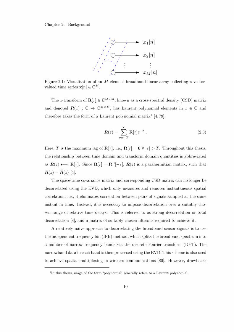
the discrete time index n and is assumed to be zero mean. A visualisation of an
array collecting broadband data is provided in Figure 2.1. Auto-correlation functions
of the M measurements in x[n] reside along the main diagonal of R[τ ], while cross-
correlation terms between the different entries of x[n] form the off-diagonal terms, such
that R[τ ] = RH[−τ ].
9
Chapter 2. Background
x1[n]
x2[n]
xM [n]
.
.
.
.
.
.
.
.
.
Figure 2.1: Visualisation of an M element broadband linear array collecting a vector-valued time series x[n] ∈ C
M .
The z-transform of R[τ ] ∈ CM×M , known as a cross-spectral density (CSD) matrix
and denoted R(z) : C → CM×M , has Laurent polynomial elements in z ∈ C and
therefore takes the form of a Laurent polynomial matrix1 [4, 79]:
R(z) =T∑
τ=−T
R[τ ]z−τ . (2.3)
Here, T is the maximum lag of R[τ ]; i.e., R[τ ] = 0 ∀ |τ | > T . Throughout this thesis,
the relationship between time domain and transform domain quantities is abbreviated
as R(z) •— R[τ ]. Since R[τ ] = RH[−τ ], R(z) is a parahermitian matrix, such that
R(z) = R(z) [4].
The space-time covariance matrix and corresponding CSD matrix can no longer be
decorrelated using the EVD, which only measures and removes instantaneous spatial
correlation; i.e., it eliminates correlation between pairs of signals sampled at the same
instant in time. Instead, it is necessary to impose decorrelation over a suitably cho-
sen range of relative time delays. This is referred to as strong decorrelation or total
decorrelation [8], and a matrix of suitably chosen filters is required to achieve it.
A relatively naive approach to decorrelating the broadband sensor signals is to use
the independent frequency bin (IFB) method, which splits the broadband spectrum into
a number of narrow frequency bands via the discrete Fourier transform (DFT). The
narrowband data in each band is then processed using the EVD. This scheme is also used
to achieve spatial multiplexing in wireless communications [80]. However, drawbacks
1In this thesis, usage of the term ‘polynomial’ generally refers to a Laurent polynomial.
10
Chapter 2. Background
with this method are that the relatively small but important correlations between
frequency bands are ignored, thus limiting the degree to which strong decorrelation
can be achieved. It can also lead to a lack of phase coherence across the bands, since
in each band the eigenvectors can experience an arbitrary phase shift and permutation
(alongside the eigenvalues) relative to neighboring bands. These features of the IFB
technique for space-time adaptive processing have previously been observed in phased
array radar applications [81].
2.3 Polynomial Matrix Eigenvalue Decomposition
2.3.1 Definition
Research in [6] generalises the EVD to the case of broadband sensor arrays and con-
volutive mixing by requiring the strong decorrelation to be implemented using an FIR
paraunitary polynomial matrix [7]. A paraunitary polynomial matrix represents a mul-
tichannel all-pass filter and, accordingly, it preserves the total signal power at every
frequency [4]. In order to achieve strong decorrelation, the paraunitary matrix seeks
to diagonalise a parahermitian polynomial matrix by means of a generalised similarity
transformation in what has become known as a polynomial matrix eigenvalue decom-
position (PEVD).
The PEVD [6] uses a paraunitary matrix F (z) or Q(z) to approximately diagonalise
a parahermitian CSD matrix R(z) such that
R(z) ≈ F (z)D(z)F (z) = Q(z)D(z)Q(z) , (2.4)
where D(z) ≈ diagd1(z), d2(z), . . . , dM (z) approximates a diagonal matrix and
is typically spectrally majorised [8] with power spectral densities (PSDs) dm(ejΩ) ≥dm+1(e
jΩ) ∀ Ω, m = 1 . . . (M − 1), where dm(ejΩ) = dm(z)|z=ejΩ . The diagonal of D(z)
contains approximate polynomial eigenvalues, and the rows and columns of F (z) and
Q(z), respectively, are approximate polynomial eigenvectors such that F (z) = Q(z).
While the definition of the PEVD in [6] generates polynomial eigenvectors of the form
of F (z), the PEVD formulations of [9, 10, 53, 54] utilise the form of Q(z). Both forms
11
Chapter 2. Background
are used in this thesis; thus, different variables are used for clarity. The paraunitary
property of the eigenvectors ensures that
F (z)F (z) = F (z)F (z) = Q(z)Q(z) = Q(z)Q(z) = IM , (2.5)
where IM is an M ×M identity matrix. Note that the decomposition in (2.4) is unique
up to permutations and arbitrary all-pass filters applied to the eigenvectors.
Equation (2.4) has only approximate equality, as the PEVD of a finite order poly-
nomial matrix is generally transcendental; i.e. it is not of finite order. However, the
approximation error can be shown to become arbitrarily small if the order of the ap-
proximation is selected sufficiently large [9]. A finite order approximation will therefore
lead to only approximate diagonality of D(z) in (2.4). Similarly, a finite order approx-
imation of F (z) or Q(z) through trimming will result in only approximate equality
in (2.5). A paraunitary matrix can be implemented as a lossless FIR filter bank that
conserves energy; as a result, the terms paraunitary matrix and paraunitary filter are
used interchangeably throughout this thesis.
Recent research in [9, 10] provides conditions for the existence and uniqueness of
eigenvalues and eigenvectors of a PEVD, such that these can be represented by a power
or Laurent series that is absolutely convergent, permitting a direct realisation in the
time domain. Further research in [11] studies the impact of estimation errors in the
sample space-time covariance matrix on its PEVD.
2.3.2 Existing PEVD Algorithms
Iterative Time Domain Algorithms
For the calculation of the PEVD, only very limited ideal cases permit an exact de-
composition. In general, PEVD algorithms have to rely on iterative approaches. The
algorithms in this section operate in the time domain; i.e., they directly manipulate
polynomial coefficients in an effort to diagonalise a parahermitian matrix. As such,
through the course of algorithm iterations, for iteration parameter i, the diagonalisa-
tion metric E(i)diag defined in Section A.3 and [45] is reduced.
12
Chapter 2. Background
An iterative gradient-based method to diagonalise a parahermitian matrix by means
of paraunitary factorisation is presented in [82], but is limited to 2 × 2 parahermitian
matrices with a specific structure found in subband coding. A fixed order approximate
EVD (AEVD) algorithm for parahermitian matrices, operating in the time domain,
was proposed in [52]. It applies a succession of first-order elementary paraunitary filter
stages but does not always compute a good approximation and does not have proven
convergence.
Second-order sequential best rotation (SBR2) [6], which has been proven to converge
to a good approximate PEVD [6,25,83], is the most well-established PEVD algorithm.
Following its implementation on an FPGA in [57–59], the algorithm has been further
developed to employ a multiple shift strategy (MS-SBR2) in [46]. Additional research
in [55] has confirmed that SBR2 converges to a spectrally majorised solution. In every
iteration, SBR2 eliminates the ‘dominant’ off-diagonal element with maximum magni-
tude of a parahermitian matrix by means of a paraunitary operation. The paraunitary
operation is not order-constrained, as in the AEVD [52], and applies a delay such that
the dominant off-diagonal element is transferred onto lag zero of the space-time covari-
ance matrix, R[0]. A Jacobi rotation [2] then eliminates that element and transfers its
energy onto the main diagonal.
In performing a delay operation, SBR2-based algorithms move an entire row and
column of the CSD matrix into the lag zero matrix, where the Jacobi rotation will
only eliminate the maximum element. The elimination of only a single element at each
iteration typically leads to slow diagonalisation performance over algorithm iterations
in practice, which the MS-SBR2 algorithm does not improve upon [66]. A second fam-
ily of algorithms based on the sequential matrix diagonalisation (SMD) algorithm [45]
advance this idea by transferring a greater quantity of energy to the diagonal of the
lag zero matrix at each iteration through the use of a direct EVD. Application of the
eigenvectors generated through an EVD of the lag zero matrix — following the shifting
of energy to lag zero — guarantees that all shifted energy is transferred to the diagonal.
Within a reasonable number of iterations, SMD is able to achieve levels of diagonali-
sation that cannot be obtained by SBR2 [45]. Particular focus is given to SMD in this
13
Chapter 2. Background
thesis for the reasons above, and those described later in Section 3.2.1, where SMD
is found to be the most computationally efficient iterative PEVD algorithm. Further
detail on the operation of SMD is therefore provided in Section A.1, as knowledge of
this algorithm may aid the reader’s understanding of subsequent chapters.
Although SMD has been shown to be able to achieve parahermitian matrix diago-
nalisation using lower order paraunitary matrices — which are beneficial for application
purposes [17–19,21–23,25] — in [45], a developed row-shift truncation strategy in [62]
is able to reduce the order of the paraunitary matrices from SBR2 but not SMD, such
that SBR2 is preferable for a low order decomposition [63].
While the original SMD algorithm transfers the energy of an entire row and column
pair [45], versions of SMD have been created that transfer the energy of multiple domi-
nant elements to the diagonal of the lag zero matrix at each iteration. The first of these,
which comes closest to matching the performance of an idealised maximum energy SMD
algorithm in [84], is denoted multiple shift maximum element SMD (MSME-SMD) [47],
with causality-constrained (C-MSME-SMD) [48] and reduced search space (RS-MSME-
SMD) [50] versions found in the respective papers. Of these multiple shift approaches,
the RS-MSME-SMD algorithm was identified as offering the fastest diagonalisation
speed of all SMD-based algorithms, while producing shorter polynomial matrices than
other multiple shift strategies [50].
Following the development of a ‘cyclic-by-row’ (CbR) approximation to the EVD
step in SMD in [49], which is able to outperform SMD with respect to diagonali-
sation speed without sacrificing performance elsewhere, low-cost CbR versions have
been created for all SMD-based algorithms. Using the CbR PEVD algorithms, the
computational cost to reach a specific level of diagonalisation is reduced below even
what is required for SBR2 [49]. Although multiple shift SMD algorithms were found
to outperform SMD in terms of diagonalisation speed in [47, 48, 50], the equivalent
CbR algorithms were found to be slower than a CbR implementation of SMD due to
the high cost of their search step [65, 66]. Therefore, when the research in this thesis
was initiated, the cyclic-by-row SMD (SMDCbR) algorithm was considered to be the
state-of-the-art iterative PEVD algorithm.
14
Chapter 2. Background
DFT-Based Frequency Domain Algorithms
A DFT-based PEVD formulation is performed in [85]; however, the order of the pa-
raunitary filter banks must be strictly limited. A second example, which transforms
the problem into a pointwise-in-frequency standard matrix decomposition and has been
shown to perform well for finite order problems [56], is provided in [53], but requires
an a priori estimate of the length of the paraunitary matrix in the decomposition.
This algorithm is summarised in Section A.2 for future reference. Such DFT-based
PEVD methods have received renewed interest in recent years [54], due to their abil-
ity to return either a spectrally majorised decomposition, or attempt to approximate
maximally smooth, analytic eigenvalues, which are necessary for good eigenvector esti-
mation [9, 10].
Given their particular relevance in Chapter 5 of this thesis, additional information
regarding the implementation of DFT-based algorithms is provided in Section 5.1.
2.3.3 Implementations of PEVD Algorithms
The PEVD has been successfully used in broadband multiple-input multiple-output
(MIMO) precoding and equalisation using linear [12–14] and non-linear [15, 16] ap-
proaches, broadband angle of arrival estimation [17–20], broadband beamforming [21–
23], optimal subband coding [8,25], joint source-channel coding [27], and scene discov-
ery [30].
A number of successful efforts to reduce the algorithmic cost of iterative PEVD
algorithms have focussed on the trimming of polynomial matrices to curb growth in
order [6, 60–62], which translates directly into a growth of computational complexity.
However, while offering promising results, the PEVD has seen limited deployment in
hardware. A parallel form of SBR2 whose performance has little dependency on the
size of the input parahermitian matrix has been designed and implemented on an
FPGA [57–59], but the SMD algorithm and its cyclic-by-row approximation, which
can achieve superior levels of diagonalisation [45, 49], have been restricted to software
applications — perhaps due to their dramatic increase in computational complexity
with parahermitian matrix spatial dimension [65,66] and non-parallelisable architecture.
15
Chapter 2. Background
For the interested reader, versions of the original SMD and SBR2 algorithms can
be found in the PEVD toolbox [86].
2.4 Simulation Software and Hardware Platform
Unless otherwise stated, all simulations in this thesis are performed within MATLABR©
R2014a under Ubuntu R© 16.04 on an MSIR© GE60-2OE with IntelR© CoreTM i7-4700MQ
2.40GHz × 8 cores, NVIDIAR© GeForceR© GTX 765M, and 8GB RAM.
16
Chapter 3
Computational Advances for the
Iterative PEVD
3.1 Introduction
As evidenced by the contents of Section 2.3.2, a number of iterative PEVD algorithms
have been developed. Despite this, the PEVD has seen limited deployment for applica-
tion purposes due to the high computational cost of these algorithms. This is especially
true for scenarios involving a large number of broadband sensors, which require the de-
composition of parahermitian matrices with a large spatial dimension, M . For example,
as M is increased, the plot of Figure 3.1 from [65] demonstrates the increasingly poor
diagonalisation versus execution time performance of the recent multiple shift maxi-
mum element SMD (MSME-SMD) algorithm. Here, the diagonalisation metric E(i)diag
defined in Section A.3 and [45] is used. For the case of a parahermitian matrix with
spatial dimensions of 20 × 20, which in practice might be generated using data from
20 sensors, MSME-SMD requires hundreds of seconds to achieve even a moderate level
of diagonalisation. Clearly, for application purposes, the required execution time of
PEVD algorithms must be reduced.
This chapter therefore details a number of novel methods to lower the computational
cost of existing iterative algorithms related to the PEVD. These methods conquer
unexplored areas of PEVD algorithm improvement by optimising matrix manipulations
17
Chapter 3. Computational Advances for the Iterative PEVD
MSME-SMD
SMD
ME-SMD
M = 4M = 10
M = 20
Ensemble-averaged algorithm execution time / s
5log
10E
E(i)
diag/[dB]
Figure 3.1: MSME-SMD, SMD [45], and maximum element SMD (ME-SMD) [45]diagonalisation speed for increasing spatial dimension M [65].
in software in Section 3.2, exploiting parahermitian matrix symmetry in Section 3.3,
minimising algorithmic redundancy in Section 3.4, and reducing the search and update
space of iterative PEVD algorithms in Sections 3.5 and 3.6. Repeated application of
the polynomial matrix QR decomposition (PQRD) to a parahermitian matrix in a
manner analogous to the QR algorithm [87] can be used to form a PEVD. A similar
application of the PQRD has been explored for the polynomial matrix singular value
decomposition (PSVD) in [43]. Improvements are therefore made to an existing PQRD
algorithm in Section 3.7, such that both PEVD and PSVD implementations that rely
on the PQRD can also benefit. Finally, improvements to an existing polynomial matrix
truncation strategy yield benefits in Section 3.8, such that polynomial matrix length
can be reduced without significantly impacting on decomposition mean square error.
18
Chapter 3. Computational Advances for the Iterative PEVD
3.2 Optimising Matrix Manipulations to Increase Algo-
rithmic Efficiency
For application purposes, PEVD algorithms inevitably have to be implemented in soft-
ware and subsequently deployed to hardware. A number of algorithmic improvements
have been made to increase the performance of several iterative PEVD algorithm ar-
chitectures [46–50,88]; however, specifics regarding the algorithms’ efficient implemen-
tation in software have not been addressed. This section therefore discusses a number
of novel, significant ways to increase the algorithmic efficiency of iterative PEVD al-
gorithms and polynomial matrix implementations without impacting accuracy. Meth-
ods to compute the product of a matrix and polynomial matrix are discussed in Sec-
tion 3.2.1. Furthermore, efficient techniques to compute the product of two polynomial
matrices are detailed in Section 3.2.2. The optimal point at which to integrate poly-
nomial matrix truncation into iterative PEVD algorithms is explored in Section 3.2.3.
Conclusions for this section are drawn in Section 3.2.4.
Elements of the work on polynomial matrix truncation in this section can be found
published in the proceedings of the 24th European Signal Processing Conference in a
paper titled ‘Memory and Complexity Reduction in Parahermitian Matrix Manipula-
tions of PEVD Algorithms’ [67].
3.2.1 Product of a Matrix and Polynomial Matrix
In a number of iterative PEVD algorithms [45,47,48,50], the product of a matrix and
polynomial matrix is computed at least once per iteration. An example of this product
can be seen in (A.5); here, it is required to transfer off-diagonal energy in the lag zero
matrix of a parahermitian matrix onto the diagonal. Given that a significant number
of iterations are typically required for convergence of a PEVD algorithm, this matrix
multiplication step quickly forms a significant portion of the computational cost of such
algorithms [45].
19
Chapter 3. Computational Advances for the Iterative PEVD
Matrix Multiplication Methods
Existing implementations of the algorithms in [45, 47, 48, 50] in MATLABR© typi-
cally make use of a polynomial matrix convolution function denoted PolyMatConv(·)from [86], whereby S(z) = PolyMatConv(Q(z),R(z)) computes the product S(z) =
Q(z)R(z), where S(z),R(z),Q(z) : C → CM×M . This function is implemented such
that the polynomial element in the mth row and nth column of S(z) is found via
sm,n(z) •— sm,n[τ ] = qm,1[τ ]∗r1,n[τ ]+qm,2[τ ]∗r2,n[τ ]+ . . .+qm,M [τ ]∗rM,n[τ ] . (3.1)
If Q(z) is instead replaced with a simple matrix of coefficients Q as in (A.5), the
implementation in (3.1) ∀ m,n — which involves a large number (M3) of convolution
operations — is not efficient. An alternative implementation for a parahermitian R(z)
can instead compute
S[τ ] = QR[τ ] , ∀ τ , (3.2)
which requires L M × M matrix multiplications, where L = 2T + 1 is the length
of R[τ ] and T is its maximum lag. Given that MATLABR© is optimised for matrix
multiplication [89], (3.2) is more efficient than (3.1) in this case. In essence, a choice is
made to interpret R(z) as a single polynomial with matrix valued coefficients in (3.2),
rather than a matrix of polynomials as in (3.1).
The formulation in (3.2) is highly parallelisable, as matrix multiplications for each
τ are independent. This work therefore proposes the following novel approach, which
enables the simultaneous computation of all lags of S[τ ]. In this approach, by placing
coefficient matrices of R[τ ] side-by-side in a horizontally concatenated matrix Rh ∈CM×ML,
Rh = [R[−T ] R[−T + 1] · · · R[T ] ] , (3.3)
one can compute
Sh = [S[−T ] S[−T + 1] · · · S[T ] ] = QRh , (3.4)
which can be rearranged with little effort to obtain S[τ ].
The product in (A.5) also requires application of QH from the right — i.e., a formu-
20
Chapter 3. Computational Advances for the Iterative PEVD
lation where S′(z) = S(z)QH. Equations (3.1) and (3.2) can be very easily modified to
accommodate this; however, the approach of (3.4) must be considered further, as the
dimensionalities of Sh ∈ CM×ML and QH ∈ C
M×M are incompatible. Instead, one can
compute S′v ∈ C
ML×M using a vertically concatenated matrix Sv ∈ CML×M :
S′v =
S′[−T ]S′[−T + 1]
...
S′[T ]
= SvQH =
S[−T ]S[−T + 1]
...
S[T ]
QH , (3.5)
which can again be rearranged to obtain S′[τ ]. A combination of (3.4) and (3.5)
therefore enables computation of the productQR(z)QH using a mixture of horizontally
and vertically concatenated matrices.
Matrix Multiplication Performance Comparison
To compare the computational costs of each of the three matrix multiplication methods,
the simulations below record the average time taken for 103 instances of each method
to compute S′(z) = QR(z)QH in MATLABR© for M ∈ 5; 10; 20 and T ∈ 50; 100,with parahermitian matrix R(z) = A(z)A(z) of length L = 2T + 1. Matrices A(z) :
C → CM×M and Q ∈ C
M×M contain coefficients drawn from a randomised complex
Gaussian source with unit variance and zero mean.
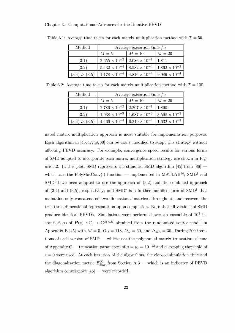
In Table 3.1, it can be seen that the combined approach utilising (3.4) and (3.5)
is faster than other methods for T = 50, while the PolyMatConv(·) function that is
widespread in existing PEVD algorithms is by far the slowest. The latter experiences
a significant slowdown as M increases, while the remaining methods decrease in speed
more gradually.
Similar results can be found in Table 3.2 for T = 100, where the increase in tem-
poral dimension has universally increased execution time requirements. Note that the
approach using PolyMatConv(·) is less affected than the other methods, but is still
significantly slower.
From these results, it can be concluded that the proposed two-dimensional concate-
21
Chapter 3. Computational Advances for the Iterative PEVD
Table 3.1: Average time taken for each matrix multiplication method with T = 50.
Method Average execution time / s
M = 5 M = 10 M = 20
(3.1) 2.655 × 10⁻² 2.086 × 10⁻¹ 1.811
(3.2) 5.432 × 10⁻⁴ 8.582 × 10⁻⁴ 1.862 × 10⁻³
(3.4) & (3.5) 1.178 × 10⁻⁴ 4.816 × 10⁻⁴ 9.986 × 10⁻⁴
Table 3.2: Average time taken for each matrix multiplication method with T = 100.
Method Average execution time / s
M = 5 M = 10 M = 20
(3.1) 2.786 × 10⁻² 2.207 × 10⁻¹ 1.890
(3.2) 1.038 × 10⁻³ 1.687 × 10⁻³ 3.598 × 10⁻³
(3.4) & (3.5) 4.466 × 10⁻⁴ 6.249 × 10⁻⁴ 1.632 × 10⁻³
nated matrix multiplication approach is most suitable for implementation purposes.
Each algorithm in [45,47,48,50] can be easily modified to adopt this strategy without
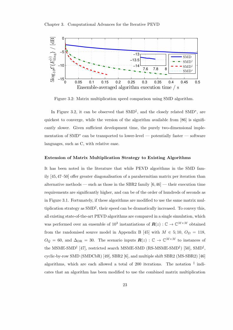
affecting PEVD accuracy. For example, convergence speed results for various forms
of SMD adapted to incorporate each matrix multiplication strategy are shown in Fig-
ure 3.2. In this plot, SMD represents the standard SMD algorithm [45] from [86] —
which uses the PolyMatConv(·) function — implemented in MATLABR©; SMD† and
SMD‡ have been adapted to use the approach of (3.2) and the combined approach
of (3.4) and (3.5), respectively; and SMD∗ is a further modified form of SMD‡ that
maintains only concatenated two-dimensional matrices throughout, and recovers the
true three-dimensional representation upon completion. Note that all versions of SMD
produce identical PEVDs. Simulations were performed over an ensemble of 103 in-
stantiations of R(z) : C → CM×M obtained from the randomised source model in
Appendix B [45] with M = 5, OD = 118, OQ = 60, and ∆DR = 30. During 200 itera-
tions of each version of SMD — which uses the polynomial matrix truncation scheme
of Appendix C — truncation parameters of µ = µt = 10−12 and a stopping threshold of
ǫ = 0 were used. At each iteration of the algorithms, the elapsed simulation time and
the diagonalisation metric E(i)diag from Section A.3 — which is an indicator of PEVD
algorithm convergence [45] — were recorded.
22
Chapter 3. Computational Advances for the Iterative PEVD
0 0.05 0.1 0.15 0.2 0.25 0.3 0.35 0.4 0.45 0.5−15
−10
−5
0
Ensemble-averaged algorithm execution time / s
5log
10EE
(i)
diag
/[dB]
SMD
SMD†
SMD‡
SMD∗7.6 7.8 8
−14
−13.5
−13
Figure 3.2: Matrix multiplication speed comparison using SMD algorithm.
In Figure 3.2, it can be observed that SMD‡, and the closely related SMD∗, are
quickest to converge, while the version of the algorithm available from [86] is signifi-
cantly slower. Given sufficient development time, the purely two-dimensional imple-
mentation of SMD∗ can be transported to lower-level — potentially faster — software
languages, such as C, with relative ease.
Extension of Matrix Multiplication Strategy to Existing Algorithms
It has been noted in the literature that while PEVD algorithms in the SMD fam-
ily [45,47–50] offer greater diagonalisation of a parahermitian matrix per iteration than
alternative methods — such as those in the SBR2 family [6,46] — their execution time
requirements are significantly higher, and can be of the order of hundreds of seconds as
in Figure 3.1. Fortunately, if these algorithms are modified to use the same matrix mul-
tiplication strategy as SMD‡, their speed can be dramatically increased. To convey this,
all existing state-of-the-art PEVD algorithms are compared in a single simulation, which
was performed over an ensemble of 103 instantiations of R(z) : C → CM×M obtained
from the randomised source model in Appendix B [45] with M ∈ 5; 10, OD = 118,
OQ = 60, and ∆DR = 30. The scenario inputs R(z) : C → CM×M to instances of
the MSME-SMD‡ [47], restricted search MSME-SMD (RS-MSME-SMD‡) [50], SMD‡,
cyclic-by-row SMD (SMDCbR) [49], SBR2 [6], and multiple shift SBR2 (MS-SBR2) [46]
algorithms, which are each allowed a total of 200 iterations. The notation ‡ indi-
cates that an algorithm has been modified to use the combined matrix multiplication
23
Chapter 3. Computational Advances for the Iterative PEVD
approach of (3.4) and (3.5). Each algorithm utilised the truncation strategy of Ap-
pendix C with polynomial matrix truncation parameters of µ = µt = 10−6. At each
iteration of the algorithms, the elapsed simulation time and diagonalisation metric E(i)diag
from Section A.3 were recorded.
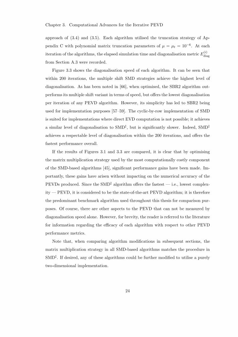
Figure 3.3 shows the diagonalisation speed of each algorithm. It can be seen that
within 200 iterations, the multiple shift SMD strategies achieve the highest level of
diagonalisation. As has been noted in [66], when optimised, the SBR2 algorithm out-
performs its multiple shift variant in terms of speed, but offers the lowest diagonalisation
per iteration of any PEVD algorithm. However, its simplicity has led to SBR2 being
used for implementation purposes [57–59]. The cyclic-by-row implementation of SMD
is suited for implementations where direct EVD computation is not possible; it achieves
a similar level of diagonalisation to SMD‡, but is significantly slower. Indeed, SMD‡
achieves a respectable level of diagonalisation within the 200 iterations, and offers the
fastest performance overall.
If the results of Figures 3.1 and 3.3 are compared, it is clear that by optimising
the matrix multiplication strategy used by the most computationally costly component
of the SMD-based algorithms [45], significant performance gains have been made. Im-
portantly, these gains have arisen without impacting on the numerical accuracy of the
PEVDs produced. Since the SMD‡ algorithm offers the fastest — i.e., lowest complex-
ity — PEVD, it is considered to be the state-of-the-art PEVD algorithm; it is therefore
the predominant benchmark algorithm used throughout this thesis for comparison pur-
poses. Of course, there are other aspects to the PEVD that can not be measured by
diagonalisation speed alone. However, for brevity, the reader is referred to the literature
for information regarding the efficacy of each algorithm with respect to other PEVD
performance metrics.
Note that, when comparing algorithm modifications in subsequent sections, the
matrix multiplication strategy in all SMD-based algorithms matches the procedure in
SMD‡. If desired, any of these algorithms could be further modified to utilise a purely
two-dimensional implementation.
24
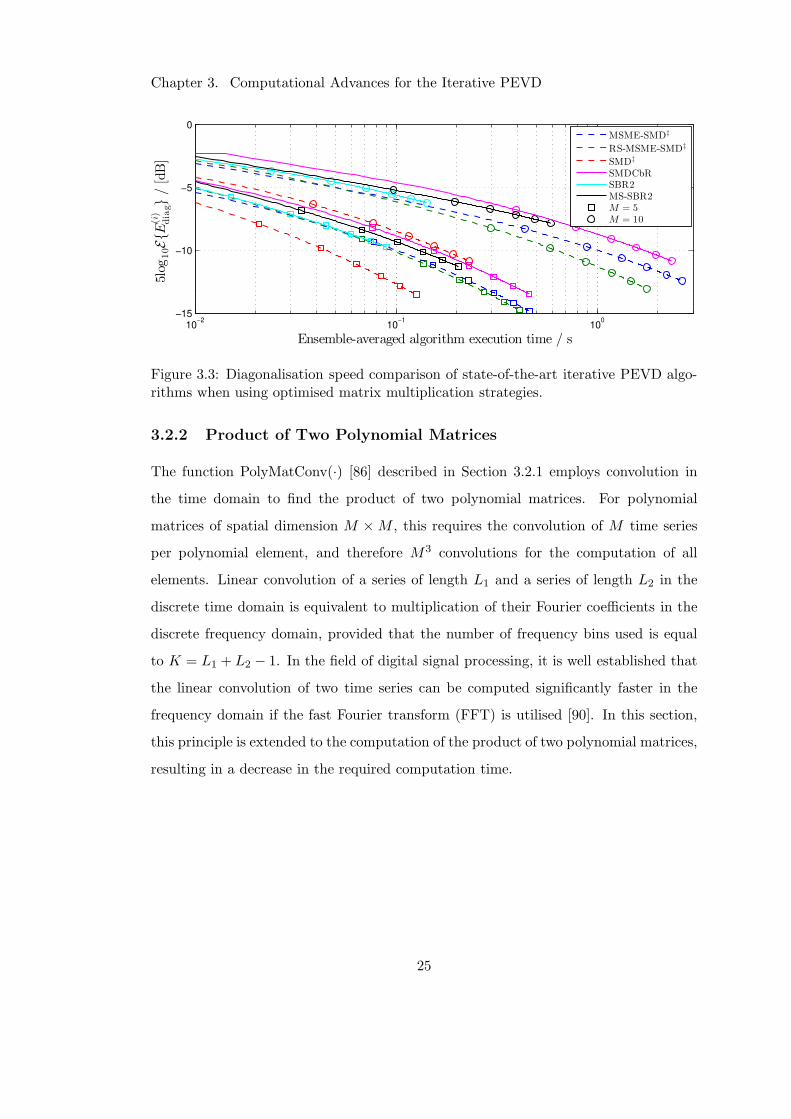
Chapter 3. Computational Advances for the Iterative PEVD
10−2
10−1
100
−15
−10
−5
0
Ensemble-averaged algorithm execution time / s
5log
10EE
(i)
diag
/[dB]
MSME-SMD‡
RS-MSME-SMD‡
SMD‡
SMDCbRSBR2MS-SBR2M = 5M = 10
Figure 3.3: Diagonalisation speed comparison of state-of-the-art iterative PEVD algo-rithms when using optimised matrix multiplication strategies.
3.2.2 Product of Two Polynomial Matrices
The function PolyMatConv(·) [86] described in Section 3.2.1 employs convolution in
the time domain to find the product of two polynomial matrices. For polynomial
matrices of spatial dimension M ×M , this requires the convolution of M time series
per polynomial element, and therefore M3 convolutions for the computation of all
elements. Linear convolution of a series of length L1 and a series of length L2 in the
discrete time domain is equivalent to multiplication of their Fourier coefficients in the
discrete frequency domain, provided that the number of frequency bins used is equal
to K = L1 + L2 − 1. In the field of digital signal processing, it is well established that
the linear convolution of two time series can be computed significantly faster in the
frequency domain if the fast Fourier transform (FFT) is utilised [90]. In this section,
this principle is extended to the computation of the product of two polynomial matrices,
resulting in a decrease in the required computation time.
25
Chapter 3. Computational Advances for the Iterative PEVD
Moving to the Frequency Domain
The product S(z) = Q(z)R(z) computed by S(z) = PolyMatConv(Q(z),R(z)), where
S(z) : C→ CM×N , Q(z) : C→ C
M×P , and R(z) : C→ CP×N , is found via
sm,n(z) •— sm,n[τ ] =
P∑
p=1
qm,p[τ ] ∗ rp,n[τ ] . (3.6)
Here, S(z) has length LS = LQ + LR − 1, where LQ and LR are the lengths of Q(z)
and R(z), respectively.
The same product can be computed in the frequency domain if Q(z) and R(z) are
evaluated at K = LS points on the unit circle (z = ejΩk , Ωk = 2πk/K) using the FFT.
Here, S[k] = S(z)|z=ejΩk is obtained via matrix multiplication:
S[k] = Q[k]R[k] , k = 0 . . . K − 1 . (3.7)
The inverse FFT (IFFT) then recovers S(z).
In MATLABR© — which is often the software of choice for the implementation
of DSP algorithms — FFT, IFFT, and matrix multiplication operations are highly
optimised [89,91–93]. An alternative implementation of PolyMatConv(·) that computes
the product of two polynomial matrices in the frequency domain as described above
is therefore well-suited to this platform. Such an implementation is introduced in this
work, and is named PolyMatConvFreq(·). A particular third-party MATLABR© library
named MTIMESX [94] is optimised for computing the product of multi-dimensional
matrices, and can therefore facilitate fast computation of S[k].
Results and Discussion
Below, the computational cost of PolyMatConv(·) is compared with the costs of two
frequency-based implementations. The first of these, encapsulated in a function denoted
PolyMatConvFreq1(·) employs the matrix multiplication routines native to MATLABR©,
while the second, denoted PolyMatConvFreq2(·) uses the MTIMESX library.
To compare the computational costs of each of the three methods, in the simulations
26
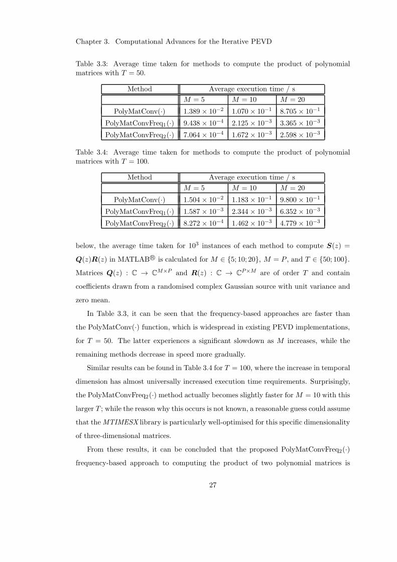
Chapter 3. Computational Advances for the Iterative PEVD
Table 3.3: Average time taken for methods to compute the product of polynomialmatrices with T = 50.
Method Average execution time / s
M = 5 M = 10 M = 20
PolyMatConv(·) 1.389 × 10⁻² 1.070 × 10⁻¹ 8.705 × 10⁻¹
PolyMatConvFreq1(·) 9.438 × 10⁻⁴ 2.125 × 10⁻³ 3.365 × 10⁻³
PolyMatConvFreq2(·) 7.064 × 10⁻⁴ 1.672 × 10⁻³ 2.598 × 10⁻³
Table 3.4: Average time taken for methods to compute the product of polynomialmatrices with T = 100.
Method Average execution time / s
M = 5 M = 10 M = 20
PolyMatConv(·) 1.504 × 10⁻² 1.183 × 10⁻¹ 9.800 × 10⁻¹
PolyMatConvFreq1(·) 1.587 × 10⁻³ 2.344 × 10⁻³ 6.352 × 10⁻³
PolyMatConvFreq2(·) 8.272 × 10⁻⁴ 1.462 × 10⁻³ 4.779 × 10⁻³
below, the average time taken for 103 instances of each method to compute S(z) =
Q(z)R(z) in MATLABR© is calculated for M ∈ 5; 10; 20, M = P , and T ∈ 50; 100.Matrices Q(z) : C → C
M×P and R(z) : C → CP×M are of order T and contain
coefficients drawn from a randomised complex Gaussian source with unit variance and
zero mean.
In Table 3.3, it can be seen that the frequency-based approaches are faster than
the PolyMatConv(·) function, which is widespread in existing PEVD implementations,
for T = 50. The latter experiences a significant slowdown as M increases, while the
remaining methods decrease in speed more gradually.
Similar results can be found in Table 3.4 for T = 100, where the increase in temporal
dimension has almost universally increased execution time requirements. Surprisingly,
the PolyMatConvFreq2(·) method actually becomes slightly faster for M = 10 with this
larger T ; while the reason why this occurs is not known, a reasonable guess could assume
that theMTIMESX library is particularly well-optimised for this specific dimensionality
of three-dimensional matrices.
From these results, it can be concluded that the proposed PolyMatConvFreq2(·)frequency-based approach to computing the product of two polynomial matrices is
27
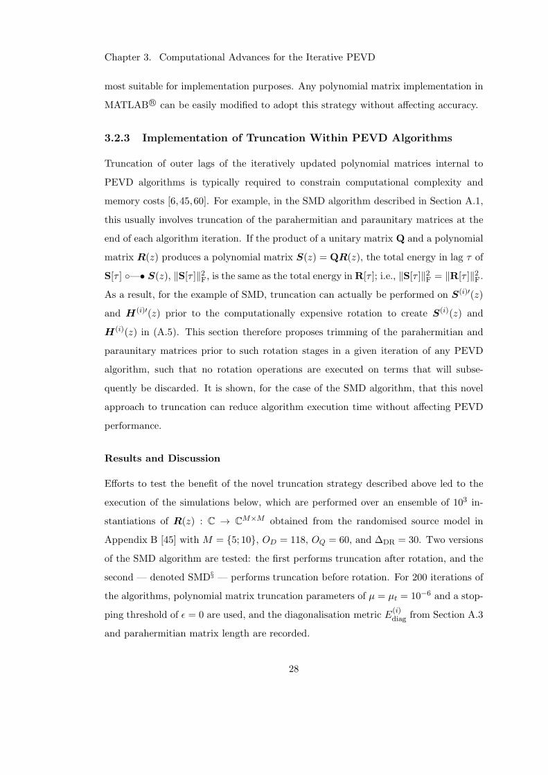
Chapter 3. Computational Advances for the Iterative PEVD
most suitable for implementation purposes. Any polynomial matrix implementation in
MATLABR© can be easily modified to adopt this strategy without affecting accuracy.
3.2.3 Implementation of Truncation Within PEVD Algorithms
Truncation of outer lags of the iteratively updated polynomial matrices internal to
PEVD algorithms is typically required to constrain computational complexity and
memory costs [6,45,60]. For example, in the SMD algorithm described in Section A.1,
this usually involves truncation of the parahermitian and paraunitary matrices at the
end of each algorithm iteration. If the product of a unitary matrix Q and a polynomial
matrix R(z) produces a polynomial matrix S(z) = QR(z), the total energy in lag τ of
S[τ ] —• S(z), ‖S[τ ]‖2F, is the same as the total energy inR[τ ]; i.e., ‖S[τ ]‖2F = ‖R[τ ]‖2F.As a result, for the example of SMD, truncation can actually be performed on S(i)′(z)
and H(i)′(z) prior to the computationally expensive rotation to create S(i)(z) and
H(i)(z) in (A.5). This section therefore proposes trimming of the parahermitian and
paraunitary matrices prior to such rotation stages in a given iteration of any PEVD
algorithm, such that no rotation operations are executed on terms that will subse-
quently be discarded. It is shown, for the case of the SMD algorithm, that this novel
approach to truncation can reduce algorithm execution time without affecting PEVD
performance.
Results and Discussion
Efforts to test the benefit of the novel truncation strategy described above led to the
execution of the simulations below, which are performed over an ensemble of 103 in-
stantiations of R(z) : C → CM×M obtained from the randomised source model in
Appendix B [45] with M = 5; 10, OD = 118, OQ = 60, and ∆DR = 30. Two versions
of the SMD algorithm are tested: the first performs truncation after rotation, and the
second — denoted SMD§ — performs truncation before rotation. For 200 iterations of
the algorithms, polynomial matrix truncation parameters of µ = µt = 10−6 and a stop-
ping threshold of ǫ = 0 are used, and the diagonalisation metric E(i)diag from Section A.3
and parahermitian matrix length are recorded.
28
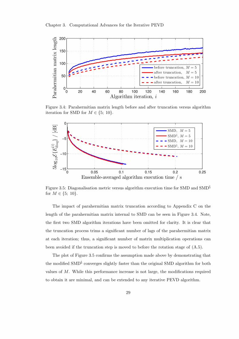
Chapter 3. Computational Advances for the Iterative PEVD
0 20 40 60 80 100 120 140 160 180 2000
50
100
150
200
Algorithm iteration, iParahermitianmatrixlength
before truncation, M = 5
after truncation, M = 5
before truncation, M = 10
after truncation, M = 10
Figure 3.4: Parahermitian matrix length before and after truncation versus algorithmiteration for SMD for M ∈ 5; 10.
0 0.05 0.1 0.15 0.2 0.25−15
−10
−5
0
Ensemble-averaged algorithm execution time / s
5log
10EE
(i)
diag
/[dB]
SMD, M = 5
SMD§, M = 5
SMD, M = 10
SMD§, M = 10
Figure 3.5: Diagonalisation metric versus algorithm execution time for SMD and SMD§
for M ∈ 5; 10.
The impact of parahermitian matrix truncation according to Appendix C on the
length of the parahermitian matrix internal to SMD can be seen in Figure 3.4. Note,
the first two SMD algorithm iterations have been omitted for clarity. It is clear that
the truncation process trims a significant number of lags of the parahermitian matrix
at each iteration; thus, a significant number of matrix multiplication operations can
been avoided if the truncation step is moved to before the rotation stage of (A.5).
The plot of Figure 3.5 confirms the assumption made above by demonstrating that
the modified SMD§ converges slightly faster than the original SMD algorithm for both
values of M . While this performance increase is not large, the modifications required
to obtain it are minimal, and can be extended to any iterative PEVD algorithm.
29
Chapter 3. Computational Advances for the Iterative PEVD
Note that, when comparing algorithm modifications directly in subsequent sections,
the implementation of truncation in any modified algorithms matches the truncation
procedure in the original algorithm to avoid bias in any algorithm performance results.
3.2.4 Summary
This section has discussed a number of novel, significant ways to increase the algorith-
mic efficiency of iterative PEVD algorithms and polynomial matrix implementations.
An efficient, two-dimensional approach to computing the product of a matrix and poly-
nomial matrix has been introduced; when integrated with existing SMD-based PEVD
algorithms, this has been shown to dramatically increase their speed. In fact, the speed
of the improved SMD algorithm has been increased to the point where SMD can now be
considered to be the most efficient, state-of-the-art iterative PEVD algorithm. Further-
more, it has been shown that the execution time of polynomial matrix implementations
can be reduced by evaluating the product of two polynomial matrices in the frequency
domain. Finally, the optimal point at which to integrate polynomial matrix truncation
into iterative PEVD algorithms has been explored.
Importantly, the algorithmic efficiency improvements discussed in this section can
be extended to any number of PEVD-based implementations without loss of accuracy.
3.3 Parahermitian Matrix Symmetry and the Half-Matrix
Approach
This section addresses savings — in terms of both computational complexity and mem-
ory use — that exploit the natural symmetry of the parahermitian structure of the
matrix being decomposed in PEVD algorithms, such that only one half of its elements
are stored and processed. A demonstration of how this approach can be implemented
within existing PEVD algorithms is shown through the modification of the SMD algo-
rithm [45] described in Section A.1. The modified form of SMD is named half-matrix
SMD (HSMD).
Based on the half-matrix representation of a parahermitian matrix defined in
30
Chapter 3. Computational Advances for the Iterative PEVD
Section 3.3.1, Section 3.3.2 provides an overview of the HSMD algorithm, Section 3.3.3
outlines the parameter search of HSMD, and Section 3.3.4 details the implementation of
column- and row-shifts in HSMD. The resource requirements and performances of SMD
and HSMD are compared in Section 3.3.5 and Section 3.3.6, respectively. Subsequently,
conclusions are provided in Section 3.3.7.
Elements of the work in this section can be found published in the proceedings of the
24th European Signal Processing Conference in a paper titled ‘Memory and Complexity
Reduction in Parahermitian Matrix Manipulations of PEVD Algorithms’ [67].
3.3.1 Half-Matrix Representation of a Parahermitian Matrix
By partitioning a parahermitian matrix R(z), it is possible to write
R(z) = R(−)(z) +R[0] +R(+)(z) , (3.8)
where R[0] is the lag zero matrix of R(z), R(+)(z) contains terms for positive lag
(τ > 0) elements only, and R(−)(z) = R(+)(z). It is therefore sufficient to record half
of R(z), which here without loss of generality is R[0] +R(+)(z). For the remainder of
this thesis, the notation · is used to represent the recorded half of a parahermitian
matrix; i.e., R(z) = R[0] +R(+)(z) and R(z) •— R[τ ], where
R[τ ] =
R[τ ], 0 ≤ τ ≤ T
0, otherwise. (3.9)
If one possesses knowledge of R(z), one has all the information required to obtain R(z),
R[τ ], and R[τ ]. Given this relationship, R(z) is therefore referred to as a parahermitian
matrix throughout the remainder of this thesis for brevity. In addition, R(z) and R[τ ]
are referred to as the ‘half-matrix’ versions of the ‘full-matrix’ representations R(z) and
R[τ ], respectively. As an example, Figure 3.6 demonstrates both half- and full-matrix
representations of a 5× 5 matrix with maximum lag T = 3.
31
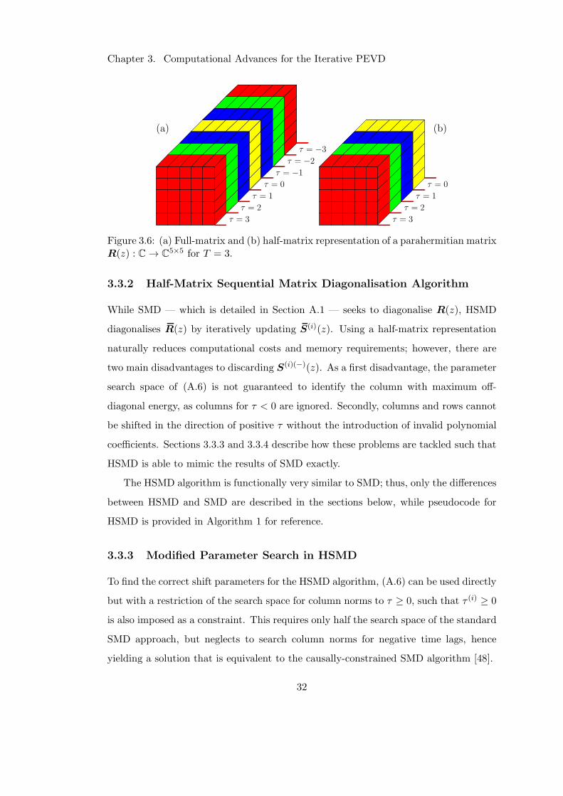
Chapter 3. Computational Advances for the Iterative PEVD
a)
= 3
= 2
= 1
= 0
= 1
= 2
= 3
= 3
= 2
= 1
= 0
b)
Figure 3.6: (a) Full-matrix and (b) half-matrix representation of a parahermitian matrixR(z) : C→ C
5×5 for T = 3.
3.3.2 Half-Matrix Sequential Matrix Diagonalisation Algorithm
While SMD — which is detailed in Section A.1 — seeks to diagonalise R(z), HSMD
diagonalises R(z) by iteratively updating S(i)(z). Using a half-matrix representation
naturally reduces computational costs and memory requirements; however, there are
two main disadvantages to discarding S(i)(−)(z). As a first disadvantage, the parameter
search space of (A.6) is not guaranteed to identify the column with maximum off-
diagonal energy, as columns for τ < 0 are ignored. Secondly, columns and rows cannot
be shifted in the direction of positive τ without the introduction of invalid polynomial
coefficients. Sections 3.3.3 and 3.3.4 describe how these problems are tackled such that
HSMD is able to mimic the results of SMD exactly.
The HSMD algorithm is functionally very similar to SMD; thus, only the differences
between HSMD and SMD are described in the sections below, while pseudocode for
HSMD is provided in Algorithm 1 for reference.
3.3.3 Modified Parameter Search in HSMD
To find the correct shift parameters for the HSMD algorithm, (A.6) can be used directly
but with a restriction of the search space for column norms to τ ≥ 0, such that τ (i) ≥ 0
is also imposed as a constraint. This requires only half the search space of the standard
SMD approach, but neglects to search column norms for negative time lags, hence
yielding a solution that is equivalent to the causally-constrained SMD algorithm [48].
32
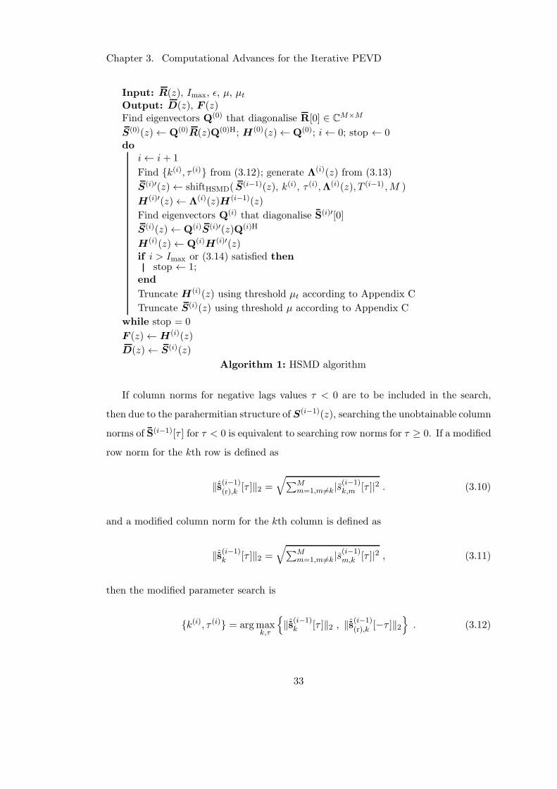
Chapter 3. Computational Advances for the Iterative PEVD
Input: R(z), Imax, ǫ, µ, µt
Output: D(z), F (z)Find eigenvectors Q(0) that diagonalise R[0] ∈ C
M×M
S(0)(z)← Q(0)R(z)Q(0)H; H(0)(z)← Q(0); i← 0; stop ← 0do
i← i+ 1
Find k(i), τ (i) from (3.12); generate Λ(i)(z) from (3.13)
S(i)′(z)← shiftHSMD(S(i−1)(z), k(i), τ (i),Λ(i)(z), T (i−1),M )
H(i)′(z)← Λ(i)(z)H (i−1)(z)
Find eigenvectors Q(i) that diagonalise S(i)′[0]
S(i)(z)← Q(i)S(i)′(z)Q(i)H
H(i)(z)← Q(i)H(i)′(z)if i > Imax or (3.14) satisfied then
stop ← 1;end
Truncate H(i)(z) using threshold µt according to Appendix C
Truncate S(i)(z) using threshold µ according to Appendix C
while stop = 0
F (z)←H(i)(z)
D(z)← S(i)(z)
Algorithm 1: HSMD algorithm
If column norms for negative lags values τ < 0 are to be included in the search,
then due to the parahermitian structure of S(i−1)(z), searching the unobtainable column
norms of S(i−1)[τ ] for τ < 0 is equivalent to searching row norms for τ ≥ 0. If a modified
row norm for the kth row is defined as
‖s(i−1)(r),k
[τ ]‖2 =
√∑M
m=1,m6=k|s(i−1)k,m [τ ]|2 . (3.10)
and a modified column norm for the kth column is defined as
‖s(i−1)k [τ ]‖2 =
√∑M
m=1,m6=k|s(i−1)m,k [τ ]|2 , (3.11)
then the modified parameter search is
k(i), τ (i) = argmaxk,τ
‖s(i−1)k [τ ]‖2 , ‖s(i−1)
(r),k [−τ ]‖2
. (3.12)
33
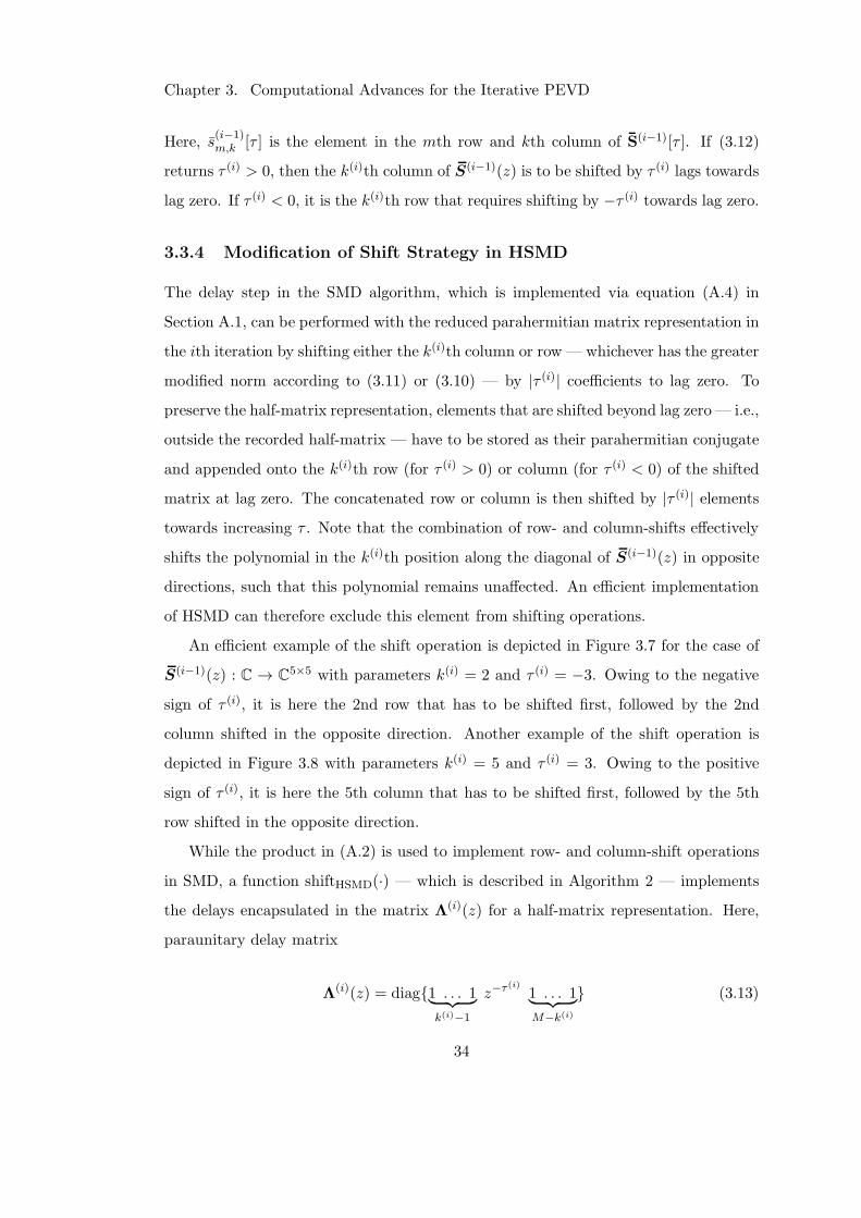
Chapter 3. Computational Advances for the Iterative PEVD
Here, s(i−1)m,k [τ ] is the element in the mth row and kth column of S(i−1)[τ ]. If (3.12)
returns τ (i) > 0, then the k(i)th column of S(i−1)(z) is to be shifted by τ (i) lags towards
lag zero. If τ (i) < 0, it is the k(i)th row that requires shifting by −τ (i) towards lag zero.
3.3.4 Modification of Shift Strategy in HSMD
The delay step in the SMD algorithm, which is implemented via equation (A.4) in
Section A.1, can be performed with the reduced parahermitian matrix representation in
the ith iteration by shifting either the k(i)th column or row — whichever has the greater
modified norm according to (3.11) or (3.10) — by |τ (i)| coefficients to lag zero. To
preserve the half-matrix representation, elements that are shifted beyond lag zero — i.e.,
outside the recorded half-matrix — have to be stored as their parahermitian conjugate
and appended onto the k(i)th row (for τ (i) > 0) or column (for τ (i) < 0) of the shifted
matrix at lag zero. The concatenated row or column is then shifted by |τ (i)| elements
towards increasing τ . Note that the combination of row- and column-shifts effectively
shifts the polynomial in the k(i)th position along the diagonal of S(i−1)(z) in opposite
directions, such that this polynomial remains unaffected. An efficient implementation
of HSMD can therefore exclude this element from shifting operations.
An efficient example of the shift operation is depicted in Figure 3.7 for the case of
S(i−1)(z) : C → C5×5 with parameters k(i) = 2 and τ (i) = −3. Owing to the negative
sign of τ (i), it is here the 2nd row that has to be shifted first, followed by the 2nd
column shifted in the opposite direction. Another example of the shift operation is
depicted in Figure 3.8 with parameters k(i) = 5 and τ (i) = 3. Owing to the positive
sign of τ (i), it is here the 5th column that has to be shifted first, followed by the 5th
row shifted in the opposite direction.
While the product in (A.2) is used to implement row- and column-shift operations
in SMD, a function shiftHSMD(·) — which is described in Algorithm 2 — implements
the delays encapsulated in the matrix Λ(i)(z) for a half-matrix representation. Here,
paraunitary delay matrix
Λ(i)(z) = diag1 . . . 1︸ ︷︷ ︸
k(i)−1
z−τ (i) 1 . . . 1︸ ︷︷ ︸
M−k(i)
(3.13)
34
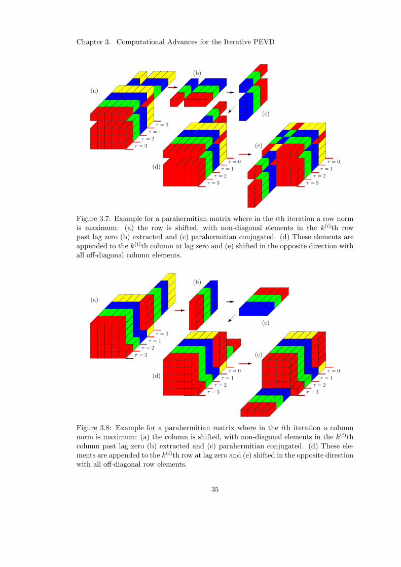
Chapter 3. Computational Advances for the Iterative PEVD
b)
d)
e)
a)
= 3
= 2
= 1
= 0
= 3
= 2
= 1
= 0
= 3
= 2
= 1
= 0
c)
Figure 3.7: Example for a parahermitian matrix where in the ith iteration a row normis maximum: (a) the row is shifted, with non-diagonal elements in the k(i)th rowpast lag zero (b) extracted and (c) parahermitian conjugated. (d) These elements areappended to the k(i)th column at lag zero and (e) shifted in the opposite direction withall off-diagonal column elements.
b)
d)
e)
a)
= 3
= 2
= 1
= 0
c)
= 3
= 2
= 1
= 0
= 3
= 2
= 1
= 0
Figure 3.8: Example for a parahermitian matrix where in the ith iteration a columnnorm is maximum: (a) the column is shifted, with non-diagonal elements in the k(i)thcolumn past lag zero (b) extracted and (c) parahermitian conjugated. (d) These ele-ments are appended to the k(i)th row at lag zero and (e) shifted in the opposite directionwith all off-diagonal row elements.
35
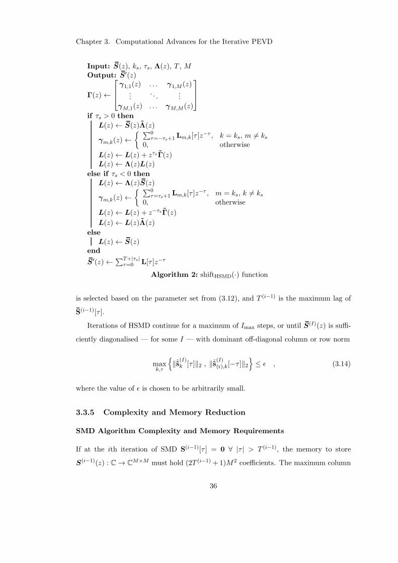
Chapter 3. Computational Advances for the Iterative PEVD
Input: S(z), ks, τs, Λ(z), T , MOutput: S′(z)
Γ(z)←
γ1,1(z) . . . γ1,M (z)...
. . ....
γM,1(z) . . . γM,M (z)
if τs > 0 then
L(z)← S(z)Λ(z)
γm,k(z)← ∑0
τ=−τs+1 Lm,k[τ ]z−τ , k = ks, m 6= ks
0, otherwise
L(z)← L(z) + zτsΓ(z)L(z)← Λ(z)L(z)
else if τs < 0 then
L(z)← Λ(z)S(z)
γm,k(z)← ∑0
τ=τs+1 Lm,k[τ ]z−τ , m = ks, k 6= ks
0, otherwise
L(z)← L(z) + z−τsΓ(z)
L(z)← L(z)Λ(z)
else
L(z)← S(z)end
S′(z)←∑T+|τs|τ=0 L[τ ]z−τ
Algorithm 2: shiftHSMD(·) function
is selected based on the parameter set from (3.12), and T (i−1) is the maximum lag of
S(i−1)[τ ].
Iterations of HSMD continue for a maximum of Imax steps, or until S(I)(z) is suffi-
ciently diagonalised — for some I — with dominant off-diagonal column or row norm
maxk,τ
‖s(I)k [τ ]‖2 , ‖s(I)(r),k[−τ ]‖2
≤ ǫ , (3.14)
where the value of ǫ is chosen to be arbitrarily small.
3.3.5 Complexity and Memory Reduction
SMD Algorithm Complexity and Memory Requirements
If at the ith iteration of SMD S(i−1)[τ ] = 0 ∀ |τ | > T (i−1), the memory to store
S(i−1)(z) : C→ CM×M must hold (2T (i−1) +1)M2 coefficients. The maximum column
36
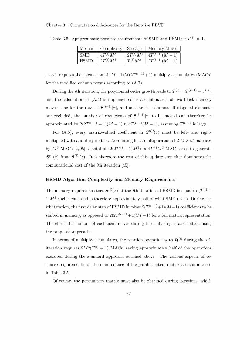
Chapter 3. Computational Advances for the Iterative PEVD
Table 3.5: Appproximate resource requirements of SMD and HSMD if T (i) ≫ 1.
Method Complexity Storage Memory Moves
SMD 4T (i)M3 2T (i)M2 4T (i−1)(M − 1)
HSMD 2T (i)M3 T (i)M2 2T (i−1)(M − 1)
search requires the calculation of (M−1)M(2T (i−1)+1) multiply-accumulates (MACs)
for the modified column norms according to (A.7).
During the ith iteration, the polynomial order growth leads to T (i) = T (i−1)+ |τ (i)|,and the calculation of (A.4) is implemented as a combination of two block memory
moves: one for the rows of S(i−1)[τ ], and one for the columns. If diagonal elements
are excluded, the number of coefficients of S(i−1)[τ ] to be moved can therefore be
approximated by 2(2T (i−1) + 1)(M − 1) ≈ 4T (i−1)(M − 1), assuming T (i−1) is large.
For (A.5), every matrix-valued coefficient in S(i)′(z) must be left- and right-
multiplied with a unitary matrix. Accounting for a multiplication of 2 M×M matrices
by M3 MACs [2, 95], a total of (2(2T (i) + 1)M3) ≈ 4T (i)M3 MACs arise to generate
S(i)(z) from S(i)′(z). It is therefore the cost of this update step that dominates the
computational cost of the ith iteration [45].
HSMD Algorithm Complexity and Memory Requirements
The memory required to store S(i)(z) at the ith iteration of HSMD is equal to (T (i) +
1)M2 coefficients, and is therefore approximately half of what SMD needs. During the
ith iteration, the first delay step of HSMD involves 2(T (i−1)+1)(M−1) coefficients to be
shifted in memory, as opposed to 2(2T (i−1)+1)(M −1) for a full matrix representation.
Therefore, the number of coefficient moves during the shift step is also halved using
the proposed approach.
In terms of multiply-accumulates, the rotation operation with Q(i) during the ith
iteration requires 2M3(T (i) + 1) MACs, saving approximately half of the operations
executed during the standard approach outlined above. The various aspects of re-
source requirements for the maintenance of the parahermitian matrix are summarised
in Table 3.5.
Of course, the paraunitary matrix must also be obtained during iterations, which
37
Chapter 3. Computational Advances for the Iterative PEVD
requires further resources; however, the requirements are the same for both SMD and
HSMD, so this aspect is omitted for brevity.
3.3.6 Results and Discussion
Simulation Scenario
The simulations below are performed over an ensemble of 103 instantiations of R(z) :
C → CM×M obtained from the randomised source model in Appendix B [45] with
M ∈ 5; 10, OD = 118, OQ = 60, and ∆DR = 30.
During PEVD algorithm iterations, a truncation parameter of µ = 10−15 and a
stopping threshold of ǫ = 0 are used. The SMD and HSMD implementations are run
until the iteratively updated parahermitian matrix is diagonalised such that diagonali-
sation metric 5 log10 E(i)diag = −15 dB, and at every iteration step the metrics defined in
Section A.3 are recorded together with the elapsed execution time.
Diagonalisation
The ensemble-averaged diagonalisation E(i)diag was calculated for both SMD and HSMD.
While both algorithms are functionally identical and exhibit the same diagonalisation
performance over algorithm iterations, the diagonalisation speed for both methods is
shown in Figure 3.9. The curves demonstrate that for M ∈ 5; 10, the lower complex-
ity associated with the HSMD implementation translates to a faster diagonalisation
than observed for the standard SMD realisation. Using a matrix with a larger spa-
tial dimension of M = 10 versus M = 5 results in slower diagonalisation for both
algorithms, but the same relative performance increase is still seen for the proposed
reduced approach.
Simulated in MATLABR©, the results in Figure 3.9 are not as impressive as the
computational savings suggested by Table 3.5. This is partly due to the requirement
of both algorithms to maintain H(i)(z). The MATLABR© profiler indicates that the
execution time for matrix multiplications (i.e., the number of matrix multiplications)
has been substantially reduced by the proposed method; however, while MATLABR©
is optimised for the employed matrix multiplication strategy from Section 3.2.1, its
38
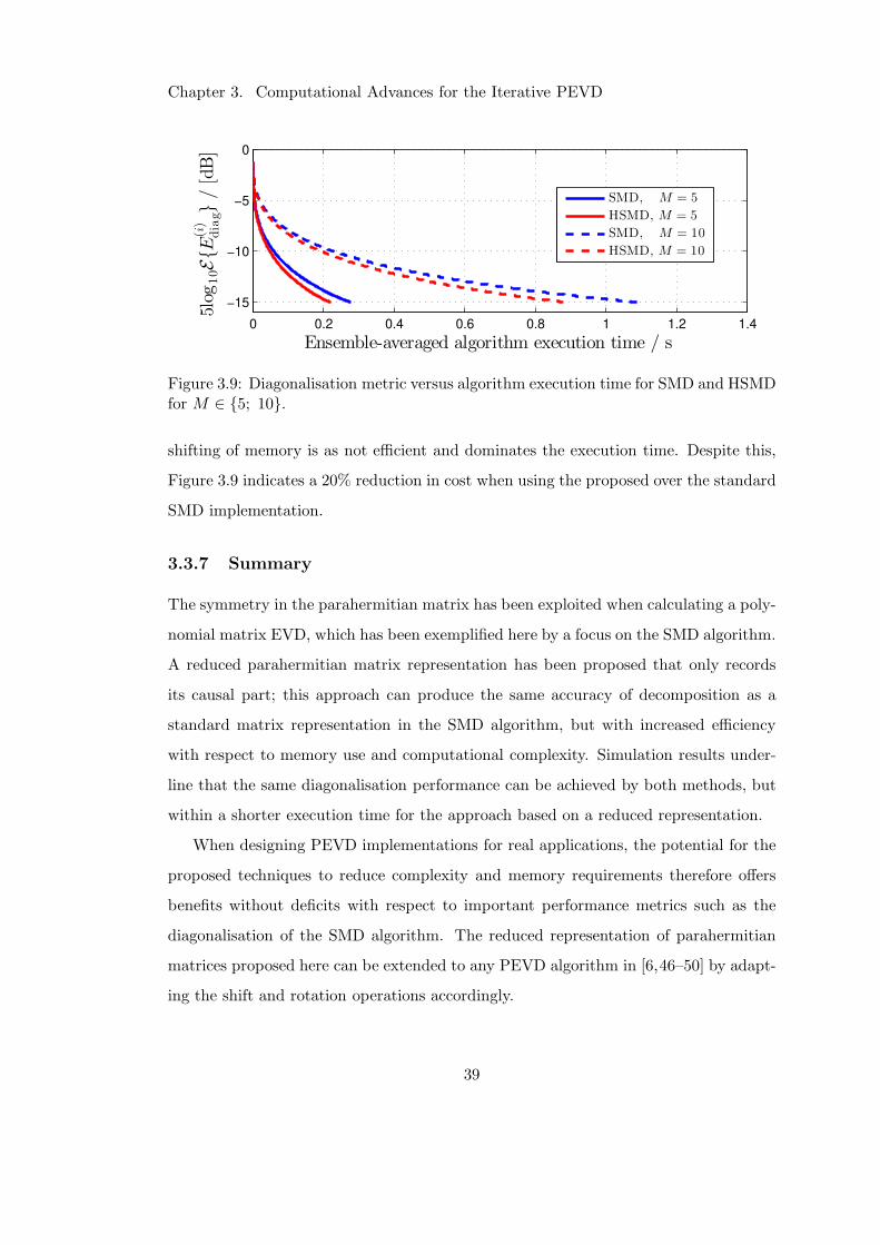
Chapter 3. Computational Advances for the Iterative PEVD
0 0.2 0.4 0.6 0.8 1 1.2 1.4
−15
−10
−5
0
Ensemble-averaged algorithm execution time / s
5log
10EE
(i)
diag
/[dB]
SMD, M = 5
HSMD, M = 5
SMD, M = 10
HSMD, M = 10
Figure 3.9: Diagonalisation metric versus algorithm execution time for SMD and HSMDfor M ∈ 5; 10.
shifting of memory is as not efficient and dominates the execution time. Despite this,
Figure 3.9 indicates a 20% reduction in cost when using the proposed over the standard
SMD implementation.
3.3.7 Summary
The symmetry in the parahermitian matrix has been exploited when calculating a poly-
nomial matrix EVD, which has been exemplified here by a focus on the SMD algorithm.
A reduced parahermitian matrix representation has been proposed that only records
its causal part; this approach can produce the same accuracy of decomposition as a
standard matrix representation in the SMD algorithm, but with increased efficiency
with respect to memory use and computational complexity. Simulation results under-
line that the same diagonalisation performance can be achieved by both methods, but
within a shorter execution time for the approach based on a reduced representation.
When designing PEVD implementations for real applications, the potential for the
proposed techniques to reduce complexity and memory requirements therefore offers
benefits without deficits with respect to important performance metrics such as the
diagonalisation of the SMD algorithm. The reduced representation of parahermitian
matrices proposed here can be extended to any PEVD algorithm in [6,46–50] by adapt-
ing the shift and rotation operations accordingly.
39
Chapter 3. Computational Advances for the Iterative PEVD
3.4 Increasing Efficiency within Cyclic-by-Row PEVD Im-
plementations
This work addresses potential computational savings that can be applied to exist-
ing so-called ‘cyclic-by-row’ (CbR) approaches for the PEVD. An SMD cyclic-by-row
(SMDCbR) approach [49] has been introduced as a low-cost variant of SMD, which
approximates the EVD step inside the SMD algorithm by a cyclic-by-row implemen-
tation of the Jacobi algorithm [2]. In this work, a method to concatenate the Jacobi
rotations in SMDCbR to reduce the computational cost of the algorithm is described,
and thresholding to the rotation process to eliminate the rotation of near-zero elements
is introduced. It is demonstrated that with the proposed techniques, computations can
be reduced without significantly impacting on algorithm convergence. The proposed
methods are advantageous for application purposes, where the SMDCbR algorithm’s
avoidance of a direct EVD computation may be useful.
Aspects of the iterative PEVD algorithm SMDCbR [49] are reviewed in Section 3.4.1,
alongside an assessment of the main algorithmic cost. To reduce the complexity of
the SMDCbR algorithm, Section 3.4.2 and Section 3.4.3 outline modifications to the
rotation step of the algorithm to concatenate and threshold the Jacobi rotations, re-
spectively. The performances of SMDCbR and its modified versions are compared in
Section 3.4.4. Conclusions for this section are drawn in Section 3.4.5.
Elements of the work in this section can be found published in the proceedings of
the 50th Asilomar Conference on Signals, Systems and Computers in a paper titled
‘Complexity and Search Space Reduction in Cyclic-by-Row PEVD Algorithms’ [68].
3.4.1 Cyclic-by-Row SMD Algorithm
Overview
The SMDCbR algorithm operates almost identically to SMD; thus, much of its descrip-
tion can be found in Section A.1. The only difference between SMDCbR and SMD arises
during the rotation stage. In iteration i of SMD, this involves the computation of a
unitary matrix Q(i) from the EVD of lag zero, S(i)′[0], and the subsequent computation
40
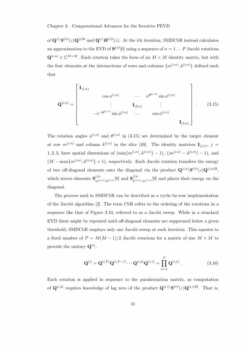
Chapter 3. Computational Advances for the Iterative PEVD
of Q(i)S(i)′(z)Q(i)H and Q(i)H(i)′(z). At the ith iteration, SMDCbR instead calculates
an approximation to the EVD of S(i)′[0] using a sequence of n = 1 . . . P Jacobi rotations
Q(i,n) ∈ CM×M . Each rotation takes the form of an M ×M identity matrix, but with
the four elements at the intersections of rows and columns m(i,n), k(i,n) defined such
that
Q(i,n) =
I(1,n)
cosφ(i,n) · · · ejθ(i,n)
sinφ(i,n)
... I(2,n)...
−e−jθ(i,n)sinφ(i,n) · · · cosφ(i,n)
I(3,n)
. (3.15)
The rotation angles φ(i,n) and θ(i,n) in (3.15) are determined by the target element
at row m(i,n) and column k(i,n) in the slice [49]. The identity matrices I(j,n), j =
1, 2, 3, have spatial dimensions of (minm(i,n), k(i,n) − 1), (|m(i,n) − k(i,n)| − 1), and
(M −maxm(i,n), k(i,n) + 1), respectively. Each Jacobi rotation transfers the energy
of two off-diagonal elements onto the diagonal via the product Q(i,n)S(i)′(z)Q(i,n)H,
which zeroes elements S(i)′
m(i,n),k(i,n)[0] and S(i)′
k(i,n),m(i,n) [0] and places their energy on the
diagonal.
The process used in SMDCbR can be described as a cyclic-by-row implementation
of the Jacobi algorithm [2]. The term CbR refers to the ordering of the rotations in a
sequence like that of Figure 3.10, referred to as a Jacobi sweep. While in a standard
EVD these might be repeated until off-diagonal elements are suppressed below a given
threshold, SMDCbR employs only one Jacobi sweep at each iteration. This equates to
a fixed number of P = M(M − 1)/2 Jacobi rotations for a matrix of size M ×M to
provide the unitary Q(i),
Q(i) = Q(i,P )Q(i,P−1) · · ·Q(i,2)Q(i,1) =
P∏
n=1
Q(i,n) . (3.16)
Each rotation is applied in sequence to the parahermitian matrix, as computation
of Q(i,2) requires knowledge of lag zero of the product Q(i,1)S(i)′(z)Q(i,1)H. That is,
41
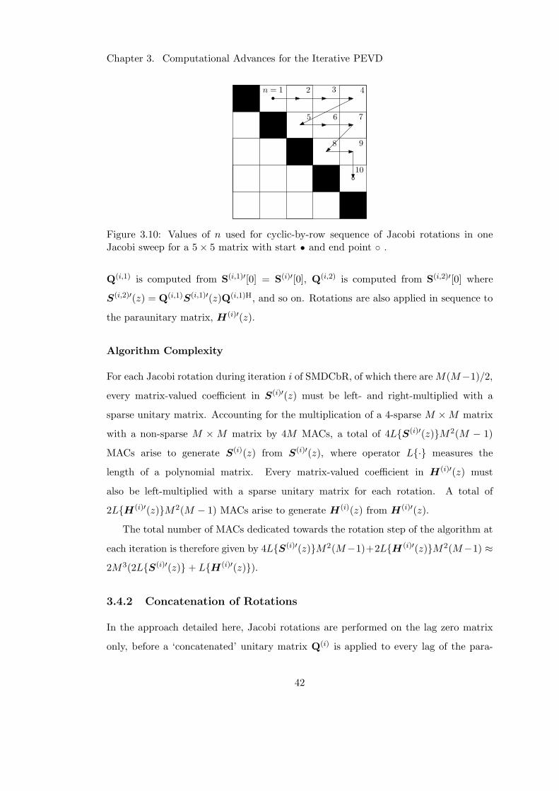
Chapter 3. Computational Advances for the Iterative PEVD
n = 1 2 3 4
5 6 7
8 9
10
Figure 3.10: Values of n used for cyclic-by-row sequence of Jacobi rotations in oneJacobi sweep for a 5× 5 matrix with start s and end point .
Q(i,1) is computed from S(i,1)′[0] = S(i)′[0], Q(i,2) is computed from S(i,2)′[0] where
S(i,2)′(z) = Q(i,1)S(i,1)′(z)Q(i,1)H, and so on. Rotations are also applied in sequence to
the paraunitary matrix, H(i)′(z).
Algorithm Complexity
For each Jacobi rotation during iteration i of SMDCbR, of which there areM(M−1)/2,every matrix-valued coefficient in S(i)′(z) must be left- and right-multiplied with a
sparse unitary matrix. Accounting for the multiplication of a 4-sparse M ×M matrix
with a non-sparse M ×M matrix by 4M MACs, a total of 4LS(i)′(z)M2(M − 1)
MACs arise to generate S(i)(z) from S(i)′(z), where operator L· measures the
length of a polynomial matrix. Every matrix-valued coefficient in H(i)′(z) must
also be left-multiplied with a sparse unitary matrix for each rotation. A total of
2LH(i)′(z)M2(M − 1) MACs arise to generate H(i)(z) from H(i)′(z).
The total number of MACs dedicated towards the rotation step of the algorithm at
each iteration is therefore given by 4LS(i)′(z)M2(M−1)+2LH (i)′(z)M2(M−1) ≈2M3(2LS(i)′(z) + LH(i)′(z)).
3.4.2 Concatenation of Rotations
In the approach detailed here, Jacobi rotations are performed on the lag zero matrix
only, before a ‘concatenated’ unitary matrix Q(i) is applied to every lag of the para-
42
Chapter 3. Computational Advances for the Iterative PEVD
hermitian and paraunitary matrices. This unitary matrix is equal to the product of all
the sparse rotation matrices applied to lag zero, and is equivalent to (3.16). The direct
application of sparse rotations to the polynomial matrices is therefore avoided, which
results in a reduction in complexity.
Each rotation is still applied in sequence, but to lag zero of the parahermitian
matrix only. That is, Q(i,1) is computed from S(i,1)′[0] = S(i)′[0], Q(i,2) is computed
from S(i,2)′[0] where S(i,2)′[0] = Q(i,1)S(i,1)′[0]Q(i,1)H, and so on. A record of the previous
n rotations is maintained in a unitary matrix Q(i,n), such that Q(i,1) = Q(i,1), Q(i,2) =
Q(i,2)Q(i,1), Q(i,3) = Q(i,3)Q(i,2), and so on. Matrix Q(i) = Q(i,P ) is then applied to
the parahermitian and paraunitary matrices in the same manner as in (A.5).
For each of the M(M − 1)/2 sparse rotations, the lag zero and unitary matrices
must be updated. Updating the lag zero matrix for each rotation involves left- and
right-multiplication with a sparse unitary matrix, costing 8M MACs; thus, a full sweep
requires 4M2(M − 1) MACs. Left-multiplying the unitary matrix for each rotation
requires 4M MACs; thus, a full sweep encompasses 2M2(M − 1) MACs. Both steps
combined therefore require 6M2(M − 1) MACs.
At each iteration, as in the SMD algorithm [45], every matrix-valued coefficient
in S(i)′(z) must be left- and right-multiplied with a non-sparse unitary matrix. Ac-
counting for the multiplication of 2 M × M matrices by M3 MACs [2, 95], a total
of 2LS(i)′(z)M3 MACs arise to generate S(i)(z) from S(i)′(z). In addition, every
matrix-valued coefficient in H(i)′(z) must be left-multiplied with a non-sparse unitary
matrix at each iteration; thus, LH(i)′(z)M3 MACs are required to generate H(i)(z)
from H(i)′(z).
The total number of MACs dedicated to the rotation stage per iteration is therefore
2LS(i)′(z)M3 + LH(i)′(z)M3 + 6M2(M − 1) ≈M3(2LS(i)′(z)+LH(i)′(z)) ifminLS(i)′(z), LH (i)′(z) ≫ 6. This is approximately equal to half of the MACs
required for the standard SMDCbR algorithm.
43
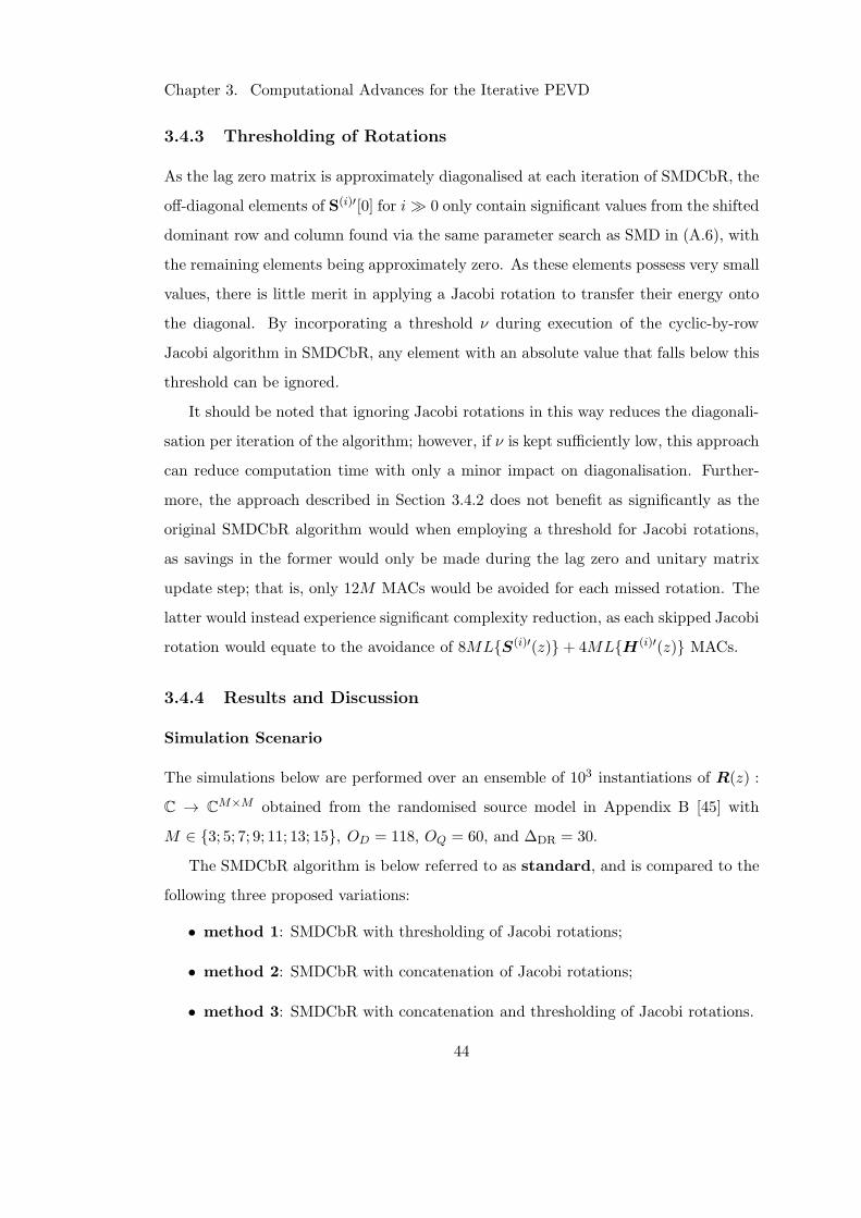
Chapter 3. Computational Advances for the Iterative PEVD
3.4.3 Thresholding of Rotations
As the lag zero matrix is approximately diagonalised at each iteration of SMDCbR, the
off-diagonal elements of S(i)′[0] for i≫ 0 only contain significant values from the shifted
dominant row and column found via the same parameter search as SMD in (A.6), with
the remaining elements being approximately zero. As these elements possess very small
values, there is little merit in applying a Jacobi rotation to transfer their energy onto
the diagonal. By incorporating a threshold ν during execution of the cyclic-by-row
Jacobi algorithm in SMDCbR, any element with an absolute value that falls below this
threshold can be ignored.
It should be noted that ignoring Jacobi rotations in this way reduces the diagonali-
sation per iteration of the algorithm; however, if ν is kept sufficiently low, this approach
can reduce computation time with only a minor impact on diagonalisation. Further-
more, the approach described in Section 3.4.2 does not benefit as significantly as the
original SMDCbR algorithm would when employing a threshold for Jacobi rotations,
as savings in the former would only be made during the lag zero and unitary matrix
update step; that is, only 12M MACs would be avoided for each missed rotation. The
latter would instead experience significant complexity reduction, as each skipped Jacobi
rotation would equate to the avoidance of 8MLS(i)′(z) + 4MLH(i)′(z) MACs.
3.4.4 Results and Discussion
Simulation Scenario
The simulations below are performed over an ensemble of 103 instantiations of R(z) :
C → CM×M obtained from the randomised source model in Appendix B [45] with
M ∈ 3; 5; 7; 9; 11; 13; 15, OD = 118, OQ = 60, and ∆DR = 30.
The SMDCbR algorithm is below referred to as standard, and is compared to the
following three proposed variations:
• method 1: SMDCbR with thresholding of Jacobi rotations;
• method 2: SMDCbR with concatenation of Jacobi rotations;
• method 3: SMDCbR with concatenation and thresholding of Jacobi rotations.
44
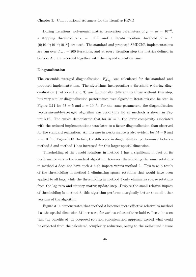
Chapter 3. Computational Advances for the Iterative PEVD
During iterations, polynomial matrix truncation parameters of µ = µt = 10−6,
a stopping threshold of ǫ = 10−6, and a Jacobi rotation threshold of ν ∈0; 10−4; 10−3; 10−2 are used. The standard and proposed SMDCbR implementations
are run over Imax = 200 iterations, and at every iteration step the metrics defined in
Section A.3 are recorded together with the elapsed execution time.
Diagonalisation
The ensemble-averaged diagonalisation, E(i)diag, was calculated for the standard and
proposed implementations. The algorithms incorporating a threshold ν during diag-
onalisation (methods 1 and 3) are functionally different to those without this step,
but very similar diagonalisation performance over algorithm iterations can be seen in
Figure 3.11 for M = 5 and ν = 10−3. For the same parameters, the diagonalisation
versus ensemble-averaged algorithm execution time for all methods is shown in Fig-
ure 3.12. The curves demonstrate that for M = 5, the lower complexity associated
with the reduced implementations translates to a faster diagonalisation than observed
for the standard realisation. An increase in performance is also evident for M = 9 and
ν = 10−3 in Figure 3.13. In fact, the difference in diagonalisation performance between
method 3 and method 1 has increased for this larger spatial dimension.
Thresholding of the Jacobi rotations in method 1 has a significant impact on its
performance versus the standard algorithm; however, thresholding the same rotations
in method 3 does not have such a high impact versus method 2. This is as a result
of the thresholding in method 1 eliminating sparse rotations that would have been
applied to all lags, while the thresholding in method 3 only eliminates sparse rotations
from the lag zero and unitary matrix update step. Despite the small relative impact
of thresholding in method 3, this algorithm performs marginally better than all other
versions of the algorithm.
Figure 3.14 demonstrates that method 3 becomes more effective relative to method
1 as the spatial dimension M increases, for various values of threshold ν. It can be seen
that the benefits of the proposed rotation concatenation approach exceed what could
be expected from the calculated complexity reduction, owing to the well-suited nature
45
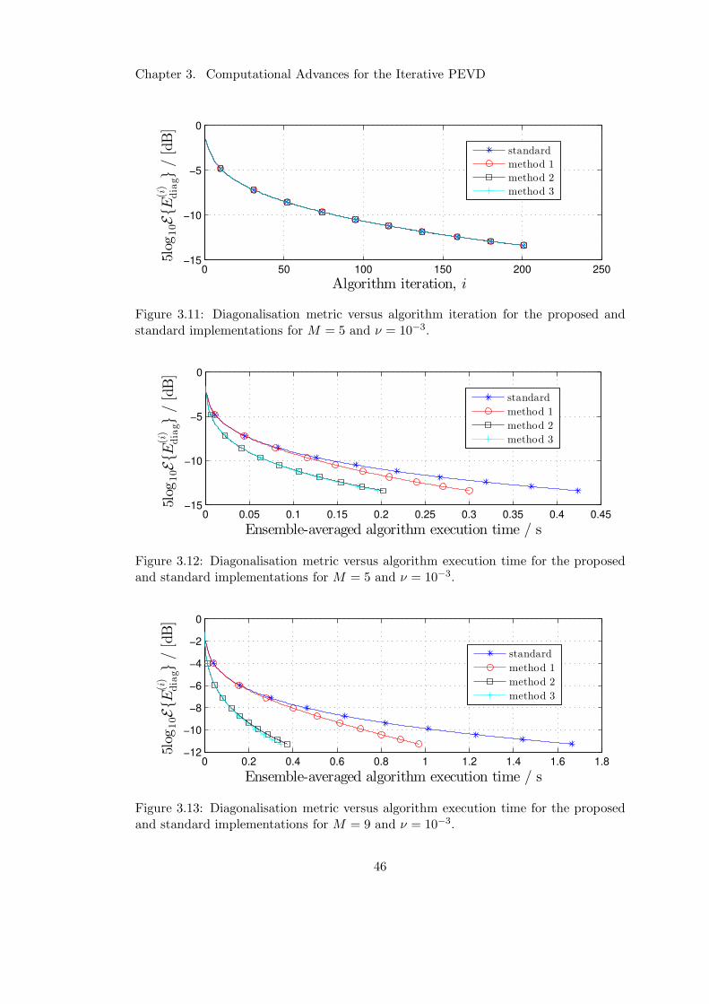
Chapter 3. Computational Advances for the Iterative PEVD
0 50 100 150 200 250−15
−10
−5
0
Algorithm iteration, i
5log
10EE
(i)
diag
/[dB]
standard
method 1
method 2
method 3
Figure 3.11: Diagonalisation metric versus algorithm iteration for the proposed andstandard implementations for M = 5 and ν = 10−3.
0 0.05 0.1 0.15 0.2 0.25 0.3 0.35 0.4 0.45−15
−10
−5
0
Ensemble-averaged algorithm execution time / s
5log
10EE
(i)
diag
/[dB]
standard
method 1
method 2
method 3
Figure 3.12: Diagonalisation metric versus algorithm execution time for the proposedand standard implementations for M = 5 and ν = 10−3.
0 0.2 0.4 0.6 0.8 1 1.2 1.4 1.6 1.8−12
−10
−8
−6
−4
−2
0
Ensemble-averaged algorithm execution time / s
5log
10EE
(i)
diag
/[dB]
standard
method 1
method 2
method 3
Figure 3.13: Diagonalisation metric versus algorithm execution time for the proposedand standard implementations for M = 9 and ν = 10−3.
46
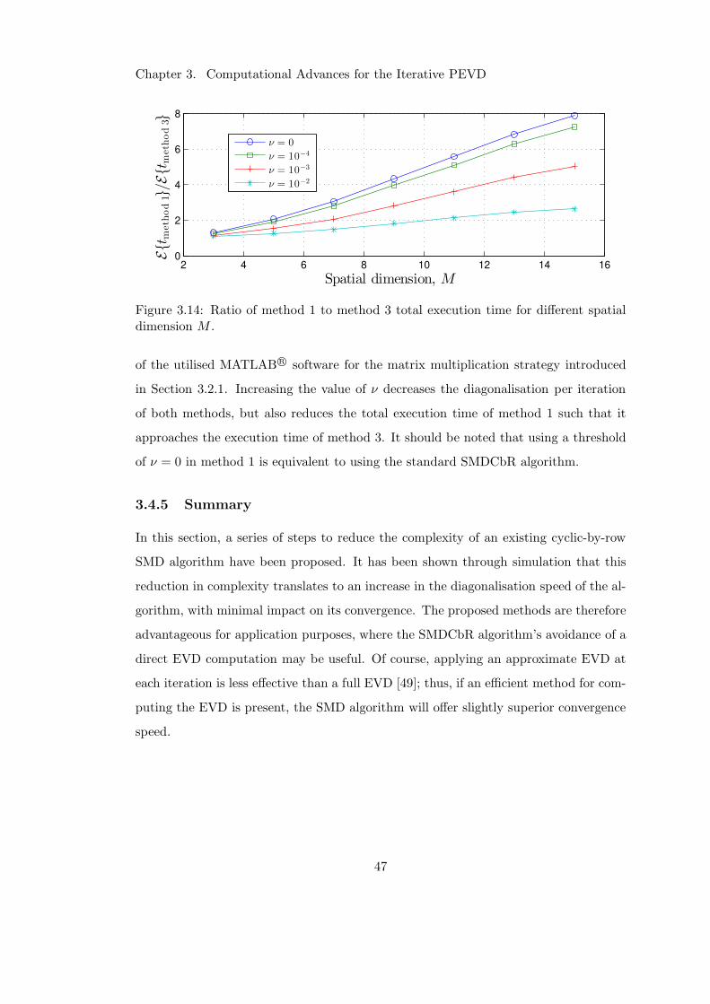
Chapter 3. Computational Advances for the Iterative PEVD
2 4 6 8 10 12 14 160
2
4
6
8
Spatial dimension, M
Et
method1/E
tmethod3
ν = 0
ν = 10−4
ν = 10−3
ν = 10−2
Figure 3.14: Ratio of method 1 to method 3 total execution time for different spatialdimension M .
of the utilised MATLABR© software for the matrix multiplication strategy introduced
in Section 3.2.1. Increasing the value of ν decreases the diagonalisation per iteration
of both methods, but also reduces the total execution time of method 1 such that it
approaches the execution time of method 3. It should be noted that using a threshold
of ν = 0 in method 1 is equivalent to using the standard SMDCbR algorithm.
3.4.5 Summary
In this section, a series of steps to reduce the complexity of an existing cyclic-by-row
SMD algorithm have been proposed. It has been shown through simulation that this
reduction in complexity translates to an increase in the diagonalisation speed of the al-
gorithm, with minimal impact on its convergence. The proposed methods are therefore
advantageous for application purposes, where the SMDCbR algorithm’s avoidance of a
direct EVD computation may be useful. Of course, applying an approximate EVD at
each iteration is less effective than a full EVD [49]; thus, if an efficient method for com-
puting the EVD is present, the SMD algorithm will offer slightly superior convergence
speed.
47
Chapter 3. Computational Advances for the Iterative PEVD
3.5 Restricting the Search Space of PEVD Algorithms
Research in [50, 88] has shown that restricting the search space of iterative PEVD
algorithms to a subset of lags around lag zero of a parahermitian matrix can bring
performance gains with little impact on algorithm convergence. In this section, a
further cost reduction technique for all iterative PEVD algorithms is introduced, and
is shown to improve the diagonalisation performance of the SMDCbR algorithm [49].
The proposed SMDCbR version is modified to limit the search of maximum off-diagonal
energy in columns to a particular range of lags surrounding lag zero. It is shown that
the size of this search segment can be determined by estimating the energy distribution
in the parahermitian matrix prior to its decomposition.
The proposed technique to limit the search space of iterative PEVD algorithms is
reviewed in Section 3.5.1. The performances of SMDCbR and a version of SMDCbR
incorporating a restricted search space approach are then compared in Section 3.5.2.
Subsequently, conclusions for this section are drawn in Section 3.5.3.
Elements of the work in this section can be found published in the proceedings of
the 50th Asilomar Conference on Signals, Systems and Computers in a paper titled
‘Complexity and Search Space Reduction in Cyclic-by-Row PEVD Algorithms’ [68].
3.5.1 Limited Search Strategy
The search step of the SMDCbR algorithm — equivalent to that of SMD and described
by (A.6) — evaluates modified column norms for all lags of the coefficient matrix
S(i−1)[τ ] ∈ CM×M . If at the ith iteration S(i−1)[τ ] = 0 ∀ |τ | > T (i−1), for some
maximum lag T (i−1) ∈ N, the search space encompasses ML(i−1)S elements, where
L(i−1)S = (2T (i−1) + 1) is the length of the parahermitian matrix.
The search step at each iteration of the modified SMDCbR algorithm uses the
column norms of the off-diagonal elements for a reduced set of the lags of the coefficient
matrix S(i−1)[τ ]. At the ith iteration, the search step is applied to a secondary matrix
S(i−1)[τ ] = 0 ∀ |τ | > δ(i−1), which is generated using the L(i−1)
S= (2δ(i−1) + 1) centre
lags of S(i−1)[τ ]; thus, the search space encompasses only ML(i−1)
Selements. If this
reduced search space can adequately contain most of the energy from the original
48
Chapter 3. Computational Advances for the Iterative PEVD
parahermitian matrix, then searching for a maximum within this search space can
reduce computation time with little impact on algorithm performance.
A narrow distribution of energy around the lag zero can therefore lead to a large
decrease in search space. As the algorithm progresses, the lags closest to lag zero become
increasingly diagonalised, and therefore the average delay applied at each iteration
increases; i.e., |τ (i)| tends to increase for increasing i. This can be accounted for by
gradually widening the search space around lag zero as the iteration number increases.
To accommodate this widening of the search space, δ(i) can be described as an increasing
function of i.
The delay magnitude, |τ (i)|, at each iteration can be considered a measure of the
concentration of energy in the parahermitian matrix. For example, if |τ (i)| increasesquickly for a small increase in i, this indicates that there is a low concentration of
energy in the lags surrounding lag zero. In the following, Xi is the random variable
that describes the |τ (i)| seen in previous instances of a PEVD algorithm. In an appli-
cation that requires a continuously updated estimate and PEVD of a parahermitian
matrix R(z), the distribution of Xi can serve as a measure of the energy distribution
in R(z) without the requirement of direct computation. Here, the search space δ(i) in
future instances of the PEVD algorithm can be controlled such that it encapsulates
the majority of Xi in prior instances. Consider the simplistic example where Xi is dis-
tributed normally; in this case, choosing δ(i) = EXi+ 1.96 std Xi — where std ·computes the standard deviation — should allow for approximately 95% of |τ (i)| infuture instances of the PEVD algorithm to be unchanged relative to an instance of the
algorithm without search space restriction. In practice, Xi is unlikely to be normally
distributed; however, the above serves as a computationally cheap method for roughly
approximating δ(i).
3.5.2 Results and Discussion
Simulation Scenario
The simulations below are performed over an ensemble of 103 instantiations of R(z) :
C → CM×M obtained from the randomised source model in Appendix B [45] with
49
Chapter 3. Computational Advances for the Iterative PEVD
M = 5, OD = 118, OQ = 60, and ∆DR = 30.
During iterations, polynomial matrix truncation parameters of µ = µt = 10−6 and
a stopping threshold of ǫ = 10−6 are used. A standard SMDCbR implementation and a
version of SMDCbR utilising the proposed limited search strategy are each allowed to
run for Imax = 200 iterations. At every iteration step the metrics defined in Section A.3
are recorded together with the elapsed execution time, the absolute delay |τ (i)| appliedto a column in the parahermitian matrix, and the lengths of the parahermitian and
paraunitary matrices, L(i)S and L
(i)H .
In this simulation scenario, the search space in the proposed implementation of
SMDCbR has been reduced to approximate the 95% confidence interval of absolute
delays applied in a previous ensemble of 103 instances of R(z), following the assumption
that these values were normally distributed. Using this information, the search space
reduction parameter evolution was identified as δ(i) = 0.15i + 24.
Diagonalisation
Figure 3.15 indicates the potential performance gain when limiting the search space
to those lags deemed likely to contain high energy. As the algorithm’s search step
is a relatively inexpensive process compared with the shifting and rotation stages,
the performance gain observed is small but significant. Time profiling in MATLABR©
indicated that the use of the limited search strategy reduces the search time by 50.6%
for the simulation used to generate Figure 3.15.
Impact on Order of Parahermitian Matrix
The impact of search space reduction on algorithm operation was investigated for the
modified SMDCbR algorithm. Figures 3.16 and 3.17 show the ensemble-averaged abso-
lute delay |τ (i)| applied to a column in iteration i of SMDCbR and its modified version,
and the length L(i)S of the parahermitian matrix in both algorithms, respectively. From
these figures, it is clear that the reduction in search space does not significantly impact
the average delay applied — and thus the order of the parahermitian matrix — at
each iteration of the proposed algorithm. In fact, since the proposed method typically
50
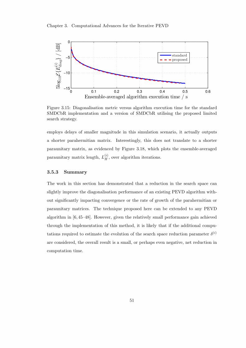
Chapter 3. Computational Advances for the Iterative PEVD
0 0.1 0.2 0.3 0.4 0.5 0.6−15
−10
−5
0
Ensemble-averaged algorithm execution time / s
5log
10EE
(i)
diag
/[dB]
standardproposed
Figure 3.15: Diagonalisation metric versus algorithm execution time for the standardSMDCbR implementation and a version of SMDCbR utilising the proposed limitedsearch strategy.
employs delays of smaller magnitude in this simulation scenario, it actually outputs
a shorter parahermitian matrix. Interestingly, this does not translate to a shorter
paraunitary matrix, as evidenced by Figure 3.18, which plots the ensemble-averaged
paraunitary matrix length, L(i)H , over algorithm iterations.
3.5.3 Summary
The work in this section has demonstrated that a reduction in the search space can
slightly improve the diagonalisation performance of an existing PEVD algorithm with-
out significantly impacting convergence or the rate of growth of the parahermitian or
paraunitary matrices. The technique proposed here can be extended to any PEVD
algorithm in [6, 45–48]. However, given the relatively small performance gain achieved
through the implementation of this method, it is likely that if the additional compu-
tations required to estimate the evolution of the search space reduction parameter δ(i)
are considered, the overall result is a small, or perhaps even negative, net reduction in
computation time.
51
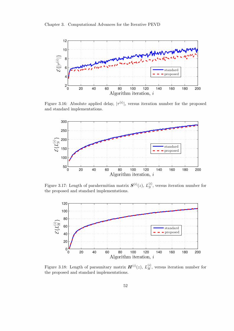
Chapter 3. Computational Advances for the Iterative PEVD
0 20 40 60 80 100 120 140 160 180 2002
4
6
8
10
12
Algorithm iteration, i
E|τ(i) |
standardproposed
Figure 3.16: Absolute applied delay, |τ (i)|, versus iteration number for the proposedand standard implementations.
0 20 40 60 80 100 120 140 160 180 20050
100
150
200
250
300
Algorithm iteration, i
EL
(i)
S
standardproposed
Figure 3.17: Length of parahermitian matrix S(i)(z), L(i)S , versus iteration number for
the proposed and standard implementations.
0 20 40 60 80 100 120 140 160 180 2000
20
40
60
80
100
120
Algorithm iteration, i
EL
(i)
H
standardproposed
Figure 3.18: Length of paraunitary matrix H(i)(z), L(i)H , versus iteration number for
the proposed and standard implementations.
52
Chapter 3. Computational Advances for the Iterative PEVD
3.6 Restricting the Update Space of PEVD Algorithms
The research conducted in the previous section has bolstered the results of [50, 88] by
confirming that restricting the search space of iterative PEVD algorithms can improve
convergence speed. However, despite focussing on only a small portion of the para-
hermitian matrix during the search step, the entire matrix must still be updated at
each iteration in these approaches. Using SMD as an example of an iterative PEVD
algorithm, the work in this section expands upon this restricted search space idea by
introducing a novel restricted update approach for the PEVD. The techniques involved
are implemented within a restricted update SMD (RSMD) algorithm, which calculates
the paraunitary matrix while restricting the search space of the algorithm and the
portion of the parahermitian matrix that is updated at each iteration. As with the
majority of iterative PEVD algorithms, the update step of SMD is its most computa-
tionally costly operation [45]; thus, a reduction in the complexity of this step is useful.
It is demonstrated that by using the proposed RSMD algorithm instead of SMD, PEVD
complexity and execution time can be significantly reduced with minimal impact on
algorithm convergence.
An overview of the method is given in Section 3.6.1, with a more detailed description
of the novel functionality in Section 3.6.2. Section 3.6.3 describes the algorithmic
complexity of the approach. Simulation results comparing the performances of SMD
and RSMD are presented in Section 3.6.4, and conclusions for this section are drawn
in Section 3.6.5.
Elements of the work in this section can be found published in the proceedings of the
7th IEEE International Workshop on Computational Advances in Multi-Sensor Adap-
tive Processing in a paper titled ‘Restricted Update Sequential Matrix Diagonalisation
for Parahermitian Matrices’ [69].
3.6.1 Restricted Update SMD Algorithm
Similarly to SMD, which is described in Section A.1, the RSMD algorithm approxi-
mates a PEVD by iteratively diagonalising a parahermitian matrix R(z) : C→ CM×M
over i = 0 . . . I iteration steps. Over the course of these iterations, the update space
53
Chapter 3. Computational Advances for the Iterative PEVD
contracts piecewise strictly monotonically. The term ‘update space’ here refers to the
number of lags in the parahermitian matrix that are updated at each iteration of the
algorithm. This restriction limits the number of search operations, but also reduces the
computations required to update the increasingly diagonalised parahermitian matrix.
The update space contracts until order zero is reached and the update space only in-
cludes the lag zero matrix. After this, in a so-called ‘regeneration’ step, the calculated
paraunitary matrix is applied to the input matrix to construct the full-sized paraher-
mitian factor. The update space is then maximised and thereafter again contracts
monotonically over the following iterations. The maximum β of index α = 0, 1, . . . , β
— where α counts the number of regenerations — is not known a priori.
Following the αth regeneration step, in the ith iteration of RSMD, S(i)(z) =
R(α)(z). Note, R(0)(z) = Q(0)R(z)Q(0)H, where Q(0) diagonalises coefficient matrix
R[0]. The restricted update stage of RSMD restricts the search and update steps typi-
cally used in the SMD algorithm to only consider an iteratively decreasing selection of
lags of S(i)(z) around lag zero at the ith iteration. When the update space of S(i)(z)
reaches zero, the restricted update stage has produced a paraunitary matrix F (α)(z)
such that matrix R(α+1)(z) = F (α)(z)R(α)(z)F (α)(z) — which is generated during the
matrix regeneration stage — is more diagonal that R(α)(z).
If the total number of algorithm iterations i exceeds a user-defined Imax, or if the
stopping criterion from SMD, (A.8), is satisfied, the RSMD algorithm ends withD(z) =
R(α+1)(z) and F (z) = F ′(α+1)(z) following the truncation of each matrix according to
Appendix C. Here, F ′(α+1)(z) is a concatenation of the paraunitary matrices generated
for indices 0 . . . α and initial matrix Q(0):
F ′(α+1)(z) = F (α)(z) · · ·F (0)(z)Q
(0) =
(α∏
x=0
F (α−x)(z)
)
Q(0) .
Algorithm 3 gives the pseudocode for RSMD. Output matrices F (z) and D(z) con-
tain polynomial eigenvectors and eigenvalues, respectively. More detail of the restricted
update component of the algorithm’s operation is provided in Section 3.6.2. Proof of
convergence of SMD — which focusses on the monotonic increase of on-diagonal en-
54
Chapter 3. Computational Advances for the Iterative PEVD
Input: R(z), µ, µt, ǫ, Imax
Output: D(z), F (z)Find eigenvectors Q(0) that diagonalise R[0]
R(0)(z)← Q(0)R(z)Q(0)H; F ′(0)(z)← Q(0); α← 0; i← 0; stop ← 0
while stop = 0 do
[F (α)(z), i, stop] ← restrictedUpdate(R(α)(z), µt, ǫ, Imax, i)
Regenerate matrix:F ′
(α+1)(z)← F (α)(z)F′(α)(z)
R(α+1)(z)← F (α)(z)R(α)(z)F (α)(z)
Truncate F ′(α+1)(z) using threshold µt according to Appendix C
Truncate R(α+1)(z) using threshold µ according to Appendix C
α← α+ 1
end
F (z)← F ′(α)(z); D(z)← R(α)(z)
Algorithm 3: RSMD Algorithm
ergy enforced by the algorithm — has been established in [45]; this proof also holds for
RSMD.
3.6.2 Restricted Update Step
The restricted update step of RSMD functions similarly to the update step of SMD
in Section A.1; however, the key difference is that RSMD increasingly restricts the
number of lags of S(i)(z) that are updated at each iteration i. Algorithm 4 provides
pseudocode for the restrictedUpdate(·) function, whose operation is discussed below.
From a parahermitian matrixR(α)(z) : C→ CM×M input to the restrictedUpdate(·)
function for index α, during the ith iteration of RSMD, a matrix S(i−1)(z) = R(α)(z)
with maximum lag T (i−1) is formed. As in the standard SMD algorithm, the k(i)th
column and row with maximum energy are found and shifted by |τ (i)| to lag zero using
a delay matrix Λ(i)(z) to produce S(i)′(z).
A unitary matrix Q(i) is generated from an EVD of lag zero S(i)′[0], but is only
applied to an ‘update region’ matrix S(i)′′(z), which contains the central (2(T (i−1) −|τ (i)|) + 1) lags of S(i)′(z). Thus, matrix S(i)(z) = Q(i)S(i)′′(z)Q(i)H is formed, which
has maximum lag T (i) = T (i−1) − |τ (i)|.The coefficients of S(i)[τ ] at lags |τ | > T (i), which are zero by definition — and not
55
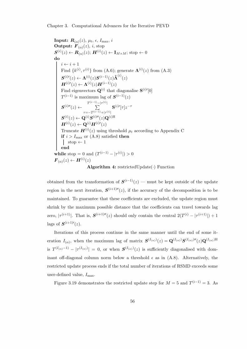
Chapter 3. Computational Advances for the Iterative PEVD
Input: R(α)(z), µt, ǫ, Imax, iOutput: F (α)(z), i, stop
S(i)(z)← R(α)(z); H(i)(z)← IM×M ; stop ← 0
do
i← i+ 1
Find k(i), τ (i) from (A.6); generate Λ(i)(z) from (A.3)
S(i)′(z)← Λ(i)(z)S(i−1)(z)Λ(i)(z)
H(i)′(z)← Λ(i)(z)H (i−1)(z)
Find eigenvectors Q(i) that diagonalise S(i)′[0]
T (i−1) is maximum lag of S(i−1)(z)
S(i)′′(z)←T (i−1)−|τ (i)|∑
τ=−T (i−1)+|τ (i)|
S(i)′[τ ]z−τ
S(i)(z)← Q(i)S(i)′′(z)Q(i)H
H(i)(z)← Q(i)H(i)′(z)
Truncate H(i)(z) using threshold µt according to Appendix Cif i > Imax or (A.8) satisfied then
stop ← 1end
while stop = 0 and (T (i−1) − |τ (i)|) > 0
F (α)(z)←H(i)(z)
Algorithm 4: restrictedUpdate(·) Function
obtained from the transformation of S(i−1)(z) — must be kept outside of the update
region in the next iteration, S(i+1)′′(z), if the accuracy of the decomposition is to be
maintained. To guarantee that these coefficients are excluded, the update region must
shrink by the maximum possible distance that the coefficients can travel towards lag
zero, |τ (i+1)|. That is, S(i+1)′′(z) should only contain the central 2(T (i) − |τ (i+1)|) + 1
lags of S(i+1)′(z).
Iterations of this process continue in the same manner until the end of some it-
eration I(α), when the maximum lag of matrix S(I(α))(z) = Q(I(α))S(I(α))′′(z)Q(I(α))H
is T (I(α)−1) − |τ (I(α))| = 0, or when S(I(α))(z) is sufficiently diagonalised with dom-
inant off-diagonal column norm below a threshold ǫ as in (A.8). Alternatively, the
restricted update process ends if the total number of iterations of RSMD exceeds some
user-defined value, Imax.
Figure 3.19 demonstrates the restricted update step for M = 5 and T (i−1) = 3. As
56
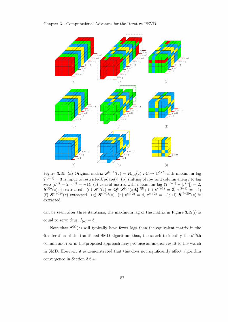
Chapter 3. Computational Advances for the Iterative PEVD
a)
= 3
= 2
= 1
=
= 1
= 2
= 3
= 3
= 2
= 1
=
= 1
= 2
= 3
= 2
= 1
=
= 1
= 2
b) c) = 4
= 4
= 2
= 1
=
= 1
= 2
d)
= 2
= 1
=
= 1
= 2
= 1
=
= 1
e) f)
= 1
=
= 1
g)
= 1
=
= 1
h)
=
i)
Figure 3.19: (a) Original matrix S(i−1)(z) = R(α)(z) : C → C5×5 with maximum lag
T (i−1) = 3 is input to restrictedUpdate(·); (b) shifting of row and column energy to lagzero (k(i) = 2, τ (i) = −1); (c) central matrix with maximum lag (T (i−1) − |τ (i)|) = 2,S(i)′′(z), is extracted. (d) S(i)(z) = Q(i)S(i)′′(z)Q(i)H; (e) k(i+1) = 3, τ (i+1) = −1;(f) S(i+1)′′(z) extracted. (g) S(i+1)(z); (h) k(i+2) = 4, τ (i+2) = −1; (i) S(i+2)′′(z) isextracted.
can be seen, after three iterations, the maximum lag of the matrix in Figure 3.19(i) is
equal to zero; thus, I(α) = 3.
Note that S(i)(z) will typically have fewer lags than the equivalent matrix in the
ith iteration of the traditional SMD algorithm; thus, the search to identify the k(i)th
column and row in the proposed approach may produce an inferior result to the search
in SMD. However, it is demonstrated that this does not significantly affect algorithm
convergence in Section 3.6.4.
57
Chapter 3. Computational Advances for the Iterative PEVD
3.6.3 Complexity Reduction
Following the methodology of the complexity calculations for SMD in Section A.1.2,
at iteration i of restrictedUpdate(·) within RSMD, the number of MACs required to
generate S(i)(z) = Q(i)S(i)′′(z)Q(i)H can be approximated by 2LS(i)′′(z)M3. Here,
operator L· computes the length of a polynomial matrix and the multiplication
of 2 M × M matrices is assumed to require M3 MACs [2, 95]. To update H(i)(z),
LH(i)′(z)M3 MACs are required. Note that LH(i)(z) is reset to one following ma-
trix regeneration. Assuming ǫ = 0, the cumulative complexity of restrictedUpdate(·) istherefore approximately
CRU(Imax) = M3Imax∑
i=1
(2LS(i)′′(z) + LH(i)′(z)) . (3.17)
During matrix regeneration, F ′(α+1)(z) = F (α(z)F
′(α)(z) and R(α+1)(z) =
F (α)(z)R(α)(z)F (α)(z) are computed. If these are computed in the frequency do-
main as recommended in Section 3.2.2 — and if the MACs required to com-
pute the FFT and IFFT are ignored — the former requires approximately
(LF (α)(z) + LF ′(α)(z) − 1)M3 MACs, and the latter requires approximately
(2LF (α)(z) + LR(α)(z) − 2)M3 MACs; thus, the cumulative complexity of ma-
trix regeneration for β total regenerations in RSMD is approximately
CMR(β) = M3β−1∑
α=0
(3LF (α)(z) + LF ′(α)(z) + LR(α)(z) − 3) .
The total cumulative complexity of RSMD can therefore be approximated as
CRSMD(Imax, β) = CRU(Imax) + CMR(β) . (3.18)
If the savings made during the restricted update step are larger than the overheads
added by the matrix regeneration step — i.e., if (CSMD(Imax)−CRU(Imax)) > CMR(β)),
where CSMD(Imax) is obtained from (A.11) — the total cumulative complexity of RSMD
will be lower than SMD.
58
Chapter 3. Computational Advances for the Iterative PEVD
3.6.4 Results and Discussion
Simulation Scenario
The simulations below are performed over an ensemble of 103 instantiations of R(z) :
C → CM×M obtained from the randomised source model in Appendix B [45] with
M ∈ 10; 20, OD = 118, OQ = 60, and ∆DR = 30.
Each algorithm is executed for a maximum of Imax = 200 iterations with a stopping
threshold of ǫ = 0 and polynomial matrix truncation parameters of µ = µt = 10−6.
At every iteration of both implementations, the diagonalisation metric defined in Sec-
tion A.3 is recorded alongside the elapsed execution time and the estimated cumulative
complexities from the equations of Sections A.1.2 and 3.6.3. The length of F (z) is
recorded upon each algorithm’s completion.
Diagonalisation
The ensemble-averaged diagonalisation was calculated for the standard SMD and pro-
posed RSMD implementations. The diagonalisation performance versus cumulative
complexity and time for both methods are shown in Figures 3.20 and 3.21, respec-
tively. The curves of Figure 3.20 demonstrate that for M ∈ 10; 20, the proposed im-
plementation operates with a lower estimated cumulative complexity than the standard
realisation, and is able to achieve a similar degree of diagonalisation — indicating that
convergence is not affected by the use of a restricted update procedure. In addition,
Figure 3.21 shows that the lower complexity associated with the proposed approach
translates to a faster diagonalisation than observed for SMD. Note that the translation
from cumulative complexity to execution time is not linear, as other processes — such
as shifting operations — contribute to the algorithm run-time that are not accounted
for in Figure 3.20.
Paraunitary Filter Length
The ensemble-averaged paraunitary filter lengths were calculated for both algorithms.
For M = 10, F (z) from SMD and RSMD was of length 84.4 and 87.1, respectively.
59
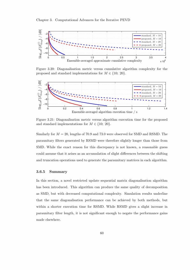
Chapter 3. Computational Advances for the Iterative PEVD
0 0.5 1 1.5 2 2.5 3 3.5 4
x 108
−10
−8
−6
−4
−2
Ensemble-averaged approximate cumulative complexity
5log
10EE
(i)
diag
/[dB]
standard, M = 10
proposed, M = 10
standard, M = 20
proposed, M = 20
Figure 3.20: Diagonalisation metric versus cumulative algorithm complexity for theproposed and standard implementations for M ∈ 10; 20.
0 0.2 0.4 0.6 0.8 1 1.2 1.4
−10
−8
−6
−4
−2
Ensemble-averaged algorithm execution time / s
5log
10EE
(i)
diag
/[dB]
standard, M = 10
proposed, M = 10
standard, M = 20
proposed, M = 20
Figure 3.21: Diagonalisation metric versus algorithm execution time for the proposedand standard implementations for M ∈ 10; 20.
Similarly for M = 20, lengths of 70.9 and 73.0 were observed for SMD and RSMD. The
paraunitary filters generated by RSMD were therefore slightly longer than those from
SMD. While the exact reason for this discrepancy is not known, a reasonable guess
could assume that it arises as an accumulation of slight differences between the shifting
and truncation operations used to generate the paraunitary matrices in each algorithm.
3.6.5 Summary
In this section, a novel restricted update sequential matrix diagonalisation algorithm
has been introduced. This algorithm can produce the same quality of decomposition
as SMD, but with decreased computational complexity. Simulation results underline
that the same diagonalisation performance can be achieved by both methods, but
within a shorter execution time for RSMD. While RSMD gives a slight increase in
paraunitary filter length, it is not significant enough to negate the performance gains
made elsewhere.
60
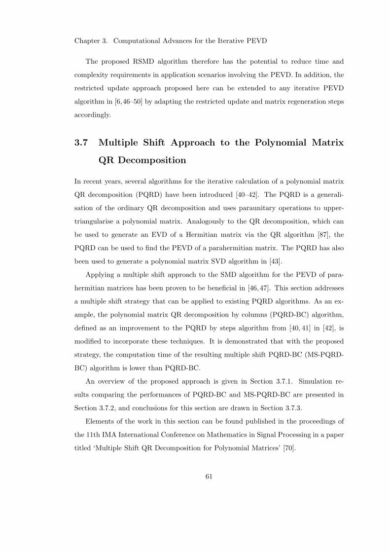
Chapter 3. Computational Advances for the Iterative PEVD
The proposed RSMD algorithm therefore has the potential to reduce time and
complexity requirements in application scenarios involving the PEVD. In addition, the
restricted update approach proposed here can be extended to any iterative PEVD
algorithm in [6,46–50] by adapting the restricted update and matrix regeneration steps
accordingly.
3.7 Multiple Shift Approach to the Polynomial Matrix
QR Decomposition
In recent years, several algorithms for the iterative calculation of a polynomial matrix
QR decomposition (PQRD) have been introduced [40–42]. The PQRD is a generali-
sation of the ordinary QR decomposition and uses paraunitary operations to upper-
triangularise a polynomial matrix. Analogously to the QR decomposition, which can
be used to generate an EVD of a Hermitian matrix via the QR algorithm [87], the
PQRD can be used to find the PEVD of a parahermitian matrix. The PQRD has also
been used to generate a polynomial matrix SVD algorithm in [43].
Applying a multiple shift approach to the SMD algorithm for the PEVD of para-
hermitian matrices has been proven to be beneficial in [46,47]. This section addresses
a multiple shift strategy that can be applied to existing PQRD algorithms. As an ex-
ample, the polynomial matrix QR decomposition by columns (PQRD-BC) algorithm,
defined as an improvement to the PQRD by steps algorithm from [40, 41] in [42], is
modified to incorporate these techniques. It is demonstrated that with the proposed
strategy, the computation time of the resulting multiple shift PQRD-BC (MS-PQRD-
BC) algorithm is lower than PQRD-BC.
An overview of the proposed approach is given in Section 3.7.1. Simulation re-
sults comparing the performances of PQRD-BC and MS-PQRD-BC are presented in
Section 3.7.2, and conclusions for this section are drawn in Section 3.7.3.
Elements of the work in this section can be found published in the proceedings of
the 11th IMA International Conference on Mathematics in Signal Processing in a paper
titled ‘Multiple Shift QR Decomposition for Polynomial Matrices’ [70].
61
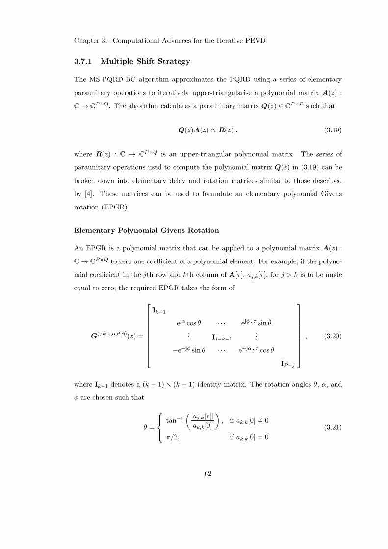
Chapter 3. Computational Advances for the Iterative PEVD
3.7.1 Multiple Shift Strategy
The MS-PQRD-BC algorithm approximates the PQRD using a series of elementary
paraunitary operations to iteratively upper-triangularise a polynomial matrix A(z) :
C→ CP×Q. The algorithm calculates a paraunitary matrix Q(z) ∈ C
P×P such that
Q(z)A(z) ≈ R(z) , (3.19)
where R(z) : C → CP×Q is an upper-triangular polynomial matrix. The series of
paraunitary operations used to compute the polynomial matrix Q(z) in (3.19) can be
broken down into elementary delay and rotation matrices similar to those described
by [4]. These matrices can be used to formulate an elementary polynomial Givens
rotation (EPGR).
Elementary Polynomial Givens Rotation
An EPGR is a polynomial matrix that can be applied to a polynomial matrix A(z) :
C→ CP×Q to zero one coefficient of a polynomial element. For example, if the polyno-
mial coefficient in the jth row and kth column of A[τ ], aj,k[τ ], for j > k is to be made
equal to zero, the required EPGR takes the form of
G(j,k,τ,α,θ,φ)(z) =
Ik−1
ejα cos θ · · · ejφzτ sin θ... Ij−k−1
...
−e−jφ sin θ · · · e−jαzτ cos θ
IP−j
, (3.20)
where Ik−1 denotes a (k − 1) × (k − 1) identity matrix. The rotation angles θ, α, and
φ are chosen such that
θ =
tan−1
( |aj,k[τ ]||ak,k[0]|
)
, if ak,k[0] 6= 0
π/2, if ak,k[0] = 0
(3.21)
62
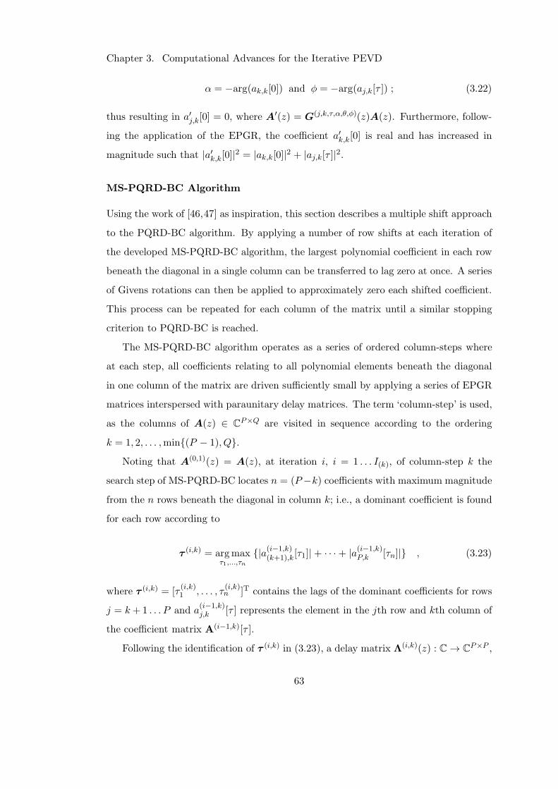
Chapter 3. Computational Advances for the Iterative PEVD
α = −arg(ak,k[0]) and φ = −arg(aj,k[τ ]) ; (3.22)
thus resulting in a′j,k[0] = 0, where A′(z) = G(j,k,τ,α,θ,φ)(z)A(z). Furthermore, follow-
ing the application of the EPGR, the coefficient a′k,k[0] is real and has increased in
magnitude such that |a′k,k[0]|2 = |ak,k[0]|2 + |aj,k[τ ]|2.
MS-PQRD-BC Algorithm
Using the work of [46,47] as inspiration, this section describes a multiple shift approach
to the PQRD-BC algorithm. By applying a number of row shifts at each iteration of
the developed MS-PQRD-BC algorithm, the largest polynomial coefficient in each row
beneath the diagonal in a single column can be transferred to lag zero at once. A series
of Givens rotations can then be applied to approximately zero each shifted coefficient.
This process can be repeated for each column of the matrix until a similar stopping
criterion to PQRD-BC is reached.
The MS-PQRD-BC algorithm operates as a series of ordered column-steps where
at each step, all coefficients relating to all polynomial elements beneath the diagonal
in one column of the matrix are driven sufficiently small by applying a series of EPGR
matrices interspersed with paraunitary delay matrices. The term ‘column-step’ is used,
as the columns of A(z) ∈ CP×Q are visited in sequence according to the ordering
k = 1, 2, . . . ,min(P − 1), Q.Noting that A(0,1)(z) = A(z), at iteration i, i = 1 . . . I(k), of column-step k the
search step of MS-PQRD-BC locates n = (P−k) coefficients with maximum magnitude
from the n rows beneath the diagonal in column k; i.e., a dominant coefficient is found
for each row according to
τ (i,k) = argmaxτ1,...,τn
|a(i−1,k)(k+1),k[τ1]|+ · · ·+ |a
(i−1,k)P,k [τn]| , (3.23)
where τ (i,k) = [τ(i,k)1 , . . . , τ
(i,k)n ]T contains the lags of the dominant coefficients for rows
j = k+1 . . . P and a(i−1,k)j,k [τ ] represents the element in the jth row and kth column of
the coefficient matrix A(i−1,k)[τ ].
Following the identification of τ (i,k) in (3.23), a delay matrix Λ(i,k)(z) : C→ CP×P ,
63
Chapter 3. Computational Advances for the Iterative PEVD
which takes the form
Λ(i,k)(z) =
Ik
zτ(i,k)1
. . .
zτ(i,k)n
, (3.24)
can be applied to A(i−1,k)(z) to induce a τ(i,k)m -fold delay to the mth row beneath the
diagonal in column k, wherem = 1 . . . n. Lag zero of the resulting matrix A(i−1,k)′(z) =
Λ(i,k)(z)A(i−1,k)(z) will contain the dominant coefficients from column k.
EPGRs are then applied to A(i−1,k)′[0] in sequence to drive elements
a(i−1,k)′(k+1),k [0] . . . a
(i−1,k)′P,k [0] to zero according to
A(i−1,k)′′[0] =(
G(k+1,k,γ1) · · ·G(P,k,γn))
A(i−1,k)′[0]
= H(i,k)A(i−1,k)′[0] , (3.25)
where the elements beneath the diagonal in the kth column of A(i−1,k)′′[0] are zero,
and G(j,k,γ) represents the EPGR required to zero element a(i−1,k)′j,k [0] of A(i−1,k)′[0].
Vector γ = [α, θ, φ]T contains the calculated rotation angles from (3.21) and (3.22) for
the targeted element. Note that G(j,k,γ) is an EPGR without shift parameter τ , and is
therefore a simple unitary matrix.
The matrix H(i,k) in (3.25) is the product of EPGRs required to drive the dominant
coefficients in iteration i of MS-PQRD-BC to zero. This unitary matrix is applied to
all lags of A(i−1,k)′(z) to generate A(i−1,k)′′(z) = H(i,k)A(i−1,k)′(z).
For stability reasons [42, 43], the final step of an iteration of MS-PQRD-BC is to
apply an inverse delay matrix Λ(i,k)(z) to produce the overall transformation
A(i,k)(z) = Λ(i,k)(z)H(i,k)Λ(i,k)(z)A(i−1,k)(z)
= Q(i,k)(z)A(i−1,k)(z) . (3.26)
This iterative process is repeated for a maximum of I(k) iterations or until all co-
64
Chapter 3. Computational Advances for the Iterative PEVD
efficients associated with polynomial elements beneath the diagonal in the kth column
of the matrix are sufficiently small in magnitude and therefore satisfy the stopping
condition
|a(i,k)j,k [τ ]| < ǫ (3.27)
for j > k and ∀ τ ∈ Z where ǫ > 0 is a prespecified small value. The overall transfor-
mation performed in the kth column-step of the algorithm is of the form
A(k)(z) = Q(k)(z)A(z) (3.28)
whereQ(k)(z) : C→ CP×P is the paraunitary product of all EPGRs and delay matrices
applied during iterations i = 1 . . . I(k) within column-steps 1 . . . k:
Q(k)(z) =
I(k)∏
i=1
Q(i,k)(z) · · ·I(1)∏
i=1
Q(i,1)(z) , (3.29)
whereI(k)∏
i=1
Q(i,k)(z) = Q(I(k),k)(z)Q(I(k)−1,k)(z) · · ·Q(2,k)(z)Q(1,k)(z) (3.30)
is the product of all EPGRs and delay matrices applied during iterations i = 1 . . . I(k)
and I(k) is the maximum number of iterations within column-step k, with I(k) = ⌈ IP−k ⌉
for some I ∈ N.
Following the kth column-step, all coefficients relating to all polynomial elements
beneath the diagonal in the kth column of the matrix A(z) will be sufficiently small.
After ℓ = min(P − 1), Q column-steps of the algorithm, all columns of the matrix
have been visited, and the transformation is of the form
R(z) = Q(z)A(z) (3.31)
where Q(z) = Q(ℓ)(z) is the paraunitary product of all EPGRs and delay matrices
applied during column-steps 1 . . . ℓ and R(z) is approximately upper-triangular.
65
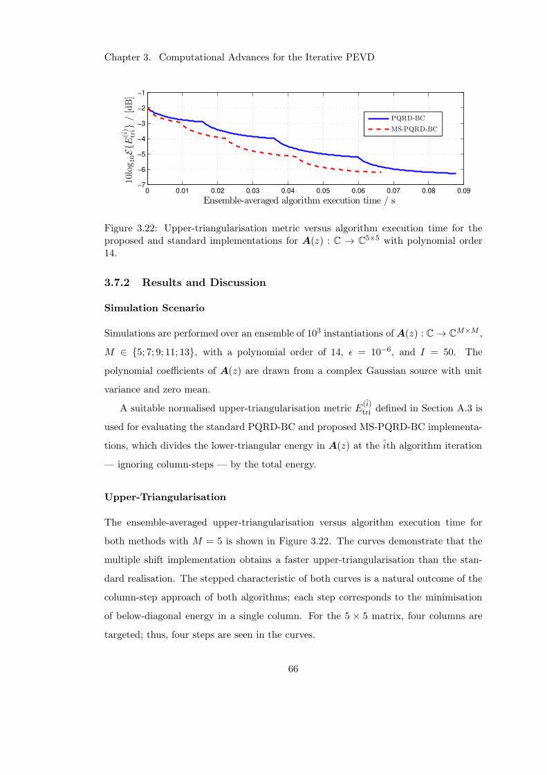
Chapter 3. Computational Advances for the Iterative PEVD
0 0.01 0.02 0.03 0.04 0.05 0.06 0.07 0.08 0.09−7
−6
−5
−4
−3
−2
−1
Ensemble-averaged algorithm execution time / s
5log
10EE
(i)
tri
/[dB]
PQRD-BC
MS-PQRD-BC10log10E
E(i)
tri/[dB]
Figure 3.22: Upper-triangularisation metric versus algorithm execution time for theproposed and standard implementations for A(z) : C → C
5×5 with polynomial order14.
3.7.2 Results and Discussion
Simulation Scenario
Simulations are performed over an ensemble of 103 instantiations of A(z) : C→ CM×M ,
M ∈ 5; 7; 9; 11; 13, with a polynomial order of 14, ǫ = 10−6, and I = 50. The
polynomial coefficients of A(z) are drawn from a complex Gaussian source with unit
variance and zero mean.
A suitable normalised upper-triangularisation metric E(i)tri defined in Section A.3 is
used for evaluating the standard PQRD-BC and proposed MS-PQRD-BC implementa-
tions, which divides the lower-triangular energy in A(z) at the ith algorithm iteration
— ignoring column-steps — by the total energy.
Upper-Triangularisation
The ensemble-averaged upper-triangularisation versus algorithm execution time for
both methods with M = 5 is shown in Figure 3.22. The curves demonstrate that the
multiple shift implementation obtains a faster upper-triangularisation than the stan-
dard realisation. The stepped characteristic of both curves is a natural outcome of the
column-step approach of both algorithms; each step corresponds to the minimisation
of below-diagonal energy in a single column. For the 5 × 5 matrix, four columns are
targeted; thus, four steps are seen in the curves.
66
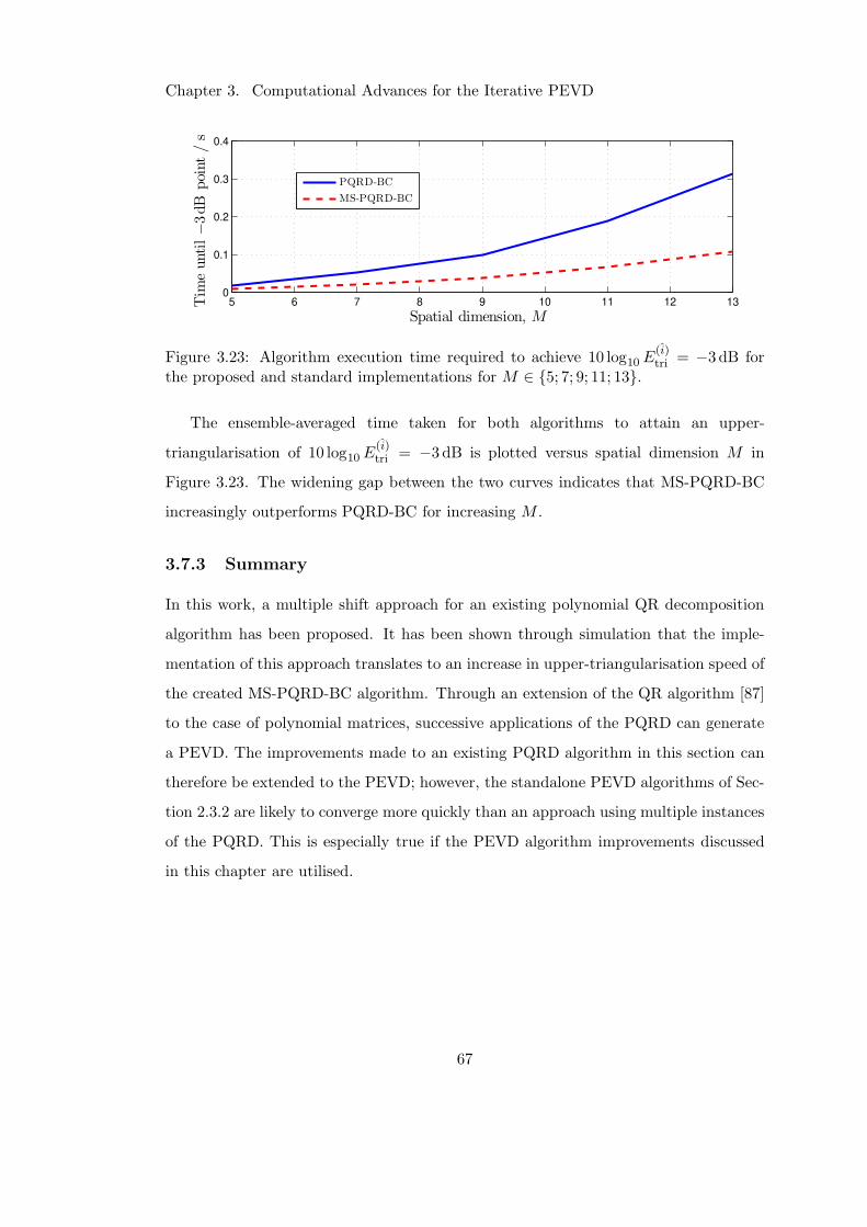
Chapter 3. Computational Advances for the Iterative PEVD
5 6 7 8 9 10 11 12 130
0.1
0.2
0.3
0.4
Spatial dimension, M
Tim
euntil−3dB
point
/s
PQRD-BC
MS-PQRD-BC
Figure 3.23: Algorithm execution time required to achieve 10 log10 E(i)tri = −3 dB for
the proposed and standard implementations for M ∈ 5; 7; 9; 11; 13.
The ensemble-averaged time taken for both algorithms to attain an upper-
triangularisation of 10 log10 E(i)tri = −3 dB is plotted versus spatial dimension M in
Figure 3.23. The widening gap between the two curves indicates that MS-PQRD-BC
increasingly outperforms PQRD-BC for increasing M .
3.7.3 Summary
In this work, a multiple shift approach for an existing polynomial QR decomposition
algorithm has been proposed. It has been shown through simulation that the imple-
mentation of this approach translates to an increase in upper-triangularisation speed of
the created MS-PQRD-BC algorithm. Through an extension of the QR algorithm [87]
to the case of polynomial matrices, successive applications of the PQRD can generate
a PEVD. The improvements made to an existing PQRD algorithm in this section can
therefore be extended to the PEVD; however, the standalone PEVD algorithms of Sec-
tion 2.3.2 are likely to converge more quickly than an approach using multiple instances
of the PQRD. This is especially true if the PEVD algorithm improvements discussed
in this chapter are utilised.
67
Chapter 3. Computational Advances for the Iterative PEVD
3.8 Compensated Row-Shift Truncation of Paraunitary
Matrices
A number of applications [17–19, 21–23, 25] utilise the PEVD’s paraunitary matrix of
polynomial eigenvectors, which can be considered to be a lossless FIR filter bank. Given
that low implementation costs are desirable, minimising the order of this matrix is of
importance.
As an extension of the traditional polynomial matrix truncation strategies in [60,61],
work in [62,63] has shown that by employing a row-shift truncation (RST) scheme for
paraunitary matrices from the SBR2 [6] PEVD algorithm, filter order can be reduced
with little loss to paraunitarity of the eigenvectors. This strategy requires a diagonal
D(z) to be effective without introducing decomposition error. In this section, a novel
variation of row-shift truncation titled compensated row-shift truncation (CRST) is
introduced; this method is able to reduce paraunitary matrix order without significantly
affecting decomposition error for even non-diagonal D(z).
An overview of the proposed approach is given in Section 3.8.1. Simulation results
comparing the performances of traditional, row-shift, and compensated row-shift trun-
cation when applied after SBR2 algorithm completion are presented in Section 3.8.2.
Further performance comparisons when using each truncation strategy at each itera-
tion of the SBR2 algorithm are given in Section 3.8.3. Conclusions for this section are
drawn in Section 3.8.4.
3.8.1 Compensated Row-Shift Truncation Strategy
The RST method [62,63] exploits ambiguity in the paraunitary matrices [62,96]. This
arises as a generalisation of a phase ambiguity inherent to eigenvectors from a standard
EVD [2], which in the polynomial case extends to arbitrary phase responses or all-pass
filters. The simplest manifestation of such filters can form an integer number of unit
delays. For a diagonal D(z), this ambiguity permits eigenvectors F (z) to be replaced
by a lower order F (z), where F (z) = Γ(z)F (z) and Γ(z) is a paraunitary diagonal
68
Chapter 3. Computational Advances for the Iterative PEVD
matrix. In this case, since diagonal matrices commute,
R(z) ≈ F (z)D(z)F (z) = ˜F (z)Γ(z)D(z)Γ(z)F (z)
= ˜F (z)D(z)F (z) , (3.32)
and D(z) in unaffected. If, however, D(z) is not diagonal — as is often the case
for a reasonable number of PEVD algorithm iterations when spatial dimension M is
large — Γ(z) does not cancel as in (3.32). In a novel variation of row-shift truncation
from [62] titled compensated row-shift truncation, this matrix Γ(z) is incorporated into
the parahermitian matrix to avoid negatively impacting the decomposition error. Since
one is typically only interested in the approximate polynomial eigenvalues stored on the
diagonal of D(z), the augmented parahermitian matrix D(z) = Γ(z)D(z)Γ(z) is used,
which has the same approximate polynomial eigenvalues. The decomposition accuracy
can now be maintained while using the lower order F (z):
R(z) ≈ ˜F (z)D(z)F (z) . (3.33)
While D(z) has a higher polynomial order than D(z), the order of the paraunitary
matrix is typically more important for application purposes [17–19,21–23,25].
From the original RST approach of [62], Γ(z) takes the form
Γ(z) = diagzτ1 , zτ2 , . . . , zτM . (3.34)
The delay matrix Γ(z) has the effect of shifting the mth row of the paraunitary matrix
F (z) by τm. These row shifts can be used to align the first polynomial coefficients in
each row of the paraunitary matrix following the independent truncation of each row
via the process below.
The matrix F (z) can be subdivided into its M row vectors fm(z) : C → C1×M ,
69
Chapter 3. Computational Advances for the Iterative PEVD
m = 1 . . .M ,
F (z) =
f1(z)...
fM (z)
. (3.35)
Each row — which has minimum lag T1,m and maximum lag T2,m — is then truncated
individually according to ftrim(fm[τ ], µ) from (C.1) in Appendix C. The row shifts, τm,
in (3.34) are then set equal to (T1,m + T3,m(µ)), m = 1 . . .M , such that the minimum
lag of each shifted row fm(z) is zero. Here, T3,m(µ) is the T3(µ) obtained via (C.1)
in Appendix C for the mth row. Following row-shift truncation, each row of F (z)
has order Tm(µ), and the order of the paraunitary matrix is maxm=1...M
Tm(µ), whereTm(µ) = T2,m − (T3,m(µ) + T4,m(µ)) and T4,m(µ) is the T4(µ) obtained via (C.1).
When applying CRST to a matrix F (z), one therefore obtains
[F (z), D(z)]← fcrst(F (z),D(z), µ) , (3.36)
where
fm[τ ] —• fm(z) = zτmT2,m∑
τ=T1,m
ftrim(fm[τ ], µ)z−τ . (3.37)
3.8.2 Truncating After Algorithm Completion
Simulation Scenario
The simulations below are performed over an ensemble of 103 instantiations of R(z) :
C → CM×M obtained from the randomised source model in Appendix B [45] with
M = 5, OD = 118, OQ = 60, and ∆DR = 30.
Three instances of SBR2 are implemented; the first uses the standard SBR2 pa-
raunitary matrix truncation strategy of Appendix C with threshold µtrad = 10−6,
the second uses the RST strategy of [62] with µRST = 10−6, and the third uses
CRST with µCRST = 10−6. Each instance of SBR2 is executed for a maximum of
Imax ∈ 1; 2; . . . ; 200 iterations with a stopping threshold of ǫ = 0 and parahermitian
matrix truncation parameter of µ = 10−12. Parahermitian matrix truncation is exe-
cuted at the end of each algorithm iteration, and immediately following CRST, but
70
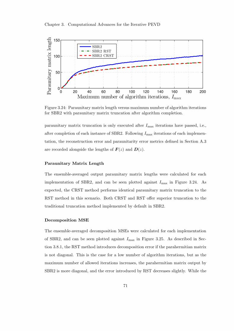
Chapter 3. Computational Advances for the Iterative PEVD
0 20 40 60 80 100 120 140 160 180 2000
50
100
150
Maximum number of algorithm iterations, Imax
Paraunitarymatrixlength
SBR2SBR2 RSTSBR2 CRST
Figure 3.24: Paraunitary matrix length versus maximum number of algorithm iterationsfor SBR2 with paraunitary matrix truncation after algorithm completion.
paraunitary matrix truncation is only executed after Imax iterations have passed, i.e.,
after completion of each instance of SBR2. Following Imax iterations of each implemen-
tation, the reconstruction error and paraunitarity error metrics defined in Section A.3
are recorded alongside the lengths of F (z) and D(z).
Paraunitary Matrix Length
The ensemble-averaged output paraunitary matrix lengths were calculated for each
implementation of SBR2, and can be seen plotted against Imax in Figure 3.24. As
expected, the CRST method performs identical paraunitary matrix truncation to the
RST method in this scenario. Both CRST and RST offer superior truncation to the
traditional truncation method implemented by default in SBR2.
Decomposition MSE
The ensemble-averaged decomposition MSEs were calculated for each implementation
of SBR2, and can be seen plotted against Imax in Figure 3.25. As described in Sec-
tion 3.8.1, the RST method introduces decomposition error if the parahermitian matrix
is not diagonal. This is the case for a low number of algorithm iterations, but as the
maximum number of allowed iterations increases, the parahermitian matrix output by
SBR2 is more diagonal, and the error introduced by RST decreases slightly. While the
71
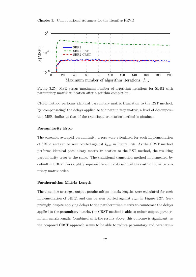
Chapter 3. Computational Advances for the Iterative PEVD
0 20 40 60 80 100 120 140 160 180 20010
−10
10−5
100
Maximum number of algorithm iterations, Imax
EM
SE
SBR2SBR2 RSTSBR2 CRST
Figure 3.25: MSE versus maximum number of algorithm iterations for SBR2 withparaunitary matrix truncation after algorithm completion.
CRST method performs identical paraunitary matrix truncation to the RST method,
by ‘compensating’ the delays applied to the paraunitary matrix, a level of decomposi-
tion MSE similar to that of the traditional truncation method is obtained.
Paraunitarity Error
The ensemble-averaged paraunitarity errors were calculated for each implementation
of SBR2, and can be seen plotted against Imax in Figure 3.26. As the CRST method
performs identical paraunitary matrix truncation to the RST method, the resulting
paraunitarity error is the same. The traditional truncation method implemented by
default in SBR2 offers slightly superior paraunitarity error at the cost of higher parau-
nitary matrix order.
Parahermitian Matrix Length
The ensemble-averaged output parahermitian matrix lengths were calculated for each
implementation of SBR2, and can be seen plotted against Imax in Figure 3.27. Sur-
prisingly, despite applying delays to the parahermitian matrix to counteract the delays
applied to the paraunitary matrix, the CRST method is able to reduce output paraher-
mitian matrix length. Combined with the results above, this outcome is significant, as
the proposed CRST approach seems to be able to reduce paraunitary and parahermi-
72
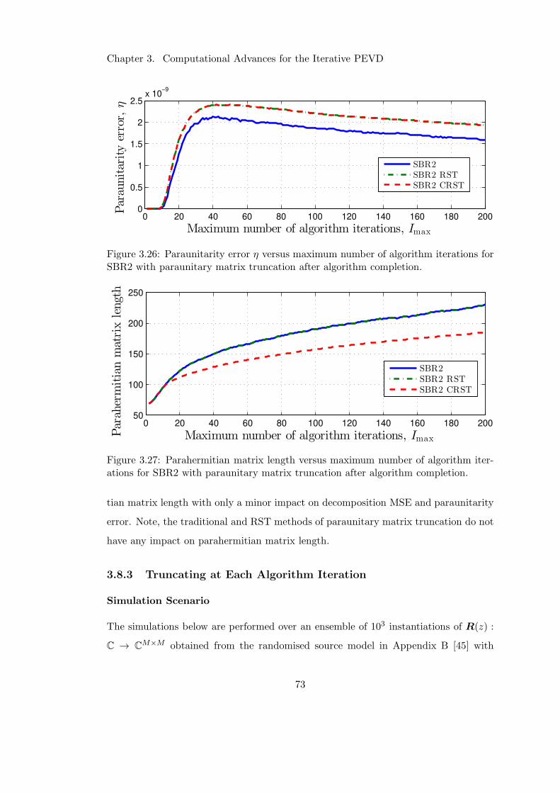
Chapter 3. Computational Advances for the Iterative PEVD
0 20 40 60 80 100 120 140 160 180 2000
0.5
1
1.5
2
2.5x 10
−9
Maximum number of algorithm iterations, Imax
Paraunitarityerror,
η
SBR2SBR2 RSTSBR2 CRST
Figure 3.26: Paraunitarity error η versus maximum number of algorithm iterations forSBR2 with paraunitary matrix truncation after algorithm completion.
0 20 40 60 80 100 120 140 160 180 20050
100
150
200
250
Maximum number of algorithm iterations, Imax
Parahermitianmatrixlength
SBR2SBR2 RSTSBR2 CRST
Figure 3.27: Parahermitian matrix length versus maximum number of algorithm iter-ations for SBR2 with paraunitary matrix truncation after algorithm completion.
tian matrix length with only a minor impact on decomposition MSE and paraunitarity
error. Note, the traditional and RST methods of paraunitary matrix truncation do not
have any impact on parahermitian matrix length.
3.8.3 Truncating at Each Algorithm Iteration
Simulation Scenario
The simulations below are performed over an ensemble of 103 instantiations of R(z) :
C → CM×M obtained from the randomised source model in Appendix B [45] with
73
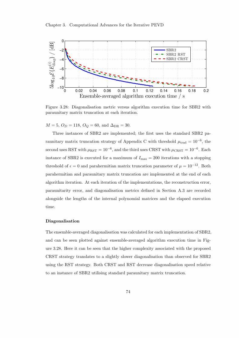
Chapter 3. Computational Advances for the Iterative PEVD
0 0.02 0.04 0.06 0.08 0.1 0.12 0.14 0.16 0.18 0.2−10
−8
−6
−4
−2
0
Ensemble-averaged algorithm execution time / s
5log
10EE
(i)
diag
/[dB]
SBR2SBR2 RSTSBR2 CRST
Figure 3.28: Diagonalisation metric versus algorithm execution time for SBR2 withparaunitary matrix truncation at each iteration.
M = 5, OD = 118, OQ = 60, and ∆DR = 30.
Three instances of SBR2 are implemented; the first uses the standard SBR2 pa-
raunitary matrix truncation strategy of Appendix C with threshold µtrad = 10−6, the
second uses RST with µRST = 10−6, and the third uses CRST with µCRST = 10−6. Each
instance of SBR2 is executed for a maximum of Imax = 200 iterations with a stopping
threshold of ǫ = 0 and parahermitian matrix truncation parameter of µ = 10−12. Both
parahermitian and paraunitary matrix truncation are implemented at the end of each
algorithm iteration. At each iteration of the implementations, the reconstruction error,
paraunitarity error, and diagonalisation metrics defined in Section A.3 are recorded
alongside the lengths of the internal polynomial matrices and the elapsed execution
time.
Diagonalisation
The ensemble-averaged diagonalisation was calculated for each implementation of SBR2,
and can be seen plotted against ensemble-averaged algorithm execution time in Fig-
ure 3.28. Here it can be seen that the higher complexity associated with the proposed
CRST strategy translates to a slightly slower diagonalisation than observed for SBR2
using the RST strategy. Both CRST and RST decrease diagonalisation speed relative
to an instance of SBR2 utilising standard paraunitary matrix truncation.
74
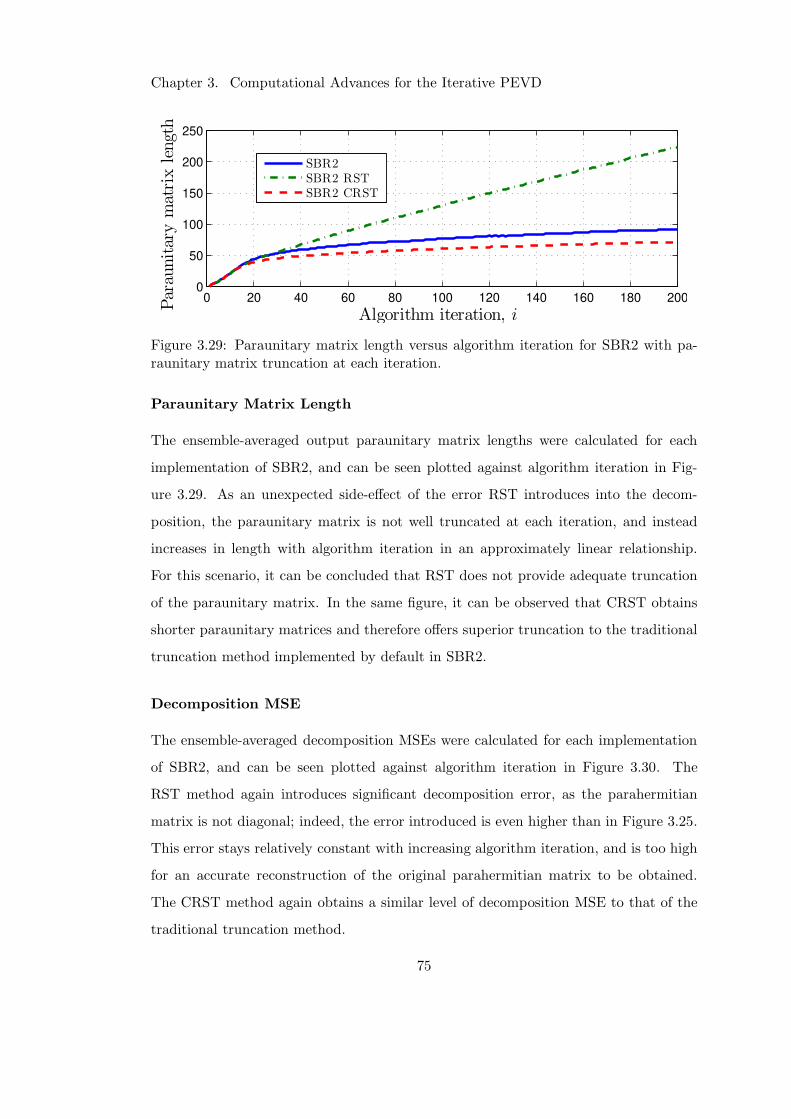
Chapter 3. Computational Advances for the Iterative PEVD
0 20 40 60 80 100 120 140 160 180 2000
50
100
150
200
250
Algorithm iteration, i
Paraunitarymatrixlength
SBR2SBR2 RSTSBR2 CRST
Figure 3.29: Paraunitary matrix length versus algorithm iteration for SBR2 with pa-raunitary matrix truncation at each iteration.
Paraunitary Matrix Length
The ensemble-averaged output paraunitary matrix lengths were calculated for each
implementation of SBR2, and can be seen plotted against algorithm iteration in Fig-
ure 3.29. As an unexpected side-effect of the error RST introduces into the decom-
position, the paraunitary matrix is not well truncated at each iteration, and instead
increases in length with algorithm iteration in an approximately linear relationship.
For this scenario, it can be concluded that RST does not provide adequate truncation
of the paraunitary matrix. In the same figure, it can be observed that CRST obtains
shorter paraunitary matrices and therefore offers superior truncation to the traditional
truncation method implemented by default in SBR2.
Decomposition MSE
The ensemble-averaged decomposition MSEs were calculated for each implementation
of SBR2, and can be seen plotted against algorithm iteration in Figure 3.30. The
RST method again introduces significant decomposition error, as the parahermitian
matrix is not diagonal; indeed, the error introduced is even higher than in Figure 3.25.
This error stays relatively constant with increasing algorithm iteration, and is too high
for an accurate reconstruction of the original parahermitian matrix to be obtained.
The CRST method again obtains a similar level of decomposition MSE to that of the
traditional truncation method.
75
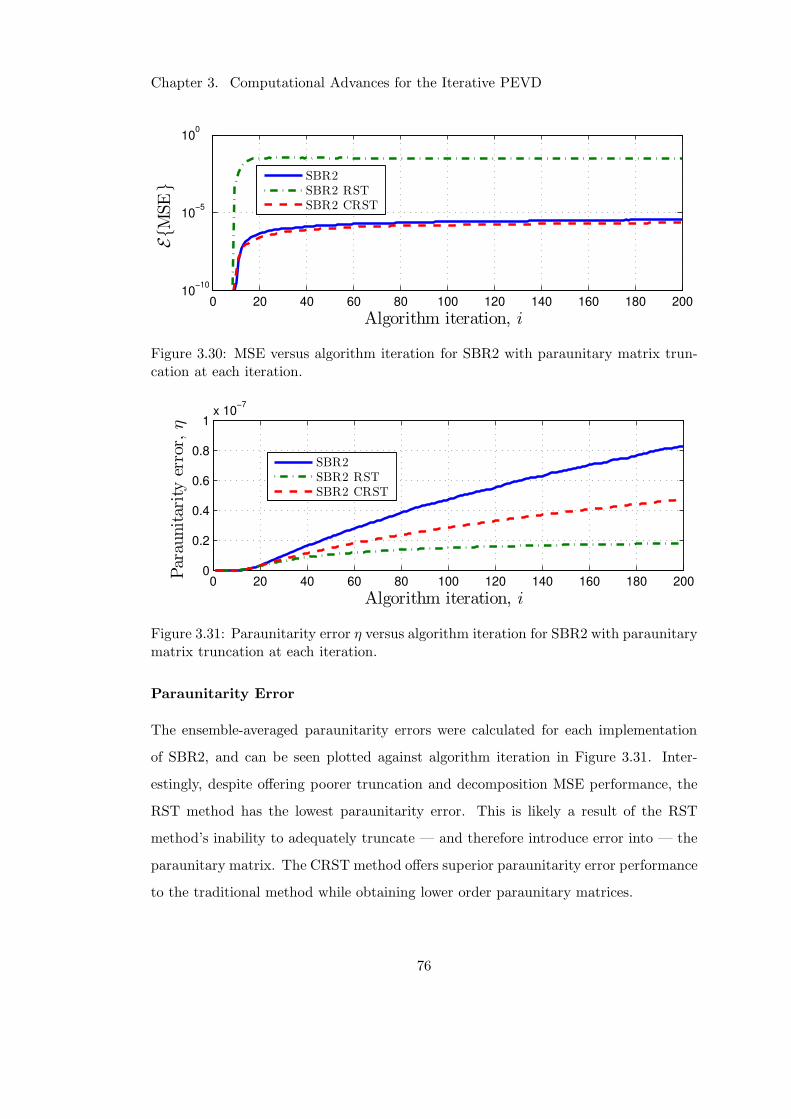
Chapter 3. Computational Advances for the Iterative PEVD
0 20 40 60 80 100 120 140 160 180 20010
−10
10−5
100
Algorithm iteration, i
EM
SE
SBR2SBR2 RSTSBR2 CRST
Figure 3.30: MSE versus algorithm iteration for SBR2 with paraunitary matrix trun-cation at each iteration.
0 20 40 60 80 100 120 140 160 180 2000
0.2
0.4
0.6
0.8
1x 10
−7
Algorithm iteration, i
Paraunitarityerror,
η
SBR2SBR2 RSTSBR2 CRST
Figure 3.31: Paraunitarity error η versus algorithm iteration for SBR2 with paraunitarymatrix truncation at each iteration.
Paraunitarity Error
The ensemble-averaged paraunitarity errors were calculated for each implementation
of SBR2, and can be seen plotted against algorithm iteration in Figure 3.31. Inter-
estingly, despite offering poorer truncation and decomposition MSE performance, the
RST method has the lowest paraunitarity error. This is likely a result of the RST
method’s inability to adequately truncate — and therefore introduce error into — the
paraunitary matrix. The CRST method offers superior paraunitarity error performance
to the traditional method while obtaining lower order paraunitary matrices.
76
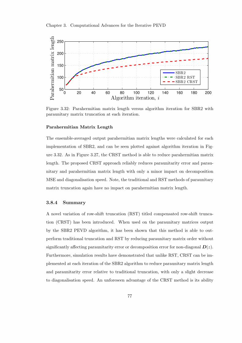
Chapter 3. Computational Advances for the Iterative PEVD
0 20 40 60 80 100 120 140 160 180 20050
100
150
200
250
Algorithm iteration, iParahermitianmatrixlength
SBR2SBR2 RSTSBR2 CRST
Figure 3.32: Parahermitian matrix length versus algorithm iteration for SBR2 withparaunitary matrix truncation at each iteration.
Parahermitian Matrix Length
The ensemble-averaged output parahermitian matrix lengths were calculated for each
implementation of SBR2, and can be seen plotted against algorithm iteration in Fig-
ure 3.32. As in Figure 3.27, the CRST method is able to reduce parahermitian matrix
length. The proposed CRST approach reliably reduces paraunitarity error and parau-
nitary and parahermitian matrix length with only a minor impact on decomposition
MSE and diagonalisation speed. Note, the traditional and RST methods of paraunitary
matrix truncation again have no impact on parahermitian matrix length.
3.8.4 Summary
A novel variation of row-shift truncation (RST) titled compensated row-shift trunca-
tion (CRST) has been introduced. When used on the paraunitary matrices output
by the SBR2 PEVD algorithm, it has been shown that this method is able to out-
perform traditional truncation and RST by reducing paraunitary matrix order without
significantly affecting paraunitarity error or decomposition error for non-diagonal D(z).
Furthermore, simulation results have demonstrated that unlike RST, CRST can be im-
plemented at each iteration of the SBR2 algorithm to reduce paraunitary matrix length
and paraunitarity error relative to traditional truncation, with only a slight decrease
to diagonalisation speed. An unforeseen advantage of the CRST method is its ability
77
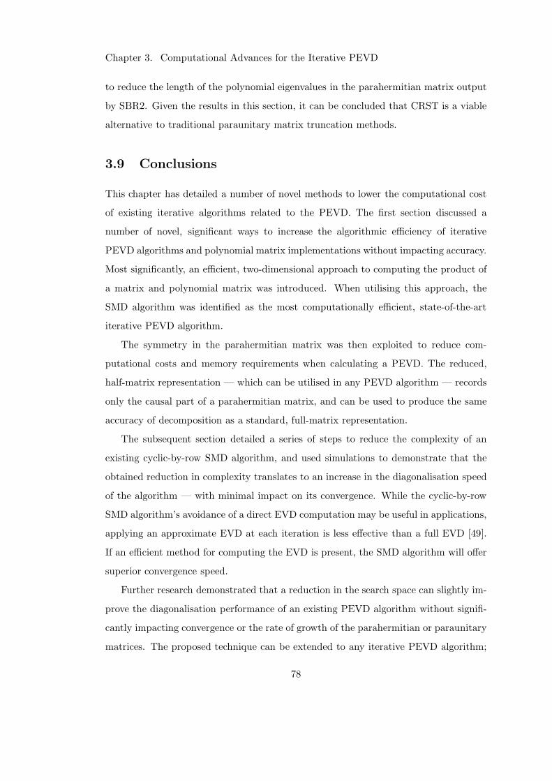
Chapter 3. Computational Advances for the Iterative PEVD
to reduce the length of the polynomial eigenvalues in the parahermitian matrix output
by SBR2. Given the results in this section, it can be concluded that CRST is a viable
alternative to traditional paraunitary matrix truncation methods.
3.9 Conclusions
This chapter has detailed a number of novel methods to lower the computational cost
of existing iterative algorithms related to the PEVD. The first section discussed a
number of novel, significant ways to increase the algorithmic efficiency of iterative
PEVD algorithms and polynomial matrix implementations without impacting accuracy.
Most significantly, an efficient, two-dimensional approach to computing the product of
a matrix and polynomial matrix was introduced. When utilising this approach, the
SMD algorithm was identified as the most computationally efficient, state-of-the-art
iterative PEVD algorithm.
The symmetry in the parahermitian matrix was then exploited to reduce com-
putational costs and memory requirements when calculating a PEVD. The reduced,
half-matrix representation — which can be utilised in any PEVD algorithm — records
only the causal part of a parahermitian matrix, and can be used to produce the same
accuracy of decomposition as a standard, full-matrix representation.
The subsequent section detailed a series of steps to reduce the complexity of an
existing cyclic-by-row SMD algorithm, and used simulations to demonstrate that the
obtained reduction in complexity translates to an increase in the diagonalisation speed
of the algorithm — with minimal impact on its convergence. While the cyclic-by-row
SMD algorithm’s avoidance of a direct EVD computation may be useful in applications,
applying an approximate EVD at each iteration is less effective than a full EVD [49].
If an efficient method for computing the EVD is present, the SMD algorithm will offer
superior convergence speed.
Further research demonstrated that a reduction in the search space can slightly im-
prove the diagonalisation performance of an existing PEVD algorithm without signifi-
cantly impacting convergence or the rate of growth of the parahermitian or paraunitary
matrices. The proposed technique can be extended to any iterative PEVD algorithm;
78
Chapter 3. Computational Advances for the Iterative PEVD
however, given the relatively small performance gains achieved through the implemen-
tation of this method, it is likely that the additional effort required to estimate the
search space reduction negates any gains made.
A more promising restricted update approach to the PEVD was then introduced.
A version of the SMD algorithm modified to incorporate this method was found to
produce the same quality of decomposition as SMD, but with decreased computational
complexity and execution time requirements. Importantly, the restricted update ap-
proach can be extended to any iterative PEVD algorithm to increase diagonalisation
speed.
With the knowledge that successive applications of the polynomial matrix QR de-
composition can generate a PEVD, improvements were then made to an existing poly-
nomial matrix QR decomposition algorithm. The resulting multiple shift approach
demonstrated superior triangularisation speed to the original method; however, exist-
ing PEVD algorithms are likely to be more efficient than using multiple instances of
the PQRD.
Finally, a novel compensated row-shift truncation approach was introduced as an
alternative to existing truncation methods. When used on the paraunitary matrices
output by the SBR2 PEVD algorithm, it was demonstrated that this approach is able to
outperform existing truncation strategies by reducing paraunitary matrix order with-
out significantly affecting paraunitarity error or decomposition error for non-diagonal
D(z). Furthermore, simulation results demonstrated that the developed method can
potentially be used to reduce the lengths of the polynomial matrices internal to PEVD
algorithms with only a slight decrease to diagonalisation speed.
While each of the methods discussed in this chapter decrease the implementation
costs of various PEVD approaches, the complexity of the algorithms grows rapidly
with the spatial dimensions of the parahermitian matrix, such that even the improved
PEVD algorithms are not well-suited for applications involving large broadband arrays.
The next chapter addresses this problem by taking additional steps to convert the
sequential form of existing PEVD algorithms to a partially parallelisable divide-and-
conquer architecture.
79
Chapter 4
Divide-and-Conquer Strategy for
PEVD Algorithms
4.1 Introduction
While the contents of Chapter 3 addressed computational advances applicable to a
number of the existing iterative PEVD algorithms discussed in Section 2.3.2, the com-
plexities of the improved algorithms are still highly dependent on the spatial dimension
of the parahermitian matrix. As discussed in the previous chapter, parahermitian ma-
trices with a large spatial dimension M — which dictates the number of rows and
columns in the matrix — can occur in scenarios involving a large number of broadband
sensors. In addition, due to the current reliance of PEVD algorithms on sequential pro-
cessing — i.e., requiring iteration i to be fully complete prior to iteration (i+1) — the
explosion in the availability of parallel processing capable hardware [97–101] has not
yet been fully exploited during the implementation of PEVD algorithms. This chapter
therefore introduces a novel methodology for the PEVD that takes inspiration from
existing so-called divide-and-conquer (DaC) solutions to eigenproblems to ‘divide’ the
PEVD of a parahermitian matrix with large spatial dimension into a number of compo-
nents involving smaller spatial dimensions, before ‘conquering’ each element separately
— and potentially simultaneously.
Below, Section 4.2 provides a brief introduction to DaC methods and their applica-
80
Chapter 4. Divide-and-Conquer Strategy for PEVD Algorithms
tion to eigenproblems, before Section 4.3 describes how DaC strategies can be extended
to the PEVD by incorporating a transformation of the input parahermitian matrix to
block diagonal form. Section 4.4 then details a novel algorithm, named sequential ma-
trix segmentation (SMS), capable of carrying out such a transformation. Based on
the framework of Section 4.3, a further novel algorithm in Section 4.5 utilises SMS to
enforce the transformation of a parahermitian matrix with large spatial dimension to
block diagonal form, before employing an existing PEVD algorithm to diagonalise each
block independently. This algorithm is suitably named divide-and-conquer SMD (DC-
SMD), owing to its use of the SMD algorithm [45] for diagonalisation purposes. In a
final effort to produce the most computationally efficient PEVD algorithm, Section 4.6
incorporates several of the computational schemes discussed in Chapter 3 within DC-
SMD and introduces parallelisation to the ‘conquer’ stage of the resulting algorithm,
which is named parallel-SMD (PSMD). Broadband source model and angle of arrival
estimation simulation results are used to compare the performances of the developed
DaC approaches with existing PEVD algorithms in Section 4.7, and conclusions for
this chapter are provided in Section 4.8.
Elements of the work in this chapter can be found published in the proceedings
of the 2017 IEEE International Workshop on Signal Processing Systems [64], and the
2017 IEEE Sensor Signal Processing for Defence Conference [20, 71]. A further paper
has been submitted to IEEE Transactions on Circuits and Systems I [72].
4.2 Divide-and-Conquer as a Methodology
In the realm of algorithm design, DaC strategies typically decompose a large prob-
lem to be solved into a number of smaller, independent subproblems; the solutions
to these subproblems are then combined to form an overall solution to the original
problem [102]. Such approaches can be extended to any number of large scale sig-
nal processing problems, and can be found in efficient sorting [103] and fast Fourier
transform algorithms [93], for example. Specifically in relation to eigenproblems, re-
search in [104] introduces a DaC method for the symmetric tridiagonal eigenproblem,
while [105] extends this approach to create a fully parallel algorithm for the symmet-
81
Chapter 4. Divide-and-Conquer Strategy for PEVD Algorithms
ric eigenvalue problem. Furthermore, in [106], a low-complexity version of the DaC
approach in [104] is presented.
While the PEVD does not explicitly involve tridiagonal matrices, there is clearly
precedent for the utilisation of DaC algorithms to obtain eigenvalues. The compu-
tational complexity of current PEVD algorithms is strongly influenced by the spatial
dimensions of the parahermitian matrix; devising a similar strategy to above that re-
duces the dimensionality of the problem is therefore of great interest. Furthermore,
if such a strategy can be developed, the parallelised and low-complexity algorithms
of [105] and [106], respectively, suggest that a low-complexity, parallelised DaC PEVD
algorithm may be obtainable.
4.3 Extending the Divide-and-Conquer Methodology to
the PEVD
4.3.1 Problem Formulation
The existing iterative PEVD algorithms discussed in Section 2.3.2 all take a purely
sequential approach. That is, the computations in iteration i + 1 of existing algo-
rithms cannot be commenced before finalising the computations in iteration i. This
is problematic for the development of a parallelised PEVD algorithm. An implicit as-
sumption within these algorithms is that the entirety of the parahermitian matrix must
be updated at each iteration to avoid the introduction of error to the decomposition;
however, this is not always the case. For example, consider the parahermitian matrix
R(z) : C→ CM×M , which can be thought of as four matrices arranged as shown:
R(z) =
R11(z) R12(z)
R21(z) R22(z)
. (4.1)
Here, R(z) is represented using parahermitian submatrices R11(z) : C →C(M−P )×(M−P ) and R22(z) : C→ C
P×P , and non-parahermitian submatrices R21(z) :
C → CP×(M−P ) and R12(z) : C → C
(M−P )×P , with R21(z) = R12(z) by definition. If
R21(z) = 0, R(z) is block diagonal, and submatrices R11(z) and R22(z) can each ex-
82
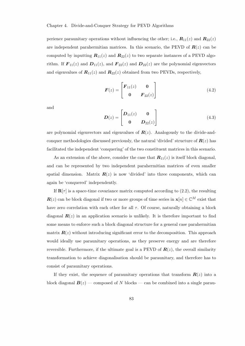
Chapter 4. Divide-and-Conquer Strategy for PEVD Algorithms
perience paraunitary operations without influencing the other; i.e., R11(z) and R22(z)
are independent parahermitian matrices. In this scenario, the PEVD of R(z) can be
computed by inputting R11(z) and R22(z) to two separate instances of a PEVD algo-
rithm. If F 11(z) and D11(z), and F 22(z) and D22(z) are the polynomial eigenvectors
and eigenvalues of R11(z) and R22(z) obtained from two PEVDs, respectively,
F (z) =
F 11(z) 0
0 F 22(z)
(4.2)
and
D(z) =
D11(z) 0
0 D22(z)
(4.3)
are polynomial eigenvectors and eigenvalues of R(z). Analogously to the divide-and-
conquer methodologies discussed previously, the natural ‘divided’ structure of R(z) has
facilitated the independent ‘conquering’ of the two constituent matrices in this scenario.
As an extension of the above, consider the case that R11(z) is itself block diagonal,
and can be represented by two independent parahermitian matrices of even smaller
spatial dimension. Matrix R(z) is now ‘divided’ into three components, which can
again be ‘conquered’ independently.
If R[τ ] is a space-time covariance matrix computed according to (2.2), the resulting
R(z) can be block diagonal if two or more groups of time series in x[n] ∈ CM exist that
have zero correlation with each other for all τ . Of course, naturally obtaining a block
diagonal R(z) in an application scenario is unlikely. It is therefore important to find
some means to enforce such a block diagonal structure for a general case parahermitian
matrix R(z) without introducing significant error to the decomposition. This approach
would ideally use paraunitary operations, as they preserve energy and are therefore
reversible. Furthermore, if the ultimate goal is a PEVD of R(z), the overall similarity
transformation to achieve diagonalisation should be paraunitary, and therefore has to
consist of paraunitary operations.
If they exist, the sequence of paraunitary operations that transform R(z) into a
block diagonal B(z) — composed of N blocks — can be combined into a single parau-
83
Chapter 4. Divide-and-Conquer Strategy for PEVD Algorithms
nitary matrix T (z) such that
B(z) = T (z)R(z)T (z) ≈
B11(z) 0 . . . 0
0 B22(z) . . ....
......
. . ....
0 . . . . . . BNN (z)
. (4.4)
As in equation (2.4), (4.4) has only approximate equality, as it is likely that the de-
composition to obtain a block diagonal matrix from a finite order polynomial matrix
is not of finite order. However, as found with the PEVD [9], it is assumed that the
approximation error will become arbitrarily small if the order of the approximation is
selected to be sufficiently large. As above, the PEVDs of each Bnn(z), n = 1 . . . N , can
be conducted in parallel to produce polynomial eigenvectors
F (z) =
F 11(z) 0 . . . 0
0 F 22(z) . . ....
......
. . ....
0 . . . . . . FNN (z)
(4.5)
and polynomial eigenvalues
D(z) =
D11(z) 0 . . . 0
0 D22(z) . . ....
......
. . ....
0 . . . . . . DNN (z)
, (4.6)
such that Bnn(z) ≈ ˜F nn(z)Dnn(z)F nn(z) and
R(z) ≈ T (z) ˜F (z)D(z)F (z)T (z) = F (z)D(z)F (z) , (4.7)
where F (z) = F (z)T (z). Matrix F (z), which is the product of two paraunitary ma-
trices and is therefore paraunitary by construction, decomposes R(z) to a diagonal
84
Chapter 4. Divide-and-Conquer Strategy for PEVD Algorithms
matrix D(z) containing polynomial eigenvalues, and can therefore be considered to
contain polynomial eigenvectors.
4.3.2 Block Diagonalising a Parahermitian Matrix
The paraunitary matrix T (z) that ‘divides’ a parahermitian matrix into block diagonal
form cannot be immediately ascertained from observation of R(z). However, using an
approach akin to iterative PEVD algorithms — which seek to iteratively diagonalise a
parahermitian matrix via paraunitary operations — an algorithm can be developed that
uses paraunitary operations to iteratively block diagonalise a parahermitian matrix.
One approach, which is described below, is to block diagonalise the parahermitian
matrix in stages.
For some user-specified P , with P < M , the first stage of the iterative process to
block diagonalise a parahermitian matrix B(0)(z) = R(z) : C→ CM×M seeks to obtain
a paraunitary matrix T (1)(z) : C→ CM×M such that
B(1)(z) = T (1)(z)B(0)(z)T (1)(z) ≈
B
(1)11 (z) 0
0 B(1)22 (z)
(4.8)
is block diagonal with two parahermitian submatrices B(1)11 (z) : C → C
(M−P )×(M−P )
and B(1)22 (z) : C → C
P×P . Note that, as in equation (4.4), this transformation is
unlikely to be achievable using finite order polynomial matrices; thus, (4.8) has only
approximate equality.
Provided that P < (M −P ), the second stage seeks to obtain a further paraunitary
matrix
T (2)(z) =
T (2)(z) 0
0 IP
, (4.9)
that operates on B(1)11 (z) such that
B(2)(z) = T (2)(z)B(1)(z)T (2)(z) ≈
B(2)11 (z) 0 0
0 B(2)22 (z) 0
0 0 B(1)22 (z)
(4.10)
85
Chapter 4. Divide-and-Conquer Strategy for PEVD Algorithms
is block diagonal with two parahermitian submatrices B(2)11 (z) : C→ C
(M−2P )×(M−2P )
and B(2)22 (z) : C → C
P×P , plus parahermitian submatrix B(1)22 (z) from before. Here,
T (2)(z) : C→ C(M−P )×(M−P ) has transformed B
(1)11 (z) into block diagonal form, while
B(1)22 (z) is influenced by identity matrix IP and is therefore unaffected.
The above process repeats a total of β times, i.e., until P ≥ (M − βP ) and
some B(β)(z) has been obtained with parahermitian submatrices B(β)11 (z) : C →
C(M−βP )×(M−βP ) and B
(β)22 (z) : C→ C
P×P , alongside a ‘dividing’ matrix
T (β)(z) =
T (β)(z) 0
0 I(β−1)P
. (4.11)
The final block diagonal parahermitian matrix can be written as
B(z) = T (z)R(z)T (z) ≈
B(β)11 (z) 0 . . . . . . 0
0 B(β)22 (z)
...... B
(β−1)22 (z)
......
. . ....
0 . . . . . . . . . B(1)22 (z)
. (4.12)
Note that matrices B(b)22 (z), b = 1 . . . β, have spatial dimensions of P ×P , while B
(β)11 (z)
is of spatial dimension (M − βP ) × (M − βP ). The overall paraunitary ‘dividing’
matrix T (z) that transforms R(z) to block diagonal form can be found by computing
the product of all T (b)(z), b = 1 . . . β, according to
T (z) = T (β)(z)T (β−1)(z) · · ·T (1)(z)
=
T (β)(z) 0
0 I(β−1)P
T (β−1)(z) 0
0 I(β−2)P
· · ·T (1)(z) , (4.13)
where the insertion of identity matrices has ensured an overall spatial dimension of
M ×M .
Once R(z) has been transformed to block diagonal form, each parahermitian sub-
matrix can be diagonalised independently through the use of a PEVD algorithm.
86
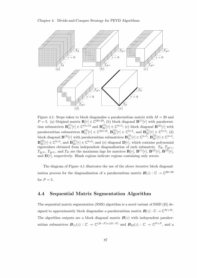
Chapter 4. Divide-and-Conquer Strategy for PEVD Algorithms
a) c)
=
TR
TR
=
T1)
T1)
=
T2)
T2)
b)
e)
=
T3)
T3)
=
TD
TD
d)
Figure 4.1: Steps taken to block diagonalise a parahermitian matrix with M = 20 andP = 5. (a) Original matrix R[τ ] ∈ C
20×20; (b) block diagonal B(1)[τ ] with parahermi-
tian submatrices B(1)11 [τ ] ∈ C
15×15 and B(1)22 [τ ] ∈ C
5×5; (c) block diagonal B(2)[τ ] with
parahermitian submatrices B(2)11 [τ ] ∈ C
10×10, B(2)22 [τ ] ∈ C
5×5, and B(1)22 [τ ] ∈ C
5×5; (d)
block diagonal B(3)[τ ] with parahermitian submatrices B(3)11 [τ ] ∈ C
5×5, B(3)22 [τ ] ∈ C
5×5,
B(2)22 [τ ] ∈ C
5×5, and B(1)22 [τ ] ∈ C
5×5; and (e) diagonal D[τ ], which contains polynomialeigenvalues obtained from independent diagonalisation of each submatrix. TR, TB(1) ,TB(2) , TB(3) , and TD are the maximum lags for matrices R[τ ], B(1)[τ ], B(2)[τ ], B(3)[τ ],and D[τ ], respectively. Blank regions indicate regions containing only zeroes.
The diagram of Figure 4.1 illustrates the use of the above iterative block diagonal-
isation process for the diagonalisation of a parahermitian matrix R(z) : C → C20×20
for P = 5.
4.4 Sequential Matrix Segmentation Algorithm
The sequential matrix segmentation (SMS) algorithm is a novel variant of SMD [45] de-
signed to approximately block diagonalise a parahermitian matrix R(z) : C→ CM×M .
The algorithm outputs are a block diagonal matrix B(z) with independent paraher-
mitian submatrices B11(z) : C → C(M−P )×(M−P ) and B22(z) : C → C
P×P , and a
87
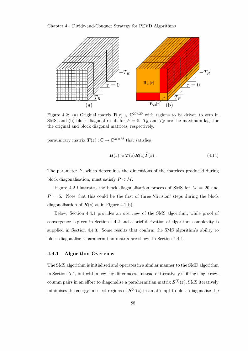
Chapter 4. Divide-and-Conquer Strategy for PEVD Algorithms
TBTR
a)
= 0
TR
= 0
b)
]
22 ]
TB
Figure 4.2: (a) Original matrix R[τ ] ∈ C20×20 with regions to be driven to zero in
SMS, and (b) block diagonal result for P = 5. TR and TB are the maximum lags forthe original and block diagonal matrices, respectively.
paraunitary matrix T (z) : C→ CM×M that satisfies
B(z) ≈ T (z)R(z)T (z) . (4.14)
The parameter P , which determines the dimensions of the matrices produced during
block diagonalisation, must satisfy P < M .
Figure 4.2 illustrates the block diagonalisation process of SMS for M = 20 and
P = 5. Note that this could be the first of three ‘division’ steps during the block
diagonalisation of R(z) as in Figure 4.1(b).
Below, Section 4.4.1 provides an overview of the SMS algorithm, while proof of
convergence is given in Section 4.4.2 and a brief derivation of algorithm complexity is
supplied in Section 4.4.3. Some results that confirm the SMS algorithm’s ability to
block diagonalise a parahermitian matrix are shown in Section 4.4.4.
4.4.1 Algorithm Overview
The SMS algorithm is initialised and operates in a similar manner to the SMD algorithm
in Section A.1, but with a few key differences. Instead of iteratively shifting single row-
column pairs in an effort to diagonalise a parahermitian matrix S(i)(z), SMS iteratively
minimises the energy in select regions of S(i)(z) in an attempt to block diagonalise the
88
Chapter 4. Divide-and-Conquer Strategy for PEVD Algorithms
matrix over I iterations; i.e., for i = 1 . . . I. If
S(i)(z) =
S
(i)11 (z) S
(i)12 (z)
S(i)21 (z) S
(i)22 (z)
(4.15)
is represented using four polynomial matrices as shown, the regions to experience energy
reduction are denoted S(i)12 (z) : C → C
(M−P )×P and S(i)21 (z) : C → C
P×(M−P ), and
are located to the top-right and bottom-left of S(i)(z), such that S(i)12 (z) = S
(i)21 (z).
These regions are highlighted in red for the example of Figure 4.2. The energy from
these regions is iteratively transferred to parahermitian submatrices S(i)11 (z) : C →
C(M−P )×(M−P ) and S
(i)22 (z) : C → C
P×P on the diagonal of S(i)(z); this results in
S(i)(z) more closely approximating a block diagonal matrix as i increases. That is, in
an ideal scenario, SMS enables the following:
limi→∞
∑
τ
∥∥∥S
(i)12 [τ ]
∥∥∥
2
F= lim
i→∞
∑
τ
∥∥∥S
(i)21 [τ ]
∥∥∥
2
F= 0 ; (4.16)
however, in reality this may require an infeasible number of iterations. A discussion on
SMS convergence in practice is provided in Section 4.4.2.
Alongside the parameter P , each instance of SMS is provided with a parameter Imax
— which defines the maximum possible number of algorithm iterations — a stopping
threshold κ, and truncation parameters µ and µt.
To achieve matrix block diagonalisation, the SMS algorithm uses a series of elemen-
tary paraunitary operations to iteratively minimise the energy in S(i)12 (z) and S
(i)21 (z).
Each elementary paraunitary operation consists of two steps: first, a delay step is
used to move the bottom-left and top-right regions with the largest energy to lag zero;
then, an EVD diagonalises the lag zero matrix, transferring the shifted energy onto the
diagonal.
Upon initialisation, the algorithm diagonalises the lag zero coefficient matrix R[0]
by means of its modal matrix Q(0), which is obtained from the ordered EVD of R[0],
such that S(0)(z) = Q(0)R(z)Q(0)H. The unitary Q(0) is applied to all coefficient
matrices R[τ ] ∀ τ , and initialises H(0)(z) = Q(0).
89
Chapter 4. Divide-and-Conquer Strategy for PEVD Algorithms
The SMS algorithm then computes
S(i)(z) = U (i)(z)S(i−1)(z)U (i)(z)
H(i)(z) = U (i)(z)H (i−1)(z) (4.17)
in the ith step, i = 1, 2, . . . I, in which
U (i)(z) = Q(i)Λ(i)(z) . (4.18)
The product in (4.18) consists of a paraunitary delay matrix
Λ(i)(z) = diag1 . . . 1︸ ︷︷ ︸
M−P
zτ(i)
. . . zτ(i)
︸ ︷︷ ︸
P
(4.19)
and a unitary matrix Q(i), such that U (i)(z) in (4.18) is paraunitary. For subsequent
discussion, it is convenient to define intermediate variables S(i)′(z) and H(i)′(z) where
S(i)′(z) = Λ(i)(z)S(i−1)(z)Λ(i)(z)
H(i)′(z) = Λ(i)(z)H (i−1)(z) . (4.20)
Matrix Λ(i)(z) is selected based on the lag position of the dominant region in the
bottom-left of S(i−1)(z) •— S(i−1)[τ ], which is identified by
τ (i) = argmaxτ
∥∥∥S
(i−1)21 [τ ]
∥∥∥
2
F, (4.21)
where∥∥∥S
(i−1)21 [τ ]
∥∥∥
2
F=
M∑
m=M−P+1
M−P∑
k=1
∣∣∣s
(i−1)m,k [τ ]
∣∣∣
2. (4.22)
Here, s(i−1)m,k [τ ] represents the element in the mth row and kth column of the coefficient
matrix S(i−1)[τ ].
The shifting process in (4.20) moves the dominant bottom-left region S(i−1)21 [τ (i)]
and dominant top-right region S(i−1)12 [−τ (i)] = S
(i−1)H21 [τ (i)] in S(i−1)[τ ] into the lag zero
coefficient matrix S(i)′[0]. The energy in the shifted regions is then transferred onto the
90
Chapter 4. Divide-and-Conquer Strategy for PEVD Algorithms
diagonal of S(i)′[0] by a unitary matrix Q(i) — which diagonalises S(i)′[0] by means of
an ordered EVD — in
S(i)(z) = Q(i)S(i)′(z)Q(i)H
H(i)(z) = Q(i)H(i)′(z) . (4.23)
The use of an ordered EVD ensures that the eigenvalues in S(i)[0] — and therefore
the polynomial eigenvalues of S(i)(z) — are sorted in descending order of power. This
results in spectral majorisation, such that the polynomial eigenvalues of B11(z) are
always greater in power that the polynomial eigenvalues of B22(z).
Note that the application of Λ(i)(z) via similarity transform shifts the bottom-right
P×P region of S(i−1)(z) in opposite directions, such that this region remains unaffected.
An efficient implementation of this similarity transform can therefore exclude this region
from shifting operations.
The orders of S(i)(z) and H(i)(z) increase at each iteration; to constrain computa-
tional complexity, truncation according to Appendix C is typically required. Parame-
ters µ and µt are used for parahermitian and paraunitary matrix truncation, respec-
tively.
After Imax iterations — for a user-defined Imax — or when the energy in S(i)21 (z) =
S(i)12 (z) has been sufficiently minimised such that
∥∥∥S
(I)21 [τ ]
∥∥∥
2
F≤ κ
∑
τ
‖R[τ ]‖2F (4.24)
at some iteration I — where κ is chosen to be arbitrarily small — the SMS algorithm
returns matrices B(z) and T (z). The latter is constructed from the concatenation of
the elementary paraunitary matrices:
T (z) = H(I)(z) = U (I)(z) · · ·U (0)(z) =
I∏
i=0
U (I−i)(z) , (4.25)
where I = minImax, I. The parahermitian submatrices of B(z), B11(z) and B22(z),
are the top-left (M − P ) × (M − P ) and the bottom-right P × P blocks of S(I)(z),
91
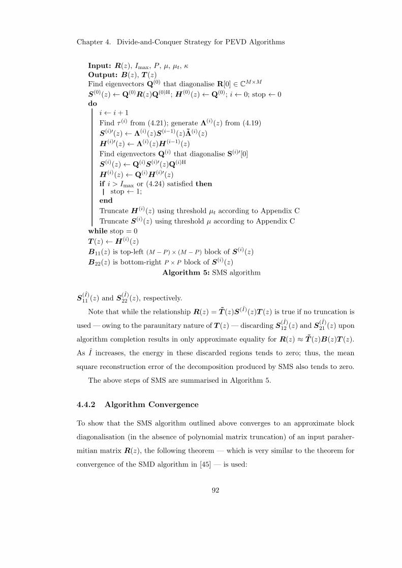
Chapter 4. Divide-and-Conquer Strategy for PEVD Algorithms
Input: R(z), Imax, P , µ, µt, κOutput: B(z), T (z)Find eigenvectors Q(0) that diagonalise R[0] ∈ C
M×M
S(0)(z)← Q(0)R(z)Q(0)H; H(0)(z)← Q(0); i← 0; stop ← 0do
i← i+ 1
Find τ (i) from (4.21); generate Λ(i)(z) from (4.19)
S(i)′(z)← Λ(i)(z)S(i−1)(z)Λ(i)(z)
H(i)′(z)← Λ(i)(z)H (i−1)(z)
Find eigenvectors Q(i) that diagonalise S(i)′[0]
S(i)(z)← Q(i)S(i)′(z)Q(i)H
H(i)(z)← Q(i)H(i)′(z)if i > Imax or (4.24) satisfied then
stop ← 1;end
Truncate H(i)(z) using threshold µt according to Appendix C
Truncate S(i)(z) using threshold µ according to Appendix C
while stop = 0
T (z)←H(i)(z)
B11(z) is top-left (M − P )× (M − P ) block of S(i)(z)
B22(z) is bottom-right P × P block of S(i)(z)
Algorithm 5: SMS algorithm
S(I)11 (z) and S
(I)22 (z), respectively.
Note that while the relationship R(z) = T (z)S(I)(z)T (z) is true if no truncation is
used — owing to the paraunitary nature of T (z) — discarding S(I)12 (z) and S
(I)21 (z) upon
algorithm completion results in only approximate equality for R(z) ≈ T (z)B(z)T (z).
As I increases, the energy in these discarded regions tends to zero; thus, the mean
square reconstruction error of the decomposition produced by SMS also tends to zero.
The above steps of SMS are summarised in Algorithm 5.
4.4.2 Algorithm Convergence
To show that the SMS algorithm outlined above converges to an approximate block
diagonalisation (in the absence of polynomial matrix truncation) of an input paraher-
mitian matrix R(z), the following theorem — which is very similar to the theorem for
convergence of the SMD algorithm in [45] — is used:
92
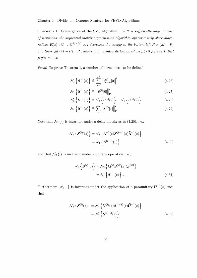
Chapter 4. Divide-and-Conquer Strategy for PEVD Algorithms
Theorem 1 (Convergence of the SMS algorithm). With a sufficiently large number
of iterations, the sequential matrix segmentation algorithm approximately block diago-
nalises R(z) : C → CM×M and decreases the energy in the bottom-left P × (M − P )
and top-right (M −P )×P regions to an arbitrarily low threshold ρ > 0 for any P that
fulfils P < M .
Proof: To prove Theorem 1, a number of norms need to be defined:
N1
S(i)(z)
,
M∑
m=1
∣∣∣s(i)m,m[0]
∣∣∣
2(4.26)
N2
S(i)(z)
,∥∥∥S
(i)[0]∥∥∥
2
F(4.27)
N3
S(i)(z)
, N2
S(i)(z)
−N1
S(i)(z)
(4.28)
N4
S(i)(z)
,∑
τ
∥∥∥S
(i)[τ ]∥∥∥
2
F. (4.29)
Note that N1 · is invariant under a delay matrix as in (4.20), i.e.,
N1
S(i)′(z)
= N1
Λ(i)(z)S(i−1)(z)Λ(i)(z)
= N1
S(i−1)(z)
, (4.30)
and that N2 · is invariant under a unitary operation, i.e.,
N2
S(i)(z)
= N2
Q(i)S(i)′(z)Q(i)H
= N2
S(i)′(z)
. (4.31)
Furthermore, N4 · is invariant under the application of a paraunitary U (i)(z) such
that
N4
S(i)(z)
= N4
U (i)(z)S(i−1)(z)U (i)(z)
= N4
S(i−1)(z)
. (4.32)
93
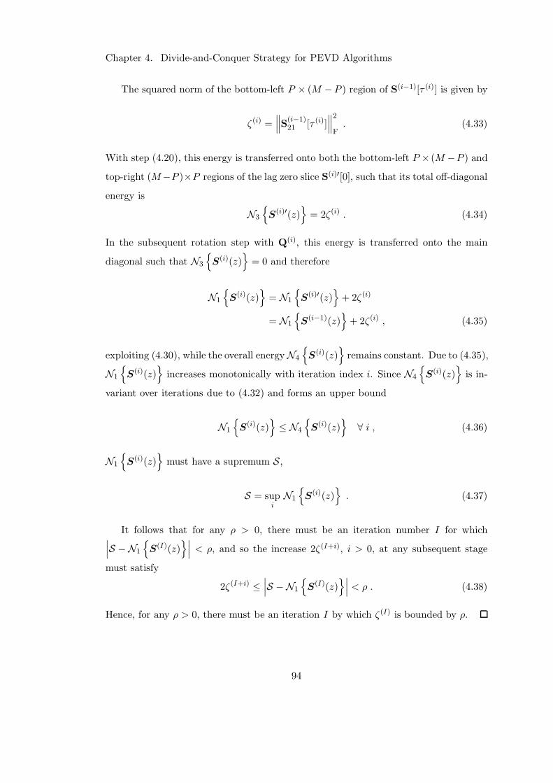
Chapter 4. Divide-and-Conquer Strategy for PEVD Algorithms
The squared norm of the bottom-left P × (M −P ) region of S(i−1)[τ (i)] is given by
ζ(i) =∥∥∥S
(i−1)21 [τ (i)]
∥∥∥
2
F. (4.33)
With step (4.20), this energy is transferred onto both the bottom-left P × (M −P ) and
top-right (M−P )×P regions of the lag zero slice S(i)′[0], such that its total off-diagonal
energy is
N3
S(i)′(z)
= 2ζ(i) . (4.34)
In the subsequent rotation step with Q(i), this energy is transferred onto the main
diagonal such that N3
S(i)(z)
= 0 and therefore
N1
S(i)(z)
= N1
S(i)′(z)
+ 2ζ(i)
= N1
S(i−1)(z)
+ 2ζ(i) , (4.35)
exploiting (4.30), while the overall energyN4
S(i)(z)
remains constant. Due to (4.35),
N1
S(i)(z)
increases monotonically with iteration index i. Since N4
S(i)(z)
is in-
variant over iterations due to (4.32) and forms an upper bound
N1
S(i)(z)
≤ N4
S(i)(z)
∀ i , (4.36)
N1
S(i)(z)
must have a supremum S,
S = supiN1
S(i)(z)
. (4.37)
It follows that for any ρ > 0, there must be an iteration number I for which∣∣∣S −N1
S(I)(z)∣∣∣ < ρ, and so the increase 2ζ(I+i), i > 0, at any subsequent stage
must satisfy
2ζ(I+i) ≤∣∣∣S −N1
S(I)(z)∣∣∣ < ρ . (4.38)
Hence, for any ρ > 0, there must be an iteration I by which ζ(I) is bounded by ρ.
94
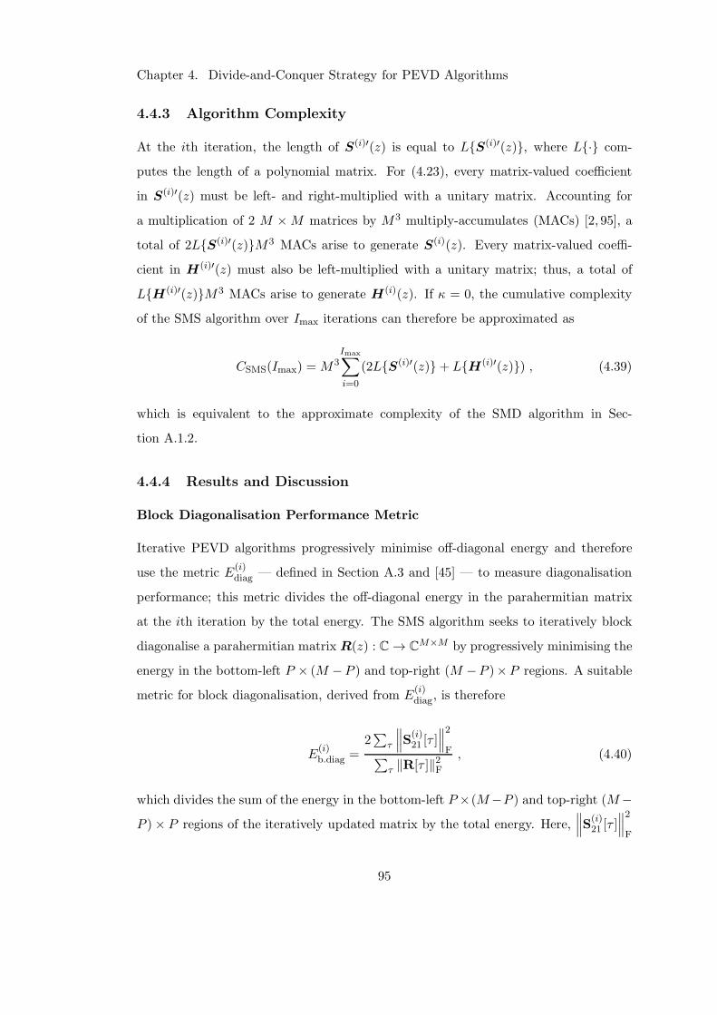
Chapter 4. Divide-and-Conquer Strategy for PEVD Algorithms
4.4.3 Algorithm Complexity
At the ith iteration, the length of S(i)′(z) is equal to LS(i)′(z), where L· com-
putes the length of a polynomial matrix. For (4.23), every matrix-valued coefficient
in S(i)′(z) must be left- and right-multiplied with a unitary matrix. Accounting for
a multiplication of 2 M ×M matrices by M3 multiply-accumulates (MACs) [2, 95], a
total of 2LS(i)′(z)M3 MACs arise to generate S(i)(z). Every matrix-valued coeffi-
cient in H(i)′(z) must also be left-multiplied with a unitary matrix; thus, a total of
LH(i)′(z)M3 MACs arise to generate H(i)(z). If κ = 0, the cumulative complexity
of the SMS algorithm over Imax iterations can therefore be approximated as
CSMS(Imax) = M3Imax∑
i=0
(2LS(i)′(z)+ LH(i)′(z)) , (4.39)
which is equivalent to the approximate complexity of the SMD algorithm in Sec-
tion A.1.2.
4.4.4 Results and Discussion
Block Diagonalisation Performance Metric
Iterative PEVD algorithms progressively minimise off-diagonal energy and therefore
use the metric E(i)diag — defined in Section A.3 and [45] — to measure diagonalisation
performance; this metric divides the off-diagonal energy in the parahermitian matrix
at the ith iteration by the total energy. The SMS algorithm seeks to iteratively block
diagonalise a parahermitian matrix R(z) : C→ CM×M by progressively minimising the
energy in the bottom-left P × (M −P ) and top-right (M −P )×P regions. A suitable
metric for block diagonalisation, derived from E(i)diag, is therefore
E(i)b.diag =
2∑
τ
∥∥∥S
(i)21 [τ ]
∥∥∥
2
F∑
τ ‖R[τ ]‖2F, (4.40)
which divides the sum of the energy in the bottom-left P ×(M−P ) and top-right (M−P )× P regions of the iteratively updated matrix by the total energy. Here,
∥∥∥S
(i)21 [τ ]
∥∥∥
2
F
95
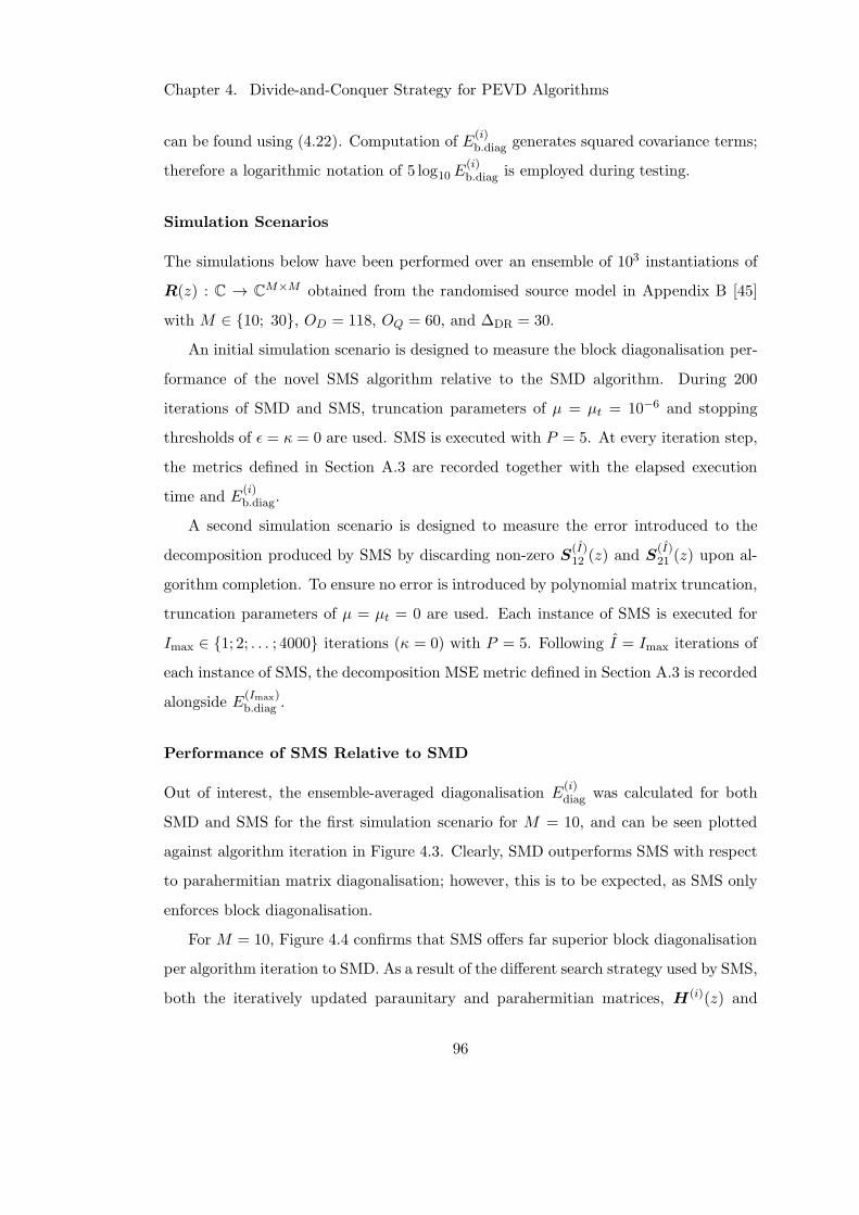
Chapter 4. Divide-and-Conquer Strategy for PEVD Algorithms
can be found using (4.22). Computation of E(i)b.diag generates squared covariance terms;
therefore a logarithmic notation of 5 log10 E(i)b.diag is employed during testing.
Simulation Scenarios
The simulations below have been performed over an ensemble of 103 instantiations of
R(z) : C → CM×M obtained from the randomised source model in Appendix B [45]
with M ∈ 10; 30, OD = 118, OQ = 60, and ∆DR = 30.
An initial simulation scenario is designed to measure the block diagonalisation per-
formance of the novel SMS algorithm relative to the SMD algorithm. During 200
iterations of SMD and SMS, truncation parameters of µ = µt = 10−6 and stopping
thresholds of ǫ = κ = 0 are used. SMS is executed with P = 5. At every iteration step,
the metrics defined in Section A.3 are recorded together with the elapsed execution
time and E(i)b.diag.
A second simulation scenario is designed to measure the error introduced to the
decomposition produced by SMS by discarding non-zero S(I)12 (z) and S
(I)21 (z) upon al-
gorithm completion. To ensure no error is introduced by polynomial matrix truncation,
truncation parameters of µ = µt = 0 are used. Each instance of SMS is executed for
Imax ∈ 1; 2; . . . ; 4000 iterations (κ = 0) with P = 5. Following I = Imax iterations of
each instance of SMS, the decomposition MSE metric defined in Section A.3 is recorded
alongside E(Imax)b.diag .
Performance of SMS Relative to SMD
Out of interest, the ensemble-averaged diagonalisation E(i)diag was calculated for both
SMD and SMS for the first simulation scenario for M = 10, and can be seen plotted
against algorithm iteration in Figure 4.3. Clearly, SMD outperforms SMS with respect
to parahermitian matrix diagonalisation; however, this is to be expected, as SMS only
enforces block diagonalisation.
For M = 10, Figure 4.4 confirms that SMS offers far superior block diagonalisation
per algorithm iteration to SMD. As a result of the different search strategy used by SMS,
both the iteratively updated paraunitary and parahermitian matrices, H(i)(z) and
96
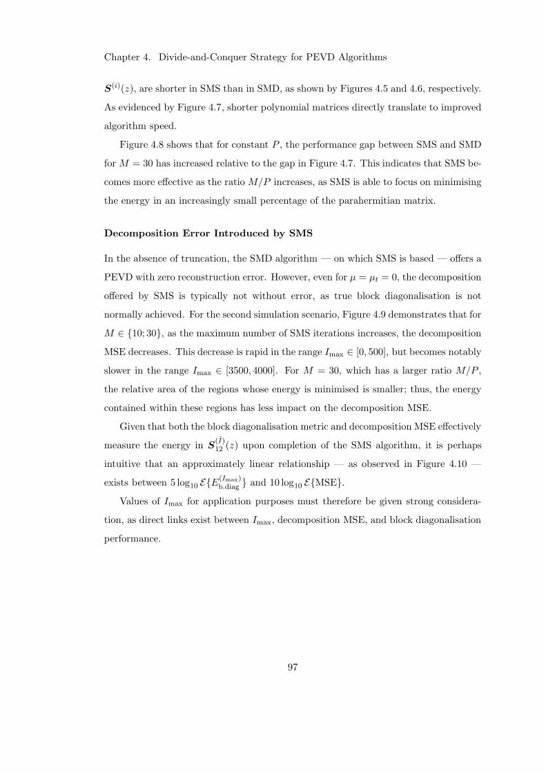
Chapter 4. Divide-and-Conquer Strategy for PEVD Algorithms
S(i)(z), are shorter in SMS than in SMD, as shown by Figures 4.5 and 4.6, respectively.
As evidenced by Figure 4.7, shorter polynomial matrices directly translate to improved
algorithm speed.
Figure 4.8 shows that for constant P , the performance gap between SMS and SMD
for M = 30 has increased relative to the gap in Figure 4.7. This indicates that SMS be-
comes more effective as the ratio M/P increases, as SMS is able to focus on minimising
the energy in an increasingly small percentage of the parahermitian matrix.
Decomposition Error Introduced by SMS
In the absence of truncation, the SMD algorithm — on which SMS is based — offers a
PEVD with zero reconstruction error. However, even for µ = µt = 0, the decomposition
offered by SMS is typically not without error, as true block diagonalisation is not
normally achieved. For the second simulation scenario, Figure 4.9 demonstrates that for
M ∈ 10; 30, as the maximum number of SMS iterations increases, the decomposition
MSE decreases. This decrease is rapid in the range Imax ∈ [0, 500], but becomes notably
slower in the range Imax ∈ [3500, 4000]. For M = 30, which has a larger ratio M/P ,
the relative area of the regions whose energy is minimised is smaller; thus, the energy
contained within these regions has less impact on the decomposition MSE.
Given that both the block diagonalisation metric and decomposition MSE effectively
measure the energy in S(I)12 (z) upon completion of the SMS algorithm, it is perhaps
intuitive that an approximately linear relationship — as observed in Figure 4.10 —
exists between 5 log10 EE(Imax)b.diag and 10 log10 EMSE.
Values of Imax for application purposes must therefore be given strong considera-
tion, as direct links exist between Imax, decomposition MSE, and block diagonalisation
performance.
97
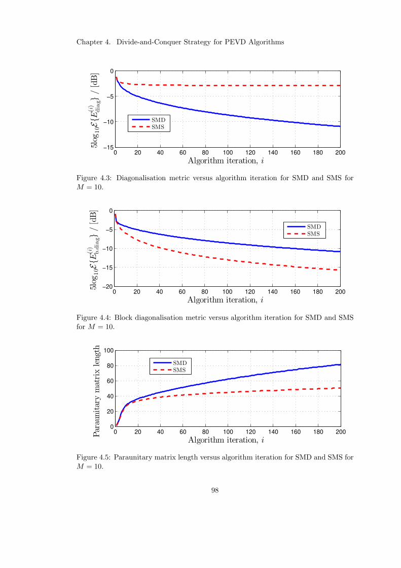
Chapter 4. Divide-and-Conquer Strategy for PEVD Algorithms
0 20 40 60 80 100 120 140 160 180 200−15
−10
−5
0
Algorithm iteration, i
5log
10EE
(i)
diag
/[dB]
SMDSMS
Figure 4.3: Diagonalisation metric versus algorithm iteration for SMD and SMS forM = 10.
0 20 40 60 80 100 120 140 160 180 200−20
−15
−10
−5
0
Algorithm iteration, i
5log
10EE
(i)
b.diag
/[dB]
SMDSMS
Figure 4.4: Block diagonalisation metric versus algorithm iteration for SMD and SMSfor M = 10.
0 20 40 60 80 100 120 140 160 180 2000
20
40
60
80
100
Algorithm iteration, i
Paraunitarymatrixlength
SMDSMS
Figure 4.5: Paraunitary matrix length versus algorithm iteration for SMD and SMS forM = 10.
98
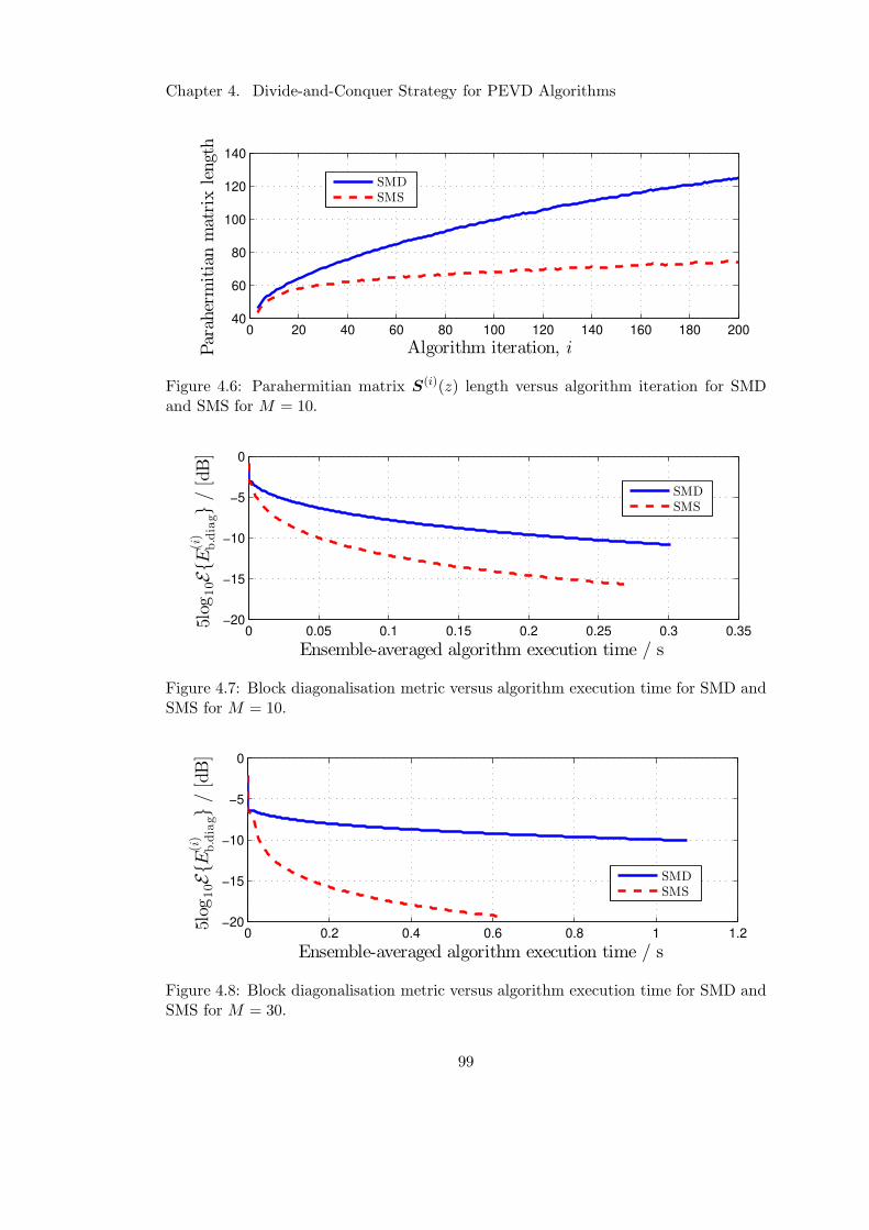
Chapter 4. Divide-and-Conquer Strategy for PEVD Algorithms
0 20 40 60 80 100 120 140 160 180 20040
60
80
100
120
140
Algorithm iteration, iParahermitianmatrixlength
SMDSMS
Figure 4.6: Parahermitian matrix S(i)(z) length versus algorithm iteration for SMDand SMS for M = 10.
0 0.05 0.1 0.15 0.2 0.25 0.3 0.35−20
−15
−10
−5
0
Ensemble-averaged algorithm execution time / s
5log
10EE
(i)
b.diag
/[dB]
SMDSMS
Figure 4.7: Block diagonalisation metric versus algorithm execution time for SMD andSMS for M = 10.
0 0.2 0.4 0.6 0.8 1 1.2−20
−15
−10
−5
0
Ensemble-averaged algorithm execution time / s
5log
10EE
(i)
b.diag
/[dB]
SMDSMS
Figure 4.8: Block diagonalisation metric versus algorithm execution time for SMD andSMS for M = 30.
99
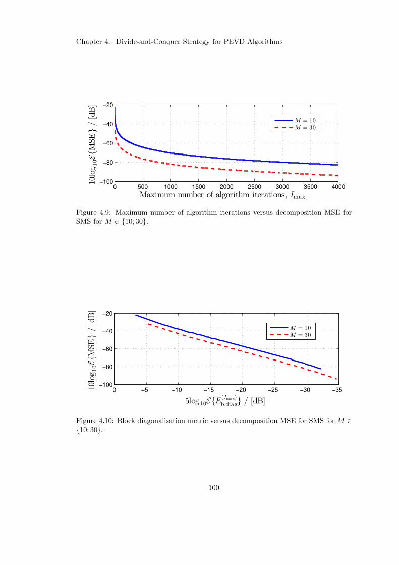
Chapter 4. Divide-and-Conquer Strategy for PEVD Algorithms
0 500 1000 1500 2000 2500 3000 3500 4000−100
−80
−60
−40
−20
Maximum number of algorithm iterations, Imax
10log10EM
SE/[dB]
M = 10M = 30
Figure 4.9: Maximum number of algorithm iterations versus decomposition MSE forSMS for M ∈ 10; 30.
−35−30−25−20−15−10−50−100
−80
−60
−40
−20
5log10EE(Imax)b.diag / [dB]
10log10EM
SE/[dB]
M = 10M = 30
Figure 4.10: Block diagonalisation metric versus decomposition MSE for SMS for M ∈10; 30.
100
Chapter 4. Divide-and-Conquer Strategy for PEVD Algorithms
4.5 Divide-and-Conquer Sequential Matrix Diagonalisa-
tion PEVD Algorithm
Inspired by the development of divide-and-conquer solutions to eigenproblems in [104–
106], this section outlines the components of a novel divide-and-conquer sequential
matrix diagonalisation (DC-SMD) PEVD algorithm — which is summarised in Sec-
tion 4.5.1. The ‘divide’ stage of this algorithm, which utilises the iterative block di-
agonalisation approaches of Sections 4.3 and 4.4, is described in Section 4.5.2, and
Section 4.5.3 details the ‘conquer’ stage. Some comments on algorithm convergence, de-
composition error, and computational complexity are provided in Sections 4.5.4, 4.5.5,
and 4.5.6, respectively.
4.5.1 Algorithm Overview
The DC-SMD algorithm diagonalises a parahermitian matrix R(z) : C→ CM×M via a
number of paraunitary operations. The algorithm outputs an approximately diagonal
matrix D(z), which contains approximate polynomial eigenvalues, and an approxi-
mately paraunitary F (z), which contains the corresponding approximate polynomial
eigenvectors, such that (2.4) is satisfied.
While all existing iterative PEVD algorithms, such as SMD — described in Sec-
tion A.1 — attempt to diagonalise an entire M ×M parahermitian matrix at once, the
DC-SMD algorithm first transforms the matrix into block diagonal form in a ‘divide’
stage before diagonalising — or ‘conquering’ — each of the smaller, now independent,
matrices on the diagonal separately. For example, a matrix R(z) : C → C20×20 might
be ‘divided’ into four 5× 5 parahermitian matrices, each of which can be diagonalised
independently. Figure 4.11, which is a condensed form of Figure 4.1, shows the state
of the parahermitian matrix at each stage of the process for this example.
If matrix R(z) is of large spatial dimension, the SMS algorithm from Section 4.4 is
repeatedly used to ‘divide’ the matrix into multiple independent parahermitian matri-
ces. Using the block diagonalisation approach of Section 4.3.2, this function generates
a paraunitary matrix T (b)(z) that ‘divides’ the top-left (M− (b−1)P )× (M − (b−1)P )
101
Chapter 4. Divide-and-Conquer Strategy for PEVD Algorithms
block of an input matrix B(b−1)(z) into two independent parahermitian matrices,
B(b)11 (z) and B
(b)22 (z), of smaller spatial dimension. B
(b)11 (z) is then subject to further
division if it still has sufficiently large spatial dimension. Note that B(0)(z) = R(z).
Following β =⌈M−M
P
⌉
‘division’ steps, for b = 1 . . . β and user-defined M and P , a
block diagonal B(z) has been obtained as in (4.12). In the alternative notation of (4.4),
B(z) comprises N = (β+1) blocks, which are denoted Bnn(z), n = 1 . . . N . The matri-
ces T (b)(z) — which SMS generates to ‘divide’ each B(b)(z) — are concatenated to form
an overall dividing matrix T (z). It is therefore possible to approximately reconstruct
R(z) from the product T (z)B(z)T (z).
As in the strategy of Section 4.3.1, each block Bnn(z), n = 1 . . . N , on the diagonal
of matrixB(z) is then diagonalised in sequence through the use of a PEVD algorithm; in
this case, SMD is used. The diagonalised outputs, Dnn(z), are placed on the diagonal
of matrix D(z), and the corresponding paraunitary matrices, F nn(z), are stored on
the diagonal of matrix F (z). Matrix B(z) can be approximately reconstructed from
˜F (z)D(z)F (z); by extension, it is possible to approximately reconstruct R(z) from the
product T (z) ˜F (z)D(z)F (z)T (z) = F (z)D(z)F (z), where F (z) = F (z)T (z).
Algorithm 6 summarises the above steps of DC-SMD in more detail. Of the pa-
rameters passed to DC-SMD, µ and µt are truncation parameters, and κ and ǫ are the
stopping thresholds for SMS and SMD, which are allowed a maximum of ID and IC
iterations. Matrices of spatial dimension greater than M × M will be subject to the
‘dividing’ process. Parameter P is an input to SMS as in Section 4.4. Matrices IM and
0M are identity and zero matrices of spatial dimensions M ×M , respectively.
4.5.2 ‘Dividing’ the Parahermitian Matrix
If R(z) is measured to have spatial dimension M > M , the ‘divide’ stage of DC-SMD
comes into effect. This stage repeatedly applies the SMS algorithm of Section 4.4 to
‘divide’ R(z) into multiple independent parahermitian matrices, and can therefore be
considered to operate in a recursive fashion. In the first recursion, the matrix B(0)(z)
input to SMS is equal to R(z) and M ′ = M . The output matrix B(1)22 (z) is stored
and subsequently diagonalised during the ‘conquer’ stage. If the second output matrix
102
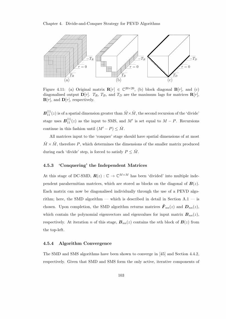
Chapter 4. Divide-and-Conquer Strategy for PEVD Algorithms
=
TR
TR
=
T
T
=
TD
TD
a) b) c)
Figure 4.11: (a) Original matrix R[τ ] ∈ C20×20, (b) block diagonal B[τ ], and (c)
diagonalised output D[τ ]. TR, TB, and TD are the maximum lags for matrices R[τ ],B[τ ], and D[τ ], respectively.
B(1)11 (z) is of a spatial dimension greater than M×M , the second recursion of the ‘divide’
stage uses B(1)11 (z) as the input to SMS, and M ′ is set equal to M − P . Recursions
continue in this fashion until (M ′ − P ) ≤ M .
All matrices input to the ‘conquer’ stage should have spatial dimensions of at most
M × M , therefore P , which determines the dimensions of the smaller matrix produced
during each ‘divide’ step, is forced to satisfy P ≤ M .
4.5.3 ‘Conquering’ the Independent Matrices
At this stage of DC-SMD, R(z) : C → CM×M has been ‘divided’ into multiple inde-
pendent parahermitian matrices, which are stored as blocks on the diagonal of B(z).
Each matrix can now be diagonalised individually through the use of a PEVD algo-
rithm; here, the SMD algorithm — which is described in detail in Section A.1 — is
chosen. Upon completion, the SMD algorithm returns matrices F nn(z) and Dnn(z),
which contain the polynomial eigenvectors and eigenvalues for input matrix Bnn(z),
respectively. At iteration n of this stage, Bnn(z) contains the nth block of B(z) from
the top-left.
4.5.4 Algorithm Convergence
The SMD and SMS algorithms have been shown to converge in [45] and Section 4.4.2,
respectively. Given that SMD and SMS form the only active, iterative components of
103
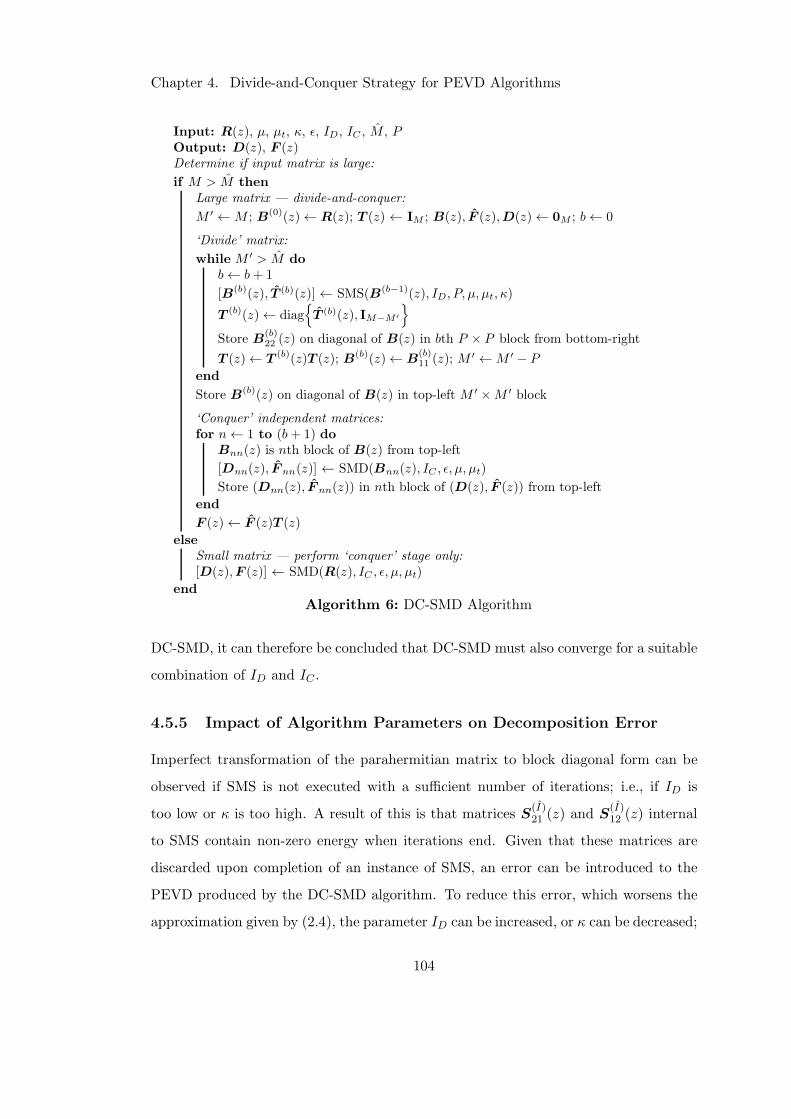
Chapter 4. Divide-and-Conquer Strategy for PEVD Algorithms
Input: R(z), µ, µt, κ, ǫ, ID, IC , M , POutput: D(z), F (z)Determine if input matrix is large:
if M > M then
Large matrix — divide-and-conquer:
M ′ ←M ; B(0)(z)← R(z); T (z) ← IM ; B(z), F (z),D(z)← 0M ; b← 0
‘Divide’ matrix:
while M ′ > M do
b← b+ 1
[B(b)(z), T (b)(z)] ← SMS(B(b−1)(z), ID, P, µ, µt, κ)
T (b)(z)← diag
T (b)(z), IM−M ′
Store B(b)22 (z) on diagonal of B(z) in bth P × P block from bottom-right
T (z)← T (b)(z)T (z); B(b)(z)← B(b)11 (z); M
′ ←M ′ − P
end
Store B(b)(z) on diagonal of B(z) in top-left M ′ ×M ′ block
‘Conquer’ independent matrices:for n← 1 to (b + 1) do
Bnn(z) is nth block of B(z) from top-left
[Dnn(z), F nn(z)] ← SMD(Bnn(z), IC , ǫ, µ, µt)
Store (Dnn(z), F nn(z)) in nth block of (D(z), F (z)) from top-left
end
F (z)← F (z)T (z)
else
Small matrix — perform ‘conquer’ stage only:[D(z),F (z)] ← SMD(R(z), IC , ǫ, µ, µt)
end
Algorithm 6: DC-SMD Algorithm
DC-SMD, it can therefore be concluded that DC-SMD must also converge for a suitable
combination of ID and IC .
4.5.5 Impact of Algorithm Parameters on Decomposition Error
Imperfect transformation of the parahermitian matrix to block diagonal form can be
observed if SMS is not executed with a sufficient number of iterations; i.e., if ID is
too low or κ is too high. A result of this is that matrices S(I)21 (z) and S
(I)12 (z) internal
to SMS contain non-zero energy when iterations end. Given that these matrices are
discarded upon completion of an instance of SMS, an error can be introduced to the
PEVD produced by the DC-SMD algorithm. To reduce this error, which worsens the
approximation given by (2.4), the parameter ID can be increased, or κ can be decreased;
104
Chapter 4. Divide-and-Conquer Strategy for PEVD Algorithms
however, both of these changes will reduce the speed and increase the complexity of
the algorithm, as more effort will be contributed to the ‘divide’ stage.
Parahermitian and paraunitary matrix truncation (for non-zero truncation param-
eters µ and µt) both introduce an error to the resulting PEVD. Larger truncation
parameter values introduce a higher degree of error. Any error from truncation both
worsens the approximation given by (2.4) and weakens the paraunitary property of
eigenvectors F (z); i.e., equality in (2.5) is no longer guaranteed if truncation is em-
ployed during generation of F (z). This problem is not unique to DC-SMD, however,
as all iterative PEVD algorithms typically employ polynomial matrix truncation to
constrain computational complexity and memory requirements [6, 60–62].
4.5.6 Algorithm Complexity
The majority of the computational cost of the DC-SMD algorithm arises from multiple
instances of SMS and SMD. The instantaneous complexity of DC-SMD therefore varies
as the algorithm progresses, due to the changing spatial dimensions of the matrices
being processed by SMS and SMD. The main cost of these internal algorithms can
be attributed to the matrix multiplication steps in (4.23) and (A.5). As mentioned
previously, multiplying twoM×M matrices together requires approximatelyM3 MAC
operations [2, 95]. Here, M captures the different spatial dimensions used throughout
DC-SMD and satisfies minM − βP, P ≤ M ≤ M . If the number of MACs required
to complete an operation is used as an estimation of computational complexity, the
computational complexity of a single matrix multiplication step in either algorithm at
iteration i for S(i)′(z) : C → CM×M and H(i)′(z) : C → C
M×M can be approximated
as
C(i)DC−SMD,M =M3(2LS(i)′(z) + LH(i)′(z)) , (4.41)
where operator L· computes the length of a polynomial matrix.
From the description of DC-SMD in Algorithm 6, it can be seen that an M ×M
matrix is only ever processed in the first recursion of the ‘divide’ stage; at all other
points in the DC-SMD algorithm, the processed matrices are of lower spatial dimen-
sion. For example, typically all but one of the parahermitian matrices in the ‘conquer’
105
Chapter 4. Divide-and-Conquer Strategy for PEVD Algorithms
stage are of spatial dimension P × P . Given that the complexity is approximately
proportional to the cube of the spatial dimension, significantly lower complexity will be
observed beyond the first recursion of DC-SMD. Simulations demonstrating how this
lower complexity, divide-and-conquer approach translates to lower algorithm execution
times are provided in Section 4.7.
4.6 Parallel-Sequential Matrix Diagonalisation PEVD Al-
gorithm
Motivated by the development of the DC-SMD algorithm in Section 4.5, here a low com-
plexity, partially parallelisable DaC approach for the PEVD— titled parallel-sequential
matrix diagonalisation (PSMD) — that improves upon the DC-SMD algorithm is de-
scribed. This algorithm achieves novelty by being the only PEVD algorithm to com-
bine the complexity reduction techniques of Sections 3.2, 3.3, 3.6, and 3.8. Following
a sequential, matrix ‘divide’ stage, which segments a large parahermitian matrix into
multiple independent parahermitian matrices, a parallelised ‘conquer’ stage is used to
diagonalise each independent matrix simultaneously. Both the ‘divide’ and ‘conquer’
stages make use of the algorithmic optimisations in Section 3.2 and the half-matrix and
restricted update algorithmic improvements from Sections 3.3 and 3.6, respectively, to
minimise algorithm complexity. The final stage of the algorithm employs the compen-
sated row-shift truncation scheme of Section 3.8 to reduce the polynomial order of the
paraunitary matrix.
The PSMD algorithm is summarised in Section 4.6.1. The implementation of com-
plexity reduction techniques within the ‘divide’ and ‘conquer’ stages of this algorithm
is described in Sections 4.6.2 and 4.6.3. Some comments on algorithm convergence, de-
composition error, and computational complexity are provided in Sections 4.6.4, 4.6.5,
and 4.6.6, respectively.
106
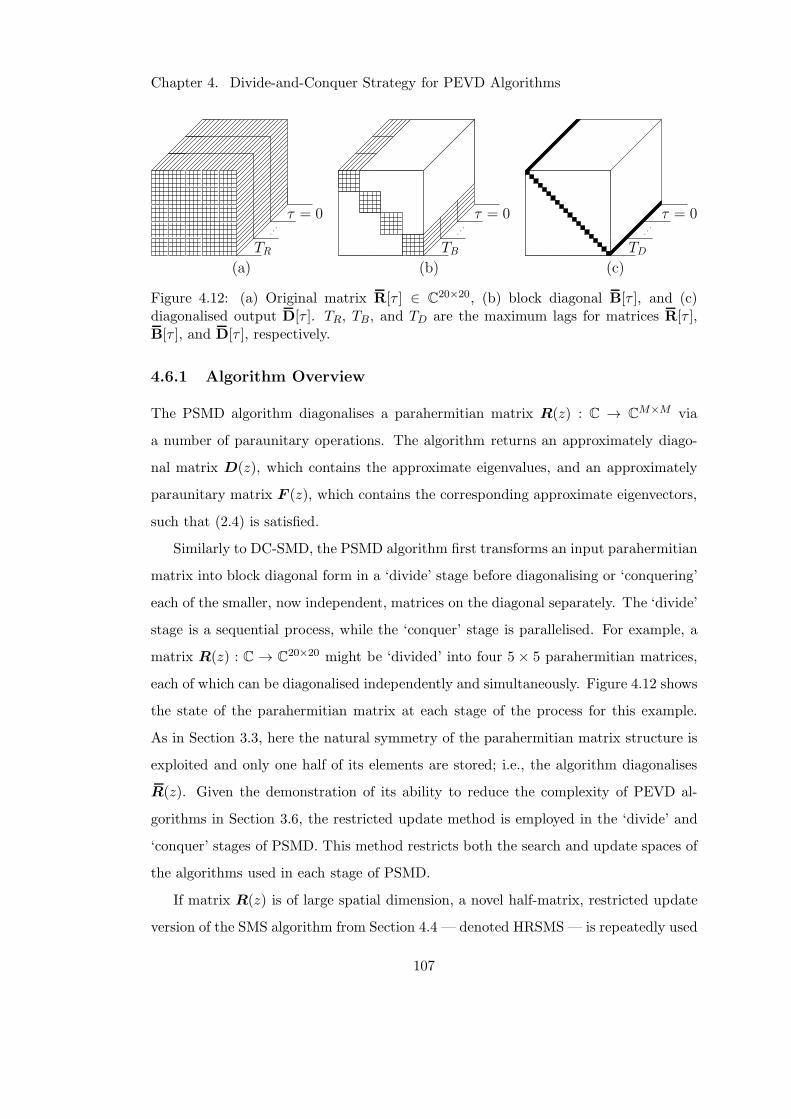
Chapter 4. Divide-and-Conquer Strategy for PEVD Algorithms
a)
= 0
TR
= 0
T
b) c)
= 0
TD
Figure 4.12: (a) Original matrix R[τ ] ∈ C20×20, (b) block diagonal B[τ ], and (c)
diagonalised output D[τ ]. TR, TB, and TD are the maximum lags for matrices R[τ ],B[τ ], and D[τ ], respectively.
4.6.1 Algorithm Overview
The PSMD algorithm diagonalises a parahermitian matrix R(z) : C → CM×M via
a number of paraunitary operations. The algorithm returns an approximately diago-
nal matrix D(z), which contains the approximate eigenvalues, and an approximately
paraunitary matrix F (z), which contains the corresponding approximate eigenvectors,
such that (2.4) is satisfied.
Similarly to DC-SMD, the PSMD algorithm first transforms an input parahermitian
matrix into block diagonal form in a ‘divide’ stage before diagonalising or ‘conquering’
each of the smaller, now independent, matrices on the diagonal separately. The ‘divide’
stage is a sequential process, while the ‘conquer’ stage is parallelised. For example, a
matrix R(z) : C → C20×20 might be ‘divided’ into four 5 × 5 parahermitian matrices,
each of which can be diagonalised independently and simultaneously. Figure 4.12 shows
the state of the parahermitian matrix at each stage of the process for this example.
As in Section 3.3, here the natural symmetry of the parahermitian matrix structure is
exploited and only one half of its elements are stored; i.e., the algorithm diagonalises
R(z). Given the demonstration of its ability to reduce the complexity of PEVD al-
gorithms in Section 3.6, the restricted update method is employed in the ‘divide’ and
‘conquer’ stages of PSMD. This method restricts both the search and update spaces of
the algorithms used in each stage of PSMD.
If matrix R(z) is of large spatial dimension, a novel half-matrix, restricted update
version of the SMS algorithm from Section 4.4 — denoted HRSMS— is repeatedly used
107
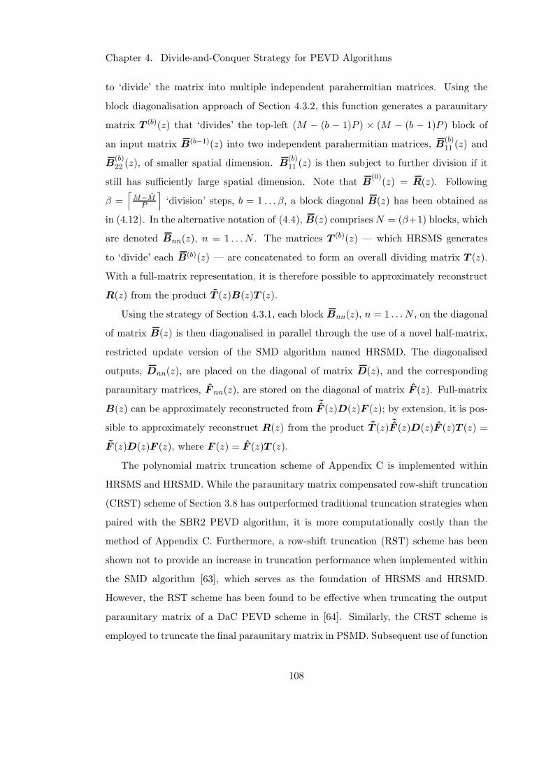
Chapter 4. Divide-and-Conquer Strategy for PEVD Algorithms
to ‘divide’ the matrix into multiple independent parahermitian matrices. Using the
block diagonalisation approach of Section 4.3.2, this function generates a paraunitary
matrix T (b)(z) that ‘divides’ the top-left (M − (b − 1)P ) × (M − (b − 1)P ) block of
an input matrix B(b−1)(z) into two independent parahermitian matrices, B(b)11 (z) and
B(b)22 (z), of smaller spatial dimension. B
(b)11 (z) is then subject to further division if it
still has sufficiently large spatial dimension. Note that B(0)
(z) = R(z). Following
β =⌈M−M
P
⌉
‘division’ steps, b = 1 . . . β, a block diagonal B(z) has been obtained as
in (4.12). In the alternative notation of (4.4), B(z) comprises N = (β+1) blocks, which
are denoted Bnn(z), n = 1 . . . N . The matrices T (b)(z) — which HRSMS generates
to ‘divide’ each B(b)(z) — are concatenated to form an overall dividing matrix T (z).
With a full-matrix representation, it is therefore possible to approximately reconstruct
R(z) from the product T (z)B(z)T (z).
Using the strategy of Section 4.3.1, each block Bnn(z), n = 1 . . . N , on the diagonal
of matrix B(z) is then diagonalised in parallel through the use of a novel half-matrix,
restricted update version of the SMD algorithm named HRSMD. The diagonalised
outputs, Dnn(z), are placed on the diagonal of matrix D(z), and the corresponding
paraunitary matrices, F nn(z), are stored on the diagonal of matrix F (z). Full-matrix
B(z) can be approximately reconstructed from ˜F (z)D(z)F (z); by extension, it is pos-
sible to approximately reconstruct R(z) from the product T (z) ˜F (z)D(z)F (z)T (z) =
F (z)D(z)F (z), where F (z) = F (z)T (z).
The polynomial matrix truncation scheme of Appendix C is implemented within
HRSMS and HRSMD. While the paraunitary matrix compensated row-shift truncation
(CRST) scheme of Section 3.8 has outperformed traditional truncation strategies when
paired with the SBR2 PEVD algorithm, it is more computationally costly than the
method of Appendix C. Furthermore, a row-shift truncation (RST) scheme has been
shown not to provide an increase in truncation performance when implemented within
the SMD algorithm [63], which serves as the foundation of HRSMS and HRSMD.
However, the RST scheme has been found to be effective when truncating the output
paraunitary matrix of a DaC PEVD scheme in [64]. Similarly, the CRST scheme is
employed to truncate the final paraunitary matrix in PSMD. Subsequent use of function
108
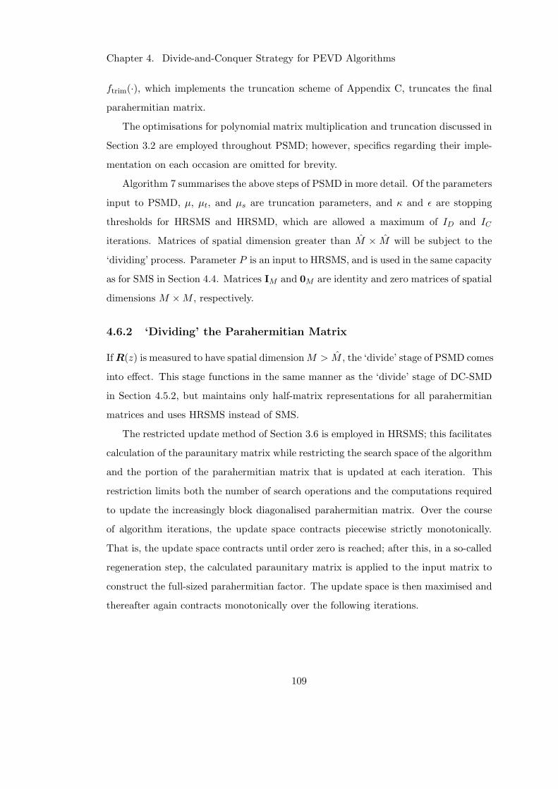
Chapter 4. Divide-and-Conquer Strategy for PEVD Algorithms
ftrim(·), which implements the truncation scheme of Appendix C, truncates the final
parahermitian matrix.
The optimisations for polynomial matrix multiplication and truncation discussed in
Section 3.2 are employed throughout PSMD; however, specifics regarding their imple-
mentation on each occasion are omitted for brevity.
Algorithm 7 summarises the above steps of PSMD in more detail. Of the parameters
input to PSMD, µ, µt, and µs are truncation parameters, and κ and ǫ are stopping
thresholds for HRSMS and HRSMD, which are allowed a maximum of ID and IC
iterations. Matrices of spatial dimension greater than M × M will be subject to the
‘dividing’ process. Parameter P is an input to HRSMS, and is used in the same capacity
as for SMS in Section 4.4. Matrices IM and 0M are identity and zero matrices of spatial
dimensions M ×M , respectively.
4.6.2 ‘Dividing’ the Parahermitian Matrix
IfR(z) is measured to have spatial dimensionM > M , the ‘divide’ stage of PSMD comes
into effect. This stage functions in the same manner as the ‘divide’ stage of DC-SMD
in Section 4.5.2, but maintains only half-matrix representations for all parahermitian
matrices and uses HRSMS instead of SMS.
The restricted update method of Section 3.6 is employed in HRSMS; this facilitates
calculation of the paraunitary matrix while restricting the search space of the algorithm
and the portion of the parahermitian matrix that is updated at each iteration. This
restriction limits both the number of search operations and the computations required
to update the increasingly block diagonalised parahermitian matrix. Over the course
of algorithm iterations, the update space contracts piecewise strictly monotonically.
That is, the update space contracts until order zero is reached; after this, in a so-called
regeneration step, the calculated paraunitary matrix is applied to the input matrix to
construct the full-sized parahermitian factor. The update space is then maximised and
thereafter again contracts monotonically over the following iterations.
109
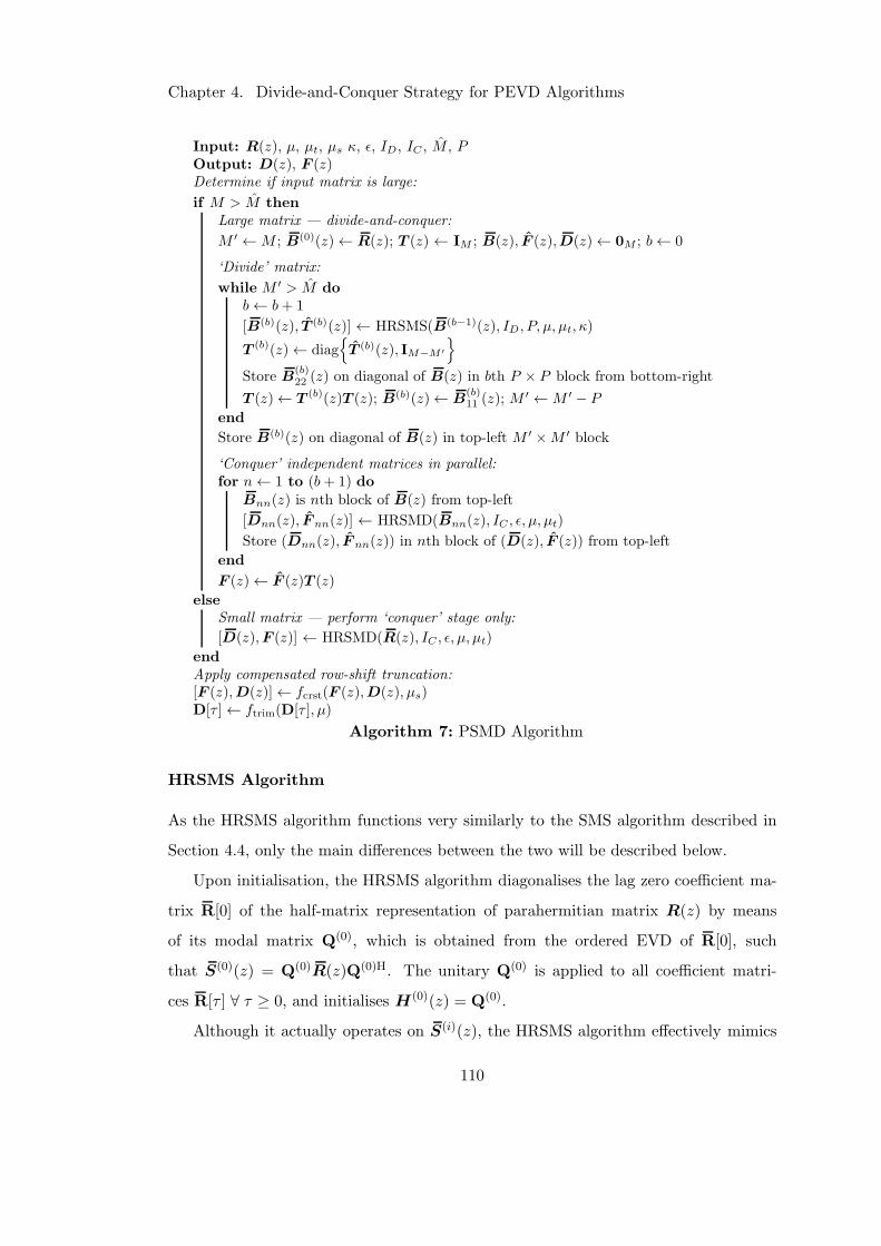
Chapter 4. Divide-and-Conquer Strategy for PEVD Algorithms
Input: R(z), µ, µt, µs κ, ǫ, ID, IC , M , POutput: D(z), F (z)Determine if input matrix is large:
if M > M then
Large matrix — divide-and-conquer:
M ′ ←M ; B(0)(z)← R(z); T (z) ← IM ; B(z), F (z),D(z)← 0M ; b← 0
‘Divide’ matrix:
while M ′ > M do
b← b+ 1
[B(b)(z), T (b)(z)] ← HRSMS(B(b−1)(z), ID, P, µ, µt, κ)
T (b)(z)← diag
T (b)(z), IM−M ′
Store B(b)22 (z) on diagonal of B(z) in bth P × P block from bottom-right
T (z)← T (b)(z)T (z); B(b)(z)← B(b)11 (z); M
′ ←M ′ − P
end
Store B(b)(z) on diagonal of B(z) in top-left M ′ ×M ′ block
‘Conquer’ independent matrices in parallel:for n← 1 to (b + 1) do
Bnn(z) is nth block of B(z) from top-left
[Dnn(z), F nn(z)] ← HRSMD(Bnn(z), IC , ǫ, µ, µt)
Store (Dnn(z), F nn(z)) in nth block of (D(z), F (z)) from top-left
end
F (z)← F (z)T (z)
else
Small matrix — perform ‘conquer’ stage only:
[D(z),F (z)] ← HRSMD(R(z), IC , ǫ, µ, µt)
end
Apply compensated row-shift truncation:[F (z),D(z)]← fcrst(F (z),D(z), µs)D[τ ]← ftrim(D[τ ], µ)
Algorithm 7: PSMD Algorithm
HRSMS Algorithm
As the HRSMS algorithm functions very similarly to the SMS algorithm described in
Section 4.4, only the main differences between the two will be described below.
Upon initialisation, the HRSMS algorithm diagonalises the lag zero coefficient ma-
trix R[0] of the half-matrix representation of parahermitian matrix R(z) by means
of its modal matrix Q(0), which is obtained from the ordered EVD of R[0], such
that S(0)(z) = Q(0)R(z)Q(0)H. The unitary Q(0) is applied to all coefficient matri-
ces R[τ ] ∀ τ ≥ 0, and initialises H(0)(z) = Q(0).
Although it actually operates on S(i)(z), the HRSMS algorithm effectively mimics
110
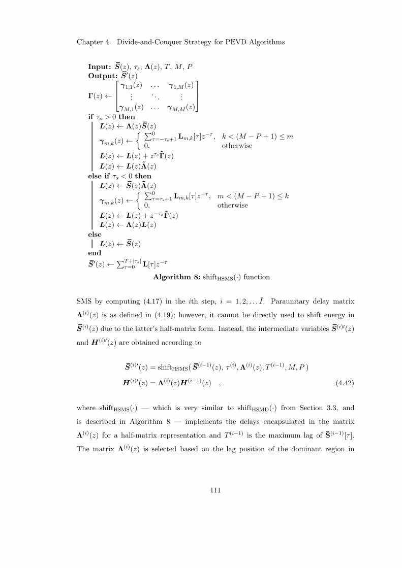
Chapter 4. Divide-and-Conquer Strategy for PEVD Algorithms
Input: S(z), τs, Λ(z), T , M , POutput: S′(z)
Γ(z)←
γ1,1(z) . . . γ1,M (z)...
. . ....
γM,1(z) . . . γM,M (z)
if τs > 0 then
L(z)← Λ(z)S(z)
γm,k(z)← ∑0
τ=−τs+1 Lm,k[τ ]z−τ , k < (M − P + 1) ≤ m
0, otherwise
L(z)← L(z) + zτsΓ(z)
L(z)← L(z)Λ(z)
else if τs < 0 then
L(z)← S(z)Λ(z)
γm,k(z)← ∑0
τ=τs+1 Lm,k[τ ]z−τ , m < (M − P + 1) ≤ k
0, otherwise
L(z)← L(z) + z−τsΓ(z)L(z)← Λ(z)L(z)
else
L(z)← S(z)end
S′(z)←∑T+|τs|τ=0 L[τ ]z−τ
Algorithm 8: shiftHSMS(·) function
SMS by computing (4.17) in the ith step, i = 1, 2, . . . I. Paraunitary delay matrix
Λ(i)(z) is as defined in (4.19); however, it cannot be directly used to shift energy in
S(i)(z) due to the latter’s half-matrix form. Instead, the intermediate variables S(i)′(z)
and H(i)′(z) are obtained according to
S(i)′(z) = shiftHSMS(S(i−1)(z), τ (i),Λ(i)(z), T (i−1),M,P )
H(i)′(z) = Λ(i)(z)H (i−1)(z) , (4.42)
where shiftHSMS(·) — which is very similar to shiftHSMD(·) from Section 3.3, and
is described in Algorithm 8 — implements the delays encapsulated in the matrix
Λ(i)(z) for a half-matrix representation and T (i−1) is the maximum lag of S(i−1)[τ ].
The matrix Λ(i)(z) is selected based on the lag position of the dominant region in
111
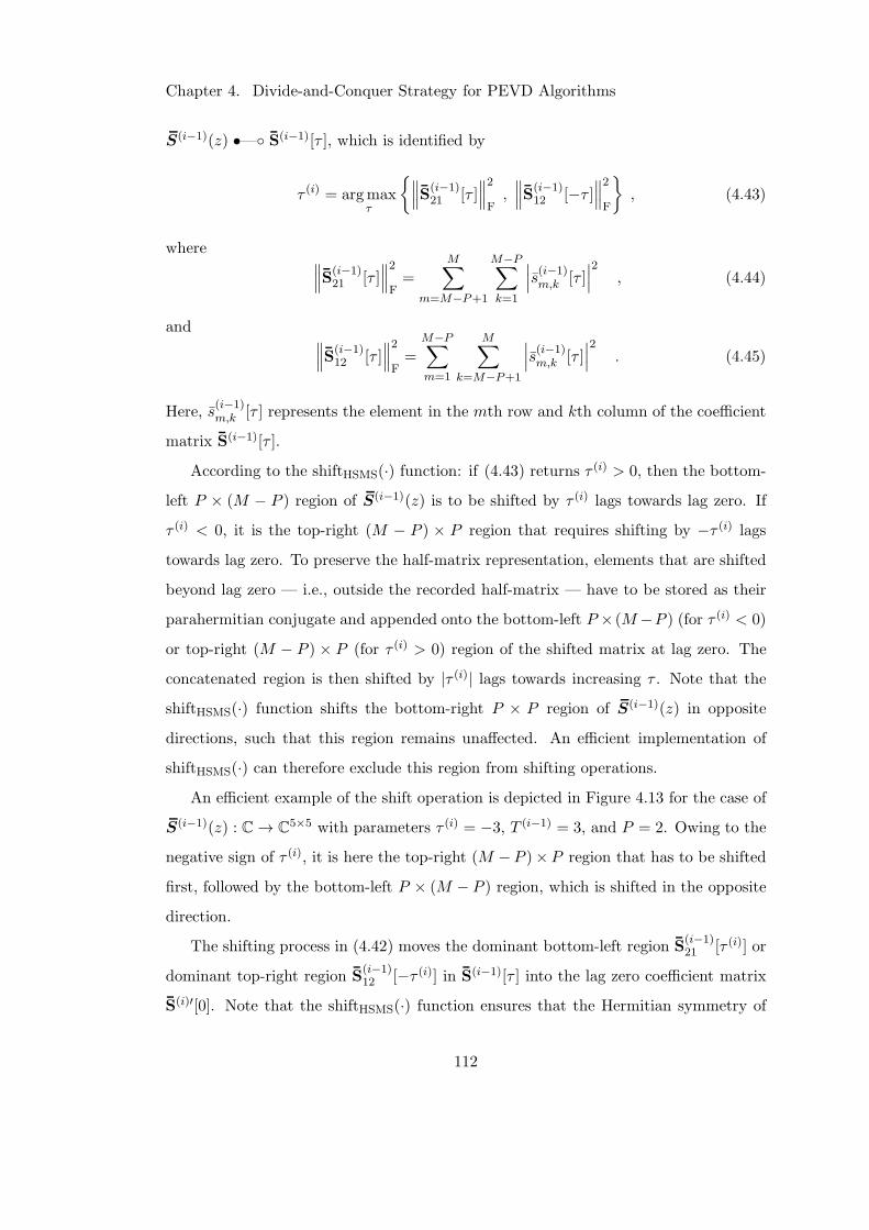
Chapter 4. Divide-and-Conquer Strategy for PEVD Algorithms
S(i−1)(z) •— S(i−1)[τ ], which is identified by
τ (i) = argmaxτ
∥∥∥S
(i−1)21 [τ ]
∥∥∥
2
F,∥∥∥S
(i−1)12 [−τ ]
∥∥∥
2
F
, (4.43)
where∥∥∥S
(i−1)21 [τ ]
∥∥∥
2
F=
M∑
m=M−P+1
M−P∑
k=1
∣∣∣s
(i−1)m,k [τ ]
∣∣∣
2, (4.44)
and∥∥∥S
(i−1)12 [τ ]
∥∥∥
2
F=
M−P∑
m=1
M∑
k=M−P+1
∣∣∣s
(i−1)m,k [τ ]
∣∣∣
2. (4.45)
Here, s(i−1)m,k [τ ] represents the element in the mth row and kth column of the coefficient
matrix S(i−1)[τ ].
According to the shiftHSMS(·) function: if (4.43) returns τ (i) > 0, then the bottom-
left P × (M − P ) region of S(i−1)(z) is to be shifted by τ (i) lags towards lag zero. If
τ (i) < 0, it is the top-right (M − P ) × P region that requires shifting by −τ (i) lags
towards lag zero. To preserve the half-matrix representation, elements that are shifted
beyond lag zero — i.e., outside the recorded half-matrix — have to be stored as their
parahermitian conjugate and appended onto the bottom-left P × (M−P ) (for τ (i) < 0)
or top-right (M − P ) × P (for τ (i) > 0) region of the shifted matrix at lag zero. The
concatenated region is then shifted by |τ (i)| lags towards increasing τ . Note that the
shiftHSMS(·) function shifts the bottom-right P × P region of S(i−1)(z) in opposite
directions, such that this region remains unaffected. An efficient implementation of
shiftHSMS(·) can therefore exclude this region from shifting operations.
An efficient example of the shift operation is depicted in Figure 4.13 for the case of
S(i−1)(z) : C→ C5×5 with parameters τ (i) = −3, T (i−1) = 3, and P = 2. Owing to the
negative sign of τ (i), it is here the top-right (M −P )×P region that has to be shifted
first, followed by the bottom-left P × (M − P ) region, which is shifted in the opposite
direction.
The shifting process in (4.42) moves the dominant bottom-left region S(i−1)21 [τ (i)] or
dominant top-right region S(i−1)12 [−τ (i)] in S(i−1)[τ ] into the lag zero coefficient matrix
S(i)′[0]. Note that the shiftHSMS(·) function ensures that the Hermitian symmetry of
112
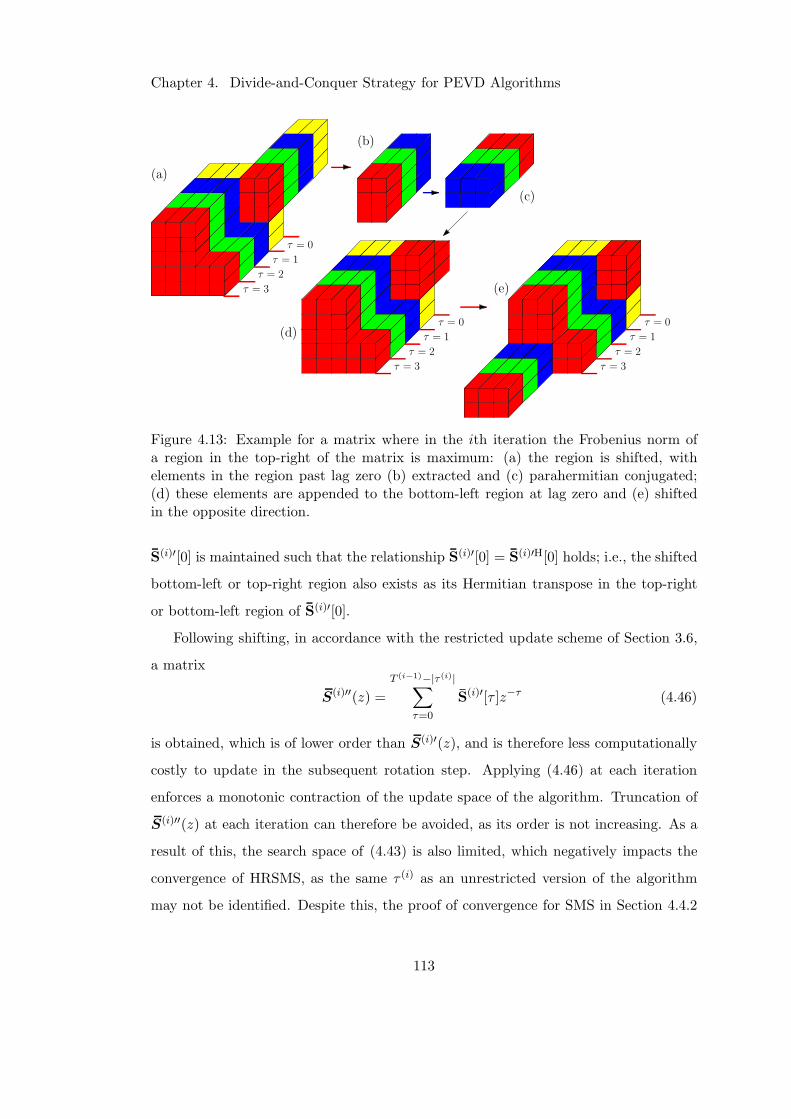
Chapter 4. Divide-and-Conquer Strategy for PEVD Algorithms
b)
d)
e)
a)
= 3
= 2
= 1
= 0
c)
= 3
= 2
= 0
= 1
= 3
= 2
= 0
= 1
Figure 4.13: Example for a matrix where in the ith iteration the Frobenius norm ofa region in the top-right of the matrix is maximum: (a) the region is shifted, withelements in the region past lag zero (b) extracted and (c) parahermitian conjugated;(d) these elements are appended to the bottom-left region at lag zero and (e) shiftedin the opposite direction.
S(i)′[0] is maintained such that the relationship S(i)′[0] = S(i)′H[0] holds; i.e., the shifted
bottom-left or top-right region also exists as its Hermitian transpose in the top-right
or bottom-left region of S(i)′[0].
Following shifting, in accordance with the restricted update scheme of Section 3.6,
a matrix
S(i)′′(z) =
T (i−1)−|τ (i)|∑
τ=0
S(i)′[τ ]z−τ (4.46)
is obtained, which is of lower order than S(i)′(z), and is therefore less computationally
costly to update in the subsequent rotation step. Applying (4.46) at each iteration
enforces a monotonic contraction of the update space of the algorithm. Truncation of
S(i)′′(z) at each iteration can therefore be avoided, as its order is not increasing. As a
result of this, the search space of (4.43) is also limited, which negatively impacts the
convergence of HRSMS, as the same τ (i) as an unrestricted version of the algorithm
may not be identified. Despite this, the proof of convergence for SMS in Section 4.4.2
113
Chapter 4. Divide-and-Conquer Strategy for PEVD Algorithms
— which focusses on the monotonic increase of on-diagonal energy enforced by the
algorithm — still holds for HRSMS.
The order of the paraunitary matrix H(i)′(z) does increase at each iteration; to
constrain computational complexity, a truncated paraunitary matrix
H(i)′′[τ ] = ftrim(H(i)′[τ ], µt) (4.47)
is obtained using the ftrim(·) function from Appendix C.
The energy in the shifted regions is then transferred onto the diagonal of S(i)′′[0] by
a unitary matrix Q(i) — which diagonalises S(i)′′[0] by means of an ordered EVD — in
S(i)(z) = Q(i)S(i)′′(z)Q(i)H
H(i)(z) = Q(i)H(i)′′(z) . (4.48)
If at this point the order of S(i)(z) is zero, a regenerated parahermitian matrix
S(i)(z)←H(i)(z)R(z)H (i)(z) (4.49)
is obtained; this is then truncated to minimise future computational complexity:
S(i)[τ ]← ftrim(S(i)[τ ], µ) . (4.50)
Note that obtaining the regenerated matrix requires the use of a full-matrix repre-
sentation. Following regeneration, algorithm iterations continue with a half-matrix
representation.
Figure 4.14 demonstrates the progression of several iterations of the HRSMS algo-
rithm for M = 5, T (i−1) = 3, and P = 2. As can be seen, after three iterations, the
maximum lag of the matrix in Figure 4.14(i) is equal to zero; at this point, parahermi-
tian matrix regeneration must occur.
After a user-defined Imax iterations, or when the energy in S(i)21 (z) and S
(i)12 (z) has
114
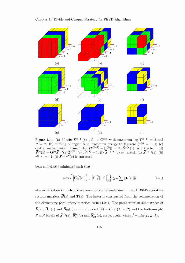
Chapter 4. Divide-and-Conquer Strategy for PEVD Algorithms
= 3
= 2
= 1
=
= 3
= 2
= 1
=
= 2
= 1
=
= 2
= 1
=
= 2
= 1
=
= 1
=
= 1
=
= 1
= =
a) c)
d) e) f)
g) h) i)
b)
Figure 4.14: (a) Matrix S(i−1)(z) : C → C5×5 with maximum lag T (i−1) = 3 and
P = 2; (b) shifting of region with maximum energy to lag zero (τ (i) = −1); (c)central matrix with maximum lag (T (i−1) − |τ (i)|) = 2, S(i)′′(z), is extracted. (d)S(i)(z) = Q(i)S(i)′′(z)Q(i)H; (e) τ (i+1) = 1; (f) S(i+1)′′(z) extracted. (g) S(i+1)(z); (h)τ (i+2) = −1; (i) S(i+2)′′(z) is extracted.
been sufficiently minimised such that
maxτ
∥∥∥S
(I)21 [τ ]
∥∥∥
2
F,∥∥∥S
(I)12 [−τ ]
∥∥∥
2
F
≤ κ∑
τ
‖R[τ ]‖2F (4.51)
at some iteration I —where κ is chosen to be arbitrarily small — the HRSMS algorithm
returns matrices B(z) and T (z). The latter is constructed from the concatenation of
the elementary paraunitary matrices as in (4.25). The parahermitian submatrices of
B(z), B11(z) and B22(z), are the top-left (M − P ) × (M − P ) and the bottom-right
P × P blocks of S(I)(z), S(I)11 (z) and S
(I)22 (z), respectively, where I = minImax, I.
115
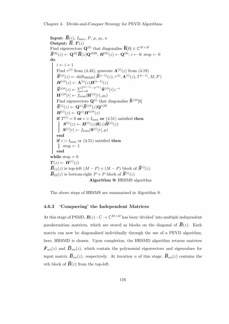
Chapter 4. Divide-and-Conquer Strategy for PEVD Algorithms
Input: R(z), Imax, P , µ, µt, κOutput: B, T (z)Find eigenvectors Q(0) that diagonalise R[0] ∈ C
M×M
S(0)(z)← Q(0)R(z)Q(0)H; H(0)(z)← Q(0); i← 0; stop ← 0do
i← i+ 1
Find τ (i) from (4.43); generate Λ(i)(z) from (4.19)
S(i)′(z)← shiftHSMS(S(i−1)(z), τ (i),Λ(i)(z), T (i−1),M,P )
H(i)′(z)← Λ(i)(z)H (i−1)(z)
S(i)′′(z)←∑T (i−1)−|τ (i)|τ=0 S(i)′[τ ]z−τ
H(i)′′[τ ]← ftrim(H(i)′[τ ], µt)
Find eigenvectors Q(i) that diagonalise S(i)′′[0]
S(i)(z)← Q(i)S(i)′′(z)Q(i)H
H(i)(z)← Q(i)H(i)′′(z)
if T (i) = 0 or i > Imax or (4.51) satisfied then
S(i)(z)←H(i)(z)R(z)H (i)(z)
S(i)[τ ]← ftrim(S(i)[τ ], µ)
end
if i > Imax or (4.51) satisfied then
stop ← 1end
while stop = 0
T (z)←H(i)(z)
B11(z) is top-left (M − P )× (M − P ) block of S(i)(z)
B22(z) is bottom-right P × P block of S(i)(z)
Algorithm 9: HRSMS algorithm
The above steps of HRSMS are summarised in Algorithm 9.
4.6.3 ‘Conquering’ the Independent Matrices
At this stage of PSMD,R(z) : C→ CM×M has been ‘divided’ into multiple independent
parahermitian matrices, which are stored as blocks on the diagonal of B(z). Each
matrix can now be diagonalised individually through the use of a PEVD algorithm;
here, HRSMD is chosen. Upon completion, the HRSMD algorithm returns matrices
F nn(z) and Dnn(z), which contain the polynomial eigenvectors and eigenvalues for
input matrix Bnn(z), respectively. At iteration n of this stage, Bnn(z) contains the
nth block of B(z) from the top-left.
116
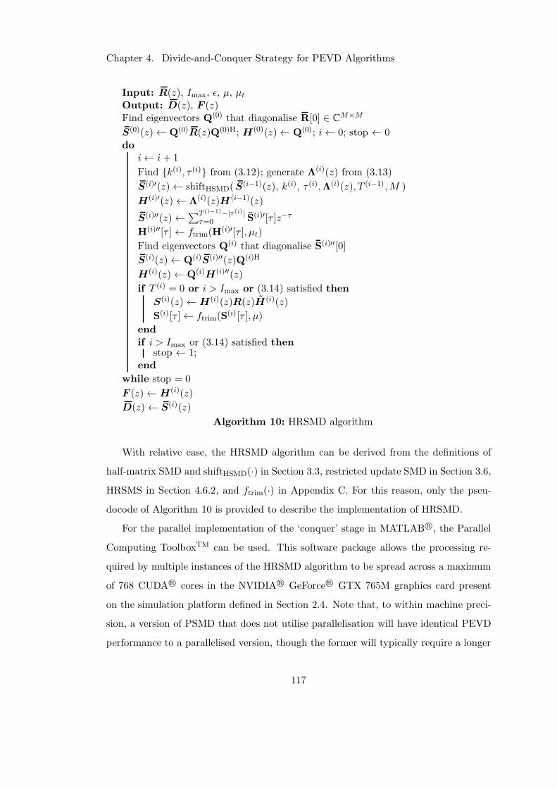
Chapter 4. Divide-and-Conquer Strategy for PEVD Algorithms
Input: R(z), Imax, ǫ, µ, µt
Output: D(z), F (z)Find eigenvectors Q(0) that diagonalise R[0] ∈ C
M×M
S(0)(z)← Q(0)R(z)Q(0)H; H(0)(z)← Q(0); i← 0; stop ← 0do
i← i+ 1
Find k(i), τ (i) from (3.12); generate Λ(i)(z) from (3.13)
S(i)′(z)← shiftHSMD(S(i−1)(z), k(i), τ (i),Λ(i)(z), T (i−1),M )
H(i)′(z)← Λ(i)(z)H (i−1)(z)
S(i)′′(z)←∑T (i−1)−|τ (i)|τ=0 S(i)′[τ ]z−τ
H(i)′′[τ ]← ftrim(H(i)′[τ ], µt)
Find eigenvectors Q(i) that diagonalise S(i)′′[0]
S(i)(z)← Q(i)S(i)′′(z)Q(i)H
H(i)(z)← Q(i)H(i)′′(z)
if T (i) = 0 or i > Imax or (3.14) satisfied then
S(i)(z)←H(i)(z)R(z)H (i)(z)
S(i)[τ ]← ftrim(S(i)[τ ], µ)
end
if i > Imax or (3.14) satisfied thenstop ← 1;
end
while stop = 0
F (z)←H(i)(z)
D(z)← S(i)(z)
Algorithm 10: HRSMD algorithm
With relative ease, the HRSMD algorithm can be derived from the definitions of
half-matrix SMD and shiftHSMD(·) in Section 3.3, restricted update SMD in Section 3.6,
HRSMS in Section 4.6.2, and ftrim(·) in Appendix C. For this reason, only the pseu-
docode of Algorithm 10 is provided to describe the implementation of HRSMD.
For the parallel implementation of the ‘conquer’ stage in MATLABR©, the Parallel
Computing ToolboxTM can be used. This software package allows the processing re-
quired by multiple instances of the HRSMD algorithm to be spread across a maximum
of 768 CUDAR© cores in the NVIDIAR© GeForceR© GTX 765M graphics card present
on the simulation platform defined in Section 2.4. Note that, to within machine preci-
sion, a version of PSMD that does not utilise parallelisation will have identical PEVD
performance to a parallelised version, though the former will typically require a longer
117
Chapter 4. Divide-and-Conquer Strategy for PEVD Algorithms
execution time.
4.6.4 Algorithm Convergence
The SMD and SMS algorithms have been shown to converge in [45] and Section 4.4.2,
respectively. Half-matrix versions of each are functionally identical and therefore also
converge. Furthermore, employing a restricted update strategy for either algorithm
does not impact the proofs of convergence provided in [45] and Section 4.4.2. Given
that HRSMD and HRSMS form the only active, iterative components of PSMD, it can
therefore be concluded that PSMD must also converge for a suitable combination of ID
and IC .
4.6.5 Impact of Algorithm Parameters on Decomposition Error
The comments made in Section 4.5.5 with respect to the introduction of error to the
decomposition produced by the DC-SMD algorithm can also be extended to PSMD.
4.6.6 Algorithm Complexity
The majority of the computational cost of the PSMD algorithm arises from multiple
instances of HRSMS and HRSMD. The instantaneous complexity of PSMD therefore
varies as the algorithm progresses, due to the changing spatial dimensions of the ma-
trices being processed by HRSMS and HRSMD, and the parallel implementation of
HRSMD. The main cost of these internal algorithms can be attributed to the matrix
multiplication step in (4.48) shared by both algorithms. UsingM to capture the differ-
ent spatial dimensions used throughout PSMD — with minM −βP, P ≤ M ≤M —
and the same assumptions as in Section 4.5.6, the computational complexity of a single
matrix multiplication step in either algorithm at iteration i for S(i)′′(z) : C→ CM×M
and H(i)′′(z) : C→ CM×M can be approximated as
C(i)PSMD,M =M3(2LS(i)′′(z)+ LH(i)′′(z)) . (4.52)
118
Chapter 4. Divide-and-Conquer Strategy for PEVD Algorithms
Note that while the process of matrix regeneration in HRSMS and HRSMD does con-
tribute towards computational complexity, the results of Section 3.6.4 have demon-
strated that savings made during the aforementioned matrix multiplication steps out-
weigh the cost of matrix regeneration over the course of algorithm iterations. The
complexity of matrix regeneration is therefore considered to be negligible.
When compared with (4.41), which estimates the complexity of an equivalent step
in DC-SMD, (4.52) will typically return a lower value. This disparity arises as a result
of the length of the restricted, half-matrix form of S(i)′′(z) being lower than the length
of the full-matrix form of S(i)′(z) in DC-SMD.
In PSMD, an M ×M matrix is only ever processed in the first recursion of the
‘divide’ stage; at all other points in the algorithm, the processed matrices are of lower
spatial dimension. Given that the complexity is approximately proportional to the cube
of the spatial dimension, significantly lower complexity will be observed beyond the first
recursion of PSMD. Simulation results that confirm the low complexity of PSMD are
provided in the subsequent section.
4.7 Simulations and Results
This section demonstrates that by employing the DaC techniques proposed in previous
sections, PEVD complexity and therefore run-time can be significantly reduced when
compared with existing iterative PEVD methods. Through the use of the broadband
source model of Appendix B [45] in Sections 4.7.1 and 4.7.2, it is possible to evaluate
the performance of DaC methods for the decomposition of parahermitian matrices of
increasingly large spatial dimension — corresponding to the acquisition of data from an
increasingly large number of broadband sensors. Furthermore, to confirm the efficacy
of the DaC methods for application purposes, the broadband angle of arrival estima-
tion simulation scenario of Section 4.7.3 couples a number of PEVD algorithms with
the spatio-spectral polynomial multiple signal classification (SSP-MUSIC) algorithm
from [18].
119
Chapter 4. Divide-and-Conquer Strategy for PEVD Algorithms
4.7.1 Source Model Simulation Scenario 1
This scenario provides an introduction to the performance of DaC methods, which do
not converge in the same manner as existing PEVD algorithms. A relatively large
spatial dimension, M , is used to demonstrate the failings of existing methods and the
suitability of DC-SMD and PSMD for applications involving large arrays of sensors.
Simulations for this scenario are performed over an ensemble of 103 instantiations
of R(z) : C→ CM×M obtained from the randomised source model in Appendix B [45]
with M = 30, OD = 118, OQ = 60, and ∆DR = 30. The performances of the exist-
ing SBR2 [6] and SMD [45] PEVD algorithms are compared with the novel DC-SMD
and PSMD algorithms. To demonstrate the flexibility of the PSMD algorithm, three
variants are tested; these are denoted PSMD1, PSMD2, and PSMD3. SBR2 and SMD
are allowed to run for 1800 and 1400 iterations, respectively, with polynomial matrix
truncation parameters µSBR2 = µSMD = 10−6. DC-SMD and PSMD1 are provided
with parameters µ = µt = µs = 10−12, κ = ǫ = 0, ID = 100, IC = 200, M = 8,
and P = 8. The remaining two variants of PSMD use identical parameters bar some
small differences: PSMD2 employs more significant polynomial matrix truncation and
is supplied with µ = µt = µs = 10−6, and PSMD3 is supplied with ID = 400. At every
iteration step of each algorithm, the performance metrics defined in Section A.3 are
recorded together with the elapsed execution time.
The multiple shift maximum element SMD (MSME-SMD) of [47] and its deriva-
tives in [48, 50] have been shown to outperform SMD in terms of diagonalisation per
algorithm iteration. However, the work of [49] demonstrates that if the update step of
each method is replaced with a lower-cost cyclic-by-row approximation, the multiple
shift class of algorithms is inferior to SMD with respect to diagonalisation per unit
of time. Given that the update steps of all SMD-based algorithms — including those
incorporating multiple shift strategies — have been updated to use the efficient ma-
trix multiplication approach of Section 3.2.1, the SMD algorithm now behaves as its
approximation in [49] and outperforms all multiple shift methods. This degradation of
multiple shift algorithm performance is due to the methods’ reliance on a more costly
search step, which has a complexity proportional to M3 [65]. For high M — as in the
120
Chapter 4. Divide-and-Conquer Strategy for PEVD Algorithms
simulation scenario here — the cost of this search step prohibits the algorithms’ im-
plementation. The multiple shift algorithms are therefore omitted from testing. Note
that the search step of SMD has a complexity proportional to only M2 [65].
A cyclic-by-row approximation to SMD from [49] was to be tested for the above
scenario, but was found to take in excess of 500 seconds to complete the same number
of iterations as SMD — when using identical algorithm parameters — for the decom-
position of one instance of R(z). Thus, this algorithm was excluded from testing.
Diagonalisation
The ensemble-averaged diagonalisation metric at each iteration for each of the tested
PEVD algorithms is plotted against the ensemble-averaged elapsed system time at each
iteration in Figure 4.15. The curves demonstrate that the proposed implementation
achieves a similar degree of diagonalisation to most of the other algorithms, but in a
shorter time. The SBR2 algorithm exhibits relatively low diagonalisation with respect
to time, and would require a great deal of additional simulation time to attain a diago-
nalisation performance similar to the other algorithms. By utilising a restricted update
approach, PSMD1 has sacrificed a small amount of diagonalisation performance to de-
crease algorithm run-time versus the DC-SMD algorithm. Increased levels of truncation
within PSMD2 have decreased algorithm run-time but have also decreased diagonalisa-
tion performance slightly. The increase in ID within PSMD3 has increased the run-time
of the ‘divide’ stage and marginally improved diagonalisation.
The ‘stepped’ characteristics of the curves for the DaC strategies of DC-SMD and
PSMD are a result of the algorithms’ two-stage implementation. The ‘divide’ steps of
the algorithms exhibit low diagonalisation for a large increase in execution time. In the
‘conquer’ steps, high diagonalisation is seen for a small increase in execution time. Note
that the data points in the curve corresponding to the parallelised ‘conquer’ stage of
PSMD could not be acquired directly, as the processing for this stage was distributed
across a number of CUDAR© cores. The missing data points were instead obtained
using knowledge of the time and diagonalisation metric values at the start and end
points of the curve, and a ground truth convergence curve for the ‘conquer’ stage of a
121
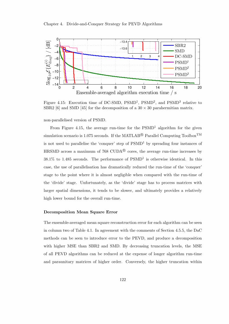
Chapter 4. Divide-and-Conquer Strategy for PEVD Algorithms
0 2 4 6 8 10 12 14 16 18 20−14
−12
−10
−8
−6
−4
−2
0
Ensemble-averaged algorithm execution time / s
5log
10EE
(i)
diag
/[dB]
SBR2
SMD
DC-SMD
PSMD1
PSMD2
PSMD3
1 2 3 4
−13.6
−13.4
Figure 4.15: Execution time of DC-SMD, PSMD1, PSMD2, and PSMD3 relative toSBR2 [6] and SMD [45] for the decomposition of a 30× 30 parahermitian matrix.
non-parallelised version of PSMD.
From Figure 4.15, the average run-time for the PSMD1 algorithm for the given
simulation scenario is 1.075 seconds. If the MATLABR© Parallel Computing ToolboxTM
is not used to parallelise the ‘conquer’ step of PSMD1 by spreading four instances of
HRSMD across a maximum of 768 CUDAR© cores, the average run-time increases by
38.1% to 1.485 seconds. The performance of PSMD1 is otherwise identical. In this
case, the use of parallelisation has dramatically reduced the run-time of the ‘conquer’
stage to the point where it is almost negligible when compared with the run-time of
the ‘divide’ stage. Unfortunately, as the ‘divide’ stage has to process matrices with
larger spatial dimensions, it tends to be slower, and ultimately provides a relatively
high lower bound for the overall run-time.
Decomposition Mean Square Error
The ensemble-averaged mean square reconstruction error for each algorithm can be seen
in column two of Table 4.1. In agreement with the comments of Section 4.5.5, the DaC
methods can be seen to introduce error to the PEVD, and produce a decomposition
with higher MSE than SBR2 and SMD. By decreasing truncation levels, the MSE
of all PEVD algorithms can be reduced at the expense of longer algorithm run-time
and paraunitary matrices of higher order. Conversely, the higher truncation within
122
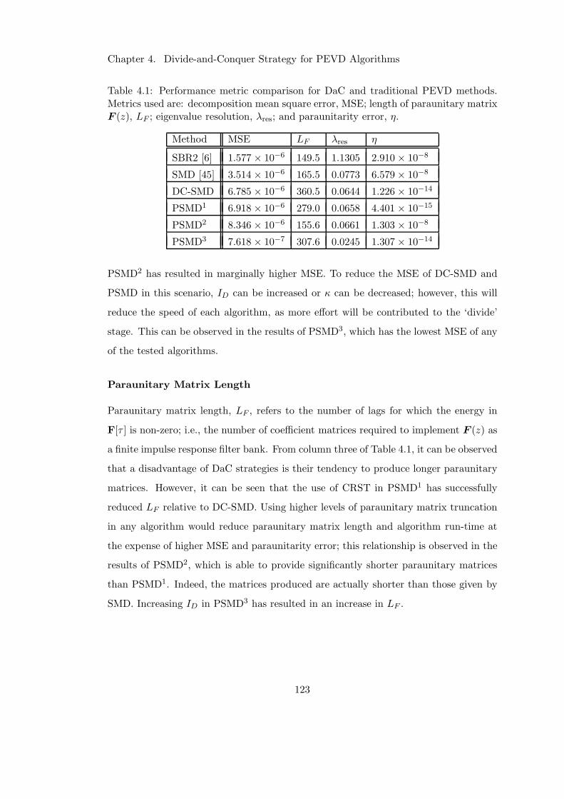
Chapter 4. Divide-and-Conquer Strategy for PEVD Algorithms
Table 4.1: Performance metric comparison for DaC and traditional PEVD methods.Metrics used are: decomposition mean square error, MSE; length of paraunitary matrixF (z), LF ; eigenvalue resolution, λres; and paraunitarity error, η.
Method MSE LF λres η
SBR2 [6] 1.577 × 10⁻⁶ 149.5 1.1305 2.910 × 10⁻⁸
SMD [45] 3.514 × 10⁻⁶ 165.5 0.0773 6.579 × 10⁻⁸
DC-SMD 6.785 × 10⁻⁶ 360.5 0.0644 1.226 × 10⁻¹⁴
PSMD1 6.918 × 10⁻⁶ 279.0 0.0658 4.401 × 10⁻¹⁵
PSMD2 8.346 × 10⁻⁶ 155.6 0.0661 1.303 × 10⁻⁸
PSMD3 7.618 × 10⁻⁷ 307.6 0.0245 1.307 × 10⁻¹⁴
PSMD2 has resulted in marginally higher MSE. To reduce the MSE of DC-SMD and
PSMD in this scenario, ID can be increased or κ can be decreased; however, this will
reduce the speed of each algorithm, as more effort will be contributed to the ‘divide’
stage. This can be observed in the results of PSMD3, which has the lowest MSE of any
of the tested algorithms.
Paraunitary Matrix Length
Paraunitary matrix length, LF , refers to the number of lags for which the energy in
F[τ ] is non-zero; i.e., the number of coefficient matrices required to implement F (z) as
a finite impulse response filter bank. From column three of Table 4.1, it can be observed
that a disadvantage of DaC strategies is their tendency to produce longer paraunitary
matrices. However, it can be seen that the use of CRST in PSMD1 has successfully
reduced LF relative to DC-SMD. Using higher levels of paraunitary matrix truncation
in any algorithm would reduce paraunitary matrix length and algorithm run-time at
the expense of higher MSE and paraunitarity error; this relationship is observed in the
results of PSMD2, which is able to provide significantly shorter paraunitary matrices
than PSMD1. Indeed, the matrices produced are actually shorter than those given by
SMD. Increasing ID in PSMD3 has resulted in an increase in LF .
123
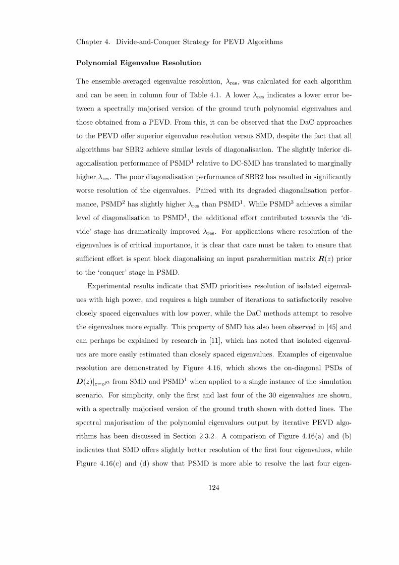
Chapter 4. Divide-and-Conquer Strategy for PEVD Algorithms
Polynomial Eigenvalue Resolution
The ensemble-averaged eigenvalue resolution, λres, was calculated for each algorithm
and can be seen in column four of Table 4.1. A lower λres indicates a lower error be-
tween a spectrally majorised version of the ground truth polynomial eigenvalues and
those obtained from a PEVD. From this, it can be observed that the DaC approaches
to the PEVD offer superior eigenvalue resolution versus SMD, despite the fact that all
algorithms bar SBR2 achieve similar levels of diagonalisation. The slightly inferior di-
agonalisation performance of PSMD1 relative to DC-SMD has translated to marginally
higher λres. The poor diagonalisation performance of SBR2 has resulted in significantly
worse resolution of the eigenvalues. Paired with its degraded diagonalisation perfor-
mance, PSMD2 has slightly higher λres than PSMD1. While PSMD3 achieves a similar
level of diagonalisation to PSMD1, the additional effort contributed towards the ‘di-
vide’ stage has dramatically improved λres. For applications where resolution of the
eigenvalues is of critical importance, it is clear that care must be taken to ensure that
sufficient effort is spent block diagonalising an input parahermitian matrix R(z) prior
to the ‘conquer’ stage in PSMD.
Experimental results indicate that SMD prioritises resolution of isolated eigenval-
ues with high power, and requires a high number of iterations to satisfactorily resolve
closely spaced eigenvalues with low power, while the DaC methods attempt to resolve
the eigenvalues more equally. This property of SMD has also been observed in [45] and
can perhaps be explained by research in [11], which has noted that isolated eigenval-
ues are more easily estimated than closely spaced eigenvalues. Examples of eigenvalue
resolution are demonstrated by Figure 4.16, which shows the on-diagonal PSDs of
D(z)|z=ejΩ from SMD and PSMD1 when applied to a single instance of the simulation
scenario. For simplicity, only the first and last four of the 30 eigenvalues are shown,
with a spectrally majorised version of the ground truth shown with dotted lines. The
spectral majorisation of the polynomial eigenvalues output by iterative PEVD algo-
rithms has been discussed in Section 2.3.2. A comparison of Figure 4.16(a) and (b)
indicates that SMD offers slightly better resolution of the first four eigenvalues, while
Figure 4.16(c) and (d) show that PSMD is more able to resolve the last four eigen-
124
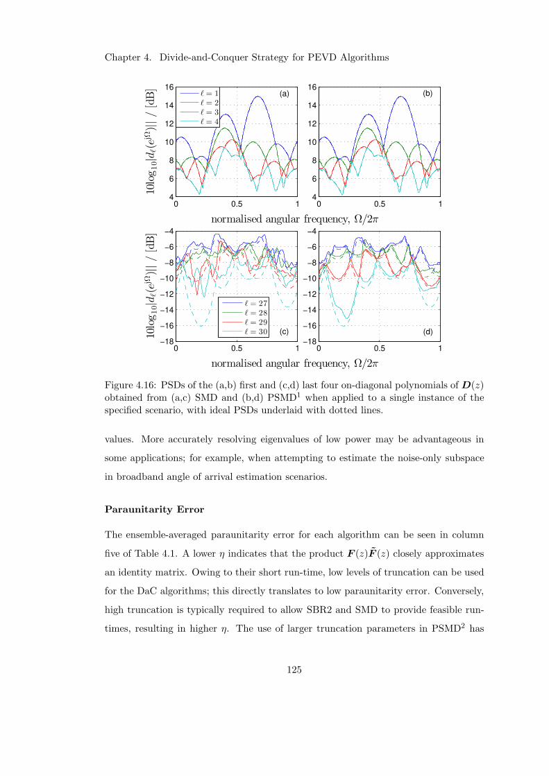
Chapter 4. Divide-and-Conquer Strategy for PEVD Algorithms
0 0.5 14
6
8
10
12
14
16
0 0.5 14
6
8
10
12
14
16
10log10|d
ℓ(ejΩ)||/[dB]
normalised angular frequency, Ω/2π
ℓ = 1ℓ = 2ℓ = 3ℓ = 4
(b)(a)
0 0.5 1−18
−16
−14
−12
−10
−8
−6
−4
0 0.5 1−18
−16
−14
−12
−10
−8
−6
−4
10log10|d
ℓ(ejΩ)||/[dB]
normalised angular frequency, Ω/2π
ℓ = 27ℓ = 28ℓ = 29ℓ = 30 (d)(c)
Figure 4.16: PSDs of the (a,b) first and (c,d) last four on-diagonal polynomials of D(z)obtained from (a,c) SMD and (b,d) PSMD1 when applied to a single instance of thespecified scenario, with ideal PSDs underlaid with dotted lines.
values. More accurately resolving eigenvalues of low power may be advantageous in
some applications; for example, when attempting to estimate the noise-only subspace
in broadband angle of arrival estimation scenarios.
Paraunitarity Error
The ensemble-averaged paraunitarity error for each algorithm can be seen in column
five of Table 4.1. A lower η indicates that the product F (z)F (z) closely approximates
an identity matrix. Owing to their short run-time, low levels of truncation can be used
for the DaC algorithms; this directly translates to low paraunitarity error. Conversely,
high truncation is typically required to allow SBR2 and SMD to provide feasible run-
times, resulting in higher η. The use of larger truncation parameters in PSMD2 has
125
Chapter 4. Divide-and-Conquer Strategy for PEVD Algorithms
resulted in a significant increase in paraunitarity error, such that η is only slightly
lower for PSMD2 than SMD. Increasing ID in PSMD3 has slightly increased η, as
more iterations of each ‘divide’ step — and therefore more truncation operations —
are completed.
4.7.2 Source Model Simulation Scenario 2
This scenario provides additional evidence to confirm the ability of DaC methods to
outperform existing PEVD algorithms as the spatial dimension of the input paraher-
mitian matrix increases. Simulations for this scenario are performed over an ensemble
of 102 instantiations of R(z) : C→ CM×M obtained from the randomised source model
in Appendix B [45] with M ∈ 10; 20; 30; 40; 50; 60; 70, OD = 118, OQ = 60, and
∆DR = 30.
The performance of the existing SMD [45] PEVD algorithm is compared with the
novel PSMD algorithm. For performance metrics other than execution time, the per-
formance of PSMD is representative of the performance of DC-SMD, so the latter is
omitted from simulations for brevity. Using a polynomial matrix truncation parameter
of µSMD = 10−6, SMD is executed until an input matrix is sufficiently diagonalised such
that the off-diagonal energy in the output matrix equals one-tenth of the total energy
in the matrix. PSMD is executed with input parameters µs ∈ 0; 10−6; 10−9; 10−12,µ = µt = 10−12, κ ∈ 2.5 × 10⁻⁶; 10−5; 5 × 10⁻⁵; 10−4, ǫ = 0, ID = 1000, IC = 200,
P = 10, and M = 10. These PSMD input parameters are deliberately chosen such that
the algorithm achieves a diagonalisation level similar to that of SMD for all M . Note
that the level of diagonalisation obtained by an instance of PSMD is mostly determined
by the choice of ‘conquer’ stage parameters IC and ǫ, as the amount of effort devoted
to the ‘divide’ stage does not significantly impact diagonalisation performance — as
seen in Figure 4.15.
At every iteration step of both algorithms, the performance metrics defined in Sec-
tion A.3 are recorded together with the elapsed execution time.
126
Chapter 4. Divide-and-Conquer Strategy for PEVD Algorithms
Diagonalisation
The ensemble-averaged diagonalisation was calculated for the SMD and PSMD imple-
mentations. By evaluating the execution times required for both algorithms to achieve
a diagonalisation level of 5 log10 E(i)diag ≈ −10 dB, it is possible to directly compare the
performance of both algorithms. Figure 4.17 uses the ratio of the execution times to
demonstrate algorithm performance for various spatial dimensions, where
tratio(M,κ) =EtSMD(−10 dB,M)EtPSMD(−10 dB,M, κ) (4.53)
and tPSMD(−10 dB,M, κ) denotes the time taken for one instance of PSMD to achieve
a diagonalisation level of approximately −10 dB for some combination of M and κ. The
value of tSMD(−10 dB,M) similarly denotes the time taken for SMD.
From Figure 4.17, it is clear that tratio(M,κ) increases with increasing spatial di-
mension M for all κ; i.e., the use of PSMD over SMD becomes more important the
larger the matrix to be factorised. Indeed, tratio(M,κ = 10−4) reaches a value of 64.4
for M = 70, signifying that PSMD is 64.4 times faster than SMD on average for this
dimensionality and κ.
In Figure 4.17, it can be seen that the PSMD algorithm run-time increases with
decreasing κ. Smaller values of κ lead to additional time being spent in the ‘divide’
stage of the algorithm and a more accurate block diagonalisation of the parahermitian
matrix. Note that even for κ = 2.5 × 10⁻⁶, the PSMD algorithm is still faster than
SMD.
Decomposition Mean Square Error
The ensemble-averaged decomposition mean square error was calculated for each
algorithm, according to Section A.3. Figure 4.18 shows the results for M ∈10; 20; 30; 40; 50; 60; 70, κ ∈ 2.5 × 10⁻⁶; 10−5; 5 × 10⁻⁵; 10−4, and µs = 0.
This plot confirms the results of Section 4.7.1 by indicating that the increased diago-
nalisation speed of PSMD typically comes at the cost of a higher decomposition error;
however, for κ = 2.5 × 10⁻⁶, the decomposition MSE has fallen below that of SMD.
127
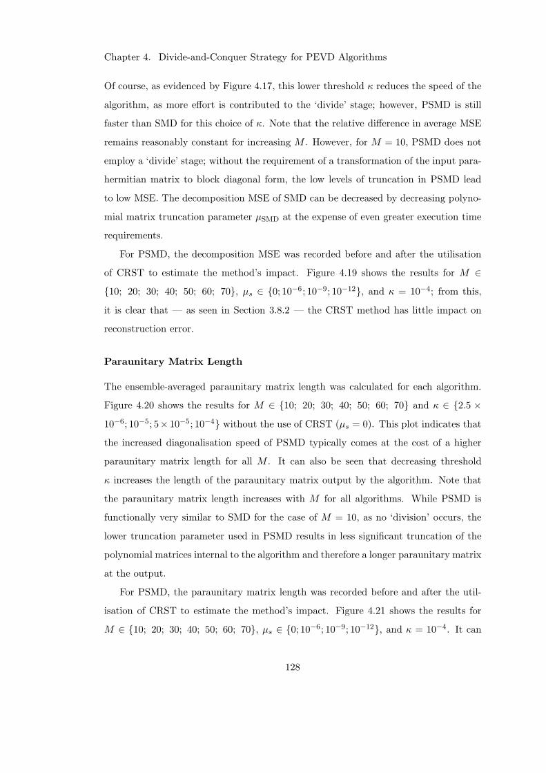
Chapter 4. Divide-and-Conquer Strategy for PEVD Algorithms
Of course, as evidenced by Figure 4.17, this lower threshold κ reduces the speed of the
algorithm, as more effort is contributed to the ‘divide’ stage; however, PSMD is still
faster than SMD for this choice of κ. Note that the relative difference in average MSE
remains reasonably constant for increasing M . However, for M = 10, PSMD does not
employ a ‘divide’ stage; without the requirement of a transformation of the input para-
hermitian matrix to block diagonal form, the low levels of truncation in PSMD lead
to low MSE. The decomposition MSE of SMD can be decreased by decreasing polyno-
mial matrix truncation parameter µSMD at the expense of even greater execution time
requirements.
For PSMD, the decomposition MSE was recorded before and after the utilisation
of CRST to estimate the method’s impact. Figure 4.19 shows the results for M ∈10; 20; 30; 40; 50; 60; 70, µs ∈ 0; 10−6; 10−9; 10−12, and κ = 10−4; from this,
it is clear that — as seen in Section 3.8.2 — the CRST method has little impact on
reconstruction error.
Paraunitary Matrix Length
The ensemble-averaged paraunitary matrix length was calculated for each algorithm.
Figure 4.20 shows the results for M ∈ 10; 20; 30; 40; 50; 60; 70 and κ ∈ 2.5 ×10⁻⁶; 10−5; 5× 10⁻⁵; 10−4 without the use of CRST (µs = 0). This plot indicates that
the increased diagonalisation speed of PSMD typically comes at the cost of a higher
paraunitary matrix length for all M . It can also be seen that decreasing threshold
κ increases the length of the paraunitary matrix output by the algorithm. Note that
the paraunitary matrix length increases with M for all algorithms. While PSMD is
functionally very similar to SMD for the case of M = 10, as no ‘division’ occurs, the
lower truncation parameter used in PSMD results in less significant truncation of the
polynomial matrices internal to the algorithm and therefore a longer paraunitary matrix
at the output.
For PSMD, the paraunitary matrix length was recorded before and after the util-
isation of CRST to estimate the method’s impact. Figure 4.21 shows the results for
M ∈ 10; 20; 30; 40; 50; 60; 70, µs ∈ 0; 10−6; 10−9; 10−12, and κ = 10−4. It can
128
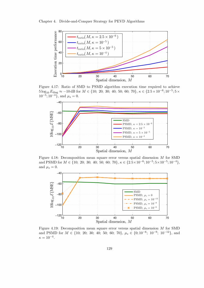
Chapter 4. Divide-and-Conquer Strategy for PEVD Algorithms
10 20 30 40 50 60 700
20
40
60
80
Spatial dimension, M
Execution
timeperform
ance
tratio(M, κ = 2.5× 10⁻⁶ )
tratio(M, κ = 10−5 )
tratio(M, κ = 5× 10⁻⁵ )
tratio(M, κ = 10−4 )
Figure 4.17: Ratio of SMD to PSMD algorithm execution time required to achieve5 log10 Ediag ≈ −10 dB for M ∈ 10; 20; 30; 40; 50; 60; 70, κ ∈ 2.5×10⁻⁶; 10−5; 5×10⁻⁵; 10−4, and µs = 0.
10 20 30 40 50 60 70−120
−100
−80
−60
−40
Spatial dimension, M
10log10EM
SE
SMD
PSMD, κ = 2.5 × 10⁻⁶
PSMD, κ = 10−5
PSMD, κ = 5 × 10⁻⁵
PSMD, κ = 10−4
Figure 4.18: Decomposition mean square error versus spatial dimension M for SMDand PSMD forM ∈ 10; 20; 30; 40; 50; 60; 70, κ ∈ 2.5×10⁻⁶; 10−5; 5×10⁻⁵; 10−4,and µs = 0.
10 20 30 40 50 60 70−120
−100
−80
−60
−40
Spatial dimension, M
10log10EM
SE
SMDPSMD, µs = 0
PSMD, µs = 10−12
PSMD, µs = 10−9
PSMD, µs = 10−6
Figure 4.19: Decomposition mean square error versus spatial dimension M for SMDand PSMD for M ∈ 10; 20; 30; 40; 50; 60; 70, µs ∈ 0; 10−6; 10−9; 10−12, andκ = 10−4.
129
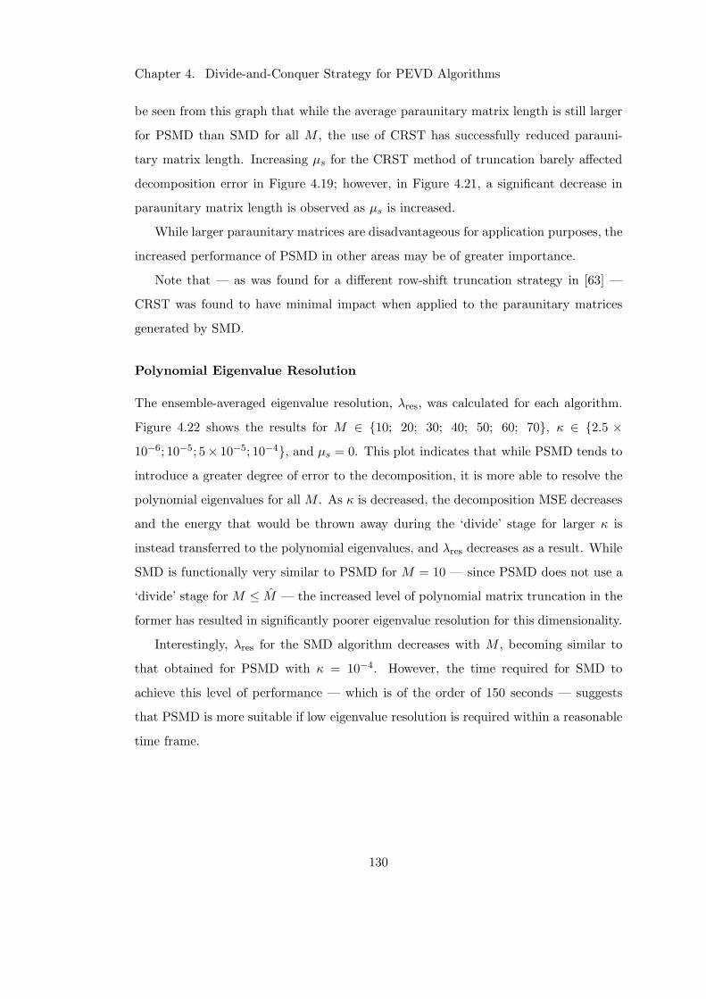
Chapter 4. Divide-and-Conquer Strategy for PEVD Algorithms
be seen from this graph that while the average paraunitary matrix length is still larger
for PSMD than SMD for all M , the use of CRST has successfully reduced parauni-
tary matrix length. Increasing µs for the CRST method of truncation barely affected
decomposition error in Figure 4.19; however, in Figure 4.21, a significant decrease in
paraunitary matrix length is observed as µs is increased.
While larger paraunitary matrices are disadvantageous for application purposes, the
increased performance of PSMD in other areas may be of greater importance.
Note that — as was found for a different row-shift truncation strategy in [63] —
CRST was found to have minimal impact when applied to the paraunitary matrices
generated by SMD.
Polynomial Eigenvalue Resolution
The ensemble-averaged eigenvalue resolution, λres, was calculated for each algorithm.
Figure 4.22 shows the results for M ∈ 10; 20; 30; 40; 50; 60; 70, κ ∈ 2.5 ×10⁻⁶; 10−5; 5× 10⁻⁵; 10−4, and µs = 0. This plot indicates that while PSMD tends to
introduce a greater degree of error to the decomposition, it is more able to resolve the
polynomial eigenvalues for all M . As κ is decreased, the decomposition MSE decreases
and the energy that would be thrown away during the ‘divide’ stage for larger κ is
instead transferred to the polynomial eigenvalues, and λres decreases as a result. While
SMD is functionally very similar to PSMD for M = 10 — since PSMD does not use a
‘divide’ stage for M ≤ M — the increased level of polynomial matrix truncation in the
former has resulted in significantly poorer eigenvalue resolution for this dimensionality.
Interestingly, λres for the SMD algorithm decreases with M , becoming similar to
that obtained for PSMD with κ = 10−4. However, the time required for SMD to
achieve this level of performance — which is of the order of 150 seconds — suggests
that PSMD is more suitable if low eigenvalue resolution is required within a reasonable
time frame.
130
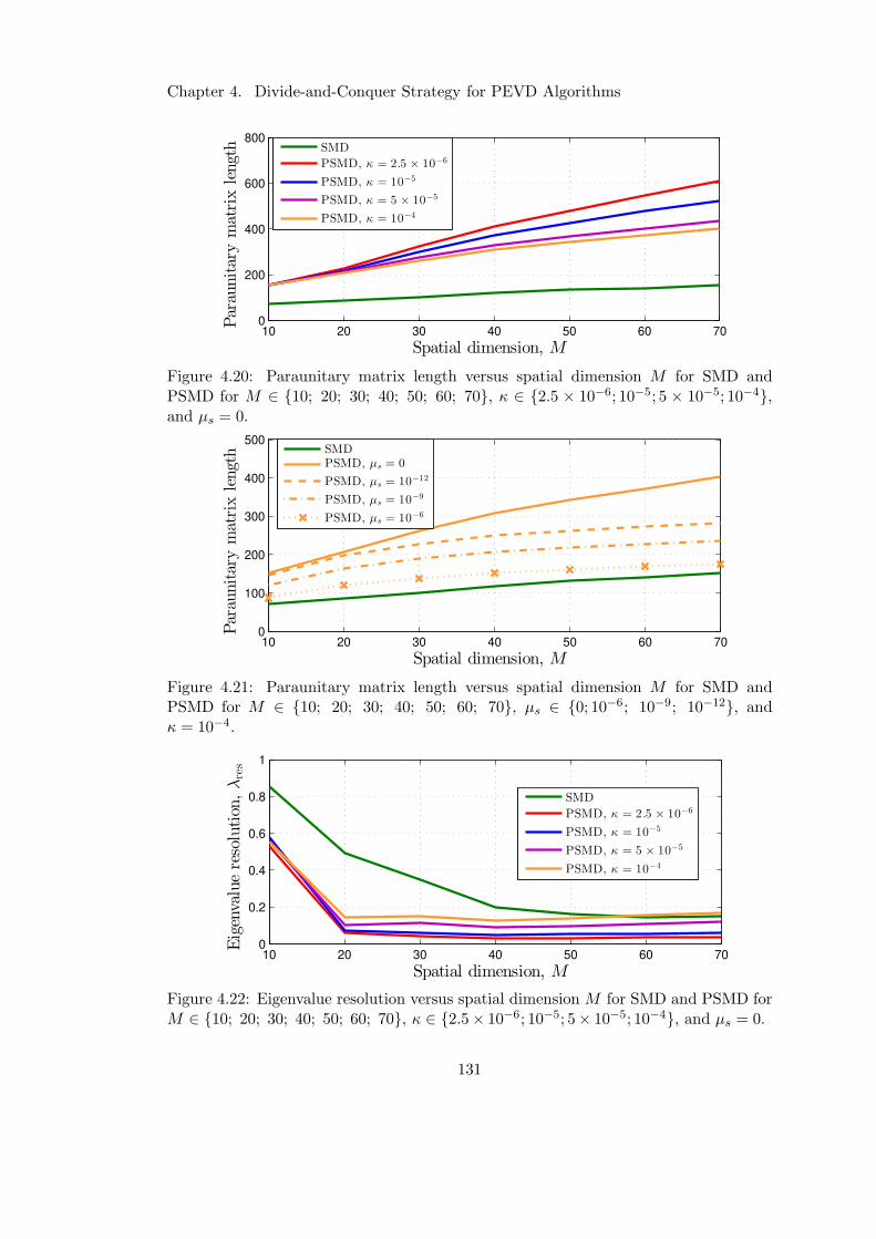
Chapter 4. Divide-and-Conquer Strategy for PEVD Algorithms
10 20 30 40 50 60 700
200
400
600
800
Spatial dimension, M
Paraunitarymatrixlength
SMD
PSMD, κ = 2.5 × 10⁻⁶
PSMD, κ = 10−5
PSMD, κ = 5 × 10⁻⁵
PSMD, κ = 10−4
Figure 4.20: Paraunitary matrix length versus spatial dimension M for SMD andPSMD for M ∈ 10; 20; 30; 40; 50; 60; 70, κ ∈ 2.5 × 10⁻⁶; 10−5; 5 × 10⁻⁵; 10−4,and µs = 0.
10 20 30 40 50 60 700
100
200
300
400
500
Spatial dimension, M
Paraunitarymatrixlength
SMDPSMD, µs = 0
PSMD, µs = 10−12
PSMD, µs = 10−9
PSMD, µs = 10−6
Figure 4.21: Paraunitary matrix length versus spatial dimension M for SMD andPSMD for M ∈ 10; 20; 30; 40; 50; 60; 70, µs ∈ 0; 10−6; 10−9; 10−12, andκ = 10−4.
10 20 30 40 50 60 700
0.2
0.4
0.6
0.8
1
Spatial dimension, M
Eigenvalueresolution,λres
SMD
PSMD, κ = 2.5 × 10⁻⁶
PSMD, κ = 10−5
PSMD, κ = 5 × 10⁻⁵
PSMD, κ = 10−4
Figure 4.22: Eigenvalue resolution versus spatial dimension M for SMD and PSMD forM ∈ 10; 20; 30; 40; 50; 60; 70, κ ∈ 2.5× 10⁻⁶; 10−5; 5× 10⁻⁵; 10−4, and µs = 0.
131
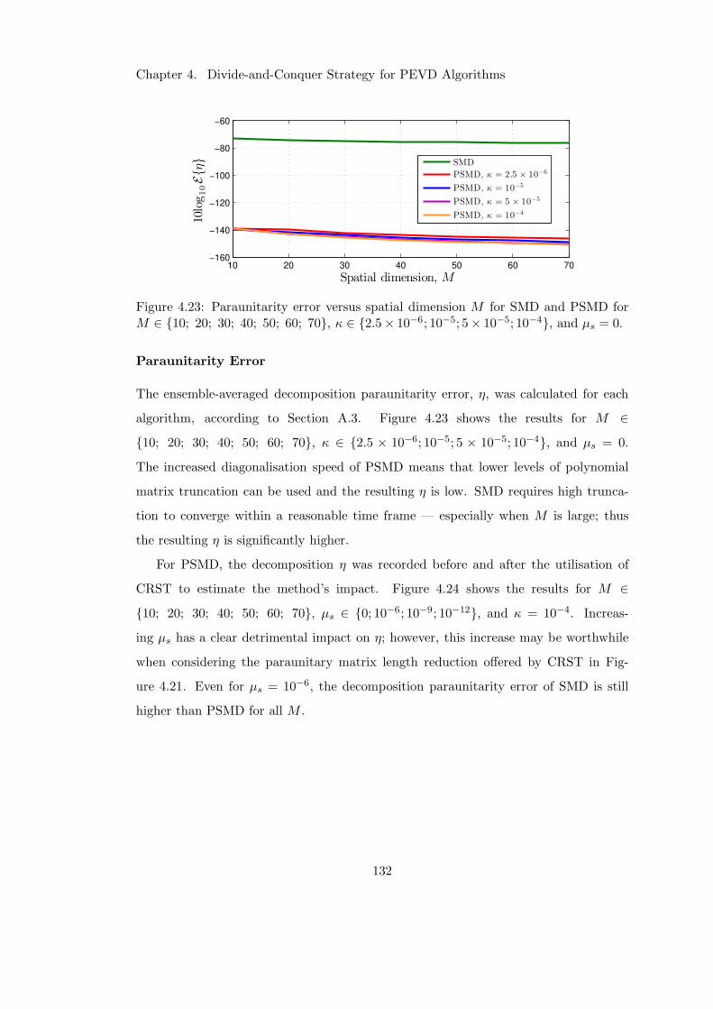
Chapter 4. Divide-and-Conquer Strategy for PEVD Algorithms
10 20 30 40 50 60 70−160
−140
−120
−100
−80
−60
Spatial dimension, M
10log10Eη
SMD
PSMD, κ = 2.5 × 10⁻⁶
PSMD, κ = 10−5
PSMD, κ = 5 × 10⁻⁵
PSMD, κ = 10−4
Figure 4.23: Paraunitarity error versus spatial dimension M for SMD and PSMD forM ∈ 10; 20; 30; 40; 50; 60; 70, κ ∈ 2.5× 10⁻⁶; 10−5; 5× 10⁻⁵; 10−4, and µs = 0.
Paraunitarity Error
The ensemble-averaged decomposition paraunitarity error, η, was calculated for each
algorithm, according to Section A.3. Figure 4.23 shows the results for M ∈10; 20; 30; 40; 50; 60; 70, κ ∈ 2.5 × 10⁻⁶; 10−5; 5 × 10⁻⁵; 10−4, and µs = 0.
The increased diagonalisation speed of PSMD means that lower levels of polynomial
matrix truncation can be used and the resulting η is low. SMD requires high trunca-
tion to converge within a reasonable time frame — especially when M is large; thus
the resulting η is significantly higher.
For PSMD, the decomposition η was recorded before and after the utilisation of
CRST to estimate the method’s impact. Figure 4.24 shows the results for M ∈10; 20; 30; 40; 50; 60; 70, µs ∈ 0; 10−6; 10−9; 10−12, and κ = 10−4. Increas-
ing µs has a clear detrimental impact on η; however, this increase may be worthwhile
when considering the paraunitary matrix length reduction offered by CRST in Fig-
ure 4.21. Even for µs = 10−6, the decomposition paraunitarity error of SMD is still
higher than PSMD for all M .
132
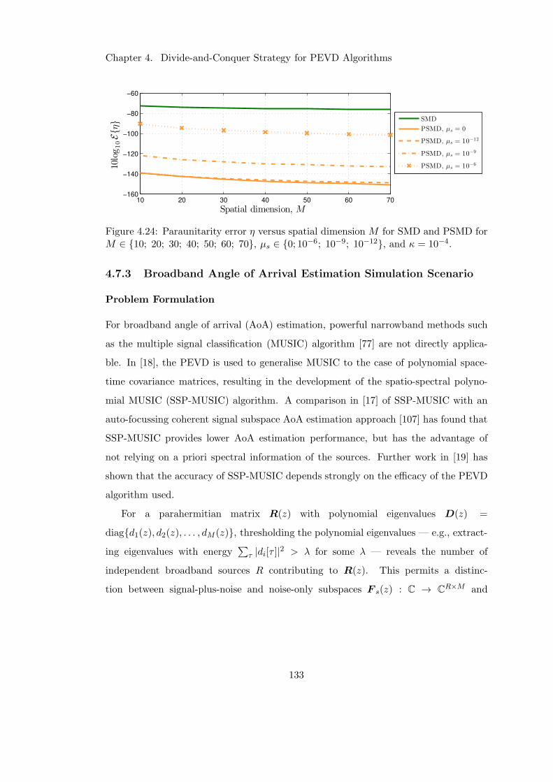
Chapter 4. Divide-and-Conquer Strategy for PEVD Algorithms
10 20 30 40 50 60 70−160
−140
−120
−100
−80
−60
Spatial dimension, M
10log10Eη
SMD
PSMD, µs = 0
PSMD, µs = 10−12
PSMD, µs = 10−9
PSMD, µs = 10−6
Figure 4.24: Paraunitarity error η versus spatial dimension M for SMD and PSMD forM ∈ 10; 20; 30; 40; 50; 60; 70, µs ∈ 0; 10−6; 10−9; 10−12, and κ = 10−4.
4.7.3 Broadband Angle of Arrival Estimation Simulation Scenario
Problem Formulation
For broadband angle of arrival (AoA) estimation, powerful narrowband methods such
as the multiple signal classification (MUSIC) algorithm [77] are not directly applica-
ble. In [18], the PEVD is used to generalise MUSIC to the case of polynomial space-
time covariance matrices, resulting in the development of the spatio-spectral polyno-
mial MUSIC (SSP-MUSIC) algorithm. A comparison in [17] of SSP-MUSIC with an
auto-focussing coherent signal subspace AoA estimation approach [107] has found that
SSP-MUSIC provides lower AoA estimation performance, but has the advantage of
not relying on a priori spectral information of the sources. Further work in [19] has
shown that the accuracy of SSP-MUSIC depends strongly on the efficacy of the PEVD
algorithm used.
For a parahermitian matrix R(z) with polynomial eigenvalues D(z) =
diagd1(z), d2(z), . . . , dM (z), thresholding the polynomial eigenvalues — e.g., extract-
ing eigenvalues with energy∑
τ |di[τ ]|2 > λ for some λ — reveals the number of
independent broadband sources R contributing to R(z). This permits a distinc-
tion between signal-plus-noise and noise-only subspaces F s(z) : C → CR×M and
133
Chapter 4. Divide-and-Conquer Strategy for PEVD Algorithms
F n(z) : C→ C(M−R)×M ,
R(z) ≈[
F s(z) F n(z)]
Ds(z) 0
0 Dn(z)
F s(z)
F n(z)
, (4.54)
where R < M , Ds(z) : C→ CR×R and Dn(z) : C→ C
(M−R)×(M−R). The SSP-MUSIC
algorithm seeks to scan the noise-only subspace F n(z) of R(z), which is spanned by
eigenvectors corresponding to eigenvalues close to the noise floor. The steering vectors
of sources that contribute to R(z) will define the signal-plus-noise subspace F s(z) and
therefore lie in the nullspace of F n(z). More detail on how the SSP-MUSIC algorithm
operates can be found in Appendix D.
Note that the structure of (4.54) is very similar to the block diagonal decomposition
of a parahermitian matrix in (4.4); i.e., consider the form
R(z) ≈[
T s(z) T n(z)]
Bs(z) 0
0 Bn(z)
T s(z)
T n(z)
, (4.55)
where paraunitary matrix T (z) =[
T s(z) T n(z)]
does not contain the eigenvectors of
R(z), but instead contains the orthonormal basis that transforms R(z) into the block
diagonal B(z) = diagBs(z),Bn(z). If an algorithm that enforces spectral majorisa-
tion of the underlying polynomial eigenvalues is used, such as SMS in Section 4.4, the
eigenvalues of Bs(z) : C → CR×R should be those corresponding to signal-plus-noise,
and the eigenvalues of Bn(z) : C → C(M−R)×(M−R) should be those corresponding
to noise. Since Bs(z) and Bn(z) are independent parahermitian matrices and T (z)
is paraunitary, the signal-plus-noise subspace T s(z), which also contains the steering
vectors of sources that contribute to R(z), lies in the nullspace of T n(z). The SSP-
MUSIC algorithm can therefore instead scan the noise-only subspace T n(z) to identify
the presence of source steering vectors in R(z). The results of Section 4.4.4 have shown
that the iterative block diagonalisation of a parahermitian matrix is possible. If, in
practice, the block diagonalisation of some R(z) is less computationally expensive or
faster than its diagonalisation through the use of the PEVD, then a decomposition of
134
Chapter 4. Divide-and-Conquer Strategy for PEVD Algorithms
the form in (4.55) may be preferable for applications involving AoA estimation. Note
that eigenvalues Ds(z) and Dn(z) can be obtained from Bs(z) and Bn(z) if desired;
however, this is not always required for the purposes of AoA estimation.
For a parahermitian matrix with large spatial dimensions, which traditional PEVD
algorithms would typically struggle to diagonalise, PSMD can be used (with IC = 0)
to transform the matrix into block diagonal form. Through smart choice of input
parameters M and P , the signal-plus-noise subspace can be isolated, and the noise-
only subspace can be used in SSP-MUSIC. For example, if 10 sources are known to
contribute to a parahermitian matrix R(z) : C→ C20×20, then PSMD can be executed
using parameters M = 10, P = 5, and IC = 0 such that the first and last 10 rows
of output matrix F (z) correspond to the signal-plus-noise and noise-only subspaces,
respectively. Given the relatively low cost of the ‘conquer’ stage of the PSMD algorithm,
and the low likelihood that a block diagonal form will perfectly separate signal-plus-
noise and noise-only subspaces, it is typically worthwhile to provide PSMD with at
least a small value for IC . Using a relatively large stopping threshold ǫ for the ‘conquer’
stage would then prevent the PSMD from spending time diagonalising parahermitian
matrices containing only noise.
Simulation Scenario
In this simulation scenario, the AoA estimation performance that PSMD offers when
paired with SSP-MUSIC is compared with the performance that SBR2 and SMD pro-
vide in a broadband AoA estimation scenario. Again, DC-SMD is omitted for brevity.
Performance of each PEVD algorithm is measured in terms of AoA estimation accuracy
and with the metrics of Section A.3. AoA estimation accuracy is measured through
a visual assessment of metric PSSP(ϑ,Ω) ∈ R>0 output by the SSP-MUSIC algorithm
in [18], which is evaluated at a range of angles of arrival, ϑ, and frequencies, Ω. A high
value of PSSP(ϑ,Ω) indicates the presence of a source at a specific angle of arrival and
frequency, while a low value indicates that no source is present.
In the simulations below, an M = 20 element array is illuminated by six broadband
sources active over a frequency range Ωj ∈ [0.1π, 0.9π], j = 1 . . . 6, and different angles
135
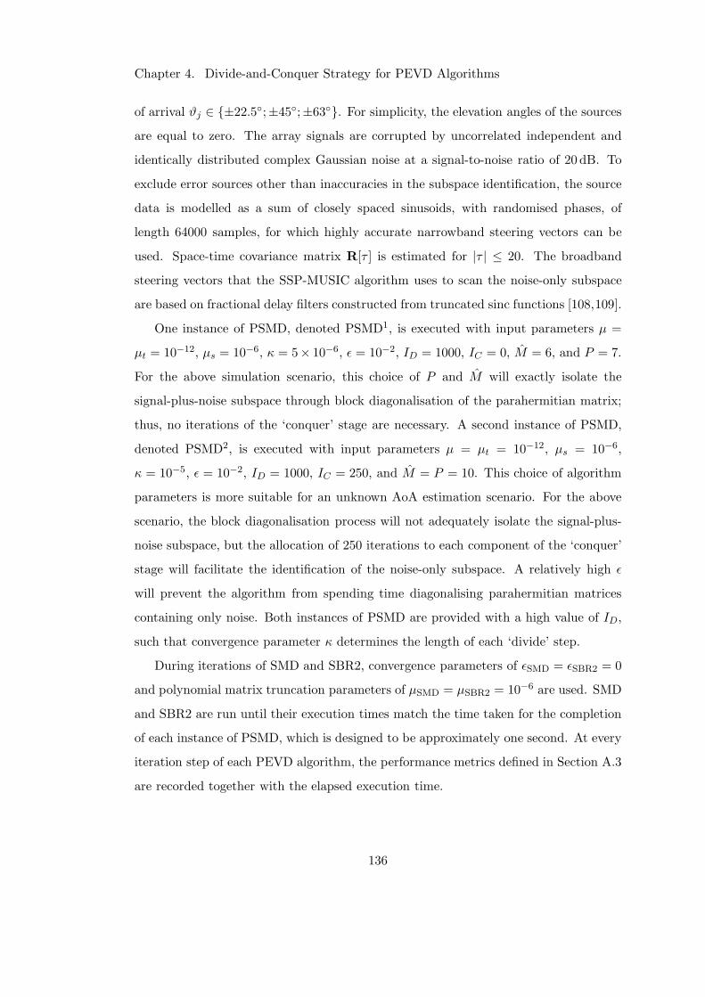
Chapter 4. Divide-and-Conquer Strategy for PEVD Algorithms
of arrival ϑj ∈ ±22.5;±45;±63. For simplicity, the elevation angles of the sources
are equal to zero. The array signals are corrupted by uncorrelated independent and
identically distributed complex Gaussian noise at a signal-to-noise ratio of 20 dB. To
exclude error sources other than inaccuracies in the subspace identification, the source
data is modelled as a sum of closely spaced sinusoids, with randomised phases, of
length 64000 samples, for which highly accurate narrowband steering vectors can be
used. Space-time covariance matrix R[τ ] is estimated for |τ | ≤ 20. The broadband
steering vectors that the SSP-MUSIC algorithm uses to scan the noise-only subspace
are based on fractional delay filters constructed from truncated sinc functions [108,109].
One instance of PSMD, denoted PSMD1, is executed with input parameters µ =
µt = 10−12, µs = 10−6, κ = 5× 10⁻⁶, ǫ = 10−2, ID = 1000, IC = 0, M = 6, and P = 7.
For the above simulation scenario, this choice of P and M will exactly isolate the
signal-plus-noise subspace through block diagonalisation of the parahermitian matrix;
thus, no iterations of the ‘conquer’ stage are necessary. A second instance of PSMD,
denoted PSMD2, is executed with input parameters µ = µt = 10−12, µs = 10−6,
κ = 10−5, ǫ = 10−2, ID = 1000, IC = 250, and M = P = 10. This choice of algorithm
parameters is more suitable for an unknown AoA estimation scenario. For the above
scenario, the block diagonalisation process will not adequately isolate the signal-plus-
noise subspace, but the allocation of 250 iterations to each component of the ‘conquer’
stage will facilitate the identification of the noise-only subspace. A relatively high ǫ
will prevent the algorithm from spending time diagonalising parahermitian matrices
containing only noise. Both instances of PSMD are provided with a high value of ID,
such that convergence parameter κ determines the length of each ‘divide’ step.
During iterations of SMD and SBR2, convergence parameters of ǫSMD = ǫSBR2 = 0
and polynomial matrix truncation parameters of µSMD = µSBR2 = 10−6 are used. SMD
and SBR2 are run until their execution times match the time taken for the completion
of each instance of PSMD, which is designed to be approximately one second. At every
iteration step of each PEVD algorithm, the performance metrics defined in Section A.3
are recorded together with the elapsed execution time.
136
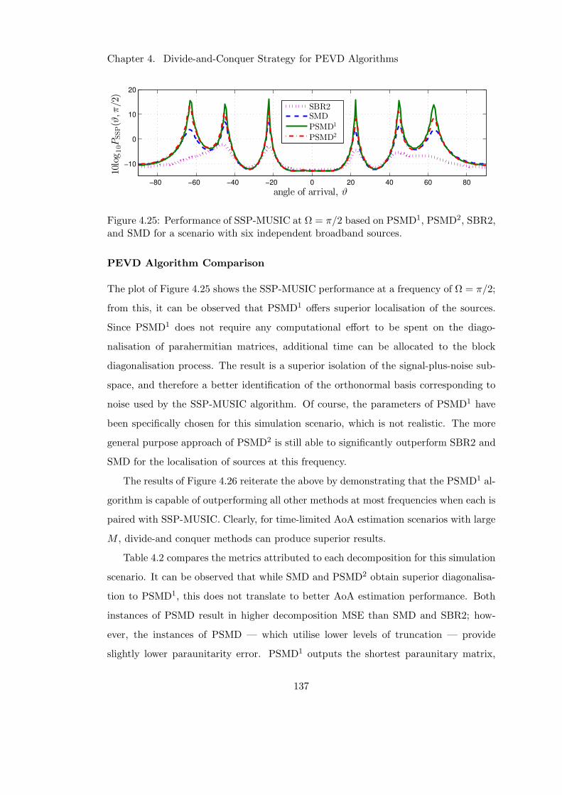
Chapter 4. Divide-and-Conquer Strategy for PEVD Algorithms
−80 −60 −40 −20 0 20 40 60 80
−10
0
10
20
angle of arrival, ϑ
10log10PSSP(ϑ,π
/2)
SBR2SMDPSMD1
PSMD2
Figure 4.25: Performance of SSP-MUSIC at Ω = π/2 based on PSMD1, PSMD2, SBR2,and SMD for a scenario with six independent broadband sources.
PEVD Algorithm Comparison
The plot of Figure 4.25 shows the SSP-MUSIC performance at a frequency of Ω = π/2;
from this, it can be observed that PSMD1 offers superior localisation of the sources.
Since PSMD1 does not require any computational effort to be spent on the diago-
nalisation of parahermitian matrices, additional time can be allocated to the block
diagonalisation process. The result is a superior isolation of the signal-plus-noise sub-
space, and therefore a better identification of the orthonormal basis corresponding to
noise used by the SSP-MUSIC algorithm. Of course, the parameters of PSMD1 have
been specifically chosen for this simulation scenario, which is not realistic. The more
general purpose approach of PSMD2 is still able to significantly outperform SBR2 and
SMD for the localisation of sources at this frequency.
The results of Figure 4.26 reiterate the above by demonstrating that the PSMD1 al-
gorithm is capable of outperforming all other methods at most frequencies when each is
paired with SSP-MUSIC. Clearly, for time-limited AoA estimation scenarios with large
M , divide-and conquer methods can produce superior results.
Table 4.2 compares the metrics attributed to each decomposition for this simulation
scenario. It can be observed that while SMD and PSMD2 obtain superior diagonalisa-
tion to PSMD1, this does not translate to better AoA estimation performance. Both
instances of PSMD result in higher decomposition MSE than SMD and SBR2; how-
ever, the instances of PSMD — which utilise lower levels of truncation — provide
slightly lower paraunitarity error. PSMD1 outputs the shortest paraunitary matrix,
137
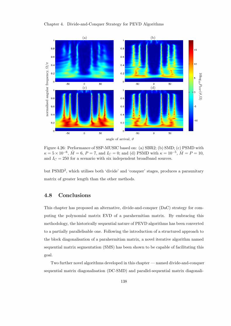
Chapter 4. Divide-and-Conquer Strategy for PEVD Algorithms
(a) (b)
(c) (d)
angle of arrival, ϑ
norm
alisedangularfreq
uen
cy,Ω/π
10log10 P
SSP(ϑ
,Ω)
Figure 4.26: Performance of SSP-MUSIC based on: (a) SBR2; (b) SMD; (c) PSMD withκ = 5× 10⁻⁶, M = 6, P = 7, and IC = 0; and (d) PSMD with κ = 10−5, M = P = 10,and IC = 250 for a scenario with six independent broadband sources.
but PSMD2, which utilises both ‘divide’ and ‘conquer’ stages, produces a paraunitary
matrix of greater length than the other methods.
4.8 Conclusions
This chapter has proposed an alternative, divide-and-conquer (DaC) strategy for com-
puting the polynomial matrix EVD of a parahermitian matrix. By embracing this
methodology, the historically sequential nature of PEVD algorithms has been converted
to a partially parallelisable one. Following the introduction of a structured approach to
the block diagonalisation of a parahermitian matrix, a novel iterative algorithm named
sequential matrix segmentation (SMS) has been shown to be capable of facilitating this
goal.
Two further novel algorithms developed in this chapter — named divide-and-conquer
sequential matrix diagonalisation (DC-SMD) and parallel-sequential matrix diagonali-
138
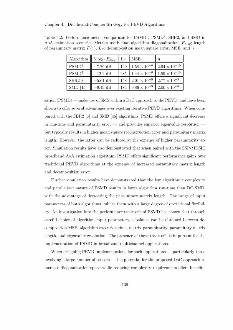
Chapter 4. Divide-and-Conquer Strategy for PEVD Algorithms
Table 4.2: Performance metric comparison for PSMD1, PSMD2, SBR2, and SMD inAoA estimation scenario. Metrics used: final algorithm diagonalisation, Ediag; lengthof paraunitary matrix F (z), LF ; decomposition mean square error, MSE; and η.
Algorithm 5 log10 Ediag LF MSE η
PSMD1 −7.76 dB 140 1.58 × 10⁻⁶ 2.94 × 10⁻¹⁰
PSMD2 −12.2 dB 285 1.44 × 10⁻⁶ 1.59 × 10⁻¹⁰
SBR2 [6] −5.61 dB 148 2.01 × 10⁻⁹ 2.77 × 10⁻⁹
SMD [45] −9.49 dB 184 9.86 × 10⁻⁹ 2.00 × 10⁻⁸
sation (PSMD)—make use of SMS within a DaC approach to the PEVD, and have been
shown to offer several advantages over existing iterative PEVD algorithms. When com-
pared with the SBR2 [6] and SMD [45] algorithms, PSMD offers a significant decrease
in run-time and paraunitarity error — and provides superior eigenvalue resolution —
but typically results in higher mean square reconstruction error and paraunitary matrix
length. However, the latter can be reduced at the expense of higher paraunitarity er-
ror. Simulation results have also demonstrated that when paired with the SSP-MUSIC
broadband AoA estimation algorithm, PSMD offers significant performance gains over
traditional PEVD algorithms at the expense of increased paraunitary matrix length
and decomposition error.
Further simulation results have demonstrated that the low algorithmic complexity
and parallelised nature of PSMD results in lower algorithm run-time than DC-SMD,
with the advantage of decreasing the paraunitary matrix length. The range of input
parameters of both algorithms imbues them with a large degree of operational flexibil-
ity. An investigation into the performance trade-offs of PSMD has shown that through
careful choice of algorithm input parameters, a balance can be obtained between de-
composition MSE, algorithm execution time, matrix paraunitarity, paraunitary matrix
length, and eigenvalue resolution. The presence of these trade-offs is important for the
implementation of PSMD in broadband multichannel applications.
When designing PEVD implementations for such applications — particularly those
involving a large number of sensors — the potential for the proposed DaC approach to
increase diagonalisation speed while reducing complexity requirements offers benefits.
139
Chapter 4. Divide-and-Conquer Strategy for PEVD Algorithms
In addition, the parallelisable nature of PSMD, which has been exploited here to re-
duce algorithm run-time, is well suited to hardware implementation. For applications
involving broadband angle of arrival estimation, the short run-time of PSMD will de-
crease the time between estimations of source locations and bandwidths; similarly, use
of PSMD will allow for signal of interest and interferer locations and bandwidths to
be updated more quickly in broadband beamforming applications. Furthermore, the
low paraunitarity error of PSMD, which facilitates the implementation of near-lossless
filter banks, is advantageous for communications applications.
140
Chapter 5
DFT-Based Alternatives for
PEVD Algorithms
5.1 Introduction
The previous chapters have dealt with a number of iterative PEVD algorithms that ma-
nipulate polynomial coefficients directly to diagonalise a parahermitian matrix. Such
algorithms — represented in [6,45–50] — form a significant proportion of the available
methods for computing the PEVD. This chapter instead investigates the less-explored
area of PEVD algorithms based on the discrete Fourier transform (DFT). Following the
introduction of a capable DFT-based PEVD (and PSVD) algorithm in [53], there has
been little research in this field; indeed, only very brief relative comparisons between
iterative and DFT-based methods had been conducted prior to the research discussed
in this chapter. While the algorithm of [53] has in almost all cases been demonstrated
to produce a compact, accurate PEVD, it requires a priori knowledge of the order of
the polynomial eigenvectors in the decomposition, and employs an eigenvalue reorder-
ing scheme that is susceptible to errors in the presence of eigenvalues with algebraic
multiplicities greater than one.
For future reference, the general structure of a DFT-based PEVD algorithm is
provided below. If the PEVD equation of (2.4) is evaluated at K discrete points on
141
Chapter 5. DFT-Based Alternatives for PEVD Algorithms
the unit circle, the following formulation can be obtained:
R[k] = Q[k]D[k]QH[k] , k = 0 . . . K − 1 , (5.1)
where R[k] = R(z)|z=ejΩk and Ωk = 2πk/K. In (5.1), Q[k] is a unitary matrix contain-
ing eigenvectors in its columns, D[k] is a diagonal matrix containing eigenvalues, and
R[k] is obtained from the K-point DFT of R[τ ] ∈ CM×M ,
R[k] = R(z)|z=ejΩk =∑
τR[τ ]e−jΩkτ , k = 0 . . . K − 1 , (5.2)
where K ≥ L and L is the length of R(z). Since each frequency bin k contains an
independent Hermitian matrix R[k], an approximate PEVD is therefore obtained via
K independent EVDs.
Noting that the decompositions in (2.4) and (5.1) are only unique up to permu-
tations and phase shifts [9], an advantage of DFT-based approaches is the option to
rearrange the eigenvalues and eigenvectors at each frequency bin if desired. If the eigen-
values in D[k] are arranged in descending order, approximate spectral majorisation of
the resulting polynomial eigenvalues occurs [53]. An analytic decomposition, whereby
both eigenvalues and eigenvectors are continuous in frequency, typically produces a
more compact decomposition, but requires additional effort. Spectral majorisation is
preferable to an analytic decomposition in only a limited number of applications, e.g.,
when the extraction of multiple-input multiple-output (MIMO) subchannels of ordered
quality [110] matters. Figure 5.1 shows the PSDs of analytic and spectrally majorised
eigenvalues for an example parahermitian matrix R(z) : C→ C2×2.
A disadvantage of DFT-based algorithms involves the inherent lack of phase coher-
ence between independent frequency bins [81]. Each eigenvector at each frequency bin
can be influenced by an arbitrary scalar phase angle and still be valid. Discontinuities
in phase between adjacent frequency bins can arise due to this ambiguity in eigen-
vector phase. To obtain a short paraunitary matrix Q(z), these discontinuities must
be smoothed by enforcing phase coherence between frequency bins [9]. In [53], this
is achieved through the use of a phase alignment function, described in Section A.2.3,
142
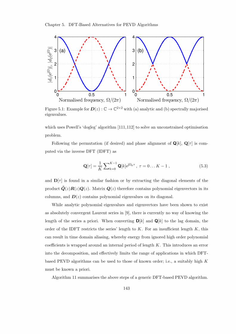
Chapter 5. DFT-Based Alternatives for PEVD Algorithms
0 0.5 10
1
2
3
4
|d1(e
jΩ)|,|d
2(e
jΩ)|
Normalised frequency, Ω/(2π)
(a)
0 0.5 10
1
2
3
4
Normalised frequency, Ω/(2π)
(b)
Figure 5.1: Example forD(z) : C→ C2×2 with (a) analytic and (b) spectrally majorised
eigenvalues.
which uses Powell’s ‘dogleg’ algorithm [111,112] to solve an unconstrained optimisation
problem.
Following the permutation (if desired) and phase alignment of Q[k], Q[τ ] is com-
puted via the inverse DFT (IDFT) as
Q[τ ] =1
K
∑K−1
k=0Q[k]ejΩkτ , τ = 0 . . . K − 1 , (5.3)
and D[τ ] is found in a similar fashion or by extracting the diagonal elements of the
product Q(z)R(z)Q(z). Matrix Q(z) therefore contains polynomial eigenvectors in its
columns, and D(z) contains polynomial eigenvalues on its diagonal.
While analytic polynomial eigenvalues and eigenvectors have been shown to exist
as absolutely convergent Laurent series in [9], there is currently no way of knowing the
length of the series a priori. When converting D[k] and Q[k] to the lag domain, the
order of the IDFT restricts the series’ length to K. For an insufficient length K, this
can result in time domain aliasing, whereby energy from ignored high order polynomial
coefficients is wrapped around an internal period of length K. This introduces an error
into the decomposition, and effectively limits the range of applications in which DFT-
based PEVD algorithms can be used to those of known order; i.e., a suitably high K
must be known a priori.
Algorithm 11 summarises the above steps of a generic DFT-based PEVD algorithm.
143
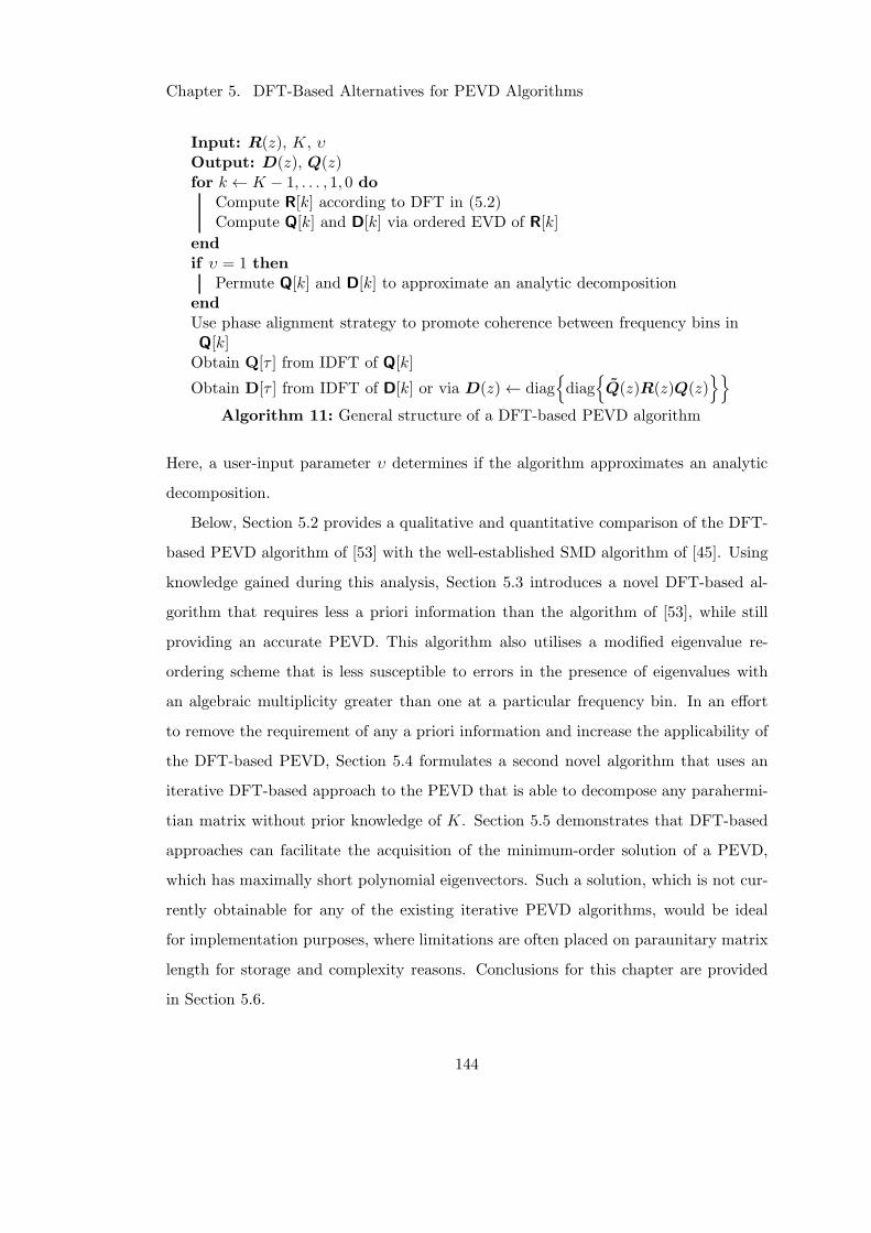
Chapter 5. DFT-Based Alternatives for PEVD Algorithms
Input: R(z), K, υOutput: D(z), Q(z)for k ← K − 1, . . . , 1, 0 do
Compute R[k] according to DFT in (5.2)Compute Q[k] and D[k] via ordered EVD of R[k]
end
if υ = 1 then
Permute Q[k] and D[k] to approximate an analytic decompositionend
Use phase alignment strategy to promote coherence between frequency bins inQ[k]Obtain Q[τ ] from IDFT of Q[k]
Obtain D[τ ] from IDFT of D[k] or via D(z)← diag
diag
Q(z)R(z)Q(z)
Algorithm 11: General structure of a DFT-based PEVD algorithm
Here, a user-input parameter υ determines if the algorithm approximates an analytic
decomposition.
Below, Section 5.2 provides a qualitative and quantitative comparison of the DFT-
based PEVD algorithm of [53] with the well-established SMD algorithm of [45]. Using
knowledge gained during this analysis, Section 5.3 introduces a novel DFT-based al-
gorithm that requires less a priori information than the algorithm of [53], while still
providing an accurate PEVD. This algorithm also utilises a modified eigenvalue re-
ordering scheme that is less susceptible to errors in the presence of eigenvalues with
an algebraic multiplicity greater than one at a particular frequency bin. In an effort
to remove the requirement of any a priori information and increase the applicability of
the DFT-based PEVD, Section 5.4 formulates a second novel algorithm that uses an
iterative DFT-based approach to the PEVD that is able to decompose any parahermi-
tian matrix without prior knowledge of K. Section 5.5 demonstrates that DFT-based
approaches can facilitate the acquisition of the minimum-order solution of a PEVD,
which has maximally short polynomial eigenvectors. Such a solution, which is not cur-
rently obtainable for any of the existing iterative PEVD algorithms, would be ideal
for implementation purposes, where limitations are often placed on paraunitary matrix
length for storage and complexity reasons. Conclusions for this chapter are provided
in Section 5.6.
144
Chapter 5. DFT-Based Alternatives for PEVD Algorithms
5.2 Comparison of Iterative and DFT-Based PEVDs
This section compares the decomposition accuracies of two fundamentally different
methods capable of computing an approximate PEVD. The first of these — sequential
matrix diagonalisation (SMD) [45] — iteratively decomposes a parahermitian matrix
by directly manipulating polynomial coefficients and is described in Section A.1, while
a second algorithm introduced in [53] and summarised in Section A.2 computes a DFT-
based decomposition using the formulation in (5.1).
Following a comparison of the algorithmic complexities of each decomposition in
Section 5.2.1, the accuracies of the polynomial eigenvalues generated by each is dis-
cussed in Section 5.2.2. The paraunitarity error induced by each algorithm is then
reviewed in Section 5.2.3, and simulations in Section 5.2.4 are used to compare the
performance of each strategy with respect to the metrics of Section A.3. From the
comparisons conducted in these sections, Section 5.2.5 is able to provide concluding
remarks that indicate the type of broadband multichannel problems that are better
suited to each algorithm.
Elements of the work in this section can be found in a paper titled ‘A Comparison
of Iterative and DFT-Based Polynomial Matrix Eigenvalue Decompositions’ [56] pub-
lished in the proceedings of the 7th IEEE International Workshop on Computational
Advances in Multi-Sensor Adaptive Processing, and in a paper titled “Correction to
‘On the Uniqueness and Existence of the Eigenvalue Decomposition of a Parahermitian
Matrix’ ” [10] published in IEEE Transactions on Signal Processing.
5.2.1 Algorithm Complexities
At the ith iteration of SMD, every matrix-valued coefficient in S(i)′(z) : C → CM×M
must be left- and right-multiplied with unitary matrixQ(i) ∈ CM×M ; similarlyH(i)′(z) :
C → CM×M is left-multiplied with Q(i). A total of 2LS(i)′(z) and LH(i)′(z) ma-
trix multiplications are therefore required to update S(i)′(z) and H(i)′(z), respectively,
where operator L· measures the length of a polynomial matrix. While potentially
lower complexity matrix multiplication methods have been derived with complexi-
ties of, e.g., O(M2.807) [2, 113] and O(M2.3728639) [114] for the multiplication of two
145
Chapter 5. DFT-Based Alternatives for PEVD Algorithms
square matrices with spatial dimension M , these often require very large M to out-
perform more traditional methods [95]. A simpler, naive assumption estimates that
the complexity of the multiplication of two M ×M matrices is of order O(M3) [2,95];
thus, it can be approximated that the complexity of one SMD iteration is of order
O(M3(2LS(i)′(z)+LH (i)′(z))) ≈ O(M3L) — if it is also assumed that the lengths
of these internal matrices are ultimately proportional to the length, L, of the input
parahermitian matrix R(z). The update step dominates the complexity of SMD [45];
thus, for a constant number of algorithm iterations, the algorithm complexity is of
order O(M3L).
In the DFT-based algorithm, for a constant number of optimisation steps, the
complexity of each of the M instantiations of the phase alignment method is O(K3)
due to matrix inversion [53,95]; thus, the total complexity of the phase alignment step
is of order O(MK3). Given that K is bounded from below by L in (A.15) for constant
N , O(MK3) can be expressed as O(ML3). The computation of the frequency domain
representation of R(z), the execution of K EVDs, and the reordering of the eigenvalues
and eigenvectors are of lower complexity than this step; thus, the total complexity of
the algorithm is approximately O(ML3).
5.2.2 Approximation of Eigenvalues
The SMD algorithm iteratively diagonalises a parahermitian matrix R(z); thus, the
approximation of the polynomial eigenvalues becomes better with each algorithm it-
eration. Almost exact diagonalisation of R(z) typically requires a large number of
iterations; this can be problematic, as the parahermitian matrix grows in order at each
iteration of SMD [45]. Truncation of the outer lags of the matrix containing lower
energy can help mitigate this growth, but risks the introduction of error into the poly-
nomial eigenvalues and resulting PEVD. The polynomial eigenvalues produced by SMD
are approximately spectrally majorised [45], and cannot be reordered. As mentioned
in Section 5.1, this is only beneficial for a subset of applications.
Matrix D(z) is computed via the product Q(z)R(z)Q(z) and is set to be exactly
diagonal in the final step of the DFT-based approach [53]; thus, diagonalisation metric
146
Chapter 5. DFT-Based Alternatives for PEVD Algorithms
Ediag = 0 for all instances of the algorithm. However, for insufficiently accurate eigen-
vectors that do not completely diagonalise R(z), directly setting off-diagonal elements
equal to zero in this way negatively impacts the decomposition MSE. The eigenvalue
approximation ultimately depends upon the accuracy of the eigenvectors, which typ-
ically increases for increasing parameters N and K, where the latter is dictated by
K ≥ 2N +L− 2. Here, N is a user-defined estimate of the output paraunitary matrix
length, and is not known a priori. The DFT-based algorithm naturally produces an
approximately spectrally majorised decomposition, but as described in Section A.2.2,
the eigenvalues can be reordered to approximate an analytic decomposition. The latter
avoids discontinuities at the intersection of eigenvalues in the frequency domain, and
typically leads to a more compact (lower order) decomposition.
5.2.3 Paraunitarity of Polynomial Eigenvectors
The eigenvectors Q(z) = F (z) generated by SMD are strictly paraunitary, as they are
created as the product of a series of elementary paraunitary matrices. While this is ad-
vantageous for some applications, some loss of paraunitarity may be acceptable if other
performance gains are made. For example, the truncation strategy of Appendix C —
which is used to truncate the paraunitary matrices within the SMD update step —
introduces a trade-off between paraunitarity error, η, and diagonalisation, Ediag, for a
given paraunitary matrix length; i.e., a larger truncation value, µ, sacrifices paraunitar-
ity to reduce the paraunitary matrix order required to achieve a certain diagonalisation.
The eigenvectors generated by the DFT-based PEVD are only approximately pa-
raunitary [53]. For increasing N , the approximation typically improves; thus, to achieve
a desired level of paraunitarity in an application, an adequate value of N must be de-
termined through experimentation. The required value of N is likely to be lower if
an analytic decomposition is sought, as discontinuities at eigenvalue intersections are
avoided. To represent such discontinuities requires infinitely long polynomials, which
do not fit well into the fixed order model of the DFT-based algorithm, as energy from
ignored high order polynomial coefficients may corrupt the extracted coefficients from
lags τ = 0 . . . N − 1 via time domain aliasing.
147
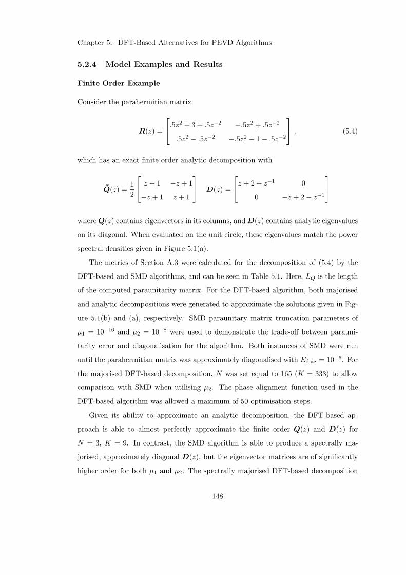
Chapter 5. DFT-Based Alternatives for PEVD Algorithms
5.2.4 Model Examples and Results
Finite Order Example
Consider the parahermitian matrix
R(z) =
.5z2 + 3 + .5z−2 −.5z2 + .5z−2
.5z2 − .5z−2 −.5z2 + 1− .5z−2
, (5.4)
which has an exact finite order analytic decomposition with
Q(z) =1
2
z + 1 −z + 1
−z + 1 z + 1
D(z) =
z + 2 + z−1 0
0 −z + 2− z−1
whereQ(z) contains eigenvectors in its columns, andD(z) contains analytic eigenvalues
on its diagonal. When evaluated on the unit circle, these eigenvalues match the power
spectral densities given in Figure 5.1(a).
The metrics of Section A.3 were calculated for the decomposition of (5.4) by the
DFT-based and SMD algorithms, and can be seen in Table 5.1. Here, LQ is the length
of the computed paraunitarity matrix. For the DFT-based algorithm, both majorised
and analytic decompositions were generated to approximate the solutions given in Fig-
ure 5.1(b) and (a), respectively. SMD paraunitary matrix truncation parameters of
µ1 = 10−16 and µ2 = 10−8 were used to demonstrate the trade-off between parauni-
tarity error and diagonalisation for the algorithm. Both instances of SMD were run
until the parahermitian matrix was approximately diagonalised with Ediag = 10−6. For
the majorised DFT-based decomposition, N was set equal to 165 (K = 333) to allow
comparison with SMD when utilising µ2. The phase alignment function used in the
DFT-based algorithm was allowed a maximum of 50 optimisation steps.
Given its ability to approximate an analytic decomposition, the DFT-based ap-
proach is able to almost perfectly approximate the finite order Q(z) and D(z) for
N = 3, K = 9. In contrast, the SMD algorithm is able to produce a spectrally ma-
jorised, approximately diagonal D(z), but the eigenvector matrices are of significantly
higher order for both µ1 and µ2. The spectrally majorised DFT-based decomposition
148
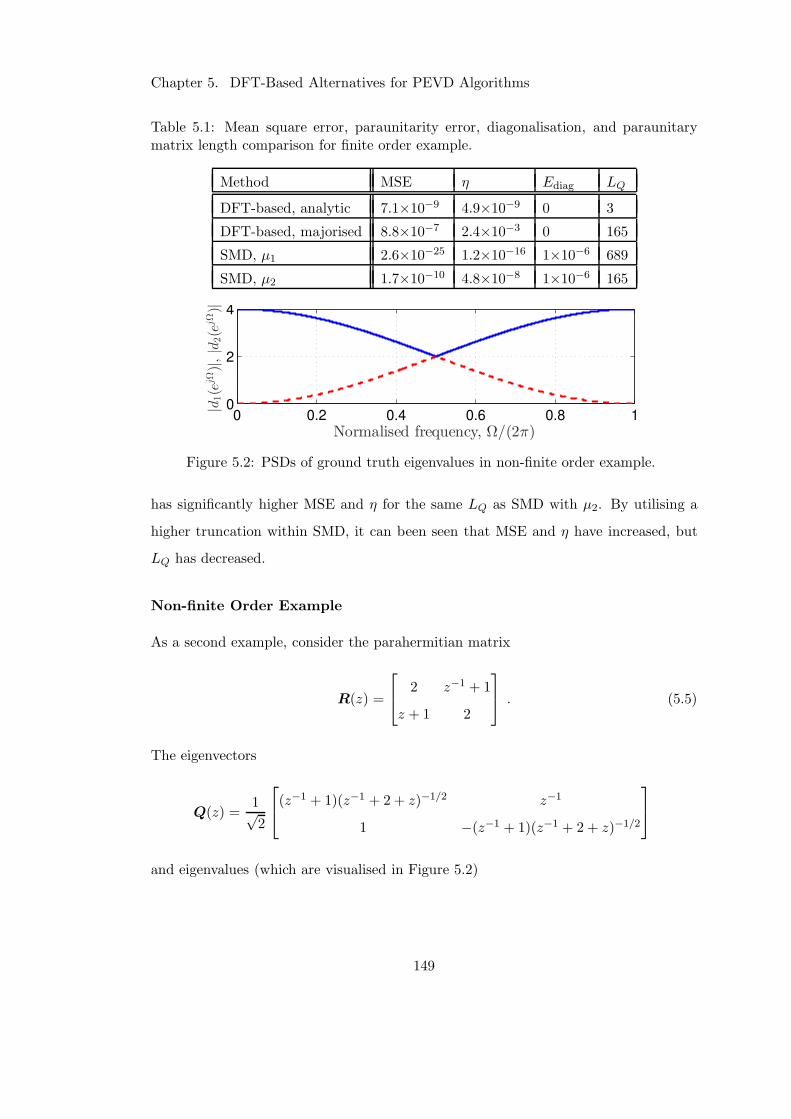
Chapter 5. DFT-Based Alternatives for PEVD Algorithms
Table 5.1: Mean square error, paraunitarity error, diagonalisation, and paraunitarymatrix length comparison for finite order example.
Method MSE η Ediag LQ
DFT-based, analytic 7.1×10⁻⁹ 4.9×10⁻⁹ 0 3
DFT-based, majorised 8.8×10⁻⁷ 2.4×10⁻³ 0 165
SMD, µ1 2.6×10⁻²⁵ 1.2×10⁻¹⁶ 1×10⁻⁶ 689
SMD, µ2 1.7×10⁻¹⁰ 4.8×10⁻⁸ 1×10⁻⁶ 165
0 0.2 0.4 0.6 0.8 10
2
4
Normalised frequency, Ω/(2π)
|d1(e
jΩ)|,|d
2(e
jΩ)|
Figure 5.2: PSDs of ground truth eigenvalues in non-finite order example.
has significantly higher MSE and η for the same LQ as SMD with µ2. By utilising a
higher truncation within SMD, it can been seen that MSE and η have increased, but
LQ has decreased.
Non-finite Order Example
As a second example, consider the parahermitian matrix
R(z) =
2 z−1 + 1
z + 1 2
. (5.5)
The eigenvectors
Q(z) =1√2
(z−1 + 1)(z−1 + 2 + z)−1/2 z−1
1 −(z−1 + 1)(z−1 + 2 + z)−1/2
and eigenvalues (which are visualised in Figure 5.2)
149
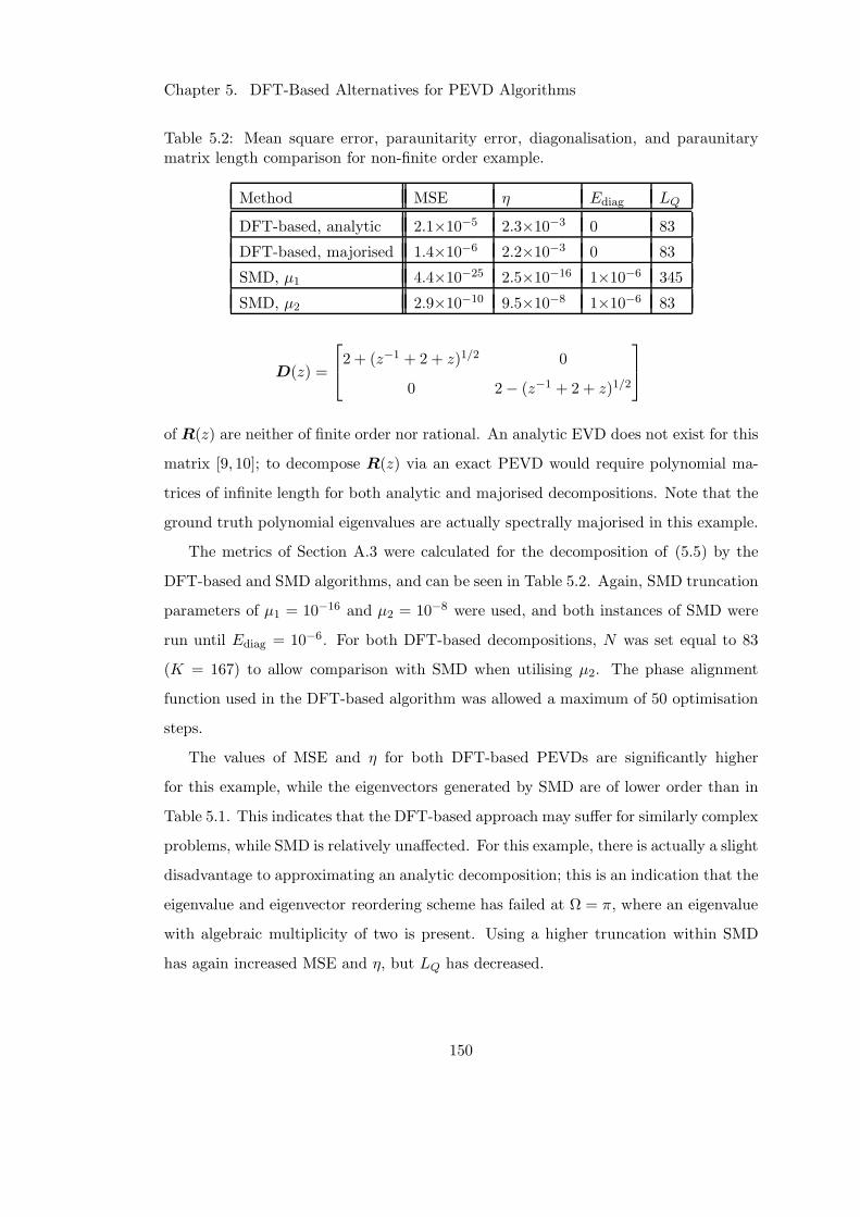
Chapter 5. DFT-Based Alternatives for PEVD Algorithms
Table 5.2: Mean square error, paraunitarity error, diagonalisation, and paraunitarymatrix length comparison for non-finite order example.
Method MSE η Ediag LQ
DFT-based, analytic 2.1×10⁻⁵ 2.3×10⁻³ 0 83
DFT-based, majorised 1.4×10⁻⁶ 2.2×10⁻³ 0 83
SMD, µ1 4.4×10⁻²⁵ 2.5×10⁻¹⁶ 1×10⁻⁶ 345
SMD, µ2 2.9×10⁻¹⁰ 9.5×10⁻⁸ 1×10⁻⁶ 83
D(z) =
2 + (z−1 + 2 + z)1/2 0
0 2− (z−1 + 2 + z)1/2
of R(z) are neither of finite order nor rational. An analytic EVD does not exist for this
matrix [9, 10]; to decompose R(z) via an exact PEVD would require polynomial ma-
trices of infinite length for both analytic and majorised decompositions. Note that the
ground truth polynomial eigenvalues are actually spectrally majorised in this example.
The metrics of Section A.3 were calculated for the decomposition of (5.5) by the
DFT-based and SMD algorithms, and can be seen in Table 5.2. Again, SMD truncation
parameters of µ1 = 10−16 and µ2 = 10−8 were used, and both instances of SMD were
run until Ediag = 10−6. For both DFT-based decompositions, N was set equal to 83
(K = 167) to allow comparison with SMD when utilising µ2. The phase alignment
function used in the DFT-based algorithm was allowed a maximum of 50 optimisation
steps.
The values of MSE and η for both DFT-based PEVDs are significantly higher
for this example, while the eigenvectors generated by SMD are of lower order than in
Table 5.1. This indicates that the DFT-based approach may suffer for similarly complex
problems, while SMD is relatively unaffected. For this example, there is actually a slight
disadvantage to approximating an analytic decomposition; this is an indication that the
eigenvalue and eigenvector reordering scheme has failed at Ω = π, where an eigenvalue
with algebraic multiplicity of two is present. Using a higher truncation within SMD
has again increased MSE and η, but LQ has decreased.
150
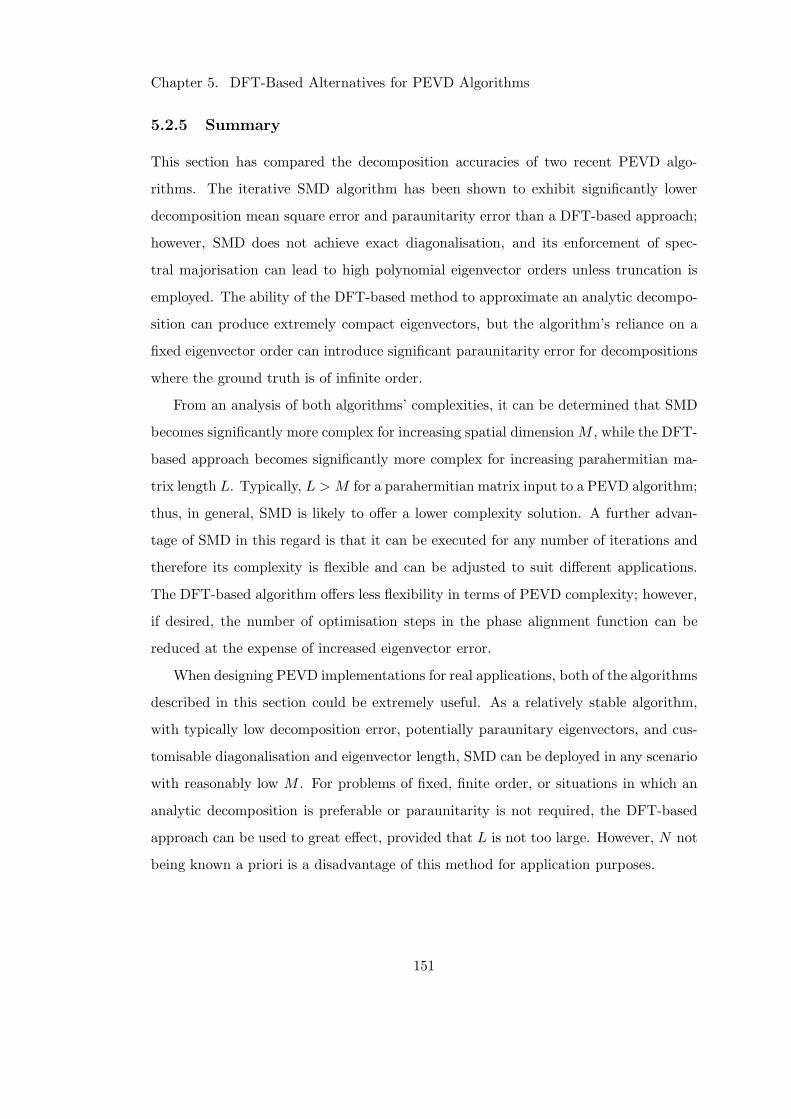
Chapter 5. DFT-Based Alternatives for PEVD Algorithms
5.2.5 Summary
This section has compared the decomposition accuracies of two recent PEVD algo-
rithms. The iterative SMD algorithm has been shown to exhibit significantly lower
decomposition mean square error and paraunitarity error than a DFT-based approach;
however, SMD does not achieve exact diagonalisation, and its enforcement of spec-
tral majorisation can lead to high polynomial eigenvector orders unless truncation is
employed. The ability of the DFT-based method to approximate an analytic decompo-
sition can produce extremely compact eigenvectors, but the algorithm’s reliance on a
fixed eigenvector order can introduce significant paraunitarity error for decompositions
where the ground truth is of infinite order.
From an analysis of both algorithms’ complexities, it can be determined that SMD
becomes significantly more complex for increasing spatial dimensionM , while the DFT-
based approach becomes significantly more complex for increasing parahermitian ma-
trix length L. Typically, L > M for a parahermitian matrix input to a PEVD algorithm;
thus, in general, SMD is likely to offer a lower complexity solution. A further advan-
tage of SMD in this regard is that it can be executed for any number of iterations and
therefore its complexity is flexible and can be adjusted to suit different applications.
The DFT-based algorithm offers less flexibility in terms of PEVD complexity; however,
if desired, the number of optimisation steps in the phase alignment function can be
reduced at the expense of increased eigenvector error.
When designing PEVD implementations for real applications, both of the algorithms
described in this section could be extremely useful. As a relatively stable algorithm,
with typically low decomposition error, potentially paraunitary eigenvectors, and cus-
tomisable diagonalisation and eigenvector length, SMD can be deployed in any scenario
with reasonably low M . For problems of fixed, finite order, or situations in which an
analytic decomposition is preferable or paraunitarity is not required, the DFT-based
approach can be used to great effect, provided that L is not too large. However, N not
being known a priori is a disadvantage of this method for application purposes.
151
Chapter 5. DFT-Based Alternatives for PEVD Algorithms
5.3 Development of a Novel DFT-Based PEVD Algorithm
The DFT-based PEVD formulation of [53] — which is summarised in Section A.2
— has been shown to perform well for finite order problems in the previous section,
but requires an a priori estimate of the length of the paraunitary matrix Q(z) in the
decomposition. In this section, a novel DFT-based PEVD algorithm that can compute
an accurate PEVD without requiring an estimate of the paraunitary matrix length is
presented. This algorithm utilises a modified eigenvalue reordering scheme that is less
susceptible to errors in the presence of eigenvalues with an algebraic multiplicity greater
than one. It has been demonstrated in [9] that the lowest order approximation to (2.4)
is possible if one attempts to approximate analytic eigenvectors which — on the unit
circle — are characterised by being infinitely differentiable. Here, a cost function that
measures the power in the derivatives of a function based on the Fourier coefficients
of their discrete samples on the unit circle is utilised. This permits an approach that
maximises eigenvector smoothness for a low order decomposition.
Below, Section 5.3.1 and Section 5.3.2 will introduce the smoothness metric and
the proposed algorithm, respectively, before Section 5.3.3 details the novel method for
eigenvalue and eigenvector reordering. Section 5.3.4 then describes how the smoothness
metric is used to align the phase of the eigenvectors, and Section 5.3.5 briefly outlines
the complexity of the algorithm. A comparison of the algorithm’s performance relative
to the method in [53] is presented in Section 5.3.6. Section 5.3.7 then provides a model
example to demonstrate the advantages of the proposed eigenvalue and eigenvector
reordering approach. Conclusions for this section are drawn in Section 5.3.8.
Elements of the work in this section can be found published in the proceedings
of the 10th IEEE Sensor Array and Multichannel Signal Processing Workshop in a
paper titled ‘Enforcing Eigenvector Smoothness for a Compact DFT-Based Polynomial
Eigenvalue Decomposition’ [73].
5.3.1 Smoothness Metric
A PEVD produces eigenvalues dm(ejΩ) and eigenvectors qm(ejΩ), where dm(ejΩ) is the
mth diagonal element of D(z)|z=ejΩ and qm(ejΩ) is the mth column of Q(z)|z=ejΩ . For
152
Chapter 5. DFT-Based Alternatives for PEVD Algorithms
the eigenvectors qm(ejΩ) to be compact in the time domain, they must be maximally
smooth on the unit circle; tied to this is the requirement for analytic eigenvectors to be
infinitely differentiable [9]. In this section, a novel metric to measure the smoothness
of eigenvectors is proposed.
If K is sufficiently large and odd, the samples F[k] = F (ejΩk), Ωk = 2πk/K, k =
0 . . . (K − 1), of a function F (ejΩ) permit its reconstruction via the Dirichlet kernel
P (ejΩ):
F (ejΩ) =
K−1∑
k=0
F[k]P (ej(Ω−Ωk)) , (5.6)
where
P (ejΩ) =1
K· sin(
K2 Ω)
sin(12Ω)=
1
K
K−1∑
ℓ=0
e−jΩ(ℓ−K−12
) . (5.7)
Thus,
F (ejΩ) =1
K
K−1∑
k=0
F[k]
K−1∑
ℓ=0
e−j(Ω−Ωk)(ℓ−K−1
2) . (5.8)
The pth derivative of F (ejΩ) can be written as
dp
dΩpF (ejΩ) =
1
K
K−1∑
k=0
F[k]
(K−1)/2∑
ℓ=−(K−1)/2
(−jℓ)pe−j(Ω−Ωk)ℓ . (5.9)
Of interest is the power contained within the pth derivative of F (ejΩ),
χ(p) =1
2π
∫ π
−π
∣∣∣∣
dp
dΩpF (ejΩ)
∣∣∣∣
2
dΩ , (5.10)
which provides some measure of the smoothness of F (ejΩ).
Note that due to orthogonality of the complex exponential terms and integration
over an integer number of fundamental periods, for a Fourier series with arbitrary
coefficients aℓ,
1
2π
∫ π
−π
∣∣∣∣∣
∑
ℓ
aℓejΩℓ
∣∣∣∣∣
2
dΩ =∑
ℓ
1
2π
∫ π
−π
∣∣∣aℓe
jΩℓ∣∣∣
2dΩ =
∑
ℓ
|aℓ|2 . (5.11)
153
Chapter 5. DFT-Based Alternatives for PEVD Algorithms
Therefore, (5.10) can be written as
χ(p) =1
K2
(K−1)/2∑
ℓ=−(K−1)/2
∣∣∣∣∣(−jℓ)p
K−1∑
k=0
F[k]ejΩkℓ
∣∣∣∣∣
2
(5.12)
=1
K2
(K−1)/2∑
ℓ=−(K−1)/2
ℓ2pfHCℓf = fHC(p)f , (5.13)
where f = [F[0],F[1], · · · ,F[K − 1]]T contains K frequency samples F[k] = F (ejΩk),
k = 0 . . . (K − 1),
Cℓ =
1 ej2πK
ℓ · · · ej2πK
(K−1)ℓ
e−j 2πK
ℓ 1...
.... . .
...
e−j 2πK
(K−1)ℓ · · · · · · 1
, (5.14)
and
C(p) =1
K2
(K−1)/2∑
ℓ=−(K−1)/2
ℓ2pCℓ . (5.15)
To consider smoothness up to the P th derivative, the metric
χ(P ) =
P∑
p=1
χ(p) = fH
P∑
p=1
C(p)
f
= fH
1
K2
(K−1)/2∑
ℓ=−(K−1)/2
Cℓ
P∑
p=1
ℓ2p
f = fHC(P )f (5.16)
can be formed, which calculates the sum of all powers of derivatives of f up to and in-
cluding the P th derivative. For even K, the derivation is similar to above and produces
χ(P ) = fH
1
K2
K2−1∑
ℓ=−K2
Cℓ
P∑
p=1
ℓ2p
f = fHC(P )f . (5.17)
Thus, the metric can be evaluated via a simple weighted inner product [2].
154
Chapter 5. DFT-Based Alternatives for PEVD Algorithms
5.3.2 Algorithm Overview
The PEVD approach presented here uses a DFT-based scheme with a similar structure
to Algorithm 11 to obtain a solution to the PEVD equation of (2.4). Section 5.3.3 dis-
cusses the method used within this scheme to approximate an analytic decomposition,
which utilises a novel, modified version of the method in [53].
As discussed in Section 5.1, discontinuities in phase between adjacent frequency
bins can arise due to ambiguity in eigenvector phase. When assessed via the metric
of Section 5.3.1, eigenvectors containing such phase discontinuities are not smooth and
return high values of χ(P ). For a short paraunitary matrix Q(z), these discontinu-
ities must be smoothed [9] and χ(P ) decreased. This is achieved through the use of a
phase alignment function, described in Section 5.3.4, which uses Powell’s ‘dogleg’ algo-
rithm [111,112] to maximise eigenvector smoothness. Contrary to the phase alignment
approach of [53], this function does not require a restriction of the paraunitary matrix
length to an a priori estimate.
Following the reordering (if desired) and phase alignment of Q[k], Q[τ ] and D[τ ]
are computed via the IDFT as in (5.3).
5.3.3 Novel Method for Reordering the Eigenvectors and Eigenvalues
In an analytic decomposition, the eigenvalues — and their eigenvectors — are arranged
such that discontinuities between adjacent frequency bins are minimised. Even for an
arrangement that provides continuous eigenvalues, such discontinuities can occur when
the eigenvalues intersect at some frequencies. The DFT-based PEVD method of [53]
uses the eigenvalue and eigenvector reordering approach described in Section A.2.2,
which is of relatively low complexity, but relies entirely on the eigenvectors. Since in
and near an eigenvalue with J-fold algebraic multiplicity the eigenvectors are ill-defined
within a J-dimensional subspace [2], the reliance of this method on eigenvectors only
is not ideal. A scheme that uses the smoothness of the eigenvalues for reordering
purposes has been shown to be robust in the presence of multiplicities in [54]; however,
this method is currently prohibitively expensive to implement.
For implementation in the proposed DFT-based PEVD algorithm, the following
155
Chapter 5. DFT-Based Alternatives for PEVD Algorithms
modification is made to the function in Section A.2.2, which has a small impact on
complexity, but improves the accuracy of the reordering procedure around a frequency
bin with eigenvalues that exhibit an algebraic multiplicity greater than one. The re-
ordering approach described in Section A.2.2 occurs as normal for k = 1, 2, . . . ,K − 1,
unless (for k > 1) an eigenvalue dm[k − 1] in D[k − 1] = diagd1[k − 1], . . . , dM [k − 1]is identified that satisfies the criterion
|dm[k − 1]− dn[k − 1]| < λ (5.18)
for some eigenvalues dn[k− 1], n ∈ Nm ⊆ 1 . . . M\m, and arbitrarily low threshold
λ. Here, the eigenvectors qm[k−1] and qn[k−1] correspond to repeated eigenvalues and
are therefore ill-defined; thus (A.18) may not identify the best ordering of eigenvectors
and eigenvalues in the kth frequency bin. For a continuous PSD, the repeated eigenvalue
dn[k−1], n ∈ m∪Nm, that follows dn[k−2] is arbitrary, while the ordering of dn[k−1]and qn[k−1] is ambiguous since the eigenvectors are ill-defined. Therefore, to maintain
the ordering established prior to the eigenvalue intersection point, each eigenvector
qn[k − 1] is set equal to its immediate predecessor qn[k − 2] for reordering purposes
only. Following the reordering of the kth frequency bin according to Section A.2.2,
eigenvectors qn[k − 1] are returned to their previous values.
5.3.4 Adjusting the Phase of the Eigenvectors to Promote Phase
Alignment
Employing a method to align the phase of eigenvectors in adjacent frequency bins
is vital for a compact, low order decomposition; i.e., for a short output paraunitary
matrix that introduces little error to the PEVD. Phase alignment can be achieved by
finding the phase changes required for each eigenvector qm[k] ∀ m,k to be maximally
smooth according to metric χ(P ). The phase of the mth eigenvector at frequency
bin k can be adjusted by an angle θ[k] according to qm[k] ← ejθ[k]qm[k]. Below, an
objective function is defined which, when minimised via an unconstrained non-linear
optimisation algorithm, can be used to determine the optimal θ[k] ∀ k to maximise the
mth eigenvector’s smoothness.
156
Chapter 5. DFT-Based Alternatives for PEVD Algorithms
Objective Function Formulation
The smoothness metric defined for odd K in (5.16) and even K in (5.17) is able to
measure the smoothness of a single function. The goal here is to compute a vector
of phases θ = [ θ[0], θ[1], · · · , θ[K − 1] ]T ∈ RK×1 such that all elements of the mth
eigenvector qm[k] ∀ k are maximally smooth. The objective function therefore measures
the smoothness of all elements of qm[k] and takes the form
f(θ) = R
M∑
n=1
fHn C(P )fn
, (5.19)
where fHn = vndiag[
ejθ[0], · · · , ejθ[K−1]]
and vn = [ qm,n[0], · · · , qm,n[K − 1] ], where
qm,n[k] denotes the nth element (row) of eigenvector qm[k]. Only the real component
of the sum in the above equation is taken, as the imaginary component should be zero.
The above equation can be rearranged to form
f(θ) = R
uH
(M∑
n=1
diagvnC(P )diagvHn )
u
, (5.20)
where uH =[ejθ[0], · · · , ejθ[K−1]
]. Setting Γ =
∑Mn=1 diagvnC(P )diagvH
n , for Γ ∈CK×K, allows for the following compact representation:
f(θ) = RuHΓu . (5.21)
One can therefore obtain θ by solving
θ = argminθ′ ∈RK×1
f(θ′) . (5.22)
Minimising the Objective Function
Given its simplicity and relatively low cost [112], Powell’s iterative ‘dogleg’ trust region
strategy [111] is employed for the unconstrained minimisation of (5.21). In iteration j,
a trust region strategy uses the gradient vector g and approximate Hessian matrix H
157
Chapter 5. DFT-Based Alternatives for PEVD Algorithms
of the objective function to construct a second-order Taylor series expansion:
mj(ϕ(j)) = f(θ(j)) +ϕ(j)Tg +ϕ(j)THϕ(j) . (5.23)
This model approximates f(θ(j) + ϕ(j)) within a trusted region of radius ∆(j) around
the current point θ(j) for some step ϕ(j), which is identified according to
ϕ(j) ← argminϕ(j)∈RK×1 | ‖ϕ(j)‖<∆(j)
mj(ϕ(j)) . (5.24)
The selected method first finds the minimiser of (5.23) along the steepest descent
direction:
ϕ(j)c = − gTg
gTHgg . (5.25)
If this point lies outside of the trusted region, the intersection of the line from the origin
to ϕ(j)c with the trust region boundary is used for ϕ(j). Otherwise, the quasi-Newton
point is found:
ϕ(j)qn = −H−1g . (5.26)
If this point lies within the trust region, ϕ(j) ← ϕ(j)qn , and the method moves to the
next iteration. Otherwise, a solution is found at the intersection of the trust region
boundary with the line from ϕ(j)c to ϕ
(j)qn .
A parameter ρ, which compares the predicted reduction in the objective function
with the actual reduction, is used to measure the strength of the approximation given
by (5.23):
ρ =f(θ(j))− f(θ(j) +ϕ(j))
mj(0)−mj(ϕ(j)). (5.27)
In practice, if ρ > 0.75, the approximation is good and the trust region is expanded
such that ∆(j+1) = min2∆(j),∆max
, where ∆max is a user-defined maximum. If
ρ < 0.25, the approximation is poor and the trust region is decreased in size such that
∆(j+1) = ∆(j)/4. Furthermore, if ρ > 0, θ(j+1) = θ(j) +ϕ(j); otherwise, θ(j+1) = θ(j).
The employed unconstrained minimisation strategy requires an initial guess of θ;
here, the initial guess is chosen to be a vector of zeroes for simplicity. Note that
158
Chapter 5. DFT-Based Alternatives for PEVD Algorithms
the initial trust region size, ∆(0), is user-defined; however, choosing ∆(0) ← ∆max is
typically valid.
Gradient Vector and Hessian Matrix Formulation
If θi = θ[i], ui is the ith element of u, and γik is the element shared by the ith row and
kth column of Γ, the objective function in (5.21) can also be written as
f(θ) =
K−1∑
i=0
K−1∑
k=0
u∗i γikuk =
K−1∑
i=0
K−1∑
k=0
γikej(θi−θk) . (5.28)
Taking the derivative with respect to θℓ yields
∂f
∂θℓ= −j
K−1∑
i=0,i 6=ℓ
γiℓej(θi−θℓ) + j
K−1∑
k=0,k 6=ℓ
γℓkej(θℓ−θk)
= −jK−1∑
i=0
γiℓej(θi−θℓ) + j
K−1∑
k=0
γ∗kℓe−j(θk−θℓ) . (5.29)
Note that γℓk = γ∗kℓ, as Γ is Hermitian by construction. Converting to matrix notation,
the gradient vector is
g =∂f
∂θ= −jdiag uΓTu∗ + jdiag
uHΓHu
= 2Rjdiag
uHΓHu
= −2I
diag
uHΓu
. (5.30)
Taking the derivative of (5.29) with respect to θp, with θℓ now fixed, one acquires
the equation for the off-diagonal elements of the Hessian matrix:
∂f
∂θℓ∂θp= −j2γpℓej(θp−θℓ) − j2γ∗pℓe
−j(θp−θℓ)
= γpℓej(θp−θℓ) + γ∗pℓe
−j(θp−θℓ) . (5.31)
159
Chapter 5. DFT-Based Alternatives for PEVD Algorithms
So the off-diagonal (OD) terms of the Hessian matrix are:
HOD = diag uΓTdiag u∗+ diaguHΓHdiag u
= 2Rdiag
uHΓdiag u
. (5.32)
Taking the derivative of (5.29) with respect to θℓ, one acquires the equation for the
diagonal elements of the Hessian matrix:
∂2f
∂θ2ℓ= −
K−1∑
i=0,i 6=ℓ
γiℓej(θi−θℓ) −
K−1∑
k=0,k 6=ℓ
γℓkej(θℓ−θk) . (5.33)
In matrix form, this equates to
HD = diag
−diag u ΓTu∗ − diaguHΓHu
= −2R
diag
diag u ΓTu∗
, (5.34)
where Γ = Γ − diagdiagΓ contains zeroes on its diagonal. The Hessian matrix is
then given by
H = HOD − diagdiagHOD+HD
= 2Rdiag
uHΓdiag u
− diagdiag
2Rdiag
uHΓdiag u
− 2R
diag
diag u ΓTu∗
= 2Rdiag
uHΓdiag u
− 2R
diag
diagΓ+ diag u ΓTu∗
= 2Rdiag
uHΓdiag u
− 2R
diag
diag uΓTu∗
, (5.35)
since diagdiag
uHΓdiagu
= diagΓ.
The second part of (5.35) is often less significant when compared to the first part;
160
Chapter 5. DFT-Based Alternatives for PEVD Algorithms
e.g., simulations typically find that
∥∥2R
diag
diag uΓTu∗
∥∥F
‖2R diag uHΓdiag u‖F≈ 10−3 . (5.36)
In numerical experiments, (5.35) is not always positive definite, which is a requirement
for this method of minimisation [112]; however, 2Rdiag
uHΓdiag u
is positive
semi-definite, as C(P ) and Γ are positive semi-definite. The following approximation
to the Hessian matrix is proposed, which is guaranteed to be positive definite and
eliminates unnecessary computation:
H = 2Rdiag
uHΓdiag u
+ αIK , (5.37)
where α is very small and IK is a K ×K identity matrix.
5.3.5 Algorithm Complexity
For a constant number of optimisation steps, the complexity of the phase alignment
step for a single eigenvector is O(K3) due to matrix inversion [53, 95]; thus, the total
complexity of the phase alignment step for M eigenvectors is of order O(MK3). The
computation of the frequency domain representation of R(z), the execution of K EVDs,
and the reordering of the eigenvalues and eigenvectors are of lower complexity than this
step; thus, the total complexity of the proposed algorithm is approximately O(MK3).
5.3.6 Source Model Simulation Scenarios and Results
The simulations below have been performed over an ensemble of 103 instantiations of
R(z) : C → CM×M obtained from the randomised source model in Appendix B [45]
with M = 5, OD = 18, OQ = 10, and ∆DR = 50.
The proposed algorithm considers smoothness up to the third derivative; i.e., the
metric χ(3) is used. A maximum of 50 minimisation steps according to Section 5.3.4
are allowed for both algorithms, and a parameter of α = 10−14 is used. Each algorithm
is instructed to approximate an analytic decomposition.
161
Chapter 5. DFT-Based Alternatives for PEVD Algorithms
Simulation Scenario 1
The method in [53], henceforth referred to as the ‘existing’ algorithm, requires knowl-
edge of the length of Q(z), LQ, prior to execution, and typically chooses a number of
frequency bins Ke = 2LQ + L − 2, where L is the length of the input matrix R(z).
The method proposed in this section, referred to as the ‘proposed’ algorithm, does
not require an input value of LQ, but instead outputs Q(z) with length equal to the
number of frequency bins Kp used in the decomposition. Note that outer lags of Q[τ ]
may contain negligible energy and can be trimmed using a threshold µt in a process
detailed in Appendix C. The first scenario provides the existing method with values of
LQ ∈ 5; 10, and uses the same generated values of Ke = Kp ∈ 47; 57 for both
algorithms.
Simulation Scenario 2
To test the case where both algorithms produce Q(z) of the same length, the second
scenario provides the proposed method with values of Kp ∈ 47; 57, and provides the
existing method with LQ = Kp such that Ke ∈ 131; 151.
Results and Discussion
The ensemble-averaged mean square reconstruction error, paraunitarity error, and LQ
were calculated for both of the algorithms and simulation scenarios, and can be seen
in Table 5.3. The table demonstrates that the proposed approach is able to provide
extremely low decomposition MSE and paraunitarity error, η. Furthermore, the exist-
ing method is not capable of achieving such performance even when using significantly
more frequency bins and generating paraunitary matrices of the same length. The algo-
rithmic complexity of both algorithms is approximately O(MK3) [53]; thus the choice
of DFT length K is extremely significant. Also shown is the impact of truncation on
performance: if paraunitary matrix length is of critical importance, then MSE and η
can be sacrificed to generate shorter matrices. Typically, increasing K is shown to
improve MSE and η at the expense of higher LQ.
162
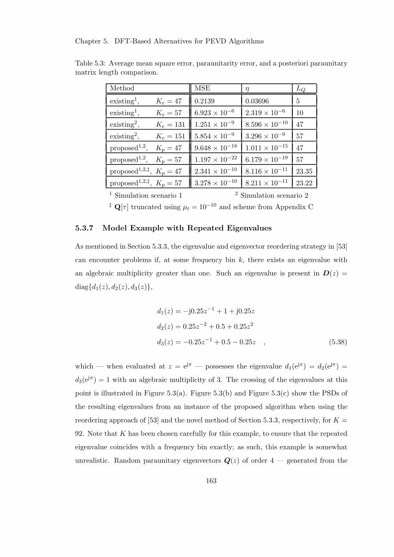
Chapter 5. DFT-Based Alternatives for PEVD Algorithms
Table 5.3: Average mean square error, paraunitarity error, and a posteriori paraunitarymatrix length comparison.
Method MSE η LQ
existing1, Ke = 47 0.2139 0.03696 5
existing1, Ke = 57 6.923 × 10⁻⁶ 2.319 × 10⁻⁶ 10
existing2, Ke = 131 1.251 × 10⁻⁹ 8.596 × 10⁻¹⁰ 47
existing2, Ke = 151 5.854 × 10⁻⁹ 3.296 × 10⁻⁹ 57
proposed1,2, Kp = 47 9.648 × 10⁻¹⁸ 1.011 × 10⁻¹⁵ 47
proposed1,2, Kp = 57 1.197 × 10⁻²² 6.179 × 10⁻¹⁹ 57
proposed1,2,‡, Kp = 47 2.341 × 10⁻¹⁰ 8.116 × 10⁻¹¹ 23.35
proposed1,2,‡, Kp = 57 3.278 × 10⁻¹⁰ 8.211 × 10⁻¹¹ 23.22
1 Simulation scenario 1 2 Simulation scenario 2‡ Q[τ ] truncated using µt = 10−10 and scheme from Appendix C
5.3.7 Model Example with Repeated Eigenvalues
As mentioned in Section 5.3.3, the eigenvalue and eigenvector reordering strategy in [53]
can encounter problems if, at some frequency bin k, there exists an eigenvalue with
an algebraic multiplicity greater than one. Such an eigenvalue is present in D(z) =
diagd1(z), d2(z), d3(z),
d1(z) = −j0.25z−1 + 1 + j0.25z
d2(z) = 0.25z−2 + 0.5 + 0.25z2
d3(z) = −0.25z−1 + 0.5 − 0.25z , (5.38)
which — when evaluated at z = ejπ — possesses the eigenvalue d1(ejπ) = d2(e
jπ) =
d3(ejπ) = 1 with an algebraic multiplicity of 3. The crossing of the eigenvalues at this
point is illustrated in Figure 5.3(a). Figure 5.3(b) and Figure 5.3(c) show the PSDs of
the resulting eigenvalues from an instance of the proposed algorithm when using the
reordering approach of [53] and the novel method of Section 5.3.3, respectively, for K =
92. Note that K has been chosen carefully for this example, to ensure that the repeated
eigenvalue coincides with a frequency bin exactly; as such, this example is somewhat
unrealistic. Random paraunitary eigenvectors Q(z) of order 4 — generated from the
163
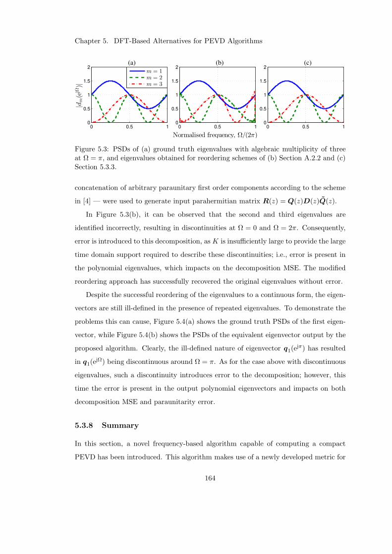
Chapter 5. DFT-Based Alternatives for PEVD Algorithms
0 0.5 10
0.5
1
1.5
2
|dm(e
jΩ)|
m = 1m = 2m = 3
0 0.5 10
0.5
1
1.5
2
Normalised frequency, Ω/(2π)
0 0.5 10
0.5
1
1.5
2(a) (b) (c)
Figure 5.3: PSDs of (a) ground truth eigenvalues with algebraic multiplicity of threeat Ω = π, and eigenvalues obtained for reordering schemes of (b) Section A.2.2 and (c)Section 5.3.3.
concatenation of arbitrary paraunitary first order components according to the scheme
in [4] — were used to generate input parahermitian matrix R(z) = Q(z)D(z)Q(z).
In Figure 5.3(b), it can be observed that the second and third eigenvalues are
identified incorrectly, resulting in discontinuities at Ω = 0 and Ω = 2π. Consequently,
error is introduced to this decomposition, as K is insufficiently large to provide the large
time domain support required to describe these discontinuities; i.e., error is present in
the polynomial eigenvalues, which impacts on the decomposition MSE. The modified
reordering approach has successfully recovered the original eigenvalues without error.
Despite the successful reordering of the eigenvalues to a continuous form, the eigen-
vectors are still ill-defined in the presence of repeated eigenvalues. To demonstrate the
problems this can cause, Figure 5.4(a) shows the ground truth PSDs of the first eigen-
vector, while Figure 5.4(b) shows the PSDs of the equivalent eigenvector output by the
proposed algorithm. Clearly, the ill-defined nature of eigenvector q1(ejπ) has resulted
in q1(ejΩ) being discontinuous around Ω = π. As for the case above with discontinuous
eigenvalues, such a discontinuity introduces error to the decomposition; however, this
time the error is present in the output polynomial eigenvectors and impacts on both
decomposition MSE and paraunitarity error.
5.3.8 Summary
In this section, a novel frequency-based algorithm capable of computing a compact
PEVD has been introduced. This algorithm makes use of a newly developed metric for
164
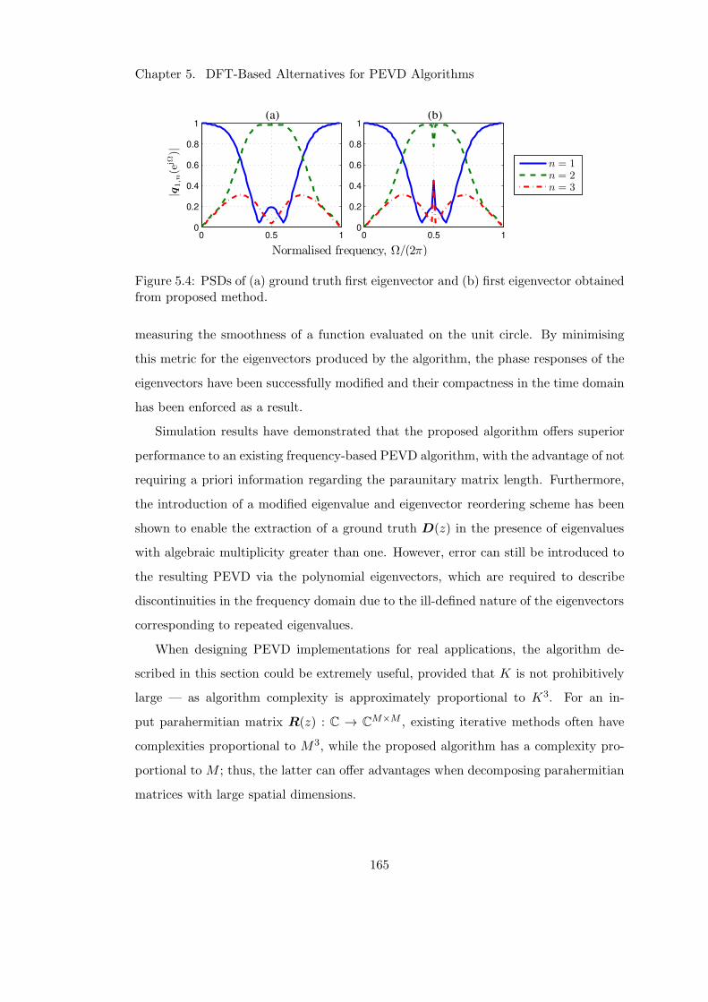
Chapter 5. DFT-Based Alternatives for PEVD Algorithms
0 0.5 10
0.2
0.4
0.6
0.8
1
Normalised frequency, Ω/(2π)
n = 1n = 2n = 3
0 0.5 10
0.2
0.4
0.6
0.8
1(b)(a)
|q1,n(e
jΩ)|
Figure 5.4: PSDs of (a) ground truth first eigenvector and (b) first eigenvector obtainedfrom proposed method.
measuring the smoothness of a function evaluated on the unit circle. By minimising
this metric for the eigenvectors produced by the algorithm, the phase responses of the
eigenvectors have been successfully modified and their compactness in the time domain
has been enforced as a result.
Simulation results have demonstrated that the proposed algorithm offers superior
performance to an existing frequency-based PEVD algorithm, with the advantage of not
requiring a priori information regarding the paraunitary matrix length. Furthermore,
the introduction of a modified eigenvalue and eigenvector reordering scheme has been
shown to enable the extraction of a ground truth D(z) in the presence of eigenvalues
with algebraic multiplicity greater than one. However, error can still be introduced to
the resulting PEVD via the polynomial eigenvectors, which are required to describe
discontinuities in the frequency domain due to the ill-defined nature of the eigenvectors
corresponding to repeated eigenvalues.
When designing PEVD implementations for real applications, the algorithm de-
scribed in this section could be extremely useful, provided that K is not prohibitively
large — as algorithm complexity is approximately proportional to K3. For an in-
put parahermitian matrix R(z) : C → CM×M , existing iterative methods often have
complexities proportional to M3, while the proposed algorithm has a complexity pro-
portional to M ; thus, the latter can offer advantages when decomposing parahermitian
matrices with large spatial dimensions.
165
Chapter 5. DFT-Based Alternatives for PEVD Algorithms
5.4 An Order-Iterated Novel DFT-Based PEVD Algo-
rithm
The novel algorithm of the previous section, which does not require a priori information
regarding the paraunitary matrix order, improved upon the algorithm of [53] in terms
of PEVD performance. However, the algorithm still requires a priori knowledge of the
DFT length, K, to be used in the decomposition. To address this problem, this section
details a novel iterative frequency-based PEVD algorithm — based on the algorithm
in Section 5.3 — which can compute an accurate PEVD without requiring paraunitary
matrix order or decomposition length information. Instead, the decomposition length
is increased within the set K ∈ 2j | j ∈ N until the decomposition error falls below
a user-specified threshold. By restricting the decomposition length to powers of two,
the computations in a given algorithm iteration can be carried forward to subsequent
iterations to reduce redundancy.
Below, Section 5.4.1 will introduce the proposed algorithm and Section 5.4.2 will
briefly outline its complexity. Using the simulation scenarios of Section 5.4.3, a com-
parison of the algorithm’s performance relative to existing iterative PEVD methods is
presented in Section 5.4.4, and conclusions are drawn in Section 5.4.5.
Elements of the work in this section can be found published in the proceedings of
the 52nd Asilomar Conference on Signals, Systems and Computers in a paper titled
‘An Iterative DFT-based Approach to the Polynomial Matrix Eigenvalue Decomposi-
tion’ [74], and in the proceedings of the 44th International Conference on Acoustics,
Speech, and Signal Processing in a paper titled ‘Iterative Approximation of Analytic
Eigenvalues of a Parahermitian Matrix EVD’ [54].
5.4.1 Algorithm Overview
The PEVD approach presented here uses an iterative DFT-based scheme with a sim-
ilar underlying structure to Algorithm 11 to obtain a solution to the PEVD equation
166
Chapter 5. DFT-Based Alternatives for PEVD Algorithms
of (2.4). In this iterative approach, equation (5.1) is adapted to
R[k] = Q[k]D[k]QH[k] , k = 0 . . . Ki − 1 , (5.39)
which uses an increasing number of frequency bins, Ki, until the decomposition MSE
falls below a user-defined threshold. Here, Ki is restricted to powers of two such that
Ki ∈ 2⌈log2L⌉+i, where L is the length of R(z), and i = 0, 1, . . . , Imax − 1 records the
current iteration. Parameter Imax is a user-defined maximum number of iterations for
the algorithm. As in other DFT-based PEVD algorithms, R[k] is obtained from the
Ki-point DFT of R[τ ],
R[k] = R(z)|z=ejΩk =∑
τR[τ ]e−jΩkτ , k = 0 . . . Ki − 1 , (5.40)
where Ωk = 2πk/Ki. Note that in iteration i, R[k] in (5.40) for k = 0, 1, . . . ,Ki − 1 is
identical to R[k] for k = 0, 2, 4, . . . ,Ki+1 − 2 in the (i + 1)th iteration. By extension,
Q[k] and D[k] from (5.39) are also the same for these k. The calculation of half of the
eigenvectors and eigenvalues can therefore be avoided at each iteration beyond the first.
Similarly, the phase alignment step can exploit this redundancy to aid optimisation.
The eigenvalue and eigenvector reordering scheme of Section 5.3.3 is employed in this
algorithm to facilitate the approximation of an analytic decomposition. If i > 0, Q[k] for
k = 0, 2, 4, . . . ,Ki − 2 can be carried through from the previous iteration; however, the
eigenvector ordering in these matrices can change, as the inner products of eigenvectors
in subsequent frequency bins have changed. The process of Section 5.3.3 must therefore
be completed as normal for k = 1, 2, . . . ,Ki − 1 at each algorithm iteration.
Phase alignment of eigenvectors in adjacent frequency bins is vital for a compact, low
order decomposition. The phase alignment strategy of Section 5.3.4 is also used here;
however, a slight modification is made to aid the optimisation process by exploiting the
iterative nature of the algorithm. The employed unconstrained minimisation strategy
requires an initial guess of θ. For i = 0, the initial guess is chosen to be a vector
of zeroes; however, in subsequent iterations of the algorithm, values of θ[k] for k =
0, 2, 4, . . . ,Ki − 2 can be carried through from the previous iteration and used to form
167
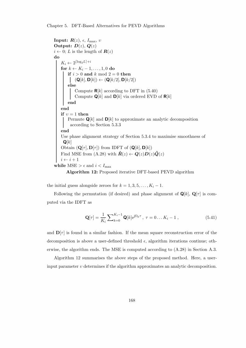
Chapter 5. DFT-Based Alternatives for PEVD Algorithms
Input: R(z), ǫ, Imax, υOutput: D(z), Q(z)i← 0; L is the length of R(z)do
Ki ← 2⌈log2L⌉+i
for k ← Ki − 1, . . . , 1, 0 do
if i > 0 and k mod 2 = 0 then
(Q[k],D[k])← (Q[k/2],D[k/2])else
Compute R[k] according to DFT in (5.40)Compute Q[k] and D[k] via ordered EVD of R[k]
end
end
if υ = 1 thenPermute Q[k] and D[k] to approximate an analytic decompositionaccording to Section 5.3.3
end
Use phase alignment strategy of Section 5.3.4 to maximise smoothness ofQ[k]Obtain (Q[τ ],D[τ ]) from IDFT of (Q[k],D[k])
Find MSE from (A.28) with R(z)← Q(z)D(z)Q(z)i← i+ 1
while MSE > ǫ and i < Imax
Algorithm 12: Proposed iterative DFT-based PEVD algorithm
the initial guess alongside zeroes for k = 1, 3, 5, . . . ,Ki − 1.
Following the permutation (if desired) and phase alignment of Q[k], Q[τ ] is com-
puted via the IDFT as
Q[τ ] =1
Ki
∑Ki−1
k=0Q[k]ejΩkτ , τ = 0 . . . Ki − 1 , (5.41)
and D[τ ] is found in a similar fashion. If the mean square reconstruction error of the
decomposition is above a user-defined threshold ǫ, algorithm iterations continue; oth-
erwise, the algorithm ends. The MSE is computed according to (A.28) in Section A.3.
Algorithm 12 summarises the above steps of the proposed method. Here, a user-
input parameter υ determines if the algorithm approximates an analytic decomposition.
168
Chapter 5. DFT-Based Alternatives for PEVD Algorithms
5.4.2 Algorithm Complexity
For a constant number of optimisation steps, the complexity of the phase alignment step
for a single eigenvector in iteration i is O(K3i ) due to the execution of matrix inversion
in the optimisation algorithm [53,95]; thus, the total complexity of the phase alignment
step for M eigenvectors is of order O(MK3i ). All other components of the algorithm
have lower complexity; thus, the total complexity of one iteration of the proposed algo-
rithm is approximately O(MK3i ). If I iterations of the algorithm are completed before
it ceases operations, the overall complexity of the proposed algorithm is determined by
the complexity of the inversion of the largest matrix and is approximately O(MK3I−1).
For fixed I, KI−1 is proportional to L; thus, the complexity can be estimated to be of
order O(ML3).
5.4.3 Simulation Scenarios
To benchmark the proposed approach, its performance is compared against the iterative
coefficient domain methods of SMD [45] and SBR2 [6]. For the proposed method, an an-
alytic (permuted) decomposition is approximated (υ = 1), and eigenvector smoothness
is measured using χ(3); i.e., up to the third derivative. To cease iterations, a decomposi-
tion MSE threshold of ǫ = 10−8 and Imax = 5 are used. A maximum of 50 minimisation
steps according to Section 5.3.4 were allowed and a parameter of α = 10−14 is employed.
Polynomial matrix truncation parameters of µ1 = 10−16 and µ2 = 10−8 are used for
SMD and a truncation parameter of µ2 is used for SBR2. Iterations of the algorithms
other than the one proposed cease if Ediag ≤ 10−6. Note that Ediag for the proposed
method is always zero, as D[τ ] is diagonal.
Simulation Scenario 1
This scenario utilises the above PEVD algorithms to decompose an ensemble of 103
instantiations of R(z) : C → CM×M obtained from the randomised source model in
Appendix B [45] with M = 5, OD = 18, OQ = 10, and ∆DR = 50. Following the
completion of each algorithm, the metrics defined in Section A.3 are recorded alongside
the lengths of the output paraunitary matrices, LQ.
169
Chapter 5. DFT-Based Alternatives for PEVD Algorithms
Simulation Scenario 2
This scenario utilises the above algorithms to decompose the theoretical parahermitian
matrix
R(z) =
2 z−1 + 1
z + 1 2
, (5.42)
which has eigenvectors and eigenvalues (which are visualised in Figure 5.2) that are
neither of finite order nor rational. An analytic EVD does not exist for this matrix [9,
10]; to decompose R(z) via an exact PEVD would require polynomial matrices of
infinite length. Execution time measurements are averaged over 103 instances of the
simulation scenario.
Simulation Scenario 3
For broadband angle of arrival (AoA) estimation, powerful narrowband methods such
as the multiple signal classification (MUSIC) algorithm [77] are not directly applicable.
In [18], the PEVD is used to generalise MUSIC to the case of polynomial matrices, re-
sulting in the development of the spatio-spectral polynomial MUSIC (SSP-MUSIC) al-
gorithm. Work in [19] demonstrates that the accuracy of SSP-MUSIC depends strongly
on the efficacy of the PEVD algorithm used. Here, the AoA estimation performances
that the above algorithms offer when paired with SSP-MUSIC are compared. For
brevity, the reader is referred to Appendix D and [18, 19] for details regarding the
implementation of SSP-MUSIC. Performance of each PEVD algorithm is measured in
terms of AoA estimation accuracy; this is determined through a visual assessment of
metric PSSP(ϑ,Ω) ∈ R>0 output by the SSP-MUSIC algorithm in [18], which is evalu-
ated at a range of angles of arrival, ϑ, and frequencies, Ω. A high value of PSSP(ϑ,Ω)
indicates the presence of a source at a specific angle of arrival and frequency, while a
low value indicates that no source is present.
In this simulation scenario, an M = 6 element array collecting broadband data in
a vector x[n] ∈ C6 is illuminated by three broadband sources characterised as follows:
• source 1 — located at ϑ1 = −45, active over a frequency range Ω′1 ∈ [0.5π, 0.9π];
170
Chapter 5. DFT-Based Alternatives for PEVD Algorithms
• source 2 — located at ϑ2 = −30, active over a frequency range Ω′2 ∈ [0.1π, 0.9π];
• source 3 — located at ϑ3 = −10, active over a frequency range Ω′3 ∈ [0.4π, 0.9π].
For simplicity, the elevation angles of the sources are equal to zero. The array sig-
nals are corrupted by uncorrelated independent and identically distributed complex
Gaussian noise at an SNR of 20 dB. To exclude error sources other than inaccuracies
in the subspace identification, the source data is modelled as a sum of closely spaced
sinusoids with randomised phases and lengths of 96000 samples, for which highly accu-
rate narrowband steering vectors can be used to simulate incidence on the array. The
broadband steering vectors that the SSP-MUSIC algorithm uses to scan the noise-only
subspace are based on fractional delay filters constructed from truncated sinc func-
tions [108, 109]. Space-time covariance matrix R[τ ] = Ex[n]xH[n − τ ] is estimated
for |τ | ≤ 20. Metric PSSP(ϑ,Ω) is averaged over 103 instances of the scenario. In each
instance, SMD and SBR2 are allowed the same execution time as the proposed method.
5.4.4 Results and Discussion
Simulation Scenario 1
It is clear from Table 5.4 that the proposed method outperforms SMD and SBR2 with
respect to all performance metrics. The good performance of the proposed algorithm for
this scenario is to be expected, as DFT-based PEVD algorithms were observed to per-
form well for finite order problems in Sections 5.2.4 and 5.3.6. The tendency of iterative
time-based PEVD algorithms to encourage spectral majorisation of the eigenvalues re-
sults in slow convergence and paraunitary matrices of high order. The proposed method
can instead opt to approximate an analytic decomposition, and converges quickly to a
low order solution.
Simulation Scenario 2
In Table 5.5, the proposed method does not perform as well for the non-finite matrix
in (5.42). As discussed in Section 5.1, limiting the decomposition to a finite number of
frequency bins (and subsequently the same number of polynomial coefficients) can result
171
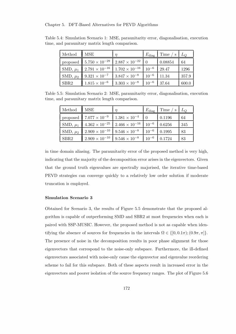
Chapter 5. DFT-Based Alternatives for PEVD Algorithms
Table 5.4: Simulation Scenario 1: MSE, paraunitarity error, diagonalisation, executiontime, and paraunitary matrix length comparison.
Method MSE η Ediag Time / s LQ
proposed 5.750 × 10⁻²⁹ 2.887 × 10⁻²² 0 0.08854 64
SMD, µ1 2.791 × 10⁻¹⁶ 1.702 × 10⁻¹⁶ 10−6 29.47 1296
SMD, µ2 9.321 × 10⁻⁷ 3.847 × 10⁻⁸ 10−6 11.34 357.9
SBR2 1.815 × 10⁻⁶ 3.303 × 10⁻⁸ 10−6 37.64 600.0
Table 5.5: Simulation Scenario 2: MSE, paraunitarity error, diagonalisation, executiontime, and paraunitary matrix length comparison.
Method MSE η Ediag Time / s LQ
proposed 7.077 × 10⁻⁹ 1.381 × 10⁻⁴ 0 0.1196 64
SMD, µ1 4.362 × 10⁻²⁵ 2.466 × 10⁻¹⁶ 10−6 0.6256 345
SMD, µ2 2.909 × 10⁻¹⁰ 9.546 × 10⁻⁸ 10−6 0.1995 83
SBR2 2.909 × 10⁻¹⁰ 9.546 × 10⁻⁸ 10−6 0.1724 83
in time domain aliasing. The paraunitarity error of the proposed method is very high,
indicating that the majority of the decomposition error arises in the eigenvectors. Given
that the ground truth eigenvalues are spectrally majorised, the iterative time-based
PEVD strategies can converge quickly to a relatively low order solution if moderate
truncation is employed.
Simulation Scenario 3
Obtained for Scenario 3, the results of Figure 5.5 demonstrate that the proposed al-
gorithm is capable of outperforming SMD and SBR2 at most frequencies when each is
paired with SSP-MUSIC. However, the proposed method is not as capable when iden-
tifying the absence of sources for frequencies in the intervals Ω ∈ [0, 0.1π); (0.9π, π].The presence of noise in the decomposition results in poor phase alignment for those
eigenvectors that correspond to the noise-only subspace. Furthermore, the ill-defined
eigenvectors associated with noise-only cause the eigenvector and eigenvalue reordering
scheme to fail for this subspace. Both of these aspects result in increased error in the
eigenvectors and poorer isolation of the source frequency ranges. The plot of Figure 5.6
172
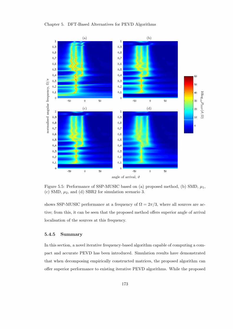
Chapter 5. DFT-Based Alternatives for PEVD Algorithms
(a) (b)
(c) (d)
angle of arrival, ϑ
norm
alisedangularfreq
uen
cy,Ω/π
10log10 P
SSP(ϑ
,Ω)
Figure 5.5: Performance of SSP-MUSIC based on (a) proposed method, (b) SMD, µ1,(c) SMD, µ2, and (d) SBR2 for simulation scenario 3.
shows SSP-MUSIC performance at a frequency of Ω = 2π/3, where all sources are ac-
tive; from this, it can be seen that the proposed method offers superior angle of arrival
localisation of the sources at this frequency.
5.4.5 Summary
In this section, a novel iterative frequency-based algorithm capable of computing a com-
pact and accurate PEVD has been introduced. Simulation results have demonstrated
that when decomposing empirically constructed matrices, the proposed algorithm can
offer superior performance to existing iterative PEVD algorithms. While the proposed
173
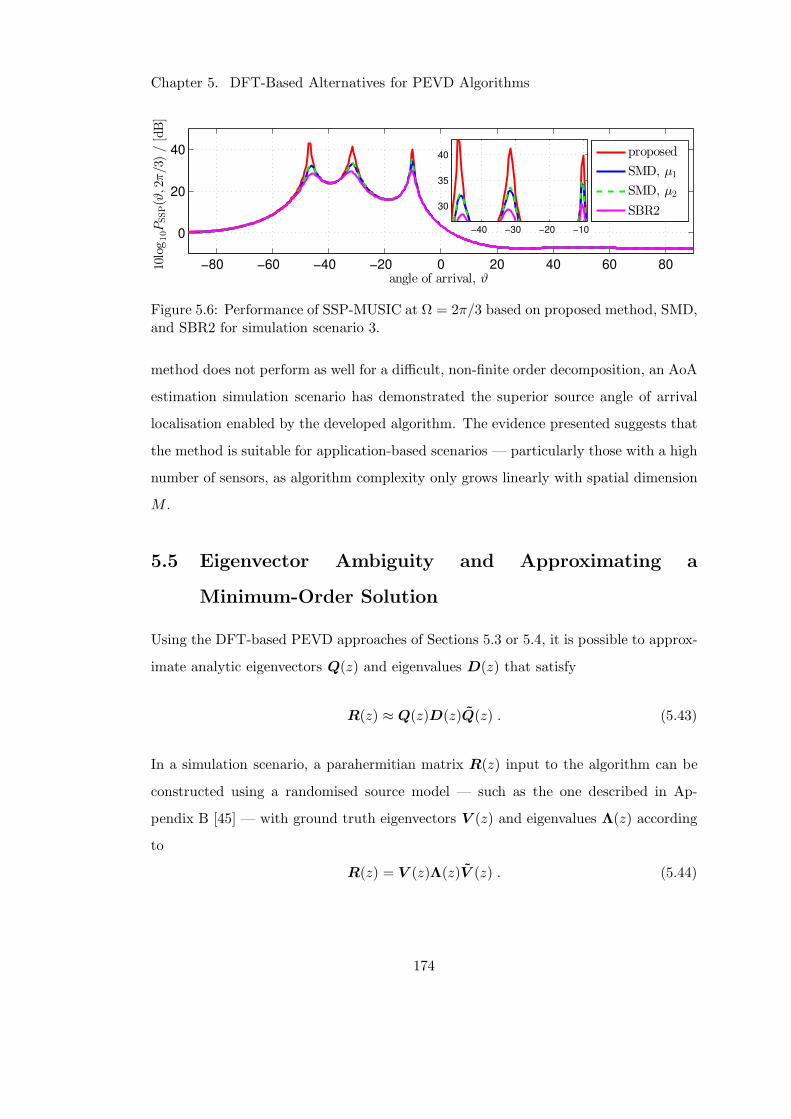
Chapter 5. DFT-Based Alternatives for PEVD Algorithms
−80 −60 −40 −20 0 20 40 60 80
0
20
40
angle of arrival, ϑ
10log10PSSP(ϑ,2π/3)/[dB]
proposed
SMD, µ1
SMD, µ2
SBR2
−40 −30 −20 −10
30
35
40
Figure 5.6: Performance of SSP-MUSIC at Ω = 2π/3 based on proposed method, SMD,and SBR2 for simulation scenario 3.
method does not perform as well for a difficult, non-finite order decomposition, an AoA
estimation simulation scenario has demonstrated the superior source angle of arrival
localisation enabled by the developed algorithm. The evidence presented suggests that
the method is suitable for application-based scenarios — particularly those with a high
number of sensors, as algorithm complexity only grows linearly with spatial dimension
M .
5.5 Eigenvector Ambiguity and Approximating a
Minimum-Order Solution
Using the DFT-based PEVD approaches of Sections 5.3 or 5.4, it is possible to approx-
imate analytic eigenvectors Q(z) and eigenvalues D(z) that satisfy
R(z) ≈ Q(z)D(z)Q(z) . (5.43)
In a simulation scenario, a parahermitian matrix R(z) input to the algorithm can be
constructed using a randomised source model — such as the one described in Ap-
pendix B [45] — with ground truth eigenvectors V (z) and eigenvalues Λ(z) according
to
R(z) = V (z)Λ(z)V (z) . (5.44)
174
Chapter 5. DFT-Based Alternatives for PEVD Algorithms
Typically, D(z) is a very good approximation to Λ(z) and is of comparable order;
however, Q(z) typically has greater order than V (z) even after moderate truncation,
as seen in the results of Section 5.3.6.
With the knowledge that each eigenvector in V (z) or Q(z) may be influenced by
an arbitrary all-pass filter and still be valid, this section investigates a method to find
some diagonal matrix U(z) with all-pass filters on its diagonal that satisfies
Q(z) = H(z)U (z) , (5.45)
whereH(z) is the paraunitary matrix that can fulfil the same purpose as Q(z) in (5.43)
with minimum-order; thus, H(z) should be of order less than or equal to the order of
V (z).
For the decomposition of R(z) : C → CM×M , the above paraunitary matrices can
be described according to U(z) = diagu1(z), u2(z), . . . , uM (z),
Q(z) =[
q1(z), q2(z), . . . , qM (z)]
=
q1,1(z) q1,2(z) . . . q1,M(z)
q2,1(z) q2,2(z) . . . q2,M(z)...
.... . .
...
qM,1(z) qM,2(z) . . . qM,M(z)
,
(5.46)
and
H(z) =[
h1(z), h2(z), . . . , hM (z)]
=
h1,1(z) h1,2(z) . . . h1,M (z)
h2,1(z) h2,2(z) . . . h2,M (z)...
.... . .
...
hM,1(z) hM,2(z) . . . hM,M (z)
.
(5.47)
Here, um(z)um(z) = 1 ∀ m and q1(z) = [q1,1(z), q2,1(z), . . . , qM,1(z)]T is the first eigen-
175
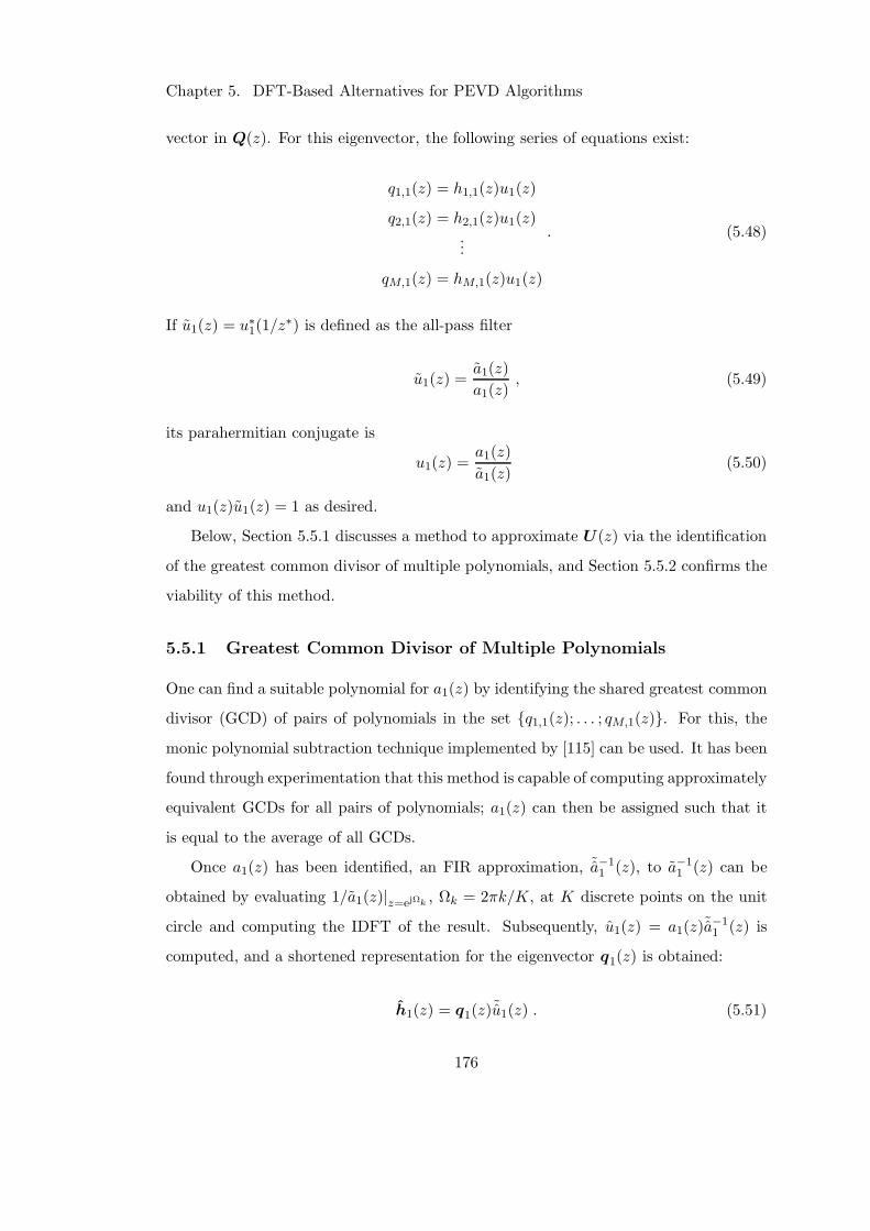
Chapter 5. DFT-Based Alternatives for PEVD Algorithms
vector in Q(z). For this eigenvector, the following series of equations exist:
q1,1(z) = h1,1(z)u1(z)
q2,1(z) = h2,1(z)u1(z)...
qM,1(z) = hM,1(z)u1(z)
. (5.48)
If u1(z) = u∗1(1/z∗) is defined as the all-pass filter
u1(z) =a1(z)
a1(z), (5.49)
its parahermitian conjugate is
u1(z) =a1(z)
a1(z)(5.50)
and u1(z)u1(z) = 1 as desired.
Below, Section 5.5.1 discusses a method to approximate U(z) via the identification
of the greatest common divisor of multiple polynomials, and Section 5.5.2 confirms the
viability of this method.
5.5.1 Greatest Common Divisor of Multiple Polynomials
One can find a suitable polynomial for a1(z) by identifying the shared greatest common
divisor (GCD) of pairs of polynomials in the set q1,1(z); . . . ; qM,1(z). For this, the
monic polynomial subtraction technique implemented by [115] can be used. It has been
found through experimentation that this method is capable of computing approximately
equivalent GCDs for all pairs of polynomials; a1(z) can then be assigned such that it
is equal to the average of all GCDs.
Once a1(z) has been identified, an FIR approximation, ˜a−11 (z), to a−1
1 (z) can be
obtained by evaluating 1/a1(z)|z=ejΩk , Ωk = 2πk/K, at K discrete points on the unit
circle and computing the IDFT of the result. Subsequently, u1(z) = a1(z)˜a−11 (z) is
computed, and a shortened representation for the eigenvector q1(z) is obtained:
h1(z) = q1(z)˜u1(z) . (5.51)
176
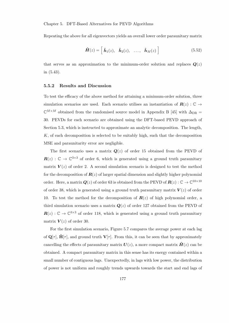
Chapter 5. DFT-Based Alternatives for PEVD Algorithms
Repeating the above for all eigenvectors yields an overall lower order paraunitary matrix
H(z) =[
h1(z), h2(z), . . . , hM (z)]
(5.52)
that serves as an approximation to the minimum-order solution and replaces Q(z)
in (5.43).
5.5.2 Results and Discussion
To test the efficacy of the above method for attaining a minimum-order solution, three
simulation scenarios are used. Each scenario utilises an instantiation of R(z) : C →CM×M obtained from the randomised source model in Appendix B [45] with ∆DR =
30. PEVDs for each scenario are obtained using the DFT-based PEVD approach of
Section 5.3, which is instructed to approximate an analytic decomposition. The length,
K, of each decomposition is selected to be suitably high, such that the decomposition
MSE and paraunitarity error are negligible.
The first scenario uses a matrix Q(z) of order 15 obtained from the PEVD of
R(z) : C → C3×3 of order 6, which is generated using a ground truth paraunitary
matrix V (z) of order 2. A second simulation scenario is designed to test the method
for the decomposition of R(z) of larger spatial dimension and slightly higher polynomial
order. Here, a matrixQ(z) of order 63 is obtained from the PEVD ofR(z) : C→ C10×10
of order 38, which is generated using a ground truth paraunitary matrix V (z) of order
10. To test the method for the decomposition of R(z) of high polynomial order, a
third simulation scenario uses a matrix Q(z) of order 127 obtained from the PEVD of
R(z) : C → C3×3 of order 118, which is generated using a ground truth paraunitary
matrix V (z) of order 30.
For the first simulation scenario, Figure 5.7 compares the average power at each lag
of Q[τ ], H[τ ], and ground truth V[τ ]. From this, it can be seen that by approximately
cancelling the effects of paraunitary matrix U(z), a more compact matrix H(z) can be
obtained. A compact paraunitary matrix in this sense has its energy contained within a
small number of contiguous lags. Unexpectedly, in lags with low power, the distribution
of power is not uniform and roughly trends upwards towards the start and end lags of
177
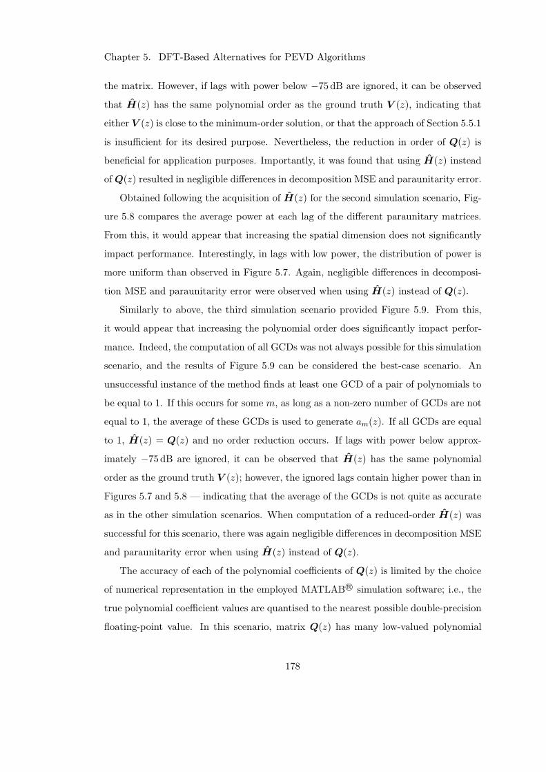
Chapter 5. DFT-Based Alternatives for PEVD Algorithms
the matrix. However, if lags with power below −75 dB are ignored, it can be observed
that H(z) has the same polynomial order as the ground truth V (z), indicating that
either V (z) is close to the minimum-order solution, or that the approach of Section 5.5.1
is insufficient for its desired purpose. Nevertheless, the reduction in order of Q(z) is
beneficial for application purposes. Importantly, it was found that using H(z) instead
of Q(z) resulted in negligible differences in decomposition MSE and paraunitarity error.
Obtained following the acquisition of H(z) for the second simulation scenario, Fig-
ure 5.8 compares the average power at each lag of the different paraunitary matrices.
From this, it would appear that increasing the spatial dimension does not significantly
impact performance. Interestingly, in lags with low power, the distribution of power is
more uniform than observed in Figure 5.7. Again, negligible differences in decomposi-
tion MSE and paraunitarity error were observed when using H(z) instead of Q(z).
Similarly to above, the third simulation scenario provided Figure 5.9. From this,
it would appear that increasing the polynomial order does significantly impact perfor-
mance. Indeed, the computation of all GCDs was not always possible for this simulation
scenario, and the results of Figure 5.9 can be considered the best-case scenario. An
unsuccessful instance of the method finds at least one GCD of a pair of polynomials to
be equal to 1. If this occurs for some m, as long as a non-zero number of GCDs are not
equal to 1, the average of these GCDs is used to generate am(z). If all GCDs are equal
to 1, H(z) = Q(z) and no order reduction occurs. If lags with power below approx-
imately −75 dB are ignored, it can be observed that H(z) has the same polynomial
order as the ground truth V (z); however, the ignored lags contain higher power than in
Figures 5.7 and 5.8 — indicating that the average of the GCDs is not quite as accurate
as in the other simulation scenarios. When computation of a reduced-order H(z) was
successful for this scenario, there was again negligible differences in decomposition MSE
and paraunitarity error when using H(z) instead of Q(z).
The accuracy of each of the polynomial coefficients of Q(z) is limited by the choice
of numerical representation in the employed MATLABR© simulation software; i.e., the
true polynomial coefficient values are quantised to the nearest possible double-precision
floating-point value. In this scenario, matrix Q(z) has many low-valued polynomial
178
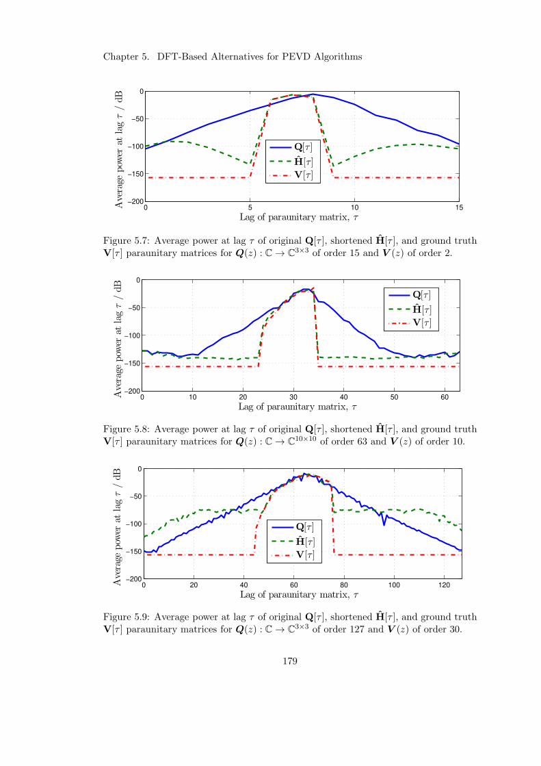
Chapter 5. DFT-Based Alternatives for PEVD Algorithms
0 5 10 15−200
−150
−100
−50
0
Lag of paraunitary matrix, τ
Average
pow
erat
lagτ/dB
Q[τ]
H[τ]
V[τ]
Figure 5.7: Average power at lag τ of original Q[τ ], shortened H[τ ], and ground truthV[τ ] paraunitary matrices for Q(z) : C→ C
3×3 of order 15 and V (z) of order 2.
0 10 20 30 40 50 60−200
−150
−100
−50
0
Lag of paraunitary matrix, τ
Average
pow
erat
lagτ/dB
Q[τ]
H[τ]
V[τ]
Figure 5.8: Average power at lag τ of original Q[τ ], shortened H[τ ], and ground truthV[τ ] paraunitary matrices for Q(z) : C→ C
10×10 of order 63 and V (z) of order 10.
0 20 40 60 80 100 120−200
−150
−100
−50
0
Lag of paraunitary matrix, τ
Average
pow
erat
lagτ/dB
Q[τ]
H[τ]
V[τ]
Figure 5.9: Average power at lag τ of original Q[τ ], shortened H[τ ], and ground truthV[τ ] paraunitary matrices for Q(z) : C→ C
3×3 of order 127 and V (z) of order 30.
179
Chapter 5. DFT-Based Alternatives for PEVD Algorithms
coefficients that can be easily corrupted by quantisation error. In the presence of too
many coefficient values with a high degree of error, the monic polynomial subtraction
technique can fail to identify the GCDs for all pairs of polynomials. If the polynomial
coefficients of Q(z) were represented with higher accuracy, the reliability of the method
might increase for paraunitary matrices with high polynomial order. Alternatively, a
more robust method for computing the GCD might give better results.
5.5.3 Summary
This section has discussed a method to approximate a minimum-order solution to the
PEVD via the identification of the greatest common divisor of multiple polynomials.
The GCD identification approach utilised in this work — which employs the monic
polynomial subtraction method of [115] — is well-behaved for short polynomials (Q(z)
of order less than 100), but sometimes fails to find accurate GCDs for all pairs of
longer polynomials. It might therefore be worthwhile to find a more robust method
for computing the GCD of polynomials of high order. Despite the shortcomings of this
approach for Q(z) of high polynomial order, it is clear that coupling a method capa-
ble of approximating a minimum-order solution with the paraunitary matrix output
by a DFT-based PEVD algorithm can yield shorter paraunitary matrices without any
disadvantages other than the time taken to approximate and utilise U(z). For applica-
tions where short paraunitary matrices are more important than increased algorithm
execution time, the method described in this section could be useful.
5.6 Conclusions
In contrast to previous chapters, which discussed modified and novel coefficient domain
PEVD algorithms, this chapter has investigated DFT-based alternatives for the PEVD.
Following an introduction of the general structure and merits of DFT-based PEVD al-
gorithms, a comparison of the characteristics of an example DFT-based algorithm with
a coefficient domain algorithm was provided. Through this comparison, it was estab-
lished that the DFT-based algorithm is particularly suited to problems of relatively
low, finite order, or situations in which an analytic decomposition is preferable or only
180
Chapter 5. DFT-Based Alternatives for PEVD Algorithms
approximate paraunitarity is required. In contrast, the SMD algorithm attained re-
liably low decomposition error and potentially paraunitary eigenvectors, and offered
customisable diagonalisation and eigenvector length. Furthermore, it was concluded
that the DFT-based approach offers a viable alternative to SMD for the decomposition
of parahermitian matrices with large spatial dimensions. However, the former algo-
rithm’s reliance on an a priori estimate of paraunitary matrix length was considered to
be disadvantageous for application purposes.
A subsequent section overcame this final point by developing a novel DFT-based
PEVD algorithm that is able to perform well without requiring a priori knowledge of
the paraunitary matrix length. By minimising a newly developed metric capable of
measuring the smoothness of the eigenvectors produced by the algorithm, the phase
responses of the eigenvectors were adjusted until phase alignment was achieved. The
resulting polynomial eigenvectors were shown to be both compact and more accurate
than those obtained by an existing DFT-based PEVD algorithm. Furthermore, the
introduction of a modified eigenvalue and eigenvector reordering scheme was shown to
enable the extraction of ground truth polynomial eigenvalues despite the presence of
eigenvalues with algebraic multiplicity greater than one.
This algorithm formed the basis of a novel iterative DFT-based algorithm capable of
adapting to any dimensionality of parahermitian matrix without an a priori estimate of
the DFT length. Simulation results demonstrated that when decomposing empirically
constructed matrices, the proposed algorithm can offer superior performance to existing
iterative PEVD algorithms. Furthermore, an angle of arrival estimation simulation
scenario demonstrated that the developed algorithm is capable of superior source angle
of arrival localisation; however, it was noted that the presence of noise hinders the
phase alignment and eigenvector and eigenvalue reordering elements of the DFT-based
approach. The evidence presented throughout this chapter suggests that frequency-
based PEVD methods are suitable for application-based scenarios — particularly those
with a high number of sensors, as algorithm complexity only grows linearly with spatial
dimension M .
Finally, a method to approximate a minimum-order solution to the PEVD was
181
Chapter 5. DFT-Based Alternatives for PEVD Algorithms
introduced. If a DFT-based algorithm is able to approximate analytic polynomial
eigenvectors of relatively low order, and if processing time is not of critical importance,
applying this method to the polynomial eigenvectors can decrease their length without
introducing error. However, it might be worthwhile to find a more robust method for
reducing the order of polynomial eigenvectors of relatively high order.
182
Chapter 6
Conclusions
6.1 Summary of Contributions
By introducing a number of novel methods to lower the computational cost of existing
iterative algorithms related to the PEVD, the research of Chapter 3 has successfully
accomplished the first of the objectives listed in Section 1.2. The proposed methods in
this chapter conquered unexplored areas of PEVD algorithm improvement by optimis-
ing matrix manipulations in software, exploiting parahermitian matrix symmetry [67],
minimising algorithmic redundancy [68], and reducing the search and update space
of iterative PEVD algorithms [68, 69]. Importantly, the significant performance gains
made possible by the half-matrix parahermitian matrix representation, restricted up-
date strategy, and matrix multiplication optimisations can be used simultaneously and
extended to any number of iterative PEVD algorithms without impacting accuracy.
Improvements were also made to an existing polynomial matrix QR decomposition al-
gorithm [70] and a polynomial matrix truncation strategy. While the latter enforced a
degree of polynomial matrix order reduction, and therefore made some steps towards
satisfying the second objective in Section 1.2, each of the improved PEVD approaches
still exhibited algorithmic complexity that grew rapidly with the spatial dimensions of
the parahermitian matrix. Some form of spatial dimension reduction was therefore re-
quired if the algorithms were to be suitable for applications involving large broadband
arrays, and by extension large parahermitian matrices.
183
Chapter 6. Conclusions
Chapter 4 addressed the problem of spatial dimension reduction — and therefore
the second objective of this research — by taking additional steps to convert the se-
quential form of existing PEVD algorithms to a reduced dimensionality, partially par-
allelisable divide-and-conquer (DaC) architecture. Simulations utilising the proposed
DaC approach demonstrated that a recursive block diagonalisation strategy can be
used to segment a large parahermitian matrix into multiple independent parahermitian
matrices of smaller spatial dimensions. These matrices were subsequently diagonalised
independently and in parallel using a PEVD algorithm that incorporated the most well-
performing complexity reduction strategies of Chapter 3. The divide-and-conquer se-
quential matrix diagonalisation [71] and parallel-sequential matrix diagonalisation [72]
algorithms created using this DaC framework exhibited convergence speeds an order of
magnitude faster than existing methods for parahermitian matrices with large spatial
dimensions [64]. In contrast to the current state-of-the-art approaches, the developed
algorithms were shown to be well-suited to deployment in application scenarios [20].
In the process of completing the third objective of this research, Chapter 5 intro-
duced the concept of DFT-based PEVD algorithms, which offer potentially analytic
and subsequently minimum-order solutions to the PEVD. A comparison of such an
algorithm with an iterative time-based PEVD algorithm established that DFT-based
algorithms are particularly suited to the generation of approximately analytic decom-
positions of relatively low, finite order, provided that only approximate paraunitarity
of the polynomial eigenvectors is required [56]. However, the DFT-based algorithm’s
reliance on an a priori estimate of the paraunitary matrix length was considered to be
disadvantageous for application purposes. A novel DFT-based PEVD algorithm over-
came this problem by utilising an alternative phase alignment strategy that relied on
the smoothness of the eigenvectors and not on a priori knowledge of the paraunitary
matrix length. The resulting polynomial eigenvectors were shown to be both compact
and more accurate than those obtained from the previously tested existing DFT-based
PEVD algorithm [73]. An extension of this algorithm, which uses an iterative approach
to remove all a priori knowledge requirements, was then found to perform well relative
to existing iterative PEVD algorithms [74]. The evidence presented throughout Chap-
184
Chapter 6. Conclusions
ter 5 has indicated that DFT-based PEVD methods are suitable for application-based
scenarios — particularly those with a high number of sensors, as their algorithmic com-
plexity only grows linearly with parahermitian matrix spatial dimension. A method to
approximate a minimum-order solution to the PEVD was then introduced. Applying
this method to the polynomial eigenvectors from an analytic PEVD successfully de-
creased their length without introducing error; however, a more robust method would
perhaps have more success when reducing the order of polynomial eigenvectors of rel-
atively high order.
In brief, the objectives set out in Section 1.2 were to reduce the computational
complexity of PEVD algorithms, to investigate dimensionality reduction of the para-
hermitian matrix, and to investigate DFT-based approaches to the PEVD. Given the
above contributions, it can be concluded that these objectives have been met. Most im-
portantly, the work in this thesis has demonstrated the flexibility of PEVD algorithms,
and has investigated, illuminated, and improved upon various aspects of these algo-
rithms to the point where they are now potentially suitable for real-time application
purposes.
6.2 Future Work
While reductions in the computational complexity of iterative PEVD algorithms have
been comprehensively discussed in this thesis, all implementations of these algorithms
— excepting SBR2 [57–59] — are currently restricted to MATLABR©. Moving to a
lower-level software language such as C would require an extended period of devel-
opment time, but would increase algorithm speed and portability substantially. In
addition, proof of convergence for the DaC algorithms of Chapter 4 would certainly be
of interest. Tied to this is the potential for an investigation into the enforcement of
spectral majorisation of the polynomial eigenvalues from the sequential matrix diago-
nalisation algorithm and by extension, the sequential matrix segmentation algorithm
(SMS). It would be useful to identify if the enforcement of block diagonalisation of a
parahermitian matrix via SMS aids or hinders spectral majorisation. Related to these
sources of future work is the potential to detect which channels contributing to a space-
185
Chapter 6. Conclusions
time covariance matrix are already weakly correlated; these channels could perhaps help
to create a ‘natural’ block diagonalisation of the resulting parahermitian matrix. The
‘divide’ scheme of a DaC algorithm might then be able to suppress any remaining small
or sparse coefficients with greater ease, and therefore reach the ‘conquer’ or subsequent
‘divide’ stages faster than a brute-force approach.
Future work in DFT-based PEVD algorithm development includes the utilisation
of alternative optimisation strategies for phase alignment of the eigenvectors. Ideally,
these would avoid the costly matrix inversion required by the novel algorithms discussed
in this thesis. Currently, the DFT-based algorithms do not scale well in terms of
parahermitian matrix order. For emerging DFT-based PEVD algorithms, lower-cost
schemes should be considered. These could utilise smoothness metrics that are less
costly than the one used in Section 5.3.1 and [54,73,74] — which has order K3 [116,117]
— and could perhaps take inspiration from the lost-cost interpolation schemes in [118],
which are of order K log2 K. A final algorithmic source of future work could involve
the identification of a more robust method for computing the greatest common divisor
of multiple polynomials; this would aid the acquisition of minimum-order solutions to
the PEVD despite the presence of polynomial eigenvectors of large order.
Of course, actually applying the new and improved PEVD algorithms discussed in
this thesis in real-world application scenarios is perhaps the largest task for future work.
For this, any of the applications detailed in Chapter 1 could be targeted. On a related
note, the greatest common divisor extraction approach of [115] used in Section 5.5 could
be extended to help with the scene recovery task in [30]. While this could facilitate the
recovery of the magnitude of any transfer functions between an unknown source and
an array of sensors, the phase information would have to be obtained from elsewhere.
With this phase information, future work could continue the efforts of [119, 120] and
attempt to estimate a room’s geometry from its impulse response.
186
Appendix A
Existing PEVD Algorithms and
Performance Metrics
A.1 Sequential Matrix Diagonalisation PEVD Algorithm
Within a reasonable number of iterations, the sequential matrix diagonalisation (SMD)
polynomial matrix eigenvalue decomposition (PEVD) algorithm defined in [45] and
its derivatives [47–50] are able to achieve superior levels of diagonalisation to other
iterative PEVD methods. Given that Section 3.2.1 also identifies that SMD is the most
computationally efficient iterative PEVD algorithm, particular focus is therefore given
to SMD in this thesis. Further detail on the operation of SMD is therefore provided
below, as knowledge of this algorithm may aid the reader’s understanding of the novel
contributions detailed in this thesis.
Below, Section A.1.1 provides a brief summary of the operations used in each iter-
ation of SMD, and Section A.1.2 evaluates the computational complexity of the algo-
rithm.
A.1.1 Algorithm Overview
The SMD algorithm approximates the PEVD using a series of elementary paraunitary
operations to iteratively diagonalise a parahermitian matrix R(z) : C → CM×M and
its associated coefficient matrix, R[τ ].
187
Appendix A. Existing PEVD Algorithms and Performance Metrics
Upon initialisation, the algorithm diagonalises the lag zero coefficient matrix R[0]
by means of its modal matrix Q(0); i.e., S(0)(z) = Q(0)R(z)Q(0)H. The unitary Q(0) —
obtained from the EVD of the lag zero slice R[0] — is applied to all coefficient matrices
R[τ ] ∀ τ , and initialises H(0)(z) = Q(0).
In the ith step, i = 1, 2, . . . I, the SMD algorithm computes
S(i)(z) = U (i)(z)S(i−1)(z)U(i)(z)
H(i)(z) = U (i)(z)H (i−1)(z) , (A.1)
in which
U (i)(z) = Q(i)Λ(i)(z) . (A.2)
The product in (A.2) consists of a paraunitary delay matrix
Λ(i)(z) = diag1 . . . 1︸ ︷︷ ︸
k(i)−1
z−τ (i) 1 . . . 1︸ ︷︷ ︸
M−k(i)
, (A.3)
and a unitary matrix Q(i), with the result that U (i)(z) in (A.2) is paraunitary.
For subsequent discussion, it is convenient to define intermediate variables S(i)′(z)
and H(i)′(z) as the outputs of a ‘shifting’ step, where
S(i)′(z) = Λ(i)(z)S(i−1)(z)Λ(i)(z)
H(i)′(z) = Λ(i)(z)H (i−1)(z) . (A.4)
A further ‘rotation’ (or ‘update’) step obtains the updated polynomial matrices
S(i)(z) = Q(i)S(i)′(z)Q(i)H
H(i)(z) = Q(i)H(i)′(z) . (A.5)
Matrices Λ(i)(z) andQ(i) are selected based on the position of the dominant off-diagonal
188
Appendix A. Existing PEVD Algorithms and Performance Metrics
column in S(i−1)(z) •— S(i−1)[τ ], as identified by the parameter set
k(i), τ (i) = argmaxk,τ
‖s(i−1)k [τ ]‖2 , (A.6)
where
‖s(i−1)k [τ ]‖2 =
√√√√
M∑
m=1,m6=k
|s(i−1)m,k [τ ]|2 (A.7)
and s(i−1)m,k [τ ] represents the element in the mth row and kth column of the coefficient
matrix S(i−1)[τ ].
The ‘shifting’ process in (A.4) moves the dominant off-diagonal row and column
into the lag zero coefficient matrix S(i)′[0]. The off-diagonal energy in the shifted row
and column is then transferred onto the diagonal by the unitary matrix Q(i) in the
‘rotation’ (or ‘update’) step of (A.5). This matrix Q(i) contains the eigenvectors that
diagonalise S(i)′[0] by means of an ordered EVD.
Truncation of outer coefficients of S(i)(z) and H(i)(z) with small Frobenius norm
is used to limit growth in order. The SMD algoithm uses the truncation approach
detailed in Appendix C.
Iterations of SMD — which has been shown to converge in [45] — continue for
a maximum of Imax steps, or until S(I)(z) is sufficiently diagonalised with dominant
off-diagonal column norm
maxk,τ‖s(I)k [τ ]‖2 ≤ ǫ , (A.8)
where the value of ǫ is chosen to be arbitrarily small. On completion, SMD generates
an approximate PEVD given by
D(z) = S(I)(z) = F (z)R(z)F (z) , (A.9)
where the parahermitian matrix D(z) approximates a diagonal matrix of polynomial
eigenvalues, I = minI, Imax, and a paraunitary matrix F (z) contains approximate
189
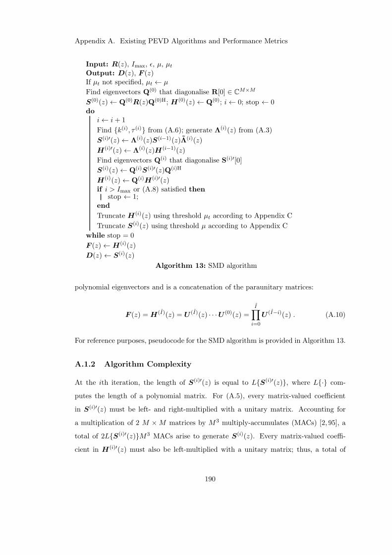
Appendix A. Existing PEVD Algorithms and Performance Metrics
Input: R(z), Imax, ǫ, µ, µt
Output: D(z), F (z)If µt not specified, µt ← µ
Find eigenvectors Q(0) that diagonalise R[0] ∈ CM×M
S(0)(z)← Q(0)R(z)Q(0)H; H(0)(z)← Q(0); i← 0; stop ← 0do
i← i+ 1
Find k(i), τ (i) from (A.6); generate Λ(i)(z) from (A.3)
S(i)′(z)← Λ(i)(z)S(i−1)(z)Λ(i)(z)
H(i)′(z)← Λ(i)(z)H (i−1)(z)
Find eigenvectors Q(i) that diagonalise S(i)′[0]
S(i)(z)← Q(i)S(i)′(z)Q(i)H
H(i)(z)← Q(i)H(i)′(z)if i > Imax or (A.8) satisfied then
stop ← 1;end
Truncate H(i)(z) using threshold µt according to Appendix C
Truncate S(i)(z) using threshold µ according to Appendix C
while stop = 0
F (z)←H(i)(z)
D(z)← S(i)(z)
Algorithm 13: SMD algorithm
polynomial eigenvectors and is a concatenation of the paraunitary matrices:
F (z) = H(I)(z) = U (I)(z) · · ·U (0)(z) =I∏
i=0
U (I−i)(z) . (A.10)
For reference purposes, pseudocode for the SMD algorithm is provided in Algorithm 13.
A.1.2 Algorithm Complexity
At the ith iteration, the length of S(i)′(z) is equal to LS(i)′(z), where L· com-
putes the length of a polynomial matrix. For (A.5), every matrix-valued coefficient
in S(i)′(z) must be left- and right-multiplied with a unitary matrix. Accounting for
a multiplication of 2 M ×M matrices by M3 multiply-accumulates (MACs) [2, 95], a
total of 2LS(i)′(z)M3 MACs arise to generate S(i)(z). Every matrix-valued coeffi-
cient in H(i)′(z) must also be left-multiplied with a unitary matrix; thus, a total of
190
Appendix A. Existing PEVD Algorithms and Performance Metrics
LH(i)′(z)M3 MACs arise to generate H(i)(z). If ǫ = 0, the cumulative complexity
of the SMD algorithm over Imax iterations can therefore be approximated as
CSMD(Imax) = M3Imax∑
i=0
(2LS(i)′(z) + LH (i)′(z)) . (A.11)
A.2 Existing DFT-Based Approach to the PEVD
A discrete Fourier transform (DFT)-based PEVD formulation, which transforms the
problem into a pointwise in frequency standard matrix decomposition, is provided
in [53]. The method can either return a spectrally majorised decomposition, or at-
tempt to compute smooth, approximately analytic, eigenvalues. The inherent drawback
of a lack of phase-coherence between independent frequency bins [81] is solved via a
quadratic non-linear minimisation problem, which encourages phase alignment between
adjacent bins. A comparison between the characteristics of this approach versus the
SMD algorithm — which is summarised in Section A.1 — is given in Section 5.2; a
description of the former is therefore provided below for reference purposes.
Section A.2.1 gives a brief overview of the DFT-based approach defined in [53], while
Sections A.2.2 and A.2.3 describe methods used within the algorithm to approximate
analytic eigenvalues and adjust eigenvector phase.
A.2.1 Algorithm Overview
The approach in [53] uses a decomposition of the form
R[k] = Q[k]D[k]QH[k] , k = 0, 1, . . . ,K − 1 , (A.12)
where Q[k] contains the eigenvectors and D[k] contains the eigenvalues obtained from
the K-point DFT of R[τ ],
R[k] = R(z)|z=ejΩk =∑
τ
R[τ ]e−jΩkτ , k = 0, 1, . . . ,K − 1 . (A.13)
191
Appendix A. Existing PEVD Algorithms and Performance Metrics
An approximate PEVD is therefore obtained via K EVDs that are pointwise in fre-
quency.
The PEVD in (2.4) corresponds to a linear convolution in the coefficient domain;
however, the DFT-based decomposition here corresponds to the circular convolution
R[ ((τ))K ] = Q[ ((τ))K ]⊛D[ ((τ))K ]⊛QH[−((τ))K ] , (A.14)
where⊛ is the circular convolution operator, and ((τ))K denotes τ moduloK. For (A.14)
to be equivalent to (2.4), the number of frequency bins must satisfy
K ≥ (2N + L− 2) , (A.15)
where L = (2T + 1) is the length of input parahermitian matrix R(z), which has
maximum lag T , and N is the assumed length of the paraunitary matrix. That is,
Q[τ ] = 0 for τ ≥ N and τ < 0. Typically, choosing K = (2N + L − 2) is valid, as
decomposition accuracy does not increase significantly for largerK [53], but algorithmic
computational complexity does.
At each frequency bin, eigenvalues are typically arranged in descending order;
this results in approximate spectral majorisation of the polynomial eigenvalues. Sec-
tion A.2.2 discusses the rearrangement of eigenvalues to approximate an analytic de-
composition.
Each eigenvector in a conventional EVD may be influenced by an arbitrary scalar
phase angle and still be valid. This ambiguity in phase of each eigenvector can lead
to discontinuities in phase between adjacent frequency bins. For a short paraunitary
matrix Q(z), these discontinuities must be smoothed. This is achieved through the
use of a phase alignment function, described in Section A.2.3, which uses the ‘dogleg’
algorithm [111] to solve an unconstrained optimisation problem.
Following phase alignment, Q[τ ] is computed as
Q[τ ] =1
K
K−1∑
k=0
Q[k]ejΩkτ , τ = 0, 1, . . . , N − 1 , (A.16)
192
Appendix A. Existing PEVD Algorithms and Performance Metrics
and D(z) is a diagonal parahermitian matrix with diagonal elements equal to the
diagonal elements of Q(z)R(z)Q(z). Any energy in lags τ = N . . .K − 1 of Q[τ ] is
ignored.
A.2.2 Reordering the Eigenvectors and Eigenvalues to Approximate
an Analytic Decomposition
If strong decorrelation is required for an application, but spectral majorisation is not,
then an analytic decomposition may be preferable. In an analytic decomposition, the
eigenvalues and their eigenvectors are arranged such that non-differentiabilities and
discontinuities, respectively, between adjacent frequency bins are minimised. Even for
an arrangement that provides continuous eigenvalues, such discontinuities can occur
when the eigenvalues intersect at some frequencies.
To approximate an analytic decomposition, the eigenvectors in adjacent frequency
bins are rearranged using the inner product
cmn[k] = qHm[k − 1]qn[k] , (A.17)
where, qm[k] is the mth column of Q[k]. For each eigenvector qm[k−1], m = 1 . . .M , a
subsequent eigenvector qm′ [k] is chosen from an initial set S = 1 . . .M of the columns
of Q[k] such that
m′ = argmaxn∈S
|cmn[k]| . (A.18)
Once m′ is identified, it is removed from the set: S ← S\m′, and the next eigenvector
is chosen. The selected eigenvectors are combined in a rearranged matrix Q′[k] =
[q1′ [k], · · · ,qM ′ [k]], and Q[k] is set equal to Q′[k]. The eigenvalues D[k] are rearranged
according to the reordering of the eigenvectors.
A.2.3 Adjusting the Phase of the Eigenvectors via Unconstrained Op-
timisation
Phase alignment of eigenvectors in adjacent frequency bins is vital for a compact, low
order decomposition. Thus, if such a decomposition is sought (e.g., here it is desired
193
Appendix A. Existing PEVD Algorithms and Performance Metrics
that only lags τ = 0 . . . N − 1 are non-zero), then phase alignment can be achieved
by finding the phase changes required for each eigenvector qm[k] ∀ m,k such that the
resulting eigenvectors are of low order.
The phase of the mth eigenvector at frequency bin k can be adjusted by an angle
θ[k] according to qm[k]← ejθ[k]qm[k]. For the mth polynomial eigenvector qm[τ ] to be
compact, it is required to find angles θ = [θ[1] . . . θ[K − 1]]T, that satisfy
qm[τ ] =1
K
K−1∑
k=0
qm[k]ejθ[k]ejΩkτ = 0 , (A.19)
for τ = N . . . K − 1. Without loss of generality, let θ[0] = 0. Note that θ does not
include θ[0]. Equation (A.19) can be expressed as
FNx(θ) + fN = 0 , (A.20)
where x(θ) = [ejθ[1], ejθ[2], . . . , ejθ[K−1]]T, fN = [qTm[0],qTm[0], . . . ,qTm[0]]T is a M(K −N)× 1 vector, and
FN =
qm[1]w−NK qm[2]w−2N
K . . . qm[K − 1]w−(K−1)NK
qm[1]w−(N+1)K qm[2]w
−2(N+1)K . . . qm[K − 1]w
−(K−1)(N+1)K
......
. . ....
qm[1]w−(K−1)K qm[2]w
−2(K−1)K . . . qm[K − 1]w
−(K−1)2
K
(A.21)
is a M(K −N)× (K − 1) matrix, with wK = ej2π/K .
In general, there may exist no phase vector θ which satisfies (A.20). However, by
minimising the energy in the coefficients for τ = N, . . . ,K−1, some θ can be obtained.
The energy in these coefficients,
J(θ) = ‖FNx(θ) + fN‖22 , (A.22)
is therefore used as the objective of an unconstrained minimisation problem. In [53], it
was found that the ‘dogleg’ trust-region strategy for unconstrained minimisation [111]
was able to satisfactorily identify the θ that minimised J(θ) for m = 1 . . .M .
194
Appendix A. Existing PEVD Algorithms and Performance Metrics
Of course, a disadvantage of this method is that it requires an estimate of N prior
to execution. If N is not sufficiently high, convergence of the ‘dogleg’ algorithm can
be poor, resulting in insufficient eigenvector phase alignment and a PEVD with a high
degree of decomposition error.
A.3 Performance Metrics
This section defines several metrics used throughout this thesis to evaluate the quality of
a PEVD. Section A.3.1 defines the well-established diagonalisation metric from [45] and
Section A.3.2 adapts this metric to the case of polynomial matrix upper-triangularisation.
Subsequently, Section A.3.3 establishes a metric to measure the accuracy of the polyno-
mial eigenvalues obtained from a PEVD, Section A.3.4 defines a metric for evaluating
the decomposition mean square error of a PEVD, and Section A.3.5 describes a parau-
nitarity metric for the polynomial eigenvectors from a PEVD. Finally, Section A.3.6
defines an intuitive metric that records paraunitary matrix length.
A.3.1 Normalised Off-Diagonal Energy
Polynomial matrix eigenvalue decomposition algorithms iteratively minimise off-
diagonal energy. To measure their performance, a suitable normalised metric E(i)diag [45]
is used, which divides the off-diagonal energy in the iteratively updated parahermitian
matrix S(i)(z) •— S(i)[τ ] ∈ CM×M at the ith algorithm iteration by the total energy
in the original parahermitian matrix R(z). The metric is defined as
E(i)diag =
∑
τ
∑Mk=1 ‖s
(i)k [τ ]‖22
∑
τ ‖R[τ ]‖2F, (A.23)
with
‖s(i)k [τ ]‖22 =
P∑
m=1,m6=k
|s(i)m,k[τ ]|2 (A.24)
where s(i)m,k[τ ] represents the element in the mth row and kth column of S(i)[τ ].
Computation of E(i)diag generates squared covariance terms; therefore a logarithmic
notation of 5 log10 E(i)diag is employed. Note that diagonalisation metric Ediag, which
195
Appendix A. Existing PEVD Algorithms and Performance Metrics
omits the iteration parameter i, measures the diagonalisation obtained by a PEVD
algorithm following the completion of all iterations.
A.3.2 Normalised Below-Diagonal Energy
Polynomial matrix QR decomposition algorithms iteratively minimise lower-triangular
energy. To measure their performance, a suitable normalised metric E(i)tri is used,
which divides the lower-triangular energy in the iteratively updated polynomial ma-
trix A(i)(z) •— A(i)[τ ] ∈ CP×Q at the ith algorithm iteration by the total energy in
the original matrix A(z). The metric is defined as
E(i)tri =
∑
τ
∑min(P−1),Qk=1 ‖a(i)k [τ ]‖22∑
τ ‖A[τ ]‖2F, (A.25)
with
‖a(i)k [τ ]‖22 =P∑
j=k+1
|a(i)j,k[τ ]|2 , (A.26)
where a(i)j,k[τ ] represents the element in the jth row and kth column of A(i)[τ ].
Note that for demonstration purposes, the iteration parameter i describes the run-
ning total of iterations, and is not reset, e.g., at the beginning of each column step of
the polynomial matrix QR decomposition by columns algorithm from [42].
Unlike the computation in (A.23), (A.25) does not necessarily square covariance
terms, therefore a logarithmic metric of 10 log10 E(i)tri is used.
A.3.3 Eigenvalue Resolution
The eigenvalue resolution is defined as the mean normalised absolute error between the
ground truth and measured eigenvalue PSDs:
λres =1
MK
M∑
m=1
K−1∑
k=0
∣∣∣∣∣
Dm,m[k]− Wm,m[k]
Wm,m[k]
∣∣∣∣∣, (A.27)
where D[k] is obtained from the K-point DFT of eigenvalues D[τ ] ∈ CM×M computed
by a PEVD and W[k] is found by appropriately associating values of the K-point DFT
196
Appendix A. Existing PEVD Algorithms and Performance Metrics
of ground truth eigenvalues W[τ ]. For example, if D[k] is obtained from an iterative
time domain PEVD algorithm and therefore approximately spectrally majorised for all
k, the eigenvalues in W[k] will be ordered such that they are also spectrally majorised.
A suitable K is identified as the smallest power of two greater than the lengths of D(z)
and W (z). The normalisation in (A.27) will give emphasis to the correct extraction of
small eigenvalues in the presence of stronger ones, and is therefore similar to the coding
gain metric in [25].
A.3.4 Decomposition Mean Square Error
Denote the mean square reconstruction error for an approximate PEVD as
MSE =1
M2L′
∑
τ‖ER[τ ]‖2F , (A.28)
where ER[τ ] = R[τ ] − R[τ ], R[τ ] ∈ CM×M , R(z) = F (z)D(z)F (z), and L′ is the
length of ER(z). Matrices D(z) and F (z) = Q(z) are polynomial eigenvalues and
eigenvectors computed by a PEVD.
A.3.5 Paraunitarity Error
The paraunitarity error for polynomial eigenvectors F (z) = Q(z) : C → CM×M ob-
tained by a PEVD is defined as
η =1
M
∑
τ‖EF [τ ]− IM[τ ]‖2F , (A.29)
where EF (z) = F (z)F (z), IM[0] is an M ×M identity matrix, and IM[τ ] for τ 6= 0 is
an M ×M matrix of zeroes.
A.3.6 Paraunitary Filter Length
The paraunitary matrix F (z) = Q(z) output by a PEVD algorithm can be implemented
as a lossless bank of finite impulse response filters in signal processing applications; a
useful metric for gauging the implementation cost of this matrix is its length, LF = LQ,
which — via the definitions in Section 2.1 — directly relates to the order of the filters.
197
Appendix B
Broadband Randomised Source
Model
A randomised source model from [45] generates a parahermitian matrix R(z) =
Q(z)D(z)Q(z), where D(z) : C → CM×M is a diagonal parahermitian matrix con-
taining the PSDs of M independent sources. These sources are spectrally shaped by
innovation filters such thatD(z) has an order of OD, with a restriction on the placement
of zeros to limit the dynamic range of the PSDs to about ∆DR dB. A random parau-
nitary matrix Q(z) : C → CM×M of order OQ performs a convolutive mixing of these
sources, such that R(z) has a full polynomial rank and an order of OR = 2OQ + OD.
Assuming that Q(z) is of minimum order — i.e., it cannot be reduced to the product of
a paraunitary matrix and a diagonal paraunitary matrix — an ideal PEVD algorithm
will recover D(z) and Q(z) (or equivalently, F (z) = Q(z)) given R(z).
198
Appendix C
State-of-the-Art in Polynomial
Matrix Truncation
The polynomial matrix truncation method from [61] is described here. This approach
reduces the order of a polynomial matrix Y (z) — which has minimum lag T1 and
maximum lag T2 — by removing the T3(µ) leading and T4(µ) trailing lags using a trim
function
ftrim(Y[τ ], µ) =
Y[τ ], T1 + T3(µ) ≤ τ ≤ T2 − T4(µ)
0, otherwise .(C.1)
The amount of energy lost by removing the T3(µ) leading and T4(µ) trailing lags of
Y[τ ] via the ftrim(·) operation is measured by
γtrim = 1−∑
τ ‖ftrim(Y[τ ], µ)‖2F∑
τ ‖Y[τ ]‖2F, (C.2)
where ‖ · ‖F is the Frobenius norm. A parameter µ is used to provide an upper bound
for γtrim. The truncation procedure can be expressed as the constrained optimisation
problem:
maximise T3(µ) + T4(µ) , s.t. γtrim ≤ µ . (C.3)
This is implemented by removing the outermost matrix coefficients of matrix Y (z)
until γtrim approaches µ from below. Note that if Y (z) is parahermitian, T1 = −T2
and T3(µ) = T4(µ) due to symmetry.
199
Appendix D
Spatio-Spectral MUSIC
Algorithm
The spatio-spectral polynomial MUSIC (SSP-MUSIC) algorithm [18] is an extension
of narrowband MUSIC [77] to the broadband case. The idea of the SSP-MUSIC al-
gorithm is to scan the noise-only subspace Qn(z) = F n(z) = [qR+1(z) . . . qM (z)] :
C → CM×(M−R), which is spanned by eigenvectors corresponding to eigenvalues close
to the noise floor, Dn(z) ≈ σ2vIM−R. The steering vectors of the R sources that con-
tribute to R(z) : C→ CM×M will define the signal-plus-noise subspace Qs(z) = F s(z)
and therefore lie in the nullspace of its complement Qn(z). As a result, the vector
Qn(ejΩ)aϑ,ϕ(e
jΩ) has to be close to the origin for aϑ,ϕ(ejΩ) to be a steering vector of
a contributing source at frequency Ω, where Qn(ejΩ) = Qn(z)|z=ejΩ and aϑ,ϕ(e
jΩ) =
aϑ,ϕ(z)|z=ejΩ . Thus, the SSP-MUSIC algorithm evaluates the reciprocal of the norm of
this vector,
PSSP(ϑ,ϕ,Ω) =1
aϑ,ϕ(z)Qn(z)Qn(z)aϑ,ϕ(z)
∣∣∣z=ejΩ
, (D.1)
which is large when aϑ,ϕ(ejΩ) is a steering vector of a contributing source. In addition
to estimating the spatial direction of sources in terms of azimuth, ϑ, and elevation,
ϕ, PSSP(ϑ,ϕ,Ω) can determine over which frequency range sources in the direction
defined by the steering vector aϑ,ϕ(z) are active. If ϕ is assumed or known to be zero,
the notation PSSP(ϑ,Ω) is used.
200
Bibliography
[1] G. W. Stewart, “The decompositional approach to matrix computation,” Com-
puting in Science & Engineering, vol. 2, no. 1, pp. 50–59, 2000.
[2] G. Golub and C. V. Loan, Matrix computations, 4th ed. Baltimore, Maryland:
John Hopkins University Press, 2013.
[3] I. Gohberg, P. Lancaster, and L. Rodman, Matrix Polynomials. New York:
Academic Press, 1982.
[4] P. P. Vaidyanathan, Multirate Systems and Filter Banks. Englewood Cliffs:
Prentice Hall, 1993.
[5] J. G. McWhirter and P. D. Baxter, “A Novel Technqiue for Broadband SVD,” in
12th Annual Workshop on Adaptive Sensor Array Processing, MIT Lincoln Labs,
Cambridge, MA, 2004.
[6] J. G. McWhirter, P. D. Baxter, T. Cooper, S. Redif, and J. Foster, “An EVD Al-
gorithm for Para-Hermitian Polynomial Matrices,” IEEE Transactions on Signal
Processing, vol. 55, no. 5, pp. 2158–2169, May 2007.
[7] S. Icart and P. Comon, “Some properties of Laurent polynomial matrices,” in
IMA International Conference on Signal Processing in Mathematics, December
2012.
[8] P. P. Vaidyanathan, “Theory of optimal orthonormal subband coders,” IEEE
Transactions on Signal Processing, vol. 46, no. 6, pp. 1528–1543, June 1998.
201
Bibliography
[9] S. Weiss, J. Pestana, and I. K. Proudler, “On the existence and uniqueness of
the eigenvalue decomposition of a parahermitian matrix,” IEEE Transactions on
Signal Processing, vol. 66, no. 10, pp. 2659–2672, May 2018.
[10] S. Weiss, J. Pestana, I. K. Proudler, and F. K. Coutts, “Corrections to ‘On
the existence and uniqueness of the eigenvalue decomposition of a parahermitian
matrix’,” IEEE Transactions on Signal Processing, vol. 66, no. 23, pp. 6325–6327,
December 2018.
[11] C. Delaosa, F. K. Coutts, J. Pestana, and S. Weiss, “Impact of space-time co-
variance estimation errors on a parahermitian matrix EVD,” in IEEE Workshop
on Sensor Array and Multichannel Signal Processing, July 2018, pp. 164–168.
[12] C. H. Ta and S. Weiss, “A design of precoding and equalisation for broad-
band MIMO systems,” in Proc. Asilomar Conf. Signals, Systems and Computers,
November 2007, pp. 1616–1620.
[13] R. Brandt and M. Bengtsson, “Wideband MIMO channel diagonalization in
the time domain,” in Proc. Int. Symp. Pers., Indoor, Mobile Radio Commun.,
September 2011, pp. 1958–1962.
[14] N. Moret, A. Tonello, and S. Weiss, “MIMO precoding for filter bank modulation
systems based on PSVD,” in Proc. IEEE 73rd Veh. Technol. Conf., May 2011.
[15] C. H. Ta and S. Weiss, “A jointly optimal precoder and block decision feed-
back equaliser design with low redundancy,” in 15th European Signal Processing
Conference, September 2007, pp. 489–492.
[16] J. Foster, J. G. McWhirter, S. Lambotharan, I. K. Proudler, M. Davies, and
J. Chambers, “Polynomial matrix QR decomposition for the decoding of fre-
quency selective multiple-input multiple-output communication channels,” IET
Signal Processing, vol. 6, no. 7, pp. 704–712, September 2012.
[17] S. Weiss, M. Alrmah, S. Lambotharan, J. McWhirter, and M. Kaveh, “Broadband
angle of arrival estimation methods in a polynomial matrix decomposition frame-
202
Bibliography
work,” in IEEE 5th Int. Workshop Comp. Advances in Multi-Sensor Adaptive
Process., December 2013, pp. 109–112.
[18] M. Alrmah, S. Weiss, and S. Lambotharan, “An extension of the MUSIC al-
gorithm to broadband scenarios using polynomial eigenvalue decomposition,” in
19th European Signal Processing Conference, August 2011, pp. 629–633.
[19] M. Alrmah, J. Corr, A. Alzin, K. Thompson, and S. Weiss, “Polynomial sub-
space decomposition for broadband angle of arrival estimation,” in Sensor Signal
Processing for Defence Conference, September 2014.
[20] F. K. Coutts, K. Thompson, S. Weiss, and I. K. Proudler, “Impact of fast-
converging PEVD algorithms on broadband AoA estimation,” in Sensor Signal
Processing for Defence Conference, December 2017.
[21] S. Redif, J. G. McWhirter, P. D. Baxter, and T. Cooper, “Robust broad-
band adaptive beamforming via polynomial eigenvalues,” in Proc. IEEE/MTS
OCEANS, September 2006.
[22] S. Weiss, S. Bendoukha, A. Alzin, F. K. Coutts, I. K. Proudler, and J. Chambers,
“MVDR broadband beamforming using polynomial matrix techniques,” in 23rd
European Signal Processing Conference, September 2015, pp. 839–843.
[23] A. Alzin, F. K. Coutts, J. Corr, S. Weiss, I. K. Proudler, and J. A. Cham-
bers, “Adaptive broadband beamforming with arbitrary array geometry,” in
IET/EURASIP ISP, December 2015.
[24] ——, “Polynomial matrix formulation-based Capon beamformer,” in IMA Inter-
national Conference on Signal Processing in Mathematics, December 2016.
[25] S. Redif, J. McWhirter, and S. Weiss, “Design of FIR paraunitary filter banks
for subband coding using a polynomial eigenvalue decomposition,” IEEE Trans-
actions on Signal Processing, vol. 59, no. 11, pp. 5253–5264, November 2011.
203
Bibliography
[26] S. Weiss, “On the design of oversampled filter banks for channel coding,” in 12th
European Signal Processing Conference, September 2004, pp. 885–888, invited
paper.
[27] S. Weiss, S. Redif, T. Cooper, C. Liu, P. D. Baxter, and J. G. McWhirter, “Pa-
raunitary oversampled filter bank design for channel coding,” EURASIP Journal
of Applied Signal Processing.
[28] S. Redif, “Convolutive blind signal separation via polynomial matrix generalised
eigenvalue decomposition,” Electronics Letters, vol. 53, no. 2, pp. 87–89, 2017.
[29] J. Corr, J. Pestana, S. Weiss, I. K. Proudler, S. Redif, and M. Moonen, “In-
vestigation of a polynomial matrix generalised EVD for multi-channel Wiener
filtering,” in Proc. Asilomar Conf. Signals, Systems and Computers, November
2016, pp. 1354–1358.
[30] S. Weiss, N. J. Goddard, S. Somasundaram, I. K. Proudler, and P. A. Nay-
lor, “Identification of broadband source-array responses from sensor second order
statistics,” in Sensor Signal Processing for Defence Conference, December 2017.
[31] C. H. Ta and S. Weiss, “Design of precoding and equalisation for broad-
band MIMO transmission,” in IEE/EURASIP Conference on DSPenabledRadio,
September 2005.
[32] W. Al-Hanafy, A. P. Millar, C. H. Ta, and S. Weiss, “Broadband SVD and
non-linear precoding applied to broadband MIMO channels,” in Proc. Asilomar
Conf. Signals, Systems and Computers, October 2008, pp. 2053–2057.
[33] W. Al-Hanafy and S. Weiss, “Comparison of precoding methods for broadband
MIMO systems,” in IEEE 3rd Int. Workshop Comp. Advances in Multi-Sensor
Adaptive Process., 2009.
[34] S. Weiss, P. Yarr, W. Al-Hanafy, A. Millar, and C.-H. Ta, “An oversampled
modulated filter bank transmultiplexer with precoding and equalisation,” in 3rd
Workshop on Power Line Communications, October 2009.
204
Bibliography
[35] A. Sandmann, A. Ahrens, and S. Lochmann, “Resource allocation in SVD-
assisted optical MIMO systems using polynomial matrix factorization,” in Proc.
16. ITG Symp. Photon. Netw., May 2015.
[36] A. Ahrens, A. Sandmann, E. Auer, and S. Lochmann, “Optimal power allocation
in zero-forcing assisted PMSVD-based optical MIMO systems,” in Sensor Signal
Processing for Defence Conference, December 2017.
[37] A. A. Nagy and S. Weiss, “Channel equalisation of a MIMO FBMC/OQAM
system using a polynomial matrix pseudo-inverse,” in 10th IEEE Workshop on
Sensor Array and Multichannel Signal Processing, July 2018, pp. 568–572.
[38] X. Mestre and D. Gregoratti, “A parallel processing approach to filterbank mul-
ticarrier MIMO transmission under strong frequency selectivity,” in IEEE Inter-
national Conference on Acoustics, Speech and Signal Processing, May 2014, pp.
8078–8082.
[39] A. I. Prez-Neira, M. Caus, R. Zakaria, D. L. Ruyet, E. Kofidis, M. Haardt,
X. Mestre, and Y. Cheng, “MIMO signal processing in offset-QAM based filter
bank multicarrier systems,” IEEE Transactions on Signal Processing, vol. 64,
no. 21, pp. 5733–5762, November 2016.
[40] J. A. Foster, J. G. McWhirter, and J. A. Chambers, “An algorithm for computing
the QR decomposition of a polynomial matrix,” in Proc. 15th Int. Conf. Digital
Signal Process., July 2007, pp. 71–74.
[41] ——, “A polynomial matrix QR decomposition with application to MIMO chan-
nel equalisation,” in Proc. Asilomar Conf. Signals, Systems and Computers,
November 2007, pp. 1379–1383.
[42] ——, “A novel algorithm for calculating the QR decomposition of a polynomial
matrix,” in IEEE International Conference on Acoustics, Speech, and Signal Pro-
cessing, April 2009, pp. 3177–3180.
205
Bibliography
[43] J. A. Foster, J. G. McWhirter, M. R. Davies, and J. A. Chambers, “An algorithm
for calculating the QR and singular value decompositions of polynomial matrices,”
IEEE Transactions on Signal Processing, vol. 58, no. 3, pp. 1263–1274, March
2010.
[44] J. G. McWhirter, “An algorithm for polynomial matrix SVD based on generalised
Kogbetliantz transformations,” in 18th European Signal Processing Conference,
August 2010, pp. 457–461.
[45] S. Redif, S. Weiss, and J. McWhirter, “Sequential matrix diagonalization algo-
rithms for polynomial EVD of parahermitian matrices,” IEEE Transactions on
Signal Processing, vol. 63, no. 1, pp. 81–89, January 2015.
[46] Z. Wang, J. G. McWhirter, J. Corr, and S. Weiss, “Multiple shift second order
sequential best rotation algorithm for polynomial matrix EVD,” in 23rd European
Signal Processing Conference, September 2015, pp. 844–848.
[47] J. Corr, K. Thompson, S. Weiss, J. McWhirter, S. Redif, and I. K. Proudler,
“Multiple shift maximum element sequential matrix diagonalisation for paraher-
mitian matrices,” in IEEE Workshop on Statistical Signal Processing, June 2014,
pp. 312–315.
[48] J. Corr, K. Thompson, S. Weiss, J. G. McWhirter, and I. K. Proudler, “Causality-
Constrained multiple shift sequential matrix diagonalisation for parahermitian
matrices,” in 22nd European Signal Processing Conference, September 2014, pp.
1277–1281.
[49] J. Corr, K. Thompson, S. Weiss, J. McWhirter, and I. K. Proudler, “Cyclic-by-
row approximation of iterative polynomial EVD algorithms,” in Sensor Signal
Processing for Defence Conference, September 2014.
[50] J. Corr, K. Thompson, S. Weiss, I. K. Proudler, and J. G. McWhirter, “Reduced
search space multiple shift maximum element sequential matrix diagonalisation
algorithm,” in IET Int. Conf. Intelligent Sig. Process., December 2015.
206
Bibliography
[51] A. Tkacenko and P. P. Vaidyanathan, “Iterative greedy algorithm for solving the
FIR paraunitary approximation problem,” IEEE Transactions on Signal Process-
ing, vol. 54, no. 1, pp. 146–160, January 2006.
[52] A. Tkacenko, “Approximate eigenvalue decomposition of para-Hermitian sys-
tems through successive FIR paraunitary transformations,” in IEEE Interna-
tional Conference on Acoustics, Speech, and Signal Processing, March 2010, pp.
4074–4077.
[53] M. Tohidian, H. Amindavar, and A. M. Reza, “A DFT-based approximate eigen-
value and singular value decomposition of polynomial matrices,” EURASIP J.
Adv. Signal Process., vol. 93, December 2013.
[54] S. Weiss, I. K. Proudler, F. K. Coutts, and J. Pestana, “Iterative approximation
of analytic eigenvalues of a parahermitian matrix EVD,” in IEEE International
Conference on Acoustics, Speech, and Signal Processing, May 2019.
[55] J. G. McWhirter and Z. Wang, “A novel insight to the SBR2 algorithm for diag-
onalising para-Hermitian matrices,” in IMA International Conference on Signal
Processing in Mathematics, December 2016.
[56] F. K. Coutts, K. Thompson, I. Proudler, and S. Weiss, “A comparison of it-
erative and DFT-based polynomial matrix eigenvalue decompositions,” in IEEE
7th Int. Workshop Comp. Advances in Multi-Sensor Adaptive Process., December
2017.
[57] S. Kasap and S. Redif, “FPGA-based design and implementation of an approx-
imate polynomial matrix EVD algorithm,” in 2012 International Conference on
Field-Programmable Technology, Dec 2012, pp. 135–140.
[58] ——, “FPGA implementation of a second-order convolutive blind signal separa-
tion algorithm,” in 2013 21st Signal Processing and Communications Applications
Conference, April 2013.
207
Bibliography
[59] ——, “Novel field-programmable gate array architecture for computing the eigen-
value decomposition of para-hermitian polynomial matrices,” IEEE Transactions
on Very Large Scale Integration (VLSI) Systems, vol. 22, no. 3, pp. 522–536,
March 2014.
[60] J. Foster, J. G. McWhirter, and J. Chambers, “Limiting the order of polynomial
matrices within the SBR2 algorithm,” in IMA International Conference on Signal
Processing in Mathematics, December 2006.
[61] C. H. Ta and S. Weiss, “Shortening the order of paraunitary matrices in SBR2
algorithm,” in Int. Conf. Information, Comm. and Sig. Process., December 2007.
[62] J. Corr, K. Thompson, S. Weiss, I. K. Proudler, and J. McWhirter, “Row-shift
corrected truncation of paraunitary matrices for PEVD algorithms,” in 23rd Eu-
ropean Signal Processing Conference, September 2015, pp. 849–853.
[63] ——, “Shortening of paraunitary matrices obtained by polynomial eigenvalue
decomposition algorithms,” in Sensor Signal Processing for Defence Conference,
September 2015.
[64] F. K. Coutts, K. Thompson, S. Weiss, and I. K. Proudler, “Analysing the perfor-
mance of divide-and-conquer sequential matrix diagonalisation for large broad-
band sensor arrays,” in IEEE International Workshop on Signal Processing Sys-
tems, October 2017.
[65] J. Corr, K. Thompson, S. Weiss, J. McWhirter, and I. K. Proudler, “Performance
trade-offs in sequential matrix diagonalisation search strategies,” in IEEE 6th
Int. Workshop Comp. Advances in Multi-Sensor Adaptive Process., December
2015.
[66] J. Corr, Advanced Algorithms for Polynomial Matrix Eigenvalue Decomposition.
Glasgow, UK: Ph.D. dissertation, Univ. of Strathclyde, 2017.
[67] F. K. Coutts, J. Corr, K. Thompson, S. Weiss, I. K. Proudler, and J. G.
McWhirter, “Memory and complexity reduction in parahermitian matrix manip-
208
Bibliography
ulations of PEVD algorithms,” in 24th European Signal Processing Conference,
August 2016, pp. 1633–1637.
[68] ——, “Complexity and search space reduction in cyclic-by-row PEVD algo-
rithms,” in Proc. Asilomar Conf. Signals, Systems and Computers, November
2016, pp. 1349–1353.
[69] F. K. Coutts, K. Thompson, I. Proudler, and S. Weiss, “Restricted update sequen-
tial matrix diagonalisation for parahermitian matrices,” in IEEE 7th Int. Work-
shop Comp. Advances in Multi-Sensor Adaptive Process., December 2017.
[70] F. K. Coutts, J. Corr, K. Thompson, S. Weiss, I. K. Proudler, and J. McWhirter,
“Multiple shift QR decomposition for polynomial matrices,” in IMA International
Conference on Signal Processing in Mathematics, December 2016.
[71] F. K. Coutts, J. Corr, K. Thompson, I. K. Proudler, and S. Weiss, “Divide-and-
conquer sequential matrix diagonalisation for parahermitian matrices,” in Sensor
Signal Processing for Defence Conference, December 2017.
[72] F. K. Coutts, I. K. Proudler, and S. Weiss, “Efficient implementation of iter-
ative polynomial matrix EVD algorithms exploiting structural redundancy and
parallelisation,” IEEE Transactions on Circuits and Systems I, Submitted March
2019.
[73] F. K. Coutts, K. Thompson, J. Pestana, I. K. Proudler, and S. Weiss, “En-
forcing eigenvector smoothness for a compact DFT-based polynomial eigenvalue
decomposition,” in IEEE Workshop on Sensor Array and Multichannel Signal
Processing, July 2018, pp. 159–163.
[74] F. K. Coutts, K. Thompson, I. K. Proudler, and S. Weiss, “An iterative DFT-
based approach to the polynomial matrix eigenvalue decomposition,” in Proc.
Asilomar Conf. Signals, Systems and Computers, October 2018, pp. 1011–1015.
[75] S. Haykin, Adaptive Filter Theory. Englewood Cliffs: Prentice Hall, 2002.
[76] I. T. Jolliffe, Principal Component Analysis. New York: Springer, 2002.
209
Bibliography
[77] R. O. Schmidt, “Multiple emitter location and signal parameter estimation,”
IEEE Transactions Ant. Prop., vol. 34, no. 3, pp. 276–280, Mar. 1986.
[78] K. J. Pope and R. E. Bogner, “Blind signal separation II: Linear, convolutive
combinations,” Digital Signal Processing, vol. 6, no. 1, pp. 17–28, January 1996.
[79] T. Kailath, Linear Systems. Englewood Cliffs: Prentice Hall, 1980.
[80] A. Paulraj, R. Nabar, and D. Gore, Introduction to Space-Time Wireless Com-
munications. Cambridge, UK: Cambridge University Press, 2003.
[81] R. Klemm, Space-time Adaptive Processing Principles and Applications. Insti-
tution of Electrical Engineers, 1998.
[82] P. A. Regalia and D.-Y. Huang, “Attainable error bounds in multirate adaptive
lossless FIR filters,” in IEEE International Conference on Acoustics, Speech, and
Signal Processing, vol. 2, May 1995, pp. 1460–1463.
[83] S. Redif, S. Weiss, and J. G. McWhirter, “An approximate polynomial matrix
eigenvalue decomposition algorithm for para-Hermitian matrices,” in Proc. 11th
IEEE Int. Symp. Signal Process. Inf. Technol., December 2011, pp. 421–425.
[84] J. Corr, K. Thompson, S. Weiss, J. G. McWhirter, and I. K. Proudler, “Maximum
energy sequential matrix diagonalisation for parahermitian matrices,” in Proc.
Asilomar Conf. Signals, Systems and Computers, November 2014, pp. 470–474.
[85] R. H. Lambert, M. Joho, and H. Mathis, “Polynomial singular values for number
of wideband source estimation and principal component analysis,” in Proc. Int.
Conf. Independ. Compon. Analysis, December 2001, pp. 379–383.
[86] “Polynomial matrix EVD toolbox.” [Online]. Available:
pevd-toolbox.eee.strath.ac.uk (Date last accessed May 29, 2019).
[87] J. G. F. Francis, “The QR transformation a unitary analogue to the LR trans-
formation – part 1,” The Computer Journal, vol. 4, no. 3, pp. 265–271, January
1961.
210
Bibliography
[88] Z. Wang, J. McWhirter, J. Corr, and S. Weiss, “Order-controlled multiple shift
SBR2 algorithm for para-hermitian polynomial matrices,” in IEEE Workshop on
Sensor Array and Multichannel Signal Processing, July 2016.
[89] MathWorksR©, “Matlab R© vectorization.” [Online]. Available:
uk.mathworks.com/help/matlab/matlab prog/vectorization.html (Date last ac-
cessed May 29, 2019).
[90] S. W. Smith, The Scientist & Engineer’s Guide to Digital Signal Processing.
California Technical Pub, 1997.
[91] MathWorksR©, “Matlab R© FFT functionality.” [Online]. Available:
https://uk.mathworks.com/help/matlab/ref/fft.html (Date last accessed May
29, 2019).
[92] M. Frigo and S. G. Johnson, “FFTW web page.” [Online]. Available:
http://www.fftw.org/ (Date last accessed May 29, 2019).
[93] ——, “The design and implementation of FFTW3,” Proceedings of the IEEE,
vol. 93, no. 2, pp. 216–231, February 2005, special issue on “Program Generation,
Optimization, and Platform Adaptation”.
[94] J. Tursa, “MTIMESX - fast matrix multi-
ply with multi-dimensional support.” [Online]. Available:
https://uk.mathworks.com/matlabcentral/fileexchange/25977 (Date last ac-
cessed May 29, 2019).
[95] S. S. Skiena, The Algorithm Design Manual. London: Springer, 2008.
[96] A. Jafarian and J. McWhirter, “A novel method for multichannel spectral fac-
torization,” in 20th European Signal Processing Conference, August 2012, pp.
1069–1073.
[97] C. Grozea, Z. Bankovic, and P. Laskov, “Facing the multicore-challenge.” Berlin,
Heidelberg: Springer-Verlag, 2010, ch. FPGA vs. Multi-core CPUs vs. GPUs:
Hands-on Experience with a Sorting Application, pp. 105–117.
211
Bibliography
[98] B. Betkaoui, D. B. Thomas, and W. Luk, “Comparing performance and energy
efficiency of FPGAs and GPUs for high productivity computing,” in 2010 In-
ternational Conference on Field-Programmable Technology, December 2010, pp.
94–101.
[99] Victor Eijkhout with Robert van de Geijn and Edmond Chow, Intro-
duction to High Performance Scientific Computing. lulu.com, 2011,
http://www.tacc.utexas.edu/∼eijkhout/istc/istc.html.
[100] J. Fowers, G. Brown, J. Wernsing, and G. Stitt, “A performance and energy
comparison of convolution on GPUs, FPGAs, and Multicore Processors,” ACM
Trans. Archit. Code Optim., vol. 9, no. 4, pp. 25:1–25:21, 2013.
[101] U. I. Minhas, S. Bayliss, and G. A. Constantinides, “GPU vs FPGA: A compar-
ative analysis for non-standard precision,” in Reconfigurable Computing: Archi-
tectures, Tools, and Applications. Springer International Publishing, 2014, pp.
298–305.
[102] G. Brassard and P. Bratley, Fundamental of Algorithmics. Prentice-Hall, 1996.
[103] C. A. R. Hoare, “Algorithm 64: Quicksort,” Commun. ACM, vol. 4, no. 7, p.
321, Jul. 1961.
[104] J. J. M. Cuppen, “A divide and conquer method for the symmetric tridiagonal
eigenproblem,” Numerische Mathematik, vol. 36, no. 2, pp. 177–195, Jun 1980.
[105] J. J. Dongarra and D. C. Sorensen, “A fully parallel algorithm for the symmet-
ric eigenvalue problem,” SIAM Journal on Scientific and Statistical Computing,
vol. 8, no. 2, pp. 139–154, 1987.
[106] D. Gill and E. Tadmor, “An O(N2) method for computing the eigensystem of
N × N symmetric tridiagonal matrices by the divide and conquer approach,”
SIAM Journal on Scientific and Statistical Computing, vol. 11, no. 1, pp. 161–
173, 1990.
212
Bibliography
[107] P. Pal and P. P. Vaidyanathan, “A novel autofocusing approach for estimating
directions-of-arrival of wideband signals,” in Proc. Asilomar Conf. Signals, Sys-
tems and Computers, November 2009, pp. 1663–1667.
[108] T. I. Laakso, V. Valimaki, M. Karjalainen, and U. K. Laine, “Splitting the Unit
Delay,” IEEE Signal Processing Magazine, vol. 13, no. 1, pp. 30–60, January
1996.
[109] J. Selva, “An efficient structure for the design of variable fractional delay fil-
ters based on the windowing method,” IEEE Transactions on Signal Processing,
vol. 56, no. 8, pp. 3770–3775, August 2008.
[110] C. H. Ta and S. Weiss, “A design of precoding and equalisation for broadband
MIMO systems,” in Proc. 15th Int. Conf. Digital Signal Process., July 2007, pp.
571–574.
[111] M. J. D. Powell, “A new algorithm for unconstrained optimization,” Nonlinear
programming, pp. 31–65, 1970.
[112] J. Nocedal and S. Wright, Numerical Optimization. NY: Springer, 1999.
[113] V. Strassen, “Gaussian elimination is not optimal,” Numer. Math., vol. 13, no. 4,
pp. 354–356, Aug. 1969.
[114] F. L. Gall, “Powers of tensors and fast matrix multiplication,” in Proceedings
of the 39th International Symposium on Symbolic and Algebraic Computation.
ACM, 2014, pp. 296–303.
[115] F. C. Chang, “Polynomial GCD derived through monic polynomial subtractions,”
ISRN Applied Mathematics, vol. 2011, 2011.
[116] S. Weiss and M. D. Macleod, “Maximally smooth dirichlet interpolation from
complete and incomplete sample points on the unit circle,” in IEEE International
Conference on Acoustics, Speech, and Signal Processing, May 2019.
213
Bibliography
[117] S. Weiss, I. K. Proudler, and M. D. Macleod, “Measuring smoothness of real-
valued functions defined by sample points on the unit circle,” in Sensor Signal
Processing for Defence Conference, May 2019.
[118] J. Selva, “FFT interpolation from nonuniform samples lying in a regular grid,”
IEEE Transactions on Signal Processing, vol. 63, no. 11, pp. 2826–2834, June
2015.
[119] I. Dokmanic, Y. Lu, and M. Vetterli, “Can one hear the shape of a room: the
2-D polygonal case,” in IEEE International Conference on Acoustics, Speech, and
Signal Processing, May 2011, pp. 321–324.
[120] A. H. Moore, M. Brookes, and P. A. Naylor, “Room geometry estimation from
a single channel acoustic impulse response,” in 21st European Signal Processing
Conference, September 2013.
214