Pricing options on illiquid assets with liquid proxiesusing utility indifference and dynamic-static hedging

Igor Halperin∗, Andrey Itkin†

(Submitted to Quantitative Finance)

May 17, 2012

Abstract

This work addresses the problem of optimal pricing and hedging of a Europeanoption on an illiquid asset Z using two proxies: a liquid asset S and a liquid Europeanoption on another liquid asset Y. We assume that the S-hedge is dynamic while theY-hedge is static. Using the indifference pricing approach we derive a HJB equationfor the value function, and solve it analytically (in quadratures) using an asymptoticexpansion around the limit of the perfect correlation between assets Y and Z. Whilein this paper we apply our framework to an incomplete market version of the credit-equity Merton’s model, the same approach can be used for other asset classes (equity,commodity, FX, etc.), e.g. for pricing and hedging options with illiquid strikes orilliquid exotic options.

1 Introduction

Consider a trader who wants to buy or sell a European option CZ on asset Z with maturityT and payoff GZ . The trader wants to hedge this position, but the underlying asset Z isilliquid. However, some liquid proxies of Z are available in the marketplace. First, there

∗Quantitative Research, JPMorgan Chase, 277 Park Avenue, New York, NY 10172, USA, email:igor.halperin@jpmorgan.com†Department of Finance and Risk Engineering, NYU Polytechnic Institute, 6 Metro Tech Center, RH

517E, Brooklyn NY 11201, USA, email: aitkin@poly.edy

1

arX

iv:1

205.

3507

v1 [

q-fi

n.PR

] 1

5 M

ay 2

012

is a financial index (or simply an index) S (such as e.g. S&P500 or CDX.NA)1 whosemarket price is correlated with Z. In addition, there is another correlated asset Y whichhas a liquidly traded option CY with a payoff GY similar to that of CZ , and with thesame maturity T . The market price pY of CY is also known.

Our trader realizes that hedging Z-derivative with the index S alone may not besufficient for a number of reasons. First, she might be faced with a situation wherecorrelation coefficients ρyz, ρsz (which for simplicity are assumed to be constant) are suchthat ρyz > ρsz. In this case we would intuitively expect a better hedge produced by usingY or CY as the hedging instruments. Second, if we bear in mind a stochastic volatility-typedynamics for Z, the stochastic volatility process may be ”unspanned”, i.e. the volatilityrisk of the option may not be traded away by hedging in option’s underlying2. If thatis the case, one might want to hedge the unspanned stochastic volatility by trading in a”similar” option with on the proxy asset Y . So our trader is contemplating a hedgingstrategy that would use both S and Y . To capture an ”unspanned” stochastic volatility,the trader wants to use a derivative CY written on Y rather than asset Y directly.

As transaction costs are usually substantially higher for options than for underlyings,our trader sets up a static hedge in CY and a dynamic hedge in St. The static hedgingstrategy amounts to selling α units of CY options at time t = 0. An optimal hedgingstrategy would be composed of a pair (α∗, π∗s) where α∗ is the optimal static hedge, andπ∗s (where 0 ≤ s ≤ T ) is an optimal dynamic hedging strategy in index St. The pair(α∗, π∗s) should be obtained using a proper model. The same model should produce thehighest/lowest price for which the trader should agree to buy or sell the Z-option.

In this paper we develop a model that formalizes the above scenario by supplementingit with the specific dynamics for asset prices St, Yt and Zt, and providing criteria ofoptimality for pricing options CZ . For the former, we use a standard correlated log-normal dynamics. For the latter, we employ the utility indifference framework with anexponential utility, pioneered by Davis [3], Hodges & Neuberger [7] and others, see e.g.[6] for a review. As will be shown below, this results in a tractable formulations withanalytical (in quadratures) expressions for optimal hedges and option prices.

As the above setting of pricing and hedging an illiquid option position using a pairof liquid proxies (e.g. a stock and an option on a different underlying) is quite general,one could visualize its potential applications for various asset classes such as equities,commodities, FX etc. For definiteness, in this paper we concentrate on a problem ofpractical interest for counterparty credit risk management 3. Namely, we consider the

1Here we refer to this instrument as an index, but it could be any ”linear” instrument such as stock,forward, etc.

2For a discussion of such scenarios for commodities markets, see [19].3Most of the formulae below, excluding those that use specific forms of payoffs, are general and

2

problem of pricing and hedging an exposure to a counterparty with an illiquid debt, andin the absence of liquidly traded CDS referencing this counterparty. For such situation,no market-implied spreads are available for the counterparty in question. Instead, oneshould rely on a model to come up with theoretical credit spreads for the counterparty. Tothis end, we use a version of the classical Merton equity-credit model [14] which is set upin a multi-name setting, and under the physical (i.e. ”real”, not ”risk-neutral”) measure.Most importantly, unlike the classical Merton’s model, we do not intend to use firm’sequity to hedge firm’s debt. Instead, illiquid debt is hedged with a proxy liquid debt,and a proxy credit index. In what follows, to differentiate our framework from that ofthe classical Merton model, we will refer to it as the Hedged Incomplete-market Merton’sDynamics, or HIMD for short.

1.1 Relation to previous literature

Our model unifies three strands in the literature on indifference pricing.The fist strand deals with hedging an option with a proxy asset, as developed in Davis

[4], Henderson & Hobson [5], Musiela & Zariphopoulou [15], and others. In this setting,one typically hedges an option on an illiquid underlying with a liquid proxy asset.

The second strand develops generalizations of the classical Merton credit-equity modelto an incomplete market setting. Typically, this is achieved by de-correlating asset valueand equity price at the level of a single firm, see e.g. Jaimungal & Sigloch [11], T. Leung& Zariphopoulou [18]. As long as we do not use firms equity to hedge firm’s debt butinstead use a liquid proxy bond as a hedge, such modification of the Merton model is notneeded in our setting.

The third strand is presented by [8] who develop a static-dynamic indifference hedgingapproach for barrier options. Ilhan and Sircar considers hedging a barrier option understochastic volatility using static hedges in vanilla options on the same underlying plusa dynamic hedge in the underlying. This results in a two-dimensional Hamilton-Jacobi-Bellmann (HJB) equation. Our construction is similar but our hedges are a proxy assetand a proxy option, while volatility is taken constant for simplicity.

2 Static hedging in indifference pricing framework

Borrowing from an approach of [8] for a similar (but not identical) setting, we now showhow the method of indifference utility pricing can be generalized to incorporate our sce-nario of a mixed dynamic-static hedge.

applicable for other similar settings.

3

To this end, let Π(YT , ZT ) be the final payoff of the portfolio consisting of our optionpositions, i.e.

Πα(YT , ZT ) = GZ − α∗GY (1)

As long as both European options CZ , CY pay at the same maturity T , we can view thisas the payoff of a combined (”static hedge portfolio”) option gαZ , which involves payoffsGZ and GY of both derivatives CZ and CY . Such option may be priced using the standardutility indifference principle. The latter states that the derivative price gαZ is such thatthe investor should be indifferent to the choice between two investment strategies. Withthe first strategy, the investor adds the derivatives to her portfolio of bonds and stocks(or indices4) S, thus taking gαZ from, and adding αpY to her initial cash x. With thesecond strategy, the investor stays with the optimal portfolio containing bonds and thestocks/indices.

The value of each investment is measured in terms of the value function defined asthe conditional expectation of utility U(WT ) of the terminal wealth WT optimized overtrading strategies. In this work, we use an exponential utility function

U(W ) = −e−γW (2)

where γ is a risk-aversion parameter. In our case, the terminal wealth is given by thefollowing expression:

WT = XT + Πα(YT , ZT )

with XT be the total wealth at time T in bonds and index S. In turn, the value functionreads

V (t, x, y, z) = supπt∈M

E[U (XT + Πα(YT , ZT ))

∣∣∣Xt = x, Yt = y, Zt = z]

(3)

where M is a set of admissible trading strategies that require holding of initial cash x.The expectation in the Eq.(3) is taken under the “real-world” measure P.

For a portfolio made exclusively of stocks/indices and bonds, the value function forthe exponential utility is known from the classical Merton’s work:

V 0(x, t) = −e−γxerτ−12η2sτ (4)

where τ = T−t, r is the risk free interest rate assumed to be constant, and ηs = (µs−r)/σsis the stock Sharpe ratio.

In our setting, in addition to bonds and stocks/indices, we want to long CZ optionand short α units of CY option to statically hedge our CZ position, or, equivalently, buythe gαz option.

4The stock is equivalent to our index S in the setting of the Merton’s optimal investment problem.

4

The value function in our problem of optimal investment in bonds, index and thecomposite option gαz has the following form:

V (x, y, z, t) = supπt∈M

E(−e−γ(XT+Πα(YT ,ZT )

∣∣∣Xt = x, Yt = y, Zt = z)

(5)

where XT is a cash equivalent of the total wealth in bonds and the index at time T . Werepresent it in a form similar to Eq.(4):

V (x, y, z, t) = −e−γxerτ−12η2sτΦ(y, z, τ) (6)

where function Φ will be calculated in the next sections. The indifference pricing equationreads

V (x, y, z, t) = V 0(x+ gαZ − αpY , t)

Plugging this in Eq.(4) and Eq.(6) and re-arranging terms, we obtain

gαZ = −1

γerτ log Φ(y, z, τ) + αpY

The highest price of the Z-derivative is given by choosing the optimal static hedge givenby the number α of the Y -derivatives, i.e.

gα∗

Z = −1

γerτ log Φα∗(y, z, τ) + α∗pY (7)

α∗ = arg maxα

−1

γerτ log Φα(y, z, τ) + αpY

where we temporarily introduced subscript α in Φα to emphasize that the value functiondepends on α through a terminal condition.

3 The HJB equation for HIMD

To use Eq.(7) and thus be able to compute both the option price and optimal statichedge, we need to find the ”reduced” value function Φ. To this end, we first derive theHamilton-Jacobi-Bellman (HJB) equation for our model, and then obtain its analytical(asymptotic) solution.

Let π = πt(x) be the dynamic investment strategy in the index St at time t startingwith the initial cash x, and Lπ be the Markov generator of price dynamics corresponding

5

to strategy π. Both the optimal dynamic strategy and the value function should beobtained as a solution of the HJB equation

Vt + supπLπV = 0 (8)

We assume that all state variables St, Yt, Zt follow a geometric Brownian motion pro-cess with constant drifts µi and volatilities σi, i ∈ (x, y, z)

dSt = µxStdt+ σxStdW(x)t

dYt = µyYtdt+ σyYtdW(y)t

dZt = µxZtdt+ σzZtdW(z)t

If our total wealth at time t is Xt = x and we invest amount π of this wealth into the indexand the rest in a risk-free bond, the stochastic differential equation for Xt is obtained asfollows:

dXt = r (Xt − π) dt+π

StdSt = (rXt + πσxηs) dt+ πσsdW

(x)t , ηs =

µx − rσx

Then Lπ reads

Lπ = (rx+ π(µx − r))Vx +1

2σ2sπ

2Vxx + µyyVy +1

2σ2yy

2Vyy + +µzzVz

+1

2σ2zz

2Vzz + ρxyσxσyπyVxy + ρxzσxσzπzVxz + ρyzσyσzyzVyz,

where V (x, y, z, t) is defined on the domain R(x, y, z, t) : [0,∞)× [0,∞)× [0,∞)× [0, T ].Since Lπ is a regular function of π, supπ is achieved at

π∗s(x) = −ηsVx + ρxyσyyVxy + ρxzσzzVxzσxVxx

Plugging this into Eq.(8), we obtain

Vt + rxVx + µyyVy +1

2σ2yy

2Vyy + µzzVz +1

2σ2zz

2Vzz + ρyzσyσzyzVyz (9)

− 1

2

(ηsVx + ρxyσyyVxy + ρxzσzzVxz)2

Vxx= 0

6

This is a nonlinear PDE with respect to the dependent variable V (t, x, y, z) with standardboundary conditions (see [15]) and the terminal condition determined by a choice of thewriter’s maximal expected utility (value function) of the terminal wealth WT .

Note that so far the derivation is valid for a generic utility function. To make furtherprogress we specialize to the case of exponential utility in Eq.(2) since it gives rise to anatural dimension reduction of the HJB equation. Indeed, the ansatz

V (t, x, y, z) = − exp(−γxer(T−τ)

)G(h, s, τ) (10)

with h = log(y/Ky), s = log(z/Kz) is both consistent with terminal condition Eq.(5) and,upon substitution in (9), leads to a PDE for function G which does not contain variablex:

Gτ = µyGh + µzGs +1

2σ2yGhh +

1

2σ2zGss + ρyzσyσzGhs (11)

− 1

2η2sG−

1

2

(ρxyσyGh + ρxzσzGs)2

G.

Here

µy = µy −1

2σ2y − ηsρxyσy , µz = µz −

1

2σ2z − ηsρxzσz

Equation Eq.(11) is defined at the domain R(h, s, t) : [−∞,∞)× [−∞,∞)× [0, T ]. Theinitial condition for this equation is obtained from Eq.(5).

In what follows, we choose a specific payoff of the form Eq.(1) with ΠY = min(Y,Ky), ΠZ =min(Z,Kz) that corresponds to a portfolio of bonds of firms Y and Z with notionalsKy, Kz

within the Merton credit-equity model. Then the terminal condition for G(h, s, τ) reads

G(h, s, 0) = exp[−γ(Kze

s− − αKyeh−)]

(12)

where s− = min(s, 0) and h− = min(h, 0).

4 Asymptotic solutions of Eq.(11)

We were not able to find a closed form solution of Eq.(11) with the initial conditionEq.(12). On the other hand, a numerical solution of this equation is expensive, espe-cially when it should be used many times for calibration to market data. Therefore, weproceed with aasymptotic solutions of Eq.(11). We suggest two approaches to constructasymptotic solutions.

7

4.1 First method

As we want to statically hedge option CZ with options on another underlying, we lookfor an asset Y that is strongly correlated with asset Z. Further, if we have a “similar”option CY on asset Y (i.e. similar maturity,type, strike, etc.), we expect that such optionprovides a good static hedge for our option CZ

5.Therefore, a natural assumption would be to consider 1− ρyz to be a small parameter

under our setup. Utilizing this idea we represent the solution of Eq.(11) as a formalperturbative expansion in powers of ε:

G =∞∑i=0

εiGi, (13)

where ε is the small parameter to be precisely defined in the next section.As we shown below, Eq.(11) can be solved analytically (in quadratures) to any order

of this expansion, thus significantly reducing the computation time.

4.1.1 The HJB equation in ”adiabatic” variables

We start with a change of variables (h, s)→ (w, v) defined as follows:

w = h1

σy+ τ

µyσy

(14)

v = −h 1

σy+ s

ρxyρxzσz

+ τ

(− µyσy

+µzσz

ρxyρxz

)Simultaneously, we change the dependent variable G→ Φ as follows:

G(h, s, τ) = e−12η2sτΦ(w, v, τ) (15)

Using Eq.(11), Eq.(14) and Eq.(15), we obtain the following PDE for function Φ:

Φτ =1

2Φww +

1

2

ρ2xz − 2ρxyρxzρyz + ρ2

xy

ρ2xz

Φvv +ρxz − ρxyρyz

ρxzΦwv −

1

2ρ2xy

Φ2w

Φ. (16)

Further we will show that v is a slow (”adiabatic”) 6 variable of our asymptotic method,while w becomes a ”fast” variable.

5As an example, we mention the case of equity options referencing the same underlying, i.e. Y = Z,but Kz 6= Ky. We may want to hedge an illiquid option with strike Kz (say, deep OTM) with a liquidoption on the same underlying but with a different strike Ky. Under this setup, we have ρyz = 1, i.e. aprefect correlation case.

6See e.g. [? ].

8

In what follows we need an inverse of Eq.(14) at τ = 0:

h = σyw , s = (v + w)ρxzσzρxy

Using this in Eq.(12), we obtain the initial condition in (w, v) variables for the functionΦ(w, v, τ):

Φ(w, v, 0) = exp[−γ(Kze

ρxzρxy

σz(v+w)− − αKyeσyw−

)](17)

where (x)− = min(x, 0) for any real x.

4.1.2 Cosine law in 3D and ”adiabatic” limit

Recall that a correlation matrix Σ of N assets can be represented as a Gram matrixwith matrix elements Σij = 〈xi,xj〉 where xi, xj are unit vectors on a N − 1 dimensionalhyper-sphere SN−1. Using the 3D geometry, it is easy to establish the following cosinelaw for correlations between three assets:

ρxy = ρyzρxz +√(

1− ρ2yz

)(1− ρ2

xz) cos(φxy), (18)

with φxy being an angle between x and its projection on the plane spanned by y, z.As discussed e.g. by [2], three variables ρxy, ρyz, φxz are independent, but ρxy, ρyz, ρxz

are not. Therefore, one of them, e.g. ρxy, has to be found using Eq.(18) given ρxz, ρyz, φxy.Further we define ε as

ε =√

1− ρ2yz 1, (19)

and also define the following constants

θ1 =

√1− ρ2

xz

ρxzcos(φxy), θ2 = 1 + θ2

1 (20)

Using Eq.(18) and definitions in Eq.(19), Eq.(20), coefficients at Φuv and Φvv in Eq.(16)are evaluated as follows:

−1 +ρxyρyzρxz

= εθ3, ρxy = ρxzβ,ρ2xz − 2ρxyρxzρyz + ρ2

xy

ρ2xy

= ε2θ2

β =√

1− ε2 + εθ1, θ3 =√

1− ε2θ1 − ε.

Accordingly using this notation Eq.(16) takes the form

Φτ =1

2Φww + εθ3Φwv +

1

2ε2θ2Φvv −

1

2ρ2xzβ

2 Φ2w

Φ(21)

9

In the limit ε→ 0 this equation does not contain any derivatives wrt v, therefore v entersthe equation only as a parameter (since G(w, v, τ) is a function of v). We call this limitthe adiabatic limit in a sense that will be explained below.

It should be noted that our expansion in powers of ε can diverge if ρxy is very small. Weexclude such situations on the ”financial” grounds assuming that all pair-wise correlationsin the triplet (St, Yt, Zt) are reasonably high (of the order of 0.4 or higher in practice),for our hedging set-up to make sense in the first place. Thus, parameter θ1 is treated asO(1)7.

4.2 Second approach

It turns out that the last equation of the previous section could be further simplified.Introducing new independent variables

u =1√θ2β

(θ2w −

θ3

εv

), v = v/ε (22)

we can transform Eq.(21) into the following equation

Φτ =1

2Φuu +

1

2θ2Φvv −

1

2ρ2xzθ2

Φ2u

Φ(23)

It is seen that in new variables the mixed derivative drops from from the equation, asso does ε. However, further let us formally introduce a multiplier µ in the term Φvv whichtransforms Eq.(23) into

Φτ =1

2Φuu +

1

2µθ2Φvv −

1

2ρ2xzθ2

Φ2u

Φ(24)

Let us also formally assume that µ is small under certain conditions. The idea of this trickis as follows. One way to construct an asymptotic solution of the Eq.(23) is to assumethat all derivatives are of the order O(1), and then estimate all the coefficients. If onemanages to find a coefficient which is O(µ), then it is possible to build an asymptoticexpansion using that coefficient (or µ itself) as a small parameter. If, however, all the

7While parameter θ2 is always O(1) and positive, parameter θ1 could be both positive and negativefor typical values of correlations. For example, if (ρxy, ρxz, ρyz) = (0.4, 0.4, 0.8), then θ1 = 0.33, whilefor (ρxy, ρxz, ρyz) = (0.3, 0.2, 0.8) it is θ1 = −0.22. The cosine law can also be used to find propervalues of correlation parameters in the limit ρyz → 1. To this end, we first use Eq.(18) to convert theestimated triplet (ρxy, ρxz, ρyz) into a triplet of independent variables (ρxz, φxy, ρyz), and then take thelimit ρyz → 1 while keeping ρxz and φxy constant.

10

coefficients in the considered PDE are of order O(1) we need to check if perhaps some ofthe derivatives in the Eq.(23) are small, e.g. O(µ). If this is the case, in order to applystandard asymptotic methods we formally have to add a small parameter µ as a multiplierto the derivative which is O(µ) 8, make an asymptotic expansion on µ, solve the obtainedequations in every order on µ, and at the end in the final solution put µ = 1. That isexactly the way we want to proceed with.

This means that instead of the Eq.(13), we now have the following expansion:

G =∞∑i=0

µiGi. (25)

To find conditions when Φvv could be small as compared with the other terms in theEq.(23), we use an inverse map at τ = 0 : (h, s)→ (u, v) 9

s =σz√θ2

(vθ1√θ2

+ u

),

h =σy√θ2

(vθ3√θ2

+ uβ

)and rewrite the payoff function Eq.(12) in the form

Φ(u, v, 0) = exp[−γ(Kze

ζσz(ω1+u)− − αKyeζσyβ(ω2+u)−

)], (26)

ω1 = vθ1√θ2

, ω2 = vθ3

β√θ2

, ζ =1√θ2

Suppose that v ≥ 0, u < −ω1 or v < 0, u < −ω2. Differentiating the payoff twiceby u and twice by v and computing the ratio of the first and second terms in the rhs ofthe Eq.(23), one can see that in the limit ε→ 0 this ratio becomes µ = θ2Φvv/Φuu = θ2

1.Typical values ρxz = 0.3, ρxy = 0.2, ρyz = 0.8 give rise to µ = 0.05, therefore the secondterm is small as compared with the first one, and µ is a good small parameter. This,however changes if ρxz is small or/and cos(φxy) is close to 1, and then µ ∝ O(1). Still inthis case we have ε < 1 which can be used as a small parameter. Therefore, our approachis as follows:

1. If θ21 1 we use Eq.(23) and find its asymptotic solutions using Eq.(25). This is

better than using Eq.(21) because first, µ is typically smaller then ε, and second,the term Φvv in our first method Eq.(13) appears only in the second order of ap-proximation while in the second method it is taken into account already in the firstorder on µ.

8In other words write Φvv = µ(Φvv/µ) = µ(Φvv), where Φvv ∝ O(1)9At ε→ 0 this is a regular map.

11

2. If, however, θ21 ∝ O(1), then µ is not anymore a small parameter, therefore we use

Eq.(21) and solve it asymptotically using Eq.(13).

In general, this argument cannot be applied if v ≥ 0, u ≥ −ω2 or v < 0, u ≥ −ω1

because then both derivatives of the payoff vanish. However, the above argument isintended to provide an intuition as to why Φvv could be much smaller that the otherterms in the rhs of Eq.(23). This intuition can be verified numerically, and our testexamples clearly demonstrate that smallness of µ often takes place. Below we discussunder which conditions this could occur.

Note that at the first glance, the described method looks similar to the quasi-classicalapproximation in quantum mechanics ([13]). The similarity comes from the observationthat transformation Eq.(22) is singular in ε which is similar to the quasi-classical limit~ → 0. If we would construct an asymptotic expansion on ε we would expand the rhsof the Eq.(23) on ε, but not the payoff function. After getting the solution of Eq.(23)in zero-order approximation on ε as a function of (u, v), we would apply the inversetransformation (u, v)→ (h, s) which is non-singular. Therefore, the final result would notcontain any singularity. Since µ = θ2

1 is defined via ρxz, ρxy and ρyz =√

1− ε2, it couldseem that µ = µ(ε), and we face a ”quasi-classical” situation.

However, as explained above, the independent parameters are ρyz, ρxz and cos(φxy).Therefore, by definition µ = θ2

1(ρxz, cos(φxy)) doesn’t depend on ρyz, or on ε. Thus, ourtwo methods actually correspond to different assumptions. The first one utilizes a strongcorrelation between assets Z and Y. The second assumes a strong correlation betweenindex S and asset Z while at the same time the vector of correlation ρxz in 3D space isnot collinear to the vector of correlation ρxy. By financial sense this means (see Eq.(18))the following.

1. Either ρxz is about 1 and, therefore, ρxy ≈ ρyz . In other words, index S stronglycorrelates to asset Z, so S is almost Z, therefore correlation of Y and Z (ρyz) isclose to correlation of Y and X (ρxy). That, in turn, means that asset Z can bedynamically hedged with S, and extra static hedge with Y doesn’t bring muchvalue. In contrast, under the former assumption static hedge plays an essential role.

2. Or cos(φxy) 1 which means that ρxy ≈ ρxzρyz. For instance, ρxz = 0.4, ρyz =0.6, ρxy = 0.24. This is an interesting case, since it differs from two previouslyconsidered assumptions on high value of either ρyz or ρxz. Indeed, all correlationscould be relatively moderate while providing a smallness of θ1.

In what follows, we describe in detail the asymptotic solutions for zero and first orderapproximations in µ, and outline a generalization of our approach to an arbitrary order

12

in µ. Asymptotic solutions in ε are constructed in a very similar way and are given inAppendix A. Also to make our notation lighter in the next section we will us v instead ofv since that should not bring any confusion.

4.3 Zero-order approximation

In the zero order approximation we set µ = 0, so that Eq.(23) does not contain derivativeswrt v:

Φ0,τ =1

2Φ0,uu −

1

2ρ2xz

(Φ0,u)2

Φ0

, (27)

where ρ2xz = θ2ρ

2xz. Therefore, dependence of the solution on v is determined by the

terminal condition. In other words, our system changes along variable u, but it remainsstatic (i.e. of the order of µ2 slow) in variable v. Using analogy with physics, we call thislimit the adiabatic limit.

The last equation can be solved by a change of dependent variable (closely relatedto the Hopf-Cole transform, see e.g. Henderson & Hobson [5], Musiela & Zariphopoulou[15]):

Φ0(τ, u, v) = [φ(τ, u, v)]1/(1−ρ2xz) (28)

which reduces Eq.(27) to the heat equation

φτ =1

2φuu, (29)

subject to the initial condition φu,v,0 = Φ(u, v, 0)1−ρ2xz . The latter can be obtained from

the Eq.(26) if one replaces γ with the ”correlation-adjusted” risk aversion parameterγ = γ(1 − ρ2

xz). It can also be written as a piece-wise analytical function having adifferent form in different intervals of u-variable. If v ≥ 0, we have

φ(u, v, 0) =

exp

[−γ(Kze

ζσz(ω1+u) − αKyeζβσy(ω2+u)

)], u < −ω1

exp[−γ(Kz − αKye

ζβσy(ω2+u))], −ω1 ≤ u < −ω2

exp [−γ (Kz − αKy)] , u ≥ −ω2,

(30)

while for v < 0 we have

φ(u, v, 0) =

exp

[−γ(Kze

ζσz(ω1+u) − αKyeζβσy(ω2+u)

)], u < −ω2

exp[−γ(Kze

ζσz(ω1+u) − αKy

)], −ω2 ≤ u < −ω1

exp [−γ (Kz − αKy)] , u ≥ −ω1

13

Using the well-known expression for the Green’s function of our heat equation G0(u′−

u, τ) = e−(u′−u)2

2τ√2πτ

(see e.g. [16]), the solution of Eq.(36) is then

φ(u, v, τ) =1√2πτ

∫ ∞−∞

e−(u′−u)2

2τ φ(u′, v, 0)du′

The explicit zero-order solution thus reads

Φ0(u, v, τ) =

[1√2πτ

∫ ∞−∞

e−(u′−u)2

2τ φ(u′, v, 0)du′]1/(1−ρ2

xz)

(31)

Note that Eq.(31) provides the general zero-order solution for the HJB equation witharbitrary initial conditions at τ = 0. For our specific initial conditions Eq.(30), thesolution is readily obtained in closed form in terms of the error (or normal cdf) function(see Appendix B). However, for numerical efficiency it might be better to use anothermethod which is based on a simple observations that the expression in square bracketsin the Eq.(31) is just a Gauss transform of the payoff. This transform can be efficientlycomputed using a Fast Gauss Transform algorithm which in our case is O(2N) with Nbeing the number of grid points in u space.

4.4 First-order approximation

For the first correction in Eq.(23) we obtain the following PDE

Φ1,τ =1

2Φ1,uu − ρ2

xz

Φ0,u

Φ0

Φ1,u +1

2ρ2xz

(Φ0,u

Φ0

)2

Φ1 + Θ1(u, v, τ) (32)

with Θ1(u, v, τ) = θ2Φ0,vv/2. This is an inhomogeneous linear PDE with variable coeffi-cients. As long as our zero-order solution of Eq.(27) already satisfies the initial condition,this equation has to be solved subject to the zero initial condition. This considerablysimplifies the further construction.

We look for a solution to Eq. (32) in the form

Φ1(u, v, τ) = [Φ0(u, v, τ)]ρ2xz H(u, v, τ)

This gives rise to an inhomogeneous heat equation for function H subject to zero initialcondition

Hτ =1

2Huu + Θ1Φ

−ρ2xz

0 .

14

Thus, using the Duhamel’s principle ([16]) we obtain

Φ1(u, v, τ) = Φρ2xz

0 (u, v, τ)

∫ τ

0

dχ

∫ ∞−∞

du′e−

(u−u′)22(τ−χ)√

2π(τ − χ)Θ1(u′, v, χ)Φ

−ρ2xz

0 (u′, v, χ) (33)

There exists a closed form approximation of the internal integral (see Appendix D).

4.5 Second order approximation and higher orders

The second order equation has the same form as the Eq.(32)

Φ2,τ =1

2Φ2,uu − ρ2

xz

Φ0,u

Φ0

Φ2,u +1

2ρ2xz

(Φ0,u

Φ0

)2

Φ2 + Θ2(u, v, τ)

where

Θ2(u, v, τ) =1

2θ2Φ1,vv −

1

2ρ2xz

[Φ2

1Φ20,u

Φ30

− 2Φ1Φ0,uΦ1,u

Φ20

+Φ2

1,u

Φ0

]As this equation has to be solved also subject to zero initial conditions, the solution isobtained in the same way as above:

Φ2(u, v, τ) = Φρ2xz

0 (u′, v, τ)

∫ τ

0

∫ ∞−∞

e−(u−u′)22(τ−χ)√

2π(τ − χ)Θ2(u, v, χ)Φ

−ρ2xz

0 (u′, v, χ)dχdu′

This shows that in higher order approximations in µ both the type of the equation andboundary conditions stay the same. Therefore, the solution to the n-th order approxima-tion reads

Φn(u, v, τ) = Φρ2xz

0 (u′, v, τ)

∫ τ

0

∫ ∞−∞

e−(u−u′)22(τ−χ)√

2π(τ − χ)Θn(u, v, χ)Φ

−ρ2xz

0 (u′, v, χ)dχdu′

where Θn can be expressed via already found solutions of order i, i = 1...n− 1 and theirderivatives on u and v. The exact representation for Θn follows combinatorial rules andreads

Θn(u, v, τ) =1

2θ2Φn−1,vv −

1

2ρ2xzΞn,

where Ξn is a coefficient at µn−1, n > 1 in the expansion of

Φ20,u

Φ0

[(1 + β1(µ))2

1 + β2(µ)− Φn + 2

Φ0

Φ0,u

Φn,u

],

β1 =∞∑i=1

µiΦi,u/Φ0,u, β2 =∞∑i=1

µiΦi/Φ0

15

in series on µ. This could be easily determined using any symbolic software, e.g. Mathe-matica. For instance Ξ3 reads

Ξ3 =(−Φ1Φ0,u + Φ0Φ1,u) (Φ2

1Φ0,u − Φ0Φ1Φ1,u + 2Φ0 (−Φ2Φ0,u + Φ0Φ2,u))

Φ40

The explicit representation of the solutions of an arbitrary order in quadratures is impor-tant because, per our definition of µ, convergence of Eq.(13) is expected to be relativelyslow. Indeed, if one wants the final precision to be about O(0.1) at ρyz = 0.8 (µ ≈ 0.36),the number of important terms m in expansion Eq.(25) could be rawly calculated asµm+1 = 0.1, which gives m = 1.25, while at precision 0.01 this yields m = 3.5.

Note that all integrals with n > 1 do not admit a closed form representation and haveto be computed numerically. Again, this could be done in an efficient manner using theFast Gauss Transform.

5 Validation of the method and some examples

To verify quality of our asymptotic method we compare two sets of results. One is obtainedusing zero and first order approximations (being computed via a series representation andΩ functions given in Appendix B in Eq.(41), Eq.(42) and Eq.(45), or using the FastGaussian Transform). Our tests showed that the number of terms in the double sum thatshould be kept is small, namely truncating the upper limit in i from infinity to imax = 10produces nearly identical results. Therefore, the total complexity of calculation is about45 computations of exp and Erfc functions which is very fast. A typical time required forthis at a standard PC with the CPU frequency 2.3 Ghz ranges from 0.68 sec (Test 1) to0.35 sec (Test 2) (see below).

The other test is performed using a numerical solution of Eq.(23). In doing so we usean implicit finite difference scheme built in a spirit of [12]. After the original non-linearequation is discretized to obtain the value function at the next time level, we need to solvea 2D algebraic system of equations each of which contains a non-linear term. This couldbe done e.g. by applying a fixed point iterative method ([17]). In other words, at the firstiteration as an initial guess we plug-in into the non-linear term the solution obtained atthe previous level of time. This reduces the equation to a linear one since the non-linearterm is explicitly approximated at this iteration. Next we solve the resulting 2D system ofequations with a block-band matrix using a 2D LU factorization. At the second iteration,the solution obtained in such a way is substituted into the non-linear term again, so againit is approximated explicitly. Then the new system of linear equations is solved and thenew approximation of the solution of the original non-linear equation is obtained. We

16

Test µx σx r ρyz Kz µz σz ρxz z0 Ky µy σy ρxy y0

1 0.04 0.25 0.02 0.8 110 0.05 0.2 0.4 100 90 0.03 0.3 0.3 1002 0.04 0.25 0.02 0.8 110 0.05 0.3 0.3 50 90 0.03 0.3 0.2 100

Table 1: Initial parameters used in test calculations.

continue this process until it converges. The number of iterations to needed for numericalconvergence depends on gradients of the value function, which are considerably influencedby the value of γ. For small values of γ (about 0.03) we need about 1-2 iterations, whilefor γ ≈ 0.3, 5-7 iterations might be necessary. For higher values of γ, the fixed pointiteration scheme could even diverge, so another method has to be used instead. It is alsoimportant to note that we solve the non-linear equation using the dependent variablelog(Φ0), rather than Φ0 to reduce relative gradients of the solution.

Note that for linear 2D parabolic equations with mixed derivatives more efficientsplitting schemes exist, see e.g. [9]. In principle, such schemes could be adopted to solveEq.(23). Though Eq.(23) is a non-linear equation, the presence of the non-linear termdoes not change its type (it is still a parabolic equation), and second, does not affectstability of the scheme if we approximate it implicitly and solve the resulting non-linearalgebraic equations. A more detailed description of this modification of the splittingscheme of Hout and Welfert will be presented elsewhere.

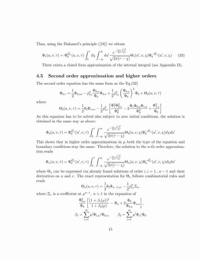
Implementation of the numerical algorithm is done similar to [10]. In typical tests weuse a non-uniform finite difference grid in u and v of size 50x50 nodes, where −50 < u <50, −30 < v < 30. The number of steps in time depends on maturity T , because we usea fixed time step δt = 0.1 yrs. Typical computational time for T = 3 yrs on the same PCat γ = 0.03 is 17 sec. In Fig 1 a 3D plot of the value function V (u, v) is presented for theinitial parameters marked in Table 1 as ’Test 1’. We also use γ = 0.03, α = 1. It is seenthat V (u, v) quickly goes to constant outside of a narrow region around u = 0 and v = 0.

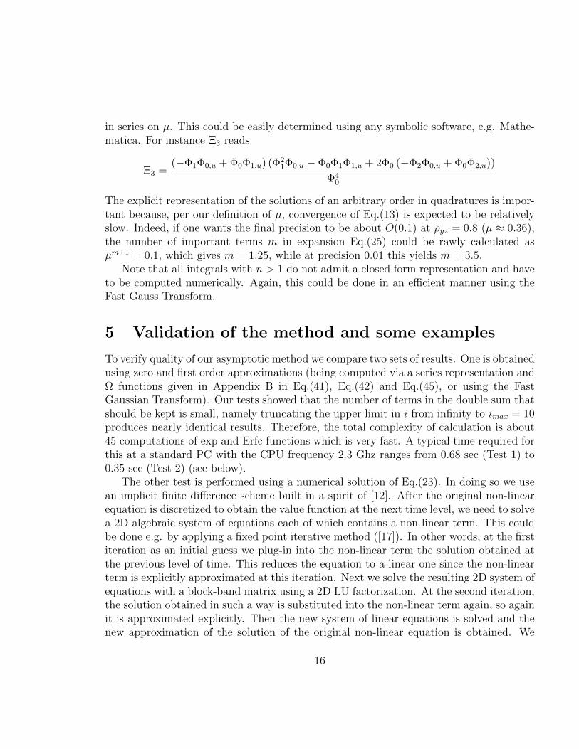
In Fig 2 the same quantities are computed for v0 = 1.22 and T =10 yrs. Here the firstplot presents comparison of the numerical solution with zero and ’0+1’ approximations.The second plot compares the zero and first order approximation. It is seen that the firstapproximation makes a small correction to the zero one in the region closed to u = 0.Also both ’0” and ’0+1’ approximations fit the exact numerical solution relatively well.This proves that our asymptotic closed form solution is robust. Results obtained with asecond set of parameters (Test 2 in the Table 1) are shown in Fig 3. In Fig 4 we presentprice gαZ computed in tests 1,2 as a function of u, where pY is Black-Scholes put price

17

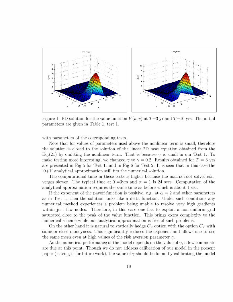
Figure 1: FD solution for the value function V (u, v) at T=3 yr and T=10 yrs. The initialparameters are given in Table 1, test 1.

with parameters of the corresponding tests.Note that for values of parameters used above the nonlinear term is small, therefore

the solution is closed to the solution of the linear 2D heat equation obtained from theEq.(21) by omitting the nonlinear term. That is because γ is small in our Test 1. Tomake testing more interesting, we changed γ to γ = 0.2. Results obtained for T = 3 yrsare presented in Fig 5 for Test 1. and in Fig 6 for Test 2. It is seen that in this case the’0+1’ analytical approximation still fits the numerical solution.

The computational time in these tests is higher because the matrix root solver con-verges slower. The typical time at T=3yrs and α = 1 is 24 secs. Computation of theanalytical approximation requires the same time as before which is about 1 sec.

If the exponent of the payoff function is positive, e.g. at α = 2 and other parametersas in Test 1, then the solution looks like a delta function. Under such conditions anynumerical method experiences a problem being unable to resolve very high gradientswithin just few nodes. Therefore, in this case one has to exploit a non-uniform gridsaturated close to the peak of the value function. This brings extra complexity to thenumerical scheme while our analytical approximation is free of such problems.

On the other hand it is natural to statically hedge CZ option with the option CY withsame or close moneyness. This significantly reduces the exponent and allows one to usethe same mesh even at high values of the risk aversion parameter γ.

As the numerical performance of the model depends on the value of γ, a few commentsare due at this point. Though we do not address calibration of our model in the presentpaper (leaving it for future work), the value of γ should be found by calibrating the model

18

Figure 2: Value function V (u, v) at T=10 yrs obtained by FD scheme, ’0’ and ’0+1’approximations. The initial parameters are given in Table 1, test 1.

Figure 3: Value function V (u, v) at T=10 yrs, comparison of the zero and first orderapproximations. The initial parameters are given in Table 1, test 1.

19

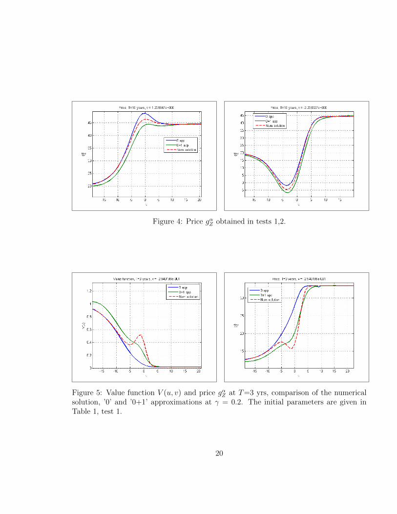
Figure 4: Price gαZ obtained in tests 1,2.

Figure 5: Value function V (u, v) and price gαZ at T=3 yrs, comparison of the numericalsolution, ’0’ and ’0+1’ approximations at γ = 0.2. The initial parameters are given inTable 1, test 1.

20

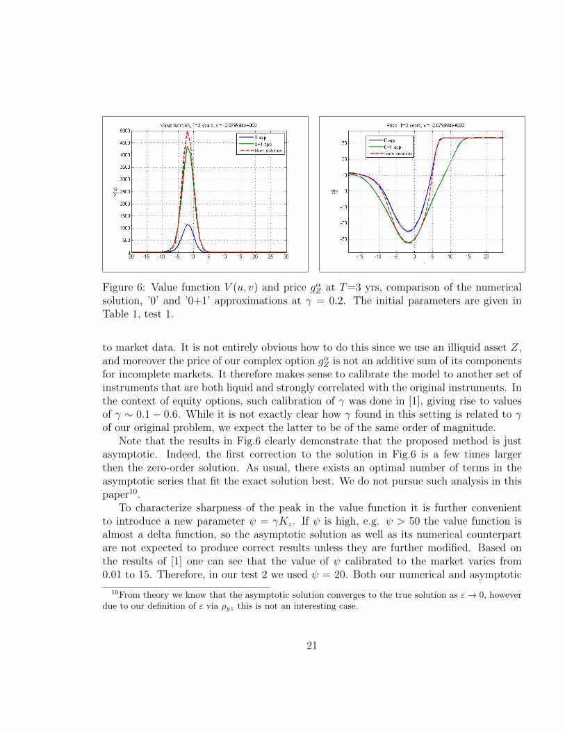
Figure 6: Value function V (u, v) and price gαZ at T=3 yrs, comparison of the numericalsolution, ’0’ and ’0+1’ approximations at γ = 0.2. The initial parameters are given inTable 1, test 1.

to market data. It is not entirely obvious how to do this since we use an illiquid asset Z,and moreover the price of our complex option gαZ is not an additive sum of its componentsfor incomplete markets. It therefore makes sense to calibrate the model to another set ofinstruments that are both liquid and strongly correlated with the original instruments. Inthe context of equity options, such calibration of γ was done in [1], giving rise to valuesof γ ∼ 0.1− 0.6. While it is not exactly clear how γ found in this setting is related to γof our original problem, we expect the latter to be of the same order of magnitude.

Note that the results in Fig.6 clearly demonstrate that the proposed method is justasymptotic. Indeed, the first correction to the solution in Fig.6 is a few times largerthen the zero-order solution. As usual, there exists an optimal number of terms in theasymptotic series that fit the exact solution best. We do not pursue such analysis in thispaper10.

To characterize sharpness of the peak in the value function it is further convenientto introduce a new parameter ψ = γKz. If ψ is high, e.g. ψ > 50 the value function isalmost a delta function, so the asymptotic solution as well as its numerical counterpartare not expected to produce correct results unless they are further modified. Based onthe results of [1] one can see that the value of ψ calibrated to the market varies from0.01 to 15. Therefore, in our test 2 we used ψ = 20. Both our numerical and asymptotic

10From theory we know that the asymptotic solution converges to the true solution as ε→ 0, howeverdue to our definition of ε via ρyz this is not an interesting case.

21

Figure 7: Optimal hedge α∗ computed based on Eq.(7) using the Brent method.

methods work with no problem for these values of ψ.In Fig 7 the optimal hedge α∗ is computed based on Eq.(7) which was solved using

Brent’s method ([17]). The initial parameters correspond to test 1 in Table 1 in the firstplot, and test 2 in the second plot. Note that for u < −15 (the first plot) and u < −20 (thesecond plot), Eq.(7) does not have a minimum, so the maximum is obtained at the edgeof the chosen interval of α. The latter could be defined based on some other preferencesof the trader, for instance, the total capital she wants to invest into this strategy etc.

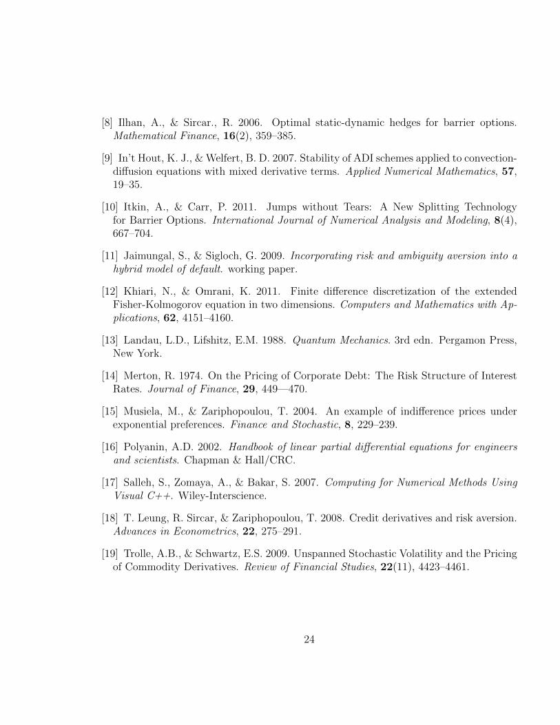
Finally, in Fig 8 price gαZ is presented as a function of α for various γ. It is seen thatthis function is convex which was first showed in [8] in a different setting. Note thatthese results were obtained using a new numerical method mentioned above. It combinesStrang’s splitting with the Fast Gaussian Transform, and accelerates calculations approx-imately by factor 40 as compared with a non-linear version of the 2d Crank-Nicholsonscheme. A detailed description of the method will be given elsewhere.

Acknowledgments

We thank Peter Carr and attendees of the ”Global Derivatives USA 2011” conference foruseful comments. I.H. would like to thank Andrew Abrahams and Julia Chislenko forsupport and interest in this work. We assume full responsibility for any remaining errors.

22

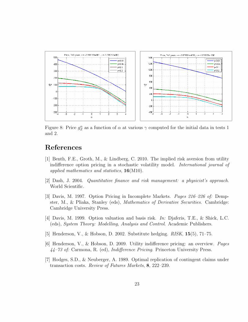
Figure 8: Price gαZ as a function of α at various γ computed for the initial data in tests 1and 2.

References

[1] Benth, F.E., Groth, M., & Lindberg, C. 2010. The implied risk aversion from utilityindifference option pricing in a stochastic volatility model. International journal ofapplied mathematics and statistics, 16(M10).

[2] Dash, J. 2004. Quantitative finance and risk management: a physicist’s approach.World Scientific.

[3] Davis, M. 1997. Option Pricing in Incomplete Markets. Pages 216–226 of: Demp-ster, M., & Pliaka, Stanley (eds), Mathematics of Derivative Securities. Cambridge:Cambridge University Press.

[4] Davis, M. 1999. Option valuation and basis risk. In: Djaferis, T.E., & Shick, L.C.(eds), System Theory: Modelling, Analysis and Control. Academic Publishers.

[5] Henderson, V., & Hobson, D. 2002. Substitute hedging. RISK, 15(5), 71–75.

[6] Henderson, V., & Hobson, D. 2009. Utility indifference pricing: an overview. Pages44–73 of: Carmona, R. (ed), Indifference Pricing. Princeton University Press.

[7] Hodges, S.D., & Neuberger, A. 1989. Optimal replication of contingent claims undertransaction costs. Review of Futures Markets, 8, 222–239.

23

[8] Ilhan, A., & Sircar., R. 2006. Optimal static-dynamic hedges for barrier options.Mathematical Finance, 16(2), 359–385.

[9] In’t Hout, K. J., & Welfert, B. D. 2007. Stability of ADI schemes applied to convection-diffusion equations with mixed derivative terms. Applied Numerical Mathematics, 57,19–35.

[10] Itkin, A., & Carr, P. 2011. Jumps without Tears: A New Splitting Technologyfor Barrier Options. International Journal of Numerical Analysis and Modeling, 8(4),667–704.

[11] Jaimungal, S., & Sigloch, G. 2009. Incorporating risk and ambiguity aversion into ahybrid model of default. working paper.

[12] Khiari, N., & Omrani, K. 2011. Finite difference discretization of the extendedFisher-Kolmogorov equation in two dimensions. Computers and Mathematics with Ap-plications, 62, 4151–4160.

[13] Landau, L.D., Lifshitz, E.M. 1988. Quantum Mechanics. 3rd edn. Pergamon Press,New York.

[14] Merton, R. 1974. On the Pricing of Corporate Debt: The Risk Structure of InterestRates. Journal of Finance, 29, 449—470.

[15] Musiela, M., & Zariphopoulou, T. 2004. An example of indifference prices underexponential preferences. Finance and Stochastic, 8, 229–239.

[16] Polyanin, A.D. 2002. Handbook of linear partial differential equations for engineersand scientists. Chapman & Hall/CRC.

[17] Salleh, S., Zomaya, A., & Bakar, S. 2007. Computing for Numerical Methods UsingVisual C++. Wiley-Interscience.

[18] T. Leung, R. Sircar, & Zariphopoulou, T. 2008. Credit derivatives and risk aversion.Advances in Econometrics, 22, 275–291.

[19] Trolle, A.B., & Schwartz, E.S. 2009. Unspanned Stochastic Volatility and the Pricingof Commodity Derivatives. Review of Financial Studies, 22(11), 4423–4461.

24

A Asymptotic solutions of the Eq.(21)

Here we describe in more detail the solutions for the zero and first order approximationin ε, and outline a generalization of our approach to an arbitrary order in ε.

A.1 Zero-order approximation

In the zero order approximation ε = 0 the Eq.(21) does not contain derivatives wrt v:

Φ0,τ =1

2Φ0,uu −

1

2ρ2xz

(Φ0,u)2

Φ0

(34)

The solution of this equation proceeds along similar lines to Sect. 4.3 using a change ofdependent variable

Φ0(τ, u, v) = [φ(τ, u, v)]1/(1−ρ2xz) (35)

which reduces Eq.(34) to the heat equation

φτ =1

2φuu, (36)

subject to the initial condition φu,v,0 = Φ(u, v, 0)1−ρ2xz . The explicit form for the latter

coincides with (30) provided we substitute γ = γ(1− ρ2xz), ω1 = 1, ζ = 1/β and ω2 = 0.

The explicit zero-order solution thus reads (compare with Eq.(31))

Φ0(u, v, τ) =

[1√2πτ

∫ ∞−∞

e−(u′−u)2

2τ φ(u′, v, 0)du′]1/(1−ρ2

xz)

(37)

Note that Eq.(37) provides the general zero-order solution for the HJB equation witharbitrary initial conditions at τ = 0. For our specific initial conditions Eq.(30), thesolution is readily obtained in closed form in terms of the error (or normal cdf) function(see Appendix B).

A.2 First-order approximation

For the first correction in the Eq.(21) we obtain the following PDE

Φ1,τ =1

2Φ1,uu − ρ2

xz

Φ0,u

Φ0

Φ1,u +1

2ρ2xz

(Φ0,u

Φ0

)2

Φ1 + Θ1(u, v, τ) (38)

where Θ1(u, v, τ) = θ3Φ0,uv.

25

This equation coincides with Eq.(32) except that the free term is different, and the cor-relation parameter is ρxz rather than ρxz. The solution proceeds as in Sect. 4.4, resultingin the following expression:

Φ1(u, v, τ) = Φρ2xz

0 (u, v, τ)

∫ τ

0

dχ

∫ ∞−∞

du′e−

(u−u′)22(τ−χ)√

2π(τ − χ)Θ1(u′, v, χ)Φ

−ρ2xz

0 (u′, v, χ) (39)

The double integral that enters this expression can be split out in two parts. One of themcould be found in closed form, while the other one requires numerical computation (seeAppendix C). Our numerical tests show that for many sets of the initial parameters thefirst integral is much higher than the second one, so the latter could be neglected. However,we were not able to identify in advance at which particular values of the parametersthis could be done. Moreover, for some other initial parameters we observe an oppositesituation.

A.3 Second order approximation and higher orders

The second order equation has the same form as Eq.(38)

Φ2,τ =1

2Φ2,uu − ρ2

xz

Φ0,u

Φ0

Φ2,u +1

2ρ2xz

(Φ0,u

Φ0

)2

Φ2 + Θ2(u, v, τ)

where

Θ2(u, v, τ) =1

2θ2Φ0,vv + θ3 (Φ1,uv − θ3Φ0,uv)−

1

2ρ2xzΦ0 (Φ1/Φ0)

′2u

As this equation has to be solved also subject to zero initial conditions, the solution isobtained in the same way as above:

Φ2(u, v, τ) = Φρ2xz

0 (u′, v, τ)

∫ τ

0

∫ ∞−∞

e−(u−u′)22(τ−χ)√

2π(τ − χ)Θ2(u, v, χ)Φ

−ρ2xz

0 (u′, v, χ)dχdu′

This shows that in higher order approximations in ε the type of the equation to solvedoesn’t change as well as the initial conditions. Therefore, the solution to the n-th orderapproximation reads

Φn(u, v, τ) = Φρ2xz

0 (u′, v, τ)

∫ τ

0

∫ ∞−∞

e−(u−u′)22(τ−χ)√

2π(τ − χ)Θn(u, v, χ)Φ

−ρ2xz

0 (u′, v, χ)dχdu′

26

where Θn can be expressed via already found solutions of order i, i = 1...n− 1 and theirderivatives on u and v. The exact representation for Θn follows combinatorial rules andreads

Θn(u, v, τ) = θ3

n∑i=1

1

(n− i+ 1)!

∂n−i+1ξ(ε)

∂εn−i+1

∣∣∣∣∣ε=0

Φi−1,uv (40)

+1

2θ2

n∑i=2

1

(n− i+ 2)!

∂n−i+2ξ2(ε)

∂εn−i+2

∣∣∣∣∣ε=0

Φi−2,vv −1

2ρ2xzΞn,

where Ξn is a coefficient at εn−1, n > 1 in the following expansion

Φ0

(∂ ln Φ0

∂u

)2

(1 + β3)

[1 +

∂ ln(1 + β)

∂u

(∂ ln Φ0

∂u

)−1]2

, β3 =∞∑i=1

εiΦi/Φ0

In particular, Ξ3 reads

Ξ3 =Φ2Φ2

0,u + Φ0 (Φ21 − 2Φ2Φ0,u)

Φ20

− 2Φ1Φ1,u

Φ0,u

+Φ0Φ2

1,u

Φ20,u

+ 2Φ2,u

The explicit representation of the solutions of an arbitrary order in quadratures is im-portant because per our definition of ε the convergence of the Eq.(13) is expected to beslow. Indeed, if one wants the final precision to be about 0.1 at ρyz = 0.8, the numberof important terms m in the expansion Eq.(13) could be rawly calculated as εm = 0.1,which gives m = 4.5.

All the integrals with n > 1 do not admit a closed form representation and have to becomputed numerically.

B Closed form solutions for the zero-order approxi-

mation

Since our payoff is a piece-wise function, the integral in Eq.(31) can be represented as asum of three integrals. We denote ω = ρxyv/ρxz and represent the zero-order solution asfollows:

Φ0(u, v, τ) =[J

(ζ)1 + J

(ζ)2 + J

(ζ)3

] 1

1−ρ2xz , ζ = sign(v)

27

where sign (−) means that ω = ρxyv/ρxz < 0, and sign (+) - that ω > 0, and

J(+)1 =

1√2πτ

∫ −ω−∞

du′e−(u′−u)2

2τ exp[−γ(Kze

σzρxzρxy

(ω+u′) − αKyeσyu′)]

(41)

= Ω

(−ω,−γKze

σzρxzρxy

ω, σz

ρxzρxy

, γαKy, σy

),

J(+)2 =

1√2πτ

∫ 0

−ωdu′e−

(u′−u)2

2τ exp[−γ(Kz − αKye

σyu′)],

= Ω (0,−γKz, 0, γαKy, σy)− Ω (−ω,−γKz, 0, γαKy, σy) ,

J(+)3 =

e−γ(Kz−αKy)

√2πτ

∫ ∞0

du′e−(u′−u)2

2τ = e−γ(Kz−αKy)

[1− 1

2Erfc

(u√2τ

)],

J(−)1 =

1√2πτ

∫ 0

−∞du′e−

(u′−u)2

2τ exp[−γ(Kze

σzρxzρxy

(ω+u′) − αKyeσyu′)]

= Ω

(0,−γKze

σzρxzρxy

ω, σz

ρxzρxy

, γαKy, σy

),

J(−)2 =

1√2πτ

∫ −ω0

du′e−(u′−u)2

2τ exp[−γ(Kze

σzρxzρxy

(ω+u′) − αKy

)]= Ω

(−ω,−γKze

σzρxzρxy

ω, σz

ρxzρxy

, γαKy, 0

)− Ω

(0,−γKze

σzρxzρxy

ω, σz

ρxzρxy

, γαKy, 0

),

J(−)3 =

e−γ(Kz−αKy)

√2πτ

∫ ∞−ω

du′e−(u′−u)2

2τ =1

2e−γ(Kz−αKy)Erfc

(−u+ ω√

2τ

).

Here Erfc(x) is the complementary error function, and

Ω(a, δ, p, β, q) ≡ 1√2πτ

∫ a

−∞eδe

pu′+βequ′

e−(u′−u)2

2τ du′ (42)

=1√2πτ

∞∑i=0

i∑j=0

δi−jβj

j!(i− j)!

∫ a

−∞e[p(i−j)+qj]u′e−

(u′−u)2

2τ du′

=1

2

∞∑i=0

i∑j=0

δi−jβj

j!(i− j)!eA(u+A τ

2 )Erfc

(u− a+ Aτ√

2τ

),

A = ip+ j(q − p).

Since the complementary error function quickly approaches zero with x 0, or 1 withx 0, the number of terms one has to keep in the above sums should not be high.

28

We also need the following function

Ju,v =1√2πτ

∫ ∞−∞

e−(u′−u)2

2τ φu′,v(u′, v, 0)du′, (43)

when computing the first order approximation. Using a general form of the payoffφ(u, v, 0) = eδ(v)epu+βequ 11, it can be represented in the form

Ju,v =1√2πτ

∫ ∞−∞

e−(u′−u)2

2τ φu′,v(u′, v, 0)du′ (44)

= δ′(v)1√2πτ

∫ ∞−∞

e−(u′−u)2

2τ epu′φ(u′, v, 0)

(p+ equ

′qβ + epu

′pδ(v)

)du′

= J (ζ)1,u,v + J (ζ)

2,u,v + J (ζ)3,u,v,

where

J (+)2,u,v = J (+)

3,u,v = J (−)3,u,v = 0,

J (+)1,u,v = −γKzσze

σzρxzρxy

ωΩ1

(−ω,−γKze

σzρxzρxy

ω, σz

ρxzρxy

, γαKy, σy

)J (−)

1,u,v = −γKzσzeσz

ρxzρxy

ωΩ1

(0,−γKze

σzρxzρxy

ω, σz

ρxzρxy

, γαKy, σy

),

J (−)2,u,v = −γKzσze

σzρxzρxy

ω

Ω1

(−ω,−γKze

σzρxzρxy

ω, σz

ρxzρxy

, γαKy, 0

)

− Ω1

(0,−γKze

σzρxzρxy

ω, σz

ρxzρxy

, γαKy, 0

),

and

Ω1(a, δ, p, β, q) =1

2

∞∑i=0

i∑j=0

δi−jβj

j!(i− j)![pΛ(p) + pδΛ(2p) + qβΛ(p+ q)] , (45)

Λ(b) ≡ eA(b)[u+A(b) τ2 ]Erfc

(u− a+ A(b)τ√

2τ

), A(b) ≡ ip+ j(q − p) + b.

11Compare with Eq.(30).

29

C Transformation of the first order solution of the

Eq.(21)

The first order approximation is given by Eq.(33) where the zero-order solution Φ0(u, v, τ)has been already computed in Appendix B. We plug in this solution into Eq.(33) to obtain

Φ1(u, v, τ) = Φρ2xz

0 (u, v, τ)

∫ τ

0

dχ

∫ ∞−∞

du′e−

(u−u′)22(τ−χ)√

2π(τ − χ)Θ1(u′, v, χ)Φ

−ρ2xz

0 (u′, v, χ) (46)

= θ3Φρ2xz

0 (u, v, τ)

∫ τ

0

dχ

∫ ∞−∞

du′e−

(u−u′)22(τ−χ)√

2π(τ − χ)J(u′, v, χ)

−ρ2xz1−ρ2xz ∂u′,vJ(u′, v, χ)

1

1−ρ2xz ,

J =[J

(ζ)1 + J

(ζ)2 + J

(ζ)3

]where the integrals J

(ζ)i , i = 1, 3 are defined in Eq.(41).

The internal integral can be simplified. Indeed, since

J−ρ2xz1−ρ2xz ∂u,vJ

1

1−ρ2xz =1

1− ρ2xz

Ju′,v +ρ2xz

(1− ρ2xz)

2

JvJu′

J

the internal integral in Eq.(46) can be represented as a sum of two integrals I1 +I2, where

I1 =1

1− ρ2xz

∫ ∞−∞

du′e−

(u−u′)22(τ−χ)√

2π(τ − χ)Ju′,v,

I2 =ρ2xz

(1− ρ2xz)

2

∫ ∞−∞

du′e−

(u−u′)22(τ−χ)√

2π(τ − χ)

JvJu′

J

As we already mentioned the second integral could be either smaller or larger thanthe second one depending on the parameters. This is illustrated in Fig. 9. The initialparameters are taken from test 1 in Table 1 with α = 1 and T = 3 yrs. In Fig. 10 thesame calculation is shown for the parameters corresponding to test 2 in Table 1.

30

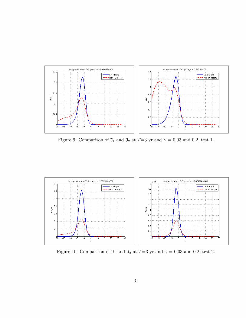
Figure 9: Comparison of I1 and I2 at T=3 yr and γ = 0.03 and 0.2, test 1.

Figure 10: Comparison of I1 and I2 at T=3 yr and γ = 0.03 and 0.2, test 2.

31

The first integral I1 can be rewritten using the integral representation of J in Eq.(31)

I1 =1

1− ρ2xz

∫ ∞−∞

du′e−

(u−u′)22(τ−χ)√

2π(τ − χ)∂u′

∫ ∞−∞

du′′e−

(u′′−u′)22χ

√2πχ

φ0,v(u′′, v, 0)

=1

1− ρ2xz

∫ ∞−∞

du′′φ0,v(u′′, v, 0)

∫ ∞−∞

du′e−

(u−u′)22(τ−χ)√

2π(τ − χ)

u′′ − u′

χ

e−(u′′−u′)2

2χ

√2πχ

=1

1− ρ2xz

∫ ∞−∞

du′′φ0,v(u′′, v, 0)

e−(u−u′′)2

2τ

√2πτ 3/2

(u′′ − u)

Substituting this into Eq.(46) and integrating over χ, we find

Φ1(u, v, τ) =θ3

1− ρ2xz

Φρ2xz

0 (u, v, τ)

∫ τ

0

dχ

∫ ∞−∞

du′′φ0,v(u′′, v, 0)

e−(u−u′′)2

2τ

√2πτ 3/2

(u′′ − u) (47)

=θ3

1− ρ2xz

Φρ2xz

0 (u, v, τ)

∫ ∞−∞

du′′φ0,v(u′′, v, 0)

e−(u−u′′)2

2τ

√2πτ

(u′′ − u)

= − θ3τ

1− ρ2xz

Φρ2xz

0 (u, v, τ)Ju,v. (48)

Thus, the first correction to the solution obtained in the zero order approximation on ε

is approximately −θ3τ

√1−ρ2

yz

1−ρ2xz

Φρ2xz

0 (u, v, τ)Ju,v, and the full solution in the ”0+1” approx-imation reads

Φ(u, v, τ) = Φ0(u, v, τ)− θ3τ

√1− ρ2

yz

1− ρ2xz

Φρ2xz

0 (u, v, τ)Ju,v

D Transformation of the first order solution of Eq.(23)

The first order approximation is given by Eq.(33). It is assumed that the zero-order solu-tion Φ0(u, v, τ) is already computed by using either the method presented in Appendix B,

32

or using the Fast Gauss Transform. We plug in this solution into Eq.(33) to obtain

Φ1(u, v, τ) = Φρ2xz

0 (u, v, τ)

∫ τ

0

dχ

∫ ∞−∞

du′e−

(u−u′)22(τ−χ)√

2π(τ − χ)Θ1(u′, v, χ)Φ

−ρ2xz

0 (u′, v, χ) (49)

=1

2θ2Φ

ρ2xz

0 (u, v, τ)

∫ τ

0

dχ

∫ ∞−∞

du′e−

(u−u′)22(τ−χ)√

2π(τ − χ)J(u′, v, χ)

−ρ2xz1−ρ2xz ∂v,vJ(u′, v, χ)

1

1−ρ2xz ,

J =[J

(ζ)1 + J

(ζ)2 + J

(ζ)3

]where the integrals J

(ζ)i , i = 1, 3 are defined in Eq.(41).

It can be seen that Eq.(49) is similar to Eq.(46) if one replaces ρxz with ρxz and

∂v,vJ(u′, v, χ)1

1−ρ2xz with ∂v,vJ(v, v, χ)1

1−ρ2xz . Therefore, we can use the same idea as inAppendix C to further simplify this integral.

Accordingly the inner integral in Eq.(49) can be rewritten as

J−ρ2xz1−ρ2xz ∂v,vJ

1

1−ρ2xz =1

1− ρ2xz

Jv,v +ρ2xz

(1− ρ2xz)

2

J2v

J

The internal integral in Eq.(49) can then be represented as a sum of two integrals I1 +I2,where

I1 =1

1− ρ2xz

∫ ∞−∞

du′e−

(u−u′)22(τ−χ)√

2π(τ − χ)Jv,v,

I2 =ρ2xz

(1− ρ2xz)

2

∫ ∞−∞

du′e−

(u−u′)22(τ−χ)√

2π(τ − χ)

J2v

J

The first integral I1 can be modified using the integral representation of J in Eq.(31)

I1 =1

1− ρ2xz

∫ ∞−∞

du′e−

(u−u′)22(τ−χ)√

2π(τ − χ)

∫ ∞−∞

du′′e−

(u′′−u′)22χ

√2πχ

φ0,vv(u′′, v, 0)

=1

1− ρ2xz

∫ ∞−∞

du′′φ0,vv(u′′, v, 0)

∫ ∞−∞

du′e−

(u−u′)22(τ−χ)√

2π(τ − χ)

e−(u′′−u′)2

2χ

√2πχ

=1

1− ρ2xz

∫ ∞−∞

du′′φ0,vv(u′′, v, 0)

e−(u−u′′)2

2τ

√2πτ

33

Substituting this into Eq.(49) and integrating over χ, we find

Φ1(u, v, τ) =1

2

θ2

1− ρ2xz

Φρ2xz

0 (u, v, τ)

∫ τ

0

dχ

∫ ∞−∞

du′′φ0,vv(u′′, v, 0)

e−(u−u′′)2

2τ

√2πτ

(50)

=τ

2

θ2

1− ρ2xz

Φρ2xz

0 (u, v, τ)

∫ ∞−∞

du′′φ0,vv(u′′, v, 0)

e−(u−u′′)2

2τ

√2πτ

Thus, the first correction to the solution obtained in the zero order approximation on

µ is approximately 12τθ2

µ1−ρ2

xzΦρ2xz

0 (u, v, τ)Jv,v, and the full solution in the ”0+1” approx-imation reads

Φ(u, v, τ) = Φ0(u, v, τ) +1

2τθ2

µ

1− ρ2xz

Φρ2xz

0 (u, v, τ)Jv,v.

34