Embed Size (px)
Citation preview
Preface i
PREFACE Praise to The One Almighty God because of His grace, His bounty, and His blessing and guidance, we could accomplish this Basic Physics I Experiment Module very well despite carelessness inside. Basic Physics I Experiment Module is intended for semester I students of all Faculties in corporated under Tahap Persiapan Bersama (TPB) Program of Institut Teknologi Bandung (ITB). This experiment module explains about Measurement Methods, Mechanics, and Waves. This module is purposed to sustain the subjects taught in theoretical lecture of Basic Physics I and as supplemental knowledge for the students as well. Experiment given in this module are about measurement methods are discussed in module 1, about waves which are discussed in module 10 and 11, while the topic for other modules is mechanics. The authors hope this experiment module could be a reference of practicum of Basic Physics I course.
Bandung, Sept 2018 Authors
Table of contents ii
TABLE OF CONTENTS PREPACE ......................................................................................... i TABLE OF CONTENTS ...................................................................... ii GUIDELINES FOR BASIC PHYSICS PRACTICUM ...........................iii MODULE 01 BASIC MEASUREMENT AND UNCERTAINTY ............ 1 MODULE 11 STANDING WAVES ON A STRING ............................ 12 MODULE 12 ROLLING MOTION ON AN INCLINED PLANE ........... 16 MODULE 13 MOMENTUM AND COLLISIONS ................................ 21 CONTRIBUTOR ............................................................................... 31 NOTE ......................................................................................... 32 REPORT FORMAT ........................................................................... 33
Guidelines For Basic Physics Practicum iii
GUIDELINES FOR BASIC PHYSICS PRACTICUM 1. Attendance
Practicummust be attended at least 80%of the total number of practicum appointed. If this requirement is not fulfilled, then the student will not pass the practicum and may lead to the failure of Basic Physics course.
Absence due to sickness must be affirmed by official letter which then is given to LFD (Basic Physics Lab) no more than two weeksafter the absence. If this requirement is not fulfilled, then the student will be charged with SANCTION 3.
Tardiness less than twenty minutes is charged withSANCTION 1. Tardiness more than twenty minutes is charged withSANCTION 3. Attendance data will be referred to the data on attendance
computer. Each students is required to confirm their attendance correctly.
2. Requirement of Attending Practicum Behave and be dressed politely. If this requirement is not
fulfilled, then the student will be charged at least with SANCTION 1.
Wear lab coat and put name tag on (with barcode). If this requirement is not fulfilled, then the student will be charged with SANCTION 2.
Finish preliminary task (TP) and do not do it around the LFD just before the practicum, violation of this will cause the TP is not graded.
Prepare yourself for the forthcoming practicum with the substance of its material. Students which are not prepared for practicum may not be permitted to attend the practicum (be charged with SANCTION 3).
3. Implementation of Practicum Obey the code of conduct applied in Basic Physics Laboratory.
Guidelines For Basic Physics Practicum iv
Follow any instruction given by the assistant and the lecturer in charge of the practicum.
Maintain cleanliness and be responsible for the integrity of experimental apparatus.
4. Assessment Practicum scoreis evaluated from Preliminary Task, Preliminary
Test, Activity, and Report. Practicum final score (AP) is the average score of practicum, i.e.
the sum of all the practicum scores is divided by the number of compulsory practicum.
Pass of practicumis evaluated from the practicum final score (AP 50) and the attendance of practicum ( 80%).
Sanctions SANCTION 1 : Score of the corresponding module minus 10. SANCTION 2 : Score of the corresponding module minus 25. SANCTION 3 : Not allowed to attend the practicum;
Score of the corresponding module = ZERO. 5. Administrative Sanction
Administrative sanction is given to students whom during the practicum cause harm, for instance, break/damage the apparatus, omit/leave the Name Tag, etc. Fine cost and substitution procedure are available at administration.
6. Make-Up Practicum and Repetition Generally, there is notany make-up practicum, except for those
who could not attend the practicum because of sickness and other permission. Make-up practicum will be held after the regular practicum has ended. A complete requirements and the schedule will be determined afterward (look for the information on collective announcement board of LFD on the first floor).
Students who intend to repeat the practicummust attend practicum as many as the total number of practicum. The students must attend the ongoing regular practicum by previously registering the
Guidelines For Basic Physics Practicum v
schedule of practicum which suits their own schedule. The registration process is performed at LFD administration before the practicum begins.
7. Others Regular practicum is held on scheduled time, i.e. Morning (07.00
- 10.00), Midday (10.30 - 13.30) and Afternoon (14.00 - 17.00). Practicum that could not be held because of holiday, electrical
failure, etc., will be replaced by substitute practicum after the all of regular practicum has been done.
Code of conduct of behaving politely in the laboratory includes the restriction of foods, drinks, smoking, using walkman, mobile phone and its kind. During practicum, it is not allowed to use mobile phone for phoning, chatting and messaging.
Code of conduct of being dressed politely in the laboratory includes the restriction of wearing sandals and its kind.
Information ofpracticum of Basic Physicsis available onannouncement board outside LFD building on the first floor. Any announcement which is collective (for all students) is written on pink papers. Announcement of each groups (Monday Morning to Friday Afternoon) is written on yellow and blue papers.
Information of practicum and any practicum tasks could be accessed on website http://lfd.itb.ac.id and OA LINE (@god0644g) or announcement board of LFD on the first floor. Students are supposed to access the website by their own and expected to know and understand the information and the tasks provided on the website.
Bandung, Sept 2018 LFD Coordinator

Module 1 - Basic Measurement And Uncertainty 1
MODULE 01 BASIC MEASUREMENT AND UNCERTAINTY
1. EXPERIMENT AIM
1.1. Be able to use and understand basic measuring devices, 1.2. Be able to determine uncertainty on single and repeated
measurements, 1.3. Be able to apply the concept of uncertainty and significant figures in
processing the measurement results.
2. EXPERIMENT APPARATUS 2.1. Ruler, 2.2. Protractor, 2.3. Amperemeter, 2.4. Iron ball, 2.5. Voltmeter, 2.6. Brass/aluminium block, 2.7. Thermometer, 2.8. Hygrometer, 2.9. Micrometer screw, 2.10. Stopwatch, 2.11. Vernier caliper, 2.12. Laboratory barometer, 2.13. Triple beam balance. 2.14. Microscope
3. BASIC THEORY 3.1 Basic measuring device
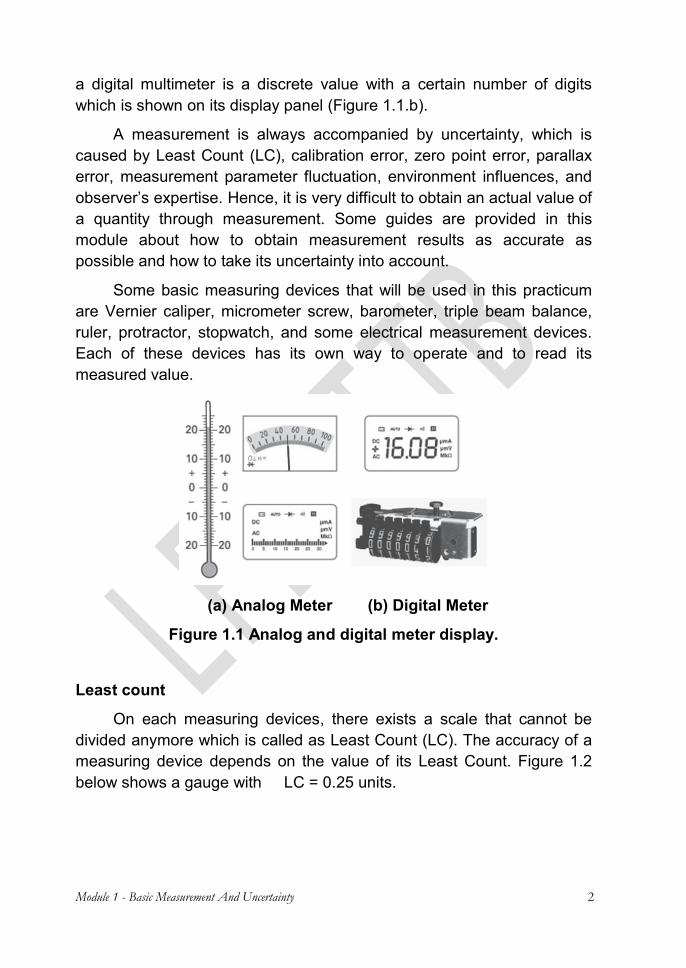
Measuring device is an instrument to determine the value or the size of a physical quantity or variable. In general, basic measuring devices are categorized into two types, i.e. analog measuring device and digital measuring device. An analog measuring device gives its results in continuous value, e.g. temperature shown by conventional thermometer, gauge pointer showing a value in the meters, or electric measurement display (Figure 1.1.a). A digital measuring device gives its results in discrete values. An electric potential or current measurement result using
Module 1 - Basic Measurement And Uncertainty 2
a digital multimeter is a discrete value with a certain number of digits which is shown on its display panel (Figure 1.1.b).
A measurement is always accompanied by uncertainty, which is caused by Least Count (LC), calibration error, zero point error, parallax error, measurement parameter fluctuation, environment influences, and observer’s expertise. Hence, it is very difficult to obtain an actual value of a quantity through measurement. Some guides are provided in this module about how to obtain measurement results as accurate as possible and how to take its uncertainty into account.
Some basic measuring devices that will be used in this practicum are Vernier caliper, micrometer screw, barometer, triple beam balance, ruler, protractor, stopwatch, and some electrical measurement devices. Each of these devices has its own way to operate and to read its measured value.
(a) Analog Meter (b) Digital Meter
Figure 1.1 Analog and digital meter display. Least count
On each measuring devices, there exists a scale that cannot be divided anymore which is called as Least Count (LC). The accuracy of a measuring device depends on the value of its Least Count. Figure 1.2 below shows a gauge with LC = 0.25 units.
Module 1 - Basic Measurement And Uncertainty 3
Figure 1.2 Main scale of a measuring device with LC = 0.25 units.
Nonius
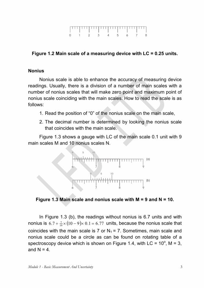
Nonius scale is able to enhance the accuracy of measuring device readings. Usually, there is a division of a number of main scales with a number of nonius scales that will make zero point and maximum point of nonius scale coinciding with the main scales. How to read the scale is as follows:
1. Read the position of “0” of the nonius scale on the main scale, 2. The decimal number is determined by looking the nonius scale
that coincides with the main scale. Figure 1.3 shows a gauge with LC of the main scale 0.1 unit with 9
main scales M and 10 nonius scales N.
Figure 1.3 Main scale and nonius scale with M = 9 and N = 10.
In Figure 1.3 (b), the readings without nonius is 6.7 units and with
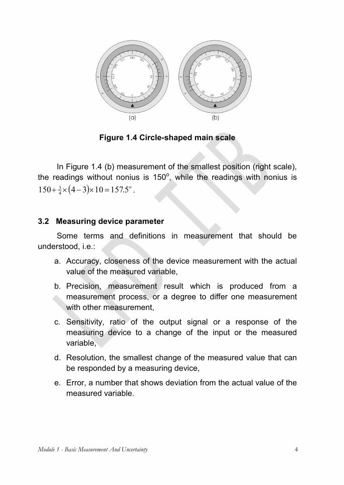
nonius is 77.61.09107.6 107 units, because the nonius scale that coincides with the main scale is 7 or N1 = 7. Sometimes, main scale and nonius scale could be a circle as can be found on rotating table of a spectroscopy device which is shown on Figure 1.4, with LC = 10o, M = 3, and N = 4.
Module 1 - Basic Measurement And Uncertainty 4
Figure 1.4 Circle-shaped main scale
In Figure 1.4 (b) measurement of the smallest position (right scale),
the readings without nonius is 150o, while the readings with nonius is o5.1571034150 43 .
3.2 Measuring device parameter Some terms and definitions in measurement that should be
understood, i.e.: a. Accuracy, closeness of the device measurement with the actual
value of the measured variable, b. Precision, measurement result which is produced from a
measurement process, or a degree to differ one measurement with other measurement,
c. Sensitivity, ratio of the output signal or a response of the measuring device to a change of the input or the measured variable,
d. Resolution, the smallest change of the measured value that can be responded by a measuring device,
e. Error, a number that shows deviation from the actual value of the measured variable.
Module 1 - Basic Measurement And Uncertainty 5
3.3 Uncertainty A measurement is always accompanied by uncertainty, which is
caused by Least Count (LC), calibration error, zero point error, spring error, presence of friction, parallax error, measurement parameter fluctuation, and influences of the environment. These things exist because the measured system is disturbed. Thus, it is very difficult to measure the actual value of a physical quantity. As the consequence, every measurement results should be reported together with its uncertainty. There are two kind of uncertainty, i.e. absolute uncertainty and relative uncertainty. Each uncertainties can be used in a single and repeated measurement.
Absolute uncertainty
Absolute uncertainty is caused by the limitation of the device itself. In a single measurement, the uncertainty is usually taken to be half of the LC. For a quantity X, then its absolute uncertainty in a single measurement is
LCx 21 (1.1) with its measurement result is written as follows.
xxX (1.2) The repeated measurement results can be written in some ways,
such as using half range uncertainty and standard deviation.
Half range uncertainty In repeated measurement, uncertainty is written differently with the
one written in single measurement. Half range uncertainty is one way to express uncertainty in repeated measurement. How to do this is as follows. a. Collect the measurement results of variable x, as many as n, that is
nxxx ...,,, 21 b. Find the mean value, x , as
Module 1 - Basic Measurement And Uncertainty 6
nxxxx n ...21 (1.3)
c. Determine the maxx and minx from the data x and the uncertainty can be written as
2
minmax xxx (1.4) d. The measurement result can be written as
xxx (1.5) For more explanation, an example of measurement results (in mm)
of quantity x which is performed four times: 153.2; 153.6; 152.8; and 153.0. The mean value is
2.15340.1538.1526.1532.153 x mm
The maximum value of the measurement results is 153.6 mm and the minimum value is 152.8 mm, then the measurement results range is
8.08.1526.153 mm and the measurement uncertainty is
4.028.0 x mm
Then, the result of measurement reported is 4.02.153 x mm
Standard deviation
If, in an observation, n measurements of quantity x are performed and the data x1, x2, ..., xn are collected, then the mean value of this quantity is
x n x x x n xn jj
n 1 1
1 21
( ) (1.6)
Deviation value of the mean value from its actual value (x0, which is impossible to be known) is given by standard deviation, that is
Module 1 - Basic Measurement And Uncertainty 7
s x xn
n x xn nx
jjn
j jjn
jn
( )( ) ( )
21
21
21
1 1 (1.7)
Standard deviation given by Eq. (1.7) states that the actual value of quantity x is within an interval from (x - sx) to (x + sx). Therefore, the measurement result is written as x = x±sx. Relative uncertainty
Relative uncertainty is a measure of uncertainty which is obtained from the ratio of absolute uncertainty to the measurement result, that is
xxUCT relative (1.8)
If relative UCT is used, then the measurement result is written as )%100 (relative UCTxX (1.9)
3.4. Uncertainty of a function of variable (propagation of
uncertainty) If a variable is a function of another variables with uncertainties,
then this variable will also have its uncertainty. This kind of thing is called as propagation of uncertainty. For example, a measurement performed gives value aa and bb . Uncertainty of a variable which is a result of an operation of these two variables is given by the formula provided in Table 1.1.
Table 1.1 Example of propagation of uncertainty. Variable Operation Result Uncertainty
bbaa
Addition bap bap Subtraction baq baq Multiplication bar
bb
aa
rr
Division bas b
baa
ss
Module 1 - Basic Measurement And Uncertainty 8
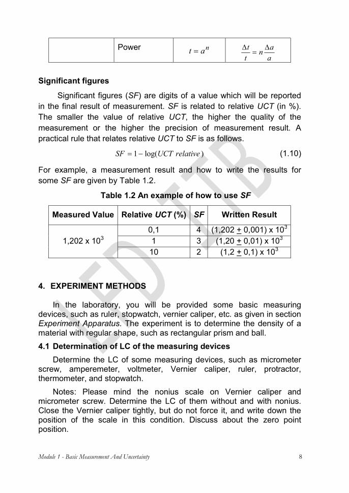
Power nat aant
t Significant figures
Significant figures (SF) are digits of a value which will be reported in the final result of measurement. SF is related to relative UCT (in %). The smaller the value of relative UCT, the higher the quality of the measurement or the higher the precision of measurement result. A practical rule that relates relative UCT to SF is as follows.
)log(1 relativeUCTSF (1.10) For example, a measurement result and how to write the results for some SF are given by Table 1.2.
Table 1.2 An example of how to use SF Measured Value Relative UCT (%) SF Written Result
1,202 x 103 0,1 4 (1,202 + 0,001) x 103 1 3 (1,20 + 0,01) x 103
10 2 (1,2 + 0,1) x 103
4. EXPERIMENT METHODS In the laboratory, you will be provided some basic measuring
devices, such as ruler, stopwatch, vernier caliper, etc. as given in section Experiment Apparatus. The experiment is to determine the density of a material with regular shape, such as rectangular prism and ball. 4.1 Determination of LC of the measuring devices
Determine the LC of some measuring devices, such as micrometer screw, amperemeter, voltmeter, Vernier caliper, ruler, protractor, thermometer, and stopwatch.
Notes: Please mind the nonius scale on Vernier caliper and micrometer screw. Determine the LC of them without and with nonius. Close the Vernier caliper tightly, but do not force it, and write down the position of the scale in this condition. Discuss about the zero point position.
Module 1 - Basic Measurement And Uncertainty 9
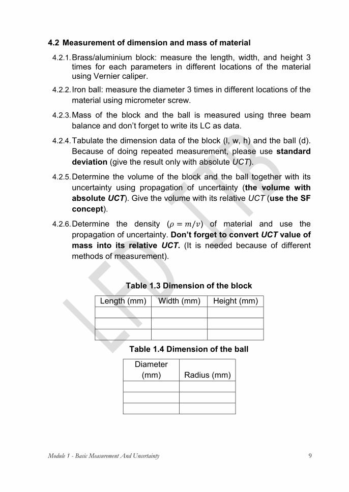
4.2 Measurement of dimension and mass of material 4.2.1. Brass/aluminium block: measure the length, width, and height 3
times for each parameters in different locations of the material using Vernier caliper.
4.2.2. Iron ball: measure the diameter 3 times in different locations of the material using micrometer screw.
4.2.3. Mass of the block and the ball is measured using three beam balance and don’t forget to write its LC as data.
4.2.4. Tabulate the dimension data of the block (l, w, h) and the ball (d). Because of doing repeated measurement, please use standard deviation (give the result only with absolute UCT).
4.2.5. Determine the volume of the block and the ball together with its uncertainty using propagation of uncertainty (the volume with absolute UCT). Give the volume with its relative UCT (use the SF concept).
4.2.6. Determine the density ( = / ) of material and use the propagation of uncertainty. Don’t forget to convert UCT value of mass into its relative UCT. (It is needed because of different methods of measurement).
Table 1.3 Dimension of the block Length (mm) Width (mm) Height (mm)
Table 1.4 Dimension of the ball Diameter
(mm) Radius (mm)
Module 1 - Basic Measurement And Uncertainty 10
4.3 Measurement of physical data of laboratorium condition 4.3.1 Measure the temperature using mercury thermometer located
near the entrance of laboratory in Celsius scale (°C) with single measurement UCT (absolute and relative).
4.3.2 Measure the humidity using hygrometer (near the laboratory entrance and in front of Module 03 room) with single measurement UCT.
4.3.3 Measure the atmospheric pressure using barometer (in front of Module 03 room). The data include the value of P and LC of the barometer, and correction factor of P because of the effect of temperature.
4.3.4 Corrected pressure, make a graph of correction factor against the P, then determine the corresponding line equation. Determine the correction value for the measured atmospheric pressure. The correction value reduce the measured value of P accompanied by its absolute UCT. Calculate regression and standard deviation using a calculator!
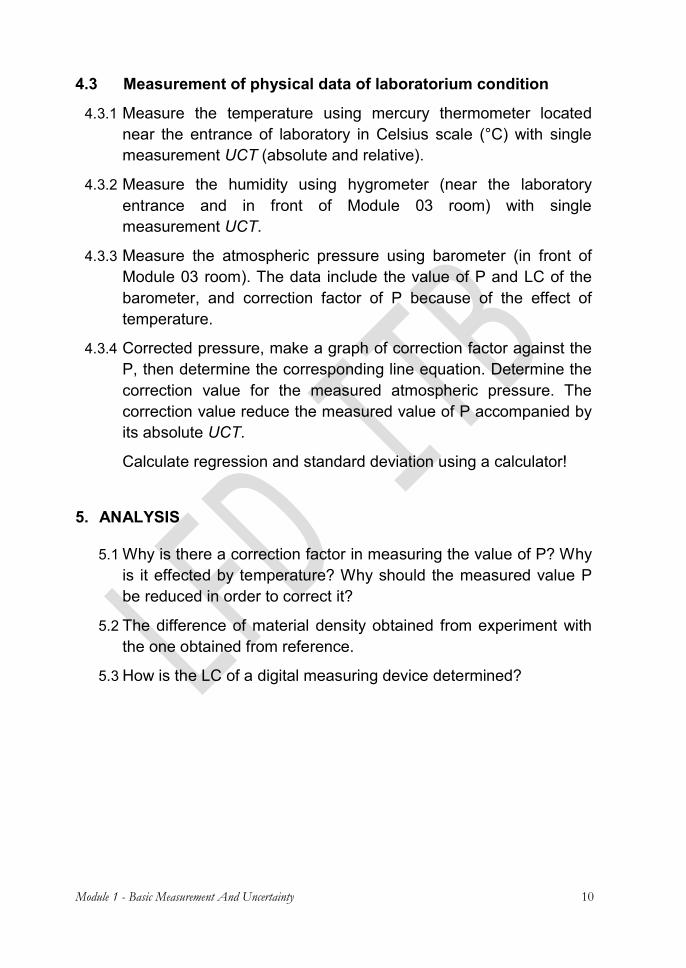
5. ANALYSIS 5.1 Why is there a correction factor in measuring the value of P? Why
is it effected by temperature? Why should the measured value P be reduced in order to correct it?
5.2 The difference of material density obtained from experiment with the one obtained from reference.
5.3 How is the LC of a digital measuring device determined?
Module 1 - Basic Measurement And Uncertainty 11
6. REFERENCES Amend, Bill. (2011) : Physics 16 Laboratory Manual, Armhest
College, 1 – 8. Darmawan Djonoputro, B. (1984) : Teori Ketidak pastian. Penerbit
ITB. Loyd, David H. (2008) : Physics Laboratory Manual, Angelo
University, 13 – 22. Physics Department. (2011) : Introductory Physics Laboratory
Manual, The City University of New York, 3 – 6. School of Physics. 1995 : Physics 160 Laboratory Manual. University
of Melbourne.
Module 11 - Standing Waves On A String 12
MODULE 11 STANDING WAVES ON A STRING
1. EXPERIMENT AIM
1.1. To comprehend the resonance phenomena of waves on a string, 1.1. To determine the speed of stationary wave/standing wave on a
string, 1.2. To determine the frequency of the vibrator.
2. EXPERIMENT APPARATUS
2.1. Melde’s experiment instruments (vibrator, pulley, weight, etc.) 1 set
2.2. Strings with various size & scissor 1 set 2.3. O’Hauss balance 1 item 2.4. Ruler 1 item
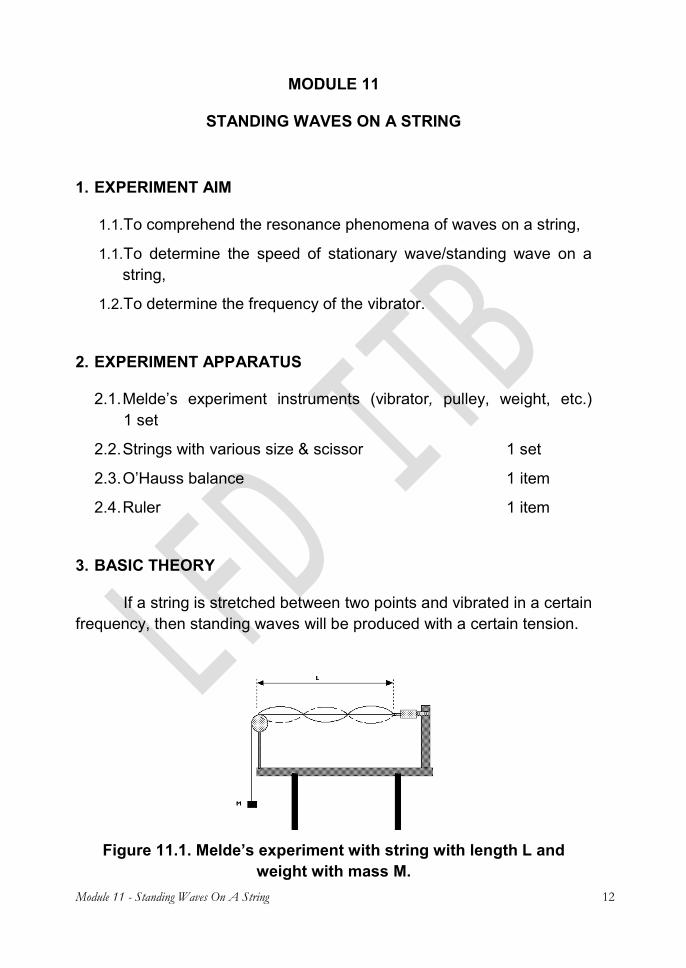
3. BASIC THEORY If a string is stretched between two points and vibrated in a certain frequency, then standing waves will be produced with a certain tension.
Figure 11.1. Melde’s experiment with string with length L and
weight with mass M.
Module 11 - Standing Waves On A String 13
Speed of waves on a string is given by
Tv , (11.1)
where T = tension of the string and = mass per unit length of the string, and the frequency is given by
T
f , (11.2)
where λ = wavelength of the standing wave. 4. EXPERIMENT METHODS 4.4. Standing wave on a single string
4.1.1. Prepare some strings. Measure length and mass of each strings in order to determine its mass per unit length,
4.1.2. Install a string on the Melde’s experiment instrument by tying one of its ends up to the vibrator,
4.1.3. On the other end, some weights, which are already measured, are hung to generate tension on the string,
4.1.4. Turn the vibrator on to generate standing waves, then measure the wavelength (λ) using roll meter,
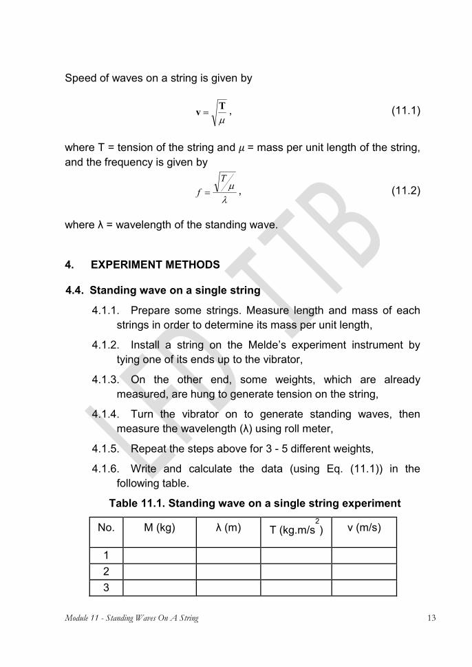
4.1.5. Repeat the steps above for 3 - 5 different weights, 4.1.6. Write and calculate the data (using Eq. (11.1)) in the
following table. Table 11.1. Standing wave on a single string experiment
No. M (kg) λ (m) T (kg.m/s2) v (m/s) 1 2 3
Module 11 - Standing Waves On A String 14
4 5
µ = ............. kg/m 4.1.7. Repeat step 4.1.2 to 4.1.6 for strings with different
thickness, then write and calculate the experiment data for respective string in similar table.
4.5. Standing wave on two connected strings with different
thickness 4.2.1. Repeat the earlier experiment steps to produce standing
waves, but using two string with different thickness which are connected as one!
4.2.2. Observe the resulting standing waves in thin-thick string case (thinner string is connected to the vibrator) and in thick-thin string case (thicker string is connected to the vibrator)!
4.2.3. Measure and compare the following parameters for each strings and configurations: wavelength, amplitude, and other observed differences!
5. REPORT 1.1 Data processing
5.1.1. Present the experiment data and calculation neatly and thoroughly (including the suitable units). Make use of table to present your data!
5.1.2. Use the data of Experiment A to determine frequency of the vibrator through linear regression according to Eq. (11.2). Do the regression for each strings using regular regression (y = mx + c) and regression with fixed intercept point on (0, 0) (y = mx)!
5.1.3. Make comparisons of parameters observed in Experiment B for those two strings configurations!
Module 11 - Standing Waves On A String 15
1.2 Analysis 5.2.1. Is Melde’s law valid according to this experiment?
Determine any parameters affecting the wavelength and the speed of waves on the strings in this experiment!
5.2.2. Explain how to determine the frequency of the vibrator in this experiment! How is the result compared to the frequency of PLN’s signal (f ≈ 50 Hz)? Which method of linear regression does give closer result to the reference (with intercept point fixed to (0, 0) or not)?
5.2.3. Explain the comparison of data (wavelength and amplitude) obtained for thicker string and thinner string according to your knowledge of propagation of wave through discontinuity!
5.2.4. How could the experiment methods you have already performed be improved so that phenomena of standing waves could be comprehended better?
6. REFERENCES
Resnick, Robert., Halliday, David, Krane, Kenneth S. (1992). Physics 4th Edition Vol. 1. John Wiley & Sons, 418 – 419.
Tyler, F. (1970) : A Laboratory Manual of Physics, Edward Arnold, 96 – 97.
Module 12 - Rolling Motion On An Inclined Plane 16
MODULE 12 ROLLING MOTION ON AN INCLINED PLANE
1. EXPERIMENT AIM
1.1. To determine constants of moment of inertia experimentally, 1.2. To determine the ratio of translational kinetic energy to rotational
kinetic energy of a rolling object. 2. EXPERIMENT APPARATUS
2.1. One set of sliding board equipped with IR sensor and interface box, 2.2. Some cylindrical objects, 2.3. Power supply and serial connection cable, 2.4. PC to control and display data from the interface, 2.5. Protractor to measure distance and determine inclination of the
sliding board. 3. BASIC THEORY
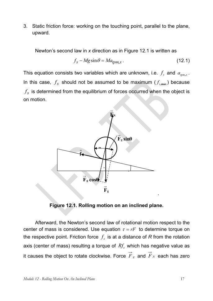
A point-particle object sliding down along an inclined plane with an angle of θ will experience an acceleration a = g sinθ. If the object is a rigid body which is able to rotate, then the motion is not as simple as the point particle. Figure 12.1 shows a uniform object with mass M and radius R rolling without slipping down along an inclined plane with an angle of θ, along the direction of x axis. Acceleration of the object atpm,x while climbing down the incline could be derived using Newton’s second law of translational motion aMFnet . and rotational motion .Inet . The first step is to draw the free body diagram of the object as in Figure 12.1, with 1. Gravitational force: downward, 2. Normal force: perpendicular to the inclined plane,
Module 12 - Rolling Motion On An Inclined Plane 17
3. Static friction force: working on the touching point, parallel to the plane, upward.
Newton’s second law in x direction as in Figure 12.1 is written as
xtpms MaMgf ,sin . (12.1) This equation consists two variables which are unknown, i.e. sf and xtpma , . In this case, sf should not be assumed to be maximum ( max,sf ) because sf is determined from the equilibrium of forces occurred when the object is
on motion.
` Figure 12.1. Rolling motion on an inclined plane.
Afterward, the Newton’s second law of rotational motion respect to the
center of mass is considered. Use equation rF to determine torque on the respective point. Friction force sf is at a distance of R from the rotation axis (center of mass) resulting a torque of sRf which has negative value as it causes the object to rotate clockwise. Force gF and NF each has zero
R Sf
sinθFg
gF cosθFg
NF
Module 12 - Rolling Motion On An Inclined Plane 18
moment arm, thus resulting no torque. Therefore, the Newton’s second law of rotational body ( Inet ) respect to its center of mass is
tpms IRf . (12.2) This equation also has two variables which are still unknown, i.e. sf and . Because the object is assumed to roll without slipping, then equation Ratpm is useful to relate xtpma , with . Note that xtpma , has positive value (object moves to x positive) and has negative value (object rotates clockwise). As a result, should be substituted with
Ra xtpm /, . Take this relation into Eq. (12.2) and simplify the equation to obtain sf .
2RaIf xtpm
tpms, (12.3)
By substituting sf in Eq. (12.1), it could be shown that
21 MRIgatpm
xtpm sin, .
(12.4)
This equation will come in handy to determine the translational acceleration of the object ( xtpma , ) on an inclined plane with an angle of . 4. EXPERIMENT METHODS
Experiment is performed by letting a rigid body rolls along an inclined plane with an adjustable angle. The sliding board is equipped with 9 pairs of infrared sensors (IR, infra red) connected to interface box. Electronic circuitry inside the interface box is to measure time interval every time the object passing each pair of IR sensors. This time interval data is then displayed on the PC to be processed further. 4.1. Start with recognizing the program to control the interface from the PC,
a. The ”Open” button is to activate communication channel between the PC and the interface,
Module 12 - Rolling Motion On An Inclined Plane 19
b. The ”Reset” button is to return the interface condition to its initial condition,
c. The ”Activate” button is to active the sensor circuitry. Measurement will start (t = 0) as soon as the object passes the first pair of IR sensor. After successfully activating the sensor system, this button changes its function to ”Turn Off” that will return the interface to non-active condition,
d. The ”Check Sensors” button is to check that all sensors are functioning normally,
e. The ”Read Data” button is to display the latest set of data which is successfully measured,
f. The ”Set Timeout” button is to adjust the maximum time interval allowed for the object to pass the first sensor to the last sensor. This kind of function is needed to end the measurement in case of the rolling object fails to reach the last sensor (e.g. the object deviates from the trajectory),
g. The ”Clear Screen” button is to clear the display on response screen.
4.2. Decide a position as the START line on the upper part of the sliding board. Maintain this position as the starting point of each measurements during the experiment,
4.3. Measure carefully the distance of the first sensor, second sensor, and so on from the zeroth sensor as position data x0, x1, x2, ... ,
4.4. Adjust inclination angle of the sliding board by putting something beneath to sustain it,
4.5. Adjust position of the object so that it can move as parallel as possible with the left and right edges of the sliding board,
4.6. From the START position, release the object and let it rolls down along the incline. Time measurement will start as soon as the object passes the first sensor and will end after the object passes the last sensor (FINISH position). If the experiment goes well, all measurement results will be displayed on response screen. Else, message ”Time Out” will appear. Write all of time measurement data as t0, t1, t2, ... ,
Module 12 - Rolling Motion On An Inclined Plane 20
4.7. Using a certain spreadsheet program (such as MS Excel), make a graph of x as a function of t and determine the parameters,
4.8. Repeat the experiment for various cylindrical objects and several inclination angle of the sliding board according to the task given by the assistant.
5. REPORT
5.1. Using the parameters obtained from the experiment (time, angle, and positions of sensors) and translational acceleration of center of mass equation, find the constant of moment of inertia of the objects!
5.2. Make a plot that compares translational kinetic energy to rotational kinetic energy in the end of the rolling motion by assuming that the object rolls without slipping during the process!
5.3. Compare the constants of moment of inertia obtained from the experiment to the existing theory. Explain why there are differences!
5.4. Why is the curve of distance (x) against time (t) not passing (0,0)? What would you conclude from the graph?
5.5. In your opinion, how can this experiment be used to detect at what angle the rolling object starts to slip?
6. REFERENCES
Resnick, Robert., Halliday, David, Krane, Kenneth S. (1992). Physics 4th Edition Vol. 1. John Wiley & Sons, 418 – 419.
Tyler, F. (1970) : A Laboratory Manual of Physics, Edward Arnold, 19.
Module 13 - Momentum And Collisions 21
MODULE 13 MOMENTUM AND COLLISIONS
1. EXPERIMENT AIM
1.1 To comprehend the principle of conservation of momentum, 1.2 To calculate velocities of the system at various states of collision, 1.3 To compare the momentum before and after a collision, 1.4 To compare the kinetic energy before and after a collision, 1.5 To observe various events of collision possible of two objects.
2. EXPERIMENT APPARATUS
2.1. Air Track set, 2.2. Photogate sensor, 2.3. Mini LabQuest, 2.4. Lattices, 2.5. Gliders, 2.6. Weights, 2.7. Weighing scale.
3. BASIC THEORY
In this module, phenomena common to our daily life will be studied, that is the phenomena of impulse and momentum. 3.1. Momentum
Momentum of an object is defined as multiplication of its mass with its velocity. Momentum represents a measure of how difficult to alter the tendency of an object’s motion. Mathematically, linear momentum is formulated as follows.
p = m.v (13.1)
Module 13 - Momentum And Collisions 22
where m is the object’s mass and v is its velocity. The total force applied to the object causes change in the momentum over time as formulated in the following equation.
∑F = (13.2) =
= ∑F = (13.3)
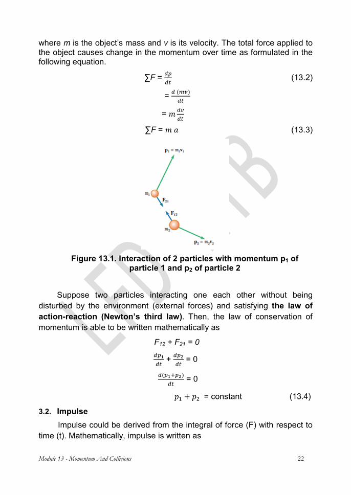
Figure 13.1. Interaction of 2 particles with momentum p1 of
particle 1 and p2 of particle 2
Suppose two particles interacting one each other without being disturbed by the environment (external forces) and satisfying the law of action-reaction (Newton’s third law). Then, the law of conservation of momentum is able to be written mathematically as
F12 + F21 = 0 + = 0
= 0 = constant (13.4)
3.2. Impulse Impulse could be derived from the integral of force (F) with respect to
time (t). Mathematically, impulse is written as
Module 13 - Momentum And Collisions 23
F = dp = F dt
I = = = p2 – p1 = ∆p (13.5)
3.3. Collision
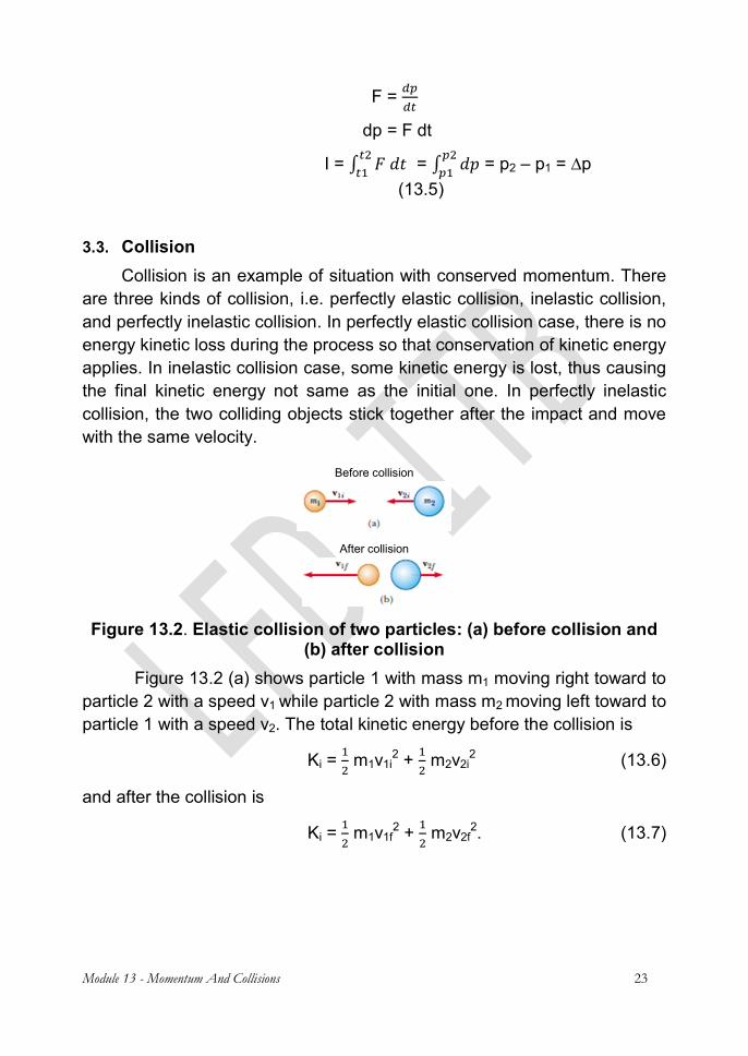
Collision is an example of situation with conserved momentum. There are three kinds of collision, i.e. perfectly elastic collision, inelastic collision, and perfectly inelastic collision. In perfectly elastic collision case, there is no energy kinetic loss during the process so that conservation of kinetic energy applies. In inelastic collision case, some kinetic energy is lost, thus causing the final kinetic energy not same as the initial one. In perfectly inelastic collision, the two colliding objects stick together after the impact and move with the same velocity.
Before collision
After collision
Figure 13.2. Elastic collision of two particles: (a) before collision and
(b) after collision Figure 13.2 (a) shows particle 1 with mass m1 moving right toward to
particle 2 with a speed v1 while particle 2 with mass m2 moving left toward to particle 1 with a speed v2. The total kinetic energy before the collision is
Ki = m1v1i2 + m2v2i2 (13.6) and after the collision is
Ki = m1v1f2 + m2v2f2. (13.7)
Module 13 - Momentum And Collisions 24
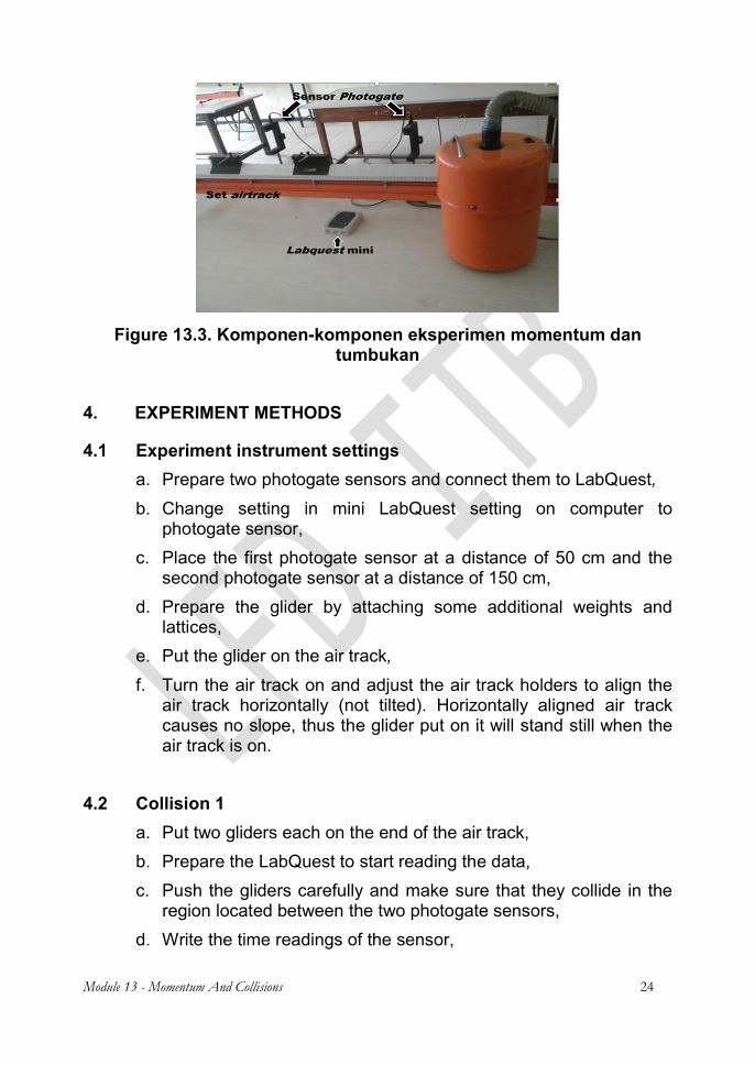
Figure 13.3. Komponen-komponen eksperimen momentum dan
tumbukan
4. EXPERIMENT METHODS 4.1 Experiment instrument settings
a. Prepare two photogate sensors and connect them to LabQuest, b. Change setting in mini LabQuest setting on computer to
photogate sensor, c. Place the first photogate sensor at a distance of 50 cm and the
second photogate sensor at a distance of 150 cm, d. Prepare the glider by attaching some additional weights and
lattices, e. Put the glider on the air track, f. Turn the air track on and adjust the air track holders to align the
air track horizontally (not tilted). Horizontally aligned air track causes no slope, thus the glider put on it will stand still when the air track is on.
4.2 Collision 1 a. Put two gliders each on the end of the air track, b. Prepare the LabQuest to start reading the data, c. Push the gliders carefully and make sure that they collide in the
region located between the two photogate sensors, d. Write the time readings of the sensor,
Module 13 - Momentum And Collisions 25
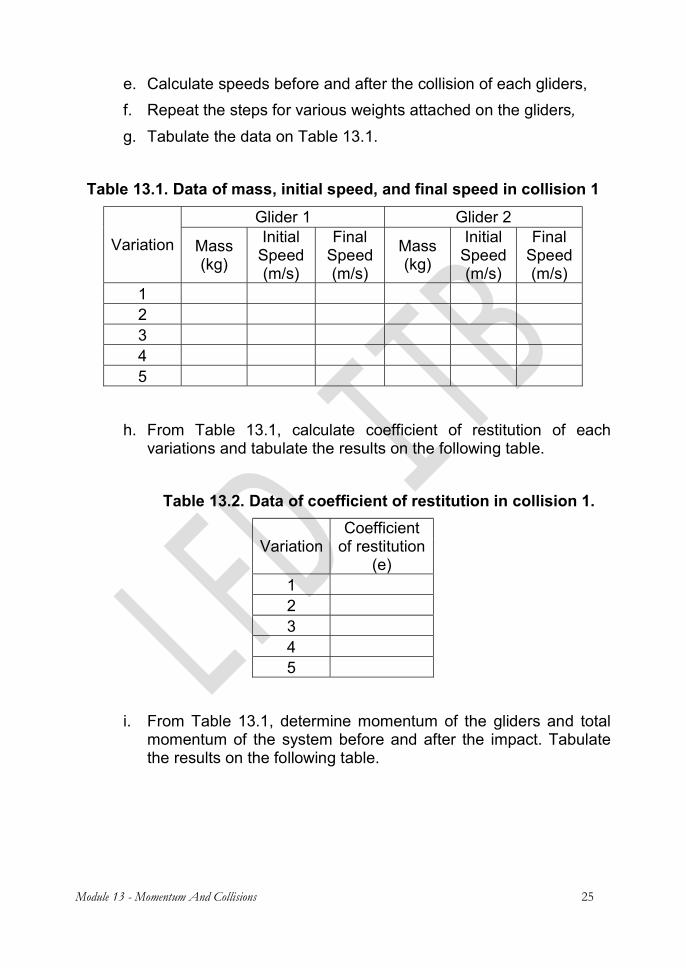
e. Calculate speeds before and after the collision of each gliders, f. Repeat the steps for various weights attached on the gliders, g. Tabulate the data on Table 13.1.
Table 13.1. Data of mass, initial speed, and final speed in collision 1
Variation Glider 1 Glider 2
Mass (kg)
Initial Speed (m/s)
Final Speed (m/s)
Mass (kg)
Initial Speed (m/s)
Final Speed (m/s)
1 2 3 4 5
h. From Table 13.1, calculate coefficient of restitution of each
variations and tabulate the results on the following table.
Table 13.2. Data of coefficient of restitution in collision 1. Variation
Coefficient of restitution
(e) 1 2 3 4 5
i. From Table 13.1, determine momentum of the gliders and total
momentum of the system before and after the impact. Tabulate the results on the following table.
Module 13 - Momentum And Collisions 26
Table 13.3. Data of momentum of glider 1, glider 2, and the system before and after the impact in collision 1.
Variation Before Collision After Collision
p glider 1 (kg m/s)
p glider 2 (kg m/s)
p system (kg m/s)
p glider 1 (kg m/s)
p glider 2 (kg m/s)
p system
(kg m/s)
1 2 3 4 5
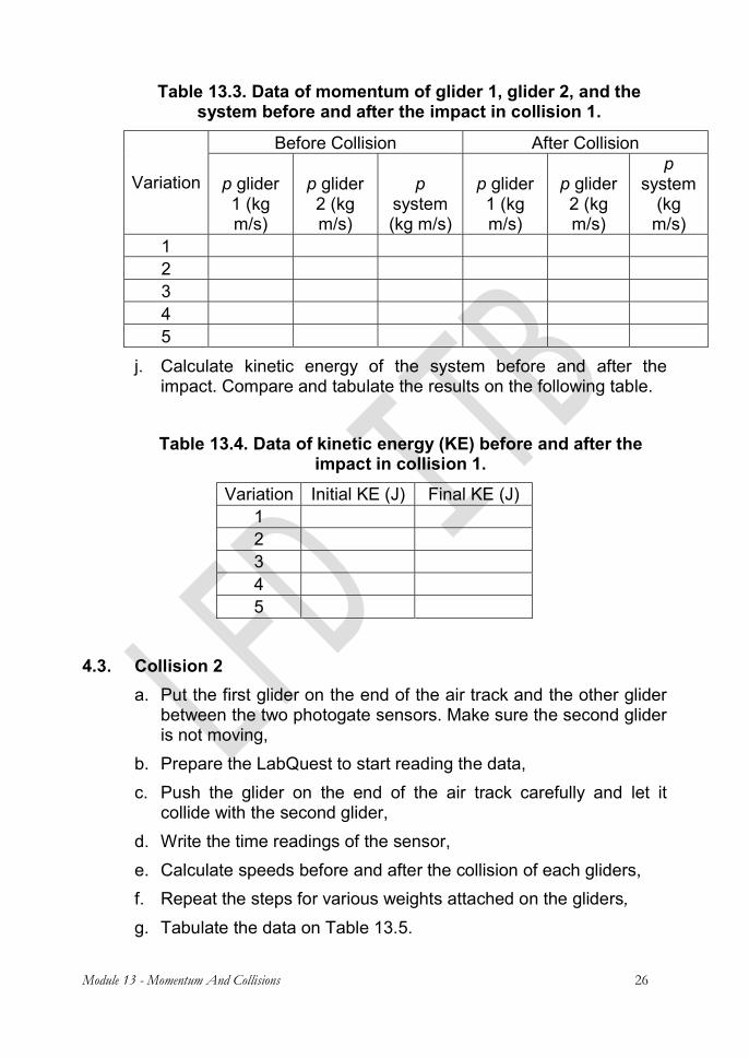
j. Calculate kinetic energy of the system before and after the impact. Compare and tabulate the results on the following table.
Table 13.4. Data of kinetic energy (KE) before and after the
impact in collision 1. Variation Initial KE (J) Final KE (J)
1 2 3 4 5
4.3. Collision 2
a. Put the first glider on the end of the air track and the other glider between the two photogate sensors. Make sure the second glider is not moving,
b. Prepare the LabQuest to start reading the data, c. Push the glider on the end of the air track carefully and let it
collide with the second glider, d. Write the time readings of the sensor, e. Calculate speeds before and after the collision of each gliders, f. Repeat the steps for various weights attached on the gliders, g. Tabulate the data on Table 13.5.
Module 13 - Momentum And Collisions 27
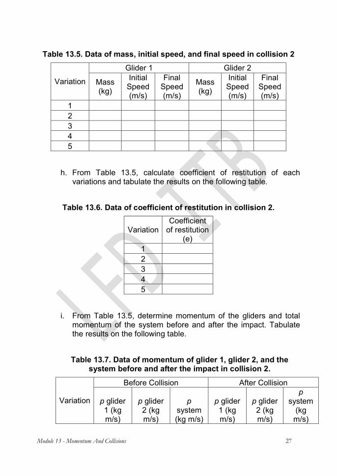
Table 13.5. Data of mass, initial speed, and final speed in collision 2
Variation Glider 1 Glider 2
Mass (kg)
Initial Speed (m/s)
Final Speed (m/s)
Mass (kg)
Initial Speed (m/s)
Final Speed (m/s)
1 2 3 4 5
h. From Table 13.5, calculate coefficient of restitution of each
variations and tabulate the results on the following table.
Table 13.6. Data of coefficient of restitution in collision 2. Variation
Coefficient of restitution
(e) 1 2 3 4 5
i. From Table 13.5, determine momentum of the gliders and total
momentum of the system before and after the impact. Tabulate the results on the following table.
Table 13.7. Data of momentum of glider 1, glider 2, and the
system before and after the impact in collision 2.
Variation Before Collision After Collision
p glider 1 (kg m/s)
p glider 2 (kg m/s)
p system (kg m/s)
p glider 1 (kg m/s)
p glider 2 (kg m/s)
p system
(kg m/s)
Module 13 - Momentum And Collisions 28
1 2 3 4 5
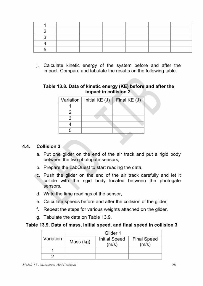
j. Calculate kinetic energy of the system before and after the impact. Compare and tabulate the results on the following table.
Table 13.8. Data of kinetic energy (KE) before and after the
impact in collision 2. Variation Initial KE (J) Final KE (J)
1 2 3 4 5
4.4. Collision 3
a. Put one glider on the end of the air track and put a rigid body between the two photogate sensors, b. Prepare the LabQuest to start reading the data, c. Push the glider on the end of the air track carefully and let it
collide with the rigid body located between the photogate sensors, d. Write the time readings of the sensor, e. Calculate speeds before and after the collision of the glider, f. Repeat the steps for various weights attached on the glider, g. Tabulate the data on Table 13.9.
Table 13.9. Data of mass, initial speed, and final speed in collision 3
Variation Glider 1
Mass (kg) Initial Speed (m/s)
Final Speed (m/s)
1 2
Module 13 - Momentum And Collisions 29
3 4 5
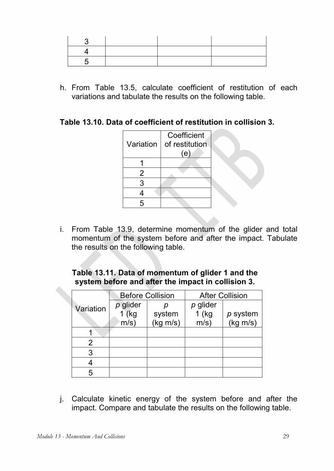
h. From Table 13.5, calculate coefficient of restitution of each
variations and tabulate the results on the following table. Table 13.10. Data of coefficient of restitution in collision 3.
Variation Coefficient
of restitution (e)
1 2 3 4 5
i. From Table 13.9, determine momentum of the glider and total
momentum of the system before and after the impact. Tabulate the results on the following table.
Table 13.11. Data of momentum of glider 1 and the system before and after the impact in collision 3.
Variation Before Collision After Collision
p glider 1 (kg m/s)
p system (kg m/s)
p glider 1 (kg m/s)
p system (kg m/s)
1 2 3 4 5
j. Calculate kinetic energy of the system before and after the
impact. Compare and tabulate the results on the following table.
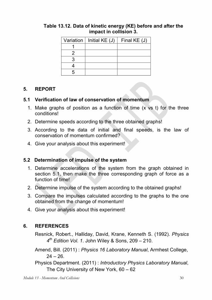
Module 13 - Momentum And Collisions 30
Table 13.12. Data of kinetic energy (KE) before and after the impact in collision 3.
Variation Initial KE (J) Final KE (J) 1 2 3 4 5
5. REPORT 5.1 Verification of law of conservation of momentum
1. Make graphs of position as a function of time (x vs t) for the three conditions!
2. Determine speeds according to the three obtained graphs! 3. According to the data of initial and final speeds, is the law of
conservation of momentum confirmed? 4. Give your analysis about this experiment!
5.2 Determination of impulse of the system
1. Determine accelerations of the system from the graph obtained in section 5.1, then make the three corresponding graph of force as a function of time!
2. Determine impulse of the system according to the obtained graphs! 3. Compare the impulses calculated according to the graphs to the one obtained from the change of momentum! 4. Give your analysis about this experiment!
6. REFERENCES Resnick, Robert., Halliday, David, Krane, Kenneth S. (1992). Physics
4th Edition Vol. 1. John Wiley & Sons, 209 – 210. Amend, Bill. (2011) : Physics 16 Laboratory Manual, Armhest College,
24 – 26. Physics Department. (2011) : Introductory Physics Laboratory Manual,
The City University of New York, 60 – 62
CONTRIBUTOR 31
CONTRIBUTOR This practical module book was written by Lecturers of Physics Studies Program: M. Hamron Hendro R. Hamron R. Soegeng Soejoto Suprapto A. Rustan Rukmantara Umar Fauzi Moerjono Doddy S. Hasbuna Kifli M. Birsyam Suparno Satira Neny K. Euis Sustini Daniel K. Pepen Arifin Triyanta Agoes S. Revision: This module book has been revised several times when the LFD is coordinated by Dr. Hendro, M.Si. The latest revision was made in 2016 by Dr. Hendro, M.Si. Assisted by technical assistants consisting of Valdi Rizki Yandri, Dewanto Kamas Utomo, Fandy Gustiara, Wilson Jefriyanto, and Jerfi.

Note 32
NOTE: Date : .…./………./20 …………………………………………………………………………………………. …………………………………………………………………………………………. …………………………………………………………………………………………. …………………………………………………………………………………………. …………………………………………………………………………………………. …………………………………………………………………………………………. …………………………………………………………………………………………. …………………………………………………………………………………………. …………………………………………………………………………………………. …………………………………………………………………………………………. …………………………………………………………………………………………. …………………………………………………………………………………………. …………………………………………………………………………………………. …………………………………………………………………………………………. …………………………………………………………………………………………. …………………………………………………………………………………………. …………………………………………………………………………………………. …………………………………………………………………………………………. …………………………………………………………………………………………. ………………………………………………………………………………………….
Report Format 33


![Predgovor [Preface.]](https://img.dokumen.tips/doc/110x75/6336ef3f20d9c9602f0b14a3/predgovor-preface.jpg)


