Embed Size (px)
Citation preview
In: Handbook on Oil Production Research ISBN: 978-1-63321-856-7
Editor: Jacquelyn Ambrosio © 2014 Nova Science Publishers, Inc.
Chapter 6
PREDICTION OF STEAM DISTILLATION
EFFICIENCY DURING STEAM INJECTION
PROCESS USING A RIGOROUS METHOD
Sh. Mohammadi,1 M. Nikookar,*2
M. R. Ehsani,1
L. Sahranavard2 and A. H. Mohammadi†
3,4
1 Department of Chemical Engineering,
Isfahan University of Technology, Isfahan, Iran 2 Department of Chemical Engineering,
Tarbiat Modares University, Tehran, Iran 3 Institut de Recherche en Génie Chimique et Pétrolier (IRGCP),
Paris Cedex, France 4 Thermodynamics Research Unit, School of Chemical Engineering,
University of KwaZulu-Natal, Howard College Campus,
Durban, South Africa
ABSTRACT
Steam distillation mechanism is one of the important and effective
mechanisms during steam injection process in fractured heavy oil
reservoirs. Due to its important effect in oil recovery, several attempts
have been made to simulate this process experimentally and theoretically.
* Corresponding Author: M. Nikookar: E-mail: [email protected]. † Corresponding Author: A. H. Mohammadi, E-mail: [email protected].
Complimentary Contributor Copy
Sh. Mohammadi, M. Nikookar, M. R. Ehsani et al. 198
Because of limitations in implementing experiments, various models have
been studied to predict the distillation effect with minimum entry
parameters. So, in this study, a Multi-Layer Perceptron (MLP) neural
network is used as an effective method to simulate the distillate recovery,
so that some parameters such as API, viscosity, characterization factor
and steam distillation factor are the input parameters and distillate yield is
the model‘s output. After gathering our data from some references, 77
data of 128 input data were used for training, 33 data for testing, and 18
data for cross validation. Then, the results of one-layer and two-layer
networks with various neurons were compared with the experimental data
and some other models.
Keywords: Heavy Oil, Steam Injection, Distillation, Neural Network, Multi
Layer Perceptron
INTRODUCTION
Naturally fractured reservoirs contain about 30% of the world oil supply.
Oil recovery from such reservoirs can be modelled as a two-step process:
mechanisms causing oil to be expelled from the matrix and mechanisms
expelling the oil through the fracture network to a production well [1].
An important phenomenon during steam injection is steam distillation of
light components of the crude oil, so that if pressure is lower than sum of the
partial pressures of water and oil, the liquid mixture will boil and give off a
vapor phase composed of steam and organic compounds. Steam and vaporized
hydrocarbons will be condensed as they reach to the cooler regions and mixed
with the crude oil and decrease its viscosity and increase the oil recovery.
Since steam is injected continuously in this process, condensation and
vaporization mechanisms are repeated during the process. [1]
Enhanced oil recovery processes based on steam injection are of the most
popular and effective methods used widely in the oil recovery industries. Oil
displacement in these processes involves simultaneous heat, mass, and fluid
transport. Several investigations have been performed to evaluate the
contribution of different mechanisms to oil recovery in these methods.
According to above studies, steam distillation mechanism highly affects
on enhanced oil recovery as same as viscosity reduction [2]. The earliest
simple mathematical models have been presented by Bailey, Holland and
Welch, and Winkle [3,4,5]. Wu and Elder [6] proposed correlations to estimate
steam distillation yields. Then, Dureksen and Hsueh [7] developed correlations
Complimentary Contributor Copy

Prediction of Steam Distillation Efficiency … 199
for prediction of steam distillation yield with different crude characteristics
and operating conditions. They also found that steam distillation yield can be
well correlated with API gravity and wax content. Langhoff and Wu [8], based
on the simple and practical method of Holland and Welch, presented one
equation for prediction of steam distillation yield. They assumed that steam
injection rate is constant and the solubility of hydrocarbon and water are
negligible [4]. Van Winkle predicts the amount of steam required for
distillation of a specific amount of a volatile material based on the Raoult and
Dalton laws [5]. Northrop and Venkatesan [9] presented an analytical model to
predict steam distillation yield by using the modified Van Winkle approach.
Their model predicts an increased distillation yield by an increased
temperature.
Some researchers calculcated steam distillation yield by using a cubic
equation of state [10]. Most of the presented models depended on efficiency
factors that are obtained from experimental data. So, they could not be used
for new crude oil samples. Therefore, using a general model that can predict
steam distillation yield with less entry parameters is necessary. Recently,
neural network has been used for thermodynamic calculation of vapor - liquid
equilibrium. Considering the above issue and also, nonlinearity of steam
distillation mechanism, using artificial neural network (ANN) for simulation
of steam distillation yield seems to be suitable. [11,12,13,14,15]
In this study, steam distillation yield during steam injection has been
modeled by the Multi Layer Preceptron (MLP). Input parameters include API,
viscosity, and steam distillation factor and output parameter is steam
distillation yield. Finally, the results of one-layer and two-layer ANN with
various neurons were compared with the experimental data and other available
models.
ARTIFICIAL NEURAL NETWORK
Components of Neural Network
Generally, one neural network includes 1) inputs and outputs: numbers as
one or more variables make inputs. After training, the input parameters are
converted to one or more output variables. The inputs are independent, but the
outputs are dependent variables. 2) neurons: the most important components of
an artificial neural network are neurons. They are placed on three types of
layer: input, output and hidden layers. The neurons of input layer receive input
Complimentary Contributor Copy
Sh. Mohammadi, M. Nikookar, M. R. Ehsani et al. 200
data and the hidden layers process them. In this layer, algebraic calculation is
done on the input data and its output is sent to the other units to the next layer.
Number of neurons in the input and output layers depends on the number of
variables. 3) weights: input variables of the network have different value.
These values are defined by weights. Weights are used in calculation before
hidden and output layers. They are obtained by training and testing the
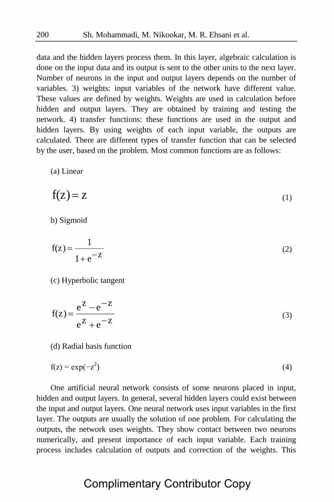
network. 4) transfer functions: these functions are used in the output and
hidden layers. By using weights of each input variable, the outputs are
calculated. There are different types of transfer function that can be selected
by the user, based on the problem. Most common functions are as follows:
(a) Linear
(1)
b) Sigmoid
(2)
(c) Hyperbolic tangent
(3)
(d) Radial basis function
f(z) = exp(−z2) (4)
One artificial neural network consists of some neurons placed in input,
hidden and output layers. In general, several hidden layers could exist between
the input and output layers. One neural network uses input variables in the first
layer. The outputs are usually the solution of one problem. For calculating the
outputs, the network uses weights. They show contact between two neurons
numerically, and present importance of each input variable. Each training
process includes calculation of outputs and correction of the weights. This
zf(z)
ze1
1f(z)
zeze
zezef(z)
Complimentary Contributor Copy
Prediction of Steam Distillation Efficiency … 201
process continues until the correct weight values are found. For some certain
input parameters, the error is defined as the difference between experimental
data and output of the network [25]. There are three criteria for stopping the
training: maximum number of epochs, training time, and target mean square
error (MSE)1. However, in many cases, the mean absolute error (MAE)
2 and
the Pearson Product Moment Correlation Coefficient (R-value)3 are considered
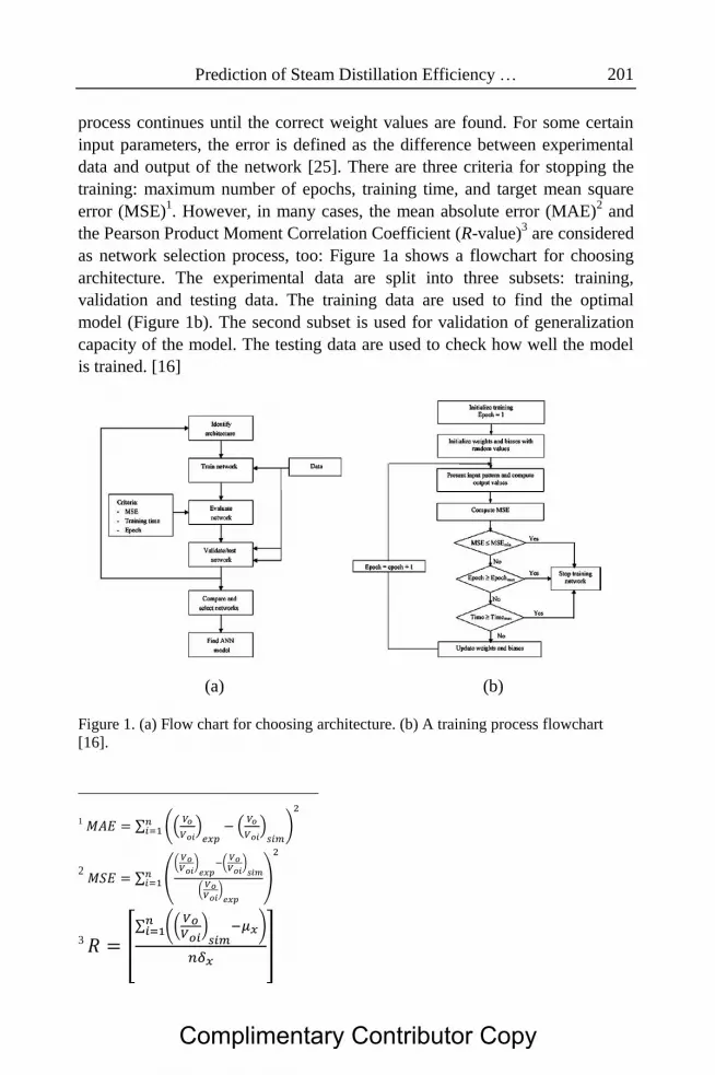
as network selection process, too: Figure 1a shows a flowchart for choosing
architecture. The experimental data are split into three subsets: training,
validation and testing data. The training data are used to find the optimal
model (Figure 1b). The second subset is used for validation of generalization
capacity of the model. The testing data are used to check how well the model
is trained. [16]
(a) (b)
Figure 1. (a) Flow chart for choosing architecture. (b) A training process flowchart
[16].
1 ∑ ((
)
(
) )
2 ∑ (
(
)
(
)
(
)
)
3 *
∑ ((
)
)
+
Complimentary Contributor Copy
Sh. Mohammadi, M. Nikookar, M. R. Ehsani et al. 202
Types of Artificial Neural Network
How to connect neurons in a neural network makes the type of network.
There are different types of neural network. The two general types are static
and dynamic. In static models, the path of data training is from input data to
hidden layer without any reverse. Whereas, in dynamic models, there are some
reverse paths from hidden layers to input layer. Static networks are named as
feedforward and dynamic models as feedback. Multi-layer perceptron and
Hopfield networks are the most popular feedforward and feedback networks,
respectively.
The feedforward networks are commonly used. These networks consist of
several layers, so that each neuron in each layer connects to the neurons of the
previous layer. These networks have one output layer and some hidden layers.
The outputs of the first layer are used as the inputs of the second layer, and the
outputs of the second layer are the inputs of the third layer. Finally, the outputs
of the last layer are the results of the network. Each layer can have different
number of neurons and different types of transfer function.
The number of neurons in the input and output layers equals to the number
of inputs and outputs variables, respectively. The disadvantage of FNNs is
determination of the ideal number of neurons in the hidden layer(s); few
neurons produce a network with low precision and a higher number leads to
over fitting and bad quality of interpolation and extrapolation. The use of
techniques such as Bayesian regularization, together with a Levenberg–
Marquardt algorithm, can help overcome this problem. One simple type of
feedforward network commonly used is perceptron neural network. [17]
PROBABILISTIC NEURAL NETWORKS
The ANNs can be used for different purposes; approximation of functions
and classification are examples of such applications. The most common types
of ANNs used for classification are the feed forward (that explained) neural
networks (FNNs) and the radial basis function (RBF) networks.
Probabilistic neural networks (PNNs) are a kind of RBFs that use a
Bayesian decision strategy [18]. In PNNs, each input has its distance from the
input vector calculated in the first layer. This process results in a vector whose
elements indicate how close the input is in relation of the training input. The
second layer produces a vector of probabilities that will be used in
determination of the input class.
Complimentary Contributor Copy
Prediction of Steam Distillation Efficiency … 203
Design of PNNs is faster than that of their feedforward counterparts, and
their generalization capabilities are very good. However, for PNNs, the
number of neurons depends on the size of the input set. Therefore, the PNNs
are bigger than the FNNs, but no optimization of the number of neurons is
necessary. [19]
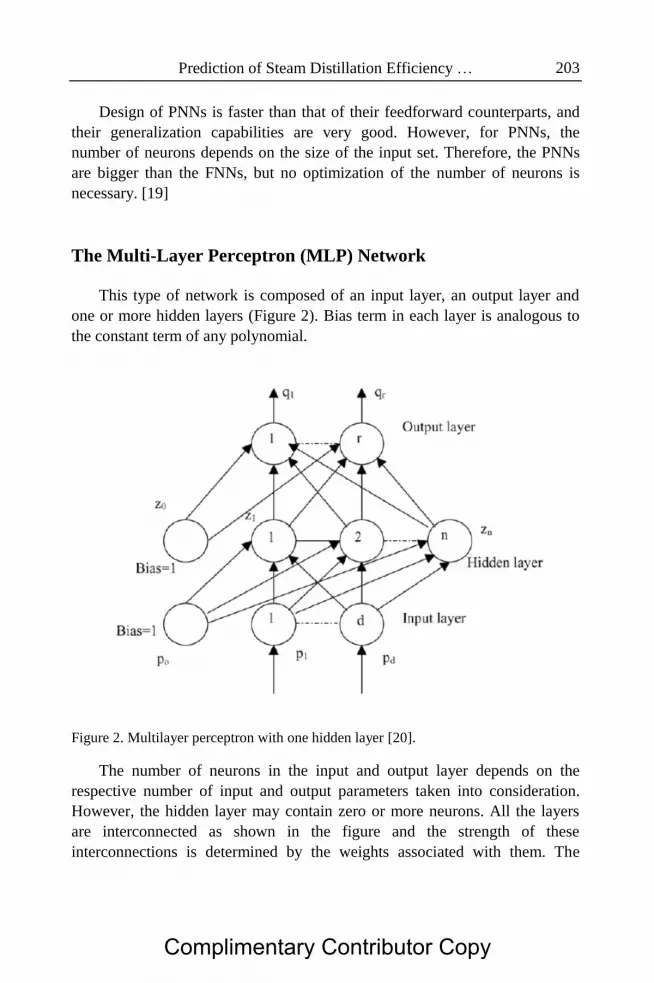
The Multi-Layer Perceptron (MLP) Network
This type of network is composed of an input layer, an output layer and
one or more hidden layers (Figure 2). Bias term in each layer is analogous to
the constant term of any polynomial.
Figure 2. Multilayer perceptron with one hidden layer [20].
The number of neurons in the input and output layer depends on the
respective number of input and output parameters taken into consideration.
However, the hidden layer may contain zero or more neurons. All the layers
are interconnected as shown in the figure and the strength of these
interconnections is determined by the weights associated with them. The
Complimentary Contributor Copy
Sh. Mohammadi, M. Nikookar, M. R. Ehsani et al. 204
output from a neuron in the hidden layer is the transformation of the weighted
sum of output from the input layers and is given as:
∑ (5)
The output from the neuron in the output layer is the transformation of the
weighted sum of output from the hidden layer and is given as:
∑ (6)
where, pi is the ith output from the input layer, zj is the jth output from the
hidden layer, wij is the weight in the first layer connecting neuron i in the input
layer to the neuron j in the hidden layer, is the weight in the second layer
connecting the neuron j in the hidden layer to the neuron k in the output layer
and g and are the transformation functions. The transformation function is
usually a sigmoid function with the most common being,
(7)
The other commonly used function is,
(8)
One of the reasons for using these transformation functions is the ease of
evaluating the derivatives required for minimization of the error function. [20]
Training
ANN is an adaptive network that changes its structure based on external or
internal information flowing through the network during the learning (training)
phase. Estimation of optimum weights and biases of network needs an
algorithm called propagation method. Several kinds of propagation methods
are available and back propagation (BP) is the easiest and simplest one with
enough reliability. BP and other usual propagation methods are explained
completely in the mathematical literatures [21,22].
Complimentary Contributor Copy
Prediction of Steam Distillation Efficiency … 205
Rules of Training
Training is implemented by change of weights in transfer function.
Generally, there are two types of training; supervised and unsupervised
trainings. In supervised training, the inputs and hidden layer variables are
defined to the model as dependent variables. But, in unsupervised training, just
the input variables are defined to the model.
Modeling Procedure: Back Propagation
For calibration of the network, firstly the data points are used to train the
network and then, some other data points (which are completely new) will be
used to test the calibrated network. As mentioned in the previous section,
training of a network requires a propagation method and BP is a simple
propagation method for training of the ANN. The algorithm of back
propagation error was chosen for our modeling. This section provides a
summary of BP.
First, data points must be divided into two parts: the first part for training
and the second part for testing. Usually about 30% of the data points are
selected randomly for the testing phase. Some random values must be chosen
as the initial guess for weights and biases, and then training phase begins.
Inputs are entered to the network and produce the output, and the output is
checked by the real data.
As explained in the previous sections: Each layer is made of some neurons
connected to the other neurons in the previous and next layers. A neuron has
an input, an output and a transfer function. The tangent hyperbolic transfer
function is one of the performed functions, expressed as the following
equation:
( )
(9)
where, is the output of the jth neuron and Sj is the input of the jth neuron,
produced by outputs of the previous layer. Sj is given 10.
∑ ( ) (10)
Complimentary Contributor Copy
Sh. Mohammadi, M. Nikookar, M. R. Ehsani et al. 206
The deviation, , defined as the difference between the appropriate output
( and the calculated output for the data point ( ) can be presented as:
(11)
where, presents the last layer. Summation of squared deviations ( ) is a
better choice for further operations, described as the following equation:
∑
(12)
Eq. (15) is used to renew weights and biases as described below:
(13)
(14)
where, α is the propagation rate and usually is chosen from 0.1 to 0.9. The last
terms of the above equations (∂F/∂wij and ∂F/∂bi) are complicated and after
straightforward algebra can be presented in the following form:
(15)
Where,
(16)
(17
(18)
The general form of Eq. (10) is given by
(19)
Complimentary Contributor Copy
Prediction of Steam Distillation Efficiency … 207
where, is the transfer function. Thus,
(20)
By replacing the equations derived above in the Eq. (13), below equation
is resulted:
(21)
In the same way, Eq. (14) can be represented as:
(22)
Eqs. (21) and (22) are used for the last layer ( , but in hidden layers, it is
required to introduce a new parameter for corrective calculations in the
following form:
(23)
where, l presents the layer number and . Thus, the last terms of Eqs. (13)
and (14) (∂F/∂wij and ∂F/∂bi) must be rewritten as:
(24)
(25)
In mathematical literatures [23, 24], there are suitable methods for
calculating left sides of Eqs. (24) and (25). in the following form:
(
)∑
(26)
Eq. (26) shows that δs of the layer (l) are calculated by δs of the next layer
( +1). ∂F can be represented as:
Complimentary Contributor Copy
Sh. Mohammadi, M. Nikookar, M. R. Ehsani et al. 208
∑
(27)
where,
(28)
(29)
(30)
The above equations are used for calculating and renewing the weights
and biases of ANN method. The selected training data points are used to
obtain the network parameters in a cycling process, e.g. cycling equal to 100
means that all training data points are used 100 times for improving the
parameters of the network. Then, the reliability of the trained network may be
checked using some new data points (testing). Small error of testing phase
confirms that the propagation method avoids over fitting [21, 22, 23, and 24].
Modeling Steps
1) Collecting the experimental data including API, viscosity, steam
injection rate, characterization factor as our inputs and steam
distillation yield as our output.
2) Editing these data in a suitable format that can be used in our
program.
3) Dividing the input file to 3 main parts such as testing, training, and
cross validation data.
4) Choosing the best transfer function (hyperbolic tangent).
5) Making different neural networks with one and two hidden layers and
different number of neurons.
6) Training these different neural networks.
7) Calculating the ARE%, MSE%, MAE%.
8) Finding the best neural network with the high accuracy.
9) Comparing our results with the previous models.
Complimentary Contributor Copy

Prediction of Steam Distillation Efficiency … 209
RESULTS AND DISCUSSION
In this study, for prediction of steam distillation yield, a multi-layer
perceptron neural network was used. Tanh-axon was selected as the transfer
function, and Levenberg–Marquardt back propagation was used in all training
steps. Input layer had four neurons consisting of API, viscosity of the crude
oil, steam distillation factor and steam characterization factor, which are
defined as follows:
(31)
(32)
Hidden layer and its number of neurons will be discussed in the next
section. Finally, the last layer has one neuron that is steam distillation yield.
Figure 3 shows this neural network used in this study.
Figure 3. Schematic of the MLP network used in this study.
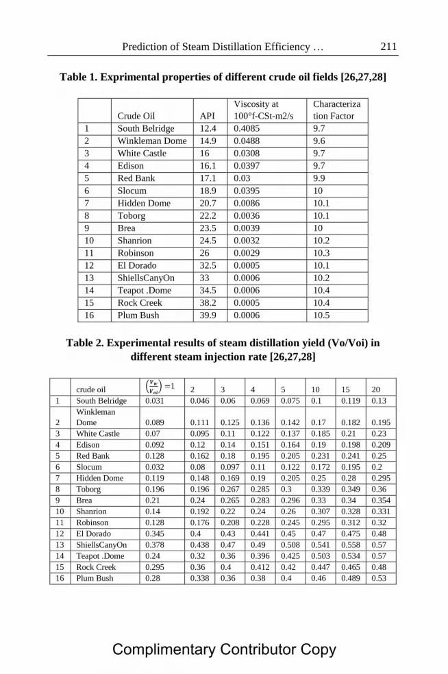
Experimental data obtained from the literature were used as training and
testing [26,27,28]. 77 data of 128 input data were used for training, 33 data for
testing, and 18 data for cross validation. The difference between experimental
and obtained results of steam distillation yield were minimized by
optimization of the weights.
gravity specefic
point boiling averagemean factorzation characteri
Complimentary Contributor Copy
Sh. Mohammadi, M. Nikookar, M. R. Ehsani et al. 210
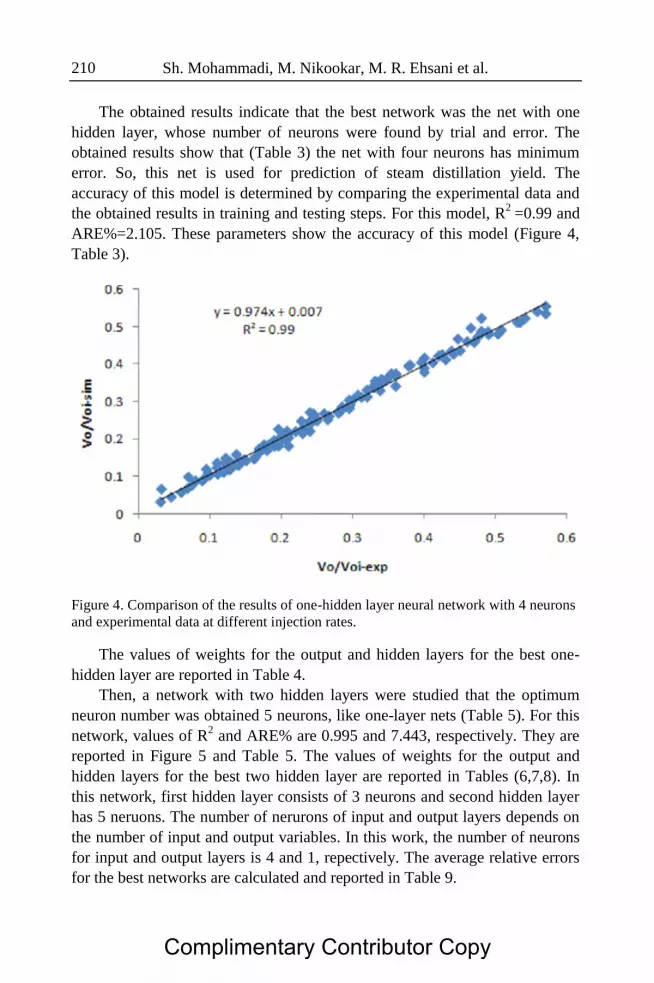
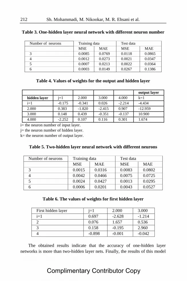
The obtained results indicate that the best network was the net with one
hidden layer, whose number of neurons were found by trial and error. The
obtained results show that (Table 3) the net with four neurons has minimum
error. So, this net is used for prediction of steam distillation yield. The
accuracy of this model is determined by comparing the experimental data and
the obtained results in training and testing steps. For this model, R2
=0.99 and
ARE%=2.105. These parameters show the accuracy of this model (Figure 4,
Table 3).
Figure 4. Comparison of the results of one-hidden layer neural network with 4 neurons
and experimental data at different injection rates.
The values of weights for the output and hidden layers for the best one-
hidden layer are reported in Table 4.
Then, a network with two hidden layers were studied that the optimum
neuron number was obtained 5 neurons, like one-layer nets (Table 5). For this
network, values of R2 and ARE% are 0.995 and 7.443, respectively. They are
reported in Figure 5 and Table 5. The values of weights for the output and
hidden layers for the best two hidden layer are reported in Tables (6,7,8). In
this network, first hidden layer consists of 3 neurons and second hidden layer
has 5 neruons. The number of nerurons of input and output layers depends on
the number of input and output variables. In this work, the number of neurons
for input and output layers is 4 and 1, repectively. The average relative errors
for the best networks are calculated and reported in Table 9.
Complimentary Contributor Copy
Prediction of Steam Distillation Efficiency … 211
Table 1. Exprimental properties of different crude oil fields [26,27,28]
Crude Oil API
Viscosity at
100°f-CSt-m2/s
Characteriza
tion Factor
1 South Belridge 12.4 0.4085 9.7
2 Winkleman Dome 14.9 0.0488 9.6
3 White Castle 16 0.0308 9.7
4 Edison 16.1 0.0397 9.7
5 Red Bank 17.1 0.03 9.9
6 Slocum 18.9 0.0395 10
7 Hidden Dome 20.7 0.0086 10.1
8 Toborg 22.2 0.0036 10.1
9 Brea 23.5 0.0039 10
10 Shanrion 24.5 0.0032 10.2
11 Robinson 26 0.0029 10.3
12 El Dorado 32.5 0.0005 10.1
13 ShiellsCanyOn 33 0.0006 10.2
14 Teapot .Dome 34.5 0.0006 10.4
15 Rock Creek 38.2 0.0005 10.4
16 Plum Bush 39.9 0.0006 10.5
Table 2. Experimental results of steam distillation yield (Vo/Voi) in
different steam injection rate [26,27,28]
crude oil (
) 1 2 3 4 5 10 15 20
1 South Belridge 0.031 0.046 0.06 0.069 0.075 0.1 0.119 0.13
2
Winkleman
Dome 0.089 0.111 0.125 0.136 0.142 0.17 0.182 0.195
3 White Castle 0.07 0.095 0.11 0.122 0.137 0.185 0.21 0.23
4 Edison 0.092 0.12 0.14 0.151 0.164 0.19 0.198 0.209
5 Red Bank 0.128 0.162 0.18 0.195 0.205 0.231 0.241 0.25
6 Slocum 0.032 0.08 0.097 0.11 0.122 0.172 0.195 0.2
7 Hidden Dome 0.119 0.148 0.169 0.19 0.205 0.25 0.28 0.295
8 Toborg 0.196 0.196 0.267 0.285 0.3 0.339 0.349 0.36
9 Brea 0.21 0.24 0.265 0.283 0.296 0.33 0.34 0.354
10 Shanrion 0.14 0.192 0.22 0.24 0.26 0.307 0.328 0.331
11 Robinson 0.128 0.176 0.208 0.228 0.245 0.295 0.312 0.32
12 El Dorado 0.345 0.4 0.43 0.441 0.45 0.47 0.475 0.48
13 ShiellsCanyOn 0.378 0.438 0.47 0.49 0.508 0.541 0.558 0.57
14 Teapot .Dome 0.24 0.32 0.36 0.396 0.425 0.503 0.534 0.57
15 Rock Creek 0.295 0.36 0.4 0.412 0.42 0.447 0.465 0.48
16 Plum Bush 0.28 0.338 0.36 0.38 0.4 0.46 0.489 0.53
Complimentary Contributor Copy
Sh. Mohammadi, M. Nikookar, M. R. Ehsani et al. 212
Table 3. One-hidden layer neural network with different neuron number
Number of neurons Training data Test data
MSE MAE MSE MAE
3 0.0085 0.0769 0.0118 0.0865
4 0.0012 0.0273 0.0021 0.0347
5 0.0007 0.0213 0.0022 0.0364
6 0.0003 0.0149 0.0267 0.1386
Table 4. Values of weights for the output and hidden layer
output layer
hidden layer j=1 2.000 3.000 4.000 k=1
i=1 -0.175 -0.341 0.026 -2.214 -4.434
2.000 0.383 -1.820 -2.415 0.907 -12.959
3.000 0.148 0.439 -0.351 -0.137 10.900
4.000 -2.252 0.107 0.116 0.301 1.674
i= the neuron number of input layer.
j= the neuron number of hidden layer.
k= the neuron number of output layer.
Table 5. Two-hidden layer neural network with different neurons
Number of neurons Training data Test data
MSE MAE MSE MAE
3 0.0015 0.0316 0.0083 0.0802
4 0.0042 0.0466 0.0075 0.0725
5 0.0024 0.0427 0.0013 0.0295
6 0.0006 0.0201 0.0043 0.0527
Table 6. The values of weights for first hidden layer
First hidden layer j=1 2.000 3.000
i=1 0.697 -2.628 -1.214
2 0.076 1.657 0.536
3 0.158 -0.195 2.960
4 -0.898 -0.001 -0.042
The obtained results indicate that the accuracy of one-hidden layer
networks is more than two-hidden layer nets. Finally, the results of this model
Complimentary Contributor Copy

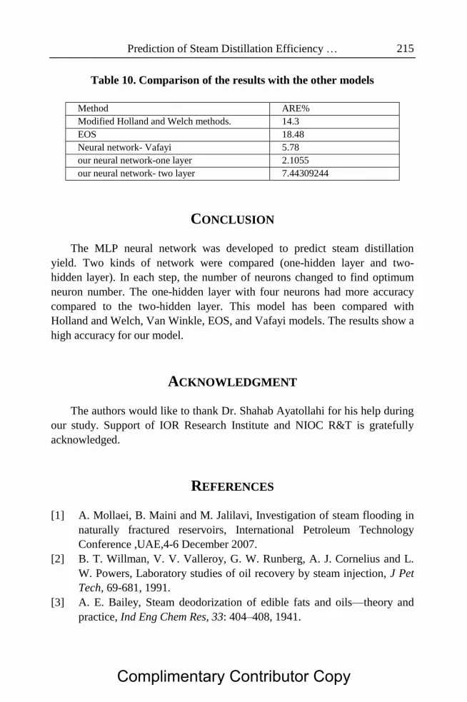
Prediction of Steam Distillation Efficiency … 213
were compared with some available models. High accuracy of this model
compared to the other models is one of the most important advantage (Table
10).
Table 7. The values of weights for the output for second hidden layer
Second hidden layer k=1 2 3 4 5
j=1 0.390 0.098 0.524 -1.979 0.378
2 0.696 0.438 2.149 0.180 -1.688
3 -0.117 0.021 1.043 -2.221 -0.357
Table 8. The values of weights for output
Out put layer m=1
k=1 0.937
2 0.572
3 -1.563
4 1.265
5 1.292
i= the neuron number of input layer.
j= the neuron number of first hidden layer.
k= the neuron number of second hidden layer.
m= the neuron number of output layer.
Figure 5. Comparison of the results of two-hidden layer neural network with 5 neurons
with experimental data at different injection rate.
Complimentary Contributor Copy

Table 9. Comparison of experimental and simulated results by testing one-hidden layer and two hidden layer in
ARE%, two-hidden layer with 5 neurons ARE%, one hidden-layer with 4 neurons
0.0228 0.077 0.1 0.0254 0.102 0.1
0.0578 0.179 0.17 0.0108 0.168 0.17
0.0044 0.185 0.185 0.0117 0.187 0.185
0.0364 0.183 0.19 0.0428 0.181 0.19
0.0657 0.215 0.231 0.0067 0.229 0.231
0.1086 0.153 0.172 0.0297 0.1666 0.172
0.1695 0.207 0.25 0.0021 0.249 0.25
0.1315 0.294 0.339 0.0017 0.344 0.339
0.0694 0.307 0.33 0.0292 0.339 0.33
0.0934 0.278 0.307 0.0201 0.3131 0.307
0.0191 0.300 0.295 0.0035 0.293 0.295
0.0930 0.426 0.47 0.0122 0.464 0.47
0.0541 0.511 0.541 0.0282 0.525 0.541
0.0318 0.486 0.503 0.0493 0.478 0.503
0.0235 0.457 0.447 0.0441 0.446 0.447
0.0038 0.461 0.46 0.0027 0.458 0.46
7.44309244 2.105483337 overall1
1
10oVwV
expoiVoV
simoiVoVexpoiVoV simoiVoV expoiVoV
expoiVoV
simoiVoVexpoiVoV simoiVoV expoiVoV
16
16
1 expoiVoV/simoiVoV
expoiVoV
overall
Complimentary Contributor Copy
Prediction of Steam Distillation Efficiency … 215
Table 10. Comparison of the results with the other models
Method ARE%
Modified Holland and Welch methods. 14.3
EOS 18.48
Neural network- Vafayi 5.78
our neural network-one layer 2.1055
our neural network- two layer 7.44309244
CONCLUSION
The MLP neural network was developed to predict steam distillation
yield. Two kinds of network were compared (one-hidden layer and two-
hidden layer). In each step, the number of neurons changed to find optimum
neuron number. The one-hidden layer with four neurons had more accuracy
compared to the two-hidden layer. This model has been compared with
Holland and Welch, Van Winkle, EOS, and Vafayi models. The results show a
high accuracy for our model.
ACKNOWLEDGMENT
The authors would like to thank Dr. Shahab Ayatollahi for his help during
our study. Support of IOR Research Institute and NIOC R&T is gratefully
acknowledged.
REFERENCES
[1] A. Mollaei, B. Maini and M. Jalilavi, Investigation of steam flooding in
naturally fractured reservoirs, International Petroleum Technology
Conference ,UAE,4-6 December 2007.
[2] B. T. Willman, V. V. Valleroy, G. W. Runberg, A. J. Cornelius and L.
W. Powers, Laboratory studies of oil recovery by steam injection, J Pet
Tech, 69-681, 1991.
[3] A. E. Bailey, Steam deodorization of edible fats and oils—theory and
practice, Ind Eng Chem Res, 33: 404–408, 1941.
Complimentary Contributor Copy

Sh. Mohammadi, M. Nikookar, M. R. Ehsani et al. 216
[4] C. D. Holland, N. E. Welch, Steam batch distillation calculation, Pet
Refin, 36: 251-253, 1957.
[5] M. Van Winkle, Distillation, McGraw-Hill, New York, USA, 1967.
[6] C. H. Wu, R. B. Elder, Correlation of crude oil steam distillation yield
with basic crude oil properties, Soc Pet Eng J, 23: 937–945, 1983.
[7] J. H. Duerksen, L. Hsueh, Steam distillation of crude oils, Soc Pet Eng J,
23: 265–271, 1983.
[8] G. A. Langhoff, and C. H. Wu, Calculation of high-temperature crude
oil water vapor separations using simulated distillation data, Soc Pet Eng
Reserv Eng, 1:483–489,1986.
[9] P. S. Northrop, V. N. Venkatesan, Analytical steam distillation model
for thermal enhanced oil recovery processes, Ind Eng Chem Res, 32:
2039–2046,1993.
[10] A. Xuana, Y. Wu, C. Peng, P. Mac, Correlation of the viscosity of pure
liquids at high pressures based on an equation of state, Fluid Phase
Equilibria 240, 15–21, 2006
[11] A. B. Bulsari, Neural Networks for Chemical Engineers, Elsevier
Science, Inc, New York, USA, section two, 1995.
[12] C. Xiaolong, C. Guangming, L. Changsheng, H. Xiaohong, Vapor–
liquid equilibrium of difluoromethane + 1,1,1,2-tetrafluoroethane system
over a temperature range from 258.15 to 343.15 K, Fluid Phase Equilib,
249: 97–103, 2006.
[13] M. T. Hagan, H. B. Demuth, M., Beale, Neural Network Design. PWS
Publishing Co, Boston,1997.
[14] T. Takagi, T. Sakura, T.Tsuji, M. Hongo, Bubble point pressure for
binary mixtures of difluoromethane with pentafluoroethane and 1,1,1,2-
tetrafluoroethane, Fluid Phase Equilib, 162: 171–179, 1999.
[15] M. T. Vafaei, R. Eslamloueyan, Sh. Ayatollahi, Petroleum and Chemical
Engineering Dept., Shiraz University, Zand Street, Shiraz, Fars, Iran
Simulation of steam distillation process using neural networks, chemical
engineering research and design 87 , 997–1002, 2009.
[16] Viet D. Nguyen et al, Prediction of vapor–liquid equilibrium data for
ternary systems using artificial neural networks, Fluid Phase Equilibria
254 (2007) 188–197
[17] Amir. H. Mohammadi et al, Determination of hydrate stability zone
using electrical conductivity data of salt aqueous solution, Fluid Phase
Equilibria 253 (2007) 36–41
[18] P. D. Wasserman, Advanced Methods in Neural Computing, Van
Nostrand Reinhold, New York, 1993.
Complimentary Contributor Copy
Prediction of Steam Distillation Efficiency … 217
[19] Jones E. Schmitz et al, Artificial neural networks for the solution of the
phase stability problem, Fluid Phase Equilibria 245 (2006) 83–87
[20] Swati Mohanty, Estimation of vapour liquid equilibria of binary
systems, carbón dioxide–ethyl caproate, ethyl caprylate and ethyl caprate
using artificial neural networks, Fluid Phase Equilibria 235 (2005) 92–
98
[21] S. Haykin, Neural Networks: A Comprehensive Foundation, Prentice-
Hall, 1998.
[22] R. Rojas, Neural Network, Springer-Verlag, Berlin, 1996.
[23] R. H. Perry, D.W. Green, Perry‘s Chemical Engineers‘ Handbook, 4th
ed, McGraw-Hill, 1999.
[24] Mani Safamirzaei et al, Modeling and predicting the Henry‘s law
constants of methyl ketones in aqueous sodium sulfate solutions with
artificial neural network, Fluid Phase Equilibria 266 (2008) 187–194
[25] D. Nguyen, R. Tan , Y. Brondial b, T. Fuchino , Prediction of vapor–
liquid equilibrium data for ternary systems using artificial neural
networks, Fluid Phase equilibria 254 (2007) 188–197.
[26] M. Langhoff, C. H. Wu, Calculation of high –temprature crude-
oil/water/vapor separations using simulated distillation data, SPE
Resrvior engineering, September 1986.
[27] H. Wu. Ching, B. Robert, Correlation of crude oil steam distillation
yields with basic crude oil properties, Society of Petroleum Engineering
of AIME, 5-17 December, 1981.
[28] N. Northrop, N. Venkat , N. Venkatesan , Analytical Steam Distillation
Model for Thermal Enhanced Oil Recovery Processes, Ind. Eng. Chem.
Res 2064-2039, 1993.
Complimentary Contributor Copy


