Embed Size (px)
Citation preview

August 18, 2009 17:48 9.75in x 6.5in b684-ch26 FA
Chapter 26
Prediction of Squat for Underkeel Clearance
Michael J. Briggs
Coastal and Hydraulics LaboratoryUS Army Engineer Research and Development Center
3909 Halls Ferry Road, Vicksburg, MS 39180-6199, [email protected]
Marc Vantorre
Ghent University, IR04, Division of Maritime TechnologyTechnologiepark Zwijnaarde 904, B 9052 Gent, Belgium
Klemens Uliczka
Federal Waterways Engineering and Research InstituteHamburg Office, Wedeler Landstrasse 157
D-22559 Hamburg, [email protected]
Pierre Debaillon
Centre d’Etudes Techniques Maritimes Et Fluviales2 bd Gambetta, BP60039, 60321 Compiegne, France
This chapter presents a summary of ship squat and its effect on vessel underkeelclearance. An overview of squat research and its importance in safe and efficientdesign of entrance channels is presented. Representative PIANC empirical for-mulas for predicting squat in canals and in restricted and open channels are dis-cussed and illustrated with examples. Most of these formulas are based on hardbottoms and single ships. Ongoing research on passing and overtaking ships inconfined channels, and offset distances and drift angles is presented. The effectof fluid bottoms or mud is described. Numerical modeling of squat is an area offuture research and some comparisons are presented and discussed.
723
August 18, 2009 17:48 9.75in x 6.5in b684-ch26 FA
724 M. J. Briggs et al.
26.1. Introduction
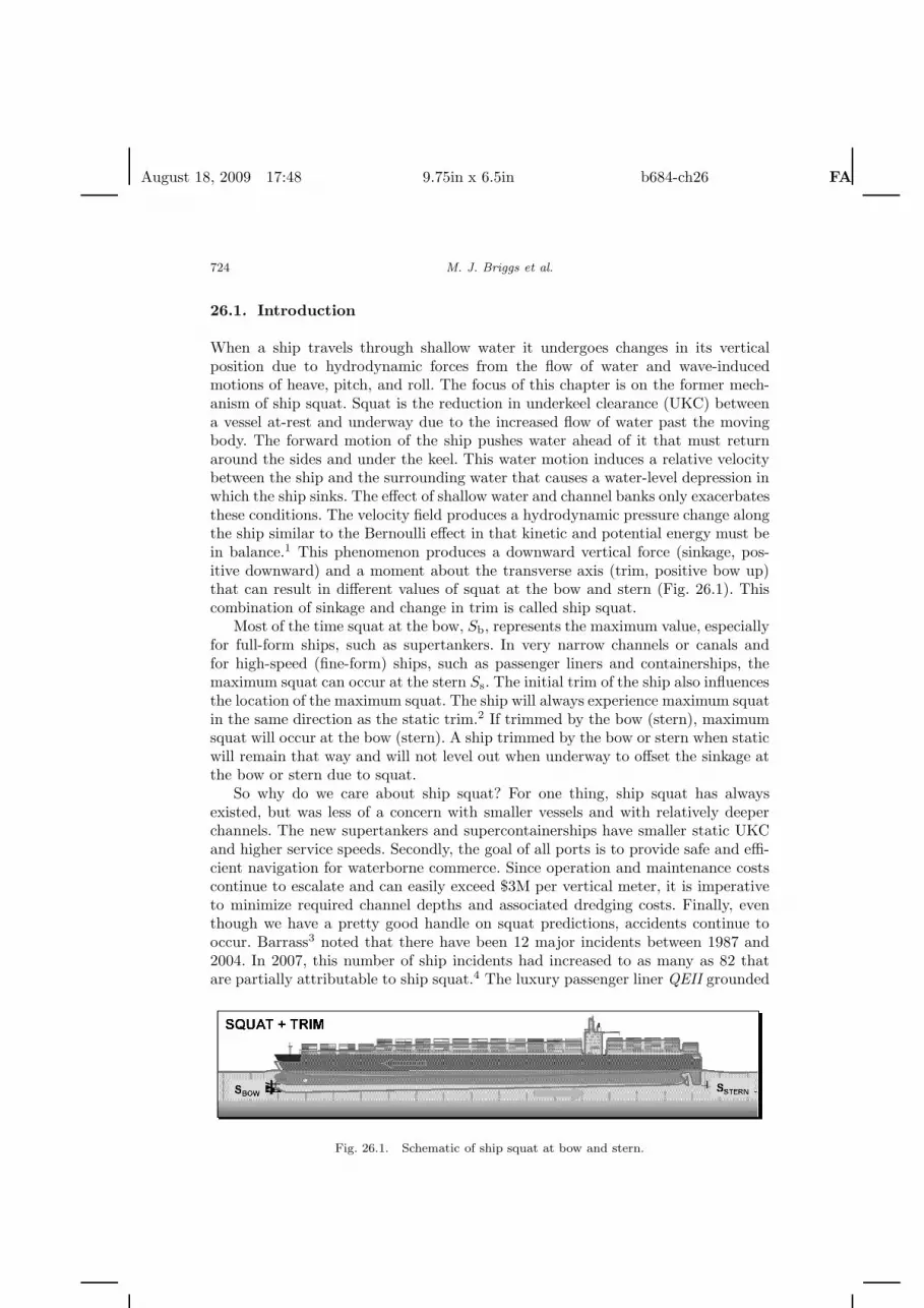
When a ship travels through shallow water it undergoes changes in its verticalposition due to hydrodynamic forces from the flow of water and wave-inducedmotions of heave, pitch, and roll. The focus of this chapter is on the former mech-anism of ship squat. Squat is the reduction in underkeel clearance (UKC) betweena vessel at-rest and underway due to the increased flow of water past the movingbody. The forward motion of the ship pushes water ahead of it that must returnaround the sides and under the keel. This water motion induces a relative velocitybetween the ship and the surrounding water that causes a water-level depression inwhich the ship sinks. The effect of shallow water and channel banks only exacerbatesthese conditions. The velocity field produces a hydrodynamic pressure change alongthe ship similar to the Bernoulli effect in that kinetic and potential energy must bein balance.1 This phenomenon produces a downward vertical force (sinkage, pos-itive downward) and a moment about the transverse axis (trim, positive bow up)that can result in different values of squat at the bow and stern (Fig. 26.1). Thiscombination of sinkage and change in trim is called ship squat.
Most of the time squat at the bow, Sb, represents the maximum value, especiallyfor full-form ships, such as supertankers. In very narrow channels or canals andfor high-speed (fine-form) ships, such as passenger liners and containerships, themaximum squat can occur at the stern Ss. The initial trim of the ship also influencesthe location of the maximum squat. The ship will always experience maximum squatin the same direction as the static trim.2 If trimmed by the bow (stern), maximumsquat will occur at the bow (stern). A ship trimmed by the bow or stern when staticwill remain that way and will not level out when underway to offset the sinkage atthe bow or stern due to squat.
So why do we care about ship squat? For one thing, ship squat has alwaysexisted, but was less of a concern with smaller vessels and with relatively deeperchannels. The new supertankers and supercontainerships have smaller static UKCand higher service speeds. Secondly, the goal of all ports is to provide safe and effi-cient navigation for waterborne commerce. Since operation and maintenance costscontinue to escalate and can easily exceed $3M per vertical meter, it is imperativeto minimize required channel depths and associated dredging costs. Finally, eventhough we have a pretty good handle on squat predictions, accidents continue tooccur. Barrass3 noted that there have been 12 major incidents between 1987 and2004. In 2007, this number of ship incidents had increased to as many as 82 thatare partially attributable to ship squat.4 The luxury passenger liner QEII grounded
Fig. 26.1. Schematic of ship squat at bow and stern.
August 18, 2009 17:48 9.75in x 6.5in b684-ch26 FA
Prediction of Squat for Underkeel Clearance 725
off Massachusetts in 1992 with a repair cost of $13M and another $50M for lostpassenger bookings.
In the early 1990s, the Maritime Commission (MarCom) of the Permanent Inter-national Association of Navigation Congresses (PIANC) formed a working group(WG30) to provide information and recommendations on the design of approachchannels.5 In the past 10 years since the WG30 report, research in squat predic-tions was a dynamic area in naval architecture with new experiments to studythe effects of fluid bottoms and passing and overtaking vessels, especially with theincreasing size of the shipping fleet. Time domain Reynolds Average Navier–StokesEquation (RANSE) numerical models are being developed to predict squat, butthese models are still being validated. In 2005, the PIANC MarCom formed a newworking group Horizontal and Vertical Dimensions of Fairways (WG49) to updatethe WG30 report on design of deep draft navigation channels.6
A summary of ship squat is presented in this chapter. In the second section,factors governing squat including ship characteristics, channel configurations, andcombined factors are discussed. Some empirical formulas from the PIANC WG30report are presented and compared in the third section. The fourth section presentssome recent research on the effect of squat on passing and overtaking ships in con-fined channels by the Federal Waterways Engineering and Research Institute (BAW)in Hamburg, Germany, and the Flanders Hydraulic Research (FHR) Laboratory inAntwerp, Belgium. It also includes numerical modeling by Delft University of Tech-nology and laboratory modeling by FHR on the effect of ship offset and drift onsquat. The fifth section summarizes the recent studies at FHR on the effect of fluidbottoms (i.e., mud) on squat. The development of numerical models to predict shipsquat is an ongoing research area. The current status of this development at Centred’Etudes Techniques Maritimes Et Fluviales (CETMEF), France, is discussed in thesixth section. Finally, a summary and conclusions of ship squat issues is presentedin the last section.
26.2. Factors Governing Squat
Prediction of ship squat depends on ship characteristics and channel configurations.These factors are often combined to create new normalized parameters to describethe squat phenomenon.
26.2.1. Ship characteristics
The main ship parameters include ship draft, T , hull shape as represented by theblock coefficient, CB, and ship speed, VS (m/s) or VK (knots). Other ship parametersinclude the length between forward and aft perpendiculars Lpp and the beam, B.The CB is a measure of the “fineness” of the vessel’s shape relative to an equivalentrectangular volume with the same dimensions. The range of values of CB is typicallybetween 0.45 for high-speed vessels and 0.85 for slow, full-size tankers and bulkcarriers. The most important ship parameter is its speed VS. This is the relativespeed of the ship in water, so fluvial and tidal currents must be included. In general,
August 18, 2009 17:48 9.75in x 6.5in b684-ch26 FA
726 M. J. Briggs et al.
squat varies as the square of the speed. Therefore, doubling the speed quadruplesthe squat and vice versa.
There are two calculated ship parameters that are based on the basic ship dimen-sions. The ship’s displacement volume ∇ (m3) is defined as
∇ = CBLppBT. (26.1)
The CB can be determined from the ∇ if the other ship dimensions are known. Theunderwater midship cross-sectional area AS is generally defined as
AS = 0.98BT. (26.2)
The “0.98” constant accounts for reduction in area due to the keel radius.7 Someresearchers ignore this and use a constant of “1.00” since the error is small relativeto other uncertainties in the squat calculations.
Finally, the bulbous bow and stern-transom are two other characteristics of aship that affect squat. Many of the early squat measurements were made beforebulbous bows were in use. Newer designs of bulbous bows, although mainly to reducedrag and increase fuel efficiency, also have an effect on squat. The newer “stern-transoms” on some ships are “blockier” (i.e., wider and less streamlined) than earliership designs and affect squat as they become more fully submerged with increasesin draft.8
26.2.2. Channel configurations
The main channel considerations are proximity of the channel sides and bottom, asrepresented by the channel depth h and cross-sectional configuration. If the ship isnot in relatively shallow water with a small UKC, squat is usually negligible. Ratiosof water depth to ship draft h/T greater than 1.5–2.0 (i.e., relatively deepwater)are usually considered safe from the influences of squat.
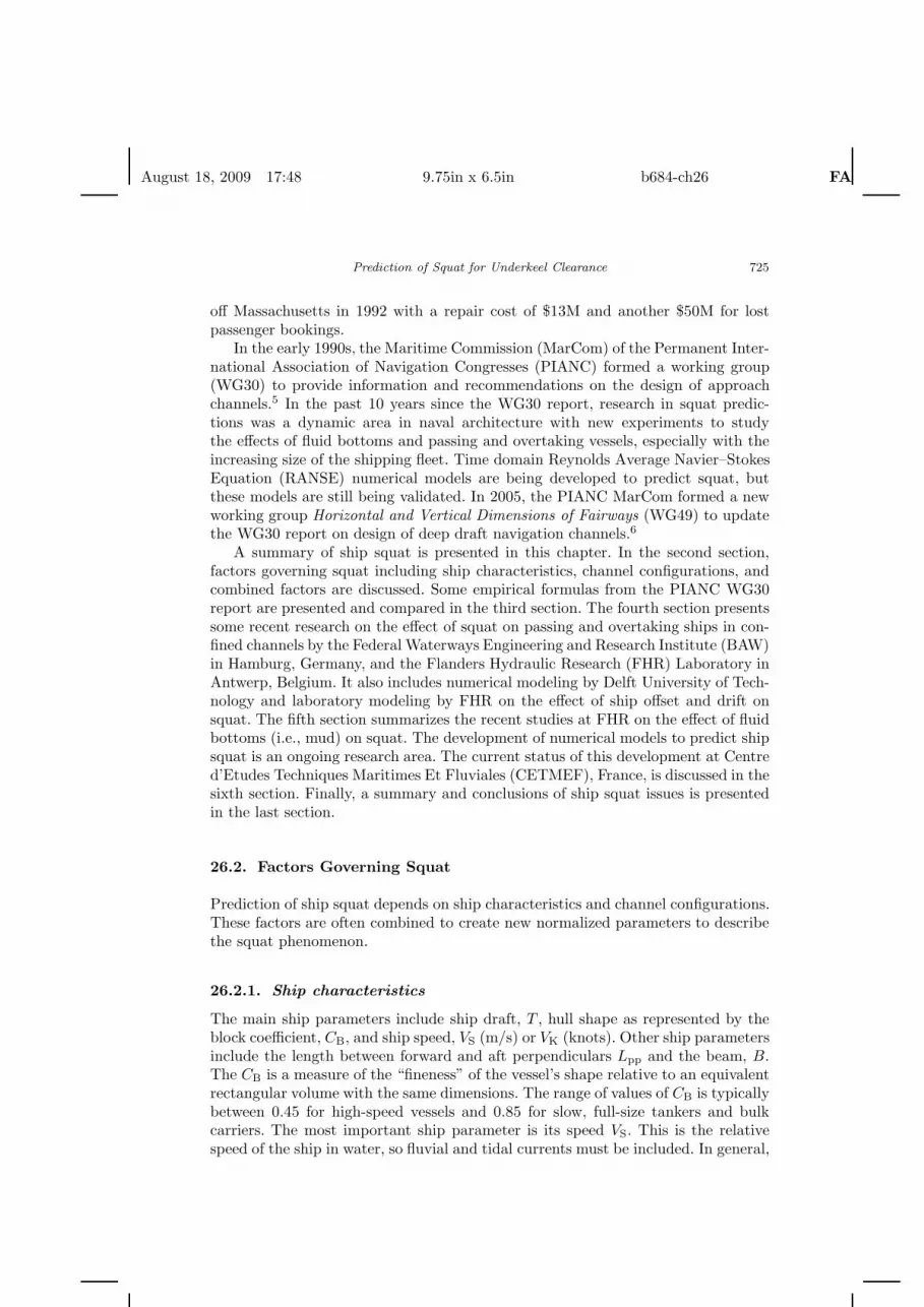
The main types of “idealized” channel configuration are (a) open or unrestricted(U), (b) confined or restricted (R), and (c) canal (C). Figure 26.2 is a schematic ofthese three types of entrance channels for ocean-going or deep draft ships. Unre-stricted channels are in relatively larger open bodies of water and usually towardthe offshore end of entrance channels. Analytically and numerically, they are easierto describe and were some of the first types studied. Sections of rivers may even
Fig. 26.2. Schematic of three channel types: unrestricted or open, restricted or confined, andcanal.

August 18, 2009 17:48 9.75in x 6.5in b684-ch26 FA
Prediction of Squat for Underkeel Clearance 727
be classified as unrestricted channels if they are wide enough. The second typeof channel is the restricted channel with an underwater trench that is typical ofdredged channels. The restricted channel is a cross between the canal and unre-stricted channel type. The trench acts as a canal by containing and influencing theflow around the ship, and the water column above the hT allows the flow to actas if the ship is in an unrestricted channel. The last type of channel is the canal.These channels are representative of channels in rivers with emergent banks. Thesides are idealized as one slope when in reality they may have compound slopes withrevetment to protect against ship waves and erosion. The canal may or may notbe exposed to tidal fluctuations. For instance, the Panama and Suez Canals have aconstant water depth.
Many channels can be characterized by two or three of these channel types as thedifferent segments or reaches of the channel have different cross-sections. Finally,many real-world channels look like combinations of these three types as one side maylook like an open unrestricted channel and the other side like a canal or restrictedchannel with side walls. Most of the PIANC empirical formulas are based on shipsin the center of symmetrical channels, so the user has to use “engineering judgment”when selecting the most appropriate formulas. New data are being collected forsome of these more realistic channel shapes, so future formulas may account forthese differences in channel shapes.
Other important parameters necessary to describe restricted channels and canalsare the channel width at the bottom of the channel W , trench height hT from thebottom of the channel to the top of the trench, and inverse bank slope n (i.e.,run/rise = 1/ tan θ). The value of n, although not necessarily an integer, typicallyhas a value such as 1, 2, or 3 representing side slopes of 1:1, 1:2, and 1:3, respectively.
How does one define the width of an unrestricted or an open channel since thereare no banks or sides? In 2004, Barrass had defined an effective width Weff for theunrestricted channel as the artificial side boundary on both sides of a moving shipwhere the ship will experience changes in performance and resistance that affectsquat, propeller RPMs, and speed.3 His width of influence FB is defined for h/Tvalues from 1.10 to 1.40 as
FB = Weff =[
7.04C0.85
B
]B. (26.3)
Mean values of FB are of the order of 8B to 8.3B for supertankers (CB range from0.81 to 0.87), 9B to 9.5B for general cargo ships (CB range from 0.68 to 0.80), and10B to 11.5B for containerships (CB range from 0.57 to 0.71).
The calculated cross-sectional area AC is the wetted cross-section of the canalor the equivalent wetted area of the restricted channel by projecting the slope tothe water surface. It is given by
AC = Wh + nh2. (26.4)
For an unrestricted channel, use Barrass’s effective width Weff for channel width Wand set n = 0 in the equation for AC.
August 18, 2009 17:48 9.75in x 6.5in b684-ch26 FA
728 M. J. Briggs et al.
26.2.3. Combined ship and channel factors
Several dimensionless parameters are required in the PIANC squat prediction for-mulas that are ratios of both ship and channel parameters. They include the depthFroude number Fnh and the blockage factor S.
The most important dimensionless parameter is Fnh, which is a measure of theship’s resistance to motion in shallow water. Most ships have insufficient power toovercome Fnh values greater than 0.6 for tankers and 0.7 for containerships. Mostof the empirical equations require that Fnh be less than 0.7. For all cases, the valueof Fnh should satisfy Fnh < 1, an effective speed barrier and the defining level forthe subcritical speed range. The Fnh is defined as
Fnh =Vs√gh
(26.5)
with gravitational acceleration g (m/s2).The blockage factor S is the fraction of the cross-sectional area of the waterway
AC that is occupied by the ship’s underwater midships cross-section AS defined as
S =AS
AC. (26.6)
Typical S values can vary from 0.03 to 0.25 or larger for restricted channels andcanals, and to 0.10 or less for unrestricted channels.3,9 Higher values may occur,for example, the canal from Terneuzen (The Netherlands) to Ghent (Belgium) isoperated with a blockage factor S = 0.275, and higher values will be evaluated inthe near future.10 The value of S is a factor in the calculation of the ship’s criticalspeed in canals and restricted channels (see Sec. 26.3.3.3 and Appendix 26.A).
26.3. PIANC Squat Formulas
26.3.1. Background
In 1997 the PIANC WG30 report included 11 empirical formulas and one graphicalmethod from nine different authors for the prediction of ship squat.5 They werebased on physical model experiments and field measurements for different ships,channels, and loading characteristics. The formulas included the pioneering work ofTuck11, Tuck and Taylor,12 and Beck et al.,13 and the early research by Hooft,14
Dand,15 Eryuzlu and Hausser,16 Romisch,17 and Millward.18,19 The PIANC recom-mends that channels be designed in two stages. The first is the “Concept” Designwhere a “quick” or “ballpark” answer is desired. The WG30 report recommended theInternational Commission for the Reception of Large Ships (ICORELS) formula20
in this phase. The second stage is the “Detailed” Design phase where more accurateand thorough predictions and comparisons are required. The WG30 recommendedthe formulas by ICORELS, Huuska,7 Barrass,21,22 and Eryuzlu et al.23 in thissecond stage.
All of these formulas give predictions of bow squat Sb, but only the Romischformula gives predictions for stern squat Ss for all channel types. The Barrass
August 18, 2009 17:48 9.75in x 6.5in b684-ch26 FA
Prediction of Squat for Underkeel Clearance 729
formula gives Ss for unrestricted channels, and for canals and restricted channelsdepending on the value of CB. Each formula has certain constraints that it shouldsatisfy before being applied, usually based on the ship and channel conditions underwhich it was developed. Caution should be exercised if these empirical formulas areused for conditions outside those for which they were developed.
In 2005 the PIANC MarCom formed WG49,6 which is in the process of reviewingand revising these formulas for an updated report on channel design (expected to becompleted in 2010). There have been some new formulations since the WG30 reportthat are being evaluated. Barrass has continued to develop and refine his formulasand now has predictions for both Sb and Ss. Ankudinov et al.24 proposed the Mar-itime Simulation and Ship Maneuverability (MARSIM) 2000 formula for maximumsquat based on a midpoint sinkage and vessel trim in shallow water. It is one of themost thorough and the most complicated formulas for predicting ship squat. TheSt. Lawrence Seaway (SLS) Trial and Very Large Crude Carriers (VLCC) formulasare based on the prototype measurements in the SLS by Stocks et al.25 Briggs26
developed a FORTRAN program to calculate squat using most of these formulas.It is not possible to include all the formulas in this chapter. We have selected
a representative sample of formulas that can be used for both phases of design.Some are the “old tried and true” formulas and some are based on new research.The Concept Design phase is by definition the simplest, of course this does notnecessarily mean that these formulas are any less accurate than some of the morecomplicated formulas. In the Detailed Design phase, it is usually a good practice toevaluate the squat with several of the formulas and calculate some statistics suchas average and range of values. In some cases, the maximum squat values might beused in design for the case of dangerous cargo and/or hard channel bottoms.
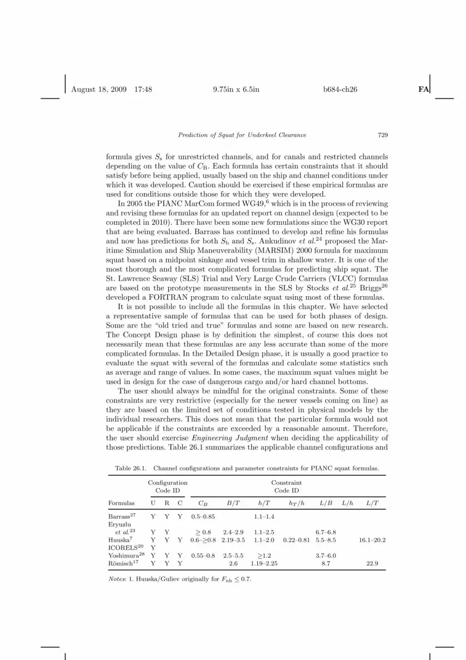
The user should always be mindful for the original constraints. Some of theseconstraints are very restrictive (especially for the newer vessels coming on line) asthey are based on the limited set of conditions tested in physical models by theindividual researchers. This does not mean that the particular formula would notbe applicable if the constraints are exceeded by a reasonable amount. Therefore,the user should exercise Engineering Judgment when deciding the applicability ofthose predictions. Table 26.1 summarizes the applicable channel configurations and
Table 26.1. Channel configurations and parameter constraints for PIANC squat formulas.
Configuration ConstraintCode ID Code ID
Formulas U R C CB B/T h/T hT /h L/B L/h L/T
Barrass27 Y Y Y 0.5–0.85 1.1–1.4Eryuzlu
et al.23 Y Y ≥ 0.8 2.4–2.9 1.1–2.5 6.7–6.8Huuska7 Y Y Y 0.6–≥0.8 2.19–3.5 1.1–2.0 0.22–0.81 5.5–8.5 16.1–20.2ICORELS20 YYoshimura28 Y Y Y 0.55–0.8 2.5–5.5 ≥1.2 3.7–6.0Romisch17 Y Y Y 2.6 1.19–2.25 8.7 22.9
Notes: 1. Huuska/Guliev originally for Fnh ≤ 0.7.
August 18, 2009 17:48 9.75in x 6.5in b684-ch26 FA
730 M. J. Briggs et al.
parameter constraints according to the individual testing conditions for the formulasin this chapter.
26.3.2. Concept design
26.3.2.1. ICORELS
The ICORELS formula20 for bow squat Sb is one of the original formulas from thePIANC WG30 report.5 It was developed for unrestricted or open channels only, soit should be used with caution if applied for restricted and canal channels. It issimilar to Hooft’s14 and Huuska’s7 equations and is defined as
Sb = CS∇
L2pp
F 2nh√
1 − F 2nh
(26.7)
where CS = 2.4 and the other factors have been previously defined.The Finnish Maritime Administration (FMA) uses this formula with different
values of CS depending on the ship’s CB.29,30
CS =
1.7 CB < 0.702.0 0.70 ≤ CB < 0.802.4 CB ≥ 0.80
. (26.8)
The BAW, however, recommends a value of CS = 2.0 for the larger containershipsof today which may have a CB < 0.70. Their research is based on many measure-ments along the restricted channel (side slope n varies from 15 to 40), 100-km long,River Elbe.31 The wider stern-transom ships (see Sec. 4.3) require CS = 3 becauseof the increased bow squat. The FHR has found CS ≥ 2.0 for modern container-ships. They typically travel at much higher speeds than the ICORELS formula wasoriginally developed, even in shallow and restricted waters. The Fnh are higher andin this speed range the effect of blockage S on the critical ship speed is considerable.For example, a very small S = 0.01 results in an important decrease in criticalspeed.10
26.3.2.2. Barrass
The Barrass4,27 formula is one of the simplest and “user friendly” and can beapplied for all channel configurations. Based on his earlier work in 1979,21 1981,22
and 2004,3 the maximum squat SMax at the bow or stern is determined by the valueof ship’s CB and Vk as
SMax =KCBV 2
k
100. (26.9)
According to Barrass,2 the value of CB determines whether SMax is at the bowSb or stern SS (requires even keel when static). He notes that full-form ships withCB > 0.7 tend to squat by the bow and fine-form ships with CB < 0.7 tend tosquat by the stern. The CB = 0.7 is an “even keel” situation with squat the same
August 18, 2009 17:48 9.75in x 6.5in b684-ch26 FA
Prediction of Squat for Underkeel Clearance 731
at both bow and stern. Of course, for channel design, one is mainly interested inthe maximum squat and not necessarily whether it is at the bow or stern.
This formula is based on a regression analysis of more than 600 laboratory andprototype measurements. Stocks et al.25 found that the Barrass formulas gave thebest results for New and Traditional Lakers in the Lake St. Francis area (unre-stricted channel) of the SLS. The BAW feels that the Barrass restricted formula isconservative for their restricted channel applications in the Elbe River.
The coefficient K4 is defined in terms of blockage factor S as
K = 5.74S0.76. (26.10)
A value of S = 0.10 is equivalent to a “wide” river (unrestricted or open waterconditions). The value of K = 1 and the denominator in the equation for SMax
remains 100. If S < 0.10, the value of K should be set to 1. For restricted channels,a value of the order of S = 0.25 gives a value of K = 2, and the denominatorbecomes 50. Thus, the effect of K is to modify the denominator constant betweenvalues of 50 to 100. Constraints on these equations are 1.10 ≤ h/T ≤ 1.40 and0.10 ≤ S ≤ 0.25. This equation can accommodate a medium width river with avalue of S between the limits of S above.
For ships in unrestricted channels that are at even keel when in a static condition(i.e., moored), one can estimate the squat at the other end of the ship (either bowor stern) based on SMax. Thus, if CB indicates the ship will squat by the bow, thenthis formula will give the squat at the stern, and vice versa:
[1 − 40(0.7 − CB)2]SMax ={
Sb CB ≤ 0.7SS CB > 0.7 . (26.11)
26.3.2.3. Yoshimura
The Overseas Coastal Area Development Institute of Japan32 and Ohtsu et al.33
proposed the following formula for Sb as part of their new Design Standard forFairways in Japan. This formula was originally developed by Yoshimura28 for openor unrestricted channels typical of Japan. The range of parameters for which thisformula is applicable is shown in Table 26.1. In 2007, Ohtsu34 proposed a smallchange to the ship velocity term Vs (last factor in the equation is now Ve) to includeS to improve its predictions in restricted channels and canals:
Ve =
Vs UnrestrictedVs
(1 − S)Restricted, canal
. (26.12)
Their Sb predictions generally fall near the average for most of the other PIANCbow squat predictions, regardless of ship type:
Sb =
[(0.7 + 1.5
1h/T
)(CB
Lpp/B
)+ 15
1h/T
(CB
Lpp/B
)3]
Ve
g
2
. (26.13)
August 18, 2009 17:48 9.75in x 6.5in b684-ch26 FA
732 M. J. Briggs et al.
26.3.3. Detailed design
26.3.3.1. Eryuzlu
One of the more recent series of physical model tests and field measurements wasconducted by Eryuzlu et al.23 for cargo ships and bulk carriers with bulbous bowsin unrestricted and restricted channels. Their tests used self-propelled models withbulbous bows. Many of the early PIANC formulas did not have ships with bulbousbows. The range of ship parameters was somewhat limited with CB ≥ 0.8, B/Tfrom 2.4 to 2.9, and Lpp/B from 6.7 to 6.8. The Eryuzlu formula should not beused for containerships unless they meet this CB criteria. They conducted somesupplemental physical model tests with an hT/h = 0.5 and n = 2 to investigate theeffect of channel width in restricted channels. The Canadian Coast Guard35 is usingthe Eryuzlu et al.23 formula exclusively. Stocks et al.25 recommended the Eryuzluformula for the chemical tankers in the Lake St. Louis section (unrestricted channel)of the SLS.
The Eryuzlu formula for Sb is defined as
Sb = 0.298h2
T
(Vs√gT
)2.289(h
T
)−2.972
Kb. (26.14)
Note that the Ship Froude number rather than Fnh is used in their equation sincethe ship draft T is used in the denominator instead of the channel depth h.
The Kb is a correction factor for channel width W relative to ship’s B given by
Kb =
3.1√W/B
W
B< 9.61
1W
B≥ 9.61
. (26.15)
One should use the second value of Kb = 1 for unrestricted channels regardlessof effective width Weff since the channel has no boundary effects on the flow andpressures on the ship.
26.3.3.2. Huuska/Guliev
The next empirical formula in the Detailed Design phase is by Huuska.7 This Finnishprofessor extended Hooft’s work for unrestricted channels to include restrictedchannels and canals by adding a correction factor for channel width Ks that Guliev36
had developed. The Spanish ROM 3.1-99 (Recommendations for Designing Mar-itime Configuration of Ports, Approach Channels, and Floatation Areas37) and theFMA recommend the Huuska/Guliev formula for all three channel configurations.In general, this formula should not be used for Fnh > 0.7. The FMA29 also includessome additional constraints for lower and upper limits as follows (Table 26.1):
• CB 0.60 to 0.80• B/T 2.19 to 3.50• Lpp/B 5.50 to 8.50• hT/h 0.22 to 0.81

August 18, 2009 17:48 9.75in x 6.5in b684-ch26 FA
Prediction of Squat for Underkeel Clearance 733
Fig. 26.3. Huuska/Guliev K1 versus S.
The Huuska/Guliev formula is defined as
Sb = CS∇
L2pp
F 2nh√
1 − F 2nh
Ks. (26.16)
The squat constant CS = 2.40 is typically used as an average value in this formula.The value for Ks for restricted channels and canals is determined from
Ks =
{7.45s1 + 0.76 s1 > 0.03
1.0 s1 ≤ 0.03(26.17)
with a corrected blockage factor s1 defined as
s1 =S
K1. (26.18)
The correction factor K1 is given by Huuska’s plot of K1 versus S for differenttrench height ratios hT/h shown in Fig. 26.3. One should use a value of hT = 0 forunrestricted channels and hT = h for canals. Appendix 26.A contains a set of leastsquare fit coefficients for Fig. 26.3 if one wants to program these curves.26
26.3.3.3. Romisch
Romisch17 developed formulas for both bow and stern squat from physical modelexperiments for all three channel configurations. His empirical formulas are some of
August 18, 2009 17:48 9.75in x 6.5in b684-ch26 FA
734 M. J. Briggs et al.
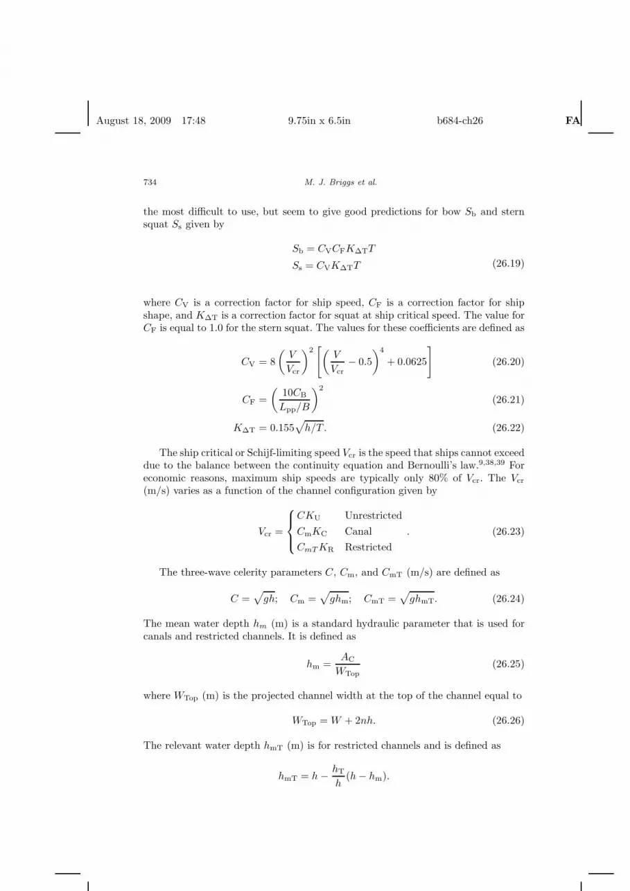
the most difficult to use, but seem to give good predictions for bow Sb and sternsquat Ss given by
Sb = CVCFK∆TT
Ss = CVK∆TT (26.19)
where CV is a correction factor for ship speed, CF is a correction factor for shipshape, and K∆T is a correction factor for squat at ship critical speed. The value forCF is equal to 1.0 for the stern squat. The values for these coefficients are defined as
CV = 8(
V
Vcr
)2[(
V
Vcr− 0.5
)4
+ 0.0625
](26.20)
CF =(
10CB
Lpp/B
)2
(26.21)
K∆T = 0.155√
h/T . (26.22)
The ship critical or Schijf-limiting speed Vcr is the speed that ships cannot exceeddue to the balance between the continuity equation and Bernoulli’s law.9,38,39 Foreconomic reasons, maximum ship speeds are typically only 80% of Vcr. The Vcr
(m/s) varies as a function of the channel configuration given by
Vcr =
CKU UnrestrictedCmKC CanalCmT KR Restricted
. (26.23)
The three-wave celerity parameters C, Cm, and CmT (m/s) are defined as
C =√
gh; Cm =√
ghm; CmT =√
ghmT. (26.24)
The mean water depth hm (m) is a standard hydraulic parameter that is used forcanals and restricted channels. It is defined as
hm =AC
WTop(26.25)
where WTop (m) is the projected channel width at the top of the channel equal to
WTop = W + 2nh. (26.26)
The relevant water depth hmT (m) is for restricted channels and is defined as
hmT = h − hT
h(h − hm).
August 18, 2009 17:48 9.75in x 6.5in b684-ch26 FA
Prediction of Squat for Underkeel Clearance 735
Table 26.2. Romisch’s KC versus 1/S.
1/S 1 6 10 20 30 ∞KC 0.0 0.52 0.62 0.73 0.78 1.0
Romisch’s correction factors KU, KC, and KR for unrestricted, canal, andrestricted channels, respectively, are defined as
KU = 0.58[(
h
T
)(Lpp
B
)]0.125
(26.27)
KC =[2 sin
(Arc sin(1 − S)
3
)]1.5
(26.28)
KR = KU(1 − hT/h) + KC(hT/h). (26.29)
Note that the KR for the restricted channel is a function of both KU and KC.Table 26.2 lists Romisch’s limited dataset for KC as a function of 1/S (i.e., AC/AS).Appendix 26.A contains more detailed descriptions of KC and some additionalequations for defining it relative to Schijf’s limiting speed and his limiting Froudenumber FHL.
26.3.4. Example problems
Three example problems are presented in this section to illustrate the differentformulas for several channel and ship types. All are for bow squat Sb. Comparisonsof the different formulas with the measured laboratory values are shown for eachexample in Figs. 26.4–26.6, respectively. Appendix 26.B contains worked examplesfor at least one Concept and one Detailed Design application for each exampleproblem.
26.3.4.1. Example 1: BAW Post-Panamax containershipin unrestricted channel
The first example is for a Post-Panamax containership traveling at Vk = 13.3 kt(Vs = 6.84m/s) in an unrestricted channel. This speed matches laboratory data(Sb = 0.70m) obtained at BAW by Flugge and Uliczka.40,41 This vessel is similarto the last generation Emma Maersk containership (launched in August 2006), butwith a larger CB. The larger CB is not realistic for the newer containerships (mosthave CB < 0.7), but was tested by BAW by “lengthening” an existing model duringdesign experiments. A comparable CB is of the order of 0.62 for a ship of this size.The dimensions of the ship and channel are listed in Table 26.3.
Figure 26.4 shows comparisons among the Barrass, Eryuzlu, Huuska, ICORELS,Romisch, and Yoshimura formulas and the measured BAW laboratory values. Thenumerical values are from a numerical model described in Sec. 26.6. In general, thebest formulas are the Yoshimura (Concept) and Eryuzlu (Detail) as they are slightly
August 18, 2009 17:48 9.75in x 6.5in b684-ch26 FA
736 M. J. Briggs et al.
9 11 13 15 17 19Vk, knots
-2.0
-1.5
-1.0
-0.5
0.0
Sb,
m
BarrassEryuzluHuuskaICORELS
R RomischYoshimura
N NumericalBAW
Unrestricted Channel Bottom
RR
R
R
R
R
R
R
R
R
N
N
N
N
N
N
N
N
Example
Bow Squat for BAW Hansa Container Ship - Unrestricted
Fig. 26.4. Comparison of BAW’s experimental measurements, empirical formulas, and numericalmodel of bow squat for a Post-Panamax containership in an unrestricted channel (open water).
7 8 9 10 11 12Vk, knots
-1.5
-1.0
-0.5
0.0
Sb,
m
BarrassHuuska
R RomischYoshimura
N NumericalFHR
Canal Bottom
Example
Bow Squat for FHR Tanker G, Condition C - Canal
R
R
R
R
R
R
R
R
R
N
N
N
N
Fig. 26.5. Comparison of FHR’s experimental measurements, empirical formulas, and numericalmodel of bow squat for a Tanker “G”, in Condition C in a canal with vertical sides.
August 18, 2009 17:48 9.75in x 6.5in b684-ch26 FA
Prediction of Squat for Underkeel Clearance 737
4 5 6 7 8Vk, knots
-1.5
-1.0
-0.5
0.0
Sb,
m
RR
RR
R
R
R
R
R
BarrassHuuska
R RomischYoshimura
N NumericalTothil
N
N
N
N
N
Canal Bottom
Bow Squat for Tothil Canadian Laker - Canal
Example
Fig. 26.6. Comparison of Tothil’s experimental measurements, empirical formulas, and numericalmodel of bow squat for a Canadian Laker in a canal.
Table 26.3. BAW’s Post-Panamax containershipin unrestricted channel.
Lpp (m) B (m) T (m) CB h (m)
400 50 17 0.84 19
conservative (i.e., larger than measured). The Romisch is slightly smaller than themeasured values, but follows the trend very well. Appendix 26.B contains workedexamples for the Concept Design formulas of Yoshimura and ICORELS and theDetail Design formulas of Eryuzlu and Romisch.
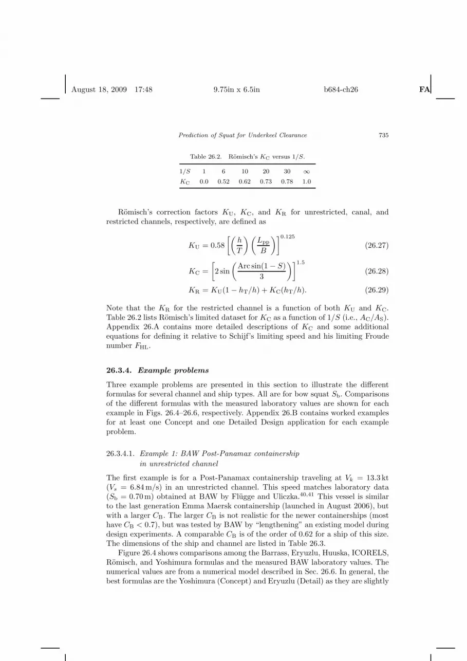
26.3.4.2. Example 2: FHR “G” Tanker in a canal with vertical side,Condition C
The second example is for the “G” Tanker, Condition C in a canal with vertical sides(similar to a restricted channel) from FHR and Ghent University.42 The 1:50 scalelaboratory experiments were performed in a 7.0-m-wide (350-m prototype) towingtank. The measured Sb = 1.18m for the ship sailing at Vk = 10kt (Vs = 5.14m/s).The ship and channel characteristics are listed in Table 26.4.
Figure 26.5 shows comparisons among the Barrass, Huuska, Romisch, andYoshimura formulas and the measured FHR laboratory values for the canal withvertical sides. The numerical values are from a numerical model that is described inSec. 26.6. In general, the best formulas are the Yoshimura (Concept) and Romisch(Detail) as they are nearly exact or slightly conservative for the smaller ship speeds

August 18, 2009 17:48 9.75in x 6.5in b684-ch26 FA
738 M. J. Briggs et al.
Table 26.4. FHR “G” Tanker in restricted channel, Condition C.
Lpp (m) B (m) T (m) CB h (m) hT (m) W (m) WTop (m) n (deg)
180 33 13 0.85 14.5 14.5 350 350 0.0
(i.e., larger than measured). Appendix 26.B contains worked examples for theYoshimura, Barrass (Concept), and Huuska (Detail). The Romisch is not includedin the worked examples for this case as it has already been demonstrated. TheBarrass is a little small, especially for higher ship speeds. The Huuska formula isconservative for all ship speeds.
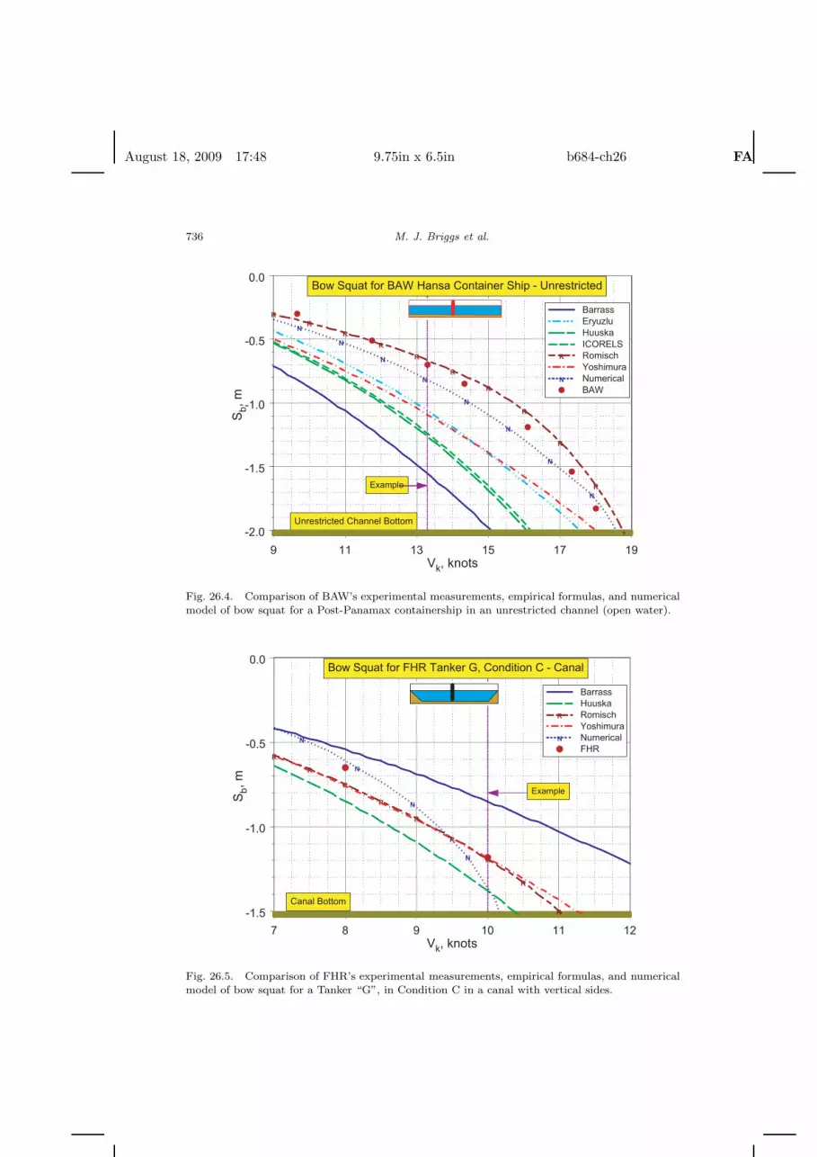
26.3.4.3. Example 3: Tothil’s Canadian Laker in a canal
The third example is for a Canadian Laker in a canal with sloping sides (typicalcanal). These data are from Tothil’s 1:48 scale model experiments.43 The measuredSb = 0.93m for the ship traveling at 6.98 kt (Vs = 3.59m/s). Ship and channelfeatures are listed in Table 26.5.
Figure 26.6 shows comparisons among the Barrass, Huuska, Romisch, andYoshimura formulas and the measured Tothil laboratory values for the canal case.The numerical values are from a numerical model that is described in Sec. 26.6. Ingeneral, the best formulas are the Barrass (Concept), Huuska (Detail), and Romisch(Detail). The Barrass is a good match for ship speeds less than 6.54 kt, but doesnot follow the measured values for increasing speeds. The Huuska is on the low side,but matches reasonably well until Vk exceeds 6.54 kt. The Romisch is on the lowside, but follows the measured trend of the data for all speeds. The Barrass andRomisch formulas are included in worked examples in Appendix 26.B.
26.4. Recent Investigations of Ship Squat
So far we have discussed the PIANC empirical formulas for predicting ship squat.These are based on “idealized” conditions with single vessels that are sailing alongthe centerline of symmetrical channels. Unfortunately, real-world channels and shiptransits are seldom this simple. This section discusses some recent research in lab-oratory and field measurements of ship head-on passing encounters and overtakingmaneuvers in two-way traffic, stern-transom effects, abrupt sills, and offset and driftangle effects for ships sailing off the centerline with drift angles.
When two ships pass or overtake each other, the water flow and correspondingsquat is affected as a function of the other ship’s size, speed, and direction oftravel, and the channels configuration. Dand44 was one of the first to study this
Table 26.5. Tothil’s Canadian Laker in a canal.
Lpp (m) B (m) T (m) CB h (m) W (m) WTop (m) n
215.6 22.9 7.77 0.86 9.33 72.3 105.9 1.8 (29 deg)
August 18, 2009 17:48 9.75in x 6.5in b684-ch26 FA
Prediction of Squat for Underkeel Clearance 739
phenomenon. He found increases in bow squat of 50–100% during passing and over-taking encounters.
During the past 10 years, the BAW has conducted many field and labo-ratory studies to investigate ship–waterway interactions, especially head-on passingencounters and overtaking maneuvers of ships in restricted channels within Germanfederal waterways. Preliminary studies of the dynamic response of large container-ships in laboratory models have shown tendencies of reduced squat.40,41,45 Theseresults were confirmed by additional model tests in restricted and unrestrictedchannels and field measurements along the Elbe River.31 The FHR (in cooperationwith the Ghent University) has conducted laboratory experiments to study passingand overtaking in their automated towing tank as part of a larger study to improvetheir ship simulator for traffic in Flemish waterways.46 Finally, the Delft Universityof Technology47 had conducted some numerical modeling of the effects of ship offsetand drift angles on ship squat. Thus, this section presents a summary of recentlaboratory, field, and numerical investigations of ship squat in real-world situationsincluding head-on passing encounters, overtaking maneuvers, wider stern-transoms,and ships with offset and drift angles.
26.4.1. Head-on passing ship encounters
26.4.1.1. BAW laboratory experiments
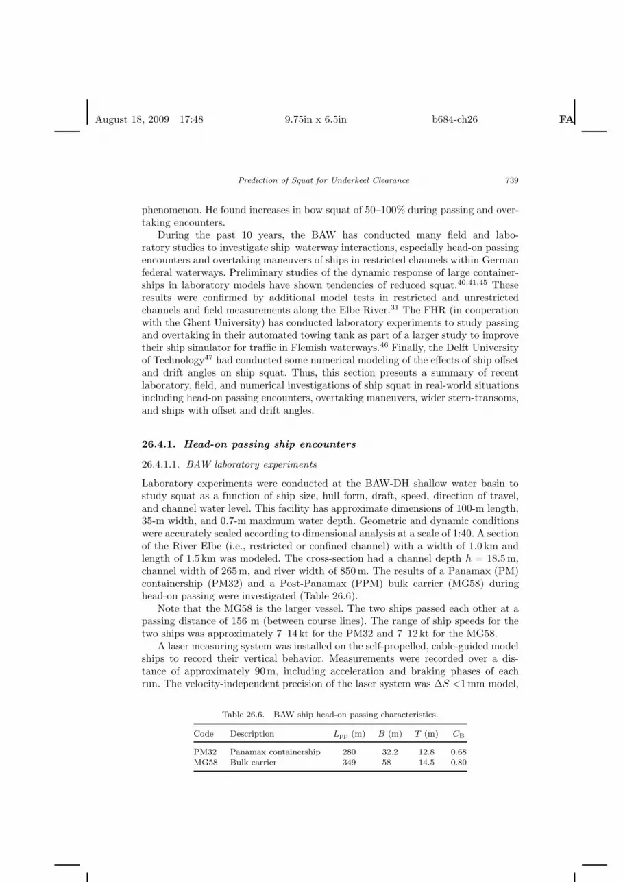
Laboratory experiments were conducted at the BAW-DH shallow water basin tostudy squat as a function of ship size, hull form, draft, speed, direction of travel,and channel water level. This facility has approximate dimensions of 100-m length,35-m width, and 0.7-m maximum water depth. Geometric and dynamic conditionswere accurately scaled according to dimensional analysis at a scale of 1:40. A sectionof the River Elbe (i.e., restricted or confined channel) with a width of 1.0 km andlength of 1.5 km was modeled. The cross-section had a channel depth h = 18.5m,channel width of 265m, and river width of 850m. The results of a Panamax (PM)containership (PM32) and a Post-Panamax (PPM) bulk carrier (MG58) duringhead-on passing were investigated (Table 26.6).
Note that the MG58 is the larger vessel. The two ships passed each other at apassing distance of 156 m (between course lines). The range of ship speeds for thetwo ships was approximately 7–14kt for the PM32 and 7–12kt for the MG58.
A laser measuring system was installed on the self-propelled, cable-guided modelships to record their vertical behavior. Measurements were recorded over a dis-tance of approximately 90m, including acceleration and braking phases of eachrun. The velocity-independent precision of the laser system was ∆S <1mm model,
Table 26.6. BAW ship head-on passing characteristics.
Code Description Lpp (m) B (m) T (m) CB
PM32 Panamax containership 280 32.2 12.8 0.68MG58 Bulk carrier 349 58 14.5 0.80

August 18, 2009 17:48 9.75in x 6.5in b684-ch26 FA
740 M. J. Briggs et al.
Fig. 26.7. Laboratory measurement of the effect of head-on passing on bow and stern squat for a
PM containership passing a large bulk carrier in the River Elbe. The dark blue curves represent thesingle runs of the containership; the light blue curves the encounters with the large bulk carrier.
corresponding to <4 cm in the prototype. Additional measurements with a point,laser-geometric method allowed for correlation of squat as a function of ship speed,with an accuracy of ∆S < 1 mm (model) for speeds up to 14 kt prototype.
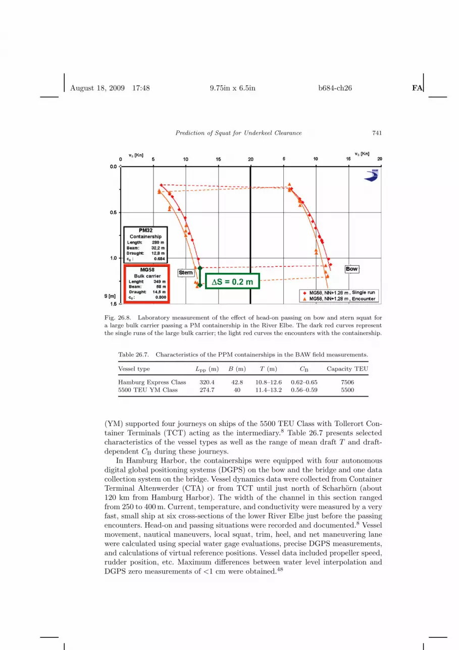
Figure 26.7 illustrates the effect of passing on bow and stern squat for the smallerPM32 containership. The measured squat for the single PM32 sailing by itself isshown in dark blue. The effect of the larger MG58 bulk carrier on the PM32 squatis shown in light blue. An additional increase in maximum bow squat for the PM32(Vk = 14kt) of ∆S ≈ 0.6m was recorded due to the passing encounter with theMG58 (Vk = 12kt). The trim of the PM32 changed from even keel for single runsin the channel and low speeds to bow trim at higher passing speeds during theencounter situation. Figure 26.8 is the analogous figure for the larger MG58 bulkcarrier, but shown in red colors for ease of readability. The larger and slower MG58experienced an additional squat of ∆S ≈ +0.2m at the stern. The trim of theMG58 changed only slightly at the stern from its original trim as a single ship inthe channel.
26.4.1.2. BAW field measurements
Field measurements of 12 transits on PPM containerships along the River Elbe weremade between April 2003 and June 2004. Meteorological conditions included verycalm to stormy (up to Beaufort Wind Scale 9). The shipping company Hapag LloydContainer Line GmbH (HLCL) supported eight journeys (transits) of HamburgExpress Class ships (7506 TEU), and Yang Ming Marine Transport Corporation
August 18, 2009 17:48 9.75in x 6.5in b684-ch26 FA
Prediction of Squat for Underkeel Clearance 741
Fig. 26.8. Laboratory measurement of the effect of head-on passing on bow and stern squat fora large bulk carrier passing a PM containership in the River Elbe. The dark red curves representthe single runs of the large bulk carrier; the light red curves the encounters with the containership.
Table 26.7. Characteristics of the PPM containerships in the BAW field measurements.
Vessel type Lpp (m) B (m) T (m) CB Capacity TEU
Hamburg Express Class 320.4 42.8 10.8–12.6 0.62–0.65 75065500 TEU YM Class 274.7 40 11.4–13.2 0.56–0.59 5500
(YM) supported four journeys on ships of the 5500 TEU Class with Tollerort Con-tainer Terminals (TCT) acting as the intermediary.8 Table 26.7 presents selectedcharacteristics of the vessel types as well as the range of mean draft T and draft-dependent CB during these journeys.
In Hamburg Harbor, the containerships were equipped with four autonomousdigital global positioning systems (DGPS) on the bow and the bridge and one datacollection system on the bridge. Vessel dynamics data were collected from ContainerTerminal Altenwerder (CTA) or from TCT until just north of Scharhorn (about120 km from Hamburg Harbor). The width of the channel in this section rangedfrom 250 to 400m. Current, temperature, and conductivity were measured by a veryfast, small ship at six cross-sections of the lower River Elbe just before the passingencounters. Head-on and passing situations were recorded and documented.8 Vesselmovement, nautical maneuvers, local squat, trim, heel, and net maneuvering lanewere calculated using special water gage evaluations, precise DGPS measurements,and calculations of virtual reference positions. Vessel data included propeller speed,rudder position, etc. Maximum differences between water level interpolation andDGPS zero measurements of <1 cm were obtained.48

August 18, 2009 17:48 9.75in x 6.5in b684-ch26 FA
742 M. J. Briggs et al.
Fig. 26.9. Cumulative distribution of the increase in squat for 125 head-on passing encounters oflarge PPM containerships (HLCL and YM) at the channel of the lower and outer River Elbe.
Squat measurement errors were estimated to be ∆S = ±0.05m for UKC determi-nation. Given the quality of the digital terrain model from area and traffic soundings,a precision of ∆UKC < ±0.2m was estimated. Precisions of ∆VS = ±0.08kt forship velocity (over ground) and ∆Φ = ±0.07deg for ship heel were also estimated.48
During the seven-hour transits of the 12 ships from Hamburg to the sea, 125head-on passing encounters were recorded. Figure 26.9 shows the increase in bow(blue diamond) and stern (red square) squat due to these head-on passing encountersand the corresponding cumulative distribution curve. The increase in squat wasabout the same at both the bow and stern. For this limited set of large containershipsin the River Elbe, the maximum increase in squat was 0.44m; 50% of the casesexperienced bow or stern squat less than 0.16m, while 90% were less than 0.33m.
26.4.1.3. FHR laboratory experiments
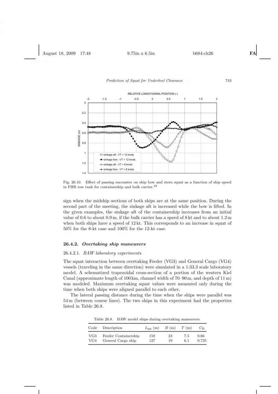
The FHR conducted comprehensive laboratory studies of head-on passingencounters to improve the quality of their ship simulator.42 Figure 26.10 illustratesthe effect on the squat of a containership (LOA = 291.3m, B = 40.3m, T = 13.5m)sailing at a forward speed of 12 kt, caused by a head-on passing encounter with abulk carrier (LOA = 310.6m, B = 37.8m, and T = 13.5m). The lateral distancedy between the two centerlines was 114.5m and the water depth h was 17.1m.The triangles indicate the sinkage fore and aft of the containership as a function ofthe relative longitudinal position of both vessels if the bulk carrier approaches ata speed of 8 kt, while the squares refer to an approach speed of 12 kt. The abscissatakes values of −1 and +1, respectively, when the bows and the sterns are locatedat the same longitudinal position. When the two bows meet, the ship’s bow sinkageincreases, whereas the stern is lifted, resulting in trim by the bow. The trim changes
August 18, 2009 17:48 9.75in x 6.5in b684-ch26 FA
Prediction of Squat for Underkeel Clearance 743
0
0.2
0.4
-2 -1.5 -1 -0.5 0 0.5 1 1.5 2
RELATIVE LONGITUDINAL POSITION (-)
0.6
0.8
1
1.2
1.4
SIN
KA
GE
(m
)
sinkage aft - VT = 12 knots
sinkage fore - VT = 12 knots
sinkage aft - VT = 8 knots
sinkage fore - VT = 8 knots
Fig. 26.10. Effect of passing encounter on ship bow and stern squat as a function of ship speed
in FHR tow tank for containership and bulk carrier.49
sign when the midship sections of both ships are at the same position. During thesecond part of the meeting, the sinkage aft is increased while the bow is lifted. Inthe given examples, the sinkage aft of the containership increases from an initialvalue of 0.6 to about 0.9m, if the bulk carrier has a speed of 8 kt and to about 1.2mwhen both ships have a speed of 12 kt. This corresponds to an increase in squat of50% for the 8-kt case and 100% for the 12-kt case.
26.4.2. Overtaking ship maneuvers
26.4.2.1. BAW laboratory experiments
The squat interaction between overtaking Feeder (VG3) and General Cargo (VG4)vessels (traveling in the same direction) were simulated in a 1:33.3 scale laboratorymodel. A schematized trapezoidal cross-section of a portion of the western KielCanal (approximate length of 100km, channel width of 70–90m, and depth of 11m)was modeled. Maximum overtaking squat values were measured only during thetime when both ships were aligned parallel to each other.
The lateral passing distance during the time when the ships were parallel was54m (between course lines). The two ships in this experiment had the propertieslisted in Table 26.8.
Table 26.8. BAW model ships during overtaking maneuvers.
Code Description Lpp (m) B (m) T (m) CB
VG3 Feeder Containership 158 23 7.5 0.66VG4 General Cargo ship 127 19 6.1 0.725
August 18, 2009 17:48 9.75in x 6.5in b684-ch26 FA
744 M. J. Briggs et al.
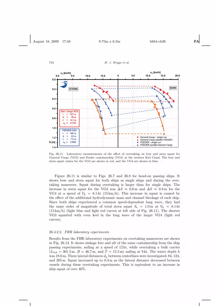
Fig. 26.11. Laboratory measurements of the effect of overtaking on bow and stern squat forGeneral Cargo (VG3) and Feeder containership (VG4) at the western Kiel Canal. The bow andstern squat values for the VG3 are shown in red, and the VG4 are shown in blue.
Figure 26.11 is similar to Figs. 26.7 and 26.8 for head-on passing ships. Itshows bow and stern squat for both ships as single ships and during the over-taking maneuver. Squat during overtaking is larger than for single ships. Theincrease in stern squat for the VG3 was ∆S ≈ 0.6m and ∆S ≈ 0.8m for theVG4 at a speed of Vk = 8.1 kt (15 km/h). This increase in squat is caused bythe effect of the additional hydrodynamic mass and channel blockage of each ship.Since both ships experienced a common speed-dependent long wave, they hadthe same order of magnitude of total stern squat Ss = 1.0m at Vk = 8.1 kt(15 km/h) (light blue and light red curves at left side of Fig. 26.11). The shorterVG3 squatted with even keel in the long wave of the larger VG4 (light redcurves).
26.4.2.2. FHR laboratory experiments
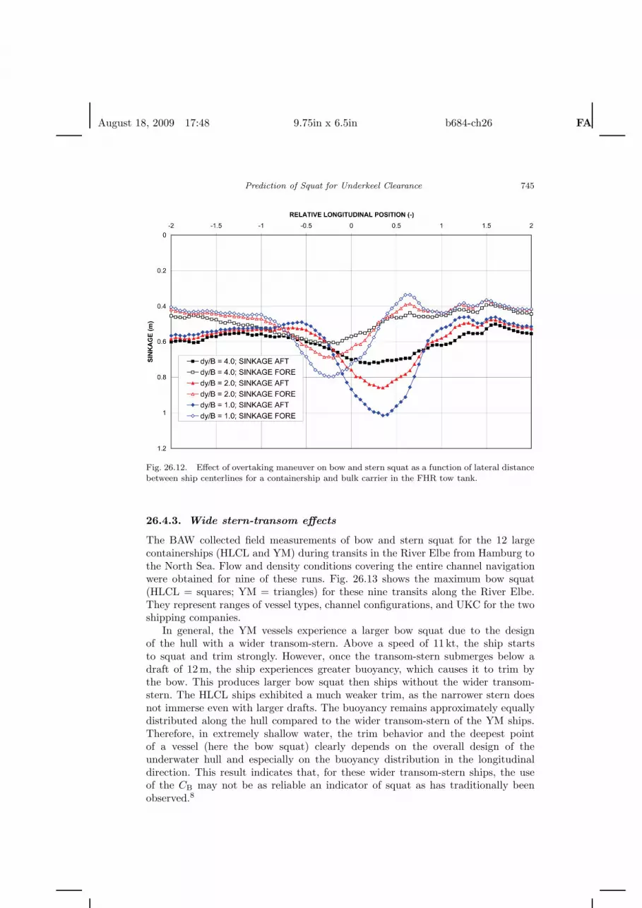
Results from the FHR laboratory experiments on overtaking maneuvers are shownin Fig. 26.12. It shows sinkage fore and aft of the same containership from the shippassing experiments, sailing at a speed of 12 kt, while overtaking a bulk carrier(LOA = 301.5m, B = 46.7m, and T = 15.5m) sailing at 8 kt. The water depth hwas 18.6m. Three lateral distances dy between centerlines were investigated: 84, 124,and 205m. Squat increased up to 0.3m as the lateral distance decreased betweenvessels during these overtaking experiments. This is equivalent to an increase inship squat of over 40%.
August 18, 2009 17:48 9.75in x 6.5in b684-ch26 FA
Prediction of Squat for Underkeel Clearance 745
Fig. 26.12. Effect of overtaking maneuver on bow and stern squat as a function of lateral distancebetween ship centerlines for a containership and bulk carrier in the FHR tow tank.
26.4.3. Wide stern-transom effects
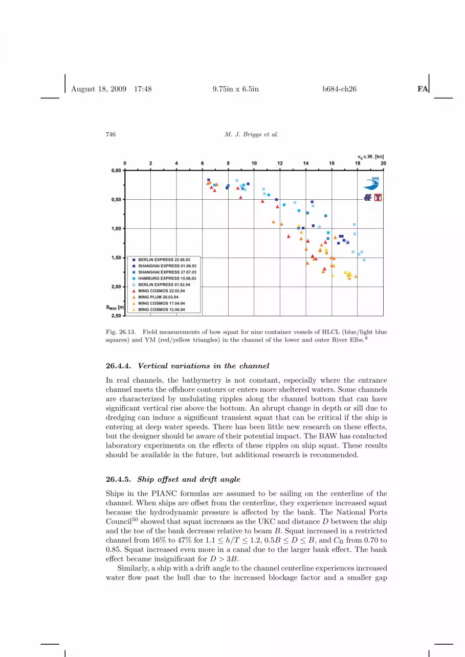
The BAW collected field measurements of bow and stern squat for the 12 largecontainerships (HLCL and YM) during transits in the River Elbe from Hamburg tothe North Sea. Flow and density conditions covering the entire channel navigationwere obtained for nine of these runs. Fig. 26.13 shows the maximum bow squat(HLCL = squares; YM = triangles) for these nine transits along the River Elbe.They represent ranges of vessel types, channel configurations, and UKC for the twoshipping companies.
In general, the YM vessels experience a larger bow squat due to the designof the hull with a wider transom-stern. Above a speed of 11 kt, the ship startsto squat and trim strongly. However, once the transom-stern submerges below adraft of 12m, the ship experiences greater buoyancy, which causes it to trim bythe bow. This produces larger bow squat then ships without the wider transom-stern. The HLCL ships exhibited a much weaker trim, as the narrower stern doesnot immerse even with larger drafts. The buoyancy remains approximately equallydistributed along the hull compared to the wider transom-stern of the YM ships.Therefore, in extremely shallow water, the trim behavior and the deepest pointof a vessel (here the bow squat) clearly depends on the overall design of theunderwater hull and especially on the buoyancy distribution in the longitudinaldirection. This result indicates that, for these wider transom-stern ships, the useof the CB may not be as reliable an indicator of squat as has traditionally beenobserved.8
August 18, 2009 17:48 9.75in x 6.5in b684-ch26 FA
746 M. J. Briggs et al.
0,00
0,50
1,00
1,50
2,00
2,50
0 2 4 6 8 10 12 14 16 18 20vS d.W. [Kn]
SMAX [m]
BERLIN EXPRESS 22.06.03
SHANGHAI EXPRESS 01.06.03
SHANGHAI EXPRESS 27.07.03
HAMBURG EXPRESS 15.06.03
BERLIN EXPRESS 01.02.04
MING COSMOS 22.02.04
MING PLUM 28.03.04
MING COSMOS 17.04.04
MING COSMOS 12.06.04
vS c.W. [kn]
0,00
0,50
1,00
1,50
2,00
2,50
0 2 4 6 8 10 12 14 16 18 20vS d.W. [Kn]
SMAX [m]
BERLIN EXPRESS 22.06.03
SHANGHAI EXPRESS 01.06.03
SHANGHAI EXPRESS 27.07.03
HAMBURG EXPRESS 15.06.03
BERLIN EXPRESS 01.02.04
MING COSMOS 22.02.04
MING PLUM 28.03.04
MING COSMOS 17.04.04
MING COSMOS 12.06.04
vS c.W. [kn]
Fig. 26.13. Field measurements of bow squat for nine container vessels of HLCL (blue/light blue
squares) and YM (red/yellow triangles) in the channel of the lower and outer River Elbe.8
26.4.4. Vertical variations in the channel
In real channels, the bathymetry is not constant, especially where the entrancechannel meets the offshore contours or enters more sheltered waters. Some channelsare characterized by undulating ripples along the channel bottom that can havesignificant vertical rise above the bottom. An abrupt change in depth or sill due todredging can induce a significant transient squat that can be critical if the ship isentering at deep water speeds. There has been little new research on these effects,but the designer should be aware of their potential impact. The BAW has conductedlaboratory experiments on the effects of these ripples on ship squat. These resultsshould be available in the future, but additional research is recommended.
26.4.5. Ship offset and drift angle
Ships in the PIANC formulas are assumed to be sailing on the centerline of thechannel. When ships are offset from the centerline, they experience increased squatbecause the hydrodynamic pressure is affected by the bank. The National PortsCouncil50 showed that squat increases as the UKC and distance D between the shipand the toe of the bank decrease relative to beam B. Squat increased in a restrictedchannel from 16% to 47% for 1.1 ≤ h/T ≤ 1.2, 0.5B ≤ D ≤ B, and CB from 0.70 to0.85. Squat increased even more in a canal due to the larger bank effect. The bankeffect became insignificant for D > 3B.
Similarly, a ship with a drift angle to the channel centerline experiences increasedwater flow past the hull due to the increased blockage factor and a smaller gap
August 18, 2009 17:48 9.75in x 6.5in b684-ch26 FA
Prediction of Squat for Underkeel Clearance 747
between the ship and the channel. The ship acts as a lifting surface as it movesasymmetrically through the water. Drift angles are usually the result of trying tocompensate for large wind forces, especially on containerships.
26.4.5.1. Delft numerical model
The Delft University of Technology (Delft) has recently completed a limited set ofnumerical modeling of ship squat for ships sailing with an offset and drift angle tothe channel centerline.47
A panel method was used in the tests for a 6500 TEU Post-Panamax containership with one draft but a range of offsets and drift angles. The potential flow modelincludes inertial effects, but no viscosity that will cause vortices and increased squatif included. The modeled ship had Lpp = 302m, B = 42.9m, T = 14m, andCB = 0.67. The canal had W = 300m and h = 16m. The UKC = 2m with offsetsof 0 and ±20m, and drift angles of 0, ±7.5 deg and ±15 deg.
They found that both offsets and drift angles increase squat, in a quadraticmanner. High drift angles should be avoided by using tugs if available. They recom-mended additional research for a range of ships, channels, UKC, offsets, and driftangles.
26.4.5.2. FHR laboratory experiments
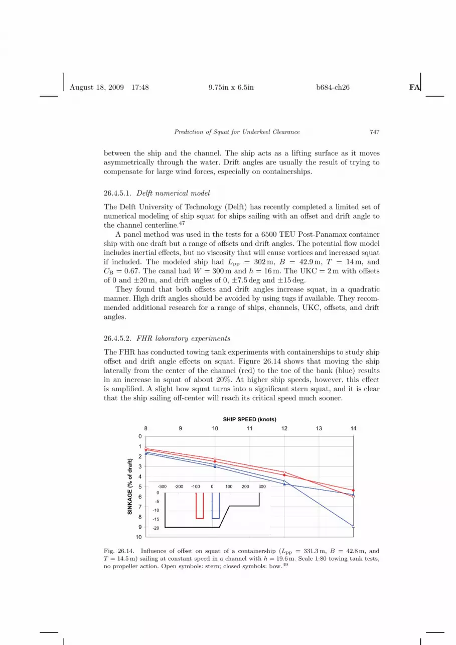
The FHR has conducted towing tank experiments with containerships to study shipoffset and drift angle effects on squat. Figure 26.14 shows that moving the shiplaterally from the center of the channel (red) to the toe of the bank (blue) resultsin an increase in squat of about 20%. At higher ship speeds, however, this effectis amplified. A slight bow squat turns into a significant stern squat, and it is clearthat the ship sailing off-center will reach its critical speed much sooner.
Fig. 26.14. Influence of offset on squat of a containership (Lpp = 331.3 m, B = 42.8m, andT = 14.5m) sailing at constant speed in a channel with h = 19.6m. Scale 1:80 towing tank tests,no propeller action. Open symbols: stern; closed symbols: bow.49
August 18, 2009 17:48 9.75in x 6.5in b684-ch26 FA
748 M. J. Briggs et al.
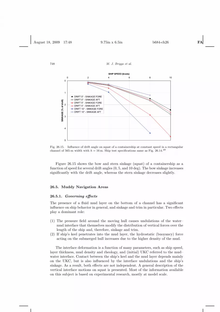
Fig. 26.15. Influence of drift angle on squat of a containership at constant speed in a rectangularchannel of 565-m width with h = 16 m. Ship test specifications same as Fig. 26.14.49
Figure 26.15 shows the bow and stern sinkage (squat) of a containership as afunction of speed for several drift angles (0, 5, and 10 deg). The bow sinkage increasessignificantly with the drift angle, whereas the stern sinkage decreases slightly.
26.5. Muddy Navigation Areas
26.5.1. Governing effects
The presence of a fluid mud layer on the bottom of a channel has a significantinfluence on ship behavior in general, and sinkage and trim in particular. Two effectsplay a dominant role:
(1) The pressure field around the moving hull causes undulations of the water–mud interface that themselves modify the distribution of vertical forces over thelength of the ship and, therefore, sinkage and trim.
(2) If ship’s keel penetrates into the mud layer, the hydrostatic (buoyancy) forceacting on the submerged hull increases due to the higher density of the mud.
The interface deformation is a function of many parameters, such as ship speed,layer thickness, mud density and rheology, and (initial) UKC referred to the mud–water interface. Contact between the ship’s keel and the mud layer depends mainlyon the UKC, but is also influenced by the interface undulations and the ship’ssinkage. As a result, both effects are not independent. A general description of thevertical interface motions on squat is presented. Most of the information availableon this subject is based on experimental research, mostly at model scale.
August 18, 2009 17:48 9.75in x 6.5in b684-ch26 FA
Prediction of Squat for Underkeel Clearance 749
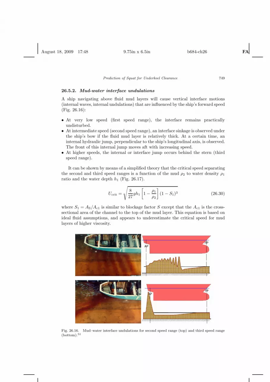
26.5.2. Mud-water interface undulations
A ship navigating above fluid mud layers will cause vertical interface motions(internal waves, internal undulations) that are influenced by the ship’s forward speed(Fig. 26.16):
• At very low speed (first speed range), the interface remains practicallyundisturbed.
• At intermediate speed (second speed range), an interface sinkage is observed underthe ship’s bow if the fluid mud layer is relatively thick. At a certain time, aninternal hydraulic jump, perpendicular to the ship’s longitudinal axis, is observed.The front of this internal jump moves aft with increasing speed.
• At higher speeds, the internal or interface jump occurs behind the stern (thirdspeed range).
It can be shown by means of a simplified theory that the critical speed separatingthe second and third speed ranges is a function of the mud ρ2 to water density ρ1
ratio and the water depth h1 (Fig. 26.17).
Ucrit =
√827
gh1
[1 − ρ1
ρ2
](1 − S1)3 (26.30)
where S1 = AS/Ac1 is similar to blockage factor S except that the Ac1 is the cross-sectional area of the channel to the top of the mud layer. This equation is based onideal fluid assumptions, and appears to underestimate the critical speed for mudlayers of higher viscosity.
Fig. 26.16. Mud–water interface undulations for second speed range (top) and third speed range(bottom).51

August 18, 2009 17:48 9.75in x 6.5in b684-ch26 FA
750 M. J. Briggs et al.
0
2
4
6
8
10
1 1.05 1.1 1.15 1.2 1.25 1.32/ 1
Ucr
it(k
no
ts)
h1 = 25 mh1 = 20 mh1 = 15 m
h1 = 10 m
0
2
4
6
8
10
1 1.05 1.1 1.15 1.2 1.25 1.3ρ2/ρ1
Ucr
it(k
no
ts)
h1 = 25 mh1 = 20 mh1 = 15 m
h1 = 10 m
h1 = 25 mh1 = 20 mh1 = 15 m
h1 = 10 m
Fig. 26.17. Critical speed separating second and third speed ranges as a function of mud–waterdensity ρ2/ρ1 ratio for different water depths h1.51
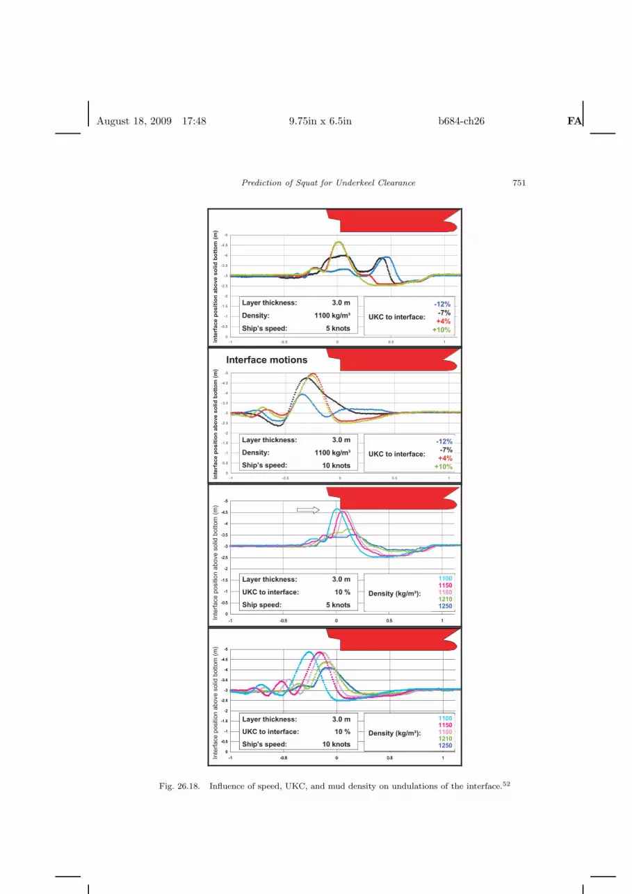
The description above is typical for motions of the mud–water interface occurringwhen a ship moves with a positive UKC above a fluid mud layer of low viscosity(black water). In case of a negative UKC (i.e., when the keel penetrates the mudlayer), a second internal wave system, comparable to the Kelvin wave system in thewater–air interface, interferes with the hydraulic jump. This may result in eitheran interface rising amidships or a double-peaked rising along the hull. Figure 26.18illustrates the effect of speed (5 and 10kt), UKC (−12% to +10%), and mud density(1100–1250kg/m3) on the interface undulation pattern.
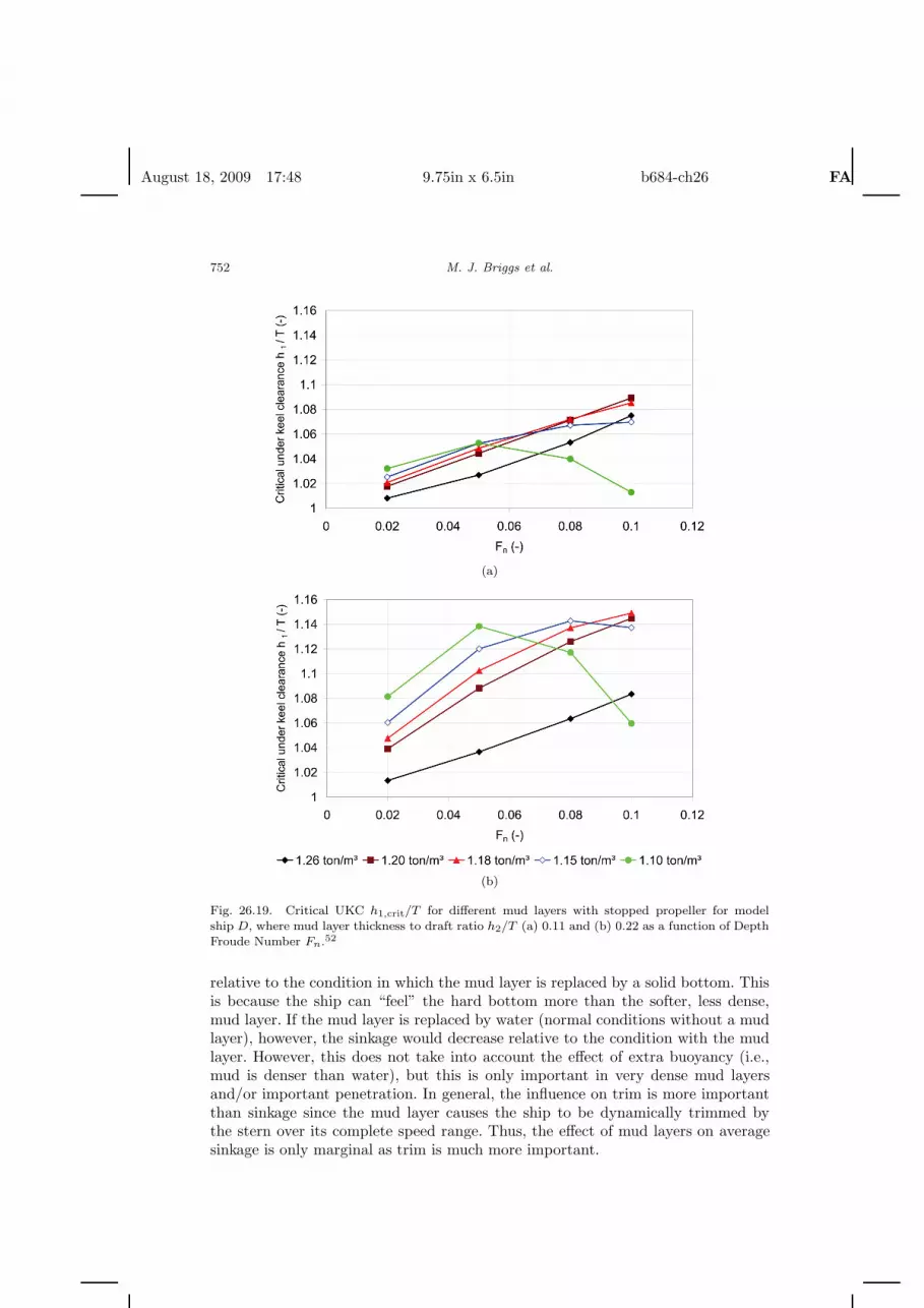
Due to the vertical motion of the interface and the ship, contact between theship’s keel and the mud layer can occur even if, initially at rest, the UKC of theship is positive relative to the mud–water interface. Figure 26.19 shows the initialUKC required to avoid contact between mud and keel as a function of Depth Froudenumber Fn (speed) for different mud characteristics.
26.5.3. Effect of mud layers on sinkage and trim
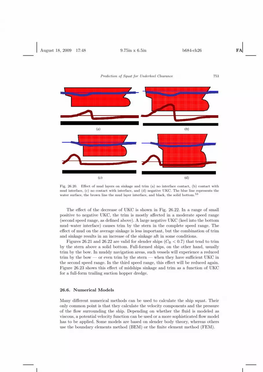
The effect of the presence of a fluid mud layer covering the bottom on the ship’svertical motions is closely related to the interface deformation. If no contact betweenthe ship’s keel and the mud layer occurs [Figs. 26.20(a) and 26.20(c)], a risinginterface yields an increased velocity of the ship relative to the water and, as aresult, a pressure drop and a local water depression. A mud–water interface sinkage,on the other hand, leads to a local decrease of the relative velocity and an increasedpressure, at least compared to the solid bottom case. In case of contact betweenkeel and a rising mud interface (Fig. 26.20(b)), the velocity of the mud relative tothe ship’s surface decreases. Contact with a lowered interface with negative UKC(Fig. 26.20(d)) leads to an increased relative fluid velocity, with associated localpressure fluctuations acting on the ship’s keel.
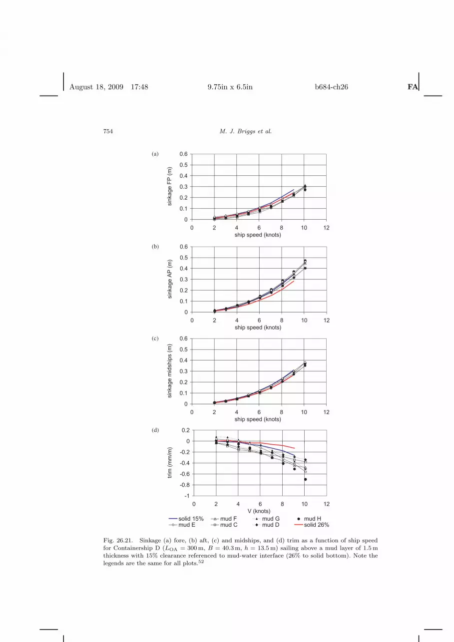
Figure 26.21 illustrates the effect of the presence of a mud layer on the sinkageand trim of a containership for the case in which the initial UKC is sufficiently largeso that the interface undulations do not cause any contact between the keel and themud layer. The sinkage for a ship sailing in a muddy bottom condition is decreased
August 18, 2009 17:48 9.75in x 6.5in b684-ch26 FA
Prediction of Squat for Underkeel Clearance 751
-5
-4.5
-4
-3.5
-3
-2.5
-2
-1.5
-1
-0.5
0
-1 -0.5 0 0.5 1
inte
rfa
ce
po
sit
ion
ab
ov
e s
oli
d b
ott
om
-12%-7%+4%
+10%
Layer thickness: 3.0 m
Density: 1100 kg/m³
Ship’s speed: 5 knots
UKC to interface:
inte
rfa
ce p
os
itio
nab
ove
soli
db
ott
om
(m)
-5
-4.5
-4
-3.5
-3
-2.5
-2
-1.5
-1
-0.5
0
-1 -0.5 0 0.5 1
inte
rfa
ce
po
sit
ion
ab
ov
e s
oli
d b
ott
om
Interface motions
-12%-7%+4%
+10%
Layer thickness:
Density:
Ship’s speed:
UKC to interface:
inte
rfac
e p
os
itio
nab
ove
solid
bo
tto
m(m
)
-5
-4.5
-4
-3.5
-3
-2.5
-2
-1.5
-1
-0.5
0
-1 -0.5 0 0.5 1
inte
rfa
ce p
osi
tio
n a
bo
ve
so
lid
bo
tto
m (
m)
11001150118012101250
Layer thickness: 3 .0 m
UKC to interface: 10 %
Ship speed: 5 knots
Density (kg/m³):
Inte
rfac
e po
sitio
nab
ove
solid
bott
om(m
)
-5
-4.5
-4
-3.5
-3
-2.5
-2
-1.5
-1
-0.5
0
-1 -0.5 0 0.5 1
inte
rfa
ce p
osi
tio
n a
bo
ve
so
lid
bo
tto
m (
m)
11001150118012101250
Layer thickness:
UKC to interface: 10 %
Ship speed:
Density (kg/m³):
Inte
rfac
e po
sitio
nab
ove
solid
bott
om(m
)
-5
-4.5
-4
-3.5
-3
-2.5
-2
-1.5
-1
-0.5
0
-1 -0.5 0 0.5 1
inte
rfac
e p
osi
tio
n a
bo
ve s
oli
d b
ott
om
(m
)
11001150118012101250
Layer thickness: 3 .0 m
UKC to interface: 10 %
Ship's speed: 10 knots
Density (kg/m³):
Inte
rfac
e po
sitio
nab
ove
solid
bott
om(m
) -5
-4.5
-4
-3.5
-3
-2.5
-2
-1.5
-1
-0.5
0
-1 -0.5 0 0.5 1
inte
rfac
e p
osi
tio
n a
bo
ve s
oli
d b
ott
om
(m
)
11001150118012101250
Layer thickness: 3 .0 m
UKC to interface: 10 %
Ship's speed: 10 knots
Density (kg/m³):
-5
-4.5
-4
-3.5
-3
-2.5
-2
-1.5
-1
-0.5
0
-1 -0.5 0 0.5 1
inte
rfac
e p
osi
tio
n a
bo
ve s
oli
d b
ott
om
(m
)
11001150118012101250
Layer thickness:
UKC to interface: 10 %
Ship's speed:
Density (kg/m³):
Inte
rfac
e po
sitio
nab
ove
solid
bott
om(m
)
3.0 m
1100 kg/m³
10 knots
3.0 m
5 knots
3.0 m
10 knots
Fig. 26.18. Influence of speed, UKC, and mud density on undulations of the interface.52
August 18, 2009 17:48 9.75in x 6.5in b684-ch26 FA
752 M. J. Briggs et al.
(a)
(b)
Fig. 26.19. Critical UKC h1,crit/T for different mud layers with stopped propeller for modelship D, where mud layer thickness to draft ratio h2/T (a) 0.11 and (b) 0.22 as a function of DepthFroude Number Fn.52
relative to the condition in which the mud layer is replaced by a solid bottom. Thisis because the ship can “feel” the hard bottom more than the softer, less dense,mud layer. If the mud layer is replaced by water (normal conditions without a mudlayer), however, the sinkage would decrease relative to the condition with the mudlayer. However, this does not take into account the effect of extra buoyancy (i.e.,mud is denser than water), but this is only important in very dense mud layersand/or important penetration. In general, the influence on trim is more importantthan sinkage since the mud layer causes the ship to be dynamically trimmed bythe stern over its complete speed range. Thus, the effect of mud layers on averagesinkage is only marginal as trim is much more important.
August 18, 2009 17:48 9.75in x 6.5in b684-ch26 FA
Prediction of Squat for Underkeel Clearance 753
Fig. 26.20. Effect of mud layers on sinkage and trim (a) no interface contact, (b) contact withmud interface, (c) no contact with interface, and (d) negative UKC. The blue line represents thewater surface, the brown line the mud layer interface, and black, the solid bottom.53
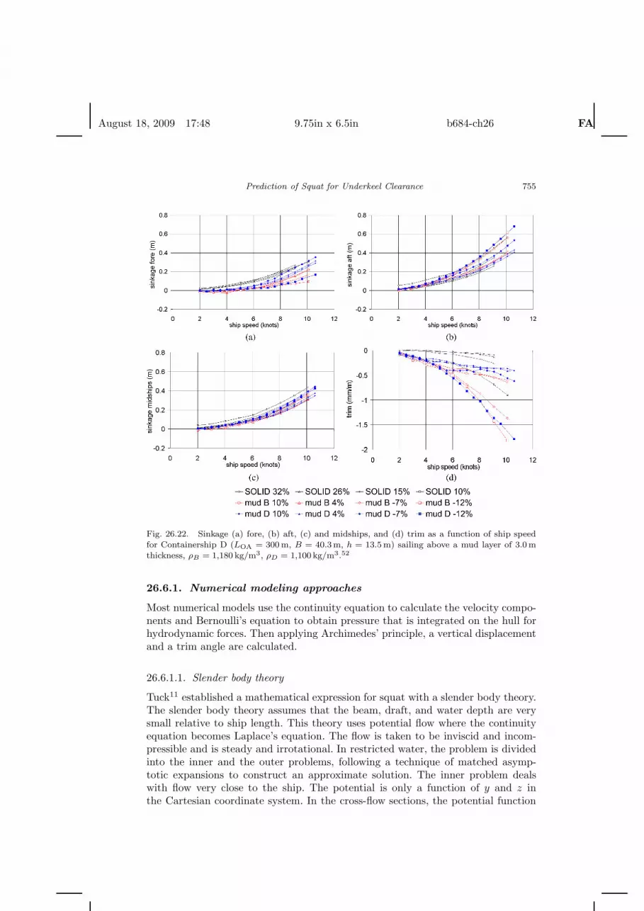
The effect of the decrease of UKC is shown in Fig. 26.22. In a range of smallpositive to negative UKC, the trim is mostly affected in a moderate speed range(second speed range, as defined above). A large negative UKC (keel into the bottommud–water interface) causes trim by the stern in the complete speed range. Theeffect of mud on the average sinkage is less important, but the combination of trimand sinkage results in an increase of the sinkage aft in some conditions.
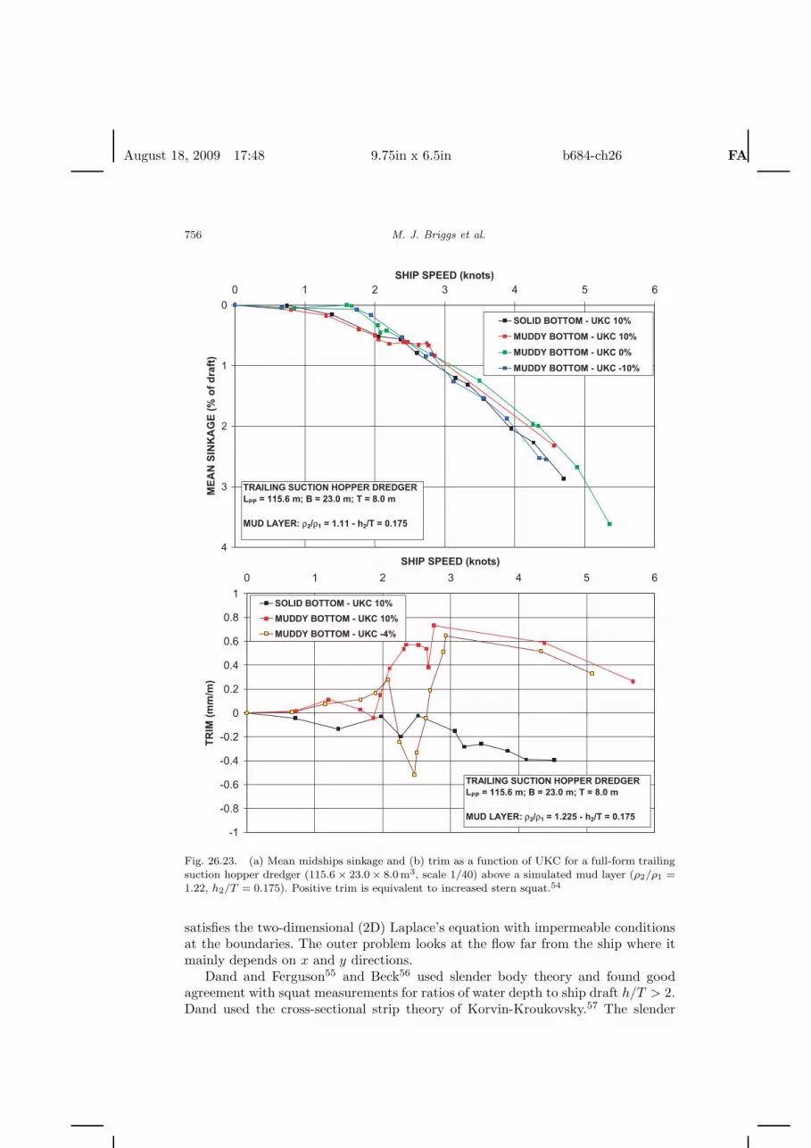
Figures 26.21 and 26.22 are valid for slender ships (CB < 0.7) that tend to trimby the stern above a solid bottom. Full-formed ships, on the other hand, usuallytrim by the bow. In muddy navigation areas, such vessels will experience a reducedtrim by the bow — or even trim by the stern — when they have sufficient UKC inthe second speed range. In the third speed range, this effect will be reduced again.Figure 26.23 shows this effect of midships sinkage and trim as a function of UKCfor a full-form trailing suction hopper dredge.
26.6. Numerical Models
Many different numerical methods can be used to calculate the ship squat. Theironly common point is that they calculate the velocity components and the pressureof the flow surrounding the ship. Depending on whether the fluid is modeled asviscous, a potential velocity function can be used or a more sophisticated flow modelhas to be applied. Some models are based on slender body theory, whereas othersuse the boundary elements method (BEM) or the finite element method (FEM).
August 18, 2009 17:48 9.75in x 6.5in b684-ch26 FA
754 M. J. Briggs et al.
0
0.1
0.2
0.3
0.4
0.5
0.6
0 2 4 6 8 10 12ship speed (knots)
sink
age
FP
(m
)
0
0.1
0.2
0.3
0.4
0.5
0.6
0 2 4 6 8 10 12ship speed (knots)
sink
age
AP
(m
)
0
0.1
0.2
0.3
0.4
0.5
0.6
0 2 4 6 8 10 12ship speed (knots)
sink
age
mid
ship
s (m
)
-1
-0.8
-0.6
-0.4
-0.2
0
0.2
0 2 4 6 8 10 12V (knots)
trim
(m
m/m
)
solid 15% mud F mud G mud Hmud E mud C mud D solid 26%
(a)
(b)
(c)
(d)
Fig. 26.21. Sinkage (a) fore, (b) aft, (c) and midships, and (d) trim as a function of ship speedfor Containership D (LOA = 300 m, B = 40.3m, h = 13.5 m) sailing above a mud layer of 1.5mthickness with 15% clearance referenced to mud-water interface (26% to solid bottom). Note thelegends are the same for all plots.52
August 18, 2009 17:48 9.75in x 6.5in b684-ch26 FA
Prediction of Squat for Underkeel Clearance 755
Fig. 26.22. Sinkage (a) fore, (b) aft, (c) and midships, and (d) trim as a function of ship speedfor Containership D (LOA = 300 m, B = 40.3m, h = 13.5 m) sailing above a mud layer of 3.0mthickness, ρB = 1,180 kg/m3, ρD = 1,100 kg/m3.52
26.6.1. Numerical modeling approaches
Most numerical models use the continuity equation to calculate the velocity compo-nents and Bernoulli’s equation to obtain pressure that is integrated on the hull forhydrodynamic forces. Then applying Archimedes’ principle, a vertical displacementand a trim angle are calculated.
26.6.1.1. Slender body theory
Tuck11 established a mathematical expression for squat with a slender body theory.The slender body theory assumes that the beam, draft, and water depth are verysmall relative to ship length. This theory uses potential flow where the continuityequation becomes Laplace’s equation. The flow is taken to be inviscid and incom-pressible and is steady and irrotational. In restricted water, the problem is dividedinto the inner and the outer problems, following a technique of matched asymp-totic expansions to construct an approximate solution. The inner problem dealswith flow very close to the ship. The potential is only a function of y and z inthe Cartesian coordinate system. In the cross-flow sections, the potential function
August 18, 2009 17:48 9.75in x 6.5in b684-ch26 FA
756 M. J. Briggs et al.
0
1
2
3
4
SHIP SPEED (knots)
ME
AN
SIN
KA
GE
(%
of
dra
ft)
SOLID BOTTOM - UKC 10%
MUDDY BOTTOM - UKC 10%
MUDDY BOTTOM - UKC 0%
MUDDY BOTTOM - UKC -10%
TRAILING SUCTION HOPPER DREDGERLPP = 115.6 m; B = 23.0 m; T = 8.0 m
MUD LAYER: ρ2/ρ1 = 1.11 - h2/T = 0.175
-1
-0.8
-0.6
-0.4
-0.2
0
0.2
0.4
0.6
0.8
1
0 1 2 3 4 5 6
0 1 2 3 4 5 6
SHIP SPEED (knots)
TR
IM (
mm
/m)
SOLID BOTTOM - UKC 10%
MUDDY BOTTOM - UKC 10%
MUDDY BOTTOM - UKC -4%
TRAILING SUCTION HOPPER DREDGERLPP = 115.6 m; B = 23.0 m; T = 8.0 m
MUD LAYER: ρ2/ρ1 = 1.225 - h2/T = 0.175
Fig. 26.23. (a) Mean midships sinkage and (b) trim as a function of UKC for a full-form trailingsuction hopper dredger (115.6 × 23.0 × 8.0m3, scale 1/40) above a simulated mud layer (ρ2/ρ1 =1.22, h2/T = 0.175). Positive trim is equivalent to increased stern squat.54
satisfies the two-dimensional (2D) Laplace’s equation with impermeable conditionsat the boundaries. The outer problem looks at the flow far from the ship where itmainly depends on x and y directions.
Dand and Ferguson55 and Beck56 used slender body theory and found goodagreement with squat measurements for ratios of water depth to ship draft h/T > 2.Dand used the cross-sectional strip theory of Korvin-Kroukovsky.57 The slender
August 18, 2009 17:48 9.75in x 6.5in b684-ch26 FA
Prediction of Squat for Underkeel Clearance 757
body method works by vertical cross-sections of the flow, so it is also called theone-dimensional (1D) theory of squat.
Gourlay58 extended the slender body theory of Tuck with the unsteady slenderbody theory. This improvement allows one to consider a ship moving in a non-uniform depth since the coordinate system is now earth-fixed, whereas it is ship-fixed for classic numerical methods. The 1D system still uses vertical cross-sectionsand decomposition into an inner and outer expansion. The pressure integration isonly made on the ship length based on the ship section B(x) at each x along thehull. Resolution of the 1D equation is made with the finite difference method. Com-parison with experimental results for soft squat situations (h/T > 4) showed goodagreement with numerical results. No tests were made for hard squat conditions(i.e., shallow depths) where flow around the ship is affected.
26.6.1.2. Boundary element method
The BEM is really based on a particular numerical resolution. It is commonlyapplied for wave-resistance calculations using Green’s function to calculate thepotential velocity function. Derivatives of the potential velocity function give thevelocity components in Cartesian coordinates. Buhring59 made a squat model calledfast boundary elements method (FBEM) based on this boundary element method.The reliability of the model has to be verified, however, as no comparisons with shipsquat measurements was found.
26.6.1.3. Computational fluid dynamics models
A number of commercially available computational fluid dynamics (CFD) modelscould be used for the prediction of squat. At the core of any CFD problem is acomputational grid or mesh where the solution is divided into thousands of elements.These elements are usually 2D quadrilaterals or triangles; and three-dimensional(3D) hexahedral, tetrahedral, or prisms. Mathematical equations are solved for eachelement by the numerical model. For hydrodynamics the Navier–Stokes equations(NSEs) can be solved to include viscosity and turbulence. The NSEs provide detailedprediction (vortices) of the flow field, but require very thin meshes, high centralprocessing unit (CPU) time, and memory storage. Its resolution is also quite difficultwith numerical instabilities. Examples of commercial CFD models include Fluentand Fidap.
Nowadays, CFD models can solve 3D problems, such as ship squat, but thecomputation domain has to be relatively narrow using NSE. To extend the widthof the computation domain, some models solve the problem by zones. Far from theship, the model solves a potential function with a nonviscous fluid and, in the vicinityof the ship, the model solves using the NSEs. The advantage of the potential flowsolution is that it requires low CPU time and less memory storage. The boundaryconditions for the NSE model are extracted from the potential flow solution. Oneexample of this kind of commercial model is ShipFlow.
In very restricted water, squat can substantially reduce the vertical cross-sectionaround the ship and can subsequently increase the flow velocity below the hull.
August 18, 2009 17:48 9.75in x 6.5in b684-ch26 FA
758 M. J. Briggs et al.
According to Bernoulli’s principle, the pressure will decrease which will make theship sink more. Numerical models have to take into account this “over squat” toprecisely calculate ship squat in all channel configurations. So when a first squatresult has been found, the model has to check that this squat is not disturbingthe hydrodynamics in such a way that squat could increase more. This checking isimportant to ensure a reliable result from the numerical model. As these commercialnumerical models do not perform squat checking, they may not be very efficient inrestricted water. The user has to be very careful and take the result with reservationssince the numerical model could in these conditions underestimate ship squat.
26.6.2. New modeling system to predict ship squat
In an unrestricted channel (i.e., open sea or large channel), “over squat” is negligible,and the previous numerical models work well unless the UKC is relatively small(h/T < 1.1). Under a 3-m UKC or in a very restricted channel, the numericalmodel has to check that the hydrodynamics are not being modified by the squat.Some empirical formulas try to make such a correction with a restriction factor thatmultiplies the squat calculated for unrestricted water. For instance, the K coefficientin Barrass and Ks for Huuska are examples of these types of correction factors.
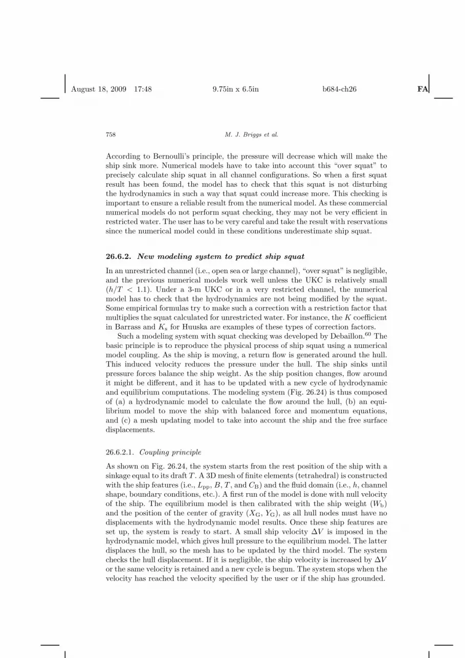
Such a modeling system with squat checking was developed by Debaillon.60 Thebasic principle is to reproduce the physical process of ship squat using a numericalmodel coupling. As the ship is moving, a return flow is generated around the hull.This induced velocity reduces the pressure under the hull. The ship sinks untilpressure forces balance the ship weight. As the ship position changes, flow aroundit might be different, and it has to be updated with a new cycle of hydrodynamicand equilibrium computations. The modeling system (Fig. 26.24) is thus composedof (a) a hydrodynamic model to calculate the flow around the hull, (b) an equi-librium model to move the ship with balanced force and momentum equations,and (c) a mesh updating model to take into account the ship and the free surfacedisplacements.
26.6.2.1. Coupling principle
As shown on Fig. 26.24, the system starts from the rest position of the ship with asinkage equal to its draft T . A 3D mesh of finite elements (tetrahedral) is constructedwith the ship features (i.e., Lpp, B, T , and CB) and the fluid domain (i.e., h, channelshape, boundary conditions, etc.). A first run of the model is done with null velocityof the ship. The equilibrium model is then calibrated with the ship weight (Wb)and the position of the center of gravity (XG, YG), as all hull nodes must have nodisplacements with the hydrodynamic model results. Once these ship features areset up, the system is ready to start. A small ship velocity ∆V is imposed in thehydrodynamic model, which gives hull pressure to the equilibrium model. The latterdisplaces the hull, so the mesh has to be updated by the third model. The systemchecks the hull displacement. If it is negligible, the ship velocity is increased by ∆Vor the same velocity is retained and a new cycle is begun. The system stops when thevelocity has reached the velocity specified by the user or if the ship has grounded.
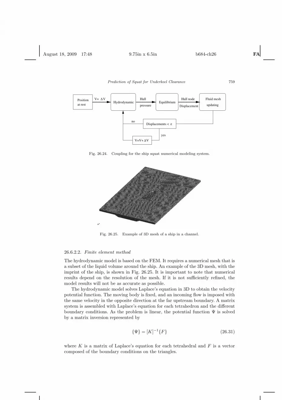
August 18, 2009 17:48 9.75in x 6.5in b684-ch26 FA
Prediction of Squat for Underkeel Clearance 759
V= V∆
V=V+ V∆
HydrodynamicPositionat rest
EquilibriumHull node Fluid mesh
updating
Displacements < ε
pressure
Hull
yes
no
Displacement
Fig. 26.24. Coupling for the ship squat numerical modeling system.
Fig. 26.25. Example of 3D mesh of a ship in a channel.
26.6.2.2. Finite element method
The hydrodynamic model is based on the FEM. It requires a numerical mesh that isa subset of the liquid volume around the ship. An example of the 3D mesh, with theimprint of the ship, is shown in Fig. 26.25. It is important to note that numericalresults depend on the resolution of the mesh. If it is not sufficiently refined, themodel results will not be as accurate as possible.
The hydrodynamic model solves Laplace’s equation in 3D to obtain the velocitypotential function. The moving body is fixed, and an incoming flow is imposed withthe same velocity in the opposite direction at the far upstream boundary. A matrixsystem is assembled with Laplace’s equation for each tetrahedron and the differentboundary conditions. As the problem is linear, the potential function Ψ is solvedby a matrix inversion represented by
{Ψ} = [K]−1{F} (26.31)
where K is a matrix of Laplace’s equation for each tetrahedral and F is a vectorcomposed of the boundary conditions on the triangles.

August 18, 2009 17:48 9.75in x 6.5in b684-ch26 FA
760 M. J. Briggs et al.
26.6.2.3. Three numerical models
In Fig. 26.24, the three numerical models are represented by shaded boxes. Thefirst model calculates the velocity components and pressure at each node of themesh. The second receives pressures at all nodes of the hull. The correspondingvertical force FPZ is obtained by integration of pressure over the hull. Squat ∆Sb isestimated as
∆Sb = αWb − FPZ
ρgSf(26.32)
where Sf is the floating surface of the ship, and α (fixed at 0.9) is a relaxationcoefficient to limit the variation of squat in a calculation cycle for the mesh updatingmodel.
Pitching θ1 and rolling θ2 angles are estimated in the second model from the xand y components of the moment equations:
tan θ1 = αWb(xG − xP)
ρg∫
x∈Sf
∫y∈Sf
x(x − x0)dx dy(26.33)
tan θ2 = αWb(yG − yP)
ρg∫
x∈Sf
∫y∈Sf
y(y − y0)dx dy. (26.34)
The equilibrium (second) model has to calculate the position of the center of verticalthrust P (xP, yP) by integration of the pressure over the hull, and O(x0, y0) thecenter of the floating surface Sf . All nodes of the ship are then vertically translatedby ∆z and rotated by θ1 around the y-axis and by θ2 around the x-axis.
The third model moves all nodes of the free surface per the results of Bernoulli’srelation, and the hull node displacements in x and y directions. Then the innernodes of the mesh are moved proportionally according to boundary modificationsand the distance from those boundaries.
Since 2006 the University of Compiegne has been working to improve Debaillon’ssquat system. As in Gourlay’s model, the coordinate system will be earth-fixed toallow ship passing or crossing and bridge pile crossings. The system will also be ableto take into account a nonuniform water depth along the channel.
26.6.3. Numerical modeling examples
Figures 26.4–26.6 showed comparisons of the PIANC empirical formulas with themeasured laboratory measurements. These figures also included comparisons withthe numerical model predictions for each example. These examples included BAW’sPPM containership in an unrestricted channel, FHR’s tanker in restricted water,and Tothil’s Canadian Laker in a canal. In general, the numerical model matchedthe measured values from the laboratory measurements very well. Details of theindividual examples are given in the following sections.
August 18, 2009 17:48 9.75in x 6.5in b684-ch26 FA
Prediction of Squat for Underkeel Clearance 761
26.6.3.1. BAW PPM containership in an unrestricted channel
The mesh contains 57,602 nodes, 255,447 tetrahedra, and 58,458 triangles. A generalcomparison between squat measurements, empirical formulas, and the numericalmodel was shown in Fig. 26.4. The numerical modeling match is very good, with amaximum error smaller than 0.12m.
26.6.3.2. FHR “G” Tanker in restricted water, Condition “C”
The mesh contains 35,149 nodes, 158,022 tetrahedra, and 33,532 triangles.Figure 26.5 showed the comparisons. The numerical model had to rotate the hull(trim) around the center of gravity. The agreement with the measured values wasreasonable.
26.6.3.3. Tothil’s Canadian Laker in canal
The mesh contains 27,191 nodes, 118,513 tetrahedra, and 28,300 triangles. A generalcomparison between squat measurements, empirical formulas, and the numericalmodel was shown in Fig. 26.6. The numerical model experienced some numericalinstability problems (rotate the hull (trim) around the center of gravity), but stillgave good predictions.
26.7. Conclusions and Outlook
This chapter has focused on some of the latest advances in predicting ship squatand its effect on underkeel clearance for channel design. Several of the more popularPIANC empirical formulas were presented for Concept and Detailed Design phases.In general, the simpler and more “user friendly” formulas were recommended forthe Concept Design phase, but this does not preclude them being used in the DetailDesign phase and vice versa. Ultimately, the designer wants the maximum squatvalue possible (bow or stern) in the Concept Design phase and a more realistic valuein the Detail Design phase. All empirical formulas have certain constraints basedon the field and laboratory data used in their development. It is up to the user toexercise Engineering Judgment when applying these formulas as they give a rangeof squat values.
The PIANC formulas were developed for “idealized” channel and sailing con-ditions for single ships. Recent research has been conducted to investigate more“real-world” conditions for the latest generation of larger ships. The BAW and FHRhave conducted extensive laboratory and field investigations of head-on passingand overtaking maneuvers, where squat is a function of ship speed and lateral sep-aration distance. Their results indicate that squat can increase 50–100% relativeto a single ship. The BAW measured maximum additional squat during passingencounters of 0.6m in the laboratory and 0.4m in the field. Similarly, the FHRmeasured maximum additional squat of 0.3–0.6m in the laboratory. For overtakingmaneuvers in the laboratory, the BAW recorded additional squat of 0.6–0.8m and
August 18, 2009 17:48 9.75in x 6.5in b684-ch26 FA
762 M. J. Briggs et al.
the FHR measured 0.2–0.3m. These additional squat values represent the effect ofthese more realistic ship and channel interactions for a range of conditions.
The BAW noted that ships with wider “transom” sterns experience more bowsquat than most ships with more streamlined transoms due to the additionalbuoyancy of the stern. They measured additional bow squat of 0.2–0.5m as afunction of ship speed.
The Delft and FHR have conducted research on ships sailing with offsets anddrift angle from the channel centerline. Delft found that both offsets and drift anglesincrease squat, in a quadratic manner. The FHR found that offsets can increasesquat by 20% and drift angles produce significant increase in bow squat and slightdecrease in stern squat.
The average sinkage of a vessel navigating in muddy channels is generallyreduced by the presence of mud layers. The dynamic trim is affected significantlyby the generation of interface undulations. For ships navigating above mud layers,the maximum sinkage is comparable to or slightly less than the values occurring ifthe mud layer were replaced by a solid bottom. Compared to the situation in whichthe mud layer is not present (i.e., replaced by water), the muddy bottom interfacealways increases the maximum sinkage, even in case of contact with the mud layer.This means that the mud layer will increase sinkage even if the ship “plows” throughit. The maximum sinkage (bow or stern) always increases when the lower part ofthe water column is replaced by fluid mud.
The designer and harbor pilots should be aware that all of these special influencescan increase squat. Sometimes, it is not economically feasible to design a channelfor all of these eventualities, but it is always possible to slow down as the conditionswarrant.
Numerical modeling of ship squat is just beginning to be developed. Histori-cally, ship modeling has been concentrated in the areas of wave resistance models.Squat modeling requires time domain models that are very computer intensive. Theincreasing cost of dredging and the larger ships coming on line have motivated manyinstitutions around the world (such as USACE, BAW, FHR, CETMEF, and FMA)to begin a more active development of ship squat models. The improvements incomputer speed and storage have made these types of models much more promising.The CETMEF numerical model matched measured laboratory values very well inthe three examples presented in this chapter.
Numerical models will continue to be improved, but field measurements andlaboratory models will still be necessary to investigate the highly nonlinear dynamicbehavior of the newer and larger ships. They will respond differently than existingships and continued study of passing and overtaking, bank and bottom effects, andsailing alignment will insure optimum and safe navigation design of channels andwaterways.
Acknowledgments
The authors wish to acknowledge the Headquarters, US Army Corps of Engineers,Ghent University, Flanders Hydraulics Research, Federal Waterways Engineeringand Research Institute, Centre d’Etudes Techniques Maritimes Et Fluviales, and the
August 18, 2009 17:48 9.75in x 6.5in b684-ch26 FA
Prediction of Squat for Underkeel Clearance 763
PIANC WG49 for authorizing publication of this chapter. Particular thanks goes toBryan Barrass, the WG49 Chair Mark McBride, original WG30 and WG49 memberWerner Dietze, and WG49 vertical subcommittee members Martin Boll, Hans Moes,Terry O’Brien, and Kohei Ohtsu who assisted with the ship squat and UKC research.Other members of the WG49 making contributions to this effort included Larry Cao,Don Cockrill, Rink Groenveld, Jarmo Hartikainen, Jose Iribarren, Susumu Naruse,Sahil Patel, Carlos Sanchidrian, Esa Sirkia, and Jos Van Doorn.
References
1. J. N. Newman, Marine Hydrodynamics (MIT Press, Cambridge, Massachusetts, 1977),pp. 329–386.
2. C. B. Barrass, Ship Squat Seminar, The Nautical Institute, Humberside Branch,September 1995, pp. 21–33.
3. C. B. Barrass, Thirty-Two Years of Research into Ship Squat, 2nd Squat Workshop2004, Elsfleth, Germany, 3–4 March 2004.
4. C. B. Barrass, Ship Squat and Interaction for Masters, Private report (2007), www.ship-squat.com.
5. PIANC, Approach Channels: A Guide for Design, Final Report of the Joint PIANC-IAPH Working Group II-30 in cooperation with IMPA and IALA, Supplement toBulletin No. 95 (1997).
6. PIANC, Horizontal and Vertical Dimensions of Fairways, Maritime Navigation Com-mission Working Group 49 (MarCom WG 49), July 2005.
7. O. Huuska, On the Evaluation of Underkeel Clearances in Finnish Waterways, HelsinkiUniversity of Technology, Ship Hydrodynamics Laboratory, Otaniemi, Report No. 9(1976).
8. K. Uliczka and B. Kondziella, Dynamic response of very large containerships inextremely shallow water, Proc. 31st PIANC Cong., Estoril, Spain (2006).
9. U.S. Army Corps of Engineers (USACE), Engineering and Design: HydraulicDesign Guidance for Deep-draft Navigation Projects, Engineer Manual 1110-2-1613,Headquarters, Washington, DC (2004).
10. M. Vantorre, Personal communication (2007).11. E. O. Tuck, Shallow-water flows past slender bodies, JFM 26(Part 1), 81–95 (1966).12. E. O. Tuck and P. J. Taylor, Shallow water problems in ship hydrodynamics, Proc.
8th Symp. Nav. Hydrod., Pasadena, CA (1970).13. R. F. Beck, J. N. Newman and E. O. Tuck, Hydrodynamic forces on ships in dredged
channels, J. Ship Res. 19(3), 166–171 (1975).14. J. P. Hooft, The behavior of a ship in head waves at restricted water depth, Int.
Shipbuild. Prog. 21(244), 367–378 (1974).15. I. W. Dand, Squat Estimation: A Graphical Method for Full Form Ships, National
Physical Laboratory, Report No. TM 348 (1975).16. N. E. Eryuzlu and R. Hausser, Experimental investigation into some aspects of large
vessel navigation in restricted waterways, Proc. Symp. Asp. Navi. Const. Waterway.Incl. Harb. Ent. 2, 1–15 (1978).
17. K. Romisch and Empfehlungen zur Bemessung von Hafeneinfahrten, WasserbaulicheMitteilungen der Technischen Universitat Dresden, Heft 1, 39–63 (1989).
18. A. Millward, A preliminary design method for the prediction of squat in shallow water,Mar. Tech. 27(1), 10–19 (1990).
August 18, 2009 17:48 9.75in x 6.5in b684-ch26 FA
764 M. J. Briggs et al.
19. A. Millward, A comparison of the theoretical and empirical prediction of squat inshallow water, Int. Shipbuilding Prog. 39(417), 69–78 (1992).
20. ICORELS (International Commission for the Reception of Large Ships), Report ofWorking Group IV, PIANC Bulletin No. 35, Supplement (1980).
21. C. B. Barrass, The phenomenon of ship squat, Int. Shipbuilding Prog. 26(294), 44–47(1979).
22. C. B. Barrass, Ship Squat — A Reply, The Naval Architect, November 1981,pp. 268–272.
23. N. E. Eryuzlu, Y. L. Cao and F. D’Agnolo, Underkeel requirements for large vessels inshallow waterways, Proc. 28th Int. Navi. Cong., PIANC, Paper S II-2, Sevilla, Spain(1994), pp. 17–25.
24. V. Ankudinov, L. L. Daggett, J. C. Hewlett and B. K. Jakobsen, Prototype mea-surement of ship sinkage in confined water, Proc. Int. Conf. Mar. Sim. Ship Maneuv.(MARSIM 2000), Orlando, FL, 8–12 May 2002.
25. D. T. Stocks, L. L. Dagget and Y. Page, Maximization of Ship Draft in the St.Lawrence Seaway Volume I: Squat Study, prepared for Transportation DevelopmentCentre, Transport Canada, June 2002.
26. M. J. Briggs, Ship Squat Predictions for Ship/Tow Simulator, Coastal and HydraulicsEngineering Technical Note CHETN-I-72, U.S. Army Engineer Research and Devel-opment Center, Vicksburg, MS (2006), http://chl.wes.army.mil/library/publications/chetn/.
27. C. B. Barrass, Ship Squat — A Guide for Masters, Private report (2002), www.ship-squat.com.
28. Y. Yoshimura, Mathematical model for the maneuvering ship motion in shallow water,J. Kansai Soc. Nav. Arch. Japan 200, 41–51 (1986).
29. FMA (Finnish Maritime Administration), The Channel Depth Practice in Finland,Bulletin, Waterways Division, Helsinki, Finland, 12 July 2005.
30. E. Sirkia, Economical efficiency to be achieved with a regulatory change only withconsideration for navigational risks, PIANC Magazine 129, 23–34 (2007).
31. K. Uliczka, B. Kondziella and G. Flugge, Dynamisches Fahrverhalten sehr großerContainerschiffe in seitlich begrenztem extremen Flachwasser, HANSA, 141, Jahrgang,Nr. 1 (2004) (in German).
32. Overseas Coastal Area Development Institute of Japan, Technical Standards andCommentaries for Port and Harbor Facilities in Japan (2002).
33. K. Ohtsu, Y. Yoshimura, M. Hirano, M. Tsugane and H. Takahashi, Design standardfor fairway in next generation, Asia Navigation Conf. 26 (2006).
34. K. Ohtsu, Personal communication (2007).35. Canadian Coast Guard, Safe Waterways (A Users Guide to the Design, Mainte-
nance and Safe Use of Waterways), Part 1(a) Guidelines for the Safe Design ofCommercial Shipping Channels, Software User Manual Version 3.0, Waterways Devel-opment Division, Fisheries and Oceans Canada, December 2001.
36. U. M. Guliev, On squat calculations for vessels going in shallow water and throughchannels, PIANC Bulletin 1(7), 17–20 (1971).
37. Puertos Del Estado, Recommendations for Maritime Works (Spain) ROM 3.1-99:Designing Maritime Configuration of Ports, Approach Channels and Floatation Areas,CEDEX, Spain (1999).
38. C. J. Huval, Lock Approach Canal Surge and Tow Squat at Lock and Dam17, Arkansas River Project; Mathematical Model Investigation, Technical ReportHL-80-17, U.S. Army Engineer Waterways Experiment Station, Vicksburg, MS(1980).
August 18, 2009 17:48 9.75in x 6.5in b684-ch26 FA
Prediction of Squat for Underkeel Clearance 765
39. V. Balanin et al., Peculiarities of navigation on canals and restricted channels, orig-inating hydraulic phenomena associated with them and their effect on the canalbed; measurements preventing slope deterioration, Paper S.I-3, 24th Int. Nav. Cong.,Leningrad, Russia (1977).
40. G. Flugge and K. Uliczka, Dynamisches Fahrverhalten und Wechselwirkungen mit derFahrrinnensohle von sehr großen Containerschiffen unter extremen Flachwasserbedin-gungen, Proceedings HTG-Kongress 2001, Hamburg (2001) (in German).
41. G. Flugge and K. Uliczka, Dynamisches Fahrverhalten mit der Fahrinnensohlevon sehr grossen Containershiffen unter extremen Flachwasserbedingungen. Hansa(2001).
42. M. Vantorre, E. Verzhbitskaya and E. Laforce, Model Test Based Formulations ofShip-Ship Interaction Forces, Ship Technology Research/Schiffstechnik, Band 49, Heft,3 August 2002.
43. J. T. Tothil, Ships in Restricted Channels, A Correlation of Model Tests, Field Mea-surements and Theory, National Research Council of Canada Mechanical EngineeringReport MB264, January 1966.
44. I. W. Dand, Some Measurements in Interaction between Ship Models Passing onParallel Courses, NMI R108, August 1981.
45. K. Uliczka and G. Flugge, Squat-Untersuchungen fur sehr große Post-Panamax-Containerschiffe, HTG/STG-Sprechtag FA Seeschifffahrststraßen, Hafen und Schiff,Hamburg (2001) (in German).
46. M. Vantorre, E. Laforce, G. Dumon and W. Wackenier, Development of a probabilisticadmittance policy for the flemish harbours, 30th PIANC Cong., Sydney, September2002.
47. H. J. de Koning Gans and H. Boonstra, Squat effects of very large container ships withdrift in a harbor environment, MTEC2007 Conference, Singapore, 26–28 September2007.
48. Ch. Maushake and S. Joswig, Messung von Squat, Trimm und Krangung sehrgroßer Containerschiffe im Rahmen von Grundsatzuntersuchungen auf der Elbe,Hydrographische Nachrichten Nr. 072, Deutsche Hydrographische Gesellschaft (2004)(in German).
49. M. Vantorre and G. Dumon, Model test based requirements for the under keelclearance in the access channels to the flemish harbours, 2nd Squat Workshop Aspectsof Under Keel Clearance in Analysis and Application, Elsfleth, March 2004.
50. National Ports Council, Ship Behavior in Ports and their Approaches — Part 2:Additional Sinkage Caused by Sailing in the Proximity of Channel Bank, ResearchTransport Headquarters, London, U.K. (1980).
51. M. Vantorre, Nautical Bottom Approach – Application to the Access to the Harbour ofZeebrugge, HANSA — Schiffahrt — Schiffbau — Hafen, 138. Jahrgang, Nr. 6 (2001),pp. 93–97.
52. G. Delefortrie, Maneuvering behavior of container vessels in muddy navigation areas,Ph.D. thesis, Ghent University (2007).
53. K. Van Craenenbroeck, M. Vantorre and P. De Wolf, Navigation in MuddyAreas: Establishing the Navigable Depth in the Port of Zeebrugge, ProceedingsCEDA/PIANC Conference 1991 (incorporating CEDA Dredging Days): AccessibleHarbours, Paper No. E4, Amsterdam (1991).
54. M. Vantorre, Systematische proevenreeksen met het zelfaangedreven schaalmodel vaneen sleephopperzuiger boven een mengsel petroleum¬trichloorethaan als slibsimulatie-materiaal experimentele waarnemingen en theoretische interpretaties. Rijksuniver-siteit Gent/Waterbouwkundig Laboratorium Borgerhout. Gent/Antwerpen (1990).

August 18, 2009 17:48 9.75in x 6.5in b684-ch26 FA
766 M. J. Briggs et al.
55. I. W. Dand and A. M. Ferguson, The squat of hull ships in shallow water, Roy. Inst.Nav. Arch. 115, 237–247 (1973).
56. R. F. Beck, Hydrodynamic forces caused by ship in confined waters, Proc. Am. Soc.Civ. Eng. 107, ASCE, EM3, June 1981, pp. 523–546.
57. B. V. Korvin-Kroukovsky, Investigations of ship motions in regular waves, Trans.SNAME 63, 386–435 (1955).
58. T. Gourlay, Mathematical and computational techniques for predicting the squat ofships. Thesis of the University of Adelaide, Australia (2000).
59. H. Buhring, Prediction of Squat by Fast Boundary Elements, 2nd Squat Workshop,Oldenburg, Germany (2004).
60. P. Debaillon, Systeme de modelisation de l’enfoncement dynamique des bateaux,Thesis of University of Compiegne, France (2005).
26.A. Appendix
26.A.1. Least square coefficients for Huuska K1 versus S
A least squares polynomial fit of Huuska’s Fig. 26.3 curves for K1 as a function ofS was calculated according to the formula:
K1 = a0 + a1S + a2S2 + a3S
3. (26.A1)
Table 26.A1 lists the correlation coefficient R2 and the polynomial coefficients foreach of the hT /h curves. This allows one to program the value for K1 without havingto manually read a plot.
26.A.2. Romisch Kc for canals and restricted channels
In Sec. 26.3.3.3, we presented an equation for Romisch’s Kc for canals and restrictedchannels as a function of the blockage factor S. The Kc given in Sec. 26.3.3.3 isequivalent to
KC =[2 cos
(π
3+
Arc cos(1 − S)3
)]1.5
. (26.A2)
Table 26.A1. Huuska K1 versus S least square fit coefficients.
Polynomial coefficients
hT /h R2 a0 a1 a2 a3
0.2 0.9988 1.0 2.7704 214.87 −569.420.4 0.9983 1.0 8.0885 89.87 −214.880.6 0.9963 1.0 −1.9528 137.6 −347.930.8 0.9991 1.0 1.9453 45.325 −129.481.0 1.0000 1.0 0.0 0.0 0.0
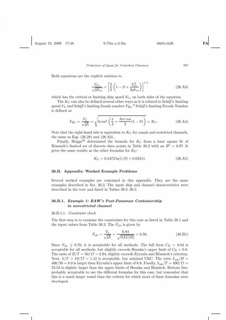
August 18, 2009 17:48 9.75in x 6.5in b684-ch26 FA
Prediction of Squat for Underkeel Clearance 767
Both equations are the explicit solution to
VCr√ghm
=[23
(1 − S +
V 2Cr
2ghm
)]1.5
(26.A3)
which has the critical or limiting ship speed VCr on both sides of the equation.The KC can also be defined several other ways as it is related to Schijf’s limiting
speed VL and Schijf’s limiting froude number FHL.9 Schijf’s limiting Froude Numberis defined as
FHL =VL√gh
=
√8 cos3
(π
3+
Arc cos3
(1 − S))
= KC. (26.A4)
Note that the right-hand side is equivalent to KC for canals and restricted channels,the same as Eqs. (26.28) and (26.A2).
Finally, Briggs26 determined the formula for KC from a least square fit ofRomisch’s limited set of discrete data points in Table 26.2 with an R2 = 0.97. Itgives the same results as the other formulas for KC:
KC = 0.2472 ln(1/S) + 0.02411. (26.A5)
26.B. Appendix: Worked Example Problems
Several worked examples are contained in this appendix. They are the sameexamples described in Sec. 26.3. The input ship and channel characteristics weredescribed in the text and listed in Tables 26.3–26.5.
26.B.1. Example 1: BAW’s Post-Panamax Containership
in unrestricted channel
26.B.1.1. Constraint check
The first step is to examine the constraints for this case as listed in Table 26.1 andthe input values from Table 26.3. The Fnh is given by
Fnh =Vs√gh
=6.84√
9.81(19)= 0.50. (26.B1)
Since Fnh ≤ 0.70, it is acceptable for all methods. The full form CB = 0.84 isacceptable for all methods, but slightly exceeds Huuska’s upper limit of CB < 0.8.The ratio of B/T = 50/17 = 2.94, slightly exceeds Eryuzlu and Romisch’s criterion.Next, h/T = 19/17 = 1.12 is acceptable, but minimal UKC. The ratio Lpp/B =400/50 = 8.0 is larger than Eryuzlu’s upper limit of 6.8. Finally, Lpp/T = 400/17 =23.53 is slightly larger than the upper limits of Huuska and Romisch. Bottom line:probably acceptable to use the different formulas for this case, but remember thatthis is a much larger vessel than the criteria for which most of these formulas weredeveloped.
August 18, 2009 17:48 9.75in x 6.5in b684-ch26 FA
768 M. J. Briggs et al.
26.B.1.2. ICORELS application
This is a logical first choice for an unrestricted channel as it is one of the first for-mulas developed as a guide. There are two steps involved in the ICORELS estimateof bow squat Sb.
The first step is to calculate the ship’s displacement volume Λ using values fromTable 26.3
∇ = CBLppBT = 0.84(400)(50)(17) = 285, 600 m3. (26.B2)
The second step is to substitute this value into the equation for bow squat Sb
from Table 26.3 and Sec. 26.B.1.1.
Sb = CS∇
L2pp
F 2nh√
1 − F 2nh
= 2.4285, 600(400)2
(0.50)2√1 − (0.50)2
= 1.24 m. (26.B3)
This value is too large compared to the measured value of Sb = 0.70m. Of course,some institutions use a smaller value of the constant CS. Thus, this value could bereduced by using a smaller CS, but it would need to be of the order of 1.4 which ismuch smaller than commonly recommended.
26.B.1.3. Yoshimura application
The Yoshimura formula is a good Concept Design application for this case. It isvery straightforward and easy to apply. Substituting values from Table 26.3 andSec. 26.B.1.1 into Yoshimura’s equation for Sb
Sb =
[(0.7 + 1.5
11.12
)(0.848.0
)+ 15
11.12
(0.848.0
)3]
(6.84)9.81
2
= 1.10 m. (26.B4)
Thus, this Concept Design application is on the high side, but at least it is aconservative estimate relative to the measured Sb = 0.70m.
26.B.1.4. Eryuzlu application
This is an example of a Detailed Design application using Eryuzlu’s formula. Thesteps are described in the following paragraphs.
The first step is to calculate the correction factor for channel width Kb. Sincethis is an unrestricted channel with no side boundaries, a value of Kb = 1 wasselected since it is assumed that Eryuzlu meant the first part of his equation to befor restricted channels only.
The second step is to substitute values from Table 26.3 and Sec. 26.B.1.1 intoEryuzlu’s equation for bow squat Sb
Sb = 0.298(19)2
17
(6.84√
9.81(17)
)2.289
(1.12)−2.972(1) = 1.06 m. (26.B5)

August 18, 2009 17:48 9.75in x 6.5in b684-ch26 FA
Prediction of Squat for Underkeel Clearance 769
This value is also larger than the measured value of Sb = 0.70m, but it is conser-vative and similar to Yoshimura’s value.
26.B.1.5. Romisch application
This is an example of a Detailed Design application using Romisch’s formula. It isprobably the most complicated of all the PIANC empirical formulas. The five stepsare described below using the values from Table 26.3 and Sec. 26.B.1.1.
The first step is to calculate the coefficients required to estimate the criticalspeed Vcr in an unrestricted channel. They are phase speed or celerity C and thecorrection factor KU.
C =√
gh =√
9.81(19) = 13.65 m/s (26.B6)
KU = 0.58[(
h
T
)(Lpp
B
)]0.125
= 0.58[(1.12)(8.0)]0.125 = 0.76 (26.B7)
Vcr = CKU = 13.65(0.76) = 10.41 m/s. (26.B8)
The second step is to calculate the correction factor for ship speed CV
CV = 8(
6.8410.41
)2[(
6.8410.41
− 0.5)4
+ 0.0625
]= 0.22. (26.B9)
The third step is the calculation of the correction factor for ship shape CF
CF =(
10CB
Lpp/B
)2
=(
10(0.84)8.0
)2
= 1.10. (26.B10)
The fourth step is the calculation of the correction factor for squat at the criticalspeed K∆T
K∆T = 0.155√
h/T = 0.155√
1.12 = 0.16. (26.B11)
The last step is to substitute these values into the equation for bow squat Sb
Sb = CVCFK∆T T = 0.22(1.10)(0.16)(17) = 0.67 m. (26.B12)
This value, although slightly small, is in excellent agreement with the BAW mea-sured value of Sb = 0.70m.
26.B.2. Example 2: FHR “G” Tanker in a canal with vertical
sides, Condition C
26.B.2.1. Constraint check
As in the first example, the first step is to determine the constraints for this caseusing Table 26.1 and input values from Table 26.4. The Fnh is given by
Fnh =Vs√gh
=5.14√
9.81(14.5)= 0.43. (26.B13)
August 18, 2009 17:48 9.75in x 6.5in b684-ch26 FA
770 M. J. Briggs et al.
Since Fnh ≤ 0.70, it is acceptable for all methods. The full form CB = 0.85 isacceptable for all the methods, but is greater than Huuska’s upper limit of CB < 0.8.The ratio of B/T = 33/13 = 2.54 is good for all methods. Next, h/T = 14.5/13 =1.12 is acceptable. The ratio Lpp/B = 180/33 = 5.45 is acceptable, although a littlelow for most methods. Finally, Lpp/T = 180/13 = 13.85 is on the low side, butacceptable. Bottom line: probably acceptable to use the different formulas for thiscase, but remember that some of the original constraints are exceeded.
26.B.2.2. Barrass application
The Barrass formula is a good Concept Design formula as it is relatively easy toapply and gives reasonable estimates.
The first step is to calculate the mid-ship cross-sectional area AS usingTable 26.4.
AS = 0.98 B T = 0.98(33)(13) = 420.42 m2. (26.B14)
The second step is to calculate the channel cross-sectional area AC. The zerovalue of slope n is to account for the vertical sides of the flume.
AC = Wh + nh2 = 350(14.5) + 0.0(14.5)2 = 5075 m2. (26.B15)
The third step is to calculate the blockage factor S given by
S =AS
AC=
420.425075
= 0.083. (26.B16)
This relatively small value of S indicates that the channel should be considered asan unrestricted channel for Barrass application.
The fourth step is to calculate the correction coefficient K given by
K = 5.74S0.76 = 5.74(0.083)0.76 = 0.87 => 1.00. (26.B17)
The value of K = 0.87 is replaced by K = 1.00 since this is the minimum valuethat Barrass intended for relatively wide channels.
The last step is to substitute the values above into the equation for Sb
SMax =KCBV 2
k
100=
1.0(0.85)(10)2
100= 0.85 m. (26.B18)
This value is a little low compared to the measured value of Sb = 1.18m, but is agood first estimate.
26.B.2.3. Yoshimura application
The first step in the Yoshimura application is to calculate the equivalent ship speedVe because it is a canal and not an unrestricted channel. The blockage factor S has
August 18, 2009 17:48 9.75in x 6.5in b684-ch26 FA
Prediction of Squat for Underkeel Clearance 771
already been calculated for the Barrass application above. Therefore, Ve is given by
Ve =Vs
(1 − S)=
5.14(1 − 0.083)
= 5.61 m/s. (26.B19)
The second step is to substitute values from above, Table 26.4, and Sec. 26.B.2.1into the Yoshimura equation for Sb
Sb =
[(0.7 + 1.5
11.12
)(0.855.45
)+ 15
11.12
(0.855.45
)3]
(5.61)9.81
2
= 1.19 m. (26.B20)
Thus, Yoshimura’s prediction is an excellent match to the measured Sb = 1.18m.
26.B.2.4. Huuska application
The last application will be using Huuska’s Detailed Design formula. Romisch’sformula gives very good agreement, but the Huuska formula will be demonstratedhere since Romisch’s was illustrated in the previous example. The Huuska formulais more complicated to use than some, but not as difficult as the Romisch. It isvery similar to the ICORELS formula, but includes a correction factor for restrictedchannels and canals.
The first step is to calculate the correction factor K1 that is used in the correctedblockage factor s1. Since hT = h for this case, which is similar to a canal, one canuse the graph from Fig. 26.3 or the least square coefficients in Appendix 26.A toget the value of K1 = 1.0.
The second step is to calculate the corrected blockage factor s1
s1 =S
K1=
0.0831.0
= 0.083. (26.B21)
The third step is to calculate the correction factor for channel width Ks, whichdepends on the value of s1. The first equation for Ks is used since s1 > 0.03.
Ks = 7.45s1 + 0.76 = 7.45(0.083) + 0.76 = 1.38. (26.B22)
The fourth step is to calculate the ship’s displacement volume Λ
∇ = CBLppBT = 0.85(180)(33)(13) = 65, 637 m3. (26.B23)
The last step is to substitute these values above into Huuska’s equation for Sb
Sb = CS∇
L2pp
F 2nh√
1 − F 2nh
Ks = 2.465, 637(180)2
(0.43)2√1 − (0.43)2
(1.38) = 1.38 m. (26.B24)
August 18, 2009 17:48 9.75in x 6.5in b684-ch26 FA
772 M. J. Briggs et al.
This value is a little large compared to the measured value. The values of bothYoshimura and Romisch are Sb = 1.19m, which are excellent matches to the mea-sured value of Sb = 1.18m.
26.B.3. Example 3: Tothil’s Canadian Laker in a canal
26.B.3.1. Constraint check
The first step is to determine the constraints for this case by comparing calculatedvalues with those in Table 26.1. Using values in Table 26.5, the Fnh is given by
Fnh =Vs√gh
=3.59√
9.81(9.33)= 0.38. (26.B25)
Since Fnh ≤ 0.70, it is acceptable for all methods. The full form CB = 0.86 isacceptable for all the methods, although it is slightly larger than the upper CB limitof both Barrass and Huuska. The ratio of B/T = 22.9/7.77 = 2.95, slightly exceedsEryuzlu’s and Romisch’s upper limits. Next, h/T = 9.33/7.77 = 1.2 is acceptable.The ratio Lpp/B = 215.6/22.9 = 9.41 is larger than most upper limits. Finally,Lpp/T = 215.6/7.77 = 27.75 is slightly larger than all upper limits. Bottom line:probably acceptable to use the different formulas for this case, but remember thatsome of the original constraints are exceeded.
26.B.3.2. Barrass application
The Barrass is a good Concept Design formula for the canal example. It is one ofthe best fits to the measured data, but is too low for higher ship speeds above 6.4 kt.It is simple to apply, but there are several steps to follow. Again, the values aresubstituted from Table 26.5 and Sec. 26.B.3.1.
The first step is to calculate the mid-ship cross-sectional area AS
AS = 0.98 B T = 0.98(22.9)(7.77) = 174.37 m2. (26.B26)
The second step is to calculate the channel cross-sectional area AC. The slopen (i.e., run/rise = 1.8 = (105.9 − 72.3)/(2 ∗ 9.33)) is equivalent to an angle ofθ = 29deg (i.e., θ = arctan(1/n)).
AC = Wh + nh2 = 72.3(9.33) + 1.8(9.33)2 = 831.25 m2. (26.B27)
The third step is to calculate the blockage factor S given by
S =AS
AC=
174.37831.25
= 0.21. (26.B28)
The fourth step is to calculate the correction coefficient K given by
K = 5.74 S0.76 = 5.74(0.21)0.76 = 1.75. (26.B29)
August 18, 2009 17:48 9.75in x 6.5in b684-ch26 FA
Prediction of Squat for Underkeel Clearance 773
The last step is to substitute the values above into the equation for Sb
SMax =KCBV 2
k
100=
1.75(0.86)(6.98)2
100= 0.73 m. (26.B30)
This value is a little low compared to the measured value of Sb = 0.93m, but is agood first estimate.
26.B.3.3. Romisch application
The Romisch formula is a good Detail Design formula, and this application willillustrate how it is used for a canal. The Romisch results are slightly low, butthe trend follows the measured values reasonably well. The main difference with theunrestricted case from before is that the correction factor KC replaces KU for thecanal application. Input values from Table 26.5 and Secs. 26.B.3.1 and 26.B.3.2 areused in this application.
The first step is to calculate the coefficients required to estimate the criticalspeed VCr in a canal. They are phase speed or celerity Cm that is based on the meanwater depth hm and the correction factor KC. Although Table 26.2 could be used,the formula for KC [from Eq. (26.28)] is used in this example.
hm =AC
WTop=
831.25105.9
= 7.85 m (26.B31)
Cm =√
ghm =√
9.81(7.85) = 8.78 m/s (26.B32)
Kc =[2 sin
(Arc sin(1 − S)
3
)]1.5
=[2 sin
(Arc sin(1 − 0.21)
3
)]1.5
= 0.46 (26.B33)
Vcr = CmKc = 8.78(0.46) = 4.06 m/s. (26.B34)
The second step is to calculate the correction factor for ship speed CV
CV = 8(
3.594.06
)2[(
3.594.06
− 0.5)4
+ 0.0625
]= 0.53. (26.B35)
The third step is the calculation of the correction factor for ship shape CF
CF =(
10CB
Lpp/B
)2
=(
10(0.86)9.41
)2
= 0.83. (26.B36)
August 18, 2009 17:48 9.75in x 6.5in b684-ch26 FA
774 M. J. Briggs et al.
The fourth step is the calculation of the correction factor for squat at the criticalspeed K∆T
K∆T = 0.155√
h/T = 0.155√
1.2 = 0.17. (26.B37)
The last step is to substitute these values into the equation for bow squat Sb
Sb = CVCFK∆T T = 0.53(0.83)(0.17)(7.77) = 0.58 m. (26.B38)
This value is 0.35m too small compared to the measured value of Sb = 0.93m.The Romisch trend is pretty good, however.


