Predicting Evaporation from MountainStreams

by

Andras J. Szeitz

B.Sc., The University of British Columbia, 2017

A THESIS SUBMITTED IN PARTIAL FULFILLMENT OF THE REQUIREMENTS FORTHE DEGREE OF

Master of Science

in

THE FACULTY OF GRADUATE AND POSTDOCTORAL STUDIES(Geography)

The University of British Columbia(Vancouver)

September 2019

© Andras J. Szeitz, 2019

The following individuals certify that they have read, and recommend to the Faculty ofGraduate and Postdoctoral Studies for acceptance, the thesis entitled:

Predicting Evaporation from Mountain Streams

submitted by Andras J. Szeitz in partial fulfillment of the requirements for thedegree

of Master of Science

in Geography

Examining Committee:

R. Dan Moore, GeographySupervisor

Brett Eaton, GeographySupervisory Committee Member

Ian McKendry, GeographySupervisory Committee Member

ii

Abstract

Evaporation can be an important control on stream temperature, particularly in the summerwhen it acts to limit daily maximum stream temperature. Evaporation from streams is usuallymodelled with the use of a wind function that includes empirically derived coefficients. A smallnumber of studies derived wind functions for individual streams; the fitted parameters variedsubstantially among sites. In this study, stream evaporation and above-stream meteorologicalconditions (at 0.5 and 1.5 m above the water surface) were measured at nine mountain streamsin southwestern British Columbia, Canada, covering a range of stream widths, temperatures,and riparian vegetation. Evaporation was measured on several days at each stream, atapproximately hourly intervals, using nine floating evaporation pans distributed across thechannels. The wind function was fit using mixed-effects models to account explicitly foramong-stream variability in the parameters. The fixed-effects parameters were tested usingleave-one-out cross-validation. The model based on 0.5-m measurements provided improvedmodel performance compared to that based on 1.5-m values, with RMSE of 0.0162 and0.0187 mm h−1, respectively, relative to a mean evaporation rate of 0.06 mm h−1. Inclusionof atmospheric stability and canopy openness as predictors improved model performancewhen using the 1.5-m meteorological measurements, with minimal improvement when basedon 0.5-m measurements. A laboratory experiment was conducted to test the influences ofaeration and flow velocity on evaporation; no significant relationship was observed, but thismay be attributable to several methodological issues.

iii

Lay Summary

Evaporation is one of the processes through which streams lose heat. As a result, evaporationcan be an important control on stream temperature in the summer months. The modelscurrently used to predict stream evaporation vary substantially, as they have been developedto predict evaporation from specific stream types. In this study, stream evaporation andweather conditions were measured at a range of forested streams in southwestern BritishColumbia, and a model was developed to be able to predict stream evaporation from streamssimilar to those surveyed through this study. Additional characteristics describing the streamswere added as variables to the model, which improved model performance. The results ofthis research will enable more accurate prediction of evaporation from mountain streams,which is particularly relevant when we are trying to understand how stream temperatureswill respond to climate change, land-use activites, or water management.

iv

Preface

This thesis is original work completed by the author. Guidance was given by the supervisorycommittee (Dan Moore, Brett Eaton, and Ian McKendry). Field assistance was provided byAnna Kaveney, Virgile Laurent, Emily West, Annie Dufficy, Stefan Gronsdahl, Emily Ballon,and Ed Yu. Laboratory assistance was provided by Rick Ketler and David Waine.A version of this work has been published as a poster presentation (Szeitz AJ, and MooreRD. Predicting Evaporation from Mountain Streams) on which the author acted as leadinvestigator and presented at the 27th IUGG General Assembly in Montréal, Canada.

v

Table of Contents

Abstract . . . . . . . . . . . . . . . . . . . . . . . . . . . . . . . . . . . . . . . . . . iii

Lay Summary . . . . . . . . . . . . . . . . . . . . . . . . . . . . . . . . . . . . . . . iv

Preface . . . . . . . . . . . . . . . . . . . . . . . . . . . . . . . . . . . . . . . . . . . v

Table of Contents . . . . . . . . . . . . . . . . . . . . . . . . . . . . . . . . . . . . viii

List of Tables . . . . . . . . . . . . . . . . . . . . . . . . . . . . . . . . . . . . . . . x

List of Figures . . . . . . . . . . . . . . . . . . . . . . . . . . . . . . . . . . . . . . xiii

Acknowledgements . . . . . . . . . . . . . . . . . . . . . . . . . . . . . . . . . . . xiv

1 Introduction . . . . . . . . . . . . . . . . . . . . . . . . . . . . . . . . . . . . . . 11.1 Motivation . . . . . . . . . . . . . . . . . . . . . . . . . . . . . . . . . . . . . 11.2 Measuring Stream Evaporation . . . . . . . . . . . . . . . . . . . . . . . . . 31.3 Modelling Stream Evaporation . . . . . . . . . . . . . . . . . . . . . . . . . . 51.4 Research Objectives and Thesis Structure . . . . . . . . . . . . . . . . . . . 7

2 Field Methods . . . . . . . . . . . . . . . . . . . . . . . . . . . . . . . . . . . . 82.1 Study Area and Streams . . . . . . . . . . . . . . . . . . . . . . . . . . . . . 82.2 Site Characteristics . . . . . . . . . . . . . . . . . . . . . . . . . . . . . . . . 112.3 Meteorological and Stream Temperature Data . . . . . . . . . . . . . . . . . 12

2.3.1 Field Measurements . . . . . . . . . . . . . . . . . . . . . . . . . . . 122.3.2 Data Processing . . . . . . . . . . . . . . . . . . . . . . . . . . . . . . 12

2.4 Stream Evaporation . . . . . . . . . . . . . . . . . . . . . . . . . . . . . . . . 132.4.1 Field Measurements . . . . . . . . . . . . . . . . . . . . . . . . . . . 132.4.2 Data Processing and Analysis . . . . . . . . . . . . . . . . . . . . . . 15

2.5 Evaporation Model Variables . . . . . . . . . . . . . . . . . . . . . . . . . . . 172.6 Statistical Analysis . . . . . . . . . . . . . . . . . . . . . . . . . . . . . . . . 18

vi

3 Laboratory Methods . . . . . . . . . . . . . . . . . . . . . . . . . . . . . . . . 213.1 Design and Construction . . . . . . . . . . . . . . . . . . . . . . . . . . . . . 213.2 Flume Flow Properties . . . . . . . . . . . . . . . . . . . . . . . . . . . . . . 223.3 Evaporation Trials . . . . . . . . . . . . . . . . . . . . . . . . . . . . . . . . 223.4 Flume Data Collection . . . . . . . . . . . . . . . . . . . . . . . . . . . . . . 253.5 Data Processing and Analysis . . . . . . . . . . . . . . . . . . . . . . . . . . 253.6 Statistical Analysis . . . . . . . . . . . . . . . . . . . . . . . . . . . . . . . . 28

4 Field Results . . . . . . . . . . . . . . . . . . . . . . . . . . . . . . . . . . . . . 294.1 Overview of the Study Period . . . . . . . . . . . . . . . . . . . . . . . . . . 294.2 Evaporation Pan Water Temperature . . . . . . . . . . . . . . . . . . . . . . 304.3 Meteorological Conditions and Evaporation Rates . . . . . . . . . . . . . . . 304.4 Statistical Analysis . . . . . . . . . . . . . . . . . . . . . . . . . . . . . . . . 34

4.4.1 Model Filtering and Performance . . . . . . . . . . . . . . . . . . . . 344.4.2 Wind Function Comparison . . . . . . . . . . . . . . . . . . . . . . . 43

5 Laboratory Results . . . . . . . . . . . . . . . . . . . . . . . . . . . . . . . . . 465.1 Relation Between Solution Molarity and Electrical Conductivity . . . . . . . 465.2 Meteorological Conditions and Evaporation Rates . . . . . . . . . . . . . . . 465.3 Statistical Analysis . . . . . . . . . . . . . . . . . . . . . . . . . . . . . . . . 47

6 Discussion . . . . . . . . . . . . . . . . . . . . . . . . . . . . . . . . . . . . . . . 516.1 Field Results . . . . . . . . . . . . . . . . . . . . . . . . . . . . . . . . . . . 51

6.1.1 Evaporation as a Component of a Stream Heat Budget . . . . . . . . 516.1.2 Assessment of Evaporation Pan Methodology . . . . . . . . . . . . . 516.1.3 Effect of Measurement Height on Performance of the Base Model . . 546.1.4 Effects of Additional Predictor Variables . . . . . . . . . . . . . . . . 556.1.5 Comparison of Wind Function Coefficients . . . . . . . . . . . . . . . 566.1.6 Application in Stream Temperature Modelling . . . . . . . . . . . . . 58

6.2 Laboratory Results . . . . . . . . . . . . . . . . . . . . . . . . . . . . . . . . 586.2.1 Flume Experiment Design . . . . . . . . . . . . . . . . . . . . . . . . 58

7 Conclusion . . . . . . . . . . . . . . . . . . . . . . . . . . . . . . . . . . . . . . . 617.1 Key Findings . . . . . . . . . . . . . . . . . . . . . . . . . . . . . . . . . . . 617.2 Recommendations for Future Work . . . . . . . . . . . . . . . . . . . . . . . 62

Bibliography . . . . . . . . . . . . . . . . . . . . . . . . . . . . . . . . . . . . . . . 64

vii

A Anemometer Calibration . . . . . . . . . . . . . . . . . . . . . . . . . . . . . . 70

B Evaporation Pan Water Temperature and Surface Area . . . . . . . . . . 73

C Meteorological Conditions and Evaporation Rates . . . . . . . . . . . . . . 76

D Evaporation Rate Error Analysis . . . . . . . . . . . . . . . . . . . . . . . . . 87

E Relation Between Solution Molarity and Electrical Conductivity . . . . . 88

viii

List of Tables

2.1 The selected study sites and their stream and riparian properties. . . . . . . 11

4.1 Historical mean monthly air temperatures and total precipitation for thePemberton region from 1969 to 2018, and for the Malcolm Knapp ResearchForest (MKRF), from 1969 to 2018. . . . . . . . . . . . . . . . . . . . . . . 29

4.2 Stream physiography, average wind speeds, and differences in wind speed. Thesheltering ratio is computed as tree height ÷ stream width, and uh refers towind speed in m s−1 measured h metres above the stream surface. The streamsare arranged by decreasing values of wind speed difference. . . . . . . . . . 33

4.3 All unique model random effect distributions, depending on the number ofmodel parameters. ID is a code to identify the significant random effects foreach model form as presented in Table 4.4. . . . . . . . . . . . . . . . . . . . 37

4.4 Model significance after the initial round of model testing. The significantmodel forms refers to the random effect distributions identified in Table 4.3.The models were fit to measurements made 0.5 and 1.5 m above the streamsurface. . . . . . . . . . . . . . . . . . . . . . . . . . . . . . . . . . . . . . . 38

4.5 Goodness-of-fit statistics computed from leave-one-out cross-validated modelpredictions for a selection of models. The random effect distribution (R.E.dist.) used for each model is provided, and the corresponding model parametersare indicated in bold. The root-mean-square error (RMSE, mm h−1), meanbias error (MBE mm h−1), mean absolute error (MAE, mm h−1), and theNash-Sutcliffe efficiency (NSE) are the model goodness-of-fit statistics provided. 38

4.6 The population-level estimated coefficients and coefficient standard errors forthe selected models. . . . . . . . . . . . . . . . . . . . . . . . . . . . . . . . . 39

4.7 A comparison of wind function coefficients, a and b, derived from streamevaporation measurements, and one commonly cited in stream temperaturemodelling studies. In the seventh column, Tp indicates the evaporation panwater temperature. . . . . . . . . . . . . . . . . . . . . . . . . . . . . . . . . 45

ix

5.1 Analysis of variance for the difference between the reduced and full evaporationmodels (Equations 3.6 and 3.5). RSS is the residual sum of squares and DF isthe degrees of freedom for the model. . . . . . . . . . . . . . . . . . . . . . . 47

6.1 Reported latent heat fluxes from a range of streams. In the table, Tw is thestream temperature, φ is the canopy closure, u is the mean wind speed, andQe is the mean latent heat flux. . . . . . . . . . . . . . . . . . . . . . . . . . 52

A.1 The statistics of anemometer measurement difference prior to and post cali-bration. The differences were computed as Field Anemometer - CalibrationAnemometer. . . . . . . . . . . . . . . . . . . . . . . . . . . . . . . . . . . . 70

x

List of Figures

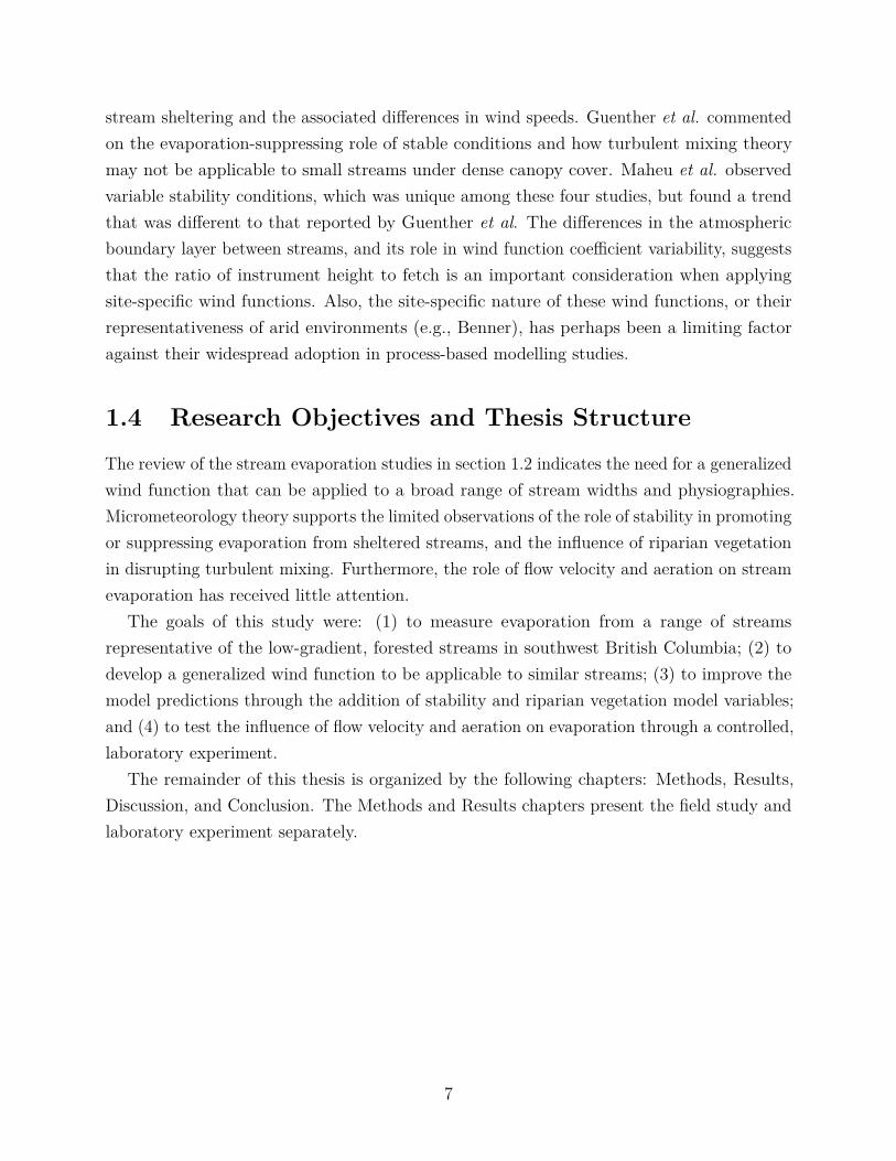
2.1 The locations of the study streams, indicated by red dots, in southwest BritishColumbia. The climate stations providing data of the regional hydroclimateare indicated by white dots. The base map source is the Stamen Terrain tileset © OpenStreetMap contributors. . . . . . . . . . . . . . . . . . . . . . . . 9

2.2 Photographs of the nine study sites. . . . . . . . . . . . . . . . . . . . . . . 102.3 The evaporation pans and meteorological station set up at Spring Creek. The

TidbiT water temperature logger is submersed near the meteorological station.This demonstrates the ideal distribution of evaporation pans in a stream andthe location of the meteorological station with respect to the pans; individualstream characteristics resulted in deviations from this ideal. . . . . . . . . . 14

2.4 The method of photographing an evaporation pan with blue dyed water forthe determination of the pan water surface area. . . . . . . . . . . . . . . . 16

3.1 Photograph of the laboratory flume. The constant-head tank is visible at thetop of the frame, with the valved plumbing supplying water to the flume. Areturn-flow pipe returns excess water to the catch-basin, seen at the bottom ofthe frame. The yellow Kestrel weather meter is seen mounted in the flume,and the fan is angled to blow air down into the flume channel. In this image,the pump supplies water to the head tank through a garden hose, but this waslater replaced by plumbing. . . . . . . . . . . . . . . . . . . . . . . . . . . . 23

3.2 Photograph illustrating the use of LEGO blocks to produce steps and roughness.The blue LEGO baseplates are glued to the top paving brick on each step andthe white LEGO bricks are attached to the baseplates. . . . . . . . . . . . . 24

3.3 Photograph showing the Kestrel weather meter measuring the wind speed overthe surface of the flow in the flume. The impeller is approximately 20 cmabove the surface of the flow. . . . . . . . . . . . . . . . . . . . . . . . . . . 26

4.1 The stream-averaged distributions of water temperature difference betweenthe evaporation pans and the stream. . . . . . . . . . . . . . . . . . . . . . 30

xi

4.2 Stream and evaporation pan water temperatures at Spring Creek during fieldwork on July 12th, 2018. . . . . . . . . . . . . . . . . . . . . . . . . . . . . 31

4.3 The stream and air temperatures at glacier-fed study sites. The panel titlesgive the day of year and location. . . . . . . . . . . . . . . . . . . . . . . . . 32

4.4 The distributions of meteorological conditions at each stream during streamevaporation measurements, arranged by increasing mean stream temperature. 35

4.5 The distributions of meteorological conditions measured 0.5 and 1.5 m abovethe stream surface, arranged by increasing mean stream temperature. . . . 36

4.6 The observed evaporation rates at each stream, arranged by increasing meanevaporation rate. The 95 % confidence intervals associated with each observa-tion due to sampling variability are indicated by the bars extending above andbelow each point. . . . . . . . . . . . . . . . . . . . . . . . . . . . . . . . . 37

4.7 Cross-validated model predictions for the base mass transfer model and thetwo best expanded models, Models 15 and 19, for meteorological measurementsmade 0.5 m and 1.5 m above the stream surface, respectively. . . . . . . . . 40

4.8 The site-specific residual error distribution for the base and expanded 0.5-mand 1.5-m models. The residuals were computed from cross-validated modelpredictions. . . . . . . . . . . . . . . . . . . . . . . . . . . . . . . . . . . . . 41

4.9 The site-specific adjustments for each model. The 0.5-m base model hadadjustments to the b coefficient, while the other models had adjustments tothe a coefficient. . . . . . . . . . . . . . . . . . . . . . . . . . . . . . . . . . 42

4.10 The evaporation rates estimated by applying six literature wind functions tothis study’s dataset. The wind function coefficients and the study referencesare provided in Table 4.7. The two panels for Maheu correspond to the windfunctions for Catamaran Brook (CB) and the Little Southwest MiramichiRiver (LSWM). The panels are ordered from 1 to 6 by decreasing modelroot-mean-square error. The predicted evaporation rates for this study arecross-validated predictions from the 1.5-m model. . . . . . . . . . . . . . . . 44

5.1 The meteorological conditions, flume water electrical conductivity, and cal-culated evaporation rates for each of the flume trials. Each subfigure titleprovides the state of the flume parameters of slope and LEGO. . . . . . . . . 48

5.2 The model-predicted evaporation rates with 95 % confidence intervals, for eachtrial. . . . . . . . . . . . . . . . . . . . . . . . . . . . . . . . . . . . . . . . 50

xii

A.1 The uncorrected and corrected field-deployed anemometer wind speed measure-ments over the calibration period compared to the calibration anemometers.The black lines represent the 1:1 line. . . . . . . . . . . . . . . . . . . . . . 71

A.2 Comparing the agreement in wind speed measurements between field anemome-ter and calibration anemometer pairs during the calibration period. The blacklines are the 1:1 lines. . . . . . . . . . . . . . . . . . . . . . . . . . . . . . . 72

B.1 Stream and evaporation pan water temperatures over the course of evaporationmeasurements. The stream water temperatures are at 10 minute temporalresolution, while the pan water temperature measurements are at approximately20 minute intervals. The grid panels are titled with the day of year and location.Days with insufficient pan water temperature measurements were omitted fromthis figure. . . . . . . . . . . . . . . . . . . . . . . . . . . . . . . . . . . . . 74

B.2 The calibration of evaporation pan water surface area. The line is the fitregression. . . . . . . . . . . . . . . . . . . . . . . . . . . . . . . . . . . . . 75

C.1 Meteorological and stream conditions, and measured evaporation rates foreach day of data collection. . . . . . . . . . . . . . . . . . . . . . . . . . . . . 77

E.1 The calibration results relating electrical conductivity to a salt solution molarity.The line is the fit regression. . . . . . . . . . . . . . . . . . . . . . . . . . . 88

xiii

Acknowledgements

This research project was realized through the contributions of many people. First andforemost, I would like to thank my supervisor, Dan Moore, for his ongoing enthusiasm forfield-based research, insistence on holding oneself to a high standard, keen attention to detail,and patient guidance. I would also like to express my deep gratitude to my lab group,Johannes Exler, Annie Dufficy, and Stefan Gronsdahl, for sharing technical expertise incoordinating a field data collection campaign and for always being available and willing todiscuss my questions and quandaries. Anna Kaveney and Virgile Laurent were invaluablefor their assistance in conducting field work, as well as Emily West and Edward Yu. Thestaff of the Department of Geography played a key role in enabling this research project tooccur. I would also like to acknowledge the contributions of William Sparling, who providedinsightful suggestions and recommendations on several aspects of my research.

This work was funded by a Natural Sciences and Engineering Research Council Discoverygrant to Dr. Dan Moore, and a CGS-M scholarship to Andras J. Szeitz.

Finally, I would like to thank my family and friends, who have always supported methrough my studies.

xiv

Chapter 1

Introduction

1.1 Motivation

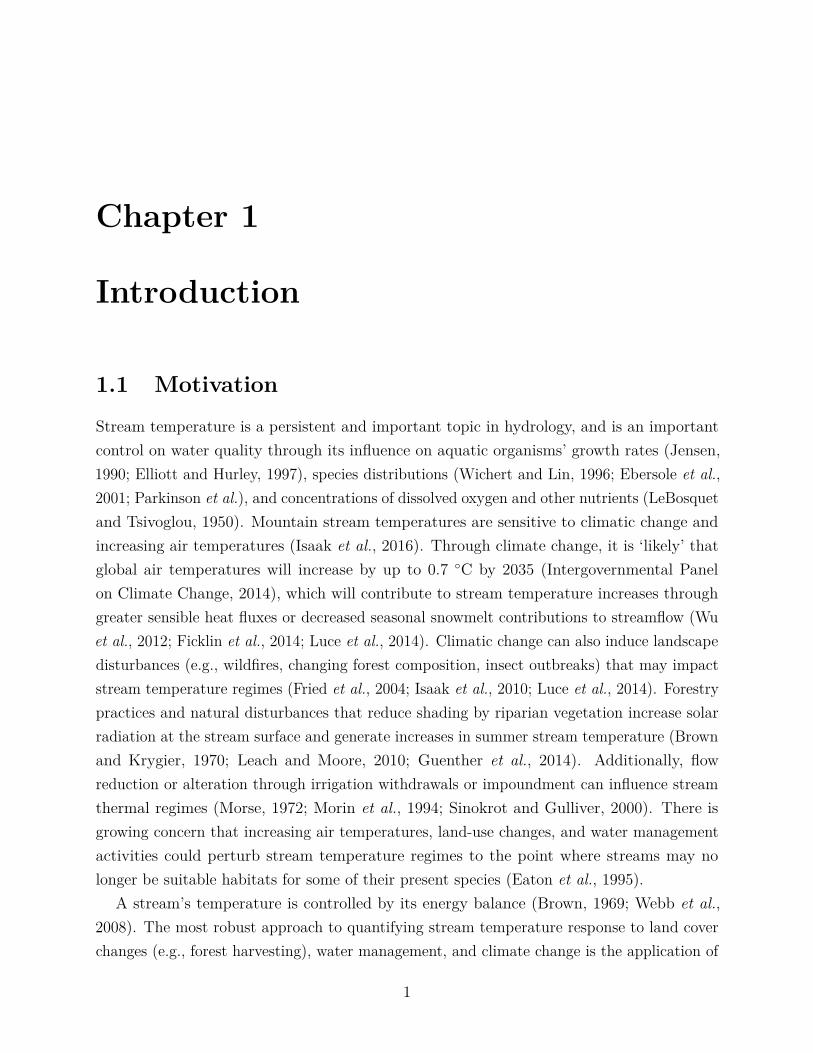
Stream temperature is a persistent and important topic in hydrology, and is an importantcontrol on water quality through its influence on aquatic organisms’ growth rates (Jensen,1990; Elliott and Hurley, 1997), species distributions (Wichert and Lin, 1996; Ebersole et al.,2001; Parkinson et al.), and concentrations of dissolved oxygen and other nutrients (LeBosquetand Tsivoglou, 1950). Mountain stream temperatures are sensitive to climatic change andincreasing air temperatures (Isaak et al., 2016). Through climate change, it is ‘likely’ thatglobal air temperatures will increase by up to 0.7 ◦C by 2035 (Intergovernmental Panelon Climate Change, 2014), which will contribute to stream temperature increases throughgreater sensible heat fluxes or decreased seasonal snowmelt contributions to streamflow (Wuet al., 2012; Ficklin et al., 2014; Luce et al., 2014). Climatic change can also induce landscapedisturbances (e.g., wildfires, changing forest composition, insect outbreaks) that may impactstream temperature regimes (Fried et al., 2004; Isaak et al., 2010; Luce et al., 2014). Forestrypractices and natural disturbances that reduce shading by riparian vegetation increase solarradiation at the stream surface and generate increases in summer stream temperature (Brownand Krygier, 1970; Leach and Moore, 2010; Guenther et al., 2014). Additionally, flowreduction or alteration through irrigation withdrawals or impoundment can influence streamthermal regimes (Morse, 1972; Morin et al., 1994; Sinokrot and Gulliver, 2000). There isgrowing concern that increasing air temperatures, land-use changes, and water managementactivities could perturb stream temperature regimes to the point where streams may nolonger be suitable habitats for some of their present species (Eaton et al., 1995).

A stream’s temperature is controlled by its energy balance (Brown, 1969; Webb et al.,2008). The most robust approach to quantifying stream temperature response to land coverchanges (e.g., forest harvesting), water management, and climate change is the application of

1

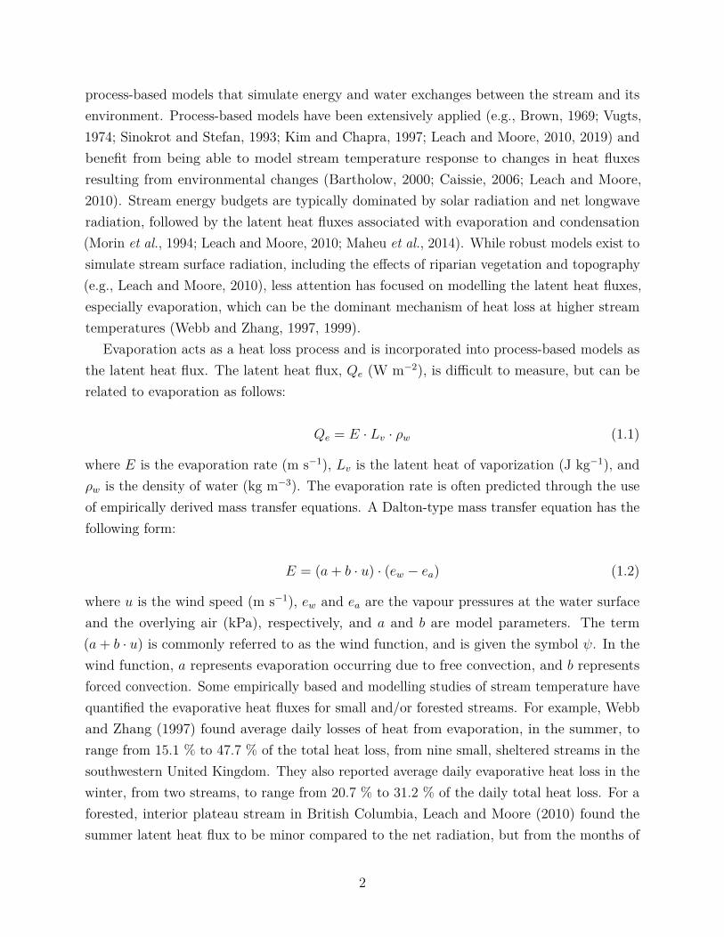
process-based models that simulate energy and water exchanges between the stream and itsenvironment. Process-based models have been extensively applied (e.g., Brown, 1969; Vugts,1974; Sinokrot and Stefan, 1993; Kim and Chapra, 1997; Leach and Moore, 2010, 2019) andbenefit from being able to model stream temperature response to changes in heat fluxesresulting from environmental changes (Bartholow, 2000; Caissie, 2006; Leach and Moore,2010). Stream energy budgets are typically dominated by solar radiation and net longwaveradiation, followed by the latent heat fluxes associated with evaporation and condensation(Morin et al., 1994; Leach and Moore, 2010; Maheu et al., 2014). While robust models exist tosimulate stream surface radiation, including the effects of riparian vegetation and topography(e.g., Leach and Moore, 2010), less attention has focused on modelling the latent heat fluxes,especially evaporation, which can be the dominant mechanism of heat loss at higher streamtemperatures (Webb and Zhang, 1997, 1999).

Evaporation acts as a heat loss process and is incorporated into process-based models asthe latent heat flux. The latent heat flux, Qe (W m−2), is difficult to measure, but can berelated to evaporation as follows:

Qe = E · Lv · ρw (1.1)

where E is the evaporation rate (m s−1), Lv is the latent heat of vaporization (J kg−1), andρw is the density of water (kg m−3). The evaporation rate is often predicted through the useof empirically derived mass transfer equations. A Dalton-type mass transfer equation has thefollowing form:

E = (a+ b · u) · (ew − ea) (1.2)

where u is the wind speed (m s−1), ew and ea are the vapour pressures at the water surfaceand the overlying air (kPa), respectively, and a and b are model parameters. The term(a+ b · u) is commonly referred to as the wind function, and is given the symbol ψ. In thewind function, a represents evaporation occurring due to free convection, and b representsforced convection. Some empirically based and modelling studies of stream temperature havequantified the evaporative heat fluxes for small and/or forested streams. For example, Webband Zhang (1997) found average daily losses of heat from evaporation, in the summer, torange from 15.1 % to 47.7 % of the total heat loss, from nine small, sheltered streams in thesouthwestern United Kingdom. They also reported average daily evaporative heat loss in thewinter, from two streams, to range from 20.7 % to 31.2 % of the daily total heat loss. For aforested, interior plateau stream in British Columbia, Leach and Moore (2010) found thesummer latent heat flux to be minor compared to the net radiation, but from the months of

2

October to March, the latent heat flux and net radiation were of the same magnitude. Morerecently, Maheu et al. (2014) and Caissie (2016) observed heat loss through evaporation as42 % and 10 % of total summer heat loss in a stream and its tributary, respectively, in NewBrunswick. As stream evaporation increases with increasing stream temperature, evaporationcould act to impose an upper limit on stream temperature in the summer months.

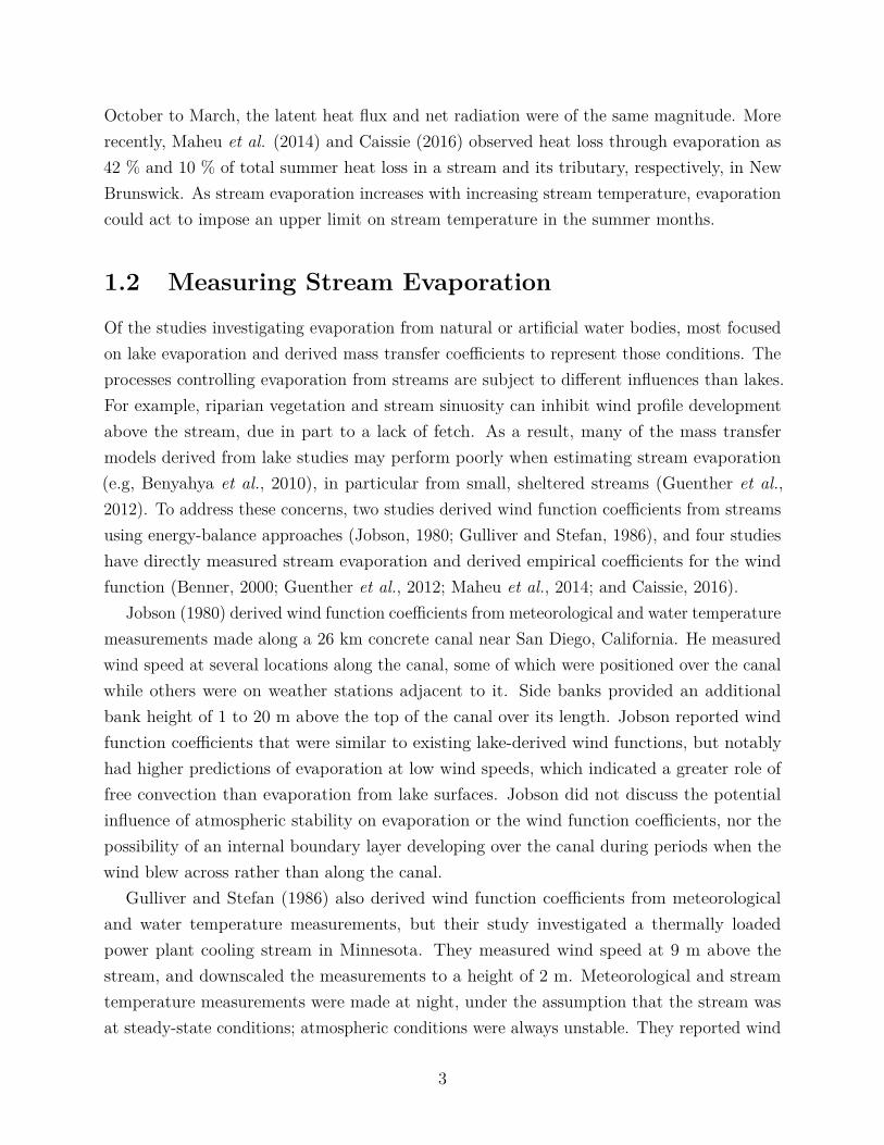
1.2 Measuring Stream Evaporation

Of the studies investigating evaporation from natural or artificial water bodies, most focusedon lake evaporation and derived mass transfer coefficients to represent those conditions. Theprocesses controlling evaporation from streams are subject to different influences than lakes.For example, riparian vegetation and stream sinuosity can inhibit wind profile developmentabove the stream, due in part to a lack of fetch. As a result, many of the mass transfermodels derived from lake studies may perform poorly when estimating stream evaporation(e.g, Benyahya et al., 2010), in particular from small, sheltered streams (Guenther et al.,2012). To address these concerns, two studies derived wind function coefficients from streamsusing energy-balance approaches (Jobson, 1980; Gulliver and Stefan, 1986), and four studieshave directly measured stream evaporation and derived empirical coefficients for the windfunction (Benner, 2000; Guenther et al., 2012; Maheu et al., 2014; and Caissie, 2016).

Jobson (1980) derived wind function coefficients from meteorological and water temperaturemeasurements made along a 26 km concrete canal near San Diego, California. He measuredwind speed at several locations along the canal, some of which were positioned over the canalwhile others were on weather stations adjacent to it. Side banks provided an additionalbank height of 1 to 20 m above the top of the canal over its length. Jobson reported windfunction coefficients that were similar to existing lake-derived wind functions, but notablyhad higher predictions of evaporation at low wind speeds, which indicated a greater role offree convection than evaporation from lake surfaces. Jobson did not discuss the potentialinfluence of atmospheric stability on evaporation or the wind function coefficients, nor thepossibility of an internal boundary layer developing over the canal during periods when thewind blew across rather than along the canal.

Gulliver and Stefan (1986) also derived wind function coefficients from meteorologicaland water temperature measurements, but their study investigated a thermally loadedpower plant cooling stream in Minnesota. They measured wind speed at 9 m above thestream, and downscaled the measurements to a height of 2 m. Meteorological and streamtemperature measurements were made at night, under the assumption that the stream wasat steady-state conditions; atmospheric conditions were always unstable. They reported wind

3

function coefficients similar to those reported by Jobson (1980), but preferred an alternativeformulation that incorporated the cube root of a stability index as a variable. The model wasdeveloped based on measurements with unstable conditions and thus may not be applicableto stable conditions. Gulliver et al. also noted that there could be instances where an internalboundary layer developed over the stream, due to crosswinds over the stream, but did notdiscuss how that may have influenced their estimated coefficients.

Benner (2000) measured evaporation on nine reaches of the Upper Middle Fork of theJohn Day River in Oregon, an aridland environment, by measuring the change in water depthin pans (similar to Class A evaporation pans) submerged in the stream. They also measuredmeteorological conditions in-stream above the evaporation pans. Benner reported windfunction coefficients similar to those of Jobson (1980), who derived coefficients for predictingevaporation from a concrete aqueduct in an arid environment. Benner also reported variabilityin wind function coefficients when fit to each study reach. The wind function coefficient,a, ranged from 0.011 to 0.204 (mm h−1 kPa−1), while b ranged from 0.026 to 0.309 (mmh−1 s m−1 kPa−1). A laboratory experiment was conducted to investigate the influence ofwater flow velocity on evaporation. In these experiments, evaporation was measured usinga pressure transducer in an evaporation pan which had a ‘mixing wheel’ to simulate waterflow, and air flow from a fan. Benner reported a significant but decreasing influence of flowvelocity on evaporation as the vapour pressure difference or wind speed increased.

Guenther et al. (2012) measured evaporation from a headwater stream prior to and afterpartial-retention harvesting in an attempt to quantify the influence of riparian vegetationdensity on stream evaporation. They measured evaporation using evaporation pans connectedto a Mariotte cylinder, and related the change in water level in the cylinder to pan evaporation.They found the a coefficient was not significant. This differed from all previous literaturederiving wind function coefficients for streams (Jobson, 1980; Gulliver and Stefan, 1986;Benner, 2000), raising the notion that the existing mass transfer model, having been originallydeveloped for sites with no vegetation canopy, does not work well in closed canopy, shelteredstream environments. The lack of an intercept for their wind function was suggested torepresent the suppressing influence of stable conditions on evaporation.

Maheu et al. (2014) measured evaporation rates from two temperate, forested streams ofdifferent widths (8 and 80 m). They introduced a method of evaporation measurement usingfloating evaporation pans, where they related the change in the mass of water in the pans toevaporation. Similarly to the aforementioned studies, they used above-stream meteorologicaldata with the evaporation measurements to derive wind function coefficients. They reportedunique wind function coefficients for each stream, in line with Benner (2000). However, theyalso reported wind function coefficients fit to evaporation and meteorological measurements

4

made during the night. Night-time conditions were unstable, and previous work suggestedthat instability should enhance evaporation (Ryan and Harleman, 1973; Gulliver and Stefan,1986). However, Maheu et al. found the free convection coefficient, a, fit to night-timemeasurements decreased relative to its value fit to daytime measurements, which was contraryto the role of stability reported by Gulliver and Stefan (1986), and suggested by Guenther etal. (2012).

Caissie (2016) expanded upon the work of Maheu et al. (2014) by measuring evaporationfrom a small, sheltered tributary to the streams studied by Maheu et al. Evaporation wasmeasured using floating evaporation pans, and meteorological measurements were madeabove-stream as well as in a forest clearing nearby. He derived wind function coefficients,and compared the observed evaporation against predicted evaporation estimated using themeteorological observations from the forest clearing as input data. Using these data as inputsto the wind function accounted for 86 % of the variability in evaporation, which indicates thatnearby meteorological data may be useful inputs to the wind function when above-streammeasurements are unavailable. Additionally, the findings of Caissie were congruous withthe previously identified trends of lower evaporation rates with increased sheltering andthe associated differences in wind speed. Caissie also suggested that there is a positiverelationship between the proportion of evaporative heat loss with respect to the stream heatbudget and the stream width.

1.3 Modelling Stream Evaporation

The general principles underlying the mass transfer equation (Equation 1.2) were firstdescribed by Dalton (1802), and a model of this form was proposed by Stelling (1882) toestimate evaporation from a land surface (Brutsaert, 1982). Many variants of Stelling’s modelhave been derived, stemming from the different environments and measurement heights usedto make meteorological observations, as well as the incorporation of modified or additionalvariables including squared wind speeds (Brady et al., 1969) or atmospheric stability (Ryanand Harleman, 1973). The mass transfer equations most commonly applied to modern streamevaporation studies were developed by Brady et al. (1969) and Webb and Zhang (1997),although equations derived by Brutsaert and Yu (1968) and Gulliver and Stefan (1986),among others, have also been utilized to predict stream evaporation.

Brutsaert and Yu (1968) sought to quantify the performance of the wind function and gaininsight into the variability of the wind function parameter values. To address this question,they measured evaporation from eight square evaporation pans of 0.09, 1.48, and 5.96 m2

surface area. Wind speed was measured 0.5, 1, 2, and 3 m above the surface. Brutsaert and Yu

5

also investigated the applicability of micrometeorology theory in predicting evaporation; theyconsidered the relative performance of the wind speed or the friction velocity as input datato the wind function. The concept of the friction velocity describes the vertical momentum,heat, or by extension, vapour flux above a surface of a given roughness (Brutsaert, 1982;Arya, 1988). Brutsaert and Yu found that wind speed was better correlated to the observedevaporation rates and suggested that at the measurement heights of 2 and 3 m, the windspeed represented the turbulent mixing just as well as the friction velocity. They also observedthat the correlation between wind speed and evaporation decreased with lower measurementheights, and concluded that wind speed measurements higher above the surface provide moreaccurate measures of turbulent mixing.

Brady et al. (1969) derived a wind function from meteorological observations made at threethermally loaded power plant cooling lakes. They measured wind speed at 7 m above the lakesurface, and were primarily interested in developing a model for predicting evaporative heatloss from cooling ponds. The wind function developed by Brady et al. has been incorporatedinto process-based studies to predict evaporation in distinctly different study environmentsand systems including natural streams (Kim and Chapra, 1997) and high Arctic streams(King and Neilson, 2019). Similarly to Brady et al., Gulliver and Stefan (1986) derivedwind functions from meteorological conditions measured 9 m above heated, unsheltered,artifical channels. The channels were warmed by waste heat from a nearby power plant, soconditions above the streams were always unstable. The wind function of Gulliver and Stefan(1986) commented on the role of stability in evaporation, and compared their wind functionfavourably with that of Ryan and Harleman (1973), which also included a stability variable.The wind function derived by Gulliver et al. has also been used in other modelling studies(e.g., Sinokrot and Stefan, 1993), but is limited in its application to natural, sheltered streamswhich may frequently have stable conditions.

Webb and Zhang (1997) did not specify how they derived the coefficients in their windfunction, but did compare predictions to evaporation in a streamside evaporation pan. Theirmeteorological measurements were made at 2 m height. This model has been applied, withapparent success, to predict evaporation and stream temperature for a range of streams(Leach and Moore, 2011; Magnusson et al., 2012; Garner et al., 2014).

The studies that measured evaporation from streams directly have primarily been focusedon deriving wind functions representative of the evaporation processes at one or two streams(Benner, 2000; Guenther et al., 2012; Maheu et al., 2014; Caissie, 2016). There is substantialvariability in the wind function coefficients from these four studies, which likely reflects theeffects of site-specific characteristics influencing evaporation. For example, the atmosphericboundary layer conditions above streams vary between sites due, in part, to differences in

6

stream sheltering and the associated differences in wind speeds. Guenther et al. commentedon the evaporation-suppressing role of stable conditions and how turbulent mixing theorymay not be applicable to small streams under dense canopy cover. Maheu et al. observedvariable stability conditions, which was unique among these four studies, but found a trendthat was different to that reported by Guenther et al. The differences in the atmosphericboundary layer between streams, and its role in wind function coefficient variability, suggeststhat the ratio of instrument height to fetch is an important consideration when applyingsite-specific wind functions. Also, the site-specific nature of these wind functions, or theirrepresentativeness of arid environments (e.g., Benner), has perhaps been a limiting factoragainst their widespread adoption in process-based modelling studies.

1.4 Research Objectives and Thesis Structure

The review of the stream evaporation studies in section 1.2 indicates the need for a generalizedwind function that can be applied to a broad range of stream widths and physiographies.Micrometeorology theory supports the limited observations of the role of stability in promotingor suppressing evaporation from sheltered streams, and the influence of riparian vegetationin disrupting turbulent mixing. Furthermore, the role of flow velocity and aeration on streamevaporation has received little attention.

The goals of this study were: (1) to measure evaporation from a range of streamsrepresentative of the low-gradient, forested streams in southwest British Columbia; (2) todevelop a generalized wind function to be applicable to similar streams; (3) to improve themodel predictions through the addition of stability and riparian vegetation model variables;and (4) to test the influence of flow velocity and aeration on evaporation through a controlled,laboratory experiment.

The remainder of this thesis is organized by the following chapters: Methods, Results,Discussion, and Conclusion. The Methods and Results chapters present the field study andlaboratory experiment separately.

7

Chapter 2

Field Methods

2.1 Study Area and Streams

Evaporation measurements were made at nine streams in southwest British Columbia, whichwere selected to sample a range of stream widths, thermal regimes, and riparian vegetationconditions that are common in the southern British Columbia Coast Mountains (Table 2.1;Figure 2.1; Figure 2.2). The streams were distributed between a coastal region (the MalcolmKnapp Research Forest) and a region approximately 100 km inland (Pemberton). The tworegions have distinct climates. The Malcolm Knapp Research Forest (MKRF) has a typicalmaritime climate with cool and wet winters, and mild summers. The Pemberton region hasrelatively colder and drier winters, with warmer and drier summers.

Regional hydroclimate data were sourced from the Pemberton BCFS climate station from1969 to 1984 and from the Pemberton Airport climate station from 1985 to 2018, and forthe Malcolm Knapp Research Forest UBC Haney RF Admin climate station for 1969 to2018. The climate stations’ respective Environment Canada Climate identifiers are 1086083,1086082, and 1103332, and the locations of the stations are shown in Figure 2.1.

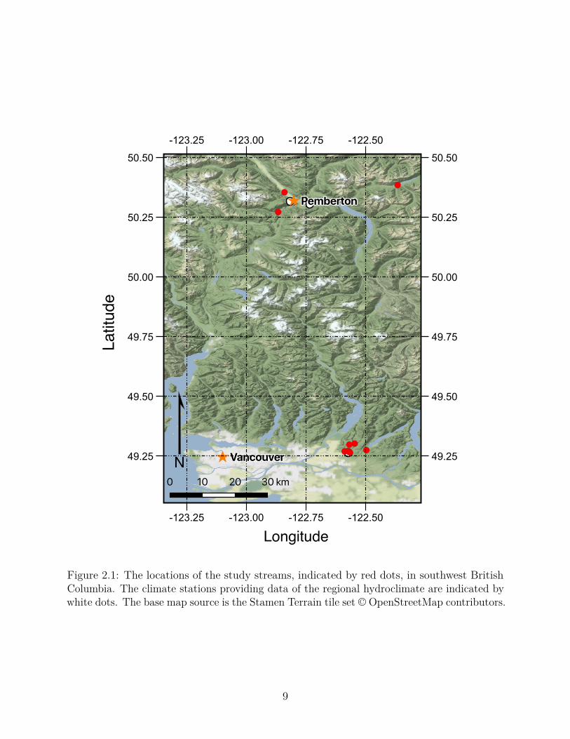
The streams were primarily located in coniferous forests, although Blaney Creek (Lower),Miller Creek, and Rutherford Creek had deciduous trees dominant in their riparian vegetation.Stream bankfull widths ranged from 3.1 m to 27.6 m, average tree heights ranged from 5.3 mto 46.7 m, and canopy openness ranged from 9 % to 70 %. Because the evaporation pans wereunstable in high-velocity flow, streams with pools or reaches with low flow velocities werechosen. A preference was also given to locations where evaporation pans could be distributedacross the width of the channel, or if that was not feasible, then across the width of a pool.Stream evaporation, stream water temperature, and above-stream meteorological conditionswere measured on 20 days between the 6th June 2018 and the 17th August 2018, and fieldmeasurements were restricted to days without precipitation.

8

Longitude

Latitude

49.25 49.25

49.50 49.50

49.75 49.75

50.00 50.00

50.25 50.25

50.50 50.50

-123.25

-123.25

-123.00

-123.00

-122.75

-122.75

-122.50

-122.50

N

Figure 2.1: The locations of the study streams, indicated by red dots, in southwest BritishColumbia. The climate stations providing data of the regional hydroclimate are indicated bywhite dots. The base map source is the Stamen Terrain tile set © OpenStreetMap contributors.

9

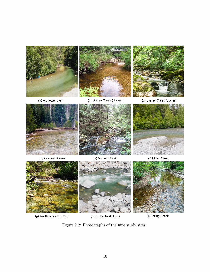
Figure 2.2: Photographs of the nine study sites.

10

Table 2.1: The selected study sites and their stream and riparian properties.

Stream StreamWidth(m)

TreeHeight(m)

CanopyOpen-ness(%)

Elevation(m)

Longitude Latitude

Alouette River 18.1 33.1 45 96 -122.497 49.275Blaney Creek (Lower) 5.5 46.7 9 52 -122.588 49.271Blaney Creek (Upper) 6.8 28.5 24 358 -122.568 49.299Cayoosh Creek 23.0 19.7 50 1139 -122.366 50.385Marion Creek 4.0 31.6 11 320 -122.546 49.303Miller Creek 27.6 26.8 57 210 -122.841 50.355North Alouette River 8.5 35.8 15 172 -122.566 49.266Rutherford Creek 18.0 5.3 70 353 -122.867 50.272Spring Creek 3.1 32.4 16 162 -122.574 49.271

2.2 Site Characteristics

At each location, measurements were made to determine bankfull stream width, tree height,and canopy openness. Bankfull stream width was measured using a Sokkia/Eslon 30-m fibreglass tape measure, except at Rutherford Creek, where an LTI Impulse 200 laserrangefinder was used. At each stream, bankfull width was measured across three transectsalong the reach in which the evaporation pans and meteorological station were deployed.

At each site, five to six mature trees representative of the local species distribution wereselected for tree height measurements. Tree height, ht (m), was calculated as follows:

ht = HD ×(

tan (θt)− tan (θb))

(2.1)

where HD is the horizontal distance from the measurement location to the tree (m), and θtand θb are the angles of inclination, in degrees, from the measurement location to the topand the bottom of the tree, respectively. The horizontal distance was measured using thefibreglass tape measure, and the angles of inclination from the measurement location weremeasured using a Suunto PM-5 inclinometer.

Canopy openness, as a proportion, was estimated from a hemispherical photograph takenat each site using the image processing software, Gap Light Analyzer (GLA) following themethods detailed by Frazer et al. (1999). Hemispherical photographs were taken using aNikon Coolpix 4500 digital camera with a Fisheye Converter FC-E8 lens attached. Thecamera was mounted on a Manfrotto 190Pro tripod, placed in the centre of the stream reachwhere evaporation and meteorological measurements were made, and levelled prior to taking aphotograph. The hemispherical photographs were taken on days when the sky was uniformly

11

overcast, or in the early morning on days with clear skies.

2.3 Meteorological and Stream Temperature Data

2.3.1 Field Measurements

Air temperature, relative humidity, and wind speed were measured approximately 1.5 m and0.5 m above the stream surface in the vicinity of the evaporation pans deployed in the stream.Rotronic HygroClip-S3 sensors were used to measure air temperature and relative humidity,and were installed in R. M. Young Model 41003 radiation shields to reduce the influenceof direct solar radiation on their measurements. Wind speed was measured with MetOne014A 3-cup anemometers, which have nominal starting threshold speeds of 0.45 m s−1. Allsensors were mounted on tripod cross-arms that extended the sensors over the centre of thestream (Figure 2.3), or in cases where the evaporation pans did not span the full streamwidth, the sensors were positioned over the centre of the evaporation pans’ distribution. Allmeteorological sensors were scanned every 10 seconds, and 10-minute averages were loggedon a Campbell Scientific CR10X datalogger.

Stream temperature was measured with an Onset TidbiT v2 water temperature logger,which recorded stream temperature every 10 minutes. The temperature logger was housedin a white PVC radiation shield to reduce direct solar radiation effects, and was tetheredto a concrete anchor to keep the logger submerged and in the vicinity of the meteorologicalstation.

2.3.2 Data Processing

The two MetOne 014A anemometers used to measure above-stream wind speed were cross-calibrated with two recently manufacturer-serviced and calibrated 014A anemometers. Eachfield-deployed anemometer was paired with a serviced and calibrated anemometer, and theysimultaneously measured wind speed over the course of two days, with wind speed measuredevery 10 seconds and 10-minute averages logged on a Campbell Scientific CR10X datalogger.The uncalibrated anemometers consistently under-reported low wind speeds in comparison tothe serviced and calibrated anemometers’ measurements, so a segmented linear regressionwas fit to each pair of uncalibrated-calibrated anemometers’ measurements. The anemometer-specific regressions were applied to adjust the above-stream wind speed measurements madeby the uncalibrated anemometers. Information regarding the calibration of the anemometersand the correction of their measurements can be found in Appendix A.

The meteorological and stream temperature measurements did not typically align with

12

the times of evaporation measurements, so the data were processed and synchronized withthe evaporation measurement intervals. To this end, the wind speed, relative humidity,air and stream temperature measurements, and the computed vapour pressures at thetwo measurement heights were linearly interpolated from 10-minute intervals to 1-minuteintervals. The evaporation pan water temperature measurements and computed saturationvapour pressures were interpolated to 1-minute intervals using cubic spline interpolation(Forsythe et al., 1977), except during the first four days of field data when insufficient pantemperature measurements restricted the use of spline interpolation. For these data, acomputed temperature difference between stream and pan water was applied instead. Finally,average values of wind speed, relative humidity, air, stream, and pan water temperature, andvapour pressures were calculated for each evaporation pan measurement interval using the1-minute interpolations.

2.4 Stream Evaporation

2.4.1 Field Measurements

Stream evaporation was measured using the gravimetric approach developed by Maheuet al. (2014). Each evaporation pan consisted of a plastic container with dimensions of21.3 × 21.3 × 5.1 cm that was supported by a square wooden frame 34 cm wide, 1.9 cmthick, with an inner opening of 21.4× 21.4 cm. The frame was painted white to minimizeabsorption of solar radiation and warming. The frame was tethered to a concrete anchor tokeep it in place when deployed in a stream. On each sampling day, nine evaporation panswere distributed across the channel, with three placed along the left and right banks, andthree in the centre of the channel (Figure 2.3).

Each evaporation pan was initially filled with stream water to within about 2 cm ofits rim, and then weighed using an Ohaus Scout SPX2201 portable balance (resolution ±0.1 g). Approximately every 1 to 1.5 hours throughout the day, each evaporation pan wasremoved from its frame, the outside of the pan was carefully wiped dry, and its mass wasreweighed. The change in mass between weighings provided the measurement of evaporationor condensation that occurred over that time interval. The temperature of the water in eachevaporation pan was measured approximately every 20 minutes using an Omega EngineeringHH-25TC thermocouple thermometer, to allow for later adjustment of the difference in watertemperature between the evaporation pans and the stream.

13

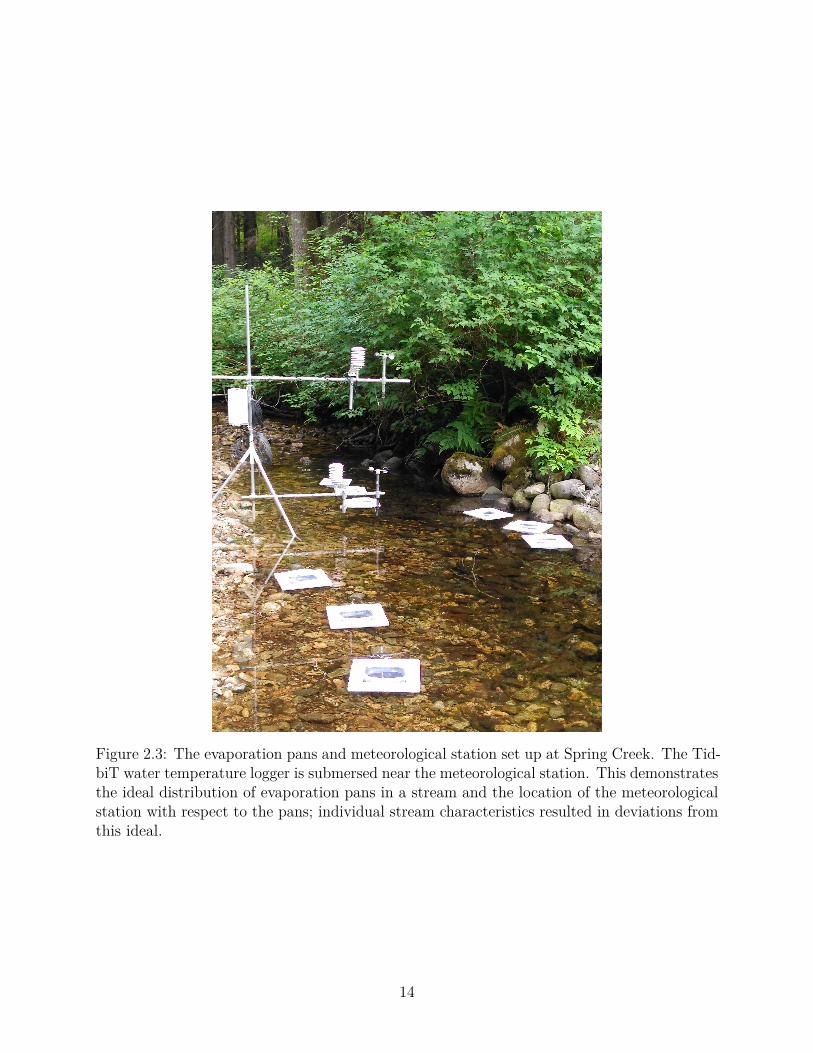
Figure 2.3: The evaporation pans and meteorological station set up at Spring Creek. The Tid-biT water temperature logger is submersed near the meteorological station. This demonstratesthe ideal distribution of evaporation pans in a stream and the location of the meteorologicalstation with respect to the pans; individual stream characteristics resulted in deviations fromthis ideal.

14

2.4.2 Data Processing and Analysis

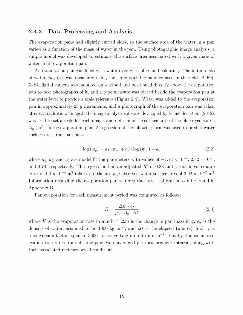
The evaporation pans had slightly curved sides, so the surface area of the water in a panvaried as a function of the mass of water in the pan. Using photographic image analysis, asimple model was developed to estimate the surface area associated with a given mass ofwater in an evaporation pan.

An evaporation pan was filled with water dyed with blue food colouring. The initial massof water, mw (g), was measured using the same portable balance used in the field. A FujiX-E1 digital camera was mounted on a tripod and positioned directly above the evaporationpan to take photographs of it, and a tape measure was placed beside the evaporation pan atthe water level to provide a scale reference (Figure 2.4). Water was added to the evaporationpan in approximately 25 g increments, and a photograph of the evaporation pan was takenafter each addition. ImageJ, the image analysis software developed by Schneider et al. (2012),was used to set a scale for each image, and determine the surface area of the blue-dyed water,Ap (m2), in the evaporation pan. A regression of the following form was used to predict watersurface area from pan mass:

ˆlog (Ap) = a1 ·mw + a2 · log (mw) + a0 (2.2)

where a1, a2, and a0 are model fitting parameters with values of −1.74× 10−4, 2.42× 10−1,and 4.74, respectively. The regression had an adjusted R2 of 0.88 and a root-mean-squareerror of 1.0× 10−4 m2 relative to the average observed water surface area of 3.92× 10−2 m2.Information regarding the evaporation pan water surface area calibration can be found inAppendix B.

Pan evaporation for each measurement period was computed as follows:

E = ∆m · cfρw · Ap ·∆t

(2.3)

where E is the evaporation rate in mm h−1, ∆m is the change in pan mass in g, ρw is thedensity of water, assumed to be 1000 kg m−3, and ∆t is the elapsed time (s), and cf isa conversion factor equal to 3600 for converting units to mm h−1. Finally, the calculatedevaporation rates from all nine pans were averaged per measurement interval, along withtheir associated meteorological conditions.

15

Figure 2.4: The method of photographing an evaporation pan with blue dyed water for thedetermination of the pan water surface area.

16

2.5 Evaporation Model Variables

Several variables were calculated from the processed meteorological, stream, and evaporationpan temperature data. The saturation vapour pressure, es(T ) (kPa), at a temperature T(◦C) was computed as:

es(T ) = 0.611× exp( 17.27 · TT + 237.26

)(2.4)

The vapour pressure at the water surface, ew, was then computed as:

ew = es(Tw) (2.5)

where Tw is the pan water temperature. The vapour pressure of the air, ea, was calculated as:

ea = es(Ta) ·RH

100 (2.6)

where Ta is the air temperature and RH is the relative humidity (%). The vapour pressuredifference, ∆e, driving evaporation was then calculated as:

∆e = ew − ea (2.7)

Two atmospheric stability indices were calculated. Both indices represent neutral conditionsat a value of zero, with unstable conditions at values > 0. One is the virtual temperaturedifference between the stream surface and the air above it, ∆θ (◦C), which represents thevertical variation in air density above the stream (Gulliver and Stefan, 1986). The virtualtemperature, θ (K), of an air parcel is calculated as:

θ = T + 273.151 + 0.378 · e/p (2.8)

where p is the atmospheric pressure (kPa), e is the vapour pressure (kPa), and T is thetemperature (◦C) of the fluid parcel. As p was not measured, a standard pressure, P , for eachfield site’s elevation was estimated using the U.S. Standard Atmosphere, 1976, atmospheremodel (U.S. Standard Atmosphere, 1976, 1976) as follows:

P = Pb ·(

TbTb + Lb · (h− hb)

) g·MaR∗·Lb

× cp (2.9)

where h is the elevation of the field site (m), and Pb, Tb, Lb, and hb are the standard pressure(101.325 kPa), temperature (288.15 K), temperature lapse rate (0.0065 K/km), and referenceelevation (0 m) where 0 < h ≤ 11, 000 m; g (m s−2) is gravitational acceleration, Ma (kg

17

mol−1) is the molar mass of air, R∗ (J mol−1 K−1) is the universal gas constant, and cp

is a conversion factor equal to 1 × 10−3 to convert from units of Pa to kPa. The virtualtemperature difference was then calculated as:

∆θ = θw − θa (2.10)

where θw is the virtual temperature at the water surface, and θa is the virtual temperature ofthe air above the water.

The second stability index used was the buoyant force, F (m s−2), which relates buoyantdifferences to temperature differences between two fluid parcels. It was calculated as:

F = g(Tw + 273.15Ta + 273.15 − 1

)(2.11)

2.6 Statistical Analysis

Model fitting began by fitting a base model with the following form:

E = (a+ b · u) ·∆e (2.12)

where u is the wind speed in m s−1, and a and b are model fitting parameters. The streamproperties and stability indices were then incorporated as additional model variables to formthe full complement of candidate models, as shown through Equations 2.13 to 2.23:

E = (a+ b · u+ c · φ) ·∆e (2.13)

E = (a+ b · u+ c · γ) ·∆e (2.14)

E = (a+ b · u+ c · φ · u) ·∆e (2.15)

E = (a+ b · u+ c · γ · u) ·∆e (2.16)

E = (a+ b · u+ c · φ+ d · γ) ·∆e (2.17)

E = (a+ b · u+ c · φ · u+ d · γ) ·∆e (2.18)

18

E = (a+ b · u+ c · φ+ d · γ · u) ·∆e (2.19)

E = (a+ b · u+ c · φ · u+ d · γ · u) ·∆e (2.20)

E = (a+ b · φ · u) ·∆e (2.21)

E = (a+ b · φ · u+ c · γ) ·∆e (2.22)

E = (a+ b · φ · u+ c · γ · u) ·∆e (2.23)

where φ is canopy openness, γ represents one of the stability indices tested (the buoyant forceand the virtual temperature difference), and c and d are model fitting parameters. Linearmixed-effects modelling was used to fit regressions to the models described above.

A linear mixed-effects model fits a linear regression to a dataset, but allows for temporal,spatial, or other subject correlations in the data to be accounted for through subject-specificadjustments to the fixed-effects coefficients. For example, a model has a fixed-effect parameter,a, and subject-specific adjustments, αi, are added such that each unique subject, i, has asubject-specific coefficient, a+αi. When there is little variability between subjects, the valuesof αi will be small in absolute magnitude relative to the value of the fixed-effects coefficients.It is the fixed-effects coefficients that are used for model validation and application to externaldatasets.

The first round of model testing was done through fitting mixed-effects linear models toeach candidate model using the maximum-likelihood approach for parameter estimation. Themixed-effects models allowed each model parameter, (a, b, and if present, c and d), to varyby site, by estimating a site-specific random effect for each parameter. All possible distribu-tions of random effects on a given model’s variables were tested, and model/random-effectcombinations which had any number of insignificant population-level estimated coefficients(p-value > 0.05) were dropped from further consideration.

The remaining models were refit to test their performance under leave-one-out cross-validation. In each iteration of the cross validation, all data for one site were withheld; themodel was fit using data for the remaining sites and then applied using data for the withheldsite. Model performance was determined by computing the root-mean-square error (RMSE,mm h−1), the mean bias error (MBE, mm h−1), the mean absolute error, (MAE, mm h−1),and the Nash-Sutcliffe efficiency (NSE), as follows:

19

RMSE =√√√√ 1n

n∑i=1

(Ei − Ei

)2(2.24)

MBE = 1n

n∑i=1

(Ei − Ei

)2(2.25)

MAE = 1n

n∑i=1|Ei − Ei| (2.26)

NSE = 1−∑ni=1

(Ei − Ei

)2

∑ni=1

(Ei − E

)2 (2.27)

where Ei is the modelled evaporation rate, and E is the mean observed evaporation rate.

20

Chapter 3

Laboratory Methods

Considering the constraints imposed by the need for the evaporation pans to be located inareas with placid flow, a laboratory study was conducted to allow study of the effects ofaeration and flow velocity on stream evaporation.

3.1 Design and Construction

A research flume was constructed in the Mountain Channel Hydraulic Experimental Labora-tory in the Department of Geography at the University of British Columbia. The flume wasdesigned based on the following principles: (1) to allow for the continuous measurement ofevaporation from the recirculating water; (2) to aerate the water as it flowed; (3) to allowfor variable flow velocity; and (4) to allow for wind to blow over the water in the flume in aquantifiable manner.

The continuous measurement of evaporation from the flume was achieved through theprinciples of conservation of mass and electrical conductivity. For a sodium chloride (salt)solution of a known volume of water and a known mass of salt, any change in the temperature-corrected electrical conductivity can be attributed to a change in the volume of water or achange in the mass of salt. By keeping the mass of salt constant and closing the system toany throughput of water other than condensation or evaporation, changes in the solution’selectrical conductivity can be related to the amount of water that is condensing or evaporating.

As shown in Figure 3.1, the flume was constructed of plywood, and the channel hadL ×W × H dimensions of 1.5 × 0.2 × 0.45 m. An elevated constant-head tank suppliedapproximately 1 L s−1 of water to the flume through a manifold mounted at the head ofthe flume. To meet the design principles, the following features were incorporated into theflume construction: two stacks of four and two concrete paving bricks (each brick measuring0.39× 0.19× 0.05 m) were placed at the beginning of the flume to produce two steps for the

21

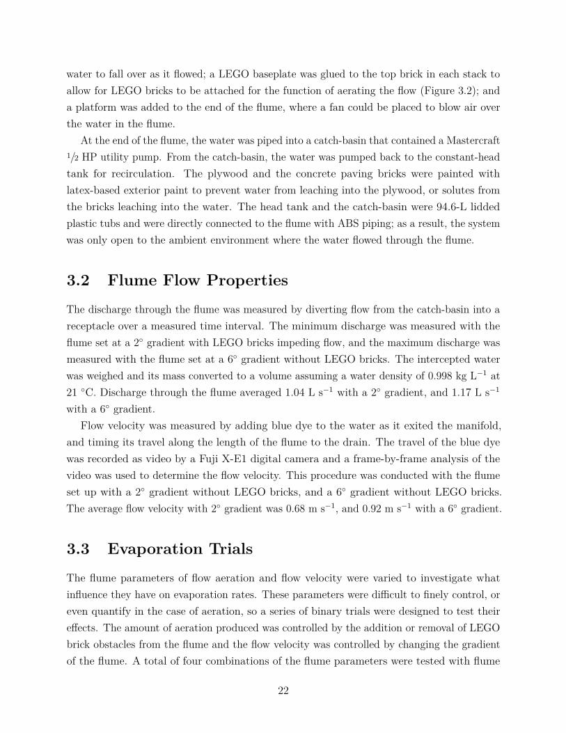
water to fall over as it flowed; a LEGO baseplate was glued to the top brick in each stack toallow for LEGO bricks to be attached for the function of aerating the flow (Figure 3.2); anda platform was added to the end of the flume, where a fan could be placed to blow air overthe water in the flume.

At the end of the flume, the water was piped into a catch-basin that contained a Mastercraft1/2 HP utility pump. From the catch-basin, the water was pumped back to the constant-headtank for recirculation. The plywood and the concrete paving bricks were painted withlatex-based exterior paint to prevent water from leaching into the plywood, or solutes fromthe bricks leaching into the water. The head tank and the catch-basin were 94.6-L liddedplastic tubs and were directly connected to the flume with ABS piping; as a result, the systemwas only open to the ambient environment where the water flowed through the flume.

3.2 Flume Flow Properties

The discharge through the flume was measured by diverting flow from the catch-basin into areceptacle over a measured time interval. The minimum discharge was measured with theflume set at a 2◦ gradient with LEGO bricks impeding flow, and the maximum discharge wasmeasured with the flume set at a 6◦ gradient without LEGO bricks. The intercepted waterwas weighed and its mass converted to a volume assuming a water density of 0.998 kg L−1 at21 ◦C. Discharge through the flume averaged 1.04 L s−1 with a 2◦ gradient, and 1.17 L s−1

with a 6◦ gradient.Flow velocity was measured by adding blue dye to the water as it exited the manifold,

and timing its travel along the length of the flume to the drain. The travel of the blue dyewas recorded as video by a Fuji X-E1 digital camera and a frame-by-frame analysis of thevideo was used to determine the flow velocity. This procedure was conducted with the flumeset up with a 2◦ gradient without LEGO bricks, and a 6◦ gradient without LEGO bricks.The average flow velocity with 2◦ gradient was 0.68 m s−1, and 0.92 m s−1 with a 6◦ gradient.

3.3 Evaporation Trials

The flume parameters of flow aeration and flow velocity were varied to investigate whatinfluence they have on evaporation rates. These parameters were difficult to finely control, oreven quantify in the case of aeration, so a series of binary trials were designed to test theireffects. The amount of aeration produced was controlled by the addition or removal of LEGObrick obstacles from the flume and the flow velocity was controlled by changing the gradientof the flume. A total of four combinations of the flume parameters were tested with flume

22

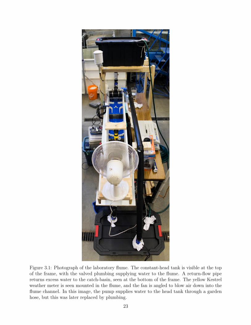
Figure 3.1: Photograph of the laboratory flume. The constant-head tank is visible at the topof the frame, with the valved plumbing supplying water to the flume. A return-flow pipereturns excess water to the catch-basin, seen at the bottom of the frame. The yellow Kestrelweather meter is seen mounted in the flume, and the fan is angled to blow air down into theflume channel. In this image, the pump supplies water to the head tank through a gardenhose, but this was later replaced by plumbing.

23

Figure 3.2: Photograph illustrating the use of LEGO blocks to produce steps and roughness.The blue LEGO baseplates are glued to the top paving brick on each step and the whiteLEGO bricks are attached to the baseplates.

24

trials (2◦, no LEGO; 2◦, LEGO; 6◦, no LEGO; 6◦, LEGO).For each trial, after ensuring the flume was dry, approximately 750 g of table salt was

weighed using a Mettler Toledo PG5002-S DeltaRange analytical balance (± 0.01 g) andadded to approximately 72 kg of tap water weighed on an Ohaus Ranger 3000 balance (± 1g). Once the flume parameters were set and the sensors were operating, the pump in thecatch-basin was powered on and the flume recirculated for approximately five hours to allowfor a sufficient amount of data to be collected. At the conclusion of each trial, the flume wasdrained and flushed with fresh water, and dried in preparation for the next trial.

3.4 Flume Data Collection

Electrical conductivity was measured with a WTW Condi 340i conductivity meter connectedto a Campbell Scientific CR10X datalogger. The conductivity probe was first immersedin a beaker filled with a sample of the water used to fill the flume for any given trial;this background electrical conductivity was recorded to adjust the measured salt solutionconductivity later. The conductivity meter was sensitive to aerated water, so the probewas immersed in the flume adjacent to the drain or in the catch-basin, dependent on whichlocation provided the least aerated water given the current flume setup. The conductivitymeter measured the voltage across the probe every 10 seconds, calculated a non-linearlytemperature-corrected voltage (mV) that is proportional to the electrical conductivity (mScm−1), and recorded 10 minute averages.

Ambient atmospheric conditions were measured using a Rotronic HygroClip-S3 in a whiteradiation shield mounted approximately 0.5 m above the flume. It measured relative humidityand air temperature every 10 seconds and logged 10 minute averages on a Campbell ScientificCR10X datalogger. Wind speed, relative humidity, and air temperature were measured witha Nielsen-Kellerman Kestrel 5500 weather meter that logged measurements every 10 minutes.The Kestrel weather meter was affixed to a crossbeam spanning the flume walls, and measuredwind speed approximately 0.2 m above the surface of flow (Figure 3.3). Water temperaturewas measured with an Onset TidbiT v2 water temperature logger suspended in the standingwater in the catch-basin. It measured and logged water temperature every 10 minutes.

3.5 Data Processing and Analysis

The first procedure was to create a calibration curve to relate the measured electricalconductivity to an estimated molarity of the solution (mol L −1). To achieve this, a solutionbelow the typical operating electrical conductivity of the flume experiments was prepared by

25

Figure 3.3: Photograph showing the Kestrel weather meter measuring the wind speed overthe surface of the flow in the flume. The impeller is approximately 20 cm above the surfaceof the flow.

26

weighing a mass of approximately 11 g of table salt on the analytical balance, and dissolvingit in a 1000 mL Pyrex No. 5600 volumetric flask (± 0.30 mL) filled with water. Thissolution was decanted into a beaker, and the initial electrical conductivity was measuredwith the WTW 340i conductivity meter and recorded. Subsequently, additions of 5 mL (±0.1 mL) of water were added to the solution using a Kimax No. 37000 pipette, and theelectrical conductivity recorded, once stable, after each addition. This continued until theelectrical conductivity of the solution was greater than the maximum electrical conductivitymeasured during the flume experiments. A linear regression was fit to the data to concludethe calibration.

The pump produced heat as it operated and caused the flume water to rapidly warmduring the beginning of each evaporation trial. The first hour of observations from eachtrial were removed to allow for the sensors to adjust and for the rate of water warming todecrease. The wind speed, air temperature, and relative humidity data from the Kestrelweather meter along with the flume water temperature data were linearly interpolated from10 minute intervals to 1 minute intervals. The interpolated data were then synchronized withthe electrical conductivity data and subsequently averaged over 30 minute intervals. Theelectrical conductivity calibration regression (Equation 3.1) was used to estimate the molarityof the solution as follows:

M = m× Γ + b (3.1)

where M is the estimated molarity of the solution in mol L−1, Γ is the electrical conductivityin mS cm−1, and m and b are the regression coefficients. The M values were then convertedto the estimated volume of water in the flume:

V = n

M(3.2)

where V is the estimated volume in L, n is the number of moles of salt in solution, calculatedas the mass of salt divided by its molar mass (58.443 g mol−1). The difference in volume,∆V , between datapoints in the time series was computed and converted to a difference indepth of water, ∆dw, in m, assuming water density is 998 kg m−3 at 21 ◦C. The evaporationrate was calculated as follows:

Ef = ∆dwAf× C (3.3)

where Ef is the estimated evaporation rate from the flume in mm h−1, Af is the area ofthe flume in m2, and C is a conversion factor equal to 2000 to convert units from m per

27

30 minutes to mm h−1. Following Equations 2.4 to 2.10, several meteorological variableswere computed, and an adjustment to the saturation vapour pressure to account for vapourpressure suppression was applied using Raoult’s Law as follows:

e1 = nwnw + ni

· e0 (3.4)

where e0 is the saturation vapour pressure of pure water in kPa, nw is the number of molesof water, ni is the number of moles of dissociated salt ions in the flume solution, and e1 isthe adjusted saturation vapour pressure, in kPa.

3.6 Statistical Analysis

Two linear models were used to test the influence of the flume parameters on the evaporationrate. A model incorporating the flume parameters as binary variables was compared to areduced model with the flume parameters omitted. The full and nested model forms were asfollows:

Ef = (q0 + q2LI2L + q6nLI6nL + q6LI6L) ·∆e+ (r0 + r2LI2L + r6nLI6nL + r6LI6L) ·∆θ +

s0 + s2LI2L + s6nLI6nL + s6LI6L

(3.5)

Ef = q0 ·∆e+ r0 ·∆θ + s0 (3.6)

where Ef is the evaporation rate in mm h−1, ∆e is the vapour pressure difference betweenthe flume water surface and the air above it (kPa), ∆θ is the virtual temperature differencein ◦C, I2L, I6nL, and I6L are binary indicator variables representing the state of the flumeparameters for aeration and flow velocity, and qi, ri, and si are estimated coefficients. Themodel coefficients, qi, ri, and si are added to the respective slopes and intercept, q0, r0, and s0,when the indicator variables have values of 1, representing the state of the flume parameters.

The model described by Equation 3.5 produces a unique regression for each flume trial;to test whether any of the regressions were significantly different than the regression fit byEquation 3.6, an analysis of variance test was conducted. A p-value < 0.05 was the thresholdchosen for statistical significance.

28

Chapter 4

Field Results

4.1 Overview of the Study Period

In general, the field work season was characterized by above-average air temperatures andbelow-average precipitation both in the Malcolm Knapp Research Forest (MKRF) and aroundPemberton. For the months of the year when field work was conducted, the historical monthlyair temperatures and mean monthly precipitation for the two field work regions are presentedin Table 4.1. The mean air temperature of the months of June, July, and August 2018 was1.7 ◦C above the historical mean for the MKRF, with 37 % (31 mm) less total precipitationthan the historical mean. The mean air temperature for the same period in Pemberton was2.3 ◦C above the historical mean and there was 19 % (7 mm) less precipitation than average.The Pemberton region has a drier climate than the MKRF, with historical mean summerrelative humidities of 69 % and 73 %, respectively.

Table 4.1: Historical mean monthly air temperatures and total precipitation for the Pembertonregion from 1969 to 2018, and for the Malcolm Knapp Research Forest (MKRF), from 1969to 2018.

Air Temperature (◦C) Precipitation (mm)Means 2018 Mean 2018

Min. Mean Max. Min. Mean Max. Total Total

PembertonJune 9.1 16.3 23.5 11.3 19.6 27.8 44.1 65.3July 11.0 19.2 27.4 11.7 21.6 31.4 33.4 9.3

August 10.7 18.9 27.0 11.6 20.1 28.6 34.0 15.6

MKRFJune 9.8 14.9 19.9 10.3 15.2 20.0 96.4 73.4July 11.7 17.6 23.4 13.6 20.5 27.4 68.6 55.4

August 11.9 17.7 23.5 13.0 19.3 25.5 68.4 17.2

29

4.2 Evaporation Pan Water Temperature

For eight of the nine streams, the evaporation pans averaged between 0.51 to 1.64 ◦Cwarmer than stream temperature. Marion Creek, however, had consistently lower pan watertemperatures, however, with an average difference of -0.66 ◦C (Figure 4.1). The trend in thewater temperature difference typically followed the stream temperature trend, but there wasfurther variability in the water temperature difference between the in-stream locations of theevaporation pans and the time of day. Individual openings in the canopy provided localizedincreases in direct sunlight to the stream. These pools of sunlight typically travelled along oracross a stream over the course of a day, and would increase the water temperature of anyevaporation pans they passed over. For example, in Figure 4.2, it can be seen that, earlyin the day, the temperatures were generally highest in the right-hand pans, intermediate inthe centre pans, and lowest in the left-hand pans. By the end of the day, this pattern hadreversed as the solar position and the pattern of shading varied. The full daily time series ofstream and evaporation pan temperatures can be found in Appendix B.

−1

0

1

2

3

4

Alouette River

Blaney Creek (Lower)

Blaney Creek (Upper)

Cayoosh Creek

Marion Creek

Miller Creek

North Alouette River

Rutherford Creek

Spring Creek

Tem

pera

ture

Diff

eren

ce (

ºC)

Figure 4.1: The stream-averaged distributions of water temperature difference between theevaporation pans and the stream.

4.3 Meteorological Conditions and Evaporation Rates

The distribution of measured and derived meteorological conditions, and the measuredevaporation rates, are presented in Figure 4.4. The meteorological and stream temperaturedata are at 10-minute intervals, and the evaporation rate measurements are at approximately

30

14

15

16

17

18

19

12:00 15:00 18:00

Time

Tem

pera

ture

(ºC

)

Centre Pans

Left Pans

Right Pans

Stream

Figure 4.2: Stream and evaporation pan water temperatures at Spring Creek during fieldwork on July 12th, 2018.

1- to 1.5-hour intervals. The full daily time series of the meteorological observations areavailable in Appendix C, in Figures C.1a to C.1t.

As seen in Figure 4.4 (top panel), air temperatures were typically greater than streamtemperature, and increased with height above the stream surface (Figure 4.5, top panel).Some exceptions exist to this trend, however, as Marion Creek had higher stream temperaturesthan air temperatures at almost all times, and Blaney Creek (Lower) experienced severalhours of nearly equal stream and air temperatures on July 5th. The study site on MarionCreek is downstream of a shallow lake that experiences substantial warming; the site atBlaney Creek (Lower) is comparatively further downstream from a lake, and one that isdeeper and remains cooler than Marion Lake. Glacier-fed streams (Miller Creek, RutherfordCreek, and Cayoosh Creek) showed an increase in the air temperature difference 1.5 and 0.5m above the stream in the afternoons, coinciding with the timing of the expected increase instreamflow contribution from glacial meltwater (Figure 4.3).

Measured wind speeds also typically increased with height above the stream surface, asexpected (Figure 4.5, middle panel). A generally negative relationship exists between theaverage difference in wind speeds, the local canopy openness, and a ‘sheltering ratio’ computedas the ratio between tree height and stream width. As seen in Table 4.2, both of the BlaneyCreek sites and Spring Creek have sheltering ratio values > 4 and canopy openness values <0.25, and they experienced the greatest average wind speed differences, ranging from 0.12to 0.22 m s−1. Conversely, Alouette River and Miller Creek have low sheltering ratios (<

31

207 − Cayoosh Ck 208 − Miller Ck

167 − Miller Ck 206 − Rutherford Ck

11:0012:00

13:0014:00

15:0016:00

10:0011:00

12:0013:00

14:0015:00

16:00

12:0013:00

14:0015:00

16:0017:00

12:0013:00

14:0015:00

16:0017:00

18:00

10

15

20

25

30

10

15

20

25

30Tem

pera

ture

(ºC

)

1.5 m0.5 mStream

Figure 4.3: The stream and air temperatures at glacier-fed study sites. The panel titles givethe day of year and location.

32

Table 4.2: Stream physiography, average wind speeds, and differences in wind speed. Thesheltering ratio is computed as tree height ÷ stream width, and uh refers to wind speed in ms−1 measured h metres above the stream surface. The streams are arranged by decreasingvalues of wind speed difference.

Stream CanopyOpen-ness

ShelteringRatio

u1.5 u0.5 ∆u

Blaney Ck. (Lower) 0.09 8.41 0.61 0.39 0.22Blaney Ck. (Upper) 0.24 4.21 0.30 0.16 0.14Spring Ck. 0.16 10.55 0.38 0.26 0.12Rutherford Ck. 0.70 0.29 1.63 1.53 0.10Marion Ck. 0.11 7.88 0.45 0.38 0.07Miller Ck. 0.57 0.97 0.48 0.42 0.05Alouette R. 0.45 1.83 1.27 1.25 0.02Cayoosh Ck. 0.50 0.86 1.19 1.17 0.02North Alouette R. 0.15 4.19 0.17 0.18 -0.01

1) and greater canopy openness values (> 0.50), and they experienced average wind speeddifferences of approximately 0.02 m s−1.

The vapour pressure at 0.5 m was greater than the vapour pressure at 1.5 m for 95 %of the observations (Figure 4.5, bottom panel). The greatest vapour pressure differenceswere associated with the highest stream temperatures, as observed at Marion Creek andAlouette River (Figure 4.4). The vapour pressure difference favoured evaporation for mostobservations.

The two stability indices, the virtual temperature difference (∆θ) and the buoyant force(F ), were nearly identical in form across all days and conditions. Both stability indices hadsimilar relative differences between the values at 1.5 and 0.5 m, with 13 and 12 % differences,respectively (Figure 4.5). The value of F indicated unstable conditions more frequently thanwas indicated by ∆θ. Conditions were generally stable at all streams except Marion Creek,with unstable conditions indicated for only 12 to 14 % of the time at heights of 1.5 and0.5 m, respectively, when considering F , and 10 to 11 % of the time when considering ∆θ.Marion Creek was dominated by unstable conditions, which occurred > 97 % of the time, atboth heights, when considering F , and 86 % to 89 % of the time at heights of 1.5 and 0.5 m,respectively, when considering ∆θ.

Evaporation rates ranged from -0.01 to 0.20 mm h−1 with a mean evaporation rate of0.06 mm h−1 (Figure 4.4). An error analysis indicated that the mean uncertainty in theevaporation rate was 0.004 mm h−1, with maximum relative errors of 134 % for the lowestevaporation rates and minimum relative errors of 3 % for high evaporation rates. The

33

sampling variability was greater than the measurement uncertainty. For three observations oflow evaporation rates, the 95 % confidence intervals of the sampling variability were greaterthan the magnitude of the observations (Figure 4.6). The median relative magnitude of thesampling variability, however, was 13 % of the magnitude of the respective evaporation rates.Details of the evaporation rate error analysis and computation of the sampling variability canbe found in Appendix D. As expected, evaporation rates generally increased with increasingvapour pressure differences and/or higher wind speed (e.g. comparing Alouette River toMarion Creek, Figure 4.4 panel 4).

4.4 Statistical Analysis

4.4.1 Model Filtering and Performance

The combinations of random effect distributions used in the model filtering process areprovided in Table 4.3, and the models that were found to be significant through the filteringprocess are summarized in Table 4.4. Of all the 196 model forms fit to the measurementsmade at 0.5 m above the stream surface, only 6 % were fully significant; of the same modelforms fit to the measurements made at 1.5 m, 42 % were fully significant. All of the modelswith fully significant parameters had physically realistic estimated coefficients.

No models that expanded upon the base model with a stability index alone were significantin any form. Both stability indices, ∆θ and F , were similarly frequent among the significantmodel forms when present along with a canopy openness variable. Models that expandedupon the base model with a canopy openness variable alone were only significant when thecanopy variable was an interaction term on the wind speed. Models that included both astability and canopy variable often had multiple forms fully significant (e.g. Models 13, 14,18, and 19, Table 4.4).

The results of the leave-one-out cross-validation model performance testing of the significantmodels are summarized in Table 4.5, and the best performing models’ estimated coefficientsare provided in Table 4.6. The base model performed well under cross-validation for both the0.5-m and 1.5-m measurements; the 0.5-m model had a root-mean-square error (RMSE) of0.0162 mm h−1 and a Nash-Sutcliffe efficiency of 0.897, while the 1.5-m model had respectivevalues of 0.0187 mm h−1 and 0.862.

Of the models based on 1.5-m measurements that passed the initial filter, 72 % improvedupon the performance of the base model under cross-validation compared to 29 % for thefiltered 0.5-m models. For the 0.5-m measurements, the best performing expanded model,Model 15, provided a 2 % reduction in the RMSE from the base model. The best performing

34

10

15

20

25

30

Tem

pera

ture

(ºC

)1.5 m above stream Stream Evaporation

0.0

0.5

1.0

1.5

2.0

2.5

Win

d S

peed

(m

s−1

)

−0.6

−0.4

−0.2

0.0

0.2

Buo

yant

For

ce (

m s

−2)

1.0

1.5

2.0

2.5

Vap

our

Pre

ssur

e (k

Pa)

0.00

0.05

0.10

0.15

0.20

Miller Ck

Cayoosh Ck

Spring Ck

Rutherford Ck

Blaney Ck (Upper)

Blaney Ck (Lower)

North Alouette R

Marion Ck

Alouette REva

pora

tion

Rat

e (m

m h

−1)

Figure 4.4: The distributions of meteorological conditions at each stream during streamevaporation measurements, arranged by increasing mean stream temperature.

35

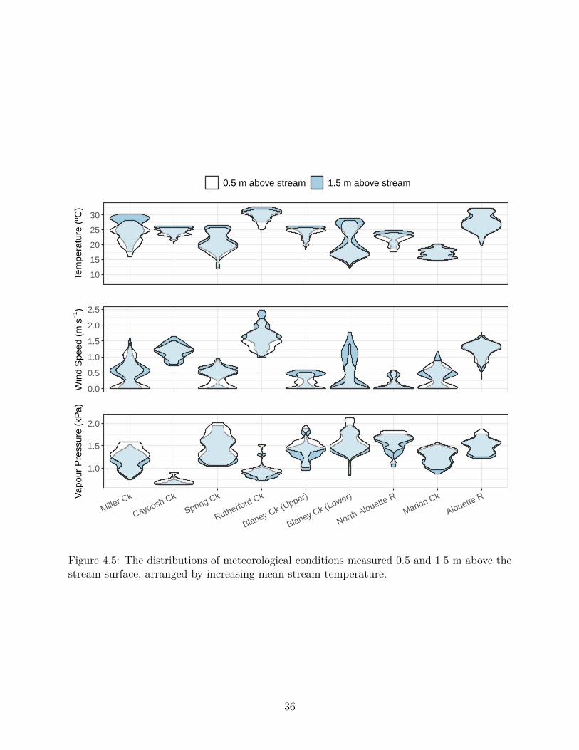
10

15

20

25

30

Tem

pera

ture

(ºC

)

0.5 m above stream 1.5 m above stream

0.0

0.5

1.0

1.5

2.0

2.5

Win

d S

peed

(m

s−1

)

1.0

1.5

2.0

Miller Ck

Cayoosh Ck

Spring Ck

Rutherford Ck

Blaney Ck (Upper)

Blaney Ck (Lower)

North Alouette R

Marion Ck

Alouette RVap

our

Pre

ssur

e (k

Pa)

Figure 4.5: The distributions of meteorological conditions measured 0.5 and 1.5 m above thestream surface, arranged by increasing mean stream temperature.

36

−0.020.000.020.040.060.080.100.120.140.160.180.200.22

Miller Ck

Spring Ck

Blaney Ck (Lower)

North Alouette R

Blaney Ck (Upper)

Cayoosh Ck

Marion Ck

Alouette R

Rutherford Ck

Obs

erve

d ev

apor

atio

n ra

te (

mm

h−1

)

Figure 4.6: The observed evaporation rates at each stream, arranged by increasing meanevaporation rate. The 95 % confidence intervals associated with each observation due tosampling variability are indicated by the bars extending above and below each point.

Table 4.3: All unique model random effect distributions, depending on the number of modelparameters. ID is a code to identify the significant random effects for each model form aspresented in Table 4.4.

Model ParametersID a b c dI •II •III • •IV •V • •VI • •VII • • •VIII •IX • •X • •XI • •XII • • •XIII • • •XIV • • •XV • • • •

37

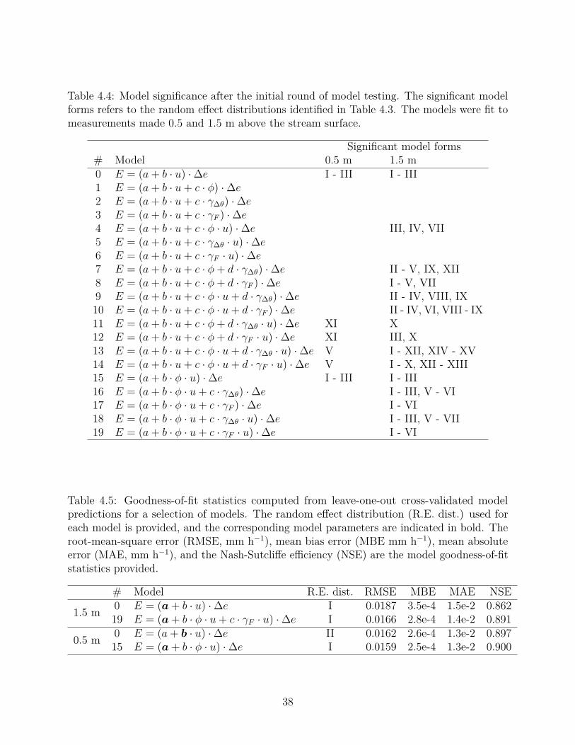
Table 4.4: Model significance after the initial round of model testing. The significant modelforms refers to the random effect distributions identified in Table 4.3. The models were fit tomeasurements made 0.5 and 1.5 m above the stream surface.

Significant model forms# Model 0.5 m 1.5 m0 E = (a+ b · u) ·∆e I - III I - III1 E = (a+ b · u+ c · φ) ·∆e2 E = (a+ b · u+ c · γ∆θ) ·∆e3 E = (a+ b · u+ c · γF ) ·∆e4 E = (a+ b · u+ c · φ · u) ·∆e III, IV, VII5 E = (a+ b · u+ c · γ∆θ · u) ·∆e6 E = (a+ b · u+ c · γF · u) ·∆e7 E = (a+ b · u+ c · φ+ d · γ∆θ) ·∆e II - V, IX, XII8 E = (a+ b · u+ c · φ+ d · γF ) ·∆e I - V, VII9 E = (a+ b · u+ c · φ · u+ d · γ∆θ) ·∆e II - IV, VIII, IX10 E = (a+ b · u+ c · φ · u+ d · γF ) ·∆e II - IV, VI, VIII - IX11 E = (a+ b · u+ c · φ+ d · γ∆θ · u) ·∆e XI X12 E = (a+ b · u+ c · φ+ d · γF · u) ·∆e XI III, X13 E = (a+ b · u+ c · φ · u+ d · γ∆θ · u) ·∆e V I - XII, XIV - XV14 E = (a+ b · u+ c · φ · u+ d · γF · u) ·∆e V I - X, XII - XIII15 E = (a+ b · φ · u) ·∆e I - III I - III16 E = (a+ b · φ · u+ c · γ∆θ) ·∆e I - III, V - VI17 E = (a+ b · φ · u+ c · γF ) ·∆e I - VI18 E = (a+ b · φ · u+ c · γ∆θ · u) ·∆e I - III, V - VII19 E = (a+ b · φ · u+ c · γF · u) ·∆e I - VI

Table 4.5: Goodness-of-fit statistics computed from leave-one-out cross-validated modelpredictions for a selection of models. The random effect distribution (R.E. dist.) used foreach model is provided, and the corresponding model parameters are indicated in bold. Theroot-mean-square error (RMSE, mm h−1), mean bias error (MBE mm h−1), mean absoluteerror (MAE, mm h−1), and the Nash-Sutcliffe efficiency (NSE) are the model goodness-of-fitstatistics provided.

# Model R.E. dist. RMSE MBE MAE NSE

1.5 m 0 E = (a + b · u) ·∆e I 0.0187 3.5e-4 1.5e-2 0.86219 E = (a + b · φ · u+ c · γF · u) ·∆e I 0.0166 2.8e-4 1.4e-2 0.891

0.5 m 0 E = (a+ b · u) ·∆e II 0.0162 2.6e-4 1.3e-2 0.89715 E = (a + b · φ · u) ·∆e I 0.0159 2.5e-4 1.3e-2 0.900

38

Table 4.6: The population-level estimated coefficients and coefficient standard errors for theselected models.

Estimated coefficient value [standard error]# a (mm h−1 kPa−1) b (mm h−1 s m−1 kPa−1) c (mm h−1 s3 m−2 kPa−1)

1.5 m 0 0.0663 [0.0079] 0.0449 [0.0069]19 0.0837 [0.0033] 0.1201 [0.0169] 0.0766 [0.0234]

0.5 m 0 0.0815 [0.0049] 0.0437 [0.0072]15 0.0944 [0.0034] 0.0684 [0.0069]

expanded model fit to the 1.5-m measurements, Model 19, provided an 11 % reduction in theRMSE. The cross-validated model predictions for the selected models in Table 4.5 are shownin Figure 4.7. While the expanded 0.5-m model had better goodness-of-fit indicators thanthe expanded 1.5-m model, it was more prone to site-specific over- or under-estimation ofevaporation as shown by the distribution of residual errors in Figure 4.8.

The best performing base and expanded models, under cross-validation, each had a mixed-effects structure with random effects on only one model parameter, as indicated in boldin Table 4.5. For the base model for the 1.5-m measurement height, the best-performingmixed-effects structure estimated site-specific adjustments for the a coefficient, while thebest mixed-effects structure for the 0.5-m base model estimated site-specific adjustmentsfor the b coefficient. For the best expanded models for both measurement heights, the bestperfoming mixed-effects structures estimated site-specific adjustments for the a coefficient.While the fixed-effects coefficients are used during model cross-validation, the magnitude ofthe site-specific adjustments for a given model provides information on how much site-specificvariability is not accounted for by the model predictors.

There was a notable difference in the variability of the site-specific adjustments betweenthe base and expanded models (Figure 4.9). The base model’s site-specific adjustments werebetween 0.4 to 37 % of the fixed-effect coefficient value for the 1.5-m model, and between1 and 25 % for the 0.5-m model. This indicates that there was site-specific variabilityunaccounted for by the base model predictors. However, the expanded model’s site-specificadjustments were less than 0.001 % of the fixed-effect coefficient value for both the 1.5-mand 0.5-m models. This indicates that the same magnitude of error reduction achieved inthe base models through site-specific adjustments could not be achieved through site-specificadjustments upon expansion of the base models with additional predictors.

39

Base Expanded

0.5 m1.5 m

0.00 0.05 0.10 0.15 0.20 0.00 0.05 0.10 0.15 0.20

0.00

0.05

0.10

0.15

0.00

0.05

0.10

0.15

Observed evaporation rate (mm h−1)

Pre

dict

ed e

vapo

ratio

n ra

te (

mm

h−1

)

Alouette RiverCayoosh CreekLower Blaney CreekMarion CreekMiller CreekNorth Alouette RiverRutherford CreekSpring CreekUpper Blaney Creek

1:1 line

Figure 4.7: Cross-validated model predictions for the base mass transfer model and the twobest expanded models, Models 15 and 19, for meteorological measurements made 0.5 m and1.5 m above the stream surface, respectively.

40

Base

Expanded

Alouette R

Blaney Ck (Lower)

Blaney Ck (Upper)

Cayoosh Ck

Marion Ck

Miller C

k

North Alouette R

Rutherford Ck

Spring Ck

−0.04

−0.02

0.00

0.02

0.04

−0.04

−0.02

0.00

0.02

0.04

Res

idua

l Err

or (

mm

h−1

)

0.5 m

1.5 m

Figure 4.8: The site-specific residual error distribution for the base and expanded 0.5-m and1.5-m models. The residuals were computed from cross-validated model predictions.

41

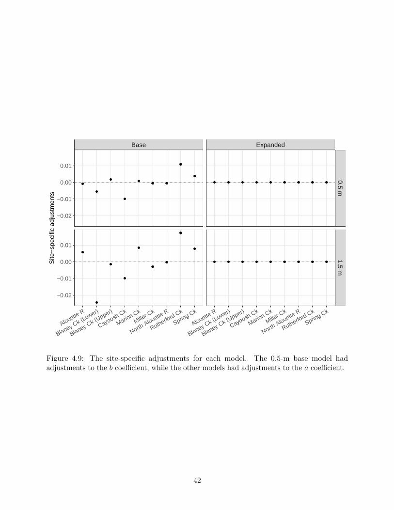
Base Expanded

0.5 m1.5 m

Alouette R

Blaney Ck (Lower)

Blaney Ck (Upper)

Cayoosh Ck

Marion Ck

Miller C

k

North Alouette R

Rutherford Ck

Spring Ck

Alouette R

Blaney Ck (Lower)

Blaney Ck (Upper)

Cayoosh Ck

Marion Ck

Miller C

k

North Alouette R

Rutherford Ck

Spring Ck

−0.02

−0.01

0.00

0.01

−0.02

−0.01

0.00

0.01

Site

−sp

ecifi

c ad

just

men

ts

Figure 4.9: The site-specific adjustments for each model. The 0.5-m base model hadadjustments to the b coefficient, while the other models had adjustments to the a coefficient.

42

4.4.2 Wind Function Comparison

The wind functions from five similar evaporation studies are presented in Table 4.7 andcompared against this study’s base model coefficients. These are studies that either directlymeasured stream evaporation (Benner, 2000; Guenther et al., 2012; Maheu et al., 2014;Caissie, 2016) or are widely adopted in stream temperature modelling studies (Webb andZhang, 1997). These literature wind functions were applied to the meteorological data fromthis study. Input data was matched to a given literature wind function measurement heightwhere available (e.g., 0.5-m measurements were used for Benner’s wind function). For windfunctions fit to measurements made 2 m above a stream, the 1.5-m height wind speeds wereadjusted using a power law relation (Sutton, 1953). No adjustments were made to the vapourpressures. The literature wind function predictions are shown in Figure 4.10 along with thecross-validated predictions from the 1.5-m base model.

43

1

3

5

2

4

6

Maheu (LSWM) Webb

Benner Guenther

Maheu (CB) Caissie

0.00 0.04 0.08 0.12 0.16 0.20 0.00 0.04 0.08 0.12 0.16 0.20

0.0

0.1

0.2

0.3

0.4

0.0

0.1

0.2

0.3

0.4

0.0

0.1

0.2

0.3

0.4

Observed evaporation rate (mm h−1)

Pre

dict

ed e

vapo

ratio

n ra

te (

mm

h−1

)

Literature wind function This study 1:1 line

Figure 4.10: The evaporation rates estimated by applying six literature wind functions tothis study’s dataset. The wind function coefficients and the study references are provided inTable 4.7. The two panels for Maheu correspond to the wind functions for Catamaran Brook(CB) and the Little Southwest Miramichi River (LSWM). The panels are ordered from 1 to 6by decreasing model root-mean-square error. The predicted evaporation rates for this studyare cross-validated predictions from the 1.5-m model.

44

Table 4.7: A comparison of wind function coefficients, a and b, derived from stream evaporationmeasurements, and one commonly cited in stream temperature modelling studies. In theseventh column, Tp indicates the evaporation pan water temperature.

Source Site a b Measurement Stream TpDescription (mm

h−1

kPa−1)

(mm h−1

s m−1

kPa−1)

height (m) width (m) measured?

This study Forestedstreams

0.0663 0.0449 1.5 3.1 to 27.6 yes0.0815 0.0437 0.5Benner(2000)

Streams in mead-ows and forest

0.144 0.085 0.5 2.7 to 19.5 yes

Guenther etal. (2012)

Forested stream - 0.0424 1.5 1.5 yes

Maheu et al.(2014)

Forested stream 0.11 0.122 2 8 noForested stream 0.123 0.035 2 80 no

Caissie et al.(2016)

Forested stream - 0.19 2 1.7 no

Webb andZhang(1997)

Streams in pas-ture and wood-land

0.055 0.059 2 0.8 to 11.3 no

45

Chapter 5

Laboratory Results

5.1 Relation Between Solution Molarity and ElectricalConductivity

The results of the electrical conductivity to molarity calibration are shown in Appendix E,Figure E.1. The regression fit to the model defined by Equation 3.1 had a root-mean-squareerror of 8.69× 10−5 mol L−1 and an adjusted R2 of 0.99. The estimated coefficients, m andb, were 1.10× 10−2 and −1.836× 10−2, respectively. The electrical conductivity calibrationspanned conductivities from 16.00 to 19.54 mS cm−1, which exceeded the range of measuredconductivities during the flume trials and ensured no trial data would need to be extrapolated.

5.2 Meteorological Conditions and Evaporation Rates

The meteorological conditions, flume water electrical conductivity, and evaporation rates arepresented in Figures 5.1a to 5.1d. The figure titles provide the flume parameter conditionsfor the given trial, where the slope is 2◦ or 6◦, and the presence/absence of LEGO is denoted‘L’ or ‘nL’. The air temperatures throughout all trials were consistently between 20.9 and21.5 ◦C. The wind speed ranged from 0.65 to 1.30 m s−1 with a mean of 0.93 m s−1. Thevariability in the measured wind speed can likely be attributed to the low precision of windspeed control available on the fan used. As the air temperatures did not experience significantfluctuation, the relative humidity tracked the trends in the vapour pressure of the air, with amean value of 1.27 kPa.

The flume water experienced sustained heating through all trials due to the heat dissipatedby the pump. Water temperatures were approximately 17 ◦C when drawn from the tap, butafter the initial 10 minutes of circulation through the flume, water temperatures warmed

46

to 21.3 ◦C, on average. The maximum water temperatures at the end of the trials rangedfrom 26.5 to 27.1 ◦C, with a mean of 26.8 ◦C. The vapour pressure at the surface of thewater increased accordingly, and ranged from a minimum of 2.82 kPa to a maximum of 3.56kPa, with a mean of 3.27 kPa. As a result of the high vapour pressures at the water surfacerelative to the air above it, the vapour pressure difference between the water and the airhad a minimum value of 1.53 kPa, maximum of 2.35 kPa, with a mean of 2.00 kPa. The airabove the flume was always unstable (∆θ > 0). The measured electrical conductivity (EC)increased as time elapsed, although the increases were not at consistent rates. For the trialswhere the flume slope was 6◦ (Figures 5.1c and 5.1d), the EC measurements showed morescatter than for the trials where the slope was 2◦ (Figures 5.1a and 5.1b). The evaporationrates were generally positive and increasing, and ranged from 0.59 to 2.96 mm h−1, with amean of 1.68 mm h−1.

5.3 Statistical Analysis

The predicted evaporation rates from Equation 3.5 are presented in Figure 5.2 along with the95 % confidence intervals. The model fit had a root-mean-square error of 0.572 mm h−1, andan adjusted R2 = 0.050. The results of the analysis of variance test are presented in Table 5.1.The test gives p = 0.8195 > 0.05 for the test between Equation 3.6 and Equation 3.5, so theaddition of the flume parameter variables does not significantly improve the model predictions.This can be interpreted as an indication that there is likely no statistically significant influenceof the flume parameters on the evaporation rate.

Table 5.1: Analysis of variance for the difference between the reduced and full evaporationmodels (Equations 3.6 and 3.5). RSS is the residual sum of squares and DF is the degrees offreedom for the model.

Model RSS DF F value p valueReduced 7.5080 18

Full 5.8894 27 0.5497 0.8195

47

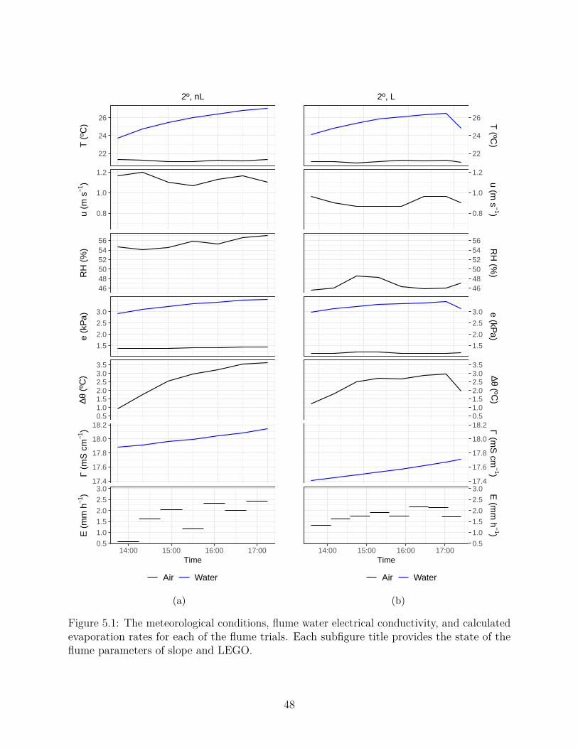
22

24

26

T (

ºC)

2º, nL

0.8

1.0

1.2

u (m

s−1

)

464850525456

RH

(%

)

1.5

2.0

2.5

3.0

e (k

Pa)

0.51.01.52.02.53.03.5

∆θ (

ºC)

17.4

17.6

17.8

18.0

18.2

Γ (m

S c

m−1

)

0.5

1.0

1.5

2.0

2.5

3.0

14:00 15:00 16:00 17:00Time

E (

mm

h−1

)

Air Water

(a)

22

24

26 T (ºC

)2º, L

0.8

1.0

1.2

u (m s

−1)

464850525456

RH

(%)

1.5

2.0

2.5

3.0 e (kPa)

0.51.01.52.02.53.03.5

∆θ (ºC)

17.4

17.6

17.8

18.0

18.2 Γ (mS

cm−1)

0.5

1.0

1.5

2.0

2.5

3.0

14:00 15:00 16:00 17:00Time

E (m

m h

−1)

Air Water

(b)

Figure 5.1: The meteorological conditions, flume water electrical conductivity, and calculatedevaporation rates for each of the flume trials. Each subfigure title provides the state of theflume parameters of slope and LEGO.

48

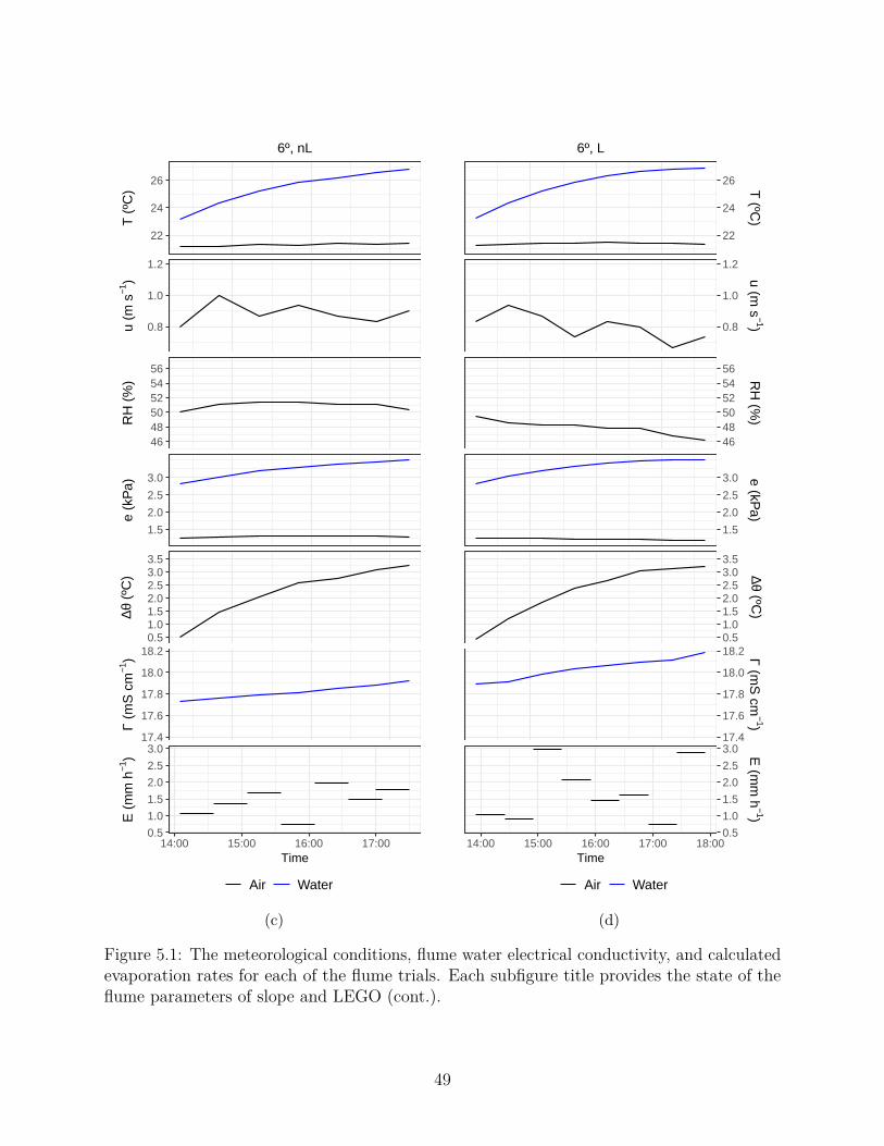
22

24

26

T (

ºC)

6º, nL

0.8

1.0

1.2

u (m

s−1

)

464850525456

RH

(%

)

1.5

2.0

2.5

3.0

e (k

Pa)

0.51.01.52.02.53.03.5

∆θ (

ºC)

17.4

17.6

17.8

18.0

18.2

Γ (m

S c

m−1

)

0.5

1.0

1.5

2.0

2.5

3.0

14:00 15:00 16:00 17:00Time

E (

mm

h−1

)

Air Water

(c)

22

24

26 T (ºC

)6º, L

0.8

1.0

1.2

u (m s

−1)

464850525456

RH

(%)

1.5

2.0

2.5

3.0 e (kPa)

0.51.01.52.02.53.03.5

∆θ (ºC)

17.4

17.6

17.8

18.0

18.2 Γ (mS

cm−1)

0.5

1.0

1.5

2.0

2.5

3.0

14:00 15:00 16:00 17:00 18:00Time

E (m

m h

−1)

Air Water

(d)

Figure 5.1: The meteorological conditions, flume water electrical conductivity, and calculatedevaporation rates for each of the flume trials. Each subfigure title provides the state of theflume parameters of slope and LEGO (cont.).

49

6, L 6, nL

2, L 2, nL

1.50 1.75 2.00 2.25 1.50 1.75 2.00 2.25

0

1

2

3

0

1

2

3

Vapour pressure difference (kPa)

Pre

dict

ed e

vapo

ratio

n ra

te (

mm

h−1

)

Figure 5.2: The model-predicted evaporation rates with 95 % confidence intervals, for eachtrial.

50

Chapter 6

Discussion

6.1 Field Results

6.1.1 Evaporation as a Component of a Stream Heat Budget

For these sheltered, forested streams, the mean and maximum evaporation rates were 0.06and 0.20 mm h−1, which correspond to heat fluxes of 41 W m−2 and 136 W m−2. Forcomparison, the latent heat fluxes measured or estimated by four evaporation or streamtemperature studies are presented in Table 6.1. Benner (2000) measured mean and maximumdaily evaporation rates of approximately 0.44 and 1.32 mm h−1 from their aridland channelreaches, which correspond to heat fluxes of 299 W m−2 and 898 W m−2, respectively. Benneralso modelled the energy budget for their study site using meteorological measurements madeon August 9th, 1996; they predicted a mean daily evaporative heat loss of 239 W m−2, whichcorresponded to 37 % of the mean total heat loss. Additionally, Maheu et al. (2014) andCaissie (2016) reported evaporative heat fluxes ranging from 10 to 42 % of their forestedstreams. Net radiation to a small, subcanopy stream comparable to those in this study wasobserved to be 128 W m−2 during midday in the summer (Brown, 1969). Assuming this value,the mean evaporation rates measured in this study would comprise 33 % of the net radiation.These results indicate that evaporation can be a moderate to significant component of theheat budget for temperate, forested streams.

6.1.2 Assessment of Evaporation Pan Methodology

Given the design of the pans and their mode of deployment in this study, each individual panwas able to provide an estimate of evaporation with a mean uncertainty of 0.004 mm h−1,relative to mean and maximum measured rates of 0.06 mm h−1 and 0.20 mm h−1, respectively.

51

Table 6.1: Reported latent heat fluxes from a range of streams. In the table, Tw is the streamtemperature, φ is the canopy closure, u is the mean wind speed, and Qe is the mean latentheat flux.

Stream % of totalStudy width (m) Tw (◦C) φ (%) u (m s−1) Qe (W m−2) heat lossBrown (1969) < 1a 11.5 80 - 7a, b 6Caissie et al., (2016) 1.7 15.1 85 to 90 0.11 1.4 10Benner (2000) 15a 19.2 - 1.4 239 37Maheu et al., (2014) 80 19.5 20 0.8a 86 42a Estimatedb Midday peak

Therefore, the pans provide a viable approach to quantifying evaporation, and could be usedin future studies to measure evaporation in a broader range of conditions (e.g., higher watertemperatures and wind speeds) to expand the range of applicability of fitted wind functions.However, there are four specific points that require further consideration: (1) the need toaccount for the non-constant surface area, (2) differences in water temperature between thepans and the stream, (3) sampling variability among pans, and (4) the inability to deploythe pans at sites with high water velocities or rough flow.

The tapered sides of the pans resulted in a non-uniform water surface area over the rangeof water masses that were measured, which resulted in up to 4 % difference in the surfacearea. If the pan opening’s dimensions were assumed to be the surface area of the pan water,it would have been a 13 % overestimate of the average measured surface area. Using thisassumption, the mean and maximum evaporation rates would have been computed as 0.05 and0.17 mm h−1, rather than the 0.06 and 0.20 mm h−1 reported. The method for determiningwater surface area developed through this research is particularly useful because it requiresno additional measurements to be made when conducting field work.

The water temperature in the evaporation pans differed substantially from that of thestream water, ranging from -1.43 ◦C lower to 4.47 ◦C higher than stream temperature. Itwas suggested by Maheu (personal communication, July 2019) that the pans be filled withfresh stream water after each mass measurement to avoid this issue. However, the timeseries of pan and stream water temperatures show that frequent pan water temperaturefluctuations occurred within measurement intervals, and warming occurred within 10 to20 minutes of pan deployment on numerous occasions (Figure B.1). If this temperaturedifference were not accounted for, the vapour pressure difference used in the wind functionwould be incorrect. For most cases, the vapour pressure difference would be underestimated,leading to an overestimate of the fitted wind function coefficients. Given the observed rates

52

of pan warming, it is recommended that future users of this methodology measure the surfacetemperature of the water in the evaporation pans with high temporal resolution (e.g., every10 minutes).

The magnitude of the sampling variability was influenced by the non-uniformity ofconditions experienced by the nine pans in a given measurement interval. These differentconditions could be caused, for example, by differences in pan heating due to sunlightinfiltrating canopy gaps, or different pan exposures to wind due to in-stream boulders, andresulted in variable evaporation rates among the pans. Streams with low evaporation ratesbut diverse pan conditions, like Spring Creek, had high relative magnitudes of samplingvariability (177 % of the mean evaporation at Spring Creek). In contrast, streams withhigh evaporation rates and uniform pan conditions, like Marion Creek, had lower relativemagnitudes of sampling variability (7 % of the mean evaporation at Marion Creek). Overall,the mean sampling variability generally increased with mean evaporation rate at a stream.For example, Miller Creek had the lowest mean evaporation rate of 0.02 mm h−1 and anassociated mean sampling variability of 0.006 mm h−1. The same values for RutherfordCreek, with the greatest mean evaporation rate, were 0.14 mm h−1 and 0.010 mm h−1,respectively. This indicates that the sampling variability, at the 95 % confidence interval, canbe high relative to low evaporation rate measurements. Considering all streams, the resultsindicate that a sampling variability of less than 15 % of the measurements can be achievedby deploying nine evaporation pans, but sampling variability will unduly increase if the pansare exposed to variable conditions not representative of the variability in stream evaporation.

The evaporation pans were also sensitive to high flow velocities and non-placid flowconditions. Of the 900 measurements of evaporation, nine were omitted due to the pansbecoming submerged by fast flow. An additional 27 observations were omitted because waterwas seen to splash in or out of the pans as they were jostled by fast flow. Benner (2000)noted that evaporation was enhanced by flowing water under low wind speeds and/or lowvapour pressure differences, which may be common conditions for small streams under adense canopy (e.g., Guenther et al., 2012). As the requirement for placid flow limits thedeployment of the evaporation pans to pools or slow flow reaches, the measured evaporationrates may not be representative of an entire reach if it contains other stream morphologieslike riffles or steps, and is subject to low wind speeds and/or vapour pressure differences.

Steep, cascading mountain streams are also of interest for stream temperature modellingstudies, but their morphologies prohibit the use of evaporation pans to derive suitablewind function coefficients. In these instances, an energy-balance approach to model streamevaporation would be more suitable, as demonstrated by recent proglacial stream temperaturemodelling work by Dufficy (2019). Dufficy reported free and forced convection coefficients

53

from a modified wind function that are greater than those derived in this study, or in otherstudies previously discussed. The reported hourly estimates for a ranged from 0.642 to 0.879mm h−1 kPa−1, and b ranged from 0.164 to 0.284 mm h−1 s m−1 kPa−1. Dufficy’s resultsindicate that the physical processes driving evaporation in a proglacial stream operate at adifferent magnitude than those present in temperate, forested mountain streams, and thatwind functions derived from evaporation pans are not applicable in these systems.

6.1.3 Effect of Measurement Height on Performance of the BaseModel

Meteorological measurements made at 0.5 m above the stream surface produced betterpredictions than measurements made at 1.5 m. Previous studies typically made meteorologicalobservations at 1.5 or 2 m height above the surface, with the exception of Benner (2000),who made them at 0.5 m. Krajewski et al. (1982) suggested measuring wind speed directlyabove the stream surface when fitting a wind function, and Dingman (2015) suggested thatthe wind function coefficients will vary with measurement height. In this study, it wasthe a coefficient that was the main difference between the wind functions fit to data fromdifferent measurement heights (0.0815 vs. 0.0663 mm h−1 kPa−1 for the ‘0.5 m’ and ‘1.5 m’model, respectively). The difference in the a parameter value indicates a greater influence ofthe vapour pressure difference on stream evaporation with decreasing measurement height,particularly when considering sheltered streams with poorly developed wind profiles.

One consideration about the choice of measurement height relates to the fact that streamstage varies with discharge, which can be particularly important for proglacial streams, whichexperience significant diel fluctuations in discharge. For example, a wind function derivedfrom measurements at a height of 0.5 m would not be accurate if the water surface rose andthe instruments were only 0.3 m above the water surface. Because the gradients of windspeed and vapour pressure should be greatest close to the water surface and decrease withincreasing height, this source of error would be greatest for wind functions derived frommeasurements at a low height and least for wind functions derived from measurements at agreater height above the water surface. Additionally, wind speed measurements made closerto the stream surface are subject to measurement uncertainty. Therefore, it is recommendedthat future studies measure meteorological conditions at approximately 1.5 m above thestream, where the application of coefficients from the ‘1.5 m’ model would likely be lesssensitive to stage-related or other changes in the measurement height.

54

6.1.4 Effects of Additional Predictor Variables

The addition of a canopy variable alone resulted in six significant model forms when fit tomeasurements made 1.5 m above the stream (Table 4.4). When tested under cross-validation,none of these models provided improvements over the base model. The addition of a stabilityvariable alone never produced a significant model. However, the addition of the variablestogether provided modest model improvement, with an 11 % reduction in root-mean-squareerror, and an increase in the Nash-Sutcliffe efficiency from 0.862 to 0.891.The expansion of the base model with a stability variable alone was never significant whenfitting the model to measurements made 0.5 m above the stream. The addition of a canopyopenness variable alone produced three significant model forms, while the addition of bothstability and canopy openness variables produced four significant model forms (Table 4.4).However, it was the addition of a canopy openness variable alone that provided some, albeitmarginal, improvement over the base model (2 % reduction in root-mean-square error,increased Nash-Sutcliffe efficiency from 0.897 to 0.900).

The results of the model fitting with stability predictors suggest that stability playsa minor role compared to the forced convection influence of wind on vapour transfer forsmall, sheltered streams. This is supported in particular by the daytime and night-timewind functions reported by Maheu et al. (2014). Daytime conditions were predominantlystable while unstable conditions dominated at night. Despite the unstable conditions, thenight-time wind function’s free convection coefficient, a, did not increase, but rather theforced convection coefficient increased from 0.035 to 0.0742 mm h−1 s m−1 kPa−1, comparedto the daytime wind function. These results are also supported by Guenther et al. (2012),who reported a wind function intercept equal to zero, indicating the dominance of forcedconvection for their small, forested stream. However, the limited range of stability conditionsobserved in this study may have been insufficient to comprehensively evaluate its influence,particularly when considering warmer, sheltered and unsheltered streams.

The additional benefit of adding stability and canopy openness predictors for both mea-surement heights was that they accounted for the site-to-site variability that could not beaccounted for by the base model (Figure 4.9). While the stability indices can be computedfrom the same meteorological data required to compute the vapour pressures, canopy open-ness is not typically available. Canopy openness can be estimated using satellite imagery(Carreiras et al., 2006), and using light detection and ranging (LiDAR) (Korhonen et al.,2011). LiDAR estimates of canopy openness are more accurate than estimates from satelliteimagery (Smith et al., 2009), but LiDAR data are currently expensive to obtain and lack thetemporal resolution of satellite imagery. Given these concerns and those discussed in section6.1.3, it is recommended to use the expanded ‘1.5 m’ model if canopy openness measurements

55

are available, or reliable estimates can be obtained, given its superior performance over thebase model. Furthermore, when additional research is done to cover a broader range ofstream temperatures, wind speeds, and stability conditions, it would be beneficial to furtherexplore the influence of stability as a predictor, to improve model performance under diverseconditions.

6.1.5 Comparison of Wind Function Coefficients

Most studies measuring stream evaporation have been focused on one or at most two streams(Guenther et al., 2012; Maheu et al., 2014; Caissie, 2016), or worked in hydroclimates differentto that of southwest British Columbia (Benner, 2000). These studies produced site-specificestimates of the wind function coefficients (Table 4.7), which represented evaporation underthe influence of the local physiography, climate, and stream characteristics. The aridlandstream reaches studied by Benner (2000) produced a wind function, fit to meteorologicalmeasurements 0.5 m above the stream, with both coefficients nearly double those foundby this study. However, Guenther et al. (2012) and Caissie (2016) derived wind functionswith the free convection term, a, equal to zero for the small, sheltered streams they studied.It is worth noting that evaporation pan warming was not accounted for by Maheu et al.(2014) and Caissie (2016). By computing the saturation vapour pressure using the streamtemperature and assuming the same value for the pans, the wind function coefficients wouldbe artificially elevated. There is some evidence of this when comparing the wind functionsof Guenther et al. and Caissie; their respective study streams are similar, but the forcedconvection coefficient reported by Caissie was substantially greater than that reported byGuenther et al. (0.19 vs 0.0424 mm h−1 s m−1 kPa−1, respectively).

Webb and Zhang (1997) also developed a generalized wind function. Although it is notspecified how they derived their wind function coefficients, it is clear they did not fit theirwind function to stream evaporation measurements. Their wind function coefficients aresimilar to those presented in this study (Table 4.7), more so for the ‘1.5 m’ model. Consideringthe ‘1.5 m’ model, the slope coefficient, b, in this study is slightly less, and the interceptslightly greater than that presented by Webb and Zhang. There is an increased differencebetween their intercept and the ‘0.5 m’ model’s intercept (0.055 vs. 0.0815 mm h−1 kPa−1),which reflects the wind function coefficient variability due to measurement height (Dingman,2015). By reaching a similar wind function empirically, this study provides validation ofthe wind function developed by Webb and Zhang, which is frequently used to model streamevaporation.

The results of the wind function comparison presented in Figure 4.10 indicate variable

56

model performance. Generally, wind functions with lower b coefficients (between 0.035 and0.06) had lower prediction errors. Models where the intercept of the wind function is zero, asin the models from Guenther et al. and Caissie, tend to over- or underestimate evaporation.An intercept equal to zero implies that there is no evaporation in the absence of wind.Given the starting-speed limitations of the cup-type anemometers typically employed formeteorological measurements, low wind speeds are likely to be under-reported. As a result,an intercept of zero may not be an accurate representation of the evaporation processesoccurring in small, sheltered streams, and is in contrast to the non-zero intercepts reportedby this study and by Webb and Zhang. The two generalized wind functions by Benner andby Webb and Zhang performed quite differently; Benner’s model consistently overestimatedevaporation whereas Webb and Zhang’s model matched the predictions from this study’sbase model. One key difference between these two studies is the climate of their respectivestudy regions. This indicates that generalized wind functions may not be good estimatorswhen applied to different environments than where they were developed.

An additional consideration is the presence of an internal boundary layer (IBL) over astream and the influence this and the measurement height will have on the wind functioncoefficients. Within an IBL, the temperature, humidity, and wind profiles will be differentthan in an overlying adjusted boundary layer (ABL) (Elliott, 1958). The ABL will representconditions more representative of the upwind land surfaces while the IBL will be adjusting tothe energy and water exchanges at the stream surface. For small (i.e. < 2 m stream width)and/or densely sheltered streams (e.g., Griffith Creek as observed by Guenther et al., 2012),relatively high measurement heights will be more likely to observe conditions in the ABL,rather than the conditions dominating evaporation at the stream surface. If the measurementheight is within an IBL, the estimated wind functions coefficients would be lower than if theywere made in an ABL above the stream; for example, if the vapour pressure difference ishigher in the IBL than the ABL, wind function coefficients fitted to measurements made inthe ABL would be elevated. Evidence of this is present when comparing the wind functioncoefficients reported by Guenther et al. (2012) and Caissie (2016) for their similar streams:they reported a wind function slope of 0.0424 vs. 0.19 mm h−1 s m−1 kPa−1, and usedmeasurement heights of 1.5 and 2 m, respectively. It is expected that wider streams will havea boundary layer representative of the stream surface conditions extend to a greater heightabove the surface, resulting in estimated wind function coefficients that are less biased.

Each of these studies investigated the evaporation processes occurring in systems ofdifferent scales and subject to different forcing conditions (e.g., the magnitude of vapourpressure difference, stability, and the strength of wind profile development). Each study bringsinsight to the influence of certain physical processes in a given context, but the differences in

57

methodologies adopted by each study limits our ability to synthesize the results in a single,transferable model. Therefore, there is a need to extend evaporation measurements to covera range of sites using a consistent methodology.

6.1.6 Application in Stream Temperature Modelling

The results from the wind function comparison in Figure 4.10 show that only Webb andZhang’s generalized wind function performed well in comparison to the predictions fromthis study. The site-specific wind functions did not perform well when applied to a range ofstreams because their wind functions were fit to represent the unique conditions and processesat individual sites. Considering the range of streams where evaporation has been measured,only one stream was wider than 30 m (the Little Southwest Miramichi River studied byMaheu et al., 2014), and only one stream had a mean temperature > 20 ◦C during the studyperiod (the Upper Middle Fork of the John Day River studied by Benner, 2000). Warm, widestreams in a temperate climate have not been well represented in the existing evaporationstudies. Due to this lack of representation, additional measurements of evaporation from warmstreams, of all widths and degrees of sheltering, in a temperate climate, are required to derivewind function coefficients capable of successfully modelling stream evaporation. In additionto the stream width, temperature, and density of riparian vegetation, the weather conditionsunder which the data were collected has been suggested to play a role in wind functionvariability as well (Jobson, 1980; Benner, 2000). To make future wind functions more robust,measurements should be made to encompass the range of typical weather conditions in astudy region. It is recommended that the wind function coefficients developed through futureresearch be applied to streams of similar thermal regimes, physiography, and hydroclimate;failure to do so may result in biased predictions of evaporation, and subsequently of latentheat fluxes.

6.2 Laboratory Results

6.2.1 Flume Experiment Design

The analysis of the flume data was unable to detect a statistically significant effect of slope orroughness on evaporation. This result is counter to the hypothesis that aeration associatedwith steep, rough channels should enhance turbulent exchange between the water and theoverlying air. The laboratory experiments conducted by Benner (2000), while limited, didindicate a relationship between the evaporation rate and flow velocity at low vapour pressuredifferences and no wind. However, Benner also noted that in the presence of wind or as the

58

vapour pressure difference increased, the influence of flowing water on the evaporation ratediminished. Recent alpine stream temperature modelling research by Dufficy (2019) indicatesthat evaporation from aerated, cascading proglacial streams with stable overlying air is notwell represented by mass transfer equations derived for lower gradient, less aerated forestedstreams. These studies indicate that aeration and flow velocity do have an influence onstream evaporation, but that the influences of vapour pressure difference, wind, and stabilityneed to be carefully considered. The statistical insignificance of this experiment may be theresult of three issues.

One notable issue was the magnitude of noise relative to the signal in the electricalconductivity (EC) measurements. Aerated water produced fluctuations of 0.10 to 0.15 mScm−1 with every scan of the EC probe (1 scan per second), while the 10-minute averages weretypically 0.01 to 0.02 mS cm−1. Without enhanced aeration, there was occasionally no changein EC between measurements, which computes to an unrealistic evaporation rate of zero. Theheat produced by the pump may have also caused several issues. The EC sensor computesa temperature-corrected electrical conductivity and may have suffered from compensationerrors due to the rapid flume warming. Additionally, the instability in the flume resultingfrom water temperatures greater than air temperatures may have enhanced evaporationto the point where the influence of flow velocity and roughness were not distinguishable.With these issues identified and held in consideration with the findings of Benner (2000) andDufficy (2019), the underlying principles of this method are likely sound and this study failedto capture the effect of slope or roughness due to methodological issues.

The issue of the signal to noise ratio could be addressed by increasing the total volumeof water lost to evaporation by increasing the flume surface area. A greater loss of volumewith each measurement interval would produce a greater change in solution concentration,resulting in a greater change in electrical conductivity. Measuring the EC in some form ofwell-mixed stilling chamber may reduce the EC measurement variability in aerated flows.Perhaps most importantly, the flume water temperature could be controlled by installinga heat exchange system that is submerged in the catch-basin. Glycol-based heat exchangesystems are scalable, efficient, and relatively inexpensive. Water-based systems are moreaffordable and are also efficient, may be unacceptably wasteful if the water is not cooled andrecycled.

The main difficulty in empirically describing the influence of aeration and flow velocityon evaporation is the difficulty associated with measuring evaporation from moving water.The primary benefit of the EC method developed for this experiment is that readily availableinstruments can be employed to measure the evaporation rate with 5- to 10-minute temporalresolution without interrupting the flow. Additionally, a recirculating flow system allows

59

for conservation of mass principles to be applied. There are other approaches that could beemployed in a controlled laboratory setting, that could not be used in natural systems. Forexample, a gravimetric approach could take advantage of fluid transfer between a measurementchamber and the flume catch-basin via a siphoning tube as changes in hydrostatic head dueto evaporation are equalized. Also, the Beer-Lambert law could be used to relate a change insolution absorbance to a change in solute concentration, again relying on the relationshipbetween water volume loss and concentration change. More sophisticated methods may alsobe employed using changes in tracer concentration (e.g. spectrofluorometry).

60

Chapter 7

Conclusion

7.1 Key Findings

Evaporation rates were measured at streams with a range of widths (3.1 to 27.6 m), temper-ature regimes, and degrees of sheltering. A total of 864 approximately hourly evaporationmeasurements were made, and the evaporation rates ranged from -0.01 to 0.20 mm h−1, witha mean rate of 0.06 mm h−1. A generalized, Dalton-type mass transfer equation was derivedusing these measurements.

Measured evaporation using the floating pans had an uncertainty of 0.004 mm h−1, whichis adequate for resolving the variability in evaporation rates through time and among sites.One complication is that water temperature in the pans differed from stream temperature byup to 4.54 ◦C, with stream-specific average differences ranging from -0.66 to 1.64 ◦C, so thatadjustments had to be made to the stream temperature time series prior to computing vapourpressure at the water surface. In future applications of this methodology, it is recommendedthat water temperature in the pans be measured approximately every 10 minutes.

The wind function was fit using measurements made 1.5 and 0.5 m above the streamand had respective root-mean-square errors of 0.0187 and 0.0162 mm h−1 under cross-validation, and respective Nash-Sutcliffe efficiencies of 0.862 and 0.897. The model fit to1.5-m measurements had an a coefficient of 0.0663 mm h−1 kPa−1, and a b coefficient of0.0449 mm h−1 s m−1 kPa−1, while the model fit to 0.5-m measurements had respectivecoefficient values of 0.0815 and 0.0437. These values are greater than the values reportedby previous studies that derived unique wind functions for small (< 2 m width), forestedstreams (Guenther et al., 2012; Caissie, 2016), but are less than the values reported fromwider streams (> 30 m width) or arid regions (Benner, 2000; Maheu et al., 2014). Thiswork validates the commonly used wind function reported by Webb and Zhang (1997), andexpands upon the only previous empirically derived generalized wind function, derived by

61

Benner (2000), but which is better suited to arid regions.Canopy openness was a significant addition to the wind function for both meteorological

measurement heights, while a stability index, the buoyant force, was a significant additiononly when the model was fit to measurements from 1.5 m. The reductions in predictionerror achieved with these additional variables were greater for measurements at 1.5 m ratherthan 0.5 m, which is in line with comments by Brutsaert and Yu (1968) regarding greaterrepresentation of turbulent mixing processes at higher measurement heights above an openwater surface. However, absolute prediction errors were smaller using measurements from 0.5m. The lack of significance of stability as a predictor for the ‘0.5 m’ model could be due tothe lack of variability in stability conditions, as conditions were typically stable.

Both the basic Dalton-type models and the expanded models had consistent performanceunder cross-validation. The addition of stability and canopy openness variables reducedsite-specific variability in evaporation predictions, as determined through the mixed-effectsmodelling approach. These results indicate that both the base and expanded models areapplicable to a range of temperate mountain streams to produce representative estimates ofevaporation.

Laboratory experiments conducted to determine the influence of aeration and flow velocityon evaporation were intended to build upon the work of Benner (2000). Aeration and flowvelocity were not determined to have a significant influence on the evaporation rate from aflume. The lack of statistical significance may be attributed to methodological issues, ratherthan being an accurate representation of the physical processes.

7.2 Recommendations for Future Work

This study produced a wind function that is applicable to a range of temperate, shelteredstreams. Future research should expand stream evaporation measurements to cover a broaderrange of streams than surveyed through this work. In particular, streams with temperaturesgreater than the maximum observed during this study (21.5 ◦C) would be worth furtherinvestigation. With higher stream temperatures, evaporation rates could increase to thepoint where it actively forces an upper limit on stream temperature, if thermal equilibrium isreached. Additionally, measuring evaporation from an expanded range of stream widths (e.g.,< 3 m and > 30 m), degrees of sheltering, and under both stable and unstable conditionswould aid the further development of a robust, generalized wind function applicable to abroader range of streams.

The lack of fetch associated with the high degree of sheltering in small, forested streamslimits the application of standard boundary layer theory and necessitates the use of empirical

62

wind functions, as derived in this study. In particular, narrow streams may have internalboundary layers that do not extend to the height of the meteorological instruments, especiallywhen winds blow across the channel. It would be useful for future studies to examine thenature of wind and humidity profiles above streams as a function of distance from the bank,the direction of airflow over the stream, and atmospheric stability. Such studies wouldprovide a stronger basis for understanding the variability of wind function coefficients andfor generating a broadly applicable model for predicting stream evaporation and associatedheat loss.

Conducting further laboratory studies is the best current approach to verify the influenceof aeration and flow velocity on evaporation. Further work to elucidate these relationshipswould be particularly helpful in interpreting and modelling evaporation rates from small,sheltered streams under low wind speed conditions, and cascading, aerated alpine streams.Future flume-based experiments would benefit from incorporating a temperature-controlmechanism to counteract undesired heating from a pump-based system, and the potentiallyconfounding influence of instability over the flume. Future studies could explore potentialalternative methodologies to measure evaporation from moving water in a laboratory setting.The following are some examples of alternative methodologies:

• a gravimetric approach that measures the mass loss associated with fluid transferbetween a measurement chamber and a flume via a siphoning tube, as changes inhydrostatic head due to evaporation are equalized;

• a spectrophotometric approach that relates changes in solution absorbance to a changein solute concentration due to evaporation;

• a spectrofluorometric approach that can measure changes in a specialized tracer con-centration due to evaporation.

63

Bibliography

Arya SP. 1988. Introduction to micrometeorology. Academic Press, San Diego.

Bartholow JM. 2000. Estimating cumulative effects of clearcutting on stream temperatures.Rivers 7: 284–297

Benner DA. 2000. Evaporative heat loss of the Upper Middle Fork of the John Day River,Northeastern Oregon. MSc thesis, Oregon State University.

Benyahya L, Caissie D, El-Jabi N, Satish MG. 2010. Comparison of microclimate vs. remotemeteorological data and results applied to a water temperature model (Miramichi River,Canada). Journal of Hydrology 380: 247–259 DOI: 10.1016/j.jhydrol.2009.10.039

Brady DK, Graves WL, Geyer JC. 1969. Surface heat exchange at power plant cooling lakes.In Cooling Water Discharge Project Report No. 5 Edison Electric Institute, New York.

Brown GW. 1969. Predicting temperatures of small streams. Water Resources Research 5:68–75 DOI: 10.1029/WR005i001p00068

Brown GW, Krygier JT. 1970. Effects of clear-cutting on stream temperature. WaterResources Research 6: 1133–1139 DOI: 10.1029/WR006i004p01133

Brutsaert W. 1982. Evaporation into the atmosphere. Springer Netherlands. DOI:10.1007/978-94-017-1497-6

Brutsaert W, Yu SL. 1968. Mass transfer aspects of pan evaporation. Journal of AppliedMeteorology 7: 563–566 DOI: 10.1175/1520-0450(1968)007<0563:MTAOPE>2.0.CO;2

Caissie D. 2006. The thermal regime of rivers: A review. Freshwater Biology 51: 1389–1406

64

DOI: 10.1111/j.1365-2427.2006.01597.x

Caissie D. 2016. River evaporation, condensation and heat fluxes within a first-order tributaryof Catamaran Brook (New Brunswick, Canada). Hydrological Processes 30: 1872–1883DOI: 10.1002/hyp.10744

Carreiras JMB, Pereira JMC, Pereira JS. 2006. Estimation of tree canopy cover in evergreenoak woodlands using remote sensing. Forest Ecology and Management 223: 45–53 DOI:10.1016/j.foreco.2005.10.056

Dalton J. 1802. Experimental essays on the constitution of mixed gases; on the force of steamor vapor from water and other liquids in different temperatures, both in a Torricellianvacuum and in air; on evaporation and on the expansion of gases by heat. Memoirs of theLiterary and Philosophical Society of Manchester 5: 535–602

Dingman SL. 2015. Physical hydrology: Third edition. Waveland Press.

Dufficy AL. 2019. Energy balance analysis of the temperature dynamics of a steep proglacialstream. MSc thesis, the University of British Columbia. DOI: 10.14288/1.0378544

Eaton JG, McCormick JH, Stefan HG, Hondzo M. 1995. Extreme value analysis of afish/temperature field database. Ecological Engineering 4: 289–305 DOI: 10.1016/0925-8574(95)92708-R

Ebersole JL, Liss WJ, Frissell CA. 2001. Relationship between stream temperature, thermalrefugia and rainbow trout Oncorhynchus mykiss abundance in arid-land streams in thenorthwestern United States. Ecology of Freshwater Fish 10: 1–10 DOI: 10.1034/j.1600-0633.2001.100101.x

Elliott JM, Hurley MA. 1997. A functional model for maximum growth of Atlantic Salmonparr, Salmo salar, from two populations in northwest England. Functional Ecology 11:592–603 DOI: 10.1046/j.1365-2435.1997.00130.x

Elliott WP. 1958. The growth of the atmospheric internal boundary layer. Eos, TransactionsAmerican Geophysical Union 39: 1048–1054 DOI: 10.1029/TR039i006p01048

Ficklin D, Barnhart B, Knouft J, Stewart I, Maurer E, Letsinger S, Whittaker G. 2014.Climate change and stream temperature projections in the Columbia River basin: Habitatimplications of spatial variation in hydrologic drivers. Hydrology and Earth System Sciences

65

18: 4897–4912 DOI: 10.5194/hess-18-4897-2014

Forsythe GE, Malcolm MA, Moler CB. 1977. Computer methods for mathematical calculations.Wiley.

Frazer GW, Canham CD, Lertzman KP. 1999. Gap Light Analyzer (GLA) Version 2.0:Imaging software to extract canopy structure and gap light transmissions indices fromtrue-colour fisheye photographs, users manual and program documentation. Simon FraserUniversity, Burnaby, British Columbia; the Institute of Ecosystem Studies, Milbrook, NewYork.

Fried JS, Torn MS, Mills E. 2004. The impact of climate change on wildfire severity: Aregional forecast for Northern California. Climatic Change 64: 169–191

Garner G, Malcolm IA, Sadler JP, Hannah DM. 2014. What causes cooling water temperaturegradients in a forested stream reach? Hydrology and Earth System Sciences 18: 5361–5376DOI: 10.5194/hess-18-5361-2014

Guenther SM, Gomi T, Moore RD. 2014. Stream and bed temperature variability in a coastalheadwater catchment: Influences of surface-subsurface interactions and partial-retentionforest harvesting. Hydrological Processes 28: 1238–1249 DOI: 10.1002/hyp.9673

Guenther SM, Moore RD, Gomi T. 2012. Riparian microclimate and evaporation froma coastal headwater stream, and their response to partial-retention forest harvesting.Agricultural and Forest Meteorology 164: 1–9 DOI: 10.1016/j.agrformet.2012.05.003

Gulliver JS, Stefan HG. 1986. Wind function for a sheltered stream. Journal of EnvironmentalEngineering 112: 387–399

Intergovernmental Panel on Climate Change. 2014. Climate change 2013 – the physical sciencebasis: Working group I contribution to the fifth assessment report of the IntergovernmentalPanel on Climate Change. Cambridge University Press. DOI: 10.1017/CBO9781107415324

Isaak DJ, Luce CH, Rieman BE, Nagel DE, Peterson EE, Horan DL, Parkes S, ChandlerGL. 2010. Effects of climate change and wildfire on stream temperatures and salmonidthermal habitat in a mountain river network. Ecological Applications 20: 1350–1371 DOI:10.1890/09-0822.1

Isaak DJ, Young MK, Luce CH, Hostetler SW, Wenger SJ, Peterson EE, Ver Hoef JM, GroceMC, Horan DL, Nagel DE. 2016. Slow climate velocities of mountain streams portend

66

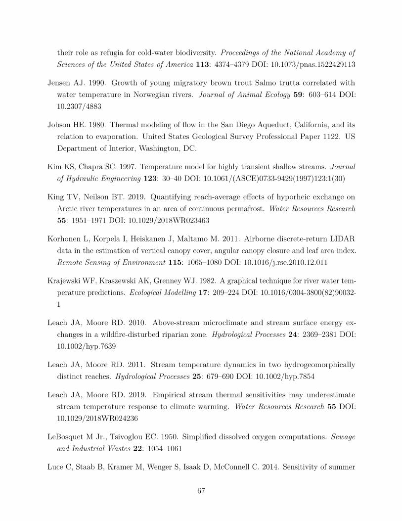
their role as refugia for cold-water biodiversity. Proceedings of the National Academy ofSciences of the United States of America 113: 4374–4379 DOI: 10.1073/pnas.1522429113

Jensen AJ. 1990. Growth of young migratory brown trout Salmo trutta correlated withwater temperature in Norwegian rivers. Journal of Animal Ecology 59: 603–614 DOI:10.2307/4883

Jobson HE. 1980. Thermal modeling of flow in the San Diego Aqueduct, California, and itsrelation to evaporation. United States Geological Survey Professional Paper 1122. USDepartment of Interior, Washington, DC.

Kim KS, Chapra SC. 1997. Temperature model for highly transient shallow streams. Journalof Hydraulic Engineering 123: 30–40 DOI: 10.1061/(ASCE)0733-9429(1997)123:1(30)

King TV, Neilson BT. 2019. Quantifying reach-average effects of hyporheic exchange onArctic river temperatures in an area of continuous permafrost. Water Resources Research55: 1951–1971 DOI: 10.1029/2018WR023463

Korhonen L, Korpela I, Heiskanen J, Maltamo M. 2011. Airborne discrete-return LIDARdata in the estimation of vertical canopy cover, angular canopy closure and leaf area index.Remote Sensing of Environment 115: 1065–1080 DOI: 10.1016/j.rse.2010.12.011

Krajewski WF, Kraszewski AK, Grenney WJ. 1982. A graphical technique for river water tem-perature predictions. Ecological Modelling 17: 209–224 DOI: 10.1016/0304-3800(82)90032-1

Leach JA, Moore RD. 2010. Above-stream microclimate and stream surface energy ex-changes in a wildfire-disturbed riparian zone. Hydrological Processes 24: 2369–2381 DOI:10.1002/hyp.7639

Leach JA, Moore RD. 2011. Stream temperature dynamics in two hydrogeomorphicallydistinct reaches. Hydrological Processes 25: 679–690 DOI: 10.1002/hyp.7854

Leach JA, Moore RD. 2019. Empirical stream thermal sensitivities may underestimatestream temperature response to climate warming. Water Resources Research 55 DOI:10.1029/2018WR024236

LeBosquet M Jr., Tsivoglou EC. 1950. Simplified dissolved oxygen computations. Sewageand Industrial Wastes 22: 1054–1061

Luce C, Staab B, Kramer M, Wenger S, Isaak D, McConnell C. 2014. Sensitivity of summer

67

stream temperatures to climate variability in the Pacific Northwest. Water ResourcesResearch 50: 3428–3443 DOI: 10.1002/2013WR014329

Magnusson J, Jonas T, Kirchner JW. 2012. Temperature dynamics of a proglacial stream:Identifying dominant energy balance components and inferring spatially integrated hy-draulic geometry. Water Resources Research 48 DOI: 10.1029/2011WR011378

Maheu A, Caissie D, St-Hilaire A, El-Jabi N. 2014. River evaporation and correspond-ing heat fluxes in forested catchments. Hydrological Processes 28: 5725–5738 DOI:10.1002/hyp.10071

Morin G, Nzakimuena T-J, Sochanski W. 1994. Prévision des températures de l’eau enrivières à l’aide d’un modèle conceptuel: Le cas de la rivière Moisie. Canadian Journal ofCivil Engineering 21: 63–75

Morse WL. 1972. Stream temperature prediction under reduced flow. Journal of theHydraulics Division 98: 1031–1047

Parkinson EA, Lea EV, Nelitz MA, Knudson JM, Moore RD. 2016. Identifying temperaturethresholds associated with fish community changes in British Columbia, Canada, tosupport identification of temperature sensitive streams. River Research and Applications32: 330–347 DOI: 10.1002/rra.2867

Ryan PJ, Harleman DRF. 1973. An analytical and experimental study of transient coolingpond behavior. Dept. of Civil Engineering, Massachusetts Institute of Technology.

Schneider CA, Rasband WS, Eliceiri KW. 2012. NIH Image to ImageJ: 25 years of imageanalysis. Nature Methods 9: 671–675 DOI: 10.1038/nmeth.2089

Sinokrot BA, Gulliver JS. 2000. In-stream flow impact on river water temperatures. Journalof Hydraulic Research 38: 339–349 DOI: 10.1080/00221680009498315

Sinokrot BA, Stefan HG. 1993. Stream temperature dynamics: Measurements and modeling.Water Resources Research 29: 2299–2312 DOI: 10.1029/93WR00540

Smith AMS, Falkowski MJ, Hudak AT, Evans JS, Robinson AP, Steele CM. 2009. A cross-comparison of field, spectral, and lidar estimates of forest canopy cover. Canadian Journalof Remote Sensing 35: 447–459 DOI: 10.5589/m09-038

Stelling E. 1882. Ueber die abhängigkeit der verdunstung des wassers von seiner temper-atur und von der feuchtigkeit und bewegung der luft. Österreichische Gesellschaft für

68

Meteorologie 17: 372–373

Sutton OG. 1953. Micrometeorology: A study of physical processes in the lowest layers of theearth’s atmosphere. McGraw-Hill, New York.

U.S. Standard Atmosphere, 1976. 1976. National Oceanic and Atmospheric Administra-tion; the National Aeronautics and Space Administration; the United States Air Force:Washington, D.C.

Vugts HF. 1974. Calculation of temperature variations of small mountain streams. Journalof Hydrology 23: 267–278 DOI: 10.1016/0022-1694(74)90007-9

Webb BW, Zhang Y. 1997. Spatial and seasonal variability in the components of theriver heat budget. Hydrological Processes 11: 79–101 DOI: 10.1002/(SICI)1099-1085(199701)11:1<79::AID-HYP404>3.0.CO;2-N

Webb BW, Zhang Y. 1999. Water temperatures and heat budgets in Dorset chalkwater courses. Hydrological Processes 13: 309–321 DOI: 10.1002/(SICI)1099-1085(19990228)13:3<309::AID-HYP740>3.0.CO;2-7

Webb BW, Hannah DM, Moore RD, Brown LE, Nobilis F. 2008. Recent advances in streamand river temperature research. Hydrological Processes 22: 902–918 DOI: 10.1002/hyp.6994

Wichert GA, Lin P. 1996. A species tolerance index for maximum water temperature. WaterQuality Research Journal 31: 875–893 DOI: 10.2166/wqrj.1996.048

Wu H, Kimball JS, Elsner MM, Mantua N, Adler RF, Stanford J. 2012. Projected climatechange impacts on the hydrology and temperature of Pacific Northwest rivers. WaterResources Research 48 DOI: 10.1029/2012WR012082

69

Appendix A

Anemometer Calibration

The calibration of the field-deployed anemometers revealed that the anemometers measuringwind speed at 1.5 m and at 0.5 m in the field had greater under-reporting of wind speedat low wind speeds compared to higher wind speeds; the mean percent differences rangedfrom -68 to -76 % for the 10th percentile of 1.5-m and 0.5-m anemometers’ measurementsrelative to the calibration anemometers, compared to the mean percent differences of -7 to -9% for the 90th percentile, respectively. The segmented linear regressions were successful incorrecting the field anemometer’s measurements to be in closer agreement with the calibrationanemometers’ measurements. The calibration reduced the mean percent differences in the 10th

and 90th percentiles to 12 to -16 % and -0.5 to -2.8 %, for the 1.5-m and 0.5-m anemometers,respectively (Table A.1). The regressions for the 1.5-m and 0.5-m anemometer calibrationshad root-mean-square errors of 0.07 and 0.12 m s−1 relative to mean wind speeds of 0.92 and0.90 m s−1, respectively.

Table A.1: The statistics of anemometer measurement difference prior to and post calibration.The differences were computed as Field Anemometer - Calibration Anemometer.

Pre-calibration Post-calibrationData Anemometer Mean Mean Mean MeanPercentile Difference Difference (%) Difference Difference (%)

(m s−1) (m s−1)

10 0.5 m -0.54 -76 -0.17 -161.5 m -0.31 -68 0.05 12

90 0.5 m -0.14 -9 -0.05 -2.81.5 m -0.11 -7 -0.01 -0.5

Both field-deployed anemometers are shown to under-report wind speed, but the 0.5-manemometer had consistently greater errors compared to the 1.5-m anemometer. This canlikely be attributed to a greater frictional resistance in the anemometer head rather than

70

0.5 m1.5 m

0.0 0.5 1.0 1.5

0.5

1.0

1.5

0.5

1.0

1.5

Field−deployed Anemometer Wind Speed (m s−1)

Cal

ibra

tion

Ane

mom

eter

Win

d S

peed

(m

s−1

)

Corrected

Uncorrected

Figure A.1: The uncorrected and corrected field-deployed anemometer wind speed measure-ments over the calibration period compared to the calibration anemometers. The black linesrepresent the 1:1 line.

occurring as a result of actual differences in wind blowing on the anemometers; as shown inFigure A.2, the calibration anemometers’ measurements during the calibration period arein agreement with each other, in contrast to the field anemometers, which show increasedscatter between their measurements despite being nearly adjacent during the calibration.This increased frictional resistance has the greatest influence at lower wind speeds, withincreased scatter visible below wind speeds of 0.7 m s−1. As a result, it is likely that thefield measurements of wind speed by the 0.5-m anemometer are under-reported even aftercorrection.

71

Calibration

Field

0.5 1.0 1.5

0.5

1.0

1.5

0.0

0.5

1.0

1.5

0.5−m Anemometer Wind Speed (m s−1)

1.5−

m A

nem

omet

er W

ind

Spe

ed (

m s

−1)

Figure A.2: Comparing the agreement in wind speed measurements between field anemometerand calibration anemometer pairs during the calibration period. The black lines are the 1:1lines.

72

Appendix B

Evaporation Pan Water Temperatureand Surface Area

The full time series of stream temperature and individual evaporation pan water temperaturesare presented in Figure B.1.

The evaporation pan mass and water surface area measurements, and the fit regression,are shown in Figure B.2. The coefficients for Equation 2.2, a1, a2, and a0, fit by the regressionwere −1.736× 10−4, 2.424× 10−1, and −4.736. The regression had a root-mean-square errorof 1.84× 10−4 m2, with an adjusted R2 of 0.88. When applied to the field data, the regressionprovides 95 % prediction intervals that correspond approximately ± 2 % of the estimatedsurface area. It is worth noting that there were four measurements of pan mass that werebeyond the range of the calibration data, so their extrapolated surface area measurements aresubject to increased uncertainty. The maximum and minimum estimated pan water surfaceareas are 0.0398 and 0.0382 m2, which correspond to -3.9 and -7.2 % differences from thesurface area obtained using the evaporation pan dimensions (0.0412 m2).

73

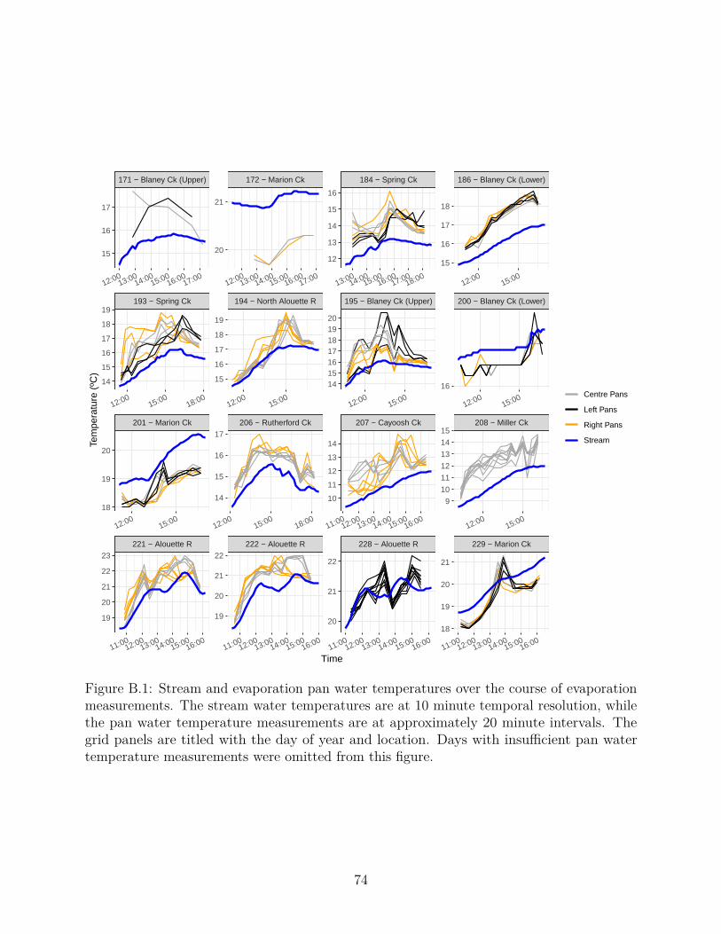
221 − Alouette R 222 − Alouette R 228 − Alouette R 229 − Marion Ck

201 − Marion Ck 206 − Rutherford Ck 207 − Cayoosh Ck 208 − Miller Ck

193 − Spring Ck 194 − North Alouette R 195 − Blaney Ck (Upper) 200 − Blaney Ck (Lower)

171 − Blaney Ck (Upper) 172 − Marion Ck 184 − Spring Ck 186 − Blaney Ck (Lower)

11:0012:00

13:0014:00

15:0016:00

11:0012:00

13:0014:00

15:0016:00

11:0012:00

13:0014:00

15:0016:00

11:0012:00

13:0014:00

15:0016:00

12:0015:00

12:0015:00

18:0011:00

12:0013:00

14:0015:00

16:0012:00

15:00

12:0015:00

18:0012:00

15:0012:00

15:0012:00

15:00

12:0013:00

14:0015:00

16:0017:00

12:0013:00

14:0015:00

16:0017:00

13:0014:00

15:0016:00

17:0018:00

12:0015:00

15

16

17

18

16

9

10

11

12

13

14

15

18

19

20

21

12

13

14

15

16

14151617181920

10

11

12

13

14

20

21

22

20

21

15

16

17

18

19

14

15

16

17

19

20

21

22

15

16

17

14

15

16

17

18

19

18

19

20

19

20

21

22

23

Time

Tem

pera

ture

(ºC

)

Centre Pans

Left Pans

Right Pans

Stream

Figure B.1: Stream and evaporation pan water temperatures over the course of evaporationmeasurements. The stream water temperatures are at 10 minute temporal resolution, whilethe pan water temperature measurements are at approximately 20 minute intervals. Thegrid panels are titled with the day of year and location. Days with insufficient pan watertemperature measurements were omitted from this figure.

74

0.0380

0.0385

0.0390

0.0395

0.0400

700 800 900 1000 1100 1200 1300

Mass of Water (g)

Sur

face

Are

a (m

2 )

Figure B.2: The calibration of evaporation pan water surface area. The line is the fitregression.

75

Appendix C

Meteorological Conditions andEvaporation Rates

The meteorological and stream temperature data in Figures C.1a to C.1t are at 10 minuteintervals, and the evaporation rate measurements are at approximately 1 to 1.5 hour intervals.The lack of wind on June 7th and July 19th at Spring Creek and Blaney Creek (Lower) wasnoted during field work, so the data are believed to be accurate (Figures C.1b and C.1l).

76

15

16

17

18

T (

ºC)

06 June 2018 − Marion Ck

0.0

0.2

0.4

0.6

u (m

s−1

)

50

60

70

RH

(%

)

1.00

1.25

1.50

1.75

2.00

e (k

Pa)

−2

−1

0

∆θ (

ºC)

−0.025

0.000

0.025

0.050

F (

m s

−2)

0.00

0.05

0.10

0.15

0.20

12:00 13:00 14:00 15:00 16:00 17:00Time

E (

mm

h−1

)

1.5 m 0.5 m Stream

(a)

11

12

13

14

T (ºC

)

07 June 2018 − Spring Ck

0.00

0.01

0.02

0.03

0.04

u (m s

−1)

70

75

80

85

90

RH

(%)

1.10

1.15

1.20

1.25

1.30

e (kPa)

−3.5

−3.0

−2.5

−2.0

−1.5

−1.0

∆θ (ºC)

−0.100

−0.075

−0.050 F (m

s−2)

0.00

0.05

0.10

0.15

0.20

11:00 12:00 13:00 14:00 15:00 16:00Time

E (m

m h

−1)

1.5 m 0.5 m Stream

(b)

Figure C.1: Meteorological and stream conditions, and measured evaporation rates for eachday of data collection.

77

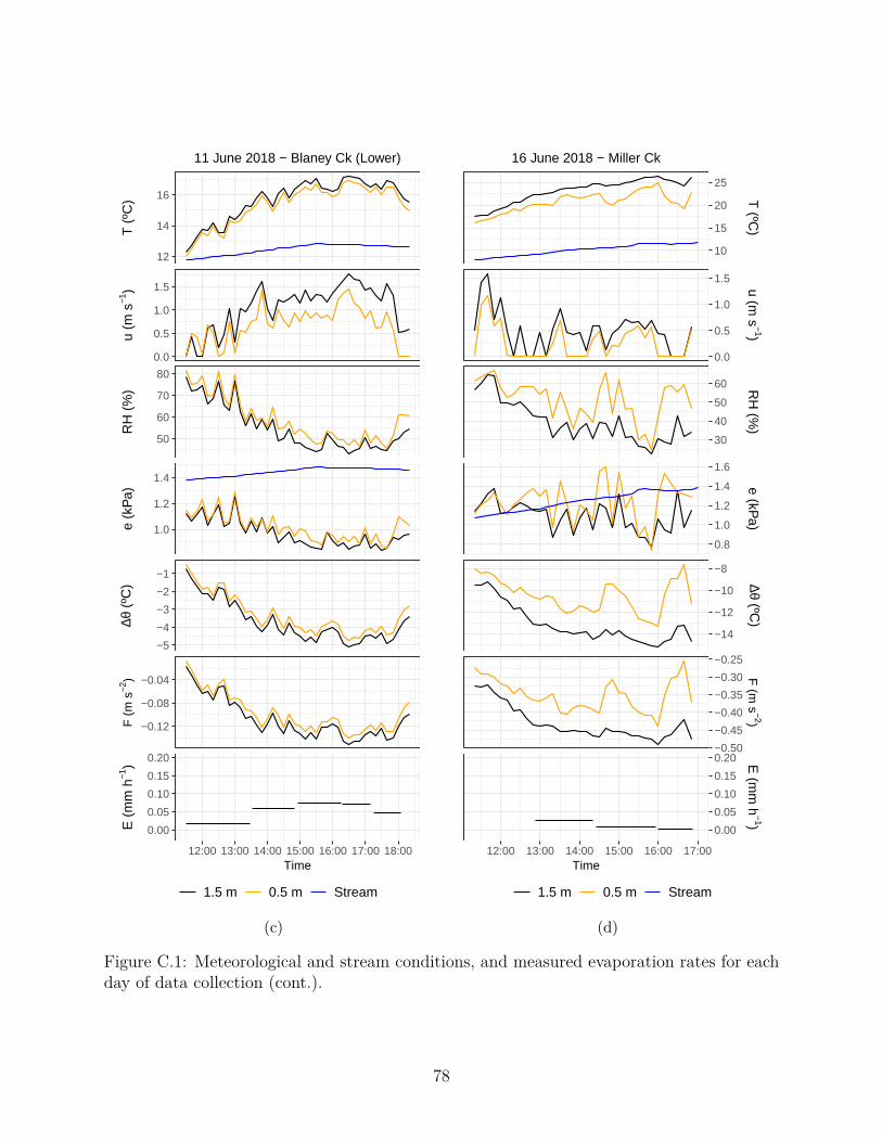
12

14

16

T (

ºC)

11 June 2018 − Blaney Ck (Lower)

0.0

0.5

1.0

1.5

u (m

s−1

)

50

60

70

80

RH

(%

)

1.0

1.2

1.4

e (k

Pa)

−5

−4

−3

−2

−1

∆θ (

ºC)

−0.12

−0.08

−0.04

F (

m s

−2)

0.00

0.05

0.10

0.15

0.20

12:00 13:00 14:00 15:00 16:00 17:00 18:00Time

E (

mm

h−1

)

1.5 m 0.5 m Stream

(c)

10

15

20

25

T (ºC

)

16 June 2018 − Miller Ck

0.0

0.5

1.0

1.5 u (m s

−1)

30

40

50

60 RH

(%)

0.8

1.0

1.2

1.4

1.6

e (kPa)

−14

−12

−10

−8

∆θ (ºC)

−0.50

−0.45

−0.40

−0.35

−0.30

−0.25

F (m

s−2)

0.00

0.05

0.10

0.15

0.20

12:00 13:00 14:00 15:00 16:00 17:00Time

E (m

m h

−1)

1.5 m 0.5 m Stream

(d)

Figure C.1: Meteorological and stream conditions, and measured evaporation rates for eachday of data collection (cont.).

78

15

18

21

24

T (

ºC)

20 June 2018 − Blaney Ck (Upper)

0.0

0.2

0.4

0.6

u (m

s−1

)

40

50

60

70

80

RH

(%

)

1.2

1.4

1.6

1.8

e (k

Pa)

−11

−9

−7

−5

∆θ (

ºC)

−0.35

−0.30

−0.25

−0.20

−0.15

F (

m s

−2)

0.00

0.05

0.10

0.15

0.20

12:00 13:00 14:00 15:00 16:00 17:00Time

E (

mm

h−1

)

1.5 m 0.5 m Stream

(e)

16

18

20 T (ºC

)

21 June 2018 − Marion Ck

0.0

0.2

0.4

0.6 u (m s

−1)

70

75

80 RH

(%)

1.25

1.50

1.75

2.00

2.25

2.50

e (kPa)

3.0

3.5

4.0

4.5

∆θ (ºC)

0.14

0.16

0.18

F (m

s−2)

0.00

0.05

0.10

0.15

0.20

12:00 13:00 14:00 15:00 16:00 17:00Time

E (m

m h

−1)

1.5 m 0.5 m Stream

(f)

Figure C.1: Meteorological and stream conditions, and measured evaporation rates for eachday of data collection (cont.).

79

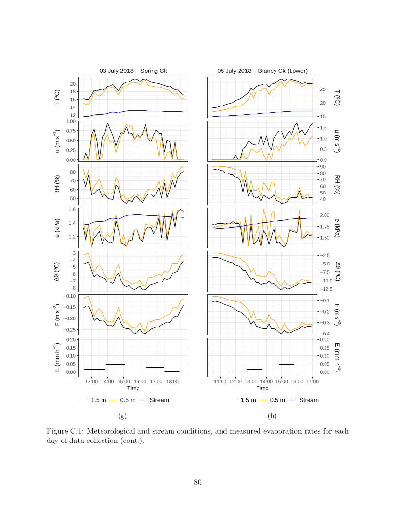
12

14

16

18

20

T (

ºC)

03 July 2018 − Spring Ck

0.00

0.25

0.50

0.75

1.00

u (m

s−1

)

50

60

70

80

RH

(%

)

1.2

1.4

1.6

e (k

Pa)

−8−7−6−5−4−3

∆θ (

ºC)

−0.25

−0.20

−0.15

−0.10

F (

m s

−2)

0.00

0.05

0.10

0.15

0.20

13:00 14:00 15:00 16:00 17:00 18:00Time

E (

mm

h−1

)

1.5 m 0.5 m Stream

(g)

15

20

25 T (ºC

)

05 July 2018 − Blaney Ck (Lower)

0.0

0.5

1.0

1.5 u (m s

−1)

405060708090

RH

(%)

1.50

1.75

2.00 e (kPa)

−12.5

−10.0

−7.5

−5.0

−2.5

∆θ (ºC)

−0.4

−0.3

−0.2

−0.1 F (m

s−2)

0.00

0.05

0.10

0.15

0.20

11:00 12:00 13:00 14:00 15:00 16:00 17:00Time

E (m

m h

−1)

1.5 m 0.5 m Stream

(h)

Figure C.1: Meteorological and stream conditions, and measured evaporation rates for eachday of data collection (cont.).

80

16

20

24

T (

ºC)

12 July 2018 − Spring Ck

0.00

0.25

0.50

0.75

u (m

s−1

)

40

50

60

70

80

RH

(%

)

1.4

1.6

1.8

2.0

e (k

Pa)

−10

−8

−6

∆θ (

ºC)

−0.30

−0.25

−0.20

−0.15

F (

m s

−2)

0.00

0.05

0.10

0.15

0.20

11:00 12:00 13:00 14:00 15:00 16:00 17:00 18:00Time

E (

mm

h−1

)

1.5 m 0.5 m Stream

(i)

15.0

17.5

20.0

22.5

25.0

T (ºC

)

13 July 2018 − North Alouette R

0.0

0.2

0.4

0.6

u (m s

−1)

40

50

60

70

80 RH

(%)

1.00

1.25

1.50

1.75

2.00

e (kPa)

−8−7−6−5−4−3

∆θ (ºC)

−0.25

−0.20

−0.15

−0.10

F (m

s−2)

0.00

0.05

0.10

0.15

0.20

11:00 12:00 13:00 14:00 15:00 16:00 17:00Time

E (m

m h

−1)

1.5 m 0.5 m Stream

(j)

Figure C.1: Meteorological and stream conditions, and measured evaporation rates for eachday of data collection (cont.).

81

16

20

24

T (

ºC)

14 July 2018 − Blaney Ck (Upper)

0.0

0.2

0.4

0.6

u (m

s−1

)

30

40

50

60

70

RH

(%

)

1.0

1.2

1.4

1.6

1.8

e (k

Pa)

−11−10

−9−8−7−6

∆θ (

ºC)

−0.35

−0.30

−0.25

−0.20

F (

m s

−2)

0.00

0.05

0.10

0.15

0.20

11:00 12:00 13:00 14:00 15:00 16:00 17:00Time

E (

mm

h−1

)

1.5 m 0.5 m Stream

(k)

16.5

17.0

17.5

18.0

18.5

T (ºC

)

19 July 2018 − Blaney Ck (Lower)

0.00.10.20.30.40.5

u (m s

−1)

70

80 RH

(%)

1.4

1.6

1.8 e (kPa)

−2.5

−2.0

−1.5

−1.0

−0.5 ∆θ (ºC)

−0.050

−0.025

0.000 F (m

s−2)

0.00

0.05

0.10

0.15

0.20

10:00 11:00 12:00 13:00 14:00 15:00 16:00 17:00Time

E (m

m h

−1)

1.5 m 0.5 m Stream

(l)

Figure C.1: Meteorological and stream conditions, and measured evaporation rates for eachday of data collection (cont.).

82

16

18

20

T (

ºC)

20 July 2018 − Marion Ck

0.0

0.2

0.4

0.6

0.8

u (m

s−1

)

50

60

70

RH

(%

)

1.0

1.5

2.0

e (k

Pa)

0

1

2

3

∆θ (

ºC)

0.050

0.075

0.100

0.125

F (

m s

−2)

0.00

0.05

0.10

0.15

0.20

11:00 12:00 13:00 14:00 15:00 16:00 17:00Time

E (

mm

h−1

)

1.5 m 0.5 m Stream

(m)

15

20

25

30

T (ºC

)

25 July 2018 − Rutherford Ck

1.0

1.5

2.0

2.5

u (m s

−1)

20

30

40 RH

(%)

0.9

1.2

1.5

1.8

e (kPa)

−17.5

−15.0

−12.5 ∆θ (ºC)

−0.60

−0.55

−0.50

−0.45

−0.40

−0.35

F (m

s−2)

0.00

0.05

0.10

0.15

0.20

12:00 13:00 14:00 15:00 16:00 17:00 18:00Time

E (m

m h

−1)

1.5 m 0.5 m Stream

(n)

Figure C.1: Meteorological and stream conditions, and measured evaporation rates for eachday of data collection (cont.).

83

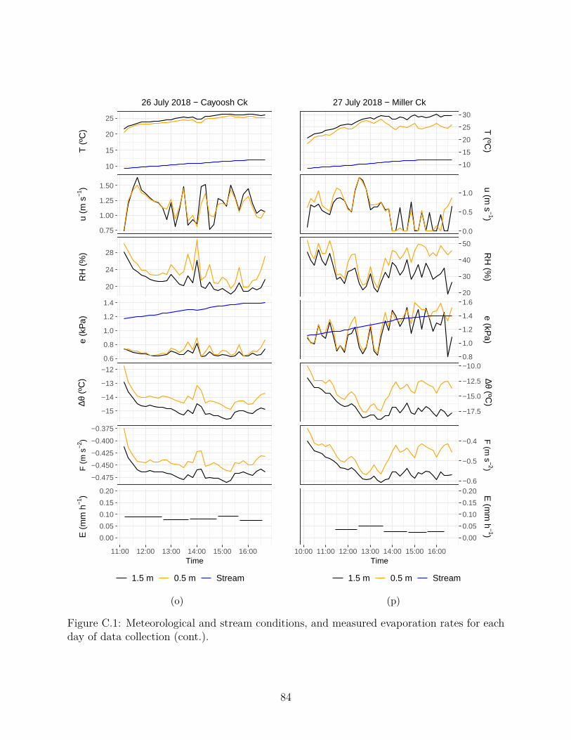
10

15

20

25

T (

ºC)

26 July 2018 − Cayoosh Ck

0.75

1.00

1.25

1.50

u (m

s−1

)

20

24

28

RH

(%

)

0.6

0.8

1.0

1.2

1.4

e (k

Pa)

−15

−14

−13

−12

∆θ (

ºC)

−0.475

−0.450

−0.425

−0.400

−0.375

F (

m s

−2)

0.00

0.05

0.10

0.15

0.20

11:00 12:00 13:00 14:00 15:00 16:00Time

E (

mm

h−1

)

1.5 m 0.5 m Stream

(o)

10

15

20

25

30

T (ºC

)

27 July 2018 − Miller Ck

0.0

0.5

1.0

u (m s

−1)

20

30

40

50

RH

(%)

0.8

1.0

1.2

1.4

1.6

e (kPa)

−17.5

−15.0

−12.5

−10.0

∆θ (ºC)

−0.6

−0.5

−0.4

F (m

s−2)

0.00

0.05

0.10

0.15

0.20

10:00 11:00 12:00 13:00 14:00 15:00 16:00Time

E (m

m h

−1)

1.5 m 0.5 m Stream

(p)

Figure C.1: Meteorological and stream conditions, and measured evaporation rates for eachday of data collection (cont.).

84

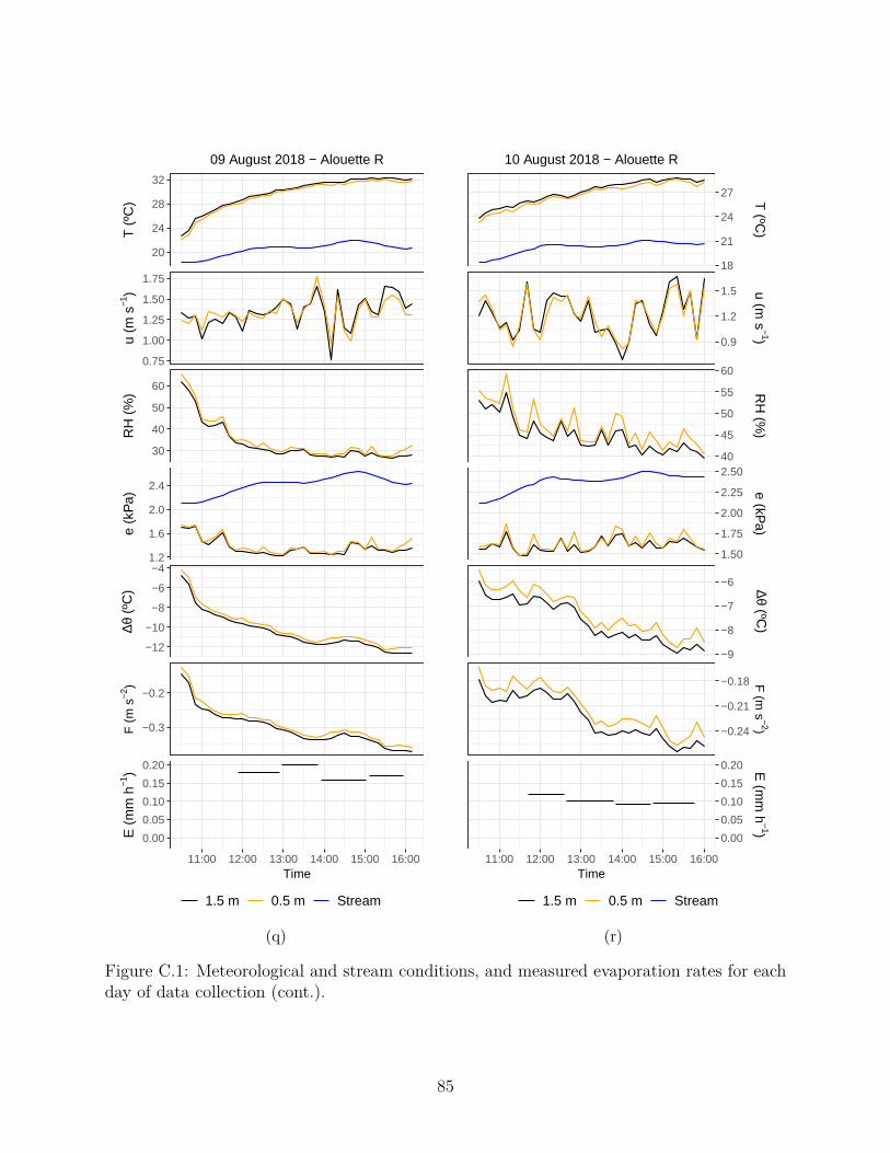
20

24

28

32

T (

ºC)

09 August 2018 − Alouette R

0.75

1.00

1.25

1.50

1.75

u (m

s−1

)

30

40

50

60

RH

(%

)

1.2

1.6

2.0

2.4

e (k

Pa)

−12

−10

−8

−6

−4

∆θ (

ºC)

−0.3

−0.2

F (

m s

−2)

0.00

0.05

0.10

0.15

0.20

11:00 12:00 13:00 14:00 15:00 16:00Time

E (

mm

h−1

)

1.5 m 0.5 m Stream

(q)

18

21

24

27 T (ºC

)

10 August 2018 − Alouette R

0.9

1.2

1.5 u (m s

−1)

40

45

50

55

60

RH

(%)

1.50

1.75

2.00

2.25

2.50

e (kPa)

−9

−8

−7

−6 ∆θ (ºC)

−0.24

−0.21

−0.18 F (m

s−2)

0.00

0.05

0.10

0.15

0.20

11:00 12:00 13:00 14:00 15:00 16:00Time

E (m

m h

−1)

1.5 m 0.5 m Stream

(r)

Figure C.1: Meteorological and stream conditions, and measured evaporation rates for eachday of data collection (cont.).

85

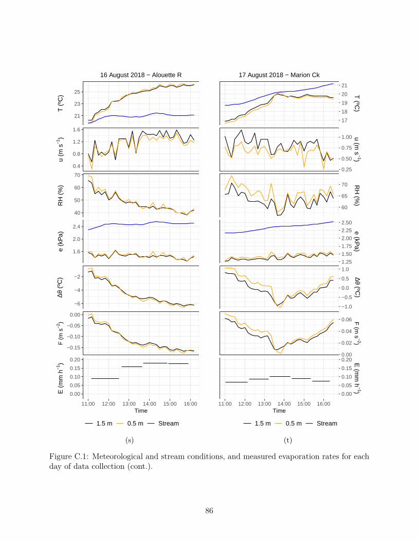
21

23

25

T (

ºC)

16 August 2018 − Alouette R

0.4

0.8

1.2

1.6

u (m

s−1

)

40

50

60

70

RH

(%

)

1.6

2.0

2.4

e (k

Pa)

−6

−4

−2

∆θ (

ºC)

−0.15

−0.10

−0.05

0.00

F (

m s

−2)

0.00

0.05

0.10

0.15

0.20

11:00 12:00 13:00 14:00 15:00 16:00Time

E (

mm

h−1

)

1.5 m 0.5 m Stream

(s)

17

18

19

20

21

T (ºC

)

17 August 2018 − Marion Ck

0.25

0.50

0.75

1.00 u (m s

−1)

60

65

70 RH

(%)

1.25

1.50

1.75

2.00

2.25

2.50

e (kPa)

−1.0

−0.5

0.0

0.5

1.0

∆θ (ºC)

0.00

0.02

0.04

0.06 F (m

s−2)

0.00

0.05

0.10

0.15

0.20

11:00 12:00 13:00 14:00 15:00 16:00Time

E (m

m h

−1)

1.5 m 0.5 m Stream

(t)

Figure C.1: Meteorological and stream conditions, and measured evaporation rates for eachday of data collection (cont.).

86

Appendix D

Evaporation Rate Error Analysis

Two measurements and one regression estimate was used to calculate each evaporation rate:the mass of the evaporation pan when it was placed into and removed from the stream;the time when the evaporation pan was placed into and removed from the stream; and theregression prediction of the evaporation pan’s average water surface area. The measurementuncertainties were calculated as follows:

δmw =√δm2

w,in + δm2w,out (D.1)

δt =√δt2in + δt2out (D.2)

δE = E ·

√√√√( δmw

∆mw

)2

+(δt

∆t

)2

+(δApAp

)2

× ce (D.3)

where δmw,i is the portable balance’s accuracy of ± 0.1 g, δti is the error in time observationof ± 60 s, δmw and δt are the combined measurement uncertainties of computing the changein evaporation pan mass (∆mw, g) and the elapsed time between mass measurements (∆t, s),δAp is the standard error of each pan water surface area prediction (δAp ≈ 1× 10−4 m2), Apis the predicted pan water surface area in m2, E is the computed evaporation rate in m s−1,δE is the evaporation rate uncertainty in mm h−1, and ce is a conversion factor equal to 3.6to convert units from m s−1 to mm h−1.

87

Appendix E

Relation Between Solution Molarityand Electrical Conductivity

The data used to fit the electrical conductivity calibration regression are presented inFigure E.1.

0.16

0.17

0.18

0.19

16 17 18 19

Electrical Conductivity (mS cm−1)

Mol

arity

(m

ol L

−1)

Figure E.1: The calibration results relating electrical conductivity to a salt solution molarity.The line is the fit regression.

88