Max-Planck-Institut für demografische ForschungMax Planck Institute for Demographic ResearchKonrad-Zuse-Strasse 1 · D-18057 Rostock · GERMANYTel +49 (0) 3 81 20 81 - 0; Fax +49 (0) 3 81 20 81 - 202; http://www.demogr.mpg.de

This working paper has been approved for release by: Gerda Ruth Neyer (neyer@demogr.mpg.de)Deputy Head of the Laboratory of Contemporary European Fertility and Family Dynamics.

© Copyright is held by the authors.

Working papers of the Max Planck Institute for Demographic Research receive only limited review.Views or opinions expressed in working papers are attributable to the authors and do not necessarilyreflect those of the Institute.

Population constraints on pooled surveys in demographic hazard modeling

MPIDR WORKING PAPER WP 2006-039NOVEMBER 2006

Michael S. Rendall (mrendall@rand.org)Ryan AdmiraalAlessandra DeRosePaola DiGiulio (digiulio@demogr.mpg.de)Mark S. HandcockFilomena Racioppi

This paper has also been published as Working Paper in the University of Washington, Seattle,Center for Statistics and the Social Sciences, Working Paper Serieshttp://www.csss.washington.edu/Papers/

Population constraints on pooled surveys in demographic hazard modeling

Michael S. Rendall*, Ryan Admiraal**, Alessandra DeRose***, Paola DiGiulio****,

Mark S. Handcock**, and Filomena Racioppi*****

Abstract

In non-experimental research, data on the same population process may be collected

simultaneously by more than one instrument. For example, in the present application, two

sample surveys and a population birth registration system all collect observations on first

births by age and year, while the two surveys additionally collect information on

women’s education. To make maximum use of the three data sources, the survey data are

pooled and the population data introduced as constraints in a logistic regression equation.

Reductions in standard errors about the age and birth-cohort parameters of the regression

equation in the order of three-quarters are obtained by introducing the population data as

constraints. A halving of the standard errors about the education parameters is achieved

by pooling observations from the larger survey dataset with those from the smaller

survey. The percentage reduction in the standard errors through imposing population

constraints is independent of the total survey sample size.

* RAND Labor and Population Program, 1776 Main Street, Santa Monica, CA 90407-2138, USA, and Pennsylvania State University, Population Research Institute, email: mrendall@rand.org, ** Center for Statistics in the Social Sciences, Padelford Hall, University of Washington, Seattle, WA 98195-4320, USA, *** University of Rome, ‘La Sapienza’, Dipartimento di studi geoeconomici, linguistici, statistici e storici per l’analisi regionale, via del Castro Laurenziano, 9, I-00161, Rome, Italy, **** Max Planck Institute for Demographic Research, Konrad-Zuse-Straße 1, 18057 Rostock, Germany, ***** University of Rome, ‘La Sapienza’, Dipartimento di Scienze Demografiche, Via Nomentana 41, I-00161, Rome, Italy. Acknowledgements: We are very grateful to Piero Giorgi for providing us with first-birth probabilities by age and cohort calculated from Italian birth-registration data, and for comments received at presentations of earlier versions at the August 2004 Meeting of the Logic and Methodology section of the International Sociological Association, and at the June 2006 Meeting of the Italian Statistical Society. This work was funded by the National Institute of Child Health and Human Development under investigator grant R01-HD043472-01, and under center grants to the RAND Labor and Population program (R24-HD050906), the Penn State University Population Research Institute (R24-HD41025), and to the University of Washington Center for Studies in Demography and Ecology (R24-HD41025); and by a grant to Alessandra DeRose from the University of Rome (Inter-faculties Research on “Integrating current data and survey samples for the analysis of family behaviors” 2000/02). Address correspondence to the first author at mrendall@rand.org. RUNNING TITLE: Population constraints on pooled surveys KEYWORDS: combining data; constrained estimation; fertility.

INTRODUCTION

Statistical methods for using population information to increase the efficiency of sample-

survey-based estimates have a long history of development in statistics (Deming and

Stephan 1942, Ireland and Kullback 1968). More recently, they have been applied to

economic and demographic data (Imbens and Lancaster 1994; Handcock, Huovilainen,

and Rendall 2000). In demographic applications, the availability of population counts of

both vital events (in registration-system data) and of population characteristics (in

population censuses and inter-censal estimates) increases the scope for realizing

efficiency gains. Moreover, because prediction is frequently a goal in demography,

efficiency gains may be especially beneficial.

The alternatives of using either population or survey data alone each have their

disadvantages. Use of population data alone limits the amount of socio-economic

information that can be incorporated into the analysis. Data from large-scale, general

purpose surveys are also increasingly considered undesirable, either for their lack of a

longitudinal dimension or for their lack of certain variables needed for specific

applications. As a result, an increasing reliance on data from small, specialist surveys has

been seen in demography. Small survey data, however, have major disadvantages with

respect to statistical efficiency. They may also be subject to bias due to attrition and other

forms of non-response. These are the concerns that have led to the development of

methods for combining population or large-scale data with small-sample survey data in

economics (Hellerstein and Imbens 1999; Ridder and Moffitt, forthcoming).

1

In previous applications to fertility estimation, Handcock and colleagues (Handcock et al

2000; Handcock, Rendall, and Cheadle 2005) introduced and implemented a constrained

maximum likelihood estimator (MLE) in a logistic regression model. They demonstrated

large efficiency gains first in estimating the intercept parameter by constraining survey

estimates to an overall fertility rate (Handcock et al 2000), and second in estimating

coefficient parameters by constraining to the fertility rates of population subgroups

(Handcock et al 2005). In the first case, the reduction in the variance about the intercept

parameter resulted in a 50% reduction in the variance about the predicted birth

probabilities. In the second case, even larger reductions in standard errors about the

parameter estimates for population subgroup coefficients were achieved. They referred to

these coefficients as being “directly constrained” by the population data. Consistent with

Imbens and Lancaster’s (1994) simulation results, however, Handcock et al (2005) found

that no more than trivial gains in efficiency may by expected for regression parameters

that are not directly constrained by population data.

The present study builds on those earlier studies by addressing the problem of how to

improve efficiency of estimation of regression parameters that are not directly

constrained by population data. It does so by pooling data across surveys while still

constraining to population data. In an application to first births by education in Italy,

observations from a larger, general-purpose survey dataset (the 1998 Multiscopo survey)

are pooled with observations from a smaller, specialist dataset (the 1995/96 Fertility and

Family Survey, or FFS). We consider only first childbearing after age 25 to focus the

analysis on the process of entry to motherhood after completion of studies, and to

2

illustrate the utility of population constraints for ages at which survey observations of

women who have not yet given birth are relatively few. Women born in the early 1950s

are compared to women born ten years later in the early 1960s, thus providing examples

of estimation respectively for complete and censored hazards.

Even though the two surveys are conducted three years apart, their retrospective fertility

histories overlap for all years up to the survey year of the FFS. This allows for the

potential to realize gains in statistical efficiency by simply pooling sample observations

across the two surveys. We first derive a basic theoretical result on the relationship

between survey sample sizes and the variance-reducing effect of inclusion of population

constraints: that the proportionate reduction in variance from the inclusion of population

constraints is independent of the size of the survey sample. This implies that pooling

observations across sample surveys will not alter the relative efficiency gains achieved

through applying population constraints. This result is confirmed empirically by

comparing the gains between unconstrained and constrained estimation when using the

smaller survey dataset only with the gains when pooling the larger survey observations

with those of the smaller survey.

The population data, however, directly constrain survey estimation only of the

relationship of age and cohort to first birth. The relationship of education to first births is

not directly constrained, and so no significant improvements in its estimation are

achieved by adding population constraints. The pooling of surveys in a constrained MLE,

3

however, achieves substantial increases in the efficiency of the estimates of the

relationship of education to first births.

The remainder of the article is organized as follows. In the Data and Method section, we

first describe the sample survey data and evaluate the comparability of the two survey

datasets against population data. We then describe the method of constrained MLE as

applied to the problem of estimating first birth probabilities using these survey and

population data sources. We also derive the main analytical result relevant to pooling the

survey datasets with constrained estimation: that the proportionate reduction in variance

of the regression parameter estimates is independent of the total sample size. In the

Results section, we compare the results obtained under constrained MLE on the pooled

survey datasets with results from estimators that either ignore the population data or that

forego the opportunity to pool the survey data. Both non-parametric and parametric

specifications of the relationship of first births to age are used in the alternatives that

ignore the population data. The Summary and Conclusions section follows.

DATA AND METHOD

Sample and Population Data

Italy has two survey datasets that collected women’s fertility histories in the 1990s: the

smaller, 1995/96 Italian Fertility and Family Survey (“FFS”, De Sandre et al 2000); and

the larger, 1998 Italian Multipurpose Survey (“Multiscopo”, ISTAT 2000). As its name

implies, the FFS was designed explicitly for fertility analysis and for other subjects

related to family formation and change. The FFS included approximately 4,800 female

4

sample members aged 20 to 49 at survey date. From the fertility history asked of all

sample members, we use here only the year of birth of a woman’s first live-born child, if

any, born up to the end of the year (1994) before the survey year. The FFS also recorded

highest educational qualification obtained, coded to ISCED (International Standard

Classification of Education, OECD 2003) categories. We coded “high education” for

women with any tertiary education qualification (ISCED codes 5 and above).

The 1998 Multiscopo is a large, general purpose survey. Its sample included more than

20,000 households with approximately 54,000 individuals. A fertility history was

collected for all female sample members aged 15 and over. We use here only the year of

birth of a woman’s first live-born child, if any, born up to the end of the year before the

survey year (1997). The Multiscopo also included a question on highest educational

qualification obtained, from which we were able to code “high education” in the same

way as for the FFS.

From both the FFS and Multiscopo, we use data from female respondents born in the

years 1951-55 and 1961-65, with the variable “year of first birth” used to assemble the

data into person-years of exposure to first birth from age 25 and above. We define age

throughout the analysis using the “generation” definition of number of years attained this

calendar year. On average this is half a year younger than the “age at last birthday”

definition. The women born in the 1950s have only just completed their childbearing

years by survey date, assuming age 44 to be the oldest age of childbearing. The FFS data,

collected in 1995/96, allow for exposure to childbearing only to age 42. The Multiscopo

5

data, collected in 1998, allow for exposure up to age 44. For the 1960s cohort, the FFS

data allow for exposure to childbearing to age 32. We use the Multiscopo data for

exposure to childbearing up to age 34.

For the entire period of our analyses, the Italian birth registration system collected details

including age of mother and how many children the mother has previously given birth to.

Using these data, Giorgi (1993) calculated first birth probabilities by single-year cohort.

We use these probabilities, subsequently updated by Giorgi to 1997, as our population-

level estimates of first-birth probabilities by single-year age. We calculated the geometric

mean of individual birth-year specific probabilities to convert them into five-year birth-

cohort averages.

Population representativeness of the two survey datasets

Handcock et al (2005) showed that even when the sample survey data deviate from being

exactly representative of the population for which the constraint data are obtained, the

constrained MLE will improve estimation compared to using an unconstrained alternative

estimator. Bias in the survey data in this case will also be reduced by incorporating the

exact population constraints, but will not be eliminated (see also Hellerstein and Imbens,

1999). We now show that in the present application, the two survey datasets sample in an

approximately unbiased way from the same population, and therefore that the issue of

estimation from non-representative survey data will not play a major role in the analysis.

6

Sample sizes and comparisons of the variables of interest between the sample and birth-

registration data, and between sample and Labour Force Survey (LFS) estimates, are

presented in Table 1. FFS and Multiscopo sample sizes are of female respondents born in

the years 1951-55 and 1961-65 respectively. There are approximately three times as

many women from both cohorts in the Multiscopo (2,100 and 2,690 respectively) as in

the FFS (760 and 840 respectively). The three extra years of observation per woman in

the Multiscopo as compared to the FFS raise the ratio to approximately four times as

many person-years of observation in the Multiscopo (see below). For the LFS, we use

published reports and special tabulations that are not accompanied by confidence

intervals or sample sizes (ISTAT 1996, 2005), and therefore treat them as if they are from

population data. The effect is to make it more likely to reject the null hypothesis of no

difference between the FFS and Multiscopo estimates and those of the LFS. Given the

very large overall sample size of the LFS (320,000 individuals each trimester in 1985 and

200,000 in 1995, ISTAT 1996), this bias is likely to be small.

[TABLE 1 ABOUT HERE]

Comparisons of education at survey date indicate small deviations only of the survey

estimates from population data, and between the surveys. Compared to the LFS of 1995,

both the FFS and Multiscopo have significantly higher proportions of women with

higher-education qualifications, at around 11 percent, but differences between the FFS

and Multiscopo are small and not significant. Surprisingly, given international trends

towards increased female participation in higher education, no statistically significant

7

change is seen across the two Italian cohorts born ten years apart in either the FFS or

Multiscopo surveys (statistical test results not shown). To check whether this lack of

observed change is due to the different ages of the women from the two cohorts at survey

date (early-to-mid 30s for the 1961-65 cohort versus early-to-mid 40s for the 1951-55

cohort), we compared also the 1951-55 cohort’s proportion with higher qualifications ten

years before, in the 1985 LFS. While the 1995 LFS recorded almost identical percentages

of women with a higher education between the 1951-55 cohort (9.4%) and the 1961-65

cohort (9.3%), only 8.0% of women from the 1951-55 cohort had a higher qualification

in 1985. The real growth in higher education across cohorts implied by the LFS,

however, is still small: from 8.0% of the 1951-55 cohort to 9.3% of the 1961-65 cohort.

The survey data on births are also similar to estimates from population data, and the FFS

and Multiscopo data are similar to each other. Compared to the birth-registration data,

both the FFS and Multiscopo have similar proportions still childless at age 24 (the

beginning of the year the woman attained age 25). The FFS proportions appear slightly

lower, than either the Multiscopo and birth registration data, and the deficit is statistically

significant compared to both the Multiscopo and birth registration estimates for the 1961-

65 cohort. The FFS and Multiscopo exhibit similar differentials by education in

proportions childlessness at age 24 (much higher among “high education” women) and

by cohort (substantially higher for the 1960s cohort than for the 1950s cohort). The lower

overall childlessness in the FFS’ 1961-65 cohort is seen to be due to the “no high

education” group.

8

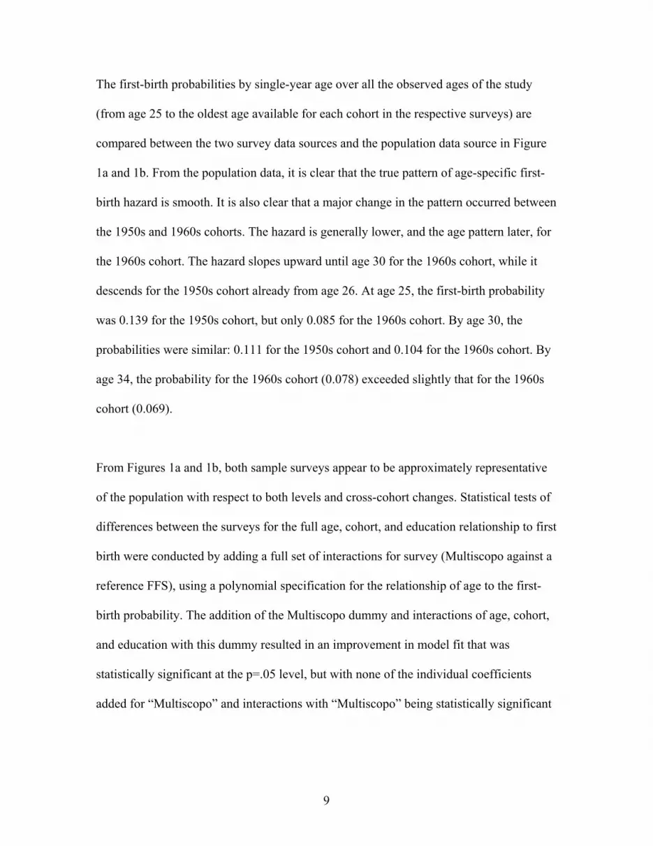
The first-birth probabilities by single-year age over all the observed ages of the study

(from age 25 to the oldest age available for each cohort in the respective surveys) are

compared between the two survey data sources and the population data source in Figure

1a and 1b. From the population data, it is clear that the true pattern of age-specific first-

birth hazard is smooth. It is also clear that a major change in the pattern occurred between

the 1950s and 1960s cohorts. The hazard is generally lower, and the age pattern later, for

the 1960s cohort. The hazard slopes upward until age 30 for the 1960s cohort, while it

descends for the 1950s cohort already from age 26. At age 25, the first-birth probability

was 0.139 for the 1950s cohort, but only 0.085 for the 1960s cohort. By age 30, the

probabilities were similar: 0.111 for the 1950s cohort and 0.104 for the 1960s cohort. By

age 34, the probability for the 1960s cohort (0.078) exceeded slightly that for the 1960s

cohort (0.069).

From Figures 1a and 1b, both sample surveys appear to be approximately representative

of the population with respect to both levels and cross-cohort changes. Statistical tests of

differences between the surveys for the full age, cohort, and education relationship to first

birth were conducted by adding a full set of interactions for survey (Multiscopo against a

reference FFS), using a polynomial specification for the relationship of age to the first-

birth probability. The addition of the Multiscopo dummy and interactions of age, cohort,

and education with this dummy resulted in an improvement in model fit that was

statistically significant at the p=.05 level, but with none of the individual coefficients

added for “Multiscopo” and interactions with “Multiscopo” being statistically significant

9

(results available from the first author on request). This indicates again that the two

surveys are sampling from approximately the same population process.

Sampling fluctuations appear to be substantially greater in the smaller FFS estimates than

in the larger Multiscopo survey estimates, as would be expected given their respective

sample sizes. Fluctuations are especially large towards the oldest ages observed for the

1960s cohort (see Figure 1b). This is due to fewer single-year age birth cohorts

contributing exposed years just before survey date. For example, only the 1961 and 1962

cohorts attain age 32 in the FFS observation period. Thus the population pattern of

increasing first birth probabilities to age 30 followed by decreases thereafter is not

evident in the sample series.

[FIGURES 1A AND 1B ABOUT HERE]

Constrained Maximum Likelihood Estimation and Unconstrained Alternatives

Estimation of the probability of first birth by age, education, and birth cohort is by

logistic regression. Let Y be an indicator variable that takes the value of 1 in the year that

a woman has her first live birth, and 0 in every year that she remains childless. Let X be a

vector of regressors that may be fixed or time-varying, and θ be a vector consisting of an

intercept β0 plus a vector of coefficients β1 for each of the regressors. This sets up the

discrete-time version of the first-birth hazard function, where age is the “duration”

variable of the hazard. The binomial logit model of this discrete-time hazard is expressed

by the first-birth probability P(Y=1|X=x) in the form:

10

P(x) = 1 / { 1+exp(-θ’x) } (1)

While this is the standard logistic regression model (e.g., Maddala 1983), we refer to it

here as the “unconstrained” model. Denote the survey data by

These are person-year observations, including multiple observations on the same women.

We ignore, however, variance-estimation complications resulting from correlations

between person-years for the same woman. Because we use the same data for both the

constrained and unconstrained estimates, and the same assumption of independence for

both of the survey datasets to be pooled, introducing this further complication should not

change our main results.

i iD = (y , x ), i=1, ..., n.

The likelihood function for the person-year data given the model of equation (1) can be

written as:

1 1

( , ; , ) ( , | , ) = ( | , ) ( | )n n

i i i i ii i

L y x P Y y X x P Y y X x P X xθ γ θ γ= =

= = = = = =∏ ∏ θ γ (2)

where the distribution of X may depend on some design parameter γ. We will assume that

the parameter space of γ and the parameter space of θ are disjoint. Under standard

regularity conditions, the value ofθ that maximizes the likelihood is an asymptotically

efficient estimator of 0θ . Under these conditions, the estimator is also asymptotically

11

unbiased and Gaussian with asymptotic variance sV , where sV is the inverse of

[ ]0

log[ ( ; | )] / ijL y xEθ θ θ∂ ∂ , the Fisher information matrix forθ (Rice 1995).

To introduce the “constrained” model, let the proportion of women with a higher

education qualification at each age a and birth cohort c be denoted by π(a,c). Then for

each age and cohort, the probability of a first birth P(a,c) can be specified as the weighted

sum of the probability of a first birth for a woman with a higher education qualification

P(a,c,1) and the probability of a first birth for a woman with no higher education

qualification P(a,c,0), where the weights are π(a,c) and 1-π(a,c). For a given set of

constants {π(a,c)}, the constraint function depends on regression parameters θ and so may

be expressed as C( )θ :

C(θ)= P(a,c) = P(a,c,1) π(a,c) + P(a,c,0) [1- π(a,c)] (3)

The set of values {P(a,c)} are known from population data, as described in the data

section above. The constrained MLE solves equation (1) subject to constraint functions

(3). If we maximize the above likelihood subject to this constraint, the estimator is still

asymptotically efficient, unbiased and Gaussian. However, while the asymptotic variance

matrix in the unconstrained version is given by the Fisher information matrix sV , in the

constrained version the asymptotic variance matrix is:

(4) T T -1S S S SV - V H [HV H ] HV

12

where ( ) /iCH jθ θ∂ ∂= ⎡⎣ ⎤⎦ is the gradient matrix of C( )θ with respect to θ . As the

second term in this expression is positive definite, the inclusion of the population

information always leads to an improvement in the estimation of 0θ . In particular, the

standard error of the estimator in the version using the population information (the

constrained model) will always be less than the one that ignores it (the unconstrained

model). Both sV and H in (4) can be estimated from the survey data using the

unconstrained model. The efficiency gain from including population information can

therefore be estimated before running a constrained model, and so before obtaining the

population data.

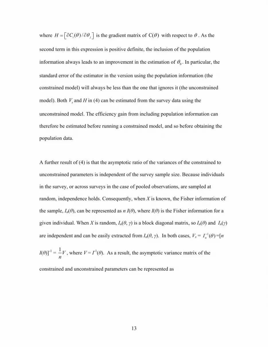
A further result of (4) is that the asymptotic ratio of the variances of the constrained to

unconstrained parameters is independent of the survey sample size. Because individuals

in the survey, or across surveys in the case of pooled observations, are sampled at

random, independence holds. Consequently, when X is known, the Fisher information of

the sample, In(θ), can be represented as n I(θ), where I(θ) is the Fisher information for a

given individual. When X is random, In(θ, γ) is a block diagonal matrix, so In(θ) and In(γ)

are independent and can be easily extracted from In(θ, γ). In both cases, Vs = 1( )nI θ− =[n

I(θ)]-1 = 1Vn

, where V = I-1(θ). As a result, the asymptotic variance matrix of the

constrained and unconstrained parameters can be represented as

13

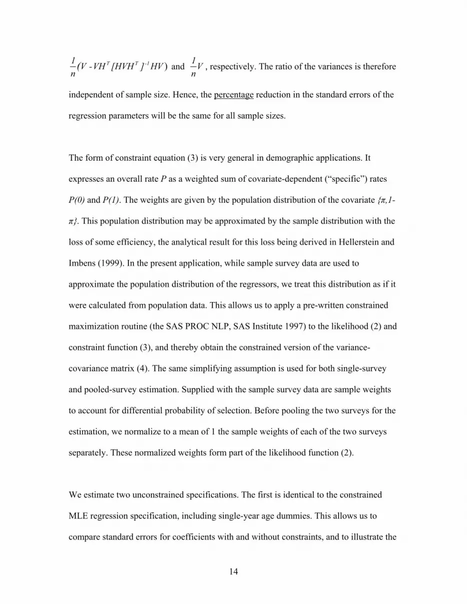
)T T -11 V - VH [HVH ] HVn

( and 1Vn

, respectively. The ratio of the variances is therefore

independent of sample size. Hence, the percentage reduction in the standard errors of the

regression parameters will be the same for all sample sizes.

The form of constraint equation (3) is very general in demographic applications. It

expresses an overall rate P as a weighted sum of covariate-dependent (“specific”) rates

P(0) and P(1). The weights are given by the population distribution of the covariate {π,1-

π}. This population distribution may be approximated by the sample distribution with the

loss of some efficiency, the analytical result for this loss being derived in Hellerstein and

Imbens (1999). In the present application, while sample survey data are used to

approximate the population distribution of the regressors, we treat this distribution as if it

were calculated from population data. This allows us to apply a pre-written constrained

maximization routine (the SAS PROC NLP, SAS Institute 1997) to the likelihood (2) and

constraint function (3), and thereby obtain the constrained version of the variance-

covariance matrix (4). The same simplifying assumption is used for both single-survey

and pooled-survey estimation. Supplied with the sample survey data are sample weights

to account for differential probability of selection. Before pooling the two surveys for the

estimation, we normalize to a mean of 1 the sample weights of each of the two surveys

separately. These normalized weights form part of the likelihood function (2).

We estimate two unconstrained specifications. The first is identical to the constrained

MLE regression specification, including single-year age dummies. This allows us to

compare standard errors for coefficients with and without constraints, and to illustrate the

14

deficiencies of sample survey data for a non-parametric approach to hazard estimation.

The second specification parameterizes the age function as polynomial, allowing for a

smoothing of the first birth relationship with age. The parametric approach to hazard

estimation is a common solution to the problem of high sampling variability with survey

data. We show here that the results obtained with this parametric approach are inferior to

those obtained by the smoothing of the age relationship with single-year age population

constraints.

RESULTS

Constrained versus unconstrained regression parameter estimates

In Table 2, constrained and unconstrained parameter estimates and standard errors are

presented for the logistic regression of first birth on age, cohort, and education. Separate

results are reported using the small (FFS) survey only, the large (Multiscopo) survey

only, and the FFS and Multiscopo surveys with their observations pooled. The function

of age and cohort to first birth is specified using single-year ages (that is, completely non-

parametric), while we parameterize (with a second-order polynomial) the education by

age interaction. This is because we have exact population information about the age and

cohort relationships, but must rely on survey data for information about the education

relationship.

[TABLE 2 ABOUT HERE]

Consistent with equation (4) in the statistical theory presented above, all standard errors

in the constrained version are as low as, or lower than, the corresponding standard errors

15

of the unconstrained version. The standard errors of the age parameters are seen to be

reduced by very large amounts by constraining survey-based estimates to the overall

population values, generally by 75 percent or more as compared to the unconstrained

version, and sometimes by as much as 90 percent. Only for the age parameters, cohort-

by-age parameters, and intercept, however, are the reductions in standard errors other

than of negligible magnitudes. That is, for none of the parameters for education and its

interaction with age and cohort is there a non-negligible reduction in the standard error.

This makes intuitive sense, as the constraints offer exact information about the

relationship of age to first childbearing, but no information about how this relationship

differs by education.

A further result of equation (4) noted in the statistical theory description above is

confirmed empirically in Table 2: the ratio of the variances of the constrained to

unconstrained parameters is independent of the survey sample size. The asymptotic result

is that the percentage reduction in the standard errors of the regression parameters from

the unconstrained to the constrained versions will be equal. This is seen to be closely

approximated in practice for the FFS and the Multiscopo. Thus even while the sample

size of the Multiscopo are approximately four times as high as the sample size of the

FFS, there is no difference in the proportionate reduction of the standard error about the

first-birth model coefficient estimates. Importantly, the standard errors for the pooled

sample are reduced by similar amounts in percentage terms as are the standard errors for

either of the two surveys alone. For example, for the age-40 coefficient, the standard

error for estimation with the FFS is reduced from an unconstrained-model 0.976 to a

16

constrained-model 0.277, an approximately 75 percent reduction. When estimating the

unconstrained and constrained models with the pooled FFS and Multiscopo, the standard

error falls from 0.311 to 0.081, again an approximately 75 percent reduction.

While the population constraints have a negligible effect on the standard errors of the

coefficients for education, and for the interaction of education with age and cohort,

pooling the two samples results in substantial reductions in these standard errors. These

reductions are seen equally in the constrained and unconstrained estimates, although we

focus on the constrained estimates. Compared with using the FFS alone, the standard

error for the parameter for the main effect (at age 25 for the 1951-55 cohort) of having a

higher education qualification is halved (from 0.337 to 0.178). Compared with using the

Multiscopo alone, the standard error for the same parameter is reduced from 0.213 to

0.178. Similarly large reductions by adding the Multiscopo data to the FFS data, and

much smaller but still substantial reductions by adding the FFS data to the Multiscopo

data, are seen in the standard errors for the parameters for higher-education interactions

with cohort and age.

The practical advantages of pooling survey data under population-constrained estimation

are best seen by graphing the predicted first birth probabilities by age, cohort, and

education. These predicted probabilities for the estimation that uses the pooled survey

data with the population information as constraints to the survey estimation are first

presented in Figures 2a and 2b. We consider these our best estimates of the relationship

of age, cohort, and education to first-birth, since they take into account all available

17

survey and population data. Confidence intervals for these estimates, as for all the

predicted probabilities presented in this article, were generated using a bootstrap

procedure (Efron and Tibshirani 1994) with 1,000 iterations. The 95% confidence

interval shown in the graphs consists of the 5th percentile and 95th percentile of the

bootstrapped estimates.

[FIGURES 2A, 2B, 2C, AND 2D ABOUT HERE]

The 1950s cohort’s predicted first-birth probabilities show highly differentiated patterns

by education (see Figure 2a). The downward-sloping profile from age 26 seen in the birth

registration data is modeled for women without a high education, while the pattern for

women with a high education is modeled as sloping steeply upwards to a peak first-birth

probability at age 31. The modeled pattern follows the observed probabilities closely for

women with no high education. The observed probabilities for women with high

education qualifications, however, fluctuate much more around the predicted line. This is

expected given that relatively few women in the cohort, and therefore also in the sample,

have a higher qualification.

Some similar remarks may be made about the 1960s cohort’s constrained estimates

versus the observed data and overall first-birth probabilities in the population data (see

Figure 2b). Up to about age 30, the fit of the lines to the observed data appears as if it

were a simple smoothing of the sample data. After age 30, however, the effect of the

constraint is clearly much stronger than seen either before age 30 or in the case of the

18

1950s cohort. The constraint pulls both education-specific lines downwards so that they

are on average much lower than their observed sample points. For the higher-education

women, for example, little evidence of a downward slope emerging by age 34 is seen in

the sample points. The implication of the predicted education-specific lines after age 30 is

that the observed sample points may be biased upwards. This may be because, for

example, non-response is differentially low for women who had children in the year

before survey date. The population data, however, are not subject to response

differentials, and therefore are expected to be unbiased. Using them in the constrained

estimation therefore will correct for bias in the survey data.

We present in Figures 2c and 2d the predicted values for the constrained estimator using

only the smaller, FFS dataset. The main objective here is to show, by contrast with

Figures 2a and 2b, how pooling survey data may lead to substantial improvements

especially in estimating those parts of the relationship for which population information

is not available. While a similar relationship of education to first birth is seen under

constrained estimation using the FFS only, the confidence intervals around the predicted

probabilities are much wider. For example, while the confidence intervals for “High

Education” and “No High Education” women over 30 in the 1950s cohort are non-

overlapping only between the ages 32 and 35 for the FFS, they are non-overlapping from

ages 31 to 38 with the combined FFS and Multiscopo surveys.

The largest improvements achieved by using all of the available data are again seen for

the 1960s cohort. Here, the constrained estimator with the FFS data results in the higher

19

educated women’s first birth hazard approaching but never exceeding the hazard for

women without a higher-education qualification (see Figure 2d). This contrasts with the

cross-over at about age 31 seen for the constrained estimator that pools the FFS and

Multiscopo data (Figure 2b). The failure of the FFS constrained estimator to model the

education cross-over is due to a combination of its observations going only up to age 32

and to its much smaller sample size. Note that at age 32, no first births were observed in

the FFS sample (see the “High Education, observed” points on the plot).

Parametric and non-parametric specifications of age in unconstrained estimation

The researcher who uses sample data only is unlikely to specify the non-parametric,

single-year age dummy model used in constrained estimation. Instead, a smooth

relationship of the first-birth probability with age is likely to be imposed parametrically.

We now illustrate graphically that both the non-parametric and parametric approaches

will be inferior to the approach that uses the population data as formal constraints to the

estimation. For the parametric version, a polynomial age specification regression with

linear, squared, and cubed terms for the reference, 1950s cohort, and with linear and

squared interaction terms for the 1960s cohort is estimated (parameter estimates available

from the first author on request). The non-parametric version uses the specification from

Table 2 above. The two versions are intended to give the range of likely alternative

estimation strategies (from completely non-parametric to the simplest parametric

specification) in the case that no statistical method for the incorporation of known

population information is available to the researcher. The predicted values for the non-

20

parametric and parametric unconstrained specifications, in all cases using the pooled

survey data, are shown in Figures 3a to 3d.

[FIGURES 3A, 3B, 3C, AND 3D ABOUT HERE]

The population line is included in the graphs to show how estimates from the sample

data, whether using non-parametric or parametric specifications, may be inconsistent with

the overall population values. This contrasts with Figures 2a and 2b, where such

inconsistency is prevented by the method of constraining to the population values. The

predicted values for the non-parametric, single-year age dummy specifications shown in

Figures 3a and 3b generate jagged lines for both the education-specific probability series.

False local peaks in the hazard, for example, occur at age 40 for the 1950s cohort and at

age 27 for the 1960s cohort. This is clearly attributable to sampling error, as the

population function is known from population data to be smooth across these ages.

Predicted values are presented in Figures 3c and 3d for the parametric version. For the

1950s cohort, the unconstrained polynomial-age specification lines are very similar in

pattern to those seen for the constrained estimate of Figure 2a. There is a similar cross-

over point, at about age 29, between the higher-qualified and not-higher-qualified

women. This parametric specification appears to model reasonably well the relationship

seen in the sample data. For the 1960s cohort, however, it produces predicted values that

exceed the population values for both higher-qualified and not-higher-qualified women

after age 30 (see Figure 3b). Such deviations from a known population relationship are

21

possible because the parametric smoothing has no effect on the overall level of the

hazard.

The effect of the population constraint in Figures 2a through 2d is now clearer when

contrasted with Figures 3a through 3d. While the patterns of first-birth probabilities in

Figures 2a through 2d appear to be similar to those that would emerge from a parametric

or non-parametric smoothing of the two education-specific series, the two education-

specific lines always surround the population constraint line. This is a result of the

population line’s being a weighted sum of the two education-specific lines at each single-

year age. This is most obvious at the point at which the education-specific lines cross,

which is forced to be the point at which they are equal to the known overall first-birth

probability in the population (the constraint line). Both the parametric and non-parametric

versions of the unconstrained estimation, in contrast, allow drift in the two education-

specific hazards from the known overall population hazard of first birth by age and

cohort.

SUMMARY AND CONCLUSIONS

Previous demographic and economic studies have demonstrated large efficiency gains

through combining population data with survey data in regression estimation. These

gains, however, have been limited to the intercept parameter and the coefficients for

variables for which population data are also available. The present study demonstrated

how this limitation can be overcome by pooling data from more than one survey sample

and constraining estimates from the pooled surveys to population data.

22

Full use of available population data was achieved by imposing population constraints by

single-year age, parity, and cohort. This introduced an exact, baseline relationship of age

to first childbearing separately for two five-year birth cohorts. Observations from a

second, large-scale survey (the 1998 Multiscopo) pooled with observations from a

specialist demographic survey (the 1995/96 FFS) allowed for much greater efficiency in

the estimation of the relationship of a key socio-economic variable (educational

attainment) to first birth by age. As expected, however, negligible reductions in the

standard errors for the parameters for education and its interaction with age and cohort

were achieved by the imposing of population constraints. The intuition for this is that the

constraints offer exact information about the relationship of age and cohort to first birth,

but no information about how this relationship differs by the education levels of cohort

members.

Additional information about how first birth differs by education was instead obtained by

pooling the data from the small survey with observations on women from the same

cohorts in a larger survey in which the education variable and fertility histories were also

present. Here, the efficiency gains over using the smaller survey alone are equivalent to

increasing the latter’s sample by the number of observations in the larger survey. Because

the larger, Multiscopo survey has approximately four times the person-year sample size

of the smaller, FFS, the standard errors about the education coefficients were

approximately half those estimated using the FFS data alone. Pooling the survey data,

moreover, does nothing to reduce the effectiveness of using population constraints. Both

23

theoretical and empirical results were presented showing that the percentage reduction in

the standard errors achieved by applying population constraints is independent of the

survey sample size, and therefore equally effective when surveys are pooled.

The structures of the survey datasets and population data used in the present study have

permitted a largely straightforward statistical treatment. The two survey datasets used

here have been treated as though they sample from the same population, and contain the

same variables needed to estimate the relationships of interest. In one practically

important way, the larger dataset also contributed variables not present in the smaller

survey. These were from observations of women at ages 43 and 44 in the 1950s cohort

and at ages 33 and 34 in the 1960s cohort. Their practical significance is that they

complete the ages of reproduction for the 1950s cohort, and extend predictions over ages

at which first birth hazards are high, especially for women with higher education, in the

1960s cohort. This presents no statistical complication for hazard modeling, since adding

ages of observation does no more than relax the degree of right-censoring of first-birth

exposure. Pooling data from surveys with more general differences in their regressor

variables is also possible, but involves greater statistical challenges (see Ridder and

Moffitt, forthcoming).

The population data used here were treated as exact, in the senses both of being unbiased

and having negligible sampling error. This assumption will not hold for all population

data collections. The Italian statistical system for the collection of births data was itself

overhauled in 1999, such that information on mother’s age and parity is no longer

24

available in a single, complete-enumeration source (LoConte et al 2003). This means that

only by using data collections that include sampling error will it be possible to construct

age- and parity-specific population constraints from 1999 onwards. This complicates, but

does not eliminate, the possibilities for improving survey estimates. Hellerstein and

Imbens (1999) show this by deriving a variance estimator that adjusts for sampling error

in “population” constraints from large-scale sample survey data.

25

REFERENCES

Deming, W. E., and Stephan, F. F. (1942) On the least squares adjustment of a sampled

frequency table when the expected marginal tables are known. The Annals of

Mathematical Statistics 11:427-424.

De Sandre, P. et al (2000) Fertility and Family Surveys in the ECE Region

Standard Country Report: Italy Geneva: United Nations Economic Commission for

Europe, Population Activities Unit.

Efron, B., and R.J. Tibshirani (1994) An Introduction to the Bootstrap New York:

Chapman and Hall.

Giorgi, P. (1993) Una rilettura della fecondità del momento per ordine di nascita

in Italia nel periodo 1950-1990 considerando la struttura per parità. Genus 40(3-4):177-

204.

Handcock, M.S., S.M. Huovilainen, and M.S. Rendall (2000) Combining

Registration-System and Survey Data to Estimate Birth Probabilities. Demography

37(2):187-192.

Handcock, M.S., M.S. Rendall, and J.E. Cheadle (2005) Improved regression

estimation of a multivariate relationship with population data on the bivariate

relationship. Sociological Methodology 35(1)291-334.

Hellerstein, J., and G.W. Imbens (1999) Imposing moment restrictions from

auxiliary data by weighting. Review of Economics and Statistics 81(1):1-14.

Imbens, G.W. and T. Lancaster (1994) Combining micro and macro data in

microeconometric models. Review of Economic Studies 61: 655-680.

26

Ireland, C. T., and Kullback, S. (1968) Contingency tables with given marginals.

Biometrika 55:179-188.

ISTAT (2000) Indagine Statisitca Multiscopo sulla Famiglia, 1998. Rome: Istituto

Nazionale di Statistica.

ISTAT (1996) Forze di Lavoro, Media 1995 Serie Annuari. Rome: Istituto

Nazionale di Statistica.

ISTAT (2005) Elaborazioni Istat su dati ricostruiti progetto MARSS. Rome:

Istituto Nazionale di Statistica.

LoConte, M., C. Castagnaro, V. Talucci, and S. Prati (2003) “The first sample

survey on births in Italy: Purposes and results.” Paper presented at the 2003 European

Population Conference, Warsaw, Poland.

Maddala, G.S. (1983) Limited-Dependent and Qualitative Variables in

Econometrics. New York: Cambridge University Press.

OECD (2003) Education Statistics and Indicators, Education at a Glance - 2002

Edition. www.oecd.org.

Rice J. A. (1995) Mathematical Statistics and Data Analysis. Pacific

Grove:Wadsworth.

Ridder, G., and R.A. Moffitt (forthcoming) The econometrics of data

combination. Handbook of Econometrics Vol.6.

SAS Institute (1997) SAS/OR Technical Report: The NLP Procedure. Cary, NC:

SAS Institute Inc.

27

Figure 1a Italy 1951-55 Cohort First Birth Probabilities by Source of data

0.00

0.02

0.04

0.06

0.08

0.10

0.12

0.14

0.16

0.18

0.20

25 26 27 28 29 30 31 32 33 34 35 36 37 38 39 40 41 42 43 44

age

FFS

Multiscopo

Biirth Registration

Figure 1b Italy 1961-65 Cohort First Birth Probabilities by Source of data

0.00

0.02

0.04

0.06

0.08

0.10

0.12

0.14

0.16

0.18

0.20

25 26 27 28 29 30 31 32 33 34

age

FFS

Multiscopo

Birth Registration

Figure 2a 1951-55 Cohort Constrained Estimation with Pooled (FFS and Multiscopo) Survey Data

0.00

0.02

0.04

0.06

0.08

0.10

0.12

0.14

0.16

0.18

0.20

0.22

0.24

25 26 27 28 29 30 31 32 33 34 35 36 37 38 39 40 41 42 43 44

age

1st

birt

h pr

obab

ility

No High Education, predictedHigh Education, predictedBirth RegistrationNo High Education, observedHigh Education, observedLower CI, No High EducationUpper CI, No High EducationLower CI, High EducationUpper CI, High Education

Figure 2b 1961-65 Cohort Constrained Estimation with Pooled (FFS and Multiscopo) Survey Data

0.00

0.02

0.04

0.06

0.08

0.10

0.12

0.14

0.16

0.18

0.20

0.22

0.24

25 26 27 28 29 30 31 32 33 34

age

1st

birt

h pr

obab

ility

No High Education, predictedHigh Education, predictedBirth RegistrationNo High Education, observedHigh Education, observedLower CI, No High EducationUpper CI, No High EducationLower CI, High EducationUpper CI, High Education

Figure 2c 1951-55 Cohort Constrained Estimation with Small (FFS) Survey

0.00

0.02

0.04

0.06

0.08

0.10

0.12

0.14

0.16

0.18

0.20

0.22

0.24

25 26 27 28 29 30 31 32 33 34 35 36 37 38 39 40 41 42

age

1st

birt

h pr

obab

ility

No High Education, predictedHigh Education, predictedBirth RegistrationNo High Education, observedHigh Education, observedlower CI, No High Educationupper CI, No High Educationlower CI, High Educationupper CI, High Education

Figure 2d 1961-65 Cohort Constrained Estimation with Small (FFS) Survey

0.00

0.02

0.04

0.06

0.08

0.10

0.12

0.14

0.16

0.18

0.20

0.22

0.24

25 26 27 28 29 30 31 32

age

1st

birt

h pr

obab

ility

No High Education, predictedHigh Education, predictedBirth RegistrationNo High Education, observedHigh Education, observedlower CI, No High Educationupper CI, No High Educationlower CI, No High Educationupper CI, High Education

Figure 3a 1951-55 Cohort Unconstrained Estimation with Pooled (FFS and Multiscopo) Survey Data

0.00

0.02

0.04

0.06

0.08

0.10

0.12

0.14

0.16

0.18

0.20

0.22

0.24

25 26 27 28 29 30 31 32 33 34 35 36 37 38 39 40 41 42 43 44

age

1st

birt

h pr

obab

ility

Birth Registration

No High Eduction, single-year age

High Education, single-year age

Lower CI, No High Education

Upper CI, No High Education

Lower CI, High Education

Upper CI, High Education

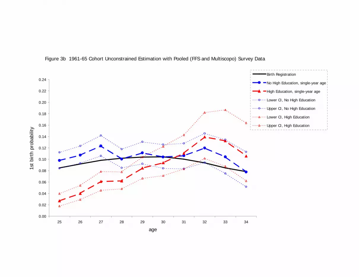
Figure 3b 1961-65 Cohort Unconstrained Estimation with Pooled (FFS and Multiscopo) Survey Data

0.00

0.02

0.04

0.06

0.08

0.10

0.12

0.14

0.16

0.18

0.20

0.22

0.24

25 26 27 28 29 30 31 32 33 34

age

1st

birt

h pr

obab

ility

Birth Registration

No High Education, single-year age

High Education, single-year age

Lower CI, No High Education

Upper CI, No High Education

Lower CI, High Education

Upper CI, High Education

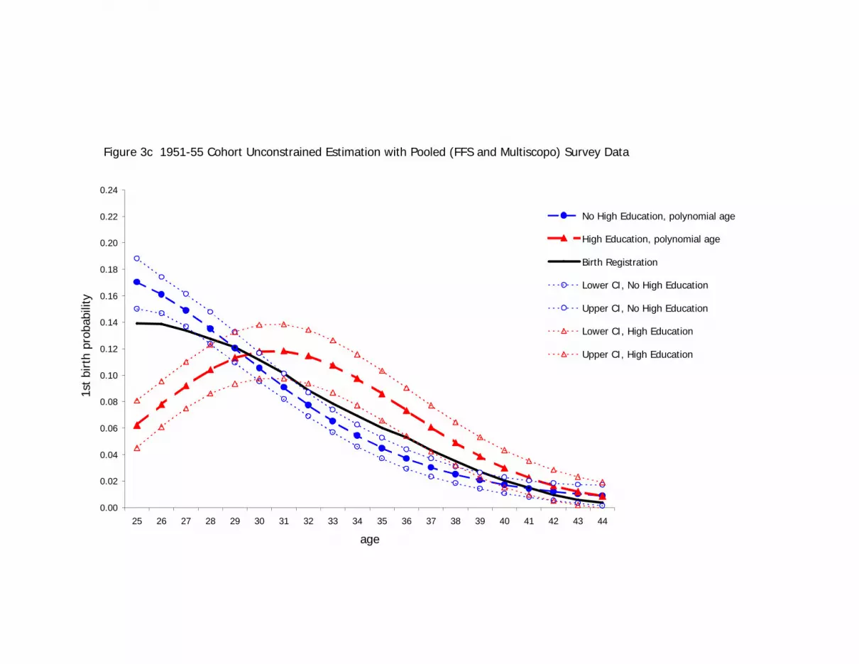
Figure 3c 1951-55 Cohort Unconstrained Estimation with Pooled (FFS and Multiscopo) Survey Data

0.00

0.02

0.04

0.06

0.08

0.10

0.12

0.14

0.16

0.18

0.20

0.22

0.24

25 26 27 28 29 30 31 32 33 34 35 36 37 38 39 40 41 42 43 44

age

1st

birt

h pr

obab

ility

No High Education, polynomial age

High Education, polynomial age

Birth Registration

Lower CI, No High Education

Upper CI, No High Education

Lower CI, High Education

Upper CI, High Education

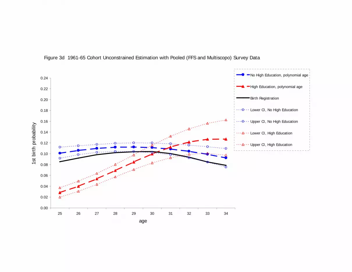
Figure 3d 1961-65 Cohort Unconstrained Estimation with Pooled (FFS and Multiscopo) Survey Data

0.00

0.02

0.04

0.06

0.08

0.10

0.12

0.14

0.16

0.18

0.20

0.22

0.24

25 26 27 28 29 30 31 32 33 34

age

1st

birt

h pr

obab

ility

No High Education, polynomial age

High Education, polynomial age

Birth Registration

Lower CI, No High Education

Upper CI, No High Education

Lower CI, High Education

Upper CI, High Education

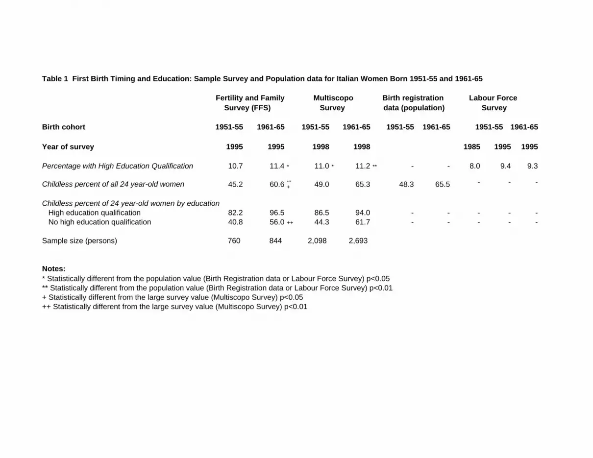
Table 1 First Birth Timing and Education: Sample Survey and Population data for Italian Women Born 1951-55 and 1961-65

Fertility and Family Multiscopo Birth registration Labour Force Survey (FFS) Survey data (population) Survey

Birth cohort 1951-55 1961-65 1951-55 1961-65 1951-55 1961-65 1951-55 1961-65

Year of survey 1995 1995 1998 1998 1985 1995 1995

Percentage with High Education Qualification 10.7 11.4 * 11.0 * 11.2 ** - - 8.0 9.4 9.3

Childless percent of all 24 year-old women 45.2 60.6 ** 49.0 65.3 48.3 65.5 - - -+

Childless percent of 24 year-old women by education High education qualification 82.2 96.5 86.5 94.0 - - - - - No high education qualification 40.8 56.0 ++ 44.3 61.7 - - - - -

Sample size (persons) 760 844 2,098 2,693

Notes:* Statistically different from the population value (Birth Registration data or Labour Force Survey) p<0.05** Statistically different from the population value (Birth Registration data or Labour Force Survey) p<0.01+ Statistically different from the large survey value (Multiscopo Survey) p<0.05++ Statistically different from the large survey value (Multiscopo Survey) p<0.01

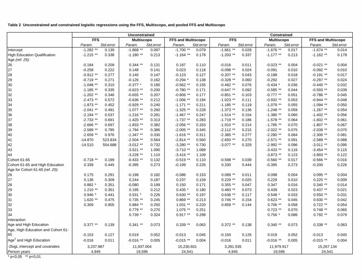
Table 2 Unconstrained and constrained logisitic regressions using the FFS, Multiscopo, and pooled FFS and Multiscopo

Unconstrained ConstrainedFFS Multiscopo FFS and Multiscopo FFS Multiscopo FFS and Multiscopo

Param. Std.error Param. Std.error Param. Std.error Param. Std.error Param. Std.error Param. Std.errorIntercept -1.282 ** 0.139 -1.868 ** 0.097 -1.700 ** 0.079 -1.661 ** 0.028 -1.676 ** 0.017 -1.674 ** 0.014High Education Qualification -1.215 ** 0.338 -1.180 ** 0.213 -1.164 ** 0.178 -1.203 ** 0.337 -1.177 ** 0.213 -1.162 ** 0.178Age (ref. 25):26 -0.184 0.209 0.344 ** 0.131 0.187 0.110 -0.016 0.011 -0.023 ** 0.004 -0.021 ** 0.00427 -0.258 0.222 0.148 0.141 0.023 0.118 -0.098 ** 0.024 -0.091 0.010 -0.092 ** 0.01028 -0.912 ** 0.277 0.140 0.147 -0.123 0.127 -0.207 ** 0.043 -0.188 0.018 -0.191 ** 0.01729 -0.719 ** 0.271 -0.126 0.162 -0.294 * 0.138 -0.328 ** 0.060 -0.292 0.027 -0.297 ** 0.02430 -1.048 ** 0.310 -0.377 * 0.180 -0.562 ** 0.155 -0.482 ** 0.076 -0.434 * 0.036 -0.440 ** 0.03231 -1.185 ** 0.335 -0.623 ** 0.200 -0.780 ** 0.171 -0.647 ** 0.092 -0.585 ** 0.044 -0.593 ** 0.03932 -1.202 ** 0.346 -0.655 ** 0.207 -0.806 ** 0.177 -0.851 ** 0.103 -0.777 ** 0.051 -0.786 ** 0.04533 -2.473 ** 0.572 -0.636 ** 0.212 -1.006 ** 0.194 -1.023 ** 0.111 -0.932 ** 0.053 -0.944 ** 0.04834 -1.873 ** 0.452 -0.929 ** 0.240 -1.171 ** 0.211 -1.185 ** 0.119 -1.079 ** 0.055 -1.094 ** 0.05035 -2.041 ** 0.491 -1.077 ** 0.260 -1.325 ** 0.228 -1.373 ** 0.136 -1.248 ** 0.059 -1.267 ** 0.05436 -2.194 ** 0.537 -1.216 ** 0.281 -1.467 ** 0.247 -1.514 ** 0.154 -1.380 ** 0.060 -1.402 ** 0.05637 -2.733 ** 0.691 -1.420 ** 0.313 -1.737 ** 0.283 -1.719 ** 0.186 -1.578 ** 0.064 -1.602 ** 0.06138 -2.666 ** 0.697 -1.833 ** 0.382 -2.056 ** 0.333 -1.910 ** 0.214 -1.785 ** 0.070 -1.807 ** 0.06739 -2.589 ** 0.785 -1.794 ** 0.386 -2.005 ** 0.345 -2.112 ** 0.215 -2.022 ** 0.075 -2.039 ** 0.07040 -2.659 ** 0.976 -1.347 ** 0.330 -1.616 ** 0.311 -2.385 ** 0.277 -2.280 ** 0.084 -2.300 ** 0.08141 -14.870 523.834 -2.504 ** 0.564 -2.814 ** 0.560 -2.650 ** 0.270 -2.571 ** 0.091 -2.589 ** 0.08842 -14.510 554.688 -3.012 ** 0.732 -3.280 ** 0.730 -3.077 ** 0.329 -2.992 ** 0.096 -3.011 ** 0.09543 -3.521 ** 1.090 -3.710 ** 1.089 -3.433 ** 0.116 -3.454 ** 0.11544 -3.228 ** 1.110 -3.416 ** 1.109 -3.873 ** 0.123 -3.893 ** 0.122Cohort 61-65 -0.718 ** 0.199 -0.433 ** 0.132 -0.519 ** 0.110 -0.598 ** 0.039 -0.560 ** 0.017 -0.566 ** 0.016Cohort 61-65 and High Education 0.339 0.445 -0.395 0.273 -0.199 0.226 0.330 0.444 -0.395 0.273 -0.200 0.226Age for Cohort 61-65 (ref. 25):26 0.175 0.291 -0.198 0.182 -0.086 0.153 0.089 ** 0.011 0.098 0.004 0.095 ** 0.00427 0.136 0.309 0.244 0.187 0.237 0.159 0.229 ** 0.025 0.229 0.010 0.225 ** 0.00928 0.882 * 0.351 -0.080 0.199 0.150 0.171 0.355 ** 0.047 0.347 0.016 0.340 ** 0.01429 1.210 ** 0.351 0.195 0.212 0.435 * 0.180 0.483 ** 0.073 0.439 0.023 0.437 ** 0.02130 0.946 * 0.441 0.531 * 0.226 0.630 ** 0.197 0.636 ** 0.117 0.548 * 0.033 0.550 ** 0.03131 1.620 ** 0.475 0.735 ** 0.245 0.869 ** 0.213 0.746 ** 0.154 0.623 ** 0.045 0.630 ** 0.04232 0.309 0.905 0.984 ** 0.250 1.031 ** 0.220 0.859 ** 0.144 0.706 ** 0.058 0.722 ** 0.05433 0.779 ** 0.270 1.075 ** 0.251 0.723 ** 0.070 0.748 ** 0.06534 0.739 * 0.324 0.917 ** 0.298 0.756 * 0.086 0.792 ** 0.079InteractionAge and High Education 0.377 ** 0.139 0.341 ** 0.073 0.339 ** 0.063 0.372 ** 0.138 0.340 ** 0.073 0.338 ** 0.063Age, High Education and Cohort 61-65 -0.153 0.127 0.019 0.052 -0.013 0.045 -0.150 0.126 0.019 0.052 -0.013 0.045Age2 and High Education -0.016 0.011 -0.016 ** 0.005 -0.015 ** 0.004 -0.016 0.011 -0.016 ** 0.005 -0.015 ** 0.004-2logL intercept and covariates 3,237.987 11,937.004 15,230.601 3,281.535 11,979.917 15,267.134Person years 4,945 19,596 24,541 4,945 19,596 24,541* p<0,05 ** p<0,01