Embed Size (px)
Citation preview
Polarization mode excitation
in index-tailored optical fibers
by acoustic long period gratings:
Development and Application
Dissertation von
Christoph Zeh2013

POLARIZATION MODE EXCITATION IN
INDEX-TAILORED OPTICAL FIBERS
BY ACOUSTIC LONG PERIOD GRATINGS:DEVELOPMENT AND APPLICATION
Dissertation
zur Erlangung des akademischen GradesDoctor rerum naturalium
vorgelegt der
Fakultat Mathematik und Naturwissenschaftender Technischen Universitat Dresden
von
Christoph Zeh
geboren am 05.12.1983 in Pirna
Gutachter:Prof. Dr. phil. II. habil. Lukas M. Eng (Technische Universitat Dresden)Prof. Dr. Qiwen Zhan (University of Dayton, Ohio, USA)
Eingereicht am: 17.05.2013 Verteidigt am: 05.11.2013
TECHNISCHE UNIVERSITAT DRESDEN 2013

Abstract
The present work deals with the development and application of an acoustic long-periodfiber grating (LPG) in conjunction with a special optical fiber (SF). The acoustic LPGconverts selected optical modes of the SF. Some of these modes are characterized bycomplex, yet cylindrically symmetric polarization and intensity patterns. Therefore,they are the guided variant of so called cylindrical vector beams (CVBs). CVBs findapplications in numerous fields of fundamental and applied optics. Here, an applicationto high-resolution light microscopy is demonstrated. The field distribution in the tightmicroscope focus is controlled by the LPG, which in turn creates the necessary polar-ization and intensity distribution for the microscope illumination. A gold nanoparticleof 30 nm diameter is used to probe the focal field with sub-wavelength resolution.
The construction and test of the acoustic LPG are discussed in detail. A key compo-nent is the piezoelectric transducer that excites flexural acoustic waves in the SF, whichare the origin of an optical mode conversion. A mode conversion efficiency of 85 % wasrealized at 785 nm optical wavelength. The efficiency is, at present, mainly limited bythe spectral positions and widths of the transducer’s acoustic resonances.
The SF used with the LPG separates the propagation constants of the second-orderpolarization modes, so they can be individually excited and are less sensitive to distor-tions than in standard weakly-guiding fibers. The influence of geometrical parametersof the fiber core on the propagation constant separation and on the mode fields is studiednumerically using the multiple multipole method. From the simulations, a simple modecoupling scheme is developed that provides a qualitative understanding of the experi-mental results achieved with the LPG. The refractive index profile of the fiber core wasoriginally developed by Ramachandran et al. However, an important step of the presentwork is to reduce the SF’s core size to counteract the the appearance of higher-ordermodes at shorter wavelengths which would otherwise spoil the mode purity.
Using the acoustic LPG in combination with the SF produces a versatile device togenerate CVBs and other phase structures beams. This fiber-optical method offers beamprofiles of high quality and achieves good directional stability of the emitted beam.Moreover, the device design is simple and can be realized at low cost. Future develop-ments of the acoustic LPG will aim at applications to fiber-optical sensors and opticalnear-field microscopy.
iii
Kurzfassung
Diese Arbeit behandelt die Entwicklung und Anwendung eines akustischen langperi-odischen Fasergitters (LPG) in Verbindung mit einer optischen Spezialfaser (SF). Dasakustische LPG wandelt ausgewahlte optische Modi der SF um. Einige dieser Modi wei-sen eine komplexe, zylindersymmetrische Polarisations- und Intensitatsverteilung auf.Diese sind eine Form der so genannten zylindrischen Vektor-Strahlen (CVBs), welche inzahlreichen Gebieten der wissenschaftlichen und angewandten Optik zum Einsatz kom-men. In dieser Arbeit wird eine Anwendung auf die hochauflosende Lichtmikroskopiedemonstriert. Die fokale Feldverteilung wird dabei durch die Auswahl der vom LPG er-zeugten Modi, welche zur Beleuchtung genutzt werden, eingestellt. Als Nachweis wirddie entstehende laterale Feldverteilung mithilfe eines Goldpartikels (Durchmesser 30
Nanometer) vermessen.Aufbau und Test des akustischen LPGs werden im Detail besprochen. Eine wichti-
ge Komponente ist ein piezoelektrischer Wandler, der akustische Biegewellen in der SFanregt. Diese sind die Ursache der Umwandlung optischer Modi. Die maximale Konver-sionseffizienz betrug 85 % bei 785 nm (optischer) Wellenlange. Die Effizienz ist derzeithauptsachlich durch die Lage der akustischen Resonanzfrequenzen des Wandlers undderen Bandbreite begrenzt.
Die benutzte SF spaltet die Ausbreitungskonstanten von Polarisationsmodi zweiterOrdnung auf, sodass diese individuell angeregt werden konnen und weniger anfallig ge-genuber Storungen der Faser sind, als das bei gewohnlichen, schwach fuhrenden Glas-fasern der Fall ist. Das zu Grunde liegende Brechzahlprofil des Faserkerns wurde vonRamachandran et al. entwickelt. Fur diese Arbeit wurde jedoch die Ausdehnung desProfils verkleinert – ein erster Schritt um Anwendungen bei kurzeren optischen Wel-lenlangen zu ermoglichen. Es werden numerische Simulationen mit der Methode dermultiplen Multipole zur Berechnung der Modenfelder und den zugehorigen Propaga-tionskonstanten vorgestellt. Diese zeigen u. a. den starken Einfluss von geometrischenVeranderungen des Faserkerns. Basierend auf den Simulationsergebnissen wird ein ein-faches Kopplungsschema fur die Modi entwickelt, welches ein qualitatives Verstandnisder experimentellen Ergebnisse ermoglicht.
In Kombination bilden die SF und das LPG ein vielseitiges Gerat zur Erzeugungvon CVBs und anderen Strahlen mit komplexer Phasenstruktur. Die Methode bestichtdurch hohe Qualitat des Strahlprofils, stabile Abstrahlrichtung, einfachen Aufbau, elek-tronische Steuerbarkeit und geringe Materialkosten. Zukunftige Weiterentwicklungendes akustischen LPGs zielen auf die Anwendung in faseroptischen Sensoren und in deroptischen Nahfeldmikroskopie ab.
iv
Contents
Abstract / Kurzfassung iii
Table of contents v
1 Introduction 1
2 Fundamentals of optical waveguides 52.1 Introduction . . . . . . . . . . . . . . . . . . . . . . . . . . . . . . . . 52.2 Maxwell’s equations and vector wave equations . . . . . . . . . . . . . 52.3 Optical waveguides . . . . . . . . . . . . . . . . . . . . . . . . . . . . 7
2.3.1 Dielectric waveguides . . . . . . . . . . . . . . . . . . . . . . 72.3.2 Metallic waveguides . . . . . . . . . . . . . . . . . . . . . . . 9
2.4 Numerical calculation of modes by the multiple multipole program . . . 102.4.1 Representation of simulated mode fields . . . . . . . . . . . . . 11
2.5 Overview of coupled mode theory . . . . . . . . . . . . . . . . . . . . 142.5.1 Coupled mode equations . . . . . . . . . . . . . . . . . . . . . 142.5.2 Co-directional coupling . . . . . . . . . . . . . . . . . . . . . 15
2.6 Summary and conclusions . . . . . . . . . . . . . . . . . . . . . . . . 16
3 Polarization control for fundamental and higher order modes 173.1 Introduction . . . . . . . . . . . . . . . . . . . . . . . . . . . . . . . . 173.2 Description of light polarization . . . . . . . . . . . . . . . . . . . . . 18
3.2.1 Stokes parameters and the polarization ellipse . . . . . . . . . . 183.2.2 Polarization of light beams in free space . . . . . . . . . . . . . 203.2.3 Polarization of light beams in optical fibers . . . . . . . . . . . 21
3.3 Short overview of cylindrical vector beam generation . . . . . . . . . . 223.4 Excitation of cylindrical vector beams in optical fibers . . . . . . . . . 27
3.4.1 Free-beam techniques . . . . . . . . . . . . . . . . . . . . . . 273.4.2 In-fiber techniques . . . . . . . . . . . . . . . . . . . . . . . . 29
v
Contents
3.5 Polarization control in optical fibers . . . . . . . . . . . . . . . . . . . 303.5.1 Phase matching and the beat length . . . . . . . . . . . . . . . 303.5.2 Polarization-maintaining single-mode fibers . . . . . . . . . . . 323.5.3 Higher-order mode polarization-maintaining fibers . . . . . . . 32
3.6 Summary and conclusions . . . . . . . . . . . . . . . . . . . . . . . . 34
4 Simulation of core-ring-fibers 364.1 Introduction . . . . . . . . . . . . . . . . . . . . . . . . . . . . . . . . 364.2 Model geometries for index-tailored optical fiber . . . . . . . . . . . . 37
4.2.1 Special fiber and fabrication . . . . . . . . . . . . . . . . . . . 374.2.2 Elliptical core boundaries . . . . . . . . . . . . . . . . . . . . 394.2.3 Overview of the applied MMP Models . . . . . . . . . . . . . . 41
4.3 Simulation results for circular core geometry . . . . . . . . . . . . . . 434.3.1 Mode fields . . . . . . . . . . . . . . . . . . . . . . . . . . . . 434.3.2 Scaling of the core radii . . . . . . . . . . . . . . . . . . . . . 434.3.3 Wavelength dependence . . . . . . . . . . . . . . . . . . . . . 48
4.4 Simulation results for non-circular geometry . . . . . . . . . . . . . . . 504.4.1 Mode fields . . . . . . . . . . . . . . . . . . . . . . . . . . . . 504.4.2 Effects of individual rotation angles . . . . . . . . . . . . . . . 534.4.3 Wavelength dependence . . . . . . . . . . . . . . . . . . . . . 56
4.5 Summary and conclusions . . . . . . . . . . . . . . . . . . . . . . . . 61
5 Long period fiber gratings 635.1 Introduction . . . . . . . . . . . . . . . . . . . . . . . . . . . . . . . . 635.2 Principle of long-period fiber gratings . . . . . . . . . . . . . . . . . . 64
5.2.1 Results from coupled mode theory . . . . . . . . . . . . . . . . 645.2.2 Types of long-period gratings . . . . . . . . . . . . . . . . . . 655.2.3 Properties of acoustic long-period fiber gratings . . . . . . . . . 67
5.3 Acoustic long-period grating setup . . . . . . . . . . . . . . . . . . . . 685.3.1 Transducer . . . . . . . . . . . . . . . . . . . . . . . . . . . . 695.3.2 Mechanical coupling . . . . . . . . . . . . . . . . . . . . . . . 725.3.3 Acoustic dispersion of an optical fiber . . . . . . . . . . . . . . 755.3.4 Optical setup . . . . . . . . . . . . . . . . . . . . . . . . . . . 775.3.5 Comparison to other acoustic LPG geometries . . . . . . . . . 81
5.4 Experimental results . . . . . . . . . . . . . . . . . . . . . . . . . . . 825.4.1 Transmission spectra . . . . . . . . . . . . . . . . . . . . . . . 82
vi
Contents
5.4.2 Discussion of transmission results . . . . . . . . . . . . . . . . 885.4.3 Direct mode field observation . . . . . . . . . . . . . . . . . . 935.4.4 Discussion of mode field observations . . . . . . . . . . . . . . 975.4.5 Time behavior and grating amplitude modulation . . . . . . . . 99
5.5 Summary and conclusions . . . . . . . . . . . . . . . . . . . . . . . . 101
6 Application of higher order fiber modes for far-field microscopy 1046.1 Introduction . . . . . . . . . . . . . . . . . . . . . . . . . . . . . . . . 1046.2 Complex beams in high-resolution far-field microscopy . . . . . . . . . 1046.3 Theoretical considerations . . . . . . . . . . . . . . . . . . . . . . . . 1066.4 Experimental details . . . . . . . . . . . . . . . . . . . . . . . . . . . 1116.5 Results . . . . . . . . . . . . . . . . . . . . . . . . . . . . . . . . . . . 1146.6 Discussion . . . . . . . . . . . . . . . . . . . . . . . . . . . . . . . . . 1186.7 Summary and conclusions . . . . . . . . . . . . . . . . . . . . . . . . 122
7 Summary and outlook 124
Acknowledgments 139
Publications related to this work 142
List of figures 144
List of tables 150
List of acronyms 151
vii

1 Introduction
According to the European Commission, “products underpinned by nanotechnology areforecast to grow from a global volume of e 200 billion in 2009 to e 2 trillion by 2015”[1]. In other words, a ten-fold increase in market volume in only six years time isexpected for materials and devices that make use of nanotechnology or nano-structuredmaterials. Such rapid technological and scientific development cannot be achieved with-out the necessary metrology (the science of measurement [2]) to characterize the prop-erties and functionality of these materials and devices. Hence, it is not surprising thatthe European Commission identified metrology as a “crucial factor” [3] for industrialinnovation specific to nanotechnology.
Optical metrology, for instance, describes techniques that use light to probe or im-age physical or chemical properties of interest. A few examples from current researchare: characterization [4, 5] and manipulation [6] of metallic nanoparticles, orientionalimaging of individual molecules [7, 8], or near-field optical defect localization in single-walled carbon nanotubes [9]. These examples have in common that they use speciallight beams called cylindrical vector beams (CVB). Due to their special properties andusefulness they have attracted great attention in the scientific community over the pastdecade [10].
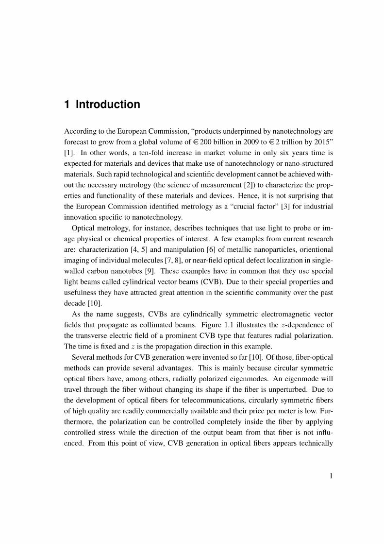
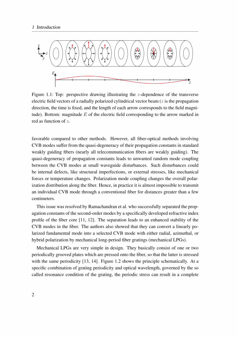
As the name suggests, CVBs are cylindrically symmetric electromagnetic vectorfields that propagate as collimated beams. Figure 1.1 illustrates the z-dependence ofthe transverse electric field of a prominent CVB type that features radial polarization.The time is fixed and z is the propagation direction in this example.
Several methods for CVB generation were invented so far [10]. Of those, fiber-opticalmethods can provide several advantages. This is mainly because circular symmetricoptical fibers have, among others, radially polarized eigenmodes. An eigenmode willtravel through the fiber without changing its shape if the fiber is unperturbed. Due tothe development of optical fibers for telecommunications, circularly symmetric fibersof high quality are readily commercially available and their price per meter is low. Fur-thermore, the polarization can be controlled completely inside the fiber by applyingcontrolled stress while the direction of the output beam from that fiber is not influ-enced. From this point of view, CVB generation in optical fibers appears technically
1
1 Introduction
z
z
x
y
E
Figure 1.1: Top: perspective drawing illustrating the z-dependence of the transverseelectric field vectors of a radially polarized cylindrical vector beam (z is the propagationdirection, the time is fixed, and the length of each arrow corresponds to the field magni-tude). Bottom: magnitude E of the electric field corresponding to the arrow marked inred as function of z.
favorable compared to other methods. However, all fiber-optical methods involvingCVB modes suffer from the quasi-degeneracy of their propagation constants in standardweakly guiding fibers (nearly all telecommunication fibers are weakly guiding). Thequasi-degeneracy of propagation constants leads to unwanted random mode couplingbetween the CVB modes at small waveguide disturbances. Such disturbances couldbe internal defects, like structural imperfections, or external stresses, like mechanicalforces or temperature changes. Polarization mode coupling changes the overall polar-ization distribution along the fiber. Hence, in practice it is almost impossible to transmitan individual CVB mode through a conventional fiber for distances greater than a fewcentimeters.
This issue was resolved by Ramachandran et al. who successfully separated the prop-agation constants of the second-order modes by a specifically developed refractive indexprofile of the fiber core [11, 12]. The separation leads to an enhanced stability of theCVB modes in the fiber. The authors also showed that they can convert a linearly po-larized fundamental mode into a selected CVB mode with either radial, azimuthal, orhybrid polarization by mechanical long-period fiber gratings (mechanical LPGs).
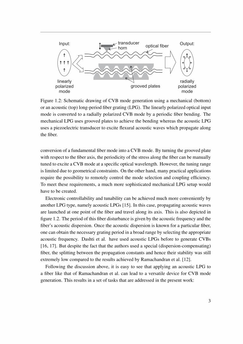
Mechanical LPGs are very simple in design. They basically consist of one or twoperiodically grooved plates which are pressed onto the fiber, so that the latter is stressedwith the same periodicity [13, 14]. Figure 1.2 shows the principle schematically. At aspecific combination of grating periodicity and optical wavelength, governed by the socalled resonance condition of the grating, the periodic stress can result in a complete
2
grooved plates
optical fiber
linearlypolarized
mode
Input: Output:
radiallypolarized
mode
transducerhorn
Figure 1.2: Schematic drawing of CVB mode generation using a mechanical (bottom)or an acoustic (top) long-period fiber grating (LPG). The linearly polarized optical inputmode is converted to a radially polarized CVB mode by a periodic fiber bending. Themechanical LPG uses grooved plates to achieve the bending whereas the acoustic LPGuses a piezoelectric transducer to excite flexural acoustic waves which propagate alongthe fiber.
conversion of a fundamental fiber mode into a CVB mode. By turning the grooved platewith respect to the fiber axis, the periodicity of the stress along the fiber can be manuallytuned to excite a CVB mode at a specific optical wavelength. However, the tuning rangeis limited due to geometrical constraints. On the other hand, many practical applicationsrequire the possibility to remotely control the mode selection and coupling efficiency.To meet these requirements, a much more sophisticated mechanical LPG setup wouldhave to be created.
Electronic controllability and tunability can be achieved much more conveniently byanother LPG type, namely acoustic LPGs [15]. In this case, propagating acoustic wavesare launched at one point of the fiber and travel along its axis. This is also depicted infigure 1.2. The period of this fiber disturbance is given by the acoustic frequency and thefiber’s acoustic dispersion. Once the acoustic dispersion is known for a particular fiber,one can obtain the necessary grating period in a broad range by selecting the appropriateacoustic frequency. Dashti et al. have used acoustic LPGs before to generate CVBs[16, 17]. But despite the fact that the authors used a special (dispersion-compensating)fiber, the splitting between the propagation constants and hence their stability was stillextremely low compared to the results achieved by Ramachandran et al. [12].
Following the discussion above, it is easy to see that applying an acoustic LPG toa fiber like that of Ramachandran et al. can lead to a versatile device for CVB modegeneration. This results in a set of tasks that are addressed in the present work:
3
1 Introduction
• Construction and test of an acoustic LPG in conjunction with an index-tailoredfiber for the individual excitation of second-order modes
• Assessment of efficiency and bandwidth of selective CVB mode excitation
• Application of this fiber-optical CVB mode generator to high-resolution micros-copy to demonstrate its usefulness
To address the tasks above, the outline of this thesis is as follows: Chapter 2 brieflysummarizes the electromagnetic theory of optical waveguides. It also includes a shortoverview of scalar coupled mode theory for guided modes propagating in the same di-rection. Chapter 3 deals with the description of the polarization of light and the basicprinciples behind polarization preservation in optical fibers. Furthermore, methods forCVB generation are reviewed and compared to the acoustic LPG approach. Chapter 4presents a numerical simulation of an index-tailored fiber fabricated after the design de-veloped by Ramchandran et al. However, compared to the latter, the core dimensionsare reduced in the present work for reducing the number of guided modes at shorterwavelengths. The mode fields and the corresponding propagation constants are calcu-lated in the simulation. Geometrical imperfections and their consequences for modecoupling will be analyzed in detail. On the basis of the simulation results, the acousticLPG incorporating the special fiber is constructed. Chapter 5 contains the basic theoryof acoustic LPGs, a comparison to other grating types, and a detailed account to the con-struction as well as the electrical, mechanical, and optical characterization of the LPG.The excitation of selected polarization modes is demonstrated. Chapter 6 documentsthe application of polarization modes generated by the acoustic LPG to high-resolutionmicroscopy. The acoustic LPG generates appropriate second-order polarization modesin the fiber which are used for illumination in the microscope. Probing the focal fieldby a gold nanoparticle shows that the field can be tailored by selection of the fiber’spolarization modes. Chapter 7 concludes the present thesis.
4
2 Fundamentals of optical waveguides
2.1 Introduction
This chapter will introduce the electromagnetic theory necessary to describe opticalwaveguides and the mode fields which can propagate within them. This includes Max-well’s equations and special forms of the vector wave equations that can be derived.Furthermore, the modal expansion of electromagnetic fields is introduced, wherebypropagating, evanescent, and radiating modes can be distinguished. Subsequently, themultiple multipole method for numerical computation of mode fields and propagationconstants is outlined. Finally, coupled mode theory, which describes power transfer be-tween modes caused by a change of the electric permittivity of the waveguide media,is introduced for co-directional mode coupling. Several of the formulas and definitionsmade in this section will be referred to in following chapters of this thesis.
2.2 Maxwell’s equations and vector wave equations
Maxwell’s equations (ME) are at the core of classical electromagnetics and form thebasis of many text books on optics [18, 19, 20, 21]. This section will only give a shortsummary of the most important equations related to ME and the resulting wave equa-tions.
ME describe the interplay of electric and magnetic fields, represented by field vec-tors E and H , respectively, and the magnetic induction and the electric displacement,represented by the vectors B and D , respectively. In their differential form, ME readas:
∇B = 0 (2.1)
∇×E +∂B
∂t= 0 (2.2)
∇D = ρ (2.3)
∇×H − ∂D
∂t= j . (2.4)
5
2 Fundamentals of optical waveguides
Here, j is the electrical current density and ρ the electrical charge density. They repre-sent the sources of electromagnetic fields. The vectors B and D are the macroscopicmaterial response to the fields H and E , respectively, which can be expressed in thefollowing constitutive equations:
B = µH = µ0H + M (2.5)
D = εE = ε0E + P . (2.6)
In the above relations, the dielectric permittivity ε and the magnetic permeability µ
were introduced. Furthermore, the magnetic and electric polarization M and P can bedefined, where ε0 and µ0 are the permittivity and permeability of vacuum, respectively.
At any boundary separating materials 1 and 2 with material properties (ε1, µ1) and(ε2, µ2), the field vectors have to fulfill the following boundary conditions:
n(B1 −B2) = 0 (2.7)
n × (E 1 −E 2) = 0 (2.8)
n(D1 −D2) = σ (2.9)
n(H 1 −H 2) = K . (2.10)
Here, σ and K are electric surface charge density and electric surface current density,respectively. The vector n is oriented normally to the boundary everywhere.
For isotropic materials, both µ and ε are scalar quantities. If there are neither freecurrents and nor free charges, the vector wave equation can be derived from ME in thefollowing form:
∇× (1
µ∇×E) + ε
∂2E
∂t2= 0 (2.11)
∇× (1
ε∇×H ) + µ
∂2H
∂t2= 0. (2.12)
The vector wave equations 2.11 and 2.12 govern the propagation of electromagneticradiation in matter. The electric and magnetic fields are coupled implicitly through εand µ, which contain the magnetic and electric polarizations, in essence the response ofthe medium to an external field.
For piecewise homogeneous media, 2.11 and 2.12 may be further reduced. Then,inside each domain i with material properties εi and µi, the fields obey:
∇2E i − µiεi∂2E i
∂t2= 0 (2.13)
∇2H i − µiεi∂2H i
∂t2= 0 (2.14)
6
2.3 Optical waveguides
If solutions to equations 2.13 and 2.14 are found, the fields are required to match at theboundaries between neighboring domains, in accordance with the boundary conditions2.7 through 2.10, to result in a solution of the general vector wave equations 2.11 and2.12.
2.3 Optical waveguides
An optical waveguide constitutes a physical structure that is able to direct electro-magnetic (EM) radiation along a defined direction in the visible (or neighboring) part ofthe spectrum. Solutions Ψ(r , t) of the vector wave equations 2.13 and 2.14 that fulfillthe boundary conditions given by the structure and material properties of the waveguideare called the modes of the waveguide. These modes form a complete and minimal setof eigenfunctions which describe all possible fields in the waveguide.
Waveguides can be classified into lossless and lossy guides. Especially for opticalfrequencies, the material loss in dielectric waveguides, like optical fibers, is often neg-ligible. So, they will be considered to be lossless throughout this work. In contrast, forwaveguides where at least part of the structure is made from metal, ohmic losses areusually present. These waveguides are called metallic waveguides. The material lossesare described by a finite imaginary part of the metal’s permittivity ε(ω).1
The distinction between lossless and lossy waveguides also plays an important role inthe classification of waveguide modes. Since the classification for lossless waveguidesis clearer and more intuitive, this type of waveguides is discussed first.
2.3.1 Dielectric waveguides
Non-magnetic dielectric materials are usually described by their refractive index whichis related to the permittivity of the medium through n2 = ε. Therefore, the waveguidestructure is characterized by its refractive index profile n(x, y, z), which determinesthe boundary conditions and hence the possible modal solutions of the vector waveequations 2.11 and 2.12.
One can distinguish between bound modes and radiation modes [22, 23]. The formerdescribe waves which propagate along the waveguide whereas the latter describe allwaves that eventually propagate away from the waveguide in perpendicular directionto the transmission axis. Furthermore, there are also evanescent modes that do not
1 ε(ω) is also called the dielectric function.
7
2 Fundamentals of optical waveguides
propagate at all. Therefore, only bound modes can transmit power over larger distancesalong the waveguide. The evanescent modes, on the other hand, represent localizedenergy, that is stored in the guide.
There is only a limited number of bound modes for each waveguide and an infinitenumber of radiation modes and evanescent modes. Every possible field can be describedas a combination of these mode fields, which is called modal expansion of the field.
If, for example, we consider a cylindrical waveguide with its propagation axis alignedin z-direction, we have a refractive index profile n = n(x, y), independent of z. Wefurther assume a time-harmonic dependence of the form exp(iωt) for the fields. Then,the field F (representing either the electric field E or the magnetic field H ) can beexpanded in terms of its bound and radiation modes. This reads as:
F (x, y, z, t) =∑ν
aνf ν(x, y)exp(iωt− iβνz)+
+∑ν
∫aν(β)f ν(x, y, β)exp(iωt− iβz)dβ. (2.15)
In the first term, a specific guided mode with index ν is characterized by its modalfield f ν , expansion coefficient aν , and wavenumber βν . The second term is similar,but instead of a summation over discrete βν there is an integration over a continuousspectrum of wavenumbers β. The radiation and evanescent modes with label ν are bothincluded in the second term. Implicitly, equation 2.15 also contains the summation overdegenerated modes having the same wavenumber, as well as forward and backwardtraveling modes (with opposite sign of βν or β). If the waveguide is bound in twodimensions, as is the case for cylindrical waveguides, actually two indexes have to beused instead of one to fully characterize all modes [24, page 27]. However, the secondindex is suppressed in equation 2.15 to keep the notation short.
Two bound modes of an unperturbed waveguide do not exchange power, and, sincelossless guides are considered here, the mode’s amplitudes remain constant. Therefore,an orthogonality relation can be defined for two modes ν and µ [24, page 26]:∫∫ ∞
−∞dxdy E tν ×H ∗
tµ = 0 for ν 6= µ. (2.16)
The subscript t stands for the transverse components of the fields while the asteriskindicates the complex conjugate.
In dielectric optical waveguides, the wavenumbers of bound modes are real valuedand positive for modes propagating in the +z direction. For simple waveguides, such as
8
2.3 Optical waveguides
single- or multi-mode fibers with a step-like refractive index profile, the guiding mecha-nism can be understood as a total internal reflection at a boundary between materials ofdifferent index of refraction. Consequently, the waves are mainly guided in the higherindex regions.
The wavenumber β of a guided mode can take on values between nhighk0 and ninfk0,where k0 = 2π/λ, and k0 and λ are the vacuum wavenumber and wavelength, respec-tively, and the following inequality holds:
nhighk0 ≥ β ≥ ninfk0. (2.17)
The value ninf is the refractive index at infinite distance from the waveguide axis, usuallyconsidered as the cladding index ncl, where the fields of guided modes are required to bezero, and nhigh is the highest index of refraction in the waveguide, which is supposed tobe located somewhere close to the waveguide axis. Motivated by the above inequality, anormalized wavenumber neff = β/k0 is often introduced, which is also called effectiveindex of a mode. Consequently, ninf < neff < nhigh holds for guided modes. Anothernormalization of the propagation constant is also common [25, eq. 8.35]:
beff =n2
eff − n2inf
n2high − n2
inf
. (2.18)
The normalized (effective) propagation constant beff , as defined in equation 2.18, willhave values from 0 to 1 for the guided modes. It is not only applicable to fibers with asimple single-step index profile, but also to more general cases, like W- and M-profiles,which are commonly found in dispersion shifted fibers [26]. The values of ninf and nhigh
have to be chosen in accordance with the specified refractive index profile.
2.3.2 Metallic waveguides
Metals are characterized by their complex and frequency dependent dielectric functionε = ε(ω). For metals at ω < ωp one has Reε < 0, due to the conductivity, andImε > 0, corresponding to ohmic heating of the metal. ωp is the plasma frequencyof the metal. The presence of losses makes the definition of guided modes non-trivial inmetallic waveguides, since the energy of a guided mode is not conserved when it prop-agates along the guide. Instead, the energy will be dissipated in the metal eventually.This is detailed, for instance, in [27, page 240] and [28, 29].
9
2 Fundamentals of optical waveguides
As a result of the presence of losses, the propagation constant of a guided mode willbecome complex and is then defined as γ = β + iα, where a positive valued α is thedamping constant. In principle, a modal expansion of the form of 2.15 is possible, withβ replaced by γ, but defining an orthogonality relation becomes much more complexand will not be attempted here, although it is still possible (see for example [30]).
If α and β are non-zero, no sharp distinction is possible between guided propagatingand evanescent modes. Nonetheless, if α becomes significantly larger than β, the modeis better described as an evanescent mode, because it will decay within a few cycles ofoscillations.
An important implication for lossy waveguides is that β is not limited to the wave-number of an equivalent lossless structure (with α = 0). Consequently, one cannotdefine a strict value range for the guided modes anymore, as was possible for losslessdielectric waveguides. At least one can usually exclude modes with very high damping(α β) from the discussion, because they are of little practical interest.
Because of the reasons mentioned above, the analysis of metallic waveguides is moredemanding than that of lossless dielectric guides. Nonetheless, metallic optical waveg-uides (also called plasmonic waveguides) are an important area of ongiong research innanotechnology, since they can tightly bind optical fields and squeeze them to extremelysmall volumes.
2.4 Numerical calculation of modes by the multiple multipoleprogram
As pointed out in [27, 29], an analytical calculation of mode fields and wavenumbersare only possible for relatively simple waveguide structures, e.g. circular symmetricguides. Usually, even for the analytical solution, transcendental equations have to besolved for the wavenumber, which again requires numerical techniques. Therefore,explicit numerical treatment may provide results more conveniently.
A very accurate numerical technique for solving electromagnetic problems, includingdifferent forms of waveguides like 2D cylindrical waveguides [28] and periodic waveg-uides (e.g. photonic crystals [31]), is the Multiple Multipole Program (MMP) [32, 27].MMP is a semi-analytical technique where the electromagnetic (EM) fields are approx-imated by a linear series expansion. Each expansion function is chosen to already fulfillthe vector wave equations 2.13 and 2.14 inside the homogeneous domain for which it isused. The expansion parameters are then calculated by minimizing the error (weighted
10
2.4 Numerical calculation of modes by the multiple multipole program
error integrals) of the fields at matching points distributed along the boundaries betweendifferent domains. This error also serves as a measure for the quality of the approxima-tion, which is very helpful during the development of the model.
Mathematically, the set of equations formed by the boundary conditions at all match-ing points can be treated as a matrix equation. For waveguides, the components of thederived MMP-matrix depend on an eigenvalue that can be calculated by solving thetranscendental equation [27, page 234-241]:
det |M(e)| = 0. (2.19)
The eigenvalue e corresponds to the normalized propagation constant γ/k0 as intro-duced in section 2.3.1. After the eigenvalue has been calculated, the MMP-matrix canbe solved for a particular value of e, which results in an eigenvector that essentiallycontains the expansion parameters for the corresponding mode field. By calculating theexpansion parameters, one has, in principle, determined the field for any point in spaceat once. Of course, in order to achieve field values in a certain region of space, oneneeds to evaluate the expansion functions for a discrete set of points, which may also becomputationally demanding.
In the following, an example of a relatively simple mode field calculation for a circu-lar cylindrical fiber will be presented.
2.4.1 Representation of simulated mode fields
To obtain a quick overview of the field distribution of a waveguide mode which is com-parable also to experimentally measured mode fields, it is useful to view the field’saveraged intensity instead of individual field components at specific moments in time,because the former is the quantity measured by photo detectors. On the other hand, thefield intensity for itself is often indistinguishable for degenerate or almost degeneratemodes, which only differ in their polarization. Therefore, information of the polariza-tion should also be contained in a mode field’s representation.
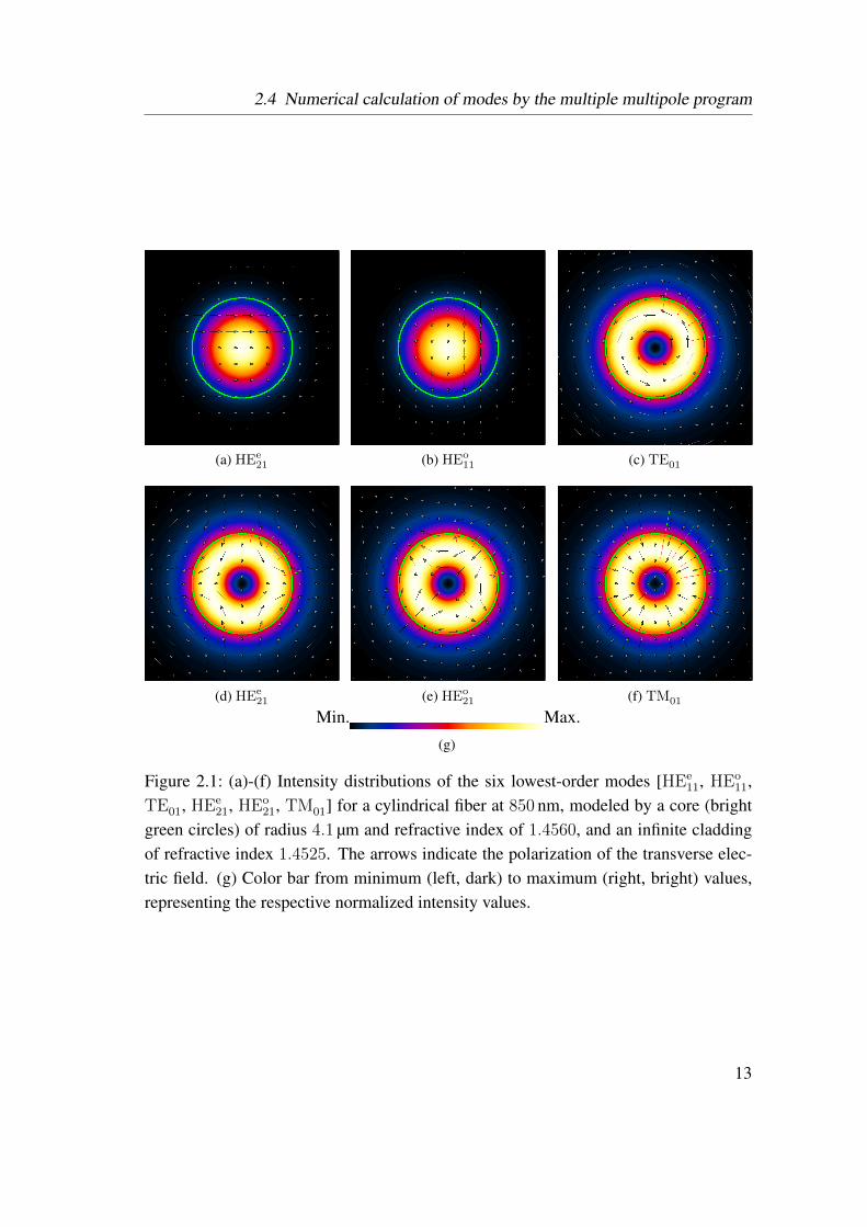
Figure 2.1 shows an example of such a mode field representation for the six lowest-order modes of a circular dielectric optical fiber with a single-step refractive index pro-file. More details are given in the figure caption. The color scale corresponds to thenormalized field intensity. The black arrows indicate the polarization of the transverseelectric field at a fixed point in the oscillation cycle. The direction and length of thearrows indicate the local orientation and strength of the transverse field, although thearrow scaling is optimized to view the arrow directions. Of course, the length and sign
11

2 Fundamentals of optical waveguides
of the transverse fields will oscillate in time and along the propagation direction, whichis important to remember when superpositions and interference of different mode fieldsare considered.
If not otherwise stated, the mode field representation of figure 2.1 (averaged intensityand arrows for transverse electric fields) will be used throughout this work.
12
2.4 Numerical calculation of modes by the multiple multipole program
(a) HEe21 (b) HEo
11 (c) TE01
(d) HEe21 (e) HEo
21 (f) TM01
Min.
(g)
Max.
Figure 2.1: (a)-(f) Intensity distributions of the six lowest-order modes [HEe11, HEo
11,TE01, HEe
21, HEo21, TM01] for a cylindrical fiber at 850 nm, modeled by a core (bright
green circles) of radius 4.1 µm and refractive index of 1.4560, and an infinite claddingof refractive index 1.4525. The arrows indicate the polarization of the transverse elec-tric field. (g) Color bar from minimum (left, dark) to maximum (right, bright) values,representing the respective normalized intensity values.
13
2 Fundamentals of optical waveguides
2.5 Overview of coupled mode theory
2.5.1 Coupled mode equations
The coupled mode theory (CMT) describes an exchange of optical power between dif-ferent modes in a waveguide due to any disturbance ∆ε(x, y, z) of the undisturbed pro-file ε(x, y). CMT bases on power conservation and the orthogonality relation and cantherefore, in its original form, only be applied to lossless problems, as described in[33, 34, 35]. The main idea is to express the fields of the perturbed guide by the modesof the unperturbed guide, but with variable amplitudes. Due to the waveguide distur-bance ∆ε(x, y, z), the modes are no longer orthogonal and will exchange power, hencethey are coupled. CMT can be used to describe unintentional disturbances, like bendsor twists of an optical fiber, as well as deliberate modifications like Bragg reflection ortransmission gratings.
Using the notation of [33], the mode amplitudesAµ andBµ for forward and backwardpropagating modes, respectively, can be introduced from the amplitude of the modeexpansions aµ and bµ in equation 2.15. This reads as:
aµ(z) = Aµ(z)e−iβµz bµ(z) = Bµ(z)eiβµz. (2.20)
Therefore, the z-dependence due to the mode propagation is separated from that due tothe disturbance ∆ε, which is contained in Aµ(z) and Bµ(z). Now the coupled modeequations can be expressed in the form [33]:
∂Aµ∂z
= − i∑Aν(Kt
νµ +Kzνµ)e−i(βν−βµ)z (2.21)
+Bν(Ktνµ −Kz
νµ)ei(βν+βµ)z,∂Bµ
∂z= i∑Aν(Kt
νµ −Kzνµ)e−i(βν+βµ)z (2.22)
+Bν(Ktνµ +Kz
νµ)ei(βν−βµ)z.
Here, the summation is understood to contain all modes ν, including bound modes andradiation modes, according to the notation of [33]. Equations 2.21 and 2.22 contain thecoupling coefficients Kt and Kz for the transverse and longitudinal (z) field compo-nents. This distinction is necessary, since only the transverse fields are orthogonal. Kt
14
2.5 Overview of coupled mode theory
and Kz are defined as:
Ktνµ = ω
∫∫ +∞
−∞dxdyE tν∆εE tµ (2.23)
Kzνµ = ω
∫∫ +∞
−∞dxdyEzν
∆ε · ε∆ε+ ε
E∗zµ. (2.24)
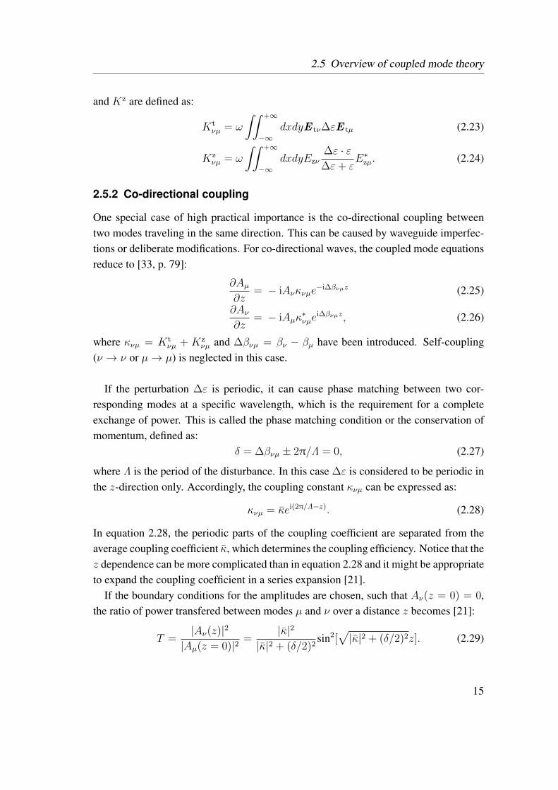
2.5.2 Co-directional coupling
One special case of high practical importance is the co-directional coupling betweentwo modes traveling in the same direction. This can be caused by waveguide imperfec-tions or deliberate modifications. For co-directional waves, the coupled mode equationsreduce to [33, p. 79]:
∂Aµ∂z
= − iAνκνµe−i∆βνµz (2.25)
∂Aν∂z
= − iAµκ∗νµe
i∆βνµz, (2.26)
where κνµ = Ktνµ + Kz
νµ and ∆βνµ = βν − βµ have been introduced. Self-coupling(ν → ν or µ→ µ) is neglected in this case.
If the perturbation ∆ε is periodic, it can cause phase matching between two cor-responding modes at a specific wavelength, which is the requirement for a completeexchange of power. This is called the phase matching condition or the conservation ofmomentum, defined as:
δ = ∆βνµ ± 2π/Λ = 0, (2.27)
where Λ is the period of the disturbance. In this case ∆ε is considered to be periodic inthe z-direction only. Accordingly, the coupling constant κνµ can be expressed as:
κνµ = κei(2π/Λ−z). (2.28)
In equation 2.28, the periodic parts of the coupling coefficient are separated from theaverage coupling coefficient κ, which determines the coupling efficiency. Notice that thez dependence can be more complicated than in equation 2.28 and it might be appropriateto expand the coupling coefficient in a series expansion [21].
If the boundary conditions for the amplitudes are chosen, such that Aν(z = 0) = 0,the ratio of power transfered between modes µ and ν over a distance z becomes [21]:
T =|Aν(z)|2
|Aµ(z = 0)|2=
|κ|2
|κ|2 + (δ/2)2sin2[
√|κ|2 + (δ/2)2z]. (2.29)
15
2 Fundamentals of optical waveguides
Equation 2.29 shows that the power is coupled sinusoidally forth and back between thetwo modes along the z-direction. Furthermore, a complete exchange of power is onlypossible, if the phase matching condition δ = 0 is satisfied. Since ∆β generally dependson the optical wavelength λ, this will be the case only for specific wavelengths. Assum-ing δ = 0, it can be further seen that the distance L after which complete exchange ofpower occurs for the first time is:
L =π
2|κ|. (2.30)
From equation 2.30 one finds that stronger coupling (with higher spatial frequencyof power exchange) is observed for higher values of κ. The value of κ follows fromthe overlap integrals 2.23 and 2.24 and depends on the mode fields and the permittivitydisturbance ∆ε.
2.6 Summary and conclusions
This chapter gave a summary of the most important equations governing the propagationof electromagnetic fields in optical waveguides. The multiple multipole method fornumerical calculation of waveguide mode fields and propagation constants was alsooutlined briefly. Finally, elements of the coupled mode theory were introduced, as willbe needed to understand the origin of the experimental results discussed in the chapter 5and 6. Especially the phase matching condition 2.27 should be borne in mind, as it is ofparamount importance in many coupled wave phenomena. In chapter 4, the normalizedpropagation constant beff and effective index neff will be frequently referred to.
16
3 Polarization control for fundamental and higherorder modes
3.1 Introduction
This chapter provides the terminology for describing the polarization of light beams infree space and in optical fibers. As outlined in section 2.2, optical radiation is classicallytreated as EM-radiation using Maxwell’s equations. When speaking of polarization, oneusually means the axis of vibration of the electric field vector in a plane perpendicularto the propagation direction of a beam of light [18, chapter 1.4]. Although, electromag-netic fields have non-zero components in all three dimensions in general. For collimatedbeams of light and beams in optical fibers, however, the component in propagation direc-tion is much weaker compared to the transverse field components and can be neglected.Furthermore, the orientation of the transverse polarization axis depends on time andspace. In the most general case, the electric field vector will perform an ellipse in thetransverse plane if observed at a fixed point in space. Thus, the important Stokes pa-rameters will be introduced to describe polarization mathematically and relations to theparameters of the polarization ellipse are given.
In practice, beams with a fixed transverse axis of vibration and those with a uni-form or symmetrical polarization distribution are mostly used. For this work in par-ticular, cylindrical vector beams are of great importance and will be introduced. Fur-thermore, some methods to generate them will be reviewed, including their respectiveadvantages and drawbacks. A focus is laid on fiber-optical methods to generate cylin-drical vector beams, since the acoustic long-period fiber gratings discussed in chapter 5are used exactly for this purpose. Finally, polarization control in optical fibers is dis-cussed briefly, whereby both single-mode polarization-maintaining fibers and higher-order mode polarization-maintaining fibers are taken into.
17
3 Polarization control for fundamental and higher order modes
3.2 Description of light polarization
3.2.1 Stokes parameters and the polarization ellipse
Stokes parameters are a mathematical description of the state of polarization of lightwhich is directly related to measurable intensities. The measurement involves two opti-cal elements the beam has to pass. These are a polarization analyzer with its transmis-sion axis at a variable angle θ with respect to the x-axis, and a quarter-wave plate (QWP)with its fast axis in x-direction, which is additionally inserted for one measurement. Inthe given orientation, the QWP retards the y-component of the electric field by a phaseangle φWP = 90 (or π/2) with respect to the x-component. The Stokes parameters cannow be determined from the intensities I(θ, φWP), which are measured after passing thepolarizer at the respective angle, as follows [18, 36]:
S0 = I(0o, 0o) + I(90o, 0o) (3.1)
S1 = I(0o, 0o)− I(90o, 0o) (3.2)
S2 = I(45o, 0o)− I(135o, 0o) (3.3)
S3 = I(45o, 90o)− I(135o, 90o). (3.4)
As can be seen from the equations above, six individual intensity values have to be mea-sured in order to fully determine the state of polarization. Only for S3 in equation 3.4,the QWP is necessary.
Since the polarization is not necessarily uniform over a transverse plane, the intensi-ties I(θ, φWP) and Stokes parameters Si also depend on the transverse position, althoughthis dependence is not expressed explicitly here.
The ratio:
η =S2
1 + S22 + S2
3
S20
(3.5)
is called the degree of polarization. The degree of polarization is linked to the temporalcoherence of the light field and describes how well the phase of the vector wave com-ponents are continuous and have a fixed relation to each other. In the simulations andexperiments of this work, only laser-light will be used. The latter can be approximatedas fully coherent continuous waves in this context. Therefore, η is considered to be 1
throughout this work. In practical applications, however, sources with lower coherenceare often used and the degree of polarization may become important if optical signalshave to be transmitted over long distances, so depolarizing effects can accumulate.
18
3.2 Description of light polarization
If η = 1 holds, the stokes parameters are not independent and, for instance, |S3|could be calculated from S0, S1, and S2. However, the sign of S3 cannot be clarifiedwithout the last measurement (equation 3.4). This piece of information corresponds tothe handedness of the polarization ellipse which the electric field vector describes whilethe wave propagates.
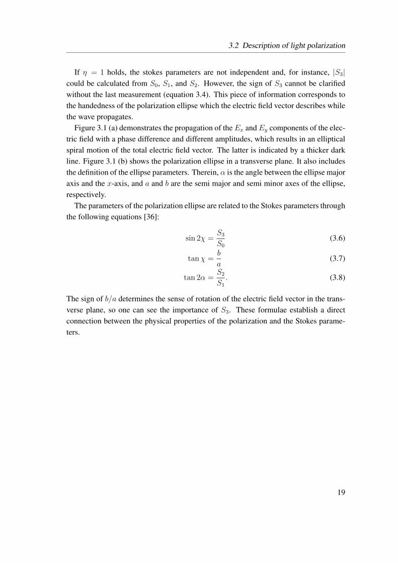
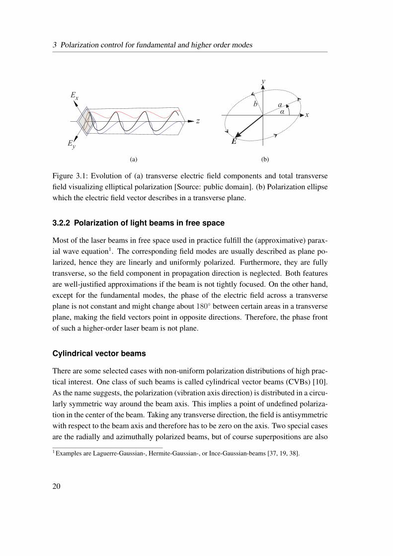
Figure 3.1 (a) demonstrates the propagation of theEx andEy components of the elec-tric field with a phase difference and different amplitudes, which results in an ellipticalspiral motion of the total electric field vector. The latter is indicated by a thicker darkline. Figure 3.1 (b) shows the polarization ellipse in a transverse plane. It also includesthe definition of the ellipse parameters. Therein, α is the angle between the ellipse majoraxis and the x-axis, and a and b are the semi major and semi minor axes of the ellipse,respectively.
The parameters of the polarization ellipse are related to the Stokes parameters throughthe following equations [36]:
sin 2χ =S3
S0
(3.6)
tanχ =b
a(3.7)
tan 2α =S2
S1
. (3.8)
The sign of b/a determines the sense of rotation of the electric field vector in the trans-verse plane, so one can see the importance of S3. These formulae establish a directconnection between the physical properties of the polarization and the Stokes parame-ters.
19
3 Polarization control for fundamental and higher order modes
z
Ex
Ey
(a)
E
b a
x
y
α
(b)
Figure 3.1: Evolution of (a) transverse electric field components and total transversefield visualizing elliptical polarization [Source: public domain]. (b) Polarization ellipsewhich the electric field vector describes in a transverse plane.
3.2.2 Polarization of light beams in free space
Most of the laser beams in free space used in practice fulfill the (approximative) parax-ial wave equation1. The corresponding field modes are usually described as plane po-larized, hence they are linearly and uniformly polarized. Furthermore, they are fullytransverse, so the field component in propagation direction is neglected. Both featuresare well-justified approximations if the beam is not tightly focused. On the other hand,except for the fundamental modes, the phase of the electric field across a transverseplane is not constant and might change about 180 between certain areas in a transverseplane, making the field vectors point in opposite directions. Therefore, the phase frontof such a higher-order laser beam is not plane.
Cylindrical vector beams
There are some selected cases with non-uniform polarization distributions of high prac-tical interest. One class of such beams is called cylindrical vector beams (CVBs) [10].As the name suggests, the polarization (vibration axis direction) is distributed in a circu-larly symmetric way around the beam axis. This implies a point of undefined polariza-tion in the center of the beam. Taking any transverse direction, the field is antisymmetricwith respect to the beam axis and therefore has to be zero on the axis. Two special casesare the radially and azimuthally polarized beams, but of course superpositions are also
1 Examples are Laguerre-Gaussian-, Hermite-Gaussian-, or Ince-Gaussian-beams [37, 19, 38].
20
3.2 Description of light polarization
possible, as for linearly polarized beams. Due to the high symmetry, it is sufficient tomathematically describe the polarization of one point in the beam. The polarizationdistribution in the transverse plane can then be inferred from symmetry. CVBs attractedgreat attention in the scientific community and their fundamentals and applications aredescribed in detail in [10]. Applications related to high resolution far-field microscopywill be discussed in section 6.2.
3.2.3 Polarization of light beams in optical fibers
Describing the exact polarization distribution of guided beams of light in optical fibersis more complex than in free space. This is because the individual mode fields are notnecessarily uniformly polarized and different propagation constants have to be takeninto account for mode combinations.
The most simple fiber geometry is a circularly symmetric, weakly guiding fiber,which has a very small difference between the refractive index of core and cladding(weakly guiding fiber). The mode fields of these fibers are usually approximated bylinearly polarized (LP) modes, that can be polarized either in the x- or the y-direction,similar to Gaussian beams in free space [35]. As is shown in figure 2.1 (a) and (b), the(exact) fundamental HE11 modes of a weakly guiding fiber can be described quite ac-curately by LP modes (labeled LP01), indeed. Although, the HE11 modes possess somesmall field component in the direction orthogonal to the main polarization direction andalso a non-zero z-component. The latter means that these guided modes are only ap-proximately transverse. The similarity between the HE11 and LP01 modes will decreaseif the refractive index difference between fiber core and cladding increases.
For the next-higher set of modes, also called the second-order modes [see figures2.1(c)-(e)], it is clear that an approximation of the physical vector modes TE01, HE21,and TM01 by LP modes cannot describe the polarization distribution well. It is inter-esting to notice, nonetheless, that truly radially and azimuthally polarized modes areamong the second-order modes, whereby TM01 and TE01 have truly transverse mag-netic or electric field, respectively. Therefore, using optical fibers for the generation ofCVBs appears to be a straightforward idea.
If the waveguide has a non-circular, e.g. elliptical, symmetry, the field and polariza-tion distributions will align with respect to the symmetry axes. The shape and polariza-tion of the higher-order modes will be much more affected than that of the fundamentalmodes. To stay with the example of an elliptical geometry, the polarizations of all modeswill be aligned with one of the ellipse principle axes. Therefore, non-fundamental
21
3 Polarization control for fundamental and higher order modes
modes can be described by LP modes much better in elliptical guides [35, sec. 13-8]. Only for high refractive index differences, deviations from the LP approximationwill again become apparent close to the interfaces between the respective waveguidemedia.
In summary, one can keep in mind that the polarization distribution in fibers is strong-ly affected by the waveguide geometry. In several situations, an approximative descrip-tion by linearly polarized modes is justified, but one should be aware of the limitations,especially if CVBs are considered. For a simple notation in the subsequent chapters, theterms linearly polarized, radially polarized, and azimuthally polarized will be used todescribe the polarization of second-higher modes in fibers with circular and non-circulargeometry, depending on which of those terms best describes the relevant properties ofthe specific mode.
3.3 Short overview of cylindrical vector beam generation
CVBs were introduced in section 3.2.2. In this section, a short overview of methodsfor generating such beams will be given. According to the recent review of [10], themethods can be classified into two categories, active and passive, whereby the passivemethods are further divided into those which do use an optical fiber and those that don’t.Considering the actual part or element of the optical setup which is responsible for theCVB generation, the different methods may be alternatively called:
1. free-beam methods (passive),
2. intra-cavity methods (active),
3. fiber-optical and waveguide methods (passive).
Without going into detail or thriving for completeness, some examples of the methodsabove will be presented in the following. The focus will set on their typical advantagesand drawbacks. More details can be found in [10], for instance.
Free-beam methods
To name a few examples, a segmented wave-plate [39], a nematic liquid crystal (LC)cell with appropriately rubbed front- and back-surfaces [40], or a spatial light modulator(SLM) [41, 42] can be used to create CVBs from a freely propagating, linearly polarizedGaussian beam.
22
3.3 Short overview of cylindrical vector beam generation
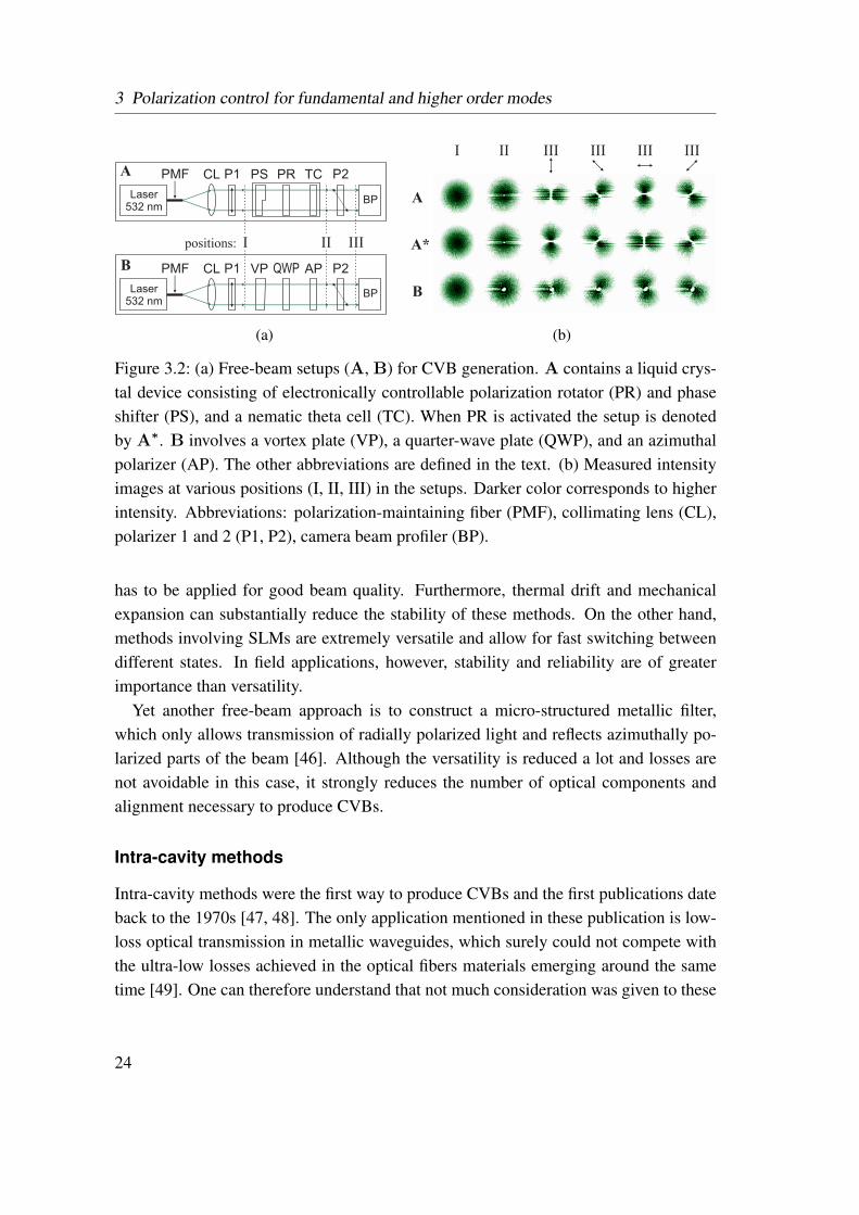
Figure 3.2 shows two examples of commercially available radial polarization con-verter arrangements. On the left hand side of the figure, the two setups, denoted as Aand B, are depicted. Measured intensity images from positions I, II, and III are depictedon the right hand side.
Setup A contains a fiber coupled laser source at 532 nm wavelength with a polariza-tion-maintaining (PM) fiber and a collimating lens (CL). The polarization optics includetwo polarizers (P1 and P2), whereby P1 has a fixed transmission axis along the verticaldirection and P2 can be rotated about defined angles. Between the polarizers are anelectronically controllable phase shifter (PS), which retards the upper half of the beamwith respect to the lower half, an electronically controllable nematic LC polarizationrotator (PR), and a nematic theta cell (TC) that converts the linearly polarized inputbeam into an azimuthally or radially polarized beam. The emerging beam is azimuthallypolarized if the PR is inactive and the input polarization axis is vertical. The setup isdenoted as A∗ if the polarization rotator is active, which results in a radially polarizedoutput beam. PS, PR, and TC are parts of a single, commercially available device [43].
In setup B only the inner three polarization controlling components are exchangedwith respect to setup A. The first of these elements is a vortex plate (VP) [44], alsocalled spiral phase element, which adds a linearly increasing phase change from 0 to 2π
along the azimuthal direction to the beam. The second element is a QWP and the thirdelement is an azimuthal polarizer (AP) [45]. The latter consists of a circular grid wirepolarizer which absorbs radial polarization components and lets azimuthal polarizationcomponents pass. The output beam from this setup is therefore an azimuthally polarizedbeam. Additional optical elements, like two half-wave plates (HWPs) [10], have to beadded if a radially polarized beam or other generalized CVBs are desired.
On the right hand side of figure 3.2 one can see the intensity images acquired by acamera beam profiler (BP) at positions I, II, or III, respectively. As can be seen, thephase step in either setup creates a defect line in the center of the beam. In setup A
the defect line extends through the full width of the beam while in setup B it appearsonly at one half of the beam width, since the vortex phase element varies the phasecontinuously expect at the step from 0 to 2π. The middle row of intensity images showsthat the polarization can be switched conveniently between azimuthal and radial byapplying a voltage to the electrically controllable polarization rotator PR.
A key advantage of these free-beam methods is that they work in a broad wavelengthrange. On the other hand, free-beam methods usually need careful alignment of theoptical elements involved, especially for LC devices, and additional spatial filtering
23
3 Polarization control for fundamental and higher order modes
Laser532 nm
Laser532 nm
BP
BP
CL
CL
TC
AP
PS
VP
I
I
II
II III III IIIIII
III
PR
QWP
PMFA
A
A*
B
B PMF
positions:
P1
P1
P2
P2
(a) (b)
Figure 3.2: (a) Free-beam setups (A, B) for CVB generation. A contains a liquid crys-tal device consisting of electronically controllable polarization rotator (PR) and phaseshifter (PS), and a nematic theta cell (TC). When PR is activated the setup is denotedby A∗. B involves a vortex plate (VP), a quarter-wave plate (QWP), and an azimuthalpolarizer (AP). The other abbreviations are defined in the text. (b) Measured intensityimages at various positions (I, II, III) in the setups. Darker color corresponds to higherintensity. Abbreviations: polarization-maintaining fiber (PMF), collimating lens (CL),polarizer 1 and 2 (P1, P2), camera beam profiler (BP).
has to be applied for good beam quality. Furthermore, thermal drift and mechanicalexpansion can substantially reduce the stability of these methods. On the other hand,methods involving SLMs are extremely versatile and allow for fast switching betweendifferent states. In field applications, however, stability and reliability are of greaterimportance than versatility.
Yet another free-beam approach is to construct a micro-structured metallic filter,which only allows transmission of radially polarized light and reflects azimuthally po-larized parts of the beam [46]. Although the versatility is reduced a lot and losses arenot avoidable in this case, it strongly reduces the number of optical components andalignment necessary to produce CVBs.
Intra-cavity methods
Intra-cavity methods were the first way to produce CVBs and the first publications dateback to the 1970s [47, 48]. The only application mentioned in these publication is low-loss optical transmission in metallic waveguides, which surely could not compete withthe ultra-low losses achieved in the optical fibers materials emerging around the sametime [49]. One can therefore understand that not much consideration was given to these
24
3.3 Short overview of cylindrical vector beam generation
exotic laser modes. However, as more applications for CVBs appeared, many adaptedand optimized intra-cavity methods were developed. An overview can again be foundin [10].
Intra-cavity methods provide a good beam quality since the beam shape is directlydetermined by the geometry of the cavity. On the other hand, these methods require awell-trained operator for alignment, they can only produce quasi-monochromatic radi-ation, due to the small line width of a laser, and they are less flexible when it comes tochanging the output polarization. Furthermore, the equipment for such devices is usu-ally quite expensive. If at least one particular CVB can be created by such a method,free-beam methods can also be applied in conjunction with intra-cavity methods to con-vert a radially polarized beam into an azimuthally polarized one, for instance.
Recently, highly compact vertical cavity surface-emitting lasers (VCSELs) were pre-sented that emit CVBs directly [50, 51]. Although the beam quality still needs improve-ment, these emitters could be combined in novel integrated sensors and other devices.For example this approach could benefit near-field optical microscopy by constructingintegrated light emitting near-field probes, as was proposed earlier by Heisig et al. [52].
Another current approach is to apply Yb-doped few-mode fibers as gain medium andmode selector in the laser cavity. Reports of this can be found in [53, 54, 55, 56, 57].[57] also demonstrated that the output mode of the laser can be switched in a controlledmanner by simply applying pressure to the fiber. A purely fiber-optical laser whichallows selection of radially or azimuthally polarized modes was presented recently in[58]. Of course, fiber-lasers have properties of both intra-cavity and fiber-optical meth-ods, but since they incorporate active light generation, they have been placed in thissection.
Fiber-optical methods
In comparison to the methods described above, fiber-optical methods for CVB genera-tion have the advantage that the output intensity and polarization distribution can poten-tially be controlled completely inside the fiber and no adjustments have to be made tothe optical path after the fiber output in order to change the output polarization. There-fore, the direction of a collimated output beam from the fiber is very stable. Additionalspatial filtering can be avoided, since the fiber already provides a suitable cylindricalbeam symmetry.
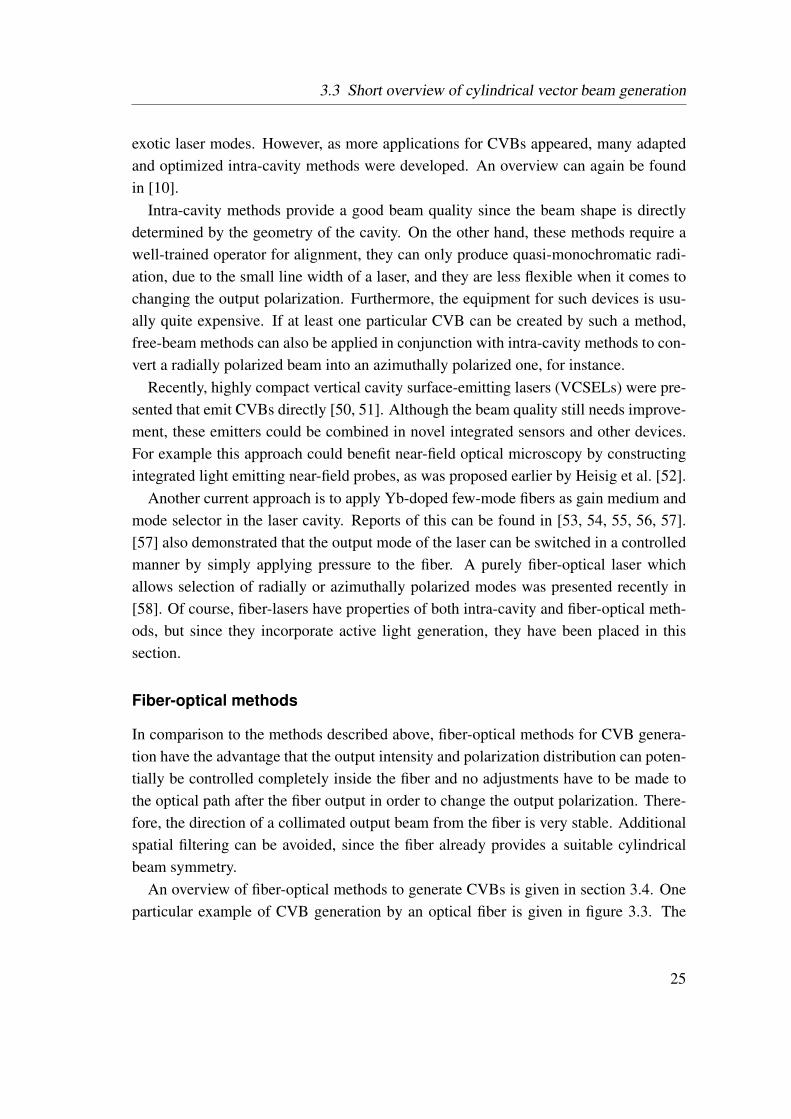
An overview of fiber-optical methods to generate CVBs is given in section 3.4. Oneparticular example of CVB generation by an optical fiber is given in figure 3.3. The
25
3 Polarization control for fundamental and higher order modes
Laser532 nm
SCL FL
HW
P VP
QW
PPMF TMFP1 P2P2:
(a) (b)
Figure 3.3: (a) Setup with optical two-mode fiber (TMF) for CVB generation. (b) Beamintensity photographs taken from the paper screen (S). Abbreviation: polarization main-taining fiber (PMF), collimating lens (CL), polarizers 1 and 2 (P1, P2), focusing lens(FL).
setup depicted in figure 3.3 (a) consists of similar free-beam components as for the free-beam methods described above, but the spatial filtering and CVB mode selection is pro-vided by an optical two-mode fiber (TMF). The most important components concerningthe polarization mode excitation are the HWP, which rotates the linear polarization in-cident from the left, and the QWP, which converts the linear polarization to ellipticalpolarization. Furthermore, the vortex plate (VP) is used to create an intensity minimumin the beam center and to provide the appropriate azimuthal phase distribution. Theresulting beam is focused by a focusing lens (FL) on the entrance face of the TMF,whereby the position of the focus is manipulated in three dimensions and the beam isalso tilted to achieve strong excitation of the desired CVB mode in the fiber. Addition-ally, the two-mode fiber is bent purposefully to assist the mode selection. The alignmentis rather time consuming, but stable over hours after initial set-up. However, any addi-tional mechanical stress to the fiber can destroy the mode purity. The steps describedhere are a combination of several techniques [59, 60, 10, 61] which are described inmore detail in section 3.4.
The intensity pattern emerging from the TMF is captured on a paper screen (S) andrecored by a camera. The image colors represent the true colors as recored by thecamera. These images are shown in figure 3.3 (b). The left most image is taken withoutthe second polarizer (P2) and the four remaining images are taken with the polarizer.The orientation of the polarizer transmission axis is indicated by the arrows above eachimage. From the shape of the intensity patterns and their orientation with respect to thepolarizer transmission axis, radially polarized light can be identified. The intensity zeroin the beam center is also clearly visible. However, the intensity pattern without P2 is notcircularly symmetric and the intensity is not equally distributed between the two lobesin the images with P2. Also, the polarizer transmission axis and the pattern orientationdeviate about a few degrees. Therefore, it is clear that not only the radially polarized
26
3.4 Excitation of cylindrical vector beams in optical fibers
TM01 mode was excited, but also other second-higher modes are present, which leadto the imperfections that were just described. Nonetheless, there are no defect lines orsimilar features distorting the beam profile, so the overall beam quality is good.
For a fair comparison to the other techniques, it has to be noticed that the fiber-opticalmethods also only work within a limited bandwidth, determined by the modal dispersioncharacteristics of the fiber. Also, great care has to be taken to reach high polarizationpurity, which is harder to achieve by fiber-optical techniques than for free-beam andintra-cavity methods. For fiber-optical and intra-cavity methods one has to notice thatthe polarization and intensity distributions which can be generated always depend onthe geometry and properties of the waveguide or cavity. In this regard, they offer lessflexibility than spatial light modulators in free-space.
A large part of this work is concerned with acoustic LPGs, which can be consideredas a pure fiber-optical method for CVB-generation. LPGs offer the possibility to elec-tronically switch the output beam between different fiber modes. The input beam isusually a linearly polarized Gaussian mode which is selectively converted to an individ-ual higher-order polarization mode. No mechanical adjustments are required after initialset-up for this method. These important features, along with the low cost of the neces-sary equipment, provide a strong motivation to study the potentials of this technique indetail.
3.4 Excitation of cylindrical vector beams in optical fibers
Different methods can be used to excite specific CVB modes in an optical fiber. Ofcourse, one possibility is to create a CVB outside of the fiber first and to couple itinto the fiber afterwards. There are, however, much more elegant ways for this task.This section shall give an overview on some of those methods. There will be a losedifferentiation between methods involving free-beams and pure fiber-optical methods,although, the distinction might be arguable in some cases.
3.4.1 Free-beam techniques
A number of different methods was introduced to excite CVBs in a two-mode fiber(TMF) from freely propagating beams. All of these methods have to avoid the excitationof the fundamental mode, which would disturb the cylindrical intensity and polarizationsymmetry. In some methods, high losses have to be taken into account.
27
3 Polarization control for fundamental and higher order modes
One of the first methods was introduced by Grosjean et al. [62], whereby the free-beam part of the set-up is much smaller than the fiber-optical part. In this particularset-up, a single-mode fiber (SMF) is coupled to a TMF with a lateral offset, henceavoiding the excitation of the fundamental mode in the latter. Since the free-beam fromthe SMF could also stem from an appropriate lens system, this method is considereda free-beam excitation for fiber CVB modes in this context [63]. The coupling effi-ciency is low (≤ 10 %) for this approach but it is simple and stable. Later, Grosjeanet al. used a freely propagating Gaussian beam and a special step-phase-plate to excitesecond-higher modes in the TMF. The mode selection is accomplished by a mechanicalpolarization controller that induces arbitrarily oriented, adjustable birefringence in thefiber [60]. This approach was further extended for the creation of broadband optical vor-tices with 150 nm optical bandwidth [64]. The mode selectivity of these methods couldbe enhanced by introducing multiple fiber bends with variable periodicity [65]. Theperiodic bending induces a resonant mode coupling between individual second-highermodes, similar to mechanical LPGs, but with much longer periods (centimeters insteadof the typical 0.1 mm to 1 mm). With this method, it is possible to create a single CVBmode with high purity at the output end-face of a long TMF, provided that there areonly moderate bends of the fiber which do not couple power from the second-higher tothe fundamental mode.
Volpe et al. took another route by exciting CVB modes from freely propagationLaguerre-Gaussian beams which already provide the necessary doughnut intensity pro-file [66]. Although, there is insufficient control over which of the CVB modes is excited,they demonstrated that any of the second-order modes can be converted to a selected oneusing half-wave plates. Zhan proposes to use a spiral phase element which creates a zerointensity in the beam center and linearly increasing phase in azimuthal transverse direc-tion [10]. The polarization mode selection is provided by the optical fiber into whichthe prepared beam is coupled.
It is also possible to selectively excite second-higher modes by only controlling thealignment (offset and tilt) of a Gaussian beam incident on the fiber entrance face [67,63]. The first work mentioned in this section [62] already made use of this principle.Others have recently picked up the idea to use tilted beams to generate CVBs [68, 61]in combination with a wave-plate in front of the TMF entrance for polarization modeselection. Although these methods are simple in design, the alignment is quite cumber-some and hard to imagine for use outside of a laboratory environment.
28
3.4 Excitation of cylindrical vector beams in optical fibers
Finally, one elegant method for CVB mode excitation in an optical fiber shall bementioned. In this case, the authors made use of focused ion beam patterning to producea grating of concentric metallic rings at the entrance of an optical fiber. The structureacts as radial polarization filter, so the TM01 mode is excited with high purity [69].
3.4.2 In-fiber techniques
The in-fiber techniques presented here describe methods whereby a fundamental HE11
mode is excited first and converted to the chosen CVB mode afterwards by pure fiber-optical means. If not otherwise stated, standard step-index fibers with a circular core areused in the two-mode wavelength regime, so that the fundamental and the second-ordermodes are allowed to propagate in the fiber core with similarly low loss.
Mc Gloin et al. describe a very simple approach to create annular beams with or-bital angular momentum, which are a mixture of appropriate CVB modes, by applyingmechanical stress to a fiber [59]. While the mode coupling is not well defined in thelatter approach, Dashti and coworkers used two complementary acoustic LPGs to gen-erate beams with orbital angular momentum in a much more controlled fashion. In thiscase, the mode conversion from fundamental to higher-order modes is well defined bythe grating resonance conditions and the acoustic LPGs also allow for a control of thephases of the output modes. Furthermore, a dispersion compensating fiber was usedinstead of a standard step-index fiber to enhance the separation between the propaga-tion constants of the second-higher modes. The latter is necessary to address individualmodes by the grating. Ramachandran et al. created one of the most stable and versatilemethods to generate CVB modes inside optical fibers so far [12]. They use mechanicalLPGs and a special index-tailored optical fiber. This fiber has even stronger separatedpropagation constants for the second-order modes than dispersion compensating fibers.Since mechanical LPGs usually have broader coupling bandwidth compared to acous-tic LPGs (due to less grating periods), this step is necessary for selective excitation ofindividual CVB modes. The enhanced propagation constant separation also makes theCVB modes more stable against external mechanical stress to the fiber. Using simi-lar mechanical LPGs as in [12], CVB modes were stably generated and guided in aphotonic crystal fiber in a temperature range of over 1000 C. This work aims at sen-sor applications [70]. Finally, in [71] an optically written, inhomogeneous fiber Bragggrating (FBG) was used in conjunction with an ultra-high NA fiber which offers similarindex-splitting as the fiber developed by Ramachandran et al. The FBG reflects the TE01
at the resonance wavelength, while other modes are transmitted. Therefore, a narrow-
29
3 Polarization control for fundamental and higher order modes
band CVB mode filter is created. One could also envision a mode filter made frommultiple FBGs which reflects all but a single selected CVB mode, so that the selectedCVB mode is transmitted with high purity.
A different route to generate CVBs in optical fibers, and to stably transmit them, isto create special optical fibers for which a selected CVB has the lowest propagationloss. If the fiber is long enough, all other modes will be damped sufficiently to make thefiber quasi single-mode. The first approach in this direction was taken by Uebel et al.,who developed a photonic crystal fiber with a solid gold core [72]. This fiber features abandwidth of 1100 nm in which the TE01 mode has the lowest loss. A photonic crystalfiber with similar properties, but made without metal core, is described in [73], andyet another fiber, with a hollow core and featuring a photonic band gap structure, ispresented in [74].
3.5 Polarization control in optical fibers
While the polarization distribution of a collimated beam of light does not change infree space, it will be easily disturbed if it propagates in an optical fiber. On the onehand, except for degenerated modes, the phase velocity of the guided modes differs,making a certain polarization distribution appear and disappear periodically along thefiber. On the other hand, geometrical imperfections and material anisotropies can inducean additional change of the phase velocities and can couple power between differentmodes. External causes for anisotropies can be mechanical stress, like bending or twistof the fiber, but also temperature changes or strong electric or magnetic fields actingupon the fiber. Therefore, the polarization distribution in an optical fiber is harder tocontrol than in free space. This section will give a short overview of how the state ofpolarization can be maintained in optical fibers.
3.5.1 Phase matching and the beat length
For an optical fiber to truly maintain the state of polarization, only modes of the samephase velocity must be excited. Otherwise, the relative phase between the modes willvary along the fiber, which leads to a change of the polarization. The length along whichtwo modes restore their initial phase relation is called the beat length, which is definedas:
Lb =λ
neff,1 − neff,2
=2π
β1 − β2
. (3.9)
30
3.5 Polarization control in optical fibers
In the above equation, λ is the vacuum wavelength, and neff,1 and neff,2 are the effectiveindexes of the corresponding modes labeled 1 and 2, and β1 and β2 are the correspondingpropagation constants.
If the fiber has perfect circular geometry and no material anisotropies are present, theorthogonally polarized modes of the HE or EH type of the same order are degenerated,which means that they have the same propagation constant and travel at the same ve-locity. For example, the even and odd HE11 modes (HEe
11, HEo11) shall be considered.
These are two polarization modes of the same order and type. If only the HEe11 and
HEo11 mode are excited in the fiber, the polarization distribution they create, given by
their amplitude and phase, will propagate through the fiber unchanged. The equality oftheir propagation constants means that they are phase-matched. Phase-matched wavescan exchange power easily at any disturbance of the material or geometry of the waveg-uide, because they can interfere constructively if they are coupled by the fiber medium.
Often, the two modes in question have different propagation constants and a beatingwill occur, as described above. For example, this will be the case if the fiber is intrinsi-cally linearly birefringent. Linear birefringence is a special form of anisotropy wherebytwo waves that are polarized along the two orthogonal birefringence axes have differentvelocities. Therefore, the polarization of a superposition of such two modes will changeperiodically along the fiber. In the presence of anisotropy, the polarization is constantonly if a single polarization mode is excited in the fiber. The polarization mode must bealigned with respect to the anisotropy to avoid coupling to other modes.
To describe polarization mode coupling in optical fibers, coupled mode theory (CMT)for co-directionally propagation modes can be used. CMT was introduced in section 2.5,but only scalar changes to the electrical permittivity of the waveguide were treated there.To calculate the coupling coefficients for general (electrical) anisotropies of the fiber,one has to use the full tensorial CMT [34]. The latter is beyond the scope of this work,though. Nonetheless, the phase matching condition (equation 2.27) remains valid inde-pendently of the cause for the mode coupling, which reads:
δ = ∆βνµ ± 2π/Λ = 0. (3.10)
δ is called detuning and describes the mismatch between the propagation constant dif-ference ∆βνµ (between the modes ν and µ) and the spatial frequency K = 2π/Λ ofthe permittivity disturbance along the propagation direction. For a general disturbance,one can expand the latter in a Fourier series of spatial frequency components [21]. Aswas discussed in section 2.5, a significant transfer of power can only be achieved at
31
3 Polarization control for fundamental and higher order modes
δ ≈ 0, corresponding to phase matching. It is therefore easy to see from equation 3.10that higher spatial frequencies are necessary if the difference between the propagationconstants ∆βνµ is increased. Since higher spatial frequencies are less likely to occurfrom random permittivity disturbances, one can use this insight to construct waveguideswhich suppress random mode coupling by increasing the propagation constant splittingbetween polarization modes. In fact, this is exactly the way polarization-maintainingfibers work [36]. The mode coupling between certain mode pairs might be stronger orweaker compared to others, depending on the type of the modes and the kind of thepermittivity disturbance. But in any case, the higher the propagation constant splitting,the lower is the efficiency of random mode coupling.
3.5.2 Polarization-maintaining single-mode fibers
Often, one wants to transmit a linearly polarized beam through an optical fiber. Thiscan be accomplished by polarization-maintaining (PM) single-mode fibers. PM-SMFshave been studied extensively already in the 1970s and 1980s [75, 76, 77]. The book ofRogers [36] provides an excellent introduction to the topic.
PM-SMFs only guide the even and odd HE11 modes. To prevent mode coupling, thepropagation constants of the HE11 modes are artificially separated strongly by eithergeometrical or stress-induced linear birefringence. The latter is the preferred choice ifthe PM fiber is to be coupled to standard SMFs, since both have a circular core geometry.
Nowadays commercially available PM-SMFs have beat lengths between the even andodd HE11 modes of 2 mm or less [78, 79]. At a wavelength of 850 nm this correspondsto an effective index difference of ≈ 4× 10⁻⁴.
3.5.3 Higher-order mode polarization-maintaining fibers
Standard polarization-maintaining (PM) fibers use geometrical or material birefringenceto split the propagation constants of orthogonally polarized fundamental modes. For thesecond-order modes (TE01, HEe
21, HEo21, and TM01) this approach will also split the
propagation constants. However, it will not provide an equal splitting between all fourmodes. Instead, two pairs of modes will result, either one made up of two orthogonallypolarized modes which have only weakly separated propagation constants, as for theisotropic circularly symmetric case. The splitting will occur for both types of birefrin-gence, although geometrical and material birefringence are different in nature and needcareful differentiation [80]. The symmetry breaking can also alter the field and polar-
32
3.5 Polarization control in optical fibers
ization distribution of the eigenmodes. Therefore, conventional PM fibers that rely onbirefringence are not suited to preserve CVB modes.
The role of the refractive index profile and magnitude
If one keeps a circularly symmetric waveguide structure to aid the propagation of CVBmodes, there will be no splitting between the even and odd hybrid modes (HE and EH).However, two modes in the second-order group are of different type, namely the TE01
mode and TM01 mode. Therefore, these modes already have different propagation con-stants, although the separation is small. For example, the effective index differencesbetween the second-higher modes is below 2× 10⁻⁶ for the mode fields of a standardweakly guiding fiber presented in figure 2.1. An effective index splitting of 2× 10⁻⁶
corresponds to a beat length ≥ 40 cm at 850 nm wavelength. Physically, one can un-derstand the difference between the propagation constants as a result of the differentboundary conditions for the electrical fields at the core-cladding boundary. In the caseof the TE01 mode, the electric field is parallel to the boundary (azimuthal direction) andin the case of the TM01 the electric field is perpendicular to the boundary (radial direc-tion). The higher the difference between the indexes of the fiber materials, the strongeris the propagation constant splitting. But standard optical fibers have rather low refrac-tive index differences, wherefore the propagation constants of the TE01 mode and TM01
mode are very similar.Ramachandran et al. proposed an optimized circularly symmetric refractive index
profile which provides an extraordinary splitting of the second-order modes [11]. Apartfrom higher refractive index differences than in standard weakly guiding fibers, Ra-machandran et al. make use of another insight, which is that the propagation constantsplitting depends on the overlap of the field and field gradient with the refractive indexprofile. This reads as [35, tb. 14-1, p. 305]:
I1 =c∫∞
0rF1
2dr
∫ ∞0
rF1(dF1/dr)(df/dr)dr (3.11)
I2 =1 · c∫∞
0rF1
2dr
∫ ∞0
F 21 (df/dr)dr. (3.12)
In the equation above, I1 and I2 are correction integrals for the calculation of propa-gation constants for vectorial second-higher modes compared to a scalar theory whichdoes not take polarization effects into account. The function F1 is the radial field distri-bution of the second-order modes, f is the refractive index profile, and c is a constant
33
3 Polarization control for fundamental and higher order modes
factor. The difference between the propagation constants is now expressible as [35,tb. 14-1, p. 305]:
β(TE01)− β(HE21) = I2 − I1 (3.13)
β(HE21)− β(TM01) = −I1 − 3I2. (3.14)
From equation 3.13 and 3.14, it becomes clear that higher values of the integrals I1 andI2 and a large difference between them will increase the polarization mode splitting ofthe second-higher modes. This requires that the refractive index profile is adapted to thedesired mode fields. Hence, for the ring-shaped fields of the second-order modes, a ringshaped index profile is appropriate [11]. The dependence of the propagation constantsplitting on different geometrical parameters of the refractive index profile is studied inchapter 4 in more detail.
Ramachandran et al. achieved an effective index splitting of 1.8× 10⁻⁴ which is al-most independent of wavelength [12, 11]. This is close to the splitting between thefundamental modes in commercially available PM-SMFs. Consequently, the speciallydesigned fibers of Ramachandran et al. prevent mode coupling between the CVB modes,even if the fiber is bent with radii down to a few millimeters. This bent-resistance wasalso confirmed later by a direct observation of the mode fields emerging from a sim-ilar fiber which was bent at defined radii [81]. In the latter work, the lowest bend ra-dius which could be achieved without noticeable mode coupling between second-highermodes was as low as 7 mm.
3.6 Summary and conclusions
This chapter dealt with the polarization of light in free space and in optical fibers. Stokesparameters and their relation to the polarization ellipse were given as a mathematicalframework. Afterwards, polarization properties of freely propagating and guided beamsof light were discussed in order to provide the terminology for subsequent parts of thiswork. Along with this, cylindrical vector beams were introduced and some methodsto generate them were discussed. Since this work deals with fiber optics, fiber-opticalmethods were given more weight then other methods. As was pointed out in this chapter,fiber-optical methods have several advantages compared to free-beam and intra-cavitymethods. They offer good beam quality, and hence do not require spatial filtering of theoutput beam, the direction of the output beam is stable, and the polarization distribution
34
3.6 Summary and conclusions
can be controlled completely inside the optical fiber. Finally, the basic principles of PMfibers for fundamental and selected higher-order modes were discussed.
A similar fiber is also used in this work in conjunction with an acoustic LPG togenerate second-higher modes. Consequently, the following chapters will deal withsimulations of the fiber mode fields and their propagation constants, the constructionand test of the acoustic LPG, and finally with an application to high-resolution far-fieldmicroscopy, respectively.
35
4 Simulation of core-ring-fibers
4.1 Introduction
This chapter deals with the numerical simulation of specially index-tailored opticalfibers, which were originally developed by Ramachandran et al. [11]. These fibers of-fer greatly enhanced stability for the second-order guided modes compared to typicalcommercially available single-mode or few-mode fibers. The stability originates froman enhanced propagation constant splitting which comes with an optimized, M-shapedstep refractive index profile of the special fiber. Ideally, the geometry of the fiber core iscircular, or in other words rotationally symmetric, so the mode fields will also acquirethis symmetry. Therefore, this fiber provides means to stably excite and guide cylindri-cal vector beams, like radially and azimuthally polarized doughnut modes, which arevery attractive for numerous applications [10].
For a circular core geometry, the mode fields and mode propagation constants can bedescribed analytically, whereby transcendental equations have to be solved. Solving thelatter is the only step which requires numerical calculations. Examples of such quasi-analytical calculations are given in [82, 26], for instance. If the geometry deviates fromthe rotationally symmetric (circular) case, numerical methods have to be involved. Forexample, an overall ellipticity of the special fiber core was already discussed in [83,84]. However, these works did not include the wavelength dependence of the martialproperties (material dispersion) and there was only an equal ellipticity assumed for thewhole core geometry. The present work extends the work in [83, 84] by includingdifferent ellipticity values for individual material boundaries in the fiber core geometryand also models material dispersion. The present model also allows for a rotation ofindividual core boundaries, which is regarded as a first step towards an understandingof more general fiber core deformations. The MMP method is used for the simulationsand the most important information about the model implementation are given. Thepropagation constants and field distributions for individual fiber modes are the directresults of the simulation. As will be shown in this chapter, the propagation constants ofthe second-order core modes of the special fiber are quite sensitive to distortions of thegeometry. This is important, since the propagation constant splitting between individual
36
4.2 Model geometries for index-tailored optical fiber
modes determines the polarization-maintaining properties of the special fiber and it isthe key property to design fiber gratings for inducing selective mode coupling. On topof that, geometrical imperfections induce a separation of otherwise degenerate modes,which has implications for the use of these fibers in applications that require polarizationinsensitive mode coupling [11, 85]. The polarization of individual mode fields is alsogreatly influenced by core deformations, which changes the coupling strength for somemode pairs in long-period gratings. Certain deformations can even enable couplingbetween mode pairs which are not allowed to couple in circular or elliptical fibers,although the long-period grating creates only a scalar permittivity perturbation.
The simulations presented here have multiples goals. Firstly, an improved under-standing of the propagation constant splitting in the second-order modes and how it isinfluenced by geometrical parameters is desired. Based on these results, the geometricalcore design could be optimized in the future to maximize the propagation constant split-ting for the desired wavelength range. Secondly, the effects of core deformations shallbe studied, which is necessary to qualitatively predict the coupling strength betweencertain mode pairs in long-period fiber gratings used in chapter 5. Furthermore, thewavelength dependence of the propagation constants needs to be calculated to predictthe necessary grating periods.
Therefore, the outline of this chapter is as follows. First, an appropriate model geome-try will be developed to describe the core of the optical fiber which is used in subsequentchapters of this work. The simulation results will then be presented for an increasingmodel complexity, starting from rotationally symmetric core boundaries, including el-lipticity of the boundaries afterwards, and treating rotated elliptical boundaries at theend. Finally, the results are summarized and conclusions for the following chapters aredrawn.
4.2 Model geometries for index-tailored optical fiber
4.2.1 Special fiber and fabrication
The special index-tailored fiber (SF) used for this work was fabricated using modifiedchemical vapor deposition (MCVD) at the Institute for Photonic Technologies (IPHT),based in Jena, Germany. Figure 4.1 (a) shows an scanning electron microscope (SEM)image of a cleaved piece of the SF. The core area gives a faint material contrast, dueto doping with GeO2 and fluorine. GeO2 is used to produce a higher index comparedto fused silica glass, while the index is lowered when fluorine is used. Figure 4.1 (b)
37
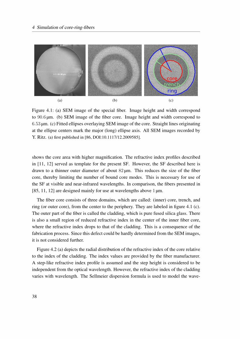
4 Simulation of core-ring-fibers
(a) (b)
ringtrenchcore
(c)
Figure 4.1: (a) SEM image of the special fiber. Image height and width correspondto 90.6 µm. (b) SEM image of the fiber core. Image height and width correspond to6.53 µm. (c) Fitted ellipses overlaying SEM image of the core. Straight lines originatingat the ellipse centers mark the major (long) ellipse axis. All SEM images recorded byY. Ritz. (a) first published in [86, DOI:10.1117/12.2009585].
shows the core area with higher magnification. The refractive index profiles describedin [11, 12] served as template for the present SF. However, the SF described here isdrawn to a thinner outer diameter of about 82 µm. This reduces the size of the fibercore, thereby limiting the number of bound core modes. This is necessary for use ofthe SF at visible and near-infrared wavelengths. In comparison, the fibers presented in[85, 11, 12] are designed mainly for use at wavelengths above 1 µm.
The fiber core consists of three domains, which are called: (inner) core, trench, andring (or outer core), from the center to the periphery. They are labeled in figure 4.1 (c).The outer part of the fiber is called the cladding, which is pure fused silica glass. Thereis also a small region of reduced refractive index in the center of the inner fiber core,where the refractive index drops to that of the cladding. This is a consequence of thefabrication process. Since this defect could be hardly determined from the SEM images,it is not considered further.
Figure 4.2 (a) depicts the radial distribution of the refractive index of the core relativeto the index of the cladding. The index values are provided by the fiber manufacturer.A step-like refractive index profile is assumed and the step height is considered to beindependent from the optical wavelength. However, the refractive index of the claddingvaries with wavelength. The Sellmeier dispersion formula is used to model the wave-
38
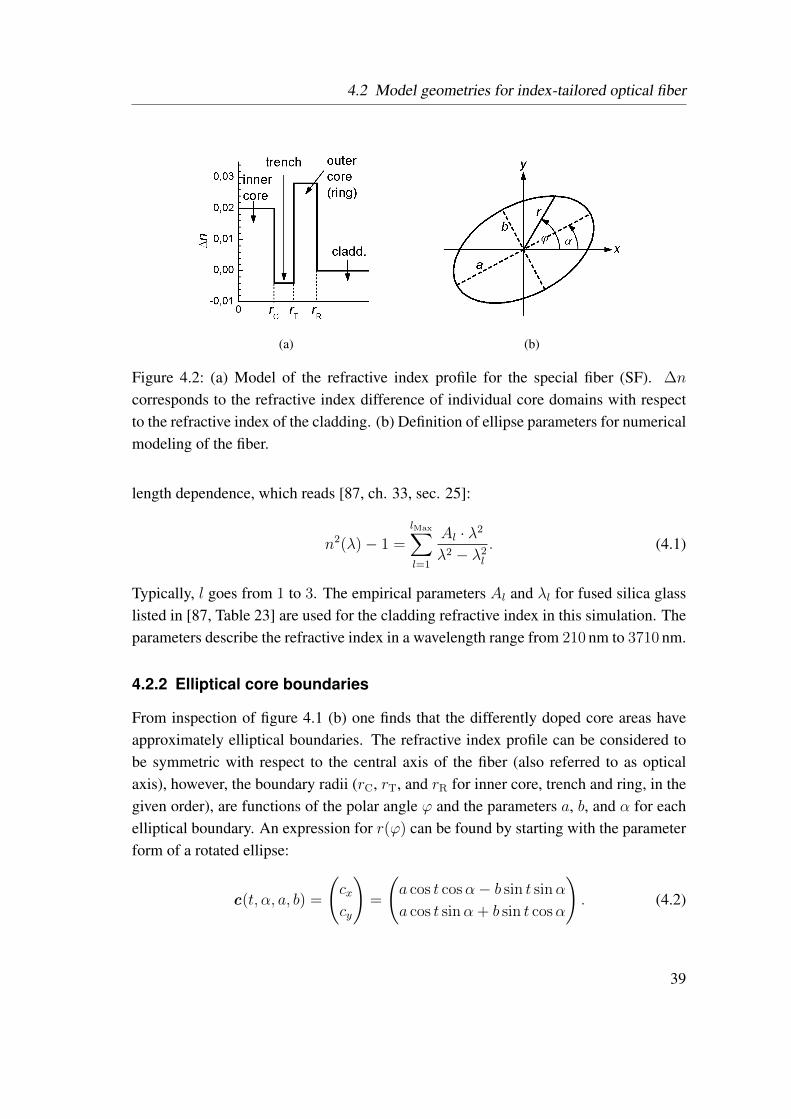
4.2 Model geometries for index-tailored optical fiber
(a) (b)
Figure 4.2: (a) Model of the refractive index profile for the special fiber (SF). ∆n
corresponds to the refractive index difference of individual core domains with respectto the refractive index of the cladding. (b) Definition of ellipse parameters for numericalmodeling of the fiber.
length dependence, which reads [87, ch. 33, sec. 25]:
n2(λ)− 1 =
lMax∑l=1
Al · λ2
λ2 − λ2l
. (4.1)
Typically, l goes from 1 to 3. The empirical parameters Al and λl for fused silica glasslisted in [87, Table 23] are used for the cladding refractive index in this simulation. Theparameters describe the refractive index in a wavelength range from 210 nm to 3710 nm.
4.2.2 Elliptical core boundaries
From inspection of figure 4.1 (b) one finds that the differently doped core areas haveapproximately elliptical boundaries. The refractive index profile can be considered tobe symmetric with respect to the central axis of the fiber (also referred to as opticalaxis), however, the boundary radii (rC, rT, and rR for inner core, trench and ring, in thegiven order), are functions of the polar angle ϕ and the parameters a, b, and α for eachelliptical boundary. An expression for r(ϕ) can be found by starting with the parameterform of a rotated ellipse:
c(t, α, a, b) =
(cxcy
)=
(a cos t cosα− b sin t sinα
a cos t sinα + b sin t cosα
). (4.2)
39
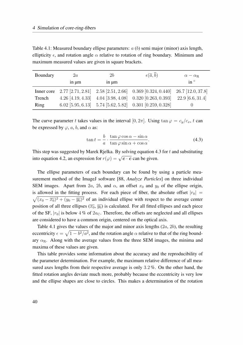
4 Simulation of core-ring-fibers
Table 4.1: Measured boundary ellipse parameters: a (b) semi major (minor) axis length,ellipticity ε, and rotation angle α relative to rotation of ring boundary. Minimum andmaximum measured values are given in square brackets.
Boundary 2a 2b ε(a, b) α− αR
in µm in µm in
Inner core 2.77 [2.71, 2.81] 2.58 [2.51, 2.66] 0.369 [0.324, 0.440] 26.7 [12.0, 37.8]
Trench 4.26 [4.19, 4.33] 4.04 [3.98, 4.08] 0.320 [0.263, 0.393] 22.9 [6.6, 31.4]
Ring 6.02 [5.95, 6.13] 5.74 [5.62, 5.82] 0.301 [0.259, 0.328] 0
The curve parameter t takes values in the interval [0, 2π]. Using tanϕ = cy/cx, t canbe expressed by ϕ, a, b, and α as:
tan t =b
a· tanϕ cosα− sinα
tanϕ sinα + cosα. (4.3)
This step was suggested by Marek Rjelka. By solving equation 4.3 for t and substitutinginto equation 4.2, an expression for r(ϕ) =
√c · c can be given.
The ellipse parameters of each boundary can be found by using a particle mea-surement method of the ImageJ software [88, Analyze Particles] on three individualSEM images. Apart from 2a, 2b, and α, an offset x0 and y0 of the ellipse origin,is allowed in the fitting process. For each piece of fiber, the absolute offset |r0| =√
(x0 − x0)2 + (y0 − y0)2 of an individual ellipse with respect to the average centerposition of all three ellipses (x0, y0) is calculated. For all fitted ellipses and each pieceof the SF, |r0| is below 4 % of 2aC. Therefore, the offsets are neglected and all ellipsesare considered to have a common origin, centered on the optical axis.
Table 4.1 gives the values of the major and minor axis lengths (2a, 2b), the resultingeccentricity ε =
√1− b2/a2, and the rotation angle α relative to that of the ring bound-
ary αR. Along with the average values from the three SEM images, the minima andmaxima of these values are given.
This table provides some information about the accuracy and the reproducibility ofthe parameter determination. For example, the maximum relative difference of all mea-sured axes lengths from their respective average is only 3.2 %. On the other hand, thefitted rotation angles deviate much more, probably because the eccentricity is very lowand the ellipse shapes are close to circles. This makes a determination of the rotation
40
4.2 Model geometries for index-tailored optical fiber
angle prone to errors. For a more solid statistical analysis, more SEM images would berequired and it has to be considered that the individual fit parameters are not indepen-dent of each other. Nonetheless, the good agreement between measured SEM imagesand the fitted elliptical material boundaries, which are depicted in figure 4.1 (c), shallsuffice as motivation for building a computer model of the fiber core based on the ob-tained parameters.
4.2.3 Overview of the applied MMP Models
As described in section 2.4, the MMP software OpenMaX is used for the simulations.Based on the ellipse parameters obtained from SEM images, computer models of thefiber core of different complexity can be created. To gain an understanding of the rela-tionship between the modal properties, namely the effective index dispersion [neff(λ)]and polarization and intensity distributions, and the geometrical parameters of the fibercore, it is useful to start with simplified geometries and increase the level of complexityafterwards. The most simple case is achieved, if the ellipticity of the material bound-aries is neglected, so that they are considered to be circular. By requiring that the circleradius rc fulfills rc =
√ab, the circles have the same area as the initial ellipses. Of
course, a rotation of the boundaries around the optical axis has no effect if they arecircles. In a second step, the ellipticity can be included, but without a rotation of theellipses. Finally, the general case of rotated ellipses is considered. This approach yieldsvaluable insight into the meaning of the various model parameters. Furthermore, thecomputational effort is minimized, since effects, which are common to all models atdifferent levels of complexity can be studied for the simple circular case first.
For all models, a harmonic time-dependence is assumed, which describes an infinitelyextended waveguide. This means that only two dimensions are modeled explicitly andcorresponding 2D-expansions have to be chosen. The cladding-to-air interface is alsonot modeled, since it has negligible effect on the core modes. In other words, an infinitecladding is assumed.
In the first model (circular boundaries) there are only six expansion functions neces-sary to describe the modes of the fiber. A Bessel function for the inner-most domain(the inner core), a Bessel and a Hankel function (2D-multipole) for the trench domainand for the ring domain, and a single Hankel function for the (outer-most) claddingdomain. Due to the symmetry of the problem, all expansions are placed at the origin(on the optical axis). This configuration is equivalent to solving the problem analyti-cally. Nonetheless, the eigenvalue problem for the propagation constants has to be dealt
41
4 Simulation of core-ring-fibers
with numerically in all cases. There are two symmetry planes which are used to reducecomputational effort. Therefore, the boundaries are only explicitly defined for the firstquadrant in the x-y-plane, with z being the direction of propagation. The other threequadrants are modeled implicitly. The order of each expansion is chosen to representthe corresponding mode and does have to agree with the symmetry properties of themodel, namely the transverse electric field must be either parallel or perpendicular ata symmetry plane. For TE0 and TM0 modes, the order is 0, while for HEi and EHi
modes the order i is a positive integer number starting from 1.
For the second model (elliptical boundaries of different eccentricities and with majoraxes aligned with the x-axis), single expansion functions do not fulfill ME any moreat the boundaries. Hence, a number of 2D-multipoles has to be distributed along eachboundary to approximate the fields inside each domain. The two symmetry planes arestill used to reduce the computational effort, and again only the first quadrant of thex-y-plane is modeled explicitly. The placement of the multipoles is done automaticallyby the OpenMaX software. Since the eccentricity of the ellipses are low and there areno sharp corners for any of the boundaries, manual positioning of the expansions isnot necessary. Seven multipole expansions (per boundary and per domain) of order 0
to 2 are sufficient to produce average relative errors along the boundaries on the orderof 10−8 or even below, depending on the specific mode, accuracy of the calculatedeigenvalue, and the choice of the last expansions (the field excitation).
In the last model (rotated elliptical boundaries of different eccentricities) there areno symmetry planes that can be used1. Therefore, four times as many expansions arerequired to achieve the same accuracy as in the second model and the full ellipses haveto be modeled explicitly. The multipole placement is again done automatically.
The following discussion is focused on the propagation constants and their differ-ences, especially between the fundamental HE11 modes and the second-order modegroup. The second-order mode group consists of TE01, HE21, and TM01. The propa-gation constants determine the polarization preservation properties of the fiber and arenecessary for designing long-period fiber gratings for efficient mode conversion. Forsome selected cases, the corresponding mode fields will also be presented.
1 As noticed by Christian Hafner, the model still has a cyclic symmetry, which means that it is transformedonto itself upon rotation of 180 around the z-axis.
42
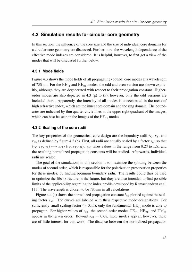
4.3 Simulation results for circular core geometry
4.3 Simulation results for circular core geometry
In this section, the influence of the core size and the size of individual core domains fora circular core geometry are discussed. Furthermore, the wavelength dependence of theeffective mode indexes are considered. It is helpful, however, to first get a view of themodes that will be discussed further below.
4.3.1 Mode fields
Figure 4.3 shows the mode fields of all propagating (bound) core modes at a wavelengthof 785 nm. For the HE11 and HE21 modes, the odd and even version are shown explic-itly, although they are degenerated with respect to their propagation constant. Higher-order modes are also depicted in 4.3 (g) to (k), however, only the odd versions areincluded there. Apparently, the intensity of all modes is concentrated in the areas ofhigh refractive index, which are the inner core domain and the ring domain. The bound-aries are indicated by thin quarter circle lines in the upper right quadrant of the images,which can best be seen in the images of the HE11 modes.
4.3.2 Scaling of the core radii
The key properties of the geometrical core design are the boundary radii rC, rT, andrR, as defined by figure 4.2 (b). First, all radii are equally scaled by a factor sall so that(rC, rT, rR) 7−→ sall · (rC, rT, rR). sall takes values in the range from 0.23 to 1.51 andthe resulting normalized propagation constants will be studied. Afterwards, individualradii are scaled.
The goal of the simulations in this section is to maximize the splitting between themodes of second order, which is responsible for the polarization preservation propertiesfor these modes, by finding optimum boundary radii. The results could thus be usedto optimize the fiber structure in the future, but they are also intended to find possiblelimits of the applicability regarding the index profile developed by Ramachandran et al.[11]. The wavelength is chosen to be 785 nm in all calculations.
Figure 4.4 (a) shows the normalized propagation constant beff plotted against the scal-ing factor sall. The curves are labeled with their respective mode designations. Forsufficiently small scaling factor (≈ 0.44), only the fundamental HE11 mode is able topropagate. For higher values of seff , the second-order modes TE01, HE21, and TM01
appear in the given order. Beyond sall = 0.65, more modes appear, however, theseare of little interest for this work. The distance between the normalized propagation
43
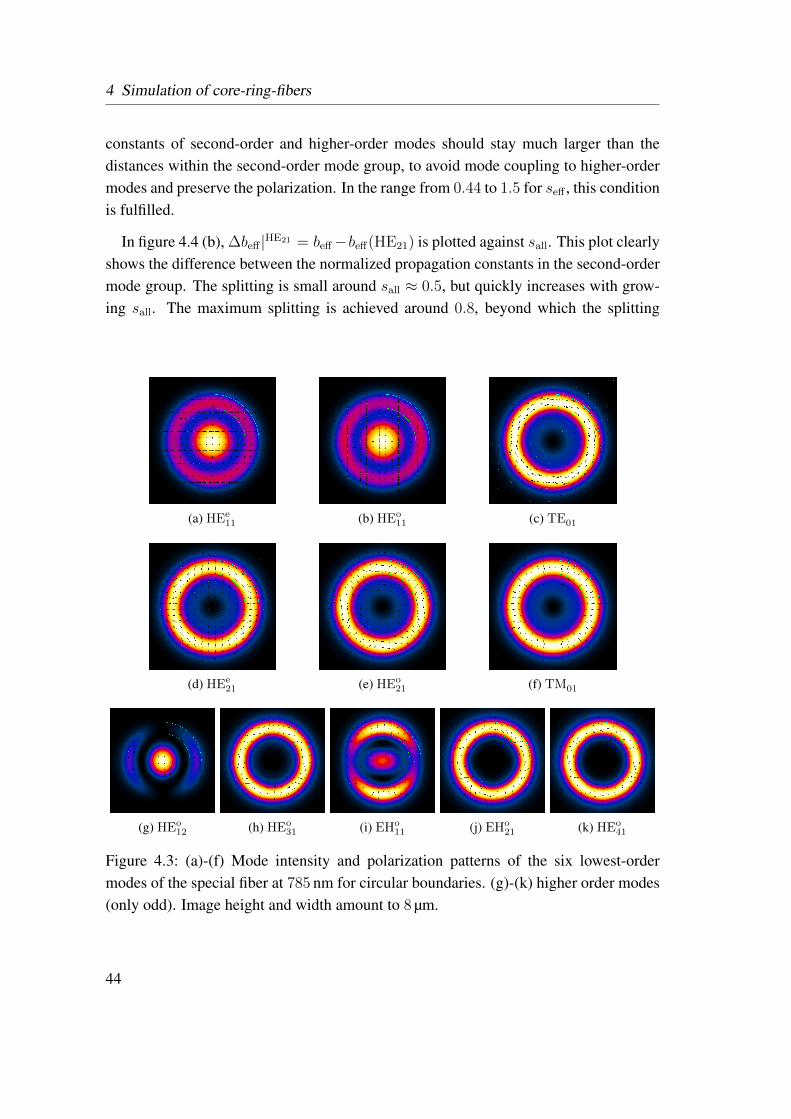
4 Simulation of core-ring-fibers
constants of second-order and higher-order modes should stay much larger than thedistances within the second-order mode group, to avoid mode coupling to higher-ordermodes and preserve the polarization. In the range from 0.44 to 1.5 for seff , this conditionis fulfilled.
In figure 4.4 (b), ∆beff |HE21 = beff−beff(HE21) is plotted against sall. This plot clearlyshows the difference between the normalized propagation constants in the second-ordermode group. The splitting is small around sall ≈ 0.5, but quickly increases with grow-ing sall. The maximum splitting is achieved around 0.8, beyond which the splitting
(a) HEe11 (b) HEo
11 (c) TE01
(d) HEe21 (e) HEo
21 (f) TM01
(g) HEo12 (h) HEo
31 (i) EHo11 (j) EHo
21 (k) HEo41
Figure 4.3: (a)-(f) Mode intensity and polarization patterns of the six lowest-ordermodes of the special fiber at 785 nm for circular boundaries. (g)-(k) higher order modes(only odd). Image height and width amount to 8 µm.
44
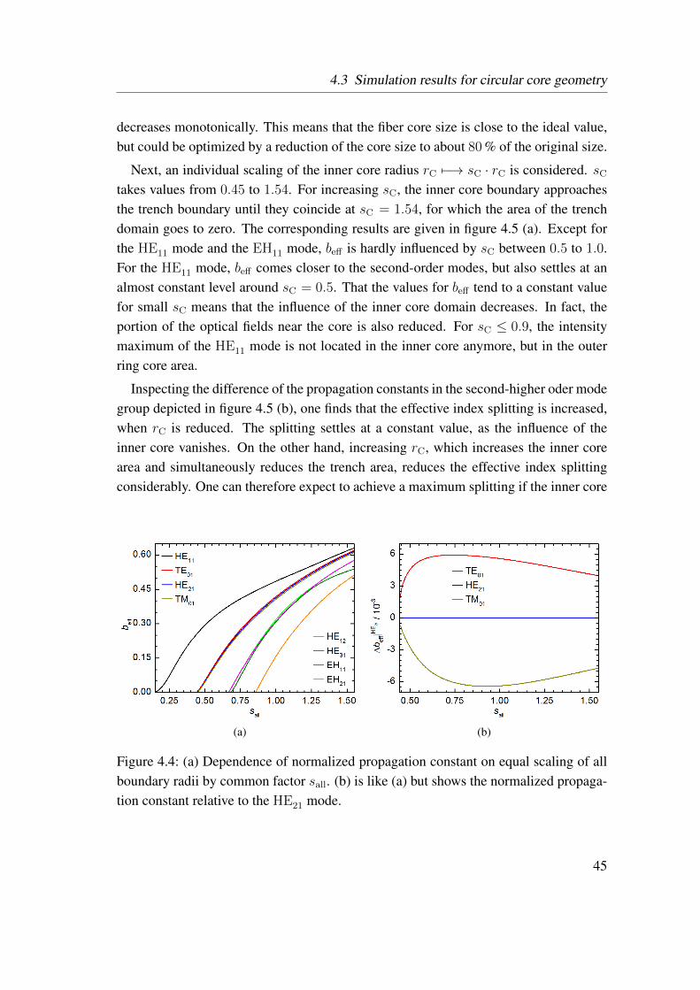
4.3 Simulation results for circular core geometry
decreases monotonically. This means that the fiber core size is close to the ideal value,but could be optimized by a reduction of the core size to about 80 % of the original size.
Next, an individual scaling of the inner core radius rC 7−→ sC · rC is considered. sC
takes values from 0.45 to 1.54. For increasing sC, the inner core boundary approachesthe trench boundary until they coincide at sC = 1.54, for which the area of the trenchdomain goes to zero. The corresponding results are given in figure 4.5 (a). Except forthe HE11 mode and the EH11 mode, beff is hardly influenced by sC between 0.5 to 1.0.For the HE11 mode, beff comes closer to the second-order modes, but also settles at analmost constant level around sC = 0.5. That the values for beff tend to a constant valuefor small sC means that the influence of the inner core domain decreases. In fact, theportion of the optical fields near the core is also reduced. For sC ≤ 0.9, the intensitymaximum of the HE11 mode is not located in the inner core anymore, but in the outerring core area.
Inspecting the difference of the propagation constants in the second-higher oder modegroup depicted in figure 4.5 (b), one finds that the effective index splitting is increased,when rC is reduced. The splitting settles at a constant value, as the influence of theinner core vanishes. On the other hand, increasing rC, which increases the inner corearea and simultaneously reduces the trench area, reduces the effective index splittingconsiderably. One can therefore expect to achieve a maximum splitting if the inner core
(a) (b)
Figure 4.4: (a) Dependence of normalized propagation constant on equal scaling of allboundary radii by common factor sall. (b) is like (a) but shows the normalized propaga-tion constant relative to the HE21 mode.
45
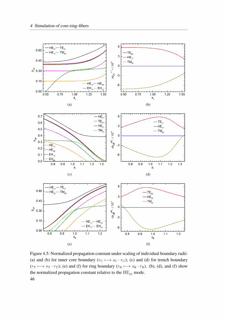
4 Simulation of core-ring-fibers
(a) (b)
(c) (d)
(e) (f)
Figure 4.5: Normalized propagation constant under scaling of individual boundary radii:(a) and (b) for inner core boundary (rC 7−→ sC · rC); (c) and (d) for trench boundary(rT 7−→ sT · rT); (e) and (f) for ring boundary (rR 7−→ sR · rR). (b), (d), and (f) showthe normalized propagation constant relative to the HE21 mode.46

4.3 Simulation results for circular core geometry
would be removed completely. However, in this case, the HE11 mode would lose itssimilarity to the fundamental, Gaussian-like HE11 mode of standard single-mode fibers.This would complicate the excitation of the HE11 mode in the SF, which is of highpractical importance. Considering the marginal possible extra splitting, it appears thatthe inner core radius is already chosen well.
The results for the the trench boundary scaling (scaling factor sT : rT 7−→ sT · rT)are depicted in figure 4.5 (c). When sT is reduced, the area of the ring core domain isincreased and the area of the trench domain is decreased, and vice versa. sT is varied sothat sT · rT stays within the interval [rC, rR]. For sT ≤ 1.0, the propagation constant ofthe fundamental and second-order mode group increases, but the distance between thegroups is almost constant. The distance between the second-higher and other modes isalso hardly effected in this range. For increasing sT, however, the propagation constantof the HE12 mode comes very close to those of the second-higher mode group, whichshould be avoided. Furthermore, for very high values of sT, the area of the ring do-main gets too small to accommodate guided mode fields and therefore, the higher-ordermodes run into cutoff.
Figure 4.5 (d) shows the corresponding propagation constant difference in the second-order mode group. There appears to be an optimum value for sT with maximum splittingaround 1.09. For higher or lower values of sT, the splitting decreases strongly.
The last scaling factor sR corresponds to the radius rR of the outermost boundaryseparating the ring core from the cladding. The results in figure 4.5 (e) show an almostreversed behavior as for a scaling of the trench boundary radius. This is understandable,since both parameters change the area of the ring domain in opposite ways. A reductionof rR also reduces the overall core area, especially the areas with high refractive index,which guide most of the optical power, and therefore, the higher-order modes run intocutoff for low values of sR.
The splitting between the modes in the second-order modes is depicted in figure 4.5 (f).It shows that the maximum splitting is achieved, if rR is reduced to about 95 % of itsoriginal value. So like in the case of scaling the the trench boundary radius, a reductionof the area of the ring domain results in the optimal splitting between the second-higheroder modes.
In conclusion, the present core geometry appears to be close to ideal for a large split-ting between the modes of the second-higher mode group at 785 nm wavelength. Aslight improvement is possible through an equal reduction of all boundary radii. Simul-taneously, this would reduce the number of higher-order modes. The maximum split-
47
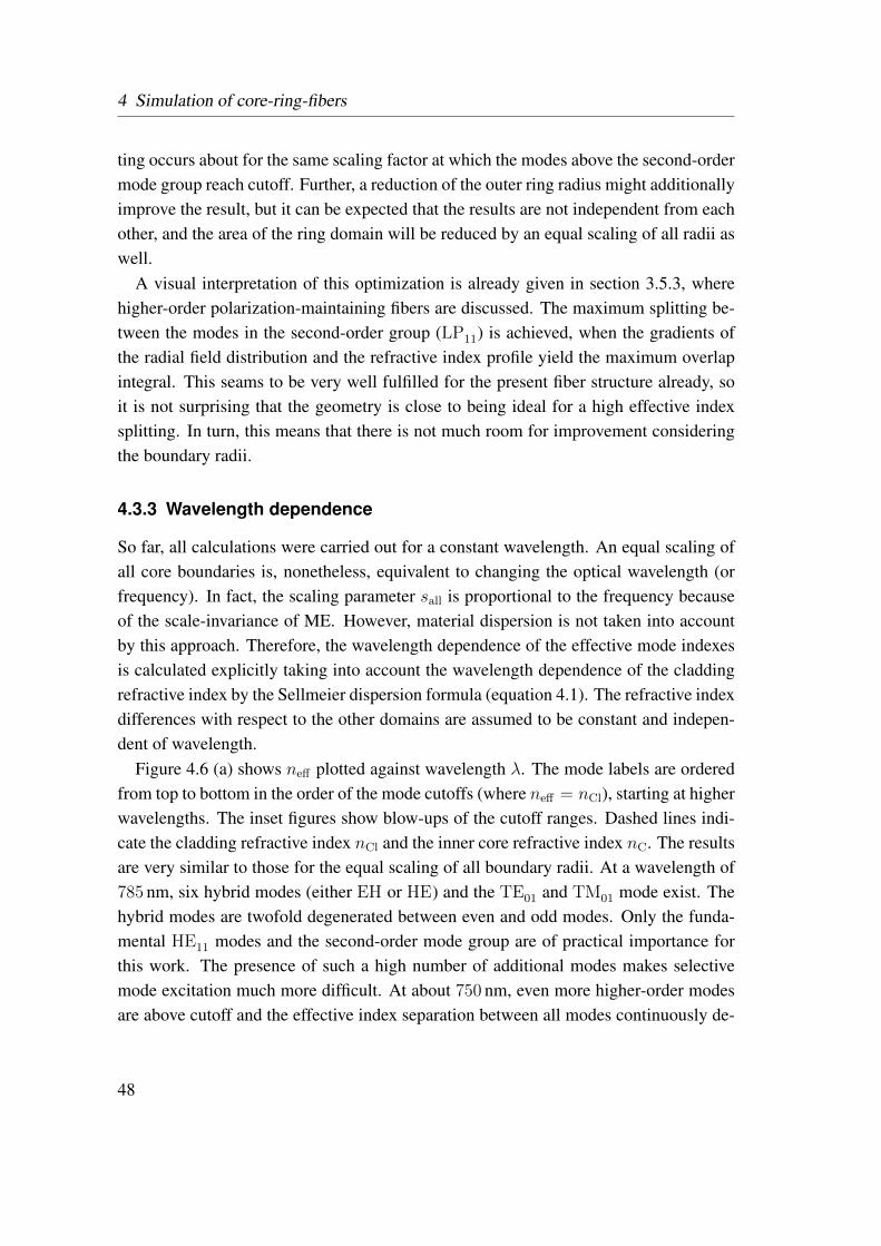
4 Simulation of core-ring-fibers
ting occurs about for the same scaling factor at which the modes above the second-ordermode group reach cutoff. Further, a reduction of the outer ring radius might additionallyimprove the result, but it can be expected that the results are not independent from eachother, and the area of the ring domain will be reduced by an equal scaling of all radii aswell.
A visual interpretation of this optimization is already given in section 3.5.3, wherehigher-order polarization-maintaining fibers are discussed. The maximum splitting be-tween the modes in the second-order group (LP11) is achieved, when the gradients ofthe radial field distribution and the refractive index profile yield the maximum overlapintegral. This seams to be very well fulfilled for the present fiber structure already, soit is not surprising that the geometry is close to being ideal for a high effective indexsplitting. In turn, this means that there is not much room for improvement consideringthe boundary radii.
4.3.3 Wavelength dependence
So far, all calculations were carried out for a constant wavelength. An equal scaling ofall core boundaries is, nonetheless, equivalent to changing the optical wavelength (orfrequency). In fact, the scaling parameter sall is proportional to the frequency becauseof the scale-invariance of ME. However, material dispersion is not taken into accountby this approach. Therefore, the wavelength dependence of the effective mode indexesis calculated explicitly taking into account the wavelength dependence of the claddingrefractive index by the Sellmeier dispersion formula (equation 4.1). The refractive indexdifferences with respect to the other domains are assumed to be constant and indepen-dent of wavelength.
Figure 4.6 (a) shows neff plotted against wavelength λ. The mode labels are orderedfrom top to bottom in the order of the mode cutoffs (where neff = nCl), starting at higherwavelengths. The inset figures show blow-ups of the cutoff ranges. Dashed lines indi-cate the cladding refractive index nCl and the inner core refractive index nC. The resultsare very similar to those for the equal scaling of all boundary radii. At a wavelength of785 nm, six hybrid modes (either EH or HE) and the TE01 and TM01 mode exist. Thehybrid modes are twofold degenerated between even and odd modes. Only the funda-mental HE11 modes and the second-order mode group are of practical importance forthis work. The presence of such a high number of additional modes makes selectivemode excitation much more difficult. At about 750 nm, even more higher-order modesare above cutoff and the effective index separation between all modes continuously de-
48
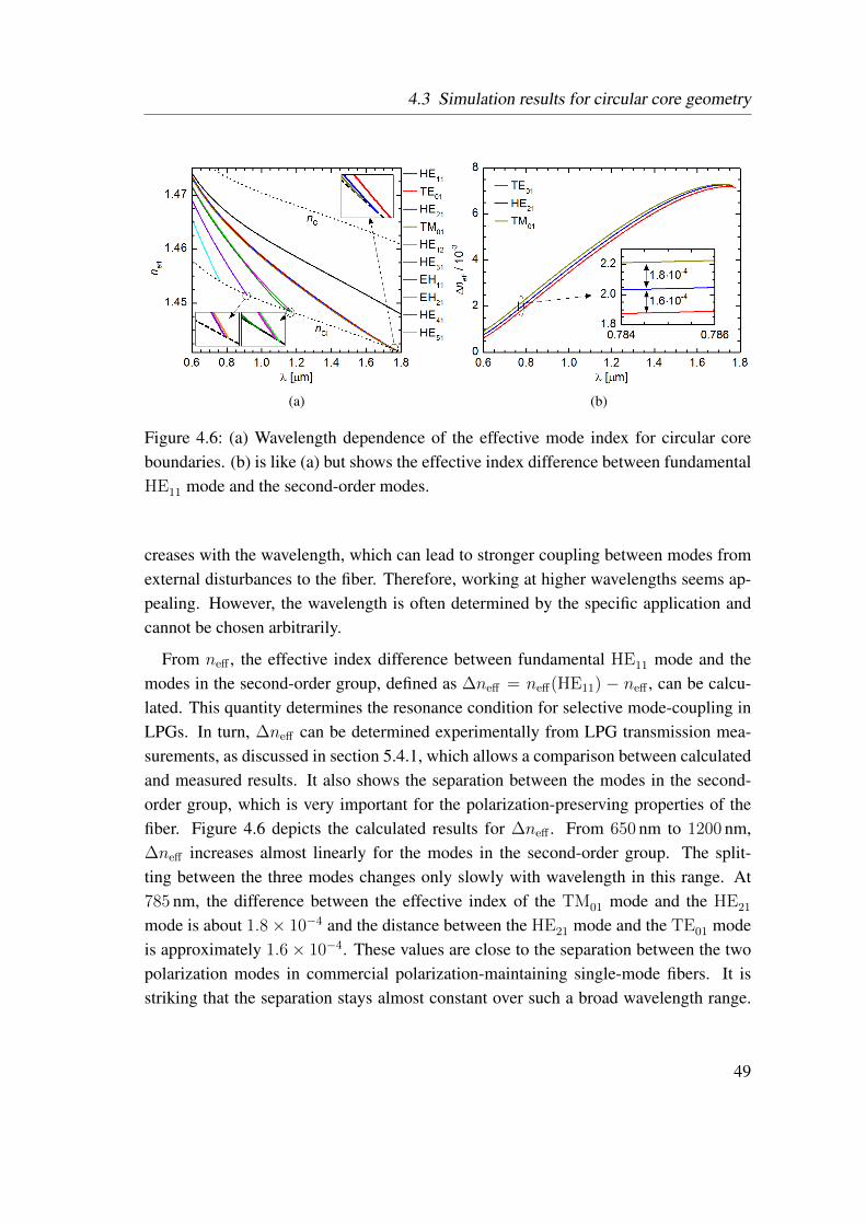
4.3 Simulation results for circular core geometry
(a) (b)
Figure 4.6: (a) Wavelength dependence of the effective mode index for circular coreboundaries. (b) is like (a) but shows the effective index difference between fundamentalHE11 mode and the second-order modes.
creases with the wavelength, which can lead to stronger coupling between modes fromexternal disturbances to the fiber. Therefore, working at higher wavelengths seems ap-pealing. However, the wavelength is often determined by the specific application andcannot be chosen arbitrarily.
From neff , the effective index difference between fundamental HE11 mode and themodes in the second-order group, defined as ∆neff = neff(HE11) − neff , can be calcu-lated. This quantity determines the resonance condition for selective mode-coupling inLPGs. In turn, ∆neff can be determined experimentally from LPG transmission mea-surements, as discussed in section 5.4.1, which allows a comparison between calculatedand measured results. It also shows the separation between the modes in the second-order group, which is very important for the polarization-preserving properties of thefiber. Figure 4.6 depicts the calculated results for ∆neff . From 650 nm to 1200 nm,∆neff increases almost linearly for the modes in the second-order group. The split-ting between the three modes changes only slowly with wavelength in this range. At785 nm, the difference between the effective index of the TM01 mode and the HE21
mode is about 1.8× 10⁻⁴ and the distance between the HE21 mode and the TE01 modeis approximately 1.6× 10⁻⁴. These values are close to the separation between the twopolarization modes in commercial polarization-maintaining single-mode fibers. It isstriking that the separation stays almost constant over such a broad wavelength range.
49
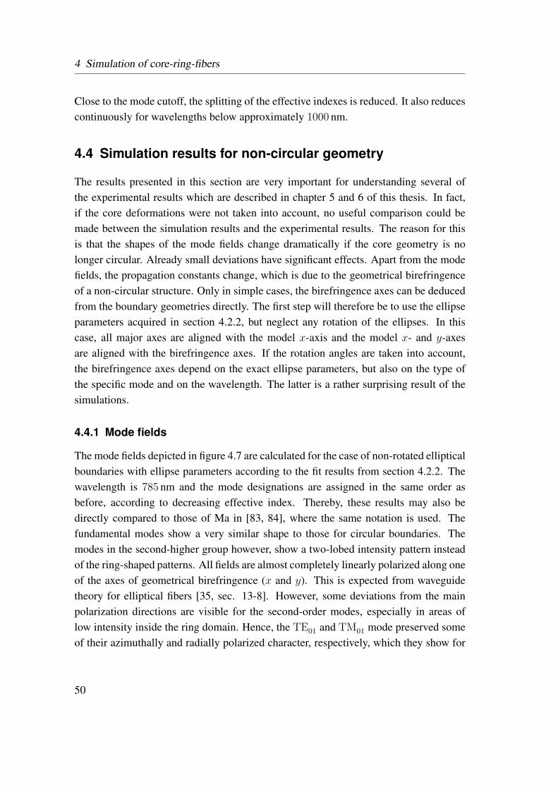
4 Simulation of core-ring-fibers
Close to the mode cutoff, the splitting of the effective indexes is reduced. It also reducescontinuously for wavelengths below approximately 1000 nm.
4.4 Simulation results for non-circular geometry
The results presented in this section are very important for understanding several ofthe experimental results which are described in chapter 5 and 6 of this thesis. In fact,if the core deformations were not taken into account, no useful comparison could bemade between the simulation results and the experimental results. The reason for thisis that the shapes of the mode fields change dramatically if the core geometry is nolonger circular. Already small deviations have significant effects. Apart from the modefields, the propagation constants change, which is due to the geometrical birefringenceof a non-circular structure. Only in simple cases, the birefringence axes can be deducedfrom the boundary geometries directly. The first step will therefore be to use the ellipseparameters acquired in section 4.2.2, but neglect any rotation of the ellipses. In thiscase, all major axes are aligned with the model x-axis and the model x- and y-axesare aligned with the birefringence axes. If the rotation angles are taken into account,the birefringence axes depend on the exact ellipse parameters, but also on the type ofthe specific mode and on the wavelength. The latter is a rather surprising result of thesimulations.
4.4.1 Mode fields
The mode fields depicted in figure 4.7 are calculated for the case of non-rotated ellipticalboundaries with ellipse parameters according to the fit results from section 4.2.2. Thewavelength is 785 nm and the mode designations are assigned in the same order asbefore, according to decreasing effective index. Thereby, these results may also bedirectly compared to those of Ma in [83, 84], where the same notation is used. Thefundamental modes show a very similar shape to those for circular boundaries. Themodes in the second-higher group however, show a two-lobed intensity pattern insteadof the ring-shaped patterns. All fields are almost completely linearly polarized along oneof the axes of geometrical birefringence (x and y). This is expected from waveguidetheory for elliptical fibers [35, sec. 13-8]. However, some deviations from the mainpolarization directions are visible for the second-order modes, especially in areas oflow intensity inside the ring domain. Hence, the TE01 and TM01 mode preserved someof their azimuthally and radially polarized character, respectively, which they show for
50
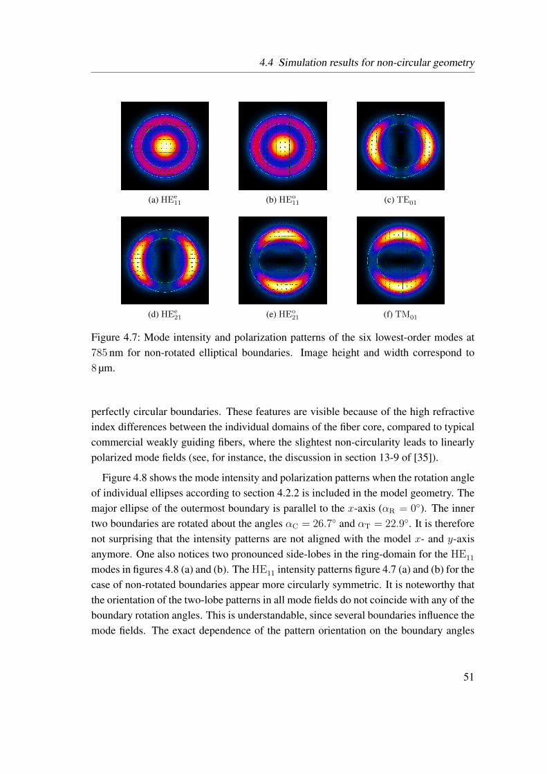
4.4 Simulation results for non-circular geometry
(a) HEe11 (b) HEo
11 (c) TE01
(d) HEe21 (e) HEo
21 (f) TM01
Figure 4.7: Mode intensity and polarization patterns of the six lowest-order modes at785 nm for non-rotated elliptical boundaries. Image height and width correspond to8 µm.
perfectly circular boundaries. These features are visible because of the high refractiveindex differences between the individual domains of the fiber core, compared to typicalcommercial weakly guiding fibers, where the slightest non-circularity leads to linearlypolarized mode fields (see, for instance, the discussion in section 13-9 of [35]).
Figure 4.8 shows the mode intensity and polarization patterns when the rotation angleof individual ellipses according to section 4.2.2 is included in the model geometry. Themajor ellipse of the outermost boundary is parallel to the x-axis (αR = 0). The innertwo boundaries are rotated about the angles αC = 26.7 and αT = 22.9. It is thereforenot surprising that the intensity patterns are not aligned with the model x- and y-axisanymore. One also notices two pronounced side-lobes in the ring-domain for the HE11
modes in figures 4.8 (a) and (b). The HE11 intensity patterns figure 4.7 (a) and (b) for thecase of non-rotated boundaries appear more circularly symmetric. It is noteworthy thatthe orientation of the two-lobe patterns in all mode fields do not coincide with any of theboundary rotation angles. This is understandable, since several boundaries influence themode fields. The exact dependence of the pattern orientation on the boundary angles
51
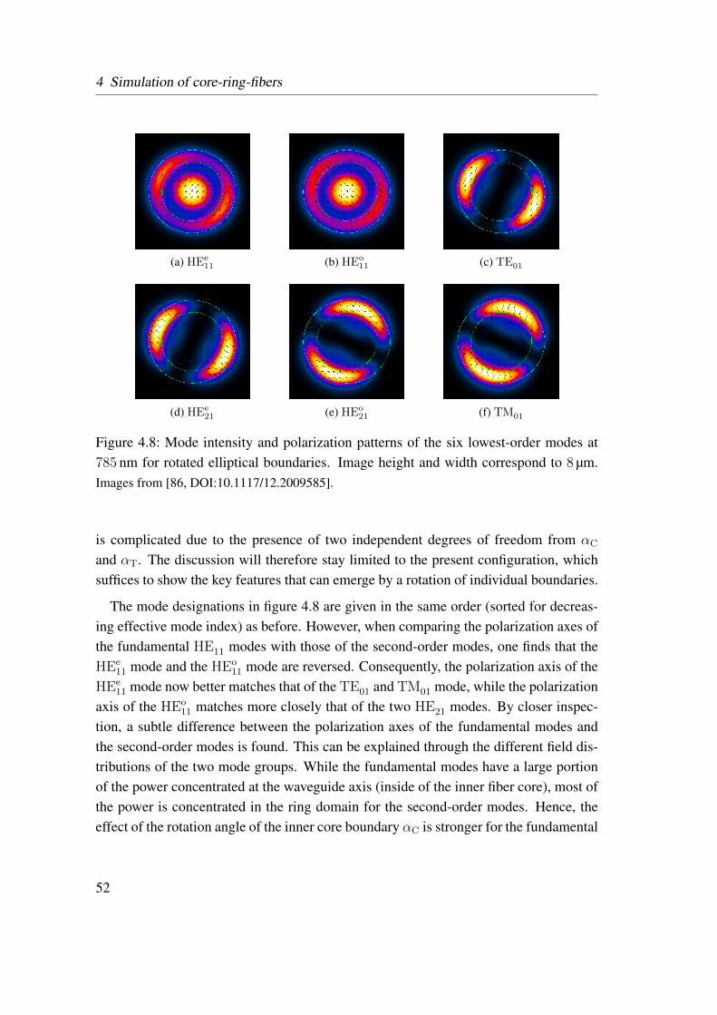
4 Simulation of core-ring-fibers
(a) HEe11 (b) HEo
11 (c) TE01
(d) HEe21 (e) HEo
21 (f) TM01
Figure 4.8: Mode intensity and polarization patterns of the six lowest-order modes at785 nm for rotated elliptical boundaries. Image height and width correspond to 8 µm.Images from [86, DOI:10.1117/12.2009585].
is complicated due to the presence of two independent degrees of freedom from αC
and αT. The discussion will therefore stay limited to the present configuration, whichsuffices to show the key features that can emerge by a rotation of individual boundaries.
The mode designations in figure 4.8 are given in the same order (sorted for decreas-ing effective mode index) as before. However, when comparing the polarization axes ofthe fundamental HE11 modes with those of the second-order modes, one finds that theHEe
11 mode and the HEo11 mode are reversed. Consequently, the polarization axis of the
HEe11 mode now better matches that of the TE01 and TM01 mode, while the polarization
axis of the HEo11 matches more closely that of the two HE21 modes. By closer inspec-
tion, a subtle difference between the polarization axes of the fundamental modes andthe second-order modes is found. This can be explained through the different field dis-tributions of the two mode groups. While the fundamental modes have a large portionof the power concentrated at the waveguide axis (inside of the inner fiber core), most ofthe power is concentrated in the ring domain for the second-order modes. Hence, theeffect of the rotation angle of the inner core boundary αC is stronger for the fundamental
52
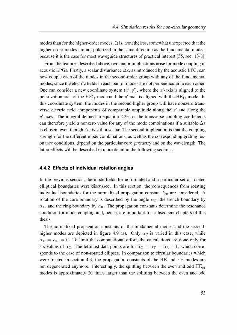
4.4 Simulation results for non-circular geometry
modes than for the higher-order modes. It is, nonetheless, somewhat unexpected that thehigher-order modes are not polarized in the same direction as the fundamental modes,because it is the case for most waveguide structures of practical interest [35, sec. 13-8].
From the features described above, two major implications arise for mode coupling inacoustic LPGs. Firstly, a scalar disturbance ∆ε, as introduced by the acoustic LPG, cannow couple each of the modes in the second-order group with any of the fundamentalmodes, since the electric fields in each pair of modes are not perpendicular to each other.One can consider a new coordinate system (x′, y′), where the x′-axis is aligned to thepolarization axis of the HEe
11 mode and the y′-axis is aligned with the HEo11 mode. In
this coordinate system, the modes in the second-higher group will have nonzero trans-verse electric field components of comparable amplitude along the x′ and along they′-axes. The integral defined in equation 2.23 for the transverse coupling coefficientscan therefore yield a nonzero value for any of the mode combinations if a suitable ∆ε
is chosen, even though ∆ε is still a scalar. The second implication is that the couplingstrength for the different mode combinations, as well as the corresponding grating res-onance conditions, depend on the particular core geometry and on the wavelength. Thelatter effects will be described in more detail in the following sections.
4.4.2 Effects of individual rotation angles
In the previous section, the mode fields for non-rotated and a particular set of rotatedelliptical boundaries were discussed. In this section, the consequences from rotatingindividual boundaries for the normalized propagation constant beff are considered. Arotation of the core boundary is described by the angle αC, the trench boundary byαT, and the ring boundary by αR. The propagation constants determine the resonancecondition for mode coupling and, hence, are important for subsequent chapters of thisthesis.
The normalized propagation constants of the fundamental modes and the second-higher modes are depicted in figure 4.9 (a). Only αC is varied in this case, whileαT = αR = 0. To limit the computational effort, the calculations are done only forsix values of αC. The leftmost data points are for αC = αT = αR = 0, which corre-sponds to the case of non-rotated ellipses. In comparison to circular boundaries whichwere treated in section 4.3, the propagation constants of the HE and EH modes arenot degenerated anymore. Interestingly, the splitting between the even and odd HE21
modes is approximately 20 times larger than the splitting between the even and odd
53
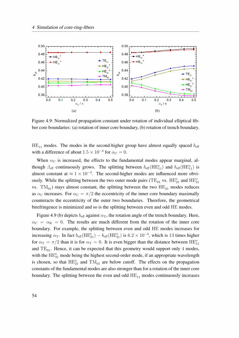
4 Simulation of core-ring-fibers
(a) (b)
Figure 4.9: Normalized propagation constant under rotation of individual elliptical fib-ber core boundaries: (a) rotation of inner core boundary, (b) rotation of trench boundary.
HE11 modes. The modes in the second-higher group have almost equally spaced beff
with a difference of about 1.5× 10⁻⁴ for αC = 0.
When αC is increased, the effects to the fundamental modes appear marginal, al-though βeff continuously grows. The splitting between beff(HEe
11) and beff(HEo11) is
almost constant at ≈ 1× 10⁻³. The second-higher modes are influenced more obvi-ously. While the splitting between the two outer mode pairs (TE01 vs. HEe
21 and HEo21
vs. TM01) stays almost constant, the splitting between the two HE21 modes reducesas αC increases. For αC = π/2 the eccentricity of the inner core boundary maximallycounteracts the eccentricity of the outer two boundaries. Therefore, the geometricalbirefringence is minimized and so is the splitting between even and odd HE modes.
Figure 4.9 (b) depicts beff against αT, the rotation angle of the trench boundary. Here,αC = αR = 0. The results are much different from the rotation of the inner coreboundary. For example, the splitting between even and odd HE modes increases forincreasing αT. In fact beff(HEe
21) − beff(HEo21) is 6.2× 10⁻³, which is 13 times higher
for αT = π/2 than it is for αT = 0. It is even bigger than the distance between HEo11
and TE01. Hence, it can be expected that this geometry would support only 4 modes,with the HEe
21 mode being the highest second-order mode, if an appropriate wavelengthis chosen, so that HEo
21 and TM01 are below cutoff. The effects on the propagationconstants of the fundamental modes are also stronger than for a rotation of the inner coreboundary. The splitting between the even and odd HE11 modes continuously increases
54
4.4 Simulation results for non-circular geometry
Figure 4.10: Normalized propagation constant under rotation of the elliptical ring coreboundary.
with αT from 2× 10⁻⁴ to 2.5× 10⁻³. Also interesting is the observation that for thedata points with αT ≥ 0.08π, the polarization of the HEe
11 mode is (almost) parallelto that of TE01 mode, similar to the results discussed in section 4.4.1 (mode fields notshown here).
Next, a rotation of the trench boundary is considered. Figure 4.10 shows the corre-sponding results for beff(αR), while αC = αT = 0. The results are very similar to thosefor the rotation of the trench boundary. The maximum splitting between the even andodd HE11 modes is slightly higher (2.6× 10⁻³), while the splitting between TE01 andHEe
21 is lower (5.6× 10⁻²). As for the previous case, the polarization of the HEe11 mode
is again (almost) parallel to that of TE01 mode (mode fields not shown here).
So far, the MMP simulations demonstrated the existence of a large propagation con-stant splitting in the second-higher mode group between the TE01, HE21, and TM01
modes, which is primarily due to the refractive index profile being tailored to the fielddistributions of these modes. On the other hand, the index profile is also responsiblefor the strong splitting between the even and odd HE21 modes that arises if small ge-ometrical imperfections, like rotated and non-rotated elliptical boundaries of small ec-centricity are introduced. Therefore, achieving exceptionally low eccentricity is muchmore important for the fabrication of these index-tailored fibers than it is for weaklyguiding fibers with much smaller refractive index differences. In general, it is foundthat a rotation of the trench or the ring boundary result in a strong increase of the prop-agation constant splitting between the even and odd HE21 modes and a notable, yetsmaller increase in splitting for the even and odd HE11 modes. A rotation of the inner
55
4 Simulation of core-ring-fibers
core boundary results in a reduction of the propagation constant splitting between theeven and odd HE21 modes, while the propagation constants of the HE11 modes remainsalmost unaffected.
The specific examples for the boundary geometries are not meant as fabrication tem-plates. They are rather meant to demonstrate the effect of more general waveguidedeformations. Of course, many of the described effects will not be as pronounced inreal-world fibers. The elliptical boundaries, which, were assumed for the non-circularsymmetric core geometries, represent highly symmetric objects that can lead to pro-nounced symmetry breaking if they are rotated against each other. Deviations fromthese perfect geometries will certainly diminish the effects. Nonetheless, it has becomeclear that the splitting between even and odd HE21 modes can become very strong forrelatively small deviations from a circularly symmetric core geometry.
4.4.3 Wavelength dependence
After several geometrical effects were studied in the previous section, the wavelengthdependence of the effective mode indexes and the mode fields will be treated in thefollowing. The general wavelength behavior of the mode effective indexes, which wasalready calculated for a circular geometrical fiber core, is not affected by the introduc-tion of rotated and non-rotated elliptical boundaries. Therefore, the discussion will belimited to the effective index difference ∆neff between the fundamental and the second-order modes, which is also the most interesting quantity for applications of the fiber foracoustic LPGs in subsequent chapters of this thesis.
For non-circular fiber geometries, the even and odd HE modes have different effec-tive mode indexes. Hence, in terms of the effective index difference, there are eightmode combinations possible between the fundamental and second-higher modes. Thetransitions HEo
11-TE01, HEe11-HEe
21, HEe11-HEo
21, and HEo11-TM01 will be called pri-
mary transitions in the following, because in the case of a non-rotated elliptical coregeometry, the polarization axis is maintained for these transitions (see figure 4.7 forcomparison). Transitions with the respective other even or odd HE11 mode will conse-quently be called secondary transitions.
The effective index difference ∆neff against the wavelength λ is depicted infigure 4.11 (a) and (b). For figure 4.11 (a), non-rotated elliptical boundaries are as-sumed, with the geometrical parameters given in table 4.1. For 4.11 (b), the ellipserotation angles are taken into account. In both figures, the primary transitions are rep-resented by solid lines, while the the secondary transitions are represented by dotted
56
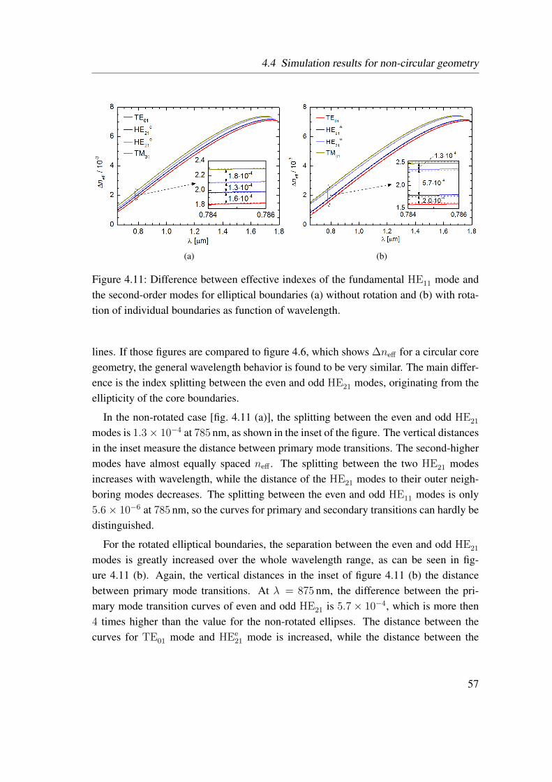
4.4 Simulation results for non-circular geometry
(a) (b)
Figure 4.11: Difference between effective indexes of the fundamental HE11 mode andthe second-order modes for elliptical boundaries (a) without rotation and (b) with rota-tion of individual boundaries as function of wavelength.
lines. If those figures are compared to figure 4.6, which shows ∆neff for a circular coregeometry, the general wavelength behavior is found to be very similar. The main differ-ence is the index splitting between the even and odd HE21 modes, originating from theellipticity of the core boundaries.
In the non-rotated case [fig. 4.11 (a)], the splitting between the even and odd HE21
modes is 1.3× 10⁻⁴ at 785 nm, as shown in the inset of the figure. The vertical distancesin the inset measure the distance between primary mode transitions. The second-highermodes have almost equally spaced neff . The splitting between the two HE21 modesincreases with wavelength, while the distance of the HE21 modes to their outer neigh-boring modes decreases. The splitting between the even and odd HE11 modes is only5.6× 10−6 at 785 nm, so the curves for primary and secondary transitions can hardly bedistinguished.
For the rotated elliptical boundaries, the separation between the even and odd HE21
modes is greatly increased over the whole wavelength range, as can be seen in fig-ure 4.11 (b). Again, the vertical distances in the inset of figure 4.11 (b) the distancebetween primary mode transitions. At λ = 875 nm, the difference between the pri-mary mode transition curves of even and odd HE21 is 5.7× 10⁻⁴, which is more then4 times higher than the value for the non-rotated ellipses. The distance between thecurves for TE01 mode and HEe
21 mode is increased, while the distance between the
57
4 Simulation of core-ring-fibers
curves for TM01 and HEo21 is decreased. However, compared to the non-rotated case,
these changes are much weaker than the change in separation of the even and odd HE21
modes. Additionally, the effective index splitting between the even and odd HE11 modesis increased to a value of 3.0× 10⁻⁵ at 785 nm, resulting in a larger separation betweenprimary and secondary transition curves in figure 4.11 (b) compared to 4.11 (a).
After discussing the wavelength dependence of the effective mode indexes for non-rotated and rotated elliptical core geometries, some aspects of the corresponding modefields are considered now. Particular attention is payed to the polarization axis.
Figure 4.12 shows the intensity and polarization pattens of the HEe11, TE01, and TM01
modes for λ = 710 nm, 1100 nm and 1515 nm. The possible mode combinations belongto the group of the secondary mode transitions. However, particularly for the lowestwavelength, the polarization axes of the HEe
11 mode and the TE01 and TM01 modes arealmost parallel to each other, which would allow for strong mode coupling by a fibergrating. For increasing wavelengths, the polarization axis of the HEe
11 mode rotatesnotably, while the polarization axis of the second-higher modes remains almost con-stant. This means that the projection of the two polarization axes is strongly wavelengthdependent and the same can be expected for the mode coupling strength.
The angle between the mode polarization axis and the model x-axis, called αp, canbe calculated by:
αp =1
N
N∑i
arctan (Eyi/Exi). (4.4)
In equation 4.4, the polarization angle is calculated from the transverse electric fieldcomponents Ex and Ey at each grid point i of the MMP calculation, and the average ofall angles is calculated. The value range is limited to [−π/2,+π/2] for arctan.
58
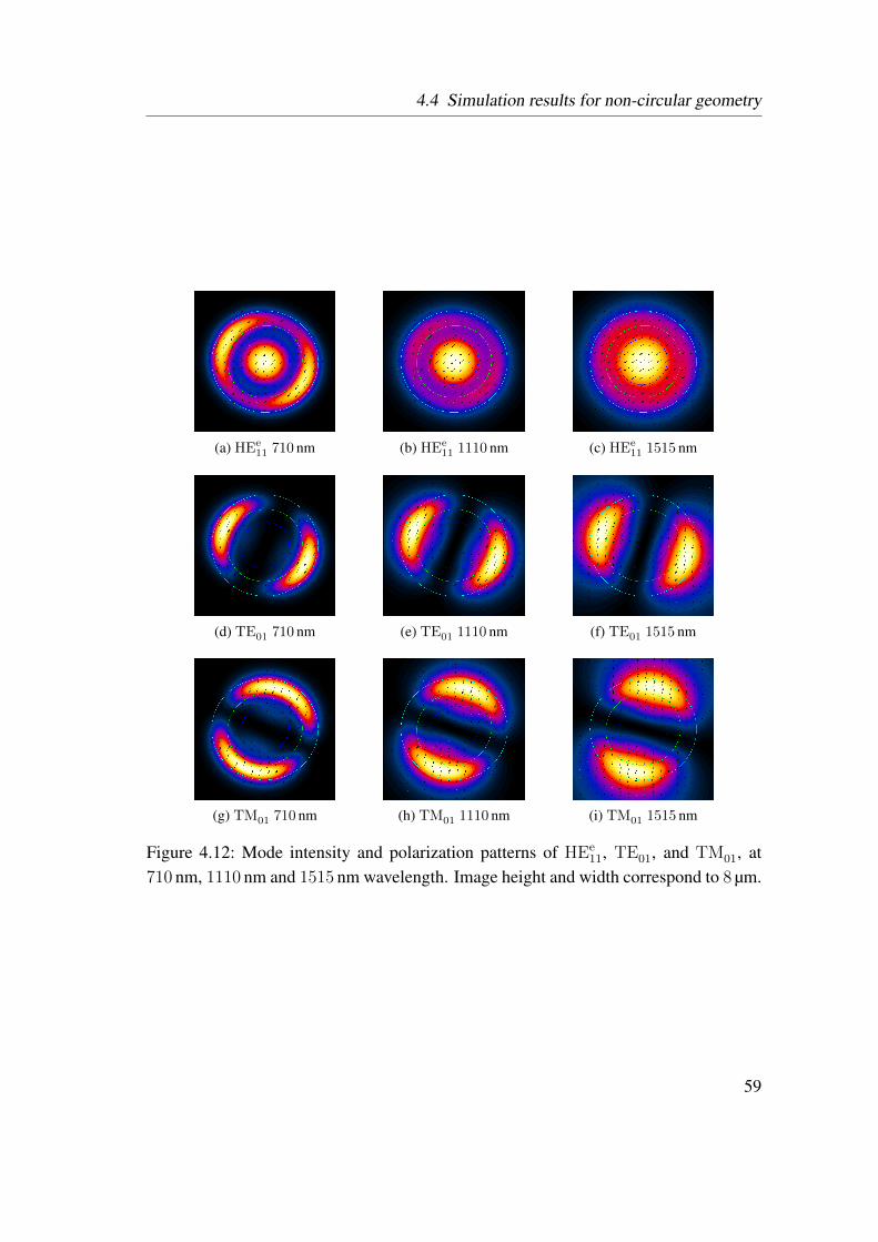
4.4 Simulation results for non-circular geometry
(a) HEe11 710 nm (b) HEe
11 1110 nm (c) HEe11 1515 nm
(d) TE01 710 nm (e) TE01 1110 nm (f) TE01 1515 nm
(g) TM01 710 nm (h) TM01 1110 nm (i) TM01 1515 nm
Figure 4.12: Mode intensity and polarization patterns of HEe11, TE01, and TM01, at
710 nm, 1110 nm and 1515 nm wavelength. Image height and width correspond to 8 µm.
59
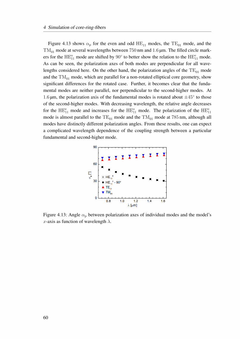
4 Simulation of core-ring-fibers
Figure 4.13 shows αp for the even and odd HE11 modes, the TE01 mode, and theTM01 mode at several wavelengths between 750 nm and 1.6 µm. The filled circle mark-ers for the HEo
11 mode are shifted by 90 to better show the relation to the HEe11 mode.
As can be seen, the polarization axes of both modes are perpendicular for all wave-lengths considered here. On the other hand, the polarization angles of the TE01 modeand the TM01 mode, which are parallel for a non-rotated elliptical core geometry, showsignificant differences for the rotated case. Further, it becomes clear that the funda-mental modes are neither parallel, nor perpendicular to the second-higher modes. At1.6 µm, the polarization axis of the fundamental modes is rotated about ±45 to thoseof the second-higher modes. With decreasing wavelength, the relative angle decreasesfor the HEe
11 mode and increases for the HEo11 mode. The polarization of the HEe
11
mode is almost parallel to the TE01 mode and the TM01 mode at 785 nm, although allmodes have distinctly different polarization angles. From these results, one can expecta complicated wavelength dependence of the coupling strength between a particularfundamental and second-higher mode.
Figure 4.13: Angle αp between polarization axes of individual modes and the model’sx-axis as function of wavelength λ.
60
4.5 Summary and conclusions
4.5 Summary and conclusions
In this chapter, a model geometry for a special index-tailored optical fiber was developedfrom SEM images of the fiber core. The geometry is described by rotated ellipses ofthree different domain boundaries, separating four domains that were assumed to havea constant refractive index. Different degrees of complexity were achieved by assumingsuitable circular, non-rotated elliptical, and rotated elliptical boundary geometries. Thegoals of the simulations were to gain a better understanding of the exceptional propa-gation constant splitting of the second-order modes, to find optimized boundary radiithat maximize this splitting, and to study the effects of core deformations. The calcu-lated mode propagation constants and mode fields also form the basis for understandingexperimental results which are described in subsequent chapters of this thesis.
The initial model with circular geometry already shows an exceptionally high split-ting of the propagation constants of the second-order modes over a broad wavelengthrange. A variation of the different boundary radii showed little room for optimizationwith respect to the current design, although a slight reduction of all core dimension canimprove the splitting at lower wavelengths, e.g. 785 nm and below. Further, the effectsof boundary ellipticity and a rotation of individual elliptical boundaries on the modefields and the propagation constants were considered. In the latter case, a large splittingof propagation constants between the even and odd HE21 modes was found, which ismuch larger than that between the even and odd HE11 modes. The splitting betweenthe two HE11 modes leads to the existence of eight instead of four possible resonanceconditions for mode transitions from one of two fundamental modes to one of foursecond-higher modes. A distinction between primary and secondary mode transitionsbased on a matching of the polarization axes of the participating modes for non-rotatedelliptical boundaries was therefore introduced. Surprisingly, it was found that the po-larization axes of the fundamental and second-higher modes might neither be parallelnor perpendicular to each other, if suitable geometrical deformations to a perfectly cir-cular fiber core are introduced. Hence, the polarization axis in primary and secondarymode transitions are no longer maintained and the mode coupling strength between aparticular pair of fundamental and second-higher modes will depend on the projectionof their polarization axes. The secondary mode transitions might even show strongermode coupling than the primary ones. It was further found that the polarization axis ofthe modes also depends on the wavelength.
In general, the polarization of a mode is influenced by how much its field feels aparticular geometrical feature of the core. For example, the second-order modes have
61
4 Simulation of core-ring-fibers
most of their power concentrated in the ring domain and a strong overlap between theirfield gradients and the refractive index gradients at the trench and at the ring boundary.So the geometry of the inner core will have lesser effects than the geometry of thetrench and the ring boundaries. Since the mode fields extend over larger areas as thewavelength increases, they will be influenced more and more by all geometrical features.However, the field gradients will also decrease for higher wavelengths, which will inturn decrease the dependence on the exact geometry and both effects might competewith each other. This discussion shows that a number of important effects arises fromdeviations from a perfectly circular fiber core geometry. The sensitivity to geometricaldeviations stems from the large steps in the refractive index profile, and the geometryhas to be controlled much more carefully during the fabrication of this type of specialindex-tailored fiber than for standard weakly guiding fibers.
62
5 Long period fiber gratings
5.1 Introduction
The construction and test of an acoustic long-period fiber grating (LPG) in conjunc-tion with the index-tailored special fiber (SF) from chapter 4 is treated in this chapter.Acoustic LPGs couple two forwardly propagating modes of an optical fiber by induc-ing a periodic permittivity disturbance in the fiber that originates from a propagatingacoustic wave. For the mode coupling to become efficient, the spatial period of thepermittivity disturbance has to be matched to the difference of propagation constants ofthe optical modes, which leads to a resonance condition relating optical and acousticalproperties of the fiber.
Acoustic LPGs were first developed in 1986 [15] and were studied extensively eversince. Their applications include tunable filters [89, 90], polarization controllers [91],or polarization dependent loss elements [92, 93], to name a few. Apart from standardSMFs, LPGs were used in conjunction with fibers of many different geometries. Amongthem are highly elliptical core fibers [94, 95], photonic crystal fibers [96, 97], and dis-persion compensating fibers [17]. The latter example is similar to this work, becausethe dispersion compensating fiber used there can be thought of a predecessor of the SFused in the present work due the similarity of their refractive index profiles.
The aim of this chapter is twofold. Firstly, the effective index difference for the modetransitions between the fundamental and second-order guided core modes of the SF willbe measured and compared to the results predicted from the simulations in chapter 4.Secondly, individual second-higher modes will be excited from the fundamental modesand the highest possible efficiency is determined.
This chapter has the following structure: Section 5.2 gives an introduction to LPGsin general, including different gratings types, but with a focus on acoustic LPGs. Sec-tion 5.3 describes the LPG setup and its development in detail. The results which wereachieved with this setup are then presented and discussed in section 5.4. Finally, sec-tion 5.5 concludes this chapter.
63
5 Long period fiber gratings
5.2 Principle of long-period fiber gratings
In long-period fiber grating (LPG), the spatial period of the permittivity modulation ∆ε
is in the range between tens of microns to a few millimeters. For these periods, co-directional coupling of fiber modes is commonly observed at the grating’s resonancewavelength. In contrast, so called fiber Bragg-gratings possess much shorter periods,leading to a contra-directional coupling of the optical modes. The latter will not bediscussed in this work.
5.2.1 Results from coupled mode theory
The principle of LPGs can be readily explained by coupled mode theory (CMT) fromchapter 2.5. A periodic disturbance of the permittivity ∆ε changes the relative power oftwo (or more) co-propagating modes of the optical fiber under consideration, hence themodes are coupled. Among other effects, this can lead to a change of the polarizationdistribution in the fiber, which is the main application of LPGs in this work. Chapter2.5 provided a relatively general description of CMT and left the origin of ∆ε open,since it depends on the specific grating type. This will be given below as required forunderstanding the experimental results of this section.
To achieve a better comparison between experiments and simulations for optical fibermodes, the phase matching condition from equation 2.27 can be rewritten by includingthe effective mode indexes neff = β/k0 = 2πβ/λ:
∆βνµ − 2π/Λ = 0 (5.1)
→ 2π(neff,ν − neff,µ
λ− 1
Λ) = 0 (5.2)
to yield the final result:
∆neff = neff,ν − neff,µ =λ
Λ. (5.3)
Usually the effective indexes (and relations between them) are functions of the opti-cal wavelength λ. Therefore, the left and the right hand side in equation 5.3 can beunderstood as independent functions of the wavelength. Hence, the grating resonancecondition is fulfilled at the point of intersection between the graphs of those functions. Ifthe grating period is known, the effective index difference of two modes can be directlydetermined from a spectroscopic measurement of the mode coupling as documented inchapter 5.4.1.
64
5.2 Principle of long-period fiber gratings
5.2.2 Types of long-period gratings
Three types of LPGs can be distinguished according to the mechanism creating theperiodic permittivity change ∆ε:
1. photo-induced LPGs,
2. mechanical LPGs,
3. acoustic LPGs.
Although, acoustic LPGs are dominantly used in this work, all three grating types weretested, and a short overview of their key properties is given in the following.
Photo-induced gratings
Photo-induced LPGs are usually produced by illumination with UV laser radiation[98, 99, 25]. The highly intense radiation changes the refractive index of the fiber mate-rial. This property of glass is called photosensitivity. The UV radiation mainly modifiesthe refractive index of the fiber core, since the germanium doped regions have higherphotosensitivity than fused silica. The effect can be further enhanced by bathing thefiber in hydrogen at high pressure before exposure (see sec. 17.10 of [25]). The peri-odicity is produced by a step-by-step illumination of single points along the fiber or byusing a phase mask, which creates an extended interference pattern. As a side note, itshall be mentioned that the use of IR radiation was also demonstrated for the fabricationof LPGs [100]. In this case, shape modifications of the fiber cladding cause an indexmodulation.
Once the grating has been written into the fiber, the resonance wavelength can betuned only slightly, a few nanometers at maximum, by applying tension to the fiber.Furthermore, the index modification is permanent. These features limit the applicabilityof optically induced LPGs if used for studying effective index differences of fiber modeson a broader wavelength range, where tunability is desired.
Mechanical gratings
Different methods are used to introduce mechanical LPGs to an optical fiber. Usually,a periodic bending and/or pressure are applied to the fiber, e.g. by pressing the fiberbetween a grooved and flat plate, or two grooved plates shifted by a half groove periodwith respect to each other [101, 102, 12]. The grating vector does not necessarily have
65
5 Long period fiber gratings
to coincide with the fiber axis, in fact the angle between them can be chosen arbitrarily ifthe grooved plates are wide enough. Therefore, the grating period is tunable over a largerrange than for the photo-induced LPGs. Furthermore, the grating can be removed bylowering the pressure applied to the fiber by the grooved plates. On the other hand, theadjustment of the period depends strongly on the accuracy of the mechanical alignment.Furthermore, the resonance wavelength depends not only on the effective period of thegrating (caused by the angle between the grating vector and the fiber axis) but also on thepressure [102]. Therefore, an optimization of the fiber period and the applied pressureto get maximum conversion at a specific wavelength can not be done independently.Another limit is the ability to fabricate grooved plates of short periods (below 200 µm)and to achieve the necessary bend radii. Nonetheless, mechanical LPGs are very easilyfabricated and do not require any sophisticated equipment.
Acoustic gratings
Acoustic LPGs consist of an ultrasonic transducer that is mechanically coupled to anoptical fiber through a tapered glass or metal cone [15, 103, 104, 105]. The transduceris driven by an electrical signal and will oscillate in a direction vertical to the fiber axis.Propagating acoustic waves are then launched into the fiber. Mostly flexural waves areused. These waves create a periodic permittivity disturbance.
The periodic permittivity disturbance propagates along the fiber with a velocity cac
that depends on the acoustic mode of the oscillation. For each acoustic mode, a dis-persion relation exists between the applied frequency fac and cac, and hence the gratingperiod Λ = cac/fac depends on the frequency. If the dispersion relation is known,the spatial period can be varied precisely through the frequency of the driving signal.Typical frequencies are in the range between 500 kHz to 10 MHz. When two modesare coupled by the acoustic LPG, the resulting mode will be frequency shifted by anamount equal to the acoustic frequency. Compared to the optical frequency, this shiftis small and the coupling can still be described by a stationary permittivity disturbance[21, Chapter 9].
One advantage of acoustic LPGs is that the oscillations of the fiber are highly sym-metric. This means that the bandwidth of the coupling can be very sharp, so opticalmodes with very closely spaced propagation constants can be addressed individually.On the other hand, the displacement amplitudes cannot be made greater than a few hun-dred nanometers because the piezoelectric transducer will eventually heat up and can bedamaged if the drive power is too high [106]. Since this displacement amplitude is small
66
5.2 Principle of long-period fiber gratings
compared to typical fiber diameters in the range of 100 µm, ∆ε is only a small perturba-tion, and hence acoustic LPGs typically need to have lengths of a few ten centimeters inorder to achieve a full power transfer between two optical modes. Consequently, acous-tic LPGs can be expected to show much narrower bandwidth than photo-induced ormechanical LPGs. They are tunable through the frequency of the electrical driving sig-nal and they are non-permanent, like mechanical LPGs. These features make acousticLPGs attractive for measuring the wavelength dependence of the effective index differ-ence ∆neff over a broad wavelength range and for selective mode excitation within thisrange.
5.2.3 Properties of acoustic long-period fiber gratings
For acoustic long-period fiber gratings (LPGs) using flexural acoustic waves, the peri-odic permittivity modulation ∆ε can be described as a scalar quantity, since the achiev-able mechanical displacements are small compared to typical fiber diameters. Referringto [107, 108] ∆ε can be written as:
∆ε = kac ε(x, y) p(x, y) cos
(2π
Λz
), (5.4)
where the following abbreviations were used:
kac = 2 (1− χ)
(2π
Λ
)2
u0, (5.5)
p (x, y) = x cosα + y sinα. (5.6)
Here, kac, ε(x, y), and p(x, y) denote the acoustic coupling strength, the permittivityof the unperturbed fiber, and the orientation of the acoustic vibration with respect tothe fibers symmetry axes, respectively. The symmetry axes of the fiber are consideredto coincide with the x- and y-direction. The period of the flexural acoustic wave isdenoted Λ. The parameter kac depends on χ, which represents the elasto-optical effect.Λ is the period length of the flexural acoustic wave, also called the grating period, andu0 is the displacement amplitude of the acoustic wave. The elasto-optical effect tendsto counteract the pure geometrical change in optical path length, which is introduced bythe acoustic wave. However, the geometrical effect is usually stronger. As pointed outin [104], χ is a function of the ratio D/Λ, where D is the fiber diameter. χ decreasesmonotonically from 0.22 to 0.02 when D/Λ increases from 0 to 1.
In equation 5.6, p(x, y) depends linearly on the transverse position variables x andy, which indicates that ∆ε takes larger values in the fiber cladding than in the fiber
67
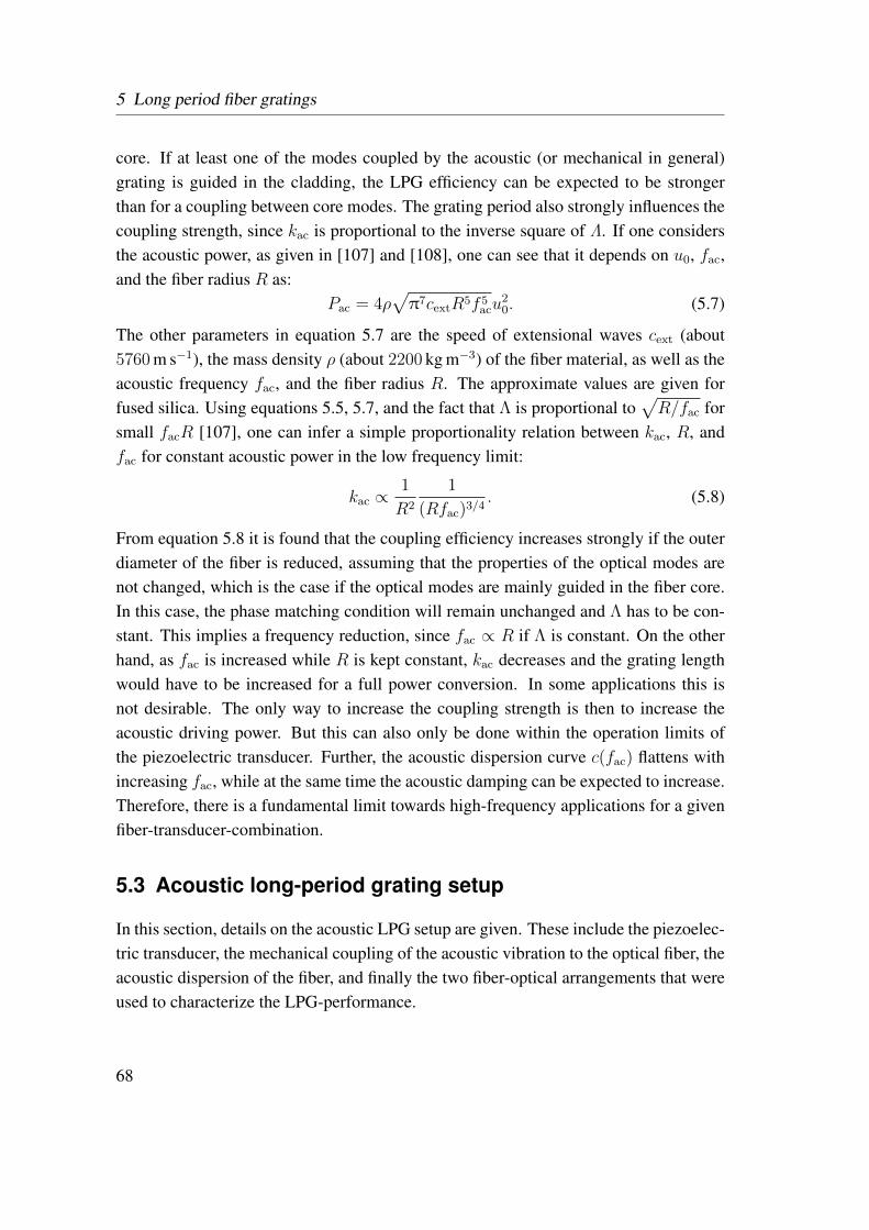
5 Long period fiber gratings
core. If at least one of the modes coupled by the acoustic (or mechanical in general)grating is guided in the cladding, the LPG efficiency can be expected to be strongerthan for a coupling between core modes. The grating period also strongly influences thecoupling strength, since kac is proportional to the inverse square of Λ. If one considersthe acoustic power, as given in [107] and [108], one can see that it depends on u0, fac,and the fiber radius R as:
Pac = 4ρ√
π7cextR5f 5acu
20. (5.7)
The other parameters in equation 5.7 are the speed of extensional waves cext (about5760 m s−1), the mass density ρ (about 2200 kg m−3) of the fiber material, as well as theacoustic frequency fac, and the fiber radius R. The approximate values are given forfused silica. Using equations 5.5, 5.7, and the fact that Λ is proportional to
√R/fac for
small facR [107], one can infer a simple proportionality relation between kac, R, andfac for constant acoustic power in the low frequency limit:
kac ∝1
R2
1
(Rfac)3/4. (5.8)
From equation 5.8 it is found that the coupling efficiency increases strongly if the outerdiameter of the fiber is reduced, assuming that the properties of the optical modes arenot changed, which is the case if the optical modes are mainly guided in the fiber core.In this case, the phase matching condition will remain unchanged and Λ has to be con-stant. This implies a frequency reduction, since fac ∝ R if Λ is constant. On the otherhand, as fac is increased while R is kept constant, kac decreases and the grating lengthwould have to be increased for a full power conversion. In some applications this isnot desirable. The only way to increase the coupling strength is then to increase theacoustic driving power. But this can also only be done within the operation limits ofthe piezoelectric transducer. Further, the acoustic dispersion curve c(fac) flattens withincreasing fac, while at the same time the acoustic damping can be expected to increase.Therefore, there is a fundamental limit towards high-frequency applications for a givenfiber-transducer-combination.
5.3 Acoustic long-period grating setup
In this section, details on the acoustic LPG setup are given. These include the piezoelec-tric transducer, the mechanical coupling of the acoustic vibration to the optical fiber, theacoustic dispersion of the fiber, and finally the two fiber-optical arrangements that wereused to characterize the LPG-performance.
68
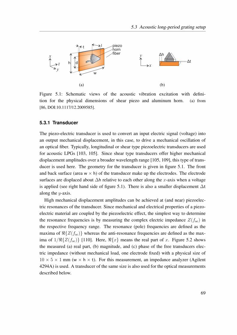
5.3 Acoustic long-period grating setup
z
x
y
dh
w
t l piezohornfiber y
xΔt
Δh
(a) (b)
Figure 5.1: Schematic views of the acoustic vibration excitation with defini-tion for the physical dimensions of shear piezo and aluminum horn. (a) from
[86, DOI:10.1117/12.2009585].
5.3.1 Transducer
The piezo-electric transducer is used to convert an input electric signal (voltage) intoan output mechanical displacement, in this case, to drive a mechanical oscillation ofan optical fiber. Typically, longitudinal or shear type piezoelectric transducers are usedfor acoustic LPGs [103, 105]. Since shear type transducers offer higher mechanicaldisplacement amplitudes over a broader wavelength range [105, 109], this type of trans-ducer is used here. The geometry for the transducer is given in figure 5.1. The frontand back surface (area w × h) of the transducer make up the electrodes. The electrodesurfaces are displaced about ∆h relative to each other along the x-axis when a voltageis applied (see right hand side of figure 5.1). There is also a smaller displacement ∆t
along the y-axis.High mechanical displacement amplitudes can be achieved at (and near) piezoelec-
tric resonances of the transducer. Since mechanical and electrical properties of a piezo-electric material are coupled by the piezoelectric effect, the simplest way to determinethe resonance frequencies is by measuring the complex electric impedance Z(fac) inthe respective frequency range. The resonance (pole) frequencies are defined as themaxima of <Z(fac) whereas the anti-resonance frequencies are defined as the max-ima of 1/<Z(fac) [110]. Here, <x means the real part of x. Figure 5.2 showsthe measured (a) real part, (b) magnitude, and (c) phase of the free transducers elec-tric impedance (without mechanical load, one electrode fixed) with a physical size of10 × 5 × 1 mm (w × h × t). For this measurement, an impedance analyzer (Agilent4294A) is used. A transducer of the same size is also used for the optical measurementsdescribed below.
69
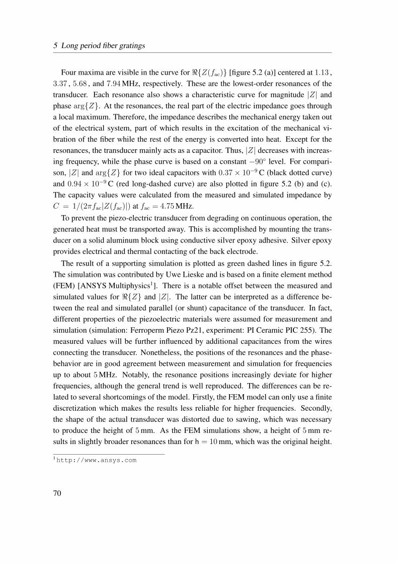
5 Long period fiber gratings
Four maxima are visible in the curve for <Z(fac) [figure 5.2 (a)] centered at 1.13 ,3.37 , 5.68 , and 7.94 MHz, respectively. These are the lowest-order resonances of thetransducer. Each resonance also shows a characteristic curve for magnitude |Z| andphase argZ. At the resonances, the real part of the electric impedance goes througha local maximum. Therefore, the impedance describes the mechanical energy taken outof the electrical system, part of which results in the excitation of the mechanical vi-bration of the fiber while the rest of the energy is converted into heat. Except for theresonances, the transducer mainly acts as a capacitor. Thus, |Z| decreases with increas-ing frequency, while the phase curve is based on a constant −90 level. For compari-son, |Z| and argZ for two ideal capacitors with 0.37× 10⁻⁹ C (black dotted curve)and 0.94× 10⁻⁹ C (red long-dashed curve) are also plotted in figure 5.2 (b) and (c).The capacity values were calculated from the measured and simulated impedance byC = 1/(2πfac|Z(fac)|) at fac = 4.75 MHz.
To prevent the piezo-electric transducer from degrading on continuous operation, thegenerated heat must be transported away. This is accomplished by mounting the trans-ducer on a solid aluminum block using conductive silver epoxy adhesive. Silver epoxyprovides electrical and thermal contacting of the back electrode.
The result of a supporting simulation is plotted as green dashed lines in figure 5.2.The simulation was contributed by Uwe Lieske and is based on a finite element method(FEM) [ANSYS Multiphysics1]. There is a notable offset between the measured andsimulated values for <Z and |Z|. The latter can be interpreted as a difference be-tween the real and simulated parallel (or shunt) capacitance of the transducer. In fact,different properties of the piezoelectric materials were assumed for measurement andsimulation (simulation: Ferroperm Piezo Pz21, experiment: PI Ceramic PIC 255). Themeasured values will be further influenced by additional capacitances from the wiresconnecting the transducer. Nonetheless, the positions of the resonances and the phase-behavior are in good agreement between measurement and simulation for frequenciesup to about 5 MHz. Notably, the resonance positions increasingly deviate for higherfrequencies, although the general trend is well reproduced. The differences can be re-lated to several shortcomings of the model. Firstly, the FEM model can only use a finitediscretization which makes the results less reliable for higher frequencies. Secondly,the shape of the actual transducer was distorted due to sawing, which was necessaryto produce the height of 5 mm. As the FEM simulations show, a height of 5 mm re-sults in slightly broader resonances than for h = 10 mm, which was the original height.
1http://www.ansys.com
70
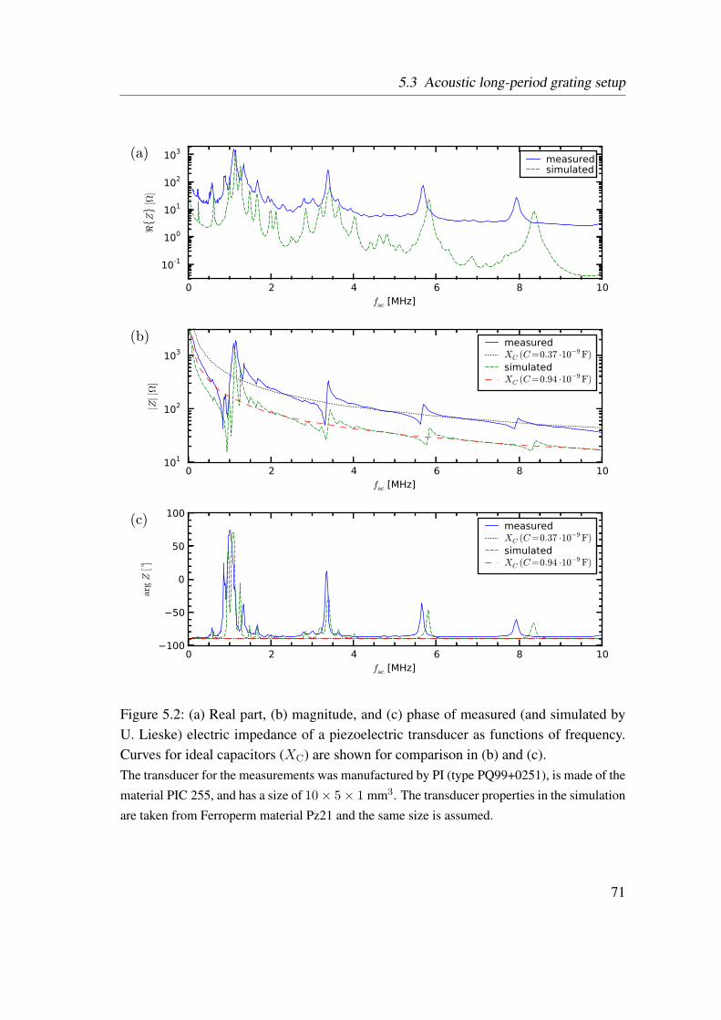
5.3 Acoustic long-period grating setup
0 2 4 6 8 10fac [MHz]
10-1
100
101
102
103< Z
[Ω]
(a) measuredsimulated
0 2 4 6 8 10fac [MHz]
101
102
103
|Z|[
Ω]
(b) measuredXC (C=0.37 ·10−9 F)
simulatedXC (C=0.94 ·10−9 F)
0 2 4 6 8 10fac [MHz]
100
50
0
50
100
argZ
[]
(c) measuredXC (C=0.37 ·10−9 F)
simulatedXC (C=0.94 ·10−9 F)
Figure 5.2: (a) Real part, (b) magnitude, and (c) phase of measured (and simulated byU. Lieske) electric impedance of a piezoelectric transducer as functions of frequency.Curves for ideal capacitors (XC) are shown for comparison in (b) and (c).The transducer for the measurements was manufactured by PI (type PQ99+0251), is made of the
material PIC 255, and has a size of 10× 5× 1 mm3. The transducer properties in the simulation
are taken from Ferroperm material Pz21 and the same size is assumed.
71
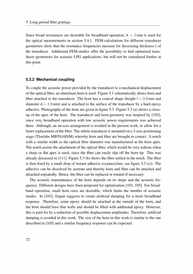
5 Long period fiber gratings
Since broad resonances are desirable for broadband operation, h = 5 mm is used forthe optical measurements in section 5.4.1. FEM-calculations for different transducergeometries show that the resonance frequencies increase for decreasing thickness t ofthe transducer. Additional FEM-studies offer the possibility to find optimized trans-ducer geometries for acoustic LPG applications, but will not be considered further atthis point.
5.3.2 Mechanical coupling
To couple the acoustic power provided by the transducer to a mechanical displacementof the optical fiber, an aluminum horn is used. Figure 5.1 schematically shows horn andfiber attached to the transducer. The horn has a conical shape (height l = 3.9 mm anddiameter d = 1.9 mm) and is attached to the surface of the transducer by a hard epoxyadhesive. Photographs of the horn are given in figure 5.3. Figure 5.3 (a) shows a close-up of the apex of the horn. The transducer and horn-geometry was inspired by [105],since very broadband operation with low acoustic power requirements was achievedthere. Although, an on-axis arrangement is avoided in the present work, to allow for afaster replacement of the fiber. The whole transducer is mounted on a 3-axis positioningstage (Thorlabs MBT616D/M) whereby horn and fiber are brought in contact. A notchwith a similar width as the optical fiber diameter was manufactured at the horn apex.The notch assists the attachment of the optical fiber, which would be very tedious whena sharp or flat apex is used, since the fiber can easily slip off the horn tip. This wasalready discussed in [111]. Figure 5.3 (b) shows the fiber settled in the notch. The fiberis then fixed by a small drop of instant adhesive (cyanacrylate, see figure 5.3 (c)). Theadhesive can be dissolved by acetone and thereby horn and fiber can be attached anddetached repeatedly. Hence, the fiber can be replaced or rotated if necessary.
The acoustic transmittance of the horn depends on its shape and the acoustic fre-quency. Different designs have been proposed for optimization [103, 105]. For broad-band operation, small horn sizes are desirable, which limits the number of acousticmodes. In [103], Engan suggests to create artificial damping for a more broadbandresponse. Therefore, some epoxy should be attached at the outside of the horn, andthe horn should have thin walls and should be filled with additional epoxy. However,this is paid for by a reduction of possible displacement amplitudes. Therefore, artificialdamping is avoided in this work. The size of the horn in this work is similar to the onedescribed in [105] and a similar frequency response can be expected.
72
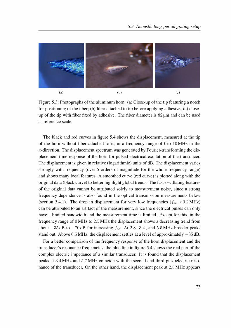
5.3 Acoustic long-period grating setup
(a) (b) (c)
Figure 5.3: Photographs of the aluminum horn: (a) Close-up of the tip featuring a notchfor positioning of the fiber; (b) fiber attached to tip before applying adhesive; (c) close-up of the tip with fiber fixed by adhesive. The fiber diameter is 82 µm and can be usedas reference scale.
The black and red curves in figure 5.4 shows the displacement, measured at the tipof the horn without fiber attached to it, in a frequency range of 0 to 10 MHz in thex-direction. The displacement spectrum was generated by Fourier-transforming the dis-placement time response of the horn for pulsed electrical excitation of the transducer.The displacement is given in relative (logarithmic) units of dB. The displacement variesstrongly with frequency (over 5 orders of magnitude for the whole frequency range)and shows many local features. A smoothed curve (red curve) is plotted along with theoriginal data (black curve) to better highlight global trends. The fast-oscillating featuresof the original data cannot be attributed solely to measurement noise, since a strongfrequency dependence is also found in the optical transmission measurements below(section 5.4.1). The drop in displacement for very low frequencies (fac <0.2 MHz)can be attributed to an artifact of the measurement, since the electrical pulses can onlyhave a limited bandwidth and the measurement time is limited. Except for this, in thefrequency range of 0 MHz to 2.5 MHz the displacement shows a decreasing trend fromabout −35 dB to −70 dB for increasing fac. At 2.8 , 3.4 , and 5.5 MHz broader peaksstand out. Above 6.5 MHz, the displacement settles at a level of approximately−85 dB.
For a better comparison of the frequency response of the horn displacement and thetransducer’s resonance frequencies, the blue line in figure 5.4 shows the real part of thecomplex electric impedance of a similar transducer. It is found that the displacementpeaks at 3.4 MHz and 5.7 MHz coincide with the second and third piezoelectric reso-nance of the transducer. On the other hand, the displacement peak at 2.8 MHz appears
73
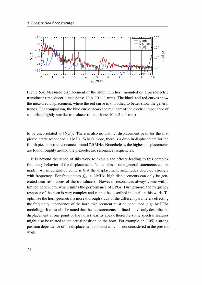
5 Long period fiber gratings
0 1 2 3 4 5 6 7 8 9 10fac [MHz]
90
75
60
45
30
15
D [
dB
]
D orig.D smoo.<Z
101
102
103
104
< Z
[Ω]
Figure 5.4: Measured displacement of the aluminum horn mounted on a piezoelectrictransducer (transducer dimensions: 10 × 10 × 1 mm). The black and red curves showthe measured displacement, where the red curve is smoothed to better show the generaltrends. For comparison, the blue curve shows the real part of the electric impedance ofa similar, slightly smaller transducer (dimensions: 10× 5× 1 mm).
to be uncorrelated to <Z. There is also no distinct displacement peak for the firstpiezoelectric resonance 1.1 MHz. What’s more, there is a drop in displacement for thefourth piezoelectric resonance around 7.9 MHz. Nonetheless, the highest displacementsare found roughly around the piezoelectric resonance frequencies.
It is beyond the scope of this work to explain the effects leading to this complexfrequency behavior of the displacement. Nonetheless, some general statements can bemade. An important outcome is that the displacement amplitudes decrease stronglywith frequency. For frequencies fac > 2 MHz, high displacements can only be gen-erated near resonances of the transducers. However, resonances always come with alimited bandwidth, which limits the performance of LPGs. Furthermore, the frequencyresponse of the horn is very complex and cannot be described in detail in this work. Tooptimize the horn geometry, a more thorough study of the different parameters effectingthe frequency dependence of the horn displacement must be conducted (e.g. by FEMmodeling). It must also be noted that the measurements outlined above only describe thedisplacement at one point of the horn (near its apex), therefore some spectral featuresmight also be related to the actual position on the horn. For example, in [105] a strongposition dependence of the displacement is found which is not considered in the presentwork.
74
5.3 Acoustic long-period grating setup
5.3.3 Acoustic dispersion of an optical fiber
The next key-component for a description of LPGs is the acoustic dispersion of an op-tical fiber. The acoustic dispersion links the phase velocity of an acoustic wave cac tothe acoustic frequency fac. Thereby, the grating period Λ is given as Λ = 2π/kac =
cac(fac)/fac (see section 5.2.3). The relation between the acoustic frequency and thegrating period must be known to calculate the effective index difference between op-tical modes coupled by an acoustic LPG. The theory of propagating acoustic modesin an optical fiber was already outlined in [107]. Although other than flexural modes,e.g. torsional waves, have been suggested and used in LPGs [112, 113, 114], onlythe lowest-order flexural mode of the fiber is considered in this work. In a number ofother works, measurements of the acoustic dispersion of an optical fiber were presented[107, 95, 115, 96], which show good agreement with the theory in [107]. However, thedetails of these measurements are only sparsely described in most cases. It is thereforehoped that producing another verifying measurement can give more insight into the ac-curacy of such measurements and to verify the validity of the theory for the particularSF used here. Consequently, measurements of cac(fac) will be given and compared tocurves calculated from theory in this section. The calculation is basically a numeri-cal eigenvalue computation. This can be prone to errors, giving all the more reason toacquire suitable measurement data for a validation of the calculation.
Figure 5.5 (a) shows the measured and calculated dispersion curve cac(fac) for thelowest-order flexural mode. The calculation is kindly provided by Lars Schubert, whoused the formulas of [116] for the numerical eigenvalue calculation and the materialproperties of fused silica glass listed in [107]. The dispersion curve is similar to asquare root for low frequencies, but approaches a constant level for higher frequencies.From [107] one can expect that there are no higher flexural modes for frequencies below30 MHz.
The measurement setup is depicted in figure 5.5 (b). The beam of a laser vibrome-ter (L-VIB2), based on a modified heterodyne Mach-Zehnder interferometer, is focusedon the surface of the optical fiber under study and the time-resolved displacement inx-direction is measured. In contrast to other measurements in this work, a commercialultra-sonic transducer (type: GE G5 MN) is used, providing a longitudinal displace-ment. This transducer is designed to show no resonances in this frequency range andtherefore gives a flat phase response. A suitable aluminum horn was designed and fab-
2 type: Polytec OFV-353 sensor head with DD-300 decoder for pulse measurements and OFV-505 sensorhead with OFV-2570 detector for single-frequency measurements
75
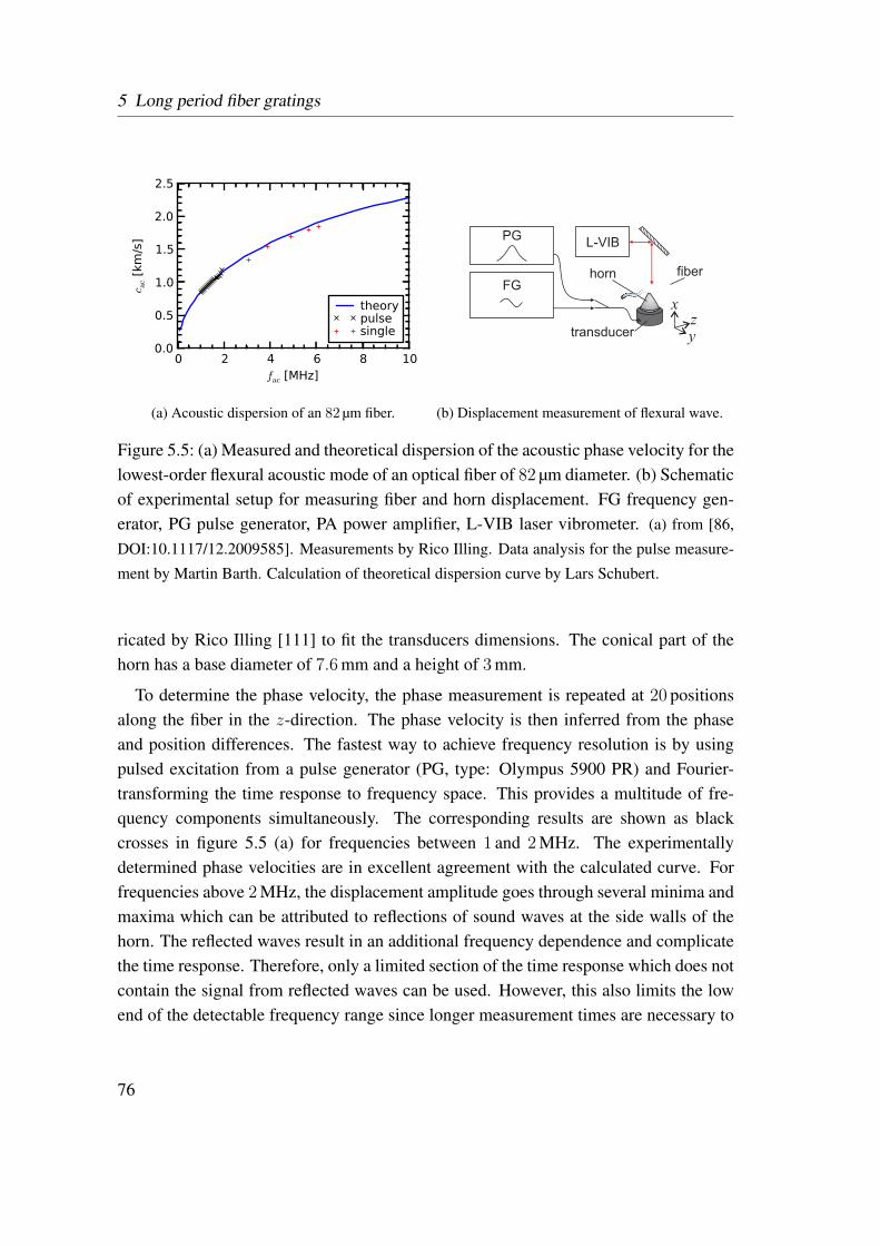
5 Long period fiber gratings
0 2 4 6 8 10fac [MHz]
0.0
0.5
1.0
1.5
2.0
2.5
c ac [k
m/s
]
theorypulsesingle
(a) Acoustic dispersion of an 82 µm fiber.
FG
L-VIBPG
zx
y
horn
transducer
fiber
(b) Displacement measurement of flexural wave.
Figure 5.5: (a) Measured and theoretical dispersion of the acoustic phase velocity for thelowest-order flexural acoustic mode of an optical fiber of 82 µm diameter. (b) Schematicof experimental setup for measuring fiber and horn displacement. FG frequency gen-erator, PG pulse generator, PA power amplifier, L-VIB laser vibrometer. (a) from [86,
DOI:10.1117/12.2009585]. Measurements by Rico Illing. Data analysis for the pulse measure-
ment by Martin Barth. Calculation of theoretical dispersion curve by Lars Schubert.
ricated by Rico Illing [111] to fit the transducers dimensions. The conical part of thehorn has a base diameter of 7.6 mm and a height of 3 mm.
To determine the phase velocity, the phase measurement is repeated at 20 positionsalong the fiber in the z-direction. The phase velocity is then inferred from the phaseand position differences. The fastest way to achieve frequency resolution is by usingpulsed excitation from a pulse generator (PG, type: Olympus 5900 PR) and Fourier-transforming the time response to frequency space. This provides a multitude of fre-quency components simultaneously. The corresponding results are shown as blackcrosses in figure 5.5 (a) for frequencies between 1 and 2 MHz. The experimentallydetermined phase velocities are in excellent agreement with the calculated curve. Forfrequencies above 2 MHz, the displacement amplitude goes through several minima andmaxima which can be attributed to reflections of sound waves at the side walls of thehorn. The reflected waves result in an additional frequency dependence and complicatethe time response. Therefore, only a limited section of the time response which does notcontain the signal from reflected waves can be used. However, this also limits the lowend of the detectable frequency range since longer measurement times are necessary to
76
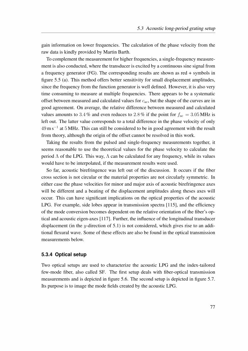
5.3 Acoustic long-period grating setup
gain information on lower frequencies. The calculation of the phase velocity from theraw data is kindly provided by Martin Barth.
To complement the measurement for higher frequencies, a single-frequency measure-ment is also conducted, where the transducer is excited by a continuous sine signal froma frequency generator (FG). The corresponding results are shown as red + symbols infigure 5.5 (a). This method offers better sensitivity for small displacement amplitudes,since the frequency from the function generator is well defined. However, it is also verytime consuming to measure at multiple frequencies. There appears to be a systematicoffset between measured and calculated values for cac, but the shape of the curves are ingood agreement. On average, the relative difference between measured and calculatedvalues amounts to 3.4 % and even reduces to 2.8 % if the point for fac = 3.05 MHz isleft out. The latter value corresponds to a total difference in the phase velocity of only49 m s−1 at 5 MHz. This can still be considered to be in good agreement with the resultfrom theory, although the origin of the offset cannot be resolved in this work.
Taking the results from the pulsed and single-frequency measurements together, itseems reasonable to use the theoretical values for the phase velocity to calculate theperiod Λ of the LPG. This way, Λ can be calculated for any frequency, while its valueswould have to be interpolated, if the measurement results were used.
So far, acoustic birefringence was left out of the discussion. It occurs if the fibercross section is not circular or the material properties are not circularly symmetric. Ineither case the phase velocities for minor and major axis of acoustic birefringence axeswill be different and a beating of the displacement amplitudes along theses axes willoccur. This can have significant implications on the optical properties of the acousticLPG. For example, side lobes appear in transmission spectra [115], and the efficiencyof the mode conversion becomes dependent on the relative orientation of the fiber’s op-tical and acoustic eigen-axes [117]. Further, the influence of the longitudinal transducerdisplacement (in the y-direction of 5.1) is not considered, which gives rise to an addi-tional flexural wave. Some of these effects are also be found in the optical transmissionmeasurements below.
5.3.4 Optical setup
Two optical setups are used to characterize the acoustic LPG and the index-tailoredfew-mode fiber, also called SF. The first setup deals with fiber-optical transmissionmeasurements and is depicted in figure 5.6. The second setup is depicted in figure 5.7.Its purpose is to image the mode fields created by the acoustic LPG.
77
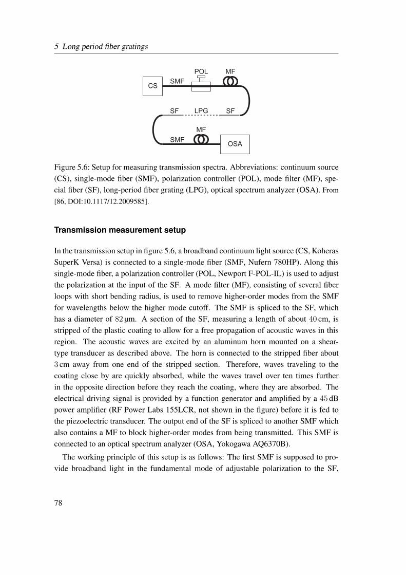
5 Long period fiber gratings
Figure 5.6: Setup for measuring transmission spectra. Abbreviations: continuum source(CS), single-mode fiber (SMF), polarization controller (POL), mode filter (MF), spe-cial fiber (SF), long-period fiber grating (LPG), optical spectrum analyzer (OSA). From
[86, DOI:10.1117/12.2009585].
Transmission measurement setup
In the transmission setup in figure 5.6, a broadband continuum light source (CS, KoherasSuperK Versa) is connected to a single-mode fiber (SMF, Nufern 780HP). Along thissingle-mode fiber, a polarization controller (POL, Newport F-POL-IL) is used to adjustthe polarization at the input of the SF. A mode filter (MF), consisting of several fiberloops with short bending radius, is used to remove higher-order modes from the SMFfor wavelengths below the higher mode cutoff. The SMF is spliced to the SF, whichhas a diameter of 82 µm. A section of the SF, measuring a length of about 40 cm, isstripped of the plastic coating to allow for a free propagation of acoustic waves in thisregion. The acoustic waves are excited by an aluminum horn mounted on a shear-type transducer as described above. The horn is connected to the stripped fiber about3 cm away from one end of the stripped section. Therefore, waves traveling to thecoating close by are quickly absorbed, while the waves travel over ten times furtherin the opposite direction before they reach the coating, where they are absorbed. Theelectrical driving signal is provided by a function generator and amplified by a 45 dBpower amplifier (RF Power Labs 155LCR, not shown in the figure) before it is fed tothe piezoelectric transducer. The output end of the SF is spliced to another SMF whichalso contains a MF to block higher-order modes from being transmitted. This SMF isconnected to an optical spectrum analyzer (OSA, Yokogawa AQ6370B).
The working principle of this setup is as follows: The first SMF is supposed to pro-vide broadband light in the fundamental mode of adjustable polarization to the SF,
78
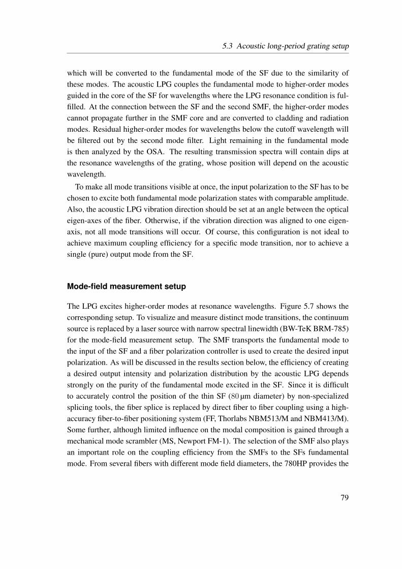
5.3 Acoustic long-period grating setup
which will be converted to the fundamental mode of the SF due to the similarity ofthese modes. The acoustic LPG couples the fundamental mode to higher-order modesguided in the core of the SF for wavelengths where the LPG resonance condition is ful-filled. At the connection between the SF and the second SMF, the higher-order modescannot propagate further in the SMF core and are converted to cladding and radiationmodes. Residual higher-order modes for wavelengths below the cutoff wavelength willbe filtered out by the second mode filter. Light remaining in the fundamental modeis then analyzed by the OSA. The resulting transmission spectra will contain dips atthe resonance wavelengths of the grating, whose position will depend on the acousticwavelength.
To make all mode transitions visible at once, the input polarization to the SF has to bechosen to excite both fundamental mode polarization states with comparable amplitude.Also, the acoustic LPG vibration direction should be set at an angle between the opticaleigen-axes of the fiber. Otherwise, if the vibration direction was aligned to one eigen-axis, not all mode transitions will occur. Of course, this configuration is not ideal toachieve maximum coupling efficiency for a specific mode transition, nor to achieve asingle (pure) output mode from the SF.
Mode-field measurement setup
The LPG excites higher-order modes at resonance wavelengths. Figure 5.7 shows thecorresponding setup. To visualize and measure distinct mode transitions, the continuumsource is replaced by a laser source with narrow spectral linewidth (BW-TeK BRM-785)for the mode-field measurement setup. The SMF transports the fundamental mode tothe input of the SF and a fiber polarization controller is used to create the desired inputpolarization. As will be discussed in the results section below, the efficiency of creatinga desired output intensity and polarization distribution by the acoustic LPG dependsstrongly on the purity of the fundamental mode excited in the SF. Since it is difficultto accurately control the position of the thin SF (80 µm diameter) by non-specializedsplicing tools, the fiber splice is replaced by direct fiber to fiber coupling using a high-accuracy fiber-to-fiber positioning system (FF, Thorlabs NBM513/M and NBM413/M).Some further, although limited influence on the modal composition is gained through amechanical mode scrambler (MS, Newport FM-1). The selection of the SMF also playsan important role on the coupling efficiency from the SMFs to the SFs fundamentalmode. From several fibers with different mode field diameters, the 780HP provides the
79
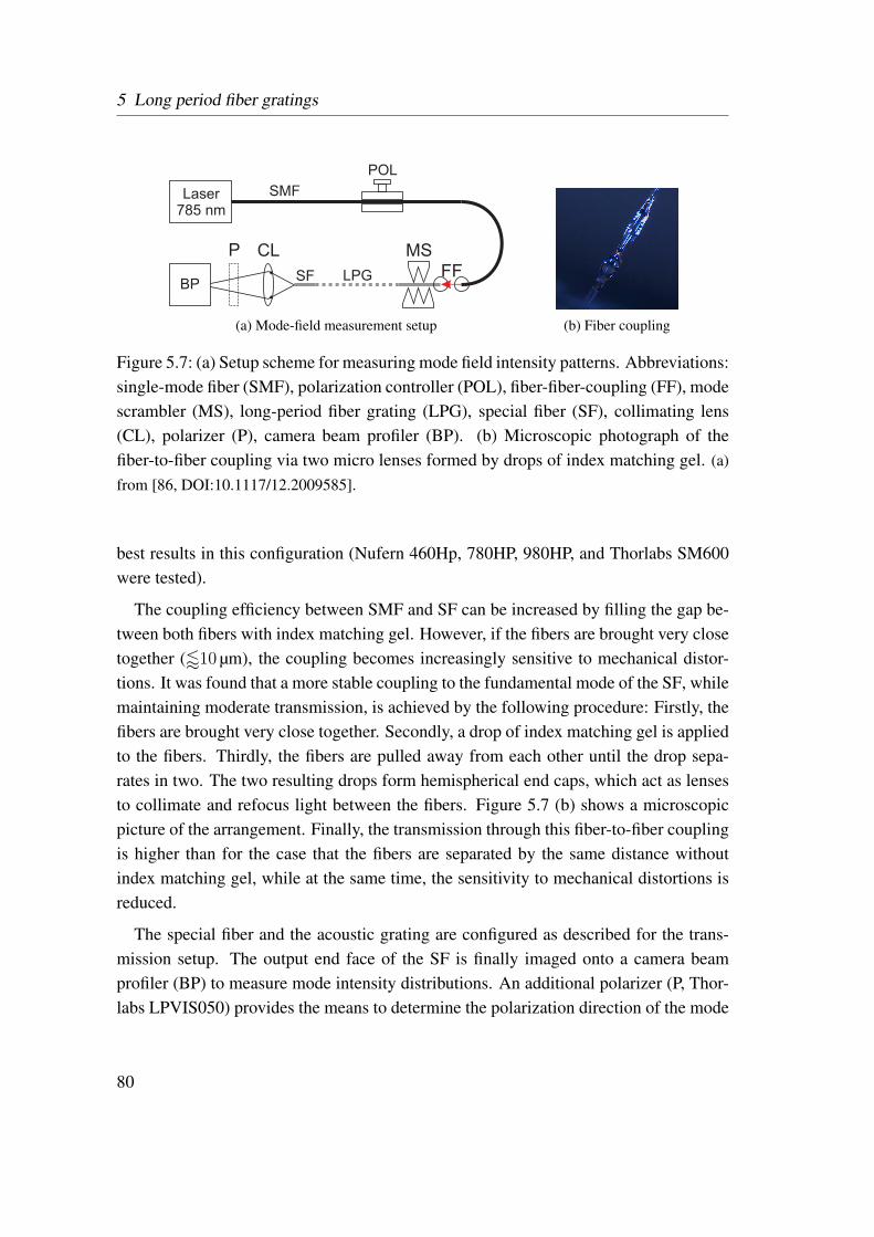
5 Long period fiber gratings
(a) Mode-field measurement setup (b) Fiber coupling
Figure 5.7: (a) Setup scheme for measuring mode field intensity patterns. Abbreviations:single-mode fiber (SMF), polarization controller (POL), fiber-fiber-coupling (FF), modescrambler (MS), long-period fiber grating (LPG), special fiber (SF), collimating lens(CL), polarizer (P), camera beam profiler (BP). (b) Microscopic photograph of thefiber-to-fiber coupling via two micro lenses formed by drops of index matching gel. (a)
from [86, DOI:10.1117/12.2009585].
best results in this configuration (Nufern 460Hp, 780HP, 980HP, and Thorlabs SM600were tested).
The coupling efficiency between SMF and SF can be increased by filling the gap be-tween both fibers with index matching gel. However, if the fibers are brought very closetogether (/10 µm), the coupling becomes increasingly sensitive to mechanical distor-tions. It was found that a more stable coupling to the fundamental mode of the SF, whilemaintaining moderate transmission, is achieved by the following procedure: Firstly, thefibers are brought very close together. Secondly, a drop of index matching gel is appliedto the fibers. Thirdly, the fibers are pulled away from each other until the drop sepa-rates in two. The two resulting drops form hemispherical end caps, which act as lensesto collimate and refocus light between the fibers. Figure 5.7 (b) shows a microscopicpicture of the arrangement. Finally, the transmission through this fiber-to-fiber couplingis higher than for the case that the fibers are separated by the same distance withoutindex matching gel, while at the same time, the sensitivity to mechanical distortions isreduced.
The special fiber and the acoustic grating are configured as described for the trans-mission setup. The output end face of the SF is finally imaged onto a camera beamprofiler (BP) to measure mode intensity distributions. An additional polarizer (P, Thor-labs LPVIS050) provides the means to determine the polarization direction of the mode
80
5.3 Acoustic long-period grating setup
fields. The distance between the collimating lens (CL, Newport M20x, 0.40 NA) andthe BP is 63.5 cm.
The initial adjustment of this LPG setup includes several steps which will be outlinedin the following. During this process the orientation of the eigen-axes of the SF canbe determined, the input polarization and fiber-to-fiber-coupling is optimized, and theoptimal acoustic frequency is found. First, the acoustic LPG is driven at a known fre-quency at which a mode transition should occur and the polarizer (P) is removed fromthe setup. Additionally, the amplitude of the driving signal is modulated at a modula-tion frequency which should be low enough for detection by the BP, but fast enough tofollow any adjustments to the setup (about 1 Hz). Now, the image from the BP shouldshow a modulation of the intensity pattern. If not, the frequency of the LPG or the inputpolarization can be adjusted until some modulation is seen. Now, the modulation of theintensity image can be maximized by further adjusting input frequency and polariza-tion and also the fiber-to-fiber coupling and mode scrambler settings. Several iterationsare usually necessary until no further improvement is possible. If an optimal setting isfound, the input polarization will be aligned to one of the eigen-axes of the SF. Theorientation of the axes can be determined using the polarizer (the axes orientations aregiven by the angles for minimum and maximum intensity in the beam center for LPGoff).
5.3.5 Comparison to other acoustic LPG geometries
In comparison to other acoustic LPG geometries, the one discussed so far offers someadvantages. By using a shear-type transducer, one can achieve higher displacement am-plitudes as by longitudinal-type transducers, although operation of longitudinal trans-ducers has been demonstrated successfully even on fibers of 125 µm diameter [95, 96,118]. However, with the setup presented in this work, one can still couple the acousticvibration to the fiber from the side, which allows for easier attachment (and detach-ment) of the fiber to the acoustic horn, because it is not necessary to thread the opticalfiber through the acoustic horn as in the on-axis arrangement of [105]. The on-axisarrangement, however, gives the possibility to couple two shear-piezos oscillating in or-thogonal direction with different amplitude, phase, and frequency to excite two opticalmodes with a controlled phase-difference. This can be useful for the creation of vortexmodes carrying orbital angular momentum [16, 17].
81
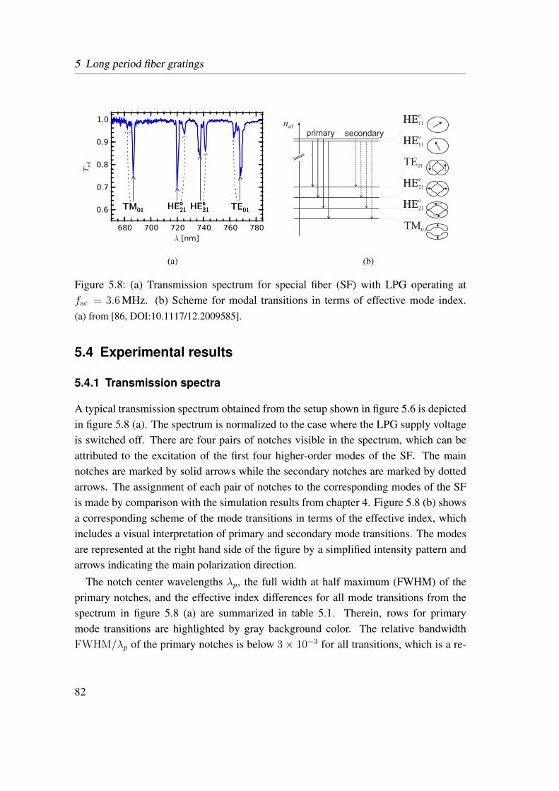
5 Long period fiber gratings
680 700 720 740 760 780λ [nm]
0.6
0.7
0.8
0.9
1.0
Tre
l
TM01TM01 HEo21HEo21 HEe
21HEe21 TE01TE01
(a)
neffprimary secondary
HE11e
HE
HE11oHE
TE01
HE21eHE
HE21oHE
TM01
(b)
Figure 5.8: (a) Transmission spectrum for special fiber (SF) with LPG operating atfac = 3.6 MHz. (b) Scheme for modal transitions in terms of effective mode index.(a) from [86, DOI:10.1117/12.2009585].
5.4 Experimental results
5.4.1 Transmission spectra
A typical transmission spectrum obtained from the setup shown in figure 5.6 is depictedin figure 5.8 (a). The spectrum is normalized to the case where the LPG supply voltageis switched off. There are four pairs of notches visible in the spectrum, which can beattributed to the excitation of the first four higher-order modes of the SF. The mainnotches are marked by solid arrows while the secondary notches are marked by dottedarrows. The assignment of each pair of notches to the corresponding modes of the SFis made by comparison with the simulation results from chapter 4. Figure 5.8 (b) showsa corresponding scheme of the mode transitions in terms of the effective index, whichincludes a visual interpretation of primary and secondary mode transitions. The modesare represented at the right hand side of the figure by a simplified intensity pattern andarrows indicating the main polarization direction.
The notch center wavelengths λp, the full width at half maximum (FWHM) of theprimary notches, and the effective index differences for all mode transitions from thespectrum in figure 5.8 (a) are summarized in table 5.1. Therein, rows for primarymode transitions are highlighted by gray background color. The relative bandwidthFWHM/λp of the primary notches is below 3× 10⁻³ for all transitions, which is a re-
82
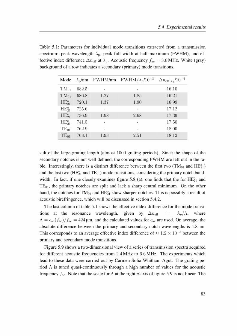
5.4 Experimental results
Table 5.1: Parameters for individual mode transitions extracted from a transmissionspectrum: peak wavelength λp, peak full width at half maximum (FWHM), and ef-fective index difference ∆neff at λp. Acoustic frequency fac = 3.6 MHz. White (gray)background of a row indicates a secondary (primary) mode transitions.
Mode λp/nm FWHM/nm FWHM/λp/10−3 ∆neff |λp/10−4
TM01 682.5 - - 16.10
TM01 686.8 1.27 1.85 16.21
HEo21 720.1 1.37 1.90 16.99
HEo21 725.6 - - 17.12
HEe21 736.9 1.98 2.68 17.39
HEe21 741.5 - - 17.50
TE01 762.9 - - 18.00
TE01 768.1 1.93 2.51 18.12
sult of the large grating length (almost 1000 grating periods). Since the shape of thesecondary notches is not well defined, the corresponding FWHM are left out in the ta-ble. Interestingly, there is a distinct difference between the first two (TM01 and HEo
21)and the last two (HEe
21 and TE01) mode transitions, considering the primary notch band-width. In fact, if one closely examines figure 5.8 (a), one finds that the for HEe
21 andTE01, the primary notches are split and lack a sharp central minimum. On the otherhand, the notches for TM01 and HEo
21 show sharper notches. This is possibly a result ofacoustic birefringence, which will be discussed in section 5.4.2.
The last column of table 5.1 shows the effective index difference for the mode transi-tions at the resonance wavelength, given by ∆neff = λp/Λ, whereΛ = cac(fac)/fac = 424 µm, and the calculated values for cac are used. On average, theabsolute difference between the primary and secondary notch wavelengths is 4.8 nm.This corresponds to an average effective index difference of ≈ 1.2× 10⁻⁵ between theprimary and secondary mode transitions.
Figure 5.9 shows a two-dimensional view of a series of transmission spectra acquiredfor different acoustic frequencies from 2.4 MHz to 6.6 MHz. The experiments whichlead to these data were carried out by Carmen-Sofia Whitham-Agut. The grating pe-riod Λ is tuned quasi-continuously through a high number of values for the acousticfrequency fac. Note that the scale for Λ at the right y-axis of figure 5.9 is not linear. The
83
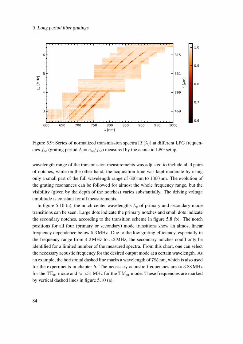
5 Long period fiber gratings
600 650 700 750 800 850 900 950 1000λ [nm]
3
4
5
6
f ac [M
Hz]
0.6
0.7
0.8
0.9
1.0
469
399
351
315
Λ [µm
]
Figure 5.9: Series of normalized transmission spectra [T (λ)] at different LPG frequen-cies fac (grating period Λ = cac/fac) measured by the acoustic LPG setup.
wavelength range of the transmission measurements was adjusted to include all 4 pairsof notches, while on the other hand, the acquisition time was kept moderate by usingonly a small part of the full wavelength range of 600 nm to 1000 nm. The evolution ofthe grating resonances can be followed for almost the whole frequency range, but thevisibility (given by the depth of the notches) varies substantially. The driving voltageamplitude is constant for all measurements.
In figure 5.10 (a), the notch center wavelengths λp of primary and secondary modetransitions can be seen. Large dots indicate the primary notches and small dots indicatethe secondary notches, according to the transition scheme in figure 5.8 (b). The notchpositions for all four (primary or secondary) mode transitions show an almost linearfrequency dependence below 5.3 MHz. Due to the low grating efficiency, especially inthe frequency range from 4.2 MHz to 5.2 MHz, the secondary notches could only beidentified for a limited number of the measured spectra. From this chart, one can selectthe necessary acoustic frequency for the desired output mode at a certain wavelength. Asan example, the horizontal dashed line marks a wavelength of 785 nm, which is also usedfor the experiments in chapter 6. The necessary acoustic frequencies are ≈ 3.88 MHzfor the TE01 mode and ≈ 5.31 MHz for the TM01 mode. These frequencies are markedby vertical dashed lines in figure 5.10 (a).
84
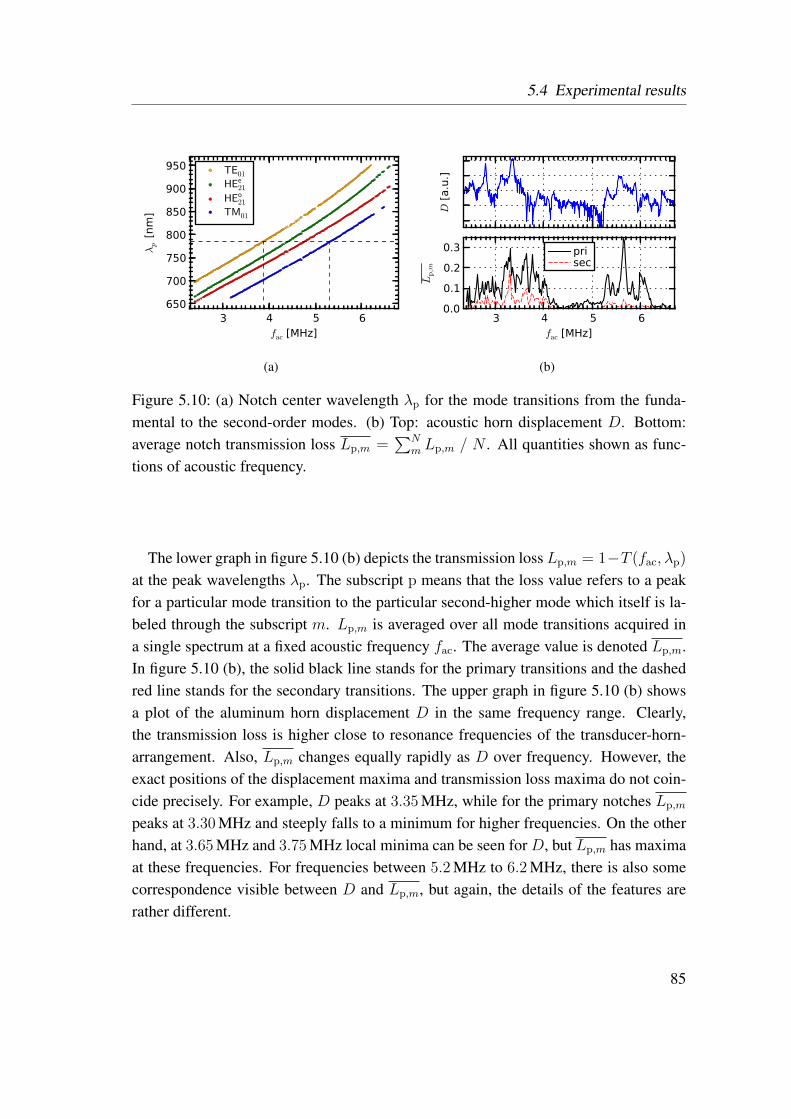
5.4 Experimental results
3 4 5 6fac [MHz]
650
700
750
800
850
900
950
λp [
nm
]
TE01
HEe21
HEo21
TM01
(a)
D [
a.u
.]
3 4 5 6fac [MHz]
0.0
0.1
0.2
0.3
Lp,m
prisec
(b)
Figure 5.10: (a) Notch center wavelength λp for the mode transitions from the funda-mental to the second-order modes. (b) Top: acoustic horn displacement D. Bottom:average notch transmission loss Lp,m =
∑Nm Lp,m / N . All quantities shown as func-
tions of acoustic frequency.
The lower graph in figure 5.10 (b) depicts the transmission loss Lp,m = 1−T (fac, λp)
at the peak wavelengths λp. The subscript p means that the loss value refers to a peakfor a particular mode transition to the particular second-higher mode which itself is la-beled through the subscript m. Lp,m is averaged over all mode transitions acquired ina single spectrum at a fixed acoustic frequency fac. The average value is denoted Lp,m.In figure 5.10 (b), the solid black line stands for the primary transitions and the dashedred line stands for the secondary transitions. The upper graph in figure 5.10 (b) showsa plot of the aluminum horn displacement D in the same frequency range. Clearly,the transmission loss is higher close to resonance frequencies of the transducer-horn-arrangement. Also, Lp,m changes equally rapidly as D over frequency. However, theexact positions of the displacement maxima and transmission loss maxima do not coin-cide precisely. For example, D peaks at 3.35 MHz, while for the primary notches Lp,m
peaks at 3.30 MHz and steeply falls to a minimum for higher frequencies. On the otherhand, at 3.65 MHz and 3.75 MHz local minima can be seen for D, but Lp,m has maximaat these frequencies. For frequencies between 5.2 MHz to 6.2 MHz, there is also somecorrespondence visible between D and Lp,m, but again, the details of the features arerather different.
85
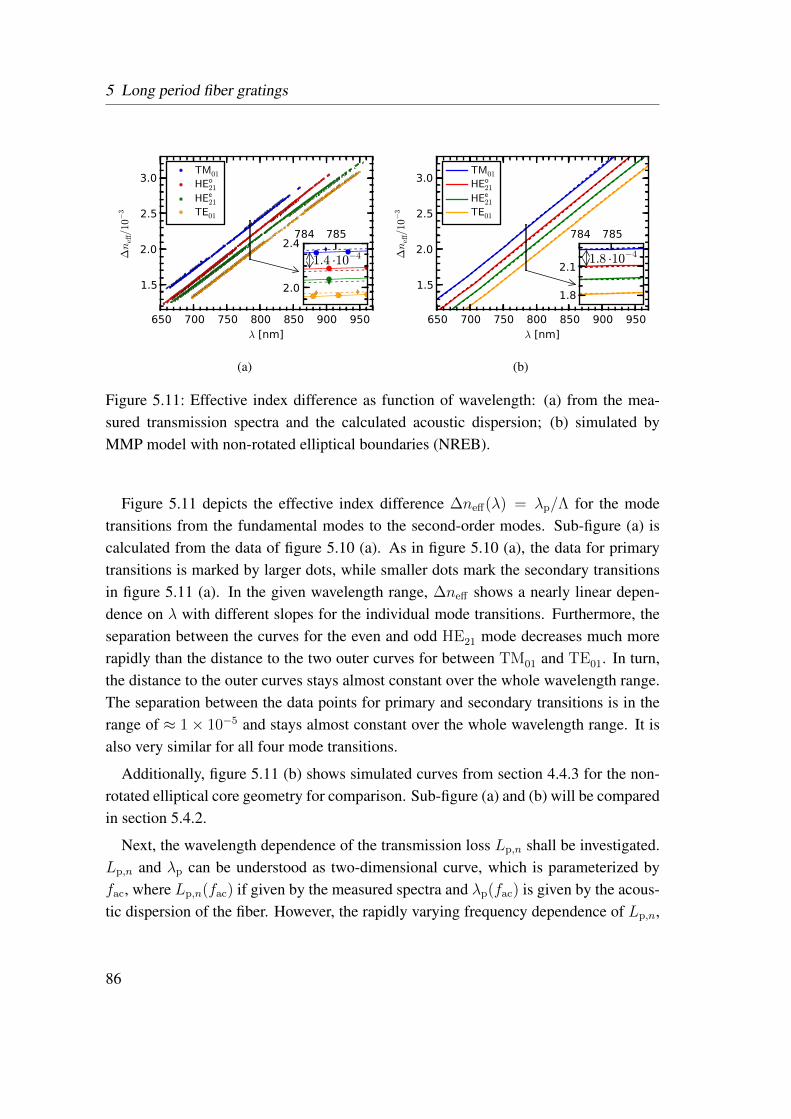
5 Long period fiber gratings
650 700 750 800 850 900 950λ [nm]
1.5
2.0
2.5
3.0
∆n
eff/
10−
3
TM01
HEo21
HEe21
TE01
784 785
2.0
2.4
1.4 ·10−4
(a)
650 700 750 800 850 900 950λ [nm]
1.5
2.0
2.5
3.0
∆n
eff/
10−
3
TM01
HEo21
HEe21
TE01
784 785
1.8
2.11.8 ·10−4
(b)
Figure 5.11: Effective index difference as function of wavelength: (a) from the mea-sured transmission spectra and the calculated acoustic dispersion; (b) simulated byMMP model with non-rotated elliptical boundaries (NREB).
Figure 5.11 depicts the effective index difference ∆neff(λ) = λp/Λ for the modetransitions from the fundamental modes to the second-order modes. Sub-figure (a) iscalculated from the data of figure 5.10 (a). As in figure 5.10 (a), the data for primarytransitions is marked by larger dots, while smaller dots mark the secondary transitionsin figure 5.11 (a). In the given wavelength range, ∆neff shows a nearly linear depen-dence on λ with different slopes for the individual mode transitions. Furthermore, theseparation between the curves for the even and odd HE21 mode decreases much morerapidly than the distance to the two outer curves for between TM01 and TE01. In turn,the distance to the outer curves stays almost constant over the whole wavelength range.The separation between the data points for primary and secondary transitions is in therange of ≈ 1× 10⁻⁵ and stays almost constant over the whole wavelength range. It isalso very similar for all four mode transitions.
Additionally, figure 5.11 (b) shows simulated curves from section 4.4.3 for the non-rotated elliptical core geometry for comparison. Sub-figure (a) and (b) will be comparedin section 5.4.2.
Next, the wavelength dependence of the transmission loss Lp,n shall be investigated.Lp,n and λp can be understood as two-dimensional curve, which is parameterized byfac, where Lp,n(fac) if given by the measured spectra and λp(fac) is given by the acous-tic dispersion of the fiber. However, the rapidly varying frequency dependence of Lp,n,
86
5.4 Experimental results
which has been shown in figure 5.10 (b), makes a comparison between different modetransitions at a particular wavelength difficult. The frequency dependence can be re-moved by dividing each transmission loss value by the maximum loss value measuredin the corresponding spectrum at the same acoustic frequency.
Figure 5.12 (a) and (b) show the resulting transmission loss values plotted againstthe peak wavelengths with the frequency correction mentioned above. This newly nor-malized transmission loss is denoted as Lp,n. In sub-figure (a), only mode transitionsinvolving the even fundamental mode (HEe
11) are used, while for (b) only the odd fun-damental modes (HEo
11) are taken into account. The mode transition scheme in figure5.8 (b) and the example spectrum in 5.8 (a) can be used for comparison.
At first glance, the data points in figure 5.12 (a) and (b) are scattered widely and noparticular wavelength dependence can be found. Nonetheless, there is a clear differencebetween the transmission loss values for individual mode transitions. This becomeseven more obvious calculating a histogram, which is shown to the right of each plot.In this histogram, the horizontal bar length corresponds to the number of transmissionloss values that fall into a particular interval with a binning of 0.2. In sub-figure (a),where only the mode transitions involving HEe
11 are taken into account, the transitionsto the two HE21 modes have the highest transmission loss across the whole wavelengthrange. Except for a small number of data points, the loss values for TE01 and TM01 arelower. If a notch could not be found, it is a transition to one of these two modes, apartfrom few exceptions. Regarding the mode transitions involving the odd fundamentalmode (HEo
11) in sub-figure (b), the opposite behavior is found. Here, it is the transitionsto the modes TE01 and TM01, which show the highest transmission loss values acrossthe whole wavelength range, while the HE21 mode transitions show lower transmissionefficiency.
87
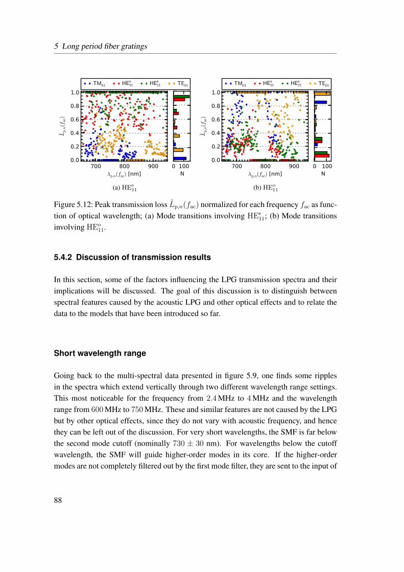
5 Long period fiber gratings
700 800 900λp,n(fac) [nm]
0.0
0.2
0.4
0.6
0.8
1.0
Lp,n(f
ac)
TM01 HEo21 HEe
21 TE01
0 100N
(a) HEe11
700 800 900λp,n(fac) [nm]
0.0
0.2
0.4
0.6
0.8
1.0
Lp,n(f
ac)
TM01 HEo21 HEe
21 TE01
0 100N
(b) HEo11
Figure 5.12: Peak transmission loss Lp,n(fac) normalized for each frequency fac as func-tion of optical wavelength; (a) Mode transitions involving HEe
11; (b) Mode transitionsinvolving HEo
11.
5.4.2 Discussion of transmission results
In this section, some of the factors influencing the LPG transmission spectra and theirimplications will be discussed. The goal of this discussion is to distinguish betweenspectral features caused by the acoustic LPG and other optical effects and to relate thedata to the models that have been introduced so far.
Short wavelength range
Going back to the multi-spectral data presented in figure 5.9, one finds some ripplesin the spectra which extend vertically through two different wavelength range settings.This most noticeable for the frequency from 2.4 MHz to 4 MHz and the wavelengthrange from 600 MHz to 750 MHz. These and similar features are not caused by the LPGbut by other optical effects, since they do not vary with acoustic frequency, and hencethey can be left out of the discussion. For very short wavelengths, the SMF is far belowthe second mode cutoff (nominally 730 ± 30 nm). For wavelengths below the cutoffwavelength, the SMF will guide higher-order modes in its core. If the higher-ordermodes are not completely filtered out by the first mode filter, they are sent to the input of
88
5.4 Experimental results
the SF. There, they can excite one of SMF’s higher-order modes directly3. Furthermore,at the interface between SF-output and the second SMF, the just mentioned higher-ordermodes will be accepted and transmitted efficiently through the SMF leading to the OSAand might not be fully removed by the second mode filter. Both effects reduce the notchdepth in the transmission spectra for short wavelengths. As a result, the notch visibilitydrops for wavelengths below 660 nm in figure 5.9. For wavelengths above 700 nm,higher-order mode effects in the SMF are negligible and the transmission of the SMF isalso almost unchanged. In turn, the reduced notch visibility for the frequency ranges of4.2 MHz to 5.2 MHz and above 6.2 MHz is caused by the acoustic grating behavior andnot by purely optical effects.
Frequency behavior of the acoustic LPG
The frequency behavior of the acoustic LPG is complex, as indicated by the rapidlyvarying transmission loss in figures 5.10 (b). A direct comparison to the measured alu-minum horn displacement reveals that the highest efficiencies can be reached close tomechanical resonances of the transducer. But apart from the transducer resonances,there must be more effects involved. For example, a varying displacement amplitudealong the aluminum horn, or a frequency dependence of the acoustic coupling betweenhorn and fiber can complicate the overall frequency response of the acoustic LPG. In thecontext of this discussion, it is sufficient to regard the overall frequency behavior as agiven instrument characteristic, which is not necessary to understand in detail. Nonethe-less, for a truly broadband operation of the acoustic LPG, the frequency behavior mustbe optimized and the rapidly varying dependence on frequency must be reduced, whilethe overall mode coupling efficiency needs to be enhanced over a broader wavelengthrange.
Origin of different notch widths
For the discussion of other spectral features, it is beneficial to make use of the modetransition scheme in figure 5.8 (b). With its help, one can can gain an understanding ofthe transmission notch positions and the different notch widths. In terms of the notchwidth, it was was found that the mode transitions can be classified into those involving
3 For example, similar second-order modes exist in the SF and the SMF, which are also called TE01,HE21, and TM01. Their mode fields are slightly different, however, they should still show a strong fieldoverlap and high coupling efficiencies can be expected.
89
5 Long period fiber gratings
TM01 and HEo21 modes or those involving TE01 and HEe
21 modes. The modes of each ofthose pairs share a similar intensity distribution. Hence, the mode conversion efficiencyin each pair is equally influenced by the acoustic vibration amplitude along the axisconnecting the two intensity lobes which are indicated in figure 5.8 (b). If the fiber isacoustically birefringent, two distinct acoustic phase velocities are present, which leadto slightly different resonance conditions. Since the grating vibration direction is ingeneral not aligned to one of the birefringent eigen-axes, both resonance conditions willlead to mode coupling at slightly different optical wavelengths. However, the strengthof the mode coupling will depend on the exact orientation of the initial acoustic vibra-tion direction, the acoustic eigen-axes, the orientation of the intensity patterns of theoptical modes and also on the length of the fiber. Therefore, acoustic birefringence is aplausible cause for the pairwise similarity of notch widths and the pairwise occurrenceof notch splitting, which also lead to a reduction of the notch depth [117]. Further-more, the results of [117] show that acoustic birefringence equally effects transitionsto modes with equal intensity patterns, independent of the optical polarization of thosemodes. Translated to this work, TM01 and HEo
21 should show comparable notch widths,and so should TE01 and HEe
21, if the notch splitting and the overall notch width areinfluenced by acoustic birefringence. Comparing the notch widths of all acquired spec-tra, the aforementioned features can be found in several of them, indeed. However, thewavelength resolution and the overall statistical quality are not sufficient to prove or dis-prove a causal relationship between the notch width and acoustic birefringence at thispoint. Twist of the fiber can create additional transmission notch splitting, as is shownin [119]. But such a twist should equally affect all four notches, and can hence be ruledout as cause for the notch splitting in the present experiments.
Comparison of measurements and simulations
If figures 5.11 (a) and (b) are compared, one finds that the measured dependence of ∆neff
on wavelength agrees with the simulation results from chapter 4 in its key properties.These are: 1.) the presence of four double notches in the transmission spectra that leadto eight transition curves; 2.) the order in which the curves for primary and secondarytransitions appear agrees with the mode coupling scheme in figure 5.8 (b); 3) the almostlinear curve shape for ∆neff(λ) for all four second-order modes over a broad wavelengthrange; 4.) similar separations between the curves for the 4 second-order modes; 5) andthe much smaller separation between the curves for primary and secondary mode tran-sitions. The simulation data for the non-rotated elliptical core geometry is chosen for
90
5.4 Experimental results
Table 5.2: Effective index difference between fundamental and second-order modes.Comparison between non-rotated elliptical boundary model (NREB), rotated ellipticalboundary model (REB), and measured data (MEAS).
Transition (∆n1 −∆n2) / 10−4
1 2 NREB REB MEAS
TE01 (pri.) HEe21 (pri.) 1.60 2.04 1.46
HEe21 (pri.) HEo
21 (pri.) 1.35 5.68 0.97HEo
21 (pri.) TM01 (pri.) 1.77 1.29 1.44average (pri.) average (sec.) 0.06 0.30 0.25
figure 5.11 (b), since it provides a better match to the measured data than the modelwith rotated elliptical boundaries. At 785 nm wavelength, the measured effective indexseparation between the TM01 mode and the HEo
21 mode is 1.4× 10⁻⁴. This is slightlysmaller than the value predicted by the simulation (1.8× 10⁻⁴). However, this result isnot surprising, since the simulation model of the fiber core certainly overestimates theheights and steepness of the real refractive index profile which is characterized by fi-nite, continuous slopes that are limited by the capabilities of the fabrication process. Aswas discussed in section 3.5.3, smaller effective index gradients reduce the propagationconstant splitting.
Table 5.2 gives an overview of the distances between the transition curves ∆neff(λ)
from the simulations and the measured values at λ = 785 nm. The first two columns inthe table indicate for which mode transitions the effective index values are compared.For example TE01 (pri.) stands for the primary mode transition to the TE01 mode. Itis compared with the curve for the primary transition to the HEe
21 mode. The last threecolumns of the table show the effective index differences between the aforementionedprimary mode transition curves acquired from the simulation with non-rotated ellipti-cal boundaries (NREB), from the model with rotated elliptical boundaries (REB), andfrom the measured values (MEAS). The measured distances between the primary modetransition curves are close to the NREB model, but on average the simulated values arestill larger by 0.3× 10⁻⁴. The highest deviation is observed for the splitting betweenthe curves for the even and odd HE21 modes.
91
5 Long period fiber gratings
The last row in table 5.2 gives the average distance between the curves for primaryand secondary mode transitions, which corresponds to the splitting of the effective in-dexes for the even and odd HE11 modes. In this case, the measured value is in betweenthe values from the REB and NREB model, but closer to the value from the the REBmodel.
In summary, there is a better qualitative agreement between simulation and mea-surement for the NREB model. One difference is that the index-splitting between thesecond-higher modes is lower while the absolute values for ∆neff are higher in the mea-surements. Possibly, the refractive index differences for the fiber core geometry areoverestimated or the accuracy of the model geometry acquired from the SEM imagesis insufficient. However, one must also keep in mind that ∆neff is calculated from thecalculated acoustic dispersion. The acoustic dispersion relation depends on tension inthe fiber, which is easily introduced or changed when the fiber is mounted. This can beresponsible for an offset of the measured curves. Another difference is the larger split-ting between the even and odd fundamental HE11 modes in the measurements comparedto the simulations. The latter is an important difference, since for the NREB model, nosecondary transitions should occur. The fact that the secondary transition curves arewell separated from the primary ones means that deviations from a perfectly ellipticalgeometry must be present in the fiber core.
So far, the scheme from figure 5.8 (b) appears to be justified for a qualitative under-standing of the mode coupling. The transmission loss values presented in figures 5.12 (a)and (b) further support the validity of this coupling scheme. Although it is not possibleto find a clear wavelength dependence of the transmission loss, the mode transitions canbe classified by their efficiency. In figure 5.12 (a), where transitions starting from theHEe
11 mode were considered, the transitions to the even and odd HE21 modes had thehighest efficiency. On the other hand, in figure 5.12 (b), the transitions starting from theHEo
11 mode and ending in the modes TE01 or TM01 have the highest efficiency. Thesefour transitions just mentioned, are in fact the primary ones according to the mode cou-pling scheme of figure 5.8 (b). So, the mode coupling scheme can explain many featuresof the measured data.
92
5.4 Experimental results
5.4.3 Direct mode field observation
Mode field images
This section describes the results acquired with the mode-field measurement setup de-picted in figure 5.7 (section 5.3.4). Figures 5.13 (a) and (b) show mode-field intensitypatterns for two different acoustic frequencies of 3.753 MHz and 5.222 MHz, in thegiven order. At a wavelength of 785 nm, the chosen frequencies mediate a couplingbetween the HE11 modes and the TE01- and TM01 mode, respectively. A direct mea-surement of the mode fields can prove the validity of the mode assignment, which wasalready used to interpret the transmission measurements. The two HE21 modes are oflittle practical importance for this work, but they were already imaged in [111] wherebythe same SF was used. Parts of the following two paragraphs, which describe the inten-sity patterns in more detail, were first published in [86].
The first (uppermost) row of images in figure 5.13 (a) and (b) shows the orientationof the polarization analyzer transmission axis. The polarizer angles αp are also given,whereby the image horizontal direction does not correspond to the laboratory x-axisfor which αp is defined. The arrows, however, are oriented correctly with respect tothe BP images. For the first (leftmost) column, no analyzer is used. The second rowfrom top shows the intensity patterns while the driving electric signal for the acousticLPG is turned off and the third row for on. The same color scale is used for both rows.The bottom row depicts the change of intensity (∆I)rel = (Ion − Ioff ) between LPGon and off in each column. The same color scale is used for all images in this row. Allintensity and difference images are normalized to the maximum pixel intensity observedin the measurement with LPG off and without polarizer. Therefore, the maximum pixelintensity is 1. The intensity values were additionally corrected for absorption by thepolarizer, so that the total intensity (sum over all pixles) for LPG off without polarizerequals the sum of total intensities from the images for αp = 40 and αp = 130 (forLPG off).
Concentrating on the images for LPG off without polarizer first, it can be seen thatin both figures (5.13 (a) and (b)) the intensity is concentrated in the beam center. Theintensity is mostly concentrated in the beam center. Further, the intensity pattern is al-most circular, except for a two side-lobes oriented approximately along the 40 analyzerarrow which overlay the image. One of the side-lobes is stronger than the other. For5.13 (a) it is the lobe in the upper left, while for 5.13 (b) it is the lobe in the lower right.
93
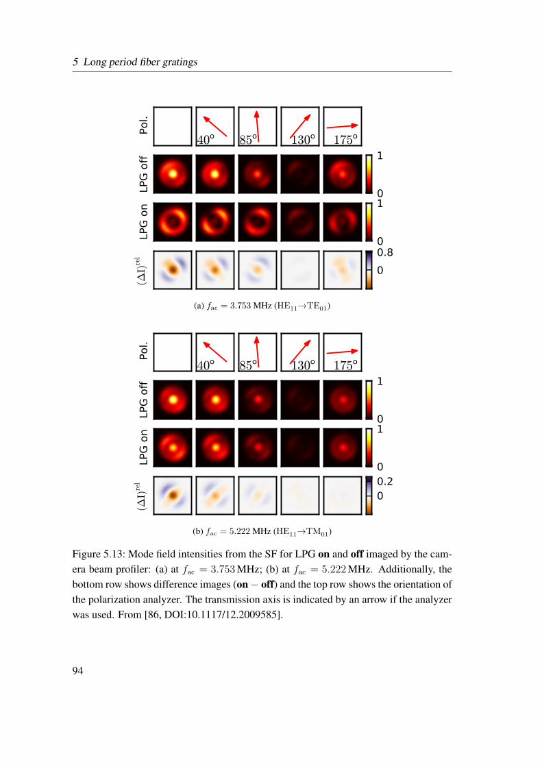
5 Long period fiber gratings
LPG
off
0
1LP
G o
n
0
1
(∆I)
rel
0
0.8
Pol.
40o 85o 130o 175o
(a) fac = 3.753 MHz (HE11→TE01)
LPG
off
0
1
LPG
on
0
1
(∆I)
rel
00.2
Pol.
40o 85o 130o 175o
(b) fac = 5.222 MHz (HE11→TM01)
Figure 5.13: Mode field intensities from the SF for LPG on and off imaged by the cam-era beam profiler: (a) at fac = 3.753 MHz; (b) at fac = 5.222 MHz. Additionally, thebottom row shows difference images (on− off) and the top row shows the orientation ofthe polarization analyzer. The transmission axis is indicated by an arrow if the analyzerwas used. From [86, DOI:10.1117/12.2009585].
94
5.4 Experimental results
Moving to the images taken with polarizer at αp = 40, only marginal differences tothe images without polarizer can be seen in figures 5.13 (a) and (b). On the other hand,the images for αp = 130 show very low intensity. Taking the last two observationstogether, one can see that the beam is linearly polarized to a high degree. Numbers willbe given further below. Interestingly, the intensity images for αp = 85 and αp = 175
are rather different. Especially the intensity patterns at the exterior of the beam havevery different intensity and are oriented in different directions. In figure 5.13 (a), thedifference is more obvious than in figure 5.13 (b). The intensity in the beam center,however, is very similar between the aforesaid polarizer angles in both figures.
When the LPG is switched on, one can observe a drop of power in the beam centerand a gain at the exterior across all images taken with and without polarization analyzer.This is visible in the third row from top of figures 5.13 (a) and (b). The effect is muchweaker at fac = 5.222 MHz compared to fac = 3.753 MHz. It can be visualized moreclearly by the difference images in the bottom row. The blue colored areas in the dif-ference images, which indicate a positive intensity change, clearly show a two-lobedintensity pattern that is similar to one of those of the second-higher modes expectedfrom the SF with elliptical core geometry. For fac = 3.753 MHz, the two-lobed pat-tern is oriented approximately perpendicular to the polarizer arrow at αp = 40. Con-versely, the two-lobed pattern is oriented approximately parallel to this polarizer arrowat fac = 5.222 MHz. The pattern rotates slightly, but noticeably in the opposite directionas the polarizer axis.
Supporting data
In the following, the qualitative observations made for the mode field images shall besupported by specific intensity values. For that purpose, figures 5.14 (a) and (b) depictthe intensity values Ic at the central pixel and the total intensities Itot related to theintensity images in figures 5.13 (a) and (b). In both figures, the intensity values aregiven for all angles αp of the polarization analyzer, including the case without analyzer.The hatched bars show the values for the case of active LPG (LPG on).
First, the polarization purity shall be considered, when the LPG is off. For a uniformlinearly polarized beam, the normalized intensity should be 1 at a particular polarizerangle and become 0 when the polarizer is rotated by ±90 with respect to that angle.αp = 130 corresponds to the angle that yields minimum intensity in the beam center inthis particular case. The ratio between the intensities in the beam center for αp = 40 toαp = 130 is approximately 95:5. For the total intensity the ratio is only 87:13. These
95
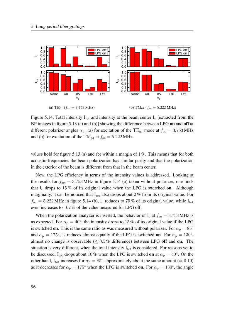
5 Long period fiber gratings
0.00.20.40.60.81.0
I c
LPG offLPG on
None 40 85 130 175αp
0.00.20.40.60.81.0
I tot
(a) TE01 (fac = 3.753 MHz)
0.00.20.40.60.81.0
I c
LPG offLPG on
None 40 85 130 175αp
0.00.20.40.60.81.0
I tot
(b) TM01 (fac = 5.222 MHz)
Figure 5.14: Total intensity Itot and intensity at the beam center Ic [extracted from theBP images in figure 5.13 (a) and (b)] showing the difference between LPG on and off atdifferent polarizer angles αp. (a) for excitation of the TE01 mode at fac = 3.753 MHzand (b) for excitation of the TM01 at fac = 5.222 MHz.
values hold for figure 5.13 (a) and (b) within a margin of 1 %. This means that for bothacoustic frequencies the beam polarization has similar purity and that the polarizationin the exterior of the beam is different from that in the beam center.
Now, the LPG efficiency in terms of the intensity values is addressed. Looking atthe results for fac = 3.753 MHz in figure 5.14 (a) taken without polarizer, one findsthat Ic drops to 15 % of its original value when the LPG is switched on. Althoughmarginally, it can be noticed that Itot also drops about 2 % from its original value. Forfac = 5.222 MHz in figure 5.14 (b), Ic reduces to 75 % of its original value, while Itot
even increases to 102 % of the value measured for LPG off.
When the polarization analyzer is inserted, the behavior of Ic at fac = 3.753 MHz isas expected. For αp = 40, the intensity drops to 15 % of its original value if the LPGis switched on. This is the same ratio as was measured without polarizer. For αp = 85
and αp = 175, Ic reduces almost equally if the LPG is switched on. For αp = 130,almost no change is observable (≤ 0.5 % difference) between LPG off and on. Thesituation is very different, when the total intensity Itot is considered. For reasons yet tobe discussed, Itot drops about 10 % when the LPG is switched on at αp = 40. On theother hand, Itot increases for αp = 85 approximately about the same amount (≈ 0.19)as it decreases for αp = 175 when the LPG is switched on. For αp = 130, the angle
96
5.4 Experimental results
of minimum intensity in the beam center, Itot increases from 0.13 to 0.21 when the LPGis switched on. Since Ic(αp = 40 o) does not change when the LPG is switched on,the intensity has increased in the exterior of the beam, which can be already seen in thecorresponding intensity image in figure 5.13 (a).
For fac = 5.22 MHz one finds very similar behavior for Ic and Itot, when the dif-ferent polarization analyzer settings are considered, apart from the effects being muchweaker. The major difference is that Itot(αp = 40o) increases slightly about 0.01, whileItot(αp = 130o) decreases about 0.02.
5.4.4 Discussion of mode field observations
Mode identification
Taking together the previous knowledge from the transmission spectra and the shape andpolarization of the mode intensity patterns, an excitation of the modes TE01 and TM01
can be identified when the LPG is switched on at fac = 3.753 MHz and 5.222 MHz,respectively. In both cases, the main polarization direction is identical, but the orienta-tion of the two intensity lobes is rotated by 90 with respect to each other. The mainbeam polarization also supports the identification of a TE01 and TM01 mode, but therotation of the two-lobe pattern in opposite direction to the analyzer rotation could in-dicate the presence of a hybrid HE21 mode (see e.g. [10]). On the other hand, forfac = 3.753 MHz and αp = 130, the LPG clearly creates azimuthally polarized light,as would be expected for the TE01 mode. Therefore, the wrong rotation direction mightbe related to the presence of a hybrid mode which is not generated by the LPG but whichwas unintentionally excited at the SF entrance.
Polarization and mode composition
In figures 5.13 (a) and (b), the fundamental mode is initially excited with the samepolarization purity. This is also supported by comparing the central intensity Ic forthe analyzer angles αp = 40 and αp = 130. However, higher-order modes are alsoexcited along with the fundamental HE11 mode, since the total intensity does not drop asmuch as the central intensity at the minimum polarizer angle. The higher-order modesare mainly guided in the outer core (ring) of the SF. Therefore, the intensity patternfor LPG off show some two-lobed pattern at the exterior of the beam, which overlaysthe expected intensity pattern for the HE11 mode. Apparently, there is an interferencebetween the fundamental and at least one other higher-order mode, which could be
97
5 Long period fiber gratings
one of the two HE21 modes, since one of the side intensity lobes is stronger than theother. One of the lobes can get brighter or darker, if the main polarization directionof this unwanted higher-order mode is aligned with that of the fundamental mode andthe relative phase difference between those modes is not exactly ±90. This phasedifference also determines which of the side lobes appears brighter.
Since an intensity pattern of a superposition of modes depends on the phase differencebetween those modes at the end of the SF, it is not possible to distinguish all possiblecombinations of modes leading to the same intensity pattern by imaging and using a po-larization analyzer only. Other methods could be used for that purpose. Time-resolvedinterference measurements for the original index tailored fibers of Ramachandran et al.,are presented in [84, 120], for instance. Alternatively, holographic methods can be usedfor mode decomposition and mode excitation [121, 122]. However, these methods arebeyond the goals of this work. Here, it is sufficient to excite the fundamental mode withhigh purity and then optimize the grating efficiency to excite a particular higher-ordermode. The optimization process which was used here is already described at the end ofsection 5.3.4. As described there, usage of an amplitude-modulated driving voltage forthe acoustic LPG is suggested during the optimization procedure. An experimentallyvaluable quantitative parameter describing the mode coupling efficiency in combinationwith the modal purity, is the change of intensity in the beam center caused by the am-plitude modulation. In an ideal case, the intensity should be maximal when the LPG isoff (only HE11 excited) and go to zero when the LPG is on (only one particular second-higher mode is excited). If the intensity in the beam center does not go to zero, eitherthe coupling efficiency is not sufficient or other modes then the necessary HE11 modeare present in the SF. In any case, the modulation depth of intensity in the beam centerwill be reduced. Therefore, only looking at the intensity in the beam center is a pow-erful tool for optimization of the acoustic frequency, the input polarization, the SMFto SF coupling, and the driving voltage amplitude. Since the optimization is reducedto the maximization of one scalar quantity, namely the intensity modulation amplitudebetween LPG on and off, one can easily automate the optimization routine, which mightbe helpful for practical applications outside a laboratory environment. It also offers thepossibility to use lock-in techniques to filter the amplitude modulation frequency.
Conversion efficiency
For fac = 3.753 MHz, the acoustic LPG couples at least 85 % of power from the funda-mental mode, which has most intensity concentrated in the inner fiber core, to the TE01
98
5.4 Experimental results
mode, which is guided mainly in the outer core. For fac = 5.222 MHz, on the otherhand, the intensity from the inner core dominates the image even if the LPG on. In thiscase, the coupling efficiency was at least 25 %. The difference of the mode conversionefficiencies can be explained by taking into account several factors. Firstly, the mechan-ical displacement of the transducer (and hence of the fiber) is lower for fac = 5.222 MHzthan for fac = 3.753 MHz, in accordance with the displacement measurements in sec-tion 5.3.2. This shortcoming can be overcome by using an optimized piezoelectric trans-ducer. Secondly, the orientation of the acoustic vibration direction with respect to thefiber core geometry was the same in both measurements, which means that it can inducecoupling with different strengths for the TE01 mode and the TM01 mode. However, nosubstantial improvement of the coupling efficiency could be reached for the TM01 modewhen the fiber was rotated with respect to the vibration direction.
Also, it has to be considered that the TM01 mode is already excited in the SF, withan intensity comparable to the HE11 mode without the LPG being on. Under these con-ditions, the power from the initially present TM01 mode is coupled back to the HE11
mode in the same manner, as the coupling occurs in the opposite direction, thereby lim-iting the visible effect of the mode coupling. The last point underlines the importanceof a high purity of the fundamental mode in the SF. A high polarization purity of theoutput modes can only be reached if solely the wanted fundamental input modes, herethe HE11 modes, are excited at the SF entrance.
One limiting factor for the purity of the initially excited fundamental mode is certainlythe large number of guided core modes at λ = 785 nm. It is therefore advisable to seekfor fiber structures which only support the fundamental and second-higher modes at thisand shorter wavelengths, but keeps a high splitting between the effective indexes of thesecond-higher modes.
5.4.5 Time behavior and grating amplitude modulation
Figure 5.15 shows a plot of the measured optical power from the beam center, relative tothe maximum power ∆Pc over time. For comparison, in the right hand side of the figure,the BP image is also given. A black frame indicates the integration area from which thesummed power is measured. The upper BP image is for LPG off and the lower imageis for LPG on. The peak-to-peak driving voltage (before amplification) Vpp is given inthe upper graph on the left of figure 5.15. The driving voltage is modulated manually,so that the acoustic grating is switched on and off repeatedly. The peak-to-peak voltage
99
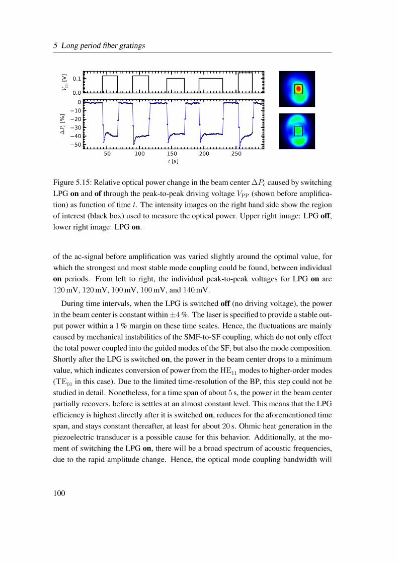
5 Long period fiber gratings
50 100 150 200 250t [s]
50
40
30
20
10
0
∆P
c [%
]
0.0
0.1
Vpp [
V]
Figure 5.15: Relative optical power change in the beam center ∆Pc caused by switchingLPG on and of through the peak-to-peak driving voltage VPP (shown before amplifica-tion) as function of time t. The intensity images on the right hand side show the regionof interest (black box) used to measure the optical power. Upper right image: LPG off,lower right image: LPG on.
of the ac-signal before amplification was varied slightly around the optimal value, forwhich the strongest and most stable mode coupling could be found, between individualon periods. From left to right, the individual peak-to-peak voltages for LPG on are120 mV, 120 mV, 100 mV, 100 mV, and 140 mV.
During time intervals, when the LPG is switched off (no driving voltage), the powerin the beam center is constant within±4 %. The laser is specified to provide a stable out-put power within a 1 % margin on these time scales. Hence, the fluctuations are mainlycaused by mechanical instabilities of the SMF-to-SF coupling, which do not only effectthe total power coupled into the guided modes of the SF, but also the mode composition.Shortly after the LPG is switched on, the power in the beam center drops to a minimumvalue, which indicates conversion of power from the HE11 modes to higher-order modes(TE01 in this case). Due to the limited time-resolution of the BP, this step could not bestudied in detail. Nonetheless, for a time span of about 5 s, the power in the beam centerpartially recovers, before is settles at an almost constant level. This means that the LPGefficiency is highest directly after it is switched on, reduces for the aforementioned timespan, and stays constant thereafter, at least for about 20 s. Ohmic heat generation in thepiezoelectric transducer is a possible cause for this behavior. Additionally, at the mo-ment of switching the LPG on, there will be a broad spectrum of acoustic frequencies,due to the rapid amplitude change. Hence, the optical mode coupling bandwidth will
100
5.5 Summary and conclusions
also be increased. However, this effect can be expected to cease within a time inverselyproportional to the acoustic frequency, which would be in the milliseconds range atmost. Clearly, the power recovery is much slower in the measurement, which makes itunlikely that the actual switching process is responsible for measured time dependence.To avoid damage to the transducer, the driving voltage is switched off after about 30 s.
For the first time the LPG is switched on, there is an overshoot before the powerstabilizes, which does not appear for the other on-periods. The origin of this differenceremains unclear. For the last on-period, where the highest driving voltage of 140 mVwas used, the strongest power drop is observed, but the slope of recovery is steeper thanin the other cases and the power does not settle at a constant level, but tends to increasefurther. The latter gives another indication that heating of the transducer is responsiblefor the power recovery and reduction of mode coupling efficiency over time, since it canbe expected that more heat is produced for higher voltage amplitudes.
From the observations described above, one can draw the conclusion that the elec-trical and mechanical setup of the LPG do not allow for a full power transfer betweenoptical modes. Only at acoustic frequencies were smaller driving voltages can achievethe same or even higher mechanical displacements, a full power transfer between twooptical modes can be achieved and maintained over longer periods of time. The acousticfrequencies, however, cannot be chosen arbitrarily, but have to be adapted to the opti-cal wavelength and the mode transition needed in the experiment. As could be seen infigure 5.10 (b), the acoustic frequencies for excitation of the TM01 and TE01 modes arenot in the range of maximum grating efficiency. It is therefore necessary to optimizethe electrical and mechanical design of the acoustic LPG for higher mode coupling ef-ficiency and more broadband operation, to exploit the full potential of the method.
5.5 Summary and conclusions
This chapter dealt with the construction of an acoustic long-period fiber grating and itsability to convert selected guided core modes in an index-tailored special fiber (SF) wasdemonstrated. The construction of the acoustic LPG and the ideas which lead to itscurrent design were discussed in detail. A multitude of optical transmission spectra wasacquired to measure the effective index splitting in the SF. Thereby, a theoretical acous-tic dispersion relation for the fiber’s lowest-order flexural mode was used, which wasbacked up by an experimental measurement of the relation between the acoustic phasevelocity and the acoustic frequency. From the transmission spectra, a mode coupling
101
5 Long period fiber gratings
scheme was developed, which allows not only to attribute individual spectral features tothe corresponding fiber mode transitions, but also gave some insight into the correctnessof the numerical models which were developed for the same SF in chapter 4. There-fore, the measured and simulated effective index difference curves agree well. Thebest agreement between measurement and simulation is achieved for the model withnon-rotated elliptical boundaries. It is not surprising that the measured effective indexsplitting between the TM01 mode and the HEo
21 mode is slightly lower than the valuepredicted by the simulation, 1.4× 10⁻⁴ compared to 1.8× 10⁻⁴, since the simulationmodel overestimates the steepness of the refractive index slopes of the fiber core.
A strong frequency dependence of the mechanical displacement of the optical fiberwas found. High displacements correspond to high optical mode coupling efficiency,but the displacement amplitude shows rapid oscillations over the frequency, which leadsto a similar dependence of the optical mode coupling efficiency. Correspondingly, themaximum power coupling efficiency which could be observed did not reach 100 %. At785 nm optical wavelength, the highest provable coupling efficiencies were 85 % be-tween a fundamental HE11 mode and the TE01 mode, and 25 % between a fundamentalHE11 mode and the TM01 mode. The coupling efficiencies were determined from adirect measurement of the intensity distributions emerging from the SF after the LPG,which also supported the mode assignment which was introduced by the mode couplingscheme.
The mode coupling efficiency is currently limited by two factors. Firstly, due to thelarge number of modes which can be guided in the SF core at near infrared wavelengths,a clean excitation of a single fundamental mode is complicated. Although great care wastaken in the experiments, unwanted modes were excited with at least 10 % of the totalpower. Secondly, the electrical and mechanical performance of the LPG did not providesufficient mechanical displacement of the fiber for a full power transfer between opticalmodes. Increasing the driving voltage could not overcome this issue since the piezo-electric performance was limited by heating of the transducer. The latter was inferredfrom the time dependence of the mode coupling efficiency, which was observed in thebeam profiler measurements.
In comparison to the original works of Ramachandran et al. [11, 12], who generatedindividual second-higher polarization modes by using mechanical LPGs with a similarSF, the present work lacks a substantial amount of coupling efficiency. Further, the SFused in [11, 12] posses better rotational symmetry of the fiber core. While the fiber coresymmetry is an issue which can only be tackled in the fabrication process, an optimiza-
102
5.5 Summary and conclusions
tion of the acoustic LPG design is certainly possible using the knowledge acquired inthis and other works. The goal has to be to achieve higher mechanical displacementsover a broader wavelength range with smooth frequency dependence in a simple andlow-cost LPG setup. Therefore, performing multi-physics numerical simulations of thefull LPG setup, including electrical and mechanical processes, are highly advisable. Forfrequencies below 1.3 MHz such simulations have recently been published [123].
Nonetheless, using an acoustic LPG for mode excitation still offers indisputable ad-vantages, since it is readily electronically controllable, the output mode can be easily se-lected via the acoustic frequency, and it is possible to combine multiple acoustic LPGs toexcite a desired mode combination [16]. Potential applications can be found for (fiber)optical sensors based on surface plasmon resonances [124], focus field and polariza-tion engineering [10, 5], or the generation of modes with orbital angular momentum fornext-generation data transmission [17, 125, 126], which the interested reader may referto for further reading.
103
6 Application of higher order fiber modes forfar-field microscopy
6.1 Introduction
The goals of the experiments in this chapter are to visualize and quantify the effectof higher-order fiber modes to high-resolution far-field microscopy. By doing so, itwill be shown that a strong longitudinal electric field component can be created in themicroscope focus at will by switching the acoustic LPG on. Hence, the usefulnessof an electronically controllable mode converter based on an acoustic LPG shall bedemonstrated.
The chapter starts with a short introduction to the development and applications ofhigher-order laser modes in far-field microscopy. Afterwards a simplified analyticaldescription of the field distributions created by the acoustic LPG is used to calculatedthe focal fields. These will be compared to the experimental results, which are discussedat the end of the chapter.
6.2 Complex beams in high-resolution far-field microscopy
This section will give some examples for application of complex beams like CVBsto far-field microscopy. In strong focusing conditions, the vectorial character of thesebeams creates peculiar effects that are exploited for the respective techniques. All tech-niques rely on a stable creation of the desired beam. In most of them, more versatilityis achieved if the polarization distribution of the excitation beam can be manipulatedat will. However, it must be ensured that the illuminating beam direction is not alteredby changing the beam polarization, which requires great care if mechanical polarizationrotators are used. This provides a motivation to study alternative approaches for creat-ing complex beams based on optical fibers together with acoustic LPGs in this work,although their applications are not limited to far-field microscopy.
The two most widely used examples of CVBs are the radially and azimuthally polar-ized doughnut beams. If strongly focused, a radially polarized beam produces a strong
104
6.2 Complex beams in high-resolution far-field microscopy
longitudinal field component which can even dominate the total field intensity in thefocus. Conversely, an azimuthally polarized beam produces a purely transverse fielddistribution in a tight focus. These effects were calculated in [127] and also demon-strated by imaging randomly oriented molecules in [128]. In the latter, the orientationof the molecular dipole moments could be estimated from their emission pattern. Zhanet al. introduced the generalized CVB concept and showed how combinations of radi-ally and azimuthally polarized beams can be used to shape the intensity distribution inthe focus [129] with implications for particle trapping and laser machining, to name afew [10]. Furthermore, Dorn et al. gave experimental prove for a reduction of the focalspot size for a radially polarized beam [130]. As another application, Failla et al. intro-duced a method to determine the orientation of metal nanorods on a surface by usingCVBs [4]. It was found a short time later that differently shaped nanoparticles (NPs),like spheres, rods, or triangles, produce discernible scattering patterns when illuminatedwith radially and azimuthally polarized beams [131], whereby the polarization modescan give complementary information. The concept of orientation determination was ex-tended just recently to simultaneously determine the orientation and position of isolatedgold nanorods in three dimensions by combined confocal scattering and luminescencemicroscopy using CVBs [132]. CVBs can also be used for confocal dark-field imaging.Advantages of this can be that the amount of defocus can be determined by comparingsignals for azimuthally and radially polarized illumination, and that edges in a certaindirection can be imaged selectively by controlling the polarization direction [133]. Fur-ther applications might emerge by using a spatial light modulator to prepare the vectorialpoint spread function in the focus as needed [134].
All of the examples discussed above directly make use of the three-dimensional po-larization properties of strongly focused CVBs. There are other methods in which oneis only interested in the total intensity distribution in the focal region that could alsoprofit from using CVBs in some cases. An example for this is [135], were optimized in-tensity patterns for fluorescence inhibition are studied. These intensity patterns are usedin combination with reversible saturable optical fluorescence transitions (RESOLFT)[136]. The most prominent method of the RESOLFT-family is stimulated emissiondepletion (STED) microscopy. In particular, a circularly polarized doughnut mode isconsidered in [135], among other beams. This particular beam can be generated bysuperimposing a radially polarized beam and an azimuthally polarized beam of equalintensity with a phase shift of π/2. If this mode combination was created in a sin-
105
6 Application of higher order fiber modes for far-field microscopy
gle fiber-optical polarization mode controller, one would benefit from the fact that bothmodes are aligned perfectly with respect to each other.
In summary, many applications of CVBs in far-field microscopy have already beenestablished and their number is still growing. In several cases it is beneficial to have amode converter at hand which can switch between different CVB polarizations withoutdistorting the beam direction. Both arguments provide a strong motivation to realize aneasy-to-operate fiber-optical solution based on acoustic LPGs. Of course, this overviewcould only cover a small part of all the work which has been conducted in relationto microscopy with CVBs. The interested reader may follow the extensive reviews in[10, 5] for more information.
6.3 Theoretical considerations
In the experiments described in subsequent sections, a spherical NP is used to probethe field distribution of tightly focused non-fundamental fiber modes. This includes atransformation of the incident laser beam by the excitation point spread function (PSF),which induces a polarization in the particle. This polarization field is the source ofbackscattered light which undergoes a back transformation through the microscopes de-tection PSF [19, Chp. 4.3]. The NP can be considered as three individual point dipoleswhich respond linearly to the local electric field. Two dipoles are oriented perpendicularto the optical axis within the object plane, and one is oriented along the optical axis, outof the object plane. Spherical NPs have a linear, isotropic polarizability. Hence, the totalscattered power depends only on the input light intensity. On the other hand, the direc-tivity of the scattered power is influenced by the local field polarization. Since a confocalsetup is used here, and to keep the discussion in bounds, the back-transformation of theimaging process will be disregarded.
In the following, possible focal field distributions are calculated to help understandingthe experimental results that follow afterwards. Thereby, it is useful to rely on wellknown analytical field expressions to avoid intensive numerical simulations.
Focal fields of Hermite-Gaussian beams
From the results of chapter 5, it is known that when the acoustic LPG is switched on,ideally, the beam emerging from the SF changes from a linearly polarized beam witha nearly Gaussian intensity profile into a beam which is characterized by two intensity
106
6.3 Theoretical considerations
maxima with opposite field polarization with respect to the optical axis and a zero in-tensity in the center of the beam. The fields of the second-higher modes from the SFare neither purely linearly nor purely radially or azimuthally polarized. Nonetheless,since the fields of the fundamental and second-higher modes are mainly linearly po-larized (along a given axis), one can get some insight into the possible focal fields byconsidering linearly polarized Hermite-Gaussian laser beams instead of the actual fieldsfrom the SF. Consequently, some deviations have to be taken into account in the actualexperiment.
The focal fields of Hermite-Gaussian (HG) beams can be expressed analytically bythe formulas given in [19, Chp. 3.7]. Four HG modes are particularly important. Theseare HGx
00, HGy00, HGy
01, and HGx10. In the far-field, all these modes are linearly polarized
along the x- or y-axis according to the superscript of the mode label. The HG00 modesrepresent the fundamental modes and they have a radially symmetric Gaussian intensitydistribution. HGy
01 and HGx10 have an antisymmetric field distribution with respect to the
y-z-plane, which leads to an intensity pattern with two equal maxima. The differencebetween these modes is that their polarization is perpendicular with respect to eachother.
Through focusing, the linearly polarized HG modes acquire a truly vectorial characterand with a few exceptions, all field components will gain non-negligible intensity. Fig-ures 6.1 (a) through (d) show the intensity |E |2 distributions of individual vector fieldcomponents as well as the total intensity for the HG modes mentioned so far. All modefields are normalized to have the same total intensity. Further, each image is scaled to amaximum of 1 and the scaling factor is given above each image. The lateral dimensionsare given in units of wavelength. For the experiments described in the following section,the total intensity |E tot|2 is the most important quantity. The differences between thetotal intensity distribution for different modes originates from their polarization proper-ties. For instance, comparing the highly focused HGx
00 and HGy00 modes in 6.1 (a) and
6.1 (b), the total intensity shows an elongated blob-like pattern along the main polar-ization direction of each mode, which is due to the presence of a markable longitudinalfield componentEz. Although the far-field intensity patterns of HGy
01 and HGx10 are also
very similar, their total intensity distributions in the focus deviate strongly. The maindifference is that for the HGy
01 mode the intensity is zero along the x- and y-axes, whilefor the HGx
10 the strong longitudinal field component leads to significant intensity in thecenter of the focus, comparable to that of the two side-maxima.
107
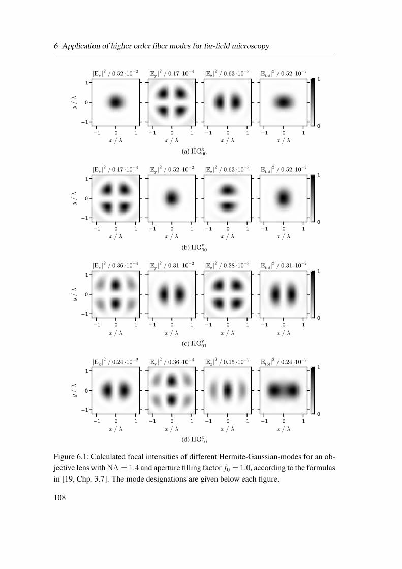
6 Application of higher order fiber modes for far-field microscopy
1 0 1
x / λ
1
0
1
y/λ
|Ex |2 / 0.52 ·10−2
1 0 1
x / λ
|Ey |2 / 0.17 ·10−4
1 0 1
x / λ
|Ez |2 / 0.63 ·10−3
1 0 1
x / λ
|Etot|2 / 0.52 ·10−2
0
1
(a) HGx00
1 0 1
x / λ
1
0
1
y/λ
|Ex |2 / 0.17 ·10−4
1 0 1
x / λ
|Ey |2 / 0.52 ·10−2
1 0 1
x / λ
|Ez |2 / 0.63 ·10−3
1 0 1
x / λ
|Etot|2 / 0.52 ·10−2
0
1
(b) HGy00
1 0 1
x / λ
1
0
1
y/λ
|Ex |2 / 0.36 ·10−4
1 0 1
x / λ
|Ey |2 / 0.31 ·10−2
1 0 1
x / λ
|Ez |2 / 0.28 ·10−3
1 0 1
x / λ
|Etot|2 / 0.31 ·10−2
0
1
(c) HGy01
1 0 1
x / λ
1
0
1
y/λ
|Ex |2 / 0.24 ·10−2
1 0 1
x / λ
|Ey |2 / 0.36 ·10−4
1 0 1
x / λ
|Ez |2 / 0.15 ·10−2
1 0 1
x / λ
|Etot|2 / 0.24 ·10−2
0
1
(d) HGx10
Figure 6.1: Calculated focal intensities of different Hermite-Gaussian-modes for an ob-jective lens with NA = 1.4 and aperture filling factor f0 = 1.0, according to the formulasin [19, Chp. 3.7]. The mode designations are given below each figure.
108
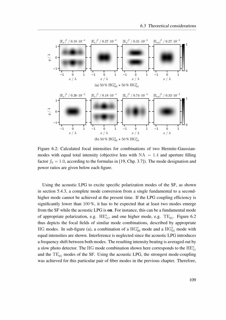
6.3 Theoretical considerations
1 0 1
x / λ
1
0
1y/λ
|Ex |2 / 0.18 ·10−4
1 0 1
x / λ
|Ey |2 / 0.27 ·10−2
1 0 1
x / λ
|Ez |2 / 0.31 ·10−3
1 0 1
x / λ
|Etot|2 / 0.27 ·10−2
0
1
(a) 50% HGy00 + 50% HGy
01
1 0 1
x / λ
1
0
1
y/λ
|Ex |2 / 0.26 ·10−2
1 0 1
x / λ
|Ey |2 / 0.18 ·10−4
1 0 1
x / λ
|Ez |2 / 0.74 ·10−3
1 0 1
x / λ
|Etot|2 / 0.33 ·10−2
0
1
(b) 50% HGx00 + 50% HGx
10
Figure 6.2: Calculated focal intensities for combinations of two Hermite-Gaussian-modes with equal total intensity (objective lens with NA = 1.4 and aperture fillingfactor f0 = 1.0, according to the formulas in [19, Chp. 3.7]). The mode designation andpower ratios are given below each figure.
Using the acoustic LPG to excite specific polarization modes of the SF, as shownin section 5.4.3, a complete mode conversion from a single fundamental to a second-higher mode cannot be achieved at the present time. If the LPG coupling efficiency issignificantly lower than 100 %, it has to be expected that at least two modes emergefrom the SF while the acoustic LPG is on. For instance, this can be a fundamental modeof appropriate polarization, e.g. HEo
11, and one higher mode, e.g. TE01. Figure 6.2thus depicts the focal fields of similar mode combinations, described by appropriateHG modes. In sub-figure (a), a combination of a HGy
00 mode and a HGy01 mode with
equal intensities are shown. Interference is neglected since the acoustic LPG introducesa frequency shift between both modes. The resulting intensity beating is averaged out bya slow photo detector. The HG mode combination shown here corresponds to the HEo
11
and the TE01 modes of the SF. Using the acoustic LPG, the strongest mode-couplingwas achieved for this particular pair of fiber modes in the previous chapter. Therefore,
109
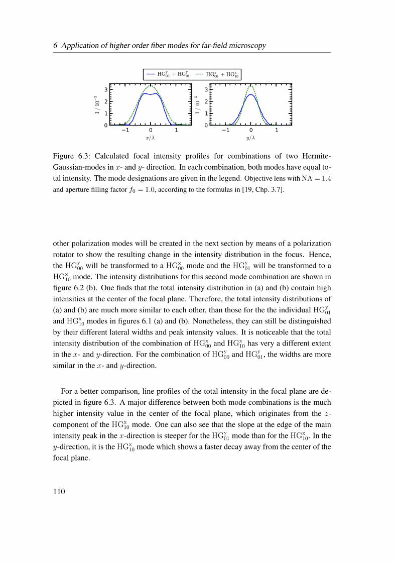
6 Application of higher order fiber modes for far-field microscopy
1 0 1x/λ
0
1
2
3I/
10−
3
HGy00 + HGy
01 HGx00 + HGx
10
1 0 1y/λ
0
1
2
3
I/
10−
3
Figure 6.3: Calculated focal intensity profiles for combinations of two Hermite-Gaussian-modes in x- and y- direction. In each combination, both modes have equal to-tal intensity. The mode designations are given in the legend. Objective lens with NA = 1.4
and aperture filling factor f0 = 1.0, according to the formulas in [19, Chp. 3.7].
other polarization modes will be created in the next section by means of a polarizationrotator to show the resulting change in the intensity distribution in the focus. Hence,the HGy
00 will be transformed to a HGx00 mode and the HGy
01 will be transformed to aHGx
10 mode. The intensity distributions for this second mode combination are shown infigure 6.2 (b). One finds that the total intensity distribution in (a) and (b) contain highintensities at the center of the focal plane. Therefore, the total intensity distributions of(a) and (b) are much more similar to each other, than those for the the individual HGy
01
and HGx10 modes in figures 6.1 (a) and (b). Nonetheless, they can still be distinguished
by their different lateral widths and peak intensity values. It is noticeable that the totalintensity distribution of the combination of HGx
00 and HGx10 has very a different extent
in the x- and y-direction. For the combination of HGy00 and HGy
01, the widths are moresimilar in the x- and y-direction.
For a better comparison, line profiles of the total intensity in the focal plane are de-picted in figure 6.3. A major difference between both mode combinations is the muchhigher intensity value in the center of the focal plane, which originates from the z-component of the HGx
10 mode. One can also see that the slope at the edge of the mainintensity peak in the x-direction is steeper for the HGy
01 mode than for the HGx10. In the
y-direction, it is the HGx10 mode which shows a faster decay away from the center of the
focal plane.
110
6.4 Experimental details
6.4 Experimental details
A confocal sample-scanning setup was built from commercial optical and mechanicalcomponents for the purpose of this study. The setup is depicted in figure 6.4. It isbased on an inverted optical microscope (Zeiss Axiovert 200 Mat). The microscopecontains a high numerical aperture objective lens (OL, α-Plan-APOCRHOMAT, 100x,1.45 NA), a non-polarizing beam splitter (BS, splitting ratio 50:50), the tube lens (TL),and a side-exit-mirror (M8). The objective lens focuses the laser radiation of 785 nmwavelength and collects back-scattered light of the same wavelength. A multi-modeoptical fiber (MMF, Thorlabs AFS50/125Y, 50 µm core diameter, 0.22 NA) is placed inthe image plane and acts as pinhole for confocal detection, while simultaneously guidingthe collected light to a photo-diode (PD1, Thorlabs PDA8A/M). Further, a laser cleanup filter (LF, Semrock LL01-785) in front of the fiber entrance prevents stray light fromreaching the detector. The laser source is a narrow-band diode pumped solid-state laser(DPSS, BW-TeK BRM-785), emitting continuously and operating in a single transversemode.
The specimen (NPS) consists of gold nanoparticles (NPs, BBInternational EM.GC30,30 nm diameter) which were randomly distributed on top of a cover-slide by “blow-drying the original colloidal suspension [. . . ] by means of an omnidirectional streamof air” [137]. From experience, one knows that this method disperses the NPs well.The scattering spectrum of a particle can be used as reference in order to prove that asingle particle of the right size is used in the experiment [138]. The particles are thenimmersed in index matching oil. The cover-slide is attached to the bottom side of a glassobject holder and the index matching oil completely fills the space between the two. Thepurpose of index-matching oil is to reduce reflections from the glass surfaces close to theparticles that could lead to a strong background dominating the measurement signals.The specimen is mounted on a scanning platform (Mad City Labs, Nano-LPS300) usedfor confocal scanning.
The laser source is coupled to a single-mode fiber (SMF, Nufern 780HP) incorpo-rating a fiber-optical polarization controller (POL, Newport F-POL-IL). The end faceof the SMF is positioned very close to the entrance face of the special fiber (SF) bymeans of a high-accuracy fiber-to-fiber positioning system (FF, Thorlabs NBM513/Mand NBM413/M). The purpose of the positioning system is to excite the fundamentalmode of the SF with as high efficiency as possible, while minimizing the excitationof other modes. This step turned out to be non-trivial but also crucial for the LPGsperformance. Hence, careful alignment of the fiber-to-fiber coupler is very important
111
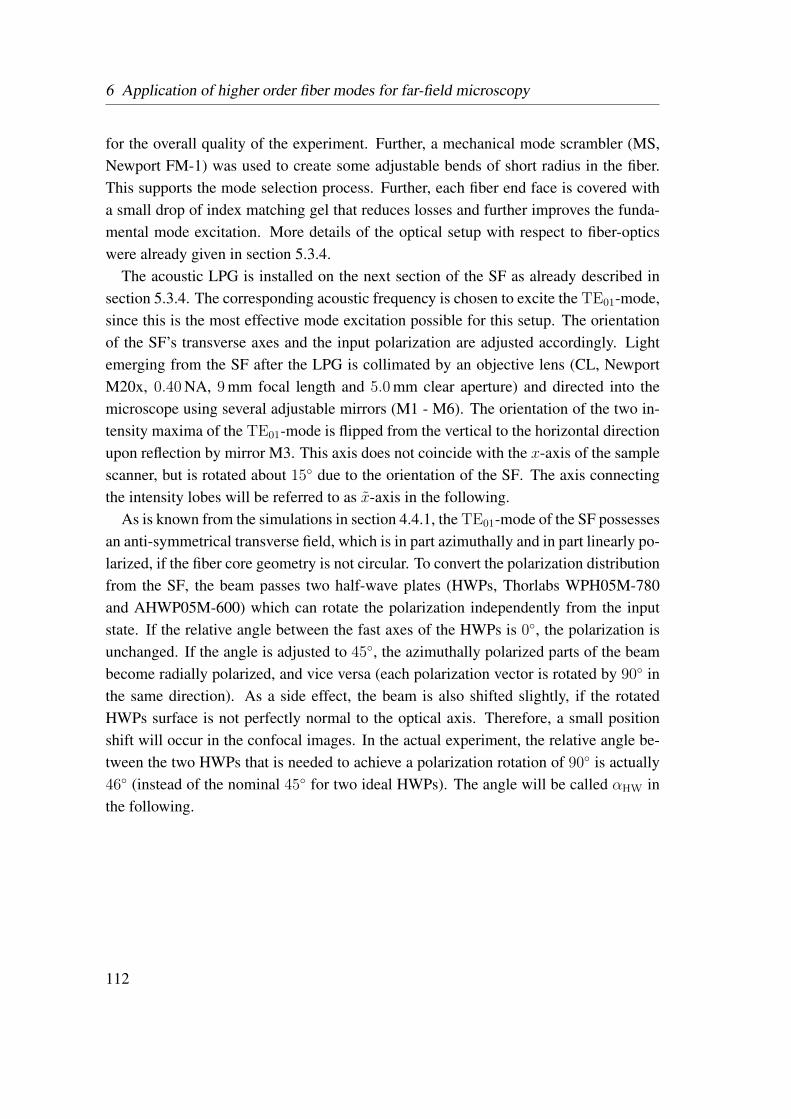
6 Application of higher order fiber modes for far-field microscopy
for the overall quality of the experiment. Further, a mechanical mode scrambler (MS,Newport FM-1) was used to create some adjustable bends of short radius in the fiber.This supports the mode selection process. Further, each fiber end face is covered witha small drop of index matching gel that reduces losses and further improves the funda-mental mode excitation. More details of the optical setup with respect to fiber-opticswere already given in section 5.3.4.
The acoustic LPG is installed on the next section of the SF as already described insection 5.3.4. The corresponding acoustic frequency is chosen to excite the TE01-mode,since this is the most effective mode excitation possible for this setup. The orientationof the SF’s transverse axes and the input polarization are adjusted accordingly. Lightemerging from the SF after the LPG is collimated by an objective lens (CL, NewportM20x, 0.40 NA, 9 mm focal length and 5.0 mm clear aperture) and directed into themicroscope using several adjustable mirrors (M1 - M6). The orientation of the two in-tensity maxima of the TE01-mode is flipped from the vertical to the horizontal directionupon reflection by mirror M3. This axis does not coincide with the x-axis of the samplescanner, but is rotated about 15 due to the orientation of the SF. The axis connectingthe intensity lobes will be referred to as x-axis in the following.
As is known from the simulations in section 4.4.1, the TE01-mode of the SF possessesan anti-symmetrical transverse field, which is in part azimuthally and in part linearly po-larized, if the fiber core geometry is not circular. To convert the polarization distributionfrom the SF, the beam passes two half-wave plates (HWPs, Thorlabs WPH05M-780and AHWP05M-600) which can rotate the polarization independently from the inputstate. If the relative angle between the fast axes of the HWPs is 0, the polarization isunchanged. If the angle is adjusted to 45, the azimuthally polarized parts of the beambecome radially polarized, and vice versa (each polarization vector is rotated by 90 inthe same direction). As a side effect, the beam is also shifted slightly, if the rotatedHWPs surface is not perfectly normal to the optical axis. Therefore, a small positionshift will occur in the confocal images. In the actual experiment, the relative angle be-tween the two HWPs that is needed to achieve a polarization rotation of 90 is actually46 (instead of the nominal 45 for two ideal HWPs). The angle will be called αHW inthe following.
112
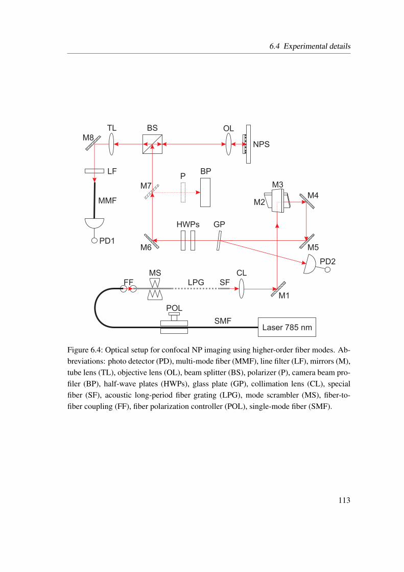
6.4 Experimental details
Figure 6.4: Optical setup for confocal NP imaging using higher-order fiber modes. Ab-breviations: photo detector (PD), multi-mode fiber (MMF), line filter (LF), mirrors (M),tube lens (TL), objective lens (OL), beam splitter (BS), polarizer (P), camera beam pro-filer (BP), half-wave plates (HWPs), glass plate (GP), collimation lens (CL), specialfiber (SF), acoustic long-period fiber grating (LPG), mode scrambler (MS), fiber-to-fiber coupling (FF), fiber polarization controller (POL), single-mode fiber (SMF).
113
6 Application of higher order fiber modes for far-field microscopy
A camera beam profiler (BP, Thorlabs BC106-VIS) is placed next to the microscope.The beam path can be switched between microscope and BP via a flip mirror (M7). TheBP is used to check the collimation and mode purity of the light emerging from thespecial fiber, to optimize the input polarization in the SMF, and to adjust the voltageand frequency applied to the LPG for best mode conversion efficiency. The opticalpath length between mirror M7 and the CCD-surface equals the path length betweenM7 and the center of the microscopes objective lens. This is to make sure that thewavefronts are plane in the back-focal plane of the objective lens. Further, a thin glassplate (GP) reflects a small amount of the light intensity to an additional photo detector(PD2, Thorlabs PM100A and S121C). The signal of the second photo detector wasmeasured along with the signal from PD1 to allow for a correction of power fluctuationswhich can be introduced by mechanical instabilities of the fiber-to-fiber coupling or bychanges of the laser output power.
The confocal scanning is performed point-wise, recording data in forward and back-ward direction of each scan line. The LPG is switched on for the measurement in back-ward direction and off in the forward direction. The focus was adjusted by maximizingthe confocal signal, while scanning on a single line over a particle. The acquisition timeper pixel is in the range of 1 ms to 5 ms. Together with the response time of the sam-ple scanner and the scanning electronics, the typical acquisition times for a 100 px by100 px image were in the range of 1 min to 5 min.
6.5 Results
In this section, confocal images for one individual spherical NP under different excita-tion conditions are presented. Figure 6.5 shows the acquired data. Sub-figure (a) and(b) represent measurements using αHW = 0 (relative angle between the two half-wave-plates’ fast axes), and sub-figure (c) and (d) represent αHW = 46. The LPG is off (nodriving voltage) (a) and (c), and for (b) and (d) the LPG is on. The data of the images isthe signal of PD1 divided by the signal of PD2. The color scale of all images is chosenequally, so it can be compared across the images.
All particle images show a single intensity blob with a (roughly) Gaussian-like inten-sity distribution. However, the particle images appear not perfectly cylindrical symmet-ric. Notably, the intensity distribution in figure 6.5 (c) (αHW = 46, LPG off), appearsto be deformed and shifted with respect to figure 6.5 (a) (αHW = 0, LPG off). The datafor figure 6.5 (c) and (d) was acquired after rotating one of the half-wave plates. Due to
114
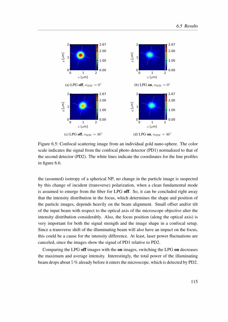
6.5 Results
0 1 2x [µm]
0
1
2
y [µ
m]
0.00
1.00
2.00
2.67
(a) LPG off, αHW = 0
0 1 2x [µm]
0
1
2
y [µ
m]
0.00
1.00
2.00
2.67
(b) LPG on, αHW = 0
0 1 2x [µm]
0
1
2
y [µ
m]
0.00
1.00
2.00
2.67
(c) LPG off, αHW = 46
0 1 2x [µm]
0
1
2
y [µ
m]
0.00
1.00
2.00
2.67
(d) LPG on, αHW = 46
Figure 6.5: Confocal scattering image from an individual gold nano-sphere. The colorscale indicates the signal from the confocal photo detector (PD1) normalized to that ofthe second detector (PD2). The white lines indicate the coordinates for the line profilesin figure 6.6.
the (assumed) isotropy of a spherical NP, no change in the particle image is suspectedby this change of incident (transverse) polarization, when a clean fundamental modeis assumed to emerge from the fiber for LPG off. So, it can be concluded right awaythat the intensity distribution in the focus, which determines the shape and position ofthe particle images, depends heavily on the beam alignment. Small offset and/or tiltof the input beam with respect to the optical axis of the microscope objective alter theintensity distribution considerably. Also, the focus position (along the optical axis) isvery important for both the signal strength and the image shape in a confocal setup.Since a transverse shift of the illuminating beam will also have an impact on the focus,this could be a cause for the intensity difference. At least, laser power fluctuations arecanceled, since the images show the signal of PD1 relative to PD2.
Comparing the LPG off images with the on images, switching the LPG on decreasesthe maximum and average intensity. Interestingly, the total power of the illuminatingbeam drops about 5 % already before it enters the microscope, which is detected by PD2.
115
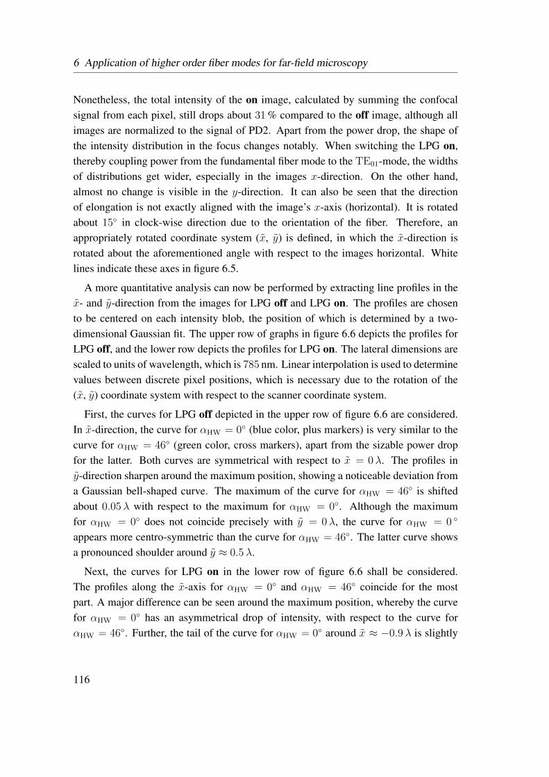
6 Application of higher order fiber modes for far-field microscopy
Nonetheless, the total intensity of the on image, calculated by summing the confocalsignal from each pixel, still drops about 31 % compared to the off image, although allimages are normalized to the signal of PD2. Apart from the power drop, the shape ofthe intensity distribution in the focus changes notably. When switching the LPG on,thereby coupling power from the fundamental fiber mode to the TE01-mode, the widthsof distributions get wider, especially in the images x-direction. On the other hand,almost no change is visible in the y-direction. It can also be seen that the directionof elongation is not exactly aligned with the image’s x-axis (horizontal). It is rotatedabout 15 in clock-wise direction due to the orientation of the fiber. Therefore, anappropriately rotated coordinate system (x, y) is defined, in which the x-direction isrotated about the aforementioned angle with respect to the images horizontal. Whitelines indicate these axes in figure 6.5.
A more quantitative analysis can now be performed by extracting line profiles in thex- and y-direction from the images for LPG off and LPG on. The profiles are chosento be centered on each intensity blob, the position of which is determined by a two-dimensional Gaussian fit. The upper row of graphs in figure 6.6 depicts the profiles forLPG off, and the lower row depicts the profiles for LPG on. The lateral dimensions arescaled to units of wavelength, which is 785 nm. Linear interpolation is used to determinevalues between discrete pixel positions, which is necessary due to the rotation of the(x, y) coordinate system with respect to the scanner coordinate system.
First, the curves for LPG off depicted in the upper row of figure 6.6 are considered.In x-direction, the curve for αHW = 0 (blue color, plus markers) is very similar to thecurve for αHW = 46 (green color, cross markers), apart from the sizable power dropfor the latter. Both curves are symmetrical with respect to x = 0λ. The profiles iny-direction sharpen around the maximum position, showing a noticeable deviation froma Gaussian bell-shaped curve. The maximum of the curve for αHW = 46 is shiftedabout 0.05λ with respect to the maximum for αHW = 0. Although the maximumfor αHW = 0 does not coincide precisely with y = 0λ, the curve for αHW = 0
appears more centro-symmetric than the curve for αHW = 46. The latter curve showsa pronounced shoulder around y ≈ 0.5λ.
Next, the curves for LPG on in the lower row of figure 6.6 shall be considered.The profiles along the x-axis for αHW = 0 and αHW = 46 coincide for the mostpart. A major difference can be seen around the maximum position, whereby the curvefor αHW = 0 has an asymmetrical drop of intensity, with respect to the curve forαHW = 46. Further, the tail of the curve for αHW = 0 around x ≈ −0.9λ is slightly
116
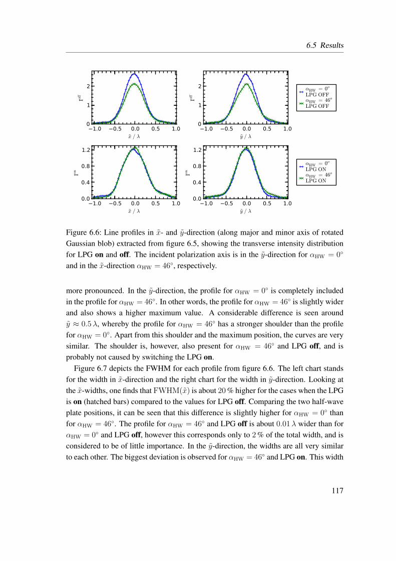
6.5 Results
1.0 0.5 0.0 0.5 1.0x / λ
0
1
2Iof
f
1.0 0.5 0.0 0.5 1.0y / λ
0
1
2
Ioff
αHW = 0o
LPG OFFαHW = 46o
LPG OFF
1.0 0.5 0.0 0.5 1.0x / λ
0.0
0.4
0.8
1.2
Ion
1.0 0.5 0.0 0.5 1.0y / λ
0.0
0.4
0.8
1.2
Ion
αHW = 0o
LPG ONαHW = 46o
LPG ON
Figure 6.6: Line profiles in x- and y-direction (along major and minor axis of rotatedGaussian blob) extracted from figure 6.5, showing the transverse intensity distributionfor LPG on and off. The incident polarization axis is in the y-direction for αHW = 0
and in the x-direction αHW = 46, respectively.
more pronounced. In the y-direction, the profile for αHW = 0 is completely includedin the profile for αHW = 46. In other words, the profile for αHW = 46 is slightly widerand also shows a higher maximum value. A considerable difference is seen aroundy ≈ 0.5λ, whereby the profile for αHW = 46 has a stronger shoulder than the profilefor αHW = 0. Apart from this shoulder and the maximum position, the curves are verysimilar. The shoulder is, however, also present for αHW = 46 and LPG off, and isprobably not caused by switching the LPG on.
Figure 6.7 depicts the FWHM for each profile from figure 6.6. The left chart standsfor the width in x-direction and the right chart for the width in y-direction. Looking atthe x-widths, one finds that FWHM(x) is about 20 % higher for the cases when the LPGis on (hatched bars) compared to the values for LPG off. Comparing the two half-waveplate positions, it can be seen that this difference is slightly higher for αHW = 0 thanfor αHW = 46. The profile for αHW = 46 and LPG off is about 0.01λ wider than forαHW = 0 and LPG off, however this corresponds only to 2 % of the total width, and isconsidered to be of little importance. In the y-direction, the widths are all very similarto each other. The biggest deviation is observed for αHW = 46 and LPG on. This width
117
6 Application of higher order fiber modes for far-field microscopy
0.0
0.1
0.2
0.3
0.4
0.5
0.6
FWHM(x) / λ
0.0
0.1
0.2
0.3
0.4
0.5
0.6
FWHM(y) / λ
αHW = 0o
LPG OFF
αHW = 0o
LPG ON
αHW = 46o
LPG OFF
αHW = 46o
LPG ON
Figure 6.7: Line widths (FWHM) in x- and y-direction (along major and minor axis ofrotated Gaussian blob) extracted from figure 6.5. Left and right graph depict FWHM(x)
and FWHM(y), respectively.
is 2 % larger than the average. So there is a small width increase for this particular case,but no general trend is visible for the y-profiles.
Finally, one can compare the aspect ratios between the x- and y-FWHMs, calculatedas FWHM(x)/FWHM(y). Considering αHW = 0 first, one gets a ratio of 0.97 forLPG off and a ratio of 1.21 for LPG on. For the y-polarized state at αHW = 46, thevalues are very similar, with 0.99 for LPG off and 1.17 for LPG on.
6.6 Discussion
In the following, the findings from this chapter shall be summarized and their originsand implications will be discussed. For the discussion, it is useful to remember thatthe polarization of the TE01 mode from the SF is aligned mainly along the y-axis forαHW = 0. Changing the angle to 46 rotates the polarization in each transverse fieldpoint about 90. This converts the initial TE01 mode to an artificial TM01 mode, ofwhich substantial parts are radially polarized. As a consequence of the changed inputpolarization distribution, the intensity in the focus center is increased for αHW = 46
compared to the case where αHW = 0, the acoustic LPG being on in both cases. TheTM01 mode creates a strong longitudinal field component in the focus which causes theincreased intensity in the focus center, which was detected by the confocal measure-ments using a spherical NP to probe the total intensity. Since this is only an indirectprove for the presence of the longitudinal electric field component, other causes for thisresult must also be examined carefully.
118
6.6 Discussion
Most certainly, the power drop which results from changing αHW from 0 to 46 in theLPG off images is connected to an artificial beam offset introduced by the HWP rotation.At this point, it is not possible to determine the difference of the plane polarizabilityanisotropy of the NP, so this is another possible cause for the power drop. Although,one would not expect such a dramatic polarization dependence1. On the other hand,the image shift is undoubtedly connected to the HWP rotation, since it was observedin additional measurements, which were not shown here, as well. A high number ofmeasurements with similar particles with a known size and aspect ratio distributionshould be conducted to quantify the sensitivity to in-plane particle anisotropy. However,other optimizations which will be discussed at the end of this section have higher apriority. Ultimately, particle shape and polarizability characterization is one possibleand promising application of higher-order polarization modes, as several publicationsin this direction have already shown [4, 139, 5].
Yet another unintentional feature of the confocal measurements is the power drop thatis observed when the acoustic LPG is switched on. This result is explicable, though.Since the total output power from the SF is not changed by the LPG, as was shown insection 5.4.3, this loss of optical power has its origin within the confocal measurement.As was explained above, there is already a power drop detected at PD2 and an evenstronger power drop in the confocal signal from detector PD1. Therefore, it is reason-able to assume that power is lost at the collimating lens (CL) and at the back-aperture ofthe microscope objective. When the acoustic LPG is switched on and higher modes areexcited, more power is concentrated in the exterior of the beam. This means that anyaperture the beam has to pass will result in stronger power loss for higher modes thanfor fundamental modes. The power loss at the objective back aperture could be reducedby decreasing the beam width through a different collimating lens. On the other hand,this would also reduce the filling factor f0 of the objective lens. But a large filling factoris necessary for achieving a small spot size in the focus and fosters the presence of allthree vector field components [19].
If one looks at the peak intensities measured when the acoustic LPG is on, one findshigher values for αHW = 46 than for αHW = 0. This is directly observable from theconfocal images, but a quantitative comparison is better possible from the extracted lineprofiles (figure 6.6). The profiles also show a dip along the x-direction for αHW = 0.
1 The manufacturer does not provide specific information about the shape distribution of the NPs.Nonetheless, SEM measurements for other experiments using the same particles supported their qualityso far.
119

6 Application of higher order fiber modes for far-field microscopy
These features are in agreement with the predictions from the theoretical considerationsin the beginning of the chapter, where possible focal field distributions for a combinationof fundamental and second-higher Hermite-Gaussian-modes are considered (e.g. figure6.3). As was discussed there, a higher on-axis intensity maximum is related to the pres-ence of a stronger longitudinal field component for the x-polarized mode combination.However, the measured differences between the two polarization mode combinations ismuch weaker than expected from the calculation. On the other hand, one has to takeinto account that the total power already drops considerably for LPG off when αHW ischanged from 0 to 46. In the light of this observation, the intensity in the center ofthe focus for LPG on and αHW =46 will be much higher, if there were no beam offsetintroduced from rotating the HWPs.
Apart from the points directly at the focus center in the x- and y-direction, the lineprofiles for LPG on are very similar, if one compares both polarization mode combina-tions. Conversely, the calculated profiles for the HG-mode combinations predicted welldistinguishable line shapes, at least in the x-direction (corresponding to the x directionof the measurement). A possible reason might be the image shape distortion from theHWP rotation, which is also likely to be responsible for the asymmetrical appearanceof shoulders in the profile, which are not present in any of the calculated profiles. Alsointerference with unintentionally excited fiber modes can have similar effects.
A major question is, if the mode conversion efficiency of the acoustic LPG is toolow to have significant effect on the focal fields. According to the results in section5.4.3, a 50 % conversion efficiency should certainly be possible, even if the LPG isoperated for longer time spans, for which a reduction in efficiency due to heating of thetransducer was observed. Even if the LPG efficiency is as low as 30 %, one should see ahigher peak value for the x-polarized mode-combinations in the on profile, nonetheless.Although, the profiles get more and more alike as the amplitude of the TE01 modereduces compared to the fundamental mode.
Finally, it must be considered that the combination of HG-modes chosen here is inap-propriate to describe the fields emerging from the SF correctly. Especially the profilesalong the y-direction with LPG off show a strong deviation from the Gaussian bell-shapearound the maximum position (upper right graph in figure 6.6). It is therefore not sur-prising that some of the subtle features from the HG focal field profiles are not presentin the measured data. One of those features is that the radially symmetric intensity dis-tribution of a not tightly-focused, linearly polarized HG00-beam gets transformed intoan elongated shaped intensity distribution in a tight focus. The direction of elongation
120
6.6 Discussion
coincides with the polarization direction of the HG00 mode. On the other hand, if oneconsiders the intensity profile of fundamental HE11 modes from the SF, one finds thatthe fiber modes have elongated intensity distributions along the same direction for bothpolarization states. See, for instance, the simulated mode fields in figure 4.7 on pagepage 51 or measured mode fields in figure 5.13 on page page 94 for comparison. Theaxis of elongation of the fiber mode intensity distribution corresponds to the x-directionin the experiment (perpendicular to the main polarization direction of the TEo
01 mode),and is determined by the fiber core geometry, not by the polarization direction.
The measurement results discussed so far indicate that an acoustic LPG together withan appropriate optical fiber can be used as a tool to selectively design the electromag-netic vector field in a microscope’s focus. The better the field distribution is understood,the more information can be extracted from a confocal image. In the present work,the field was studied by probing it with a very simple, well known structure, a spheri-cal gold NP. These particles can be assumed to have an isotropic polarizability, so thepower scattered by them is independent of the local field polarization and just measuresthe local intensity. The quality of this assumption determines in part the quality of themeasurement results, since it cannot be separated from other effects in some cases, likea power drop due to a beam offset. On the other hand, it is not important to exactlyknow the polarizability properties to show the presence of a longitudinal field compo-nent in the focus. The difference between the particle images for illumination with aTE01 mode or an artificial TM01, created by rotating the polarization of the TE01 mode,are a direct consequence of the field polarization properties in any case. The only plau-sible explanation for the increased intensity in the focus center for the TM01 mode isthe presence of an additional, longitudinal field-component, which is not there for theTE01 mode. The individual polarizability components of the NP will thus only changethe relative scattered intensities for each electric field component.
One of the unwanted features of the confocal measurements is the image deformationand shift when rotating one of the HWPs for changing αHW. Although great care wastaken in the experiment, some beam offset could not be avoided due to the mechanicalnature of this adjustment. An electro-optical polarization rotator could be used to getrid of this drawback, however, as will be discussed later, optimizing the acoustic LPGwould render any additional polarization optics redundant. Additionally, interferencesbetween wanted and unwanted modes from the SF fibers may also lead to a deformationof the intensity distribution. Hence, a high purity of the SF-fundamental mode must beachieved.
121
6 Application of higher order fiber modes for far-field microscopy
To conclude this section, some issues shall be addressed that are considered crucialfor an optimization of the technique. The first of them is the necessity of a clean fun-damental mode. As long as the mode distribution in the SF is not controlled better, onecannot predict what the field distributions in the focus will look like. Hence, one cannotrely on this technique for the characterization of unknown specimens. Also, it is one ofthe key advantages of a fiber-based polarization converter that no spatial filtering of theoutput modes is required, since their shape is highly symmetric by design. But this canonly be fully exploited if interferences due to spurious, unwanted modes are avoided.
The second issue is the undefined mode conversion efficiency of the acoustic LPG,which is probably considerably below 100 %. Although it might not be necessary or noteven wanted in some experiments to convert the fundamental fiber mode completely toa single second-higher mode, it reduces the freedom to create arbitrarily shaped focalfields, if a full mode conversion cannot be achieved. It will also be necessary to increasethe working frequency range of the acoustic LPG in order to access all second-highermodes at will. If all modes can be addressed individually, the desired polarization (andintensity) distribution can be created without changing the laser beam direction. Forinstance, switching between radially and azimuthally polarized beams would not alterthe laser focus position. Changing the polarization mode could be made as easy aspushing a button, making readjustments related to the polarization of the excitation lightfield unnecessary. This would certainly be an advantage for similar setups.
Finally, for the characterization of NPs and other anisotropic nano-objects it would bebeneficial to include a polarization analyzer into the detection path of the confocal setup.Thereby, more information on individual components of the polarizability tensor can beextracted, due to different emission patterns for each of them. Theoretical backgroundon this topic can be found in chapter 4 of [19].
6.7 Summary and conclusions
This chapter dealt with the application of an acoustic LPG for confocal microscopy. Theacoustic LPG converts linearly polarized beams into beams with complex polarizationpatterns which can be used to tailor vectorial electromagnetic fields in a tight microscopefocus. The LPG incorporates a special optical fiber which allows the selective excitationand transport of the aforementioned polarization patterns, which are either single guidedmodes of this fiber or superpositions thereof. In this chapter, a metal nanoparticle (NP)was used to map the focal intensity distribution. This way, it was demonstrated that
122
6.7 Summary and conclusions
individual field components and different intensity patterns can be created by tightlyfocusing the output beam from the special optical fiber.
To get some basic understanding of the focal fields which are created from one par-ticular second-higher mode of the SF, the fields emerging from the fiber were approxi-mately described by well known Hermite-Gaussian beams of low order. The focal fieldsfor these beams were calculated using readily available analytical formulas. The mainresults of this calculation are the intensity distributions in the microscope focus for acombination of a HGy
00 mode and a HGy01 mode, and for a combination of a HGx
00 modeand a HGx
10 mode. The major difference between the focal intensity distribution of bothmode combinations is the much stronger intensity peak in the focus center for the lattercombination. Transverse intensity profiles show more subtle differences. These differ-ences are, however, of lesser importance, since the HG modes are a crude approximationof the fields from the SF.
After the theoretical consideration of the expected focal fields, the experimental setupand the results acquired with it were presented. A strong intensity maximum was in-deed found for an artificial TM01 mode, which was created from a TE01 fiber-mode byrotating the polarization vectors about 90 with an appropriate polarization insensitiverotator. The intensity profiles in the focus showed deviations from the calculated pro-files, which was to be expected, since the HG modes are only a crude approximation ofthe fiber’s fields.
The discussion showed that the acoustic LPG together with the special fiber can in-deed be used to create desired vector fields in a microscope focus. However, severalissues have still to be tackled to make this technique more reliable. The biggest ob-stacles were presented at the end of the discussion and included the mode cleanlinessin the SF, the mode coupling efficiency of the acoustic LPG, and the need for an in-creased operation bandwidth of the acoustic LPG. The applications of the fiber-opticalpolarization mode converter are not limited to (confocal) microscopy, but can go handin hand with many current developments in fiber-optics, near-field optical microscopy,or plasmonics, to name a few.
123
7 Summary and outlook
The overall goal of this work was to develop an acoustic long-period fiber grating (LPG)in conjunction with an index-tailored few-mode optical fiber (SF) for the excitation ofcylindrical vector beams and other complex polarization modes. These polarizationmodes are applied to high-resolution far-field microscopy. However, the acoustic LPGin conjunction with the SF can be useful for many more scientific and technologicalapplications. Some possible further developments will be addressed in the outlook atthe end of this section.
A thorough numerical study of the mode fields and propagation constants of the SFwas presented. The model geometry for this simulation was extracted from scanningelectron microscope images of the fiber core. In the simulation, circular, non-rotatedelliptical, and rotated elliptical boundaries between domains of different refractive indexwere assumed. The simulation revealed the following:
• For a circular geometry, the radially polarized TM01 mode and the azimuthallypolarized TE01 mode are separated by up to a value of 1.8× 10⁻⁴ from the hy-brid HE21 modes at 785 nm wavelength in terms of the normalized propagationconstant. This demonstrates that the results by Ramachandran et al. [11, 12] forgreater wavelengths can be extended to the visible range by a moderate, techni-cally feasible reduction of the fiber core dimensions. The effective index sepa-ration provides similar polarization-maintaining properties for the second-ordermodes of the SF as standard polarization-maintaining fibers do for the linearlypolarized fundamental modes.
• For non-rotated elliptical boundaries, the propagation constants of the hybridmodes (HE and EH) split up. Also, the mode-fields of second-order modeschange substantially compared to the circular geometry, becoming almost com-pletely linearly polarized. The last two observations were expected. But, in con-trast to weakly guiding fibers with a single core-cladding boundary, the specialrefractive index profile of the SF provides a much larger splitting of the propaga-tion constants for the second-order hybrid modes, HEe
21 and HEo21, compared to
the fundamental modes, HEe11 and HEo
11.
124
• For rotated elliptical boundaries, the results are similar to the non-rotated casewith the following exceptions: The splitting between the even and odd HE21
modes is highly geometry-dependent, considering the rotation of individual ellip-tical core boundaries. One also finds that the polarization axes of the fundamentaland second-order modes are neither parallel nor perpendicular to each other. Thisallows coupling from each of the fundamental modes to each of the second-ordermodes by an acoustic LPG. The mode coupling strength therefore depends on theprojection of the mode polarization axes, and, what’s more, the polarization axesorientations depend on the wavelength.
The effects described above manifest themselves as a complex mode coupling behaviorbetween the fundamental and second-order modes. This was experimentally observedusing the acoustic LPGs for selective mode conversion and measuring the wavelengthdependent difference between the effective propagation constants of the coupled modes.The optical mode coupling behavior could be understood qualitatively by using a simplemode coupling scheme. The scheme classifies the eight possible mode transitions intofour pairs of transitions, each of them containing a primary and a secondary one.
The LPG setup was described in detail, including the acoustic dispersion of the fiberand the electro-mechanical resonances of the transducer. Through a measurement of theacoustic phase velocity of the lowest-order flexural waves, the applicability of the exist-ing theory from [107] was confirmed for the present SF. The piezoelectric resonancesof the transducer were characterized by individually measuring the electric impedanceand the mechanical displacement as functions of frequency. The electrical measurementwas compared to a numerical simulation. Apart from an offset, both results agree well.The offset is related to inaccurate material properties in the simulation. The mechanicaldisplacement of the transducer shows a strong frequency dependence and a low band-width. These features currently limit the mode coupling efficiency. At 785 nm opticalwavelength, 85 % and 25 % efficiency were reached for the excitation of the TE01 modeand the TM01 mode, respectively. The corresponding acoustic frequencies were out-side the resonance range, so by optimizing the transducer design, much higher modeconversion efficiency, close to 100 % is technically feasible.
The separation between the effective propagation constants of the TM01 mode andthe HE21 mode was measured to be 1.4× 10⁻⁴ at 785 nm wavelength and depends onlyweakly on the wavelength. The measured separation is smaller than predicted by theoptical simulations of the SF’s core. On the other hand, the model of the fiber core cer-
125
7 Summary and outlook
tainly overestimates the height and steepness of the real refractive index profile. Hence,it is not surprising that the measured propagation constant separation is weaker.
In spite of the incomplete mode coupling by the acoustic LPG, it was demonstratedthat the fiber-optical mode converter can be applied to confocal microscopy. In particu-lar, it was shown that the vectorial electromagnetic field in a tight microscope focus canbe tailored by selection and transformation of appropriate polarization modes. Map-ping the transverse focal intensity distribution by a spherical gold nanoparticle of 30 nmdiameter revealed a significant difference of the intensity in the focus center which orig-inates from the presence (or absence) of a strong longitudinal electric field componentin the focus. This, in turn, correlates with the presence (or absence) of a radially polar-ized electric field component in the illuminating beam. Tailoring the vectorial electro-magnetic field in the microscope focus can be used to measure anisotropic propertiesof a specimen. It can also be used to adapt the incident field to the microscopic orien-tation of a nano-scaled object in order to maximize or suppress the light absorption oremission by that object. Hence, control over the focal field is a powerful experimentaltool.
To further improve the mode coupling efficiency and polarization mode purity, thereare two issues to be considered. The first one is the performance of the piezoelectrictransducer. The electrical and mechanical design needs to be optimized for greater dis-placement amplitudes, lower power requirements, and better broadband operation. Al-though, some of these qualities usually counteract each other, it is certainly possible tofind an optimum for a particular LPG application. A first step would be to use a thinnerpiezoelectric plate which has a higher fundamental resonance frequency. More possi-bilities for improvements can certainly be found by numerical simulations of differenttransducer designs, including the mechanical coupling to the fiber.
The second issue is the special fiber design. To achieve (completely) cylindricallysymmetric intensity and polarization patterns, the symmetry of the fiber core has tobe refined in the fabrication process. Furthermore, the number of propagating modeshas to be reduced in order to (1) suppress the excitation of unwanted modes at theentrance of the SF and (2) to limit the probability for random mode coupling. In bothcases, the polarization mode purity would be spoiled. The effects will worsen if evenshorter wavelengths are to be addressed where more guided modes exist. To reduce thenumber of modes, one might decrease the size of the fiber core. This, however, willalso decrease the accuracy of the geometry and, at the same time, will make it harder tocouple light into the fiber. It is therefore interesting to observe upcoming fiber designs
126
which provide larger mode field areas compared to the optical wavelength, but maintainthe strong separation of propagation constants of the second-order modes.
While the aforementioned issues need to be addressed to improve the mode couplingefficiency and polarization mode purity, the fiber-optical mode converter can readilybe used for a number of other applications. One possibility is to use the polarizationconverter for plasmonic fiber-optical sensors [124]. If the fiber is covered by a thinmetal layer, the radially polarized TM01 mode can couple to a similar surface plasmonpolariton mode (short: plasmon mode). For a very thin (below ≈ 50 nm) metal coatingthe plasmon field penetrates the metal film and is guided at the inner and outer metalsurface. The plasmon mode is extremely sensitive to changes of the refractive index ofthe surrounding medium as this changes the resonance wavelength and propagation lossof the plasmon mode. Thus, this principle can be used for “quantitative detection ofchemical and biological species” [140]. Thereby, the number of possible applications isonly limited by the available surface chemistry.
Another, quite similar application is near-field optical microscopy [81, 86]. The sameplasmon modes as described above can be used here, with the only difference being thatthe fiber has to be tapered. The taper will concentrate optical energy towards the tip ofthe fiber. This light spot can be used to probe the optical properties of surfaces and smallobjects with sub-wavelength resolution. Due to the frequency shift of the optical modeswhich were excited by the acoustic LPG, one can also, quite naturally, use heterodyneinterferometric detection to enhance the near-field optical signal.
It can be expected that many more applications will emerge in the near future.
127
Bibliography
[1] Website of the European Commission. 15.05.2013, URL http://ec.
europa.eu/nanotechnology.
[2] Merriam Webster online dictionary. 15.05.2013, URL http://www.
merriam-webster.com/dictionary/metrology.
[3] Website of the European Commission. 15.05.2013, URL http://ec.
europa.eu/nanotechnology/key_en.html.
[4] A. V. Failla, H. Qian, H. Qian, A. Hartschuh, and A. J. Meixner: Orientationalimaging of subwavelength Au particles with higher order laser modes. Nano Lett.6, 1374, 2006.
[5] T. Zuchner, A. V. Failla, and A. J. Meixner: Light microscopy with doughnutmodes: A concept to detect, characterize, and manipulate individual nanoobjects.Angew. Chem. Int. Ed. 50, 5274, 2011.
[6] Q. Zhan: Trapping metallic Rayleigh particles with radial polarization. Opt. Ex-press 12, 3377, 2004.
[7] M. A. Lieb, J. M. Zavislan, and L. Novotny: Single-molecule orientations deter-mined by direct emission pattern imaging. J. Opt. Soc. Am. B 21, 1210, 2004.
[8] H. Ishitobi, I. Nakamura, N. Hayazawa, Z. Sekkat, and S. Kawata: Orientationalimaging of single molecules by using azimuthal and radial polarizations. J. Phys.Chem. B 114, 2565, 2010.
[9] C. Georgi and A. Hartschuh: Tip-enhanced raman spectroscopic imaging of lo-calized defects in carbon nanotubes. Appl. Phys. Lett. 97, 143117, 2010.
[10] Q. Zhan: Cylindrical vector beams: from mathematical concepts to applications.Adv. Opt. and Photon. 1, 1, 2009.
[11] S. Ramachandran, S. Golowich, M. Yan, E. Monberg, F. Dimarcello, J. Fleming,S. Ghalmi, and P. Wisk: Lifting polarization degeneracy of modes by fiber design:a platform for polarization-insensitive microbend fiber gratings. Opt. Lett. 30,2864, 2005.
128
Bibliography
[12] S. Ramachandran, P. Kristensen, and M. F. Yan: Generation and propagation ofradially polarized beams in optical fibers. Opt. Lett. 34, 2525, 2009.
[13] R. C. Youngquist, J. L. Brooks, and H. J. Shaw: Birefringent-fiber polarizationcoupler. Opt. Lett. 8, 656, 1983.
[14] R. C. Youngquist, J. L. Brooks, and H. J. Shaw: Two-mode fiber modal coupler.Opt. Lett. 9, 177, 1984.
[15] B. Y. Kim, J. N. Blake, H. E. Engan, and H. J. Shaw: All-fiber acousto-opticfrequency shifter. Opt. Lett. 11, 389, 1986.
[16] P. Z. Dashti, Q. Li, C.-H. Lin, and H. P. Lee: Coherent acousto-optic mode cou-pling in dispersion- compensating fiber by two acoustic gratings with orthogonalvibration directions. Opt. Lett. 28, 1403, 2003.
[17] P. Z. Dashti, F. Alhassen, and H. P. Lee: Observation of orbital angular momen-tum transfer between acoustic and optical vortices in optical fiber. Phys. Rev.Lett. 96, 043604, 2006.
[18] M. Born and E. Wolf: Principles of Optics. Cambridge University Press, 7th(expanded) edition edition, 1999.
[19] L. Novotny and B. Hecht: Principles of nano-optics. Cambridge University Press,2006.
[20] G. R. Fowles: Introduction to modern optics; 2nd ed. Dover, New York, NY,1989.
[21] A. Yariv and P. Yeh: Optical waves in crystals, volume 5. Wiley New York, 1984.
[22] A. W. Snyder and J. D. Love: Optical Waveguide Theory, chapter 11, pp. 208–237. Chapman & Hall, London, 1983.
[23] A. W. Snyder and J. D. Love: Optical Waveguide Theory, chapter 25, pp. 514–533. Chapman & Hall, London, 1983.
[24] H. Kogelnik: Guided-Wave Optoelectronics, volume 26 of Electronics and Pho-tonics, chapter 2.2, pp. 20–35. Springer-Verlag Berlin Heidelberg New York, 2ndedition, 1990.
[25] A. Ghatak and K. Thyagarajan: An Introduction to Fiber Optics. Cambridge Uni-versity Press, 1998.
[26] F. Nunes, C. de Souza Melo, and H. da Silva Filho: Theoretical study of coaxialfibers. Appl. Opt. 35, 388, 1996.
129
Bibliography
[27] C. Hafner: Post-modern electromagnetics: using intelligent Maxwell solvers.John Wiley, 1999.
[28] L. Novotny and C. Hafner: Light propagation in a cylindrical waveguide with acomplex, metallic, dielectric function. Phys. Rev. E 50, 4094, 1994.
[29] C. Hafner and J. Smajic: Eigenvalue analysis of lossy dispersive waveguides. J.Mod. Opt. 58, 467, 2011.
[30] A. A. Barybin: Modal expansions and orthogonal complements in the the-ory of complex media waveguide excitation by external sources for isotropic,anisotropic, and bianisotropic media. Arxiv preprint physics/9809040 1998.
[31] C. Engstrom, C. Hafner, and K. Schmidt: Computations of lossy bloch waves intwo-dimensional photonic crystals. J. Comput. Theor. Nanosci. 6, 775, 2009.
[32] C. Hafner: The generalized multiple multipole technique for computational elec-tromagnetics. Artech, 1990.
[33] H. Kogelnik: Guided-Wave Optoelectronics, volume 26 of Electronics and Pho-tonics, chapter 2.6, pp. 74–88. Springer-Verlag Berlin Heidelberg New York, 2edition, 1990.
[34] D. Marcuse: Coupled-mode theory for anisotropic optical waveguides. Bell Sys-tem Technical Journal 54, 985, 1975.
[35] A. W. Snyder and J. D. Love: Optical Waveguide Theory. Chapman & Hall,London, 1st edition, 1983.
[36] A. J. Rogers: Polarization in optical fibers. Artech House, Boston, 2008.
[37] H. Kogelnik and T. Li: Laser beams and resonators. Proc. IEEE 54, 1312 , 1966.
[38] M. A. Bandres and J. C. Gutierrez-Vega: Ince–gaussian modes of the paraxialwave equation and stable resonators. J. Opt. Soc. Am. A 21, 873, 2004.
[39] G. Machavariani, Y. Lumer, I. Moshe, A. Meir, and S. Jackel: Efficient extracav-ity generation of radially and azimuthally polarized beams. Opt. Lett. 32, 1468,2007.
[40] M. Stalder and M. Schadt: Linearly polarized light with axial symmetry gener-ated by liquid-crystal polarization converters. Opt. Lett. 21, 1948, 1996.
[41] M. A. A. Neil, F. Massoumian, R. Juskaitis, and T. Wilson: Method for the gen-eration of arbitrary complex vector wave fronts. Opt. Lett. 27, 1929, 2002.
[42] C. Maurer, A. Jesacher, S. Furhapter, S. Bernet, and M. Ritsch-Marte: Tailoringof arbitrary optical vector beams. N. J. Phys. 9, 78, 2007.
130
Bibliography
[43] ARCoptix S.A, Switzerland, company website. 22.04.2013, URL http://www.
arcoptix.com/.
[44] Vortex phase plate, RPC Photonics, Inc., USA, company website. 22.04.2013,URL http://www.rpcphotonics.com/vortex.asp.
[45] Polarization axis finder, T.S.I Inc., USA, company website. 22.04.2013,URL http://www.tsi.com/Products/_Product-Accessories/
Polarization-Axis-Finder-10901A.aspx.
[46] Z. Zhou, Q. Tan, and G. Jin: Cylindrically polarized vortex beams generated bysubwavelength concentric Al metallic gratings. J. Opt. 13, 075004, 2011.
[47] D. Pohl: Operation of a ruby laser in the purely transverse electric mode te[sub01]. Appl. Phys. Lett. 20, 266, 1972.
[48] Y. Mushiake, K. Matsumura, and N. Nakajima: Generation of radially polarizedoptical beam mode by laser oscillation. Proc. IEEE 60, 1107, 1972.
[49] S. Nagel: Optical fibre-the expanding medium. Circuits and Devices Magazine,IEEE 5, 36, 1989.
[50] L. Cai, J. Zhang, W. Bai, Q. Wang, X. Wei, and G. Song: Generation of compactradially polarized beam at 850 nm in vertical-cavity surface-emitting laser viaplasmonic modulation. Appl. Phys. Lett. 97, 201101, 2010.
[51] B. Xu, J. Liu, L. Cai, H. Hu, Q. Wang, X. Wei, and G. Song: The generation of acompact azimuthally polarized vertical-cavity surface emitting laser beam withradial slits. Chinese Phys. Lett. 30, 034206, 2013.
[52] S. Heisig, O. Rudow, and E. Oesterschulze: Scanning near-field optical mi-croscopy in the near-infrared region using light emitting cantilever probes. Appl.Phys. Lett. 77, 1071, 2000.
[53] J. Li, K. Ueda, M. Musha, A. Shirakawa, and L. Zhong: Generation of radiallypolarized mode in yb fiber laser by using a dual conical prism. Opt. Lett. 31,2969, 2006.
[54] D. Lin, K. Xia, J. Li, R. Li, K. Ueda, G. Li, and X. Li: Efficient, high-power, andradially polarized fiber laser. Opt. Lett. 35, 2290, 2010.
[55] D. Lin, K. Xia, R. Li, X. Li, G. Li, K. Ueda, and J. Li: Radially polarized andpassively q-switched fiber laser. Opt. Lett. 35, 3574, 2010.
[56] R. Zhou, J. W. Haus, P. E. Powers, and Q. Zhan: Vectorial fiber laser usingintracavity axial birefringence. Opt. Express 18, 10839, 2010.
131
Bibliography
[57] R. Zheng, C. Gu, A. Wang, L. Xu, and H. Ming: An all-fiber laser generatingcylindrical vector beam. Opt. Express 18, 10834, 2010.
[58] B. Sun, A. Wang, L. Xu, C. Gu, Z. Lin, H. Ming, and Q. Zhan: Low-thresholdsingle-wavelength all-fiber laser generating cylindrical vector beams using afew-mode fiber bragg grating. Opt. Lett. 37, 464, 2012.
[59] D. McGloin, N. B. Simpson, and M. J. Padgett: Transfer of orbital angular mo-mentum from a stressed fiber-optic waveguide to a light beam. Appl. Opt. 37,469, 1998.
[60] T. Grosjean, A. Sabac, and D. Courjon: A versatile and stable device allowingthe efficient generation of beams with radial, azimuthal or hybrid polarizations.Opt. Commun. 252, 12, 2005.
[61] Z. Fang, Y. Yao, K. Xia, M. Kang, K. ichi Ueda, and J. Li: Vector mode excitationin few-mode fiber by controlling incident polarization. Opt. Commun. 294, 177 ,2013.
[62] T. Grosjean, D. Courjon, and M. Spajer: An all-fiber device for generating radi-ally and other polarized light beams. Opt. Commun. 203, 1, 2002.
[63] M. Imai and E. Hara: Excitation of the Fundamental and Low-Order Modes ofOptical Fiber Waveguides with Gaussian Beams. 2: Offset Beams. Appl. Opt. 14,169, 1975.
[64] T. Grosjean, M. Suarez, and A. Sabac: Generation of polychromatic radially andazimuthally polarized beams. Appl. Phys. Lett. 93, 231106, 2008.
[65] D. Kalaidji, M. Spajer, and T. Grosjean: All-fiber controller of radial polarizationusing a periodic stress. Opt. Lett. 36, 205, 2011.
[66] G. Volpe and D. Petrov: Generation of cylindrical vector beams with few-modefibers excited by Laguerre–Gaussian beams. Opt. Commun. 237, 89, 2004.
[67] M. Imai and E. H. Hara: Excitation of fundamental and low-order modes of op-tical fiber waveguides by gaussian beams. 1: Tilted beams. Appl. Opt. 13, 1893,1974.
[68] N. K. Viswanathan and V. V. G. Inavalli: Generation of optical vector beamsusing a two-mode fiber. Opt. Lett. 34, 1189, 2009.
[69] W. Chen, W. Han, D. C. Abeysinghe, R. L. Nelson, and Q. Zhan: Generatingcylindrical vector beams with subwavelength concentric metallic gratings fabri-cated on optical fibers. J. Optics 13, 015003, 2011.
132
Bibliography
[70] J. Demas, M. D. W. Grogan, T. Alkeskjold, and S. Ramachandran: Sensing withoptical vortices in photonic-crystal fibers. Opt. Lett. 37, 3768, 2012.
[71] C. Jocher, C. Jauregui, C. Voigtlander, F. Stutzki, S. Nolte, J. Limpert, andA. Tunnermann: Fiber based polarization filter for radially and azimuthally po-larized light. Opt. Express 19, 19582, 2011.
[72] P. Uebel, M. A. Schmidt, M. Scharrer, and P. S. J. Russell: An azimuthally polar-izing photonic crystal fibre with a central gold nanowire. N. J. Phys. 13, 063016,2011.
[73] X.-X. Zhang, S.-G. Li, S. Liu, Y. Du, and X.-P. Zhu: Generation of hollow beamfrom photonic crystal fiber with an azimuthally polarized mode. Opt. Commun.285, 5079 , 2012.
[74] D. Shemuly, A. M. Stolyarov, Z. M. Ruff, L. Wei, Y. Fink, and O. Shapira: Prepa-ration and transmission of low-loss azimuthally polarized pure single mode inmultimode photonic band gap fibers. Opt. Express 20, 6029, 2012.
[75] I. Kaminow: Polarization in optical fibers. Quant. Electron. 17, 15, 1981.
[76] S. Rashleigh: Origins and control of polarization effects in single-mode fibers(A). J. Opt. Soc. Am. 72, 1808, 1982.
[77] J. Noda, K. Okamoto, and Y. Sasaki: Polarization-maintaining fibers and theirapplications. J. Lightw. Technol. 4, 1071, 1986.
[78] Corning PM 850 online data sheet. 28.04.2013, URL http://www.
corning.com/WorkArea/showcontent.aspx?id=18341.
[79] Fibercore HB 800 online data sheet. 28.04.2013, URL http://www.
fibercore.com/product/standard-pm-fiber.
[80] K. Alekseev, A. Volyar, and T. Fadeeva: Spin-orbit interaction and evolution ofoptical eddies in perturbed weakly directing optical fibers. Opt. Spectrosc. 93,588, 2002.
[81] C. Zeh, R. Spittel, S. Unger, J. Opitz, B. Kohler, J. Kirchhof, H. Bartelt, andL. Eng: Polarization mode preservation in elliptical index tailored optical fibersfor apertureless scanning near-field optical microscopy. Appl. Phys. Lett. 97,103108, 2010.
[82] A. C. Boucouvalas: Coaxial optical fiber coupling. J. Lightw. Technol. 3, 1151,1985.
133
Bibliography
[83] Y. Ma: Characterization of Higher Order Modes in Optical Fibers. Ph.D. the-sis, Universitat Erlangen-Nurnberg, Universitatsstrase. 4, 91054 Erlangen, 2009,URL http://d-nb.info/99556454X/34.
[84] Y. Ma, Y. Sych, G. Onishchukov, S. Ramachandran, U. Peschel, B. Schmauss,and G. Leuchs: Fiber-modes and fiber-anisotropy characterization using low-coherence interferometry. Appl. Phys. B: Lasers Opt. 96, 345, 2009.
[85] S. Ramachandran: Dispersion-tailored few-mode fibers: A versatile platform forin-fiber photonic devices. J. Lightw. Technol. 23, 3426, 2005.
[86] C. Zeh, R. Illing, B. Kohler, J. Opitz, L. M. Eng, and T. Hartling: Polarizationcontrol in optical fibers and applications in optical microscopy and spectroscopy.Proc. SPIE 2013, http://dx.doi.org/10.1117/12.2009585.
[87] M. Bass (editor): Handbook of optics - 2 : Devices, measurements, and proper-ties. McGraw-Hill, New York, 2. ed. edition, 1995.
[88] ImageJ online documentation. 27.02.2013, URL http://rsbweb.nih.
gov/ij/docs/menus/analyze.html.
[89] D. Ostling and H. E. Engan: Narrow-band acousto-optic tunable filtering in atwo-mode fiber. Opt. Lett. 20, 1247, 1995.
[90] K. Hong, H. Park, B. Kim, I. Hwang, W. Jin, J. Ju, and D. Yeom: 1000; nmtunable acousto-optic filter based on photonic crystal fiber. Appl. Phys. Lett. 92,031110, 2008.
[91] P. Z. Dashti and H. P. Lee: All-fiber narrowband polarization controller based oncoherent acousto-opticmode coupling in single-mode fiber. Opt. Lett. 29, 2426,2004.
[92] H. G. Jung, S. H. Lee, H. C. Ji, B.-Y. Kim, S.-Y. Shin, G. J. Hyung, S. H. Lee,H. C. Ji, B.-Y. Kim, and S.-Y. Shin: Tunable polarization-dependent loss ele-ment based on acoustooptic mode coupling in a polarization-maintaining fiber.Photon. Techn. Lett. 16, 1510, 2004.
[93] R. Huang, F. Alhassen, D. Tseng, O. Boyraz, and H. P. Lee: An all-fiber tunablepolarization-dependent loss element pp. 1–3, 2007.
[94] S. Huang, J. Blake, and B. Kim: Perturbation effects on mode propagation inhighly elliptical core two-mode fibers. J. Lightw. Technol. 8, 23, 1990.
[95] D. Ostling, B. Langli, and H. E. Engan: Intermodal beat lengths in birefringenttwo-mode fibers. Opt. Lett. 21, 1553, 1996.
134
Bibliography
[96] M. W. Haakestad and H. E. Engan: Acoustooptic properties of a weakly multi-mode solid core photonic crystal fiber. J. Lightw. Technol. 24, 838, 2006.
[97] B. T. Kuhlmey, F. Luan, L. Fu, D.-I. Yeom, B. J. Eggleton, A. Wang, and J. C.Knight: Experimental reconstruction of bands in solid core photonic bandgapfibres using acoustic gratings. Opt. Express 16, 13845, 2008.
[98] K. Hill and G. Meltz: Fiber bragg grating technology fundamentals andoverview. J. Lightw. Technol. 15, 1263 , 1997.
[99] S. A. Vasil’ev, O. I. Medvedkov, I. G. Korolev, A. S. Bozhkov, A. S. Kurkov, andE. M. Dianov: Fibre gratings and their applications. Quant. Electron. 35, 1085,2005.
[100] Y. Wang: Review of long period fiber gratings written by CO2 laser. J. Appl.Phys. 108, 081101, 2010.
[101] S. Savin, M. Digonnet, G. Kino, and H. Shaw: Tunable mechanically inducedlong-period fiber gratings. Opt. Lett. 25, 710, 2000.
[102] K. S. Lee and J. Y. Cho: Polarization-mode coupling in birefringent fiber grat-ings. J. Opt. Soc. Am. A 19, 1621, 2002.
[103] H. E. Engan, D. Ostling, P. O. Kval, and J. O. Askautrud: Wide-band opera-tion of horns for excitation of acoustic modes in optical fibers. volume 2360, pp.568–571, SPIE, 1994, URL http://link.aip.org/link/?PSI/2360/
568/1.
[104] S. H. Yun, I. K. Hwang, and B. Y. Kim: All-fiber tunable filter and laser basedon two-mode fiber. Opt. Lett. 21, 27, 1996.
[105] S. Lee, H. Kim, I. Hwang, and S. Yun: Highly-efficient broadband acoustic trans-ducer for all-fibre acousto-optic devices. Electron. Lett. 39, 1309, 2003.
[106] PI Ceramic GmbH: Properties of piezoelectric actuators. 18.01.2013, URLhttp://www.piceramic.com/pdf/Piezo_Actuator_Dynamic_
Operation_Properties_Piezo_Drivers.pdf.
[107] H. Engan, B. Kim, J. Blake, and H. Shaw: Propagation and optical interactionof guided acoustic waves in two-mode optical fibers. J. Lightw. Technol. 6, 428 ,1988.
[108] T. Birks, P. Russell, and D. Culverhouse: The acousto-optic effect in single-modefiber tapers and couplers. J. Lightw. Technol. 14, 2519 , 1996.
135
Bibliography
[109] PI Ceramic GmbH: Displacement modes of piezoelectric actuators. 18.01.2013,URL http://www.piceramic.com/pdf/Piezo_Actuator_
Displacement_Modes.pdf.
[110] Ieee standard definitions and methods of measurement for piezoelectric vibrators.1966.
[111] R. Illing: Untersuchung der Modenkopplung in langperiodischen akustischenFasergittern. Master’s thesis, Fachhochschule Jena, 2011.
[112] M. Berwick, C. Pannell, P. Russell, and D. Jackson: Demonstration of birefrin-gent optical fibre frequency shifter employing torsional acoustic waves. Electron.Lett. 27, 713 , 1991.
[113] H. E. Engan: Analysis of polarization-mode coupling by acoustic torsional wavesin optical fibers. J. Opt. Soc. Am. A 13, 112, 1996.
[114] K. J. Lee, K. S. Hong, H. C. Park, and B. Y. Kim: Polarization coupling in ahighly birefringent photonic crystal fiber by torsional acoustic wave. Opt. Ex-press 16, 4631, 2008.
[115] B. Langli and K. Bløtekjær: Effect of acoustic birefringence on acoustoopticinteraction in birefringent two-mode optical fibers. J. Lightw. Technol. 21, 528,2003.
[116] S. Izadpanah, G. R. Rashed, and S. Sodagar: Using ultrasonic guided waves inevaluation of pipes. The e-Journal of Nondestructive Testing 14, 2009.
[117] S. D. Lim, H. C. Park, I. K. Hwang, and B. Y. Kim: Combined effects of opticaland acoustic birefringence on acousto-optic mode coupling in photonic crystalfiber. Opt. Express 16, 6125, 2008.
[118] M. W. Haakestad and H. E. Engan: Acoustooptic characterization of a birefrin-gent two-mode photonic crystal fiber. In Optical Fiber Sensors, p. ThA3, OpticalSociety of America, 2006.
[119] S. D. Lim, H. C. Park, and B. Y. Kim: Twist effect on spectral properties oftwo-mode fiber acousto-optic filters. Opt. Express 16, 13042, 2008.
[120] D. Schimpf, R. Barankov, and S. Ramachandran: Cross-correlated C 2 imagingof fiber and waveguide modes. Opt. Express 19, 13008, 2011.
[121] T. Kaiser, D. Flamm, S. Schroter, and M. Duparre: Complete modal decomposi-tion foroptical fibers using cgh-basedcorrelation filters. Opt. Express 17, 9347,2009.
136
Bibliography
[122] D. Flamm, C. Schulze, D. Naidoo, S. Schroter, A. Forbes, and M. Duparre:All-digital holographic tool for mode excitation and analysis in optical fibers.J. Lightw. Technol. 31, 1023, 2013.
[123] A. A. Pohl, R. A. Oliveira, R. E. Silva, C. A. Marques, J. Neves, PaulodeTarso,K. Cook, J. Canning, and R. Nogueira: Advances and new applications using theacousto-optic effect in optical fibers. Photon. Sensors 3, 1, 2013.
[124] T. Schuster, R. Herschel, N. Neumann, and C. Schaffer: Miniaturized long-periodfiber grating assisted surface plasmon resonance sensor. J. Lightw. Technol. p. 1,2011.
[125] D. L. Andrews (editor): Structured Light and Its Applications. Academic Press,2008.
[126] N. Bozinovic, S. Golowich, P. Kristensen, and S. Ramachandran: Control oforbital angular momentum of light with optical fibers. Opt. Lett. 37, 2451, 2012.
[127] K. Youngworth and T. Brown: Focusing of high numerical aperture cylindrical-vector beams. Opt. Express 7, 77, 2000.
[128] L. Novotny, M. R. Beversluis, K. S. Youngworth, and T. G. Brown: Longitudinalfield modes probed by single molecules. Phys. Rev. Lett. 86, 5251, 2001.
[129] Q. Zhan and J. Leger: Focus shaping using cylindrical vector beams. Opt. Ex-press 10, 324, 2002.
[130] R. Dorn, S. Quabis, and G. Leuchs: Sharper focus for a radially polarized lightbeam. Phys. Rev. Lett. 91, 233901, 2003.
[131] T. Zuchner, A. V. Failla, A. Hartschuh, and A. J. Meixner: A novel approach todetect and characterize the scattering patterns of single au nanoparticles usingconfocal microscopy. J. Microsc. 229, 337, 2008.
[132] F. Wackenhut, A. V. Failla, T. Zuchner, M. Steiner, and A. Meixner: Three-dimensional photoluminescence mapping and emission anisotropy of single goldnanorods. Appl. Phys. Lett. 100, 263102, 2012.
[133] D. P. Biss, K. S. Youngworth, and T. G. Brown: Dark-field imaging withcylindrical-vector beams. Appl. Opt. 45, 470, 2006.
[134] M. R. Beversluis, L. Novotny, and S. J. Stranick: Programmable vector point-spread function engineering. Opt. Express 14, 2650, 2006.
[135] J. Keller, A. Schonle, and S. W. Hell: Efficient fluorescence inhibition patternsfor resolft microscopy. Opt. Express 15, 3361, 2007.
[136] S. W. Hell: Far-field optical nanoscopy. Science 316, 1153, 2007.
137
Bibliography
[137] P. Olk: Optical properties of individual nano-sized gold particle pairs - Mie scat-tering, fluorescence and Raman scattering. Ph.D. thesis, Technische UniversitatDresden, 2008, URL http://nbn-resolving.de/urn:nbn:de:bsz:
14-ds-1218612352686-00553.
[138] T. Hartling: Photochemical tuning of surface plasmon resonances in metalnanoparticles. Ph.D. thesis, Technische Universitat Dresden, 2009, URL http:
//nbn-resolving.de/urn:nbn:de:bsz:14-qucosa-19600.
[139] H. Piwonski, A. Hartschuh, N. Urbaniska, M. Pietraszkiewicz, J. Sepioa, A. J.Meixner, and J. Waluk: Polarized spectroscopy studies of single molecules ofporphycenes: Tautomerism and orientationae. J. Phys. Chem. C 113, 11514,2009.
[140] B. D. Gupta and R. K. Verma: Surface plasmon resonance-based fiber opticsensors: Principle, probe designs, and some applications. J. Sensors 2009, ID979761, 2009.
138
Acknowledgments
I am very grateful for the possibility to carry out my doctoral research at the FraunhoferInstitute for Nondestructive Testing (Dresden branch) and I the appreciate the support Ireceived.
First of all, I thank Prof. Dr. Lukas M. Eng of the Institute of Applied Photophysics atTechnische Universitat Dresden for supervising and supporting this work. I am gratefulfor your countless good ideas and the fruitful scientific discussions we shared, and Ithank you for reviewing this thesis. I equally appreciate the supervision from Dr. JorgOpitz, Dr. Bernd Kohler, and Dr. Thomas Hartling at Fraunhofer IZFP Dresden. Youwere always open-minded and found time for discussions when I needed them. Fur-thermore, the projects I worked on together with you provided the necessary financialsupport. I also thank Prof. Dr. Qiwen Zhan of the Electro-Optics Program and the De-partment of Electrical & Computer Engineering at the University of Dayton (OH), USA,for his collaboration and help on the generation of CVBs as well as for his willingnessto act as the second reviewer for this thesis. I am also grateful to Dr. Weibin Chenfor showing me how to generate CVBs in a two-mode optical fiber during my visit inDayton.
A core idea at the early stages of this work was to replace mechanical long periodgratings for mode excitation by their acoustic counterparts. This was suggested byFalk Eilenberger at the first DokDok (doctoral students conference for the discussionof optical concepts) 2011 in Naumburg. I am very grateful for that, since, obviously,this work would not have been possible in this form without acoustic LPGs. There aremore people I have to thank in this context: Dr. Sonja Unger, who manufactured theindex-tailored fibers at the IPHT in Jena, and Ron Spittel (also IPHT), who performedadditional numerical simulations of the fiber with another technique which helped meverifying my MMP results.
Regarding the MMP simulations, I would like to acknowledge Prof. Dr. ChristianHafner for answering numerous questions on MMP and for giving me an insight intooptical waveguide modeling.
It was a pleasure to work in the friendly and helpful environment of the groups for Op-tical Nanosensorics, Micro- and Nano-Evaluation, and Inspection and Diagnosis Meth-
139
Acknowledgments
ods of the IZFP. There is a number of people from the IZFP I have to mention for theircontributions: Rico Illing’s work on his master thesis provided several insights for theconstruction of the acoustic LPG used in this work, which formed the basis for thisthesis. Carmen-Sofia Whitham-Agut worked as intern at the IZFP under my supervi-sion and contributed to the MMP simulations and to the transmission measurements forthe acoustic LPG. Daniel Fischer kindly provided me with lab space and access to thecontinuum light source and the optical spectrum analyzer. I am thankful that I coulduse the impedance analyzer and the vector network analyzer of Thomas Klesse. UweLieske and Dr. Lars Schubert provided FEM simulations of the piezoelectric transducerand a calculation of the acoustic phase velocity dispersion, respectively. Martin Barthcalculated the dispersion relation from measurement data acquired with his and ThomasWindisch’s laser vibrometers. Many of my mathematical questions were answered byMarek Rjelka – it is always good to have a mathematician at hand. I also thank MartinKuttner, Sven Niese, Yvonne Ritz, and Dr. Rudiger Rosenkranz for performing electronmicroscopy and ion beam milling of several optical fiber samples. Martin Kuttner andSven Niese also helped with their programming skills by developing different scanningsoftwares and the helpful JabRef wrapper, respectively. Ronny Schlegel programmedthe scanning and data acquisition software used for the microscopy experiments.
For the construction of the transducer Dr. Thomas Herzog and the team of SusanneHillmann provided their expertise and materials. Edgar Schubert, Elke Fischer, andFrank Macher helped on many occasions by constructing and fabricating custom partsfor different set-ups. Daria Kovalenko prepared chemically etched optical fibers andfiber tips. Finally, Susan Derenko provided the gold nano-spheres used in the mi-croscopy experiments. I thank you all for your support.
I am very happy about the trans-institutional collaboration with the people of theMicro Wave Photonics Lab at the Technische Universitat Dresden, who granted me ac-cess to their equipment and fabricated UV-written long period fiber gratings: TobiasSchuster, Michael Haas, Dr. Niels Neumann, and their colleagues. From the IAPP Isimilarly acknowledge Ralf Raupach for sharing his experience on analog amplifiers,Dr. Alexander Haußmann for providing access to the optics labs and the fiber puller,and Vera Hoffmann for letting me have one of her nano-rod array samples.
Moreover, I thank Dr. Rene Kullock for providing his bibliography style template andDr. Jens Ehrig for prove reading the manuscript.
Finally, I am grateful for the support I received from my family who made it possiblefor me to study physics in the first place. Last but not least: Dear Katja, thank you
140

for being at my side during all the PhD-time, thank you for the welcome distractionswhen I was lost in science, and thank you for all the motivation and encouragement youprovided.
141
Publications related to this work
Papers (peer-reviewed)
• C. Zeh, R. Spittel, S. Unger, J. Opitz, B. Kohler, J. Kirchhof, H. Bartelt, andL. M. Eng: “Polarization mode preservation in elliptical index tailored opticalfibers for apertureless scanning near-field optical microscopy”. Appl. Phys. Lett.97:103108 (2010).
Patents
• C. Zeh, R. Illing, B. Kohler, J. Opitz, and L. M. Eng: “Verfahren zur optis-chen Nahfeld-Messung mit Transmissionssonden“. German patent application:DE 10 2012 015 923.4.
Conference proceedings
• T. Hartling, C. Schuster, B. Hommel, C. Zeh, R. Wuchrer, and R. Hillmann:“Laserbasierte Messung mechanischer Spannung in PV-Silizium unter Nutzungindustrietauglicher optischer Prufsysteme”. Wissenschaftliche Berichte der HSMittweida Nr. 4, 8 (2012).
• C. Zeh, R. Illing, B. Kohler, J. Opitz, L. M. Eng, and T. Hartling: “Polarizationcontrol in optical fibers and applications in optical microscopy and spectroscopy”.Proc. SPIE Vol. 8693 (2013), DOI:10.1117/12.2009585.
In preparation
• C. Zeh, R. Illing, B. Kohler, J. Opitz, L. M. Eng, and T. Hartling: “Developmentof an acousto-optic fiber polarization mode controller and it’s application for high-resolution microscopy”.
142
Talks
• C. Zeh, R. Spittel, S. Unger, J. Opitz, B. Kohler, J. Kirchhof, H. Bartelt, and L. M. Eng: “Broad-band polarization control and preservation for scanning near-field optical microscopy”. Con-tributed talk on the Doctoral student’s conference for the discussion of optical concepts (DokDok),Naumburg, Germany (21st - 25th March 2011).
• C. Zeh, R. Illing, B. Kohler, J. Opitz, and L. M. Eng: “Excitation of radial and other complexpolarization states in special optical fibers by long period fiber gratings“. Contributed talk on theDPG Fruhjahrstagung, Berlin, Germany (25th - 30th March 2012).
• C. Zeh, R. Illing, B. Kohler, J. Opitz, L. M. Eng, and T. Hartling: “Polarization control in opticalfibers and applications in optical microscopy and spectroscopy”. Contributed talk on the SPIESmart Structures / NDE Conference Nbr. 8693, San Diego, California, USA (10th - 14th March2013). Talk presented by T. Hartling.
Posters
• C. Zeh, R. Spittel, S. Unger, J. Opitz, B. Kohler, J. Kirchhof, H. Bartelt, and L. M. Eng: “Indextailored optical fibers for plasmon enhanced scanning near-field microscopy and spectroscopy”.DPG Physics School Nanophotonics meets Quantum Optics, Bad Honnef, Germany (19th - 24thSeptember 2010).
• C. Zeh, R. Spittel, S. Unger, J. Opitz, B. Kohler, J. Kirchhof, H. Bartelt, and L. M. Eng: “Indextailored optical fibers for plasmon enhanced scanning near-field optical microscopy and spec-troscopy”. NanoBioViews SPM & OPTICAL TWEEZERS Symposium, Berlin, Germany (6th -7th October 2010). Also published on http://www.imaging-git.com.
• C. Zeh, R. Spittel, S. Unger, J. Opitz, B. Kohler, J. Kirchhof, H. Bartelt, and L. M. Eng: “Broad-band polarization control and preservation for scanning near-field optical microscopy”. DPGFruhjahrstagung, Dresden, Germany (13th - 18th March 2011).
• C. Zeh, R. Spittel, S. Unger, J. Opitz, B. Kohler, J. Kirchhof, H. Bartelt, and L. M. Eng: “Broad-band polarization control and preservation for scanning near-field optical microscopy”. 5th inter-national conference on surface plasmon photonics, Busan, Korea (15th - 20th May 2011).
• C. Zeh, D. Kovalenko, M. Kuttner, B. Kohler, J. Opitz, and L. M. Eng: “Nano-Raman microscopewith novel probe design for high-resolution surface investigations”. DPG Fruhjahrstagung, Berlin,Germany (25th - 30th March 2012).
• C. Zeh, D. Kovalenko, M. Kuttner, B. Kohler, J. Opitz, and L. M. Eng: “Nano-Raman micro-scope with novel probe design for high-resolution surface investigations”. Nanofair Conference,Dresden, Germany (1st - 2nd July 2012).
• C. Zeh, R. Illing, B. Kohler, J. Opitz, and L. M. Eng: “Polarization control in optical fibers fornear-field optical microscopy”. 12th international conference on near-field optics, nanophotonicsand related techniques, Donostia - San Sebastian, Spain (3rd - 7th September 2012).
Awards related to publications
• Poster award at NanoBioViews SPM & OPTICAL TWEEZERS Symposium, Berlin, October2010
• Institutspreis des Fraunhofer IZFP fur die beste internationale Veroffentlichung 2011 (fur Appl.Phys. Lett. 97:103108, 2010)
143
List of Figures
1.1 Top: perspective drawing illustrating the z-dependence of the transverseelectric field vectors of a radially polarized cylindrical vector beam (zis the propagation direction, the time is fixed, and the length of eacharrow corresponds to the field magnitude). Bottom: magnitude E of theelectric field corresponding to the arrow marked in red as function of z. 2
1.2 Schematic drawing of CVB mode generation using a mechanical (bot-tom) or an acoustic (top) long-period fiber grating (LPG). The linearlypolarized optical input mode is converted to a radially polarized CVBmode by a periodic fiber bending. The mechanical LPG uses groovedplates to achieve the bending whereas the acoustic LPG uses a piezo-electric transducer to excite flexural acoustic waves which propagatealong the fiber. . . . . . . . . . . . . . . . . . . . . . . . . . . . . . . 3
2.1 (a)-(f) Intensity distributions of the six lowest-order modes [HEe11, HEo
11,TE01, HEe
21, HEo21, TM01] for a cylindrical fiber at 850 nm, modeled by
a core (bright green circles) of radius 4.1 µm and refractive index of1.4560, and an infinite cladding of refractive index 1.4525. The arrowsindicate the polarization of the transverse electric field. (g) Color barfrom minimum (left, dark) to maximum (right, bright) values, repre-senting the respective normalized intensity values. . . . . . . . . . . . . 13
3.1 Evolution of (a) transverse electric field components and total transversefield visualizing elliptical polarization [Source: public domain]. (b) Po-larization ellipse which the electric field vector describes in a transverseplane. . . . . . . . . . . . . . . . . . . . . . . . . . . . . . . . . . . . 20
144
List of Figures
3.2 (a) Free-beam setups (A, B) for CVB generation. A contains a liquidcrystal device consisting of electronically controllable polarization rota-tor (PR) and phase shifter (PS), and a nematic theta cell (TC). When PRis activated the setup is denoted by A∗. B involves a vortex plate (VP),a quarter-wave plate (QWP), and an azimuthal polarizer (AP). The otherabbreviations are defined in the text. (b) Measured intensity images atvarious positions (I, II, III) in the setups. Darker color corresponds tohigher intensity. Abbreviations: polarization-maintaining fiber (PMF),collimating lens (CL), polarizer 1 and 2 (P1, P2), camera beam profiler(BP). . . . . . . . . . . . . . . . . . . . . . . . . . . . . . . . . . . . . 24
3.3 (a) Setup with optical two-mode fiber (TMF) for CVB generation. (b)Beam intensity photographs taken from the paper screen (S). Abbre-viation: polarization maintaining fiber (PMF), collimating lens (CL),polarizers 1 and 2 (P1, P2), focusing lens (FL). . . . . . . . . . . . . . 26
4.1 (a) SEM image of the special fiber. Image height and width correspondto 90.6 µm. (b) SEM image of the fiber core. Image height and widthcorrespond to 6.53 µm. (c) Fitted ellipses overlaying SEM image ofthe core. Straight lines originating at the ellipse centers mark the ma-jor (long) ellipse axis. All SEM images recorded by Y. Ritz. (a) first
published in [86, DOI:10.1117/12.2009585]. . . . . . . . . . . . . . . . . . 38
4.2 (a) Model of the refractive index profile for the special fiber (SF). ∆n
corresponds to the refractive index difference of individual core do-mains with respect to the refractive index of the cladding. (b) Definitionof ellipse parameters for numerical modeling of the fiber. . . . . . . . . 39
4.3 (a)-(f) Mode intensity and polarization patterns of the six lowest-ordermodes of the special fiber at 785 nm for circular boundaries. (g)-(k)higher order modes (only odd). Image height and width amount to 8 µm. 44
4.4 (a) Dependence of normalized propagation constant on equal scaling ofall boundary radii by common factor sall. (b) is like (a) but shows thenormalized propagation constant relative to the HE21 mode. . . . . . . . 45
4.5 Normalized propagation constant under scaling of individual boundaryradii: (a) and (b) for inner core boundary (rC 7−→ sC · rC); (c) and(d) for trench boundary (rT 7−→ sT · rT); (e) and (f) for ring bound-ary (rR 7−→ sR · rR). (b), (d), and (f) show the normalized propagationconstant relative to the HE21 mode. . . . . . . . . . . . . . . . . . . . . 46
145
List of Figures
4.6 (a) Wavelength dependence of the effective mode index for circular coreboundaries. (b) is like (a) but shows the effective index difference be-tween fundamental HE11 mode and the second-order modes. . . . . . . 49
4.7 Mode intensity and polarization patterns of the six lowest-order modesat 785 nm for non-rotated elliptical boundaries. Image height and widthcorrespond to 8 µm. . . . . . . . . . . . . . . . . . . . . . . . . . . . . 51
4.8 Mode intensity and polarization patterns of the six lowest-order modesat 785 nm for rotated elliptical boundaries. Image height and width cor-respond to 8 µm. Images from [86, DOI:10.1117/12.2009585]. . . . . . . . 52
4.9 Normalized propagation constant under rotation of individual ellipticalfibber core boundaries: (a) rotation of inner core boundary, (b) rotationof trench boundary. . . . . . . . . . . . . . . . . . . . . . . . . . . . . 54
4.10 Normalized propagation constant under rotation of the elliptical ringcore boundary. . . . . . . . . . . . . . . . . . . . . . . . . . . . . . . . 55
4.11 Difference between effective indexes of the fundamental HE11 modeand the second-order modes for elliptical boundaries (a) without rota-tion and (b) with rotation of individual boundaries as function of wave-length. . . . . . . . . . . . . . . . . . . . . . . . . . . . . . . . . . . . 57
4.12 Mode intensity and polarization patterns of HEe11, TE01, and TM01, at
710 nm, 1110 nm and 1515 nm wavelength. Image height and widthcorrespond to 8 µm. . . . . . . . . . . . . . . . . . . . . . . . . . . . . 59
4.13 Angle αp between polarization axes of individual modes and the model’sx-axis as function of wavelength λ. . . . . . . . . . . . . . . . . . . . . 60
5.1 Schematic views of the acoustic vibration excitation with definition forthe physical dimensions of shear piezo and aluminum horn. (a) from
[86, DOI:10.1117/12.2009585]. . . . . . . . . . . . . . . . . . . . . . . . 69
5.2 (a) Real part, (b) magnitude, and (c) phase of measured (and simulatedby U. Lieske) electric impedance of a piezoelectric transducer as func-tions of frequency. Curves for ideal capacitors (XC) are shown for com-parison in (b) and (c).The transducer for the measurements was manufactured by PI (type PQ99+0251),
is made of the material PIC 255, and has a size of 10× 5× 1 mm3. The trans-
ducer properties in the simulation are taken from Ferroperm material Pz21 and
the same size is assumed. . . . . . . . . . . . . . . . . . . . . . . . . . . 71
146
List of Figures
5.3 Photographs of the aluminum horn: (a) Close-up of the tip featuring anotch for positioning of the fiber; (b) fiber attached to tip before apply-ing adhesive; (c) close-up of the tip with fiber fixed by adhesive. Thefiber diameter is 82 µm and can be used as reference scale. . . . . . . . 73
5.4 Measured displacement of the aluminum horn mounted on a piezoelec-tric transducer (transducer dimensions: 10 × 10 × 1 mm). The blackand red curves show the measured displacement, where the red curve issmoothed to better show the general trends. For comparison, the bluecurve shows the real part of the electric impedance of a similar, slightlysmaller transducer (dimensions: 10× 5× 1 mm). . . . . . . . . . . . . 74
5.5 (a) Measured and theoretical dispersion of the acoustic phase velocityfor the lowest-order flexural acoustic mode of an optical fiber of 82 µmdiameter. (b) Schematic of experimental setup for measuring fiber andhorn displacement. FG frequency generator, PG pulse generator, PApower amplifier, L-VIB laser vibrometer. (a) from [86, DOI:10.1117/12.2009585].
Measurements by Rico Illing. Data analysis for the pulse measurement by
Martin Barth. Calculation of theoretical dispersion curve by Lars Schubert. . . 76
5.6 Setup for measuring transmission spectra. Abbreviations: continuumsource (CS), single-mode fiber (SMF), polarization controller (POL),mode filter (MF), special fiber (SF), long-period fiber grating (LPG),optical spectrum analyzer (OSA). From [86, DOI:10.1117/12.2009585]. . . 78
5.7 (a) Setup scheme for measuring mode field intensity patterns. Ab-breviations: single-mode fiber (SMF), polarization controller (POL),fiber-fiber-coupling (FF), mode scrambler (MS), long-period fiber grat-ing (LPG), special fiber (SF), collimating lens (CL), polarizer (P), cam-era beam profiler (BP). (b) Microscopic photograph of the fiber-to-fibercoupling via two micro lenses formed by drops of index matching gel.(a) from [86, DOI:10.1117/12.2009585]. . . . . . . . . . . . . . . . . . . . 80
5.8 (a) Transmission spectrum for special fiber (SF) with LPG operating atfac = 3.6 MHz. (b) Scheme for modal transitions in terms of effectivemode index. (a) from [86, DOI:10.1117/12.2009585]. . . . . . . . . . . . . 82
5.9 Series of normalized transmission spectra [T (λ)] at different LPG fre-quencies fac (grating period Λ = cac/fac) measured by the acousticLPG setup. . . . . . . . . . . . . . . . . . . . . . . . . . . . . . . . . 84
147
List of Figures
5.10 (a) Notch center wavelength λp for the mode transitions from the funda-mental to the second-order modes. (b) Top: acoustic horn displacementD. Bottom: average notch transmission loss Lp,m =
∑Nm Lp,m / N . All
quantities shown as functions of acoustic frequency. . . . . . . . . . . . 85
5.11 Effective index difference as function of wavelength: (a) from the mea-sured transmission spectra and the calculated acoustic dispersion; (b)simulated by MMP model with non-rotated elliptical boundaries (NREB). 86
5.12 Peak transmission loss Lp,n(fac) normalized for each frequency fac asfunction of optical wavelength; (a) Mode transitions involving HEe
11;(b) Mode transitions involving HEo
11. . . . . . . . . . . . . . . . . . . . 88
5.13 Mode field intensities from the SF for LPG on and off imaged by thecamera beam profiler: (a) at fac = 3.753 MHz; (b) at fac = 5.222 MHz.Additionally, the bottom row shows difference images (on − off) andthe top row shows the orientation of the polarization analyzer. The trans-mission axis is indicated by an arrow if the analyzer was used. From[86, DOI:10.1117/12.2009585]. . . . . . . . . . . . . . . . . . . . . . 94
5.14 Total intensity Itot and intensity at the beam center Ic [extracted from theBP images in figure 5.13 (a) and (b)] showing the difference betweenLPG on and off at different polarizer angles αp. (a) for excitation of theTE01 mode at fac = 3.753 MHz and (b) for excitation of the TM01 atfac = 5.222 MHz. . . . . . . . . . . . . . . . . . . . . . . . . . . . . . 96
5.15 Relative optical power change in the beam center ∆Pc caused by switch-ing LPG on and of through the peak-to-peak driving voltage VPP (shownbefore amplification) as function of time t. The intensity images on theright hand side show the region of interest (black box) used to measurethe optical power. Upper right image: LPG off, lower right image: LPGon. . . . . . . . . . . . . . . . . . . . . . . . . . . . . . . . . . . . . . 100
6.1 Calculated focal intensities of different Hermite-Gaussian-modes for anobjective lens with NA = 1.4 and aperture filling factor f0 = 1.0, ac-cording to the formulas in [19, Chp. 3.7]. The mode designations aregiven below each figure. . . . . . . . . . . . . . . . . . . . . . . . . . 108
6.2 Calculated focal intensities for combinations of two Hermite-Gaussian-modes with equal total intensity (objective lens with NA = 1.4 and aper-ture filling factor f0 = 1.0, according to the formulas in [19, Chp. 3.7]).The mode designation and power ratios are given below each figure. . . 109
148
List of Figures
6.3 Calculated focal intensity profiles for combinations of two Hermite-Gaussian-modes in x- and y- direction. In each combination, bothmodes have equal total intensity. The mode designations are given inthe legend. Objective lens with NA = 1.4 and aperture filling factor f0 = 1.0,
according to the formulas in [19, Chp. 3.7]. . . . . . . . . . . . . . . . . . 1106.4 Optical setup for confocal NP imaging using higher-order fiber modes.
Abbreviations: photo detector (PD), multi-mode fiber (MMF), line fil-ter (LF), mirrors (M), tube lens (TL), objective lens (OL), beam split-ter (BS), polarizer (P), camera beam profiler (BP), half-wave plates(HWPs), glass plate (GP), collimation lens (CL), special fiber (SF),acoustic long-period fiber grating (LPG), mode scrambler (MS), fiber-to-fiber coupling (FF), fiber polarization controller (POL), single-modefiber (SMF). . . . . . . . . . . . . . . . . . . . . . . . . . . . . . . . . 113
6.5 Confocal scattering image from an individual gold nano-sphere. Thecolor scale indicates the signal from the confocal photo detector (PD1)normalized to that of the second detector (PD2). The white lines indi-cate the coordinates for the line profiles in figure 6.6. . . . . . . . . . . 115
6.6 Line profiles in x- and y-direction (along major and minor axis of ro-tated Gaussian blob) extracted from figure 6.5, showing the transverseintensity distribution for LPG on and off. The incident polarization axisis in the y-direction for αHW = 0 and in the x-direction αHW = 46,respectively. . . . . . . . . . . . . . . . . . . . . . . . . . . . . . . . . 117
6.7 Line widths (FWHM) in x- and y-direction (along major and minor axisof rotated Gaussian blob) extracted from figure 6.5. Left and right graphdepict FWHM(x) and FWHM(y), respectively. . . . . . . . . . . . . . 118
149
List of Tables
4.1 Measured boundary ellipse parameters: a (b) semi major (minor) axislength, ellipticity ε, and rotation angle α relative to rotation of ringboundary. Minimum and maximum measured values are given in squarebrackets. . . . . . . . . . . . . . . . . . . . . . . . . . . . . . . . . . . 40
5.1 Parameters for individual mode transitions extracted from a transmis-sion spectrum: peak wavelength λp, peak full width at half maximum(FWHM), and effective index difference ∆neff at λp. Acoustic fre-quency fac = 3.6 MHz. White (gray) background of a row indicatesa secondary (primary) mode transitions. . . . . . . . . . . . . . . . . . 83
5.2 Effective index difference between fundamental and second-order modes.Comparison between non-rotated elliptical boundary model (NREB),rotated elliptical boundary model (REB), and measured data (MEAS). . 91
150

List of acronyms
BP camera beam profiler
CMT coupled mode theory
CVB cylindrical vector beam
EM electromagnetic
FEM finite element method
FBG fiber Bragg grating
FWHM full width at half maximum
HWP half-wave plate
IR infrared
LC liquid crystal
LP linearly polarized
LPG long-period fiber grating
ME Maxwell’s equations
MMP Multiple Multipole Program
NP nanoparticle
OSA optical spectrum analyzer
PM polarization-maintaining
PSF point spread function
QWP quarter-wave plate
151

List of acronyms
SEM scanning electron microscope
SF special fiber
SLM spatial light modulator
SMF single-mode fiber
TMF two-mode fiber
UV ultraviolet
152
Erklarung
Hiermit versichere ich, dass ich die vorliegende Arbeit ohne unzulassige Hilfe Dritterund ohne Benutzung anderer als der angegebenen Hilfsmittel angefertigt habe; die ausfremden Quellen direkt oder indirekt ubernommenen Gedanken sind als solche kennt-lich gemacht. Die Arbeit wurde bisher weder im Inland noch im Ausland in gleicheroder ahnlicher Form einer anderen Prufungsbehorde vorgelegt.
Die vorliegende Arbeit wurde am Fraunhofer Institut fur Zerstorungsfreie Prufverfahren,Institutsteil Dresden (IZFP-D) unter der wissenschaftlichen Betreuung von Prof. Dr.phil. II. habil. Lukas M. Eng (TU Dresden) angefertigt.
Es haben keine fruheren Promotionsverfahren stattgefunden.
Die Promotionsordnung der Fakultat Mathematik und Naturwissenschaften der Techni-schen Universitat Dresden erkenne ich an.
Christoph Zeh
Dresden, den 17.05.2013


