ProceedingsGIREP-EPEC Conference 2011

August 1 – 5, Jyväskylä, Finland

Physics Alive

Editors:Anssi Lindell

Anna-Leena KähkönenJouni Viiri

ISBN 978-951-39-4801-6Proceedings GIREP-EPEC Conference 2011, Physics AliveJYFL Research Report no. 10/2012University of Jyväskylä

PREFACE

This book brings together the selected papers presented in the international GIREP-EPEC 2011conference, which was held in Jyväskylä, Finland 1st-5th August 2011. Each paper was blindreviewed by members of the scientific committee. Papers were subsequently revised by authorsaccording to reviewers’ comments. These versions have finally been reviewed by the editors toimprove consistency of style and language.

Most of the contributions incorporate the theme of the conference, Physics Alive. The collectionof papers emphasizes the efforts toward increasing student motivation in Physics and teachingthe lively and developing field of Physics in lively manner. As an outcome of a conference ofdiverse topics and audience, the articles vary in objectives and methodology - and that is whythey make a unique collection of interesting research questions, methods and results to improveteaching of Physics. We hope that you will find this book as a valuable resource of informationand new ideas.

This book and electronic publication constitute a single product. When referring to any ofthe papers, whether in the book or in the online content, the reference should be: [Au-thor(s)](2012).[Paper title]. In A. Lindell, A.-L. Kähkönen, & J. Viiri (Eds.), Physics Alive.Proceedings of the GIREP-EPEC 2011 Conference, (page numbers). Jyväskylä: University ofJyväskylä.

Finally, we acknowledge all the authors for their contributions and the assistance of the review-ers and the International Scientific Committee:

Carl Angell, Norway; Constantinos P. Constantinou, Cyprus; Leos Dvorak, Czech Republic;Ton Ellermeijer, Netherlands; Claudia Haagen-Schuetzenhoefer, Austria; Ismo Koponen, Fin-land; Robert Lambourne, UK; Ian Lawrence, UK, Matti Leino, Finland; Jukka Maalampi, Fin-land; Leopold Mathelitsch, Austria; Juha Merikoski, Finland; Marisa Michelini, Italy; Nicos Pa-padouris, Cyprus; Wim Peeters, Belgium; Gorazd Planinsic, Slovenia; Dimitris Psillos, Greece;Lorenzo Santi, Italy; Antti Savinainen, Finland; Laurence Viennot, France.

Anssi LindellChair of the GIREP-EPEC 2011 ConferenceEditor

Jouni ViiriAssociate Editor

Anna-Leena KähkönenSecretary of the Editorial Board

University of Jyväskylä,Jyväskylä, FinlandJune 2012

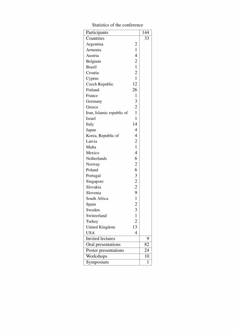
Statistics of the conference

Participants 144Countries 33Argentina 2Armenia 1Austria 4Belgium 2Brazil 1Croatia 2Cyprus 1Czech Republic 12Finland 26France 1Germany 3Greece 2Iran, Islamic republic of 1Israel 1Italy 14Japan 4Korea, Republic of 4Latvia 2Malta 1Mexico 4Netherlands 6Norway 2Poland 6Portugal 3Singapore 2Slovakia 2Slovenia 9South Africa 1Spain 2Sweden 3Switzerland 1Turkey 2United Kingdom 13USA 4Invited lectures 9Oral presentations 82Poster presentations 24Workshops 10Symposium 1

Contents

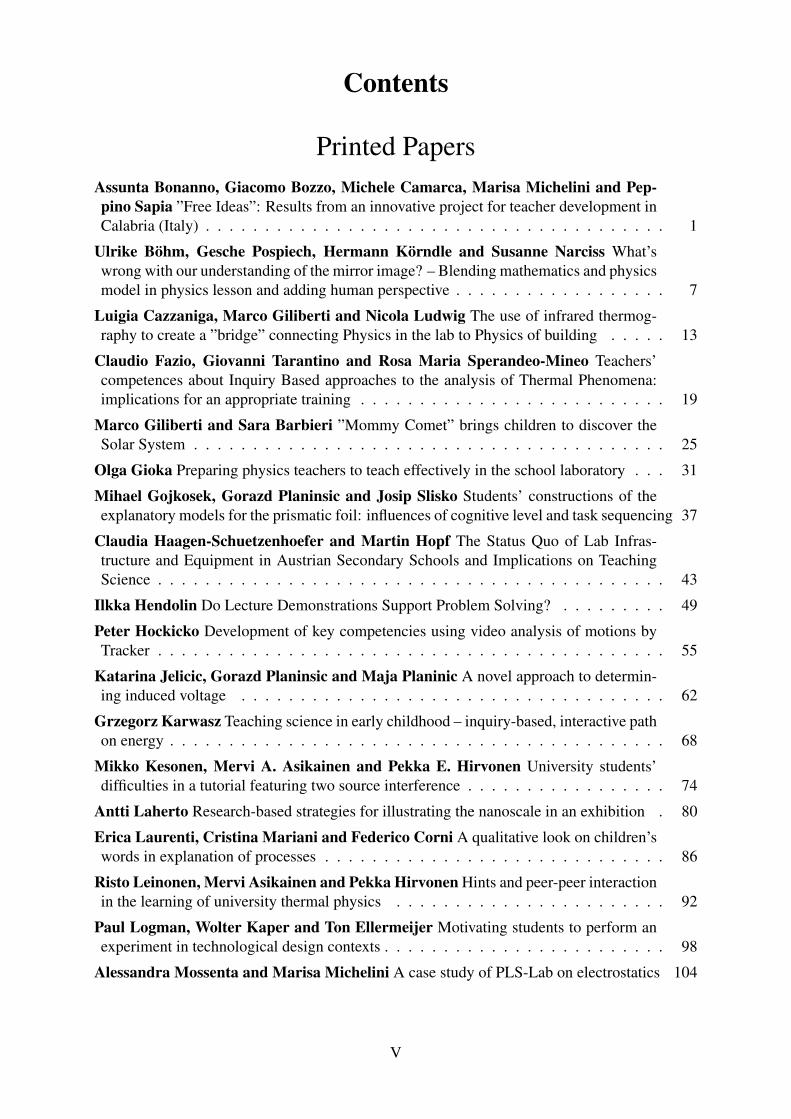
Printed PapersAssunta Bonanno, Giacomo Bozzo, Michele Camarca, Marisa Michelini and Pep-pino Sapia ”Free Ideas”: Results from an innovative project for teacher development inCalabria (Italy) . . . . . . . . . . . . . . . . . . . . . . . . . . . . . . . . . . . . . . . 1

Ulrike Böhm, Gesche Pospiech, Hermann Körndle and Susanne Narciss What’swrong with our understanding of the mirror image? – Blending mathematics and physicsmodel in physics lesson and adding human perspective . . . . . . . . . . . . . . . . . . 7

Luigia Cazzaniga, Marco Giliberti and Nicola Ludwig The use of infrared thermog-raphy to create a ”bridge” connecting Physics in the lab to Physics of building . . . . . 13

Claudio Fazio, Giovanni Tarantino and Rosa Maria Sperandeo-Mineo Teachers’competences about Inquiry Based approaches to the analysis of Thermal Phenomena:implications for an appropriate training . . . . . . . . . . . . . . . . . . . . . . . . . . 19

Marco Giliberti and Sara Barbieri ”Mommy Comet” brings children to discover theSolar System . . . . . . . . . . . . . . . . . . . . . . . . . . . . . . . . . . . . . . . . 25

Olga Gioka Preparing physics teachers to teach effectively in the school laboratory . . . 31

Mihael Gojkosek, Gorazd Planinsic and Josip Slisko Students’ constructions of theexplanatory models for the prismatic foil: influences of cognitive level and task sequencing 37

Claudia Haagen-Schuetzenhoefer and Martin Hopf The Status Quo of Lab Infras-tructure and Equipment in Austrian Secondary Schools and Implications on TeachingScience . . . . . . . . . . . . . . . . . . . . . . . . . . . . . . . . . . . . . . . . . . . 43

Ilkka Hendolin Do Lecture Demonstrations Support Problem Solving? . . . . . . . . . 49

Peter Hockicko Development of key competencies using video analysis of motions byTracker . . . . . . . . . . . . . . . . . . . . . . . . . . . . . . . . . . . . . . . . . . . 55

Katarina Jelicic, Gorazd Planinsic and Maja Planinic A novel approach to determin-ing induced voltage . . . . . . . . . . . . . . . . . . . . . . . . . . . . . . . . . . . . 62

Grzegorz Karwasz Teaching science in early childhood – inquiry-based, interactive pathon energy . . . . . . . . . . . . . . . . . . . . . . . . . . . . . . . . . . . . . . . . . . 68

Mikko Kesonen, Mervi A. Asikainen and Pekka E. Hirvonen University students’difficulties in a tutorial featuring two source interference . . . . . . . . . . . . . . . . . 74

Antti Laherto Research-based strategies for illustrating the nanoscale in an exhibition . 80

Erica Laurenti, Cristina Mariani and Federico Corni A qualitative look on children’swords in explanation of processes . . . . . . . . . . . . . . . . . . . . . . . . . . . . . 86

Risto Leinonen, Mervi Asikainen and Pekka Hirvonen Hints and peer-peer interactionin the learning of university thermal physics . . . . . . . . . . . . . . . . . . . . . . . 92

Paul Logman, Wolter Kaper and Ton Ellermeijer Motivating students to perform anexperiment in technological design contexts . . . . . . . . . . . . . . . . . . . . . . . . 98

Alessandra Mossenta and Marisa Michelini A case study of PLS-Lab on electrostatics 104

V

Pasi Nieminen, Antti Savinainen, Niina Nurkka and Jouni Viiri An Intervention forUsing Multiple Representations of Force in Upper Secondary School Courses . . . . . . 111

David Sands Profiling the mechanics knowledge of UK university entrants using theForce Concept Inventory . . . . . . . . . . . . . . . . . . . . . . . . . . . . . . . . . . 117

Antti Savinainen, Asko Mäkynen, Pasi Nieminen and Jouni Viiri An InterventionUsing an Interaction Diagram for Teaching Newton’s Third Law in Upper SecondarySchool . . . . . . . . . . . . . . . . . . . . . . . . . . . . . . . . . . . . . . . . . . . 123

Suvi Tala Gaining knowledge-building expertise in nanomodelling . . . . . . . . . . . . 129

Hildegard Urban-Woldron Physics Teachers: Gaining Confidence in Integrating Edu-cational Technologies into Student Learning . . . . . . . . . . . . . . . . . . . . . . . 134

Onne van Buuren, Peter Uylings and Ton Ellermeijer The use of formulas by lowerlevel secondary school students when building computer models . . . . . . . . . . . . . 140

Ed van den Berg Long term effects of an innovative physics teacher education programin the Philippines . . . . . . . . . . . . . . . . . . . . . . . . . . . . . . . . . . . . . . 149

Norbert van Veen and Ed van den Berg Interactive White Board in Physics Teaching;Beneficial for Physics Achievement? . . . . . . . . . . . . . . . . . . . . . . . . . . . 155

Electronic Papershttps://www.jyu.fi/en/congress/girep2011

Sara Barbieri, Marco Giliberti and Claudio Fazio Conduction as a prerequisite tosuperconductivity . . . . . . . . . . . . . . . . . . . . . . . . . . . . . . . . . . . . . 161

Pavel Brom and Frantisek Lustig Integrated e-learning and the opportunity for anyoneto explore the nature of polarisation of light . . . . . . . . . . . . . . . . . . . . . . . . 167

Jitka Bruestlova and Pavel Dobis Exploring Physical Properties of Ferromagnetic Ma-terials in Student Laboratories . . . . . . . . . . . . . . . . . . . . . . . . . . . . . . . 173

Ignacio Campos Flores, José Luis Jiménez Ramírez, Gabriela Del Valle Díaz Muñozand Guadalupe Hernández Morales The source of confusion in courses of modernphysics of college level . . . . . . . . . . . . . . . . . . . . . . . . . . . . . . . . . . 179

Sergej Faletic and Gorazd Planinsic Analyzing polarized light produced by reflectionand scattering . . . . . . . . . . . . . . . . . . . . . . . . . . . . . . . . . . . . . . . . 185

Sergej Faletic, Mihael Gojkosek and Katarina Jelicic MUSE workshop: reflectionsand feedback . . . . . . . . . . . . . . . . . . . . . . . . . . . . . . . . . . . . . . . . 191

Sergej Faletic, Gorazd Planinsic and Ales Mohoric ”How things work?” – Undergrad-uate optional course for physics students . . . . . . . . . . . . . . . . . . . . . . . . . 197

Tomas Franc Gravitational Assisted Trajectories – making your own pictures and trajec-tory study . . . . . . . . . . . . . . . . . . . . . . . . . . . . . . . . . . . . . . . . . . 202

Rui G. Neves, Judah L. Schwartz, Jorge C. Silva, Vítor D. Teodoro and Pedro C.Vieira Learning Introductory Physics with Computational Modelling and InteractiveEnvironments . . . . . . . . . . . . . . . . . . . . . . . . . . . . . . . . . . . . . . . . 208

Osamu Hirayama Demonstration and experiments of rolling motion of cylindrical ob-jects down a slope . . . . . . . . . . . . . . . . . . . . . . . . . . . . . . . . . . . . . 214

VI

Jose Luis Jimenez, Ignacio Campos and Jose Antonio Eduardo Roa Neri The searchof conceptual clarity in two problems in electromagnetism: a finite wire with constantcurrent and the concept of test charge . . . . . . . . . . . . . . . . . . . . . . . . . . . 220

Zdenka Koupilova, Dana Mandikova, Marie Snetinova and Zdenek Sabatka Elec-tronic Collection of Solved Physics Problems – How to Create Your Own New Problem 226

Tomaž Kranjc and Nada Razpet Using School Measurements to Rate the Quality ofthe Environment . . . . . . . . . . . . . . . . . . . . . . . . . . . . . . . . . . . . . . 230

Yasuhiro Kudo and Eizo Ohno Using Microtribology to Teach Friction . . . . . . . . . 236

Robert Lambourne The European Physical Society and Educational Physics . . . . . . 242

Cristina Mariani, Federico Corni and Hans U. Fuchs A didactic approach to and cur-ricular perspectives of the construction of the energy concept in primary school . . . . . 248

Julietta Mirzoyan Armenian Student Performance in Science: Results From TIMSS . . 254

Arto Mutanen and Antti Rissanen Adjusting cadets’ reasoning skills with strategicquestioning . . . . . . . . . . . . . . . . . . . . . . . . . . . . . . . . . . . . . . . . . 260

Eizo Ohno Analytic frameworks for studying science classroom discourse with dynamicsemantic approach . . . . . . . . . . . . . . . . . . . . . . . . . . . . . . . . . . . . . 266

Nicola Pizzolato, Onofrio Rosario Battaglia and Rosa Maria Sperandeo-Mineo AnInquiry Based Approach to the study of energy exchange by thermal radiation . . . . . 272

Nada Razpet and Tomaž Kranjc A Physics Students is Getting Ready for Vacations . . 278

Sabrina Rossi, Enrica Giordano and Nicoletta Lanciano The Parallel Globe and theGlobo Local Project . . . . . . . . . . . . . . . . . . . . . . . . . . . . . . . . . . . . 284

Ivan Ruddock Physical concepts and misconceptions . . . . . . . . . . . . . . . . . . . 290

Zdenek Sabatka, Leos Dvorak and Vera Koudelkova Demonstration Experiments inElectricity and Magnetism for Future Teachers . . . . . . . . . . . . . . . . . . . . . . 296

IndexesList of Authors . . . . . . . . . . . . . . . . . . . . . . . . . . . . . . . . . . . . . . . 302

VII

”Free Ideas”: Results from an innovative project for teacher development in

Calabria (Italy)

Assunta Bonanno 1, Giacomo Bozzo 1, Michele Camarca 1, Marisa Michelini 2, Peppino Sapia 1

peppino.sapia@fis.unical.it 1 Physics Education Research Group, Physics Department - University of Calabria,

Italy and 2 Physics Education Research Unit, Department of Chemistry, Physics and

Environment - University of Udine, Italy

The paper illustrates the most important actions of a project granted by the administration of Calabria (a region of Southern Italy) aimed to promote the dissemination of good teaching practices based on the use of scientific laboratories and assisted by the proper utilization of new technologies. It has involved 29 schools spread throughout the Region and operating in highly differentiated socio-economic contexts. In the aim to bridge the gap between the educational research and the school teaching practice, the learning paths supplied to students have planned the simultaneous presence in the classroom of two teaching professionals having different roles and referred to as ”experimenter” and ”trainer” teacher. The former was identified by the school manager among teachers in service, while the latter was selected by a competition among people usually involved in educational research. The teaching activities with students were directly conducted by the experimenter, supported throughout the educational path by the trainer teacher. Analysis of project outcomes highlights some peculiarities in the interaction dynamics between the two professionals, giving useful hints for the design of effective training of teacher in service.

1. Introduction

There are many indicators testifying the steadily worsening in the level of scientific knowledge possessed by the population in general and by young people in particular, paradoxically in an epoch characterized by a wide diffusion of technological equipment and devices. A lot of disaffection to science (Bonanno et al., 2009; Mazur E., 1997; Sokoloff et al., 2007) is clearly reflected in the reduction of enrollment in scientific faculties (McDermott L.C., 1990), more serious in Italy than in the rest of the world. Among the various surveys conducted at the international level on student scientific knowledge, the OCSE-PISA investigation, for youngsters in the age group 14-15 years, have raised some worry and concern in Italy since its results lie significantly below the European average. The same surveys showed that large inhomogeneities and differences exist in the country, so that while the northern regions lie even above the European average, the southern regions remain far below it, pulling the national average towards bad results above mentioned. Various experiences conducted so far show that it is appropriate to privilege interventions at the secondary school (in the age group 11-15 years) aimed to upgrade teaching methodologies and to modernize laboratories and technological infrastructures (Gervasio et al., 2008; Bonanno et al., 2011; Michelini M., 1992; Grayson & McDermott; 1996; Sokoloff et al., 2007). For what is specifically concerning the latter, in the recent past the Calabria administration had largely funded schools which intended to improve their scientific laboratories and their ICT facilities, but the most part of these new supplies have been left under-utilized because of the inadequate

1

preparation of involved teachers. Further investments were also devolved to teacher training, since the educational innovation necessarily involves it (McDermott L.C., 1990). However, the performed experiences have largely shown that the training practice bulls down to a simple information when it is not accompanied by a collective reflection, a careful revision and a creative application. Moreover, when the educational opportunities (albeit for limitations in time and resources) are reduced to a simple knowledge transfer, they leave a rooted and deep mistrust about the possibility that what is learned can then be translated into the daily teaching practice (also in consideration of personal operating realities often too different from those outlined) (Michelini M., 2007). The project "Free Ideas", founded at the Faculty of Sciences of University of Calabria by the regional administration, wanted to meet the specific problem of spreading the use of existing facilities and, to do that, proposed a teacher training model based on two positions: the experimenter-teacher (ET) 1 and the trainer-teacher (TT). The former, identified and nominated by the school manager among his in service teachers, was the professional designated to directly lead the teaching activity in the classroom; while the latter was devoted to support the ET especially from the methodological point of view. For this reason, the TT was identified through a competitive procedure aimed to select candidates who had gained good experience in laboratory activities, had built a good expertise in new technologies and data acquisition, had familiarity with the educational research and the innovative teaching actions. The two teacher figures were employed, after a brief initial training, to conduct the learning path (chosen by the school and lasting 30 hours) in the classroom during extracurricular lessons and in co-presence. This operational strategy has allowed to fully contextualize the intervention, making it functional for the educational goals chosen and privileged by each involved institute. The learning paths were targeted to 1360 students aged 11-16 (coming from 29 schools operating in deeply heterogeneous socio-economic contexts) and were structured into three broad themes (Environment, Energy and Waves) involving the cultural areas of mathematics, physics and natural sciences. All the activities were planned in order to create operative conditions in which the students could participate actively in the learning process (Bonanno et Al., 2009; Michelini & Cobal, 2002) becoming finally able to think, to propose personal interpretations and to critically reconsider contents. In the following sections, we describe the main actions of intervention and the monitoring procedures. Then we illustrate some specific aims of the conducted survey, the methodology implemented for the data analysis and finally we conclude with the result discussion.

2. Main actions of intervention, monitoring strategies and research questions

The main actions of intervention can be classified into three different categories: 1. instruction of involved teachers (71 experimenter and 51 trainer), 2. delivering of learning path to students, 3. action monitoring.

Experimenter and trainer teachers, on average, possessed well diversified competencies. In fact while the former was marked by a significant experience gained in the field of traditional teaching and in a well-defined socio-economic

1 The in service teachers have been named as “experimenters” in the sense that they are deputed to “experience” directly the new methodologies in their classrooms, making comparisons with respect to the results obtained by their traditional teaching practices.

2

context, the latter was, on the contrary, an expert in innovative teaching methods and in the use of new communication technologies. The initial formation of these two figures was carried out by providing two seminars (each lasting three-hours and focused on the most advanced frontiers of research in science education) to be attended all together. This activity was shortly followed by a specific training, differentiated according to the various lines of intervention and divided into two additional meetings for a total of 5 hours. At this point each experimenter teacher was assigned to a trainer teacher to whom he could express his requirements and needs with respect to arising technological problems, could ask for help about the innovative teaching methodologies and could discuss the articulation of proposed experimental learning path. At this stage (for which both teachers where expected to work for further nine hours) a detailed planning of the learning path was prepared and agreed. In the classroom, the didactic activity was conducted by the experimenter teacher but with the simultaneous presence of his trainer, ready to get involved if unexpected problems raised. The quality of the collaboration between experimenter and trainer teachers was crucial to the achievement of expected learning goals and, for these reasons, it was carefully monitored. Moreover, we wanted to get useful information on this mode of operation in which the tasks of the two teacher figures was essentially reversed if compared to practices usually adopted for extra-curricular activities. In fact in all other interventions, promoted within the national operational plan, the innovative training action (addressed to students) is entrusted to an expert coming from outside the institution, while a subordinate role of tutoring and assistance is reserved to the teachers working inside the school. The activity monitoring has provided for registers of attendance control, distribution of open and closed-response tests, creation of website for gathering information and for sharing results. Monitoring has made clear that this approach has found favor with both the professionals involved (experimenter and trainer teacher), and both mutually recognized the importance of the input given by the colleague. We can definitely conclude that the wanted enhancement of the role of the teacher usually working in the institution (effectively supported but not replaced) has returned, as the major achievement, the awareness of the rewarding quality of his own work and the value of collaboration and confrontation (see also below). It should be emphasized that for the two figures, who have cooperated on various learning paths, significant heterogeneities can easily be supposed with regard to personal attitudes and expectations. To identify and characterize these differences, we conducted well-designed interviews in order to investigate significant aspects of the teaching experience referable to some specific dimensions of the Pedagogical Contents Knowledge - PCK (Shulman, 1986; Etkina, 2010). In particular, our investigation has been directed to respond to four research questions:

1. Do ETs and TTs differ: a. in the weight attributed to specific aspects of the laboratorial teaching

experience? (see Fig. 1 for investigated aspects); b. in the focusing of general conceptual knots?

2. Among ETs and TTs who have carried out the same learning module, do they differ in:

a. identifying how to address conceptual knots? b. focusing specific issues of the performed didactic activity?

3

3. Results and discussion

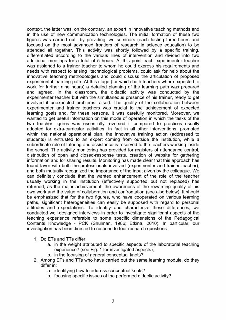
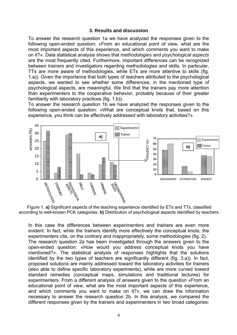
To answer the research question 1a we have analyzed the responses given to the following open-ended question: «From an educational point of view, what are the most important aspects of this experience, and which comments you want to make on it?». Data statistical analysis shows that methodologies and psychological aspects are the most frequently cited. Furthermore, important differences can be recognized between trainers and investigators regarding methodologies and skills. In particular, TTs are more aware of methodologies, while ETs are more attentive to skills (fig. 1.a)). Given the importance that both types of teachers attributed to the psychological aspects, we wanted to see whether some differences, in the mentioned type of psychological aspects, are meaningful. We find that the trainers pay more attention than experimenters to the cooperative behavior, probably because of their greater familiarity with laboratory practices (fig. 1.b)). To answer the research question 1b we have analyzed the responses given to the following open-ended question: «What are conceptual knots that, based on this experience, you think can be effectively addressed with laboratory activities?». In this case the differences between experimenters and trainers are even more evident. In fact, while the trainers identify more effectively the conceptual knots, the experimenters cite, on the contrary and inappropriately, some methodologies (fig. 2). The research question 2a has been investigated through the answers given to the open-ended question: «How would you address conceptual knots you have mentioned?». The statistical analysis of responses highlights that the solutions identified by the two types of teachers are significantly different (fig. 3.a)). In fact, proposed solutions are mainly addressed toward the laboratory activities for trainers (also able to define specific laboratory experiments), while are more curved toward standard remedies (conceptual maps, simulations and traditional lectures) for experimenters. From a different analysis of answers given to the question «From an educational point of view, what are the most important aspects of this experience, and which comments you want to make on it?», we can draw the information necessary to answer the research question 2b. In this analysis, we compared the different responses given by the trainers and experimenters in two broad categories:

Figure 1. a) Significant aspects of the teaching experience identified by ETs and TTs, classified according to well-known PCK categories. b) Distribution of psychological aspects identified by teachers.

a)

b)

4

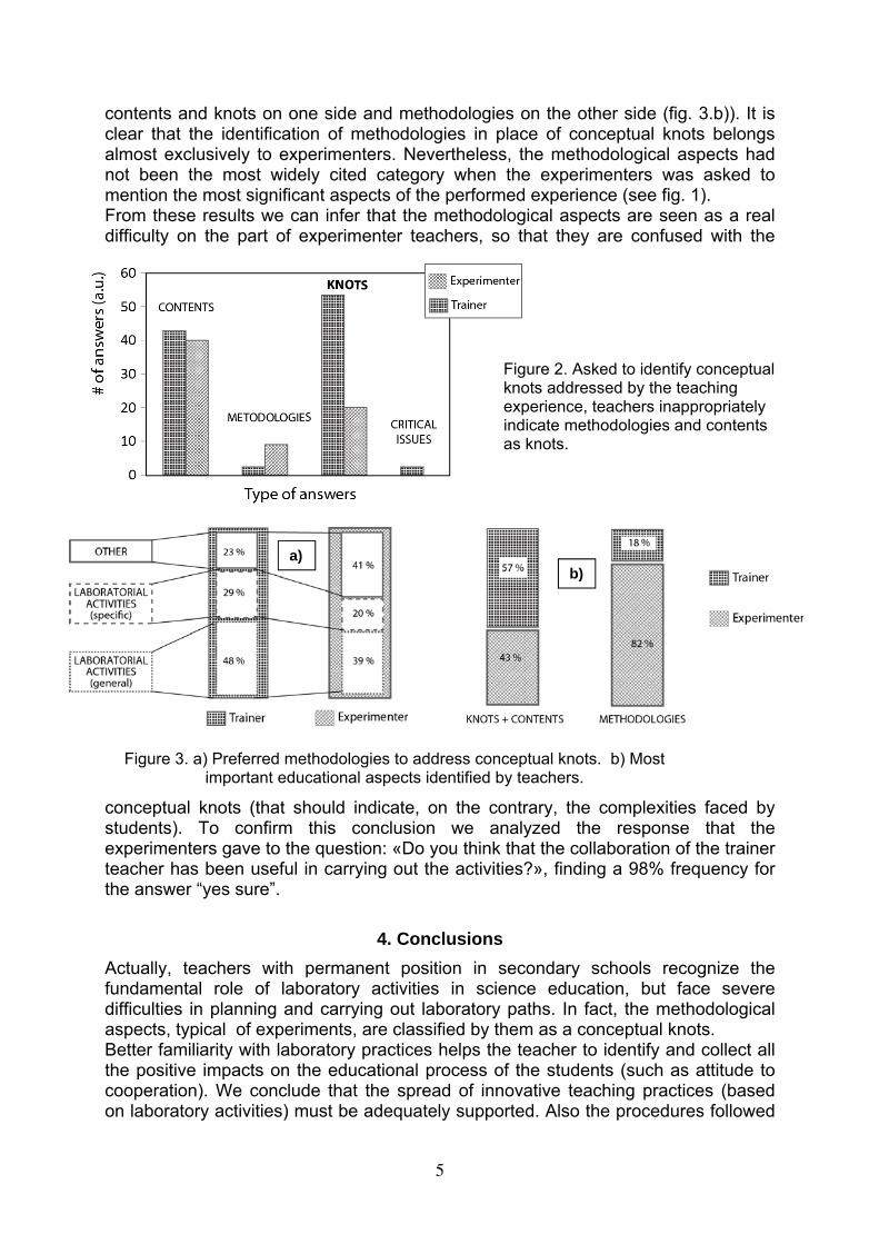
contents and knots on one side and methodologies on the other side (fig. 3.b)). It is clear that the identification of methodologies in place of conceptual knots belongs almost exclusively to experimenters. Nevertheless, the methodological aspects had not been the most widely cited category when the experimenters was asked to mention the most significant aspects of the performed experience (see fig. 1). From these results we can infer that the methodological aspects are seen as a real difficulty on the part of experimenter teachers, so that they are confused with the

conceptual knots (that should indicate, on the contrary, the complexities faced by students). To confirm this conclusion we analyzed the response that the experimenters gave to the question: «Do you think that the collaboration of the trainer teacher has been useful in carrying out the activities?», finding a 98% frequency for the answer “yes sure”.

4. Conclusions

Actually, teachers with permanent position in secondary schools recognize the fundamental role of laboratory activities in science education, but face severe difficulties in planning and carrying out laboratory paths. In fact, the methodological aspects, typical of experiments, are classified by them as a conceptual knots. Better familiarity with laboratory practices helps the teacher to identify and collect all the positive impacts on the educational process of the students (such as attitude to cooperation). We conclude that the spread of innovative teaching practices (based on laboratory activities) must be adequately supported. Also the procedures followed

Figure 2. Asked to identify conceptual knots addressed by the teaching experience, teachers inappropriately indicate methodologies and contents as knots.

a) b)

Figure 3. a) Preferred methodologies to address conceptual knots. b) Most important educational aspects identified by teachers.

5

so far in providing extracurricular education to students could be modified to make them functional to the training of teachers in service. In fact, though proper funds must be supplied to upgrade technological infrastructure of schools (science labs, multimedia rooms and equipment), the teacher training plays a crucial role and, when not properly addressed, will waste or nullify the resources devoted to educational innovation. The lines of intervention adopted in the "Free Ideas" project had the same costs of the activities typically funded from the operative national plan, but made the interventions more easily repeatable in the involved schools and created the institutional channels (between University and schools) that can be activated when further assistance will be needed.

Bibliography

Bonanno, A., Bozzo, G., Camarca, M., Oliva, A., & Sapia, P. (2009). Four physics jars. Il Nuovo Cimento , 31 C (4), 601-615.

Bonanno, A., Bozzo, G., Camarca, C., & Sapia, P. (2011). Using a PC and external media to quantitatively investigate electromagnetic induction. Phys. Educ., 46(4), 385-394.

Etkina E. (2010). Pedagogical content knowledge and preparation of high school physics teachers. Phys. Rev. ST-PER, 6, 020110/1-26.

Gervasio, M., Michelini, M., & Viola, R. (2008). Sensors as extension of senses via USB: three case studies on thermal, optical and electrical phenomena. Konferencja Laboratoria Fizyczne Sterowane Komputerowo. Toruń: http://dydaktyka.fizyka.umk.pl/komputery/pliki/Articolo_Torun_v2.pdf.

Grayson, D. J., McDermott, L. (1996). Use of the computer for research on student thinking in physics. Am. J. Phys., 64(5), 557-565.

Mazur, E. (1997). Peer Instruction: a user's manual. Upper Saddle River, New Jersey (USA): Prentice Hall, Inc.

McDermott, L. C. (1990). A perspective on teacher preparation in physics and other sciences: The need for special science courses for theachers. Am. J. Phys. , 58 (8), 734-742.

Merrill, M. D. (1992). Constructivism and instructional design. In T. M. Duffy, & D. H. Jonassened, Constructivism and technology of instruction. Hillsdale, New Jersey: Lawrence Erlbaum Associates.

Michelini, M. (1992). L'elaboratore nel laboratorio didattico di fisica: nuove opportunità per l'apprendimento. Giornale di Fisica, 23(4), 269.

Michelini, M., & Cobal , M. (2002). Developing Formal Thinking in Physics. Forum (Rome).

Michelini, M. (2007). Educazione scientifica ed approcci di ricerca in didattica della fisica. La fisica nel processo formativo. Seminario di studi "Cultura Scientifica e Ricerca Didattica". Reggio Emilia: Unità di Ricerca in Didattica della Fisica .

Shulman L. S. (1986). Paradigms and research programs in the study of teaching, in Handbook of Research on Teaching, 3rd ed.,edited by M. C. Witrock, Macmillan, New York, NY.

Sokoloff, D. R., Laws, P. W., & Thornton, K. R. (2007). RealTime Physics: active learning labs tronsforming the introductory laboratory. Eur. J. Phys., 28, S83-S94.

6

What’s wrong with our understanding of the mirror image? – Blending mathematics and physics model in physics lesson

and adding human perspective

Ulrike Böhm, Gesche Pospiech, Hermann Körndle, Susanne Narciss

Technische Universität Dresden, Germany, Ulrike.Boehm@mailbox.tu-dresden.de

The mirror image is one of the phenomena most misunderstood in early physics education. Starting from the discussion about the principles of physics modelling and mental modelling we show that one root of misunderstanding lies in the use of different model construction in mathematics and physics to explain this phenomenon.

We developed a didactic model to describe the processes of modelling in physics classes. The core concept is the segmentation of the scientific model in model perspectives (e. g. mirror image: mathematics, physics, human). Based on these three model perspectives we developed a special training for students (sixth grade, 11-12 year-olds) to promote the understanding of the mirror image.

The purposes of this study were (a) to investigate the understanding of the plane mirror phenomenon of novices in geometrical optics, and (b) to evaluate the multiple-perspective modelling training. In the study 89 students (sixth grade) from three schools participated as control group after their first instruction in geometrical optics and 72 students were taught by using specially designed worksheets in their physics lessons (treatment group). During the worksheet sessions they learned three different model perspectives step by step. This investigation focuses on finding a correlation between the understanding of image formation (plane mirror) and the use of model perspectives. The data show that understanding is improved and manifested in a better description of physics issues and more detailed information in the drawings of the students’ answers.

Theoretical Background

Already early researchers like AlHazen and Euler found that for the explanation of the mirror image two different kinds of modelling are needed. The first one is an optical (geometrical optics) argumentation and the second one is a non-optical (organic) argumentation – which we then have to link.

The optical argumentation includes (1) the correct application of the law of reflection and (2) the description of light with geometrical optics (modelling a light beam as if it is a pencil of rays). The non-optical argumentation describes the ‘way’ from the retina to our brain and the corresponding interpretation (what we think to see).

Results of numerous studies (e.g. Blumör and Wiesner (1992a), Galili, Bendall, and Goldberg (1993), Jung (1981)) show that the understanding of the mirror image phenomenon is quite unsatisfactory. In our opinion there are two main problems based on (1) the mathematical modelling of the mirror image and (2) the interpretation of the signals reaching the retina or any other imaging system. To discuss these problems in a more detailed way we developed a theoretical framework to describe the processes of physics modelling in school.

The Didactic Model

According to Stachowiak’s theory of modelling (1973) nobody can describe the real world – only a model of the real world. In particular novices have problems to understand science because they do not understand that teachers are talking about

7

models of the reality and not about reality itself. Sometimes the teachers themselves do not notice this. This is one of the most important problems in modern science teaching – physics theories should be taught in a way acknowledging that these theories are models of the real world (Hägele (2000), Kircher (1995)). In shaping these modelling processes science teachers have to pay attention on how students acquire scientific concepts (i.e. epistemic processes). The process of constructing mental models during the acquisition of physics knowledge plays an important role in understanding physics phenomena (Norman (1983), Carey (1985)).

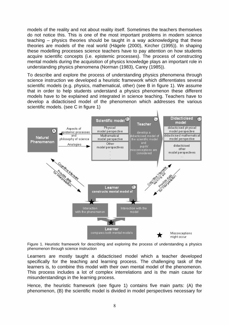
To describe and explore the process of understanding physics phenomena through science instruction we developed a heuristic framework which differentiates several scientific models (e.g. physics, mathematical, other) (see B in figure 1). We assume that in order to help students understand a physics phenomenon these different models have to be explained and integrated in science teaching. Teachers have to develop a didacticised model of the phenomenon which addresses the various scientific models. (see C in figure 1)

Figure 1. Heuristic framework for describing and exploring the process of understanding a physics phenomenon through science instruction

Learners are mostly taught a didacticised model which a teacher developed specifically for the teaching and learning process. The challenging task of the learners is, to combine this model with their own mental model of the phenomenon. This process includes a lot of complex interrelations and is the main cause for misunderstandings in the learning process.

Hence, the heuristic framework (see figure 1) contains five main parts: (A) the phenomenon, (B) the scientific model is divided in model perspectives necessary for

8

explaining and understanding the phenomenon, (C) the teacher, (D) the didacticised model (also divides in model perspectives) of the phenomenon and (E) the learner who interacts with both, the phenomenon and the didacticised model.

According to this framework, in understanding a physics phenomenon the learner has two models to handle with: (1) the own mental model and (2) the didacticised model of this phenomenon. Hence, in science education a learner is not approaching a physics phenomenon in the way researchers do it. Researchers develop a scientific model which describes the phenomenon as detailed as possible. This scientific model is then examined by experiments and by applying it to the real world.

Three Model Perspectives

The new idea for teaching a physics phenomenon is to divide the scientific model into different parts (perspectives) of the model according to different science areas. Only all model perspectives together can explain the phenomenon correctly. If only some (not all) model perspectives are used, the learner is not able to understand the phenomenon in a correct way. With this framework it is also possible to discuss the role of the mathematical model perspective in the process of understanding natural phenomena.

According to Greca and Moreira (2002) the model of a natural phenomenon is divided into two model perspectives: (1) the one of physics and (2) the one of mathematics. For Greca and Moreira the physics model of a theory is described with linguistic symbols and the mathematical model is described with mathematical symbols; understanding physics in school is achieved if it is possible to predict a physics phenomenon from its physics model.

To understand complex physics phenomena (like the mirror image) other perspectives besides the physics and mathematics perspective of modelling are necessary for understanding. The explanation, how we can see the mirror image (we call it ‘human’ model perspective) is indispensable.

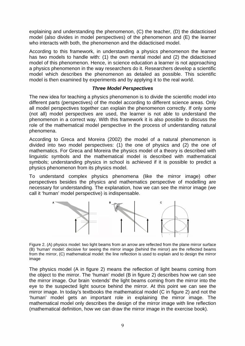
Figure 2. (A) physics model: two light beams from an arrow are reflected from the plane mirror surface (B) ’human’ model: decisive for seeing the mirror image (behind the mirror) are the reflected beams from the mirror, (C) mathematical model: the line reflection is used to explain and to design the mirror image The physics model (A in figure 2) means the reflection of light beams coming from the object to the mirror. The ‘human’ model (B in figure 2) describes how we can see the mirror image. Our brain ‘extends’ the light beams coming from the mirror into the eye to the suspected light source behind the mirror. At this point we can see the mirror image. In today’s textbooks the mathematical model (C in figure 2) and not the ‘human’ model gets an important role in explaining the mirror image. The mathematical model only describes the design of the mirror image with line reflection (mathematical definition, how we can draw the mirror image in the exercise book).

9

Most problems in student’s understanding of the mirror image occur by blending the mathematics and physics perspective – and not to mention the ‘human’ perspective. Using the mathematical model with the concept of “line reflection” the image is really existing. At this point we have to answer the question: ”What kind of image is the mirror image?” Mitchell (2009) said: ”You can hang a picture, but you can’t hang an image.” Hence we have to discuss different kinds of pictures. One question, however, remains: Can young children (early learners of physics) really understand the discussion of the mirror image in comparison to a picture? For understanding the mirror image phenomenon strong pre-concepts are necessary to be changed in order to build a new theory. Thus the understanding of the mirror image needs a strong conceptual change (Carey, 1985).

Blending the mathematics and the physics perspective

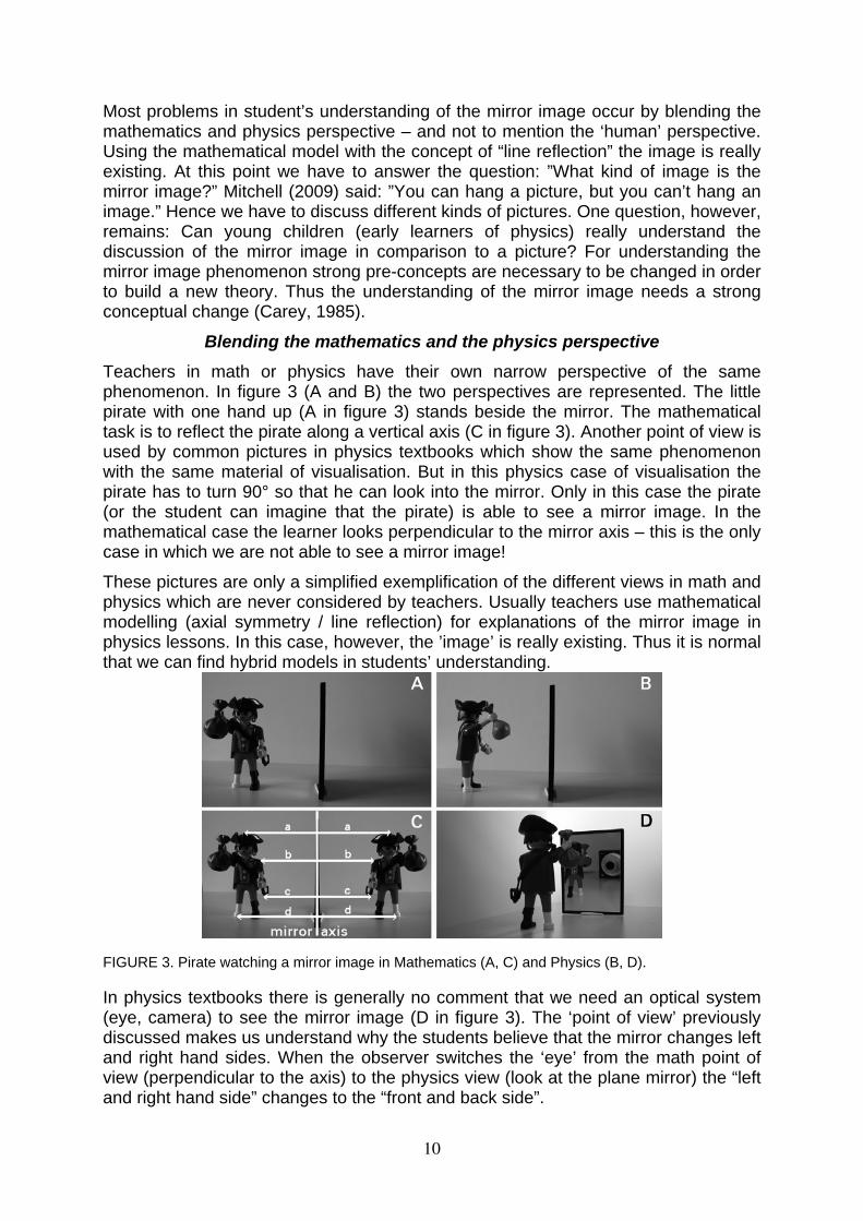
Teachers in math or physics have their own narrow perspective of the same phenomenon. In figure 3 (A and B) the two perspectives are represented. The little pirate with one hand up (A in figure 3) stands beside the mirror. The mathematical task is to reflect the pirate along a vertical axis (C in figure 3). Another point of view is used by common pictures in physics textbooks which show the same phenomenon with the same material of visualisation. But in this physics case of visualisation the pirate has to turn 90° so that he can look into the mirror. Only in this case the pirate (or the student can imagine that the pirate) is able to see a mirror image. In the mathematical case the learner looks perpendicular to the mirror axis – this is the only case in which we are not able to see a mirror image!

These pictures are only a simplified exemplification of the different views in math and physics which are never considered by teachers. Usually teachers use mathematical modelling (axial symmetry / line reflection) for explanations of the mirror image in physics lessons. In this case, however, the ’image’ is really existing. Thus it is normal that we can find hybrid models in students’ understanding.

FIGURE 3. Pirate watching a mirror image in Mathematics (A, C) and Physics (B, D). In physics textbooks there is generally no comment that we need an optical system (eye, camera) to see the mirror image (D in figure 3). The ‘point of view’ previously discussed makes us understand why the students believe that the mirror changes left and right hand sides. When the observer switches the ‘eye’ from the math point of view (perpendicular to the axis) to the physics view (look at the plane mirror) the “left and right hand side” changes to the “front and back side”.

10

Integration of the three models in physics lessons

We developed two worksheets to foster student’s knowledge by explaining the three model perspectives step by step. They are based on the especially developed training consisting of various PowerPoint presentations (Böhm, Pospiech, Körndle, & Narciss, 2010). The mirror image is explained step by step using the three perspectives of modeling and integrating prior knowledge. The students learn the three perspectives in their own specialist meaning and their integration in the physics model to explain the mirror image. The students become familiar with the role of the mathematical model – they do not need it to understand the mirror image, but they can use it for an easy depiction. Nevertheless they always have to consider that they have to ‘turn the eye’ by side to see the mirror image.

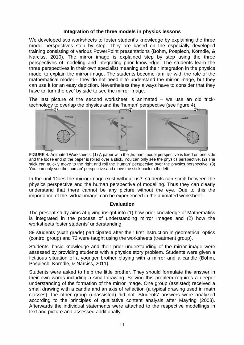
The last picture of the second worksheet is animated – we use an old trick-technology to overlap the physics and the ‘human’ perspective (see figure 4).

FIGURE 4. Animated Worksheets: (1) A paper with the ‚human’ model perspective is fixed on one side and the loose end of the paper is rolled over a stick. You can only see the physics perspective. (2) The stick can quickly move to the right and roll the ‘human’ perspective over the physics perspective. (3) You can only see the ‘human’ perspective and move the stick back to the left. In the unit ‘Does the mirror image exist without us?’ students can scroll between the physics perspective and the human perspective of modelling. Thus they can clearly understand that there cannot be any picture without the eye. Due to this the importance of the ‘virtual image’ can be experienced in the animated worksheet.

Evaluation

The present study aims at giving insight into (1) how prior knowledge of Mathematics is integrated in the process of understanding mirror images and (2) how the worksheets foster students’ understanding.

89 students (sixth grade) participated after their first instruction in geometrical optics (control group) and 72 were taught using the worksheets (treatment group).

Students’ basic knowledge and their prior understanding of the mirror image were assessed by providing students with a physics story problem. Students were given a fictitious situation of a younger brother playing with a mirror and a candle (Böhm, Pospiech, Körndle, & Narciss, 2011).

Students were asked to help the little brother. They should formulate the answer in their own words including a small drawing. Solving this problem requires a deeper understanding of the formation of the mirror image. One group (assisted) received a small drawing with a candle and an axis of reflection (a typical drawing used in math classes), the other group (unassisted) did not. Students’ answers were analyzed according to the principles of qualitative content analysis after Mayring (2003). Afterwards the individual statements were attached to the respective modellings in text and picture and assessed additionally.

11

Results and Conclusions

Significant differences between the individual groups (‘assisted’ and ‘unassisted’) in the examined control group (N = 89) concerning the achievement could be found. For students of the ‘worksheet group’ (N = 72) we did not find this differences between the individual groups (‘assisted’ and ‘unassisted’). Furthermore the students of the ‘worksheet group’ obtained significantly better achievements in both individual groups (‘assisted’ and ‘unassisted’) than the control group.

These results indicate, as discussed above, that the mathematical model perspective is not useful to develop a deeper understanding of the mirror image. Furthermore the study revealed that students of the control group with the assistance (eliciting the mathematical model) used the mathematical modelling perspective significantly more often, than students without the assisting hint. This interrelation cannot be found in the ‘worksheet group’.

With this investigation it can be shown that the transparent use of different model perspectives in physics lessons is very effective with respect to the amount of instructional time which is comparable to normal lessons to foster students’ understanding of the mirror image.

References

Blumör, R. & Wiesner, H. (1992a). Das Spiegelbild. Untersuchungen zu Schülervorstellungen und Lernprozessen (Teil 1). Sachunterricht und Mathematik in der Primarstufe, 1, 2–6.

Böhm, U., Pospiech, G., Körndle, H., & Narciss, S. (2010). Multiperspective modelling in the process of constructing and understanding physical theories using the example of the plane mirror image. In B. Paosawatyanyong & P. Wattanakasiwich (Eds.), International Conference on Physics Education: ICPE 2009 (Vol. 1263, pp. 143–146). AIP Conference Proceedings.

Carey, S. (1985). Conceptual change in childhood. Cambridge: MIT Press. Devlin, Keith, J. (1994). Mathematics, the science of patterns: the search for order in

life, mind, and the universe. New York: Scientific American Library Galili, I., Bendall, S., & Goldberg, F. (1993). The Effects of Prior Knowledge and

Instruction on Understanding Image Formation. Journal of Research in Science Teaching, 30(3), 271–301.

Greca, I. M. & Moreira, M. A. (2002). Mental, Physical, and Mathematical Models in the Teaching and Learning of Physics. Science Education, 86(1), 106–121.

Hägele, P. C. (2000). Physik - Weltbild oder Naturbild? In Tagung der Deutschen Physikalischen Gesellschaft (Ed.), DPG-Tagung Regensburg.

Jung, W. (1981). Ergebnisse einer Optik-Erhebung. physica didactica, 9 (Heft 1), 19–34.

Kircher, E. (1995). Studien zur Physikdidaktik: Erkenntnis- und wissenschaftstheoretische Grundlagen. Habilitationsschrift. Kiel: Institut für die Pädagogik der Naturwissenschaften (IPN).

Mitchell, W. J. T. (2008). In G. Frank (Ed.), Bildtheorie. Frankfurt am Main: Suhrkamp Verlag.

Norman, D. A. (1983). Some Oberservations on Mental Models. In D. Gentner & A. Stevens (Eds.), Mental Models (pp. 7–14). Hillsdale, NJ: Lawrence Erlbaum Associates.

Stachowiak, H. (1973). Allgemeine Modelltheorie. Wien, New York: Springer-Verlag.

12

The use of infrared thermography to create a “bridge” connecting Physics in the lab to Physics of building

Luigia Cazzaniga°, Marco Giliberti* and Nicola Ludwig*

° ITCG “Primo Levi”, Via Briantina, 64, 20038 Seregno (Monza), Italy e-mail: luigia.cazzaniga@tin.it

* Department of Physics, Università degli Studi di Milano

Abstract

The use of a thermal camera in a teaching learning process will be presented. The activity, which took place in a secondary school, was part of a multidisciplinary project based on the energy problem, in particular associated with energy consumption in buildings. A thermal camera was used by a group of students to detect heat leakages due to thermal bridges in the school structure. The students had a first approach to some building control-related problems, in particular concerning heat transfer phenomena, creating a link between the study of thermodynamic and its real-life application. A series of laboratory activities, based on the so called “students ownership of learning methodology” were planned and performed by the students themselves. In University laboratory further experiences with a thermal camera helped to develop, explain and interpret the students’ hand-made lab activities on thermal conductivity The importance of the task is connected with two main aspects: the use of new approaches and methods in Physics teaching, increasing students’ motivation, and the “infusion” of a cutting-edge technology (thermography) in a teaching learning process, showing that it may become a good cognitive tool promoting the fundamental approach to the “scientific methodology”.

1. Introduction

1.1 Problem statement

The activity object of this paper was carried out in an Italian secondary school which educates future building Surveyors. A considerable amount of the students, after passing their final examination, face the Job market. Students have low scores in maths and in scientific subjects, related to a series of problems in abstract reasoning (to make an example, out of 3 second classes, in last year, 62 total students, the average insufficient marks stand for 54% in Mathematics, 38.7% in Physics and 41% in Science). Students are attracted by new discoveries, vanguard technologies and their application to reality. School often takes them into account by planning and performing a lot of expedients regarding, in particular scientific and technological subjects. However, in many cases, their value related to cognitive learning is not meaningful. This problem was the starting point of our work which addressed the energy issue: the energy requalification of buildings. The aims were: to counter students’ disaffection towards Physics learning (making it easier and “friendly” to understand and describe the phenomena concerning heat transfer processes and to connect some theoretical contents to the reality). We chose to face the energy issue also because of social and territorial requirements: the energy “consumption” due to heating and climatization needs of existing buildings represents a huge amount of the Italian energy balance. In this paper only the activities concerning Physical contents will be described.

1.2 Literature review

The theoretical framework of our research is based on three different topics: Infrared Thermography and building detection, Physics Education (thermodynamic and its teaching - learning related problems), Instructional technology. Thermovision in building inspection is addressed to the study of the monument by giving visual documentation of not-in-sight

13

structural elements (Ludwig N., 2004). An adequate theoretical model of heat transfer allows to process the temperature increase of the surfaces during a test. In case of building materials both low conductivity and thickness allow to use a simple solution of the heat transfer equation in the approximation of adiabatic and semi-infinite medium (Ludwig N., 2003). In this conditions surface temperature depends on the square root of the time. (Phillipson M., Stupart A., 1995). Educational Physics research analyzed a number of conceptual difficulties encountered by students in their study on thermodynamic. They seem to be related to some aspects in a teaching sequence, like the differentiation state – process (Vicentini M. 1999), (Truesdell C.A. 1980), to common misconceptions, in particular related to the ideas of heat and temperature (Adawi and Linder, 2005), (Lewis E. L. and M. Linn, 1994), to heat transfer problems (Zheng H. and Keith J. M., 2003). Recent experiences recommend inquiry as an effective approach to develop students’ conceptual understandings in Physics in the areas of heat and temperature (Manzoor Ali Khan, 2009). In education, by instructional technology we mean "the theory and practice of design, development, utilization, management, and evaluation of processes and resources for learning” (from Wikipedia): the core concept is technology impact on learning. Koschmann (1996) relates the role of technology in a teaching learning process to the choice of a learning theory and to the choice of teaching method. The educational applications of IR thermography were first discussed by Vollmer et al.(2001). At that time the thermal cameras were very expensive; after almost ten years their use became much more common. Other examples followed: Möllmann K. P. and Vollmer M., (2007), Vollmer M. and Möllmann K. P. (2010).

1.3 Statement of intentions: research question and description of activities

Our research question was: “How can an infrared camera, used as a building detection instrument, became a cognitive tool in a Physics school laboratory?” According to Abraham Arcavi (2000) the research may be classified as a “problem – driven” one. After an introductory lesson held by a local professional on base concepts of thermo vision, a group of students performed the mapping of the school building to detect thermal bridges. By analyzing data, a series of consideration emerged, also considering other examples concerning building inspection, looking for Physics explanation of thermal images. In the Physics laboratory a class realized some handmade experiments on heat transfer phenomena, which were explained and interpreted thanks to some activities carried out at University under the same condition with an infrared camera.

2. Method

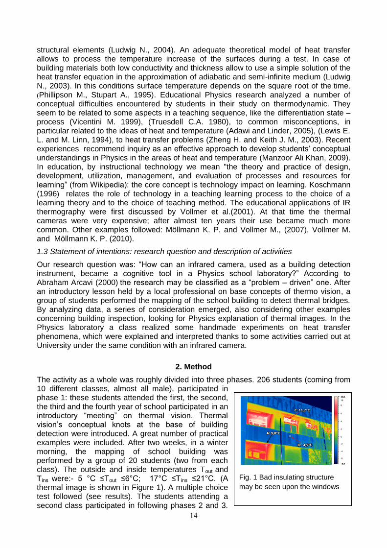
The activity as a whole was roughly divided into three phases. 206 students (coming from 10 different classes, almost all male), participated in phase 1: these students attended the first, the second, the third and the fourth year of school participated in an introductory “meeting” on thermal vision. Thermal vision’s conceptual knots at the base of building detection were introduced. A great number of practical examples were included. After two weeks, in a winter morning, the mapping of school building was performed by a group of 20 students (two from each class). The outside and inside temperatures Tout and Tins were:- 5 °C ≤Tout ≤6°C; 17°C ≤Tins ≤21°C. (A thermal image is shown in Figure 1). A multiple choice test followed (see results). The students attending a second class participated in following phases 2 and 3.

Fig. 1 Bad insulating structure

may be seen upon the windows

A: 9,0°CA: 9,0°CA: 9,0°CA: 9,0°CA: 9,0°CA: 9,0°CA: 9,0°CA: 9,0°CA: 9,0°C

B: -4,9°CB: -4,9°CB: -4,9°CB: -4,9°CB: -4,9°CB: -4,9°CB: -4,9°CB: -4,9°CB: -4,9°C

C: 11,7°CC: 11,7°CC: 11,7°CC: 11,7°CC: 11,7°CC: 11,7°CC: 11,7°CC: 11,7°CC: 11,7°C

-7,7

-6

-4

-2

0

2

4

6

8

10,1

°C

14

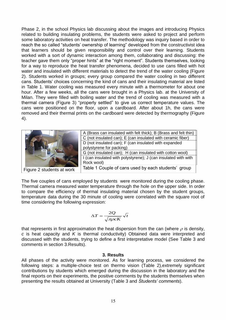
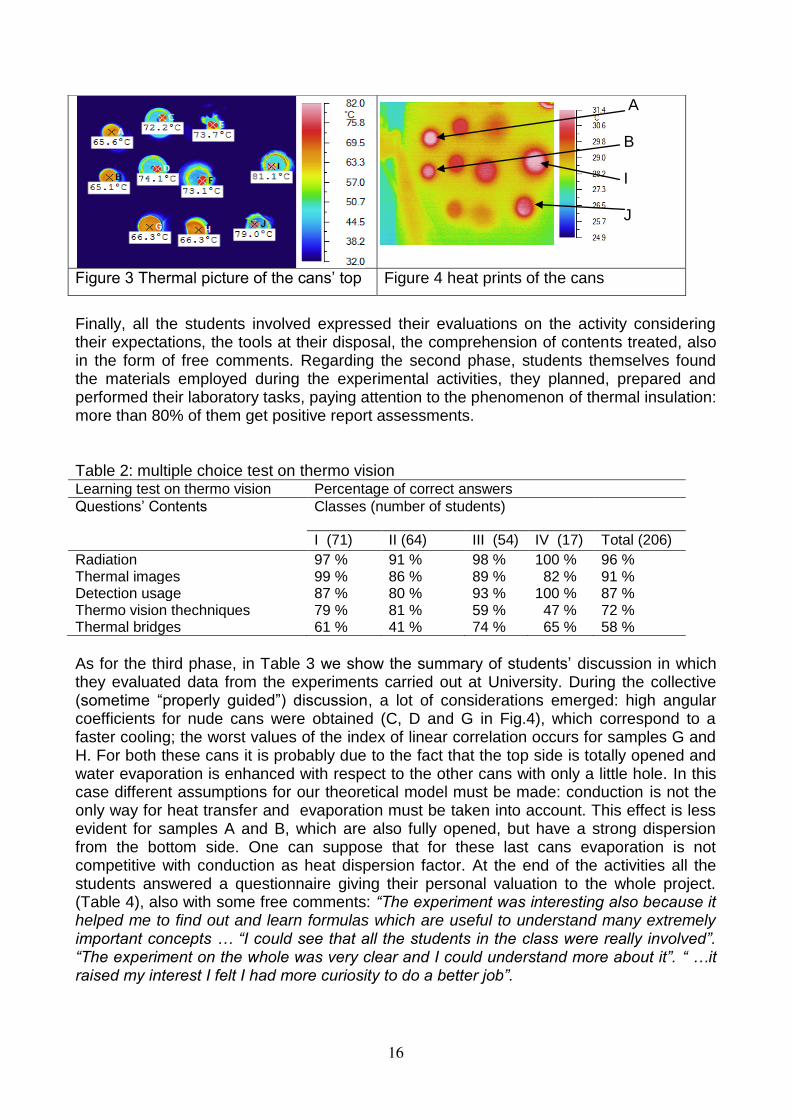
Phase 2, in the school Physics lab discussing about the images and introducing Physics related to building insulating problems, the students were asked to project and perform some laboratory activities on heat transfer. The methodology was inquiry based in order to reach the so called “students’ ownership of learning” developed from the constructivist idea that learners should be given responsibility and control over their learning. Students worked with a sort of dynamic interaction among them, collaborating and discussing: the teacher gave them only “proper hints” at the “right moment”. Students themselves, looking for a way to reproduce the heat transfer phenomena, decided to use cans filled with hot water and insulated with different materials to detect the trend of the water cooling (Figure 2). Students worked in groups; every group compared the water cooling in two different cans. Students’ choices concerning the kind of cans and their insulating material are listed in Table 1. Water cooling was measured every minute with a thermometer for about one hour. After a few weeks, all the cans were brought in a Physics lab. at the University of Milan. They were filled with boiling water and the trend of cooling was measured with a thermal camera (Figure 3) “properly settled” to give us correct temperature values. The cans were positioned on the floor, upon a cardboard. After about 1h, the cans were removed and their thermal prints on the cardboard were detected by thermography (Figure 4).

The five couples of cans employed by students were monitored during the cooling phase. Thermal camera measured water temperature through the hole on the upper side. In order to compare the efficiency of thermal insulating material chosen by the student groups, temperature data during the 30 minute of cooling were correlated with the square root of time considering the following expression:

that represents in first approximation the heat dispersion from the can (where is density, c is heat capacity and K is thermal conductivity) Obtained data were interpreted and discussed with the students, trying to define a first interpretative model (See Table 3 and comments in section 3.Results).

3. Results All phases of the activity were monitored. As for learning process, we considered the following steps: a multiple-choice test on thermo vision (Table 2),extremely significant contributions by students which emerged during the discussion in the laboratory and the final reports on their experiments, the positive comments by the students themselves when presenting the results obtained at University (Table 3 and Students’ comments).

Figure 2 students at work

A (Brass can insulated with felt thick); B (Brass and felt thin)

C (not insulated can); E (can insulated with ceramic fiber)

D (not insulated can); F (can insulated with expanded polystyrene for packing)

G (not insulated can); H (can insulated with cotton wool)

I (can insulated with polystyrene); J (can insulated with with Rock wool)

Table 1 Couple of cans used by each students’ group

tcK

QT

2

15

Finally, all the students involved expressed their evaluations on the activity considering their expectations, the tools at their disposal, the comprehension of contents treated, also in the form of free comments. Regarding the second phase, students themselves found the materials employed during the experimental activities, they planned, prepared and performed their laboratory tasks, paying attention to the phenomenon of thermal insulation: more than 80% of them get positive report assessments. Table 2: multiple choice test on thermo vision Learning test on thermo vision Percentage of correct answers

Questions’ Contents Classes (number of students)

I (71) II (64) III (54) IV (17) Total (206)

Radiation 97 % 91 % 98 % 100 % 96 % Thermal images 99 % 86 % 89 % 82 % 91 % Detection usage 87 % 80 % 93 % 100 % 87 % Thermo vision thechniques 79 % 81 % 59 % 47 % 72 % Thermal bridges 61 % 41 % 74 % 65 % 58 %

As for the third phase, in Table 3 we show the summary of students’ discussion in which they evaluated data from the experiments carried out at University. During the collective (sometime “properly guided”) discussion, a lot of considerations emerged: high angular coefficients for nude cans were obtained (C, D and G in Fig.4), which correspond to a faster cooling; the worst values of the index of linear correlation occurs for samples G and H. For both these cans it is probably due to the fact that the top side is totally opened and water evaporation is enhanced with respect to the other cans with only a little hole. In this case different assumptions for our theoretical model must be made: conduction is not the only way for heat transfer and evaporation must be taken into account. This effect is less evident for samples A and B, which are also fully opened, but have a strong dispersion from the bottom side. One can suppose that for these last cans evaporation is not competitive with conduction as heat dispersion factor. At the end of the activities all the students answered a questionnaire giving their personal valuation to the whole project. (Table 4), also with some free comments: “The experiment was interesting also because it helped me to find out and learn formulas which are useful to understand many extremely important concepts … “I could see that all the students in the class were really involved”. “The experiment on the whole was very clear and I could understand more about it”. “ …it raised my interest I felt I had more curiosity to do a better job”.

A B I J

Figure 3 Thermal picture of the cans’ top Figure 4 heat prints of the cans

16

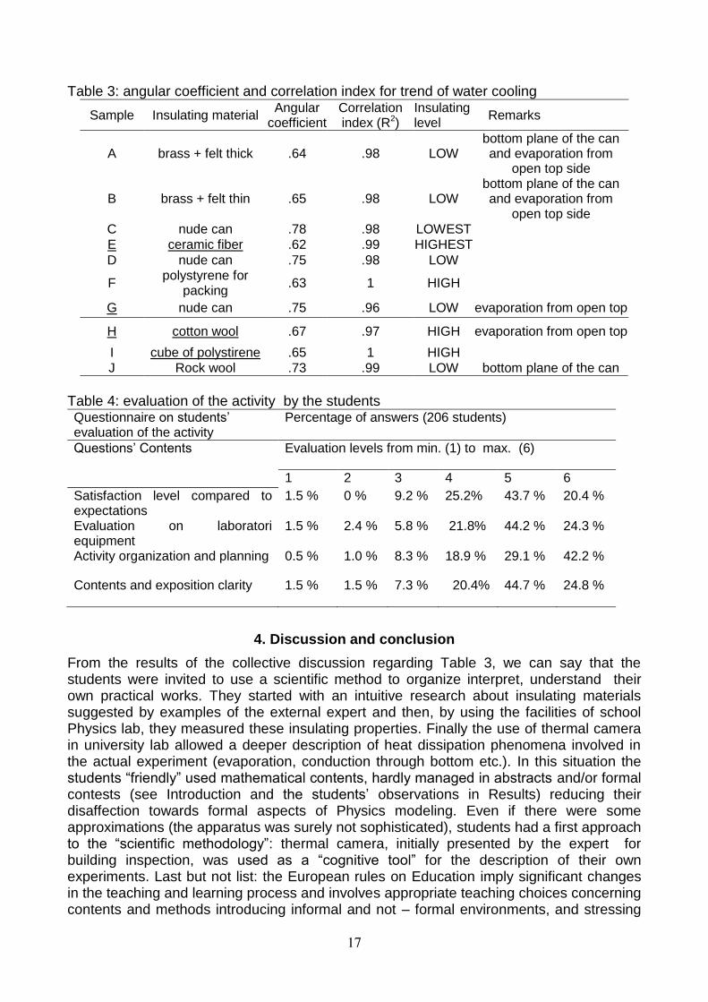
Table 3: angular coefficient and correlation index for trend of water cooling

Sample Insulating material Angular

coefficient Correlation index (R2)

Insulating level

Remarks

A brass + felt thick .64 .98 LOW bottom plane of the can and evaporation from

open top side

B brass + felt thin .65 .98 LOW bottom plane of the can and evaporation from

open top side C nude can .78 .98 LOWEST

E ceramic fiber .62 .99 HIGHEST

D nude can .75 .98 LOW

F polystyrene for

packing .63 1 HIGH

G nude can .75 .96 LOW evaporation from open top

H cotton wool .67 .97 HIGH evaporation from open top

I cube of polystirene .65 1 HIGH

J Rock wool .73 .99 LOW bottom plane of the can

Table 4: evaluation of the activity by the students Questionnaire on students’ evaluation of the activity

Percentage of answers (206 students)

Questions’ Contents Evaluation levels from min. (1) to max. (6)

1 2 3 4 5 6

Satisfaction level compared to expectations

1.5 % 0 % 9.2 % 25.2% 43.7 % 20.4 %

Evaluation on laboratori equipment

1.5 % 2.4 % 5.8 % 21.8% 44.2 % 24.3 %

Activity organization and planning 0.5 % 1.0 % 8.3 % 18.9 % 29.1 % 42.2 %

Contents and exposition clarity 1.5 % 1.5 % 7.3 % 20.4% 44.7 % 24.8 %

4. Discussion and conclusion

From the results of the collective discussion regarding Table 3, we can say that the students were invited to use a scientific method to organize interpret, understand their own practical works. They started with an intuitive research about insulating materials suggested by examples of the external expert and then, by using the facilities of school Physics lab, they measured these insulating properties. Finally the use of thermal camera in university lab allowed a deeper description of heat dissipation phenomena involved in the actual experiment (evaporation, conduction through bottom etc.). In this situation the students “friendly” used mathematical contents, hardly managed in abstracts and/or formal contests (see Introduction and the students’ observations in Results) reducing their disaffection towards formal aspects of Physics modeling. Even if there were some approximations (the apparatus was surely not sophisticated), students had a first approach to the “scientific methodology”: thermal camera, initially presented by the expert for building inspection, was used as a “cognitive tool” for the description of their own experiments. Last but not list: the European rules on Education imply significant changes in the teaching and learning process and involves appropriate teaching choices concerning contents and methods introducing informal and not – formal environments, and stressing

17

the importance of the active role of students in their learning process, this suggests that it worthwhile to go on in this “direction”.

References

Abraham Arcavi, (2000) Problem-driven research in mathematics education Journal of Mathematical Behavior 19 141±173

Adawi, T. and Linder C., (2005). What's hot and what's not: A phenomenographic study of lay adults' conceptions of heat and temperature. Paper presented at the 11th biennial EARLI conference, University of Cyprus, Nicosia, August 23-27, 2005

E. L. Lewis and M. Linn, (1994). Heat energy and temperature concepts of adolescents, adults, and experts: Implications for curricular improvements. Journal of Research in Science Teaching,vol. 31, pp. 657-677

H. Zheng and J. M. Keith, (2003).Web-Based Instructional Tools for Heat and Mass Transfer, in American Society for Engineering Education Annual Conference & Exposition, Nashville,Tennessee.

Koschmann, Timothy, (1996). Paradigm Shifts and Instructional Technology. Chapter 1. CSCL, theory and practice of an emerging paradigm Mahwah, New Jersey Lawrence Associates, Inc.

Möllmann K. P. and M. Vollmer, (2007). Infrared thermal imaging as a tool in university physics education. European Journal of Physics vol. 28, pp. S37-S50.

Ludwig L.(2003): Thermographic testing on building using a simplified heat transfer model. Materials evaluation Vol.61, 5 pp 599-603.

Ludwig L., Redaelli V., Rosina E. e Augelli F.: Moisture detection in wood and plaster by IR thermography. Infrared Physics & Tecnologies 46 (2004) 161-166, Elsevier ISSN 1350-4495

Manzoor Ali Khan, (2009). Teaching of heat and temperature by hypothetical inquiry approach: A sample of inquiry teaching J. Phys. Tchr. Educ. Online, 5(2), www.phy.ilstu.edu/jpteo Autumn 2009

Phillipson M., Stupart A., (1995) Temperature and moisture conditions in masonry: frost performance, Proceedings of Int. Symposium on Moisture Problems in Building Walls, Porto (Portuga1,) September, l, pp.405-415

Ribando R. J. , Richards L. G. , and O’Leary G. W. , (2004). Hands-On” Approach to Teaching Undergraduate Heat Transfer," in 2004 ASME Curriculum Inn. Award Honorable Mention

Snell J., (2010). "RESNET & Infrared Thermography," in Home Energy, pp. 48-52.

Truesdell C.A.,(1980) - The tragicomical history of thermodynamics, Springer Verlag Berlin

Vicentini M., (1999) - Acta Scientiarum, 21 pp. 795-803 Vollmer M. and Möllmann K.-P. , (2010). Infrared Thermal Imaging: Fundamentals,

Research and Applications, 1st ed. Berlin: Wiley-VCH. Vollmer M, Möllmann K.-P. , Pinno F., and Karstädt D., (2001) There is more to see than

eyes can detect. Physics Teacher, vol. 39, pp. 371-376.

18

Teachers’ competences about Inquiry Based approache s to the analysis of Thermal Phenomena: implications for an appropriate training .

Claudio Fazio, Giovanni Tarantino & Rosa Maria Sperandeo-Mineo

claudio.fazio@unipa.it – giovanni.tarantino19@unipa.it – rosamaria.mineo@unipa.it

UOP_PERG (University of Palermo Physics Education Research Group) Dipartimento di Fisica, Università di Palermo (Italia)

In this paper we present some preliminary results of a course for in-service teacher education held at University of Palermo in the framework of ESTABLISH, an EU FP7 Project aimed at extending the use of Inquiry Based Science Education in secondary level schools across Europe. In particular, we will report results of a survey performed with 15 second level Italian teachers about the ways they approach the analysis of a simple thermal physics situation, their typical conceptions and some aspects of their attitude with respect to methods aimed at performing classroom investigation in the light of the specific operative processes of an IB approach.

Introduction

Innovation in science education is providing an opportunity for research to focus in developing classroom resources that enhance student learning on key learning goals. In addition to establishing a coherent framework for the science topics at the different grade levels, many research results suggest that students should learn science by engaging in inquiry processes that allow them to reflect how scientific knowledge is constructed. By inquiry we refer to learning experiences that engage students in various integrated activities of identifying questions, collecting and interpreting evidence, formulating explanations, and communicating their findings, that are consistent with science standards and recent reports (Duschl, Schweingruber,& Shouse, 2007; National Research Council, 2000; Singer, Hilton, & Schweingruber, 2005). Recently, researchers have distinguished inquiry from active or hands-on instruction and tried to describe the elements of instruction (defined as marks of successful IB approaches) that help students to build more coherent and generative understanding (Clark & Linn, 2003; Linn & Hsi, 2000). With regard to the features of IB teaching, teachers especially need to gain Pedagogical Content Knowledge (PCK) enabling them to “engage students in asking and answering scientific questions, designing and conducting investigations, collecting and analyzing data, developing explanations based on evidence, and communicating and justifying findings” (Beyer, Delgado, Davis, & Krajcik, 2009, p. 978). In this paper we present some preliminary research results about ways to involve in-service teachers in training activities on Inquiry Based (IB) approach, with particular relevance to the study of the development of PCK, in the framework of the EU project ESTABLISH (www.establish-fp7.eu).

Theoretical Background

Although innovative curriculum materials provide support for teachers implementing innovation in their classrooms, students’ experiences and activities depend on how teachers choose to use the supplied resources. Researchers conceptualized teachers’ use of innovative curriculum materials in different ways, ranging from acknowledging teachers’ role in adapting such materials to stressing the need for teachers to implement new materials with fidelity to how they were designed. Pinto (2004) found that teachers’ transformations of pedagogical innovations often demote the designers’ intentions. Although it is well acknowledged that the complexity of the classroom requires each

19

teacher to adapt materials to their setting, the effects of these decisions can substantially modify the rational and the background of the pedagogical innovation. Many research papers have pointed out that teachers need to develop a robust understanding of the subject matter content to be taught, as well as knowledge related to the teaching of subject matter, that is PCK (Shulman, 1986). Relevant elements entailing PCK have been defined in literature ((Borko & Putnam, 1996; Gess-Newsome, J., & N. G. Lederman, N. G., 1999) and a deep awareness of the purposes for teaching science (Magnusson, Krajcik, & Borko, 1999) has been considered a relevant factor. Teaching IB science entails ambitious learning goals for students and thus is complex and difficult for teachers to enact (Marx, Blumenfeld, Krajcik,&Soloway, 1997; Roehrig & Luft, 2004). Moreover, most of teachers also have not experienced IB instruction as learners and thus need guidance in enacting this type of instruction (Windschitl, 2003). Researches specifically aimed at the implementation of the IB approaches to physics education have shown that teachers aren’t able to make the transition from a purely transmitting didactics to an IB one only through the illustration of the new methods and strategies. Training experiences based on new theoretical models and new strategies have to be provided. Our approach starts from the awareness that if PCK has to be constructed on a deep understand of subject matter, PCK concerning IB has to be based on a clear understanding of what a IB approach to problems means and what are its basic procedures. Founding on research related to the Inquiry Based (IB) methodology and to models of the teachers training, our research takes as theoretical framework the following key points:

a) the need of a disciplinary reconstruction of the physics to be taught on the basis of the assumption that the key ideas of the teaching of a scientific discipline are based on the real world and on the prior students’ knowledge;

b) the activation of IB-type teaching methods requires from one hand a deep disciplinary knowledge, from the other hand a knowledge of the inquiry procedures;

c) the necessity for the teachers to acquire awareness of pedagogic innovation through the acquisition of those that have been underlined as the specific competences of the innovation.

Our local project of teacher education proposes, therefore, the followings objective:

• to analyze conceptions, reasoning schemes and teachers’ knowledge in the light of the specific operative processes of an IB approach and to study how these can enhance or thwart the introduction of innovative strategies and contents;

• to develop and to experiment a Training Action (TA) that proposes subjects and strategies focused on the specific operative processes of an IB approach;

• to underline critical aspects of the relationship between innovation and teacher, that can drive to the finding of guidelines for training.

Method

Given its purpose of experimental research, the TAs developed in the framework of the ESTABLISH Project are organised in workshops that include the participation of 15/20 teachers with different backgrounds (graduation, pre-service training, kind of teaching experience). The workshop structure tries to answer to the demands made evident in the three key points of the training model. For this reason each workshop is characterized by different typologies of intervention:

20

1. a first action consists of putting teachers in a real problematic situation, facing them with a new problem, whose solution requires the activation of the typical operative processes (theoretical and experimental) of scientific investigation;

2. a second type of action consists in the analysis of classroom situations in which groups of students are engaged in developing procedures for the solution of specific problems. Such an analysis will underline (through the comparison with the specific experiences of the single teachers and the analysis of the research results) the conceptual knots of the process of students’ knowledge construction and the teacher guiding role.

3. A third workshop step is devoted to the analysis of specific proposals of IB pathway, related to the analyzed physical area and to become confident with the pedagogical tools necessary to support a proposal of experimentation in classroom.

4. As final activity teachers prepare some specific proposals of experimentation of an IB pathway suitable for their classroom context. During the experimental phase a series of meetings will allow the comparison among different experiences and the evaluation of the working hypotheses.

We here refer about the first action, performed with 15 in-service teachers during a 3 hour workshop, and will report results aimed at answer to the following research question:

1) Which kinds of approaches to a complex problem are preferred by teachers? Which cognitive resources are involved?

2) Which guide lines for training activities are suggested by such preferred approaches?

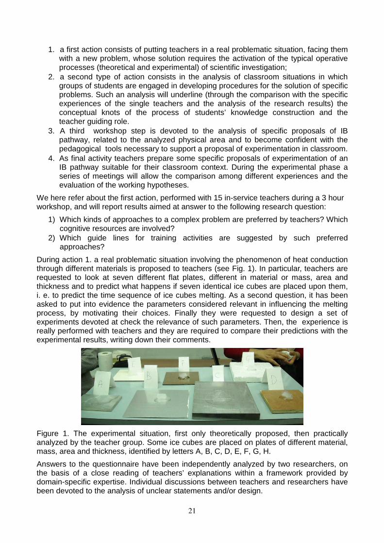
During action 1. a real problematic situation involving the phenomenon of heat conduction through different materials is proposed to teachers (see Fig. 1). In particular, teachers are requested to look at seven different flat plates, different in material or mass, area and thickness and to predict what happens if seven identical ice cubes are placed upon them, i. e. to predict the time sequence of ice cubes melting. As a second question, it has been asked to put into evidence the parameters considered relevant in influencing the melting process, by motivating their choices. Finally they were requested to design a set of experiments devoted at check the relevance of such parameters. Then, the experience is really performed with teachers and they are required to compare their predictions with the experimental results, writing down their comments.

Figure 1. The experimental situation, first only theoretically proposed, then practically analyzed by the teacher group. Some ice cubes are placed on plates of different material, mass, area and thickness, identified by letters A, B, C, D, E, F, G, H.

Answers to the questionnaire have been independently analyzed by two researchers, on the basis of a close reading of teachers’ explanations within a framework provided by domain-specific expertise. Individual discussions between teachers and researchers have been devoted to the analysis of unclear statements and/or design.

21

Results

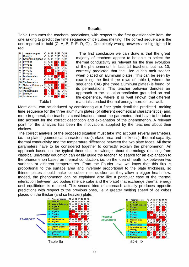
Table I resumes the teachers’ predictions, with respect to the first questionnaire item, the one asking to predict the time sequence of ice cubes melting. The correct sequence is the one reported in bold (C, A, B, F, E, D, G) . Completely wrong answers are highlighted in red.

Table I

The first conclusion we can draw is that the great majority of teachers appear to be able to select the thermal conductivity as relevant for the time evolution of the phenomenon. In fact, all teachers, but no. 10, correctly predicted that the ice cubes melt sooner when placed on aluminum plates. This can be seen by examining the first three rows of table I, where the sequence CAB (the three aluminum plates) is found, or its permutations. This teacher behavior denotes an approach to the situation prediction grounded on real life experience, where it is well known that different materials conduct thermal energy more or less well.

More detail can be deduced by considering at a finer grain detail the predicted melting time sequence for the three aluminum plates (of different geometrical characteristics) and, more in general, the teachers’ considerations about the parameters that have to be taken into account for the correct description and explanation of the phenomenon. A relevant point for the analysis has been the motivations supplied by the teachers about their choices. The correct analysis of the proposed situation must take into account several parameters, i.e. the plates’ geometrical characteristics (surface area and thickness), thermal capacity, thermal conductivity and the temperature difference between the two plate faces. All these parameters have to be considered together to correctly explain the phenomenon. An approach based on the typical theoretical knowledge about thermology resulting from classical university education can easily guide the teacher to search for an explanation to the phenomenon based on thermal conduction, i.e. on the idea of heath flux between two surfaces at different temperatures. From the Fourier law, we know that this flux is proportional to the surface area and inversely proportional to the plate thickness, so thinner plates should make ice cubes melt quicker, as they allow a bigger heath flow. Indeed, the phenomenon can be explained also like a particular case of the thermal interaction between two bodies (the ice cube and the plate) that exchange thermal energy until equilibrium is reached. This second kind of approach actually produces opposite predictions with respect to the previous ones, i.e. a greater melting speed of ice cubes placed on the thicker (and so heavier) plate.

Table IIa

Table IIb

22

In Table IIa the 6 teachers that appear to describe the phenomenon only on the basis of the Fourier law are evidenced (n. 5, 6, 7, 10, 13 and 14). Almost all wrote that the ice cube placed on plate B (the thinner aluminum one) is the first to melt. Teacher no. 10, instead, has predicted that the second ice cube to melt is the one placed on plate E, i.e. on a bakelite one that is thicker only than plate B. In this case, the teacher seem to fail to take into account even the thermal conductivity coefficient and to consider as relevant in the thermal conductivity process only the plate thickness. Table IIb shows 5 teachers (n. 1, 2, 3, 4 and 15) that seem to consider thermal capacity as relevant for the explanation of the phenomenon, but not plate thickness or thermal conductivity coefficient. They actually found the correct melting sequence for ice placed on aluminium plates, but in answers to the second question did not cite the plate geometrical properties or thermal conductivity coefficient in the explicit description of parameters that can have a relevance in the phenomenon. The correct approach to the phenomenon explanation is evidenced only by teachers n. 8, 9, 11 and 12 (evidenced in yellow in Tables IIa and IIb). They found and commented all relevant variables and predicted the correct melting sequence, except than in some cases, with an inversion between E, F, and D plates (bakelite, plexiglass and wood). In answers to the third question, all teachers compared their predictions with results from the really performed experiment. The majority of those that predicted the melting of the ice cubes on the basis of a partial acknowledgement of relevant variables expressed, in different ways, a sort of “surprise” with respect to the results. They said that they never thought that such an apparently simple phenomenon is to be explained by taking into account so many variables. Moreover, many of them explicitly admitted that the mental line they followed in predicting the time evolution of ice melting was mainly driven by memory of subjects studied during past courses. Only a few made reference to the necessary comparison between what they remembered from textbooks and real-life experience. The great majority of teachers at last commented that the approach the proposed situation posed them some difficulties, as it is one that is not part of their theoretical knowledge about thermology.

Discussion and conclusions

The analysis of data previously reported, as well as a accurate reading of motivations to the second question allow us to draw some conclusions with respect to our research questions. The majority of teachers showed an approach mainly involving the activation of cognitive resources as memory of past learning experience in order to make sense of reality. By comparing and contrasting the teachers’ answers and the explanations of their choices it can be pointed out that the way the proposed situation is first considered, or “read-out”, plays a crucial role in achieving an accurate description and activating the correct strategies to select the relevant variables. In some cases, these strategies seems to activate “textbook-like” cognitive resources like memory and formulas, acting as conceptual obstacles to the IB approach. This approach, in many cases, works like a sort of “short-circuit of knowledge”, avoiding a phenomenological approach to the problem and an accurate analysis of the involved variables before the formulation of hypotheses. This last conclusion seems to be enforced by the consideration that 3 out of the 4 teachers that correctly explained the ice melting process are not graduated in Physics and probably have superficially analyzed thermal conduction in their University courses. So, it seems that previous knowledge (particularly that coming from university) built in environments not linked with real life experience, is not really significant for the learner and acts as an obstacle for the inquiry competences that we want to develop in teachers. Practices as

23

formulating hypotheses or design appropriate experiments are strongly influenced by the searching of appropriate physical laws. Guide lines for future TAs suggested by the approaches followed by our teachers can be synthesizes as follows. During the training time, characteristics of IB practices must be explicitly addressed from a epistemological point of view, as well as problem based activities that are not too much focused on specific disciplinary knowledge. Preliminary results about teacher TAs involving environments based on problems and situations not belonging to the field where teachers are expert show a greater involvement of teachers that pay a greater attention to inquiry procedures rather than to the correct application of disciplinary knowledge. In this way the previously cited “short-circuit of knowledge” seems to be avoided and teachers can activate the reasoning resources necessary for a profitable development of their PCK based on IB Science Education.

References

Beyer, C. J., Delgado, C., Davis, E. A., & Krajcik, J. S. (2009). Investigating teacher learning supports in high school biology curricular programs to inform the design of educative curriculum materials. Journal of Research in Science Teaching 46(9), 977-998. Borko, H., & Putnam, R. T. (1996). Learning to Teach. In D. C. Berliner & R. C. Calfee (Eds.), Handbook of Educational Psychology , 673-708. New York: Macmillan Clark, D. B., & Linn, M. C. (2003). Scaffolding knowledge integration through curricular depth. Journal of Learning Sciences, 12(4), 451-494. Duschl, R. A., Heidi A. Schweingruber, H. A. & Shouse, A. W. (2007) (Eds.), Taking Science to School: Washington, D. C: National Academies Press Gess-Newsome, J., & N. G. Lederman, N. G.,(1999) (Eds.), Examining Pedagogical Content Knowledge. Dordrecht, The Netherlands: Kluwer Academic Publishers.Linn, M.C, Hsi, S. (2000). Computers, Teachers, Peers. Mahwah, NJ Erlbaum Magnusson, S., Krajcik, J., & Borko, H. (1999). Nature, sources, and development of pedagogical content knowledge for science teaching. In J. Gess-Newsome & N. G. Lederman, N. G.,(1999) (Eds.), Examining Pedagogical Content Knowledge. Dordrecht, The Netherlands: Kluwer Academic Publishers. Marx, R.W., Blumenfeld, P.C., Krajcik, J.S.,&Soloway, E. (1997). Enacting project-based science. The Elementary School Journal, 97(4), 341–358. National Research Council. (2000). Inquiry and the National Science Education Standards.Washington, DC: National Academy Press.Singer, S., Hilton, M. & Schweingruber, H. (2005). Needing a New Approach to Science Labs. The Science Teacher, 72(7), 10. Pinto´, R. (2004). Introducing curriculum innovations in science: Identifying teachers’ transformations and the design of related teacher education. Science Education, 89, 1–12. Roehrig, G.H.,& Luft, J.A. (2004). Constraints experienced by beginning secondary science teachers in implementing scientific inquiry lessons. International Journal of Science Education, 26(1), 3–24. Shulman, L.S. (1986). Those who understand: Knowledge growth in teaching. Educational Researcher, 15(5), 4–14. Windschitl, M. (2003). Inquiry projects in science teacher education: What can investigative experiences reveal about teacher thinking and eventual classroom practice? Science Education, 87(1), 112–143. www.establish-fp7.eu

24

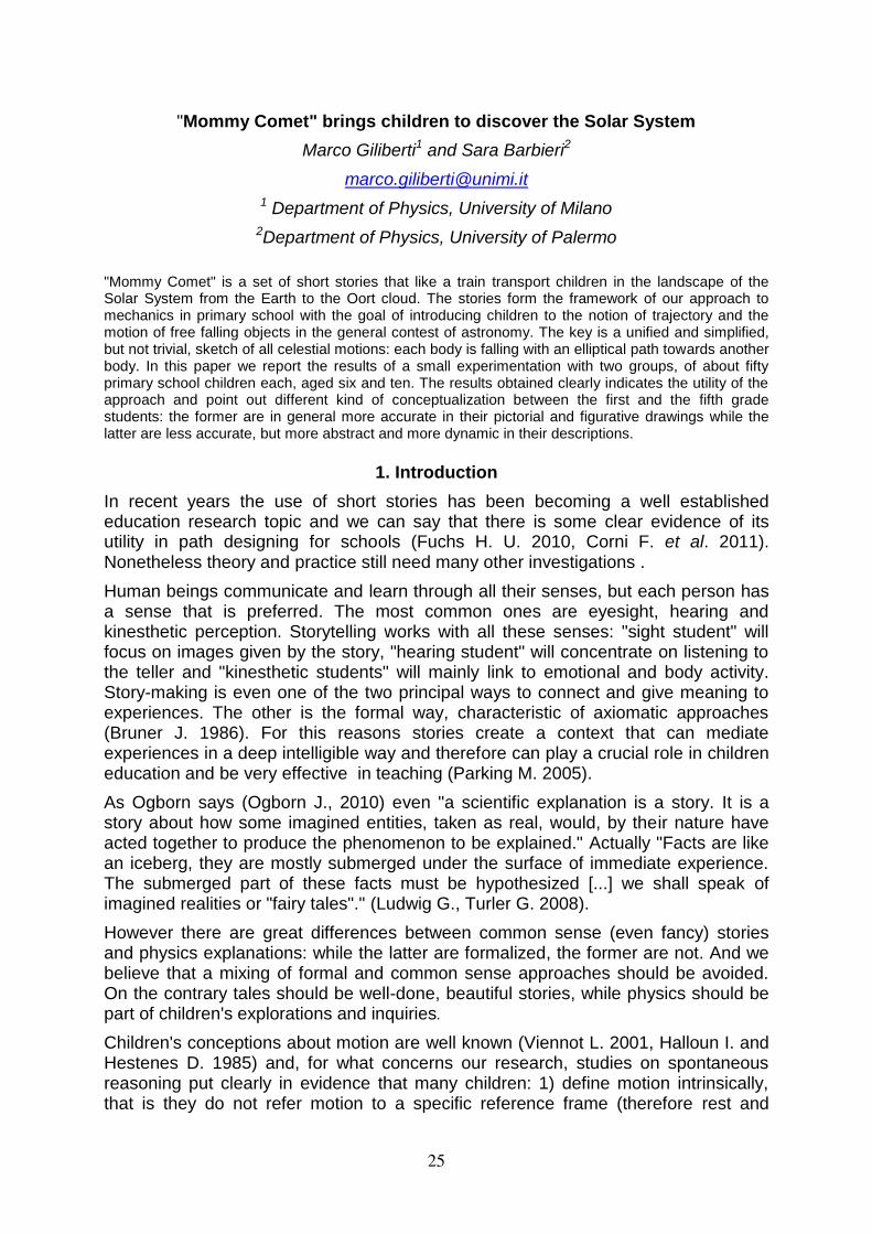
"Mommy Comet" brings children to discover the Solar System

Marco Giliberti1 and Sara Barbieri2

marco.giliberti@unimi.it

1 Department of Physics, University of Milano

2Department of Physics, University of Palermo

"Mommy Comet" is a set of short stories that like a train transport children in the landscape of the Solar System from the Earth to the Oort cloud. The stories form the framework of our approach to mechanics in primary school with the goal of introducing children to the notion of trajectory and the motion of free falling objects in the general contest of astronomy. The key is a unified and simplified, but not trivial, sketch of all celestial motions: each body is falling with an elliptical path towards another body. In this paper we report the results of a small experimentation with two groups, of about fifty primary school children each, aged six and ten. The results obtained clearly indicates the utility of the approach and point out different kind of conceptualization between the first and the fifth grade students: the former are in general more accurate in their pictorial and figurative drawings while the latter are less accurate, but more abstract and more dynamic in their descriptions.

1. Introduction

In recent years the use of short stories has been becoming a well established education research topic and we can say that there is some clear evidence of its utility in path designing for schools (Fuchs H. U. 2010, Corni F. et al. 2011). Nonetheless theory and practice still need many other investigations .

Human beings communicate and learn through all their senses, but each person has a sense that is preferred. The most common ones are eyesight, hearing and kinesthetic perception. Storytelling works with all these senses: "sight student" will focus on images given by the story, "hearing student" will concentrate on listening to the teller and "kinesthetic students" will mainly link to emotional and body activity. Story-making is even one of the two principal ways to connect and give meaning to experiences. The other is the formal way, characteristic of axiomatic approaches (Bruner J. 1986). For this reasons stories create a context that can mediate experiences in a deep intelligible way and therefore can play a crucial role in children education and be very effective in teaching (Parking M. 2005).

As Ogborn says (Ogborn J., 2010) even "a scientific explanation is a story. It is a story about how some imagined entities, taken as real, would, by their nature have acted together to produce the phenomenon to be explained." Actually "Facts are like an iceberg, they are mostly submerged under the surface of immediate experience. The submerged part of these facts must be hypothesized [...] we shall speak of imagined realities or "fairy tales"." (Ludwig G., Turler G. 2008).

However there are great differences between common sense (even fancy) stories and physics explanations: while the latter are formalized, the former are not. And we believe that a mixing of formal and common sense approaches should be avoided. On the contrary tales should be well-done, beautiful stories, while physics should be part of children's explorations and inquiries.

Children's conceptions about motion are well known (Viennot L. 2001, Halloun I. and Hestenes D. 1985) and, for what concerns our research, studies on spontaneous reasoning put clearly in evidence that many children: 1) define motion intrinsically, that is they do not refer motion to a specific reference frame (therefore rest and

25

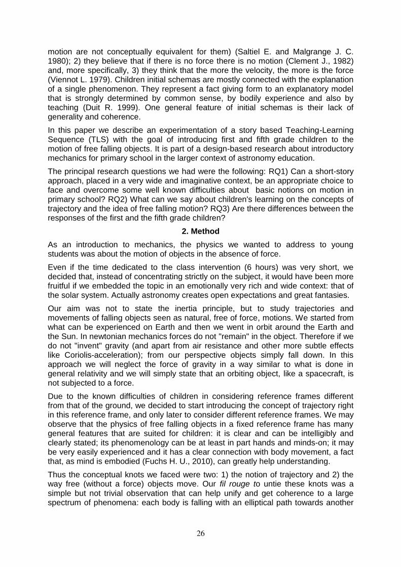
motion are not conceptually equivalent for them) (Saltiel E. and Malgrange J. C. 1980); 2) they believe that if there is no force there is no motion (Clement J., 1982) and, more specifically, 3) they think that the more the velocity, the more is the force (Viennot L. 1979). Children initial schemas are mostly connected with the explanation of a single phenomenon. They represent a fact giving form to an explanatory model that is strongly determined by common sense, by bodily experience and also by teaching (Duit R. 1999). One general feature of initial schemas is their lack of generality and coherence.

In this paper we describe an experimentation of a story based Teaching-Learning Sequence (TLS) with the goal of introducing first and fifth grade children to the motion of free falling objects. It is part of a design-based research about introductory mechanics for primary school in the larger context of astronomy education.

The principal research questions we had were the following: RQ1) Can a short-story approach, placed in a very wide and imaginative context, be an appropriate choice to face and overcome some well known difficulties about basic notions on motion in primary school? RQ2) What can we say about children's learning on the concepts of trajectory and the idea of free falling motion? RQ3) Are there differences between the responses of the first and the fifth grade children?

2. Method

As an introduction to mechanics, the physics we wanted to address to young students was about the motion of objects in the absence of force.

Even if the time dedicated to the class intervention (6 hours) was very short, we decided that, instead of concentrating strictly on the subject, it would have been more fruitful if we embedded the topic in an emotionally very rich and wide context: that of the solar system. Actually astronomy creates open expectations and great fantasies.

Our aim was not to state the inertia principle, but to study trajectories and movements of falling objects seen as natural, free of force, motions. We started from what can be experienced on Earth and then we went in orbit around the Earth and the Sun. In newtonian mechanics forces do not "remain" in the object. Therefore if we do not "invent" gravity (and apart from air resistance and other more subtle effects like Coriolis-acceleration); from our perspective objects simply fall down. In this approach we will neglect the force of gravity in a way similar to what is done in general relativity and we will simply state that an orbiting object, like a spacecraft, is not subjected to a force.

Due to the known difficulties of children in considering reference frames different from that of the ground, we decided to start introducing the concept of trajectory right in this reference frame, and only later to consider different reference frames. We may observe that the physics of free falling objects in a fixed reference frame has many general features that are suited for children: it is clear and can be intelligibly and clearly stated; its phenomenology can be at least in part hands and minds-on; it may be very easily experienced and it has a clear connection with body movement, a fact that, as mind is embodied (Fuchs H. U., 2010), can greatly help understanding.

Thus the conceptual knots we faced were two: 1) the notion of trajectory and 2) the way free (without a force) objects move. Our fil rouge to untie these knots was a simple but not trivial observation that can help unify and get coherence to a large spectrum of phenomena: each body is falling with an elliptical path towards another

26

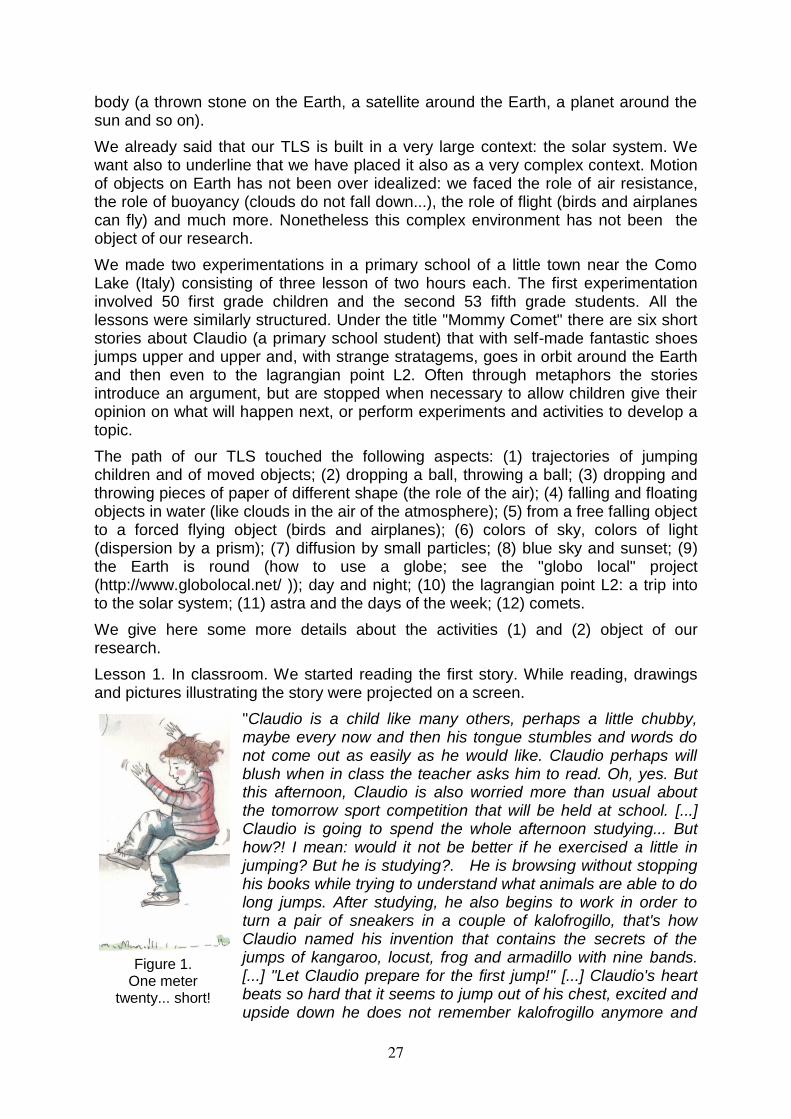
body (a thrown stone on the Earth, a satellite around the Earth, a planet around the sun and so on).

We already said that our TLS is built in a very large context: the solar system. We want also to underline that we have placed it also as a very complex context. Motion of objects on Earth has not been over idealized: we faced the role of air resistance, the role of buoyancy (clouds do not fall down...), the role of flight (birds and airplanes can fly) and much more. Nonetheless this complex environment has not been the object of our research.

We made two experimentations in a primary school of a little town near the Como Lake (Italy) consisting of three lesson of two hours each. The first experimentation involved 50 first grade children and the second 53 fifth grade students. All the lessons were similarly structured. Under the title "Mommy Comet" there are six short stories about Claudio (a primary school student) that with self-made fantastic shoes jumps upper and upper and, with strange stratagems, goes in orbit around the Earth and then even to the lagrangian point L2. Often through metaphors the stories introduce an argument, but are stopped when necessary to allow children give their opinion on what will happen next, or perform experiments and activities to develop a topic.

The path of our TLS touched the following aspects: (1) trajectories of jumping children and of moved objects; (2) dropping a ball, throwing a ball; (3) dropping and throwing pieces of paper of different shape (the role of the air); (4) falling and floating objects in water (like clouds in the air of the atmosphere); (5) from a free falling object to a forced flying object (birds and airplanes); (6) colors of sky, colors of light (dispersion by a prism); (7) diffusion by small particles; (8) blue sky and sunset; (9) the Earth is round (how to use a globe; see the "globo local" project (http://www.globolocal.net/ )); day and night; (10) the lagrangian point L2: a trip into to the solar system; (11) astra and the days of the week; (12) comets.

We give here some more details about the activities (1) and (2) object of our research.

Lesson 1. In classroom. We started reading the first story. While reading, drawings and pictures illustrating the story were projected on a screen.

"Claudio is a child like many others, perhaps a little chubby, maybe every now and then his tongue stumbles and words do not come out as easily as he would like. Claudio perhaps will blush when in class the teacher asks him to read. Oh, yes. But this afternoon, Claudio is also worried more than usual about the tomorrow sport competition that will be held at school. [...] Claudio is going to spend the whole afternoon studying... But how?! I mean: would it not be better if he exercised a little in jumping? But he is studying?. He is browsing without stopping his books while trying to understand what animals are able to do long jumps. After studying, he also begins to work in order to turn a pair of sneakers in a couple of kalofrogillo, that's how Claudio named his invention that contains the secrets of the jumps of kangaroo, locust, frog and armadillo with nine bands. [...] "Let Claudio prepare for the first jump!" [...] Claudio's heart beats so hard that it seems to jump out of his chest, excited and upside down he does not remember kalofrogillo anymore and

Figure 1. One meter

twenty... short!

27

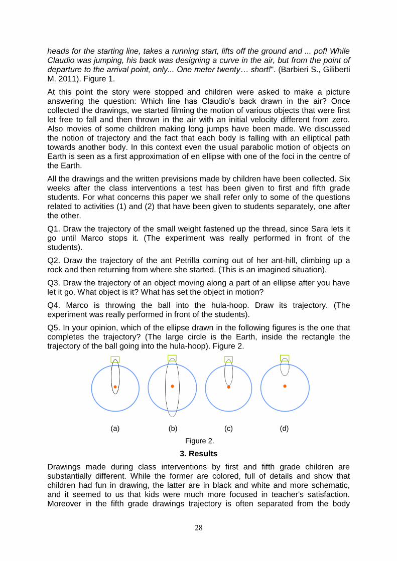
heads for the starting line, takes a running start, lifts off the ground and ... pof! While Claudio was jumping, his back was designing a curve in the air, but from the point of departure to the arrival point, only... One meter twenty… short!". (Barbieri S., Giliberti M. 2011). Figure 1.

At this point the story were stopped and children were asked to make a picture answering the question: Which line has Claudio’s back drawn in the air? Once collected the drawings, we started filming the motion of various objects that were first let free to fall and then thrown in the air with an initial velocity different from zero. Also movies of some children making long jumps have been made. We discussed the notion of trajectory and the fact that each body is falling with an elliptical path towards another body. In this context even the usual parabolic motion of objects on Earth is seen as a first approximation of en ellipse with one of the foci in the centre of the Earth.

All the drawings and the written previsions made by children have been collected. Six weeks after the class interventions a test has been given to first and fifth grade students. For what concerns this paper we shall refer only to some of the questions related to activities (1) and (2) that have been given to students separately, one after the other.

Q1. Draw the trajectory of the small weight fastened up the thread, since Sara lets it go until Marco stops it. (The experiment was really performed in front of the students).

Q2. Draw the trajectory of the ant Petrilla coming out of her ant-hill, climbing up a rock and then returning from where she started. (This is an imagined situation).

Q3. Draw the trajectory of an object moving along a part of an ellipse after you have let it go. What object is it? What has set the object in motion?

Q4. Marco is throwing the ball into the hula-hoop. Draw its trajectory. (The experiment was really performed in front of the students). Q5. In your opinion, which of the ellipse drawn in the following figures is the one that completes the trajectory? (The large circle is the Earth, inside the rectangle the trajectory of the ball going into the hula-hoop). Figure 2.

(a) (b) (c) (d)

Figure 2.

3. Results

Drawings made during class interventions by first and fifth grade children are substantially different. While the former are colored, full of details and show that children had fun in drawing, the latter are in black and white and more schematic, and it seemed to us that kids were much more focused in teacher's satisfaction. Moreover in the fifth grade drawings trajectory is often separated from the body

28

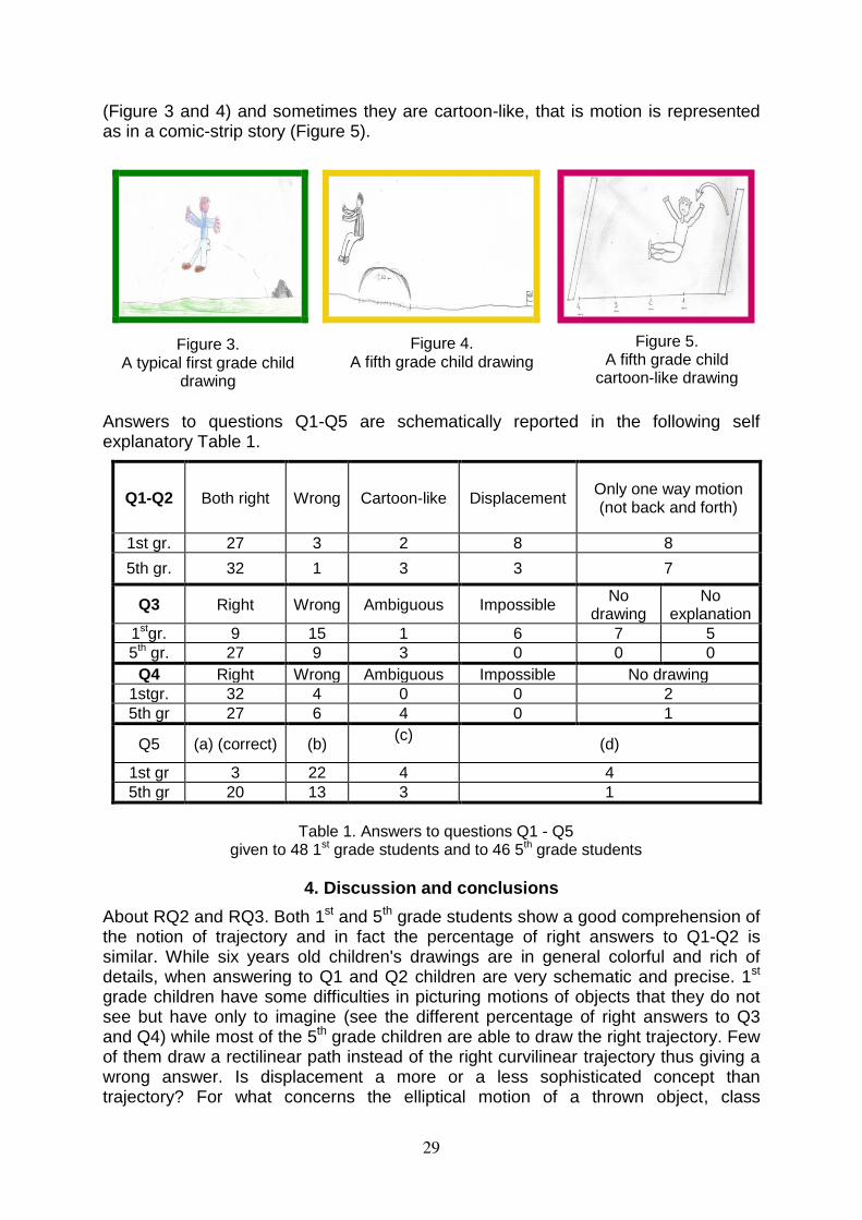
(Figure 3 and 4) and sometimes they are cartoon-like, that is motion is represented as in a comic-strip story (Figure 5).

Answers to questions Q1-Q5 are schematically reported in the following self explanatory Table 1.

Q1-Q2 Both right Wrong Cartoon-like Displacement Only one way motion (not back and forth)

1st gr. 27 3 2 8 8

5th gr. 32 1 3 3 7

Q3 Right Wrong Ambiguous Impossible No

drawing No

explanation

1stgr. 9 15 1 6 7 5

5th gr. 27 9 3 0 0 0

Q4 Right Wrong Ambiguous Impossible No drawing

1stgr. 32 4 0 0 2

5th gr 27 6 4 0 1

Q5 (a) (correct) (b) (c)

(d)

1st gr 3 22 4 4

5th gr 20 13 3 1

4. Discussion and conclusions

About RQ2 and RQ3. Both 1st and 5th grade students show a good comprehension of the notion of trajectory and in fact the percentage of right answers to Q1-Q2 is similar. While six years old children's drawings are in general colorful and rich of details, when answering to Q1 and Q2 children are very schematic and precise. 1st grade children have some difficulties in picturing motions of objects that they do not see but have only to imagine (see the different percentage of right answers to Q3 and Q4) while most of the 5th grade children are able to draw the right trajectory. Few of them draw a rectilinear path instead of the right curvilinear trajectory thus giving a wrong answer. Is displacement a more or a less sophisticated concept than trajectory? For what concerns the elliptical motion of a thrown object, class

Figure 5. A fifth grade child

cartoon-like drawing

Figure 4. A fifth grade child drawing

Figure 3. A typical first grade child

drawing

Table 1. Answers to questions Q1 - Q5 given to 48 1st grade students and to 46 5th grade students

29

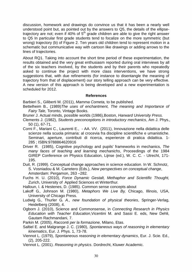
discussion, homework and drawings do convince us that it has been a nearly well understood point but, as pointed out by the answers to Q5, the details of the ellipse-trajectory are not; even if 40% of 5th grade children are able to give the right answer to Q5 In particular first grade students tend to focalize on the more symmetric (but wrong) trajectory (b) of Figure 2. Ten years old children tend to represent motion in a schematic but communicative way with cartoon like drawings or adding arrows to the lines of trajectories.

About RQ1. Taking into account the short time period of these experimentation, the results obtained and the very great enthusiasm reported during oral interviews by all of the six teachers involved, by the students and by their parents who repeatedly asked to continue the project with more class interventions, we have strong suggestions that, with due refinements (for instance to disentangle the meaning of trajectory from that of displacement) our story telling approach can be very effective. A new version of this approach is being developed and a new experimentation is scheduled for 2012.

References

Barbieri S., Giliberti M. (2011), Mamma Cometa, to be published. Bettelheim B., (1989)The uses of enchantment, The meaning and Importance of

Fairy Tale, Toronto, Vintage Books. Bruner J. Actual minds, possible worlds (1986),Boston, Harward University Press. Clements J. (1982), Students preconceptions in introductory mechanics, Am J. Phys.,

50 (1), 67-71. Corni F., Mariani C., Laurenti E., - AA. VV. (2011), Innovazione nella didattica delle

scienze nella scuola primaria: al crocevia fra discipline scientifiche e umanistiche. Seminari, aperture, contributi di ricerca, esperienze di pratica didattica. 1-285 ; ISBN:9788864620916

Driver R. (1985), Cognitive psychology and pupils' frameworks in mechanics, The many faces of teaching and learning mechanichs, Proceedings of the 1984 GIREP Conference on Physics Education, Lijnse (ed.), W. C. C. - Utrecht, 171-195.

Duit, R. (1999). Conceptual change approaches in science education. In W. Schnotz, S. Vosniadou & M. Carretero (Eds.), New perspectives on conceptual change, Amsterdam: Pergamon, 263 –282.

Fuchs H. U. (2010), Force Dynamic Gestalt, Methaphor and Scientific Thought, Zurich, University of Applied Sciences et Winterthur.

Halloun, I. & Hestenes, D. (1985). Common sense concepts about Lakoff G., Johnson M. (1980), Metaphors We Live By, Chicago, Illinois, USA,

University of Chicago Press. Ludwig G., Thurler G. A., new foundation of physical theories, Springer-Verlag,

Heidelberg (2008), 4. Ogborn J. (2010), Science and Commonsense, in Connecting Research in Physics

Education with Teacher Education,Vicentini M. and Sassi E. eds, New Dehli, Gautam Rachmandani, 7.

Parkin M. (2005), Racconti per la formazione, Milano, Etas. Saltiel E. and Malgrange J. C. (1980), Spontaneous ways of reasoning in elementary

kinematics, Eur. J. Phys. 1, 73-78. Viennot L. (1979), Spontaneous reasoning in elementary dynamics, Eur. J. Scie. Ed.,

(2), 205-222. Viennot L. (2001). Reasoning in physics. Dordrecht, Kluwer Academic.

30

Preparing physics teachers to teach effectively in the school laboratory

Olga GiokaDepartment of Physics, University of Ioannina, GR-45-110, Greece

E-mail: ogioka@cc.uoi.gr

AbstractIn this paper, we firstly present the aims of the two modules of a pre-service teacher educationprogram in the Physics Department, University of Ioannina, which focused on preparingtrainee teachers to teach in the laboratory. We then report on the research study designed tolook at the successes and challenges that prospective physics teachers experienced whenteaching laboratory work throughout our pre-service teacher education program. Forty-eighttrainee teachers participated. They were observed when teaching, interviewed twice and theirwritten work (teaching plans, written tasks and portfolios) was collected. Changes andimprovement in teachers were examined, as teaching practice progressed. We found thatteacher learning about pupils’ difficulties and common mistakes related to laboratory workand then, learning about how to help pupils improve is a gradual process which requires moretime than the two semesters of our program. This study reinforces the importance ofprograms for trainee and beginning physics teachers. It suggests that there is a need forspecialized programs for initial physics teacher training to address the development ofteaching practices specific to the teaching in the school physics laboratory.

Key words: laboratory work, ‘concepts of evidence’, initial physics teacher training

IntroductionIn physics education, many secondary pupils experience difficulties in thelaboratory. As a consequence, teachers should be prepared for how to teachthis difficult issue effectively. Adequate preparation of secondary physicsteachers is vital to ensuring good teaching of physics in schools. The visionfor improving physics teaching and learning in secondary schools should bethat universities model effective teaching and learning approaches in theirphysics courses for physics students who are prospective physics teachers(Loucks-Horsley et al., 2010). Trainee teachers have needs which must beconsidered in planning and implementing their initial education. An importantfeature of effective physics teacher education is the sense of ownership of theintended innovations. As Ogborn (2002) emphasized, teachers should begiven a sense of ownership of that innovation; that it belongs to them and it isnot simply imposed to them.

The two modules “Teaching physics experiments to pupils” I and II inour teacher education program

In Greece, the secondary science curriculum gives much attention toconceptual knowledge leaving little space for teaching of experiments.Requirements for high-stake exams restrict teachers’ instruction and timeavailable to teach lab work. In our department, an initiative was taken toprepare our student teachers for how to teach experiments effectively in theschool physics laboratory: to address the knowledge and understandingsrequired to teach scientific skills and methods explicitly (Lunetta, Hofstein andClough, 2007; Tamir, 1989). The goal has been to develop a goodunderstanding of what makes ‘good scientific evidence’ (Gott and Duggan,2003) firstly, in teachers and secondly, in their pupils. The term of ‘conceptsof evidence’, as introduced by Gott and Duggan refers to the necessaryunderstandings to explore scientific evidence thoroughly. In simpler words,the aim has been to teach and develop the criteria for good quality in physicsexperiments:What makes a good set of data?What makes a good graph?

31

What makes a good analysis and explanation?What makes a good evaluation?What makes a good lab report?That is, the teacher should teach pupils how to decide on the evidence to becollected, how to draw the graph, how to interpret it, to use it in the analysis ofevidence and the evaluation of the experiment. The notions of reliability andvalidity have also been components of an understanding of scientific evidenceand hence, they are included in the modules.The two modules entitled “Teaching physics experiments to pupils” I and IIhave also addressed important issues closely related to the role of theteacher. Teachers need to know more and more deeply than we expect theirpupils to do. They need to know about pupil learning difficulties with physicslaboratory work and they have to develop appropriate teaching andassessment strategies. In addition, the teacher has to make decisions aboutthe goals (what he wants his pupils to learn), what to do ‘next’ in response to aparticular pupil attainment. It is a matter of professional judgment for theteacher to increase the demands of the activity and/ or reduce his assistanceand guidance. For example, how much freedom the teacher may give topupils for the latter to make the planning of the experiment, how muchguidance, help, feedback and support when they carry out the investigation,and finally, how the teacher assesses their achievement and progress. Wewant our teachers to be able and knowledgeable to make their own decisionsand not to rely on the teacher’s guide, or textbooks which do not address theabove issues. Each module was taught for three hours a week for fifteenweeks. We have used typical school science experiments with simple physicsso as not to complicate the ideas. In fact, we are not interested in developingnew or different experiments, but to keep the ones in a typical secondaryscience curriculum with different teaching aims, that of the development ofpractical skills and ‘concepts of evidence’.In summary, the innovation of the program is that we, firstly, wanted to takeinto account understandings related to scientific evidence and related pupildifficulties, as they appear in the literature. Then, we wanted to prepareteachers for how better to respond to pupil needs. In a few words, it is whatteachers should know in order to help pupils attain the goals of the laboratory.For the purpose of this manuscript, we decided to focus only on the part ofteachers: to explore teachers’ attempts to get prepared and look at theirconcerns, needs and difficulties. A second paper will look at pupils’ learning.The research question guiding this study is: “What are the difficulties andchallenges of trainee physics teachers in relation to the teaching of physicslaboratory work in secondary education?”

The studyContext and Participants

The present study was situated in the context of a one-year teacher educationprogram, aiming at qualifying participants to teach physics in secondary schoolsin Greece. Before entering this program, the participants had completed allmodules of the undergraduate physics program, the laboratory coursesincluded. In the context of this program, the teachers taught in practice schoolsfor about seven to ten lessons per week. They also participated in institutionalmeetings and workshops two afternoons a week on average. Teachers hadopportunities firstly, to be taught about laboratory work and ‘concepts ofevidence’, as described above. Then, they were asked to design lesson plans,carry them out in their practice schools and share their experiences with theircolleagues at meetings in the department.

32

Research DesignForty-eight trainee physics teachers were observed when teaching in the localstate schools which are in partnership with our department for initial teachertraining. We collected their written work (written tasks, portfolios and teachingplans) over a period of two semesters. Questions in the written tasks reflectthe issues underlined by the two modules and the workshops, especially therole of the teacher and were completed after their teaching. We also invitedthem to talk about their needs and concerns and make suggestions withregard to the improvements of the teacher education program. Portfoliosdocumented in fine detail the activities that they designed and conducted. Inaddition, teachers were interviewed twice (around the beginning and near theend of the program). Semi-structured interviews were conducted with theparticipants in order to let each teacher to talk about his/her own expectationsfrom the program and to introduce issues that we had not thought of (Kvale,2009). Particular attention has been given to the research ethics (Gregory,2003) and the associated issues (anonymity of participants, the role of theresearcher).

ResultsAt the beginning of the program, twenty-four teachers experienced difficultiesin understanding that with the school physics experiments we aim to developan understanding of good quality of scientific evidence. They consideredexperiments as a means for verifying theory or illustrating the relationshipbetween variables, by explaining that “experiments help pupils understandtheory better and visualize the relationship between variables”. This idea is inthe wrong direction to the one we wanted them to develop through theteaching of the two modules, which was to explicitly teach experimental skillsand develop understanding of ‘concepts of evidence’ in pupils. In contrast, agroup of fifteen teachers started by adopting the intended goal: thedevelopment of understandings related to ‘concepts of evidence’. Around theend of the program, there was a clear shift (thirty-three teachers) to theintended idea that by carrying out an experiment we want to teach anddevelop an understanding of good quality of evidence in pupils.Also, twenty-six teachers had difficulties in planning a series of lessons withexperiments. This group of teachers experienced the shift from student toteacher to be difficult: “It is very different to carry out an experiment in theundergraduate program by following the given instructions, than guiding yourpupils as a secondary teacher”. When they talked about the introductorylesson, they restricted themselves around preparation for teaching conceptualknowledge, without referring to the process and investigative skills necessaryto carry out the activity. At the same time, only ten teachers talked aboutintroductory lessons containing process skills. As they explained in theinterviews, in the traditional undergraduate physics laboratory courses theywere given instructions in the form of ‘recipes’. Such laboratory courses didnot leave much room for a deeper understanding and for taking initiatives.They also acknowledged that the two modules of the program were helpful asthey were taught how to plan a lesson or a sequence of lessons and how toproceed as teachers. Also, through help and collaboration among oneanother in workshops and meetings, they shared experiences and madeprogress. Around the end of the program, twenty-six teachers, in total, wereconfident in planning laboratory lessons on the basis of what they had beentaught. Twenty teachers asked for more guidance and instructional materials.With regard to teachers’ judgments about the instructions given from thephysics educator and the provided learning materials, three different groups of33

teachers appeared: Seventeen teachers, from the beginning, were happy toplan and proceed on their own as trainee teachers. They enjoyed takinginitiatives and planning how to teach laboratory lessons based on the modulesand workshops. They said they liked the fact that they were given somefreedom on how to proceed, which questions to deal with, make decisionsabout how to teach and so on. This is clearly in contrast with what they usedto do in their undergraduate lab courses.A second group (ten teachers) said that they were happy to make their owndecisions but they would need more help and discuss teaching issues withphysics educators and experienced teachers in workshops and practiceschools. They asked for more practice and collaboration between them.A third group (twenty-one) asked for more guidance and clear instructions onhow to plan and proceed as teachers when teaching laboratory classes. “Iwould need written instructions on how to carry out the experiment and then,how to teach it to my class, so that I know what exactly to do as teacher”.These teachers did not like the frustration associated with the planningprocess, especially at the beginning of their training. They asked for moredetailed materials to help them with teaching. With time and around the end ofthe program, the first group consisted of thirty-two, the second of eleven,while the third group of only five teachers.At the beginning of their training, twenty-one teachers did not demonstratesufficient knowledge of and adequate skills to teach ‘concepts of evidence’.For example, the issue was quite often: “How many measurements arenecessary?” The common idea among trainee teachers was that “we need totake as more measurements as possible” without justifying their answer. Lessoften they explained this idea by saying that one needs to take a certainnumber of measurements in order to eliminate errors and identify anomalouspoints. Few teachers related the quality of measurements to the quality of thegraph: to identify patterns and relationships between variables. However, onlya few (five) of our participants demonstrated a good understanding of the roleof the graph in the analysis of evidence by quoting figures from the graph tosubstantiate any quantitative statements made. In addition, a good graph isused as a tool to evaluate the whole activity. Many of our teachers did nothave time to focus on the role of graph, because of limited lesson time.Through involvement in the program’s activities, the participants’ limitedknowledge of and subsequently, confidence and ability to teachunderstandings related to ‘concepts of evidence’ gradually improved.The analysis of the interviews at the beginning and near the end revealed agradual development in their ability and competence in employing strategiestaught in the program (choice of different learning goals, provision of feedbackand so on). Their teaching plans and written tasks is a source of informationabout the changes in teachers’ use of different teaching strategies andreflection on the changes that they underwent during the period of theprogram. In particular, teachers demonstrated a good understanding of pupils’common difficulties in the laboratory and were successful in responding topupils with a range of teaching strategies. Collaboration between theparticipants in the workshops and meetings seemed to be critical.When asked to make suggestions, they demonstrated an increasing interestin sharing their concerns. They were happy with the provided instructionalmaterials and asked for further teaching resources. They wanted to learnmore about how to assess pupils’ performance on laboratory work, an issuethat we did not have much time to deal with deeply. They asked for morepractice in schools in order to have the opportunity to teach more experimentsduring their training. Another important issue, related to the one justdiscussed, is the extent to which they asked for more guidance and support34

by their tutors or teacher mentors in practice schools. We have to admit thatalthough the development of our program would also need teacher mentors’help, we did not work to this direction. We think that in the follow-up phase,we should facilitate better collaboration and trust between the two parts.

Discussion and conclusionsThe study illustrates the limitations of a two-semester course to promote thegoals of our training program. We found that learning about pupils’ difficultiesand common mistakes related to laboratory work and then, learning how tohelp pupils with specific difficulties is a gradual process which requires moretime than the two semesters of our program. Teacher learning is a slowprocess and yet, it is essential to allow time for teachers to learn in ameaningful way. Our teachers found the provided learning materials veryhelpful, as well as the support they received from the instructor of the twomodules and from one another in the workshops and meetings. This confirmsearlier findings by Eylon and Bagno that the real context of teaching and on-going guidance by more experienced teachers are important ingredients inprograms that allow teachers to develop desired teaching skills (Eylon andBagno, 2006).Overall, the participants succeeded in shifting from the dominant idea thatwith school experiments we aim to help pupils understand theory better andillustrate scientific principles and relationships. With practice and time, theydeveloped a good understanding of how to teach practical skills and scientificevidence.But, we would like more teachers to have referred to the role of graphs in theexperimental procedure (judgment of the quality of scientific evidence,evaluation of the process). Many of our teachers did not have time to focus onthe role of graph (they run out of time) or this issue was often neglected. Weassume that this point is missing, or not well communicated in theundergraduate lab courses. This issue should be taken into seriousconsideration, firstly, at the undergraduate level. Undergraduate physics labcourses need to give more time and value to the drawn graph to address thetheme of quality of scientific evidence, graphs and analysis. Time should bedevoted so that it becomes clear that graphs are a tool for judging the qualityof evidence, and next, for judging the quality of the whole process. Graphsneed to be used. Graphs are not the end of the experiment. “Does somethingneed to change if the experiment will be repeated?”The findings of insufficient knowledge of physics were confirmed by researchstudies on pre-service and in-service teachers’ preparation to teach laboratorywork in physics in other countries (Nivalain et al., 2010). Secondly,insufficient knowledge of physics needs to be taken into account if we wantto improve teacher education programs. More time and importance shouldbe given to a good understanding and development of ‘concepts ofevidence’ in trainee teachers. We also want to improve collaboration andsupport by the mentor teachers in schools. Questions related to our worktowards this direction maybe the following:How can mentor teachers integrate into the program process so that theybetter support our trainee teachers?How could our department and practice schools work together to support ourteachers?It would be interesting to follow the same participants over the first in-serviceyears to trace their development and progress. Or, compare the professionaldevelopment of the participants with those who did not attend the twomodules, but followed the normal undergraduate program for physics teachereducation. More research is needed to better understand the challenges and35

difficulties in different schools with different curricula.This study reinforces the importance of programs for trainee and beginningphysics teachers. It suggests that there is a need for specialized programs forphysics teacher education to address the development of teaching practicesspecific to the teaching in the school physics laboratory.

REFERENCESEylon, B-S. and Bagno, E. (2006). Research-design model for professional development ofteachers: Designing lessons with specific education research. Physical Review Special -Topics Physics Education Research 2, 020106 (2006), 1-14.Gott, R. and Duggan, S. (2003). Understanding and using scientific evidence. How tocritically evaluate data. London: Sage.Gregory, I. (2003). Ethics in research. London: Continuum.Kvale, S. (2009). InterViews: Learning the craft of qualitative research interviewing (2ndedition). London: Sage.Loucks-Horsley, S., Stiles, K. E., Mundry, S., Love, N. and Hewson, P. E. (2010). Designingprofessional development for teachers of science and mathematics. London: Sage.Lunetta, V. N., Hofstein, A. and Clough, M. P. (2007) Learning and teaching in the schoolscience laboratory: An analysis of research. Theory and Practice. In S. K. Abell and N. G.Lederman (Eds.) Second Handbook of Research on Science Education (pp 303-441).Mahwah, NJ: Lawrence Erlbaum Publishers.Nivalain, V., Asikainen, M. A., Sormunen, K. and Hirvonen, P. E. (2010). Pre-service and in-service teachers’ challenges in the planning of practical work in physics. Journal of ScienceTeacher Education, 21, 393-409.Ogborn, J. (2002). Ownership and transformation: Teachers using curriculum innovations.Physics Education, 37(2), 142-146.Tamir, P. (1989). Training teachers to teach effectively in the laboratory. Science Education,73(1), 59-69.

36

Students’ constructions of the explanatory models for the prismatic foil: influences of cognitive level and task sequencing

Mihael Gojkošek1, Gorazd Planinšič1 and Josip Sliško2

gojkosek@fmf.uni-lj.si

1Faculty of Mathematics and Physics, University of Ljubljana, Slovenia

2Facultad de Ciencias Fisico Matematicas, Benemerita Universidad Autonoma de Puebla, Mexico

In this paper some general findings of the research on students' abilities to construct explanatory models are presented. In the study 360 students from Slovenian grammar-schools were included. Based on observations of two simple experiments with prism foil they tried to explain how the foil works and sketch a model of its structure. Students' results were compared with their achievements on the Lawson’s Classroom test of scientific reasoning, which we used as a reference test. More than 75% of all students' explanatory models can be classified into six groups, depending on the phenomena and optical elements included in the interpretation of foil’s structure. Data analyses show cognitive levels of students are related with the type of explanatory model used in the interpretations. Analyses also show that the order in presenting the sequence of experiments to students affects the degree of surprise and consequently students’ motivation for solving the problem.

1. Introduction

Building explanations of observed phenomena and on them based testable predictions about future phenomena are fundamental features of scientific work in physics and other sciences. Nevertheless, authentic explanatory and predictive tasks are not sufficiently present in science education, even if it is allegedly inquiry-oriented (Chinn & Malhorta, 2002). Research on students’ explanations of relatively simple optical phenomena revealed that their pre- and post-instruction knowledge has conceptual gaps which are obstacles for its adequate application in building explanatory models (Galili, Goldberg & Bendall, 1993; Kaewkhong et al., 2010). Although declarative knowledge about optical processes and laws are necessary for explanation construction by students, that process might as well depend on their cognitive abilities. Accordingly, our research questions in this study were: a) How is quality of students’ explanatory models of surprising light interaction with a foil related to their cognitive level (ability of scientific reasoning)? b) How does the sequence of observational experiments of this interaction affect students’ ability to construct explanatory models? c) Is confidence in one’s explanatory model related to cognitive level of the subject?

Prismatic foil

Prismatic foil, called also prism foil or brightness enhancement film, is easy available optical element, which offers several interesting applications suitable for teaching introductory physics (Planinšič & Gojkošek, 2011). It is part of a backlight system in LCD monitors and can be obtained by dismounting any used monitor. One side of the foil is flat, while the other side consists of prismatic ridges with angles of about 90° at their apices and with distance of about 0,05 mm between the neighbor apices. The thickness of the prism foil is about 0,15 mm. Although the application of the prism foil in LCD monitors is related to interesting physics in itself, additionally various examples of how it can be used in physics teaching at undergraduate level were proposed in the article mentioned above.

37

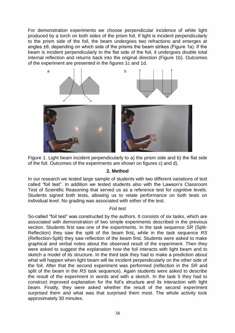
For demonstration experiments we choose perpendicular incidence of white light produced by a torch on both sides of the prism foil. If light is incident perpendicularly to the prism side of the foil, the beam undergoes two refractions and emerges at angles ±θ, depending on which side of the prisms the beam strikes (Figure 1a). If the beam is incident perpendicularly to the flat side of the foil, it undergoes double total internal reflection and returns back into the original direction (Figure 1b). Outcomes of the experiment are presented in the figures 1c and 1d.

Figure 1. Light beam incident perpendicularly to a) the prism side and b) the flat side of the foil. Outcomes of the experiments are shown on figures c) and d).

2. Method

In our research we tested large sample of students with two different variations of test called “foil test”. In addition we tested students also with the Lawson’s Classroom Test of Scientific Reasoning that served us as a reference test for cognitive levels. Students signed both tests, allowing us to relate performance on both tests on individual level. No grading was associated with either of the test.

Foil test

So-called “foil test” was constructed by the authors. It consists of six tasks, which are associated with demonstration of two simple experiments described in the previous section. Students first saw one of the experiments. In the task sequence SR (Split-Reflection) they saw the split of the beam first, while in the task sequence RS (Reflection-Split) they saw reflection of the beam first. Students were asked to make graphical and verbal notes about the observed result of the experiment. Then they were asked to suggest the explanation how the foil interacts with light beam and to sketch a model of its structure. In the third task they had to make a prediction about what will happen when light beam will be incident perpendicularly on the other side of the foil. After that the second experiment was performed (reflection in the SR and split of the beam in the RS task sequence). Again students were asked to describe the result of the experiment in words and with a sketch. In the task 5 they had to construct improved explanation for the foil’s structure and its interaction with light beam. Finally, they were asked whether the result of the second experiment surprised them and what was that surprised them most. The whole activity took approximately 30 minutes.

38

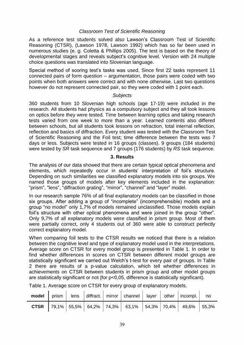
Classroom Test of Scientific Reasoning

As a reference test students solved also Lawson’s Classroom Test of Scientific Reasoning (CTSR), (Lawson 1978, Lawson 1992) which has so far been used in numerous studies (e. g. Coletta & Phillips 2005). The test is based on the theory of developmental stages and reveals subject’s cognitive level. Version with 24 multiple choice questions was translated into Slovenian language.

Special method of scoring test’s tasks was used. Since first 22 tasks represent 11 connected pairs of form question – argumentation, those pairs were coded with two points when both answers were correct and with none otherwise. Last two questions however do not represent connected pair, so they were coded with 1 point each.

Subjects

360 students from 10 Slovenian high schools (age 17-19) were included in the research. All students had physics as a compulsory subject and they all took lessons on optics before they were tested. Time between learning optics and taking research tests varied from one week to more than a year. Learned contents also differed between schools, but all students took lessons on refraction, total internal reflection, reflection and basics of diffraction. Every student was tested with the Classroom Test of Scientific Reasoning and the Foil test; time difference between the tests was 7 days or less. Subjects were tested in 16 groups (classes). 9 groups (184 students) were tested by SR task sequence and 7 groups (176 students) by RS task sequence.

3. Results

The analysis of our data showed that there are certain typical optical phenomena and elements, which repeatedly occur in students’ interpretation of foil’s structure. Depending on such similarities we classified explanatory models into six groups. We named those groups of models after key elements included in the explanation: “prism”, “lens”, “diffraction grating”, “mirror”, “channel” and “layer” model.

In our research sample 76% of all final explanatory models can be classified in those six groups. After adding a group of “incomplete” (incomprehensible) models and a group “no model” only 1,7% of models remained unclassified. Those models explain foil’s structure with other optical phenomena and were joined in the group “other”. Only 9,7% of all explanatory models were classified in prism group. Most of them were partially correct, only 4 students out of 360 were able to construct perfectly correct explanatory model.

When comparing foil tests to the CTSR results we noticed that there is a relation between the cognitive level and type of explanatory model used in the interpretations. Average score on CTSR for every model group is presented in Table 1. In order to find whether differences in scores on CTSR between different model groups are statistically significant we carried out Welch’s t-test for every pair of groups. In Table 2 there are results of a p-value calculation, which tell whether differences in achievements on CTSR between students in prism group and other model groups are statistically significant or not (for p<0,05, difference is statistically significant).

Table 1. Average score on CTSR for every group of explanatory models.

model prism lens diffract. mirror channel layer other incompl. no

CTSR 79,1% 55,5% 64,2% 74,3% 63,1% 54,3% 70,4% 49,6% 55,3%

39

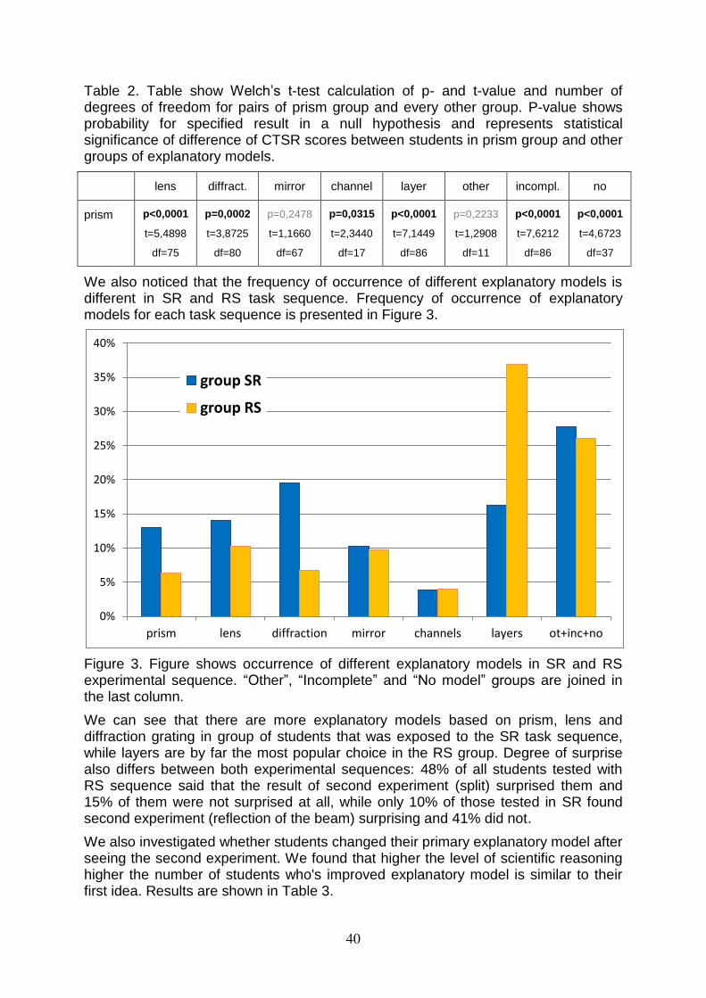
Table 2. Table show Welch’s t-test calculation of p- and t-value and number of degrees of freedom for pairs of prism group and every other group. P-value shows probability for specified result in a null hypothesis and represents statistical significance of difference of CTSR scores between students in prism group and other groups of explanatory models.

lens diffract. mirror channel layer other incompl. no

prism p<0,0001

t=5,4898

df=75

p=0,0002

t=3,8725

df=80

p=0,2478

t=1,1660

df=67

p=0,0315

t=2,3440

df=17

p<0,0001

t=7,1449

df=86

p=0,2233

t=1,2908

df=11

p<0,0001

t=7,6212

df=86

p<0,0001

t=4,6723

df=37

We also noticed that the frequency of occurrence of different explanatory models is different in SR and RS task sequence. Frequency of occurrence of explanatory models for each task sequence is presented in Figure 3.

Figure 3. Figure shows occurrence of different explanatory models in SR and RS experimental sequence. “Other”, “Incomplete” and “No model” groups are joined in the last column.

We can see that there are more explanatory models based on prism, lens and diffraction grating in group of students that was exposed to the SR task sequence, while layers are by far the most popular choice in the RS group. Degree of surprise also differs between both experimental sequences: 48% of all students tested with RS sequence said that the result of second experiment (split) surprised them and 15% of them were not surprised at all, while only 10% of those tested in SR found second experiment (reflection of the beam) surprising and 41% did not.

We also investigated whether students changed their primary explanatory model after seeing the second experiment. We found that higher the level of scientific reasoning higher the number of students who's improved explanatory model is similar to their first idea. Results are shown in Table 3.

0%

5%

10%

15%

20%

25%

30%

35%

40%

prism lens diffraction mirror channels layers ot+inc+no

group SR

group RS

40

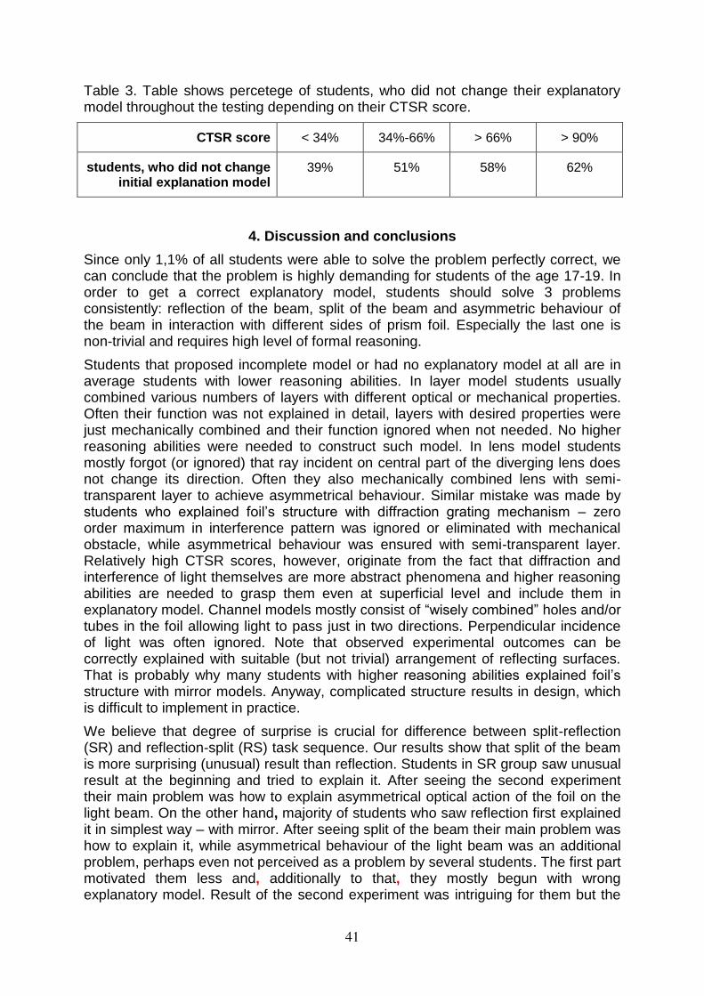
Table 3. Table shows percetege of students, who did not change their explanatory model throughout the testing depending on their CTSR score.

CTSR score < 34% 34%-66% > 66% > 90%

students, who did not change initial explanation model

39% 51% 58% 62%

4. Discussion and conclusions

Since only 1,1% of all students were able to solve the problem perfectly correct, we can conclude that the problem is highly demanding for students of the age 17-19. In order to get a correct explanatory model, students should solve 3 problems consistently: reflection of the beam, split of the beam and asymmetric behaviour of the beam in interaction with different sides of prism foil. Especially the last one is non-trivial and requires high level of formal reasoning.

Students that proposed incomplete model or had no explanatory model at all are in average students with lower reasoning abilities. In layer model students usually combined various numbers of layers with different optical or mechanical properties. Often their function was not explained in detail, layers with desired properties were just mechanically combined and their function ignored when not needed. No higher reasoning abilities were needed to construct such model. In lens model students mostly forgot (or ignored) that ray incident on central part of the diverging lens does not change its direction. Often they also mechanically combined lens with semi-transparent layer to achieve asymmetrical behaviour. Similar mistake was made by students who explained foil’s structure with diffraction grating mechanism – zero order maximum in interference pattern was ignored or eliminated with mechanical obstacle, while asymmetrical behaviour was ensured with semi-transparent layer. Relatively high CTSR scores, however, originate from the fact that diffraction and interference of light themselves are more abstract phenomena and higher reasoning abilities are needed to grasp them even at superficial level and include them in explanatory model. Channel models mostly consist of “wisely combined” holes and/or tubes in the foil allowing light to pass just in two directions. Perpendicular incidence of light was often ignored. Note that observed experimental outcomes can be correctly explained with suitable (but not trivial) arrangement of reflecting surfaces. That is probably why many students with higher reasoning abilities explained foil’s structure with mirror models. Anyway, complicated structure results in design, which is difficult to implement in practice.

We believe that degree of surprise is crucial for difference between split-reflection (SR) and reflection-split (RS) task sequence. Our results show that split of the beam is more surprising (unusual) result than reflection. Students in SR group saw unusual result at the beginning and tried to explain it. After seeing the second experiment their main problem was how to explain asymmetrical optical action of the foil on the light beam. On the other hand, majority of students who saw reflection first explained it in simplest way – with mirror. After seeing split of the beam their main problem was how to explain it, while asymmetrical behaviour of the light beam was an additional problem, perhaps even not perceived as a problem by several students. The first part motivated them less and, additionally to that, they mostly begun with wrong explanatory model. Result of the second experiment was intriguing for them but the

41

problem seems to be too demanding for them to solve it in a single step. It seems that students were more successful in problem solving, when they saw surprising data at the beginning of the task. Similar findings were reported by Ahtee and Hakkarainen (2005).

Staying with the initial explanatory model after seeing the result of the second experiment is a behaviour seen more frequently in students with higher level of scientific reasoning. Despite additional data, which suggested its incorrectness, these students did not change their initial explanatory model, but rather tried to complement or expand it.

Our research shows that only students with high formal reasoning level are able to reveal the structure of prism foil. Formal reasoning ability therefore seems to be a necessary precondition for efficient building of explanatory models.

5. Acknowledgement

Our acknowledgements go to Anton E. Lawson, Leoš and Irena Dvořak, Gašper Cankar and to following high-school teachers: Vitomir Babič, Ruben Belina, Peter Gabrovec, Jasmina Jančič, Peter Jevšenak, Vida Kariž-Merhar, Stane Kodba, Andrej Lobnik, Karmen Vidmar, Maruša Potokar and Ivica Tomić,

References

Ahtee, M. & Hakkarainen, O. (2005). Importance of the order of demonstrations in changing pupils' conceptions. NorDiNa, 1, retrieved from: http://www.naturfagsenteret.no/c1515377/tidsskrift/innholdsliste.html?tid=1489795

Chinn, C. A. & Malhotra, B. A. (2002). Epistemologically authentic inquiry in schools: A theoretical framework for evaluating inquiry tasks. Sci. Education, 86(2), 175-218.

Coletta, V. P. & Phillips, J. A. (2005). Interpreting FCI scores: Normalized gain, preinstruction scores and scientific reasoning ability. American Journal of Physics, 73(12), 1172-1182.

Galili, I., Goldberg, F. & Bendall, S. (1993). The effects of prior knowledge and instruction on understanding image formation. Journal of Research in Science Teaching 30(3), 271-301.

Kaewkhong, K., Mazzolini, A., Narumon Emarat, N. & Arayathanitkul, K. (2010). Thai high-school students’ misconceptions about and models of light refraction through a planar surface. Physics Education 45(1), 91-107.

Lawson, A. E. (1978). The development and validation of a classroom test of formal reasoning. Journal of Research in Science Teaching, 15(1), 11-24.

Lawson, A. E. (1992). What do tests of formal reasoning actually measure? Journal of Research in Science Teaching, 29(9), 965-983.

Planinšič, G. & Gojkošek, M. (2011). Prism foil from an LCD monitor as a tool for teaching introductory optics. European Journal of Physics, 32(2), 601-613.

42

The Status Quo of Lab Infrastructure and Equipment in Austrian Secondary Schools and Implications on Teaching Science Claudia Haagen-Schützenhöfer and Martin Hopf

claudia.haagen@univie.ac.at Austrian Educational Competence Centre Physics, University of Vienna, Austria

By the end of their school careers, students have spent thousands of hours in classrooms. Conse-quently, the quality of classroom learning environments is important for students’ teaching-learning experiences and has been investigated in a dozens of studies (Fraser, 2007). Due to the importance of lab settings in science teaching, an instrument assessing lab-based learning environments was developed (Fraser, Giddings, & McRobbie, 1995). However, infrastructural components of science lab classes have so far been neglected to be one essential factor determining lab learning environments. Hardly any research has been carried out on facility design especially focusing on lab settings. The aim of the investigation presented was to find out about the situation of science lab instruction in Aus-trian secondary schools focusing on infrastructure and equipment. For data collection a survey was conducted among secondary school teachers. The results reveal three main problem areas concern-ing lab-based learning environments. Teachers are dissatisfied with the general access to lab rooms, their infrastructure as well as the quality of equipment available.

Introduction Practical work is generally regarded as one important pillar of successful science in-struction. Although educational research has repeatedly shown that the output of practical work does not live up to these expectations, the majority of teachers still believe in its power (Singer, Hilton, & Schweingruber, 2006). Teachers see practical work as a successful strategy to foster students’ content knowledge and practical abilities. The low impact of lab activities on Austrian students’ achievement is fre-quently seen as a consequence of the bad conditions of practical work itself in Aus-trian schools. The general availability of lab rooms, their infrastructure as well as the quality of equipment available is in the focus of Austrian science teachers’ criticism. In addition, teachers seem to be dissatisfied with the quality of rebuilding projects initiated by government for outdated science classrooms (Czaja, 2010). However, there is no empirical data available on teachers’ attitudes and on the status quo of lab infrastructure and equipment in Austrian secondary schools. Although lab work is seen as a very important component of science instruction at all educational levels, the question of facility design has hardly been treated up to now (Nehrer, 1982). So far, the issue of facility design was addressed for the first time by Wilson in the mid-1990s. Then, a non-interactive introductory physics course at uni-versity level was changed into a collaborative group-learning environment (“Compre-hensive Unified Physics Learning Environment physics studio”) aiming at an im-provement of the relationship between course and lab classes (Wilson, 1994). This redesigning of the course structure required a redesigning of facilities. A similar pro-cess can be traced in Beichner’s SCALE-UP project at North Carolina State Universi-ty where a collaborative lab-based learning environment for large, introductory col-lege courses triggered classroom redesign (Beichner et al., 2007). The history of both projects shows that interactive and collaborative learning environments in sci-ence lab classes rely on appropriate facility design, supporting a variety of learning and teaching scenarios. In addition, it needs to be mentioned that both projects are not only successful in promoting interactive and collaborative learning but also on the

43

level of output. Empirical data shows that in both project settings, student achieve-ment is significantly better compared to conventional introductory courses (Beichner et al., 2007; Wilson, 1994). However, these two cases, where appropriate lab settings turned out to be a prereq-uisite for achieving the project’s prime objective namely collaborative learning envi-ronments, seem to be exceptions. In general, classroom design for science lab clas-ses, especially on the level of secondary education, has been neglected to be one important factor determining the quality of lab learning environments. The facility de-sign of science lab classrooms is left to the choice of architects (Lidsky, 2004) and to the restrictions of governmental guidelines, which are hardly based on research find-ings. This current situation of facility design, which may not only be true for the Austrian school system, was the starting point of the investigation presented here. The main idea was to determine the status quo and to find out which factors could improve the current situation. The research questions guiding this investigation are presented here:

• How are lab rooms used in Austrian secondary schools? • Do lab rooms meet teachers’ needs? • Which ideas do teachers have about “perfect lab rooms“? • How are conversion and refitting measures of lab rooms evaluated by teach-

ers? Methods

The aim of the investigation reported was to get an overview of current conditions concerning infrastructure and equipment in science labs in Austrian secondary schools. Therefore a questionnaire for science teachers was developed which was closely modelled on the research questions presented above.

The Sample

The survey was carried out during the largest nationwide conference for continuing education for chemistry and physics teachers. Each year over 300 chemistry and physics teachers take part in this conference which lasts for one week. The partici-pants teach physics and/or chemistry in all different types of school on the lower and upper secondary level. Teachers from all parts of Austria participate in this confer-ence. Usually, there is at maximum one physics and chemistry teacher present per school. This provided the opportunity to get insight into a maximum number of differ-ent schools. The questionnaires were distributed during the opening ceremony of the conference. After explaining the motivation for the survey the participants were asked to fill in the questionnaires and drop them in return boxes. Questionnaires were distributed among more than 200 participants, 80 questionnaires were returned and 68 were fully filled in and taken as basis for analysis.

The Questionnaire

The questionnaire developed for this survey contained 30 questions which were part-ly in an open (2), semi-open (14) and multiple-choice format (14). The questions were developed to investigate four main item complexes focusing on different sub-topics.

44

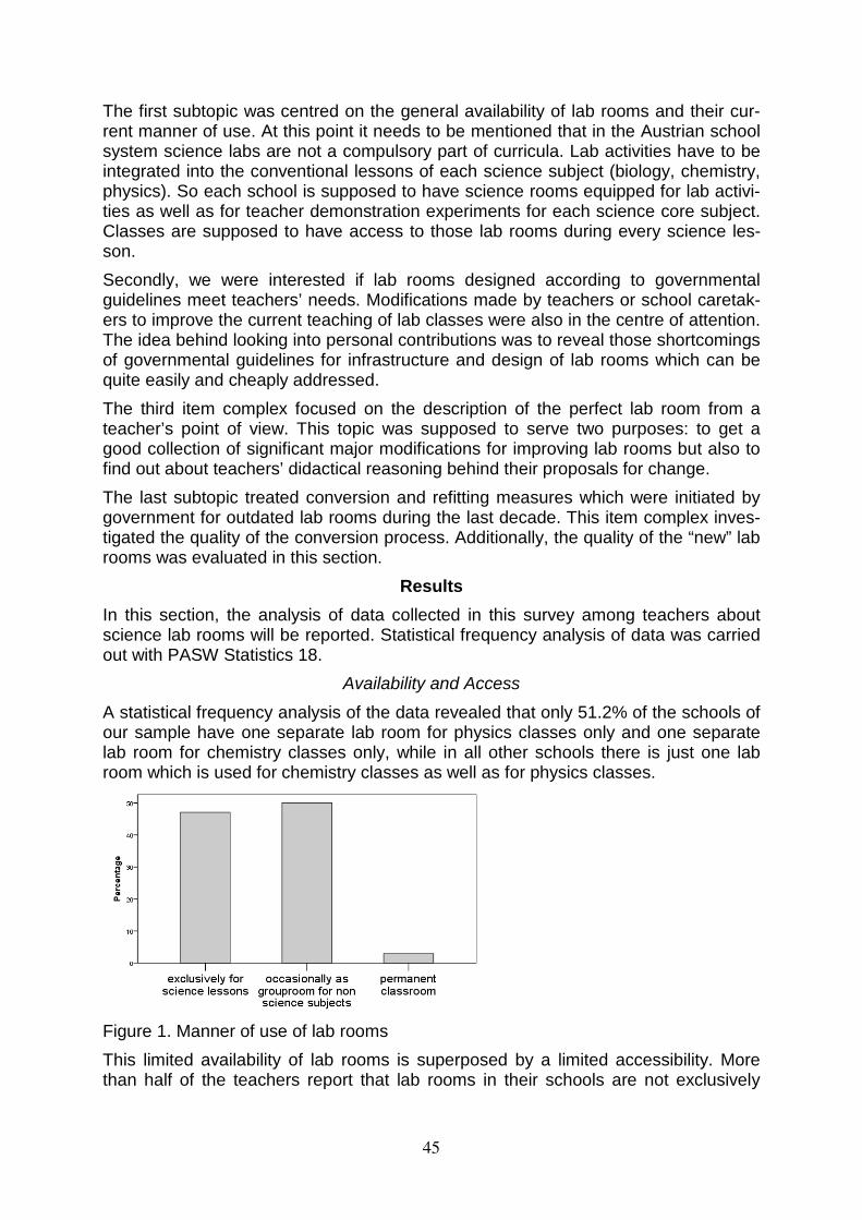
The first subtopic was centred on the general availability of lab rooms and their cur-rent manner of use. At this point it needs to be mentioned that in the Austrian school system science labs are not a compulsory part of curricula. Lab activities have to be integrated into the conventional lessons of each science subject (biology, chemistry, physics). So each school is supposed to have science rooms equipped for lab activi-ties as well as for teacher demonstration experiments for each science core subject. Classes are supposed to have access to those lab rooms during every science les-son. Secondly, we were interested if lab rooms designed according to governmental guidelines meet teachers’ needs. Modifications made by teachers or school caretak-ers to improve the current teaching of lab classes were also in the centre of attention. The idea behind looking into personal contributions was to reveal those shortcomings of governmental guidelines for infrastructure and design of lab rooms which can be quite easily and cheaply addressed. The third item complex focused on the description of the perfect lab room from a teacher’s point of view. This topic was supposed to serve two purposes: to get a good collection of significant major modifications for improving lab rooms but also to find out about teachers’ didactical reasoning behind their proposals for change. The last subtopic treated conversion and refitting measures which were initiated by government for outdated lab rooms during the last decade. This item complex inves-tigated the quality of the conversion process. Additionally, the quality of the “new” lab rooms was evaluated in this section.

Results In this section, the analysis of data collected in this survey among teachers about science lab rooms will be reported. Statistical frequency analysis of data was carried out with PASW Statistics 18.

Availability and Access

A statistical frequency analysis of the data revealed that only 51.2% of the schools of our sample have one separate lab room for physics classes only and one separate lab room for chemistry classes only, while in all other schools there is just one lab room which is used for chemistry classes as well as for physics classes.

Figure 1. Manner of use of lab rooms This limited availability of lab rooms is superposed by a limited accessibility. More than half of the teachers report that lab rooms in their schools are not exclusively

45

used for science lessons, but also occasionally as group room for other subjects or in a few cases even as permanent classroom (see Figure 1).

Modifications made by Teachers or School Caretakers

Lab rooms designed and equipped according to governmental guidelines do not seem to meet teachers’ needs fully. In 46% of the cases, teachers state that standard features of science lab rooms in their schools were modified by themselves or by school caretakers. The analysis of data shows four main areas of useful modifications of lab rooms car-ried out: The most frequently mentioned modifications were additional installations of audio-visual materials like DVD and CD player, projection walls, camcorders to pro-ject close-ups of demonstration experiments etc., data projector, computer working stations as well as internet access for teacher or/and students. Secondly, hands-on material and/or equipment for student lab activities were added to existing standard equipment. Thirdly, additional storage room was created. Finally, many teachers highlighted the negative influence of fixed benches for collaborative learning settings. Consequently, additional moveable benches and chairs were integrated.

The perfect Lab Room

Results concerning the perfect lab room from a teacher’s perspective are presented in two sections, one dealing with infrastructural ideas and one focusing on sugges-tions concerning furniture and equipment. As far as infrastructure is concerned, the question of space was discussed most frequently. In 58.3% of the cases, teachers opt for a lab room layout that is arranged in such a way that mini-lectures, group dis-cussions and collaborative lab activities in small groups can be done. 23.9% of the teachers emphasised the importance of the availability of working stations for all stu-dents. In the schools of those teachers the number of students per class sometimes exceeds the number of lab benches available. So the surplus number of students has either to share a lab bench with a second student, or they have to work at “normal” benches without necessary lab features. The infrastructure of the teacher preparation rooms was also mentioned by 8.1% of the teachers. Here it was emphasised that the preparation room needs to be adjacent to the lab room and easily accessible through an extra wide, self-opening door that facilitates the transport of lab equipment. In the category Furniture and Equipment, 61.2% of the teachers emphasised the im-portance of moveable lab benches and seats so that the setting can be adapted to different phases and modes of instruction easily. Another topic mentioned by 26.4% of all teachers was sufficient, well maintained equipment for student lab activities as well as for demonstration experiments. About one quarter pointed out the necessity of furniture adaptable to students’ individual physical dimensions. So far, lab rooms which are used by students between 10 and 19 years have been equipped with non-adjustable benches of one size. A final point of discussion was the functional compo-nents integrated into the teacher’s worktable and into the students’ lab benches. Here 34.8% agreed on supply of gas, water, electricity (AC/DC adjustable) for stu-dent lab benches and 25.3% on a teacher’s worktable equipped with gas, water, electricity, computer, internet access and audio-visual material.

Conversion and Refitting Measures

The last section of the results treats conversion and refitting measures. The focus is put on the process of conversion and on teachers’ assessment of “renewed” lab

46

rooms. According to the data of the survey presented here, nearly 50% of lab rooms have been refitted during the last decade. In the following, emerging issues during the conversion process are summarized. Teachers frequently criticized a lack of communication between architects, contract-ed companies, headmasters, school authorities and teachers. Time management posed another problem as the measures could not be finished in most schools on time. In the majority of cases conversion work went on during the school year. Addi-tionally, in about one third of the cases equipment or infrastructure did not work after the contracted companies had finished their work. This caused further delays. Major problems were also caused by the very tight and partly old fashioned governmental guidelines for lab rooms. To investigate teachers’ assessment of the “renewed” lab rooms 5 point likert scales were used ranging from 1 (=very good) to 5 (=not acceptable). The general impres-sion of the “renewed” lab rooms was rated as medium (m=2.26; s=1.318).

Figure 2. Functionality of converted lab rooms

Figure 3. Learning environment provided by converted lab rooms

This general impression was split up into two different subcategories, functionality (see Figure 2) and quality of learning environment (see Figure 3). On average, both categories were assessed as medium (Functionality: m=2.20 s=1.157; Learning envi-ronment m=2.24; s=1.185). The distribution indicates that about two third of the teachers questioned, rated functionality and the quality of the learning environment of refitted lab rooms as very good or good.

Discussion & Conclusion According to this survey on lab infrastructure in Austrian secondary schools three main problem areas could be identified: teachers are dissatisfied with lab rooms’ in-frastructure, the quality of equipment available as well as with the general access to lab rooms. The number and the type of modifications made by teachers or school caretakers to upgrade the material learning environment of lab rooms indicate a huge potential for quick and cheap improvements in the field of infrastructure and equipment. This is also true for suggestions made concerning “perfect lab rooms”. It has to be empha-sized that the teachers of our sample have quite similar ideas for both, the improve-

47

ment of existing lab rooms and the design of “perfect lab rooms”. Their ideas even match suggestions by researchers in the majority of cases (Wilson, 1994). However, what turned out to be quite frustrating for teachers is that their ideas are not taken up by authorities for governmental guidelines for lab rooms. In general, teachers experience the process of conversion often as time consuming and frustrating. Although they are usually at least partly involved in the planning pro-cess, teachers’ suggestions are not implemented often enough due to very tight and partly outdated governmental guidelines. Another problem poses bad communication between involved parties and bad time management. After all, converted lab rooms are positively assessed by the majority of teachers. So, the conclusion can be drawn that conversion measures are positive in general but minor changes in procedures could have big effects on teachers’ satisfaction and on the quality of teaching. The availability and accessibility of lab rooms seems to be one main problem influ-encing the integration of lab activities into science teaching. As science classes fre-quently do not have regular access to lab rooms, phases of practical work cannot take place due to didactical indicators but they rely on the availability of rooms and thus influence the teaching-learning process massively. Within the research design presented here, students’ learning output was not tested. So, the actual kind of influ-ence on the quality of learning output cannot be specified. This survey shows, how-ever, that the current situation of lab infrastructure & equipment in Austrian second-ary schools is – as teachers frequently complain – really far from ideal. After gaining insight in this status quo, in a next step the correlation between the quality of lab in-frastructure / accessibility and student learning output needs to be investigated.

References Beichner, R., Saul, J., Abbott, D., Morse, J., Deardorff, D., Allain, R., et al. (2007).

The student-centred activities for large enrollment undergraduate programs (SCALE-UP) project. Research-based reform of university physics, 1(1), 1–42.

Czaja, W. (2010, June 26). Bestehende Schulbauten besser nützen: Charta "Schulumbau". derStandard on-line. Retrieved from http://derstandard.at/1277336787779/Charta-SchulUmBau-Bestehende-Schulbauten-besser-nutzen

Fraser, B. (2007). Classroom Learning Environments. In S. K. Abell (Ed.), Handbook of research on science education (pp. 103–124). Mahwah NJ: LEA.

Fraser, B., Giddings, G., & McRobbie, C. (1995). Evolution and validation of a per-sonal form of an instrument for assessing science lab classroom environments. Journal of Research in Science Teaching, 32(4), 399–422.

Lidsky, A. (2004). How financial and resource issues constrain or enable lab activi-ties.: Presentation to the Committee on High School Science Laboratories: Role and Vision, June 3-4, National Research Council, Washington, DC.

Nehrer, M. (1982). Schulbau in Österreich von 1945 bis heute. Horn: Berger. Singer, S. R., Hilton, M. L., & Schweingruber, H. A. (Eds.) (2006). America's Lab Re-

port: Investigations in High School Science. Washington: National Academies Press.

Wilson, J. (1994). The CUPLE physics studio. The Physics Teacher, 32, 518–523.

48

Do Lecture Demonstrations Support Problem Solving?

Ilkka Hendolin

ilkka.hendolin@helsinki.fi

Department of Physics, University of Helsinki

Lecture demonstrations are a widely used method of teaching physics. They have been traditionally considered as an effective way to teach physics as well as to motivate and entertain students, but recent study in this field has challenged some of these assumptions. To study these notions an experiment was arranged at the University of Helsinki where the same physics subject matter was lectured to two similar groups of students, one with lecture demonstrations and the other without. Differences in learning were searched for by meticulously examining students’ answers to weekly exercise problems. Two experiments with two different groups of students and a total of four exercise problems showed no significant differences. In a case where demonstrations do not closely match the context in given test questions it would appear that demonstrations actually do not support problem solving very much. Further research would be needed to find out exactly how and what kind of physics can actually be learned by watching demonstrations. .

1. Introduction

Demonstrations are a traditional part of physics lectures, widely used across the field of physics education. Teachers use demonstrations to show physics phenomena and clarify concepts, as well as to motivate and entertain students (Miller 1969; Freier 1981; Johnston 1981; Pinkston 1981; Swartz & Miner 1997). These stated roles, more like objectives, have been around for ages, but only recently has physics education research started to investigate to which extent these goals can be attained. In fact, several studies suggest that little is learned from traditional lecture demonstrations (Crouch, Fagen, Callan & Mazur, 2004; Roth, McRobbie, Lucas & Boutonné, 1997) whereas demonstrations incorporated into interactive engagement (IE) teaching methods have been proved to support physics learning (Sokoloff & Thornton, 1997; Crouch et al., 2004; Moll & Milner-Bolotin, 2009). There is also evidence on the benefits of interactive approaches from the field of physics teaching in general (Hake, 1998; Francis, Adams & Noonan, 1998) as well as from educational psychology (Pintrich, 1999). The above-mentioned studies on the effect of demonstrations have concentrated on measuring skills in qualitative reasoning (Sokoloff & Thornton, 1997) and/or problem solving in physical situations that are similar or identical to the ones presented in demonstrations (Crouch et al., 2004; Moll & Milner-Bolotin, 2009). These approaches do not necessarily correspond fully with common practices of physics teaching. Measuring learning with assignments that very closely match the demonstrations that were showed could almost be interpreted as “teaching to the test”, while qualitative reasoning on the other hand represents just one of the aspects of mastering physics. Grasping the conceptual structure of physics as well as understanding the relationship between models and reality are arguably among the most important objectives for physics teaching. Nevertheless problem solving, in one form or another, is often brought up as the vital practical skill to be learned in physics studies (Hestenes 1987; McDermott 1991). It is frequently required in physics studies, not

49

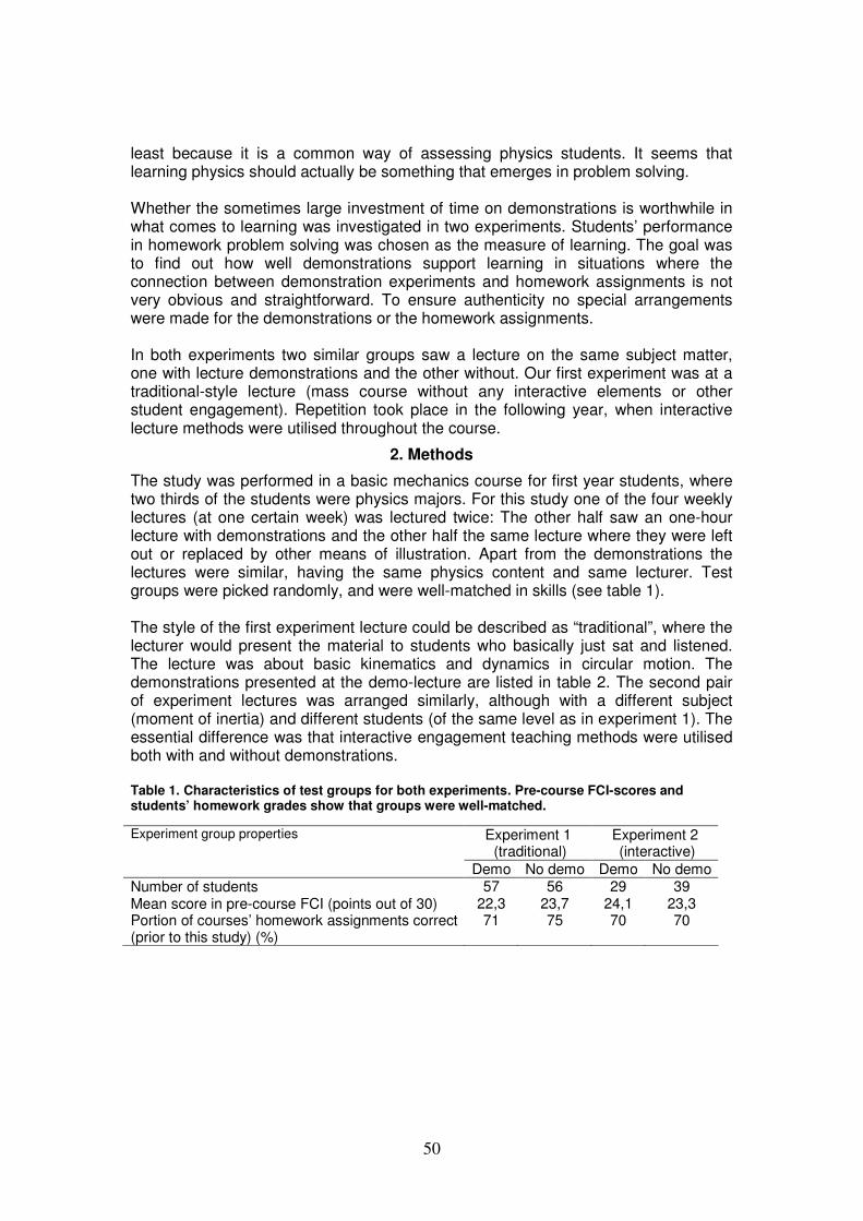
least because it is a common way of assessing physics students. It seems that learning physics should actually be something that emerges in problem solving. Whether the sometimes large investment of time on demonstrations is worthwhile in what comes to learning was investigated in two experiments. Students’ performance in homework problem solving was chosen as the measure of learning. The goal was to find out how well demonstrations support learning in situations where the connection between demonstration experiments and homework assignments is not very obvious and straightforward. To ensure authenticity no special arrangements were made for the demonstrations or the homework assignments. In both experiments two similar groups saw a lecture on the same subject matter, one with lecture demonstrations and the other without. Our first experiment was at a traditional-style lecture (mass course without any interactive elements or other student engagement). Repetition took place in the following year, when interactive lecture methods were utilised throughout the course.

2. Methods

The study was performed in a basic mechanics course for first year students, where two thirds of the students were physics majors. For this study one of the four weekly lectures (at one certain week) was lectured twice: The other half saw an one-hour lecture with demonstrations and the other half the same lecture where they were left out or replaced by other means of illustration. Apart from the demonstrations the lectures were similar, having the same physics content and same lecturer. Test groups were picked randomly, and were well-matched in skills (see table 1). The style of the first experiment lecture could be described as “traditional”, where the lecturer would present the material to students who basically just sat and listened. The lecture was about basic kinematics and dynamics in circular motion. The demonstrations presented at the demo-lecture are listed in table 2. The second pair of experiment lectures was arranged similarly, although with a different subject (moment of inertia) and different students (of the same level as in experiment 1). The essential difference was that interactive engagement teaching methods were utilised both with and without demonstrations. Table 1. Characteristics of test groups for both experiments. Pre-course FCI-scores and students’ homework grades show that groups were well-matched.

Experiment group properties Experiment 1 (traditional)

Experiment 2 (interactive)

Demo No demo Demo No demo Number of students 57 56 29 39 Mean score in pre-course FCI (points out of 30) 22,3 23,7 24,1 23,3 Portion of courses’ homework assignments correct (prior to this study) (%)

71 75 70 70

50

Table 2. Demonstrations presented at the experiment lectures

The IE methods used were an adaptation of Peer Instruction (Mazur, 1997) and Interactive Lecture Demonstrations (Sokoloff & Thornton, 1997). There were three interactive sequences during each experiment lecture. Interactive sequences consisted of a multiple-choice question presented to the students, a 2-3 minute discussion in small groups followed by answering with electronical polling devices, a demonstration to reveal the answer (in two questions out of the total three) and possibly a short discussion on the subject.

In both experiments, two homework problems had been chosen to measure learning at the experiment lectures (see Appendix). Teaching to the test was to be avoided, and therefore these problems were just picked from the pool of standard homework assignments. They each require slightly different skills: Problem 1 is a graphical representation task, problem 2 is a traditional physics exercise problem, problem 3 is about qualitative reasoning and problem 4 is purely mathematical in nature. Students’ answers to these exercise problems were examined carefully to reveal possible differences between the performances of the two groups. This included checking the correctness of calculations, judging the quality of physical reasoning and evaluating the overall physicality of the solution. This examination was followed by an analysis of the types of mistakes made by the students who had not solved the problems correctly.

3. Results

3.1 Experiment lecture with traditional teaching methods

Table 3 shows the results of exercise problems associated with the first experiment. Differences between the groups are small, and only the portion of wrong answers to problem 1 differs slightly.

Examination of the mistakes the students’ had made revealed just one difference: In problem 1 those who had seen demonstrations had more often drawn an acceleration vector to the point where the car had in fact been stated to be at rest.

3.2 Experiment lecture with interactive engagement teaching methods

The results of the second experimental lecture with IE methods (table 4) also reveal only minor differences between demo- and no demo groups. Problem 4 was quite difficult for the students, and only about 60 % passed in an answer. In problem 4 there is a slight difference in favour of the non-demo group (p = 0,16 in two-sample z-test, following the methods outlined in chapter 8 of Moore and McGabe (1993)).

Demonstrations presented at the lectures (in order of appearance)

Experiment 1 (traditional) Experiment 2 (IE)

1. Presentation of demo equipment, the track of and object in circular motion

1. Torque and rotational inertia (part of an IE sequence)

2. Direction of the velocity of an object in circular motion

2. Moment of inertia about different axes of a disc (part of an IE sequence )

3. Acceleration of an object in constant and changing circular motion

3. Quantification of moment of inertia (several experiments entwined with lecturing)

4. Forces on an object in circular motion 5. Relation of angular velocity and centripetal force

51

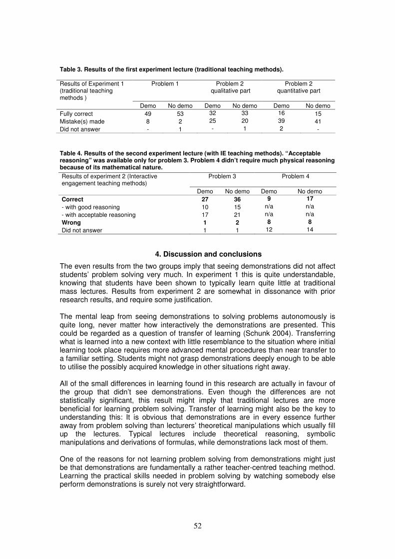
Table 3. Results of the first experiment lecture (traditional teaching methods).

Table 4. Results of the second experiment lecture (with IE teaching methods). “Acceptable reasoning” was available only for problem 3. Problem 4 didn’t require much physical reasoning because of its mathematical nature.

4. Discussion and conclusions

The even results from the two groups imply that seeing demonstrations did not affect students’ problem solving very much. In experiment 1 this is quite understandable, knowing that students have been shown to typically learn quite little at traditional mass lectures. Results from experiment 2 are somewhat in dissonance with prior research results, and require some justification. The mental leap from seeing demonstrations to solving problems autonomously is quite long, never matter how interactively the demonstrations are presented. This could be regarded as a question of transfer of learning (Schunk 2004). Transferring what is learned into a new context with little resemblance to the situation where initial learning took place requires more advanced mental procedures than near transfer to a familiar setting. Students might not grasp demonstrations deeply enough to be able to utilise the possibly acquired knowledge in other situations right away. All of the small differences in learning found in this research are actually in favour of the group that didn’t see demonstrations. Even though the differences are not statistically significant, this result might imply that traditional lectures are more beneficial for learning problem solving. Transfer of learning might also be the key to understanding this: It is obvious that demonstrations are in every essence further away from problem solving than lecturers’ theoretical manipulations which usually fill up the lectures. Typical lectures include theoretical reasoning, symbolic manipulations and derivations of formulas, while demonstrations lack most of them. One of the reasons for not learning problem solving from demonstrations might just be that demonstrations are fundamentally a rather teacher-centred teaching method. Learning the practical skills needed in problem solving by watching somebody else perform demonstrations is surely not very straightforward.

Results of Experiment 1 (traditional teaching methods )

Problem 1 Problem 2 qualitative part

Problem 2 quantitative part

Demo No demo Demo No demo Demo No demo

Fully correct 49 53 32 33 16 15

Mistake(s) made 8 2 25 20 39 41

Did not answer - 1 - 1 2 -

Results of experiment 2 (Interactive engagement teaching methods)

Problem 3 Problem 4

Demo No demo Demo No demo

Correct 27 36 9 17

- with good reasoning 10 15 n/a n/a

- with acceptable reasoning 17 21 n/a n/a

Wrong 1 2 8 8

Did not answer 1 1 12 14

52

However, according to feedback and informal discussions with students over the years, lecture demonstrations are almost invariably found to be motivating and entertaining. Therefore using demonstrations is still probably worthwhile, especially knowing that keeping physics students committed is a major challenge these days. Demonstrations probably support physics learning too, but the questions of how and what kind of physics is learned from demonstrations would deserve more research in order to utilise this unique teaching method as effectively as possible.

References

Crouch, C.H., Fagen, A.P., Callan, J.P. & Mazur, E. (2004). Classroom demonstrations: Learning tools or entertainment?, American Journal of Physics, 72(6), 835-838.

Francis, G.E., Adams, J.P. & Noonan, E.J. (1998). Do they stay fixed?, The Physics Teacher, 36(8), 488-490.

Freier, G. (1981). The use of demonstrations in physics teaching, The Physics Teacher, 19(6), 384-386.

Hake, R.R. (1998). Interactive-engagement versus traditional methods: A six-thousand-student survey of mechanics test data for introductory physics courses, American Journal of Physics, 66(1), 64-74.

Hestenes, D. (1992). Toward a modeling theory of physics instruction, American Journal of Physics, 55(5), 440-454.

Johnston, J.B. (1981). The lecture demonstration: A developing crisis, The Physics Teacher, 19(6), 393-394.

Mazur, E. (1997). Peer instruction: a user's manual, Upper Saddle River, N.J.: Prentice Hall.

McDermott, L.C. (1991). Millikan Lecture 1990: What we teach and what is learned - Closing the gap, American Journal of Physics, 59(4), 301-315.

Miller, J.S. (1969). Demonstrations in physics, Sydney: Ure Smith. Moll, R.F. & Milner-Bolotin, M. (2009). The effect of interactive lecture experiments on

student academic achievement and attitudes towards physics, Canadian Journal of Physics, 2009, 87(8) 917-924.

Moore, D. S. & McGabe, G. P. (1993). Introduction to the practice of statistics, second edition, New York: W.H. Freeman and Company.

Pinkston, E.R. (1981). The use of demonstrations in teaching introductory physics, The Physics Teacher, 19(6), 387-388.

Pintrich, P.R. (1999). The role of motivation in promoting and sustaining self-regulated learning, International Journal of Educational Research, 31(6), 459-470.

Roth, W., McRobbie, C.J., Lucas, K.B. & Boutonné, S. (1997). Why may students fail to learn from demonstrations? A social practice perspective on learning in physics, Journal of Research in Science Teaching, 34(5), 509-533.

Schunk, D.H. (2009). Learning theories: an educational perspective, 5th ed. edn., Upper Saddle River, N.J.: Pearson/Merrill Prentice Hall.

Sokoloff, D.R. & Thornton, R.K. (1997). Using interactive lecture demonstrations to create an active learning environment, The Physics Teacher, 35(6), 340-347.

Swartz, C.E. & Miner, T. (1997). Teaching introductory physics: a sourcebook, Woodbury, NY.: AIP Press.

53

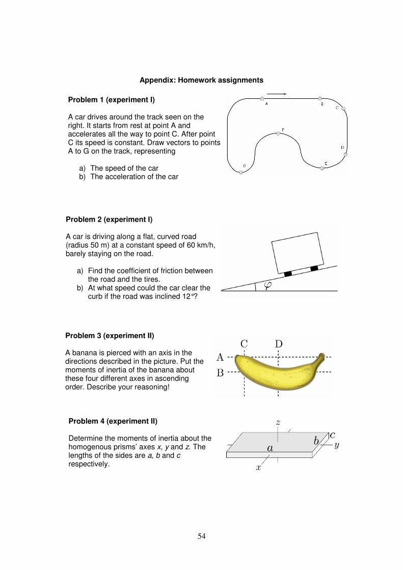
Appendix: Homework assignments

Problem 2 (experiment I) A car is driving along a flat, curved road (radius 50 m) at a constant speed of 60 km/h, barely staying on the road.

a) Find the coefficient of friction between the road and the tires.

b) At what speed could the car clear the curb if the road was inclined 12°?

Problem 1 (experiment I) A car drives around the track seen on the right. It starts from rest at point A and accelerates all the way to point C. After point C its speed is constant. Draw vectors to points A to G on the track, representing

a) The speed of the car b) The acceleration of the car

Problem 3 (experiment II) A banana is pierced with an axis in the directions described in the picture. Put the moments of inertia of the banana about these four different axes in ascending order. Describe your reasoning!

Problem 4 (experiment II) Determine the moments of inertia about the homogenous prisms’ axes x, y and z. The lengths of the sides are a, b and c respectively.

54

Development of key competencies using video analysis of motions by Tracker

Peter Hockicko1

hockicko@fyzika.uniza.sk

1 Department of Physics, Faculty of Electrical Engineering, University of Žilina, Slovakia

This paper reports on practical experience with the students in conducting the analysis of physical problems and offers some practical advice for teachers of physics as to which situations are more or less suitable for the analysis. Some students´ analysis of motions, e.g. calculating the slope or the area of a velocity versus time graph, determination of physical parameters and comparison of real situations with analytic and dynamic models, are presented, too.

Comparison of the traditional teaching methods with the method of the video analysis using the program Tracker has revealed that the latter method is easier for the students, they have fun when recording and analyzing their own videos, they can set individual pace for their work. It is statistically confirm that the competencies of the students and their knowledge are developed and increased by working with Tracker. This video analysis and modeling tool helps them to understand the natural sciences principles and phenomena more deeply, develops skills of abstraction and projection, awakes curiosity towards nature and surrounding world and makes physics a lot more fun.

1. Introduction

Video analysis using program Tracker (Open Source Physics) in the educational process introduces a new creative method of teaching physics, makes natural sciences more interesting for students (Brown 2009). Exploring the laws of nature in this way can be amazing for the students because this educational software is illustrative, interactive, inspires them to think creatively, improves their performance and it can help in studying physics. With the help of a high-speed camera (for the preparation of motion files - video experiments) and the program Tracker the students can study certain motion in detail. The video analysis gives the students simple and easy way to understand the process of movement. The program Tracker seems to be a useful modeling tool, too. The computer modeling enables the students to relate the results of measurements to theory, showing relations between

the graphs obtained using a model and a measurement. One post‐instruction assessment of student ability to interpret kinematics graphs indicated that groups which used a video analysis tools generally performed better than students taught via traditional instruction (Beichner 1996).

It was found that the use of multimedia teaching aids in technical education on the 2nd level of primary schools significantly affects the level of knowledge of pupils, particularly in terms of performing, remembering, understanding, specific transfer and active learning (Stebila 2011). It is not easy to explain empirical laws and dynamic phenomena by means of textbooks. New techniques attract students’ attention. If studying physics is accompanied with work on computers, a new form of education arises that will become very attractive (at all stages of the educational process - starting with primary schools (Children´s Universities) and ending with universities) (Hockicko 2010). It is very important to use the multimedia tools also in other subjects including basic education to make science and technology more appealing and to address the scientific apathy crisis of young people (Bussei 2003). The game provides many examples that can bring physics to life in the classroom. Especially

55

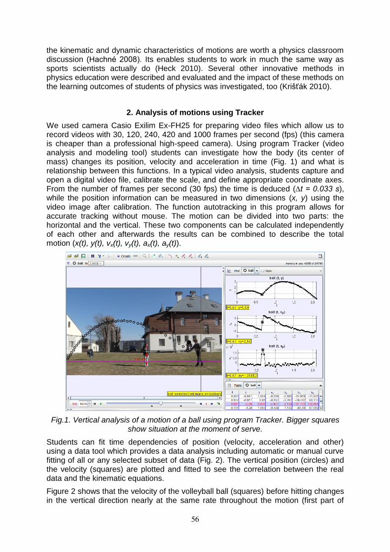
the kinematic and dynamic characteristics of motions are worth a physics classroom discussion (Hachné 2008). Its enables students to work in much the same way as sports scientists actually do (Heck 2010). Several other innovative methods in physics education were described and evaluated and the impact of these methods on the learning outcomes of students of physics was investigated, too (Krišťák 2010).

2. Analysis of motions using Tracker

We used camera Casio Exilim Ex-FH25 for preparing video files which allow us to record videos with 30, 120, 240, 420 and 1000 frames per second (fps) (this camera is cheaper than a professional high-speed camera). Using program Tracker (video analysis and modeling tool) students can investigate how the body (its center of mass) changes its position, velocity and acceleration in time (Fig. 1) and what is relationship between this functions. In a typical video analysis, students capture and open a digital video file, calibrate the scale, and define appropriate coordinate axes. From the number of frames per second (30 fps) the time is deduced (∆t = 0.033 s), while the position information can be measured in two dimensions (x, y) using the video image after calibration. The function autotracking in this program allows for accurate tracking without mouse. The motion can be divided into two parts: the horizontal and the vertical. These two components can be calculated independently of each other and afterwards the results can be combined to describe the total motion (x(t), y(t), vx(t), vy(t), ax(t), ay(t)).

Fig.1. Vertical analysis of a motion of a ball using program Tracker. Bigger squares show situation at the moment of serve.

Students can fit time dependencies of position (velocity, acceleration and other) using a data tool which provides a data analysis including automatic or manual curve fitting of all or any selected subset of data (Fig. 2). The vertical position (circles) and the velocity (squares) are plotted and fitted to see the correlation between the real data and the kinematic equations.

Figure 2 shows that the velocity of the volleyball ball (squares) before hitting changes in the vertical direction nearly at the same rate throughout the motion (first part of

56

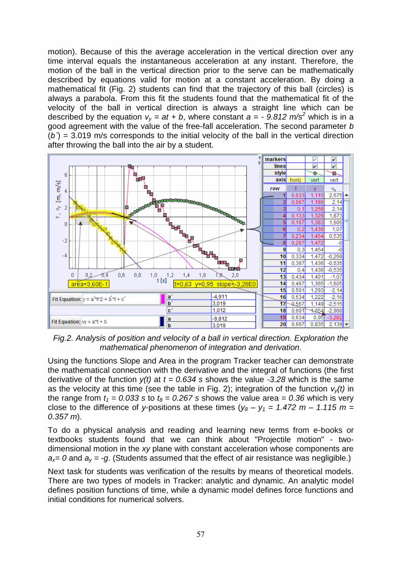
motion). Because of this the average acceleration in the vertical direction over any time interval equals the instantaneous acceleration at any instant. Therefore, the motion of the ball in the vertical direction prior to the serve can be mathematically described by equations valid for motion at a constant acceleration. By doing a mathematical fit (Fig. 2) students can find that the trajectory of this ball (circles) is always a parabola. From this fit the students found that the mathematical fit of the velocity of the ball in vertical direction is always a straight line which can be described by the equation vy = at + b, where constant a = - 9.812 m/s2 which is in a good agreement with the value of the free-fall acceleration. The second parameter b (b´) = 3.019 m/s corresponds to the initial velocity of the ball in the vertical direction after throwing the ball into the air by a student.

Fig.2. Analysis of position and velocity of a ball in vertical direction. Exploration the mathematical phenomenon of integration and derivation.

Using the functions Slope and Area in the program Tracker teacher can demonstrate the mathematical connection with the derivative and the integral of functions (the first derivative of the function y(t) at t = 0.634 s shows the value -3.28 which is the same as the velocity at this time (see the table in Fig. 2); integration of the function vy(t) in the range from t1 = 0.033 s to t8 = 0.267 s shows the value area = 0.36 which is very close to the difference of y-positions at these times (y8 – y1 = 1.472 m – 1.115 m = 0.357 m).

To do a physical analysis and reading and learning new terms from e-books or textbooks students found that we can think about "Projectile motion" - two-dimensional motion in the xy plane with constant acceleration whose components are ax= 0 and ay = -g. (Students assumed that the effect of air resistance was negligible.)

Next task for students was verification of the results by means of theoretical models. There are two types of models in Tracker: analytic and dynamic. An analytic model defines position functions of time, while a dynamic model defines force functions and initial conditions for numerical solvers.

57

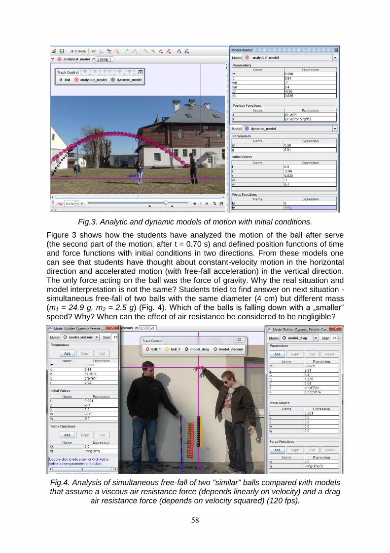
Fig.3. Analytic and dynamic models of motion with initial conditions.

Figure 3 shows how the students have analyzed the motion of the ball after serve (the second part of the motion, after t = 0.70 s) and defined position functions of time and force functions with initial conditions in two directions. From these models one can see that students have thought about constant-velocity motion in the horizontal direction and accelerated motion (with free-fall acceleration) in the vertical direction. The only force acting on the ball was the force of gravity. Why the real situation and model interpretation is not the same? Students tried to find answer on next situation - simultaneous free-fall of two balls with the same diameter (4 cm) but different mass (m1 = 24.9 g, m2 = 2.5 g) (Fig. 4). Which of the balls is falling down with a „smaller“ speed? Why? When can the effect of air resistance be considered to be negligible?

Fig.4. Analysis of simultaneous free-fall of two "similar" balls compared with models that assume a viscous air resistance force (depends linearly on velocity) and a drag

air resistance force (depends on velocity squared) (120 fps).

58

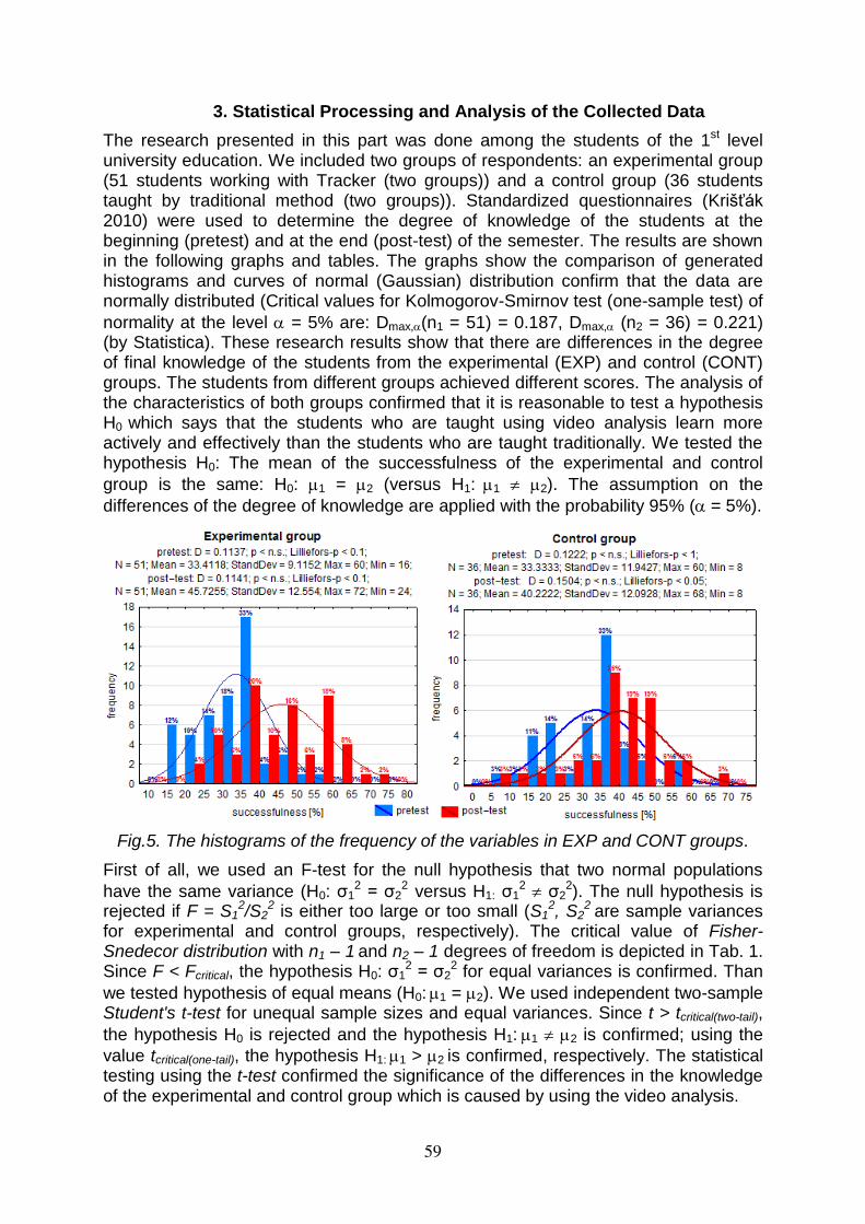
3. Statistical Processing and Analysis of the Collected Data

The research presented in this part was done among the students of the 1st level university education. We included two groups of respondents: an experimental group (51 students working with Tracker (two groups)) and a control group (36 students taught by traditional method (two groups)). Standardized questionnaires (Krišťák 2010) were used to determine the degree of knowledge of the students at the beginning (pretest) and at the end (post-test) of the semester. The results are shown in the following graphs and tables. The graphs show the comparison of generated histograms and curves of normal (Gaussian) distribution confirm that the data are normally distributed (Critical values for Kolmogorov-Smirnov test (one-sample test) of

normality at the level = 5% are: Dmax,(n1 = 51) = 0.187, Dmax, (n2 = 36) = 0.221) (by Statistica). These research results show that there are differences in the degree of final knowledge of the students from the experimental (EXP) and control (CONT) groups. The students from different groups achieved different scores. The analysis of the characteristics of both groups confirmed that it is reasonable to test a hypothesis H0 which says that the students who are taught using video analysis learn more actively and effectively than the students who are taught traditionally. We tested the hypothesis H0: The mean of the successfulness of the experimental and control

group is the same: H0: 1 = 2 (versus H1: 1 2). The assumption on the

differences of the degree of knowledge are applied with the probability 95% ( = 5%).

Fig.5. The histograms of the frequency of the variables in EXP and CONT groups.

First of all, we used an F-test for the null hypothesis that two normal populations

have the same variance (H0: σ12 = σ2

2 versus H1: σ12 σ2

2). The null hypothesis is rejected if F = S1

2/S22 is either too large or too small (S1

2, S22 are sample variances

for experimental and control groups, respectively). The critical value of Fisher-Snedecor distribution with n1 – 1 and n2 – 1 degrees of freedom is depicted in Tab. 1. Since F < Fcritical, the hypothesis H0: σ1

2 = σ22 for equal variances is confirmed. Than

we tested hypothesis of equal means (H0: 1 = 2). We used independent two-sample Student's t-test for unequal sample sizes and equal variances. Since t > tcritical(two-tail),

the hypothesis H0 is rejected and the hypothesis H1: 1 2 is confirmed; using the

value tcritical(one-tail), the hypothesis H1: 1 > 2 is confirmed, respectively. The statistical testing using the t-test confirmed the significance of the differences in the knowledge of the experimental and control group which is caused by using the video analysis.

59

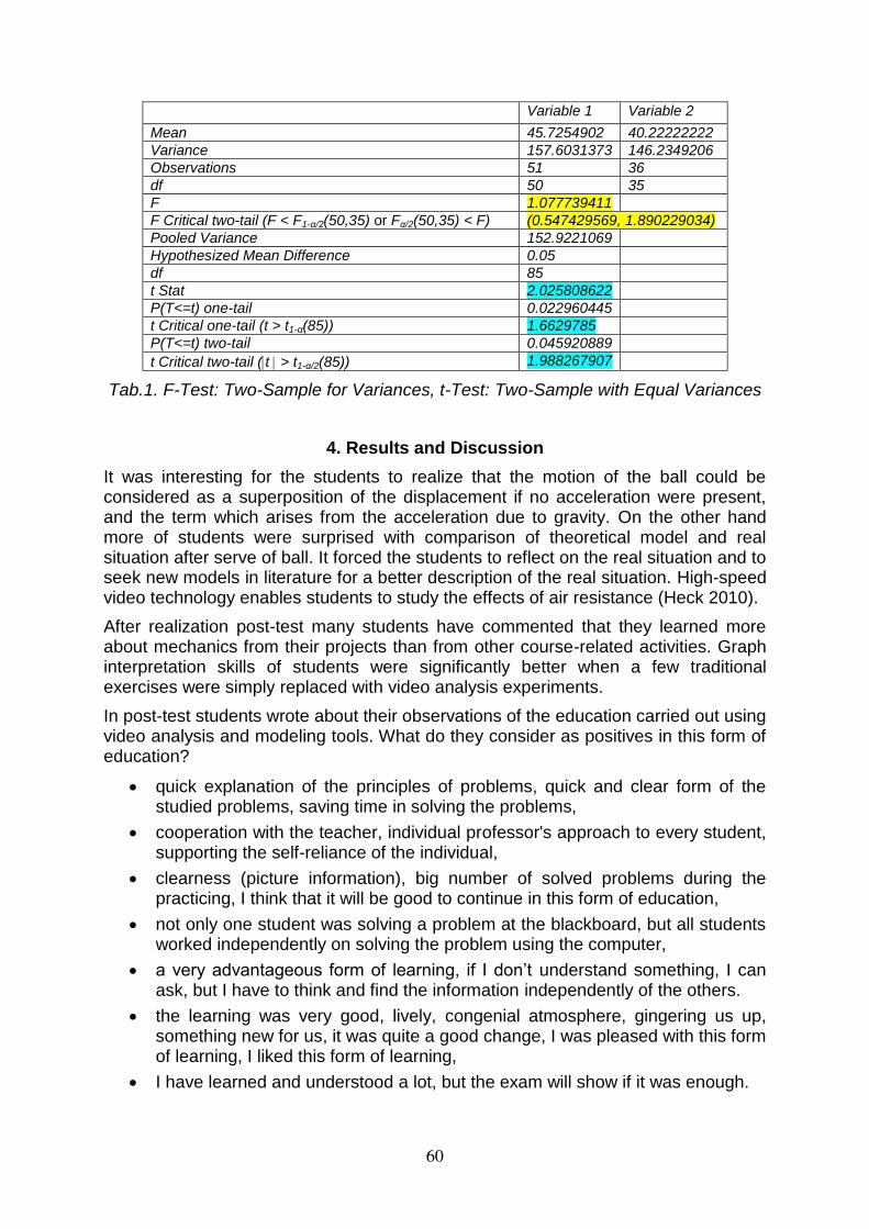
Variable 1 Variable 2

Mean 45.7254902 40.22222222

Variance 157.6031373 146.2349206

Observations 51 36

df 50 35

F 1.077739411

F Critical two-tail (F < F1-α/2(50,35) or Fα/2(50,35) < F) (0.547429569, 1.890229034)

Pooled Variance 152.9221069

Hypothesized Mean Difference 0.05

df 85

t Stat 2.025808622

P(T<=t) one-tail 0.022960445

t Critical one-tail (t > t1-α(85)) 1.6629785

P(T<=t) two-tail 0.045920889

t Critical two-tail (t > t1-α/2(85)) 1.988267907

Tab.1. F-Test: Two-Sample for Variances, t-Test: Two-Sample with Equal Variances

4. Results and Discussion

It was interesting for the students to realize that the motion of the ball could be considered as a superposition of the displacement if no acceleration were present, and the term which arises from the acceleration due to gravity. On the other hand more of students were surprised with comparison of theoretical model and real situation after serve of ball. It forced the students to reflect on the real situation and to seek new models in literature for a better description of the real situation. High-speed video technology enables students to study the effects of air resistance (Heck 2010).

After realization post-test many students have commented that they learned more about mechanics from their projects than from other course-related activities. Graph interpretation skills of students were significantly better when a few traditional exercises were simply replaced with video analysis experiments.

In post-test students wrote about their observations of the education carried out using video analysis and modeling tools. What do they consider as positives in this form of education?

quick explanation of the principles of problems, quick and clear form of the studied problems, saving time in solving the problems,

cooperation with the teacher, individual professor's approach to every student, supporting the self-reliance of the individual,

clearness (picture information), big number of solved problems during the practicing, I think that it will be good to continue in this form of education,

not only one student was solving a problem at the blackboard, but all students worked independently on solving the problem using the computer,

a very advantageous form of learning, if I don’t understand something, I can ask, but I have to think and find the information independently of the others.

the learning was very good, lively, congenial atmosphere, gingering us up, something new for us, it was quite a good change, I was pleased with this form of learning, I liked this form of learning,

I have learned and understood a lot, but the exam will show if it was enough.

60

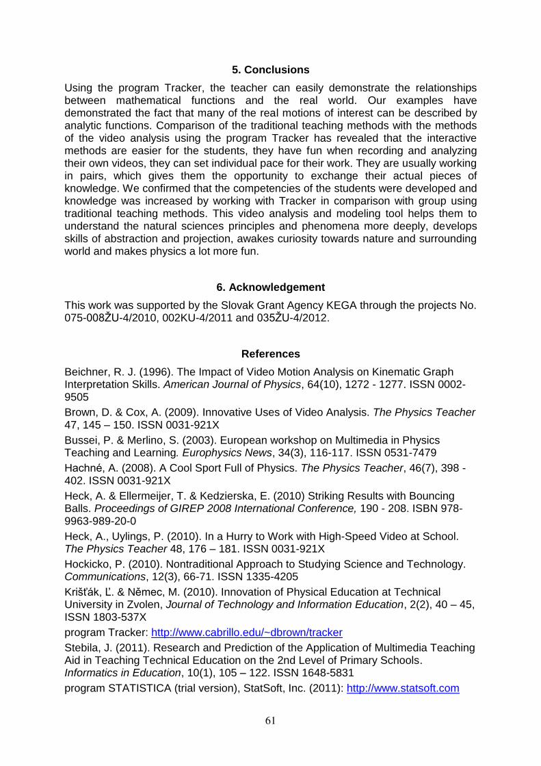
5. Conclusions

Using the program Tracker, the teacher can easily demonstrate the relationships between mathematical functions and the real world. Our examples have demonstrated the fact that many of the real motions of interest can be described by analytic functions. Comparison of the traditional teaching methods with the methods of the video analysis using the program Tracker has revealed that the interactive methods are easier for the students, they have fun when recording and analyzing their own videos, they can set individual pace for their work. They are usually working in pairs, which gives them the opportunity to exchange their actual pieces of knowledge. We confirmed that the competencies of the students were developed and knowledge was increased by working with Tracker in comparison with group using traditional teaching methods. This video analysis and modeling tool helps them to understand the natural sciences principles and phenomena more deeply, develops skills of abstraction and projection, awakes curiosity towards nature and surrounding world and makes physics a lot more fun.

6. Acknowledgement

This work was supported by the Slovak Grant Agency KEGA through the projects No. 075-008ŽU-4/2010, 002KU-4/2011 and 035ŽU-4/2012.

References

Beichner, R. J. (1996). The Impact of Video Motion Analysis on Kinematic Graph Interpretation Skills. American Journal of Physics, 64(10), 1272 - 1277. ISSN 0002-9505

Brown, D. & Cox, A. (2009). Innovative Uses of Video Analysis. The Physics Teacher 47, 145 – 150. ISSN 0031-921X

Bussei, P. & Merlino, S. (2003). European workshop on Multimedia in Physics Teaching and Learning. Europhysics News, 34(3), 116-117. ISSN 0531-7479

Hachné, A. (2008). A Cool Sport Full of Physics. The Physics Teacher, 46(7), 398 - 402. ISSN 0031-921X

Heck, A. & Ellermeijer, T. & Kedzierska, E. (2010) Striking Results with Bouncing Balls. Proceedings of GIREP 2008 International Conference, 190 - 208. ISBN 978-9963-989-20-0

Heck, A., Uylings, P. (2010). In a Hurry to Work with High-Speed Video at School. The Physics Teacher 48, 176 – 181. ISSN 0031-921X

Hockicko, P. (2010). Nontraditional Approach to Studying Science and Technology. Communications, 12(3), 66-71. ISSN 1335-4205

Krišťák, Ľ. & Němec, M. (2010). Innovation of Physical Education at Technical University in Zvolen, Journal of Technology and Information Education, 2(2), 40 – 45, ISSN 1803-537X

program Tracker: http://www.cabrillo.edu/~dbrown/tracker

Stebila, J. (2011). Research and Prediction of the Application of Multimedia Teaching Aid in Teaching Technical Education on the 2nd Level of Primary Schools. Informatics in Education, 10(1), 105 – 122. ISSN 1648-5831

program STATISTICA (trial version), StatSoft, Inc. (2011): http://www.statsoft.com

61

A novel approach to determining induced voltage

Katarina Jeličić1, Gorazd Planinšič2 and Maja Planinić3

katarinajelicic@gmail.com

1Ph.D. student, Faculty of Mathematics and Physics, University of Ljubljana, Slovenia

2Faculty of Mathematics and Physics, University of Ljubljana, Slovenia and

3Faculty of Science, University of Zagreb, Croatia

Abstract

High school students in Croatia and Slovenia have difficulties with determining induced voltage when wire loops enter or exit magnetic fields. We proposed and tested a new technique for determining induced voltage in wire loops of various shapes. The technique uses a simple tool, accessible to every teacher, made from transparent foil and paper. We implemented a quasi-experimental design (using both pre-test and post-test, without a control group) and tested the new tool and corresponding problem-solving technique on 78 high school students in Croatia who already learned about electromagnetic induction. Students were tested a week before participating in a workshop where they were taught how to determine induced voltage using the tool proposed here. A week after the workshop they were post-tested. We found that 32% of students benefited from the exercise and showed improvement in understanding when and how voltage is induced in wire loops. Tools like this may help students in transition from concrete to formal thinking when solving problems related to more abstract physical phenomena, such as magnetic induction.

1. Introduction

For better conceptual understanding of physical concepts, students need effective and applicable tools to help them apply basic concepts in solving physics problems.

In mechanics, such tools are motion and body diagrams, energy bars etc. But when it comes to magnetism and electromagnetic induction, the number of available problem-solving tools accessible to students drops significantly. In order to determine

induced voltage in a wire loop, when it is entering or exiting the magnetic field, students need to make several steps that require different tasks of different cognitive demand: determine the shape of the loop, determine the direction of the magnetic

field, estimate the time dependence of magnetic flux and finally perform mathematical procedures necessary to calculate induced voltage.

1. Problem statement

In Croatia and Slovenia, a high school student who wants to enroll to university needs to take the national exam (called matura) at the end of their high school

education. Matura consists of required and elective subjects. Physics is one of the elective subjects often chosen by high school students. We noticed that Slovene students taking the matura exam in physics have difficulties with assignments that

ask them to determine induced voltage or current direction in wire loops moving through magnetic fields. An example of such matura question (Slovenian National Examinations Centre, 2006) is shown in Figure 1. The majority of students (59%)

answered that question incorrectly. Answer B was the most commonly chosen distracter (34%). Questions of this sort appear every year and systematically show students’ difficulties.

62

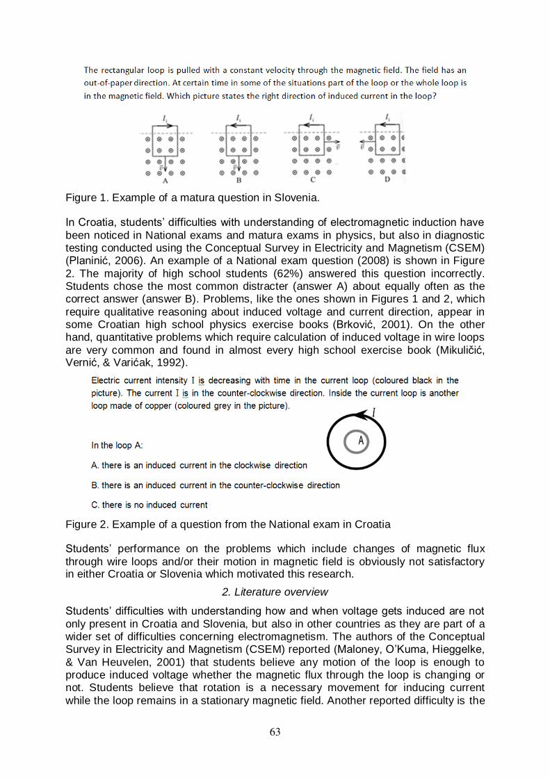
Figure 1. Example of a matura question in Slovenia.

In Croatia, students’ difficulties with understanding of electromagnetic induction have

been noticed in National exams and matura exams in physics, but also in diagnostic testing conducted using the Conceptual Survey in Electricity and Magnetism (CSEM) (Planinić, 2006). An example of a National exam question (2008) is shown in Figure

2. The majority of high school students (62%) answered this question incorrectly. Students chose the most common distracter (answer A) about equally often as the correct answer (answer B). Problems, like the ones shown in Figures 1 and 2, which

require qualitative reasoning about induced voltage and current direction, appear in some Croatian high school physics exercise books (Brković, 2001). On the other hand, quantitative problems which require calculation of induced voltage in wire loops

are very common and found in almost every high school exercise book (Mikuličić, Vernić, & Varićak, 1992).

Figure 2. Example of a question from the National exam in Croatia

Students’ performance on the problems which include changes of magnetic flux

through wire loops and/or their motion in magnetic field is obviously not satisfactory in either Croatia or Slovenia which motivated this research.

2. Literature overview

Students’ difficulties with understanding how and when voltage gets induced are not

only present in Croatia and Slovenia, but also in other countries as they are part of a wider set of difficulties concerning electromagnetism. The authors of the Conceptual Survey in Electricity and Magnetism (CSEM) reported (Maloney, O’Kuma, Hieggelke,

& Van Heuvelen, 2001) that students believe any motion of the loop is enough to produce induced voltage whether the magnetic flux through the loop is changing or not. Students believe that rotation is a necessary movement for inducing current

while the loop remains in a stationary magnetic field. Another reported difficulty is the

63

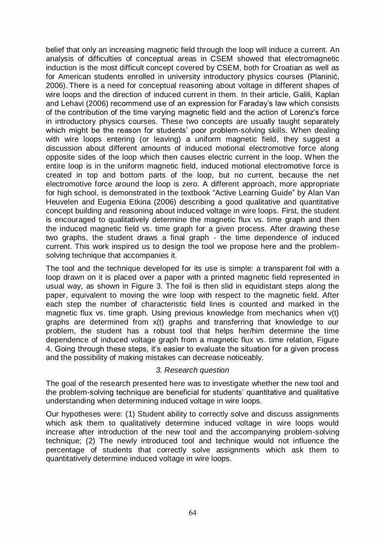
belief that only an increasing magnetic field through the loop will induce a current. An analysis of difficulties of conceptual areas in CSEM showed that electromagnetic

induction is the most difficult concept covered by CSEM, both for Croatian as well as for American students enrolled in university introductory physics courses (Planinić, 2006). There is a need for conceptual reasoning about voltage in different shapes of

wire loops and the direction of induced current in them. In their article, Galili, Kaplan and Lehavi (2006) recommend use of an expression for Faraday’s law which consists of the contribution of the time varying magnetic field and the action of Lorenz’s force

in introductory physics courses. These two concepts are usually taught separately which might be the reason for students’ poor problem-solving skills. When dealing with wire loops entering (or leaving) a uniform magnetic field, they suggest a

discussion about different amounts of induced motional electromotive force along opposite sides of the loop which then causes electric current in the loop. When the entire loop is in the uniform magnetic field, induced motional electromotive force is

created in top and bottom parts of the loop, but no current, because the net electromotive force around the loop is zero. A different approach, more appropriate for high school, is demonstrated in the textbook “Active Learning Guide” by Alan Van

Heuvelen and Eugenia Etkina (2006) describing a good qualitative and quantitative concept building and reasoning about induced voltage in wire loops. First, the student is encouraged to qualitatively determine the magnetic flux vs. time graph and then

the induced magnetic field vs. time graph for a given process. After drawing these two graphs, the student draws a final graph - the time dependence of induced current. This work inspired us to design the tool we propose here and the problem-solving technique that accompanies it.

The tool and the technique developed for its use is simple: a transparent foil with a loop drawn on it is placed over a paper with a printed magnetic field represented in usual way, as shown in Figure 3. The foil is then slid in equidistant steps along the

paper, equivalent to moving the wire loop with respect to the magnetic field. After each step the number of characteristic field lines is counted and marked in the magnetic flux vs. time graph. Using previous knowledge from mechanics when v(t)

graphs are determined from x(t) graphs and transferring that knowledge to our problem, the student has a robust tool that helps her/him determine the time dependence of induced voltage graph from a magnetic flux vs. time relation, Figure

4. Going through these steps, it’s easier to evaluate the situation for a given process and the possibility of making mistakes can decrease noticeably.

3. Research question

The goal of the research presented here was to investigate whether the new tool and the problem-solving technique are beneficial for students’ quantitative and qualitative understanding when determining induced voltage in wire loops.

Our hypotheses were: (1) Student ability to correctly solve and discuss assignments

which ask them to qualitatively determine induced voltage in wire loops would increase after introduction of the new tool and the accompanying problem-solving technique; (2) The newly introduced tool and technique would not influence the

percentage of students that correctly solve assignments which ask them to quantitatively determine induced voltage in wire loops.

64

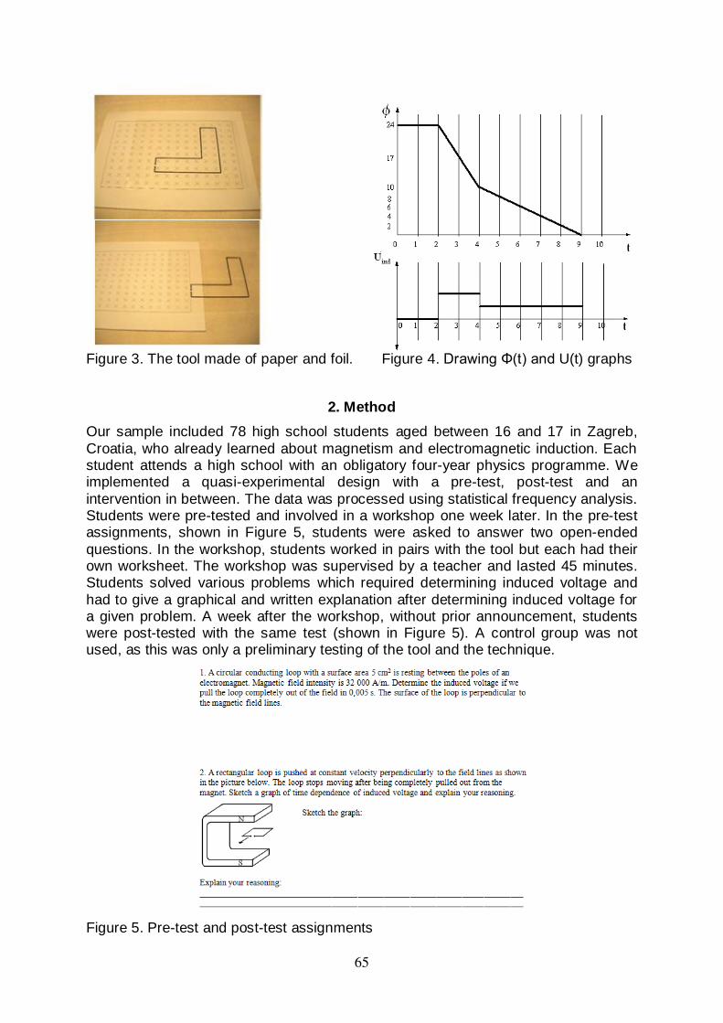
Figure 3. The tool made of paper and foil. Figure 4. Drawing Φ(t) and U(t) graphs

2. Method

Our sample included 78 high school students aged between 16 and 17 in Zagreb,

Croatia, who already learned about magnetism and electromagnetic induction. Each student attends a high school with an obligatory four-year physics programme. We implemented a quasi-experimental design with a pre-test, post-test and an

intervention in between. The data was processed using statistical frequency analysis. Students were pre-tested and involved in a workshop one week later. In the pre-test assignments, shown in Figure 5, students were asked to answer two open-ended

questions. In the workshop, students worked in pairs with the tool but each had their own worksheet. The workshop was supervised by a teacher and lasted 45 minutes. Students solved various problems which required determining induced voltage and

had to give a graphical and written explanation after determining induced voltage for a given problem. A week after the workshop, without prior announcement, students were post-tested with the same test (shown in Figure 5). A control group was not used, as this was only a preliminary testing of the tool and the technique.

Figure 5. Pre-test and post-test assignments

65

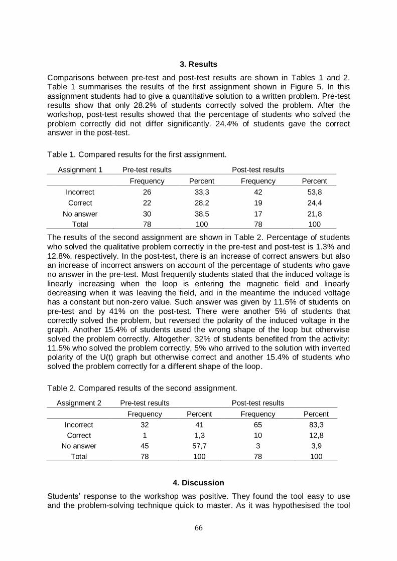
3. Results

Comparisons between pre-test and post-test results are shown in Tables 1 and 2. Table 1 summarises the results of the first assignment shown in Figure 5. In this

assignment students had to give a quantitative solution to a written problem. Pre-test results show that only 28.2% of students correctly solved the problem. After the workshop, post-test results showed that the percentage of students who solved the

problem correctly did not differ significantly. 24.4% of students gave the correct answer in the post-test.

Table 1. Compared results for the first assignment.

Assignment 1 Pre-test results Post-test results

Frequency Percent Frequency Percent

Incorrect 26 33,3 42 53,8

Correct 22 28,2 19 24,4

No answer 30 38,5 17 21,8

Total 78 100 78 100

The results of the second assignment are shown in Table 2. Percentage of students

who solved the qualitative problem correctly in the pre-test and post-test is 1.3% and

12.8%, respectively. In the post-test, there is an increase of correct answers but also an increase of incorrect answers on account of the percentage of students who gave no answer in the pre-test. Most frequently students stated that the induced voltage is

linearly increasing when the loop is entering the magnetic field and linearly decreasing when it was leaving the field, and in the meantime the induced voltage has a constant but non-zero value. Such answer was given by 11.5% of students on

pre-test and by 41% on the post-test. There were another 5% of students that correctly solved the problem, but reversed the polarity of the induced voltage in the graph. Another 15.4% of students used the wrong shape of the loop but otherwise

solved the problem correctly. Altogether, 32% of students benefited from the activity: 11.5% who solved the problem correctly, 5% who arrived to the solution with inverted polarity of the U(t) graph but otherwise correct and another 15.4% of students who solved the problem correctly for a different shape of the loop.

Table 2. Compared results of the second assignment.

Assignment 2 Pre-test results Post-test results

Frequency Percent Frequency Percent

Incorrect 32 41 65 83,3

Correct 1 1,3 10 12,8

No answer 45 57,7 3 3,9

Total 78 100 78 100

4. Discussion

Students’ response to the workshop was positive. They found the tool easy to use and the problem-solving technique quick to master. As it was hypothesised the tool

66

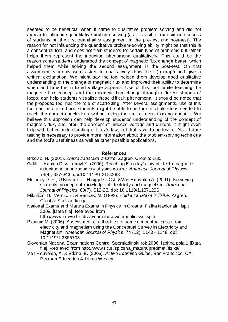
seemed to be beneficial when it came to qualitative problem solving and did not appear to influence quantitative problem solving (as it is visible from similar success

of students on the first quantitative assignment in the pre-test and post-test). The reason for not influencing the quantitative problem-solving ability might be that this is a conceptual tool, and does not train students for certain type of problems but rather

helps them represent the induction phenomena qualitatively. This could be the reason some students understood the concept of magnetic flux change better, which helped them while solving the second assignment in the post-test. On that

assignment students were asked to qualitatively draw the U(t) graph and give a written explanation. We might say the tool helped them develop good qualitative understanding of the change of magnetic flux and improved their ability to determine

when and how the induced voltage appears. Use of this tool, while teaching the magnetic flux concept and the magnetic flux change through different shapes of loops, can help students visualise these difficult phenomena. It should be noted that

the proposed tool has the role of scaffolding. After several assignments, use of this tool can be omitted and students might be able to perform multiple steps needed to reach the correct conclusions without using the tool or even thinking about it. We

believe this approach can help develop students’ understanding of the concept of magnetic flux, and later, the concept of induced voltage and current. It might even help with better understanding of Lenz’s law, but that is yet to be tested. Also, future

testing is necessary to provide more information about the problem-solving technique and the tool’s usefulness as well as other possible applications.

References

Brković, N. (2001). Zbirka zadataka iz fizike, Zagreb, Croatia: Luk.

Galili I., Kaplan D. & Lehavi Y. (2006). Teaching Faraday’s law of electromagnetic induction in an introductory physics course. American Journal of Physics,

74(4), 337-343. doi:10.1119/1.2180283 Maloney D. P., O’Kuma T.L., Hieggelke C.J. &Van Heuvelen A. (2001). Surveying

students’ conceptual knowledge of electricity and magnetism. American

Journal of Physics, 69(7), S12-23. doi: 10.1119/1.1371296 Mikuličić, B., Vernić, E. & Varićak, M. (1992). Zbirka zadataka iz fizike, Zagreb,

Croatia: Skolska knjiga.

National Exams and Matura Exams in Physics in Croatia. Fizika Nacionalni ispit 2008. [Data file]. Retrieved from http://www.ncvvo.hr./drzavnamatura/web/public/svi_ispiti

Planinić M. (2006). Assessment of difficulties of some conceptual areas from

electricity and magnetism using the Conceptual Survey in Electricity and Magnetism, American Journal of Physics, 74 (12), 1143 - 1148. doi:

10.1119/1.2366733

Slovenian National Examinations Centre. Spomladinski rok 2006. Izpitna pola 1 [Data file]. Retrieved from http://www.ric.si/splosna_matura/predmeti/fizika/

Van Heuvelen, A. & Etkina, E. (2006). Active Learning Guide, San Francisco, CA:

Pearson Education Addison Wesley.

67

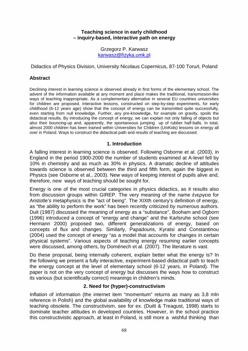
Teaching science in early childhood – inquiry-based, interactive path on energy

Grzegorz P. Karwasz

karwasz@fizyka.umk.pl

Didactics of Physics Division, University Nicolaus Copernicus, 87-100 Toruń, Poland Abstract

Declining interest in learning science is observed already in first forms of the elementary school. The advent of the information available at any moment and place makes the traditional, transmission-like ways of teaching inappropriate. As a complementary alternative in several EU countries universities for children are proposed. Interactive lessons, constructed on step-by-step experiments, for early childhood (6-12 years age) show that the concept of energy can be transmitted quite successfully, even starting from null knowledge. Further, any pre-knowledge, for example on gravity, spoils the didactical results. By introducing the concept of energy, we can explain not only falling of objects but also their bouncing-up and, apparently, the spontaneous jumping up of rubber half-balls. In total, almost 2000 children has been trained within Universities for Children (UniKids) lessons on energy all over in Poland. Ways to construct the didactical path and results of teaching are discussed.

1. Introduction

A falling interest in learning science is observed. Following Osborne et al. (2003), in England in the period 1900-2000 the number of students examined at A-level fell by 10% in chemistry and as much as 30% in physics. A dramatic decline of attitudes towards science is observed between the third and fifth form, again the biggest in Physics (see Osborne et al., 2003). New ways of keeping interest of pupils alive and, therefore, new ways of teaching should be sought for.

Energy is one of the most crucial categories in physics didactics, as it results also from discussion groups within GIREP. The very meaning of the name ένεργεια for Aristotle’s metaphysics is the “act of being”. The XIXth century’s definition of energy, as “the ability to perform the work” has been recently criticized by numerous authors. Duit (1987) discussed the meaning of energy as a “substance”, Booham and Ogborn (1996) introduced a concept of “energy and change” and the Karlsruhe school (see Hermann 2000) proposed two, different generalizations of energy, based on concepts of flux and changes. Similarly, Papadouris, Kyratsi and Constantinou (2004) used the concept of energy “as a model that accounts for changes in certain physical systems”. Various aspects of teaching energy resuming earlier concepts were discussed, among others, by Doménech et al. (2007). The literature is vast.

Do these proposal, being internally coherent, explain better what the energy is? In the following we present a fully interactive, experiment-based didactical path to teach the energy concept at the level of elementary school (6-12 years, in Poland). The paper is not on the very concept of energy but discusses the ways how to construct its various (but scientifically correct) meanings in children’s minds.

2. Need for (hyper)-constructivism

Inflation of information (the internet item “momentum” returns as many as 3,8 mln reference in Polish) and the global availability of knowledge make traditional ways of teaching obsolete. The constructivism, see for ex. (Duitt & Treagust, 1998) starts to dominate teacher attitudes in developed countries. However, in the school practice this constructivistic approach, at least in Poland, is still more a wishful thinking than

68

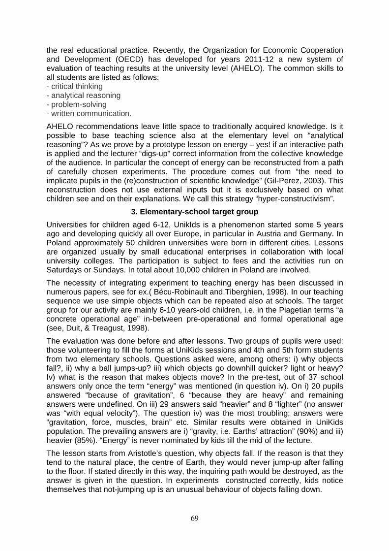
the real educational practice. Recently, the Organization for Economic Cooperation and Development (OECD) has developed for years 2011-12 a new system of evaluation of teaching results at the university level (AHELO). The common skills to all students are listed as follows: - critical thinking - analytical reasoning - problem-solving - written communication.

AHELO recommendations leave little space to traditionally acquired knowledge. Is it possible to base teaching science also at the elementary level on “analytical reasoning”? As we prove by a prototype lesson on energy – yes! if an interactive path is applied and the lecturer “digs-up” correct information from the collective knowledge of the audience. In particular the concept of energy can be reconstructed from a path of carefully chosen experiments. The procedure comes out from “the need to implicate pupils in the (re)construction of scientific knowledge” (Gil-Perez, 2003). This reconstruction does not use external inputs but it is exclusively based on what children see and on their explanations. We call this strategy “hyper-constructivism”.

3. Elementary-school target group

Universities for children aged 6-12, UnikIds is a phenomenon started some 5 years ago and developing quickly all over Europe, in particular in Austria and Germany. In Poland approximately 50 children universities were born in different cities. Lessons are organized usually by small educational enterprises in collaboration with local university colleges. The participation is subject to fees and the activities run on Saturdays or Sundays. In total about 10,000 children in Poland are involved.

The necessity of integrating experiment to teaching energy has been discussed in numerous papers, see for ex.( Bécu-Robinault and Tiberghien, 1998). In our teaching sequence we use simple objects which can be repeated also at schools. The target group for our activity are mainly 6-10 years-old children, i.e. in the Piagetian terms “a concrete operational age” in-between pre-operational and formal operational age (see, Duit, & Treagust, 1998).

The evaluation was done before and after lessons. Two groups of pupils were used: those volunteering to fill the forms at UniKids sessions and 4th and 5th form students from two elementary schools. Questions asked were, among others: i) why objects fall?, ii) why a ball jumps-up? iii) which objects go downhill quicker? light or heavy? Iv) what is the reason that makes objects move? In the pre-test, out of 37 school answers only once the term “energy” was mentioned (in question iv). On i) 20 pupils answered “because of gravitation”, 6 “because they are heavy” and remaining answers were undefined. On iii) 29 answers said “heavier” and 8 “lighter” (no answer was “with equal velocity”). The question iv) was the most troubling; answers were “gravitation, force, muscles, brain” etc. Similar results were obtained in UniKids population. The prevailing answers are i) “gravity, i.e. Earths’ attraction” (90%) and iii) heavier (85%). “Energy” is never nominated by kids till the mid of the lecture.

The lesson starts from Aristotle’s question, why objects fall. If the reason is that they tend to the natural place, the centre of Earth, they would never jump-up after falling to the floor. If stated directly in this way, the inquiring path would be destroyed, as the answer is given in the question. In experiments constructed correctly, kids notice themselves that not-jumping up is an unusual behaviour of objects falling down.

69

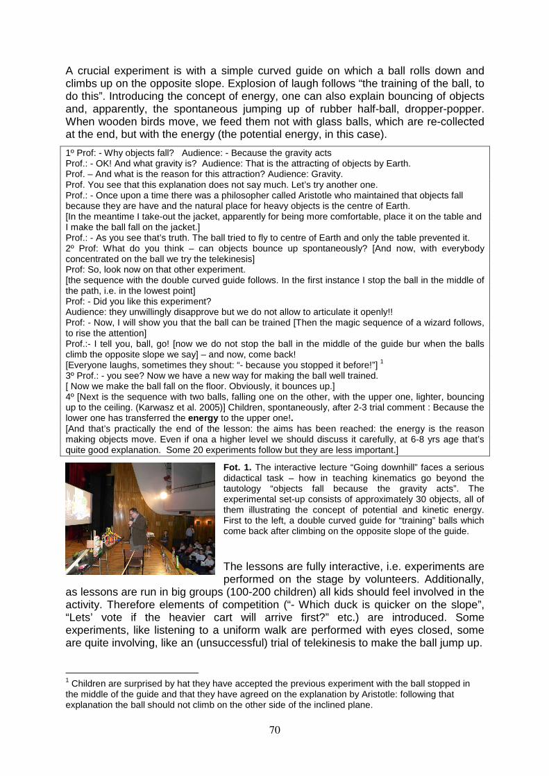
A crucial experiment is with a simple curved guide on which a ball rolls down and climbs up on the opposite slope. Explosion of laugh follows “the training of the ball, to do this”. Introducing the concept of energy, one can also explain bouncing of objects and, apparently, the spontaneous jumping up of rubber half-ball, dropper-popper. When wooden birds move, we feed them not with glass balls, which are re-collected at the end, but with the energy (the potential energy, in this case).

1º Prof: - Why objects fall? Audience: - Because the gravity acts Prof.: - OK! And what gravity is? Audience: That is the attracting of objects by Earth. Prof. – And what is the reason for this attraction? Audience: Gravity. Prof. You see that this explanation does not say much. Let’s try another one. Prof.: - Once upon a time there was a philosopher called Aristotle who maintained that objects fall because they are have and the natural place for heavy objects is the centre of Earth. [In the meantime I take-out the jacket, apparently for being more comfortable, place it on the table and I make the ball fall on the jacket.] Prof.: - As you see that’s truth. The ball tried to fly to centre of Earth and only the table prevented it. 2º Prof: What do you think – can objects bounce up spontaneously? [And now, with everybody concentrated on the ball we try the telekinesis] Prof: So, look now on that other experiment. [the sequence with the double curved guide follows. In the first instance I stop the ball in the middle of the path, i.e. in the lowest point] Prof: - Did you like this experiment? Audience: they unwillingly disapprove but we do not allow to articulate it openly!! Prof: - Now, I will show you that the ball can be trained [Then the magic sequence of a wizard follows, to rise the attention] Prof.:- I tell you, ball, go! [now we do not stop the ball in the middle of the guide bur when the balls climb the opposite slope we say] – and now, come back! [Everyone laughs, sometimes they shout: “- because you stopped it before!”] 1 3º Prof.: - you see? Now we have a new way for making the ball well trained. [ Now we make the ball fall on the floor. Obviously, it bounces up.] 4º [Next is the sequence with two balls, falling one on the other, with the upper one, lighter, bouncing up to the ceiling. (Karwasz et al. 2005)] Children, spontaneously, after 2-3 trial comment : Because the lower one has transferred the energy to the upper one!. [And that’s practically the end of the lesson: the aims has been reached: the energy is the reason making objects move. Even if ona a higher level we should discuss it carefully, at 6-8 yrs age that’s quite good explanation. Some 20 experiments follow but they are less important.]

Fot. 1. The interactive lecture “Going downhill” faces a serious didactical task – how in teaching kinematics go beyond the tautology “objects fall because the gravity acts”. The experimental set-up consists of approximately 30 objects, all of them illustrating the concept of potential and kinetic energy. First to the left, a double curved guide for “training” balls which come back after climbing on the opposite slope of the guide.

The lessons are fully interactive, i.e. experiments are performed on the stage by volunteers. Additionally,

as lessons are run in big groups (100-200 children) all kids should feel involved in the activity. Therefore elements of competition (“- Which duck is quicker on the slope”, “Lets’ vote if the heavier cart will arrive first?” etc.) are introduced. Some experiments, like listening to a uniform walk are performed with eyes closed, some are quite involving, like an (unsuccessful) trial of telekinesis to make the ball jump up.

1 Children are surprised by hat they have accepted the previous experiment with the ball stopped in the middle of the guide and that they have agreed on the explanation by Aristotle: following that explanation the ball should not climb on the other side of the inclined plane.

70

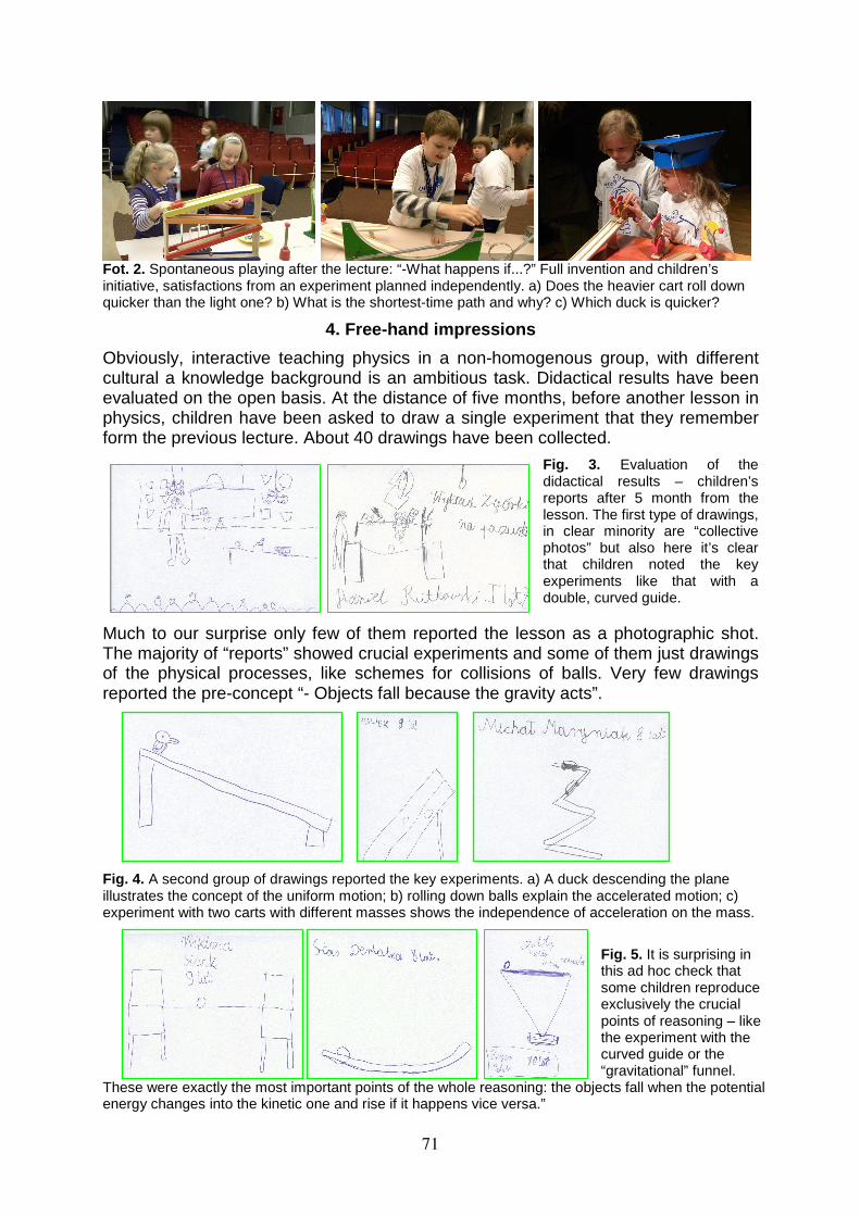
Fot. 2. Spontaneous playing after the lecture: “-What happens if...?” Full invention and children’s initiative, satisfactions from an experiment planned independently. a) Does the heavier cart roll down quicker than the light one? b) What is the shortest-time path and why? c) Which duck is quicker?

4. Free-hand impressions

Obviously, interactive teaching physics in a non-homogenous group, with different cultural a knowledge background is an ambitious task. Didactical results have been evaluated on the open basis. At the distance of five months, before another lesson in physics, children have been asked to draw a single experiment that they remember form the previous lecture. About 40 drawings have been collected.

Fig. 3. Evaluation of the didactical results – children’s reports after 5 month from the lesson. The first type of drawings, in clear minority are “collective photos” but also here it’s clear that children noted the key experiments like that with a double, curved guide.

Much to our surprise only few of them reported the lesson as a photographic shot. The majority of “reports” showed crucial experiments and some of them just drawings of the physical processes, like schemes for collisions of balls. Very few drawings reported the pre-concept “- Objects fall because the gravity acts”.

Fig. 4. A second group of drawings reported the key experiments. a) A duck descending the plane illustrates the concept of the uniform motion; b) rolling down balls explain the accelerated motion; c) experiment with two carts with different masses shows the independence of acceleration on the mass.

Fig. 5. It is surprising in this ad hoc check that some children reproduce exclusively the crucial points of reasoning – like the experiment with the curved guide or the “gravitational” funnel.

These were exactly the most important points of the whole reasoning: the objects fall when the potential energy changes into the kinetic one and rise if it happens vice versa.”

71

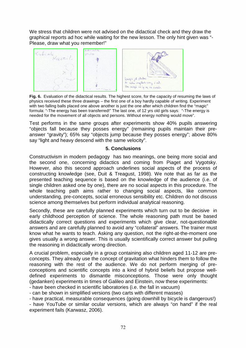
We stress that children were not advised on the didactical check and they draw the graphical reports ad hoc while waiting for the new lesson. The only hint given was “-Please, draw what you remember!”

Fig. 6. Evaluation of the didactical results. The highest score, for the capacity of resuming the laws of physics received these three drawings – the first one of a boy hardly capable of writing. Experiment with two falling balls placed one above another is just the one after which children find the “magic” formula: “-The energy has been transferred!” The last one, of 12 yrs old girls says: “-The energy is needed for the movement of all objects and persons. Without energy nothing would move”.

Test performs in the same groups after experiments show 40% pupils answering “objects fall because they posses energy” (remaining pupils maintain their pre-answer “gravity”); 65% say “objects jump because they posses energy”; above 80% say “light and heavy descend with the same velocity”.

5. Conclusions

Constructivism in modern pedagogy has two meanings, one being more social and the second one, concerning didactics and coming from Piaget and Vygotsky. However, also this second approach underlines social aspects of the process of constructing knowledge (see, Duit & Treagust, 1998). We note that as far as the presented teaching sequence is based on the knowledge of the audience (i.e. of single children asked one by one), there are no social aspects in this procedure. The whole teaching path aims rather to changing social aspects, like common understanding, pre-concepts, social erroneous sensibility etc. Children do not discuss science among themselves but perform individual analytical reasoning.

Secondly, these are carefully planned experiments which turn out to be decisive in early childhood perception of science. The whole reasoning path must be based didactically correct questions and experiments which give clear, not-questionable answers and are carefully planned to avoid any “collateral” answers. The trainer must know what he wants to teach. Asking any question, not the right-at-the-moment one gives usually a wrong answer. This is usually scientifically correct answer but pulling the reasoning in didactically wrong direction.

A crucial problem, especially in a group containing also children aged 11-12 are pre-concepts. They already use the concept of gravitation what hinders them to follow the reasoning with the rest of the audience. We do not perform merging of pre-conceptions and scientific concepts into a kind of hybrid beliefs but propose well-defined experiments to dismantle misconceptions. Those were only thought (gedanken) experiments in times of Galileo and Einstein, now these experiments: - have been checked in scientific laboratories (i.e. the fall in vacuum) - can be shown in simplified versions (two carts with different masses) - have practical, measurable consequences (going downhill by bicycle is dangerous!) - have YouTube or similar ocular versions, which are always “on hand” if the real experiment fails (Karwasz, 2006).

72

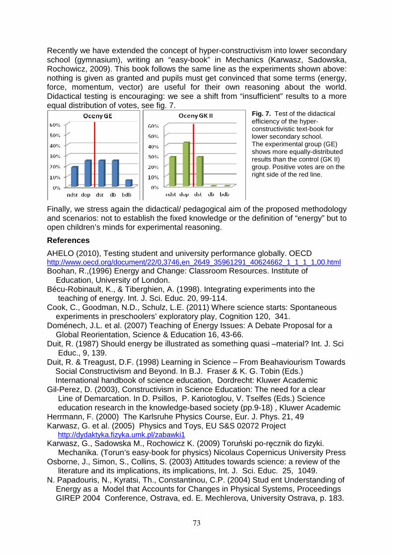
Recently we have extended the concept of hyper-constructivism into lower secondary school (gymnasium), writing an “easy-book” in Mechanics (Karwasz, Sadowska, Rochowicz, 2009). This book follows the same line as the experiments shown above: nothing is given as granted and pupils must get convinced that some terms (energy, force, momentum, vector) are useful for their own reasoning about the world. Didactical testing is encouraging: we see a shift from “insufficient” results to a more equal distribution of votes, see fig. 7.

Fig. 7. Test of the didactical efficiency of the hyper-constructivistic text-book for lower secondary school. The experimental group (GE) shows more equally-distributed results than the control (GK II) group. Positive votes are on the right side of the red line.

Finally, we stress again the didactical/ pedagogical aim of the proposed methodology and scenarios: not to establish the fixed knowledge or the definition of “energy” but to open children’s minds for experimental reasoning.

References

AHELO (2010), Testing student and university performance globally. OECD http://www.oecd.org/document/22/0,3746,en_2649_35961291_40624662_1_1_1_1,00.html Boohan, R.,(1996) Energy and Change: Classroom Resources. Institute of Education, University of London. Bécu-Robinault, K., & Tiberghien, A. (1998). Integrating experiments into the teaching of energy. Int. J. Sci. Educ. 20, 99-114. Cook, C., Goodman, N.D., Schulz, L.E. (2011) Where science starts: Spontaneous experiments in preschoolers’ exploratory play, Cognition 120, 341. Doménech, J.L. et al. (2007) Teaching of Energy Issues: A Debate Proposal for a Global Reorientation, Science & Education 16, 43-66. Duit, R. (1987) Should energy be illustrated as something quasi –material? Int. J. Sci Educ., 9, 139. Duit, R. & Treagust, D.F. (1998) Learning in Science – From Beahaviourism Towards

Social Constructivism and Beyond. In B.J. Fraser & K. G. Tobin (Eds.) International handbook of science education, Dordrecht: Kluwer Academic

Gil-Perez, D. (2003), Constructivism in Science Education: The need for a clear Line of Demarcation. In D. Psillos, P. Kariotoglou, V. Tselfes (Eds.) Science education research in the knowledge-based society (pp.9-18) , Kluwer Academic Herrmann, F. (2000) The Karlsruhe Physics Course, Eur. J. Phys. 21, 49 Karwasz, G. et al. (2005) Physics and Toys, EU S&S 02072 Project http://dydaktyka.fizyka.umk.pl/zabawki1 Karwasz, G., Sadowska M., Rochowicz K. (2009) Toruński po-ręcznik do fizyki. Mechanika. (Torun’s easy-book for physics) Nicolaus Copernicus University Press Osborne, J., Simon, S., Collins, S. (2003) Attitudes towards science: a review of the literature and its implications, its implications, Int. J. Sci. Educ. 25, 1049. N. Papadouris, N., Kyratsi, Th., Constantinou, C.P. (2004) Stud ent Understanding of Energy as a Model that Accounts for Changes in Physical Systems, Proceedings GIREP 2004 Conference, Ostrava, ed. E. Mechlerova, University Ostrava, p. 183.

73

University students’ difficulties in a tutorial featuring two source interference

Mikko Kesonen, Mervi A. Asikainen, and Pekka E. Hirvonen

mikko.kesonen@uef.fi

Department of Physics and Mathematics, University of Eastern Finland, Finland

Tutorials in Introductory Physics provides research-based instructional materials that have demonstrably improved students’ understanding of physics. Nevertheless, it requires special arrangements such as small classroom sessions with two instructors. In this study, we designed a 90-minute multi-phased tutorial intervention for a lecture hall environment on the topic of two source interference. Fifty-nine students participated in the intervention succeeding lecture-based instruction during a course of Basic Physics IV at the University of Eastern Finland. During the intervention we investigated the effectiveness of tutorial tasks by posing paper-and-pencil test questions both before and after the tutorial tasks. The test questions consisted of snapshot pictures of a web animation that were essentially different from the graphical representation of the tutorial tasks and the tasks used previously in the course. The results show that the number of correct answers to the test questions increased after completion of the tutorial tasks. However, the students still had difficulties in linking the different representations and applying the concepts of path length difference and phase difference. Consequently, the tutorial should emphasize different representations in order to help students to achieve a more robust understanding.

Introduction

In recent years, systematic research in the field of Physics Education Research (PER) has uncovered a gap between learning objectives and students’ learning achievements after traditional lecture-based instruction (McDermott, 1991). To reduce the gap, researchers have identified common difficulties experienced by students that have created a basis for developing new instructional materials and methods. One of them is Tutorials in Introductory Physics (tutorials) developed by PER Group at the University of Washington (McDermott et al. 2003; 2010a; 2010b). Each tutorial involves four steps: pre-test, worksheets, homework, and post-test. These steps are intended to support the learning of a specific topic in introductory physics after the presentation of lectures.

The pre-test challenges students to apply their knowledge to novel situations that will inform instructors about the students’ learning achievements after attending lectures. Following the pre-test, the students participate in a tutorial session (50 min) where they work with carefully structured tutorial worksheets (4-6 pages). The session is held in a small classroom with 20-24 students working in groups of three or four under the guidance of two instructors. The worksheet includes qualitative tasks and hands-on experiments aimed at dividing the reasoning process into a step of precisely the right size for the students to stay actively involved. The instructors’ role is to support the students’ own thinking so that they will be able to deduce the correct answers themselves. Ideas that develop during the tutorial session are then reinforced by the tutorial homework, which approaches the topic from a slightly different angle that creates an environment for practicing the topic. The post-test questions are subsequently asked in a course exam and are used to evaluate the students’ progress as a result of the course.

In general, the tutorials supplement traditional instruction by providing these four steps, which promote the students’ active mental engagement in the process of learning physics. The tutorials have proved to be an effective way of improving students’ qualitative understanding of physics. In doing so, they also support students’ abilities to solve numerical problems and help them to link physics with real-life situations (McDermott, 2001).

74

Two source interference is a topic that has proven to be difficult for students to grasp. After the topic has been lectured on, students often fail to predict the areas of constructive and destructive interference by using equations rather than by applying the concept of path length difference (Knight, 2008b). Ambrose et al. (1999) have found that students confuse the concepts path length and path length difference and misunderstand the role played by the relative direction of the waves. The students typically predict that constructive interference occurs when the path length is a whole number of wavelengths (e.g. 300λ) or when the waves move in the same direction.

To overcome these difficulties, a tutorial named two source interference has been designed (Wosilait et al. 1999; see McDermott et al. 2010a, pp. 213-217). Earlier, the effectiveness of tutorials has been studied by comparing students’ pre- and post-test results when tutorials have been conducted in a small classroom (McDermott, 2001). Our aim in the present study is to widen this tradition by investigating the effectiveness of tutorial tasks undertaken in a lecture hall setting. Hence, we are looking for an answer to the following research question: How does students’ performance change as a result of tutorial tasks in the context of two source interference when the tutorial is conducted in a lecture hall? In answering this, we provide information on (1) how we undertook the tutorials in a lecture hall setting, (2) students’ performance before and after the tutorial tasks when the tasks were undertaken in such an environment, and (3) recommendations for developing the tutorial.

Context, intervention, and methods

The intervention was implemented in an introductory course, Basic Physics IV, during the spring semester 2011. The course covers the basics of waves, ray and wave optics, and modern physics, following the textbook by Randall Knight (2008a). The course itself consists of 40 lecture hours and 20 exercise hours. In the lectures the lecturer explains the content with the aid of PowerPoint slides and also highlights important points by providing handwritten examples, demonstrations, and stop-to-think questions. In the exercises, the course assistant and student volunteers present the correct solutions to the weekly homework assignments. The topic of two source interference was covered during lectures and exercises presented two weeks prior to the intervention itself.

A total of 59 students participated in the intervention, which was held in a lecture hall during a 90-minute lecture period. During the intervention the students worked on tutorial worksheets dealing with two source interference under the guidance of the lecturer and the assistant. The worksheets were divided into four sections1, with each section including a test question. When the students worked through a section, they first answered a test question, then performed the tutorial tasks, and finally answered the same test question again. Three out of the four sections were covered in 90 minutes. The present paper presents the results of the first two sections.

In order to elicit information about the students’ understanding, the test questions were presented in the context of a novel representation that had not been used previously either in the tutorial tasks or prior to the course. The test questions concerned snapshot pictures of a web animation2 showing the superposition of two circular waves, with the areas of constructive and destructive interference represented as they would appear in a real-life situation. This differed from the graphical representation of the two overlapping circular

1 Section 1, pp. 213-214, tasks II A-C; section 2, pp. 214-216, tasks II D-J; section 3, pp. 216 tasks III A;

section 4, pp. 217, tasks III B-C (McDermott, 2010a). 2 The animation can be found at http://ngsir.netfirms.com/englishhtm/Interference.htm

75

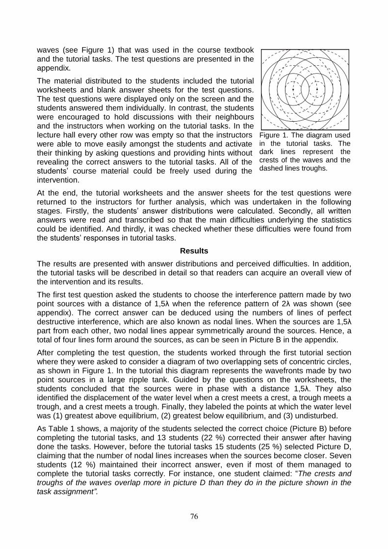
waves (see Figure 1) that was used in the course textbook and the tutorial tasks. The test questions are presented in the appendix.

The material distributed to the students included the tutorial worksheets and blank answer sheets for the test questions. The test questions were displayed only on the screen and the students answered them individually. In contrast, the students were encouraged to hold discussions with their neighbours and the instructors when working on the tutorial tasks. In the lecture hall every other row was empty so that the instructors were able to move easily amongst the students and activate their thinking by asking questions and providing hints without revealing the correct answers to the tutorial tasks. All of the students’ course material could be freely used during the intervention.

At the end, the tutorial worksheets and the answer sheets for the test questions were returned to the instructors for further analysis, which was undertaken in the following stages. Firstly, the students’ answer distributions were calculated. Secondly, all written answers were read and transcribed so that the main difficulties underlying the statistics could be identified. And thirdly, it was checked whether these difficulties were found from the students’ responses in tutorial tasks.

Results

The results are presented with answer distributions and perceived difficulties. In addition, the tutorial tasks will be described in detail so that readers can acquire an overall view of the intervention and its results.

The first test question asked the students to choose the interference pattern made by two point sources with a distance of 1,5λ when the reference pattern of 2λ was shown (see appendix). The correct answer can be deduced using the numbers of lines of perfect destructive interference, which are also known as nodal lines. When the sources are 1,5λ part from each other, two nodal lines appear symmetrically around the sources. Hence, a total of four lines form around the sources, as can be seen in Picture B in the appendix.

After completing the test question, the students worked through the first tutorial section where they were asked to consider a diagram of two overlapping sets of concentric circles, as shown in Figure 1. In the tutorial this diagram represents the wavefronts made by two point sources in a large ripple tank. Guided by the questions on the worksheets, the students concluded that the sources were in phase with a distance 1,5λ. They also identified the displacement of the water level when a crest meets a crest, a trough meets a trough, and a crest meets a trough. Finally, they labeled the points at which the water level was (1) greatest above equilibrium, (2) greatest below equilibrium, and (3) undisturbed.

As Table 1 shows, a majority of the students selected the correct choice (Picture B) before completing the tutorial tasks, and 13 students (22 %) corrected their answer after having done the tasks. However, before the tutorial tasks 15 students (25 %) selected Picture D, claiming that the number of nodal lines increases when the sources become closer. Seven students (12 %) maintained their incorrect answer, even if most of them managed to complete the tutorial tasks correctly. For instance, one student claimed: “The crests and troughs of the waves overlap more in picture D than they do in the picture shown in the task assignment”.

Figure 1. The diagram used in the tutorial tasks. The dark lines represent the crests of the waves and the dashed lines troughs.

76

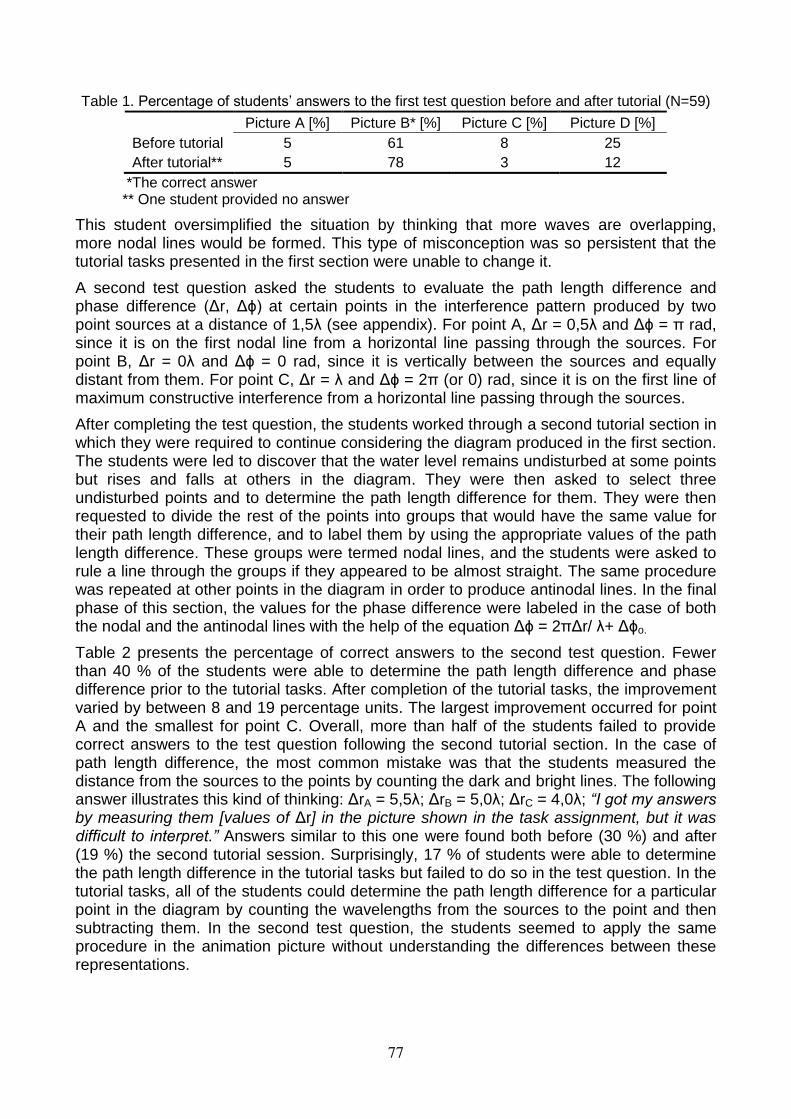
Table 1. Percentage of students’ answers to the first test question before and after tutorial (N=59)

Picture A [%] Picture B* [%] Picture C [%] Picture D [%]

Before tutorial 5 61 8 25

After tutorial** 5 78 3 12

*The correct answer ** One student provided no answer

This student oversimplified the situation by thinking that more waves are overlapping, more nodal lines would be formed. This type of misconception was so persistent that the tutorial tasks presented in the first section were unable to change it.

A second test question asked the students to evaluate the path length difference and phase difference (Δr, Δϕ) at certain points in the interference pattern produced by two point sources at a distance of 1,5λ (see appendix). For point A, Δr = 0,5λ and Δϕ = π rad, since it is on the first nodal line from a horizontal line passing through the sources. For point B, Δr = 0λ and Δϕ = 0 rad, since it is vertically between the sources and equally distant from them. For point C, Δr = λ and Δϕ = 2π (or 0) rad, since it is on the first line of maximum constructive interference from a horizontal line passing through the sources.

After completing the test question, the students worked through a second tutorial section in which they were required to continue considering the diagram produced in the first section. The students were led to discover that the water level remains undisturbed at some points but rises and falls at others in the diagram. They were then asked to select three undisturbed points and to determine the path length difference for them. They were then requested to divide the rest of the points into groups that would have the same value for their path length difference, and to label them by using the appropriate values of the path length difference. These groups were termed nodal lines, and the students were asked to rule a line through the groups if they appeared to be almost straight. The same procedure was repeated at other points in the diagram in order to produce antinodal lines. In the final phase of this section, the values for the phase difference were labeled in the case of both the nodal and the antinodal lines with the help of the equation Δϕ = 2πΔr/ λ+ Δϕo.

Table 2 presents the percentage of correct answers to the second test question. Fewer than 40 % of the students were able to determine the path length difference and phase difference prior to the tutorial tasks. After completion of the tutorial tasks, the improvement varied by between 8 and 19 percentage units. The largest improvement occurred for point A and the smallest for point C. Overall, more than half of the students failed to provide correct answers to the test question following the second tutorial section. In the case of path length difference, the most common mistake was that the students measured the distance from the sources to the points by counting the dark and bright lines. The following answer illustrates this kind of thinking: ΔrA = 5,5λ; ΔrB = 5,0λ; ΔrC = 4,0λ; “I got my answers by measuring them [values of Δr] in the picture shown in the task assignment, but it was difficult to interpret.” Answers similar to this one were found both before (30 %) and after (19 %) the second tutorial session. Surprisingly, 17 % of students were able to determine the path length difference in the tutorial tasks but failed to do so in the test question. In the tutorial tasks, all of the students could determine the path length difference for a particular point in the diagram by counting the wavelengths from the sources to the point and then subtracting them. In the second test question, the students seemed to apply the same procedure in the animation picture without understanding the differences between these representations.

77

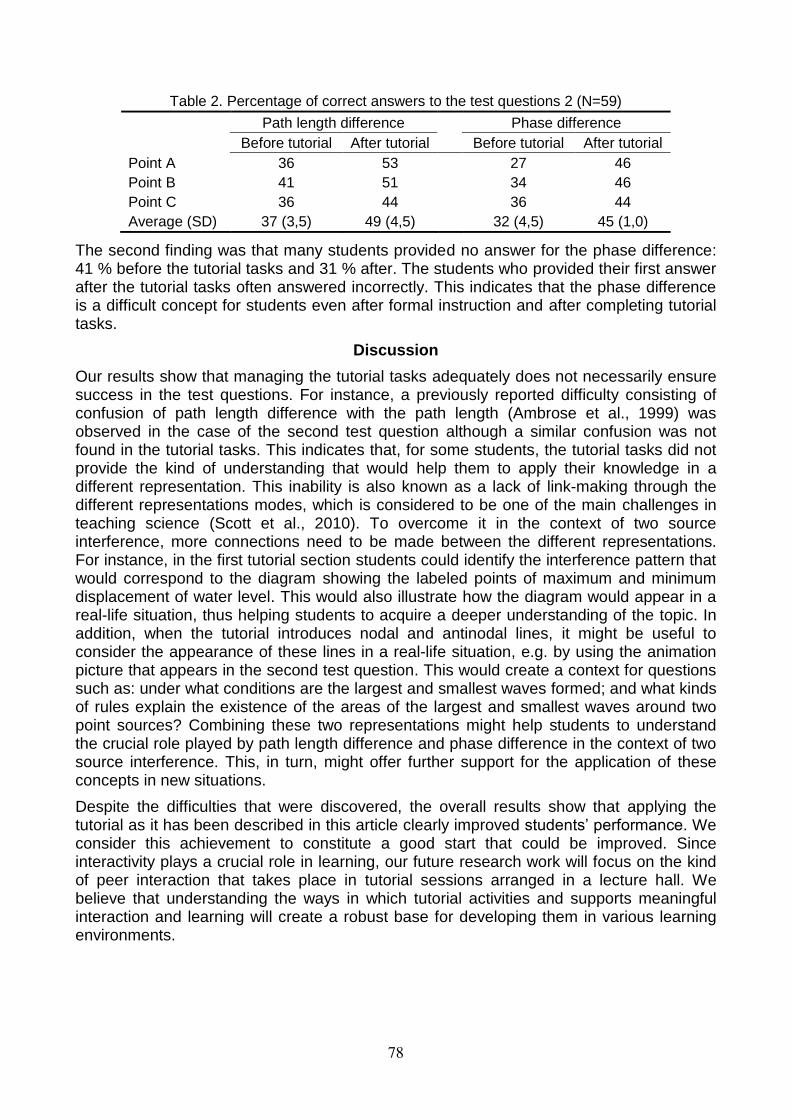
Table 2. Percentage of correct answers to the test questions 2 (N=59)

Path length difference Phase difference

Before tutorial After tutorial Before tutorial After tutorial

Point A 36 53 27 46

Point B 41 51 34 46

Point C 36 44 36 44

Average (SD) 37 (3,5) 49 (4,5) 32 (4,5) 45 (1,0)

The second finding was that many students provided no answer for the phase difference: 41 % before the tutorial tasks and 31 % after. The students who provided their first answer after the tutorial tasks often answered incorrectly. This indicates that the phase difference is a difficult concept for students even after formal instruction and after completing tutorial tasks.

Discussion

Our results show that managing the tutorial tasks adequately does not necessarily ensure success in the test questions. For instance, a previously reported difficulty consisting of confusion of path length difference with the path length (Ambrose et al., 1999) was observed in the case of the second test question although a similar confusion was not found in the tutorial tasks. This indicates that, for some students, the tutorial tasks did not provide the kind of understanding that would help them to apply their knowledge in a different representation. This inability is also known as a lack of link-making through the different representations modes, which is considered to be one of the main challenges in teaching science (Scott et al., 2010). To overcome it in the context of two source interference, more connections need to be made between the different representations. For instance, in the first tutorial section students could identify the interference pattern that would correspond to the diagram showing the labeled points of maximum and minimum displacement of water level. This would also illustrate how the diagram would appear in a real-life situation, thus helping students to acquire a deeper understanding of the topic. In addition, when the tutorial introduces nodal and antinodal lines, it might be useful to consider the appearance of these lines in a real-life situation, e.g. by using the animation picture that appears in the second test question. This would create a context for questions such as: under what conditions are the largest and smallest waves formed; and what kinds of rules explain the existence of the areas of the largest and smallest waves around two point sources? Combining these two representations might help students to understand the crucial role played by path length difference and phase difference in the context of two source interference. This, in turn, might offer further support for the application of these concepts in new situations.

Despite the difficulties that were discovered, the overall results show that applying the tutorial as it has been described in this article clearly improved students’ performance. We consider this achievement to constitute a good start that could be improved. Since interactivity plays a crucial role in learning, our future research work will focus on the kind of peer interaction that takes place in tutorial sessions arranged in a lecture hall. We believe that understanding the ways in which tutorial activities and supports meaningful interaction and learning will create a robust base for developing them in various learning environments.

78

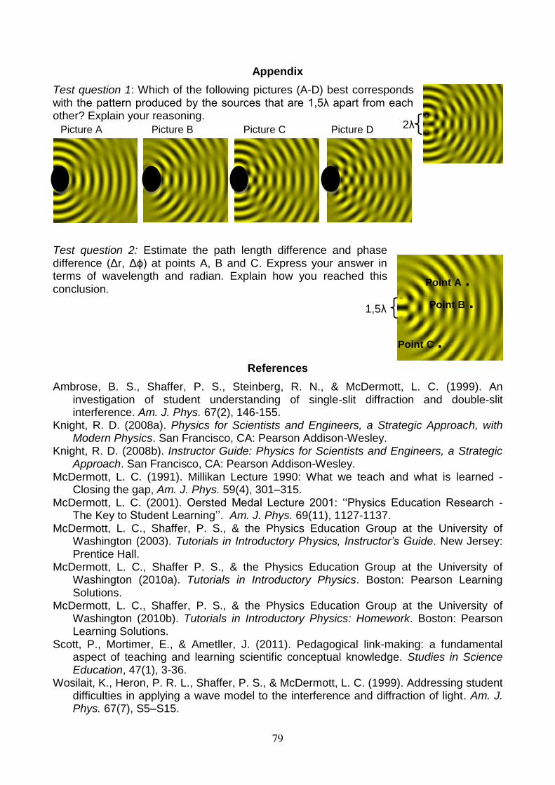
Appendix

Test question 1: Which of the following pictures (A-D) best corresponds with the pattern produced by the sources that are 1,5λ apart from each other? Explain your reasoning.

Test question 2: Estimate the path length difference and phase difference (Δr, Δϕ) at points A, B and C. Express your answer in terms of wavelength and radian. Explain how you reached this conclusion.

References

Ambrose, B. S., Shaffer, P. S., Steinberg, R. N., & McDermott, L. C. (1999). An investigation of student understanding of single-slit diffraction and double-slit interference. Am. J. Phys. 67(2), 146-155.

Knight, R. D. (2008a). Physics for Scientists and Engineers, a Strategic Approach, with Modern Physics. San Francisco, CA: Pearson Addison-Wesley.

Knight, R. D. (2008b). Instructor Guide: Physics for Scientists and Engineers, a Strategic Approach. San Francisco, CA: Pearson Addison-Wesley.

McDermott, L. C. (1991). Millikan Lecture 1990: What we teach and what is learned -Closing the gap, Am. J. Phys. 59(4), 301–315.

McDermott, L. C. (2001). Oersted Medal Lecture 2001: ‘‘Physics Education Research - The Key to Student Learning’’. Am. J. Phys. 69(11), 1127-1137.

McDermott, L. C., Shaffer, P. S., & the Physics Education Group at the University of Washington (2003). Tutorials in Introductory Physics, Instructor’s Guide. New Jersey: Prentice Hall.

McDermott, L. C., Shaffer P. S., & the Physics Education Group at the University of Washington (2010a). Tutorials in Introductory Physics. Boston: Pearson Learning Solutions.

McDermott, L. C., Shaffer, P. S., & the Physics Education Group at the University of Washington (2010b). Tutorials in Introductory Physics: Homework. Boston: Pearson Learning Solutions.

Scott, P., Mortimer, E., & Ametller, J. (2011). Pedagogical link-making: a fundamental aspect of teaching and learning scientific conceptual knowledge. Studies in Science Education, 47(1), 3-36.

Wosilait, K., Heron, P. R. L., Shaffer, P. S., & McDermott, L. C. (1999). Addressing student difficulties in applying a wave model to the interference and diffraction of light. Am. J. Phys. 67(7), S5–S15.

Picture B 2λ Picture A Picture C Picture D

1,5λ

Point A .

Point B .

Point C .

79

Research-based strategies for illustrating the nanoscale in an exhibition

Antti Laherto Department of Physics, University of Helsinki, Finland

antti.laherto@helsinki.fi

Abstract: While the fields of nanoscience and nanotechnology (NST) are advancing rapidly and raising their societal significance, general public’s awareness of these fields has remained at a low level. It has frequently been argued that the public understanding of NST should be enhanced to facilitate informed decision-making and science-technology-society dialogue on these emerging fields. Informal learning environments such as exhibitions in museums and science centres have a potential to respond to these demands. The study presented here lays some groundwork for research-based development of a nanoscience exhibition by mapping the educational, communicational and museological challenges related to nanoscale science. Potential visitors’ perspectives were analysed by reviewing educational research literature on teaching and learning the nanoscale concepts, and by interviewing science centre visitors. On the basis of the results, the study suggests several strategies for illustrating nanoscale science in an exhibition: ways of supporting visitors’ scale conception, presenting images and visualisations deliberately, and using scale models and macroscopic analogies.

Introduction

The fields of nanoscience and nanotechnology (NST) are developing rapidly, and being connected to several prospects of societally and environmentally significant applications and implications. These emerging fields have also gained growing public interest and media attention. However, and perhaps paradoxically, results of several surveys and polls have shown that despite the public’s interest in and somewhat positive attitudes towards NST, people’s awareness and knowledge of the fields has remained at a very low level (Crone, 2010). This state of affairs has aroused some concerns, since it is likely that in the near future citizens have to make more and more decisions on NST-related issues – both at the personal level, as consumers, and also at the societal level, regarding the future paths of NST (Baird, Nordmann, & Schummer, 2004). Informal learning environments such as exhibitions in museums and science centres have been suggested to have a significant potential not only to educate the public about NST but also to contribute to the science-technology-society dialogue (Castellini et al., 2007; Crone, 2010; Zenner & Crone, 2008).

This paper is a part of a research project that creates a design framework (Edelson, 2002) for the development of an exhibition on NST. The purpose of the project is to analyse the fields of NST from an educational perspective in order to find well-grounded approaches for exhibition design. The focus of this paper is not on the applications and implications of nanotechnology but specifically on the challenges related to the scientific understanding of “the nanoscale”. The term here refers not only to measurement units but essentially also to its objects and phenomena, the tools with which the nanoscale (or the “nanoworld”) can be accessed, and the models that describe the phenomena at that scale (cf. Stevens, Sutherland, & Krajcik, 2009).

Size and scale are only a few of the several educationally significant features of NST – in fact, it can be argued that the most essential ideas involve scale only indirectly. However, since the scale and the smallness of 'nano-objects' pose several

80

communicational and museographic challenges regarding exhibition development, they are worth focusing on in this study.

Methods

First, a literature review was carried out, involving educational research on teaching and learning the nanoscale concepts, including e.g. studies on typical learning difficulties related to this content, and studies on visitors’ learning in nanoscience exhibitions. Only a quite limited amount of such research has been published, so it was not problematic to demarcate the literature to be analysed. A few common themes clearly emerged from the literature, and the analysis focused on them.

The empirical part consisted of a survey in order to get a grasp of potential visitors’ perspectives on NST. The survey was conducted in the form of a standardized open-ended interview (Patton, 1990). The beginning of the interview aimed to find out the level of awareness the respondent has about NST. Since the public awareness on these emerging fields was presumed to be quite low, in the latter part of the interview some descriptions were given to respondents in order to help them ponder on the meanings of NST. Furthermore, the survey also aimed at learning about the specific communicational challenges related to the use of visualisations of nanoscale objects. To that end, an image and a video were shown to the respondents together with some explanations and questions.

Interviews were carried out in the lobby of the Finnish science centre Heureka. The interviewees were randomly picked among the adult visitors. The interviews took about ten minutes in average, including the filling-in of the background questionnaire. The number of the interviewees was 28. Age of the respondents varied from 20 to 62 years, with a quite even distribution. Educational background varied from secondary school to the academic level. A great majority (93%) were at least “quite interested” in both science and technology, as it was anticipated concerning science centre visitors.

The interviewees’ responses were analysed by identifying a few answer categories per each question and categorizing respondents’ answers in those categories (Patton, 1990). Due to the small sample, no strong generalizations can be made concerning the general public or even the visitors of the science centre. Together with the results of the literature analysis the results, however, are useful in getting a tentative insight into the potential visitors’ awareness and interest regarding NST, and some idea of the communicational challenges concerning the nanoscale issues.

Results

Literature analysis

The analysis of literature on NST teaching and learning showed that various studies have quite coherently pointed out certain challenges in understanding the nanoscale and its concepts.

Several studies have shown that people of all ages have major problems in understanding the scale of NST (Castellini et al., 2007; Tretter, Jones, Andre, Negishi, & Minogue, 2006). In their study on students’ (of various ages) and experts’ understanding of size and scale of objects, Tretter et al. (2006) conclude (not surprisingly) that students tend to have most problems in scales from which they do not have direct experiences, especially microscopic and sub-microscopic scales.

81

However, the size conceptualisation seems to be easier using relative comparisons than absolute sizes. Also, size landmarks, or points of reference, seem to be an important tool for anchoring conceptions of spatial scale (Tretter, 2008).

Besides the fact that the scale itself is difficult to comprehend, an additional challenge in NST communication rises because the public does not have a good grasp of the terminology and concepts regarding atoms and molecules and lack knowledge of the atomic structure of matter (Crone, 2010). It is common to conceptualize matter as being continuous rather than particulate. Children use the terms "atom", "molecule", "cell" very ambiguously, and have a lot of misconceptions (Murriello, Contier, & Knobel, 2009). Additionally, students tend to use “scaling” erraneously (and this may be made worse by using macroscopic models of nanoscale phenomena) and assume that atoms/molecules have the same properties as the macroscopic substance they are part of.

Since the behaviour of nanoscale particles is governed by quantum effects, discussing it in proper terms requires highly sophisticated concepts. This certainly poses educational challenges and risks of generating misconceptions (Sabelli et al., 2005). Careless simplification of the sophisticated concepts of NST, especially in quantum mechanics, leads to superficiality and risk of misrepresenting.

In order to learn about the NST-related learning challenges that are specific to exhibitions, publications concerning nano-exhibitions were also searched for to be included in the literature analysis. While several exhibitions on the topics of NST have been launched in recent years in museums and science centres all over the world, there are only a few publications reporting experiences of those projects from an educational viewpoint. When discussing the Brazilian NanoAventura exhibition, Murriello, Contier and Knobel (2009) stress that the most important museographic and communicational challenge in designing exhibits on NST relates to the fact that the objects the fields are based on are invisible to naked eye. Exactly same notion is stated also in evaluation of It’s a Nanoworld, a travelling exhibition on NST funded by National Science Foundation in the U.S. (Batt, Waldron, & Trautmann, 2004). While NanoAventura solved the dilemma of displaying nano-objects in an exhibition by using computer games and virtual representations, It’s a Nanoworld employed concrete macroscopic models and analogies. In the following, these two approaches among some others are discussed.

Visitor survey

The results of survey supported many of the aforementioned findings of the literature analysis.

Almost all the respondents (96%) had heard or read at least something about nanoscience and nanotechnology, the mass media (newspapers, television and popular science magazines) being the most important sources of information. When asked about their conception of the meaning of “nanoscience and nanotechnology”, 71% of the respondents coupled the terms with some kind of “smallness”. Every fourth interviewee even mentioned the level of atoms or molecules here. On the other hand, 50% of the respondents associated NST with new technological products, e.g. faster computers, stronger materials and tiny robots.

As the visitor survey was expected to give an additional insight into the communicational challenges discussed in the literature analysis, the questions

82

regarding visitors’ perception of the scanning tunneling microscope image1 were of special interest. Firstly, without any explanation the respondents were asked to interpret what is depicted in the image. Only 25% of the interviewees named any nanoscale objects (molecules, atoms etc.), whereas most of the respondents associated the image with either macroscopic objects (35%) such as “an island” or “a waterdrop” or microscopic objects (29%) such as “a cell”. After the respondents were told that there is a ring of iron atoms on a copper surface and the diameter of the ring is ca. 7 nanometre, 25% of the respondents knew that the image is created with an electron microscope, whereas 36% suggested that it is made by computer modeling, without experimental instruments. After that, the interviewer told that it is a STM image, briefly explained the operating principle of STM, and then asked the respondent to say something about the iron atoms or the copper surface. Even after this attempt for a contextualization, most of the respondents (57%) came up with false, macroscopic conclusions about the image, for example suggesting that the copper surface is “rough”, “soft” or “jelly-like”, or that the iron atoms are “sharp” or “rusty”, or that “iron is warmer than copper”. Still, many respondents reached fully proper conclusions about the nanostructure, stating e.g. that iron atoms are of equal size and symmetric, or that it is possible to manipulate matter on atomic scale.

Also these results bring out that discussing the nanoscale and its phenomena seems like a natural and necessary starting point for the exhibition, although the potential visitors are probably interested in nanotechnological applications too. Special attention is needed when using visualizations of the nanoscale in order to convey the right epistemological ideas with them.

Implications: strategies for an exhibition

Here, on the basis of the above-reported results, some notions are suggested that could support illustrating nanoscale science in an exhibition.

Illustrating the continuum of scales & providing size landmarks

Because of the “smallness” of the nanoscale and its counterintuitive phenomena are very difficult to conceptualise, in education they should not be considered in isolation. Instead, an exhibition should guide visitors there by starting from the macroscopic scale, advancing through microscopic range and finally to the nanoscale. This kind of relative approach may help visitors to construct a continuum of scales and integrate their views of matter across scales. An effective way of displaying this continuum in an exhibition is a scale spectrum with carefully chosen anchoring objects as size landmarks from each scale (for an example of an illustrative scale continuum, see Tretter, 2008). Proportional reasoning can be employed by illustrations such as “if a football would be the size of the Earth, then a fullerene would be the size of a football”. Besides pictorial presentations, even more effective way of supporting scale conception is provided by the powers of 10 –videos, recommended e.g. by Tretter (2008), Castellini (2007) and Sabelli et al. (2005). However, if a visitor gets a grasp of the linear scale continuum from macroscopic world to the nanoscale, it does not yet mean that (s)he has some understanding of any key ideas of NST, such as size-dependent properties of matter. Still, that visitor has a good foundation on which (s)he can situate later insights of nanoscale objects and phenomena.

1 The image shown was of the “quantum corral”, available e.g. at http://www.almaden.ibm.com/vis/stm/.

83

Using images and visualisations

As discussed above, research has shown that personal experiences are essential in understanding scales. Since it is not possible to obtain direct experiences at the nanoscale, and quantum phenomena cannot be replicated at the macroscale, images, visualisations and simulations must be used instead. The power of visual representations in communicating NST is, of course, a double-edged sword. Public’s understanding of these images and the impact of images to public’s conceptions has been just recently became a research interest (e.g. Landau, Groscurth, Wright, & Condit, 2009). The risks of causing misconceptions has been noted by many (see e.g. Tretter, 2008). Oversimplified use of images in public communication of NST can mislead learners into false models of direct sense perception and epistemological misunderstandings (Baird et al., 2004). For example, it is questionable indeed what is “seeing atoms” by using a SEM or STM.

Using scale models and analogies to macroscopic objects

Another strategy for illustrating nanoscale objects in an exhibition is by using macroscopic scale models and analogies. They are popular in public communication of NST, especially in models of the structure of matter, as well as in macroscopic models of electron microscopy. These models and analogies are powerful in anchoring the issues in learner's everyday experiences. This is especially crucial in informal learning environments: because of the free-choice-learning nature of them, it is a necessity to address visitors’ needs and interests in an exhibition in order to gain any contact. Therefore, the macroscopic points of comparison should be chosen so that they are relevant to visitors.

Demonstrating nanoscale phenomena by using macroscopic analogies is tempting indeed. It should be noted, however, that they do not reflect the discontinuous change of properties at certain size, or any other quantum phenomena. Consequently, there is a major risk of causing misconceptions and, even, contradicting the major learning goal: properties of objects change discontinuously at certain size. Due to these concerns, this kind of exhibits should be evaluated before used in an exhibition in order to find out the potential misconceptions they may generate (cf. Sabelli et al., 2005).

Still, analogical models may be especially helpful in illuminating scaling effects (as suggested by Tretter et al., 2006). These effects mostly follow from the simple and classically understood way how a change in the size of an object affects the ratio of its surface area to volume. Macroscopic analogies may be useful in illustrating this: for an example, surface-area-to-volume experiments with different size pieces of ice to illustrate heat loss.

Accessing the nanoscale by instruments

Instead of drawing solely on visualisations and macroscopic analogies, it is both useful and possible to provide visitors with a “real” access to nanoscale phenomena by using e.g. a scanning tunnelling microscope (STM) or an atomic force microscope (AFM) (suggested also by Sabelli et al., 2005). There are reasonably-priced instruments for educational purposes available, and also applications for remote access to an AFM placed in a university laboratory. These methods have been used even in classrooms (see e.g. Jones, 2008), and the resources are yet better in museums.

84

Discussion

It has been argued in this paper that scale-related issues are a natural starting point for development of an informal learning environment on NST. Despite several educational challenges, according to the analysis there are reasonable strategies to illustrate the nanoscale and its objects in an exhibition. Supporting visitors’ scale conception by presenting scales as a continuum with size landmarks, using images and visualisations, as well as using macroscopic models and analogies (only in the context of scaling effects!) are effective tools for that. Each of these approaches entail some pitfalls too, so they should be used only deliberately. Also, it should also be noted that an exhibition should not focus too much on the scale itself, but on the properties of matter that are the essence of NST after all.

References

Baird, D., Nordmann, A., & Schummer, J. (Eds.). (2004). Discovering the nanoscale. Amsterdam: IOS Press.

Batt, C., Waldron, A., & Trautmann, C. (2004). It's a nanoworld: A study of use. Retrieved Sept 28, 2011, from http://eduinc.org/ItsaNanoWorldSummativeStudy.pdf.

Castellini, O., Welejko, G., Holladay, C., Theim, T., Zenner, G., & Crone, W. (2007). Nanotechnology and the public: Effectively communicating nanoscale science and engineering concepts. Journal of Nanoparticle Research, 9(2), 183-189.

Crone, W. (2010). Bringing nano to the public: A collaboration opportunity for researchers and museums. Journal of Nano Education, 2(1-2), 102-116.

Edelson, D. (2002). Design research: What we learn when we engage in design. Journal of the Learning Sciences, 11(1), 105.

Jones, G. (2008). Exploring nanoscale science with middle and high school students. In A. Sweeney, & S. Seal (Eds.), Nanoscale science and engineering education (pp. 81-89). Stevenson Ranch, CA: American Scientific Publishers.

Landau, J., Groscurth, C., Wright, L., & Condit, C. (2009). Visualizing nanotechnology: The impact of visual images on lay American audience associations with nanotechnology. Public Und. of Science, 18(3), 325-337.

Murriello, S., Contier, D., & Knobel, M. (2009). NanoAventura: An interactive exhibition on nanoscience and nanotechnology as an educational tool. Journal of Nano Education, 1(1), 96-105.

Patton, M. (1990). Qualitative evaluation and research methods. Newbury Park, CA: Sage Publications.

Sabelli, N., Schank, P., Rosenquist, A., Stanford, T., Patton, C., Cormia, R., et al. (2005). Report of the workshop on science and technology education at the nanoscale. Draft, October. Technical Report. Menlo Park, CA: SRI International.

Tretter, T. (2008). Nanoscience and conceptions of size and scale in precollege education. In A. E. Sweeney, & S. Seal (Eds.), Nanoscale science and engineering education (pp. 149-166). CA: American Scientific Publishers.

Tretter, T., Jones, M., Andre, T., Negishi, A., & Minogue, J. (2006). Conceptual boundaries and distances: Students' and experts' concepts of the scale of scientific phenomena. Journal of Research in Science Teaching, 43(3), 282-319.

Zenner, G., & Crone, W. (2008). Introducing nanotechnology and society issues into the classroom. In A. E. Sweeney, & S. Seal (Eds.), Nanoscale science and engineering education (pp. 622-647). Stevenson Ranch, CA: American Scientific Publishers.

85

A qualitative look on children’s words in explanation of processes

Erica Laurenti, Cristina Mariani, Federico Corni Faculty of Education, University of Modena and Reggio Emilia, Italy

A didactic path, devoted to build the concept of energy for primary school pupils, has been experimented. Energy is proposed as the proportion between the products of the amounts of the involved extensive quantities multiplied by the changes of the corresponding potentials. This paper presents a qualitative investigation about the language initially used by pupils to describe and interpret the processes and its evolution during the development of the didactic path. The theoretical framework is the figurative and embodied thought. The adopted interpretative key for analysis is addressed to point out some recurring linguistic-cognitive categories, semantically related to the “force-power” of entities in an interaction. The work consists in the individuation of the presence/absence of these force-power elements, through an analysis of the pupils discourses. The analysis results converge into an interpretative framework, in form of the keywords the teacher may use to assess the learning progress of each student. The research question is: how it can be constructed an analysis grid of language using language categories crossed with a scale of energy concept growth, so that it can be used to show the pupils concept evolution?

Introduction

Linguistics (Talmy, 1988) and theories of Metaphoric Thought (Gibbs, 2008) individuate some categories and structures, in daily language, related to scientific concepts (Fuchs, 2007). The aim of this research is to individuate an analysis instrument for the pupils language, concerning descriptions and interpretations about interaction phenomena.

In the first section, this article will present the theoretical and methodological framework. The structure of lessons is shown in the second section. The third section describes the criteria used to analyze student language. Finally, the resulting analysis grid is presented.

The embodied figurative thought

The cognitive linguistic approach of embodied cognition states that children thought works with a set of basic image-schemas. They are built in early childhood and remain stable as tools of understanding, through the process of metaphorical projection (Grady, 2005). Fuchs argues (2007) that some of the image-schemas, identified in the language and commonly used by people to speak about the world, can be related to the variables used in the physics of continuum and the recent theory of the dynamics of heat (Fuchs, 1996). From these considerations follows the idea of using these image-schemas for an investigation about the concepts of physics for primary school children. Image-schemas involved, called by Fuchs “Force Dynamic Gestalts (FDG)”, are those of Quantity (Rainer et al., 2000), Quality and Force-Power. They are used by people to understand and talk about physical phenomena, but initially they are undifferentiated. The metaphorical projection of these image-schemas on phenomena creates similarities, thus various phenomena, such as those involving the behavior of fluids, heat, electricity, movement and chemicals, can be understood using a common and analogical structure. Physics and science education for young pupils consists in the effort of the teacher to differentiate these image-schemas. That means to differentiate the language used to express them. We can look at the progresses in the learning process using the mirror of the differentiation of language about the contents of learning. To this purpose we use Talmy’s categorizations of language to better analyze that language.

The disciplinary knowledge

86

The framework we propose describes a flow of energy, in a phenomenon, as the sum of the products of the involved currents of extensive quantities and the corresponding differences of potential involved. In this way each phenomenon presents a quantity (fluid-like, extensive quantity, amount of substance) and a quality associated with (potential, intensive quantity, intensity) (Fuchs, 2007, Hermann, 2006). These extensive quantities are considered as energy carriers: the energy flow of a complex process consists of the different energy carriers and their potential variations, involved in a process of interaction, combined in a chain.

The methodology

The Vigotskjan social-cognition highlights the role of verbal and social interaction in the learning context. The shared meanings are approximations to scientific concepts, which children need to acquire for their knowledge. Discussions and conversations guided by the teacher could promote the moving from the zone of current development to the zone of proximal development of each student (Vygotsky, 1978). The teacher’s task is to encourage a change in the children language that expresses what they understand. The expressions used are instruments to promote a conceptual change (Mariani et al., 2011a), but at the same time they are the tools to evaluate it (Corni et al., 2011).

Research Question

The research question relies on the consideration that when a learning progress is on, we can evaluate at the same time a language evolution, so that a better identification of the variables that explain a phenomenon corresponds to a more accurate use of terminology that identifies those variables. The question is: how it can be constructed an analysis grid of language using language categories crossed with a scale of energy concept growth, so that it can be used to show the pupils concept evolution?

To answer this question, instead of starting from a pure theoretical level of comprehension of content, we referred to a real experimentation. Students of the 5th grade followed a trial path to build the concept of energy, within the framework presented above.

The steps followed are reported in synthesis below. First we built a scale of the conceptualization of energy. We found 5 categories, indicators of a certain phase of the evolution of energy concept, referring both to Talmy’s language categories concerning interaction forces and to Fuchs’s language categories concerning variables involved in the energy concept. We compared the students expressions at the different phases of the trial path, searching for changes in the language. When we found a certain phase of concept evolution we analyzed the expressions used for each of them. Then we had the need to create criteria for the comparison. We used grammar categories as nouns, adverbs, verbs used. We crossed these language categories with conceptual categories, indicators of a certain phase of the evolution of energy concept.

Context of data acquisition

Both the kind and sequence of questions proposed in the didactical path, and the particular class chosen could influence the kind of expressions we analyzed and their evolution. For these reasons we explain the context of data acquisition.

87

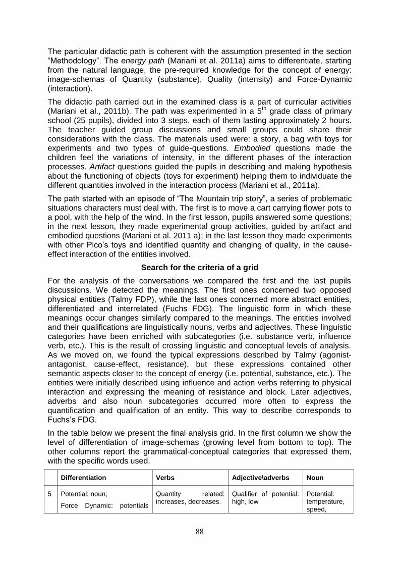
The particular didactic path is coherent with the assumption presented in the section “Methodology”. The energy path (Mariani et al. 2011a) aims to differentiate, starting from the natural language, the pre-required knowledge for the concept of energy: image-schemas of Quantity (substance), Quality (intensity) and Force-Dynamic (interaction).

The didactic path carried out in the examined class is a part of curricular activities (Mariani et al., 2011b). The path was experimented in a 5th grade class of primary school (25 pupils), divided into 3 steps, each of them lasting approximately 2 hours. The teacher guided group discussions and small groups could share their considerations with the class. The materials used were: a story, a bag with toys for experiments and two types of guide-questions. Embodied questions made the children feel the variations of intensity, in the different phases of the interaction processes. Artifact questions guided the pupils in describing and making hypothesis about the functioning of objects (toys for experiment) helping them to individuate the different quantities involved in the interaction process (Mariani et al., 2011a).

The path started with an episode of “The Mountain trip story”, a series of problematic situations characters must deal with. The first is to move a cart carrying flower pots to a pool, with the help of the wind. In the first lesson, pupils answered some questions; in the next lesson, they made experimental group activities, guided by artifact and embodied questions (Mariani et al. 2011 a); in the last lesson they made experiments with other Pico’s toys and identified quantity and changing of quality, in the cause-effect interaction of the entities involved.

Search for the criteria of a grid

For the analysis of the conversations we compared the first and the last pupils discussions. We detected the meanings. The first ones concerned two opposed physical entities (Talmy FDP), while the last ones concerned more abstract entities, differentiated and interrelated (Fuchs FDG). The linguistic form in which these meanings occur changes similarly compared to the meanings. The entities involved and their qualifications are linguistically nouns, verbs and adjectives. These linguistic categories have been enriched with subcategories (i.e. substance verb, influence verb, etc.). This is the result of crossing linguistic and conceptual levels of analysis. As we moved on, we found the typical expressions described by Talmy (agonist-antagonist, cause-effect, resistance), but these expressions contained other semantic aspects closer to the concept of energy (i.e. potential, substance, etc.). The entities were initially described using influence and action verbs referring to physical interaction and expressing the meaning of resistance and block. Later adjectives, adverbs and also noun subcategories occurred more often to express the quantification and qualification of an entity. This way to describe corresponds to Fuchs’s FDG.

In the table below we present the final analysis grid. In the first column we show the level of differentiation of image-schemas (growing level from bottom to top). The other columns report the grammatical-conceptual categories that expressed them, with the specific words used.

Differentiation Verbs Adjective\adverbs Noun

5 Potential: noun;

Force Dynamic: potentials

Quantity related: increases, decreases.

Qualifier of potential: high, low

Potential: temperature, speed,

88

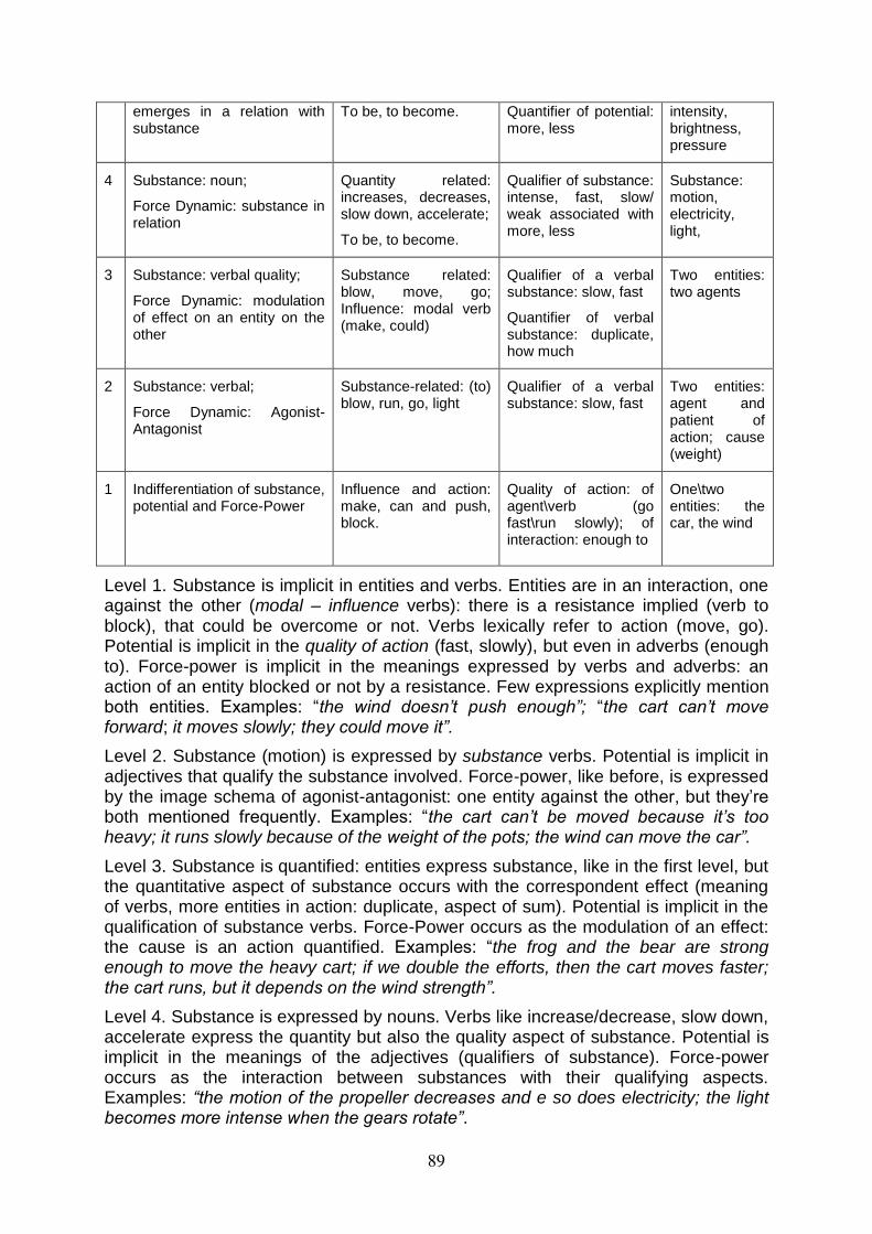
emerges in a relation with substance

To be, to become. Quantifier of potential: more, less

intensity, brightness, pressure

4 Substance: noun;

Force Dynamic: substance in relation

Quantity related: increases, decreases, slow down, accelerate;

To be, to become.

Qualifier of substance: intense, fast, slow/ weak associated with more, less

Substance: motion, electricity, light,

3 Substance: verbal quality;

Force Dynamic: modulation of effect on an entity on the other

Substance related: blow, move, go; Influence: modal verb (make, could)

Qualifier of a verbal substance: slow, fast

Quantifier of verbal substance: duplicate, how much

Two entities: two agents

2 Substance: verbal;

Force Dynamic: Agonist-Antagonist

Substance-related: (to) blow, run, go, light

Qualifier of a verbal substance: slow, fast

Two entities: agent and patient of action; cause (weight)

1 Indifferentiation of substance, potential and Force-Power

Influence and action: make, can and push, block.

Quality of action: of agent\verb (go fast\run slowly); of interaction: enough to

One\two entities: the car, the wind

Level 1. Substance is implicit in entities and verbs. Entities are in an interaction, one against the other (modal – influence verbs): there is a resistance implied (verb to block), that could be overcome or not. Verbs lexically refer to action (move, go). Potential is implicit in the quality of action (fast, slowly), but even in adverbs (enough to). Force-power is implicit in the meanings expressed by verbs and adverbs: an action of an entity blocked or not by a resistance. Few expressions explicitly mention both entities. Examples: “the wind doesn’t push enough”; “the cart can’t move forward; it moves slowly; they could move it”.

Level 2. Substance (motion) is expressed by substance verbs. Potential is implicit in adjectives that qualify the substance involved. Force-power, like before, is expressed by the image schema of agonist-antagonist: one entity against the other, but they’re both mentioned frequently. Examples: “the cart can’t be moved because it’s too heavy; it runs slowly because of the weight of the pots; the wind can move the car”.

Level 3. Substance is quantified: entities express substance, like in the first level, but the quantitative aspect of substance occurs with the correspondent effect (meaning of verbs, more entities in action: duplicate, aspect of sum). Potential is implicit in the qualification of substance verbs. Force-Power occurs as the modulation of an effect: the cause is an action quantified. Examples: “the frog and the bear are strong enough to move the heavy cart; if we double the efforts, then the cart moves faster; the cart runs, but it depends on the wind strength”.

Level 4. Substance is expressed by nouns. Verbs like increase/decrease, slow down, accelerate express the quantity but also the quality aspect of substance. Potential is implicit in the meanings of the adjectives (qualifiers of substance). Force-power occurs as the interaction between substances with their qualifying aspects. Examples: “the motion of the propeller decreases and e so does electricity; the light becomes more intense when the gears rotate”.

89

Level 5. Potential is explained and expressed by nouns, like substance. Adjectives (high\low) and adverbs (more\less) mean “increase\decrease”. Force-power is expressed by a relation between the different potentials that increase\decrease in an interaction chain. Example: “The temperature increases; if we put two candles there is more air, more pressure”1.

Discussion, Summary and Conclusion

The sentences said by the children at the beginning and at the end of the whole path are characterized by a different language. The pupils started to distinguish between the object or the concrete agent and what they are really talking about: motion, heat and the corresponding speed and temperature. The interaction between that entities occurs in articulated sentences where variations of qualities are connected one to another. The results show that the children’s natural language concerning complex processes varies, if guided by the teacher using the children’s words themselves. In this paper we have presented a grid of analysis of pupils’ language, constructed in a designed way it could be sensitive to language change in the development of the didactic path. In this way we built a tool able to assess the pupils’ level of understanding concepts about energy, starting from their language.

References

Corni, F., Giliberti, E., Mariani, C. (2011). Semiotic mediation and didactical cycle as methodological reference for primary school teachers. The biannual ESERA conference 2011.

Fuchs, H., Corni, F., Giliberti, E., Mariani, C. (in press). Force Dynamic Gestalt of Natural Phenomena: Teaching the Concept of Energy. The biannual conference of the European Science Education Research Association.September 5th-9th 2011, Lyon, FRANCE.

Fuchs, H.U. (2007). From image schemas to dynamical models in fluids, electricity, heat, and motion. An essay on physic educational research, Zurich University of applied sciences at Winterthur.

Fuchs, H.U. (1996) The Dynamics of Heat, New York: Springer.

Grady, J. (2005). Primary metaphors as inputs to conceptual integration. Journal of Pragmatics, 37(10), 1595-1614.

Hermann, F. (2006). Der Karlsruher Physikkurs. Repubblica e Cantone Ticino/Dipartimento dell'educazione, della cultura e dello sport/Divisione della scuola / Centro didattico cantonale.

Laurenti, E., Giliberti, E., Mariani, C., Corni, F., (2011). Il progetto piccolo scienziati: Idrolandia ed Ergolandia, le valigie di Pico. F. Corni, C. Mariani, E. Laurenti (Eds). Atti del Convegno Innovazione nella didattica delle scienze nella scuola primaria: al crocevia fra discipline scientifiche e umanistiche (91-100). Modena: Artestampa.

Mariani, C., Laurenti, E., Corni, F. (2011 a). Hands on-minds on activities to construct the concept of energy in primary school: experiments, games and group

1 See in Appendix the extracts from the discussions. Numbers refer to the levels in the table.

90

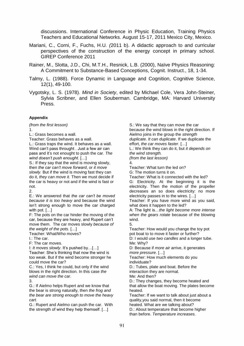
discussions. International Conference in Physic Education, Training Physics Teachers and Educational Networks. August 15-17, 2011 Mexico City, Mexico.

Mariani, C., Corni, F., Fuchs, H.U. (2011 b). A didactic approach to and curricular perspectives of the construction of the energy concept in primary school. GIREP Conference 2011

Rainer, M., Slotta, J.D., Chi, M.T.H., Resnick, L.B. (2000), Naïve Physics Reasoning: A Commitment to Substance-Based Conceptions, Cognit. Instruct., 18, 1-34.

Talmy, L. (1988). Force Dynamic in Language and Cognition, Cognitive Science, 12(1), 49-100.

Vygotsky, L. S. (1978). Mind in Society, edited by Michael Cole, Vera John-Steiner, Sylvia Scribner, and Ellen Souberman. Cambridge, MA: Harvard University Press.

Appendix

(from the first lesson) 1. L.: Grass becomes a wall. Teacher: Grass behaves as a wall. L.: Grass traps the wind. It behaves as a wall. Wind can’t pass throught . Just a few air can pass and it’s not enought to push the car. The wind doesn’t push enought. […] S.: If they say that the wind is moving slowly, then the car can’t move forward, or it move slowly. But if the wind is moving fast they can do it, they can move it. Then we must decide if the car is heavy or not and if the wind is fast or not. 2. E.: We answered that the car can’t be moved because it is too heavy and because the wind isn’t strong enough to move the car charged with pot. […] F: The pots on the car hinder the moving of the car, because they are heavy, and Rupert can’t move them. The car moves slowly because of the weight of the pots. […] Teacher: What/Who moves? I.: The car. F: The car moves. I: It moves slowly. It’s pushed by…[…] Teacher: She’s thinking that now the wind is too weak. But if the wind become stronger he could move the car? C.: Yes, I think he could, but only if the wind blows in the right direction. In this case the wind can move the car. 3. G.: If Aielmo helps Rupert and we know that the bear is strong naturally, then the frog and the bear are strong enough to move the heavy cart. G.: Rupert and Aielmo can push the car. With the strength of wind they help themself. […]

S.: We say that they can move the car because the wind blows in the right direction. If Aielmo joins in the group the strength duplicate. It can duplicate. If we duplicate the effort, the car moves faster. […] L.: We think they can do it, but it depends on the wind strength. (from the last lesson) 4. Teacher: What turn the led on? G: The motion turns it on. Teacher: What is it connected with the led? G: Electricity. At the beginning it is the electricity. Then the motion of the propeller decreases an so does electricity: no more electricity passes in to the wires. […] Teacher: If you have more wind as you said, what does it happen to the led? A: The light is…the light become more intense when the gears rotate because of the blowing wind. 5. Teacher: How would you change the toy pot pot boat to to move it faster or further? D: I would use two candles and a longer tube. Me: Why? D: Because if more air arrive, it generates more pressure. […] Teacher: How much elements do you individuate? D.: Tubes, plate and boat. Before the interaction they are normal. Me: And then? D.: They changes, they become heated and that allow the boat moving. The plates become heated. Teacher: If we want to talk about just about a quality,you said normal, then it become heated. What are we talking about? D.: About temperature that become higher than before. Temperature increases.

91

Hints and peer-peer interaction in the learning of university thermal physics Risto Leinonen, Mervi Asikainen and Pekka E. Hirvonen

risto.leinonen@uef.fi Department of Physics and Mathematics, University of Eastern Finland

We believe that a majority of university students may grasp the crucial pieces of information taught during traditional instruction but they lack an ability to apply this knowledge in tasks requiring profound conceptual understanding. We ran tests to find whether this ability can be boosted by means of a one-hour teaching sequence staged after lecture-based teaching in two different physics courses. The data was collected by using conceptual tasks concerning ideal gas processes. Firstly, the students worked by themselves without assistance. Secondly, the students were given hints, already familiar from the lectures, and were asked to review and reformulate their answers. Finally, the students discussed their answers with their peers, and, where necessary, evaluated and reformulated them. The proportion of correct answers increased significantly, by up to 26 percentage units. Hence, students appeared to benefit from the intervention. However, their success with some topics did not improve at all. This indicates that we need to analyze carefully the various phases of the intervention and consider whether the intervention would require new phases, such as introducing students’ well-known misconceptions explicitly. We are planning to widen our data collection using interviews and recordings to acquire further information about students’ discussions and thinking.

Introduction

The term scaffolding originally referred to a process where a learner could succeed in a previously unattainable task when guided by a more knowledgeable person (Wood, Bruner, & Ross, 1976). The definition of the concept was later broadened to cover other forms of learning support (e.g. Puntambekar & Hübscher, 2005), such as support offered to a larger cohort and with support offered by peers (Ge & Land, 2003; Greening, 1998). In the present study, the concept is used in its broader meaning. Several examples of the benefits of scaffolding can be found in the literature (e. g. Puntamkebar & Kolodner, 2005; Wood et al., 1976), but we find them of little help when drawing up hypotheses since scaffolding can appear in a number of different forms. The problems involved in learning thermal physics are demonstrably numerous (e.g. Leinonen, Räsänen, Asikainen, & Hirvonen, 2009; Meltzer, 2004). In this study, the well-documented misconceptions and other problems were classified on the basis of the frequency and significance of the findings (see Table 1). This summary of misconceptions and problems provided one of the starting-points and also a motivation factor in designing the intervention described below. We believe that a majority of students grasp the essential pieces of information during the instruction, but they lack the ability to apply their knowledge in situations requiring conceptual understanding rather than quantitative problem-solving skills. In the present study, it was our intention to discover whether it is possible to enhance traditional teaching in terms of overcoming well-known misconceptions, but with only minor modifications, utilizing various forms of scaffolding. Hence, our research question was formulated as follows: To what extent does scaffolding, as a form of offering hints and peer-peer interaction, help university students, after instruction, to solve qualitative tasks concerning the multi-phased process of an ideal gas?

92

Table 1. Students’ common misconceptions and problems classified according to their frequency and significance.

Finding Reference(s) Net work and net heat during a cyclic process are zero

Loverude et al., 2002; Meltzer, 2004

Inability to apply the first law of thermodynamics Leinonen et al., 2009; Loverude et al., 2002; Meltzer, 2004

Not understanding work as an energy transfer mechanism

Loverude et al., 2002; Meltzer, 2004

Relation between temperature and particles’ kinetic energy is not understood

Meltzer, 2004

Heat is used as a state variable Meltzer, 2004 Work is used as a state variable Loverude et al., 2002; Meltzer, 2004 Problems with macroscopic ideal gas model Leinonen et al. 2009; Loverude et al.

2002 Problems with microscopic models Loverude et al. 2002 Problems in distinguishing concepts or processes

Loverude et al. 2002; Kautz, Heron, Shaffer, & McDermott, 2005

Problems with pV diagram Meltzer, 2004

Methods and context The intervention took place in the context of two physics courses taught at the University of Eastern Finland. The introductory level course Basic Physics II1 served as a context for piloting the intervention, and then, based on the results obtained from the pilot study, we carried out a redesigned, actual intervention during the second-year Thermal Physics course2

In order to test students’ understanding we used a conceptual test concerned with the cyclic process of an ideal gas (Meltzer, 2004). For success in the test, the student should understand the first law of thermodynamics, thermal processes, and interdependences for certain quantities. Because the pilot study was conducted in the introductory course of physics instead of the thermal physics course, the test was mildly modified so that the questions could be answered based on the course content. In practice, this meant replacing references to the particles’ kinetic energy with references to the thermal energy. However, the piloting phase was designed only to evaluate characteristics of the intervention phases and hints, so small modifications caused no problems in the data analysis.

. Both courses are rather conventional lecture courses including problem-solving exercises that are checked in small groups. The samples consisted of 69 and 31 students, respectively.

The test also served as teaching material. The intervention began by letting the students take the test with no help, relying on the knowledge that they had grasped during the teaching. After taking the test, they were then offered a number of hints

1 Course content and material are based on Knight’s (2008b) textbook 2 Course content and material are based on Schroeder’s (1999) textbook

93

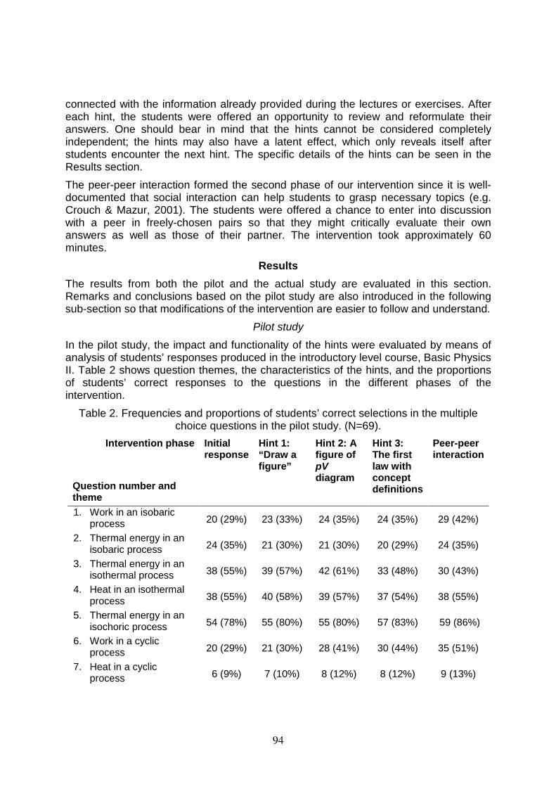
connected with the information already provided during the lectures or exercises. After each hint, the students were offered an opportunity to review and reformulate their answers. One should bear in mind that the hints cannot be considered completely independent; the hints may also have a latent effect, which only reveals itself after students encounter the next hint. The specific details of the hints can be seen in the Results section. The peer-peer interaction formed the second phase of our intervention since it is well-documented that social interaction can help students to grasp necessary topics (e.g. Crouch & Mazur, 2001). The students were offered a chance to enter into discussion with a peer in freely-chosen pairs so that they might critically evaluate their own answers as well as those of their partner. The intervention took approximately 60 minutes.

Results The results from both the pilot and the actual study are evaluated in this section. Remarks and conclusions based on the pilot study are also introduced in the following sub-section so that modifications of the intervention are easier to follow and understand.

Pilot study

In the pilot study, the impact and functionality of the hints were evaluated by means of analysis of students’ responses produced in the introductory level course, Basic Physics II. Table 2 shows question themes, the characteristics of the hints, and the proportions of students’ correct responses to the questions in the different phases of the intervention.

Table 2. Frequencies and proportions of students’ correct selections in the multiple choice questions in the pilot study. (N=69).

Intervention phase Question number and theme

Initial response

Hint 1: “Draw a figure”

Hint 2: A figure of pV diagram

Hint 3: The first law with concept definitions

Peer-peer interaction

1. Work in an isobaric process 20 (29%) 23 (33%) 24 (35%) 24 (35%) 29 (42%)

2. Thermal energy in an isobaric process 24 (35%) 21 (30%) 21 (30%) 20 (29%) 24 (35%)

3. Thermal energy in an isothermal process 38 (55%) 39 (57%) 42 (61%) 33 (48%) 30 (43%)

4. Heat in an isothermal process 38 (55%) 40 (58%) 39 (57%) 37 (54%) 38 (55%)

5. Thermal energy in an isochoric process 54 (78%) 55 (80%) 55 (80%) 57 (83%) 59 (86%)

6. Work in a cyclic process 20 (29%) 21 (30%) 28 (41%) 30 (44%) 35 (51%)

7. Heat in a cyclic process 6 (9%) 7 (10%) 8 (12%) 8 (12%) 9 (13%)

94

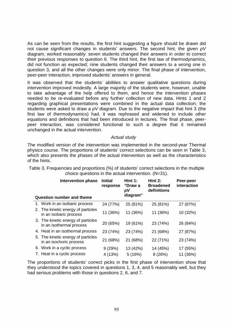
As can be seen from the results, the first hint suggesting a figure should be drawn did not cause significant changes in students’ answers. The second hint, the given pV diagram, worked reasonably: seven students changed their answers in order to correct their previous responses to question 6. The third hint, the first law of thermodynamics, did not function as expected; nine students changed their answers to a wrong one in question 3, and all the other changes were only minor. The final phase of intervention, peer-peer interaction, improved students’ answers in general. It was observed that the students’ abilities to answer qualitative questions during intervention improved modestly. A large majority of the students were, however, unable to take advantage of the help offered to them, and hence the intervention phases needed to be re-evaluated before any further collection of new data. Hints 1 and 2 regarding graphical presentations were combined in the actual data collection; the students were asked to draw a pV diagram. Due to the negative impact that hint 3 (the first law of thermodynamics) had, it was rephrased and widened to include other equations and definitions that had been introduced in lectures. The final phase, peer-peer interaction, was considered functional to such a degree that it remained unchanged in the actual intervention.

Actual study

The modified version of the intervention was implemented in the second-year Thermal physics course. The proportions of students’ correct selections can be seen in Table 3, which also presents the phases of the actual intervention as well as the characteristics of the hints. Table 3. Frequencies and proportions (%) of students’ correct selections in the multiple

choice questions in the actual intervention. (N=31). Intervention phase

Question number and theme

Initial response

Hint 1: “Draw a pV diagram”

Hint 2: Broadened definitions

Peer-peer interaction

1. Work in an isobaric process 24 (77%) 25 (81%) 25 (81%) 27 (87%) 2. The kinetic energy of particles

in an isobaric process 11 (36%) 11 (36%) 11 (36%) 10 (32%)

3. The kinetic energy of particles in an isothermal process 20 (65%) 19 (61%) 23 (74%) 26 (84%)

4. Heat in an isothermal process 23 (74%) 23 (74%) 21 (68%) 27 (87%) 5. The kinetic energy of particles

in an isochoric process 21 (68%) 21 (68%) 22 (71%) 23 (74%)

6. Work in a cyclic process 9 (29%) 13 (42%) 14 (45%) 17 (55%) 7. Heat in a cyclic process 4 (13%) 5 (16%) 8 (26%) 11 (36%)

The proportions of students’ correct picks in the first phase of intervention show that they understood the topics covered in questions 1, 3, 4, and 5 reasonably well, but they had serious problems with those in questions 2, 6, and 7.

95

The first hint about drawing a pV diagram, designed to offer help in question 6, worked well: four students out of the total of 31 changed their answers to the correct one based on the diagrams they had sketched. The second hint consisting of equations and definitions introduced in the lectures was clearly helpful in questions 3 and 7. Surprisingly, zero change was observed in question 2. Despite the hints, students had problems in understanding work as an energy transfer method. The final phase, peer-peer interaction, increased the number of students’ correct choices substantially. The biggest impact of their discussions with peers was observed in questions 3, 4, 6, and 7. The minor negative change in question 2 was rather surprising. On the basis of these results, however, we can conclude that students can usually exploit peer-peer interaction reasonably well. Generally, the actual intervention improved students’ answers significantly: the increase in the number of correct answers averaged 13 percentage units, and as its best the increase was 26 percentage units in question 6.

Discussion Our intervention proved to be a functional way of enhancing students’ learning in large-enrolment classes. Generally, the hints and peer-peer interaction helped students with the topics, but the questions concerning the kinetic energy of particles in an isobaric process and heat in a cyclic process were exceptions. These topics were apparently too difficult for the students to grasp despite the help offered. It also seems that a certain proportion of students have to possess sufficient pre-understanding to be able to take advantage of the discussions during a peer-peer interaction phase, as has been documented elsewhere (Crouch & Mazur, 2001). Our intervention appears to offer a promising way of modifying traditional lecture-based university teaching, but we think that it could be improved further by exploiting students’ own thinking and self-evaluation better. One idea is to introduce the well-known misconceptions to students. These are already taken into account in certain textbooks (e.g. Knight, 2008b) so it would seem logical to extend this idea to the teaching intervention itself. This may represent a considerable challenge for any lecturer, but modern textbooks with their supplementary materials can be a great help; one does not have to be intimately familiar with physics education research because the instructor guide (Knight, 2008a) provides a succinct overview of the most essential misconceptions. With regard to peer-peer interaction, we are keen to see if discussion in bigger groups could be even more effective (Alexepoulou & Driver, 1996). We also consider it worthwhile to conduct follow-up testing in order to see whether changes are long-lasting. In the future we will also pay attention to the reasoning that underlies students’ answers by analyzing their explanations and using audio recordings and interviews. These may provide interesting information about students’ conceptions and discussions during the intervention.

96

References Alexepoulou, E. & Driver, R. (1996). Small-group discussions in physics: Peer

interaction modes in pairs and fours. Journal of Research in Science Teaching, 33, 1099-1114.

Crouch, C. J. & Mazur, E. (2001). Peer instruction: Ten years of experience and results. American Journal of Physics, 69, 970-977.

Ge, X. & Land, S. M. (2003). Scaffolding students’ problem-solving processes in an ill-structured task using question prompts and peer interactions. Educational Technology Research and Development, 51, 21-38.

Greening, T. (1998). Scaffolding for success in problem-based learning. Medical Education Online, 3, 1-15.

Kautz, C. H., Heron P. R. L., Loverude M. E., and McDermott L. C. (2005). Student understanding of the ideal gas law, Part 1: A macroscopic perspective. American Journal of Physics, 73, 1055-1063.

Knight, R. D. (2008a). Instructor guide. Physics for scientists and engineers – A strategic approach (Second edition). San Francisco, CA: Addison-Wesley.

Knight, R. D. (2008b). Physics for scientists and engineers – A strategic approach (Second edition). San Francisco, CA: Addison-Wesley.

Leinonen, R., Räsänen, E., Asikainen M., & Hirvonen, P. E. (2009). Students’ pre-knowledge as a guideline in the teaching of introductory thermal physics at university. European Journal of Physics, 30, 593-604.

Loverude M., Kautz C. H., & Heron P. (2002). Student understanding of the first law of thermodynamics: Relating work to the adiabatic compression of an ideal gas. American Journal of Physics, 70, 137-148.

Meltzer D. (2004). Investigation of students’ reasoning regarding heat, work, and the first law of thermodynamics in an introductory calculus-based general physics course. American Journal of Physics, 72, 1432-1446.

Puntambekar S. & Hübscher R. (2005). Tools for scaffolding students in a complex learning environment: What have we gained and what have we missed? Educational Psychologist, 40(1), 1-12.

Puntambekar S. & Kolodner J. L. (2005). Toward Implementing Distributed Scaffolding: Helping Students Learn Science from Design. Journal of Research in Science Teaching, 42(2), 185-217.

Schroeder, D. V. (1999). An introduction to thermal physics. United States: Addison-Wesley.

Wood, D., Bruner, J. S., & Ross, G. (1976). The role of tutoring in problem solving. Journal of Child Psychology and Psychiatry and Allied Disciplines, 17, 89–100.

97

Motivating students to perform an experiment in technological design contexts P.S.W.M. Logman1, W.H. Kaper1 and A.L. Ellermeijer2

logman@uva.nl 1 Faculty of Science, University of Amsterdam, The Netherlands and

2 Centre for Microcomputer Applications, Amsterdam, The Netherlands

In a teaching-learning sequence on the subject of energy we have tried technological design contexts to motivate students by using only context-based reasons to perform experiments on the subject of energy. We use these experiments to have the students reinvent practical laws of energy conservation from their data. We expected students to see the need for an experiment to test their designs but in our first try-out we encountered some problems with this, basically blocking the intended path to understanding energy conservation. In our second try-out we have improved the learning materials effectively hereby finding several contextual reasons for students to perform an experiment but also an unexpected reason for students not to perform an experiment.

Introduction

In the Netherlands curriculum innovation committees for the exact sciences have chosen a context-based approach to education (Eijkelhof et al., 2006). Pilot (Pilot et al., 2006) says further investigation is needed on attaining abstract concepts in context-based education. As it is one of the more abstract concepts in physics we chose energy conservation as a concept that we will try to attain in a context based teaching-learning sequence. In order to achieve our goal we chose to use the guided reinvention approach (Freudenthal, 1991) and have the students discover their own conservation laws from their own experiments.

For using contexts in education Gilbert describes four models, of which he regards “contexts as the social circumstances” as the most promising (Gilbert, 2006). We will adhere to this model, because it avoids putting the concept in the center of attention too early for students to be able to reinvent it1. Gilbert describes a number of criteria for the use of contexts based on this model:

i. Contexts must arise from the students themselves, from actual social issues or industrial settings and must address the zone of nearest development in students.

ii. The assignments need to clarify a certain way of operating and must consist of clear examples of major concepts.

iii. The context needs to give rise to a coherent jargon for students to use. The context decides which concepts are useful to achieve this.

iv. Every important subject needs to be related to background knowledge. Students need to be able to recontextualize.

In our case we are looking for contexts in which practical laws involving energy conservation can be reinvented by performing experiments. Practices in which physical laws are discovered are the practices of either technological designers or scientists (ii). Staying as close to real life experiences as possible (i) we decided to start with technological design practices. To clarify the technological design way of operating we decided to use designing principles from the Techniek15+ approach (ii) developed by a project group involving five Dutch universities, regional engineering companies, and engineering societies (i) (Techniek15+, 2002). In the problem orientation phase Techniek15+ connects the context to the background knowledge of

1 The other extreme is to regard contexts as illustrations of concepts. Gilbert mentions some intermediate

possibilities too.

98

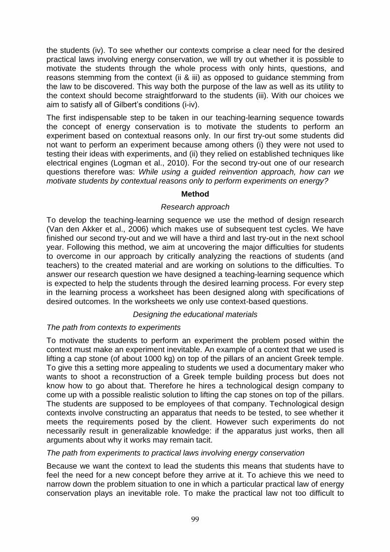
the students (iv). To see whether our contexts comprise a clear need for the desired practical laws involving energy conservation, we will try out whether it is possible to motivate the students through the whole process with only hints, questions, and reasons stemming from the context (ii & iii) as opposed to guidance stemming from the law to be discovered. This way both the purpose of the law as well as its utility to the context should become straightforward to the students (iii). With our choices we aim to satisfy all of Gilbert‟s conditions (i-iv).

The first indispensable step to be taken in our teaching-learning sequence towards the concept of energy conservation is to motivate the students to perform an experiment based on contextual reasons only. In our first try-out some students did not want to perform an experiment because among others (i) they were not used to testing their ideas with experiments, and (ii) they relied on established techniques like electrical engines (Logman et al., 2010). For the second try-out one of our research questions therefore was: While using a guided reinvention approach, how can we motivate students by contextual reasons only to perform experiments on energy?

Method

Research approach

To develop the teaching-learning sequence we use the method of design research (Van den Akker et al., 2006) which makes use of subsequent test cycles. We have finished our second try-out and we will have a third and last try-out in the next school year. Following this method, we aim at uncovering the major difficulties for students to overcome in our approach by critically analyzing the reactions of students (and teachers) to the created material and are working on solutions to the difficulties. To answer our research question we have designed a teaching-learning sequence which is expected to help the students through the desired learning process. For every step in the learning process a worksheet has been designed along with specifications of desired outcomes. In the worksheets we only use context-based questions.

Designing the educational materials

The path from contexts to experiments

To motivate the students to perform an experiment the problem posed within the context must make an experiment inevitable. An example of a context that we used is lifting a cap stone (of about 1000 kg) on top of the pillars of an ancient Greek temple. To give this a setting more appealing to students we used a documentary maker who wants to shoot a reconstruction of a Greek temple building process but does not know how to go about that. Therefore he hires a technological design company to come up with a possible realistic solution to lifting the cap stones on top of the pillars. The students are supposed to be employees of that company. Technological design contexts involve constructing an apparatus that needs to be tested, to see whether it meets the requirements posed by the client. However such experiments do not necessarily result in generalizable knowledge: if the apparatus just works, then all arguments about why it works may remain tacit.

The path from experiments to practical laws involving energy conservation

Because we want the context to lead the students this means that students have to feel the need for a new concept before they arrive at it. To achieve this we need to narrow down the problem situation to one in which a particular practical law of energy conservation plays an inevitable role. To make the practical law not too difficult to

99

reinvent we chose experiments that involve only one or two forms of energy. In the case of the reconstruction of the Greek temple the desired practical2 law of energy conservation is ∑(m∙h)before = ∑(m∙h)after or any equivalent notation. This law has as preconditions that it is only valid when the objects concerned are balanced and that there is little friction. To make sure students need such a solution we require the lifting of the cap stone to be safe and we hoped (and hinted) that students would see the safety benefit of a balanced solution. Also, to lift the stone as easily as possible there must be as little friction as possible. Besides all that we expected the students choosing the balancing counterweight to be a factor lighter than the cap stone because otherwise lifting the counterweight would pose the same problem as lifting the cap stone.

Generalization of the practical laws of energy conservation

In a discussion with the students on their findings in three different contexts (lifting a heavy object, designing a thermostatic water tap, and designing a rollercoaster), we aim to generalize the various reinvented practical laws of energy conservation by combining them into one. Because such a generalization of physical laws is not a part of the job that a technological designer does we chose a scientific context to perform these generalizations but this is beyond the scope of this paper.

In the end we expect the students to be able to combine practical laws of energy conservation themselves. Combining more and more laws of energy conservation we expect the students to come up with the idea that for any situation one can create a law of energy conservation particular to that situation. We will report more on our results concerning these generalizations in a future paper.

Data collection

Our first try-out involved one teacher teaching 8 couples of students. The second try-out involved three teachers (including the teacher from the first try-out) teaching respectively 11, 15, and 12 couples of students. We have designed several technological design contexts in which the requirements were varied to see how they affect the learning process. Faced with a few unforeseen obstacles for the students in the second try-out the teachers spontaneously added some requirements to guide the students in overcoming these obstacles.

To see whether the context-based questions work as expected we look at students‟ notes and verbal reactions to the questions and compare them to our expectations. To this end we make audio recordings and collect students‟ notes. To make sure to what extent only context-based questions, hints, or reasonings are used by the teachers we analyze their conversations with the students. If any unexpected questions are used we analyze the effect on the students: do the students acknowledge the question as connected to the context and does the question help them along in their progress towards the energy concept.

Results

Below we report our progress on the reasons for students not to perform an experiment found in the first try-out.

2 In this case practical means it is as easy as possible to apply the law to the case at hand. So all constants that

cancel out will not play a role in the solution to the contextual problem and can therefore not be discovered.

100

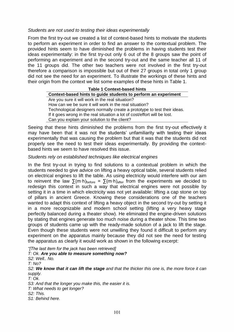
Students are not used to testing their ideas experimentally

From the first try-out we created a list of context-based hints to motivate the students to perform an experiment in order to find an answer to the contextual problem. The provided hints seem to have diminished the problems in having students test their ideas experimentally: in the first try-out only 6 out of the 8 groups saw the point of performing an experiment and in the second try-out and the same teacher all 11 of the 11 groups did. The other two teachers were not involved in the first try-out therefore a comparison is impossible but out of their 27 groups in total only 1 group did not see the need for an experiment. To illustrate the workings of these hints and their origin from the context we list some examples of these hints in Table 1.

Table 1 Context-based hints

Context-based hints to guide students to perform an experiment

Are you sure it will work in the real situation? How can we be sure it will work in the real situation? Technological designers normally create a prototype to test their ideas. If it goes wrong in the real situation a lot of cost/effort will be lost. Can you explain your solution to the client?

Seeing that these hints diminished the problems from the first try-out effectively it may have been that it was not the students‟ unfamiliarity with testing their ideas experimentally that was causing the problem but that it was that the students did not properly see the need to test their ideas experimentally. By providing the context-based hints we seem to have resolved this issue.

Students rely on established techniques like electrical engines

In the first try-out in trying to find solutions to a contextual problem in which the students needed to give advice on lifting a heavy optical table, several students relied on electrical engines to lift the table. As using electricity would interfere with our aim to reinvent the law ∑(m∙h)before = ∑(m∙h)after from the experiments we decided to redesign this context in such a way that electrical engines were not possible by setting it in a time in which electricity was not yet available: lifting a cap stone on top of pillars in ancient Greece. Knowing these considerations one of the teachers wanted to adapt this context of lifting a heavy object in the second try-out by setting it in a more recognizable and modern school setting (lifting a very heavy stage perfectly balanced during a theater show). He eliminated the engine-driven solutions by stating that engines generate too much noise during a theater show. This time two groups of students came up with the ready-made solution of a jack to lift the stage. Even though these students were not unwilling they found it difficult to perform any experiment on the apparatus mainly because they did not see the need for testing the apparatus as clearly it would work as shown in the following excerpt:

“[The last item for the jack has been retrieved] T: Ok. Are you able to measure something now? S2: Well.. No. T: No? S2: We know that it can lift the stage and that the thicker this one is, the more force it can supply. T: Ok. S3: And that the longer you make this, the easier it is. T: What needs to get longer? S2: This. S1: Behind here.

101

T: Oh that one ! And how much does this thing go up when you let that piece go up once, twice or ten times? S1: Yes, we can measure that. T: Is this important for our problem or am I asking stupid questions? S1: Well, in itself.. Then you know how much this one goes up but then we would need another one (another jack) with a different size. T: Yes, you would need one more with a different size. Yes. Can you reconstruct the principle? S1: As soon as you know those proportions one can calculate the other proportions as well, one could say. T: Ok. Is that height also important for the problem itself? For the real stage? S2: Yes. S1: It has to come up 50 cm.”

The excerpt shows the teacher asking what physical law explains the working principle of a jack. This is not a context-based question as there is no need for the students to answer this question to come to a solution to the contextual problem. Through this we realized that in the engine-driven solutions to the lifting assignment in the first try-out the problem was that engines are a ready-made technique which take away the students‟ need to perform an experiment to find out whether their solution will work. Of course eliminating this need for an experiment also takes away the chance to reinvent the desired practical law of energy conservation.

Another small number of groups decided to use manual laborers or animals to lift the heavy cap stone. One could argue that these solutions are ready-made „techniques‟ of the ancient Greeks. In a group discussion about all the investigated solutions, the students in general agreed that these solutions involving manual laborers or animals would still benefit from the knowledge behind other solutions that did make it easier to lift heavy material. To the desired learning process it is therefore essential that at least a few groups in a class find solutions that make lifting easier.

On the problem with established techniques we can conclude that it would be best to choose the context in such a way that ready-made techniques are excluded as a possible solution to the context (e.g. by setting it in a time or place where the ready-made techniques are not available) but this may reveal other, most likely simpler, ready-made techniques in the new setting. In our case for example the problem of using many people or animals to lift the heavy material is still to be addressed.

For the other two contexts we found similar results where it has to be noted that these contexts were already set before the time of the appropriate invention. In the case of the water tap manufacturer it was easy to motivate the students to perform an experiment by telling them that this particular manufacturer did know how to make water taps but did not yet know how to manufacture a thermostatic water tap. In the case of the rollercoaster it was not hard at all to motivate students to do an experiment even though on the internet in the rollercoaster database (www.rcdb.com) there is a lot of data available on height and maximum speed of many rollercoasters around the world. With this data students could have easily evaded performing an experiment but none did. It is however remarkable that in the lifting assignment we observed students looking on the internet for solutions whereas in this context they did not look for it or did not find it. The reasons these contexts showed less problems in motivating students to perform an experiment may also lie in the fact that the students had already solved a similar contextual problem in the lifting assignment and now knew better what was expected by the teacher or were simply more attracted by experiments with hot water and rollercoasters.

102

Discussion and conclusion

Technological design contexts appear to be useful if one wants to create context-based educational materials in which one desires the students to perform experiments. However to technological designers, educational designers, and teachers it may be obvious to perform an experiment to test one‟s ideas but for students this idea is not immediately self-evident. To help teachers to make the students see the need for an experiment the created list of context-based hints is helpful.

If one desires to have students reinvent a certain physical principle from an experiment in a context-based approach one has to be aware that ready-made techniques available in the context can obstruct students to see the need for the physical principle behind such a technique. To make sure students perform experiments in which the desired physical principle will become clear, contextual problems can be chosen such that the solution to students is yet unknown or can be set in a time in which the solution was unknown. Roth (Roth, 2001) has used technological design contexts in many situations as well and has set a similar lifting problem in the arctic where power supply may go faulty but the need for lifting heavy objects is ever present (i.e. he set the contextual problem in a place where a ready-made solution is not available).

Completely avoiding ready-made techniques however is impossible because in any new setting other ready-made techniques will be available. Contextual problems should therefore be chosen such that solving them can not be done with a ready-made technique that obscures the physical principle we are aiming at. This can be done by the right choice of context or else by setting the context in a time or place in which the undesired ready-made technique is unavailable. By setting extra requirements on the contextual problems (e.g. asking for a rollercoaster with the highest speed suggesting as little friction as possible) it is possible to motivate students to perform experiments suitable to reinvent desired physical laws.

References

Eijkelhof, H., Mulder, G., Pieters, M., van Weert, C., & Zeldenrust, F. (2006). Natuurkunde leeft. visie op natuurkunde in havo en vwo. Amsterdam: Nederlandse Natuurkundige Vereniging.

Freudenthal, H. (1991). In Freudenthal H. (Ed.), Revisiting mathematics education China lectures. Dordrecht: Kluwer Academic.

Gilbert, J. K. (2006). On the nature of “Context” in chemical education. International Journal of Science Education, 28(9), 957-976.

Logman, P. S. W. M., Kaper, W. H., & Ellermeijer, A. L. (2010). Energy: An experiment-based route from context to concept. GIREP-ICPE-MPTL 2010, Reims, France.

Pilot, A., & Bulte, A. M. W. (2006). The use of “Contexts” as a challenge for the chemistry curriculum: Its successes and the need for further development and understanding. International Journal of Science Education, 28(9), 1087-1112.

Roth, W. M. (2001). Learning science through technological design. Journal of Research in Science Teaching, 38(7), 768-790. doi:10.1002/tea.1031

Techniek15+. (2002). Techniek 15+ Projectgroep Techniek 15+. Van den Akker, J., Gravemeijer, K., McKenney, S., & Nieveen, N. (2006).

Educational design research. London: Routledge.

103

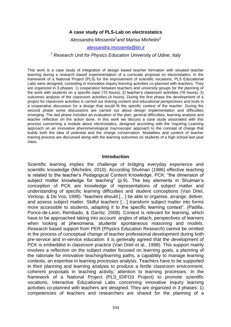
A case study of PLS-Lab on electrostatics

Alessandra Mossenta1and Marisa Michelini1

alessandra.mossenta@tin.it

1 Research Unit for Physics Education University of Udine, Italy

This work is a case study of integration of design based teacher formation with situated teacher learning during a research based experimentation of a curricular proposal on electrostatics. In the framework of a National Project (PLS) for the improvement of scientific vocations, PLS Educational Labs were designed, consisting in innovative inquiry learning activities co-planned with teachers. They are organized in 3 phases: 1) cooperation between teachers and university groups for the planning of the work with students on a specific topic (10 hours); 2) teacher’s classroom activities (16 hours); 3) outcomes analysis of the classroom activities (4 hours). During the first phase the development of a project for classroom activities is carried out sharing content and educational perspectives and tools in a cooperative discussion for a design that would fit the specific context of the teacher. During the second phase some discussions are carried out about design implementation and difficulties emerging. The last phase includes an evaluation of the plan, general difficulties, learning analysis and teacher reflection on the action done. In this work we discuss a case study associated with this process concerning a module about electrostatics, designed according with the Inquiring Learning approach on an innovative phenomenological macroscopic approach to the concept of charge that builds both the idea of potential and the charge conservation. Modalities and content of teacher training process are discussed along with the learning outcomes on students of a high school last-year class.

Introduction

Scientific learning implies the challenge of bridging everyday experience and scientific knowledge (Michelini, 2010). According Shulman (1986) effective teaching is related to the teacher’s Pedagogical Content Knowledge, PCK: ―the dimension of subject matter knowledge for teaching‖ (p.9). The key elements in Shulman’s conception of PCK are knowledge of representations of subject matter and understanding of specific learning difficulties and student conceptions (Van Driel, Verloop, & De Vos, 1998). ―teachers should […] be able to organise, arrange, deliver, and assess subject matter. Skilful teachers […] transform subject matter into forms more accessible to students, adapting it to the specific learning context‖. (Padilla, Ponce-de-Leon, Rembado, & Garritz, 2008). Context is relevant for learning, which have to be approached taking into account angles of attach, perspectives of learners when looking at phenomena, students’ spontaneous reasoning and models. Research based support from PER (Physics Education Research) cannot be omitted in the process of conceptual change of teacher professional development during both pre-service and in-service education: it is generally agreed that the development of PCK is embedded in classroom practice (Van Driel et al., 1998). This support mainly involves a reflection on the subject matter focused on learning goals, a planning of the rationale for innovative teaching/learning paths, a capability to manage learning contexts, an expertise in learning processes analysis. Teachers have to be supported in their planning and learning analysis to produce a fertile classroom environment, coherent proposals in teaching activity, attention to learning processes. In the framework of a National Project (PLS_IDIFO3 Project) to promote scientific vocations, Interactive Educational Labs concerning innovative inquiry learning activities co-planned with teachers are designed. They are organized in 3 phases: 1) competencies of teachers and researchers are shared for the planning of a

104

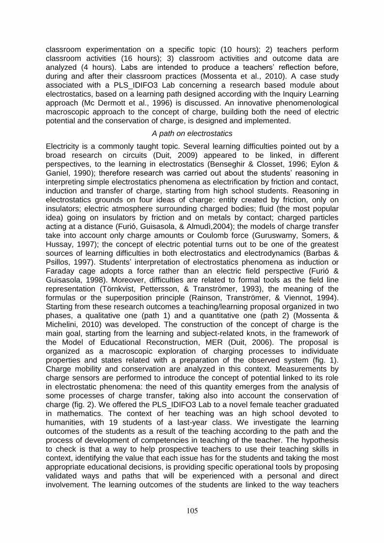
classroom experimentation on a specific topic (10 hours); 2) teachers perform classroom activities (16 hours); 3) classroom activities and outcome data are analyzed (4 hours). Labs are intended to produce a teachers’ reflection before, during and after their classroom practices (Mossenta et al., 2010). A case study associated with a PLS_IDIFO3 Lab concerning a research based module about electrostatics, based on a learning path designed according with the Inquiry Learning approach (Mc Dermott et al., 1996) is discussed. An innovative phenomenological macroscopic approach to the concept of charge, building both the need of electric potential and the conservation of charge, is designed and implemented.

A path on electrostatics

Electricity is a commonly taught topic. Several learning difficulties pointed out by a broad research on circuits (Duit, 2009) appeared to be linked, in different perspectives, to the learning in electrostatics (Benseghir & Closset, 1996; Eylon & Ganiel, 1990); therefore research was carried out about the students’ reasoning in interpreting simple electrostatics phenomena as electrification by friction and contact, induction and transfer of charge, starting from high school students. Reasoning in electrostatics grounds on four ideas of charge: entity created by friction, only on insulators; electric atmosphere surrounding charged bodies; fluid (the most popular idea) going on insulators by friction and on metals by contact; charged particles acting at a distance (Furiό, Guisasola, & Almudì,2004); the models of charge transfer take into account only charge amounts or Coulomb force (Guruswamy, Somers, & Hussay, 1997); the concept of electric potential turns out to be one of the greatest sources of learning difficulties in both electrostatics and electrodynamics (Barbas & Psillos, 1997). Students’ interpretation of electrostatics phenomena as induction or Faraday cage adopts a force rather than an electric field perspective (Furiό & Guisasola, 1998). Moreover, difficulties are related to formal tools as the field line representation (Törnkvist, Pettersson, & Tranströmer, 1993), the meaning of the formulas or the superposition principle (Rainson, Tranströmer, & Viennot, 1994). Starting from these research outcomes a teaching/learning proposal organized in two phases, a qualitative one (path 1) and a quantitative one (path 2) (Mossenta & Michelini, 2010) was developed. The construction of the concept of charge is the main goal, starting from the learning and subject-related knots, in the framework of the Model of Educational Reconstruction, MER (Duit, 2006). The proposal is organized as a macroscopic exploration of charging processes to individuate properties and states related with a preparation of the observed system (fig. 1). Charge mobility and conservation are analyzed in this context. Measurements by charge sensors are performed to introduce the concept of potential linked to its role in electrostatic phenomena: the need of this quantity emerges from the analysis of some processes of charge transfer, taking also into account the conservation of charge (fig. 2). We offered the PLS_IDIFO3 Lab to a novel female teacher graduated in mathematics. The context of her teaching was an high school devoted to humanities, with 19 students of a last-year class. We investigate the learning outcomes of the students as a result of the teaching according to the path and the process of development of competencies in teaching of the teacher. The hypothesis to check is that a way to help prospective teachers to use their teaching skills in context, identifying the value that each issue has for the students and taking the most appropriate educational decisions, is providing specific operational tools by proposing validated ways and paths that will be experienced with a personal and direct involvement. The learning outcomes of the students are linked to the way teachers

105

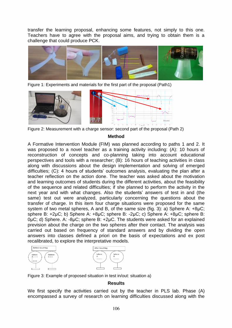
transfer the learning proposal, enhancing some features, not simply to this one. Teachers have to agree with the proposal aims, and trying to obtain them is a challenge that could produce PCK.

Figure 1: Experiments and materials for the first part of the proposal (Path1)

Figure 2: Measurement with a charge sensor: second part of the proposal (Path 2)

Method

A Formative Intervention Module (FIM) was planned according to paths 1 and 2. It was proposed to a novel teacher as a training activity including: (A): 10 hours of reconstruction of concepts and co-planning taking into account educational perspectives and tools with a researcher; (B): 16 hours of teaching activities in class along with discussions about the design implementation and solving of emerged difficulties; (C): 4 hours of students’ outcomes analysis, evaluating the plan after a teacher reflection on the action done. The teacher was asked about the motivation and learning outcomes of students during the different activities, about the feasibility of the sequence and related difficulties; if she planned to perform the activity in the next year and with what changes. Also the students’ answers of test in and (the same) test out were analyzed, particularly concerning the questions about the transfer of charge. In this item four charge situations were proposed for the same system of two metal spheres, A and B, of the same size (fig. 3): a) Sphere A: +8μC; sphere B: +2μC; b) Sphere A: +8μC; sphere B: -2μC; c) Sphere A: +8μC; sphere B: 0μC; d) Sphere. A: -8μC; sphere B: +2μC. The students were asked for an explained prevision about the charge on the two spheres after their contact. The analysis was carried out based on frequency of standard answers and by dividing the open answers into classes defined a priori on the basis of expectations and ex post recalibrated, to explore the interpretative models.

Figure 3: Example of proposed situation in test in/out: situation a)

Results

We first specify the activities carried out by the teacher in PLS lab. Phase (A) encompassed a survey of research on learning difficulties discussed along with the

106

activities of the path designed to elicit students’ ideas and to help them in building their knowledge; experiments were performed and equipment were provided to the teacher to repeat them; worksheets for the students were discussed as tools to support the proposed SPEA (Situation, Prevision, Experiment, Analysis, Michelini & Viola, 2009) strategy and test in/out was built by the teacher starting from learning difficulties and questions to point out them emerged from literature and her own class experience. During this period, divided in 4 sessions, the teacher developed a review about her subject matter knowledge; she recognized the learning knots and her difficulty in explaining phenomena as induction, the role of insulators and metals in electrification, the meaning of the triboelectric series, the transfer of charge, and finally the role of experience in highlighting them. The teacher claimed that she needed a new teaching approach, to enhance the students’ interest and learning outcomes. In phase (B) contacts gave to the teacher support in analysis of the answers of the test in according to the reasoning previously discussed, in performing the activity and in introducing some changes: she planned an intermediate test about the qualitative part of the path (proposing the behavior of a leaf electroscope as an explaining task for students, making them aware of the low level of their initial involvement in the activity); she added ending experiments with capacitors, to explore the role of different materials between the plates; she proposed some experiments to younger pupils in other classes to understand the role of the students of the intervention class in approaching the path. In phase (C) the teacher enriched the common analysis of test answers with her knowledge of the way to approach to the learning work of the students and expressed a feedback about the feasibility of the activity, referring difficulties of students in understanding the new inquiry based learning approach at the beginning of the activity, and changes she would make in her plan, shortening some discussions in path one. She related her teaching about potential, enhancing the role of charge amounts in objects of the same size, with some answers of students, that identified size and potential of the objects involved in the charge transfer. Her opinion about the effect of the proposal on students was that successful outcomes were linked to the students’ interest in the subject matter, only of a few students, or to her warnings about the importance of the concept of potential, when the change in students’ beliefs was almost total.

Students’ outcomes about the transfer of charge in test in/out

Test in

In situation a), 50% of pupils explain the final situation in terms of evolution of systems in different states towards a common state of equilibrium (process); 33% explain the impossibility of transfer with a reasoning based on the Coulombian force. Analyzing the answers in the other proposed situations (b, d), two kinds of process emerge in answers admitting a charge flux for equilibrium, expressed with the same final charge on both spheres: 1) a charge transfer from the more charged sphere to the other with neutralization of opposite charge (3/18 students) and 2) a charge flux in both directions to reach the same configuration of charge on both spheres without a need of neutralization (6/18 students). Reasoning based on the idea of force is expressed in different situations and produces several images about the processes and the final charge distributions (see table 1).

Table 1: Prevision about the final different charge on spheres in situation b), of different charge in amount and sign before the contact (Sph. A: +8μC; sph. B: -2μC). N= number of students; * not coherent answer in situation d), differing only for the signs of the charges.

107

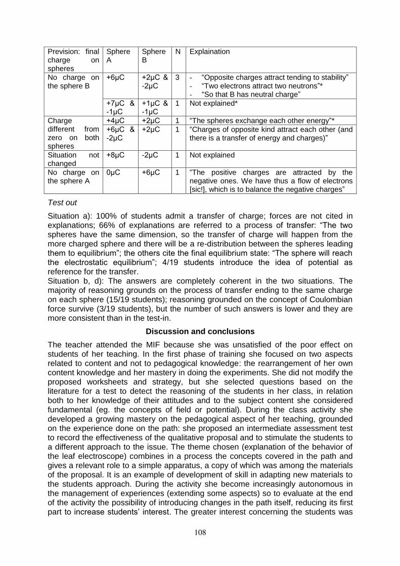
Prevision: final charge on spheres

Sphere A

Sphere B

N Explaination

No charge on the sphere B

+6μC +2μC & -2μC

3 - ―Opposite charges attract tending to stability‖ - ―Two electrons attract two neutrons‖* - ―So that B has neutral charge‖

+7μC & -1μC

+1μC & -1μC

1 Not explained*

Charge different from zero on both spheres

+4μC +2μC 1 ―The spheres exchange each other energy‖*

+6μC & -2μC

+2μC 1 ―Charges of opposite kind attract each other (and there is a transfer of energy and charges)‖

Situation not changed

+8μC -2μC 1 Not explained

No charge on the sphere A

0μC +6μC 1 ―The positive charges are attracted by the negative ones. We have thus a flow of electrons [sic!], which is to balance the negative charges‖

Test out

Situation a): 100% of students admit a transfer of charge; forces are not cited in explanations; 66% of explanations are referred to a process of transfer: ―The two spheres have the same dimension, so the transfer of charge will happen from the more charged sphere and there will be a re-distribution between the spheres leading them to equilibrium‖; the others cite the final equilibrium state: ―The sphere will reach the electrostatic equilibrium‖; 4/19 students introduce the idea of potential as reference for the transfer. Situation b, d): The answers are completely coherent in the two situations. The majority of reasoning grounds on the process of transfer ending to the same charge on each sphere (15/19 students); reasoning grounded on the concept of Coulombian force survive (3/19 students), but the number of such answers is lower and they are more consistent than in the test-in.

Discussion and conclusions

The teacher attended the MIF because she was unsatisfied of the poor effect on students of her teaching. In the first phase of training she focused on two aspects related to content and not to pedagogical knowledge: the rearrangement of her own content knowledge and her mastery in doing the experiments. She did not modify the proposed worksheets and strategy, but she selected questions based on the literature for a test to detect the reasoning of the students in her class, in relation both to her knowledge of their attitudes and to the subject content she considered fundamental (eg. the concepts of field or potential). During the class activity she developed a growing mastery on the pedagogical aspect of her teaching, grounded on the experience done on the path: she proposed an intermediate assessment test to record the effectiveness of the qualitative proposal and to stimulate the students to a different approach to the issue. The theme chosen (explanation of the behavior of the leaf electroscope) combines in a process the concepts covered in the path and gives a relevant role to a simple apparatus, a copy of which was among the materials of the proposal. It is an example of development of skill in adapting new materials to the students approach. During the activity she become increasingly autonomous in the management of experiences (extending some aspects) so to evaluate at the end of the activity the possibility of introducing changes in the path itself, reducing its first part to increase students’ interest. The greater interest concerning the students was

108

for improving the correctness of answers rather than for understanding their reasoning or for giving them exempla of global and coherent ways for looking at phenomena. The questionnaire data (test in) show a mixed picture in relation to students' ideas on the charge transfer: half of the students look at the charge transfer between two identical like charged objects in terms of systems in different states evolving towards a common condition in a process (not unique, and without taking into account the role of the positive and negative charges from the knowledge about the structure of matter) and 33% in terms of Coulomb force. These types of reasoning can also be found in situations where unlike charged spheres are put in contact, but they are specified in different models: the two main models to explain the transfer are a supply model (with a skewed vision of the system of spheres) and a distribution model, where the role of the spheres is independent from the charge on them. The final state is characterized in different ways, so different predictions are stated: the neutral state, in particular, turns out to be "stable" and is associated with varied previsions, both in situations where the spheres are initially oppositely charged and when one of them is neutral. This is aided by a local view using the concept of force, which would affect only part of the charge on the spheres, and by difficulties in the use of this concept that are also observed in mechanics. These results confirm the literature findings but enrich them with a variety of reasoning paths corresponding to the same final charge distribution or model. The improvements noted in the answers of the test-out, reflecting both the efficacy of the proposal and of the teaching style adopted, were not attributed by the teacher to her effectiveness and professional growth nor she ascribed to them her capability in finding critical points and possible solutions about the not well learned content, in the first part of the proposal. This acknowledgment was implicit. Central elements in the formation of the teacher’s PCK were: clarity of the role of each experimental step, with respect both to the learning difficulties and to the proposal for the construction of knowledge, only possible with a teacher education experiential and situated; awareness of the need of a subject matter reconstruction in a pedagogical perspective, which can come to the teachers from an analysis of the inconsistencies of their subject matter knowledge and at the same time recognizing the internal consistency and the global value in interpreting of the proposal. These elements become real growth of competence for the teacher only if explicitly recognized, to be transferred into daily teaching practice. This implies a teacher education based on innovative materials for both students’ learning and teacher training and mirroring discussions: it can only be a result of educational research, because of the multiple factors involved, and it is incumbent on the PER with regard to content, methods and investigation of effects.

References

Barbas, A., & Psillos, D. (1997). Causal reasoning as a base for advancing a systemic approach to simple electrical circuits. Research in Science Education, 27 (3) 445 – 459.

Benseghir, A., & Closset, J.L. (1996) The electrostatics – electrokinetics transition. Historical and educational difficulties. International Journal of Science Education, 18 (2), 179 -191.

Eylon, B., & Ganiel, U. (1990) Macro – micro relationship: the missing link between electrostatics and electrodynamics in students’ reasoning. International Journal of Science Education, 12 (1), 79 -94.

109

Duit, R. (2009). Bibliography STCSE – Teachers’ and Students’ Conceptions and Science Education. Kiel, Germany: IPN – Leibniz Institute for Science Education (http://www.ipn.uni-kiel.de/aktuell/stcse/stcse.html).

Duit, R. (2006), Science Education Research - An Indispensable Prerequisite for Improving Instructional Practice, ESERA Summer School, Braga, (2006) at http://www.naturfagsenteret.no/esera/summerschool2006.html.

Furió, C., & Guisasola, J. (1998). Difficulties in learning the concept of electric field. Science Education, 82 (4) 417-526.

Furió, C., Guisasola, J., & Almudì, J. M. (2004). Elementary electrostatic phenomena: historical hindrances and students’ difficulties. Canadian Journal of Science, Mathematics and Technology education, 4 (3) 291 - 313.

Guruswamy, C., Somers, M. D. & Hussey, R. G. (1997). Students’ understanding of the transfer of charge between conductors. Physics Education, 32 (2) 91 – 96.

Mc Dermott, C. L., & the Physics Education Group at the University of Washington (1996) Physics by Inquiry New York: Wiley.

Michelini, M. (2010) Building bridges between common sense ideas and a physics description of phenomena to develop formal thinking in L. Menabue & G. Santoro (Eds.) New Trends in Science and Technology Education (pp 256-274) vol. 1, Bologna CLUEB.

Michelini, M., & Viola, R. (2009) Electromagnetic induction: a proposal for a teaching/learning path, in A. Bilsel & M. U. Garip (Eds) Papers to the Frontiers in Science Education Research Conference (p. 325-333), Famagusta Cyprus EMU.

Mossenta, A., Michelini, M., Magnoler, P., Copetti, P., Del Fabbro, C., Minisini, L., & Santi, D. (2010). An environment to share in-service training on the net: an action-research about charge in primary and middle school Il Nuovo Cimento C, 3 183-188.

Mossenta, A., & Michelini, M. (2010).Conservation of Charge to understand potential using on-line charge measurements, Il Nuovo Cimento C, 3, 205-210.

Padilla, K., Ponce-de-León, A. M., Rembado, F. M., & Garritz, A. (2008) Undergraduate Professors' Pedagogical Content Knowledge: The case of 'amount of substance', International Journal of Science Education, 30 (10), 1389 — 1404.

Rainson, S., Tranströmer, G., & Viennot, L. (1994). Students’ understanding of superposition of electric fields. American Journal of Physics 62 (11) 1026 – 1032.

Shulman, L. S. (1986). Those who understand: knowledge growth in teaching. Educational Researcher, 15( 2) 4 - 14.

Törnkvist, S., Pettersson, K. A., & Tranströmer, G. (1993). Confusion by representation: on student’ s comprehension of the electric field concept. American Journal of Physics 61 (4) 335 - 338.

Van Driel, J.H., Verloop, N., & De Vos, W. (1998). Developing science teachers’ pedagogical content knowledge. Journal of Research in Science Teaching, 35(6), 673–695.

110

An Intervention for Using Multiple Representations of Force in Upper Secondary School Courses

Pasi Nieminen1, Antti Savinainen1, Niina Nurkka2, and Jouni Viiri1

pasi.k.nieminen@jyu.fi

1Department of Teacher Education, University of Jyväskylä, Finland

2Faculty of Health Care and Social Services, Saimaa University of Applied Sciences, Finland

Previous research has emphasised the importance of multiple representations for learning and understanding physics concepts. Students should learn to construct multiple representations of physical processes and learn to move in any direction between these representations. For this purpose, we designed teaching material emphasising multiple representations within the context of forces. The material and short instructions (i.e., intervention) were given to two experienced upper secondary school teachers who were not involved in designing the intervention. They used the intervention material in their mechanics courses in fall 2009 (students n = 28 altogether). The effect of the intervention on the learning of forces and representations was evaluated using a multiple-choice test, that is, the Representational Variant of the Force Concept Inventory (R-FCI), as a pre- and post-test. In addition, students’ answers to exercises of the intervention material were copied and collected. All lessons were video recorded and the teachers were interviewed after the course. The results were compared with the R-FCI baseline data (n = 22 altogether) collected prior to the intervention from the same mechanics course taught by the same teachers in fall 2008. Our results suggest that the intervention material was useful for students’ learning of the force concept and multiple representations.

Introduction

This study concentrated on multiple representations of upper secondary school physics in the context of Newtonian mechanics. The focus was on external representations (e.g., graphs and vectors) as distinct from internal, mental representations. In the school context, external representations can be seen as communicative tools between a teacher, students and media (e.g., books), and also as cognitive tools when students are working alone, for example, in problem solving. Instead of processing everything internally in their minds, they can create an external representation and thus reduce the cognitive load (Schnotz, Baadte, Müller, & Rasch, 2010).

Multiple representations refer to the circumstances where various representations are used for learning a concept or solving a problem instead of, for example, only verbal and mathematical representations. Multiple representations have many functions in learning (Ainsworth, 1999). They can complement and constrain other representations, and construct a more complete understanding. According to Van Heuvelen and Zou (2001), multiple representations are useful in physics education as they foster students’ understanding of physics problems, building a bridge between verbal and mathematical representations, and helping students develop images that give meaning to mathematical symbols. These researchers argue that students should be taught to construct multiple representations and to move in any direction between these representations. Furthermore, studies in physics education research have shown that the representational format in which a problem is posed significantly affects student performance (Meltzer, 2005; Nieminen, Savinainen, & Viiri, 2010).

111

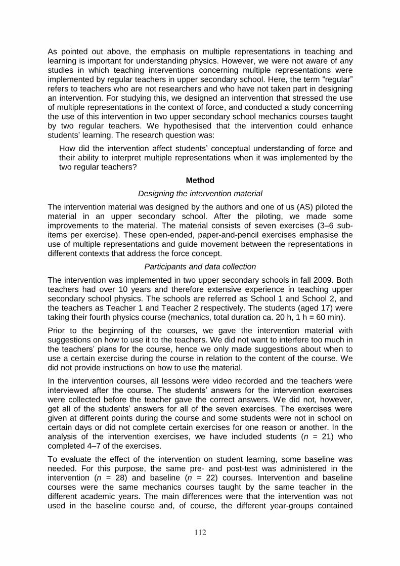
As pointed out above, the emphasis on multiple representations in teaching and learning is important for understanding physics. However, we were not aware of any studies in which teaching interventions concerning multiple representations were implemented by regular teachers in upper secondary school. Here, the term “regular” refers to teachers who are not researchers and who have not taken part in designing an intervention. For studying this, we designed an intervention that stressed the use of multiple representations in the context of force, and conducted a study concerning the use of this intervention in two upper secondary school mechanics courses taught by two regular teachers. We hypothesised that the intervention could enhance students’ learning. The research question was:

How did the intervention affect students’ conceptual understanding of force and their ability to interpret multiple representations when it was implemented by the two regular teachers?

Method

Designing the intervention material

The intervention material was designed by the authors and one of us (AS) piloted the material in an upper secondary school. After the piloting, we made some improvements to the material. The material consists of seven exercises (3–6 sub-items per exercise). These open-ended, paper-and-pencil exercises emphasise the use of multiple representations and guide movement between the representations in different contexts that address the force concept.

Participants and data collection

The intervention was implemented in two upper secondary schools in fall 2009. Both teachers had over 10 years and therefore extensive experience in teaching upper secondary school physics. The schools are referred as School 1 and School 2, and the teachers as Teacher 1 and Teacher 2 respectively. The students (aged 17) were taking their fourth physics course (mechanics, total duration ca. 20 h, 1 h = 60 min).

Prior to the beginning of the courses, we gave the intervention material with suggestions on how to use it to the teachers. We did not want to interfere too much in the teachers’ plans for the course, hence we only made suggestions about when to use a certain exercise during the course in relation to the content of the course. We did not provide instructions on how to use the material.

In the intervention courses, all lessons were video recorded and the teachers were interviewed after the course. The students’ answers for the intervention exercises were collected before the teacher gave the correct answers. We did not, however, get all of the students’ answers for all of the seven exercises. The exercises were given at different points during the course and some students were not in school on certain days or did not complete certain exercises for one reason or another. In the analysis of the intervention exercises, we have included students (n = 21) who completed 4–7 of the exercises.

To evaluate the effect of the intervention on student learning, some baseline was needed. For this purpose, the same pre- and post-test was administered in the intervention (n = 28) and baseline (n = 22) courses. Intervention and baseline courses were the same mechanics courses taught by the same teacher in the different academic years. The main differences were that the intervention was not used in the baseline course and, of course, the different year-groups contained

112

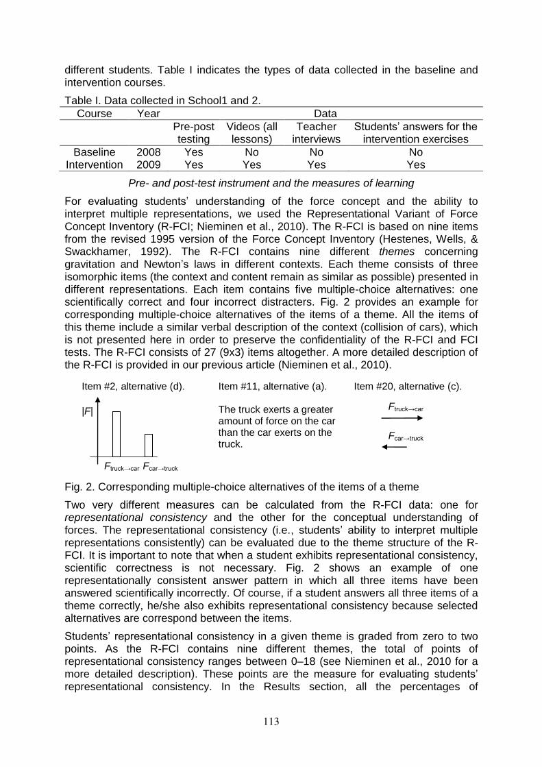
different students. Table I indicates the types of data collected in the baseline and intervention courses.

Table I. Data collected in School1 and 2.

Course Year Data

Pre-post testing

Videos (all lessons)

Teacher interviews

Students’ answers for the intervention exercises

Baseline 2008 Yes No No No Intervention 2009 Yes Yes Yes Yes

Pre- and post-test instrument and the measures of learning

For evaluating students’ understanding of the force concept and the ability to interpret multiple representations, we used the Representational Variant of Force Concept Inventory (R-FCI; Nieminen et al., 2010). The R-FCI is based on nine items from the revised 1995 version of the Force Concept Inventory (Hestenes, Wells, & Swackhamer, 1992). The R-FCI contains nine different themes concerning gravitation and Newton’s laws in different contexts. Each theme consists of three isomorphic items (the context and content remain as similar as possible) presented in different representations. Each item contains five multiple-choice alternatives: one scientifically correct and four incorrect distracters. Fig. 2 provides an example for corresponding multiple-choice alternatives of the items of a theme. All the items of this theme include a similar verbal description of the context (collision of cars), which is not presented here in order to preserve the confidentiality of the R-FCI and FCI tests. The R-FCI consists of 27 (9x3) items altogether. A more detailed description of the R-FCI is provided in our previous article (Nieminen et al., 2010).

Fig. 2. Corresponding multiple-choice alternatives of the items of a theme

Two very different measures can be calculated from the R-FCI data: one for representational consistency and the other for the conceptual understanding of forces. The representational consistency (i.e., students’ ability to interpret multiple representations consistently) can be evaluated due to the theme structure of the R-FCI. It is important to note that when a student exhibits representational consistency, scientific correctness is not necessary. Fig. 2 shows an example of one representationally consistent answer pattern in which all three items have been answered scientifically incorrectly. Of course, if a student answers all three items of a theme correctly, he/she also exhibits representational consistency because selected alternatives are correspond between the items.

Students’ representational consistency in a given theme is graded from zero to two points. As the R-FCI contains nine different themes, the total of points of representational consistency ranges between 0–18 (see Nieminen et al., 2010 for a more detailed description). These points are the measure for evaluating students’ representational consistency. In the Results section, all the percentages of

Ftruck→car Fcar→truck

|F|

Item #2, alternative (d). Item #11, alternative (a). The truck exerts a greater amount of force on the car than the car exerts on the truck.

Ftruck→car

Fcar→truck

Item #20, alternative (c).

113

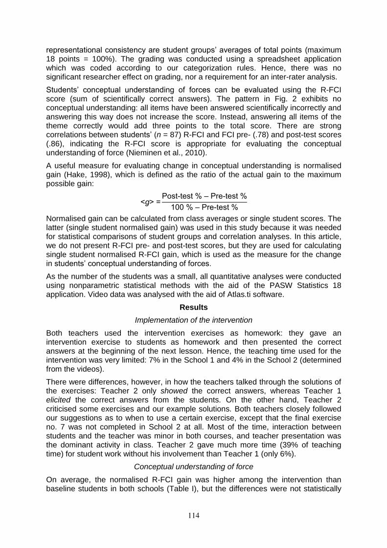
representational consistency are student groups’ averages of total points (maximum 18 points = 100%). The grading was conducted using a spreadsheet application which was coded according to our categorization rules. Hence, there was no significant researcher effect on grading, nor a requirement for an inter-rater analysis.

Students’ conceptual understanding of forces can be evaluated using the R-FCI score (sum of scientifically correct answers). The pattern in Fig. 2 exhibits no conceptual understanding: all items have been answered scientifically incorrectly and answering this way does not increase the score. Instead, answering all items of the theme correctly would add three points to the total score. There are strong correlations between students’ (n = 87) R-FCI and FCI pre- (.78) and post-test scores (.86), indicating the R-FCI score is appropriate for evaluating the conceptual understanding of force (Nieminen et al., 2010).

A useful measure for evaluating change in conceptual understanding is normalised gain (Hake, 1998), which is defined as the ratio of the actual gain to the maximum possible gain:

ost test – re test

– re test

Normalised gain can be calculated from class averages or single student scores. The latter (single student normalised gain) was used in this study because it was needed for statistical comparisons of student groups and correlation analyses. In this article, we do not present R-FCI pre- and post-test scores, but they are used for calculating single student normalised R-FCI gain, which is used as the measure for the change in students’ conceptual understanding of forces.

As the number of the students was a small, all quantitative analyses were conducted using nonparametric statistical methods with the aid of the PASW Statistics 18 application. Video data was analysed with the aid of Atlas.ti software.

Results

Implementation of the intervention

Both teachers used the intervention exercises as homework: they gave an intervention exercise to students as homework and then presented the correct answers at the beginning of the next lesson. Hence, the teaching time used for the intervention was very limited: 7% in the School 1 and 4% in the School 2 (determined from the videos).

There were differences, however, in how the teachers talked through the solutions of the exercises: Teacher 2 only showed the correct answers, whereas Teacher 1 elicited the correct answers from the students. On the other hand, Teacher 2 criticised some exercises and our example solutions. Both teachers closely followed our suggestions as to when to use a certain exercise, except that the final exercise no. 7 was not completed in School 2 at all. Most of the time, interaction between students and the teacher was minor in both courses, and teacher presentation was the dominant activity in class. Teacher 2 gave much more time (39% of teaching time) for student work without his involvement than Teacher 1 (only 6%).

Conceptual understanding of force

On average, the normalised R-FCI gain was higher among the intervention than baseline students in both schools (Table I), but the differences were not statistically

114

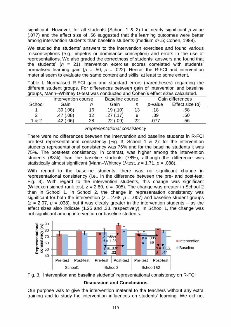
significant. However, for all students (School 1 & 2) the nearly significant p-value (.077) and the effect size of .56 suggested that the learning outcomes were better among intervention students than baseline students (medium d≈.5; Cohen, 1988).

We studied the students’ answers to the intervention exercises and found various misconceptions (e.g., impetus or dominance conception) and errors in the use of representations. We also graded the correctness of students’ answers and found that the students’ (n = 21) intervention exercise scores correlated with students’ normalised learning gain (ρ = .50, p = .022). Hence, the R-FCI and intervention material seem to evaluate the same content and skills, at least to some extent.

Table I. Normalised R-FCI gain and standard errors (parentheses) regarding the different student groups. For differences between gain of intervention and baseline groups, Mann–Whitney U-test was conducted and Cohen’s effect sizes calculated.

Intervention course Baseline course Gain differences School Gain n Gain n p-value Effect size (d)

1 .39 (.08) 16 .19 (.10) 13 .18 .58 2 .47 (.08) 12 .27 (.17) 9 .39 .50

1 & 2 .42 (.06) 28 .22 (.09) 22 .077 .56

Representational consistency

There were no differences between the intervention and baseline students in R-FCI pre-test representational consistency (Fig. 3; School 1 & 2): for the intervention students representational consistency was 76% and for the baseline students it was 75%. The post-test consistency, in contrast, was higher among the intervention students (83%) than the baseline students (78%), although the difference was statistically almost significant (Mann–Whitney U-test, z = 1.71, p = .088).

With regard to the baseline students, there was no significant change in representational consistency (i.e., in the difference between the pre- and post-test; Fig. 3). With regard to the intervention students, this change was significant (Wilcoxon signed-rank test, z = 2.80, p = .005). The change was greater in School 2 than in School 1. In School 2, the change in representation consistency was significant for both the intervention (z = 2.68, p = .007) and baseline student groups (z = 2.07, p = .038), but it was clearly greater in the intervention students – as the effect sizes also indicate (1.25 and .33, respectively). In School 1, the change was not significant among intervention or baseline students.

Fig. 3. Intervention and baseline students’ representational consistency on R-FCI

Discussion and Conclusions

Our purpose was to give the intervention material to the teachers without any extra training and to study the intervention influences on students’ learning. We did not

40

50

60

70

80

90

Pre-test Post-test Pre-test Post-test Pre-test Post-test

School1 School2 School1&2

Re

pre

se

nta

tio

na

l c

on

sis

ten

cy (

%)

Intervention

Baseline

p = .007 d = 1.25

p = .038 d = .33

p = .005 d = .59

p = .088 d = .44

115

instruct the teachers in how to use the intervention material. Both teachers used the material as homework exercises, which meant that the teaching time used for the intervention was very limited in both schools. The teachers had taught the mechanics course many times before, and they said in the interviews that they had not changed their teaching with the exception of including the new homework exercises (intervention material).

Despite the lightness of the implementation, the results suggest that the intervention increased students’ understanding of force (medium effect sizes were found in normalised gain of the R-FCI scores). In addition, the change in representational consistency was greater in intervention students than in baseline students, especially in School 2. Qualitative analysis of the video data collected could bring more information about, for example, why representational consistency increased more in School 2. The intervention was used only in these two courses and with a small number of students, hence one needs to be careful with the generalisation of the results to a larger population. A replication study in other courses and schools would be of value.

The results of this intervention support the assumption that the use of multiple external representations benefits student learning. The positive results with this light intervention may well suggest that research-informed teaching material could be effective in supporting student learning even when no extra training is provided to regular teachers.

Acknowledgement

This work has been supported by the Academy of Finland (Project No. 132316).

References

Ainsworth, S. (1999). The functions of multiple representations. Computers & Education, 33(2–3), 131–152.

Cohen, J. (1988). Statistical power analysis for the behavioral sciences (2nd ed.). Hillsdale, New Jersey: Lawrence Erlbaum.

Hake, R. R. (1998). Interactive-engagement versus traditional methods: A six-thousand-student survey of mechanics test data for introductory physics courses. American Journal of Physics, 66(1), 64–74.

Hestenes, D., Wells, M., & Swackhamer, G. (1992). Force concept inventory. The Physics Teacher, 30(3), 141–158.

Meltzer, D. E. (2005). Relation between students' problem-solving performance and representational format. American Journal of Physics, 73(5), 463–478.

Nieminen, P., Savinainen, A., & Viiri, J. (2010). Force concept inventory based multiple-choice test for investigating students' representational consistency. Physical Review Special Topics – Physics Education Research, 6(2), 020109.

Schnotz, W., Baadte, C., Müller, A., & Rasch, R. (2010). Creative thinking and problem solving with depictive and descriptive representations. In L. Verschaffel, E. De Corte, T. de Jong & J. Elen (Eds.), Use or representations in reasoning and problem solving: Analysis and improvement (pp. 11–35). Milton Park, UK: Routledge.

Van Heuvelen, A., & Zou, X. L. (2001). Multiple representations of work-energy processes. American Journal of Physics, 69(2), 184–194.

116

Profiling the mechanics knowledge of UK university entrants using the Force

Concept Inventory

David Sands

Department of Physical Sciences,

University of Hull.

e-mail: d.sands@hull.ac.uk

Physics education research has revealed that students can demonstrate alternative conceptions of

the physical world that are not only stubbornly resistant to change but can actively inhibit the learning

of Newtonian ideas. The force concept inventory (FCI) provides a well known test of understanding in

mechanics based on some of these misconceptions. For the past three years the first year cohort at

Hull has been tested using the FCI prior to a course of instruction in mechanics based around

modelling in VPython. Primarily this testing was undertaken to establish the baseline knowledge, but

detailed analysis reveals not only that a very large range of capabilities exists within a cohort, from

barely any understanding of mechanics concepts right through to what amounts to a functional

understanding, but also that, taken question by question, the results from each cohort are remarkably

similar. Thus, whilst there might be no such thing as a typical student there is at least a typical cohort

characterised by a distribution of correct answers on the FCI. Attention is focused on first-time UK

students, and the findings are therefore directly relevant to the UK HE physics community. The

question-by-question responses illustrate not only which concepts are well understood, but also

where confusion exists and which alternative conceptions the students tend to hold. The implications

for curriculum design are discussed briefly.

1. Introduction

It was David Ausubel who famously wrote, “The most important single factorinfluencing learning is what the learner already knows. Ascertain this and teach himaccordingly” (Ausubel, 1968). Nowhere is this more true than in mechanics. Physicseducation research has revealed that students can demonstrate alternativeconceptions of the physical world that are not only stubbornly resistant to change butcan actively inhibit the learning of Newtonian ideas. For example, Andrea di Sessareports in a study from the 1980s (di Sessa, 1987) that both graduate students andyoung children exhibit very similar naïve views, implying that these alternative viewsdevelop early in childhood and can persist right through the subsequent years offormal education, even beyond graduation. It’s not enough simply to determine thatstudents don’t know, say, Newton’s third law of motion, we also need to know whatview they hold in its stead. Fortunately, this is relatively easy in mechanics as theforce concept inventory (FCI) provides a well known test of understanding inmechanics (Redish,2003). Indeed, the FCI has played some part in revealing howcommon are some of these alternative conceptions.

The validity of the FCI as an instrument for measuring conceptual understanding ismuch discussed within the open literature (Huffman and Heller, 1995; Planinic et al,2010; Wallace and Bailey, 2010). In particular, the question has arisen as to whetherthe FCI provides a measure of a student’s coherent understanding of the forceconcept or whether it provides a snapshot of different aspects of their knowledge andunderstanding (Heller and Huffman, 1995; Hestenes and Halloun, 1995; Huffmanand Heller, 1995). The numbers of students involved in this study are too small toaddress this question directly, though the trends observed over a three year periodallow some comment on the consistency of the FCI as a diagnostic test. The pattern

117

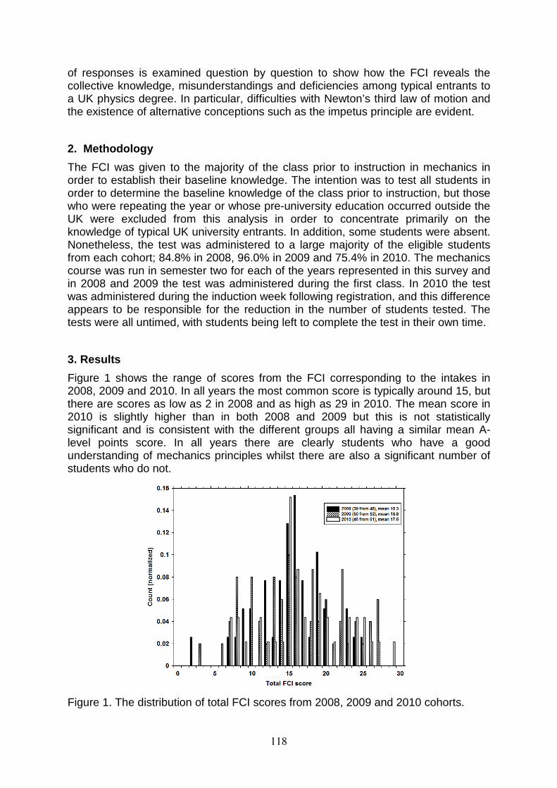
of responses is examined question by question to show how the FCI reveals thecollective knowledge, misunderstandings and deficiencies among typical entrants toa UK physics degree. In particular, difficulties with Newton’s third law of motion andthe existence of alternative conceptions such as the impetus principle are evident.

2. Methodology

The FCI was given to the majority of the class prior to instruction in mechanics inorder to establish their baseline knowledge. The intention was to test all students inorder to determine the baseline knowledge of the class prior to instruction, but thosewho were repeating the year or whose pre-university education occurred outside theUK were excluded from this analysis in order to concentrate primarily on theknowledge of typical UK university entrants. In addition, some students were absent.Nonetheless, the test was administered to a large majority of the eligible studentsfrom each cohort; 84.8% in 2008, 96.0% in 2009 and 75.4% in 2010. The mechanicscourse was run in semester two for each of the years represented in this survey andin 2008 and 2009 the test was administered during the first class. In 2010 the testwas administered during the induction week following registration, and this differenceappears to be responsible for the reduction in the number of students tested. Thetests were all untimed, with students being left to complete the test in their own time.

3. Results

Figure 1 shows the range of scores from the FCI corresponding to the intakes in2008, 2009 and 2010. In all years the most common score is typically around 15, butthere are scores as low as 2 in 2008 and as high as 29 in 2010. The mean score in2010 is slightly higher than in both 2008 and 2009 but this is not statisticallysignificant and is consistent with the different groups all having a similar mean A-level points score. In all years there are clearly students who have a goodunderstanding of mechanics principles whilst there are also a significant number ofstudents who do not.

Figure 1. The distribution of total FCI scores from 2008, 2009 and 2010 cohorts.

118

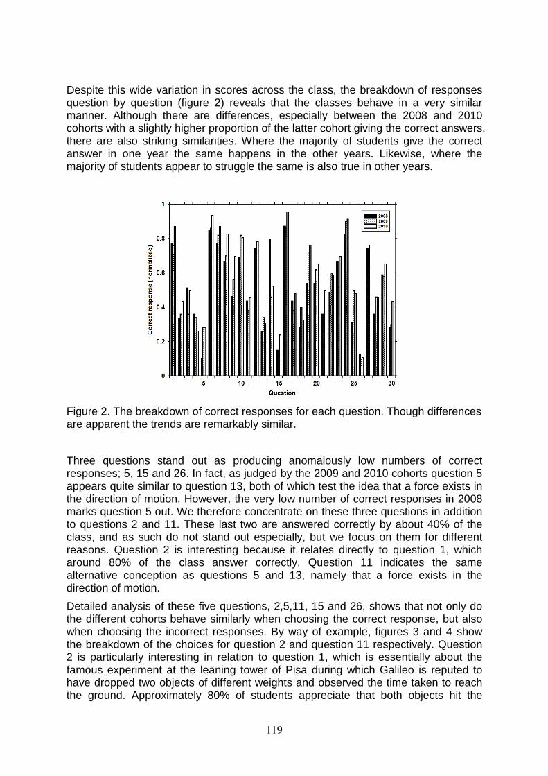
Despite this wide variation in scores across the class, the breakdown of responsesquestion by question (figure 2) reveals that the classes behave in a very similarmanner. Although there are differences, especially between the 2008 and 2010cohorts with a slightly higher proportion of the latter cohort giving the correct answers,there are also striking similarities. Where the majority of students give the correctanswer in one year the same happens in the other years. Likewise, where themajority of students appear to struggle the same is also true in other years.

Figure 2. The breakdown of correct responses for each question. Though differencesare apparent the trends are remarkably similar.

Three questions stand out as producing anomalously low numbers of correctresponses; 5, 15 and 26. In fact, as judged by the 2009 and 2010 cohorts question 5appears quite similar to question 13, both of which test the idea that a force exists inthe direction of motion. However, the very low number of correct responses in 2008marks question 5 out. We therefore concentrate on these three questions in additionto questions 2 and 11. These last two are answered correctly by about 40% of theclass, and as such do not stand out especially, but we focus on them for differentreasons. Question 2 is interesting because it relates directly to question 1, whicharound 80% of the class answer correctly. Question 11 indicates the samealternative conception as questions 5 and 13, namely that a force exists in thedirection of motion.

Detailed analysis of these five questions, 2,5,11, 15 and 26, shows that not only dothe different cohorts behave similarly when choosing the correct response, but alsowhen choosing the incorrect responses. By way of example, figures 3 and 4 showthe breakdown of the choices for question 2 and question 11 respectively. Question2 is particularly interesting in relation to question 1, which is essentially about thefamous experiment at the leaning tower of Pisa during which Galileo is reputed tohave dropped two objects of different weights and observed the time taken to reachthe ground. Approximately 80% of students appreciate that both objects hit the

119

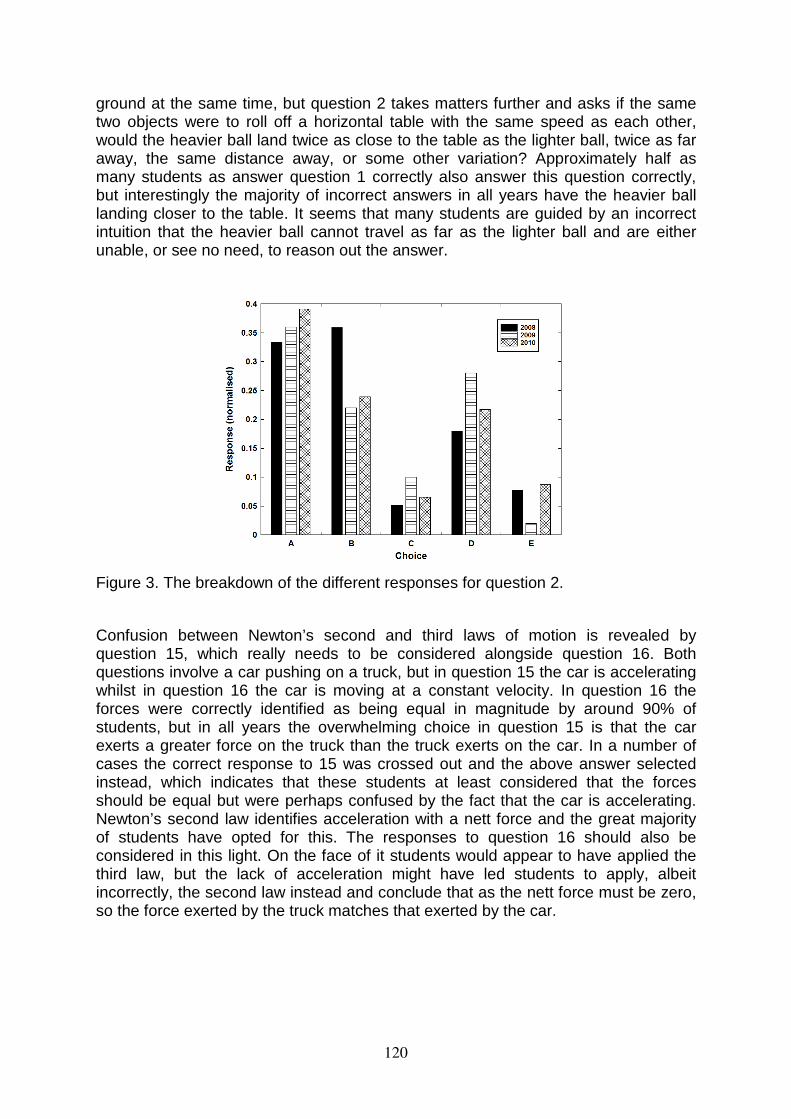
ground at the same time, but question 2 takes matters further and asks if the sametwo objects were to roll off a horizontal table with the same speed as each other,would the heavier ball land twice as close to the table as the lighter ball, twice as faraway, the same distance away, or some other variation? Approximately half asmany students as answer question 1 correctly also answer this question correctly,but interestingly the majority of incorrect answers in all years have the heavier balllanding closer to the table. It seems that many students are guided by an incorrectintuition that the heavier ball cannot travel as far as the lighter ball and are eitherunable, or see no need, to reason out the answer.

Figure 3. The breakdown of the different responses for question 2.

Confusion between Newton’s second and third laws of motion is revealed byquestion 15, which really needs to be considered alongside question 16. Bothquestions involve a car pushing on a truck, but in question 15 the car is acceleratingwhilst in question 16 the car is moving at a constant velocity. In question 16 theforces were correctly identified as being equal in magnitude by around 90% ofstudents, but in all years the overwhelming choice in question 15 is that the carexerts a greater force on the truck than the truck exerts on the car. In a number ofcases the correct response to 15 was crossed out and the above answer selectedinstead, which indicates that these students at least considered that the forcesshould be equal but were perhaps confused by the fact that the car is accelerating.Newton’s second law identifies acceleration with a nett force and the great majorityof students have opted for this. The responses to question 16 should also beconsidered in this light. On the face of it students would appear to have applied thethird law, but the lack of acceleration might have led students to apply, albeitincorrectly, the second law instead and conclude that as the nett force must be zero,so the force exerted by the truck matches that exerted by the car.

120

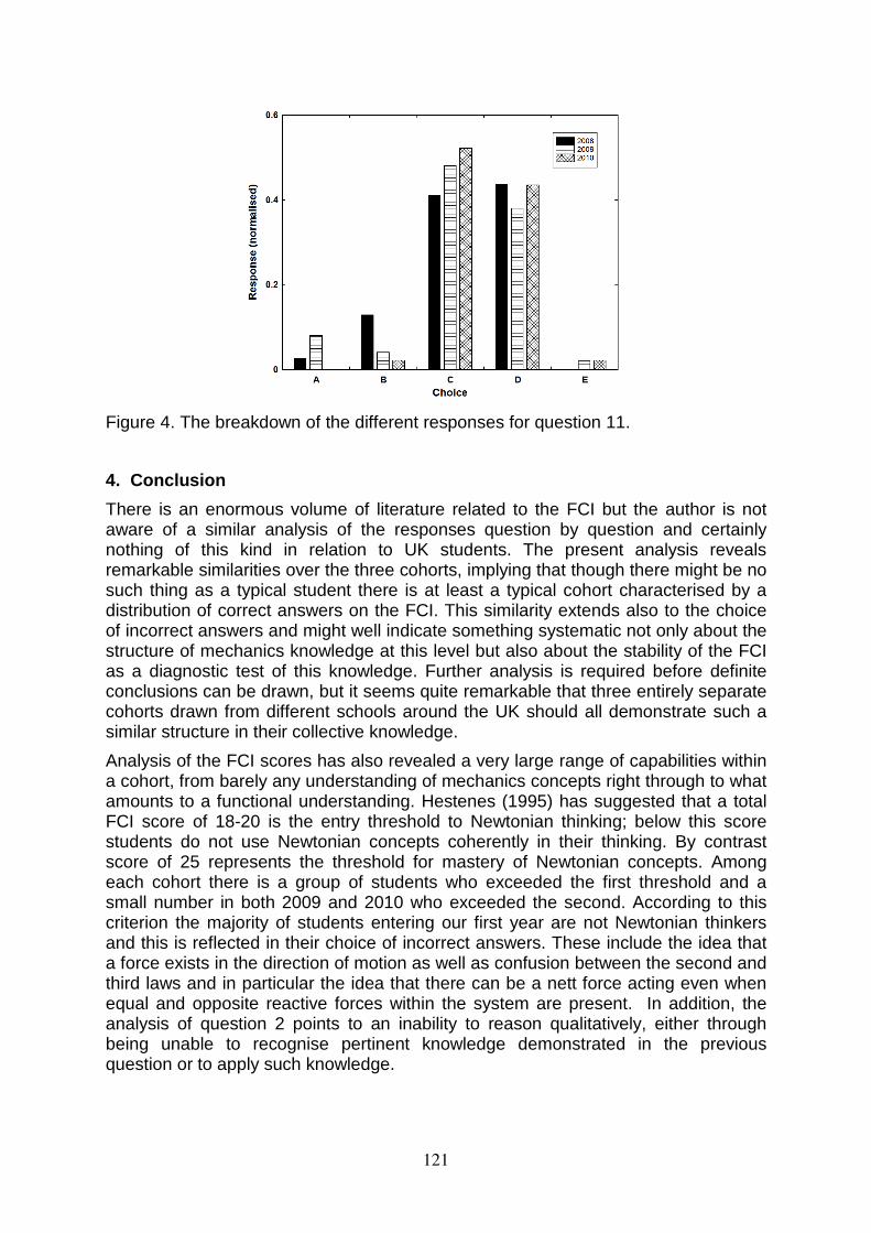
Figure 4. The breakdown of the different responses for question 11.

4. Conclusion

There is an enormous volume of literature related to the FCI but the author is notaware of a similar analysis of the responses question by question and certainlynothing of this kind in relation to UK students. The present analysis revealsremarkable similarities over the three cohorts, implying that though there might be nosuch thing as a typical student there is at least a typical cohort characterised by adistribution of correct answers on the FCI. This similarity extends also to the choiceof incorrect answers and might well indicate something systematic not only about thestructure of mechanics knowledge at this level but also about the stability of the FCIas a diagnostic test of this knowledge. Further analysis is required before definiteconclusions can be drawn, but it seems quite remarkable that three entirely separatecohorts drawn from different schools around the UK should all demonstrate such asimilar structure in their collective knowledge.

Analysis of the FCI scores has also revealed a very large range of capabilities withina cohort, from barely any understanding of mechanics concepts right through to whatamounts to a functional understanding. Hestenes (1995) has suggested that a totalFCI score of 18-20 is the entry threshold to Newtonian thinking; below this scorestudents do not use Newtonian concepts coherently in their thinking. By contrastscore of 25 represents the threshold for mastery of Newtonian concepts. Amongeach cohort there is a group of students who exceeded the first threshold and asmall number in both 2009 and 2010 who exceeded the second. According to thiscriterion the majority of students entering our first year are not Newtonian thinkersand this is reflected in their choice of incorrect answers. These include the idea thata force exists in the direction of motion as well as confusion between the second andthird laws and in particular the idea that there can be a nett force acting even whenequal and opposite reactive forces within the system are present. In addition, theanalysis of question 2 points to an inability to reason qualitatively, either throughbeing unable to recognise pertinent knowledge demonstrated in the previousquestion or to apply such knowledge.

121

References

Ausubel, D. P. (1968). Educational psychology: A cognitive view. New York: Holt,Rinehart and Winston.

di Sessa, A. (1987). The Third Revolution in Computers and Education, Journal ofResearch into Science Teaching, 24(4), 343-367.

Heller, P., & Huffman, D. (1995). Interpreting The Force Concept Inventory: Aresponse to Huffman and Heller, The Physics Teacher, 33, 503-511.

Hestenes, D., & Halloun, I. (1995). Interpreting The Force Concept Inventory: AReply to Hestenes and Halloun, The Physics Teacher, 33, 502-506.

Huffman, D., & Heller, P. (1995). What Does the Force Concept Inventory ActuallyMeasure? The Physics Teacher, 33, 138-143.

Planinic, M., Ivanjek, L., & Susac, A. (2010). Rasch Model based analysis of theForce Concept Inventory, Physical Review Special Topics –Physics EducationResearch, 6, 010103

Redish, Edward F. (2003). Teaching Physics With The Physics Suite, John Wiley &Sons, USA.

Smith, J. I., & Tanner, K. (2010). The Problem Of Revealing How Students Think:Concept Inventories and Beyond, CBE-Life Science Education 9, 1-5

Wallace, C. S., & Bailey, J. M. (2010). Do Concept Inventories Actually MeasureAnything? Astronomy Education Review, 9, 010116-1.

122

An Intervention Using an Interaction Diagram for Teaching Newton’s Third Law in Upper Secondary School

Antti Savinainen, Asko Mäkynen, Pasi Nieminen and Jouni Viiri

antti.savinainen@kuopio.fi

Department of Teacher Education, University of Jyväskylä, Finland

Many studies show that students have difficulties with Newton’s third law (N3 law). In this study we investigated the use of Interaction Diagrams (ID; a visualizable tool for identifying and representing interactions between objects) in fostering students’ understanding of N3 law. The intervention material was designed to aid the use of IDs and teaching of N3 law. There were two groups: the intervention group (n=51), using the textbook and the intervention materials; and the textbook group (n=26), using only the textbook addressing the ID. The additional time investment in the intervention group was about 45 min. The intervention group answered four pre-test questions on N3 law. Both groups answered four post-test questions on N3 law, and eight questions on IDs after the teaching. The intervention group showed very good understanding of N3 law whereas they did poorly, as expected, in the pre-test. The quality of their IDs was very good in general. The textbook group showed some understanding of N3 law but their results were generally poorer (both in terms of IDs and N3 law) than those of the intervention group. Our results suggest that emphasising the ID is beneficial in learning N3 law.

1. Introduction

Many articles have been published on students’ understandings of Newton’s third law (N3 law; see for example Brown, 1989; Montanero, Suero, Perez, & Pardo, 2002; Kariotoglou, Spyrtou, & Tselfes, 2009). The findings commonly indicate that after traditional teaching most students have a poor understanding of N3 law and of the force concept in general. Perhaps the most common view among students is that of force as an innate or acquired property of objects, which implies that forces are not seen as arising from an interaction between objects. Many students also seem to think in terms of a 'dominance principle', where a heavier or faster object exerts a greater force than the other object. Furthermore, students’ understandings of the force concept are very often context dependent, meaning that a student may show correct understanding in some exercises involving the force concept but fail to apply this in other contexts (Bao, Hogg, & Zollmann, 2002; Savinainen & Viiri, 2008). In addition, a good conceptual understanding of the force concept involves the use of multiple representations such as verbal, vectorial, and graphical representations (Nieminen, Savinainen, & Viiri, 2010).

There is evidence that the difficulties with N3 law can be overcome to a great extent with the use of a representation which we call an Interaction Diagram (Savinainen, Scott, & Viiri, 2005; Hinrichs, 2005). The Interaction Diagram (ID) provides a visualizable tool for identifying and representing interactions between objects, thus helping students to perceive forces as the property of an interaction instead of a property of an object. There are various ways of visualizing the objects and interactions between them (for example, see Turner, 2003): we use the version of Hatakka, Saari, Sirviö, Viiri, and Yrjänäinen (2004) in this study because it includes writing down the interactions in terms of pushing and pulling (Fig. 1). Hence, one can argue that it involves N3 law even more explicitly than the other versions of IDs.

The earlier studies reporting evidence for the usefulness of IDs (or a similar tool) have involved only teachers who were acting as researchers at the same time

123

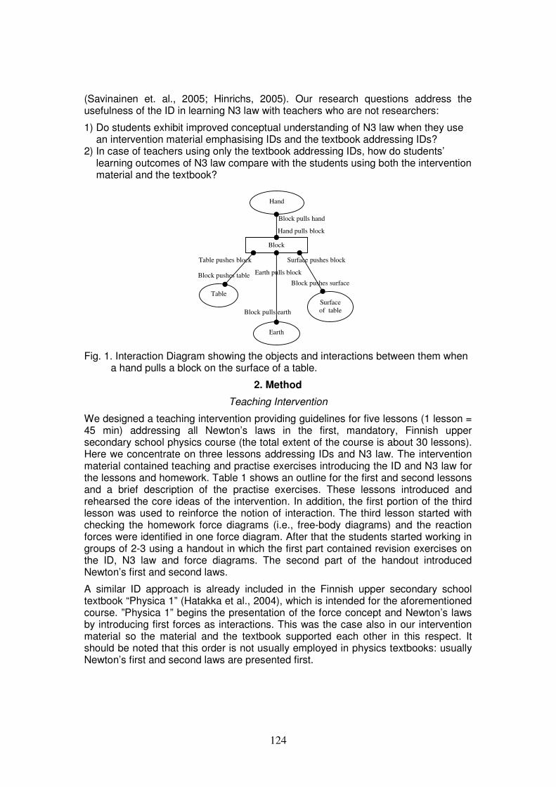
(Savinainen et. al., 2005; Hinrichs, 2005). Our research questions address the usefulness of the ID in learning N3 law with teachers who are not researchers:

1) Do students exhibit improved conceptual understanding of N3 law when they use an intervention material emphasising IDs and the textbook addressing IDs?

2) In case of teachers using only the textbook addressing IDs, how do students’ learning outcomes of N3 law compare with the students using both the intervention material and the textbook?

Fig. 1. Interaction Diagram showing the objects and interactions between them when a hand pulls a block on the surface of a table.

2. Method

Teaching Intervention

We designed a teaching intervention providing guidelines for five lessons (1 lesson = 45 min) addressing all Newton’s laws in the first, mandatory, Finnish upper secondary school physics course (the total extent of the course is about 30 lessons). Here we concentrate on three lessons addressing IDs and N3 law. The intervention material contained teaching and practise exercises introducing the ID and N3 law for the lessons and homework. Table 1 shows an outline for the first and second lessons and a brief description of the practise exercises. These lessons introduced and rehearsed the core ideas of the intervention. In addition, the first portion of the third lesson was used to reinforce the notion of interaction. The third lesson started with checking the homework force diagrams (i.e., free-body diagrams) and the reaction forces were identified in one force diagram. After that the students started working in groups of 2-3 using a handout in which the first part contained revision exercises on the ID, N3 law and force diagrams. The second part of the handout introduced Newton’s first and second laws.

A similar ID approach is already included in the Finnish upper secondary school textbook “Physica 1” (Hatakka et al., 2004), which is intended for the aforementioned course. ”Physica 1” begins the presentation of the force concept and Newton’s laws by introducing first forces as interactions. This was the case also in our intervention material so the material and the textbook supported each other in this respect. It should be noted that this order is not usually employed in physics textbooks: usually Newton’s first and second laws are presented first.

Block pushes surface

Surface pushes block

Block

Hand

Earth

Table

Surface

of table

Block pulls hand

Hand pulls block

Earth pulls block

Block pulls earth

Block pushes table

Table pushes block

124

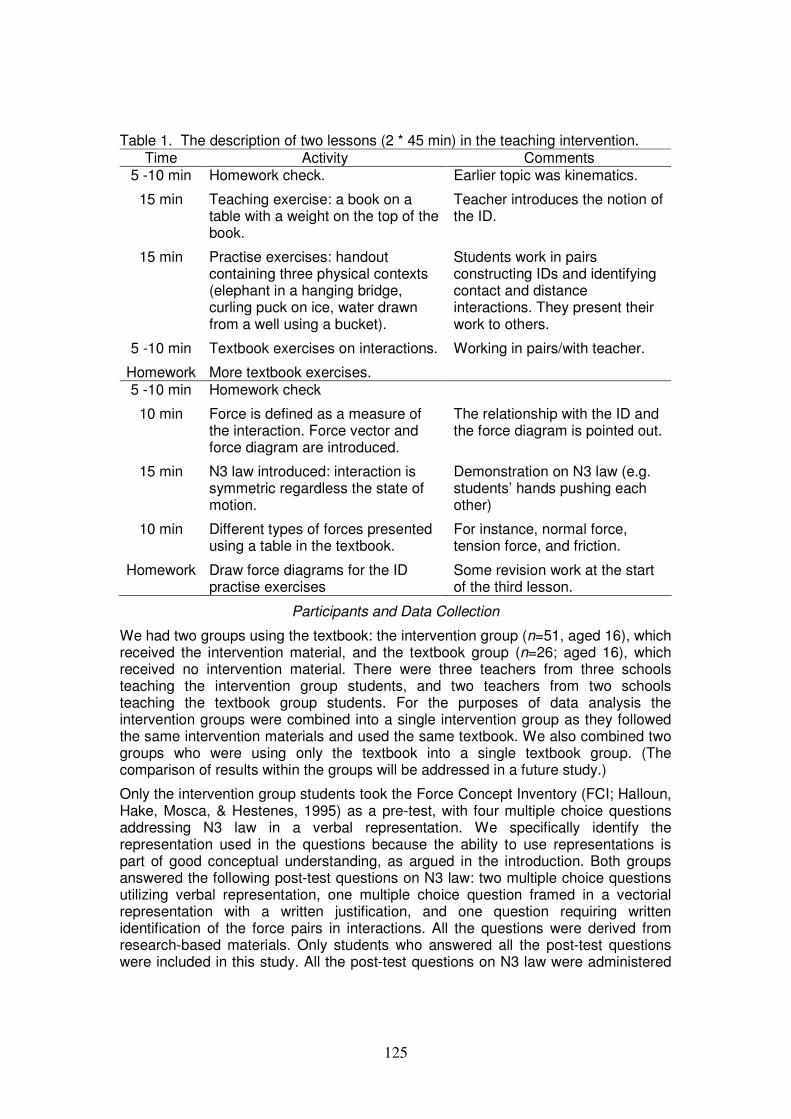
Table 1. The description of two lessons (2 * 45 min) in the teaching intervention. Time Activity Comments

5 -10 min Homework check. Earlier topic was kinematics.

15 min Teaching exercise: a book on a table with a weight on the top of the book.

Teacher introduces the notion of the ID.

15 min Practise exercises: handout containing three physical contexts (elephant in a hanging bridge, curling puck on ice, water drawn from a well using a bucket).

Students work in pairs constructing IDs and identifying contact and distance interactions. They present their work to others.

5 -10 min Textbook exercises on interactions. Working in pairs/with teacher.

Homework More textbook exercises. 5 -10 min Homework check

10 min Force is defined as a measure of the interaction. Force vector and force diagram are introduced.

The relationship with the ID and the force diagram is pointed out.

15 min N3 law introduced: interaction is symmetric regardless the state of motion.

Demonstration on N3 law (e.g. students’ hands pushing each other)

10 min Different types of forces presented using a table in the textbook.

For instance, normal force, tension force, and friction.

Homework Draw force diagrams for the ID practise exercises

Some revision work at the start of the third lesson.

Participants and Data Collection

We had two groups using the textbook: the intervention group (n=51, aged 16), which received the intervention material, and the textbook group (n=26; aged 16), which received no intervention material. There were three teachers from three schools teaching the intervention group students, and two teachers from two schools teaching the textbook group students. For the purposes of data analysis the intervention groups were combined into a single intervention group as they followed the same intervention materials and used the same textbook. We also combined two groups who were using only the textbook into a single textbook group. (The comparison of results within the groups will be addressed in a future study.)

Only the intervention group students took the Force Concept Inventory (FCI; Halloun, Hake, Mosca, & Hestenes, 1995) as a pre-test, with four multiple choice questions addressing N3 law in a verbal representation. We specifically identify the representation used in the questions because the ability to use representations is part of good conceptual understanding, as argued in the introduction. Both groups answered the following post-test questions on N3 law: two multiple choice questions utilizing verbal representation, one multiple choice question framed in a vectorial representation with a written justification, and one question requiring written identification of the force pairs in interactions. All the questions were derived from research-based materials. Only students who answered all the post-test questions were included in this study. All the post-test questions on N3 law were administered

125

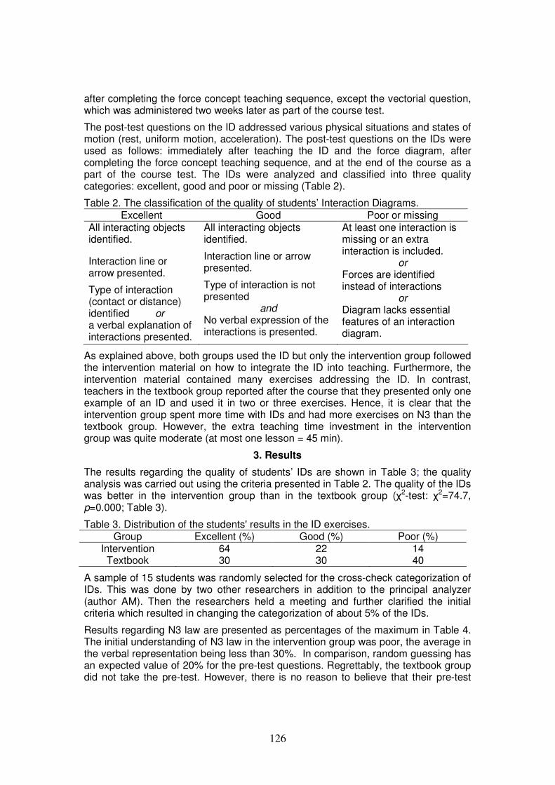
after completing the force concept teaching sequence, except the vectorial question, which was administered two weeks later as part of the course test.

The post-test questions on the ID addressed various physical situations and states of motion (rest, uniform motion, acceleration). The post-test questions on the IDs were used as follows: immediately after teaching the ID and the force diagram, after completing the force concept teaching sequence, and at the end of the course as a part of the course test. The IDs were analyzed and classified into three quality categories: excellent, good and poor or missing (Table 2).

Table 2. The classification of the quality of students’ Interaction Diagrams. Excellent Good Poor or missing

All interacting objects identified.

Interaction line or arrow presented.

Type of interaction (contact or distance) identified or a verbal explanation of interactions presented.

All interacting objects identified.

Interaction line or arrow presented.

Type of interaction is not presented

and No verbal expression of the interactions is presented.

At least one interaction is missing or an extra interaction is included.

or Forces are identified instead of interactions

or Diagram lacks essential features of an interaction diagram.

As explained above, both groups used the ID but only the intervention group followed the intervention material on how to integrate the ID into teaching. Furthermore, the intervention material contained many exercises addressing the ID. In contrast, teachers in the textbook group reported after the course that they presented only one example of an ID and used it in two or three exercises. Hence, it is clear that the intervention group spent more time with IDs and had more exercises on N3 than the textbook group. However, the extra teaching time investment in the intervention group was quite moderate (at most one lesson = 45 min).

3. Results

The results regarding the quality of students’ IDs are shown in Table 3; the quality analysis was carried out using the criteria presented in Table 2. The quality of the IDs was better in the intervention group than in the textbook group (χ2-test: χ2=74.7, p=0.000; Table 3).

Table 3. Distribution of the students' results in the ID exercises. Group Excellent (%) Good (%) Poor (%)

Intervention 64 22 14 Textbook 30 30 40

A sample of 15 students was randomly selected for the cross-check categorization of IDs. This was done by two other researchers in addition to the principal analyzer (author AM). Then the researchers held a meeting and further clarified the initial criteria which resulted in changing the categorization of about 5% of the IDs.

Results regarding N3 law are presented as percentages of the maximum in Table 4. The initial understanding of N3 law in the intervention group was poor, the average in the verbal representation being less than 30%. In comparison, random guessing has an expected value of 20% for the pre-test questions. Regrettably, the textbook group did not take the pre-test. However, there is no reason to believe that their pre-test

126

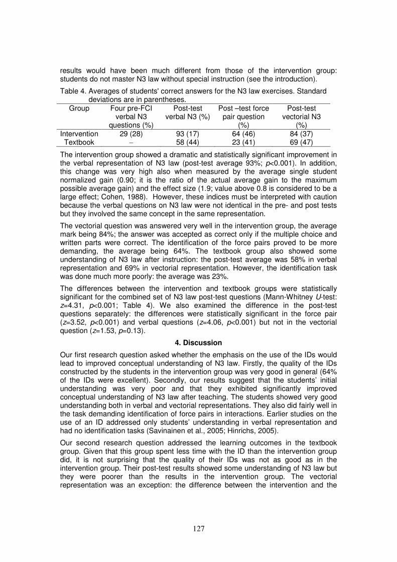
results would have been much different from those of the intervention group: students do not master N3 law without special instruction (see the introduction).

Table 4. Averages of students' correct answers for the N3 law exercises. Standard deviations are in parentheses.

Group Four pre-FCI verbal N3

questions (%)

Post-test verbal N3 (%)

Post –test force pair question

(%)

Post-test vectorial N3

(%) Intervention 29 (28) 93 (17) 64 (46) 84 (37) Textbook – 58 (44) 23 (41) 69 (47)

The intervention group showed a dramatic and statistically significant improvement in the verbal representation of N3 law (post-test average 93%; p<0.001). In addition, this change was very high also when measured by the average single student normalized gain (0.90; it is the ratio of the actual average gain to the maximum possible average gain) and the effect size (1.9; value above 0.8 is considered to be a large effect; Cohen, 1988). However, these indices must be interpreted with caution because the verbal questions on N3 law were not identical in the pre- and post tests but they involved the same concept in the same representation.

The vectorial question was answered very well in the intervention group, the average mark being 84%; the answer was accepted as correct only if the multiple choice and written parts were correct. The identification of the force pairs proved to be more demanding, the average being 64%. The textbook group also showed some understanding of N3 law after instruction: the post-test average was 58% in verbal representation and 69% in vectorial representation. However, the identification task was done much more poorly: the average was 23%.

The differences between the intervention and textbook groups were statistically significant for the combined set of N3 law post-test questions (Mann-Whitney U-test: z=4.31, p<0.001; Table 4). We also examined the difference in the post-test questions separately: the differences were statistically significant in the force pair (z=3.52, p<0.001) and verbal questions (z=4.06, p<0.001) but not in the vectorial question (z=1.53, p=0.13).

4. Discussion

Our first research question asked whether the emphasis on the use of the IDs would lead to improved conceptual understanding of N3 law. Firstly, the quality of the IDs constructed by the students in the intervention group was very good in general (64% of the IDs were excellent). Secondly, our results suggest that the students’ initial understanding was very poor and that they exhibited significantly improved conceptual understanding of N3 law after teaching. The students showed very good understanding both in verbal and vectorial representations. They also did fairly well in the task demanding identification of force pairs in interactions. Earlier studies on the use of an ID addressed only students’ understanding in verbal representation and had no identification tasks (Savinainen et al., 2005; Hinrichs, 2005).

Our second research question addressed the learning outcomes in the textbook group. Given that this group spent less time with the ID than the intervention group did, it is not surprising that the quality of their IDs was not as good as in the intervention group. Their post-test results showed some understanding of N3 law but they were poorer than the results in the intervention group. The vectorial representation was an exception: the difference between the intervention and the

127

textbook groups was not statistically significant. The textbook group did not succeed well in identifying interaction force pairs. Overall, the results in other post-test tasks in the textbook group suggest that even a brief use of the ID may improve conceptual understanding of N3 law. However, because of the lack of a pre-test and the smaller amount of time spent with the ID and N3 law, the comparisons between the intervention and textbook groups should be interpreted with caution.

In conclusion, our intervention group results suggest that emphasising the ID is beneficial in learning N3 law even when the teachers have not received special training in the use of the ID.

5. Acknowledgement

This work has been supported by the Academy of Finland (Project No. 132316).

References

Bao, L., Hogg, K., & Zollman, D. (2002). Model analysis of fine structures of student models: An example with Newton’s third law. American Journal of Physics, 70(7), 766- 778.

Brown, D. E. (1989). Students' concept of force: the importance of understanding Newton’s third law. Physics Education, 24, 353-358.

Cohen, J. (1988). Statistical power analysis for the behavioral sciences (2nd edition). Hillsdale, NJ: Erlbaum.

Halloun, I., Hake, R., Mosca, E., & Hestenes, D. (1995). Force Concept Inventory (Revised 1995). Password protected at <http://modeling.asu.edu/r&e/research.html>. Accessed on 19.10.2011.

Hatakka, J., Saari, H., Sirviö, J., Viiri, J., & Yrjänäinen, S. (2004). Physica 1. WSOY: Porvoo.

Hinrichs, B. (2005). Using the system schema representational tool to promote student understanding of Newton’s third law. In Marx, J., Heron, P., & Franklin, S. (Eds.) AIP Conference Proceedings - 2004 Physics Education Research Conference, 790 (pp. 117-120). New York: Melville.

Kariotoglou, P., Spyrtou, A., & Tselfes, V. (2009). How student teachers understand distance force interactions in different contexts. International Journal of Science and Mathematics Education, 7, 851-873.

Montanero, M., Suero, M. I., Perez, A. L., & Pardo, P. J. (2002). Implicit theories of static interactions between two bodies. Physics Education, 37(4), 318- 323.

Nieminen, P., Savinainen A., & Viiri, J. (2010). Force Concept Inventory-based multiple-choice test for investigating students' representational consistency. Physical Review Special Topics - Physics Education Research, 6(2), 020109-1-12

Savinainen, A., Scott, P., & Viiri, J. (2005). Using a bridging representation and social interactions to foster conceptual change: Designing and evaluating an instructional sequence for Newton’s third law. Science Education, 89, 175-195.

Savinainen, A. & Viiri, J. (2008). The Force Concept Inventory as a measure of students' conceptual coherence. International Journal of Science and Mathematics Education, 6(4), 719-740.

Turner, L. (2003). System schemas. The Physics Teacher, 41, 404-408.

128

Gaining knowledge-building expertise in nanomodelli ng

Suvi Tala

suvi.tala@helsinki.fi

Department of Physics, University of Helsinki

The nature of the expertise that young scientists attempt to gain by participating in research groups is a relatively little-explored question. This study employs multidimensional empirical methods in order to reveal practicing nanomodellers’ (N=10), perspectives on their knowledge-building expertise – and on young scientists’ development of expertise through education. The main method used was contextualized interviewing: the practitioners were not explicitly asked to give their views about their expertise but rather on tools and skills that are needed in and views guiding their particular knowledge-building projects – and how these abilities are leaned in the process. Modelling in the virtual world plays a major role in nanoscience – as it increasingly does in many fields of science. Thus the study adds to our understanding of the nature of scientific knowledge building and gaining expertise in that. This in turn may be used in the education of the scientists of the future.

1. Introduction

What novice scientists learn in their education defines how they do science in the future. In this way, the education of scientists contributes to scientific and technological progress. What young natural scientists learn in their enculturation into the knowledge-building practices of science is anyway a relatively little-explored question. This study employs multidimensional empirical methods in order to reveal practicing nanophysicists’, both experts’ and apprentices’ (PhDs), perspectives on expertise in the knowledge-construction and -justification processes of nanophysics – and on enculturation into this expertise. The nanophysicists whose views are examined here work in a field where the traditional conceptions of scientific knowledge-building do not apply (Humphreys 2004): there is no particular established theory encompassing nanophysics, and the accuracy of detection and experimentation in the nanoworld is limited; meaning that computer modelling plays a central role. This study can thus add to our understanding of scientific knowledge building and attaining expertise in this area.

Contributory expertise (Collins & Robert 2007) essentially rests on the knowledge and skills which develop with one’s experience in a domain. An expert’s knowledge includes factual knowledge as well as conceptual, procedural and metacognitional understanding, which (s)he synthesizes and merges with appropriate skills for successful action (cf. the taxonomy of knowledge by Anderson & Krathwohl 2001). As an expert interviewed in this study stated, this merging is guided by a “special insight”. He went on to say that: “It is something I cannot describe in words. It is taught nowhere.” Chemical physicist Michael Polanyi (1958, 1966) already wrote about the existence of tacit kind knowledge lying at the heart of contributory expertise and guiding a scientist’s actions. He defined it as a feature of the individual scientist, a type of personal knowledge which cannot be made explicit: “We can know more than we can tell” (Polanyi 1966, p. 4). Nowadays, tacit knowledge is also discussed as something, which a group of experts share and which can be (partly) revealed through careful analysis carried out in interdisciplinary co-operation (Collins & Sanders 2006; Collins 2010).

It is because of the shared nature of expertise that it is seen natural for novice scientists to be educated as integrated members of research groups. Learning in such wide apprentice-master systems has been previously discussed in other contexts (e.g., Cate & Durning 2007; Gamble 2001; Gardner 2008; Laudel & Gläser

129

2008). Such education of young natural scientists, wherein they gain expertise by working with experts and other apprentices, has often been mentioned as an example of an authentic, constructive and socially motivating context for learning (e.g. Boyle & Boice 1998, Gardner 2008), but is still a poorly understood process. When young scientists gain expertise by working in a particular project, there is a danger that the objectives of the research project will dominate over the educational goals. Indeed, it is not easy for an apprentice to learn and for an expert to explain the ideas that guide research practices, because expert scientists’ intuitive mode of reasoning guides decision-making in the research groups. Thus, it is important to clearly articulate to young scientists the expertise they are gaining.

There seem to be two kinds of tacit aspects in scientists’ expertise. Firstly, when one reaches the higher levels of expertise (cf. Dreyfus & Dreyfus 1986), deep tacit understanding directs her/his intuitive grasp of situations and (s)he no longer considers the basics. Secondly, at the heart of expertise lies shared insight (Lave & Wenger 1991), which directs the knowledge-construction and -justification practices together with understanding the different interpretations of these practices. The tacit knowledge of the later type is what this study focuses on. The Finnish nanomodellers wanted to recognize and articulate their understanding of this tacit “insight” as well as other mainly tacit components of their expertise for educational purposes. Together with a number of scholars from other fields (Argyris 1993; Cianciolo et al. 2006; Eraut 2000; Schon 1983), they realized that young scientists’ learning in apprentice-master systems could be better supported on the basis of an analysis of the tacit expertise the young scientists are gaining. In this regard, the present study also deepens our views about nature of science and nature of scientific modelling in particular.

2. Questionnaire and interview contextualized in th e interviewees’ projects

The informants in this phenomenological case study were Finnish material physicists studying nanophenomena through “realistic simulations”: 5 experts (E) and 5 apprentices (A). To gain deeper insight the study employs multidimensional methods: The informants answered a written questionnaire contextualized to their ongoing projects. Then they were interviewed one by one. The interviews were semi-structured on the basis of the interviewees’ responses to the questionnaire and their scientific articles they provided in advance. The questionnaire and interviews were developed in a collaboration between researchers in physics, physics education and philosophy.

The transcript interviews together with the responses to the questionnaire were analysed by qualitative content analysis answering the following question: “What constitutes the core of the expertise of nanomodellers’ knowledge building and how it is learned?” The interviewees checked the analysis; the interpretations were corrected according to the interviewers’ requests (validity). It was noted that the same viewpoints emerged repeatedly in the responses of the successful nanomodellers (reliability). The results are introduced here by presenting quotations which depict typical views.

3. Results: building a brick tower of expertise

Nanomodellers combine scientific and technological knowledge of different kinds in their technoscientific (Tala 2009) capability, which prepares them for activity in the reality of nanomodelling. In doing so, they follow tacit methodological and epistemological ideas (“insight”), defining the rules of knowledge construction and justification. But then, an important part of one’s expertise in nanomodelling is the

130

ability to build the connections to experimental reality; by employing Humpreys’ (2004) idea of trading zones, this can be called trading zone -expertise. Additionally, one should be able to apply her/his expertise in modelling tasks in other contexts to progress in developing applied expertise1. In what follows, these bricks of expertise are briefly introduced.

Beginning with employed knowledge, an apprentice nanomodeller needs factual knowledge and must acquire a very good conceptual understanding of the basics of physics, material physics, chemistry, mathematics and “metamathematics”, all of which merge in modelling: “[our] modelling is made of different theories like a patchwork” (E) (for details, see Tala 2011). Furthermore, this scientific knowledge also merges with technological knowledge, such as “the basic principles of coding” and understanding the challenges posed by very limited computer power.

The merging of science and technology needs to be taken into account when interpreting knowledge-building through modelling. For example, as one expert pointed out, “the physical model fitted in a computer is never the same as the original physical template which provided the starting point”. A central question in this interpreting is naturally the relation between modelling and “reality”: At the beginning of enculturation, interviewed apprentices seem to have a tendency towards overarching realism. Respectively, the expert modellers highlighted other than representational roles of models. Along with the growth of expertise, the young scientists seemed to omit a flexible, instrumental view of models and modelling: “a model doesn’t care about the actual conditions or claim that it explains them, since the only important property of a model is its functionality” (an advanced apprentice). The independence of a model is seen to reach even the extend that “a model lives its own life” (A). Thus it can be said that what is reached is not a one-to-one similarity relation between the model and the system modelled, but a workable model, through running which on a computer can be produced knowledge about its dynamics – and finally an understanding about the world’s processes. Successful apprentices will begin to perceive their models as tools, which remain independent of both theory and experimentation, but which are developed in a two-way fitting between computer modelling and experimentation.

This scientific and technological framework leads them, for example, to “look for an intuitively clear model which includes the essential [features of] processes and not much else” (an advanced apprentice) – and then to “effective coding” (E). It is because of this connection built in the fitting that models are able to help us understand the “real-world”. This two-way fitting is reached through co-operation between the two knowledge-building communities – modellers and experimenters – both of whom have their own methodological and epistemological views, language and models. This co-operation means trading ideas, measurements, models, experimental ability and computer power2, where the objective of the modellers is to make the vital connections to experimentation and the experimenters’ to arrive at functional explanations. Maintaining this trading plays a central role in expertise. Thus the modellers also must learn to see the situations through the eyes of the experimenters – and vice versa. Indeed, to be able to build the connections to theory and experimentation through interaction, young nanomodellers must learn to use and

1 ‘Applied expertise’ comes near to the terms ‘adaptive expertise’ (Kimball & Holyok 2000) or ‘referred expertise’ (Collins & Robert 2007). 2 cf. Galison’s (1997) idea about trading zones

131

also develop intercultural modes of communication (cf. Collins, Evans & Gorman 2007; Ribeiro 2007; Wenger 1999). This ability develops in novice scientists through extensive experience 3 and seemed to develop more quickly in the interviewed apprentices who particularly mentioned an interest in reflective, interdisciplinary discussion.

As a part of trading zone expertise, apprentices should learn to recognize and communicate the possibilities and limitations of the epistemological and methodological views guiding their communities. Beginning apprentices use the given models and methods in the same way as black boxes: “The question of how the model is derived is not an easy one and I can’t answer it. I only use it.” But, finally, after completing their PhD they should be able even to “sell” and apply their expertise in another contexts of the job market. The ability to apply one’s expertise in other contexts is particularly important in nanoscience, as in many other new areas such as the software domain and scientific fields related to other quickly developing technology in which new tools and methodologies continue to emerge and where existing knowledge and methods can quickly become obsolete. As successful examples, one expert told of an apprentice who had left his group and started to simulate situations in biophysics, of some others who as medical physicists were at the moment simulating the irradiation on tissue and yet an another who was simulating the development of the stock quotations. Concerning the latter, the expert said: “He learned to deal with a huge amount of data while working for us and tried to obtain some relevant knowledge from it. Now he performs the same task [in a bank], indeed with models of very different kinds”. Optimally, an apprentice gains the ability to extend the possibilities of the methods and cross the limits for scientific and technological progress.

4. Conclusions and implications

This study revealed nanomodellers’ views of their expertise and how this expertise is attained. It thus provides a basis for supporting the education of young scientists. Apprentices’ learning can be supported by providing them – and the experts guiding them – with explicit knowledge about expertise as well as tools for reflection. In addition to support in developing an understanding of expertise and an ability to reflect, apprentices need interdisciplinary contacts supporting reflective discussion. For example, as one expert suggested: “We should have a course on the theory of scientific modelling. It should not teach modelling techniques, but should concentrate on questions [of the meta-level] like the ones you have just asked me [in this questionnaire and interview]”. At best, such a course should be organized through interdisciplinary co-operation or on an interdisciplinary basis combining an understanding of the field’s actual knowledge building practices, the analytical tools provided by science studies, and understanding about learning. Furthermore, the present study can improve our views of nature and the basis of physics, particularly the creation of physical knowledge through modelling.

3 Expertise research has found that more than the amount of experience in the field in question, special aspects of experience, such as its breadth and variety, are closely related to expert performance (Sonnentag, Niesen & Volmer 2006).

132

References

Anderson, L. W., & Krathwohl, D. R. (Eds.) (2001). A Taxonomy for learning, teaching and assessing: A revision of Bloom's taxonomy of educational objectives. New York: Longman.

Argyris, C. (1993). Knowledge for action. San Francisco, CA: Jossey-Bass.

Boyle, P. & Boice, B. (1998). Best Practices for Enculturation: Collegiality, Mentoring, and Structure, New Directions for higher Education, 101.

Cianciolo, A. T., Matthew, C., Wagner, R. K. & Sternberg, R. J. (2006). Tacit knowledge, practical intelligence, and expertise. In K. A. Ericsson, N. Charness, P. Feltovich, & R. Hoffman (Eds.).The Cambridge handbook of expertise and expert performance (pp. 613-632). New York: Cambridge University Press.

Collins, H. & Robert, E. (2007). Rethinking expertise. London: University of Chicago Press.

Dreyfus, H. L. & Dreyfus, S.E. (1986). Mind over machine: The power of human intuition and expertise in the era of the computer. Oxford: Basil Blackwell.

Eraut, M. (2000). Non-formal Learning and Tacit knowledge in professional work. British Journal of Educational Psychology, 70(1), 113–136.

Galison, P. (1997). Image & logic: A material culture of microphysics. Chicago: The University of Chicago Press.

Gardner, S. K. (2008). “What’s too much and what’s too little?”: The Process of becoming an independent researcher in doctoral education. The Journal of Higher Education, 79(3).

Humphreys, P. (2004). Extending ourselves. New York: Oxford University Press.

Kimball, D. R., & Holyoak, K. J. (2000). Transfer and expertise. In E. Tulving & F. I. M. Craik (Eds.) The Oxford handbook of memory (pp. 109-122). New York: Oxford University Press.

Lave, J. & Wenger, E. (1991). Situated learning: Legitimate peripheral participation. Cambridge: Cambridge University Press.

Schon, Donald A. (1983).The reflective practitioner: How professionals think In action. New York: Basic Book.

Sonnentag, S., Niesen, C. & Volmer, J. (2006). Expertise in software design. In A. Ericsson, N. Charness, P. Feltovich & R. Hoffman (Eds.). The Cambridge handbook on expertise and expert performance (pp.373-387). New York: Cambridge University Press.

Tala, S. (2009). Unified view of science and technology for education: Technoscience and technoscience education. Science & Education, 18(7-8), 275–298.

Tala, S. (2011). Enculturation into technoscience: Analysis of the views of novices and experts on modelling and learning in nanophysics. Science & Education, 20(7-8), 733–760.

133

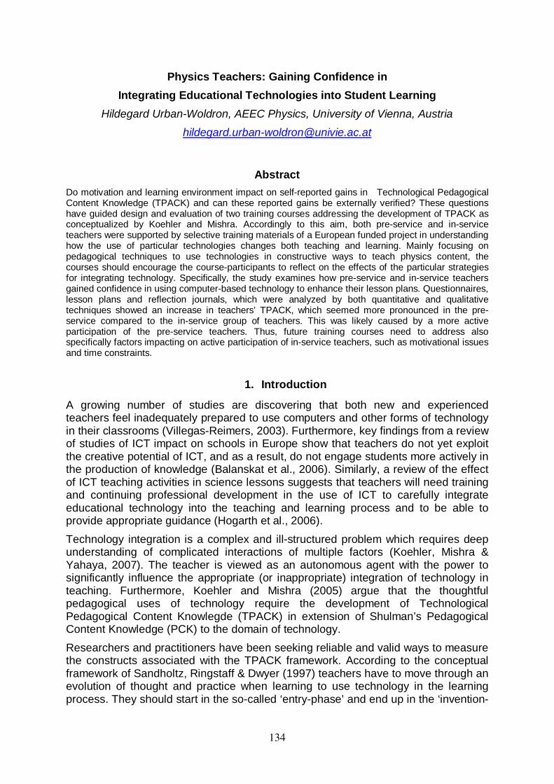
Physics Teachers: Gaining Confidence in Integrating Educational Technologies into Student Learning

Hildegard Urban-Woldron, AEEC Physics, University of Vienna, Austria

hildegard.urban-woldron@univie.ac.at

Abstract Do motivation and learning environment impact on self-reported gains in Technological Pedagogical Content Knowledge (TPACK) and can these reported gains be externally verified? These questions have guided design and evaluation of two training courses addressing the development of TPACK as conceptualized by Koehler and Mishra. Accordingly to this aim, both pre-service and in-service teachers were supported by selective training materials of a European funded project in understanding how the use of particular technologies changes both teaching and learning. Mainly focusing on pedagogical techniques to use technologies in constructive ways to teach physics content, the courses should encourage the course-participants to reflect on the effects of the particular strategies for integrating technology. Specifically, the study examines how pre-service and in-service teachers gained confidence in using computer-based technology to enhance their lesson plans. Questionnaires, lesson plans and reflection journals, which were analyzed by both quantitative and qualitative techniques showed an increase in teachers’ TPACK, which seemed more pronounced in the pre-service compared to the in-service group of teachers. This was likely caused by a more active participation of the pre-service teachers. Thus, future training courses need to address also specifically factors impacting on active participation of in-service teachers, such as motivational issues and time constraints.

1. Introduction

A growing number of studies are discovering that both new and experienced teachers feel inadequately prepared to use computers and other forms of technology in their classrooms (Villegas-Reimers, 2003). Furthermore, key findings from a review of studies of ICT impact on schools in Europe show that teachers do not yet exploit the creative potential of ICT, and as a result, do not engage students more actively in the production of knowledge (Balanskat et al., 2006). Similarly, a review of the effect of ICT teaching activities in science lessons suggests that teachers will need training and continuing professional development in the use of ICT to carefully integrate educational technology into the teaching and learning process and to be able to provide appropriate guidance (Hogarth et al., 2006). Technology integration is a complex and ill-structured problem which requires deep understanding of complicated interactions of multiple factors (Koehler, Mishra & Yahaya, 2007). The teacher is viewed as an autonomous agent with the power to significantly influence the appropriate (or inappropriate) integration of technology in teaching. Furthermore, Koehler and Mishra (2005) argue that the thoughtful pedagogical uses of technology require the development of Technological Pedagogical Content Knowlegde (TPACK) in extension of Shulman’s Pedagogical Content Knowledge (PCK) to the domain of technology. Researchers and practitioners have been seeking reliable and valid ways to measure the constructs associated with the TPACK framework. According to the conceptual framework of Sandholtz, Ringstaff & Dwyer (1997) teachers have to move through an evolution of thought and practice when learning to use technology in the learning process. They should start in the so-called ‘entry-phase’ and end up in the ‘invention-

134

phase’ discovering new uses for technology tools and using technology as a flexible tool in the classroom to facilitate the emergence of new teaching and learning practices. Harris and her colleagues (2009) promote in amendment of published self-report surveys for assessing TPACK an instrument that supports a performance-based evaluation of TPACK, enabling a triangulation of self-report data and external assessments. Their “TPACK-based technology integration assessment rubric” should support teacher educators to more accurately assess the quality of technology integration in their students’ lesson plans by reflecting on four dimensions: curriculum-based technology use, using technology in teaching/learning, compatibility with curriculum goals & instructional strategies, fit of content, pedagogy and technology together. The paper reports on the integration of selective teacher training materials, which were used through blended learning courses for both pre-service and in-service physics teachers. The design and the evaluation of the courses were based on the frameworks of Sandholtz and her colleagues as well as on the assessment rubric of Harris and her colleagues. Focusing on the development of TPACK, the study aimed to examine how both physics teacher candidates and practicing physics teachers used computer-based technology to enhance their lesson plans by selecting appropriate technology tools from the course materials of a European funded project as well as creating learning opportunities for students. Teaching materials covered three different physics topics: “Cooling & change of state”, “basic electricity concepts” and “motion & forces”. For each topic, up to three types of activities, exploiting the use of ICT to stimulate thinking and promote understanding of basic physics concepts, were offered: data-logging, simulation and modelling. The purpose of the study was to investigate prospective and practicing teachers’ development of TPACK attempting to address two broad questions: 1. Is there a relationship between the perceptions of the learning environment,

motivational orientations and the self-reported evolution of TPACK? 2. Are self-reported knowledge gains in TPACK in agreement with external

assessment of teachers’ own lesson plan designs?

2. Method Participants and Setting

The participants of the study included 17 prospective physics teachers / 9 female, 8 male, mean age of 23.2 years (SD=2.1 years) and 12 practicing physics teachers / 8 female, 4 male; mean teaching experience of 14.1 years (SD=7.2 years). All participants were novices in the field of technology integration in physics teaching and learning. Although the formats of the courses differed, both courses were designed as blended-learning courses, in which for communication and collaboration as well as for the distribution of the training materials and the questionnaires an electronic platform, based on the software Moodle, was used. a) The course A for the practicing teachers lasted 10 months and started with a one

half-day face-to-face teacher training session, where the teachers were primarily introduced to the use of motion sensors used along with graphing calculators by trainer demonstration and the development of models with the software VenSim. Continuative descriptions of the presented examples and tutorials for

135

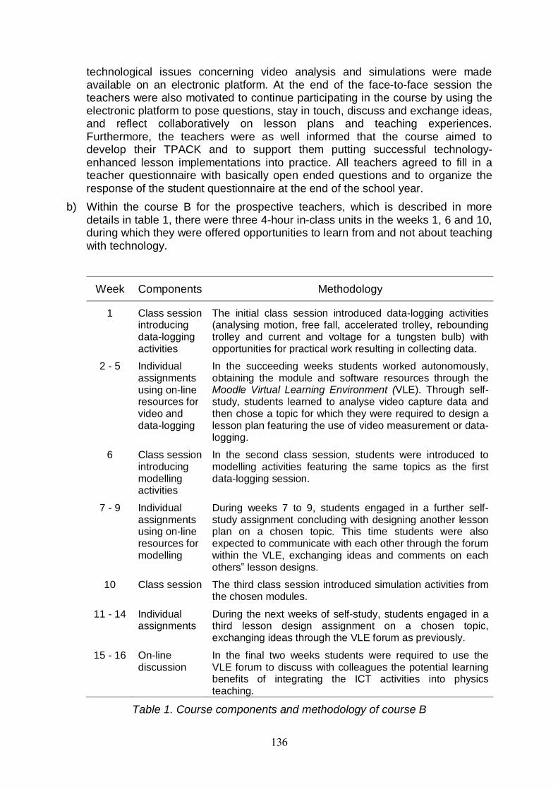
technological issues concerning video analysis and simulations were made available on an electronic platform. At the end of the face-to-face session the teachers were also motivated to continue participating in the course by using the electronic platform to pose questions, stay in touch, discuss and exchange ideas, and reflect collaboratively on lesson plans and teaching experiences. Furthermore, the teachers were as well informed that the course aimed to develop their TPACK and to support them putting successful technology-enhanced lesson implementations into practice. All teachers agreed to fill in a teacher questionnaire with basically open ended questions and to organize the response of the student questionnaire at the end of the school year.

b) Within the course B for the prospective teachers, which is described in more details in table 1, there were three 4-hour in-class units in the weeks 1, 6 and 10, during which they were offered opportunities to learn from and not about teaching with technology.

Week Components Methodology

1 Class session introducing data-logging activities

The initial class session introduced data-logging activities (analysing motion, free fall, accelerated trolley, rebounding trolley and current and voltage for a tungsten bulb) with opportunities for practical work resulting in collecting data.

2 - 5 Individual assignments using on-line resources for video and data-logging

In the succeeding weeks students worked autonomously, obtaining the module and software resources through the Moodle Virtual Learning Environment (VLE). Through self-study, students learned to analyse video capture data and then chose a topic for which they were required to design a lesson plan featuring the use of video measurement or data-logging.

6 Class session introducing modelling activities

In the second class session, students were introduced to modelling activities featuring the same topics as the first data-logging session.

7 - 9 Individual assignments using on-line resources for modelling

During weeks 7 to 9, students engaged in a further self-study assignment concluding with designing another lesson plan on a chosen topic. This time students were also expected to communicate with each other through the forum within the VLE, exchanging ideas and comments on each others‟ lesson designs.

10 Class session The third class session introduced simulation activities from the chosen modules.

11 - 14 Individual assignments

During the next weeks of self-study, students engaged in a third lesson design assignment on a chosen topic, exchanging ideas through the VLE forum as previously.

15 - 16 On-line discussion

In the final two weeks students were required to use the VLE forum to discuss with colleagues the potential learning benefits of integrating the ICT activities into physics teaching.

Table 1. Course components and methodology of course B

136

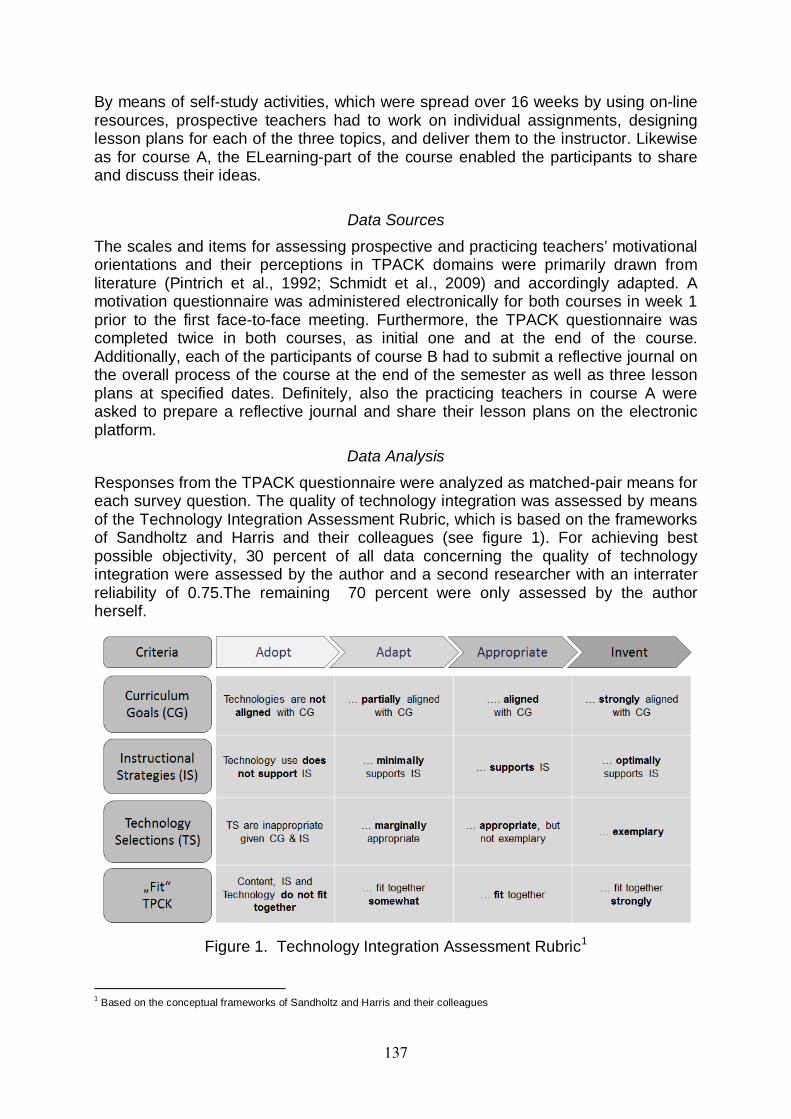
By means of self-study activities, which were spread over 16 weeks by using on-line resources, prospective teachers had to work on individual assignments, designing lesson plans for each of the three topics, and deliver them to the instructor. Likewise as for course A, the ELearning-part of the course enabled the participants to share and discuss their ideas.

Data Sources

The scales and items for assessing prospective and practicing teachers’ motivational orientations and their perceptions in TPACK domains were primarily drawn from literature (Pintrich et al., 1992; Schmidt et al., 2009) and accordingly adapted. A motivation questionnaire was administered electronically for both courses in week 1 prior to the first face-to-face meeting. Furthermore, the TPACK questionnaire was completed twice in both courses, as initial one and at the end of the course. Additionally, each of the participants of course B had to submit a reflective journal on the overall process of the course at the end of the semester as well as three lesson plans at specified dates. Definitely, also the practicing teachers in course A were asked to prepare a reflective journal and share their lesson plans on the electronic platform.

Data Analysis

Responses from the TPACK questionnaire were analyzed as matched-pair means for each survey question. The quality of technology integration was assessed by means of the Technology Integration Assessment Rubric, which is based on the frameworks of Sandholtz and Harris and their colleagues (see figure 1). For achieving best possible objectivity, 30 percent of all data concerning the quality of technology integration were assessed by the author and a second researcher with an interrater reliability of 0.75.The remaining 70 percent were only assessed by the author herself.

Figure 1. Technology Integration Assessment Rubric1

1 Based on the conceptual frameworks of Sandholtz and Harris and their colleagues

137

Also, the relationship among motivational orientations, perceived TPACK and pre-post-difference as well as the quality of TPACK inferred from the lesson plans was analyzed. As the primary method of data examination for the reflective journals and the open questions verbal inductive analysis was used. Accordingly, the data were assigned to four categories, resulting in a numerical overview of the outcomes. All items of the questionnaires were aligned on a Likert scale, ranging from 1, “I totally disagree“ to 4, “I totally agree“. As 8 out of 12 practicing teachers did not actively use the VLE by asking questions, encouraging colleagues in discussions, exchanging materials and lesson plans and did not even fill in the questionnaires, only data analysis related to course B could be seriously performed. The participants' questionnaires, lesson plans and reflection journals were sources of data. Data were analyzed, incorporating both quantitative and qualitative techniques, to determine the effectiveness of the course materials and the course design on pre-service physics teachers' development of TPACK.

3. Results

The findings of the study indicate that most of the prospective teachers and 4 of the practicing teachers, who actively participated in the courses, value the materials as well as the design of the course. Course participants rate the courses to be helpful for developing a critical understanding of TPACK, independently from gender and motivational orientations. A cluster analysis (see table 2) of the motivational scales shows that the participants of the study can be arranged to three groups: 29% (CL1) report high estimates for goal orientation, content task value and self-efficacy. Whereas 47% of the students in CL 3 are confident in their abilities for accomplishing and performing the future tasks, they are not so highly intrinsically motivated and convinced about the importance and usefulness of the course. 24% of the students in CL2 can be described as students with motivational strategies clearly underneath the mean of 2.5.

MCL1 SDCL1 MCL2 SDCL2 MCL3 SDCL3

Intrinsic goal orientation 3.25 0.53 2.00 0.88 2.16 0.82 Self- efficacy for learning and performance 3.18 0.09 1.38 0.00 3.13 0.93

Content task value 3.43 0.17 1.50 0.00 2.27 0.94 Number of students 5 4 8

Table 2. Descriptive statistics of motivational strategies

In addition, ANOVA shows that there is also a significant difference between the groups' mean scores concerning the quality of the corresponding lesson plans (F(2)=9,02, p<0.05). For example, students in CL1 attain 14 points on average out of a maximum of 16 points for their third lesson plans, whereas students from group 2 only reach a mean score of 6 points.

138

4. Discussion and conclusions

To summarize, the findings of the study suggest that there is not only a strong relationship between the perceptions of the learning environment, motivational orientations and the self-reported evolution of TPACK, but additionally, students who report higher gains in TPACK outperform their colleagues in terms of the quality of their lesson plans. The results also indicate that the training materials stimulate, at least, all actively engaged course participants to thoughtfully reconsider the use of technologies in constructive ways to teach content focusing on conceptual understanding and self-regulated learning of their students. As a consequence, on the one hand, the predominately encouraging results of the study motivate further research on how to best design teacher education programs in preparing future educators for the challenge of teaching in the 21st century. On the other hand both researchers and teacher trainers have to figure out, how practicing teachers can be best supported to perceive how technological tools can transform pedagogical strategies and content representations for teaching specific topics. References Balanskat, A., Blamire, R. & Kefala, St. (2006). The ICT Impact Report. European

Schoolnet. Harris, J., Mishra, P. & Koehler, M. (2009). Teachers’ technological pedagogical

content knowledge and learning activity types: Curriculum-based technology integration reframed. Journal of Research on Technology in Education, 41(4), 393-416.

Hogarth, S., Bennett, J., Lubben, F., Campell, B. & Robinson, A. (2006). ICT in science teaching. Technical report. In: Research Evidence in Education Library: EPPI-Centre, Social Science Research Unit, Institute of Education, University of London.

Koehler, M. & Mishra, P. (2005). What happens when teachers design educational technology? Journal for Educational Computing Research, Vol. 32(2). 131-152.

Koehler, M. J., Mishra, P. & Yahay, K. (2007). Tracing the development of teacher knowledge in a design seminar: Integrating content, pedagogy and technology. Computers & Education, 49, 740-762

Pintrich, P.R., Smith, D.A.F., Garcia, T. & McKeachie, W.J. (1992). A Manual for the Use of the Motivated Strategies for Learning Questionnaire (MSLQ). Washington, DC: Office of Educational Research and Improvement.

Sandholtz, J. H., Ringstaff, C. & Dwyer, D. C. (1997). Teaching with technology: Creating student-centered classrooms. New York: Teachers College Press.

Schmidt, D.A., Baran, E., Thompson, A.D., Mishra, P., Kohler, M.J. & Shin, T.S. (2009). Technological Pedagogical Content Knowledge: The Development and Validation of an Assessment Instrument for Preservice Teachers. JRTE, 42(2), 123-149.

Villegas-Reimers, E. (2003). Teacher professional development: an international review of the literature. UNESCO: International Institute for Educational Planning. Paris.

139

The use of formulas by lower level secondary school students when building computer models.

Onne van Buuren1, Peter Uylings2 and Ton Ellermeijer3 O.P.M.vanBuuren@UvA.nl

1 University of Amsterdam; 2 ILO, University of Amsterdam; 3 C.M.A., Amsterdam.

By means of a classroom experiment and a questionnaire, the understanding by lower level secondary school students of the calculation process and the use of formulas (direct relations) in a graphical computer model was investigated. It appeared that students could understand the calculation process on a numerical level, but had problems with the creation and use of formulas. Students did not yet have a clear understanding of the concept of a formula. The term ‘formula’ must be defined more clearly. Suggestions are given for improvement of the learning sequence leading to the use of direct relations in a computer model.

1. Introduction

Until recently, most research on quantitative computational modelling in education has been focussed on the higher educational levels, often with modelling courses on a project base only. There are good reasons for starting with modelling at an earlier age (van Buuren, Uylings, & Ellermeijer, 2010a), and in integrating it into the curriculum (Schecker, 1998). Therefore, in the past three years we have been working on the design of a learning path on modelling, integrated into the Dutch physics curriculum, starting from the initial phases (age: 13-14 years) (van Buuren, Uylings, & Ellermeijer, 2010a, 2010b). This learning path is tested in school practice. The modelling approach used is the ‘system dynamical’ stock and flow approach developed by J.W. Forrester (Forrester, 1968). Examples of software tools built for this approach are Stella (Steed, 1992) and Coach 6 (Heck, Kedzierska, & Ellermeijer, 2009). With computer models, students can solve difference equations numerically that otherwise would be beyond their mathematical capabilities. In graphical computer models these difference equations are not entered in the model as formulas. Instead, combinations of graphical ‘stock and flow’ symbols are used. Although in this way the difference equations are not used explicitly, a certain level of understanding of the different roles of the variables is still required. In addition, students still need the ability to use formulas for variables that are defined by direct relations. Even more advanced students don’t possess the required levels of understanding automatically (Doerr, 1996; Hogan & Thomas, 2001; H. Schecker, 2005; Westra, 2008; van Buuren, Uylings, & Ellermeijer, 2010b). Therefore, the development of understanding of formulas and variables, and their connection to graphical models, must be tuned carefully. The terms ‘formula’ and ‘variable’ both have many different meanings in mathematics and science (Heck, 2001; Malisani & Spagnolo, 2008). Here, we consider the term variable, which is of great importance to the concept of a formula. We confine ourselves to three of its meanings, stemming from mathematics and increasing in level of abstraction: 1. Placeholder: a variable that stands for one number, known or unknown. 2. Generalised number: an indeterminate number that appears in generalisations

and in general methods. 3. Variable object, a symbol for an object with varying value (Heck, 2001), often in

functional relationship to another variable, as “a thing that varies” (Malisani & Spagnolo, 2008), with a “changing nature” (Graham & Thomas, 2000).

140

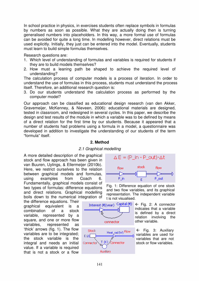
Fig. 1: Difference equation of one stock and two flow variables, and its graphical representation. The independent variable t is not visualised.

Fig. 2: A connector indicates that a variable is defined by a direct relation involving the other variable.

Fig. 3: Auxiliary variables are used for variables that are not stock or flow variables.

In school practice in physics, in exercises students often replace symbols in formulas by numbers as soon as possible. What they are actually doing then is turning generalised numbers into placeholders. In this way, a more formal use of formulas can be avoided for quite a long time. In modelling however, direct relations must be used explicitly. Initially, they just can be entered into the model. Eventually, students must learn to build simple formulas themselves.

Research questions are: 1. Which level of understanding of formulas and variables is required for students if

they are to build models themselves? 2. How must a leaning path be shaped to achieve the required level of

understanding? The calculation process of computer models is a process of iteration. In order to understand the use of formulas in this process, students must understand the process itself. Therefore, an additional research question is: 3. Do our students understand the calculation process as performed by the

computer model?

Our approach can be classified as educational design research (van den Akker, Gravemeijer, McKenney, & Nieveen, 2006): educational materials are designed, tested in classroom, and redesigned in several cycles. In this paper, we describe the design and test results of the module in which a variable was to be defined by means of a direct relation for the first time by our students. Because it appeared that a number of students had problems using a formula in a model, a questionnaire was developed in addition to investigate the understanding of our students of the term “formula” itself.

2. Method

2.1 Graphical modelling

A more detailed description of the graphical stock and flow approach has been given in van Buuren, Uylings, & Ellermeijer (2010b). Here, we restrict ourselves to the relation between graphical models and formulas, using examples from Coach 6. Fundamentally, graphical models consist of two types of formulas: difference equations and direct relations. Graphical modelling boils down to the numerical integration of the difference equations. Their graphical equivalent is a combination of a stock variable, represented by a square, and one or more flow variables, represented as ‘thick’ arrows (fig. 1). The flow variables are to be integrated; the stock variable is the integral and needs an initial value. If a variable is required that is not a stock or a flow

141

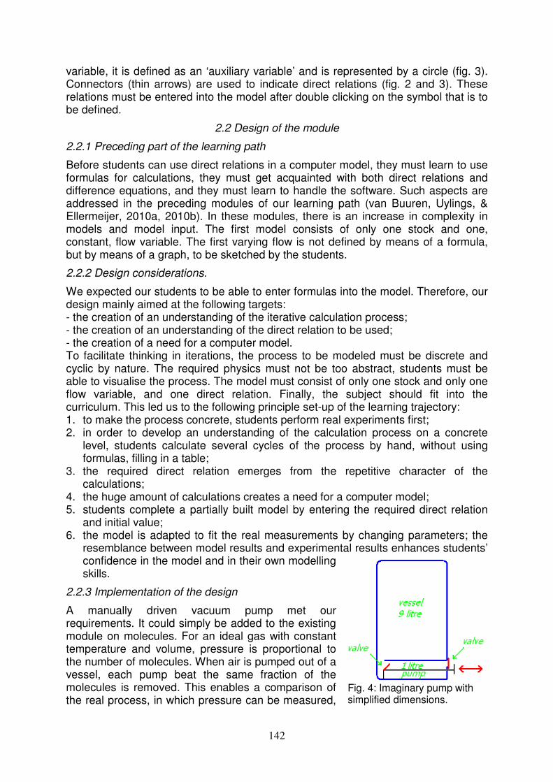
Fig. 4: Imaginary pump with simplified dimensions.

variable, it is defined as an ‘auxiliary variable’ and is represented by a circle (fig. 3). Connectors (thin arrows) are used to indicate direct relations (fig. 2 and 3). These relations must be entered into the model after double clicking on the symbol that is to be defined.

2.2 Design of the module

2.2.1 Preceding part of the learning path

Before students can use direct relations in a computer model, they must learn to use formulas for calculations, they must get acquainted with both direct relations and difference equations, and they must learn to handle the software. Such aspects are addressed in the preceding modules of our learning path (van Buuren, Uylings, & Ellermeijer, 2010a, 2010b). In these modules, there is an increase in complexity in models and model input. The first model consists of only one stock and one, constant, flow variable. The first varying flow is not defined by means of a formula, but by means of a graph, to be sketched by the students.

2.2.2 Design considerations.

We expected our students to be able to enter formulas into the model. Therefore, our design mainly aimed at the following targets: - the creation of an understanding of the iterative calculation process; - the creation of an understanding of the direct relation to be used; - the creation of a need for a computer model. To facilitate thinking in iterations, the process to be modeled must be discrete and cyclic by nature. The required physics must not be too abstract, students must be able to visualise the process. The model must consist of only one stock and only one flow variable, and one direct relation. Finally, the subject should fit into the curriculum. This led us to the following principle set-up of the learning trajectory: 1. to make the process concrete, students perform real experiments first; 2. in order to develop an understanding of the calculation process on a concrete

level, students calculate several cycles of the process by hand, without using formulas, filling in a table;

3. the required direct relation emerges from the repetitive character of the calculations;

4. the huge amount of calculations creates a need for a computer model; 5. students complete a partially built model by entering the required direct relation

and initial value; 6. the model is adapted to fit the real measurements by changing parameters; the

resemblance between model results and experimental results enhances students’ confidence in the model and in their own modelling skills.

2.2.3 Implementation of the design

A manually driven vacuum pump met our requirements. It could simply be added to the existing module on molecules. For an ideal gas with constant temperature and volume, pressure is proportional to the number of molecules. When air is pumped out of a vessel, each pump beat the same fraction of the molecules is removed. This enables a comparison of the real process, in which pressure can be measured,

142

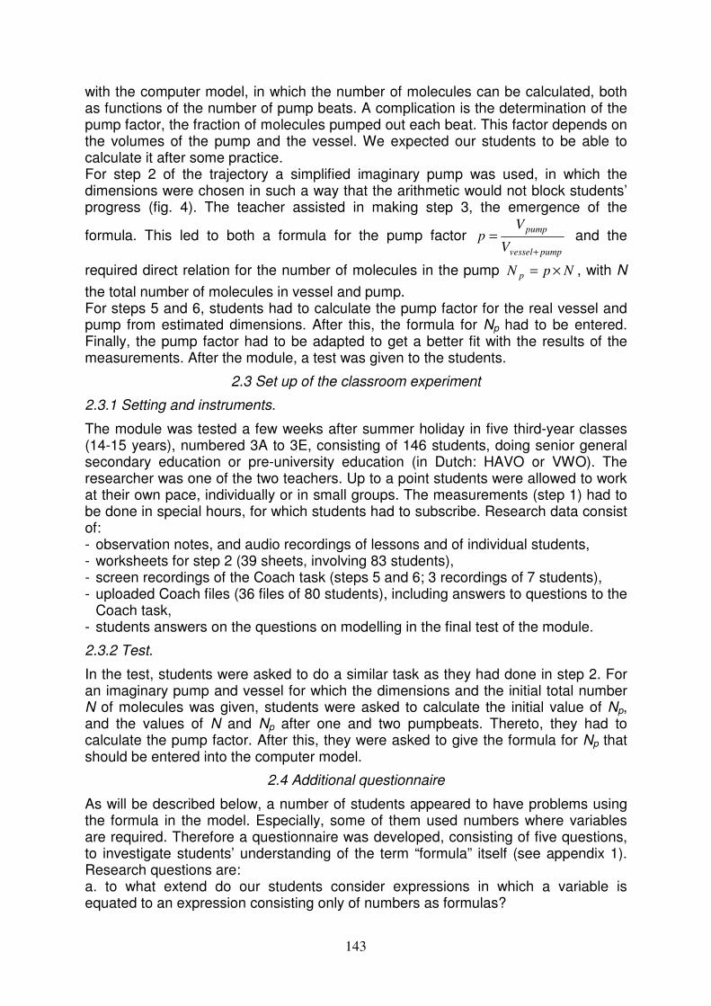
with the computer model, in which the number of molecules can be calculated, both as functions of the number of pump beats. A complication is the determination of the pump factor, the fraction of molecules pumped out each beat. This factor depends on the volumes of the pump and the vessel. We expected our students to be able to calculate it after some practice. For step 2 of the trajectory a simplified imaginary pump was used, in which the dimensions were chosen in such a way that the arithmetic would not block students’ progress (fig. 4). The teacher assisted in making step 3, the emergence of the

formula. This led to both a formula for the pump factor pumpvessel

pump

V

Vp

+

= and the

required direct relation for the number of molecules in the pump NpN p ×= , with N

the total number of molecules in vessel and pump. For steps 5 and 6, students had to calculate the pump factor for the real vessel and pump from estimated dimensions. After this, the formula for Np had to be entered. Finally, the pump factor had to be adapted to get a better fit with the results of the measurements. After the module, a test was given to the students.

2.3 Set up of the classroom experiment

2.3.1 Setting and instruments.

The module was tested a few weeks after summer holiday in five third-year classes (14-15 years), numbered 3A to 3E, consisting of 146 students, doing senior general secondary education or pre-university education (in Dutch: HAVO or VWO). The researcher was one of the two teachers. Up to a point students were allowed to work at their own pace, individually or in small groups. The measurements (step 1) had to be done in special hours, for which students had to subscribe. Research data consist of: - observation notes, and audio recordings of lessons and of individual students, - worksheets for step 2 (39 sheets, involving 83 students), - screen recordings of the Coach task (steps 5 and 6; 3 recordings of 7 students), - uploaded Coach files (36 files of 80 students), including answers to questions to the

Coach task, - students answers on the questions on modelling in the final test of the module.

2.3.2 Test.

In the test, students were asked to do a similar task as they had done in step 2. For an imaginary pump and vessel for which the dimensions and the initial total number N of molecules was given, students were asked to calculate the initial value of Np, and the values of N and Np after one and two pumpbeats. Thereto, they had to calculate the pump factor. After this, they were asked to give the formula for Np that should be entered into the computer model.

2.4 Additional questionnaire

As will be described below, a number of students appeared to have problems using the formula in the model. Especially, some of them used numbers where variables are required. Therefore a questionnaire was developed, consisting of five questions, to investigate students’ understanding of the term “formula” itself (see appendix 1). Research questions are: a. to what extend do our students consider expressions in which a variable is equated to an expression consisting only of numbers as formulas?

143

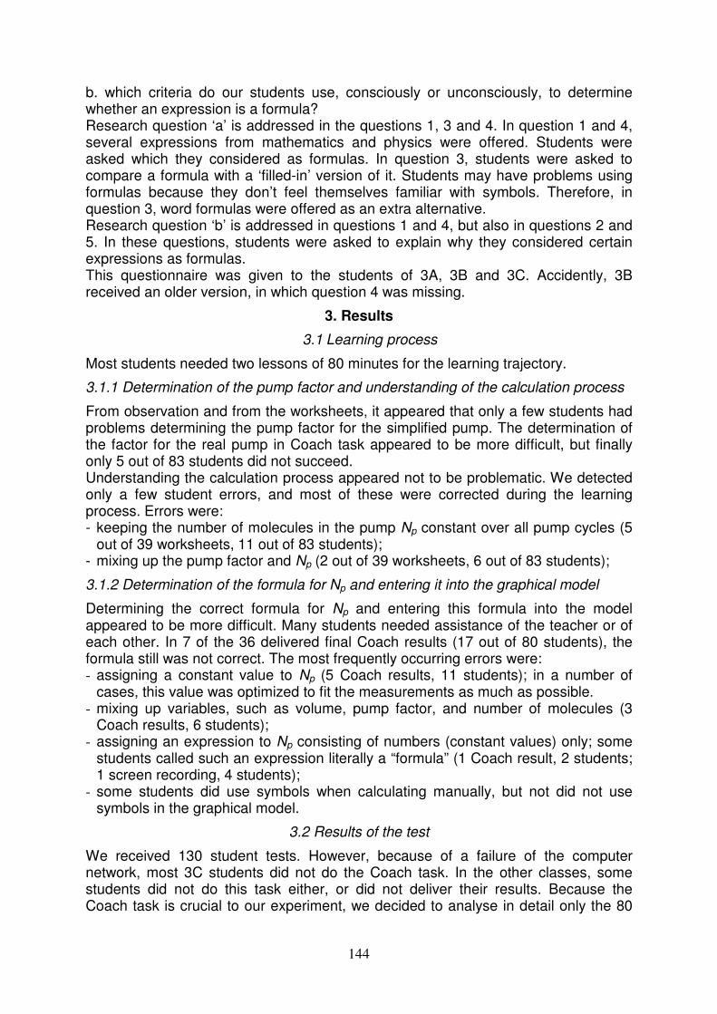
b. which criteria do our students use, consciously or unconsciously, to determine whether an expression is a formula? Research question ‘a’ is addressed in the questions 1, 3 and 4. In question 1 and 4, several expressions from mathematics and physics were offered. Students were asked which they considered as formulas. In question 3, students were asked to compare a formula with a ‘filled-in’ version of it. Students may have problems using formulas because they don’t feel themselves familiar with symbols. Therefore, in question 3, word formulas were offered as an extra alternative. Research question ‘b’ is addressed in questions 1 and 4, but also in questions 2 and 5. In these questions, students were asked to explain why they considered certain expressions as formulas. This questionnaire was given to the students of 3A, 3B and 3C. Accidently, 3B received an older version, in which question 4 was missing.

3. Results

3.1 Learning process

Most students needed two lessons of 80 minutes for the learning trajectory.

3.1.1 Determination of the pump factor and understanding of the calculation process

From observation and from the worksheets, it appeared that only a few students had problems determining the pump factor for the simplified pump. The determination of the factor for the real pump in Coach task appeared to be more difficult, but finally only 5 out of 83 students did not succeed. Understanding the calculation process appeared not to be problematic. We detected only a few student errors, and most of these were corrected during the learning process. Errors were: - keeping the number of molecules in the pump Np constant over all pump cycles (5

out of 39 worksheets, 11 out of 83 students); - mixing up the pump factor and Np (2 out of 39 worksheets, 6 out of 83 students);

3.1.2 Determination of the formula for Np and entering it into the graphical model

Determining the correct formula for Np and entering this formula into the model appeared to be more difficult. Many students needed assistance of the teacher or of each other. In 7 of the 36 delivered final Coach results (17 out of 80 students), the formula still was not correct. The most frequently occurring errors were: - assigning a constant value to Np (5 Coach results, 11 students); in a number of

cases, this value was optimized to fit the measurements as much as possible. - mixing up variables, such as volume, pump factor, and number of molecules (3

Coach results, 6 students); - assigning an expression to Np consisting of numbers (constant values) only; some

students called such an expression literally a “formula” (1 Coach result, 2 students; 1 screen recording, 4 students);

- some students did use symbols when calculating manually, but not did not use symbols in the graphical model.

3.2 Results of the test

We received 130 student tests. However, because of a failure of the computer network, most 3C students did not do the Coach task. In the other classes, some students did not do this task either, or did not deliver their results. Because the Coach task is crucial to our experiment, we decided to analyse in detail only the 80

144

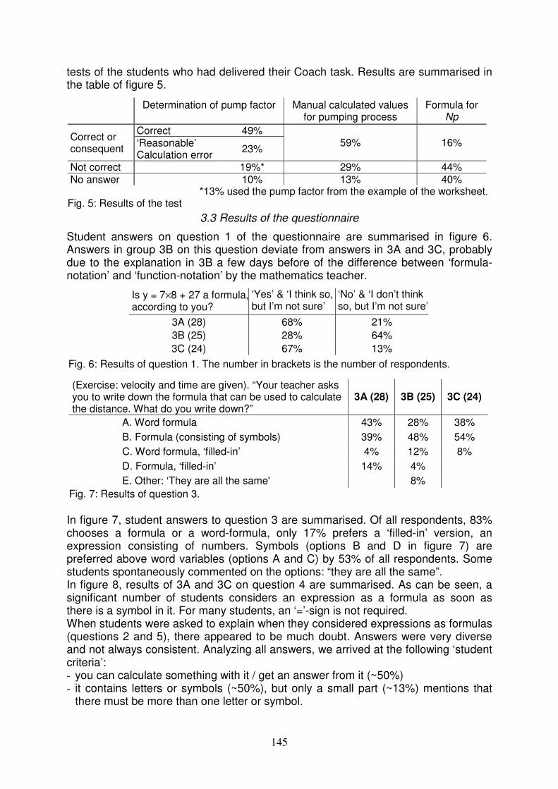
Is y = 7×8 + 27 a formula, according to you?

‘Yes’ & ‘I think so, but I’m not sure’

‘No’ & ‘I don’t think so, but I’m not sure’

3A (28) 68% 21%

3B (25) 28% 64%

3C (24) 67% 13%

Fig. 6: Results of question 1. The number in brackets is the number of respondents. (Exercise: velocity and time are given). “Your teacher asks you to write down the formula that can be used to calculate the distance. What do you write down?”

3A (28) 3B (25) 3C (24)

A. Word formula 43% 28% 38%

B. Formula (consisting of symbols) 39% 48% 54%

C. Word formula, ‘filled-in’ 4% 12% 8%

D. Formula, ‘filled-in’ 14% 4%

E. Other: ‘They are all the same' 8%

Fig. 7: Results of question 3.

tests of the students who had delivered their Coach task. Results are summarised in the table of figure 5.

3.3 Results of the questionnaire

Student answers on question 1 of the questionnaire are summarised in figure 6. Answers in group 3B on this question deviate from answers in 3A and 3C, probably due to the explanation in 3B a few days before of the difference between ‘formula-notation’ and ‘function-notation’ by the mathematics teacher.

In figure 7, student answers to question 3 are summarised. Of all respondents, 83% chooses a formula or a word-formula, only 17% prefers a ‘filled-in’ version, an expression consisting of numbers. Symbols (options B and D in figure 7) are preferred above word variables (options A and C) by 53% of all respondents. Some students spontaneously commented on the options: “they are all the same”. In figure 8, results of 3A and 3C on question 4 are summarised. As can be seen, a significant number of students considers an expression as a formula as soon as there is a symbol in it. For many students, an ‘=’-sign is not required. When students were asked to explain when they considered expressions as formulas (questions 2 and 5), there appeared to be much doubt. Answers were very diverse and not always consistent. Analyzing all answers, we arrived at the following ‘student criteria’: - you can calculate something with it / get an answer from it (~50%) - it contains letters or symbols (~50%), but only a small part (~13%) mentions that

there must be more than one letter or symbol.

Determination of pump factor Manual calculated values for pumping process

Formula for Np

Correct or consequent

Correct 49% 59% 16% ‘Reasonable’

Calculation error 23%

Not correct 19%* 29% 44% No answer 10% 13% 40%

*13% used the pump factor from the example of the worksheet. Fig. 5: Results of the test

145

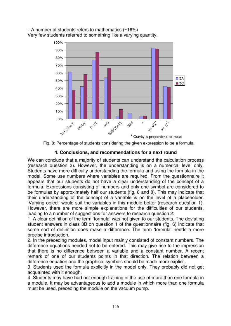
Fig. 8: Percentage of students considering the given expression to be a formula.

- A number of students refers to mathematics (~16%) Very few students referred to something like a varying quantity.

4. Conclusions, and recommendations for a next round

We can conclude that a majority of students can understand the calculation process (research question 3). However, the understanding is on a numerical level only. Students have more difficulty understanding the formula and using the formula in the model. Some use numbers where variables are required. From the questionnaire it appears that our students do not have a clear understanding of the concept of a formula. Expressions consisting of numbers and only one symbol are considered to be formulas by approximately half our students (fig. 6 and 8). This may indicate that their understanding of the concept of a variable is on the level of a placeholder. ‘Varying object’ would suit the variables in this module better (research question 1). However, there are more simple explanations for the difficulties of our students, leading to a number of suggestions for answers to research question 2: 1. A clear definition of the term ‘formula’ was not given to our students. The deviating student answers in class 3B on question 1 of the questionnaire (fig. 6) indicate that some sort of definition does make a difference. The term ‘formula’ needs a more precise introduction. 2. In the preceding modules, model input mainly consisted of constant numbers. The difference equations needed not to be entered. This may give rise to the impression that there is no difference between a variable and a constant number. A recent remark of one of our students points in that direction. The relation between a difference equation and the graphical symbols should be made more explicit. 3. Students used the formula explicitly in the model only. They probably did not get acquainted with it enough. 4. Students may have had not enough training in the use of more than one formula in a module. It may be advantageous to add a module in which more than one formula must be used, preceding the module on the vacuum pump.

146

5. In our module, students not only had to use a formula, they also had to reconstruct it. Construction of formulas is difficult, even for higher level students (Schaap, Vos, Ellermeijer, & Goedhart, 2011). More training is required. 6. Students do not always rehearse experiments and modelling tasks when preparing for a test. They should be invited to do so, or the textbook must be adjusted, to refer more to the experiments and models. These suggestions will be tried out in the next version of our learning path.

References

Doerr, H. M. (1996). Stella ten years later: A review of the literature. International Journal of Computers for Mathematical Learning, 1(2), 201-224.

Forrester, J. W. (1968). Principles of Systems. Mit Pr. Graham, A. T., & Thomas, M. O. J. (2000). Building a Versatile Understanding of

Algebraic Variables with a Graphic Calculator. Educational Studies in Mathematics, 41(3), 265-282.

Heck, A, Kedzierska, E., & Ellermeijer, T. (2009). Design and implementation of an integrated computer working environment for doing mathematics and science. Journal of Computers in Mathematics and Science Teaching, 28(2), 147-161.

Heck, Andre. (2001). Variables in Computer Algebra, Mathematics and Science. International Journal of Computer Algebra in Mathematics Education, 8(3), 195-221.

Hogan, K., & Thomas, D. (2001). Cognitive Comparisons of Students’ Systems Modeling in Ecology. Journal of Science Education and Technology, 10(4), 319-345.

Malisani, E., & Spagnolo, F. (2008). From arithmetical thought to algebraic thought: The role of the “variable.” Educational Studies in Mathematics, 71(1), 19-41.

Schaap, S., Vos, P., Ellermeijer, T., & Goedhart, M. (2011). De vertaalslag van een situatie naar een wiskundige formule; een studie naar vraagstellingen en leerlingprestaties op het centraal examen wiskunde B1. Tijdschrift voor Didactiek der beta-wetenschappen, 28(1), 3-31.

Schecker, H. (2005). Learning Mechanics with Modelling Systems. Presented at the Proceedings of the Fifth International ESERA Conference on Contributions of Research to Enhancing Students’ Interest in Learning Science, Barcelona.

Schecker, H. P. (1998). Physik - Modellieren. Stuttgart: Ernst Klett Verlag. Steed, M. (1992). Stella, A Simulation Construction Kit: Cognitive Process and

Educational Implications. Journal of Computers in Mathematics and Science Teaching, 11(1), 39-52.

Westra, R. (2008). Learning and teaching ecosystem behaviour in secondary education. Utrecht: CDβ Press.

van Buuren, O., Uylings, P., & Ellermeijer, T. (2010a). Towards a learning path on computer modelling. In D. Raine, C. Hurkett, & L. Rogers (Eds.), Physics Community and Cooperation: Selected Contributions from the GIREP-EPEC & PHEC 2009 International Conference. Presented at the GIREP conference 2009, Leicester.

van Buuren, O., Uylings, P., & Ellermeijer, T. (2010b). A modelling learning path, integrated in the secondary school curriculum, starting from the initial phases of physics education. Presented at the GIREP Conference 2010, Reims.

van den Akker, J., Gravemeijer, K., McKenney, S., & Nieveen, N. (Eds.). (2006). Educational Design Research. London and New York: Routledge.

147

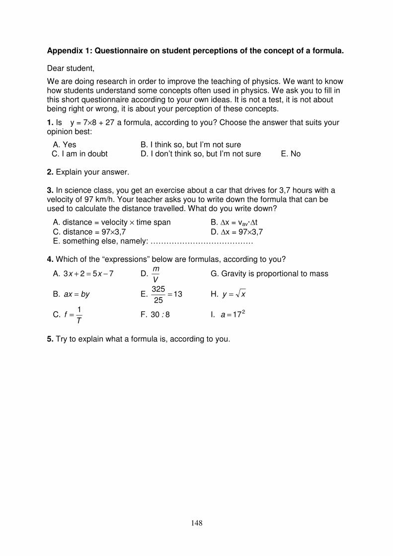
Appendix 1: Questionnaire on student perceptions of the concept of a formula.

Dear student,

We are doing research in order to improve the teaching of physics. We want to know how students understand some concepts often used in physics. We ask you to fill in this short questionnaire according to your own ideas. It is not a test, it is not about being right or wrong, it is about your perception of these concepts.

1. Is y = 7×8 + 27 a formula, according to you? Choose the answer that suits your opinion best:

A. Yes B. I think so, but I’m not sure C. I am in doubt D. I don’t think so, but I’m not sure E. No

2. Explain your answer. 3. In science class, you get an exercise about a car that drives for 3,7 hours with a velocity of 97 km/h. Your teacher asks you to write down the formula that can be used to calculate the distance travelled. What do you write down?

A. distance = velocity × time span B. ∆x = vav·∆t

C. distance = 97×3,7 D. ∆x = 97×3,7 E. something else, namely: …………………………………

4. Which of the “expressions” below are formulas, according to you?

A. 7523 −=+ xx D. V

m G. Gravity is proportional to mass

B. byax = E. 1325

325= H. xy =

C. T

f1

= F. 830 : I. 217=a

5. Try to explain what a formula is, according to you.

148

Long term effects of an innovative physics teacher education program in the Philippines

Ed van den Berg

e.berg@vu.nl Centre for Teacher Education, Free University, Amsterdam and Department of

Teacher Education, Hogeschool van Amsterdam, Netherlands In 1996 innovative, double major teacher education programs for Physics & Mathematics and Physics & Chemistry were initiated at the University of San Carlos in Cebu, Philippines. Both programs require 4 years of study. From the outset the focus was on making a difference in the quality of Science and Mathematics Teacher Education, producing teachers with a good mastery of subject matter and able to teach the subjects in exciting and effective ways in typical Philippine crowded and resource-poor classrooms. The programs recruit top high school graduates using a promotion and scholarship scheme and then expose them to the best science lecturers at the university, and create a special learning environment for the duration of their training. Early 2011 a study was conducted to assess long term effects of the programs through a tracer study of the 300 alumni, interviews, and 22 classroom visits to observe their teaching. Of the 300 alumni 245 are still teaching of whom 33 abroad (mainly USA) and 212 in the Philippines. Alumni are highly valued by principals of the top schools in Cebu and their students win many local and even national science competitions. Their teaching is competent with lots of interaction and good subject matter mastery, but they are also facing some typical Philippine education problems.

Introduction Long term assessments of education projects and particularly international assistance projects are rare. Usually evaluation is limited to progress reports while the project is running and a final report at the end. However, I had an opportunity to return to a teacher education project 7 years after international assistance had ended. My assessment focused on alumni of the program. Where are they teaching? How do they teach? Is the program’s “brand” of teaching visible? What problems do they face in the educational system in the Philippines? The Philippines is an island archipelago with over 80 million people and a population growth of 2.4% per year. There are about 14 million students in elementary schools and 6.8 million students in the 4-year (grade 7-10) High School. The system has not been able to keep up with population growth. Many public schools in the Central Visayas region have over 60 students per class rather than the 40 common in other countries of Asia. Problems with educational quality are serious as documented in a Congressional Report (1993), TIMSS results (Balce et al., 2000) where the Philippines ranked 36th out of 38 on both the science and the mathematics tests, and the 2004 High School Readiness Test for elementary school leavers, where 50% of the students scored below 30% and were considered not ready for grade 7 (Olivares, 2004). Eighty percent of the chemistry teachers and ninety percent of the physics teachers are considered not qualified in these subjects (Ogena, 1993; Golla & de Guzman, 1998; Somerset et al, 1999a; Alcedo, 2002). These teachers majored in other subjects and were then asked or forced to teach physics or chemistry. Typical classroom teaching: Somerset et al. (1999b) observed over 60 science and mathematics lessons in 15 public and private high schools in the Central Visayas. Most of these visits had been announced thus lessons were best prepared. Although they observed some outstanding lessons, most lessons were ineffective due to limited mastery of mathematics and science pedagogy. Alfafara and Dalman (Berg et

149

al., 1998) spent several weeks in two large public high schools. They observed over 60 lessons by 8 teachers. Most observation visits were unannounced thus assessing typical rather than best prepared teaching. Typical lessons consisted of the following: 1) checking attendance, 2) a 5-minute review of the previous lesson, 3) 20-30 minutes of note taking, 4) 20-30 minutes of teacher questions on the notes which usually could be answered by reading a sentence from the notes, 5) a short quiz with peer correction afterwards. Somerset (2002) tested 567 grade 8 and 10 students from 15 schools on basic arithmetic and metric estimation. He and his team also observed the teaching and concluded that most math lessons consisted of rules and drills without attention to concepts and contexts. In response to the poor educational achievement, the shortage of physics and chemistry teachers and the poor quality of teaching the University of San Carlos (USC) in 1996 founded a 4-year Bachelor of Education pre-service teacher education program with a double major in either Physics/Chemistry or Physics/Mathematics with the following key features: 1. Selective admission of 30 students per year through a massive promotion,

recruitment and selection campaign supported by scholarships (before there had been 1 or 2 physics, math, and chemistry teacher education students per year).

2. Emphasis on mastery of physics/math/chemistry and subject specific pedagogy suitable for resource poor classrooms with large classes (Berg, 1996).

3. Some special physics courses to make sure that teacher education students are exposed to “model” teaching in science. Other courses are taken together with science and engineering students.

4. Apart from rigorous emphasis on basic concepts, the program also promotes “fun” physics through discrepant events demonstrations (Liem, 1987), explanation of everyday phenomena (Hewitt, 1998), science exhibitions, science theatre (Berg, 2009), and science competitions.

For further details see Berg (2003), available from the author. From 1996-2004 USC was one of 12 universities worldwide to receive large-scale institutional development funding from the Government of the Netherlands. Amongst others USC requested assistance from the Free University in Amsterdam for the development of its Science and Mathematics Teacher Education programs. USC was the only private university in the Dutch scheme and as such, although affected by the typical problems of SE Asian universities, it did have short decision lines making it possible to move quickly and dynamically in implementing the projects. The support included faculty and student scholarships, long term expert support for program and staff development and teaching, consultancies, and lab equipment. From 1996 – 2010 the program produced 300 teachers.

Research questions and methodology The main research questions for the long-term evaluation were:

1. What happened to students (to be called alumni) who graduated from the 4-year teacher education program? Are they still teaching? Are they indeed achieving “top” positions in science teaching like work in more prestigious high schools and special science high schools?

2. Are the special features of science/math teaching in the pre-service program (high interaction, emphasis on concepts, motivation in fun science demo’s) still

150

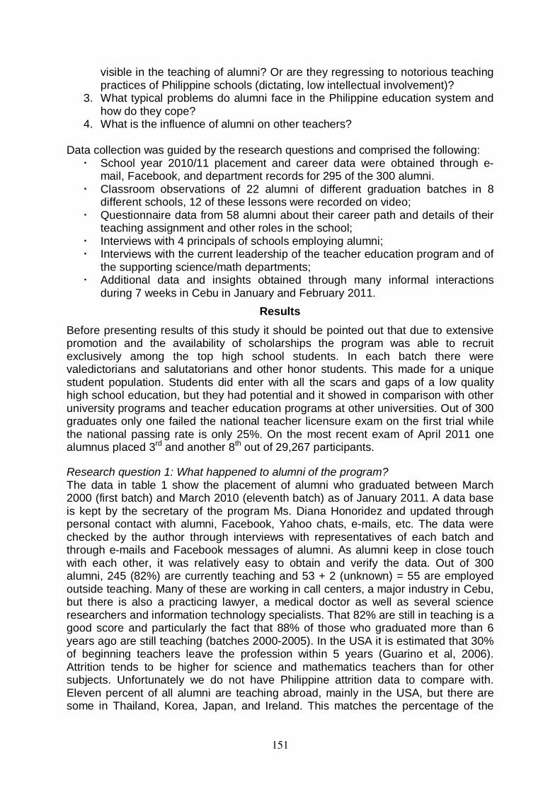
visible in the teaching of alumni? Or are they regressing to notorious teaching practices of Philippine schools (dictating, low intellectual involvement)?

3. What typical problems do alumni face in the Philippine education system and how do they cope?

4. What is the influence of alumni on other teachers? Data collection was guided by the research questions and comprised the following: School year 2010/11 placement and career data were obtained through e-

mail, Facebook, and department records for 295 of the 300 alumni. Classroom observations of 22 alumni of different graduation batches in 8

different schools, 12 of these lessons were recorded on video; Questionnaire data from 58 alumni about their career path and details of their

teaching assignment and other roles in the school; Interviews with 4 principals of schools employing alumni; Interviews with the current leadership of the teacher education program and of

the supporting science/math departments; Additional data and insights obtained through many informal interactions

during 7 weeks in Cebu in January and February 2011. Results

Before presenting results of this study it should be pointed out that due to extensive promotion and the availability of scholarships the program was able to recruit exclusively among the top high school students. In each batch there were valedictorians and salutatorians and other honor students. This made for a unique student population. Students did enter with all the scars and gaps of a low quality high school education, but they had potential and it showed in comparison with other university programs and teacher education programs at other universities. Out of 300 graduates only one failed the national teacher licensure exam on the first trial while the national passing rate is only 25%. On the most recent exam of April 2011 one alumnus placed 3rd and another 8th out of 29,267 participants. Research question 1: What happened to alumni of the program? The data in table 1 show the placement of alumni who graduated between March 2000 (first batch) and March 2010 (eleventh batch) as of January 2011. A data base is kept by the secretary of the program Ms. Diana Honoridez and updated through personal contact with alumni, Facebook, Yahoo chats, e-mails, etc. The data were checked by the author through interviews with representatives of each batch and through e-mails and Facebook messages of alumni. As alumni keep in close touch with each other, it was relatively easy to obtain and verify the data. Out of 300 alumni, 245 (82%) are currently teaching and 53 + 2 (unknown) = 55 are employed outside teaching. Many of these are working in call centers, a major industry in Cebu, but there is also a practicing lawyer, a medical doctor as well as several science researchers and information technology specialists. That 82% are still in teaching is a good score and particularly the fact that 88% of those who graduated more than 6 years ago are still teaching (batches 2000-2005). In the USA it is estimated that 30% of beginning teachers leave the profession within 5 years (Guarino et al, 2006). Attrition tends to be higher for science and mathematics teachers than for other subjects. Unfortunately we do not have Philippine attrition data to compare with. Eleven percent of all alumni are teaching abroad, mainly in the USA, but there are some in Thailand, Korea, Japan, and Ireland. This matches the percentage of the

151

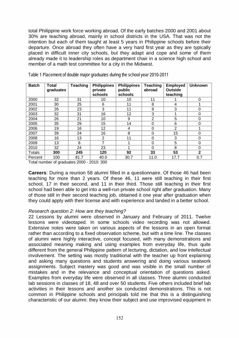
total Philippine work force working abroad. Of the early batches 2000 and 2001 about 30% are teaching abroad, mainly in school districts in the USA. That was not the intention but each of them taught at least 5 years in Philippine schools before their departure. Once abroad they often have a very hard first year as they are typically placed in difficult inner city schools, but they adapt and cope and some of them already made it to leadership roles as department chair in a science high school and member of a math test committee for a city in the Midwest. Table 1 Placement of double major graduates during the school year 2010-2011 Batch Total

graduates Teaching Philippines

private schools

Philippines public schools

Teaching abroad

Employed Outside teaching

Unknown

2000 32 31 10 10 11 1 0 2001 30 25 6 11 8 4 1 2002 26 23 3 11 9 3 0 2003 32 31 16 12 3 1 0 2004 26 21 10 9 2 5 0 2005 35 29 15 14 0 6 0 2006 19 16 12 4 0 2 1 2007 39 24 16 8 0 15 0 2008 16 13 2 11 0 3 0 2009 13 8 7 1 0 5 0 2010 32 24 23 1 0 8 0 Totals 300 245 120 92 33 53 2 Percent 100 81.7 40.0 30.7 11.0 17.7 0.7 Total number of graduates 2000 - 2010: 300 Careers: During a reunion 58 alumni filled in a questionnaire. Of those 46 had been teaching for more than 2 years. Of these 46, 11 were still teaching in their first school, 17 in their second, and 11 in their third. Those still teaching in their first school had been able to get into a well-run private school right after graduation. Many of those still in their second teaching job, obtained it one year after graduation when they could apply with their license and with experience and landed in a better school. Research question 2: How are they teaching? 22 Lessons by alumni were observed in January and February of 2011. Twelve lessons were videotaped. In some schools video recording was not allowed. Extensive notes were taken on various aspects of the lessons in an open format rather than according to a fixed observation scheme, but with a time line. The classes of alumni were highly interactive, concept focused, with many demonstrations and associated meaning making and using examples from everyday life, thus quite different from the general Philippine pattern of lecturing, dictation, and low intellectual involvement. The setting was mostly traditional with the teacher up front explaining and asking many questions and students answering and doing various seatwork assignments. Subject mastery was good and was visible in the small number of mistakes and in the relevance and conceptual orientation of questions asked. Examples from everyday life were observed in all classes. Three alumni conducted lab sessions in classes of 18, 48 and over 50 students. Five others included brief lab activities in their lessons and another six conducted demonstrations. This is not common in Philippine schools and principals told me that this is a distinguishing characteristic of our alumni: they know their subject and use improvised equipment in

152

labs and demonstrations. Detailed observations and example lesson descriptions have been included in a longer version of the paper (available from the author). Research question 3: What typical problems do alumni face in the Philippine education system and how do they cope?

Interview: two young female teachers are handling Physics and Chemistry at a rural public high school. They organize an annual science exhibition at their school just like they experienced in their teacher education program. Their main problem in teaching: in the afternoon quite a few students leave and do not come back. The teachers visited their parents, but parents let them.

This is a problem in more rural schools. Schools start sometime between 7.00 am and 8.00 am and run until 16.00 or 17.00 pm. That is a very long school day but nobody questions it. Many lessons in the Philippines (and elsewhere) are not very efficient with time. Nevertheless, for teachers this lack of motivation is a very serious problem, are they (teachers) wasting their effort?

In an elite high school which over the past 8 years has employed many science and mathematics alumni, I observed 2 good lessons and 2 outstanding lessons. However, I was surprised that in every lesson, the teacher collected an assignment from every student. Teaching 5 lessons a day with 40 students per class the teacher would have to check 200 assignments every day, leaving little time for preparation of the next lesson and turning the professional teacher into a slave. Furthermore, for the students the focus of a lesson might degenerate into a piece of paper. The teachers said they had to collect every single homework and seatwork assignment, otherwise it would not be done seriously in this elite school. My own explanation is that when they just started teaching the teachers had a hard time dealing with the unruly elite students. Then they needed the threat of assignments with grades in order to gain control. Now that they do have experience and control, they still believe that students will only work when threatened with assignments and grades and so both the teachers and students are now enslaved in a pattern.

After the classroom observations we discussed several alternatives to reduce the grading load but I do not yet know what has come of it. It should be emphasized that these are good teachers whom most principals would be happy to hire. In Philippine high schools physics is frequently limited to mechanics, often because the teacher feels less confident in other topics, or because they want to offer the best preparation for the first university physics course. To my great disappointment I encountered this situation in two schools and it concerned alumni with outstanding subject matter mastery. In one of these schools this has now been corrected. Research question 4: What is the influence of alumni on other teachers? Alumni founded active science teachers associations on the islands of Cebu and Bohol where other science teachers also participate. Alumni have presented at national conferences. Students of alumni are very visible in regional and national finals of science competitions like the Intel competition. At half of the schools visited alumni were heading the science department and seemed to have good cooperation with other science teachers and are being consulted by them on matters of science knowledge and teaching methods. One alumnus is now principal of a new science high school. Of the alumni in the USA, two are now heading the science department in their schools and one is on a city wide mathematics assessment committee.

153

Conclusions The alumni of the double major programs have made a good name for themselves. They are actively recruited by the top private schools and public science high schools and are appreciated by their principals. Over 80% remain in teaching 5 years after graduation. The lessons of alumni are competent, very interactive, and include demonstrations and frequent references to everyday science phenomena. With their large classes, their teaching is teacher-centered. Understandably their teaching is affected by some of the typical problems of the Philippine education system and some fall into traps of that system such as all the paper checking with elite students or teaching only mechanics. The alumni do play an important role in improving the quality of science and mathematics education in the region.

Literature Alcedo, C. (2002). Teachers supply and demand in the Philippines. HDNED, The World Bank.

Retrieved July 4, 2002, from: www1.worldbank.org/education. Balce, M., Carale, L., Ferido, M., Guzman, F. de, Mendoza, A., Ogena, E., Savellano, J., & Talisayon,

V. (2000). Third International Mathematics and Science Study- Repeat: The Philippine Participation (Vol 1). Manila, Philippines: Science Education Institute-Department of Science and Technology.

Berg, E. van den (1996). Science teacher development in developing countries. ICASE Science Education International, 7(3), 3-8.

Berg, E. van den (2003). Science/Math and Science/Math Education Courses in the BSEd Physics-Mathematics and Physics-Chemistry Programs at the University of San Carlos. Amsterdam: Centre for International Cooperation, Vrije Universiteit.

Berg, E. van den (2009). Theater in Physics Teacher Education. The Physics Teacher, 47(6),350-352. Berg, E van den., Alfafara, R., & Dalman, T. (1998). Case studies of science and mathematics

teaching in the Philippines and lessons for teacher and school development. Paper presented at the annual conference of the National Association of Research in Science Teaching, San Diego.

Berg, E. van den, Locaylocay, J., Gallos, M. (2006). A Physics Teacher Education Program in the Philippines. Forum on Education Spring 2006 Newsletter American Physical Society, 33-37. http://www.aps.org/units/fed/newsletters/spring2006/vandenberg.html

Berg, E. van den, Locaylocay, J.R.,Gallos, M.R. (2007). Ten Best Practices in a Science and Mathematics Teacher Education Program in the Philippines. In M. Nagao,J. Rogan , M. Magno (editors): Mathematics and Science Education in Developing Countries: Issues, Experiences and Cooperation Prospects. Diliman, Quezon City: The University of the Philippines Press, 231-251.

Congressional Commission on Education. (1993). Making Education Work: An Agenda for Reform. Congress of the Republic of the Philippines. Quezon City, Philippines.

Fullan, M.G. (1991, 2001). The new meaning of educational change (2nd edition, 3rd edition). London: Cassell Educational Ltd.

Golla, E. F., & de Guzman, E. S. (1998). Teacher preparation in science and mathematics education: A situational analysis. In E. B Ogena & F. G. Brawner (Eds.), Science education in the Philippines: Challenges for development (Vol.1,pp.41-106). Manila:Science Education Congress.

Guarino, C. M., Santibanez, L., & Daley, G. A. (2006). Teacher recruitment and retention: A review of the recent empirical literature. Review of Educational Research, 76(2), 173-208.

Hewitt, P. G. (1998). Conceptual Physics (8th edition). Addison-Wesley. Liem, T. (1987). Invitations to Science Inquiry. Chino Hills, California: Science Inquiry Enterprises. Ogena, E. (1993). Science Teacher Education Report. Bicutan, Metro Manila: Department of Science

and Technology. Olivares, B. (2004). Philippine Daily Inquirer. June 6. Somerset, A.H., Alfafara, R. & Dalman, T. (1999a). Science and Mathematics Teachers in Central

Visayas Region, Republic of the Philippines: Initial Training, Deployment and Subsequent Professional Development. Cebu City: SMEI-USC, Talamban Campus.

Somerset, A.H., Alfafara, R. & Dalman, T. (1999b). Teaching and Learning Science and Mathematics in the Classroom: Effective and Ineffective Pedagogy Compared. Cebu City (Philippines): SMEI-USC, Talamban Campus.

Somerset, A. (2002). Basic Number Skills: Why Students Fail. UP-NISMED, University of the Philippines, Diliman, Quezon City, Philippines.

154

Interactive White Board in Physics Teaching;Beneficial for Physics Achievement?

Norbert van Veen1, Ed van den Berg2

nveen@uva.nl1 University of Amsterdam, The Netherlands

and2Department of Physics, Vrije Universiteit, Amsterdam, The Netherlands

Schools have invested massively in interactive white boards (IWB). Interactive white boards can beused for powerpoints and films but they can also support enhanced teaching strategies i.e. moreactive learning and learner-centred teaching, which can lead to higher order learning and enrichteaching through the use of multimedia, as the IWB acts as a digital converging medium for all ICTresources available to teachers. However, research done on the benefits of IWB use, has still toprovide evidence that IWB use, can contribute to physics understanding. This research is focused onthe difference between teaching using an ordinary whiteboard and using the interactive whiteboardand compares students' achievement in physics. This study was a crossover study with two 9th gradeclasses in a Dutch high school. The interventions comprised seven lessons on mechanics and sevenlessons on electricity. One class was experimental group in mechanics and control group in electricity.The other class was control group in mechanics and experimental group in physics. Afterthe interventions students’ achievement was compared and students gave feedback on the differencebetween IWB lessons and “common” white board lessons. Only one of the two interventions showed asignificant difference in physics achievement, but the students were very positive about the use of IWBto aid physics teaching.

Introduction

Interactive white boards (IWBs) seem to be the holy grail of education in the twentyfirst century. Schools buy them and expect teachers to use them to benefit differentlearning styles of students. Unfortunately not much time and money is spent onteaching teachers how to use these IWBs effectively (Armstrong, Barnes, Sutherland,Curran & Mills, 2005). Most teachers, as is my experience as a teacher trainer in IWBuse, tend to use the IWB as a large screen for a projected computer desktop, andperform normal tasks on the computer but to a larger audience. These methods donot increase understanding, but only increase the pace of the lessons and makethem more rather than less teacher centered. As a physics teacher in a secondaryhigh school in the Netherlands and as teacher trainer in IWB use, the (first) authorsees the use of IWB in physics lessons of colleagues being limited to a medium onwhich they only write and show internet sites. The IWB used in this manner will notprovide extra support for students’ different learning styles. But the IWB has thepotential to have students and teachers perform actions that can contribute to betterachievement by students (Armstrong et al., 2005) as it is also capable of supporting(active/effective) teaching strategies. These active/effective teaching strategies canpromote higher order learning by students. Unfortunately not much is known aboutthe influence of IWB on achievement in physics, no literature to this date hasmentioned effects of IWB use on physics achievement by students in secondaryeducation. Therefore results from similar disciplines in science education arediscussed here. A study by Dhindsa and Haji Emran (2006) in two chemistry classesshowed better results in an organic chemistry related topic using the combination ofIWB and constructivist teaching methods compared to traditionally taught classes.The critical question remains if better results by students were caused by using the

155

IWB or the constructivist teaching methods. Also Swan, Schenker & Kratcoski (2008)described small improvements in achievement by students in mathematics when theywere taught using IWB. They concluded that more and effective use of IWB can haveinfluence on achievement. A research study in the UK between 2004-2006 onprimary schools (Somekh, Haldane, Jones, Lewin, Steadman, Scrimshaw, et al.,2007), showed increased attainment gains with pupils’ increased exposure to beingtaught math and science with an interactive whiteboard. The authors postulated thatthis positive impact could be related to the length of time that teachers had used thetechnology and had been able to embed it in their practice. Research has shown thatmotivation, engagement and self esteem of students increases, when IWB is used inteaching, but only as long as students perceive that it is not another way of pumpinginformation into them (Blanton, 2008) and as long as the novelty factor of the IWBhas not worn out ( Higgins, Beauchamp & Miller, 2007). Somekh et al. (2007) clearlystate the importance of long term exposure to IWB lessons to measure effects ingains. They found that in mathematics, average and high attaining pupils madegreater progress with more exposure to IWBs. This study aims to investigate whetherusing the IWB in secondary physics education can influence the achievement ofstudents in physics.

How can the IWB be used in physics teaching?

Some of the important advantages of IWB are aiding visual learning, increasingmotivation, teachers being able to review earlier lessons with students and thedegree to which the teacher and students can work together on forming newconceptions and create knowledge in physics using IWB. According to Hennessy,Deaney, Ruthven & Winterbottom (2007) the use of IWB fosters interactive teachingso that teachers can use higher order questioning and pupils’ active contributions arevalued as they can test their developing understanding against collective meaning.According to Kennewell (2006) most characteristics of effective teaching are aided byIWBs: clear presentations, appropriate pacing, modeling of skills, interactivequestioning, smooth flow of activity, efficient resource management, assessment/diagnosis/feedback and matching learning tasks to student attributes. According toHennesy et al. (2007) and Webb (2005) the impact of IWBs (ICT) on learning isdependent on the mediating role of the teacher and his or her pedagogical choicesrather than technical interactivity which is usually critical in ICT supported learningenvironments. Examples of IWB in physics teaching have not been found inliterature, but strategies with IWB using visualizations, animations and being ableexplain concepts using digital resources seem to be methods that can be used inphysics. The IWB also allows the teacher to show a concept in varied ways, e.g.showing a picture of a phenomenon in which the concept plays a role, then a movieof the concept can be shown in which the concept is explained, pre designedassignments can be made on the handouts. A concept can be better understood bystudents as it can be represented visually in variety of ways and acted upon bystudents (Molenaar, 2002). IWB provides a multidimensional learning experience,offering students with seamless, easy and effective access to these multimediaresources and also enables teachers and learners to use them more interactively.IWB creates more possibilities for exploring video pedagogically because of itssimple and effective, manipulative screen. The IWB can assist for example by usingthe voting feature which helps students to externalize their ideas and get feedbackdirectly. The voting system allows the teacher diagnose student conceptions.

156

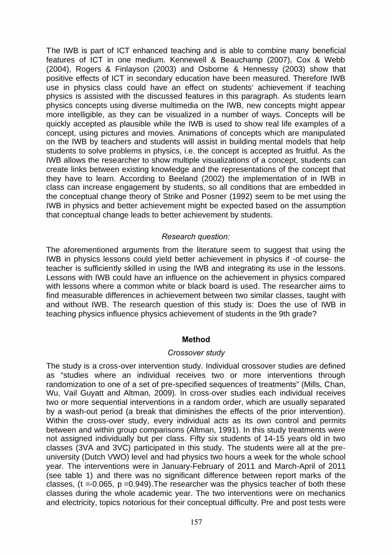
The IWB is part of ICT enhanced teaching and is able to combine many beneficialfeatures of ICT in one medium. Kennewell & Beauchamp (2007), Cox & Webb(2004), Rogers & Finlayson (2003) and Osborne & Hennessy (2003) show thatpositive effects of ICT in secondary education have been measured. Therefore IWBuse in physics class could have an effect on students’ achievement if teachingphysics is assisted with the discussed features in this paragraph. As students learnphysics concepts using diverse multimedia on the IWB, new concepts might appearmore intelligible, as they can be visualized in a number of ways. Concepts will bequickly accepted as plausible while the IWB is used to show real life examples of aconcept, using pictures and movies. Animations of concepts which are manipulatedon the IWB by teachers and students will assist in building mental models that helpstudents to solve problems in physics, i.e. the concept is accepted as fruitful. As theIWB allows the researcher to show multiple visualizations of a concept, students cancreate links between existing knowledge and the representations of the concept thatthey have to learn. According to Beeland (2002) the implementation of in IWB inclass can increase engagement by students, so all conditions that are embedded inthe conceptual change theory of Strike and Posner (1992) seem to be met using theIWB in physics and better achievement might be expected based on the assumptionthat conceptual change leads to better achievement by students.

Research question:

The aforementioned arguments from the literature seem to suggest that using theIWB in physics lessons could yield better achievement in physics if -of course- theteacher is sufficiently skilled in using the IWB and integrating its use in the lessons.Lessons with IWB could have an influence on the achievement in physics comparedwith lessons where a common white or black board is used. The researcher aims tofind measurable differences in achievement between two similar classes, taught withand without IWB. The research question of this study is: Does the use of IWB inteaching physics influence physics achievement of students in the 9th grade?

Method

Crossover study

The study is a cross-over intervention study. Individual crossover studies are definedas “studies where an individual receives two or more interventions throughrandomization to one of a set of pre-specified sequences of treatments” (Mills, Chan,Wu, Vail Guyatt and Altman, 2009). In cross-over studies each individual receivestwo or more sequential interventions in a random order, which are usually separatedby a wash-out period (a break that diminishes the effects of the prior intervention).Within the cross-over study, every individual acts as its own control and permitsbetween and within group comparisons (Altman, 1991). In this study treatments werenot assigned individually but per class. Fifty six students of 14-15 years old in twoclasses (3VA and 3VC) participated in this study. The students were all at the pre-university (Dutch VWO) level and had physics two hours a week for the whole schoolyear. The interventions were in January-February of 2011 and March-April of 2011(see table 1) and there was no significant difference between report marks of theclasses, (t =-0.065, p =0.949).The researcher was the physics teacher of both theseclasses during the whole academic year. The two interventions were on mechanicsand electricity, topics notorious for their conceptual difficulty. Pre and post tests were

157

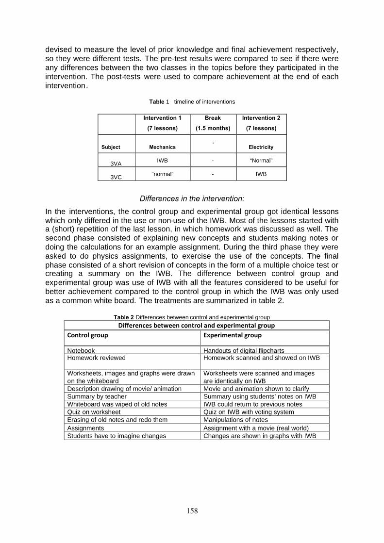
devised to measure the level of prior knowledge and final achievement respectively,so they were different tests. The pre-test results were compared to see if there wereany differences between the two classes in the topics before they participated in theintervention. The post-tests were used to compare achievement at the end of eachintervention.

Table 1 timeline of interventions

Intervention 1

(7 lessons)

Break

(1.5 months)

Intervention 2

(7 lessons)

Subject Mechanics-

Electricity

3VA IWB - “Normal”

3VC “normal” - IWB

Differences in the intervention:

In the interventions, the control group and experimental group got identical lessonswhich only differed in the use or non-use of the IWB. Most of the lessons started witha (short) repetition of the last lesson, in which homework was discussed as well. Thesecond phase consisted of explaining new concepts and students making notes ordoing the calculations for an example assignment. During the third phase they wereasked to do physics assignments, to exercise the use of the concepts. The finalphase consisted of a short revision of concepts in the form of a multiple choice test orcreating a summary on the IWB. The difference between control group andexperimental group was use of IWB with all the features considered to be useful forbetter achievement compared to the control group in which the IWB was only usedas a common white board. The treatments are summarized in table 2.

Table 2 Differences between control and experimental groupDifferences between control and experimental group

Control group Experimental group

Notebook Handouts of digital flipchartsHomework reviewed Homework scanned and showed on IWB

Worksheets, images and graphs were drawnon the whiteboard

Worksheets were scanned and imagesare identically on IWB

Description drawing of movie/ animation Movie and animation shown to clarifySummary by teacher Summary using students’ notes on IWBWhiteboard was wiped of old notes IWB could return to previous notesQuiz on worksheet Quiz on IWB with voting systemErasing of old notes and redo them Manipulations of notesAssignments Assignment with a movie (real world)Students have to imagine changes Changes are shown in graphs with IWB

158

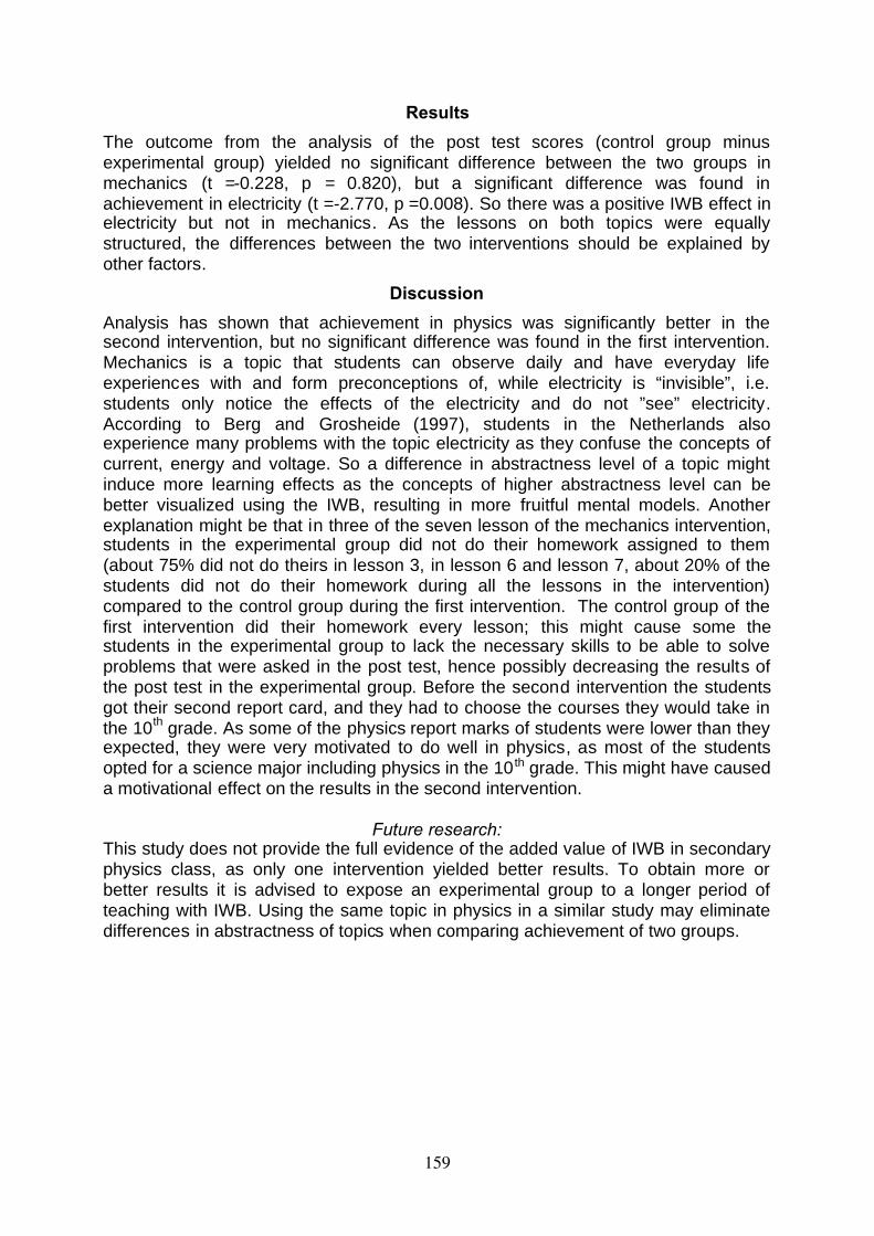
Results

The outcome from the analysis of the post test scores (control group minusexperimental group) yielded no significant difference between the two groups inmechanics (t =-0.228, p = 0.820), but a significant difference was found inachievement in electricity (t =-2.770, p =0.008). So there was a positive IWB effect inelectricity but not in mechanics. As the lessons on both topics were equallystructured, the differences between the two interventions should be explained byother factors.

Discussion

Analysis has shown that achievement in physics was significantly better in thesecond intervention, but no significant difference was found in the first intervention.Mechanics is a topic that students can observe daily and have everyday lifeexperiences with and form preconceptions of, while electricity is “invisible”, i.e.students only notice the effects of the electricity and do not ”see” electricity.According to Berg and Grosheide (1997), students in the Netherlands alsoexperience many problems with the topic electricity as they confuse the concepts ofcurrent, energy and voltage. So a difference in abstractness level of a topic mightinduce more learning effects as the concepts of higher abstractness level can bebetter visualized using the IWB, resulting in more fruitful mental models. Anotherexplanation might be that in three of the seven lesson of the mechanics intervention,students in the experimental group did not do their homework assigned to them(about 75% did not do theirs in lesson 3, in lesson 6 and lesson 7, about 20% of thestudents did not do their homework during all the lessons in the intervention)compared to the control group during the first intervention. The control group of thefirst intervention did their homework every lesson; this might cause some thestudents in the experimental group to lack the necessary skills to be able to solveproblems that were asked in the post test, hence possibly decreasing the results ofthe post test in the experimental group. Before the second intervention the studentsgot their second report card, and they had to choose the courses they would take inthe 10th grade. As some of the physics report marks of students were lower than theyexpected, they were very motivated to do well in physics, as most of the studentsopted for a science major including physics in the 10 th grade. This might have causeda motivational effect on the results in the second intervention.

Future research:This study does not provide the full evidence of the added value of IWB in secondaryphysics class, as only one intervention yielded better results. To obtain more orbetter results it is advised to expose an experimental group to a longer period ofteaching with IWB. Using the same topic in physics in a similar study may eliminatedifferences in abstractness of topics when comparing achievement of two groups.

159

ReferencesAltman, D. (1991). Practical Statistics for Medical Research. London: Chapman & Hall.Armstrong, V., Barnes, S., Sutherland, R., Curran, S., Mills, S. & Thompson, I., (2005) Collaborative

research methodology for investigating teaching and learning: the use of interactivewhiteboard technology, Educational Review, 57(4), 457-469.

Blanton, P. (2008) Using Interactive Whiteboard to Enhance Student Learning, The Physics Teacher,46(3).

Beeland, W.D. Jr (2002) Student engagement, visual learning and technology: can interactivewhiteboards help? Annual Conference of the Association of Information Technology forTeaching Education, Trinity College, Dublin.

Berg, E. van den, Grosheide, W. (1997). Learning and teaching about energy, power, current andvoltage. School Science Review, 78(284), 89-94.

Cox, M. J., & Webb, M. (Eds.). (2004). A review of the research literature relating to ICT andpedagogy. Coventry: Becta/London: DfES.

Dhindsa, H.S. & Emran, S.H., (2006) Use of the interactive whiteboard in contructivist teaching forhigher student achievement. In Stewart, S. M., Olearski, J. E. and Thompson, D. (Eds).Proceedings of the Second Annual Conference for Middle East Teachers of Science,Mathematics and Computing (pp. 175-188). Abu Dhabi: METSMaC

Hennessy, S., Deaney, R., Ruthven, K. & Winterbottom, M. (2007) Pedagogical strategies for usingthe interactive whiteboard to foster learner participation in school science, Learning, Mediaand Technology, 32(3), 283 – 301.

Higgins, S., Beauchamp, G. & Miller, G. (2007) Reviewing the literature on interactive whiteboards,Learning, Media and technology, 32(3), 213-224.

Kennewell, S., (2005) Researching the influence of interactive presentation tools on teachers’pedagogy. Paper presented at the British Educational Research Association AnnualConference, University of Glamorgan, pp. 14-17.

Kennewell, S., & Beauchamp, G. (2007).The features of interactive white boards and their influenceon learning, Learning ,Media and Technology, 32(3), 227–241.

Mills E.J., Chan A.W., Wu P., Vail A., Guyatt G.H., & Altman, D.G. (2009). Design, analysis, andpresentation of crossover trials. BioMed Central, 10(27), 1-6.

Molenaar, P. (2002). Virtueel Practicum (Virtual Laboratory)Digital multimedia materials for physics education. GIREP 2002 Conference, Lund, Sweden.

Osborne, J., & Hennessy, S. (2003) Literature review in science education and the role of ICT:Promise, problems and future directions. London: Futurelab.

Rogers, L. & Finlayson, H. (2004) Developing successful pedagogy with information andcommunications technology: how are science teachers meeting the challenge? Technology,Pedagogy and Education, 13(3), 287 – 305.

Somekh, B., Haldane, M., Jones, K., Lewin, C., Steadman, S., Scrimshaw, P., et al. (2007). Evaluationof the primary schools whiteboard project. Coventry, UK: BECTA

Strike, K. A., & Posner, G. J. (1992). A revisionist theory of conceptual change. In R. A. Duschl & R. J.Hamilton (Eds.), Philosophy of science, cognitive psychology,and educational theory andpractice, 147–176. Albany: State University of New York Press.

Swan, K., Schenker, J. & Kratcoski, A., (2008) The Effects of the Use of Interactive Whiteboards onStudent Achievement. In Proceedings of World Conference on Educational Multimedia,Hypermedia and Telecommunications, pp. 3290-3297.

Webb, M., (2005) Affordances of ICT in science learning: implications for an integrated pedagogy,International Journal of Science Education , 27(6), 705–735.

160

Conduction as a prerequisite for superconductivity

Sara Barbieri1, Marco Giliberti2, Claudio Fazio1

sara71.roberta@yahoo.it

1Dipartimento di Fisica, Università di Palermo, Italy

2Dipartimento di Fisica, Università di Milano, Italy

As the number of high school students interested in modern physics is always increasing, the University of Milan is developing a project on superconductivity in which experiments and theory are proposed to students. The present paper is divided into two main parts. The first analyzes the basic concepts necessary to understand superconductivity. For a start we propose the first step of a design-based research were students learn the London phenomenological approach. In this way students’ can get the explanation of experiments easy to obtain in the lab-room, such as Meissner effect and the measure of the critical temperature of a type II superconductor. The second part analyzes the results obtained from a written test given to students after a two-hour lesson on conduction. The results highlighted students’ conceptual understanding of electrical conduction and we found out that the

relation between electric field and current density (J = E) which is the core of our proposal, can even be useful to overcome common conceptions related to electrical circuits.

1. Introduction

We present an approach to the teaching of electrical conduction that has been developed in the context of PLS3 2011 (Scientific Degree Plan 3) under a grant of the Italian Ministry of Education. The approach involved 73 high-school students that had already dealt with electrical conduction at high school, so we planned a two-hours lesson at the Physics Department of the University of Milan. The core of the

approach is the relationship J=E (where J is the current density and E is the electric field). The main motivation under our choice is that the analogue relationship J = -kA (where J is the superconductive current density and A is the vector potential) will be the key point of our presentation of superconductivity, that we will address in another

paper. A further motivation for the choice J=E is that the usual approach based on the Ohm’s laws leads students to some well-known difficulties in facing and resolving electrical circuits (Mc Dermott,1992; Fredette,1980; Vetter,2004). Typical students’ difficulties on electrical circuits are 1) concepts such as current, voltage, resistance, energy are often undefined and undistinguished; 2) even when students are able to state definitions, they apply them to real circuits with difficulty; 3) battery is seen as a source of constant current; 4) bulbs, wires or resistors use up, or slow down current.

In our proposal Ohm’s laws become a consequence of the local law J=E. Using this relationship, we will show that resistance in series and in parallel may be more simply recognized in various experimental situations. Now we want to clarify both the physical and the educational frameworks we are referring to. For the physical framework we refer to Table1 which shows the essential concepts of the three levels of comprehension of superconductivity: Level 1, the main phenomenology; Level 2, the London’s theory; Level 3, the BCS theory. For the educational framework we adopt a design-based research to develop our proposal, we proceed with an educational reconstruction of the contents and we refer to the study of Hewson and Hennessey (Treagust and Duit,2008) to test the conceptual understanding of the students. In their study the authors use three criteria to describe the improvement in students’ conceptual understanding: intelligibility, plausibility and fruibility, whose meaning will be clarified later. We evaluate the obtained results by a comparison between two similar groups of about 70 students: the test group consisting of

161

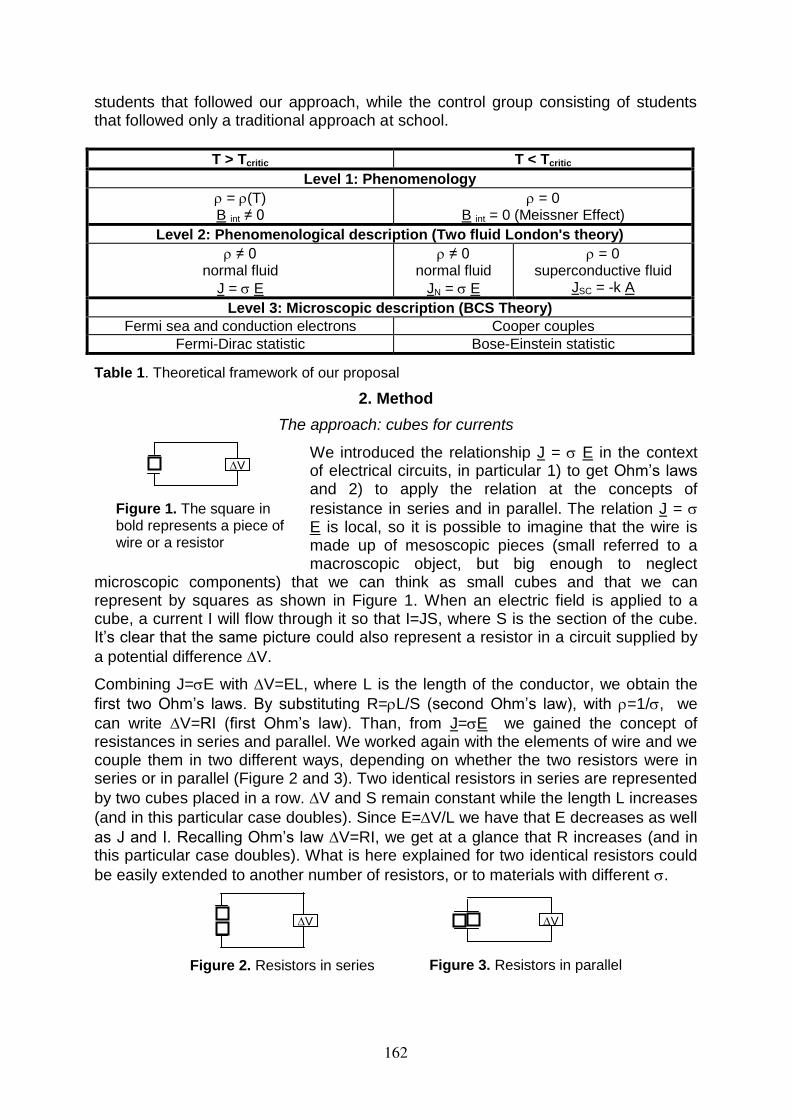
students that followed our approach, while the control group consisting of students that followed only a traditional approach at school.

T > Tcritic T < Tcritic

Level 1: Phenomenology

= (T) B int ≠ 0

= 0 B int = 0 (Meissner Effect)

Level 2: Phenomenological description (Two fluid London's theory)

≠ 0 normal fluid

J = E

≠ 0 normal fluid

JN = E

= 0 superconductive fluid

JSC = -k A

Level 3: Microscopic description (BCS Theory)

Fermi sea and conduction electrons Cooper couples

Fermi-Dirac statistic Bose-Einstein statistic

Table 1. Theoretical framework of our proposal

2. Method

The approach: cubes for currents

We introduced the relationship J = E in the context of electrical circuits, in particular 1) to get Ohm’s laws and 2) to apply the relation at the concepts of

resistance in series and in parallel. The relation J = E is local, so it is possible to imagine that the wire is made up of mesoscopic pieces (small referred to a macroscopic object, but big enough to neglect

microscopic components) that we can think as small cubes and that we can represent by squares as shown in Figure 1. When an electric field is applied to a cube, a current I will flow through it so that I=JS, where S is the section of the cube. It’s clear that the same picture could also represent a resistor in a circuit supplied by

a potential difference V.

Combining J=E with V=EL, where L is the length of the conductor, we obtain the

first two Ohm’s laws. By substituting R=L/S (second Ohm’s law), with =1/, we

can write V=RI (first Ohm’s law). Than, from J=E we gained the concept of resistances in series and parallel. We worked again with the elements of wire and we couple them in two different ways, depending on whether the two resistors were in series or in parallel (Figure 2 and 3). Two identical resistors in series are represented

by two cubes placed in a row. V and S remain constant while the length L increases

(and in this particular case doubles). Since E=V/L we have that E decreases as well

as J and I. Recalling Ohm’s law V=RI, we get at a glance that R increases (and in this particular case doubles). What is here explained for two identical resistors could

be easily extended to another number of resistors, or to materials with different .

V V

Figure 2. Resistors in series Figure 3. Resistors in parallel

V

Figure 1. The square in bold represents a piece of wire or a resistor

162

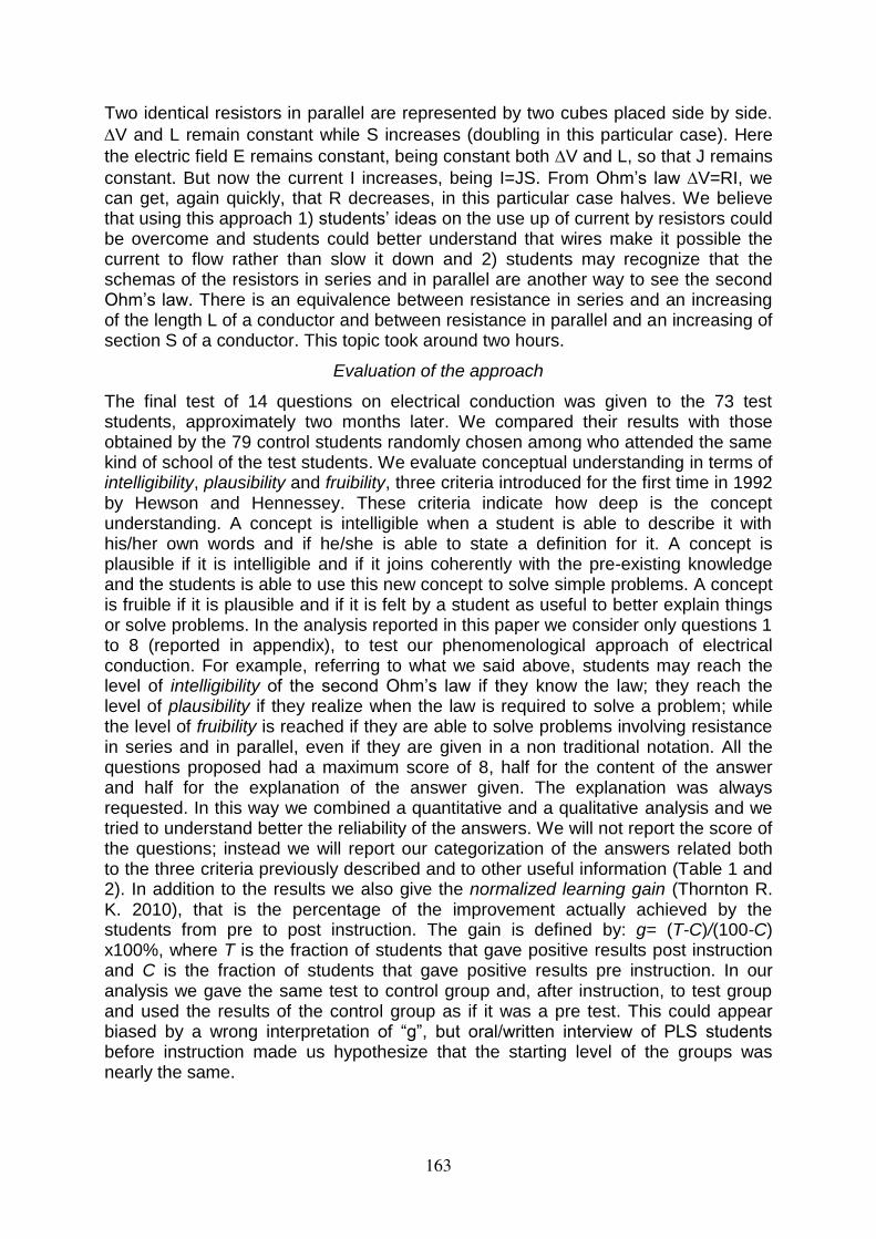
Two identical resistors in parallel are represented by two cubes placed side by side.

V and L remain constant while S increases (doubling in this particular case). Here

the electric field E remains constant, being constant both V and L, so that J remains

constant. But now the current I increases, being I=JS. From Ohm’s law V=RI, we can get, again quickly, that R decreases, in this particular case halves. We believe that using this approach 1) students’ ideas on the use up of current by resistors could be overcome and students could better understand that wires make it possible the current to flow rather than slow it down and 2) students may recognize that the schemas of the resistors in series and in parallel are another way to see the second Ohm’s law. There is an equivalence between resistance in series and an increasing of the length L of a conductor and between resistance in parallel and an increasing of section S of a conductor. This topic took around two hours.

Evaluation of the approach

The final test of 14 questions on electrical conduction was given to the 73 test students, approximately two months later. We compared their results with those obtained by the 79 control students randomly chosen among who attended the same kind of school of the test students. We evaluate conceptual understanding in terms of intelligibility, plausibility and fruibility, three criteria introduced for the first time in 1992 by Hewson and Hennessey. These criteria indicate how deep is the concept understanding. A concept is intelligible when a student is able to describe it with his/her own words and if he/she is able to state a definition for it. A concept is plausible if it is intelligible and if it joins coherently with the pre-existing knowledge and the students is able to use this new concept to solve simple problems. A concept is fruible if it is plausible and if it is felt by a student as useful to better explain things or solve problems. In the analysis reported in this paper we consider only questions 1 to 8 (reported in appendix), to test our phenomenological approach of electrical conduction. For example, referring to what we said above, students may reach the level of intelligibility of the second Ohm’s law if they know the law; they reach the level of plausibility if they realize when the law is required to solve a problem; while the level of fruibility is reached if they are able to solve problems involving resistance in series and in parallel, even if they are given in a non traditional notation. All the questions proposed had a maximum score of 8, half for the content of the answer and half for the explanation of the answer given. The explanation was always requested. In this way we combined a quantitative and a qualitative analysis and we tried to understand better the reliability of the answers. We will not report the score of the questions; instead we will report our categorization of the answers related both to the three criteria previously described and to other useful information (Table 1 and 2). In addition to the results we also give the normalized learning gain (Thornton R. K. 2010), that is the percentage of the improvement actually achieved by the students from pre to post instruction. The gain is defined by: g= (T-C)/(100-C) x100%, where T is the fraction of students that gave positive results post instruction and C is the fraction of students that gave positive results pre instruction. In our analysis we gave the same test to control group and, after instruction, to test group and used the results of the control group as if it was a pre test. This could appear biased by a wrong interpretation of “g”, but oral/written interview of PLS students before instruction made us hypothesize that the starting level of the groups was nearly the same.

163

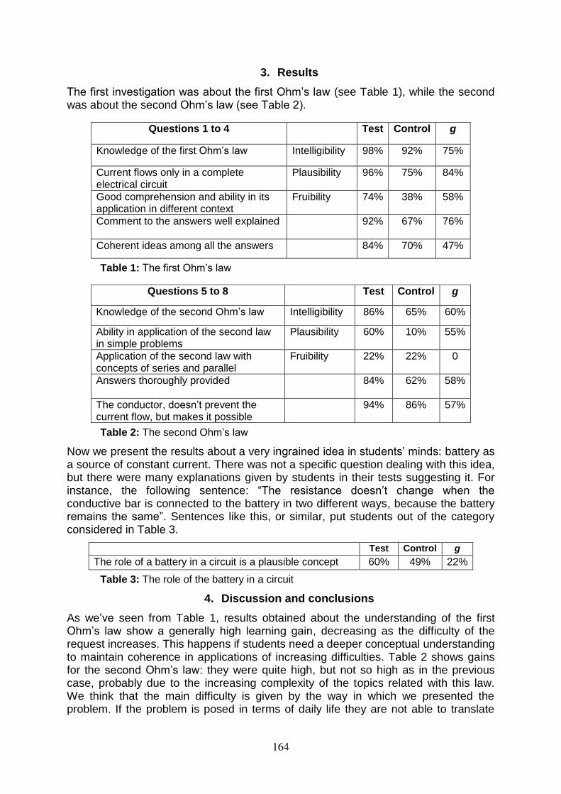
3. Results

The first investigation was about the first Ohm’s law (see Table 1), while the second was about the second Ohm’s law (see Table 2).

Questions 1 to 4 Test Control g

Knowledge of the first Ohm’s law Intelligibility 98% 92% 75%

Current flows only in a complete electrical circuit

Plausibility

96% 75% 84%

Good comprehension and ability in its application in different context

Fruibility 74% 38% 58%

Comment to the answers well explained 92% 67% 76%

Coherent ideas among all the answers 84% 70% 47%

Table 1: The first Ohm’s law

Questions 5 to 8 Test Control g

Knowledge of the second Ohm’s law Intelligibility 86% 65% 60%

Ability in application of the second law in simple problems

Plausibility 60% 10% 55%

Application of the second law with concepts of series and parallel

Fruibility 22% 22% 0

Answers thoroughly provided

84% 62% 58%

The conductor, doesn’t prevent the current flow, but makes it possible

94% 86% 57%

Table 2: The second Ohm’s law

Now we present the results about a very ingrained idea in students’ minds: battery as a source of constant current. There was not a specific question dealing with this idea, but there were many explanations given by students in their tests suggesting it. For instance, the following sentence: “The resistance doesn’t change when the conductive bar is connected to the battery in two different ways, because the battery remains the same”. Sentences like this, or similar, put students out of the category considered in Table 3.

Test Control g

The role of a battery in a circuit is a plausible concept 60% 49% 22%

Table 3: The role of the battery in a circuit

4. Discussion and conclusions

As we’ve seen from Table 1, results obtained about the understanding of the first Ohm’s law show a generally high learning gain, decreasing as the difficulty of the request increases. This happens if students need a deeper conceptual understanding to maintain coherence in applications of increasing difficulties. Table 2 shows gains for the second Ohm’s law: they were quite high, but not so high as in the previous case, probably due to the increasing complexity of the topics related with this law. We think that the main difficulty is given by the way in which we presented the problem. If the problem is posed in terms of daily life they are not able to translate

164

those terms into scientific language, to which they are familiar for these problems, to get the solution. So, while they easily recognize resistance in series and parallel when they are represented in traditional way, they are not able to do the same where the context is different, for example similar to that of the lab-room. On the other hand, a concept can be deeply understood only if it is used for a long time. And this did not happen for our students, who never performed experiments with electrical circuits in our lab-room; therefore this topic will be more carefully and thoroughly developed in the next cycle of our designed-based research. The result obtained in Table 3 is even more interesting: although we did not explicitly discuss the functioning of a battery during the lessons, nonetheless we can see an average conceptual gain of 22%. As we believe that students could gain a deeper understanding about electrical conduction in a circuit if they understood the role of a battery we are planning a new cycle of lessons in which this topic is more clearly discussed. Often in literature battery is presented as a source of constant potential difference. We think it should be important to treat in detail the physics involved to explain how a battery works. A battery is a source of constant potential difference only if the internal resistance is negligible compared with the resistance of the entire circuit, otherwise it works as a source of constant current (as it happens when dealing with a large number of resistors in parallel). The usual simplification, of internal resistance negligible, is not well declared and students can’t become sufficiently conscious of the problem. Teachers’ unclear behaviour like this, in our opinion, cause confusion and lack of coherence in students’ thinking. In developing this first step of our design-based research we have referred to classical physics even though superconductivity cannot be understood classically. Classical physics has been necessary in order to operate an educational reconstruction of the contents. The results obtained allow us to say

that the approach to electrical conduction based on the relationship J=E is possible and works well. Furthermore this relationship will have its analogue in superconductivity with the relationship J=kA for the supercurrents, but this is beyond the aims of our paper and will be developed in detail in the next PLS project on superconductivity (2011-2012). In the new project the problem of superconductivity will be the final part of a longer sequence that will include other topics necessary to develop superconductivity, such as wave theory and elements of quantum theory.

References

Fredette N., & Lochhead J.(1980). Student conceptions of simple circuits. The physics teacher, March.

London F., & London H. (1934). The electromagnetic equations of the Supraconductor. Clarendon Laboratory, Oxford.

McDermott L., & Shaffer P. S. (1992). Research as a guide for curriculum development: an example from introductory electricity. Part I: investigation of students’ understanding. Am. J. Phys. 60 (11).

Pippard A. B. (1952). An experimental and theoretical study of the relation between magnetic field and current in superconductor. The royal Society Mond Laboratory, University of Cambridge.

Thornton R. K. (2010). Effective learning environments for computer supported instruction in the physics classroom, laboratory and distance education. In Vicentini M., & Sassi E. (General Editions) Connecting research in physics education with teacher education, Vol 2, New Dhely, Gutam Rachmandani.

165

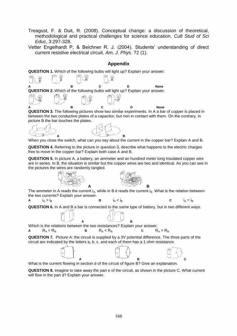
Treagust, F. & Duit, R. (2008). Conceptual change: a discussion of theoretical, methodological and practical challenges for science education. Cult Stud of Sci Educ, 3:297-328.

Vetter Engelhardt P, & Beichner R. J. (2004). Students’ understanding of direct current resistive electrical circuit. Am. J. Phys. 72 (1).

Appendix

QUESTION 1. Which of the following bulbs will light up? Explain your answer.

A B C D None QUESTION 2. Which of the following bulbs will light up? Explain your answer.

A B C D None QUESTION 3. The following pictures show two similar experiments. In A a bar of copper is placed in between the two conductive plates of a capacitor, but non in contact with them. On the contrary, in picture B the bar touches the plates.

A B When you close the switch, what can you say about the current in the copper bar? Explain A and B.

QUESTION 4. Referring to the picture in question 3, describe what happens to the electric charges free to move in the copper bar? Explain both case A and B.

QUESTION 5. In picture A, a battery, an ammeter and an hundred meter long insulated copper wire are in series. In B, the situation is similar but the copper wires are two and identical. As you can see in the pictures the wires are randomly tangled.

A B The ammeter in A reads the current iA, while in B it reads the current iB. What is the relation between the two currents? Explain your answer. A iA > iB B iA < iB C iA = iB

QUESTION 6. In A and B a bar is connected to the same type of battery, but in two different ways.

A B Which is the relations between the two resistances? Explain your answer. A RA = RB B RA < RB C RA > RB

QUESTION 7. Picture A: the circuit is supplied by a 3V potential difference. The three parts of the circuit are indicated by the letters a, b, c, and each of them has a 1 ohm resistance.

A B C What is the current flowing in section d of the circuit of figure B? Give an explanation.

QUESTION 8. Imagine to take away the part e of the circuit, as shown in the picture C. What current will flow in the part d? Explain your answer.

166

Integrated e-learning and the opportunity for anyone to explore the nature of polarization of light

Pavel Brom, František Lustig

Pavel.Brom@mff.cuni.cz

Laboratory of General Physics Education, Faculty of Math and Physics, Charles University in Prague, Czech Republic

Abstract: Students and young people interested in optics have limited or no possibilities to operate with expensive optical elements like waveplates and optomechanical devices. A new remote experiment on the polarization of light that is available for free at www.ises.info brings opportunity to measure, modify, and study the polarization state of light and to use it in various applications like crossing polarizers, spintronics, etc.

We describe a new remote experiment and a set of tasks and problems for secondary school and university students. They may explore various sources of light (a bulb, laser LED, …) and they may verify the Malus law for crossed polarizers. One can measure all basic polarization states of light (linear polarization, circular and elliptical polarization) using the dependence of light intensity on the angle of rotation of the polarizer. A half- and a quarter-waveplate is used for the modification of the polarization state of light.

Some virtual experiments (simulations, applets) and e-texts are included in order to help students to understand the theory. The teaching-learning sequence may be controled by the teacher, e-texts or LMS. This strategy using the integration of real remote experiments, simulations (applets), and traditional e-learning means is called the integrated e-learning.

Introduction and Motivation

Many applications in our every-day are based on polarization of light: a polarizing filters for cameras, LCD displays of our mobile phones, notebooks, etc. Advanced applications will use circularly polarized light (e.g. spintronics devices in the future). Some elements are easily available and low-cost (polarizers, polaroid foil), but the other are not (e.g. waveplates). Students may explore the nature of polarization of light and the variety of its applications within an interesting strategy that we call integrated e-learning [Schauer, Ožvoldová, Lustig, 2009].

Within transformation of physics education [Wieman, Perkins (2005)] where the authors recommend to use simulations, the integrated e-learning strategy aims to exploit more e-learning means like e-texts, multimedia objects, simulations (applets, virtual experiments), and especially real remotely controlled experiments [Eckert et al. (2009); Gröber et al. (2007)]. Experimenting is regarded to be an essential part of physics education and inquiry-based science education. Recipe labs are substituted by research labs [Schauer et al. (2008)].

In this paper we present a new remotely controlled experiment where students may play with expensive optical elements, exploring the physics of polarization of light. A couple of typical experimental results and outcomes are provided. We describe the other e-resources and we suggest how to use them. The remote experiment may become a part of any e-textbook or e-text. The way of use depends on teacher’s and/or student’s decisions and needs and the curriculum as well. Main advantages are possibility to interact with the graphical user interface repeatedly, without the teacher’s or supervisor’s assistance, and perhaps with no time limitations (when nobody else is waiting in a queue for the control of the experimental setup).

167

1. Real Remote Experiment

One can measure the intensity of light behind a rotating polarizer (i. e. an analyzer) in order to determine the polarization state of light. Furthermore, a user can prepare linearly polarized light by an inserted polarizer and modify it by waveplates. All real remote experiments at www.ises.info are free of use and accessible for anyone 24/7 [Brom, Lustig et al. (2011); Schauer, Lustig, Ožvoldová (2009); Schauer et al. (2008)]. Users need only the JAVA Runtime Environment installed on the PC for the control of an experiment and for downloading their own experimental data as well.

Secondary school students may measure what kind of light produces a bulb, a white LED and a red laser pointer. From the most important applications a LCD display and crossed polarizers are demonstrated.

University students and advanced younger students will learn about all possible polarization states (linear, circular, elliptical) and the way of their mathematical description. Students will try to modify linear polarization for circular polarization with a multiple-order quarter waveplate and to verify the prepared polarization state with a zero-order quarter waveplate [Born, Wolf (1999)]. Furthermore, the experimental data are affected by noise, asymmetry, and very little offset, so students should apply some advanced methods of graphical data processing – data smoothing and/or fitting with the model function

)(sin)(cos)( 2min

2max ψαψαα −+−= III , minmax II ≥ (1)

where α is the angle of rotation of the analyzer, ψ is the angle of the rotation of the polarization ellipse, I(α) is the measured intensity of light behind the analyzer, Imax and Imin are the maximum and minimum values of the measured light intensity that can be determined from experimental data and that correspond to the major (a) and minor (b) axis of the polarization ellipse

max

min

I

I

a

b = , 0≥≥ ba , 0>a . (2)

The fourth free parameter can be determined when a zero-order quarter waveplate with known fast axis is inserted into the path of light.

2. Virtual experiments (simulations, applets)

Students should also use a couple of nice applets that help them to visualize all the possible polarization states of light and to practise the way of their modifications with waveplates. We recommend for the university level and perhaps for secondary schools five applets created with the use of Easy JAVA Simulations (EJS) from the Open Source Physics project [Christian et al. (2011)]: a) the polarization states of the reflected and transmitted wave, b) visualization of various polarization states described by the Jones vector, c) effect of a polarizer while it is rotated, d) effect of a half waveplate while it is rotated, and e) modification of polarization states by the rotation of a quarter waveplate.

These applets are easy enough and intuitive to use. Moreover, one can change the point of view by dragging the picture with the mouse for the best visualization. Links to these sims and the other good applets can be found in the e-text.

168

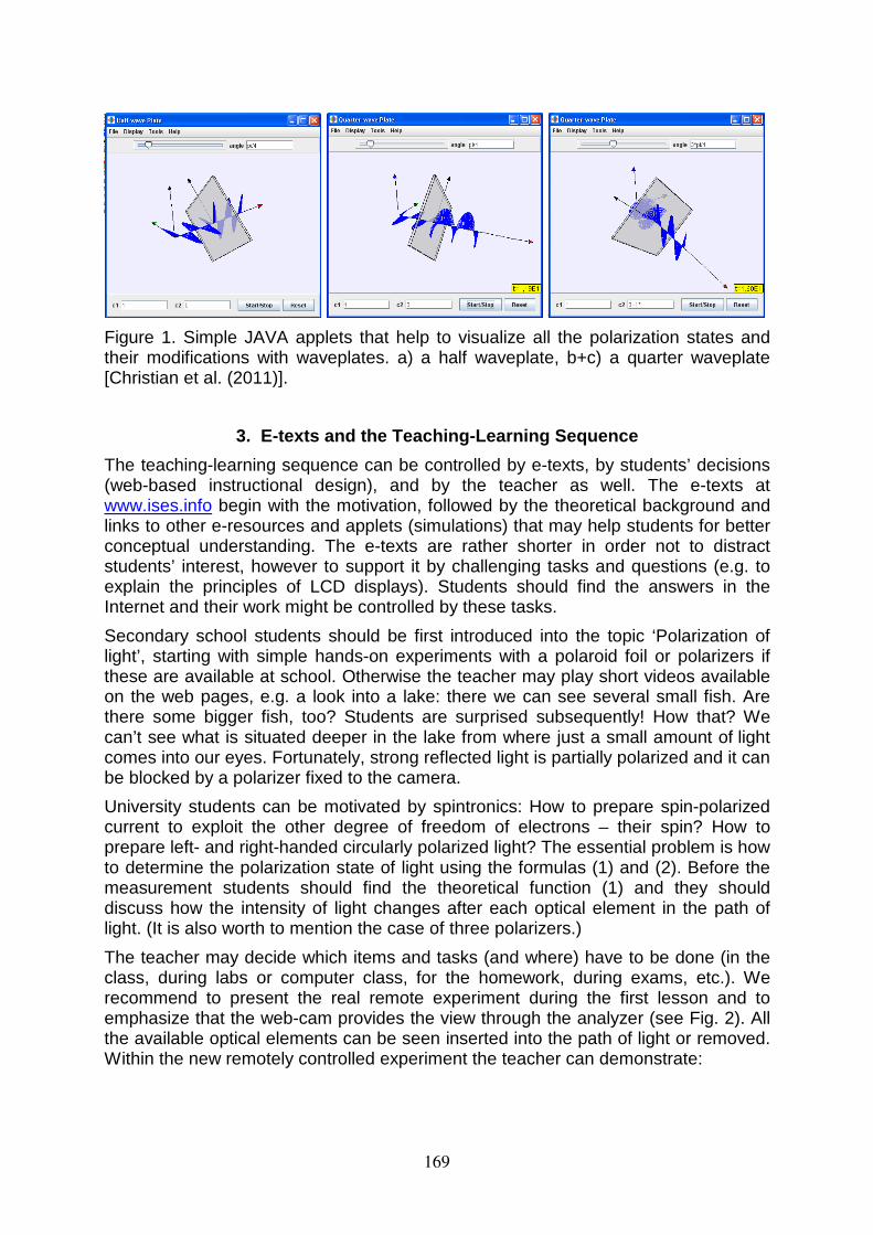
Figure 1. Simple JAVA applets that help to visualize all the polarization states and their modifications with waveplates. a) a half waveplate, b+c) a quarter waveplate [Christian et al. (2011)].

3. E-texts and the Teaching-Learning Sequence

The teaching-learning sequence can be controlled by e-texts, by students’ decisions (web-based instructional design), and by the teacher as well. The e-texts at www.ises.info begin with the motivation, followed by the theoretical background and links to other e-resources and applets (simulations) that may help students for better conceptual understanding. The e-texts are rather shorter in order not to distract students’ interest, however to support it by challenging tasks and questions (e.g. to explain the principles of LCD displays). Students should find the answers in the Internet and their work might be controlled by these tasks.

Secondary school students should be first introduced into the topic ‘Polarization of light’, starting with simple hands-on experiments with a polaroid foil or polarizers if these are available at school. Otherwise the teacher may play short videos available on the web pages, e.g. a look into a lake: there we can see several small fish. Are there some bigger fish, too? Students are surprised subsequently! How that? We can’t see what is situated deeper in the lake from where just a small amount of light comes into our eyes. Fortunately, strong reflected light is partially polarized and it can be blocked by a polarizer fixed to the camera.

University students can be motivated by spintronics: How to prepare spin-polarized current to exploit the other degree of freedom of electrons – their spin? How to prepare left- and right-handed circularly polarized light? The essential problem is how to determine the polarization state of light using the formulas (1) and (2). Before the measurement students should find the theoretical function (1) and they should discuss how the intensity of light changes after each optical element in the path of light. (It is also worth to mention the case of three polarizers.)

The teacher may decide which items and tasks (and where) have to be done (in the class, during labs or computer class, for the homework, during exams, etc.). We recommend to present the real remote experiment during the first lesson and to emphasize that the web-cam provides the view through the analyzer (see Fig. 2). All the available optical elements can be seen inserted into the path of light or removed. Within the new remotely controlled experiment the teacher can demonstrate:

169

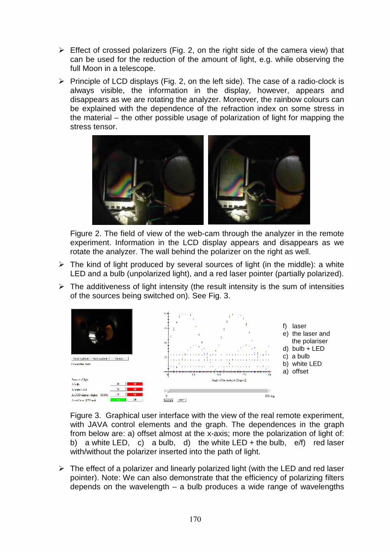
Effect of crossed polarizers (Fig. 2, on the right side of the camera view) that can be used for the reduction of the amount of light, e.g. while observing the full Moon in a telescope.

Principle of LCD displays (Fig. 2, on the left side). The case of a radio-clock is always visible, the information in the display, however, appears and disappears as we are rotating the analyzer. Moreover, the rainbow colours can be explained with the dependence of the refraction index on some stress in the material – the other possible usage of polarization of light for mapping the stress tensor.

Figure 2. The field of view of the web-cam through the analyzer in the remote experiment. Information in the LCD display appears and disappears as we rotate the analyzer. The wall behind the polarizer on the right as well.

The kind of light produced by several sources of light (in the middle): a white LED and a bulb (unpolarized light), and a red laser pointer (partially polarized).

The additiveness of light intensity (the result intensity is the sum of intensities of the sources being switched on). See Fig. 3.

f) laser e) the laser and the polariser d) bulb + LED c) a bulb b) white LED a) offset

Figure 3. Graphical user interface with the view of the real remote experiment, with JAVA control elements and the graph. The dependences in the graph from below are: a) offset almost at the x-axis; more the polarization of light of: b) a white LED, c) a bulb, d) the white LED + the bulb, e/f) red laser with/without the polarizer inserted into the path of light.

The effect of a polarizer and linearly polarized light (with the LED and red laser pointer). Note: We can also demonstrate that the efficiency of polarizing filters depends on the wavelength – a bulb produces a wide range of wavelengths

170

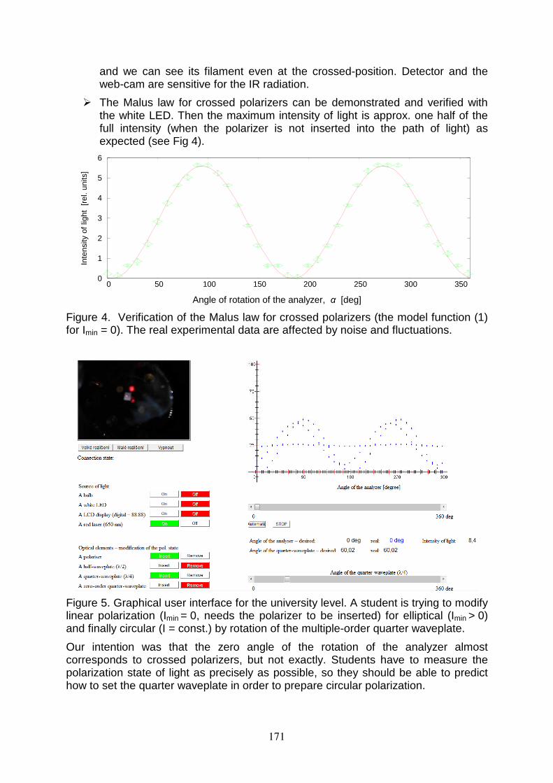
and we can see its filament even at the crossed-position. Detector and the web-cam are sensitive for the IR radiation.

The Malus law for crossed polarizers can be demonstrated and verified with the white LED. Then the maximum intensity of light is approx. one half of the full intensity (when the polarizer is not inserted into the path of light) as expected (see Fig 4).

0

1

2

3

4

5

6

0 50 100 150 200 250 300 350

Inte

nsity

of l

ight

[re

l. un

its]

Angle of the analyzer [deg]

Angle of rotation of the analyzer, α [deg]

Figure 4. Verification of the Malus law for crossed polarizers (the model function (1) for Imin = 0). The real experimental data are affected by noise and fluctuations.

Figure 5. Graphical user interface for the university level. A student is trying to modify linear polarization (Imin = 0, needs the polarizer to be inserted) for elliptical (Imin > 0) and finally circular (I = const.) by rotation of the multiple-order quarter waveplate.

Our intention was that the zero angle of the rotation of the analyzer almost corresponds to crossed polarizers, but not exactly. Students have to measure the polarization state of light as precisely as possible, so they should be able to predict how to set the quarter waveplate in order to prepare circular polarization.

171

Conclusion

We have managed to develop a new remote experiment on polarization of light that enables for students to operate with expensive and not easily accessible optical elements like waveplates and precise optomechanical devices, in order to study the polarization state of light, the ways of its modification and possible applications as well. Within the inquiry-based science education, students will get familiar with important skills like derivation of the model function, reading from graph, and graphical processing of real experimental data that are affected by noise.

The other means of the integrated e-learning strategy (e-texts, multimedia objects, applets on polarization of light) seem to be useful for both students and teachers. Unfortunately, there is a lack of applets visualizing e.g. the movement of electrons in a polaroid foil and the polarizing effect for better conceptual understanding.

Acknowledgment

We wish to thank to Grant agency of the Charles University in Prague for the financial support of the project no. 446611 Pilot survey of effectiveness of the remote laboratory experiments at UK MFF within the integrated e-learning method.

References

Born, M., Wolf, E. (1999): Principles of optics (7th ed.). Cambridge, United Kingdom: Cambridge University Press.

Brom, P., Lustig, F., et al. (2011). Polarization of light. Remote laboratory experiment, Czech Republic: Charles University in Prague, Faculty of Math and Physics, http://www.ises.info.

Christian, W., et al. (2003–2011). The OSP Simulations on Polarization. The Open Source Physics Project. http://www.opensourcephysics.org.

Eckert, B., Gröber, S., Jodl, H. J. (2009). Distance Education in Physics via Internet. Am. J. Dist. Edu, 23 (3), 125–138.

Gröber, S., Vetter, M., Eckert, B., Jodl, H. J. (2007): Experimenting from a Distance – Remotely Controlled Laboratory (RCL). Eur. J. Phys, 28 (3), 127–141.

Schauer, F., Lustig, F., Ožvoldová, M. (2009). ISES – Internet School Experimental System for Computer-Based Laboratories in Physics. In Aung, W., et al. (Eds.), Innovations 2009 (USA), World Innovations in Engineering Education and Research. iNEER Special Volume 2009 (pp. 109–118). MD, USA: Potomac.

Schauer, F., Lustig, F., Dvořák, J., Ožvoldová, M. (2008): Easy to build remote laboratory with data transfer using ISES – Internet School Experimental System ISES. Eur. J. Phys, 29, 753–765.

Schauer, F., Ožvoldová, M., Lustig, F. (2009): Integrated e-Learning – New Strategy of Cognition of Real World in Teaching Physics. In Aung, W., et al. (Eds.), Innovations 2009 (USA), World Innovations in Engineering Education and Research. iNEER Special Volume 2009 (pp. 119–135). MD, USA: Potomac.

Wieman, C., Perkins, K. (2005): Transforming Physics Education. In Physics Today, Vol. 58 (pp. 36–41). USA: American Institute of Physics.

172

EXPLORING PHYSICAL PROPERTIES OF FERROMAGNETIC MATERIALS IN STUDENT LABORATORIES Jitka Bruestlova and Pavel Dobis

brustla@feec.vutbr.cz

Department of Physics, Brno University of Technology, Czech Republic

Abstract: The paper describes a laboratory experiment intended for undergraduate students of Electrical Engineering as part of a general 1st year physics course. In the course of the measurement, students determine the Curie temperature of iron.

The Curie temperature is a physical constant and refers to a characteristic property of ferromagnetic materials. Above the Curie temperature, a material loses its ferromagnetic properties. In a ferromagnetic material, elementary dipoles are aligned into the so – called domains and the domains – through their arrangement – bring about the internal magnetic field of the material –magnetization. At temperatures above the Curie point the ordered state is destroyed, magnetic dipoles become chaotically disordered and the material no more exhibits ferromagnetic properties. This change comes about in an abrupt manner at reaching the Curie temperature.

Magnetic domains and their behavior under action of an external magnetic field belong to frequent questions of students. In order to facilitate the understanding of this phenomenon, magnetic domains are visualized and observed in a microscope under variable external magnetic field.

Keywords: student laboratory experiment, Curie temperature, visualized magnetic domains

1. INTRODUCTION Undergraduate students of Electrical Engineering at Brno University of Technology pass the basic course of general physics in the first and second semester, i.e. at the beginning of their studies. Their previous knowledge and experience in mathematics and physics are very small. Explanation of magnetic properties of materials cannot start from their quantum nature. Only the description of macroscopic features of diamagnetism, paramagnetism and ferromagnetism is possible. Several textbooks are available. Physics courses at the Brno University of Technology use the textbook by Halliday, Resnick and Walker (2006).

In laboratory exercises that are a part of basic course of general physics students make experiments with ferromagnetic materials. They study the behavior of these materials near the Curie temperature or the effects of saturation and hysteresis during the magnetization of a ferromagnetic material. The explanation of these phenomena is not possible without understanding the concept of a magnetic domain.

Magnetic domains and their behavior under action of an external magnetic field belong to frequent questions of students. For better understanding of magnetic domains, the experiment was completed with a tool which makes the domains visible and allows the observation of their behavior under changes of an external magnetic field.

2. CURIE TEMPERATURE 2.1. Magnetic Domains

Atoms exhibit magnetic dipole moments that determine the magnetic properties of materials. Electrons orbit around the nucleus. These orbital motions may be

173

regarded as flows of electric current within the atom, and these currents give rise to magnetic dipole moments. Besides that, electrons have their intrinsic spin magnetic dipole moments. The net magnetic dipole moment of an atom with more electrons can equal zero. These atoms or molecules form the diamagnetic materials. The external magnetic field does not act on the material as the whole but affects the motion of individual electrons. Atoms of paramagnetic materials exhibit permanent magnetic dipole moments. Because of thermal motion, these magnetic dipole moments are randomly oriented and their magnetic fields average to zero. In an external magnetic field Bext, magnetic dipole moments tend to align with the field. According to the experimental Curie law the value of the magnetization M is

extCM BT

= , (1)

where T is temperature and C is called the Curie constant; it depends on the quantum model of the respective material. Increasing external magnetic field Bext increases the parallel alignment of atomic magnetic dipole moments, and the magnetization of the material increases. When the temperature increases, the alignment is disturbed by thermal motion and the magnetization of the material decreases. This law is just an approximation and is valid for weak fields and higher temperatures only. Atomic magnetic dipole moments can align also in the absence of an external magnetic field. Analogous to loops of wires with currents, magnetic dipole moments of atoms act on each other and tend to align in parallel. This interaction is small in paramagnetic materials. The situation differs in ferromagnetic materials. The effect of mutual interaction of atomic magnetic dipole moments can be considered as an action of internal magnetic field that aligns these dipole moments. The internal magnetic field Bint reaches great values that cannot be produced by external electric currents. According to quantum mechanics this interaction is due to spin – spin forces between neighboring atoms. This quantum mechanical effect is called exchange interaction. Due to these forces the alignment of atomic magnetic moments occurs in small regions of the material even without an external magnetic field. Microscopic magnetized regions (sizes 10–3 mm3 – 10 mm3), called magnetic domains, arise at this spontaneous magnetization. But the domains are oriented at random, and the material is found in a nonmagnetic state. The domains are separated from each other by thin boundary layers with the thickness of several hundreds of atomic planes where the vector of magnetization rotates from the direction of one domain to the direction of the neighboring domain. The internal energy of such an arrangement is less than the internal energy of the state of complete alignment. The domain structure of ferromagnetic materials is resistant to disruptive effect of the thermal motion. However, above a certain critical temperature TC, called the Curie temperature, the spin – spin forces cannot maintain the alignment of magnetic dipole moments in domains and the material becomes paramagnetic. As soon as the temperature decreases below the critical temperature, the domain structure rebuilds. The Curie temperature for iron is 1043 K (770 °C).

174

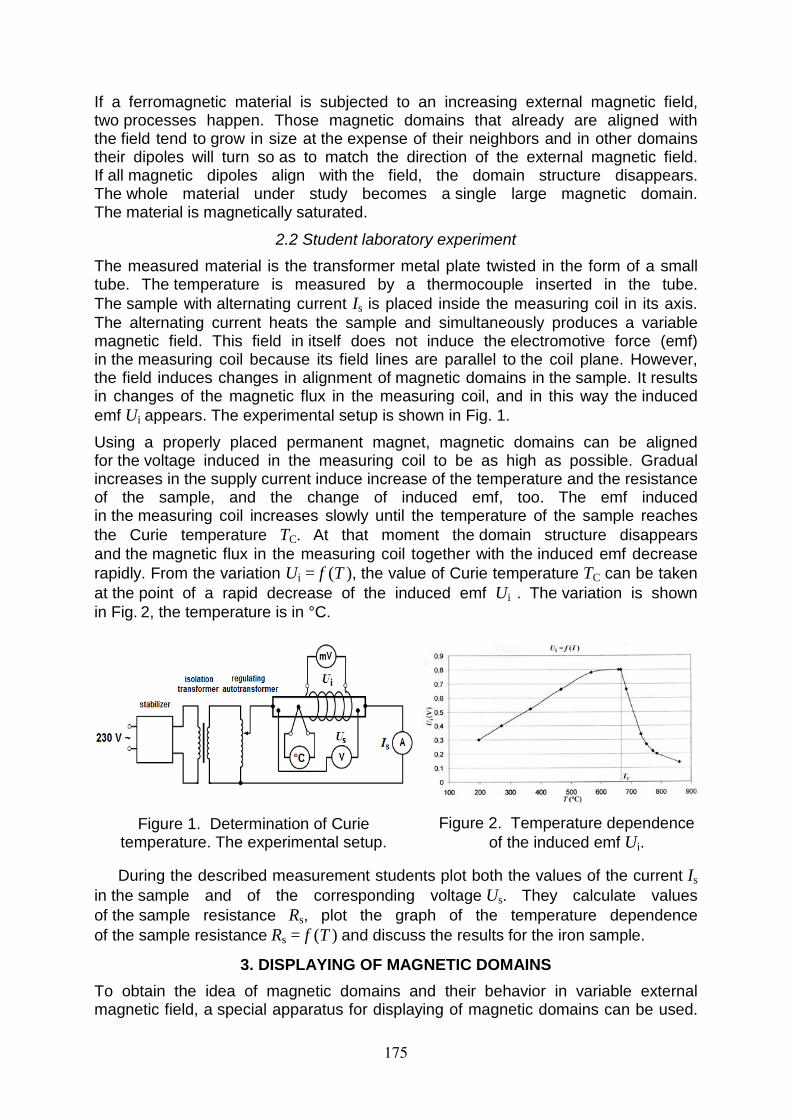
If a ferromagnetic material is subjected to an increasing external magnetic field, two processes happen. Those magnetic domains that already are aligned with the field tend to grow in size at the expense of their neighbors and in other domains their dipoles will turn so as to match the direction of the external magnetic field. If all magnetic dipoles align with the field, the domain structure disappears. The whole material under study becomes a single large magnetic domain. The material is magnetically saturated.

2.2 Student laboratory experiment

The measured material is the transformer metal plate twisted in the form of a small tube. The temperature is measured by a thermocouple inserted in the tube. The sample with alternating current Is is placed inside the measuring coil in its axis. The alternating current heats the sample and simultaneously produces a variable magnetic field. This field in itself does not induce the electromotive force (emf) in the measuring coil because its field lines are parallel to the coil plane. However, the field induces changes in alignment of magnetic domains in the sample. It results in changes of the magnetic flux in the measuring coil, and in this way the induced emf Ui appears. The experimental setup is shown in Fig. 1.

Using a properly placed permanent magnet, magnetic domains can be aligned for the voltage induced in the measuring coil to be as high as possible. Gradual increases in the supply current induce increase of the temperature and the resistance of the sample, and the change of induced emf, too. The emf induced in the measuring coil increases slowly until the temperature of the sample reaches the Curie temperature TC. At that moment the domain structure disappears and the magnetic flux in the measuring coil together with the induced emf decrease rapidly. From the variation Ui = f (T ), the value of Curie temperature TC can be taken at the point of a rapid decrease of the induced emf Ui . The variation is shown in Fig. 2, the temperature is in °C.

Figure 1. Determination of Curie

temperature. The experimental setup. Figure 2. Temperature dependence

of the induced emf Ui.

During the described measurement students plot both the values of the current Is in the sample and of the corresponding voltage Us. They calculate values of the sample resistance Rs, plot the graph of the temperature dependence of the sample resistance Rs = f (T ) and discuss the results for the iron sample.

3. DISPLAYING OF MAGNETIC DOMAINS To obtain the idea of magnetic domains and their behavior in variable external magnetic field, a special apparatus for displaying of magnetic domains can be used.

175

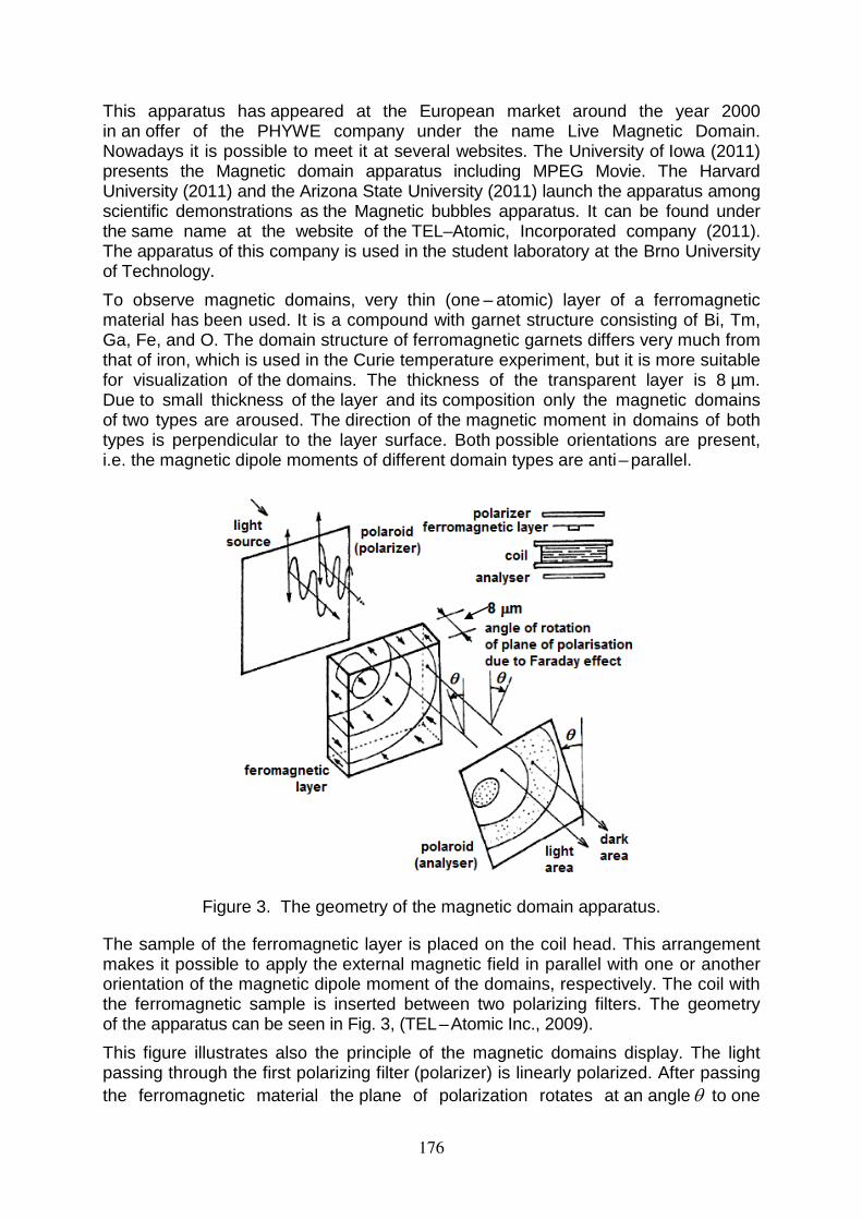
This apparatus has appeared at the European market around the year 2000 in an offer of the PHYWE company under the name Live Magnetic Domain. Nowadays it is possible to meet it at several websites. The University of Iowa (2011) presents the Magnetic domain apparatus including MPEG Movie. The Harvard University (2011) and the Arizona State University (2011) launch the apparatus among scientific demonstrations as the Magnetic bubbles apparatus. It can be found under the same name at the website of the TEL–Atomic, Incorporated company (2011). The apparatus of this company is used in the student laboratory at the Brno University of Technology. To observe magnetic domains, very thin (one – atomic) layer of a ferromagnetic material has been used. It is a compound with garnet structure consisting of Bi, Tm, Ga, Fe, and O. The domain structure of ferromagnetic garnets differs very much from that of iron, which is used in the Curie temperature experiment, but it is more suitable for visualization of the domains. The thickness of the transparent layer is 8 µm. Due to small thickness of the layer and its composition only the magnetic domains of two types are aroused. The direction of the magnetic moment in domains of both types is perpendicular to the layer surface. Both possible orientations are present, i.e. the magnetic dipole moments of different domain types are anti – parallel.

Figure 3. The geometry of the magnetic domain apparatus.

The sample of the ferromagnetic layer is placed on the coil head. This arrangement makes it possible to apply the external magnetic field in parallel with one or another orientation of the magnetic dipole moment of the domains, respectively. The coil with the ferromagnetic sample is inserted between two polarizing filters. The geometry of the apparatus can be seen in Fig. 3, (TEL – Atomic Inc., 2009). This figure illustrates also the principle of the magnetic domains display. The light passing through the first polarizing filter (polarizer) is linearly polarized. After passing the ferromagnetic material the plane of polarization rotates at an angle θ to one

176

or to the other side due to influence of the internal magnetic field. This rotation of the polarizing plane is called the Faraday Effect. The second polarizing filter (analyzer) is rotated just at the angle θ with respect to the polarizer. Behind the analyzer, the intensity of polarized light passing one of the domains type decreases, the intensity of the light passing the other domain type remains unchanged. The domains appear like bright and dark areas. All parts mentioned above are encased in a cylindrical metal container with diameter of 50 mm (see Fig. 4).

Figure 4. Magnetic domain apparatus. Figure 5. The experimental set up with magnetic domain apparatus.

(a) The state with equal areas (light and dark) of each domain. No external field.

(b) Increasing light area. External field: + 0.50Bsat

(c) Almost one light domain. External field: + 0.99Bsat

(d) Increasing dark area. External field: – 0.50Bsat

(e) Almost one dark domain. External field: – 0.99Bsat

Figure 6. Views as seen through a microscope ×100 magnification.

The picture from the apparatus is enlarged by a microscope, recorded by a camera and displayed at the PC monitor. For increasing external magnetic field the dark area of domains with parallel internal magnetic field grows in size at the expense

177

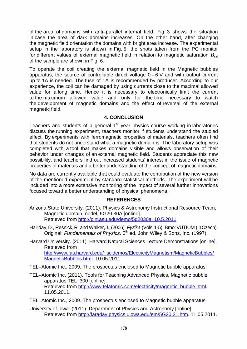
of the area of domains with anti–parallel internal field. Fig. 3 shows the situation in case the area of dark domains increases. On the other hand, after changing the magnetic field orientation the domains with bright area increase. The experimental setup in the laboratory is shown in Fig. 5; the shots taken from the PC monitor for different values of external magnetic field in relation to magnetic saturation Bsat of the sample are shown in Fig. 6. To operate the coil creating the external magnetic field in the Magnetic bubbles apparatus, the source of controllable direct voltage 0 – 6 V and with output current up to 1A is needed. The fuse of 1A is recommended by producer. According to our experience, the coil can be damaged by using currents close to the maximal allowed value for a long time. Hence it is necessary to electronically limit the current to the maximum allowed value and only for the time necessary to watch the development of magnetic domains and the effect of reversal of the external magnetic field.

4. CONCLUSION Teachers and students of a general 1st year physics course working in laboratories discuss the running experiment, teachers monitor if students understand the studied effect. By experiments with ferromagnetic properties of materials, teachers often find that students do not understand what a magnetic domain is. The laboratory setup was completed with a tool that makes domains visible and allows observation of their behavior under changes of an external magnetic field. Students appreciate this new possibility, and teachers find out increased students’ interest in the issue of magnetic properties of materials and a better understanding of the concept of magnetic domains. No data are currently available that could evaluate the contribution of the new version of the mentioned experiment by standard statistical methods. The experiment will be included into a more extensive monitoring of the impact of several further innovations focused toward a better understanding of physical phenomena.

REFERENCES Arizona State University. (2011). Physics & Astronomy Instructional Resource Team,

Magnetic domain model, 5G20.30A [online]. Retrieved from http://pirt.asu.edu/demo/5g2030a. 10.5.2011

Halliday, D., Resnick, R. and Walker, J., (2006). Fyzika (Vols. 1-5). Brno: VUTIUM (In Czech). Original: Fundamentals of Physics. 5th ed. John Wiley & Sons, Inc. (1997).

Harvard University. (2011). Harvard Natural Sciences Lecture Demonstrations [online]. Retrieved from http://www.fas.harvard.edu/~scidemos/ElectricityMagnetism/MagneticBubbles/ MagneticBubbles.html. 10.05.2011

TEL–Atomic Inc., 2009. The prospectus enclosed to Magnetic bubble apparatus. TEL–Atomic Inc. (2011). Tools for Teaching Advanced Physics, Magnetic bubble

apparatus TEL–300 [online]. Retrieved from http://www.telatomic.com/electricity/magnetic_bubble.html. 11.05.2011.

TEL–Atomic Inc., 2009. The prospectus enclosed to Magnetic bubble apparatus. University of Iowa. (2011). Department of Physics and Astronomy [online].

Retrieved from http://faraday.physics.uiowa.edu/em/5G20.21.htm. 11.05.2011.

178

The source of confusion in courses of modern physics of college level

I.Campos1, J.L. Jiménez2, G.del Valle3, M.G.Hernández3 , 1Facultad de Ciencias,UNAM, iecampos@prodigy.net.mx,

2Departamento de Física,UAM Iztapalapa, jlj@xanum.uam.mx 3Departamento de Ciencias Básicas,UAM Azcapotzalco, [ddg@correo.azc.uam.mx,

gpe@correo.azc.uam.mx]

Abstract In the interest of conceptual clarity and simplicity, we analyze two examples of conceptual obscurity appearing in textbooks of modern physics in the light of real experiments, not “thinking experiments”: a) wave particle duality) and b) tunneling. As we show the experiments do not require “mystic interpretations”, but an “ensemble” interpretation, as that proposed by Einstein. Thus the student can see the quantum systems are as real as classical systems.

1.Introduction

The great difficulties that students have when they are introduced to quantum mechanics are well known. Sometimes they are told that quantum mechanics is paradoxical, that our classical prejudices are the main obstacles to accept that Nature is mysterious in the quantum realm. And worse, sometimes they are told that in quantum mechanics simply there is nothing to understand. We have a mathematical structure that somehow “works”. Our aim in this work is to show that the above points of view are but some of the approaches to the interpretation of quantum mechanics. Indeed, we have Einstein’s interpretation of the wave function as describing not a single particle, but an ensemble of particles identically prepared in some quantum state. This point of view is supported by experiments as we show in the work. We review the two slits experiment and the tunnel effect, both, from the orthodox point of view, and from the point of view of the ensemble interpretation of quantum mechanics. We hope that these different views will be useful for those who want understand as far as possible the quantum world.

2.Wave-particle duality

2.1.de Broglie and the wave particle duality Though the wave-particle duality begins in1905 with Einstein´s proposal of quanta of radiation, it was de Broglie who made the important contribution of associating a wave to a material particle. This was the fundament on which Schrödinger built wave mechanics. It is interesting to recall how de Broglie could associate wave to a material particle. de Broglie considered a particle of rest mass om and velocity v cβ= with respect to a stationary observer. According to Planck´s postulate, E hν= , and Einstein´s definition

179

of rest energy, 20 oE m c= , the material particle must have associated, at rest, a

frequency 2o om c hν = , which de Broglie associated to a periodic internal

phenomenon. If the particle has a velocity ν with respect to the observer, the energy transforms according to a Lorentz transformation as

2

o oE E m c hγ γ ν= = = (1) and then the frequency transforms as

2.o

om ch

γν γν= =

(2)

However, if the frequency is considered as the reciprocal of the period, 1 Tν = , the Lorentz transformation is

1

1 1 .o

oT Tν

νγ γ

= = = (3)

It was this discrepancy which led de Broglie to associate a wave to a material particle, showing that if the internal periodic motion has frequency 1ν , the fictitious wave of frequency ν is always in phase with the internal periodic motion.

De Broglie found that the phase velocity of such a wave is 2c v , which is greater than c , and then the wave cannot be a physical wave. Thus from the very beginning it was clear that the wave associated to the particle had very peculiar properties. When Schrödinger discovered the wave equation for the de Broglie waves, the meaning of these waves was uncertain. The first interpretation was given by Schrödinger, who interpreted 2eψ as a charge density, where ψ is the amplitude of the wave. This interpretation, however, did not prevail. There were other interpretations (Jammer,1966) until M. Born proposed the interpretation of 2ψ as a probability density. Then ψ itself must be interpreted as a probability amplitude. This is by now the standard interpretation of ψ . However, the physical interpretation of quantum mechanics is not yet settled because there are several interpretations of probability, and hence Feymann´s dictum (1985): no one understand quantum mechanics. 2.2. Interpretations of probability and the tunnel effect. Probability in quantum mechanics has been interpreted in different ways. For example, Heisenberg gave it the meaning of “potentia”, akin to the Aristotelian concept of potentia as a kind of latent possibility. On the other hand, the Copenhaguen interpretation, now considered the orthodox interpretation, considers probability as degree of knowledge of the state of a physical system. Hence there must be an observer who possesses this degree of knowledge. In this way system and observer become united, as Bohr contended. This interpretation gives rise to statements like “Quantum mechanics doe not refer to Nature, but to our knowledge of Nature”, and other subjectivist statements. Usually in

180

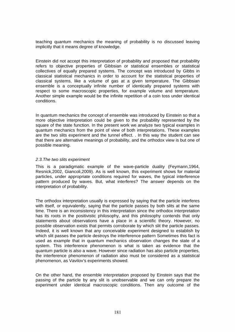
teaching quantum mechanics the meaning of probability is no discussed leaving implicitly that it means degree of knowledge. Einstein did not accept this interpretation of probability and proposed that probability refers to objective properties of Gibbsian or statistical ensembles or statistical collectives of equally prepared systems. The concept was introduced by Gibbs in classical statistical mechanics in order to account for the statistical properties of classical systems, like a volume of gas at a given temperature. The Gibbsian ensemble is a conceptually infinite number of identically prepared systems with respect to some macroscopic properties, for example volume and temperature. Another simple example would be the infinite repetition of a coin toss under identical conditions. In quantum mechanics the concept of ensemble was introduced by Einstein so that a more objective interpretation could be given to the probability represented by the square of the state function. In the present work we analyze two typical examples in quantum mechanics from the point of view of both interpretations. These examples are the two slits experiment and the tunnel effect. . In this way the student can see that there are alternative meanings of probability, and the orthodox view is but one of possible meaning. 2.3.The two slits experiment This is a paradigmatic example of the wave-particle duality (Feymann,1964, Resnick,2002, Giancoli,2009). As is well known, this experiment shows for material particles, under appropriate conditions required for waves, the typical interference pattern produced by waves. But, what interferes? The answer depends on the interpretation of probability. The orthodox interpretation usually is expressed by saying that the particle interferes with itself, or equivalently, saying that the particle passes by both slits at the same time. There is an inconsistency in this interpretation since the orthodox interpretation has its roots in the positivistic philosophy, and this philosophy contends that only statements about observations have a place in a scientific theory. However, no possible observation exists that permits corroborate by which slit the particle passes. Indeed, it is well known that any conceivable experiment designed to establish by which slit passes the particle destroys the interference pattern Sometimes this fact is used as example that in quantum mechanics observation changes the state of a system. This interference phenomenon is what is taken as evidence that the quantum particle is also a wave. However since radiation has also particle properties, the interference phenomenon of radiation also must be considered as a statistical phenomenon, as Vavilov’s experiments showed. On the other hand, the ensemble interpretation proposed by Einstein says that the passing of the particle by any slit is unobservable and we can only prepare the experiment under identical macroscopic conditions. Then any outcome of the

181

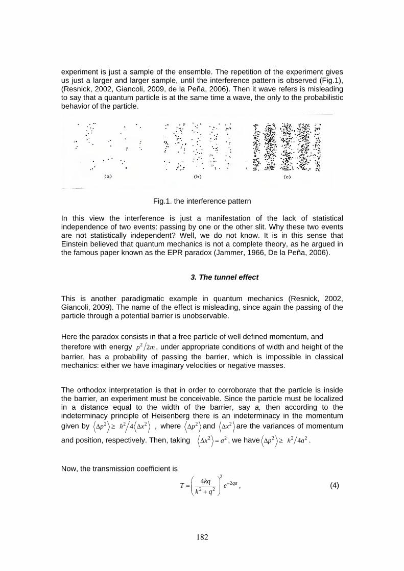
experiment is just a sample of the ensemble. The repetition of the experiment gives us just a larger and larger sample, until the interference pattern is observed (Fig.1), (Resnick, 2002, Giancoli, 2009, de la Peña, 2006). Then it wave refers is misleading to say that a quantum particle is at the same time a wave, the only to the probabilistic behavior of the particle.

Fig.1. the interference pattern

In this view the interference is just a manifestation of the lack of statistical independence of two events: passing by one or the other slit. Why these two events are not statistically independent? Well, we do not know. It is in this sense that Einstein believed that quantum mechanics is not a complete theory, as he argued in the famous paper known as the EPR paradox (Jammer, 1966, De la Peña, 2006).

3. The tunnel effect

This is another paradigmatic example in quantum mechanics (Resnick, 2002, Giancoli, 2009). The name of the effect is misleading, since again the passing of the particle through a potential barrier is unobservable. Here the paradox consists in that a free particle of well defined momentum, and therefore with energy 2 2p m , under appropriate conditions of width and height of the barrier, has a probability of passing the barrier, which is impossible in classical mechanics: either we have imaginary velocities or negative masses. The orthodox interpretation is that in order to corroborate that the particle is inside the barrier, an experiment must be conceivable. Since the particle must be localized in a distance equal to the width of the barrier, say a, then according to the indeterminacy principle of Heisenberg there is an indeterminacy in the momentum given by 2 2 2 4 ,p xΔ ≥ Δ where 2pΔ and 2xΔ are the variances of momentum

and position, respectively. Then, taking 2 2x aΔ = , we have 2 2 2 4p aΔ ≥ .

Now, the transmission coefficient is

22

2 24 qakqT e

k q−⎛ ⎞

= ⎜ ⎟⎜ ⎟+⎝ ⎠, (4)

182

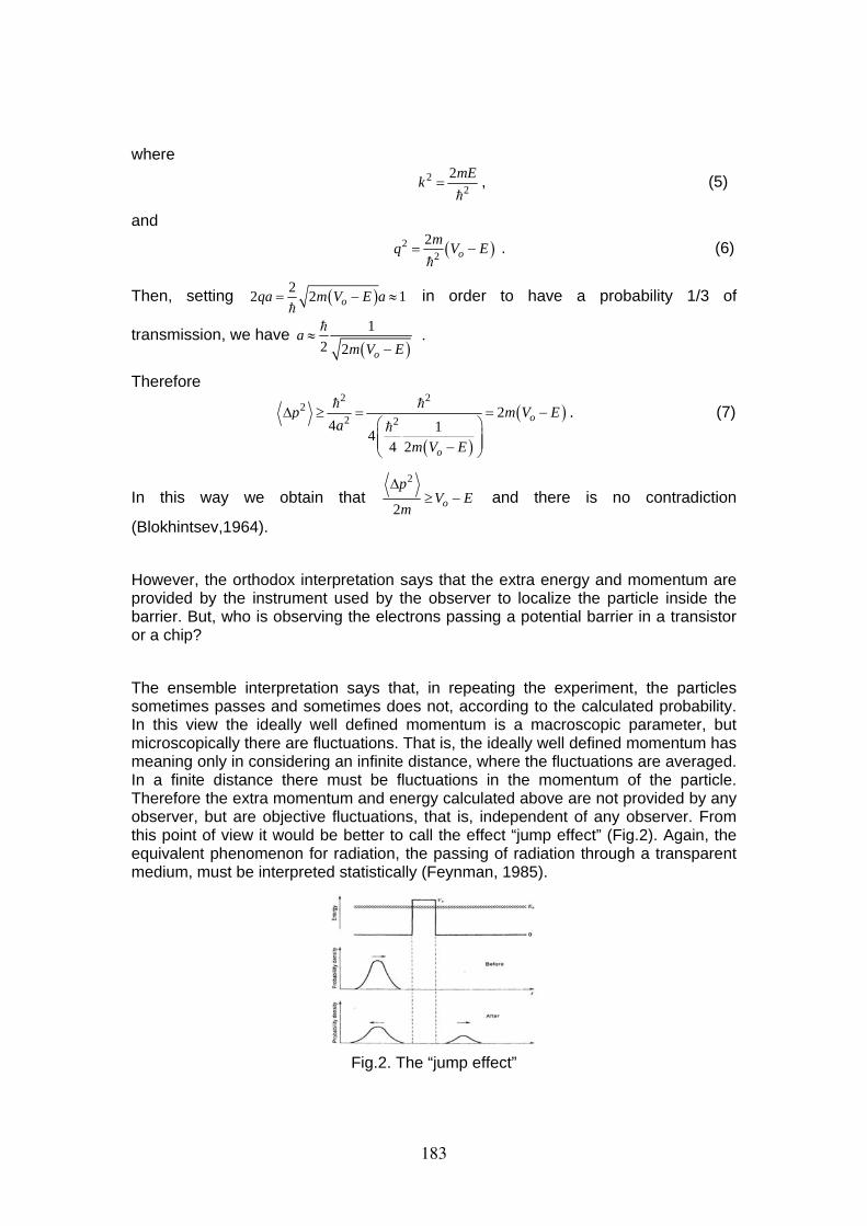
where

2

22mEk = , (5)

and

( )2

22

omq V E= − . (6)

Then, setting ( )22 2 1oqa m V E a= − ≈ in order to have a probability 1/3 of

transmission, we have ( )1 .

2 2 o

am V E

≈−

Therefore

( )

( )2 2

22 2

24 14

4 2

o

o

p m V Ea

m V E

Δ ≥ = = −⎛ ⎞⎜ ⎟⎜ ⎟−⎝ ⎠

. (7)

In this way we obtain that 2

2 o

pV E

m

Δ≥ − and there is no contradiction

(Blokhintsev,1964). However, the orthodox interpretation says that the extra energy and momentum are provided by the instrument used by the observer to localize the particle inside the barrier. But, who is observing the electrons passing a potential barrier in a transistor or a chip? The ensemble interpretation says that, in repeating the experiment, the particles sometimes passes and sometimes does not, according to the calculated probability. In this view the ideally well defined momentum is a macroscopic parameter, but microscopically there are fluctuations. That is, the ideally well defined momentum has meaning only in considering an infinite distance, where the fluctuations are averaged. In a finite distance there must be fluctuations in the momentum of the particle. Therefore the extra momentum and energy calculated above are not provided by any observer, but are objective fluctuations, that is, independent of any observer. From this point of view it would be better to call the effect “jump effect” (Fig.2). Again, the equivalent phenomenon for radiation, the passing of radiation through a transparent medium, must be interpreted statistically (Feynman, 1985).

Fig.2. The “jump effect”

183

As we can see, the debate about the interpretation of quantum mechanics continues, and the orthodox interpretation is but one possibility.

2. Conclusions

As we have seen, part of the difficulty in understanding quantum mechanics is that we are attaching properties of a statistical ensemble to a single particle. The quantum particle is then subjected to objective fluctuations whose statistical properties are correctly described by the wave function. In the two slits experiment the interference pattern appears as the collective effect of many particles, what does not mean that a particle is a wave. The wave particle duality rather describes statistical properties of an ensemble. Thus there appears the idea that the classical limit of quantum mechanics is a statistical mechanics, rather than the classical mechanics of a particle. We are convinced that discussing these alternatives in quantum mechanics courses will give students a feeling of science in the making. Anyway, behind the quantum phenomena there appears to be an intrinsic stochastic element that we still do not understand completely. The challenge stands.

References Blokhintsev, D.I. (1964). Principles of Quantum Mechanics. Boston: Allyn and Bacon. De La Peña, L. (2006). Introducción a la Mecánica Cuántica (In spanish). México,D.F. Universidad Autónoma de México y Fondo de Cultura Económica. Feynman,R.,Leighton, R., and Sands. M. (1964). The Feynman Lectures on Physics Vol 3. New Jersey:Addison-Wesley Feynman, R. (1985). QED the Strange Theory of Light and Matter. Princeton University Press Giancoli, D.C. (2009). Physics for Scientist and Engineers, with Modern Physics,4th. Edition. Pearson Prentice Hall. Jammer, M. (1966).The Conceptual Development of Quantum Mechanics. New York: McGraw-Hill. Resnick, R., Halliday D. and Krane, K.S. (2002). Physics. 5th Edition. John Wiley & Sons.

184

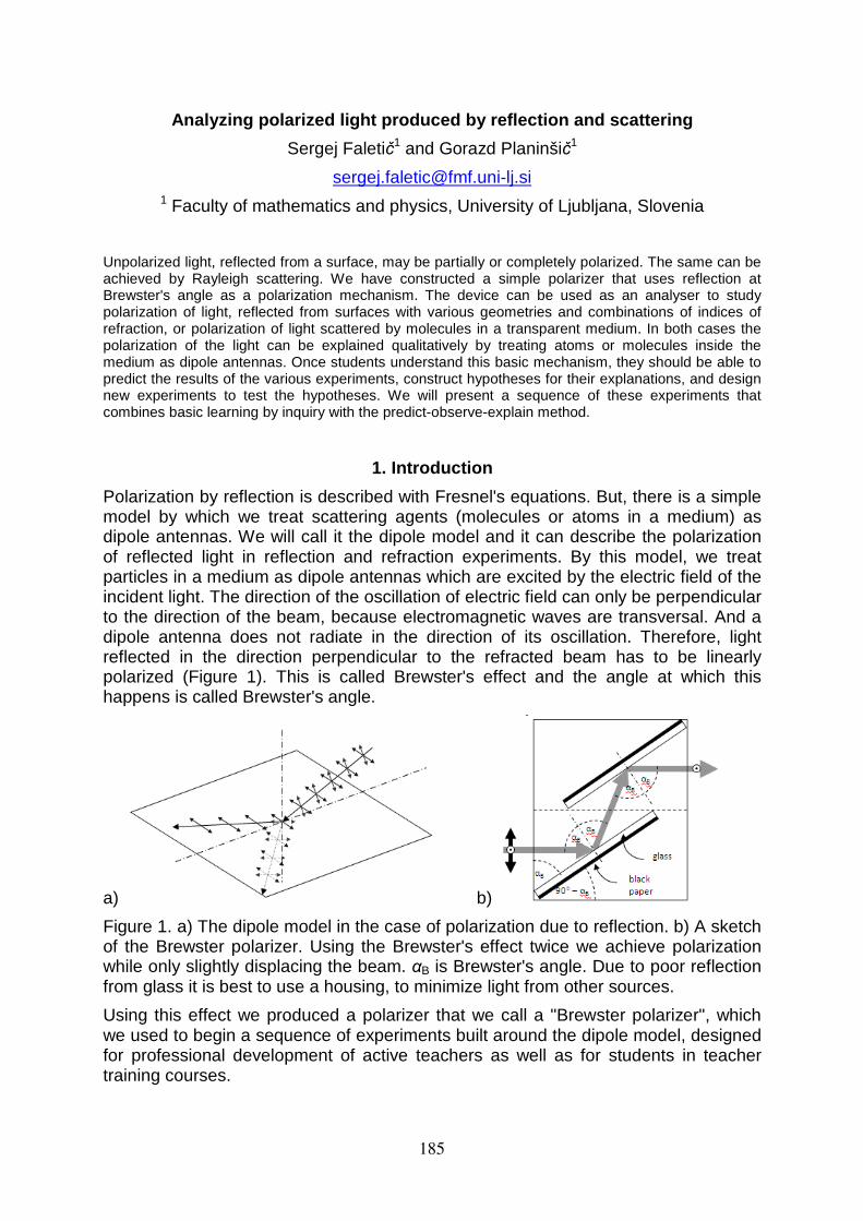
Analyzing polarized light produced by reflection and scattering

Sergej Faletič1 and Gorazd Planinšič1

sergej.faletic@fmf.uni-lj.si 1 Faculty of mathematics and physics, University of Ljubljana, Slovenia

Unpolarized light, reflected from a surface, may be partially or completely polarized. The same can be achieved by Rayleigh scattering. We have constructed a simple polarizer that uses reflection at Brewster's angle as a polarization mechanism. The device can be used as an analyser to study polarization of light, reflected from surfaces with various geometries and combinations of indices of refraction, or polarization of light scattered by molecules in a transparent medium. In both cases the polarization of the light can be explained qualitatively by treating atoms or molecules inside the medium as dipole antennas. Once students understand this basic mechanism, they should be able to predict the results of the various experiments, construct hypotheses for their explanations, and design new experiments to test the hypotheses. We will present a sequence of these experiments that combines basic learning by inquiry with the predict-observe-explain method.

1. Introduction

Polarization by reflection is described with Fresnel's equations. But, there is a simple model by which we treat scattering agents (molecules or atoms in a medium) as dipole antennas. We will call it the dipole model and it can describe the polarization of reflected light in reflection and refraction experiments. By this model, we treat particles in a medium as dipole antennas which are excited by the electric field of the incident light. The direction of the oscillation of electric field can only be perpendicular to the direction of the beam, because electromagnetic waves are transversal. And a dipole antenna does not radiate in the direction of its oscillation. Therefore, light reflected in the direction perpendicular to the refracted beam has to be linearly polarized (Figure 1). This is called Brewster's effect and the angle at which this happens is called Brewster's angle.

a) b)

Figure 1. a) The dipole model in the case of polarization due to reflection. b) A sketch of the Brewster polarizer. Using the Brewster's effect twice we achieve polarization while only slightly displacing the beam. αB is Brewster's angle. Due to poor reflection from glass it is best to use a housing, to minimize light from other sources.

Using this effect we produced a polarizer that we call a "Brewster polarizer", which we used to begin a sequence of experiments built around the dipole model, designed for professional development of active teachers as well as for students in teacher training courses.

185

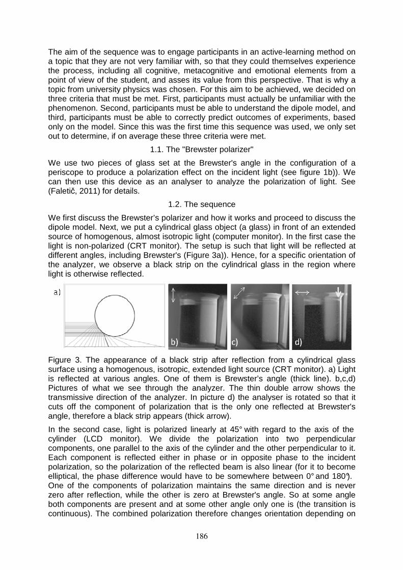
The aim of the sequence was to engage participants in an active-learning method on a topic that they are not very familiar with, so that they could themselves experience the process, including all cognitive, metacognitive and emotional elements from a point of view of the student, and asses its value from this perspective. That is why a topic from university physics was chosen. For this aim to be achieved, we decided on three criteria that must be met. First, participants must actually be unfamiliar with the phenomenon. Second, participants must be able to understand the dipole model, and third, participants must be able to correctly predict outcomes of experiments, based only on the model. Since this was the first time this sequence was used, we only set out to determine, if on average these three criteria were met.

1.1. The "Brewster polarizer"

We use two pieces of glass set at the Brewster's angle in the configuration of a periscope to produce a polarization effect on the incident light (see figure 1b)). We can then use this device as an analyser to analyze the polarization of light. See (Faletič, 2011) for details.

1.2. The sequence

We first discuss the Brewster’s polarizer and how it works and proceed to discuss the dipole model. Next, we put a cylindrical glass object (a glass) in front of an extended source of homogenous, almost isotropic light (computer monitor). In the first case the light is non-polarized (CRT monitor). The setup is such that light will be reflected at different angles, including Brewster's (Figure 3a)). Hence, for a specific orientation of the analyzer, we observe a black strip on the cylindrical glass in the region where light is otherwise reflected.

Figure 3. The appearance of a black strip after reflection from a cylindrical glass surface using a homogenous, isotropic, extended light source (CRT monitor). a) Light is reflected at various angles. One of them is Brewster’s angle (thick line). b,c,d) Pictures of what we see through the analyzer. The thin double arrow shows the transmissive direction of the analyzer. In picture d) the analyser is rotated so that it cuts off the component of polarization that is the only one reflected at Brewster's angle, therefore a black strip appears (thick arrow).

In the second case, light is polarized linearly at 45° with regard to the axis of the cylinder (LCD monitor). We divide the polarization into two perpendicular components, one parallel to the axis of the cylinder and the other perpendicular to it. Each component is reflected either in phase or in opposite phase to the incident polarization, so the polarization of the reflected beam is also linear (for it to become elliptical, the phase difference would have to be somewhere between 0° and 180°). One of the components of polarization maintains the same direction and is never zero after reflection, while the other is zero at Brewster's angle. So at some angle both components are present and at some other angle only one is (the transition is continuous). The combined polarization therefore changes orientation depending on

186

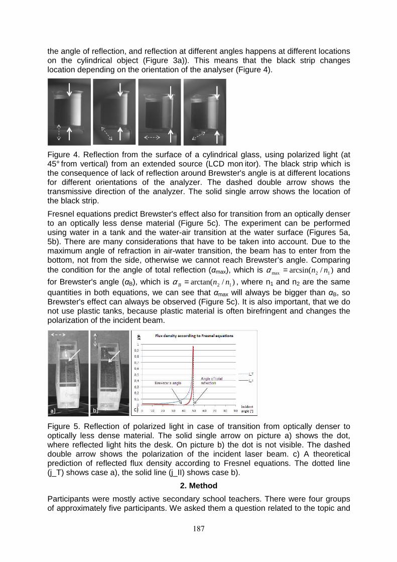
the angle of reflection, and reflection at different angles happens at different locations on the cylindrical object (Figure 3a)). This means that the black strip changes location depending on the orientation of the analyser (Figure 4).

Figure 4. Reflection from the surface of a cylindrical glass, using polarized light (at 45° from vertical) from an extended source (LCD mon itor). The black strip which is the consequence of lack of reflection around Brewster's angle is at different locations for different orientations of the analyzer. The dashed double arrow shows the transmissive direction of the analyzer. The solid single arrow shows the location of the black strip.

Fresnel equations predict Brewster's effect also for transition from an optically denser to an optically less dense material (Figure 5c). The experiment can be performed using water in a tank and the water-air transition at the water surface (Figures 5a, 5b). There are many considerations that have to be taken into account. Due to the maximum angle of refraction in air-water transition, the beam has to enter from the bottom, not from the side, otherwise we cannot reach Brewster’s angle. Comparing the condition for the angle of total reflection (αmax), which is )/arcsin( 12max nn=α and

for Brewster's angle (αB), which is )/arctan( 12 nnB =α , where n1 and n2 are the same quantities in both equations, we can see that αmax will always be bigger than αB, so Brewster's effect can always be observed (Figure 5c). It is also important, that we do not use plastic tanks, because plastic material is often birefringent and changes the polarization of the incident beam.

Figure 5. Reflection of polarized light in case of transition from optically denser to optically less dense material. The solid single arrow on picture a) shows the dot, where reflected light hits the desk. On picture b) the dot is not visible. The dashed double arrow shows the polarization of the incident laser beam. c) A theoretical prediction of reflected flux density according to Fresnel equations. The dotted line (j_T) shows case a), the solid line (j_II) shows case b).

2. Method

Participants were mostly active secondary school teachers. There were four groups of approximately five participants. We asked them a question related to the topic and

187

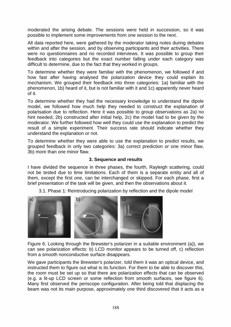
moderated the arising debate. The sessions were held in succession, so it was possible to implement some improvements from one session to the next.

All data reported here, were gathered by the moderator taking notes during debates within and after the session, and by observing participants and their activities. There were no questionnaires and no recorded interviews. It was possible to group their feedback into categories but the exact number falling under each category was difficult to determine, due to the fact that they worked in groups.

To determine whether they were familiar with the phenomenon, we followed if and how fast after having analysed the polarization device they could explain its mechanism. We grouped their feedback into three categories: 1a) familiar with the phenomenon, 1b) heard of it, but is not familiar with it and 1c) apparently never heard of it.

To determine whether they had the necessary knowledge to understand the dipole model, we followed how much help they needed to construct the explanation of polarisation due to reflection. Here it was possible to group observations as 2a) no hint needed, 2b) constructed after initial help, 2c) the model had to be given by the moderator. We further followed how well they could use the explanation to predict the result of a simple experiment. Their success rate should indicate whether they understand the explanation or not.

To determine whether they were able to use the explanation to predict results, we grouped feedback in only two categories: 3a) correct prediction or one minor flaw, 3b) more than one minor flaw.

3. Sequence and results

I have divided the sequence in three phases, the fourth, Rayleigh scattering, could not be tested due to time limitations. Each of them is a separate entity and all of them, except the first one, can be interchanged or skipped. For each phase, first a brief presentation of the task will be given, and then the observations about it.

3.1. Phase 1: Reintroducing polarization by reflection and the dipole model

Figure 6. Looking through the Brewster’s polarizer in a suitable environment (a)), we can see polarization effects: b) LCD monitor appears to be turned off, c) reflection from a smooth nonconductive surface disappears.

We gave participants the Brewster's polarizer, told them it was an optical device, and instructed them to figure out what is its function. For them to be able to discover this, the room must be set up so that there are polarization effects that can be observed (e.g. a lit-up LCD screen or some reflection from smooth surfaces, see figure 6). Many first observed the periscope configuration. After being told that displacing the beam was not its main purpose, approximately one third discovered that it acts as a

a) b) c)

188

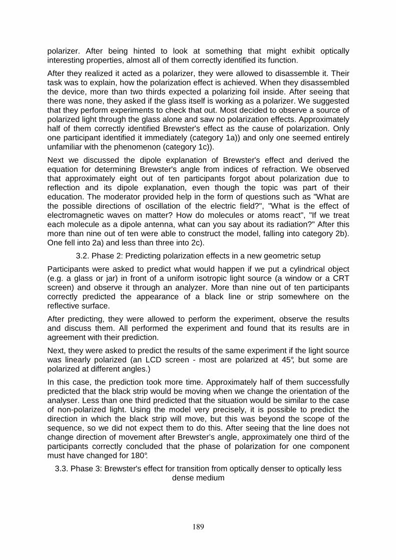
polarizer. After being hinted to look at something that might exhibit optically interesting properties, almost all of them correctly identified its function.

After they realized it acted as a polarizer, they were allowed to disassemble it. Their task was to explain, how the polarization effect is achieved. When they disassembled the device, more than two thirds expected a polarizing foil inside. After seeing that there was none, they asked if the glass itself is working as a polarizer. We suggested that they perform experiments to check that out. Most decided to observe a source of polarized light through the glass alone and saw no polarization effects. Approximately half of them correctly identified Brewster's effect as the cause of polarization. Only one participant identified it immediately (category 1a)) and only one seemed entirely unfamiliar with the phenomenon (category 1c)).

Next we discussed the dipole explanation of Brewster's effect and derived the equation for determining Brewster's angle from indices of refraction. We observed that approximately eight out of ten participants forgot about polarization due to reflection and its dipole explanation, even though the topic was part of their education. The moderator provided help in the form of questions such as "What are the possible directions of oscillation of the electric field?", "What is the effect of electromagnetic waves on matter? How do molecules or atoms react", "If we treat each molecule as a dipole antenna, what can you say about its radiation?" After this more than nine out of ten were able to construct the model, falling into category 2b). One fell into 2a) and less than three into 2c).

3.2. Phase 2: Predicting polarization effects in a new geometric setup

Participants were asked to predict what would happen if we put a cylindrical object (e.g. a glass or jar) in front of a uniform isotropic light source (a window or a CRT screen) and observe it through an analyzer. More than nine out of ten participants correctly predicted the appearance of a black line or strip somewhere on the reflective surface.

After predicting, they were allowed to perform the experiment, observe the results and discuss them. All performed the experiment and found that its results are in agreement with their prediction.

Next, they were asked to predict the results of the same experiment if the light source was linearly polarized (an LCD screen - most are polarized at 45°, but some are polarized at different angles.)

In this case, the prediction took more time. Approximately half of them successfully predicted that the black strip would be moving when we change the orientation of the analyser. Less than one third predicted that the situation would be similar to the case of non-polarized light. Using the model very precisely, it is possible to predict the direction in which the black strip will move, but this was beyond the scope of the sequence, so we did not expect them to do this. After seeing that the line does not change direction of movement after Brewster’s angle, approximately one third of the participants correctly concluded that the phase of polarization for one component must have changed for 180°.

3.3. Phase 3: Brewster's effect for transition from optically denser to optically less dense medium

189

Participants were asked, whether Brewster’s effect occurs for transition from optically denser to optically less dense medium. They were allowed to perform experiments to find the answer to this question.

More than eight out of ten participants hypothesized, that the effect should still be observed in such a transition. They mostly did not calculate the angle, but rather decided to perform the experiment so that they move a fully or partially polarized laser pointer from 0° to 90° and observe the reflec ted beam on a surface. They directed the laser beam through a side surface and did not see the effect. Some seemed to have started doubting their hypothesis. We discussed the situation until they realized that they may not have yet reached Brewster’s angle. After this they directed the beam through the bottom surface and succeeded in finding Brewster’s angle and observe the Brewster’s effect. With regard to whether the angle of total reflection might be lower than Brewster’s angle, they mainly calculated both angles for water-air transition and compared them. None of them attempted to give a generalized conclusion. This is understandable, given the time limitations of the activity.

Many of these experiments can be done in various ways. For example, we may choose to use polarized light and observe with the naked eye, or we can use non-polarized light and observe through a polarizer. This applies to most of the above experiments.

4. Conclusion and discussion

We developed a sequence centred around the phenomenon of polarization due to reflection (i.e. Brewster's effect). The sequence was aimed at active teachers in professional development program. It was designed to expose them to a teaching-learning sequence in which they were actively involved, and which topic was challenging to them. The intention was to bring them as close as possible to the role of a learner.

We determined three criteria to be successful in our goal. The participants had to not be familiar with the topic. Provided some help, the participants should be able to construct the model by themselves. And participants should be able to use the model to make predictions. It was found that the first criterion was met by a vast majority. In constructing the model, help was necessary for most of them, but after that, all groups managed to successfully finish the task. We are planning to explore ways to facilitate the construction of the model with minimal help. Almost all participants were able to use the model to predict the result of a simple experiment, thus meeting the third criterion. Approximately half of them were able to correctly predict the result of a more complex experiment, showing that for them it is a challenging task, but not impossible, which is exactly the difficulty level we were aiming for. Our conclusion is, therefore, that such a sequence is acceptable as one that puts teachers in the role of learners in an active-learning environment.

References

PHOTON projects. Retrieved 30.9.2011 from http://www.nebhe.org/programs-overview/photon/overview/

Rafizadeh, D., Caplan, D., (1995), Optics in the fish tank, Optics & photonic news, 6(5), p.45

Faletič, S., (2011), Poskusi s polarizacijo pri odboju, Retrieved 28.3.2012 from http://sss.fmf.uni-lj.si/index.php?mode=4

190

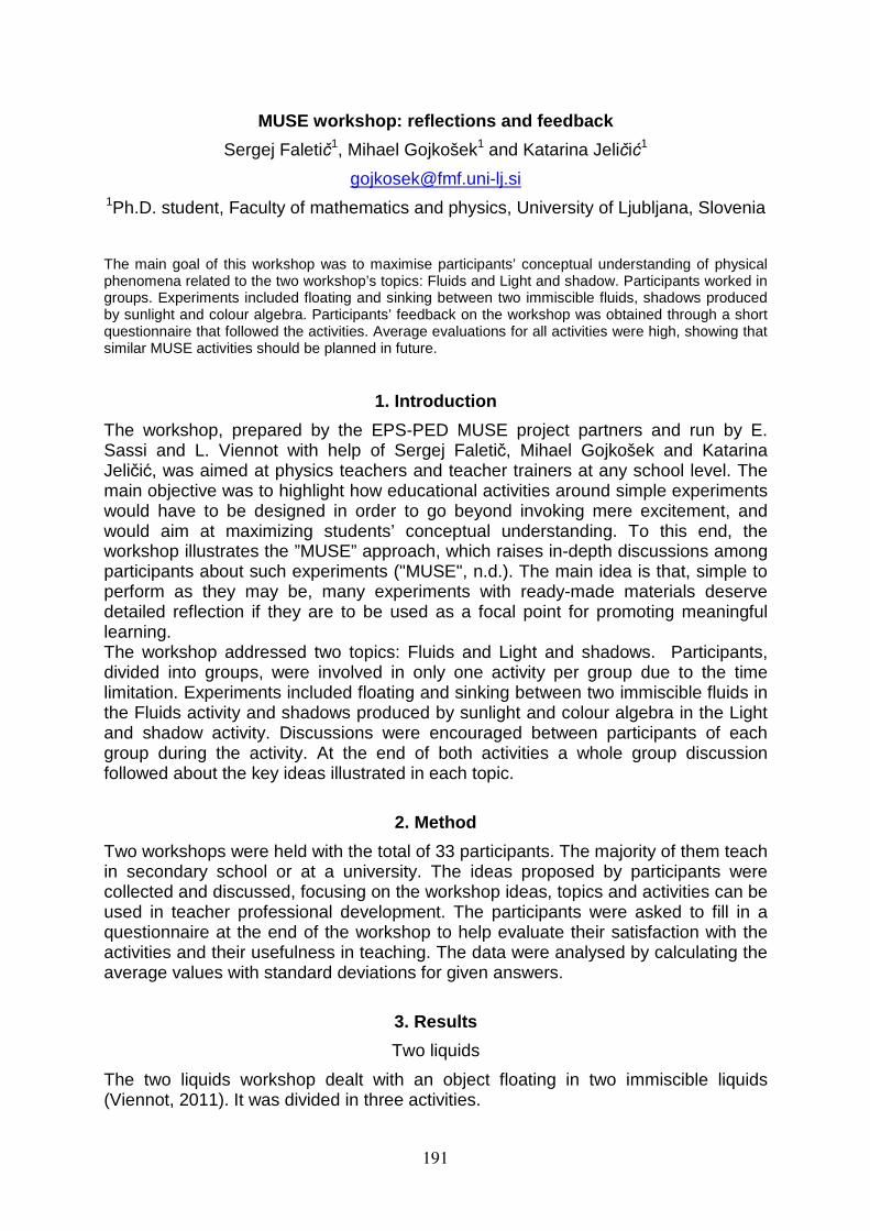
MUSE workshop: reflections and feedback

Sergej Faletič1, Mihael Gojkošek1 and Katarina Jeličić1

gojkosek@fmf.uni-lj.si 1Ph.D. student, Faculty of mathematics and physics, University of Ljubljana, Slovenia

The main goal of this workshop was to maximise participants’ conceptual understanding of physical phenomena related to the two workshop’s topics: Fluids and Light and shadow. Participants worked in groups. Experiments included floating and sinking between two immiscible fluids, shadows produced by sunlight and colour algebra. Participants’ feedback on the workshop was obtained through a short questionnaire that followed the activities. Average evaluations for all activities were high, showing that similar MUSE activities should be planned in future.

1. Introduction

The workshop, prepared by the EPS-PED MUSE project partners and run by E. Sassi and L. Viennot with help of Sergej Faletič, Mihael Gojkošek and Katarina Jeličić, was aimed at physics teachers and teacher trainers at any school level. The main objective was to highlight how educational activities around simple experiments would have to be designed in order to go beyond invoking mere excitement, and would aim at maximizing students’ conceptual understanding. To this end, the workshop illustrates the ”MUSE” approach, which raises in-depth discussions among participants about such experiments ("MUSE", n.d.). The main idea is that, simple to perform as they may be, many experiments with ready-made materials deserve detailed reflection if they are to be used as a focal point for promoting meaningful learning. The workshop addressed two topics: Fluids and Light and shadows. Participants, divided into groups, were involved in only one activity per group due to the time limitation. Experiments included floating and sinking between two immiscible fluids in the Fluids activity and shadows produced by sunlight and colour algebra in the Light and shadow activity. Discussions were encouraged between participants of each group during the activity. At the end of both activities a whole group discussion followed about the key ideas illustrated in each topic.

2. Method

Two workshops were held with the total of 33 participants. The majority of them teach in secondary school or at a university. The ideas proposed by participants were collected and discussed, focusing on the workshop ideas, topics and activities can be used in teacher professional development. The participants were asked to fill in a questionnaire at the end of the workshop to help evaluate their satisfaction with the activities and their usefulness in teaching. The data were analysed by calculating the average values with standard deviations for given answers.

3. Results

Two liquids

The two liquids workshop dealt with an object floating in two immiscible liquids (Viennot, 2011). It was divided in three activities.

191

Activity 1

A cylinder is floating in water and oil with a density lower than that of the cylinder is poured on top of the water. Participants were asked to describe how the cylinder would move, discuss possible problems that students would have with this task, discuss what would happen if the cylinder was pushed down until it is covered by oil and check all their predictions with experiments.

During the discussion it was pointed out that it is not clear with regard to what the movement of the cylinder is being observed, whether to its initial position or to the top surface bordering with air. It was also noted that it might be important to describe that oil is poured only on top of the water, and does not hit the cylinder, otherwise the picture may be misleading. While describing how the cylinder would move, we noticed that many participants used analysis of various limiting situations, such as thinking of what would happen if air was poured, if water was poured and what should happen if the liquid with density between air and water was used. Some added that up-thrust is proportional to density of the liquid. There was one comment that students might think that pouring oil on top of water would be irrelevant. (Note: this might be due to the fact that oil does not reach either the top or the bottom of the cylinder and hence does not exert a force in the vertical direction.) There were no relevant comments on the rest of the activity.

Activity 2

Participants were given the classical solution 1221 /)( ρρρ hHh s −= (1) and its derivation procedure. h1 and h2 are the heights of the parts of the cylinder immersed in water and oil, respectively, H is the total height of the cylinder, ρ1 and ρ2 are densities of water and oil respectively and ρs is the density of the cylinder (Figure 1). They were asked to discuss the solution, comment whether the solution is valid in both cases, when the cylinder is completely covered with oil and when it is only partially covered in oil (Figure 1), and to explain how equation (1) is consistent with the experimental result.

a) b)

Figure 1. The cylinder floating in two liquids. a) Fully covered by the second liquid, b) partially in air.

In the final discussion we noticed that all participants correctly identified the connection between equation (1) and the results of the experiment. It was also pointed out that the symbol "∆" may be unfamiliar to some students and that expressing the solution without it might be more appropriate.

Activity 3

h1

h2

H

Liquid 1

Liquid 2

h1

h2

H

Liquid 1

Liquid 2

192

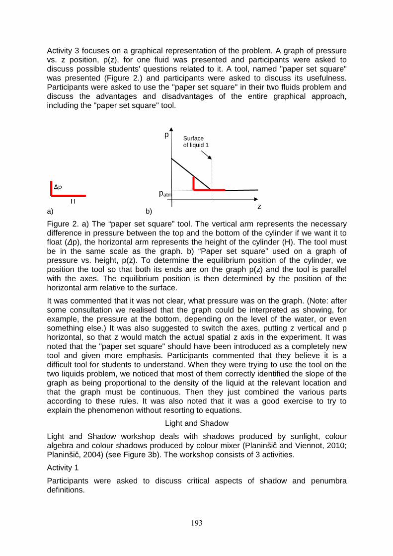
Activity 3 focuses on a graphical representation of the problem. A graph of pressure vs. z position, p(z), for one fluid was presented and participants were asked to discuss possible students' questions related to it. A tool, named "paper set square" was presented (Figure 2.) and participants were asked to discuss its usefulness. Participants were asked to use the "paper set square" in their two fluids problem and discuss the advantages and disadvantages of the entire graphical approach, including the "paper set square" tool.

a) b)

Figure 2. a) The “paper set square” tool. The vertical arm represents the necessary difference in pressure between the top and the bottom of the cylinder if we want it to float (∆p), the horizontal arm represents the height of the cylinder (H). The tool must be in the same scale as the graph. b) “Paper set square” used on a graph of pressure vs. height, p(z). To determine the equilibrium position of the cylinder, we position the tool so that both its ends are on the graph p(z) and the tool is parallel with the axes. The equilibrium position is then determined by the position of the horizontal arm relative to the surface.

It was commented that it was not clear, what pressure was on the graph. (Note: after some consultation we realised that the graph could be interpreted as showing, for example, the pressure at the bottom, depending on the level of the water, or even something else.) It was also suggested to switch the axes, putting z vertical and p horizontal, so that z would match the actual spatial z axis in the experiment. It was noted that the "paper set square" should have been introduced as a completely new tool and given more emphasis. Participants commented that they believe it is a difficult tool for students to understand. When they were trying to use the tool on the two liquids problem, we noticed that most of them correctly identified the slope of the graph as being proportional to the density of the liquid at the relevant location and that the graph must be continuous. Then they just combined the various parts according to these rules. It was also noted that it was a good exercise to try to explain the phenomenon without resorting to equations.

Light and Shadow

Light and Shadow workshop deals with shadows produced by sunlight, colour algebra and colour shadows produced by colour mixer (Planinšič and Viennot, 2010; Planinšič, 2004) (see Figure 3b). The workshop consists of 3 activities.

Activity 1

Participants were asked to discuss critical aspects of shadow and penumbra definitions.

p

z

patm

Surface of liquid 1

193

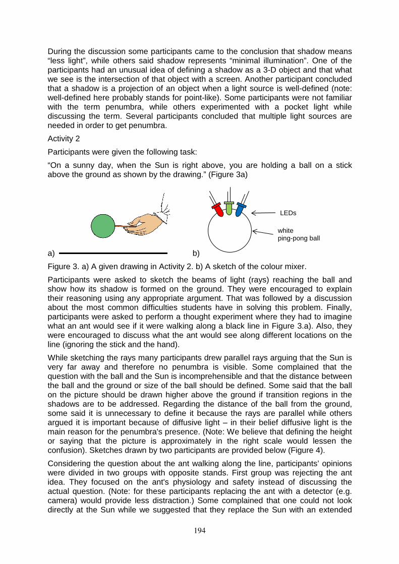
During the discussion some participants came to the conclusion that shadow means “less light”, while others said shadow represents “minimal illumination”. One of the participants had an unusual idea of defining a shadow as a 3-D object and that what we see is the intersection of that object with a screen. Another participant concluded that a shadow is a projection of an object when a light source is well-defined (note: well-defined here probably stands for point-like). Some participants were not familiar with the term penumbra, while others experimented with a pocket light while discussing the term. Several participants concluded that multiple light sources are needed in order to get penumbra.

Activity 2

Participants were given the following task:

“On a sunny day, when the Sun is right above, you are holding a ball on a stick above the ground as shown by the drawing.” (Figure 3a)

a) b)

Figure 3. a) A given drawing in Activity 2. b) A sketch of the colour mixer.

Participants were asked to sketch the beams of light (rays) reaching the ball and show how its shadow is formed on the ground. They were encouraged to explain their reasoning using any appropriate argument. That was followed by a discussion about the most common difficulties students have in solving this problem. Finally, participants were asked to perform a thought experiment where they had to imagine what an ant would see if it were walking along a black line in Figure 3.a). Also, they were encouraged to discuss what the ant would see along different locations on the line (ignoring the stick and the hand).

While sketching the rays many participants drew parallel rays arguing that the Sun is very far away and therefore no penumbra is visible. Some complained that the question with the ball and the Sun is incomprehensible and that the distance between the ball and the ground or size of the ball should be defined. Some said that the ball on the picture should be drawn higher above the ground if transition regions in the shadows are to be addressed. Regarding the distance of the ball from the ground, some said it is unnecessary to define it because the rays are parallel while others argued it is important because of diffusive light – in their belief diffusive light is the main reason for the penumbra's presence. (Note: We believe that defining the height or saying that the picture is approximately in the right scale would lessen the confusion). Sketches drawn by two participants are provided below (Figure 4).

Considering the question about the ant walking along the line, participants’ opinions were divided in two groups with opposite stands. First group was rejecting the ant idea. They focused on the ant's physiology and safety instead of discussing the actual question. (Note: for these participants replacing the ant with a detector (e.g. camera) would provide less distraction.) Some complained that one could not look directly at the Sun while we suggested that they replace the Sun with an extended

LEDs

white ping-pong ball

194

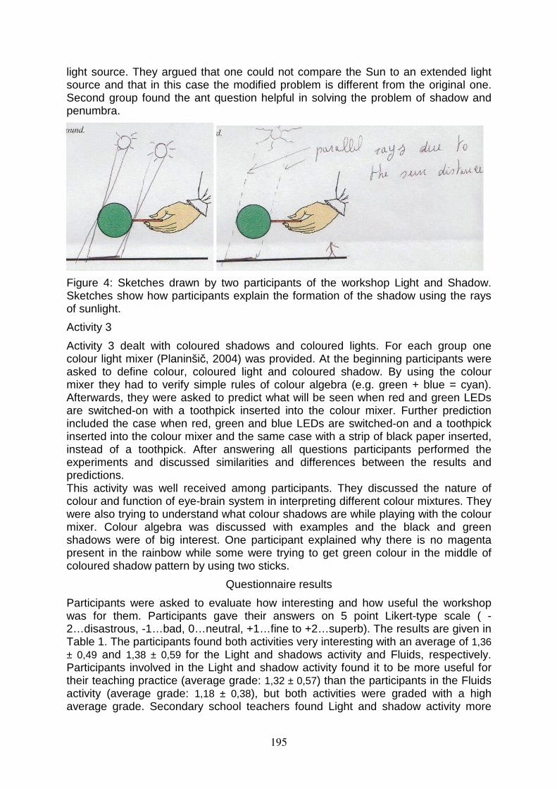
light source. They argued that one could not compare the Sun to an extended light source and that in this case the modified problem is different from the original one. Second group found the ant question helpful in solving the problem of shadow and penumbra.

Figure 4: Sketches drawn by two participants of the workshop Light and Shadow. Sketches show how participants explain the formation of the shadow using the rays of sunlight.

Activity 3

Activity 3 dealt with coloured shadows and coloured lights. For each group one colour light mixer (Planinšič, 2004) was provided. At the beginning participants were asked to define colour, coloured light and coloured shadow. By using the colour mixer they had to verify simple rules of colour algebra (e.g. green + blue = cyan). Afterwards, they were asked to predict what will be seen when red and green LEDs are switched-on with a toothpick inserted into the colour mixer. Further prediction included the case when red, green and blue LEDs are switched-on and a toothpick inserted into the colour mixer and the same case with a strip of black paper inserted, instead of a toothpick. After answering all questions participants performed the experiments and discussed similarities and differences between the results and predictions. This activity was well received among participants. They discussed the nature of colour and function of eye-brain system in interpreting different colour mixtures. They were also trying to understand what colour shadows are while playing with the colour mixer. Colour algebra was discussed with examples and the black and green shadows were of big interest. One participant explained why there is no magenta present in the rainbow while some were trying to get green colour in the middle of coloured shadow pattern by using two sticks.

Questionnaire results

Participants were asked to evaluate how interesting and how useful the workshop was for them. Participants gave their answers on 5 point Likert-type scale ( -2…disastrous, -1…bad, 0…neutral, +1…fine to +2…superb). The results are given in Table 1. The participants found both activities very interesting with an average of 1,36 ± 0,49 and 1,38 ± 0,59 for the Light and shadows activity and Fluids, respectively. Participants involved in the Light and shadow activity found it to be more useful for their teaching practice (average grade: 1,32 ± 0,57) than the participants in the Fluids activity (average grade: 1,18 ± 0,38), but both activities were graded with a high average grade. Secondary school teachers found Light and shadow activity more

195

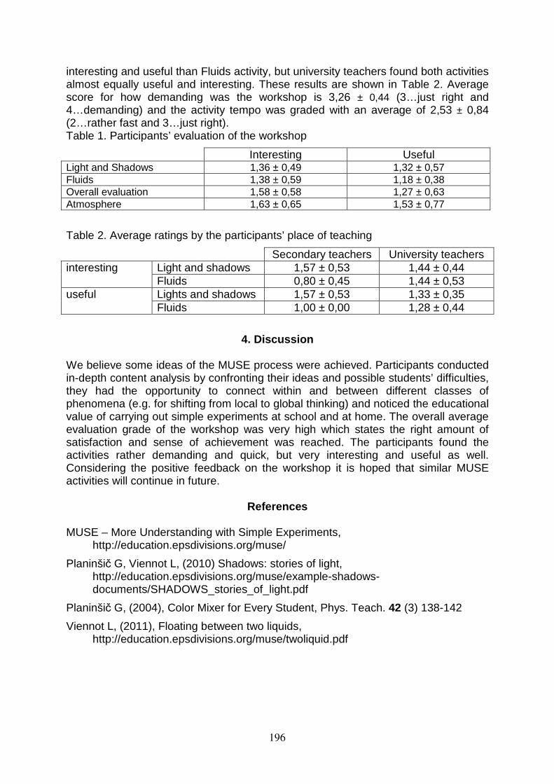
interesting and useful than Fluids activity, but university teachers found both activities almost equally useful and interesting. These results are shown in Table 2. Average score for how demanding was the workshop is 3,26 ± 0,44 (3…just right and 4…demanding) and the activity tempo was graded with an average of 2,53 ± 0,84 (2…rather fast and 3…just right). Table 1. Participants’ evaluation of the workshop

Interesting Useful Light and Shadows 1,36 ± 0,49 1,32 ± 0,57 Fluids 1,38 ± 0,59 1,18 ± 0,38 Overall evaluation 1,58 ± 0,58 1,27 ± 0,63 Atmosphere 1,63 ± 0,65 1,53 ± 0,77

Table 2. Average ratings by the participants’ place of teaching

Secondary teachers University teachers interesting Light and shadows 1,57 ± 0,53 1,44 ± 0,44

Fluids 0,80 ± 0,45 1,44 ± 0,53 useful Lights and shadows 1,57 ± 0,53 1,33 ± 0,35

Fluids 1,00 ± 0,00 1,28 ± 0,44

4. Discussion We believe some ideas of the MUSE process were achieved. Participants conducted in-depth content analysis by confronting their ideas and possible students’ difficulties, they had the opportunity to connect within and between different classes of phenomena (e.g. for shifting from local to global thinking) and noticed the educational value of carrying out simple experiments at school and at home. The overall average evaluation grade of the workshop was very high which states the right amount of satisfaction and sense of achievement was reached. The participants found the activities rather demanding and quick, but very interesting and useful as well. Considering the positive feedback on the workshop it is hoped that similar MUSE activities will continue in future.

References MUSE – More Understanding with Simple Experiments,

http://education.epsdivisions.org/muse/

Planinšič G, Viennot L, (2010) Shadows: stories of light, http://education.epsdivisions.org/muse/example-shadows-documents/SHADOWS_stories_of_light.pdf

Planinšič G, (2004), Color Mixer for Every Student, Phys. Teach. 42 (3) 138-142

Viennot L, (2011), Floating between two liquids, http://education.epsdivisions.org/muse/twoliquid.pdf

196

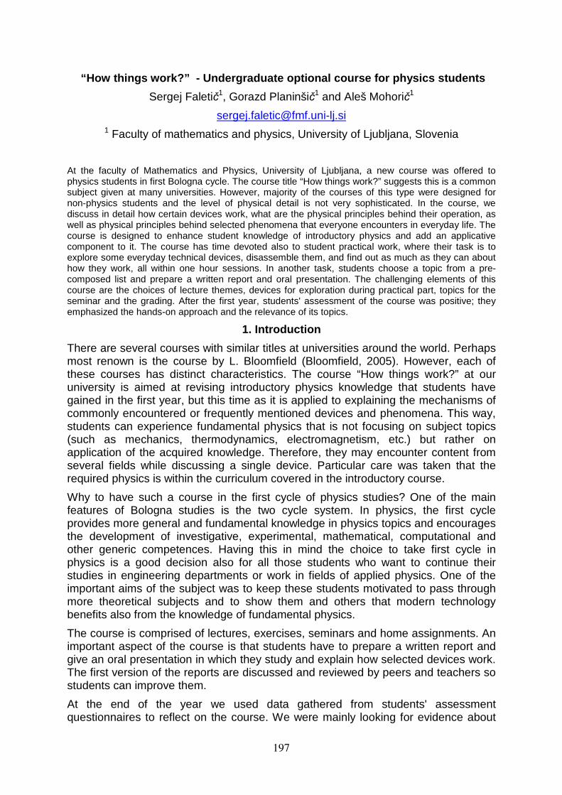
“How things work?” - Undergraduate optional cours e for physics students

Sergej Faletič1, Gorazd Planinšič1 and Aleš Mohorič1

sergej.faletic@fmf.uni-lj.si 1 Faculty of mathematics and physics, University of Ljubljana, Slovenia

At the faculty of Mathematics and Physics, University of Ljubljana, a new course was offered to physics students in first Bologna cycle. The course title “How things work?” suggests this is a common subject given at many universities. However, majority of the courses of this type were designed for non-physics students and the level of physical detail is not very sophisticated. In the course, we discuss in detail how certain devices work, what are the physical principles behind their operation, as well as physical principles behind selected phenomena that everyone encounters in everyday life. The course is designed to enhance student knowledge of introductory physics and add an applicative component to it. The course has time devoted also to student practical work, where their task is to explore some everyday technical devices, disassemble them, and find out as much as they can about how they work, all within one hour sessions. In another task, students choose a topic from a pre-composed list and prepare a written report and oral presentation. The challenging elements of this course are the choices of lecture themes, devices for exploration during practical part, topics for the seminar and the grading. After the first year, students' assessment of the course was positive; they emphasized the hands-on approach and the relevance of its topics.

1. Introduction

There are several courses with similar titles at universities around the world. Perhaps most renown is the course by L. Bloomfield (Bloomfield, 2005). However, each of these courses has distinct characteristics. The course “How things work?” at our university is aimed at revising introductory physics knowledge that students have gained in the first year, but this time as it is applied to explaining the mechanisms of commonly encountered or frequently mentioned devices and phenomena. This way, students can experience fundamental physics that is not focusing on subject topics (such as mechanics, thermodynamics, electromagnetism, etc.) but rather on application of the acquired knowledge. Therefore, they may encounter content from several fields while discussing a single device. Particular care was taken that the required physics is within the curriculum covered in the introductory course.

Why to have such a course in the first cycle of physics studies? One of the main features of Bologna studies is the two cycle system. In physics, the first cycle provides more general and fundamental knowledge in physics topics and encourages the development of investigative, experimental, mathematical, computational and other generic competences. Having this in mind the choice to take first cycle in physics is a good decision also for all those students who want to continue their studies in engineering departments or work in fields of applied physics. One of the important aims of the subject was to keep these students motivated to pass through more theoretical subjects and to show them and others that modern technology benefits also from the knowledge of fundamental physics.

The course is comprised of lectures, exercises, seminars and home assignments. An important aspect of the course is that students have to prepare a written report and give an oral presentation in which they study and explain how selected devices work. The first version of the reports are discussed and reviewed by peers and teachers so students can improve them.

At the end of the year we used data gathered from students' assessment questionnaires to reflect on the course. We were mainly looking for evidence about

197

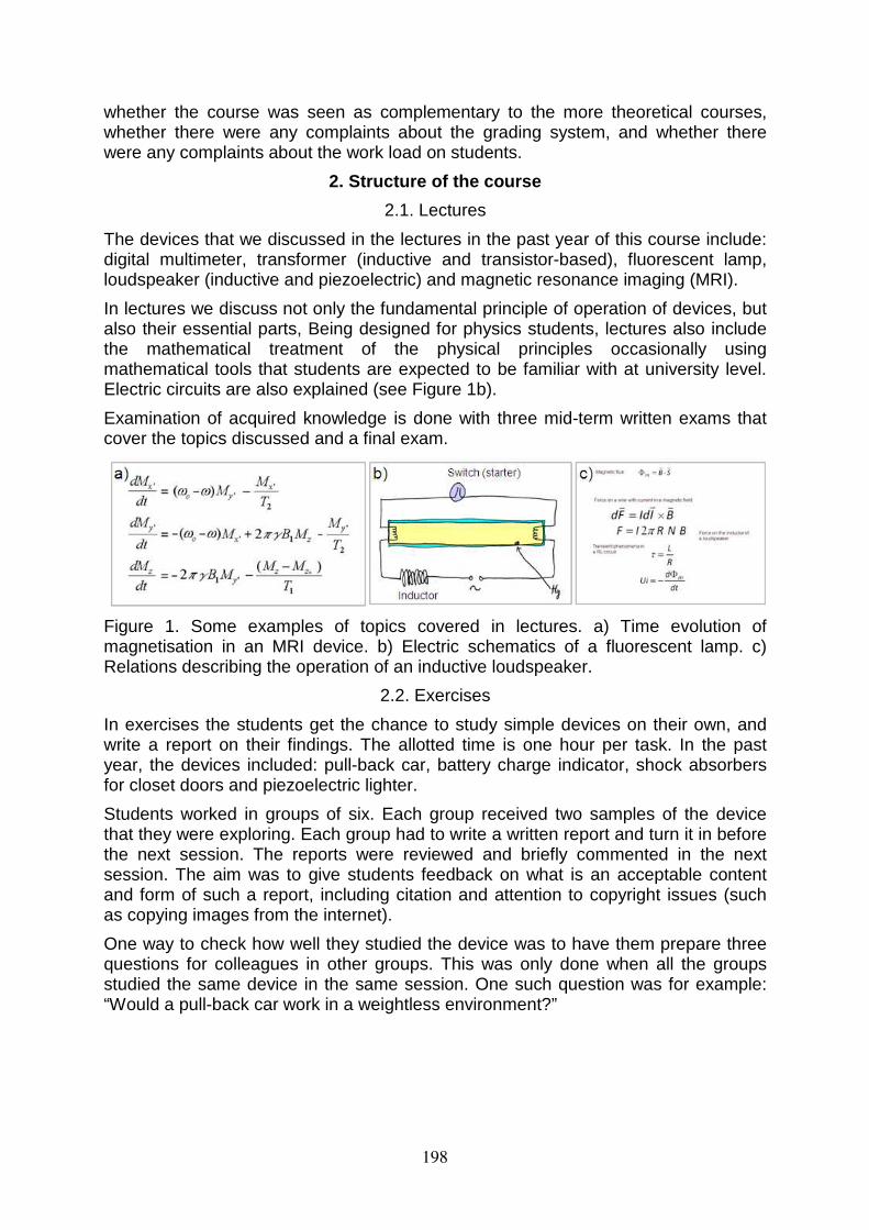
whether the course was seen as complementary to the more theoretical courses, whether there were any complaints about the grading system, and whether there were any complaints about the work load on students.

2. Structure of the course

2.1. Lectures

The devices that we discussed in the lectures in the past year of this course include: digital multimeter, transformer (inductive and transistor-based), fluorescent lamp, loudspeaker (inductive and piezoelectric) and magnetic resonance imaging (MRI).

In lectures we discuss not only the fundamental principle of operation of devices, but also their essential parts, Being designed for physics students, lectures also include the mathematical treatment of the physical principles occasionally using mathematical tools that students are expected to be familiar with at university level. Electric circuits are also explained (see Figure 1b).

Examination of acquired knowledge is done with three mid-term written exams that cover the topics discussed and a final exam.

Figure 1. Some examples of topics covered in lectures. a) Time evolution of magnetisation in an MRI device. b) Electric schematics of a fluorescent lamp. c) Relations describing the operation of an inductive loudspeaker.

2.2. Exercises

In exercises the students get the chance to study simple devices on their own, and write a report on their findings. The allotted time is one hour per task. In the past year, the devices included: pull-back car, battery charge indicator, shock absorbers for closet doors and piezoelectric lighter.

Students worked in groups of six. Each group received two samples of the device that they were exploring. Each group had to write a written report and turn it in before the next session. The reports were reviewed and briefly commented in the next session. The aim was to give students feedback on what is an acceptable content and form of such a report, including citation and attention to copyright issues (such as copying images from the internet).

One way to check how well they studied the device was to have them prepare three questions for colleagues in other groups. This was only done when all the groups studied the same device in the same session. One such question was for example: “Would a pull-back car work in a weightless environment?”

198

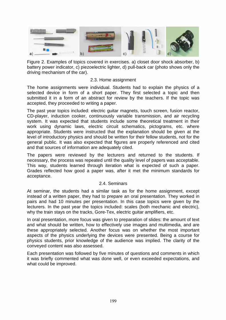
Figure 2. Examples of topics covered in exercises. a) closet door shock absorber, b) battery power indicator, c) piezoelectric lighter, d) pull-back car (photo shows only the driving mechanism of the car).

2.3. Home assignment

The home assignments were individual. Students had to explain the physics of a selected device in form of a short paper. They first selected a topic and then submitted it in a form of an abstract for review by the teachers. If the topic was accepted, they proceeded to writing a paper.

The past year topics included: electric guitar magnets, touch screen, fusion reactor, CD-player, induction cooker, continuously variable transmission, and air recycling system. It was expected that students include some theoretical treatment in their work using dynamic laws, electric circuit schematics, pictograms, etc. where appropriate. Students were instructed that the explanation should be given at the level of introductory physics and should be written for their fellow students, not for the general public. It was also expected that figures are properly referenced and cited and that sources of information are adequately cited.

The papers were reviewed by the lecturers and returned to the students. If necessary, the process was repeated until the quality level of papers was acceptable. This way, students learned through iteration what is expected of such a paper. Grades reflected how good a paper was, after it met the minimum standards for acceptance.

2.4. Seminars

At seminar, the students had a similar task as for the home assignment, except instead of a written paper, they had to prepare an oral presentation. They worked in pairs and had 10 minutes per presentation. In this case topics were given by the lecturers. In the past year the topics included: scales (both mechanic and electric), why the train stays on the tracks, Gore-Tex, electric guitar amplifiers, etc.

In oral presentation, more focus was given to preparation of slides: the amount of text and what should be written, how to effectively use images and multimedia, and are these appropriately selected. Another focus was on whether the most important aspects of the physics underlying the devices were presented. Being a course for physics students, prior knowledge of the audience was implied. The clarity of the conveyed content was also assessed.

Each presentation was followed by five minutes of questions and comments in which it was briefly commented what was done well, or even exceeded expectations, and what could be improved.

199

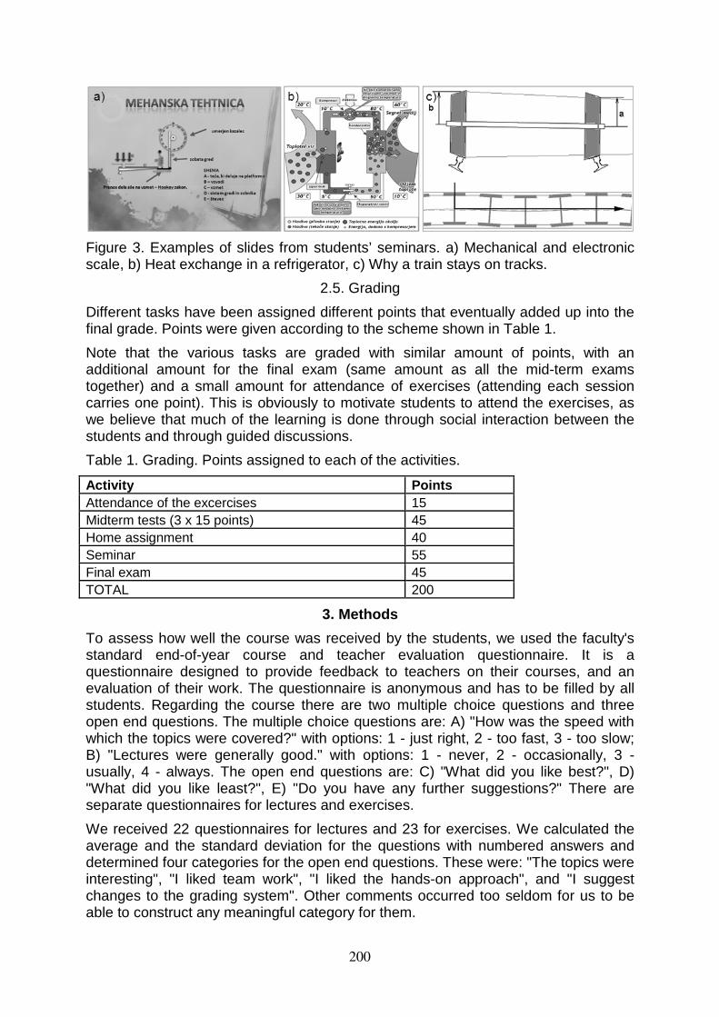
Figure 3. Examples of slides from students’ seminars. a) Mechanical and electronic scale, b) Heat exchange in a refrigerator, c) Why a train stays on tracks.

2.5. Grading

Different tasks have been assigned different points that eventually added up into the final grade. Points were given according to the scheme shown in Table 1.

Note that the various tasks are graded with similar amount of points, with an additional amount for the final exam (same amount as all the mid-term exams together) and a small amount for attendance of exercises (attending each session carries one point). This is obviously to motivate students to attend the exercises, as we believe that much of the learning is done through social interaction between the students and through guided discussions.

Table 1. Grading. Points assigned to each of the activities.

Activity Points Attendance of the excercises 15 Midterm tests (3 x 15 points) 45 Home assignment 40 Seminar 55 Final exam 45 TOTAL 200

3. Methods

To assess how well the course was received by the students, we used the faculty's standard end-of-year course and teacher evaluation questionnaire. It is a questionnaire designed to provide feedback to teachers on their courses, and an evaluation of their work. The questionnaire is anonymous and has to be filled by all students. Regarding the course there are two multiple choice questions and three open end questions. The multiple choice questions are: A) "How was the speed with which the topics were covered?" with options: 1 - just right, 2 - too fast, 3 - too slow; B) "Lectures were generally good." with options: 1 - never, 2 - occasionally, 3 - usually, 4 - always. The open end questions are: C) "What did you like best?", D) "What did you like least?", E) "Do you have any further suggestions?" There are separate questionnaires for lectures and exercises.

We received 22 questionnaires for lectures and 23 for exercises. We calculated the average and the standard deviation for the questions with numbered answers and determined four categories for the open end questions. These were: "The topics were interesting", "I liked team work", "I liked the hands-on approach", and "I suggest changes to the grading system". Other comments occurred too seldom for us to be able to construct any meaningful category for them.

200

4. Results

From the questionnaires we found that the speed with which the topics were covered was considered just right (1.0 ± 0.0), and the lectures and exercises were good almost always (3.48 ± 0.60 for lectures and 3.61 ± 0.50 for exercises). Eight people commented that the topics were interesting; five commented that they liked the hands-on approach in the part of the exercises when they disassembled devices; four commented that they liked team work, and nine suggested changes to the grading system. Two of these suggested a less rigorous system, two suggested a more immediate feedback on their progress, one suggested that reports from the practical work at exercises should also be included in the grading; one suggested that attendance should be excluded, and three suggest modifying the system somehow, but without any specific suggestions.

5. Conclusion and discussion

We introduced the "How thing work?" course to provide a complementary course to the more theoretical courses. The aim was to revise physics that students already learned through it application in commonly encountered or frequently mentioned devices. The student assessment of the course at the end of the year showed that the course was well accepted. Students liked the chance to see ordinary devices disassembled and learn how they work, which might mean that they did see it as complementary to the other, more theoretical courses. There were no complaints about the amount of home work assigned to them, so we assume that it was just right. There were suggestions about the grading system. There were five suggestions to change the system itself. As stated in the introduction, we believe that being present during the lectures and exercises is an important part of the learning process, so attendance must be encouraged somehow. The inclusion of the report on practical work into the grading system makes sense, so we will consider this option. Other suggestions were about the timing of the feedback, and the criteria for grades. Students scored well with seminars, home assignments and attendance, but not so well on mid-term and final exams. We believe that this is due to the fact that seminars and home assignments were iterated many times before being accepted, while midterm exams can only be taken once.

References

Bloomfield, L. (2005). How Things Work: The Physics of Everyday Life (2nd ed.). Wiley.

201

Gravitational Assisted Trajectories –

making your own pictures and trajectory study

Tomas Franc

Tomas.Franc@mff.cuni.cz

Astronomical Institute of Charles University, Faculty of Mathematics and Physics,

Charles University in Prague, Prague, Czech Republic

Abstract

Attracting more high school students to physics is very difficult. A possibility which can help to succeed

can be the gravitational assist (GA). This technique is used for interplanetary flights – the spacecraft

changes its direction or speed (with respect to the Sun) during a planetary flyby. One possibility how to

start teaching the GA can be making our own pictures of spacecrafts’ trajectories and graphs like the

velocity-time graph of a spacecraft. This paper includes the instructions how to do it – where we can

get data, which program we can use and it presents some examples. All this offers many advantages –

students will meet and will work with a mathematical program, they will work with REAL data, they will

get nice pictures and as a result they will want to know how the GA works – which is our goal.

Introduction

Astronomy and astronautics are very interesting parts of physics, in our case sendingspacecrafts to other planets, their complicated trajectories, their discoveries and im-ages, missions’ problems, their endings, etc. The teaching of the gravitational assist(GA) has many educational advantages like better understanding of different frames ofreference, showing to students that physics laws are valid not only on the Earth but alsoin space, studying graphs, working with different coordinates’ systems, realizing somefacts about our Solar system, etc. The first step in teaching the GA can be studyingspacecrafts’ trajectories. And we can make our own diagrams.

The gravitational assist

When a spacecraft flies past a much more massive body (a planet or a moon), thebody acts on the spacecraft via its gravitational force and changes the spacecraft’svelocity relative to the Sun. NASA used this technique called gravitational assist inmany missions. The GA allows reaching Mercury or the Sun, leaving our Solar system,saving fuel, shortening travel time to distant planets, etc. The GA is used for changingspacecrafts’ flight directions and for accelerating or decelerating, but how can this bepossible? Because the Law of energy conservation. What energy the spacecraft gets(or looses) – that energy looses (or gets) the planet.

Missions which used the gravitational assist

Missions to other planets that used the GA (in brackets are launch dates): Pioneer 10

(1972), Pioneer 11 (1973), Mariner 10 (1973), Voyager 1 & 2 (both 1977), Galileo

(1989), Ulysses (1990), Cassini (1997), Messenger (2004), New Horizons (2006),Dawn (2007), Juno (2011). Planned missions: BepiColombo (2014), Solar Probe Plus

(2018). Brief information about most of these missions can be found in [1]. For thispaper we chose the Galileo mission.

202

Galileo mission facts

The Galileo probe was launched on February 18, 1989, it was the first mission to ex-plore Jupiter and its moons in more detail than any previous spacecraft. There wereused three GAs: one with Venus (February 2, 1990) and two with the Earth (Decem-ber 8, 1990 and December 8, 1992). On October 29, 1991, Galileo made the first closeapproach (1 600 km distance from the surface) to an asteroid Gaspra. On a secondpass through the asteroid belt, Galileo discovered a miniature moon orbiting asteroidIda. This tiny body was named Dactyl. The spacecraft arrived to Jupiter on December 7,1995. The Galileo mission ended on September 21, 2003 during its direct impact intothe Jupiter’s dense atmosphere. A list of close encounters with Jupiter’s moons canbe found in a Fact Sheet [2] about Galileo (and we have to realize that during eachencounter with the Jupiter’s moon occured the GA).

Preparing data

Obtaining data

NASA JPL maintains very powerful HORIZONS Web-Interface [3] where we can getheliocentric coordinates (radial distance, longitude and latitude) and velocities of plan-ets and spacecrafts (and much much more!). We chose time step 1 hour – we got122 059 positions for 1 spacecraft for the whole mission! For all pictures, which containtrajectories of 1 spacecraft and 5 planets and Galileo’s velocities, we got 2 319 101numbers!

Importing data into a suitable program

In this step we had to choose a suitable program. There are many possibilities and wechose Wolfram Mathematica (WM) (version 8), [4]. Before data importing, we converteddata into a suitable form for WM: 1 column for 1 coordinate (for example the radialdistance) in 1 .txt file (a possible way how to do it is using Microsoft Excel, [5] – opena .txt file in MS Excel, delete unwanted columns and save it as .txt file).

Cartesian coordinates

For WM we had1 to transform data from (spherical) heliocentric to (spherical) Cartesiancoordinates – it is the spherical transformation:

x = r cos ϑ cos ϕ,

y = r cos ϑ sin ϕ,

z = r sin ϑ,

where r is the radial distance, ϑ is the longitude and ϕ is the latitude (the origin of theframe of reference is the Sun and the positive x-axis heads to the Vernal equinox). Andnow we have everything ready for making our own diagrams.

1Actually, the WM can make a plot directly with coordinates obtained from [3] (WM commandListPointPlot3D), but it takes much longer than using the command Line.

203

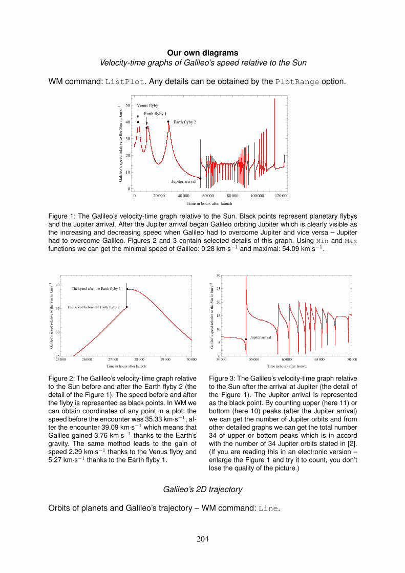
Our own diagrams

Velocity-time graphs of Galileo’s speed relative to the Sun

WM command: ListPlot. Any details can be obtained by the PlotRange option.

0 20 000 40 000 60 000 80 000 100 000 120 000

0

10

20

30

40

50

Time in hours after launch

Gal

ileo

÷ssp

eed

rela

tiv

eto

the

Su

nin

km

s-1 Venus flyby

Earth flyby 1

Earth flyby 2

Jupiter arrival

Figure 1: The Galileo’s velocity-time graph relative to the Sun. Black points represent planetary flybysand the Jupiter arrival. After the Jupiter arrival began Galileo orbiting Jupiter which is clearly visible asthe increasing and decreasing speed when Galileo had to overcome Jupiter and vice versa – Jupiterhad to overcome Galileo. Figures 2 and 3 contain selected details of this graph. Using Min and Max

functions we can get the minimal speed of Galileo: 0.28 km·s−1 and maximal: 54.09 km·s−1.

25 000 26 000 27 000 28 000 29 000 30 00025

30

35

40

Time in hours after launch

Gal

ileo

÷ssp

eed

rela

tiv

eto

the

Su

nin

km

s-1

The speed before the Earth flyby 2

The speed after the Earth flyby 2

Figure 2: The Galileo’s velocity-time graph relativeto the Sun before and after the Earth flyby 2 (thedetail of the Figure 1). The speed before and afterthe flyby is represented as black points. In WM wecan obtain coordinates of any point in a plot: thespeed before the encounter was 35.33 km·s−1, af-ter the encounter 39.09 km·s−1 which means thatGalileo gained 3.76 km·s−1 thanks to the Earth’sgravity. The same method leads to the gain ofspeed 2.29 km·s−1 thanks to the Venus flyby and5.27 km·s−1 thanks to the Earth flyby 1.

50 000 55 000 60 000 65 000 70 0000

5

10

15

20

25

30

Time in hours after launch

Gal

ileo

÷ssp

eed

rela

tiv

eto

the

Su

nin

km

s-1

Jupiter arrival

Figure 3: The Galileo’s velocity-time graph relativeto the Sun after the arrival at Jupiter (the detail ofthe Figure 1). The Jupiter arrival is representedas the black point. By counting upper (here 11) orbottom (here 10) peaks (after the Jupiter arrival)we can get the number of Jupiter orbits and fromother detailed graphs we can get the total number34 of upper or bottom peaks which is in accordwith the number of 34 Jupiter orbits stated in [2].(If you are reading this in an electronic version –enlarge the Figure 1 and try it to count, you don’tlose the quality of the picture.)

Galileo’s 2D trajectory

Orbits of planets and Galileo’s trajectory – WM command: Line.

204

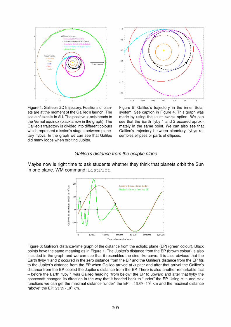
Vernal equinox

Galileo÷s trajectory:

- from launch to Venus flyby

- from Venus flyby to Earth flyby 1

- from Earth flyby 1 to Earth flyby 2

- from Earth flyby 2 to Jupiter arrival

- orbiting Jupiter

Planets÷ orbits:

-Mercury

- Venus

- Earth

-Mars

- Jupiter

-4 -2 0 2 4

-4

-2

0

2

4

Figure 4: Galileo’s 2D trajectory. Positions of plan-ets are at the moment of the Galileo’s launch. Thescale of axes is in AU. The positive x-axis heads tothe Vernal equinox (black arrow in the graph). TheGalileo’s trajectory is divided into different colourswhich represent mission’s stages between plane-tary flybys. In the graph we can see that Galileodid many loops when orbiting Jupiter.

-1.5 -1.0 -0.5 0.0 0.5 1.0 1.5

-2.0

-1.5

-1.0

-0.5

0.0

0.5

1.0

Figure 5: Galileo’s trajectory in the inner Solarsystem. See caption in Figure 4. This graph wasmade by using the PlotRange option. We cansee that the Earth flyby 1 and 2 occured aproxi-mately in the same point. We can also see thatGalileo’s trajectory between planetary flybys re-sembles ellipses or parts of ellipses.

Galileo’s distance from the ecliptic plane

Maybe now is right time to ask students whether they think that planets orbit the Sunin one plane. WM command: ListPlot.

0 20 000 40 000 60 000 80 000 100 000 120 000

-10

0

10

20

Time in hours after launch

Gal

ileo

’sd

ista

nce

fro

mth

eE

Pin

10

6k

m Jupiter’s distance from the EP

Galileo’s distance from the EP

Figure 6: Galileo’s distance-time graph of the distance from the ecliptic plane (EP) (green colour). Blackpoints have the same meaning as in Figure 1. The Jupiter’s distance from the EP (brown colour) is alsoincluded in the graph and we can see that it resembles the sine-like curve. It is also obvious that theEarth flyby 1 and 2 occured in the zero distance from the EP and the Galileo’s distance from the EP fitsto the Jupiter’s distance from the EP when Galileo arrived at Jupiter and after that arrival the Galileo’sdistance from the EP copied the Jupiter’s distance from the EP. There is also another remarkable fact– before the Earth flyby 1 was Galileo heading “from below” the EP to upward and after that flyby thespacecraft changed its direction in the way that it headed back to “under” the EP. Using Min and Max

functions we can get the maximal distance “under” the EP: −16.89 · 106 km and the maximal distance“above” the EP: 23.39 · 106 km.

205

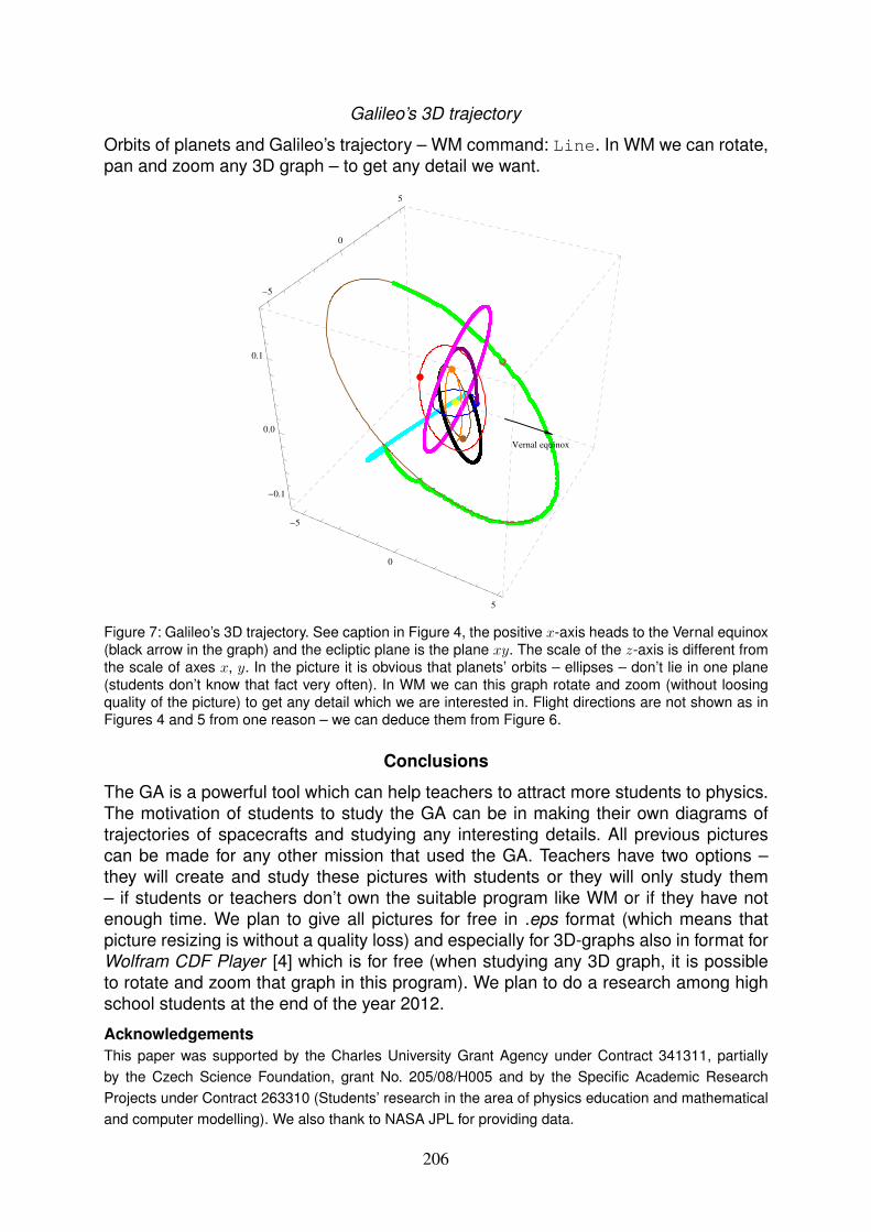
Galileo’s 3D trajectory

Orbits of planets and Galileo’s trajectory – WM command: Line. In WM we can rotate,pan and zoom any 3D graph – to get any detail we want.

Vernal equinox

-5

0

5

-5

0

5

-0.1

0.0

0.1

Figure 7: Galileo’s 3D trajectory. See caption in Figure 4, the positive x-axis heads to the Vernal equinox(black arrow in the graph) and the ecliptic plane is the plane xy. The scale of the z-axis is different fromthe scale of axes x, y. In the picture it is obvious that planets’ orbits – ellipses – don’t lie in one plane(students don’t know that fact very often). In WM we can this graph rotate and zoom (without loosingquality of the picture) to get any detail which we are interested in. Flight directions are not shown as inFigures 4 and 5 from one reason – we can deduce them from Figure 6.

Conclusions

The GA is a powerful tool which can help teachers to attract more students to physics.The motivation of students to study the GA can be in making their own diagrams oftrajectories of spacecrafts and studying any interesting details. All previous picturescan be made for any other mission that used the GA. Teachers have two options –they will create and study these pictures with students or they will only study them– if students or teachers don’t own the suitable program like WM or if they have notenough time. We plan to give all pictures for free in .eps format (which means thatpicture resizing is without a quality loss) and especially for 3D-graphs also in format forWolfram CDF Player [4] which is for free (when studying any 3D graph, it is possibleto rotate and zoom that graph in this program). We plan to do a research among highschool students at the end of the year 2012.

Acknowledgements

This paper was supported by the Charles University Grant Agency under Contract 341311, partially

by the Czech Science Foundation, grant No. 205/08/H005 and by the Specific Academic Research

Projects under Contract 263310 (Students’ research in the area of physics education and mathematical

and computer modelling). We also thank to NASA JPL for providing data.

206

References

[1] Franc T. (2011). The Gravitational Assist. WDS’11 Proceedings of Contributed Pa-

pers: Part III - Physics (eds. J. Safrankova and J. Pavlu), pp. 55–60, Prague, Mat-fyzpress.

[2] Galileo Legacy Site: http://solarsystem.nasa.gov/galileo/[3] HORIZONS Web-Interface: http://ssd.jpl.nasa.gov/horizons.cgi[4] Wolfram Research: Mathematica: http://www.wolfram.com/[5] Microsoft Excel: http://office.microsoft.com/excel/

207

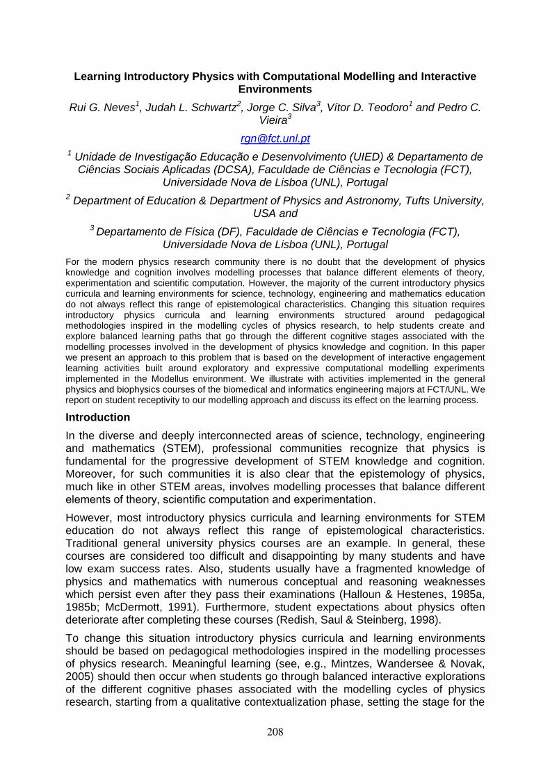
Learning Introductory Physics with Computational Modelling and Interactive Environments

Rui G. Neves1, Judah L. Schwartz2, Jorge C. Silva3, Vítor D. Teodoro1 and Pedro C. Vieira3

rgn@fct.unl.pt

1 Unidade de Investigação Educação e Desenvolvimento (UIED) & Departamento de Ciências Sociais Aplicadas (DCSA), Faculdade de Ciências e Tecnologia (FCT),

Universidade Nova de Lisboa (UNL), Portugal

2 Department of Education & Department of Physics and Astronomy, Tufts University, USA and

3 Departamento de Física (DF), Faculdade de Ciências e Tecnologia (FCT), Universidade Nova de Lisboa (UNL), Portugal

For the modern physics research community there is no doubt that the development of physics knowledge and cognition involves modelling processes that balance different elements of theory, experimentation and scientific computation. However, the majority of the current introductory physics curricula and learning environments for science, technology, engineering and mathematics education do not always reflect this range of epistemological characteristics. Changing this situation requires introductory physics curricula and learning environments structured around pedagogical methodologies inspired in the modelling cycles of physics research, to help students create and explore balanced learning paths that go through the different cognitive stages associated with the modelling processes involved in the development of physics knowledge and cognition. In this paper we present an approach to this problem that is based on the development of interactive engagement learning activities built around exploratory and expressive computational modelling experiments implemented in the Modellus environment. We illustrate with activities implemented in the general physics and biophysics courses of the biomedical and informatics engineering majors at FCT/UNL. We report on student receptivity to our modelling approach and discuss its effect on the learning process.

Introduction

In the diverse and deeply interconnected areas of science, technology, engineering and mathematics (STEM), professional communities recognize that physics is fundamental for the progressive development of STEM knowledge and cognition. Moreover, for such communities it is also clear that the epistemology of physics, much like in other STEM areas, involves modelling processes that balance different elements of theory, scientific computation and experimentation.

However, most introductory physics curricula and learning environments for STEM education do not always reflect this range of epistemological characteristics. Traditional general university physics courses are an example. In general, these courses are considered too difficult and disappointing by many students and have low exam success rates. Also, students usually have a fragmented knowledge of physics and mathematics with numerous conceptual and reasoning weaknesses which persist even after they pass their examinations (Halloun & Hestenes, 1985a, 1985b; McDermott, 1991). Furthermore, student expectations about physics often deteriorate after completing these courses (Redish, Saul & Steinberg, 1998).

To change this situation introductory physics curricula and learning environments should be based on pedagogical methodologies inspired in the modelling processes of physics research. Meaningful learning (see, e.g., Mintzes, Wandersee & Novak, 2005) should then occur when students go through balanced interactive explorations of the different cognitive phases associated with the modelling cycles of physics research, starting from a qualitative contextualization phase, setting the stage for the

208

definition, exploration, interpretation and validation of the relevant mathematical physics models, and ending with the communication of modelling results and the development of generalizations.

As shown by many research efforts (see, e.g., Blum, Galbraith, Henn & Niss, 2007; Handelsman et al., 2005; McDermott & Redish, 1999; Slooten, van den Berg & Ellermeijer, 2006), the learning processes in various STEM areas can effectively be enhanced when students are embedded in environments with activities that approximately recreate the cognitive involvement of scientists in modelling research activities. As opposed to traditional instruction, these approaches have shown to be able to engage students in interactive learning processes that are better suited to promote knowledge performance and resolve cognitive conflicts with common sense beliefs or incorrect scientific ideas.

Fundamental for the development of research based modelling approaches is an early balanced integration of activities with computational knowledge and technologies. However, professional languages like Fortran (Bork, 1967), Pascal (Redish & Wilson, 1993) or, more recently, Python (Chabay & Sherwood, 2008), or even educational languages like Logo (Papert, 1980) or Boxer (diSessa, 2000), require the development of a working knowledge of programming, a fact that also holds with professional scientific computation software like Mathematica or Matlab.

To reduce such cognitive load and focus the learning activities on the concepts of physics and mathematics, several computer modelling systems have been developed, for example, the DMS (Ogborn, 1985), Stella (Richmond, 2004), Coach (Heck, Kadzierska & Ellermeijer, 2009), EJS (Christian & Esquembre, 2007), Modellus (Neves, Silva &Teodoro, 2011; Neves & Teodoro, 2010 Teodoro & Neves, 2011) and Phet simulations (Wieman, Perkins & Adams, 2008).

In spite of these advances, a balanced integration of computational modelling knowledge and technologies in introductory physics courses remains an open problem, critically dependent on both curricular and technological innovations. In this work, we present an approach to improve such balanced integration that is based on the development of interactive engagement learning activities built around exploratory and expressive computational modelling experiments implemented in the Modellus environment.

Physics Knowledge, Cognition and Learning Processes

Let us start with a brief discussion of the fundamental theoretical aspects underlying our approach. As in other STEM areas, the development of physics knowledge and reasoning requires rigorous declarative and procedural specifications of abstract concepts and of the connections existing between them (Reif, 2008). A successful construction of models or theories involves operational familiarization, theoretical consistency requirements and a precise relation with the relevant referents, either in the universe of phenomena or in abstract mathematical worlds. Physics knowledge and reasoning are then related but distinctly different from the corresponding every day or common sense structures. An important cognitive barrier for the learning processes is thus the need to distinguish between different but closely related concepts. When students try to adjust their prior knowledge to the new physics contexts, unresolved cognitive conflicts arising from the superficial similarity between elements of everyday and physics knowledge and reasoning can create persistent learning difficulties.

209

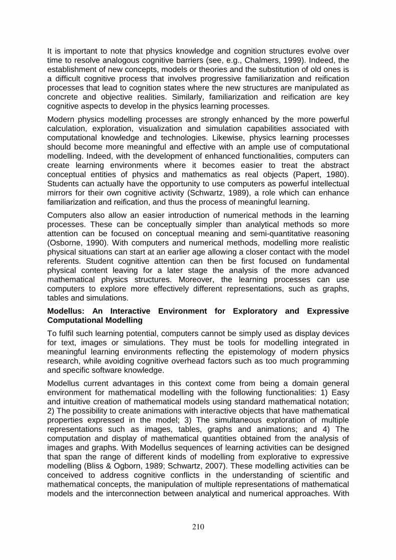
It is important to note that physics knowledge and cognition structures evolve over time to resolve analogous cognitive barriers (see, e.g., Chalmers, 1999). Indeed, the establishment of new concepts, models or theories and the substitution of old ones is a difficult cognitive process that involves progressive familiarization and reification processes that lead to cognition states where the new structures are manipulated as concrete and objective realities. Similarly, familiarization and reification are key cognitive aspects to develop in the physics learning processes.

Modern physics modelling processes are strongly enhanced by the more powerful calculation, exploration, visualization and simulation capabilities associated with computational knowledge and technologies. Likewise, physics learning processes should become more meaningful and effective with an ample use of computational modelling. Indeed, with the development of enhanced functionalities, computers can create learning environments where it becomes easier to treat the abstract conceptual entities of physics and mathematics as real objects (Papert, 1980). Students can actually have the opportunity to use computers as powerful intellectual mirrors for their own cognitive activity (Schwartz, 1989), a role which can enhance familiarization and reification, and thus the process of meaningful learning.

Computers also allow an easier introduction of numerical methods in the learning processes. These can be conceptually simpler than analytical methods so more attention can be focused on conceptual meaning and semi-quantitative reasoning (Osborne, 1990). With computers and numerical methods, modelling more realistic physical situations can start at an earlier age allowing a closer contact with the model referents. Student cognitive attention can then be first focused on fundamental physical content leaving for a later stage the analysis of the more advanced mathematical physics structures. Moreover, the learning processes can use computers to explore more effectively different representations, such as graphs, tables and simulations.

Modellus: An Interactive Environment for Exploratory and Expressive Computational Modelling

To fulfil such learning potential, computers cannot be simply used as display devices for text, images or simulations. They must be tools for modelling integrated in meaningful learning environments reflecting the epistemology of modern physics research, while avoiding cognitive overhead factors such as too much programming and specific software knowledge.

Modellus current advantages in this context come from being a domain general environment for mathematical modelling with the following functionalities: 1) Easy and intuitive creation of mathematical models using standard mathematical notation; 2) The possibility to create animations with interactive objects that have mathematical properties expressed in the model; 3) The simultaneous exploration of multiple representations such as images, tables, graphs and animations; and 4) The computation and display of mathematical quantities obtained from the analysis of images and graphs. With Modellus sequences of learning activities can be designed that span the range of different kinds of modelling from explorative to expressive modelling (Bliss & Ogborn, 1989; Schwartz, 2007). These modelling activities can be conceived to address cognitive conflicts in the understanding of scientific and mathematical concepts, the manipulation of multiple representations of mathematical models and the interconnection between analytical and numerical approaches. With

210

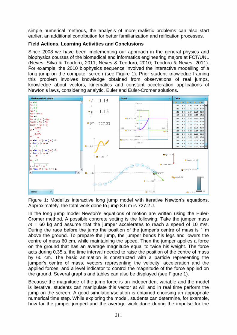
simple numerical methods, the analysis of more realistic problems can also start earlier, an additional contribution for better familiarization and reification processes.

Field Actions, Learning Activities and Conclusions

Since 2008 we have been implementing our approach in the general physics and biophysics courses of the biomedical and informatics engineering majors at FCT/UNL (Neves, Silva & Teodoro, 2011; Neves & Teodoro, 2010; Teodoro & Neves, 2011). For example, the 2010 biophysics sequence involved the interactive modelling of a long jump on the computer screen (see Figure 1). Prior student knowledge framing this problem involves knowledge obtained from observations of real jumps, knowledge about vectors, kinematics and constant acceleration applications of Newton’s laws, considering analytic, Euler and Euler-Cromer solutions.

Figure 1: Modellus interactive long jump model with iterative Newton’s equations. Approximately, the total work done to jump 8.6 m is 727.2 J.

In the long jump model Newton’s equations of motion are written using the Euler-Cromer method. A possible concrete setting is the following. Take the jumper mass m = 60 kg and assume that the jumper accelerates to reach a speed of 10 m/s. During the race before the jump the position of the jumper’s centre of mass is 1 m above the ground. To prepare the jump, the jumper bends his legs and lowers the centre of mass 60 cm, while maintaining the speed. Then the jumper applies a force on the ground that has an average magnitude equal to twice his weight. The force acts during 0.35 s, the time interval needed to raise the position of the centre of mass by 60 cm. The basic animation is constructed with a particle representing the jumper’s centre of mass, vectors representing the velocity, acceleration and the applied forces, and a level indicator to control the magnitude of the force applied on the ground. Several graphs and tables can also be displayed (see Figure 1).

Because the magnitude of the jump force is an independent variable and the model is iterative, students can manipulate this vector at will and in real time perform the jump on the screen. A good simulation/solution is obtained choosing an appropriate numerical time step. While exploring the model, students can determine, for example, how far the jumper jumped and the average work done during the impulse for the

211

jump. Students can change the model settings easily and analyse the jump physics for different jumpers and jump conditions. The possibility to change the mathematical model and immediately observe the consequences on the animation, graphs and tables is a powerful cognitive element to enhance familiarization and reification.

In all the courses the activities were successful in identifying and resolving student difficulties in key physical and mathematical concepts. For example, in the 2010 biophysics course, the average grade was 70 % and all 55 students were able to pass on the computational modelling component. To have real time visible correspondence between the animations with interactive objects and the object’s mathematical properties defined in the model, and to manipulate several different representations were instrumental factors to achieve this. Using Modelllus students were able to actively explore and create mathematical physics models and animations. They also built models with differential equations, obtaining analytical and numerical solutions.

Likert scale questionnaires showed that the majority of students reacted positively to the new approach (Neves, Silva & Teodoro, 2011). For example, on the 2010 biophysics course 69 % of the students manifested a clear average positive opinion. Students showed preference for group work with teacher guidance and considered Modellus helpful and user friendly in the processes of learning mathematical physics models. The supporting interactive PDF documents with embedded video guidance and free space for multimedia answers or comments were considered interesting and well designed. However, students also felt that the extra content load of the new computational modelling activities required more than the available class time. Future research will involve improved implementation actions, a more detailed assessment of the effective learning outcomes and the creation of new Modellus functionalities.

References

Bliss, J., & Ogborn, J. (1989). Tools for exploratory learning. Journal of Computer Assisted Learning, 5, 37-50.

Blum, W., Galbraith, P., Henn, H.-W., & Niss, M. (Eds.) (2007). Modelling and applications in mathematics education. New York: Springer.

Bork, A. (1967). Fortran for physics. Reading, MA: Addison-Wesley.

Chabay, R., & Sherwood, B. (2008). Computational physics in the introductory calculus-based course. American Journal of Physics, 76, 307-313.

Chalmers, A. (1999). What is this thing called science? London: Open University Press.

Christian, W., & Esquembre, F. (2007). Modeling physics with Easy Java Simulations. The Physics Teacher, 45, 475-480.

diSessa, A. (2000). Changing minds: Computers, learning and literacy. Cambridge, MA: MIT Press.

Halloun, I., & Hestenes, D. (1985a). The initial knowledge state of college physics students. American Journal of Physics, 53, 1043-1056.

Halloun, I., & Hestenes, D. (1985b). Common-sense concepts about motion. American Journal of Physics, 53, 1056-1065.

Handelsman, J., Ebert-May, D., Beichner, R., Bruns, P., Chang, A., DeHaan, R., et al. (2005). Education: Scientific teaching. Science, 304, 521-522.

212

Heck, A., Kadzierska, E., & Ellermeijer, T. (2009). Design and implementation of an integrated computer working environment. Journal of Computers in Mathematics and Science Teaching, 28, 147-161.

McDermott, L. (1991). Millikan lecture 1990: What we teach and what is learned -closing the gap. American Journal of Physics, 59, 301-315.

McDermott, L., & Redish, E. (1999). Resource letter: Per-1: Physics education research. American Journal of Physics, 67, 755-767.

Mintzes, J., Wandersee, J., & Novak, J. (2005). Teaching science for understanding: a human constructivist view. Burlington, MA: Elsevier Academic Press.

Neves, R., Silva, J., & Teodoro, V. (2011). Improving learning in science and mathematics with exploratory and interactive computational modelling. In G. Kaiser, W. Blum, R. Borromeo-Ferri, & G. Stillman (Eds.), International perspectives on the teaching and learning of mathematical modelling: Vol. 1. ICTMA14 - Trends in teaching and learning of mathematical modelling (pp. 331-341). Dordrecht: Springer.

Neves, R., & Teodoro, V. (2010). Enhancing science and mathematics education with computational modelling. Journal of Mathematical Modelling and Application, 1, 2-15.

Ogborn, J. (1985). Dynamic modelling system. Harlow, Essex, UK: Longman.

Osborne, J. (1990). Sacred cows in physics - towards a redefinition of physics education. Physics Education, 25, 189-196.

Papert, S. (1980). Mindstorms: Children, computers and powerful ideas. New York: Basic Books.

Reif, F. (2008). Applying cognitive science to education: thinking and learning in scientific and other complex domains. Cambridge, MA: MIT Press.

Redish, E., Saul, J., & Steinberg, R. (1998). Student expectations in introductory physics. American Journal of Physics, 66, 212-224.

Redish, E., & Wilson, J. (1993). Student programming in the introductory physics course: MUPPET. American Journal of Physics, 61, 222-232.

Richmond, B. (2004). An introduction to systems thinking with Stella. Lebanon, NH: ISEE Systems, Inc.

Schwartz, J. (1989). Intellectual mirrors: A step in the direction of making schools knowledge-making places. Harvard Educational Review, 59, 217- 222.

Schwartz, J. (2007). Models, simulations, and exploratory environments: A tentative taxonomy. In R. Lesh, E. Hamilton, & J. Kaput (Eds.), Foundations for the future in mathematics education (pp. 161-172). Mahwah, NJ: Lawrence Erlbaum Associates.

Slooten, O., van den Berg, E., & Ellermeijer, T. (Eds.) (2006). Proceedings of the GIREP 2006 conference: Modelling in physics and physics education. Amsterdam: University of Amsterdam and European Physical Society.

Teodoro, V., & Neves, R. (2011). Mathematical modelling in science and mathematics education. Computer Physics Communications, 182, 8-10.

Wieman, C., Perkins, K., & Adams, W. (2008). Oersted medal lecture 2007: Interactive simulations for teaching physics: what works, what doesn’t and why. American Journal of Physics, 76, 393-399.

213

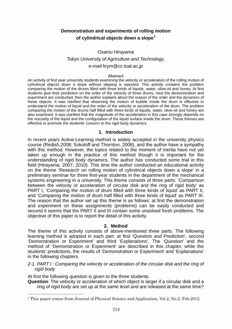
Demonstration and experiments of rolling motion

of cylindrical objects down a slope1

Osamu Hirayama

Tokyo University of Agriculture and Technology,

e-mail:hrym@cc.tuat.ac.jp

Abstract An activity of first year university students examining the velocity or acceleration of the rolling motion of cylindrical objects down a slope without slipping is reported. This activity contains the problem comparing the motion of the drums filled with three kinds of liquids, water, olive-oil and honey. At first students give their prediction on the order of the velocity of three drums, next the demonstration and experiment are conducted, then the author explains about the reason of the order and the dynamics of these objects. It was clarified that observing the motion of bubble inside the drum is effective to understand the motion of liquid and the order of the velocity or acceleration of the drum. The problem comparing the motion of the drums half filled with three kinds of liquids, water, olive-oil and honey are also examined. It was clarified that the magnitude of the acceleration in this case strongly depends on the viscosity of the liquid and the configuration of the liquid surface inside the drum. These themes are effective to promote the students’ concern to the rigid body dynamics.

1. Intro uction d

In recent years Active-Learning method is widely accepted in the university physics course (Redish,2008; Sokoloff and Thornton, 2008), and the author have a sympathy with this method. However, the topics related to the moment of inertia have not yet taken up enough in the practice of this method though it is important for the understanding of rigid body dynamics. The author has conducted some trial in this field (Hirayama, 2007, 2010). This time the author conducted an educational activity on the theme ‘Research on rolling motion of cylindrical objects down a slope’ in a preliminary seminar for three first-year students in the department of the mechanical systems engineering in a university. This theme consists of three parts: ‘Comparison between the velocity or acceleration of circular disk and the ring of rigid body’ as PART I, ‘Comparing the motion of drum filled with three kinds of liquid’ as PART II, and ‘Comparing the motion of drum half filled with three kinds of liquid’ as PART III. The reason that the author set up this theme is as follows: at first the demonstration and experiment on these assignments (problems) can be easily conducted and second it seems that the PART II and III contain some unsolved fresh problems. The objective of this paper is to report the detail of this activity.

2. Method The theme of this activity consists of above-mentioned three parts. The following learning method is adopted in each part: at first ‘Question and Prediction’, second ‘Demonstration or Experiment’ and third ‘Explanations’. The ‘Question’ and the method of ‘Demonstration or Experiment’ are described in this chapter, while the students’ predictions, the results of ‘Demonstration or Experiment’ and ‘Explanations’ in the following chapters.

2-1. PART I : Comparing the velocity or acceleration of the circular disk and the ring of

rigid body At first the following question is given to the three students. Question: The velocity or acceleration of which object is larger if a circular disk and a

ring of rigid body are set up at the same level and are released at the same time?

1 This paper comes from Journal of Physical Science and Application, Vol.2, No.2, Feb.2012.

214

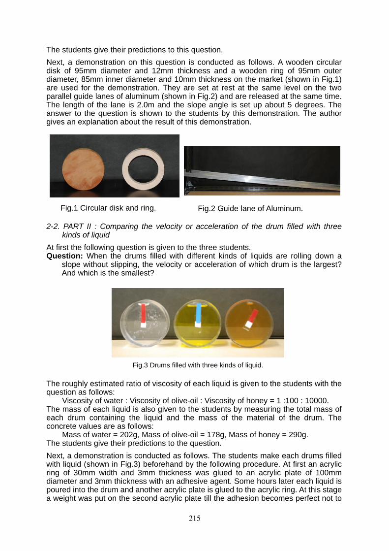
T

he students give their predictions to this question.

Next, a demonstration on this question is conducted as follows. A wooden circular disk of 95mm diameter and 12mm thickness and a wooden ring of 95mm outer diameter, 85mm inner diameter and 10mm thickness on the market (shown in Fig.1) are used for the demonstration. They are set at rest at the same level on the two parallel guide lanes of aluminum (shown in Fig.2) and are released at the same time. The length of the lane is 2.0m and the slope angle is set up about 5 degrees. The answer to the question is shown to the students by this demonstration. The author gives an explanation about the result of this demonstration.

Fig.1 Circular disk and ring. Fig.2 Guide lane of Aluminum.

2-2. PART II : Comparing the velocity or acceleration of the drum filled with three kinds of liquid

At first the following question is given to the three students. Question: When the drums filled with different kinds of liquids are rolling down a

slope without slipping, the velocity or acceleration of which drum is the largest? And which is the smallest?

Fig.3 Drums filled with three kinds of liquid.

The roughly estimated ratio of viscosity of each liquid is given to the students with the question as follows:

Viscosity of water : Viscosity of olive-oil : Viscosity of honey = 1 :100 : 10000. The mass of each liquid is also given to the students by measuring the total mass of each drum containing the liquid and the mass of the material of the drum. The concrete values are as follows:

Mass of water = 202g, Mass of olive-oil = 178g, Mass of honey = 290g. The students give their predictions to the question.

Next, a demonstration is conducted as follows. The students make each drums filled with liquid (shown in Fig.3) beforehand by the following procedure. At first an acrylic ring of 30mm width and 3mm thickness was glued to an acrylic plate of 100mm diameter and 3mm thickness with an adhesive agent. Some hours later each liquid is poured into the drum and another acrylic plate is glued to the acrylic ring. At this stage a weight was put on the second acrylic plate till the adhesion becomes perfect not to

215

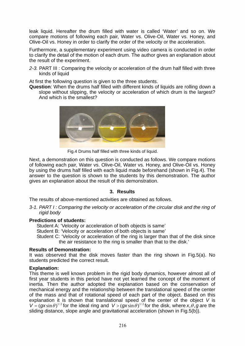
leak liquid. Hereafter the drum filled with water is called ‘Water’ and so on. We compare motions of following each pair, Water vs. Olive-Oil, Water vs. Honey, and

live-Oil vs. Honey in order to clarify the order of the velocity or the acceleration. O Furthermore, a supplementary experiment using video camera is conducted in order to clarify the detail of the motion of each drum. The author gives an explanation about the result of the experiment.

2-3. PART III : Comparing the velocity or acceleration of the drum half filled with three

kinds of liquid

At first the following question is given to the three students. Question: When the drums half filled with different kinds of liquids are rolling down a

slope without slipping, the velocity or acceleration of which drum is the largest? And which is the smallest?

Fig.4 Drums half filled with three kinds of liquid. Next, a demonstration on this question is conducted as follows. We compare motions of following each pair, Water vs. Olive-Oil, Water vs. Honey, and Olive-Oil vs. Honey by using the drums half filled with each liquid made beforehand (shown in Fig.4). The answer to the question is shown to the students by this demonstration. The author gives an explanation about the result of this demonstration.

3. Re ults s

T

he results of above-mentioned activities are obtained as follows.

3-1. PART I : Comparing the velocity or acceleration of the circular disk and the ring of rigid body

Predictions of students: Student A: ‘Velocity or acceleration of both objects is same’ Student B: ‘Velocity or acceleration of both objects is same’ Student C: ‘Velocity or acceleration of the ring is larger than that of the disk since

the air resistance to the ring is smaller than that to the disk.’ Results of Demonstration: It was observed that the disk moves faster than the ring shown in Fig.5(a). No tudents predicted the correct result. s

Explanation: This theme is well known problem in the rigid body dynamics, however almost all of first year students in this period have not yet learned the concept of the moment of inertia. Then the author adopted the explanation based on the conservation of mechanical energy and the relationship between the translational speed of the center of the mass and that of rotational speed of each part of the object. Based on this explanation it is shown that translational speed of the center of the object V is

2/1 for the ideal ring and 2/1 for the disk, where)sin( gxV )sin( gxV gx ,, are the sliding distance, slope angle and gravitational acceleration (shown in Fig.5(b)).

216

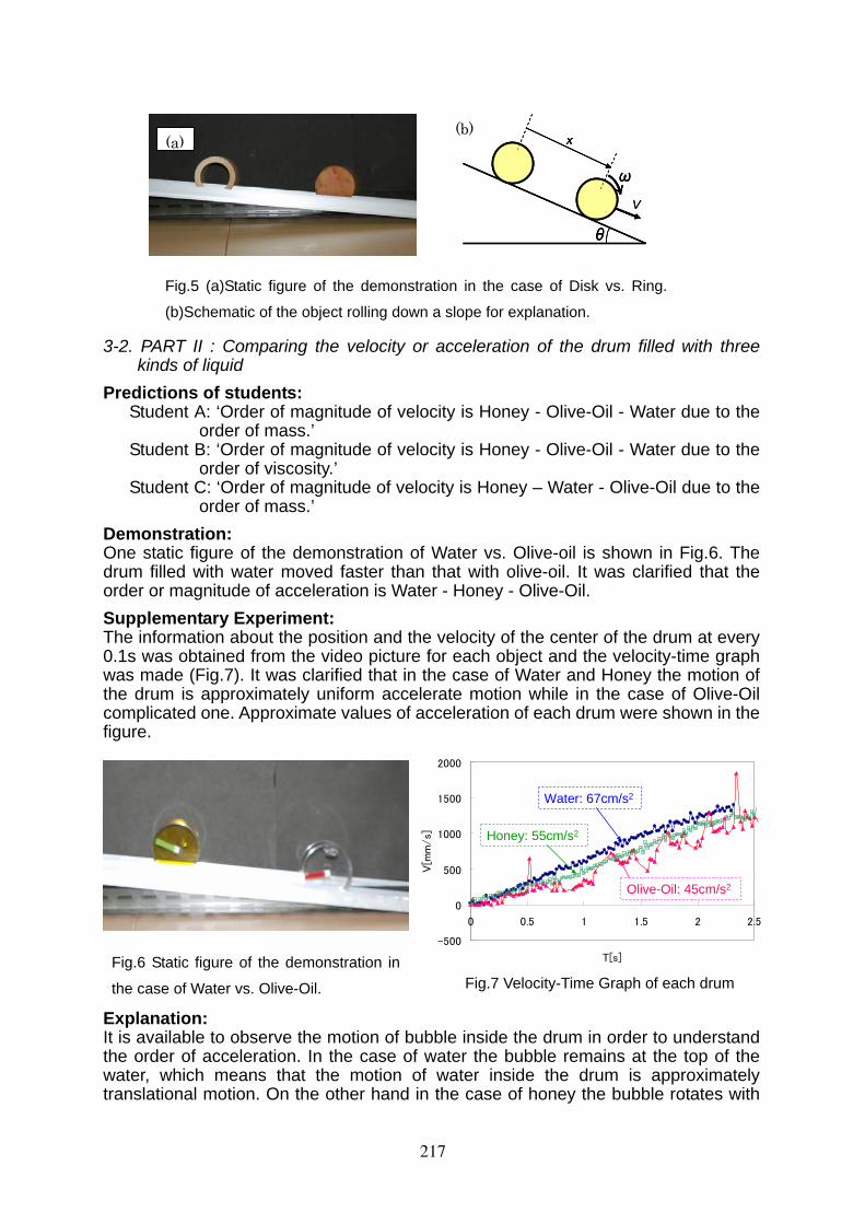
3-2. kinds of liquid

iction

PART II : Comparing the velocity or acceleration of the drum filled with three

red s of students:

gnitude of velocity is Honey - Olive-Oil - Water due to the

Student nitude of velocity is Honey - Olive-Oil - Water due to the

Student de of velocity is Honey – Water - Olive-Oil due to the

emonstraof the demonstration of Water vs. Olive-oil is shown in Fig.6. The

ion and the velocity of the center of the drum at every

observe the motion of bubble inside the drum in order to understand

P Student A: ‘Order of ma

order of mass.’ B: ‘Order of magorder of viscosity.’

C: ‘Order of magnituorder of mass.’

tion: D

One static figure drum filled with water moved faster than that with olive-oil. It was clarified that the order or magnitude of acceleration is Water - Honey - Olive-Oil.

upplementary Experiment: SThe information about the posit0.1s was obtained from the video picture for each object and the velocity-time graph was made (Fig.7). It was clarified that in the case of Water and Honey the motion of the drum is approximately uniform accelerate motion while in the case of Olive-Oil complicated one. Approximate values of acceleration of each drum were shown in the figure.

Explanation: It is available tothe order of acceleration. In the case of water the bubble remains at the top of the water, which means that the motion of water inside the drum is approximately translational motion. On the other hand in the case of honey the bubble rotates with

Fig.5 (a)Static figure of the demonstration in the case of Disk vs. Ring.

(b)Schematic of the object rolling down a slope for explanation.

V

θ

ω

x

V

θ

ω

x

θ

ω

(b)(a) x

Fig.6 Static figure of the demonstration in

-500

0

500

1000

1500

2000

0 0.5 1 1.5 2 2.5

T[s]

V[m

m/s]

the case of Water vs. Olive-Oil.

Water: 67cm/s2

Honey: 55cm/s2

Olive-Oil: 45cm/s2

-500

0

500

1000

1500

2000

0 0.5 1 1.5 2 2.5

T[s]

V[m

m/s]

Water: 67cm/s2

Honey: 55cm/s2

Olive-Oil: 45cm/s2

Fig.7 Velocity-Time Graph of each drum

217

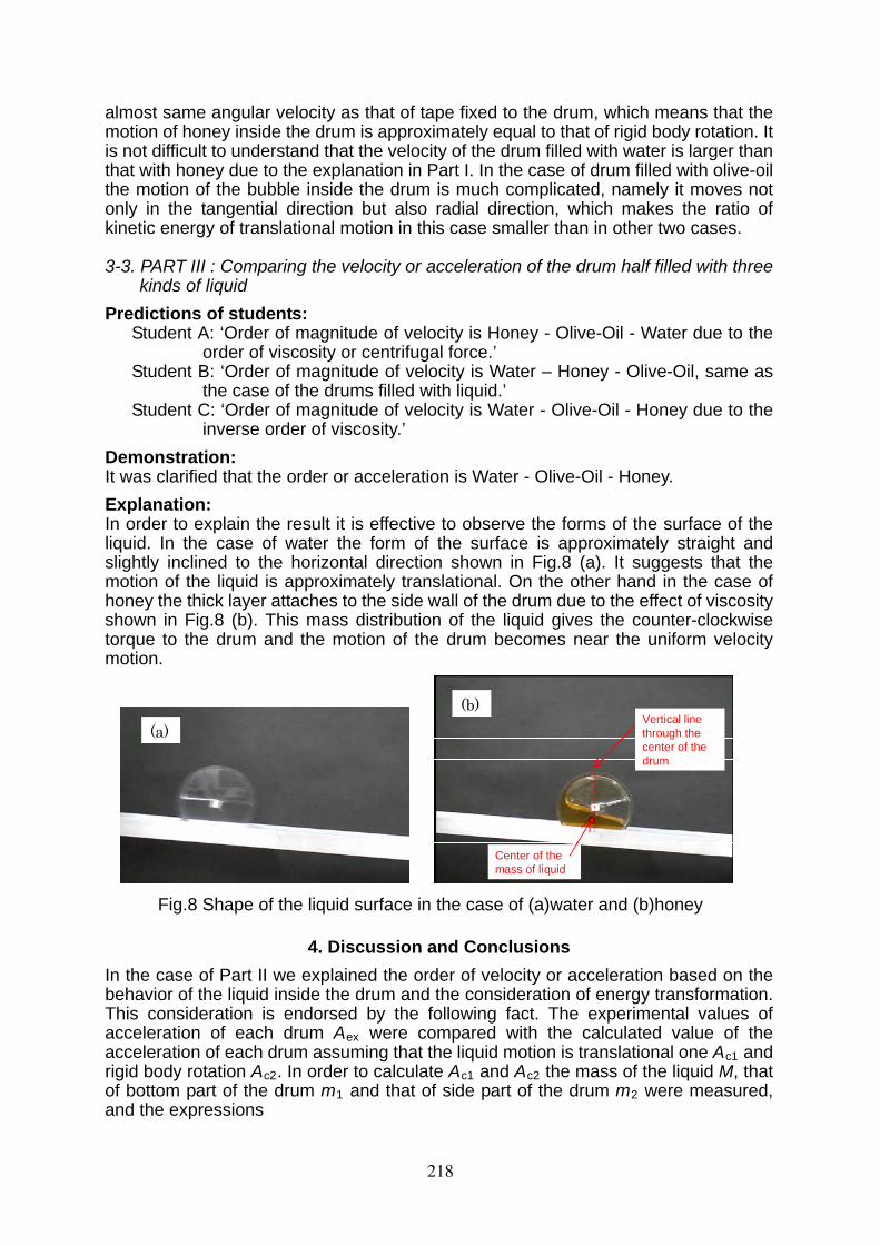
almost same angular velocity as that of tape fixed to the drum, which means that the motion of honey inside the drum is approximately equal to that of rigid body rotation. It is not difficult to understand that the velocity of the drum filled with water is larger than that with honey due to the explanation in Part I. In the case of drum filled with olive-oil the motion of the bubble inside the drum is much complicated, namely it moves not only in the tangential direction but also radial direction, which makes the ratio of kinetic energy of translational motion in this case smaller than in other two cases. 3-3. PART III : Comparing the velocity or acceleration of the drum half filled with three

red dents: gnitude of velocity is Honey - Olive-Oil - Water due to the

Student ater – Honey - Olive-Oil, same as

Student ter - Olive-Oil - Honey due to the

emonstrat the order or acceleration is Water - Olive-Oil - Honey.

lain the result it is effective to observe the forms of the surface of the

4. Discussion and Conclusions

In the case of Part II we e cceleration based on the

kinds of liquid

ictions of stuP Student A: ‘Order of ma

order of viscosity or centrifugal force.’ B: ‘Order of magnitude of velocity is Wthe case of the drums filled with liquid.’

C: ‘Order of magnitude of velocity is Wainverse order of viscosity.’

tion: D

It was clarified tha

xplanation: EIn order to expliquid. In the case of water the form of the surface is approximately straight and slightly inclined to the horizontal direction shown in Fig.8 (a). It suggests that the motion of the liquid is approximately translational. On the other hand in the case of honey the thick layer attaches to the side wall of the drum due to the effect of viscosity shown in Fig.8 (b). This mass distribution of the liquid gives the counter-clockwise torque to the drum and the motion of the drum becomes near the uniform velocity motion.

xplained the ord r of velocity or ae

behavior of the liquid inside the drum and the consideration of energy transformation. This consideration is endorsed by the following fact. The experimental values of acceleration of each drum Aex were compared with the calculated value of the acceleration of each drum assuming that the liquid motion is translational one Ac1 and rigid body rotation Ac2. In order to calculate Ac1 and Ac2 the mass of the liquid M, that of bottom part of the drum m1 and that of side part of the drum m2 were measured, and the expressions

Fig.8 Shape of the liquid surface in the case of (a)water and (b)honey

Center of the mass of liquid

Vertical line

through the center of thedrum

(b)

Center of the

Vertical line

(a) through the

center of thedrum

mass of liquid

218

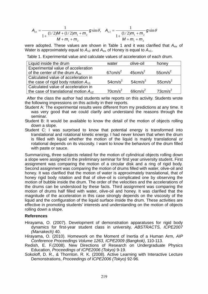
sin)2/1(

1

1,sin

)2/1()2/1(1

1

21

212

21

211 g

mmM

mmAg

mmM

mmMA cc

were adopted. These values are shown in Table 1 and it was clarified that Aex of ater is approximately equal to AW

c2 and Aex of Honey is equal to Ac1.

Table 1. Experimental value and calculate values of acceleration of each drum.

Liquid inside the drum water olive-oil honey Experimental value of acceleration of the center of the drum Aex 67cm/s2 45cm/s2 55cm/s2 Calculated value of acceleration in the case of rigid body rotation Ac1 54cm/s2 54cm/s2 55cm/s2 Calculated value of acceleration in the case of translational motion Ac2 70cm/s2 69cm/s2 73cm/s2

After the class the author had students write reports on this activity. Students wrote

the following impressions on this activity in their reports. Student A: The experimental results were different from my predictions at any time. It

was very good that we could clarify and understand the reasons through the seminar.

Student B: It would be available to know the detail of the motion of objects rolling down a slope.

Student C: I was surprised to know that potential energy is transformed into translational and rotational kinetic energy. I had never known that when the drum is filled with liquid whether the motion of the liquid is mainly translational or rotational depends on its viscosity. I want to know the behaviors of the drum filled with paste or sauce.

Summarizing, three subjects related for the motion of cylindrical objects rolling down a slope were assigned in the preliminary seminar for first year university student. First assignment was comparing the motion of a circular disk and a ring of rigid body. Second assignment was comparing the motion of drums filled with water, olive-oil and honey. It was clarified that the motion of water is approximately translational, that of honey rigid body rotation and that of olive-oil is complicated one by observing the motion of bubble inside the drum. The order of the velocities and the accelerations of the drums can be understood by these facts. Third assignment was comparing the motion of drums half filled with water, olive-oil and honey. It was clarified that the magnitude of the acceleration in this case strongly depends on the viscosity of the liquid and the configuration of the liquid surface inside the drum. These activities are effective in promoting students’ interests and understanding on the motion of objects olling down a slope. r

R

eferences

Hirayama, O. (2007). Development of demonstration apparatuses for rigid body dynamics for first-year student class in university, ABSTRACTS, ICPE2007 (Marrakech) 40.

Hirayama, O. (2010). Homework on the Moment of Inertia of a Human Arm, AIP Conference Proceedings Volume 1263, ICPE2009 (Bangkok), 110-113.

Redish, E. F.(2008). New Directions of Research on Undergraduate Physics Education, Proceedings of ICPE2006 (Tokyo) 9-19.

Sokoloff, D. R., & Thornton. R. K. (2008). Active Learning with Interactive Lecture Demonstrations, Proceedings of ICPE2006 (Tokyo) 92-96.

219

The search of conceptual clarity in two problems in electromagnetism: a finite wire with constant current and the concept of test charge

J. L. Jiménez1, I. Campos2 and J. A. E. Roa Neri3*

1 Departamento de Física, División de Ciencias Básicas e Ingeniería, Universidad Autónoma Metropolitana Unidad Iztapalapa.

2 Departamento de Física, Facultad de Ciencias, Universidad Nacional Autónoma de México.

3 Área de Física Teórica y Materia Condensada, División de Ciencias Básicas e Ingeniería, Universidad Autónoma Metropolitana Unidad Azcapotzalco.

* Corresponding author: rnjae@correo.azc.uam.mx

Abstract

In most texts on electromagnetism delicate or subtle conceptual aspects are overlooked, producing in perceptive students some confusion. In the present work we discuss two examples of conceptual obscurity. A) The magnetic field of a finite wire carrying a constant current, and B) the concept of test charge. We show that the finite wire with constant current is not really a problem in magnetostatics, while to understand the concept of test charge, we need to discuss the distinction between external and proper fields. These examples surely help students of beginning and intermediate university courses to understand these conceptual aspects in electromagnetism.

1. Introduction

The conceptual aspects of any physical subject are usually hard to deal with, but these are the most important themes in the education of any physics student. These conceptual aspects compel the student to analyze in deep the meaning of the concepts involved. In this work we discuss two conceptual problems that challenge the student of electromagnetism.

In Section 2, the magnetic field of a finite wire is analyzed. We show that if it is neglected the origin of the constant current it is also neglected fundamental aspects of the problem with great conceptual content that may be very useful to the student. The conservation of charge is a fundamental principle and it must be considered in order to get a correct flux of charge in a finite wire with constant current. In this way a consistent study of an electromagnetic situation is completely reached.

In Section 3, the concept of test charge is the focus of the discussion. We argue that the notion of an infinitesimal charge is confusing, since in Nature only finite charges seem to exist. In a general analysis both kind of fields, external and proper, must be taken into account and we exhibit the conditions under which only the external ones contribute to the force. In fact, in most cases the self interaction can be neglected except when one studies the radiation reaction, where self-interaction is relevant.

The aim in this paper is to offer the discussion of very fundamental aspects of electromagnetism in order to help the students to reach a deep understanding of it.

220

2. Segment of wire carrying a constant current

In undergraduate texts on electromagnetism Ampère´s law is used to calculate the magnetic field of an infinite straight wire carrying a constant current. Next the example of a finite segment of wire carrying a constant current is used to illustrate that the lack of symmetry does not permit the application of Ampère´s law, and the Biot-Savart law must be used instead, finding [Clayton and Nasar (1987), Resnick et al (2002), Tipler (2003), Young and Freedman (2008)]

, (1)

where

and

, respectively.

However, here we find a typical oversimplification that makes appear this problem as an example in magnetostatics, when indeed it is not. The question is that it is not discussed how a constant current can be established in a finite segment of wire. Where the charge comes from? Where does it go? This point is crucial and can be reformulated with the question, does charge conservation holds? As we will see, the answer is no, and this is obviously inconsistent with the laws of electromagnetism. Let us analyze this point. The law of conservation of charge is

. (2)

Then, if is a constant different of zero evidently there must be charge changing in time, so that eq. (2) holds.

In the present example, as solved in elementary and intermediate texts, there is not

any that guarantees conservation of charge. Then we have an evident violation of charge conservation, situation completely unacceptable.

This problem has been discussed from different points of view [Hnizdo (2003), Charitat and Graner (2003), Jiménez et al (2008)]. What we present here is an elementary approach accessible to beginning students of science and engineering.

Equation (2) implies that there must be charges depending on time at both ends of the wire given by

, (3)

and without lose of generality we can consider Q 0 as zero. With these charges there is associated an electric field given by

. (4)

It is important to note that in spite its appearance of a Coulombian field, it is not an electrostatic field, since the charges at the ends depend on time.

On the other hand, it is easy to show that if one proceeds to calculate the rotational of the field (1) the result is

, (5)

which does not satisfy the Ampère law of magnetostatics

221

(6)

because is a constant different from zero only in the z axis. But if we calculate the displacement current with the electric field (4), it results

. (7)

Then, what is happening? As we can see the Amperè-Maxwell law

(8)

is not satisfied . The displacement current appears but the current density is lost! As we will see bellow, the calculation of the rotational of the magnetic field has subtle aspects, usually overlooked, that is convenient to exhibit.

In fact, now we have that

, (9)

which comes from the integral form of Amperè’s law for a straight wire with constant current. We can see it as follows. As it is well known, in this case the magnetic field is given by

, (10)

then it must be satisfied that

; (11)

in order to this equation be satisfied, the identity (9) must hold.

To continue the calculation of the rotational it is necessary to use the following identity

(12)

with

(13)

and

. (14)

Then, using eq. (13) and (14) and after some laborious calculations the rotational of the field is the one given in eq. (5). It is easy to see that the first term on the right of

eq. (5) corresponds to

and the second one to

; therefore eq. (5) satisfies

the Ampère-Maxwell law eq. (8). It is important to remember that the conservation of the charge was the cornerstone used by Maxwell to establish the fundamental laws of Electrodynamics. It is a matter of consistency to study the behaviour of the charge in a finite wire. It is very important to emphasize the role that the singularities play in the analysis of the electromagnetic field and it is necessary to use distributions, even in elementary problems, for a better understanding. Rather than an obstacle, distributions are a conceptual aid for understanding.

222

3. About the concept of test charge. External fields and self fields

It is usual in basic university courses on electromagnetism to introduce the concept of electric field together with the concept of test charge. The “operational” definition of electric field is given by

, (15)

where is the force acting on the test charge due to the electric field . Frequently it is argued [Giancoli (2008)] that must be a very small charge, tending to zero, in order to avoid disturbing the field that is explored. There are some confusing aspects in this procedure. We must always have in mind that in Nature there are only finite charges. The texts expends a lot of time establishing this fact. So, what means to

take the limit ? What happen if the test charge is finite? How the field in which it is immersed is altered?

We can also see the problem in the following way: if in eq. (15) and the force on the charge must be finite, then the field must tend to infinity. One way of avoiding this problem is considering that is only the external field, thus eq. (15) can

be interpreted as , where is the field produced by the

particle with charge . By assuming that can be discarded, only

remains.

As we will see it is very important, for a good understanding of electromagnetic theory, that the student recognize, as early as possible, that the field appearing in Maxwell´s equations refer to the total fields, , and analogously for

magnetic fields . The Maxwell equations, on the other hand, can

be cast into the form of inhomogeneous wave equations, either for the potentials or for the fields.

Thus these linear, inhomogeneous, partial differential equations have as general solutions homogeneous solutions, corresponding to the case of no sources, (that is,

and are zero). On the other hand, we have particular solutions for the case of and different from zero. So, the general solutions are linear combinations of homogeneous solutions plus a particular inhomogeneous solution. This combination of solutions must satisfy the boundary conditions of the problem.

The physical interpretation of these solutions is that, for a given region of space, the homogeneous solutions are associated to charges and currents out of the region of interest, while the inhomogeneous solutions are associated to charges and currents within the given region, and correspond to self fields. Thus if we consider as the region of interest all space, we have only inhomogeneous solutions or self fields. The distinction between self and external fields is a crucial one when radiation reaction is studied.

Taking into account this distinction we can consider the Lorentz force density,

, (16)

where the usual interpretation is that the fields appearing in (16) are only the external fields by the arguments given above. By the way, the Lorentz force was considered an additional postulate until the advent of relativity, where it is seen as a consequence of the Lorentz transformations of the fields, but it can be demonstrated that electromagnetic theory implies that the force density (16) involves total fields. This can be done by means of vector and tensor identities, directly from the Maxwell

223

equations [Schwartz (1987), Heald and Marion (1995), Jiménez and Campos (1995), Griffiths (1999)].

Students of intermediate level or even (junior) graduates can approach the problem of test charges as follows.

Since the Maxwell equations refer to macroscopic electromagnetism, the momentum balance deduced from them is

, (17)

where the fields are the total fields, that is, homogeneous (external) fields, plus

inhomogeneous (self) fields. Also, and are any distributions of charge and current, and not only infinitesimal point charges.

Now we show with the aid of eq. (17) that the concept of test charge as an infinitesimal point charge is superfluous in electrostatics. In this case eq. (17) reduces to

. (18)

Let us consider now a point but finite charge inside a constant field which is the external field. Then the total field is in this case

. (19)

The force on charge q is the volume integral of eq. (18), and with the divergence

theorem we have that the force will be the surface integral over a closed surface surrounding the charge. Given the spherical symmetry of the self field, only the field

contributes to the force on the charge; then the eq. (15) is recovered.

Hence we conclude that in electrostatics there is no need of the concept of test charge. However, in the general case external as well as self fields act on a charge and current distribution. Indeed, as we say above, in studying radiation reaction, it is the interaction with the self field what it is studied.

4. Conclusions

In discussing problems in magnetostatics it is very important to check that conservation of charge is not violated. Simple problems do not always have simple solutions, but some of these problems may help to a better understanding of conceptual aspects, providing a more significant learning.

In most texts on electromagnetism the concept of field is introduced concurrently with the concept of test charge, implying that only the external field acts on the test charge. We consider that it is necessary that students distinguish external fields from self fields, both solutions of Maxwell´s equations, as well as the association of these fields with homogeneous and inhomogeneous solutions of the Maxwell equations.

Acknowledgements

The authors are grateful with L. A. Peralta for helping in the elaboration of the manuscript.

224

References

Charitat, T., & Graner, N. (2003). About the magnetic field of a finite wire. Eur. J. Phys. 24 267-270.

Clayton, C. R., & Nasar, S. A. (1987). Introduction to Electromagnetic Fields. New York: McGrawHill.

Giancoli, D. C. (2008). Physics for Scientists and Engineers Vol 2. 4th Ed. Upper Saddle River, NJ: Pearson Education, Inc.

Griffiths, D. J (1999). Introduction to Electrodynamics. 3rd Ed. New Jersey: Prentice Hall.

Hnizdo, H. (2003). Comment on “About the magnetic field of a finite wire”. Eur. J. Phys. 24 L15-L16.

Heald, M. H., & Marion, J. B. (1995). Classical Electromagnetic Radiation. 3rd Ed. Forth Worth: Saunders.

Jiménez, J. L., & Campos, I. (1995). The balance of energy and momentum in classical electrodynamics. In: T. Barret & D. Grimes (Eds.), Advanced Electromagnetic Theory and Applications (464-495). New Jersey: Ed. World Scientific.

Jiménez, J. L., Campos, I., & Aquino, N. (2008). Exact electromagnetic field produced by a finite wire with constant current. Eur. J. Phys. 29 163-175.

Resnick, R., Halliday, D. & Krane, K. (2002). Physics Vol. 2 5th Ed. New York: John Wiley & Sons.

Schwartz, M. (1987). Principles of Electrodynamics. New York: Dover.

Tipler, P. A. (2003). Physics for Scientist and Engineers 5th Ed. New York and Basingstoke: Freeman & Co.

Young, H. D., & R. A. Freeman, R. A. (2008). University Physics with Modern Physics Vol. 2. 12th Ed. San Francisco: Pearson Education Inc.

225

Electronic Collection of Solved Physics Problems – How to Create Your Own New Problem

Zdeňka Koupilová, Dana Mandiková, Marie Snětinová, Zdeněk Šabatka

marie.snetinova@mff.cuni.cz

Department of Physics Education, Faculty of Mathematics and Physics, Charles University in Prague, Czech Republic

Problem solving is one of the basic skills which students should learn during their physics education. In some schools quantitative problems are parts of lectures accompanying the physics course or specially designed seminars, focused on practicing of problem solving, which accompany each lecture. Unfortunately, in both cases there is lack of time to practice this ability enough, especially for students with inadequate previous education or mathematical skills. In addition hardly any suitable material for home study of these students exists in Czech. For this reason we have developed a collection of fully solved problems in physics (Koupilová et al., 2011). The collection contains elaborately annotated solutions, as well as notes, various hints and other tools to support students’ will to solve the problems independently. The collection exists in electronic version and so it is possible to be used interactively to lead students to solve problems without previous reading of the detailed solution. The user interface of the collection was mainly presented on the last years’ GIREP conferences. This year we introduce the administrator interface instead. This interface was designed with emphasis on an easy and comfortable inserting of new problems into the collection.

Introduction

Solving quantitative physics tasks is used at all school levels as a relatively easy way how to practice gained knowledge and how to deepen the understanding of the physics context. But there is not enough time to solve sufficient number of problems during school lessons and seminars. Moreover, students come to schools with different problem solving skills. Therefore, it is useful to provide students with sufficient opportunities for their home study.

The common collections of unsolved problems used in the Czech Republic (e.g. Lepil, 1995) are not very suitable for home study, because students do not have any support when they are incapable to solve the problem independently. On the other hand, only reading a solved problem is not an appropriate way how to learn to solve physics problems either. For this reason an electronic collection of problems (Koupilová et al., 2011) is being developed in our department.

The database uses interactive components and links to help its users to learn how to solve physics problems independently. All problems in the collection contain elaborately annotated solutions, various hints, notes and other tools to lead users to active thinking about presented physics problems. The collection is designed especially for students to practice and deepen the knowledge gained at secondary school and for secondary school students with a greater interest in physics. But it could be useful for physics teachers as well.

User interface

The electronic collection was designed to suit the majority of users. It means to be simple to handle as well as to be interesting. The main aspect during the creation of the user interface was to design the structure of the whole database sufficiently flexible and multi-purpose.

226

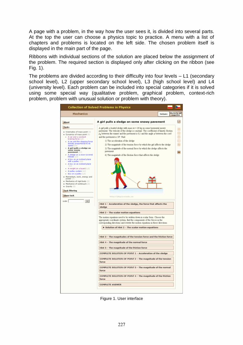
A page with a problem, in the way how the user sees it, is divided into several parts. At the top the user can choose a physics topic to practice. A menu with a list of chapters and problems is located on the left side. The chosen problem itself is displayed in the main part of the page.

Ribbons with individual sections of the solution are placed below the assignment of the problem. The required section is displayed only after clicking on the ribbon (see Fig. 1).

The problems are divided according to their difficulty into four levels – L1 (secondary school level), L2 (upper secondary school level), L3 (high school level) and L4 (university level). Each problem can be included into special categories if it is solved using some special way (qualitative problem, graphical problem, context-rich problem, problem with unusual solution or problem with theory).

Figure 1. User interface

227

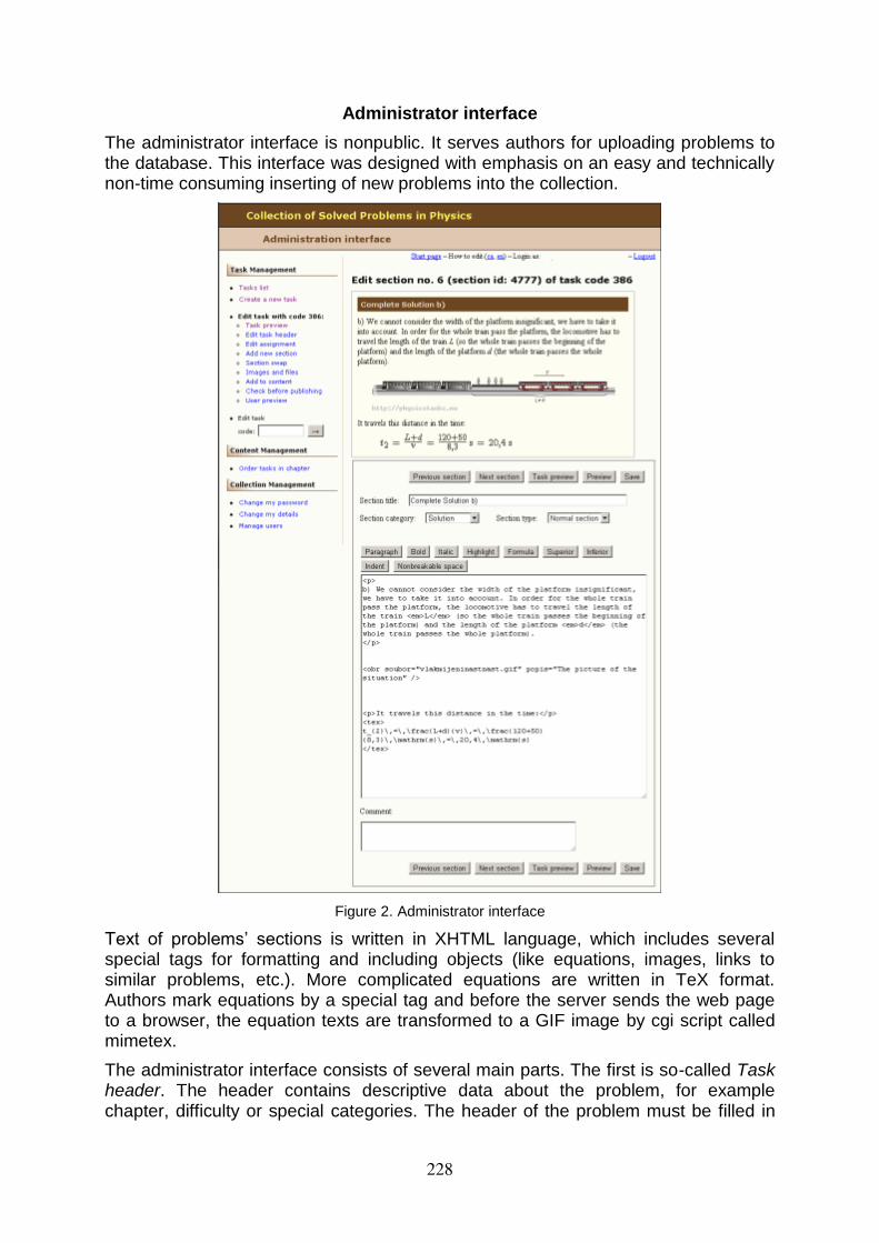
Administrator interface

The administrator interface is nonpublic. It serves authors for uploading problems to the database. This interface was designed with emphasis on an easy and technically non-time consuming inserting of new problems into the collection.

Figure 2. Administrator interface

Text of problems’ sections is written in XHTML language, which includes several special tags for formatting and including objects (like equations, images, links to similar problems, etc.). More complicated equations are written in TeX format. Authors mark equations by a special tag and before the server sends the web page to a browser, the equation texts are transformed to a GIF image by cgi script called mimetex.

The administrator interface consists of several main parts. The first is so-called Task header. The header contains descriptive data about the problem, for example chapter, difficulty or special categories. The header of the problem must be filled in

228

before an author starts to create a new problem. After creating the task header, it is possible to insert an assignment of the problem and individual sections of the solution.

How to become a task creator

At the present time the electronic collection has not only Czech but also English and Polish version, and it is prepared for extension to other languages. The administrator interface is completely in English for this reason.

We offer to all interested persons a database and the interface to create own collection of fully solved problems. If you are interested to setting up a collection with problems in your language, please contact us at the address: sbirka@kdf.mff.cuni.cz.

Conclusion

We introduced the electronic collection of fully solved problems in physics and primarily its administrator interface at the workshop in GIREP-EPEC 2011. Participants of the workshop had an opportunity to try creating their own task. They worked in the administrator interface and found the submitting of the tasks (into the collection) really simple and user friendly.

In this workshop we discussed the usability of the collection. According to reactions of participants, the electronic collection is suitably designed and could be useful and helpful in physics education.

The collection is available at the website of the Department of Physics Education, Faculty of Mathematics and Physics, Charles University in Prague: http://physicstasks.eu/. It is available for students of the department as well as for public.

Because we obtained very positive experience in using the collection in Czech (according to users – students as well as teachers – response) we have translated the administrator interface into English and we offer the database and the interface to other task creators.

Acknowledgement

The present work was supported by the Charles University Grant Agency (grant No. 374711).

References

Koupilová, Z., et al. (2011, July 28). Collection of Solved Problems in Physics. Retrieved from: http://physicstasks.eu/

Lepil, O., et al. (1995). Fyzika: Sbírka úloh pro střední školy. Praha: Prometheus. (only in Czech)

Žák, V. (2011). Fyzikální úlohy pro střední školy. Praha: Prometheus. (only in Czech)

229

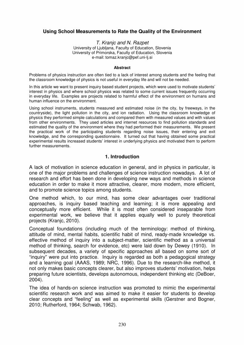
Using School Measurements to Rate the Quality of the Environment

T. Kranjc and N. Razpet University of Ljubljana, Faculty of Education, Slovenia University of Primorska, Faculty of Education, Slovenia

e-mail: tomaz.kranjc@pef.uni-lj.si

Abstract

Problems of physics instruction are often tied to a lack of interest among students and the feeling that the classroom knowledge of physics is not useful in everyday life and will not be needed.

In this article we want to present inquiry based student projects, which were used to motivate students’ interest in physics and where school physics was related to some current issues frequently occurring in everyday life. Examples are projects related to harmful effect of the environment on humans and human influence on the environment.

Using school instruments, students measured and estimated noise (in the city, by freeways, in the countryside), the light pollution in the city, and ion radiation. Using the classroom knowledge of physics they performed simple calculations and compared them with measured values and with values from other environments. They used articles and internet resources to find pollution standards and estimated the quality of the environment where they had performed their measurements. We present the practical work of the participating students regarding noise issues, their entering and exit knowledge, and the corresponding questionnaire. It turned out that having obtained some practical experimental results increased students’ interest in underlying physics and motivated them to perform further measurements.

1. Introduction

A lack of motivation in science education in general, and in physics in particular, is one of the major problems and challenges of science instruction nowadays. A lot of research and effort has been done in developing new ways and methods in science education in order to make it more attractive, clearer, more modern, more efficient, and to promote science topics among students.

One method which, to our mind, has some clear advantages over traditional approaches, is inquiry based teaching and learning; it is more appealing and conceptually more efficient. While it is most often considered inseparable from experimental work, we believe that it applies equally well to purely theoretical projects (Kranjc, 2010).

Conceptual foundations (including much of the terminology: method of thinking, attitude of mind, mental habits, scientific habit of mind, ready-made knowledge vs. effective method of inquiry into a subject-matter, scientific method as a universal method of thinking, search for evidence, etc) were laid down by Dewey (1910). In subsequent decades, a variety of specific approaches all based on some sort of “inquiry” were put into practice. Inquiry is regarded as both a pedagogical strategy and a learning goal (AAAS, 1989; NRC, 1996). Due to the research-like method, it not only makes basic concepts clearer, but also improves students’ motivation, helps preparing future scientists, develops autonomous, independent thinking etc (DeBoer, 2004).

The idea of hands-on science instruction was promoted to mimic the experimental scientific research work and was aimed to make it easier for students to develop clear concepts and “feeling” as well as experimental skills (Gerstner and Bogner, 2010; Rutherford, 1964; Schwab, 1962).

230

The idea of “inquiry based” education is often linked to laboratory work, which may be completely integrated into the course and basically drives it. This should create an “investigative science learning environment” (ISLE), which is aimed to help students understand how the body of knowledge is constructed and develop scientific habits of mind (Etkina and Van Heuvelen, 2001; Karelina and Etkina, 2007). In the lab, students design their own experiments and proceed in a scientific-like way: find relations, make and test hypotheses, communicate, discuss and question results, make decisions, get used to team work, write reports etc and, at every step, spend some time in “sense-making” of their actions (Etkina, 2010).

Demir and Abell (2010) take from NRC (2000) “five essential features” of inquiry as a pedagogical process: a student (a) engages in scientifically oriented questions, (b) gives priority to evidence in responding to questions, (c) formulates explanations from evidence; (d) connects explanations to scientific knowledge, and (e) communicates and justifies explanations. While these “features” may seem obvious and represent the basic characteristics of a scientific-like research work, they are not self-evident to students in their practical procedures (not rarely they give priority to previously acquired knowledge rather than to experimental or other evidence) and a lot of effort is needed to overcome their pre-made misconceptions (Kranjc and Razpet, 2010).

Several authors investigated the influence of a teacher’s background, experiences, and conceptions of science instruction, on his/her methods of teaching science. Previous science experiences may have negative influence on teachers’ views of inquiry (Windschitl, 2003). Teachers may hold competing belief sets—constraining and promoting inquiry, the first originating primarily from a school culture, the latter from individual teacher’s experience in science learning (Wallace and Kang, 2004). Teachers’ conceptions of presenting science are difficult to change (Koballa et al., 2005). This is a very important point: if science teachers are expected to implement some kind of inquiry-based teaching in their classes, they should receive appropriate beliefs, habits and practices during their study from their teachers and from their school environment.

“Students’ authentic questions” are justly considered one of the basic features of inquiry based instruction (Keys and Bryan, 2001). This may induce them to perform their own practical “research” propelled by their curiosity and/or particular interest. According to Haury (1993), “there is no authentic investigation or meaningful learning if there is no inquiring mind seeking an answer, solution, explanation, or decision.” Sometimes, it is possible for such interests to be included within regular physics instruction, sometimes they can also be performed outside of the regular classes. Starting from questions seemingly far from topics of physics instruction, inquiry based instruction may make it possible to learn physics in a natural way.

The research questions therefore are: On the basis of what is known to be interesting for students, can, and to what extent, the “curriculum” physics be learnt by taking a detour and considering topics that are more appealing but not necessarily included in the curriculum? To what extent can “non-curriculum” material be offered to students without “endangering” the curriculum?

It should be emphasized that treating the “non-curriculum” topics is not a waste of time (neither for students nor for the teacher). They show that physics is linked to the everyday life, that it gives answers to the questions of everyday life, and offers solutions to everyday problems.

231

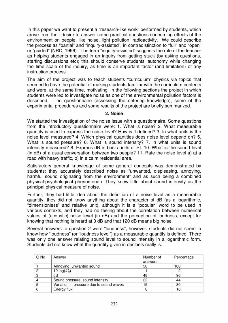
In this paper we want to present a “research-like work” performed by students, which arose from their desire to answer some practical questions concerning effects of the environment on people, like noise, light pollution, radioactivity. We could describe the process as “partial” and “inquiry-assisted”, in contradistinction to “full” and “open” or “guided” (NRC, 1996). The term “inquiry-assisted” suggests the role of the teacher as helping students engaged in an inquiry from getting stuck (by asking questions, starting discussions etc); this should conserve students’ autonomy while changing the time scale of the inquiry, as time is an important factor (and limitation) of any instruction process.

The aim of the project was to teach students “curriculum” physics via topics that seemed to have the potential of making students familiar with the curriculum contents and were, at the same time, motivating. In the following sections the project in which students were led to investigate noise as one of the environmental pollution factors is described. The questionnaire (assessing the entering knowledge), some of the experimental procedures and some results of the project are briefly summarized.

2. Noise

We started the investigation of the noise issue with a questionnaire. Some questions from the introductory questionnaire were: 1. What is noise? 2. What measurable quantity is used to express the noise level? How is it defined? 3. In what units is the noise level measured? 4. Which physical quantities does noise level depend on? 5. What is sound pressure? 6. What is sound intensity? 7. In what units is sound intensity measured? 8. Express dB in basic units of SI. 10. What is the sound level (in dB) of a usual conversation between two people? 11. Rate the noise level a) at a road with heavy traffic, b) in a calm residential area.

Satisfactory general knowledge of some general concepts was demonstrated by students: they accurately described noise as “unwanted, displeasing, annoying, harmful sound originating from the environment” and as such being a combined physical-psychological phenomenon. They knew little about sound intensity as the principal physical measure of noise.

Further, they had little idea about the definition of a noise level as a measurable quantity, they did not know anything about the character of dB (as a logarithmic, “dimensionless” and relative unit), although it is a “popular” word to be used in various contexts, and they had no feeling about the correlation between numerical values of (acoustic) noise level (in dB) and the perception of loudness, except for knowing that nothing is heard at 0 dB and that 120 dB means big noise.

Several answers to question 2 were “loudness”; however, students did not seem to know how “loudness” (or “loudness level”) as a measurable quantity is defined. There was only one answer relating sound level to sound intensity in a logarithmic form. Students did not know what the quantity given in decibels really is.

Q No Answer Number of

answers Percentage

1 Annoying, unwanted sound 50 100 2 10 log(I/I0) 1 2 3 dB 48 96 4 Sound pressure, sound intensity 22 44 5 Variation in pressure due to sound waves 15 30 6 Energy flux 8 16

232

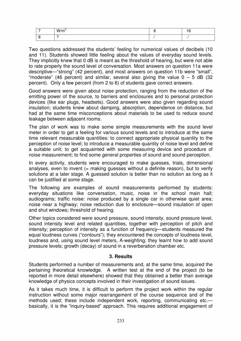
7 W/m2 8 16 8 ? / /

Two questions addressed the students’ feeling for numerical values of decibels (10 and 11). Students showed little feeling about the values of everyday sound levels. They implicitly knew that 0 dB is meant as the threshold of hearing, but were not able to rate properly the sound level of conversation. Most answers on question 11a were descriptive—“strong” (42 percent), and most answers on question 11b were “small”, “moderate” (46 percent) and similar, several also giving the value 0 – 5 dB (32 percent). Only a few percent (from 2 to 6) of students gave correct answers.

Good answers were given about noise protection, ranging from the reduction of the emitting power of the source, to barriers and enclosures and to personal protection devices (like ear plugs, headsets). Good answers were also given regarding sound insulation; students knew about damping, absorption, dependence on distance, but had at the same time misconceptions about materials to be used to reduce sound leakage between adjacent rooms.

The plan of work was to make some simple measurements with the sound level meter in order to get a feeling for various sound levels and to introduce at the same time relevant measurable quantities: to connect appropriate physical quantity to the perception of noise level; to introduce a measurable quantity of noise level and define a suitable unit; to get acquainted with some measuring device and procedure of noise measurement; to find some general properties of sound and sound perception.

In every activity, students were encouraged to make guesses, trials, dimensional analyses, even to invent (= making guesses without a definite reason), but to verify solutions at a later stage. A guessed solution is better than no solution as long as it can be justified at some stage.

The following are examples of sound measurements performed by students: everyday situations like conversation, music, noise in the school main hall; audiograms; traffic noise: noise produced by a single car in otherwise quiet area; noise near a highway; noise reduction due to enclosure—sound insulation of open and shut windows; threshold of hearing.

Other topics considered were sound pressure, sound intensity, sound pressure level, sound intensity level and related quantities, together with perception of pitch and intensity; perception of intensity as a function of frequency—students measured the equal loudness curves (“contours”); they encountered the concepts of loudness level, loudness and, using sound level meters, A-weighting; they learnt how to add sound pressure levels; growth (decay) of sound in a reverberation chamber etc.

3. Results

Students performed a number of measurements and, at the same time, acquired the pertaining theoretical knowledge. A written test at the end of the project (to be reported in more detail elsewhere) showed that they obtained a better than average knowledge of physics concepts involved in their investigation of sound issues.

As it takes much time, it is difficult to perform the project work within the regular instruction without some major rearrangement of the course sequence and of the methods used; these include independent work, reporting, communicating etc.—basically, it is the “inquiry-based” approach. This requires additional engagement of

233

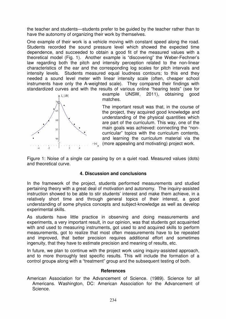
the teacher and students—students prefer to be guided by the teacher rather than to have the autonomy of organizing their work by themselves.

One example of their work is a vehicle moving with constant speed along the road. Students recorded the sound pressure level which showed the expected time dependence, and succeeded to obtain a good fit of the measured values with a theoretical model (Fig. 1). Another example is “discovering” the Weber-Fechner’s law regarding both the pitch and intensity perception related to the non-linear characteristics of the ear and the corresponding log scales for pitch intervals and intensity levels. Students measured equal loudness contours; to this end they needed a sound level meter with linear intensity scale (often, cheaper school instruments have only the A-weighted scale). They compared their findings with standardized curves and with the results of various online “hearing tests” (see for

example UNSW, 2011), obtaining good matches.

The important result was that, in the course of the project, they acquired good knowledge and understanding of the physical quantities which are part of the curriculum. This way, one of the main goals was achieved: connecting the “non-curricular” topics with the curriculum contents, and learning the curriculum material via the (more appealing and motivating) project work.

Figure 1: Noise of a single car passing by on a quiet road. Measured values (dots) and theoretical curve.

4. Discussion and conclusions

In the framework of the project, students performed measurements and studied pertaining theory with a great deal of motivation and autonomy. The inquiry-assisted instruction showed to be able to stir students’ interest and make them achieve, in a relatively short time and through general topics of their interest, a good understanding of some physics concepts and subject-knowledge as well as develop experimental skills.

As students have little practice in observing and doing measurements and experiments, a very important result, in our opinion, was that students got acquainted with and used to measuring instruments, got used to and acquired skills to perform measurements, got to realize that most often measurements have to be repeated and improved, that better precision requires additional effort and sometimes ingenuity, that they have to estimate precision and meaning of results, etc.

In future, we plan to continue with the project work using inquiry-assisted approach, and to more thoroughly test specific results. This will include the formation of a control groups along with a “treatment” group and the subsequent testing of both.

References

American Association for the Advancement of Science. (1989). Science for all Americans. Washington, DC: American Association for the Advancement of Science.

234

Dewey, J. (1910). Science as subject matter and as method. Science, 31 (786), 121–127.

DeBoer, G.E. (2004). Historical perspective on inquiry teaching in schools. In L. Flick & N. Lederman (Eds.), Scientific inquiry and the nature of science: Implications for teaching, learning, and teacher education (pp. 17–35). Dordrecht, The Netherlands: Kluwer.

Demir, A. and Abell, S.K. (2010). Views of Inquiry: Mismatches Between Views of Science Education Faculty and Students of an Alternative Certification Program. Journal of research and science teaching, 47 (6), 716-741.

Etkina, E. and Van Heuvelen, A., 2001. Investigative Science Learning Environment: Using the processes of science and cognitive strategies to learn physics, Proceedings of the 2001 Physics Education Research Conference. Rochester, NY, PERC publishing, 17-21.

Etkina, E. (2010). Helping our students learn physics and think like scientists (plenary talk), GIREP-ICPE-MPTL Conference 2010, “Teaching and Learning Physics today: Challenges? Benefits?”, Aug. 22 – 27, 2010, Reims, France.

Gerstner, S. and Bogner, F.X. (2010). Cognitive Achievement and Motivation in Handson and TeacherCentred Science Classes: Does an additional handson consolidation phase (concept mapping) optimise cognitive learning at work stations? International Journal of Science EducationVolume, 32 (7), 849-870.

Haury, D. L. (1993). Teaching Science through Inquiry. ERIC/CSMEE Digest. http://www.ericdigests.org/1993/inquiry.htm (visited October 19, 2011).

Karelina, A. and Etkina, E., 2007. Acting like a physicist: Student approach study to experimental design, Phys. Rev. ST Physics Ed. Research 3, 020106.

Keys, C.W., & Bryan, L.A. (2001). Co-constructing inquiry-based science with teachers: Essential research for lasting reform. Journal of Research in Science Teaching, 38, 631–645.

Koballa, T.R., Glynn, S.M., Upson, L., & Coleman, D.C. (2005). Conceptions of teaching science held by novice teachers in an alternative certification program. Journal of Science Teacher Education, 16, 287–308.

Kranjc, T. (2010). Intuitive approach to defects in liquid crystals. Submitted for publication in proceedings GIREP-ICPE-MPTL Conference 2010, “Teaching and Learning Physics today: Challenges? Benefits?”, Aug. 22 – 27, 2010, Reims, France.

Kranjc, T. and Razpet, N. (2010). We are teaching students - what do they know?. In: RAINE, Derek (Ed.). Physics community and cooperation : selected contributions. Leicester: Lulu, The Centre for Interdisciplinary Science, cop. 2010, str. 65-75.

National Research Council. (1996). National science education standards. Washington, DC: National Academy Press.

National Research Council. (2000). Inquiry and the national science education standards. Washington, DC: National.

Rutherford, F.J. (1964). The role of inquiry in science teaching. Journal of Research in Science Teaching, 2, 80–84.

Schwab, J.J. (1962). The teaching of science as enquiry. In J.J. Schwab & P.F. Brandwein (Eds.), The teaching of science (pp. 1–103). Cambridge, MA: Harvard University.

UNSW, http://www.phys.unsw.edu.au/music/ (site visited July 26, 2011). Windschitl, M. (2003). Inquiry projects in science teacher education: What can

investigative experiences reveal about teacher thinking and eventual classroom practice? Science Education, 87, 112–143.

235

UsingUsingUsingUsing MicrotribologyMicrotribologyMicrotribologyMicrotribology totototo TeachTeachTeachTeach FrictionFrictionFrictionFrictionYasuhiro Kudo1 and Eizo Ohno2

gzq05637@nifty.com1 Hokkaido University Graduate School of Education, Japan and

2Hokkaido University Faculty of Education, Japan

Friction is a familiar word for students. However, many students don’t understand friction as ascientific concept. The concept of friction is taught as phenomenological laws and the micro-scopic mechanism of friction are not explained in high school physics in Japan. Microtribologyhas been developing in the 20th century, and microscopic mechanisms of friction are revealed. Inthis article, we use one of the results of microtribology (the real contact points) in order to showchildren and students a difference between apparent contact area and real contact area. Thefeasibility studies of the teaching materials are conducted with elementary school children andteacher training university students in Japan. The teaching materials are the following: (A) Sandaland floorboards having asperities, (B) Transparent box containing glass beads, (C) Block whichhas ripped sponge attached to it, (D) Coins and a football field. The result of the feasibility studiesshows that the image of the real contact points helps children and students understand the word‘friction’ as a scientific concept and properties of friction.

1.1.1.1. IntroductionIntroductionIntroductionIntroduction1.1 Background

Friction is a familiar word for children. Junior high school students usually use theword ’friction’ in everyday conversation. However, many students don’t understandfriction as a scientific concept. Friction forces are unavoidable in our daily lives. Thefriction force opposes sliding of the touching objects relative to each other around us.Students need ‘friction’ as a scientific concept in order to explain motions of objectsby using the laws of dynamical mechanics.The following four properties of friction are important. The properties 1) to 4) aredescribed in high school physics textbooks in Japan. However, the microscopicmechanism about those properties is not explained (Kudo 2007, 2009). Themicroscopic mechanism related to the properties 3) and 4) (kinetic friction) is stillunder research in the microtribology. Therefore, we consider the properties 1), 2), inthis article.1) The magnitude of static friction force has a maximum value that is proportional tothe normal force.

2) The magnitude of static friction force is independent of the apparent contact area.3) The magnitude of kinetic friction force is proportional to the normal force and lowerthan the maximum value of static friction force.

4) The magnitude of kinetic friction force does not depend on the sliding velocity.1.2 Microtribology

Microtribology has been developing in 20th century and microscopic mechanisms offriction are revealed (Dowson 1998, Bhushan 2002). According to the intensiveresearch, the real microscopic area of contact is much less than the apparentmacroscopic contact area (Figure 1(a)). The real contact consists of small points(Bowden and Tabor 1954). The number of the real contact points is proportional to

236

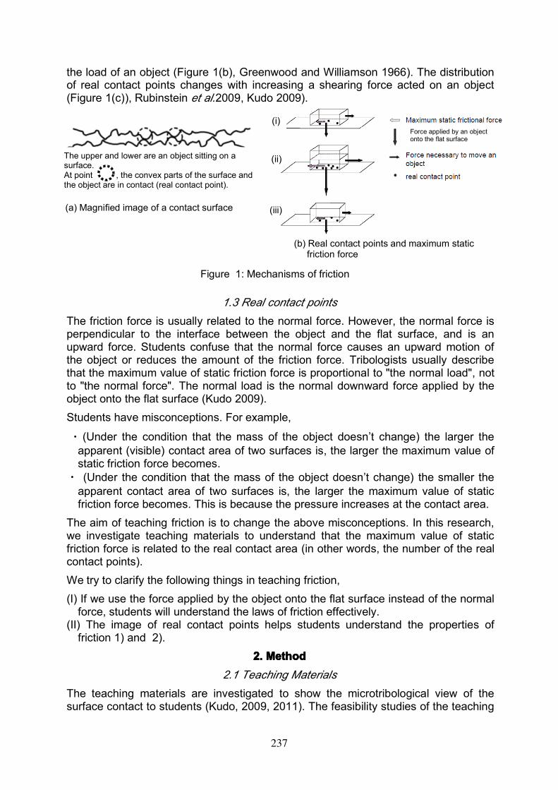
the load of an object (Figure 1(b), Greenwood and Williamson 1966). The distributionof real contact points changes with increasing a shearing force acted on an object(Figure 1(c)), Rubinstein et al.2009, Kudo 2009).

1.3 Real contact pointsThe friction force is usually related to the normal force. However, the normal force isperpendicular to the interface between the object and the flat surface, and is anupward force. Students confuse that the normal force causes an upward motion ofthe object or reduces the amount of the friction force. Tribologists usually describethat the maximum value of static friction force is proportional to "the normal load", notto "the normal force". The normal load is the normal downward force applied by theobject onto the flat surface (Kudo 2009).Students have misconceptions. For example,

・ (Under the condition that the mass of the object doesn’t change) the larger theapparent (visible) contact area of two surfaces is, the larger the maximum value ofstatic friction force becomes.

・ (Under the condition that the mass of the object doesn’t change) the smaller theapparent contact area of two surfaces is, the larger the maximum value of staticfriction force becomes. This is because the pressure increases at the contact area.

The aim of teaching friction is to change the above misconceptions. In this research,we investigate teaching materials to understand that the maximum value of staticfriction force is related to the real contact area (in other words, the number of the realcontact points).We try to clarify the following things in teaching friction,(I) If we use the force applied by the object onto the flat surface instead of the normalforce, students will understand the laws of friction effectively.

(II) The image of real contact points helps students understand the properties offriction 1) and 2).

2.2.2.2. MethodMethodMethodMethod2.1 Teaching Materials

The teaching materials are investigated to show the microtribological view of thesurface contact to students (Kudo, 2009, 2011). The feasibility studies of the teaching

(a) Magnified image of a contact surface

(b) Real contact points and maximum staticfriction force

The upper and lower are an object sitting on asurface.At point , the convex parts of the surface andthe object are in contact (real contact point).

Force applied by an objectonto the flat surface

(i)

(ii)

(iii)

Figure 1: Mechanisms of friction

237

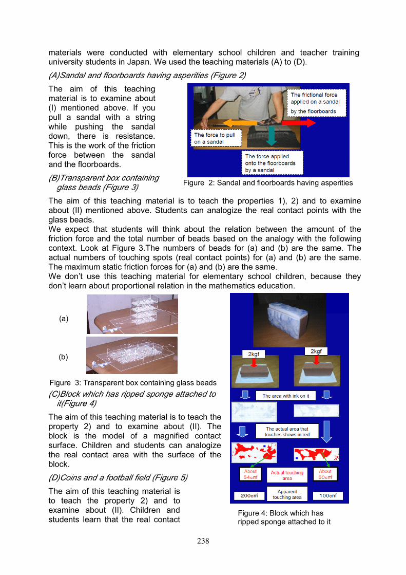
materials were conducted with elementary school children and teacher traininguniversity students in Japan. We used the teaching materials (A) to (D).(A)Sandal and floorboards having asperities (Figure 2)The aim of this teachingmaterial is to examine about(I) mentioned above. If youpull a sandal with a stringwhile pushing the sandaldown, there is resistance.This is the work of the frictionforce between the sandaland the floorboards.(B)Transparent box containingglass beads (Figure 3)

The aim of this teaching material is to teach the properties 1), 2) and to examineabout (II) mentioned above. Students can analogize the real contact points with theglass beads.We expect that students will think about the relation between the amount of thefriction force and the total number of beads based on the analogy with the followingcontext. Look at Figure 3.The numbers of beads for (a) and (b) are the same. Theactual numbers of touching spots (real contact points) for (a) and (b) are the same.The maximum static friction forces for (a) and (b) are the same.We don’t use this teaching material for elementary school children, because theydon’t learn about proportional relation in the mathematics education.

(C)Block which has ripped sponge attached toit(Figure 4)

The aim of this teaching material is to teach theproperty 2) and to examine about (II). Theblock is the model of a magnified contactsurface. Children and students can analogizethe real contact area with the surface of theblock.(D)Coins and a football field (Figure 5)The aim of this teaching material isto teach the property 2) and toexamine about (II). Children andstudents learn that the real contact

Figure 2: Sandal and floorboards having asperities

Figure 3: Transparent box containing glass beads

(a)

(b)

Figure 4: Block which hasripped sponge attached to it

238

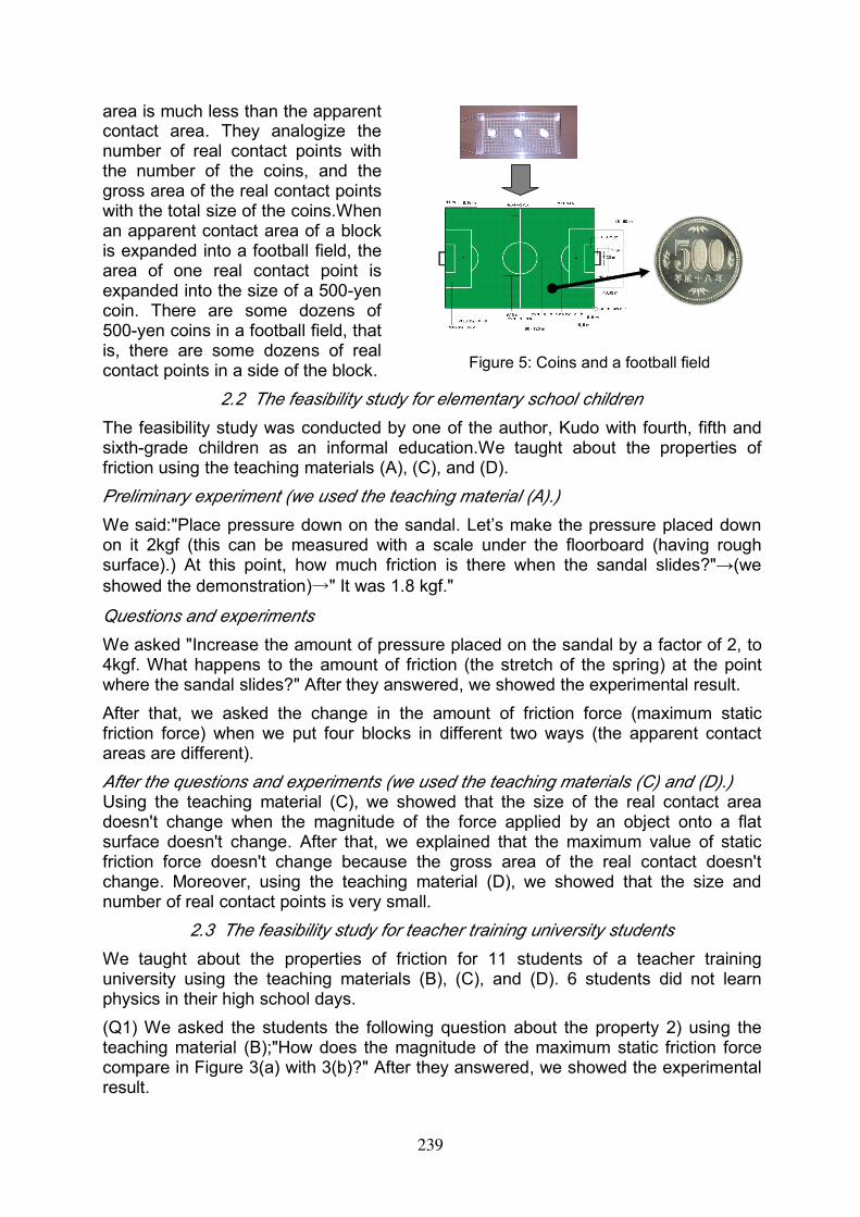
area is much less than the apparentcontact area. They analogize thenumber of real contact points withthe number of the coins, and thegross area of the real contact pointswith the total size of the coins.Whenan apparent contact area of a blockis expanded into a football field, thearea of one real contact point isexpanded into the size of a 500-yencoin. There are some dozens of500-yen coins in a football field, thatis, there are some dozens of realcontact points in a side of the block.

2.2 The feasibility study for elementary school childrenThe feasibility study was conducted by one of the author, Kudo with fourth, fifth andsixth-grade children as an informal education.We taught about the properties offriction using the teaching materials (A), (C), and (D).Preliminary experiment (we used the teaching material (A).)We said:"Place pressure down on the sandal. Let’s make the pressure placed downon it 2kgf (this can be measured with a scale under the floorboard (having roughsurface).) At this point, how much friction is there when the sandal slides?"→(weshowed the demonstration)→" It was 1.8 kgf."

Questions and experimentsWe asked "Increase the amount of pressure placed on the sandal by a factor of 2, to4kgf. What happens to the amount of friction (the stretch of the spring) at the pointwhere the sandal slides?" After they answered, we showed the experimental result.After that, we asked the change in the amount of friction force (maximum staticfriction force) when we put four blocks in different two ways (the apparent contactareas are different).After the questions and experiments (we used the teaching materials (C) and (D).)Using the teaching material (C), we showed that the size of the real contact areadoesn't change when the magnitude of the force applied by an object onto a flatsurface doesn't change. After that, we explained that the maximum value of staticfriction force doesn't change because the gross area of the real contact doesn'tchange. Moreover, using the teaching material (D), we showed that the size andnumber of real contact points is very small.

2.3 The feasibility study for teacher training university studentsWe taught about the properties of friction for 11 students of a teacher traininguniversity using the teaching materials (B), (C), and (D). 6 students did not learnphysics in their high school days.(Q1) We asked the students the following question about the property 2) using theteaching material (B);"How does the magnitude of the maximum static friction forcecompare in Figure 3(a) with 3(b)?" After they answered, we showed the experimentalresult.

Figure 5: Coins and a football field

239

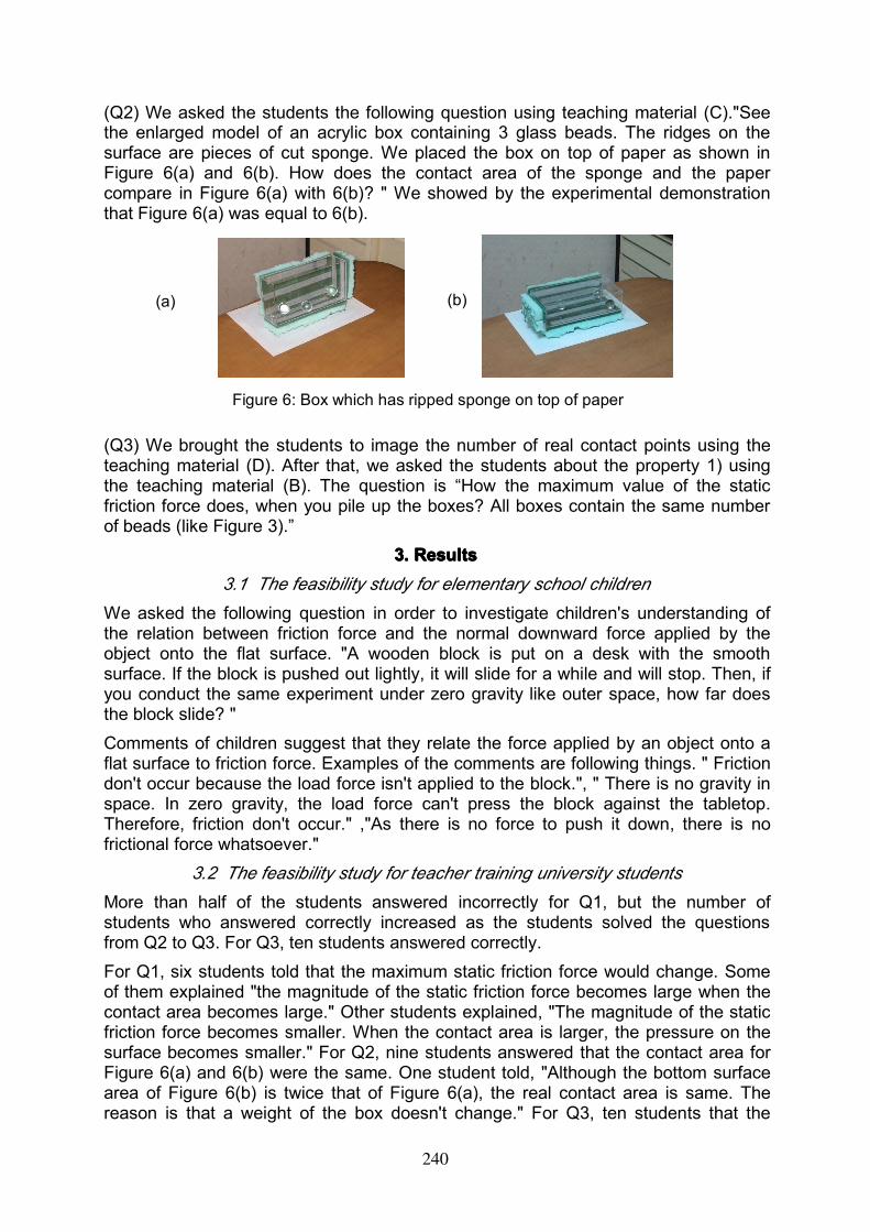
(Q2) We asked the students the following question using teaching material (C)."Seethe enlarged model of an acrylic box containing 3 glass beads. The ridges on thesurface are pieces of cut sponge. We placed the box on top of paper as shown inFigure 6(a) and 6(b). How does the contact area of the sponge and the papercompare in Figure 6(a) with 6(b)? " We showed by the experimental demonstrationthat Figure 6(a) was equal to 6(b).

(Q3) We brought the students to image the number of real contact points using theteaching material (D). After that, we asked the students about the property 1) usingthe teaching material (B). The question is “How the maximum value of the staticfriction force does, when you pile up the boxes? All boxes contain the same numberof beads (like Figure 3).”

3.3.3.3. ResultsResultsResultsResults3.1 The feasibility study for elementary school children

We asked the following question in order to investigate children's understanding ofthe relation between friction force and the normal downward force applied by theobject onto the flat surface. "A wooden block is put on a desk with the smoothsurface. If the block is pushed out lightly, it will slide for a while and will stop. Then, ifyou conduct the same experiment under zero gravity like outer space, how far doesthe block slide? "Comments of children suggest that they relate the force applied by an object onto aflat surface to friction force. Examples of the comments are following things. " Frictiondon't occur because the load force isn't applied to the block.", " There is no gravity inspace. In zero gravity, the load force can't press the block against the tabletop.Therefore, friction don't occur." ,"As there is no force to push it down, there is nofrictional force whatsoever."

3.2 The feasibility study for teacher training university studentsMore than half of the students answered incorrectly for Q1, but the number ofstudents who answered correctly increased as the students solved the questionsfrom Q2 to Q3. For Q3, ten students answered correctly.For Q1, six students told that the maximum static friction force would change. Someof them explained "the magnitude of the static friction force becomes large when thecontact area becomes large." Other students explained, "The magnitude of the staticfriction force becomes smaller. When the contact area is larger, the pressure on thesurface becomes smaller." For Q2, nine students answered that the contact area forFigure 6(a) and 6(b) were the same. One student told, "Although the bottom surfacearea of Figure 6(b) is twice that of Figure 6(a), the real contact area is same. Thereason is that a weight of the box doesn't change." For Q3, ten students that the

(a) (b)

Figure 6: Box which has ripped sponge on top of paper

240

maximum value of the static friction force increased. Six of them answered that themaximum value of the static friction force was proportional to the number of boxes.One student told that the friction force was constant.

4.4.4.4. DiscussionDiscussionDiscussionDiscussion andandandand ConclusionsConclusionsConclusionsConclusionsIn this article, we used one of the results of microtribology (the real contact points) inorder to teach the properties of friction. The teaching materials were investigated toimage the real contact points. The feasibility studies of the teaching materials wereconducted with elementary school children and teacher training university students.The result of those studies shows that the learners grasp an image of the real contactpoints on the analogy of coins on a football field. Presumably, the rough spongemodel of the interface is effective to consider the relation of the real contact area andthe apparent contact area. The students utilize the transparent boxes with somebeads and understand that the number of beads is related (proportional) to themaximum value of the static friction force. In conclusion, the image of the real contactpoints of microtribology helps children and students understand the word ‘friction’ asa scientific concept and the properties of friction.We carried out two small-scale feasibility studies in this research. We should developa lesson plan for high school students. The issues of kinetic friction remain to bestudied and further investigation is needed.

5.5.5.5. AcknowledgementAcknowledgementAcknowledgementAcknowledgementThis study was supported by the Souen Child center and the nonprofit organization"butukura"(Sapporo-City).

ReferencesReferencesReferencesReferencesDowson, D. (1998). History of Tribology, 2nd ed. London: Professional EngineeringPub.Bhushan, B. (2002). Introduction to tribology. Hoboken, New Jersey: John Wiley andSons.Bowden, F. P. & Tabor, D. (1954). The Friction and Lubrication of Solids. Oxford:Clarendon Press.Greenwood, J. A. & Williamson, J. B. P. (1966). Contact of nominally flat surfaces.Proceedings of the Royal Society of London, Series A, 295, 300-319.Rubinstein, S. M. ,Cohen, G. & Fineberg, J. (2009). Visualizing stick-slip:experimental observations of processes governing the nucleation of frictional sliding,Journal of Physics D: Applied Physics, 42, doi:10.1088/0022-3727/42/21/214016.Kudo,Y. (2007). Proposal for a Tribology Class for High School Students, Journal ofJapanese Society of Tribologists, 52(10), 705-710 (in Japanese).Kudo,Y. (2009). A Study on Structures of Educational Content and TeachingMaterials of Friction Law Set up by Considering Contacting Mechanism, Theory andPractice of Education, Research Bulletin of Hokkaido Society for the Study ofEducation, 4, 55-64 (in Japanese).Kudo,Y. (2011). An Instruction of Frictional Force for Primary School Children. ～Setup by Considering Contacting Mechanism～ , Theory and Practice of Education,Research Bulletin of Hokkaido Society for the Study of Education, 6, 53-62 (inJapanese).

241

The European Physical Society and Educational Physics

Robert Lambourne The Open University, UK,

Email: r.j.lambourne@open.ac.uk Abstract This contribution reviews the role of the European Physical Society (EPS) in physics education and describes some of its plans for the future. It starts with some general comments on the nature and purpose of the EPS and the particular importance it attaches to physics education. It then considers the relationship between the EPS Physics Education Division (PED) and other physics education bodies such as GIREP, MPTL (Multimedia in Physics Teaching and Learning) and STEPS II (Shareholders Tune European Physics Studies). It briefly describes the aims of particular PED activities such as the MUSE project (More Understanding from Simple Experiments) and the EPS-PED Secondary Teaching Award. Finally it considers the way in which broader aspects of physics education, such as the Bologna process, are approached within the EPS and the way that Individual Members of the EPS can influence its policies and contribute to its future development.

Introduction - the future of physics studies and the EPS Physics is vital to any proper understanding of the physical world, the environment and modern technology. Yet physics is not a universally popular subject; many see it as hard, dull and abstract. Globally, university-level studies are booming but physics is not keeping pace with the general expansion. Physics is expensive to teach, good physics teachers are not always easy to recruit, good students are hard to find. Around the world, and certainly within Europe, physics has need of friends and supporters.

The European Physical Society (EPS) exists to promote physics and support physicists in Europe. It acts through political lobbying, meetings, conferences, publications, prizes, grants, student fellowships and a range of other activities including public outreach. Founded in 1968 it has 41 national member societies (collectively representing about 100 000 physicists), 3000 individual members and about 50 ‘institutional’ associate members (including CERN and ESA). Its 11 Divisions cover all the main areas of physics from Particle Physics to Biophysics, including Physics Education. There are also 7 interdivisional groups (including Computational Physics, History of Physics, and Physics for Development). For further details see www.eps.org/.

The headquarters of the EPS are located in purpose built accommodation on the campus of the Université d’ Haute-Alsace in Mulhouse, France. The current President is Luisa Cifarelli who is also President of the Italian Physical Society. The President chairs the EPS Council and heads the Executive Committee. Support is provided by a range of other committees and a permanent secretariat headed by the Secretary General David Lee.

EPS divisional aims and the goals of the Physics Education Division

The various EPS Divisions have their own goals but they share the following common aims:

• promoting excellent physics research

242

• supplying a European view on important questions relating to physics • acting as a catalyst bringing together physicists from different countries • acting as a liaison between physicists working in different fields.

The EPS Physics Education Division (PED) was created in the Spring of 2000. In addition to supporting the common divisional aims listed above, its specific goals include:

• supporting and assisting physics teachers at all levels to maintain and improve the quality of physics teaching

• bridging the gap between those teaching physics in schools and universities • being a source of information and informed opinion regarding physics

education across Europe • strengthening the perception of physics in society.

One of the key roles that the PED can play is that of improving the contact and flow of information between researchers in all areas of physics and those involved in teaching physics at all levels. This naturally includes the contact between researchers in educational physics and those responsible for delivering and supporting formal physics education in schools and universities and informal physics education in a wide range of settings.

Other concerns that are particularly important in the European context include; monitoring differences in the educational systems in different countries and examining their consequences, sharing information about developments in initial teacher training and in-service teacher education, and contributing to discussions on the implementation of the Bologna process (the process whereby a unified Higher Education Area is being created in Europe). Also important is the relation and representation of European physics education to work going on elsewhere, particularly through bodies such as the International Commission on Physics Education (ICPE) and its parent body - the International Union of Pure and Applied Physics (IUPAP).

Modern physics education is a fast moving field, subject to changes arising from politics and fashion as well as the deeper influences of demography, technology and real advances in our scientific understanding of the educational process. The following subsections briefly describe some of the activities through which the PED is striving to meet its goals in this rapidly developing environment.

Conference support and organization:

Each year the PED distributes EPS funds to a number of bodies that are organizing conferences on various aspects of physics education in Europe. Long standing recipients of these funds include GIREP and the Multimedia in Physics Teaching and Learning Workshops (MPTL) but funds have also supported a number of other initiative such as the General Fora of the European Physics Education Network (EUPEN) and its successor (STEPS 2).

The PED also organises its own conference series, known as the European Physics Education Conference (EPEC). The first of these took place in Bad Honnef, Germany in 2005. Subsequent EPECs have all been held in odd-numbered years and have been jointly organized with GIREP; at Opatija, Croatia in 2007, Leicester, UK in 2009

243

and now, Jyväskylä, Finland in 2011. The co-location of EPEC and GIREP reflects a general aim of the PED, which is to encourage the consolidation of conferences through cooperation.

Involvement in a range of physics education bodies:

There have always been strong links between the PED and a number of other physics education bodies. Members of the PED Board have often also been officers or board members in GIREP, EUPEN and MPTL, and several have been highly active in the International Commission on Physics Education that was mentioned earlier. These links have helped the flow of information and led to a number of joint activities, such as the GIREP-EPEC meetings. Good relations also exist with the large and active American Association of Physics Teachers (AAPT) and with the Asian Physics Education Network (ASPEN) and the Latin American Physics Education Network (LAPEN) though no joint activities have yet emerged in these cases.

The MUSE Project: More Understanding with Simple Experiments:

The MUSE project resulted from some concerns of the PED Board relating to laboratory-based learning in schools and draws heavily on the talents of those Board members with a direct involvement in schools and/or teacher training. The target audience for the project consists of in-service and pre-service teachers together with the wider physics education and physics education research communities The main goals of the project are

• to go beyond excitement by helping students to get more understanding from simple experiments;

• to offer teachers some new approaches and methods to be used in classroom practice thus enlarging their range of choices.

To meet these goals the members of the MUSE Team (Laurence Viennot Gorazd Planinšič, Elena Sassi, Christian Ucke and Costas Constantinou) have been devising and publicising simple experiments that go beyond what may be described as 'teaching rituals'. These experiments help to promote discussion of the conflict between physics understanding and overly naive ideas and reasoning strategies. In this way they emphasise the added value of experimental work and spotlight viewpoints not often presented in current teaching materials.

MUSE was the subject of a workshop presented at this Conference by members of the Team and is reported elsewhere in these proceedings. More detailed information about the project can be found in that report and at the project website http://education.epsdivisions.org/muse .

Support for physics outreach activities:

Outreach (to the general public) and informal education of all kinds is an important concern of the EPS and the PED. Many major research conferences, not just those concerned with educational physics, now include one or more public events as part of the programme and some have a public part of the conference website.

244

Institutional Associates of the EPS such as CERN and the European Space Agency (ESA) devote significant parts of their budget to outreach and education as do many smaller organizations. The PED monitors these activities and in some cases is able to support them. For example financial support has been provided to the particle physics masterclasses and to the International Young Physicists Tournament (IYPT) which was chaired for a number of years by Gunnar Tibell who was also a member of the PED Board. (For more about IYPT see http://iypt.org/Home.)

The PED Board takes a particular interest in the problem of language in physics outreach. Research conferences and publications are usually presented in English but, to be effective, physics outreach activities must normally be in the local language. The PED Board is especially interested in those developments that allow good ideas in outreach to transcend the barriers that arise from the use of local languages.

Prizes and awards:

One of the most enjoyable duties of an EPS Division is the recognition of achievement in the field for which it is responsible. In many cases this relates directly to research achievement and can be based on the evidence provided by papers published in international journals and conference proceedings. Education is different.

The PED does not yet present an award for research in Educational Physics though it intends to do so, especially as the field is growing in strength. However, there is an EPS award, administered by the PED, that recognizes achievement in secondary teaching. This is specifically not a research award so it cannot be based on journal articles since the reporting of teaching achievement is still very incomplete, especially at school level. For that reason the selection committee bases its decisions on nominations received from the national physical societies that make up the EPS, or their officially nominated representatives (such as a national teaching organization). The societies are particularly encouraged to nominate those who have already won a national award, especially if the achievement might be transferred to other countries. The award is made in odd numbered years, at the relevant European Physics Education Conference. It consists of a certificate and 1000 euros. In 2009 the award went to Slavomir Tuleja from Slovakia, and in 2011 to Becky Parker from the UK. (More about the Award can be found at the PED website, http://education.epsdivisions.org/.)

Mention should also be made of the prestigious Gero Thomas prize which the EPS presents to those, whatever their field, who have made particularly significant contributions to the development of the Society itself. On at least two occasions this award has gone to those who are primarily recognized for their important contributions to educational physics.

Contributions to reports and papers:

The EPS produces a range of position papers and reports on a variety of issues. The existing EPS position paper on Education is being revised with increased emphasis on physics education research at all levels. Independently of this activity there have been significant reports on teacher training and physics education research. A major

245

EPS project reviewing the implementation of the Bologna process has resulted in detailed reports on all three cycles (Bachelor, Master and Doctoral) of the physics degree in Europe. Many of these activities have been reported on the PED website quoted above and some have led to articles in EPS journals such as Europhysics News or the European Journal of Physics.

Other EPS educational activities

The activities described above have emphasised the role of education within the EPS and particularly the role of the Physics Education Division but there are many other EPS activities that touch on education to a greater or lesser extent.

Student Fellowships are normally awarded to those working for a Masters degree and are intended to allow them to spend three months or more visiting an institution in another European country. Three Student Fellowships are awarded annually on the basis of excellence.

In addition to its PED conference support activities, the EPS also makes available general conference support and special funds for the award of poster prizes to postgraduate students. These poster prizes are obviously appreciated by those who win but they also have a clear educational aspect. They provide a degree of focus for poster sessions and ensure that all the posters are carefully examined and assessed by those involved in the judging.

Finally mention should be made of the EPS-coordinated proposal that the UN should proclaim 2015 as the International Year of Light. From the outset this proposal has recognized the key role that physics education should play. It is yet another indication of the emphasis the EPS gives to educational physics right across its spectrum of activities.

Conclusion and prospect

The last few years have seen a seen a substantial review of EPS that has emphasised the organization's dual role as both a member organization and an umbrella organization for the national physical societies of Europe. It is expected that the review will result in some rebalancing of activities between these two roles but it is encouraging to see the repeated recognition of the importance of physics education that has been a feature of the discussion. One outcome will be a drive to recruit many more Individual Members and to give them an enhanced role in the Society. There will be improved communication and more opportunity for Individual Members to have their voices heard. The years ahead will provide many opportunities for all members of the EPS - individual, corporate and institutional - to influence educational physics in Europe and help to strengthen is relation to all the other areas of EPS activity. Much has been achieved but much more remains to be done.

Acknowledgements

The author wishes to thank all of the past and current members of the PED Board whose actions and comments have contributed to this article, particularly; Costas

246

Constantinou, Hendrik Ferdinande, Gorazd Planinsic, David Sands, Elena Sassi, Urbaan Titulaer, Christian Ucke, Laurence Viennot and Els de Wolf.

247

A didactic approach to and curricular perspectives of the construction of the energy concept in primary school

Cristina Mariani1, Federico Corni1, Hans U. Fuchs2 1University of Modena and Reggio Emilia, I

2Zurich,University of Applied Sciences at Winterthur, CH cristina.mariani@unimore.it

Abstract

We propose activities and materials of a didactic approach to be used for constructing the energy concept in grades 4-5. Our approach integrates disciplinary, methodological and didactic aspects. We construct the energy concept from the cause-effect relationship of physical interactions by focusing on the differences of potentials (fall and rise of potentials) of the extensive quantities involved (such as fluids or heat). Students are introduced to the idea of energy being the agent responsible for the coupling of two processes. They will learn how the fall of an extensive quantity through its potential difference (cause) leads to the build-up of a secondary potential difference through which a different extensive quantity is “pumped uphill” (effect). Raising the potential of a certain amount of an extensive quantity by a certain value is caused by a proportionate lowering of the potential of a certain amount of another extensive quantity. The coupling of two processes is achieved by a kind of balance between cause and effect. The concept of energy then arises from the identification of the “proportion” between two processes taking part in an interaction.

I. Introduction Children and teachers alike demonstrate profound misconceptions when it comes to the subject of energy. Generally, researchers find that learning about energy has little lasting effect on students (Finegold and Trumper, 1989; Trumper, 1990; Kruger et al., 1992). After two decades of research the appropriate way to teach energy is still a subject of debate among physicists and education researchers (Millar, 2005). We present an innovative path to the energy concept that starts with children’s reasoning and takes into account results of educational research and a conceptual analysis of theories of physics (Fuchs, 2010). To clarify the abstract nature of primary thought of young children, we apply results of cognitive linguistics (Lakoff and Johnson, 1999; Johnson, 1987; Talmy, 1988) that show how children and adults speak about natural, emotional, and social phenomena using metaphorical projection of image schemas. Metaphoric projections form the core of the conceptualization of an experiential gestalt of physical, social, and emotional forces we call Force Dynamic Gestalt (FDG) (Fuchs, 2007). Various phenomena, such as those involving the behaviour of fluids, electricity, heat, motion, and chemicals, treated separately by different fields of science, can be understood in terms of analogous basic and simple structures already present in children’s minds. The purpose of this article is to explain how it is possible to build a didactic path connecting the FDG and the scientific concept of energy. Guidelines for design are deduced from the theoretical, methodological and didactical frameworks explicated.

II. Frameworks

248

II.1. Theoretical framework Our approach is based on some simple concepts which are fundamental in terms of their role in the discipline (Fuchs, 2010) and elementary in terms of their affinity with primary images in the child’s mind derived from early experience (Fuchs et al., 2011). The mind makes sense of experience by metaphorically projecting three schemas onto fundamental aspects of the FDG of concrete phenomena: 1. Quantity (substance)—referring to the scientific concept of extensive quantity. 2. Vertical level (quality, intensity)—referring to the scientific concept of intensive quantity (related to the concept of generalized potential). 3. Force or power as the source of the scientific notion of energy. The scientific concept of energy can be constructed in early childhood if we manage to differentiate these figures of thought that also serve as the schematic structures of formal science. These schemas are necessary and sufficient for describing and interpreting three important aspects of physical phenomena in which energy is involved: coupling of processes, chaining of devices, and storage (Fuchs, 2010, Ch. 2). The energy concept is developed by identifying the relation between the fall and rise of potentials (FDG-quality) and the flow of extensive quantities (FDG-quantity) involved in a process of interaction (FDG-force/power). Consider a hydroelectric power plant for example. The interaction takes place between falling water and the combination of the turbine and generator. Initially, the water is at a high level, afterwards it is at a low level. Electricity, on the other hand, comes to the plant at low potential and leaves at high potential. There exists a balance between extensive and intensive quantities of cause (water) and extensive and intensive quantities of effect (electricity). More water will result in more electricity or in a higher potential of electricity; the same result is achieved if we let the water fall from a higher level. The basic concept of energy, then, arises from identifying the "proportion" (qualitative or semi-quantitative in primary school) between products of fluxes of quantities and of potential differences.

II.2. Methodological and didactic frameworks

II.2.1. Narrative thought and affective engagement. Following cognitive linguistic theories (Johnson, 1987), the interpretation of the world is achieved by projecting image schemas that are developed in early childhood onto aspects of experience. Their metaphoric projection onto phenomena gives us the meaning of the world. Speaking and writing well about phenomena by using natural language will be the first step toward a useful conceptualization of the processes of nature. This will help us overcome the notion of a dichotomy between narrative and paradigmatic thought. In contrast to Bruner (1986), we believe that narrative and paradigmatic forms of understanding represent a polarity that opens up a spectrum between the poles of narrative and paradigmatic thought (Fuchs, 2011). In the child, a story allows for affective engagement and gives value to imagination and creativity the teacher may draw upon (Corni et al. 2010; Mariani et al. 2011a). II.2.2. Meaning construction is a mediated process that requires the teacher’s guidance.

249

The methodology of science teaching and learning can be developed from a semiotic point of view, following the contributions of mathematics education (Bartolini Bussi & Mariotti, 2008; Corni et al., 2011). The concept of energy (see II.1) is the piece of knowledge to be mediated. In order to foster its emergence in and appropriation by students, the teacher designs the tasks — suggested by the story — to be solved by means of a given “artefact.” In our context “artefacts” that mediate this knowledge come from different sources: experimental apparatuses (e.g., a wind mill, a jet-car, a putt-putt boat,...), games played by children, and the story itself. The story is a medium and a background for all classroom activities. Children produce individual texts (acts, drawings, oral or written texts) related to the concrete situation of using an “artefact” (situated texts). The analysis of these texts allows the teacher to make inferences about pupils’ understanding of the situation. The individual texts need to be collectively discussed and systematized at different levels of decontextualisation with the help of the teacher. The aim of the whole process is to nurture the maturation of situated texts under the teacher’s supervision by an iterative didactic cycle (DC) that includes experimental activities, the individual production of output (oral and written texts, drawings, sketches, gestures, gazes and sounds...) and collective discussions (CD) (Corni et al., 2011).

III. Guidelines for the design of a didactical path about energy For brevity, our focus in this paper will be on grades 4-5 of the curricular path. A path designed according to these guidelines has been tested in five 5th grade classrooms. The concepts of quantity and intensity are considered pre-requisite (developed in earlier school years) and recalled with the following goals: (1) to facilitate the identification of relevant variables, e.g, quantity (size), quality (intensity or potential) and its differences in cause and effect, and their mutual relations; (2) to study physical phenomena (coupling of processes; chaining of devices, and storage); (3) to foster the decontextualization of the variables accompanied by a gradual evolution of language—from every-day to formal language. The following steps (performed qualitatively) are part of a recursive cycle: 1. Analysis of cause-effect interactions. 2. Evidence of pairs of extensive-intensive quantities involved in interactions. 3. Differentiation of the quantities involved. 4. Focusing on the changes of the intensive quantities. 5. Recognition of the proportionality between the products of extensive quantities and

their associated potential differences. A story serves as the background for all activities. The first part of the story is for recognizing the relevant variables of the processes and it introduces problematic situations. Experimental activities are inserted into this background. The aim of the second part of the story is to guide children toward the decontextualization and the generalization of the concepts. The story offers different contexts in which the flow or storage of extensive quantities and their potentials can be recognized.

250

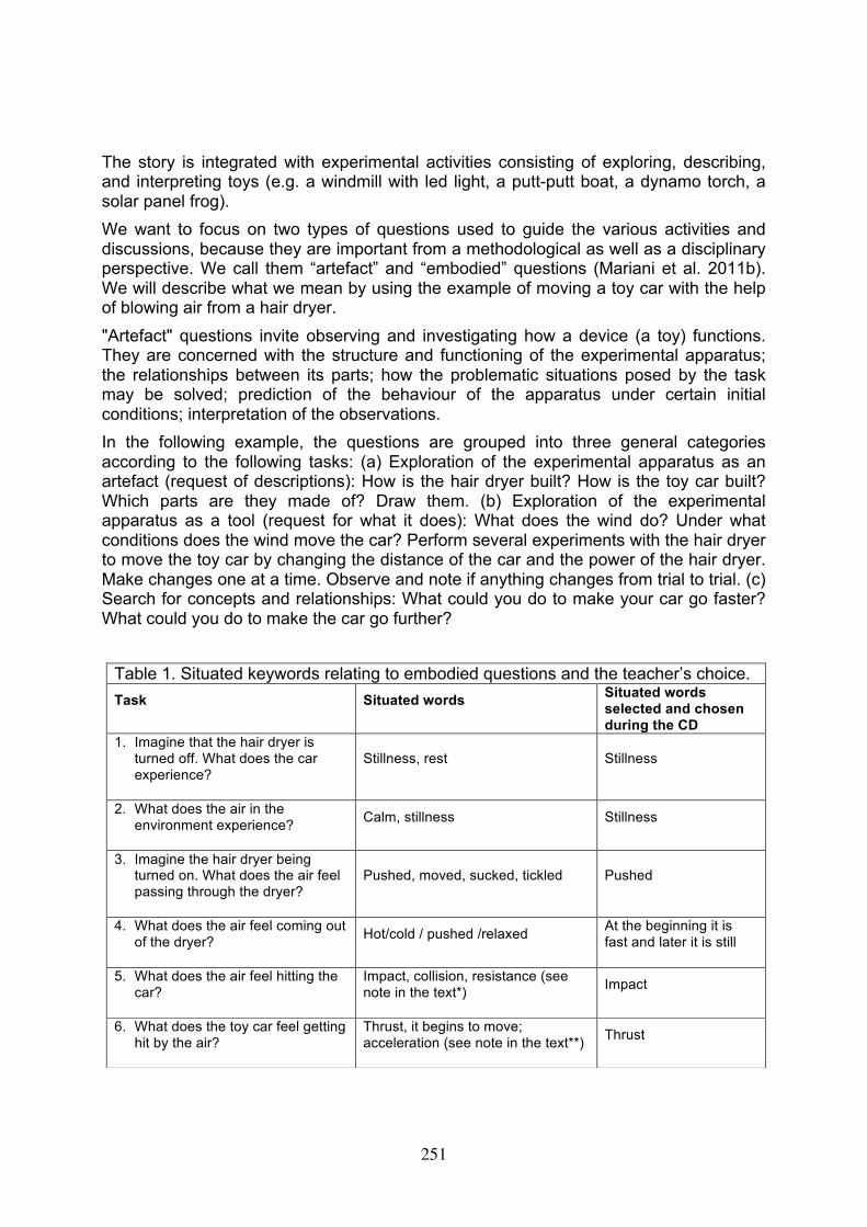
The story is integrated with experimental activities consisting of exploring, describing, and interpreting toys (e.g. a windmill with led light, a putt-putt boat, a dynamo torch, a solar panel frog). We want to focus on two types of questions used to guide the various activities and discussions, because they are important from a methodological as well as a disciplinary perspective. We call them “artefact” and “embodied” questions (Mariani et al. 2011b). We will describe what we mean by using the example of moving a toy car with the help of blowing air from a hair dryer. "Artefact" questions invite observing and investigating how a device (a toy) functions. They are concerned with the structure and functioning of the experimental apparatus; the relationships between its parts; how the problematic situations posed by the task may be solved; prediction of the behaviour of the apparatus under certain initial conditions; interpretation of the observations. In the following example, the questions are grouped into three general categories according to the following tasks: (a) Exploration of the experimental apparatus as an artefact (request of descriptions): How is the hair dryer built? How is the toy car built? Which parts are they made of? Draw them. (b) Exploration of the experimental apparatus as a tool (request for what it does): What does the wind do? Under what conditions does the wind move the car? Perform several experiments with the hair dryer to move the toy car by changing the distance of the car and the power of the hair dryer. Make changes one at a time. Observe and note if anything changes from trial to trial. (c) Search for concepts and relationships: What could you do to make your car go faster? What could you do to make the car go further?

Table 1. Situated keywords relating to embodied questions and the teacher’s choice. Task Situated words Situated words

selected and chosen during the CD

1. Imagine that the hair dryer is turned off. What does the car experience?

Stillness, rest Stillness

2. What does the air in the environment experience? Calm, stillness Stillness

3. Imagine the hair dryer being turned on. What does the air feel passing through the dryer?

Pushed, moved, sucked, tickled Pushed

4. What does the air feel coming out of the dryer? Hot/cold / pushed /relaxed At the beginning it is

fast and later it is still

5. What does the air feel hitting the car?

Impact, collision, resistance (see note in the text*) Impact

6. What does the toy car feel getting hit by the air?

Thrust, it begins to move; acceleration (see note in the text**) Thrust

251

The "embodied" questions invite children to imagine being a device, and/or an extensive quantity with its quality before and after the interaction. These questions are particularly powerful for stimulating children to produce personal situated texts in which the teacher can trace and single out keywords for the discussion. In Table 1 above, we present possible “embodied” questions. The keywords emerge from the answers of children and can be used and selected by the teacher to guide the collective discussion. Table 1 is from an experiment in a 5th grade class. In the actual debate, the intervention by the teacher is important in several respects: (1) to address the hypotheses and answers of children when they consider mechanical rather than thermal aspects (see Columns 2 and 3, 4th line); (2) to find the right time to use the words "resistance"(*) and "acceleration"(**) which are spontaneously introduced by some children; (3) to proposes two substitute questions (***) which were more accurate for the present purpose: (8i) Imagine that the hair dryer has just been turned off. What does the toy car experience? (8ii) Imagine that the hair dryer has been turned off for some time. What does the toy car experience?

IV. Discussion and conclusions This paper shows the feasibility to anchor scientific meaning construction to children’s reasoning starting from the image schemas of the FDG. We have suggested a methodology that makes the teacher confident in the use of natural language, believing that narrative and paradigmatic understandings represent a polarity spanning narrative and paradigmatic thought. The evolution of the language of children needs to be accompanied and directed by the teacher. In this important task, the use of “artefact” and “embodied” questions can be helpful. “Artefact” questions aim to improve the ability to observe and describe phenomena and devices. The richness of relationships between different parts of the object and the observation of chains of devices is promoted and, as result, language evolution is improved. “Embodied” questions allow anchoring reasoning to experience and, as a consequence, exploiting the image schemas that we already have. As a result, the teaching/learning process can take advantage of this fruitful connection and avoid a superimposed meaning construction. Although we start with natural non-formal language, the identification of relevant extensive and intensive variables and their relations are encouraged. If teachers develop the habit of stimulating children with “artefact” and “embodied” questions, recognizing the keywords and following the evolution of children’s language, they get a double benefit: they anchor their teaching practice to children's language and they use children’s discourses to evaluate learning.

V. References Bartolini Bussi, M. G. & Mariotti, M. A. (2008). Semiotic mediation in the mathematics

classroom: Artifacts and signs after a Vygotskian perspective. In L. English & al.

7. What does the air feel during encountering the toy car? Slowdown; reduction of speed Reduction of speed

8. Imagine that the dryer has been turned off. What does the toy car experience?

Slowdown, reduction of speed Begins to slow down; friction; it stops (see note in*** in text)

252

(Eds.), Handbook of International Research in Mathematics Education, second edition (pp. 746-783). New York and London: Routledge.

Bruner, J. (1986). Actual minds, possible worlds. Cambridge, MA: Harvard University Press.

Corni, F., Giliberti, E., Mariani, C. (2010). A story as innovative medium for science education in primary school, GIREP-ICPE-MPTL 2010 Proceedings.

Corni F. Giliberti E., Mariani C. (2011). Semiotic mediation and didactical cycle as methodological reference for primary school teachers. Journal of Emergent Science, 2, 35-38.

Finegold, M., Trumper, R. (1989). Categorizing pupils’ explanatory frameworks in energy as a means to the development of a teaching approach. Research in Science Education, 19, 97-110.

Fuchs, H. U. (2007). From Image Schemas to Dynamical Models in Fluids, Electricity, Heat, and Motion. An Essay on Physics Education Research. Retrieved from https://home.zhaw.ch/~fuh/LITERATURE/Literature.html

Fuchs, H. U. (2010). The Dynamics of Heat. A Unified Approach to Thermodynamics and Heat Transfer. Springer, New York.

Fuchs, H.U. (2011). Force Dynamic Gestalt, Metaphor, and Scientific Thought. Atti del Convegno "Innovazione nella didattica delle scienze nella scuola primaria: al crocevia fra discipline scientifiche e umanistiche", Ed. Artestampa, Modena

Fuchs, H., Corni, F., Giliberti, E., Mariani, C. (2011). Force Dynamic Gestalt of Natural Phenomena: Teaching the Concept of Energy. The biannual conference of the ESERA 2011 Lyon, France.

Johnson, M. (1987). The Body in the Mind, University of Chicago Press, Chicago. Kruger, C., Palacio, D., Summers, M. (1992). Surveys of English primary teachers’

conceptions of force, energy, and materials, Science Education, 76, 339-351. Lakoff, G., Johnson, M. (1999). Philosophy in the Flesh, Basic Books, New York, NY. Mariani, C., Giliberti, E., Corni, F. (2011a). Storie e percorsi. Atti del Convegno

Innovazione nella didattica delle scienze nella scuola primaria: al crocevia fra discipline scientifiche e umanistiche. Ed. Artestampa, Modena.

Mariani, C., Laurenti, E., Corni, F. (2011b). Hands-on, minds-on activities to construct the concept of energy in primary school: Experiments, games and group discussions, International Conference on Physics Education ICPE 2011 Proceedings.

Millar, R. (2005). Teaching about energy. Department of Educational Studies Research Paper 2005/11. York University. Retrived from http://www.york.ac.uk/

Talmy, L. (1988). Force dynamics in language and cognition. Cognitive Science 12,49-100.

Trumper, R. (1990). Being constructive: An alternative approach to the teaching of the energy concept (parts one and two). International J. of Science Education, 12, 343-354 and 13, 1-10.

253

Armenian Student Performance in Science: Results from TIMSS

Julietta Mirzoyan

julietta.mirzoyan@mail.com

Science education research department, National Institute of Education of the Ministry of Education and Science, Armenia

In the TIMSS 2007 assessment, Armenia`s fourth- grade and eighth- grade students` science average scores, the percentages of students performing at the international advanced benchmark, as well as the 95

th percentile scores increased dramatically compared to the TIMSS 2003 results. Also, the achievement

gap between high and low performing students at both grades increased enormously in a four- year period. This paper presents and discusses these findings from the secondary analysis of the TIMSS 2003 and TIMSS 2007 datasets. The overall improvement of our students` science achievements is certainly associated with the intensive growth of the national economy and significant developments in social sphere in the 2000s. The increase of inequalities in learning outcomes among Armenian students may be associated with the promotion of market mechanisms in school management and the transition to per student financing formula. To keep physics and other science disciplines alive for all Armenian students we must develop and implement special measures to support low achievers in science subjects. The paper examines the performance of Armenia`s students in an international context, particularly, in comparison to their peers from the former socialist countries, which participated in the TIMSS studies.

Introduction

Since 1998, Armenia, a small post-Soviet transitional country, has been engaged in a systemic reform of general education with two main aims: 1) to make the school system relevant to the new ideological, political and socioeconomic realities; 2) to improve the quality of education so deeply deteriorated during the first years of Independence. To monitor the progress towards the main aims of the reform on the basis of internationally comparable evidence on students` achievements, in 2002, Armenia entered the Trends in International Mathematics and Science Study (TIMSS) program of the International Association for the Evaluation of Educational Achievement (IEA) and participated in its 2003, 2007 and 2011 assessments. The science results from TIMSS 2003 and TIMSS 2007 are published in the IEA`s International Science Reports (Martin et all, 2004, 2008). The results from TIMSS 2011 will be released in December 2012. The country also took part in the TIMSS 2008 Advanced.

In the reform documents, the average scores of Armenian 4th- and 8th - grade students in mathematics and science in TIMSS 2003 are accepted as a baseline data, a point of reference on the quality level of general basic education. Thus, the achievements of students in the TIMSS tests are of great importance for educational policy making in Armenia. However, the two national reports on Armenian participation in TIMSS 2003 and TIMSS 2004 are very superficial. Unfortunately, they do not analyze achievements of the Armenian students in an international context and in light of the reform measures. Both reports mainly present information on the average achievement scores of students from all eleven regional administrative divisions of Armenia. The Armenian education research community is almost fully unaware of the participation of the county in TIMSS. No single paper in Armenian educational periodicals has references to the publications on the TIMSS 2003 and 2007 assessments.

254

The research, presented in this paper, had three main objectives:

To reveal the most essential changes in the Armenian students science achievements between TIMSS 2003 and 2007;

To determine the main background factors that could be associated with these changes;

The following research questions were addressed:

How did the main TIMSS science performance indicators of Armenian students change between 2003 and 2007?

How did the main indicators of socioeconomic development of the country change between 2003 and 2007?

What are the main directions of general education reform in Armenia? What objectives have been implemented prior to 2007?

How do the changes in the science achievements of Armenian students between 2003 and 2007 relate to the socioeconomic and educational background factors?

Methods of the research included:

The secondary analysis of the TIMSS 2003 and TIMSS 2007 datasets.

The review of the Armenian general education reform documents, available reports and other publications on the progress of educational transformations.

The paper examines the performance of Armenia`s students in an international context, particularly, in comparison to their peers from the former socialist countries, which participated in the TIMSS studies.

Changes in Armenian student science achievements between theTIMSS 2003 and TIMSS 2007 assessments

Changes in average scores

Armenia`s fourth and eighth-grade students` science performance in TIMSS 2003 was very disappointing, though poor results were expected. At the fourth grade, the national average score was significantly lower than the international average. Armenian students outperformed their peers only from Iran, Philippines, Tunisia and Morocco. All post-socialist countries that participated in TIMSS 2003 at the fourth grade (Latvia, Hungary, the Russian Federation, Lithuania, Moldova, and Slovenia), scored higher than Armenia. At the eighth grade, the national average score was also lower than the international average. All post-socialist countries- Estonia, Hungary, Slovenia, Lithuania, Slovak Republic, the Russian Federation, Latvia, Bulgaria, Moldova, Romania, and Serbia, except Macedonia, ranked higher than Armenia.

The TIMSS 2003 assessment results for Armenia firmly confirmed a nation-wide shared opinion that the quality of general education declined dramatically over the years of Independence. The TIMSS 2003 results also revealed that the quality of general education in Armenia was the worst, compared to almost all post-socialist nations that participated in the TIMSS assessments. As to the main reason for the situation, according to the Government of Armenia (2003), “The transition period has had a negative impact on the education system of Armenia. In particular, the reduction of

255

public spending in education gave rise to a deterioration of the quality of education services” (p.84).

In TIMSS 2007, Armenia`s average score at the fourth grade remained lower than the international scale average. Armenia outperformed Ukraine and Georgia. The Russian Federation, Latvia, Hungary, Kazakhstan, the Slovak Republic, Slovenia, the Czech Republic and Lithuania achieved significantly higher average scores than Armenia. At grade 8, the national science average score was also lower than the international scale average. Our 8th- graders performed better than their counterparts from Ukraine, Serbia, Bulgaria, Bosnia and Herzegovina, Romania and Georgia, and worse than students from Hungary, the Czech Republic, Slovenia, the Russian Federation and Lithuania. It is necessary to note that in TIMSS 2003, Serbia, Bulgaria and Romania showed better results than Armenia.

Despite remaining lower than the international average scores in TIMSS 2007, the science achievements of the Armenian 4th- and 8th – grade students improved dramatically in the four - year period between 2003 and 2007 as measured by the TIMSS tests. The country`s average scores at fourth and eighth grades increased by 48 and 27 points respectively. Among all 36 participating nations, Armenia had the highest increase of science average score at the fourth grade. At the eighth grade, only three of 49 countries (Ghana, Tunisia and Bahrain) had higher increase of the national average scores than Armenia. In the report How World`s Most Improved School Systems Keep Getting Better (Mourshed, Chijioke, & Barber, 2010), Armenia is included in the list of 20 countries and educational systems, which improved significantly the quality of general education through systemic (whole-system) reforms. The Armenian results in TIMSS 2007 served as a basis for the decision to include our country in this report. According to the authors of the report, the dramatic increase of the country`s national average scores in mathematics and science between 2003 and 2007 indicated big positive changes in how our school system performs.

Changes in performance at the international benchmarks for science achievements and in percentile scores

The TIMSS 2007 assessment revealed two other changes in science performance of Armenian students in both grades: 1) the disproportionately big increase of the percentages of students performing at the international advanced benchmark; 2) the disproportionately big increase of the 95th percentile scores.

In TIMSS 2007, the percentage of Armenian fourth- graders performing at the international advanced benchmark reached 12 percent, which is similar to Japan, and became significantly, almost two times more higher, than the relevant international median percentage (7%). Among post-socialist countries, only the Russian Federation and Hungary had a higher than Armenia percentage of their fourth-grade students performing at the highest benchmark. But at the three other international benchmarks (low, intermediate and high) the Armenian results were considerably lower than relevant international median numbers. To the international pool of only 7 percent of failed fourth-grade students (those who scored lower than 400 points) Armenia added 23 percent of its students, while in the same pool Japanese students comprised only three percent.

256

The percentage of Armenia`s fourth - grade failed students was the second highest among all post-socialist countries.

The percentage of the Armenian eighth - graders at the international advanced benchmark was eight percent in TIMSS 2007, which is similar to Australia and Lithuania and almost three times higher than the international median percentage (3%). Among post-socialist countries only Hungary, the Czech Republic, Slovenia and the Russian Federation achieved better results than Armenia. At the three other benchmarks the country`s results were just higher than international average numbers, and considerably lower than that of Australia and Lithuania. Armenia added 17 percent of its students to the international pool of failed eighth-graders. The percentages of failed students from Australia and Lithuania were much lower- only eight and seven percent respectively.

Compared to the TIMSS 2003 results, the percentages of the Armenian students at both grades, that performed at each of the four international science benchmarks, increased in the TIMSS 2007 assessment, but in an extremely disproportionate way. The proportions of the fourth- and eighth- grade students performing at international advanced benchmark increased dramatically from 2 to 12 percent and from 1 to 8 percent respectively. At the three remaining benchmarks the increases were modest, especially for the fourth- grade students.

Changes in student performance can also be illustrated by analyzing percentile scores. In Armenian grades 4 and 8, significant changes took place between the 95th and 5th science percentile scores in the four-year period. The gaps between the highest and the lowest performers in science at both grade levels became very large compared to almost all other TIMSS nations. At the fourth grade, the 95th percentile score increased by 111 points, and became the second highest (after Singapore) among all nations. However, at the same grade the 5th percentile score increased only by 33 points, and the gap between the highest and the lowest achievers became the fourth largest internationally (after Tunisia, Qatar and Morocco). Compared by the 95th science percentile score in 2007, the Armenian 8th - graders were outperformed only by their peers from the four Asian countries (Singapore, Chinese Taipei, Japan and Korea) and England. Between 2003 and 2007, at the eighth grade, the 95th percentile score increased by 73 points. At the same time, the 5th percentile score increased only by one point and the gap between the highest and lowest achievers became one of the largest internationally. The gaps between the highest and lowest achieving science students at both grades in Armenia were the largest among all post-socialist countries. These results showed the essential rise of inequalities in students’ educational outcomes during the four - year period between TIMSS 2003 and 2007.

Changes in background factors between 2003 and 2007 and their influence on student achievements

Unprecedented developments, both positive and negative, in the performance of the Armenian students in science between the TIMSS 2003 and TIMSS 2007 assessments described above, could be caused only by the essential changes in the country`s socioeconomic situation and ongoing educational reform processes. Like all post-socialist countries, Armenia inherited a very well developed system of general education. Our experience once again clearly demonstrated the decisive influence of

257

socioeconomic factors on the quality of school education. The rapid decline in the country`s economy over the first years of Independence caused a severe long-lasting crisis in all spheres of social life, including education, which appeared to be, literally, in a “free fall”. Armenia`s results in TIMSS 2003 clearly demonstrated the deterioration of general education.

From the end of the 1990s, the process of recovery has begun and the years between 2003 and 2007 became the most economically productive in the post-Soviet history of Armenia. As a consequence, significant reduction of poverty and especially the extreme poverty and increase of average monthly salary were reached. The country`s Human Development Index (HDI) improved from 0.729 in 2003 to 0.775 in 2007. From the end of the 1990s, education has become a priority area in the state politics. All these developments coupled with good traditions in teaching physics and other science disciplines, inherited from the Soviet period of our history, could cause a significant improvement of the quality of education in this curriculum area, revealed by the TIMSS 2007.

Improved economic situation made it possible to begin in 1998 systemic (whole-system) reform of general education in Armenia. Within the framework of the World Bank (WB) financed Education Management and Financing Reform (EMFR) project, serious measures to decentralize the management in general education were implemented. In 2002-2005, all schools in Armenia moved to a per - student financing scheme. Besides, schools became providers of additional paid services for their students. The rise of inequalities between Armenian high and low performing students, revealed by TIMSS-2007, could be associated with the new school management and financing mechanisms, which promote decentralization, school autonomy, competition between schools, and parental choice and involvement. It is clear, that for students, coming from families with low socioeconomic background, the possibility of access to quality education has declined.

The second phase of the educational reform in Armenia began in 2004 with the Education Quality and Relevance Project (EQRP), also financed by the WB. Within the EQRP, new standards, syllabuses and textbooks for all school subjects were developed, a massive teacher training was conducted. The first five - year part of this project was finished in 2009. Its influence on the Armenian students` science achievements will be analyzed after publication of the TIMSS 2011 International Science Report in December 2012.

Closing remarks

The TIMSS 2007 results clearly indicated improvement in science education quality in Armenian schools. In the second part of the EQRP, the implementation of which is now in progress, new special measures are planned to enhance physics and other science subjects teaching and learning in the country`s schools. They include science subjects teachers in-service training in student-centered methodology, inquiry learning and computer use in science lessons. School science laboratories will be enriched by new equipment. As it was shown above, the TIMSS-2007 results also revealed a big new problem - the rising inequalities in students’ achievements mainly associated with per student financing scheme, decentralization policy and promotion of market mechanisms

258

in our schools. If we would like to keep physics and other science disciplines alive for all Armenian students, not just for the best, we must develop and implement special

measures to improve the achievements of the lowest performing students.

References

Government of Armenia (2003). Poverty reduction strategy paper. Yerevan.

Martin, M.O., Mullis, I.V.S., Gonzalez, E.J., & Chrostowski, S.J. (2004). TIMSS 2003

international science report: Findings from IEA’s Trends in International Mathematics and Science Study at the fourth and eighth grades. Chestnut Hill, MA: Boston College.

Martin, M.O., Mullis, I.V.S., & Foy, P. (2008). TIMSS 2007 International Science Report: Findings from IEA’s Trends in International Mathematics and Science Study at the fourth and eighth grades. Chestnut Hill, MA: Boston College.

Mourshed, M., Chijioke, C., Barber, M. (2010). How the world’s most improved school systems keep getting better. McKinsey&Company. Retrieved from http://mckinseyonsociety.com/downloads/reports/Education/How-the-Worlds- Most-Improved-School-Systems-Keep-Getting-Better_Download- version_Final.pdf

259

Adjusting cadets’ reasoning skills with strategic questioning Arto Mutanen1, Antti Rissanen2

antti.rissanen@mil.fi 1Finnish Naval Academy, Finland and 2National Defence University, Finland

In classroom teaching of physics, basic laboratory exercises and demonstrations play different kinds of roles. Questioning is a common method in instruction within such activities. However the role of questioning is less prominent during lecturing. Neither, much consensus is gained about successful questioning. What kind of questioning gives added value and how the common findings in this research area can be integrated to the daily physics teaching practice? In the early 20th century, the basic problem of the philosophy of science was the justification of knowledge. However, from the 1960s on, scientific discovery has been under extensive study in the philosophy of science. This includes the study of the whole scientific inquiry process and the study of experimentation or observation as a factor of scientific inquiry. One focus in the study of scientific discovery has been to understand the actual search for new knowledge via questioning. This approach has interesting interconnections with new pedagogical approaches.

Introduction

Questions open the door to dialogue and discovery and are an invitation to creativity and breakthrough thinking (Vogt et al., 2003). Therefore, productive questioning techniques in physics education mean a continuous challenge. It is remarked that the standard lecture setting is too impersonal and linear for actual learning; but something related to the learning process is clearly occurring (Harrison, 2000). A long-standing issue addressed by the PER community is students’ conceptual understanding of physics rather than only their ability to solve problems. The questioning method as such is an interesting topic both philosophically and pedagogically. A questioning method has been developed in pedagogy – basically this has been done independently of the development in philosophy. In the following contemplations, the questioning dilemma is discussed from the viewpoint of cadets’ instructional challenges in physics. A theoretical literature review is utilized to provide rationales for the arguments. Daily observations of cadets’ physics classroom instruction provide an action research type approach for concluding findings.

Literature review Questions are no longer seen as isolated events but moreover elements of larger contexts (Wilkinson & Hye Son, 2009). Many students see lectures as occasions to take notes instead of forums for learning (Hunter & Tattle, 1999). Teachers think that lectures are intended for capturing knowledge but actually tutorials help students to learn analytical thinking skills (Isaacs, 1992). The pedagogical literature in this context is wide and includes recommendations for suitable questioning practices even if the effects of the acquired questioning practice are more presumed than examined (Dillon, 1986). Ciardiello (1998) identifies 4 types of questions: memory questions, convergent thinking questions (why, how – questions), divergent thinking questions (questions asking imagination, prediction etc.), and evaluative questions. Morgan and Saxton (2006) categorize questions by intended function; questions eliciting information, shaping understanding, and supporting reflection. Higher-level questions (questions demanding applicative, analytical, or synthetical thinking) are

260

often emphasized as a good instructional habit, but it is not sure that asking higher-level or authentic questions (whose answer is not pre-specified) contributes cognitive benefits for students (Wilkinson & Hye Son, 2009). According to studies, 80-90% of the presented questions represent questions which belong to the factual level (facts, knowledge) (Ciardiello, 1998). It is assumed that lower-order questions are effective for less able learners, while higher-order questions are more effective for older and more able learners. All studies do not show that teacher questions stimulate student thinking (Dillon, 1986). The overall effects of teacher questioning are not clear: it is not known whether teacher questioning as an instructional tool is any better than other instructional methods. Teacher questions may also have negative effects on students’ cognitive processes, and hence teachers should ask fewer questions and substitute questioning with a mix of other alternatives (Dillon, 1982). According to Harlen (2005), productive teachers’ questions lead to scientific activities while unproductive questions lead students mechanically to look up ideas in books or from teacher. Klymkowski et al (2006) remind that better conceptual questions probe better student understanding even if creating such questions can be difficult and often involves multiple rounds of analyzing student responses and revising question whereas questions that elicit a reflex response are easier to write and grade, easier for the student to answer but can only give the illusion of understanding. In the recent educational research the viewpoint has shifted from teacher’s questions to student responses and student-generated questions: “those who would seek knowledge – students – are not asking questions at all” (Dillon, 1986; Wilkinson & Hye Son, 2009). Harper et al. (2003) tried to enhance students’ questioning activity with structured weekly reports, but 30% of the reports submitted by students contained no questions. Also optional means (web-based, anonymous questions) were not successful either. Marbach-Ad and Sokolove (2000) noticed that an active-learning setting (in which time is devoted to questioning with feedback and grading) motivated students to ask more research-oriented questions. Students’ bigger role in questioning makes the whole process of questioning more effective (Van der Meij, 1994). Snider (2004) found the PISER method (The Peer Instruction and Student Electronic Response) motivating and useful because it also offered data for continuous assessment. It is also supposed that it is useful to train students in question generation (Ciardiello, 1998). Philosophers and pedagogic experts have developed questioning methods also together (see, e.g. Hakkarainen & Sintonen, 2002). Hakkarainen & Sintonen have considered interrogative model of inquiry as a general theoretical framework. They see the interrogative model as a general strategic framework in which the questioning in classroom can be reframed.

Research question This report will focus on two research questions: (1) What pedagogical literature and connected empirical findings say about fruitful questioning and how common philosophical contemplations touch this topic? (2) What kind of useful insights presented findings and recommendations could offer to cadets’ physics teaching and how the ideas of the interrogative approach could be integrated to these learning strategies?

Questioning as a philosophical dilemma In philosophy, questioning has been employed as a general method for knowledge seeking for thousands of years. The roots of questioning methods in the written history of philosophy go back to the Socratic Method of Questioning (elenchus) that

261

was explicated by Plato in his dialogues. Socrates can be seen as one of the first known practical pedagogists and Plato as one of the first theoretical pedagogists. The work of Socrates and Plato laid a foundation for the theory and practice of teaching and learning. The Socratic questioning method is well known: Socratic questioning is a strategy in which questions direct the process and answers provide the factual information and guarantee consensus. Aristotle systematized the questioning method in his philosophy. In Topica, Aristotle studies the strategies for different kinds of question-answer processes. The philosophy of Socrates, Plato and Aristotle can be understood as the foundation of western philosophy and science. This foundation was not only methodological and scientific, but also pedagogical. Western science has been in continuous dialogue with this foundation. Our understanding of the very character of physical nature has increased thanks to the development of natural science. There are a huge amount of technical applications based on achievements in natural science. However, the contexts of applications become more complex and the people who need the knowledge are heterogeneous in terms of their skills and background knowledge. The development of fresh pedagogical approaches to answer these challenges is a demanding task. At the beginning of the 20th century, physics was the science according to mainstream philosophy of science, mainly because physics involves looking at proper and reliable knowledge about reality. As a result, the problem of reliability became a major problem in the philosophy of science. Hence, any problems concerning learning and discovery were not considered to be central. Reichenbach made his famous distinction between the context of discovery and justification. He argued that “the act of discovery escapes logical analysis” (Reichenbach, 1963, p. 231). The idea that the discovery is not within the scope of philosophical analysis was very influential in the first few decades of the 20th century. The separation of the contexts can be seen as a consequence of logical philosophy, especially that of the Vienna Circle. This tradition has been influential also in pedagogy. (Sintonen, 1986) From the 1960s on, philosophers have been interested in the problem of discovery. Popper took the problem of discovery under philosophical study in his Logic der Forschung, published in Vienna in 1934: his conclusion was that there is no such logic. However, the logic of discovery became a subject of study. The study of the logic of discovery is a study of the whole inquiry process. (Jung, 1996) The questioning method is a promising approach in characterizing the logic of discovery, i.e., the logic of knowledge acquisition. The questioning method has a long history and modern mathematical and philosophical logic allow us to characterize it. In fact, there are several approaches to the questioning method. (See Hintikka, 1976, 2007; Jung, 1996) The logic of questions and answers refers to the practice of questions and answers – an answer does what it is intended to do only if the questioner understands it. That is, epistemic considerations have to be taken into consideration; both scientific inquiry and learning are an active search for new knowledge. Both in inquiry and in learning, the agent intends to gain understanding – to change the epistemic state of the agent. (Hintikka, 2007) The search for new knowledge can be seen as a central aspect in modern science (Niiniluoto, 1987). The search for new knowledge implies that scientific reasoning should be ampliative. However, there is no generally accepted ampliative reasoning method. Especially, deductive logic is known to be non-ampliative. (Kelly, 1996; Niiniluoto, 1987) The lack of ampliative logic implies a

262

negative attitude toward the logic of discovery because it cannot be subsumed under philosophical analysis: ''The initial stage, the act of conceiving or inventing a theory, seems to me neither to call for logical analysis nor to be susceptible of it. The question how it happens that a idea occurs to a man – whether it is a musical theme, a dramatic conflict, or a scientific theory – may be of great interest to empirical psychology; but it is irrelevant to the logical analysis of scientific knowledge.'' (Popper, 1968, p.31) The rejection of the logic of discovery implied that in philosophy the logic of justification became the main theme of the philosophy of science. In philosophy, “as to the task of the logic of knowledge – in contradistinction to the psychology of knowledge – I shall proceed on the assumption that it consists solely in investigating the methods employed in those systematic tests to which every new idea must be subjected if it is to be seriously entertained.'' (Popper, 1968, p. 31) The logic of testing and of justification started a development of logic of induction (e.g. Hintikka, 2007).In philosophy in the late 1950s and especially in the 1960s, logical interest in propositional attitudes was increasing. (Lenzen, 1978) At the same time, logic of questions and answers was developed further.

Interrogative approach to inquiry and learning The notion of questioning strategy is common to all of the interrogative models. (Jung, 1996) Hintikka’s interrogative model of inquiry is intended to characterize explicitly the construction process of knowledge within scientific inquiry: the construction process is a strategic two-level process. These levels refer to two different kinds of questions. Big questions explicate the goal of the whole inquiry process while operational questions show how the detailed information is found out. The strategy binds the whole process into a single goal-tracking process. The two-level nature of the process allows us to characterize the notion of induction in a new way. Hintikka (2007) and Kelly (1996) see that the strategic questioning process bridges the way from ignorance to knowledge. In an experiment for example, we look for functional dependencies between those factors we are interested in. The big question considers the existence of the functional dependence. Later, operational questions are utilized on the level of observations and measurements. While an interrogative model characterizes the whole process as a single strategic process, the whole experimental setting has to be built up such that the intended functional dependency – if it really exists – can be seen. Basically the results of an experiment are just separate values of a quantity – separate answers to operational questions. Generally, a dialog represents a linguistic question-answer process between the participants. However, in a factual knowledge-seeking process, the dialog must be connected to the factual object of study. This is closely connected to present-day pedagogical theories (Hakkarainen & Sintonen, 2002). The experimental application emphasizes the role of the object in the dialogue; what is important is not the dialogue as such but the dialogue with the object of study. (Hintikka, 1982) A construction process of knowledge is essentially goal-directed. A natural theoretical framework for the questioning method can be seen as a mathematical theory of games. Game theory explicates the roles of the goal and (game) rules in the questioning process and in this questioning game, the players are more like colleagues than tutor and student. (See Hintikka, 2007)

263

Concluding remarks The questioning skills of teachers and learners are strategic skills that orientate the learning process. The orientation or questioning strategy pictures the general map of the learning framework and the answers fill in the needed factual details. A fruitful questioning policy emphasizes displacement from teacher-generated questions to student-generated questions. This means that teachers should evaluate or maybe reduce their own question intensity but however give enough space for questioning in normal practice. Actually, teachers should encourage students to ask questions, so that also typical listeners take part to such activity. This no doubt requires an atmosphere where the lecturer and students are equal cooperators and where even simple questions and responses (reflex and ad hoc) are allowed. For a strategic questioning the interrogative model as an idea as such might be fruitful. However, there are still challenges in normal pedagogy when trying to adapt these ideas. Even if the lecturer’s role is to give more space for students’ questions the situational evaluation and control is of high importance. What students should know in order to gain the intended understanding? How to unify the factual information and theoretical (mathematical) information and how to create better conceptual questions? This means that students should understand the strategic whole: the big question and its interconnection with the smaller ones. It is useful to understand that a good question is not actually one question but often a combination of detailed small questions (question chain). How then to encourage students to use their creative minds with inspiring discussions that combine factual, convergent, and divergent elements? How students are able to critical evaluation of the whole epistemic and practical situation in which knowledge formation takes place instead of pure knowledge capturing? The intention is not to learn a predetermined lesson, but to learn how to take the learning process under strategic control. Therefore, it is not enough that students understand the fundamental concepts behind phenomenon but they must also be able to elaborate and create new questions and insights. As teachers and as students we must have constant readiness to give space for quite new paths in our thinking and protect us from too guiding attitudes in our teaching and analytical processing. This means that we must be able to re-evaluate our opinions. This requires that continuous formative assessment should also be extended to the questioning policy to see what kind of practices actually support the learning. More intensive tutoring in questioning policy may produce fruitful practices or at least takes this topic more in focus.

References Ciardiello, A. V. (1998). Did you ask a good question today? Alternative cognitive and metacognitive strategies, Journal of Adolescent & Adult Literacy, 42(3), 210-219. Dillon, J. T. (1986). Questioning, (Chapter 4). In O. Hargie (Ed.). A Handbook of Communication Skills. London: Croom Helm. Dillon, J. T. (1988). Questioning in education, In M. Meyer (Ed.). Questions and Questioning. Berlin: Walter de Gruyter & Co. Hakkarainen, K., & Sintonen, M. (2002). The interrogative model of inquiry and computer-supported collaborative learning, Science & Education, 11(1), 25-43. Harlen, W. (2005). Primary Science: Taking the Plunge. Portsmouth: Heinemann.

264

Harper, K. A., Etkina, E., & Lin, Y. (2003). Encouraging and analyzing student questions in a large physics course: meaningful patterns for instructors. Journal of Research in Science Teaching, 40, 776-791. Harrison, D. (2002). How does the delivery of information help students to learn, Physics Virtual Bookshelf. University of Toronto, Physics Department. Hintikka, J. (1976). The Semantics of Questions and the Questions of Semantics, Acta Philosophica Fennica, 28(4), Philosophical Society of Finland. Hintikka, J. (1982). A dialogical model of teaching, Syntheses 51, 39-59. Hintikka, J. (2007). Socratic Epistemology, Cambridge University Press. Hunter, S., & Tattle, J. (1999). Lectures. Why don't students attend? Why do students attend? Proceedings from: HERDSA Annual International Conference. Melbourne. Isaacs, G. (1992). Ends and means: What learning goals are served by what methods, Research and Development in Higher Education, 15, 205-212. Jung, S. (1996). The Logic of Discovery: an interrogative approach to scientific inquiry. New York: Peter Lang. Kelly, K. (1996). The Logic of Reliable Inquiry. Oxford University Press. Klymkowsky, M., Gheen, R., & Garvin-Doxas, K. (2006). Avoiding reflex responses: Strategies for revealing students’ conceptual understanding in Biology. Proceedings from: Physics Education Research Conference. Syracuse, NY. Lenzen, W. (1978). Recent work in epistemic logic, Acta philosophica Fennica, 30(1), North-Holland. Marbach-Ad, G., & Sokolove, P.G. (2000). Can undergraduate biology students learn to ask better questions? Journal of Research in Science Teaching, 37, 854-870. Van der Meij, H. (1994). Student questioning: A componential analysis, Learning and Individual Differences, 6(2), 137-161. Morgan, N., & Saxton, J. (2006). Asking better questions (2nd ed.). Markhamn: Pembroke Ltd. Niiniluoto, I. (1987). Truthlikeness. Dordrecht: D. Reidel. Popper, K. (1968). The Logic of Scientific Discovery. London: Harper, (Original work. published in German 1934). Reichenbach, H. (1963). The rise of scientific philosophy (9th printing). Berkeley, CA: University of California Press. Sintonen, M. (1986). Positivismi, In I. Niiniluoto and E. Saarinen (Eds.). Vuosisatamme filosofia, Helsinki: WSOY. Snider, L. (2004). Teaching students to think using peer instruction and student electronic response (PISNER) for enhancement of conceptual and critical learning, CDTLink, 8(1), 4-5. Vogt, E., Brown, J., & Isaacs, D. (2003). The Art of Powerful Questions: Catalyzing insight, innovation and action. Mill Valley, CA: Whole System Associates. Wilkinson, I., & Hye Son, E. (2009). Questioning, In E. Anderman & H. Anderman (Eds.) Psychology of Classroom Learning: An Encyclopedia (pp. 723-728). Detroit, MI: Gale/Cengage.

265

Analytic frameworks for studying science classroom discourse with dynamic semantic approach

Eizo Ohno

eohno@edu.hokudai.ac.jp Faculty of Education, Hokkaido University, Japan

There are several analytic frameworks (e.g. conversation analysis and discourse analysis) for inter-preting classroom discourse. In this article, an analytic framework is constructed with using dynamic semantics, Segmented Discourse Representation Theory or SDRT (Asher & Lascarides, 2003). The process of interpretation is distributed into two stages. In the first stage interpretation, the reliance on linguistic information, compositional and lexical semantics and so on, is maximized and the non-linguistic information such as beliefs, intuitions, world knowledge, is treated as occasion requires. Co-herent structures of science classroom discourse are investigated with using the rhetorical relations of SDRT. An intermediate interpretation is made at the first stage of interpretation. The intermediate in-terpretation is represented as a diagram in which utterances are connected with the rhetorical rela-tions. Depending on interactions between a teacher and students, the diagram is getting longer hori-zontally, or branches off and grows vertically. The records of science classroom discourse at a junior high and elementary schools are analyzed.

1. Introduction

“Talk” in science lessons is important. The recent studies draw our attention to the role of social interaction between a teacher and students (Mortimer & Scott, 2003). Classroom discourse in science lessons is complex processes. Analytic frameworks for studying such processes are required and investigated in order to reveal how communicative competence and critical thinking are involved in science lessons.

Some difficulties and Background When we advance our analysis of classroom discourse, we use inferences supported by rich information sources; teacher’s intention, students’ cognitive states, and their social and cultural background. However, we cannot access directly to these infor-mation sources. We must interpret and obtain some content of the information sources prior to advancing our interpretation. This situation causes a circular inter-pretation. In this research, we introduce a process of interpretation consisting of two stages. Researchers usually analyze transcripts written by their native language. For exam-ple, the author proceeds with a whole analysis in Japanese. After completing the analysis in Japanese, the author translates a Japanese transcript to English one by using the interpretation obtained by analyzing the original Japanese transcript. The English transcript might not contradict the analysis process. The language barrier causes some difficulties, when the author tries to give a lot of details of the analysis process and explain the validity of interpretation to foreign researchers in English. There are two major analytic frameworks, the conversation analysis and the dis-course analysis, to interpret the discourse (Levinson, 1983). When we analyze tran-scripts of classroom discourse, the segments of discourse are generally coded by us-ing some categories. Those categories have to be tight enough to be able to capture our interpretation. Establishing clearly defined categories and strategies for coding is

266

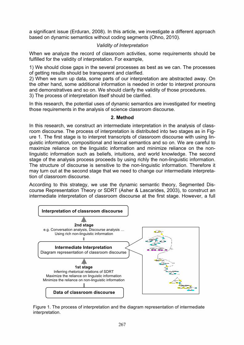
a significant issue (Erduran, 2008). In this article, we investigate a different approach based on dynamic semantics without coding segments (Ohno, 2010).

Validity of Interpretation

When we analyze the record of classroom activities, some requirements should be fulfilled for the validity of interpretation. For example, 1) We should close gaps in the several processes as best as we can. The processes of getting results should be transparent and clarified. 2) When we sum up data, some parts of our interpretation are abstracted away. On the other hand, some additional information is needed in order to interpret pronouns and demonstratives and so on. We should clarify the validity of those procedures. 3) The process of interpretation itself should be clarified. In this research, the potential uses of dynamic semantics are investigated for meeting those requirements in the analysis of science classroom discourse.

2. Method In this research, we construct an intermediate interpretation in the analysis of class-room discourse. The process of interpretation is distributed into two stages as in Fig-ure 1. The first stage is to interpret transcripts of classroom discourse with using lin-guistic information, compositional and lexical semantics and so on. We are careful to maximize reliance on the linguistic information and minimize reliance on the non-linguistic information such as beliefs, intuitions, and world knowledge. The second stage of the analysis process proceeds by using richly the non-linguistic information. The structure of discourse is sensitive to the non-linguistic information. Therefore it may turn out at the second stage that we need to change our intermediate interpreta-tion of classroom discourse. According to this strategy, we use the dynamic semantic theory, Segmented Dis-course Representation Theory or SDRT (Asher & Lascarides, 2003), to construct an intermediate interpretation of classroom discourse at the first stage. However, a full

Data of classroom discourse

1st stage Inferring rhetorical relations of SDRT

Maximize the reliance on linguistic information Minimize the reliance on non-linguistic information

Intermediate Interpretation Diagram representation of classroom discourse

2nd stage e.g. Conversation analysis, Discourse analysis …

Using rich non-linguistic information

Interpretation of classroom discourse

Figure 1. The process of interpretation and the diagram representation of intermediate interpretation.

267

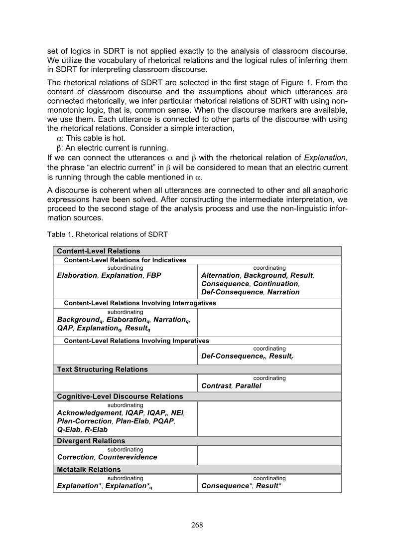
set of logics in SDRT is not applied exactly to the analysis of classroom discourse. We utilize the vocabulary of rhetorical relations and the logical rules of inferring them in SDRT for interpreting classroom discourse. The rhetorical relations of SDRT are selected in the first stage of Figure 1. From the content of classroom discourse and the assumptions about which utterances are connected rhetorically, we infer particular rhetorical relations of SDRT with using non-monotonic logic, that is, common sense. When the discourse markers are available, we use them. Each utterance is connected to other parts of the discourse with using the rhetorical relations. Consider a simple interaction, α: This cable is hot. β: An electric current is running.

If we can connect the utterances α and β with the rhetorical relation of Explanation, the phrase “an electric current” in β will be considered to mean that an electric current is running through the cable mentioned in α. A discourse is coherent when all utterances are connected to other and all anaphoric expressions have been solved. After constructing the intermediate interpretation, we proceed to the second stage of the analysis process and use the non-linguistic infor-mation sources.

Table 1. Rhetorical relations of SDRT

Content-Level Relations Content-Level Relations for Indicatives

subordinating Elaboration, Explanation, FBP

coordinating Alternation, Background, Result, Consequence, Continuation, Def-Consequence, Narration

Content-Level Relations Involving Interrogatives subordinating

Backgroundq, Elaborationq, Narrationq, QAP, Explanationq, Resultq

Content-Level Relations Involving Imperatives coordinating

Def-Consequencer, Resultr

Text Structuring Relations coordinating

Contrast, Parallel Cognitive-Level Discourse Relations

subordinating Acknowledgement, IQAP, IQAPr, NEI, Plan-Correction, Plan-Elab, PQAP, Q-Elab, R-Elab

Divergent Relations subordinating

Correction, Counterevidence

Metatalk Relations subordinating

Explanation*, Explanation*q coordinating

Consequence*, Result*

268

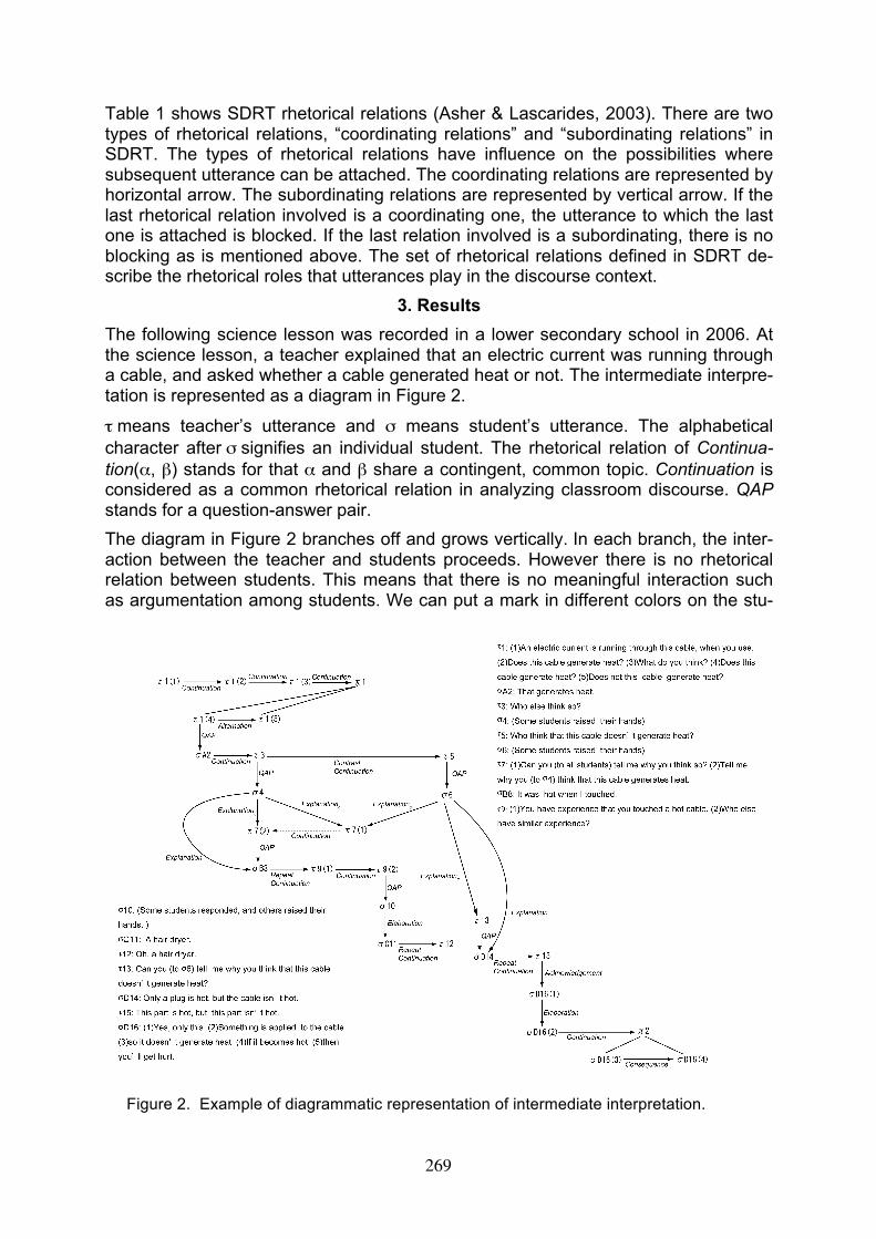
Table 1 shows SDRT rhetorical relations (Asher & Lascarides, 2003). There are two types of rhetorical relations, “coordinating relations” and “subordinating relations” in SDRT. The types of rhetorical relations have influence on the possibilities where subsequent utterance can be attached. The coordinating relations are represented by horizontal arrow. The subordinating relations are represented by vertical arrow. If the last rhetorical relation involved is a coordinating one, the utterance to which the last one is attached is blocked. If the last relation involved is a subordinating, there is no blocking as is mentioned above. The set of rhetorical relations defined in SDRT de-scribe the rhetorical roles that utterances play in the discourse context.

3. Results The following science lesson was recorded in a lower secondary school in 2006. At the science lesson, a teacher explained that an electric current was running through a cable, and asked whether a cable generated heat or not. The intermediate interpre-tation is represented as a diagram in Figure 2.

τ means teacher’s utterance and σ means student’s utterance. The alphabetical character after σ signifies an individual student. The rhetorical relation of Continua-tion(α, β) stands for that α and β share a contingent, common topic. Continuation is considered as a common rhetorical relation in analyzing classroom discourse. QAP stands for a question-answer pair. The diagram in Figure 2 branches off and grows vertically. In each branch, the inter-action between the teacher and students proceeds. However there is no rhetorical relation between students. This means that there is no meaningful interaction such as argumentation among students. We can put a mark in different colors on the stu-

Figure 2. Example of diagrammatic representation of intermediate interpretation.

269

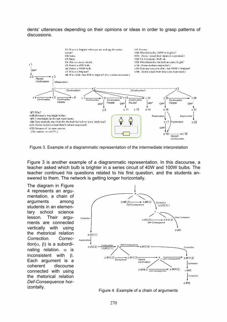
dents’ utterances depending on their opinions or ideas in order to grasp patterns of discussions.

Figure 3 is another example of a diagrammatic representation. In this discourse, a teacher asked which bulb is brighter in a series circuit of 40W and 100W bulbs. The teacher continued his questions related to his first question, and the students an-swered to them. The network is getting longer horizontally. The diagram in Figure 4 represents an argu-mentation, a chain of arguments among students in an elemen-tary school science lesson. Their argu-ments are connected vertically with using the rhetorical relation Correction. Correc-tion(α, β) is a subordi-nating relation. α is inconsistent with β. Each argument is a coherent discourse connected with using the rhetorical relation Def-Consequence hor-izontally.

Figure 3. Example of a diagrammatic representation of the intermediate interpretation

Figure 4. Example of a chain of arguments

270

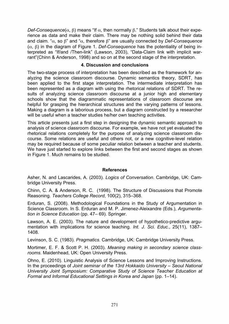
Def-Consequence(α, β) means “If α, then normally β.” Students talk about their expe-rience as data and make their claim. There may be nothing solid behind their data and claim. “α, so β” and “α, therefore β” are usually connected by Def-Consequence (α, β) in the diagram of Figure 1. Def-Consequence has the potentiality of being in-terpreted as “If/and /Then-link” (Lawson, 2003), “Data-Claim link with implicit war-rant”(Chinn & Anderson, 1998) and so on at the second stage of the interpretation.

4. Discussion and conclusions The two-stage process of interpretation has been described as the framework for an-alyzing the science classroom discourse. Dynamic semantics theory, SDRT, has been applied to the first stage interpretation. The intermediate interpretation has been represented as a diagram with using the rhetorical relations of SDRT. The re-sults of analyzing science classroom discourse at a junior high and elementary schools show that the diagrammatic representations of classroom discourse are helpful for grasping the hierarchical structures and the varying patterns of lessons. Making a diagram is a laborious process, but a diagram constructed by a researcher will be useful when a teacher studies he/her own teaching activities. This article presents just a first step in designing the dynamic semantic approach to analysis of science classroom discourse. For example, we have not yet evaluated the rhetorical relations completely for the purpose of analyzing science classroom dis-course. Some relations are useful and others not, or a new cognitive-level relation may be required because of some peculiar relation between a teacher and students. We have just started to explore links between the first and second stages as shown in Figure 1. Much remains to be studied.

References Asher, N. and Lascarides, A. (2003). Logics of Conversation. Cambridge, UK: Cam-bridge University Press. Chinn, C. A. & Anderson, R. C. (1998). The Structure of Discussions that Promote Reasoning. Teachers College Record, 100(2), 315–368. Erduran, S. (2008). Methodological Foundations in the Study of Argumentation in Science Classroom. In S. Erduran and M. P. Jimenez-Aleixandre (Eds.), Argumenta-tion in Science Education (pp. 47– 69). Springer. Lawson, A. E. (2003). The nature and development of hypothetico-predictive argu-mentation with implications for science teaching. Int. J. Sci. Educ., 25(11), 1387– 1408. Levinson, S. C. (1983). Pragmatics. Cambridge, UK: Cambridge University Press. Mortimer, E. F. & Scott P. H. (2003). Meaning making in secondary science class-rooms. Maidenhead, UK: Open University Press. Ohno, E. (2010). Linguistic Analysis of Science Lessons and Improving Instructions. In the proceedings of Joint seminar of the 13rd Hokkaido University – Seoul National University Joint Symposium: Comparative Study of Science Teacher Education at Formal and Informal Educational Settings in Korea and Japan (pp. 1–14).

271

An Inquiry Based Approach to the study of energy exchange

by thermal radiation

Nicola Pizzolato, Onofrio Rosario Battaglia and Rosa Maria Sperandeo-Mineo

nicola.pizzolato@unipa.it

UOP_PERG (University of Palermo Physics Education Research Group)

Dipartimento di Fisica, Università di Palermo (Italia)

A teaching-learning sequence regarding the investigation of energy exchange by thermal radiation, conduction and convection is under development within the context of “Establish”, a FP7 European Project aimed at promoting and developing Inquiry Based Science Education in European Secondary Schools. Here we present some relevant laboratory activities of this inquiry-oriented teaching/learning sequence for secondary school level students (or even first-level university ones), aimed at investigating the physics of energy transmission by thermal radiation. In traditional laboratory work, the focus of students activities is mostly dedicated on verifying information previously transferred by the teacher. Our teaching-learning sequence is instead organized by firstly engaging students by scientifically oriented questions about real life situations, such as thermal insulation of houses and the use of energy saving materials. This introductory phase of topic exploration, mainly based on students’ prior knowledge, is followed by a discussion about the relevant physical quantities which should be taken into account in a contest of a laboratory activity of measurements. A scientific investigation on the energy exchange between a powered resistor and its surrounding environment during the heating and cooling processes is proposed. Students are stimulated to design and carry out their own laboratory activity by collecting, processing and analysing data, in order to discover new concepts or laws and obtain more meaningful conceptual understanding of the physics underlying the process of energy exchange by thermal radiation.

1. Introduction

Inquiry Based Science Education (IBSE) is a functional way of considering teaching and learning activities, developed to cope the need of today economic, environmental and social realities that demand new science skills and higher-order thinking abilities from our students (Rocard et al., 2007). IB approaches to science education focus on student constructed learning as opposed to traditional teacher-transmitted information. Inquiry based curriculum and teaching techniques have emerged as a combination of several theories such as constructivism, multiple intelligences (Gardner, 1983) and accelerated learning (Burnaford et al., 2009), with the aim of enhance learning based on increased student involvement, multiple ways of knowing and sequential phases of cognition. Furthermore, by stimulating the development of students' multiple intelligences, more types of students achieve a successful contribution, while others are engaged on more than one level of knowledge. This process leads to more complete cognition by building on previously learned knowledge. Science education carried out by following an inquiry-based approach appears to be more effective to develop independent and critical thinking skills, positive attitudes and curiosity toward science (Shymansky, 1984; Kyle et al, 1988; Hall & McCurdy, 1990; Beerer and Bodzin, 2003; Campbell et al., 2010).

A quantitative study on the effectiveness of an IB approach applied to laboratory activities during an introductory course of biology has shown that students achieved 6% higher grades on biology content exams as opposed to the control group, which completed a more traditional information-transmission modelled laboratory (Leonard, 1983). Student derived investigations brings about a more relevant and meaningful knowledge (Polman, J.L., 2000, Stephens and Clement, 2010).

272

In this view, we are developing a teaching-learning sequence regarding the investigation of energy exchange by thermal radiation, conduction and convection, within the context of “Establish”, an FP7 European Project aimed at promoting and developing IBSE in European secondary schools. Our teaching-learning sequence is organized by firstly engaging students by scientifically oriented questions about real life situations, such as thermal insulation of houses and the use of energy saving materials. Students are invited to design and build by themselves a scale model of an energy-efficient house, through the understanding of relevant concepts regarding the energy flow in thermal systems. Students are directly involved into modelling and practical activities and they are stimulated to carry out their own experiments.

As a part of this inquiry-oriented teaching/learning sequence, here we present some relevant laboratory activities for secondary school level students, or even first-level university ones, aimed at investigating the physics of energy transfer by thermal radiation. A scientific investigation on the energy exchange between a powered resistor and its surrounding environment during the heating and cooling processes is proposed. Students are stimulated to plan and carry out their own laboratory activity by collecting, processing and analysing data, in order to learn new concepts or laws and obtain more meaningful conceptual understanding of the physics underlying the process of energy exchange by thermal radiation. Our approach is different from structured inquiry, in which students are guided through some laboratory activities where the end result of an experiment is often useful to validate a true-false hypothesis [Nottis et al., 2010]; here we propose a learning path based on active exploration and the experimental results are always object of discussions.

This paper is organized as follows: in Sect. 2 we present the experimental procedure and a description of the inquiry-lab learning path; the results are shown in Sect. 3 and the discussion and concluding remarks are given in Sect. 4.

2. Method

The classroom activities are introduced through a phase of topic exploration, mainly based on students’ prior knowledge, is followed by a discussion about the relevant physical quantities which should be taken into account in a contest of a laboratory activity of measurements. From their previous studies, students should know that the energy exchange between an emitting body and its surrounding is caused by the processes of conduction, convection and radiation. By discussing between each other, students should gather that, in the absence of a medium, as in a vacuum system, the conduction and convection cannot take place. Students are initially left free to design their own experiments to study the emission of thermal radiation. Then, they are introduced to the laboratory and invited to adapt their plans about conducting the experiments with the available measurement facility for the study of energy exchange by thermal radiation.

Guide to the experimental activity

The temperature of a powered resistor inside a vacuum tube can be measured during the heating and cooling process with the equipment shown in Fig. 1. The system is composed by a vacuum pump which is connected to a vacuum tube containing the resistor; the pump can lower the pressure inside the tube up to 0.01 bar. The temperature of the resistor is measured by mean of a thermocouple which is placed inside the vacuum tube and whose tip is in contact with the resistor surface. The thermocouple is externally connected to an amplifier module and interfaced to the lab computer. The resistor is a ceramic-type with the following physical

273

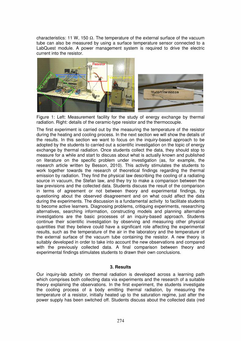
characteristics: 11 W, 150 Ω. The temperature of the external surface of the vacuum tube can also be measured by using a surface temperature sensor connected to a LabQuest module. A power management system is required to drive the electric current into the resistor.

ResistorResistor

Power Power managmentmanagment

PC

inte

rfac

e

PC

inte

rfac

e

VacuumVacuum pumppump

ResistorResistor

Power Power managmentmanagment

PC

inte

rfac

e

PC

inte

rfac

e

VacuumVacuum pumppump

Figure 1: Left: Measurement facility for the study of energy exchange by thermal radiation. Right: details of the ceramic-type resistor and the thermocouple.

The first experiment is carried out by the measuring the temperature of the resistor during the heating and cooling process. In the next section we will show the details of the results. In this section we want to focus on the inquiry-based approach to be adopted by the students to carried out a scientific investigation on the topic of energy exchange by thermal radiation. Once students collect the data, they should stop to measure for a while and start to discuss about what is actually known and published on literature on the specific problem under investigation (as, for example, the research article written by Besson, 2010). This activity stimulates the students to work together towards the research of theoretical findings regarding the thermal emission by radiation. They find the physical law describing the cooling of a radiating source in vacuum, the Stefan law, and they try to make a comparison between the law previsions and the collected data. Students discuss the result of the comparison in terms of agreement or not between theory and experimental findings, by questioning about the observed disagreement and on what could affect the data during the experiments. The discussion is a fundamental activity to facilitate students to become active learners. Diagnosing problems, critiquing experiments, researching alternatives, searching information, constructing models and planning alternative investigations are the basic processes of an inquiry-based approach. Students continue their scientific investigation by observing and measuring other physical quantities that they believe could have a significant role affecting the experimental results, such as the temperature of the air in the laboratory and the temperature of the external surface of the vacuum tube containing the resistor. A new theory is suitably developed in order to take into account the new observations and compared with the previously collected data. A final comparison between theory and experimental findings stimulates students to drawn their own conclusions.

3. Results

Our inquiry-lab activity on thermal radiation is developed across a learning path which comprises both collecting data via experiments and the research of a suitable theory explaining the observations. In the first experiment, the students investigate the cooling process of a body emitting thermal radiation, by measuring the temperature of a resistor, initially heated up to the saturation regime, just after the power supply has been switched off. Students discuss about the collected data (red

274

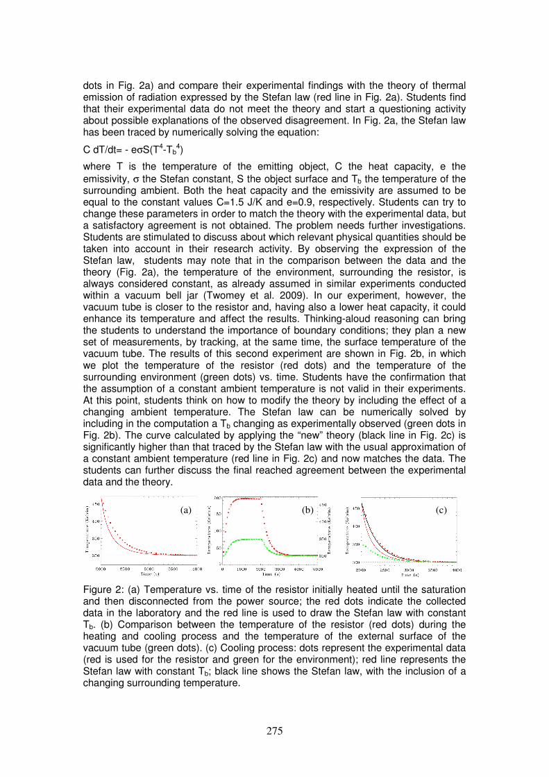
dots in Fig. 2a) and compare their experimental findings with the theory of thermal emission of radiation expressed by the Stefan law (red line in Fig. 2a). Students find that their experimental data do not meet the theory and start a questioning activity about possible explanations of the observed disagreement. In Fig. 2a, the Stefan law has been traced by numerically solving the equation:

C dT/dt= - eσS(T4-Tb4)

where T is the temperature of the emitting object, C the heat capacity, e the

emissivity, σ the Stefan constant, S the object surface and Tb the temperature of the surrounding ambient. Both the heat capacity and the emissivity are assumed to be equal to the constant values C=1.5 J/K and e=0.9, respectively. Students can try to change these parameters in order to match the theory with the experimental data, but a satisfactory agreement is not obtained. The problem needs further investigations. Students are stimulated to discuss about which relevant physical quantities should be taken into account in their research activity. By observing the expression of the Stefan law, students may note that in the comparison between the data and the theory (Fig. 2a), the temperature of the environment, surrounding the resistor, is always considered constant, as already assumed in similar experiments conducted within a vacuum bell jar (Twomey et al. 2009). In our experiment, however, the vacuum tube is closer to the resistor and, having also a lower heat capacity, it could enhance its temperature and affect the results. Thinking-aloud reasoning can bring the students to understand the importance of boundary conditions; they plan a new set of measurements, by tracking, at the same time, the surface temperature of the vacuum tube. The results of this second experiment are shown in Fig. 2b, in which we plot the temperature of the resistor (red dots) and the temperature of the surrounding environment (green dots) vs. time. Students have the confirmation that the assumption of a constant ambient temperature is not valid in their experiments. At this point, students think on how to modify the theory by including the effect of a changing ambient temperature. The Stefan law can be numerically solved by including in the computation a Tb changing as experimentally observed (green dots in Fig. 2b). The curve calculated by applying the “new” theory (black line in Fig. 2c) is significantly higher than that traced by the Stefan law with the usual approximation of a constant ambient temperature (red line in Fig. 2c) and now matches the data. The students can further discuss the final reached agreement between the experimental data and the theory.

Figure 2: (a) Temperature vs. time of the resistor initially heated until the saturation and then disconnected from the power source; the red dots indicate the collected data in the laboratory and the red line is used to draw the Stefan law with constant Tb. (b) Comparison between the temperature of the resistor (red dots) during the heating and cooling process and the temperature of the external surface of the vacuum tube (green dots). (c) Cooling process: dots represent the experimental data (red is used for the resistor and green for the environment); red line represents the Stefan law with constant Tb; black line shows the Stefan law, with the inclusion of a changing surrounding temperature.

(a) (b) (c)

275

4. Discussion and conclusions

In this paper we present a teaching/learning path based on a set of inquiry-laboratory activities aimed at driving students to the understanding of the physics underlying the process of thermal radiation. Students are engaged by questions regarding their every-day experience that lend themselves to scientific investigations and they are stimulated to design their own experiments. Such experiments are discussed in the classroom and adapted to the equipments at disposal. Students collect, process and analyse the data of a previously heated resistor, cooling in a vacuum system. The experimental findings are compared with the available theories and students discuss about the results of the comparison. “Do our experimental data meet the theory?” This is the question. If the answer is “yes”, everything is fine. If the answer is “no”, as usual, students should check their experiment and think which physical phenomenon could affect the data. Then, they can turn back to the theory, eventually modifying the previous one, and conduct a new comparison. In this way, students are involved into a real scientific research that can bring up to results unexpected even for the teachers, such as the importance of the temperature of the surrounding environment into the study of the energy exchange by thermal radiation. If the agreement between theory and collected data is still not completely satisfying, as the most usual case, students could guess that maybe they used a not perfectly correct value of heat capacity and/or emissivity in the numerical solution of the Stefan law and perform further investigations on how the accordance between data and theory can be improved by changing these parameters.

Traditional methods of teaching physics, mainly based on transmission of information and laws, bring about a not lasting and effective learning. Inquiry based physics education represents a valid alternative to traditional teaching. The main goal of a physics effective teaching path should be the improvement of the reasoning skills of the students, who become brain-trained to observe and understand the natural phenomena. Our teaching-learning path by mean of an inquiry lab on the topic of energy exchange by thermal radiation has been presented to groups of secondary school physics teachers, in order to assess its feasibility and pedagogical potential effectiveness. Preliminary results have shown a positive feedback from involved teachers, which have considered this inquiry-based learning path an open way of scientifically investigating the physics of thermal emission by radiation; they also have evaluated the opportunity to easily extend this inquiry lab in order to include many different and interesting experimental paths on the energy exchange by conduction and convection. The experimentation of this inquiry-lab learning path on high school students is under implementation and the results will be the subject of a forthcoming paper.

Acknowledgement

This work was developed within the context of “Establish”, an FP7 European project, grant agreement n. 244749.

References

Besson, U. (2010). Cooling and warming laws: an exact analytical solution. European Journal of Physics 31, 1107-1121

Beerer, K. and bodzin, A. M. (2003). Promoting Inquiry Based Science Instruction: the validation of the Science Teacher Inquiry Rubric (STIR). Journal of Elementary Science Education 15, 2, 39-49

276

Burnaford, G.E., Fischer, J., Hobson, D. (2009). Teachers doing research: The Power of Action Through Inquiry (2nd ed.). Mahwah, New Jersey: Lawrence Erlbaum Associates. ISBN 0-8058-3589-X.

Campbell, T., Abd-Hamid, N. H., & chapman, H. (2010). Development of Instruments to assess Teacher and Student Perception of Inquiry Experiences in Science Classrooms. Journal of Science Education 21, 13-30

Gardner, H. (1983). Frames of Mind: The Theory of Multiple Intelligences. New York: Basic Books.

Kyle, W.C., Jr., Bonnstetter, R.J., & Gadsden, T., Jr., (1988). An implementation study: an analysis of elementary students' and teachers' attitudes toward science in process-approach vs. traditional science classes. Journal of Research in Science Teaching 25, 103-120.

Hall, D. A. and McCurdy, D. W. (1990). A comparison of a biological science curriculum study (BSCS) laboratory and a traditional laboratory on student achievement at two private liberal arts colleges. Journal of Research in Science Teaching 27, 625-636.

Leonard, W.H. (1983). An experimental study of a BSCS-style laboratory approach for university general biology. Journal of Research in Science Teaching 20, 807-813.

Polman, J.L. (2000). Designing Project-Based Science: Connecting Learners Through Guided Inquiry. New York: Teachers College Press, Columbia University.

Nottis, K.E.K., Prince, M.J., Vigeant, M.A. (2010). Building an understanding of heat transfer concepts in undergraduate courses. US-China Education Review, 7, ISSN 1548-6613, USA.

Rocard, M., Csermely, P., Jorde, D., Lenzen, D., Walberg-Henriksson, H., Hemmo, V. (2007). Science Education Now: A renewed Pedagogy for the Future of Europe. EU Research Report, ISSN 1018-5593.

Shymansky, J.A. (1984). BSCS programs: just how effective were they? The American Biology Teacher 46, 54-57.

Stephens, A.L., Clement, J.J. (2010). Documenting the use of expert scientific reasoning process by high school physics students. Physical Review Special Topics – Physics Education Research 6, 020122.

Twomey, P., O’Sullivan, C. and O’Riordan, J. (2009). An experimental investigation of the role of radiation in laboratory bench-top experiments in thermal physics. European Journal of Physics 30, 559-566.

277

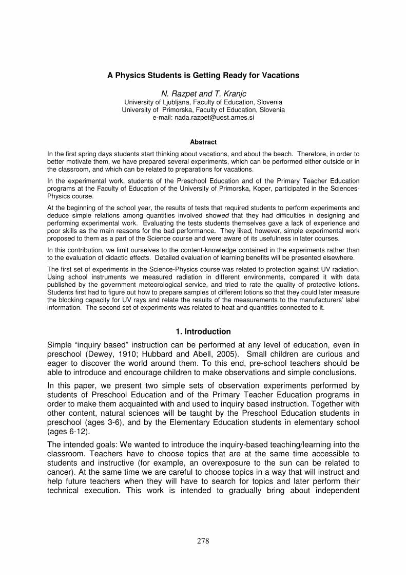
A Physics Students is Getting Ready for Vacations

N. Razpet and T. Kranjc University of Ljubljana, Faculty of Education, Slovenia

University of Primorska, Faculty of Education, Slovenia e-mail: nada.razpet@uest.arnes.si

Abstract

In the first spring days students start thinking about vacations, and about the beach. Therefore, in order to better motivate them, we have prepared several experiments, which can be performed either outside or in the classroom, and which can be related to preparations for vacations.

In the experimental work, students of the Preschool Education and of the Primary Teacher Education programs at the Faculty of Education of the University of Primorska, Koper, participated in the Sciences-Physics course.

At the beginning of the school year, the results of tests that required students to perform experiments and deduce simple relations among quantities involved showed that they had difficulties in designing and performing experimental work. Evaluating the tests students themselves gave a lack of experience and poor skills as the main reasons for the bad performance. They liked, however, simple experimental work proposed to them as a part of the Science course and were aware of its usefulness in later courses.

In this contribution, we limit ourselves to the content-knowledge contained in the experiments rather than to the evaluation of didactic effects. Detailed evaluation of learning benefits will be presented elsewhere.

The first set of experiments in the Science-Physics course was related to protection against UV radiation. Using school instruments we measured radiation in different environments, compared it with data published by the government meteorological service, and tried to rate the quality of protective lotions. Students first had to figure out how to prepare samples of different lotions so that they could later measure the blocking capacity for UV rays and relate the results of the measurements to the manufacturers’ label information. The second set of experiments was related to heat and quantities connected to it.

1. Introduction

Simple “inquiry based” instruction can be performed at any level of education, even in preschool (Dewey, 1910; Hubbard and Abell, 2005). Small children are curious and eager to discover the world around them. To this end, pre-school teachers should be able to introduce and encourage children to make observations and simple conclusions.

In this paper, we present two simple sets of observation experiments performed by students of Preschool Education and of the Primary Teacher Education programs in order to make them acquainted with and used to inquiry based instruction. Together with other content, natural sciences will be taught by the Preschool Education students in preschool (ages 3-6), and by the Elementary Education students in elementary school (ages 6-12).

The intended goals: We wanted to introduce the inquiry-based teaching/learning into the classroom. Teachers have to choose topics that are at the same time accessible to students and instructive (for example, an overexposure to the sun can be related to cancer). At the same time we are careful to choose topics in a way that will instruct and help future teachers when they will have to search for topics and later perform their technical execution. This work is intended to gradually bring about independent

278

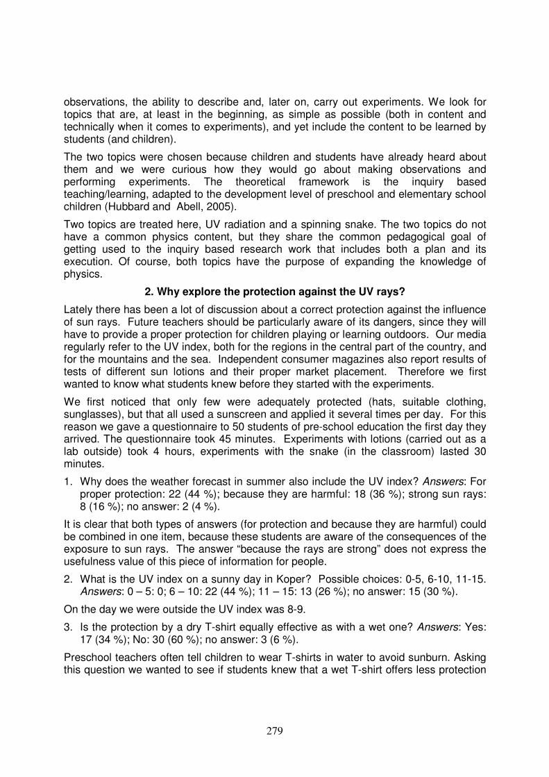
observations, the ability to describe and, later on, carry out experiments. We look for topics that are, at least in the beginning, as simple as possible (both in content and technically when it comes to experiments), and yet include the content to be learned by students (and children).

The two topics were chosen because children and students have already heard about them and we were curious how they would go about making observations and performing experiments. The theoretical framework is the inquiry based teaching/learning, adapted to the development level of preschool and elementary school children (Hubbard and Abell, 2005).

Two topics are treated here, UV radiation and a spinning snake. The two topics do not have a common physics content, but they share the common pedagogical goal of getting used to the inquiry based research work that includes both a plan and its execution. Of course, both topics have the purpose of expanding the knowledge of physics.

2. Why explore the protection against the UV rays?

Lately there has been a lot of discussion about a correct protection against the influence of sun rays. Future teachers should be particularly aware of its dangers, since they will have to provide a proper protection for children playing or learning outdoors. Our media regularly refer to the UV index, both for the regions in the central part of the country, and for the mountains and the sea. Independent consumer magazines also report results of tests of different sun lotions and their proper market placement. Therefore we first wanted to know what students knew before they started with the experiments.

We first noticed that only few were adequately protected (hats, suitable clothing, sunglasses), but that all used a sunscreen and applied it several times per day. For this reason we gave a questionnaire to 50 students of pre-school education the first day they arrived. The questionnaire took 45 minutes. Experiments with lotions (carried out as a lab outside) took 4 hours, experiments with the snake (in the classroom) lasted 30 minutes.

1. Why does the weather forecast in summer also include the UV index? Answers: For proper protection: 22 (44 %); because they are harmful: 18 (36 %); strong sun rays: 8 (16 %); no answer: 2 (4 %).

It is clear that both types of answers (for protection and because they are harmful) could be combined in one item, because these students are aware of the consequences of the exposure to sun rays. The answer “because the rays are strong” does not express the usefulness value of this piece of information for people.

2. What is the UV index on a sunny day in Koper? Possible choices: 0-5, 6-10, 11-15. Answers: 0 – 5: 0; 6 – 10: 22 (44 %); 11 – 15: 13 (26 %); no answer: 15 (30 %).

On the day we were outside the UV index was 8-9.

3. Is the protection by a dry T-shirt equally effective as with a wet one? Answers: Yes: 17 (34 %); No: 30 (60 %); no answer: 3 (6 %).

Preschool teachers often tell children to wear T-shirts in water to avoid sunburn. Asking this question we wanted to see if students knew that a wet T-shirt offers less protection

279

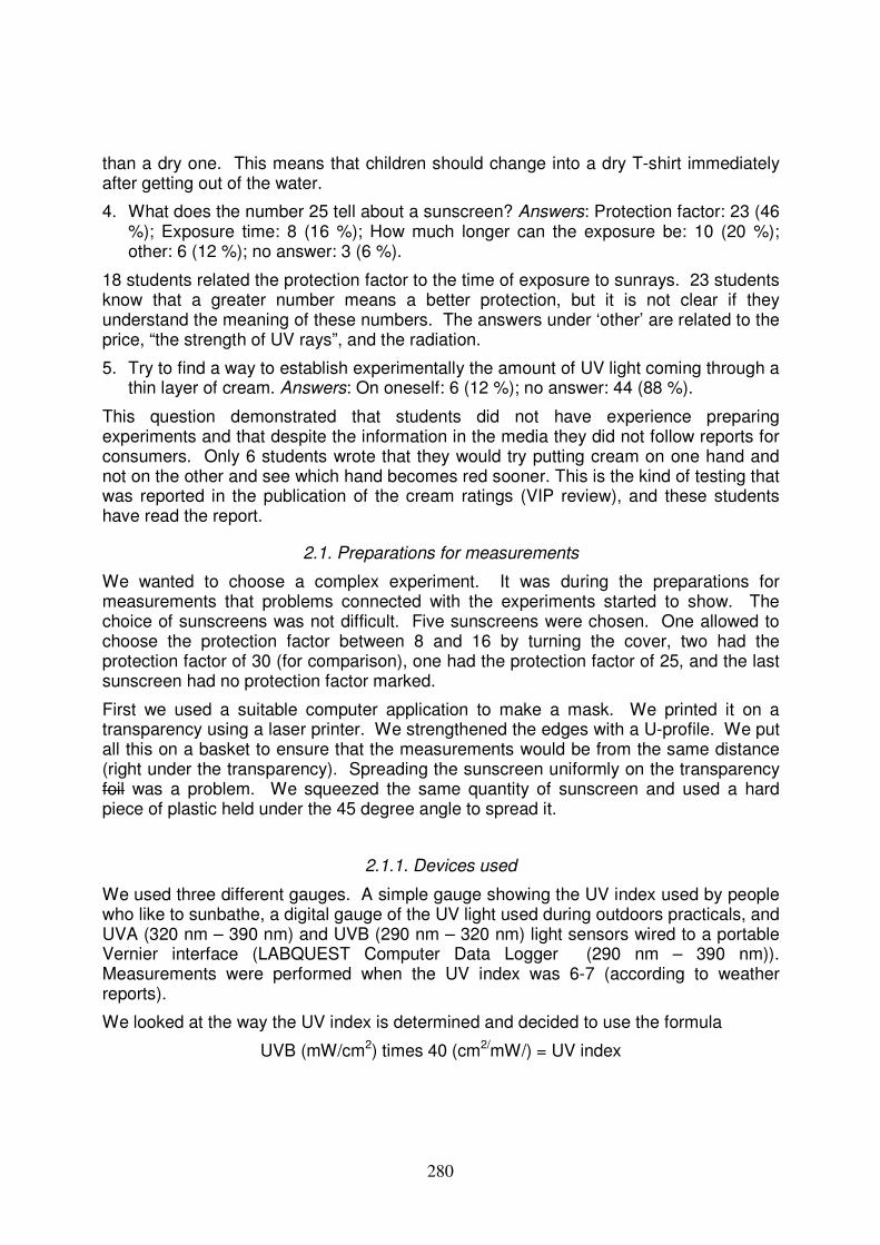
than a dry one. This means that children should change into a dry T-shirt immediately after getting out of the water.

4. What does the number 25 tell about a sunscreen? Answers: Protection factor: 23 (46 %); Exposure time: 8 (16 %); How much longer can the exposure be: 10 (20 %); other: 6 (12 %); no answer: 3 (6 %).

18 students related the protection factor to the time of exposure to sunrays. 23 students know that a greater number means a better protection, but it is not clear if they understand the meaning of these numbers. The answers under ‘other’ are related to the price, “the strength of UV rays”, and the radiation.

5. Try to find a way to establish experimentally the amount of UV light coming through a thin layer of cream. Answers: On oneself: 6 (12 %); no answer: 44 (88 %).

This question demonstrated that students did not have experience preparing experiments and that despite the information in the media they did not follow reports for consumers. Only 6 students wrote that they would try putting cream on one hand and not on the other and see which hand becomes red sooner. This is the kind of testing that was reported in the publication of the cream ratings (VIP review), and these students have read the report.

2.1. Preparations for measurements

We wanted to choose a complex experiment. It was during the preparations for measurements that problems connected with the experiments started to show. The choice of sunscreens was not difficult. Five sunscreens were chosen. One allowed to choose the protection factor between 8 and 16 by turning the cover, two had the protection factor of 30 (for comparison), one had the protection factor of 25, and the last sunscreen had no protection factor marked.

First we used a suitable computer application to make a mask. We printed it on a transparency using a laser printer. We strengthened the edges with a U-profile. We put all this on a basket to ensure that the measurements would be from the same distance (right under the transparency). Spreading the sunscreen uniformly on the transparency foil was a problem. We squeezed the same quantity of sunscreen and used a hard piece of plastic held under the 45 degree angle to spread it.

2.1.1. Devices used

We used three different gauges. A simple gauge showing the UV index used by people who like to sunbathe, a digital gauge of the UV light used during outdoors practicals, and UVA (320 nm – 390 nm) and UVB (290 nm – 320 nm) light sensors wired to a portable Vernier interface (LABQUEST Computer Data Logger (290 nm – 390 nm)). Measurements were performed when the UV index was 6-7 (according to weather reports).

We looked at the way the UV index is determined and decided to use the formula

UVB (mW/cm2) times 40 (cm2/mW/) = UV index

280

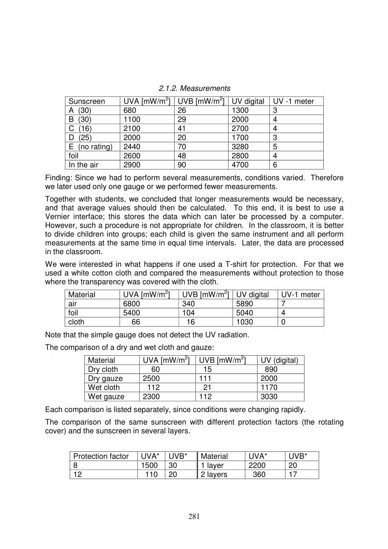
2.1.2. Measurements

Sunscreen UVA [mW/m2] UVB [mW/m2] UV digital UV -1 meter A (30) 680 26 1300 3 B (30) 1100 29 2000 4 C (16) 2100 41 2700 4 D (25) 2000 20 1700 3 E (no rating) 2440 70 3280 5 foil 2600 48 2800 4 In the air 2900 90 4700 6

Finding: Since we had to perform several measurements, conditions varied. Therefore we later used only one gauge or we performed fewer measurements.

Together with students, we concluded that longer measurements would be necessary, and that average values should then be calculated. To this end, it is best to use a Vernier interface; this stores the data which can later be processed by a computer. However, such a procedure is not appropriate for children. In the classroom, it is better to divide children into groups; each child is given the same instrument and all perform measurements at the same time in equal time intervals. Later, the data are processed in the classroom.

We were interested in what happens if one used a T-shirt for protection. For that we used a white cotton cloth and compared the measurements without protection to those where the transparency was covered with the cloth.

Material UVA [mW/m2] UVB [mW/m2] UV digital UV-1 meter air 6800 340 5890 7 foil 5400 104 5040 4 cloth 66 16 1030 0

Note that the simple gauge does not detect the UV radiation.

The comparison of a dry and wet cloth and gauze:

Material UVA [mW/m2] UVB [mW/m2] UV (digital) Dry cloth 60 15 890 Dry gauze 2500 111 2000 Wet cloth 112 21 1170 Wet gauze 2300 112 3030

Each comparison is listed separately, since conditions were changing rapidly.

The comparison of the same sunscreen with different protection factors (the rotating cover) and the sunscreen in several layers.

Protection factor UVA* UVB* Material UVA* UVB* 8 1500 30 1 layer 2200 20 12 110 20 2 layers 360 17

281

16 350 16 3 layers 70 15

(* - in mW/m2.) Several other measurements were performed. For example, with the same sunscreen subjected to longer times of exposure to sunrays, adding water under the foil and observing the resulting changes. These measurements are not presented.

Looking at the UV indices we see that measurements performed with the simple gauge showing the UV index do not match the index obtained by the formula. This was not a surprise. There are several reasons for that. Measurements would have to be performed over a longer period of time and averaged, they would have to be done at the same time to ensure a valid comparison.

2.2. What have we learned?

It is very difficult to make comparisons when a sunscreen is applied to different bases. The school should have several gauges of the same kind and each student would measure the penetration of different sunscreens. A sunscreen used on a skin of course reacts with the skin. This means that it performs differently than on a transparency. However, a qualitative rating of a cream can still be made.

Students also learn that simple measurements performed outdoors in a short time cannot be compared with professional measurements, however they can still get a qualitative comparison (more or less).

We read in a journal that the protection factor is related to the transmission. The protection factor of 20 is supposed to let through 1/20 of the UVB rays. This way we quickly see that 100 percent protection does not exist.

3. Experiments with the revolving snake

The second set of experiments is related to heat. This theme is also of current interest due to the global warming and the cost of heating. It can be related to the heat insulation of dwelling spaces. Students can discover many things using a home-made measuring device called the “snake”. Measuring the angular velocity of its spinning, the difference between the temperatures of a body that radiates heat (like a radiator or a candle) and the ambient air can be estimated. In our experience simple measuring devices, made by students themselves, have several advantages (Buttemer, 2006; Goldberg and Boulanger, 1981; Corni et al., 2007). For example, constructing them students learn how to solve basic technical problems, they are interesting because they show that one does not always need sophisticated commercial instruments to get simple estimates. Simple measuring devices also more clearly show the physics content of phenomena.

Results of the questionnaire by which we assessed students’ knowledge about heat will be presented elsewhere. They show that students are not familiar with the notions of heat and heat flow. Therefore we designed several experiments. Students liked best experiments with the revolving snake (a paper wind turbine in some books).

282

3.1. How to construct a revolving snake?

During its construction several difficulties have to be resolved. First, a paper of the right thickness has to be chosen (not too thick, not too thin). Then the length of the snake has to be determined and the snake has to be correctly attached to a knitting needle, so that it can spin freely.

We construct it as follows. We put a knitting needle on a supporting plate, attach a snap fastener to the middle of the snake and hang it on the tip of the needle. When the snake is put on top of a warm radiator it spins. The bigger the difference between the temperature of the radiator and the surrounding air the greater the heat flow and the faster the spinning of the snake.

Interesting results are obtained when the snake is hung over surfaces (paper sheets) of different color. If the air is not moving, almost nothing is happening. However, during a slight breeze the snake spins faster above a black than above a white paper.

Of course there are further issues and experiments. We can vary the snake size, make different choices of a paper etc.

4. Conclusion

All experiments described above invite further measurements and improvements. This is exactly the appeal of such an approach. The teacher can engage students who make fast or slow measurements, and who are more or less skillful. At the same time he/she can show them connections with what they hear daily.

References

Buttemer, H. (2006). Inquiry on Board. Science and children, October 2006, 34-39. Dewey, J. (1910). Science as subject matter and as method. Science, 31 (786), 121–

127. Demir, A. and Abell, S.K. (2010). Views of Inquiry: Mismatches Between Views of

Science Education Faculty and Students of an Alternative Certification Program. Journal of research and science teaching, 47 (6), 716-741.

Goldberg, H.S., Boulanger, F.D. (1981). Science for elementary school teachers: A quantitative approach. Am. J. Phys., 49 (2), 120-124.

Hubbard, P., & Abell, S. (2005). Setting sail or missing the boat: Comparing the beliefs of preservice elementary teachers with and without an inquiry-based physics course. Journal of Science Teacher Education, 16, 5–25.

Corni, F., Giliberti, E., Michelini, M., Stefanel, A. (2007). The basic models in the experimental work of student-teachers of primary school. GIREP 2006, Amsterdam.

Vernier Software & Technology, LabQuest Quick – Start Guide, Open Source Software. VIP, Zveza potrošnikov Slovenije (Consumer Association of Slovenia), 7-8/2011,

Ljubljana.

283

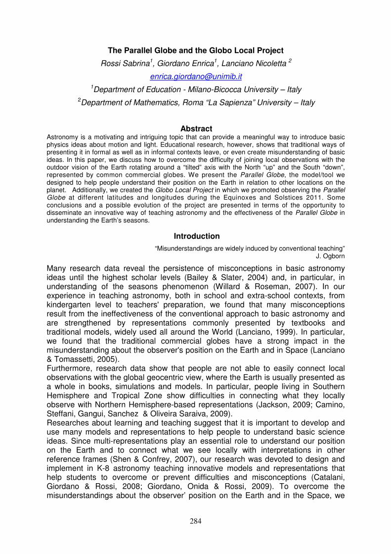
The Parallel Globe and the Globo Local Project

Rossi Sabrina1, Giordano Enrica1, Lanciano Nicoletta 2

enrica.giordano@unimib.it 1Department of Education - Milano-Bicocca University – Italy

2Department of Mathematics, Roma “La Sapienza” University – Italy

Abstract Astronomy is a motivating and intriguing topic that can provide a meaningful way to introduce basic physics ideas about motion and light. Educational research, however, shows that traditional ways of presenting it in formal as well as in informal contexts leave, or even create misunderstanding of basic ideas. In this paper, we discuss how to overcome the difficulty of joining local observations with the outdoor vision of the Earth rotating around a “tilted” axis with the North “up” and the South “down”, represented by common commercial globes. We present the Parallel Globe, the model/tool we designed to help people understand their position on the Earth in relation to other locations on the planet. Additionally, we created the Globo Local Project in which we promoted observing the Parallel Globe at different latitudes and longitudes during the Equinoxes and Solstices 2011. Some conclusions and a possible evolution of the project are presented in terms of the opportunity to disseminate an innovative way of teaching astronomy and the effectiveness of the Parallel Globe in understanding the Earth’s seasons.

Introduction

“Misunderstandings are widely induced by conventional teaching” J. Ogborn

Many research data reveal the persistence of misconceptions in basic astronomy ideas until the highest scholar levels (Bailey & Slater, 2004) and, in particular, in understanding of the seasons phenomenon (Willard & Roseman, 2007). In our experience in teaching astronomy, both in school and extra-school contexts, from kindergarten level to teachers' preparation, we found that many misconceptions result from the ineffectiveness of the conventional approach to basic astronomy and are strengthened by representations commonly presented by textbooks and traditional models, widely used all around the World (Lanciano, 1999). In particular, we found that the traditional commercial globes have a strong impact in the misunderstanding about the observer's position on the Earth and in Space (Lanciano & Tomassetti, 2005). Furthermore, research data show that people are not able to easily connect local observations with the global geocentric view, where the Earth is usually presented as a whole in books, simulations and models. In particular, people living in Southern Hemisphere and Tropical Zone show difficulties in connecting what they locally observe with Northern Hemisphere-based representations (Jackson, 2009; Camino, Steffani, Gangui, Sanchez & Oliveira Saraiva, 2009). Researches about learning and teaching suggest that it is important to develop and use many models and representations to help people to understand basic science ideas. Since multi-representations play an essential role to understand our position on the Earth and to connect what we see locally with interpretations in other reference frames (Shen & Confrey, 2007), our research was devoted to design and implement in K-8 astronomy teaching innovative models and representations that help students to overcome or prevent difficulties and misconceptions (Catalani, Giordano & Rossi, 2008; Giordano, Onida & Rossi, 2009). To overcome the misunderstandings about the observer’ position on the Earth and in the Space, we

284

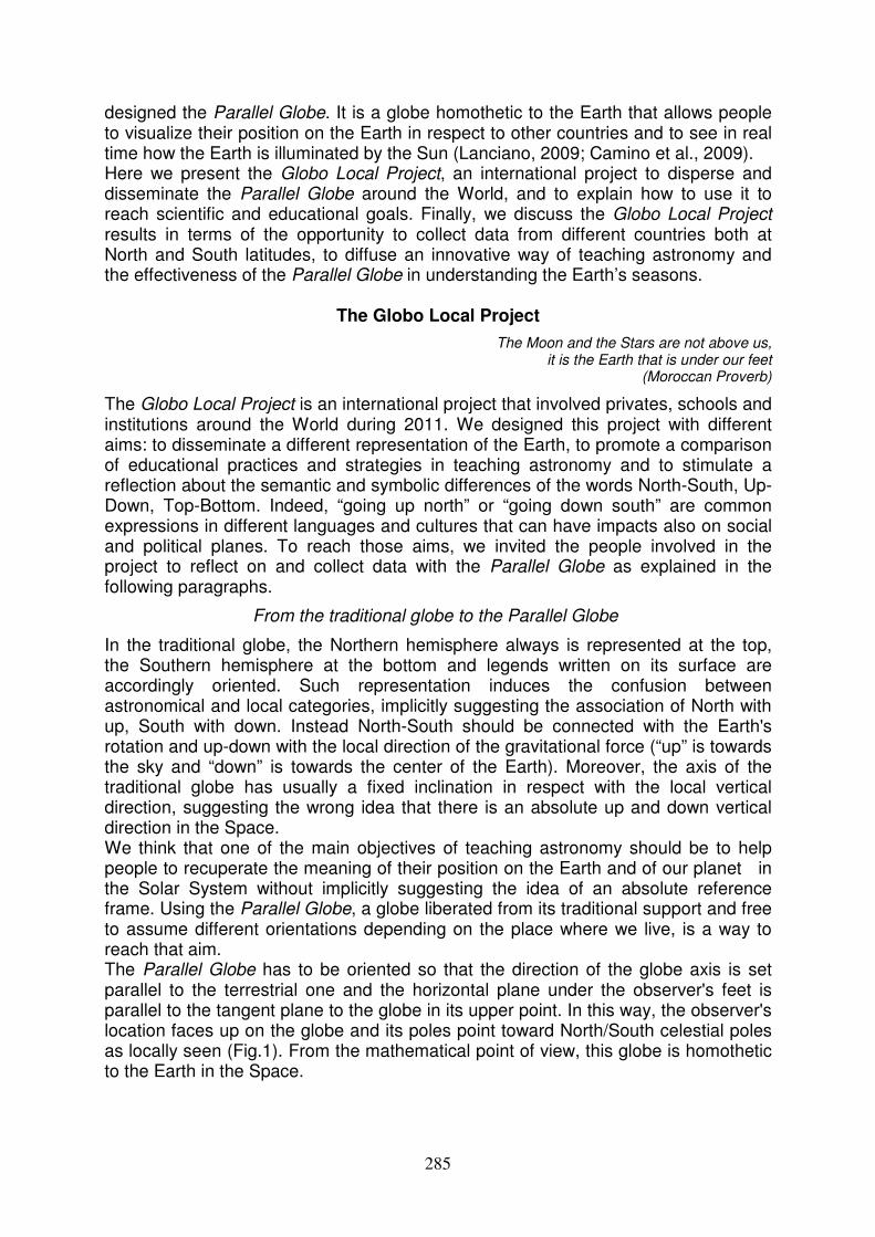
designed the Parallel Globe. It is a globe homothetic to the Earth that allows people to visualize their position on the Earth in respect to other countries and to see in real time how the Earth is illuminated by the Sun (Lanciano, 2009; Camino et al., 2009). Here we present the Globo Local Project, an international project to disperse and disseminate the Parallel Globe around the World, and to explain how to use it to reach scientific and educational goals. Finally, we discuss the Globo Local Project results in terms of the opportunity to collect data from different countries both at North and South latitudes, to diffuse an innovative way of teaching astronomy and the effectiveness of the Parallel Globe in understanding the Earth’s seasons.

The Globo Local Project

The Moon and the Stars are not above us, it is the Earth that is under our feet

(Moroccan Proverb)

The Globo Local Project is an international project that involved privates, schools and institutions around the World during 2011. We designed this project with different aims: to disseminate a different representation of the Earth, to promote a comparison of educational practices and strategies in teaching astronomy and to stimulate a reflection about the semantic and symbolic differences of the words North-South, Up-Down, Top-Bottom. Indeed, “going up north” or “going down south” are common expressions in different languages and cultures that can have impacts also on social and political planes. To reach those aims, we invited the people involved in the project to reflect on and collect data with the Parallel Globe as explained in the following paragraphs.

From the traditional globe to the Parallel Globe

In the traditional globe, the Northern hemisphere always is represented at the top, the Southern hemisphere at the bottom and legends written on its surface are accordingly oriented. Such representation induces the confusion between astronomical and local categories, implicitly suggesting the association of North with up, South with down. Instead North-South should be connected with the Earth's rotation and up-down with the local direction of the gravitational force (“up” is towards the sky and “down” is towards the center of the Earth). Moreover, the axis of the traditional globe has usually a fixed inclination in respect with the local vertical direction, suggesting the wrong idea that there is an absolute up and down vertical direction in the Space. We think that one of the main objectives of teaching astronomy should be to help people to recuperate the meaning of their position on the Earth and of our planet in the Solar System without implicitly suggesting the idea of an absolute reference frame. Using the Parallel Globe, a globe liberated from its traditional support and free to assume different orientations depending on the place where we live, is a way to reach that aim. The Parallel Globe has to be oriented so that the direction of the globe axis is set parallel to the terrestrial one and the horizontal plane under the observer's feet is parallel to the tangent plane to the globe in its upper point. In this way, the observer's location faces up on the globe and its poles point toward North/South celestial poles as locally seen (Fig.1). From the mathematical point of view, this globe is homothetic to the Earth in the Space.

285

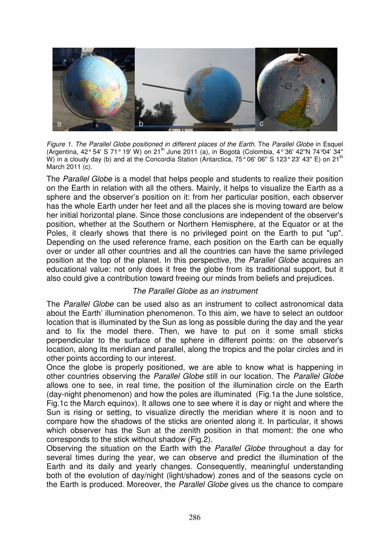
a

Figure 1. The Parallel Globe positioned in different places of the Earth. The Parallel Globe in Esquel (Argentina, 42° 54' S 71° 19' W) on 21

th June 2011 (a), in Bogotà (Colombia, 4° 36' 42''N 74°04' 34''

W) in a cloudy day (b) and at the Concordia Station (Antarctica, 75° 06' 06'' S 123° 23' 43'' E) on 21th

March 2011 (c).

The Parallel Globe is a model that helps people and students to realize their position on the Earth in relation with all the others. Mainly, it helps to visualize the Earth as a sphere and the observer’s position on it: from her particular position, each observer has the whole Earth under her feet and all the places she is moving toward are below her initial horizontal plane. Since those conclusions are independent of the observer's position, whether at the Southern or Northern Hemisphere, at the Equator or at the Poles, it clearly shows that there is no privileged point on the Earth to put "up". Depending on the used reference frame, each position on the Earth can be equally over or under all other countries and all the countries can have the same privileged position at the top of the planet. In this perspective, the Parallel Globe acquires an educational value: not only does it free the globe from its traditional support, but it also could give a contribution toward freeing our minds from beliefs and prejudices.

The Parallel Globe as an instrument

The Parallel Globe can be used also as an instrument to collect astronomical data about the Earth’ illumination phenomenon. To this aim, we have to select an outdoor location that is illuminated by the Sun as long as possible during the day and the year and to fix the model there. Then, we have to put on it some small sticks perpendicular to the surface of the sphere in different points: on the observer's location, along its meridian and parallel, along the tropics and the polar circles and in other points according to our interest. Once the globe is properly positioned, we are able to know what is happening in other countries observing the Parallel Globe still in our location. The Parallel Globe allows one to see, in real time, the position of the illumination circle on the Earth (day-night phenomenon) and how the poles are illuminated (Fig.1a the June solstice, Fig.1c the March equinox). It allows one to see where it is day or night and where the Sun is rising or setting, to visualize directly the meridian where it is noon and to compare how the shadows of the sticks are oriented along it. In particular, it shows which observer has the Sun at the zenith position in that moment: the one who corresponds to the stick without shadow (Fig.2). Observing the situation on the Earth with the Parallel Globe throughout a day for several times during the year, we can observe and predict the illumination of the Earth and its daily and yearly changes. Consequently, meaningful understanding both of the evolution of day/night (light/shadow) zones and of the seasons cycle on the Earth is produced. Moreover, the Parallel Globe gives us the chance to compare

a b c

286

what we observe from our particular position on the Earth with what other people observe simultaneously from other positions.

Figure 2. The Parallel Globe as an astronomical instrument. The Parallel Globe in Milan (Italy, 45° 27' 52.48'' N 09° 09' 57'' E) at noon on March equinox 2011(a) and in the afternoon on June solstice 2011 (b). In Fig. 2a, the shadows of the sticks positioned along the Milan meridian lay on the Meridian itself pointing to the North in the Northern hemisphere and to the South in the Southern hemisphere. The shadows of the sticks positioned along the Equator lay on the Equator itself pointing respectively to the East and to the West of the stick on the meridian (that has no shadow). In Fig. 2 b, the shadows of the sticks positioned along the Cancer Tropic lay on the Tropic itself. The visible sticks positioned along the Equator have shadows pointing to the South- West.

The Parallel Globe all around the World

The Globo Local Project scheduled four international events in coincidence with the 2011 equinoxes and solstices. During those days, we invited the people involved in the project to organize public events, seminars and systematic collection of data, mainly through pictures, on the Parallel Globe. We also invited them to collect documentation of the events by pictures and reports and to share them through the public website www.globolocal.net. Privates, schools and institutions from Italy, France, Spain, Portugal, Poland, Argentina, Colombia, Chile, Brazil and Antarctica have joined the project with a total of thirty-six participants. Some of them were previously involved in research projects on astronomy teaching. Others were involved for the first time, like the primary school future teachers of the Teaching Astronomy Course at the Faculty of Education of Milano-Bicocca. In that case, we used the project to motivate and support both the learning about basic astronomical ideas and the reflection on how to teach them.

The results

All materials collected before and during the Project are available on the project website in different languages. It represents a rich and a powerful database both for didactic and cultural aims as it joins together scientific data and participating people. In the http://didascienze.formazione.unimib.it/globolocal/home.htm page there is the list of the Parallel Globe’ pictures done along a day by participants, at or close to 2011 equinoxes and solstices (before, at and after noon). Links are available to the participants’ pages where people shared information about their history, images of their environment and sometimes videos of the school lessons. We found that previous knowledge and confidence with the tool and individual interests strongly influenced the approach to the project leading to a participation that was even a spot or a systemic activity. In some cases, like Avezzano and Settimo Milanese in Italy, the project was seen as an opportunity to begin a long term

b a

287

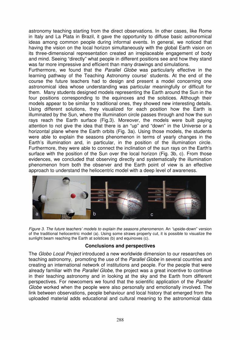
astronomy teaching starting from the direct observations. In other cases, like Rome in Italy and La Plata in Brazil, it gave the opportunity to diffuse basic astronomical ideas among common people during informal events. In general, we noticed that having the vision on the local horizon simultaneously with the global Earth vision on its three-dimensional representation created an irreplaceable engagement of body and mind. Seeing “directly” what people in different positions see and how they stand was far more impressive and efficient than many drawings and simulations. Furthermore, we found that the Parallel Globe was particularly effective in the learning pathway of the Teaching Astronomy course’ students. At the end of the course the future teachers had to design and present a model concerning one astronomical idea whose understanding was particular meaningfully or difficult for them. Many students designed models representing the Earth around the Sun in the four positions corresponding to the equinoxes and the solstices. Although their models appear to be similar to traditional ones, they showed new interesting details. Using different solutions, they visualized for each position how the Earth is illuminated by the Sun, where the illumination circle passes through and how the sun rays reach the Earth surface (Fig.3). Moreover, the models were built paying attention to not give the idea that there is an “up” and “down” in the Universe or a horizontal plane where the Earth orbits (Fig. 3a). Using those models, the students were able to explain the seasons phenomenon in terms of yearly changes in the Earth’s illumination and, in particular, in the position of the illumination circle. Furthermore, they were able to connect the inclination of the sun rays on the Earth's surface with the position of the Sun over the local horizon (Fig. 3b, c). From those evidences, we concluded that observing directly and systematically the illumination phenomenon from both the observer and the Earth point of view is an effective approach to understand the heliocentric model with a deep level of awareness.

Figure 3. The future teachers’ models to explain the seasons phenomenon. An “upside-down” version of the traditional heliocentric model (a). Using some straws properly cut, it is possible to visualize the sunlight beam reaching the Earth at solstices (b) and equinoxes (c).

Conclusions and perspectives

The Globo Local Project introduced a new worldwide dimension to our researches on teaching astronomy, promoting the use of the Parallel Globe in several countries and creating an international network of institutions and people. For the people that were already familiar with the Parallel Globe, the project was a great incentive to continue in their teaching astronomy and in looking at the sky and the Earth from different perspectives. For newcomers we found that the scientific application of the Parallel Globe worked when the people were also personally and emotionally involved. The link between observations, people behaviour and local history that emerged from the uploaded material adds educational and cultural meaning to the astronomical data

a b c

288

collection. In general, the project was an excellent opportunity to experiment a synergy between scientific education for citizens in formal and informal contexts. Sharing the Parallel Globe through the Globo Local Project gave till now a lot of opportunities to improve astronomy teaching, however we think that others could be implemented. A future evolution could consider “synchronized” observations (in the same daylight zone, at the same longitude, etc) to identify further global and local astronomic elements and extending the observations during the night, on the celestial sphere over the globe. We hope to extend the project to other countries, possibly scattered all over the Earth surface, so that it can become an opportunity for comparisons and reflections related to different experiences in educational research and curricular innovation.

Acknowledgment

We thank colleagues, teachers, students and all other participants who have shared photos, comments and materials. In particular, we thank Paolo Perfetti for his reports from Antarctica and R. Esposito, A. Fenaroli and S. Carnevale for their models.

References

Bailey, J. M., & Slater, T.F. (2004). A review of Astronomy Education Research. The Astronomy Education Review, 2 (2), 20-45

Camino, N., Steffani, M.H., Gangui, A., Sanchez, A., & Oliveira Saraiva, M. (2009). Observations conjunta del Equinoccio de marzo. Ensino da Astronomia, Caderno 31

Catalani, P., Giordano, E., & Rossi S. (2008). The lunar phases in the middle school. Nuovo Cimento B, 122 (06-07), 813-82

Giordano, E., Onida, M., & Rossi, S. (2009). From the Earth to the Universe: a teaching proposal about basic concepts in Earth Sciences and Astronomy for compulsory school. Enseñanza de las Ciencias. Extra, 2889-2892

Jackson, E. (2009). Practical astronomical activities during daytime. Revista Latino-Americana de Educação em Astronomia – RELEA, 8, 71-88

Lanciano, N. (1999). Obstacle conceptions and didactic obstacles in Astronomy experience field. In M. Bandiera, S. Caravita, E. Torracca & M. Vicentini (Eds) Research in science education in Europe: the picture expands. 238-245 Rome

Lanciano, N., Tomassetti, T. (2005). Perception de soi sur une planète sphérique dans le méga espace: observation, représentation, conceptualisation. Atti CIEAEM 57, 278-283

Lanciano, N. (2009). Strumenti per i giardini del Cielo. Bergamo, IT: Edizioni Junior

Shen, J. & Confrey, J. (2007). From conceptual change to transformative modeling: A case study of an elementary teacher in learning astronomy. Science Education, 91 (6), 948-966

Willard, T., and Roseman, J. E. (2007). Progression of the Reasons for Seasons. Knowledge Sharing Institute of the Center for Curriculum Materials in Science (Washington, DC)

289

Physical concepts and misconceptions

Ivan S. Ruddock

i.s.ruddock@strath.ac.uk

Nonlinear Spectroscopy and Sensing, Department of Physics, University of Strathclyde, Glasgow, United Kingdom

The place of concepts in undergraduate physics teaching is discussed along with some general observations on science in the media. A class with the specific aim of making students aware of concepts in physics is described in detail. Via a range of activities such as group discussion, writing essays and giving presentations, students analyse the development of physics, the role of significant individuals, the demonstration and teaching of physics, and physics in the public domain.

1. Introduction

Physics graduates are valued for the generic or “soft skills” they have accumulated during their courses and their ability to see the links between disparate areas of science. Employers frequently rate these attributes more highly than specialist knowledge; but how do students see the “big picture”, or answer the question “how did we get to here from there?”, when they are being taught increasingly specialised material as their degree courses progress through the years?

An approach adopted in the University of Strathclyde is described in this paper, and is the basis of a level 4 class, Physical Concepts. In Scotland, higher education’s academic levels are in a range of 1 → 5 in line with the Scottish Credit and Qualifications Framework’s descriptors [SCQF]; 1 → 3 is equivalent to the Bologna Bachelor, 1 → 4 is the Scottish “honours” Bachelor and 1 → 5 is the Scottish integrated Master. Physical Concepts is compulsory for students of the honours BSc course in Physics with Teaching in which the secondary school teaching qualification is awarded along with the physics degree. It is also a popular option for mainstream physics students. The aim of Physical Concepts is to track the development of key concepts in physics and review how this shapes current understanding. At its conclusion, students have a better appreciation of physics as an evolving subject rooted in practical usefulness but with a coherent and self-contained structure of concept and theory. Physical Concepts is an example of a “soft skills” class that satisfies the SCQF’s requirements for a degree course and as well as those of the United Kingdom’s Institute of Physics for accreditation purposes.

2. Concepts in physics

Public interest in relatively fundamental physics is frequently raised by the media, usually in response to natural disasters, large amounts of funding being requested or spent, or by some potential hazard suddenly becoming topical. For example, the Large Hadron Collider is something that almost everyone has heard of even if its purpose is unclear. In the United Kingdom, physics is now enjoying a high profile due to the activities of celebrity physicists (Jim Al Khalili, Brian Cox) who regularly present science based programmes on television and radio. Even in the popular press such as Metro, a free daily newspaper, there is significant reporting of science.

3. Misconceptions

Before discussing the different ways in which physical concepts can be explored with students, it is worthwhile looking at some examples of how they have been misunderstood and indeed abused in the public domain.

290

Marilyn vos Savant is an American writer who became a public figure following her inclusion in the Guinness Book of World Records in the highest IQ category. For the past twenty-five years she has been the author of “Ask Marilyn”, a column in Parade magazine distributed widely in the USA via Sunday newspapers. In it she answers questions posed by the general public and on 20th May 2001 was asked: "Earth's gravity holds spaceships in orbit, but the things inside them are weightless and float around. Why doesn't gravity have an effect inside?" [Sawicki (2011)] Marilyn's answer was: "When a space shuttle is orbiting the Earth, the sum of the "downward" (gravitational) force and the "forward" (inertial force) of the moving ship and its contents nearly equals zero. So both the ship and its contents are in free fall, which makes everything weightless. They stay in orbit while they're "falling" (being pulled toward the Earth) because the inertial force (centrifugal force, in this case) of the moving vehicle is radial - away from the Earth." This confused set of statements contains errors which students and the general public frequently make - a belief in centrifugal forces and incorrect vector addition, but at least it acknowledges that so-called weightlessness in orbit is due to “falling”.

While one must be prepared for occasional lapses in the understanding of basic concepts demonstrated by non-specialists, the same should not be true when dealing with professional scientists and engineers. Eric Laithwaite (1921-97) was a professor of electrical engineering in Imperial College, London and the inventor of the linear induction motor and a pioneer of Maglev transport. In the 1960s and 1970s he made regular television appearances on science programmes to promote his own research, to express opinions on engineering matters and to judge school science competitions. His glittering career eventually stalled in 1974 when he presented a Friday Evening Discourse at the Royal Institution, London and chose gyroscopes as his subject. In it he claimed that they weighed substantially less when rotating than when stationary [Wallgate (1974)]. Despite the subsequent furore, he spent much of the rest of his life working on gyroscopes with the aim of demonstrating an anti-gravity reactionless drive while conceding that they operated fully in accord with Newtonian mechanics.

4. Concepts in undergraduate physics

If concepts are important, are they being addressed in undergraduate degree programmes? University courses and the school curriculum can lead to a piecemeal understanding of physics in which demonstrable competence in completing exercises disguises deficiencies in the understanding of basic concepts. The products of this system are comfortable with quantitative tests yet insecure with qualitative questions. When asked to explain something, students and even their teachers sometimes find it difficult to separate the “wood” (the underlying concepts) from the “trees” (the equations to perform the calculations). This view is echoed by Paul Hewitt, author of the popular textbook Conceptual Physics, who described being a physics student in an article in Physics World, the United Kingdom’s Institute of Physics magazine: “This was my experience as a student. In every physics course I took, the first two stages hardly existed (stage 1 – informal hands-on experience, stage 2 – explanations and definitions). There were no activities, very little time was spent on concept development, and we went directly to stage 3 – applications. It was problem solving from day one. I was trained to solve problems based on concepts that I did not understand. I never developed a gut feel for concepts until graduate school, and these were not honed until I began teaching.” [Hewitt (2004)]

291

Conceptual understanding, or the lack of, has been an issue in physics education for many years. The usual method to monitor the impact of teaching in a specific area is via analytical quantitative tools known as concept inventories. Conceptual understanding is also seriously tested in the undergraduate research project oral examination, the PhD viva-voce examination and certain types of job interviews. It is only fair to students that they have experience and practice in analysing and discussing fundamental ideas. With Physical Concepts being designed for the BSc in Physics with Teaching, this issue is revisited briefly in Section 6.

5. “Physical Concepts” at the University of Strathclyde

Physical Concepts normally has a weekly one hour meeting during a twelve week semester with extra time allocated for presentations. The usual format is for the lecturer to give an introductory talk followed by brainstorming and group discussion. Each session finishes by reporting back from the groups and notification of the next assignment which is frequently based on the theme of the meeting. The class is assessed by essays and oral presentations including peer assessment of the latter.

Infamous predictions

“Prediction is very difficult, especially about the future” is a familiar quotation variously attributed to Niels Bohr and others. Everyone is tempted into making rash predictions on the basis of existing knowledge, and depending on the reputation of the individual, these are remembered and quoted when proven to be incorrect. The analysis of the original justification for a specific prediction provides the basis for a novel exercise linking together disparate areas of physics. For example, Thomas Edison’s “Fooling around with alternating current is just a waste of time. Nobody will use it, ever” [Cerf & Navasky (1998)] provides a trail to the promoters of DC and AC current (Edison v George Westinghouse and Nikola Tesla), the opposing arguments in the 19th century “current wars”, the physics of the advantages and disadvantages of DC and AC power transmission and voltage control, the development of DC and AC electrical machines, the perceived risks of DC and AC power, and 21st century applications of DC such as short distance power transmission and railway traction. Similarly, “…so far as astronomy is concerned, we must confess that we do appear to be fast approaching the limits of our knowledge” from Simon Newcomb, Canadian-born American astronomer in 1888 [Newcomb (1888)], challenges students to identify what was known in 1888, what technical developments have since enabled new facts and theories to be established (radio and X-ray astronomy etc.), and what important observations have been made since 1888 (nebulae being external galaxies, expansion of the universe etc.).

How did we get to here?

Despite Henry Ford saying “History is more or less bunk” [Chicago Tribune (1916)], there is much to be gained by a knowledge of the historical basis of any science. Perhaps a better guide is Theodore Roosevelt who allegedly declared “I believe that the more you know about the past, the better you are prepared for the future”. Physics has developed via the resolution of opposing theories, sometimes completely contradictory. In the “official” history of physics, established theories have been modified and overthrown as experimental evidence has emerged, frequently driven by improvements in instrumentation. This view of the development of physics provides the basis for an exercise – How did we get to here? – which attempts to identify how the subject has progressed. There are many choices of topic that emerged from two opposing theories, models or concepts. Examples include the

292

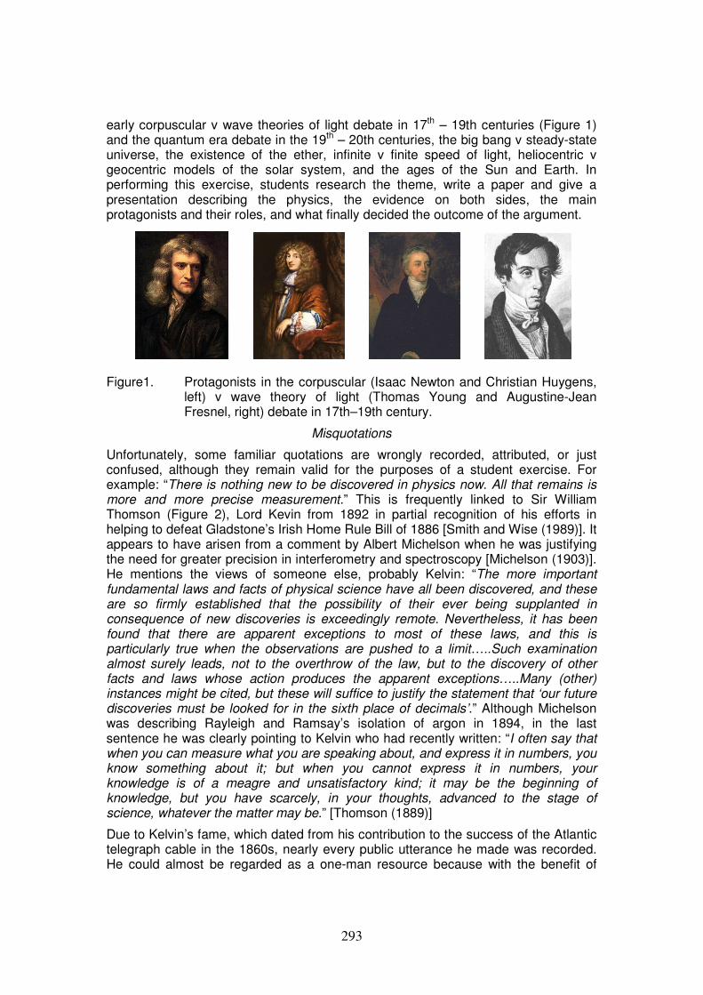
early corpuscular v wave theories of light debate in 17th – 19th centuries (Figure 1) and the quantum era debate in the 19th – 20th centuries, the big bang v steady-state universe, the existence of the ether, infinite v finite speed of light, heliocentric v geocentric models of the solar system, and the ages of the Sun and Earth. In performing this exercise, students research the theme, write a paper and give a presentation describing the physics, the evidence on both sides, the main protagonists and their roles, and what finally decided the outcome of the argument.

Figure1. Protagonists in the corpuscular (Isaac Newton and Christian Huygens,

left) v wave theory of light (Thomas Young and Augustine-Jean Fresnel, right) debate in 17th–19th century.

Misquotations

Unfortunately, some familiar quotations are wrongly recorded, attributed, or just confused, although they remain valid for the purposes of a student exercise. For example: “There is nothing new to be discovered in physics now. All that remains is more and more precise measurement.” This is frequently linked to Sir William Thomson (Figure 2), Lord Kevin from 1892 in partial recognition of his efforts in helping to defeat Gladstone’s Irish Home Rule Bill of 1886 [Smith and Wise (1989)]. It appears to have arisen from a comment by Albert Michelson when he was justifying the need for greater precision in interferometry and spectroscopy [Michelson (1903)]. He mentions the views of someone else, probably Kelvin: “The more important fundamental laws and facts of physical science have all been discovered, and these are so firmly established that the possibility of their ever being supplanted in consequence of new discoveries is exceedingly remote. Nevertheless, it has been found that there are apparent exceptions to most of these laws, and this is particularly true when the observations are pushed to a limit…..Such examination almost surely leads, not to the overthrow of the law, but to the discovery of other facts and laws whose action produces the apparent exceptions…..Many (other) instances might be cited, but these will suffice to justify the statement that ‘our future discoveries must be looked for in the sixth place of decimals’.” Although Michelson was describing Rayleigh and Ramsay’s isolation of argon in 1894, in the last sentence he was clearly pointing to Kelvin who had recently written: “I often say that when you can measure what you are speaking about, and express it in numbers, you know something about it; but when you cannot express it in numbers, your knowledge is of a meagre and unsatisfactory kind; it may be the beginning of knowledge, but you have scarcely, in your thoughts, advanced to the stage of science, whatever the matter may be.” [Thomson (1889)]

Due to Kelvin’s fame, which dated from his contribution to the success of the Atlantic telegraph cable in the 1860s, nearly every public utterance he made was recorded. He could almost be regarded as a one-man resource because with the benefit of

293

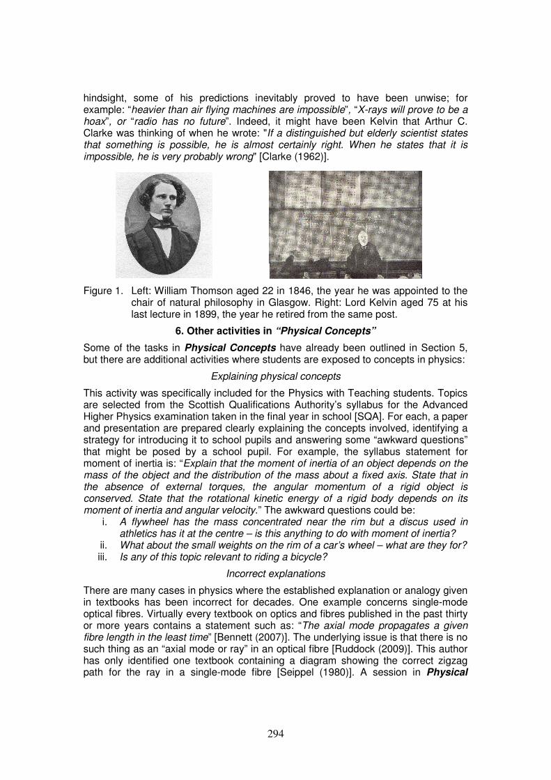
hindsight, some of his predictions inevitably proved to have been unwise; for example: “heavier than air flying machines are impossible”, “X-rays will prove to be a hoax”, or “radio has no future”. Indeed, it might have been Kelvin that Arthur C. Clarke was thinking of when he wrote: "If a distinguished but elderly scientist states that something is possible, he is almost certainly right. When he states that it is impossible, he is very probably wrong" [Clarke (1962)].

Figure 1. Left: William Thomson aged 22 in 1846, the year he was appointed to the chair of natural philosophy in Glasgow. Right: Lord Kelvin aged 75 at his last lecture in 1899, the year he retired from the same post.

6. Other activities in “Physical Concepts”

Some of the tasks in Physical Concepts have already been outlined in Section 5, but there are additional activities where students are exposed to concepts in physics:

Explaining physical concepts

This activity was specifically included for the Physics with Teaching students. Topics are selected from the Scottish Qualifications Authority’s syllabus for the Advanced Higher Physics examination taken in the final year in school [SQA]. For each, a paper and presentation are prepared clearly explaining the concepts involved, identifying a strategy for introducing it to school pupils and answering some “awkward questions” that might be posed by a school pupil. For example, the syllabus statement for moment of inertia is: “Explain that the moment of inertia of an object depends on the mass of the object and the distribution of the mass about a fixed axis. State that in the absence of external torques, the angular momentum of a rigid object is conserved. State that the rotational kinetic energy of a rigid body depends on its moment of inertia and angular velocity.” The awkward questions could be:

i. A flywheel has the mass concentrated near the rim but a discus used in athletics has it at the centre – is this anything to do with moment of inertia?

ii. What about the small weights on the rim of a car’s wheel – what are they for? iii. Is any of this topic relevant to riding a bicycle?

Incorrect explanations

There are many cases in physics where the established explanation or analogy given in textbooks has been incorrect for decades. One example concerns single-mode optical fibres. Virtually every textbook on optics and fibres published in the past thirty or more years contains a statement such as: “The axial mode propagates a given fibre length in the least time” [Bennett (2007)]. The underlying issue is that there is no such thing as an “axial mode or ray” in an optical fibre [Ruddock (2009)]. This author has only identified one textbook containing a diagram showing the correct zigzag path for the ray in a single-mode fibre [Seippel (1980)]. A session in Physical

294

Concepts is devoted to analysing examples of such misleading teaching material.

Demonstrating physical concepts

Groups of students examine sets of physics demonstration apparatus or toys such as the simple pendulum, Cartesian divers and the fine beam tube. They attempt to identify the physics that is being demonstrated and then report back with each group offering one suggestion for each apparatus in turn until their ideas are exhausted. In the fine beam tube for example, there is thermionic emission, electrostatic force and acceleration, transverse magnetic force, centripetal force and acceleration, energy transfer to residual gas, relaxation and emission of fluorescence.

Testing conceptual understanding

In the spirit of a concept inventory, groups of students devise simple multiple choice questions to test conceptual understanding of a topic in basic physics such as classical mechanics or DC circuits.

Physical concepts in the public domain

Students identify those physical concepts which are currently important issues as far as the general public, media and government are concerned. Examples considered have included the LHC and the Higgs boson, power cable safety, nuclear waste storage, return to the moon, high speed rail travel, asteroids and renewable energy.

6. Conclusions

An undergraduate class focusing on concepts in physics in the most general way and how they shape current understanding has been outlined. In it, students gain an appreciation of concepts and their linkages by examining the contributions of important individuals, by their testing and experimental demonstration, by explaining selected examples in the secondary school syllabus and by analysing concepts underlying current issues in the public domain. In addition, the class provides extensive experience of group discussion, essay writing and presentations.

References

Bennett, C.A. (2007). Principles of Physical Optics, New York, NY: Wiley. Cerf, C. & Navasky, V.S. (1998), The Experts Speak: The Definitive Compendium of

Authoritative Misinformation, New York, NY: Villard. Clarke, A.C. (1962). Profiles of the Future: An Inquiry into the Limits of the Possible.

London: Gollancz. Ford, H. (1916). Chicago Tribune, 25 May. Hewitt, P. (2004). The three stages of learning. Physics World, September, 16-17. Michelson, A.A. (1903). Light Waves and their Uses, Chicago: Univ. Chicago Press. Newcomb, S (1888). The Sidereal Messenger, 7, 69. Ruddock, I.S. (2009). European Journal of Physics, 30, 303-309. Sawicki, M. (2011). Mikolaj Sawicki, John A. Logan College, Illinois, USA maintains

Bad Physics, a website devoted to exposing incorrect explanations of physics. Seippel, R.G. (1980). Optoelectronics. Reston, VA: Reston Publishing. Smith, C. & Wise, N.W. (1989). Energy and Empire. Cambridge: Camb. Univ. Press. SCQF provides information and guidance on all levels of education. SQA. is the accreditation and awarding body for school and vocational qualifications. Thomson, W. (1889). Electrical Units of Measurement. Popular Lectures and

Addresses, London: Macmillan 1, 73. Wallgate, R. (1974). Eric Laithwaite defies Newton. New Scientist, 64, 470.

295

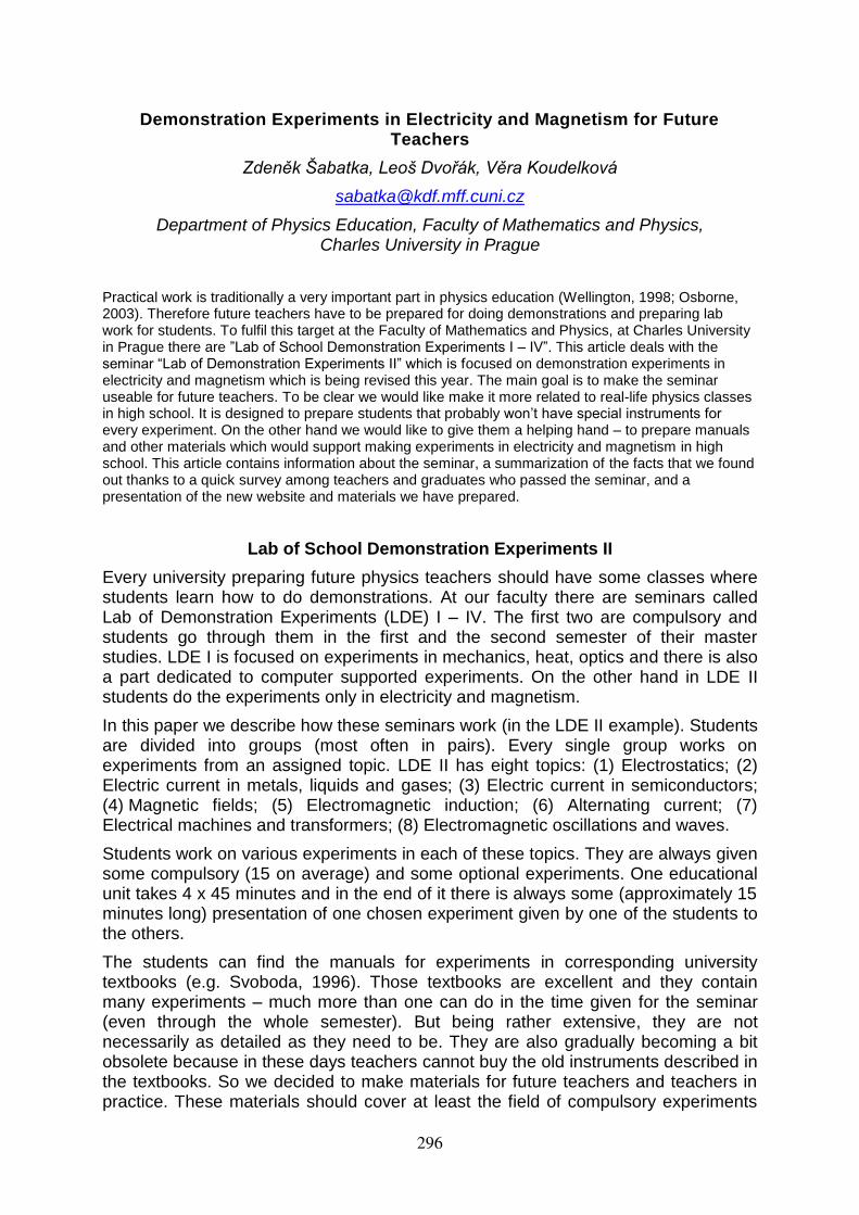
Demonstration Experiments in Electricity and Magnetism for Future Teachers

Zdeněk Šabatka, Leoš Dvořák, Věra Koudelková

sabatka@kdf.mff.cuni.cz

Department of Physics Education, Faculty of Mathematics and Physics, Charles University in Prague

Practical work is traditionally a very important part in physics education (Wellington, 1998; Osborne, 2003). Therefore future teachers have to be prepared for doing demonstrations and preparing lab work for students. To fulfil this target at the Faculty of Mathematics and Physics, at Charles University in Prague there are ”Lab of School Demonstration Experiments I – IV”. This article deals with the seminar “Lab of Demonstration Experiments II” which is focused on demonstration experiments in electricity and magnetism which is being revised this year. The main goal is to make the seminar useable for future teachers. To be clear we would like make it more related to real-life physics classes in high school. It is designed to prepare students that probably won’t have special instruments for every experiment. On the other hand we would like to give them a helping hand – to prepare manuals and other materials which would support making experiments in electricity and magnetism in high school. This article contains information about the seminar, a summarization of the facts that we found out thanks to a quick survey among teachers and graduates who passed the seminar, and a presentation of the new website and materials we have prepared.

Lab of School Demonstration Experiments II

Every university preparing future physics teachers should have some classes where students learn how to do demonstrations. At our faculty there are seminars called Lab of Demonstration Experiments (LDE) I – IV. The first two are compulsory and students go through them in the first and the second semester of their master studies. LDE I is focused on experiments in mechanics, heat, optics and there is also a part dedicated to computer supported experiments. On the other hand in LDE II students do the experiments only in electricity and magnetism.

In this paper we describe how these seminars work (in the LDE II example). Students are divided into groups (most often in pairs). Every single group works on experiments from an assigned topic. LDE II has eight topics: (1) Electrostatics; (2) Electric current in metals, liquids and gases; (3) Electric current in semiconductors; (4) Magnetic fields; (5) Electromagnetic induction; (6) Alternating current; (7) Electrical machines and transformers; (8) Electromagnetic oscillations and waves.

Students work on various experiments in each of these topics. They are always given some compulsory (15 on average) and some optional experiments. One educational unit takes 4 x 45 minutes and in the end of it there is always some (approximately 15 minutes long) presentation of one chosen experiment given by one of the students to the others.

The students can find the manuals for experiments in corresponding university textbooks (e.g. Svoboda, 1996). Those textbooks are excellent and they contain many experiments – much more than one can do in the time given for the seminar (even through the whole semester). But being rather extensive, they are not necessarily as detailed as they need to be. They are also gradually becoming a bit obsolete because in these days teachers cannot buy the old instruments described in the textbooks. So we decided to make materials for future teachers and teachers in practice. These materials should cover at least the field of compulsory experiments

296

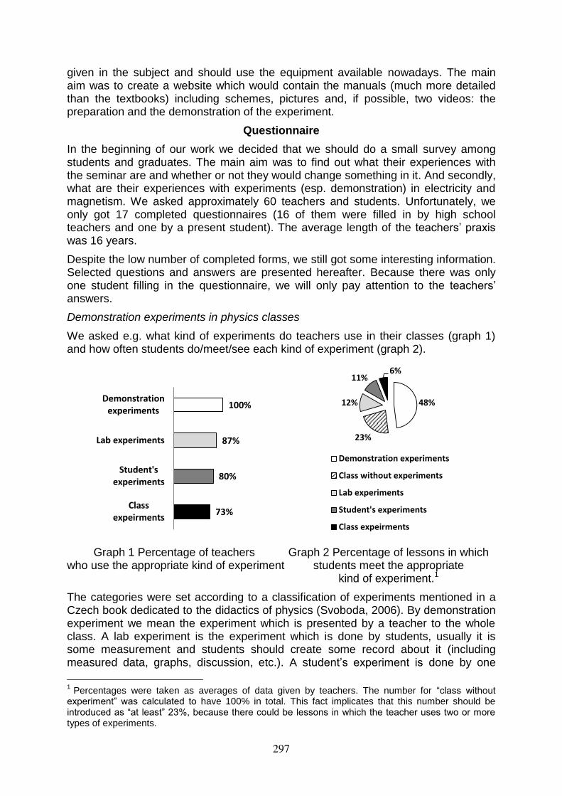
given in the subject and should use the equipment available nowadays. The main aim was to create a website which would contain the manuals (much more detailed than the textbooks) including schemes, pictures and, if possible, two videos: the preparation and the demonstration of the experiment.

Questionnaire

In the beginning of our work we decided that we should do a small survey among students and graduates. The main aim was to find out what their experiences with the seminar are and whether or not they would change something in it. And secondly, what are their experiences with experiments (esp. demonstration) in electricity and magnetism. We asked approximately 60 teachers and students. Unfortunately, we only got 17 completed questionnaires (16 of them were filled in by high school teachers and one by a present student). The average length of the teachers’ praxis was 16 years.

Despite the low number of completed forms, we still got some interesting information. Selected questions and answers are presented hereafter. Because there was only one student filling in the questionnaire, we will only pay attention to the teachers’ answers.

Demonstration experiments in physics classes

We asked e.g. what kind of experiments do teachers use in their classes (graph 1) and how often students do/meet/see each kind of experiment (graph 2).

Graph 1 Percentage of teachers Graph 2 Percentage of lessons in which who use the appropriate kind of experiment students meet the appropriate kind of experiment.1

The categories were set according to a classification of experiments mentioned in a Czech book dedicated to the didactics of physics (Svoboda, 2006). By demonstration experiment we mean the experiment which is presented by a teacher to the whole class. A lab experiment is the experiment which is done by students, usually it is some measurement and students should create some record about it (including measured data, graphs, discussion, etc.). A student’s experiment is done by one

1 Percentages were taken as averages of data given by teachers. The number for “class without

experiment” was calculated to have 100% in total. This fact implicates that this number should be introduced as “at least” 23%, because there could be lessons in which the teacher uses two or more types of experiments.

100%

87%

80%

73%

Demonstrationexperiments

Lab experiments

Student'sexperiments

Classexpeirments

48%

23%

12%

11% 6%

Demonstration experiments

Class without experiments

Lab experiments

Student's experiments

Class expeirments

297

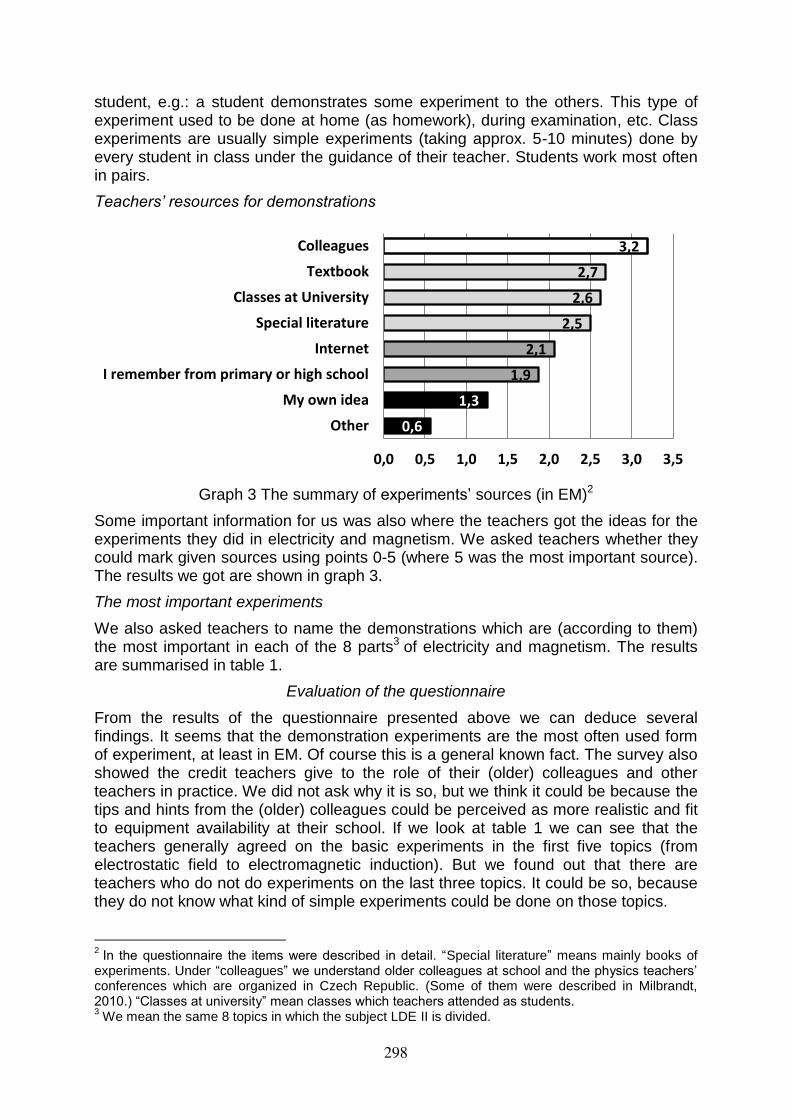
student, e.g.: a student demonstrates some experiment to the others. This type of experiment used to be done at home (as homework), during examination, etc. Class experiments are usually simple experiments (taking approx. 5-10 minutes) done by every student in class under the guidance of their teacher. Students work most often in pairs.

Teachers’ resources for demonstrations

Graph 3 The summary of experiments’ sources (in EM)2

Some important information for us was also where the teachers got the ideas for the experiments they did in electricity and magnetism. We asked teachers whether they could mark given sources using points 0-5 (where 5 was the most important source). The results we got are shown in graph 3.

The most important experiments

We also asked teachers to name the demonstrations which are (according to them) the most important in each of the 8 parts3 of electricity and magnetism. The results are summarised in table 1.

Evaluation of the questionnaire

From the results of the questionnaire presented above we can deduce several findings. It seems that the demonstration experiments are the most often used form of experiment, at least in EM. Of course this is a general known fact. The survey also showed the credit teachers give to the role of their (older) colleagues and other teachers in practice. We did not ask why it is so, but we think it could be because the tips and hints from the (older) colleagues could be perceived as more realistic and fit to equipment availability at their school. If we look at table 1 we can see that the teachers generally agreed on the basic experiments in the first five topics (from electrostatic field to electromagnetic induction). But we found out that there are teachers who do not do experiments on the last three topics. It could be so, because they do not know what kind of simple experiments could be done on those topics.

2 In the questionnaire the items were described in detail. “Special literature” means mainly books of

experiments. Under “colleagues” we understand older colleagues at school and the physics teachers’ conferences which are organized in Czech Republic. (Some of them were described in Milbrandt, 2010.) “Classes at university” mean classes which teachers attended as students. 3 We mean the same 8 topics in which the subject LDE II is divided.

0,6

1,3

1,9

2,1

2,5

2,6

2,7

3,2

0,0 0,5 1,0 1,5 2,0 2,5 3,0 3,5

Other

My own idea

I remember from primary or high school

Internet

Special literature

Classes at University

Textbook

Colleagues

298

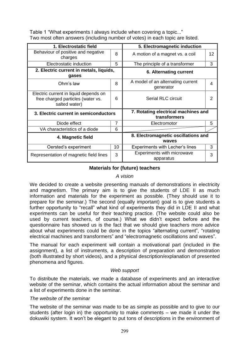
Table 1 “What experiments I always include when covering a topic...” Two most often answers (including number of votes) in each topic are listed.

1. Electrostatic field 5. Electromagnetic induction

Behaviour of positive and negative charges

8 A motion of a magnet vs. a coil 12

Electrostatic induction 5 The principle of a transformer 3

2. Electric current in metals, liquids, gases

6. Alternating current

Ohm’s law 8 A model of an alternating current generator

4

Electric current in liquid depends on free charged particles (water vs.

salted water)

6 Serial RLC circuit 2

3. Electric current in semiconductors 7. Rotating electrical machines and transformers

Diode effect 7 Electromotor 5

VA characteristics of a diode 6

4. Magnetic field 8. Electromagnetic oscillations and waves

Oersted’s experiment 10 Experiments with Lecher’s lines 3

Representation of magnetic field lines 3 Experiments with microwave apparatus

3

Materials for (future) teachers

A vision

We decided to create a website presenting manuals of demonstrations in electricity and magnetism. The primary aim is to give the students of LDE II as much information and materials for the experiment as possible. (They should use it to prepare for the seminar.) The second (equally important) goal is to give students a further opportunity to “recall” what kind of experiments they did in LDE II and what experiments can be useful for their teaching practice. (The website could also be used by current teachers, of course.) What we didn’t expect before and the questionnaire has showed us is the fact that we should give teachers more advice about what experiments could be done in the topics “alternating current”, “rotating electrical machines and transformers” and “electromagnetic oscillations and waves”.

The manual for each experiment will contain a motivational part (included in the assignment), a list of instruments, a description of preparation and demonstration (both illustrated by short videos), and a physical description/explanation of presented phenomena and figures.

Web support

To distribute the materials, we made a database of experiments and an interactive website of the seminar, which contains the actual information about the seminar and a list of experiments done in the seminar.

The website of the seminar

The website of the seminar was made to be as simple as possible and to give to our students (after login in) the opportunity to make comments – we made it under the dokuwiki system. It won’t be elegant to put tons of descriptions in the environment of

299

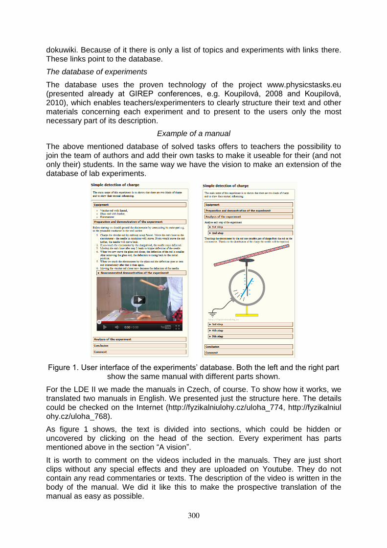
dokuwiki. Because of it there is only a list of topics and experiments with links there. These links point to the database.

The database of experiments

The database uses the proven technology of the project www.physicstasks.eu (presented already at GIREP conferences, e.g. Koupilová, 2008 and Koupilová, 2010), which enables teachers/experimenters to clearly structure their text and other materials concerning each experiment and to present to the users only the most necessary part of its description.

Example of a manual

The above mentioned database of solved tasks offers to teachers the possibility to join the team of authors and add their own tasks to make it useable for their (and not only their) students. In the same way we have the vision to make an extension of the database of lab experiments.

Figure 1. User interface of the experiments’ database. Both the left and the right part show the same manual with different parts shown.

For the LDE II we made the manuals in Czech, of course. To show how it works, we translated two manuals in English. We presented just the structure here. The details could be checked on the Internet (http://fyzikalniulohy.cz/uloha_774, http://fyzikalniul ohy.cz/uloha_768).

As figure 1 shows, the text is divided into sections, which could be hidden or uncovered by clicking on the head of the section. Every experiment has parts mentioned above in the section “A vision”.

It is worth to comment on the videos included in the manuals. They are just short clips without any special effects and they are uploaded on Youtube. They do not contain any read commentaries or texts. The description of the video is written in the body of the manual. We did it like this to make the prospective translation of the manual as easy as possible.

300

Conclusions

By combining videos, pictures and a text description including an explanation of the physical phenomena we offer teachers and future teachers materials for their preparation for classes. The website of the seminar with students’ comments and the database of demonstration experiments is (and will be), of course, available (only for viewing) for the general public, too.

Future

The main current goal is to cover the demonstration experiments which are used in the seminar LDE II. In the future, we plan to use the same system for the rest of the LDE seminars.

The next step will be to use the database in the other project of our faculty - Interactive physics laboratory (Šabatka, 2009). This is a place where high school students and their teachers can come and make their own measurements and hands-on experiments. We think such a website could be a good way to distribute the texts for their home preparation before coming to us.

We would appreciate if any teachers (or departments) from abroad would be interested in such a database. If you want to share an interesting experiment, please contact us. We will show you how to add it to the database or we will add it ourselves. Our wish is to develop an extensive database of physics demo experiments for teachers – preferably not only in the Czech language.

Acknowledgement

The work described in this article was supported by grant FRVŠ 1120/2011/G6 of Czech Ministry of Education, Youth and Sports.

References

Koupilová, Z., Mandíková, D., Matějíčková, L., Snětinová, M. (2008). Electronic collection of solved problems in mechanics and electromagnetism. GIREP 2008 Conference. Available at http://lsg.ucy.ac.cy/girep2008/ComprehensiveView.htm. (Cited 27. 10. 2011).

Koupilová, Z., Mandíková, D., Snětinová, M. (2010). Electronic database of solved tasks in physics. GIREP - ICPE - MPTL 2010 Conference.

Milbrandt, R. (2010). Innovative physics teaching conferences in the Czech Republic. The Physics Teacher, 48(6), 395-396. doi: 10.1119/1.3479719

Osborne, J., Monk, M. (2003). Good Practice in School Science Teaching: What Research Has to Say. Berkshire: Open University Press.

Šabatka, Z., Drozd, Z., Dvořák, L. (2009). Activities for high school students: from demonstra-tion experiments to an interactive laboratory. GIREP-EPEC 2009 Conference (Oral Sessions – Experiments).

Svoboda, E., Kolářová, R. (2006). Didaktika fyziky zakladni a stredni skoly: Vybrane kapitoly. Praha: Karolinum.

Svoboda, M., at al. (1996). Praktikum skolnich pokusu II. Praha: Karolinum.

Wellington, J. (1998). Practical Work in School Science: Which Way Now? London: Routledge.

301

List of Authors

AAsikainen Mervi, 92Asikainen Mervi A., 74

BBarbieri Sara, 25, 161Battaglia Onofrio Rosario, 272Bonanno Assunta, 1Bozzo Giacomo, 1Brom Pavel, 167Bruestlova Jitka, 173Böhm Ulrike, 7

CC. Silva Jorge, 208C. Vieira Pedro, 208Camarca Michele, 1Campos Flores Ignacio, 179Campos Ignacio, 220Cazzaniga Luigia, 13Corni Federico, 86, 248

DD. Teodoro Vítor, 208Del Valle Díaz Muñoz Gabriela, 179Dobis Pavel, 173Dvorak Leos, 296

EEllermeijer Ton, 98, 140

FFaletic Sergej, 185, 191, 197Fazio Claudio, 19, 161Franc Tomas, 202Fuchs Hans U., 248

GG. Neves Rui, 208Giliberti Marco, 13, 25, 161Gioka Olga, 31Giordano Enrica, 284Gojkosek Mihael, 37, 191

HHaagen-Schuetzenhoefer Claudia, 43Hendolin Ilkka, 49Hernández Morales Guadalupe, 179

Hirayama Osamu, 214Hirvonen Pekka, 92Hirvonen Pekka E., 74Hockicko Peter, 55Hopf Martin, 43

JJelicic Katarina, 62, 191Jiménez Ramírez José Luis, 179Jimenez Jose Luis, 220

KKaper Wolter, 98Karwasz Grzegorz, 68Kesonen Mikko, 74Koudelkova Vera, 296Koupilova Zdenka, 226Kranjc Tomaž, 230, 278Kudo Yasuhiro, 236Körndle Hermann, 7

LLaherto Antti, 80Lambourne Robert, 242Lanciano Nicoletta, 284Laurenti Erica, 86Leinonen Risto, 92Logman Paul, 98Ludwig Nicola, 13Lustig Frantisek, 167

MMandikova Dana, 226Mariani Cristina, 86, 248Michelini Marisa, 1, 104Mirzoyan Julietta, 254Mohoric Ales, 197Mossenta Alessandra, 104Mutanen Arto, 260Mäkynen Asko, 123

NNarciss Susanne, 7Nieminen Pasi, 111, 123Nurkka Niina, 111

OOhno Eizo, 236, 266

302

List of Authors

PPizzolato Nicola, 272Planinic Maja, 62Planinsic Gorazd, 37, 62, 185, 197Pospiech Gesche, 7

RRazpet Nada, 230, 278Rissanen Antti, 260Roa Neri Jose Antonio Eduardo, 220Rossi Sabrina, 284Ruddock Ivan, 290

SSabatka Zdenek, 226, 296Sands David, 117Sapia Peppino, 1Savinainen Antti, 111, 123Schwartz Judah L., 208Slisko Josip, 37Snetinova Marie, 226Sperandeo-Mineo Rosa Maria, 19, 272

TTala Suvi, 129Tarantino Giovanni, 19

UUrban-Woldron Hildegard, 134Uylings Peter, 140

Vvan Buuren Onne, 140van den Berg Ed, 149, 155van Veen Norbert, 155Viiri Jouni, 111, 123

303