Physicochemical changes to soil and sediment in managed realignment sites following tidal inundation

1

Physicochemical changes to soil and sediment in

managed realignment sites following tidal

inundation

Margaret Kadiri

A thesis submitted for the Degree of the Doctor of Philosophy

Department of Geography,

Queen Mary University of London

January, 2010

2

Declaration

I, Margaret Kadiri , confirm that the work presented in this thesis is my own. Where

information has been derived from other sources, I confirm that this has been indicated in

the thesis.

3

Abstract

The recognition of the value of salt marshes and concerns over salt marsh loss has led to

the adoption of managed realignment in coastal areas. Managed realignment involves the

landward relocation of the seawall, allowing an area of agricultural land to be tidally

inundated. It is believed that managed realignment sites can act as a sink for

contaminants. However, these sites may also act as a contaminant source and pose a

risk to estuarine biota.

In this thesis, the potential for metal and herbicide release from agricultural soil and

dredged sediment in managed realignment sites was investigated by laboratory

microcosm experiments. The agricultural soil and dredged sediment were subjected to

two different salinities and drying-rewetting treatments. Results indicate the release of

metals (Cu, Ni and Zn) and herbicides (simazine, atrazine and diuron) was dependent on

their strength of binding to the soil and sediment, and complexation and competition

reactions between seawater anions, cations and the sorbed metals. The release patterns

indicated that metal and herbicide release into overlying water may continue for extended

periods of time after an initial rapid release. The total metal and herbicide loads released

into the overlying water followed the order: Cu < Zn < Ni and diuron < atrazine < simazine

with a greater release from the soil than sediment. The increase in CO2 release,

mineralisation rates, total metal and herbicide loads after drying and rewetting the soil

suggested an increase in the mineralisation of organic matter and the release of organic

matter associated metals and herbicides. Results of linear regression analyses provided

evidence that the release of the metals and herbicides as DOC-complexes was important

for soil but not for sediment. These findings indicate that there is a lower potential for

contaminant release from managed realignment sites where dredged sediments are

beneficially re-used.

4

Acknowledgements

I would like to express my sincere appreciation to my supervisors, Dr Kate Spencer and

Dr Kate Heppell for their academic guidance, patience and continuous support

throughout the course of this PhD. I am also grateful to Queen Mary, University of

London for providing me with a college studentship.

I would like to thank Mark Dixon and Colin Scott for providing me with valuable data and

information on the managed realignment site at Wallasea Island. Thanks also go to Prof.

Andy Baird, Prof. Steven Gilmour and Dr Lisa Belyea for their help and valuable advice in

developing the model used in this study and on statistical analysis. I also want to express

my heartfelt thanks to everybody who assisted me with fieldwork particularly on cold

winter days: Simon Dobinson, Laura Shotbolt, Mark Tarplee, Stuart Glenday, Lorna

Linch, Fotis Sgouridis, Paul Morris, Steve Forden, Kalmond Ma, Bob Grabowski and

Grieg Davis. Thanks also goes to Mark Trimmer who was instrumental in my use of the

GC at the Biological and Chemical Sciences Department at Queen Mary for the analysis

of gas samples, Ed Oliver for his help producing maps of Wallasea Island managed

realignment site and Laura Shotbolt for training on the analytical techniques used.

Thanks must also be extended to the postgrads in the Geography Department at Queen

Mary, University of London particularly Lorna, Bob, Grieg, Danny, Fotis and Heather with

whom I shared an office for their friendship.

Most importantly, I want to express my deepest appreciation to my biggest supporters,

my family, particularly my dad and mom, Aunty Mary, Maxwell, Solomon, Joy, Blessing,

Efe and Uncle Es. Without their constant love, support and encouragement I would not

have been able to complete this PhD. I also am very grateful to Greta, Tosin, Aoibheann,

Ruth, Suzanne, Bena, Sabrina, Matilda, Nneka, Lydia, Isioma and all my other friends too

numerous to mention for their support.

Finally, I am profoundly grateful to GOD, for his unfailing love, grace and guidance, and

most importantly, for seeing me through to the completion of this PhD.

5

Table of Contents

Declaration 2

Abstract 3

Acknowledgements 4

Table of Contents 5

List of Figures 10

List of Tables 14

Chapter 1 Introduction 16

1.1 1 General Introduction 16

1.2 1 Nature of salt marshes 17

1.3 Value of salt marshes 19

1.4 Loss of salt marshes 22

1.5 Salt marsh restoration through managed

realignment 23

1.6 1 Sorption-desorption of metals and herbicides 28

1.6.1 1 Sorption-desorption of metals 28

1.6.2 1 Sorption-desorption of herbicides 28

1.7 1 Changes to sediment and soil in managed

realignment sites

30

1.8 1 Modelling contaminant release 33

1.9 Aim and objectives 34

Chapter 2 Physical and chemical changes in sediment s at Wallasea

Island managed realignment site.

37

2.1 Introduction 37

2.2 Materials and methods 39

2.2.1 Site Description 39

2.2.2 1 Sediment sampling 47

2.2.3 Sample preparation and analysis 49

6

2.2.3.1 Moisture and organic matter content 49

2.2.3.2 Dry bulk density and porosity 49

2.2.3.3 Particle size analysis 50

2.2.3.4 pH 50

2.2.3.5 Porewater dissolved organic carbon (DOC)

and chloride (Cl)

51

2.2.3.6 Analysis of DOC 51

1 2.2.3.7 Analysis of Cl 52

2.2.4 Statistical Analysis 52

2.3 Results and Discussion 53

2.3.1 Meteorological conditions 53

2.3.2 Changes in sediment parameters 53

2.4 Summary and conclusion 67

Chapter 3 Laboratory Experiments: Methodology 69

3.1 1 Introduction 69

3.2 Sediment and soil collection 69

3.3 1 Laboratory microcosm experiments 70

3.3.1 1 Column microcosm 70

3.3.2 Experiment procedure 71

3.3.3 1 Sediment and soil spiking procedure 73

3.3.4 1 Experimental designs 79

3.3.4.1 Experimental design: effect of salinity on

metals and herbicides release from soil and

sediment (salinity treatment)

79

3.3.4.2 Experimental design: effect of drying and

rewetting on metals and herbicides release

from soil and sediment (drying-rewetting

treatment)

80

3.4 33333 Carbon mineralisation experiments 81

3.5 1 Batch sorption experiments 84

3.5.1 1 Metal sorption experiments 84

3.5.2 1 Herbicides sorption experiments 85

3.6 1 Analytical techniques 85

7

3.6.1 Inductively coupled plasma optical emission

spectrometry (ICP-OES)

85

3.6.2 1 On-line solid phase extraction-high

performance liquid chromatography (online

SPE-LC)

87

3.6.3 1 Gas chromatography (GC) 89

3.7 1 Statistical Analysis 90

Chapter 4 Experimental Results 92


4.2 1 Soil and sediment properties 92

4.3 1 The effect of salinity on contaminant release

from managed realignment soil and sediment:

results

93

4.3.1 1 Partition coefficient data under two different

salinity treatments

93

4.3.2 1 Column microcosm experimental data under

two different salinity treatments

94

4.3.2.1 Release of metals into the overlying water

under the low and high salinity treatment

95

4.3.2.2 Release of herbicides into the overlying water

under low and high salinity treatments

97

4.3.2.3 The release of DOC into the overlying water

under low and high salinity treatment

99

4.3.2.41 pH values in the overlying water under low

and high salinity treatments

100

4.4 The effect of drying and rewetting on

contaminant release from managed

realignment soil and sediment: results

101

44.4.1.1 Release of metals into the overlying water

under the drying-rewetting treatment

102

44.4.1.2 Release of herbicides into the overlying water


109

44.4.1.3 Release of DOC into the overlying water


112

8

4.5

Carbon mineralisation, CO2 release and

microbial biomass

114

4.5.1 CO2 released from fully wet soil and sediment 115

4.5.2 CO2 released from dried-rewet soil and

sediment

116

4.5.3 Soil and sediment microbial biomass data 117

Chapter 5 The release of metals and herbicides from managed realignment soil

and sediment


5.2 1 Effect of salinity on the release of metals and

herbicides from soil and sediment

119

5.2.1 1 Effect of salinity on the release of metals from

soil and sediment

121

5.2.2 1 Effect of salinity on the release of herbicides

from soil and sediment

127

5.3 1 Effect of drying and rewetting on the release

of metals and herbicides from soil and

sediment

133

5.3.1 1 CO2 release, carbon mineralisation rate and

microbial biomass of soil and sediment

134

5.3.2 Effect of drying and rewetting on the release

of metals and herbicides from soil and

sediment

136

5.3.2.1 Release patterns of the metals and

herbicides from soil and sediment under

drying-rewetting treatment

136

5.3.2.21 Effect of drying and rewetting on the release

of metals from soil

137


of metals from sediment

139

1 5.3.2.4 Effect of drying and rewetting on the release

of herbicides from soil

140

1

9


of herbicide from sediment

143

5.4 1 Summary and conclusion 145

Chapter 6 Mechanisms of metal and herbicide release from soil and

sediment

148


6.2 1 Diffusive contaminant transport 149

6.3 Measures for the evaluation of model

performance

152

6.4 1 Model Description 154

6.5 1 Model parameters 157

6.6 1 Results 160

6.7 1 Discussion 179

6.8 Summary and conclusion 182

Chapter 7 Summary and conclusions 183

7.1 Introduction 183

7.2 Summary of findings 184

7.3 1 Limitation of study 188

7.4 Recommendations 190

7.5 Scope for future work 191

References 192

Appendices 216

10

List of Figures

Figure Legend Page

1.1

Diagrammatic representation of the vegetation zones and tidal

changes in the water level at a typical salt marsh.

20

2.1 Map of the south east coast of England showing the location of

Wallasea Island

40

2.2 Aerial photo of Wallasea Island Managed Realignment site showing

the River Crouch and the arable agricultural land.

42

2.3 Sediment discharge into a containment bund at Wallasea Island

Managed Realignment site.

43

2.4 Map of Wallasea Island showing the three locations of the managed

realignment site.

44

2.5 Surface elevation profile across the managed realignment site. 45

2.6 Water level and site elevation at the NSM, RSM, NMF and RMF. 46

2.7 Monthly average moisture content in surface sediment layer at the

RSM, RMF, NSM and NMF.

55

2.8 Monthly average moisture content in the surface (0-2 cm) and

subsurface (8-10 cm) sediment in the NSM and RSM.

57

2.9 Monthly average organic matter content at the sediment surface in

the RSM, RMF, NSM and NMF.

59

2.10 Monthly average organic matter content at the sediment surface and

8-10cm subsurface layers at the RSM and NSM.

60

2.11 Monthly average bulk density data in the RSM and NSM. 61

2.12 Monthly average porosity data in the RSM and NSM during the study

period.

62

2.13 Monthly average pH values in the RSM, RMF,NSM and NMF. 63

2.14 Monthly average CI content in the RSM, RMF, NSM and NMF. 65

2.15 Monthly average DOC porewater concentrations in the RSM, RMF,

NSM and NMF.

66

3.1 Schematic diagram of the laboratory column microcosm. 71

3.2 Average porewater concentrations of Ni, Zn, and Cu in the soil and

sediment over 21 days.

77

11

3.3 Average porewater concentrations of simazine, atrazine and diuron

in the soil and sediment over 21 days

78

4.1 Concentrations of (a) Zn, (b) Ni and (c) Cu released from the soil and

(d) Zn, (e) Ni and (f) Cu released from the sediment under the low

and high salinity treatments.

96

4.2 Concentrations of (a) simazine, (b) atrazine and (c) diuron released

from the soil and (d) simazine, (e) atrazine and (f) diuron released

from the sediment under low and high salinity conditions.

98

4.3 Concentrations of (a) DOC released from the soil and (b) DOC

released from the sediment under the low and high salinity

treatments.

100

4.4 pH values of the overlying water for the soil (a) and pH values of the

overlying water for the sediment (b) under low and high salinity

treatments.

101


(d) Zn, (e) Ni and (f) Cu released from the sediment under the first

drying-rewetting and fully wet treatments.

103


(d) Zn, (e) Ni and (f) Cu released from the sediment under the two

drying-rewetting treatments.

105



from the sediment under the drying-rewetting and fully wet

treatments.

108



from the sediment under the two drying-rewetting treatments.

111

4.9 Concentrations of (a) DOC release from the soil and (b) DOC

release from the sediment under the drying-rewetting and fully wet

treatments.

112

4.10 Concentrations of (a) DOC release from the soil and (b) DOC

release from the sediment under the two drying-rewetting treatments.

114

4.11 Cumulative CO2 release from the fully wet soil and sediment. 115

12

4.12 Carbon mineralisation rates under fully wet soil and sediment

treatment.

116

4.13

4.14

4.15

5.1

5.2

5.3

6.1

Cumulative CO2 release from the dried-wet soil and sediment.

Carbon mineralisation rates under dried-rewet soil and sediment

treatment

Soil and sediment microbial biomass before drying, immediately after

drying and 6 days after rewetting.

Total loads of Ni, Zn and Cu released from the soil and sediment

under (a) low and (b) high salinity treatments.

Comparison of organic carbon partition coefficients Koc for simazine,

atrazine and diuron in the soil and sediment.

Total loads of simazine, atrazine and diuron released from the soil

and sediment under (a) low and (b) high salinity treatments.

An illustration of the finite difference model arrangement in the soil

and sediment experimental column.

117

117 118 125 129 132 155

6.2 Predicted and measured concentration data for (a, d) Zn, (b, e) Cu

and (c, f) Ni released into the overlying water column from the soil

and sediment respectively at low and high salinity treatments.

164

6.3 Predicted and measured concentration data for (a, d) simazine, (d, e)

atrazine, (c, f) diuron released into the overlying water column from

the soil and sediment respectively under the low and high salinity

treatments.

165

6.4 Predicted and measured concentration data for (a, d) Zn, (b, e) Cu,

and (c, f) Ni released into the overlying water column from the soil

and sediment respectively under the drying-rewetting treatment.

166

6.5 Predicted and measured concentration data for (a, d) simazine, (b, e)

atrazine, (c, f) diuron released into the overlying water column from

the soil and sediment respectively under the drying-rewetting

treatment.

167

6.6 Analysis of residuals between the predicted and measured

concentration data for (a, d) Zn, (b, e) Cu, (c, f) Ni released into the

overlying water from the soil and sediment respectively under the low

salinity treatment.

169

13


concentration data for (a, d) Zn, (b, e) Cu, (c, f) Ni released from the

soil and sediment respectively under the high salinity treatment.

170


concentration data for (a, d) simazine, (b, e) atrazine, (c, f) diuron

released into the overlying water column from the soil and sediment

respectively under the low salinity treatment.

171



released into the underlying water column from the soil and sediment

respectively under the high salinity treatment.

171


concentration data for (a, d) Zn, (b, d) Cu, (c, f) Ni released from the

soil and sediment respectively under the drying-wetting treatment.

173



released from the soil and sediment respectively under the drying-

rewetting treatment.

174

14

List of Tables

Table Legend Page

1.1 Main values of wetlands (modified from Tiner, 1987). 21

1.2 Proportions (%) of salt marsh lost from Essex and The Orwell in

Suffolk, from 1973-1988 and from 1988-1997/8 (modified from

Hughes and Paramor 2004).

23

2.1 List of samples collected and measurements taken at each sampling

location.

48

2.2 Monthly average temperature and monthly total precipitation in

Wallasea Island from January to December 2007

53

2.3 Range of sediment parameters in the surface sediment at the RSM,

NSM, RMF and NMF.

56

3.1 Composition of sea salt (Sigma Aldrich) 72

3.2 Physico-chemical properties of simazine, atrazine and diuron. 73

3.3 Operating conditions of the Varian Vista-PRO spectrometer. 86

3.4 ICP-OES detection limits of, Cu, Ni, and Zn in mg l-1 86

3.5 Recoveries of simazine, atrazine and diuron (average ± 1 SD) 89

3.6 Limit of detection (SN ≥ 3) of simazine, atrazine and diuron. 89

4.1 Properties of the soil and sediment used in this study. 93

4.2 Average partition coefficients of Cu, Ni and Zn for soil and sediment

at 5‰ and 20‰ salinity(average ± SE, n=9)

94

4.3 Average partition coefficients of simazine, atrazine and diuron for soil

and sediment at 5‰ and 20‰ salinity(average ± SE, n=6)

94

4.4 Total metal loads (mg) released into the overlying water from the soil

and sediment under the low and high salinity treatments (average ±

SE, n=3)

97

4.5 Total herbicide loads (µg) released into the overlying water from soil

and sediment under low and high salinity treatment (average ± SE,

n=3).

99

4.6 Total DOC loads (mg) released into the overlying water from the soil

and sediment under the low and high salinity treatments (average ±

SE, n=3).

100

15

4.7 Total metal loads (mg) released into the overlying water under the

fully wet and the first drying-rewetting treatment over the same

period (average ± SE, n=3).

104

4.8 Total metal loads (mg) released into the overlying water under the

two drying-rewetting treatments (average ± SE, n=3).

106

4.9 Total herbicide loads (µg) released into the overlying water under the

fully wet and the first drying-rewetting treatments over the same time

period (average ± SE, n=3).

109

4.10 Total herbicide loads (µg) released into the overlying water under the

two drying-rewetting treatments (average ± SE, n=3).

112


and sediment under the fully wet and the first drying-rewetting

treatment (average ± SE, n=3).

113


and sediment under the first and second drying-rewetting treatment

(average ± SE, n=3).

114

5.1 Theoretical initial metal concentrations (assuming instantaneous

equilibrium) and measured initial metal concentrations in the

overlying water.

126

6.1 Model parameters used in predicting the column experimental data

for Zn, Cu, Ni, simazine, atrazine and diuron.

158

6.2 Goodness of fit criteria for the evaluation of the model performance. 162

6.3 Slope of the exponential curves fitted to the predicted and measured

contaminant concentrations under the low and high salinity

treatments.

176

6.4 Slope of the exponential curves fitted to the predicted and measured

contaminant concentrations under the drying-rewetting treatment.

177

6.5 Goodness of fit criteria for the evaluation of the performance of the

refined model

178

16

Chapter 1: Introduction

1.1 General Introduction

In recent years, there has been a paradigm shift in the management of coastal areas

from the maintenance of seawalls to the restoration of coastal habitats (Crooks et al.,

2002). Integral to this shift is the recognition of salt marshes as an important part of the

coastal system and its significance relative to other global ecosystems. Costanza et al.

(1997) estimated the average annual global value of different ecosystems and attributed

a value of $ 1,648 yr-1 x 109 to salt marshes and mangroves (the tropical equivalent of salt

marshes). The annual global value of salt marshes was equivalent to that of lakes and

rivers. Salt marshes provide several economic and environmental benefits such as

coastal flood defence enhancement (Tiner et al., 1987). However, salt marshes are under

threat from rising sea levels and associated salt marsh loss. In the UK, the area of salt

marshes along the Colne, Blackwater and Stour estuaries in Essex reduced by 42 %

between 1988 and 1997/8 due to salt marsh erosion (Hughes and Paramor, 2004). The

loss of salt marshes coupled with the high cost of maintaining and upgrading seawalls

has resulted in salt marsh restoration through managed realignment (Andrews et al.,

2006). Managed realignment aims to restore salt marsh to coastal areas by the landward

relocation of seawalls, allowing the tidal inundation of low-lying agricultural land. It is

intended that the reintroduction of tidal inundation will promote salt marsh development

which in turn will serve as a natural coastal flood defence in front of the seawall. Apart

from salt marsh restoration and the enhancement of coastal defence, managed

realignment may provide other potential benefits, one of which includes providing a sink

for metals and other particle reactive contaminants (NRA, 1994, Andrews et al., 2006;

Cave et al., 2005). Andrews et al. (2006) indicated that managed realignment sites can

serve as a sink for metals because it provides space for the accumulation of sediments.

However, physical and chemical changes in sediments such as salinity changes can

affect the binding of contaminants to sediments and result in contaminant release

(Calmano et al., 1992; Gambrell et al., 1991). Consequently, changes in the physical and

chemical conditions in the soil and sediment in managed realignment sites following tidal

inundation can result in the release of contaminants into estuarine waters. The release of

these contaminants may affect estuarine water quality and have adverse effects on living

organisms in the food chain (Call et al., 1987; Moriarty, 1999) leading to man.

17

In this thesis, a series of investigations (a field study, laboratory experiments and

modelling investigation) were conducted which were aimed at assessing the potential for

contaminant release from agricultural soil and dredged sediment following tidal inundation

in managed realignment sites. Both inorganic and organic contaminants (i.e. metals and

herbicides) were considered. The following sections provide background information on

salt marshes and managed realignment, describe the sorption-desorption of metals and

herbicides and the changes to agricultural soil and dredged sediment in managed

realignment sites which can result in the potential release of metals and herbicides into

estuarine waters.

1.2 Nature of salt marshes

There are several definitions of salt marshes. Beeftink (1977) defined a salt marsh as a

“natural or semi-natural halophytic grassland and dwarf brushwood on the alluvial

sediment bordering seawater bodies whose water table fluctuates either tidally or non-

tidally”. Bates and Jackson (1980) defined a salt marsh as a flat, poorly drained land

which is subject to periodic flooding by seawater and is usually covered by a thick mat of

grassy halophytic (salt-tolerant) plants. Adam (1990) defined a salt marsh as an area

vegetated by herbs, grasses or low shrubs bordering seawater bodies. Allen and Pye

(1992) defined a salt marsh as an area of land covered by halophytic vegetation which is

frequently inundated by seawater.

Salt marshes are found in the middle and high latitudes along intertidal shores throughout

the world (Mitsch and Gosselink, 2000). They develop in sheltered low energy areas with

medium to large tidal ranges (< 3 m) where alluvial sediment become deposited on

intertidal mudflat. The alluvial sediments are derived from upland run-off, reworked

marine deposits, coastal erosion and fluvial transport (William et al., 1994; Pethick, 1984;

Mitsch and Gosselink, 2000). In the UK, approximately 45,300 ha (4.53 x 108 m2) of salt

marshes are found along the coastline with one fifth of the total area of salt marshes in

England found along the coast of Norfolk, Suffolk and Essex (Burd, 1989, 2003).

Salt marshes develop between Mean High Water Neap (MHWN) and Mean High Water

Spring (MHWS) (French, 2006; Legget and Dixon 1994; Pye and French, 1993). They are

periodically inundated by sea water which infiltrates the saltmarsh sediment during high

tide and drains at low tide (Boorman and Hazelden, 2002; Williams et al., 1994). While

18

the frequency and duration of tidal inundation depends on the elevation of the marsh

surface relative to the sea-level and the tidal regime which varies temporally at several

timescales, the ease with which the marsh drains depends on the topography of the salt

marsh (Rozas, 1995; Mitsch and Gosselink, 2000; Pethick, 1980; ABP, 1998),

Salt marshes are situated in a buffer zone between marine and terrestrial habitats and

are usually fronted by mudflats (Boorman, 2003; Adam, 1990). They are often divided by

muddy creeks of characteristic dendritic patterns which serve as important conduits for

material such as particulate organic matter between the marsh and the adjacent estuary

(Pye, 2000; Mitsch and Gosselink, 2000). Higher seawater velocities are experienced in

the creeks compared to the salt marsh surface because the velocities are reduced at the

marsh surface by the surface roughness of the salt marsh plants (Boorman et al., 1998).

The lowest limit of the distribution of individual salt marsh plants species depends on

several factors such as tolerance to tidal inundation, salinity and water movement whilst

the upper limit is determined by factors such as interspecific competition, with those

plants species less tolerant of tidal inundation occurring at higher elevation (Shunway and

Bertness, 1992; Sanchez et al., 1996; Davy et al., 2000, Pennings and Callaway, 1992).

The plants established at lower elevation impede the water flow and enables suspended

sediments to settle, thereby promoting sediment deposition. This increases the height of

the area and creates a suitable environment for the establishment of plant species less

tolerant of tidal inundation (Boorman et al., 1998). The different responses by different

salt marsh plant species produce a zonation pattern or a successional sequence from low

to high elevation as shown in Figure 1.1 (Boorman, 2003).

Salt marshes act as transformers of nutrients by importing dissolved oxidized inorganic

forms (nitrite, nitrate, phosphate) and exporting dissolved and particulate reduced forms

(ammonium, organic nitrogen and phosphorus compounds) (Odum, 1988). They function

either as sinks or sources of nutrients depending on a variety of factors such as the

successional age of the marsh, salinity, presence of upland sources of nutrients, tidal

range, presence of litter layer, and the magnitude and stability of nutrient flux in the

estuary to which the marsh is coupled (Stevenson et al., 1977; Osgood, 2000). Typically,

older salt marshes with well developed inorganic and organic nutrient pools are likely to

be exporters of nutrients while younger systems are expected to import nutrients

(Childers, 1994).

19

Salt marsh sediments are mainly made up of silt and clay sized particles and they are rich

in organic matter deposited from coastal waters and trapped into the salt marsh or from

organic production within the marsh (Mitsch and Gosselink, 2000; Nixon, 1980).

Generally, salt marsh sediments have reducing conditions which is reflected by their low

redox potential (Howes, 1981). The redox potential decreases with increasing sediment

depth due to the utilization of a sequence of terminal electron acceptors (O2, NO3-; Mn4+;

Fe3+; SO42-, CO2) by a vertical succession of microbes with different tendencies to oxidise

organic matter as a carbon source (Froelich et al., 1979). Consequently, salt marsh

sediments are redox-stratified and exhibit a vertical succession of oxic and anoxic zones

(Koretsky et al., 2003). The depth of the oxic zone can range from a few mm to tens of

cm (Zwolsman et al., 1993). The transition between the oxic and anoxic zones is called

the redoxcline and is identified by a visual change in colour from reddish-brown at the

surface to dark greyish-black at depth which is synonymous with the presence of ferric

oxide precipitates at the surface and insoluble pyrite at depth (Williams et al., 2004).

1.3 Value of salt marshes

Salt marshes have several values which are summarised in Table 1.1. However, the main

values of salt marshes to the UK Environment Agency (EA) which has a statutory duty to

promote the conservation of coastal areas are the value to conservation and the

enhancement of coastal flood defence (NRA, 1992).

The value of salt marshes to conservation has been recognised for many years. Salt

marshes provide habitats, food sources and breeding areas for a wide range of

organisms which are vital to the coastal ecosystem as a whole (Beeftink and Rozema,

1988). Salt marshes also provide suitable habitats for a range of invertebrates, birds and

fishes. The dense invertebrate fauna are an important food source for mussels, cockles,

birds and fishes (Boorman, 1992) and they also play a significant role in sedimentary

processes by secreting binding mucus which stabilises deposited sediments (Legget and

Dixon, 1994; Daborn et al., 1993).

20

Figure 1.1 Diagrammatic representation of the vegetation zones and tidal changes in the

water level at a typical salt marsh (after Boorman, 2003).

Salt marshes serve as a feeding, roosting and nesting areas to a large number of birds

including migratory and over-wintering birds. For example, the salt marshes in south-east

England provide suitable feeding, breeding and roosting areas for up to 250,000

waterfowls and waders (Dixon, 1998). While birds utilise the exposed surface of the salt

marsh, the creeks provide a transitory habitat for fishes. These creeks serve as sheltered

spawning and nursery sites (King and Lester, 1995; Boorman, 1992). King and Lester

(1995) indicated that salt marshes increase the fishery potential of coastal waters. The

creeks also serve as feeding sites for fishes. Fishes such as grey mullet feed on algae on

the creek banks, bass feeds on invertebrate fauna and flat fish such as plaice move into

creeks at high tides (King and Lester, 1995). Due to the importance of the salt marshes in

supporting these habitats, most of the salt marshes in England have several national and

international conservation designations (Hughes and Paramor, 2004). More than 80 % of

the salt marshes in south-east England are Sites of Special Scientific Interest (SSSI),

Environmentally Sensitive Areas (ESA), Special Protected Areas (SPA), Special Areas of

Conservation (SAC) and Ramsar sites (Paramor and Hughes, 2004).

21

Table 1.1 Major values of wetlands (modified from Tiner, 1987)

Values Uses

Socio-economic Fishing, wildfowling, recreation, aesthetics

Education and scientific research

Livestock grazing, flood control, erosion control

Protection from the wave damage

Ground water recharge and water supply

Environmental quality Nutrient recycling, water quality maintenance

Pollution filters, aquatic productivity

Oxygen production, microclimate regulator

Salt marshes play a significant role in enhancing coastal flood defence by dissipating

wave energy so that little energy remains on the landward limit (Pethick, 1992; Toft and

Maddrell, 1995; Moller et al., 2001). Moller et al. (1999) indicated that salt marshes

dissipate wave energy through the reduction in water depth over the marsh and the

increased friction of the vegetated surface reducing wave height. However, the

effectiveness of salt marshes in enhancing coastal flood defence depends on the width of

the salt marsh that is in front of the seawall. For example, a 3 m high seawall with an 80

m wide salt marsh in front of it will give adequate protection. If there is a 30 m wide salt

marsh, a 5 m seawall is needed. However, a 12 m wide salt marsh is needed if there is

no seawall (NRA, 1992; Boorman, 2003). Salt marshes also reduce the impact of wave

action on the seawall thereby offering protection to the seawall and reducing its

maintenance cost (Dixon and Weight, 1996; King and Lester, 1995, Leggett and Dixon,

1994). King and Lester (1995) estimated that the loss of saltmarsh from Essex would cost

£ 600 million for the increased maintenance of the seawall.

22

1.4 Loss of salt marshes

Historically, there has been a significant loss of coastal wetlands globally as a result of

human activities. Over the last century, more than 70% of California’s coastal wetlands in

the USA and approximately 40 % of the coastal wetlands in France have been lost (ABP,

1998). This is mainly because salt marshes were not considered to be important and as a

result many salt marshes were drained and reclaimed for agricultural, industrial and

recreational purposes (Moy and Levin, 1991). However, in recent years, loss of salt

marshes has been extensively reported and they are now seen as a threatened

ecosystem (Harmsworth and Long, 1986; Nuttle et al., 1997). Some of the causes of

these losses include drought, hurricanes, subsidence due to relative sea level rise,

discharges of materials (e.g. nutrient loadings from domestic sewage and agricultural run-

off) and erosion (Tiner, 1987). In the UK, significant areas of salt marsh have been lost to

reclamation extensively practiced historically. However, there are current concerns over

the erosional loss of salt marshes particularly in south-east England (Table 1.2). These

losses have great implications for both conservation and coastal flood defence. The

recent salt marsh erosion has been attributed to the prevention of the landward migration

of salt marshes, by seawalls, in response to rising sea levels (Boorman, 1992; Turner,

1995; Burd, 1992). As the outer marsh zones move landward, the inner marsh zones are

unable to migrate due to the presence of the sea wall. The salt marshes become

squeezed between the static sea wall and the rising sea level leading to the progressive

loss of salt marshes. This process has been termed ‘coastal squeeze’ (Boorman, 1992;

Turner, 1995; Burd, 1992). However, Hughes and Paramor (2004) have argued that an

increase in bioturbation and herbivory by the rag worm Nereis diversicolor as opposed to

coastal squeeze, may be responsible for the salt marsh erosion in south-east England.

Salt marsh erosion is expected to continue as sea level rise in south-east England has

been estimated to range from 1 – 4 mm year-1 (Boorman, 1992; Turner, 1995;

Underwood, 1997; Hughes, 2001).

23

Table 1.2 Proportions (%) of saltmarsh lost from Essex and the Orwell in Suffolk, from

1973 – 1988 and from 1988 – 1997/8. (modified from Hughes and Paramor, 2004)

1973 - 1988 1988 – 1997/8

Total lost Pioneer zone Total

Orwell 40 74 23

Stour 44 60 28

Colne 12 53 7

Blackwater 23 74 7

1.5. Salt marsh restoration through managed realignment

Salt marshes are at a great risk of erosion due to climate change and sea level rise. The

continuing rate of salt marsh erosion in south-east England due to sea level rise has been

estimated to be 40 ha year-1 (Coastal Geomorphological Partnership, 2000). Balcombe

(1992) indicated that salt marshes could disappear in 50 years except deliberate

measures are taken to protect them. The concerns over salt marsh erosion due to rising

sea levels as well as the high cost of maintaining and upgrading seawalls has led to

considerations for a more cost-effective and sustainable coastal management strategy

(Andrews et al., 2006; Shepherd et al 2007). Most of the seawalls in south-east England

have reached the end of their design life as they were constructed after the North sea

storm surge of 1953 and they now need expensive upgrading and maintenance (Moller et

al., 1999). However, the maintenance and upgrading of the seawalls are deemed

uneconomical particularly when it is more expensive than the value of the land protected

(Dixon and Weight, 1996). This is the case for 25 % of the seawalls on the Essex coast

where the cost of maintenance is more than the value of the land protected (Hughes and

Paramor, 2004). In addition, the biological diversity in salt marshes has been recognized

in law under the European Union Habitat Directive 92/43/EEC. The directive maintains a

‘no-net-loss’ policy in total habitat area and the UK has an obligation, under this directive,

to maintain and restore salt marshes to the total area present in 1992 (UK Biodiversity

Group, 1999). Hence, the UK is committed under the EU Habitat Directive and the UK

Biodiversity Action Plan, to develop strategies to conserve and enhance biodiversity in

salt marshes. As a result of the need to comply with the Habitat directive as well as the

concerns about salt marsh erosion due to rising sea levels and the high cost of

maintenance and upgrading of seawalls, coastal managers and policy makers have now

24

adopted the soft engineering technique known as managed realignment over the hard

engineering option (i.e. seawalls). This soft engineering technique aims to achieve a

dynamic equilibrium in coastal environments and hence regard salt marshes as an

important part of the coastal environment (MAFF, 1993).

Managed realignment (also known as managed retreat or set back) involves constructing

a new sea wall further inland on higher ground and deliberately breaching the existing

seawall, allowing for the tidal inundation of the area between the existing and new

seawall. Salt marsh plants colonise the inundated area and dissipate wave energy, thus

offering coastal flood protection. Managed realignment also reduces the effect of coastal

squeeze by allowing the landward migration of salt marshes with rising sea levels,

creates a more sustainable seawall and meets conservation objectives. Managed

realignment is a cheaper alternative to maintaining and upgrading existing seawalls

(French, 2006). The cost of implementing a managed realignment scheme at Northey

Island on the Blackwater Estuary in Essex in 1992 was approximately £22,000 while the

estimated cost of upgrading and maintaining the existing seawall was between £30,000

and £55,000 (Leafe, 1992). Given that realignment reduces the impact of wave action,

the new seawall need not be constructed to the same specifications as the existing wall,

thus reducing implementation costs (Brampton, 1992). In addition to the fulfillment of the

flood defence and conservation objectives, an additional proposed benefit of managed

realignment is that the site may act as a sink for contaminants such as metals and

organic contaminants from estuarine waters (NRA, 1994; MacLeod et al., 1999).

Managed realignment sites are periodically inundated by seawater during high tide and

drained at low tide. The extent of the tidal inundation and drainage depends on the site

elevation relative to the tide, the topography of the site and the ease with which the site

drains (ABP, 1998). Areas at low elevation relative to the tide are regularly inundated by

the tides twice daily. Conversely, areas at higher elevation relative to the tide are

irregularly inundated, mainly by spring tides (Scott pers. comm., 2006) making these

areas susceptible to wetting and drying cycles.

Typically, managed realignment is implemented on reclaimed agricultural land partly

because the land had originally been salt marsh and therefore has a proven ability to

support such an environment (French, 2006). After the seawall is breached, the soil is

inundated and estuarine sediments start to accumulate. The accretion of sediment in a

25

managed realignment site is required for the restoration of salt marsh plants. This is

because, over time, there is a drop in elevation in reclaimed areas relative to the tide due

to dewatering and compaction and the accretion of sediment raises the land elevation to

a suitable level (between MHWN and MHWS) for salt marsh plants to develop (French,

2006; Crooks and Pye, 2000). As a result, managed realignment has also been

implemented by importing dredged estuarine sediments into the site in order to raise the

elevation of the site. The sediments used are usually from maintenance dredging of

navigation routes in estuaries (ABPmer, 2004). Since estuaries are sinks for

contaminants, these estuarine sediments can have significant contaminant levels (Cave

et al., 2005; Spencer et al., 2002) which can be incorporated into the managed

realignment site. Andrews et al. (2006) has highlighted that managed realignment

provides accommodation space for sediment accumulation, therefore they act as a sink

for metal and other particle reactive contaminants. However, the binding of contaminants

to sediments is not permanent and these contaminants may be released due to physical

and chemical changes in the sediment (Gambrell et al., 1991; Ip et al., 2007). In addition,

contaminants may be present in the pre-inundated agricultural land due to land use

practices such as herbicide usage for crop production. Herbicides are widely used in

agriculture in the UK to control the spread of weeds during crop production (CABI, 2003).

In 2004, approximately 10, 600 tonnes of herbicides were applied to agricultural land for

UK crop production (DEFRA, 2006). The application of herbicides may cause herbicide

enrichment in agricultural soil. These herbicides may be released from the soil due to

physical and chemical changes in the soil environment following tidal inundation in a

managed realignment site.

Metals are of environmental concern because of their wide spread use, potential toxic

effect on organisms and long residence time in the environment as they cannot be

degraded to innocuous by-products. Certain metals are essential for living organisms in

trace amounts such as Cu, Zn, Co and Mo but exposure to high concentrations can have

toxic biological effects (Forstner and Wittmann, 1981; Kaputska et al., 2004). The toxicity

of these metals depends on several factors such as the form of the metals (i.e. dissolved

metals or metals associated with particulate matter), presence of other metals, the

conditions and behavioral response of the organisms (Forstner and Wittmann, 1981).

Other metals such as Pb, Hg, Cd, Ni and As that have no metabolic role can also have

adverse effects on organisms once exposure to a certain threshold and uptake are

26

exceeded (Moriarty, 1999). In contrast to metals, organic contaminants such as

herbicides are synthesized compounds which are designed to have adverse effects on

weeds in order to control their spread during crop production (CABI, 2003). Several

herbicides are used in agriculture in the UK with simazine and atrazine being the two

most widely used triazine herbicides accounting for 28 % and 33 % respectively of the

total triazine herbicides used for crop production in 2004 (DEFRA, 2006). In addition to

their usage for crop production, some phenylurea herbicides such as diuron are also

used as biocides in antifoulant paints for boats and ships to protect their hull from

colonization by bacteria and algae (Voulvoulis et al., 1999). Herbicides can be inherently

harmful to non-target organisms which make them an environmental concern. Laboratory

experiments have shown that diuron at a concentration greater than 78 µg L-1 can result

in the death of the fish Pimephales promelas (Call et al., 1987). These contaminants can

also enter into the food chain and potentially result in bioaccumulation in higher

organisms such as oysters and ultimately affect human health. For example, simazine

and atrazine are known to be potential endocrine disruptors (a range of substances which

can interfere with the hormone systems of humans) (COM, 2001).

Managed realignment schemes have been implemented in other countries such as

Germany, United States, Japan and The Netherlands since the 1970’s (ABP, 1998). The

drivers for the implementation of the scheme vary geographically but generally include

salt marsh restoration and creation, recovery of threatened species, improvement of

landscape integrity and flood defence (Spencer et al., 2008). In the UK, the main drivers

for the implementation of managed realignment are salt marsh restoration in order to

comply with the no-net loss policy of the EU Habitat Directive and the enhancemant of

coastal flood defence (Andrews et al., 2006). In the UK, several managed realignment

schemes have been commissioned, mainly in south-east England where there is

considerable salt marsh erosion. Some of these include the managed realignment

scheme at Tollesbury fleet and Orplands Farm which were commissioned in 1995, the

scheme at Abbott Hall which was commissioned in 1996 and the scheme at Wallasea

Island which was commissioned in 2006. Due to concerns over the eventual fate of

dredged sediments and their ecological consequences, only a few managed realignment

schemes have been implemented by flooding sites where dredged sediment have been

beneficially re-used to raise the elevation of the site for salt marsh plant establishment in

the UK (ABP, 1998; Bolam et al., 2005). The restoration of coastal habitats in these

27

managed realignment sites partly depends on the sediment properties. For example,

macrofaunal colonisation depends upon the bulk density and particle size of the

sediments and changes in these parameters (Bolam et al., 2005; Bolam et al., 2004).

Organic matter is essential for the growth of aerial tissue and rhizomes in salt marsh

cordgrass (Padgett and Brown, 1999). Nutrient uptake by salt marsh plants which is

necessary for their development can be affected by sediment pH (ABP, 1998). Callaway

(2001) indicated that drainage and compaction can impede root development in salt

marsh plants. In the UK, sediment parameters are the least considered in monitoring

assessments which are conducted to evaluation the success of these sites despite their

importance for habitat restoration (Spencer et al., 2008). The monitoring that is carried

out in managed realignment sites usually includes measurement of sediment accretion

and/or erosion, water level, current flow and wave characteristics, species diversity and

abundance of the saltmarsh and invertebrate habitats (Leggett et al., 2005; ABP, 1998).

More habitat restoration/creation schemes have been implemented using dredged

sediments in the United States compared to the UK (ABP, 1998). Hence, several studies

have monitored the changes in the sediment parameters in restored and created salt

marshes in the United States (Lindau and Hossner, 1981; Moy and Levin, 1991, Streever,

2000; Shafer and Streever, 2000; Craft et al., 1999, Edward and Proffitt, 2003). These

studies were designed to compare the physical and chemical parameters of the sediment

in restored and created salt marshes with those in nearby natural salt marshes which

served as developmental targets. This comparison is based on an assumption that over

time, the sediment parameters in a created salt marsh become similar to those in the

natural salt marsh and the created salt marsh may function in a similar manner to the

natural salt marsh (Stolt et al., 2000). The parameters that are often monitored include

organic matter content, sediment texture, bulk density and particle size (Moy and Levin,

1991; Shafer and Streever, 2000; Edward and Proffitt, 2003; Craft et al., 1999). Craft et

al. (1999) observed that the organic matter content in a created saltmarsh in North

Carolina was significantly lower compared to a nearby natural saltmarsh. However,

Shafer and Streever (2000) found slight differences in the organic carbon content

between created and natural saltmarshes along the Texas coast. Similar studies on salt

marshes restored on sites where dredged sediments have been beneficially re-used in

the UK (ABP, 1998), and as a result, there is insufficient understanding of sediment

28

maturation in these sites and the effect of changes in these sediments on habitat

development.

1.6 Sorption-desorption of metals and herbicides

1.6.1. Sorption-desorption of metals

In soil and sediment, some metals are incorporated into the crystalline sillicates by

irreversible adsorption reactions. However, majority of metals are precipitated with

carbonates, precipitated with or sorbed by ion exchange to Fe and Mn oxides and

hydroxides, complexed with organic matter and adsorbed by ion-exchange to clay

minerals (Eggleton and Thomas, 2004; Forstner and Wittmann, 1981; Salomons and

Forstner, 1984; Alloway, 1995). In the majority of anoxic sediments, metals are primarily

bound to the sulphide phase (Jenne, 1976; Simpson et al., 1998; Eggleton and Thomas,

2004). Although these metals may precipitate as sulphides directly, given the high

concentration of Fe and Mn in sediments, they are more likely to co-precipitate with FeS

and MnS (Eggleton and Thomas, 2004). Changes in the physicochemical conditions in

soil and sediment such as salinity, redox and pH have been observed to affect these

metal particulate interactions, leading to metal desorption (Bauske and Goetz, 1993;

Calmano et al., 1992; Millward and Liu, 2003; Gambrel et al., 1991). Therefore, metals

which sorb to Fe and Mn oxides and hydroxides, carbonates, organic matter, sulphides

and clay minerals are the metals that can potentially be affected by physical and chemical

changes in the soil and sediment environment in managed realignment sites following

tidal inundation.

Metal sorption has been shown to be a two stage process with an initial rapid sorption of

metals onto particle surfaces, followed by a much slower sorption which is related to the

diffusion of the metals into micropores and Fe oxides in particles (Millward and Turner,

1995; Mustafa et al; 2004, Liu et al., 1998; Selim and Amacher, 2001). The diffusion can

lead to the formation of strongly bound metals over time (Millward and Liu, 2003) which

can limit metal desorption into the porewater.

1.6.2. Sorption-desorption of herbicides

Herbicides sorb mainly to organic matter and clay particles, with organic matter being the

most important sorption site (Chiou, 1989; Gao et al., 1998; Voulvoulis et al., 2002). Clay

particles become important for the sorption of herbicides if the herbicide molecules are

29

ionically charged (Laird et al., 1994; Spark and Swift, 2002). Herbicides such as simazine

and atrazine can either be ionically charged or neutral. The distribution of these

herbicides into the ionic and neutral forms depends on their respective dissociation

constants (pKa) and the pH of the system. At pKa > pH, these herbicides exist as cations

and sorb by cation exchange to clay particles while at pKa < pH, neutral forms become

dominant and sorb by hydrophobic partitioning to organic matter (Seol and Lee, 2001).

Other herbicides such as diuron (which is a phenylurea herbicide) are neutral with no

surface charge and sorb by hydrophobic partitioning to organic matter. Hydrophobic

partitioning is analogous to the partitioning of a hydrophobic compound between an

aqueous phase and organic solvent phase. Partitioning refers to the homogenous

distribution of the sorbed organic contaminant throughout the entire volume of the organic

phase (Chiou et a., 1989; Warren et al., 2003). There are other sorption mechanisms

which can occur instantaneously upon contact of herbicides and soil/sediment which

include hydrogen bonding, Van der Waal forces and electrostatic interactions such as

dipole-dipole interactions (Gevao et al., 2002).

The sorption of organic contaminants is often regarded as biphasic with an initial rapid

sorption phase followed by a slow sorption phase (Ball and Roberts, 1991; Wu and

Gschwend, 1986; Brusseau and Rao, 1989; Pignatello et al., 1993). The slow sorption

has been attributed to the diffusion of organic contaminants into pores within particles

(intraparticle diffusion or sorption retarded particle diffusion) (Ball and Roberts, 1991; Wu

and Gschwend, 1986) and diffusion into the organic matter matrix (intra-sorbent diffusion

or retarded organic matter diffusion) (Brusseau and Rao, 1989; Pignatello and Xing,

1996; Brusseau et al., 1991). Slow sorption can lead to the formation of strongly bound

contaminant residues over time which is resistant to desorption (Pignatello and Xing,

1996). Therefore, sorbed organic contaminants may be easily desorbed, desorbed with

varying degree of difficulty or not desorbed at all. In general, the desorption of organic

contaminants decreases with increasing contaminant n-octanol-water partition coefficient

(Kow) (Karickhoff and Morris, 1985). The n-octanol-water partition coefficient (Kow) is used

to assess the contaminant hydrophobicity and it reflects the affinity of the organic

contaminant to sorb to organic matter (Hassett and Banwart, 1989; Chiou and Kile,

1994).

30

1.7. Changes to sediment and soil in managed realignment sites

Maintenance-dredged estuarine sediments are usually anoxic and changes can occur in

the physicochemical conditions in these sediments following their importation into a

managed realignment site to raise the elevation of the site for salt marsh plant

establishment. After dredging, the sediments are transported through pipelines to the site

and they usually have high moisture content (ABPmer, 2004). The moisture content in

dredged sediment can be greater than 60 % of the total weight of the sediments

(Vermeulen et al., 2003). Hence, the sediments require dewatering. Dewatering can

occur either through evaporation, run-off or drainage. Sedimentation and consolidation

also occur during dewatering. As sediment particles start to settle, those less than 2 µm

in diameter (clay minerals) may flocculate and form floc (Vermeulen et al., 2003). Floc

formation occurs when negative charges on the particles are neutralised by seawater

cations (Open University, 1999). The flocs then start to form bonds and this is the

beginning of the self-weight consolidation of the sediment particles. The pressure

resulting from the weight of the sediments forces out pore water and causes further

consolidation (Vermeulen et al., 2003). These processes (dewatering, sedimentation and

consolidation) transform the sediment from a soft to a hard consistency, improve

aeration, increase permeability and lead to subsidence of the surface of the sediment and

the formation of prisms separated by shrinkage cracks (Vermeulen et al., 2003). The

improved sediment aeration can result in an increase in redox potential, an increase in

microbial activity and a decrease in pH primarily due to the oxidation of metal sulphides

formed under the anoxic conditions (Petersen et al., 1997; Simpson et al., 1998; 2000).

The oxidation of metal sulphides can result in the release of sulphide bound metals into

the porewater (Eggleton and Thomas, 2004). Metals co-precipitated with or adsorbed to

FeS and MnS are rapidly oxidised due to their relative solubility in oxic conditions while

more stable sulphide bound metals such as CuS and FeS2 take longer to be oxidised due

to their slower oxidation kinetics (Caetano et al., 2003; Eggleton and Thomas, 2004).

Flooding of agricultural soil in a managed realignment site can lead to physical and

chemical changes in the soil environment. The influx of seawater into the soil results in an

increase in salinity as the fresh water in the soil pores is replaced by seawater (Blackwell

et al., 2004; Boorman and Hazelden, 2002). The increase in salinity can affect the

organisation of the clay particles and increase their susceptibility to dispersion. These

changes can lead to water-logging of the soil, loss of soil structure and a reduction in

31

hydraulic conductivity (Crooks and Pye, 2000; Blackwell et al., 2004; Emmerson, 2000).

As the soil becomes water-logged, O2 is depleted in the soil due to the continued

microbial utilization of O2 for organic matter oxidation and the low solubility of O2 in water

(McBride, 1994). When the dissolved O2 reduces to trace levels (about 10-6M), anaerobic

conditions develop and this is reflected in a decrease in redox potential accompanied by

an increase in pH towards neutrality (pH 6.7 to pH 7.2) (McBride, 1994; Mitsch and

Gosselink, 2000). Anaerobic microbial communities that are capable of utilizing

alternative terminal electron acceptors for the oxidation of organic matter develop (Mitsch

and Gosselink, 2000; Williams et al., 2004; Corstanje and Reddy, 2004). The alternative

terminal electron acceptors are utilized in the following sequence: NO3-, MnO2, Fe(OH)3,

SO42- and CO2 (Salomon and Forstner, 1984; Mitsch and Gosselink, 2000). The reduction

of Fe3+ and Mn4+ can lead to the release of co-precipitated and sorbed metals into the

porewater (Williams et al., 1994; Spencer et al., 2002). These reduction reactions require

continued soil flooding to saturate the pore spaces in order to create anaerobic conditions

and organic matter in order to support microbial activity. Once the soil drains and O2 re-

enters the soil, many of the reduction reactions are reversed and the redox potential is

increased, the reduced Fe and Mn are oxidised, and pH is decreased (McBride, 1994).

An increase in the salinity of soil and sediment can result in metal desorption from the soil

and sediment particles (Millward and Turner, 1995; Millward and Liu, 2003; Paalman et

al., 1994; Gambrell et al., 1991; Calmano et al., 1992). This is due to competition

between seawater cations (Na+, Mg2+, K+ and Ca2+) and the sorbed metals for binding

sites on the soil and sediment particles leading to metal desorption into the porewater.

The metals that are readily desorbed are those sorbed by cation exchange reactions onto

the particle surface (Warren and Haack, 2001). Furthermore, seawater is enriched with

high concentrations of seawater anions (Cl and SO42-) which can form soluble complexes

with sorbed metals (Turner and Millward, 2002; Millward and Liu, 2003; Paalman et al.,

1994). The formation of these soluble complexes can also result in metal desorption from

the soil and sediment particles into the porewater. Organic contaminants exhibit different

behaviours in response to changes in salinity depending on whether they are ionically

charged or neutral. In general, the solubility of uncharged neutral organic contaminants

such as diuron show an inverse relationship with the concentration of dissolved salts in

solution due to salting out effect. Salting out refers to the reduction in the aqueous

solubility of neutral organic contaminants due to the more ordered and compressible

32

nature of water in the presence of dissolved ions (Turner and Millward, 2002; Turner and

Rawling, 2001). The water-ion interactions and the compression of water molecules in

hydration spheres act to salt out the organic solute from solution (Turner and Millward,

2002). Therefore, as salinity increases, the sorption of these contaminants is expected to

increase as the dissolved contaminant concentration in the porewater decreases. For

organic contaminants which carry a charge and bind to particles by cation exchange, an

increase in salinity can lead to a decrease in the sorption of these contaminants to

particle surfaces due to competition reactions with seawater cations (Burton et al., 2004)

leading to desorption into the porewater.

As previously described in Section 1.5, managed realignment sites are periodically

inundated and drained which makes them susceptible to wetting and drying cycles

particularly in areas of high elevation. Several studies have found that such drying and

rewetting can enhance the mineralisation of soil organic matter which is reflected in the

increased formation of CO2 (Van Gestel et al., 1993; Degens and Sparkling, 1995; Miller

et al., 2005; Fierer and Schimel, 2003, Haney et al., 2004; Bottner, 1985; Magid et al.,

1999; Kieft et al., 1987; Lundquist et al., 1999; Appel, 1998). This is due to the disruption

of soil aggregates following drying and rewetting which exposes organic matter previously

trapped within the soil. The exposure of organic matter stimulates microbial activity which

results in enhanced organic matter mineralisation and CO2 release (Kieft et al., 1987;

Lundquist et al., 1999; Appel, 1998). The increase in the mineralisation of organic matter

due to drying and rewetting can also lead to an increase in the release of dissolved

organic matter (DOC) (Fierer and Schimel, 2003; Miller et al., 2005; Reemtsma et al.,

2000). Unlike soil, studies on the effect of drying and rewetting on organic matter

mineralisation in sediments are limited and have focussed on changes in microbial

metabolism and nutrient cycling (Amalfitano et al., 2008; Baldwin and Mitchell, 2000). The

enhanced mineralisation of soil organic matter following drying and rewetting can have

implications for the release of metals and herbicides from soil and sediment into the

porewater given that organic matter is an important binding site for metals (Forstner and

Wittmann, 1981; Salomons and Forstner, 1984; Alloway, 1995) and herbicides (Gao et

al., 1998; Voulvoulis et al., 2002, Chiou et al., 1989) The enhanced mineralisation of soil

organic matter due to drying and rewetting may affect the binding of the metals and

herbicides to the soil organic matter and result in the increased solubility and release of

organic matter associated metals and herbicides into the porewater. This potential for

33

metal and herbicide release from soil and sediment in managed realignment sites due to

the effect of drying and rewetting cycles on the mineralisation of organic matter has not

been previously considered.

1.8 Modelling contaminant release

Contaminant release is mainly controlled by physical transport (diffusion and advection),

chemical (sorption and desorption) and biological processes (bioturbation) (Vandenberg

et al., 2001). Diffusion is often the dominant transport mechanism in fine-grained

sediments with high clay and silt content, low permeability and low hydraulic conductivity

(Grathwohl, 1998; Huettel et al., 2003; Berner, 1980). Diffusion describes mass transport

due to the random motion of solute molecules (Grathwohl, 1998). Solute molecules are

constantly in random motion, colliding with water molecules in the process. This results in

the net movement of molecules from a region of high concentration to a region of low

concentration. Transport by advection can be caused hydrological flows (Boudreau,

1997). Hydrological flows can cause pressure gradients that force porewater across the

sediment-water interface (Huettel et al., 1998). The intensity of the advective porewater

exchange is dependent on intrinsic permeability, occurring mainly in coarse sandy

sediment with permeability greater than 10-12 m2 (Huettel and Rusch, 2000; Huettel et al.,

2003). Bioturbation refers to the daily activities of benthic organisms such as sediment

ingestion/defecation, burrowing, excavation and tube construction which can result in

enhanced particle, dissolved and sorbed solute transport (Reible et al., 1996; Aller and

Aller, 1992; Aller and Aller, 1998). Bioturbation usually occurs in the upper few

centimetres of sediments and it can increase fluxes from/into the overlying water (Warren

et al., 2003; Reible et al., 1996). The principal agents include macro-invertebrates such

as polychaetes, oligochaetes, chironomides and crustaceans. Bioturbation is a significant

transport mechanism in aquatic environments comprising organic rich sediments with

high biological productivity and where sediment resuspension by erosive forces is

negligible (Reible et al., 1996; Warren et al., 2003).

Models based on the physical transport processes have been developed to predict

contaminant transport and fate in aquatic systems (Valsaraj et al., 1998; Qaisi et al.,

1996; Valsaraj and Sojitra, 1997; Allan et al., 2004; Daniels et al., 1998, Bekhit and

Hassan, 2005). In the development of contaminant transport models, it is necessary to

represent the operating process in the model as mathematical differential equations.

34

There are two general ways of solving these resulting equations: analytically or

numerically. Based on this, models can be described as analytical or numerical.

Analytical models are based on simplified assumptions and they are only applicable to

simple systems due to the need to produce exact solutions (Go et al., 2008; Grathwohl,

1998). However, most environmental systems are often described by functions for which

there are no analytical solutions due to the complexity of these systems (Wainwright and

Mulligan, 2004). For example, in modelling contaminant transport, the contaminant

concentration may constantly be altered in a way that is not regular, and analytical

solutions may not be possible in these situations. In these cases, numerical solutions are

frequently the only option. Numerical models can accommodate temporal and spatial

variability inherent in environmental systems. For example, Allan et al. (2004)

investigated the spatially explicit diffusive transport of organic contaminants in river

sediments using numerical modelling. The sorption and desorption kinetics of organic

contaminants have also been examined using numerical modelling (Wu and Gschwend,

1986).

1.9 Aim and objectives

One of the justifications for the implementation of managed realignment offered by the

UK Environment Agency is that these sites can serve as a sink for contaminants from

estuarine waters (NRA, 1994). Andrews et al. (2006) and Cave et al. (2005) have also

indicated that managed realignment sites can be important stores for metals and other

particle reactive contaminants. However, these sites may also serve as a source of

contaminants to estuarine waters due to changes in the physical and chemical conditions

in the soil and sediment environment following tidal inundation.

In the UK, there are only a few managed realignment sites where dredged sediments

have been beneficially re-used to raise the elevation of the site for salt marsh

establishment (ABP, 1998). In order to comply with the EU Habitat Directive, the

requirement of the Biodiversity Action Plan is for an annual rate of habitat restoration of

60 ha year-1, with an additional 40 ha year-1 for 15 years (UK Biodiversity Group, 1999).

With this scale of habitat restoration, the implementation of managed realignment by

flooding of agricultural soil or sites where dredged sediments have been beneficially re-

used is likely to increase in the future. Estuarine sediments can have significant metal

levels due to anthropogenic contamination of the estuarine environment and the strong

35

affinity of metals for particulate matter (Spencer et al., 2002; Cave et al., 2005). Herbicide

application during crop production may also result in herbicide enrichment in agricultural

soils. In managed realignment sites, salinity changes in agricultural soil and dredged

sediment following tidal inundation may lead to the release of these metals and

herbicides into estuarine waters. In addition, drying and rewetting cycles can increase the

mineralisation of soil organic matter (Van Gestel et al., 1993; Degens and Sparkling,

1995; Miller et al., 2005; Fierer and Schimel, 2003). Such increased organic matter

mineralisation due to drying and wetting cycles in managed realignment sites following

tidal inundation may result in the release of organic matter associated metals and

herbicides. While several studies have examined the biological and ecological

development of managed realignment sites (Garbutt et al., 2006; Wolters et al., 2005;

Bolam and Whomersley, 2005; Hughes and Paramor, 2004), only a few studies have

examined geochemical changes in agricultural soil in these sites (Emmerson et al., 2000;

MacLeod et al., 1999). These studies have indicated that there is a release of metals

following tidal inundation of agricultural soil in managed realignment sites. Darby et al.

(1986) also observed the release of metals from the dredged sediments in created salt

marshes. However, there have been no studies on the fate of soil and sediment

associated organic contaminants such as herbicides in managed realignment sites. Given

that our current understanding of the fate of contaminants in managed realignment sites

is limited, this thesis sets out to address this by considering the following aim and

objectives.

The overall aim of this thesis was to examine the potential for metal and herbicide release

from agricultural soil and dredged sediment in managed realignment sites following tidal

inundation. In order to achieve this aim, a series of investigations were conducted which

included a field study, laboratory experiments and a modelling investigation. The specific

research objectives were:

• To examine the physical and chemical changes in sediment exposed to drying-

wetting cycles and salinity changes in the Wallasea Island Managed realignment

site in order to inform the laboratory experiments, and to examine by comparison,

whether the sediment parameters in the restored salt marsh and mudflat were

approaching those in a natural salt marsh and mudflat.

• To examine the effect of salinity on the release of metals and herbicides from

agricultural soil and dredged sediment

36

• To examine the effect of drying and rewetting on the release of metals and

herbicides from agricultural soil and dredged sediment

• To investigate, using a diffusion model, the mechanisms of metal and herbicide

release from agricultural soil and dredged sediment under the experimental

conditions in this study.

37

Chapter 2 Physical and chemical changes in sediment s at Wallasea Island

managed realignment site.

2.1 Introduction

The main goals of managed realignment in the UK are habitat restoration and the

enhancement of coastal flood defence. The restored salt marsh compensates for salt

marsh loss due to coastal squeeze and provides an area over which wave energy is

dissipated thereby enhancing coastal flood defence (Shepherd et al., 2007; Boorman,

2003). Typically, managed realignment is implemented on low-lying reclaimed agricultural

land and the restoration of salt marsh plants requires the accretion of sediments to raise

the land to an elevation suitable for salt marsh plant development (French, 2006; Crooks

and Pye, 2000). As a result, managed realignment has also been implemented by

importing dredged estuarine sediments into the site to raise the elevation of the site.

Estuarine sediments can be a sink for contaminants and they can have significant

contaminant levels (Cave et al., 2005; Spencer et al., 2002; Comber et al., 2002).

However, these sediments are not permanent sinks and changes in the physical and

chemical conditions in the sediment can result in a release of the contaminants. Changes

in sediment parameters such as pH and salinity have been shown to result in the release

of metals (Gambrell et al., 1991; Calmano et al., 1993; Emmerson et al., 2001). The

extent of these changes in sediments in managed realignment sites and hence the

potential for contaminant release will depend on the frequency and duration of sediment

tidal inundation and drainage which in turn depends on the elevation of the sites. As

earlier described in Chapter 1, drying and wetting cycles, and salinity changes to

agricultural soil and dredged sediment in managed realignment sites can lead to the

potential release of contaminants from the soil and sediment into estuarine water and this

is examined through laboratory experiments described in Chapter 3. A field study will be

beneficial in identifying the salinity conditions in the sediment and the periodicity of

sediment inundation and drainage at a managed realignment in order that the conditions

can be simulated for the purposes of the laboratory experiments.

A number of studies have monitored the changes in the physical and chemical

parameters of sediments in habitat restoration/creation schemes where dredged

sediments have been beneficially re-used in the United States (Lindau and Hossner,

1981; Moy and Levin, 1991; Streever, 2000; Shafer and Streever, 2000). These studies

38

compared the physical and chemical parameters of the sediment in restored and created

salt marshes with those of nearby natural salt marshes. The use of this approach is

based on an assumption that over time, the sediment parameters in a restored or created

salt marsh become similar to those in the natural salt marsh, hence the restored or

created salt marsh is likely to function in a similar manner to the natural salt marsh over

time (Stolt et al., 2000). Similar studies on salt marshes restored on sites where dredged

sediments have been beneficially re-used are limited in the UK (ABP, 1998), hence

sediment maturation in these sites are poorly understood.

This chapter presents the findings of a field study which assessed the physical and

chemical changes in sediments exposed to drying-wetting cycles and salinity changes at

Wallasea Island managed realignment site in order to inform the laboratory column

microcosm experiments which examined the effect of drying-rewetting and salinity on the

release of metals and herbicides from soil and sediment in managed realignment sites

and to examine, by comparison, whether the sediments parameters of the restored salt

marsh and mudflat were approaching those of a natural salt marsh and mudflat adjacent

to the managed realignment site. This was achieved by using a multi-parameter

monitoring approach to track the changes in the sediment at the Wallasea Island

managed realignment site over a 12-month period. Wallasea Island managed

realignment site is the largest managed realignment site in the UK where dredged

sediment have been beneficially re-used to raise the elevation of the site for salt marsh

plant establishment. The sediment parameters which were measured include moisture

content, organic matter content, bulk density and porosity, pH, porewater DOC and

porewater Cl content. Cl content was used as a proxy for sediment salinity; organic

matter content and porewater dissolved organic carbon were measured to evaluate

changes in organic matter; changes in sediment compaction were evaluated by

measuring bulk density and estimating porosity and pH gave a measure of the sediment

alkalinity. In addition, the on-site conditions (e.g. atmospheric temperature) were used to

design the laboratory experiments (Chapter 3, Section 3.3.2 and 3.3.4) in order to ensure

that the experiments simulated practical conditions at a managed realignment site. This

study provides valuable insight on the changes to beneficially re-used sediments in

managed realignment schemes. Such information will be valuable in evaluating the status

of similar schemes.

39

2.2 Materials and methods

2.2.1 Site Description

Wallasea Island (510 36.999N; 000 49.299E) is located in Essex, south-east England

(Figure 2.1). It is bordered to the north and south by the Crouch and Roach estuaries

respectively. The Crouch estuary converges with the Roach estuary on the north east

corner of Wallasea Island and forms a single system that drains into the sea between the

Thames and the Blackwater estuaries. From the confluence, the Crouch and the Roach

estuaries extend for approximately 30 km and 15 km before reaching their tidal limits at

Battlesbridge Mill and Rochford respectively (ABPmer, 2004). The Crouch estuary is a

micro-tidal coastal plain system with low volumes of fresh water input relative to the

volume of the estuary (Waldock, 1999; ABPmer, 2004). For most of the year, the estuary

is dominated by flows of high-salinity waters along much of its length (approximately 25 -

31 ‰) (Bolam et al., 2004; ABPmer, 2004).

The estuary system is a relatively shallow and narrow channel that is entirely defended

by seawalls. The system is ebb dominated and suffers from poor 'flushing' on the low ebb

tides (Bolam et al., 2004; ABPmer, 2004). This results in the deposition of sediment and a

decrease in channel depth. With rising sea levels, and as tidal velocities increase, erosion

has become a dominant feature of the estuary channel, placing considerable stress on

existing seawalls (ABPmer, 2004).

The estuary has limited intertidal margins which consist mainly of mudflats with narrow

fringes of salt marsh (ABPmer, 2004). Much of the intertidal area has been reclaimed and

the salt marshes have been subjected to excessive erosion. These two factors have

resulted in approximately 50 % reduction in the inter-tidal area along the Crouch estuary

(Cottle et al., 2002). Despite its greatly diminished extent, the remaining salt marshes

continue to support a significant number of birds, particularly the wintering water birds

such as the brent goose and up to 20,000 waterfowls (Cottle et al., 2002; Chesman et al.,

2006). The salt marshes are also important for the assemblage of several species of rare

invertebrates such as the scarce emerald damselfly and an assemblage of nationally

scarce plants such as shrubby sea-blite (Cottle et al., 2002). By virtue of the species

diversity of the plants and invertebrates and the abundance of the bird population, the

area is deemed important for conservation. It has several national and international

designations. It is a Special Protection Area (SPA) for wild birds (designated under the

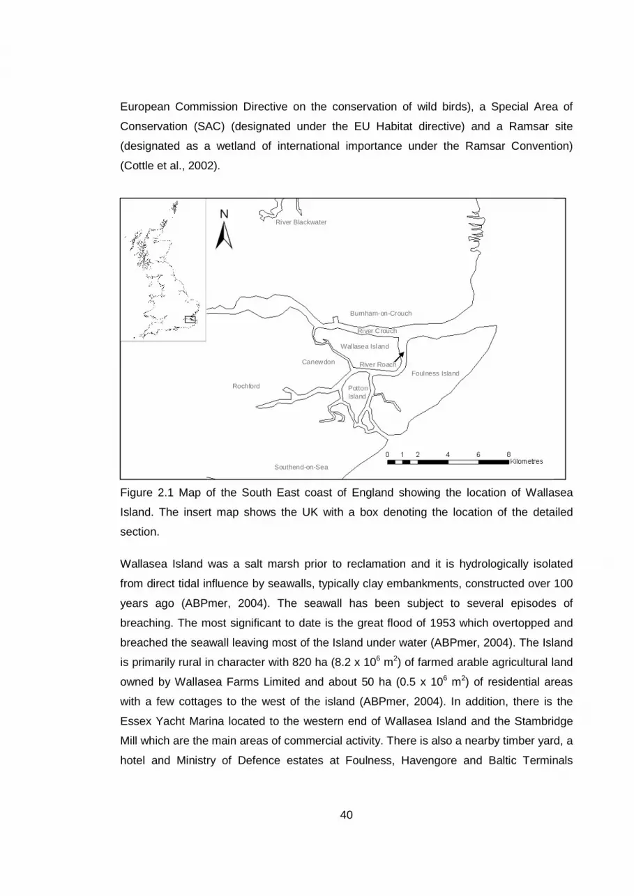
40

European Commission Directive on the conservation of wild birds), a Special Area of

Conservation (SAC) (designated under the EU Habitat directive) and a Ramsar site

(designated as a wetland of international importance under the Ramsar Convention)

(Cottle et al., 2002).

Figure 2.1 Map of the South East coast of England showing the location of Wallasea

Island. The insert map shows the UK with a box denoting the location of the detailed

section.

Wallasea Island was a salt marsh prior to reclamation and it is hydrologically isolated

from direct tidal influence by seawalls, typically clay embankments, constructed over 100

years ago (ABPmer, 2004). The seawall has been subject to several episodes of

breaching. The most significant to date is the great flood of 1953 which overtopped and

breached the seawall leaving most of the Island under water (ABPmer, 2004). The Island

is primarily rural in character with 820 ha (8.2 x 106 m2) of farmed arable agricultural land

owned by Wallasea Farms Limited and about 50 ha (0.5 x 106 m2) of residential areas

with a few cottages to the west of the island (ABPmer, 2004). In addition, there is the

Essex Yacht Marina located to the western end of Wallasea Island and the Stambridge

Mill which are the main areas of commercial activity. There is also a nearby timber yard, a

hotel and Ministry of Defence estates at Foulness, Havengore and Baltic Terminals

Wallasea Island

River Crouch

Rochford

River Blackwater

Burnham-on-Crouch

Southend-on-Sea

PottonIsland

Foulness Island

Canewdon River Roach

Wallasea IslandWallasea Island

River Crouch

Rochford

River Blackwater

Burnham-on-Crouch

Southend-on-Sea

PottonIsland

Foulness Island

Canewdon River Roach

41

respectively to the north western end of the Island. The closest built up area is Burnham-

On-Crouch which is 3 km north of Wallasea Island, on the north bank of the Crouch

estuary. The Crouch estuary is extensively used for recreational activities such as water

skiing, sailing, canoeing and wind surfing. The harbour is one of the leading sailing and

power boating centres in the UK (ABPmer, 2004)

The managed realignment site is located on the north eastern bank of Wallasea Island,

south shore of the Crouch estuary (Figure 2.2). Before May 2005, the seawall in this area

of the Island (north eastern bank) was in a deplorable condition because it was steadily

eroded by repeated tidal force and wave energy (ABPmer, 2004). There was a high risk

of the seawall breaching in an unmanaged way which could result in the flooding of the

Island and other significant potential effects on the estuary. As a result, a new seawall

was constructed on the north eastern bank of the Island in 2005, with the new seawall set

back 400 m from the original seawall (ABPmer, 2004). The area between the original and

the new seawall formed the managed realignment site which is approximately 108 ha

(1.08 x 106 m2) in size and 4 km in length. Before construction, the site was a part of the

820 ha (8.2 x 106 m2) arable agricultural land owned by Wallasea Farms Limited. The

primary objective of the managed realignment scheme was to compensate for the loss of

habitats that occurred following port developments at Lappel Bank in the Medway and at

Fagbury Flats in the Orwell Estuary. The objective overlapped with providing a robust

defence against flooding from the sea (ABPmer, 2004).

Several studies have indicated that the elevation most suitable for salt marsh plant

establishment in the UK lies between Mean High Water Neap and Mean High Water

Spring (French, 2006; Legget and Dixon 1994; Pye and French, 1993). The Mean Low

Water and Mean High Water Neap tide levels in the Crouch estuary are at 0.65 and 1.85

m ODN respectively while the Mean Low Water and Mean High Water Spring tide levels

are at 1.65 and 2.85 m ODN respectively (ABPmer, 2004). Since the land at Wallasea

Island is at a relatively low elevation, the land surface had to be raised to an intertidal

threshold elevation relative to the tidal level suitable for salt marsh establishment

(ABPmer, 2004). To achieve this, the managed realignment site was raised by importing

into the site, approximately 700,000 tonnes of dredged sediment sourced from

maintenance dredging at the Port of Harwich (ABPmer, 2004).

42

Figure 2.2 Aerial photo of Wallasea Island Managed Realignment site showing the River

Crouch and the arable agricultural land. Courtesy of Colin Scott, ABPmer Limited,

Southampton.

Discharge pipelines connected to a trailer suction dredger were used to pump the

dredged sediment ashore between the pre-constructed containment bunds and the new

seawall (Figure 2.3). The bunds, designed such that they erode over a period of 5 – 10

years, ensured the retention of the fine grained sediment, allowing it to settle, dewater

and consolidate. The sediment was pumped as a thick slurry with a bulk density of

approximately 1.25 g cm-3 (ABPmer, 2004). The original seawall was breached at six

locations to facilitate the restoration of intertidal habitats in the managed realignment site

following tidal inundation. The site was divided into three hydrodynamically separate

restored areas namely Area A west, Area A east and Area B, with each area exchanging

water with the adjacent estuary but no flows between neighbouring areas of the wider

realignment site (ABPmer, 2004) .

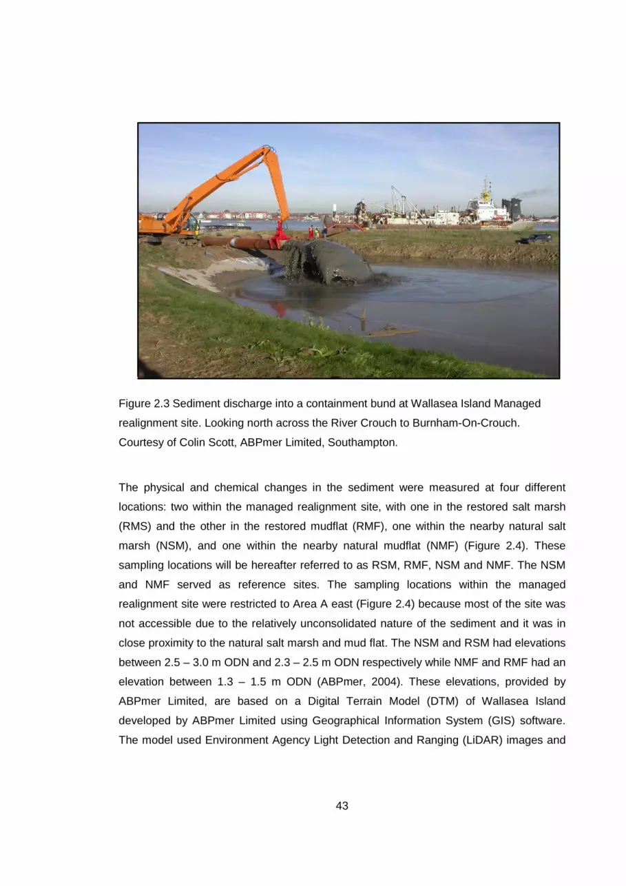
43

Figure 2.3 Sediment discharge into a containment bund at Wallasea Island Managed

realignment site. Looking north across the River Crouch to Burnham-On-Crouch.

Courtesy of Colin Scott, ABPmer Limited, Southampton.

The physical and chemical changes in the sediment were measured at four different

locations: two within the managed realignment site, with one in the restored salt marsh

(RMS) and the other in the restored mudflat (RMF), one within the nearby natural salt

marsh (NSM), and one within the nearby natural mudflat (NMF) (Figure 2.4). These

sampling locations will be hereafter referred to as RSM, RMF, NSM and NMF. The NSM

and NMF served as reference sites. The sampling locations within the managed

realignment site were restricted to Area A east (Figure 2.4) because most of the site was

not accessible due to the relatively unconsolidated nature of the sediment and it was in

close proximity to the natural salt marsh and mud flat. The NSM and RSM had elevations

between 2.5 – 3.0 m ODN and 2.3 – 2.5 m ODN respectively while NMF and RMF had an

elevation between 1.3 – 1.5 m ODN (ABPmer, 2004). These elevations, provided by

ABPmer Limited, are based on a Digital Terrain Model (DTM) of Wallasea Island

developed by ABPmer Limited using Geographical Information System (GIS) software.

The model used Environment Agency Light Detection and Ranging (LiDAR) images and

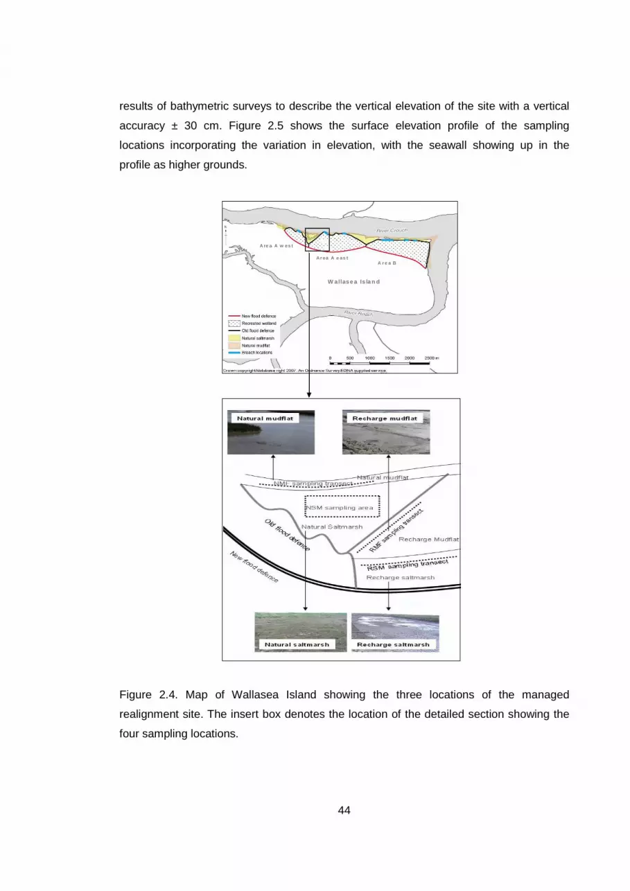
44

results of bathymetric surveys to describe the vertical elevation of the site with a vertical

accuracy ± 30 cm. Figure 2.5 shows the surface elevation profile of the sampling

locations incorporating the variation in elevation, with the seawall showing up in the

profile as higher grounds.

Figure 2.4. Map of Wallasea Island showing the three locations of the managed

realignment site. The insert box denotes the location of the detailed section showing the

four sampling locations.

W allase a Is la n d

A re a A w es t

A r ea A e as tA r e a B


A re a A w es t



A re a A w es t



A re a A w es t


45

Ele

vatio

n (m

OD

N)

Distance (m)

Natural saltmarsh

Recharge mudflat

Recharge saltmarsh

InlandMHW

MLW

Old seawallNew seawall

Ele

vatio

n (m

OD

N)

Distance (m)

Natural saltmarsh

Recharge mudflat

Recharge saltmarsh

InlandMHWS

MHWN


Ele

vatio

n (m

OD

N)

Distance (m)

Natural saltmarsh

Recharge mudflat

Recharge saltmarsh

InlandMHW

MLW


Ele

vatio

n (m

OD

N)

Distance (m)

Natural saltmarsh

Recharge mudflat

Recharge saltmarsh

InlandMHWS

MHWN


Figure 2.5 Surface elevation profile across the managed realignment site. The profile

show vertical elevation (mODN) and distance from the sea (m). MHWS and MHWN

represent Mean High Water Spring and Mean High Water Neap. Courtesy of Colin Scott,

ABPmer Limited, Southampton.

Due to the similar elevations of the restored sites and the respective natural reference

sites, the frequency and duration of tidal inundation of the sites were also similar (Figure

2.6). The frequency of tidal inundation was estimated based on the relationship between

the site surface elevation and the water level. The frequency of inundation at the RMF

and NMF were estimated to be approximately 43 %, covered by neap and spring tides

indicating that these sampling locations were regularly flooded. In contrast, the RSM and

NSM were not regularly flooded by tides. While the estimated frequency of inundation at

the RSM was approximately 15 %, the frequency of inundation at the NSM was estimated

to be approximately 10 %. These estimates were based on the site elevation (provided by

ABPmer Limited) and predicted water level data (Crouch Harbour Authority tide

timetable). Hence, the above percentages may be underestimated.

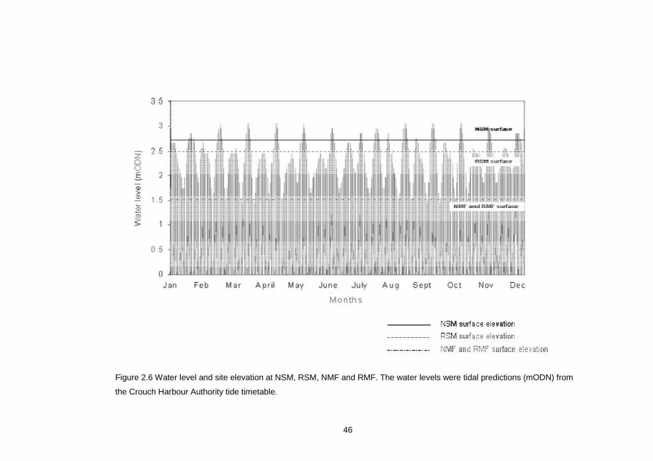
46

Figure 2.6 Water level and site elevation at NSM, RSM, NMF and RMF. The water levels were tidal predictions (mODN) from

the Crouch Harbour Authority tide timetable.

47

2.2.2. Sediment sampling

As stated earlier, samples were collected from four sampling locations: RSM, RMF, NSM

and NMF. Random sampling is preferred because every part of the sampling area has an

equal probability of being sampled thereby reducing bias in the generated data set.

However, random sampling was not possible at the four sampling locations because the

relatively unconsolidated sediment within the managed realignment site and the natural

mudflat presented a safety hazard which limited accessibility. Therefore, systematic

sampling was employed in the RSM, RMF and NMF. Even though systematic sampling

was the only option, the selected sampling locations and the sample size were deemed

appropriate to give a good representation of the changes in the sediment over the study

period.

Due to the limited accessibility, sampling was carried out along three permanent

transects marked at each end with wooden stacks in the RSM, RMF and NMF (Figure

2.4). At each sampling location, sediment samples were collected monthly at 10 sampling

points, each 5 m apart over the 12-month study period from January to December 2007.

However, samples were collected for only 9-months in the NMF from April to December

2007. The 10 samples collected for each month served as replicates.

Random sampling rather than systematic sampling was employed in the NSM because of

the easy access of the entire salt marsh. Within the NSM, a 169 m2 rectangular sampling

area was chosen and marked with wooden stacks. This area had distinct pioneer, lower

and middle salt marsh vegetation that was representative of a well established salt

marsh. Within the marked area, samples were collected each month from 10 randomly

selected sampling points determined by a random number generator and these samples

served as replicates. Care was taken not to re-sample a previous sample point.

At each sampling point, a stainless steel hand-held trowel was used to collect surface

samples from the top 2 cm of the sediment. The samples were placed in a waterproof

polyethylene bags, clearly labeled. The samples were analysed immediately after

collection.

In the RSM and NSM, hollow bulk density rings (5.2 cm in diameter, 2.5 cm in height)

were used to collect undisturbed sediment samples. Samples were collected at each

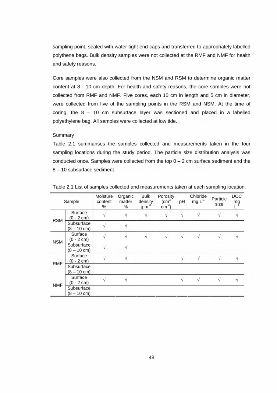
48

sampling point, sealed with water tight end-caps and transferred to appropriately labelled

polythene bags. Bulk density samples were not collected at the RMF and NMF for health

and safety reasons.

Core samples were also collected from the NSM and RSM to determine organic matter

content at 8 - 10 cm depth. For health and safety reasons, the core samples were not

collected from RMF and NMF. Five cores, each 10 cm in length and 5 cm in diameter,

were collected from five of the sampling points in the RSM and NSM. At the time of

coring, the 8 – 10 cm subsurface layer was sectioned and placed in a labelled

polyethylene bag. All samples were collected at low tide.

Summary

Table 2.1 summarises the samples collected and measurements taken in the four

sampling locations during the study period. The particle size distribution analysis was

conducted once. Samples were collected from the top 0 – 2 cm surface sediment and the

8 – 10 subsurface sediment.

Table 2.1 List of samples collected and measurements taken at each sampling location.

Sample Moisture content

%

Organic matter

%

Bulk density g m-3

Porosity (cm3 cm-3)

pH Chloride mg L-1

Particle size

DOC mg L-1

Surface (0 - 2 cm) √ √ √ √ √ √ √ √

RSM Subsurface (8 – 10 cm)

√ √

Surface (0 - 2 cm) √ √ √ √ √ √ √ √

NSM Subsurface (8 – 10 cm)

√ √

Surface (0 - 2 cm)

√ √ √ √ √ √ RMF

Subsurface (8 – 10 cm)

Surface (0 - 2 cm) √ √ √ √ √ √

NMF Subsurface (8 – 10 cm)

49

2.2.3 Sample preparation and analysis

2.2.3.1 Organic matter and moisture content

Different methods have been developed for the determination of organic matter content in

soil and sediment such as loss-on-ignition (LOI), wet oxidation using hydrogen peroxide

or potassium dichromate (Rowell, 1994). In this study, organic matter content was

determined by loss-on-ignition because it is rapid, inexpensive and safer compared to the

other methods. LOI is used as an approximate measure of the organic matter content,

following ignition of the soil or sediment at 500 – 550 OC. When soil or sediment is

ignited, the organic portion oxidizes to CO2, H2O and a small amount of ash. Thus, the

measurement of the mass lost during ignition can be used as an estimate of the organic

matter content. Given that LOI is a mass loss based method, it is important to recognize

that the loss of other components of the soil or sediment during ignition can affect the

estimates. Structural water adsorbed to clay particles or present as part of the mineral

lattice can be lost during ignition along with volatile salts and inorganic carbon leading to

an over-estimation of organic matter content (Rowell, 1994).

In this study, approximately 10 g (± 0.01) sub-sample was weighed into a crucible. The

sub-sample was oven-dried at 105 0C overnight, cooled in a desiccator and reweighed.

The percentage moisture content was calculated. The oven-dried sample was then

placed in a muffle furnace at 550 0C for 4 hours. The ignited sub-sample was cooled in a

desiccator and re-weighed to estimate the organic matter content.

2.2.3.2 Dry bulk density and porosity

Bulk density samples were placed in an oven at 105 0C over night, cooled in a desiccator

and weighed to give the mass of the oven-dried sample. Bulk density was determined by

dividing the mass of the oven-dried sample by the volume of the sample.

The sample porosity was calculated using the bulk density and particle density as:

Porosity = 1 – bulk density (g cm-3)

Particle density (g cm-3)

where the particle density was assumed to be 2.65 g cm-3 (Rowell, 1994).

50

2.2.3.3. Particle size analysis

The particle size distribution (i.e. clay, silt and sand fractions) of the sediment samples

were analysed using a Laser Diffraction Particle Size Analyser (Beckmann). Laser

diffraction is a rapid technique which covers a wide range of particle sizes (from 0 to 2000

µm) and therefore covers the whole range likely to be encountered in these sediments.

The sizes of the clay fraction (< 4 µm), the silt fraction (4 - 63 µm) and the sand fraction

(63 - 2000 µm) are equivalent to the Wentworth scale. Prior to the analysis, the organic

matter was removed to allow for the analysis of the particle size of the mineral fraction

(clay, silt and sand), as organic matter can bind the particles together (Rowell, 1994). The

removal of organic matter can also lead to the disaggregation of large aggregates.

Organic matter can be removed through ignition or through wet oxidation using hydrogen

peroxide. While ignition is a rapid method of removing organic matter, loss of structural

water from clay particles during ignition may result in changes in the size of the clay

particles. Thus, in this study, hydrogen peroxide was used to remove organic matter.

Prior to the analysis, hydrogen peroxide was added to the samples and the samples were

heated at around 80 oC on a hotplate until no further reaction occurred. The samples

were then resuspended using sodium hexametaphosphate dissolved in deionised water

which served as a dispersant.

2.2.3.4. pH

The sample pH was determined by using a sample suspension made with deionised

water. 100 g (± 0.01) sub-sample was carefully weighed into a conical flask. 100ml of

deionised water was added and the flask was sealed with parafilm. The pH of the

deionised water was pH 5.9. The suspension was shaken for 30 minutes on a flat bed

shaker to disperse the sediment in the water. This sample preparation ensured that

adequate water was available in the sample to make liquid contact with the pH electrode

(Craft et al., 2002). The pH of the sediment suspension was determined using a HANNA

pH electrode and a HANNA HI 83140 pH meter. The pH meter was calibrated prior to use

with two calibration solutions at pH 4 and 7. The pH electrode was rinsed with deionised

water and wiped dry between sample readings.

51

2.2.3.5. Porewater dissolved organic carbon (DOC) and chloride (Cl)

The measurements of DOC and Cl were made from extracts of sample suspensions.

Sample suspensions were used because the samples contained small volumes of

porewater which were not adequate for the techniques used for the analysis of DOC and

Cl. As a result, sample suspensions were prepared by adding deionised water to the

samples and the added deionised water was accounted for after the analysis in order to

determine the porewater concentrations. To determine the porewater concentration after

the analysis, the sample oven-dry weight was subtracted from the sample wet weight (i.e.

before the addition of deionised water) to get the actual mass of the porewater in the

sample. Assuming that the density of the porewater was one, the volume of the

porewater in the sample was determined. The total mass of DOC and Cl in the sample

(i.e. added deionised water plus porewater) was calculated by multiplying the measured

concentration of DOC and Cl by the volume of the sample. The total mass was divided by

the volume of porewater to obtain the concentration of DOC and Cl in the porewater.

100 g (± 0.01) sub-sample was weighed into a 250 ml plastic beaker and 100 ml of

deionised water was added, hence the solid-to-water ratio was 1:1. The beaker was

sealed with parafilm and shaken on a flat bed shaker for 10 minutes. The sample

suspension was transferred to plastic centrifuge tubes and centrifuged for 30 minutes at

2500 rpm. The supernatant was filtered through pre-rinsed (10 mL rinse with deionised

water) 0.45 µm hydrophilic polyethersulphone membrane filter paper (Supor®) discarding

the first 10 mL of the extract. The extract was split into two sub-samples for DOC and Cl

analysis and stored at 4 0C prior to analysis. Filtration was carried out using a filter paper

with a 0.45 µm pore size hydrophilic polyethersulphone membrane filter paper (Supor®) in

order to separate the DOC fraction from the particulate organic carbon fraction and to

remove particulates that can contaminate the analytical equipment. Filter papers were

changed between samples to avoid contamination.

2.2.3.6. Analysis of DOC

Dissolved organic carbon analysis was carried out on a HyperToc Carbon analyser with a

non-dispersive infrared detector (NDIR) using the UV-persulphate non-purgeable organic

carbon (NPOC) method. This method is one of the three commonly used methods for the

analysis of DOC in seawater (Aminot et al., 2004; Packard et al., 2000). Unlike the high

temperature catalytic oxidation and the wet chemical oxidation methods, the UV-

52

persulphate method ensured the fast and complete oxidation of organic carbon in the

difficult salt matrix. It involves the oxidation of organic carbon to CO2 by persulphate in the

presence of UV light. Prior to analysis, HCl acid was added to the sample and it was

sparged with O2 gas at a flow rate of 10 ml min-1 to remove the inorganic carbon before

the addition of persulphate. The O2 gas was used as a carrier gas to lead the CO2

produced through to the infra-red detector for quantification. The system had an

automated autosampler which injected the sample into the UV reactor, two infra-red

detectors and was supported by the ThEuS software. The generated peaks were

integrated in order to calculate the concentration of DOC. The reagents used were 1.5 M

sodium persulphate solution and 5% v/v HCl. Standards of known concentrations

prepared from potassium hydrogen phthalate were used for calibration before each

analytical run. One quality control standard and a duplicate sample were incorporated in

each analytical run to assess repeatability and precision within each run.

2.2.3.7. Analysis of Cl

Cl was analysed using a Dionex ICS-2500 chromatographic system with a Dionex ED-50

conductivity detector. A 2 x 250 mm RFICTM IonPac® AS18 analytical column with an

IonPac AS18 guard column was used. The system had an AS50 autosampler for

automated sample injection and Chromeleon software for system control and data

processing. The eluent used was 100 mM KOH pumped by a GP-50 gradient pump at a

flow rate of 0.25 ml min-1 in a gradient mode. A set of four calibration standards at varying

concentrations were made up and used for calibration before each run. One standard and

a duplicate sample were analysed in each analytical run in order to assess repeatability

and precision.

2.2.4. Statistical Analysis

Statistical analysis was conducted using SPSS statistical package (Version 16). A

Levene test of homogeneity of variance was carried out to test for equal variances in the

data and several dataset had unequal variances. In addition, the datasets were not

symmetrical and normally distributed and the assumptions of the parametric t-test could

not be met. Hence, a Mann-Whitney test was employed to test for differences in the

datasets between the sediment parameters in the reference sites (NSM and NMF) and in

the managed realignment site (RSM and RMF). Mann-Whitney test is a non-parametric

test which tests for significant differences between groups of samples. Although this test

53

is less powerful than the equivalent parametric t-test, the Mann-Whitney test does not

make any assumptions about the dataset.

2.3. Results and Discussion

2.3.1. Meteorological conditions

The monthly average atmospheric temperature and monthly total precipitation conditions

during the sampling period are presented in Table 2.2. The precipitation and temperature

data were obtained from ABPmer Limited on-site weather station. Table 2.2 shows that

there were higher temperatures in the spring and summer than in the winter and autumn.

The highest monthly total precipitation and monthly average temperature recorded on-site

were in May and August respectively.

Table 2.2 Monthly average temperature and monthly total precipitation in Wallasea Island

from January to December 2007. Data presented courtesy of Colin Scott, ABPmer

Limited, Southampton.

Months Monthly average temperature ( 0C) Monthly total precipitation (mm)

January * n/a n/a

February 6 86.8

March 8 63.2

April 12 1.2

May 13 88.8

June 16 52.2

July * n/a n/a

August 17 47.6

September 15 23.4

October 12 39.2

November 0 22.8

December 6 82.0

* Data for January and July were not available (n/a) due to a fault in the weather station during this

period.

2.3.2. Changes in sediment parameters

Moisture content

The monthly average moisture content measurements at the sediment surface are

presented in Figure 2.7 and the ranges recorded are presented in Table 2.3. The

54

complete data are available in Appendix 1. The lowest moisture contents were in the

RSM and the highest moisture contents were observed in the NSM. The moisture content

values recorded in the NMF and RMF were intermediate between those in the NSM and

RSM. The range of sediment moisture content values in the NSM, RMF and NMF

indicate that these sediments were water-saturated (Table 2.3). Seasonal fluctuations

were observed at the four sampling locations with lower moisture contents during the

summer months (Figure 2.7). However, the seasonal variability in the sediment moisture

contents were least evident in the RMF and NMF where the sediments were continuously

wet by more frequent tidal inundation compared to the RSM and NSM.

Infiltration of the sediment with seawater during tidal inundation and precipitation can lead

to high sediment moisture content while evaporation and drainage can lead to low

sediment moisture content. Hence, changes in the sediment moisture content are mainly

due to a combination of tidal inundation, precipitation, evaporation and drainage. The

lower moisture contents at all the sampling locations observed during the summer is likely

due to higher atmospheric temperatures in the summer compared to the other seasons

(Table 2.2) and therefore, higher evaporation from the sediments. However, the months

with the highest average moisture content did not coincide with the months with the

highest monthly total precipitation (Table 2.2). This is probably due to the contributing

effect of the other factors that control sediment moisture content.

Sediment texture and organic matter content can also affect the sediment moisture

content (Crooks et al., 2002). The NSM had a sandy silt texture with a higher sand and

lower clay and silt content than the RSM (Table 2.3). Given that sand particles have lower

water holding capacity and are more easily drained than clay and silt particles (Brady and

Weil, 2002), the NSM was expected to have a lower moisture content than the RSM.

However, the results obtained were contrary, suggesting that the higher moisture content

in the NSM may be due to the higher organic matter content in the NSM compared to the

RSM (Table 2.3) which increased the residence time of water in the NSM. Therefore,

organic matter seems to play a more dominant role than the sediment texture in affecting

the sediment moisture content at the NSM. Crooks and Pye (2000) observed high

moisture content and poor drainage in established salt marsh sediments in Essex, south-

east England due to a deficiency in calcium carbonate. The deficiency reduced the

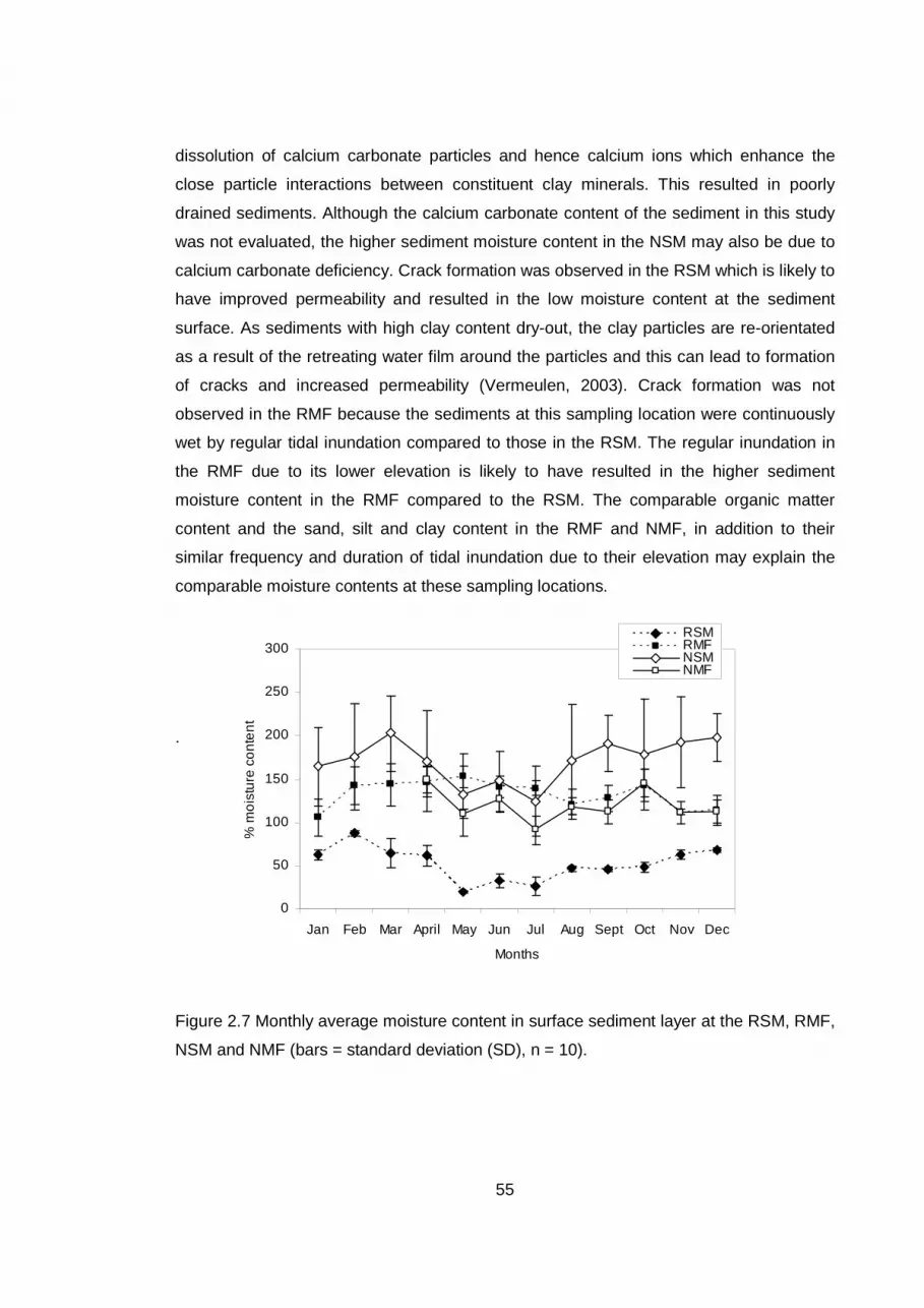
55

0

50

100

150

200

250

300

Jan Feb Mar April May Jun Jul Aug Sept Oct Nov Dec

Months

% m

ois

ture

co

nte

nt

RSMRMFNSMNMF

dissolution of calcium carbonate particles and hence calcium ions which enhance the

close particle interactions between constituent clay minerals. This resulted in poorly

drained sediments. Although the calcium carbonate content of the sediment in this study

was not evaluated, the higher sediment moisture content in the NSM may also be due to

calcium carbonate deficiency. Crack formation was observed in the RSM which is likely to

have improved permeability and resulted in the low moisture content at the sediment

surface. As sediments with high clay content dry-out, the clay particles are re-orientated

as a result of the retreating water film around the particles and this can lead to formation

of cracks and increased permeability (Vermeulen, 2003). Crack formation was not

observed in the RMF because the sediments at this sampling location were continuously

wet by regular tidal inundation compared to those in the RSM. The regular inundation in

the RMF due to its lower elevation is likely to have resulted in the higher sediment

moisture content in the RMF compared to the RSM. The comparable organic matter

content and the sand, silt and clay content in the RMF and NMF, in addition to their

similar frequency and duration of tidal inundation due to their elevation may explain the

comparable moisture contents at these sampling locations.

.

Figure 2.7 Monthly average moisture content in surface sediment layer at the RSM, RMF,

NSM and NMF (bars = standard deviation (SD), n = 10).

56

Table 2.3. Range of sediment parameters in the surface sediment at the RSM, NSM,

RMF and NMF.

RSM NSM RMF NMF

Moisture (%) 11 – 107a 67 – 280a 79 – 183b 63 – 170b

Organic matter (%) 6 – 14a 12 – 26a 7 – 16b 9 – 13b

Bulk density (gcm-

1) 0.8 – 1.6a 0.4 – 0.7a

Porosity (cm3 cm-3) 0.3 – 0.7a 0.6 – 0.9a

pH 7.2 – 8.2a 6.8 – 7.7 a 6.6 – 7.4b 7.0 – 7.5b

Cl (mgL-1) 1,760 – 28,852a 164 – 18,525a 1,379 – 13,165b 3,149 – 19,537b

DOC (mgL-1) 13 – 237b 7 – 266b 11 – 191b 10 – 156b

Clay (%) 37 28 37 36

Silt (%) 49 32 47 51

Sand (%) 14 40 16 14

a denotes significant difference between sampling locations (i.e. RSM and NSM; RMF and NMF) at

p < 0.05 significance level, b denotes no significant difference. The clay fraction was < 4 µm, the

silt fraction was 4 - 63 µm and the sand fraction was 63 - 2000 µm.

Sediment moisture content in the surface and the 8 – 10 cm subsurface sediment in the

RSM and NSM were compared in Figure 2.8. The complete data in the 8 – 10 cm

subsurface sediment are presented in Appendix 1. Unlike the moisture content at the

sediment surface, there were fewer changes between the monthly averages in the

subsurface sediment in the RSM and no seasonal trends were observed. The moisture

contents in the subsurface sediments were approximately three times higher than those

in the surface sediments in the summer months in the RSM. These findings suggest that

the surface sediments are more exposed to wetting and drying than the subsurface

sediments. High evaporation from the RSM during the hot summer months is likely to be

the main factor responsible for the lower moisture content in the surface sediment

compared to the subsurface sediment. In the NSM, the temporal changes in the moisture

content in the subsurface sediments were relatively similar to those observed in the

surface sediments with the surface sediments having slightly higher moisture contents

(Figure 2.8). Evaporation from the surface sediment and uptake of water by salt marsh

plant roots from the subsurface sediment in the NSM are likely to have resulted in the

57

0

50

100

150

200

250

300

Jan Feb Mar April May June July Aug Sept Oct Nov Dec

Months

% m

oist

ure

co

nten

t

0 - 2 cm NSM layer8 - 10 cm NSM layer0 - 2 cm RSM layer8 - 10 RSM layer

slight differences in the moisture content between the surface and subsurface sediments.

Crooks et al. (2002) also observed minimal changes in the moisture content of salt marsh

sediment over a 0 – 60 cm depth profile.

Figure 2.8 Monthly average moisture content in the surface (0 – 2 cm) and subsurface (8

– 10 cm) sediment in the NSM and RSM (bars = standard deviation (SD), n = 5).

Organic matter content

The monthly average organic matter content data in the surface sediment are presented

in Figure 2.9. The complete data are presented in Appendix 2. The organic matter

content in the RSM, RMF and NMF were comparable with ranges from 6 % to 14 %, 7 %

to 16 % and 9 % to 13 % respectively (Table 2.3). The organic matter content in the NSM

was approximately twice as high as those in the RSM with a range from 12 to 26 %.

Whilst slight variations were observed in the RSM, RMF and NMF, a progressive

increase in the organic matter content was observed in the NSM.

Organic matter content is generally a balance between inputs and outputs (Kentula,

2000). Whilst inputs of salt marsh plant litter and organic-rich sediment from the water

column are sources of organic matter, output is due to decomposition by microbes and

other organisms (Mitsch and Gosselink, 2000). Hence the higher organic matter content

58

in the vegetated NSM compared to the unvegetated RSM is likely due to the presence of

established saltmarsh plants which provide a source of plant litter that contributes to the

organic matter content in the NSM. The vegetation in the NSM is also likely to trap detrital

organic matter, leading to higher organic matter content compared to the RSM. The

activities of various burrowing invertebrates present in salt marsh such as Nereis

diversicolor incorporates the organic-rich plant litter into the sediment. Furthermore, the

high moisture content in the NSM reduces sediment aeration, providing suitable

conditions for anaerobiosis. This in turn may have led to the microbial utilization of

alternative electron sinks such as NO3-, Mn4+, Fe3+, SO4

2- and CO2 in the absence of O2

for organic matter decomposition and such anaerobic processes proceed at a slower rate

than aerobic decomposition (Williams et al., 1994; Bishel-Machung et al., 1996; Craft et

al., 2002; Portnoy and Giblin, 1997; Sun et al., 2002) leading to organic matter

accumulation in the NSM. The progressive increase in the sediment organic matter

content observed in the NSM (Figure 2.9) further suggests organic matter accumulation

at the sediment surface in the NSM. Slight variations were observed in the organic matter

content in the RSM and RMF but no progressive increase was found (Figure 2.9). An

increase in the organic matter content may not be evident at these sampling locations

because the rate at which organic matter accumulates due to organic-rich sediment

accretion equals the rate at which organic matter is lost due to decomposition given that

these sampling locations were unvegetated. However, as salt marsh plants colonise the

managed realignment site and organic matter starts to accumulate, an increase in the

organic matter content is likely to become evident. The sediment organic matter contents

observed in the RMF and NMF were comparable and this is probably due to the lack of

vegetation at both sampling locations.

59

0

5

10

15

20

25

30


Months

% O

rgan

ic m

atte

r

RSMRMFNSMNMF

Figure 2.9 Monthly average organic matter content at sediment surface in the RSM, RMF,

NSM and NMF (bars = standard deviation (SD), n = 10).

The monthly average organic matter content data in the surface and the 8 – 10 cm

subsurface sediment in the RSM and NSM were compared in Figure 2.10 (see Appendix

2 for the complete subsurface sediment organic matter content data). In the NSM, the

organic matter content in the subsurface sediments with a range from 10 % – 20 % was

lower than those at the surface sediments. However, the organic matter in the subsurface

sediment in the RSM ranged from 6 % – 11 % and was comparable to those in the

surface sediment. The lower organic matter content in subsurface sediment compared to

the surface sediment in the NSM agrees with the study of Bishel-Machung et al. (1996)

where decreasing organic matter content was observed with depth. The lower subsurface

sediment organic matter content in the NSM is likely due to organic matter accumulation

at the sediment surface. In the RSM, no change was observed in the organic matter

content with depth, further suggesting that there was no organic matter accumulation in

the surface sediment at this sampling location.

60

0

5

10

15

20

25

30


Months

% O

rga

nic

mat

ter

0-2 cm RSM layer

8-10 cm RSM layer

0-2 cm NSM layer

8-10 cm NSM layer

Figure 2.10. Monthly average organic matter content at the sediment surface and 8 – 10

cm subsurface layers at the RSM and NSM (bars = standard deviation (SD), n = 5).

Bulk density and porosity

Figure 2.11 and 2.12 shows the monthly average bulk density and porosity data for the

RSM and NSM. The complete data is presented in Appendix 3. It should be noted that

there are no bulk density or porosity data for the RMF and NMF because the relatively

unconsolidated sediment within the restored and natural mudflat presented a safety

hazard. The bulk density values in the RSM ranged from 0.8 - 1.6 g cm-3 whilst the range

in the NSM was from 0.4 – 0.7 g cm-3 (Table 2.3). These ranges show that the bulk

density values in the RSM were approximately twice as high as those in the NSM (Table

2.5). The porosity values in the RSM were lower compared to the NSM with ranges from

0.3 - 0.7 cm3 cm-3 and 0.6 - 0.9 cm3 cm-3 respectively (Table 2.3). The sediment bulk

density and porosity values remained relatively constant in both the RSM and NSM over

the study period with slight variations observed (Figure 2.11 and 2.12).

Bulk density and porosity depend on the proportion of the total pore spaces occupied by

air and the density of the particles (Rowell, 1994). Sediment bulk density and porosity can

be affected by the sand, silt and clay content, organic matter content, the presence of

plant roots and bioturbation by invertebrates. The relatively stable sediment bulk density

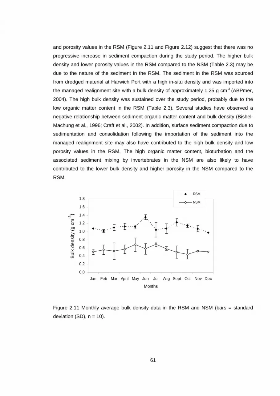
61

0.0

0.2

0.4

0.6

0.8

1.0

1.2

1.4

1.6

1.8


Months

Bul

k de

nsity

(g

cm-3

)

RSM

NSM

and porosity values in the RSM (Figure 2.11 and Figure 2.12) suggest that there was no

progressive increase in sediment compaction during the study period. The higher bulk

density and lower porosity values in the RSM compared to the NSM (Table 2.3) may be

due to the nature of the sediment in the RSM. The sediment in the RSM was sourced

from dredged material at Harwich Port with a high in-situ density and was imported into

the managed realignment site with a bulk density of approximately 1.25 g cm-3 (ABPmer,

2004). The high bulk density was sustained over the study period, probably due to the

low organic matter content in the RSM (Table 2.3). Several studies have observed a

negative relationship between sediment organic matter content and bulk density (Bishel-

Machung et al., 1996; Craft et al., 2002). In addition, surface sediment compaction due to

sedimentation and consolidation following the importation of the sediment into the

managed realignment site may also have contributed to the high bulk density and low

porosity values in the RSM. The high organic matter content, bioturbation and the

associated sediment mixing by invertebrates in the NSM are also likely to have

contributed to the lower bulk density and higher porosity in the NSM compared to the

RSM.

Figure 2.11 Monthly average bulk density data in the RSM and NSM (bars = standard

deviation (SD), n = 10).

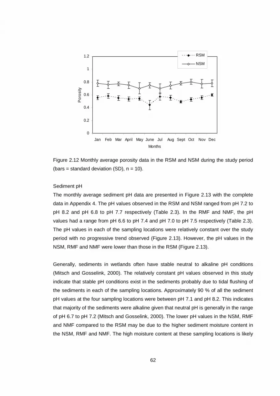
62

0

0.2

0.4

0.6

0.8

1

1.2

Jan Feb Mar April May June Jul Aug Sept Oct Nov Dec

Months

Por

osi

ty

RSM

NSM

Figure 2.12 Monthly average porosity data in the RSM and NSM during the study period

(bars = standard deviation (SD), n = 10).

Sediment pH

The monthly average sediment pH data are presented in Figure 2.13 with the complete

data in Appendix 4. The pH values observed in the RSM and NSM ranged from pH 7.2 to

pH 8.2 and pH 6.8 to pH 7.7 respectively (Table 2.3). In the RMF and NMF, the pH

values had a range from pH 6.6 to pH 7.4 and pH 7.0 to pH 7.5 respectively (Table 2.3).

The pH values in each of the sampling locations were relatively constant over the study

period with no progressive trend observed (Figure 2.13). However, the pH values in the

NSM, RMF and NMF were lower than those in the RSM (Figure 2.13).

Generally, sediments in wetlands often have stable neutral to alkaline pH conditions

(Mitsch and Gosselink, 2000). The relatively constant pH values observed in this study

indicate that stable pH conditions exist in the sediments probably due to tidal flushing of

the sediments in each of the sampling locations. Approximately 90 % of all the sediment

pH values at the four sampling locations were between pH 7.1 and pH 8.2. This indicates

that majority of the sediments were alkaline given that neutral pH is generally in the range

of pH 6.7 to pH 7.2 (Mitsch and Gosselink, 2000). The lower pH values in the NSM, RMF

and NMF compared to the RSM may be due to the higher sediment moisture content in

the NSM, RMF and NMF. The high moisture content at these sampling locations is likely

63

6.0

7.0

8.0

9.0


Months

pH

un

its

RSMRMFNSMNMF

to have resulted in reduced sediment aeration and the development of reducing

conditions in the sediment. Most reducing reactions which occur under these conditions

consume hydrogen ions which can lead to an increase in pH (McBride, 1994). However,

at alkaline pHs, the reducing conditions can lower pH when metal ions such as Fe2+ and

Mn2+, made soluble by reduction, precipitate as carbonates. The precipitation reaction

can generate H+ which can counter those consumed by reduction (McBride, 1994).

Consequently, the precipitation of metal ions as carbonates in the alkaline, water-

saturated sediments in the NSM, RMF and NMF may have led to the generation of H+

and hence, a decrease in pH at the NSM, RMF and NMF compared to the RSM.

Figure 2.13 Monthly average pH values in the RSM, RMF, NSM and NMF (bars =

standard deviation (SD), n = 10).

Sediment porewater Cl

The monthly average sediment porewater Cl concentration data are shown in Figure 2.14

and the range at each sampling location presented in Table 2.3. The complete data are

presented in Appendix 5. Seasonal variability in the sediment porewater Cl

concentrations were observed in the RSM, NSM, RMF and NMF with higher

concentrations measured in the summer months and lower concentrations in the winter

months (Figure 2.14). While the sediment porewater Cl concentration in the RSM was

higher than that in the NSM particularly in June and July, the sediment porewater Cl

64

concentrations in the RMF and NMF were relatively similar and both sampling locations

showed the same temporal trend (Figure 2.14).

Sediment porewater salinity is controlled by a variety of factors including the frequency

and duration of tidal inundation, precipitation, evaporation, freshwater inflow, sediment

texture and presence of salt marsh vegetation (Otero and Macias, 2002; Mitsch and

Gosselink, 2000). In this study, the sediment porewater Cl concentration was used as a

proxy for salinity. The increase in the porewater salinity in the summer compared to the

winter at all the sampling locations is likely due to the higher summer temperatures

(Table 2.2) which led to higher evaporation, leaving behind high salt concentrations at the

sediment surface. The higher salinity at the sediment surface in the RSM compared to

the NSM during the summer (Figure 2.15) is attributed to higher evaporation from the

RSM due to the lack of salt marsh plants and the lower moisture content in the RSM

(Figure 2.7). Likewise, the salinity at the sediment surface in the RSM was higher

compared to the RMF and this is likely due to less tidal flushing in the RSM which leads

to a greater accumulation of salts in the RSM compared to the RMF (Figure 2.7). In the

winter, precipitation is likely to have resulted in the dilution of the high salt concentrations

at the sediment surface, thereby leading to a decrease in the porewater salinity at the

sampling locations (Figure 2.15). A similar pattern of seasonal variation in the salinity of

salt marsh sediments has been reported by Otero and Macias (2002) with high salinities

during the summer and low salinities in the winter. The similar observations at the RMF

and NMF may be due to both sampling locations having the same surface elevation.

Hence they experience similar frequencies and durations of flooding, and associated salt

inputs.

65

0

10000

20000

30000


Months

Chl

ori

de c

on

ten

t (m

g L

-1)

RSMRMFNSMNMF

Figure 2.14 Monthly average Cl content in the RSM, RMF, NSM and NMF (bars =


Porewater dissolved organic carbon (DOC)

The monthly average porewater DOC concentrations measured in the RSM, RMF, NSM

and NMF are presented in Figure 2.15 with the complete data in Appendix 6. The range

of porewater DOC concentrations at the four sampling locations are shown in Table 2.3.

Temporal variations were observed at all the sampling locations during the study period.

DOC concentrations in sediment porewater reflects the balance between inputs from

plant root exudates, decomposition of plant litter, particulate organic matter, dead

microbial biomass and losses from sediment fluxes to the estuary, adsorption to particles,

uptake by heterotrophic bacteria and other organisms (Koepfler et al., 1993). In this

study, higher porewater DOC concentrations were expected in the NSM compared to

RSM because of the higher organic matter content in the NSM sediment. However, the

DOC concentrations at these sampling locations were similar (Table 2.4). In the RMF and

NMF, the porewater DOC concentrations were also comparable (Table 2.4). Higher DOC

concentrations were observed in the summer at the RSM and NSM. The sediment

porewater DOC concentration measured in the RSM in July was approximately three

times higher than that measured in June (51.3 mg L-1 to 139.7 mg L-1) (Figure 2.15).

Similarly, a fivefold increase was observed in the porewater DOC concentration in the

66

0

100

200

300


Months

DO

C (m

g L

-1)

RSMRMFNSMNMF

NSM between June and July (29.3 mg L-1 to 140.2 mg L-1) (Figure 2.15). Several field

studies have observed higher porewater DOC concentrations in sediments in the summer

(Herndl et al., 1987; Hargrave and Phillips, 1989; Koepfler et al., 1993). The increase in

porewater DOC was due to an increase in microbial biomass activity in the summer and

hence, an increase in the rate of decomposition of particulate organic matter. The higher

porewater DOC concentrations observed in the summer in this study may be due to an

increase in the microbial biomass activity and decomposition of organic matter at the

sampling locations. The presence of the filamentous green alga Enteromorpha sp. in the

RSM in the summer is also likely to have provided an additional carbon source for

decomposition into DOC in the RSM. The higher porewater DOC concentrations were not

observed in the RMF and NMF in the summer probably due to greater tidal flushing of

DOC from the RMF and NMF into the estuary due to more frequent tidal inundation at

these sampling locations compared to the RSM and NSM.

Figure 2.15 Monthly average DOC porewater concentrations in the RSM, RMF, NSM and

NMF (bars = standard deviation (SD), n = 10).

67

2.4. Summary and conclusion

This chapter has identified little or no change in the organic matter content, bulk density,

porosity and pH values in the sediment at the restored salt marsh and mudflat within the

Wallasea Island managed realignment site during the 12-months study period. However,

lower moisture contents and higher porewater Cl concentrations were observed in the

sediment in the hotter summer months due to higher atmospheric temperatures and

hence, higher evaporation in the summer. The porewater Cl concentration was used as a

proxy for salinity and the seasonal range in the porewater salinity (i.e. maximum and

minimum monthly average porewater Cl concentrations in the summer and winter

respectively) was used as the two different salinity treatments in the laboratory column

microcosm experiments so that the experiments simulated the field conditions. In

addition, the sediment porewater DOC concentration in the restored salt marsh was

higher in the summer, probably due to increased microbial biomass activity, higher

decomposition rate and the presence of the filamentous green alga Enteromorpha sp. in

the restored salt marsh in the summer which is likely to have provided an additional

carbon source for decomposition.

This chapter has also shown that the sediment parameters (i.e. moisture content, organic

matter content, pH, porewater Cl and porewater DOC) in the natural and restored mudflat

were similar. However, the same cannot be said for the salt marsh pair as most of the

sediment parameters were different and far from approaching those in the natural salt

marsh. The organic matter content was higher in the natural salt marsh compared to the

restored salt marsh due to the presence of an additional source of organic matter from

plant litter and organic matter accumulation in the natural salt marsh. The organic matter

content in the restored saltmarsh should begin to accumulate and approach that in the

natural saltmarsh as saltmarsh plants start to colonise the site. The sediment moisture

content was also higher in the natural salt marsh compared to the restored salt marsh

probably due to calcium carbonate deficiency and higher organic matter content in the

natural salt marsh and crack formation in the restored salt marsh. Higher sediment bulk

density and lower porosity were observed in the restored salt marsh compared to the

natural saltmarsh which was likely due to the lower organic matter content and higher

bulk density of the imported sediment, and the surface sediment compaction due to

sedimentation and consolidation following the importation of the sediment into the

managed realignment site. The sediment pH values were lower in the natural salt marsh

68

compared to the restored salt marsh probably due to the generation of H+ following the

precipitation of metal ions as carbonates in the water-saturated alkaline sediments in the

natural salt marsh. Higher Cl concentrations were observed in the restored salt marsh

compared to the natural salt marsh in the summer which was likely due to the lack of salt

marsh plants and hence higher evaporation from the restored salt marsh. These findings

indicate that further years are required before the sediments in the restored salt marsh

become similar to those in the natural salt marsh.

69

Chapter 3 Laboratory Experiments: Methodology

3.1. Introduction

This chapter describes the laboratory experiments that were conducted to examine the

effects of salinity and drying and rewetting on the release of metals and herbicides from

agricultural soil and dredged sediment in managed realignment sites following tidal

inundation. The experiments were designed to simulate conditions in a managed

realignment site. This was done by using field observations obtained from the study at

Wallasea Island managed realignment site described in Chapter 2. The chapter begins

with details of the collection and storage of the soil and sediment used for the

experiments. It then describes the experiments that were performed which include the

column microcosm experiments, conducted under two different salinity and drying-

rewetting treatments, carbon mineralisation experiments and batch sorption experiments.

The carbon mineralisation experiments were conducted to test the hypothesis that

organic matter mineralisation will be enhanced during drying and rewetting of the soil and

sediment leading to the release of organic matter associated metals and herbicides into

the overlying water. The batch sorption experiments were conducted to calculate the

partition coefficients (Kd) of the metals and herbicides in order to evaluate the changes in

contaminant binding to the soil and sediment with changes in salinity.

3.2. Sediment and soil collection

The sediment was collected from Wallasea Island managed realignment site. The soil

was collected from Wallasea Farms, the arable agricultural land adjacent to the managed

realignment site (Chapter 2, Figure 2.2). Surface soil and sediment samples were

collected randomly from the managed realignment site and the arable agricultural land

and mixed into composite soil and sediment samples. Following collection, the soil and

sediment samples were returned to the laboratory, sieved to < 4 mm and stored in water

tight plastic buckets at 4 0C for the six months duration of the entire experiments. It is

important to recognise the potential changes that can occur in soil and sediment during

storage. These include changes in microbial activity which can cause changes to the

concentrations of ammonia, sulphides and biologically-active components in the

porewater; changes in redox properties; changes in speciation and partitioning of

baseline metals and loss of baseline organic contaminants due to microbial degradation.

Prior to the start of the experiments, the soil and sediment properties (pH, organic matter

70

content, sand, silt and clay content) were determined using standard methods described

in Chapter 2 (Section 2.2.3).

3.3. Laboratory microcosm experiments

3.3.1. Column microcosm

Experimental systems such as mesocosms and microcosms have frequently been used

in toxicological, ecological and biogeochemical studies of aquatic and terrestrial

ecosystems (Johnson et al., 1986; Wielder et al., 1990; Horne 1991, Ahn et al., 2001;

Tueben and Verhoef, 1992; Van Wensem, 1989). Microcosm experiments have been

performed in the laboratory to examine the release fluxes of DOC and organic

contaminants from sediments (Valsaraj et al., 1996; Ortiz et al., 2004), microbial activity

in soils by measuring CO2 production and the availability of macronutrients in soil

(Lundquist et al., 1999; Tueben and Verhoef, 1992) and the effect of herbicides on the

productivity and biogeochemical functions of wetland plants and invertebrates (Johnson,

1986). Microcosms have been frequently used because they are considered analogous to

the natural system (Tueben and Verhoef, 1992). These microcosms provide a means of

conducting field-level experiments under controlled, replicated and repeatable conditions

which are difficult to achieve in the field (Ahn and Mitsch, 2002; Verhoef, 1996). Although

the complex array of interactions found in the field may not always be simulated by

microcosms, they are still considered models of natural systems (Ahn and Mitsch, 2002;

Tueben and Verhoef, 1992). In this study, the experiments were conducted in simple

column microcosms which allowed for the control of the experimental conditions, the

simulation of tidal inundation in a managed realignment site and replication of the

experiments.

In the column microcosms, artificial sea water flowed over the surface of the soil and

sediment, simulating natural tidal inundation at a managed realignment site. A schematic

diagram of the column microcosm is shown in Figure 3.1. The design of the columns was

adapted from Ortiz et al. (2004). Each microcosm was 60 cm in length and 10 cm in

diameter. The microcosms were made of glass with an air inlet and a sampling outlet.

The lid was fitted with a water inlet connected by flexible tubing to a reservoir containing

artificial seawater, allowing water supply to be initiated at the soil and sediment surface.

However, the water inlet was designed such that the artificial seawater flow into the

column was not directly against the soil and sediment surface (Figure 3.1). This was done

71

in order to minimise turbulence and particle resuspension due to direct water flow against

the soil and sediment surface, thereby reducing the transport of contaminants into the

overlying water column by re-suspended particles.

Figure 3.1 Schematic diagram of the laboratory column microcosm

3.3.2 Experimental procedure

Each microcosm was packed gently with approximately 800g (wet weight) of either soil or

sediment slurry spiked with the studied metals and herbicides. Both the soil and sediment

were spiked according to the procedure described in Section 3.3.3. After packing the

microcosms with the soil and sediment under the same conditions, they were left to

dewater and consolidate. This was done in order to simulate the Wallasea Island

managed realignment site where the sediment used to raise the elevation of the site was

allowed to dewater and consolidate before the seawall was breached (Chapter 2, Section

2.2.1). In these experiments, 4 days were chosen for dewatering and consolidation

because of the high clay and silt content in the soil and sediment (Chapter 4, Table 4.1).

Following dewatering and consolidation, the overlying supernatant at the soil and

sediment surface was removed. The microcosms were then kept in a temperature control

cabinet maintained at 10 0C. This temperature which was within the range of the

Sampling outlet

Artificial seawaterinlet Column Lid

Tubing to artificial seawater reservoir

Tube connector

Air inlet

Soil/Sediment

Sampling outlet

Artificial seawaterinlet Column Lid

Tubing to artificial seawater reservoir

Tube connector

Air inlet

Soil/Sediment

72

atmospheric temperature observed in the field site where the monthly average

atmospheric temperature recorded ranged from 6 – 17 0C (Chapter 2, Table 2.3).

Artificial seawater was delivered by a peristaltic pump (Watson-Marlow Bredel Pumps

Ltd, UK) to the microcosms in the temperature control cabinet with the water flowing

laterally over the soil and sediment surface. Artificial seawater, made from deionised

water and sea salt (Sigma Aldrich, UK) was used instead of the natural seawater to

ensure that dissolved organic carbon was not present in the seawater introduced into the

microcosms. The presence of dissolved organic carbon in the seawater can facilitate

contaminant release (Kalbitz and Wenrich, 1998; Gao et al., 1998) which may mask

release due to salinity effects and drying-rewetting cycles. Table 3.1 shows the

composition of the sea salt. The artificial seawater was delivered at a flow rate of 1.6 ml

min-1 in order to minimise particle resuspension from the soil/sediment surface. Samples

were then collected from the overlying water (Section 3.3.4.1 and 3.3.4.2). The first

sample was collected one hour after the initial delivery of artificial seawater to allow

sufficient water flow into the microcosms. Each sample was collected over a one hour

period to collect adequate sample volume for analysis.

Table 3.1 Composition of sea salt (Sigma Aldrich)

Components Concentration (mg l-1)

Chloride 19,290

Sodium 10,780

Sulphate 2,660

Magnesium 1,320

Potassium 420

Calcium 400

Carbonate 200

Boron 5.6

Bromide 56

Iodide 0.24

Fluoride 1.0

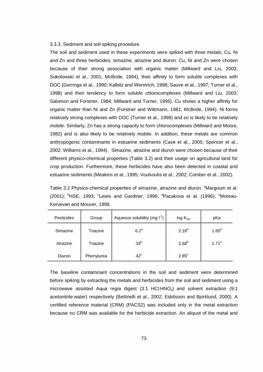
73

3.3.3. Sediment and soil spiking procedure

The soil and sediment used in these experiments were spiked with three metals; Cu, Ni

and Zn and three herbicides; simazine, atrazine and diuron. Cu, Ni and Zn were chosen

because of their strong association with organic matter (Millward and Liu, 2003;

Sokolowski et al., 2001; McBride, 1994), their affinity to form soluble complexes with

DOC (Gerringa et al., 1990; Kalbitz and Wennrich, 1998; Sauve et al., 1997; Turner et al.,

1998) and their tendency to form soluble chlorocomplexes (Millward and Liu, 2003;

Salomon and Forstner, 1984; Millward and Turner, 1995). Cu shows a higher affinity for

organic matter than Ni and Zn (Forstner and Wittmann, 1981; McBride, 1994). Ni forms

relatively strong complexes with DOC (Turner et al., 1998) and so is likely to be relatively

mobile. Similarly, Zn has a strong capacity to form chlorocomplexes (Millward and Moore,

1982) and is also likely to be relatively mobile. In addition, these metals are common

anthropogenic contaminants in estuarine sediments (Cave et al., 2005; Spencer et al.,

2002; Williams et al., 1994). Simazine, atrazine and diuron were chosen because of their

different physico-chemical properties (Table 3.2) and their usage on agricultural land for

crop production. Furthermore, these herbicides have also been detected in coastal and

estuarine sediments (Meakins et al., 1995; Voulvoulis et al., 2002; Comber et al., 2002).

Table 3.2 Physico-chemical properties of simazine, atrazine and diuron. aMargoum et al.

(2001); bHSE, 1993; cLewis and Gardiner, 1996; dPacakova et al. (1996); eMoreau-

Kervevan and Mouver, 1998.

Pesticides Group Aqueous solubility (mg l-1) log Kow pKa

Simazine Triazine 6.2a 2.18a 1.65d

Atrazine Triazine 33b 2.68b 1.71e

Diuron Phenylurea 42c 2.85c

The baseline contaminant concentrations in the soil and sediment were determined

before spiking by extracting the metals and herbicides from the soil and sediment using a

microwave assisted Aqua regia digest (3:1 HCl:HNO3) and solvent extraction (9:1

acetonitrile:water) respectively (Bettinelli et al., 2002; Eskilsoon and Bjorklund, 2000). A

certified reference material (CRM) (PACS2) was included only in the metal extraction

because no CRM was available for the herbicide extraction. An aliquot of the metal and

74

herbicide extracts were then filtered through a 0.45 µm hydrophilic polyethersulphone

membrane filter (Supor®, Germany) filter paper before analysis by inductively coupled

plasma optical emission spectrometry (ICP-OES) and high performance liquid

chromatography (HPLC) with UV detection.

In the soil and sediment, the baseline Cu, Ni and Zn concentrations ranged from 12 - 23

mg kg-1, 25 - 33 mg kg-1 and 65 - 80 mg kg-1 respectively while the baseline simazine,

atrazine and diuron concentrations ranged from 0.02 - 0.05 mg kg-1, 0.01 - 0.03 mg kg-1

and 0.008 - 0.01 mg kg-1 respectively. The recovery of Cu, Ni and Zn based on the

comparison with the CRM were very high (81 - 90 % for Cu; 83 - 92 % for Ni and 91 - 92

% for Zn) indicating that the extraction method was efficient in extracting the metals.

The soil and sediment were made into slurries before the addition of the metals and

herbicides. This was done to aid the even distribution of the added metals and herbicides

within the soil and sediment in order to produce homogenously contaminated soil and

sediment (Northcott and Jones, 2000). The slurries were made by adding 400ml of

deionised water to 1600g of soil and sediment giving a 4:1 solid-liquid ratio. Prior to

spiking with the metals and herbicides, the sediment was fully oxidised in order to

eliminate sulphides such as FeS2, thereby avoiding metal release due to sulphide

oxidation during the column microcosm experiments. Metal release due to sulphide

oxidation can mask the release due to salinity effects and drying-rewetting cycles and

may result in higher metal concentrations in the overlying water column during the

experiments. The sediment was oxidised by shaking in large Nalgene bottles open to the

atmosphere (Buykx et al., 2000). It was mixed with a whisk periodically until a stable

positive redox potential (greater than 120 mV) was measured which took 7 days.

The soil and sediment were spiked to attain 1000 mg kg-1 Cu, Ni and Zn concentrations

and 7.5 mg kg-1 simazine, atrazine and diuron concentrations, assumed from mass

balance. The metal concentration in the spiked soil and sediment were within the range

observed in sites with moderately to heavily contaminated sediments (200 – 7600 mg kg-

1) (Burton et al., 2006). The herbicide concentration in the spiked soil and sediment were

expected to be lower than those applied to agricultural land for crop production. Given

that the baseline metal and herbicide concentrations in the samples were negligible

compared to the metal and herbicide concentrations following spiking, the metals and

75

herbicides released from the samples into the overlying water during the column

experiments were not expected to be significantly confounded by the release of the

baseline contaminants.

The spiking concentrations ensured that the metal and herbicide concentrations released

from the soil and sediment into the overlying water during the column microcosm

experiments exceeded the limit of detection of the analytical techniques used for analysis.

A composite herbicide spike solution was made up from simazine, atrazine and diuron

standards (powder form) (Fluka, analytical grade) in acetonitrile to a concentration of 60

mg l-1. The high concentration of the herbicide spike solution and the low solubility of the

herbicides in water (Table 3.2) necessitated the use of acetonitrile to ensure all the

herbicides were soluble and they did not precipitate out of solution. 100 ml of the

herbicide spike solution was added to 800 g (wet weight) of the soil and sediment

slurries. After adding the spike solution, the slurries were vigorously agitated on a flat bed

shaker at 300 rpm for 1 hour. The spiked soil and sediment were then placed in a fume

cupboard for 6 hours to allow the residual acetonitrile to evaporate thereby minimising its

effect in the soil and sediment. Following evaporation, 200 ml of the spike solution of Cu,

Ni and Zn at a concentration of 4000 mg l-1 was added to the herbicide-spiked soil and

sediment. The spike solution was made up from metals’ nitrate salts (Aldrich, analytical

grade with 99% purity) dissolved in ultra-pure water (Milli-QTM). Following the metal

addition, the spiked soil and sediment were agitated for 1 hour and allowed to equilibrate

at 10 0C for 21 days. Simpson et al. (2004) suggested that sediments spiked with metals

should be equilibrated between 18 – 25 0C because the metals bind more strongly to the

sediment particles due to faster kinetic reactions at this temperature range. However,

within this temperature range, organic contaminants are likely to undergo considerable

degradation. Therefore, the spiked soil and sediment were kept at 10 0C during the

equilibration period.

Several studies have observed that metal and herbicide sorption to soil and sediment is

biphasic with an initial rapid phase followed by a slow phase (Millward and Turner, 1995;

Mustafa et al; 2004, Liu et al., 1998; Selim and Amacher, 2001; Ball and Roberts, 1991;

Wu and Gschwend, 1986; Brusseau and Rao, 1989). Slow sorption is related to the

diffusion of the metals and herbicides into particle matrices which can take days to

76

months. Hence, it was important to allow enough time period for the reactions to be

completed after spiking. This also prevented abnormally high metal and herbicide

porewater concentrations which can lead to high fluxes into the overlying water. The

recommended time for equilibration vary from 10 – 70 days for Cu, Ni and Zn and organic

contaminants depending on the properties of the contaminant, the available binding sites

and particle size distribution of the soil and sediment (Simpson et al., 2004; Northcott and

Jones, 2000). In this study, an equilibration period of 21 days was chosen after a

preliminary experiment was conducted to determine a sufficient time period for

equilibration due to the differences in the properties of the soil and sediment (Chapter 4,

Table 4.1). In the preliminary experiment, the soil and sediment were spiked with the

metals and herbicides at the concentrations stated above. After spiking the soil and

sediment, the metal and herbicide porewater concentrations were measured during

equilibration on day 1, 5, 7, 9, 12, 14, 16, 19 and 21. Contaminant porewater

concentrations were measured because they are indicative of contaminant partitioning

between the solid and liquid phase (Northcott and Jones, 2000). 10 g soil and sediment

samples were weighed into non-reactive PTFE tubes (Nalgene) in duplicates. The

samples were centrifuged at 3000 rpm for 15 minutes. The porewater was decanted,

filtered using a 0.45 µm PTFE filter (Nalgene) and analysed for the metals by inductively

coupled plasma optical emission spectrometry (ICP-OES) (Section 3.6.1) and for

herbicides by high performance liquid chromatography (HPLC) in direct injection mode

(Section 3.6.2). The metal and herbicide porewater concentrations in the soil and

sediment were within 10 % of the average concentrations. The average metal and

herbicide porewater concentrations in the soil and sediment indicated that 21 days was

sufficient length of time for bulk of the contaminants to bind to the soil and sediment at

the spiking concentrations (Figure 3.2 and 3.3).

77

Figure 3.2 Average porewater concentrations of Ni, Zn and Cu in the soil and sediment

over 21 days (n = 2).

Soil

0

200

400

600

0 5 10 15 20 25

Days

Por

ewat

er n

icke

l mgl

-1

Soil

0

200

400

600

0 5 10 15 20 25

Days

Por

ewat

er z

inc

mg

l-1

Soil

0

10

20

30

40

50

0 5 10 15 20 25

Days

Por

ewat

er c

oppe

r m

g l-1

Soil

0

200

400

600

0 5 10 15 20 25

Days

Por

ewat

er n

icke

l mgl

-1

Soil

0

200

400

600

0 5 10 15 20 25

Days

Por

ewat

er z

inc

mg

l-1

Soil

0

10

20

30

40

50

0 5 10 15 20 25

Days

Por

ewat

er c

oppe

r m

g l-1

Sediment

0

200

400

600

0 5 10 15 20 25

Days

Por

ewat

er n

icke

l mg

l-1

Sediment

0

200

400

600

0 5 10 15 20 25

Days

Por

ewat

er z

inc

mg

l-1

Sediment

0.00

0.05

0.10

0.15

0 5 10 15 20 25

Days

Por

ewat

er c

oppe

r m

g l-1

Sediment

0

200

400

600

0 5 10 15 20 25

Days

Por

ewat

er n

icke

l mg

l-1

Sediment

0

200

400

600

0 5 10 15 20 25

Days

Por

ewat

er z

inc

mg

l-1

Sediment

0.00

0.05

0.10

0.15

0 5 10 15 20 25

Days

Por

ewat

er c

oppe

r m

g l-1

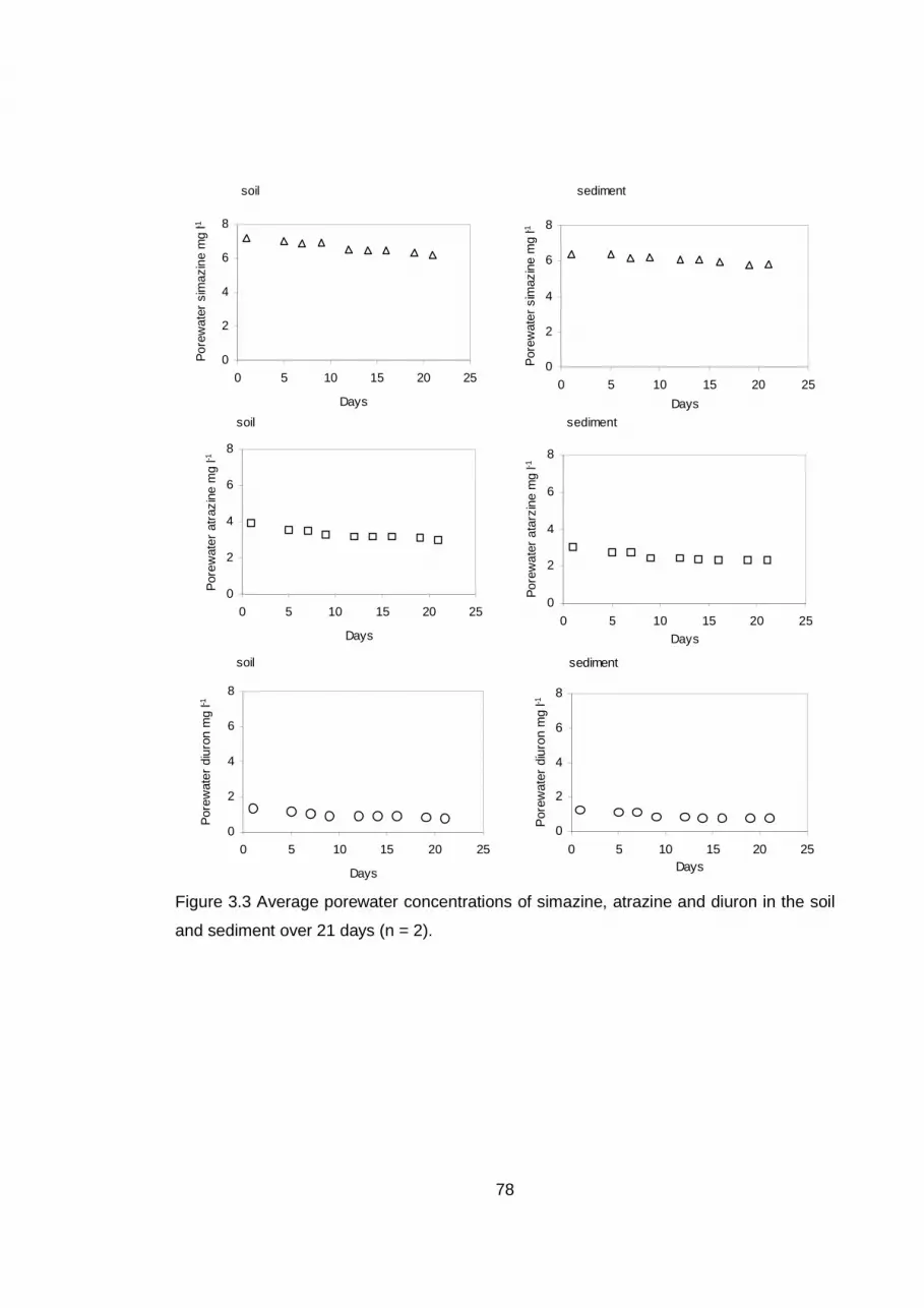
78

Figure 3.3 Average porewater concentrations of simazine, atrazine and diuron in the soil

and sediment over 21 days (n = 2).

soil

0

2

4

6

8

0 5 10 15 20 25

Days

Por

ewat

er s

imaz

ine

mg

l-1

soil

0

2

4

6

8

0 5 10 15 20 25

Days

Por

ewat

er a

traz

ine

mg

l-1

soil

0

2

4

6

8

0 5 10 15 20 25

Days

Por

ewat

er d

iuro

n m

g l-1

soil

0

2

4

6

8

0 5 10 15 20 25

Days

Por

ewat

er s

imaz

ine

mg

l-1

soil

0

2

4

6

8

0 5 10 15 20 25

Days

Por

ewat

er a

traz

ine

mg

l-1

soil

0

2

4

6

8

0 5 10 15 20 25

Days

Por

ewat

er d

iuro

n m

g l-1

sediment

0

2

4

6

8

0 5 10 15 20 25

Days

Por

ewat

er s

imaz

ine

mg

l-1

sediment

0

2

4

6

8

0 5 10 15 20 25

Days

Por

ewat

er a

tarz

ine

mg

l-1

sediment

0

2

4

6

8

0 5 10 15 20 25Days

Por

ewat

er d

iuro

n m

g l-1

sediment

0

2

4

6

8

0 5 10 15 20 25

Days

Por

ewat

er s

imaz

ine

mg

l-1

sediment

0

2

4

6

8

0 5 10 15 20 25

Days

Por

ewat

er a

tarz

ine

mg

l-1

sediment

0

2

4

6

8

0 5 10 15 20 25Days

Por

ewat

er d

iuro

n m

g l-1

79

3.3.4. Experimental designs

3.3.4.1. Experimental design: effect of salinity on metals and herbicides release from soil

and sediment (salinity treatment)

To investigate the effect of salinity on the release of metals and herbicides from soil and

sediment, the microcosms were continuously flooded with artificial seawater throughout

the duration of these experiments. The experiments were performed in triplicate. During

the experiments, the metals, herbicides and DOC concentrations released into the

overlying water column were measured. The salinity of the artificial seawater delivered to

the microcosms was 5 and 20 representing low and high salinity treatments respectively

in these experiments. These two different salinity treatments reflect the seasonal range

(minimum and maximum) in the salinity of the sediment porewater observed in the field

study (Chapter 2, Figure 2.14). Although the salinity of the natural sea water which

inundates the field site was not measured directly during the field study, the sediment

porewater Cl concentrations were measured and were used as a proxy for salinity.

The experiments were carried out over 21 days. There was no observation of anoxia in

the soil and sediment in the microcosms throughout the duration of the experiment.

Samples from the overlying water were collected twice daily, with a 6-hour interval

between sampling for the first 12 days and then a 3-day interval for the remainder of the

experiment. This was done in order to assess the release pattern of the metals,

herbicides and DOC over time. Immediately after collection, the sample pH was

measured using a HANNA HI 83140 pH meter. The samples were then filtered through a

0.45 µm pre-rinsed (10 ml rinse with deionised water) hydrophilic polyethersulphone

membrane filter (Supor®, Germany). The 0.45 µm hydrophilic membrane filter separated

out the DOC fraction from particulate organic matter and prevented the sorption of the

herbicides or metals to the filter. Aliquots of the filtrate were then analysed for the metals

by ICP-OES (Section 3.6.1); herbicides by the on-line solid phase extraction-high

performance liquid chromatography (on-line SPE-HPLC) (Section 3.6.2) and DOC using

a HyperToc carbon analyser with a non-dispersive infrared detector (Chapter 2, Section

2.2.3.6). Due to analytical and time constraints, herbicides were analysed in only one of

the two samples collected daily for the first 12 days, in addition to those collected during

the remaining 9 days of the experiment.

80

A control experiment was performed under the conditions described above with unspiked

soil and sediment. While the initial Ni and Zn concentrations released from the soil into

the overlying water ranged from 0.04 – 0.06 mg l-1 and 0.05 – 0.09 mg l-1 respectively, the

initial Cu, simazine, atrazine and diuron concentrations were below the limit of detection

of the analytical techniques used for the analyses. In the case of the sediment, the initial

Cu, Ni, Zn, simazine, atrazine and diuron concentrations released into the overlying water

were below the limit of detection of the analytical techniques used for the metal and

herbicide analyses. This indicates that the baseline metals and herbicides released from

the soil and sediment into the overlying during the column experiment were negligible and

hence was not significantly confounding or contributing to contaminant release.

3.3.4.2 Experimental design: effect of drying and rewetting on metals and herbicides

release from soil and sediment (drying-rewetting treatment)

To investigate the effect of drying and rewetting on the release of metals and herbicides,

the soil and sediment were dried at 25 0C for 7 days and then continuously rewet at 10 0C

for 5 days with artificial seawater at a salinity of 20. This was repeated resulting in two

dry-rewet cycles over a 24-day period. The duration of the drying and rewetting periods

were based on an estimated 43 % frequency of tidal inundation in the Wallasea Island

managed realignment site (Chapter 2, Section 2.2.1). This estimate was based on the

site elevation data (provided by ABPmer Limited, Southampton) and water level data

(Crouch Harbour Authority tide timetable). These experiments were performed in

triplicate.

Sampling was carried out only during both cycles of continuous rewetting and the

aqueous samples were collected from the overlying water twice daily with a 6-hour

interval between sampling. The samples were filtered through a 0.45 µm pre-rinsed (10

ml rinse with deionised water) hydrophilic polyethersulphone membrane filter paper

(Supor®, Germany). Aliquots of the filtrate were then analysed for metals by ICP-OES

(Section 3.6.1), herbicides by the on-line SPE-HPLC (Section 3.6.2) and DOC using a

HyperToc carbon analyser with a non-dispersive infrared detector (Chapter 2, Section

2.2.3.6). Similar to the experimental design described in Section 3.3.4.1, only one of the

two samples collected daily was analysed for the herbicides due to analytical and time

constraints.

81

3.4 Carbon mineralisation experiments

Drying and rewetting of soil can lead to the disruption of aggregates which exposes

organic matter trapped within the soil. The exposure of organic matter stimulates

microbial activity which leads to enhanced organic matter mineralisation, DOC release

and CO2 release (Degens and Sparkling, 1995; Van Gestel et al., 1993; Fierer and

Schimel, 2003). The mineralisation of soil microbial biomass-derived substrates resulting

from the death of part of the microbial population during drying can also lead to an

increase in CO2 release following rewetting of dried soil (Bottner et al., 1985; Van Gestel

et al., 1993; Haney et al., 2004). Since organic matter is an important binding site for

metals (Salomons and Forstner, 1984; Alloway, 1995) and herbicides (Gao et al., 1998;

Voulvoulis et al., 2002), the enhanced mineralisation of organic matter due to drying and

rewetting may result in the release of organic matter associated metals and herbicides. In

order to test the hypothesis that organic matter mineralisation will be enhanced during

drying and rewetting of the soil and sediment and lead to the release of organic matter

associated contaminants, carbon mineralisation experiments were conducted. Carbon

mineralisation can be determined by measuring CO2 accumulation in the headspace of

incubated soil and sediment (Fierer and Schimel, 2002; Lundquist et al., 1999; Canfield et

al., 1993; Dauwe et al., 2001). In this study, carbon mineralisation was determined by

measuring CO2 in the headspace of microcosms containing fully wet and dried-rewet

soil/sediment.

The experiments were set up to run simultaneously with those described in Section

3.3.4.2 and were carried out in triplicate, using the same column microcosms as those

described in Section 3.3.1. The air inlet, water inlet and sampling outlet were fitted with

Suba-seal gas impermeable rubber septa in order to create an air-tight chamber (Figure

3.1). Spiked soil and sediment were packed into the column microcosms following the

procedures of Section 3.3.3. The microcosms were then divided into two groups. In group

one, the microcosms were kept in a temperature control cabinet maintained at 10 0C and

artificial seawater at a salinity of 20 was delivered to the microcosms by a peristaltic

pump at a flow rate of 1.6 ml min-1 for one hour so as to fully wet the soil and sediment.

The water inlet was then sealed with a gas impermeable rubber septum. The microcosms

were left for one hour to allow the gases within the headspace to equilibrate before

sampling. The headspace was then sampled once daily over the 15 days duration of the

experiment. In group two, microcosms containing the soil and sediment were dried in the

82

temperature control cabinet for 7 days at 25 0C. After drying, the temperature was

reduced to 10 0C and artificial seawater at a salinity of 20 was supplied to the microcosms

at a flow rate of 1.6 ml min-1 for one hour. The water inlet was then sealed with a gas

impermeable rubber septum in order to create an air-tight chamber and the gases within

the headspace were left to equilibrate for one hour before sampling. Headspace samples

were collected once daily for 6 days. An additional set of microcosms containing soil and

sediment which were used for microbial biomass determination were included in group

two. The soil and sediment microbial biomass were determined in order to assess the

changes in microbial biomass due to drying and rewetting.

Gas samples (2 ml) were withdrawn from the headspace via the sampling septum using a

gas tight syringe (Hamilton, Switzerland). The collected gas samples were then injected

into gas tight exetainer vials (Labco, UK) and filled with deionised water using a two way

valve. The vials were inverted and stored at room temperature until analysis. The inverted

position kept the gas samples above water and hence prevented atmospheric gas

exchange. The analysis was carried out using gas chromatography (GC) with a flame

ionisation detector described in Section 3.6.3. The storage of CO2 gas above water may

lead to CO2 dissolution in the deionised water. As a result, the concentration of CO2

dissolved in the deionised water during storage was calculated using Henry’s law and the

CO2 solubility coefficient (Stumm and Morgan, 1981). The calculated CO2 concentration

was added to the measured CO2 concentration in the headspace of the vial to get the

total CO2 concentration (headspace plus water).

The mineralisation rate was calculated as the rate of change of CO2 concentration per

unit mass of the soil/sediment per day using the formula:

Mineralisation rate (µgCO2kg-1d-1) = [CO2]i – [CO2]i-1 (3.1)

t

where [CO2] is CO2 concentration in headspace (µg CO2 kg-1), i is sample number and t

(day) is time between sampling.

The mineralisation rate on day 1 could not be calculated because two samples were

needed to calculate the mineralisation rate.

83

The soil and sediment microbial biomass were determined using the substrate induced

respiration method. The most commonly used methods for the determination of microbial

biomass are substrate induced respiration (Anderson and Domsch, 1978; West and

Sparkling, 1986; Lin and Brookes, 1999; Degens and Harris, 1997) and chloroform

fumigation-extraction (Franzleubbers et al., 2000; Magid et al., 1999). In this study, the

substrate induced respiration method was used because it determines the active living

microbial biomass (Hoper, 2006; Lin and Brookes, 1999) hence the changes due to

microbial death during drying could be estimated. The microbial biomass in the soil and

sediment were determined just before drying, after drying and 6 days after rewetting the

soil and sediment. On the specified days, the additional microcosms containing the soil

and sediment were removed from the temperature control cabinet and samples

equivalent to 1 g dry weight were placed in 10 mL gas-tight exetainer vials (Labco, UK). 2

ml of glucose solution was added to each exetainer vial (West and Sparkling, 1986).

Glucose was used because most microbes can easily utilize it as a carbon source (Lin

and Brookes, 1999). After glucose addition, the vials were sealed and then shaken for 5

minutes on a wrist action shaker at 100 oscillations per minute to ensure the even

distribution of glucose within the soil and sediment samples. The vials were then

incubated at 22 0C in a temperature control cabinet for 4 hours before sampling (Degens

and Harris, 1997). The incubation period allowed for measurable CO2 levels in the

headspace of the vials. A 2ml gas sample was withdrawn from the headspace of the vial

using a gas tight syringe (Hamilton, Switzerland). The collected gas samples were then

injected, using a two-way valve, into gas tight exetainer vials (Labco, UK) filled with

deionised water. The vials were then inverted and stored at room temperature until

analysis. The analysis was carried out using gas chromatography (Section 3.7.2). The

concentration of CO2 dissolved in the deionised water during storage was accounted for

using Henry’s law and the solubility coefficient of CO2 (Stumm and Morgan, 1981). The

microbial biomass was calculated according to Anderson and Domsch (1978):

Microbial biomass (µgCg-1) = µlCO2g-1hr-1 x 40.04 + 0.37 (3.2)

where 40.04 and 0.37 are constants.

84

3.5 Batch sorption experiments

Batch sorption experiments were conducted to determine the partition coefficients of the

metals and herbicides at two different salinities (5 and 20) in order to evaluate the

changes in contaminant binding to the soil and sediment with changes in salinity. The

concentrations of the metals and herbicides associated with the solid and liquid phase

were fitted to a linear sorption isotherm to calculate the partition coefficients (Kd). The

coefficients reflect the relative distributions of the metals and the herbicides between the

solid and liquid phase. The partition coefficient was calculated as follows:

aq

sd C

CK = (3.3)

where dK (l kg-1) is the partition coefficient, sC (mg kg-1) is the contaminant

concentration in the solid phase and aqC (mg l-1) is the contaminant concentration in the

liquid phase.

In this study, the partition coefficients were derived from mass balance calculations. As a

result, other processes such as contaminant loss either due to degradation or adsorption

to container walls during batch sorption experiments can affect the coefficients. Particle

concentration can also affect partition coefficients. Turner and Millward (2002) notes that

Kd has an inverse dependence on particle concentration as suspended particles are an

important control on contaminant partitioning. The dependence of Kd on particle

concentrations can compromise the extrapolation of the coefficients to different

environmental conditions.

3.5.1 Metal sorption experiments

4 g of air-dried soil and sediment samples were weighed into clean centrifuge tubes.

Artificial seawater at salinities of 5 and 20 were spiked with nitrate salts of Cu, Ni and Zn

(Aldrich, analytical grade) to achieve composite solutions with three final spiking

concentrations: 200, 500 and 1000 µg l-1. 20ml of the spiked solutions were then added to

the soil and sediment samples to give a solid-liquid ratio of 1:5. The tubes were placed on

a flat bed shaker and agitated at 300 oscillations per minute for 24 hours after which the

85

samples were filtered through a 0.45 µm cellulose nitrate membrane filter paper

(Whatman). 10 ml aliquots of the filtrate were acidified with 2 % nitric and stored at 4 0C

until analysis by ICP-OES (Section 3.6.1). The experiments were conducted with

triplicates for each spiking concentration at room temperature with two blank and two

control samples included. All the plastic and glassware used were cleaned by soaking for

24 hours in Decon solution, rinsing in deionised water three times, followed by soaking

again in 10 % nitric solution overnight and then rinsing three times in deionised water.

The control samples did not indicate any significant loss of metals to the walls of the

centrifuge tubes.

3.6.2 Herbicide sorption experiments

4 g of air-dried soil and sediment samples were weighed into clean non-reactive PTFE

tubes. Similar to the metals sorption experiments, artificial seawater at salinities of 5 and

20 were spiked with Cu, Ni and Zn (powder form) (Fluka, analytical grade) to achieve

composite solutions with three final spiking concentrations: 200, 500 and 1000 µg l-1. 20

ml of the spiked solutions were added to the soil and sediment samples. The tubes were

sealed and agitated, at room temperature, on a flatbed shaker for 24 hours at 300

oscillations per minute. After 24 hours, the samples were filtered using a 0.45 µm

disposable PTFE membrane syringe filter (Nalgene). 1 ml aliquots of the sample filtrates

were transferred to amber vials and stored at 4 0C until analysis by HPLC technique in

direct injection mode (Section 3.6.2). The experiments were conducted at room

temperature with duplicate for each spiking concentration, two blank and two control

samples. The PTFE tubes used were cleaned by soaking for 24 hours in Decon solution,

rinsing three times in deionised water and then in HPLC grade acetonitrile to remove any

traces of herbicides. The control samples did not indicate any sorption of the herbicides

onto the PTFE tubes.

3.6 Analytical techniques

3.6.1 Inductively coupled plasma optical emission spectrometry (ICP-OES)

The overlying water samples collected from the microcosm experiments and samples

from the metal batch sorption experiments were analysed for Cu, Ni and Zn using ICP-

OES (Varian Vista-PROTM). The instrument was equipped with a one-piece low flow

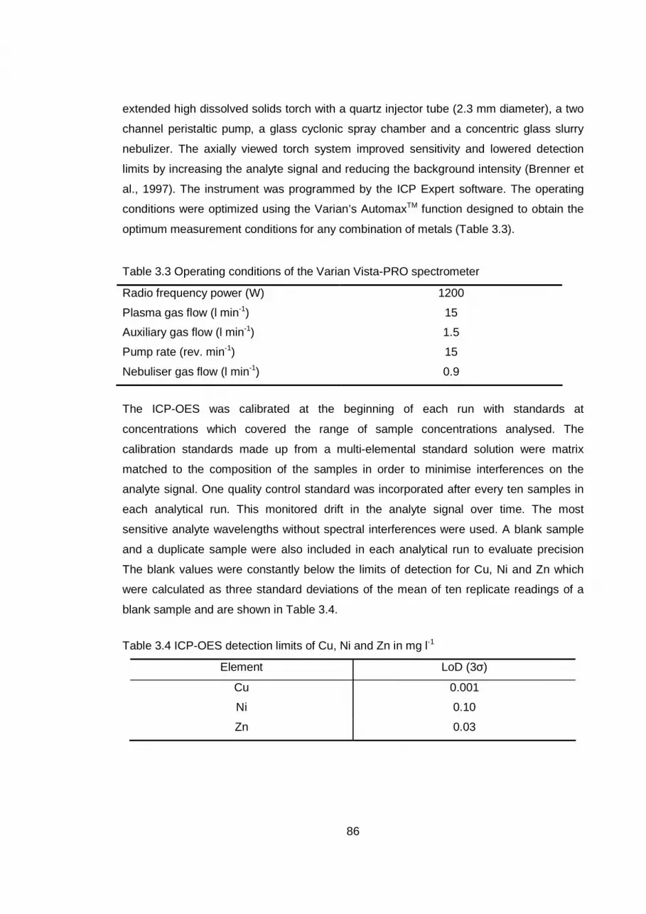
86

extended high dissolved solids torch with a quartz injector tube (2.3 mm diameter), a two

channel peristaltic pump, a glass cyclonic spray chamber and a concentric glass slurry

nebulizer. The axially viewed torch system improved sensitivity and lowered detection

limits by increasing the analyte signal and reducing the background intensity (Brenner et

al., 1997). The instrument was programmed by the ICP Expert software. The operating

conditions were optimized using the Varian’s AutomaxTM function designed to obtain the

optimum measurement conditions for any combination of metals (Table 3.3).

Table 3.3 Operating conditions of the Varian Vista-PRO spectrometer

Radio frequency power (W) 1200

Plasma gas flow (l min-1) 15

Auxiliary gas flow (l min-1) 1.5

Pump rate (rev. min-1) 15

Nebuliser gas flow (l min-1) 0.9

The ICP-OES was calibrated at the beginning of each run with standards at

concentrations which covered the range of sample concentrations analysed. The

calibration standards made up from a multi-elemental standard solution were matrix

matched to the composition of the samples in order to minimise interferences on the

analyte signal. One quality control standard was incorporated after every ten samples in

each analytical run. This monitored drift in the analyte signal over time. The most

sensitive analyte wavelengths without spectral interferences were used. A blank sample

and a duplicate sample were also included in each analytical run to evaluate precision

The blank values were constantly below the limits of detection for Cu, Ni and Zn which

were calculated as three standard deviations of the mean of ten replicate readings of a

blank sample and are shown in Table 3.4.

Table 3.4 ICP-OES detection limits of Cu, Ni and Zn in mg l-1

Element LoD (3σ)

Cu 0.001

Ni 0.10

Zn 0.03

87

3.6.2 On-line solid phase extraction-high performance liquid chromatography (on-line

SPE-HPLC)

The samples collected from the overlying water in the microcosm experiments and

samples from the herbicide sorption experiment were analysed for simazine, atrazine and

diuron by HPLC. The technique has been recommended for the analysis of non-volatile

and thermolabile pesticides such as those considered in this study due to the low

temperature conditions associated with the technique (Field, 1997; Pico, 2000). In

addition, HPLC allows for the direct analysis of aqueous samples (Hernandez et al.,

2001). However, sample pre-concentration by solid phase extraction (SPE) prior to the

HPLC analysis was necessary for the analysis of the overlying water samples collected

from the microcosm experiments. This was because the concentrations of the herbicides

contained in some of the samples were below the detection levels by direct injection into

the HPLC.

SPE is used for the extraction of organic contaminants in aqueous samples with a wide

range of polarities by passing the aqueous samples through a sorbent material which

retains the organic contaminants (Hennion, 1999). The on-line SPE procedure was

automated using a MIDAS autosampler and Prospekt-2TM solid-phase extraction unit

consisting of an Accelerated Cartridge Exchanger (ACE) and High Pressure Dispenser

(HDP) (Spark Holland, The Netherlands). The MIDAS autosampler loaded the samples

on to SPE cartridges on the ACE and the HPD delivered the solvent for extraction. The

procedure was programmed by the SparkLink (v 2.3) software operated on a Hewlett-

Packard L1720. PLRP-S cartridges (10 x 2 mm i.d.) (Spark Holland, The Netherlands)

containing styrene-divinylbenzene polymeric sorbent material were used because of their

stability over the entire pH range (1 – 14) and their large specific surface area which

enables them to effectively retain analytes such as the herbicides considered in this study

(Hennion, 1999). The SPE procedure required only a small amount of solvent, making it

very economical and cost effective. The automation allowed for multiple sample

extractions, minimised sample handling resulting in more reproducible results and

decreased the risk of sample contamination (Hernandez et al., 2001). Prior to sample

loading, the SPE cartridges were preconditioned with 2 ml of acetonitrile and equilibrated

with 14 ml of ultra-pure water both delivered at 5 ml min-1. 1 ml of the sample was loaded

on to the preconditioned cartridge at 4 ml min-1. The sample volume was kept to a

minimum in order to avoid clogging up the sorbent in the cartridges with particulate

88

material and to maintain satisfactory detection levels for all the studied herbicides with

good recoveries. Following sample loading, the cartridge was first washed with 1 ml of

ultra-pure water at 4 ml min-1 and then backwashed with another 1 ml of ultra-pure water

at 2 ml min-1. Finally, the herbicides retained on the cartridges were eluted with

acetonitrile directly into the LC column by valve switching.

The HPLC unit (Agilent 1100 Series) comprised of a quaternary pump, a solvent

degasser, a temperature controlled Wellplate autosampler and ultra-violet photodiode

array detector (UV-DAD). The unit was controlled by the ChemStation software (v 4.1)

operated on a Hewlett-Packard L1720 lab based computer. The LC analytical column

used for separating the herbicides was a SupelcosilTM ABZ+ (25 cm in length, 4.6 mm in

diameter, 5 µm particle size) (Supelco, Belfonte, USA) and it was maintained at a

temperature of 40 0C. Disposable guard columns were used to protect the column from

the build up of particulates that could contaminate the column and interfere with its

performance. The sample was injected into the column at a flow rate of 1 ml min-1 and a

gradient elution was carried out using acetonitrile (LC solvent A) and ultra-pure water (LC

solvent B) according to the following programme: from LC solvent A-B (35 %:65 %) to LC

solvent A-B (60 %:40 %) in 15 minutes and then returned to LC solvent A-B (35 %:65 %)

in 5 minutes. After 5 minutes of stabilisation, the next sample was injected. The detection

wavelength for quantification on the UV-DAD was set at 240 nm because the

chromatographic peaks were effectively resolved with good peak shapes which were

maintained at this wavelength. The chromatographic peak areas were automatically

integrated. However, the integration was adjusted manually using the ChemStation

software on occasions when the integration algorithm did not adequately integrate the

peaks.

At the beginning of each run, the system was calibrated with standards (concentrations

range from 0.01 – 500 µg l-1) which were subjected to the complete online SPE-HPLC

technique to ensure that the standards and samples passed through the same process.

One quality control standard was analysed after every ten samples. This monitored drift

in the analyte signal intensity and the performance of the HPLC between the analyses of

samples over time. A blank sample and a duplicate sample were also included in each

analytical run.

89

The % recovery and detection limits are presented in Table 3.5 and 3.6 respectively. The

% recovery was determined by analysing triplicate composite herbicide solutions at 3

initial concentrations (50, 100 and 500 µg l-1) and calculating the ratio between the initial

concentration of the herbicide and the measured concentration after solid phase

extraction and analysis, expressed as a percentage. The % recoveries indicate that the

method was satisfactory for the analysis of the herbicides. The blank samples were below

the limit of detection for each of the herbicides which were calculated by using the lowest

calibration standard with a signal:noise ratio ≥ 3 (i.e. the ratio between the peak intensity

and the noise) (Ferrer and Barcelo et al., 1999).

Table 3.5. Recoveries of simazine, atrazine and diuron (average ± standard deviation

(SD), n = 3).

Herbicides Spiked level (µg l-1) % recovery

Simazine 50 85 ± 2.2

100 89 ± 8.2

500 86 ± 6.2

Atrazine 50 93 ± 4.5

100 89 ± 4.7

500 96 ± 3.9

Diuron 50 90 ± 7.9

100 91 ± 6.9

500 95 ± 4.9

Table 3.6. Limit of detection (SN ≥ 3) of simazine, atrazine and diuron

Simazine Atrazine Diuron

LOD (µg l-1) 0.1 0.1 0.05

3.6.3. Gas chromatography (GC)

The headspace samples collected from the organic matter mineralisation experiments

and the microbial biomass incubations were analysed for CO2 using gas chromatograph

(GC). The GC unit (Agilent Technologies, Cheshire) was equipped with a flame ionisation

detector (FID), an electronic integrator and an autosampler (Gerstel, GmbH, Germany). A

90

stainless steel column (1.8 m length, 12mm diameter) packed with Porapak Q (80/100

mesh, particle size 0.13 – 0.15 mm) (Alltech Ltd) was used for analysis. The column and

FID detector were maintained at a constant temperature of 30 0C and 385 0C

respectively. The analysis was conducted with hydrogen gas and zero grade air at a flow

rate of 430 ml min-1. The GC was programmed by the Agilent ChemStation software

operated on a Hewlett-Packard L1720 lab based computer. The system was calibrated

with standards prepared from 99.99 % CO2 gas (1, 5, 20, 100, 200, 500 µl) at the

beginning of each run. . A 100 µl sample was withdrawn from the headspace gas sample

by the autosampler using a gas-tight syringe and injected into the GC. The headspace

CO2 concentration was calculated from the peak area using the electronic integrator and

calibrated against the standards. One standard sample and a duplicate sample were

included in each analytical run to monitor drift during the analysis and to evaluate

precision.

3.7. Statistical Analysis

Statistical analysis was carried out using SPSS statistical package (Version 16). Linear

regression analysis was conducted on the DOC, metal and herbicide concentrations

measured in the overlying water under the drying-rewetting treatment to determine the

relationship between DOC, the metals and herbicides. Linear regression is a powerful

parametric test which determines the strength of the relationship between two variables

and describes how much of the variation in one variable (dependent variable) is

explained by the relationship with the other variable (independent variable) (Quinn and

Keough, 2002). The coefficients of determination from the regression analysis were

interpreted as the proportion of variance in the metal and herbicide concentrations

attributable to the variance in the DOC concentrations. The concentration data that had

unequal variances and asymmetric distributions were log-transformed in order to meet

the assumptions of the test.

A two-way ANOVA was used to test for significant differences between the partition

coefficients (log Kd) for soil and sediment at salinities of 5 and 20 calculated from the

batch sorption experiments; between the total contaminant loads and between the total

DOC loads released into the overlying water from the soil and sediment under the

treatments in the column experiments. Two-way ANOVA is a parametric test which tests

for significant differences between the effects of two different factors simultaneously and

91

interactions between the factors. The total metal, herbicide and DOC loads were

determined by multiplying the average measured metal, herbicide and DOC

concentrations between sampling periods by the time interval between sampling and

dividing by the flow rate at which artificial seawater was delivered to the microcosm. The

loads at each sampling period were then summed to get the total load. Due to the small

sample size for the two-way ANOVA, emphasis was placed in Chapter 5, on discussing

the trends observed for the total metal and herbicide loads released into the overlying

water from the soil and sediment. Instances where significant differences were observed

are highlighted. The dataset that had unequal variances and asymmetric distributions

were log-transformed to meet the assumptions of the test.

92

Chapter 4: Experimental Results

4.1. Introduction

This chapter presents the laboratory experimental data obtained from the batch sorption,

column microcosm and carbon mineralisation experiments which examine the effect of

salinity and drying and rewetting on the release of metals and herbicides from agricultural

soil and dredged sediment in managed realignment sites following tidal inundation. Batch

sorption experiments were conducted to calculate partition coefficients (Kd) of the

contaminants at two different salinities (5 and 20) in order to evaluate the changes in

contaminant binding with changes in salinity. Column microcosm experiments gave rise

to two datasets, one to investigate the effect of two different salinities (5 and 20), and one

to investigate the effect of drying-rewetting conditions on contaminant release from the

soil and sediment. The two sets of experimental data were obtained by measuring the

contaminants released from the soil and sediment into overlying water and the observed

patterns of release will be described. pH and DOC are important controls on both metal

and herbicide release and hence these data are also presented. Soil and sediment

microbial biomass data and headspace CO2 data measured during the carbon

mineralisation experiments will be presented in order to test the hypothesis that organic

matter mineralisation will be enhanced during drying and rewetting of the soil and

sediment leading to the release of organic matter associated contaminants into the

overlying water. These experimental data will be discussed in Chapter 5.

4.2. Soil and sediment properties

Properties of the soil and sediment used in this study are presented in Table 4.1. The soil

and sediment comprised predominantly silt and clay sized particles. The organic matter

content in the sediment was higher than the soil. These soil and sediment properties

were within the range reported for salt marsh soil (Edwards and Proffitt, 2003; Shafer and

Streever, 2000; Craft et al., 1999; MacLeod et al., 1999), hence the soil and sediment

used were representative of salt marsh soils.

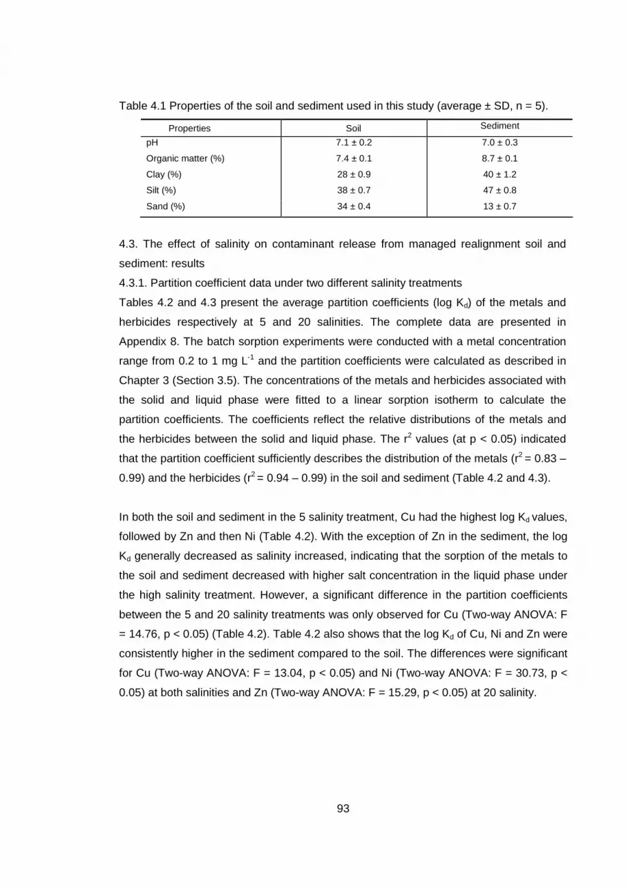
93

Table 4.1 Properties of the soil and sediment used in this study (average ± SD, n = 5).

Properties Soil Sediment

pH 7.1 ± 0.2 7.0 ± 0.3

Organic matter (%) 7.4 ± 0.1 8.7 ± 0.1

Clay (%) 28 ± 0.9 40 ± 1.2

Silt (%) 38 ± 0.7 47 ± 0.8

Sand (%) 34 ± 0.4 13 ± 0.7

4.3. The effect of salinity on contaminant release from managed realignment soil and

sediment: results

4.3.1. Partition coefficient data under two different salinity treatments

Tables 4.2 and 4.3 present the average partition coefficients (log Kd) of the metals and

herbicides respectively at 5 and 20 salinities. The complete data are presented in

Appendix 8. The batch sorption experiments were conducted with a metal concentration

range from 0.2 to 1 mg L-1 and the partition coefficients were calculated as described in

Chapter 3 (Section 3.5). The concentrations of the metals and herbicides associated with

the solid and liquid phase were fitted to a linear sorption isotherm to calculate the

partition coefficients. The coefficients reflect the relative distributions of the metals and

the herbicides between the solid and liquid phase. The r2 values (at p < 0.05) indicated

that the partition coefficient sufficiently describes the distribution of the metals (r2 = 0.83 –

0.99) and the herbicides (r2 = 0.94 – 0.99) in the soil and sediment (Table 4.2 and 4.3).

In both the soil and sediment in the 5 salinity treatment, Cu had the highest log Kd values,

followed by Zn and then Ni (Table 4.2). With the exception of Zn in the sediment, the log

Kd generally decreased as salinity increased, indicating that the sorption of the metals to

the soil and sediment decreased with higher salt concentration in the liquid phase under

the high salinity treatment. However, a significant difference in the partition coefficients

between the 5 and 20 salinity treatments was only observed for Cu (Two-way ANOVA: F

= 14.76, p < 0.05) (Table 4.2). Table 4.2 also shows that the log Kd of Cu, Ni and Zn were

consistently higher in the sediment compared to the soil. The differences were significant

for Cu (Two-way ANOVA: F = 13.04, p < 0.05) and Ni (Two-way ANOVA: F = 30.73, p <

0.05) at both salinities and Zn (Two-way ANOVA: F = 15.29, p < 0.05) at 20 salinity.

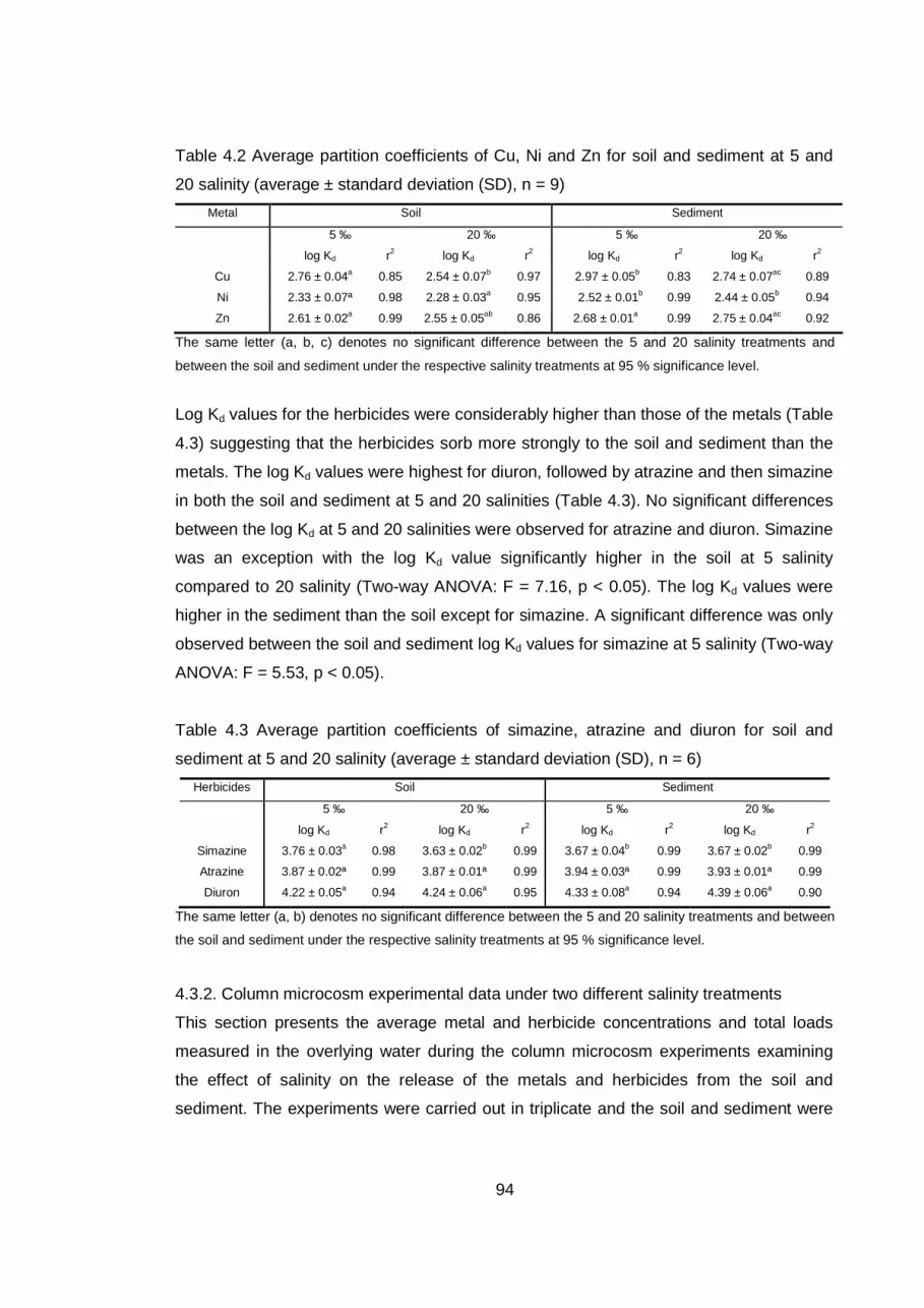
94

Table 4.2 Average partition coefficients of Cu, Ni and Zn for soil and sediment at 5 and

20 salinity (average ± standard deviation (SD), n = 9)

Metal Soil Sediment

5 ‰ 20 ‰ 5 ‰ 20 ‰

log Kd r2 log Kd r2 log Kd r2 log Kd r2

Cu 2.76 ± 0.04a 0.85 2.54 ± 0.07b 0.97 2.97 ± 0.05b 0.83 2.74 ± 0.07ac 0.89

Ni 2.33 ± 0.07ª 0.98 2.28 ± 0.03a 0.95 2.52 ± 0.01b 0.99 2.44 ± 0.05b 0.94

Zn 2.61 ± 0.02a 0.99 2.55 ± 0.05ab 0.86 2.68 ± 0.01a 0.99 2.75 ± 0.04ac 0.92

The same letter (a, b, c) denotes no significant difference between the 5 and 20 salinity treatments and

between the soil and sediment under the respective salinity treatments at 95 % significance level.

Log Kd values for the herbicides were considerably higher than those of the metals (Table

4.3) suggesting that the herbicides sorb more strongly to the soil and sediment than the

metals. The log Kd values were highest for diuron, followed by atrazine and then simazine

in both the soil and sediment at 5 and 20 salinities (Table 4.3). No significant differences

between the log Kd at 5 and 20 salinities were observed for atrazine and diuron. Simazine

was an exception with the log Kd value significantly higher in the soil at 5 salinity

compared to 20 salinity (Two-way ANOVA: F = 7.16, p < 0.05). The log Kd values were

higher in the sediment than the soil except for simazine. A significant difference was only

observed between the soil and sediment log Kd values for simazine at 5 salinity (Two-way

ANOVA: F = 5.53, p < 0.05).

Table 4.3 Average partition coefficients of simazine, atrazine and diuron for soil and

sediment at 5 and 20 salinity (average ± standard deviation (SD), n = 6)

Herbicides Soil Sediment

5 ‰ 20 ‰ 5 ‰ 20 ‰

log Kd r2 log Kd r2 log Kd r2 log Kd r2

Simazine 3.76 ± 0.03a 0.98 3.63 ± 0.02b 0.99 3.67 ± 0.04b 0.99 3.67 ± 0.02b 0.99

Atrazine 3.87 ± 0.02ª 0.99 3.87 ± 0.01ª 0.99 3.94 ± 0.03ª 0.99 3.93 ± 0.01ª 0.99

Diuron 4.22 ± 0.05a 0.94 4.24 ± 0.06a 0.95 4.33 ± 0.08a 0.94 4.39 ± 0.06a 0.90

The same letter (a, b) denotes no significant difference between the 5 and 20 salinity treatments and between

the soil and sediment under the respective salinity treatments at 95 % significance level.

4.3.2. Column microcosm experimental data under two different salinity treatments

This section presents the average metal and herbicide concentrations and total loads

measured in the overlying water during the column microcosm experiments examining

the effect of salinity on the release of the metals and herbicides from the soil and

sediment. The experiments were carried out in triplicate and the soil and sediment were

95

continuously flooded with artificial seawater at two different salinities, 5 and 20 (referred

to in the text as low and high salinity treatments respectively). pH and DOC data are also

presented here as they are important parameters that control metal and herbicide

release. The total contaminant and DOC load were calculated by multiplying the average

contaminant and DOC concentrations between sampling periods by the time interval

between the sampling and dividing by the flow rate at which artificial seawater was

delivered to the microcosm. The loads for each time period were then summed to get the

total load.

4.3.2.1 Release of metals into the overlying water under the low and high salinity

treatments

Figure 4.1 presents the average concentrations of Cu, Ni and Zn released from the soil

and sediment to the overlying water under low and high salinity treatments (see Appendix

9 for the complete data set). For both the soil and sediment, there were high

concentrations of Cu, Ni and Zn in the overlying water in the first 24 hours which declined

rapidly and remained relatively constant for the remainder of the experiment. This release

pattern suggests an initial phase of rapid release followed by a phase of slow release.

Table 4.4 shows the total metal loads released into the overlying water from the soil and

sediment over the course of the experiments under the low and high salinity treatments.

With the exception of Cu released from the sediment, the total metal loads released from

the soil and sediment into the overlying water were higher under the high salinity

treatment compared to the low salinity treatment. However, the results of the two-way

ANOVA showed that there was no significant difference in the total metal loads released

into the overlying water from the soil and sediment under the high salinity treatment in

comparison to the low salinity treatment except for Ni. The total Ni load released from the

sediment under the high salinity treatment was significantly higher than that released

under the low salinity treatment (Two-way ANOVA: F = 5.51, p < 0.05). The total Cu, Ni

and Zn loads released into the overlying water from the sediment were lower than those

released from the soil (Table 4.4). However, the differences in the total loads between

the soil and sediment were only significant for Ni and Zn under the low salinity treatment

(Two-way ANOVA: F = 3.42, p < 0.05 for Ni and F = 7.51, p < 0.05 for Zn) and for Cu

under both treatments (Two-way ANOVA: F = 17.37, p < 0.05). Although the soil and

sediment were spiked with all three metals at the same concentration, the total load of

96

the individual metals released into the overlying water from the soil and sediment were in

the order: Ni > Zn > Cu with the Cu loads two orders of magnitude lower than those of Ni

and Zn under both salinity treatments.

Soil Sediment

Figure 4.1 Concentrations of (a) Zn, (b) Ni and (c) Cu released from soil and (d) Zn, (e)

Ni and (f) Cu released from sediment under the low and high salinity treatments (bars =


0

10

20

30

40

50

0 100 200 300 400 500Time (hours )

Nic

kel (

mg

L-1

)

High salin ity

Low sal ini ty

0

10

20

30

40

0 100 200 300 400 500

Time (hours)

Zin

c (m

g L

-1)

High sa linity

Low s a lin ity

0

5

10

15

20

0 100 200 300 400 500

Time (hours)

Nic

kel (

mg

L-1)

High sal inity

Low salinity

0

4

8

12

0 100 200 300 400 500

Tim e (hours)Zi

nc

(mg

L-1

)

H igh s al in i ty

Low sa lin ity

(a) (d)

(b) (e)

0

10

20

30

40

50

0 100 200 300 400 500Time (hours )

Nic

kel (

mg

L-1

)

High salin ity

Low sal ini ty

0

10

20

30

40

0 100 200 300 400 500

Time (hours)

Zin

c (m

g L

-1)

High sa linity

Low s a lin ity

0

5

10

15

20

0 100 200 300 400 500

Time (hours)

Nic

kel (

mg

L-1)

High sal inity

Low salinity

0

4

8

12

0 100 200 300 400 500

Tim e (hours)Zi

nc

(mg

L-1

)

H igh s al in i ty

Low sa lin ity

(a) (d)

(b) (e)

0.0

0.1

0.2

0.3

0.4

0.5

0 100 200 300 400 500

Time (hours)

Cop

per

(m

g L

-1)

High salinity

Low salinity

0.0

0.1

0.2

0.3

0.4

0.5

0 100 200 300 400 500

Time (hours)

Cop

per (

mg

L-1)

High salinity

Low salinity

(c) (f)

0.0

0.1

0.2

0.3

0.4

0.5

0 100 200 300 400 500

Time (hours)

Cop

per

(m

g L

-1)

High salinity

Low salinity

0.0

0.1

0.2

0.3

0.4

0.5

0 100 200 300 400 500

Time (hours)

Cop

per (

mg

L-1)

High salinity

Low salinity

(c) (f)

0.0

0.1

0.2

0.3

0.4

0.5

0 100 200 300 400 500

Time (hours)

Cop

per

(m

g L

-1)

High salinity

Low salinity

0.0

0.1

0.2

0.3

0.4

0.5

0 100 200 300 400 500

Time (hours)

Cop

per

(m

g L

-1)

High salinity

Low salinity

0.0

0.1

0.2

0.3

0.4

0.5

0 100 200 300 400 500

Time (hours)

Cop

per (

mg

L-1)

High salinity

Low salinity

(c) (f)

0.0

0.1

0.2

0.3

0.4

0.5

0 100 200 300 400 500

Time (hours)

Cop

per (

mg

L-1)

High salinity

Low salinity

(c) (f)

0.0

0.1

0.2

0.3

0.4

0.5

0 100 200 300 400 500

Time (hours)

Cop

per

(m

g L

-1)

High salinity

Low salinity

0.0

0.1

0.2

0.3

0.4

0.5

0 100 200 300 400 500

Time (hours)

Cop

per

(m

g L

-1)

High salinity

Low salinity

0.0

0.1

0.2

0.3

0.4

0.5

0 100 200 300 400 500

Time (hours)

Cop

per (

mg

L-1)

High salinity

Low salinity

(c) (f)

97

Table 4.4 Total metal loads (mg) released into the overlying water from the soil and

sediment under the low and high salinity treatments (average ± SD, n = 3).

Metals Soil Sediment

Low salinity High salinity Low salinity High salinity

Cu (mg) 0.6 ± 0.2ª 0.7 ± 0.2ª 0.3 ± 0.1 b 0.3 ± 0.04b

Ni (mg) 25 ± 4.3bc 28 ± 4.8b 13 ± 2.3a 27 ± 4.6b

Zn (mg) 23 ± 2.3ª 24 ± 4.6ª 11 ± 2.2b 18 ± 2.9ab

The same letter (a, b, c) denotes no significant difference between the low and high salinity treatments and

between the soil and sediment under the respective salinity treatments at 95 % significance level.

4.3.2.2. Release of herbicides into the overlying water under low and high salinity

treatments

The average concentrations of simazine, atrazine and diuron released from the soil and

sediment into the overlying water under the low and high salinity treatments are

presented in Figure 4.2, with the complete data in Appendix 10. The simazine, atrazine

and diuron concentrations in the overlying water were high in the first 24 hours, followed

by a rapid decrease to relatively constant concentrations indicating an initial rapid release

phase followed by a slow release phase.

Table 4.5 presents the total herbicide load (µg) released into the overlying water from the

soil and sediment under the low and high salinity treatments. The total simazine, atrazine

and diuron loads released into the overlying water from the soil were higher than those

released from the sediment under both salinity treatments. However, the differences

were not significant (Table 4.5). Similarly, the total simazine, atrazine and diuron loads

released under the low salinity treatment were not significantly different from those

released under the high salinity treatment. Table 4.5 also highlights differences in the

individual herbicide load released into the overlying water from the soil and sediment.

Simazine had the highest load in the overlying water, followed by atrazine and then

diuron despite the soil and sediment having been spiked with all three herbicides at the

same concentration.

98

Soil Sediment

Figure 4.2 Concentrations of (a) simazine, (b) atrazine and (c) diuron released from the

soil and (d) simazine, (e) atrazine and (f) diuron released from sediment under low and

high salinity treatments (bars = standard deviation (SD), n = 3).

0

200

400

600

800

0 100 200 300 400 500Time (hours)

Sim

azin

e (µ

g L-1

)

High salinity

Low salinity

0

100

200

300

400

500

0 100 200 300 400 500

Time (hours)

Sim

azin

e (µ

g L-1

)

High salinity

Low salinity

(a) (d)

0

200

400

600

800

0 100 200 300 400 500Time (hours)

Sim

azin

e (µ

g L-1

)

High salinity

Low salinity

0

100

200

300

400

500

0 100 200 300 400 500

Time (hours)

Sim

azin

e (µ

g L-1

)

High salinity

Low salinity

(a) (d)

0

50

100

150

200

250

300

0 100 200 300 400 500Time (hours)

Atr

azi

ne

(µ

g L

-1)

High salinity

Low salinity

0

30

60

90

120

150

0 100 200 300 400 500

Time (hours)

Atra

zine

(µg

L-1

)

High salinity

Low salinity

(b) (e)

0

20

40

60

80

0 100 200 300 400 500Time (hours)

Diu

ron

(µg

L-1

)

High salinity

Low salinity

0

10

20

30

0 100 200 300 400 500

Time (hours)

Diu

ron (

µg L

-1)

High salinity

Low salinity

(c)(f))

0

50

100

150

200

250

300

0 100 200 300 400 500Time (hours)

Atr

azi

ne

(µ

g L

-1)

High salinity

Low salinity

0

30

60

90

120

150

0 100 200 300 400 500

Time (hours)

Atra

zine

(µg

L-1

)

High salinity

Low salinity

(b) (e)

0

20

40

60

80

0 100 200 300 400 500Time (hours)

Diu

ron

(µg

L-1

)

High salinity

Low salinity

0

10

20

30

0 100 200 300 400 500

Time (hours)

Diu

ron (

µg L

-1)

High salinity

Low salinity

(c)(f))

99

Table 4.5 Total herbicide loads (µg) released into the overlying water from soil and

sediment under low and high salinity treatment (average ± standard deviation SD, n = 3)



Simazine (µg) 1303 ± 259.2a 1423 ± 429.5a 1117 ± 206.1a 1045 ± 51.40a

Atrazine (µg) 318 ± 93.1a 381 ± 117a 231 ± 78.9a 311 ± 108a

Diuron (µg) 59 ± 8.6a 74 ± 21a 54 ± 9.1a 56 ± 15a

The same letter (a) denotes no significant difference between the 5 and 20 salinity treatments and between


4.3.2.3. The release of DOC into the overlying water under low and high salinity

treatment

The average DOC concentrations released into the overlying water from the soil and

sediment under the low and high salinity treatments are presented in Figure 4.3. The

complete results can be found in Appendix 11. The release patterns of DOC were similar

to those of the metals (Figure 4.1) and herbicides (Figure 4.2) with high DOC

concentrations in the overlying water in the first 24 hours which rapidly decreased to

relatively constant levels indicating rapid and slow release phases.

Table 4.6 shows the total DOC loads released into the overlying water from the soil and

sediment. The total DOC loads released from the soil and sediment were higher under

the low salinity compared to the high salinity treatment. Whilst a higher total DOC load

was released into the overlying water from the soil than the sediment under the low

salinity treatment, a lower total DOC load was released from the soil than the sediment

under the high salinity treatment. However, the differences were not statistically

significant.

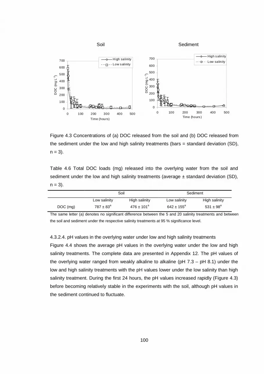
100

Soil Sediment

Figure 4.3 Concentrations of (a) DOC released from the soil and (b) DOC released from

the sediment under the low and high salinity treatments (bars = standard deviation (SD),

n = 3).

Table 4.6 Total DOC loads (mg) released into the overlying water from the soil and

sediment under the low and high salinity treatments (average ± standard deviation (SD),

n = 3).

Soil Sediment


DOC (mg) 787 ± 83a 476 ± 101a 642 ± 155a 531 ± 98a

The same letter (a) denotes no significant difference between the 5 and 20 salinity treatments and between


4.3.2.4. pH values in the overlying water under low and high salinity treatments

Figure 4.4 shows the average pH values in the overlying water under the low and high

salinity treatments. The complete data are presented in Appendix 12. The pH values of

the overlying water ranged from weakly alkaline to alkaline (pH 7.3 – pH 8.1) under the

low and high salinity treatments with the pH values lower under the low salinity than high

salinity treatment. During the first 24 hours, the pH values increased rapidly (Figure 4.3)

before becoming relatively stable in the experiments with the soil, although pH values in

the sediment continued to fluctuate.

0

100

200

300

400

500

600

700

0 100 200 300 400 500

Time (hours)

DO

C (m

g L

-1)

H igh salinity

Low s alinity

0

100

200

300

400

500

600

700

0 100 200 300 400 500

Time (hours )

DO

C (

mg

L-1

)

H igh s alinity

Low salinity

0

100

200

300

400

500

600

700

0 100 200 300 400 500

Time (hours)

DO

C (m

g L

-1)

H igh salinity

Low s alinity

0

100

200

300

400

500

600

700

0 100 200 300 400 500

Time (hours )

DO

C (

mg

L-1

)

H igh s alinity

Low salinity

101

Soil Sediment

Figure 4.4 pH values of the overlying water for the soil (a) and pH values of the overlying

water for the sediment (b) under low and high salinity treatments (bars = standard


4.4. The effect of drying and rewetting on contaminant release from managed

realignment soil and sediment: results

4.4.1 Column microcosm experimental data under drying-rewetting treatment

The effect of drying and rewetting on the release of metals and herbicides from the soil

and sediment into the overlying water was investigated using column microcosm

experiments. The experiments were designed to have two drying-rewetting treatments

with the soil and sediment dried for 7 days and then continuously rewet for 5 days with

artificial seawater at a salinity of 20 in each treatment as described in Chapter 3, Section

3.3.4.2. The average metal, herbicide and DOC concentrations measured in the overlying

water are presented in this section, with the complete data available in Appendices 13, 14

and 15 respectively. Comparisons were made between the experimental data under the

first drying-rewetting treatment and data described in Section 4.3.2.1 where the soil and

sediment were continuously flooded under high salinity treatment (referred to as ‘fully wet’

treatment in this section) in order to highlight any differences between the total loads.

7.0

7.5

8.0

8.5

9.0

0 50 100 150 200 250Time (hours)

pH

High salinity

Low salinity

7.0

7.5

8.0

8.5

9.0

0 50 100 150 200 250

Time (hours)

pH

High salinity

Low salinity

(a) (b)

7.0

7.5

8.0

8.5

9.0

0 50 100 150 200 250Time (hours)

pH

High salinity

Low salinity

7.0

7.5

8.0

8.5

9.0

0 50 100 150 200 250

Time (hours)

pH

High salinity

Low salinity

(a) (b)

102

4.4.1.1 Release of metals into the overlying water under the drying-rewetting treatment

Figure 4.5 shows the average metal concentrations released from the soil and sediment

into the overlying water under the first drying-rewetting and the fully wet treatment over

the same time period. The complete data for the metal concentrations released into the

overlying water under the drying-rewetting treatment are presented in Appendix 13.

Under the drying-rewetting treatment, high metal concentrations in the overlying water

were observed in the first 24 hours following wetting, followed by a decrease which

reaches a plateau with little or no change in the concentrations. The release pattern

indicates an initial rapid release phase followed by a slow release phase.

Table 4.7 shows the total metal loads released into the overlying water from the soil and

sediment under the first drying-rewetting treatment and for comparison the fully wet

treatment over the same time period. Despite the soil and sediment having been spiked

with all three metals at the same concentration, the total Cu, Ni and Zn loads released

into the overlying water from the soil under the drying-rewetting treatment were

significantly higher than those released from the sediment (Two-way ANOVA: F = 40.13,

p < 0.05 for Cu; F = 15.80, p < 0.05 for Ni and F = 14.37, p < 0.05 for Zn). In addition, the

Cu load released into the overlying water from the soil and sediment were two orders of

magnitudes lower than the Ni and Zn load released.

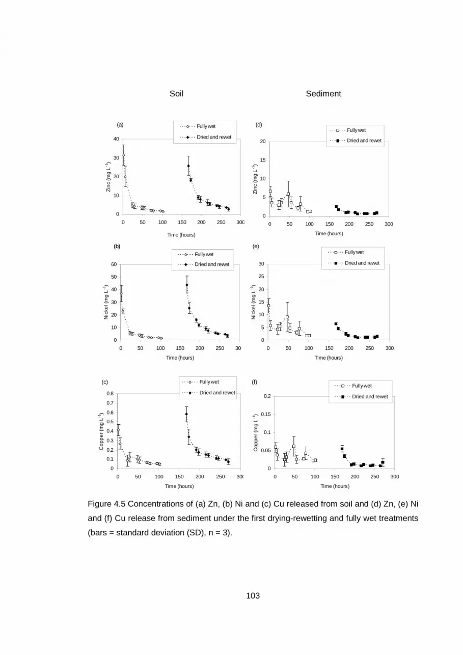
103

Soil Sediment

Figure 4.5 Concentrations of (a) Zn, (b) Ni and (c) Cu released from soil and (d) Zn, (e) Ni

and (f) Cu release from sediment under the first drying-rewetting and fully wet treatments


0

10

20

30

40

50

60

0 50 100 150 200 250 300

Time (hours)

Nic

kel (

mg

L-1

)

Fully wet

Dried and rewet

0

5

10

15

20

25

30

0 50 100 150 200 250 300

Time (hours)

Nic

kel (

mg

L-1

)Fully wet

Dried and rewet

0

10

20

30

40

0 50 100 150 200 250 300

Time (hours)

Zinc

(m

g L

-1)

Fully wet

Dried and rewet

0

5

10

15

20

0 50 100 150 200 250 300

Time (hours)

Zinc

(m

g L

-1)

Fully wet

Dried and rewet

(a)

(b) (e)

(d)

0

10

20

30

40

50

60

0 50 100 150 200 250 300

Time (hours)

Nic

kel (

mg

L-1

)

Fully wet

Dried and rewet

0

5

10

15

20

25

30

0 50 100 150 200 250 300

Time (hours)

Nic

kel (

mg

L-1

)Fully wet

Dried and rewet

0

10

20

30

40

0 50 100 150 200 250 300

Time (hours)

Zinc

(m

g L

-1)

Fully wet

Dried and rewet

0

5

10

15

20

0 50 100 150 200 250 300

Time (hours)

Zinc

(m

g L

-1)

Fully wet

Dried and rewet

(a)

(b) (e)

(d)

0

0.1

0.2

0.3

0.4

0.5

0.6

0.7

0.8

0 50 100 150 200 250 300

Time (hours)

Cop

pe

r (m

g L

-1)

Fully wet

Dried and rewet

0

0.05

0.1

0.15

0.2

0 50 100 150 200 250 300

Time (hours)

Cop

per

(mg

L-1

)

Fully wet

Dried and rewet

(c) (f)

0

0.1

0.2

0.3

0.4

0.5

0.6

0.7

0.8

0 50 100 150 200 250 300

Time (hours)

Cop

pe

r (m

g L

-1)

Fully wet

Dried and rewet

0

0.05

0.1

0.15

0.2

0 50 100 150 200 250 300

Time (hours)

Cop

per

(mg

L-1

)

Fully wet

Dried and rewet

(c) (f)

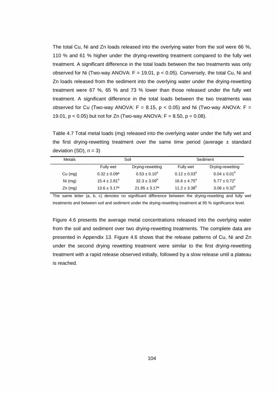
104

The total Cu, Ni and Zn loads released into the overlying water from the soil were 66 %,

110 % and 61 % higher under the drying-rewetting treatment compared to the fully wet

treatment. A significant difference in the total loads between the two treatments was only

observed for Ni (Two-way ANOVA: F = 19.01, p < 0.05). Conversely, the total Cu, Ni and

Zn loads released from the sediment into the overlying water under the drying-rewetting

treatment were 67 %, 65 % and 73 % lower than those released under the fully wet

treatment. A significant difference in the total loads between the two treatments was

observed for Cu (Two-way ANOVA: F = 8.15, p < 0.05) and Ni (Two-way ANOVA: F =

19.01, p < 0.05) but not for Zn (Two-way ANOVA: F = 8.50, p = 0.08).

Table 4.7 Total metal loads (mg) released into the overlying water under the fully wet and

the first drying-rewetting treatment over the same time period (average ± standard

deviation (SD), n = 3)


Fully wet Drying-rewetting Fully wet Drying-rewetting

Cu (mg) 0.32 ± 0.09ª 0.53 ± 0.10a 0.12 ± 0.03a 0.04 ± 0.01b

Ni (mg) 15.4 ± 2.81a 32.3 ± 3.09b 16.6 ± 4.75a 5.77 ± 0.72c

Zn (mg) 13.6 ± 3.17ª 21.95 ± 3.17ª 11.2 ± 3.38b 3.08 ± 0.32b

The same letter (a, b, c) denotes no significant difference between the drying-rewetting and fully wet

treatments and between soil and sediment under the drying-rewetting treatment at 95 % significance level.

Figure 4.6 presents the average metal concentrations released into the overlying water

from the soil and sediment over two drying-rewetting treatments. The complete data are

presented in Appendix 13. Figure 4.6 shows that the release patterns of Cu, Ni and Zn

under the second drying rewetting treatment were similar to the first drying-rewetting

treatment with a rapid release observed initially, followed by a slow release until a plateau

is reached.

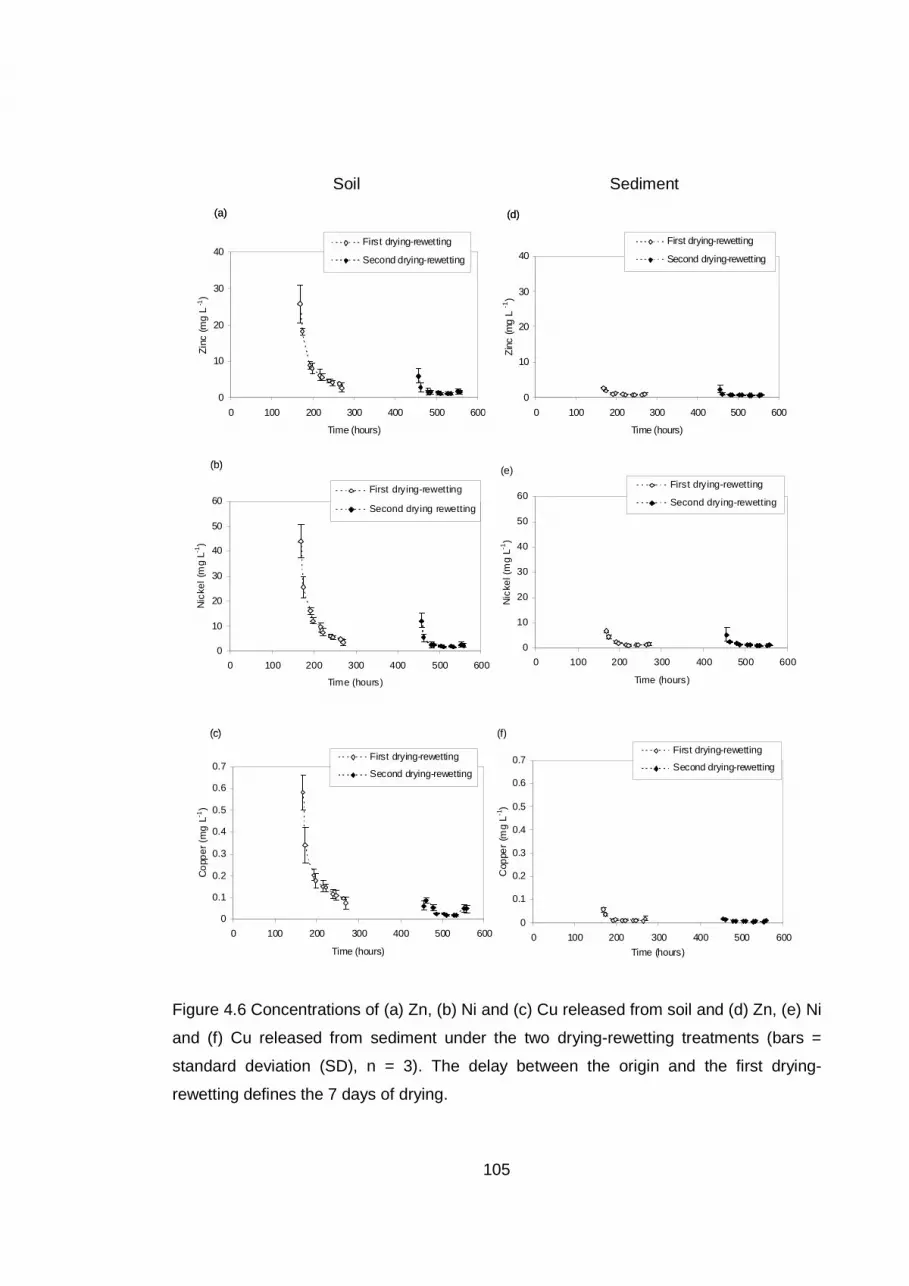
105

Soil Sediment

Figure 4.6 Concentrations of (a) Zn, (b) Ni and (c) Cu released from soil and (d) Zn, (e) Ni

and (f) Cu released from sediment under the two drying-rewetting treatments (bars =

standard deviation (SD), n = 3). The delay between the origin and the first drying-

rewetting defines the 7 days of drying.

0

10

20

30

40

50

60

0 100 200 300 400 500 600

Time (hours)

Nic

kel

(mg

L-1)

First drying-rewetting

Second drying rewetting

(b)

0

10

20

30

40

50

60

0 100 200 300 400 500 600

Time (hours)

Nic

kel (

mg

L-1)


Second drying-rewetting

(e)

0

10

20

30

40

50

60

0 100 200 300 400 500 600

Time (hours)

Nic

kel

(mg

L-1)


Second drying rewetting

(b)

0

10

20

30

40

50

60

0 100 200 300 400 500 600

Time (hours)

Nic

kel (

mg

L-1)



(e)

(a)

0

10

20

30

40

0 100 200 300 400 500 600

Time (hours)

Zin

c (m

g L

-1)



0

10

20

30

40

0 100 200 300 400 500 600

Time (hours)

Zin

c (m

g L

-1)



(d)(a)

0

10

20

30

40

0 100 200 300 400 500 600

Time (hours)

Zin

c (m

g L

-1)



0

10

20

30

40

0 100 200 300 400 500 600

Time (hours)

Zin

c (m

g L

-1)



(d)

0

0.1

0.2

0.3

0.4

0.5

0.6

0.7

0 100 200 300 400 500 600

Time (hours)

Co

pper

(m

g L-1

)



0

0.1

0.2

0.3

0.4

0.5

0.6

0.7

0 100 200 300 400 500 600

Time (hours)

Cop

per

(mg

L-1

)



(c) (f)

0

0.1

0.2

0.3

0.4

0.5

0.6

0.7

0 100 200 300 400 500 600

Time (hours)

Co

pper

(m

g L-1

)



0

0.1

0.2

0.3

0.4

0.5

0.6

0.7

0 100 200 300 400 500 600

Time (hours)

Cop

per

(mg

L-1

)



(c) (f)

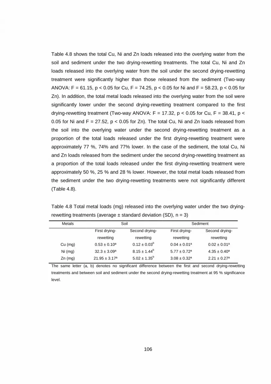
106

Table 4.8 shows the total Cu, Ni and Zn loads released into the overlying water from the

soil and sediment under the two drying-rewetting treatments. The total Cu, Ni and Zn

loads released into the overlying water from the soil under the second drying-rewetting

treatment were significantly higher than those released from the sediment (Two-way

ANOVA: F = 61.15, p < 0.05 for Cu, F = 74.25, p < 0.05 for Ni and F = 58.23, p < 0.05 for

Zn). In addition, the total metal loads released into the overlying water from the soil were

significantly lower under the second drying-rewetting treatment compared to the first

drying-rewetting treatment (Two-way ANOVA: F = 17.32, p < 0.05 for Cu, F = 38.41, p <

0.05 for Ni and F = 27.52, p < 0.05 for Zn). The total Cu, Ni and Zn loads released from

the soil into the overlying water under the second drying-rewetting treatment as a

proportion of the total loads released under the first drying-rewetting treatment were

approximately 77 %, 74% and 77% lower. In the case of the sediment, the total Cu, Ni

and Zn loads released from the sediment under the second drying-rewetting treatment as

a proportion of the total loads released under the first drying-rewetting treatment were

approximately 50 %, 25 % and 28 % lower. However, the total metal loads released from

the sediment under the two drying-rewetting treatments were not significantly different

(Table 4.8).

Table 4.8 Total metal loads (mg) released into the overlying water under the two drying-

rewetting treatments (average ± standard deviation (SD), n = 3)


First drying-

rewetting

Second drying-

rewetting

First drying-

rewetting

Second drying-

rewetting

Cu (mg) 0.53 ± 0.10ª 0.12 ± 0.03b 0.04 ± 0.01ª 0.02 ± 0.01ª

Ni (mg) 32.3 ± 3.09ª 8.15 ± 1.44b 5.77 ± 0.72ª 4.35 ± 0.40ª

Zn (mg) 21.95 ± 3.17ª 5.02 ± 1.35b 3.08 ± 0.32ª 2.21 ± 0.27ª

The same letter (a, b) denotes no significant difference between the first and second drying-rewetting

treatments and between soil and sediment under the second drying-rewetting treatment at 95 % significance

level.

107

4.4.1.2 Release of herbicides into the overlying water under the drying-rewetting

treatment

The average concentrations of simazine, atrazine and diuron released into the overlying

water from the soil and sediment under the first drying-rewetting and fully wet treatment

over the same period are presented in Figure 4.7, with the complete data for the

herbicide concentrations released under the drying-rewetting treatment in Appendix 14.

Similar to the fully wet treatment, an initial rapid release from the soil and sediment was

observed in the first 24 hours, followed by a slow release reaching relatively constant

concentrations.

Table 4.9 shows the total herbicide loads released into the overlying water from the soil

and sediment under the first drying-rewetting and fully wet treatment over the same time

period. Although the soil and sediment were spiked with all three herbicides at the same

concentration, the total simazine, atrazine and diuron loads released into the overlying

water from the soil were higher than those released from the sediment. However, the

difference was only significant for diuron (Two-way ANOVA: F = 5.11, p < 0.05) (Table

4.9). In addition, the total diuron load in the overlying water was one order of magnitude

lower than those of atrazine and simazine.

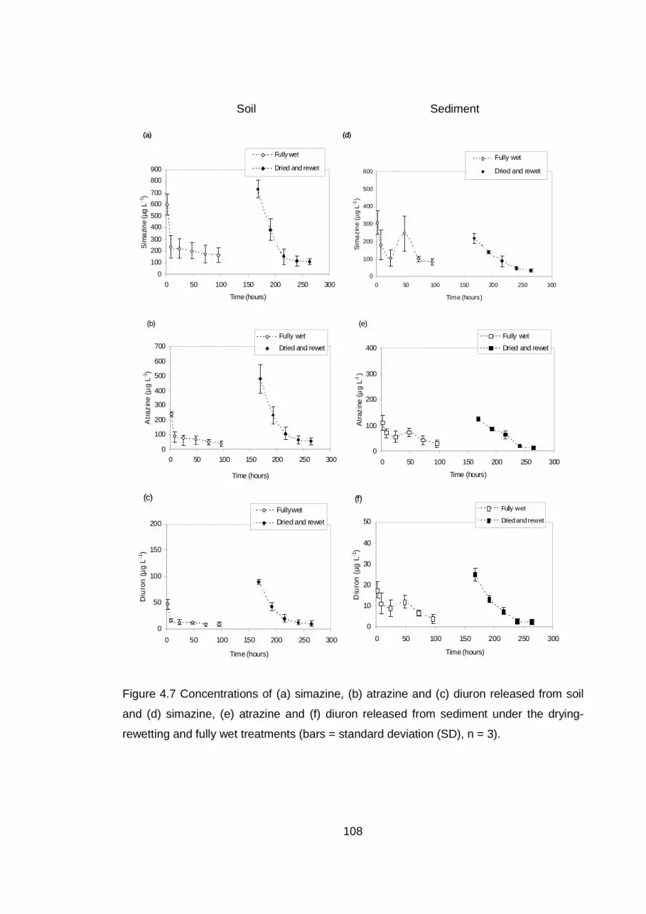
108

Soil Sediment

Figure 4.7 Concentrations of (a) simazine, (b) atrazine and (c) diuron released from soil

and (d) simazine, (e) atrazine and (f) diuron released from sediment under the drying-

rewetting and fully wet treatments (bars = standard deviation (SD), n = 3).

(a) (d)

0

100

200

300

400

500

600

700

800

900

0 50 100 150 200 250 300

Time (hours)

Sim

azi

ne

(µg

L-1

)

Fully wet

Dried and rewet

0

100

200

300

400

500

600

0 50 100 150 200 250 300

Time (hours)

Sim

azi

ne

(µg

L-1

)

Fully wet

Dried and rewet

(a) (d)

0

100

200

300

400

500

600

700

800

900

0 50 100 150 200 250 300

Time (hours)

Sim

azi

ne

(µg

L-1

)

Fully wet

Dried and rewet

0

100

200

300

400

500

600

0 50 100 150 200 250 300

Time (hours)

Sim

azi

ne

(µg

L-1

)

Fully wet

Dried and rewet

0

100

200

300

400

500

600

700

0 50 100 150 200 250 300

Time (hours)

Atr

azin

e (µ

g L-1

)

Fully wet

Dried and rewet

0

100

200

300

400

0 50 100 150 200 250 300

Time (hours)

Atr

azin

e (µ

g L-1

)

Fully wet

Dried and rewet

(b) (e)

0

100

200

300

400

500

600

700

0 50 100 150 200 250 300

Time (hours)

Atr

azin

e (µ

g L-1

)

Fully wet

Dried and rewet

0

100

200

300

400

0 50 100 150 200 250 300

Time (hours)

Atr

azin

e (µ

g L-1

)

Fully wet

Dried and rewet

(b) (e)

0

50

100

150

200

0 50 100 150 200 250 300

Time (hours)

Diu

ron

(µg

L-1

)

Fully wet

Dried and rewet

0

10

20

30

40

50

0 50 100 150 200 250 300

Time (hours)

Diu

ron

(µg

L-1

)

Fully wet

Dried and rewet

(c) (f)

0

50

100

150

200

0 50 100 150 200 250 300

Time (hours)

Diu

ron

(µg

L-1

)

Fully wet

Dried and rewet

0

10

20

30

40

50

0 50 100 150 200 250 300

Time (hours)

Diu

ron

(µg

L-1

)

Fully wet

Dried and rewet

(c) (f)

109

Whilst the total atrazine and diuron loads released into the overlying water from the soil

were approximately 29 % and 42 % higher under the drying-rewetting than the fully wet

treatment, the simazine load was approximately 28 % lower under the drying rewetting

treatment. For the sediment, the total loads of simazine, atrazine and diuron released

under the drying-rewetting treatment were approximately 64 %, 44 % and 50 % lower

than those released under the fully wet treatment. No significant differences in the

herbicide loads between the fully wet and drying-rewetting treatments were observed for

either the soil or sediment (Table 4.9).

Table 4.9 Total herbicide loads (µg) released into the overlying water under the fully wet

and the first drying-rewetting treatments over the same time period (average ± standard




Simazine (µg) 375.4 ± 135.8a 270.4 ± 87.9a 314.4 ± 52.9a 112.6 ± 19.1a

Atrazine (µg) 125.1 ± 31.6a 162.0 ± 55.8a 110.9 ± 22.9a 62.1 ± 6.1a

Diuron (µg) 21.5 ± 4.8a 30.7 ± 9.6a 18.1 ± 2.6b 9.0 ± 1.1b

The same letter (a, b) denotes no significant difference between the drying-rewetting and fully wet treatments

and between soil and sediment under the drying-rewetting treatment at 95 % significance level.

Figure 4.8 shows the average concentrations of simazine, atrazine and diuron released

into the overlying water from the soil and sediment under the two drying-rewetting

treatments with the complete data in Appendix 14. The release patterns under the second

drying-rewetting treatment were similar to the first drying-rewetting treatment with an

initial rapid release observed, followed by a slow release.

Table 4.10 shows the total simazine, atrazine and diuron loads released into the overlying

water from the soil and sediment under the two drying-rewetting treatments. The total

simazine, atrazine and diuron loads released into the overlying water from the soil were

higher but not significantly different from those released from the sediment (Table 4.10).

The total simazine, atrazine and diuron loads released into the overlying water from the

soil under the second drying-rewetting treatment as a proportion of the total metal load

released under the first drying-rewetting treatment reduced by approximately 50 %, 61 %

and 71 % respectively. Significant differences in the total herbicide loads between the first

and second drying-rewetting treatments were only observed for atrazine (Two-way

110

ANOVA: F = 4.82, p < 0.05) and diuron (Two-way ANOVA: F = 12.08, p < 0.05) (Table

4.10). In the sediment, the total simazine, atrazine and diuron loads released into the

overlying water under the second drying-rewetting treatment as a proportion of the total

load released under the first drying-rewetting treatment reduced by approximately 4 %,

31 % and 14 %. No significant differences were observed in the total loads between the

first and second drying-rewetting treatments for simazine, atrazine and diuron.

111

Soil Sediment

Figure 4.8 Concentrations of (a) simazine, (b) atrazine and (c) diuron released from soil

and (d) simazine, (e) atrazine and (f) diuron released from sediment under the two drying-

rewetting treatments (bars = standard deviation (SD), n = 3). The delay between the

origin and the first drying-rewetting defines the 7 days of drying.

0

100

200

300

400

500

600

700

800

900

0 100 200 300 400 500 600

Time (hours)

Sim

az

ine

(µ

g L

-1)

Firs t drying-rewetting


0

100

200

300

400

500

600

700

800

900

0 100 200 300 400 500 600

Time (hours)

Sim

azin

e (µ

g L

-1)



(a) (d)

0

100

200

300

400

500

600

700

800

900

0 100 200 300 400 500 600

Time (hours)

Sim

az

ine

(µ

g L

-1)



0

100

200

300

400

500

600

700

800

900

0 100 200 300 400 500 600

Time (hours)

Sim

azin

e (µ

g L

-1)



(a) (d)

0

100

200

300

400

500

600

700

0 100 200 300 400 500 600

Time (hours)

Atr

azin

e (µ

g L

-1)



0

100

200

300

400

500

600

700

0 100 200 300 400 500 600

Time (hours)

Atr

azi

ne

(µg

L-1

)



(b) (e)

0

100

200

300

400

500

600

700

0 100 200 300 400 500 600

Time (hours)

Atr

azin

e (µ

g L

-1)



0

100

200

300

400

500

600

700

0 100 200 300 400 500 600

Time (hours)

Atr

azi

ne

(µg

L-1

)



(b) (e)

0

50

100

150

200

0 100 200 300 400 500 600

Time (hours)

Diu

ron

(µg

L-1

)



0

50

100

150

200

0 100 200 300 400 500 600

Tim e (hours )

Diu

ron

(µg

L-1)



(c) (f)

0

50

100

150

200

0 100 200 300 400 500 600

Time (hours)

Diu

ron

(µg

L-1

)



0

50

100

150

200

0 100 200 300 400 500 600

Tim e (hours )

Diu

ron

(µg

L-1)



(c) (f)

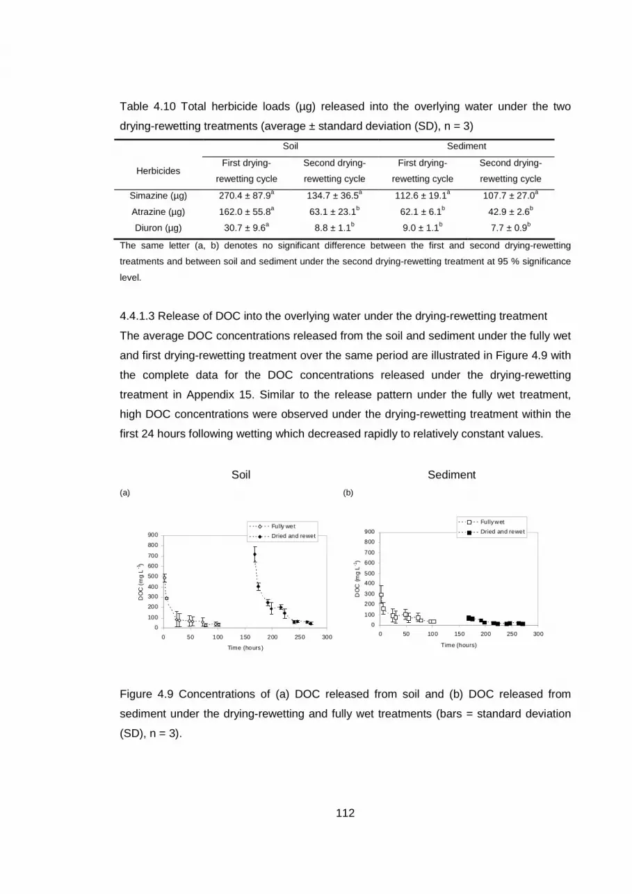
112

Table 4.10 Total herbicide loads (µg) released into the overlying water under the two

drying-rewetting treatments (average ± standard deviation (SD), n = 3)

Soil Sediment

Herbicides First drying-

rewetting cycle

Second drying-

rewetting cycle

First drying-

rewetting cycle

Second drying-

rewetting cycle

Simazine (µg) 270.4 ± 87.9a 134.7 ± 36.5a 112.6 ± 19.1a 107.7 ± 27.0a

Atrazine (µg) 162.0 ± 55.8a 63.1 ± 23.1b 62.1 ± 6.1b 42.9 ± 2.6b

Diuron (µg) 30.7 ± 9.6a 8.8 ± 1.1b 9.0 ± 1.1b 7.7 ± 0.9b

The same letter (a, b) denotes no significant difference between the first and second drying-rewetting

treatments and between soil and sediment under the second drying-rewetting treatment at 95 % significance

level.

4.4.1.3 Release of DOC into the overlying water under the drying-rewetting treatment

The average DOC concentrations released from the soil and sediment under the fully wet

and first drying-rewetting treatment over the same period are illustrated in Figure 4.9 with

the complete data for the DOC concentrations released under the drying-rewetting

treatment in Appendix 15. Similar to the release pattern under the fully wet treatment,

high DOC concentrations were observed under the drying-rewetting treatment within the

first 24 hours following wetting which decreased rapidly to relatively constant values.

Soil Sediment

(a) (b)

Figure 4.9 Concentrations of (a) DOC released from soil and (b) DOC released from

sediment under the drying-rewetting and fully wet treatments (bars = standard deviation

(SD), n = 3).

0

100

200

300

400

500

600

700

800

900

0 50 100 150 200 250 300

Time (hours )

DO

C (m

g L

-1)

Fully wet

Dried and rewet

0

100

200

300

400

500

600

700

800

900

0 50 100 150 200 250 300

Time (hours)

DO

C (m

g L

-1)

Fully wet

Dried and rewet

0

100

200

300

400

500

600

700

800

900

0 50 100 150 200 250 300

Time (hours )

DO

C (m

g L

-1)

Fully wet

Dried and rewet

0

100

200

300

400

500

600

700

800

900

0 50 100 150 200 250 300

Time (hours)

DO

C (m

g L

-1)

Fully wet

Dried and rewet

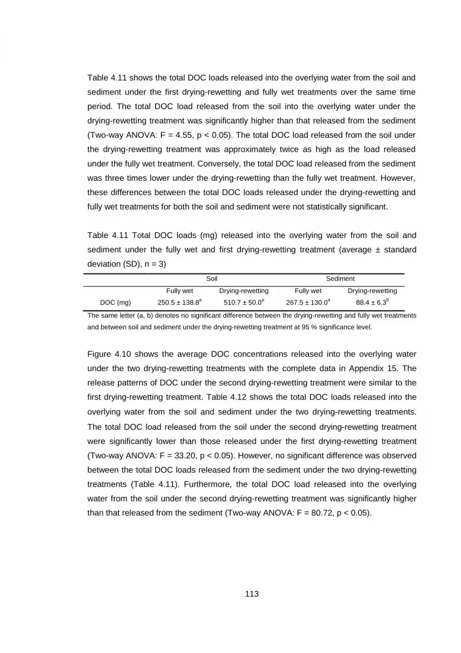
113

Table 4.11 shows the total DOC loads released into the overlying water from the soil and

sediment under the first drying-rewetting and fully wet treatments over the same time

period. The total DOC load released from the soil into the overlying water under the

drying-rewetting treatment was significantly higher than that released from the sediment

(Two-way ANOVA: F = 4.55, p < 0.05). The total DOC load released from the soil under

the drying-rewetting treatment was approximately twice as high as the load released

under the fully wet treatment. Conversely, the total DOC load released from the sediment

was three times lower under the drying-rewetting than the fully wet treatment. However,

these differences between the total DOC loads released under the drying-rewetting and

fully wet treatments for both the soil and sediment were not statistically significant.


sediment under the fully wet and first drying-rewetting treatment (average ± standard


Soil Sediment


DOC (mg) 250.5 ± 138.8a 510.7 ± 50.0a 267.5 ± 130.0a 88.4 ± 6.3b



Figure 4.10 shows the average DOC concentrations released into the overlying water

under the two drying-rewetting treatments with the complete data in Appendix 15. The

release patterns of DOC under the second drying-rewetting treatment were similar to the

first drying-rewetting treatment. Table 4.12 shows the total DOC loads released into the

overlying water from the soil and sediment under the two drying-rewetting treatments.

The total DOC load released from the soil under the second drying-rewetting treatment

were significantly lower than those released under the first drying-rewetting treatment

(Two-way ANOVA: F = 33.20, p < 0.05). However, no significant difference was observed

between the total DOC loads released from the sediment under the two drying-rewetting

treatments (Table 4.11). Furthermore, the total DOC load released into the overlying

water from the soil under the second drying-rewetting treatment was significantly higher

than that released from the sediment (Two-way ANOVA: F = 80.72, p < 0.05).

114

Soil Sediment

Figure 4.10 Concentrations of (a) DOC released from soil and (b) DOC released from

sediment under the two drying-rewetting treatments (bars = standard deviation (SD), n =

3). The delay between the origin and the first drying-rewetting defines the 7 days of

drying.


sediment under the first and second drying-rewetting treatment (average ± standard


Soil Sediment

First drying-

rewetting cycle

Second drying-

rewetting cycle

First drying

rewetting cycle

Second drying-

rewetting cycle

DOC (mg) 510.7 ± 50.0a 144.7 ± 24.9b 88.4 ± 6.3a 62.6 ± 10.1a



4.5 Carbon mineralisation, CO2 release and microbial biomass

The average headspace CO2, soil and sediment microbial biomass data measured during

the carbon mineralisation experiments are presented below with the full data in Appendix

16. These data test the hypothesis that microbial activity and organic matter

mineralisation will be stimulated during the drying-rewetting of the soil and sediment

which will lead to the release of metals and herbicides associated with organic matter.

The experiments were conducted with fully wet soil and sediment and dried-rewet soil

and sediment which were dried for 7 days and then rewet with artificial seawater at 20 ‰

0

100

200

300

400

500

600

700

800

900

0 100 200 300 400 500 600

Time (hours)

DO

C (

mg

L-1

)



0

100

200

300

400

500

600

700

800

900

0 100 200 300 400 500 600

Time (hours)

DO

C (m

g L

-1)



0

100

200

300

400

500

600

700

800

900

0 100 200 300 400 500 600

Time (hours)

DO

C (

mg

L-1

)



0

100

200

300

400

500

600

700

800

900

0 100 200 300 400 500 600

Time (hours)

DO

C (m

g L

-1)



115

0

5

10

15

20

25

30

35

40

0 5 10 15 20Time (days)

Cu

mul

ativ

e C

O2

(µg

CO

2 kg

-1)

Soil

Sediment

for 1 hour. The CO2 released into the headspace from the fully wet and dried-rewet soil

and sediment were measured for 15 days (i.e. from the beginning of the experiment) and

6 days (i.e. after rewetting the soil/sediment) respectively. The soil and sediment

microbial biomass were measured before drying, after drying and six days after rewetting

by substrate induced respiration method described in Chapter 3, Section 3.4. The carbon

mineralisation rate in the soil and sediment were determined from the CO2 data as

described in Chapter 3, Section 3.4. The carbon mineralisation rates were used as a

measure of soil and sediment organic matter mineralisation.

4.5.1. CO2 released from fully wet soil and sediment

Average cumulative CO2 released from the fully wet soil and sediment and mineralisation

rates are given in Figure 4.11 and 4.12 with the full data in Appendix 16. The cumulative

CO2 released ranged from 8 - 26 µg CO2 kg-1 soil (wet weight) and 11 - 33 µg CO2 kg-1

sediment (wet weight) for the soil and sediment respectively. The increase in the

cumulative CO2 released for the soil and sediment suggest the production of CO2 as

organic matter in the soil and sediment is mineralised. The cumulative CO2 released from

the sediment was higher than that released from the soil. In contrast, the carbon

mineralisation rates generally decreased in the soil and sediment (Figure 4.12).

Figure 4.11 Cumulative CO2 release from the fully wet soil and sediment (bars = standard


116

0

1

2

3

4

0 5 10 15 20

Time (days)

Min

era

isa

tion

rate

(µ

g k

g-1 d

-1)

Soil

Sediment

Figure 4.12 Carbon mineralisation rates under fully wet soil and sediment treatment (bars

= standard deviation (SD), n = 3).

4.5.2. CO2 released from dried-rewet soil and sediment

Figures 4.13 and 4.14 show the cumulative CO2 released from the dried-rewet soil and

sediment and the mineralisation rates respectively. An increase was observed in the

cumulative CO2 released from the soil and sediment with ranges from 1613 - 7458 µg

CO2 kg-1 soil and 2619 - 4803 µg CO2 kg-1 sediment indicating greater cumulative CO2

release from the soil. The ranges of CO2 release for these dried-rewet soil and sediment

were two orders of magnitude higher than those released from the fully wet soil and

sediment. The mineralisation rate in the soil and sediment decreased and became

relatively constant for the remainder of the experiment (Figure 4.14) with the

mineralisation rates in the soil higher than those in the sediment. Mineralisation rates in

the dried-rewet soil and sediment were two to three orders of magnitude higher than

those in the fully wet soil and sediment suggesting that drying and rewetting led to an

increase in carbon mineralisation in the soil and sediment.

117

0

2000

4000

6000

8000

10000

0 1 2 3 4 5 6 7

Time (days)

Cu

mu

lativ

e C

O2

(µg

CO

2 kg-1

)

Soil

Sediment

0

400

800

1200

1600

2000

0 2 4 6 8

Time (days)

Ra

te o

f CO

2 p

rod

uct

ion

(µ

g k

g-1 d

-1)

Soil

Sediment

Figure 4.13 Cumulative CO2 released from the dried-wet soil and sediment (bars =


Figure 4.14 Carbon mineralisation rates under dried-rewet soil and sediment treatment


4.5.3. Soil and sediment microbial biomass data

Figure 4.15 presents the soil and sediment microbial biomass data measured by

substrate induced respiration method before drying, after drying and 6 days after

rewetting. Differences were observed between the sediment and soil microbial biomass

before drying, after drying and 6 days after rewetting. The microbial biomass varied

118

0

20

40

60

80

100

120

140

Before drying After drying 6 days after rewetting

µg

mic

robi

al b

iom

ass

C g

-1 s

oil/s

edim

ent

Soil

Sediment

during the experiment with the sediment microbial biomass decreasing and the soil

microbial biomass increasing. However, before drying, the microbial biomass was higher

in the sediment than the soil but after drying, the microbial biomass became lower in the

sediment than the soil.

Figure 4.15 Soil and sediment microbial biomass before drying, immediately after drying

and 6 days after rewetting (bars = standard deviation (SD), n = 3).

119

Chapter 5 The release of metals and herbicides from managed realignment

soil and sediment

5.1. Introduction

Tidal inundation of soil and sediment by seawater in managed realignment sites is

accompanied by several changes in the soil and sediment chemistry. For example, as

seawater inundates the soil, the fresh water in the soil pores is replaced by saline

solution, and the salinity of the porewater increases (Blackwell et al., 2004; Boorman and

Hazelden, 2002). An increase in pH can also occur following the inundation of soil and

sediment by seawater (Mitsch and Gosselink, 2000). These changes can affect the

binding of contaminants to the soil and sediment leading to contaminant release into the

overlying water during tidal inundation. In addition, the periodic tidal inundation and

drainage in these environments exposes the soil and sediment to drying-rewetting cycles

which may lead to increased organic matter mineralisation, increased DOC release and

the potential release of organic matter associated contaminants into the overlying water.

In this thesis, the effect of salinity and drying-rewetting cycles on the release of metals

(Cu, Ni and Zn) and herbicides (simazine, atrazine and diuron) from soil and sediment in

managed realignment sites was investigated by laboratory simulation experiments. This

chapter discusses the results of the laboratory experiments presented in Chapter 4. Total

contaminant loads released into the overlying water from the soil and sediment were

measured under two different salinities and drying-rewetting cycles which gave an

indication of the nature of the likely processes affecting the potential release of metal and

herbicide from soil and sediment in managed realignment sites.

5.2. Effect of salinity on the release of metals and herbicides from soil and sediment

Flooding soil and sediment with seawater can lead to an increase in the salinity of the soil

and sediment porewater. This increase in salinity can in turn lead to an increase in

porewater metal concentrations through the influence of seawater cations (i.e. Na+, Ca2+,

Mg2+, K+) which compete with the sorbed metals for cation exchange binding sites and,

seawater anions (Cl and SO42-) which form soluble complexes with metals (Turner and

Millward, 2002; Phillips et al., 2004; Riba et al., 2003). An increase in salinity can also be

accompanied by changes in pH (Turner and Millward, 2002) which can also affect metal

sorption to soil and sediment. An increase in pH can lead to an increase in the sorption of

120

metals through less competition from H+ ions for cation exchange sorption sites; the

increased formation of metal binding sites on Fe and Mn oxides; hydrolysis of metals

leading to the formation of hydroxyl cations which are more likely to bind to the solid

phase; and more negatively charged pH dependent sorption sites (Forstner and

Wittmann, 1981; Alloway, 1995; Jackson, 1998; Rate et al., 2000; Standring et al., 2002;

Peng et al., 2003). Conversely, a decrease in pH can lead to more positively charged

particle surfaces through association with additional H+ ions (Brady and Weil, 2002;

Zwolsman et al., 1993). The concentration of dissolved metals in solution, therefore,

increases under low pH conditions.

Metals take part in a number of interactions in soil and sediment. Metals can be

incorporated into crystalline silicates (Jenne, 1976). They can also be precipitated with

carbonates or sulphides, co-precipitated or sorbed to Fe and Mn oxides and hydroxides,

sorbed or incorporated into clay minerals and complexed with organic matter (Eggleton

and Thomas, 2004; Simpson et al., 1998; Salomons and Forstner, 1984; Alloway, 1995).

Changes in salinity have been observed to affect the latter metal particulate interactions,

resulting in metal desorption (Bauske and Goetz, 1993; Millward and Liu, 2003; Gambrel

et al., 1991).

Charge distribution, polarity, hydrophobicity, basicity and acidity are some properties of

herbicides which control their binding to soil and sediment (Khan, 1978, Gevao et al.,

2000). Triazine herbicides such as simazine and atrazine are weakly basic herbicides

hence they can undergo ionisation and become positively charged depending on the pH

of the system and their respective acid dissociation constants (pKa) (Seol and Lee, 2001;

McBride, 1994). Changes in solution pH can change the charge distribution and binding

of the triazine herbicides to the soil and sediment and lead to desorption into solution.

Seawater cations may also displace charged triazine herbicides binding by cation

exchange on soil and sediment particles and lead to higher herbicide concentrations in

solution. Phenyl urea herbicides such as diuron are neutral molecules and do not

undergo ionisation, hence their sorption and desorption is not affected by pH. However,

an increase in salinity can lead to an increase in the sorption of these neutral organic

contaminants due to salting out effect (Turner and Millward, 2002; Turner and Rawling,

2001).

121

Herbicides bind mainly to organic matter and clay particles in soil and sediment, with

organic matter being the primary binding component (Chiou, 1989; Gao et al., 1998;

Voulvoulis et al., 2002). Clay particles become important for the sorption of triazine

herbicides if their molecules are charged (Laird et al., 1994; Spark and Swift, 2002). At

pKa < pH, organic bases such as triazines exist as neutral species particularly when the

primary sorption domain is organic matter while at pKa > pH, a considerable amount of

the herbicides exist as cations and undergo cation exchange (Weber et al., 1969; Seol

and Lee, 2001).

The effect of salinity on the release of metals (Zn, Ni and Cu) and herbicides (simazine,

atrazine and diuron) was examined under two different salinities; 5 and 20 referred to as

low and high salinity treatments respectively. The effect of salinity on the release of the

metals from the soil and from the sediment following the inundation with artificial

seawater will be considered together in Section 5.2.1, followed by the effect of salinity on

the release of the herbicides from the soil and from the sediment in Section 5.2.2.

5.2.1. Effect of salinity on the release of metals from soil and sediment

The log Kd values of Cu, Ni and Zn calculated in the batch sorption experiments ranged

from 2.54 to 2.97 L kg -1, 2.28 to 2.52 L kg -1 and 2.55 to 2.75 L kg -1 respectively in both

the soil and sediment (Chapter 4, Table 4.2). These log Kd values are within the ranges

reported in the literature. Phillips et al (2004) reported log Kd values of 2.02 L kg -1 to 4.22

L kg -1 for Zn and 3.41 – 4.19 L kg -1 for Cu in sediments. The Kd (expressed on a log10

basis) for Ni, Zn and Cu was found to range from 0.48 to 3.86 L kg -1, 0.86 to 3.26 L kg -1

and 2.31 to 3.36 L kg -1 respectively in sandy aquifer material (Christensen et al., 1996;

2000). Usman et al. (2008) reported Kd (expressed on a log10 basis) for Ni, Zn and Cu of

2.2 L kg-1, 2.08 L kg -1 and 2.9 L kg-1 in soil. In this study, the log Kd values of Cu, Ni and

Zn were consistently higher in the sediment than the soil (Chapter 4, Table 4.2) indicating

that the metals were binding more strongly to the sediment than the soil and/or there was

a greater availability of binding sites in the sediment at both 5 and 20 salinities. The

differences between the partition coefficients were significant for Cu (Two-way ANOVA: F

= 13.04, p < 0.05) and Ni (Two-way ANOVA: F = 30.73, p < 0.05) at both salinities and Zn

(Two-way ANOVA: F = 15.29, p < 0.05) at a salinity of 20. The greater availability of

binding sites for the metals in the sediment is due to the higher clay and organic matter

122

content in the sediment compared to the soil (Chapter 4, Table 4.1). In addition, oxic

estuarine sediments such as those used in this study often comprise Fe and Mn oxides

and carbonates which are important binding sites for metals (Eggleton and Thomas,

2004; Forstner and Wittmann, 1981; Filguieras et al., 2002). Although the Fe and Mn

oxides and carbonate content in the soil and sediment were not evaluated in this study,

the sediment is likely to have a greater amount of these solid phases than the soil which

may also be contributing to the higher partition coefficients in the sediment. Several

mechanisms such as complexation, precipitation and cation exchange interactions are

likely to have contributed simultaneously to the binding of Cu, Ni and Zn to the soil and

sediment solid phases in this study.

At a salinity of 5, log Kd values of the metals were in the order Cu > Zn > Ni in both the

soil and sediment (Chapter 4, Table 4.2) with Cu the most strongly bound and Ni the least

strongly bound. Cu is known to be strongly associated with organic matter and often

shows the greatest affinity for Fe oxides compared to Ni and Zn (Millward and Liu, 2003;

Forstner and Wittmann, 1981; Stephens et al., 2001; Alloway, 1995; McBride, 1994). The

trend in the log Kd values corresponds with the reported binding strength of Cu, Ni and Zn

to organic matter which is in the order Cu > Zn > Ni (Filgueiras et al., 2002; Forstner and

Wittmann, 1981; Alloway, 1995). This suggests that the relative differences in the log Kd

values among the metals may in part be due to the differences in the strength of binding

of Cu, Ni and Zn to organic matter with Cu being the most strongly bound, followed by Zn

and then Ni. In addition, Cu, Ni and Zn can form soluble chlorocomplexes in seawater

(Turner, 1998; Phillips et al., 2004; Riba et al., 2003) which keeps the metals in solution

and reduces sorption. The complexation of Cu, Ni and Zn with Cl is generally in the

preferential order Zn > Ni > Cu (Forstner and Wittmann, 1981) indicating that Zn has the

greatest tendency to form soluble chlorocomplexes and hence the least likely to bind to

the soil and sediment. However, in this study, Ni was the least bound to the soil and

sediment suggesting that the conditions at the salinity of 5 was more favourable for the

formation of soluble Ni chlorocomplexes compared to Zn.

The sorption of Cu, Ni and Zn to soil and sediment has been reported to decrease with

increasing salinity due to competitive adsorption by seawater cations (i.e. Na+, Mg2+, K+

and Ca2+) and the formation of stable soluble complexes with seawater anions (i.e. Cl and

SO42-) (Millward and Turner, 1995; Phillips et al. 2004; Comber et al., 1996). Accordingly,

123

in this study, lower log Kd values were observed for the metals at the salinity of 20

compared to those at the salinity of 5 except for Zn in the sediment (Chapter 4, Table

4.2). The difference between the log Kd values at the salinities of 5 and 20 were

statistically significant for Cu (Two-way ANOVA: F = 14.76, p < 0.05). At the salinity of 20,

the log Kd values were in the order Cu/Zn > Ni suggesting that at the higher salinity, Cu

formed more soluble chlorocomplexes compared to Zn which lowered Cu sorption to the

soil and sediment in this study. Bourg (1987) also found that an increase in chlorinity

suppressed Cu sorption more than that of Zn.

Metal release from the soil and sediment into the overlying water in the column

experiments is controlled by a combination of processes within the soil and sediment, and

at the soil/sediment-water interface. Following the introduction of artificial seawater, an

initial rapid release phase of Cu, Ni and Zn was observed followed by a slow release

phase from the soil and sediment for the remainder of the experiments (Chapter 4, Figure

4.1). The initial rapid release is attributed to the release of readily available metals

present in the porewater and weakly sorbed to the soil and sediment following the

exchange and mixing of the artificial seawater with the porewater. Thereafter, desorption

and diffusion is likely to have transported the metals from the interior of the soil and

sediment column towards the surface from where they are released into the overlying

water during the slow release phase. Several kinetic and transport studies with soil and

sediment have observed an initial rapid release, followed by a slow and continued

release for extended periods of time (Millward and Liu, 2003, Mustafa et al; 2004, Liu et

al., 1998). The latter phase is due to the slow release of metals which have become more

strongly bound over time due to migration from weak to strong binding sites on the

particle surface and diffusion into Fe oxides and micropores within particles (Millward and

Liu, 2003; Selim and Amacher, 2001; Wang and Xing, 2002; Mustafa et al., 2004; Almas

et al., 2000). In this study, portions of the metals may have become strongly bound to the

soil and sediment during the 21 days equilibration period of the spiked soil and sediment

due to transfer to strong binding sites and diffusion into micropores and Fe oxides,

limiting metal desorption during the slow release phase.

Several studies have observed that seawater cations and anions are effective in

mobilizing metals sorbed to soil and sediment through competition and complexation

reactions respectively (Calmano et al., 1992; Paalman et al., 1994; Millward and Liu,

124

2003). This suggests that in these column experiments, competition between seawater

cations and the sorbed metals for cation exchange binding sites is likely to have resulted

in the displacement of the metal ions into the overlying water. The formation of soluble

metal complexes with the seawater anions is also likely to have led to metal desorption

from the soil and sediment into the overlying water. The total metal loads released into

the overlying water from the soil and sediment under the low salinity treatment was in the

order Ni > Zn > Cu with the Cu load two orders of magnitude lower than those of Zn and

Ni despite the soil and sediment having been spiked at the same concentration (Chapter

4, Table 4.4). This relative order among the metals had an inverse relationship with the

log Kd values of the metals at the salinity of 5 as depicted in Figure 5.1a suggesting that

the total metal loads released into the overlying water were dependent on the log Kd

values. Therefore, the strength of binding of Cu, Ni and Zn to the soil and sediment was

also important for metal release from the soil and sediment at low salinity. Cu, being the

most strongly bound, was the most resistant to desorption and therefore had the lowest

load released into the overlying water compared to Zn and Ni. Millward and Liu (2003)

also observed a similar order for the desorption of Cu, Ni and Zn from sediment.

At high salinity, the total loads of Zn and Ni released into the overlying water from the soil

and sediment were higher than those released at low salinity (Chapter 4, Table 4.4). The

differences were statistically significant for the total Ni load released from the sediment

(Two-way ANOVA: F = 5.51, p < 0.05). The increase in pH (from pH 7.25 to pH 8.1)

observed during the experiments is unlikely to have increased metal desorption and

release into the overlying water. Metals become more strongly associated with soil and

sediment as pH increases (Alloway, 1995; Jackson, 1998; Standring et al., 2002; Peng et

al., 2003). Therefore, lower total metal loads would be expected to be released into the

overlying water with an increase in pH. The increase in the competitive and complexation

effects of seawater cations and anions under the high salinity treatment is likely to have

led to greater desorption of Zn and Ni bound to cation exchange binding sites and hence

higher total loads in the overlying water. In addition, the total Ni loads released from the

soil and sediment into the overlying water was higher than those of Zn (Chapter 4, Table

4.4). The inverse relationship between the log Kd values and total loads for Ni and Zn at

high salinity (Figure 5.1b) suggests that the relative differences between the total Ni and

Zn loads is partly due to their binding strength to the soil and sediment.

125

Figure 5.1 Total loads of Ni, Zn and Cu released from the soil and sediment under (a) low

and (b) high salinity treatments (bars = standard deviation (SD), n = 3). The inset graphs

are the log Kd of Ni, Zn and Cu for the soil and sediment at the respective salinities.

At the salinity of 20, Zn and Cu had similar log Kd values in the batch sorption

experiments, yet the total Cu loads released into the overlying water from the soil and

sediment during the column experiments were much lower (Figure 5.1b). The different

behaviour of Cu compared to Zn suggests that Cu was more strongly bound to the soil

and sediment during the 21 days equilibration period of the spiked soil and sediment

used in the column experiments relative to the 24 hours equilibration in the batch sorption

experiments. This is probably because Cu tends to bind more strongly to soil and

sediment than Zn over time. Several studies have indicated that metals are more strongly

bound to particles over time due to their transfer from surface to interior binding sites and

diffusion into Fe oxides and micropores within particles with Cu having a greater ease of

transfer than Zn (Riewerts et al., 2000; Griscom et al., 2000; Almas et al., 2000; Burton et

al., 2006; Lu et al., 2005). In order to evaluate if Cu was binding more strongly than Ni

and Zn to the soil and sediment used in the column microcosm experiments, the

theoretical initial concentrations of Cu, Ni and Zn in the first sample collected from the

column microcosm experiments were calculated using an instantaneous equilibrium

approach (Heppell et al., 2000) and compared to the measured initial concentration from

the column experiments.

0

20

40

60

80

Ni Zn Cu

To

tal l

oa

d (

mg

)

Soil

Sediment

0

20

40

60

80

Ni Zn Cu

To

tal l

oa

d (

mg

)

Soil

Sediment

2

2.4

2.8

3.2

Ni Zn Cu

2

2.4

2.8

3.2

Ni Zn Cu

(a) (b)

0

20

40

60

80

Ni Zn Cu

To

tal l

oa

d (

mg

)

Soil

Sediment

0

20

40

60

80

Ni Zn Cu

To

tal l

oa

d (

mg

)

Soil

Sediment

2

2.4

2.8

3.2

Ni Zn Cu

2

2.4

2.8

3.2

Ni Zn Cu

0

20

40

60

80

Ni Zn Cu

To

tal l

oa

d (

mg

)

Soil

Sediment

2

2.4

2.8

3.2

Ni Zn Cu

2

2.4

2.8

3.2

Ni Zn Cu

(a) (b)

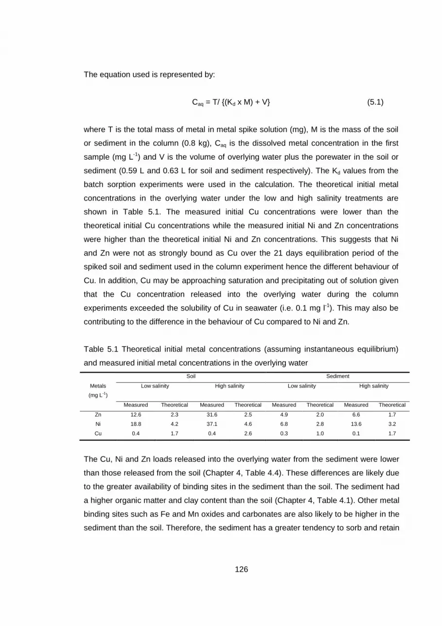
126

The equation used is represented by:

Caq = T/ {(Kd x M) + V} (5.1)

where T is the total mass of metal in metal spike solution (mg), M is the mass of the soil

or sediment in the column (0.8 kg), Caq is the dissolved metal concentration in the first

sample (mg L-1) and V is the volume of overlying water plus the porewater in the soil or

sediment (0.59 L and 0.63 L for soil and sediment respectively). The Kd values from the

batch sorption experiments were used in the calculation. The theoretical initial metal

concentrations in the overlying water under the low and high salinity treatments are

shown in Table 5.1. The measured initial Cu concentrations were lower than the

theoretical initial Cu concentrations while the measured initial Ni and Zn concentrations

were higher than the theoretical initial Ni and Zn concentrations. This suggests that Ni

and Zn were not as strongly bound as Cu over the 21 days equilibration period of the

spiked soil and sediment used in the column experiment hence the different behaviour of

Cu. In addition, Cu may be approaching saturation and precipitating out of solution given

that the Cu concentration released into the overlying water during the column

experiments exceeded the solubility of Cu in seawater (i.e. 0.1 mg l-1). This may also be

contributing to the difference in the behaviour of Cu compared to Ni and Zn.

Table 5.1 Theoretical initial metal concentrations (assuming instantaneous equilibrium)

and measured initial metal concentrations in the overlying water

Soil Sediment

Metals

(mg L-1)


Measured Theoretical Measured Theoretical Measured Theoretical Measured Theoretical

Zn 12.6 2.3 31.6 2.5 4.9 2.0 6.6 1.7

Ni 18.8 4.2 37.1 4.6 6.8 2.8 13.6 3.2

Cu 0.4 1.7 0.4 2.6 0.3 1.0 0.1 1.7

The Cu, Ni and Zn loads released into the overlying water from the sediment were lower

than those released from the soil (Chapter 4, Table 4.4). These differences are likely due

to the greater availability of binding sites in the sediment than the soil. The sediment had

a higher organic matter and clay content than the soil (Chapter 4, Table 4.1). Other metal

binding sites such as Fe and Mn oxides and carbonates are also likely to be higher in the

sediment than the soil. Therefore, the sediment has a greater tendency to sorb and retain

127

the metals more strongly resulting in lower metal loads released into the overlying water.

This is reflected in the higher Cu, Ni and Zn partition coefficients in the sediment than the

soil (Chapter 4, Table 4.2). The differences in the total loads released from the soil and

sediment were statistically significant for Ni (Two-way ANOVA: F = 3.42, p < 0.05) and Zn

(Two-way ANOVA: F = 7.51, p < 0.05) under low salinity and for Cu (Two-way ANOVA: F

= 17.37, p < 0.05) under both salinities.

5.2.2. Effect of salinity on the release of herbicides from the soil and sediment

At pKa < pH, organic bases such as triazines (i.e. simazine and atrazine) exist as neutral

species particularly when the primary sorption domain is organic matter while at pKa >

pH, a considerable amount of the herbicides exist as cations and undergo cation

exchange (Weber et al., 1969; Seol and Lee, 2001). In these experiments, the simazine

and atrazine molecules sorbed to the soil and sediment are likely to be primarily

uncharged because the soil pH (pH 7.1) and sediment pH (pH 7.0) were much larger than

the reported pKa values of simazine (pKa 1.65) (Pacakova et al., 1996) and atrazine (pKa

1.71) (Moreau-Kervevan and Mouvet, 1998). Diuron exists only as a neutral molecule and

hence is not influenced by pH.

The log Kd values of simazine, atrazine and diuron ranged from 3.63 to 3.76 L kg -1, 3.87

to 3.94 L kg-1 and 4.22 to 4.39 L kg -1 respectively in both the soil and sediment (Chapter

4, Table 4.3). Except for simazine, the log Kd values of the herbicides for the sediment

were higher than those for the soil at both 5 and 20 salinities (Chapter 4, Table 4.3)

suggesting that the herbicides were more strongly associated with the sediment than the

soil. To determine if the differences were due to the influence of the herbicide sorption to

organic matter or the clay particles, the organic carbon normalised partition coefficient

(Koc) (i.e. the soil and sediment partition coefficient normalised to the organic carbon

fraction) of the soil and sediment was calculated as:

oc

doc f

KK = (5.2)

where ocf is the organic carbon fraction. The equation assumes that all the herbicide

sorption is due to the organic carbon in the soil and sediment and it is commonly used for

describing the extent of herbicide sorption to soil and sediment (Leake and Gatweiler,

128

1995; Heppell et al., 2009). Since organic matter is made up of approximately 50 % to 58

% organic carbon (Weber et al., 2000; vanLoon and Duffy, 2000), the organic carbon

fraction in this study was assumed to be 54 % of the organic matter content (i.e. average

of 50 % and 58 % organic carbon). Weber et al. (2000) also assumed that organic matter

comprised 54 % organic carbon. The Koc values (expressed on a log10 basis) of simazine,

atrazine and diuron ranged from 3.04 to 3.30 L kg -1, 3.29 to 3.48 L kg -1 and 3.54 to 4.02

L kg -1 respectively. These log Koc values are within the range reported in the literature.

Gawlik et al. (1998) reported Koc values (expressed on a log10 basis) for simazine of 3.07

L kg -1 in soil. Moreau and Mouvet (1997) reported a Koc value (expressed on a log10

basis) of 2.67 L kg -1 for atrazine in soil. The log Koc value for diuron was found to range

from 2.28 to 5.20 L kg -1 in sediment (Comber et al., 2002). Figure 5.2 illustrates that the

Koc values of simazine, atrazine and diuron for the sediment were comparable to those for

the soil suggesting that organic matter was responsible for the differences in binding

between the soil and sediment and organic matter was the controlling factor by which

simazine, atrazine and diuron were bound to the soil and sediment. Since the simazine

and atrazine molecules were primarily uncharged within the soil and sediment pH range

used in this study, the herbicides are likely to be binding to organic matter either by

hydrogen bonding, van der Waal forces, dipole-dipole interaction, hydrophobic

partitioning or a combination of these mechanisms. The precise nature of the binding

mechanisms of these herbicides to the soil and sediment could not be determined from

the data collected.

129

Figure 5.2 Comparison of organic carbon partition coefficients (Koc) for simazine, atrazine

and diuron in the soil and sediment (bars = standard deviation (SD), n = 6).

At the salinity of 5, differences were observed among the log Kd of the individual

herbicides with diuron having the highest log Kd, followed by atrazine and then simazine

in both the soil and sediment (Chapter 4, Table 4.3). These differences indicate that

diuron was most strongly sorbed to the soil and sediment while simazine was the least

sorbed of the three herbicides. The strength of atrazine sorption was intermediate

between that of diuron and simazine. The differences in the hydrophobicity (i.e. n-octanol-

water partition coefficient (log Kow)) of the herbicides may account for these differences in

the binding strength observed among the herbicides. The n-octanol-water partition

coefficient reflects the affinity of an organic compound to bind to natural organic matter.

The higher the log Kow of an organic compound, the more strongly bound the compound

is to organic matter (Hassett and Banwart, 1989; Chiou and Kile, 1994). The

experimentally derived log Kow reported for diuron (2.85) was highest, followed by that of

atrazine (2.68) and then simazine (2.17) (Lewis and Gardiner, 1996; HSE, 1993;

Margoum et al., 2001) indicating that diuron was more hydrophobic compared to atrazine

and simazine. These data support the observation in this present study with diuron being

most strongly associated with the soil and sediment organic matter, followed by atrazine

and then simazine.

0

1

2

3

4

5


Lo

g K

oc

(L K

g-1)

Simazine

Atrazine

Diuron

Sediment Soil

0

1

2

3

4

5


Lo

g K

oc

(L K

g-1)

Simazine

Atrazine

Diuron

Sediment Soil

130

Solution ionic strength and salt concentration can affect the binding of charged organic

compounds to clay particles (Schwarzenbach, Gschwend and Imboden, 2003). In this

study, the log Kd at 5 and 20 salinities were comparable with no significant differences

observed except for simazine in the soil (Chapter 4, Table 4.3). Given that the increase in

salinity had no effect on the sorption of the herbicides further implies that the herbicides

were primarily uncharged and hence, were not binding predominantly by ion exchange

interactions with the negative surface charges on the clay particles. No significant salting

out effect was observed for any of the herbicides as their log Kd values at the salinity of

20 were not significantly higher than those at the salinity of 5 (Chapter 4, Table 4.3). At

the salinity of 20, diuron had the highest log Kd, followed by atrazine and then simazine

(Chapter 4, Table 4.3). This suggests that at the salinity of 20, the relative differences

among the log Kd values of the herbicides is likely due to the binding strength of the

herbicides to organic matter given that the log Kd values and the reported log Kow of the

herbicides were in the same order (i.e. diuron > atrazine > simazine). Several studies

have indicated that the sorption of weakly polar organic compounds such as the studied

herbicides are unaffected by changes in solution ionic strength and salt concentrations

(Schwarzenbach, Gschwend and Imboden, 2003; Voulvoulis et al., 2002). The reason for

the anomalous behaviour of simazine in the soil remains unclear.

The temporal release patterns of simazine, atrazine and diuron from the soil and

sediment into the overlying water in the column experiments showed an initial rapid

release phase with the influx of artificial seawater, followed by a slow release phase for

the remainder of the experiment (Chapter 4, Figure 4.2). The initial rapid release phase is

likely due to the exchange and mixing of the porewater and the artificial seawater leading

to the release of readily available herbicides present in the porewater and weakly sorbed

to the soil and sediment. Thereafter, desorption and diffusion is likely to have transported

the herbicides from the interior of the soil and sediment column towards the surface from

where they are released into the overlying water during the latter slow release phase.

Several studies on the uptake and release of organic contaminants from soil and

sediment have also observed that the release of organic contaminants is biphasic with an

initial rapid release phase and a slow release phase (McCall and Agin, 1985; Kan et al.,

1994; Carroll et al., 1994; Lee et al., 2000). A readily available labile fraction is released

during the initial rapid phase (Carroll et al., 1994; Lee et al., 2000). The latter phase has

been attributed to the slow release of the contaminants due to diffusion into pores within

131

particles (intra-particle diffusion or sorption retarded particle diffusion) (Ball and Roberts,

1991; Wu and Gschwend, 1986) and diffusion into the organic matter matrix (intra-

sorbent diffusion or retarded organic matter diffusion) (Brusseau and Rao, 1989;

Pignatello and Xing, 1996; Brusseau et al., 1991). In these experiments, portions of

simazine, atrazine and diuron may have diffused into the organic matter matrix and the

pores in the soil and sediment particles during the 21 days equilibration period of the

spiked soil and sediment which limited herbicide desorption during the slow release

phase.

The total herbicide loads released into the overlying water from the soil and sediment

under the low salinity treatment were in the order simazine > atrazine > diuron. The total

atrazine and diuron loads were one and two orders of magnitude lower than that of

simazine despite the soil and sediment having been spiked at the same concentration

(Chapter 4, Table 4.5). The order of the partition coefficients (log Kd) of simazine, atrazine

and diuron contrasts with the order of the total load of the individual herbicides released

into the overlying water as shown in Figure 5.3a. This suggests that the relative

difference among the total herbicide loads is due to the strength of binding of the

individual herbicides to the soil and sediment organic matter. Diuron with the highest log

Kd values was most strongly sorbed to the soil and sediment, hence least likely to be

desorbed, followed by atrazine and then simazine. Consistent with these differences in

the binding strength of the herbicides, diuron had the lowest total load while simazine had

the highest total load and the total atrazine load was intermediate between that of

simazine and diuron.

The total simazine, atrazine and diuron loads released into the overlying water from the

soil and sediment at high salinity were not significantly higher than those released into the

overlying water at low salinity (Chapter 4, Table 4.5 ) suggesting that the increase in

salinity did not significantly increase the release of any of the herbicides from the soil and

sediment. This is probably because the herbicide molecules remained predominantly

uncharged at both salinities as indicated by the observed pH range (pH 7.3 to pH 8.1)

under the low and high salinity treatments during the experiments which were

considerably higher than the pKa values of the herbicides (pKa 1.65 for simazine

(Pacakova et al., 1996) and pKa 1.71 for atrazine (Moreau-Kervevan and Mouvet, 1998)).

The increase in salinity, therefore, did not significantly increase herbicide release into the

132

overlying water under these experimental conditions. Similar to the low salinity treatment,

an inverse relationship was observed between the simazine, atrazine and diuron log Kd

values and the total herbicide loads released from the soil and sediment. These findings

suggest that the strength of binding of the herbicides to organic matter is likely to control

the release of these herbicides at high salinity.

Higher total simazine, atrazine and diuron loads were released into the overlying water

from the soil than the sediment during the column experiments (Chapter 4, Table 4.5)

suggesting that the herbicides are more easily desorbed from the soil than the sediment.

This is likely due to the higher organic matter content in the sediment than the soil which

led to stronger binding of the herbicides to the sediment with a lower tendency for

desorption (Chapter 4, Table 4.1) hence, the lower herbicide loads released into the

overlying water.

(a) (b)

Figure 5.3 Total loads of simazine, atrazine and diuron released from the soil and

sediment under (a) low and (b) high salinity treatments (bars = standard deviation (SD), N

= 3). The inset graphs are the log Kd of simazine, atrazine and diuron for the soil and

sediment at the respective salinities.

0

500

1000

1500

2000

2500

simazine atrazine diuron

Tota

l load

(µg)

Soil

Sediment

3

4

5


0

500

1000

1500

2000

2500


Tota

l load

(µg)

Soil

Sediment

3

4

5


0

500

1000

1500

2000

2500


Tota

l load

(µg)

Soil

Sediment

3

4

5


0

500

1000

1500

2000

2500


Tota

l load

(µg)

Soil

Sediment

3

4

5


133

5.3. Effect of drying and rewetting on the release of metals and herbicides from soil and

sediment

Several studies have examined the effect of drying and rewetting on microbial activity,

CO2 release and organic matter mineralisation in soils (Degens and Sparkling, 1995; Van

Gestel et al., 1993; Kieft et al., 1987, Fierer and Schimel, 2003; Bottner, 1985; Haney et

al., 2004, Franzluebbers et al., 1990; Miller et al., 2005; Pulleman and Tietema, 1999).

These studies have observed that drying and rewetting of soil can lead to the disruption

of aggregates which exposes organic matter trapped within the soil. The exposure of the

organic matter stimulates microbial activity which leads to enhanced organic matter

mineralisation and CO2 release (Degens and Sparkling, 1995; Van Gestel et al., 1993;

Fierer and Schimel, 2003). An increase in organic matter mineralisation in soil can also

result in an increase in the release of DOC (Fierer and Schimel, 2003; Miller et al., 2005;

Reemtsma et al., 2000). Unlike the soil, studies on the effect of drying and rewetting on

microbial activity, CO2 release and organic matter mineralisation in sediment are limited

and have focussed on changes in microbial metabolism and nutrient cycling (Amalfitano

et al., 2008; Baldwin and Mitchell, 2000). The mineralisation of organic matter due to

drying and rewetting has potential implications for the release of metals and herbicides

from the soil and sediment. Cu, Ni and Zn can bind to organic matter with Cu having the

highest binding affinity for organic matter among these metals (Forstner and Wittmann,

1981; McBride, 1994). Organic contaminants such as simazine, atrazine and diuron bind

to organic matter (Gevao et al, 2000; Pignatello and Xing, 1996). Therefore, an increase

in organic matter mineralisation due to drying and rewetting can result in the release of

the organic matter associated metals and herbicides.

In these experiments, the soil and sediment were inundated with artificial seawater at a

salinity of 20 and subjected to two drying-rewetting treatments in order to test the

hypothesis that organic matter mineralisation will be increased during drying and

rewetting of the soil and sediment leading to the release of organic matter associated

metals and herbicides into the overlying water. In addition to the concentration of the

metals, herbicides and DOC released into the overlying water, CO2 release from the fully

wet and dried-rewet soil and sediment were measured and the carbon mineralisation

rates were determined to reflect organic matter mineralisation. The changes in soil and

sediment microbial biomass before drying, after drying and after rewetting were also

measured. The changes in CO2 release, carbon mineralisation rates and microbial

134

biomass will first be discussed, followed by the contaminant release from the soil and

sediment into the overlying water after drying and rewetting.

5.3.1 CO2 release, carbon mineralisation rate and microbial biomass of soil and sediment

The cumulative CO2 release and the carbon mineralisation rates were higher in the fully

wet sediment compared to the fully wet soil (Chapter 4, Figure 4.11 and 4.12). The

microbial biomass was also higher in the sediment compared to the soil before drying

(Chapter 4, Figure 4.15). Unlike soil where the organic matter is derived mainly from the

decomposition of plant debris and roots (Hedges and Kile, 1995), the major input of

organic matter in estuarine sediment is rapidly sinking particles of terrestrial and marine

origin which have undergone extensive mineralisation of the labile organic matter fraction

in the water column before accumulating in the sediment (Cotano and Villate, 2006;

Hedges and Kiel, 1995). Therefore, organic matter in these sediments comprises highly

degraded and refractory organic material (Baldock et al., 2004; Hedges and Oades,

1997; Gallizia et al., 2004). Although the proportion of the labile and refractory organic

matter pools in the soil and sediment used in this study were not evaluated, the sediment

organic matter is likely to be more refractory and hence less mineralisable than the soil

organic matter. Hence, the higher carbon mineralisation rates and CO2 release from the

sediment compared to the soil were probably due the higher sediment microbial biomass

which in turn led to higher microbial activity and mineralisation in the sediment compared

to the soil.

The cumulative CO2 release and the carbon mineralisation rates in the soil and sediment

subjected to the dry-rewet treatment were two to three orders of magnitude higher than

those observed in the fully wet soil and sediment (Chapter 4, Section 4.5.1 and 4.5.2).

This suggests that the drying-rewetting treatment of the soil and sediment enhanced

carbon mineralisation and the release of CO2. The higher CO2 release may be due to the

mineralisation of carbon exposed to microbial activity by drying and rewetting. Dead

microbes in the soil due to drying can serve as a carbon source for mineralisation by the

surviving microbes following rewetting and lead to an increase in CO2 release (Bottner,

1985; Haney et al., 2004). In this study, no reduction in the soil microbial biomass pool

was observed after drying the soil (Chapter 4, Figure 4.15) suggesting that the soil

microbes survived the drying period. Hence, it is unlikely that dead microbial biomass

was the organic carbon source responsible for the higher mineralisation and CO2 release

135

from the soil in these experiments. This is possibly because the microbes in the soil were

resistant to the imposed drying temperature of 25 0C. Since the organic carbon source

cannot be explained by dead microbial biomass during drying, the other possible carbon

source is the soil organic matter. Hence, the higher mineralisation and CO2 release from

the soil is likely due to increased microbial activity on the soil organic matter previously

protected in aggregates but rendered more available to the heat resistant microbes as a

result of drying and rewetting. In addition, the increase in the soil microbial biomass after

drying and rewetting (Chapter 4, Figure 4.15), which indicates microbial population

growth, may have also contributed to the higher mineralisation of organic matter and CO2

release from the soil. In the natural soil environment, the soil microbial population is

exposed to external stresses such as temperature changes and drying-rewetting cycles,

hence they were rapidly adaptable to the experimental conditions which probably resulted

in their growth. In the sediment, a reduction in the microbial biomass was observed after

drying (Chapter 4, Figure 4.15) indicating the death of part of the microbial population

during the drying period, probably because the microbes were less resistant to drying

since they are adapted to living in more stable environmental conditions under seawater.

However, the surviving microbes effectively mineralised the available carbon source,

which resulted in the increased CO2 release from the sediment. The mineralised carbon

source is likely to have been the dead microbial cells because the total carbon from the

dead microbes after drying was 16 µg C g-1 sediment and the total carbon that was

released as CO2 over the course of the experiment was 1.31 µg C g-1 sediment indicating

that the CO2 released may have resulted mainly from the mineralisation of the dead

microbes. It is also possible that the mineralisation of sediment organic matter exposed to

microbial activity due to drying and rewetting led to the higher CO2 release. However, this

is unlikely because recently accumulated labile organic material are more readily

mineralised during drying and rewetting (Degens and Sparkling, 1995; Marumoto et al.,

1977) and the labile fraction of sediment organic matter are extensively mineralised in the

water column resulting in highly degraded and refractory organic matter in sediments

(Baldock et al., 2004; Hedges and Kile, 1995; Cotano and Villate, 2006; Hedges and

Oades, 1997; Gallizia et al., 2004; Keil et al., 1994) which tends to be less mineralisable.

Therefore, the dead microbes are likely to have been the carbon source that was

mineralised in the sediment which led to the higher mineralisation rates and CO2 release

from the sediment.

136

5.3.2. Effect of drying and rewetting on the release of metals and herbicides from soil and

sediment

Comparisons were made between the total Cu, Ni and Zn loads released into the

overlying water under the drying-rewetting treatment and those released under the high

salinity treatment described in Section 5.2.1 (referred to in this section as fully wet

treatment). Differences between the total contaminant loads released under these two

treatments were attributed to the effect of drying and rewetting on metal and herbicide

release. The release pattern of the metals and herbicides from the soil and sediment

were described in Section 5.3.2.1, the effect of drying and rewetting on the release of Cu,

Ni and Zn from the soil was discussed in Section 5.3.2.2 and Sections 5.3.2.3 goes on to

discuss the effect of drying and rewetting on metal release from the sediment. The effect

of a second drying-rewetting treatment was also discussed relative to the first drying-

rewetting treatment in the respective sections. The effect of drying and rewetting on

herbicide release from the soil and sediment were discussed in a similar manner as the

metals in Sections 5.3.2.4 and 5.3.2.5.

5.3.2.1. Release patterns of the metals and herbicides from the soil and sediment under

the drying-rewetting treatment

Under the drying-rewetting treatment, there was an initial rapid release of the metals and

herbicides from the soil and sediment with the influx of artificial seawater, followed by a

slow release into the overlying water (Chapter 4, Figure 4.5 and 4.7). These release

patterns were similar to those observed under the fully wet treatment. The initial rapid

release was likely due to the exchange and mixing of the soil/sediment porewater and the

artificial seawater which led to the release of the readily available metals and herbicides

present in the porewater and weakly sorbed to the soil and sediment. Afterwards,

desorption and diffusion is likely to have transported the metals and herbicides from the

interior of the soil and sediment column towards the surface for release into the overlying

water. Several studies have described metals and herbicides release as a two phase

process with an initial rapid release phase, followed by a slow release phase (Mustafa et

al., 2004; Millward and Liu, 2003; Kan et al., 1994; Carroll et al., 1994) which have been

attributed to various mechanisms described in Section 5.2.1 and 5.2.2 for metals and

herbicides respectively. In this study, portions of the metals and herbicides may have

become strongly bound to the soil and sediment during the 21-days equilibration period of

the spiked soil and sediment which were slowly desorbed and released into the overlying

137

water after the initial rapid release. The various mechanisms described in Section 5.2.1

and 5.2.2 may also account for the metals and herbicides becoming strongly bound in

this study.

5.3.2.2. Effect of drying and rewetting on the release of metals from soil

The higher CO2 release and mineralisation rates in the dried-rewet soil compared to the

fully wet soil and the increase in the soil microbial biomass after drying and rewetting

indicate higher soil organic matter mineralisation due to drying and rewetting. In addition,

the total DOC load released from the soil into the overlying water under the drying-

rewetting treatment was higher than that released under the fully wet treatment (Chapter

4, Table 4.11) further suggesting that drying and rewetting led to higher mineralisation of

soil organic matter. The total DOC load released into the overlying water was

approximately 104 % higher under the drying-rewetting treatment relative to the fully wet

treatment. Cu, Ni and Zn bind to organic matter, Fe and Mn oxides, carbonates and clay

minerals in soil (Alloway, 1995; McBride, 1994). Therefore, it was expected that the Cu,

Ni and Zn associated with the soil organic matter will be released into the overlying water

and result in higher total metal loads in the overlying water under the drying-rewetting

treatment relative to the fully wet treatment. In addition, the increase in the total metal

loads under the drying-rewetting treatment relative to the fully wet treatment was also

expected to be in the order Cu > Zn > Ni due to their affinity to bind to organic matter

(Filgueiras et al., 2002; Forstner and Wittmann, 1981; Alloway, 1995). In agreement with

the expectations, the total Cu, Ni and Zn loads released into the overlying water under

the drying-rewetting treatment were higher than those released under the fully wet

treatment (Chapter 4, Table 4.7) indicating that drying and rewetting led to the release of

organic matter associated Cu, Ni and Zn into the overlying water. The total Ni load was

significantly higher (Two-way ANOVA: F = 19.01, p < 0.05). The total Ni, Cu and Zn loads

released into the overlying water under the drying-rewetting treatment relative to the fully

wet treatment increased by approximately 110 %, 66 % and 61 % respectively. Hence,

the relative percentage increase among the metals was in the order Ni > Cu > Zn which

was different from the expected order, probably due to the association of the metals with

DOC.

Several studies have observed that DOC forms soluble complexes with Cu, Ni and Zn

which can facilitate their release from soils (Gerringa et al., 1990; Kalbitz and Wennrich,

138

1998; Sauve et al., 1997). In this study, in order to determine if DOC complexation with

the metals under the drying-rewetting treatment was important for the release of Cu, Ni

and Zn, the concentrations of Cu, Ni, Zn and DOC in the overlying water were analysed

by linear regression. The results of the linear regression indicated that there were

significant relationships between the metals and DOC with 50 %, 79 % and 55 % of the

variations in the Cu, Ni, Zn concentrations explained by the variation in the DOC

concentrations (p < 0.05). These results indicate that significant proportions of Cu, Ni and

Zn in the overlying water were released from the soil as DOC-complexes. This was

treated as evidence for suggesting that the formation of DOC-metal complexes was

contributing to the release of these metals under the drying-rewetting treatment. Given

that 79 % of the variation in Ni concentrations was explained by DOC and Ni had the

highest relative increase in the total load released compared to the Cu and Zn (i.e. 110

%) suggests that Ni formed complexes with DOC more readily than Zn and Cu. Tuner et

al. (1998) demonstrated that Ni has a relatively low particle affinity due to its strong

association with DOC. The release of the metals as DOC complexes into the overlying

water is likely to account for why the increase in the total metal loads under the drying-

rewetting treatment relative to the fully wet treatment did not follow the expected order (i.

e. Cu > Zn > Ni).

The total DOC load released into the overlying water decreased significantly under the

second drying-rewetting treatment compared to the first treatment (Two-way ANOVA: F =

33.20, p < 0.05) (Chapter 4, Table 4.12) suggesting lower organic matter mineralisation.

This is likely due to less organic matter available after the mineralisation under the first

drying-rewetting treatment. Fierer and Schimel (2002) also observed a decrease in DOC

as a result of a decrease in organic matter mineralisation with subsequent drying and

rewetting of soil. The total DOC load released into the overlying water under the second

drying-rewetting treatment as a proportion of the total DOC load released under the first

drying-rewetting treatment reduced by approximately 72 %. Similar to the total DOC load,

the total Cu, Ni and Zn loads released into the overlying water under the second drying-

rewetting treatment were significantly lower than those released under the first treatment

(Two-way ANOVA: F = 17.32, p < 0.05 for Cu; F = 38.41, p < 0.05 for Ni and F = 27.5 , p

< 0.05 for Zn) (Chapter 4, Table 4.8). The total Cu, Ni and Zn loads released into the

overlying water under the second drying-rewetting treatment as a proportion of the total

metal loads released under the first drying-rewetting treatment reduced by approximately

139

77 %, 74% and 77% respectively. This suggests that, after the first drying-rewetting

treatment, there was less organic matter for mineralisation which in turn led to reduced

release of organic matter associated metals as well as DOC associated metals hence the

lower total metal loads observed in the overlying water under the second drying-rewetting

treatment. Less metals in the soil after the metal release under the first drying-rewetting

treatment is also likely to have contributed to the lower total metal loads released into the

overlying water under the second drying-rewetting treatment.

5.3.2.3. Effect of drying and rewetting on the release of metals from sediment

In the sediment, drying and rewetting led to an increase in mineralisation hence the

higher CO2 release and mineralisation rates observed in the dried-rewet sediment

compared to the fully wet sediment. As previously discussed in Section 5.3.1, the higher

CO2 release and mineralisation rates in the sediment are likely due to the mineralisation

of dead microbes resulting from the death of part of the microbial population during drying

rather than the mineralisation of sediment organic matter. Therefore, organic matter

associated metals were unlikely to be released into the overlying water. The total Cu, Ni

and Zn loads released into the overlying water from the sediment under the drying-

rewetting treatment were lower than those released under the fully wet treatment

(Chapter 4, Table 4.7). The total Cu, Ni and Zn loads released into the overlying water

were approximately 67 %, 65 % and 73 % lower under the drying-rewetting treatment

relative to the fully wet treatment. Significant differences between the total loads released

under the drying-rewetting and fully wet treatment were observed for Cu (Two-way

ANOVA: F = 8.15, p < 0.05) and Ni (Two-way ANOVA: F = 8.50, p < 0.05). The lower

total metal loads released under the drying-rewetting treatment compared to the fully wet

treatment was probably due to the adsorption of the metals to Fe and Mn oxides formed

during the drying period. Bordas and Bourg (1998) and Thomson et al. (1980) reported

that drying of oxic sediments at 25 OC resulted in the formation of Fe and Mn oxides

which led to decreased Cu and Zn extractability, with the effect increasing with an

increase in drying temperature. Rapin et al. (1996) also observed that air-drying led to a

decrease in the extractability of Zn. This was attributed to changes in the chemistry of Fe

and Mn oxides caused by exposure to air. These studies indicate that drying of oxic

sediments leads to a change in the distribution of metals to more strongly bound forms.

Accordingly, the adsorption of the metals to Fe and Mn oxides formed as the sediments

were exposed to air during the 7 days drying period in these experiments may account for

140

the lower total Cu, Ni and Zn loads released into the overlying water under the drying-

rewetting treatment compared to the fully wet treatment (Chapter 4, Table 4.7).

Similar to the metals, the total DOC load released into the overlying water under the

drying-rewetting treatment was lower compared to that released under the fully wet

treatment (Chapter 4, Table 4.11). The total DOC load was approximately 67 % lower

under the drying-rewetting treatment relative to the fully wet treatment. In order to

determine if the formation of DOC-metal complexes was contributing to the release of Cu,

Ni and Zn from the sediment, a linear regression analysis of the DOC, Cu, Ni and Zn

concentrations in the overlying water was conducted. The results of the regression

analysis indicate that the relationships between DOC and the metals were not significant

(p > 0.05). The variation in the DOC concentrations could account for only 8 %, 28 % and

13 % of the observed variation in the Cu, Ni and Zn concentrations in the overlying water.

This suggests that significant proportions of the metals were not released into the

overlying water as DOC-metal complexes under these experimental conditions. It is

notable that the variation in the Ni concentrations explained by DOC was highest

compared to that of Cu and Zn suggesting that Ni had the greatest affinity to form

complexes with DOC compared to the other metals.

The total Cu, Ni and Zn loads released into the overlying water under the second drying-

rewetting treatment were lower than those released under the first drying-rewetting

treatment. The total Cu, Ni and Zn loads released into the overlying water under the

second drying-rewetting treatment as a proportion of the total metal loads released under

the first drying-rewetting treatment reduced by approximately 50 %, 25 % and 28 %

respectively. The lower total metal loads in the overlying water suggests further

adsorption of the metals to the Fe and Mn oxides formed when the sediments were

exposed to air during the drying period hence the lower total metal loads in the overlying

water under the second drying-rewetting treatment.

5.3.2.4 Effect of drying and rewetting on the release of herbicides from soil

The higher total DOC load released from the soil under the drying-rewetting treatment

compared to the fully wet treatment, the higher CO2 release and mineralisation rates in

the dried-rewet soil compared to the fully wet soil and the increase in soil microbial

biomass after drying and rewetting all suggest that drying and rewetting led to a higher

141

mineralisation of soil organic matter. As a result, higher total herbicide loads were

expected to be released into the overlying water under the drying-rewetting treatment

compared to the fully wet treatment given that the herbicides were binding primarily to

organic matter. Also, the percentage increase in the total herbicide loads released under

the drying-rewetting treatment relative to the fully wet treatment were expected to be in

the order: diuron > atrazine > simazine due to their strength of binding to organic matter.

Diuron is the most hydrophobic (log Kow of 2.85) of the studied herbicides and thus the

most strongly bound to organic matter, followed by atrazine (log Kow of 2.68) and then

simazine (log Kow of 2.17) (Lewis and Gardiner, 2006; HSE, 1993; Margoum et al., 2001).

In agreement with the expectations, the increase in the total herbicide loads released into

the overlying water followed the expected order with diuron > atrazine > simazine. The

total atrazine and diuron loads in the overlying water under the drying-rewetting treatment

relative to the fully wet treatment increased by approximately 29 % and 42% respectively

while the simazine load decreased by approximately 28 %. The relative percentage

increase of diuron was greater than that of atrazine and simazine which is consistent with

the hydrophobicity of the herbicide and hence its strength of binding to organic matter.

The percentage decrease in the total simazine load under the drying-rewetting treatment

relative to the fully wet treatment may be due to simazine degradation under the drying-

rewetting treatment.

Several studies have observed that the mobility of herbicides such as those considered in

this study can be enhanced due to their complexation with DOC (Graber et al., 1995; Gao

et al., 1998). In this study, the higher total DOC load and the higher total herbicide loads

released into the overlying water under the drying-rewetting treatment compared to the

fully wet treatment suggests that the herbicides may be released from the soil as DOC-

complexes. In order to determine if the release of the herbicides as DOC-complexes was

important in these experiments, the DOC, simazine, atrazine and diuron concentrations in

the overlying water were analysed by linear regression. The results of the analysis

indicates that there were significant relationships between DOC and the herbicides with

the variations in the DOC concentrations accounting for 65%, 68% and 76% of the

variations in the atrazine, diuron and simazine concentrations respectively (p < 0.05).

These results suggest that significant proportions of the herbicides were released as

DOC-complexes from soil into the overlying water.

142

The total DOC load released into the overlying water was significantly lower under the

second drying-rewetting treatment compared to the first drying-rewetting treatment (Two-

way ANOVA: F = 33.20, p < 0.05) (Chapter 4, Table 4.12) suggesting lower organic

matter mineralisation under the second drying-rewetting treatment. The total DOC load

released into the overlying water under the second drying-rewetting treatment as a

proportion of the total load released under the first drying-rewetting treatment reduced by

approximately 72 %. This is probably due to less organic matter available for

mineralisation after the first drying-rewetting treatment. Similar to the total DOC load, the

total simazine, atrazine and diuron loads released into the overlying water under the

second drying-rewetting treatment were lower than those released under the first

treatment. Significant differences in the total loads between the first and second drying-

rewetting treatments were observed for atrazine (Two-way ANOVA: F = 4.82, p < 0.05)

and diuron (Two-way ANOVA: F = 12.08, p < 0.05) (Chapter 4, Table 4.10). These

findings suggest that there was less organic matter mineralisation under the second

drying-rewetting treatment which in turn resulted in less release of organic matter

associated and DOC associated herbicides hence the lower herbicide loads released

under the second drying-rewetting treatment. In addition, the lower total herbicide loads

released into the overlying water is also likely due to less herbicides in the sediment for

release at the start of the second drying-rewetting treatment. The total simazine, atrazine

and diuron loads released under the second drying-rewetting treatment as a proportion of

the total load released under the first drying-rewetting treatment reduced by

approximately 50%, 61% and 71% respectively. The relative differences among the

herbicides was consistent with the hydrophobicity (log Kow) of the herbicides suggesting

that the strength of binding of the herbicides to organic matter also contributed to the

release of the herbicides under the second drying-rewetting treatment.

Microbial population, oxygen availability and temperature are important factors facilitating

the degradation of herbicides (Alexander, 1981; Meakins et al., 1995; Larsen et al., 2001)

The degradation of simazine, atrazine and diuron into their degradation products, which

are hydroxysimazine, desethylsimazine, hydroxyatrazine, desethylatrazine and 3,4-

dichloroaniline, directly results in a decrease in the herbicide loads in the soil and hence,

lower concentrations are released into the overlying water during the column

experiments.

143

A study by White et al. (1998) on the effect of wetting and drying cycles on the

bioavailability of aged organic contaminants in soil found that subjecting soil to drying and

wetting cycles enhanced the degradation of phenanthrene. Accordingly, the decrease in

the total simazine, atrazine and diuron loads in the overlying water in these experiments

may also be due to degradation. Degradation due to the experimental drying temperature

is unlikely because the temperature under the first and second drying-rewetting

treatments were the same. However, herbicide degradation due to increased microbial

activity as a result of the microbial population growth within the soil column may have

contributed to the decrease in the total simazine, atrazine and diuron loads in the

overlying water under the second drying-rewetting treatment. Microbial degradation may

also account for the decrease in the total simazine load released under the first drying-

rewetting treatment relative to the fully wet treatment. Given the data collected in this

study, it is difficult to determine the relative importance of degradation under these

experimental conditions.

5.3.2.5. Effect of drying and rewetting on the release of herbicide from sediment

Higher CO2 release and mineralisation rates were observed under the drying-rewetting

treatment compared to the fully wet treatment (Chapter 4, Section 4.5.2). As previously

discussed in Section 5.3.1., dead microbes due to drying rather than sediment organic

matter is the likely carbon source that was mineralised to CO2 by the microbes that

survived the drying period. This suggests that the herbicides associated with the

sediment organic matter were unlikely to be released into the overlying water under the

drying-rewetting treatment. The total simazine, atrazine and diuron loads released into

the overlying water under the drying-rewetting treatment were approximately 64 %, 44 %

and 50 % lower relative to the fully wet treatment. These lower total herbicide loads in the

overlying water under the drying-rewetting treatment compared to the fully wet treatment

is likely to be a consequence of simazine, atrazine and diuron degradation within the

sediment column under the drying-rewetting treatment. Several studies have reported

that high temperatures and adequate oxygen supply favours the microbial degradation of

herbicides (Seol and Lee, 2001; Larsen et al., 2001; Warren et al., 2003). Topp et al.

(1995) observed atrazine degradation under aerobic conditions but not under anaerobic

conditions in sediments. This suggests that herbicides can be more readily degraded in

aerated sediments than in water-saturated sediments. In this study, the exposure of the

144

sediment to air and the drying temperature (i.e. 25 0C) during the 7-days drying period is

likely to have provided more suitable conditions for the microbial degradation of simazine,

atrazine and diuron under the drying-rewetting treatment compared to the fully wet

treatment leading to the lower herbicide loads under the drying-rewetting treatment.

Several studies have indicated that atrazine and simazine are moderately persistent

herbicides with degradation rates in sediments ranging from 15 – 30 days half-life for

atrazine (Jones et al., 1982), 29 - 57 days half-life for atrazine and 26 - 44 days half-life

for simazine (Labbs et al., 2007). Howard et al. (1991) reported a degradation rate of 120

days half-life for diuron. In this study, the degradation rate of the herbicides could not be

evaluated given the data collected.

The total DOC load released into the overlying water was approximately 67 % lower

under the drying rewetting treatment compared to the fully wet treatment. This lower total

DOC load and the lower total herbicide loads released under the drying-rewetting

treatment compared to the fully wet treatment suggest that there was a relationship

between the release of the herbicides and DOC. A linear regression analysis was

conducted with the DOC, simazine, atrazine and diuron concentrations released into the

overlying water to determine if the herbicides release as DOC-complexes was important

in these experiments. The result of the analysis indicates that the relationships between

the herbicides and DOC were not significant (p > 0.05). Only 41%, 31% and 22% of the

variation in simazine, atrazine and diuron concentrations in the overlying water could be

explained by the variation in the DOC concentrations. This suggests that the release of

the herbicides as DOC-complexes was not significantly contributing to the release of

atrazine, diuron and simazine from the sediment into the overlying water.

The total simazine, atrazine and diuron loads released into the overlying water under the

second drying-rewetting treatment were slightly lower than those released under the first

drying-rewetting treatment (Chapter 4; Table 4.10). The total simazine, atrazine and

diuron loads released under the second drying-rewetting treatment as a proportion of the

total load released under the first drying-rewetting treatment reduced by approximately 4

%, 31 % and 14 % respectively. These slightly lower herbicide loads released under the

second drying-rewetting treatment are likely due to further degradation occurring within

the sediment column during the second drying period. In addition, less herbicides in the

sediment for release after degradation under the first drying-rewetting treatment is also

145

likely to have contributed to the lower total herbicide loads released into the overlying

water under the second drying-rewetting treatment.

5.4. Summary and conclusion

This chapter has identified that the release of metals (Cu, Ni and Zn) from the soil and

sediment into the overlying water at low and high salinities (i.e. 5 and 20 respectively)

was dependent on the strength of binding of the metals to the soil and sediment,

competition between seawater cations and the sorbed metals for binding sites on the soil

and sediment particles and the formation of soluble complexes between the sorbed

metals and seawater anions. The importance of the strength of binding of the metals for

release was revealed by the inverse relationship between the total metal loads (which

followed the order Ni > Zn > Cu) and their log Kd values (which was in the order Cu > Zn

> Ni). Higher total Zn and Ni loads were released into the overlying water at high salinity

than at low salinity which was likely due to an increase in the competition and

complexation reactions between the seawater cations, anions and the sorbed metals. Cu

was more strongly bound to the soil and sediment than Ni and Zn which limited its

release compared to the release of Ni and Zn. The metal release was lower from the

sediment than the soil due to greater availability of binding sites and hence greater metal

retention in the sediment. The release of the herbicides from the soil and sediment into

the overlying water at low and high salinity was mainly dependent on the strength of

binding of the herbicides to the soil and sediment organic matter which was in the order

diuron > atrazine > simazine. The total herbicide loads released into the overlying water

followed the order simazine > atrazine > diuron, with higher total loads released from the

soil than the sediment due to the higher organic matter content in the sediment. The

increase in salinity did not significantly increase the release of any of the herbicides from

the soil and sediment probably because the herbicides molecules were primarily

uncharged at both low and high salinity.

Drying and rewetting resulted in an increase in the mineralisation of soil organic matter

and the total DOC load released into the overlying water due to increased microbial

activity on the soil organic matter previously protected within the soil aggregates but

made available by drying and rewetting. This in turn led to the release of organic matter

associated metals and herbicides into the overlying water which was indicated by the

higher total metal and herbicide loads in the overlying water under the drying-rewetting

146

compared to the fully wet experimental conditions. The significant relationships between

DOC, the metals and herbicides which were demonstrated by the results of the linear

regression analysis provided evidence that the release of the metals and herbicides as

DOC-complexes from the soil was important. The total metal and herbicide loads

released into the overlying water were significantly lower after the second drying and

rewetting of the soil compared to the first drying and rewetting which was probably due to

less release of organic matter associated and DOC-associated metals and herbicides

and less metals and herbicides in the soil for release at the start of the second drying and

rewetting.

Drying and rewetting led to the mineralisation of dead microbes in the sediment which

resulted from the death of part of the microbial population during drying, indicated by the

observed decrease in the sediment microbial biomass after drying the sediment. The

organic matter associated metals and herbicides were unlikely to be released into the

overlying water since the sediment organic matter was not the carbon source that was

mineralised. In comparison with the fully wet treatment, lower total Cu, Ni and Zn loads

were released into the overlying water from the sediment after drying and rewetting

probably due to the adsorption of the metals to Fe and Mn oxides formed when the

sediments were exposed to air during the 7-days drying period. Similarly, the exposure of

the sediment to air and the drying temperature during the drying period may have led to

the degradation of the herbicides in the sediment column and the lower total simazine,

atrazine and diuron total loads released into the overlying water after drying and rewetting

relative to the fully wet experimental conditions. The results of a linear regression

analysis showed that there were no significant relationships between DOC, the metals

and herbicides indicating that DOC-complexation was unlikely to be important for metal

and herbicide release from the sediment. The lower total metal and herbicide loads

released into the overlying water after the second drying and rewetting of the sediment

compared to the first drying and rewetting was likely a consequence of further metal

adsorption to Fe and Mn oxides and further herbicide degradation during the second

drying period as well as less herbicides in the sediment for release after their degradation

under the first drying-rewetting treatment.

Similar temporal release patterns were observed under the low salinity, high salinity and

drying-rewetting experimental conditions with an initial rapid release of the metals and

147

herbicides, followed by a slow release into the overlying water. The initial rapid release

was attributed to the release of readily available metals and herbicides present in the

porewater and weakly sorbed to the soil and sediment, followed by the slow release of

strongly bound metals and herbicides.

148

Chapter 6: Mechanisms of metal and herbicide releas e from soil and

sediment

6.1. Introduction

One justification for the implementation of managed realignment is that they provide a

sink for contaminants from estuarine waters (NRA, 1994). Andrews et al. (2006) indicated

that managed realignment would increase sediment storage capacity and provide an

effective sink for metals and other particle reactive contaminants and increase the burial

of organic carbon. This is further supported by Shepherd et al. (2007) who indicated that

organic carbon, nitrate and phosphorus storage would be enhanced in managed

realignment schemes. These studies suggest that managed realignment provides

biogeochemical benefits for the environment. However, the periodic tidal inundation of the

soil and sediment by seawater in managed realignment sites may cause changes in the

physicochemical conditions in the soil and sediment which can affect the binding of the

metals and herbicides to the soil and sediment. Changes in salinity, pH and redox

potential can affect the binding of contaminants to soil and sediment and lead to their

release (Gambrell et al., 1991; Calmano et al., 1992). This occurrence of these changes

in the soil and sediment in managed realignment sites following tidal inundation can lead

to the release of contaminants such as metals and herbicides present in the pre-

inundated soil and sediment into the overlying water. In addition, the periodic inundation

of the soil and sediment can lead to drying-rewetting cycles which can enhance the

mineralisation of organic matter and consequently the release of DOC and organic matter

associated metals and herbicides. Although the effects of such mobilisation are difficult to

assess, it has implications for water quality and can pose a risk to higher organisms. The

connection with water quality is of concern in relation to the EU Water Framework

Directive (222/60/EC) which requires that good ecological status of surface, transitional

and coastal waters be maintained.

In this study, laboratory column microcosm experiments were conducted with the aim of

examining the potential release of metals (Cu, Ni and Zn) and herbicides (simazine,

atrazine and diuron) from soil and sediment in managed realignment sites following tidal

inundation. The experiments focused on the effect of salinity and drying-rewetting cycles

on the release of these contaminants from the soil and sediment into overlying water. The

metal and herbicide concentrations released into the overlying water under two salinity

149

treatments (5 and 20 referred to as low and high salinity) and drying-rewetting treatment

were measured during the experiments. The observations from these experiments

discussed in Chapter 5 indicated that there was an initial rapid release of Cu, Ni, Zn,

simazine, atrazine and diuron from the soil and sediment, followed by a slow continued

release for the remainder of the experiments. These release patterns were indicative of

the diffusion of the metals and herbicides from the soil and sediment into the overlying

water. The objective of this chapter was to investigate, using a diffusion model, the

mechanisms of metal and herbicide release from the soil and sediment under the

experimental conditions in this study. This was achieved by:

• using the diffusion model to predict the metal and herbicide concentrations

released into the overlying water from the soil and sediment and

• assessing the agreement between the model predictions and the experimental

metal and herbicide concentration data using several assessment methods.

Disagreements between the model predictions and the experimental data were

attributed to other mechanisms contributing to the metals and herbicides release

from the soil and sediment in the column microcosm experiments but not

accounted for in the model.

The model simulations were based on the metal and herbicide porewater concentrations

in the soil and sediment at the start of the column microcosm experiments, the properties

of contaminants and the soil/sediment properties. Statistical goodness-of-fit measures

were used to evaluate the performance of the model. The following sections examine the

modelling of diffusive contaminant transport, the various statistical goodness of fit criteria

used for assessing the performance of models, describes the model developed in this

study and the model parameters used for the model simulations.

6.2. Diffusive contaminant transport

Diffusion is an important contaminant transport mechanism in natural porous media such

as soil and sediment (Grathwohl, 1998). Diffusion describes mass transport due to the

random thermal motion of solute molecules (Grathwohl, 1998). It involves the net transfer

of solute molecules from regions of high concentration to regions of low concentration.

Several studies have examined contaminant diffusion in water-saturated soil and

sediment environments. For example, dissolved metal fluxes have been determined by

using porewater gradients of the dissolved metals to estimate the diffusive flux of the

150

metals at the sediment water interface (Sawlan and Murray, 1983; Caetano et al., 2007).

Monterroso et al. (2007) estimated the diffusive fluxes of Cu, Pb, Zn, Cd, Fe and Mn from

the top 2.5 cm of a sediment core using Fick’s Law and found that the sediment-water

exchange of the metals were hindered by sulphide formation. Several studies have also

examined the diffusive transport of organic contaminants in soil and sediment (Valsaraj et

al., 1998; Qaisi et al., 1996; Valsaraj and Sojitra, 1997; Allan et al., 2004; Daniels et al.,

1998, Bekhit and Hassan, 2005). In addition, diffusion based models have also been

used to examine the sorption/desorption kinetics of organic contaminants in soil and

sediment particles in several studies (Pignatello et al., 1993; Ball and Roberts, 1991,

Brusseau et al., 1991).

In the modelling context, the main advantage of a simple model, such as the one

developed in this study, concerns parsimony (i.e. using no more complex a model than is

absolutely necessary) (Wainright and Mulligan, 2004). A parsimonious model is usually

the one with the greatest predictive power and the least parameters and process

complexity (Wainright and Mulligan, 2004). Thomann (1998) emphasised that there is a

real danger that model complexity will be equated to a greater level of model success in

representing the actual system. Simple models can achieve as high a level of

performance as more complex models in terms of simulating the target variables (Perrin

et al., 2001). Complex models usually need more input parameters for more detailed

process descriptions and this has advantages from a theoretical point of view (Wainright

and Mulligan, 2004; Wania and Mackay, 1999). However, the greater the number of input

parameters, the more likely they are to be cross-correlated with each extra parameter

adding relatively little to model predictive capability (Wainright and Mulligan, 2004).

Moreover, the relatively large observational data sets needed for the evaluation of the

performance of complex models are usually not available, thereby increasing the degree

of uncertainty associated with the model predictions (Wania and Mackay, 1999). Another

reason for keeping a model simple is that high model complexity may lead to users losing

mental contact with the model due to the limitation of the human mind to grasp the

significance of large quantities of data (Wania and Mackay, 1999). Wainwright and

Mulligan (2004) pointed out that when developing a model, simplicity must be strived for

but not at the expense of model performance.

151

In numerical modelling, several numerical solution methods are available to solve the

differential equations such as the finite difference, finite element or finite volume methods

(Smith, 1985; Anlauf and Liu, 1990; Versteeg and Malalasekera, 1995; Smith and

Griffiths, 1998). However, the finite difference methods are the most commonly-used,

with simplicity and easy implementation as their main advantages (Zheng and Bennett,

1995). In the finite difference methods, the transport equations are approximated using

grids representing the change in property values that describe the model system. The

finite difference method was used in this study.

Numerical models can be developed in a Microsoft Excel spreadsheet (Hardisty et al.,

1993; Grathwohl, 1998). It is also possible to develop a model using codes which require

high level computer programming languages such as FOTRAN, BASIC, Pascal, C++ and

Java. Microsoft Excel offers a simple modelling environment and allows for rapid analysis

of model sensitivity to changes in input parameters. Compared to the high level

programming languages, Microsoft Excel is much easier to learn as it is not a specialist

software and does not have steep learning curves (Mulligan and Wainwright, 2004).

Microsoft Excel is also particularly useful at the early stage of model development

(Mulligan and Wainwright, 2004) and hence was adopted in this study.

Models require input parameters in order to run the model simulations, and the model

input parameters have some degree of uncertainty associated with them (Wainwright and

Mulligan, 2004). In addition, assumptions such as those which define the model boundary

conditions are also needed for model simulations. These uncertainties and assumptions

can affect the performance of the model in representing the actual system. Hence,

contaminant transport models need to be tested; such model testing shows the capability

of the model in predicting contaminant fate and behaviour. Model testing also indicates

the accuracy of the model predictions, thereby providing evidence which increases

confidence in the model and promotes its acceptance and usage (Sterman, 2002,

Tedeschi, 2006). Hence, the evaluation of the performance of a model is an important

step in the development of a model (Tedeschi, 2006). In chemistry, analytical bias is

estimated by the use of certified reference materials or by comparing a given method with

another method. This general evaluation approach has been used in modelling studies to

evaluate the performance of a numerical model by comparing its predictions against

those of an analytical model which serves as a reference (Go et al., 2008). However, this

152

approach is limited to simple systems because analytical models are unable to make

satisfactory predictions in complicated environmental systems. Usually, model

performance is evaluated by using one or more statistical goodness-of-fit criteria between

the model predictions and measured field data or measured data from experiments set-

up to simulate field conditions (Wainwright and Mulligan, 2004).

6.3. Measures for the evaluation of model performance

The goodness-of-fit measures usually used in describing a model’s performance relative

to the measured data include coefficients of determination, Nash-Sutcliffe efficiency

coefficient, the root mean square error and mean absolute error (Tedeschi, 2006).

Cichota et al. (2004) suggested that it is important to calculate the root mean square and

mean absolute errors in order to improve understanding of the model’s predictive power.

It also provides information about the quality of the model and conclusions can be made

about its validity (Ljung, 1987).

The coefficient of determination ( )2r is the most frequently used goodness-of-fit criteria.

The coefficient of determination 2r , represents the proportion of variance in the observed

data explained by the model predictions. The coefficient of determination, 2r , is defined

as

( ) ( )

( ) ( )

2

1

2

1

2

12

−⋅−

−⋅−=

∑∑

∑

==

=N

iobsobs

N

ipredpred

N

iobsobspredpred

XXXX

XXXXr (6.1)

where predX is the predicted data value, obsX is the observed data value, predX

and obsX are the means of the predicted and observed data values respectively.

The value of 2r varies from 1, which indicates a perfect relationship between the

predicted and observed data, to 0, which indicates no relationship. However, the

coefficient may be oversensitive to extreme values (i.e. outliers) and insensitive to

proportional deviations between predicted and observed values (Legates and McCabe,

153

1999). Because the coefficient of determination is not a robust statistical measure, it is

prudent to use it in conjunction with other measures of goodness-of-fit such as measures

of model error.

The Nash-Sutcliffe efficiency coefficient ( NS ) represents the deviation of the predicted

data from the observed data in relation to the scattering of the observed data. It is a

measure of the mean squared error to the observed variance given by:

( )

( )∑

∑

=

=

−

−−= N

iobsobs

N

ipredobs

XX

XXNS

1

2

1

2

1 (6.2)

If the NS efficiency coefficient is equal to 1, then the error is zero. This is indicative of an

explained variance of 100 % which means the predicted and observed data fit perfectly.

Unlike the correlation coefficient, the NS efficiency coefficient does not suffer from

proportionality effects but it is still sensitive to extreme values (i.e. outliers) (Legate and

McCabe, 1999).

The root mean squared error ( RMSE ) is a generalised measure of standard deviation

and often considered the most valid indicator of relative model quality (Cichota et al.,

2004; Willmott, 1981). RMSE is defined as:

RMSE = ( )2/1

21

−∑ predobs XX

N (6.3)

Although the RMSE is more sensitive than the other measures, the squared term may

give disproportionate weight to large errors (Go et al., 2008).

The mean absolute error ( MAE ) is an absolute indicator of the agreement between

model predictions and measured data. It is given by:

154

MAE = ( )∑=

−

N

ipredobs XX

N 1

1 (6.4)

where N is the total number of observed data values. The MAE is less sensitive to

outliers than the NS efficiency coefficient and the RMSE (Wainright and Mulligan, 2004).

A MAE of zero suggests an absolute agreement between the predicted and observed

data.

6.4. Model Description

A time dependent, one-dimensional diffusion model was used to predict the Zn, Cu, Ni,

simazine, atrazine and diuron concentrations released from the soil and sediment into the

overlying water in the column microcosm experiments. The system was assumed to

consist of a water column overlying a soil/sediment column and the volume of the water

column was constant. The model was based on the diffusion of metal cations and

herbicide molecules from a region of high concentration to a region of low concentration.

Hence, the diffusive contaminant flux was driven by a concentration gradient. The

contaminant flux was quantified using Fick’s first law (Crank, 1975) given by

z

CDJ eff ∂

∂−= (6.5)

where J is the magnitude of contaminant flux (g m-2 s-1), effD is the effective diffusion

coefficient of the contaminant (m2 s-1), C is the contaminant concentration (g m-3) and z

is soil and sediment depth (m). The model equation was solved using the finite difference

numerical method by assuming that the overlying water column and the soil/sediment

column are divided into thin notional layers with a constant depth called cells as depicted

in Figure 6.1. Thin layers were required to obtain a good representation of the system,

especially vertical variability in contaminant concentrations through the soil and sediment

profile.

155

Figure 6.1. An illustration of the finite difference model arrangement in the soil and

sediment experimental column

The contaminant mass transferred into cell i in a given time can be written in the finite

difference form as:

tz

CCD

t

C iieff ∆

∆−=

∂∂ −1 (6.6)

where z∆ is the distance between the mid-point of adjacent cells (m) and t∆ is timestep

(sec).

The magnitude of contaminants in a particular cell depends on the contaminant

concentration coming into the particular cell and that going out. The mass of the

contaminant entering and leaving cell i (Figure 6.1) during a timestep, assuming that the

flow rate is constant during the timestep is given by:

∆∆−−∆

∆−=∆ +− tA

z

CCDtA

z

CCDM ii

effii

effi

)()( 11 (6.7)

where iM is the mass of contaminant in cell i, A is the area of sediment through which

diffusion occurs.

Cell i

Cell i+1

Ci-1

Ci

Ci+1

Ci-1

Ci

Ci+1

Cw

Cell i-1

Water column

Soil or sedimentcolumn

Cell i

Cell i+1

Ci-1

Ci

Ci+1

Ci-1

Ci

Ci+1

Cw

Cell i-1

Water column


Diffusion

Cell i

Cell i+1

Ci-1

Ci

Ci+1

Ci-1

Ci

Ci+1

Cw

Cell i-1

Water column


Cell i

Cell i+1

Ci-1

Ci

Ci+1

Ci-1

Ci

Ci+1

Cw

Cell i-1

Water column


Diffusion

156

Equation 6.7 can be rearranged as follows:

( )

tADz

CCCM eff

iiii ∆

∆+−=∆ +− 11 2

(6.8)

Converting the change in mass to change in concentration, Equation 6.8 was divided by

the volume of porewater and rewritten as

z

tDz

CCC

Ceff

iii

i ∆∆

∆+−

=∆+−

ϕ

)2( 11

(6.9)

where ϕ is the soil or sediment porosity (m3 m-3). The volume of porewater was given

by zA ∆××ϕ .

Boundary conditions at the top and bottom of the model calculation domain were chosen

to reflect what transpires at the upper and lower boundaries of the system being

modelled. They can be concentration (Dirichlet), flux (Neumann) or mixed (Robin)

conditions depending on the nature of the system and the assumptions that have been

made (Hassanizadeh and Gray, 1989). In this study, the upper boundary condition was

defined by the contaminant flux at the soil or sediment-water interface. The contaminants

can diffuse to or from the overlying water column and to or from the soil or sediment

surface (i.e. cell 1) depending on the concentration gradient. Assuming the diffusion

across the soil or sediment-water interface is occurring across a half cell’s depth and that

between the cells 1 and 2 is occurring across a full cell’s depth, the change in

contaminant concentration in the porewater in cell 1 (i.e. the upper boundary) is defined

by:

z

tDz

CCC

Ceff

w

∆∆

∆+−

=∆ ϕ

21

1

32

(6.10)

where wC is the concentration in the overlying water column.

157

To calculate the change in contaminant concentration released into the overlying water

column ( wC ) over time, the contaminant lost to water flowing over the soil and sediment

and the exchange of contaminant between the water column and the first layer of the soil

or sediment (cell 1) were determined. Since the water flowing over the soil or sediment

initially contained no contaminant, this was not accounted for in the calculation. Assuming

that the volume of the overlying water column above the soil or sediment was constant,

the change in the contaminant concentration was given by:

Vz

CCtADCVC w

effwtw

∆−

∆−−=∆5.0

1 (6.11)

where tV is the volume of water (m3) above the soil or sediment during a particular

timestep, V is the volume of the column above the soil or sediment.

The lower boundary specifies the bottom of the soil or sediment column (i.e. cell n). The

condition at this boundary was defined by a concentration gradient of zero because no

diffusive flux was expected to take place across this boundary layer. This allowed

contaminant concentrations in the soil or sediment column to adjust to changes in the

contaminant concentration in the overlying water column. The governing equation for cell

n was:

(6.12)

6.5. Model parameters

The model input parameters are summarised in Table 6.1. The water flow rate, water

column depth, area over which diffusion occurred and the simulation time were all

obtained from the laboratory column microcosm experiments described in Chapter 3. A

suitable time step and cell thickness were also chosen and inputted into the model. A

timestep of 300 seconds and cell thickness of 0.05 m were chosen so that any changes

in the contaminant concentration could be captured by the model. Whilst the soil and

sediment porosities were measured, the effective diffusion coefficients of the metal

( )

z

tDz

CC

Cp

nn

n ∆∆

∆−

=∆−

ϕ

1

158

cations and herbicide molecules were estimated using an empirical equation. Empirically

estimated effective diffusion coefficients have been used in several studies (Go, 2008;

Cussler, 1997). The effective diffusion coefficients were estimated using the equation

proposed by Berner (1980):

2θ

DDeff = (6.13)

where effD is the effective diffusion coefficient of each contaminant in soil or sediment (m2

s-1), D is the diffusion coefficient of each contaminant in water (m2 s-1) and 2θ is the

tortuosity factor.

Table 6.1. Model parameters used in predicting the column experimental data for Zn, Cu,

Ni, simazine, atrazine and diuron

Parameters

Flow rate, ml min-1 1.6

Water column depth, m 0.02

Diffusion area, m2 0.01

Soil porosity, m3m-3 0.79

Sediment porosity, m3m-3 0.82

Cell thickness, m 0.05

Time step, sec 300

Simulation time, days 24

The diffusion coefficients of the herbicide molecules were estimated using empirical

equations. There are several empirical equations available for estimating the molecular

diffusion coefficient of compounds in liquid, some of which include the Stokes-Einstein

equation (McClung and Kivelson, 1968) and molar volume based equations such as the

Scheibel equation (Scheibel, 1954), the Wilke-Chang equation (Wilke and Chang, 1955)

and the Hayduk-Laurie equation (Hayduk and Laurie, 1974). The Stokes-Einstein

equation can only be used if the solute molecules are spherical with a radius that is five

159

times greater than that of the solvent molecules (Cussler, 1997). Given that the size and

shape of the herbicide molecules were not determined in this study, the Wilke-Chang

equation was used in this study to estimate the molecular diffusion coefficients of the

herbicide molecules. The use of this equation is not limited by the shape and radius of the

solute molecules. The Wilke-Change equation has been widely used in many studies

(van der Wielen et al., 1997; Niesner and Heintz, 2000, Li and Carr, 1997; Allan et al.,

2004). The Wilke-Change equation is:

( )

6.0

5.08104.7

V

TMxD

µφ−

= (6.14)

where φ is the association parameter (which is 2.6 for water), M is the molecular mass

of water (g mol-1), T is absolute temperature (K), µ is the viscosity of water (cP), V is the

molar volume of each herbicide at boiling point (cm3 mol-1).

Published molar volumes calculated with the le Bas method were used (Mackay et al.,

1997). This was because a study by Sastri et al. (1996) suggested that the le Bas method

was the most accurate for calculating molar volumes of compounds in liquids. The

viscosity of water was calculated using the empirical formula (Yaws, 1999):

2523

10 102631.110773.1107925.1

2158.10log TxxT

x −−−

−++−=µ (6.15)

where T is absolute temperature (K).

The estimated diffusion coefficients of simazine, atrazine and diuron were 4.23 x 10-10 m2

s-1, 4.00 x 10-10 m2 s-1 and 4.29 x 10-10 m2 s-1. In contrast to the herbicides, the diffusion

coefficients of the metal cations were obtained from published literature (Li and Gregory,

1974) but corrected to the temperature at which the column experiments were performed

(12 o C). The diffusion coefficient of Zn, Ni and Cu were 4.87 x 10-10, 4.94 x 10-10 and 4.59

x 10-10 m2 s-1.

160

The diffusion coefficient of metal cations and herbicide molecules in water is about one

order of magnitude higher than their effective diffusion coefficient in soil or sediment. This

is due to the presence of the soil or sediment particles which reduce the area through

which diffusion takes place. In addition, the pore spaces in soil or sediment through which

the diffusing contaminant ions and molecules travel are convoluted due to the different

particle sizes and the packing arrangement. Hence diffusion takes place over a longer

distance and this is accounted for in Equation 6.13 by the tortuosity factor. Tortuosity is

defined as the ratio of the distance traveled by diffusing ions and molecules in a porous

medium to the linear distance traveled in a particle free-medium (Sweerts et al., 1991).

Tortuosity has been estimated indirectly by measuring electrical resistivity (McDuff and

Ellis, 1979), however, in this study it was estimated using the Modified Weissberg

equation. The tortuosity values estimated using this equation had the best fit to data from

lacustrine and marine sediment (Boudreau, 1996).

Based on the Modified Weissberg equation, tortuosity is given by:

( )22 ln1 ϕθ −= (6.16)

where ϕ is the porosity of soil or sediment (m3 m-3).

6.6. Results

Table 6.2 presents the results of the goodness-of-fit criteria used to evaluate the

performance of the model. The model runs were based on the average metal and

herbicide concentrations in the soil and sediment porewater at the start of column

experiments. The coefficients of determination (r2) (at p < 0.05 significance level)

indicated that the variance in the predicted metal and herbicide concentrations accounted

for 97 % - 98 % of the variance in the measured Cu, Ni and Zn concentrations and 87 % -

92 % of the variance in the measured simazine, atrazine and diuron concentrations

released from the soil into the overlying water under the low and high salinity treatments.

In the case of the sediment, 52 – 97 % of the variance in the measured Cu, Ni and Zn

concentrations and 72 % - 87 % of the variance in the measured simazine, atrazine and

diuron concentrations released into the overlying water under the low and high salinity

treatments were accounted for by the variation in the predicted metal and herbicide

concentrations. The relatively high r2 values indicated that the model performed

161

reasonably well in predicting the measured concentrations in the overlying water in the

column microcosm experiments. It is notable that the coefficients of determination for the

predicted and measured metal concentrations released from the sediment into the

overlying water were lower under the high salinity treatment compared to the low salinity

treatment (Table 6.2).

No standard range of values for Nash-Sutcliffe (NS) efficiency coefficient is available to

judge a model’s performance as acceptable (Engel et al., 2007). Ramanarayanan et al.

(1997) judged the performance of the Agricultural Policy Environmental Extender (APEX)

model as satisfactory when the correlation coefficient was greater than 0.5 and the NS

coefficient was greater than 0.4. Santhi et al. (2001) used an NS efficiency coefficient of

0.5 as a criterion to evaluate if the Streamtube Model for Advective and Reactive

Transport (SWAT) water quality model’s performance was satisfactory. In this study, an

NS efficiency coefficient of 0.4 was used as a threshold to judge the performance of the

model. Not all the NS coefficients were greater than or equal to 0.5 (Table 6.2)

suggesting that there were some measure of error associated with the model predictions.

These errors which were reflected in the mean absolute error (MAE) and the root mean

squared error (RMSE) shown in Table 6.2, were very close to zero with the exception of

Zn and Ni. The low MAE and RMSE indicated that the model performed well in predicting

the metal and herbicide release from the soil and sediment into the overlying water in the

column microcosm experiments. The high MAE and RMSE for Zn and Ni may be due to

the high initial Zn and Ni concentrations released from the soil and sediment into the

overlying water during the column experiments which appear as outliers in the

experimental dataset. The limitation of MAE and RMSE is their sensitivity to outliers.

Although the different goodness-of-fit criteria have limitations, obtaining relatively

reasonable values for some of the model simulation runs indicated that the model

performed relatively well in predicting the metal and herbicide concentrations released

from the soil and sediment into the overlying water in the column microcosm experiments.

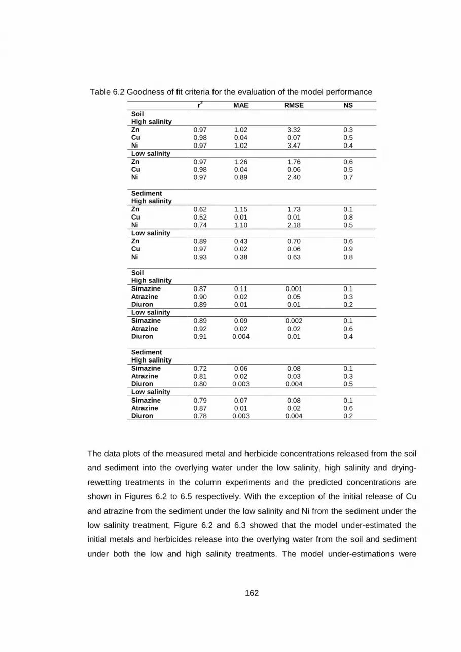
162

Table 6.2 Goodness of fit criteria for the evaluation of the model performance

r2 MAE RMSE NS Soil High salinity Zn 0.97 1.02 3.32 0.3 Cu 0.98 0.04 0.07 0.5 Ni 0.97 1.02 3.47 0.4 Low salinity Zn 0.97 1.26 1.76 0.6 Cu 0.98 0.04 0.06 0.5 Ni 0.97 0.89 2.40 0.7 Sediment High salinity Zn 0.62 1.15 1.73 0.1 Cu 0.52 0.01 0.01 0.8 Ni 0.74 1.10 2.18 0.5 Low salinity Zn 0.89 0.43 0.70 0.6 Cu 0.97 0.02 0.06 0.9 Ni 0.93 0.38 0.63 0.8 Soil High salinity Simazine 0.87 0.11 0.001 0.1 Atrazine 0.90 0.02 0.05 0.3 Diuron 0.89 0.01 0.01 0.2 Low salinity Simazine 0.89 0.09 0.002 0.1 Atrazine 0.92 0.02 0.02 0.6 Diuron 0.91 0.004 0.01 0.4 Sediment High salinity Simazine 0.72 0.06 0.08 0.1 Atrazine 0.81 0.02 0.03 0.3 Diuron 0.80 0.003 0.004 0.5 Low salinity Simazine 0.79 0.07 0.08 0.1 Atrazine 0.87 0.01 0.02 0.6 Diuron 0.78 0.003 0.004 0.2

The data plots of the measured metal and herbicide concentrations released from the soil

and sediment into the overlying water under the low salinity, high salinity and drying-

rewetting treatments in the column experiments and the predicted concentrations are

shown in Figures 6.2 to 6.5 respectively. With the exception of the initial release of Cu

and atrazine from the sediment under the low salinity and Ni from the sediment under the

low salinity treatment, Figure 6.2 and 6.3 showed that the model under-estimated the

initial metals and herbicides release into the overlying water from the soil and sediment

under both the low and high salinity treatments. The model under-estimations were

163

observed to be greater for the soil than the sediment particularly for metal release from

the soil under the high salinity treatment. Figure 6.4 showed that under the drying-

rewetting treatment, the model also under-estimated the initial release of the metals from

the soil but not from the sediment. In the case of the herbicides, the model under-

estimated the initial release from both the soil and sediment with the under-estimations

greater for the soil than the sediment (Figure 6.5). Given that the model assumes that

diffusion was the only mechanism controlling contaminant release, the observed model

under-estimations suggest that other mechanisms in addition to diffusion were

contributing to contaminant release during the initial phase of the column microcosm

experiments.

164

Soil Sediment

Figure 6.2 Predicted and measured concentration data for (a, d) Zn, (b, e) Cu and (c, f) Ni

released into the overlying water column from the soil and sediment respectively under

the low and high salinity treatments (bars = standard deviation (SD), n = 3).

0

0.1

0.2

0.3

0.4

0.5

0.6

0.7

0.8

0 500000 1000000 1500000 2000000

Time (sec)

Co

ppe

r (m

g L

-1)

Predicted Cu

Observed Cu at low salinity

Observed Cu at high salinity

0

5

10

15

20

25

30

35

40

45

0 500000 1000000 1500000 2000000

Time (sec)

Zin

c (m

g L

-1)

Predicted Zn

Observed Zn at low salinity

Observed Zn at high salinity

0

0.1

0.2

0.3

0.4

0.5

0.6

0.7

0.8

0 500000 1000000 1500000 2000000

Time (sec)

Cop

per (

mg

L-1

)

Predicted Cu



0

5

10

15

20

25

30

35

40

45

0 500000 1000000 1500000 2000000

Time (sec)

Zinc

(m

g L

-1)

Predicted Zn



0

0.1

0.2

0.3

0.4

0.5

0.6

0.7

0.8

0 500000 1000000 1500000 2000000

Time (sec)

Co

ppe

r (m

g L

-1)

Predicted Cu



0

5

10

15

20

25

30

35

40

45

0 500000 1000000 1500000 2000000

Time (sec)

Zin

c (m

g L

-1)

Predicted Zn



0

0.1

0.2

0.3

0.4

0.5

0.6

0.7

0.8

0 500000 1000000 1500000 2000000

Time (sec)

Cop

per (

mg

L-1

)

Predicted Cu



0

5

10

15

20

25

30

35

40

45

0 500000 1000000 1500000 2000000

Time (sec)

Zinc

(m

g L

-1)

Predicted Zn



0

5

10

15

20

25

30

35

40

45

0 500000 1000000 1500000 2000000

Time (sec)

Ni (

mg

L-1

)

Predicted Ni

Observed Ni at low salinity

Observed Ni at high salinity

0

10

20

30

40

0 500000 1000000 1500000 2000000

Time (sec)

Ni (

mg

L-1

)

Predicted Ni



0

5

10

15

20

25

30

35

40

45

0 500000 1000000 1500000 2000000

Time (sec)

Ni (

mg

L-1

)

Predicted Ni



0

10

20

30

40

0 500000 1000000 1500000 2000000

Time (sec)

Ni (

mg

L-1

)

Predicted Ni



165

Soil Sediment

Figure 6.3 Predicted and measured concentration data for (a, d) simazine, (b, e) atrazine

and (c, f) diuron released into the overlying water column from the soil and sediment

respectively under the low and high salinity treatments (bars = standard deviation (SD), n

= 3).

0.0

0.5

1.0

1.5

0 500000 1000000 1500000 2000000

Time (sec)

Sim

azin

e (m

g L

-1)

Predicted simazine

Observed simazine at low salinity

Observed simazine at high salinity

0

0.5

1

1.5

0 500000 1000000 1500000 2000000

Time (sec)

Sim

azin

e (m

g L

-1)

Predicted simazine



0.0

0.1

0.2

0.3

0.4

0.5

0 500000 1000000 1500000 2000000

Time (sec)

Atr

azin

e (m

g L-1

)

Predicted atrazine

Observed atrazine at low salinity

Observed atrazine at high salinity

0.0

0.1

0.2

0.3

0.4

0.5

0 500000 1000000 1500000 2000000

Time (sec)

Atr

azin

e (m

g L-1

)

Predicted atrazine



0.0

0.5

1.0

1.5

0 500000 1000000 1500000 2000000

Time (sec)

Sim

azin

e (m

g L

-1)

Predicted simazine



0

0.5

1

1.5

0 500000 1000000 1500000 2000000

Time (sec)

Sim

azin

e (m

g L

-1)

Predicted simazine



0.0

0.1

0.2

0.3

0.4

0.5

0 500000 1000000 1500000 2000000

Time (sec)

Atr

azin

e (m

g L-1

)

Predicted atrazine



0.0

0.1

0.2

0.3

0.4

0.5

0 500000 1000000 1500000 2000000

Time (sec)

Atr

azin

e (m

g L-1

)

Predicted atrazine



0.00

0.02

0.04

0.06

0.08

0 500000 1000000 1500000 2000000

Time (sec)

Diu

ron

(m

g L

-1)

Predicted diuron

Observed diuron at low salinity

Observed diuron at high salinity

0.00

0.02

0.04

0.06

0.08

0 500000 1000000 1500000 2000000

Time (sec)

Diu

ron

(m

g L

-1)

Predicted diuron



0.00

0.02

0.04

0.06

0.08

0 500000 1000000 1500000 2000000

Time (sec)

Diu

ron

(m

g L

-1)

Predicted diuron



0.00

0.02

0.04

0.06

0.08

0 500000 1000000 1500000 2000000

Time (sec)

Diu

ron

(m

g L

-1)

Predicted diuron



166

Soil Sediment

Figure 6.4 Predicted and measured concentration data for (a, d) Zn, (b, e) Cu and (c, f) Ni

released into the overlying water column from the soil and sediment respectively under

the drying-rewetting treatment (bars = standard deviation (SD), n = 3).

0

10

20

30

40

50

604800 748800 892800

Time (sec)

Zn

(mg

L-1

)

Predicted Zn

Observed Zn

0

0.5

1

604800 748800 892800

Time (sec)

Cu

(m

g L

-1)

Predicted Cu

Observed Cu

0

10

20

30

40

50

604800 748800 892800

Time (sec)

Zn

(mg

L-1

)

Predicted Zn

Obseved Zn

0

0.5

1

604800 748800 892800

Time (sec)

Cu

(mg

L-1

)Predicted Cu

Observed Cu

0

10

20

30

40

50

604800 748800 892800

Time (sec)

Zn

(mg

L-1

)

Predicted Zn

Observed Zn

0

0.5

1

604800 748800 892800

Time (sec)

Cu

(m

g L

-1)

Predicted Cu

Observed Cu

0

10

20

30

40

50

604800 748800 892800

Time (sec)

Zn

(mg

L-1

)

Predicted Zn

Obseved Zn

0

0.5

1

604800 748800 892800

Time (sec)

Cu

(mg

L-1

)Predicted Cu

Observed Cu

0

20

40

60

80

604800 748800 892800

Time (sec)

Ni (

mg

L-1

)

Predcited Ni

Observed Ni

0

20

40

60

80

604800 748800 892800

Time (sec)

Ni (

mg

L-1

)

Predcietd Ni

Observed Ni

0

20

40

60

80

604800 748800 892800

Time (sec)

Ni (

mg

L-1

)

Predcited Ni

Observed Ni

0

20

40

60

80

604800 748800 892800

Time (sec)

Ni (

mg

L-1

)

Predcietd Ni

Observed Ni

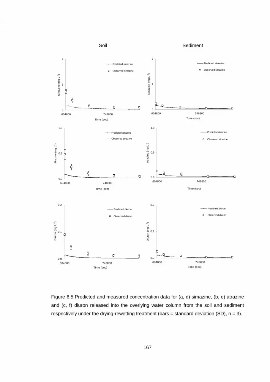
167

Soil Sediment

Figure 6.5 Predicted and measured concentration data for (a, d) simazine, (b, e) atrazine

and (c, f) diuron released into the overlying water column from the soil and sediment

respectively under the drying-rewetting treatment (bars = standard deviation (SD), n = 3).

0

1

2

604800 748800

Time (sec)

Sim

azi

ne

(m

g L

-1)

Predicted simazine

Observed simazine

0

1

2

604800 748800

Time (sec)

Sim

azi

ne

(m

g L

-1)

Predicted simazine

Observed simazine

0.0

0.5

1.0

604800 748800

Time (sec)

Atr

azi

ne

(m

g L

-1)

Predicted atrazine

Observed atrazine

0.0

0.5

1.0

604800 748800

Time (sec)

Atr

azi

ne

(m

g L

-1)

Predicted atrazine

Observed atrazine

0

1

2

604800 748800

Time (sec)

Sim

azi

ne

(m

g L

-1)

Predicted simazine

Observed simazine

0

1

2

604800 748800

Time (sec)

Sim

azi

ne

(m

g L

-1)

Predicted simazine

Observed simazine

0.0

0.5

1.0

604800 748800

Time (sec)

Atr

azi

ne

(m

g L

-1)

Predicted atrazine

Observed atrazine

0.0

0.5

1.0

604800 748800

Time (sec)

Atr

azi

ne

(m

g L

-1)

Predicted atrazine

Observed atrazine

0.0

0.5

1.0

604800 748800

Time (sec)

Atr

azi

ne

(m

g L

-1)

Predicted atrazine

Observed atrazine

0.0

0.5

1.0

604800 748800

Time (sec)

Atr

azi

ne

(m

g L

-1)

Predicted atrazine

Observed atrazine

0.0

0.1

0.2

604800 748800

Time (sec)

Diu

ron

(m

g L

-1)

Predicted diuron

Observed diuron

0.0

0.1

0.2

604800 748800

Time (sec)

Diu

ron

(mg

L-1

)

Predicted diuron

Observed diuron

0.0

0.1

0.2

604800 748800

Time (sec)

Diu

ron

(m

g L

-1)

Predicted diuron

Observed diuron

0.0

0.1

0.2

604800 748800

Time (sec)

Diu

ron

(mg

L-1

)

Predicted diuron

Observed diuron

168

The normal probability plots of the residuals between the predicted and measured metal

and herbicide concentrations under the low salinity, high salinity and the drying-rewetting

treatments are shown in Figures 6.6 to 6.11 respectively. The normal probability plots

were used to analyse the distribution of the residuals. This was done by plotting the

sorted residual values against theoretical values from the standard normal distribution

(Go et al., 2008). If the plotted values are linear and in a uniform band around zero, this

indicates that the residuals are normally distributed and the model adequately represents

the actual system. However, departure from linearity or “tailings” indicates that the

residuals are not normally distributed (Go et al., 2008). Such asymmetric distribution of

residuals is indicative of an inadequate representation of the actual system by the model

(Ljung, 1987; Soderstrom and Stoica, 1989) probably due to mechanisms which were not

accounted for in the model.

The distribution of the residuals between the predicted and measured metal and

herbicide concentrations under the low and high salinity treatments for the soil and

sediment showed distinct tailings at one end of each of the plots (Figure 6.6 to 6.9).

Under the drying-rewetting treatment, the residual plots for the metal concentrations

showed distinct tailings at one end of each of the plots for the soil but not for the sediment

(Figure 6.10). Similarly, the plots of the residuals between the predicted and measured

herbicide concentrations under the drying-rewetting treatment showed distinct tailings at

one end of each of the plots for the soil but very slight tailings on the plots for the

sediment (Figure 6.11). The tailings were in the positive range of residual values on the

plots (Figure 6.6 to 6.11) suggesting that the model was under-estimating metal and

herbicide release and hence agreeing with the visual observations of the data plots in

Figures 6.2 to 6.5 described above. The asymmetric distribution of the residuals is likely

due to other mechanisms contributing to the release of the metals and herbicides into the

overlying water during the column experiments which were not accounted for in the

model.

169

Soil Sediment

Figure 6.6 Analysis of residuals between the predicted and measured concentration data

for (a, d) Zn, (b, e) Cu and (c, f) Ni released into the overlying water from the soil and

sediment respectively under the low salinity treatment.

-2

-1.5

-1

-0.5

0

0.5

1

1.5

2

-6-4-20246

Zn Res iduals

Sta

ndar

d de

viat

ion

s

-2

-1.5

-1

-0.5

0

0.5

1

1.5

2

-6-4-20246

Zn Res iduals

Sta

nda

rd d

evia

tions

(a) (d)

-2

-1.5

-1

-0.5

0

0.5

1

1.5

2

-6-4-20246

Zn Res iduals

Sta

ndar

d de

viat

ion

s

-2

-1.5

-1

-0.5

0

0.5

1

1.5

2

-6-4-20246

Zn Res iduals

Sta

nda

rd d

evia

tions

(a) (d)

-2

-1.5

-1

-0.5

0

0.5

1

1.5

2

-0.3-0.2-0.100.10.20.3

Cu Res iduals

Sta

nda

rd d

evi

atio

ns

(b)

-2

-1.5

-1

-0.5

0

0.5

1

1.5

2

-0.3-0.2-0.100.10.20.3

Cu Residuals

Sta

nda

rd d

evi

atio

ns

(e)

-2

-1.5

-1

-0.5

0

0.5

1

1.5

2

-0.3-0.2-0.100.10.20.3

Cu Res iduals

Sta

nda

rd d

evi

atio

ns

(b)

-2

-1.5

-1

-0.5

0

0.5

1

1.5

2

-0.3-0.2-0.100.10.20.3

Cu Residuals

Sta

nda

rd d

evi

atio

ns

(e)

(c) (f)

-2

-1.5

-1

-0.5

0

0.5

1

1.5

2

-10-50510

Ni Res iduals

Sta

ndar

d d

evi

atio

ns

-2

-1.5

-1

-0.5

0

0.5

1

1.5

2

-10-50510

Ni Res iduals

Sta

ndar

d d

evi

atio

ns

(c) (f)

-2

-1.5

-1

-0.5

0

0.5

1

1.5

2

-10-50510

Ni Res iduals

Sta

ndar

d d

evi

atio

ns

-2

-1.5

-1

-0.5

0

0.5

1

1.5

2

-10-50510

Ni Res iduals

Sta

ndar

d d

evi

atio

ns

170

Soil Sediment


for (a, d) Zn, (b, e) Cu and (c, f) Ni released from the soil and sediment respectively under

the high salinity treatment.

-2

-1.5

-1

-0.5

0

0.5

1

1.5

2

-24-18-12-606121824

Zn Res idualsS

tan

dard

dev

iatio

ns

-2

-1.5

-1

-0.5

0

0.5

1

1.5

2

-24-18-12-606121824

Zn Res iduals

Sta

ndar

d d

evi

atio

ns

(a) (d)

-2

-1.5

-1

-0.5

0

0.5

1

1.5

2

-24-18-12-606121824

Zn Res idualsS

tan

dard

dev

iatio

ns

-2

-1.5

-1

-0.5

0

0.5

1

1.5

2

-24-18-12-606121824

Zn Res iduals

Sta

ndar

d d

evi

atio

ns

(a) (d)

(c) (f)

-2

-1.5

-1

-0.5

0

0.5

1

1.5

2

-30-24-18-12-60612182430

Ni Residuals

Sta

nda

rd d

evi

atio

ns

-2

-1.5

-1

-0.5

0

0.5

1

1.5

2

-30-24-18-12-60612182430

Ni Residuals

Sta

nda

rd d

evia

tions

(c) (f)

-2

-1.5

-1

-0.5

0

0.5

1

1.5

2

-30-24-18-12-60612182430

Ni Residuals

Sta

nda

rd d

evi

atio

ns

-2

-1.5

-1

-0.5

0

0.5

1

1.5

2

-30-24-18-12-60612182430

Ni Residuals

Sta

nda

rd d

evia

tions

-2

-1.5

-1

-0.5

0

0.5

1

1.5

2

-0.3-0.2-0.100.10.20.3

Cu Res iduals

Sta

nda

rd d

evia

tions

-2

-1.5

-1

-0.5

0

0.5

1

1.5

2

-0.3-0.2-0.100.10.20.3

Cu Residuals

Sta

nda

rd d

evi

atio

ns

(e)(b)

-2

-1.5

-1

-0.5

0

0.5

1

1.5

2

-0.3-0.2-0.100.10.20.3

Cu Res iduals

Sta

nda

rd d

evia

tions

-2

-1.5

-1

-0.5

0

0.5

1

1.5

2

-0.3-0.2-0.100.10.20.3

Cu Residuals

Sta

nda

rd d

evi

atio

ns

(e)(b)

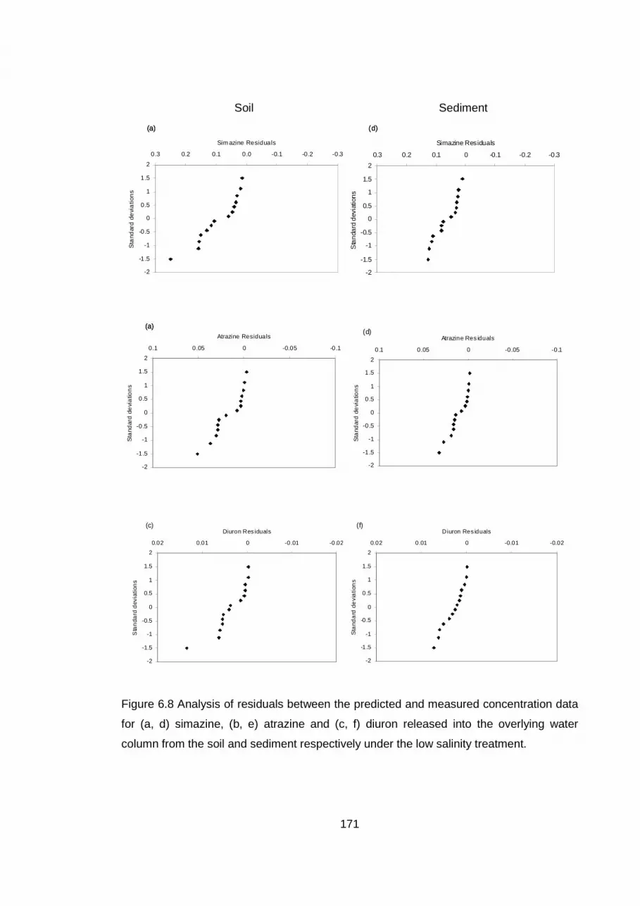
171

Soil Sediment


for (a, d) simazine, (b, e) atrazine and (c, f) diuron released into the overlying water

column from the soil and sediment respectively under the low salinity treatment.

-2

-1.5

-1

-0.5

0

0.5

1

1.5

2

-0.1-0.0500.050.1

Atrazine Residuals

Sta

ndar

d d

evi

atio

ns

-2

-1.5

-1

-0.5

0

0.5

1

1.5

2

-0.1-0.0500.050.1

Atrazine Res iduals

Sta

ndar

d d

evi

atio

ns

(a)(d)

-2

-1.5

-1

-0.5

0

0.5

1

1.5

2

-0.1-0.0500.050.1

Atrazine Residuals

Sta

ndar

d d

evi

atio

ns

-2

-1.5

-1

-0.5

0

0.5

1

1.5

2

-0.1-0.0500.050.1

Atrazine Res iduals

Sta

ndar

d d

evi

atio

ns

(a)(d)

-2

-1.5

-1

-0.5

0

0.5

1

1.5

2

-0.02-0.0100.010.02

Diuron Res iduals

Sta

nda

rd d

evia

tion

s

-2

-1.5

-1

-0.5

0

0.5

1

1.5

2

-0.02-0.0100.010.02

Diuron Res iduals

Sta

nda

rd d

evi

atio

ns

(c) (f)

-2

-1.5

-1

-0.5

0

0.5

1

1.5

2

-0.02-0.0100.010.02

Diuron Res iduals

Sta

nda

rd d

evia

tion

s

-2

-1.5

-1

-0.5

0

0.5

1

1.5

2

-0.02-0.0100.010.02

Diuron Res iduals

Sta

nda

rd d

evi

atio

ns

(c) (f)

(a) (d)

-2

-1.5

-1

-0.5

0

0.5

1

1.5

2

-0.3-0.2-0.10.00.10.20.3

Sim azine Residuals

Sta

ndar

d d

evi

atio

ns

-2

-1.5

-1

-0.5

0

0.5

1

1.5

2

-0.3-0.2-0.100.10.20.3

Simazine Residuals

Sta

nda

rd d

evia

tions

(a) (d)

-2

-1.5

-1

-0.5

0

0.5

1

1.5

2

-0.3-0.2-0.10.00.10.20.3

Sim azine Residuals

Sta

ndar

d d

evi

atio

ns

-2

-1.5

-1

-0.5

0

0.5

1

1.5

2

-0.3-0.2-0.100.10.20.3

Simazine Residuals

Sta

nda

rd d

evia

tions

172

Soil Sediment


for (a, d) simazine, (b, e) atrazine and (c, f) diuron released into the overlying water

column from the soil and sediment respectively under the high salinity treatment.

-2

-1.5

-1

-0.5

0

0.5

1

1.5

2

-0.5-0.4-0.3-0.2-0.100.10.20.30.40.5

Simazine Residuals

Sta

nd

ard

de

via

tion

s

(a)

-2

-1.5

-1

-0.5

0

0.5

1

1.5

2

-0.5-0.4-0.3-0.2-0.100.10.20.30.40.5

Simazine Res iduals

Sta

nda

rd d

evia

tions

(d)

-2

-1.5

-1

-0.5

0

0.5

1

1.5

2

-0.5-0.4-0.3-0.2-0.100.10.20.30.40.5

Simazine Residuals

Sta

nd

ard

de

via

tion

s

(a)

-2

-1.5

-1

-0.5

0

0.5

1

1.5

2

-0.5-0.4-0.3-0.2-0.100.10.20.30.40.5

Simazine Res iduals

Sta

nda

rd d

evia

tions

(d)

-2

-1.5

-1

-0.5

0

0.5

1

1.5

2

-0.2-0.100.10.2

Atrazine Res iduals

Sta

nda

rd d

evi

atio

ns

-2

-1.5

-1

-0.5

0

0.5

1

1.5

2

-0.2-0.100.10.2

Atrazine Res iduals

Sta

bda

rd d

evi

atio

ns

(e)(b)

-2

-1.5

-1

-0.5

0

0.5

1

1.5

2

-0.2-0.100.10.2

Atrazine Res iduals

Sta

nda

rd d

evi

atio

ns

-2

-1.5

-1

-0.5

0

0.5

1

1.5

2

-0.2-0.100.10.2

Atrazine Res iduals

Sta

bda

rd d

evi

atio

ns

(e)(b)

(c)

-2

-1.5

-1

-0.5

0

0.5

1

1.5

2

-0.04-0.0200.020.04

Diuron Res iduals

Sta

nda

rd d

eva

ition

s

-2

-1.5

-1

-0.5

0

0.5

1

1.5

2

-0.04-0.0200.020.04

Diuron Residuals

Sta

nda

rd d

evi

atio

ns

(f)(c)

-2

-1.5

-1

-0.5

0

0.5

1

1.5

2

-0.04-0.0200.020.04

Diuron Res iduals

Sta

nda

rd d

eva

ition

s

-2

-1.5

-1

-0.5

0

0.5

1

1.5

2

-0.04-0.0200.020.04

Diuron Residuals

Sta

nda

rd d

evi

atio

ns

(f)

173

Soil Sediment

Figure 6.10 Analysis of residuals between the predicted and measured concentration

data for (a, d) Zn, (b, e) Cu and (c, f) Ni released from the soil and sediment respectively

under the drying-rewetting treatment.

(a)

-2

-1.5

-1

-0.5

0

0.5

1

1.5

2

-20-1001020

Zn Res iduals

Sta

nda

rd d

evi

atio

ns

-2

-1.5

-1

-0.5

0

0.5

1

1.5

2

-20-1001020

Zn Residuals

Sta

nda

rd d

evi

atio

ns

(d)(a)

-2

-1.5

-1

-0.5

0

0.5

1

1.5

2

-20-1001020

Zn Res iduals

Sta

nda

rd d

evi

atio

ns

-2

-1.5

-1

-0.5

0

0.5

1

1.5

2

-20-1001020

Zn Residuals

Sta

nda

rd d

evi

atio

ns

(d)

-2

-1.5

-1

-0.5

0

0.5

1

1.5

2

-0.5-0.4-0.3-0.2-0.100.10.20.30.40.5

Cu Res iduals

Sta

ndr

ad

dev

iatio

ns

(b)

-2

-1.5

-1

-0.5

0

0.5

1

1.5

2

-0.5-0.4-0.3-0.2-0.100.10.20.30.40.5

Cu Res iduals

Sta

ndar

d d

evi

atio

ns

(e)

-2

-1.5

-1

-0.5

0

0.5

1

1.5

2

-0.5-0.4-0.3-0.2-0.100.10.20.30.40.5

Cu Res iduals

Sta

ndr

ad

dev

iatio

ns

(b)

-2

-1.5

-1

-0.5

0

0.5

1

1.5

2

-0.5-0.4-0.3-0.2-0.100.10.20.30.40.5

Cu Res iduals

Sta

ndar

d d

evi

atio

ns

(e)

-2

-1.5

-1

-0.5

0

0.5

1

1.5

2

-40-2002040

Ni Res iduals

Sta

nd

ard

de

via

tions

-2

-1.5

-1

-0.5

0

0.5

1

1.5

2

-40-2002040

Ni Residuals

Sta

nd

ard

de

via

tions

(c) (f)

-2

-1.5

-1

-0.5

0

0.5

1

1.5

2

-40-2002040

Ni Res iduals

Sta

nd

ard

de

via

tions

-2

-1.5

-1

-0.5

0

0.5

1

1.5

2

-40-2002040

Ni Residuals

Sta

nd

ard

de

via

tions

(c) (f)

174

Soil Sediment

Figure 6.11 Analysis of residuals between the predicted and measured concentration

data for (a, d) simazine, (b, e) atrazine and (c, f) diuron released from the soil and

sediment respectively under the drying-rewetting treatment.

-2

-1.5

-1

-0.5

0

0.5

1

1.5

2

-1-0.500.51

Simazine Res idualsS

tan

dard

de

viat

ion

s

-2

-1.5

-1

-0.5

0

0.5

1

1.5

2

-1-0.500.51

Simazine Residuals

Sta

nd

ard

dev

iatio

ns

(a) (d)

-2

-1.5

-1

-0.5

0

0.5

1

1.5

2

-1-0.500.51

Simazine Res idualsS

tan

dard

de

viat

ion

s

-2

-1.5

-1

-0.5

0

0.5

1

1.5

2

-1-0.500.51

Simazine Residuals

Sta

nd

ard

dev

iatio

ns

(a) (d)

-2

-1.5

-1

-0.5

0

0.5

1

1.5

2

-0.5-0.4-0.3-0.2-0.100.10.20.30.40.5

Atrazine Res iduals

Sta

nd

ard

de

via

tions

-2

-1.5

-1

-0.5

0

0.5

1

1.5

2

-0.5-0.4-0.3-0.2-0.100.10.20.30.40.5

Atrazine Residuals

Sta

ndar

d d

evi

atio

ns

(b) (e)

-2

-1.5

-1

-0.5

0

0.5

1

1.5

2

-0.5-0.4-0.3-0.2-0.100.10.20.30.40.5

Atrazine Res iduals

Sta

nd

ard

de

via

tions

-2

-1.5

-1

-0.5

0

0.5

1

1.5

2

-0.5-0.4-0.3-0.2-0.100.10.20.30.40.5

Atrazine Residuals

Sta

ndar

d d

evi

atio

ns

(b) (e)

-2

-1.5

-1

-0.5

0

0.5

1

1.5

2

-0.1-0.0500.050.1

Diuron Res iduals

Sta

ndar

d d

evi

atio

ns

(c) (f)

-2

-1.5

-1

-0.5

0

0.5

1

1.5

2

-0.1-0.0500.050.1

Diuron Residuals

Sta

nda

rd d

evia

tion

s

-2

-1.5

-1

-0.5

0

0.5

1

1.5

2

-0.1-0.0500.050.1

Diuron Res iduals

Sta

ndar

d d

evi

atio

ns

(c) (f)

-2

-1.5

-1

-0.5

0

0.5

1

1.5

2

-0.1-0.0500.050.1

Diuron Residuals

Sta

nda

rd d

evia

tion

s

175

In order to estimate the rate of release of the predicted and measured metals and

herbicides, exponential curves were fitted to the predicted and measured contaminant

concentrations under both salinity treatments and the drying-rewetting treatment. The

slopes of the fitted curves reflect the rate of the metals and herbicides release under the

low and high salinity treatments and the drying-rewetting treatment and are shown in

Table 6.3 and Table 6.4 respectively. The rate of release for the measured metal and

herbicide concentrations for both the soil and sediment under the low and high salinity

treatments were higher than those for the predicted metal and herbicide concentrations

under the low and high salinity treatments (Table 6.3). With the exception of Cu and Zn in

the sediment, higher rates of release were also observed for the measured metal and

herbicide concentrations released from the soil and sediment under the drying-rewetting

treatment compared to the predicted concentrations (Table 6.4). The disagreements

between the rates of release for the measured and predicted metal and herbicide

concentrations further suggests that the model under-estimated the release of the metals

and herbicides from the soil and sediment in the column microcosm experiments.

176

Table 6.3 Slope of the exponential curves fitted to the predicted and measured

contaminant concentrations under the low and high salinity treatments

Soil Sediment

Slope

(mg L-1 sec-1)

Slope

(mg L-1 sec-1)

Measured Zn

Low salinity 5.0 x 10-3 5.1 x 10-3

Measured Zn

High salinity 6.5 x 10 -3 6.0 x 10-3

Predicted Zn 3.0 x 10 -3 3.0 x 10 -3

Measured Cu

Low salinity 5.4 x 10-3 5.9 x 10 -3

Measured Cu

High salinity 5.1 x 10-3 3.4 x 10-3

Predicted Cu 3.1 x 10-3 3.1 x 10 -3

Measured Ni

Low salinity 9.0 x 10-3 5.2 x 10-3

Measured Ni

High salinity 10.4 x 10-3 6.3 x 10-3

Predicted Ni 5.7 x 10-3 3.1 x 10-3

Measured simazine

Low salinity 5.0 x 10-3 4.7 x 10-3

Measured simazine

High salinity 5.0 x 10 -3 4.0 x 10-3

Predicted simazine 3.0 x 10 -3 3.0 x 10 -3

Measured atrazine

Low salinity 6.9 x 10-3 6.7 x 10 -3

Measured atrazine


Predicted atrazine 3.1 x 10-3 3.1 x 10 -3

Measured diuron

Low salinity 7.2 x 10-3 5.2 x 10-3

Measured diuron


Predicted diuron 3.1 x 10-3 3.0 x 10-3

177

Table 6.4 Slope of the exponential curves fitted to the predicted and measured

contaminant concentrations under the drying-rewetting treatment

Slope

mg L-1sec-1

Slope

mg L-1sec-1

Measured Zn 19.3 x 10-3 11.0 x 10-3

Predicted Zn 12.2 x 10-3 12.2 x 10-3

Measured Cu 16.3 x 10-3 12.2 x 10 -3

Predicted Cu 12.2 x 10-3 12.2 x 10 -3

Measured Ni 22.0 x 10-3 14.5 x 10-3

Predicted Ni 12.3 x 10-3 12.2 x 10-3

Measured simazine 25.4 x 10-3 25.3 x 10-3

Predicted simazine 20.1 x 10-3 20.1 x 10-3

Measured atrazine 29.0 x 10-3 33.0 x 10-3

Predicted atrazine 20.1 x 10-3 20.1 x 10 -3

Measured diuron 28.5 x 10-3 32.2 x 10-3

Predicted diuron 20.1 x 10-3 20.1 x 10-3

In order to improve the agreement between the model predictions and the observed data,

the performance of the model was optimised by adjusting model parameters (i.e. le Bas

molar volumes and diffusion coefficients of the herbicides and metals) used for the

simulation runs. Table 6.5 shows the goodness-of-fit criteria used to assess the

performance of the model after adjusting the model parameters. The coefficients of

determination (r2) increased from 97 % - 98 % to 98 % - 99 % for the metals and from 87

% - 92 % to 91 – 95 % for the herbicides in the soil. In the case of the sediment, the r2

values increased from 52 % - 97 % to 79 % - 98 % for the metals and from 72 % - 87 %

to 83 % – 93 % for the herbicides. The coefficients of determination (r2) were all

significant at the 0.01 probability level. The higher r2 values indicates that the model

performed better in predicting the measured metal and herbicide concentrations in the

overlying water in the column experiments after adjusting the model parameters. All the

NS coefficients were greater than or equal to 0.4 which was the threshold used in this

study to judge the performance of the model (Table 6.5). Ramanarayanan et al. (1997)

also used NS coefficient of 0.4 to judge the performance of the Agricultural Policy

Environmental Extender (APEX) model as satisfactory. Compared to the mean absolute

error (MAE) and the root mean squared error (RMSE) obtained before adjusting the

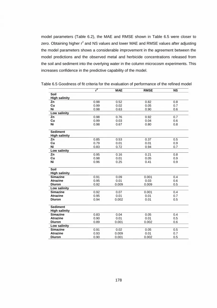
178

model parameters (Table 6.2), the MAE and RMSE shown in Table 6.5 were closer to

zero. Obtaining higher r2 and NS values and lower MAE and RMSE values after adjusting

the model parameters shows a considerable improvement in the agreement between the

model predictions and the observed metal and herbicide concentrations released from

the soil and sediment into the overlying water in the column microcosm experiments. This

increases confidence in the predictive capability of the model.

Table 6.5 Goodness of fit criteria for the evaluation of performance of the refined model

r2 MAE RMSE NS Soil High salinity Zn 0.98 0.52 0.82 0.8 Cu 0.99 0.02 0.05 0.7 Ni 0.98 0.63 0.90 0.6 Low salinity Zn 0.98 0.76 0.92 0.7 Cu 0.99 0.03 0.04 0.6 Ni 0.98 0.67 0.80 0.8 Sediment High salinity Zn 0.85 0.53 0.37 0.5 Cu 0.79 0.01 0.01 0.9 Ni 0.83 0.72 0.94 0.7 Low salinity Zn 0.95 0.16 0.21 0.8 Cu 0.98 0.01 0.05 0.9 Ni 0.96 0.25 0.41 0.9 Soil High salinity Simazine 0.91 0.09 0.001 0.4 Atrazine 0.95 0.01 0.03 0.6 Diuron 0.92 0.009 0.009 0.5 Low salinity Simazine 0.92 0.07 0.001 0.4 Atrazine 0.95 0.01 0.01 0.7 Diuron 0.94 0.002 0.01 0.5 Sediment High salinity Simazine 0.83 0.04 0.05 0.4 Atrazine 0.90 0.01 0.01 0.5 Diuron 0.89 0.001 0.002 0.6 Low salinity Simazine 0.91 0.02 0.05 0.5 Atrazine 0.93 0.009 0.01 0.7 Diuron 0.90 0.001 0.002 0.5

179

6.7. Discussion

Under both the low and high salinity treatment, the data plots showed that the model

under-estimated the initial metal and herbicide release into the overlying water from the

soil and sediment in the column microcosm experiments with the exception of the initial

release of Cu, Ni and atrazine from the sediment (Figure 6.2 and 6.3); the model under-

estimation was greater for the soil than the sediment particularly under the high salinity

treatment; the normal probability plots of the residuals between the measured and

predicted metal and herbicide concentrations showed tailings at one end of each of the

plots in Figure 6.6 to 6.9 and the rates of release of the measured metal and herbicide

concentrations from the soil and sediment were higher compared to those of the

predicted concentrations (Table 6.3). These observations suggest that the model under-

predicted the metals and herbicides release into the overlying water from the soil and

sediment in the column microcosm experiments. This is likely due to other mechanisms in

addition to diffusion contributing to the release of the metals and herbicides under the

experimental conditions.

Competition and complexation between the seawater cations (Na+, Ca2+, K+ and Mg2+),

anions (Cl and SO42-) and the sorbed metals are likely mechanisms which occurred

during the column experiments in addition to diffusion. Several studies have observed

that seawater cations and anions are effective in mobilizing sorbed metals such as those

considered in this study from soil and sediment into solution through competition and

complexation reactions respectively (Emmerson et al., 2001; Paalman et al., 1994;

Millward and Liu, 2003). The lower coefficients of determination (r2) for the predicted and

measured metal concentrations released from the sediment under high salinity treatment

(Zn (0.62); Cu (0.52) and Ni (0,74)) compared to the low salinity treatment (Zn (0.89); Cu

(0.97) and Ni (0.93)) (Table 6.2) and the greater model under-estimation of metal release

from the soil under the high salinity treatment compared to low salinity treatment (Figure

6.2) suggests a greater formation of complexes between the seawater anions and the

sorbed metals and the greater displacement of sorbed metals by seawater cations for

cation exchange binding sites at high salinity compared to low salinity.

Resuspended particles can lead to contaminant transport into the water column when

sufficient energy from advecting water is available to raise particles into the water column

(Calamari, 1993). In this study, particles from the soil/sediment-water interface may have

180

been re-suspended into the water column due to the influx of artificial seawater into the

column microcosm during the experiments which in turn may have led to higher

measured metal and herbicide concentrations in the overlying water compared to the

predicted concentrations. The lower model under-estimations for the sediment compared

to the soil suggests that particle resuspension likely occurred during the column

microcosm experiments and contributed to the release of metals and herbicides into the

overlying water. Fine-grained sediments such as those used in the column experiments

are readily compacted and cohesive due to strong electrostatic forces which bind the

particles together to form a cohesive mass, making them resistant to entrainment and

resuspension (Masselink and Hughes, 2003; Pethick, 1984). Therefore, the sediments

are likely to be more resistant to resuspension than the soil. In addition, fine particles with

diameters less than 10 µm are more difficult to entrain than particles with diameters

greater than 10 µm, with the degree of difficulty increasing as the particle diameter

decreases (Masselink and Hughes, 2003),. In this study, 50 % of the particles in the

sediment had a diameter less than 10 µm while only 25 % of the particles in the soil had a

diameter less than 10 µm. This suggests that the sediment particles were less

resuspendible than the soil particles which in turn resulted in less metals and herbicides

release from the sediment into the overlying water compared to the soil.

Under the drying-rewetting treatment, the data plots showed that the model under-

estimated the initial metal release from the soil but not from the sediment (Figures 6.4);

the normal probability residual plots for the metals showed distinct tailings at one end of

each of the plots for the soil but not for the sediment (Figure 6.10) and the rate of release

were higher for the measured metal concentrations compared to the predicted

concentrations for the soil but not for the sediment except for Ni (Table 6.4). For the

herbicides, the data plots showed that the model under-estimated the initial herbicide

release from both the soil and sediment but the under-estimation was greater for the soil

than the sediment (Figures 6.5); the normal probability residual plots for the herbicides

showed tailings at one end of each of the plots for the soil but only very slight tailings

were observed for the sediment (Figure 6.11) and the rates of release of the measured

herbicide concentrations from the soil and sediment were higher compared to those of

the predicted concentrations (Table 6.3). These observations suggest that diffusion is

likely the dominant mechanism controlling the release of the metals from the sediment

after drying and rewetting except for Ni. Other mechanisms were contributing to the

181

release of the metals and herbicides from the soil and herbicides from the sediments

hence the observed model under-estimations. DOC can form complexes with metals and

herbicides such as those considered in this study which can facilitate their mobility in soils

and sediments (Weng et al., 2002; Sauve et al., 2000; Kalbitz and Wennrich, 1998;

Garber et al., 1995; Nelson et al., 2001; Williams et al., 2000). Accordingly, DOC

complexation with the metals and herbicides is likely to be contributing to the release of

the metals and herbicides from the soil and the release of herbicides from the sediments

in the column experiments in addition to diffusion. Reemtsma et al. (2000) and Miller et

al. (2005) observed an increase in DOC concentrations in soil as a result of an increase

in organic matter mineralisation with drying and rewetting of soil. The difference between

the soil and sediment is likely a consequence of higher DOC-contaminant associated

release from the soil than the sediment under the experimental conditions. The strong

association of Ni with DOC which results in its low particle affinity (Turner et al., 1998)

may account for the higher rates of release of Ni from the sediment compared to the

other metals. The visual observations are consistent with the results of the linear

regression analysis of the DOC, metal and herbicide concentrations discussed in Chapter

5 (Chapter 5, Section 5.3.2.2 to 5.3.2.5). For the soil, the results of the linear regression

showed that there were strong significant relationships between the DOC and the metals

released into the overlying water with 50 %, 79 % and 55 % of the variations in the Cu,

Ni, Zn concentrations explained by the variation in the DOC concentrations (p < 0.05).

Similarly, there were significant relationships between the DOC and the herbicides

released into the overlying water with the variations in the DOC concentrations

accounting for 65%, 68% and 76% of the variations in the atrazine, diuron and simazine

concentrations respectively (p < 0.05). But for the sediment, the relationship between

DOC, the metals and herbicides released into the overlying water were not significant (p

> 0.05). Only 41%, 31% and 22% of the variations in simazine, atrazine and diuron

concentrations and 13 %, 28 % and 8 % of the variations in the Zn, Ni and Cu

concentrations in the overlying water could be explained by the variation in the DOC

concentrations. The variation in the Ni concentrations explained by the DOC

concentrations was higher compared to the other metals. These results suggested that

significant proportions of the metals and herbicides were released as DOC-complexes

from the soil but not from the sediment hence agreeing with the visual observations from

the normal probability residual and data plots for the metals and herbicides release under

the drying-rewetting treatment.

182

6.8 Summary and conclusion

By using a diffusion model, this chapter has shown that other mechanisms, in addition to

diffusion, contributed to metal and herbicide release from the soil and sediment into the

overlying water in the column experiments under the experimental conditions in this

study. The goodness-of-fit criteria showed that the model performed reasonably well in

simulating the metal and herbicide release from the soil and sediment into the overlying

water column in the column experiments. Visual observations of the data plots, the

normal probability residual plots and the rates of release for the measured and predicted

metal and herbicide concentrations indicated that the model under-predicted the metals

and herbicides release from the soil and sediment into the overlying water column in the

column experiments. This was attributed to other mechanisms occurring during the

column experiments but not accounted for in the model. The lower coefficients of

determination and, the greater model under-estimation under the high salinity treatment

compared to the low salinity treatment suggested that salinity effects due complexation

and competition reactions contributed to the release of the metals into the overlying water

in the column experiments. The observed difference in the model under-estimations for

the soil and sediment under the salinity treatments indicated that particle resuspension is

also likely to have contributed to the metals and herbicides release into the overlying

water in the column experiments. Under the drying-rewetting treatment, DOC association

with the metals and herbicides is likely to have contributed to the metals and herbicides

release in the experiments particularly from the soil.

183

Chapter 7: Synthesis and conclusion

7.1. Introduction

The recognition of the intrinsic value of salt marshes as part of the coastal ecosystem and

the threat to salt marshes due to rising sea levels has led to the current strategy of

managed realignment. The main goals of managed realignment in the UK are habitat

restoration and the enhancement of coastal flood defence. The restored salt marsh

compensates for salt marsh loss due to coastal squeeze and provides a cost effective

and sustainable seawall for coastal areas by dissipating wave energy (Shepherd et al.,

2007; Moller et al., 1999). Managed realignment is usually implemented on reclaimed

agricultural land. However, in low-lying areas, dredged sediments are beneficially re-used

to raise the elevation of land for salt marsh plant development. One of the subsidiary

justifications for the implementation of managed realignment is that they can be important

sinks for metals and other particle reactive contaminants from estuarine waters (NRA,

1994; Macleod et al; 1999; Andrew et al., 2006; Cave et al., 2005). However, managed

realignment sites may serve as a source of contaminants to the estuarine waters due to

changes in the physical and chemical conditions in the soil and sediment following tidal

inundation.

The overall aim of this thesis was to examine the potential for metal and herbicide release

from agricultural soil and dredged sediment in managed realignment sites following tidal

inundation. In order to achieve this aim, a series of investigations were conducted which

include a field study, laboratory experiments and a model investigation. The field study

examined the physical and chemical changes in sediments exposed to drying-wetting

cycles and salinity changes in the Wallasea Island managed realignment site in order to

inform the laboratory experiments, and examined by comparison, whether the sediments

parameters in the restored salt marsh and mudflat were approaching those in a natural

salt marsh and mudflat (Chapter 2). Wallasea Island managed realignment site is the

largest managed realignment site in the UK where dredged sediments have been

beneficially re-used to raise the elevation of the site for salt marsh plant development.

The laboratory experiments examined the effect of salinity and, drying and rewetting on

the release of metals and herbicides from agricultural soil and dredged sediments

(Chapter 5). A diffusion model was used to investigate the mechanisms of metal and

184

herbicide release from the soil and sediment in the column experiments under the

experimental conditions in this study (Chapter 6).

7.2 Summary of findings

The field study (Chapter 2) showed that the sediment organic matter content, bulk

density, porosity and pH values in the restored salt marsh and mudflat were maintained

during the 12-month study period at Wallasea Island managed realignment site with little

or no changes observed. However, considerable seasonal changes were observed in the

moisture content, porewater Cl and DOC concentrations. Lower moisture contents and

higher porewater Cl concentrations were observed in the sediment in the summer

compared to the winter due to higher atmospheric temperatures and hence, higher

evaporation in the summer. Higher porewater DOC concentrations in the restored salt

marsh were also observed in the summer, probably due to increased microbial biomass

activity, higher decomposition rates and the presence of the filamentous green alga

Enteromorpha sp. which is likely to have provided an additional carbon source for

decomposition. The comparison of the sediment parameters in the restored salt marsh

and mudflat within the managed realignment site and a nearby natural salt marsh and

mudflat showed that while the sediment parameters in the restored and natural mudflats

were similar, most of the sediment parameters in the restored and natural salt marshes

(i.e. organic matter content, moisture content, bulk density, porosity, pH and porewater

Cl) were different. The lack of an additional source of organic matter from plant litter and

organic matter accumulation is likely to have resulted in the significantly lower organic

matter content in the restored salt marsh compared to the natural salt marsh. The lower

sediment organic matter content contributed to the lower moisture content, higher bulk

density and lower porosity in the restored salt marsh compared to the natural salt marsh.

The sediment pH values were lower in the natural salt marsh compared to the restored

salt marsh probably due to the precipitation of metal ions as carbonates which generated

H+ that countered those consumed by reduction in the alkaline, water-saturated

sediments in the natural salt marsh. These findings indicated that the sediment

parameters in the restored salt marsh were far from approaching those in the natural salt

marsh and further years may be required before they become similar.

185

The sediment porewater Cl concentrations were used as a proxy for salinity and the

seasonal range (i. e. the maximum and minimum monthly average concentrations in the

summer and winter respectively) were used as the two different salinity treatments (i.e. 5

and 20 referred to as low and high salinity) in the laboratory column microcosm

experiments (Chapter 5) which examined the effect of salinity on the release of metals

and herbicides from agricultural soil and dredged sediment in managed realignment sites.

Higher total metal loads (Ni and Zn) were released from the soil and sediment into the

overlying water at high salinity compared to low salinity due to an increase in the

competition and complexation reactions between the seawater cations (Na+, K+, Ca2+,

Mg2+), anions (Cl and SO42-) and the sorbed metals (Chapter 5). This observation agrees

with those from other studies which have also observed metal desorption and release into

saline water due to complexation and competition effects (Paalman et al., 1994; Millward

and Liu, 2003). The model predictions in Chapter 6 supports this finding from the

laboratory experiments that salinity effect due to complexation and competition reactions

contributed to metal release. This was indicated by the greater model under-estimations,

lower coefficients of determination for metal release into the overlying water at high

salinity compared to low salinity (Chapter 6). In addition, the strength of binding of the

metals to the soil and sediment was also important for metal release into the overlying

water at low and high salinity (Chapter 5). The total metal loads released into the

overlying water followed the order Cu < Zn < Ni due to the strength of binding of the

metals to the soil and sediment (which was in the order Cu > Zn > Ni) with the metal

release higher from the soil than the sediment. In the case of the herbicides, the release

from the soil and sediment into the overlying water at low and high salinity was primarily

dependent on the strength of binding of the herbicides to the soil and sediment organic

matter and followed the order simazine < atrazine < diuron (Chapter 5). The model

predictions also indicated that particle resuspension was likely to have contributed to

metal and herbicide release from the soil and sediment into the overlying water at low

and high salinity (Chapter 6). This was indicated by the observed difference in the model

under-estimations for the soil and sediment.

As earlier described in Chapter 1, drying and rewetting can result in the disruption of soil

aggregates which exposes organic matter previously trapped within the soil. The

exposure of the organic matter increases microbial activity which can result in an

increase in the mineralisation of soil organic matter (Lundquist et al., 1999; Appel, 1998;

186

Fierer and Schimel, 2003). The increased mineralisation of organic matter may result in

contaminant release given that organic matter is an important binding site for metals and

herbicides. The experiments which examined the effect of drying and rewetting on the

release of metals and herbicides from soil and sediment tested the hypothesis that

organic matter mineralisation will be increased during drying and rewetting of the soil and

sediment leading to the release of organic matter associated metals and herbicides into

the overlying water (Chapter 5). The experimental conditions were based on the

frequency of tidal inundation in the Wallasea Island managed realignment site (Chapter

2). Drying and rewetting resulted in an increase in the mineralisation of soil organic

matter and an increase in the release of DOC from the soil. This was due to increased

microbial activity on the soil organic matter previously protected within the soil aggregates

but made available to the microbes by drying and rewetting. This in turn led to the release

of organic matter associated metals and herbicides from the soil into the overlying water

reflected in the higher total metal and herbicide loads released into the overlying water

after drying and rewetting compared to the fully wet experimental conditions. The results

of a linear regression analysis provided evidence that the release of the metals and

herbicides as DOC-complexes contributed significantly to metal and herbicide release

from the soil into the overlying water particularly for Ni which is likely due to its known

strong association with DOC (Turner et al., 1998).

In the sediment, increased mineralisation was also observed due to drying and rewetting.

But unlike the soil, the increased mineralisation in the sediment was due to increased

microbial activity on dead microbes which resulted from the death of part of the microbial

population during drying rather than the sediment organic matter. This was indicated by

the observed decrease in the sediment microbial biomass after drying the sediment which

is likely to have provided a readily mineralisable labile organic carbon source. Estuarine

sediments such as those used in this study, generally have organic matter that are highly

degraded and refractory with their labile organic matter fraction extensively mineralised

(Baldock et al., 2004; Cotano and Villate, 2006; Hedges and Oades, 1997; Gallizia et al.,

2004). This may also have contributed to the difference in the source of carbon that was

mineralised in the soil and sediment. No reduction in the sediment organic matter content

was observed during the field study (Chapter 2), further suggesting that the sediment

organic matter was not the carbon source that was responsible for the increased

mineralisation observed after drying and rewetting during the laboratory microcosm

187

experiments. Hence, organic matter associated metals and herbicides were unlikely to be

released into the overlying water in these experiments. The total herbicide and metal

loads released from the sediment into the overlying water were lower under the drying

and rewetting compared to the fully wet experimental conditions probably due to the

microbial degradation of the herbicides and the adsorption of the metals to Fe and Mn

oxides formed during the 7-days drying period. The results of a linear regression analysis

provided evidence that the release of the metals and herbicides as DOC-complexes was

not significantly contributing to metal and herbicide release from the sediment into the

overlying water (Chapter 5). These findings indicate that there is a greater potential for

the release of organic matter associated and DOC associated metals and herbicides from

the soil than sediment due to the effect of drying and rewetting on the mineralisation of

organic matter.

The total metal and herbicide loads released from the soil into the overlying water were

significantly lower after the second drying and rewetting of the soil compared to the first

drying and rewetting. This is probably due to less release of organic matter associated

and DOC associated metals and herbicides into the overlying water after organic matter

mineralisation in the first drying and rewetting of the soil and less metals and herbicides

in the soil for release at the start of the second drying and rewetting. Similarly, lower total

metal and herbicide loads were released into the overlying water after the second drying

and rewetting of the sediment compared to the first drying and rewetting. This suggests

further metal adsorption to Fe and Mn oxides and herbicide degradation during the 7-

days drying period. Less herbicides in the sediment for release after their degradation

under the first drying-rewetting treatment may also have contributed to the lower total

herbicide loads released into the overlying water under the second drying-rewetting

treatment.

.

Regarding the temporal metals and herbicides release patterns, the column experiments

identified an initial rapid metal and herbicide release phase followed by a much slower

continuous release phase (Chapter 5). The metals and herbicides readily available in the

porewater and weakly sorbed to the soil and sediment particles are likely to have been

released during the initial rapid phase while the metals and herbicides strongly bound to

the soil and sediment due to transfer from weak to strong binding sites on particle

surfaces and diffusion into pores, Fe oxides and organic matter matrix were slowly

188

released during the latter phase. The slow continuous release indicates that metals and

herbicides release from agricultural soil and dredged sediment from managed

realignment sites following tidal inundation may continue for extended periods of time

after the initial rapid release.

This study has provided valuable insight into the changes in sediments beneficially re-

used to raise the elevation of low-lying agricultural land for salt marsh development in

managed realignment sites. Such information will be beneficial in evaluating the status of

similar schemes. This research has identified important processes which influence metal

and herbicide release from agricultural soil and dredged sediment following tidal

inundation in managed realignment sites which have been previously overlooked. These

include the complexation of DOC with metals and herbicides which facilitates their

release into estuarine waters, the mineralisation of organic matter due to increased

microbial activity and the subsequent release of organic matter associated contaminants

and the complexation and competition reaction between sorbed metals, seawater anions

and cations following tidal inundation leading to the release of metals. This research has

also highlighted that metals and herbicides release from agricultural soil and dredged

sediment in managed realignment sites may persist for weeks and even months after an

initial rapid release. These findings improve our current understanding of the processes

controlling contaminant release from managed realignment sites. In addition, with climate

change and global sea levels expected to rise by 44 ± 23 cm by 2070, the frequency of

storminess and the occurrence of catastrophic events are predicted to increase (IPCC,

1990). This suggests that low-lying countries such as Bangladesh and Thailand are likely

to be flooded over the next 60 years and this study gives some indication of what the fate

of agricultural soil associated contaminants in these countries might be.

7.3 Limitation of study

Microcosm experiments have been performed in the laboratory to study processes in

aquatic and terrestrial systems (Johnson et al., 1986; Ortiz et al., 2004; Valsaraj et al.,

1996). This is mainly because microcosms are considered analogous to natural systems

(Tueben and Verhoef, 1992). However, the degree to which the microcosm experimental

conditions simulate the natural system is an important criterion for extrapolation of the

microcosm experimental results to the field situation (Tueben and Verhoef, 1992). In this

study, laboratory column microcosm experiments were conducted to examine the

189

potential for metal and herbicide release from agricultural soil and dredged sediment

following tidal inundation in managed realignment sites. These experimental conditions

were based on the salinity conditions and the drying-wetting cycles (through the

estimated frequency of tidal inundation) at the Wallasea Island managed realignment site.

In addition, on-site field conditions were used to design the laboratory microcosm

experiments (Chapter 3, Section 3.3.2). This ensured that the experiments simulated

conditions at Wallasea Island managed realignment site and similar sites so that the

findings from the microcosm experiments could be extrapolated to these sites. However,

the soil and sediment used in the microcosm experiments were spiked with relatively high

herbicide concentrations and with metal concentrations that were within the range

expected in moderately to heavily contaminated sediments (Simpson et al., 2004; Burton

et al., 2006). The spiking concentrations ensured that the metal and herbicide

concentrations released from the soil and sediment into the overlying water during the

column microcosm experiments exceeded the limit of detection of the analytical

techniques used. In the UK, managed realignment schemes are unlikely to be

implemented on agricultural land or by using dredged sediments with this level of

contamination. The licensing process for the Wallasea Island managed realignment site

included an evaluation of the sediment quality before they were beneficially re-used. This

involved the analysis of metals and organic contaminants in the sediment to determine if

their concentrations were below the threshold levels in the CEFAS (Centre for

Environment, Fisheries and Aquaculture Science) sediment quality guidelines as there

are currently no European Union sediment quality guidelines (Birchenough pers comm.,

2006). The concentrations of the spiked soil and sediment used for the microcosm

experiments exceeded the threshold levels in the sediment quality guidelines. As a result,

it was not possible to estimate, using the concentrations measured in the overlying water

in the column microcosm experiments, the metal and herbicide concentrations that can

potentially be released into estuarine waters in managed realignment sites in the UK.

Hence, the potential ecotoxicological risks to estuarine biota in these environments could

not be estimated. However, this study has improved our current understanding of the

processes controlling the release of soil/sediment-associated contaminants in managed

realignment sites following tidal inundation. Furthermore, in countries where there are no

sediment quality guidelines, dredged sediments with the level of contaminants used in

this study could be beneficially re-used during managed realignment. The contaminant

concentrations released into the overlying water in this study can be useful in estimating

190

the contaminant loads that may potentially be released into overlying water in such

managed realignment schemes.

7.4 Recommendations

Based on the findings in this study (Section 7.2), several recommendations are made

below which are likely to minimise the potential for metal and herbicide release from

managed realignment sites following tidal inundation.

(1) This study has shown that there is a greater potential for the release of metals

and herbicides into overlying water from agricultural soil than dredged sediment.

Based on this, consideration should be given to implementing managed

realignment schemes on sites where dredged sediments can be beneficially re-

used rather than agricultural land. Presently in the UK, more managed

realignment sites have been implemented by flooding agricultural land and only a

few schemes exist where dredged sediments are beneficially re-used. This

recommendation is also relevant for the management of coastal areas in other

countries such as the low-lying Baltic Sea coast in Germany where there are

plans for the implementation of several managed realignment schemes (Rupp and

Nicholls, 2002).

(2) This study has revealed that the release of metals and herbicides into the

overlying water was lower from dried-rewet sediment compared to fully wet

sediment. Therefore, sediments should be completely dried-out before tidal

inundation in sites where dredged sediment are beneficially re-used as this can

reduce the potential release of contaminants following tidal inundation.

(3) This study also indicated that particle resuspension contributed to metal and

herbicide release from the soil and sediment into the overlying water. Hence,

measures that minimise particle resuspension in managed realignment sites are

likely to also minimise contaminant release and these should be considered. This

may be achieved by planting salt marsh vegetation in these sites as this improves

sediment stability and minimises particle resuspension.

191

7.5. Scope for future work

• Field scale mesocosms experiments which examine contaminant release should

be carried out. This will aid in assessing the risk posed by the release of

contaminants from managed realignment sites on estuarine water quality and

biota. This will also provide the opportunity to examine the effect of biological

processes such as bioturbation on contaminant release (which was not

investigated in this study) in these environments. It is unknown how this process

would affect contaminant release or the observations from the laboratory

microcosm experiments conducted in this study.

• Additional experiments should be carried out to examine the microbial

degradation of herbicides in the soil and sediment under field conditions. This will

identify the importance of microbial degradation relative to the herbicide release

mechanisms.

• A contaminant reaction and transport model which provides quantitative estimates

of contaminant concentrations that could potentially be released from agricultural

soil and dredged sediment following tidal inundation in managed realignment sites

would be beneficial for informing management decisions. Such a model could be

useful for estimating contaminant release from potential managed realignment

sites. In addition, the model could also assist site managers in assessing site

specific risks in the short-, medium- and long-term. This could inform risk-based

decision making and assist in developing comprehensive site management

strategies. Hence, further work on refining the contaminant diffusion model

developed in this study should be carried out to enable its usage as a

management tool for managed realignment sites.

192

References

ABP (1998) Review of Coastal Habitat Creation, Restoration and Recharge Schemes. ABP Research and Consulting Ltd., Report No R909. ABP Southampton. ABPmer (2004) Wallasea Island North Bank Realignment: Environmental Statement. Project Ref: R/3439/3, Report No: R.1114. ABP Marine Environmental Research Ltd., Southhampton. Adam, P. (1990) Saltmarsh ecology: Cambridge University Press. Ahn, C., Mitsch, W.J., and Wolfe, W.E. (2001) Effects of recycled fgd liner material on water quality and macrophytes of constructed wetlands: A mesocosm experiment. Water Research 35: 633-642. Ahn, C., and Mitsch, W.J. (2002) Scaling considerations of mesocosm wetlands in simulating large created freshwater marshes. Ecological Engineering 18: 327-342. Alexander, M. (1981) Biodegradation of chemicals of environmental concern. Science 211: 132-138. Allan, I.J., House, W.A., Parker, A., and Carter, J.E. (2004) Transport and distribution of lindane and simazine in a riverine environment: measurements in bed sediments and modelling. Pest Management Science 60: 417-433. Allen, J.R.L., and Pye, A.K. (1992) Saltmarshes : morphodynamics, conservation and engineering significance: Cambridge University press. Aller, R.C., and Aller, J.Y. (1992) Meiofauna and Solute Transport in Marine Muds. Limnology and Oceanography 37: 1018-1033. Aller, R.C., and Aller, J.Y. (1998) The effect of biogenic irrigation intensity and solute exchange on diagenetic reaction rates in marine sediments. Journal of Marine Research 56: 905-936. Alloway, B.J. (1995) Heavy metals in soils. London: Blackie Academic & Professional. Almas, A.R., Salbu, B., and Singh, B.R. (2000) Changes in partitioning of cadmium-109 and zinc-65 in soil as affected by organic matter addition and temperature. Soil Science Society of America Journal 64: 1951-1958. Amalfitano, S., Fazi, S., Zoppini, A., Caracciolo, A.B., Grenni, P., and Puddu, A. (2008) Responses of benthic bacteria to experimental drying in sediments from Mediterranean temporary rivers. Microbial Ecology 55: 270-279. Aminot, A., and Kérouel, R. (2004) Dissolved organic carbon, nitrogen and phosphorus in the N-E Atlantic and the N-W Mediterranean with particular reference to non-refractory fractions and degradation. Deep Sea Research Part I: Oceanographic Research Papers 51: 1975-1999.

193

Anderson, J.P.E., and Domsch, K.H. (1978) A physiologically active method for the quantitative measurement of microbial biomass in soils. Soil Biology and Biochemistry 10: 215 – 221. Andrews, J.E., Burgess, D., Cave, R.R., Coombes, E.G., Jickells, T.D., Parkes, D.J., and Turner, R.K. (2006) Biogeochemical value of managed realignment, Humber estuary, UK. Science of The Total Environment 371: 19-30. Anlauf, R., and Liu, Y.P. (1990) Simulation of simple one-dimensional transport processes. In Models for processes in the soil: programs and exercises. Richter, J., and Anlauf, R. (eds): Catena Verlag. Appel, T. (1998) Non-biomass soil organic N - the substrate for N mineralization flushes following soil drying-rewetting and for organic N rendered CaCl2-extractable upon soil drying. Soil Biology & Biochemistry 30: 1445-1456. Balcombe, M. (1992) Making waves against walls. Surveyor: 10 - 12. Baldock, J.A., Masiello, C.A., Gelinas, Y., and Hedges, J.I. (2004) Cycling and composition of organic matter in terrestrial and marine ecosystems. Marine Chemistry 92: 39-64. Baldwin, D.S., and Mitchell, A.M. (2000) The effects of drying and re-flooding on the sediment and soil nutrient dynamics of lowland river-floodplain systems: A synthesis. Regulated Rivers-Research & Management 16: 457-467. Ball, W.P., and Roberts, P.V. (1991) Long-Term Sorption of Halogenated Organic-Chemicals by Aquifer Material .1. Equilibrium. Environmental Science & Technology 25: 1223-1237. Bates, R.L., and Jackson, J.A. (1980) Glossary of geology. Falls Church, Virginia.: American Geological Institute. Bauske, B., and Goetz, D. (1993) Effects of Deicing-Salts on Heavy-Metal Mobility. Acta Hydrochimica Et Hydrobiologica 21: 38-42. Beeftink, W.G. (1977) Salt marshes. In The Coastline. Branch, R.S.K. (ed): Wiley, Chichester, pp. 3 - 121. Beeftink, W.G., and Rozema, J. (1988) The nature and functioning of saltmarshes. In Pollution of the North Sea: An Assessment. Salomons, W., Bayne, B.L., Dursman, E.K., and Forstner, U. (eds): Springer-Verlag, Berlin, Germany, pp. 59 - 87. Bekhit, H.M., and Hassen, A.E. (2005) Two-dimensional modelling of contaminant transport in porous media in the presence of colloids. Advances in Water Resources 28: 1320 - 1335. Berner, R.A. (1980) Early diagenesis: a theoretical approach. Princeton; Guildford: Princeton University Press.

194

Bettinelli M., Beone G.M., Spezia S., and Baffi C. (2000) Determination of heavy metals in soils and sediments by microwave-assisted digestion and inductively coupled plasma optical emission spectrometry analysis, Analytica Chimica Acta 424:289-296. Bishel-Machung, L., Brooks, R.P., Yates, S.S., and Hoover, K.L. (1996) Soil properties of reference wetlands and wetland creation projects in Pennsylvania. Wetlands 16: 532-541. Blackwell, M.S.A., Hogan, D.V., and Maltby, E. (2004) The short-term impact of managed realignment on soil environmental variables and hydrology. Estuarine, Coastal and Shelf Science 59: 687-701. Bolam, S.G., Whomersley, P., and Schratzberger, M. (2004) Macrofaunal recolonization on intertidal mudflats: effect of sediment organic and sand content. Journal of Experimental Marine Biology and Ecology 306: 157-180. Bolam, S.G., and Whomersley, P. (2005) Development of macrofaunal communities on dredged material used for mudflat enhancement: a comparison of three beneficial use schemes after one year. Marine Pollution Bulletin 50: 40-47. Boorman, L.A. (1992) The environmental consequences of climatic change in British saltmarsh vegetation. Wetlands Ecology and Management 2: 11 - 21. Boorman, L.A., Garbutt, A., and Barratt, D. (1998) The role of vegetation in determining patterns of the accretion of saltmarsh sediment. In Sedimentary processes in the inter-tidal zone. Black, K.S., Paterson, D.M., and Cramp, A. (eds). London: Geological Society Special Publication, pp. 389 - 399. Boorman, L., and Hazelden, J. (2002) New salt marshes for old - Salt marsh creation and management. Littoral 2002, The changing Coast. EUROCOAST. Portugal. Boorman, L. (2003) Saltmarsh review. An overview of coastal saltmarshes, their dynamics and sensitivity characteristics for conservation and management. J.N.C.C. Report No. 334. Joint Nature Conservation Committee, Peterborough, pp. 144. Bordas, F., and Bourg, A.C.M. (1998) A critical evaluation of sample pretreatment for storage of contaminated sediments to be investigated for the potential mobility of their heavy metal load. Water Air and Soil Pollution 103: 137-149. Bottner, P. (1985) Response of Microbial Biomass to Alternate Moist and Dry Conditions in a Soil Incubated with C-14-Labeled and N-15-Labelled Plant-Material. Soil Biology & Biochemistry 17: 329-337. Boudreau, B.P. (1996) The diffusive tortuosity of fine-grained unlithified sediments. Geochimica et Cosmochimica Acta 60: 3139-3142. Boudreau, B.P. (1997) A one-dimensional model for bed boundary layer particle exchange. Journal of Marine Systems 11: 279-303. Bourg, A.C.M. (1987) Trace-metal adsorption modelling and particle water interactions in estuarine environments. Continental Shelf Research 7: 1319-1332.

195

Brady, N.C., and Weil, R.R. (2002) The nature and properties of soils. Upper Saddle River, N.J.: Prentice Hall. Brampton, A.H. (1992) Engineering significance if saltmarshes. In Saltmarshes: Morphodynamics, Conservation and Engineering Significance. Allen, J.R.L., and Pye, K. (eds): Cambridge University Press, pp. 115 - 122. Brenner, I.B., Zander, A., Cole, M., and Wiseman, A. (1997) Comparison of axially and radially viewed inductively coupled plasmas for multi-element analysis: Effect of sodium and calcium. Journal of Analytical Atomic Spectrometry 12: 897-906. Brusseau, M.L., and Rao, P.S.C. (1989) Sorption Nonideality during Organic Contaminant Transport in Porous-Media. Critical Reviews in Environmental Control 19: 33-99. Brusseau, M.L., Jessup, R.E., and Rao, P.S.C. (1991) Nonequilibrium Sorption of Organic-Chemicals - Elucidation of Rate-Limiting Processes. Environmental Science & Technology 25: 134-142. Burd, F. (1992) Erosion and vegetation change on the saltmarshes of Essex and north Kent between 1973 and 1988. Research and Survey in Nature Conservation, No. 42: Nature Conservancy Council, Peterborough, UK. Burton, E.D., Phillips, I.R., and Hawker, D.W. (2004) Sorption and desorption behavior of tributyltin with natural sediments. Environmental Science & Technology 38: 6694-6700. Burton, E.D., Phillips, I.R., and Hawker, D.W. (2006) Factors controlling the geochemical partitioning of trace metals in estuarine sediments. Soil & Sediment Contamination 15: 253-276. Buykx, S.E.J., Bleijenberg, M., van den Hoop, M.A.G.T., and Loch, J.P.G. (2000) The effect of oxidation and acidification on the speciation of heavy metals in sulfide-rich freshwater sediments using a sequential extraction procedure. Journal of Environmental Monitoring 2: 23-27. CABI (2003) British Crop Protection Council and CABI: The UK Pesticide Guide 2003. CABI Publishing, UK. Caetano, M., Madureira, M.J., and Vale, C. (2003) Metal remobilisation during resuspension of anoxic contaminated sediment: short-term laboratory study. Water Air and Soil Pollution 143: 23-40. Caetano, M., Madureira, M.J., and Vale, C. (2007) Exchange of Cu and Cd across the sediment-water interface in intertidal mud flats from Ria Formosa (Portugal). 36th ECSA Conference 2004. Lisbon, Portugal, pp. 147-155. Calamari, D.E. (1993) Chemical exposure predictions: Workshop on chemical exposure prediction : Selected papers. Boca Raton: Lewis Publishers.

196

Call, D.J., Brooke, L.T., Kent, R.J., Knuth, M.L., Poirier, S.H., Huot, J.M., and Lima, A.R. (1987) Bromacil and Diuron Herbicides - Toxicity, Uptake, and Elimination in Fresh-Water Fish. Archives of Environmental Contamination and Toxicology 16: 607-613. Callaway, J.C. (2001) Hydrology and substrate. In Handbook for restoring tidal wetlands. Zedler, J.B. (ed). Boca Raton; London: CRC Press, 439 pp. Calmano, W., Ahlf, W., and Bening, J.C. (1992) Chemical Mobility and Bioavailability of Sediment-Bound Heavy-Metals Influenced by Salinity. Hydrobiologia 235: 605-610. Canfield, D.E., Thamdrup, B., and Hansen, J.W. (1993) The Anaerobic Degradation of Organic-Matter in Danish Coastal Sediments - Iron Reduction, Manganese Reduction, and Sulfate Reduction. Geochimica Et Cosmochimica Acta 57: 3867-3883. Carroll, K.M., Harkness, M.R., Bracco, A.A., and Balcarcel, R.R. (1994) Application of a Permeant Polymer Diffusional Model to the Desorption of Polychlorinated-Biphenyls from Hudson River Sediments. Environmental Science & Technology 28: 253-258. Cave, R.R., Andrews, J.E., Jickells, T., and Coombes, E.G. (2005) A review of sediment contamination by trace metals in the Humber catchment and estuary, and the implications for future estuary water quality. Estuarine, Coastal and Shelf Science 62: 547-557. Chang, P., and Wilke, C.R. (1955) Some Measurements of Diffusion in Liquids. Journal of Physical Chemistry 50: 592 - 596. Chesman, B.S., Burt, G.R., and Lanston, W.J. (2006) Characterisation of European Marine Sites: Essex Estuaries European Marine Sites: Essex Estuaries European Marine Sites. Marine Biological Association of United Kingdom Occasional Publication 17: 198. Childers, D.L. (1994) Fifteen years of marsh flume: A review of marsh-water column interactions in Southeastern USA estuaries. In Global Wetlands: Old World and New. Mitsch, W.J. (ed): Elsevier Science, New York, pp. 277 - 293. Chiou, C.T. (1989) Theoretical Considerations of the Partition Uptake of Nonionic Organic Compounds by Soil Organic Matter. In Reactions and movement of organic chemicals in soils. Sawhney, B.L., and Brown, K. (eds). Atlanta, USA: Soil Science Society of America, pp. 1 - 30. Chiou, C.T., and Kile, D.E. (1994) Effects of Polar and Nonpolar Interactions on the Partition of Organic-Compounds in Soil Organic-Matter. Abstracts of Papers of the American Chemical Society 207: 80. Christensen, T.H., Lehmann, N., Jackson, T., and Holm, P.E. (1996) Cadmium and nickel distribution coefficients for sandy aquifer materials. Journal of Contaminant Hydrology 24: 75-84. Christensen, T.H., Astrup, T., Boddum, J.K., Hansen, B.O., and Redemann, S. (2000) Copper and zinc distribution coefficients for sandy aquifer materials. Water Research 34: 709-712.

197

Cichota, R., Elias, E.A., and van Lier, Q.D. (2004) Testing a finite-difference model for soil heat transfer by comparing numerical and analytical solutions. Environmental Modelling & Software 19: 495-506. Coastal Geomorphology Partnership (2000) Erosion of Saltmarshes of Essex between 1988 and 1998. Department of Marine Sciences and Coastal Management, University of Newcastle, Newcastle, UK. COM (2001) Commission of the European Communities. Communication from the Commission to the Council and the European Parliament on the implementation of the Community Strategy for Endocrine Disrupters. (COM (1999)706), Brussels. Comber, S.D.W., Gardner, M.J., Gunn, A.M., and Whalley, C. (1996) Kinetics of trace metal sorption to estuarine suspended particulate matter. Chemosphere 33: 1027-1040. Comber, S.D.W., Franklin, G., Gardner, M.J., Watts, C.D., Boxall, A.B.A., and Howcroft, J. (2002) Partitioning of marine antifoulants in the marine environment. Science of the Total Environment 286: 61-71. Comber, S.D.W., Gardner, M.J., and Boxall, A.B.A. (2002) Survey of four marine antifoulant constituents (copper, zinc, diuron and Irgarol 1051) in two UK estuaries. Journal of Environmental Monitoring 4: 417-425. Corstanje, R., and Reddy, K.R. (2004) Response of Biogeochemical Indicators to a Drawdown and Subsequent Reflood. Journal of Environmental Quality 33: 2357-2366. Costanza, R., d'Arge, R., de Groot, R., Farber, S., Grasso, M., Hannon, B. et al. (1997) The value of the world's ecosystem services and natural capital. Nature 387: 253-260. Cotano, U., and Villate, F. (2006) Anthropogenic influence on the organic fraction of sediments in two contrasting estuaries: A biochemical approach. Marine Pollution Bulletin 52: 404-414. Cottle, R., Pethick, J., and Dalton, H. (2002) Essex Coast and Estuaries Coastal Habitat Management Plan (CHaMP) Final Report. Project no: 3G5472/01/C01/HMAR/Hayw, Posford Haskoning Ltd., West Sussex, UK. Craft, C.B., Reader, J.N., Sacco, J.N., and Broome, S.W. (1999) Twenty-five years of ecosystem development of constructed Spartina alterniflora (Loisel) marshes Ecological Applications 9: 1405 - 1409. Craft, C., Broome, S., and Campbell, C. (2002) Fifteen years of vegetation and soil development after brackish-water marsh creation. Restoration Ecology 10: 248-258. Crank, J. (1975) The mathematics of diffusion. Oxford: Clarendon Press. Crooks, S., and Pye, K. (2000) Sedimentological controls on the erosional loss of saltmarhses: implications for flood defence and habitat recreation. In Coastal and estuarine environments: sedimentology, geomorphology and geoarchaeology. Geological Society special publication. Pye, K., and Allen, J.R.L. (eds). Bath: Geological Society, pp. 207 - 222.

198

Crooks, S., Schutten, J., Sheern, G.D., Pye, K., and Davy, A.J. (2002) Drainage and elevation as factors in the restoration of salt marsh in Britain. Restoration Ecology 10: 591-602. Cussler, E.L. (1997) Diffusion: mass transfer in fluid systems. Cambridge: Cambridge University Press. Daborn, G.R., Amos, C.L., Brylinsky, M., Christian, H., Drapeau, G., Faas, R.W. et al. (1993) An Ecological Cascade Effect - Migratory Birds Affect Stability of Intertidal Sediments. Limnology and Oceanography 38: 225-231. Daniels, W.M., House, W.A., Zhmud, B.V., Rae, J.E., and Parker, A. (1998) Diffusive movement of simazine and lindane in river-bed sediments. Pesticide Science 54: 212-222. Darby, D.A., Adams, D.D., and T., N.W. (1986) Early sediment changes and element mobilisation in a man-made estuarine marsh. In Sediments and Water Interactions. G., S.P. (ed): Springer Verlag, New York, pp. 343 - 351. Dauwe, B., Middelburg, J.J., and Herman, P.M.J. (2001) Effect of oxygen on the degradability of organic matter in subtidal and intertidal sediments of the North Sea area. Marine Ecology-Progress Series 215: 13-22. Davy, A.J., Costa, C.S.B., Yallop, A.R., Proudfoot, A.M., and Mohamed, M.F. (2000) Biotic interactions in plant communities of saltmarshes. In British saltmarshes. Sherwood, B.R.E., Gardiner, B.G.E., and Harris, T.E. (eds): Forrest Text, pp. 109 - 127. DEFRA (2006) Department for Environment, Food and Rural Affairs: Pesticide Usage Statistics, Central Science Laboratory. http://pustats.csl.gov.uk/myresults.cfm. Accessed 6/12/2006. Degens, B.P., and Sparkling, G.P. (1995) Repeated Wet-Dry Cycles Do Not Accelerate the Mineralization of Organic C Involved in the Macro-Aggregation of a Sandy Loam Soil. Plant and Soil 175: 197-203. Degens, B.P., and Harris, J.A. (1997) Development of a physiological approach to measuring the catabolic diversity of soil microbial communities. Soil Biology & Biochemistry 29: 1309-1320. Dixon, A.M., and Weight, R.S. (1996) Managing coastal re-alignment- Case study at Orplands seawall, Blackwater Estuary, Essex. Saltmarsh Management for Flood Defence. CBI Conference Centre, London: Foundation for Water Research, Marlow, pp. 161 - 191. Dixon, A.M., Leggett, D.J., and Weight, R.C. (1998) Habitat Creation Opportunities for Landward Coastal Re-alignment: Essex Case Studies. Water and Environment Journal 12: 107-112.

199

Edwards, K.R., and Proffitt, C.E. (2003) Comparison of wetland structural characteristics between created and natural salt marshes in southwest Louisiana, USA. Wetlands 23: 344-356. Eggleton, J., and Thomas, K.V. (2004) A review of factors affecting the release and bioavailability of contaminants during sediment disturbance events. Environment International 30: 973-980. Emmerson, R.H.C., Birkett, J.W., Scrimshaw, M., and Lester, J.N. (2000) Solid phase partitioning of metals in managed retreat soils: field changes over the first year of tidal inundation. Science of the Total Environment 254: 75-92. Emmerson, R.H.C., Scrimshaw, M.D., Birkett, J.W., and Lester, J.N. (2001) Solid phase partitioning of metals in Managed Realignment soils: laboratory studies in timed soil sea-water batch mixtures. Applied Geochemistry 16: 1621-1630. Eskilsson, C. S. and Bjorklund, E. (2000) Analytical-scale microwave-assisted extraction. Journal of Chromatography A 902: 227-250. Engel, B., Storm, D., White, M., Arnold, J., and Arabi, M. (2007) A hydrologic/water quality model application protocol. Journal of the American Water Resources Association 43: 1223-1236. Ferrer, I., and Barcelo, D. (1999) Simultaneous determination of antifouling herbicides in marina water samples by on-line solid-phase extraction followed by liquid chromatography-mass spectrometry. Journal of Chromatography A 854: 197-206. Field, J.A., Reed, R.L., Sawyer, T.E., and Martinez, M. (1997) Diuron and its metabolites in surface water and ground water by solid phase extraction and in-vial elution. Journal of Agricultural and Food Chemistry 45: 3897-3902. Fierer, N., and Schimel, J. P. (2002) Effects of drying-rewetting frequency on soil carbon and nitrogen transformations. Soil Biology and Biochemistry 34: 777-787. Fierer, N., and Schimel, J.P. (2003) A Proposed Mechanism for the Pulse in Carbon Dioxide Production Commonly Observed Following the Rapid Rewetting of a Dry Soil. Soil Sci Soc Am J 67: 798-805. Filgueiras, A.V., Lavilla, I., and Bendicho, C. (2002) Chemical sequential extraction for metal partitioning in environmental solid samples. Journal of Environmental Quality 4: 823 - 857. Forstner, U., and Wittmann, G.T.W. (1981) Metal pollution in the aquatic environment. Berlin: Springer. Franzluebbers, A.J., Haney, R.L., Honeycutt, C.W., Schomberg, H.H., and Hons, F.M. (2000) Flush of Carbon Dioxide Following Rewetting of Dried Soil Relates to Active Organic Pools. Soil Science Society of America Journal 64: 613-623. French, P.W. (2006) Managed realignment - The developing story of a comparatively new approach to soft engineering. Estuarine, Coastal and Shelf Science 67: 409-423.

200

Froelich, P.N., Klinkhammer, G.P., Bender, M.L., Luedtke, N.A., Heath, G.R., Cullen, D. et al. (1979) Early Oxidation of Organic-Matter in Pelagic Sediments of the Eastern Equatorial Atlantic - Suboxic Diagenesis. Geochimica Et Cosmochimica Acta 43: 1075-1090. Gallizia, I., Vezzulli, L., and Fabiano, M. (2004) Oxygen supply for biostimulation of enzymatic activity in organic-rich marine ecosystems. Soil Biology and Biochemistry 36: 1645-1652. Gambrell, R.P., Wiesepape, J.B., Patrick, W.H., and Duff, M.C. (1991) The Effects of pH, Redox, and Salinity on Metal Release from a Contaminated Sediment. Water Air and Soil Pollution 57-8: 359-367. Gao, J.P., Maguhn, J., Spitzauer, P., and Kettrup, A. (1998) Sorption of pesticides in the sediment of the teufelsweiher pond (Southern Germany). II: competitive adsorption, desorption of aged residues and effect of dissolved organic carbon. Water Research 32: 2089-2094. Garbutt, R.A., Reading, C.J., Wolters, M., Gray, A.J., and Rothery, P. (2006) Monitoring the development of intertidal habitats on former agricultural land after the managed realignment of coastal defences at Tollesbury, Essex, UK. Marine Pollution Bulletin 53: 155-164. Gawlik, B.M., Feicht, E.A., Karcher, W., Kettrup, A., and Muntau, H. (1998) Application of the European reference soil set (EUROSOILS) to a HPLC-screening method for the estimation of soil adsorption coefficients of organic compounds. Chemosphere 36: 2903-2919. Gerringa, L.J.A., Vandermeer, J., and Cauwet, G. (1990) Complexation of copper and nickel in the dissolved phase of marine sediment slurries. 11th International Symposium on Chemistry of the Mediterranean: Reactivity of Chemical Species in Aquatic Environments. Primosten, Yugoslavia: Elsevier Science pp. 51-70. Gevao, B., Semple, K.T., and Jones, K.C. (2000) Bound pesticide residues in soils: a review. Environmental Pollution 108: 3-14. Go, J. (2008) Numerical Modelling of Organic Contaminant Reaction and Transport in Bed-Sediments. Unpublished Thesis. Graber, E.R., Gerstl, Z., Fischer, E., and Mingelgrin, U. (1995) Enhanced Transport of Atrazine under Irrigation with Effluent. Soil Science Society of America Journal 59: 1513-1519. Grathwohl, P. (1998) Diffusion in natural porous media: contaminant transport, sorption/desorption and dissolution kinetics. Boston; London: Kluwer Academic. Griscom, S.B., Fisher, N.S., and Luoma, S.N. (2000) Geochemical influences on assimilation of sediment-bound metals in clams and mussels. Environmental Science & Technology 34: 91-99.

201

Haney, R.L., Franzluebbers, A.J., Porter, E.B., Hons, F.M., and Zuberer, D.A. (2004) Soil Carbon and Nitrogen Mineralization: Influence of Drying Temperature. Soil Science Society of America Journal 68: 489-492. Hardisty, J., Taylor, D.M., and Taylor, D. (1993) Computerised environmental modelling : a practical introduction using Excel. Chichester ; New York: J. Wiley & Sons. Hargrave, B.T., and Phillips, G.A. (1989) Decay Times of Organic-Carbon in Sedimented Detritus in a Macrotidal Estuary. Marine Ecology-Progress Series 56: 271-279. Harmsworth, G.C., and Long, S.P. (1986) An Assessment of Salt-Marsh Erosion in Essex, England, with Reference to the Dengie Peninsula. Biological Conservation 35: 377-387. Hassanizadeh, S.M., and Gray, W.G. (1989) Boundary and Interface Conditions in Porous Media. Water Resources Research 25: 1705-1715. Hassett, J.J., and Banwart, W.L. (1989) The Sorption of Non-polar Organics to Soils and Sediments. In Reactions and movement of organic chemicals in soils Sawhney, B.L., and Brown, K. (eds). Atlanta, USA: Soil Science Society of America, pp. 31 - 44. Hayduk, W., and Laurie, H. (1974) Prediction of diffusion coefficients for non-electrolytes in dilute aqueous solutions. American Institute of Chemical Engineering Journal 20: 611 - 615. Hedges, J.I., and Keil, R.G. (1995) Sedimentary organic matter preservation: an assessment and speculative synthesis. Marine Chemistry 49: 81-115. Hedges, J.I., and Oades, J.M. (1997) Comparative organic geochemistries of soils and marine sediments. Organic Geochemistry 27: 319-361. Hennion, M.C. (1999) Solid-phase extraction: method development, sorbents, and coupling with liquid chromatography. Journal of Chromatography A 856: 3-54. Heppell, C.M., Burt, T.P., Williams, R.J., and Johnson, A.C. (2000) A laboratory investigation of the release of a conservative tracer and herbicide from topsoil aggregates under varying rainfall intensities. Soil Use and Management 16: 175-182. Heppell, C.M., Wharton, G., Cotton, J.A.C., Bass, J.A.B., and Roberts, S.E. (2009) Sediment storage in the shallow hyporheic of lowland vegetated river reaches. Hydrological Processes 23: 2239-2251. Hernandez, F., Sancho, J.V., Pozo, O., Lara, A., and Pitarch, E. (2001) Rapid direct determination of pesticides and metabolites in environmental water samples at sub-mu g/l level by on-line solid-phase extraction-liquid chromatography-electrospray tandem mass spectrometry. Journal of Chromatography A 939: 1-11. Herndl, G.J., Faganeli, J., Fanuko, N., Peduzzi, P., and Turk, V. (1987) Role of Bacteria in the Carbon and Nitrogen Flow between Water-Column and Sediment in a Shallow Marine Bay (Bay of Piran, Northern Adriatic Sea). Marine Ecology 8: 221-236.

202

Hoper, H. (2006) Substrate induced Respiration. In Microbiological Methods for Assessing Soil Quality. Bloem, J., Hopkins, D.W., and Benedetti, A. (eds). London, UK.: CABI Publishing, pp. 84 - 92. Horne, A.J. (1991) Selenium Detoxification in Wetlands by Permanent Flooding .1. Effects on a Macroalga, an Epiphytic Herbivore, and an Invertebrate Predator in the Long-Term Mesocosm Experiment at Kesterson Reservoir, California. Water Air and Soil Pollution 57-8: 43-52. Howes, B.L., Howarth, R.W., Teal, J.M., and Valiela, I. (1981) Oxidation-Reduction Potentials in a Salt-Marsh - Spatial Patterns and Interactions with Primary Production. Limnology and Oceanography 26: 350-360. HSE (1993) Health and Safety Executive Evaluation of Fully Approved or Provisionally Approved Products: Evaluation of Atrazine (2) 71 Department for Environment, Food and Rural Affairs, York, UK. Huettel, M., Ziebis, W., Forster, S., and Luther, G.W. (1998) Advective Transport Affecting Metal and Nutrient Distributions and Interfacial Fluxes in Permeable Sediments. Geochimica et Cosmochimica Acta 62: 613-631. Huettel, M., and Rusch, A. (2000) Transport and degradation of phytoplankton in permeable sediment. Limnology and Oceanography 45: 534-549. Huettel, M., Roy, H., Precht, E., and Ehrenhauss, S. (2003) Hydrodynamic impact on biogeochemical processes in aquatic sediments. Hydrobiologia 494: 231-236. Hughes, R.G. (2001) Biological and physical processes that affect saltmarsh erosion and saltmarsh restoration: development of hypotheses. In Ecological Studies: Ecological Compasirons of Sedimentary Shores. Reise, K. (ed): Springer Verlag, Berlin, Germany, pp. 173 - 192. Hughes, R.G., and Paramor, O.A.L. (2004) On the loss of saltmarshes in south-east England and methods for their restoration. Journal of Applied Ecology 41: 440-448. Ip, C.C.M., Li, X.-D., Zhang, G., Wai, O.W.H., and Li, Y.-S. (2007) Trace metal distribution in sediments of the Pearl River Estuary and the surrounding coastal area, South China. Environmental Pollution 147: 311-323. IPCC (1990) Scientific assessment of climate change, a policymakers summary. Intergovernmental Panel on Climate Change, WMO, Geneva and Nairobi. Jackson, T.A. (1998) The biogeochemical and ecological significance of interactions between colloid minerals and trace elements. In Environmental Interactions of Clay. Parker, A., and Rae, J.E. (eds). Berlin; London: Springer, p. 271. Jenne, E.A. (1976) Trace element sorption by soils and sediments - sites and processes. In Molybdenum in the Environment. Chappell, W., and Petersen, K. (eds): Dekker, New York, pp. 425 - 553.

203

Johnson, B.T. (1986) Potential impact of selected agricultural chemical contaminants on a northern prairie wetland - a microcosm evaluation. Environmental Toxicology and Chemistry 5: 473-485. Jones, T.W., Kemp, W.M., Stevenson, J.C., and Means, J.C. (1982) Degradation of Atrazine in Estuarine Water Sediment Systems and Soils. Journal of Environmental Quality 11: 632-638. Kalbitz, K., and Wennrich, R. (1998) Mobilization of heavy metals and arsenic in polluted wetland soils and its dependence on dissolved organic matter. The Science of The Total Environment 209: 27-39. Kan, A.T., Fu, G.M., and Tomson, M.B. (1994) Adsorption-Desorption Hysteresis in Organic Pollutant and Soil Sediment Interaction. Environmental Science & Technology 28: 859-867. Kan, A.T., Chen, W., and Tomson, M.B. (2000) Desorption kinetics of neutral hydrophobic organic compounds from field-contaminated sediment. Environmental Pollution 108: 81-89. Kapustka, L.A., Clements, W.H., Ziccardi, L., Paquin, P.R., Sprenger, M., and Wall, D. (2004) Ecological effect of metals. United States Environmental Protection Agency Risk Assessment Forum: http://cfpub.epa.gov/ncea/cfm. accessed 10/12/2005. Karickhoff, S.W., and Morris, K.R. (1985) Sorption dynamics of hydrophobic pollutants in sediment suspensions. Environmental Toxicology and Chemistry 4: 469-479. Keil, R.G., Montlucon, D.B., Prahl, F.G., and Hedges, J.I. (1994) Sorptive Preservation of Labile Organic-Matter in Marine-Sediments. Nature 370: 549-552. Kentula, M.E. (2000) Perspectives on setting success criteria for wetland restoration. Ecological Engineering 15: 199-209. Khan, S.U. (1978) The Interaction of Organic Matter with Pesticides. In Soil Organic Matter. Schnitzer, M., and Khan, S.U. (eds). Amsterdam; Oxford: Elsevier, pp. 137 - 166. Kieft, T.L., Wilch, E., Oconnor, K., Ringelberg, D.B., and White, D.C. (1997) Survival and phospholipid fatty acid profiles of surface and subsurface bacteria in natural sediment microcosms. Applied and Environmental Microbiology 63: 1531-1542. King, S.E., and Lester, J.N. (1995) The value of salt marsh as a sea defence. Marine Pollution Bulletin 30: 180-189. Koepfler, E.T., Benner, R., and Montagna, P.A. (1993) Variability of Dissolved Organic-Carbon in Sediments of a Seagrass Bed and an Unvegetated Area within an Estuary in Southern Texas. Estuaries 16: 391-404. Koretsky, C.M., Moore, C.M., Lowe, K.L., Meile, C., Dichristina, T.J., and VAN Cappellen, P. (2003) Seasonal oscillation of microbial iron and sulfate reduction in saltmarsh sediments (Sapelo Island, GA, USA). Biogeochemistry 64: 179-203.

204

Laabs, V., Wehrhan, A., Pinto, A., Dores, E., and Amelung, W. (2007) Pesticide fate in tropical wetlands of Brazil: An aquatic microcosm study under semi-field conditions. Chemosphere 67: 975-989. Laird, D.A., Yen, P.Y., Koskinen, W.C., Steinheimer, T.R., and Dowdy, R.H. (1994) Sorption of Atrazine on Soil Clay Components. Environmental Science & Technology 28: 1054-1061. Larsen, L., Jorgensen, C., and Aamand, J. (2001) Potential Mineralization of Four Herbicides in a Ground Water-Fed Wetland Area. Journal of Environmental Quality 30: 24-30. Leafe, R. (1992) Northey Island - an experimental set back. Earth Science Conservation 31: 21 - 22. Leake, C.R., and Gatzweiler, E.W. (1995) The Relative Importance of Adsorption and Desorption Constants to the Assessment of Pesticide Leaching Potential in Soil. Pesticide Movement to Water: 19-24. Lee, S., Kommalapati, R.R., Valsaraj, K.T., Pardue, J.H., and Constant, W.D. (2002) Rate-limited desorption of volatile organic compounds from soils and implications for the remediation of a Louisiana Superfund site. Environmental Monitoring and Assessment 75: 87-105. Legates, D.R., and McCabe, G.J. (1999) Evaluating the use of "goodness-of-fit" measures in hydrologic and hydroclimatic model validation. Water Resources Research 35: 233-241. Leggett, D.J., and Dixon, A.M. (1994) Management of the Essex saltmarshes for flood defence. Proceedings of a Conference on Wetland Management, Institution of Civil Engineers, London. Leggett, D., Cooper, N., and Harvey, R. (2005) Coastal and Estuarine Managed Realignment - Design Issues. CIRIA, London. Lewis, S., and Gardiner, J. (1996) Proposed environmental quality standards for diuron, linuron, chlorotoluron and isoproturon in water. Research and Development Note 439, Environment Agency, Bristol, UK. Li, Y.H., and Gregory, S. (1974) Diffusion of Ions in Sea-Water and in Deep-Sea Sediments. Geochimica et Cosmochimica Acta 38: 703-714. Li, J.W., and Carr, P.W. (1997) Accuracy of empirical correlations for estimating diffusion coefficients in aqueous organic mixtures. Analytical Chemistry 69: 2530-2536. Lin, Q., and Brookes, P.C. (1999) An evaluation of the substrate-induced respiration method. Soil Biology and Biochemistry 31: 1969-1983. Lindau, C.W., and Hossner, L.R. (1981) Substrate characterisation of an experimental marsh and three natural marshes. Soil Science Society of America Journal 45: 1171 - 1176.

205

Liu, Y.P., Millward, G.E., and Harris, J.R.W. (1998) Modelling the Distributions of Dissolved Zn and Ni in the Tamar Estuary Using Hydrodynamics Coupled with Chemical Kinetics. Estuarine, Coastal and Shelf Science 47: 535-546. Ljung, L. (1987) System identification: theory for the user. Englewood Cliffs ; London: Prentice-Hall. Lu, A., Zhang, S., and Shan, X.-q. (2005) Time effect on the fractionation of heavy metals in soils. Geoderma 125: 225-234. Lundquist, E.J., Jackson, L.E., and Scow, K.M. (1999) Wet-dry cycles affect dissolved organic carbon in two California agricultural soils. Soil Biology and Biochemistry 31: 1031-1038. Mackay, D., Shiu, W.Y., and Ma, K.C. (1997) Illustrated handbook of physical-chemical properties and environmental fate for organic chemicals. Vol.V, Pesticide chemicals. Boca Raton: Lewis Publishers. MacLeod, C.L., Scrimshaw, M.D., Emmerson, R.H.C., Chang, Y.H., and Lester, J.N. (1999) Geochemical changes in metal and nutrient loading at Orplands Farm Managed Retreat site, Essex, UK (April 1995-1997). Marine Pollution Bulletin 38: 1115-1125. MAFF (1993) Ministry of Agriculture, Fisheries and Food: Coastal Defence and the Environment: a guide to good practice. Ministry of Agriculture, Fisheries and Food, London, UK. Magid, J., Kjaergaard, C., Gorissen, A., and Kuikman, P.J. (1999) Drying and rewetting of a loamy sand soil did not increase the turnover of native organic matter, but retarded the decomposition of added C-14-labelled plant material. Soil Biology & Biochemistry 31: 595-602. Margoum, C., Guoy, V., Madrigal, I., Benoit, P., Smith, J., Johnson, A., and Williams, R. (2001) Sorption properties of isoproturon and diflufenican on ditch bed sediments and organic matter rich materials from ditch, grassed strips and forest soils. British Crop Protection Council symposium proceedings Pesticide Behaviour in Soils and Water, pp. 183 - 188. Marumoto, T., Kai, H., Yoshida, T., and Harada, T. (1977) Relationship between and accumulation of organic matter becoming decomposable due to drying of soil and microbial cells. Soil Science and Plant Nutrition 23: 1 - 8. Masselink, G., and Hughes, M.G. (2003) Introduction to coastal processes and geomorphology. London: Arnold. McBride, M.B. (1994) Environmental chemistry of soils. New York ; Oxford: Oxford University Press. Mccall, P.J., and Agin, G.L. (1985) Desorption-Kinetics of Picloram as Affected by Residence Time in the Soil. Environmental Toxicology and Chemistry 4: 37-44.

206

McClung, R.E.D., and Kivelson, D. (1968) ESR Linewidths in Solution. V. Studies of Spin-Rotational Effects Not Described by Rottional Difussion Theory. The Journal of Chemical Physics 49: 3380 - 3391. Meakins, N.C., Bubb, J.M., and Lester, J.N. (1995) The mobility, partitioning and degradation of atrazine and simazine in the salt marsh environment. Marine Pollution Bulletin 30: 812-819. Miller, A.E., Schimel, J.P., Meixner, T., Sickman, J.O., and Melack, J.M. (2005) Episodic rewetting enhances carbon and nitrogen release from chaparral soils. Soil Biology & Biochemistry 37: 2195-2204. Millward, G.E., and Moore, R.M. (1982) The Adsorption of Cu, Mn and Zn by Iron Oxyhydroxide in Model Estuarine Solutions. Water Research 16: 981-985. Millward, G.E., and Turner, A. (1995) Trace elements in estuaries. In Trace elements in natural waters. Salbu, B., and Steinnes, E. (eds). Florida: CRC Press Boca Raton, pp. 223 - 245. Millward, G.E., and Liu, Y.P. (2003) Modelling metal desorption kinetics in estuaries. The Science of The Total Environment 314-316: 613-623. Mitsch, W.J., and Gosselink, J.G. (2000) Wetlands. New York; Chichester: John Wiley & Sons. Moller, I., Spencer, T., French, J.R., Leggett, D.J., and Dixon, M. (1999) Wave transformation over salt marshes: A field and numerical modelling study from north Norfolk, England. Estuarine Coastal and Shelf Science 49: 411-426. Moller, I., Spencer, T., French, J.R., Leggett, D.J., and Dixon, M. (2001) The sea-defence value of salt marshes: Field evidence from north Norfolk. Journal of the Chartered Institution of Water and Environmental Management 15: 109-116. Monterroso, P., Pato, P., Pereira, M.E., Millward, G.E., Vale, C., and Duarte, A. (2007) Metal-contaminated sediments in a semi-closed basin: Implications for recovery. Estuarine Coastal and Shelf Science 71: 148-158. Moreau, C., and Mouvet, C. (1997) Sorption and Desorption of Atrazine, Deethylatrazine, and Hydroxyatrazine by Soil and Aquifer Solids. Journal of Environmental Quality 26: 416-424. Moreau-Kervevan, C., and Mouvet, C. (1998) Adsorption and desorption of atrazine, deethylatrazine, and hydroxyatrazine by soil components. Journal of Environmental Quality 27: 46-53. Moriarty, F. (1999) Ecotoxicology: the study of pollutants in ecosystems. London: Academic. Moy, L.D., and Levin, L.A. (1991) Are Spartina Marshes a Replaceable Resource - a Functional-Approach to Evaluation of Marsh Creation Efforts. Estuaries 14: 1-16.

207

Mustafa, G., Singh, B., and Kookana, R.S. (2004) Cadmium adsorption and desorption behaviour on goethite at low equilibrium concentrations: effects of pH and index cations. Chemosphere 57: 1325-1333. Nash, J.E., and Sutciffe, J.V. (1970) River flow forecasting through conceptual models, Part I - a discussion of principles. Journal of Hydrology, 27: 287 - 290. Nelson, S.D., Letey, J., Farmer, W.J., Williams, C.F., and Ben-Hur, M. (2000) Herbicide application method effects on napropamide complexation with dissolved organic matter. Journal of Environmental Quality 29: 987-994. Niesner, R., and Heintz, A. (2000) Diffusion coefficients for aromatics in aqueous solution. Journal of Chemical and Engineering Data 45: 1121 - 1124. Nixon, S.W. (1980) Between coastal marshes and coastal waters - a review of twenty years of speculation and research on the role of saltmarshes in estuarine productivity and water chemistry. In Estuarine and Wetland Processes. Hamilton, P., and MacDonald, K.B. (eds): NewYork: Plenum, pp. 437 - 525. Northcott, G.L., and Jones, K.C. (2000) Spiking hydrophobic organic compounds into soil and sediment: A review and critique of adopted procedures. Environmental Toxicology and Chemistry 19: 2418-2430. NRA (1992) East Anglian Salt Marshes: NRA Anglian Region, National Rivers Authority. 12 pp. NRA (1994) National Rivers Authority: Blackwater Catchment Management Plan: Consultation Report.: NRA Anglian Region. 127 pp. Nuttle, W.K., Brinson, M.M., Cahoon, D., Callaway, J.C., Christian, R.R., Chmura, G.L. et al. (1997) Conserving coastal wetlands despite sea level rise. EOS 78: 257 - 261. Odum, W.E. (1988) Comparative Ecology of Tidal Fresh-Water and Salt Marshes. Annual Review of Ecology and Systematics 19: 147-176. Open University (1999) Waves, tides and shallow-water processes. Butterwort-Heinemann, Oxford. Ortiz, E., Luthy, R.G., Dzombak, D.A., and Smith, J.R. (2004) Release of Polychlorinated Biphenyls from River Sediment to Water under Low-Flow Conditions: Laboratory Assessment. Journal of Environmental Engineering 130: 126-135. Osgood, D.T. (2000) Subsurface hydrology and nutrient export from barrier island marshes at different todal ranges. Wetlands Ecology and Management 8: 133 - 146. Otero, X.L., and Macias, F. (2002) Spatial and seasonal variation in heavy metals in interstitial water of salt marsh soils. Environmental Pollution 120: 183-190. Paalman, M.A.A., Vanderweijden, C.H., and Loch, J.P.G. (1994) Sorption of Cadmium on Suspended Matter under Estuarine Conditions - Competition and Complexation with Major Sea-Water Ions. Water Air and Soil Pollution 73: 49-60.

208

Pacakova, V., Stulik, K., and Jiskra, J. (1996) High-performance separations in the determination of triazine herbicides and their residues. Journal of Chromatography A 754: 17-31. Padgett, D.E., and Brown, J.L. (1999) Effects of drainage and soil organic content on growth of Spartina alterniflora (Poaceae) in an artificial salt marsh mesocosm. American Journal of Botany 86: 697-702. Paramor, O.A.L., and Hughes, R.G. (2004) The effects of bioturbation and herbivory by the polychaete Nereis diversicolor on loss of saltmarsh in south-east England. Journal of Applied Ecology 41: 449-463. Peng, S.H., Wang, W.X., and Chen, J.S. (2003) Partitioning of trace metals in suspended sediments from Huanghe and Changjiang Rivers in Eastern China. Water Air and Soil Pollution 148: 243-258. Pennings, S.C., and Callaway, R.M. (1992) Salt-Marsh Plant Zonation - the Relative Importance of Competition and Physical Factors. Ecology 73: 681-690. Perrin, C., Michel, C., and Andreassian, V. (2001) Does a large number of parameters enhance model performance? Comparative assessment of common catchment model structures on 429 catchments. Journal of Hydrology 242: 275-301. Petersen, W., Willer, E., and Willamowski, C. (1997) Remobilization of trace elements from polluted anoxic sediments after resuspension in oxic water. Water Air and Soil Pollution 99: 515-522. Pethick, J.S. (1980) Velocity Surges and Asymmetry in Tidal Channels. Estuarine and Coastal Marine Science 11: 331-345. Pethick, J.S. (1984) An introduction to coastal geomorphology. London: Edward Arnold. Pethick, J.S. (1992) Saltmarsh geomorphology. In Saltmarshes: Morphodynamics, Conservation and Engineering Significance. Allen, J.R.L., and Pye, K. (eds): Cambridge University Press, pp. 41 - 62. Phillips, I.R., Lamb, D.T., Hawker, D.W., and Burton, E.D. (2004) Effects of pH and salinity on copper, lead, and zinc sorption rates in sediments from Moreton Bay, Australia. Bulletin of Environmental Contamination and Toxicology 73: 1041-1048. Pico, Y., Font, G., Molto, J.C., and Manes, J. (2000) Pesticide residue determination in fruits and vegetables by liquid chromatography-mass spectrometry. Journal of Chromatography A 882: 153-173. Pignatello, J.J., Ferrandino, F.J., and Huang, L.Q. (1993) Elution of Aged and Freshly Added Herbicides from a Soil. Environmental Science & Technology 27: 1563-1571. Pignatello, J.J., and Xing, B.S. (1996) Mechanisms of slow sorption of organic chemicals to natural particles. Environmental Science & Technology 30: 1-11.

209

Portnoy, J.W., and Giblin, A.E. (1997) Biogeochemical effects of seawater restoration to diked salt marshes. Ecological Applications 7: 1054-1063. Pulleman, M., and Tietema, A. (1999) Microbial C and N transformations during drying and rewetting of coniferous forest floor material. Soil Biology & Biochemistry 31: 275-285. Pye, K., and French, P.W. (1993) Erosion and accretion processes on British saltmarshes. Vol. I. Report to Ministry of Agriculture Fisheries and Food (MAFF). Cambridge Environmental Research Consultants, Cambridge. Pye, K. (2000) Saltmarsh erosion in south east England: mechanisms, causes and implications. In British saltmarshes. Sherwood, B.R., Gardiner, B.G., and Harris, T. (eds). London: Forrest Text, pp. 359 - 396. Qaisi, K.M., Ro, K.S., Reible, D., Thibodeaux, L.J., Valsaraj, K.T., and Constant, W.D. (1996) Transport process of tnt from flooded highly contaminated surface soil bed. Journal of Environmental Science and Health Part A-Environmental Science and Engineering & Toxic and Hazardous Substance Control 31: 2515-2532. Quinn, G.P., and Keough, M.J. (2002) Experimental design and data analysis for biologists. Cambridge: Cambridge University Press. Ramanarayanan, T.S., Williams, J.R., Dugas, W.A., Hauck, L.M., and McFarland, A.M.S. (1997) Using APEX to identify alternative practices for animal waste management 97 - 2209. St. Joseph, Michigan, ASAE. Rapin, F., Tessier, A., Campbell, P.G.C., and Carignan, R. (1986) Potential Artifacts in the Determination of Metal Partitioning in Sediments by a Sequential Extraction Procedure. Environmental Science & Technology 20: 836-840. Rate, A.W., Robertson, A.E., and Borg, A.T. (2000) Distribution of heavy metals in near-shore sediments of the Swan River estuary, Western Australia. Water Air and Soil Pollution 124: 155-168. Reemtsma, T., Savric, I., and Jekel, M. (2003) A potential link between the turnover of soil organic matter and the release of aged organic contaminants. Environmental Toxicology and Chemistry 22: 760-766. Reible, D.D., Popov, V., Valsaraj, K.T., Thibodeaux, L.J., Lin, F., Dikshit, M. et al. (1996) Contaminant fluxes from sediment due to tubificid oligochaete bioturbation. Water Research 30: 704-714. Riba, I., Garcia-Luque, E., Blasco, J., and Delvalls, T.A. (2003) Bioavailability of heavy metals bound to estuarine sediments as a function of pH and salinity values. Chemical Speciation and Bioavailability 15: 101-114. Rieuwerts, J.S., Farago, M.E., Cikrt, M., and Bencko, V. (2000) Differences in lead bioavailability between a smelting and a mining area. Water Air and Soil Pollution 122: 203-229.

210

Rowell, D.L. (1994) Soil science : methods and applications. Harlow, Essex: Longman Scientific & Technical; New York : Wiley. Rozas, L.P. (1995) Hydroperiod and Its Influence on Nekton Use of the Salt-Marsh - a Pulsing Ecosystem. Estuaries 18: 579-590. Rupp, S., and Nicholls, R.J. (2002) Managed Realignment of Coastal Flood Defences: A Comparison between England and Germany. Proceedings of “Dealing with Flood Risk”, an interdisciplinary seminar on the regional implications of modern flood management.. Kappel, B. V. (ed), Delft Hydraulics, Germany. Salomons, W., and Forstner, U. (1984) Metals in the hydrocycle. Berlin: Springer. Sanchez, J.M., Izco, J., and Medrano, M. (1996) Relationships between vegetation zonation and altitude in a salt-marsh system in northwest Spain. Journal of Vegetation Science 7: 695-702. Sastri, S., Mohanti, S., and Rao, K. (1996) Liquid volume at boiling point. The Canadian Journal of Chemical and Engineering 74: 170 - 172. Sauve, S., McBride, M.B., Norvell, W.A., and Hendershot, W.H. (1997) Copper solubility and speciation of in situ contaminated soils: Effects of copper level, pH and organic matter. Water Air and Soil Pollution 100: 133-149. Scheibel, E.G. (1954) Liquid Diffusivities. Viscosity of Gases. Industrial & Engineering Chemistry 46: 2007. Schwarzenbach, R.P., Gschwend, P.M., and Imboden, D.M. (2003) Environmental organic chemistry. New York; Chichester: Wiley-Interscience. Selim, H.M.E., and Amacher, M.C. (2001) Sorption and release of heavy metals in soils: non-linear kinetics. In Heavy metals release in soils. Selim, H.M.E., and Sparks, D. (eds). Boca Raton, FL: Lewis Publishers, pp. 1 - 30. Seol, Y., and Lee, L.S. (2001) Coupled effects of treated effluent irrigation and wetting-drying cycles on transport of triazines through unsaturated soil columns. Journal of Environmental Quality 30: 1644-1652. Shafer, D.J., and Streever, W.J. (2000) A comparison of 28 natural and dredged material salt marshes in Texas with an emphasis on geomorphological variables. Wetlands Ecology and Management 8: 353 - 366. Shepherd, D., Burgess, D., Jickells, T., Andrews, J., Cave, R., Turner, R.K. et al. (2007) Modelling the effects and economics of managed realignment on the cycling and storage of nutrients, carbon and sediments in the Blackwater estuary UK. Estuarine Coastal and Shelf Science 73: 355-367. Shumway, S.W., and Bertness, M.D. (1992) Salt Stress Limitation of Seedling Recruitment in a Salt-Marsh Plant Community. Oecologia 92: 490-497.

211

Simpson, S.L., Apte, S.C., and Batley, G.E. (1998) Effect of short term resuspension events on trace metal speciation in polluted anoxic sediments. Environmental Science & Technology 32: 620-625. Simpson, S.L., Apte, S.C., and Batley, G.E. (2000) Effect of short-term resuspension events on the oxidation of cadmium, lead, and zinc sulfide phases in anoxic estuarine sediments. Environmental Science & Technology 34: 4533-4537. Simpson, S.L., Angel, B.M., and Jolley, D.F. (2004) Metal equilibration in laboratory-contaminated (spiked) sediments used for the development of whole-sediment toxicity tests. Chemosphere 54: 597-609. Smith, G.D. (1985) Numerical solution of partial differential equations : finite difference methods. Oxford: Clarendon. Smith, I.M., and Griffiths, D.V. (1998) Programming the Finite Element Method. Chichester: John Wiley and Sons. Soderstrom, T. and Stoica, P. (1989) System identification. New York ; London: Prentice Hall. Sokolowski, A., Wolowicz, M., and Hummel, H. (2001) Distribution of dissolved and labile particulate trace metals in the overlying bottom water in the Vistula River plume (southern Baltic Sea). Marine Pollution Bulletin 42: 967-980. Spark, K.M., and Swift, R.S. (2002) Effect of soil composition and dissolved organic matter on pesticide sorption. Science of the Total Environment 298: 147-161. Spencer, K.L. (2002) Spatial variability of metals in the inter-tidal sediments of the Medway Estuary, Kent, UK. Marine Pollution Bulletin 44: 933-944. Spencer, K.L., Cundy, A.B., Davies-Hearn, S., Hughes, R., Turner, S., and MacLeod, C.L. (2008) Physicochemical changes in sediments at Orplands Farm, Essex, UK following 8 years of managed realignment. Estuarine, Coastal and Shelf Science 76: 608-619. Standring, W.J.F., Oughton, D.H., and Salbu, B. (2002) Remobilisation of 109Cd, 65Zn and 54Mn from freshwater-labelled river sediments when mixed with seawater. Environment International 28: 185-195. Stephens, S.R., Alloway, B.J., Parker, A., Carter, J.E., and Hodson, M.E. (2001) Changes in the leachability of metals from dredged canal sediments during drying and oxidation. Environmental Pollution 114: 407-413. Sterman, J.D. (2002) All models are wrong: reflections on becoming a system scientist. System Dynamics Review 18: 501 - 531. Stevenson, J.C., Heinle, D.R., Flemer, D.A., Small, R.J., Rowland, R.A., and Ustach, J.F. (1977) Nutrient exchanges between brackish water marshes and the estuary. In Estuarine Processes. Wiley, M. (ed): New York: Academic, pp. 219 - 240.

212

Stolt, M.H., Genthner, M.H., Daniels, L., Groover, V.A., Nagle, S., and Haering, K.C. (2000) Comparison of soil and other environmental conditions in constructed and adjacent palustrine reference wetlands. Wetlands 20: 671 - 683. Streever, W.J. (2000) Spartina alterniflora marshes on dregded material: A critical review of the ongoing debate over success. Wetlands Ecology and Management 8: 295 - 316. Stumm, W., and Morgan, J.J. (1981) Aquatic chemistry: an introduction emphasizing chemical equilibria in natural waters. New York; Chichester: Wiley. Sun, M.Y., Aller, R.C., Lee, C., and Wakeham, S.G. (2002) Effects of oxygen and redox oscillation on degradation of cell-associated lipids in surficial marine sediments. Geochimica et Cosmochimica Acta 66: 2003-2012. Sweerts, J.-P.R.A., Kelly, C.A., Rudd, J.W.M., Hesslein, R., and Cappenberg, T.E. (1991) Similarity of Whole-Sediment Molecular Diffusion Coefficients in Freshwater Sediments of Low and High Porosity. Limnology and Oceanography 36: 335-342. Tedeschi, L.O. (2006) Assessment of the adequacy of mathematical models. Agricultural Systems 89: 225-247. Teuben, A., and Verhoef, H.A. (1992) Relevance of microcosm and mesocosm experiments for studying soil ecosystem processes. Soil Biology & Biochemistry 24: 1179-1183. Thomann, R.V. (1998) The future "golden age" of predictive models for surface water quality and ecosystem management. Journal of Environmental Engineering-ASCE 124: 94-103. Thomson E.A., Luoma S.N., Cain D.J., and Johansson C. (1980) The effect of sample storage on the extraction of Cu, Zn, Fe, Mn and organic material from oxidized estuarine sediments, Water, Air and Soil Pollution 14:215-233. Tiner, R.W. (1987) Wetlands of the United States: current status and trends. United States Fish and Wildlife Services. . Toft, A.R., and Maddrell, R.J. (1995) A guide to the understanding and management of saltmarshes. Research and Development Note 324 National Rivers Authority, Peterborough Topp, E., Gutzman, D.W., Bourgoin, B., Millette, J., and Gamble, D.S. (1995) Rapid mineralization of the herbicide atrazine in alluvial sediments and enrichment cultures Environmental Toxicology and Chemistry 14: 743-747. Turner, K.M. (1995) Managed realignment as a coastal management option. Biological Journal of the Linnean Society 56: 217 - 219. Turner, A., Nimmo, M., and Thuresson, K.A. (1998) Speciation and sorptive behaviour of nickel in an organic-rich estuary (Beaulieu, UK). Marine Chemistry 63: 105-118.

213

Turner, A., and Rawling, M.C. (2001) The influence of salting out on the sorption of neutral organic compounds in estuaries. Water Research 35: 4379-4389. Turner, A., and Millward, G.E. (2002) Suspended Particles: Their Role in Estuarine Biogeochemical Cycles. Estuarine, Coastal and Shelf Science 55: 857-883. UK Biodiversity Group (1999) Tranche 2 Action Plans. Volume V. Maritime Species and Habitats. English Nature. Peterborough, UK. Underwood, G.J.C. (1997) Microalgal colonization in a saltmarsh restoration scheme. Estuarine Coastal and Shelf Science 44: 471-481. Usman, A.R.A. (2008) The relative adsorption selectivities of Pb, Cu, Zn, Cd and Ni by soils developed on shale in New Valley, Egypt. Geoderma 144: 334-343. Valsaraj, K.T., Verma, S., Sojitra, I., Reible, D.D., and Thibodeaux, L.J. (1996) Diffusive transport of organic colloids from sediment beds. Journal of Environmental Engineering-ASCE 122: 722-729. Valsaraj, K.T., and Sojitra, I. (1997) Transport of hydrophobic organic compounds by colloids through porous media .3. Diffusion from sediment porewater to overlying water in laboratory microcosms. Colloids and Surfaces a-Physicochemical and Engineering Aspects 121: 125-133. Valsaraj, K.T., Qaisi, K.M., Constant, W.D., Thibodeaux, L.J., and Ro, K.S. (1998) Diffusive transport of 2,4,6-trinitrotoluene (TNT) from contaminated soil to overlying water. Journal of Hazardous Materials 59: 1-12. van der Wielen, L., Zomerdijk, M., Houwers, J., and Luyben, K. (1997) Diffusivities of organic electrolytes in water. Chemical Engineering Journal 66: 111 - 121. Van Gestel, M., Merckx, R., and Vlassak, K. (1993) Microbial Biomass Responses to Soil Drying and Rewetting - the Fate of Fast-Growing and Slow-Growing Microorganisms in Soils from Different Climates. Soil Biology & Biochemistry 25: 109-123. Van Wensem, J. (1989) A terrestrial micro-ecosystem for measuring effects of pollutants on isopod-mediated litter decomposition. Hydrobiologia 188: 507-516. Vandenberg, G.A., Meijers, G.G., Vanderheijdt, L.M., and Zwolsman, J.J.G. (2001) Dredging-related mobilisation of trace metals: A case study in the Netherlands. Water Research 35: 1979 - 1986. VanLoon, G.W., and Duffy, S.J. (2000) Environmental chemistry: a global perspective. Oxford: Oxford University Press. Verhoef, H.A. (1996) The role of soil microcosms in the study of ecosystem processes. Ecology 77: 685-690. Vermeulen, J., Grotenhuis, T., Joziasse, J., and Rulkens, W. (2003) Ripening of clayey dredged sediments during temporary upland disposal: a bioremediation technique. Journal of Soils and Sediments 3: 49 - 59.

214

Versteeg, H.K., and Malalasekera, W. (1995) An introduction to computational fluid dynamics: the finite volume method. Harlow: Longman Scientific & Technical. Voulvoulis, N., Scrimshaw, M.D., and Lester, J.N. (1999) Alternative antifouling biocides. Applied Organometallic Chemistry 13: 135-143. Voulvoulis, N., Scrimshaw, M.D., and Lester, J.N. (2002) Partitioning of selected antifouling biocides in the aquatic environment. Marine Environmental Research 53: 1-16. Wainwright, J., and Mulligan, M. (2004) Modelling and Model Building. In Environmental modelling : finding simplicity in complexity. Wainwright, J., and Mulligan, M. (eds). Chichester: Wiley, pp. 7 - 68. Waldock, R., Rees, H.L., Matthiessen, P., and Pendle, M.A. (1999) Surveys of the benthic infauna of the Crouch Estuary (UK) in relation to TBT contamination. Journal of the Marine Biological Association of the United Kingdom 79: 225-232. Wang, K.J., and Xing, B.S. (2002) Adsorption and desorption of cadmium by goethite pretreated with phosphate. Chemosphere 48: 665-670. Wania, F., and Mackay, D. (1999) The evolution of mass balance models of persistent organic pollutant fate in the environment. Environmental Pollution 100: 223-240. Warren, L.A., and Haack, E.A. (2001) Biogeochemical controls on metal behaviour in freshwater environments. Earth-Science Reviews 54: 261-320. Warren, N., Allan, I.J., Carter, J.E., House, W.A., and Parker, A. (2003) Pesticides and other micro-organic contaminants in freshwater sedimentary environments - a review. Applied Geochemistry 18: 159-194. Weber, J.B., Weed, S.B., and Ward, T.M. (1969) Adsorption of s-triazines by soil organic matter. Weed Science 17: 417 - 421. Weber, J.B., Wilkerson, G.G., Linker, H.M., Wilcut, J.W., Leidy, R.B., Senseman, S. et al. (2000) A proposal to standardize soil/solution herbicide distribution coefficients. Weed Science 48: 75-88. Weng, L., Temminghoff, E.J.M., Lofts, S., Tipping, E., and Van Riemsdijk, W.H. (2002) Complexation with Dissolved Organic Matter and Solubility Control of Heavy Metals in a Sandy Soil. Environmental Science & Technology 36: 4804-4810. West, A.W., and Sparkling, G.P. (1986) Modifications to the Substrate Induced Respiration Method to Permit Measurement of Microbial Biomass in Soils of Differing Water Contents. Journal of Microbiological Methods 5: 177-189. White, J.C., Quinones-Rivera, A., and Alexander, M. (1998) Effect of wetting and drying on the bioavailability of organic compounds sequestered in soil. Environmental Toxicology and Chemistry 17: 2378-2382.

215

Wieder, R.K., Linton, M.N., and Heston, K.P. (1990) Laboratory Mesocosm Studies of Fe, Al, Mn, Ca, and Mg Dynamics in Wetlands Exposed to Synthetic Acid Coal-Mine Drainage. Water Air and Soil Pollution 51: 181-196. Williams, T.P., Bubb, J.M., and Lester, J.N. (1994) Metal Accumulation within Salt-Marsh Environments - a Review. Marine Pollution Bulletin 28: 277-290. Williams, C.F., Agassi, M., Letey, J., Farmer, W.J., Nelson, S.D., and Ben-Hur, M. (2000) Facilitated transport of napropamide by dissolved organic matter through soil columns. Soil Science Society of America Journal 64: 590-594. Willmott, C.J. (1981) On the validation of model. Physical Geography 2: 184 - 194. Wolters, M.I.N.E., Garbutt, A.N.G.U., and Bakker, J.P. (2005) Plant colonization after managed realignment: the relative importance of diaspore dispersal. Journal of Applied Ecology 42: 770-777. Wu, S.C., and Gschwend, P.M. (1986) Sorption Kinetics of Hydrophobic Organic-Compounds to Natural Sediments and Soils. Environmental Science & Technology 20: 717-725. Yaws, C.L. (1999) Chemical properties handbook: physical, thermodynamic, environmental, transport, safety, and health related properties for organic and inorganic chemicals. New York ; London: McGraw-Hill. Zheng, C., and Bennett, G.D. (1995) Applied contaminant transport modeling: theory and practice. New York ; London: Van Nostrand Reinhold. Zwolsman, J.J.G., Berger, G.W., and Vaneck, G.T.M. (1993) Sediment Accumulation Rates, Historical Input, Postdepositional Mobility and Retention of Major Elements and Trace-Metals in Salt-Marsh Sediments of the Scheldt Estuary, SW Netherlands. Marine Chemistry 44: 73-94.

216

Appendix 1 Sediment moisture content (%) data in th e restored saltmarsh (RSM), restored mudflat (RMF), natural

saltmarsh (NSM), natural mudflat (NMF) and moisture content (%) data in the restored and natural saltm arshes at 8 –

10 cm depth.

JANUARY FEBRUARY MARCH APRIL MAY JUNE JULY AUGUST SEPTEMBER OCTOBER NOVEMBER DECEMBERRSM1 51.2 86.8 41.9 52.0 19.0 22.4 11.0 43.1 47.1 36.3 60.0 70.6RSM2 60.6 86.7 49.5 47.0 20.4 33.7 17.9 46.4 45.1 50.9 71.2 71.0RSM3 59.3 88.2 68.9 42.3 18.8 20.8 40.1 43.5 46.2 44.8 60.3 71.8RSM4 69.8 83.5 64.7 66.0 19.4 33.6 25.0 50.5 48.1 53.1 58.9 66.0RSM5 73.4 89.2 73.8 44.2 19.7 46.8 19.7 49.0 43.5 46.0 61.5 69.1RSM6 65.4 92.1 87.7 68.9 21.7 33.0 40.4 44.9 45.6 52.3 58.0 67.9RSM7 58.8 84.2 72.4 56.0 18.7 32.0 32.9 47.7 49.6 42.4 70.7 66.3RSM8 62.2 92.5 54.3 73.9 17.7 31.6 25.2 52.6 46.1 55.9 66.1 69.9RSM9 64.2 83.7 52.2 106.8 22.3 33.7 16.1 46.7 43.6 50.0 57.8 61.3

RSM10 59.7 90.2 56.6 55.3 22.3 42.9 36.4 43.9 40.8 51.4 67.7 68.7 JANUARY FEBRUARY MARCH APRIL MAY JUNE JUY AUGUST SEPTEMBER OCTOBER NOVEMBER DECEMBER

RMF1 113.7 160.6 98.6 173.3 143.4 166.2 144.5 139.4 149.4 157.7 118.8 141.8RMF2 91.1 155.5 153.7 126.9 155.7 147.4 146.6 101.5 142.3 111.6 104.3 138.0RMF3 91.6 120.5 140.8 158.4 152.2 141.0 148.0 128.5 135.4 172.3 126.0 129.7RMF4 150.4 119.5 155.5 151.6 158.3 142.3 133.9 108.8 112.7 143.2 109.1 107.8RMF5 98.4 148.9 112.1 134.4 142.1 139.6 143.4 142.0 120.7 142.7 129.0 120.1RMF6 103.4 106.0 163.7 148.0 152.9 127.8 145.6 127.0 110.6 131.8 124.5 113.2RMF7 79.1 167.8 172.7 127.6 134.8 152.6 123.6 82.6 103.2 140.7 116.0 86.5RMF8 128.6 163.1 151.7 127.0 182.7 132.3 139.0 119.2 130.3 168.8 104.6 104.8RMF9 94.5 146.7 128.1 156.6 152.0 120.4 141.0 131.1 127.0 134.3 101.8 104.6RMF10 119.4 133.9 158.5 167.7 153.6 140.4 124.1 128.9 146.4 125.6 83.8 93.6

JANUARY FEBRUARY MARCH APRIL MAY JUNE JULY AUGUST SEPTEMBER OCTOBER NOVEMBER DECEMBERNSM1 151.0 265.9 247.7 205.5 176.3 171.6 205.9 213.7 211.3 133.2 168.6 196.9NSM2 222.3 224.4 160.9 239.7 90.0 167.1 151.7 198.8 168.0 197.5 164.5 183.1NSM3 131.2 197.8 227.1 256.4 175.6 190.3 148.5 113.4 212.4 67.4 191.7 140.2NSM4 219.3 119.6 218.8 232.1 177.1 175.6 157.3 108.2 221.4 144.9 216.8 194.9NSM5 108.9 144.0 279.6 144.4 110.3 179.6 122.4 184.5 132.2 246.3 278.9 219.2NSM6 141.8 162.6 140.3 125.2 95.1 111.1 86.9 162.2 169.7 257.1 178.0 243.9NSM7 118.7 115.4 196.4 127.1 100.4 146.3 100.5 256.2 190.7 207.7 100.1 205.2NSM8 132.0 274.3 168.0 165.0 89.5 136.4 106.1 274.9 241.1 218.0 149.3 215.0NSM9 196.8 110.4 221.5 98.9 90.9 107.3 91.3 104.0 205.6 217.1 221.3 180.2

NSM10 222.7 145.2 168.2 112.6 212.4 88.8 72.8 106.7 159.6 96.0 255.3 193.7

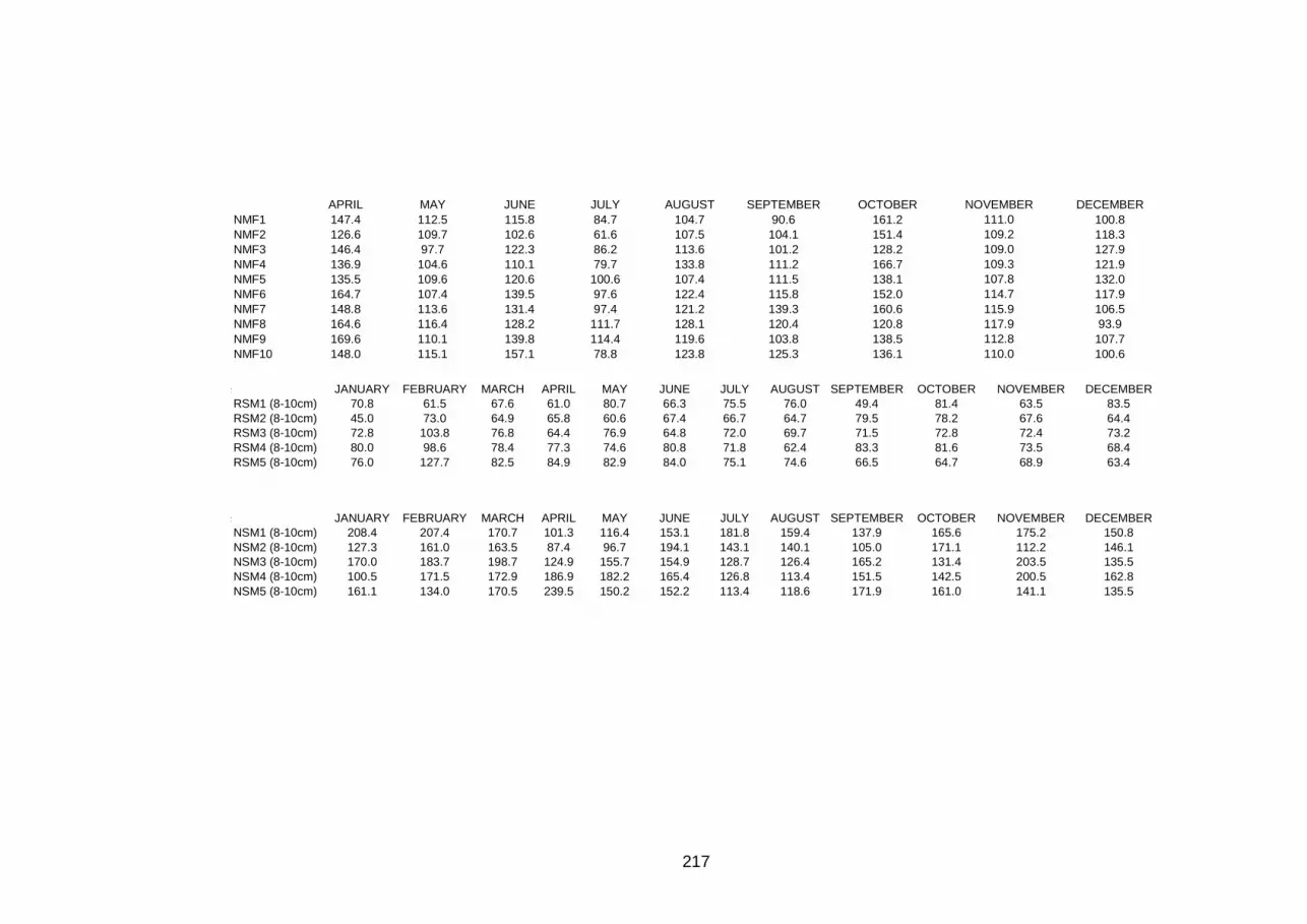
217

APRIL MAY JUNE JULY AUGUST SEPTEMBER OCTOBER NOVEMBER DECEMBER

NMF1 147.4 112.5 115.8 84.7 104.7 90.6 161.2 111.0 100.8NMF2 126.6 109.7 102.6 61.6 107.5 104.1 151.4 109.2 118.3NMF3 146.4 97.7 122.3 86.2 113.6 101.2 128.2 109.0 127.9NMF4 136.9 104.6 110.1 79.7 133.8 111.2 166.7 109.3 121.9NMF5 135.5 109.6 120.6 100.6 107.4 111.5 138.1 107.8 132.0NMF6 164.7 107.4 139.5 97.6 122.4 115.8 152.0 114.7 117.9NMF7 148.8 113.6 131.4 97.4 121.2 139.3 160.6 115.9 106.5NMF8 164.6 116.4 128.2 111.7 128.1 120.4 120.8 117.9 93.9NMF9 169.6 110.1 139.8 114.4 119.6 103.8 138.5 112.8 107.7NMF10 148.0 115.1 157.1 78.8 123.8 125.3 136.1 110.0 100.6

OCTOBER JANUARY FEBRUARY MARCH APRIL MAY JUNE JULY AUGUST SEPTEMBER OCTOBER NOVEMBER DECEMBERRSM1 (8-10cm) 70.8 61.5 67.6 61.0 80.7 66.3 75.5 76.0 49.4 81.4 63.5 83.5RSM2 (8-10cm) 45.0 73.0 64.9 65.8 60.6 67.4 66.7 64.7 79.5 78.2 67.6 64.4RSM3 (8-10cm) 72.8 103.8 76.8 64.4 76.9 64.8 72.0 69.7 71.5 72.8 72.4 73.2RSM4 (8-10cm) 80.0 98.6 78.4 77.3 74.6 80.8 71.8 62.4 83.3 81.6 73.5 68.4RSM5 (8-10cm) 76.0 127.7 82.5 84.9 82.9 84.0 75.1 74.6 66.5 64.7 68.9 63.4

OCTOBER JANUARY FEBRUARY MARCH APRIL MAY JUNE JULY AUGUST SEPTEMBER OCTOBER NOVEMBER DECEMBERNSM1 (8-10cm) 208.4 207.4 170.7 101.3 116.4 153.1 181.8 159.4 137.9 165.6 175.2 150.8NSM2 (8-10cm) 127.3 161.0 163.5 87.4 96.7 194.1 143.1 140.1 105.0 171.1 112.2 146.1NSM3 (8-10cm) 170.0 183.7 198.7 124.9 155.7 154.9 128.7 126.4 165.2 131.4 203.5 135.5NSM4 (8-10cm) 100.5 171.5 172.9 186.9 182.2 165.4 126.8 113.4 151.5 142.5 200.5 162.8NSM5 (8-10cm) 161.1 134.0 170.5 239.5 150.2 152.2 113.4 118.6 171.9 161.0 141.1 135.5

218

Appendix 2 Sediment organic matter content (%) data in the restored saltmarsh (RSM), restored mudflat (RMF),

natural saltmarsh (NSM), natural mudflat (NMF) and organic matter content (%) data in the restored and natural

saltmarshes at 8 – 10 cm depth. JANUARY FEBRUARY MARCH APRIL MAY JUNE JULY AUGUST SEPTEMBER OCTOBER NOVEMBER DECEMBER

RSM1 7.3 9.4 9.6 11.5 9.4 7.9 7.6 8.7 10.4 7.9 6.7 6.9RSM2 8.1 9.6 8.2 11.4 9.8 8.4 10.4 9.2 10.3 12.8 8.6 9.3RSM3 9.5 9.4 9.5 11.9 10.6 9.3 11.0 9.4 11.3 7.7 8.8 8.6RSM4 11.4 8.6 9.4 12.5 9.3 9.9 11.0 10.9 10.2 11.2 9.1 8.9RSM5 10.8 8.9 9.6 12.1 12.3 10.0 12.0 10.5 9.6 10.5 9.1 11.6RSM6 8.7 8.6 10.5 12.2 11.2 9.6 10.5 10.2 9.4 10.4 8.6 7.8RSM7 9.2 9.2 9.0 12.2 12.6 12.7 11.4 11.5 9.5 5.5 6.2 10.2RSM8 11.8 8.8 9.4 13.3 11.9 12.2 12.8 10.7 8.3 10.4 8.3 10.9RSM9 8.6 9.4 9.9 13.8 13.6 12.3 12.5 12.3 7.7 12.3 7.8 8.9RSM10 8.8 10.0 9.6 12.1 13.6 12.2 13.0 11.6 5.6 11.5 9.8 10.1

JANUARY FEBRUARY MARCH APRIL MAY JUNE JULY AUGUST SEPTEMBER OCTOBER NOVEMBER DECEMBERRMF1 9.3 10.8 11.8 12.3 11.3 11.7 12.4 11.6 11.1 9.4 9.8 10.0RMF2 8.9 10.8 9.6 10.6 10.2 11.5 12.1 8.9 10.7 8.6 9.3 10.2RMF3 9.7 9.2 10.4 10.9 11.1 13.9 11.4 10.7 10.8 9.8 11.6 9.1RMF4 9.9 11.3 9.7 12.6 11.1 11.2 11.7 9.8 9.7 10.1 9.7 11.9RMF5 10.5 9.4 10.3 11.2 9.5 10.7 12.5 11.3 9.9 10.0 9.9 9.5RMF6 9.4 8.9 10.4 11.5 10.4 10.0 11.0 11.2 9.3 10.0 10.0 9.3RMF7 7.1 10.1 10.7 10.9 10.6 11.0 11.7 10.1 10.0 13.4 10.0 8.3RMF8 9.7 9.9 10.2 10.2 11.2 10.7 10.5 9.9 10.4 9.7 9.8 16.2RMF9 8.3 10.3 11.1 12.6 12.9 10.0 11.3 11.3 10.0 11.0 9.2 9.7RMF10 8.7 10.1 10.0 11.3 11.5 10.1 11.2 10.7 10.8 9.7 9.1 8.9

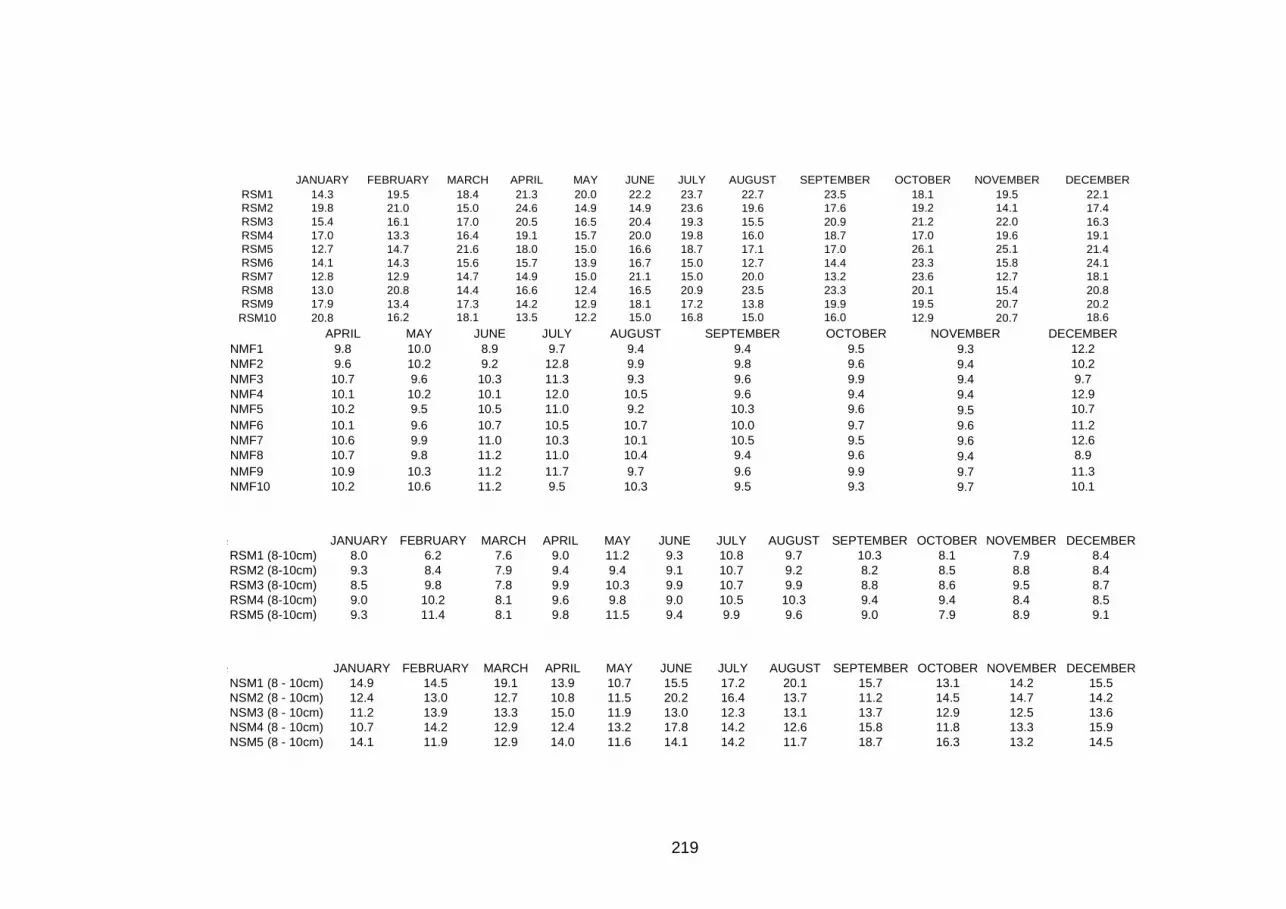
219

JANUARY FEBRUARY MARCH APRIL MAY JUNE JULY AUGUST SEPTEMBER OCTOBER NOVEMBER DECEMBERRSM1 14.3 19.5 18.4 21.3 20.0 22.2 23.7 22.7 23.5 18.1 19.5 22.1RSM2 19.8 21.0 15.0 24.6 14.9 14.9 23.6 19.6 17.6 19.2 14.1 17.4RSM3 15.4 16.1 17.0 20.5 16.5 20.4 19.3 15.5 20.9 21.2 22.0 16.3RSM4 17.0 13.3 16.4 19.1 15.7 20.0 19.8 16.0 18.7 17.0 19.6 19.1RSM5 12.7 14.7 21.6 18.0 15.0 16.6 18.7 17.1 17.0 26.1 25.1 21.4RSM6 14.1 14.3 15.6 15.7 13.9 16.7 15.0 12.7 14.4 23.3 15.8 24.1RSM7 12.8 12.9 14.7 14.9 15.0 21.1 15.0 20.0 13.2 23.6 12.7 18.1RSM8 13.0 20.8 14.4 16.6 12.4 16.5 20.9 23.5 23.3 20.1 15.4 20.8RSM9 17.9 13.4 17.3 14.2 12.9 18.1 17.2 13.8 19.9 19.5 20.7 20.2RSM10 20.8 16.2 18.1 13.5 12.2 15.0 16.8 15.0 16.0 12.9 20.7 18.6

APRIL MAY JUNE JULY AUGUST SEPTEMBER OCTOBER NOVEMBER DECEMBERNMF1 9.8 10.0 8.9 9.7 9.4 9.4 9.5 9.3 12.2NMF2 9.6 10.2 9.2 12.8 9.9 9.8 9.6 9.4 10.2NMF3 10.7 9.6 10.3 11.3 9.3 9.6 9.9 9.4 9.7NMF4 10.1 10.2 10.1 12.0 10.5 9.6 9.4 9.4 12.9NMF5 10.2 9.5 10.5 11.0 9.2 10.3 9.6 9.5 10.7NMF6 10.1 9.6 10.7 10.5 10.7 10.0 9.7 9.6 11.2NMF7 10.6 9.9 11.0 10.3 10.1 10.5 9.5 9.6 12.6NMF8 10.7 9.8 11.2 11.0 10.4 9.4 9.6 9.4 8.9NMF9 10.9 10.3 11.2 11.7 9.7 9.6 9.9 9.7 11.3NMF10 10.2 10.6 11.2 9.5 10.3 9.5 9.3 9.7 10.1

OCTOBER JANUARY FEBRUARY MARCH APRIL MAY JUNE JULY AUGUST SEPTEMBER OCTOBER NOVEMBER DECEMBERRSM1 (8-10cm) 8.0 6.2 7.6 9.0 11.2 9.3 10.8 9.7 10.3 8.1 7.9 8.4RSM2 (8-10cm) 9.3 8.4 7.9 9.4 9.4 9.1 10.7 9.2 8.2 8.5 8.8 8.4RSM3 (8-10cm) 8.5 9.8 7.8 9.9 10.3 9.9 10.7 9.9 8.8 8.6 9.5 8.7RSM4 (8-10cm) 9.0 10.2 8.1 9.6 9.8 9.0 10.5 10.3 9.4 9.4 8.4 8.5RSM5 (8-10cm) 9.3 11.4 8.1 9.8 11.5 9.4 9.9 9.6 9.0 7.9 8.9 9.1

OCTOBER JANUARY FEBRUARY MARCH APRIL MAY JUNE JULY AUGUST SEPTEMBER OCTOBER NOVEMBER DECEMBERNSM1 (8 - 10cm) 14.9 14.5 19.1 13.9 10.7 15.5 17.2 20.1 15.7 13.1 14.2 15.5NSM2 (8 - 10cm) 12.4 13.0 12.7 10.8 11.5 20.2 16.4 13.7 11.2 14.5 14.7 14.2NSM3 (8 - 10cm) 11.2 13.9 13.3 15.0 11.9 13.0 12.3 13.1 13.7 12.9 12.5 13.6NSM4 (8 - 10cm) 10.7 14.2 12.9 12.4 13.2 17.8 14.2 12.6 15.8 11.8 13.3 15.9NSM5 (8 - 10cm) 14.1 11.9 12.9 14.0 11.6 14.1 14.2 11.7 18.7 16.3 13.2 14.5

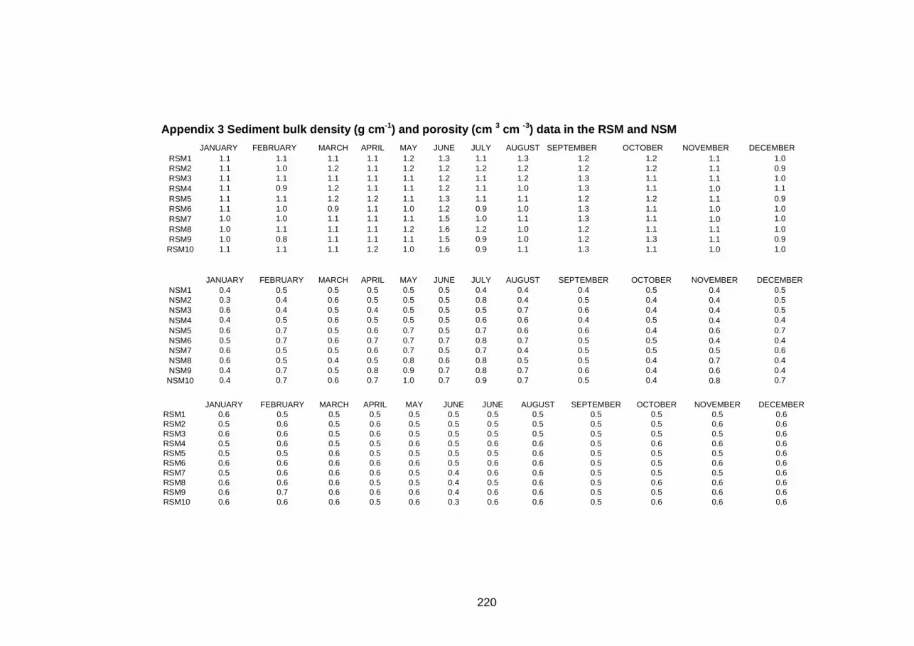
220

Appendix 3 Sediment bulk density (g cm -1) and porosity (cm 3 cm -3) data in the RSM and NSM JANUARY FEBRUARY MARCH APRIL MAY JUNE JULY AUGUST SEPTEMBER OCTOBER NOVEMBER DECEMBER


JANUARY FEBRUARY MARCH APRIL MAY JUNE JULY AUGUST SEPTEMBER OCTOBER NOVEMBER DECEMBER

NSM1 0.4 0.5 0.5 0.5 0.5 0.5 0.4 0.4 0.4 0.5 0.4 0.5NSM2 0.3 0.4 0.6 0.5 0.5 0.5 0.8 0.4 0.5 0.4 0.4 0.5NSM3 0.6 0.4 0.5 0.4 0.5 0.5 0.5 0.7 0.6 0.4 0.4 0.5NSM4 0.4 0.5 0.6 0.5 0.5 0.5 0.6 0.6 0.4 0.5 0.4 0.4NSM5 0.6 0.7 0.5 0.6 0.7 0.5 0.7 0.6 0.6 0.4 0.6 0.7NSM6 0.5 0.7 0.6 0.7 0.7 0.7 0.8 0.7 0.5 0.5 0.4 0.4NSM7 0.6 0.5 0.5 0.6 0.7 0.5 0.7 0.4 0.5 0.5 0.5 0.6NSM8 0.6 0.5 0.4 0.5 0.8 0.6 0.8 0.5 0.5 0.4 0.7 0.4NSM9 0.4 0.7 0.5 0.8 0.9 0.7 0.8 0.7 0.6 0.4 0.6 0.4NSM10 0.4 0.7 0.6 0.7 1.0 0.7 0.9 0.7 0.5 0.4 0.8 0.7

JANUARY FEBRUARY MARCH APRIL MAY JUNE JUNE AUGUST SEPTEMBER OCTOBER NOVEMBER DECEMBER


221

JANUARY FEBRUARY MARCH APRIL MAY JUNE JULY AUGUST SEPTEMBER OCTOBER NOVEMBER DECEMBERNSM1 0.8 0.8 0.8 0.8 0.8 0.8 0.8 0.8 0.8 0.8 0.8 0.8NSM2 0.8 0.8 0.7 0.8 0.8 0.8 0.7 0.8 0.8 0.8 0.8 0.8NSM3 0.7 0.8 0.8 0.8 0.8 0.8 0.8 0.7 0.8 0.8 0.8 0.8NSM4 0.8 0.8 0.8 0.8 0.8 0.8 0.8 0.7 0.8 0.8 0.8 0.8NSM5 0.8 0.7 0.8 0.7 0.7 0.8 0.7 0.7 0.7 0.8 0.7 0.7NSM6 0.8 0.7 0.7 0.7 0.7 0.7 0.7 0.7 0.8 0.8 0.8 0.8NSM7 0.7 0.8 0.8 0.7 0.7 0.8 0.7 0.8 0.8 0.8 0.8 0.7NSM8 0.7 0.8 0.8 0.8 0.6 0.7 0.7 0.8 0.8 0.8 0.7 0.8NSM9 0.8 0.7 0.8 0.7 0.6 0.7 0.7 0.7 0.8 0.8 0.7 0.8NSM10 0.8 0.7 0.7 0.7 0.6 0.7 0.6 0.7 0.8 0.7 0.6 0.7

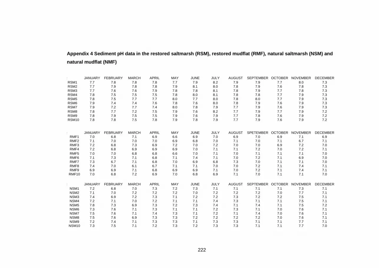
222

Appendix 4 Sediment pH data in the restored saltmar sh (RSM), restored mudflat (RMF), natural saltmarsh (NSM) and

natural mudflat (NMF)

OCTOBER JANUARY FEBRUARY MARCH APRIL MAY JUNE JULY AUGUST SEPTEMBER OCTOBER NOVEMBER DECEMBERRSM1 7.7 7.8 7.8 7.8 7.7 7.9 8.2 7.9 7.9 7.7 8.0 7.3RSM2 7.7 7.9 7.8 7.8 7.9 8.1 8.0 7.8 7.9 7.6 7.8 7.3RSM3 7.7 7.6 7.6 7.9 7.8 7.8 8.1 7.8 7.9 7.7 7.8 7.3RSM4 7.8 7.5 7.5 7.5 7.8 8.0 8.1 7.8 7.8 7.7 7.9 7.3RSM5 7.8 7.5 7.7 7.7 8.0 7.7 8.0 7.8 8.0 7.7 7.9 7.3RSM6 7.9 7.4 7.4 7.6 7.8 7.6 8.0 7.8 7.9 7.6 7.9 7.3RSM7 7.9 7.2 7.7 7.4 8.0 7.8 7.9 7.7 7.9 7.6 7.9 7.3RSM8 7.8 7.7 7.2 7.5 7.9 7.6 8.2 7.7 7.9 7.7 7.9 7.2RSM9 7.8 7.9 7.5 7.5 7.9 7.6 7.9 7.7 7.8 7.6 7.9 7.2RSM10 7.8 7.8 7.5 7.8 7.9 7.8 7.9 7.7 7.9 7.6 7.9 7.2

OCTOBER JANUARY FEBRUARY MARCH APRIL MAY JUNE JULY AUGUST SPETEMBER OCTOBER NOVEMBER DECEMBER

RMF1 7.0 6.8 7.1 6.9 6.6 6.9 7.0 6.9 7.0 6.9 7.1 6.9RMF2 7.1 7.0 7.0 7.0 6.9 6.8 7.0 7.1 7.0 7.1 6.7 7.1RMF3 7.2 6.8 7.3 6.9 7.2 7.0 7.2 7.0 7.0 6.9 7.2 7.0RMF4 7.2 6.8 6.9 6.9 6.9 7.0 7.1 7.1 7.2 7.0 7.2 7.1RMF5 7.0 7.0 6.8 6.8 6.6 7.0 7.1 7.0 7.1 7.1 7.1 7.0RMF6 7.1 7.3 7.1 6.8 7.1 7.4 7.1 7.0 7.2 7.1 6.9 7.0RMF7 7.3 6.7 7.1 6.8 7.0 6.9 6.8 7.3 7.0 7.1 7.1 7.0RMF8 7.4 7.0 6.1 6.7 7.1 7.1 7.0 7.0 7.2 7.1 7.4 7.1RMF9 6.9 6.9 7.1 6.8 6.9 6.9 7.1 7.0 7.2 7.1 7.4 7.1

RMF10 7.0 6.8 7.2 6.9 7.0 6.8 6.9 7.1 7.0 7.1 7.1 7.0

OCTOBER JANUARY FEBRUARY MARCH APRIL MAY JUNE JULY AUGUST SEPTEMBER OCTOBER NOVEMBER DECEMBERNSM1 7.2 6.8 7.0 7.3 7.2 7.3 7.1 7.1 7.1 7.1 7.3 7.1NSM2 7.1 7.0 7.2 7.2 7.2 7.0 7.2 7.2 7.2 7.0 7.7 7.1NSM3 7.4 6.9 7.2 7.3 7.1 7.2 7.2 7.3 7.2 7.2 7.5 7.1NSM4 7.2 7.1 7.0 7.2 7.1 7.1 7.4 7.3 7.1 7.1 7.5 7.1NSM5 7.8 7.3 6.9 7.3 7.2 7.3 7.4 7.1 7.4 7.1 7.5 7.2NSM6 7.3 7.6 7.1 7.3 7.1 7.1 7.2 7.3 7.1 7.0 7.6 7.1NSM7 7.5 7.6 7.1 7.4 7.3 7.1 7.2 7.1 7.4 7.0 7.6 7.1NSM8 7.5 7.6 6.9 7.3 7.3 7.2 7.2 7.2 7.2 7.0 7.6 7.1NSM9 7.2 7.4 7.1 7.3 7.3 7.1 7.3 7.3 7.1 7.1 7.7 7.1

NSM10 7.3 7.5 7.1 7.2 7.3 7.2 7.3 7.3 7.1 7.1 7.7 7.0

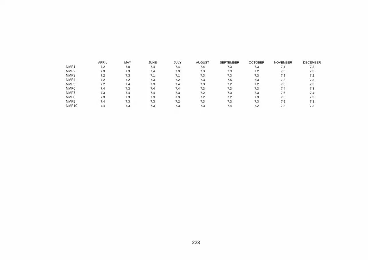
223

APRIL MAY JUNE JULY AUGUST SEPTEMBER OCTOBER NOVEMBER DECEMBERNMF1 7.2 7.0 7.4 7.4 7.4 7.3 7.3 7.4 7.3NMF2 7.3 7.3 7.4 7.3 7.3 7.3 7.2 7.5 7.3NMF3 7.2 7.3 7.1 7.1 7.3 7.3 7.3 7.2 7.2NMF4 7.2 7.2 7.3 7.2 7.3 7.5 7.3 7.3 7.3NMF5 7.2 7.4 7.3 7.4 7.3 7.2 7.2 7.3 7.3NMF6 7.4 7.3 7.4 7.4 7.3 7.3 7.3 7.4 7.3NMF7 7.3 7.4 7.4 7.3 7.2 7.3 7.3 7.5 7.4NMF8 7.3 7.3 7.3 7.3 7.2 7.2 7.3 7.3 7.3NMF9 7.4 7.3 7.3 7.2 7.3 7.3 7.3 7.5 7.3NMF10 7.4 7.3 7.3 7.3 7.3 7.4 7.2 7.3 7.3

224

Appendix 5 Sediment porewater Cl concentration (mg L-1) data in the restored saltmarsh (RSM), restored mu dflat

(RMF), natural saltmarsh (NSM) and natural mudflat (NMF)


RSD % 3.3 9.1 2.3 3.6 5.1 8.2 5.5 1.2 9.8 5.6 2.6 3.9RSM1 7210.07 5289.02 9461.14 11799.27 16269.12 22365.13 11687.64 9065.97 8155.74 5790.91 4547.99 6904.09RSM2 7168.22 3541.38 9770.22 11533.77 8799.88 16332.07 25873.71 9334.52 8651.13 7168.22 2224.12 6710.73RSM3 7533.04 4278.72 7550.71 10918.47 12725.79 24823.91 15701.70 8967.05 8686.77 7533.04 5513.37 7667.71RSM4 6727.89 5494.87 7443.23 10348.96 8508.16 14238.23 13290.49 8695.96 8577.09 6727.89 4872.81 6561.32RSM5 7026.79 6340.46 8197.27 10877.85 9895.00 24640.57 22350.29 8907.46 9859.51 7026.79 1760.20 7388.17RSM6 7037.76 5681.46 6428.57 9669.72 7858.27 11210.91 11877.95 7564.84 7319.29 7037.76 3315.91 5307.09RSM7 7542.32 6283.70 7425.81 12380.64 11381.60 28851.75 17504.81 7597.92 8335.72 7542.32 2482.98 6866.70RSM8 5874.45 7002.78 7001.95 9896.08 12495.47 22030.09 26451.01 7152.13 8804.48 5874.45 3052.10 6792.38RSM9 7947.06 6085.10 8731.65 9464.95 9917.92 28796.23 25205.40 11540.26 9259.34 7947.06 3595.18 7720.08RSM10 8054.88 4849.58 9459.18 10760.02 9498.81 10487.70 14511.89 9158.95 10308.62 6960.85 5106.40 3949.44

JANUARY FEBRUARY MARCH APRIL MAY JUNE JULY AUGUST SPETEMBER OCTOBER NOVEMBER DECEMBERRSD % 6.5 2.3 2.5 1.2 1.6 0.8 3.9 6.6 5.2 2.7 1.5 1.1RMF1 4932.05 4105.52 4133.86 5299.43 6557.33 1378.45 13164.66 3991.85 8446.71 2959.86 2362.73 4835.31RMF2 5389.53 4652.00 4919.04 3879.86 5430.69 1753.45 7044.67 4991.51 5304.55 5305.89 2731.15 6241.69RMF3 5053.72 5051.87 4714.22 7215.70 4623.25 4199.10 11211.87 4929.29 7094.07 3108.35 2633.72 6229.78RMF4 3815.69 5540.18 4381.22 4537.67 4338.76 7405.92 7856.01 4398.52 5648.82 4570.16 3089.01 7062.52RMF5 4814.72 5162.05 5297.52 7406.84 6207.49 6948.58 7781.49 4657.16 6412.82 3201.32 5881.74 7062.53RMF6 4784.51 5160.10 4842.65 6916.03 4021.16 3334.02 9754.47 4964.37 6043.31 5388.25 2290.63 6068.43RMF7 5378.07 5552.25 4728.28 3907.53 6224.22 3738.18 9476.63 6926.57 6140.60 4070.71 2205.76 8347.38RMF8 5533.53 4094.51 4153.74 8864.80 6435.17 5596.71 10086.48 5695.70 5401.31 3121.67 3370.29 7079.34RMF9 4369.47 5562.87 5112.26 4354.95 5336.07 9917.44 9370.35 4131.18 7346.50 5418.34 2971.37 6539.69RMF10 5809.48 5785.95 5871.85 8165.60 7193.71 2937.20 11110.24 5095.02 5392.36 4125.98 3054.74 6689.68

JANUARY FEBRUARY MARCH APRIL MAY JUNE JULY AUGUST SEPTEMBER OCTOBER NOVEMBER DECEMBERRSD % 1.8 3.2 4.6 0.7 0.4 1.1 1.7 3.6 4.1 5.1 1.6 3.1NSM1 4433.31 3319.16 3986.74 6731.52 8171.90 4084.47 8058.27 6999.99 6707.32 4221.61 1977.81 4476.79NSM2 3651.38 4348.72 6479.47 6276.42 7521.88 11816.19 8200.36 7133.77 7110.23 4254.62 1752.46 2973.31NSM3 4351.47 4577.09 5589.10 6625.62 10111.60 7017.01 7923.97 5843.36 6101.75 13151.25 2999.55 3299.96NSM4 3354.54 6166.18 3027.10 5913.82 8359.28 5514.15 10754.80 6894.82 5723.28 5224.05 2602.05 3695.15NSM5 4463.69 4245.02 3145.36 5980.25 11949.89 6215.79 12345.82 6161.63 9747.00 4198.47 2812.18 3333.98NSM6 4673.17 4035.02 3064.46 7338.62 9441.01 12484.56 7516.89 4752.06 6872.38 4217.22 2500.42 4411.87NSM7 5007.77 3983.10 5776.79 8462.86 8559.76 8494.36 8157.45 6991.27 9131.18 4855.81 1783.99 4489.04NSM8 4298.01 3104.60 5102.02 5664.63 8924.62 10949.24 13638.60 7640.09 6779.93 6091.81 1788.43 4511.17NSM9 4012.66 4209.53 5213.67 9718.00 7222.26 13539.30 10095.22 9570.58 7386.75 5854.64 1479.41 4224.38NSM10 4001.30 5402.38 4614.04 10369.32 8918.02 18525.28 14686.27 6757.60 7382.87 6056.89 1968.19 3443.23

225

APRIL MAY JUNE JULY AUGUST SEPTEMBER OCTOBER NOVEMBER DECEMBERRSD % 0.5 3.1 4.4 1.8 1.6 0.6 2.2 2.5 0.9NMF1 6948.66 6841.47 5008.88 11625.16 6027.23 6354.26 3925.19 4566.95 7643.42NMF2 5436.88 8165.76 5646.21 12355.92 5373.27 6752.77 4415.96 4035.65 7109.51NMF3 4888.65 9664.16 5269.31 18017.59 8161.57 7029.16 5519.21 5693.92 8951.92NMF4 4989.14 8443.83 14740.14 14529.61 4063.25 12904.17 4042.51 4063.79 7301.52NMF5 8563.20 7444.00 6562.92 11907.72 5308.66 7276.45 5357.50 4639.60 6948.38NMF6 7489.49 9062.89 7320.09 11079.91 3542.14 6618.37 4990.67 4153.84 8602.26NMF7 5640.67 9988.00 6397.55 13413.07 7062.32 7542.63 3690.76 4609.51 7773.55NMF8 6547.29 8412.06 9570.63 13706.78 4128.91 6503.74 6339.18 3149.31 19537.44NMF9 7713.71 9674.94 5200.73 12123.93 4985.01 7158.21 4668.07 3593.81 6850.59NMF10 7446.12 6722.73 5078.18 15648.02 3480.75 6334.13 6449.25 3756.84 7050.32

226

Appendix 6 Sediment porewater DOC (mg L -1) concentration data in the restored saltmarsh (RSM ), restored mudflat

(RMF), natural saltmarsh (NSM) and natural mudflat (NMF)

JANUARY FEBRUARY MARCH APRIL MAY JUNE JULY AUGUST SEPTEMBER OCTOBER NOVEMBER DECEMBERRSD % 4.6 0.7 1.2 5.1 1.7 1.2 4.5 1.4 1.1 0.3 2.8 1.9RSM1 44.91 27.76 65.99 117.76 75.57 66.57 135.06 180.63 67.21 12.70 24.92 137.14RSM2 38.90 17.04 75.77 104.42 66.57 34.62 129.00 91.50 123.18 60.41 40.59 146.19RSM3 51.89 37.82 79.65 53.25 99.95 80.54 73.95 130.64 101.85 48.92 45.95 184.16RSM4 57.40 60.34 45.07 94.55 74.96 26.08 152.85 164.23 90.17 29.84 77.88 110.75RSM5 72.16 55.74 25.80 87.03 110.29 33.11 197.51 164.49 88.51 32.99 62.00 142.97RSM6 45.82 51.68 75.08 81.19 77.68 30.88 88.26 204.47 71.66 19.82 58.69 112.07RSM7 51.49 40.26 72.20 116.48 82.85 72.69 129.34 200.89 111.58 45.37 22.87 196.31RSM8 46.91 60.30 66.14 96.91 73.97 56.89 155.34 139.94 102.53 62.61 58.75 132.91RSM9 62.81 55.70 31.27 83.63 63.96 61.32 149.14 269.93 102.65 28.55 236.94 187.40RSM10 52.57 32.64 48.75 99.76 106.05 50.27 185.96 125.97 93.60 38.11 62.96 52.88


RSD % 3.4 3.1 1.2 5.7 4.1 1.5 1.3 1.1 0.8 2.7 1.1 0.6RMF1 33.43 46.44 35.33 74.12 28.84 143.03 43.37 77.17 71.79 55.02 96.97 95.41RMF2 44.75 45.48 34.72 71.07 30.47 84.75 33.84 70.79 41.20 62.11 68.22 75.90RMF3 36.82 28.11 27.61 136.97 17.86 64.42 50.45 49.67 51.05 69.32 64.01 78.04RMF4 27.60 42.21 31.28 124.44 29.98 61.45 35.72 34.37 61.45 55.63 61.44 103.65RMF5 32.76 30.90 46.63 97.10 39.32 45.40 40.26 39.43 78.26 61.96 59.17 77.54RMF6 35.26 31.98 67.31 126.06 10.90 20.37 60.20 51.27 42.88 83.66 83.29 69.87RMF7 28.27 17.46 47.63 106.16 83.79 17.80 35.54 65.92 76.59 43.51 59.17 161.42RMF8 38.62 26.84 33.85 119.24 106.74 28.87 41.26 55.28 35.06 69.34 75.10 77.28RMF9 40.09 40.26 36.12 191.26 32.00 31.96 34.37 48.38 33.59 75.60 77.96 90.88

RMF10 29.26 34.99 27.25 172.25 36.72 28.67 32.74 38.82 54.96 56.56 65.72 101.60


RSD % 1.1 0.8 5.5 4.7 3.4 2.30 0.7 3.3 0.8 5.6 3.3 1.5NSM1 57.76 26.48 82.12 63.02 33.49 32.41 104.05 79.89 46.57 101.58 12.18 20.96NSM2 63.76 20.93 17.02 49.20 25.05 20.82 80.61 81.89 72.36 86.12 46.55 37.28NSM3 44.39 33.63 25.35 87.10 49.78 17.86 139.50 103.43 144.18 35.49 22.01 21.23NSM4 60.38 16.65 87.18 145.42 29.57 18.79 117.06 127.84 66.79 43.50 38.55 46.22NSM5 29.01 32.49 30.94 74.46 50.72 27.96 126.89 139.54 115.04 69.65 26.89 20.27NSM6 33.16 32.60 11.64 59.09 41.04 32.22 134.14 93.00 39.15 61.96 6.70 18.02NSM7 35.29 34.94 18.18 71.27 27.31 29.09 120.54 115.16 109.45 75.07 38.66 38.97NSM8 39.09 26.53 18.44 46.37 40.56 28.67 139.81 129.78 33.18 120.66 19.03 32.16NSM9 47.33 62.18 30.47 62.99 22.33 44.74 173.49 85.94 75.20 125.51 24.94 41.31

NSM10 53.37 52.29 7.70 76.05 26.66 40.90 266.41 136.12 62.08 79.71 39.92 33.50

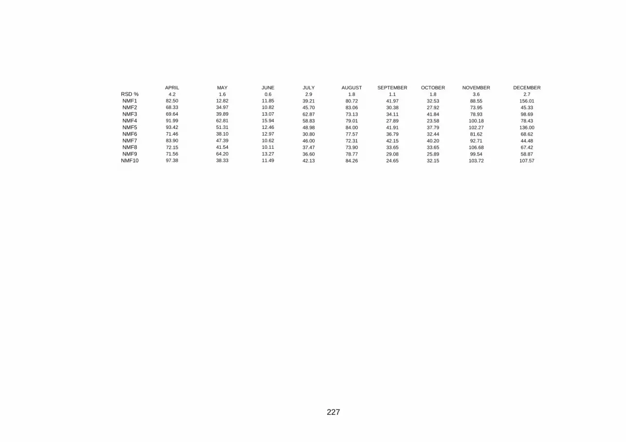
227

APRIL MAY JUNE JULY AUGUST SEPTEMBER OCTOBER NOVEMBER DECEMBERRSD % 4.2 1.6 0.6 2.9 1.8 1.1 1.8 3.6 2.7NMF1 82.50 12.82 11.85 39.21 80.72 41.97 32.53 88.55 156.01NMF2 68.33 34.97 10.82 45.70 83.06 30.38 27.92 73.95 45.33NMF3 69.64 39.89 13.07 62.87 73.13 34.11 41.84 78.93 98.69NMF4 91.99 62.81 15.94 58.83 79.01 27.89 23.58 100.18 78.43NMF5 93.42 51.31 12.46 48.98 84.00 41.91 37.79 102.27 136.00NMF6 71.46 38.10 12.97 30.80 77.57 36.79 32.44 81.62 68.62NMF7 83.90 47.39 10.62 46.00 72.31 42.15 40.20 92.71 44.48NMF8 72.15 41.54 10.11 37.47 73.90 33.65 33.65 106.68 67.42NMF9 71.56 64.20 13.27 36.60 78.77 29.08 25.89 99.54 58.87

NMF10 97.38 38.33 11.49 42.13 84.26 24.65 32.15 103.72 107.57

228

Appendix 7 Properties of agricultural soil and dred ged sediment

pH Organic matter (%)

Clay (%)

Silt (%)

Sand (%)

7.2 7.6 26.6 38.8 34.6 7.1 7.4 29.1 36.3 33.6 7.1 7.2 26.1 35.5 33.5 7.1 7.3 30.8 38.9 35.4

Soil

7.1 7.5 28.9 37.9 34.1 6.9 9.0 39.7 47.2 13.6 7.0 8.4 45.2 43.6 10.1 6.9 8.6 39.4 47.5 14.5 7.0 8.6 38.5 47.6 13.4

Sediment

7.0 8.8 39.2 47.7 12.8

229

Appendix 8 Partition coefficients (log K d) of the metals and herbicides for

agricultural soil and dredged sediment at 5 ‰ and 2 0 ‰ salinity.

Samples Cu Ni Zn

soil1_5 2.68 2.29 2.58

soil2_5 2.60 2.26 2.56

soil3_5 2.64 2.27 2.53

soil4_5 2.68 2.28 2.68

soil5_5 2.73 2.36 2.59

soil6_5 2.79 2.34 2.63

soil7_5 2.87 2.38 2.67

soil8_5 2.89 2.39 2.57

soil9_5 2.93 2.37 2.69

soil1_20 2.28 2.15 2.42

soil2_20 2.28 2.16 2.35

soil3_20 2.29 2.19 2.33

soil4_20 2.56 2.29 2.62

soil5_20 2.56 2.31 2.57

soil6_20 2.57 2.49 2.53

soil7_20 2.79 2.32 2.71

soil8_20 2.78 2.32 2.71

soil9_20 2.81 2.32 2.73

sediment1_5 2.80 2.53 2.67

sediment2_5 2.81 2.58 2.67

sediment3_5 2.78 2.54 2.73

sediment4_5 2.99 2.50 2.69

sediment5_5 2.99 2.53 2.65

sediment6_5 2.98 2.51 2.69

sediment7_5 3.14 2.45 2.69

sediment8_5 3.12 2.50 2.67

sediment9_5 3.12 2.58 2.68

sediment1_20 2.54 2.63 2.58

sediment2_20 2.52 2.71 2.78

sediment3_20 2.52 2.41 2.58

sediment4_20 2.71 2.37 2.76

sediment5_20 2.74 2.32 2.74

sediment6_20 2.73 2.29 2.85

sediment7_20 2.98 2.33 2.78

sediment8_20 2.98 2.46 2.93

sediment9_20 2.97 2.41 2.71

230

Samples Simazine Atrazine Diuron

soil1_5 3.84 3.92 4.39

soil2_5 3.82 3.94 4.34

soil3_5 3.75 3.88 4.21

soil4_5 3.74 3.86 4.21

soil5_5 3.71 3.82 4.09

soil6_5 3.67` 3.83 4.09

soil1_20 3.52 3.85 4.46

soil2_20 2.69 3.94 4.38

soil3_20 2.61 3.85 4.19

soil4_20 3.63 3.88 4.21

soil5_20 3.63 3.88 4.16

soil6_20 3.57 3.84 4.07

sediment1_5 3.70 4.02 4.57

sediment2_5 3.85 4.05 4.58

sediment3_5 3.62 3.90 4.21

sediment4_5 3.64 3.86 4.29

sediment5_5 3.61 3.89 4.16

sediment6_5 3.63 3.89 4.20

sediment1_20 3.68 3.93 4.55

sediment2_20 3.74 3.99 4.59

sediment3_20 3.68 3.91 4.41

sediment4_20 3.65 3.93 4.35

sediment5_20 3.61 3.81 4.19

sediment6_20 3.64 3.91 4.25

231

S oil H igh sa lin ity Low sa lin ityS am ple C u N i Zn S am ple C u N i Z nH W 1 0.30 30.15 36.80 LW 1 0.56 24.68 15.20H W 2 0.15 21.81 28.51 LW 2 0.39 17.99 11.20H W 3 0.03 2.95 7.24 LW 3 0.10 3.72 3.36H W 4 0.03 2.44 6.13 LW 4 0.16 6.41 5.95H W 5 0.04 2.13 5.44 LW 5 0.18 6.90 5.34H W 6 0.03 1.98 5.03 LW 6 0.12 4.30 3.92H W 7 0.04 1.85 2.65 LW 7 0.09 3.66 3.23H W 8 0.03 1.63 2.27 LW 8 0.07 2.71 2.39H W 9 0.03 1.30 2.30 LW 9 0.08 3.09 2.69H W 10 0.03 1.28 1.71 LW 10 0.06 2.30 1.97H W 11 0.02 1.04 1.50 LW 11 0.04 1.60 1.34H W 12 0.03 0.92 1.55 LW 12 0.03 1.33 1.08H W 13 0.02 0.84 1.36 LW 13 0.04 1.55 1.27H W 14 0.02 0.80 1.39 LW 14 0.03 1.56 1.27H W 15 0.01 0.72 0.96 LW 15 0.03 1.12 0.90H W 16 0.02 0.80 0.99 LW 16 0.02 0.93 0.72H W 17 0.02 0.77 0.81 LW 17 0.03 1.21 0.94H W 18 0.02 0.68 0.85 LW 18 0.03 1.09 0.82H W 19 0.01 0.69 0.92 LW 19 0.04 1.86 1.42H W 20 0.02 0.66 0.90 LW 20 0.04 1.51 1.19H W 21 0.02 0.70 0.83 LW 21 0.04 1.65 1.32H W 22 0.02 0.68 0.92 LW 22 0.03 1.19 0.95H W 23 0.03 0.69 0.88 LW 23 0.03 0.98 0.75H W 24 0.46 30.90 20.60 LW 24 0.27 12.50 12.50H W 25 0.31 20.00 10.30 LW 25 0.21 9.52 9.52H W 26 0.21 8.45 2.53 LW 26 0.07 2.60 3.60H W 27 0.18 7.11 2.15 LW 27 0.06 2.27 2.27H W 28 0.17 6.21 1.90 LW 28 0.04 1.57 2.57H W 29 0.16 5.70 1.79 LW 29 0.03 1.35 1.35H W 30 0.08 3.01 1.69 LW 30 0.03 1.33 1.33H W 31 0.07 2.61 1.45 LW 31 0.04 1.84 1.84H W 32 0.07 2.94 1.20 LW 32 0.03 1.01 1.01H W 33 0.05 2.13 1.06 LW 33 0.02 0.73 0.73H W 34 0.06 1.85 0.86 LW 34 0.02 0.92 0.92H W 35 0.05 1.86 0.79 LW 35 0.02 0.69 0.69H W 36 0.05 1.70 0.72 LW 36 0.03 0.88 0.88H W 37 0.05 1.71 0.70 LW 37 0.02 0.69 0.69H W 38 0.04 1.19 0.62 LW 38 0.03 1.32 1.32H W 39 0.04 1.20 0.72 LW 39 0.01 0.44 0.44H W 40 0.03 1.00 0.65 LW 40 0.03 1.20 1.20H W 41 0.03 1.06 0.61 LW 41 0.04 1.31 1.31H W 42 0.03 1.14 0.61 LW 42 0.02 0.91 0.91H W 43 0.03 1.07 0.57 LW 43 0.01 0.34 0.34H W 44 0.02 1.47 0.64 LW 44 0.02 0.86 0.86H W 45 0.03 1.10 0.63 LW 45 0.02 0.75 0.75H W 46 0.03 1.05 0.40 LW 46 0.01 2.16 2.16H W 47 0.48 50.18 37.30 LW 47 0.32 19.11 10.11H W 48 0.35 26.85 21.10 LW 48 0.17 16.42 7.42H W 49 0.03 5.60 4.63 LW 49 0.17 6.37 5.37H W 50 0.16 4.85 4.90 LW 50 0.15 5.23 5.23H W 51 0.11 3.67 3.60 LW 51 0.14 4.86 4.86H W 52 0.09 2.88 2.86 LW 52 0.12 4.42 4.42H W 53 0.07 2.15 2.07 LW 53 0.07 2.10 2.10H W 54 0.06 2.16 1.94 LW 54 0.04 1.25 1.25H W 55 0.06 2.17 1.99 LW 55 0.06 1.71 1.71H W 56 0.06 1.81 1.73 LW 56 0.05 1.40 1.40H W 57 0.04 1.34 1.30 LW 57 0.04 1.15 1.15H W 58 0.05 1.04 0.97 LW 58 0.04 1.10 1.10H W 59 0.04 1.10 1.06 LW 59 0.03 0.92 0.92H W 60 0.04 1.22 1.12 LW 60 0.05 1.18 1.18H W 61 0.03 0.70 0.63 LW 61 0.02 0.56 0.56H W 62 0.04 1.46 1.32 LW 62 0.03 0.72 0.72H W 63 0.04 1.18 1.11 LW 63 0.02 0.69 0.75H W 64 0.02 0.55 0.50 LW 64 0.02 0.68 0.69H W 65 0.02 0.58 0.54 LW 65 0.02 0.58 0.68H W 66 0.01 0.19 0.17 LW 66 0.02 0.62 0.58H W 67 0.04 1.08 1.03 LW 67 0.01 0.51 0.62H W 68 0.03 0.95 0.85 LW 68 0.02 0.54 0.51H W 69 0.02 0.71 0.59 LW 69 0.02 0.75 0.54

Appendix 9 Concentrations of Cu, Ni and Zn (mg L -1) released from the soil and

sediment to the overlying water under low and high salinity treatments

232

S edim ent H igh sa lin ity Low sa lin ityS am ple C u N i Zn S am ple C u N i Z nH S 1 0.06 10.64 5.02 LS1 0.31 8.03 3.20H S 2 0.02 3.38 2.62 LS2 0.28 5.18 2.28H S 3 0.01 1.73 2.41 LS3 0.16 2.01 1.30H S 4 0.01 2.00 4.97 LS4 0.03 3.80 2.56H S 5 0.02 5.48 10.60 LS5 0.05 4.36 3.41H S 6 0.02 1.49 6.17 LS6 0.02 1.93 1.23H S 7 0.02 2.01 3.06 LS7 0.01 1.59 0.97H S 8 0.02 1.64 7.14 LS8 0.01 0.91 0.58H S 9 0.02 1.51 1.30 LS9 0.01 0.70 0.40H S 10 0.02 1.49 1.50 LS10 0.01 0.53 0.32H S 11 0.01 1.02 0.95 LS11 0.01 0.94 0.55H S 12 0.02 0.97 0.24 LS12 0.01 0.73 0.42H S 13 0.02 1.07 0.55 LS13 0.01 1.10 0.63H S 14 0.02 0.88 1.11 LS14 0.01 0.79 0.47H S 15 0.01 1.05 0.33 LS15 0.01 0.55 0.31H S 16 0.02 0.93 1.44 LS16 0.01 0.47 0.26H S 17 0.02 0.89 1.08 LS17 0.01 0.41 0.21H S 18 0.01 0.76 0.34 LS18 0.01 0.69 0.36H S 19 0.01 0.71 0.34 LS19 0.01 0.47 0.24H S 20 0.01 0.60 0.27 LS20 0.01 0.64 0.35H S 21 0.01 0.71 0.67 LS21 0.01 0.52 0.26H S 22 0.02 1.09 0.42 LS22 0.01 0.63 0.34H S 23 0.02 0.93 0.35 LS23 0.01 0.41 0.18H S 24 0.08 19.21 9.40 LS24 0.33 4.52 4.52H S 25 0.07 9.50 6.06 LS25 0.21 3.34 3.34H S 26 0.06 8.03 5.31 LS26 0.02 1.05 1.05H S 27 0.06 6.65 4.53 LS27 0.08 0.82 0.82H S 28 0.05 5.81 4.09 LS28 0.02 1.92 0.92H S 29 0.05 5.14 3.66 LS29 0.01 0.61 0.61H S 30 0.03 2.77 2.04 LS30 0.01 0.69 0.69H S 31 0.03 1.96 1.40 LS31 0.01 0.56 0.56H S 32 0.03 2.06 1.29 LS32 0.01 0.59 0.59H S 33 0.02 1.94 1.26 LS33 0.01 0.64 0.64H S 34 0.02 1.51 0.96 LS34 0.01 0.48 0.48H S 35 0.03 1.50 1.00 LS35 0.01 0.37 0.37H S 36 0.02 1.21 0.76 LS36 0.01 0.43 0.43H S 37 0.02 1.16 0.74 LS37 0.01 0.38 0.38H S 38 0.01 0.87 0.56 LS38 0.01 0.69 0.69H S 39 0.02 0.95 0.62 LS39 0.01 0.33 0.33H S 40 0.01 0.85 0.54 LS40 0.01 0.38 0.38H S 41 0.01 0.82 0.53 LS41 0.01 0.40 0.40H S 42 0.02 0.92 0.56 LS42 0.01 0.38 0.38H S 43 0.01 0.88 0.58 LS43 0.02 0.71 0.71H S 44 0.01 0.72 0.45 LS44 0.01 0.39 0.39H S 45 0.02 0.79 0.53 LS45 0.01 0.35 0.35H S 46 0.02 0.10 0.10 LS46 0.01 0.48 0.48H S 47 0.04 10.99 5.51 LS47 0.27 7.93 6.93H S 48 0.03 4.65 2.27 LS48 0.15 4.87 4.87H S 49 0.00 2.98 1.10 LS49 0.04 4.12 4.12H S 50 0.03 7.67 1.30 LS50 0.03 3.67 3.67H S 51 0.11 16.44 2.99 LS51 0.03 3.31 3.31H S 52 0.01 7.94 1.00 LS52 0.03 3.09 3.09H S 53 0.03 4.40 1.37 LS53 0.02 1.33 1.33H S 54 0.08 10.25 1.14 LS54 0.01 1.00 1.00H S 55 0.02 1.96 1.06 LS55 0.01 1.18 1.18H S 56 0.03 2.22 0.98 LS56 0.01 0.79 0.79H S 57 0.01 1.37 0.69 LS57 0.01 0.89 0.89H S 58 0.01 0.36 0.67 LS58 0.01 0.70 0.70H S 59 0.01 0.81 0.72 LS59 0.01 0.59 0.59H S 60 0.01 1.59 0.61 LS60 0.01 0.58 0.58H S 61 0.01 0.52 0.76 LS61 0.01 0.38 0.38H S 62 0.00 0.39 0.65 LS62 0.01 0.43 0.43H S 63 0.01 0.46 0.62 LS63 0.01 0.39 0.39H S 64 0.01 0.51 0.51 LS64 0.01 0.40 0.40H S 65 0.01 0.60 0.49 LS65 0.00 0.34 0.34H S 66 0.00 0.37 0.41 LS66 0.01 0.38 0.38H S 67 0.01 1.03 0.49 LS67 0.03 0.75 0.75H S 68 0.01 1.29 0.79 LS68 0.01 0.38 0.38H S 69 0.01 0.59 0.93 LS69 0.01 0.37 0.37

233

Cu Ni Zn Cu Ni ZnHS3 0.01 1.73 2.41 HW2 0.15 21.81 28.51HS3 duplicate 0.01 1.62 2.49 HW2 duplicate 0.15 20.93 28.93RSD % 6.73 4.47 2.31 RSD % 3.77 2.92 1.03HS5 0.02 5.48 10.60 HW3 0.03 2.95 7.24HS5 duplicate 0.02 5.21 9.72 HW3 duplicate 0.03 3.01 7.19RSD % 8.32 3.54 6.12 RSD % 9.75 1.32 0.49HS9 0.02 1.51 1.30 HW23 0.03 0.69 0.88HS9 duplicate 0.02 1.60 1.23 HW23 duplicate 0.03 0.62 0.93RSD % 8.73 4.23 3.91 RSD % 7.15 7.64 3.99HS25 0.07 9.50 6.06 HW26 0.21 8.45 2.53HS25 duplicate 0.06 10.10 5.98 HW26 duplicate 0.19 8.56 2.49RSD % 9.72 4.33 0.94 RSD % 5.69 0.88 1.13HS28 0.05 5.81 4.09 HW28 0.17 6.21 1.90HS28 duplicate 0.05 5.67 4.13 HW28 duplicate 0.18 6.18 1.85RSD % 5.44 1.78 0.69 RSD % 6.50 0.30 2.08LS2 0.28 5.18 2.28 LW3 0.10 3.72 3.36LS2 duplicate 0.25 5.02 2.19 LW3 duplicate 0.11 3.81 3.29RSD % 7.72 2.11 2.85 RSD % 5.98 1.61 1.49LS5 0.05 4.36 3.41 LW5 0.18 6.90 5.34LS5 duplicate 0.05 4.48 3.23 LW5 duplicate 0.17 6.70 5.41RSD % 2.60 1.83 3.83 RSD % 5.36 2.09 0.92LS6 0.02 1.93 1.23 LW9 0.08 3.09 2.69LS6 duplicate 0.02 2.01 1.27 LW9 duplicate 0.09 3.19 2.56RSD % 2.11 3.10 2.26 RSD % 6.07 2.34 3.50LS23 0.01 0.41 0.18 LW25 0.21 9.52 9.52LS23 duplicate 0.00 0.46 0.17 LW25 duplicate 0.25 9.61 9.48RSD % 1.43 8.99 2.47 RSD % 9.88 0.67 0.30LS25 0.21 3.34 3.34 LW28 0.04 1.57 2.57LS25 duplicate 0.20 3.21 3.42 LW28 duplicate 0.05 1.62 2.39RSD % 4.14 2.81 1.67 RSD % 9.57 2.22 5.13LS30 0.01 0.69 0.69 LW34 0.02 0.92 0.92LS30 duplicate 0.01 0.60 0.71 LW34 duplicate 0.02 1.05 1.04RSD % 6.73 10.16 1.81 RSD % 7.07 9.10 8.43

RSD% for Cu, Ni and Zn concentrations released from the soil and sediment to the

overlying water under low and high salinity treatments

234

Soil High salinity treatment Low salinity treatmentSample Simazine Atrazine Diuron Sample Simazine Atrazine DiuronHW1 776.10 248.10 45.49 LW1 282.16 119.99 29.69HW2 419.76 103.61 19.31 LW2 155.91 42.56 9.02HW3 384.68 100.63 19.87 LW3 130.59 23.39 3.98HW5 339.22 76.67 14.52 LW5 237.40 35.81 7.83HW7 321.29 64.45 11.65 LW7 133.10 25.55 4.85HW9 281.00 29.27 8.00 LW9 106.51 19.64 2.85HW11 241.47 27.18 6.83 LW11 73.77 4.37 4.47HW13 115.12 20.70 5.74 LW13 62.25 3.01 4.52HW15 111.02 17.84 5.00 LW15 36.73 6.79 2.57HW17 84.60 12.54 2.85 LW17 49.32 7.07 1.06HW19 71.34 11.67 1.83 LW19 60.53 12.75 2.64HW21 65.81 10.85 1.37 LW21 61.18 9.23 1.51HW22 59.45 4.31 0.65 LW22 53.17 6.05 0.41HW23 419.76 103.61 19.31 LW23 37.80 4.59 0.47HW24 490.90 189.42 30.96 LW24 602.65 178.67 31.43HW25 183.64 112.65 19.20 LW25 364.64 124.26 22.44HW26 146.44 86.29 14.99 LW26 365.03 83.04 13.30HW28 127.90 92.40 12.08 LW28 234.30 64.45 9.98HW30 113.74 73.55 10.07 LW30 210.13 50.27 6.94HW32 133.36 70.93 16.71 LW32 239.67 25.26 6.22HW34 122.61 63.80 12.78 LW34 200.15 21.44 5.48HW36 65.49 35.58 6.38 LW36 123.84 22.44 5.44HW38 59.77 31.52 5.06 LW38 124.83 18.98 5.40HW40 53.74 27.32 4.37 LW40 58.18 8.38 1.99HW42 49.08 21.84 2.55 LW42 59.64 9.64 1.57HW44 39.89 17.21 3.76 LW44 56.52 4.21 0.66HW45 22.71 17.40 3.31 LW45 25.94 2.74 0.64HW46 21.36 1.19 2.61 LW46 20.30 1.13 0.75HW47 532.66 286.54 64.96 LW47 371.68 105.79 15.82HW48 100.07 51.37 10.01 LU48 276.56 95.68 11.31HW49 131.14 30.04 3.05 LW49 152.28 70.04 11.39HW51 135.60 32.00 8.03 LW51 125.72 70.10 9.91HW53 80.27 17.82 2.80 LW53 101.42 55.84 7.17HW55 75.69 17.16 2.12 LW55 128.42 83.32 13.56HW57 82.69 17.25 4.63 LW57 103.20 64.84 11.05HW59 58.43 11.10 1.85 LW59 52.04 27.26 5.38HW61 19.57 5.56 1.91 LW61 32.97 13.45 0.18HW63 51.32 8.29 1.29 LW63 40.12 17.51 1.80HW65 27.17 2.86 1.52 LW65 49.99 13.99 1.21HW67 43.83 6.89 1.22 LW67 29.97 11.64 2.25HW68 46.73 6.56 0.56 LW68 19.75 10.48 0.96HW69 31.42 3.21 0.23 LW69 19.90 4.59 0.54

Appendix 10 Concentrations of simazine, atrazine and diuron (µg L-1) released from

the soil and sediment into the overlying water unde r the low and high salinity

treatments

235

Sediment High salinity treatment Low salinity treatmentsample Simazine Atrazine Diuron Simazine Atrazine DiuronHS1 426.87 106.62 17.76 LS1 229.14 56.33 12.69HS2 318.81 79.28 12.66 LS2 172.85 16.85 9.40HS3 152.02 47.52 9.78 LS3 97.70 11.81 1.11HS5 134.99 37.06 7.09 LS5 199.66 39.56 8.99HS7 68.87 32.20 5.69 LS7 72.79 9.71 2.31HS9 55.82 14.26 2.27 LS9 40.79 3.46 1.67HS11 50.95 8.09 2.26 LS11 129.97 10.80 7.54HS13 55.05 13.19 2.55 LS13 68.97 9.30 1.04HS15 93.62 11.20 4.57 LS15 30.33 4.77 1.70HS17 66.53 6.95 2.22 LS17 29.57 1.47 0.50HS19 54.47 6.64 2.57 LS19 33.60 2.32 0.18HS21 72.04 6.87 1.57 LS21 49.27 2.00 1.37HS22 60.57 4.97 0.93 LS22 50.31 3.90 1.55HS23 16.98 5.20 0.44 LS23 31.69 2.44 0.83HS24 303.59 126.12 24.33 LS24 369.31 102.55 17.37HS25 190.82 107.68 18.96 LS25 223.15 71.84 8.42HS26 152.23 102.64 15.52 LS26 288.82 36.94 7.06HS28 160.15 81.93 11.79 LS28 182.20 36.05 7.96HS30 110.63 67.35 9.42 LS30 174.11 29.98 5.62HS32 116.67 57.29 7.89 LS32 167.61 18.31 5.59HS34 102.64 66.43 12.60 LS34 170.61 19.08 5.24HS36 61.03 30.46 5.10 LS36 87.93 16.48 5.64HS38 41.64 21.68 3.17 LS38 88.21 12.49 4.74HS40 42.50 18.27 2.43 LS40 74.30 6.56 2.11HS42 44.15 15.62 1.33 LS42 47.37 7.89 1.89HS44 34.85 12.58 3.14 LS44 45.56 2.81 1.85HS45 15.60 11.92 2.10 LS45 49.89 1.60 0.67HS46 14.90 9.42 0.95 LS46 19.43 1.09 0.54HS47 193.54 96.14 11.09 LS47 237.73 109.53 17.79HS48 28.97 21.53 2.02 LS48 144.99 78.48 13.23HS49 10.39 13.11 1.66 LS49 118.19 62.14 9.69HS51 442.95 99.84 17.30 LS51 107.90 66.96 11.65HS53 124.42 27.74 4.79 LS53 90.09 54.81 7.19HS55 82.26 14.67 1.21 LS55 115.84 58.20 12.64HS57 75.25 11.54 1.18 LS57 91.44 41.64 8.85HS59 41.95 7.58 2.76 LS59 43.99 19.12 3.03HS61 13.66 3.64 1.77 LS61 36.46 14.01 1.47HS63 58.33 9.20 1.75 LS63 37.94 15.88 1.96HS65 30.92 2.47 1.67 LS65 35.00 10.59 0.45HS67 58.83 6.73 0.71 LS67 31.66 11.53 2.72HS68 48.17 5.98 1.82 LS68 15.24 3.97 0.11HS69 36.51 3.36 1.41 LS69 15.73 7.70 4.74

236

Simazine Atrazine Diuron Simazine Atrazine DiuronHS3 152.02 47.52 9.78 HW3 384.68 100.63 19.87HS3 duplicate 149.91 44.89 9.89 HW3 duplicate 381.39 98.78 18.52RSD % 0.99 4.02 0.81 RSD % 0.61 1.32 4.97HS5 134.99 37.06 7.09 HW23 419.76 103.61 19.31HS5 duplicate 130.23 34.56 6.98 HW23 duplicate 416.89 101.76 21.02RSD % 2.54 4.93 1.13 RSD % 0.49 1.28 6.01HS25 190.82 107.68 18.96 HW26 146.44 86.29 14.99HS25 duplicate 187.87 106.98 18.56 HW26 duplicate 149.26 88.16 13.70RSD % 1.10 0.46 1.49 RSD % 1.35 1.52 6.36HS28 160.15 81.93 11.79 HW28 127.90 92.40 12.08HS28 duplicate 162.01 83.03 11.54 HW28 duplicate 129.01 91.89 13.40RSD % 0.81 0.94 1.53 RSD % 0.61 0.39 7.31LS2 172.85 16.85 9.40 LW3 130.59 23.39 3.98LS2 duplicate 174.23 16.97 9.12 LW3 duplicate 131.20 21.96 3.86RSD % 0.56 0.51 2.10 RSD % 99.53 106.52 103.14LS5 199.66 39.56 8.99 LW5 237.40 35.81 7.83LS5 duplicate 198.76 38.72 8.65 LW5 duplicate 235.54 34.75 7.42RSD % 0.32 1.51 2.69 RSD % 0.56 2.12 3.82LS6 31.69 2.44 0.83 LW9 106.51 19.64 2.85LS6 duplicate 27.99 2.41 0.79 LW9 duplicate 109.10 17.58 2.82RSD % 8.76 0.90 3.76 RSD % 1.70 7.84 0.64LS23 174.11 29.98 5.62 LW25 364.64 124.26 22.44LS23 duplicate 173.24 31.01 5.89 LW25 duplicate 360.59 122.76 20.95RSD % 0.36 2.39 3.30 RSD % 0.79 0.86 4.86LS30 223.15 71.84 8.42 LW28 234.30 64.45 9.98LS30 duplicate 220.78 69.98 7.34 LW28 duplicate 231.98 62.63 8.71RSD % 0.75 1.85 9.67 RSD % 0.70 2.03 9.64HW2 419.76 103.61 19.31 LW34 200.15 21.44 5.48HW2 duplicate 421.21 101.56 18.23 LW34 duplicate 198.60 20.61 5.84RSD % 0.24 1.42 4.06 RSD % 1.10 5.55 8.26

RSD % for simazine, atrazine and diuron concentrations (µg L-1) released from the soil

and sediment into the overlying water under the low and high salinity treatments

237

Soil High salinity Low salinity Sediment High salinity Low salinitySample DOM Sample DOM Sample DOM Sample DOMHW1 562.46 LW1 573.86 HS1 332.16 LS1 215.91HW2 271.24 LW2 346.76 HS2 142.86 LS2 87.62HW3 7.12 LW3 116.94 HS3 57.10 LS3 39.72HW4 2.84 LW4 92.52 HS4 12.72 LS4 51.80HW5 5.40 LW5 62.32 HS5 21.20 LS5 80.61HW6 11.24 LW6 35.87 HS6 36.64 LS6 40.31HW7 12.10 LW7 13.54 HS7 27.00 LS7 35.38HW8 9.80 LW8 38.71 HS8 25.16 LS8 22.12HW9 8.34 LW9 57.08 HS9 19.52 LS9 16.70HW10 9.94 LW10 55.76 HS10 14.02 LS10 22.12HW11 19.54 LW11 29.66 HS11 24.80 LS11 22.04HW12 45.98 LW12 38.22 HS12 50.90 LS12 29.76HW13 39.30 LW13 40.46 HS13 46.28 LS13 31.14HW14 46.98 LW14 32.18 HS14 50.84 LS14 21.82HW15 31.16 LW15 33.58 HS15 41.50 LS15 26.01HW16 30.44 LW16 22.88 HS16 32.68 LS16 18.36HW17 25.84 LW17 39.66 HS17 35.26 LS17 25.02HW18 24.98 LW18 30.18 HS18 31.50 LS18 29.06HW19 26.28 LW19 78.30 HS19 30.12 LS19 30.16HW20 24.74 LW20 11.38 HS20 29.74 LS20 7.02HW21 14.78 LW21 14.08 HS21 29.98 LS21 11.44HW22 11.50 LW22 15.48 HS22 33.94 LS22 14.48HW23 24.62 LW23 35.54 HS23 49.74 LS23 30.60HW24 472.68 LW24 677.72 HS24 423.20 LS24 422.24HW25 292.32 LW25 558.62 HS25 274.14 LS25 323.24HW26 230.02 LW26 84.84 HS26 217.96 LS26 73.44HW27 201.10 LW27 77.84 HS27 198.36 LS27 44.80HW28 172.71 LW28 28.08 HS28 184.10 LS28 34.20HW29 145.48 LW29 11.08 HS29 155.30 LS29 15.36HW30 141.88 LW30 20.36 HS30 148.26 LS30 22.84HW31 59.80 LW31 29.98 HS31 64.96 LS31 21.48HW32 75.56 LW32 15.00 HS32 70.64 LS32 17.04HW33 64.30 LW33 9.90 HS33 60.14 LS33 18.48HW34 21.98 LW34 44.36 HS34 21.32 LS34 56.70HW35 44.82 LW35 65.14 HS35 43.40 LS35 54.34HW36 13.98 LW36 65.24 HS36 18.16 LS36 51.98HW37 25.01 LW37 66.26 HS37 19.96 LS37 53.96HW38 14.38 LW38 37.64 HS38 10.80 LS38 36.78HW39 20.24 LW39 42.04 HS39 17.54 LS39 32.30HW40 4.88 LW40 91.66 HS40 2.76 LS40 42.60HW41 9.78 LW41 95.86 HS41 14.50 LS41 41.26HW42 8.58 LW42 62.70 HS42 3.92 LS42 39.86HW43 10.72 LW43 38.82 HS43 8.68 LS43 53.64HW44 1.92 LW44 60.62 HS44 0.24 LS44 27.56HW45 1.14 LW45 41.02 HS45 1.34 LS45 22.20HW46 0.90 LW46 52.84 HS46 14.02 LS46 25.66HW47 424.78 LW47 529.02 HS47 136.62 LS47 393.72HW48 309.44 LW48 543.22 HS48 66.80 LS48 349.96HW49 10.98 LW49 221.26 HS49 7.50 LS49 237.88HW50 22.98 LW50 217.42 HS50 24.30 LS50 239.38HW51 35.30 LW51 243.12 HS51 107.06 LS51 236.84HW52 39.12 LW52 220.88 HS52 17.84 LS52 219.82HW53 24.86 LW53 206.46 HS53 46.90 LS53 206.28HW54 21.20 LW54 76.68 HS54 53.78 LS54 78.72HW55 33.62 LW55 65.52 HS55 29.58 LS55 87.66HW56 31.54 LW56 79.10 HS56 40.52 LS56 85.48HW57 19.30 LW57 29.74 HS57 28.18 LS57 24.14HW58 22.54 LW58 53.98 HS58 11.24 LS58 59.66HW59 23.40 LW59 25.98 HS59 22.80 LS59 25.50HW60 14.30 LW60 32.78 HS60 23.68 LS60 32.28HW61 17.30 LW61 23.30 HS61 17.30 LS61 17.68HW62 14.32 LW62 22.64 HS62 9.98 LS62 27.72HW63 27.02 LW63 8.52 HS63 15.76 LS63 6.40HW64 13.20 LW64 23.30 HS64 11.54 LS64 22.70HW65 20.02 LW65 6.24 HS65 24.64 LS65 14.40HW66 3.52 LW66 16.92 HS66 4.72 LS66 19.40HW67 11.90 LW67 2.90 HS67 8.58 LS67 2.00HW68 26.70 LW68 7.46 HS68 12.48 LS68 18.30HW69 26.04 LW69 11.74 HS69 25.98 LS69 14.12

Appendix 11 DOC concentrations (mg L -1) released into the overlying water from

the soil and sediment under the low and high salini ty treatments

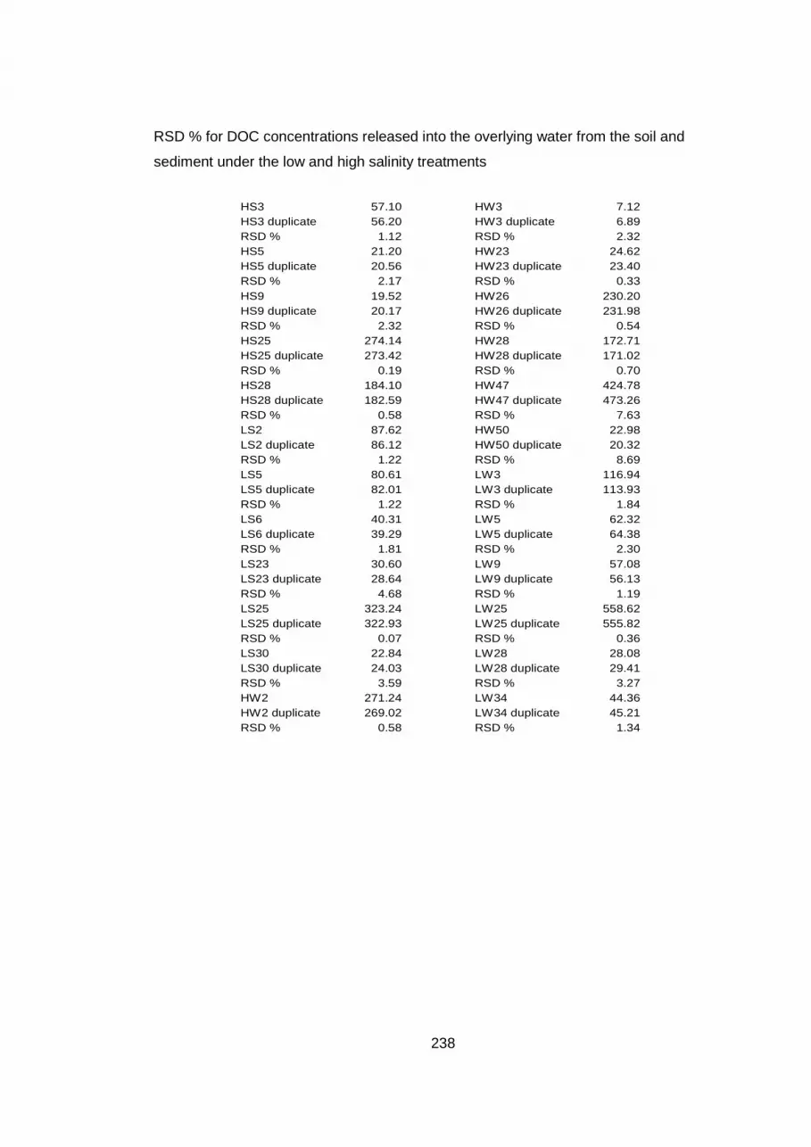
238

HS3 57.10 HW3 7.12HS3 duplicate 56.20 HW3 duplicate 6.89RSD % 1.12 RSD % 2.32HS5 21.20 HW23 24.62HS5 duplicate 20.56 HW23 duplicate 23.40RSD % 2.17 RSD % 0.33HS9 19.52 HW26 230.20HS9 duplicate 20.17 HW26 duplicate 231.98RSD % 2.32 RSD % 0.54HS25 274.14 HW28 172.71HS25 duplicate 273.42 HW28 duplicate 171.02RSD % 0.19 RSD % 0.70HS28 184.10 HW47 424.78HS28 duplicate 182.59 HW47 duplicate 473.26RSD % 0.58 RSD % 7.63LS2 87.62 HW50 22.98LS2 duplicate 86.12 HW50 duplicate 20.32RSD % 1.22 RSD % 8.69LS5 80.61 LW3 116.94LS5 duplicate 82.01 LW3 duplicate 113.93RSD % 1.22 RSD % 1.84LS6 40.31 LW5 62.32LS6 duplicate 39.29 LW5 duplicate 64.38RSD % 1.81 RSD % 2.30LS23 30.60 LW9 57.08LS23 duplicate 28.64 LW9 duplicate 56.13RSD % 4.68 RSD % 1.19LS25 323.24 LW25 558.62LS25 duplicate 322.93 LW25 duplicate 555.82RSD % 0.07 RSD % 0.36LS30 22.84 LW28 28.08LS30 duplicate 24.03 LW28 duplicate 29.41RSD % 3.59 RSD % 3.27HW2 271.24 LW34 44.36HW2 duplicate 269.02 LW34 duplicate 45.21RSD % 0.58 RSD % 1.34

RSD % for DOC concentrations released into the overlying water from the soil and

sediment under the low and high salinity treatments

239

Soil High salinity Low salinity Sediment High salinity Low salinitySample pH Sample pH Sample pH Sample pHHW1 7.5 LW1 7.5 HS1 7.8 LS1 7.8HW2 7.8 LW2 7.4 HS2 8.1 LS2 7.8HW3 7.9 LW3 7.5 HS3 7.9 LS3 7.8HW4 8.0 LW4 7.5 HS4 7.9 LS4 7.8HW5 8.0 LW5 7.6 HS5 8.0 LS5 7.8HW6 8.0 LW6 7.5 HS6 8.0 LS6 7.8HW7 8.0 LW7 7.5 HS7 8.0 LS7 7.7HW8 8.0 LW8 7.5 HS8 7.9 LS8 7.8HW9 8.1 LW9 7.5 HS9 8.1 LS9 7.9HW10 8.0 LW10 7.6 HS10 8.2 LS10 7.9HW11 8.0 LW11 7.6 HS11 8.2 LS11 7.9HW12 8.1 LW12 7.5 HS12 8.2 LS12 7.7HW13 8.1 LW13 7.4 HS13 8.0 LS13 7.6HW14 8.0 LW14 7.4 HS14 8.1 LS14 7.8HW15 8.1 LW15 7.3 HS15 8.0 LS15 7.5HW16 7.9 LW16 7.3 HS16 7.9 LS16 7.5HW17 8.0 LW17 7.5 HS17 8.1 LS17 7.8HW18 8.0 LW18 7.3 HS18 8.1 LS18 7.8HW19 8.1 LW19 7.6 HS19 8.1 LS19 7.7HW20 8.1 LW20 7.7 HS20 8.1 LS20 7.7HW21 8.0 LW21 7.5 HS21 8.0 LS21 7.8HW22 8.0 LW22 7.3 HS22 7.9 LS22 7.5HW23 8.0 LW23 7.2 HS23 8.1 LS23 7.6HW24 7.3 LW24 7.2 HS24 7.8 LS24 7.3HW25 7.9 LW25 7.3 HS25 8.3 LS25 8.0HW26 8.0 LW26 7.6 HS26 8.0 LS26 7.9HW27 7.9 LW27 7.6 HS27 7.9 LS27 7.9HW28 7.9 LW28 7.4 HS28 7.7 LS28 7.4HW29 8.0 LW29 7.0 HS29 8.2 LS29 7.3HW30 8.0 LW30 7.4 HS30 7.9 LS30 7.4HW31 8.0 LW31 7.6 HS31 7.8 LS31 7.9HW32 8.1 LW32 7.7 HS32 8.1 LS32 8.0HW33 8.2 LW33 7.6 HS33 8.1 LS33 8.1HW34 7.8 LW34 7.3 HS34 7.8 LS34 7.5HW35 7.9 LW35 7.2 HS35 8.2 LS35 7.6HW36 7.9 LW36 7.2 HS36 8.0 LS36 7.5HW37 8.2 LW37 7.4 HS37 8.3 LS37 7.3HW38 8.1 LW38 7.1 HS38 8.1 LS38 7.7HW39 8.0 LW39 7.2 HS39 7.9 LS39 7.1HW40 8.2 LW40 7.2 HS40 8.2 LS40 7.6HW41 8.2 LW41 7.2 HS41 8.1 LS41 7.6HW42 8.2 LW42 6.9 HS42 8.3 LS42 7.7HW43 8.3 LW43 6.9 HS43 8.3 LS43 7.2HW44 7.8 LW44 7.2 HS44 7.8 LS44 7.2HW45 7.7 LW45 7.2 HS45 7.8 LS45 7.2HW46 8.0 LW46 7.1 HS46 8.1 LS46 7.7HW47 7.7 LW47 7.1 HS47 7.9 LS47 7.5HW48 7.9 LW48 7.2 HS48 8.0 LS48 7.5HW49 7.9 LW49 7.2 HS49 7.9 LS49 7.5HW50 8.0 LW50 7.2 HS50 8.0 LS50 7.4

Appendix 12 pH values in the overlying water under the low and high salinity

treatments

240

HW51 8.0 LW51 7.3 HS51 8.1 LS51 7.5HW52 8.0 LW52 7.3 HS52 8.0 LS52 7.4HW53 8.0 LW53 7.3 HS53 8.0 LS53 7.3HW54 8.0 LW54 7.3 HS54 8.1 LS54 7.3HW55 8.1 LW55 7.4 HS55 8.1 LS55 7.5HW56 8.1 LW56 7.3 HS56 8.1 LS56 7.5HW57 8.1 LW57 7.4 HS57 8.1 LS57 7.4HW58 8.1 LW58 7.4 HS58 7.9 LS58 7.4HW59 7.9 LW59 7.4 HS59 7.9 LS59 7.5HW60 7.9 LW60 7.3 HS60 7.9 LS60 7.4HW61 7.9 LW61 7.3 HS61 8.0 LS61 7.4HW62 8.0 LW62 7.4 HS62 7.9 LS62 7.5HW63 7.8 LW63 7.3 HS63 7.7 LS63 7.4HW64 7.8 LW64 7.3 HS64 7.8 LS64 7.4HW65 8.1 LW65 7.3 HS65 8.1 LS65 7.8HW66 7.8 LW66 7.4 HS66 8.2 LS66 7.5HW67 7.8 LW67 7.5 HS67 7.9 LS67 7.4HW68 7.8 LW68 7.3 HS68 7.8 LS68 7.3HW69 8.0 LW69 7.1 HS69 8.0 LS69 7.7

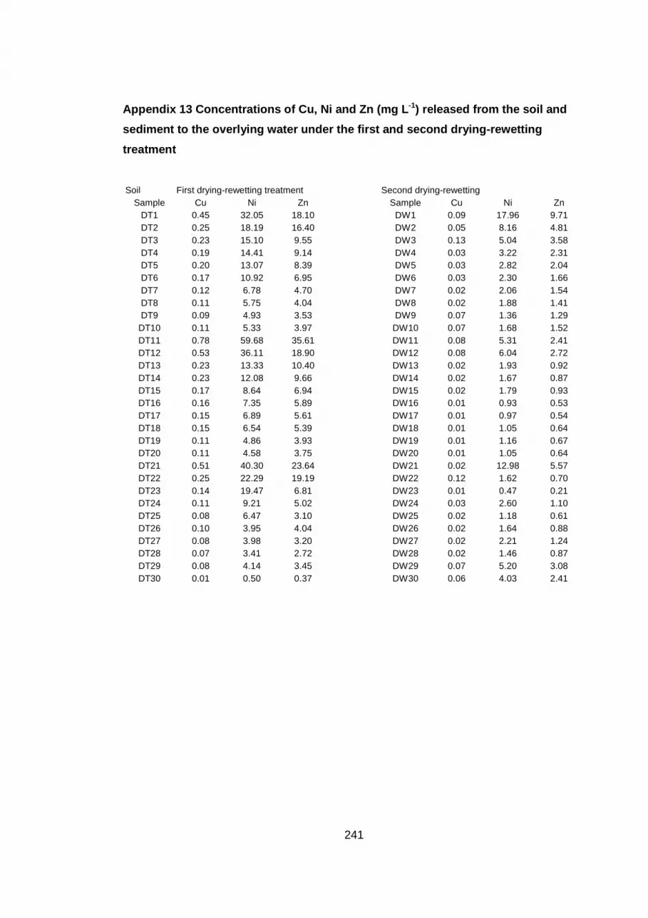
241

Soil First drying-rewetting treatment Second drying-rewettingSample Cu Ni Zn Sample Cu Ni Zn

DT1 0.45 32.05 18.10 DW1 0.09 17.96 9.71DT2 0.25 18.19 16.40 DW2 0.05 8.16 4.81DT3 0.23 15.10 9.55 DW3 0.13 5.04 3.58DT4 0.19 14.41 9.14 DW4 0.03 3.22 2.31DT5 0.20 13.07 8.39 DW5 0.03 2.82 2.04DT6 0.17 10.92 6.95 DW6 0.03 2.30 1.66DT7 0.12 6.78 4.70 DW7 0.02 2.06 1.54DT8 0.11 5.75 4.04 DW8 0.02 1.88 1.41DT9 0.09 4.93 3.53 DW9 0.07 1.36 1.29

DT10 0.11 5.33 3.97 DW10 0.07 1.68 1.52DT11 0.78 59.68 35.61 DW11 0.08 5.31 2.41DT12 0.53 36.11 18.90 DW12 0.08 6.04 2.72DT13 0.23 13.33 10.40 DW13 0.02 1.93 0.92DT14 0.23 12.08 9.66 DW14 0.02 1.67 0.87DT15 0.17 8.64 6.94 DW15 0.02 1.79 0.93DT16 0.16 7.35 5.89 DW16 0.01 0.93 0.53DT17 0.15 6.89 5.61 DW17 0.01 0.97 0.54DT18 0.15 6.54 5.39 DW18 0.01 1.05 0.64DT19 0.11 4.86 3.93 DW19 0.01 1.16 0.67DT20 0.11 4.58 3.75 DW20 0.01 1.05 0.64DT21 0.51 40.30 23.64 DW21 0.02 12.98 5.57DT22 0.25 22.29 19.19 DW22 0.12 1.62 0.70DT23 0.14 19.47 6.81 DW23 0.01 0.47 0.21DT24 0.11 9.21 5.02 DW24 0.03 2.60 1.10DT25 0.08 6.47 3.10 DW25 0.02 1.18 0.61DT26 0.10 3.95 4.04 DW26 0.02 1.64 0.88DT27 0.08 3.98 3.20 DW27 0.02 2.21 1.24DT28 0.07 3.41 2.72 DW28 0.02 1.46 0.87DT29 0.08 4.14 3.45 DW29 0.07 5.20 3.08DT30 0.01 0.50 0.37 DW30 0.06 4.03 2.41

Appendix 13 Concentrations of Cu, Ni and Zn (mg L -1) released from the soil and

sediment to the overlying water under the first and second drying-rewetting

treatment

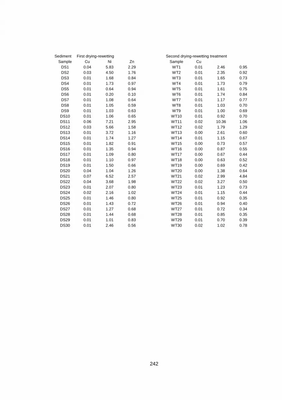
242

Sediment First drying-rewetting Second drying-rewetting treatmentSample Cu Ni Zn Sample Cu

DS1 0.04 5.83 2.29 WT1 0.01 2.46 0.95DS2 0.03 4.50 1.76 WT2 0.01 2.35 0.92DS3 0.01 1.68 0.84 WT3 0.01 1.65 0.73DS4 0.01 1.73 0.97 WT4 0.01 1.73 0.79DS5 0.01 0.64 0.94 WT5 0.01 1.61 0.75DS6 0.01 0.20 0.10 WT6 0.01 1.74 0.84DS7 0.01 1.08 0.64 WT7 0.01 1.17 0.77DS8 0.01 1.05 0.59 WT8 0.01 1.03 0.70DS9 0.01 1.03 0.63 WT9 0.01 1.00 0.69

DS10 0.01 1.06 0.65 WT10 0.01 0.92 0.70DS11 0.06 7.21 2.95 WT11 0.02 10.36 1.06DS12 0.03 5.66 1.58 WT12 0.02 1.79 1.29DS13 0.01 3.72 1.16 WT13 0.00 2.61 0.60DS14 0.01 1.74 1.27 WT14 0.01 1.15 0.67DS15 0.01 1.82 0.91 WT15 0.00 0.73 0.57DS16 0.01 1.35 0.94 WT16 0.00 0.87 0.55DS17 0.01 1.09 0.80 WT17 0.00 0.67 0.44DS18 0.01 1.10 0.97 WT18 0.00 0.63 0.52DS19 0.01 1.50 0.66 WT19 0.00 0.69 0.42DS20 0.04 1.04 1.26 WT20 0.00 1.38 0.64DS21 0.07 6.52 2.57 WT21 0.02 2.99 4.84DS22 0.04 3.68 1.98 WT22 0.02 3.27 0.50DS23 0.01 2.07 0.80 WT23 0.01 1.23 0.73DS24 0.02 2.16 1.02 WT24 0.01 1.15 0.44DS25 0.01 1.46 0.80 WT25 0.01 0.92 0.35DS26 0.01 1.43 0.72 WT26 0.01 0.94 0.40DS27 0.01 1.27 0.68 WT27 0.01 0.72 0.34DS28 0.01 1.44 0.68 WT28 0.01 0.85 0.35DS29 0.01 1.01 0.83 WT29 0.01 0.70 0.39DS30 0.01 2.46 0.56 WT30 0.02 1.02 0.78

243

Cu Ni ZnDT2 0.25 18.19 16.40DT2 duplicate 0.23 17.69 15.92RSD% 3.55 1.98 2.10DT12 0.53 36.11 18.90DT12 duplicate 0.50 34.99 18.21RSD% 4.41 2.22 2.63DT25 0.08 6.47 3.10DT25 duplicate 0.08 5.82 2.91RSD% 4.11 7.51 4.44DW7 0.02 2.06 1.54DW7 duplicate 0.02 2.17 1.69RSD% 10.10 3.78 6.47DW15 0.02 1.79 0.93DW15 duplicate 0.02 1.85 0.89RSD% 7.49 2.20 2.77DW25 0.02 1.18 0.61DW25 duplicate 0.02 1.25 0.52RSD% 9.57 3.86 10.94DS3 0.01 1.68 0.84DS3 duplicate 0.01 1.54 0.92RSD% 9.20 6.27 6.73DS14 0.01 1.74 1.27DS14 duplicate 0.01 1.65 1.32RSD% 9.63 3.56 2.73DS28 0.01 1.44 0.68DS28 duplicate 0.01 1.52 0.74RSD% 9.74 3.63 6.46WT5 0.01 1.61 0.75WT5 duplicate 0.01 1.69 0.69RSD% 9.43 3.62 5.70WT12 0.02 1.79 1.29WT12 duplicate 0.02 1.64 1.18RSD% 7.84 6.02 6.57WT21 0.02 2.99 4.84WT21 duplicate 0.01 2.82 4.79RSD% 7.68 4.17 0.79

RSD% for Cu, Ni and Zn concentrations released from the soil and sediment to the

overlying water under the drying-rewetting treatment

244

Soil First drying-rewetting treatment Second drying-rewettingSample Simazine Atrazine Diuron Sample Simazine Atrazine Diuron

DT1 740.36 477.50 95.99 DW1 359.12 246.49 38.67DT3 312.32 221.16 37.20 DW3 166.82 114.11 15.83DT5 152.12 96.77 15.54 DW5 165.39 110.95 6.06DT7 86.24 54.07 9.13 DW7 84.03 45.27 4.58DT9 74.88 39.32 5.81 DW9 75.65 12.68 2.72DT11 861.78 650.60 92.75 DW11 170.02 105.33 15.84DT13 574.21 338.43 57.87 DW13 58.79 32.64 6.05DT15 272.23 177.80 32.15 DW15 53.89 30.451 5.73DT17 201.96 108.77 22.03 DW17 29.89 14.79 2.66DT19 158.61 100.56 20.19 DW19 34.95 16.16 2.13DT21 598.48 314.39 80.93 DW21 264.58 137.24 31.93DT23 264.45 139.64 32.63 DW23 145.87 75.03 18.46DT25 33.74 43.65 12.17 DW25 77.83 31.78 7.54DT27 48.77 26.55 5.85 DW27 69.37 12.72 3.24DT29 88.73 21.79 4.50 DW29 34.95 9.36 0.41

Sediment First drying-rewetting Second drying-rewetting treatmentSample Simazine Atrazine Diuron Sample Simazine Atrazine Diuron

DS1 173.62 132.55 26.37 WT1 183.30 76.12 16.01DS3 124.90 94.88 13.82 WT3 70.29 51.72 9.72DS5 83.24 89.59 5.28 WT5 66.52 21.94 10.09DS7 54.29 24.00 2.27 WT7 36.02 13.84 3.40DS9 54.45 5.86 1.02 WT9 34.48 37.21 1.52

DS11 108.40 1.03 19.25 WT11 134.95 117.08 19.37DS13 75.12 7.21 10.42 WT13 88.43 34.36 6.09DS15 37.99 5.66 6.25 WT15 48.46 28.34 3.82DS17 23.78 3.72 4.92 WT 17 33.75 15.06 2.10DS19 22.32 1.74 4.98 WT19 74.46 13.03 3.03DS21 130.68 1.82 29.44 WT21 154.85 158.58 40.19DS23 88.86 1.35 15.89 WT23 318.14 62.15 12.86DS25 62.44 1.09 11.24 WT25 142.40 25.28 4.88DS27 12.38 1.10 1.41 WT27 62.79 21.61 2.61DS29 10.42 1.50 1.65 WT29 47.74 11.78 1.57

Appendix 14 Concentrations of simazine, atrazine an d diuron (µg L -1) released from

the soil and sediment to the overlying water under the first and second drying-

rewetting treatments

245

Simazine atrazine diuronDT17 201.96 108.77 22.03DT17 duplicate 199.23 106.87 21.23RSD% 0.96 1.25 2.61DT25 33.74 43.65 12.17DT25 duplicate 32.43 44.79 11.67RSD% 2.79 1.83 2.98DW17 29.89 14.79 2.66DW17 duplicate 28.57 15.03 2.32RSD% 3.19 1.16 9.73DW25 77.83 31.78 7.54DW25 duplicate 76.49 32.54 7.92RSD% 1.23 1.67 3.50DS3 124.90 94.88 13.82DS3 duplicate 123.61 95.28 12.46RSD% 0.73 0.30 7.30DS17 23.78 3.72 4.92DS17 duplicate 22.73 3.82 4.03RSD% 3.19 1.92 14.01DS25 62.44 1.09 11.24DS25 duplicate 61.72 1.20 11.13RSD% 0.82 6.55 0.68WT3 70.29 51.72 9.72WT3 duplicate 71.02 50.56 8.89RSD% 0.73 1.60 6.33WT 17 33.75 15.06 2.10WT17 duplicate 32.67 14.92 2.21RSD% 2.30 0.67 3.69WT25 142.40 25.28 4.88WT25 duplicate 141.72 24.69 5.09RSD% 0.34 1.68 2.97

RSD % for simazine, atrazine and diuron concentrations (µg L-1) released from the soil

and sediment into the overlying water under the first and second drying-rewetting

treatment.

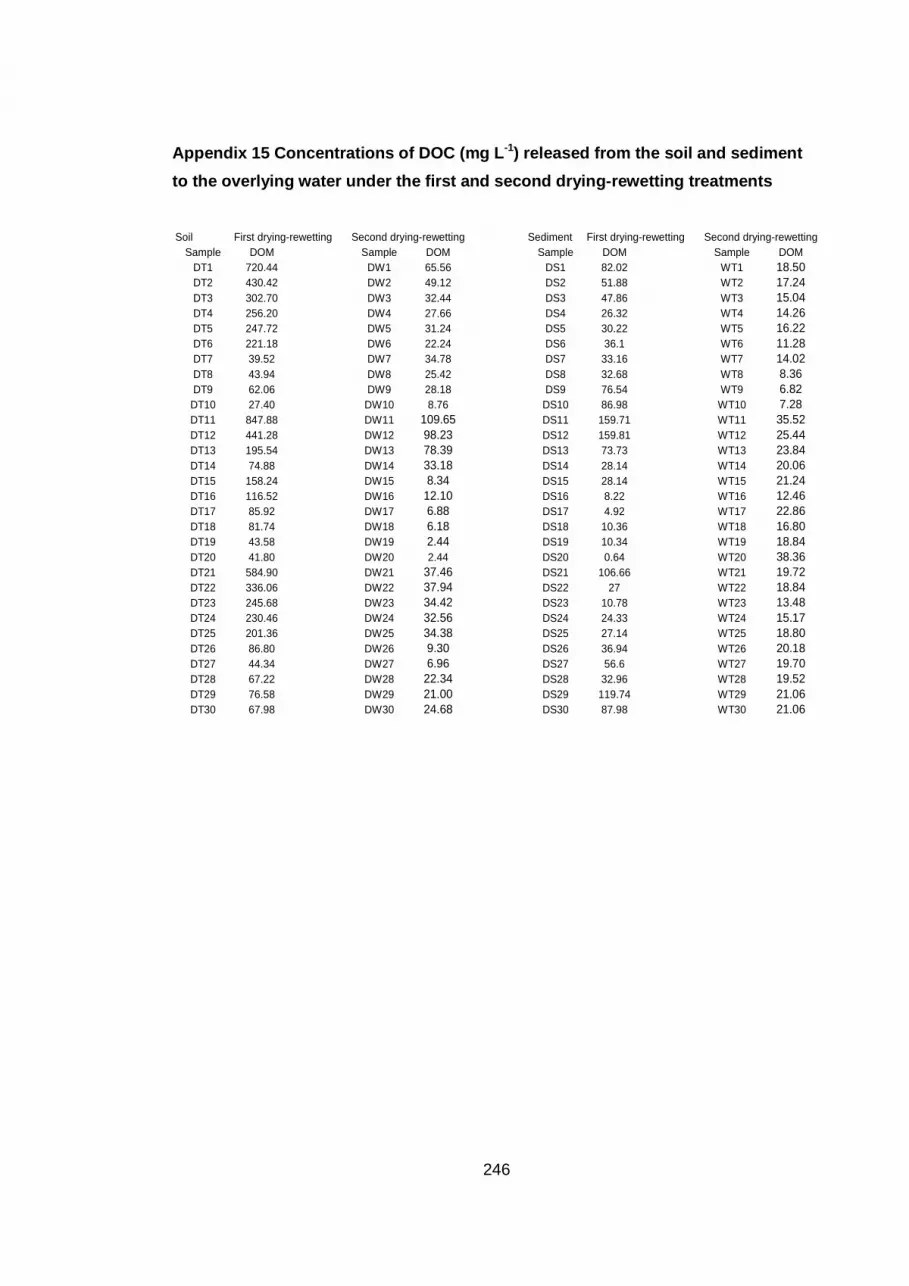
246

Soil First drying-rewetting Second drying-rewetting Sediment First drying-rewetting Second drying-rewetting Sample DOM Sample DOM Sample DOM Sample DOM

DT1 720.44 DW1 65.56 DS1 82.02 WT1 18.50DT2 430.42 DW2 49.12 DS2 51.88 WT2 17.24DT3 302.70 DW3 32.44 DS3 47.86 WT3 15.04DT4 256.20 DW4 27.66 DS4 26.32 WT4 14.26DT5 247.72 DW5 31.24 DS5 30.22 WT5 16.22DT6 221.18 DW6 22.24 DS6 36.1 WT6 11.28DT7 39.52 DW7 34.78 DS7 33.16 WT7 14.02DT8 43.94 DW8 25.42 DS8 32.68 WT8 8.36DT9 62.06 DW9 28.18 DS9 76.54 WT9 6.82

DT10 27.40 DW10 8.76 DS10 86.98 WT10 7.28DT11 847.88 DW11 109.65 DS11 159.71 WT11 35.52DT12 441.28 DW12 98.23 DS12 159.81 WT12 25.44DT13 195.54 DW13 78.39 DS13 73.73 WT13 23.84DT14 74.88 DW14 33.18 DS14 28.14 WT14 20.06DT15 158.24 DW15 8.34 DS15 28.14 WT15 21.24DT16 116.52 DW16 12.10 DS16 8.22 WT16 12.46DT17 85.92 DW17 6.88 DS17 4.92 WT17 22.86DT18 81.74 DW18 6.18 DS18 10.36 WT18 16.80DT19 43.58 DW19 2.44 DS19 10.34 WT19 18.84DT20 41.80 DW20 2.44 DS20 0.64 WT20 38.36DT21 584.90 DW21 37.46 DS21 106.66 WT21 19.72DT22 336.06 DW22 37.94 DS22 27 WT22 18.84DT23 245.68 DW23 34.42 DS23 10.78 WT23 13.48DT24 230.46 DW24 32.56 DS24 24.33 WT24 15.17DT25 201.36 DW25 34.38 DS25 27.14 WT25 18.80DT26 86.80 DW26 9.30 DS26 36.94 WT26 20.18DT27 44.34 DW27 6.96 DS27 56.6 WT27 19.70DT28 67.22 DW28 22.34 DS28 32.96 WT28 19.52DT29 76.58 DW29 21.00 DS29 119.74 WT29 21.06DT30 67.98 DW30 24.68 DS30 87.98 WT30 21.06

Appendix 15 Concentrations of DOC (mg L -1) released from the soil and sediment

to the overlying water under the first and second d rying-rewetting treatments

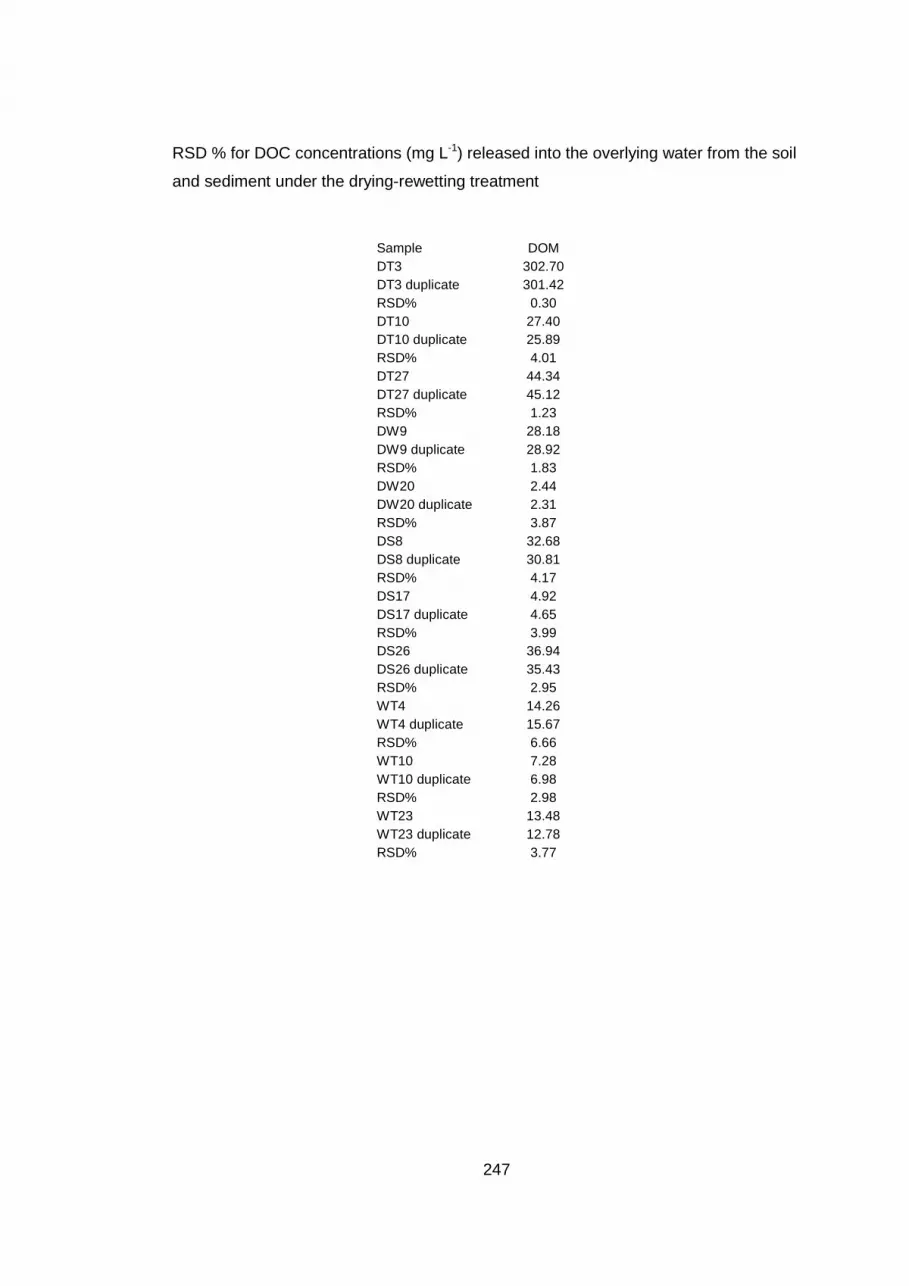
247

Sample DOMDT3 302.70DT3 duplicate 301.42RSD% 0.30DT10 27.40DT10 duplicate 25.89RSD% 4.01DT27 44.34DT27 duplicate 45.12RSD% 1.23DW9 28.18DW9 duplicate 28.92RSD% 1.83DW20 2.44DW20 duplicate 2.31RSD% 3.87DS8 32.68DS8 duplicate 30.81RSD% 4.17DS17 4.92DS17 duplicate 4.65RSD% 3.99DS26 36.94DS26 duplicate 35.43RSD% 2.95WT4 14.26WT4 duplicate 15.67RSD% 6.66WT10 7.28WT10 duplicate 6.98RSD% 2.98WT23 13.48WT23 duplicate 12.78RSD% 3.77

RSD % for DOC concentrations (mg L-1) released into the overlying water from the soil

and sediment under the drying-rewetting treatment

248

Fully wet soil Fully wet sedimentSample CO2 Carbon mineraliation rate Sample CO2 Carbon mineralisation rate

FW1 9.10 FT1 9.96FW2 14.23 2.56 FT2 12.83 1.44FW3 14.67 1.86 FT3 15.86 1.97FW4 15.04 1.49 FT4 18.11 2.04FW5 16.02 1.38 FT5 20.93 2.19FW6 20.71 1.45 FT6 27.78 2.23FW7 26.84 1.97 FT7 27.61 1.96FW8 20.54 1.14 FT8 26.75 1.68FW9 25.94 1.53 FT9 27.73 1.62FW10 21.78 1.06 FT10 28.17 1.52FW11 20.07 0.73 FT11 29.91 1.33FW12 19.22 0.63 FT12 28.92 1.18FW13 24.20 0.89 FT13 31.24 1.25FW14 23.10 0.78 FT14 32.38 1.25FW15 16.22 0.37 FT15 28.93 1.00FW16 9.26 FT16 13.88FW17 14.15 2.45 FT17 15.14 0.63FW18 14.82 1.85 FT18 17.58 1.23FW19 15.55 1.57 FT19 20.86 1.75FW20 17.91 1.73 FT20 23.38 1.90FW21 19.74 1.31 FT21 30.75 2.11FW22 22.52 1.47 FT22 28.40 1.61FW23 19.34 1.01 FT23 27.92 1.40FW24 21.90 1.15 FT24 29.89 1.46FW25 19.09 0.82 FT25 29.07 1.27FW26 19.98 0.71 FT26 30.99 1.14FW27 22.09 0.80 FT27 29.28 0.96FW28 26.25 1.00 FT28 32.47 1.09FW29 27.79 1.03 FT29 33.09 1.07FW30 20.60 0.60 FT30 27.06 0.69FW31 5.34 FT31 8.92FW32 11.60 3.13 FT32 12.79 1.94FW33 12.12 2.26 FT33 14.64 1.91FW34 12.43 1.77 FT34 15.27 1.59FW35 13.54 1.64 FT35 18.47 1.91FW36 15.08 1.22 FT36 25.02 2.01FW37 20.06 1.64 FT37 26.68 1.97FW38 17.24 1.19 FT38 26.31 1.74FW39 20.08 1.34 FT39 25.41 1.50FW40 18.78 1.12 FT40 27.26 1.53FW41 23.77 1.23 FT41 29.30 1.36FW42 23.63 1.14 FT42 29.67 1.30FW43 26.66 1.25 FT43 30.30 1.26FW44 27.10 1.21 FT44 32.08 1.29FW45 17.24 0.63 FT45 32.42 1.24

Appendix 16 Cumulative headspace CO 2 (µg CO2 kg -1), carbon mineralisation rate

(µg kg -1 day -1) and microbial biomass (µg C g -1) data

249

Dried-rewet soil Dried-rewet sedimentSample CO2 Carbon mineraliation rate Sample CO2 Carbon mineraliation rate

DR1 1592.57 DY1 2510.88DR2 4674.76 1541.10 DY2 3779.07 634.10DR3 4426.07 944.50 DY3 4328.19 605.77DR4 5150.95 889.60 DY4 4276.47 441.40DR5 6125.10 906.51 DY5 4618.83 421.59DR6 7444.88 975.38 DY6 4802.60 381.95DR7 1767.47 DY7 2421.92DR8 4596.54 1501.98 DY8 3475.20 482.16DR9 4345.07 917.50 DY9 4490.26 659.79DR10 5033.55 860.25 DY10 4028.87 379.50DR11 6344.09 950.31 DY11 4299.72 357.77DR12 7280.68 948.02 DY12 4672.41 360.26DR13 1478.77 DY13 2922.92DR14 4803.90 1605.67 DY14 4033.08 761.10DR15 4580.10 995.84 DY15 4109.35 532.82DR16 5253.31 915.19 DY16 4544.90 508.51DR17 5865.09 854.50 DY17 4697.34 437.29DR18 7649.79 1009.54 DY18 4932.92 403.67

CO2 CO2

FW7 26.84 FT19 20.86FW7 duplicate 24.21 FT19 duplicate 19.42RSD% 7.29 RSD% 5.06FW14 23.10 FT27 29.28FW14 duplicate 25.96 FT27 duplicate 28.69RSD% 8.26 RSD% 1.43FW23 19.34 FT37 26.68FW23 duplicate 18.27 FT37 duplicate 25.42RSD% 4.01 RSD% 3.42FW35 13.54 FT45 32.42FW35 duplicate 14.95 FT45 duplicate 30.61RSD% 7.02 RSD% 4.06FW44 27.10 DR3 4426.07FW44 duplicate 26.06 DR3 duplicate 4415.64RSD% 2.78 RSD% 0.17FT5 20.93 DY5 4618.83FT5 duplicate 22.67 DY5 duplicate 4602.61RSD% 5.64 RSD% 0.25

RSD % for cumulative headspace CO2 (µg CO2 kg -1)

250

Microbial biomass (µg C g-1 soil/sediment)mb1-soil 70.09mb2-soil 93.04mb3-soil 87.91mb4-soil 82.14mb5-soil 98.84mb6-soil 97.87mb7-soil 116.60mb8-soil 117.86mb9-soil 102.44mc1-sediment 104.26mc2-sediment 79.81mc3-sediment 95.66mc4-sediment 85.97mc5-sediment 77.19mc6-sediment 67.92mc7-sediment 68.95mc8-sediment 81.67mc9-sediment 63.11

251

Appendix 17 Linear regression equations for the rel ationship between DOC, metals

and herbicides released from the soil and sediment into the overlying water

Linear regression equations for DOC, metal and herbicide concentrations released from

soil

Linear regression Equation r2

Cu 2.852 + (0.872 x DOC) 0.50

Ni 1.044 + (1.107 x DOC) 0.79

Zn 1.482 + (8.20 x DOC) 0.55

Simazine -0.375 + (1.085 x DOC) 0.76

Atrazine 0.587 + (0.781 x DOC) 0.65

Diuron 1.090 + (0.826 x DOC) 0.68

Linear regression equations for DOC, metal and herbicide concentrations released from

the sediment

Linear regression Equation r2

Cu 1.866 + (1.366 x DOC) 0.08

Ni 1.178 + (0.666 x DOC) 0.28

Zn 1.866 + (1.366 x DOC) 0.13

Simazine -0.162 + (0.811 x DOC) 0.40

Atrazine 0.453 + (0.571 x DOC) 0.31

Diuron 1.011 + (0.453 x DOC) 0.22

Documents

Physicochemical changes to soil and sediment in managed realignment sites following tidal inundation