Phylogenetic Inference Using Molecular Data

FERRAN PALERO1 & KEITH A. CRANDALL2

1 Departament de Genetica, Universitat de Barcelona, Av. Diagonal 645, 08028 Barcelona, Spain2 Department of Biology, Brigham Young University, Provo, Utah 84602, U.S.A.

ABSTRACT

We review phylogenetic inference methods with a special emphasis on inference from moleculardata. We begin with a general comment on phylogenetic inference using DNA sequences, followedby a clear statement of the relevance of a good alignment of sequences. Then we provide a generaldescription of models of sequence evolution, including evolutionary models that account for rateheterogeneity along the DNA sequences or complex secondary structure (i.e., ribosomal genes). Wethen present an overall description of the most relevant inference methods, focusing on key conceptsof general interest. We point out the most relevant traits of methods such as maximum parsimony(MP), distance methods, maximum likelihood (ML) and Bayesian inference (BI). Finally, we discussdifferent measures of support for the estimated phylogeny and discuss how this relates to confidencein particular nodes of a phylogeny reconstruction.

1 INTRODUCTION

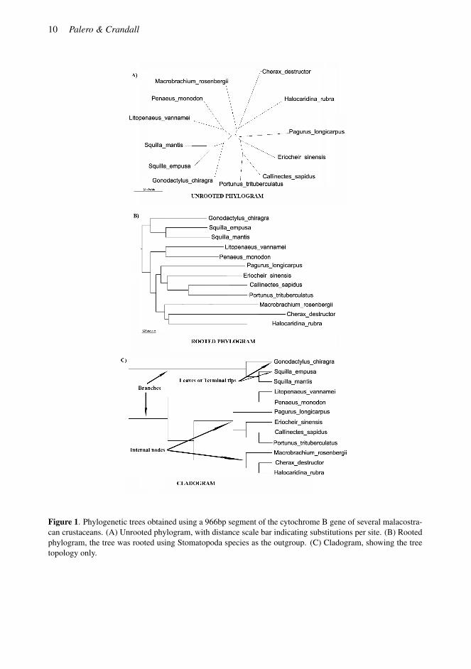
The main objective of molecular phylogenetic analysis is to infer the evolutionary history of a groupof species and represent it as an hierarchical branching diagram, a cladogram or phylogenetic tree(Edwards & Cavalli-Sforza 1964). The contemporary taxa in that tree (as opposed to the recon-structed ancestral taxa) are called leaves or terminal tips. Internal nodes represent ancestral diver-gences into two or more (polytomy) genetically isolated groups (Fig. 1). Clades are characterizedby shared possession of uniquely-derived evolutionary novelties (synapomorphies). Therefore, phy-logenetic analysis can be partially regarded as an attempt to recognize the identity and taxonomicdistribution of synapomorphies. These could be any kind of inherited phenotypic or genotypic char-acteristics; it could be the evolutionary appearance of a nauplius larva or the fixation of a changefrom guanine to adenine at a particular site in a DNA sequence. Thus, phylogenies become essentialtools for comparative biology (Harvey & Pagel 1991).

The tree topology is the information on the order of relationships, while the lengths of thebranches in the tree can represent the evolutionary distances that separate nodes (phylogram) ornot (cladogram). It is important to recognize if branches have been drawn to scale in order to knowthe relative distance between different species. This is particularly important, since if the sequencesdo not all evolve at the same rate, it is not possible to have a well-defined time axis on the tree withthe standard methods. At this point we should also differentiate between rooted and unrooted trees.Even though biologists tend to think about trees as being rooted and pointing from “lower complex-

10 Palero & Crandall

Figure 1. Phylogenetic trees obtained using a 966bp segment of the cytochrome B gene of several malacostra-can crustaceans. (A) Unrooted phylogram, with distance scale bar indicating substitutions per site. (B) Rootedphylogram, the tree was rooted using Stomatopoda species as the outgroup. (C) Cladogram, showing the treetopology only.

Phylogenetic Inference Using Molecular Data 11

ity” to “higher complexity,” most phylogenetic methods do not result in a rooted tree (see ModelingEvolution section below). We generally need to define an outgroup by using external evidence notincluded in the molecular dataset (Weston 1994). Only then can rooted trees inform us about thetemporal order of events and about which species have high rates of molecular evolution.

1.1 Why should we use molecules when we already have morphology-based taxonomies?

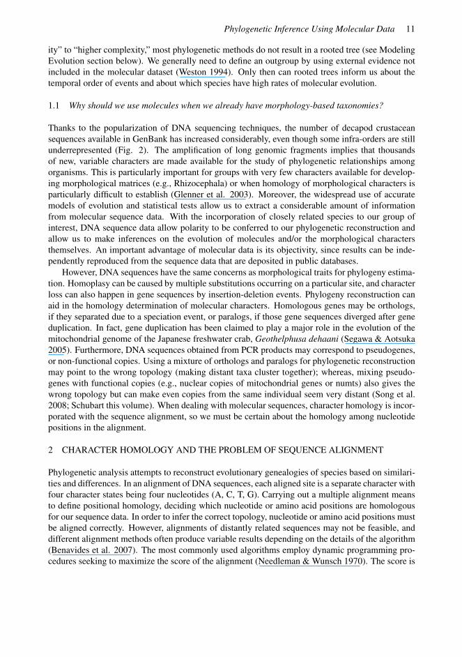
Thanks to the popularization of DNA sequencing techniques, the number of decapod crustaceansequences available in GenBank has increased considerably, even though some infra-orders are stillunderrepresented (Fig. 2). The amplification of long genomic fragments implies that thousandsof new, variable characters are made available for the study of phylogenetic relationships amongorganisms. This is particularly important for groups with very few characters available for develop-ing morphological matrices (e.g., Rhizocephala) or when homology of morphological characters isparticularly difficult to establish (Glenner et al. 2003). Moreover, the widespread use of accuratemodels of evolution and statistical tests allow us to extract a considerable amount of informationfrom molecular sequence data. With the incorporation of closely related species to our group ofinterest, DNA sequence data allow polarity to be conferred to our phylogenetic reconstruction andallow us to make inferences on the evolution of molecules and/or the morphological charactersthemselves. An important advantage of molecular data is its objectivity, since results can be inde-pendently reproduced from the sequence data that are deposited in public databases.

However, DNA sequences have the same concerns as morphological traits for phylogeny estima-tion. Homoplasy can be caused by multiple substitutions occurring on a particular site, and characterloss can also happen in gene sequences by insertion-deletion events. Phylogeny reconstruction canaid in the homology determination of molecular characters. Homologous genes may be orthologs,if they separated due to a speciation event, or paralogs, if those gene sequences diverged after geneduplication. In fact, gene duplication has been claimed to play a major role in the evolution of themitochondrial genome of the Japanese freshwater crab, Geothelphusa dehaani (Segawa & Aotsuka2005). Furthermore, DNA sequences obtained from PCR products may correspond to pseudogenes,or non-functional copies. Using a mixture of orthologs and paralogs for phylogenetic reconstructionmay point to the wrong topology (making distant taxa cluster together); whereas, mixing pseudo-genes with functional copies (e.g., nuclear copies of mitochondrial genes or numts) also gives thewrong topology but can make even copies from the same individual seem very distant (Song et al.2008; Schubart this volume). When dealing with molecular sequences, character homology is incor-porated with the sequence alignment, so we must be certain about the homology among nucleotidepositions in the alignment.

2 CHARACTER HOMOLOGY AND THE PROBLEM OF SEQUENCE ALIGNMENT

Phylogenetic analysis attempts to reconstruct evolutionary genealogies of species based on similari-ties and differences. In an alignment of DNA sequences, each aligned site is a separate character withfour character states being four nucleotides (A, C, T, G). Carrying out a multiple alignment meansto define positional homology, deciding which nucleotide or amino acid positions are homologousfor our sequence data. In order to infer the correct topology, nucleotide or amino acid positions mustbe aligned correctly. However, alignments of distantly related sequences may not be feasible, anddifferent alignment methods often produce variable results depending on the details of the algorithm(Benavides et al. 2007). The most commonly used algorithms employ dynamic programming pro-cedures seeking to maximize the score of the alignment (Needleman & Wunsch 1970). The score is

12 Palero & Crandall

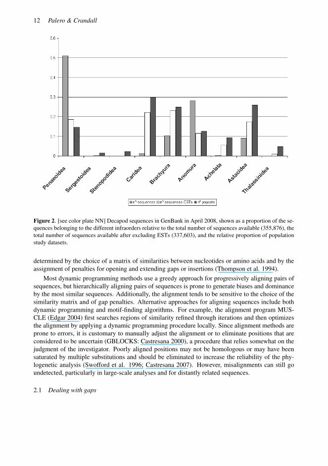
Figure 2. [see color plate NN] Decapod sequences in GenBank in April 2008, shown as a proportion of the se-quences belonging to the different infraorders relative to the total number of sequences available (355,876), thetotal number of sequences available after excluding ESTs (337,603), and the relative proportion of populationstudy datasets.

determined by the choice of a matrix of similarities between nucleotides or amino acids and by theassignment of penalties for opening and extending gaps or insertions (Thompson et al. 1994).

Most dynamic programming methods use a greedy approach for progressively aligning pairs ofsequences, but hierarchically aligning pairs of sequences is prone to generate biases and dominanceby the most similar sequences. Additionally, the alignment tends to be sensitive to the choice of thesimilarity matrix and of gap penalties. Alternative approaches for aligning sequences include bothdynamic programming and motif-finding algorithms. For example, the alignment program MUS-CLE (Edgar 2004) first searches regions of similarity refined through iterations and then optimizesthe alignment by applying a dynamic programming procedure locally. Since alignment methods areprone to errors, it is customary to manually adjust the alignment or to eliminate positions that areconsidered to be uncertain (GBLOCKS: Castresana 2000), a procedure that relies somewhat on thejudgment of the investigator. Poorly aligned positions may not be homologous or may have beensaturated by multiple substitutions and should be eliminated to increase the reliability of the phy-logenetic analysis (Swofford et al. 1996; Castresana 2007). However, misalignments can still goundetected, particularly in large-scale analyses and for distantly related sequences.

2.1 Dealing with gaps

Phylogenetic Inference Using Molecular Data 13

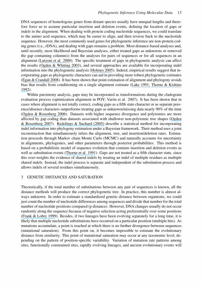
DNA sequences of homologous genes from distant species usually have unequal lengths and there-fore force us to assume particular insertion and deletion events, defining the location of gaps orindels in the alignment. When dealing with protein coding nucleotide sequences, we could translateto the amino acid sequence, which may be easier to align, and then reverse back to the nucleotidesequence. However, the most commonly used genes for phylogenetic inference are non-protein cod-ing genes (i.e., rDNA), and dealing with gaps remains a problem. Most distance-based analyses and,until recently, most likelihood and Bayesian analyses, either treated gaps as unknowns or removedthe gap containing column(s) from the analyses for pairs of sequences or for all sequences in analignment (Lutzoni et al. 2000). The specific treatment of gaps in phylogenetic analysis can affectthe results (Ogden & Whiting 2003), and several approaches are available for incorporating indelinformation into the phylogenetic analysis (Holmes 2005). Indeed, empirical results suggest that in-corporating gaps as phylogenetic characters can aid in providing more robust phylogenetic estimates(Egan & Crandall 2008). It has been shown that point estimation of alignment and phylogeny avoidsbias that results from conditioning on a single alignment estimate (Lake 1991; Thorne & Kishino1992).

Within parsimony analysis, gaps may be incorporated as transformations during the cladogramevaluation process (optimization alignment in POY; Varon et al. 2007). It has been shown that incases where alignment is not totally correct, coding gaps as a fifth state character or as separate pres-ence/absence characters outperforms treating gaps as unknown/missing data nearly 90% of the time(Ogden & Rosenberg 2006). Datasets with higher sequence divergence and polytomies are moreaffected by gap coding than datasets associated with shallower non-polytomic tree shapes (Ogden& Rosenberg 2007). Redelings & Suchard (2005) describe a statistical method for incorporatingindel information into phylogeny estimation under a Bayesian framework. Their method uses a jointreconstruction that simultaneously infers the alignment, tree, and insertion/deletion rates. Estima-tion proceeds through Markov chain Monte Carlo (MCMC) and naturally accounts for uncertaintyin alignments, phylogenies, and other parameters through posterior probabilities. This method isbased on a probabilistic model of sequence evolution that contains insertion and deletion events aswell as substitution events (Thorne et al. 1991). Gaps are not treated as a fifth character state, sincethis over-weights the evidence of shared indels by treating an indel of multiple residues as multipleshared indels. Instead, the indel process is separate and independent of the substitution process andallows indels of several residues simultaneously.

3 GENETIC DISTANCES AND SATURATION

Theoretically, if the total number of substitutions between any pair of sequences is known, all thedistance methods will produce the correct phylogenetic tree. In practice, this number is almost al-ways unknown. In order to estimate a standardized genetic distance between organisms, we couldjust count the number of nucleotide differences among sequences and divide that number for the totalnumber of nucleotide positions compared (p distance). However, DNA changes usually do not occurrandomly along the sequence because of negative selection acting preferentially over some positions(Frank & Lobry 1999). Besides, if two lineages have been evolving separately for a long time, it islikely that multiple nucleotide substitutions have occurred on a particular position (multiple hits). Asmutations accumulate, a point is reached at which there is no further divergence between sequences(mutational saturation). From this point on, it becomes impossible to estimate the evolutionarydistance from similarity. This point of mutational saturation may occur at any taxonomic level, de-pending on the pattern of position-specific variability. Variation of mutation rate patterns amongsites, functionally constrained sites, rapidly evolving lineages, and ancient evolutionary events will

14 Palero & Crandall

make the estimates of distances uncertain (Philippe & Forterre 1999). Different molecules evolve atdifferent rates, and some of the fast-evolving genes will be saturated with changes even for closelyrelated taxa. Using fast-evolving genes for phylogenetic inference of distantly related species couldprovide misleading results. A sensible approach for tackling this problem of saturation would beto use molecular markers that present a slower mutation rate and using an appropriate nucleotidesubstitution model in order to correct the observed distance for the multiple hits. However, if thegene evolves too slowly, there will be very little variation among the sequences, and there will betoo little information to construct a phylogeny. Phylogenetic methods are likely to become unreli-able if the sequences are too different from one another, and this should be borne in mind when thechoice of gene sequences is made initially. Typically, a combination of genes is needed to accuratelyreconstruct phylogenetic relationships, with faster evolving genes resolving close relationships andmore slowly evolving genes resolving deeper relationships.

4 MODELING EVOLUTION AND MODEL SELECTION

More complex models, taking into account a variety of biological phenomena, generally providemore accurate estimates of phylogeny regardless of the method (e.g., parsimony, likelihood, dis-tance, Bayesian) (Huelsenbeck 1995). The most common models of DNA evolution include basefrequency, base exchangeability, and rate heterogeneity parameters. The parameter values are usu-ally estimated from the dataset in each particular analysis (model selection). Finally, the evolutionarymodels are defined by matrices containing the relative rates of all possible replacements (transitionprobability matrix), which allow us to calculate the probabilities of change from any nucleotide toany other nucleotide (Lio & Goldman 1998). Most models assume reversibility of the transitionprobability matrix so that no inferences about evolutionary direction can be made unless furtherinformation extrinsic to the sequences themselves (e.g., fossil record) is supplied.

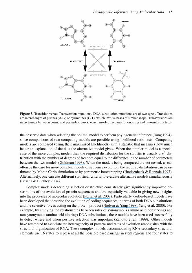
The base frequency parameters describe the frequencies of the nucleotide bases averaged over allsequence sites and over the tree. These parameters can be considered to represent constraints on basefrequencies due to effects such as overall GC content, and they act as weighting factors in a model bymaking certain bases more likely to arise when substitutions occur. Base exchangeability parametersdescribe the relative tendencies of bases to be substituted for one another (Fig. 3). These parametersrepresent a measure of the biochemical similarity of bases, since transitions (i.e., C↔T or A↔G)usually occur more often than transversions (e.g., C↔G) (Brown et al. 1982; but see also Kelleret al. 2007). Furthermore, mutation rates vary considerably among sites of DNA and amino acidsequences or among loci, because of constraints of the genetic code, selection for gene function, etc.In fact, we have to consider that if most of the nucleotide positions in our sequences evolve ratherslowly or do not change at all (invariant sites), then base changes will tend to accumulate in a fewvariable sites, and sequence saturation will be reached much more quickly and at a lower divergencethan expected under simpler models that do not incorporate rate heterogeneity or a proportion ofinvariant sites. The most widespread approach to modeling rate heterogeneity among sequence sitesis to describe each site’s rate as a random draw from a gamma distribution (Yang 1994). The shapeof the gamma distribution is controlled by a parameter α. Large values of α suggest that sites evolveat a similar rate, while small values of the parameter α imply higher levels of rate heterogeneityamong sites and the presence of many sites with lower rates of evolution. It is also possible toassign specific rates of substitution to different parts of the sequence in order to account for theheterogeneity on the mutation rate (e.g., to the three codon positions of protein coding sequences orto different domains in rRNA).

We can use the likelihood framework to estimate parameter values and their standard errors from

Phylogenetic Inference Using Molecular Data 15

Figure 3. Transition versus Transversion mutations. DNA substitution mutations are of two types. Transitionsare interchanges of purines (A-G) or pyrimdines (C-T), which involve bases of similar shape. Transversions areinterchanges between purine and pyrmidine bases, which involve exchange of one-ring and two-ring structures.

the observed data when selecting the optimal model to perform phylogenetic inference (Yang 1994),since comparisons of two competing models are possible using likelihood ratio tests. Competingmodels are compared (using their maximized likelihoods) with a statistic that measures how muchbetter an explanation of the data the alternative model gives. When the simpler model is a specialcase of the more complex model, then the required distribution for the statistic is usually a χ2 dis-tribution with the number of degrees of freedom equal to the difference in the number of parametersbetween the two models (Goldman 1993). When the models being compared are not nested, as canoften be the case for more complex models of sequence evolution, the required distribution can be es-timated by Monte Carlo simulation or by parametric bootstrapping (Huelsenbeck & Rannala 1997).Alternatively, one can use different statistical criteria to evaluate alternative models simultaneously(Posada & Buckley 2004).

Complex models describing selection or structure consistently give significantly improved de-scriptions of the evolution of protein sequences and are especially valuable in giving new insightsinto the processes of molecular evolution (Porter et al. 2007). Particularly, codon-based models havebeen developed that describe the evolution of coding sequences in terms of both DNA substitutionsand the selective forces acting on the protein product (Nielsen & Yang 1998; Yang et al. 2000). Forexample, by studying the relationships between rates of synonymous (amino acid conserving) andnonsynonymous (amino acid altering) DNA substitutions, these models have been used successfullyto detect where and when positive selection was important (Zanotto et al. 1999). Other modelshave attempted to associate the heterogeneity of patterns and rates of evolution among sites with thestructural organization of RNA. These complex models accommodating RNA secondary structuralelements use 16 states to represent all the possible base pairings in stem regions and four states to

16 Palero & Crandall

model loops (Schoniger & von Haeseler 1994).Finally, while employing multiple alternative models in phylogenetic analysis might be seen as

more rigorous, if this approach is to be meaningful there needs to be some quality control on themodels employed (Grant & Kluge 2003). Similarly, all methods of phylogenetic inference assume amodel of evolution, either implicitly or explicitly. For example, a strict parsimony analysis assumesall character changes are of equal weight. Thus, it becomes incumbent upon the researcher to justifythe choice of model, even if it is an implicit model used to describe character evolution. If there areno restrictions on allowable models, virtually any given phylogeny may be found to be supportedby some models and refuted by others. The model averaging approach by Lee & Hugall (2006)addresses both issues: a large number of possible models can be employed, but the results of eachmodel are weighted according to its fit, so that the results of implausible models carry little weighton the final estimate. Likewise, statistically testing alternative models of evolution allows one todetermine if the addition of more parameters makes a significant improvement in a likelihood score(Posada & Crandall 2001).

5 SEARCHING FOR TREES IN A BROAD TREE SPACE

The reconstruction of a phylogenetic tree using molecular data is an attempt to statistically infer thebest estimate of evolutionary relationships given some criterion. While the “true tree” is the goal,what phylogenetic methods actually do is optimize a tree given some model and optimality criterion.Thus, we are actually searching for not the “true tree” but rather the “optimal tree” and hope thatthe latter has some relationship to the former. There are two processes involved in this inference:estimation of the topology and estimation of branch lengths for a given tree topology. When a topol-ogy is known, statistical estimation of branch lengths is relatively simple, and one can use severalstatistical methods such as the least squares and the maximum likelihood methods. The problem isthe estimation or reconstruction of a topology. The number of possible topologies increases rapidlywith the number of sequences (Swofford et al. 1996), and it is generally very difficult to choosethe correct topology among them. In phylogenetic inference, a certain optimization principle suchas the maximum likelihood (ML) or minimum evolution (ME) principle is often used for evaluatingdifferent tree scores and choosing the topology and branch lengths that gives an optimal score, sothat we need to have tree searching strategies to help us finding the “optimal tree.”

Exhaustive search. The exhaustive algorithm evaluates all possible trees. Because it examinesall possible topologies, exhaustive searches guarantee the most optimal tree(s), but it is very slow(using 12 taxa, more than 600 million trees are evaluated). The advantage of the exhaustive searchis the ability to completely explore the tree space and thereby plot the optimality score distribution.This histogram may indicate the ‘quality’ of your matrix, in the sense that there should be a tail tothe left such that few short trees are ‘isolated’ from the greater mass of less optimal trees (but seeKitchin et al. 1998).

Branch and bound. The branch-and-bound algorithm is guaranteed to find all optimal trees,given some criterion (e.g., maximum parsimony). It discards whole classes of trees that it hasdetermined are suboptimal, without the need to examine all of those one by one. The savings isgreater the less homoplasy there is in the data. However, in cases where there are many conflictsbetween information from different characters and much parallelism and convergence, the branchand bound strategy does not perform particularly well. Moreover, branch and bound methods stillhave a complexity that is exponential, and it is not recommended to use the branch-and-boundalgorithm for data sets with more than 12 taxa.

Heuristic searches. Since most datasets today contain large numbers of sequences, exhaustive

Phylogenetic Inference Using Molecular Data 17

and branch-and-bound searches quickly become impractical. We then turn to heuristic searches.Heuristic searches attempt to survey the tree space reasonably well without guaranteeing to find themost optimal tree(s). The key to good heuristic searching is the ability to move around the treespace and spend time exploring reasonable alternative topologies. Thus, a wide variety of branchswapping algorithms have been developed to achieve this goal.

Nearest-neighbor interchange (NNI). This heuristic algorithm adds taxa sequentially, in theorder they are given in the matrix, to the branch where they will give least increase in tree length(Robinson 1971; Moore et al. 1973). After each taxon is added, all nearest neighbor trees areswapped to try to find an even shorter tree. Like all heuristic searches, this one is much faster thanthe algorithms above and can be used for large numbers of taxa, but it is not guaranteed to find all orany of the optimal trees. To decrease the likelihood of ending up on a suboptimal local minimum,a number of reorderings can be specified. For each reordering, the order of input taxa could berandomly permutated and another heuristic search attempted.

Subtree pruning and regrafting (SPR) is similar to NNI, but with a more elaborate branchswapping scheme. In order to find a shorter tree, a subtree is cut off the tree and regrafted onto allother branches in the tree to find the best alternative (Swofford 2003). This is done after each taxonhas been added, and for all possible subtrees. While slower than NNI, SPR will often find shortertrees (Felsenstein 2004).

Tree bisection and reconnection (TBR) is similar to SPR, but with an even more completebranch swapping scheme. The tree is divided into two parts, and these are reconnected throughevery possible pair of branches in order to find a shorter tree. This is done after each taxon is added,and for all possible divisions of the tree (Swofford 2003). TBR will often find shorter trees than SPRand NNI, but it is more time consuming.

The Ratchet. Different characters in the data may well recommend different trees to us. To pre-vent the search from becoming focused on a limited set of trees, it may help to use different startingtrees as recommended by various subsets of characters. In the ratchet approach, we pick up somecharacters and increase their representation by increasing their weight (Nixon 1999; Felsenstein2004). This moves the search to a tree recommended by this reweighted dataset; then we searchfrom that starting point using the full set of characters.

Given the enormously large size of the tree space even for a small data set, all we can do is hopethat if we have searched for a long time without finding any improvement, then we have probablyfound the best tree. The problem with long-range moves tends to be that they are rather disrup-tive, moving the search far from the optimal tree. Most real search programs use a combination ofNNIs and slightly longer range moves that have been tested and found to be reasonably efficient atfinding optimal trees as quickly as possible. The MCMC method (see below) is a way of searchingtree space that allows both uphill and downhill moves, allowing for suboptimal tree topologies tobe sampled during the search. Regardless of the optimality criterion used, a key aspect of effectiveheuristic tree searching is to perform the analysis multiple times with different starting positions tobe sure the tree space has been reasonably sampled.

6 INFERENCE METHODS

Ideally, the inference method used will extract the maximum amount of information available in thesequence data, will combine this with prior knowledge of patterns of sequence evolution (includedin the evolutionary model), and will deal with model parameters (e.g., the transition/transversion ra-tio) whose values are not known a priori. The major inference methods for molecular phylogeneticsare maximum likelihood, Bayesian inference, distance methods and maximum parsimony.

18 Palero & Crandall

6.1 Maximum likelihood

Likelihood-based techniques allow a wide variety of phylogenetic inferences from sequence data anda robust statistical assessment of all results. The likelihood of an hypothesis is equal to the probabil-ity of observing the data (sequence alignment) if that hypothesis (tree topology) were correct, giventhe chosen model of sequence evolution (Felsenstein 1981, 1988). Thus, a model of nucleotide oramino acid replacement allows the calculation of the likelihood for any possible combinations oftree topology and branch lengths. It permits the inference of phylogenetic trees and also makinginferences simultaneously about the patterns and processes of evolution. A great attraction of thelikelihood approach in phylogenetics is the existence of a wealth of powerful statistical theory; forexample, the ability to perform robust statistical hypothesis tests (see below) and the knowledge thatML phylogenetic estimates are statistically consistent (given enough data and an adequate model,ML will always give the correct tree topology) (Rogers 1997). These strong statistical foundationssuggest that likelihood techniques are the most powerful for phylogeny reconstruction and for un-derstanding sequence evolution. Simulation studies show that ML methods generally outperformdistance and parsimony methods over a broad range of realistic conditions, and recent developmentsin distance and parsimony methodology have concentrated on elucidating the relationships of thesemethods to ML inference and exploiting this understanding to adapt the methods so that they per-form more like ML methods (Steel & Penny 2000; Bruno et al. 2000). However, ML suffers fromcomputational intensity, making ML estimation impractical when dealing with several thousands ofsequences (Zhang 1999), but better algorithms are being developed continually that can accommo-date an increasingly large number of sequences for ML analyses (Stamatakis 2005).

The ML method is a well-established statistical method of parameter estimation; it gives thesmallest variance of a parameter estimate when sample size is large. In the construction of phy-logenetic trees, maximization of the likelihood is done for each topology separately by using adifferent likelihood function, and the topology with the highest (maximum) likelihood is chosen asan estimate of the true topology. Since different topologies represent different probability spaces ofparameters, it is not clear whether the maximum likelihood tree is expected to be the true tree unlessan infinite number of nucleotides are examined (Felsenstein 2004). Finally, it should be mentionedthat the statistical foundation of phylogeny estimation by ML has not been well established, andsome authors have pointed out that topologies are parameters, but these parameters are not includedin the likelihood function that is being maximized (Nei 1996; Yang 1996).

6.2 Bayesian methods

When inferring phylogenies, we should consider methods that deal directly with ensembles of pos-sible trees, rather than chasing after a single best one, and we should be able to consider the infor-mation in the data and any prior information about the probabilities of the events. The fundamentalimportance of evolutionary models is that they contain parameters, and if specific values can beassigned to these parameters based on observations, such as an alignment of DNA sequences, thenbiologists can learn something about how molecular evolution has occurred. Although both maxi-mum likelihood and Bayesian analyses are based upon the likelihood function, there are fundamentaldifferences in how the two methods treat parameters. ML makes inferences about the parameters ofinterest while fixing the values for the other parameters (nuisance parameters). However, Bayesiansassign a prior probability distribution to the nuisance parameters and the posterior probability iscalculated by integrating over all possible values of those nuisance parameters, weighting each by

Phylogenetic Inference Using Molecular Data 19

its prior probability. The advantage of this is that inferences about the parameters of interest do notdepend upon any particular value for the nuisance parameters. The disadvantage is that it may bedifficult to specify a reasonable prior for the parameters. Nevertheless, when there is a large amountof information in the data and the likelihood function changes rapidly as the parameter values arealtered, the choice of prior is not so important and it is possible to use uniform or non-informativepriors. All branch lengths could be set as equally likely a priori, and a suitable non-informativechoice of prior for base frequencies could be to set all sets of frequencies that add up to one asequally probable.

Markov models are routinely used in several domains of science and do not belong specificallyto the Bayesian inference methodology; however, they have revolutionized genetic inferences inmany aspects (Beaumont & Rannala 2004). A Markov model is a mathematical model for a processwith changes of state over time, in which future events occur by chance and depend only on thecurrent state and not on the history of how that state was reached. In molecular phylogenetics, thestates of the process are the possible nucleotides or amino acids present at a given time and positionin a sequence, and state changes represent mutations in sequences. Therefore, starting from anevolutionary model and a set of nucleotide frequencies, we can get to an equilibrium at which anystate has a probability of occurrence that does not depend on the initial state of the process.

Under the MCMC search in a Bayesian framework, the probability of finding a tree will beproportional to its likelihood multiplied by its prior probability. In that case, the new tree is eitheraccepted or rejected, using a rule known as the Metropolis algorithm. If the likelihood of the pro-posed tree is larger than the likelihood of the current one, the proposed topology is accepted and itbecomes the next tree in the sample. If it is rejected, then the next tree in the sample is a repeat ofthe original tree. It also allows moves that decrease the likelihood, in order to allow for samplingof suboptimal trees. When the MCMC chain reaches the equilibrium, the probability of observingeach tree must be constant. This property is known as detailed balance. It is necessary to strike abalance between moves that alter branch lengths and those that alter topology. If changes are verylarge, then the likelihood ratio of the states will be far from 1, and the likelihood of accepting thedownhill move for sampling suboptimal trees will be very small. Finally, failure to diagnose a lackof convergence of the MCMC chain will lead to incorrect tree topology estimates (Huelsenbeck etal. 2002).

6.3 Distance methods

Distance matrix methods calculate a measure of the distance between each pair of species and thenfind a tree that predicts the observed set of distances as closely as possible. This leaves out allinformation from higher order combinations of character states, reducing the data matrix to a simpletable of pairwise distances. Distance methods use the same models of evolution as ML to estimatethe evolutionary distance between each pair of sequences from the set under analysis and then try tofit a phylogenetic tree to those distances. The distances will usually be ML estimates for each pairof sequences (considered independently of the other sequences). Disadvantages of distance methodsinclude the inevitable loss of evolutionary information when a sequence alignment is converted topairwise distances and the inability to deal with models containing parameters for which the valuesare not known a priori (Steel et al. 1988). We are trying to find the n-species tree that is impliedby these distances. The difficulty in doing this is that the individual distances are not exactly thepath lengths in the full n-species tree between those two species. Since we are dealing with pairwisedistances, we need to be able to find the full tree that does the best job of approximating theseindividual two-species trees.

20 Palero & Crandall

In order for distances that are used in these analyses to have the proper expectations, it is es-sential that they are expected to be proportional to the total branch length between the species. Ifthe distances do not have the linearity property, then wrenching conflicts between fitting the longdistances and fitting the short distances arise, and the tree is the worse for them. There are sev-eral distance matrix methods available in the literature. Two examples are minimum evolution andneighbor-joining.

Minimum Evolution. This method seeks to find the tree with the shortest overall branch lengths.First, the least squares trees are determined for different topologies, and the choice is made amongthem by choosing the one of shortest total length. Rzhetsky & Nei (1993) showed that if the distanceswere unbiased estimates of the true distance (many distances are not unbiased) then the expectedtotal length of the true tree was shorter than the expected total length of any other. However, thatis not the same as showing that the total length is always shorter for the true tree, as the lengthsvary along their expectation. Gascuel et al. (2001) have found cases where the minimum evolutionis inconsistent when branch lengths are inferred by weighted least squares or by generalized leastsquares.

Neighbor-Joining. NJ is a clustering method that produces unrooted trees. It works by suc-cessively clustering pairs of sequences together. It is related to the UPGMA method of inferringa branching diagram from a distance matrix. Unlike the UPGMA method, NJ can facilitate con-temporary tips of uneven length. This makes it a more appropriate tree reconstruction method thanUPGMA in those instances when evolution has not proceeded in a strictly clock-like fashion. NJis guaranteed to recover the true tree if the distance matrix happens to be an exact reflection of atree. However, in the real world, distances will not be exactly additive, and therefore NJ is just oneapproximation. Furthermore, the NJ tree may be misleading. If the input distances are not close tobeing additive, because pairwise distances were not properly calculated or because sequences werenot properly aligned, then NJ will give the wrong tree.

NJ is useful to rapidly search for a good tree that can then be improved by other criteria. Ota &Li (2001) use neighbor-joining and bootstrapping to find an initial tree and identify which regionsare candidates for rearrangement. They then use ML for further refinement. This results in a sub-stantial improvement in speed over pure likelihood methods. Moreover, modifications of NJ havebeen developed to allow for differential weighting in the algorithm to take into account differencesin statistical noise. Gascuel (1997) has modified the NJ to allow for the variances and covariancesof the distances to be proportional to the branch lengths. This is a good approximation provided thatthe branch lengths are not too long.

6.4 Maximum parsimony

The theoretical basis of this method is the philosophical idea that the best hypothesis to explain aprocess is the one that requires the smallest number of assumptions (Occam’s Razor). If there areno backward and no parallel substitutions at each nucleotide site (no homoplasy) and the number ofinformative nucleotides examined is very large, maximum parsimony (MP) methods are expected toprovide the correct (realized) tree. MP assumes that maximizing the congruence among characterswill be equal to minimizing incongruence (homoplasy) (Farris 1983; Scotland 1997). Therefore,computing programs will count the number of mutational changes (steps) we need to explain a par-ticular tree and repeat this counting for thousands of trees. The tree or trees that need a minimumnumber of changes to explain the relationships between species will be accepted as the most parsi-monious tree.

There are two main dynamic programming algorithms for counting the number of changes of

Phylogenetic Inference Using Molecular Data 21

state. In both cases, the algorithm does not function by actually placing changes or reconstructingstates at the nodes of the tree. The Fitch algorithm works for characters with any number of statesprovided one can change from any one to any other (Kluge & Farris 1969). Fitch characters arereversible and unordered, meaning that all changes have equal cost. This is the criterion with fewestassumptions, and is therefore generally preferable. The Fitch algorithm can be carried out in a num-ber of operations that are directly proportional to the number of species on the tree, and, therefore,the algorithm is less computationally demanding than other methods. The Sankoff algorithm startsby assuming that one has a table of the cost of changes between each character state and each otherstate. In this case, one computes the total cost of the most parsimonious combinations of events bycomputing it for each character. Given that a node is assigned a particular character-state, we willcompute the minimal cost of all the events in the subtree that starts from that node and accept it asthe most parsimonious result.

Other algorithms allow us to reconstruct character states at the nodes of the tree. The Camin-Sokal Parsimony algorithm (C-S) assumes that we know the ancestral state of the character. In itssimplest form, only two states are allowed (presence/absence) and reversals are impossible. Oneapplication of C-S parsimony is in the evolution of small deletions of DNA, when we have noreason to believe that they could revert spontaneously. In more complex cases, when deletionsoverlap and we cannot be entirely sure whether any one of them is present or absent, C-S parsimonywould not be appropriate. C-S parsimony infers a rooted tree, since it will favour the placementof the root in one particular part of the tree. In its simplest form, Dollo parsimony assumes thatthere are two states (ancestral/derived). The main difference with C-S parsimony is that in thiscase the derived state is allowed to evolve only once, but it is allowed to revert to the ancestralstate multiple times. The number of these reversions is the quantity being minimized, and it isalso an inherently rooted method. In ‘unweighted’ (=equal weighting) MP methods, nucleotide oramino acid substitutions are assumed to occur in all directions with equal or nearly equal probability.In reality, however, certain substitutions (e.g., transitional changes) occur more often than othersubstitutions (e.g., transversional changes). It is therefore reasonable to give different weights todifferent types of substitutions when the minimum number of substitutions for a given topology isto be computed. MP methods incorporating a weight matrix for the different types of change areweighted MP methods.

Once the most parsimonious phylogenetic tree has been recovered, we can still wonder aboutthe amount of parallelism or reversal that is found on the tree. A particular character state mayhave evolved independently in two lineages, and multiple hits may cause a particular nucleotideposition to return to an ancestral state. Several indices have been developed to measure the relativeamount of homoplasy found in a particular tree. For example, the per-character consistency index(ci) is defined as m/s, where m is the minimum possible number of character changes (steps) onany tree, and s is the actual number of steps on the current tree. This index hence varies from one(no homoplasy) towards zero (a lot of homoplasy). The ensemble consistency index CI is a similarindex, but summed over all characters.

The per-character retention index (ri) is defined as the ratio of (1) the differences between themaximal number of steps for the character on any cladogram and the actual number of steps on thecurrent tree and (2) the differences between the maximal number of steps for the character on anycladogram and the minimum possible number of character changes on any tree (Farris 1989). There-fore, the retention index becomes zero when the site is least informative for MP tree construction,that is, when the difference between the maximal number of steps for the character on any clado-gram and the actual number of steps on the current tree is zero.

22 Palero & Crandall

7 NODE SUPPORT AND TREE COMPARISON

Measures of nodal support provide a useful summary of how well data support the relationshipsdefined by a tree. In the MP approach, the Bremer support (decay index) for a clade can be computedas a measure of the confidence on that particular clade. The Bremer support is the number of extrasteps you need to construct a tree (consistent with the characters) where that clade is no longerpresent. When several genes are included in the analysis, the parsimony-based method of partitionedbranch support (PBS) estimates the amount that each dataset contributes to a particular clade support,so that we can estimate the extent to which the data partition supports the most parsimonious treeover trees not including a particular clade (Gatesy et al. 1999). An equivalent “partitioned likelihoodsupport” (PLS) can be obtained for each dataset under a likelihood-based approach (Lee & Hugall2003). Most measures of nodal support attempt to estimate the degree to which an analysis hasconverged on a stable result. Of course, high support values do not mean that a node is accurate,only that it is well supported by the data. It is well known that model misspecification and taxonsampling can mislead the analysis (Hedtke et al. 2006).

Currently, the nonparametric bootstrap is one of the most widely used methods for assessingnodal support (Felsenstein 1985). The nonparametric bootstrap is a statistical method by which dis-tributions that are difficult to calculate exactly can be estimated by the repeated creation and analysisof artificial datasets. A number of replicates (typically at least 1000) of the original characters (e.g.,sites of a DNA sequence alignment) are randomly produced with replacement, obtaining a newdataset in which some characters are represented more than once, some appear once, and some aredeleted. The perturbed datasets are each analyzed in the same manner as for the real data, and thenumber of times that each grouping of species appears in the resulting profile of cladograms is takenas an index of relative support for that grouping.

Perhaps the best interpretation of the bootstrap is that it quantifies the sensitivity of a node toperturbations in the data (Holmes 2005). However, as commonly implemented, the bootstrap givesa biased estimate of accuracy (Hillis & Bull 1993; Holmes 2005), where accuracy is defined as theprobability of obtaining a correct phylogenetic reconstruction (Penny et al. 1992). The statisticaltheory of bootstrap requires that all positions of an alignment are independently and identically dis-tributed, and this assumption does not apply to nucleotide or amino acid sequences. It is worthyto point out the difference between nonparametric and parametric bootstrap. In the nonparametricbootstrap, new datasets are generated by resampling from the original data, whereas in the para-metric bootstrap, the data are simulated according to the hypothesis being tested. This well knownbias of the bootstrap has led researchers to seek other methods of estimating nodal support, andperhaps the most popular alternative is Bayesian posterior probability (Larget & Simon 1999; Yang& Rannala 1997). A nodal posterior probability is the probability that a given node is found in thetrue tree, conditional on the observed data, and the model (including both the prior model and thelikelihood model). Early observations of Bayesian inference in phylogenetics demonstrated a ten-dency for posterior probabilities to be more extreme than ML nonparametric bootstrap proportions,although the two tended to be correlated (Buckley et al. 2002). Finally, Lewis et al. (2005) demon-strated that if a polytomy exists but is not accommodated in the prior, resolution of the polytomywill be arbitrary and the nodal support indicated by the posterior probability will appear unusuallyhigh compared to ML bootstraps. Because we have little knowledge of the goodness of fit betweendata and model in typical phylogenetic studies (although goodness of fit tests do exist), we havelittle idea of the seriousness of the problem of model misspecification in current implementations ofBayesian phylogenetic inference. Goodness of fit tests define how well a statistical model fits a setof observations. Measures of goodness of fit typically summarize the discrepancy between observed

Phylogenetic Inference Using Molecular Data 23

values and the values expected under the model in question. The great advantage of the Bayesianposterior probability is that this statistic is drawn from the same distribution that determines the bestestimate of tree topology, as opposed to a bootstrap analysis that requires 1000 reruns of the analysis.

7.1 Statistical tests of tree topologies

A variety of topology tests have been designed to compare different trees and thereby test alternativehypotheses of phylogenetic relationships. There is a fundamental difference between testing a prioriphylogenetic hypotheses versus testing those generated through analyses. The Templeton (1983)test and Kashino-Hasegawa (KH) test (Kishino & Hasegawa 1989) are nonparametric tests designedto compare pairs of topologies selected before a phylogenetic analysis is run, with the Templetontest using a parsimony framework and the KH test using a likelihood framework. However, theseapproaches may become too liberal when one of the alternative topologies is one estimated fromthe data (Goldman et al. 2000). In this case, the most widely used parametric test is the Swofford-Olsen-Waddell-Hillis (SOWH) test (Swofford et al. 1996), which uses parametric bootstrappingto simulate replicate datasets that are in turn used to obtain the null distribution. Shimodaira &Hasegawa (1999) have described a non-parametric bootstrap test that directly succeeds the KH-test,considering all possible topologies and making the proper allowance for their comparison with theML topology derived from the same data. Because of the nature of the null hypotheses employedby the nonparametric tests, the Templeton, SH, and KH tests are generally more conservative thanthe parametric tests (Aris-Brosou 2003; Buckley 2002; Goldman et al. 2000). The more explicitreliance on models of evolution by the parametric tests makes them very powerful tests, yet theyare also more susceptible to model misspecification (Buckley 2002; Huelsenbeck et al. 1996; Shi-modaira 2002). Bayesian tests of topology are becoming more commonly implemented than thefrequentist tests (Aris-Brosou 2003; Suchard et al. 2005). The Bayesian tests generally rely onBayes factors to compare marginal likelihoods generated under two hypotheses corresponding todifferent topologies (Kass & Raftery 1995). The use of Bayes factors in testing topologies willlikely receive much greater attention in the future, since it allows for comparison of models that arenot hierarchically nested (Nylander et al. 2004).

8 USING MULTIPLE GENES

The best phylogenetic estimates come from using robust inference methods coupled with realisticevolutionary models. However, good estimates of phylogeny ultimately depend on good data sets.The two most obvious ways of increasing the accuracy of a phylogenetic inference are to includemore sequences in the data and/or to increase the length of the sequences used. Goldman (1998)showed that adding more sequences to an analysis does not increase the amount of information relat-ing to different parts of the tree uniformly over that tree, whereas the use of longer sequences resultsin a linear increase in information over the whole of the tree. A potentially powerful approach isto analyze the sequences as a concatenated whole or ‘meta-sequence.’ The simplest analysis wouldbe to assume that all the genes have the same patterns and rates of evolution (Cao et al. 1994).This naıve method should only be used when there is substantial evidence of a consistent evolu-tionary pattern across all the genes, which can be assessed by statistical tests of different models(as described above). Otherwise, differences amongst gene replacement patterns or rates can leadto biased results. More advanced analyses of concatenated sequences are possible, which allow forheterogeneity of evolutionary patterns among the genes studied (Yang 1996b). This heterogeneitymight be as complex as allowing each gene to evolve with different replacement patterns, and with

24 Palero & Crandall

different rates of replacement in all branches of the genes trees (Yang 1997).The contradictions in the different phylogenetic reconstructions based on analysis of different

protein, gene, or noncoding sequences raise questions concerning the variability of evolutionaryprocesses and the reliability of averaging schemes such as sequence concatenation (Teichmann &Mitchison 1999). Lateral transfer, fusion events, and recombination can make the evolutionary re-lationships among genes unreliable indicators of the phylogenetic relationships among the species.In that case, the Partition Homogeneity Test or incongruence length difference (ILD) test (Farriset al. 1994) could be used for testing if every gene in the analysis is giving a heterogeneous sig-nal under the maximum parsimony framework. However, this heterogeneity can come solely frombranch length differences and is not necessarily indicative of topological differences with differentdata subsets. Finally, in the so-called ‘total evidence’ approach, genes are concatenated end to end,including also information from morphological characters, and the whole dataset is analyzed usingparsimony (Ahyong & O’Meally 2004). This has the great advantage of taking into account the dif-ferent amounts of sequence in different loci and of combining the evidence in a single tree that doesnot depend on an arbitrary choice of consensus tree method. Still, if different loci have substantiallydifferent rates of change, combining them into one dataset obscures evidence that indicates that onelocus should be treated differently from another. In order to include this heterogeneity in the phy-logenetic analysis, Kolaczkowski & Thornton (2004) recently presented a new mixture model toaccount for partitioned sequences. Even though there were some concerns about the computationalburdens of implementing more complex evolutionary models, these concerns can be accommodatedin a likelihood-based analysis. By using MCMC sampling, mixture models and likelihood-basedapproaches could be used even when evolution is heterogeneous (Pagel & Meade 2004).

9 SUMMARY OF METHODS AND CONCLUSION

“The time will come I believe, though I shall not live to see it, when we shall have fairlytrue genealogical trees of each great kingdom of nature.”

Darwin 1857.

Throughout this review, several methods have been introduced that try to infer phylogenetic re-lationships between species using molecular data. (1) Maximum parsimony seeks to find the treethat is compatible with the minimum number of substitutions among sequences. Finding a maxi-mally parsimonious cladogram is usually a computationally intensive task, but for large problems,fast heuristic algorithms can be employed, even though they cannot guarantee to find the optimalcladogram. Parsimony analysis has been criticized for requiring very stringent assumptions of con-stancy for substitution rates across sites and similar substitution rates among lineages. It has beenfound that the performance of MP deteriorates when mutational rates differ between nucleotides oracross sites (Yang 1996) or if evolutionary rates are highly variable among evolutionary lineages(Hendy & Penny 1989; DeBry 1992).

As more-divergent sequences are analyzed, the overall degree of homoplasy generally increases,and this implies that the true evolutionary tree becomes less likely to be the one with the least numberof changes. Furthermore, when two evolutionary lineages that have undergone a high level of se-quence evolution are separated by a short lineage, the long lineages will tend to be spuriously joinedin the most parsimonious cladogram produced from the resulting sequence data. Combinations ofconditions when this occurs are often called the ‘Felsenstein zone,’ and parsimony is particularly

Phylogenetic Inference Using Molecular Data 25

affected by this problem because of its inability to deal with homoplasy (Huelsenbeck 1997). Nev-ertheless, MP methods have some advantages over other tree-building methods. Parsimony analysisis very useful for dealing with morphological characters or some types of molecular data such asinsertion sequences and insertion/deletions, and weighted MP methods can be constructed to incor-porate information on the evolutionary process.

(2) Distance methods such as neighbor-joining seek to reconstruct the tree topology that bestrepresents the matrix of distances between pairs of taxonomic units. As with all greedy methods,the NJ algorithm is not guaranteed to find the globally best solution to a general distance matrixwith error (Pearson et al. 1999). In an effort to alleviate this problem, some generalizations of theNJ method have been proposed that explore multiple low-error paths in progressively clustering thesequences (Kumar 1996; Pearson et al. 1999). However, the most serious problem with distancemethods is that they require a reliable measure of evolutionary distances between sequences. Whenevolutionary rates vary from site to site in molecular sequences, distances can be corrected for thisvariation. When variation of rates is large, these corrections become important. In likelihood meth-ods, the correction can use information from changes in one part of the tree to inform the correctionin others, but a distance matrix method is inherently incapable of propagating the information inthis way. Thus, distance matrix methods must use information about rate variation substantially lessefficiently than likelihood methods (Felsenstein 2004).

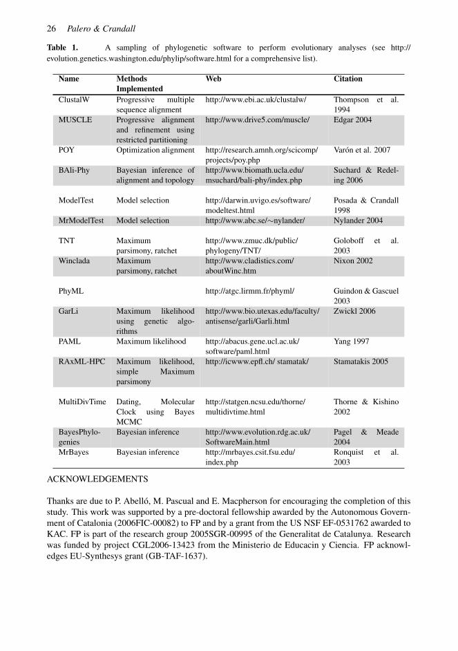
(3) Likelihood-based methods permit the application of mathematical models that incorporateour knowledge on typical patterns of sequence evolution, resulting in more powerful inferences.Furthermore, they use a complete statistical methodology that permits hypothesis tests, enablingvalidation of the results at all stages: from the values of parameters in evolutionary models, throughthe comparison of competing models describing the biological factors most important in sequenceevolution, to the testing of hypotheses of evolutionary relationship. Computer programs for therobust statistical evolutionary analysis of molecular sequence data are widely available (Table 1).

Nevertheless, ML methods do not directly assign probabilities to the parameters, and if one wantsto describe the uncertainty in an estimate, one has to repeat the analysis multiple times (bootstrap)increasing the computational cost. In Bayesian inference, information can be drawn directly fromthe simulated joint distribution of parameters at a reasonable computational cost. On the other hand,a review of the current Bayesian phylogenetic literature indicates that much more emphasis needsto be placed on developing more realistic models, checking the effects of the priors, and monitoringthe convergence of posterior distributions.

All in all, it should be pointed out that systematic error will confound any tree reconstructionmethod. Situations such as long-branch-attraction and base-compositional bias are examples ofsystematic bias. When inferring phylogenies, we try to define the actual succession of divergenceevents from the present sampled sequences. This means that the actual genes sampled (gain and lossof genes happens, but we rely only on those genes for which homology can be ascertained), speciessampled (extinction of intermediate taxa), selection (causing either among sites or among loci ratevariation) and the population parameters (mutation rates, recombination rates, effective populationsizes, etc.) all may influence the strength of the phylogenetic signal. In conclusion, phylogeneticinference should be approached not as a tool for getting a definitive answer for a taxonomical prob-lem, but rather as a tool for asking new questions on the evolution of molecules and morphology indifferent species and for trying to uncover the causes of such differences in their evolution.

26 Palero & Crandall

Table 1. A sampling of phylogenetic software to perform evolutionary analyses (see http://evolution.genetics.washington.edu/phylip/software.html for a comprehensive list).

Name MethodsImplemented

Web Citation

ClustalW Progressive multiplesequence alignment

http://www.ebi.ac.uk/clustalw/ Thompson et al.1994

MUSCLE Progressive alignmentand refinement usingrestricted partitioning

http://www.drive5.com/muscle/ Edgar 2004

POY Optimization alignment http://research.amnh.org/scicomp/projects/poy.php

Varon et al. 2007

BAli-Phy Bayesian inference ofalignment and topology

http://www.biomath.ucla.edu/msuchard/bali-phy/index.php

Suchard & Redel-ing 2006

ModelTest Model selection http://darwin.uvigo.es/software/modeltest.html

Posada & Crandall1998

MrModelTest Model selection http://www.abc.se/∼nylander/ Nylander 2004

TNT Maximumparsimony, ratchet

http://www.zmuc.dk/public/phylogeny/TNT/

Goloboff et al.2003

Winclada Maximumparsimony, ratchet

http://www.cladistics.com/aboutWinc.htm

Nixon 2002

PhyML http://atgc.lirmm.fr/phyml/ Guindon & Gascuel2003

GarLi Maximum likelihoodusing genetic algo-rithms

http://www.bio.utexas.edu/faculty/antisense/garli/Garli.html

Zwickl 2006

PAML Maximum likelihood http://abacus.gene.ucl.ac.uk/software/paml.html

Yang 1997

RAxML-HPC Maximum likelihood,simple Maximumparsimony

http://icwww.epfl.ch/ stamatak/ Stamatakis 2005

MultiDivTime Dating, MolecularClock using BayesMCMC

http://statgen.ncsu.edu/thorne/multidivtime.html

Thorne & Kishino2002

BayesPhylo-genies

Bayesian inference http://www.evolution.rdg.ac.uk/SoftwareMain.html

Pagel & Meade2004

MrBayes Bayesian inference http://mrbayes.csit.fsu.edu/index.php

Ronquist et al.2003

ACKNOWLEDGEMENTS

Thanks are due to P. Abello, M. Pascual and E. Macpherson for encouraging the completion of thisstudy. This work was supported by a pre-doctoral fellowship awarded by the Autonomous Govern-ment of Catalonia (2006FIC-00082) to FP and by a grant from the US NSF EF-0531762 awarded toKAC. FP is part of the research group 2005SGR-00995 of the Generalitat de Catalunya. Researchwas funded by project CGL2006-13423 from the Ministerio de Educacin y Ciencia. FP acknowl-edges EU-Synthesys grant (GB-TAF-1637).

Phylogenetic Inference Using Molecular Data 27

REFERENCES

Ahyong, S.T. & O’Meally, D. 2004. Phylogeny of the Decapoda. Reptantia: resolution using threemolecular loci and morphology. Raffl. Bull. Zool. 52:673693.

Aris-Brosou, S. 2003. Least and most powerful phylogenetic tests to elucidate the origin of the seedplants in presence of conflicting signals under misspecified models. Syst. Biol. 52:781-793.

Beaumont, M. & Rannala B. 2004. The Bayesian revolution in genetics. Nat. Rev. Genet. 5:251261.Benavides, E., Baum, R.,McClellan, D. & Sites, J.W. 2007. Molecular phylogenetics of the lizard

genus Microlophus (Squamata:Tropiduridae): Aligning and retrieving indel signal from nuclearintrons. Syst. Biol. 56:776-797.

Brown, W.M. et al. 1982. Mitochondrial DNA sequences of primates: tempo and mode of evolution.J. Mol. Evol. 18:225239.

Bruno, W.J. et al. 2000. Weighted neighbor-joining: a likelihood-based approach to distance basedphylogeny reconstruction. Mol. Biol. Evol. 17:189197.

Buckley, T.R. 2002. Model misspecification and probabilistic tests of topology: evidence fromempirical data sets. Syst. Biol. 51:509-523.

Buckley, T.R., Arensburger, P., Simon, C., & Chambers. G. K. 2002. Combined data, Bayesianphylogenetics, and the origin of the New Zealand cicada genera. Syst. Biol. 51:4-18.

Cao, Y. et al. 1994. Phylogenetic relationships among eutherian orders estimated from inferredsequences of mitochondrial proteins: instability of a tree based on a single gene. J. Mol. Evol.39:519527.

Castresana, J. 2000. Selection of conserved blocks from multiple alignments for their use in phylo-genetic analysis. Mol. Biol. Evol. 17:540-552.

Castresana, J. 2007. Topological variation in single-gene phylogenetic trees. Genome Biol. 8:216.Drummond, A.J. & Rambaut, A. 2007. BEAST: Bayesian evolutionary analysis by sampling trees.

BMC Evol. Biol. 7:214.Edgar, R.C. 2004. MUSCLE: multiple sequence alignment with high accuracy and high throughput.

Nucl. Acids Res. 32:1792-97.Edwards, A.W.F. & Cavalli-Sforza, L.L. 1964. Reconstruction of evolutionary trees. Pp. 67-76 in

J. McNeill, ed. Phenetic and phylogenetic classification. Systematics Association Publication,London.

Egan, A.N. & Crandall, K.A. 2008. Incorporating gaps as phylogenetic characters across eightDNA regions: Ramifications for North American Psoraleeae (Leguminosae) Mol. Phylo. Evol.46:532-546.

Farris J.S. 1983. The logical basis of phylogenetic analysis. In: Advances in Cladistics (Edited byPlatnick N.I. & Funk V.A.), pp. 1-36. Columbia Uni. Press, New York.

Farris, J.S. 1989. The retention index and the rescaled consistency index. Cladistics 5:417-419.Farris, J.S., Kallersj, M., Kluge, A.G. & Bult, C. 1994. Testing significance of incongruence. Cladis-

tics 10:315-319.Felsenstein, J. 1978. The number of evolutionary trees. Syst. Zool. 27:2733.Felsenstein, J. 1981. Evolutionary trees from DNAsequences: a maximum likelihood approach. J.

Mol. Evol. 17:368376.Felsenstein, J. 1985. Confidence limits on phylogenies: an approach using the bootstrap. Evolution

39:783791.Felsenstein, J. 2004. Inferring Phylogenies. Sinauer Associates Inc., Massachusetts. 664 pp.Felsenstein, J. 2005. PHYLIP (Phylogeny Inference Package) version 3.6. Distributed by the author.

28 Palero & Crandall

Department of Genome Sciences, University of Washington, Seattle.Frank, A.C. & Lobry, J.R. 1999. Asymmetric substitution patterns: a review of possible underlying

mutational or selective mechanisms. Gene 238:6577.Gascuel, O. 1997. BIONJ: an improved version of the NJ algorithm based on a simple model of

sequence data. Mol. Biol. Evol. 14:685695.Gascuel, O., Bryant, D., & Denis, F. 2001. Strengths and limitations of the minimum-evolution

principle. Syst. Biol. 50:621-627.Gatesy, J., O’Grady, P. & Baker R.H. 1999. Corroboration among data sets in simultaneous analysis:

Hidden support for phylogenetic relationships among higher-level artiodactyl taxa. Cladistics15:271 313.

Glenner, H., Lutzen, J. & Takahashi, T. 2003. Molecular evidence for a monophyletic clade ofasexually reproducing parasitic barnacles: Polyascus, new genus (Cirripedia: Rhizocephala). J.Crust. Biol. 23:548-557.

Goldman, N. 1993. Statistical tests of models of DNA substitution. J. Mol. Evol. 36:182198.Goldman, N. 1998. Phylogenetic information and experimental design in molecular systematics.

Proc. R. Soc. London Ser. B 265:17791786.Goloboff, P., Farris, J.S. & Nixon, K. 2003. TNT: Tree analysis using new technology Program and

documentation, available from the authors, and at http://www.zmuc.dk/public/phylogeny.Guindon, S. & Gascuel, O. 2003. A simple, fast and accurate algorithm to estimate large phylogenies

by maximum likelihood. Syst. Biol. 52:696704.Harvey, P. H. & Pagel, M.D. 1991. The Comparative Method in Evolutionary Biology. Oxford

University Press, Oxford.Hasegawa, M. & Kishino, H. 1989. Confidence limits on the maximum-likelihood estimate of the

hominoid tree from mitochondrial-DNA sequences. Evolution 43:672677.Hedtke, S.M., Townsend, T.M., & Hillis, D.M. 2006. Resolution of phylogenetic conflict in large

data sets by increased taxon sampling. Syst. Biol. 55:522529.Holmes, I. 2005. Using evolutionary Expectation Maximization to estimate indel rates. Bioinfor-

matics 21:22942300.Huelsenbeck, J.P. 1995. Performance of phylogenetic methods in simulation. Syst. Biol. 44:1748.Huelsenbeck, J.P. 1997. Is the Felsenstein zone a fly trap? Syst. Biol. 46:6974.Huelsenbeck, J.P. & Rannala, B. 1997. Phylogenetic methods come of age: testing hypotheses in an

evolutionary context. Science 276:227232.Kass, R.E. & Raftery, A.E. 1995. Bayes factors. J. Amer. Stat. Assoc. 90:773-795.Keller, I., Bensasson, D. & Nichols, R.A. 2007. Transition-Transversion Bias Is Not Universal:

A Counter Example from Grasshopper Pseudogenes. PLoS Genet 3(2): e22. doi:10.1371/journal.pgen.0030022

Kishino, H. & Hasegawa, M. 1989. Evaluation of the maximum likelihood estimate of the evolu-tionary tree topologies from DNA sequence data, and the branching order in Hominoidea. J.Mol. Evol. 29:170179.

Kitchin, I.J., Forey, P.L., Humphries, C.J. & Williams, D.M. 1998. Cladistics. Oxford UniversityPress, Oxford.

Kolaczkowski B. & Thornton, J.W. 2004. Performance of maximum parsimony and likelihoodphylogenetics when evolution is heterogeneous, Nature 431:980984.

Lake, J.A. 1991. The order of sequence alignment can bias the selection of tree topology. Mol. Biol.Evol. 8:378-385.

Larget, B. & Simon, D. 1999. Markov chain Monte Carlo algorithms for the Bayesian analysis ofphylogenetic trees. Mol. Biol. Evol. 16:750759.

Phylogenetic Inference Using Molecular Data 29

Lee, M.S.Y. & Hugall, A. F. 2003. Partitioned likelihood support. and the evaluation of data setconflict. Syst. Biol. 52:15-22.

Lee, M.S.Y. & Hugall, A.F. 2006. Model type, implicit data weighting, and model averaging inphylogenetics. Mol. Phyl. Evol. 38:848857.

Lio, P. & Goldman, N. 1998. Models of molecular evolution and phylogeny. Genome Res. 8:1233-1244.

Lutzoni, F., Wagner, P., Reeb, V. & Zoller, S. 2000. Integrating ambiguously aligned regions ofDNA sequences in phylogenetic analyses without violating positional homology. Syst. Biol.49:628-651.

Mau, B. et al. 1999. Bayesian phylogenetic inference via Markov chain Monte Carlo methods.Biometrics 55:112.

Moore, G., Goodman, M. & Barnabas, J. 1973. An iterative approach from the standpoint of theadditive hypothesis to the dendrogram problem posed by molecular data sets. J. Theor. Biol.38:423-457.

Needleman S.B. & Wunsch C.D. 1970. A general method applicable to the search for similarities inthe amino acid sequence of two proteins. J. Mol. Biol. 48:443-53.

Nielsen, R. & Yang, Z. 1998. Likelihood models for detecting positively selected amino acid sitesand applications to the HIV-1 envelope gene. Genetics 148:929936.

Nixon, K.C. 1999. The Parsimony Ratchet, a new method for rapid parsimony analysis. Cladistics15:407-414.

Nixon, K.C. 2002. WinClada ver. 1.00.08 Published by the author, Ithaca, NY.Nylander, J.A.A. 2004. MrModeltest v2. Program distributed by the author. Evolutionary Biology

Centre, Uppsala University.Nylander, J.A., Ronquist, F., Huelsenbeck, J.P. & Nieves-Aldrey, J.L. 2004. Bayesian phylogenetic

analysis of combined data. Syst. Biol. 53:4767.Ogden, T.H. & Whiting, M. 2003. The problem with “the Paleoptera Problem”: sense and sensitiv-

ity. Cladistics 19:432442.Ogden, T.H. & Rosenberg, M. 2006. How should gaps be treated in parsimony? A comparison of

approaches using simulation. Mol. Phylo. Evol. 42:817826.Ogden, T.H. & Rosenberg, M. 2007. Alignment and topological accuracy of the direct optimization

approach via POY and traditional phylogenetics via ClustalW + PAUP*. Syst. Biol. 56:182-193.Ota, S. & Li, W.H. 2001. NJML+: An extension of the NJML method to handle protein sequence.

data and computer software implementation, Mol. Biol. Evol. 18:1983-1992.Pagel, M. & Meade, A. 2004. A phylogenetic mixture model for detecting pattern-heterogeneity in

gene sequence of character-state data. Syst. Biol. 53:571-581.Philippe, H. & Forterre, P. 1999. The rooting of the universal tree of life is not reliable. J. Mol. Evol.

49:509-523.Porter, M.L., Cronin, T., McClellan, D.A. & Crandall, K.A. 2007. Molecular characterization of

crustacean visual pigments and the evolution of pancrustacean opsins. Mol. Biol. Evol. 24:253-268.

Posada, D. & Crandall, K.A. 1998. Modeltest: testing the model of DNA substitution. Bioinformat-ics 14:817-818.

Posada, D. & Crandall, K.A. 2001. Selecting the best-fit model of nucleotide substitution. Syst.Biol. 50:580-601.

Posada, D. & Buckley, T.R. 2004. Model selection and model averaging in phylogenetics: Advan-tages of Akaike Information Criterion and Bayesian approaches over Likelihood Ratio Tests.Syst. Biol. 53:793-808.

30 Palero & Crandall

Redelings, B. & Suchard, M. 2005. Joint Bayesian estimation of alignment and phylogeny. Syst.Biol. 54:401-418.

Robinson, D.F. 1971. Comparison of labeled trees with Valency Three. J. Combin. Theor. 11:105-119.

Rogers, J.S. 1997. On the consistency of maximum likelihood estimation of phylogenetic trees fromnucleotide sequences. Syst. Biol. 46:354357.

Ronquist, F. & Huelsenbeck, J.P. 2003. MRBAYES 3: Bayesian phylogenetic inference under mixedmodels. Bioinformatics 19:1572-1574.

Rzhetsky, A. & Nei, M. 1993. Theoretical foundation of the minimum evolution method of phylo-genetic inference. Mol. Biol. Evol. 10:1073-1095.

Schoniger, M. & von Haeseler, A. 1994. A stochastic model for the evolution of autocorrelatedDNA sequences. Mol. Phylo. Evol. 3:240247.

Segawa, R.D. & Aotsuka, T. 2005. The mitochondrial genome of the Japanese freshwater crab,Geothelphusa dehaani (Crustacea: Brachyura): evidence for its evolution via gene duplication.Gene 355:28-39.

Shimodaira, H. & Hasegawa, M. 1999. Multiple comparisons of log-likelihoods with applicationsto phylogenetic inference. Mol. Biol. Evol. 16:11141116.

Song, H., Buhay, J.E. Whiting, M.F. & Crandall, K.A. 2008. DNA barcoding overestimates thenumber of species when nuclear mitochondrial pseudogenes are coamplified. Proc. Nat. Acad.Sci. USA :in press.

Stamatakis, A., Ludwig, T. & Meier, H. 2005. RAxML-III: a fast program for maximum likelihood-based inference of large phylogenetic trees. Bioinformatics 21:456-463.

Steel, M.A. et al. 1988. Loss of information in genetic distances. Nature 336:118.Steel, M. & Penny, D. 2000. Parsimony, likelihood, and the role of models in molecular phyloge-

netics. Mol. Biol. Evol. 17:839850.Suchard, M.A. & Redelings, B.D. 2006. BAli-Phy: simultaneous Bayesian inference of alignment

and phylogeny. Bioinformatics 22:2047-2048.Swofford, D. L. 2003. PAUP*. Phylogenetic Analysis Using Parsimony (*and Other Methods).

Version 4. Sinauer Associates, Sunderland, Massachusetts.Swofford, D.L., Olsen, G.J., Waddell, P.J. & Hillis, D.M. 1996. Phylogenetic inference. In: Molec-

ular Systematics, second edition (Edited by Hillis D.M., Moritz C.& Mable B.K.), pp. 407-514.Sinauer Associates, Sunderland.

Tamura, K., Dudley, J., Nei, M. & Kumar, S. 2007. MEGA4: Molecular Evolutionary GeneticsAnalysis (MEGA) software version 4.0. Mol. Biol. Evol. 24:1596-1599.

Teichmann, S.A. & Mitchison, G. 1999. Making family trees from gene families. Nat. Genet.21:66-67.

Templeton, A.R. 1983. Convergent evolution and nonparametric inferences from restriction dataand DNA sequences. Pp. 151-179 in B. S. Weir, ed. Statistical Analysis of DNA Sequence Data.Marcel Dekker, Inc., New York.

Thompson, J.D., Higgins, D.G. & Gibson, T.J. 1994. CLUSTAL W: improving the sensitivity ofprogressive multiple sequence alignment through sequence weighting, positions-specific gappenalties and weight matrix choice. Nucl. Acids Res. 22:4673-4680.

Thorne, J.L., Kishino, H. & Felsenstein, J. 1991. An evolutionary model for maximum likelihoodalignment of DNA sequences. J. Mol. Evol. 33:114-124.

Thorne, J.L. & Kishino, H. 1992. Freeing phylogenies from artifacts of alignment. Mol. Biol. Evol.9:1148-1162.

Thorne, J.L. & Kishino, H. 2002. Divergence time and evolutionary rate estimation with multilocus

Phylogenetic Inference Using Molecular Data 31

data. Syst. Biol. 51:689702.Varon, A., Vinh, L.S., Bomash, I. & Wheeler, W.C. 2007. POY 4.0 Beta 2635. American Museum

of Natural History.Weston, P.H. 1994. Methods for rooting cladistic trees. In: Models in Phylogeny Reconstruction

(Edited by Scotland R.W., Siebert D.J. & Williams D.M.), pp. 125-155. Oxford Uni. Press,Oxford.

Yang, Z. et al. 1994. Comparison of models for nucleotide substitution used in maximum-likelihoodphylogenetic estimation. Mol. Biol. Evol. 11:316324.

Yang, Z. 1996a. Among-site rate variation and its impact on phylogenetic analysis. Trends Ecol.Evol. 11:367372.

Yang, Z. 1996b. Maximum-likelihood models for combined analyses of multiple sequence data. J.Mol. Evol. 42: 587596.

Yang, Z. 1997. PAML: a program package for phylogenetic analysis by maximum likelihood.CABIOS 13:555556.

Yang, Z. & Rannala, B. 1997. Bayesian phylogenetic inference using DNA sequences: Markovchain Monte Carlo methods. Mol. Biol. Evol. 14:717724.

Yang, Z. et al. 2000. Codon-substitution models for heterogeneous selection pressure at amino acidsites. Genetics 155:431449.

Zanotto, P.M. et al. 1999. Genealogical evidence for positive selection in the nef gene of HIV-1.Genetics 153:10771089.

Zwickl, D. J. 2006. Genetic algorithm approaches for the phylogenetic analysis of large biologicalsequence datasets under the maximum likelihood criterion. Ph.D. dissertation, The University ofTexas at Austin.