Embed Size (px)
Citation preview

David Galvão Nunes Vaz de Mascarenhas
PHOTOMETRIC COLOURS OF CENTAURS
Dissertação no âmbito do Mestrado em Astrofísica e Instrumentação para o Espaço
orientada pelo Doutor Nuno Vasco Munhoz Peixinho Miguel e apresentada ao
Departamento de Física da Faculdade de Ciências e Tecnologia da Universidade de
Coimbra.
Fevereiro de 2020


iii
Acknowledgements:
This dissertation is, for me, the culmination of over two years of work and the result of
a lifelong interest that grew into a passion early on which, ultimately, made me decide to alter
my life’s trajectory after beginning my career as an IT engineer. I wished to dedicate myself to
the frontier of space science fully. For me, there is no greater calling.
There are countless people I would wish to thank for supporting me and enabling me
to undertake this journey in many aspects; however, for the sake of brevity, I shall limit myself
to those who had a direct impact on this dissertation.
Firstly, I wish to thank my advisor, Nuno Peixinho, who has been nothing if not
impeccable in his support throughout my time in Coimbra; his dedication to his students and
his faith in their abilities should serve as an inspiration for many. His guidance in this
dissertation has proven invaluable time and again and much of my introduction into the
professional world of astronomical research wouldn’t have been possible without his infallible
desire to include his students in all related activities and opportunities available.
I also wish to thank the remaining members of the evaluation jury, for their time and
availability.
My parents and brother have been invaluable throughout my efforts and they deserve
praise for the endless support and encouragement they each gave in their own way. My
mother, in particular, seemed to have a limitless supply of patience and energy to help me
achieve my goals.
Andrey Solovov, Sérgio Gomes, Ana Vasconcelos and Cédric Pereira; classmates and
friends – you have all not only helped with my work and my studies, but you have made the
experience all that much more enjoyable.
Ana Galvão. You have been an excellent friend since the day we met; you saw me
through both the best and worst of these past two years, both academically and personally. It
is something I shall never forget.
Colm Dodd. Your friendship has been as important to me now as it has over this past
decade. Your insights, suggestions and encouragement were invaluable not just for many
aspects of this dissertation, but also for myself.
Joana Marques, who has not only been a good, kind friend, but also the reason for
which it was literally possible to hand in this dissertation on time, as well; if not for your keen
memory and insight, the results of this work would have likely remained on hold for a year.
Fernando Pinheiro, for the many insights into IRAF and the processes of data
reduction, along with many hours of thoroughly enjoyable and fascinating conversation.
Finally, I wish to thank the FCT (Fundação para a Ciência e Tecnologia) and CITEUC
(Centro de Investigação da Terra e do Espaço da Universidade de Coimbra) for the research
scholarship, “Lápitas – Bolsa de Licenciado”, which gave rise to this overall dissertation.

iv
v
Abstract:
The objective of this dissertation is the observational, astronomical study of the surface
reflectivity of three small bodies of the solar system of the Centaur family – 2010 FH92, 2011
MM4 and 2013 PH44 –, combined with other Centaurs available in the literature, through the
photometric analysis of their colours, i.e. the measurement of the difference of the reflectivity
in different wavelengths, and comparison with the previously-measured members of this
population from the literature. This was achieved through the data reduction of astronomical
optical observations taken from the 3.5 meter and 2.2 meter telescopes at the Hispano-
Germanic Calar Alto Observatory Complex (CAHA) at Calar Alto, Spain. These observations
were originally conducted in July and September of 2014 (for the 3.5 meter telescope) and
January, February and October of 2014 (for the 2.2 meter telescope).
This was the first astronomical photometric study performed of any of these three
Centaurs. The measured B-R colours – i.e. the differences between the magnitudes measured
on the B and R filters of the Johnson system – were 0.89±0.38 for 2010 FH92, 0.15±39.82 for
2011 MM4 and 1.68±0.42 for 2013 PH44. The signal of object 2011 MM4 was too low for
photometric measurements. The colour error bar for 2010 FH92 was, unfortunately and
evidently, too high to provide a useful value. 2013 PH44 presents an ultrared colour – i.e. a
colour that is much higher than the solar B-R colour – even though it has observational errors
in that colour’s determination that do not permit that assertion to be definitive.
The Centaur population colour bimodality hypothesis was run through Hartigan’s
statistical dip test and, contrary to the conclusions from 2012 and 2013, failed to reject the
unimodality hypothesis with our sample, given that the confidence level obtained from the test
was 86.41% (i.e. p-value = 0.01359). In spite of the lack of statistical confirmation for the
bimodality with a confidence level over at least 95%, the Wilcoxon rank-sum test was used to
test the non-existence of different median values of orbital inclinations for the redder Centaurs
and the less red Centaurs, rejecting the null hypothesis with a 97.5% confidence level. Extra
plot comparisons with other parameters, such as the objects’ perihelia, semimajor axes,
Tisserand parameters, B-R colours, orbital inclinations and orbital eccentricities were
conducted. No other new conclusions relative to the distributions of the Centaur population
were obtained.
Keywords: Centaurs; Photometry; Small Solar System Bodies; Tisserand Parameter;
Colours.

vi
vii
Resumo:
O objectivo desta dissertação é o estudo astronómico, observacional, da reflectividade
das superfícies de três pequenos corpos do sistema solar da família dos Centauros – 2010
FH92, 2011 MM4 e 2013 PH44 –, em combinação com Centauros disponíveis na literatura,
através da análise fotométrica das cores dos mesmos, i.e. da medição da diferença de
reflectividades em diferentes comprimentos de onda, e comparações com outros membros
desta população previamente estudados na literatura. Isto foi possível com a redução de
dados de observações astronómicas ópticas efectuadas com os telescópios de 3.5 metros e
2.2 metros do Hispano-Germanic Calar Alto Observatory Complex (CAHA) em Calar Alto, na
Espanha. Estas observações foram feitas em Julho e Setembro de 2014 (para o telescópio
de 3.5 metros) e Janeiro, Fevereiro e Outubro de 2014 (para o telescópio de 2.2 metros).
Este foi o primeiro estudo fotométrico astronómicos efectuado para qualquer um
destes três Centauros. As cores B-R medidas – i.e. as diferenças entre as magnitudes
medidas no filtro B e no filtro R do sistema Johnson – foram 0.89 ± 0.38 para o 2010 FH92,
0.15 ± 39.82 para o 2011 MM4 e 1.68 ± 0.42 para o 2013 PH44. O sinal do objecto 2011 MM4
foi demasiado baixo para permitir medições fotométricas. A barra de erros da cor do objecto
2010 FH92 foi, lamentavelmente e evidentemente, demasiado elevada para que nos
fornecesse um valor útil. O objecto 2013 PH44 apresente uma cor ultravermelha – i.e. uma
cor bastante mais alta que a cor B-R solar – embora possua erros observacionais na
determinação dessa cor que não permitem que essa afirmação seja definitiva.
A hipótese da bimodalidade das cores B-R da população dos Centauros foi testada
através do teste estatístico dip test de Hartigan e, contrariamente às conclusões de 2012 e
2013, com a nossa amostra não se rejeita a hipótese de unimodalidade, dado o nível de
confiança obtido com o nosso teste ser de apenas 86,41% (i.e. p.valor = 0.01359). Apesar da
não confirmação estatística da bimodalidade com um nível de confiança superior a pelo
menos 95%, foi testada, com o teste de rank-sum de Wilcoxon, a não existência de diferentes
valores médios de inclinações orbitais dos Centauros mais vermelhos e dos menos
vermelhos, rejeitando-se a hipótese nula com um nível de confiança de 97.5%. Gráficos para
comparações suplementares foram criados com outros parâmetros, como os periélios, semi-
eixos maiores, parâmetros de Tisserand, cores B-R, inclinações orbitais e excentricidades
orbitais. Não se obtiveram novas conclusões relativamente às distribuições da população dos
Centauros.
Palavras-chave: Centauros; Fotometria; Pequenos Corpos do Sistema Solar; Parâmetro de
Tisserand; Cores.

viii
ix
Table of Contents
1 Introduction ...................................................................................................................... 1
1.1 Some Definitions and Concepts ................................................................................... 1
1.1.1 Some notes regarding terminology used in this dissertation .................................. 1
1.1.2 Colours ................................................................................................................. 2
1.1.3 Tisserand’s Parameter .......................................................................................... 2
1.2 Small Solar System Objects ........................................................................................ 3
1.2.1 Centaurs ............................................................................................................... 3
1.2.2 Comets ................................................................................................................. 5
1.2.3 Trojans .................................................................................................................. 6
1.2.4 Beyond Neptune ................................................................................................... 7
1.2.4.1 Kuiper Belt ..................................................................................................... 8
1.2.4.1.1 Classical KBOs .................................................................................... 9
1.2.4.1.2 RKBOs .............................................................................................. 10
1.2.4.2 Scattered Disc ............................................................................................. 10
1.2.4.3 Oort Cloud ................................................................................................... 11
1.2.4.4 Others .......................................................................................................... 11
1.2.5 Damocloids ......................................................................................................... 12
1.3 Comparisons and Relation to Centaurs ..................................................................... 12
1.4 Centaur Bimodal Colours ........................................................................................... 13
2 Observations .................................................................................................................. 17
2.1 Used Instrumentation ................................................................................................. 17
2.1.1 3.5 m Telescope ................................................................................................. 17
2.1.2 2.2 m Telescope ................................................................................................. 18
2.2 Methods and Concepts .............................................................................................. 19
2.2.1 Airmass and Extinction ....................................................................................... 19
2.2.2 Point Spread Function ........................................................................................ 19
2.2.3 Seeing ................................................................................................................ 20
2.2.4 Magnitude .......................................................................................................... 20
2.2.4.1 Zero-Point ................................................................................................... 21
2.2.5 Photometry ......................................................................................................... 21
2.2.5.1 Photometric Calibration with Standard Stars ............................................... 22
2.2.6 Johnson-Cousins Filters ..................................................................................... 23
2.2.6.1 GRIZ Filters ................................................................................................ 24
2.2.7 Star Field Observations ...................................................................................... 25
2.3 Observed Objects ..................................................................................................... 25
x
3 Data Reduction ............................................................................................................... 29
3.1 State of raw data ...................................................................................................... 29
3.2 Image defects ........................................................................................................... 30
3.2.1 Noise .................................................................................................................. 30
3.2.2 Artefacts .............................................................................................................. 31
3.3 Reduction Procedures ............................................................................................... 32
3.3.1 Trim .................................................................................................................... 32
3.3.2 Bias Correction ................................................................................................... 33
3.3.3 Flat Field Correction ............................................................................................ 34
3.3.4 Target Identification ............................................................................................ 36
3.3.5 Science Image Combination ............................................................................... 40
3.3.6 Raw Photometric Values .................................................................................... 41
3.3.7 Photometric Calibrations ..................................................................................... 46
3.3.7.1 Retrieving Surveyed Magnitudes ................................................................. 47
3.3.7.2 Converting and Calibrating Star Magnitudes ................................................ 51
3.3.7.3 Final Calibration ........................................................................................... 53
4 Analysis and Discussion ............................................................................................... 55
4.1 Colours ..................................................................................................................... 55
4.2 Bimodality ................................................................................................................. 56
4.3 Inclination ................................................................................................................. 57
4.4 Tisserand Parameter Comparisons ........................................................................... 59
4.5 Other Comparisons.................................................................................................... 62
4.6 Conclusions and Future Work ................................................................................... 66
APPENDIX A ...................................................................................................................... 69
APPENDIX B ...................................................................................................................... 73
APPENDIX C ...................................................................................................................... 77
APPENDIX D ...................................................................................................................... 87
REFERENCES ................................................................................................................. 109
xi
List of Figures
Figure 1.1: Amount of volatile/supervolatile materials lost through sublimation at respective
distances from the Sun ......................................................................................................... 5
Figure 1.2: The distributions of Centaurs, KBOs and SDOs .................................................. 8
Figure 1.3: 486958 Arrokoth .................................................................................................. 9
Figure 1.4: Colour distributions of some discussed populations .......................................... 15
Figure 2.1: Overhead view of the Hispano-Germanic Calar Alto Observatory Complex (CAHA)
........................................................................................................................................... 17
Figure 2.2: 3.5 m telescope at Calar Alto ........................................................................... 18
Figure 2.3: 2.2 m telescope at Calar Alto ........................................................................... 18
Figure 2.4: UBVRI passbands for the Bessell filters ........................................................... 23
Figure 2.5: griz passbands for the Pan-STARRS 1 system ................................................ 25
Figure 2.6: 2012 DD61 transiting over a background star .................................................. 26
Figure 2.7: The expected location of 2013 TP145 ............................................................... 27
Figure 3.1: A zoomed-in view of a raw frame of the 2013 PH44 observations .................... 32
Figure 3.2: Example of a final bias image ........................................................................... 34
Figure 3.3: AstFinder showing 2011 MM4’s location at the time of observation .................. 36
Figure 3.4: 20011 MM4 from AstFinder (left) with the corresponding view from the observation
data (right). ......................................................................................................................... 37
Figure 3.5: Same views as figure 3.4, with visual guides ..................................................... 37
Figure 3.6: A zoomed-in view of 2011 MM4 ........................................................................ 38
Figure 3.7: Radial profile of 2011 MM4's first B-filter exposure ............................................ 38
Figure 3.8: Focussed view of 2011 MM4 over five different frames from the B filter exposures
........................................................................................................................................... 39
Figure 3.9: 2011 MM4’s movement, with visual guides ....................................................... 39
Figure 3.10: 2011 MM4 in B filter (left) and 2010 FH92 in R filter (right) .............................. 40
Figure 3.11: MKAPFILE interactive window for 2010 FH92 data from B filter with aperture radii
plotted against its respective corrections ............................................................................ 45
Figure 3.12: The same view as figure 3.11, but with outlying stars flagged for omittance from
the corrections computation ................................................................................................ 45
Figure 3.13: Residues of the growth curve corrections for 2010 FH92 ................................ 46
Figure 3.14: One of the 2.2 m telescope’s star field images with a star intended for calibration
use highlighted in green ..................................................................................................... 48
Figure 3.15: The same star as in figure 3.14, as seen on the Pan-STARRS1, release 1 (DR1)
data on Aladin. .................................................................................................................... 48
Figure 3.16: The same star as that highlighted in figure 3.14, as seen in the 2Mass data on
the KStars software, with coordinates information displayed ............................................... 49
Figure 3.17: Pan-STARRS search webpage ....................................................................... 50
Figure 3.18: Results from the Pan-STARRS survey ............................................................ 50
xii
Figure 4.1: Histogram of "strict" Centaur (B-R) colours ....................................................... 56
Figure 4.2: Centaur orbital inclination angles and their respective B-R colours .................. 58
Figure 4.3: B-R and inclination for selected Centaurs, with respective "dominant" planet
indicated for each ............................................................................................................... 60
Figure 4.4: Same view as figure 4.3, with removed error bars for easier viewing ................ 60
Figure 4.5: Centaur colours versus all four of their Tisserand Parameters .......................... 61
Figure 4.6: Same as figure 4.5, except with Neptune removed to facilitate points visibility .. 62
Figure 4.7: B-R colour versus eccentricity ........................................................................... 63
Figure 4.8: B-R colour versus semimajor axis ..................................................................... 63
Figure 4.9: B-R colour versus Perihelion ............................................................................. 64
Figure 4.10: B-R colour versus Aphelion ............................................................................. 64
Figure 4.11: Second study of perihelion .............................................................................. 65
Figure C.1: User Interface for the Tisserand Parameter Calculation Program ..................... 77
Figure D.1: User Interface for the Standard Star Conversion and Calibration Program ....... 87
xiii
List of Tables
Table 2.1: Default filter passbands used in the 3.5 m telescope at Calar Alto ..................... 24
Table 2.2: Default filter passbands used in the 2.2 m telescope at Calar Alto ..................... 24
Table 2.3: Basic orbital parameters of relevant objects ...................................................... 26
Table 3.1: Exposure times and number of frames for each observed object ....................... 29
Table 3.2: Results of quadratic filter conversion and star calibrations ................................. 52
Table 3.3: Results of linear filter conversion and star calibrations ....................................... 53
Table 3.4: Retrieved raw photometric values of Centaurs ................................................... 53
Table 3.5: Calibrated Centaur magnitudes with quadratic filter conversions ........................ 54
Table 3.6: Calibrated Centaur magnitudes with linear filter conversions .............................. 54
Table 3.7: Final (B-R) colours of studied object with quadratic filter conversion .................. 54
Table 3.8: Final (B-R) colours of studied object with linear filter conversion ........................ 54
Table 4.1: Results of Spearman correlation tests for distributions shown in figures 4.7 to 4.11
........................................................................................................................................... 66

xiv
xv
Abbreviations:
a – Semimajor Axis
AU – Astronomical Units
CAHA – Centro Astronómico Hispano en Andalucía
CCD – Charge-Coupled Device
CKBO – Classical Kuiper Belt Object
DR1 – Pan-STARRS Data Release 1
DS9 – SAOImageDS9
e – Orbital Eccentricity
e- – Electrons
FITS – Flexible Image Transport System
FOV – Field of View
FTP – File Transfer Protocol
FWHM – Full Width at Half Maximum
Gyr – Thousand Million Years
HFC – Halley Family Comet
i – Orbital Inclination
IAU – International Astronomical Union
IRAF -- Image Reduction and Analysis Facility
JFC – Jupiter Family Comet
JPL – Jet Propulsion Laboratory
KBO – Kuiper Belt Object
kyr – Thousand Years
LPC – Long Period Comet
Myr – Million Years
NOAO – National Optical Astronomy Observatory
Pan-STARRS – Panoramic Survey Telescope and Rapid Response System
PS1 – Pan-STARRS survey 1
PSF – Point Spread Function
Q – Aphelion
q – Perihelion

xvi
RKBO – Resonant Kuiper Belt Object
SDO – Scattered Disc Object
S/N – Signal-to-Noise Ratio
SPC – Short Period Comet
SSSB – Small Solar System Body
TNO – Trans-Neptunian Object
TP – Tisserand Parameter (P can be replaced with J for Jupiter, S for Saturn, U for Uranus
and N for Neptune)
1
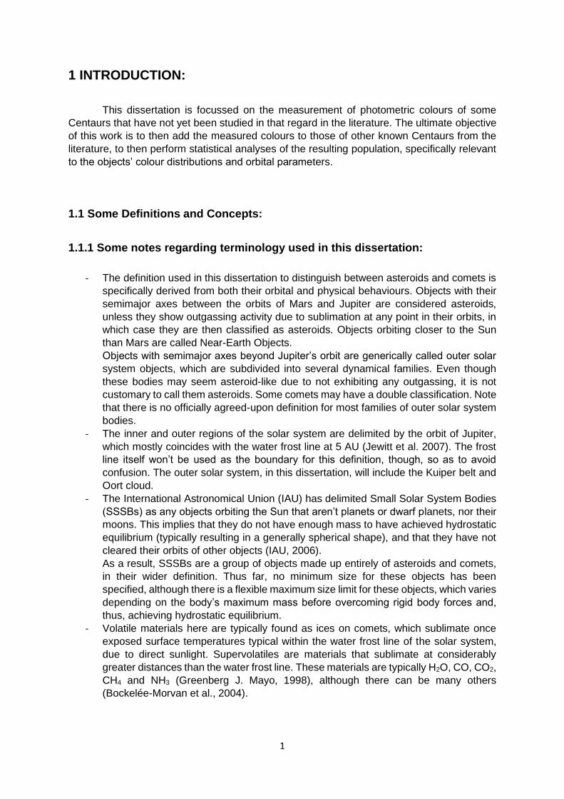
1 INTRODUCTION:
This dissertation is focussed on the measurement of photometric colours of some
Centaurs that have not yet been studied in that regard in the literature. The ultimate objective
of this work is to then add the measured colours to those of other known Centaurs from the
literature, to then perform statistical analyses of the resulting population, specifically relevant
to the objects’ colour distributions and orbital parameters.
1.1 Some Definitions and Concepts:
1.1.1 Some notes regarding terminology used in this dissertation:
- The definition used in this dissertation to distinguish between asteroids and comets is
specifically derived from both their orbital and physical behaviours. Objects with their
semimajor axes between the orbits of Mars and Jupiter are considered asteroids,
unless they show outgassing activity due to sublimation at any point in their orbits, in
which case they are then classified as asteroids. Objects orbiting closer to the Sun
than Mars are called Near-Earth Objects.
Objects with semimajor axes beyond Jupiter’s orbit are generically called outer solar
system objects, which are subdivided into several dynamical families. Even though
these bodies may seem asteroid-like due to not exhibiting any outgassing, it is not
customary to call them asteroids. Some comets may have a double classification. Note
that there is no officially agreed-upon definition for most families of outer solar system
bodies.
- The inner and outer regions of the solar system are delimited by the orbit of Jupiter,
which mostly coincides with the water frost line at 5 AU (Jewitt et al. 2007). The frost
line itself won’t be used as the boundary for this definition, though, so as to avoid
confusion. The outer solar system, in this dissertation, will include the Kuiper belt and
Oort cloud.
- The International Astronomical Union (IAU) has delimited Small Solar System Bodies
(SSSBs) as any objects orbiting the Sun that aren’t planets or dwarf planets, nor their
moons. This implies that they do not have enough mass to have achieved hydrostatic
equilibrium (typically resulting in a generally spherical shape), and that they have not
cleared their orbits of other objects (IAU, 2006).
As a result, SSSBs are a group of objects made up entirely of asteroids and comets,
in their wider definition. Thus far, no minimum size for these objects has been
specified, although there is a flexible maximum size limit for these objects, which varies
depending on the body’s maximum mass before overcoming rigid body forces and,
thus, achieving hydrostatic equilibrium.
- Volatile materials here are typically found as ices on comets, which sublimate once
exposed surface temperatures typical within the water frost line of the solar system,
due to direct sunlight. Supervolatiles are materials that sublimate at considerably
greater distances than the water frost line. These materials are typically H2O, CO, CO2,
CH4 and NH3 (Greenberg J. Mayo, 1998), although there can be many others
(Bockelée-Morvan et al., 2004).
2
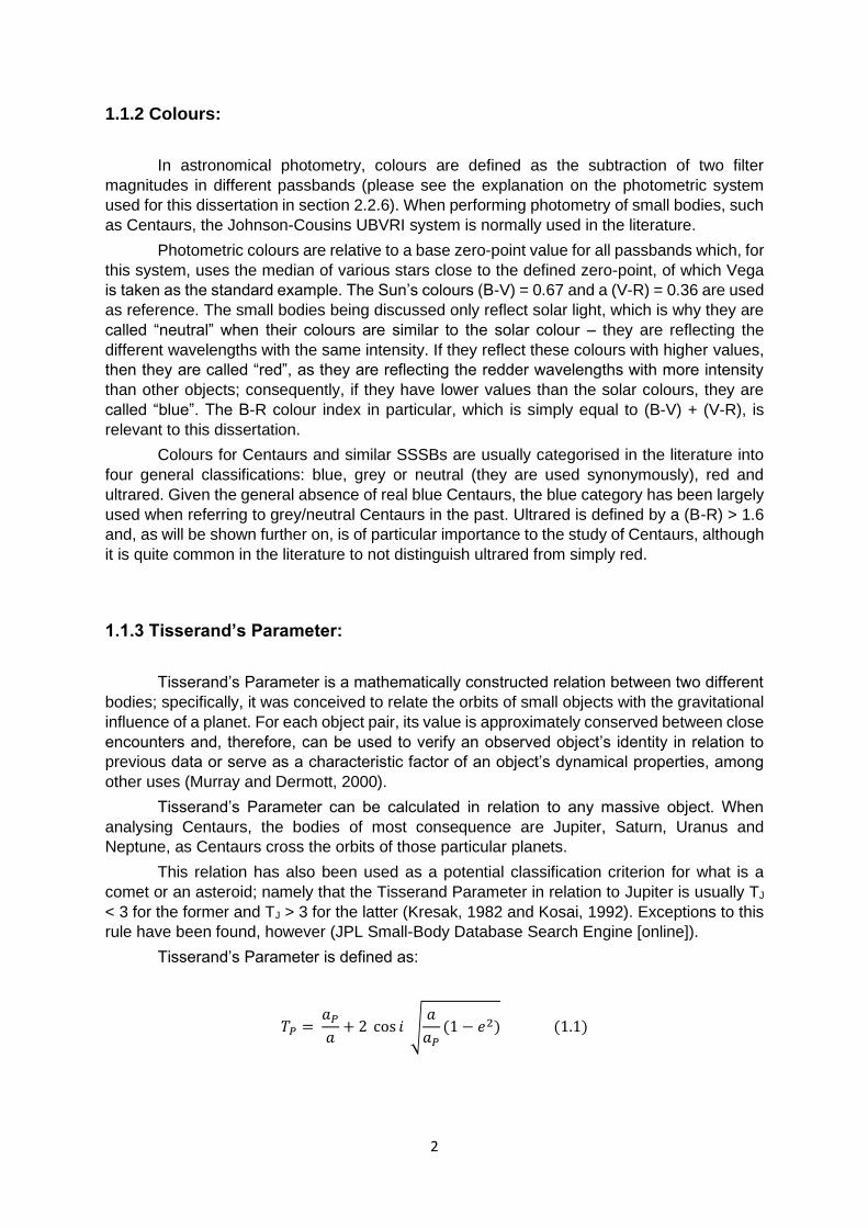
1.1.2 Colours:
In astronomical photometry, colours are defined as the subtraction of two filter
magnitudes in different passbands (please see the explanation on the photometric system
used for this dissertation in section 2.2.6). When performing photometry of small bodies, such
as Centaurs, the Johnson-Cousins UBVRI system is normally used in the literature.
Photometric colours are relative to a base zero-point value for all passbands which, for
this system, uses the median of various stars close to the defined zero-point, of which Vega
is taken as the standard example. The Sun’s colours (B-V) = 0.67 and a (V-R) = 0.36 are used
as reference. The small bodies being discussed only reflect solar light, which is why they are
called “neutral” when their colours are similar to the solar colour – they are reflecting the
different wavelengths with the same intensity. If they reflect these colours with higher values,
then they are called “red”, as they are reflecting the redder wavelengths with more intensity
than other objects; consequently, if they have lower values than the solar colours, they are
called “blue”. The B-R colour index in particular, which is simply equal to (B-V) + (V-R), is
relevant to this dissertation.
Colours for Centaurs and similar SSSBs are usually categorised in the literature into
four general classifications: blue, grey or neutral (they are used synonymously), red and
ultrared. Given the general absence of real blue Centaurs, the blue category has been largely
used when referring to grey/neutral Centaurs in the past. Ultrared is defined by a (B-R) > 1.6
and, as will be shown further on, is of particular importance to the study of Centaurs, although
it is quite common in the literature to not distinguish ultrared from simply red.
1.1.3 Tisserand’s Parameter:
Tisserand’s Parameter is a mathematically constructed relation between two different
bodies; specifically, it was conceived to relate the orbits of small objects with the gravitational
influence of a planet. For each object pair, its value is approximately conserved between close
encounters and, therefore, can be used to verify an observed object’s identity in relation to
previous data or serve as a characteristic factor of an object’s dynamical properties, among
other uses (Murray and Dermott, 2000).
Tisserand’s Parameter can be calculated in relation to any massive object. When
analysing Centaurs, the bodies of most consequence are Jupiter, Saturn, Uranus and
Neptune, as Centaurs cross the orbits of those particular planets.
This relation has also been used as a potential classification criterion for what is a
comet or an asteroid; namely that the Tisserand Parameter in relation to Jupiter is usually TJ
< 3 for the former and TJ > 3 for the latter (Kresak, 1982 and Kosai, 1992). Exceptions to this
rule have been found, however (JPL Small-Body Database Search Engine [online]).
Tisserand’s Parameter is defined as:
𝑇𝑃 = 𝑎𝑃
𝑎+ 2 cos 𝑖 √
𝑎
𝑎𝑃(1 − 𝑒2) (1.1)
3
Where TP is the Tisserand Parameter for a given planet, aP is the semimajor axis of
the planet and a, e and i are the semimajor axis, eccentricity and inclination of the affected
smaller body.
1.2 Small Solar System Bodies:
As the compositional origins of Centaurs isn’t yet fully understood, there are multiple
hypothesis put forward to explain their makeup, which have connections to other small bodies
in the solar system. As such, other populations that make up what are known as Small Solar
System Bodies (or SSSBs) shall be presented with the intent of exploring possible
relationships between them and the Centaurs.
According to the IAU definition of SSSBs, this class of objects can be divided into
various known subgroups, which can be categorised according to their composition and orbital
characteristics; the following sections present an overview of these different populations.
1.2.1 Centaurs:
Centaurs are a class of bodies that are considered to be a transition group between
TNOs and archetypal comets. They are generically classified as any small body that orbits the
Sun between Jupiter and Neptune and, typically, cross the one or more orbits of the giant
planets. Specifically, there are multiple definitions for these objects in the literature, however
the most commonly used is that they are objects that are not in a 1:1 resonance with a planet
and that have orbits with perihelia and semimajor axes between 5.2 AU and 30.1 AU (Jewitt,
2009). According to this exact definition, there are 335 known Centaurs (JPL Small-Body
Database Search Engine [online]), out of which 33 have measured albedos, which vary
between 0.215 to 0.033, of which the majority are between 0.083 and 0.044. It is also possible
for an object generically classified as a comet to also be a Centaur, an example of such is
29P/Schwassmann-Wachmann 1 (Sarid et al., 2019).
JPL’s internal definition ignores the objects’ perihelia and only defines them as small
bodies that do not belong to any other class (trojans, Jupiter family comets, etc) that have
semimajor axes between 5.5 AU and 30.1 AU (JPL, Orbit Classification, Centaur [online]).
With this definition there are 502 known Centaurs, of which 50 have measured albedos, which
range between 0.215 and 0.02. The majority of these objects have albedos between 0.089
and 0.044.
Regardless of the definition used, with the current available data, it is shown that these
are generally dark objects.
Due to the nature of these objects’ orbits, which cross the paths of the giant planets
and, thus, may suffer gravitational disturbances, the Centaurs are considered to be an
unstable population with lifetimes in the order of a few million years to 100Myr (Tiscareno and
Malhotra, 2003). This instability and short average lifespan (compared to the age of the solar
system) implies that known Centaurs are young and should be an intermediate orbital state of
objects that likely originated in the Kuiper belt, currently in the process of transiting to Jupiter-
family comets (JFCs), or some other fate (Jewitt, 2009).
4
Most of these objects will not become JFCs, as two thirds of Centaurs are expected to
experience a gravitational interaction with one of the giant planets that will lead to the
Centaur’s ejection from the solar system. The remainder will be dispersed into the inner solar
system, which result in a direct collision with a planet, the Sun, or insertion into a JFC orbit
(Tiscareno and Malhotra, 2003).
Some Centaurs show activity similar to that of comets beyond the orbit of Jupiter
through the loss of mass at rates that vary between a few kilograms per second to multiple
tonnes per second (Jewitt, 2009). These objects have been dubbed “active Centaurs” and the
mechanism present for their outgassing is distinct from that associated to comets, as the
activity is observed beyond the frost line, where typical water ice is sufficiently heated to
sublimate. This activity shouldn’t be occurring due to sublimation of solid carbon monoxide or
carbon dioxide since, in those cases, inactive Centaurs would also be undergoing the same
outgassing process.
It is important to note, however, that active Centaurs have mean perihelia significantly
smaller than their inactive counterparts – specifically 5.9 AU, as opposed to the 12.4 AU mean
of the overall population. This suggests that their outgassing mechanisms are still driven by
thermal effects from solar radiation (Jewitt, 2009).
With these considerations, it has been hypothesised that the primary cause for the
objects’ mass loss is the transformation of amorphous ices into a crystalline structure, which
then liberates gasses otherwise trapped underneath the surface, such as CO. The external
limit for a crystallisation zone in which this process can occur is at around 12.5 AU from the
Sun (Jewitt et al., 2017).
There is a probable bimodal colour distribution among the Centaur population, with
groupings in the red and almost-neutral regions (please see section 1.4 for more details).
There are examples of objects with intermediate colours, with all known colours
ranging from almost-neutral to “ultrared.” This extreme is consistent with organic compounds
(i.e., carbon-containing ices, such as CO2) that have been irradiated by high-energy particles
– cosmic rays and ultra-violet solar radiation (e.g. McDonald et al. 1996, Thompson et al.
1987; see also Trujillo et al., 2005). This process releases hydrogen and generates complex
organic compounds, dubbed tholins, which eventually form a dark, red mantle on the surface
of the body, protecting underlying basic compounds which should remain in their initial state.
Active Centaurs, however, might have bluer colours (i.e., less red) due to their surfaces
having been covered with deposits of materials expelled by their outgassing activity, which
have been seen to have neutral-to-blue colours in comas measured thus far (Jewitt, 2015).
Until now, out of all known active Centaurs, there is only one known to have ultrared
matter on its surface – 2013 UL10. The peculiar case of 2013 UL10 might help determine how
accurate the outgassing resurfacing hypothesis is and how long active Centaurs take to
transition from red to blue or neutral colours, given that it has likely only recently begun its
outgassing and the nucleus is distinctly red, whereas its surrounding gas shows more neutral
colours (Epifani et all., 2018). Note, however, that if Centaurs originate in the Kuiper Belt,
many of them must have been injected into the Centaur region already with neutral surfaces.
It is worth noting that colour measurements of the nuclei of Active Centaurs can be
inexact, as there can be significant photometric contamination from the surrounding blue
comas. This would give their respective nucleus, from the observer’s perspective, a bluer
colour than they actually have.
5
1.2.2 Comets:
Comets have been known since antiquity (e.g. Barrett, 1978) due to the ease of
observing large active nuclei when passing close to Earth. Before these objects were
understood, they were often seen as portents of disaster and suffering, playing a major role in
astrological practices.
Comets are, classically, SSSBs mainly composed of ices that undergo loss of mass
through outgassing when exposed to enough heat due to solar radiation. This process is
mainly caused by the sublimation of icy matter on the comet’s nucleus. This results in what is
called a coma of gases and dust around said nucleus, which can be accompanied by visible
tails due to the force exerted by solar wind and radiation pressure (Broiles et al., 2015). These
tails can be composed of one or more streams of ejected particles and another, distinct stream
of ions (e.g. Behar et al., 2018). The exact distances at which these outgassing activities begin
depend on the primary composition of the ice present in the object. Water ice is typically the
most abundant volatile found on known comet populations, which begins to sublimate at about
5 AU from the Sun (also referred to as the frost line) (see review: Mumma and Charnley,
2011).
Molecules known as supervolatiles, such as CO2, CO, O2 or N2, may sublimate at
distances far superior to water’s frost line. An example of this is of comet C/2017 K2
(PANSTARRS), which was observed to outgas as it travelled towards the inner solar system,
at a distance of 23,7 AU, beyond the orbit of Uranus and the limit of the crystallisation zone
mentioned previously (Oort, 1951 and Hui et al., 2017). This object has a surface composition
of supervolatile ices and, to date, is the most distant active comet ever recorded.
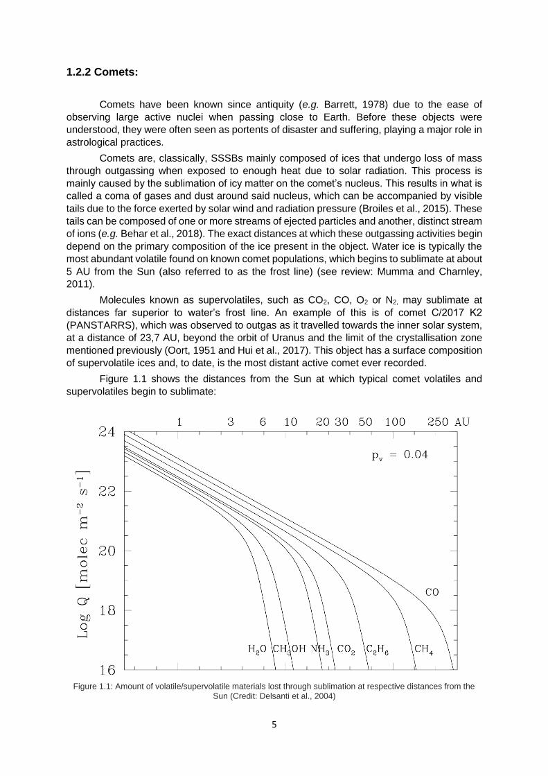
Figure 1.1 shows the distances from the Sun at which typical comet volatiles and
supervolatiles begin to sublimate:
Figure 1.1: Amount of volatile/supervolatile materials lost through sublimation at respective distances from the
Sun (Credit: Delsanti et al., 2004)
6
There are three primary groups of comets:
1. Jupiter Family Comets (JFCs), which have orbital periods of up to 20 years;
2. Halley Family Comets (HFCs), which have periods of 20 to 200 years;
3. Long Period Comets (LPCs), which have periods of more than 200 years.
Classically, JFCs and HFCs are grouped together into a general class known as Short
Period Comets (SPCs).
An orbital property also used to categorize these classes comes from their relationship
to Jupiter. JFCs are objects which were captured into their current orbits due to their
gravitational interactions with Jupiter (thus their name). They have a Tisserand Parameter
between 2 and 3 in relation to the giant planet (Levison, 1996).
In contrast, HFCs and LPCs have orbits which are more independent of Jupiter’s
gravitational influence, having a TJ < 2.
Using this definition, as of the time of writing, there are 682 known JFCs, 89 HTCs and
435 LPCs (JPL Small-Body Database Search Engine [online]). A notable aspect of LPCs is
that 118 specimens have orbital periods between 200 and 1kyr, whereas the remaining
population have periods of over 1kyr, implying very eccentric orbits, approaching parabolas.
Generally, independent of their classification, most comet nuclei have low albedos,
inferior to 0.1 (Davidsson and Skorov, 2002).
The long and short period comet groups show identical mean optical colours in their
outgassed materials. These particles, in turn, show identical colours to those of their
respective nuclei, without any observed cases of ultrared matter.
Jewitt (2012) indicates that comet nuclei and Damocloids (see section 1.2.5 ) are
descended directly from Centaurs and, thus, KBOs (see section 1.2.4.1). As comet nuclei and
Damocloids present no ultrared matter, it is required that said matter is lost during its descent
into the inner solar system. This is discussed further in sections 1.2.1 and 1.4.
The average lifetime of comets is very small, compared to the age of the solar system
– roughly 10kyr for SPCs, which corresponds to about 1,000 orbits, whereas most LPCs don’t
survive more than 50 orbits (Whitman et al., 2006). This implies that these populations need
to be continually replenished from external reservoirs of primordial objects.
Consequently, it is believed SPCs originate from the Kuiper Belt and LPCs come from
a more distant region called the Oort Cloud (see sections 1.2.4.1 and 1.2.4.3). An important
feature of LPCs is that about 45% of their population has a retrograde orbit (JPL Small-Body
Database Search Engine [online]), which gives credence to the hypothesis of their Oort Cloud
origins, as a random sampling of said group would mimic those orbital parameters.
1.2.3 Trojans:
Trojans are SSSBs that “share” the orbit of a planet – with a 1:1 resonance around the
Sun (a co-orbital configuration), occupying a region around a Lagrange point (typically L4 and
L5) of the two massive bodies in the three-body system. It is also possible for natural satellites
to have Trojans, occupying Lagrange points of the planet-satellite system in that case
(Whitman et al., 2006).
Currently, the planets Earth, Mars, Jupiter, Uranus and Neptune are known to have
Trojans, although, so far, only those in resonance with Jupiter and with Neptune have been
7
reported as stable (Marzari et al., 2003a, 2003b). Venus, Ceres and the large asteroid Vesta
have been known to have temporary Trojans (Christou and Wiegert, 2012). Currently, only
Jupiter and Neptune Trojans can give any useful statistical information for this dissertation’s
topic.
Jupiter has the most known Trojans in the solar system, with 7753 confirmed objects
at the time of writing (JPL Small-Body Database Search Engine [online]). Their low albedos
(the majority of which are measured between 0.04 and 0.08) and red surface colours suggest
these objects are rich in organic materials, although it might not strictly be the case
(Cruikshank et al., 2001). They do not show, however, ultrared matter (Jewitt, 2008).
Neptune Trojans, in contrast, only have 24 known members (IAU – Minor Planets
Center: List of Neptune Trojans), seven of which have high orbital inclinations (over 25º), which
suggests these objects are distributed in a large cloud that is perpendicularly wide in relation
to the ecliptic. Similarly to Jupiter’s Trojans, this is indicative of a captured population, rather
than one that formed in situ (Jewitt, 2018). The currently low number of detected Neptune
Trojans is explained by its large distance to Earth, when compared to Jupiter, which therefore
makes them harder to detect.
Simulations show that Neptune is not presently capable of capturing new stable
Trojans, which implies that its current population is entirely primordial, likely captured during
the period of planetary migration (Sheppard and Trujillo, 2006).
1.2.4 Beyond Neptune:
The trans-Neptunian region of the solar system has shown a large amount of complexity
in terms of object populations and their different characteristics. Any object with a semimajor
axis greater than Neptune’s (at 30.07 AU (NSSDCA – Neptune Fact Sheet [online])) is
considered part of this region. Three primary regions are defined:
1. The Kuiper Belt; (in some older works also known as Edgeworth-Kuiper Belt);
2. The Scattered Disc (which some authors do not separate from the Kuiper Belt);
3. The Oort Cloud.
Trans-Neptunian Objects (TNOs) are a vast category that encompasses all objects past
Neptune that orbit the Sun (this technically includes the Oort Cloud, although its members are
not colloquially referred to as TNOs). These bodies are, most likely, the most primordial
objects of the solar system, having suffered very few compositional alterations since their
original formation. Among them are Pluto, Eris, Makemake and Haumea, the only confirmed
dwarf planets recognised by the IAU, bar Ceres. It is, however, estimated that there could be
hundreds more already-detected dwarf planets among the trans-Neptunian SSSBs (Brown –
How many dwarf planets are there in the outer solar system? [online]). It is believed that all
comets (excluding visiting extrasolar objects) were originally TNOs or Oort Cloud objects and
some have been observed to migrate into the inner solar system directly from beyond the orbit
of Neptune (Hui et al., 2017).
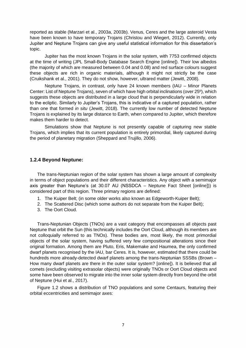
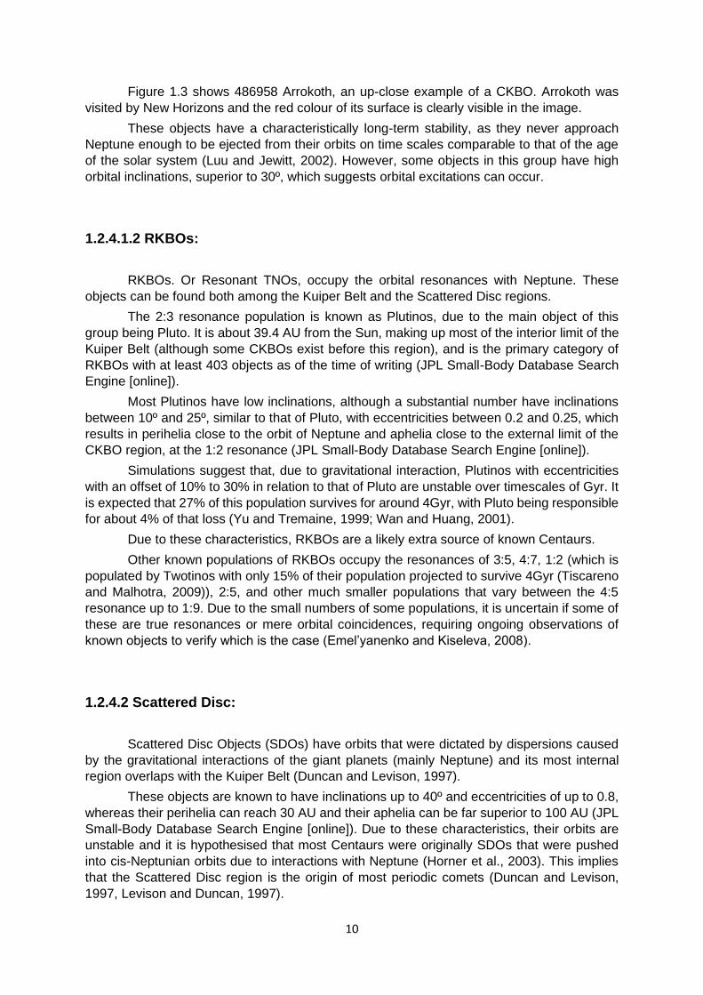
Figure 1.2 shows a distribution of TNO populations and some Centaurs, featuring their
orbital eccentricities and semimajor axes:
8
Figure 1.2: The distributions of Centaurs, KBOs and SDOs according to their orbital eccentricities and semimajor axes. Note: We do not discuss the Detached Objects in this dissertation; they are sometimes considered to be an
extension of the SDOs in the literature (Credit: Jewitt, The Resonant KBOs: Mean Motion Resonance [online])
1.2.4.1 Kuiper Belt:
The Kuiper Belt, also less known as the Edgeworth-Kuiper Belt, is populated by KBOs
(Kuiper Belt Objects). They are the only known SSSB population known, outside of Centaurs,
whose members are known to have ultrared colours (Jewitt, 2008). This group is subdivided
into two major categories: Classical KBOs (CKBOs or the less used “Cubewanos”) and
Resonant KBOs (RKBOs). It is worth noting that, usually, the expressions “TNOs” and “KBOs”
are used interchangeably.
The general KBO population extends out to around ~50 AU and, while this limit is
confirmed by observation (Jewitt, 2008), there are no demonstrated dynamical theories for
why this population does not extend beyond this point. Currently, there are two main lines of
hypotheses that can explain this feature:
1. Close passing stars: it is possible that a neighbouring star passed at a distance of 150
AU from the Sun, which cleared out this zone of dispersed objects. If this occurred, it
would have likely been soon after the Sun’s formation, before it had escaped the
cluster of stars with which it was born, as the current stellar neighbourhood is too
9
dispersed – with an average distance of 1 parsec between stars – for an encounter of
this type to be likely (e.g. Trujillo and Brown, 2002).
2. Planet migration: the more consensual hypothesis, which considers that this limit is
simply the distance to which objects were swept out by the 1:2 resonance with Neptune
as it migrated out to its present orbit. Presently, the population at the 1:2 resonance
coincides with the external edge of the Kuiper Belt at 50 AU (Levison and Morbidelli,
2003), that is, the external edge of almost circular orbits.
As for the colours of the objects, KBOs (or TNOs) present a wide colour distribution, from
neutral up to ultrared. After much debate, a consensus has been reached that there is a
tendency for bimodality of colours among KBOs between grey and red objects, even though
objects with intermediate colours do exist (Tegler et al., 2016). This tendency is clearly
discerned among Centaurs. A hypothesis has been proposed in which KBOs originated from
two primordial populations that formed in the early solar system. The greyer objects would
have formed in the inner solar system and, due to planetary migration, were dragged out to
distant orbits, joining the redder objects which had originally formed in more external regions
(Wong and Brown, 2017). Nonetheless, many red objects would have also formed in less
external regions, and they are now also mixed with the “native” outer red objects, although on
dynamically more excited orbits.
1.2.4.1.1 Classical KBOs:
CKBOs orbit the Sun beyond Neptune, do not cross its orbit and do not occupy a
resonance region with it. They have a semimajor axis between 40 and 47 AU, just before the
1:2 resonance with Neptune. They have low eccentricities (almost-circular orbits) and, in some
cases, low orbital inclinations, similar to the classical planets (from which this group derives
its name). These are known as the “cold” classical KBOs. “Hot” classical KBOs are those that
have higher inclinations – between 5º and 30º. Note that some orbital overlap between “hot”
and “cold” CKBOs is expected.
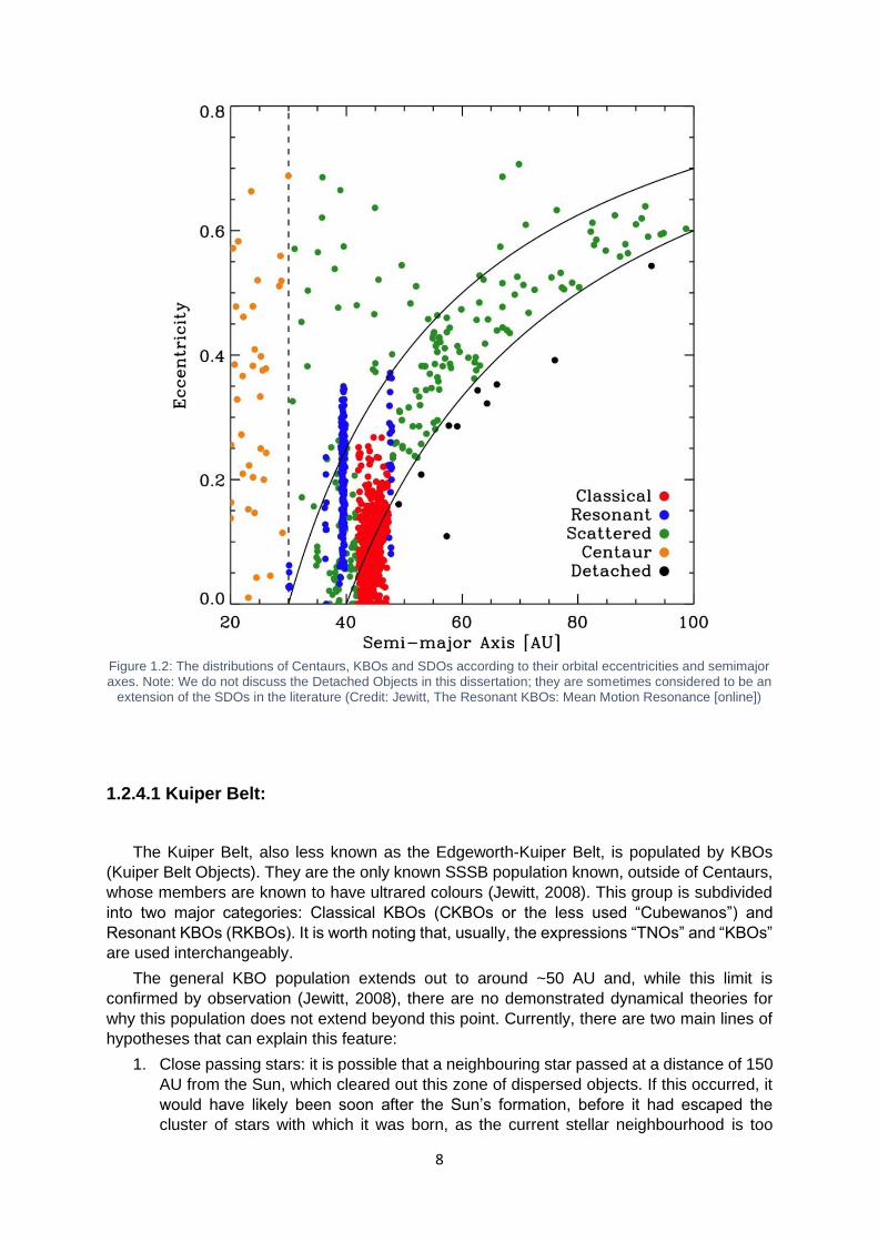
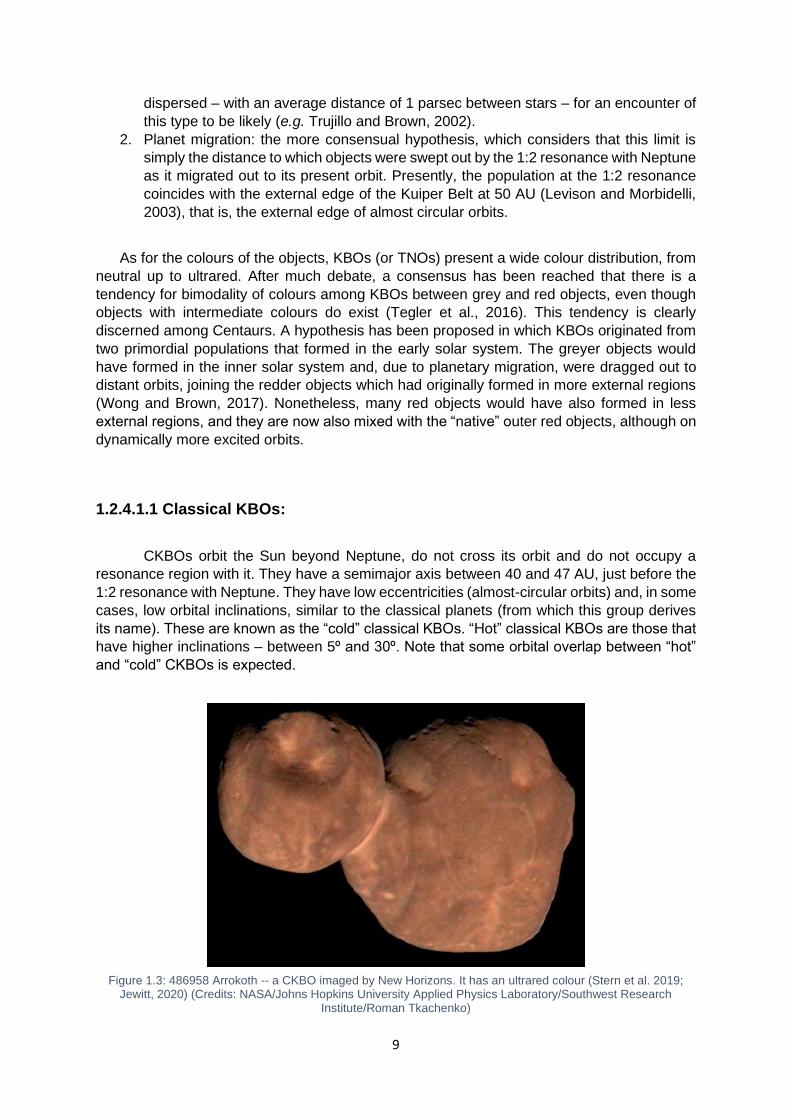
Figure 1.3: 486958 Arrokoth -- a CKBO imaged by New Horizons. It has an ultrared colour (Stern et al. 2019; Jewitt, 2020) (Credits: NASA/Johns Hopkins University Applied Physics Laboratory/Southwest Research
Institute/Roman Tkachenko)
10
Figure 1.3 shows 486958 Arrokoth, an up-close example of a CKBO. Arrokoth was
visited by New Horizons and the red colour of its surface is clearly visible in the image.
These objects have a characteristically long-term stability, as they never approach
Neptune enough to be ejected from their orbits on time scales comparable to that of the age
of the solar system (Luu and Jewitt, 2002). However, some objects in this group have high
orbital inclinations, superior to 30º, which suggests orbital excitations can occur.
1.2.4.1.2 RKBOs:
RKBOs. Or Resonant TNOs, occupy the orbital resonances with Neptune. These
objects can be found both among the Kuiper Belt and the Scattered Disc regions.
The 2:3 resonance population is known as Plutinos, due to the main object of this
group being Pluto. It is about 39.4 AU from the Sun, making up most of the interior limit of the
Kuiper Belt (although some CKBOs exist before this region), and is the primary category of
RKBOs with at least 403 objects as of the time of writing (JPL Small-Body Database Search
Engine [online]).
Most Plutinos have low inclinations, although a substantial number have inclinations
between 10º and 25º, similar to that of Pluto, with eccentricities between 0.2 and 0.25, which
results in perihelia close to the orbit of Neptune and aphelia close to the external limit of the
CKBO region, at the 1:2 resonance (JPL Small-Body Database Search Engine [online]).
Simulations suggest that, due to gravitational interaction, Plutinos with eccentricities
with an offset of 10% to 30% in relation to that of Pluto are unstable over timescales of Gyr. It
is expected that 27% of this population survives for around 4Gyr, with Pluto being responsible
for about 4% of that loss (Yu and Tremaine, 1999; Wan and Huang, 2001).
Due to these characteristics, RKBOs are a likely extra source of known Centaurs.
Other known populations of RKBOs occupy the resonances of 3:5, 4:7, 1:2 (which is
populated by Twotinos with only 15% of their population projected to survive 4Gyr (Tiscareno
and Malhotra, 2009)), 2:5, and other much smaller populations that vary between the 4:5
resonance up to 1:9. Due to the small numbers of some populations, it is uncertain if some of
these are true resonances or mere orbital coincidences, requiring ongoing observations of
known objects to verify which is the case (Emel’yanenko and Kiseleva, 2008).
1.2.4.2 Scattered Disc:
Scattered Disc Objects (SDOs) have orbits that were dictated by dispersions caused
by the gravitational interactions of the giant planets (mainly Neptune) and its most internal
region overlaps with the Kuiper Belt (Duncan and Levison, 1997).
These objects are known to have inclinations up to 40º and eccentricities of up to 0.8,
whereas their perihelia can reach 30 AU and their aphelia can be far superior to 100 AU (JPL
Small-Body Database Search Engine [online]). Due to these characteristics, their orbits are
unstable and it is hypothesised that most Centaurs were originally SDOs that were pushed
into cis-Neptunian orbits due to interactions with Neptune (Horner et al., 2003). This implies
that the Scattered Disc region is the origin of most periodic comets (Duncan and Levison,
1997, Levison and Duncan, 1997).
11
It has been suggested that the only truly distinguishing factor between SDOs and
KBOs is their relation to Neptune. Many researchers, in the literature, make an explicit
distinction between the objects of these two populations; whereas others consider the
Scattered Disc simply an external region of the Kuiper Belt, and therefore consider SDOs as
a family of KBOs, much like the Classical KBOs are. At time scales of the age of the solar
system, these objects can migrate from one class to the other multiple times (see review:
Morbidelli and Brown, 2004).
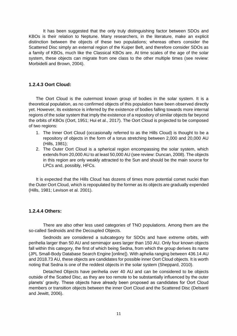
1.2.4.3 Oort Cloud:
The Oort Cloud is the outermost known group of bodies in the solar system. It is a
theoretical population, as no confirmed objects of this population have been observed directly
yet. However, its existence is inferred by the existence of bodies falling towards more internal
regions of the solar system that imply the existence of a repository of similar objects far beyond
the orbits of KBOs (Oort, 1951; Hui et al., 2017). The Oort Cloud is projected to be composed
of two regions:
1. The Inner Oort Cloud (occasionally referred to as the Hills Cloud) is thought to be a
repository of objects in the form of a torus stretching between 2,000 and 20,000 AU
(Hills, 1981);
2. The Outer Oort Cloud is a spherical region encompassing the solar system, which
extends from 20,000 AU to at least 50,000 AU (see review: Duncan, 2008). The objects
in this region are only weakly attracted to the Sun and should be the main source for
LPCs and, possibly, HFCs.
It is expected that the Hills Cloud has dozens of times more potential comet nuclei than
the Outer Oort Cloud, which is repopulated by the former as its objects are gradually expended
(Hills, 1981; Levison et al. 2001).
1.2.4.4 Others:
There are also other less used categories of TNO populations. Among them are the
so-called Sednoids and the Decoupled Objects.
Sednoids are considered a subcategory for SDOs and have extreme orbits, with
perihelia larger than 50 AU and semimajor axes larger than 150 AU. Only four known objects
fall within this category, the first of which being Sedna, from which the group derives its name
(JPL Small-Body Database Search Engine [online]). With aphelia ranging between 436.14 AU
and 2018.73 AU, these objects are candidates for possible inner Oort Cloud objects. It is worth
noting that Sedna is one of the reddest objects in the solar system (Sheppard, 2010).
Detached Objects have perihelia over 40 AU and can be considered to be objects
outside of the Scatted Disc, as they are too remote to be substantially influenced by the outer
planets’ gravity. These objects have already been proposed as candidates for Oort Cloud
members or transition objects between the inner Oort Cloud and the Scattered Disc (Delsanti
and Jewitt, 2006).
12
Their orbits are very elliptical and they have semimajor axes in the order of hundreds of
AU. These orbits have not been explained by the traditional dispersion models due to the giant
planets. There are a few hypotheses, such as:
1. Influence of a passing nearby star (Morbidelli and Levison, 2004);
2. Influence of a distant, unobserved planetary-mass object (sometimes referred to as
“Planet Nine” or “Planet X”) (Gomes et al., 2006);
3. Old interactions with Neptune if it had a more eccentric orbit in the past (Gladman et
al., 2002);
4. Interactions with primordial planets as they were ejected from the early solar system
after their formation (Gladman and Chan, 2006).
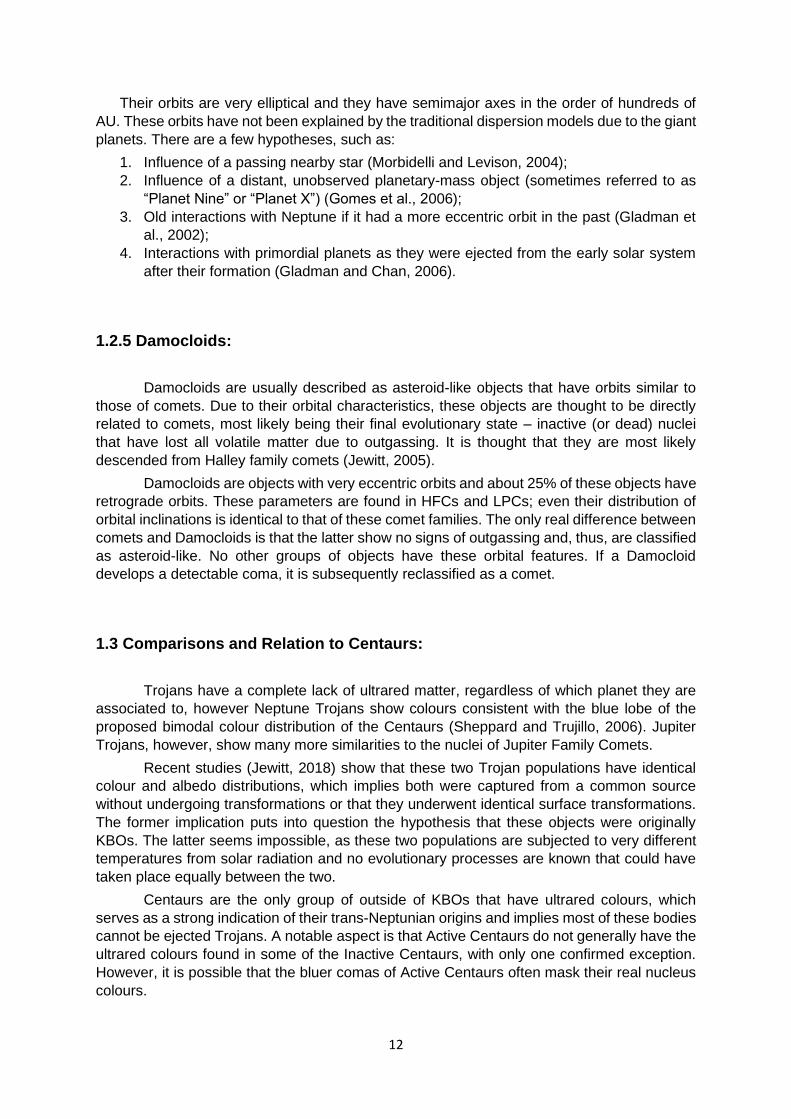
1.2.5 Damocloids:
Damocloids are usually described as asteroid-like objects that have orbits similar to
those of comets. Due to their orbital characteristics, these objects are thought to be directly
related to comets, most likely being their final evolutionary state – inactive (or dead) nuclei
that have lost all volatile matter due to outgassing. It is thought that they are most likely
descended from Halley family comets (Jewitt, 2005).
Damocloids are objects with very eccentric orbits and about 25% of these objects have
retrograde orbits. These parameters are found in HFCs and LPCs; even their distribution of
orbital inclinations is identical to that of these comet families. The only real difference between
comets and Damocloids is that the latter show no signs of outgassing and, thus, are classified
as asteroid-like. No other groups of objects have these orbital features. If a Damocloid
develops a detectable coma, it is subsequently reclassified as a comet.
1.3 Comparisons and Relation to Centaurs:
Trojans have a complete lack of ultrared matter, regardless of which planet they are
associated to, however Neptune Trojans show colours consistent with the blue lobe of the
proposed bimodal colour distribution of the Centaurs (Sheppard and Trujillo, 2006). Jupiter
Trojans, however, show many more similarities to the nuclei of Jupiter Family Comets.
Recent studies (Jewitt, 2018) show that these two Trojan populations have identical
colour and albedo distributions, which implies both were captured from a common source
without undergoing transformations or that they underwent identical surface transformations.
The former implication puts into question the hypothesis that these objects were originally
KBOs. The latter seems impossible, as these two populations are subjected to very different
temperatures from solar radiation and no evolutionary processes are known that could have
taken place equally between the two.
Centaurs are the only group of outside of KBOs that have ultrared colours, which
serves as a strong indication of their trans-Neptunian origins and implies most of these bodies
cannot be ejected Trojans. A notable aspect is that Active Centaurs do not generally have the
ultrared colours found in some of the Inactive Centaurs, with only one confirmed exception.
However, it is possible that the bluer comas of Active Centaurs often mask their real nucleus
colours.
13
If Centaurs do have amorphous ice on their surfaces, as indicated in section 1.2.1, this
implies that the KBOs they originated from must have surfaces at least partially composed of
amorphous ice, as well. It also infers that JFCs which descended from Centaurs also have
amorphous ice, which has been found likely, as outgassing activities have been found on JFCs
at heliocentric distances superior to 6 AU, beyond the water sublimation limit (Meech et al.,
2009).
Comets do not present nuclei with ultrared matter. Together with what has been
observed of other populations, such as the Centaurs and Damocloids, this suggests that
ultrared matter is lost whenever an object migrates into the inner solar system. Active Centaurs
begin outgassing and lose their ultrared matter at about the same heliocentric distance – 10
AU – which implies that these processes are directly related.
This effect on the Active Centaurs is likely caused by the object’s gradual resurfacing
due to ejected material falling back to the main body. This process should be applicable to
any object that undergoes mass loss through outgassing, which would explain the complete
lack of ultrared matter in the entire comet population.
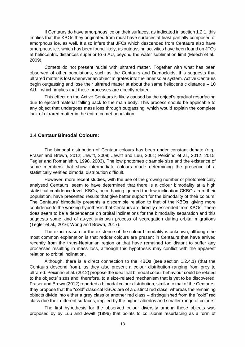
1.4 Centaur Bimodal Colours:
The bimodal distribution of Centaur colours has been under constant debate (e.g.,
Fraser and Brown, 2012; Jewitt, 2009; Jewitt and Luu, 2001; Peixinho et al., 2012, 2015;
Tegler and Romanishin, 1998, 2003). The low photometric sample size and the existence of
some members that show intermediate colours made determining the presence of a
statistically verified bimodal distribution difficult.
However, more recent studies, with the use of the growing number of photometrically
analysed Centaurs, seem to have determined that there is a colour bimodality at a high
statistical confidence level. KBOs, once having ignored the low-inclination CKBOs from their
population, have presented results that give better support for the bimodality of their colours.
The Centaurs’ bimodality presents a discernible relation to that of the KBOs, giving more
confidence to the working hypothesis that Centaurs are directly descended from KBOs. There
does seem to be a dependence on orbital inclinations for the bimodality separation and this
suggests some kind of as-yet unknown process of segregation during orbital migrations
(Tegler et al., 2016; Wong and Brown, 2017).
The exact reason for the existence of the colour bimodality is unknown, although the
most common explanation is that redder colours are present in Centaurs that have arrived
recently from the trans-Neptunian region or that have remained too distant to suffer any
processes resulting in mass loss, although this hypothesis may conflict with the apparent
relation to orbital inclination.
Although, there is a direct connection to the KBOs (see section 1.2.4.1) (that the
Centaurs descend from), as they also present a colour distribution ranging from grey to
ultrared. Peixinho et al. (2012) propose the idea that bimodal colour behaviour could be related
to the objects’ sizes and, therefore, to a size-related mechanism that is yet to be discovered.
Fraser and Brown (2012) reported a bimodal colour distribution, similar to that of the Centaurs;
they propose that the “cold” classical KBOs are of a distinct red class, whereas the remaining
objects divide into either a grey class or another red class – distinguished from the “cold” red
class due their different surfaces, implied by the higher albedos and smaller range of colours.
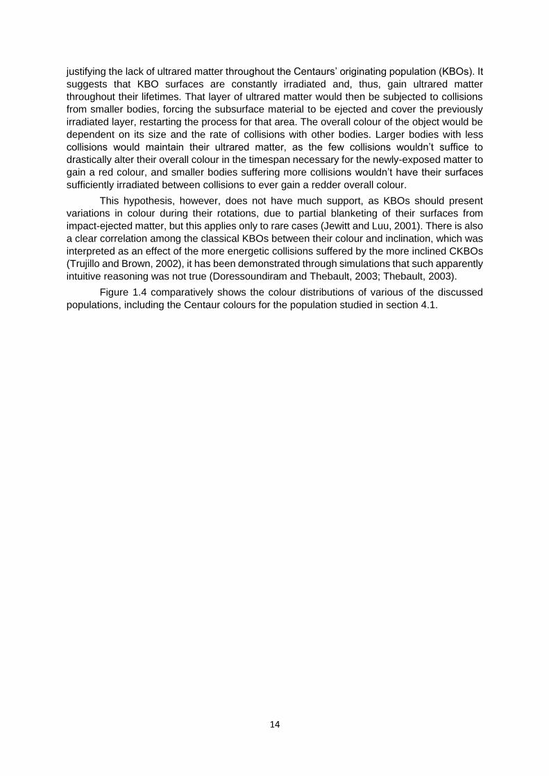
The first hypothesis for the observed colour diversity among these objects was
proposed by by Luu and Jewitt (1996) that points to collisional resurfacing as a form of
14
justifying the lack of ultrared matter throughout the Centaurs’ originating population (KBOs). It
suggests that KBO surfaces are constantly irradiated and, thus, gain ultrared matter
throughout their lifetimes. That layer of ultrared matter would then be subjected to collisions
from smaller bodies, forcing the subsurface material to be ejected and cover the previously
irradiated layer, restarting the process for that area. The overall colour of the object would be
dependent on its size and the rate of collisions with other bodies. Larger bodies with less
collisions would maintain their ultrared matter, as the few collisions wouldn’t suffice to
drastically alter their overall colour in the timespan necessary for the newly-exposed matter to
gain a red colour, and smaller bodies suffering more collisions wouldn’t have their surfaces
sufficiently irradiated between collisions to ever gain a redder overall colour.
This hypothesis, however, does not have much support, as KBOs should present
variations in colour during their rotations, due to partial blanketing of their surfaces from
impact-ejected matter, but this applies only to rare cases (Jewitt and Luu, 2001). There is also
a clear correlation among the classical KBOs between their colour and inclination, which was
interpreted as an effect of the more energetic collisions suffered by the more inclined CKBOs
(Trujillo and Brown, 2002), it has been demonstrated through simulations that such apparently
intuitive reasoning was not true (Doressoundiram and Thebault, 2003; Thebault, 2003).
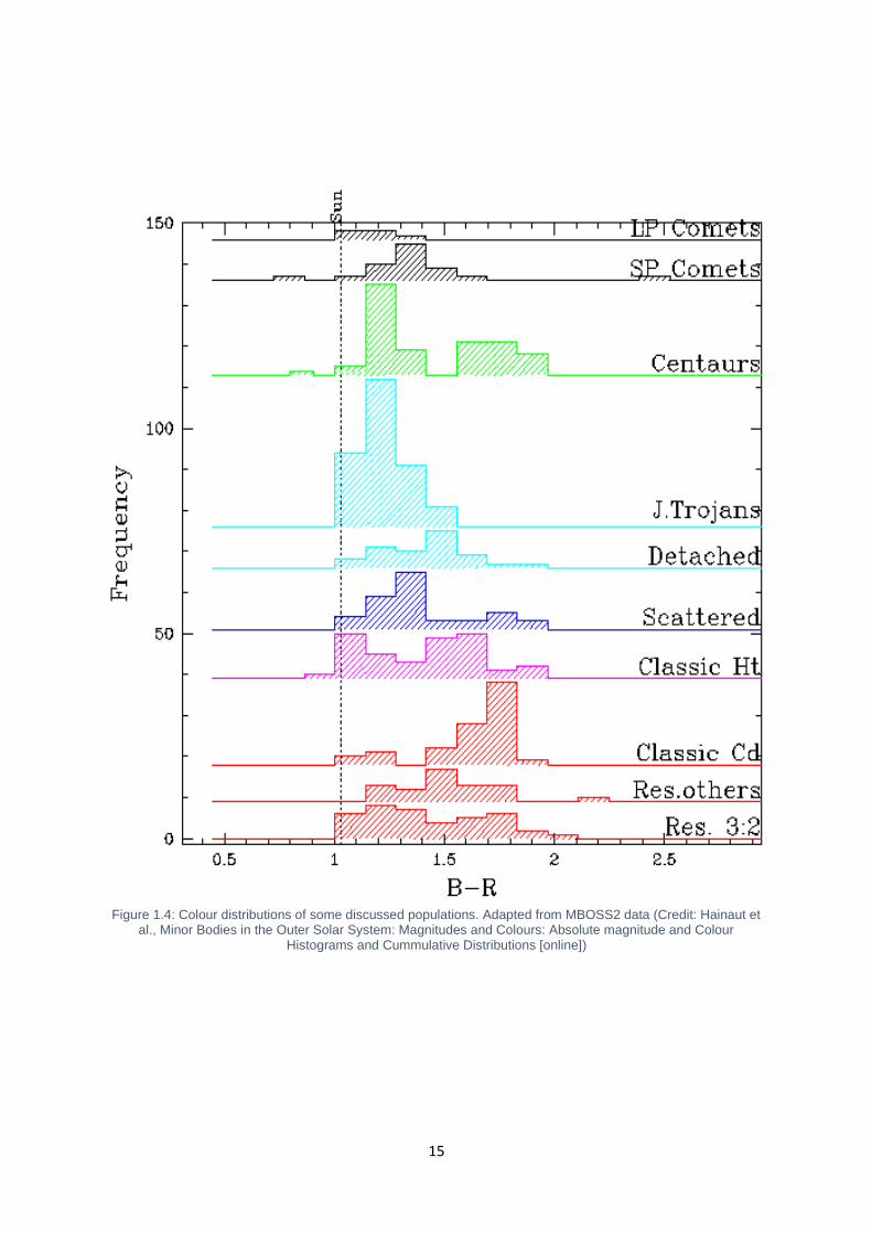
Figure 1.4 comparatively shows the colour distributions of various of the discussed
populations, including the Centaur colours for the population studied in section 4.1.
15
Figure 1.4: Colour distributions of some discussed populations. Adapted from MBOSS2 data (Credit: Hainaut et
al., Minor Bodies in the Outer Solar System: Magnitudes and Colours: Absolute magnitude and Colour Histograms and Cummulative Distributions [online])

16
17
2 OBSERVATIONS:
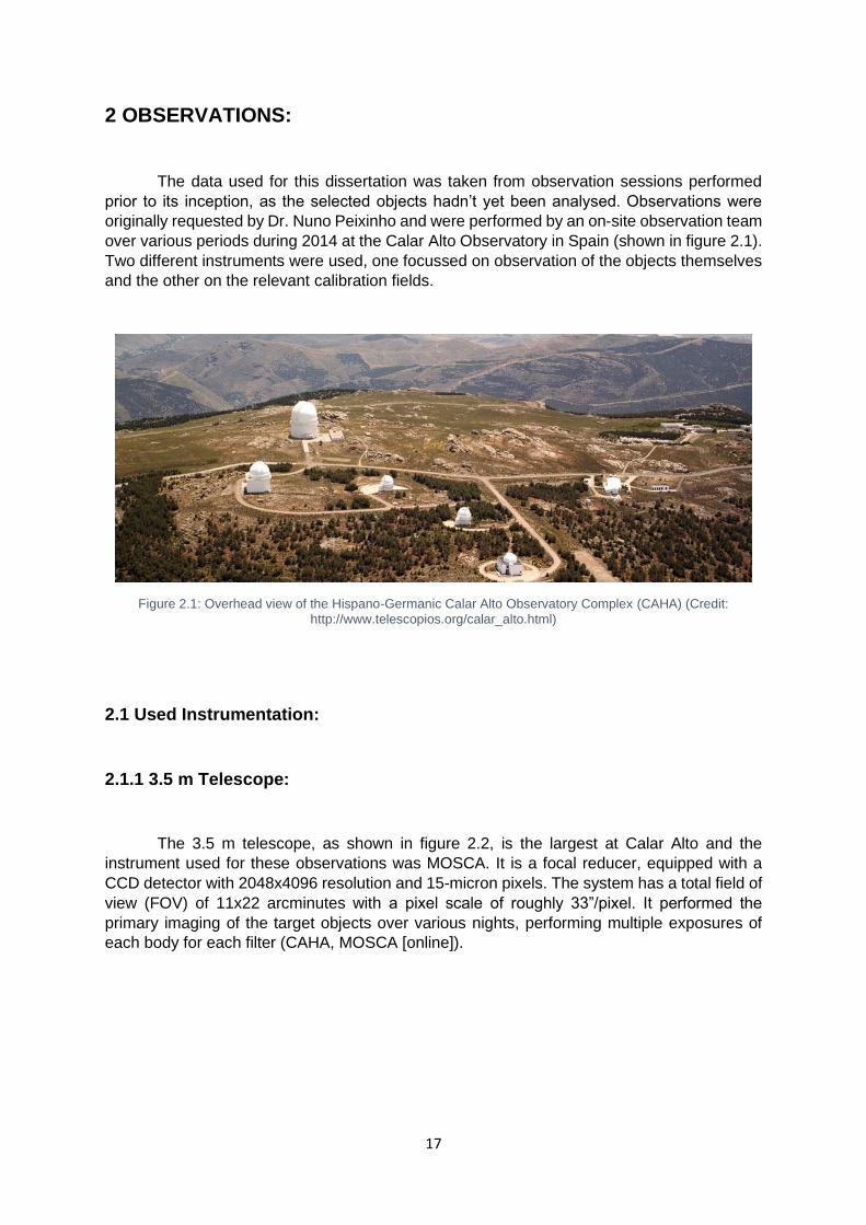
The data used for this dissertation was taken from observation sessions performed
prior to its inception, as the selected objects hadn’t yet been analysed. Observations were
originally requested by Dr. Nuno Peixinho and were performed by an on-site observation team
over various periods during 2014 at the Calar Alto Observatory in Spain (shown in figure 2.1).
Two different instruments were used, one focussed on observation of the objects themselves
and the other on the relevant calibration fields.
Figure 2.1: Overhead view of the Hispano-Germanic Calar Alto Observatory Complex (CAHA) (Credit:
http://www.telescopios.org/calar_alto.html)
2.1 Used Instrumentation:
2.1.1 3.5 m Telescope:
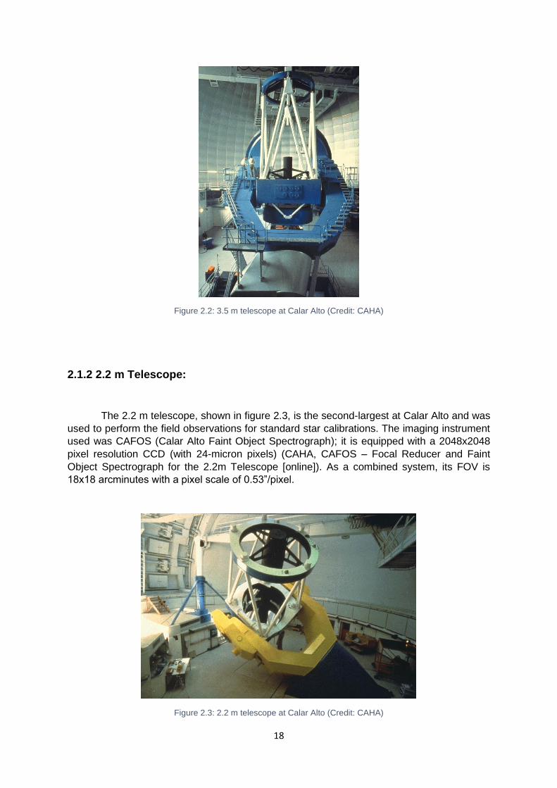
The 3.5 m telescope, as shown in figure 2.2, is the largest at Calar Alto and the
instrument used for these observations was MOSCA. It is a focal reducer, equipped with a
CCD detector with 2048x4096 resolution and 15-micron pixels. The system has a total field of
view (FOV) of 11x22 arcminutes with a pixel scale of roughly 33”/pixel. It performed the
primary imaging of the target objects over various nights, performing multiple exposures of
each body for each filter (CAHA, MOSCA [online]).
18
Figure 2.2: 3.5 m telescope at Calar Alto (Credit: CAHA)
2.1.2 2.2 m Telescope:
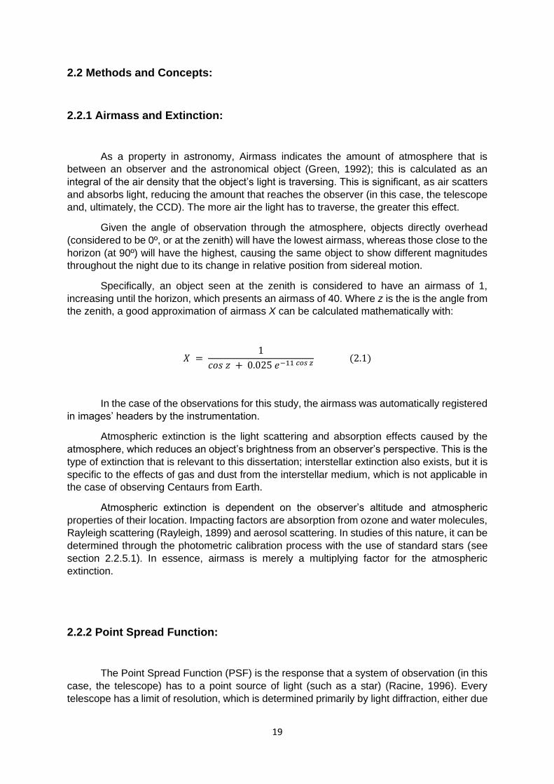
The 2.2 m telescope, shown in figure 2.3, is the second-largest at Calar Alto and was
used to perform the field observations for standard star calibrations. The imaging instrument
used was CAFOS (Calar Alto Faint Object Spectrograph); it is equipped with a 2048x2048
pixel resolution CCD (with 24-micron pixels) (CAHA, CAFOS – Focal Reducer and Faint
Object Spectrograph for the 2.2m Telescope [online]). As a combined system, its FOV is
18x18 arcminutes with a pixel scale of 0.53”/pixel.
Figure 2.3: 2.2 m telescope at Calar Alto (Credit: CAHA)
19
2.2 Methods and Concepts:
2.2.1 Airmass and Extinction:
As a property in astronomy, Airmass indicates the amount of atmosphere that is
between an observer and the astronomical object (Green, 1992); this is calculated as an
integral of the air density that the object’s light is traversing. This is significant, as air scatters
and absorbs light, reducing the amount that reaches the observer (in this case, the telescope
and, ultimately, the CCD). The more air the light has to traverse, the greater this effect.
Given the angle of observation through the atmosphere, objects directly overhead
(considered to be 0º, or at the zenith) will have the lowest airmass, whereas those close to the
horizon (at 90º) will have the highest, causing the same object to show different magnitudes
throughout the night due to its change in relative position from sidereal motion.
Specifically, an object seen at the zenith is considered to have an airmass of 1,
increasing until the horizon, which presents an airmass of 40. Where z is the is the angle from
the zenith, a good approximation of airmass X can be calculated mathematically with:
𝑋 = 1
𝑐𝑜𝑠 𝑧 + 0.025 𝑒−11 𝑐𝑜𝑠 𝑧 (2.1)
In the case of the observations for this study, the airmass was automatically registered
in images’ headers by the instrumentation.
Atmospheric extinction is the light scattering and absorption effects caused by the
atmosphere, which reduces an object’s brightness from an observer’s perspective. This is the
type of extinction that is relevant to this dissertation; interstellar extinction also exists, but it is
specific to the effects of gas and dust from the interstellar medium, which is not applicable in
the case of observing Centaurs from Earth.
Atmospheric extinction is dependent on the observer’s altitude and atmospheric
properties of their location. Impacting factors are absorption from ozone and water molecules,
Rayleigh scattering (Rayleigh, 1899) and aerosol scattering. In studies of this nature, it can be
determined through the photometric calibration process with the use of standard stars (see
section 2.2.5.1). In essence, airmass is merely a multiplying factor for the atmospheric
extinction.
2.2.2 Point Spread Function:
The Point Spread Function (PSF) is the response that a system of observation (in this
case, the telescope) has to a point source of light (such as a star) (Racine, 1996). Every
telescope has a limit of resolution, which is determined primarily by light diffraction, either due
20
to the atmosphere or the instrument itself. This will blur out any point source to a minimal size
in a viewed image, consisting of a central disk with fainter concentric circles surrounding it.
More specifically, the PSF is the normalised intensity distribution of this resulting image. The
PSF applies uniformly to any structure observed in an image.
2.2.3 Seeing:
Seeing is a term used in astronomy to describe the quality of the visibility of stellar
objects for a particular point in time, depending on how much the atmosphere negatively
impacts the observation. Specifically, it is measured as the Full Width at Half Maximum
(FWHM) of the signal of a point source, known as the PSF (please see section 2.2.2). A good
seeing is considered to be about 1” or lower.
2.2.4 Magnitude:
In astronomy, magnitude is the brightness of an object within a certain passband,
measured logarithmically, each “step” on the scale having √1005 th the brightness of the
previous. As such, a 6th magnitude star is exactly 100 times dimmer than a 1st magnitude star.
This system is based on the one developed in ancient Greece by Hipparchus over two
millennia ago, in which stars were classified into different magnitudes by how large they would
appear to the naked eye. Hipparchus catalogue the observable stars with this system, in which
the faintest stars were 6th magnitude. Only later, in 1856, did Norman Robert Pogson
mathematically formalise the modern definition that a difference of 5 magnitudes equates to
100 times the difference in brightness between two objects (Pogson, 1857). With telescopes,
it became possible to observe objects far beyond the 6th magnitude.
- Apparent magnitude, typically represented by m, is the magnitude of an object as
measured by an observer from a particular vantage point (typically from the surface of
Earth), implying it is dependent on multiple factors, namely on the object’s distance
from the observer, its intrinsic luminosity or reflected luminosity and the extinction
affecting its observation.
- Absolute magnitude is defined as the apparent magnitude of an object under specific
theoretical circumstances. This is, if the object were viewed from a distance of 1 AU
from both the Sun and the observer, with 0º angle between the observe, Sun and body
(solar opposition). This provides a universal standardisation for comparisons of
magnitudes, for all stellar objects.
Apparent magnitude can be described mathematically by:
𝑚 = −2.5 ∗ log10 𝐹 + 𝑐 (2.2)
21
Where F is the flux (counts/second) and c is a constant that calibrates for the zero-
point of the system (see section 2.2.4.1).
Instrumental magnitude is the uncalibrated apparent magnitude of an object – in this
case, the apparent magnitude of objects in the images reduced in this study, prior to
photometric calibrations being applied. As such, measurements taken with this type of
magnitude are only comparable to measurements taken of objects within the same image.
2.2.4.1 Zero-Point:
A zero-point is a point of scale reference for photometric systems in which the
measured magnitude is 0. Vega is usually used for this purpose, as it is a reasonably visible
star in the northern hemisphere and, historically, is close to Hipparchus’ 0th magnitude. More
precisely, it is the magnitude of an object that generates exactly 1 count/second in a given
apparatus. As a result, different instruments with different characteristics produce different
zero-points.
With the use of formula 2.2, for a given instrument, Vega (or whichever star with a
known magnitude of 0 is of intended use for this purpose) can be measured and c corrected
to have m = 0. The constant c is, therefore, the parameter that describes the zero-point
calibration for a given instrument.
2.2.5 Photometry:
Photometry, in astronomy, is the exercise of measuring an object’s light intensity (flux).
An object’s light is observed through a telescope and registered (in this case with the use of a
CCD), with the objective of ultimately acquiring a value of magnitude for that object. To achieve
this, the CCD image itself only contains the raw information and must have its data reduced,
measured and then calibrated.
For the case of this dissertation, it was necessary to perform photometry on point
sources of light, which, in general terms, implies measuring all of the light detected from the
object and subtracting the flux presented by the background sky. The technique used to
achieve this is called aperture photometry; it consists of virtually delimiting the area of the
image the object is present in with an aperture (in this case, a circular one, centred on the
target) and summing all detected counts.
To determine the size of the aperture, it is necessary to determine the PSF’s centre
over the target object (to ascertain the central point of the aperture), along with its respective
FWHM. The FWHM is used to determine the radius of the aperture, which is usually a multiple
of this value – the radius should be enough to encompass an area in which virtually 100% of
the target’s light is present, but not so large it encompasses light from other nearby objects.
An annulus is then described around the aperture with the intent of selecting an area
containing only nearby background sky, which is also measured. This measurement is used
22
to estimate the flux of the background sky that is contributing to the counts measured from the
object, so that it may be subtracted to acquire the target’s instrumental magnitude.
IRAF performs most of these computations internally, and uses the following formula
to determine the error associated to a flux measurement:
𝑒𝑟𝑟𝑜𝑟 = √−2.5
𝐹 + 𝑎𝑟𝑒𝑎 ∗ 𝑠𝑡𝑑𝑒𝑣2 + 𝑎𝑟𝑒𝑎2 ∗
𝑠𝑡𝑑𝑒𝑣2
𝑛𝑠𝑘𝑦 (2.3)
The measured magnitude error is then given by:
𝑚𝑎𝑔𝑛𝑖𝑡𝑢𝑑𝑒𝑒𝑟𝑟𝑜𝑟 = 1.0857 ∗ 𝑒𝑟𝑟𝑜𝑟
𝑓𝑙𝑢𝑥 (2.4)
Where F is the measured flux, area is the area of the aperture in square pixels, stdev
is the calculated standard deviation of the distribution of background counts and nsky is
number of pixels measured for the background sky (NOAO – IRAF Help page for the phot task
or topic [online]).
A complete description of how this process was executed can be read in section 3.3.
2.2.5.1 Photometric Calibration with Standard Stars:
Photometric calibration is the process of converting a photometrically acquired
instrumental magnitude into an apparent magnitude corrected to a standard system (or a
“calibrated magnitude”). To do this, one can collect known information of stars that have been
measured to a high degree of precision, or standard stars, which are available in catalogues
(please see section 2.2.7).
All standard stars have their calibrated and instrumental magnitude values available,
according to the equipment they were respectively observed with, along with the respective
airmass it was observed through. Through a direct comparison to the measurements taken
during observation, the atmospheric extinction coefficient and the photometric zero-point can
be obtained.
In the case of this dissertation, the filter systems (please see sections 2.2.6 and 3.3.7)
between the standard magnitudes and the instrumental ones were well matched (ultimately
due to having converted the former); therefor it was unnecessary to perform colour correction
in these calibrations.
The calibrated magnitude can be attained, thus, by correcting for atmospheric effects
(see section 2.2.1) and the photometric zero-point:
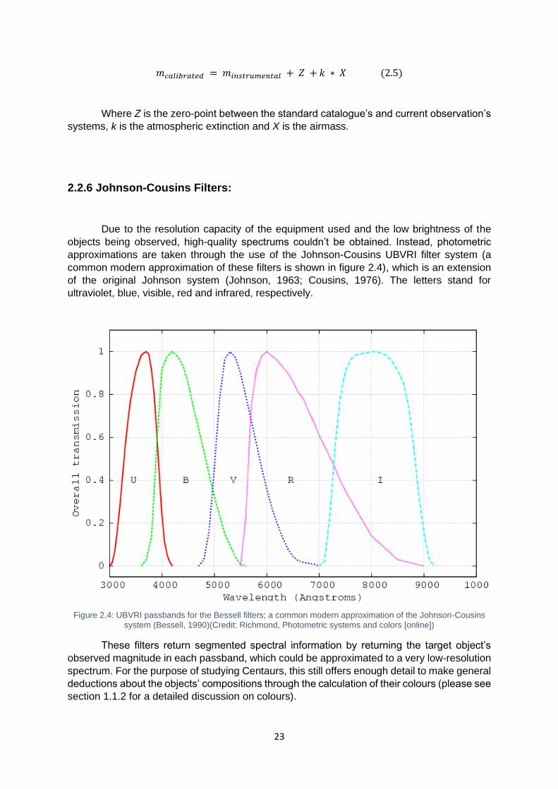
23
𝑚𝑐𝑎𝑙𝑖𝑏𝑟𝑎𝑡𝑒𝑑 = 𝑚𝑖𝑛𝑠𝑡𝑟𝑢𝑚𝑒𝑛𝑡𝑎𝑙 + 𝑍 + 𝑘 ∗ 𝑋 (2.5)
Where Z is the zero-point between the standard catalogue’s and current observation’s
systems, k is the atmospheric extinction and X is the airmass.
2.2.6 Johnson-Cousins Filters:
Due to the resolution capacity of the equipment used and the low brightness of the
objects being observed, high-quality spectrums couldn’t be obtained. Instead, photometric
approximations are taken through the use of the Johnson-Cousins UBVRI filter system (a
common modern approximation of these filters is shown in figure 2.4), which is an extension
of the original Johnson system (Johnson, 1963; Cousins, 1976). The letters stand for
ultraviolet, blue, visible, red and infrared, respectively.
Figure 2.4: UBVRI passbands for the Bessell filters; a common modern approximation of the Johnson-Cousins
system (Bessell, 1990)(Credit: Richmond, Photometric systems and colors [online])
These filters return segmented spectral information by returning the target object’s
observed magnitude in each passband, which could be approximated to a very low-resolution
spectrum. For the purpose of studying Centaurs, this still offers enough detail to make general
deductions about the objects’ compositions through the calculation of their colours (please see
section 1.1.2 for a detailed discussion on colours).
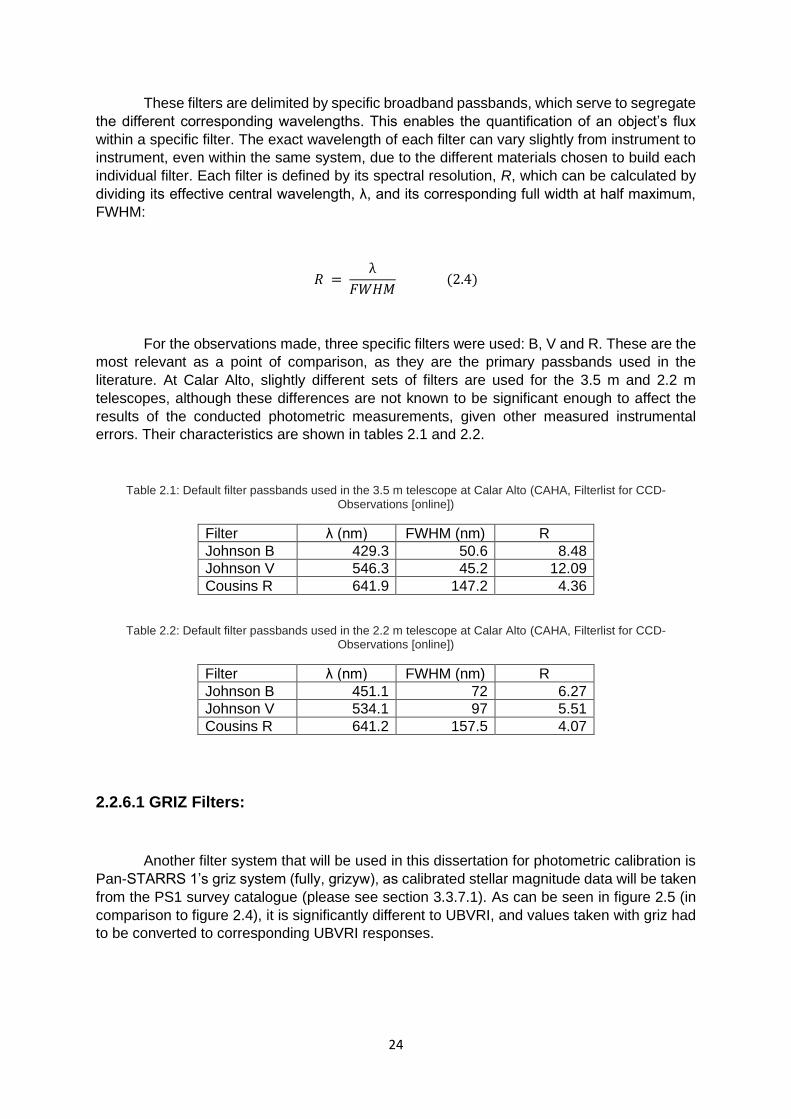
24
These filters are delimited by specific broadband passbands, which serve to segregate
the different corresponding wavelengths. This enables the quantification of an object’s flux
within a specific filter. The exact wavelength of each filter can vary slightly from instrument to
instrument, even within the same system, due to the different materials chosen to build each
individual filter. Each filter is defined by its spectral resolution, R, which can be calculated by
dividing its effective central wavelength, λ, and its corresponding full width at half maximum,
FWHM:
𝑅 = λ
𝐹𝑊𝐻𝑀 (2.4)
For the observations made, three specific filters were used: B, V and R. These are the
most relevant as a point of comparison, as they are the primary passbands used in the
literature. At Calar Alto, slightly different sets of filters are used for the 3.5 m and 2.2 m
telescopes, although these differences are not known to be significant enough to affect the
results of the conducted photometric measurements, given other measured instrumental
errors. Their characteristics are shown in tables 2.1 and 2.2.
Table 2.1: Default filter passbands used in the 3.5 m telescope at Calar Alto (CAHA, Filterlist for CCD-
Observations [online])
Filter λ (nm) FWHM (nm) R
Johnson B 429.3 50.6 8.48
Johnson V 546.3 45.2 12.09
Cousins R 641.9 147.2 4.36
Table 2.2: Default filter passbands used in the 2.2 m telescope at Calar Alto (CAHA, Filterlist for CCD-Observations [online])
Filter λ (nm) FWHM (nm) R
Johnson B 451.1 72 6.27
Johnson V 534.1 97 5.51
Cousins R 641.2 157.5 4.07
2.2.6.1 GRIZ Filters:
Another filter system that will be used in this dissertation for photometric calibration is
Pan-STARRS 1’s griz system (fully, grizyw), as calibrated stellar magnitude data will be taken
from the PS1 survey catalogue (please see section 3.3.7.1). As can be seen in figure 2.5 (in
comparison to figure 2.4), it is significantly different to UBVRI, and values taken with griz had
to be converted to corresponding UBVRI responses.
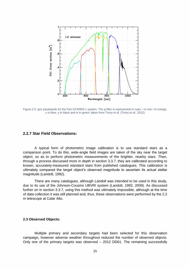
25
Figure 2.5: griz passbands for the Pan-STARRS 1 system. The g filter is represented in cyan, r in red, i in orange, z in blue, y in black and w in green; taken from Tonry et al. (Tonry et al., 2012)
2.2.7 Star Field Observations:
A typical form of photometric image calibration is to use standard stars as a
comparison point. To do this, wide-angle field images are taken of the sky near the target
object, so as to perform photometric measurements of the brighter, nearby stars. Then,
through a process discussed more in depth in section 3.3.7, they are calibrated according to
known, accurately-measured standard stars from published catalogues. This calibration is
ultimately compared the target object’s observed magnitude to ascertain its actual stellar
magnitude (Landolt, 1992).
There are many catalogues, although Landolt was intended to be used in this study,
due to its use of the Johnson-Cousins UBVRI system (Landolt, 1992, 2009). As discussed
further on in section 3.3.7, using this method was ultimately impossible, although at the time
of data collection it was still planned and, thus, these observations were performed by the 2.2
m telescope at Calar Alto.
2.3 Observed Objects:
Multiple primary and secondary targets had been selected for this observation
campaign, however adverse weather throughout reduced the number of observed objects.
Only one of the primary targets was observed – 2012 DD61. The remaining successfully
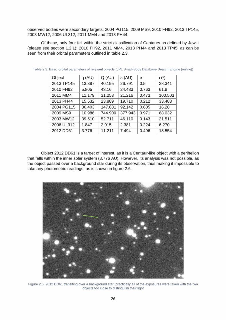
26
observed bodies were secondary targets: 2004 PG115, 2009 MS9, 2010 FH92, 2013 TP145,
2003 MW12, 2006 UL312, 2011 MM4 and 2013 PH44.
Of these, only four fell within the strict classification of Centaurs as defined by Jewitt
(please see section 1.2.1): 2010 FH92, 2011 MM4, 2013 PH44 and 2013 TP45, as can be
seen from their orbital parameters outlined in table 2.3.
Table 2.3: Basic orbital parameters of relevant objects (JPL Small-Body Database Search Engine [online])
Object q (AU) Q (AU) a (AU) e i (º)
2013 TP145 13.387 40.195 26.791 0.5 28.341
2010 FH92 5.805 43.16 24.483 0.763 61.8
2011 MM4 11.179 31.253 21.216 0.473 100.503
2013 PH44 15.532 23.889 19.710 0.212 33.483
2004 PG115 36.403 147.881 92.142 0.605 16.28
2009 MS9 10.986 744.900 377.943 0.971 68.032
2003 MW12 39.510 52.711 46.110 0.143 21.511
2006 UL312 1.847 2.915 2.381 0.224 6.270
2012 DD61 3.776 11.211 7.494 0.496 18.554
Object 2012 DD61 is a target of interest, as it is a Centaur-like object with a perihelion
that falls within the inner solar system (3.776 AU). However, its analysis was not possible, as
the object passed over a background star during its observation, thus making it impossible to
take any photometric readings, as is shown in figure 2.6.
Figure 2.6: 2012 DD61 transiting over a background star; practically all of the exposures were taken with the two
objects too close to distinguish their light
27
Photometric observations of these objects were attempted in the Johnson-B, Johnson-
V and Cousins-R filters. Of the four, only 2010 FH92 had its images taken in the V filter, as
not enough observation time was left to do so in the cases of the other relevant target objects.
Of the three objects, 2013 TP145 was not analysed in any way, as it wasn’t visible in
any of the filters, such as can be seen in the example in figure 2.7. The on-site observer
reported not being able to detect the target visually with their instrumentation, either. A low
apparent magnitude with the bad seeing registered during observations would justify this
discrepancy. It is also possible that this object’s ephemeris was computed incorrectly, since
its orbital parameters have been estimated using few observations (JPL takes all of its orbital
parameter calculations from two separate observations performed with a 21-day interval in
2013). This would result in the object being in an unexpected position in future observation
attempts. As an aside, objects are lost quite frequently due to ephemeris calculated with low
accuracies; it is also not uncommon to subsequently rediscover these same objects.
Figure 2.7: The expected location of 2013 TP145

28
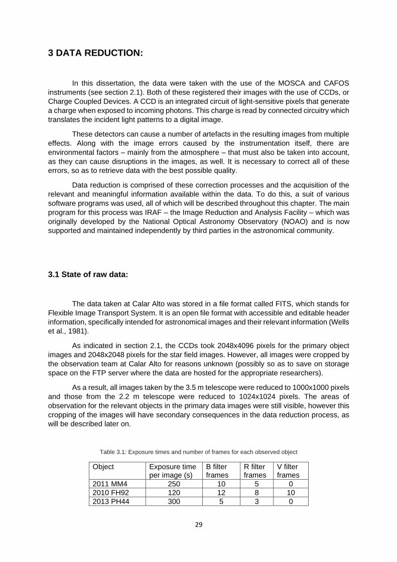
29
3 DATA REDUCTION:
In this dissertation, the data were taken with the use of the MOSCA and CAFOS
instruments (see section 2.1). Both of these registered their images with the use of CCDs, or
Charge Coupled Devices. A CCD is an integrated circuit of light-sensitive pixels that generate
a charge when exposed to incoming photons. This charge is read by connected circuitry which
translates the incident light patterns to a digital image.
These detectors can cause a number of artefacts in the resulting images from multiple
effects. Along with the image errors caused by the instrumentation itself, there are
environmental factors – mainly from the atmosphere – that must also be taken into account,
as they can cause disruptions in the images, as well. It is necessary to correct all of these
errors, so as to retrieve data with the best possible quality.
Data reduction is comprised of these correction processes and the acquisition of the
relevant and meaningful information available within the data. To do this, a suit of various
software programs was used, all of which will be described throughout this chapter. The main
program for this process was IRAF – the Image Reduction and Analysis Facility – which was
originally developed by the National Optical Astronomy Observatory (NOAO) and is now
supported and maintained independently by third parties in the astronomical community.
3.1 State of raw data:
The data taken at Calar Alto was stored in a file format called FITS, which stands for
Flexible Image Transport System. It is an open file format with accessible and editable header
information, specifically intended for astronomical images and their relevant information (Wells
et al., 1981).
As indicated in section 2.1, the CCDs took 2048x4096 pixels for the primary object
images and 2048x2048 pixels for the star field images. However, all images were cropped by
the observation team at Calar Alto for reasons unknown (possibly so as to save on storage
space on the FTP server where the data are hosted for the appropriate researchers).
As a result, all images taken by the 3.5 m telescope were reduced to 1000x1000 pixels
and those from the 2.2 m telescope were reduced to 1024x1024 pixels. The areas of
observation for the relevant objects in the primary data images were still visible, however this
cropping of the images will have secondary consequences in the data reduction process, as
will be described later on.
Table 3.1: Exposure times and number of frames for each observed object
Object Exposure time per image (s)
B filter frames
R filter frames
V filter frames
2011 MM4 250 10 5 0
2010 FH92 120 12 8 10
2013 PH44 300 5 3 0
30
Astronomical imaging requires long exposure times for faint or distant objects, so that
more photons can be gathered to generate as clear a signal as possible Table 3.1 shows the
exposure times for the studied Centaurs, along with the number of frames taken for each of
the related filters. For objects like Centaurs, instruments such as Calar Alto’s 3.5 m telescope
require exposures in the order of minutes. As certain objects are more luminous in certain
filters than others, different amounts of images – or frames – are taken for each, so as to
gather enough cumulative data in each passband; this is clear from the observation data used
in this dissertation, as is shown in table 3.1.
3.2 Image defects:
3.2.1 Noise:
All CCD imaging will have a related amount of degradation, however long exposures
are particularly susceptible to cumulative forms of noise, potentially causing the signal-to-
noise ratio (S/N) to lower significantly. There are three main types of noise prevalent in CCD
imaging:
1. Dark Current Noise (also known as thermal noise) is a result of the statistical
fluctuations of the thermal signal generated by the CCD system itself. This noise is
proportional to the temperature of the system’s semiconductor substrate (typically
made of silicone). This noise is due to electrons generated by thermal effects that
contribute to the measured signal. Cooling systems are used to mitigate this effect.
Dark current frames (“darks”) are usually long-exposure images taken with the
camera’s sensors covered, so as to not receive any external light whatsoever. None
were taken for the observations in this study and, as such, no respective calibration
processes were performed.
The bias is a 0-second integration of the dark current, used to determine a CCD’s
temperature gradient in a given moment and purposefully-induced excess charge
(Howell, 2001). Bias frames can be acquired with a 0-second exposure image.
2. Readout Noise is caused by the amplifier connected to the CCD chip, producing errors
when it converts the detector’s charge into a corresponding variation in voltage for the
analogue signal. Unlike dark current, readout noise doesn’t accumulate over time, as
it is only generated during the read process.
3. Sky Background Noise and other types of shot noise are caused by random variations
in the incidence of photons. Due to this type of noise, multiple images of the same
target will present intensity disparities between each other. Shot noise can be reduced
with longer exposures and image stacking. For photometry, the sky background noise
can be measured and removed statistically from signal measured from an intended
object, as is shown in section 3.3.6, ideally reducing further to negligible levels.

31
3.2.2 Artefacts:
There are a number of factors that can have very noticeable effects on images, which can
interfere with the data; this must be understood and taken into account during the data
reduction process. These can be due to the state of the equipment in use or environmental
effects on that equipment. Typical artefacts can be:
1. Diffraction spikes – these are features usually visible as part of bright sources (such
as stars) which are caused by the wave-like nature of light interacting with the
telescope’s physical structure. The secondary mirror is most reflector telescopes (as
is the case for the ones used for this dissertation) is held in place by a number of struts,
also referred to as spiders.
Light diffracts around these struts before reaching the primary mirror and, thus, is
registered in the detector. This is what causes the classic spike-like structures visible
around bright stars in images.
2. Dust – particles of various natures can contaminate several parts of the apparatus,
such as the mirrors, the CCD’s housing window or the filters. All of these are usually
cleaned on a regularly, however it is always possible for foreign bodies to be found on
these surfaces during observations. They are typically seen as smudges or dark halos
in the resulting images, due to being out of focus.
3. Bad columns and traps – these artefacts are due to malfunctions in the CCD itself.
Columns in CCDs can be operating incorrectly or not at all; this can happen due to
various electronic or mechanical reasons, however they will invariably have one of two
effects – either the pixels are detecting intensities incorrectly (often creating very bright
columns) or they are completely dead (seen as completely dark columns, as if they
didn’t receive any light whatsoever).
Traps have a similar effect as dead columns; however, they are only partial. CCDs
read pixels by having their charges transferred sequentially to a single receptor at the
end of each column. When a pixel is damaged and incapable of transferring or
receiving a charge, any pixels above it will not be able to transfer their own charges
past it and, thus, are never read. This leaves a dark column that begins at the top of
the CCD and ends at the damaged pixel.
4. Pixel saturation – this occurs when a pixel is exposed for so long to a source of light
(generating more of a charge than it is capable of storing reliably – in MOSCA’s case,
60,000 e-) that excess electrons start to bleed over to nearby pixels on the same
column. This typically happens when a bright star is imaged, with the effect worsening
with longer exposures. The visual result is a vertical trail of completely white pixels
emanating from the source star.
5. Cosmic rays – these are artefacts that are completely independent of the type of
apparatus used, its quality or its state of maintenance. They are the results of high
energy particles impacting the CCD during photon acquisition; they deposit energy
directly into the atomic structure of the sensor itself, liberating electrons which are
registered with the intended data. As the name implies, these particles can be due to
high-energy cosmic phenomenon. However, another source can be the decay of
radioactive particles present within the immediate environment of the CCD itself, such
as its housing.
Visually, cosmic rays can be seen as bright pixels not related to any actual star in the
image; often in the form of single pixels, tight groupings of a few pixels or a short trail,
with very little or no diffusion.
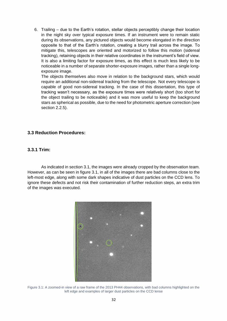
32
6. Trailing – due to the Earth’s rotation, stellar objects perceptibly change their location
in the night sky over typical exposure times. If an instrument were to remain static
during its observations, any pictured objects would become elongated in the direction
opposite to that of the Earth’s rotation, creating a blurry trail across the image. To
mitigate this, telescopes are oriented and motorized to follow this motion (sidereal
tracking), retaining objects in their relative coordinates in the instrument’s field of view.
It is also a limiting factor for exposure times, as this effect is much less likely to be
noticeable in a number of separate shorter-exposure images, rather than a single long-
exposure image.
The objects themselves also move in relation to the background stars, which would
require an additional non-sidereal tracking from the telescope. Not every telescope is
capable of good non-sidereal tracking. In the case of this dissertation, this type of
tracking wasn’t necessary, as the exposure times were relatively short (too short for
the object trailing to be noticeable) and it was more useful to keep the background
stars as spherical as possible, due to the need for photometric aperture correction (see
section 2.2.5).
3.3 Reduction Procedures:
3.3.1 Trim:
As indicated in section 3.1, the images were already cropped by the observation team.
However, as can be seen in figure 3.1, in all of the images there are bad columns close to the
left-most edge, along with some dark shapes indicative of dust particles on the CCD lens. To
ignore these defects and not risk their contamination of further reduction steps, an extra trim
of the images was executed.
Figure 3.1: A zoomed-in view of a raw frame of the 2013 PH44 observations, with bad columns highlighted on the left edge and examples of larger dust particles on the CCD lense
33
This was done with the use of IRAF’s CCDPROC routine, which is a utility designed to
apply all initial calibration processes to the science images. This includes the application of all
bias, dark and flat frames, among other functions, such as illumination or fringe correction,
which were not relevant to this particular study.
In this case, CCDPROC was set to only trim the images down to 860x950 pixels by
defining the region of useful data as “[140:1000,50:1000]”. Note that IRAF’s defines specific
regions of an image with the notation “[X1:X2,Y1:Y2]”, where X defines pixel columns and Y
defines pixel rows. This process was applied to all images taken with the MOSCA instrument,
including calibration images, so as to keep their proportions and coordinate positioning correct
in relation to each other.
IRAF uses some information contained in FITS headers to perform internal
computations and it throws an error if it ever finds conflicting values. So as to avoid these
errors, a number of header properties had to be altered in the images; namely Datasec,
Ccdsec and Biassec. Biassec indicated where the overscan of the image is – a region
reserved for a secondary form of bias correction that wasn’t used in this study, as it was no
longer present in the received images due to the original cropping by the observation team.
As a result, this property was set to [0:0,0:0]. Datasec and Ccdsec were both set to
[1:1,861:951]. Respectively, these properties indicate the science-relevant area of the image
and the total area of the image, which coincide entirely in this case.
The header changes were performed with IRAF’s HEDIT utility, which serves
exclusively to view and modify header information in FITS images. Images from the 2.2 m
telescope were treated to similar minor trimming procedures.
3.3.2 Bias Correction:
The first of the calibration processes is treatment of the image bias. For each
observation night, a number of bias frames were taken and it is first necessary to determine
which of these images are suitable for use. This is done with the use of the IMSTAT routine,
which performs a statistical analysis of each image. The returned values indicate the mean,
median and mode of the pixel distribution, along with their standard deviation, skew and the
minimum and maximum detected pixel values.
With this information, it was possible to detect and remove anomalous bias images,
due to having extremely high or low deviations from the norm, which could have been caused
by any number of factors during the bias frame capture, such as electronic interference during
the readout process (Howell, 2001). For instance, a result with a very high standard deviation
is indicative of an anomalous bias frame.
Once these outlying images were removed from the bias list, a routine called
ZEROCOMBINE was executed on the final selection of bias frames to produce an average
frame for calibration. ZEROCOMBINE serves to average a group of bias frames into a single
final bias image. During this process, each pixel will have a list of available values,
corresponding to the number of bias frames being used. The highest of these values will
always be ignored, so as to exclude energy deposited by coincidental cosmic rays or
radioactive particle decay within the instrument (please see section 3.2.1).
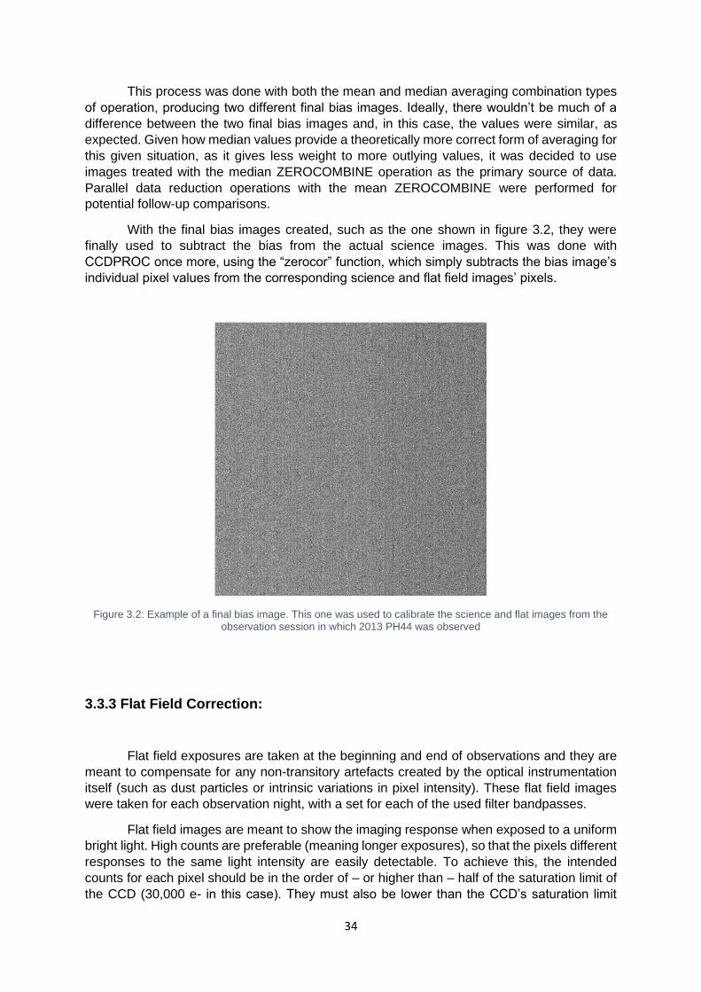
34
This process was done with both the mean and median averaging combination types
of operation, producing two different final bias images. Ideally, there wouldn’t be much of a
difference between the two final bias images and, in this case, the values were similar, as
expected. Given how median values provide a theoretically more correct form of averaging for
this given situation, as it gives less weight to more outlying values, it was decided to use
images treated with the median ZEROCOMBINE operation as the primary source of data.
Parallel data reduction operations with the mean ZEROCOMBINE were performed for
potential follow-up comparisons.
With the final bias images created, such as the one shown in figure 3.2, they were
finally used to subtract the bias from the actual science images. This was done with
CCDPROC once more, using the “zerocor” function, which simply subtracts the bias image’s
individual pixel values from the corresponding science and flat field images’ pixels.
Figure 3.2: Example of a final bias image. This one was used to calibrate the science and flat images from the observation session in which 2013 PH44 was observed
3.3.3 Flat Field Correction:
Flat field exposures are taken at the beginning and end of observations and they are
meant to compensate for any non-transitory artefacts created by the optical instrumentation
itself (such as dust particles or intrinsic variations in pixel intensity). These flat field images
were taken for each observation night, with a set for each of the used filter bandpasses.
Flat field images are meant to show the imaging response when exposed to a uniform
bright light. High counts are preferable (meaning longer exposures), so that the pixels different
responses to the same light intensity are easily detectable. To achieve this, the intended
counts for each pixel should be in the order of – or higher than – half of the saturation limit of
the CCD (30,000 e- in this case). They must also be lower than the CCD’s saturation limit
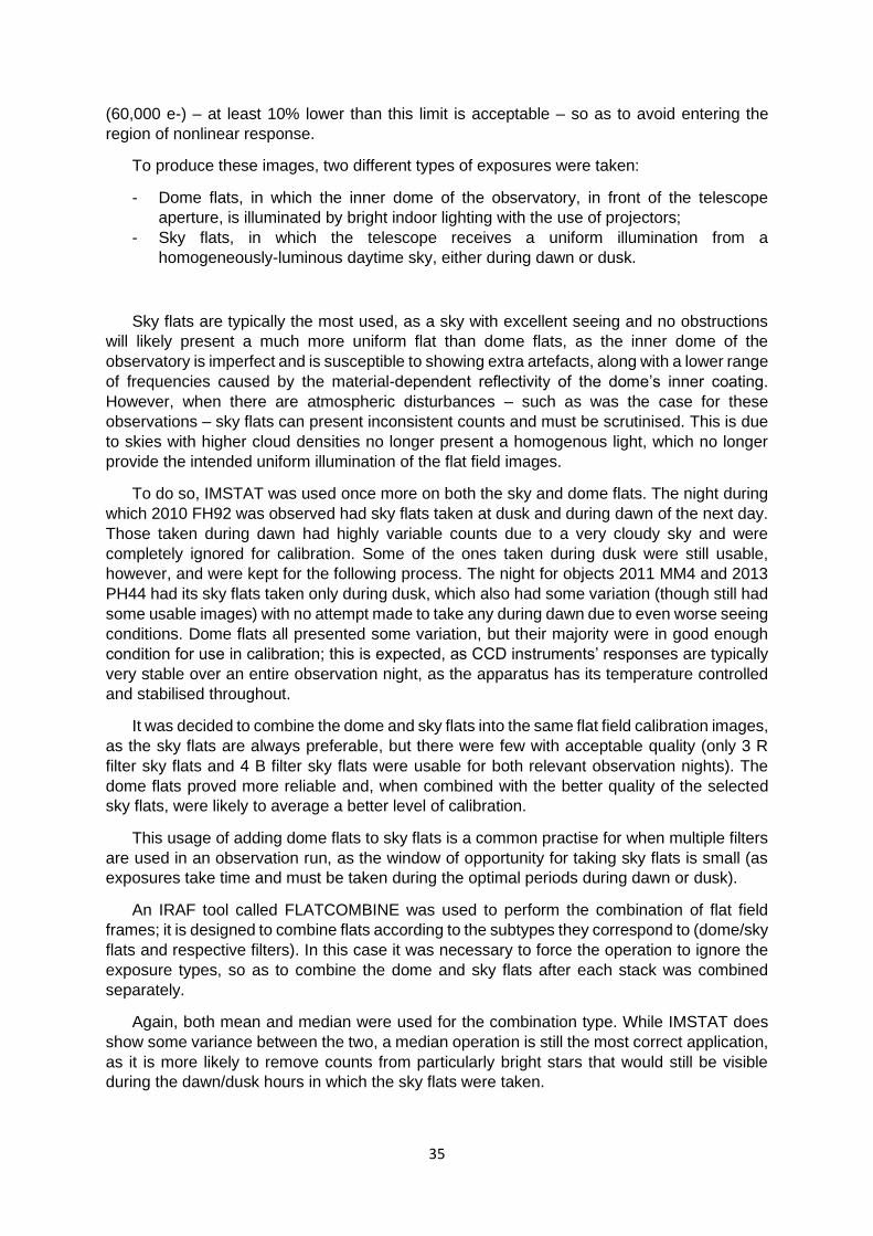
35
(60,000 e-) – at least 10% lower than this limit is acceptable – so as to avoid entering the
region of nonlinear response.
To produce these images, two different types of exposures were taken:
- Dome flats, in which the inner dome of the observatory, in front of the telescope
aperture, is illuminated by bright indoor lighting with the use of projectors;
- Sky flats, in which the telescope receives a uniform illumination from a
homogeneously-luminous daytime sky, either during dawn or dusk.
Sky flats are typically the most used, as a sky with excellent seeing and no obstructions
will likely present a much more uniform flat than dome flats, as the inner dome of the
observatory is imperfect and is susceptible to showing extra artefacts, along with a lower range
of frequencies caused by the material-dependent reflectivity of the dome’s inner coating.
However, when there are atmospheric disturbances – such as was the case for these
observations – sky flats can present inconsistent counts and must be scrutinised. This is due
to skies with higher cloud densities no longer present a homogenous light, which no longer
provide the intended uniform illumination of the flat field images.
To do so, IMSTAT was used once more on both the sky and dome flats. The night during
which 2010 FH92 was observed had sky flats taken at dusk and during dawn of the next day.
Those taken during dawn had highly variable counts due to a very cloudy sky and were
completely ignored for calibration. Some of the ones taken during dusk were still usable,
however, and were kept for the following process. The night for objects 2011 MM4 and 2013
PH44 had its sky flats taken only during dusk, which also had some variation (though still had
some usable images) with no attempt made to take any during dawn due to even worse seeing
conditions. Dome flats all presented some variation, but their majority were in good enough
condition for use in calibration; this is expected, as CCD instruments’ responses are typically
very stable over an entire observation night, as the apparatus has its temperature controlled
and stabilised throughout.
It was decided to combine the dome and sky flats into the same flat field calibration images,
as the sky flats are always preferable, but there were few with acceptable quality (only 3 R
filter sky flats and 4 B filter sky flats were usable for both relevant observation nights). The
dome flats proved more reliable and, when combined with the better quality of the selected
sky flats, were likely to average a better level of calibration.
This usage of adding dome flats to sky flats is a common practise for when multiple filters
are used in an observation run, as the window of opportunity for taking sky flats is small (as
exposures take time and must be taken during the optimal periods during dawn or dusk).
An IRAF tool called FLATCOMBINE was used to perform the combination of flat field
frames; it is designed to combine flats according to the subtypes they correspond to (dome/sky
flats and respective filters). In this case it was necessary to force the operation to ignore the
exposure types, so as to combine the dome and sky flats after each stack was combined
separately.
Again, both mean and median were used for the combination type. While IMSTAT does
show some variance between the two, a median operation is still the most correct application,
as it is more likely to remove counts from particularly bright stars that would still be visible
during the dawn/dusk hours in which the sky flats were taken.
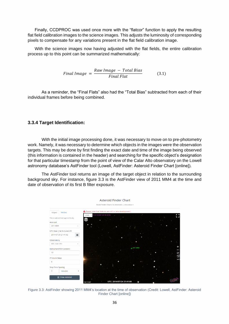
36
Finally, CCDPROC was used once more with the “flatcor” function to apply the resulting
flat field calibration images to the science images. This adjusts the luminosity of corresponding
pixels to compensate for any variations present in the flat field calibration image.
With the science images now having adjusted with the flat fields, the entire calibration
process up to this point can be summarized mathematically:
𝐹𝑖𝑛𝑎𝑙 𝐼𝑚𝑎𝑔𝑒 = 𝑅𝑎𝑤 𝐼𝑚𝑎𝑔𝑒 − 𝑇𝑜𝑡𝑎𝑙 𝐵𝑖𝑎𝑠
𝐹𝑖𝑛𝑎𝑙 𝐹𝑙𝑎𝑡 (3.1)
As a reminder, the “Final Flats” also had the “Total Bias” subtracted from each of their
individual frames before being combined.
3.3.4 Target Identification:
With the initial image processing done, it was necessary to move on to pre-photometry
work. Namely, it was necessary to determine which objects in the images were the observation
targets. This may be done by first finding the exact date and time of the image being observed
(this information is contained in the header) and searching for the specific object’s designation
for that particular timestamp from the point of view of the Calar Alto observatory on the Lowell
astronomy database’s AstFinder tool (Lowell, AstFinder: Asteroid Finder Chart [online]).
The AstFinder tool returns an image of the target object in relation to the surrounding
background sky. For instance, figure 3.3 is the AstFinder view of 2011 MM4 at the time and
date of observation of its first B filter exposure.
Figure 3.3: AstFinder showing 2011 MM4’s location at the time of observation (Credit: Lowell, AstFinder: Asteroid Finder Chart [online])
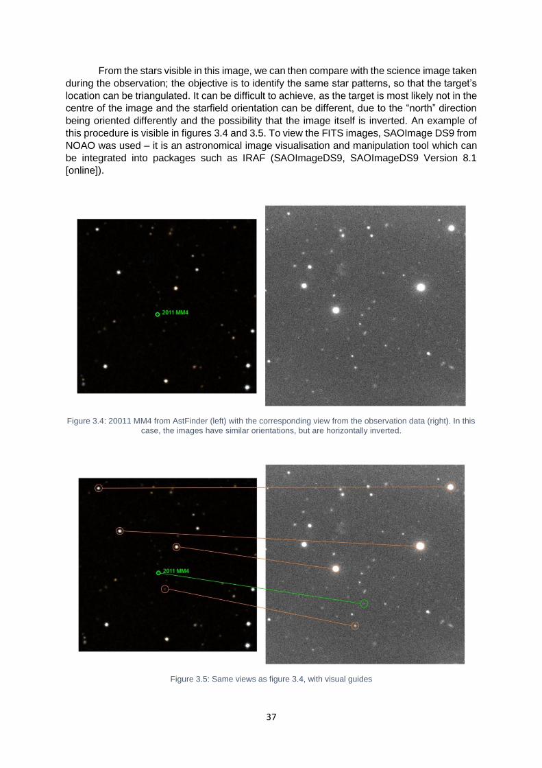
37
From the stars visible in this image, we can then compare with the science image taken
during the observation; the objective is to identify the same star patterns, so that the target’s
location can be triangulated. It can be difficult to achieve, as the target is most likely not in the
centre of the image and the starfield orientation can be different, due to the “north” direction
being oriented differently and the possibility that the image itself is inverted. An example of
this procedure is visible in figures 3.4 and 3.5. To view the FITS images, SAOImage DS9 from
NOAO was used – it is an astronomical image visualisation and manipulation tool which can
be integrated into packages such as IRAF (SAOImageDS9, SAOImageDS9 Version 8.1
[online]).
Figure 3.4: 20011 MM4 from AstFinder (left) with the corresponding view from the observation data (right). In this
case, the images have similar orientations, but are horizontally inverted.
Figure 3.5: Same views as figure 3.4, with visual guides
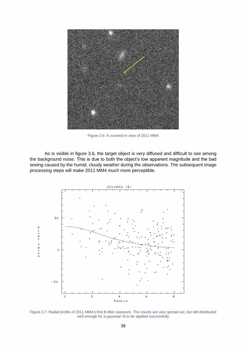
38
Figure 3.6: A zoomed-in view of 2011 MM4
As is visible in figure 3.6, the target object is very diffused and difficult to see among
the background noise. This is due to both the object’s low apparent magnitude and the bad
seeing caused by the humid, cloudy weather during the observations. The subsequent image
processing steps will make 2011 MM4 much more perceptible.
Figure 3.7: Radial profile of 2011 MM4's first B-filter exposure. The counts are very spread out, but still distributed well enough for a gaussian fit to be applied successfully
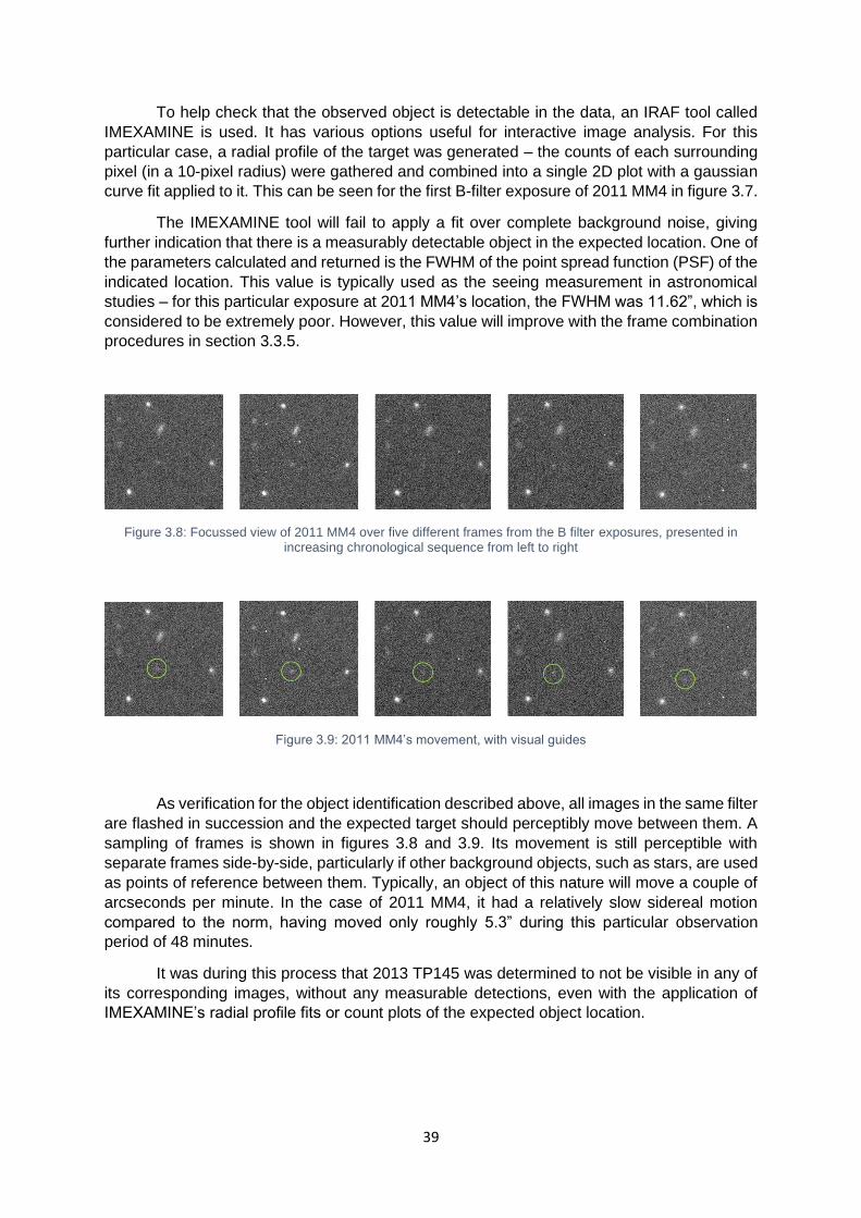
39
To help check that the observed object is detectable in the data, an IRAF tool called
IMEXAMINE is used. It has various options useful for interactive image analysis. For this
particular case, a radial profile of the target was generated – the counts of each surrounding
pixel (in a 10-pixel radius) were gathered and combined into a single 2D plot with a gaussian
curve fit applied to it. This can be seen for the first B-filter exposure of 2011 MM4 in figure 3.7.
The IMEXAMINE tool will fail to apply a fit over complete background noise, giving
further indication that there is a measurably detectable object in the expected location. One of
the parameters calculated and returned is the FWHM of the point spread function (PSF) of the
indicated location. This value is typically used as the seeing measurement in astronomical
studies – for this particular exposure at 2011 MM4’s location, the FWHM was 11.62”, which is
considered to be extremely poor. However, this value will improve with the frame combination
procedures in section 3.3.5.
Figure 3.8: Focussed view of 2011 MM4 over five different frames from the B filter exposures, presented in increasing chronological sequence from left to right
Figure 3.9: 2011 MM4’s movement, with visual guides
As verification for the object identification described above, all images in the same filter
are flashed in succession and the expected target should perceptibly move between them. A
sampling of frames is shown in figures 3.8 and 3.9. Its movement is still perceptible with
separate frames side-by-side, particularly if other background objects, such as stars, are used
as points of reference between them. Typically, an object of this nature will move a couple of
arcseconds per minute. In the case of 2011 MM4, it had a relatively slow sidereal motion
compared to the norm, having moved only roughly 5.3” during this particular observation
period of 48 minutes.
It was during this process that 2013 TP145 was determined to not be visible in any of
its corresponding images, without any measurable detections, even with the application of
IMEXAMINE’s radial profile fits or count plots of the expected object location.

40
3.3.5 Science Image Combination:
Once the targets in the images were identified, it was necessary to combine each stack
of images with the same filter into corresponding single image with the target object
overlapping among them. To achieve this overlapping, each image will have to be shifted, as
the object moves relatively to the background sky between exposures. This is so that the
object’s intensity is summed over the various frames to make it as visibly sharp as possible
for the photometric measurements.
Firstly, the target objects in each frame are measured with IRAF’s IMEXAMINE tool.
The same command that performs the radial plot (as described in section 3.3.4) also indicates
the measured central point of maximum flux of the detected object (in pixel coordinates). Given
that these objects are point sources of light, this method is the best available to most
accurately approximate their centroids in these exposures.
The retrieved coordinates are then used to shift the positions of the images in x and y
coordinates in relation to each other, so that the centre of the target object overlaps between
each. This is performed with IRAF’s IMSHIFT tool.
Note that the calculated coordinates are not integers – they can include fractions of
pixels and, thus, pixels will not overlap perfectly between frames. Due to this, a bilinear
interpolation type was selected to perform this operation. The first image in the stack is not
shifted and is used as the base coordinate reference for the other images. Their respective x
and y coordinates are subtracted and the results are used as the input values for the IMSHIFT
operation.
Figure 3.10: 2011 MM4 in B filter (left) and 2010 FH92 in R filter (right). The target objects are highlighted.
Background star trailing is clearly visible in both images
Once the shifts were performed, the IMCOMBINE routine was called to sum each stack
of images according to their filter type for each object. As can be seen in figure 3.10, the result
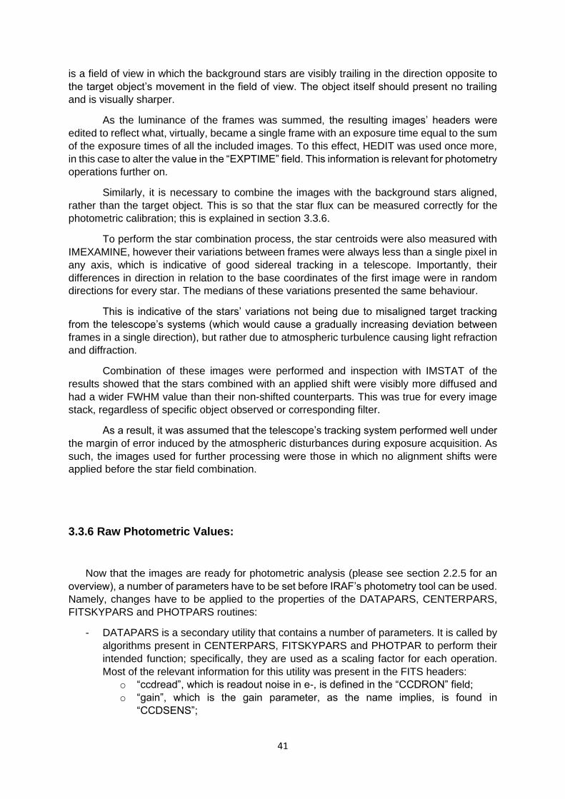
41
is a field of view in which the background stars are visibly trailing in the direction opposite to
the target object’s movement in the field of view. The object itself should present no trailing
and is visually sharper.
As the luminance of the frames was summed, the resulting images’ headers were
edited to reflect what, virtually, became a single frame with an exposure time equal to the sum
of the exposure times of all the included images. To this effect, HEDIT was used once more,
in this case to alter the value in the “EXPTIME” field. This information is relevant for photometry
operations further on.
Similarly, it is necessary to combine the images with the background stars aligned,
rather than the target object. This is so that the star flux can be measured correctly for the
photometric calibration; this is explained in section 3.3.6.
To perform the star combination process, the star centroids were also measured with
IMEXAMINE, however their variations between frames were always less than a single pixel in
any axis, which is indicative of good sidereal tracking in a telescope. Importantly, their
differences in direction in relation to the base coordinates of the first image were in random
directions for every star. The medians of these variations presented the same behaviour.
This is indicative of the stars’ variations not being due to misaligned target tracking
from the telescope’s systems (which would cause a gradually increasing deviation between
frames in a single direction), but rather due to atmospheric turbulence causing light refraction
and diffraction.
Combination of these images were performed and inspection with IMSTAT of the
results showed that the stars combined with an applied shift were visibly more diffused and
had a wider FWHM value than their non-shifted counterparts. This was true for every image
stack, regardless of specific object observed or corresponding filter.
As a result, it was assumed that the telescope’s tracking system performed well under
the margin of error induced by the atmospheric disturbances during exposure acquisition. As
such, the images used for further processing were those in which no alignment shifts were
applied before the star field combination.
3.3.6 Raw Photometric Values:
Now that the images are ready for photometric analysis (please see section 2.2.5 for an
overview), a number of parameters have to be set before IRAF’s photometry tool can be used.
Namely, changes have to be applied to the properties of the DATAPARS, CENTERPARS,
FITSKYPARS and PHOTPARS routines:
- DATAPARS is a secondary utility that contains a number of parameters. It is called by
algorithms present in CENTERPARS, FITSKYPARS and PHOTPAR to perform their
intended function; specifically, they are used as a scaling factor for each operation.
Most of the relevant information for this utility was present in the FITS headers:
o “ccdread”, which is readout noise in e-, is defined in the “CCDRON” field;
o “gain”, which is the gain parameter, as the name implies, is found in
“CCDSENS”;
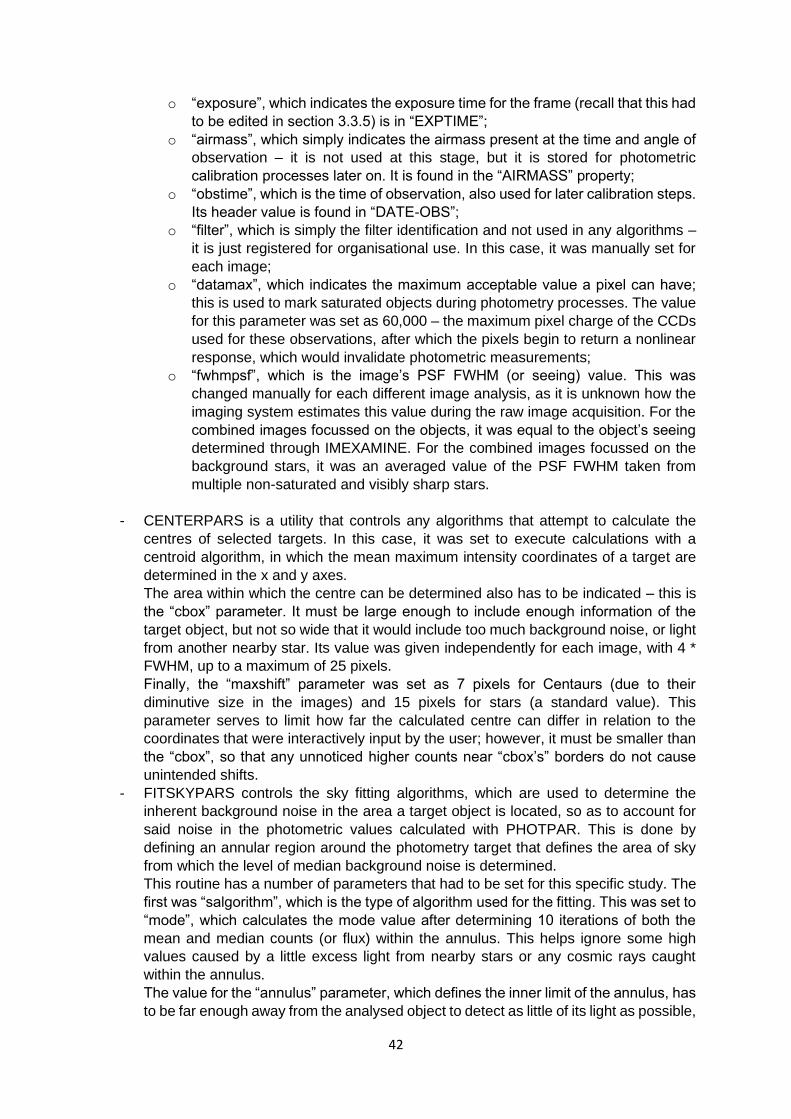
42
o “exposure”, which indicates the exposure time for the frame (recall that this had
to be edited in section 3.3.5) is in “EXPTIME”;
o “airmass”, which simply indicates the airmass present at the time and angle of
observation – it is not used at this stage, but it is stored for photometric
calibration processes later on. It is found in the “AIRMASS” property;
o “obstime”, which is the time of observation, also used for later calibration steps.
Its header value is found in “DATE-OBS”;
o “filter”, which is simply the filter identification and not used in any algorithms –
it is just registered for organisational use. In this case, it was manually set for
each image;
o “datamax”, which indicates the maximum acceptable value a pixel can have;
this is used to mark saturated objects during photometry processes. The value
for this parameter was set as 60,000 – the maximum pixel charge of the CCDs
used for these observations, after which the pixels begin to return a nonlinear
response, which would invalidate photometric measurements;
o “fwhmpsf”, which is the image’s PSF FWHM (or seeing) value. This was
changed manually for each different image analysis, as it is unknown how the
imaging system estimates this value during the raw image acquisition. For the
combined images focussed on the objects, it was equal to the object’s seeing
determined through IMEXAMINE. For the combined images focussed on the
background stars, it was an averaged value of the PSF FWHM taken from
multiple non-saturated and visibly sharp stars.
- CENTERPARS is a utility that controls any algorithms that attempt to calculate the
centres of selected targets. In this case, it was set to execute calculations with a
centroid algorithm, in which the mean maximum intensity coordinates of a target are
determined in the x and y axes.
The area within which the centre can be determined also has to be indicated – this is
the “cbox” parameter. It must be large enough to include enough information of the
target object, but not so wide that it would include too much background noise, or light
from another nearby star. Its value was given independently for each image, with 4 *
FWHM, up to a maximum of 25 pixels.
Finally, the “maxshift” parameter was set as 7 pixels for Centaurs (due to their
diminutive size in the images) and 15 pixels for stars (a standard value). This
parameter serves to limit how far the calculated centre can differ in relation to the
coordinates that were interactively input by the user; however, it must be smaller than
the “cbox”, so that any unnoticed higher counts near “cbox’s” borders do not cause
unintended shifts.
- FITSKYPARS controls the sky fitting algorithms, which are used to determine the
inherent background noise in the area a target object is located, so as to account for
said noise in the photometric values calculated with PHOTPAR. This is done by
defining an annular region around the photometry target that defines the area of sky
from which the level of median background noise is determined.
This routine has a number of parameters that had to be set for this specific study. The
first was “salgorithm”, which is the type of algorithm used for the fitting. This was set to
“mode”, which calculates the mode value after determining 10 iterations of both the
mean and median counts (or flux) within the annulus. This helps ignore some high
values caused by a little excess light from nearby stars or any cosmic rays caught
within the annulus.
The value for the “annulus” parameter, which defines the inner limit of the annulus, has
to be far enough away from the analysed object to detect as little of its light as possible,
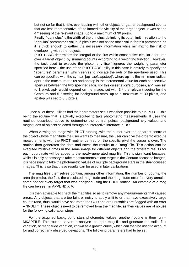
43
but not so far that it risks overlapping with other objects or gather background counts
that are less representative of the immediate vicinity of the target object. It was set as
4 * seeing of the relevant image, up to a maximum of 30 pixels.
Finally, “dannulus” is the width of the annulus, delimiting its outer limit in relation to the
“annulus” parameter’s value. 5 pixels was set as the static value for this parameter, as
it is thick enough to gather the necessary information while minimizing the risk of
overlapping with other objects.
- PHOTPARS determines the integral of the flux within consecutive circular apertures
over a target object, by summing counts according to a weighting function. However,
the task used to execute the photometry itself ignores the weighting parameter
specified here – the use of the PHOTPARS utility in this case is entirely to specify the
“apertures” parameter, which serves to indicate the radii of the apertures used. This
can be specified with the syntax “[ap1:apN:apstep]”, where ap1 is the minimum radius,
apN is the maximum radius and apstep is the incremental value for each consecutive
aperture between the two specified radii. For this dissertation’s purposes, ap1 was set
to 1 pixel, apN would depend on the image, set with 3 * the relevant seeing for the
Centaurs and 5 * seeing for background stars, up to a maximum of 30 pixels, and
apstep was set to 0.5 pixels.
Once all of these utilities had their parameters set, it was then possible to run PHOT – this
being the routine that is actually executed to take photometric measurements. It uses the
routines described above to determine the central points, background sky values and
magnitudes of objects selected through an interactive interface in DS9.
When viewing an image with PHOT running, with the cursor over the apparent centre of
the object whose magnitude the user wants to measure, the user can give the order to execute
measurements with the PHOT routine, centred on the specific pixel the cursor is over. The
routine then generates the data and saves the results to a “mag” file. This action can be
executed multiple times in the same image for different objects and the different results for
each coordinate will be added to the newly-generated mag file. This is significant because,
while it is only necessary to take measurements of one target in the Centaur-focussed images,
it is necessary to take the photometric values of multiple background stars in the star-focussed
images. This is so that these results can be used in later calibrations.
The mag files themselves contain, among other information, the number of counts, the
area (in pixels), the flux, the calculated magnitude and the magnitude error for every annulus
computed for every target that was analysed using the PHOT routine. An example of a mag
file can be seen in APPENDIX A.
It is then advisable to check the mag files so as to remove any measurements that caused
errors. Any objects that are too faint or noisy to apply a fit to or that have excessively large
counts (and, thus, would have saturated the CCD and are unusable) are flagged with an error
– “INDEF”. These objects need to be removed from the mag file, as their values are of no use
for the following calibration steps.
For the acquired background stars photometric values, another routine is then run –
MKAPFILE. This routine serves to analyse the input mag file and generate the radial flux
variation, or magnitude variation, known as a growth curve, which can then be used to account
for and correct any observed deviations. The following parameters had to be set:
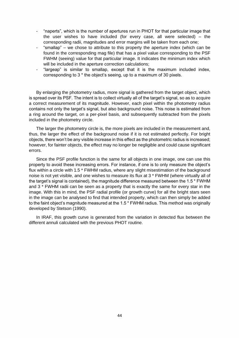
44
- “naperts”, which is the number of apertures run in PHOT for that particular image that
the user wishes to have included (for every case, all were selected) – the
corresponding radii, magnitudes and error margins will be taken from each one;
- “smallap” – we chose to attribute to this property the aperture index (which can be
found in the corresponding mag file) that has a pixel value corresponding to the PSF
FWHM (seeing) value for that particular image. It indicates the minimum index which
will be included in the aperture correction calculations;
- “largeap” is similar to smallap, except that it is the maximum included index,
corresponding to 3 * the object’s seeing, up to a maximum of 30 pixels.
By enlarging the photometry radius, more signal is gathered from the target object, which
is spread over its PSF. The intent is to collect virtually all of the target’s signal, so as to acquire
a correct measurement of its magnitude. However, each pixel within the photometry radius
contains not only the target’s signal, but also background noise. This noise is estimated from
a ring around the target, on a per-pixel basis, and subsequently subtracted from the pixels
included in the photometry circle.
The larger the photometry circle is, the more pixels are included in the measurement and,
thus, the larger the effect of the background noise if it is not estimated perfectly. For bright
objects, there won’t be any visible increase in this effect as the photometric radius is increased;
however, for fainter objects, the effect may no longer be negligible and could cause significant
errors.
Since the PSF profile function is the same for all objects in one image, one can use this
property to avoid these increasing errors. For instance, if one is to only measure the object’s
flux within a circle with 1.5 * FWHM radius, where any slight misestimation of the background
noise is not yet visible, and one wishes to measure its flux at 3 * FWHM (where virtually all of
the target’s signal is contained), the magnitude difference measured between the 1.5 * FWHM
and 3 * FWHM radii can be seen as a property that is exactly the same for every star in the
image. With this in mind, the PSF radial profile (or growth curve) for all the bright stars seen
in the image can be analysed to find that intended property, which can then simply be added
to the faint object’s magnitude measured at the 1.5 * FWHM radius. This method was originally
developed by Stetson (1990).
In IRAF, this growth curve is generated from the variation in detected flux between the
different annuli calculated with the previous PHOT routine.
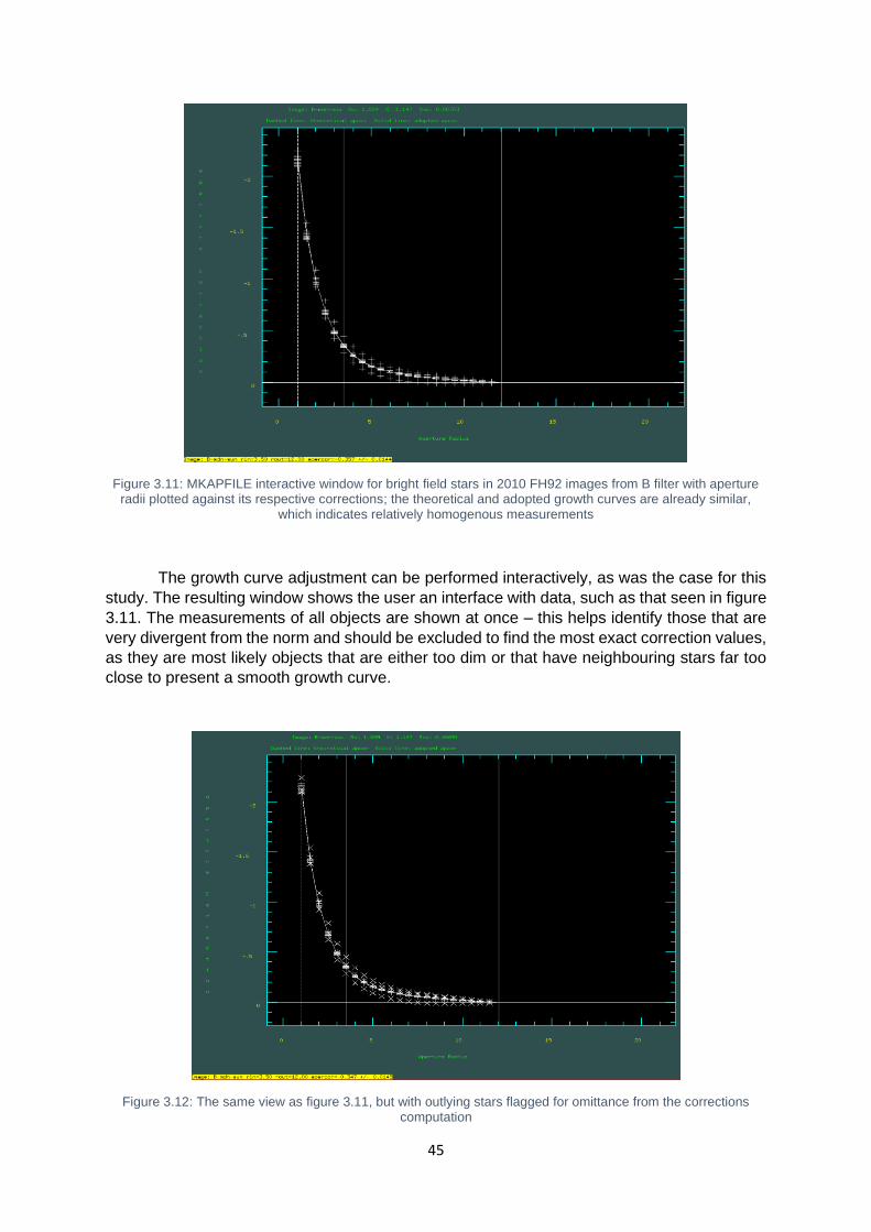
45
Figure 3.11: MKAPFILE interactive window for bright field stars in 2010 FH92 images from B filter with aperture radii plotted against its respective corrections; the theoretical and adopted growth curves are already similar,
which indicates relatively homogenous measurements
The growth curve adjustment can be performed interactively, as was the case for this
study. The resulting window shows the user an interface with data, such as that seen in figure
3.11. The measurements of all objects are shown at once – this helps identify those that are
very divergent from the norm and should be excluded to find the most exact correction values,
as they are most likely objects that are either too dim or that have neighbouring stars far too
close to present a smooth growth curve.
Figure 3.12: The same view as figure 3.11, but with outlying stars flagged for omittance from the corrections computation
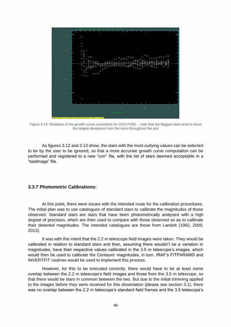
46
Figure 3.13: Residues of the growth curve corrections for 2010 FH92 -- note that the flagged stars tend to show
the largest deviations from the norm throughout the plot
As figures 3.12 and 3.13 show, the stars with the most outlying values can be selected
to be by the user to be ignored, so that a more accurate growth curve computation can be
performed and registered to a new “corr” file, with the list of stars deemed acceptable in a
“bestmags” file.
3.3.7 Photometric Calibrations:
At this point, there were issues with the intended route for the calibration procedures.
The initial plan was to use catalogues of standard stars to calibrate the magnitudes of those
observed. Standard stars are stars that have been photometrically analysed with a high
degree of precision, which are then used to compare with those observed so as to calibrate
their detected magnitudes. The intended catalogues are those from Landolt (1992, 2009,
2013).
It was with this intent that the 2.2 m telescope field images were taken. They would be
calibrated in relation to standard stars and then, assuming there wouldn’t be a variation in
magnitudes, have their respective values calibrated in the 3.5 m telescope’s images, which
would then be used to calibrate the Centaurs’ magnitudes, in turn. IRAF’s FITPARAMS and
INVERTFIT routines would be used to implement this process.
However, for this to be executed correctly, there would have to be at least some
overlap between the 2.2 m telescope’s field images and those from the 3.5 m telescope, so
that there would be stars in common between the two. But due to the initial trimming applied
to the images before they were received for this dissertation (please see section 3.1), there
was no overlap between the 2.2 m telescope’s standard field frames and the 3.5 telescope’s
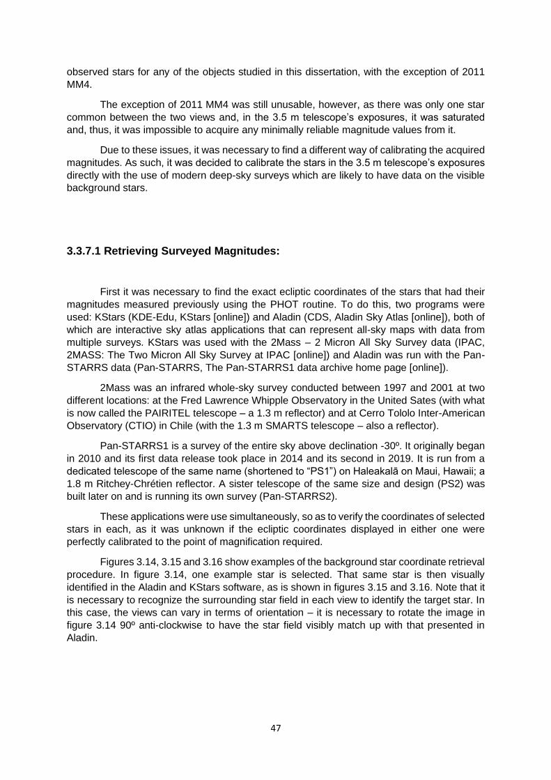
47
observed stars for any of the objects studied in this dissertation, with the exception of 2011
MM4.
The exception of 2011 MM4 was still unusable, however, as there was only one star
common between the two views and, in the 3.5 m telescope’s exposures, it was saturated
and, thus, it was impossible to acquire any minimally reliable magnitude values from it.
Due to these issues, it was necessary to find a different way of calibrating the acquired
magnitudes. As such, it was decided to calibrate the stars in the 3.5 m telescope’s exposures
directly with the use of modern deep-sky surveys which are likely to have data on the visible
background stars.
3.3.7.1 Retrieving Surveyed Magnitudes:
First it was necessary to find the exact ecliptic coordinates of the stars that had their
magnitudes measured previously using the PHOT routine. To do this, two programs were
used: KStars (KDE-Edu, KStars [online]) and Aladin (CDS, Aladin Sky Atlas [online]), both of
which are interactive sky atlas applications that can represent all-sky maps with data from
multiple surveys. KStars was used with the 2Mass – 2 Micron All Sky Survey data (IPAC,
2MASS: The Two Micron All Sky Survey at IPAC [online]) and Aladin was run with the Pan-
STARRS data (Pan-STARRS, The Pan-STARRS1 data archive home page [online]).
2Mass was an infrared whole-sky survey conducted between 1997 and 2001 at two
different locations: at the Fred Lawrence Whipple Observatory in the United Sates (with what
is now called the PAIRITEL telescope – a 1.3 m reflector) and at Cerro Tololo Inter-American
Observatory (CTIO) in Chile (with the 1.3 m SMARTS telescope – also a reflector).
Pan-STARRS1 is a survey of the entire sky above declination -30º. It originally began
in 2010 and its first data release took place in 2014 and its second in 2019. It is run from a
dedicated telescope of the same name (shortened to “PS1”) on Haleakalā on Maui, Hawaii; a
1.8 m Ritchey-Chrétien reflector. A sister telescope of the same size and design (PS2) was
built later on and is running its own survey (Pan-STARRS2).
These applications were use simultaneously, so as to verify the coordinates of selected
stars in each, as it was unknown if the ecliptic coordinates displayed in either one were
perfectly calibrated to the point of magnification required.
Figures 3.14, 3.15 and 3.16 show examples of the background star coordinate retrieval
procedure. In figure 3.14, one example star is selected. That same star is then visually
identified in the Aladin and KStars software, as is shown in figures 3.15 and 3.16. Note that it
is necessary to recognize the surrounding star field in each view to identify the target star. In
this case, the views can vary in terms of orientation – it is necessary to rotate the image in
figure 3.14 90º anti-clockwise to have the star field visibly match up with that presented in
Aladin.
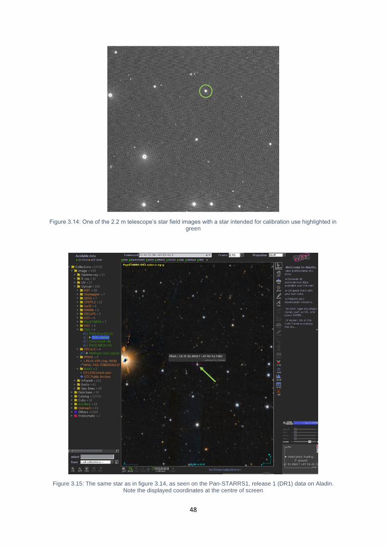
48
Figure 3.14: One of the 2.2 m telescope’s star field images with a star intended for calibration use highlighted in green
Figure 3.15: The same star as in figure 3.14, as seen on the Pan-STARRS1, release 1 (DR1) data on Aladin. Note the displayed coordinates at the centre of screen
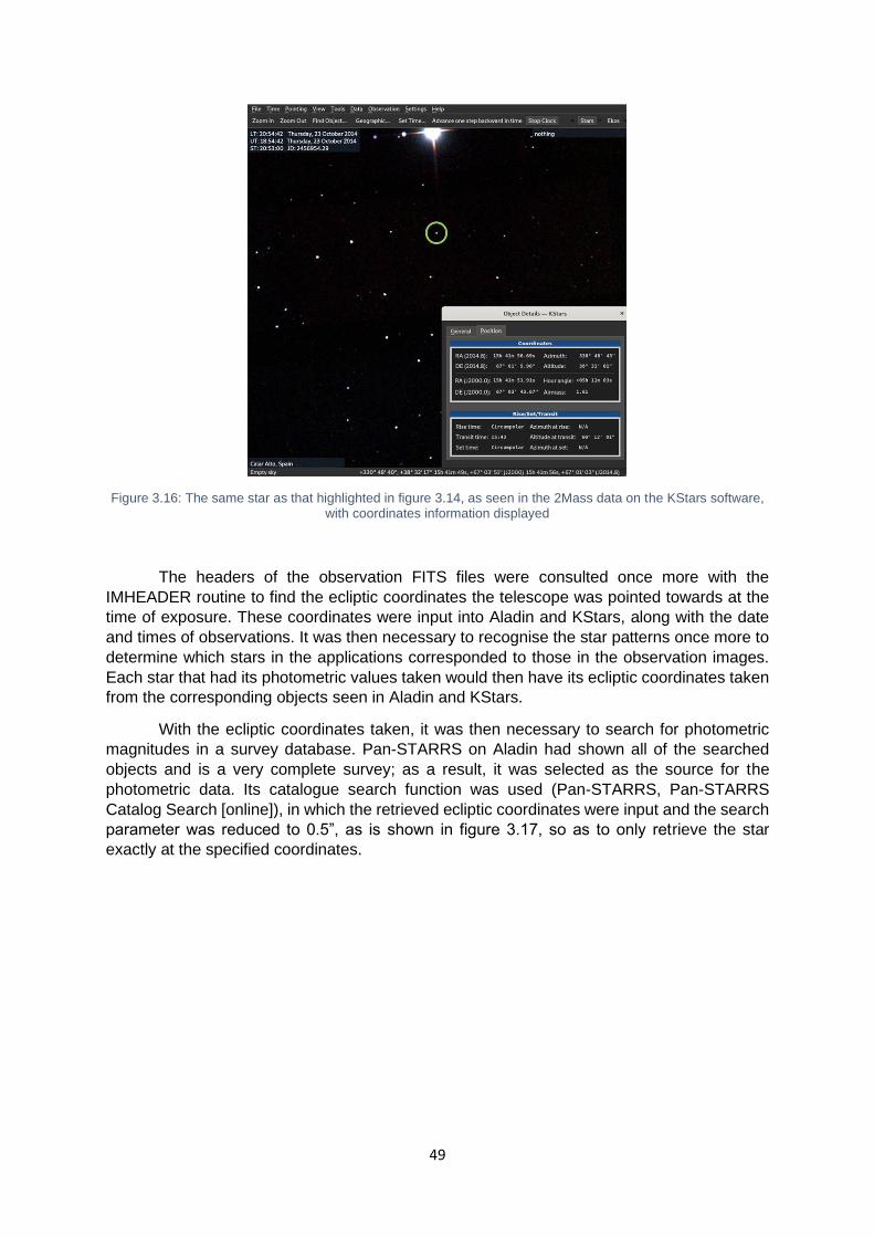
49
Figure 3.16: The same star as that highlighted in figure 3.14, as seen in the 2Mass data on the KStars software, with coordinates information displayed
The headers of the observation FITS files were consulted once more with the
IMHEADER routine to find the ecliptic coordinates the telescope was pointed towards at the
time of exposure. These coordinates were input into Aladin and KStars, along with the date
and times of observations. It was then necessary to recognise the star patterns once more to
determine which stars in the applications corresponded to those in the observation images.
Each star that had its photometric values taken would then have its ecliptic coordinates taken
from the corresponding objects seen in Aladin and KStars.
With the ecliptic coordinates taken, it was then necessary to search for photometric
magnitudes in a survey database. Pan-STARRS on Aladin had shown all of the searched
objects and is a very complete survey; as a result, it was selected as the source for the
photometric data. Its catalogue search function was used (Pan-STARRS, Pan-STARRS
Catalog Search [online]), in which the retrieved ecliptic coordinates were input and the search
parameter was reduced to 0.5”, as is shown in figure 3.17, so as to only retrieve the star
exactly at the specified coordinates.
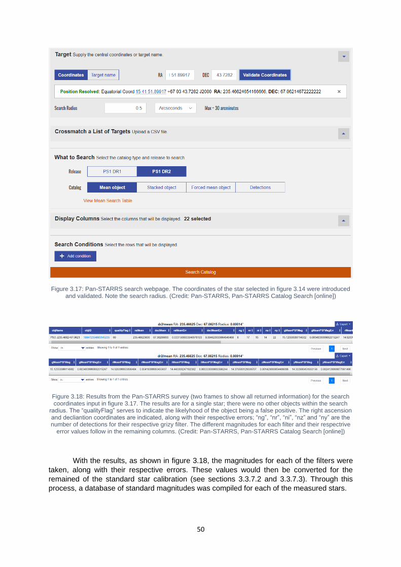
50
Figure 3.17: Pan-STARRS search webpage. The coordinates of the star selected in figure 3.14 were introduced and validated. Note the search radius. (Credit: Pan-STARRS, Pan-STARRS Catalog Search [online])
Figure 3.18: Results from the Pan-STARRS survey (two frames to show all returned information) for the search coordinates input in figure 3.17. The results are for a single star; there were no other objects within the search
radius. The “qualityFlag” serves to indicate the likelyhood of the object being a false positive. The right ascension and decliantion coordinates are indicated, along with their respective errors; “ng”, “nr”, “ni”, “nz” and “ny” are the number of detections for their respective grizy filter. The different magnitudes for each filter and their respectrive
error values follow in the remaining columns. (Credit: Pan-STARRS, Pan-STARRS Catalog Search [online])
With the results, as shown in figure 3.18, the magnitudes for each of the filters were
taken, along with their respective errors. These values would then be converted for the
remained of the standard star calibration (see sections 3.3.7.2 and 3.3.7.3). Through this
process, a database of standard magnitudes was compiled for each of the measured stars.
51
3.3.7.2 Converting and Calibrating Star Magnitudes:
The Pan-STARRS data presents one issue, which is that it does not use the UBVRI
Johnson-Cousins filter system which with this study’s data was acquired. Instead, it uses a
the grizy system. This system isn’t directly compatible with the UBVRI system and, as such, a
conversion is required. Tonry et al. (2012) developed a conversion process for a number of
filter systems, including the Johnson-Cousins UBVRI and Pan-STARRS’ grizy. They provide
both a quadratic (3.2) and linear (3.3) formulae:
𝑦𝑞𝑢𝑎𝑑𝑟𝑎𝑡𝑖𝑐 = 𝐴0 + 𝐴1𝑥 + 𝐴2𝑥2 (3.2)
Where A0 is 0.212, A1 is 0.556 and A2 is 0.034 when determining B, with an error
margin of 0.032; A0 is -0.137, A1 is -0.108 and A2 is -0.029 when determining R, with an error
margin of 0.015.
𝑦𝑙𝑖𝑛𝑒𝑎𝑟 = 𝐵0 + 𝐵1𝑥 (3.3)
Where B0 is 0.213 and B1 is 0.587 when determining B, with an error margin of 0.034;
B0 is -0.138 and B1 is -0.131 when determining R, with an error margin of 0.015.
In both cases, x is (g-r) from the Pan-STARRS1 data. Depending on the filter being
calibrated to, y can either be (B-g) or (R-r) – g and r being filter values from Pan-STARRS1
and B and R being the final UBVRI values that must be retrieved for calibrations.
Filter Conversion and Calibration Program:
A program was written to facilitate the data processing at this stage, as there are
various calculations to perform with information from multiple sources and categories; having
an automated process to execute these steps would not only save time, but also avoid human
error. The main code and the appearance of the user interface are provided in APPENDIX D,
respectively.
C# was chosen as the language to build this program, due to being part of the .Net
platform – which provides a well-developed and easy toolset to integrate with Windows
operating systems – and also due to its available libraries and syntax which facilitate the
access and manipulation of locally stored information, when compared to C++, for instance.
The user first loads a csv file with data taken from the Pan-STARRS database, followed
by the bestmags file generated by IRAF, corresponding to the intended filter. At the user’s
order, the Pan-STARRS data is then converted to the Johnson-Cousins BVRI filter system
through both the quadratic and linear formulas from Tonry et al. (Tonry et al., 2012), described
previously. In this same function, the program will determine which stars in the data, if any,
must be ignored due to missing values from the Pan-STARRS survey and, thus, exclude the
corresponding stars measured with IRAF from the observation data.
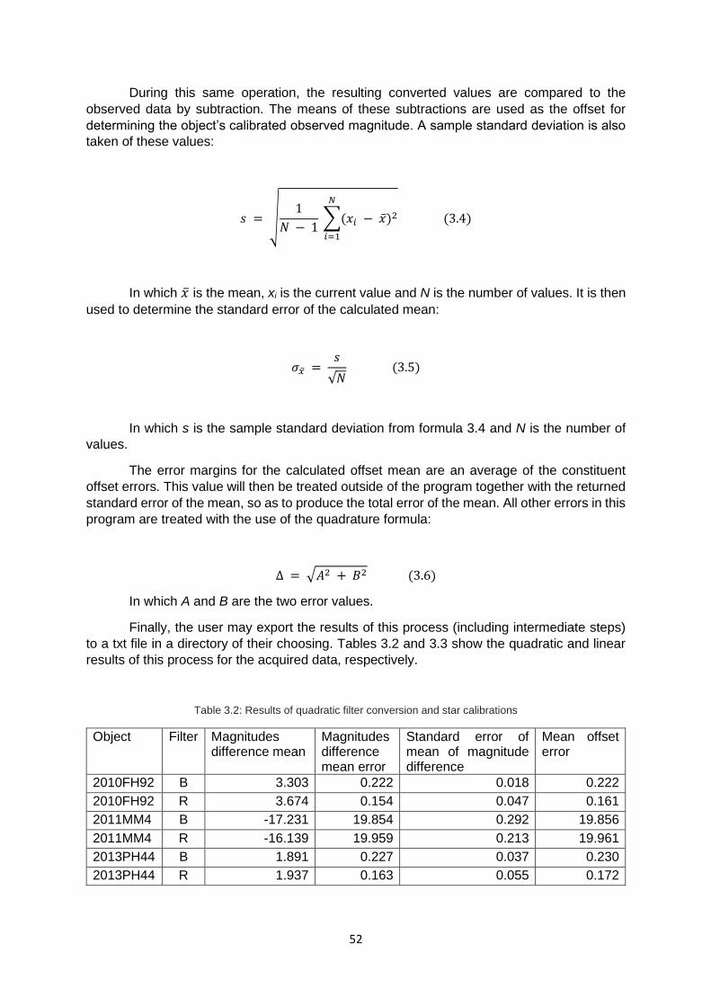
52
During this same operation, the resulting converted values are compared to the
observed data by subtraction. The means of these subtractions are used as the offset for
determining the object’s calibrated observed magnitude. A sample standard deviation is also
taken of these values:
𝑠 = √1
𝑁 − 1 ∑(𝑥𝑖 − �̅�)2
𝑁
𝑖=1
(3.4)
In which �̅� is the mean, xi is the current value and N is the number of values. It is then
used to determine the standard error of the calculated mean:
𝜎�̅� = 𝑠
√𝑁 (3.5)
In which s is the sample standard deviation from formula 3.4 and N is the number of
values.
The error margins for the calculated offset mean are an average of the constituent
offset errors. This value will then be treated outside of the program together with the returned
standard error of the mean, so as to produce the total error of the mean. All other errors in this
program are treated with the use of the quadrature formula:
Δ = √𝐴2 + 𝐵2 (3.6)
In which A and B are the two error values.
Finally, the user may export the results of this process (including intermediate steps)
to a txt file in a directory of their choosing. Tables 3.2 and 3.3 show the quadratic and linear
results of this process for the acquired data, respectively.
Table 3.2: Results of quadratic filter conversion and star calibrations
Object Filter Magnitudes difference mean
Magnitudes difference mean error
Standard error of mean of magnitude difference
Mean offset error
2010FH92 B 3.303 0.222 0.018 0.222
2010FH92 R 3.674 0.154 0.047 0.161
2011MM4 B -17.231 19.854 0.292 19.856
2011MM4 R -16.139 19.959 0.213 19.961
2013PH44 B 1.891 0.227 0.037 0.230
2013PH44 R 1.937 0.163 0.055 0.172
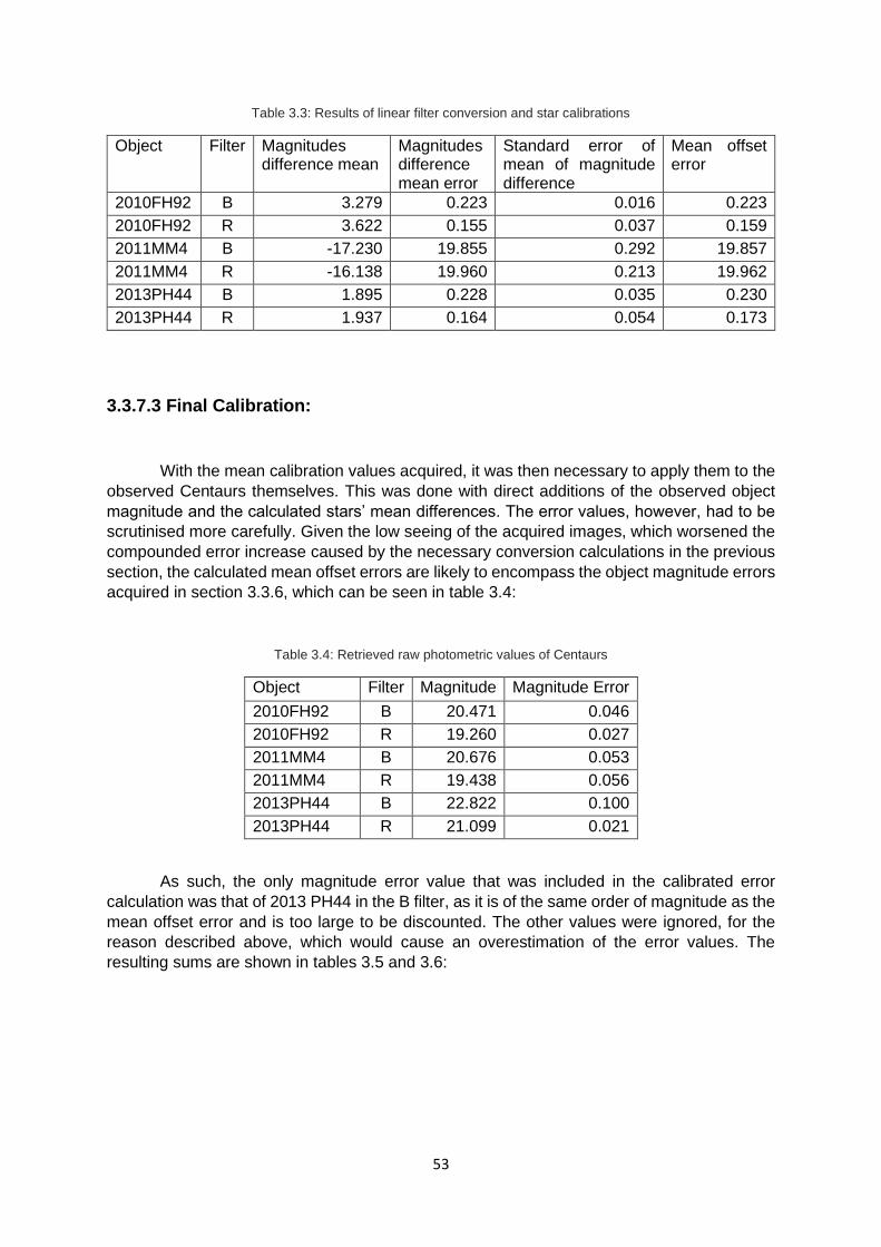
53
Table 3.3: Results of linear filter conversion and star calibrations
Object Filter Magnitudes difference mean
Magnitudes difference mean error
Standard error of mean of magnitude difference
Mean offset error
2010FH92 B 3.279 0.223 0.016 0.223
2010FH92 R 3.622 0.155 0.037 0.159
2011MM4 B -17.230 19.855 0.292 19.857
2011MM4 R -16.138 19.960 0.213 19.962
2013PH44 B 1.895 0.228 0.035 0.230
2013PH44 R 1.937 0.164 0.054 0.173
3.3.7.3 Final Calibration:
With the mean calibration values acquired, it was then necessary to apply them to the
observed Centaurs themselves. This was done with direct additions of the observed object
magnitude and the calculated stars’ mean differences. The error values, however, had to be
scrutinised more carefully. Given the low seeing of the acquired images, which worsened the
compounded error increase caused by the necessary conversion calculations in the previous
section, the calculated mean offset errors are likely to encompass the object magnitude errors
acquired in section 3.3.6, which can be seen in table 3.4:
Table 3.4: Retrieved raw photometric values of Centaurs
Object Filter Magnitude Magnitude Error
2010FH92 B 20.471 0.046
2010FH92 R 19.260 0.027
2011MM4 B 20.676 0.053
2011MM4 R 19.438 0.056
2013PH44 B 22.822 0.100
2013PH44 R 21.099 0.021
As such, the only magnitude error value that was included in the calibrated error
calculation was that of 2013 PH44 in the B filter, as it is of the same order of magnitude as the
mean offset error and is too large to be discounted. The other values were ignored, for the
reason described above, which would cause an overestimation of the error values. The
resulting sums are shown in tables 3.5 and 3.6:
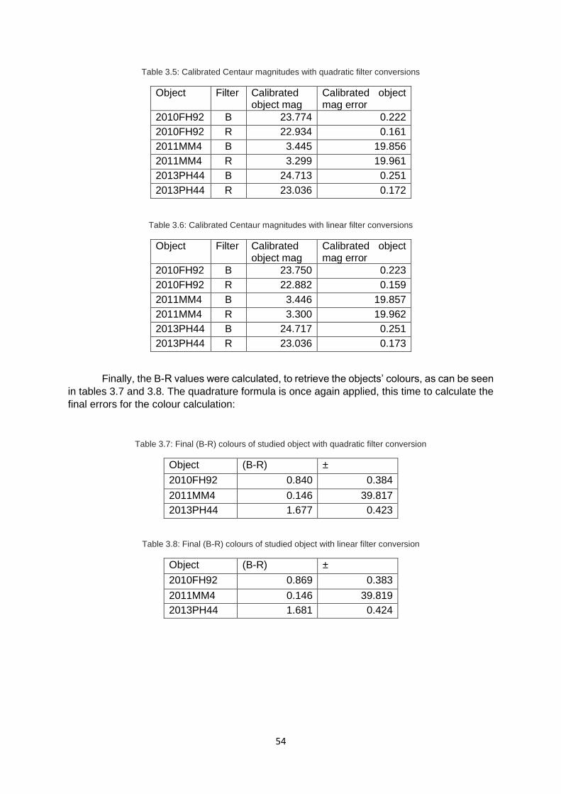
54
Table 3.5: Calibrated Centaur magnitudes with quadratic filter conversions
Object Filter Calibrated object mag
Calibrated object mag error
2010FH92 B 23.774 0.222
2010FH92 R 22.934 0.161
2011MM4 B 3.445 19.856
2011MM4 R 3.299 19.961
2013PH44 B 24.713 0.251
2013PH44 R 23.036 0.172
Table 3.6: Calibrated Centaur magnitudes with linear filter conversions
Object Filter Calibrated object mag
Calibrated object mag error
2010FH92 B 23.750 0.223
2010FH92 R 22.882 0.159
2011MM4 B 3.446 19.857
2011MM4 R 3.300 19.962
2013PH44 B 24.717 0.251
2013PH44 R 23.036 0.173
Finally, the B-R values were calculated, to retrieve the objects’ colours, as can be seen
in tables 3.7 and 3.8. The quadrature formula is once again applied, this time to calculate the
final errors for the colour calculation:
Table 3.7: Final (B-R) colours of studied object with quadratic filter conversion
Object (B-R) ±
2010FH92 0.840 0.384
2011MM4 0.146 39.817
2013PH44 1.677 0.423
Table 3.8: Final (B-R) colours of studied object with linear filter conversion
Object (B-R) ±
2010FH92 0.869 0.383
2011MM4 0.146 39.819
2013PH44 1.681 0.424
55
4 ANALYSIS AND DISCUSSION:
With the photometric measurements calibrated, the results could then be analysed. To
have a point of comparison, a series of “strict” Centaurs, as outlined by Peixinho et al. (2019)
was used. The objects outlined in this list are considered to be Centaurs in accordance with
one of the most commonly-used (and limiting, hence “strict”) definitions – that the perihelion
and semimajor axis both be between the orbits of the giant planets Jupiter and Neptune
(between 5.2 AU and 30.1 AU) (Gladman, 2008) – and present B-R colours retrieved from a
survey by Tegler, Romanishin, and Consolmagno (Tegler et al., Kuiper Belt Object Magnitudes
and Surface Colors [online]). A full list with selected objects with their respective properties is
available in APPENDIX B.
4.1 Colours:
Unfortunately, the estimated photometric errors for the studied objects are very large,
as compared to typical errors for B-R photometric measurements of Centaurs (which vary
between ± 0.12 and ± 0.02, as shown on APPENDIX B). This wasn’t entirely unexpected,
given the quality of the seeing for the relevant observations. Followed is an overview of each
individual object:
2010 FH92 presented a low B-R, which would make it, by far, the bluest object so far
measured of the “strict” Centaurs – the population varies between 1.97 ± 0.11 and 1.03 ± 0.04,
whereas 2010 FH92 presents a B-R of either about 0.84 ± 0.38 or about 0.87 ± 0.38,
depending on having used the quadratic or linear conversions for the standard stars,
respectively; this is, however, not at all significant, given the error bars. Considering its wide
error bars, which could easily put it much closer to the mean colour of (B-R) = 1.2 of bluer
objects (any with (B-R) < 1.4), we cannot overinterpret its low colour value. Its measured
FWHM was the best out of all of the measured Centaurs, with 3.7” for both the B and R filters
in their final calibrated images (although this is by no means considered to be “good” seeing,
either).
2011 MM4 was imaged during a particularly cloudy period and, as such, had a very
“bad” seeing. Its FWHM was measured to be about 5.5” in the final calibrated B filter image
and 10.4” in the R filter. As such, it is not entirely unsurprising that it has such a large error of
about 39.82 and an extremely unlikely B-R of 0.15. Evidently, no object can be used for
analysis with a magnitude error of about 40. It can, however, be considered an apt example
of resulting measurements of an object with an extremely low and degraded signal-to-noise
ratio (or S/N) due to atmospheric conditions.
2013 PH44 was imaged with a less-than-ideal sky, like the other objects, but with a
particularly “bad” seeing in the B filters. The average FWHM for those was 9”, although the R
filter presented a relatively more reasonable seeing of 3.6”. As a result, the object’s B-R colour
error is still very large, at ± 0.42. Although, a (B-R) = 1.68 indicates that this Centaur is ultrared
(see section 1.1.2 for more on this topic). However, the error margin cannot be ignored – it is
still so wide that 2013 PH44 could possibly even be part of the “blue” population, if we consider
the debatable bimodality discussed in section 1.4.
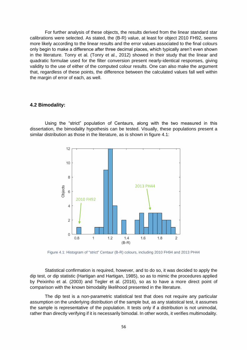
56
For further analysis of these objects, the results derived from the linear standard star
calibrations were selected. As stated, the (B-R) value, at least for object 2010 FH92, seems
more likely according to the linear results and the error values associated to the final colours
only begin to make a difference after three decimal places, which typically aren’t even shown
in the literature. Tonry et al. (Tonry et al., 2012) showed in their study that the linear and
quadratic formulae used for the filter conversion present nearly-identical responses, giving
validity to the use of either of the computed colour results. One can also make the argument
that, regardless of these points, the difference between the calculated values fall well within
the margin of error of each, as well.
4.2 Bimodality:
Using the “strict” population of Centaurs, along with the two measured in this
dissertation, the bimodality hypothesis can be tested. Visually, these populations present a
similar distribution as those in the literature, as is shown in figure 4.1:
Figure 4.1: Histogram of "strict" Centaur (B-R) colours, including 2010 FH94 and 2013 PH44
Statistical confirmation is required, however, and to do so, it was decided to apply the
dip test, or dip statistic (Hartigan and Hartigan, 1985), so as to mimic the procedures applied
by Peixinho et al. (2003) and Tegler et al. (2016), so as to have a more direct point of
comparison with the known bimodality likelihood presented in the literature.
The dip test is a non-parametric statistical test that does not require any particular
assumption on the underlying distribution of the sample but, as any statistical test, it assumes
the sample is representative of the population. It tests only if a distribution is not unimodal,
rather than directly verifying if it is necessarily bimodal. In other words, it verifies multimodality.
2010 FH92
2013 PH44
57
It does this through monotone regression – i.e. a kind of fit that minimizes the mean squared
error (this is, the average of the errors between the regression line and the data points), which
uses a free-form line, in which it finds an approximation to the data with a non-decreasing
constraint.
This test applies a unimodal function to the data, following the best fit possible, and
compares it with the sample’s empirical distribution function, so as to find the maximum
difference between the two. This difference will approach 0 for unimodal distributions and
positive numbers for non-unimodal distributions.
An implementation of this test is available in the R language (R Documentation, dip.test
[online]), which was used for this work.
The result was that these selected objects only show a multimodal (implied bimodal)
colour population at the 86.41% confidence level, which is not enough to reject the null
hypothesis of unimodality (the null hypothesis would only be rejected at a minimum 95%
confidence level, roughly equivalent to a 2σ result, and at least a 90% would be required for
suggested multimodality with some significance).
This is a far cry from the 99.96% confidence level reported by Tegler et al. (Tegler et
al., 2016), better than the canonical 3σ, however the populations used by the two studies are
very different. The “strict” population used in this study has a total of 50 objects, which is a
considerably smaller population, which might not give an accurate colour distribution
representation of the wider population used by Tegler et al. (2016).
To help evaluate the impact the two objects measured in this dissertation had, the
same test was performed with only the objects referenced from Peixinho et al. (2019), yielding
an even lower 82.2% confidence level.
Even though, statistically, the two colour groups may be “extracted” from a parent
distribution with a continuous colour variation, ranging from grey/neutral to very red – hence
being simply a sampling effect – for the sake of simplicity they will be referred to as the
grey/neutral colour group and the red group.
4.3 Inclination:
The Centaurs’ orbital inclinations (typically represented as i, measured in degrees)
were also studied in this dissertation, as Tegler et al. (2016) noted that there was a correlation
between the objects’ (B-R) colours (when considered as a bimodal distribution) and their
orbital inclinations, showing with a 99.3% confidence level that the red colour group had a
smaller orbital inclination distribution than the grey group.
Once again, to maintain the point of comparison, the same statistical test was used as
that in the referenced literature – the Wilcoxon rank-sum test (Wilcoxon, 1945), also known as
the Mann-Whitney U test. Like Hartigan’s dip statistic (see section 4.2), it is non-parametric.
This test is designed to verify if two distributions are different or, to be more precise, to verify
if it is likely or not that one randomly selected element of one sample is greater than a randomly
selected element of another sample. Meaning, the null hypothesis is that randomly selected
members of one population will not have a different value to those of another population.
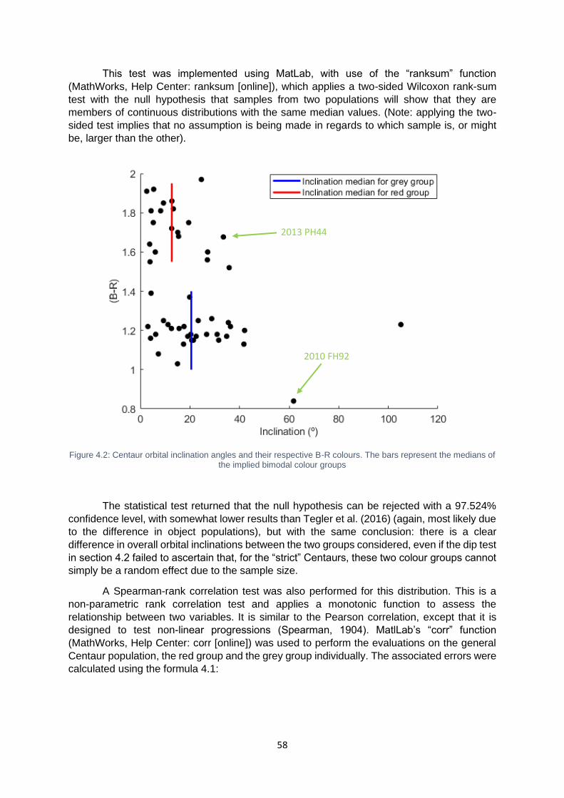
58
This test was implemented using MatLab, with use of the “ranksum” function
(MathWorks, Help Center: ranksum [online]), which applies a two-sided Wilcoxon rank-sum
test with the null hypothesis that samples from two populations will show that they are
members of continuous distributions with the same median values. (Note: applying the two-
sided test implies that no assumption is being made in regards to which sample is, or might
be, larger than the other).
Figure 4.2: Centaur orbital inclination angles and their respective B-R colours. The bars represent the medians of the implied bimodal colour groups
The statistical test returned that the null hypothesis can be rejected with a 97.524%
confidence level, with somewhat lower results than Tegler et al. (2016) (again, most likely due
to the difference in object populations), but with the same conclusion: there is a clear
difference in overall orbital inclinations between the two groups considered, even if the dip test
in section 4.2 failed to ascertain that, for the “strict” Centaurs, these two colour groups cannot
simply be a random effect due to the sample size.
A Spearman-rank correlation test was also performed for this distribution. This is a
non-parametric rank correlation test and applies a monotonic function to assess the
relationship between two variables. It is similar to the Pearson correlation, except that it is
designed to test non-linear progressions (Spearman, 1904). MatlLab’s “corr” function
(MathWorks, Help Center: corr [online]) was used to perform the evaluations on the general
Centaur population, the red group and the grey group individually. The associated errors were
calculated using the formula 4.1:
2010 FH92
2013 PH44
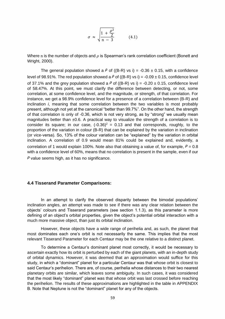
59
𝜎 ≈ √1 +
𝜌2
2n − 3
(4.1)
Where n is the number of objects and 𝜌 is Spearman’s rank correlation coefficient (Bonett and
Wright, 2000).
The general population showed a of ((B-R) vs i) = -0.36 ± 0.15, with a confidence
level of 98.91%. The red population showed a of ((B-R) vs i) = -0.09 ± 0.15, confidence level
of 37.1% and the grey population showed a of ((B-R) vs i) = -0.20 ± 0.15, confidence level
of 58.47%. At this point, we must clarify the difference between detecting, or not, some
correlation, at some confidence level, and the magnitude, or strength, of that correlation. For
instance, we get a 98.9% confidence level for a presence of a correlation between (B-R) and
inclination i, meaning that some correlation between the two variables is most probably
present, although not yet at the canonical “better than 99.7%”. On the other hand, the strength
of that correlation is only of -0.36, which is not very strong, as by “strong” we usually mean
magnitudes better than ±0.6. A practical way to visualize the strength of a correlation is to
consider its square; in our case, (-0.36)2 = 0.13 and that corresponds, roughly, to the
proportion of the variation in colour (B-R) that can be explained by the variation in inclination
(or vice-versa). So, 13% of the colour variation can be “explained” by the variation in orbital
inclination. A correlation of 0.9 would mean 81% could be explained and, evidently, a
correlation of 1 would explain 100%. Note also that obtaining a value of, for example, = 0.8
with a confidence level of 60%, means that no correlation is present in the sample, even if our
value seems high, as it has no significance.
4.4 Tisserand Parameter Comparisons:
In an attempt to clarify the observed disparity between the bimodal populations’
inclination angles, an attempt was made to see if there was any clear relation between the
objects’ colours and Tisserand parameters (see section 1.1.3), as this parameter is more
defining of an object’s orbital properties, given the object’s potential orbital interaction with a
much more massive object, than just its orbital inclination.
However, these objects have a wide range of perihelia and, as such, the planet that
most dominates each one’s orbit is not necessarily the same. This implies that the most
relevant Tisserand Parameter for each Centaur may be the one relative to a distinct planet.
To determine a Centaur’s dominant planet most correctly, it would be necessary to
ascertain exactly how its orbit is perturbed by each of the giant planets, with an in-depth study
of orbital dynamics. However, it was deemed that an approximation would suffice for this
study, in which a “dominant” planet for a particular Centaur was that whose orbit is closest to
said Centaur’s perihelion. There are, of course, perihelia whose distances to their two nearest
planetary orbits are similar, which leaves some ambiguity. In such cases, it was considered
that the most likely “dominant” planet was that whose orbit was last crossed before reaching
the perihelion. The results of these approximations are highlighted in the table in APPENDIX
B. Note that Neptune is not the “dominant” planet for any of the objects.
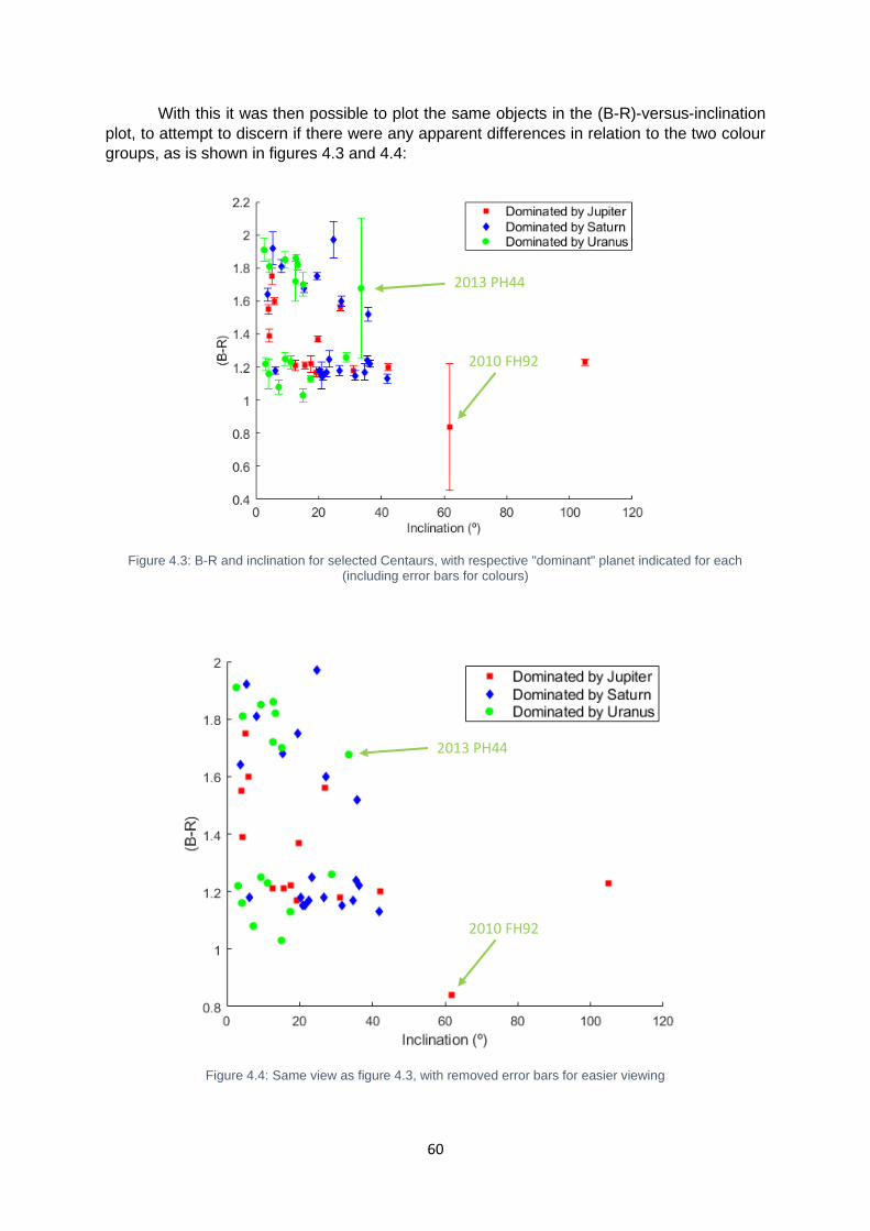
60
With this it was then possible to plot the same objects in the (B-R)-versus-inclination
plot, to attempt to discern if there were any apparent differences in relation to the two colour
groups, as is shown in figures 4.3 and 4.4:
Figure 4.3: B-R and inclination for selected Centaurs, with respective "dominant" planet indicated for each (including error bars for colours)
Figure 4.4: Same view as figure 4.3, with removed error bars for easier viewing
2010 FH92
2013 PH44
2010 FH92
2013 PH44
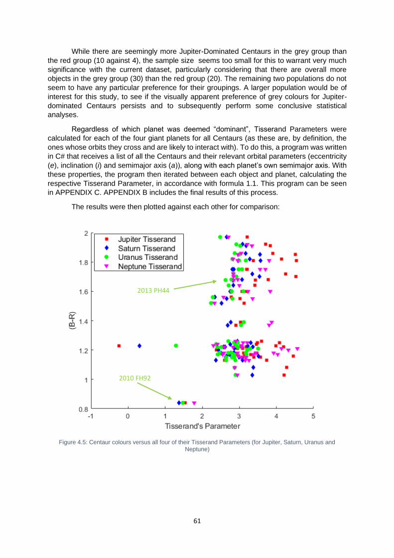
61
While there are seemingly more Jupiter-Dominated Centaurs in the grey group than
the red group (10 against 4), the sample size seems too small for this to warrant very much
significance with the current dataset, particularly considering that there are overall more
objects in the grey group (30) than the red group (20). The remaining two populations do not
seem to have any particular preference for their groupings. A larger population would be of
interest for this study, to see if the visually apparent preference of grey colours for Jupiter-
dominated Centaurs persists and to subsequently perform some conclusive statistical
analyses.
Regardless of which planet was deemed “dominant”, Tisserand Parameters were
calculated for each of the four giant planets for all Centaurs (as these are, by definition, the
ones whose orbits they cross and are likely to interact with). To do this, a program was written
in C# that receives a list of all the Centaurs and their relevant orbital parameters (eccentricity
(e), inclination (i) and semimajor axis (a)), along with each planet’s own semimajor axis. With
these properties, the program then iterated between each object and planet, calculating the
respective Tisserand Parameter, in accordance with formula 1.1. This program can be seen
in APPENDIX C. APPENDIX B includes the final results of this process.
The results were then plotted against each other for comparison:
Figure 4.5: Centaur colours versus all four of their Tisserand Parameters (for Jupiter, Saturn, Uranus and
Neptune)
2010 FH92
2013 PH44
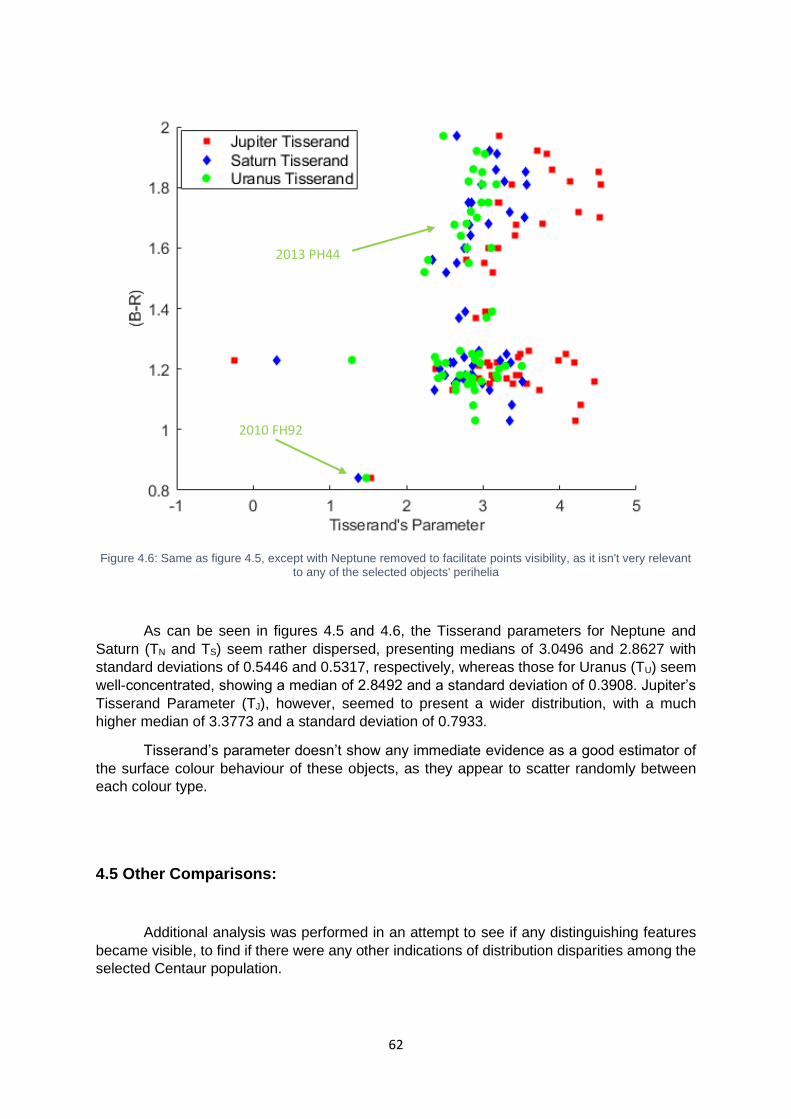
62
Figure 4.6: Same as figure 4.5, except with Neptune removed to facilitate points visibility, as it isn't very relevant to any of the selected objects' perihelia
As can be seen in figures 4.5 and 4.6, the Tisserand parameters for Neptune and
Saturn (TN and TS) seem rather dispersed, presenting medians of 3.0496 and 2.8627 with
standard deviations of 0.5446 and 0.5317, respectively, whereas those for Uranus (TU) seem
well-concentrated, showing a median of 2.8492 and a standard deviation of 0.3908. Jupiter’s
Tisserand Parameter (TJ), however, seemed to present a wider distribution, with a much
higher median of 3.3773 and a standard deviation of 0.7933.
Tisserand’s parameter doesn’t show any immediate evidence as a good estimator of
the surface colour behaviour of these objects, as they appear to scatter randomly between
each colour type.
4.5 Other Comparisons:
Additional analysis was performed in an attempt to see if any distinguishing features
became visible, to find if there were any other indications of distribution disparities among the
selected Centaur population.
2010 FH92
2013 PH44
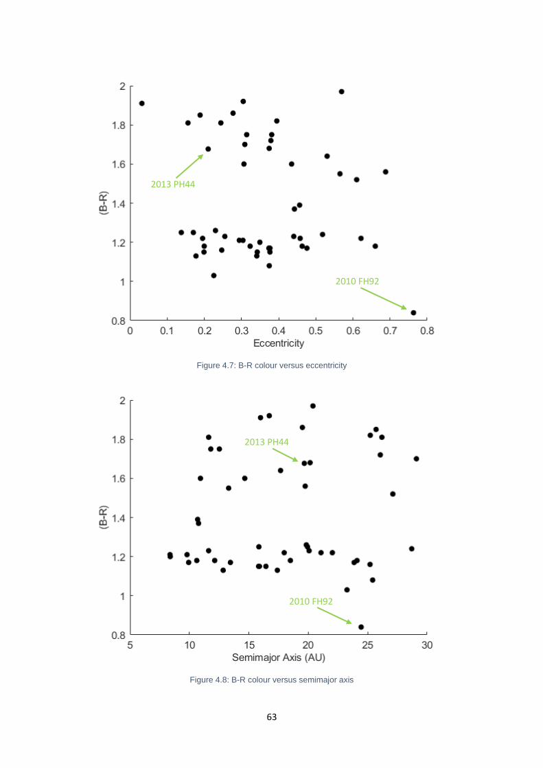
63
Figure 4.7: B-R colour versus eccentricity
Figure 4.8: B-R colour versus semimajor axis
2010 FH92
2010 FH92
2013 PH44
2013 PH44
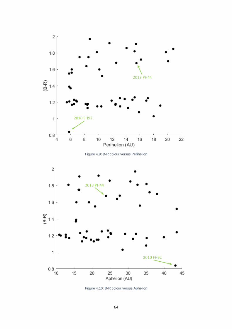
64
Figure 4.9: B-R colour versus Perihelion
Figure 4.10: B-R colour versus Aphelion
2010 FH92
2010 FH92
2013 PH44
2013 PH44
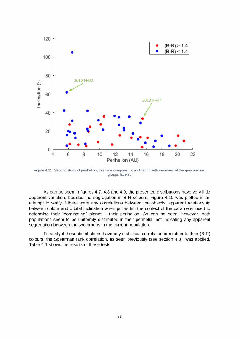
65
Figure 4.11: Second study of perihelion, this time compared to inclination with members of the grey and red groups labeled
As can be seen in figures 4.7, 4.8 and 4.9, the presented distributions have very little
apparent variation, besides the segregation in B-R colours. Figure 4.10 was plotted in an
attempt to verify if there were any correlations between the objects’ apparent relationship
between colour and orbital inclination when put within the context of the parameter used to
determine their “dominating” planet – their perihelion. As can be seen, however, both
populations seem to be uniformly distributed in their perihelia, not indicating any apparent
segregation between the two groups in the current population.
To verify if these distributions have any statistical correlation in relation to their (B-R)
colours, the Spearman rank correlation, as seen previously (see section 4.3), was applied.
Table 4.1 shows the results of these tests:
2010 FH92
2013 PH44
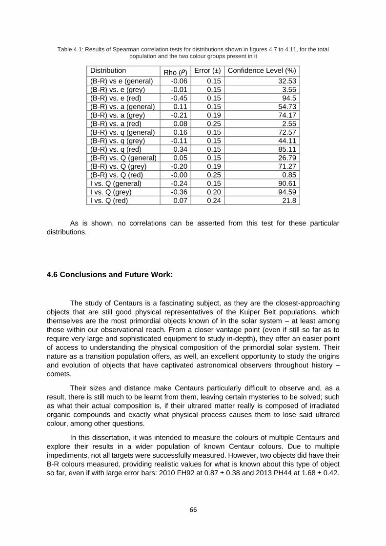
66
Table 4.1: Results of Spearman correlation tests for distributions shown in figures 4.7 to 4.11, for the total population and the two colour groups present in it
Distribution Rho ( ) Error (±) Confidence Level (%)
(B-R) vs e (general) -0.06 0.15 32.53
(B-R) vs. e (grey) -0.01 0.15 3.55
(B-R) vs. e (red) -0.45 0.15 94.5
(B-R) vs. a (general) 0.11 0.15 54.73
(B-R) vs. a (grey) -0.21 0.19 74.17
(B-R) vs. a (red) 0.08 0.25 2.55
(B-R) vs. q (general) 0.16 0.15 72.57
(B-R) vs. q (grey) -0.11 0.15 44.11
(B-R) vs. q (red) 0.34 0.15 85.11
(B-R) vs. Q (general) 0.05 0.15 26.79
(B-R) vs. Q (grey) -0.20 0.19 71.27
(B-R) vs. Q (red) -0.00 0.25 0.85
I vs. Q (general) -0.24 0.15 90.61
I vs. Q (grey) -0.36 0.20 94.59
I vs. Q (red) 0.07 0.24 21.8
As is shown, no correlations can be asserted from this test for these particular
distributions.
4.6 Conclusions and Future Work:
The study of Centaurs is a fascinating subject, as they are the closest-approaching
objects that are still good physical representatives of the Kuiper Belt populations, which
themselves are the most primordial objects known of in the solar system – at least among
those within our observational reach. From a closer vantage point (even if still so far as to
require very large and sophisticated equipment to study in-depth), they offer an easier point
of access to understanding the physical composition of the primordial solar system. Their
nature as a transition population offers, as well, an excellent opportunity to study the origins
and evolution of objects that have captivated astronomical observers throughout history –
comets.
Their sizes and distance make Centaurs particularly difficult to observe and, as a
result, there is still much to be learnt from them, leaving certain mysteries to be solved; such
as what their actual composition is, if their ultrared matter really is composed of irradiated
organic compounds and exactly what physical process causes them to lose said ultrared
colour, among other questions.
In this dissertation, it was intended to measure the colours of multiple Centaurs and
explore their results in a wider population of known Centaur colours. Due to multiple
impediments, not all targets were successfully measured. However, two objects did have their
B-R colours measured, providing realistic values for what is known about this type of object
so far, even if with large error bars: 2010 FH92 at 0.87 ± 0.38 and 2013 PH44 at 1.68 ± 0.42.
67
2013 PH44 is a red Centaur, most likely even ultrared, which would mean its surface
is covered with irradiated organics, or tholins, but its error bar does not allow us to confidently
state this. On the other hand, 2010 FH92 presents a blue colour – by far the bluest in the
“strict” population included for follow-up analysis – making it a good target for further studies
in order to confirm its surface colour with a much lower error bar. Nonetheless, this object is
firmly within the “grey” colour type of Centaurs.
A “strict” population of known Centaurs was included for group analysis in the attempt
of verifying previously published results and expanding on them, if possible. The previously-
verified bimodal colour of these objects was only attained with a 86.4% confidence level, which
isn’t enough to reject unimodality, although the sample size of this population is quite small
due to how limiting the definition for it is. This also raises the issue of what is the most adequate
definition of a Centaur, as it interferes drastically with the conclusions on the studies of these
objects. We must bear in mind that Centaurs were discovered before the Kuiper Belt and the
distinct dynamical families of Kuiper Belt Objects, and that it might not make much sense to
classify Centaurs as separate from the Scattered Disc Objects.
A test was also conducted to check this population for the orbital inclination disparity
between the two colour groups presented in the literature and confirmed it for this population
with a confidence level of 97.5%. That is, that the red Centaurs have, on average, lower
inclinations than the grey ones. This result, found by Tegler et al. (2016), is interesting,
although puzzling, as dynamical studies show that Centaurs do not preserve their initial orbital
inclinations (Volk and Malhotra, 2013).
To explore the possible relationships between Centaur distributions and their orbital
attributes beyond their inclinations, a series of other comparisons were made, using their
Tisserand Parameters, B-R colours, orbital inclinations, perihelia, aphelia, semimajor axes
and eccentricities. No significant trends were observed, however, thus resulting in no new
insights beyond the null results.
A clear issue with the current understanding of these objects stems from their
definition. As they are a transition population with unstable orbits and no clear boundary, exact
notions of how to define a Centaur vary in the literature. Further, more in-depth studies of the
population’s characteristics could present a clearer definition of what exactly constitutes a
Centaur.
Other further work in this field will necessarily require more observations of these
objects, particularly to gather more measurements of their colours and a better refinement of
their ephemerides. A higher quality – and not just quantity – of measurements is necessary,
naturally, as determining their exact compositions is of prime importance to understanding not
only their nature and that of related populations, but also the historical development of the
solar system – particularly the formation of the TNO populations.
With currently available technology and observatories, future studies should focus on
acquiring the remaining colours of known Centaurs and, importantly, their sizes, as the
objects’ size-colour correlations have not been fully explored and it is necessary to either
confirm or rule out this parameter as a possible mechanism for the observed colour
bimodality.
Another aspect that should be explored more fully is the “separation” region between
Centaurs and SDOs, to better determine how distinct these objects are from one another
and see if they should be considered separate populations from a physical standpoint.

68
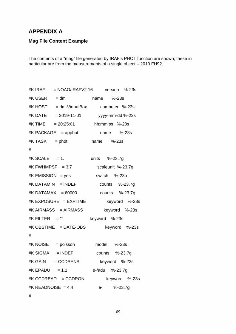
69
APPENDIX A
Mag File Content Example
The contents of a “mag” file generated by IRAF’s PHOT function are shown; these in
particular are from the measurements of a single object – 2010 FH92.
#K IRAF = NOAO/IRAFV2.16 version %-23s
#K USER = dm name %-23s
#K HOST = dm-VirtualBox computer %-23s
#K DATE = 2019-11-01 yyyy-mm-dd %-23s
#K TIME = 20:25:01 hh:mm:ss %-23s
#K PACKAGE = apphot name %-23s
#K TASK = phot name %-23s
#
#K SCALE = 1. units %-23.7g
#K FWHMPSF = 3.7 scaleunit %-23.7g
#K EMISSION = yes switch %-23b
#K DATAMIN = INDEF counts %-23.7g
#K DATAMAX = 60000. counts %-23.7g
#K EXPOSURE = EXPTIME keyword %-23s
#K AIRMASS = AIRMASS keyword %-23s
#K FILTER = "" keyword %-23s
#K OBSTIME = DATE-OBS keyword %-23s
#
#K NOISE = poisson model %-23s
#K SIGMA = INDEF counts %-23.7g
#K GAIN = CCDSENS keyword %-23s
#K EPADU = 1.1 e-/adu %-23.7g
#K CCDREAD = CCDRON keyword %-23s
#K READNOISE = 4.4 e- %-23.7g
#
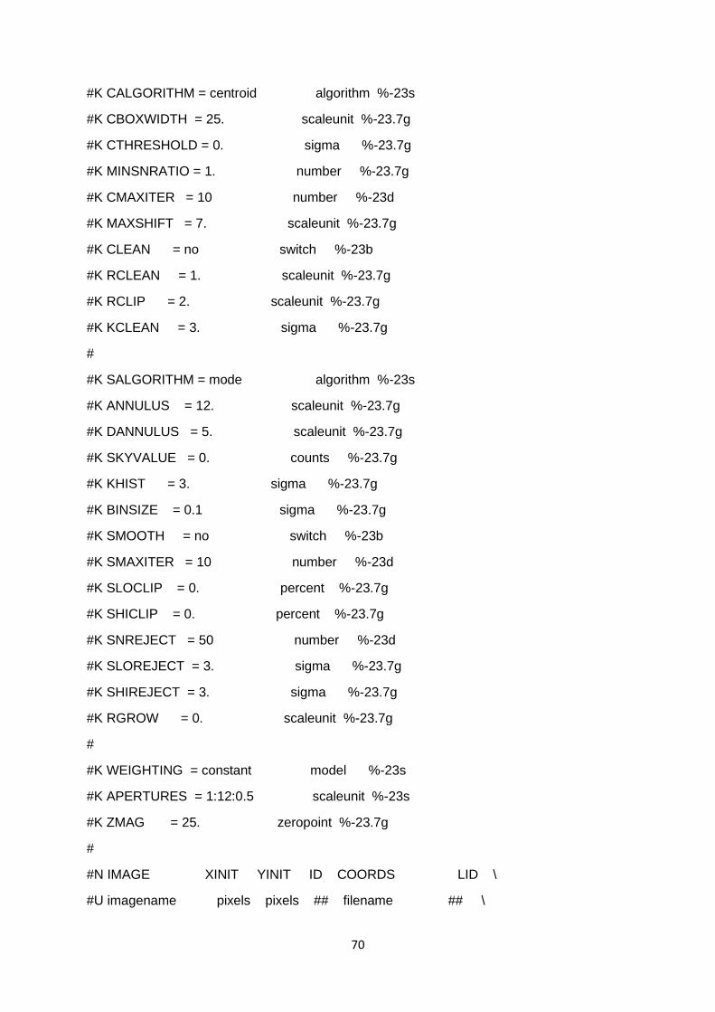
70
#K CALGORITHM = centroid algorithm %-23s
#K CBOXWIDTH = 25. scaleunit %-23.7g
#K CTHRESHOLD = 0. sigma %-23.7g
#K MINSNRATIO = 1. number %-23.7g
#K CMAXITER = 10 number %-23d
#K MAXSHIFT = 7. scaleunit %-23.7g
#K CLEAN = no switch %-23b
#K RCLEAN = 1. scaleunit %-23.7g
#K RCLIP = 2. scaleunit %-23.7g
#K KCLEAN = 3. sigma %-23.7g
#
#K SALGORITHM = mode algorithm %-23s
#K ANNULUS = 12. scaleunit %-23.7g
#K DANNULUS = 5. scaleunit %-23.7g
#K SKYVALUE = 0. counts %-23.7g
#K KHIST = 3. sigma %-23.7g
#K BINSIZE = 0.1 sigma %-23.7g
#K SMOOTH = no switch %-23b
#K SMAXITER = 10 number %-23d
#K SLOCLIP = 0. percent %-23.7g
#K SHICLIP = 0. percent %-23.7g
#K SNREJECT = 50 number %-23d
#K SLOREJECT = 3. sigma %-23.7g
#K SHIREJECT = 3. sigma %-23.7g
#K RGROW = 0. scaleunit %-23.7g
#
#K WEIGHTING = constant model %-23s
#K APERTURES = 1:12:0.5 scaleunit %-23s
#K ZMAG = 25. zeropoint %-23.7g
#
#N IMAGE XINIT YINIT ID COORDS LID \
#U imagename pixels pixels ## filename ## \
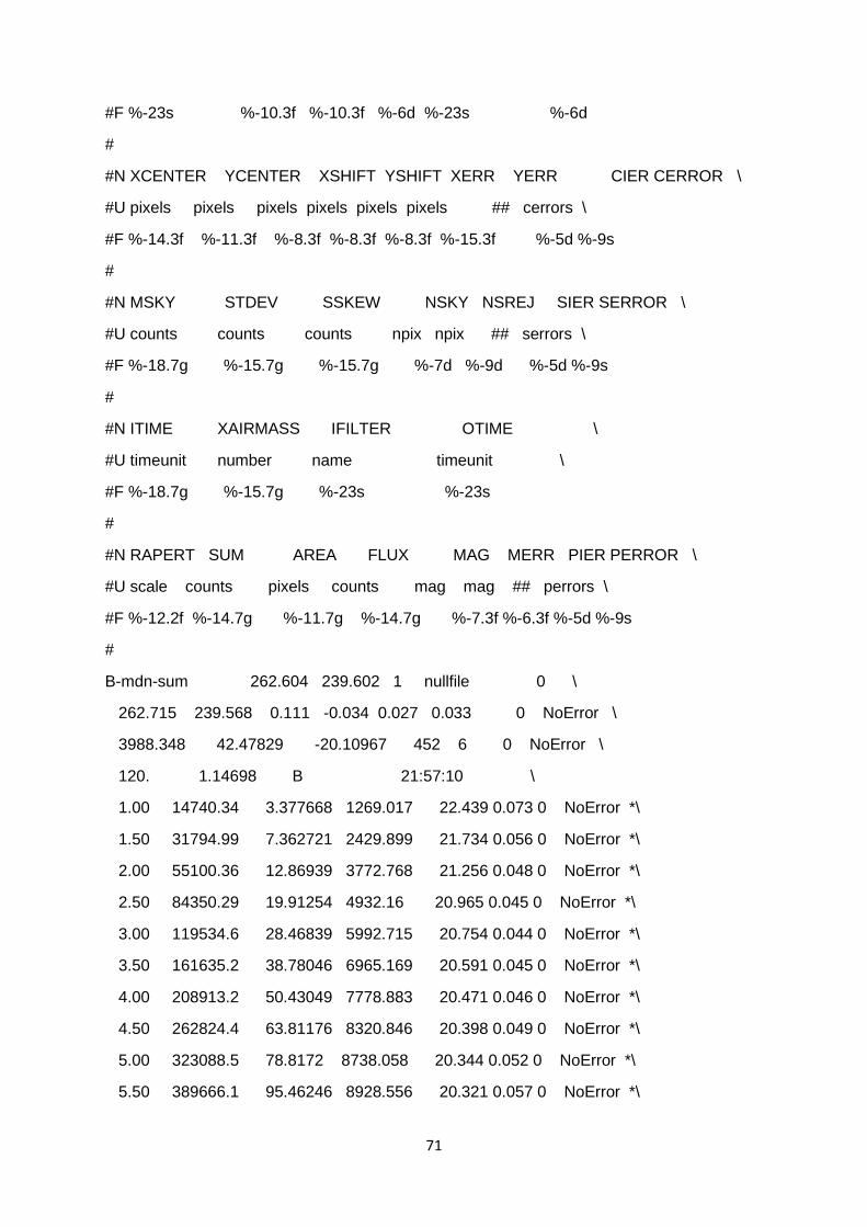
71
#F %-23s %-10.3f %-10.3f %-6d %-23s %-6d
#
#N XCENTER YCENTER XSHIFT YSHIFT XERR YERR CIER CERROR \
#U pixels pixels pixels pixels pixels pixels ## cerrors \
#F %-14.3f %-11.3f %-8.3f %-8.3f %-8.3f %-15.3f %-5d %-9s
#
#N MSKY STDEV SSKEW NSKY NSREJ SIER SERROR \
#U counts counts counts npix npix ## serrors \
#F %-18.7g %-15.7g %-15.7g %-7d %-9d %-5d %-9s
#
#N ITIME XAIRMASS IFILTER OTIME \
#U timeunit number name timeunit \
#F %-18.7g %-15.7g %-23s %-23s
#
#N RAPERT SUM AREA FLUX MAG MERR PIER PERROR \
#U scale counts pixels counts mag mag ## perrors \
#F %-12.2f %-14.7g %-11.7g %-14.7g %-7.3f %-6.3f %-5d %-9s
#
B-mdn-sum 262.604 239.602 1 nullfile 0 \
262.715 239.568 0.111 -0.034 0.027 0.033 0 NoError \
3988.348 42.47829 -20.10967 452 6 0 NoError \
120. 1.14698 B 21:57:10 \
1.00 14740.34 3.377668 1269.017 22.439 0.073 0 NoError *\
1.50 31794.99 7.362721 2429.899 21.734 0.056 0 NoError *\
2.00 55100.36 12.86939 3772.768 21.256 0.048 0 NoError *\
2.50 84350.29 19.91254 4932.16 20.965 0.045 0 NoError *\
3.00 119534.6 28.46839 5992.715 20.754 0.044 0 NoError *\
3.50 161635.2 38.78046 6965.169 20.591 0.045 0 NoError *\
4.00 208913.2 50.43049 7778.883 20.471 0.046 0 NoError *\
4.50 262824.4 63.81176 8320.846 20.398 0.049 0 NoError *\
5.00 323088.5 78.8172 8738.058 20.344 0.052 0 NoError *\
5.50 389666.1 95.46246 8928.556 20.321 0.057 0 NoError *\
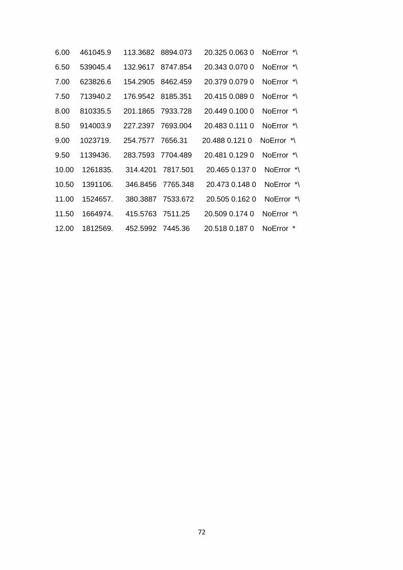
72
6.00 461045.9 113.3682 8894.073 20.325 0.063 0 NoError *\
6.50 539045.4 132.9617 8747.854 20.343 0.070 0 NoError *\
7.00 623826.6 154.2905 8462.459 20.379 0.079 0 NoError *\
7.50 713940.2 176.9542 8185.351 20.415 0.089 0 NoError *\
8.00 810335.5 201.1865 7933.728 20.449 0.100 0 NoError *\
8.50 914003.9 227.2397 7693.004 20.483 0.111 0 NoError *\
9.00 1023719. 254.7577 7656.31 20.488 0.121 0 NoError *\
9.50 1139436. 283.7593 7704.489 20.481 0.129 0 NoError *\
10.00 1261835. 314.4201 7817.501 20.465 0.137 0 NoError *\
10.50 1391106. 346.8456 7765.348 20.473 0.148 0 NoError *\
11.00 1524657. 380.3887 7533.672 20.505 0.162 0 NoError *\
11.50 1664974. 415.5763 7511.25 20.509 0.174 0 NoError *\
12.00 1812569. 452.5992 7445.36 20.518 0.187 0 NoError *
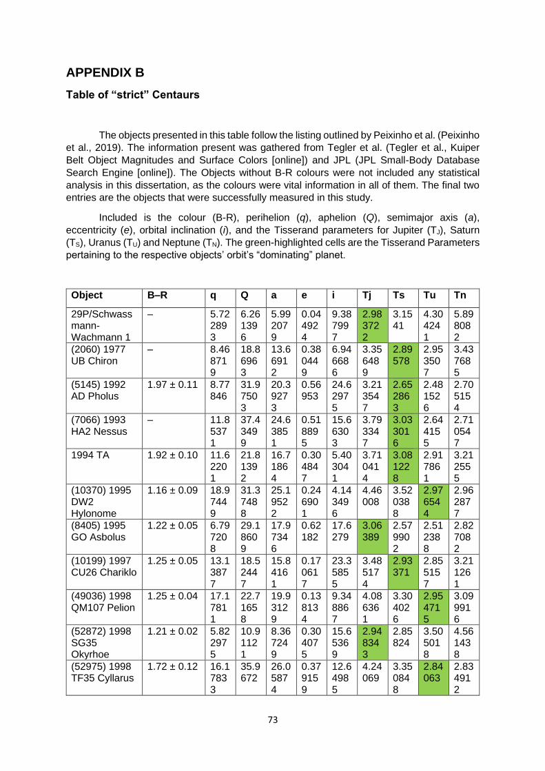
73
APPENDIX B
Table of “strict” Centaurs
The objects presented in this table follow the listing outlined by Peixinho et al. (Peixinho
et al., 2019). The information present was gathered from Tegler et al. (Tegler et al., Kuiper
Belt Object Magnitudes and Surface Colors [online]) and JPL (JPL Small-Body Database
Search Engine [online]). The Objects without B-R colours were not included any statistical
analysis in this dissertation, as the colours were vital information in all of them. The final two
entries are the objects that were successfully measured in this study.
Included is the colour (B-R), perihelion (q), aphelion (Q), semimajor axis (a),
eccentricity (e), orbital inclination (i), and the Tisserand parameters for Jupiter (TJ), Saturn
(TS), Uranus (TU) and Neptune (TN). The green-highlighted cells are the Tisserand Parameters
pertaining to the respective objects’ orbit’s “dominating” planet.
Object B–R q Q a e i Tj Ts Tu Tn
29P/Schwassmann-Wachmann 1
– 5.722893
6.261396
5.992079
0.044924
9.387997
2.983722
3.1541
4.304241
5.898082
(2060) 1977 UB Chiron
– 8.468719
18.86963
13.66912
0.380449
6.946686
3.356489
2.89578
2.953507
3.437685
(5145) 1992 AD Pholus
1.97 ± 0.11 8.77846
31.97503
20.39273
0.56953
24.62975
3.213547
2.652863
2.481526
2.705154
(7066) 1993 HA2 Nessus
– 11.85371
37.43499
24.63851
0.518895
15.66303
3.793347
3.033016
2.644155
2.710547
1994 TA 1.92 ± 0.10 11.62201
21.81392
16.71864
0.304847
5.403041
3.710414
3.081228
2.917861
3.212555
(10370) 1995 DW2 Hylonome
1.16 ± 0.09 18.97449
31.37488
25.19522
0.246901
4.143496
4.46008
3.520388
2.976544
2.962877
(8405) 1995 GO Asbolus
1.22 ± 0.05 6.797208
29.18609
17.97346
0.62182
17.6279
3.06389
2.579902
2.512388
2.827082
(10199) 1997 CU26 Chariklo
1.25 ± 0.05 13.13877
18.52447
15.84161
0.170617
23.35855
3.485174
2.93371
2.855157
3.211261
(49036) 1998 QM107 Pelion
1.25 ± 0.04 17.17811
22.71658
19.93129
0.138134
9.348867
4.086361
3.304026
2.954715
3.099916
(52872) 1998 SG35 Okyrhoe
1.21 ± 0.02 5.822975
10.91121
8.367249
0.304075
15.65369
2.948343
2.85824
3.505018
4.561438
(52975) 1998 TF35 Cyllarus
1.72 ± 0.12 16.17833
35.9672
26.05874
0.379159
12.64985
4.24069
3.350848
2.84063
2.834912
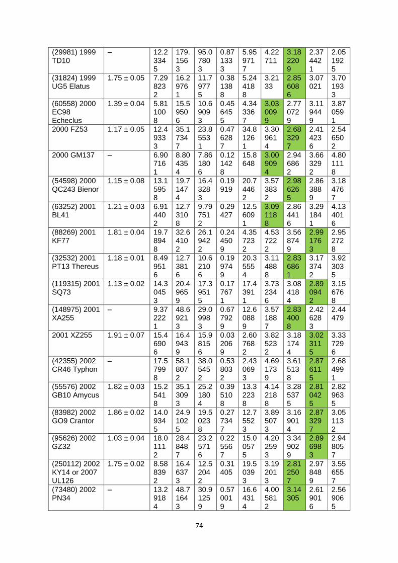
74
(29981) 1999 TD10
– 12.23345
179.1563
95.07803
0.871333
5.959717
4.22711
3.182209
2.374421
2.051925
(31824) 1999 UG5 Elatus
1.75 ± 0.05 7.298232
16.29761
11.79775
0.381388
5.244188
3.2133
2.856086
3.07021
3.701933
(60558) 2000 EC98 Echeclus
1.39 ± 0.04 5.811008
15.59506
10.69093
0.456455
4.343367
3.030099
2.770729
3.119449
3.870591
2000 FZ53 1.17 ± 0.05 12.49333
35.17347
23.85531
0.476287
34.81261
3.309614
2.683297
2.414236
2.546502
2000 GM137 – 6.907161
8.804354
7.861806
0.121428
15.8648
3.009094
2.946862
3.663292
4.801118
(54598) 2000 QC243 Bienor
1.15 ± 0.08 13.15958
19.71474
16.43283
0.19919
20.74462
3.573832
2.986265
2.863889
3.184767
(63252) 2001 BL41
1.21 ± 0.03 6.914402
12.73108
9.797512
0.29427
12.56091
3.091188
2.864416
3.291841
4.134016
(88269) 2001 KF77
1.81 ± 0.04 19.78948
32.64102
26.19422
0.244509
4.357232
4.537222
3.568749
2.991763
2.952728
(32532) 2001 PT13 Thereus
1.18 ± 0.01 8.499516
12.73816
10.62106
0.199749
20.35554
3.114888
2.836861
3.173742
3.923035
(119315) 2001 SQ73
1.13 ± 0.02 14.30453
20.49659
17.39515
0.177671
17.43911
3.732346
3.084184
2.890942
3.156768
(148975) 2001 XA255
– 9.372221
48.69213
29.09983
0.677929
12.60889
3.571887
2.834008
2.426283
2.44479
2001 XZ255 1.91 ± 0.07 15.46906
16.49439
15.98156
0.032069
2.607682
3.825232
3.181744
3.023115
3.337296
(42355) 2002 CR46 Typhon
– 17.57998
58.18072
38.05452
0.538032
2.430693
4.691739
3.615138
2.876115
2.684991
(55576) 2002 GB10 Amycus
1.82 ± 0.03 15.25418
35.13093
25.21804
0.395108
13.32238
4.142188
3.285375
2.810425
2.829635
(83982) 2002 GO9 Crantor
1.86 ± 0.02 14.09345
24.91025
19.50238
0.277347
12.75523
3.895073
3.169014
2.873297
3.051132
(95626) 2002 GZ32
1.03 ± 0.04 18.01112
28.48487
23.25716
0.225567
15.00575
4.202593
3.349029
2.896983
2.948057
(250112) 2002 KY14 or 2007 UL126
1.75 ± 0.02 8.588392
16.46373
12.52042
0.31405
19.50393
3.192013
2.812507
2.978489
3.556557
(73480) 2002 PN34
– 13.29184
48.71643
30.91259
0.570019
16.64314
4.005812
3.14305
2.619016
2.569065
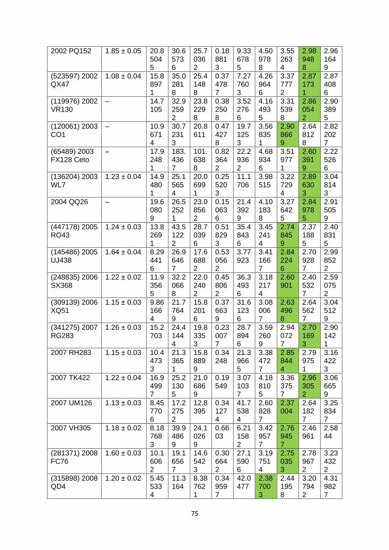
75
2002 PQ152 1.85 ± 0.05 20.85045
30.65736
25.70362
0.188813
9.336785
4.509788
3.552634
2.989488
2.961649
(523597) 2002 QX47
1.08 ± 0.04 15.88971
35.02818
25.41488
0.374787
7.277603
4.269646
3.377772
2.871731
2.874086
(119976) 2002 VR130
– 14.7105
32.92592
23.82298
0.382508
3.522766
4.164935
3.315398
2.860542
2.903895
(120061) 2003 CO1
– 10.96714
30.72313
20.8611
0.474278
19.71253
3.568351
2.908669
2.648128
2.822027
(65489) 2003 FX128 Ceto
– 17.92481
183.4367
101.6388
0.823642
22.29362
4.689346
3.519771
2.603919
2.225266
(136204) 2003 WL7
1.23 ± 0.04 14.94801
25.15654
20.06991
0.255203
11.1706
3.98515
3.227294
2.896303
3.048143
2004 QQ26 – 19.60809
26.52521
23.08562
0.150636
21.43929
4.101838
3.276425
2.849785
2.915059
(447178) 2005 RO43
1.24 ± 0.03 13.82691
43.51222
28.70396
0.518293
35.48436
3.452414
2.748459
2.371885
2.408315
(145486) 2005 UJ438
1.64 ± 0.04 8.294416
26.96467
17.66882
0.530562
3.77923
3.411667
2.842246
2.709287
2.998522
(248835) 2006 SX368
1.22 ± 0.02 11.93565
32.20668
22.02402
0.458062
36.34936
3.182174
2.60901
2.405327
2.590752
(309139) 2006 XQ51
1.15 ± 0.03 9.861664
21.77649
15.82016
0.376639
31.61236
3.080067
2.634968
2.645627
3.045129
(341275) 2007 RG283
1.26 ± 0.03 15.2703
24.41444
19.83353
0.230077
28.78946
3.592609
2.940727
2.701693
2.901421
2007 RH283 1.15 ± 0.03 10.44733
21.33651
15.88899
0.34248
21.39665
3.384727
2.858444
2.799751
3.164223
2007 TK422 1.22 ± 0.04 16.94997
25.21305
21.06869
0.19549
3.071037
4.188105
3.363757
2.963052
3.066659
2007 UM126 1.13 ± 0.03 8.457706
17.22752
12.8395
0.341274
41.75384
2.608287
2.37004
2.641827
3.258347
2007 VH305 1.18 ± 0.02 8.187683
39.94869
24.10269
0.6603
6.211582
3.429577
2.769457
2.46961
2.5844
(281371) 2008 FC76
1.60 ± 0.03 10.16062
19.16567
14.65423
0.306642
27.15906
3.197514
2.750353
2.789672
3.234322
(315898) 2008 QD4
1.20 ± 0.02 5.455334
11.3164
8.387621
0.349597
42.0477
2.387003
2.441958
3.207942
4.319827
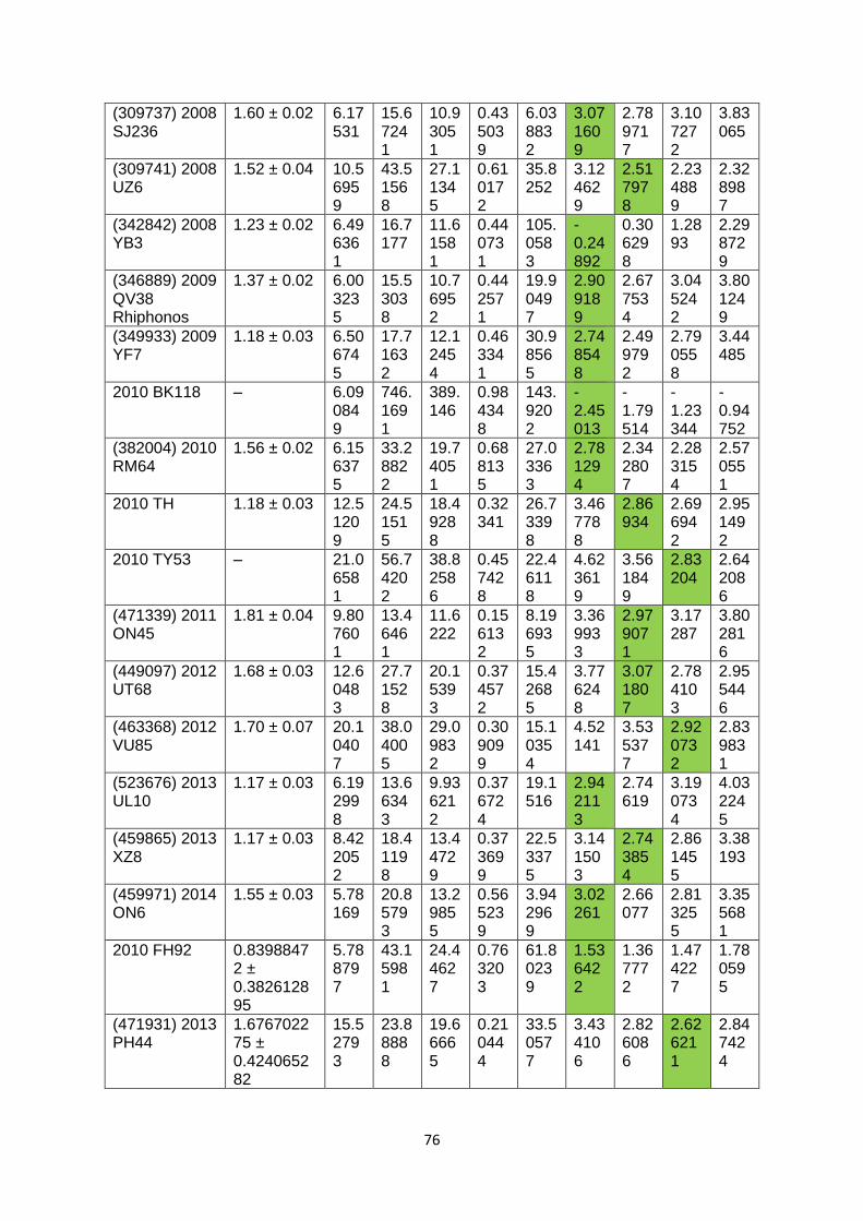
76
(309737) 2008 SJ236
1.60 ± 0.02 6.17531
15.67241
10.93051
0.435039
6.038832
3.071609
2.789717
3.107272
3.83065
(309741) 2008 UZ6
1.52 ± 0.04 10.56959
43.51568
27.11345
0.610172
35.8252
3.124629
2.517978
2.234889
2.328987
(342842) 2008 YB3
1.23 ± 0.02 6.496361
16.7177
11.61581
0.440731
105.0583
-0.24892
0.306298
1.2893
2.298729
(346889) 2009 QV38 Rhiphonos
1.37 ± 0.02 6.003235
15.53038
10.76952
0.442571
19.90497
2.909189
2.677534
3.045242
3.801249
(349933) 2009 YF7
1.18 ± 0.03 6.506745
17.71632
12.12454
0.463341
30.98565
2.748548
2.499792
2.790558
3.44485
2010 BK118 – 6.090849
746.1691
389.146
0.984348
143.9202
-2.45013
-1.79514
-1.23344
-0.94752
(382004) 2010 RM64
1.56 ± 0.02 6.156375
33.28822
19.74051
0.688135
27.03363
2.781294
2.342807
2.283154
2.570551
2010 TH 1.18 ± 0.03 12.51209
24.51515
18.49288
0.32341
26.73398
3.467788
2.86934
2.696942
2.951492
2010 TY53 – 21.06581
56.74202
38.82586
0.457428
22.46118
4.623619
3.561849
2.83204
2.642086
(471339) 2011 ON45
1.81 ± 0.04 9.807601
13.46461
11.6222
0.156132
8.196935
3.369933
2.979071
3.17287
3.802816
(449097) 2012 UT68
1.68 ± 0.03 12.60483
27.71528
20.15393
0.374572
15.42685
3.776248
3.071807
2.784103
2.955446
(463368) 2012 VU85
1.70 ± 0.07 20.10407
38.04005
29.09832
0.309099
15.10354
4.52141
3.535377
2.920732
2.839831
(523676) 2013 UL10
1.17 ± 0.03 6.192998
13.66343
9.936212
0.376724
19.1516
2.942113
2.74619
3.190734
4.032245
(459865) 2013 XZ8
1.17 ± 0.03 8.422052
18.41198
13.44729
0.373699
22.53375
3.141503
2.743854
2.861455
3.38193
(459971) 2014 ON6
1.55 ± 0.03 5.78169
20.85793
13.29855
0.565239
3.942969
3.02261
2.66077
2.813255
3.355681
2010 FH92 0.83988472 ± 0.382612895
5.788797
43.15981
24.44627
0.763203
61.80239
1.536422
1.367772
1.474227
1.780595
(471931) 2013 PH44
1.676702275 ± 0.424065282
15.52793
23.88888
19.66665
0.210444
33.50577
3.434106
2.826086
2.626211
2.847424
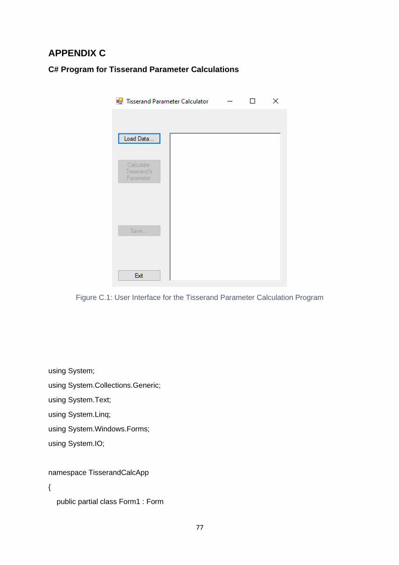
77
APPENDIX C
C# Program for Tisserand Parameter Calculations
Figure C.1: User Interface for the Tisserand Parameter Calculation Program
using System;
using System.Collections.Generic;
using System.Text;
using System.Linq;
using System.Windows.Forms;
using System.IO;
namespace TisserandCalcApp
{
public partial class Form1 : Form
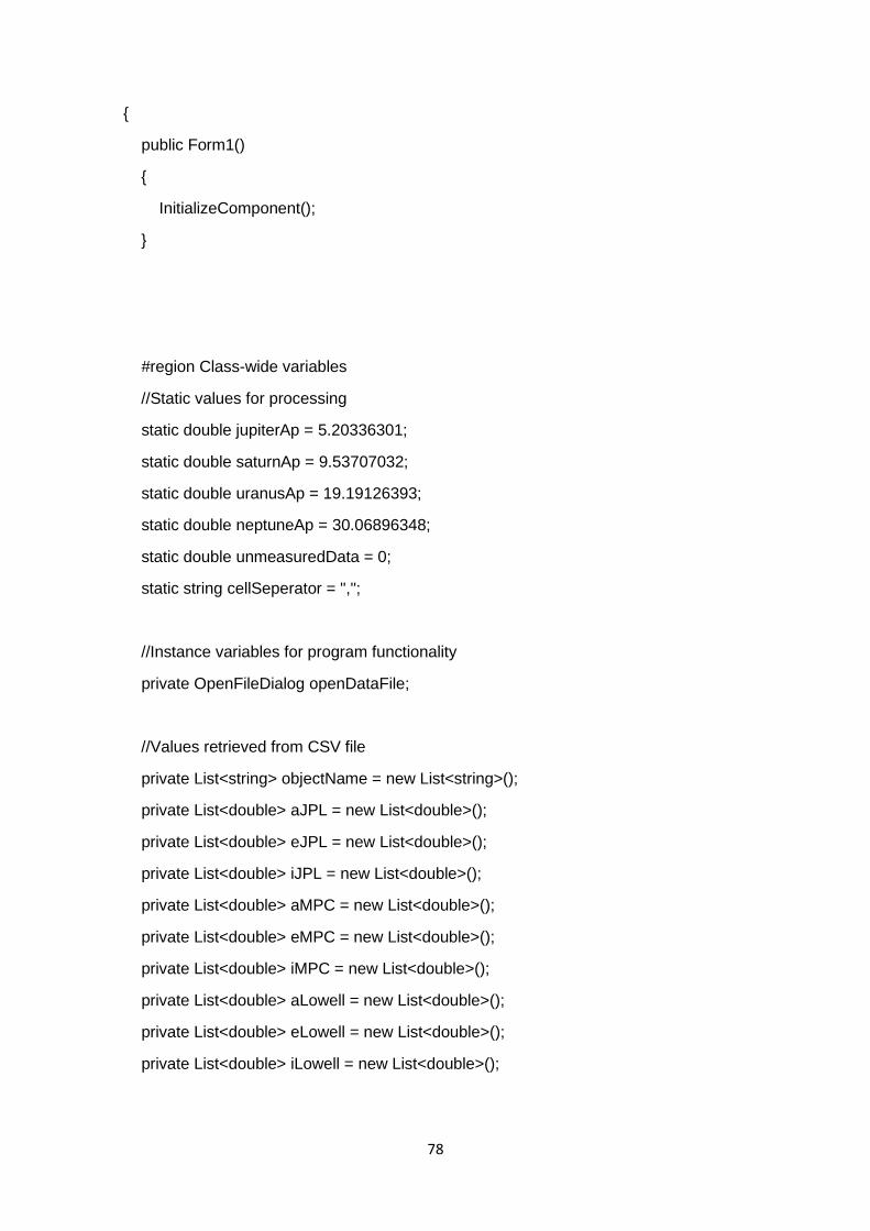
78
{
public Form1()
{
InitializeComponent();
}
#region Class-wide variables
//Static values for processing
static double jupiterAp = 5.20336301;
static double saturnAp = 9.53707032;
static double uranusAp = 19.19126393;
static double neptuneAp = 30.06896348;
static double unmeasuredData = 0;
static string cellSeperator = ",";
//Instance variables for program functionality
private OpenFileDialog openDataFile;
//Values retrieved from CSV file
private List<string> objectName = new List<string>();
private List<double> aJPL = new List<double>();
private List<double> eJPL = new List<double>();
private List<double> iJPL = new List<double>();
private List<double> aMPC = new List<double>();
private List<double> eMPC = new List<double>();
private List<double> iMPC = new List<double>();
private List<double> aLowell = new List<double>();
private List<double> eLowell = new List<double>();
private List<double> iLowell = new List<double>();
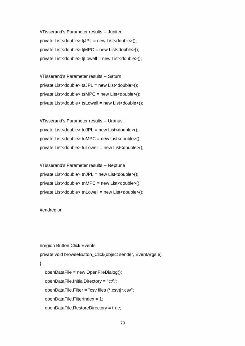
79
//Tisserand's Parameter results -- Jupiter
private List<double> tjJPL = new List<double>();
private List<double> tjMPC = new List<double>();
private List<double> tjLowell = new List<double>();
//Tisserand's Parameter results -- Saturn
private List<double> tsJPL = new List<double>();
private List<double> tsMPC = new List<double>();
private List<double> tsLowell = new List<double>();
//Tisserand's Parameter results -- Uranus
private List<double> tuJPL = new List<double>();
private List<double> tuMPC = new List<double>();
private List<double> tuLowell = new List<double>();
//Tisserand's Parameter results -- Neptune
private List<double> tnJPL = new List<double>();
private List<double> tnMPC = new List<double>();
private List<double> tnLowell = new List<double>();
#endregion
#region Button Click Events
private void browseButton_Click(object sender, EventArgs e)
{
openDataFile = new OpenFileDialog();
openDataFile.InitialDirectory = "c:\\";
openDataFile.Filter = "csv files (*.csv)|*.csv";
openDataFile.FilterIndex = 1;
openDataFile.RestoreDirectory = true;
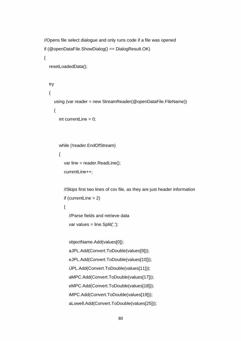
80
//Opens file select dialogue and only runs code if a file was opened
if (@openDataFile.ShowDialog() == DialogResult.OK)
{
resetLoadedData();
try
{
using (var reader = new StreamReader(@openDataFile.FileName))
{
int currentLine = 0;
while (!reader.EndOfStream)
{
var line = reader.ReadLine();
currentLine++;
//Skips first two lines of csv file, as they are just header information
if (currentLine > 2)
{
//Parse fields and retrieve data
var values = line.Split(',');
objectName.Add(values[0]);
aJPL.Add(Convert.ToDouble(values[9]));
eJPL.Add(Convert.ToDouble(values[10]));
iJPL.Add(Convert.ToDouble(values[11]));
aMPC.Add(Convert.ToDouble(values[17]));
eMPC.Add(Convert.ToDouble(values[18]));
iMPC.Add(Convert.ToDouble(values[19]));
aLowell.Add(Convert.ToDouble(values[25]));
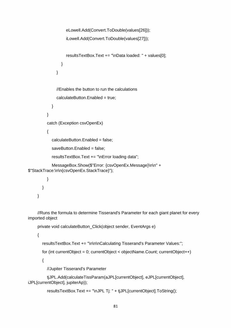
81
eLowell.Add(Convert.ToDouble(values[26]));
iLowell.Add(Convert.ToDouble(values[27]));
resultsTextBox.Text += "\nData loaded: " + values[0];
}
}
//Enables the button to run the calculations
calculateButton.Enabled = true;
}
}
catch (Exception csvOpenEx)
{
calculateButton.Enabled = false;
saveButton.Enabled = false;
resultsTextBox.Text += "\nError loading data";
MessageBox.Show($"Error: {csvOpenEx.Message}\n\n" +
$"StackTrace:\n\n{csvOpenEx.StackTrace}");
}
}
}
//Runs the formula to determine Tisserand's Parameter for each giant planet for every
imported object
private void calculateButton_Click(object sender, EventArgs e)
{
resultsTextBox.Text += "\n\n\nCalculating Tisserand's Parameter Values:";
for (int currentObject = 0; currentObject < objectName.Count; currentObject++)
{
//Jupiter Tisserand's Parameter
tjJPL.Add(calculateTissParam(aJPL[currentObject], eJPL[currentObject],
iJPL[currentObject], jupiterAp));
resultsTextBox.Text += "\nJPL Tj: " + tjJPL[currentObject].ToString();
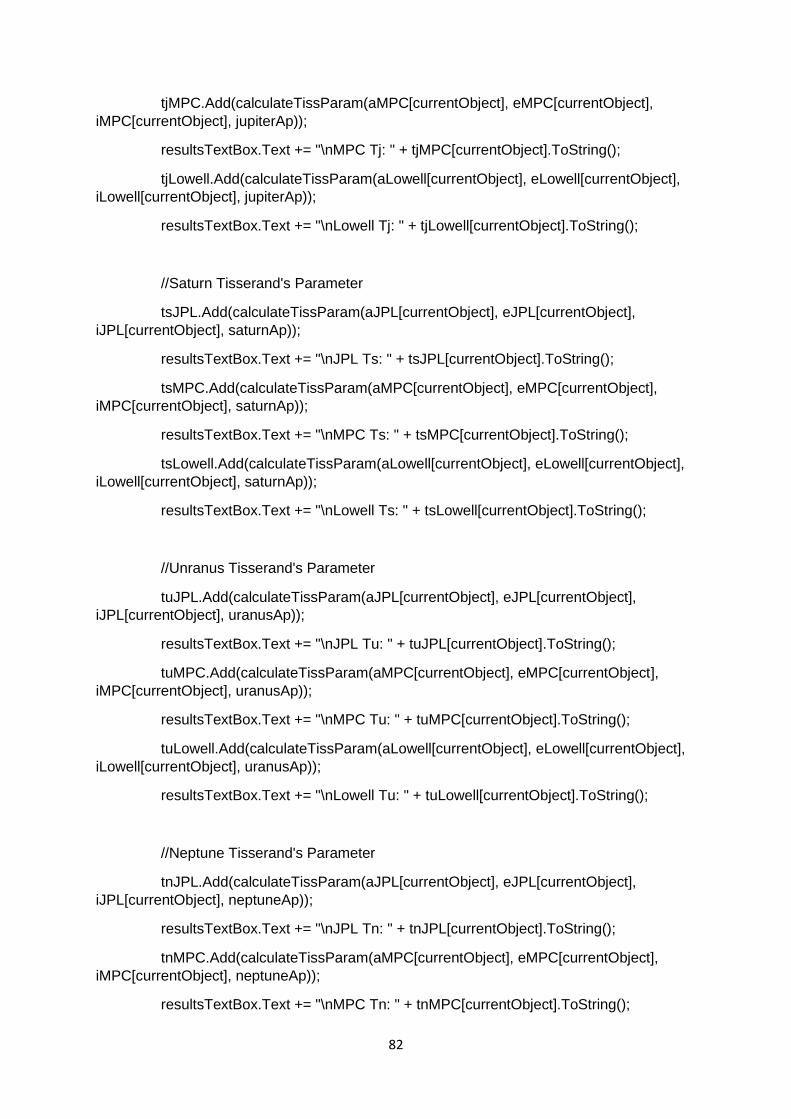
82
tjMPC.Add(calculateTissParam(aMPC[currentObject], eMPC[currentObject],
iMPC[currentObject], jupiterAp));
resultsTextBox.Text += "\nMPC Tj: " + tjMPC[currentObject].ToString();
tjLowell.Add(calculateTissParam(aLowell[currentObject], eLowell[currentObject],
iLowell[currentObject], jupiterAp));
resultsTextBox.Text += "\nLowell Tj: " + tjLowell[currentObject].ToString();
//Saturn Tisserand's Parameter
tsJPL.Add(calculateTissParam(aJPL[currentObject], eJPL[currentObject],
iJPL[currentObject], saturnAp));
resultsTextBox.Text += "\nJPL Ts: " + tsJPL[currentObject].ToString();
tsMPC.Add(calculateTissParam(aMPC[currentObject], eMPC[currentObject],
iMPC[currentObject], saturnAp));
resultsTextBox.Text += "\nMPC Ts: " + tsMPC[currentObject].ToString();
tsLowell.Add(calculateTissParam(aLowell[currentObject], eLowell[currentObject],
iLowell[currentObject], saturnAp));
resultsTextBox.Text += "\nLowell Ts: " + tsLowell[currentObject].ToString();
//Unranus Tisserand's Parameter
tuJPL.Add(calculateTissParam(aJPL[currentObject], eJPL[currentObject],
iJPL[currentObject], uranusAp));
resultsTextBox.Text += "\nJPL Tu: " + tuJPL[currentObject].ToString();
tuMPC.Add(calculateTissParam(aMPC[currentObject], eMPC[currentObject],
iMPC[currentObject], uranusAp));
resultsTextBox.Text += "\nMPC Tu: " + tuMPC[currentObject].ToString();
tuLowell.Add(calculateTissParam(aLowell[currentObject], eLowell[currentObject],
iLowell[currentObject], uranusAp));
resultsTextBox.Text += "\nLowell Tu: " + tuLowell[currentObject].ToString();
//Neptune Tisserand's Parameter
tnJPL.Add(calculateTissParam(aJPL[currentObject], eJPL[currentObject],
iJPL[currentObject], neptuneAp));
resultsTextBox.Text += "\nJPL Tn: " + tnJPL[currentObject].ToString();
tnMPC.Add(calculateTissParam(aMPC[currentObject], eMPC[currentObject],
iMPC[currentObject], neptuneAp));
resultsTextBox.Text += "\nMPC Tn: " + tnMPC[currentObject].ToString();
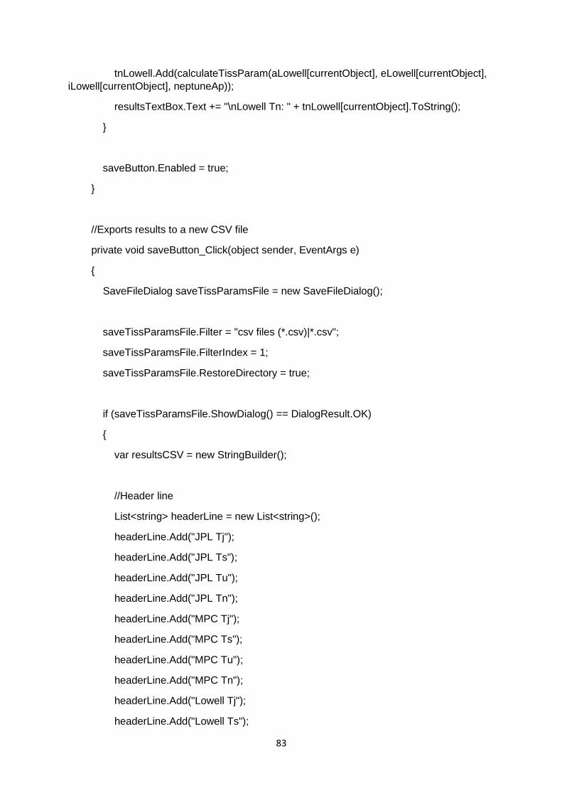
83
tnLowell.Add(calculateTissParam(aLowell[currentObject], eLowell[currentObject],
iLowell[currentObject], neptuneAp));
resultsTextBox.Text += "\nLowell Tn: " + tnLowell[currentObject].ToString();
}
saveButton.Enabled = true;
}
//Exports results to a new CSV file
private void saveButton_Click(object sender, EventArgs e)
{
SaveFileDialog saveTissParamsFile = new SaveFileDialog();
saveTissParamsFile.Filter = "csv files (*.csv)|*.csv";
saveTissParamsFile.FilterIndex = 1;
saveTissParamsFile.RestoreDirectory = true;
if (saveTissParamsFile.ShowDialog() == DialogResult.OK)
{
var resultsCSV = new StringBuilder();
//Header line
List<string> headerLine = new List<string>();
headerLine.Add("JPL Tj");
headerLine.Add("JPL Ts");
headerLine.Add("JPL Tu");
headerLine.Add("JPL Tn");
headerLine.Add("MPC Tj");
headerLine.Add("MPC Ts");
headerLine.Add("MPC Tu");
headerLine.Add("MPC Tn");
headerLine.Add("Lowell Tj");
headerLine.Add("Lowell Ts");
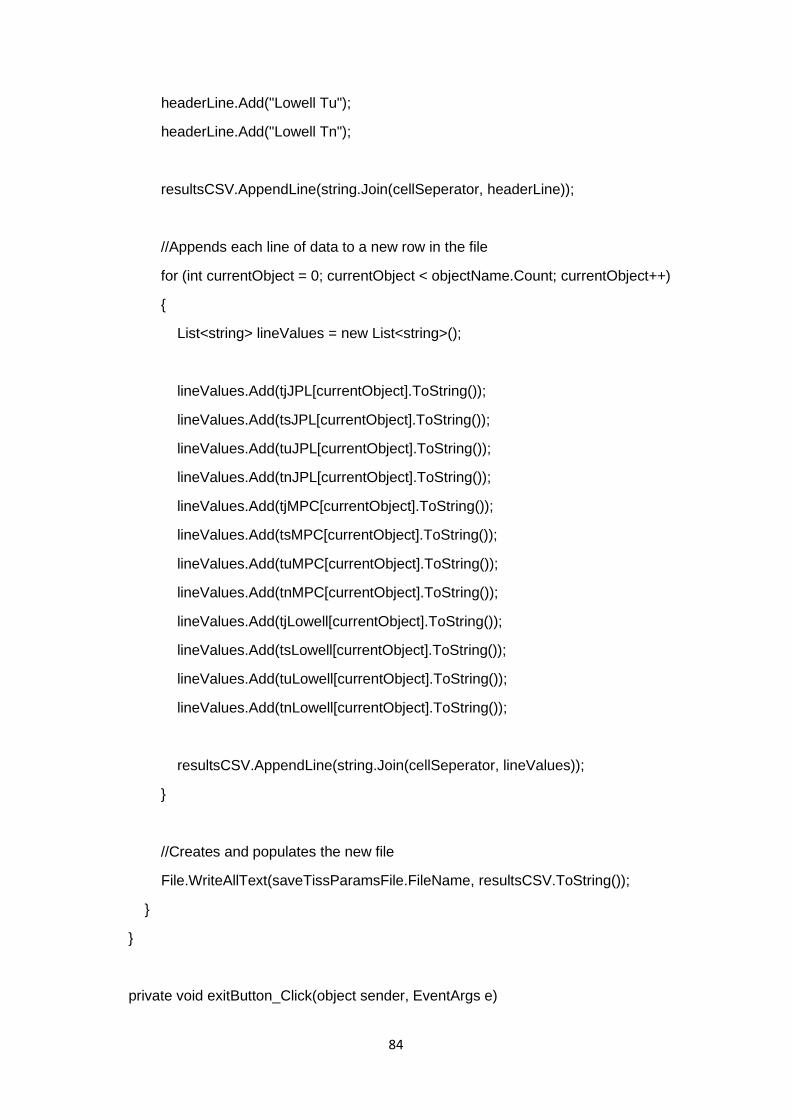
84
headerLine.Add("Lowell Tu");
headerLine.Add("Lowell Tn");
resultsCSV.AppendLine(string.Join(cellSeperator, headerLine));
//Appends each line of data to a new row in the file
for (int currentObject = 0; currentObject < objectName.Count; currentObject++)
{
List<string> lineValues = new List<string>();
lineValues.Add(tjJPL[currentObject].ToString());
lineValues.Add(tsJPL[currentObject].ToString());
lineValues.Add(tuJPL[currentObject].ToString());
lineValues.Add(tnJPL[currentObject].ToString());
lineValues.Add(tjMPC[currentObject].ToString());
lineValues.Add(tsMPC[currentObject].ToString());
lineValues.Add(tuMPC[currentObject].ToString());
lineValues.Add(tnMPC[currentObject].ToString());
lineValues.Add(tjLowell[currentObject].ToString());
lineValues.Add(tsLowell[currentObject].ToString());
lineValues.Add(tuLowell[currentObject].ToString());
lineValues.Add(tnLowell[currentObject].ToString());
resultsCSV.AppendLine(string.Join(cellSeperator, lineValues));
}
//Creates and populates the new file
File.WriteAllText(saveTissParamsFile.FileName, resultsCSV.ToString());
}
}
private void exitButton_Click(object sender, EventArgs e)
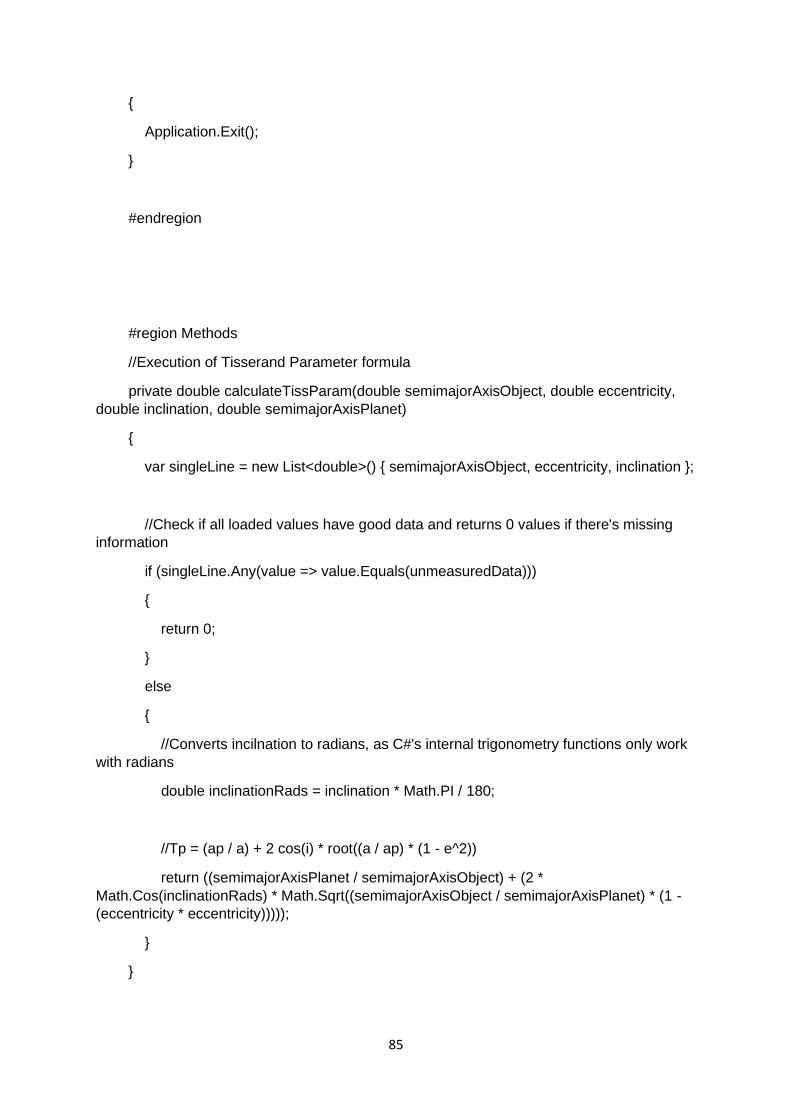
85
{
Application.Exit();
}
#endregion
#region Methods
//Execution of Tisserand Parameter formula
private double calculateTissParam(double semimajorAxisObject, double eccentricity,
double inclination, double semimajorAxisPlanet)
{
var singleLine = new List<double>() { semimajorAxisObject, eccentricity, inclination };
//Check if all loaded values have good data and returns 0 values if there's missing
information
if (singleLine.Any(value => value.Equals(unmeasuredData)))
{
return 0;
}
else
{
//Converts incilnation to radians, as C#'s internal trigonometry functions only work
with radians
double inclinationRads = inclination * Math.PI / 180;
//Tp = (ap / a) + 2 cos(i) * root((a / ap) * (1 - e^2))
return ((semimajorAxisPlanet / semimajorAxisObject) + (2 *
Math.Cos(inclinationRads) * Math.Sqrt((semimajorAxisObject / semimajorAxisPlanet) * (1 -
(eccentricity * eccentricity)))));
}
}
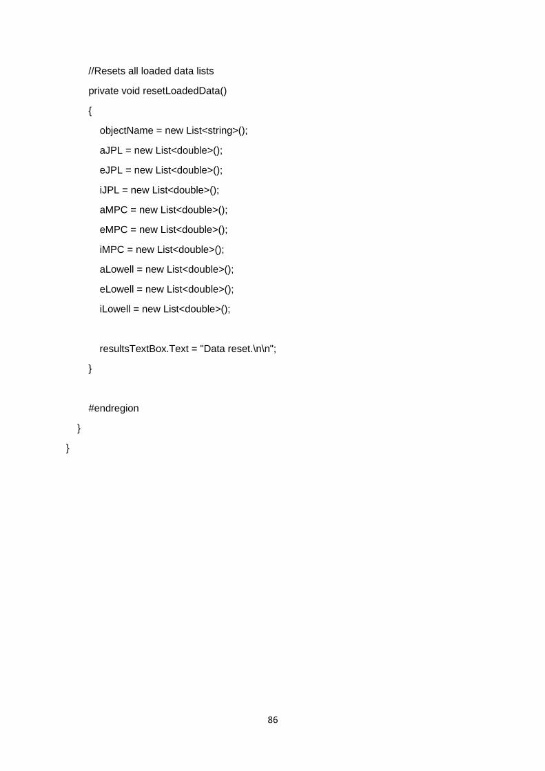
86
//Resets all loaded data lists
private void resetLoadedData()
{
objectName = new List<string>();
aJPL = new List<double>();
eJPL = new List<double>();
iJPL = new List<double>();
aMPC = new List<double>();
eMPC = new List<double>();
iMPC = new List<double>();
aLowell = new List<double>();
eLowell = new List<double>();
iLowell = new List<double>();
resultsTextBox.Text = "Data reset.\n\n";
}
#endregion
}
}

87
APPENDIX D
C# Program for the Conversion of Standard Star Filter Values and the
Subsequent Observed Star Calibrations
Figure D.1: User Interface for the Standard Star Conversion and Calibration Program
using System;
using System.Collections.Generic;
using System.Linq;
using System.Windows.Forms;
using System.IO;
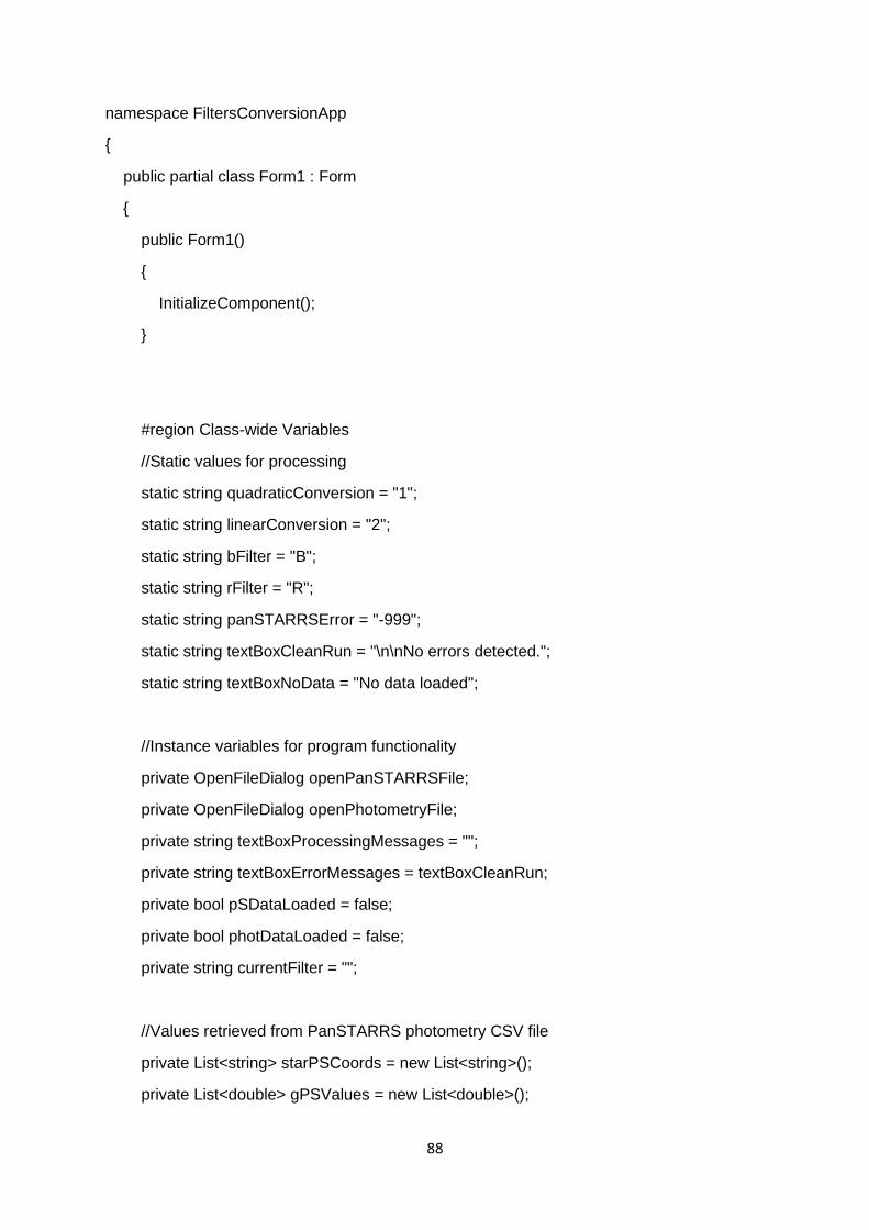
88
namespace FiltersConversionApp
{
public partial class Form1 : Form
{
public Form1()
{
InitializeComponent();
}
#region Class-wide Variables
//Static values for processing
static string quadraticConversion = "1";
static string linearConversion = "2";
static string bFilter = "B";
static string rFilter = "R";
static string panSTARRSError = "-999";
static string textBoxCleanRun = "\n\nNo errors detected.";
static string textBoxNoData = "No data loaded";
//Instance variables for program functionality
private OpenFileDialog openPanSTARRSFile;
private OpenFileDialog openPhotometryFile;
private string textBoxProcessingMessages = "";
private string textBoxErrorMessages = textBoxCleanRun;
private bool pSDataLoaded = false;
private bool photDataLoaded = false;
private string currentFilter = "";
//Values retrieved from PanSTARRS photometry CSV file
private List<string> starPSCoords = new List<string>();
private List<double> gPSValues = new List<double>();
89
private List<double> gPSErrorValues = new List<double>();
private List<double> rPSValues = new List<double>();
private List<double> rPSErrorValues = new List<double>();
private List<bool> goodPSData = new List<bool>();
//Values retrieved from observation's filter photometry text file
private List<string> starPixelCoords = new List<string>();
private List<double> photValues = new List<double>();
private List<double> photErrorValues = new List<double>();
//Coefficients used for filter conversion
static Tuple<double, double, double, double> bQuadraticCoefficients()
{
//Values: A0, A1, A2, Error
return new Tuple<double, double, double, double>(0.212, 0.556, 0.034, 0.032);
}
static Tuple<double, double, double> bLinearCoefficients()
{
//Values: B0, B1, Error
return new Tuple<double, double, double>(0.213, 0.587, 0.034);
}
static Tuple<double, double, double, double> rQuadraticCoefficients()
{
//Values: A0, A1, A2, Error
return new Tuple<double, double, double, double>(0.137, 0.108, 0.029, 0.015);
}
static Tuple<double, double, double> rLinearCoefficients()
{
//Values: B0, B1, Error
return new Tuple<double, double, double>(0.138, 0.131, 0.015);
}
90
//Converted filter values and total errors after conversion operations
private List<double> convertedQuadraticValues = new List<double>();
private List<double> convertedQuadraticErrorValues = new List<double>();
private List<double> totalQuadraticErrorValues = new List<double>();
private List<double> convertedLinearValues = new List<double>();
private List<double> convertedLinearErrorValues = new List<double>();
private List<double> totalLinearErrorValues = new List<double>();
//Values for calibration operations
private List<double> quadraticValueDifferences = new List<double>();
private List<double> quadraticErrorStarValues = new List<double>();
private List<double> linearValueDifferences = new List<double>();
private List<double> linearErrorStarValues = new List<double>();
//Values for final calibrations
private double standardDeviationQuadratic = 0;
private double standardDeviationErrorQuadratic = 0;
private double standardDeviationLinear = 0;
private double standardDeviationErrorLinear = 0;
#endregion Class-wide Variables
#region Button Calls
//Button method. Opens file browsing dialog to select PanSTARRS data file
private void pSDataBrowseButton_Click(object sender, EventArgs e)
{
openPanSTARRSFile = new OpenFileDialog();
openPanSTARRSFile.InitialDirectory = "c:\\";
openPanSTARRSFile.Filter = "csv files (*.csv)|*.csv";
openPanSTARRSFile.FilterIndex = 1;
91
openPanSTARRSFile.RestoreDirectory = true;
//Opens file select dialogue and only runs code if a file was opened
if (@openPanSTARRSFile.ShowDialog() == DialogResult.OK)
{
pSValuesReset();
try
{
using (var reader = new StreamReader(@openPanSTARRSFile.FileName))
{
convertedValuesReset();
bool firstLine = true;
while (!reader.EndOfStream)
{
var line = reader.ReadLine();
//Condition used to skip csv header line
if (firstLine == false)
{
//Parse fields and retrieve data
var values = line.Split(',');
starPSCoords.Add(values[0]);
gPSValues.Add(Convert.ToDouble(values[23]));
gPSErrorValues.Add(Convert.ToDouble(values[24]));
rPSValues.Add(Convert.ToDouble(values[33]));
rPSErrorValues.Add(Convert.ToDouble(values[34]));
var singleLine = new List<string>() { values[23], values[24], values[33],
values[34] };
92
//Check if any of the loaded values have PanSTARRS error code rather
than real values
if (singleLine.Any(value => value.Contains(panSTARRSError)))
{
goodPSData.Add(false);
}
else
{
goodPSData.Add(true);
}
}
else
{
firstLine = false;
}
}
textBoxProcessingMessages += "Data loaded successfully from " +
@openPanSTARRSFile.FileName;
for (var photometryLine = 0; photometryLine < starPSCoords.Count;
photometryLine++)
{
if (photometryLine == 0)
{
textBoxProcessingMessages += "\n\nNew photometry stack
processed:\n";
}
if (goodPSData[photometryLine].Equals(true))
{
textBoxProcessingMessages += "\nStar coordiantes: " +
starPSCoords[photometryLine];
93
}
else
{
if (textBoxErrorMessages == textBoxCleanRun)
{
textBoxErrorMessages = "\n\nBad data detected:\n";
}
textBoxErrorMessages += "\nStar coordiantes: " +
starPSCoords[photometryLine] + "\n" + "Error line: " + (photometryLine + 1).ToString();
}
}
textBoxErrorMessages += "\n\n\n\n";
textBoxProcessingMessages += textBoxErrorMessages;
processingResultsTextBox.Text = textBoxProcessingMessages;
pSLoadedTextBox.Text = "Data loded: " + openPanSTARRSFile.FileName;
pSLoadedTextBox.Enabled = true;
pSDataLoaded = true;
checkAllDataLoaded();
}
}
catch (Exception csvOpenEx)
{
pSDataLoaded = false;
runCalibrationButton.Enabled = false;
saveResultButton.Enabled = false;
pSLoadedTextBox.Text = textBoxNoData;
MessageBox.Show($"Error: {csvOpenEx.Message}\n\n" +
$"StackTrace:\n\n{csvOpenEx.StackTrace}");
94
}
}
}
//Button method. Opens file browsing dialog to select filter photometry data file from
own data, corresponding to the PanSTARRS data file
private void photDataBrowseButton_Click(object sender, EventArgs e)
{
openPhotometryFile = new OpenFileDialog();
openPhotometryFile.InitialDirectory = "c:\\";
openPhotometryFile.Filter = "txt files (*.txt)|*.txt|All files (*.*)|*.*";
openPhotometryFile.FilterIndex = 2; //"All files" is selected by default, as text files in
some linux systems may not be saved with a .txt
openPhotometryFile.RestoreDirectory = true;
//Opens file select dialogue and only runs code if a file was opened
if (openPhotometryFile.ShowDialog() == DialogResult.OK)
{
filterValuesReset();
try
{
using (var reader = new StreamReader(openPhotometryFile.FileName))
{
convertedValuesReset();
while (!reader.EndOfStream)
{
//Parse line of text into an array of individual characters
var line = reader.ReadLine().ToCharArray();
//Condition used to skip header lines or lines not containing enough data (a
line with data has to have exactly 113 characters due to IRAF's formatting)
95
if (line.Length == 112 && line[0] != '#')
{
var retrievedValues = concatinateFilterValues(line);
starPixelCoords.Add(retrievedValues.Item1);
photValues.Add(retrievedValues.Item2);
photErrorValues.Add(retrievedValues.Item3);
//Determines filter type
currentFilter = line[34].ToString();
}
}
textBoxProcessingMessages += "\n\nData loaded successfully from " +
openPhotometryFile.FileName;
for (int photometryLine = 0; photometryLine < starPixelCoords.Count;
photometryLine++)
{
if (photometryLine == 0)
{
textBoxProcessingMessages += "\n\nNew photometry stack
processed:\n";
}
textBoxProcessingMessages += "\nStar coordiantes: " +
starPixelCoords[photometryLine] + " B: " + photValues[photometryLine] + " Error: " +
photErrorValues[photometryLine];
}
processingResultsTextBox.Text = textBoxProcessingMessages;
photLoadedTextBox.Text = "Data loded: " + openPhotometryFile.FileName;
photLoadedTextBox.Enabled = true;
96
photDataLoaded = true;
checkAllDataLoaded();
}
}
catch (Exception csvOpenEx)
{
photDataLoaded = false;
runCalibrationButton.Enabled = false;
saveResultButton.Enabled = false;
photLoadedTextBox.Text = textBoxNoData;
MessageBox.Show($"Error: {csvOpenEx.Message}\n\n" +
$"StackTrace:\n\n{csvOpenEx.StackTrace}");
}
}
}
//Button method. Executes all of the conversion and subsequent calibration operations
for given data files
private void runCalibrationButton_Click(object sender, EventArgs e)
{
convertedValuesReset();
string errorTextBoxText = "\n\nERROR when converting values on lines:";
string errorMessage = "";
int linesCount = 0;
linesCount = starPixelCoords.Count;
//Verifies that all loaded files have same number of datas points
if (starPSCoords.Count != linesCount)
{
MessageBox.Show("Error: Number of lines do not match between data sets. Load
correctly corresponding files and try again.", "Incorrect files", MessageBoxButtons.OK,
MessageBoxIcon.Error);
}
97
else
{
//Executes filter conversions
for (int photometryLine = 0; photometryLine < starPSCoords.Count;
photometryLine++)
{
//Returned values: Conversion execution flag, execution information message,
converted filter value, converted filter error value, total error value for converted filter value
var conversionQuardaticB = FilterConversion(quadraticConversion,
currentFilter, Convert.ToDouble(gPSValues[photometryLine]),
Convert.ToDouble(rPSValues[photometryLine]),
Convert.ToDouble(rPSErrorValues[photometryLine]),
Convert.ToDouble(rPSErrorValues[photometryLine]));
var conversionLinearB = FilterConversion(linearConversion, currentFilter,
Convert.ToDouble(gPSValues[photometryLine]),
Convert.ToDouble(rPSValues[photometryLine]),
Convert.ToDouble(rPSErrorValues[photometryLine]),
Convert.ToDouble(rPSErrorValues[photometryLine]));
if (conversionQuardaticB.Item1 == true)
{
convertedQuadraticValues.Add(conversionQuardaticB.Item3);
convertedQuadraticErrorValues.Add(conversionQuardaticB.Item4);
totalQuadraticErrorValues.Add(conversionQuardaticB.Item5);
errorMessage = conversionQuardaticB.Item2;
}
if (conversionLinearB.Item1 == true)
{
convertedLinearValues.Add(conversionLinearB.Item3);
convertedLinearErrorValues.Add(conversionLinearB.Item4);
totalLinearErrorValues.Add(conversionLinearB.Item4);
errorMessage = conversionLinearB.Item2;
}
else
{
errorTextBoxText += photometryLine.ToString() + errorMessage;
98
textBoxProcessingMessages += errorTextBoxText;
processingResultsTextBox.Text = textBoxProcessingMessages;
//Remove corresponding elements from observation data
starPixelCoords.RemoveAt(photometryLine);
photValues.RemoveAt(photometryLine);
photErrorValues.RemoveAt(photometryLine);
}
}
//Send results to textbox
textBoxProcessingMessages += "\n\nCalibration values:\n";
processingResultsTextBox.Text = textBoxProcessingMessages;
int skippedLines = 0;
for (var photometryLine = 0; photometryLine < starPSCoords.Count;
photometryLine++)
{
//Ignores lines that had PanSTARRS error codes
if (goodPSData[photometryLine] == true)
{
textBoxProcessingMessages += "Star at " + starPSCoords[photometryLine] +
":\n";
//Quadratic star magnitude differences and respective errors
quadraticValueDifferences.Add(convertedQuadraticValues[photometryLine] -
photValues[photometryLine]);
quadraticErrorStarValues.Add(ExecuteQuadratureCalc(convertedQuadraticErrorValues[phot
ometryLine], photErrorValues[photometryLine]));
textBoxProcessingMessages += "Quadratic " + currentFilter + ": " +
quadraticValueDifferences[photometryLine - skippedLines].ToString();
99
textBoxProcessingMessages += " +/- " +
quadraticErrorStarValues[photometryLine - skippedLines].ToString() + "\n";
//Linear star magnitude differences and respective errors
linearValueDifferences.Add(convertedLinearValues[photometryLine] -
photValues[photometryLine]);
linearErrorStarValues.Add(ExecuteQuadratureCalc(convertedLinearErrorValues[photometry
Line], photErrorValues[photometryLine]));
textBoxProcessingMessages += "Linear " + currentFilter + ": " +
linearValueDifferences[photometryLine - skippedLines].ToString();
textBoxProcessingMessages += " +/- " +
linearErrorStarValues[photometryLine - skippedLines].ToString() + "\n";
}
else
{
skippedLines++;
}
}
//Calculates all means for stars differences
double quadraticMean = quadraticValueDifferences.Average();
double quadraticErrorMean = quadraticErrorStarValues.Average();
double linearMean = linearValueDifferences.Average();
double linearErrorMean = linearErrorStarValues.Average();
//Retrieves standard deviations for all star offsets and calcualtes the respective
standard errors of their means
standardDeviationQuadratic =
ExecuteSampleStandardDeviationCalc(quadraticValueDifferences, quadraticMean);
standardDeviationErrorQuadratic =
ExecuteStandardErrorMeanCalc(standardDeviationQuadratic,
quadraticValueDifferences.Count);
standardDeviationLinear =
ExecuteSampleStandardDeviationCalc(linearValueDifferences, linearMean);
100
standardDeviationErrorLinear =
ExecuteStandardErrorMeanCalc(standardDeviationLinear, linearValueDifferences.Count);
textBoxProcessingMessages += "\n\nFinal stars calibration:\nMeans:\n";
textBoxProcessingMessages += "Quadratic " + currentFilter + ": " +
quadraticMean.ToString() + " +/- " + quadraticErrorMean.ToString() + "\n";
textBoxProcessingMessages += "Linear " + currentFilter + ": " +
linearMean.ToString() + " +/- " + linearErrorMean.ToString() + "\n";
textBoxProcessingMessages += "Standard error of the mean:\n";
textBoxProcessingMessages += "Quadratic " + currentFilter + ": +/- " +
standardDeviationErrorQuadratic.ToString() + "\n";
textBoxProcessingMessages += "Linear " + currentFilter + ": +/- " +
standardDeviationErrorLinear.ToString() + "\n";
processingResultsTextBox.Text = textBoxProcessingMessages;
//Make "Save..." button usable
saveResultButton.Enabled = true;
}
}
//Exports the results to a text file with a save file dialog
private void saveResultButton_Click(object sender, EventArgs e)
{
SaveFileDialog saveCalibratedPhotsFile = new SaveFileDialog();
saveCalibratedPhotsFile.Filter = "txt files (*.txt)|*.txt|All files (*.*)|*.*";
saveCalibratedPhotsFile.FilterIndex = 1;
saveCalibratedPhotsFile.RestoreDirectory = true;
if (saveCalibratedPhotsFile.ShowDialog() == DialogResult.OK)
{
File.WriteAllText(saveCalibratedPhotsFile.FileName,
textBoxProcessingMessages);
101
}
}
//Clears the textbox and clears any processed conversion results
private void clearResultsButton_Click(object sender, EventArgs e)
{
textBoxErrorMessages = "";
processingResultsTextBox.Text = "";
textBoxProcessingMessages = "";
convertedValuesReset();
saveResultButton.Enabled = false;
}
//Closes the program
private void exitButton_Click(object sender, EventArgs e)
{
Application.Exit();
}
#endregion Button Calls
#region Methods
//Checks if all files are loaded to enable "Run calibration" button
private void checkAllDataLoaded()
{
if (pSDataLoaded == true && photDataLoaded == true)
{
runCalibrationButton.Enabled = true;
}
}
102
//Resets loaded PanSTARRS values
private void pSValuesReset()
{
starPSCoords = new List<string>();
gPSValues = new List<double>();
gPSErrorValues = new List<double>();
rPSValues = new List<double>();
rPSErrorValues = new List<double>();
goodPSData = new List<bool>();
}
//Resets loaded observation values
private void filterValuesReset()
{
starPixelCoords = new List<string>();
photValues = new List<double>();
photErrorValues = new List<double>();
}
//Resets the converted values lists to empty lists
private void convertedValuesReset()
{
convertedQuadraticValues = new List<double>();
convertedQuadraticErrorValues = new List<double>();
totalQuadraticErrorValues = new List<double>();
convertedLinearValues = new List<double>();
convertedLinearErrorValues = new List<double>();
totalLinearErrorValues = new List<double>();
standardDeviationQuadratic = 0;
standardDeviationErrorQuadratic = 0;
103
standardDeviationLinear = 0;
standardDeviationErrorLinear = 0;
quadraticValueDifferences = new List<double>();
quadraticErrorStarValues = new List<double>();
linearValueDifferences = new List<double>();
linearErrorStarValues = new List<double>();
}
//Concatenates the retrieved characters into a full string and returns them as doubles
private Tuple<string, double, double> concatinateFilterValues(char[] photChars)
{
double magnitude = 0;
double magError = 0;
char[] magnitudeRaw = new char[6];
char[] magErrorRaw = new char[5];
string coordinates = "";
try
{
//Retrieves the X/Y coordinates from the observation image as a string. This value
is contained within 71st to 86th characters in the line (array indexing starts at 0)
for (int charIndex = 70; charIndex <= 85; charIndex++)
{
coordinates += photChars[charIndex];
}
//Retrieves magnitude value. This value is contained within 91st to 96th characters
in the line (array indexing starts at 0)
for (int charIndex = 89; charIndex <= 94; charIndex++)
{
104
magnitudeRaw[charIndex - 89] = photChars[charIndex];
}
//Retrieves error value. This value is contained within 101st to 105ft characters in
the line (array indexing starts at 0)
for (int charIndex = 99; charIndex <= 103; charIndex++)
{
magErrorRaw[charIndex - 99] = photChars[charIndex];
}
magnitude = Convert.ToDouble(new string(magnitudeRaw));
magError = Convert.ToDouble(new string(magErrorRaw));
}
catch (Exception concatException)
{
MessageBox.Show("Error while treating photometry data: " +
concatException.Message + "\n\nStack Trace: " + concatException.StackTrace,
"Concatination Error", MessageBoxButtons.OK, MessageBoxIcon.Error);
}
//Returned values: Measured magnitude, corresponding error
return Tuple.Create(coordinates, magnitude, magError);
}
//Performs filter conversion operations
private Tuple<bool, string, double, double, double> FilterConversion(string
conversionType, string filter, double g, double r, double gError, double rError)
{
bool conversionPossible = true;
string conversionMessage = "";
double convertedFilterValue = 0;
double convertedFilterErrorValue = 0;
double formulaErrorValue = 0;
double totalError = 0;
105
try
{
if (conversionType == quadraticConversion)
{
if (filter == bFilter)
{
convertedFilterValue =
ExecuteQuadraticConversion(bQuadraticCoefficients().Item1,
bQuadraticCoefficients().Item2, bQuadraticCoefficients().Item3, (g - r), g);
convertedFilterErrorValue =
ExecuteQuadraticConversion(bQuadraticCoefficients().Item1,
bQuadraticCoefficients().Item2, bQuadraticCoefficients().Item3, (gError - rError), gError);
formulaErrorValue = bQuadraticCoefficients().Item4;
}
else if (filter == rFilter)
{
convertedFilterValue =
ExecuteQuadraticConversion(rQuadraticCoefficients().Item1, rQuadraticCoefficients().Item2,
rQuadraticCoefficients().Item3, (g - r), r);
convertedFilterErrorValue =
ExecuteQuadraticConversion(rQuadraticCoefficients().Item1, rQuadraticCoefficients().Item2,
rQuadraticCoefficients().Item3, (gError - rError), rError);
formulaErrorValue = rQuadraticCoefficients().Item4;
}
else
{
conversionPossible = false;
conversionMessage = "Program ERROR: No applicable conversion filter
selected";
}
}
else if (conversionType == linearConversion)
{
if (filter == bFilter)
106
{
convertedFilterValue =
ExecuteLinearConversion(bLinearCoefficients().Item1, bLinearCoefficients().Item2, (g - r),
g);
convertedFilterErrorValue =
ExecuteLinearConversion(bLinearCoefficients().Item1, bLinearCoefficients().Item2, (gError -
rError), gError);
formulaErrorValue = bLinearCoefficients().Item3;
}
else if (filter == rFilter)
{
convertedFilterValue = ExecuteLinearConversion(rLinearCoefficients().Item1,
rLinearCoefficients().Item2, (g - r), r);
convertedFilterErrorValue =
ExecuteLinearConversion(rLinearCoefficients().Item1, rLinearCoefficients().Item2, (gError -
rError), rError);
formulaErrorValue = rLinearCoefficients().Item3;
}
else
{
conversionPossible = false;
conversionMessage = "Program ERROR: No applicable conversion filter
selected";
}
}
else
{
conversionPossible = false;
conversionMessage = "Program ERROR: No applicable conversion type
selected";
}
//Calculate resulting errors
if (conversionPossible == true)
{
107
double formulaFilterError = ExecuteQuadratureCalc(convertedFilterValue,
formulaErrorValue);
double formulaErrorError = ExecuteQuadratureCalc(convertedFilterErrorValue,
formulaErrorValue);
totalError = ExecuteQuadratureCalc(formulaFilterError, formulaErrorError);
}
}
catch (Exception convEx)
{
conversionPossible = false;
conversionMessage = $"Conversion ERROR: {convEx.Message}\n\n" +
$"StackTrace:\n\n{convEx.StackTrace}";
}
//Returned values: Conversion execution flag, execution information message,
converted filter value, converted filter error value, total error value for converted filter value
return Tuple.Create(conversionPossible, conversionMessage, convertedFilterValue,
convertedFilterErrorValue, totalError);
}
private double ExecuteQuadraticConversion(double a0, double a1, double a2, double
grColour, double filterSpecificValue)
{
//A0 + A1(g-r) + A2(g-r)^2 + [g or r]
return (a0 + (a1 * grColour) + (a2 * grColour * grColour) + filterSpecificValue);
}
private double ExecuteLinearConversion(double b0, double b1, double grColour,
double filterSpecificValue)
{
//B0 + B1(g-r) + [g or r]
return (b0 + (b1 * grColour) + filterSpecificValue);
}
private double ExecuteQuadratureCalc(double value1, double value2)
108
{
//root(X^2 + Y^2)
return (Math.Sqrt((value1 * value1) + (value2 * value2)));
}
private double ExecuteSampleStandardDeviationCalc(List<double> magVariations,
double magVarMean)
{
double sampleStandardDeviation = 0;
int totalMagValues = magVariations.Count;
//s = root((1/(N-1) * sum(Xi - mean)^2))
sampleStandardDeviation = Math.Sqrt(magVariations.Sum(x => (x - magVarMean) *
(x - magVarMean)) / (totalMagValues - 1));
return sampleStandardDeviation;
}
private double ExecuteStandardErrorMeanCalc(double standardDev, double
errorMean)
{
//StandardErrorOfTheMean = StandardDeviation / root(N)
return (standardDev / Math.Sqrt(errorMean));
}
#endregion Methods
}
}
109
REFERENCES:
Barrett, A. A. Observations of Comets in Greek and Roman Sources Before A.D. 410. Journal of the
Royal Astronomical Society of Canada. 1978, 72, pp. 81.
Behar, E.; Nilsson, H.; Henri, P.; Bercic, L.; Nicolaou, G.; Wieser, G. S.; Wieser, M.; Tabone, B.;
Saillenfest, M.; Goetz, C. The root of a comet tail: Rosetta ion observations at comet 67P/Churyumov-
Gerasimenko. Astronomy & Astrophysics. 2018, 6616, A21.
Bessell, M. S. UBVRI Passbands. Publications of the Astronomical Society of the Pacific. October 1990,
102, pp. 1181-1199.
Bockelée-Morvan, D.; Crovisier, J.; Mumma, M. J.; Weaver, H. A. The Composition of Cometary
Volatiles. In: M. C. Festou, H. U. Keller, and H. A. Weaver, eds. Comets II. Tuscon: University of Arizona
Press, 2004, pp. 391-423.
Bonett, D.G.; Wright, T.A. Sample size requirements for estimating Pearson, Kendall and Spearman
correlations. Psychometrika. 2000, 65, pp. 23–28.
Broiles, T. W.; Burch, J. L.; Clark, G.; Koenders, C.; Behar, E.; Goldstein, G.; Fuselier, S. A.; Mandt, K.
E.; Mokashi, P.; Samara, M. Rosetta observations of solar wind interaction with the comet
67P/Churyumov-Gerasimenko. Astronomy & Astrophysics. 2015, 583, A21.
Brown, M. How many dwarf planets are there in the solar system? (updates daily) [online]. California
Institute of Technology. [Viewed date: 20 February 2020].
Available from: <http://web.gps.caltech.edu/~mbrown/dps.html>
CAHA – Centro Astronómico Hispano en Andalucía. CAFOS - Focal Reducer and Faint Object
Spectrograph for the 2.2m Telescope [online]. CAHA. [Viewed date: 2 February, 2020].
Available from: <http://w3.caha.es/CAHA/Instruments/CAFOS/cafos_overview.html>
CAHA – Centro Astronómico Hispano en Andalucía. Filterlist for CCD-Observations [online]. CAHA.
[Viewed date: 2 February, 2020].
Available from: <https://www.caha.es/CAHA/Instruments/filterlist.html>
CAHA – Centro Astronómico Hispano en Andalucía. MOSCA [online]. CAHA. [Viewed date: 2 February,
2020].
Available from: <http://w3.caha.es/CAHA/Instruments/MOSCA/index.html>
110
CDS – Centre de Données astronomiques de Strasbourg. Aladin Sky Atlas [online]. Université de
Strasbourg/CNRS. [Viewed date: 15 February 2020].
Available from: <https://aladin.u-strasbg.fr/aladin-f.gml>
Christou, A. A.; Wiegert, P. A population of Man Belt Asteroids co-orbiting with Ceres and Vesta. Icarus.
January 2012, 217, pp. 27-42.
Cousins, A. W. J. VRI Standards in the E Regions. Memoirs of the Royal Astronomical Society. 1976,
81, pp. 25-36.
Cruikshank, D. P.; Ore, C. M. D.; Roush, T. L.; Geballe, T. R.; Owen, T. C.; Bregh, C.; Cash, M. D.;
Hartmann, W. K. Constraints on the Composition of Trojan Asteroid 624 Hektor. Icarus. October 2001,
153, pp. 348-360.
Davidsson, B. J. R.; Skorov, Y. V. On the Light.Absorbing Surface Layer of Cometary Nuclei: I.
Radiative Transfer. Icarus. March 2002, 156, pp. 223-248.
Delsanti, A.; Hainaut, O.; Jourdeuil, E.; Meech, K.J.; Boehnhardt, H.; Barrera, L. Simultaneous visible-
near IR photometric study of Kuiper belt Object surfaces with the ESO/Very Large Telescopes.
Astronomy & Astrophysics. 2004, 417, pp. 1145-1158.
Delsanti A., Jewitt D. (2006) The Solar System Beyond the Planets. In: Blondel P.; Mason J.W. (eds)
Solar System Update. Springer Praxis Books, 2006, pp. 267.
Doressoundiram, A.; Thebault, P. Colors and collision rates within the Kuiper belt: problems with the
collisional resurfacing scenario. Icarus. March 2003, 162, pp. 27-37.
Duncan, M.J. Dynamical Origin of Comets and Their Reservoirs. Space Science Reviews. Springer,
July 2008, 138, pp. 109–126.
Duncan, M. J.; Levison, H. F. A disk of scattered icy objects and the origin of Jupiter-family comets.
Science. June 1997, 276, pp. 1670-1672.
Emel’yanenko, V. V.; Kiselava, E. L.; Resonant motion of trans-Neptunian objects in high-eccentricity
orbits. Astronomy Letters. Springer, 2009, 34, pp. 271-279.
Epifani, E. M.; Dotto, E.; Ieva, S.; Perna, D.; Palumbo, P.; Micheli, M.; Perozzi, E. 523676 (2013 UL10):
The First Active Red Centaur? Astronomy & Astrophysics. December 2018, 620, A93.
111
Fraser, W. C.; Brown, M. E. The Hubble Wide Field Camera 3 Test of Surfaces in the Outer Solar
System: The Compositional Classes of the Kuiper Belt. The Astrophysical Journal. The American
Astronomical Society, April 2012, 749, pp. 33.
Gladman, B; Chan, C. Production of the Extended Scattered Disk by Rogue Planets. The Astrophysical
Journal. The American Astronomical Society, June 2006, 643, L135-L138.
Gladman, B., Marsden, B. G., & Vanlaerhoven, C. Nomenclature in the Outer Solar system. In: Barucci,
M. A.; Boehnhardt, H.; Cruikshank, D. P.; Morbidelli, A., eds. The Solar System Beyond Neptune.
Tucson: University of Arizona Press, 2008, 43-57.
Gladman, B.; Holman, M.; Grav, T.; Kavelaars, J.; Nicholson, J.; Aksnes, K.; Petit, J.-M. Evidence for
an Extended Scattered Disk. Icarus. June 2002, 157, pp. 269-279.
Gomes, R. S.; Matese, J. J.; Lissauer, J. J.; A distant planetary-mass solar companion may have
produced distant detached objects. Icarus. October 2006, 184, pp. 589-601.
Green, D. W. E. Magnitude Corrections for Atmospheric Extinction. International Comet Quarterly. July
1992, 14, pp. 55-59.
Greenberg, J. Mayo. Making a Comet Nucleus. Astronomy and Astrophysics. Leiden: Astron.
Astrophys. 1998, 330, 375-380.
Hainaut, O. R.; Boehnhardt, H.; Protopapa, S. Minor Bodies in the Outer Solar System: Magnitudes and
Colours: Absolute magnitude and Colour Histograms and Cummulative Distributions [online]. MBOSS-
2; ESO – European Southern Observatory. [Viewed date: 20 February 2020].
Available from: <https://www.eso.org/~ohainaut/MBOSS/mbossWeb_hist.html>
Hartigan, J. A.; Hartigan, P. M. The Dip Test of Unimodality. The Annals of Statistics. The Institute of
Mathematical Statistics, 1985, 13, pp. 70.84.
Hills, J. G. Comet showers and the steady-state infall of comets from the Oort cloud. Astronomical
Journal. November 1981, 86, pp. 1730-1740.
Horner, J.; Evans, N. W.; Bailey, M. E.; Asher, D. J. The populations of comet-like bodies in the Solar
system. Monthly Notices of the Royal Astronomical Society. August 2003, 343, pp. 1057-1066.
Howell, S. B. Overscan and Bias. In: Howell, S. B., ed. Handbook of CCD Astronomy. 2nd ed.
Cambridge: Cambridge University Press, 2001, pp. 37-39.
112
Hui, M.-T.; Jewitt, D.; Clark, D. Pre-Discovery Observations and Orbit of Comet C/2017 K2
(PANSTARRS). The Astronomical Journal. The American Astronomical Society, December 2017, 155,
pp. 25.
IAU – International Astronomical Union. Resolution B5: Definition of a Planet in the Solar System. IAU,
2006. [Viewed date: 2 January 2020].
Available from: <https://www.iau.org/static/resolutions/Resolution_GA26-5-6.pdf>
IAU – International Astronomical Union. Minor Planets Center: List of Neptune Trojans [online]. IAU,
2020. [Viewed date: 10 February 2020].
Available from: <https://minorplanetcenter.net/iau/lists/NeptuneTrojans.html>
IPAC. 2MASS: The Two Micros All Sky Survey at IPAC [online]. Caltech – California Institute of
Technology, 2006. [Viewed date: 15 February 2020].
Available from: <https://old.ipac.caltech.edu/2mass/>
Jewitt, D. The Resonant KBOs: Mean Motion Resonances [online]. UCLA – University of California, Los
Angeles. [Viewed date: 14 February 2020].
Available from: <http://www2.ess.ucla.edu/~jewitt/kb/resonant.html>
Jewitt, D. A First Look at the Damocloids. The Astronomical Journal. The American Astronomical
Society, January 2005, 129, pp. 530-538.
Jewitt, D. Kuiper Belt and Comets: An Observational Perspective. In: Jewitt, D.; Morbidelli, A.; Rauer,
H. Tans-Neptunian Objects and Comets. Springer, 2008, pp. 1-78. Saas-Fee Advanced Course 35.
Swiss Society for Astrophysics and Astronomy.
Jewitt, D. The Active Centaurs. The Astronomical Journal. The American Astronomical Society, May
2009, 137, pp. 4296-4312.
Jewitt, D. Color Systematics of Comets and Related Bodies. The Astronomical Journal. The American
Astronomical Society, December 2015, 150, pp. 201.
Jewitt, D. The Trojan Color Conundrum. The Astrophysical Journal. The American Astronomical
Society, February 2018, 155, pp. 56.
Jewitt, D. A deep dive into the abyss. Science, February 2020, aba6889.

113
Jewitt, D.; Chizmadia, L.; Grimm, R.; Prialnik, D. Water in the Small Bodies of the Solar System. In: B.
Reipurth, D. Jewitt, and K. Keil, eds. Protostars and Planets V. Tucson: University of Arizona Press,
2007, pp. 863-878.
Jewitt, D.; Hui, Man-To; Mutchler, M.; Weaver, H.; Li, J.; Agarwal, J. A Comet Active Beyond the
Crystallization Zone. The Astrophysical Journal Letters. The American Astronomical Society, October
2017, 847, article ID L19, pp. 5.
Jewitt, D. C.; Luu, J. X. Colors and Spectra of Kuiper Belt Objects. The Astronomical Journal. The
American Astronomical Society, October 2001, 122, pp. 2099-2114.
Johnson, H. L. Photometric Systems. In: Strand, K. A. Basic Astronomical Data: Stars and Stellar
Systems. Chicago: University of Chicago Press, 1963, pp. 204-224.
JPL – Jet Propulsion Laboratory, NASA, California Institute of Technology. Solar System Dynamics:
JPL Small-Body Database Search Engine [online]. [Viewed date: 10 February 2020].
Available from: <https://ssd.jpl.nasa.gov/sbdb_query.cgi>
JPL – Jet Propulsion Laboratory, NASA, California Institute of Technology. Orbital Classification:
Centaurs [online]. [Viewed date: 10 February 2020].
Available from: <https://ssd.jpl.nasa.gov/sbdb_help.cgi?class=CEN>
KDE-Edu – KDE Education Project. KStars [online]. KDE. [Viewed date: 15 February 2020].
Available from: <https://edu.kde.org/kstars/>
Kosai, H. Short-period comets and Apollo-Amor-Aten type asteroids in view of Tisserand invariant.
Celestial Mechanics and Dynamical Astronomy, March 1992, 54, 237.
Kresak, L. On the similarity of orbits of associated comets, asteroids and meteoroids. Bulletin of the
Astronomical Institutes of Czechoslovakia, May 1982, 33, 104.
Landolt, A. U. UBVRI Photometric Standard Stars in the Magnitude Range 11.5<V<16.0 Around the
Celestial Equator. The Astronomical Journal. July 1992, 104, pp. 340-491.
Landolt, A. U. UBVRI Photometric Standard Stars Around the Celestial Equator: Updates and Additions.
The Astronomical Society. The American Astronomical Society, May 2009, 137, pp. 4186-4269.
Landolt, A. U. UBVRI Photometric Standard Stars Around the Sky at +50 deg Declination. The
Astronomical Journal. The American Astronomical Society, November 2013, 146, pp. 131.
114
Levison, H. F. Comet Taxonomy. Astronomical Society of the Pacific: Conference Series. 1996, 107,
pp. 173.
Levison, H. F.; Dones, L.; Duncan, M. J. The Origin of Halley-Type Comets: Probing the Inner Oort
Cloud. The Astronomical Journal. The American Astronomical Society, April 2001, 121, pp. 2253-2267.
Levison, H. F.; Duncan, M. J. From the Kuiper Belt to Jupiter-Family Comets: The Spatial Distribution
of Ecliptic Comets. Icaurs. May 1997. 127, pp. 13-32.
Levison, H. F.; Morbidelli, A.; The formation of the Kuiper belt by the outward transport of bodies during
Neptune’s migration. Nature, November 2003, 426, 419-421.
Lowell astroDB. AstFinder: Asteroid Finder Chart [online]. Lowell Observatory. [Viewed date: 15
February 2020].
Available from: <https://asteroid.lowell.edu/astfinder/>
Luu, J.; Jewitt, D. Color Diversity Among the Centaurs and Kuiper Belt Objects. The Astronomical
Journal, November 1996, 112, 5, pp. 2310-2318.
Luu, J. X.; Jewitt, D. C.; Kuiper Belt Objects: Relics from the Accretion Disk of the Sun. Annual Reviews
of Astronomy and Astrophysics. September 2002, 40, pp. 63-101.
Marzari, F.; Tricarico, P.; Scholl, H. The MATROS project: Stability of Uranus and Neptune Trojans.
The case of 2001 QR322. Astronomy & Astrophysics. 2003a, 410, pp. 725-734.
Marzari, F.; Tricarico, P.; Scholl, H. Stability of Jupiter Trojans investigated using frequency map
analysis: the MATROS project. Monthly Notices of the Royal Astronomical Society. November 2003b,
345, pp. 1091-1100.
MathWorks. Help Center: corr [online]. MathWorks. [Viewed date: 19 February 2020].
Available from: <https://www.mathworks.com/help/stats/corr.html>
MathWorks. Help Center: ranksum [online]. MathWorks. [Viewed date: 19 February 2020].
Available from: <https://www.mathworks.com/help/stats/ranksum.html>
McDonald, G. D.; Whited, L. J.; DeRuither, C.; Khare, B. N.; Patnaik, A.; Sagan, C. Production and
Chemical Analysis of Cometary Ice Tholins. Icarus. July 1996, 122, pp. 107-117.
115
Morbidelli, A.; Brown, M. E. The Kuiper Belt and the Primordial Evolution of the Solar System. In: Festou,
M. C.; Keller, H. U.; Weaver, H. A.; eds. Comets II. Tuscon: University of Arizona Press, 2004, pp. 175-
191.
Morbidelli, A.; Levison, H. F. Scenarios for the Origin of the Orbits of the Trans-neptunian Objects 2000
CR105 and 2003 VB12 (Sedna). The Astronomical Journal. The American Astronomical Society,
November 2004, 128, pp. 2564-2576.
Mumma, M. J.; Charnley, S. B. The Chemical Composition of Comets—Emerging Taxonomies and
Natal Heritage. Annual Reviews of Astronomy and Astrophysics. 2011, 49, pp. 471-524.
Murray, C. D.; Dermott, S. F. The Restricted Three-Body Problem. In: Carl D. Murray, Stanley F.
Dermott, eds. Solar System Dynamics. Cambridge: Cambridge University Press, 2000, pp. 63-129.
NOAO – National Optical Astronomy Observatory. IRAF Help page for the phot task or topic [online].
NOAO, 2000. [Viewed date: 1 February 2020].
Available from: <http://iraf.noao.edu/scripts/irafhelp?phot>
NSSDCA – NASA Space Science Data Coordinated Archive. Neptune Fact Sheet [online]. NSSDCA.
[Viewed date: 12 February 2020].
Available from: <https://nssdc.gsfc.nasa.gov/planetary/factsheet/neptunefact.html>
Oort, J. H. Origin and Development of Comets. The Observatory. The Halley Lecture for 1951, delivered
at Oxford on May 1. August, 1951.
Pan-STARRS. The Pan-STARRS1 data archive home page [online]. STScI – Space Telescope Science
Institute. [Viewed date: 15 February 2020].
Available from: <https://panstarrs.stsci.edu/>
Pan-STARRS. Pan-STARRS Catalog Search [online]. STScI – Space Telescope Science Institute.
[Viewed date: 15 February 2020].
Available from: <https://catalogs.mast.stsci.edu/panstarrs/>
Peixinho, N.; Delsanti, A.; Doressoundiram, A. Reanalyzing the visible colors or Centaurs and KBOs:
what is there and what we might be missing. Astronomy & Astrophysics. 2015, 577, A35.
Peixinho, N.; Delsanti, A.; Guilbert-Lepoutre, A.; Gafeira, R.; Lacerda, P. The bimodal colors of
Centaurs and small Kuiper belt objects. Astronomy & Astrophysics. 2012, 546, A86.
116
Peixinho, N.; Doressoundiram, A.; Delsanti, A.; Boehnhasdt, H.; Baruccis, M. A.; Belskaya, I. Reopening
the TNOs color controversy: Centaurs bimodality and TNOs unimodality. Astronomy & Astrophysics.
2003, 410, L29-L32.
Peixinho, N.; Thirouin, A.; Tegler, S. C.; Di Sisto, R. P.; Delsanti, A.; Gilbert-Lepoutre, A.; Bauer, J. G.
From Centaurs to comets: 40 years. In: Prialnik, D.; Barucci, M. A.; Young, L. The Trans-Neptunian
Solar System. 1st Edition. Elsevier, November 2019, pp. 307-329.
Pogson, N. Magnitudes of Thirty-six of the Minor Planets for the first day of each month of the year
1857. Monthly Notices of the Royal Astronomical Society. 1857, 17, pp. 12-15.
R Documentation. Dip.test [online]. R Project. [Viewed date: 20 February 2020].
Available from: <https://www.rdocumentation.org/packages/diptest/versions/0.75-7/topics/dip.test>
Racine, R. The Telescope Point-Spread Function. Publications of the Astronomical Society of the
Pacific. August 1996, 108, pp. 699-705.
Rayleigh, Lord. XXXIV. On the transmission of light through an atmosphere containing small particles
in suspension, and on the origin of the blue of the sky. 1899.
Richmond, M. Photometric systems and colors [online]. Rochester Institute of Technology. [Viewed
date: 3 February, 2020].
Available from: <http://spiff.rit.edu/classes/phys445/lectures/colors/colors.html>
SAOImageDS9. SAOImageDS9 Version 8.1 [online]. Smithsonian Astrophysical Observatory. [Viewed
date: 5 January 2020].
Available from: <http://ds9.si.edu/site/Home.html>
Sarid, G.; Volk, K.; Steckloff, J. K.; Harris, W.; Womack, M.; Woodney, L. M. 29P/Schwassmann-
Wachmann 1, A Centaur in the Gateway to the Jupiter-family Comets. The Astrophysical Journal
Letters. The American Astronomical Society, September 2019, 883, article ID L25, pp. 7.
Sheppard, S. S. The Colors of Extreme Outer Solar System Objects. The Astronomical Journal. The
American Astronomical Society, April 2010, 139, pp. 1394-1405.
Sheppard, S. S.; Trujillo, C. A. A Thick Cloud of Neptune Trojans and Their Colors. Science, 28 July
2006, 3313, pp. 51-514.
117
Spearman, C. The Proof and Measurement of Association between Two Things. The American Journal
of Psychology. University of Illinois Press, January 1904, 15, pp. 72-101.
Stern, S. A.; Weaver, H. A.; Spencer, J. R.; Olkin, C. B.; Gladstone, G. R.; Grundy, W. M.; Moore, J.
M.; Cruikshank, D. P. Initial results from the New Horizons exploration of 2014 MU69, a small Kuiper
Belt object. Science, May 2019, 364, eaaw9771.
Stetson, P. B. On the Growth-Curve Method for Calibrating Stellar Photometry with CCDs. Publications
of the Astronomical Society of the Pacific. August 1990, 102, pp. 932-948.
Tegler, S. C.; Romanishin, W. Two distinct populations of Kuiper-belt objects. Nature. 1998, 392, pp.
49-51.
Tegler, S. C.; Romanishin, W. Resolution of the Kuiper belt color Constroversy: two distinct color
populations. Icarus. 2003, 161, pp. 181-191.
Tegler, S. C.; Romanishin, W; Consolmagno, S. J. Two Color Populations of Kuiper Belt and Centaur
Objects and the Smaller Orbital Inclinations of Red Centaur Objects. The Astronomical Journal. The
American Astronomical Society, December 2016, 152, pp. 210.
Tegler; Romanishin; Consolmagno. Kuiper Belt Object Magnitudes and Surface Colors [online].
Northern University of Arizona. [Viewed date: 26 January 2020].
Available from: <http://www.physics.nau.edu/~tegler/research/survey.htm>
Thebault, P. A. Numerical Check of the Collisional Resurfacing Scenario. Earth, Moon, and Planets.
Springer, June 2003, 92, pp. 233-241.
Thompson, W.R.; Murray, B.; Khare, B.; Sagan, C. Coloration and darkening of methane clathrate and
other ices by charged particle irradiation: Applications to the outer solar system. Journal of Geophysical
Research: Space Physics. 1987, 92, pp. 14933-14947.
Tiscareno, M. S.; Malhotra, R. The dynamics of known Centaurs. The Astronomical Journal. December
2003, 126, pp. 3122–3131.
Tiscareno, M. S.; Malhotra, R. Chaotic Diffusion of Resonant Kuiper Belt Objects. The Astronomical
Journal. The American Astronomical Society, September 2009, 138, pp. 827-837.
Tonry, J. L.; Stubbs, C. W.; Lykke, K. R.; Doherty, P.; Shivvers, I. S.; Burgett, W. S.; Chambers, K. C.;
Hodapp, K. W.; Kaiser, N.; Kudritzki, R.-P.; Magnier, E. A.; Morgan, J. S.; Price, P. A.; Wainscoat, R. J.
The Pan-STARRS1 Photometric System. The Astrophysical Journal. The American Astronomical
Society, May 2012, 750, pp. 99.
118
Trujillo, C. A.; Brown, M. E. A Correlation between Inclination and Color in the Classical Kuiper Belt.
The Astrophysical Journal. The American Astronomical Society, February 2002, 556, L125-L128.
Trujillo, C. A.; Brown, M. E.; Rabinowitz, D. L.; Geballe, T. R. Near-Infrared Surface Properties of the
Two Intrinsically Brightest Minor Planets: (90377) Sedna and (90482) Orcus. The Astrophysical Journal.
The American Astronomical Society, July 2005, 627, pp. 1057-1065.
Volk, K., Malhotra, R. Do Centaurs preserve their source inclinations? Icarus. February 2013, 224, pp.
66–73.
Wan, X.-S.; Huang, T.-Y. The orbit evolution of 32 plutinos over 100 million year. Astronomy &
Astrophysics. 2001, 368, pp. 700-705.
Wells, D. C.; Greisen, E. W.; Harten, R. H. FITS: A Flexible Image Transport System. Astronomy &
Astrophysics Supplement Series. June 1981, 44, pp. 363-370.
Whitman, K.; Morbidelli, A.; Jedicke, R. The size-frequency distribution of dormant Jupiter family
comets. Icarus. July 2006, 183, PP. 101-114.
Wilcoxon, F. Individual Comparisons by Ranking Methods. Biometrics Bulletin. International Biometric
Society, December 1945, 1, pp. 80-83.
Wong, I.; Brown, M. E.; The Bimodal Color Distribution of Small Kuiper Belt Objects. The Astronomical
Journal. The American Astronomical Society, April 2017, 153, pp. 145.
Yu, Q.; Tremaine, S. The Dynamics of Plutinos. The Astronomical Journal. The American Astronomical
Society, October 1999, 118, pp. 1873-1881.


