Embed Size (px)
Citation preview
Department of Engineering
PhD Thesis
A Study into the 2D and 3D Laser Forming of Metallic Components
Thesis submitted in accordance with the requirements of The University of Liverpool for the degree of
Doctor in Philosophy
By
Stuart Paul Edwardson
March 2004 Stuart P. Edwardson Laser Group Department of Engineering The University of Liverpool Liverpool, UK L69 3GH Email: [email protected] Web: www.lasers.org.uk

A Study into the 2D and 3D Laser Forming of Metallic Components
Stuart P. Edwardson PhD Thesis i
Declaration
I hereby declare that all of the work contained within this dissertation has not been
submitted for any other qualification.
Signed:
Date:
Word Count = 91360
A Study into the 2D and 3D Laser Forming of Metallic Components
Stuart P. Edwardson PhD Thesis ii
Abstract
The work presented in this thesis is primarily concerned with the process of laser
forming or laser bending of metal sheet material with a high power infra-red
defocused laser beam.
Presented in this thesis are results of investigations into the 2D and 3D laser
forming of metallic components. 2D laser forming encompasses laser forming
operations that utilise two dimensional out-of-plane bends to produce three
dimensional results e.g. a fold. 3D laser forming encompasses laser forming
operations that can utilise combinations of multi-axis two dimensional out-of plane
bends and in-plane localised shortening to produce three dimensional spatially
formed parts e.g. a dome.
There has been a considerable amount of work completed on 2D laser
forming to date, however due to the many variables in the process and numbers of
materials and material types that can be laser formed a full understanding of the
process is some way off. The work on 2D laser forming presented in this thesis aims
to increase the knowledge and understanding of the process, in particular the
transient thermo-mechanical and asymmetrical effects plus aspects for closed loop
controlled LF. Materials investigated include mild steel, aluminium AA1050,
aluminium AA6061, Ti6Al4V and newly developed Metal Laminate Composite
Materials sometimes referred to as Fibre Metal Laminates.
In order to advance the laser forming process still further for realistic forming
applications and for straightening and aligning operations in a manufacturing
environment it is necessary to consider 3D laser forming. Less work has been
completed in this field compared to 2D laser forming, however the process has been
shown to have a great deal of potential. In order to compete directly with
conventional forming techniques though, such as die forming the process must be
proven to be reliable, repeatable, cost effective and flexible. The work presented in
this thesis on 3D laser forming aims to prove the viability of this technique as a
direct manufacturing tool and as a means of post-conventional forming (or
processing e.g. chemical etching) distortion removal. To this aim progress towards
repeatable closed loop controlled 3D LF is presented. The materials investigated
were mild steel and Ti6Al4V.
A Study into the 2D and 3D Laser Forming of Metallic Components
Stuart P. Edwardson PhD Thesis iii
Acknowledgements
The author gratefully acknowledges all of the contributions and help given in order
complete this work. In particular acknowledgements are given to the following
people and organisations:
I would like to thank all of the members of the Laser group past and present
that have contributed to this work. In particular my supervisors/advisors Professor
Ken Watkins, Dr Geoff Dearden and my original supervisor Dr Jonathan Magee for
help and support throughout my PhD. Thanks are also given to the lab manger Andy
Snaylam and the mechanical and electronics technicians John McCulloch and Dave
Blanchard without whom the research wouldn’t exist.
In addition I would like to thank Professor Wesley Cantwell of the impact
research centre for contributions and collaborations within this research in more
recent times.
I would like to thank everybody at the Lairdside Laser Engineering Centre
(LLEC) for the use of their facilities and expertise; these include Dr Martin Sharp,
Dr Paul French (also of the laser group) and Anthony Walker.
An acknowledgement and thanks for the contribution to the development of a
3D laser forming model and closed loop system are given to Dr Andrew Moore of
Heriot Watt University, Edinburgh.
I would like to thank all of the Students, both undergraduate and post-
graduate, that I have worked with during the course of my PhD for the contributions
made to it, these include; Heather Tjia, Jonathan Howard, Chiung-Hao Chen (Jason),
Ian McArthy, Paul Simpson, Konstantinos Baltas, Marcus Rashford, Gabriel Cooke
and Tejas Voralia.
I would like to thank the EPSRC, BAE SYSTEMS and Rolls-Royce for the
funding of the project and providing materials. In particular at BAE SYSTEMS I
would like to thank Professor Len Cooke, Dr Jagjit Sidhu and Dr Neil Calder and Dr
Jeff Allen at Roll-Royce for their help and assistance throughout.
Finally I would like to thank all my family and friends for supporting me
over the years, special thanks go to Eleanor without whom I couldn’t have done it.
A Study into the 2D and 3D Laser Forming of Metallic Components
Stuart P. Edwardson PhD Thesis iv
Table of Contents
Declaration i
Abstract ii
Acknowledgements iii
Table of Contents iv
List of Figures viii
List of Tables xxiv
List of Symbols xxvi
1.0 Introduction 1 2.0 Literature Review 4 2.1 Introduction 4 2.2 Process Origins 4 2.3 Laser Forming Mechanisms 5 2.3.1 The Temperature Gradient Mechanism (TGM) 7 2.3.2 The Buckling Mechanism (BM) 10 2.3.3 The Shortening or Upsetting Mechanism (UM) 13 2.4 Analytical Models 15 2.4.1 Two Layer Models for the TGM 15 2.4.2 The Residual Stress Model for the TGM 20 2.4.3 The Buckling Mechanism 25 2.4.4 The Shortening Mechanism 27 2.5 Numerical Models 28 2.5.1 Temperature Gradient Mechanism 29 2.5.2 The Buckling Mechanism 30 2.5.3 The Shortening Mechanism 32 2.5.4 Further Numerical Modelling 33 2.6 Previous Experimental Work 35 2.6.1 Fundamental Investigations 35 2.6.2 Magee ’98 41 2.6.3 Recent research in macro-scale 2D LF 47 2.6.4 Recent advances in 2D LF for micro-scale applications 49 2.6.5 Developments towards 3D LF capability 52 2.6.6 Material and Metallurgical Studies 54 2.7 Potential Applications & Competing Processes 57
2.7.1 Projections for Potential Applications of Laser Forming in Shipbuilding 58
2.7.2 Potential Applications in the Aerospace Sector 60 2.8 State of the Art 62 2.9 Synopsis for Present Research 63 3.0 Experimental Procedure 64
3.1 General Set-up 64
A Study into the 2D and 3D Laser Forming of Metallic Components
Stuart P. Edwardson PhD Thesis v
3.1.1 Hardware 64 3.1.2 Software 73 3.1.3 Absorptive Coatings 78 3.2 2D Laser Forming 83
3.2.1 Empirical Study - Characterisation of the Laser Forming Process 83
3.2.1.1 Mild Steel CR4 84 3.2.1.2 Ti6Al4V 86 3.2.1.3 AA 1050 88 3.2.1.4 AA 6061 89 3.2.2 Thermal Analysis 92 3.2.2.1 Thermocouple Study 92 3.2.2.2 Thermal (IR) Imaging Study 94 3.2.2.3 Forced Cooling Study 97 3.2.3 Displacement / Time Analysis 98
3.2.4 Strain Gauge Analysis 99 3.2.4.1 Transverse Strain 100 3.2.4.2 Longitudinal Strain 102
3.2.5 Finite Element Analysis (FEA) 102 3.2.6 Metallurgical Study 105 3.2.7 Closed Loop Control 108 3.2.8 Thick Section and Large Area 2D Forming for Ship Building 109 3.2.9 Laser Forming of Novel Materials –
Metal Laminate Composite (MLC) Materials 112 3.2.9.1 Materials 112 3.2.9.2 Experimental 114
3.2.10 Application Example – Aero Engine Strut 116 3.3 3D Laser Forming 119 3.3.1 Empirical Study 121 3.3.2 Development of a Geometry based Model for
3D Laser Forming using Matlab 124 3.3.3 3D Laser Forming Demonstrator System 126
4.0 2D Laser Forming – Results and Discussion 128 4.1 Empirical Study - Characterisation of the Laser Forming Process 128 4.1.1 1.5mm Mild Steel CR4 129 4.1.2 0.9-3.2mm Ti6Al4V 137 4.1.3 0.9mm AA1050 156 4.1.4 1.6mm AA 6061 O/T4/T6 160 4.2 Thermal Analysis 171 4.2.1 Thermocouple Study 171 4.2.2 Thermal (IR) Imaging Study 177 4.2.3 Forced Cooling Study 185 4.3 Displacement / Time Analysis 189
4.4 Strain Gauge Analysis 195 4.4.1Transverse Strain 195 4.4.2 Longitudinal Strain 204 4.5 Finite Element Analysis (FEA) 211 4.5.1 Development of a Graded Mesh Model 211 4.5.2 Thermal Analysis 213
A Study into the 2D and 3D Laser Forming of Metallic Components
Stuart P. Edwardson PhD Thesis vi
4.5.3 Displacement 222 4.5.4 Transverse Strain E11 226 4.5.5 Longitudinal Strain E22 230 4.5.6 Transverse Stress S11 233 4.5.7 Longitudinal Stress S22 236 4.6 Metallurgical Study 239 4.6.1 1.5mm Mild Steel CR4 239 4.6.2 1.6mm Al6061 O/T4/T6 252 4.7 Closed Loop Control 259 4.8 Thick Section and Large Area 2D Laser Forming for Ship Building 265 4.9 Laser Forming of Novel Materials –
Metal Laminate Composite (MLC) Materials 274 4.9.1 Feasibility Study 274 4.9.2 Laser Forming Characteristics of MLC Materials 276 4.9.3 Implications of Laser Forming on Material Integrity 276 4.9.4 Laser Forming of More Complex MLC Components 281 4.9.5 Laser Forming of Thermosetting MLC Materials 283
4.10 Application Example – Aero Engine Strut 287 5.0 3D Laser Forming – Results and Discussion 293 5.1 Empirical Study 293 5.1.1 The Saddle Shape 293 5.1.2 The Pillow Shape 303 5.1.3 The Twisted Shape 305 5.1.4 Thick Section 3D Laser Forming for Ship Building 310
5.2 Development of a Geometry based Model for 3D Laser Forming using Matlab 314
5.2.1 Initial Predictions and Results of Scan Paths for the Pillow Shape 314
5.2.2 Application of the Model to the Saddle Shape 323 5.2.3 Developable and Non-Developable Surfaces –
Bending Strain and In-Plane Strain Requirements for 3D Laser Forming 326
5.3 3D Laser Forming Demonstrator System 330 6.0 Conclusions and Future Work 343 6.1 Conclusions 343
6.1.1 2D Laser Forming Empirical Study 343 6.1.2 Thermal Analysis 345 6.1.3 Displacement / Time Analysis 347 6.1.4 Strain Gauge Analysis 348 6.1.5 Finite Element Analysis 349 6.1.6 Metallurgical Study 350 6.1.7 2D Closed Loop Control 351 6.1.8 Thick Section and Large Area 2D Forming for Ship Building 352 6.1.9 Laser Forming of Metal Laminate Composite Materials 353 6.1.10 Application Example – Aero Engine Strut 354 6.1.11 3D Laser Forming Empirical Study 354 6.1.12 Development of a Geometry based Model for
3D Laser Forming using Matlab 355
A Study into the 2D and 3D Laser Forming of Metallic Components
Stuart P. Edwardson PhD Thesis vii
6.1.13 3D Laser Forming Demonstrator System 357 6.2 Future Work 359
References 361 List of Publications to Date by the Author 373 Appendix 375 A1. Matlab Code I A2. Abaqus Input Files IV A3. Beam Diameter Prediction X A4. Safety Interlocks & System Layout for the Electrox Workstation No. 2 XIII A5. MEL M5 & M1 Laser Range Finder Specifications XV A6. Example Galil CNC code XVIII
A Study into the 2D and 3D Laser Forming of Metallic Components List of Figures
Stuart P. Edwardson PhD Thesis viii
List of Figures
Figure 1.1: Examples of 2D forming to produce a 3D part, and 3D forming to produce a spatially formed part. 2
Figure 1.2: Laser formed examples of 2D forming to produce a 3D part, and 3D forming to produce a spatially formed part, both in Aluminium. 3
Figure 2.3.1: Laser Forming Set-up & Process Variables 5
Figure 2.3.2: The Laser Forming Mechanisms 6
Figure 2.3.3: Energy conditions required for the TGM 7
Figure 2.3.4: Principle of the Temperature Gradient Mechanism (TGM) 9
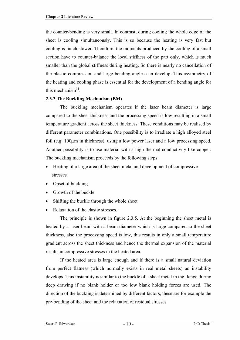
Figure 2.3.5: Stages in the Buckling Mechanism (BM) 11
Figure 2.3.6: The Upsetting (Shortening) Mechanism (UM) 13
Figure 2.4.1: Forces and moments acting in the two layer model 15
Figure 2.4.2: Comparison of solutions for the two layer models 20
Figure 2.4.3: Layout for the residual stress model 20
Figure 2.4.4: Critical operating region for the TGM 25
Figure 2.4.5: Model Geometry for the Buckling Mechanism 26
Figure 2.5.1: Development of the bending angle during Buckling Mechanism 31
Figure 2.5.2: Distribution of the upper and lower surface temperatures and displacements during the Buckling Mechanism 31
Figure 2.5.3: Distribution of the upper and lower surface strains during the Buckling Mechanism 31
Figure 2.5.4: Plastic restraining in extrusion bending 32
Figure 2.6.1: Time run of the strain development 38 Figure 2.6.2: Time run of the bend angle 38 Figure 2.6.3: Decreasing bend rate with increasing scans over an identical track 39 Figure 2.6.4: Bend angle with increasing traverse velocity for Ti6Al4V using a
large beam diameter 42 Figure 2.6.5: Bend angle with increasing traverse velocity for AA 2024 T3 42 Figure 2.6.6: Bend angle with increasing number of scans over the same track 43 Figure 2.6.7: Ideal bend angle and exaggerated view of edge effects 43 Figure 2.6.8: Demonstrator Part 45 Figure 2.6.9: Circle line system with square root radius increase
(inside to out), and resulting contour plot of sample 46 Figure 2.6.10: Actuator for CD lens adjustment by micro LF 50
Figure 2.6.11: LF of 50µm thick beams in wet-etched silicon micro-scale structures 51
Figure 2.6.12: 3-D Laser Forming: routes to practical realisation and key elements required 53
Figure 2.6.13: SEM micrographs of Ti6Al4V formed in (a) air and (b) argon. (Forming parameters: 760W / 30mms-1). 55
Figure 2.6.14: Hardness variation with depth through the sheet thickness for Ti6Al4V (760W 30mm/s 6mm beam). 55
Figure 2.7.1: Some Current Forming Techniques in Shipbuilding 58 Figure 2.7.2: Bulbous Bow from the QM2 59 Figure 2.7.3: Hot creep formed ‘A’ frame strut, possible to
manufacture using LF 62
Page No.
A Study into the 2D and 3D Laser Forming of Metallic Components List of Figures
Stuart P. Edwardson PhD Thesis ix
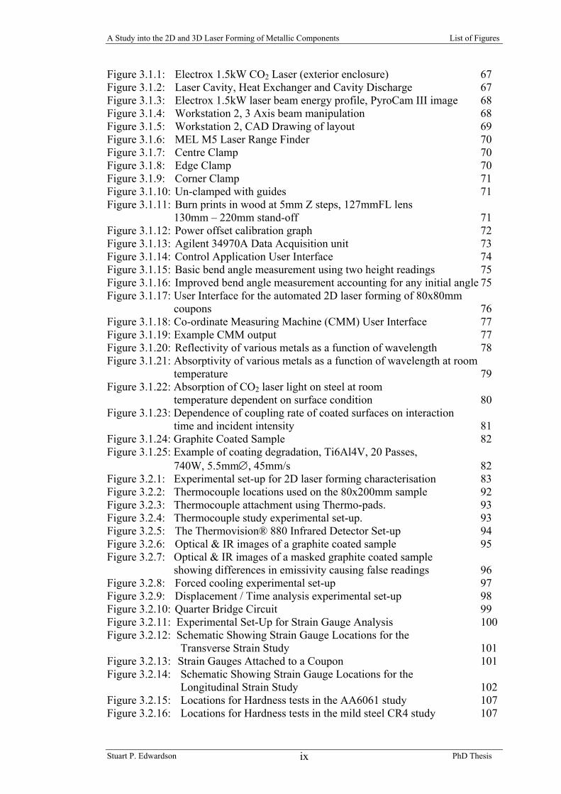
Figure 3.1.1: Electrox 1.5kW CO2 Laser (exterior enclosure) 67 Figure 3.1.2: Laser Cavity, Heat Exchanger and Cavity Discharge 67 Figure 3.1.3: Electrox 1.5kW laser beam energy profile, PyroCam III image 68 Figure 3.1.4: Workstation 2, 3 Axis beam manipulation 68 Figure 3.1.5: Workstation 2, CAD Drawing of layout 69 Figure 3.1.6: MEL M5 Laser Range Finder 70 Figure 3.1.7: Centre Clamp 70 Figure 3.1.8: Edge Clamp 70 Figure 3.1.9: Corner Clamp 71 Figure 3.1.10: Un-clamped with guides 71 Figure 3.1.11: Burn prints in wood at 5mm Z steps, 127mmFL lens
130mm – 220mm stand-off 71 Figure 3.1.12: Power offset calibration graph 72 Figure 3.1.13: Agilent 34970A Data Acquisition unit 73 Figure 3.1.14: Control Application User Interface 74 Figure 3.1.15: Basic bend angle measurement using two height readings 75 Figure 3.1.16: Improved bend angle measurement accounting for any initial angle 75 Figure 3.1.17: User Interface for the automated 2D laser forming of 80x80mm
coupons 76 Figure 3.1.18: Co-ordinate Measuring Machine (CMM) User Interface 77 Figure 3.1.19: Example CMM output 77 Figure 3.1.20: Reflectivity of various metals as a function of wavelength 78 Figure 3.1.21: Absorptivity of various metals as a function of wavelength at room
temperature 79
Figure 3.1.22: Absorption of CO2 laser light on steel at room temperature dependent on surface condition 80
Figure 3.1.23: Dependence of coupling rate of coated surfaces on interaction time and incident intensity 81
Figure 3.1.24: Graphite Coated Sample 82 Figure 3.1.25: Example of coating degradation, Ti6Al4V, 20 Passes,
740W, 5.5mm∅, 45mm/s 82 Figure 3.2.1: Experimental set-up for 2D laser forming characterisation 83 Figure 3.2.2: Thermocouple locations used on the 80x200mm sample 92 Figure 3.2.3: Thermocouple attachment using Thermo-pads. 93 Figure 3.2.4: Thermocouple study experimental set-up. 93 Figure 3.2.5: The Thermovision® 880 Infrared Detector Set-up 94 Figure 3.2.6: Optical & IR images of a graphite coated sample 95 Figure 3.2.7: Optical & IR images of a masked graphite coated sample
showing differences in emissivity causing false readings 96 Figure 3.2.8: Forced cooling experimental set-up 97 Figure 3.2.9: Displacement / Time analysis experimental set-up 98 Figure 3.2.10: Quarter Bridge Circuit 99 Figure 3.2.11: Experimental Set-Up for Strain Gauge Analysis 100 Figure 3.2.12: Schematic Showing Strain Gauge Locations for the
Transverse Strain Study 101 Figure 3.2.13: Strain Gauges Attached to a Coupon 101 Figure 3.2.14: Schematic Showing Strain Gauge Locations for the
Longitudinal Strain Study 102 Figure 3.2.15: Locations for Hardness tests in the AA6061 study 107 Figure 3.2.16: Locations for Hardness tests in the mild steel CR4 study 107
A Study into the 2D and 3D Laser Forming of Metallic Components List of Figures
Stuart P. Edwardson PhD Thesis x
Figure 3.2.17: Software User Interface for closed loop 2D laser forming 108 Figure 3.2.18: Initial study Set-up 110 Figure 3.2.19: Ferranti 8kW CO2 laser, 0.9x1.5m table,
800x400mm sample 110 Figure 3.2.20: 5 Axis beam delivery system 110 Figure 3.2.21: Schematic of the MLC lay-ups used in the investigation 113 Figure 3.2.22: 4/3 Polyamide based FML as Received Section 114 Figure 3.2.23: MLC Experimental Set-up 116 Figure 3.2.24: CAD drawing of an RR Trent 700 Aero Engine ‘A’ frame strut
component. 117
Figure 3.2.25: CAD drawing of an RR Trent 700 Aero Engine ‘A’ frame strut component (magnified). 117
Figure 3.2.26: Set-up for the laser forming of the strut section from 200x100mm 1.6mm Ti64 sheet. 118
Figure 3.2.27: Set-up for the full scale laser forming of the strut section from 3.2mm Mild Steel sheet. 118
Figure 3.3.1: 3D Primitive, ‘The Saddle Shape’ 119 Figure 3.3.2: 3D Primitive, ‘The Pillow Shape’ 119 Figure 3.3.3: 3D Primitive, ‘The Twisted Shape’ 120 Figure 3.3.4: Experimental Set-up for the 3D Laser Forming empirical study 121 Figure 3.3.5: Set-up for thick section 3D LF 122 Figure 3.3.6: 3D Laser Forming using a Laser Dyne 890 5 Axis Gantry 123 Figure 3.3.7: Improved 3D Laser Forming Set-up 125 Figure 4.1.1: 2D LF process map for 1.5mm mild steel CR4, 3mm Beam Dia 129 Figure 4.1.2: 2D LF process map for 1.5mm mild steel CR4, 5.5 mm Beam Dia. 129 Figure 4.1.3: 2D LF process map for 1.5mm mild steel CR4, 8mm Beam Dia. 129 Figure 4.1.4: 1.5mm mild steel CR4, 3mm Beam Dia., 760W, 55mm/s,
30 pass 132 Figure 4.1.5: 1.5mm mild steel CR4, 5.5mm Beam Dia., 760W, 30mm/s,
30 pass 132 Figure 4.1.6: 1.5mm mild steel CR4, 8mm Beam Dia., 760W, 20mm/s,
30 pass 132 Figure 4.1.7: Laser forming of 1.5mm mild steel CR4, 3mm Beam Dia.,
at various inter-pass time delays 134 Figure 4.1.8: Effect of inter-pass time delay on the laser forming of
1.5mm mild steel CR4, 3mm Beam Dia. 135 Figure 4.1.9: Laser forming of 1.5mm mild steel CR4, 5.5mm Beam Dia.,
at various inter-pass time delays 135 Figure 4.1.10: Effect of inter-pass time delay on the laser forming of
1.5mm mild steel CR4, 5.5mm Beam Dia. 135 Figure 4.1.11: Laser forming of 1.5mm mild steel CR4, 8mm Beam Dia.,
at various inter-pass time delays 135 Figure 4.1.12: Effect of inter-pass time delay on the laser forming of
1.5mm mild steel CR4, 8mm Beam Dia. 136 Figure 4.1.13: 2D LF process map for 0.9mm Ti64, 3mm Beam Dia. 137 Figure 4.1.14: 2D LF process map for 0.9mm Ti64, 5.5mm Beam Dia. 137 Figure 4.1.15: 2D LF process map for 0.9mm Ti64, 8mm Beam Dia. 138 Figure 4.1.16: 0.9mm Ti64, 3mm Beam Dia., 500W, 40mm/s, 30 pass 139 Figure 4.1.17: 0.9mm Ti64, 5.5mm Beam Dia., 500W, 30mm/s, 20 pass 140 Figure 4.1.18: 0.9mm Ti64, 8mm Beam Dia., 900W, 40mm/s, 20 pass 140
A Study into the 2D and 3D Laser Forming of Metallic Components List of Figures
Stuart P. Edwardson PhD Thesis xi
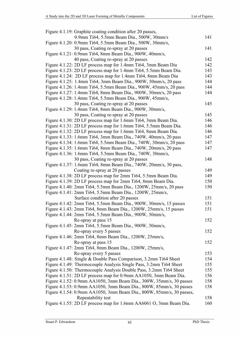
Figure 4.1.19: Graphite coating condition after 20 passes, 0.9mm Ti64, 5.5mm Beam Dia., 500W, 30mm/s 141
Figure 4.1.20: 0.9mm Ti64, 5.5mm Beam Dia., 500W, 30mm/s, 30 pass, Coating re-spray at 20 passes 141
Figure 4.1.21: 0.9mm Ti64, 8mm Beam Dia., 900W, 40mm/s, 40 pass, Coating re-spray at 20 passes 142
Figure 4.1.22: 2D LF process map for 1.4mm Ti64, 3mm Beam Dia 142 Figure 4.1.23: 2D LF process map for 1.4mm Ti64, 5.5mm Beam Dia. 143 Figure 4.1.24: 2D LF process map for 1.4mm Ti64, 8mm Beam Dia 143 Figure 4.1.25: 1.4mm Ti64, 3mm Beam Dia., 900W, 50mm/s, 20 pass 144 Figure 4.1.26: 1.4mm Ti64, 5.5mm Beam Dia., 900W, 45mm/s, 20 pass 144 Figure 4.1.27: 1.4mm Ti64, 8mm Beam Dia., 900W, 30mm/s, 20 pass 144 Figure 4.1.28: 1.4mm Ti64, 5.5mm Beam Dia., 900W, 45mm/s,
30 pass, Coating re-spray at 20 passes 145 Figure 4.1.29: 1.4mm Ti64, 8mm Beam Dia., 900W, 30mm/s,
30 pass, Coating re-spray at 20 passes 145 Figure 4.1.30: 2D LF process map for 1.6mm Ti64, 3mm Beam Dia. 146 Figure 4.1.31: 2D LF process map for 1.6mm Ti64, 5.5mm Beam Dia. 146 Figure 4.1.32: 2D LF process map for 1.6mm Ti64, 8mm Beam Dia. 146 Figure 4.1.33: 1.6mm Ti64, 3mm Beam Dia., 740W, 40mm/s, 20 pass 147 Figure 4.1.34: 1.6mm Ti64, 5.5mm Beam Dia., 740W, 30mm/s, 20 pass 147 Figure 4.1.35: 1.6mm Ti64, 8mm Beam Dia., 740W, 20mm/s, 20 pass 147 Figure 4.1.36: 1.6mm Ti64, 5.5mm Beam Dia., 740W, 30mm/s,
30 pass, Coating re-spray at 20 passes 148 Figure 4.1.37: 1.6mm Ti64, 8mm Beam Dia., 740W, 20mm/s, 30 pass,
Coating re-spray at 20 passes 149 Figure 4.1.38: 2D LF process map for 2mm Ti64, 5.5mm Beam Dia. 149 Figure 4.1.39: 2D LF process map for 2mm Ti64, 8mm Beam Dia. 150 Figure 4.1.40: 2mm Ti64, 5.5mm Beam Dia., 1200W, 25mm/s, 20 pass 150 Figure 4.1.41: 2mm Ti64, 5.5mm Beam Dia., 1200W, 25mm/s,
Surface condition after 20 passes 151 Figure 4.1.42: 2mm Ti64, 5.5mm Beam Dia., 900W, 30mm/s, 15 passes 151 Figure 4.1.43: 2mm Ti64, 8mm Beam Dia., 1200W, 25mm/s, 15 passes 151 Figure 4.1.44: 2mm Ti64, 5.5mm Beam Dia., 900W, 30mm/s,
Re-spray at pass 15 152 Figure 4.1.45: 2mm Ti64, 5.5mm Beam Dia., 900W, 30mm/s,
Re-spray every 5 passes 152 Figure 4.1.46: 2mm Ti64, 8mm Beam Dia., 1200W, 25mm/s,
Re-spray at pass 15 152 Figure 4.1.47: 2mm Ti64, 8mm Beam Dia., 1200W, 25mm/s,
Re-spray every 5 passes 153 Figure 4.1.48: Single & Double Pass Comparison, 3.2mm Ti64 Sheet 154 Figure 4.1.49: Thermocouple Analysis Single Pass, 3.2mm Ti64 Sheet 155 Figure 4.1.50: Thermocouple Analysis Double Pass, 3.2mm Ti64 Sheet 155 Figure 4.1.51: 2D LF process map for 0.9mm AA1050, 3mm Beam Dia. 156 Figure 4.1.52: 0.9mm AA1050, 3mm Beam Dia., 300W, 35mm/s, 30 passes 158 Figure 4.1.53: 0.9mm AA1050, 3mm Beam Dia., 800W, 85mm/s, 30 passes 158 Figure 4.1.54: 0.9mm AA1050, 3mm Beam Dia., 800W, 85mm/s, 30 passes,
Repeatability test 158 Figure 4.1.55: 2D LF process map for 1.6mm AA6061 O, 3mm Beam Dia. 160
A Study into the 2D and 3D Laser Forming of Metallic Components List of Figures
Stuart P. Edwardson PhD Thesis xii
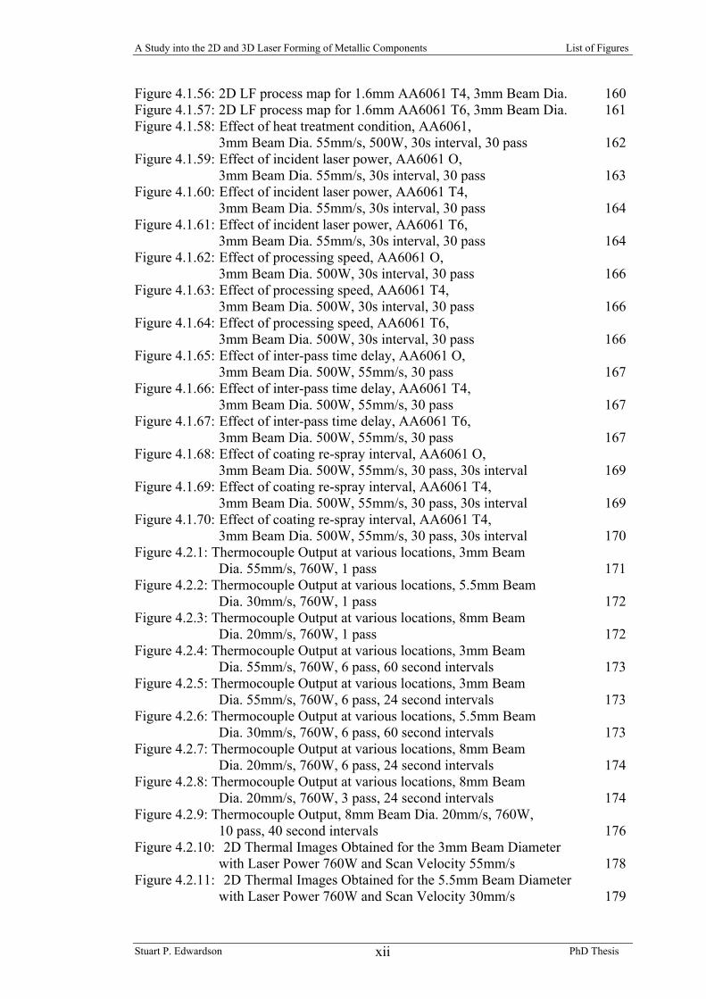
Figure 4.1.56: 2D LF process map for 1.6mm AA6061 T4, 3mm Beam Dia. 160 Figure 4.1.57: 2D LF process map for 1.6mm AA6061 T6, 3mm Beam Dia. 161 Figure 4.1.58: Effect of heat treatment condition, AA6061,
3mm Beam Dia. 55mm/s, 500W, 30s interval, 30 pass 162 Figure 4.1.59: Effect of incident laser power, AA6061 O,
3mm Beam Dia. 55mm/s, 30s interval, 30 pass 163 Figure 4.1.60: Effect of incident laser power, AA6061 T4,
3mm Beam Dia. 55mm/s, 30s interval, 30 pass 164 Figure 4.1.61: Effect of incident laser power, AA6061 T6,
3mm Beam Dia. 55mm/s, 30s interval, 30 pass 164 Figure 4.1.62: Effect of processing speed, AA6061 O,
3mm Beam Dia. 500W, 30s interval, 30 pass 166 Figure 4.1.63: Effect of processing speed, AA6061 T4,
3mm Beam Dia. 500W, 30s interval, 30 pass 166 Figure 4.1.64: Effect of processing speed, AA6061 T6,
3mm Beam Dia. 500W, 30s interval, 30 pass 166 Figure 4.1.65: Effect of inter-pass time delay, AA6061 O,
3mm Beam Dia. 500W, 55mm/s, 30 pass 167 Figure 4.1.66: Effect of inter-pass time delay, AA6061 T4,
3mm Beam Dia. 500W, 55mm/s, 30 pass 167 Figure 4.1.67: Effect of inter-pass time delay, AA6061 T6,
3mm Beam Dia. 500W, 55mm/s, 30 pass 167 Figure 4.1.68: Effect of coating re-spray interval, AA6061 O,
3mm Beam Dia. 500W, 55mm/s, 30 pass, 30s interval 169 Figure 4.1.69: Effect of coating re-spray interval, AA6061 T4,
3mm Beam Dia. 500W, 55mm/s, 30 pass, 30s interval 169 Figure 4.1.70: Effect of coating re-spray interval, AA6061 T4,
3mm Beam Dia. 500W, 55mm/s, 30 pass, 30s interval 170 Figure 4.2.1: Thermocouple Output at various locations, 3mm Beam
Dia. 55mm/s, 760W, 1 pass 171 Figure 4.2.2: Thermocouple Output at various locations, 5.5mm Beam
Dia. 30mm/s, 760W, 1 pass 172 Figure 4.2.3: Thermocouple Output at various locations, 8mm Beam
Dia. 20mm/s, 760W, 1 pass 172 Figure 4.2.4: Thermocouple Output at various locations, 3mm Beam
Dia. 55mm/s, 760W, 6 pass, 60 second intervals 173 Figure 4.2.5: Thermocouple Output at various locations, 3mm Beam
Dia. 55mm/s, 760W, 6 pass, 24 second intervals 173 Figure 4.2.6: Thermocouple Output at various locations, 5.5mm Beam
Dia. 30mm/s, 760W, 6 pass, 60 second intervals 173 Figure 4.2.7: Thermocouple Output at various locations, 8mm Beam
Dia. 20mm/s, 760W, 6 pass, 24 second intervals 174 Figure 4.2.8: Thermocouple Output at various locations, 8mm Beam
Dia. 20mm/s, 760W, 3 pass, 24 second intervals 174 Figure 4.2.9: Thermocouple Output, 8mm Beam Dia. 20mm/s, 760W,
10 pass, 40 second intervals 176 Figure 4.2.10: 2D Thermal Images Obtained for the 3mm Beam Diameter
with Laser Power 760W and Scan Velocity 55mm/s 178 Figure 4.2.11: 2D Thermal Images Obtained for the 5.5mm Beam Diameter
with Laser Power 760W and Scan Velocity 30mm/s 179
A Study into the 2D and 3D Laser Forming of Metallic Components List of Figures
Stuart P. Edwardson PhD Thesis xiii
Figure 4.2.12: 2D Thermal Images Obtained for the 8mm Beam Diameter with Laser Power 760W and Scan Velocity 20mm/s 180
Figure 4.2.13: Comparison of the Temperature Distributions for the 3mm, 5.5mm and 8mm Diameter Laser Beams 181
Figure 4.2.14: Temperature Distribution for the 3mm Incident Beam 181 Figure 4.2.15: Temperature Distribution of the 5.5mm Incident Beam 182 Figure 4.2.16: Temperature Distribution of the 8mm Incident Beam 182 Figure 4.2.17: Thermocouple Output, 3mm Beam Dia. 55mm/s,
760W, 4 pass, 40 second intervals, no cooling 185 Figure 4.2.18: Thermocouple Output, 3mm Beam Dia. 55mm/s,
760W, 4 pass, 40 second intervals, With cooling 185 Figure 4.2.19: Thermocouple Output, 5.5mm Beam Dia. 30mm/s,
760W, 4 pass, 40 second intervals, no cooling 186 Figure 4.2.20: Thermocouple Output, 5.5mm Beam Dia. 30mm/s,
760W, 4 pass, 40 second intervals, With cooling 186 Figure 4.2.21: Thermocouple Output, 8mm Beam Dia. 20mm/s,
760W, 4 pass, 40 second intervals, no cooling 186 Figure 4.2.22: Thermocouple Output, 8mm Beam Dia. 20mm/s,
760W, 4 pass, 40 second intervals, With cooling 186 Figure 4.2.23: 3mm Beam Dia. 55mm/s, 760W, 30 pass, 40 second
intervals, with and without cooling 187 Figure 4.2.24: 5.5mm Beam Dia. 30mm/s, 760W, 30 pass, 40 second
intervals, with and without cooling 187 Figure 4.2.25: 8mm Beam Dia. 20mm/s, 760W, 30 pass, 40 second
intervals, with and without cooling 188 Figure 4.3.1: Displacement/Time, 3mm Beam Dia. 760W, 55mm/s,
All 6 passes, 60s int. 189 Figure 4.3.2: Displacement/Time, 3mm Beam Dia. 760W, 55mm/s,
pass 1, 60s int. 189 Figure 4.3.3: Displacement/Time, 3mm Beam Dia. 760W, 55mm/s,
pass 6, 60s int. 189 Figure 4.3.4: Displacement/Time, 5.5mm Beam Dia. 760W, 30mm/s,
All 6 passes, 60s int. 190 Figure 4.3.5: Displacement/Time, 5.5mm Beam Dia. 760W, 30mm/s,
pass 1, 60s int. 190 Figure 4.3.6: Displacement/Time, 5.5mm Beam Dia. 760W, 30mm/s,
pass 6, 60s int. 190 Figure 4.3.7: Displacement/Time, 8mm Beam Dia. 760W, 20mm/s,
All 6 passes, 60s int. 190 Figure 4.3.8: Displacement/Time, 8mm Beam Dia. 760W, 20mm/s,
pass 1, 60s int. 191 Figure 4.3.9: Displacement/Time, 8mm Beam Dia. 760W, 20mm/s,
pass 6, 60s int. 191 Figure 4.3.10: Schematic of possible reasons for ‘S’ curve bend angle
development 194 Figure 4.4.1: Strain Gauge Output at 46mm Top Surface, 10mm from 1st edge 195 Figure 4.4.2: Strain Gauge Output at 46mm Top Surface, 30mm from 1st edge 196 Figure 4.4.3: Strain Gauge Output at 46mm Top Surface, 50mm from 1st edge 196 Figure 4.4.4: Strain Gauge Output at 46mm Top Surface, 70mm from 1st edge 196
A Study into the 2D and 3D Laser Forming of Metallic Components List of Figures
Stuart P. Edwardson PhD Thesis xiv
Figure 4.4.5: Strain Gauge Output at 46mm Bottom Surface, 10mm from 1st edge 196
Figure 4.4.6: Strain Gauge Output at 46mm Bottom Surface, 30mm from 1st edge 197
Figure 4.4.7: Strain Gauge Output at 46mm Bottom Surface, 50mm from 1st edge 197
Figure 4.4.8: Strain Gauge Output at 46mm Bottom Surface, 70mm from 1st edge 197
Figure 4.4.9: Strain Gauge Output at 10mm Top Surface, 10mm from 1st edge 199 Figure 4.4.10: Strain Gauge Output at 10mm Top Surface, 40mm from 1st edge
(Centreline) 199 Figure 4.4.11: Strain Gauge Output at 10mm Top Surface, 70mm from 1st edge 199 Figure 4.4.12: Strain Gauge Output at 10mm Bottom Surface,
10mm from 1st edge 200 Figure 4.4.13: Strain Gauge Output at 10mm Bottom Surface,
40mm from 1st edge (Centreline) 201 Figure 4.4.14: Strain Gauge Output at 10mm Bottom Surface,
70mm from 1st edge 201 Figure 4.4.15: Visualisation of the strain output close to the scan line
at the start of a pass 202 Figure 4.4.16: Visualisation of the strain output close to the scan line
at the end of a pass 203 Figure 4.4.17: Output from gauges on the top surface at 46mm from the
scan line, longitudinal strain 204 Figure 4.4.18: Output from gauges on the Bottom surface at 46mm
from the scan line, longitudinal strain 204 Figure 4.4.19: Exaggerated view of edge effects 205 Figure 4.4.20: Output from gauge at 10mm from 1st edge on the top
surface at 10mm from the scan line, longitudinal strain 206 Figure 4.4.21: Output from gauge on the centreline on the top
surface at 10mm from the scan line, longitudinal strain 206 Figure 4.4.22: Output from gauge at 70mm from 1st edge on the top
surface at 10mm from the scan line, longitudinal strain 207 Figure 4.4.23: Output from gauge at 10mm from 1st edge on the lower
surface at 10mm from the scan line, longitudinal strain 207 Figure 4.4.24: Output from gauge on the centreline on the lower surface
at 10mm from the scan line, longitudinal strain 207 Figure 4.4.25: Output from gauge at 70mm from 1st edge on the lower
surface at 10mm from the scan line, longitudinal strain 207 Figure 4.4.26: Visualisation of the longitudinal strain output close to the
scan line at the start of a pass 209 Figure 4.4.27: Visualisation of the longitudinal strain output close to the
scan line at the end of a pass 210 Figure 4.5.1: Initial 1200 element FEA model developed 211 Figure 4.5.2: 580 element graded mesh model 212 Figure 4.5.3: Variation in peak upper surface temperature with absorption
coefficient (model output). 214 Figure 4.5.4: Temperature output from the FEA model at 10 and 22mm
from the scan line for a) Upper surface b) Lower surface 5.5mm beam dia. 760W, 30mm/s, single pass, A=0.85 214
A Study into the 2D and 3D Laser Forming of Metallic Components List of Figures
Stuart P. Edwardson PhD Thesis xv
Figure 4.5.5: Thermocouple measurements at 10 and 22mm from the scan line for a) Upper surface b) Lower surface 5.5mm beam dia. 760W, 30mm/s, single pass 215
Figure 4.5.6: Model Output, 3D contour plot of temperature at; a) Mid-pass b) End of pass c) t=4.2s d) t=46.2s 3mm beam dia. 760W, 55mm/s, single pass, A=0.85 216
Figure 4.5.7: Temperature output at various distances from the scan line along the centreline of the plate, Upper Surface 3mm beam dia. 760W, 55mm/s, single pass, A=0.85 216
Figure 4.5.8: Temperature output at various distances from the scan line along the centreline of the plate, Lower Surface
3mm beam dia. 760W, 55mm/s, single pass, A=0.85 216 Figure 4.5.9: Model Output, 3D contour plot of temperature at;
a) Mid-pass b) End of pass c) t=4.5s d) t=28.6s 5.5mm beam dia. 760W, 30mm/s, single pass, A=0.85 217
Figure 4.5.10: Temperature output at various distances from the scan line along the centreline of the plate, Upper Surface 5.5mm beam dia. 760W, 30mm/s, single pass, A=0.85 217
Figure 4.5.11: Temperature output at various distances from the scan line along the centreline of the plate, Lower Surface 5.5mm beam dia. 760W, 30mm/s, single pass, A=0.85 217
Figure 4.5.12: Model Output, 3D contour plot of temperature at; a) Mid-pass b) End of pass c) t=5.4s d) t=34.4s 8mm beam dia. 760W, 20mm/s, single pass, A=0.85 218
Figure 4.5.13: Temperature output at various distances from the scan line along the centreline of the plate, Upper Surface
8mm beam dia. 760W, 20mm/s, single pass, A=0.85 218 Figure 4.5.14: Temperature output at various distances from the
scan line along the centreline of the plate, Lower Surface 8mm beam dia. 760W, 20mm/s, single pass, A=0.85 218
Figure 4.5.15: Temperature output at various distances from the scan line along at Edge 1, Upper Surface 5.5mm beam dia. 760W, 30mm/s, single pass, A=0.85 220
Figure 4.5.16: Temperature output at various distances from the scan line along at Edge 2, Upper Surface 5.5mm beam dia. 760W, 30mm/s, single pass, A=0.85 221
Figure 4.5.17: Widening of the HAZ near the edge in mild steel 5.5mm beam dia. 760W, 30mm/s 221
Figure 4.5.18: Final displacement output, magnification factor =30 5.5mm beam dia. 760W, 30mm/s, single pass, A=0.85 222
Figure 4.5.19: Model Output, 3D contour plot of temperature and displacement at; a)Start of pass b) Mid-pass c) End of pass d) t=49s 5.5mm beam dia. 760W, 30mm/s, single pass, A=0.85 223
Figure 4.5.20: Displacement/time output, free end of the plate on the centreline 5.5mm beam dia. 760W, 30mm/s, single pass, A=0.85 224
Figure 4.5.21: Height contour plots of the formed plate, magnification factor =30 5.5mm beam dia. 760W, 30mm/s, single pass, A=0.85 224
Figure 4.5.22: Displacement/time output, free end of the plate 5.5mm beam dia. 760W, 30mm/s, single pass, A=0.85 225
A Study into the 2D and 3D Laser Forming of Metallic Components List of Figures
Stuart P. Edwardson PhD Thesis xvi
Figure 4.5.23: 3D contour plots of E11 at; a) Start b) Near Start c) Near End of pass d) t=29.5s 5.5mm beam dia. 760W, 30mm/s, single pass, A=0.85 226
Figure 4.5.24: Transverse strain E11 at ~10mm from scan line near edge 1 Upper surface: a) Model output b) Strain gauge output 5.5mm beam dia. 760W, 30mm/s, single pass, A=0.85 227
Figure 4.5.25: Transverse strain E11 at ~10mm from scan line at the centre Upper Surface: a) Model output b) Strain gauge output 5.5mm beam dia. 760W, 30mm/s, single pass, A=0.85 228
Figure 4.5.26: Transverse strain E11 at ~10mm from scan line near edge 2 Upper Surface: a) Model output b) Strain gauge output 5.5mm beam dia. 760W, 30mm/s, single pass, A=0.85 228
Figure 4.5.27: 3D contour plots of E22 at; a) Start b) Mid Pass c) End of pass d) t=19.5s 5.5mm beam dia. 760W, 30mm/s, single pass, A=0.85 230
Figure 4.5.28: Longitudinal strain E22, centre of the scan line near edge 1 Upper Surface
5.5mm beam dia. 760W, 30mm/s, single pass, A=0.85 231 Figure 4.5.29: Longitudinal strain E22, centre of the scan line, plate centre
Upper Surface 5.5mm beam dia. 760W, 30mm/s, single pass, A=0.85 231
Figure 4.5.30: Longitudinal strain E22, centre of the scan line near edge 2 Upper Surface
5.5mm beam dia. 760W, 30mm/s, single pass, A=0.85 232 Figure 4.5.31: 3D contour plots of S11 at;
a) Start b) Mid Pass c) End of pass d) t=49.5s 5.5mm beam dia. 760W, 30mm/s, single pass, A=0.85 233
Figure 4.5.32: Schematic of the stress distribution around the laser beam during laser forming 234
Figure 4.5.33: Transverse Stress S11, centre of the scan line near edge 1 Upper Surface
5.5mm beam dia. 760W, 30mm/s, single pass, A=0.85 234 Figure 4.5.34: Transverse Stress S11, centre of the scan line, plate centre
Upper Surface 5.5mm beam dia. 760W, 30mm/s, single pass, A=0.85 235
Figure 4.5.35: Transverse Stress S11, centre of the scan line near edge 2 Upper Surface
5.5mm beam dia. 760W, 30mm/s, single pass, A=0.85 235 Figure 4.5.36: 3D contour plots of S22 at;
a) Start b) Mid Pass c) End of pass d) t=29.5s 5.5mm beam dia. 760W, 30mm/s, single pass, A=0.85 236
Figure 4.5.37: Transverse Stress S22, centre of the scan line near edge 1 Upper Surface
5.5mm beam dia. 760W, 30mm/s, single pass, A=0.85 237 Figure 4.5.38: Transverse Stress S22, centre of the scan line, plate centre
Upper Surface 5.5mm beam dia. 760W, 30mm/s, single pass, A=0.85 238
Figure 4.5.39: Transverse Stress S22, centre of the scan line near edge 2 Upper Surface
5.5mm beam dia. 760W, 30mm/s, single pass, A=0.85 238
A Study into the 2D and 3D Laser Forming of Metallic Components List of Figures
Stuart P. Edwardson PhD Thesis xvii
Figure 4.6.1: Iron-Carbon Equilibrium Phase Diagram with some typical microstructures 239
Figure 4.6.2: Microstructure of the ‘as-received’ coupon (x500 magnifications) 241
Figure 4.6.3: 1.5mm Mild Steel, 3mm beam diameter 760W, 55mm/s, 1 pass, Top Middle and Bottom of the HAZ section (x500 magnifications) 242
Figure 4.6.4: 1.5mm Mild Steel, 3mm beam diameter 760W, 55mm/s, 10 passes, Top Middle and Bottom of the HAZ section (x500 magnifications) 242
Figure 4.6.5: 1.5mm Mild Steel, 3mm beam diameter 760W, 55mm/s, 30 passes, Top Middle and Bottom of the HAZ section (x500 magnifications) 243
Figure 4.6.6: 1.5mm Mild Steel, 5.5mm beam diameter 760W, 30mm/s, 1 pass, Top Middle and Bottom of the HAZ section (x500 magnifications) 243
Figure 4.6.7: 1.5mm Mild Steel, 5.5mm beam diameter 760W, 30mm/s, 10 passes, Top Middle and Bottom of the HAZ section (x500 magnifications) 244
Figure 4.6.8: 1.5mm Mild Steel, 5.5mm beam diameter 760W, 30mm/s, 30 passes, Top Middle and Bottom of the HAZ section (x500 magnifications) 244
Figure 4.6.9: 1.5mm Mild Steel, 8mm beam diameter 760W, 20mm/s, 1 pass, Top Middle and Bottom of the HAZ section (x500 magnifications) 245
Figure 4.6.10: 1.5mm Mild Steel, 8mm beam diameter 760W, 20mm/s, 10 passes, Top Middle and Bottom of the HAZ section (x500 magnifications) 245
Figure 4.6.11: 1.5mm Mild Steel, 8mm beam diameter 760W, 20mm/s, 30 passes, Top Middle and Bottom of the HAZ section (x500 magnifications) 246
Figure 4.6.12: Typical microstructure of AA 6061 (x250 optical) 253 Figure 4.6.13: AA 6061 O
‘As Received’ 253
Figure 4.6.14: AA 6061 O After 5 passes 253
Figure 4.6.15: AA 6061 O After 30 passes 254
Figure 4.6.16: AA 6061 T4 ‘As Received’ 254
Figure 4.6.17: AA 6061 T4 After 5 passes 254
Figure 4.6.18: AA 6061 T4 After 30 passes 254
Figure 4.6.19: AA 6061 T6 ‘As Received’ 254
Figure 4.6.20: AA 6061 T6 After 5 passes 254
Figure 4.6.21: AA 6061 T6 After 30 passes 254
Figure 4.6.22: AA 6061 O - a) 0 pass, b) 5 pass c) 30 pass 257
A Study into the 2D and 3D Laser Forming of Metallic Components List of Figures
Stuart P. Edwardson PhD Thesis xviii
Figure 4.6.23: AA 6061 T4 - a) 0 pass, b) 5 pass c) 30 pass 257 Figure 4.6.24: AA 6061 T6 - a) 0 pass, b) 5 pass c) 30 pass 257 Figure 4.7.1: Laser forming of 1.5mm mild steel CR4, 3mm beam dia.
760W 10 – 70mm/s process map 260 Figure 4.7.2: Closed loop laser forming of 1.5mm mild steel CR4,
3mm beam dia. 760W, 20° target, attempt 1 261 Figure 4.7.3: Closed loop laser forming of 1.5mm mild steel CR4,
3mm beam dia. 760W, 20° target, attempt 2 261 Figure 4.7.4: Laser forming of 0.9mm AA1050, 3mm beam dia.
300W 10 – 90mm/s process map 262 Figure 4.7.5: Closed loop laser forming of 0.9mm AA1050,
3mm beam dia. 300W, 20° target, attempt 1 263 Figure 4.7.6: Closed loop laser forming of 0.9mm AA1050,
3mm beam dia. 300W, 20° target, attempt 2 264 Figure 4.7.7: Closed loop laser forming of 0.9mm AA1050,
3mm beam dia. 300W, 30° target 264 Figure 4.8.1: Part-cylinder formed from 390x180x5mm mild steel plate 266 Figure 4.8.2: CMM 3D contour plot of part-cylinder geometry formed from
390x180x5mm mild steel plate 266 Figure 4.8.3: Schematic of the LF strategy used to form a part-cylinder along
the Y axis in an 800x400mm sheet. 267 Figure 4.8.4: 800x400x5mm mild steel sheet formed into a
part-cylinder. 267 Figure 4.8.5: Height measurements along the two longer X axis edges of an
800x400x5mm mild steel sheet formed into a part-cylinder. 268 Figure 4.8.6: Height measurements along the two shorter Y axis edges of an
800x400x5mm mild steel sheet formed into a part-cylinder. 268 Figure 4.8.7: Schematic of the LF strategy used to form a part-cylinder
along the longitudinal X axis 800x400x5mm mild steel sheet. 269 Figure 4.8.8: Laser forming a part-cylinder along the longitudinal X axis from
800x400x5mm mild steel sheet. 269 Figure 4.8.9: Height measurements along the two longer X axis edges of an
800x400x5mm mild steel sheet formed into a part-cylinder along the X axis. 270
Figure 4.8.10: Height measurements along the two shorter Y axis edges of an 800x400x5mm mild steel sheet formed into a part-cylinder along the X axis. 270
Figure 4.8.11: Thermocouple measurement locations 271 Figure 4.8.12: Thermocouple output, 1 double pass, 800x400x5mm
mild steel sheet 272 Figure 4.8.13: Thermocouple output, 1 double pass, 800x400x5mm
mild steel sheet 272 Figure 4.9.1: Treating the section as a metallic solid results in a buckling
of the Upper Laminate due to non-TGM parameters and excessive heating 275
Figure 4.9.2: Laser forming the upper laminate alone results in a positive bend, no melting and no obvious damage 275
Figure 4.9.3: Laser Forming of 1.38mm 2/1 glass reinforced polyamide based MLC 275
Figure 4.9.4: Repeatability Test, 1.38mm 2/1 Polyamide based MLC 276
A Study into the 2D and 3D Laser Forming of Metallic Components List of Figures
Stuart P. Edwardson PhD Thesis xix
Figure 4.9.5: The Effect of Increasing No. of Layers on the Laser Forming of Polyamide based MLC 276
Figure 4.9.6: The Effect of Increasing No. of Layers on the Laser Forming of Self-Reinforced Polypropylene MLC 277
Figure 4.9.7: The Effect of Increasing No. of Layers on the Laser Forming of Glass-Reinforced Polypropylene MLC 277
Figure 4.9.8: The Effect of Fibre Orientation on the Laser Forming of Glass-Reinforced Polypropylene based MLC 278
Figure 4.9.9: Thermocouple Output for a 0.3mm Al 2024 Foil, Centreline Bottom Surface 279
Figure 4.9.10: 2/1 Polyamide based MLC after 5 passes, 200W, 90mm/s, 2.5mmØ 280
Figure 4.9.11: Upper layer cracked due to non-optimum excessive heating. 281 Figure 4.9.12: De-lamination due to failure in bonding layer. 281 Figure 4.9.13: 200x100mm Part-Cylinder formed from 2/1 polyamide
based MLC 282 Figure 4.9.14: 240x80mm Part-Cylinder formed from 2/1 polypropylene
based MLC 282 Figure 4.9.15: Laser forming 2/1 GLARE type materials, initial feasibility test 284 Figure 4.9.16: Laser forming 2/1 GLARE type materials at various
processing speeds 284 Figure 4.9.17: Laser forming a multiple scan line large radii bend,
2/1 GLARE type material, 240x80mm 285 Figure 4.9.18: Laser forming a multiple scan line large radii bend,
2/1 GLARE type material, 240x80mm (reverse angle) 286 Figure 4.10.1: Initial method to produce the ‘A’ frame strut from
400x200mm mild steel sheet. 287 Figure 4.10.2: Result of initial attempt to produce the ‘A’ frame strut from
400x200mm mild steel sheet. 288 Figure 4.10.3: Method used to produce the ‘A’ frame strut section from
200x100x1.6mm Ti64 sheet. 288 Figure 4.10.4: ‘A’ frame strut section production from 200x100x1.6mm
Ti64 sheet. Forming the sharp bends at the edges first 289 Figure 4.10.5: ‘A’ frame strut section production from 200x100x1.6mm
Ti64 sheet. Forming the gradual large radii bend at the centre to complete the geometry. 290
Figure 4.10.6: Method used to produce the full sized ‘A’ frame strut from 574x175x3.2mm mild steel sheet. 291
Figure 4.10.7: U channel formed first in 574x175x3.2mm mild steel sheet 291 Figure 4.10.8: Large radii bend at the centre added to complete the geometry 291 Figure 5.1.1: Scan Strategy 1, Speed 15mm/s 294 Figure 5.1.2: 3D Contour Plot Strategy 1 294 Figure 5.1.3: Contour Plot Strategy 1 294 Figure 5.1.4: Contour Plot Strategy 1 (end view) 294 Figure 5.1.5: Strategy 2, Speed 20mm/s 295 Figure 5.1.6: 3D Contour plot Strategy 2 295 Figure 5.1.7: Contour Plot Strategy 2 295 Figure 5.1.8: Contour Plot Strategy 2 (end view) 295 Figure 5.1.9: Strategy 3, Speed 30 mm/s 296
A Study into the 2D and 3D Laser Forming of Metallic Components List of Figures
Stuart P. Edwardson PhD Thesis xx
Figure 5.1.10: 3D Contour Plot Strategy 3 296 Figure 5.1.11: Contour Plot Strategy 3 296 Figure 5.1.12: Contour Plot Strategy 3 (end view) 296 Figure 5.1.13: Strategy 4, Speed 30mm/s 297 Figure 5.1.14: 3D Contour Plot Strategy 4 297 Figure 5.1.15: Contour Plot Strategy 4 297 Figure 5.1.16: Contour Plot Strategy 4 (end view) 297 Figure 5.1.17: Strategy 5, Speed 20mm/s 298 Figure 5.1.18: 3D Contour Plot Strategy 5 298 Figure 5.1.19: Contour Plot Strategy 5 299 Figure 5.1.20: Contour Plot Strategy 5 (end view) 299 Figure 5.1.21: Strategy 5: square plate 20mm/s 299 Figure 5.1.22: 3D Contour Plot Strategy 5 (square plate) 299 Figure 5.1.23: 3D Contour Plot (side) Strategy 5 (square) 300 Figure 5.1.24: Contour Plot Strategy 5 (square) 300 Figure 5.1.25: 1.6mm Ti64. Strategy 5 300 Figure 5.1.26: 1.6mm Ti64. Strategy 5 300 Figure 5.1.27: 1.6mm Ti64. Strategy 5 contour plot 300 Figure 5.1.28: Strategy 6: 5.5mm beam dia. 40mm/s
400x200x1.5mm Mild Steel 301 Figure 5.1.29: 3D Contour Plot Strategy 6 (pass1) 301 Figure 5.1.30: 3D Contour Plot Strategy 6 (pass1) 301 Figure 5.1.31: Contour Plot Strategy 6 (pass1) 301 Figure 5.1.32: 3D Contour Plot Strategy 6 (pass2) 302 Figure 5.1.33: 3D Contour Plot Strategy 6 (pass2) 302 Figure 5.1.34: Contour Plot Strategy 6 (pass2) 302 Figure 5.1.35: 3D Contour Plot Strategy 6 (pass3) 302 Figure 5.1.36: 3D Contour Plot Strategy 6 (pass3) 302 Figure 5.1.37: Contour Plot Strategy 6 (pass3) 302 Figure 5.1.38: Pillow Shape Strategy: 5.5mm beam dia. 40mm/s 304 Figure 5.1.39: 3D Contour Plot Pillow Shape Strategy 304 Figure 5.1.40: 3D Contour Plot Pillow Shape Strategy 304 Figure 5.1.41: Contour Plot Pillow Shape Strategy 304 Figure 5.1.42: Distorted pillow shape due to over forming. 305 Figure 5.1.43: Twisted Shape Strategy 1 306 Figure 5.1.44: 3D Contour Plot Twisted Shape Strategy 1 306 Figure 5.1.45: 3D Contour Plot Twisted Shape Strategy 1 306 Figure 5.1.46: Contour Plot Twisted Shape Strategy 1 306 Figure 5.1.47: Twisted Shape Strategy 2, 760W, 50mm/s, 5.5mm beam dia. 306 Figure 5.1.48: 3D Contour Plot Twisted Shape Strategy 2
(upper surface, pass1) 307 Figure 5.1.49: 3D Contour Plot (side) Twisted Shape Strategy 2
(upper surface, pass1) 307 Figure 5.1.50: Contour Plot Twisted Shape Strategy 2
(upper surface, pass1) 307 Figure 5.1.51: 3D Contour Plot Twisted Shape Strategy 2
(lower surface, pass1) 308 Figure 5.1.52: Contour Plot Twisted Shape Strategy 2
(lower surface, pass1) 308
A Study into the 2D and 3D Laser Forming of Metallic Components List of Figures
Stuart P. Edwardson PhD Thesis xxi
Figure 5.1.53: 3D Contour Plot Twisted Shape Strategy 2 (lower surface, pass2) 308
Figure 5.1.54: Contour Plot Twisted Shape Strategy 2 (lower surface, pass2) 308
Figure 5.1.55: 3D Contour Plot Twisted Shape Strategy 2 (lower surface, pass3) 309
Figure 5.1.56: 3D Contour Plot (side) Twisted Shape Strategy 2 (lower surface, pass3) 309
Figure 5.1.57: Contour Plot Twisted Shape Strategy 2 (lower surface, pass3) 309
Figure 5.1.58: 3D Contour Plot Saddle Shape, 5mm Mild Steel 310 Figure 5.1.59: 3D Contour Plot Saddle Shape, 5mm Mild Steel 310 Figure 5.1.60: Contour Plot Saddle Shape, 5mm Mild Steel 310 Figure 5.1.61: Saddle Shape, 5mm Mild Steel, image of longer edge 310 Figure 5.1.62: Scaled ‘race track’ strategy for the 800x400x5mm
mild steel plates 311 Figure 5.1.63: 800x400x5mm mild steel, height measurements
along shorter edges 312 Figure 5.1.64: 800x400x5mm mild steel, height measurements
along longer edges 312 Figure 5.1.65: 800x400x5mm mild steel plate after processing
with ‘race track’ 312 Figure 5.2.1: The Bezier surface patch 314
Figure 5.2.2: Matlab output showing a Bezier surface patch for a pillow shape 315
Figure 5.2.3: Contour plots of constant gradient values in X and Y for the Bezier interpolated surface of the pillow shape 316
Figure 5.2.4: Matlab data point output of the (overlaid) gradient based scan strategy for the pillow shape and forming results. dz/dy then dz/dx, alternating directions, 5.5mm beam diameter, 760W and 50mm/s 317
Figure 5.2.5: Quiver plot and contour plot of the resultant gradient vector and magnitude in X and Y for the pillow shape 318
Figure 5.2.6: Constant gradient vector direction based scan strategy for the pillow shape 318
Figure 5.2.7: Constant gradient vector direction based scan strategy forming result 318
Figure 5.2.8: Illustration of required forming direction for a given gradient vector 319
Figure 5.2.9: Quiver plot of resultant gradient vector rotated by 90° for pillow shape 319
Figure 5.2.10: Matlab data point output of contour lines of constant height for the pillow shape and forming results. 9 contours, 5.5mm beam diameter, 760W and 50mm/s 320
Figure 5.2.11: Schematic of possible reason why lines of constant height give a usable scan pattern for a surface 321
Figure 5.2.12: Height contour plot of pillow surface with an indication of the required gradient vector magnitude at points along the contour lines 322
Figure 5.2.13: Matlab output showing a Bezier surface patch for a saddle shape, based on rotated and interpolated control point data 323
A Study into the 2D and 3D Laser Forming of Metallic Components List of Figures
Stuart P. Edwardson PhD Thesis xxii
Figure 5.2.14: Contour plots of constant gradient values in X and Y for the Bezier interpolated surface of the saddle shape 323
Figure 5.2.15: Quiver plot of resultant gradient vector rotated by 90° for saddle shape 324
Figure 5.2.16: Height contour plot of saddle surface with an indication of the required gradient vector magnitude at points along the contour lines. Blue indicates positive deflection, Red indicates negative deflection 325
Figure 5.2.17: Developable and non-developable surfaces, analogous to the 3D laser forming of continuous surfaces 326
Figure 5.3.1: CNC File Generation by Matlab 331 Figure 5.3.2: Elliptic paraboloid or pillow shape 332
Figure 5.3.3: Hyperbolic paraboloid or saddle shape 332
Figure 5.3.4: Matlab output using an elliptic paraboloid definition for the pillow shape 333
Figure 5.3.5: Matlab output using a hyperbolic paraboloid definition for the saddle shape 333
Figure 5.3.6: Predicted scan strategy and speed distribution for the pillow shape 333
Figure 5.3.7: Laser formed elliptic paraboloid based pillow shape, 5.5mm beam diameter, 760W, 45-55mm/s 334
Figure 5.3.8: Repeatability tests 2 and 3 334
Figure 5.3.9: Standard deviation between each of the repeatability tests 334
Figure 5.3.10: Desired 20mm max deflection pillow shape and error plot between it and the flat unformed sheet 336
Figure 5.3.11: Predicted scan strategy and speed distribution for pass 1 336
Figure 5.3.12: Speed selection based on 2D LF data for a 5.5mm beam diameter and 760W. 50mm/s selected as a minimum speed. All other speeds distributed in the range 50 to 85mm/s 337
Figure 5.3.13: Pass 1 forming result, 5.5mm beam diameter and 760W. Maximum forming ~8mm 337
Figure 5.3.14: Comparison between formed surface after pass 1 and desired shape, ~12mm difference. Error plot gives a prediction for the next pass 337
Figure 5.3.15: Scan strategy prediction for pass 2. Calibration with pass 1 data gives a strain calibration scaling factor for the speed based on the current plate’s forming characteristics 338
Figure 5.3.16: Speed distribution used for pass 2. As there is less required forming the minimum process speed has automatically increased to 67mm/s so as to avoid overshoot. The predicted induced strain has also been adjusted according to the pass 1 data 338
Figure 5.3.17: Pass 2 results, 5.5mm beam diameter and 760W. ~17mm maximum deflection 338
Figure 5.3.18: Comparison between formed surface after pass 2 and desired shape, ~4.5mm difference. Error plot now gives a prediction for the next pass. More forming along the longer edges now is required. 339
Figure 5.3.19: Scan strategy prediction for pass 3. No further calibration is performed after the pass 1 data. The Galil controller can easily reproduce smooth motion based on the complex scan prediction 339
A Study into the 2D and 3D Laser Forming of Metallic Components List of Figures
Stuart P. Edwardson PhD Thesis xxiii
Figure 5.3.20: Speed distribution used for pass 3. As only fine adjustments are required a speed range of 73.13 to 85.4mm/s is predicted. 339
Figure 5.3.21: Pass 3 results, 5.5mm beam diameter and 760W. ~21mm maximum deflection (slight overshoot) 340
Figure 5.3.22: Comparison between formed surface after pass 3 and desired shape, +/- ~2.5mm error. Small overshoot has occurred 340
Figure 5.3.23: Predicted scan strategy for pass 4 suggests forming on the reverse side of the plate (red dots) to account for the overshoot. Forming had to be ended here as this capability was not yet included in the system 340
Figure 5.3.24: Image of a laser formed 400x200x1.5mm mild steel plate showing the complex scan patterns realised over the surface. 341
A Study into the 2D and 3D Laser Forming of Metallic Components List of Tables
Stuart P. Edwardson PhD Thesis xxiv
List of Tables
Table 2.3.1: Outline of the 3 main LF mechanisms 14 Table 2.7.1: Degree of application potential for LF in various stages
of a general product life-cycle (not specific to component scale, material or geometry) 57
Table 3.1.1: Typical values of reflectivity of various surfaces
to 10.6µm radiation at normal angles of incidence 80 Table 3.2.1: Material designation according to different
international standards. (Mild Steel CR4) 84 Table 3.2.2: Material composition by weight percentage of Mild Steel CR4 84 Table 3.2.3: Mechanical properties of Mild Steel CR4. 84 Table 3.2.4: Thermal Properties of Mild Steel CR4. 85 Table 3.2.5: Material designation according to different
international standards. (Ti-6Al-4V) 87 Table 3.2.6: Material composition by weight percentage of Ti-6Al-4V. 87 Table 3.2.7: Mechanical properties of Ti-6Al-4V. 87 Table 3.2.8: Thermal Properties of Ti-6Al-4V. 87 Table 3.2.9: Material designation according to
different international standards. (1050-H14) 88 Table 3.2.10: Material composition by weight percentage 88
of Aluminium 1050-H14. Table 3.2.11: Mechanical properties of Aluminium 1050-H14 89 Table 3.2.12: Thermal Properties of Aluminium 1050-H14. 89 Table 3.2.13: Material designation according to
different international standards (AA6061) 90 Table 3.2.14: Material composition by weight percentage of AA6061 90 Table 3.2.15: Mechanical properties of AA6061 in three different tempers 91 Table 3.2.16: Thermal Properties of AA 6061 in three different tempers 91
Page No.
A Study into the 2D and 3D Laser Forming of Metallic Components List of Tables
Stuart P. Edwardson PhD Thesis xxv
Table 3.2.17: Technical Data for the Thermovision® 880 Infrared Detector 95 Table 3.2.18: Lens Specifications for the Infrared Detector 95 Table 3.2.19: AA6061 Samples considered in study 105 Table 4.6.1: 1.5mm Mild Steel, ‘As received’ Vickers hardness 248
Table 4.6.2: 1.5mm Mild Steel,3mm beam diameter 760W,
55mm/s, 1 pass, Vickers hardness 248
Table 4.6.3: 1.5mm Mild Steel,3mm beam diameter 760W,
55mm/s, 10 passes, Vickers hardness 248
Table 4.6.4: 1.5mm Mild Steel, 3mm beam diameter 760W,
55mm/s, 30 passes, Vickers hardness 248 Table 4.6.5: 1.5mm Mild Steel, 5.5mm beam diameter 760W,
30mm/s, 1 pass, Vickers hardness 248
Table 4.6.6: 1.5mm Mild Steel, 5.5mm beam diameter 760W,
30mm/s, 10 passes, Vickers hardness 249
Table 4.6.7: 1.5mm Mild Steel, 5.5mm beam diameter 760W,
30mm/s, 30 passes, Vickers hardness 249
Table 4.6.8: 1.5mm Mild Steel, 8mm beam diameter 760W,
20mm/s, 1 pass, Vickers hardness 249
Table 4.6.9: 1.5mm Mild Steel, 8mm beam diameter 760W,
20mm/s, 10 passes, Vickers hardness 249
Table 4.6.10: 1.5mm Mild Steel, 8mm beam diameter 760W,
20mm/s, 30 passes, Vickers hardness 249
Table 4.6.11: Hardness results for AA 6061 O/T4/T6 256 Table 4.6.12: Irradiated section thickness measurements
for AA 6061 O/T4/T6 258
A Study into the 2D and 3D Laser Forming of Metallic Components List of Symbols
Stuart P. Edwardson PhD Thesis xxvi
List of Symbols S.I. Units
A - Absorption (constant)
b - Breadth of plastic zone
Cp - Specific heat capacity
d1 - Laser beam diameter
D - Ratio of depth of plastic zone to sheet thickness
E - Elastic Modulus
Enn – Strain in the n direction, n=1, 2, 3 (Abaqus Notation)
F - Force
Fn - Fourier number
f - Lens focal length
I - Moment of Inertia
I0 - Intensity at centre of laser beam
kf - Temperature dependent Yield stress
k , λ - Thermal conductivity
1 - Length
lh - Length of heated zone
11 - Length of plastically strained zone
12 - Length of elastically strained zone
M - Bending moment
M2 - Beam Quality Factor
m - Mass
N - In-plane force
P, p1 - Laser power
Q - Dimensionless power
Q1 - Average energy input
R - Radius of curvature
r1 - Laser beam radius
S - Dimensionless velocity
Snn – Stress in the n direction, n=1, 2, 3 (Abaqus Notation)
s0 - Sheet thickness
s1 - Depth of plastic zone
A Study into the 2D and 3D Laser Forming of Metallic Components List of Symbols
Stuart P. Edwardson PhD Thesis xxvii
T - Temperature
Tc - Critical temperature for plastic flow
t - time
u - displacement
v1 - Velocity
W0 - Minimum Beam Waist
W(z) - Beam Waist at distance z
w - Displacement of a plate
x, y, z - Cartesian co-ordinates
Y - Yield Strength
α - Thermal diffusivity
α b - Bend angle
α th - Coefficient of thermal expansion
γxy - Shear Strain in the xy plane
∆T - Time of heating
∆T - Average temperature of heated zone
∆T’ - Temperature increase
ε - Strain
εn - Strain in n direction (n = x, y, z etc.)
ε in - Inherent strain (maximum plastic strain less elastic strain during heating)
ε pm - Maximum plastic strain
κ - Thermal diffusivity
λ - Wavelength
ρ - Mass density
σ - Stress
υ - Poisson’s ratio
Chapter 1 Introduction
Stuart P. Edwardson PhD Thesis - 1 -
Chapter 1
Introduction
The work presented in this thesis is primarily concerned with the process of laser
forming or laser bending of metal sheet material with a high power infra-red
defocused laser beam.
The laser forming process (LF) has become viable for the shaping of metallic
components, as a means of rapid prototyping and of adjusting and aligning. Laser
forming is of significant value to industries that previously relied on expensive
stamping dies and presses for prototype evaluations. Relevant industry sectors
include aerospace, automotive, shipbuilding and microelectronics. In contrast with
conventional forming techniques, this method requires no mechanical contact and
thus promotes the idea of ‘Virtual Tooling’. It also offers many of the advantages of
process flexibility and automation associated with other laser manufacturing
techniques, such as laser cutting and marking 1, 2, 3.
Laser forming can produce metallic, predetermined shapes with minimal
distortion. Investigations are also ongoing into the removal of unwanted distortion
from other manufacturing processes. The process has its origins in flame bending for
ship construction, with the earliest work on LF beginning in the mid-1980s 4, 5. The
process has similarities to the well-established torch flame bending used on large
sheet material in the shipbuilding industry 6, 7, 8, 9, but a great deal more control of the
final product can be achieved. The process employs a defocused laser beam to
induce thermal stresses without melting in the surface of a workpiece in order to
produce controlled distortion. These internal stresses induce plastic strains, bending
or shortening the material, or result in a local elastic plastic buckling of the work
piece depending on the mechanism active 10, 11. The exact mechanisms of the process
are outlined in the next chapter.
It can be argued that the use of a defocused laser to form could be replicated
by cheaper more cost-effective means, e.g. a plasma torch 12. It could also be argued
Chapter 1 Introduction
Stuart P. Edwardson PhD Thesis - 2 -
that laser forming would be a secondary process when considering the cost-
effectiveness of a laser system, in that a system would be purchased for primarily a
cutting or welding operation, proven to be cost effective and competitive, and used
for laser forming as a bonus additional process. However, there are circumstances
where the unique capabilities of laser forming alone can achieve the desired result
such as micro-forming 13.
The range of metals and other materials that can be laser formed is
considerable. As there is only localised heating involved, below the melting
temperature, the bulk properties are not altered and good metallurgical properties are
retained in the irradiated area 14, 15. Materials of particular interest are specialist high
strength alloys 16. These include titanium and aluminium alloys. These materials are
widely used in the aerospace industry where the implementation of laser bending as
a replacement of existing manufacturing processes is under investigation 17, 18, 19 as
well as other industry areas 20.
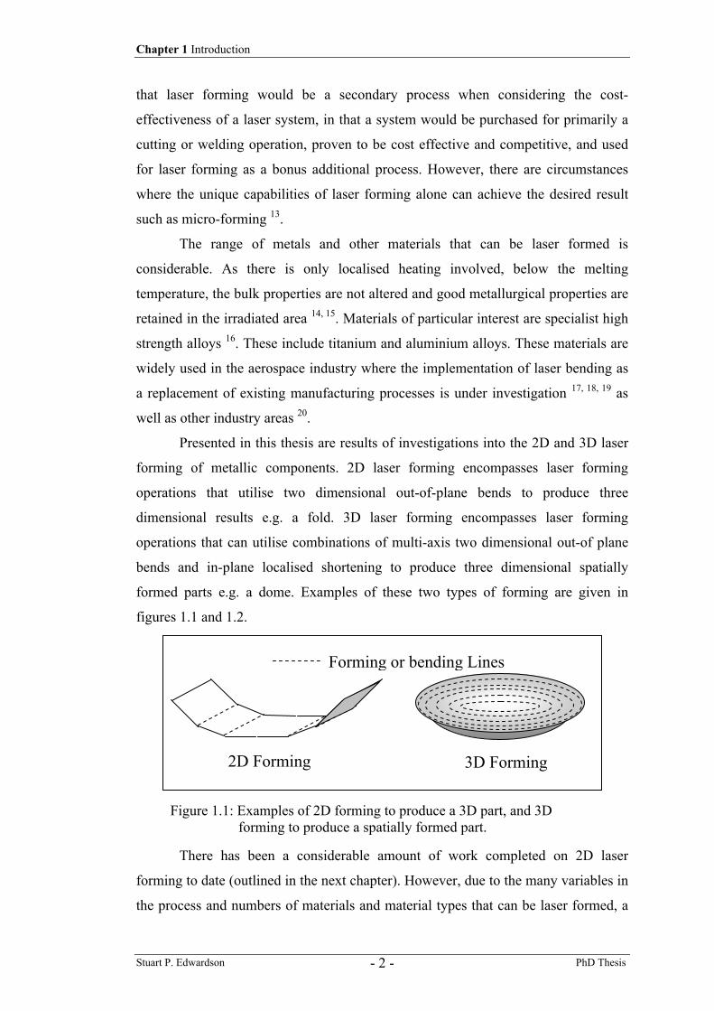
Presented in this thesis are results of investigations into the 2D and 3D laser
forming of metallic components. 2D laser forming encompasses laser forming
operations that utilise two dimensional out-of-plane bends to produce three
dimensional results e.g. a fold. 3D laser forming encompasses laser forming
operations that can utilise combinations of multi-axis two dimensional out-of plane
bends and in-plane localised shortening to produce three dimensional spatially
formed parts e.g. a dome. Examples of these two types of forming are given in
figures 1.1 and 1.2.
There has been a considerable amount of work completed on 2D laser
forming to date (outlined in the next chapter). However, due to the many variables in
the process and numbers of materials and material types that can be laser formed, a
Forming or bending Lines
2D Forming 3D Forming
Figure 1.1: Examples of 2D forming to produce a 3D part, and 3D forming to produce a spatially formed part.
Chapter 1 Introduction
Stuart P. Edwardson PhD Thesis - 3 -
full understanding of the process is some way off. The work on 2D laser forming
presented in this thesis aims to increase the knowledge and understanding of the
process, in particular the transient thermo-mechanical and asymmetrical effects plus
aspects for closed loop controlled LF. Materials investigated include mild steel,
aluminium AA1050, aluminium AA6061, Ti6Al4V and newly developed Metal
Laminate Composite Materials.
In order to advance the laser forming process still further for realistic forming
applications and for straightening and aligning operations in a manufacturing
environment, it is then necessary to consider 3D laser forming. Less work has been
completed in this field compared to 2D LF, however the process has been shown to
have a great deal of potential (discussed next chapter). In order to compete directly
with conventional forming techniques though, such as die forming, the process must
be proven to be reliable, repeatable, cost effective and flexible. It is the potential
flexibility of 3D laser forming that offers the greatest benefits, in that a change to a
required part geometry could be implemented easily through the CAD driven process,
this can be compared to the expensive and in-flexible hard tooling requirements of
the die forming process. The work presented in this thesis on 3D laser forming aims
to prove the viability of this technique as a direct manufacturing tool and as a means
of correcting unwanted distortion (perhaps from processes such as chemical etching).
To this aim progress towards repeatable closed loop controlled 3D LF is presented.
The materials investigated were mild steel and Ti6Al4V.
The work presented in this thesis contributed to a larger EPSRC funded
research programme entitled ‘Laser Forming of Aerospace Alloys – A Direct
Fabrication Technique’. The research programme involved a consortium of 3
universities; The University of Liverpool, Heriot Watt University and Cambridge
University; and 2 industrial partners; BAE SYSTEMS and Rolls-Royce plc.
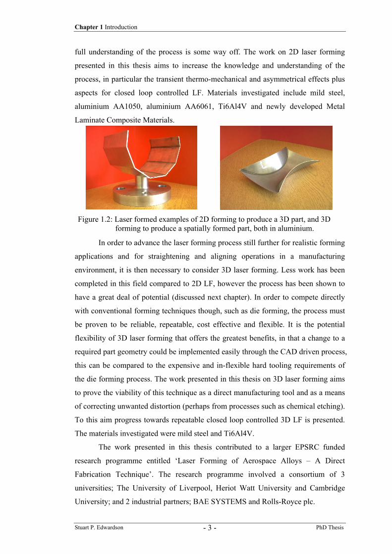
Figure 1.2: Laser formed examples of 2D forming to produce a 3D part, and 3D forming to produce a spatially formed part, both in aluminium.
Chapter 2 Literature Review
Stuart P. Edwardson PhD Thesis - 4 -
Chapter 2
Literature Review 2.1 Introduction This chapter presents some background to laser forming. It reviews the mechanisms
and models for laser forming currently available in the literature, previous
experimental work of note and the potential and current applications of the process.
A synopsis for the current research is also given.
2.2 Process Origins Laser forming originates from the similar process of flame bending or “line heating”
which uses an oxy-acetylene torch as the heat source 8, 21. Flame bending has been
used extensively for profiling and straightening heavy engineering components such
as beams and girders for construction purposes and decking and hull plates for the
shipbuilding industry 6, 7, 9. The diffuse nature of the flame used in line heating
makes the process rely heavily on operator skill. A flame heat source produces a
constant temperature at the surface of the workpiece and it is difficult to establish a
steep thermal gradient (which is often necessary for the process) in thin sections and
materials with a high thermal conductivity. Consequently the operator must spend
much time learning about the heating conditions which will produce the desired
result by trial and error. The heating rates associated with laser beams impinging on
metallic objects are high and steep thermal gradients are easily achieved. In addition
the laser beam can be applied to a very localised region as opposed to the flame.
These advantages along with the potential for automation have led to research into
laser forming.
Chapter 2 Literature Review
Stuart P. Edwardson PhD Thesis - 5 -
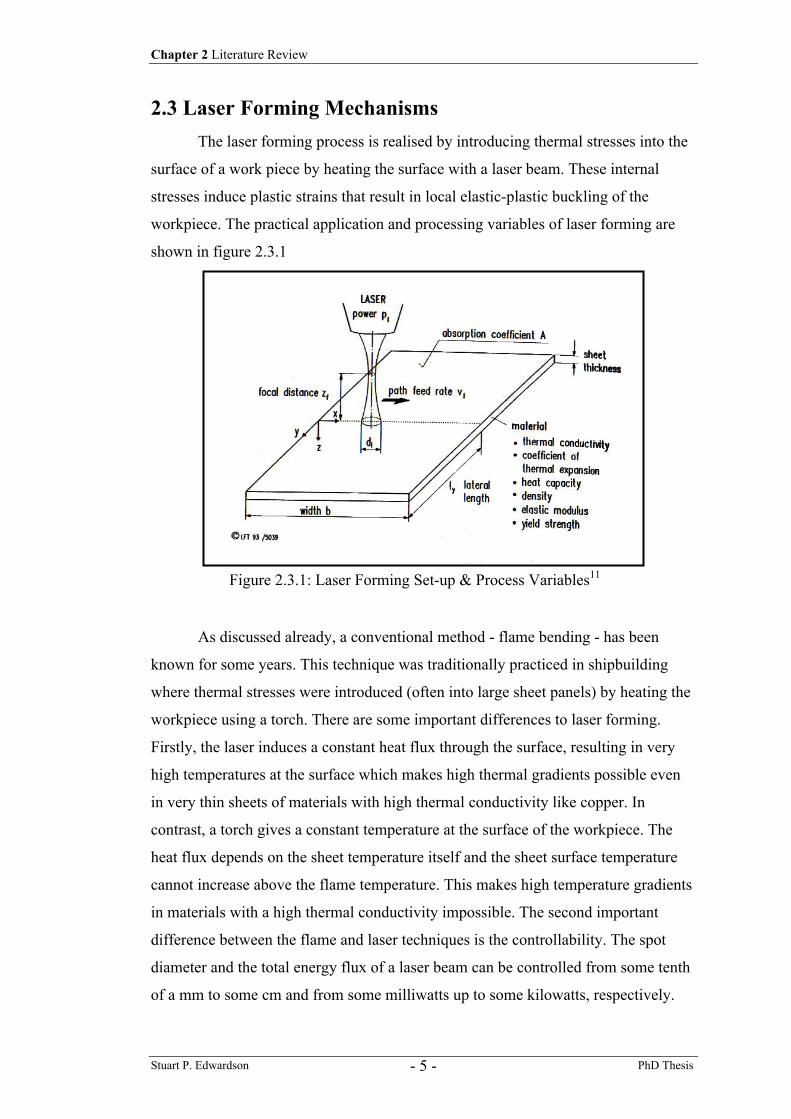
2.3 Laser Forming Mechanisms The laser forming process is realised by introducing thermal stresses into the
surface of a work piece by heating the surface with a laser beam. These internal
stresses induce plastic strains that result in local elastic-plastic buckling of the
workpiece. The practical application and processing variables of laser forming are
shown in figure 2.3.1
As discussed already, a conventional method - flame bending - has been
known for some years. This technique was traditionally practiced in shipbuilding
where thermal stresses were introduced (often into large sheet panels) by heating the
workpiece using a torch. There are some important differences to laser forming.
Firstly, the laser induces a constant heat flux through the surface, resulting in very
high temperatures at the surface which makes high thermal gradients possible even
in very thin sheets of materials with high thermal conductivity like copper. In
contrast, a torch gives a constant temperature at the surface of the workpiece. The
heat flux depends on the sheet temperature itself and the sheet surface temperature
cannot increase above the flame temperature. This makes high temperature gradients
in materials with a high thermal conductivity impossible. The second important
difference between the flame and laser techniques is the controllability. The spot
diameter and the total energy flux of a laser beam can be controlled from some tenth
of a mm to some cm and from some milliwatts up to some kilowatts, respectively.
Figure 2.3.1: Laser Forming Set-up & Process Variables11
Chapter 2 Literature Review
Stuart P. Edwardson PhD Thesis - 6 -
The control of a flame is much more problematic. The energy flux or flame
temperature depends on the oxygen content of the gas mixture which is difficult to
control. In addition, the flame diameter is much larger than that of a laser beam and
also very hard to control11.
Due to the very good control offered by the laser beam, different types of
temperature fields can be generated, yielding different forming mechanisms and
results. These mechanisms are described below.
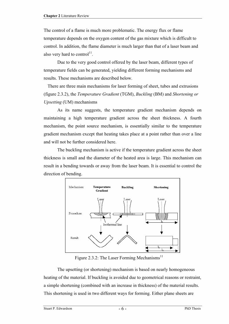
There are three main mechanisms for laser forming of sheet, tubes and extrusions
(figure 2.3.2), the Temperature Gradient (TGM), Buckling (BM) and Shortening or
Upsetting (UM) mechanisms
As its name suggests, the temperature gradient mechanism depends on
maintaining a high temperature gradient across the sheet thickness. A fourth
mechanism, the point source mechanism, is essentially similar to the temperature
gradient mechanism except that heating takes place at a point rather than over a line
and will not be further considered here.
The buckling mechanism is active if the temperature gradient across the sheet
thickness is small and the diameter of the heated area is large. This mechanism can
result in a bending towards or away from the laser beam. It is essential to control the
direction of bending.
The upsetting (or shortening) mechanism is based on nearly homogeneous
heating of the material. If buckling is avoided due to geometrical reasons or restraint,
a simple shortening (combined with an increase in thickness) of the material results.
This shortening is used in two different ways for forming. Either plane sheets are
Figure 2.3.2: The Laser Forming Mechanisms11
Chapter 2 Literature Review
Stuart P. Edwardson PhD Thesis - 7 -
treated with this mechanism resulting in spatially formed parts or extrusions are
treated, giving specially bent extrusions11.
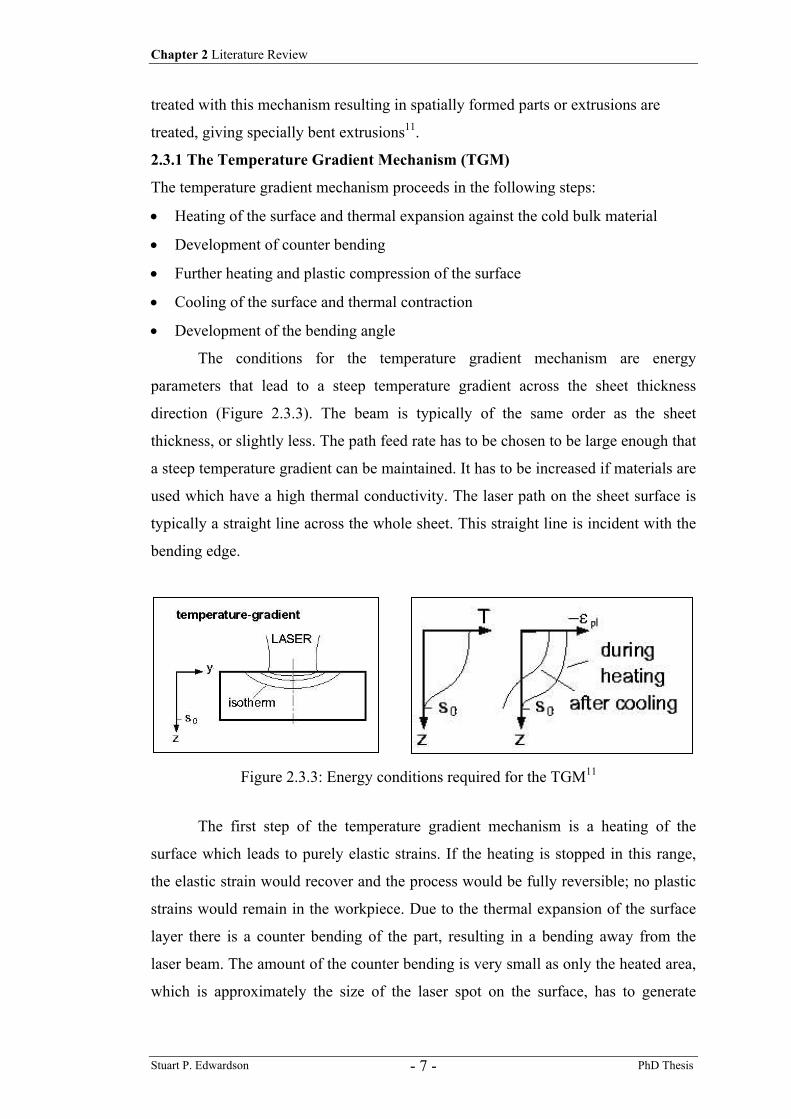
2.3.1 The Temperature Gradient Mechanism (TGM)
The temperature gradient mechanism proceeds in the following steps:
• Heating of the surface and thermal expansion against the cold bulk material
• Development of counter bending
• Further heating and plastic compression of the surface
• Cooling of the surface and thermal contraction
• Development of the bending angle
The conditions for the temperature gradient mechanism are energy
parameters that lead to a steep temperature gradient across the sheet thickness
direction (Figure 2.3.3). The beam is typically of the same order as the sheet
thickness, or slightly less. The path feed rate has to be chosen to be large enough that
a steep temperature gradient can be maintained. It has to be increased if materials are
used which have a high thermal conductivity. The laser path on the sheet surface is
typically a straight line across the whole sheet. This straight line is incident with the
bending edge.
The first step of the temperature gradient mechanism is a heating of the
surface which leads to purely elastic strains. If the heating is stopped in this range,
the elastic strain would recover and the process would be fully reversible; no plastic
strains would remain in the workpiece. Due to the thermal expansion of the surface
layer there is a counter bending of the part, resulting in a bending away from the
laser beam. The amount of the counter bending is very small as only the heated area,
which is approximately the size of the laser spot on the surface, has to generate
Figure 2.3.3: Energy conditions required for the TGM11
Chapter 2 Literature Review
Stuart P. Edwardson PhD Thesis - 8 -
forces which produce the counter bending of the whole sheet. The counter bending
effect is detrimental for the development of a plastic bending angle towards the laser
beam. This is so because the counter bending is identical to a relaxation of the
surface stresses at the heated surface. So the thermal expansion leads to lower
surface stresses and therefore the fraction of the thermal strain which is converted
into plastic strain is less than without counter bending.
Further heating leads to a decrease of the flow stress in the heated area and a
further increase of the thermal expansion of the surface layer. At a certain
temperature which depends on the material and the geometry and the amount of
counter bending, the thermal strains reach the elastic strain which can be carried by
the material at the given temperature. A further increase of the temperature results in
a conversion of the thermal expansion into plastic compressive strains. These plastic
compressive strains are accumulated until the heating stops or surface melting
occurs. The heating of a certain point of the surface stops after the laser beam has
passed this point. Then cooling sets in.
In contrast to the heating part of the cycle, where the heat flow is through the
surface due to the coupling of the laser energy, cooling proceeds by heat conduction
in the part. Energy losses by radiation and heat conduction into the environment are
of less importance and can be neglected. Cooling is mainly due to self-quenching
which is also observed in laser surface treatments. The heat flows into the
surrounding sheet metal and gives cooling rates which lead to a cooling of the heated
area within some seconds, typically 10-20 s, which has to be compared with heating
times of about 0.5s. During cooling a shrinkage of the heated material sets in. Due to
the fact that the surface was plastically compressed during heating it is shorter after
cooling to room temperature compared to the non-heated layers of the sheet. Due to
the different length of the surface layer and the lower layer of the sheets bending
angle towards the laser beam develops. The magnitude of the bending angle depends
on the coupled energy, the geometry of the part and the thermal and mechanical
properties of the material. It lies typically between 0.1 degrees and 3 degrees after
one laser pass.
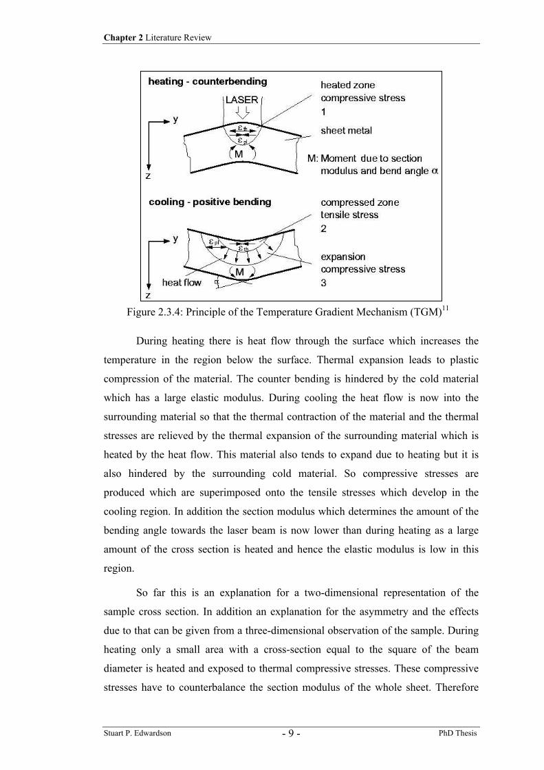
The asymmetry of the process is the reason why the thermal expansion leads
to plastic compression of the sheet and the thermal contraction does not lead to a
plastic tension of the material, this would cancel the plastic compression and
therefore hinder a development of a bending angle (Figure 2.3.4).
Chapter 2 Literature Review
Stuart P. Edwardson PhD Thesis - 9 -
During heating there is heat flow through the surface which increases the
temperature in the region below the surface. Thermal expansion leads to plastic
compression of the material. The counter bending is hindered by the cold material
which has a large elastic modulus. During cooling the heat flow is now into the
surrounding material so that the thermal contraction of the material and the thermal
stresses are relieved by the thermal expansion of the surrounding material which is
heated by the heat flow. This material also tends to expand due to heating but it is
also hindered by the surrounding cold material. So compressive stresses are
produced which are superimposed onto the tensile stresses which develop in the
cooling region. In addition the section modulus which determines the amount of the
bending angle towards the laser beam is now lower than during heating as a large
amount of the cross section is heated and hence the elastic modulus is low in this
region.
So far this is an explanation for a two-dimensional representation of the
sample cross section. In addition an explanation for the asymmetry and the effects
due to that can be given from a three-dimensional observation of the sample. During
heating only a small area with a cross-section equal to the square of the beam
diameter is heated and exposed to thermal compressive stresses. These compressive
stresses have to counterbalance the section modulus of the whole sheet. Therefore
Figure 2.3.4: Principle of the Temperature Gradient Mechanism (TGM)11
Chapter 2 Literature Review
Stuart P. Edwardson PhD Thesis - 10 -
the counter-bending is very small. In contrast, during cooling the whole edge of the
sheet is cooling simultaneously. This is so because the heating is very fast but
cooling is much slower. Therefore, the moments produced by the cooling of a small
section have to counter-balance the local stiffness of the part only, which is much
smaller than the global stiffness during heating. So there is nearly no cancellation of
the plastic compression and large bending angles can develop. This asymmetry of
the heating and cooling phase is essential for the development of a bending angle for
this mechanism11.
2.3.2 The Buckling Mechanism (BM)
The buckling mechanism operates if the laser beam diameter is large
compared to the sheet thickness and the processing speed is low resulting in a small
temperature gradient across the sheet thickness. These conditions may be realised by
different parameter combinations. One possibility is to irradiate a high alloyed steel
foil (e.g. 100µm in thickness), using a low power laser and a low processing speed.
Another possibility is to use material with a high thermal conductivity like copper.
The buckling mechanism proceeds by the following steps:
• Heating of a large area of the sheet metal and development of compressive
stresses
• Onset of buckling
• Growth of the buckle
• Shifting the buckle through the whole sheet
• Relaxation of the elastic stresses.
The principle is shown in figure 2.3.5. At the beginning the sheet metal is
heated by a laser beam with a beam diameter which is large compared to the sheet
thickness, also the processing speed is low, this results in only a small temperature
gradient across the sheet thickness and hence the thermal expansion of the material
results in compressive stresses in the heated area.
If the heated area is large enough and if there is a small natural deviation
from perfect flatness (which normally exists in real metal sheets) an instability
develops. This instability is similar to the buckle of a sheet metal in the flange during
deep drawing if no blank holder or too low blank holding forces are used. The
direction of the buckling is determined by different factors, these are for example the
pre-bending of the sheet and the relaxation of residual stresses.
Chapter 2 Literature Review
Stuart P. Edwardson PhD Thesis - 11 -
In the centre of the buckle the temperature is very high so that the flow stress
is low in this region. Therefore the bending in this region is nearly totally plastic. In
contrast the root of the buckle which is far away from the centre of the beam is
heated to a much lesser extent. So the temperature is low and the flow stress in this
region is high. Therefore the bending of the sheet in this region is fully elastic.
Due to further heating the thermal expansion of the material increases the
height of the buckle. As the laser beam is guided across the surface with the
processing speed the buckle is also shifted along the bending edge. Now the existing
buckle predetermines the direction of the buckling and the remaining part of the
sheet buckles in the same direction as the sheet has done at the beginning. While the
beam is guided across the surface the stiffness of the part is changed. At the
beginning of the buckling process the bending arms were held in the original plane
due to the stiff surrounding material. As an increasing amount of the sheet is formed
by the buckle the forces that hold the bending arms straight, decrease. Therefore the
elastic part of the buckle relaxes and only the plastic part remains in the sheet. This
leads to the development of the bending angle which can be seen after irradiating the
whole bending edge. After finishing the irradiation the elastic strains are fully
relaxed so that an angular section remains. The buckling mechanism results typically
in bending angles between 1 and 15 degrees. This is significantly larger than
observed for the temperature gradient mechanism. This is not a result of a higher
degree of performance but a result of the fact that using the buckling mechanism
Figure 2.3.5: Stages in the Buckling Mechanism (BM)11
Chapter 2 Literature Review
Stuart P. Edwardson PhD Thesis - 12 -
more energy can be coupled into the workpiece in one step. Trying the same for the
temperature gradient mechanism either surface melting or buckling would occur,
depending on the spot size of the laser beam. Therefore the energy which can be
coupled into the workpiece is restricted for the temperature gradient mechanism.
Another typical feature of the buckling mechanism is that the bending angle
can be positive (concave bending towards the laser beam), or negative (convex
bending away from the laser beam). Of course it is essential to control the direction
of bending for a reliable process. Otherwise this bending mechanism cannot be used
in manufacturing. For a reliable control of the bending direction the controlling
parameters on the bending direction must be understood. In practice there are two
main important factors which determine the direction of bending. These are the
plastic pre-bending of the sheet and the relaxation of the residual stresses. A plastic
pre-bending often occurs as a result of storing the sheet in a coil or a handling
operation like cutting. These operations give a pre-bending which is first well
defined but the direction of pre-bending may be lost during arbitrary handling of the
parts. Therefore plastic pre-bending will lead with a probability of 50 % each to a
positive and negative bending angle. But it is possible of course to produce a plastic
pre-bending in a well-controlled manner. This may be done by pre-bending the sheet
using the temperature gradient mechanism which always gives positive bending
angles. So a pre-bending may be defined giving also 100 % positive bending angles
after the irradiation with parameters according to the buckling mechanism. This is
the usual way to get well defined bending using the buckling mechanism.
The second important parameter that determines the direction of bending is
the asymmetric relaxation of residual stresses. After rolling there are normally
compressive stresses in the surface and tensile stresses in the core of the sheet.
When working with a relatively high processing speed we get an asymmetric
relaxation of these residual stresses. Due to the temperature gradient produced by
the radiation, the stresses in the heated surface are relaxed first. In this moment the
compressive stresses are removed from the surface resulting in a positive curvature
of the sheet due to the remaining residual stresses. Even if the relaxation of the
residual stresses proceeds and a symmetric state is reached after a certain time, the
asymmetric relaxation at the beginning gives an instability such that the buckling is
always away from the laser beam yielding a bending angle towards the laser beam11.
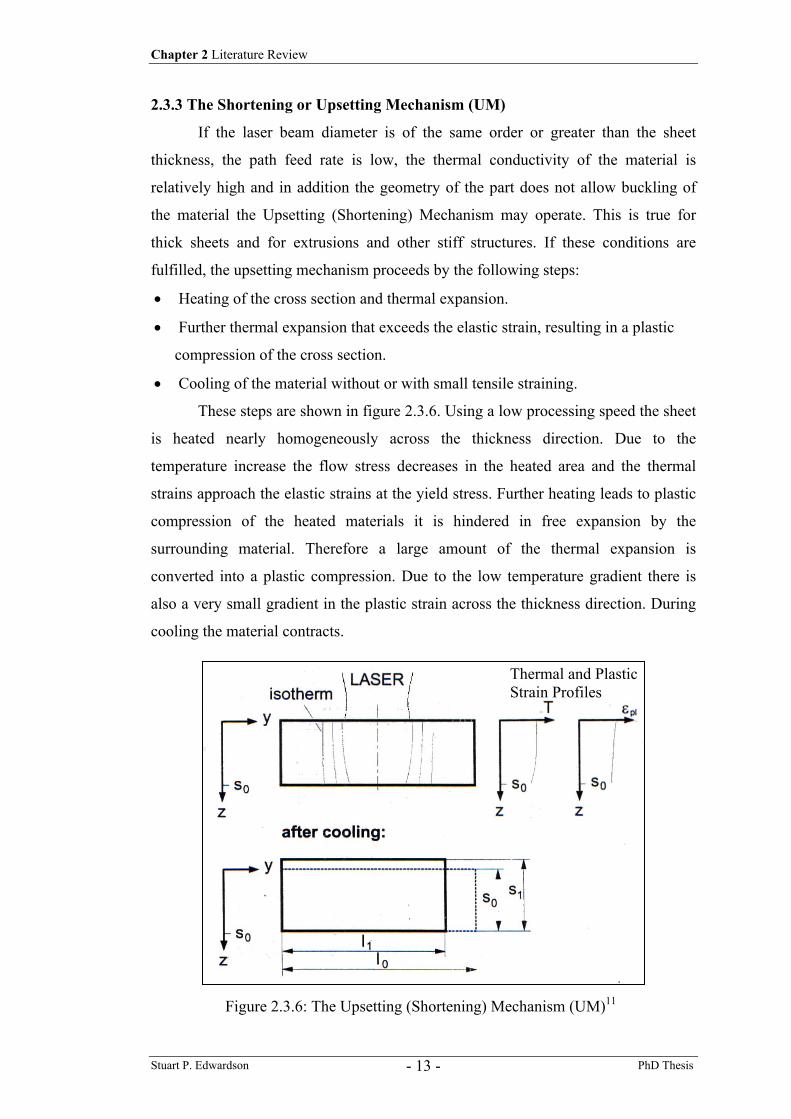
Chapter 2 Literature Review
Stuart P. Edwardson PhD Thesis - 13 -
2.3.3 The Shortening or Upsetting Mechanism (UM)
If the laser beam diameter is of the same order or greater than the sheet
thickness, the path feed rate is low, the thermal conductivity of the material is
relatively high and in addition the geometry of the part does not allow buckling of
the material the Upsetting (Shortening) Mechanism may operate. This is true for
thick sheets and for extrusions and other stiff structures. If these conditions are
fulfilled, the upsetting mechanism proceeds by the following steps:
• Heating of the cross section and thermal expansion.
• Further thermal expansion that exceeds the elastic strain, resulting in a plastic
compression of the cross section.
• Cooling of the material without or with small tensile straining.
These steps are shown in figure 2.3.6. Using a low processing speed the sheet
is heated nearly homogeneously across the thickness direction. Due to the
temperature increase the flow stress decreases in the heated area and the thermal
strains approach the elastic strains at the yield stress. Further heating leads to plastic
compression of the heated materials it is hindered in free expansion by the
surrounding material. Therefore a large amount of the thermal expansion is
converted into a plastic compression. Due to the low temperature gradient there is
also a very small gradient in the plastic strain across the thickness direction. During
cooling the material contracts.
Figure 2.3.6: The Upsetting (Shortening) Mechanism (UM)11
Thermal and Plastic Strain Profiles
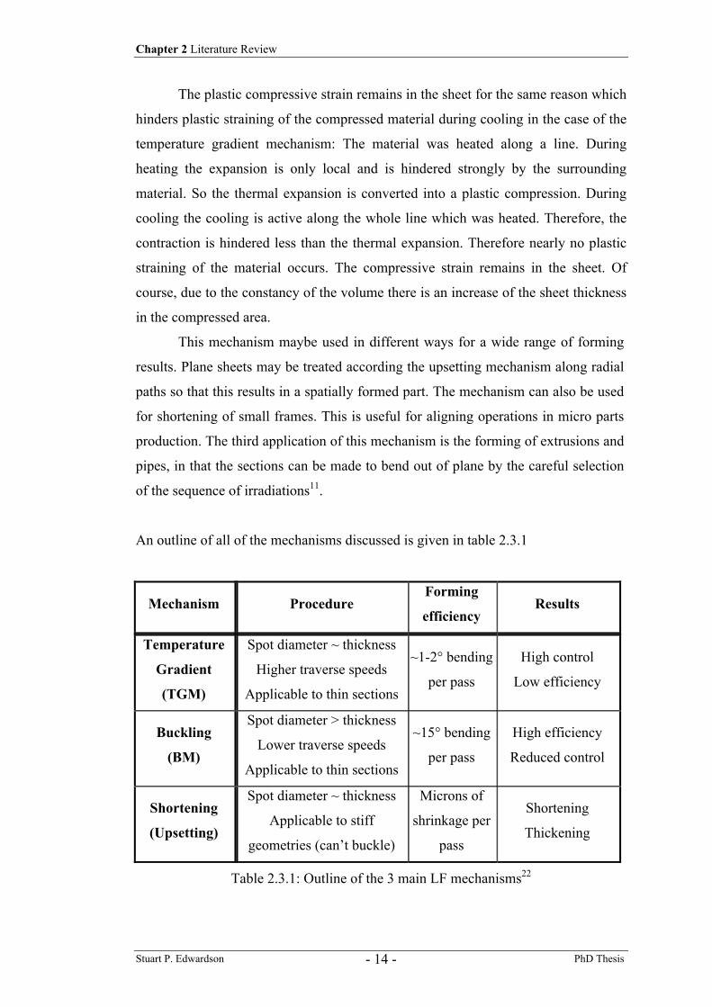
Chapter 2 Literature Review
Stuart P. Edwardson PhD Thesis - 14 -
The plastic compressive strain remains in the sheet for the same reason which
hinders plastic straining of the compressed material during cooling in the case of the
temperature gradient mechanism: The material was heated along a line. During
heating the expansion is only local and is hindered strongly by the surrounding
material. So the thermal expansion is converted into a plastic compression. During
cooling the cooling is active along the whole line which was heated. Therefore, the
contraction is hindered less than the thermal expansion. Therefore nearly no plastic
straining of the material occurs. The compressive strain remains in the sheet. Of
course, due to the constancy of the volume there is an increase of the sheet thickness
in the compressed area.
This mechanism maybe used in different ways for a wide range of forming
results. Plane sheets may be treated according the upsetting mechanism along radial
paths so that this results in a spatially formed part. The mechanism can also be used
for shortening of small frames. This is useful for aligning operations in micro parts
production. The third application of this mechanism is the forming of extrusions and
pipes, in that the sections can be made to bend out of plane by the careful selection
of the sequence of irradiations11.
An outline of all of the mechanisms discussed is given in table 2.3.1
Mechanism Procedure Forming
efficiency Results
Temperature
Gradient
(TGM)
Spot diameter ~ thickness
Higher traverse speeds
Applicable to thin sections
~1-2° bending
per pass
High control
Low efficiency
Buckling
(BM)
Spot diameter > thickness
Lower traverse speeds
Applicable to thin sections
~15° bending
per pass
High efficiency
Reduced control
Shortening
(Upsetting)
Spot diameter ~ thickness
Applicable to stiff
geometries (can’t buckle)
Microns of
shrinkage per
pass
Shortening
Thickening
Table 2.3.1: Outline of the 3 main LF mechanisms22
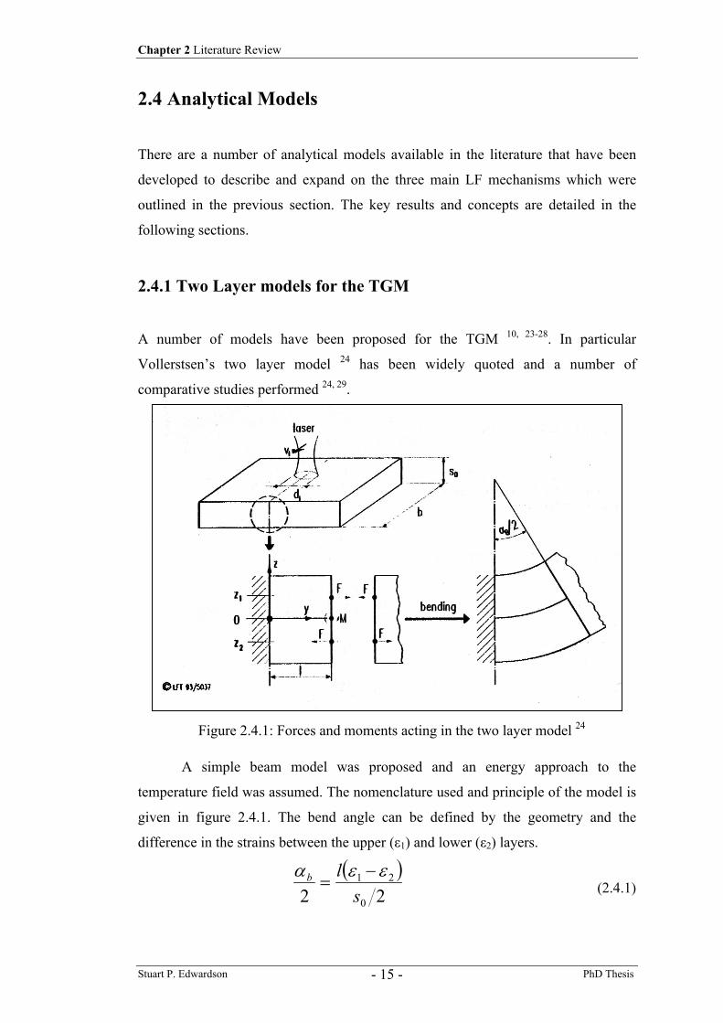
Chapter 2 Literature Review
Stuart P. Edwardson PhD Thesis - 15 -
2.4 Analytical Models
There are a number of analytical models available in the literature that have been
developed to describe and expand on the three main LF mechanisms which were
outlined in the previous section. The key results and concepts are detailed in the
following sections.
2.4.1 Two Layer models for the TGM
A number of models have been proposed for the TGM 10, 23-28. In particular
Vollerstsen’s two layer model 24 has been widely quoted and a number of
comparative studies performed 24, 29.
A simple beam model was proposed and an energy approach to the
temperature field was assumed. The nomenclature used and principle of the model is
given in figure 2.4.1. The bend angle can be defined by the geometry and the
difference in the strains between the upper (ε1) and lower (ε2) layers.
( )22 0
21
slb εεα −
= (2.4.1)
Figure 2.4.1: Forces and moments acting in the two layer model 24
Chapter 2 Literature Review
Stuart P. Edwardson PhD Thesis - 16 -
Using beam theory, the strain within each layer may be calculated. Beam theory
states:
zRE
IM σ
== (2.4.2)
Where:
( )∫= 2
0
2h
dzzzBI (2.4.3)
R is the radius of curvature, M is the bending moment, I is the moment of inertia, E
is the Elastic Modulus and σ is the stress in the beam at z.
Considering the geometry illustrated in figure 2.4.1 the strain in the upper layer
(assuming it is compressed) is given by:
( ) TzEIM
AEF
th∆+−= αε 11
1
111 (2.4.4)
An important assumption made here is that all the thermal expansion of the upper
layer given by the is converted into plastic compression. In reality this is not the case
as some energy is used to elastically strain the material up to its temperature
dependent yield point. However an appreciable amount of elastic straining does not
occur because the free thermal expansion is greatly hindered by the cold and rigid
surrounding material. In addition, the yield stress of the heated zone is reduced to
almost zero during heating since it is temperature dependent. It may be acceptable
under these conditions to omit these parameters and assume that all the thermal
expansion is converted into plastic compression. During cooling as the heat flows
into the surrounding regions there may be a tensile plastic restraining of the
previously compressed zone.
After the plastic compression development the strain of the upper layer is given by:
( )'
11
1
111 Tz
EIM
AEF
th∆−−= αε (2.4.5)
∆T’ is the maximum temperature difference between the upper and lower layers of
the sheet. The strain of the lower layer is given by:
( ) 22
2
221 z
EIM
AEF
−=ε (2.4.6)
Chapter 2 Literature Review
Stuart P. Edwardson PhD Thesis - 17 -
Here I2 is the second moment of area. From the previously described beam theory
the fraction of the moment M and the product El yield the local curvature. For large
curvatures it is assumed that:
( ) ( ) ( ) lEIM
EIM
EIM b
22
2
1
1 α=== (2.4.7)
The bending angle αb can then be found by combining the equations for the upper
and the lower layers (eq 2.4.5 and 2.4.6) along with equation 2.4.1:
∆−+−−−= '1
11
2
220 224 T
lz
AEF
lz
AEF
sl
thbb
b ααα
α (2.4.8)
Where the force F is given by:
lsEI
sMF b
002α
== (2.4.9)
And substituting z1-z2 = s0/2 into 2.4.8 and 2.5.9 yields:
( )( ) 0
'
22110
2211 44s
TlAEAEs
AEAEEI thb
bb
∆++
+=
αα
αα (2.4.10)
The cross sections of the beams are described by:
11 bsA = (2.4.11)
And
( )102 ssbA −= (2.4.12)
The section moment is given by:
12
30bsI = (2.4.13)
Assuming E1 = E2 the equation for the bend angle is then given by:
( )30
101'12
ssslsTth
b−∆= αα (2.4.14)
To calculate the bend angle with this formula requires knowledge of the length of the
heated zone l, the depth of heating s1, and the temperature rise of the upper layer ∆T’.
This requires the co-ordinates to be found as a function of the temperature. i.e. in the
form of:
l=f(T) (2.4.15)
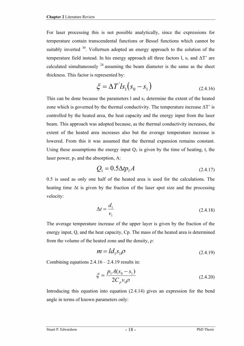
Chapter 2 Literature Review
Stuart P. Edwardson PhD Thesis - 18 -
For laser processing this is not possible analytically, since the expressions for
temperature contain transcendental functions or Bessel functions which cannot be
suitably inverted 30. Vollertsen adopted an energy approach to the solution of the
temperature field instead. In his energy approach all three factors l, s1 and ∆T’ are
calculated simultaneously 24 assuming the beam diameter is the same as the sheet
thickness. This factor is represented by:
( )101' sslsT −∆=ξ (2.4.16)
This can be done because the parameters l and s1 determine the extent of the heated
zone which is governed by the thermal conductivity. The temperature increase ∆T’ is
controlled by the heated area, the heat capacity and the energy input from the laser
beam. This approach was adopted because, as the thermal conductivity increases, the
extent of the heated area increases also but the average temperature increase is
lowered. From this it was assumed that the thermal expansion remains constant.
Using these assumptions the energy input Q1 is given by the time of heating, t, the
laser power, p1 and the absorption, A:
AtpQ 11 5.0 ∆= (2.4.17)
0.5 is used as only one half of the heated area is used for the calculations. The
heating time ∆t is given by the fraction of the laser spot size and the processing
velocity:
1
1
vdt =∆ (2.4.18)
The average temperature increase of the upper layer is given by the fraction of the
energy input, Q, and the heat capacity, Cp. The mass of the heated area is determined
from the volume of the heated zone and the density, ρ:
ρ11sldm = (2.4.19)
Combining equations 2.4.16 – 2.4.19 results in:
ρξ
1
101
2)(
vCssAp
p
−= (2.4.20)
Introducing this equation into equation (2.4.14) gives an expression for the bend
angle in terms of known parameters only:
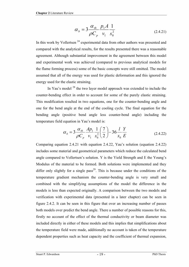
Chapter 2 Literature Review
Stuart P. Edwardson PhD Thesis - 19 -
201
1 13sv
ApC p
thb ρ
αα = (2.4.21)
In this work by Vollertsen 24 experimental data from other authors was presented and
compared with the analytical results, for the results presented there was a reasonable
agreement. Although substantial improvement in the agreement between this model
and experimental work was achieved (compared to previous analytical models for
the flame forming process) some of the basic concepts were still omitted. The model
assumed that all of the energy was used for plastic deformation and this ignored the
energy used for the elastic straining.
In Yau’s model 28 the two layer model approach was extended to include the
counter-bending effect in order to account for some of the purely elastic straining.
This modification resulted in two equations, one for the counter-bending angle and
one for the bend angle at the end of the cooling cycle. The final equation for the
bending angle (positive bend angle less counter-bend angle) including the
temperature field equation in Yau’s model is:
EY
sl
svAp
C p
thb
0201
1 362713 −
=
ρα
α (2.4.22)
Comparing equation 2.4.21 with equation 2.4.22, Yau’s solution (equation 2.4.22)
includes some material and geometrical parameters which reduce the calculated bend
angle compared to Vollertsen’s solution. Y is the Yield Strength and E the Young’s
Modulus of the material to be formed. Both solutions were implemented and they
differ only slightly for a single pass29. This is because under the conditions of the
temperature gradient mechanism the counter-bending angle is very small and
combined with the simplifying assumptions of the model the difference in the
models is less than expected originally. A comparison between the two models and
verification with experimental data (presented in a later chapter) can be seen in
figure 2.4.2. It can be seen in this figure that over an increasing number of passes
both models over predict the bend angle. There a number of possible reasons for this,
firstly no account of the effect of the thermal conductivity or beam diameter was
included directly in either of these models and this implies that simplifications about
the temperature field were made, additionally no account is taken of the temperature
dependent properties such as heat capacity and the coefficient of thermal expansion,
Chapter 2 Literature Review
Stuart P. Edwardson PhD Thesis - 20 -
assumed constant. Another factor in these models is that they predict a constant bend
angle increase with increasing numbers of passes, it has been seen in a number of
published studies that the bend angle rate falls off with increasing numbers of passes 29, to be discussed later, these equations do not take into account factors such as
coating degradation (absorption dependent) and section thickening29.
2.4.2 The Residual Stress Model for the TGM
Vollertsen extended the work on the temperature gradient mechanism in another
model to include the effects of a realistic temperature field analytically, 25 and a
more realistic strain distribution was included. This model used the residual stress
approach often used in welding analysis. The strains in the y & z directions were the
only strains considered in the analysis, i.e. an infinitesimal strip in the direction in
which the laser beam is scanning (x) is considered (figure 2.2.3).
Figure 2.4.2: Comparison of solutions for the two layer models
Figure 2.4.3: Layout for the residual stress model
Chapter 2 Literature Review
Stuart P. Edwardson PhD Thesis - 21 -
Initially it is assumed that that there is a boundary temperature or isotherm TB above
which the thermal expansion that is hindered by the surrounding material leads to
plastic compression.
An elliptical strain distribution was assumed and was given by:
221
1
)( zss
z in −=ε
ε (2.4.23)
εin is the inherent strain, this is the maximum plastic strain due to thermal expansion
less the purely elastic strain during heating, such as:
)()(
TETk
T fthin −∆=αε (2.4.24)
Plastic strain occurs if the strain due to the thermal expansion exceeds the purely
elastic strain. The elastic strain is governed by temperature dependent properties, in
that the flow or yield stress and Young’s modulus fall as the temperature increases,
thus making it easier to produce a plastic compression and hence bend a material.
s1 represents the depth of the plastic zone. If the plastic zone is less than the sheet
thickness, s0, then integration of the local strains results in the local bending moment,
the plate is said to bend about this depth s1. The bending moment can be determined
from beam theory, equation 2.4.2, substituting for I:
∫= Bdzzz
M B2σ
(2.4.25)
Substituting for σ and B yields:
dzzszdxEMs
B ∫
−= 1
00
2)(ε (2.4.26)
Substituting eq. 2.4.23 in 2.4.26 and integrating yields:
−=
38
21
10sssdxEM inB
πε (2.4.27)
From geometrical conditions it is known that the bending angle is given by the
fraction of twice the length of the bent zone and the curvature. From the previously
described beam theory (eq. 2.4.2) the fraction of the transverse bending moment
and the Elastic modulus times the moment of inertia yields the inverse of the
curvature, such that:
Chapter 2 Literature Review
Stuart P. Edwardson PhD Thesis - 22 -
Rl
b2
=α (2.4.28)
and
EIM
RB=
1 (2.4.29)
where:
12
30dxsI = (2.4.30)
Substituting these equations into eq. 2.4.27 and rearranging for αb yields:
( )1030
1 83 ssslsin
b −= πεα (2.4.31)
To calculate the bend angles with these formulas requires knowledge of the depth of
the plastic zone, s0 and the length of the plastic zone, l. These may be obtained from
the proposed temperature field calculation. The solution to the temperature field
however, was an approximation of the Fourier equation of three dimensional heat
conduction for a finite area source. As the length and depth of the plastic zone were
required for the solution, the co-ordinates were required as a function of the
temperature. An approximate solution in the range relevant to laser bending was
used as it was not possible to invert this form of the heat equation in a suitable
fashion analytically to give the depth co-ordinate. Details of this approximation can
be found in the reference25.
The depth of the plastic zone was given by:
22
34ln 32
1
atPP
NTs f
ff
c
−= − (2.4.32)
The length of the heated zone was given by:
−= − 23
34ln
214 f
f
c
ff P
NT
PatPl (2.4.33)
Chapter 2 Literature Review
Stuart P. Edwardson PhD Thesis - 23 -
This model showed the importance of the thermal conductivity on the process.
A slight change in the thermal conductivity changes the thermal expansion and the
position of the elastic-plastic interface, as the average temperature in the irradiated
zone is sensitive to slight changes in the thermal conductivity. Consequently it is
possible that the bend angle itself is sensitive to small changes in the thermal
conductivity. This is contrary to what was reported in the two 1ayer model. In
addition with this model the contribution of the thermal strain to the plastic bending
was found by subtracting the fraction of the yield stress and the elastic modulus from
the thermal expansion (equation 2.4.24). As mentioned both the yield stress and the
elastic modulus are temperature dependent, this required the function which related
those parameters to temperature to be known in order to calculate this contribution
accurately.
Provided with accurate information about the temperature dependent
mechanical properties the model can predict the bend angles with reasonable
accuracy for an analytical route, comparison with experimental data showed this 25.
Mucha et al 26 also modelled the TGM and has provided bend angle
equations for rectangular, triangular, elliptical and circular shaped plastic zones.
These shapes depend on the materials thermal properties and the laser processing
parameters used. Again the y & z directions (assuming the same co-ordinate system
as Vollertsen, figure 2.4.3) are the only directions considered relevant for the
analysis. The formulas for the bend angles for the different shaped plastic zones were
found to be:
Rectangular:
( ) 30
10116s
ssTlsthb −∆= αα (2.4.34)
Triangular:
( ) 30
101123s
ssTlsthb −∆=αα (2.4.35)
Elliptical:
( ) 30
101 2183s
ssTlsthb −∆= παα (2.4.36)
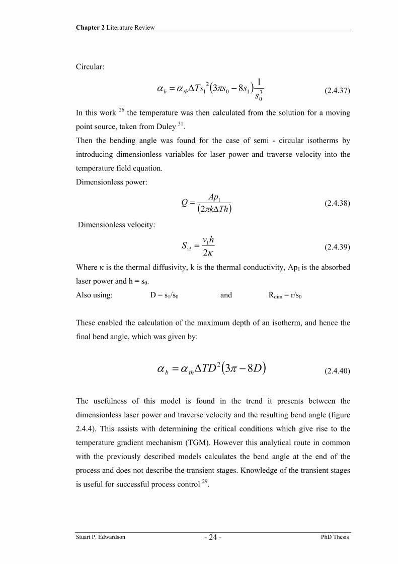
Chapter 2 Literature Review
Stuart P. Edwardson PhD Thesis - 24 -
Circular:
( ) 30
102
1183s
ssTsthb −∆= παα (2.4.37)
In this work 26 the temperature was then calculated from the solution for a moving
point source, taken from Duley 31.
Then the bending angle was found for the case of semi - circular isotherms by
introducing dimensionless variables for laser power and traverse velocity into the
temperature field equation.
Dimensionless power:
( )ThkApQ∆
=π2
1 (2.4.38)
Dimensionless velocity:
κ21hvSvl = (2.4.39)
Where κ is the thermal diffusivity, k is the thermal conductivity, Ap1 is the absorbed
laser power and h = s0.
Also using: D = s1/s0 and Rdim = r/s0
These enabled the calculation of the maximum depth of an isotherm, and hence the
final bend angle, which was given by:
( )DTDthb 832 −∆= παα (2.4.40)
The usefulness of this model is found in the trend it presents between the
dimensionless laser power and traverse velocity and the resulting bend angle (figure
2.4.4). This assists with determining the critical conditions which give rise to the
temperature gradient mechanism (TGM). However this analytical route in common
with the previously described models calculates the bend angle at the end of the
process and does not describe the transient stages. Knowledge of the transient stages
is useful for successful process control 29.
Chapter 2 Literature Review
Stuart P. Edwardson PhD Thesis - 25 -
In analytical work by Magee 29 it was agued that the above models for the
TGM, although they have advanced the understanding of the process on a
rudimentary level, are incomplete in terms of practical laser forming due to gross
simplifications. The mechanics of the process are defined in terms of the engineering
theory of bending and specifically beam theory. The transverse bending moment has
been used to find the curvature and the temperature field was approximated using an
energy approach, or by an approximation of the solution for the temperature field
from a static laser beam impinging on a thin sheet. Future forming operations will be
concerned with forming an initially flat sheet into a final geometry which is three
dimensional, therefore a model which analyses transverse bending moments only,
and predicts only and angular deformation is of limited use for practical forming. It
was shown in this work that there are other forces and moments acting in laser
forming apart from the transverse bending moments. This indicates that there should
in theory be two bend angles in laser forming under certain conditions, the angle
transverse to the direction of scanning and the angle parallel to the direction of
scanning. 2.4.3 The Buckling Mechanism As described previously the requirements for the initiation of the BM on sheet metal
are that the laser beam diameter on the surface of the sheet is approximately an order
of magnitude greater than the sheet thickness and that the material has a suitable
thermal conductivity so that the laser processing parameters employed do not result
Figure 2.4.4: Critical operating region for the TGM26
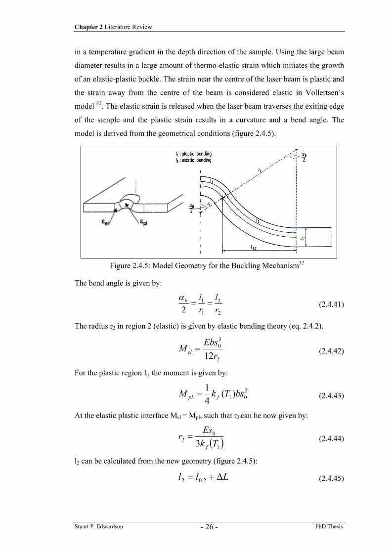
Chapter 2 Literature Review
Stuart P. Edwardson PhD Thesis - 26 -
in a temperature gradient in the depth direction of the sample. Using the large beam
diameter results in a large amount of thermo-elastic strain which initiates the growth
of an elastic-plastic buckle. The strain near the centre of the laser beam is plastic and
the strain away from the centre of the beam is considered elastic in Vollertsen’s
model 32. The elastic strain is released when the laser beam traverses the exiting edge
of the sample and the plastic strain results in a curvature and a bend angle. The
model is derived from the geometrical conditions (figure 2.4.5).
The bend angle is given by:
2
2
1
1
2 rl
rlb ==
α (2.4.41)
The radius r2 in region 2 (elastic) is given by elastic bending theory (eq. 2.4.2).
2
30
12rEbsM el = (2.4.42)
For the plastic region 1, the moment is given by:
201)(
41 bsTkM fpl = (2.4.43)
At the elastic plastic interface Mel = Mpl, such that r2 can be now given by:
( )1
02 3 Tk
Esrf
= (2.4.44)
l2 can be calculated from the new geometry (figure 2.4.5):
Lll ∆+= 2.02 (2.4.45)
Figure 2.4.5: Model Geometry for the Buckling Mechanism32
Chapter 2 Literature Review
Stuart P. Edwardson PhD Thesis - 27 -
where:
=
2sin22.0
brl α (2.4.46)
and
hth lTl ∆=∆ α (2.4.47)
Where ∆T is the average temperature of the heated zone of dimensions lh, ∆x and s0. ∆T is calculated from the absorbed laser power Ap1 the processing velocity v1 and the heat capacity and density, ρcp of the material.
10
1
2 vscApTpρ
=∆ (2.4.48)
l2 may be calculated from:
10
122 22sin
vscApfrl
p
thb
ραα ′
+
= (2.4.49)
ƒ’ is the fraction of the thermal expansion that leads to an expansion of region 2. Using a value of 0.5 results in:
120
11
4)(3
2sin
2 vcEsTkAp
p
fthbb
ρααα
+
= (2.4.50)
Using the sine series expansion, the last expression for the bend angle was simplified. The final equation for the bending angle was:
31
201
11 1)(36
=
svAp
EcTk
p
fthb ρ
αα (2.4.51)
Of note here is the much lower dependency of the bend angle on the temperature
gradient which is consistent with the buckling mechanism theory described earlier.
2.4.4 The Shortening Mechanism
Kraus 33 has modelled box section laser bending. Using the upsetting mechanism box
sections or extrusions can be made to bend out of plane by careful selection of the
sequence of irradiations. A similar approach has been used to Vollertsen’s models
where a geometry / strain relationship is drawn between the processing parameters
Chapter 2 Literature Review
Stuart P. Edwardson PhD Thesis - 28 -
and the bending angle. The final equation describing the bend angle in this case was
found to be:
( )( )( )
−
−=
1
1120011
1
221
TEdTk
ssdcvbAp
bf
p
thb ρ
αα (2.4.52)
The model assumed that three of the four sides of the box section were heated
simultaneously to initiate the bending. In reality the sides are usually irradiated
sequentially. However for the purposes of an analytical model this effect would be
very difficult to include. Numerical studies into the sequence of irradiations in
extrusion bending have also been carried out by Kraus using finite element methods.
2.5 Numerical Models
Given the complexity of analytically modelling forming processes such as laser
bending where the workpiece temperatures, dimensions and properties are changing
both in time and space and which depend on many variables (figure 2.3.1), the
numerical approach is often more beneficial for modelling these situations29. The
improvement in computational efficiency in recent years has made such large scale
numerical studies more viable. Numerical models have been available for a number
of years for the flame forming process 8, 34, 35, 36, 37. However it is only in recent times
that emphasis has been placed on laser bending. With the release of more user
friendly numerical modelling software packages such as ALGOR and ABAQUS
coupled with faster computers, the use of numerical models as a research tool for
both academic and industrial sectors is becoming more prevalent, indeed one such
model is included in this thesis. The ability to investigate a complex process in a
non-destructive manor in any situation is extremely useful, however as with any
model assumptions are made and the quality of the output data is only as good as the
quality of the input data.
A number of the numerical models for each mechanism available in the literature are
outlined in the next sections.
Chapter 2 Literature Review
Stuart P. Edwardson PhD Thesis - 29 -
2.5.1 Temperature Gradient Mechanism
Vollertsen developed a finite difference model 38 for a two dimensional (2D) analysis
of the process. The temperature dependent material parameters were included in the
model by taking values at particular temperatures of interest and linearly
interpolating between them, and then those functions were used to relate the
temperature to the material properties. A rectangular shaped source was used to
represent the laser beam and the resultant two dimensional (2D) temperature field
was used to calculate the thermal expansion, strains and stresses in the elements.
Then, accounting for the stiffness of the whole sheet, a calculation was made to
assess in which elements the stress exceeded the temperature dependent yield stress.
Then the elastic strain in those elements was reduced by the amount that exceeded
the yield stress.
The amount of strain that exceeded the maximum elastic strain at the yield stress was
converted into a plastic strain. A loop was initiated which continued with this
calculation until there was equilibrium of forces and moments. After the thermal
field had finished being computed, the bending angle was calculated from the length
of the upper and lower layers of an element in conjunction with the sheet thickness.
This model provided a very fast means of calculating the effects of various process
parameters, but the simple boundary conditions that limited this approach led to the
modelling with the finite element method (FEM) 39.
In Alberti et al model 40 of the TGM the finite element method was used first
to evaluate the temperature field and then the results of this analysis were input into
a mechanical analysis. Illustrations for the temperature field and the deformation
were provided at various stages of the process. Emphasis was placed on the
importance of the temperature dependence of the yield stress of the material. A
constant decay law was assumed for the relationship between increasing temperature
and decreasing yield stress. Steel plates were considered in the analysis. Another
numerical simulation by the same author looked at the combined process of thermal
and mechanical bending 41. As this is a process and not solely laser bending no
further details are given here.
Hsiao et al have used the commercial package ABAQUS to model the
process 42. They used the modelling in their work to emphasise the importance of the
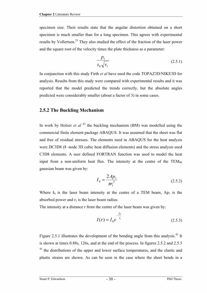
Chapter 2 Literature Review
Stuart P. Edwardson PhD Thesis - 30 -
specimen size. Their results state that the angular distortion obtained on a short
specimen is much smaller than for a long specimen. This agrees with experimental
results by Vollertsen.23 They also studied the effect of the fraction of the laser power
and the square root of the velocity times the plate thickness as a parameter:
10
1
vsp
(2.5.1)
In conjunction with this study Firth et al have used the code TOPAZ3D/NIKE3D for
analysis. Results from this study were compared with experimental results and it was
reported that the model predicted the trends correctly, but the absolute angles
predicted were considerably smaller (about a factor of 3) in some cases.
2.5.2 The Buckling Mechanism
In work by Holzer et al 43 the buckling mechanism (BM) was modelled using the
commercial finite element package ABAQUS. It was assumed that the sheet was flat
and free of residual stresses. The elements used in ABAQUS for the heat analysis
were DC3D8 (8 -node 3D cubic heat diffusion elements) and the stress analysis used
C3D8 elements. A user defined FORTRAN function was used to model the heat
input from a non-uniform heat flux. The intensity at the centre of the TEM00
gaussian beam was given by:
21
10
2rApIπ
= (2.5.2)
Where I0 is the laser beam intensity at the centre of a TEM beam, Ap1 is the
absorbed power and r1 is the laser beam radius.
The intensity at a distance r from the centre of the laser beam was given by:
1
2
0)( rr
eIrI−
= (2.5.3)
Figure 2.5.1 illustrates the development of the bending angle from this analysis.43 It
is shown at times 0.88s, 126s, and at the end of the process. In figures 2.5.2 and 2.5.3 43 the distributions of the upper and lower surface temperatures, and the elastic and
plastic strains are shown. As can be seen in the case where the sheet bends in a
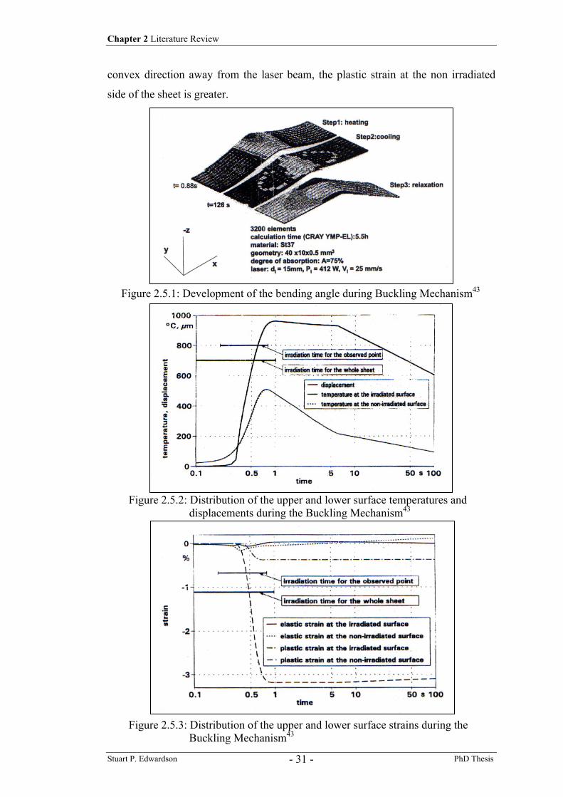
Chapter 2 Literature Review
Stuart P. Edwardson PhD Thesis - 31 -
convex direction away from the laser beam, the plastic strain at the non irradiated
side of the sheet is greater.
Figure 2.5.1: Development of the bending angle during Buckling Mechanism43
Figure 2.5.2: Distribution of the upper and lower surface temperatures and displacements during the Buckling Mechanism43
Figure 2.5.3: Distribution of the upper and lower surface strains during the Buckling Mechanism43
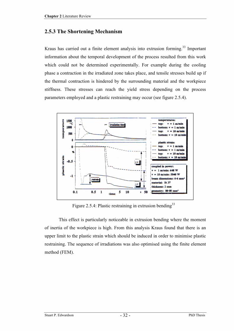
Chapter 2 Literature Review
Stuart P. Edwardson PhD Thesis - 32 -
2.5.3 The Shortening Mechanism
Kraus has carried out a finite element analysis into extrusion forming.33 Important
information about the temporal development of the process resulted from this work
which could not be determined experimentally. For example during the cooling
phase a contraction in the irradiated zone takes place, and tensile stresses build up if
the thermal contraction is hindered by the surrounding material and the workpiece
stiffness. These stresses can reach the yield stress depending on the process
parameters employed and a plastic restraining may occur (see figure 2.5.4).
This effect is particularly noticeable in extrusion bending where the moment
of inertia of the workpiece is high. From this analysis Kraus found that there is an
upper limit to the plastic strain which should be induced in order to minimise plastic
restraining. The sequence of irradiations was also optimised using the finite element
method (FEM).
Figure 2.5.4: Plastic restraining in extrusion bending33
Chapter 2 Literature Review
Stuart P. Edwardson PhD Thesis - 33 -
2.5.4 Further Numerical Modelling
A number of other numerical studies have been conducted of note that don’t
necessarily fit into the above categories 44 - 55. With improvements to computational
time and reliability researchers are increasingly regarding numerical models as
essential (if not the only) research tools. This is reflected in the increase in
publications of numerical based research in recent years. A summary of the results
and conclusions of a number of papers of note is given here.
In 1999 Yu et al 44 at MIT published numerical based research of laser
forming. Presented was an Abaqus based finite element model for thermo-
mechanical analysis of the LF process. A rezoning or re-meshing technique
(redrawing the fine mesh around the beam as it moves) was employed to greatly
reduce the simulation time yet preserve the required accuracy. A comparison of the
numerical results and experimental data on 2.53cm thick mild steel using 2.6 kW of
CO2 laser power, obtained from Penn State University, showed the effectiveness of
the model. However the observed errors between the model and experimental data
were attributed to the inaccurate estimation of the heat absorption rate (coupling rate)
and the heat convection and radiation coefficients. It was concluded that a more
accurate estimation of these parameters is essential for FEA modelling.
Li & Yao 45 at Columbia University in 1999 presented numerical based work
on the effects of strain rate in laser forming. An FEA model was created in Abaqus
of an 80 x 40 x 0.89mm mild steel coupon laser formed using a CO2 laser source
(Gaussian distribution), only half the coupon was modelled (symmetry assumed). It
was found in this study that with strain rate increase, the thermal-induced distortion
decreases and the bend angle reduces. The bend angle decreases by about 30% for
nearly doubled strain rate under the conditions used. Residual stress in the Y
direction (transverse) increases moderately with strain rate, with a doubled strain rate
residual stress increases by about 15%. From coupled experimental work it was
found that with a strain rate increase the hardness of the formed sample decreases
due to the reduced work hardening. This numerical/experimental approach was
continued at Columbia with work on laser forming with constant line energy 46 and
analysis and prediction of edge effects in laser bending 47.
In 2000 Li & Yao 50 presented numerical (FEA) work on the use of laser
forming to bend tubes, a development on extrusion bending 33. The mechanism was
Chapter 2 Literature Review
Stuart P. Edwardson PhD Thesis - 34 -
found to be a combination of thickening (shortening mechanism) of the laser scanned
region due to thermally induced axial compressive stress, and a slightly outward
displacement of the region caused by a component of the thermally induced
circumferential stress. As a result bending is primarily achieved through the
thickening of the scanned region instead of the thinning of the un-scanned region.
The absence, when compared to conventional tube bending, of appreciable wall
thinning is one of the major advantages of laser bent tubes. It was concluded from
this study that the bending efficiency increases with the maximum scanning angle
(distance scanned around the tube) up to a critical point. In addition the asymmetry
of the LF process can be reduced by varying the scanning speed or employing a two-
segment scanning scheme.
In 2001 Cosenza et al 52 presented an explicit fully coupled thermo-
mechanical FE analysis of the LF process, again using Abaqus. This study proposed
a new FE modelling approach utilizing a dynamic explicit algorithm as opposed to
the traditional implicit models. This permits the reduction of CPU times because of
the linearity and the independence of the final set of equations. The FEA model of
the LF of 140 x 20 x 3mm Fe360 sheet using a 6kW CO2 laser source showed
reasonable agreement with experimentally found data.
In 2002 Lee et al 55 in Taiwan published a study into the pulsed LF of thin
sheets (20x10x1mm 304 Stainless Steel) using a single (or multiple) CO2 laser pulse
of an elliptical beam the width of the sample. This has applications in micro laser
forming (discussed later). An Abaqus FE model was developed to simulate this
unique set-up, and a good agreement was found with experimental data. The
conclusions drawn from this study were that the bend angle increases with laser
power and the laser radiation time. The bending angle decreases with the thickness
of the specimen, provided the peak temperature of the specimen is below the melting
point. It was found that if there is a high temperature gradient between the upper and
lower surfaces a positive bend angle is produced, for a low thermal gradient a
negative bend angle is produced. Finally it was concluded that the mechanisms of
pulsed laser forming are dependent upon a number of operation parameters, the main
influences are the laser power, the heating time (pulse length), the clamping
arrangement, the thermal properties and the residual stress state of the specimen.
Chapter 2 Literature Review
Stuart P. Edwardson PhD Thesis - 35 -
2.6 Previous Experimental Work The following sections summarise important experimental work that has been carried
out to date in the field of laser forming. Included is early fundamental research and
more recent developments in 2D and 3D, macro and micro laser forming of
numerous materials.
2.6.1 Fundamental Investigations In 1985 Namba 56 published one of the first experimental papers on laser forming.
The materials investigated in this work included Ti, Al, AISI 304 stainless steel and
carbon steel. The materials were irradiated with a 1.5kW CO laser using a defocused
beam with traverse speeds in the range of 5 - 15m/min. Namba claimed the
deformation is caused by the steep thermal gradient which results in thermal
expansion, thermal stress and plastic deformation. The following parameters were
described as affecting the bend angle 56
1) Incident laser beam power
2) Laser beam diameter
3) Power density distribution of the laser beam
4) Absorptivity of laser beam on a material surface
5) Scanning speed of laser beam
6) Number of repetitions of laser beam scans
7) Density of the material, specific heat capacity of the material
8) Thermal expansion coefficient
9) Yield strength
10) Young’s modulus
11) Poisson’s ratio
12) Strain hardening coefficient
13) The dimensions of the workpiece
14) The melting temperature of the material and the fracture strength of the material.
In 1987 Scully determined that the positive bend angle (hence no buckling) is
equal to the fraction of the power and the square root of the traverse speed times the
plate thickness.4 That relationship was taken from earlier work by Masubuchi et al 57
on flame forming and can be seen in equation 2.6.1.
Chapter 2 Literature Review
Stuart P. Edwardson PhD Thesis - 36 -
1
1
vsp
oB =α (2.6.1)
Later work in 1994 by Vollertsen has shown that there is a strong linear
dependence of the bend angle on the laser power. The dependence of the bend angle
on the processing speed has been reported in further work by Vollertsen as well 23.
Vollertsen is credited with producing a considerable amount of the early
fundamental research on laser forming, including naming the individual mechanisms
(although the names are not in use by every research group around the world), a
summary of the key results and conclusions drawn from this research 23 is given here.
In the experiments carried out relating to processing speed dependence, a
power law was assumed between the bend angle and the processing speed. A linear
dependence was obtained for 3.5mm sheet with scanning speeds in the range 7 -70
mm/s, the gradient was found to be -0.63. A negative slope was to be expected as
this is derived from the notion that the increase in processing speed decreases the
coupled energy. As the bend angle is proportional to the coupled energy it is
expected that the bend angle should decrease linearly with increasing speed.
However at lower speeds it was found that this is not the case. It was found that the
bend angle continues to increase up to a point with increasing traverse speed. This
behaviour may be attributed to the fact that the temperature gradient is increased
with increasing velocity and the time for heat conduction in the depth direction of the
sheet is reduced. Ultimately this results in the difference of the plastic strains
between the upper and the lower layer of the sheet being more pronounced and a
greater bend angle per unit time may be achieved. Of course if the velocity is
increased to a very high value then the temperature increase will be small and only
an elastically reversible bending may occur. Also of note from this work is the
concept of a threshold energy for the process. It was shown that no plastic
deformation occurs below a given energy input. Therefore the boundary energy
which will produce the onset of bending can be related to the temperature the
material must reach at the limit of the thermal strain at the yield point stress.
The thermal conductivity of the workpiece material is of vital importance in
laser bending. The thermal conductivity determines the temperature field and hence
the development of the thermal strain. If a materia1 is a good conductor it is unlikely
that a thermal gradient of sufficient magnitude can be created to initiate the bend
Chapter 2 Literature Review
Stuart P. Edwardson PhD Thesis - 37 -
with the temperature gradient mechanism unless the heat can be put into the sheet
sufficiently fast. In general it is better that the material should be a relatively poor
conductor in order for the temperature gradient mechanism to occur.
The role of thermal conductivity on the buckling and shortening mechanisms
is slightly different. If the workpiece material has a high thermal conductivity then
the size of the irradiated area will increase rapidly thus decreasing the average
temperature of the material, the plastic straining and hence the bend angle. The
distinction is drawn however as forming will still occur for the latter mechanisms
(not thermal gradient dependent) but no bending will occur in the former case (TGM)
if the temperature gradient is diminished to a large extent by a high thermal
conductivity. The effect has been physically modelled by Vollertsen. It is considered
of great importance not only due to the previously described factors but also due to
the fact that the strength of the material changes with differing thermal conductivities.
The conductivity can be related to the age hardening state of the material. Time age
hardenable state then has a role in influencing the thermal conductivity and the
elastic reversible bending of the material, and ultimately the bend angle. Clearly
there are complex dependencies for the thermal conductivity.
Further work showed a linear influence of the fraction of the coefficient of
thermal expansion and the specific heat times the mass density when plotted against
the bend angle. This shows the influence of the material parameters on the bend
angle. This is useful as the two layer model 24 assumes the same relationship
between these parameters. The amount of forming depends critically on the thermal
expansion. The thermal expansion is determined from the temperature increase and
the coefficient of thermal expansion, the temperature increase of a volume is
indirectly proportional to the volumetric heat capacity 23.
In other research an early program in laser forming was that of the Laser line
Heating (LLH) which formed part of the Navy Manufacturing Technology program
(ManTech) in the U.S.A. The material investigated in this program was heavy duty
6.25 - 25 mm mild steel plate4. Important results from this work show how the
temperature changes as a function of time for the given material and how the micro
strain changes as a function of time also. The micro strain was obtained by means of
strain gauges mounted on the bottom of the plate surface. Scully noted the change in
the strain between the heating and cooling cycles as shown in figure 2.6.1.
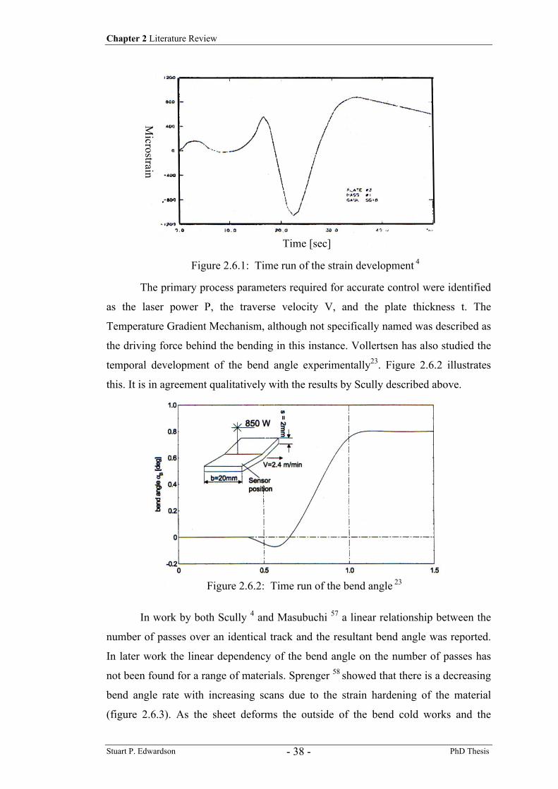
Chapter 2 Literature Review
Stuart P. Edwardson PhD Thesis - 38 -
The primary process parameters required for accurate control were identified
as the laser power P, the traverse velocity V, and the plate thickness t. The
Temperature Gradient Mechanism, although not specifically named was described as
the driving force behind the bending in this instance. Vollertsen has also studied the
temporal development of the bend angle experimentally23. Figure 2.6.2 illustrates
this. It is in agreement qualitatively with the results by Scully described above.
In work by both Scully 4 and Masubuchi 57 a linear relationship between the
number of passes over an identical track and the resultant bend angle was reported.
In later work the linear dependency of the bend angle on the number of passes has
not been found for a range of materials. Sprenger 58 showed that there is a decreasing
bend angle rate with increasing scans due to the strain hardening of the material
(figure 2.6.3). As the sheet deforms the outside of the bend cold works and the
Time [sec]
Microstrain
Figure 2.6.1: Time run of the strain development 4
Figure 2.6.2: Time run of the bend angle 23
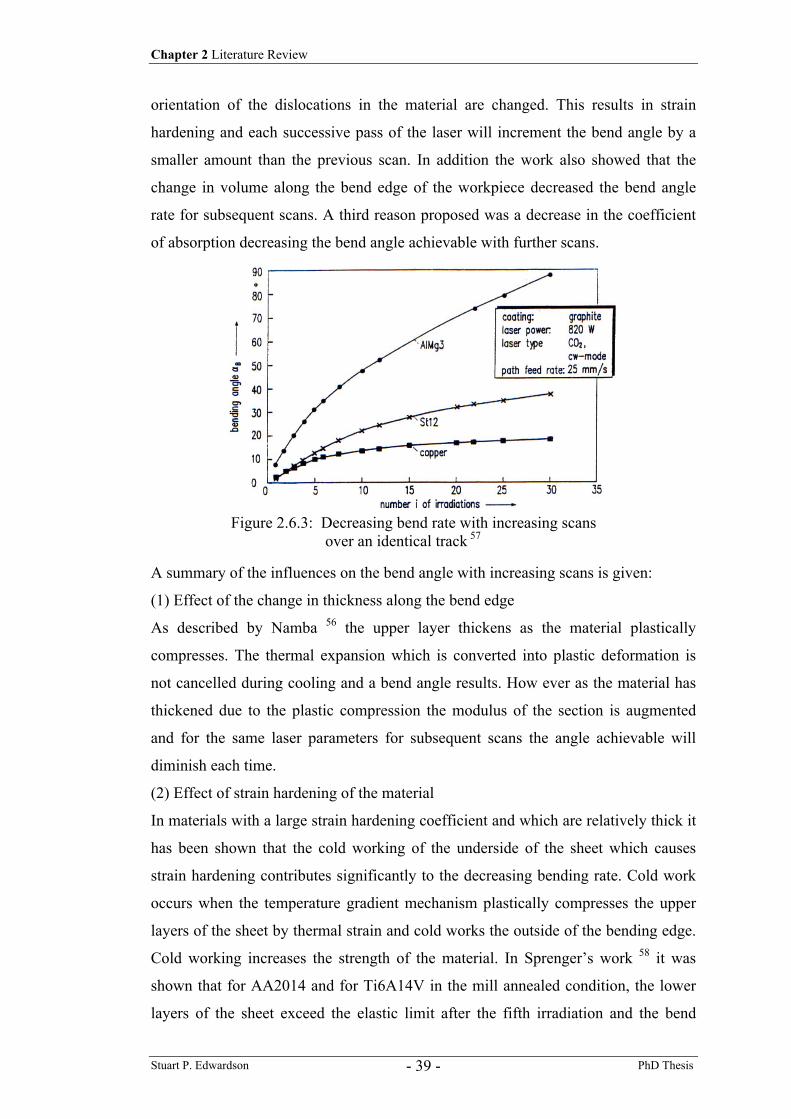
Chapter 2 Literature Review
Stuart P. Edwardson PhD Thesis - 39 -
orientation of the dislocations in the material are changed. This results in strain
hardening and each successive pass of the laser will increment the bend angle by a
smaller amount than the previous scan. In addition the work also showed that the
change in volume along the bend edge of the workpiece decreased the bend angle
rate for subsequent scans. A third reason proposed was a decrease in the coefficient
of absorption decreasing the bend angle achievable with further scans.
A summary of the influences on the bend angle with increasing scans is given:
(1) Effect of the change in thickness along the bend edge
As described by Namba 56 the upper layer thickens as the material plastically
compresses. The thermal expansion which is converted into plastic deformation is
not cancelled during cooling and a bend angle results. How ever as the material has
thickened due to the plastic compression the modulus of the section is augmented
and for the same laser parameters for subsequent scans the angle achievable will
diminish each time.
(2) Effect of strain hardening of the material
In materials with a large strain hardening coefficient and which are relatively thick it
has been shown that the cold working of the underside of the sheet which causes
strain hardening contributes significantly to the decreasing bending rate. Cold work
occurs when the temperature gradient mechanism plastically compresses the upper
layers of the sheet by thermal strain and cold works the outside of the bending edge.
Cold working increases the strength of the material. In Sprenger’s work 58 it was
shown that for AA2014 and for Ti6A14V in the mill annealed condition, the lower
layers of the sheet exceed the elastic limit after the fifth irradiation and the bend
Figure 2.6.3: Decreasing bend rate with increasing scans over an identical track 57
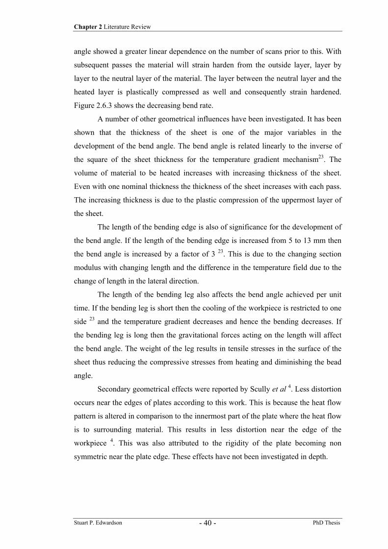
Chapter 2 Literature Review
Stuart P. Edwardson PhD Thesis - 40 -
angle showed a greater linear dependence on the number of scans prior to this. With
subsequent passes the material will strain harden from the outside layer, layer by
layer to the neutral layer of the material. The layer between the neutral layer and the
heated layer is plastically compressed as well and consequently strain hardened.
Figure 2.6.3 shows the decreasing bend rate.
A number of other geometrical influences have been investigated. It has been
shown that the thickness of the sheet is one of the major variables in the
development of the bend angle. The bend angle is related linearly to the inverse of
the square of the sheet thickness for the temperature gradient mechanism23. The
volume of material to be heated increases with increasing thickness of the sheet.
Even with one nominal thickness the thickness of the sheet increases with each pass.
The increasing thickness is due to the plastic compression of the uppermost layer of
the sheet.
The length of the bending edge is also of significance for the development of
the bend angle. If the length of the bending edge is increased from 5 to 13 mm then
the bend angle is increased by a factor of 3 23. This is due to the changing section
modulus with changing length and the difference in the temperature field due to the
change of length in the lateral direction.
The length of the bending leg also affects the bend angle achieved per unit
time. If the bending leg is short then the cooling of the workpiece is restricted to one
side 23 and the temperature gradient decreases and hence the bending decreases. If
the bending leg is long then the gravitational forces acting on the length will affect
the bend angle. The weight of the leg results in tensile stresses in the surface of the
sheet thus reducing the compressive stresses from heating and diminishing the bead
angle.
Secondary geometrical effects were reported by Scully et al 4. Less distortion
occurs near the edges of plates according to this work. This is because the heat flow
pattern is altered in comparison to the innermost part of the plate where the heat flow
is to surrounding material. This results in less distortion near the edge of the
workpiece 4. This was also attributed to the rigidity of the plate becoming non
symmetric near the plate edge. These effects have not been investigated in depth.
Chapter 2 Literature Review
Stuart P. Edwardson PhD Thesis - 41 -
2.6.2 Magee ‘98
The experimental work summarised in this section consisted of empirical work
carried out on AA 2024 T3 aluminium alloy and Ti6Al4V titanium alloy. Parametric
investigations were carried out by J. Magee29, a PhD researcher in the University of
Liverpool, into the single and multi-pass, large and small beam diameter 2D laser
forming of these materials, which led to the development of a 2D laser forming
demonstrator system for a part cylinder shape. Development of scan strategies for
the 3D laser forming of dish shapes was also carried out. This work was part of a
joint research programme between the University of Liverpool and BAE Systems.
This work formed a precursor for the present research within this thesis and as such a
more detailed account is given of the work.
PARAMETRIC STUDY – This work investigated the factors influencing the
angular dimensions of laser formed 80x80mm 0.8-1mm gauge plates of Ti6Al4V
and AA 2024 T3, commonly used aerospace alloys. The plates were clamped at one
end, graphite coated and irradiated with a PRC 10.6µm CO2 laser. Altering the
power density and the interaction time of the laser beam incident on the samples
varied the energy input to the plate surface.
The experimental results revealed that the bend angle development is
critically dependent on the energy supplied to the plate surface. Two distinct studies
were carried out (using a large and small beam diameter) on two materials (a
titanium and aluminium alloy), with different thermal and mechanical properties. In
the case of the titanium alloy it was found that the temperature gradient mechanism
was active for both studies, both for the large and small laser beam diameter to sheet
thickness ratios. This was attributed to the low thermal conductivity of the titanium
alloy. An optimum traverse velocity in terms of maximising the bend angle achieved
per scan was identified for this material when the beam diameter was in the order of
12 times the sheet thickness (figure 2.6.4).
Below the optimum velocity the bend angle dropped due to the loss of a high
temperature gradient and hence a smaller amount of differential straining through the
thickness direction. These results support the idea that the temperature gradient, and
the efficiency of the process, increase as the processing speed increases. This
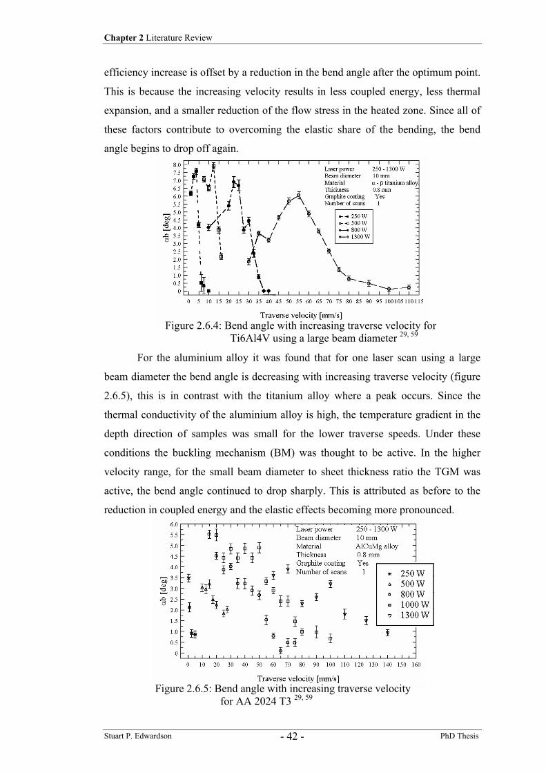
Chapter 2 Literature Review
Stuart P. Edwardson PhD Thesis - 42 -
efficiency increase is offset by a reduction in the bend angle after the optimum point.
This is because the increasing velocity results in less coupled energy, less thermal
expansion, and a smaller reduction of the flow stress in the heated zone. Since all of
these factors contribute to overcoming the elastic share of the bending, the bend
angle begins to drop off again.
For the aluminium alloy it was found that for one laser scan using a large
beam diameter the bend angle is decreasing with increasing traverse velocity (figure
2.6.5), this is in contrast with the titanium alloy where a peak occurs. Since the
thermal conductivity of the aluminium alloy is high, the temperature gradient in the
depth direction of samples was small for the lower traverse speeds. Under these
conditions the buckling mechanism (BM) was thought to be active. In the higher
velocity range, for the small beam diameter to sheet thickness ratio the TGM was
active, the bend angle continued to drop sharply. This is attributed as before to the
reduction in coupled energy and the elastic effects becoming more pronounced.
Figure 2.6.4: Bend angle with increasing traverse velocity for Ti6Al4V using a large beam diameter 29, 59
Figure 2.6.5: Bend angle with increasing traverse velocity for AA 2024 T3 29, 59
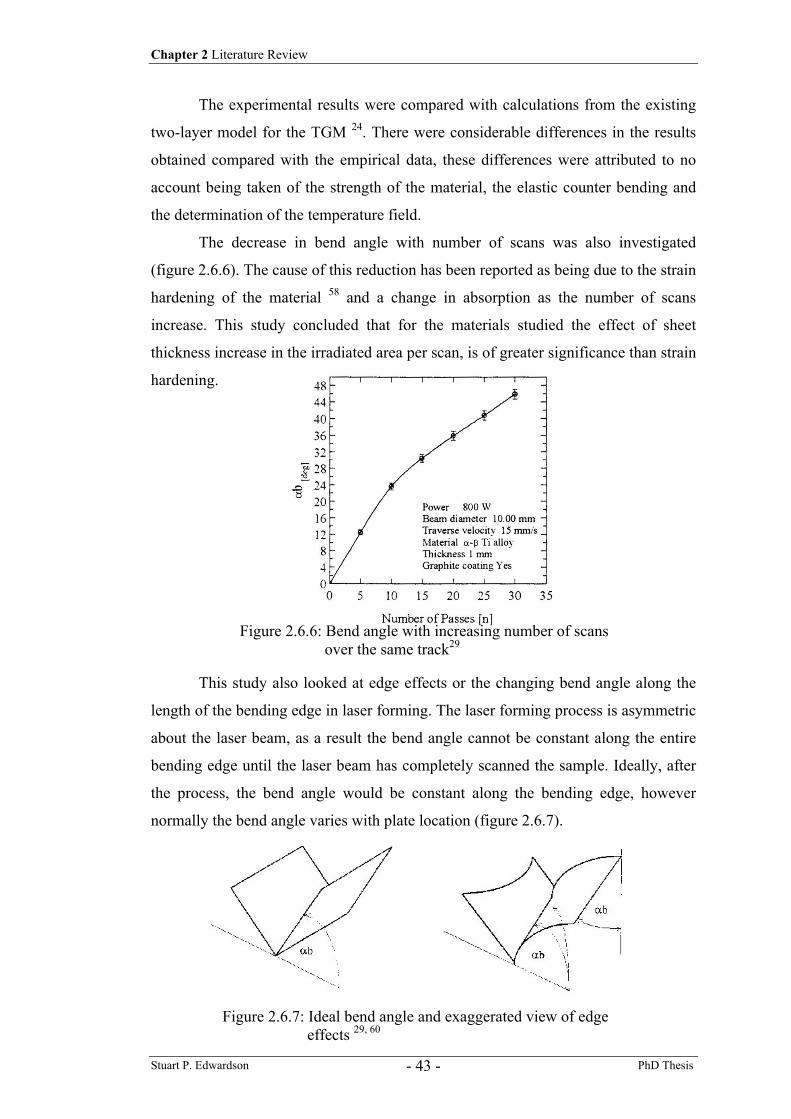
Chapter 2 Literature Review
Stuart P. Edwardson PhD Thesis - 43 -
The experimental results were compared with calculations from the existing
two-layer model for the TGM 24. There were considerable differences in the results
obtained compared with the empirical data, these differences were attributed to no
account being taken of the strength of the material, the elastic counter bending and
the determination of the temperature field.
The decrease in bend angle with number of scans was also investigated
(figure 2.6.6). The cause of this reduction has been reported as being due to the strain
hardening of the material 58 and a change in absorption as the number of scans
increase. This study concluded that for the materials studied the effect of sheet
thickness increase in the irradiated area per scan, is of greater significance than strain
hardening.
This study also looked at edge effects or the changing bend angle along the
length of the bending edge in laser forming. The laser forming process is asymmetric
about the laser beam, as a result the bend angle cannot be constant along the entire
bending edge until the laser beam has completely scanned the sample. Ideally, after
the process, the bend angle would be constant along the bending edge, however
normally the bend angle varies with plate location (figure 2.6.7).
Figure 2.6.6: Bend angle with increasing number of scans over the same track29
Figure 2.6.7: Ideal bend angle and exaggerated view of edge effects 29, 60
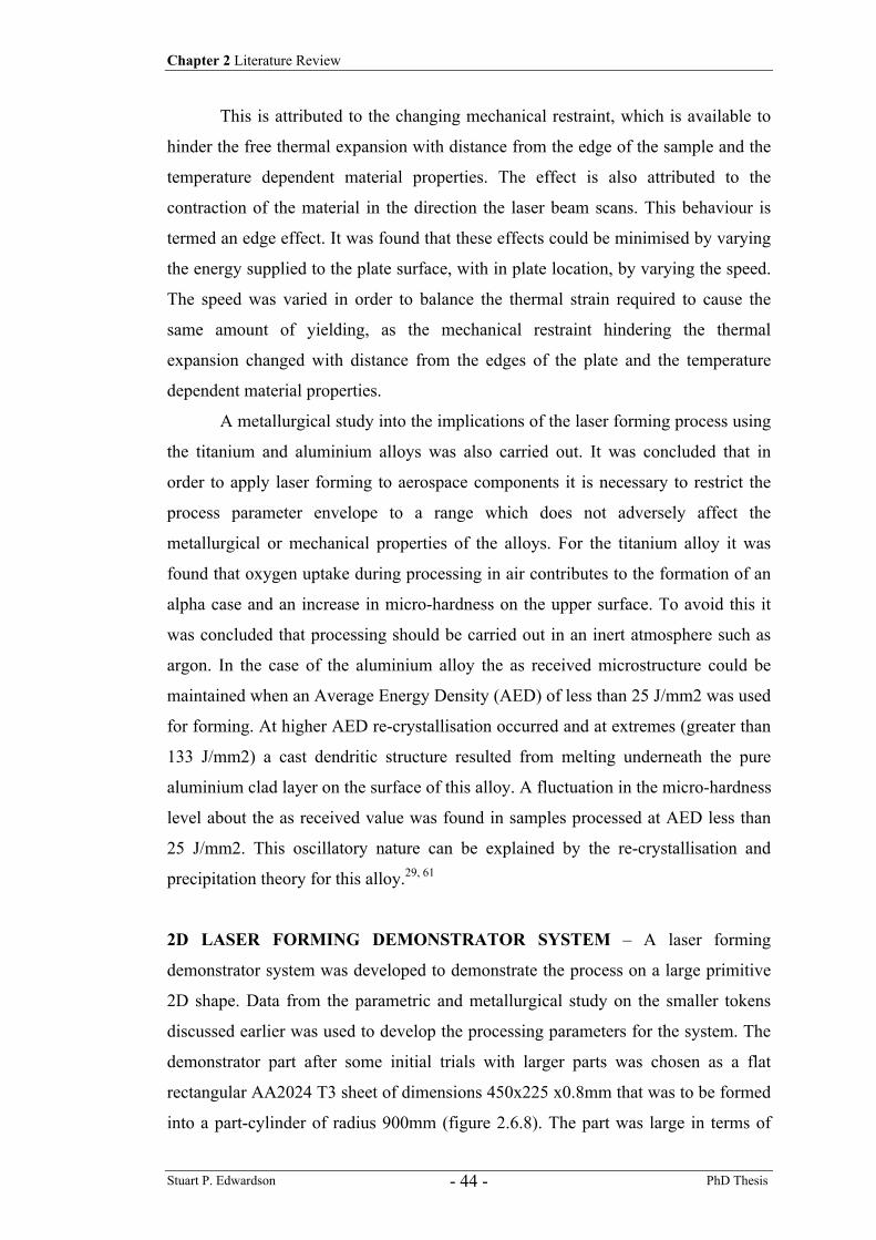
Chapter 2 Literature Review
Stuart P. Edwardson PhD Thesis - 44 -
This is attributed to the changing mechanical restraint, which is available to
hinder the free thermal expansion with distance from the edge of the sample and the
temperature dependent material properties. The effect is also attributed to the
contraction of the material in the direction the laser beam scans. This behaviour is
termed an edge effect. It was found that these effects could be minimised by varying
the energy supplied to the plate surface, with in plate location, by varying the speed.
The speed was varied in order to balance the thermal strain required to cause the
same amount of yielding, as the mechanical restraint hindering the thermal
expansion changed with distance from the edges of the plate and the temperature
dependent material properties.
A metallurgical study into the implications of the laser forming process using
the titanium and aluminium alloys was also carried out. It was concluded that in
order to apply laser forming to aerospace components it is necessary to restrict the
process parameter envelope to a range which does not adversely affect the
metallurgical or mechanical properties of the alloys. For the titanium alloy it was
found that oxygen uptake during processing in air contributes to the formation of an
alpha case and an increase in micro-hardness on the upper surface. To avoid this it
was concluded that processing should be carried out in an inert atmosphere such as
argon. In the case of the aluminium alloy the as received microstructure could be
maintained when an Average Energy Density (AED) of less than 25 J/mm2 was used
for forming. At higher AED re-crystallisation occurred and at extremes (greater than
133 J/mm2) a cast dendritic structure resulted from melting underneath the pure
aluminium clad layer on the surface of this alloy. A fluctuation in the micro-hardness
level about the as received value was found in samples processed at AED less than
25 J/mm2. This oscillatory nature can be explained by the re-crystallisation and
precipitation theory for this alloy.29, 61
2D LASER FORMING DEMONSTRATOR SYSTEM – A laser forming
demonstrator system was developed to demonstrate the process on a large primitive
2D shape. Data from the parametric and metallurgical study on the smaller tokens
discussed earlier was used to develop the processing parameters for the system. The
demonstrator part after some initial trials with larger parts was chosen as a flat
rectangular AA2024 T3 sheet of dimensions 450x225 x0.8mm that was to be formed
into a part-cylinder of radius 900mm (figure 2.6.8). The part was large in terms of
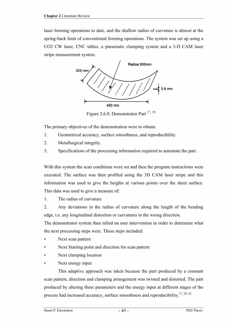
Chapter 2 Literature Review
Stuart P. Edwardson PhD Thesis - 45 -
laser forming operations to date, and the shallow radius of curvature is almost at the
spring-back limit of conventional forming operations. The system was set up using a
CO2 CW laser, CNC tables, a pneumatic clamping system and a 3-D CAM laser
stripe measurement system.
The primary objectives of the demonstration were to obtain:
1. Geometrical accuracy, surface smoothness, and reproducibility.
2. Metallurgical integrity.
3. Specifications of the processing information required to automate the part.
With this system the scan conditions were set and then the program instructions were
executed. The surface was then profiled using the 3D CAM laser stripe and this
information was used to give the heights at various points over the sheet surface.
This data was used to give a measure of:
1. The radius of curvature
2. Any deviations in the radius of curvature along the length of the bending
edge, i.e. any longitudinal distortion or curvatures in the wrong direction.
The demonstrator system then relied on user intervention in order to determine what
the next processing steps were. These steps included:
• Next scan pattern
• Next Starting point and direction for scan pattern
• Next clamping location
• Next energy input
This adaptive approach was taken because the part produced by a constant
scan pattern, direction and clamping arrangement was twisted and distorted. The part
produced by altering these parameters and the energy input at different stages of the
process had increased accuracy, surface smoothness and reproducibility.17, 29, 62
Figure 2.6.8: Demonstrator Part 17, 29
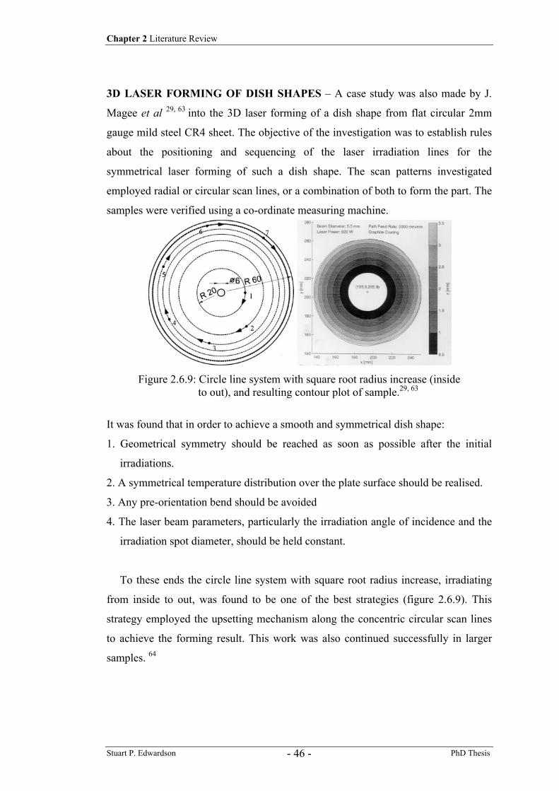
Chapter 2 Literature Review
Stuart P. Edwardson PhD Thesis - 46 -
3D LASER FORMING OF DISH SHAPES – A case study was also made by J.
Magee et al 29, 63 into the 3D laser forming of a dish shape from flat circular 2mm
gauge mild steel CR4 sheet. The objective of the investigation was to establish rules
about the positioning and sequencing of the laser irradiation lines for the
symmetrical laser forming of such a dish shape. The scan patterns investigated
employed radial or circular scan lines, or a combination of both to form the part. The
samples were verified using a co-ordinate measuring machine.
It was found that in order to achieve a smooth and symmetrical dish shape:
1. Geometrical symmetry should be reached as soon as possible after the initial
irradiations.
2. A symmetrical temperature distribution over the plate surface should be realised.
3. Any pre-orientation bend should be avoided
4. The laser beam parameters, particularly the irradiation angle of incidence and the
irradiation spot diameter, should be held constant.
To these ends the circle line system with square root radius increase, irradiating
from inside to out, was found to be one of the best strategies (figure 2.6.9). This
strategy employed the upsetting mechanism along the concentric circular scan lines
to achieve the forming result. This work was also continued successfully in larger
samples. 64
Figure 2.6.9: Circle line system with square root radius increase (inside to out), and resulting contour plot of sample.29, 63
Chapter 2 Literature Review
Stuart P. Edwardson PhD Thesis - 47 -
2.6.3 Recent research in macro-scale 2D LF 65
There have been a number of other 2D laser forming experimental investigations
recently published that are of note 66-81. The experiments and conclusions of a
number of them are outlined here.
Chan et al 66 in Hong Kong published work in 2000 on the laser forming by a
low power Nd:YAG laser (90W max) of thin stainless steel (0.25-1mm thick).
Although some of the results had been observed before in other studies there were a
few interesting findings: A threshold heat input was observed in the process, below
which no bending occurs. In addition when the energy input was above critical value
the bend angle stops increasing with any further increase in heat input, possibly due
to the loss of thermal gradient through the thickness.
In 2001 Mucha et al 67 from Poland presented a paper on a comparative study
of the laser forming of plates using circular and rectangular beam cross-sections. It
was shown that the shape of the incident laser beam has a large effect on the LF
process, for the same energy parameters the bend angle generated by the rectangular
beam is 1.3 to 2.5 times greater than the one generated by the circular beam. In
addition it was argued that a greater control of the process could be achieved using a
rectangular beam. Also in the work was an extensive analytical model, it was argued
that the dimensionless form of the derived dependencies from this model would be a
useful method of selecting appropriate processing parameters for any material.
Liqun et al 69,70 from the Harbin Instiute of Technology, China, have
published a number of interesting studies on LF. There has been an increase in recent
years of the number of papers to come out of China in the laser materials processing
field in general. Research on using different cooling methods in LF and an update on
the factors involved in multi-pass LF have been presented. It was found that the use
of an effective cooling method can significantly increase the process efficiency of LF.
A number of cooling methods were employed including water jet and high pressure
CO2 gas cooling from the underside of the plate. It was found that cooling can
increase the temperature gradient through the thickness, however the peak
temperature in the sample is decreased (hence the bend angle is also) and so the
benefits of having cooling during processing are lessened. In addition the high
temperature difference between the top and bottom of the plate can cause unwanted
Chapter 2 Literature Review
Stuart P. Edwardson PhD Thesis - 48 -
metallurgical effects such as an increase in hardness. Effective cooling after each
pass would be the answer to improve process efficiency. In another study work was
presented on multi-pass laser forming and the factors influencing the bend angle fall
off at higher numbers of passes, although many of the results had been observed in
previous work a number of key results were of interest. The work was conducted on
2mm thick aluminium using a 2kW Nd:YAG laser and a 10mm beam diameter, thus
no coating was required. It was observed that there was a significant thickening of
the sample in the irradiated area and that the thickening became more pronounced
after 20 irradiations (0.5mm thickness increase). It was argued that this thickening
effect was a large factor in the bend angle rate fall off after 20 or more irradiations, a
thicker sheet is harder to bend as it were. It was also found that the tensile strength of
the sample decreased with increasing irradiations, thus ruling out this factor as a
possible reason for bend angle fall off.
The industrial viability of LF depends on the process efficiency and speed
compared to other competitive techniques, in combination with repeatable accuracy.
Mechanical forming of thin sheet material is relatively fast and can produce large
deformations in a single process step, but it is inaccurate (due to variable ‘spring-
back’ and tool wear). In contrast, LF is comparatively slow, but offers a high degree
of control and remote application. To exploit the combined attributes of LF and
mechanical forming, a hybrid forming process has been proposed and demonstrated
by Magee and De Vin, in which LF is applied as a secondary process to adjust
mechanically formed parts 73, 74.
A high degree of control is required for LF to be an industrially viable
process, especially for 3-D LF, which is in its infancy. To address this for 2-D LF,
Thompson and Pridham at Dundee investigated a closed-loop control system, for the
case of laser bending to a pre-defined bend angle with some success. 75, 76, 77 Other
approaches to this problem have been taken, Cheng and Lin in Taiwan have
published work on using a neural network to predict and hence control the bend
angle during the laser forming of 304 stainless steel.78 This intelligent approach
could be a useful method of accounting for the many variables and unknowns in the
process. Peck and Jones79 are developing this approach into a commercial system for
the manufacture of single unit windshield wiper blades for Trico Products Corp. The
system employs a high power diode laser to laser form and heat treat a continuous
metal strip fed underneath it, this metal strip when cut to length forms the curved
Chapter 2 Literature Review
Stuart P. Edwardson PhD Thesis - 49 -
backbone of the windshield wiper. A trained neural network provided by NA
Technologies monitors the process and can make adjustments on the fly to the power
output of the diode laser and hence the bend angle, this type of laser is well suited to
this dynamic power requirement.
The use of pulsed laser energy for LF has also been under investigation by
some researchers80, 81, and this has lead to possibilities for new LF mechanisms.
Laser Peen Forming (an extension of Laser Peening 80) or Laser Shock Forming81, in
which the application of a negative residual stress to one side of a component results
in a bending effect, is a key example that is now being realised through the
emergence of high pulse energy Nd:Glass lasers.
2.6.4 Recent advances in 2D LF for micro-scale applications 65
Pioneering studies on micro-scale LF by Hoving and co-workers at Philips 13 helped
establish some important results for precise adjustment of components by the
shortening or Upsetting Mechanism. Following on from this, the Philips research
team have developed a number of micro-adjustment applications for LF 13, 82, with
the first concept being the laser adjustment of digital audio head mounting frames. A
second application under development is the laser adjustment of reed switches. Here,
out-of-plane LF (laser bending) is used for adjustment of the 10-50 micron gap
between the two nickel-iron reed elements, which then determines the value of the
magnetic field above which the reed switch closes in operation. The process is
carried out using a 30W cw Argon-Ion laser beam which is able to pass through the
sealed glass tube, so that the operation can be carried out after manufacture of the
sealed envelope switch (both on new switches and for the adjustment of previously
rejected units). The precision of adjustment results in a reduced spread of ampere
winding values, with a corresponding reduction in customer sort / reject rates.
Thirdly, actuator frames have been designed and investigated by the Philips team for
micron level adjustments of a lens by LF during the final assembly of a CD player,
one of a number of applications for this product’s optical train. Through a study of
several actuator designs, one resembling a ‘Basket Ball Basket’ (figure 2.6.10) was
found to give the greatest flexibility of movement & reduced number of process
steps to achieve the desired lens alignment. Freedom of movement in a number of
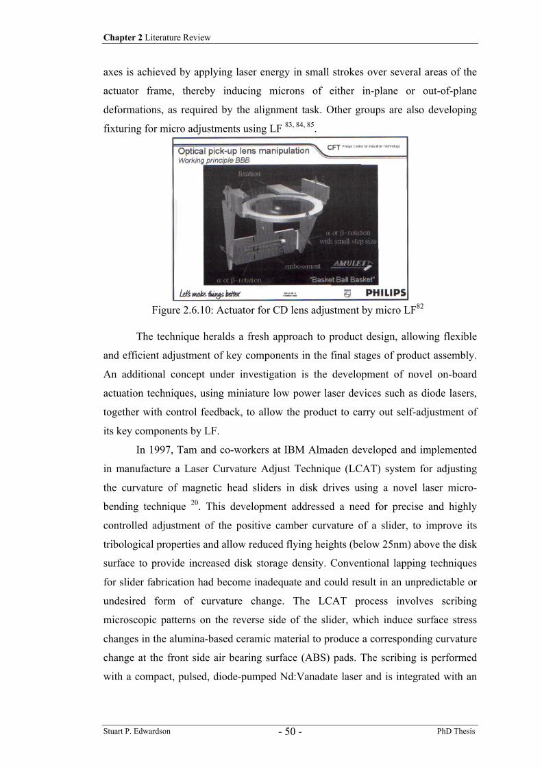
Chapter 2 Literature Review
Stuart P. Edwardson PhD Thesis - 50 -
axes is achieved by applying laser energy in small strokes over several areas of the
actuator frame, thereby inducing microns of either in-plane or out-of-plane
deformations, as required by the alignment task. Other groups are also developing
fixturing for micro adjustments using LF 83, 84, 85.
The technique heralds a fresh approach to product design, allowing flexible
and efficient adjustment of key components in the final stages of product assembly.
An additional concept under investigation is the development of novel on-board
actuation techniques, using miniature low power laser devices such as diode lasers,
together with control feedback, to allow the product to carry out self-adjustment of
its key components by LF.
In 1997, Tam and co-workers at IBM Almaden developed and implemented
in manufacture a Laser Curvature Adjust Technique (LCAT) system for adjusting
the curvature of magnetic head sliders in disk drives using a novel laser micro-
bending technique 20. This development addressed a need for precise and highly
controlled adjustment of the positive camber curvature of a slider, to improve its
tribological properties and allow reduced flying heights (below 25nm) above the disk
surface to provide increased disk storage density. Conventional lapping techniques
for slider fabrication had become inadequate and could result in an unpredictable or
undesired form of curvature change. The LCAT process involves scribing
microscopic patterns on the reverse side of the slider, which induce surface stress
changes in the alumina-based ceramic material to produce a corresponding curvature
change at the front side air bearing surface (ABS) pads. The scribing is performed
with a compact, pulsed, diode-pumped Nd:Vanadate laser and is integrated with an
Figure 2.6.10: Actuator for CD lens adjustment by micro LF82
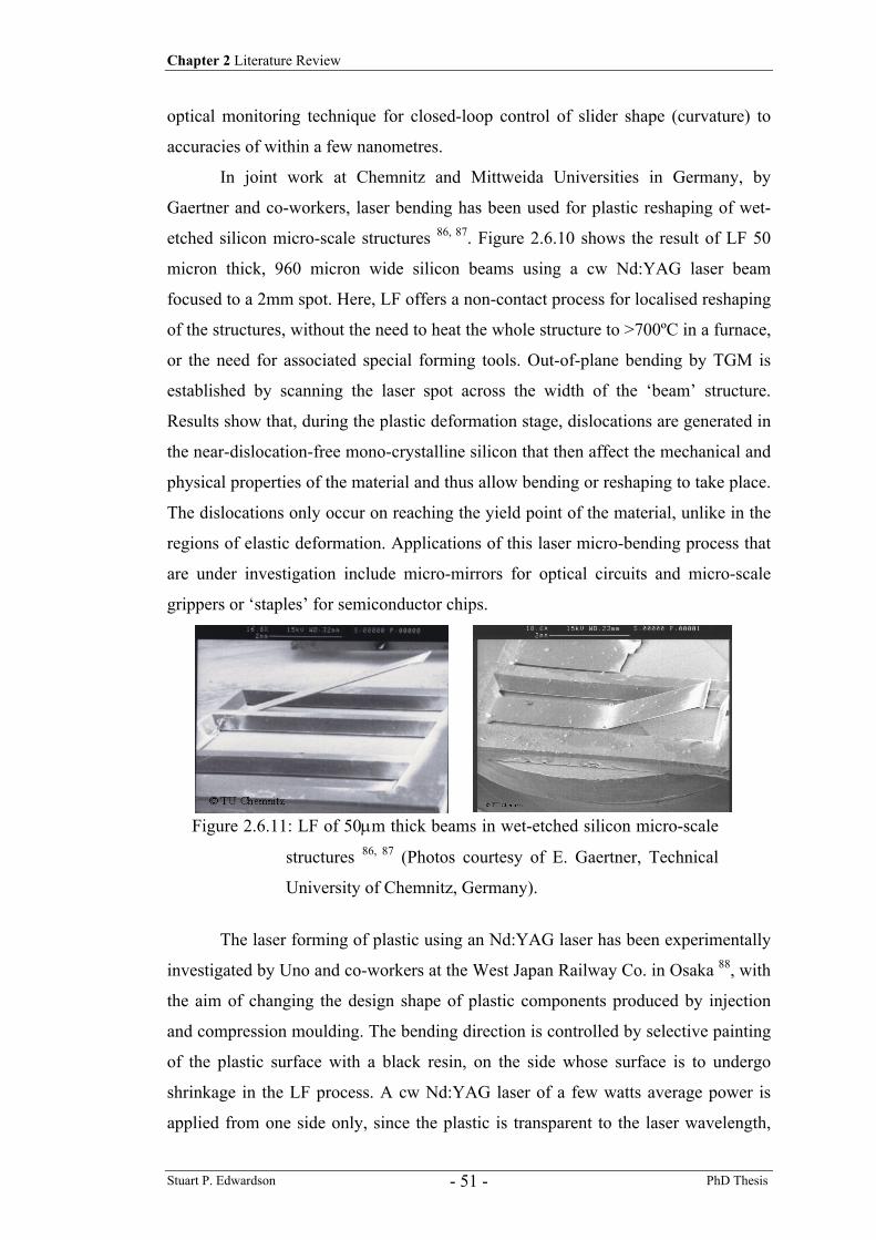
Chapter 2 Literature Review
Stuart P. Edwardson PhD Thesis - 51 -
optical monitoring technique for closed-loop control of slider shape (curvature) to
accuracies of within a few nanometres.
In joint work at Chemnitz and Mittweida Universities in Germany, by
Gaertner and co-workers, laser bending has been used for plastic reshaping of wet-
etched silicon micro-scale structures 86, 87. Figure 2.6.10 shows the result of LF 50
micron thick, 960 micron wide silicon beams using a cw Nd:YAG laser beam
focused to a 2mm spot. Here, LF offers a non-contact process for localised reshaping
of the structures, without the need to heat the whole structure to >700ºC in a furnace,
or the need for associated special forming tools. Out-of-plane bending by TGM is
established by scanning the laser spot across the width of the ‘beam’ structure.
Results show that, during the plastic deformation stage, dislocations are generated in
the near-dislocation-free mono-crystalline silicon that then affect the mechanical and
physical properties of the material and thus allow bending or reshaping to take place.
The dislocations only occur on reaching the yield point of the material, unlike in the
regions of elastic deformation. Applications of this laser micro-bending process that
are under investigation include micro-mirrors for optical circuits and micro-scale
grippers or ‘staples’ for semiconductor chips.
The laser forming of plastic using an Nd:YAG laser has been experimentally
investigated by Uno and co-workers at the West Japan Railway Co. in Osaka 88, with
the aim of changing the design shape of plastic components produced by injection
and compression moulding. The bending direction is controlled by selective painting
of the plastic surface with a black resin, on the side whose surface is to undergo
shrinkage in the LF process. A cw Nd:YAG laser of a few watts average power is
applied from one side only, since the plastic is transparent to the laser wavelength,
Figure 2.6.11: LF of 50µm thick beams in wet-etched silicon micro-scale
structures 86, 87 (Photos courtesy of E. Gaertner, Technical
University of Chemnitz, Germany).
Chapter 2 Literature Review
Stuart P. Edwardson PhD Thesis - 52 -
with the resin then transferring its absorbed heat to the material from the surface to
which it is adhered.
A number of other studies fall into the micro scale LF area 89-92, these involve
the laser forming of thin metallic foils using low power lasers. Complex structures
can be formed in these thin materials with very little power, thus applications can be
found in the electronics industry for alignment (mentioned earlier) and for the
manufacture of mounts and housings for components. In work by Yoshioka et al 90,
91 92 at the Chiba institute in Japan a method of sample holding was developed to
reduce unwanted distortion when forming thin foils. A sample was held in place
using a glass plate over it, the sample was then irradiated through the glass and not
allowed to deform. Once the plate was lifted after processing, the part sprung into the
desired shape, thus eliminating any asymmetric or temporal effects. For more
complex shapes a mask was used to hold the sample down during processing.
2.6.5 Developments towards 3D LF capability 65
A considerable amount of research recently in LF has been aimed at prototyping of
3-D components and structures for applications in aerospace, automotive and artistic
design 18, 63, 64, 93-107
It has been shown that laser forming shows great potential for the
manufacturing of metallic components, using a 2D straight line or 3D spatial
forming approach. However in order to advance the process further for realistic
forming applications and for straightening and aligning operations in a
manufacturing industry it is necessary to develop systems for accurate and repeatable
part production. Figure 2.6.12 outlines the possible routes and key elements required
to the practical realisation of 3D laser forming 22. A predictive or an adaptive
approach can be taken.
Intelligent predictive systems, perhaps based on Knowledge-Based Systems
(KBS), neural networks or thermo-mechanical models can achieve predictability
through a knowledge of the material (including its stress history) combined with a
developed, highly tuned process model / control algorithm. Systems of this type have
been reported by a number of groups 98, 99, 100.
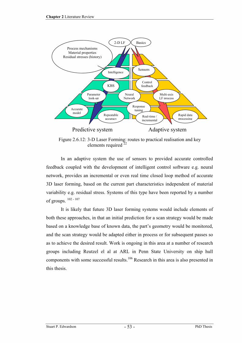
Chapter 2 Literature Review
Stuart P. Edwardson PhD Thesis - 53 -
In an adaptive system the use of sensors to provided accurate controlled
feedback coupled with the development of intelligent control software e.g. neural
network, provides an incremental or even real time closed loop method of accurate
3D laser forming, based on the current part characteristics independent of material
variability e.g. residual stress. Systems of this type have been reported by a number
of groups. 102 - 107
It is likely that future 3D laser forming systems would include elements of
both these approaches, in that an initial prediction for a scan strategy would be made
based on a knowledge base of known data, the part’s geometry would be monitored,
and the scan strategy would be adapted either in process or for subsequent passes so
as to achieve the desired result. Work is ongoing in this area at a number of research
groups including Reutzel el al at ARL in Penn State University on ship hull
components with some successful results.106 Research in this area is also presented in
this thesis.
Predictive system Adaptive system
IntelligenceSensors
KBS
Parameter look-up
Neural Network
Repeatableaccuracy
Accurate model
Control feedback
Response tuning
Multi-axis LF process
Rapid data processing
2-D LF Basics
Real-time /incremental
Process mechanisms Material properties
Residual stresses (history)
Figure 2.6.12: 3-D Laser Forming: routes to practical realisation and key elements required 22
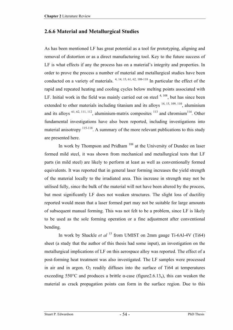
Chapter 2 Literature Review
Stuart P. Edwardson PhD Thesis - 54 -
2.6.6 Material and Metallurgical Studies
As has been mentioned LF has great potential as a tool for prototyping, aligning and
removal of distortion or as a direct manufacturing tool. Key to the future success of
LF is what effects if any the process has on a material’s integrity and properties. In
order to prove the process a number of material and metallurgical studies have been
conducted on a variety of materials. 4, 14, 15, 61, 62, 108-118 In particular the effect of the
rapid and repeated heating and cooling cycles below melting points associated with
LF. Initial work in the field was mainly carried out on steel 4, 108, but has since been
extended to other materials including titanium and its alloys 14, 15, 109, 110, aluminium
and its alloys 61, 62, 111, 112, aluminium-matrix composites 113 and chromium114. Other
fundamental investigations have also been reported, including investigations into
material anisotropy 115-118. A summary of the more relevant publications to this study
are presented here.
In work by Thompson and Pridham 108 at the University of Dundee on laser
formed mild steel, it was shown from mechanical and metallurgical tests that LF
parts (in mild steel) are likely to perform at least as well as conventionally formed
equivalents. It was reported that in general laser forming increases the yield strength
of the material locally to the irradiated area. This increase in strength may not be
utilised fully, since the bulk of the material will not have been altered by the process,
but most significantly LF does not weaken structures. The slight loss of ductility
reported would mean that a laser formed part may not be suitable for large amounts
of subsequent manual forming. This was not felt to be a problem, since LF is likely
to be used as the sole forming operation or a fine adjustment after conventional
bending.
In work by Shackle et al 15 from UMIST on 2mm gauge Ti-6Al-4V (Ti64)
sheet (a study that the author of this thesis had some input), an investigation on the
metallurgical implications of LF on this aerospace alloy was reported. The effect of a
post-forming heat treatment was also investigated. The LF samples were processed
in air and in argon. O2 readily diffuses into the surface of Ti64 at temperatures
exceeding 550°C and produces a brittle α-case (figure2.6.13a), this can weaken the
material as crack propagation points can form in the surface region. Due to this
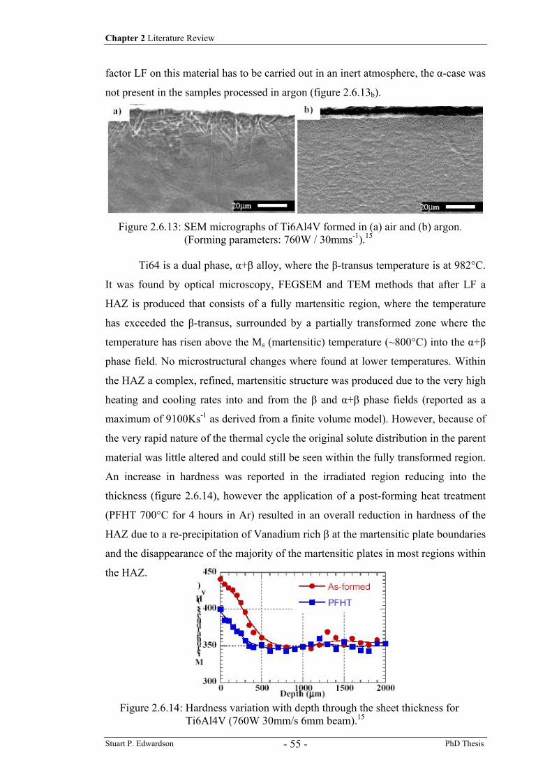
Chapter 2 Literature Review
Stuart P. Edwardson PhD Thesis - 55 -
factor LF on this material has to be carried out in an inert atmosphere, the α-case was
not present in the samples processed in argon (figure 2.6.13b).
Ti64 is a dual phase, α+β alloy, where the β-transus temperature is at 982°C.
It was found by optical microscopy, FEGSEM and TEM methods that after LF a
HAZ is produced that consists of a fully martensitic region, where the temperature
has exceeded the β-transus, surrounded by a partially transformed zone where the
temperature has risen above the Ms (martensitic) temperature (~800°C) into the α+β
phase field. No microstructural changes where found at lower temperatures. Within
the HAZ a complex, refined, martensitic structure was produced due to the very high
heating and cooling rates into and from the β and α+β phase fields (reported as a
maximum of 9100Ks-1 as derived from a finite volume model). However, because of
the very rapid nature of the thermal cycle the original solute distribution in the parent
material was little altered and could still be seen within the fully transformed region.
An increase in hardness was reported in the irradiated region reducing into the
thickness (figure 2.6.14), however the application of a post-forming heat treatment
(PFHT 700°C for 4 hours in Ar) resulted in an overall reduction in hardness of the
HAZ due to a re-precipitation of Vanadium rich β at the martensitic plate boundaries
and the disappearance of the majority of the martensitic plates in most regions within
the HAZ.
Figure 2.6.14: Hardness variation with depth through the sheet thickness for Ti6Al4V (760W 30mm/s 6mm beam).15
Figure 2.6.13: SEM micrographs of Ti6Al4V formed in (a) air and (b) argon. (Forming parameters: 760W / 30mms-1).15
Chapter 2 Literature Review
Stuart P. Edwardson PhD Thesis - 56 -
A tensile test on the LF samples was also reported, it was found that during
tensile deformation the higher hardness of the HAZ acted as a local constraint on
plastic deformation and failure always occurred in the parent material away from the
irradiated area. The bulk tensile properties of the Ti64 sheet consequently remained
relatively unaffected by the LF process. Studies in other alloys of Titanium14, 109, 110
also confirmed the viability of LF with these materials.
Work on aluminium and aluminium alloys by Merklien et al 111, 112 at the
University of Erlangen revealed the microstuctural development and mechanical
properties in laser formed Al1050 and an Al6082 in two heat treatment conditions
T41 and T61. The work was conducted on 80mm wide 1mm thick samples using a
1kW cw Nd:YAG laser, a graphite coating was still used however. SEM and TEM
methods were used for analysis. Changes in the mechanical behaviour as well as in
the microstructure were observed. The soft and annealed AA-1050 showed
hardening due to the LF process. This was proved by hardness tests and by
SEM/TEM images showing the dislocation motion and changes in microstructure.
For the two heat treatments of the Al6082 there were little or no differences in
forming characteristics over a number of irradiations found between them. For the
artificially aged T61 alloy, the hardness produced by ageing is lost in the HAZ and
immediate area after LF and is comparable to the naturally aged T41 values. For the
T41 alloy only a slight decrease in hardness is observed in the HAZ.
In 2003 Yao et al 118 from Columbia University presented research on the
effect of material anisotropy on the laser forming process, both numerical and
experimental results. Cold rolled sheet metal exhibit anisotropic properties which are
mostly caused by preferred orientations of grains developed during rolling reductions.
The anisotropic index or R value of a material in a particular orientation was
determined using an ASTM standard tensile test. The grain textures in the formed
samples were determined using an electron back-scatter diffraction method (EBSD).
It was found that there was a significant difference in the laser forming
characteristics of the cold rolled AISI 1010 mild steel depending on the orientation
of the scan line to the rolling direction in the sample. It was found that the
anisotropic effects increased with increased rolling reductions i.e. thinner materials.
It was also concluded that the higher the temperature achieved in the sample the less
the materials’ anisotropy has an effect.
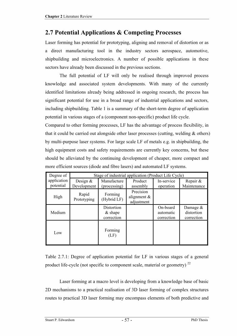
Chapter 2 Literature Review
Stuart P. Edwardson PhD Thesis - 57 -
2.7 Potential Applications & Competing Processes Laser forming has potential for prototyping, aligning and removal of distortion or as
a direct manufacturing tool in the industry sectors aerospace, automotive,
shipbuilding and microelectronics. A number of possible applications in these
sectors have already been discussed in the previous sections.
The full potential of LF will only be realised through improved process
knowledge and associated system developments. With many of the currently
identified limitations already being addressed in ongoing research, the process has
significant potential for use in a broad range of industrial applications and sectors,
including shipbuilding. Table 1 is a summary of the short-term degree of application
potential in various stages of a (component non-specific) product life cycle.
Compared to other forming processes, LF has the advantage of process flexibility, in
that it could be carried out alongside other laser processes (cutting, welding & others)
by multi-purpose laser systems. For large scale LF of metals e.g. in shipbuilding, the
high equipment costs and safety requirements are currently key concerns, but these
should be alleviated by the continuing development of cheaper, more compact and
more efficient sources (diode and fibre lasers) and automated LF systems.
Stage of industrial application (Product Life Cycle) Degree of application potential
Design & Development
Manufacture (processing)
Product assembly
In-service operation
Repair & Maintenance
High Rapid Prototyping
Forming (Hybrid LF)
Precision alignment & adjustment
Medium Distortion & shape
correction
On-board automatic correction
Damage & distortion correction
Low Forming (LF)
Table 2.7.1: Degree of application potential for LF in various stages of a general
product life-cycle (not specific to component scale, material or geometry) 22
Laser forming at a macro level is developing from a knowledge base of basic
2D mechanisms to a practical realisation of 3D laser forming of complex structures
routes to practical 3D laser forming may encompass elements of both predictive and
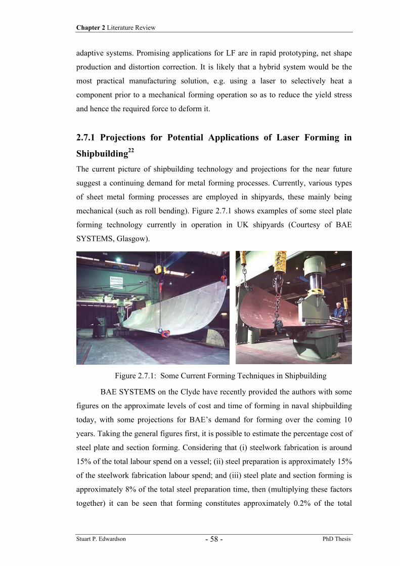
Chapter 2 Literature Review
Stuart P. Edwardson PhD Thesis - 58 -
adaptive systems. Promising applications for LF are in rapid prototyping, net shape
production and distortion correction. It is likely that a hybrid system would be the
most practical manufacturing solution, e.g. using a laser to selectively heat a
component prior to a mechanical forming operation so as to reduce the yield stress
and hence the required force to deform it.
2.7.1 Projections for Potential Applications of Laser Forming in
Shipbuilding22
The current picture of shipbuilding technology and projections for the near future
suggest a continuing demand for metal forming processes. Currently, various types
of sheet metal forming processes are employed in shipyards, these mainly being
mechanical (such as roll bending). Figure 2.7.1 shows examples of some steel plate
forming technology currently in operation in UK shipyards (Courtesy of BAE
SYSTEMS, Glasgow).
BAE SYSTEMS on the Clyde have recently provided the authors with some
figures on the approximate levels of cost and time of forming in naval shipbuilding
today, with some projections for BAE’s demand for forming over the coming 10
years. Taking the general figures first, it is possible to estimate the percentage cost of
steel plate and section forming. Considering that (i) steelwork fabrication is around
15% of the total labour spend on a vessel; (ii) steel preparation is approximately 15%
of the steelwork fabrication labour spend; and (iii) steel plate and section forming is
approximately 8% of the total steel preparation time, then (multiplying these factors
together) it can be seen that forming constitutes approximately 0.2% of the total
Figure 2.7.1: Some Current Forming Techniques in Shipbuilding
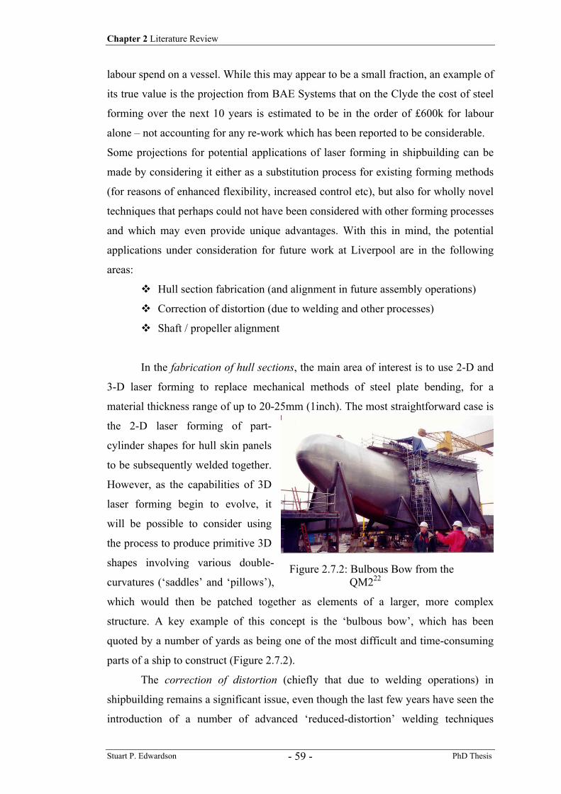
Chapter 2 Literature Review
Stuart P. Edwardson PhD Thesis - 59 -
Figure 2.7.2: Bulbous Bow from the QM222
labour spend on a vessel. While this may appear to be a small fraction, an example of
its true value is the projection from BAE Systems that on the Clyde the cost of steel
forming over the next 10 years is estimated to be in the order of £600k for labour
alone – not accounting for any re-work which has been reported to be considerable.
Some projections for potential applications of laser forming in shipbuilding can be
made by considering it either as a substitution process for existing forming methods
(for reasons of enhanced flexibility, increased control etc), but also for wholly novel
techniques that perhaps could not have been considered with other forming processes
and which may even provide unique advantages. With this in mind, the potential
applications under consideration for future work at Liverpool are in the following
areas:
Hull section fabrication (and alignment in future assembly operations)
Correction of distortion (due to welding and other processes)
Shaft / propeller alignment
In the fabrication of hull sections, the main area of interest is to use 2-D and
3-D laser forming to replace mechanical methods of steel plate bending, for a
material thickness range of up to 20-25mm (1inch). The most straightforward case is
the 2-D laser forming of part-
cylinder shapes for hull skin panels
to be subsequently welded together.
However, as the capabilities of 3D
laser forming begin to evolve, it
will be possible to consider using
the process to produce primitive 3D
shapes involving various double-
curvatures (‘saddles’ and ‘pillows’),
which would then be patched together as elements of a larger, more complex
structure. A key example of this concept is the ‘bulbous bow’, which has been
quoted by a number of yards as being one of the most difficult and time-consuming
parts of a ship to construct (Figure 2.7.2).
The correction of distortion (chiefly that due to welding operations) in
shipbuilding remains a significant issue, even though the last few years have seen the
introduction of a number of advanced ‘reduced-distortion’ welding techniques
Chapter 2 Literature Review
Stuart P. Edwardson PhD Thesis - 60 -
(including laser-based or laser hybrids 119). For many larger projects, the manual re-
working of weld distortion can effectively use up 30% of the total ship production
labour costs and the new techniques referred to above can often only be applied to
ship deck flat panel construction, where component geometry allows. Therefore,
there must be significant potential for using an advanced 3-D laser forming system to
address at least some of this need. As an example, BAE Systems report that they
perceive potential issues around plate distortion in projects such as the Type 45
Destroyer programme, which requires a light hull structure in order to deliver its
specified sea speed. Since laser cutting is already being used and laser welding is
currently under investigation, there is now growing interest in laser forming for thin
plate if it can deliver productivity, throughput or cost savings.
Shaft alignment –Investigations have be reported using laser forming for the
straightening of rod and cylindrical tubes at smaller scales, where a glancing
incidence of the laser beam allows an almost self-straightening effect to be
established as the component is rotated and the laser beam moved along the
component length. It would be of interest to see if this could be scaled up to marine
shaft parts.
Ships propellers are large components cast from special alloys and their
performance characteristics depend strongly on the curvature variations along their
surfaces. Once cast, if modifications are required either during production or at a
later maintenance / repair phase, this requires large-scale and expensive machining
capability. This is a further area for investigation of laser forming
2.7.2 Potential Applications in the Aerospace Sector As mentioned LF can be useful for prototyping, aligning and removal of distortion or
as a direct manufacturing tool. Current forming practices in the Aerospace sector
include traditional die forming, super-plastic forming (of Ti) and hot creep forming.
Lf can certainly compete with die forming in terms of process flexibility and cost
(apart from initial laser investment), in particular for low volume parts and
prototypes, where the cost of the die or hard tooling can be in excess of £5K. The
structures that can be formed using the vacuum or blown forming technique in super-
plastic forming of titanium alloys would be difficult to achieve using LF, however
the components can have considerable distortions post-forming and a large amount
Chapter 2 Literature Review
Stuart P. Edwardson PhD Thesis - 61 -
of man hours are used in the manual removal of distortion, usually by a skilled
hammer. LF (3D LF) could be used here for the removal of distortion; however there
may be a limit on the complexity of distortion that could be rectified further research
would reveal this. The distortion removal aspect of LF also could be used in the
chemical etching process, where the removal of material from a component, usually
to reduce weight, can produce unwanted distortion. Again these parts are invariably
manually straightened and so LF could be used to automate the process, particularly
where the distortions are uniform and reasonably repeatable.
An area where LF has the most potential to replace an existing process is hot
creep forming. This process involves the forming of material, usually titanium alloy,
using a heated die and press tool. A plate (sprayed with Boron Nitride to aid thermal
diffusivity) is placed in the press tool and die, the plate is then heated to 800°C and
formed over the die using much less force and inducing much less stress in the
component when compared to cold forming. If Ti64 is used, the plate is then sand
and vapour blasted prior to chemical etching to remove the α-case (mentioned earlier)
due to the process taking place in air. The disadvantages of this process specific to
LF are:
Long tool change-over times (1/2 day)
Long warm up/cool down times of the die (16 Hours)
Removal of α-case
Cost of effluent disposal
Cost of tooling
Storage of tooling
Inflexibility
Cooling of dies between components
High energy consumption (20Kw/H)
LF has a number of advantages over hot creep forming in these areas:
Increased flexibility
Reduced tooling costs
Possible Single piece forming of components
Reduced need for etching (Argon atmosphere or local shrouding)
Faster changeover times (batches of 1 possible)
Simple product changes
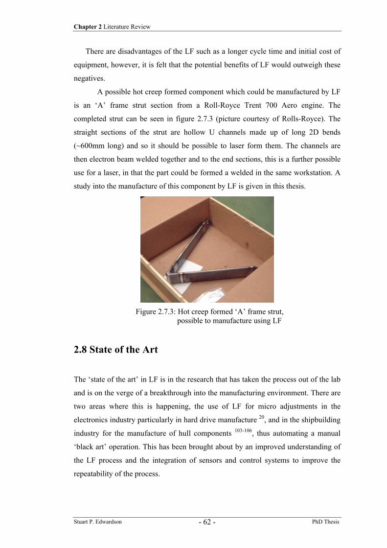
Chapter 2 Literature Review
Stuart P. Edwardson PhD Thesis - 62 -
Figure 2.7.3: Hot creep formed ‘A’ frame strut, possible to manufacture using LF
There are disadvantages of the LF such as a longer cycle time and initial cost of
equipment, however, it is felt that the potential benefits of LF would outweigh these
negatives.
A possible hot creep formed component which could be manufactured by LF
is an ‘A’ frame strut section from a Roll-Royce Trent 700 Aero engine. The
completed strut can be seen in figure 2.7.3 (picture courtesy of Rolls-Royce). The
straight sections of the strut are hollow U channels made up of long 2D bends
(~600mm long) and so it should be possible to laser form them. The channels are
then electron beam welded together and to the end sections, this is a further possible
use for a laser, in that the part could be formed a welded in the same workstation. A
study into the manufacture of this component by LF is given in this thesis.
2.8 State of the Art
The ‘state of the art’ in LF is in the research that has taken the process out of the lab
and is on the verge of a breakthrough into the manufacturing environment. There are
two areas where this is happening, the use of LF for micro adjustments in the
electronics industry particularly in hard drive manufacture 20, and in the shipbuilding
industry for the manufacture of hull components 103-106, thus automating a manual
‘black art’ operation. This has been brought about by an improved understanding of
the LF process and the integration of sensors and control systems to improve the
repeatability of the process.
Chapter 2 Literature Review
Stuart P. Edwardson PhD Thesis - 63 -
2.9 Synopsis for Present Research
There has been a considerable amount of work completed on 2D laser forming to
date, however due to the many variables in the process and numbers of materials and
material types that can be laser formed a full understanding of the process is some
way off. The work on 2D laser forming presented in this thesis aims to increase the
knowledge and understanding of the process, in particular the transient thermo-
mechanical and asymmetrical effects plus aspects for closed loop controlled LF.
Materials investigated include mild steel, aluminium 1050, aluminium 6061 (in three
heat treatments O, T4 & T6), Ti6AL4V and newly developed Metal Laminate
Composite Materials (or Fibre Metal Laminates).
In order to advance the laser forming process still further for realistic forming
applications and for straightening and aligning operations in a manufacturing
environment it is necessary to consider 3D laser forming. Less work has been
completed in this field compared to 2D LF, however the process has been shown to
have a great deal of potential. In order to compete directly with conventional forming
techniques though, such as die forming the process must be proven to be reliable,
repeatable, cost effective and flexible. It is the potential flexibility of 3D laser
forming that offers the greatest benefits, in that a change to a required part geometry
could be implemented easily through the CAD driven process, this can be compared
to the expensive and in-flexible hard tooling requirements of the die forming process.
The work presented in this thesis on 3D laser forming aims to prove the viability of
this technique as a direct manufacturing tool and as a means of post-conventional
forming (or processing e.g. chemical etching) distortion removal. To this aim
progress towards repeatable closed loop controlled 3D LF is presented. The materials
investigated were mild steel and Ti6Al4V.
Chapter 3 Experimental Procedure
Stuart P. Edwardson PhD Thesis - 64 -
Chapter 3
Experimental Procedure This chapter reviews the equipment, set-up and procedures for each of the studies
undertaken for this thesis. For clarity of presentation, the studies are divided into
sections entitled ‘2D laser forming’ and ‘3D laser forming’. As mentioned earlier,
2D laser forming encompasses laser forming operations that utilise two dimensional
out-of-plane bends to produce three dimensional results e.g. a fold. 3D laser forming
encompasses laser forming operations that can utilise combinations of multi-axis two
dimensional out-of plane bends and in-plane localised shortening to produce three
dimensional spatially formed parts such as a dome.
3.1 General Set-up This section details the general experimental set-up used, not specific to any of the
individual investigations, such as the laser, beam manipulation and software tools.
The hardware and software developed for this work are detailed in the following
sub-sections.
3.1.1 Hardware Except where stated, all of the experimental laser forming studies reported in this
thesis were performed on a specially designed and constructed CO2 laser system that
was developed for laser forming operations as part of this research.
As the process involves the use of a high power laser, some background is
given here on their construction and type:
Chapter 3 Experimental Procedure
Stuart P. Edwardson PhD Thesis - 65 -
A laser beam is a high intensity monochromatic (single wavelength) coherent
beam of light, which is generated by a laser cavity. A laser cavity is an optical
oscillator made up of two mirrors placed parallel to each other and containing an
active medium (can be a gas, solid or liquid). If energy is supplied to the medium
(normally in the form of a DC or RF electrical power supply or in the form of
focussed pulses of light, or in the form of a chemical reaction, depending on laser
type) it must be capable of amplifying the light passing between the two mirrors by
the mechanism of stimulated emission, hence the name LASER is an acronym for
the process. Light Amplification by the Stimulated Emission of Radiation
One of the mirrors that make up the cavity is only partially reflective while
the other mirror is totally reflective. This means that a fraction of the light oscillating
between the two mirrors can be allowed to escape along the optical axis as the
working beam (usually a shutter prevents the beam propagating when not required).
For the CO2 laser used in this study the active medium in this laser type is
carbon dioxide gas. The carbon dioxide molecule is made up of a carbon atom
covalently bonded to two oxygen atoms. While constrained by the atomic bonds
between them, these atoms naturally oscillate about each other as a result of thermal
energy. The molecule can exist in a number of discrete energy states which depend
on the orientation of the oxygen atoms with respect to the carbon atom in the
molecule. The principle of the process is that a photon (or energy) of a particular
wavelength (10.6µm in the case of this laser type) is produced as the CO2 molecule
transforms from an upper energy state to a lower (conservation of energy principle).
The requirement to produce a laser cavity in which there is amplification of the light
energy produced (lasing) is that the lifetime of the upper laser level is higher than
that of the lower laser level, which is the case for the carbon dioxide molecule. Then
population inversion can be achieved by the selective excitation of the upper laser
level.
The production of carbon dioxide molecules in the various energy states is
achieved in the cavity by subjecting the gas to a high voltage electric discharge. It is
in this way that energy is pumped into the system to eventually obtain the laser beam
with which useful work can be carried out. In order to maintain a high population of
upper laser level molecules a process of selective excitation to the upper laser level is
achieved by addition of nitrogen to the carbon dioxide. Nitrogen has the property
that it only has one excited state and the energy level of this excited state is very
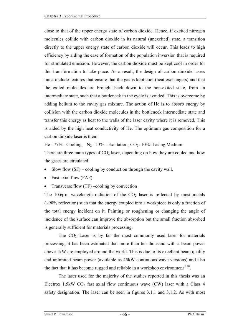
Chapter 3 Experimental Procedure
Stuart P. Edwardson PhD Thesis - 66 -
close to that of the upper energy state of carbon dioxide. Hence, if excited nitrogen
molecules collide with carbon dioxide in its natural (unexcited) state, a transition
directly to the upper energy state of carbon dioxide will occur. This leads to high
efficiency by aiding the ease of formation of the population inversion that is required
for stimulated emission. However, the carbon dioxide must be kept cool in order for
this transformation to take place. As a result, the design of carbon dioxide lasers
must include features that ensure that the gas is kept cool (heat exchangers) and that
the exited molecules are brought back down to the non-exited state, from an
intermediate state, such that a bottleneck in the cycle is avoided. This is overcome by
adding helium to the cavity gas mixture. The action of He is to absorb energy by
collision with the carbon dioxide molecules in the bottleneck intermediate state and
transfer this energy as heat to the walls of the laser cavity where it is removed. This
is aided by the high heat conductivity of He. The optimum gas composition for a
carbon dioxide laser is then:
He - 77% - Cooling, N2 - 13% - Excitation, CO2- 10%- Lasing Medium
There are three main types of CO2 laser, depending on how they are cooled and how
the gases are circulated:
• Slow flow (SF) – cooling by conduction through the cavity wall.
• Fast axial flow (FAF)
• Transverse flow (TF) –cooling by convection
The 10.6µm wavelength radiation of the CO2 laser is reflected by most metals
(~90% reflection) such that the energy coupled into a workpiece is only a fraction of
the total energy incident on it. Painting or roughening or changing the angle of
incidence of the surface can improve the absorption but the small fraction absorbed
is generally sufficient for materials processing.
The CO2 Laser is by far the most commonly used laser for materials
processing, it has been estimated that more than ten thousand with a beam power
above 1kW are employed around the world. This is due to its excellent beam quality
and unlimited beam power (available as 45kW continuous wave versions) and also
the fact that it has become rugged and reliable in a workshop environment 120.
The laser used for the majority of the studies reported in this thesis was an
Electrox 1.5kW CO2 fast axial flow continuous wave (CW) laser with a Class 4
safety designation. The laser can be seen in figures 3.1.1 and 3.1.2. As with most
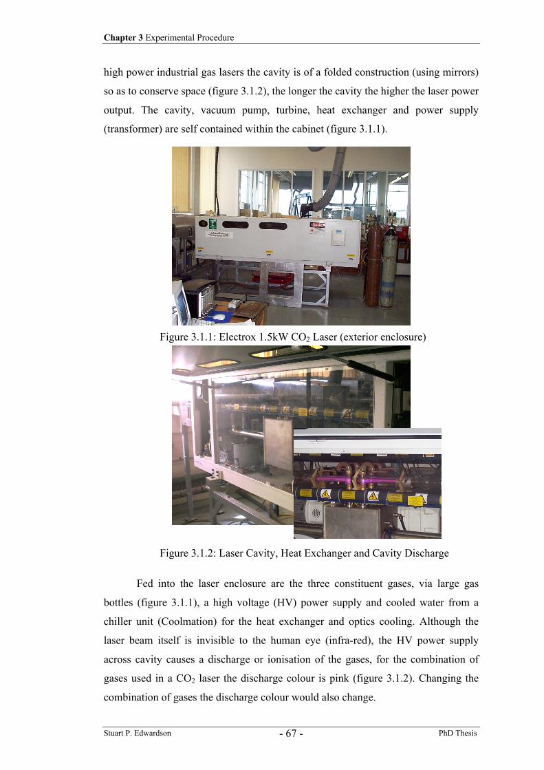
Chapter 3 Experimental Procedure
Stuart P. Edwardson PhD Thesis - 67 -
high power industrial gas lasers the cavity is of a folded construction (using mirrors)
so as to conserve space (figure 3.1.2), the longer the cavity the higher the laser power
output. The cavity, vacuum pump, turbine, heat exchanger and power supply
(transformer) are self contained within the cabinet (figure 3.1.1).
Fed into the laser enclosure are the three constituent gases, via large gas
bottles (figure 3.1.1), a high voltage (HV) power supply and cooled water from a
chiller unit (Coolmation) for the heat exchanger and optics cooling. Although the
laser beam itself is invisible to the human eye (infra-red), the HV power supply
across cavity causes a discharge or ionisation of the gases, for the combination of
gases used in a CO2 laser the discharge colour is pink (figure 3.1.2). Changing the
combination of gases the discharge colour would also change.
Figure 3.1.1: Electrox 1.5kW CO2 Laser (exterior enclosure)
Figure 3.1.2: Laser Cavity, Heat Exchanger and Cavity Discharge
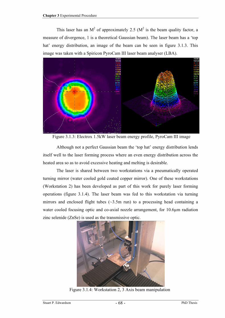
Chapter 3 Experimental Procedure
Stuart P. Edwardson PhD Thesis - 68 -
This laser has an M2 of approximately 2.5 (M2 is the beam quality factor, a
measure of divergence, 1 is a theoretical Gaussian beam). The laser beam has a ‘top
hat’ energy distribution, an image of the beam can be seen in figure 3.1.3. This
image was taken with a Spiricon PyroCam III laser beam analyser (LBA).
Although not a perfect Gaussian beam the ‘top hat’ energy distribution lends
itself well to the laser forming process where an even energy distribution across the
heated area so as to avoid excessive heating and melting is desirable.
The laser is shared between two workstations via a pneumatically operated
turning mirror (water cooled gold coated copper mirror). One of these workstations
(Workstation 2) has been developed as part of this work for purely laser forming
operations (figure 3.1.4). The laser beam was fed to this workstation via turning
mirrors and enclosed flight tubes (~3.5m run) to a processing head containing a
water cooled focusing optic and co-axial nozzle arrangement, for 10.6µm radiation
zinc selenide (ZnSe) is used as the transmissive optic.
Figure 3.1.3: Electrox 1.5kW laser beam energy profile, PyroCam III image
Figure 3.1.4: Workstation 2, 3 Axis beam manipulation
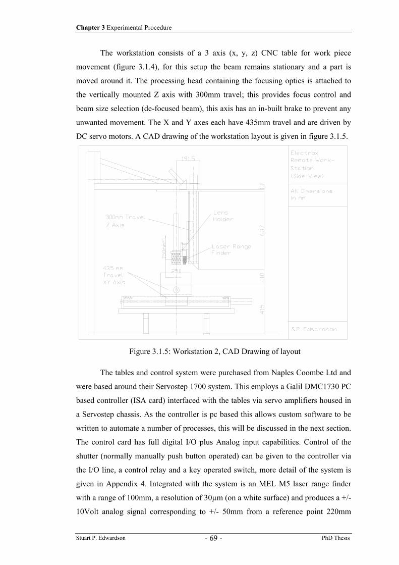
Chapter 3 Experimental Procedure
Stuart P. Edwardson PhD Thesis - 69 -
The workstation consists of a 3 axis (x, y, z) CNC table for work piece
movement (figure 3.1.4), for this setup the beam remains stationary and a part is
moved around it. The processing head containing the focusing optics is attached to
the vertically mounted Z axis with 300mm travel; this provides focus control and
beam size selection (de-focused beam), this axis has an in-built brake to prevent any
unwanted movement. The X and Y axes each have 435mm travel and are driven by
DC servo motors. A CAD drawing of the workstation layout is given in figure 3.1.5.
The tables and control system were purchased from Naples Coombe Ltd and
were based around their Servostep 1700 system. This employs a Galil DMC1730 PC
based controller (ISA card) interfaced with the tables via servo amplifiers housed in
a Servostep chassis. As the controller is pc based this allows custom software to be
written to automate a number of processes, this will be discussed in the next section.
The control card has full digital I/O plus Analog input capabilities. Control of the
shutter (normally manually push button operated) can be given to the controller via
the I/O line, a control relay and a key operated switch, more detail of the system is
given in Appendix 4. Integrated with the system is an MEL M5 laser range finder
with a range of 100mm, a resolution of 30µm (on a white surface) and produces a +/-
10Volt analog signal corresponding to +/- 50mm from a reference point 220mm
Figure 3.1.5: Workstation 2, CAD Drawing of layout
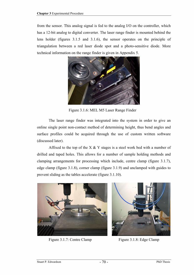
Chapter 3 Experimental Procedure
Stuart P. Edwardson PhD Thesis - 70 -
from the sensor. This analog signal is fed to the analog I/O on the controller, which
has a 12-bit analog to digital converter. The laser range finder is mounted behind the
lens holder (figures 3.1.5 and 3.1.6), the sensor operates on the principle of
triangulation between a red laser diode spot and a photo-sensitive diode. More
technical information on the range finder is given in Appendix 5.
The laser range finder was integrated into the system in order to give an
online single point non-contact method of determining height, thus bend angles and
surface profiles could be acquired through the use of custom written software
(discussed later).
Affixed to the top of the X & Y stages is a steel work bed with a number of
drilled and taped holes. This allows for a number of sample holding methods and
clamping arrangements for processing which include, centre clamp (figure 3.1.7),
edge clamp (figure 3.1.8), corner clamp (figure 3.1.9) and unclamped with guides to
prevent sliding as the tables accelerate (figure 3.1.10).
Figure 3.1.6: MEL M5 Laser Range Finder
Figure 3.1.7: Centre Clamp Figure 3.1.8: Edge Clamp
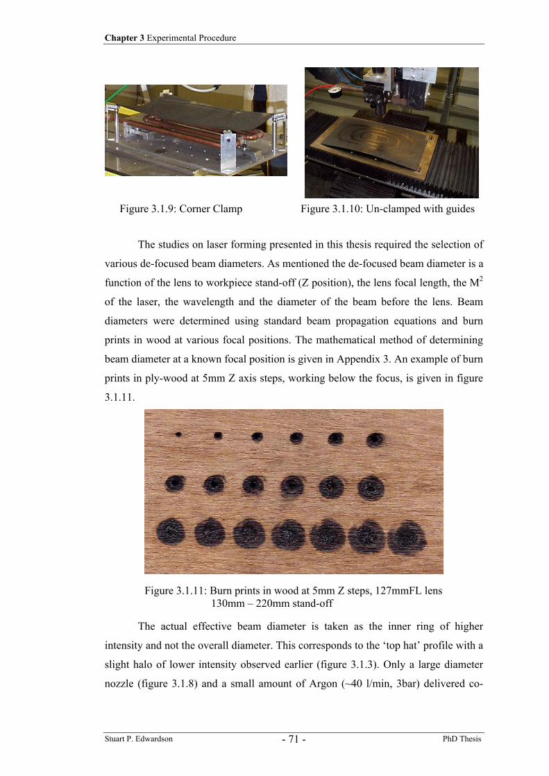
Chapter 3 Experimental Procedure
Stuart P. Edwardson PhD Thesis - 71 -
The studies on laser forming presented in this thesis required the selection of
various de-focused beam diameters. As mentioned the de-focused beam diameter is a
function of the lens to workpiece stand-off (Z position), the lens focal length, the M2
of the laser, the wavelength and the diameter of the beam before the lens. Beam
diameters were determined using standard beam propagation equations and burn
prints in wood at various focal positions. The mathematical method of determining
beam diameter at a known focal position is given in Appendix 3. An example of burn
prints in ply-wood at 5mm Z axis steps, working below the focus, is given in figure
3.1.11.
The actual effective beam diameter is taken as the inner ring of higher
intensity and not the overall diameter. This corresponds to the ‘top hat’ profile with a
slight halo of lower intensity observed earlier (figure 3.1.3). Only a large diameter
nozzle (figure 3.1.8) and a small amount of Argon (~40 l/min, 3bar) delivered co-
Figure 3.1.9: Corner Clamp Figure 3.1.10: Un-clamped with guides
Figure 3.1.11: Burn prints in wood at 5mm Z steps, 127mmFL lens 130mm – 220mm stand-off
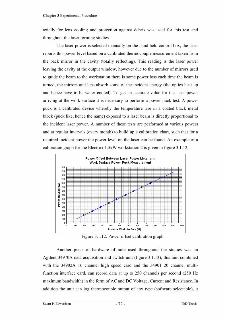
Chapter 3 Experimental Procedure
Stuart P. Edwardson PhD Thesis - 72 -
axially for lens cooling and protection against debris was used for this test and
throughout the laser forming studies.
The laser power is selected manually on the hand held control box, the laser
reports this power level based on a calibrated thermocouple measurement taken from
the back mirror in the cavity (totally reflecting). This reading is the laser power
leaving the cavity at the output window, however due to the number of mirrors used
to guide the beam to the workstation there is some power loss each time the beam is
turned, the mirrors and lens absorb some of the incident energy (the optics heat up
and hence have to be water cooled). To get an accurate value for the laser power
arriving at the work surface it is necessary to perform a power puck test. A power
puck is a calibrated device whereby the temperature rise in a coated black metal
block (puck like, hence the name) exposed to a laser beam is directly proportional to
the incident laser power. A number of these tests are performed at various powers
and at regular intervals (every month) to build up a calibration chart, such that for a
required incident power the power level on the laser can be found. An example of a
calibration graph for the Electrox 1.5kW workstation 2 is given in figure 3.1.12.
Another piece of hardware of note used throughout the studies was an
Agilent 34970A data acquisition and switch unit (figure 3.1.13), this unit combined
with the 34902A 16 channel high speed card and the 34901 20 channel multi-
function interface card, can record data at up to 250 channels per second (250 Hz
maximum bandwidth) in the form of AC and DC Voltage, Current and Resistance. In
addition the unit can log thermocouple output of any type (software selectable), it
Figure 3.1.12: Power offset calibration graph
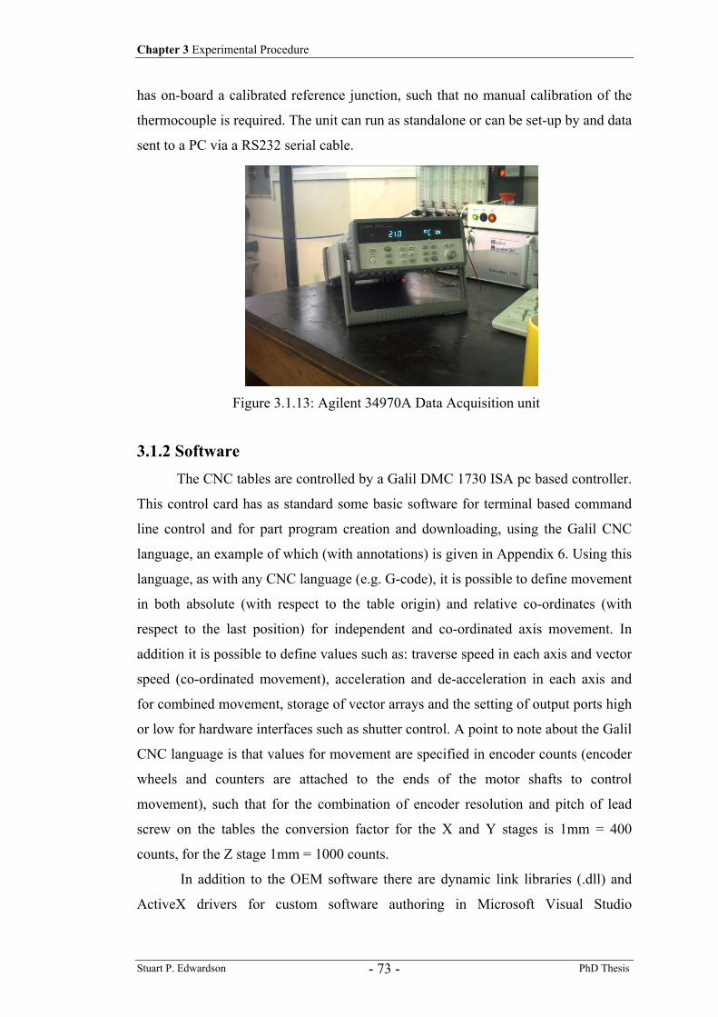
Chapter 3 Experimental Procedure
Stuart P. Edwardson PhD Thesis - 73 -
has on-board a calibrated reference junction, such that no manual calibration of the
thermocouple is required. The unit can run as standalone or can be set-up by and data
sent to a PC via a RS232 serial cable.
3.1.2 Software The CNC tables are controlled by a Galil DMC 1730 ISA pc based controller.
This control card has as standard some basic software for terminal based command
line control and for part program creation and downloading, using the Galil CNC
language, an example of which (with annotations) is given in Appendix 6. Using this
language, as with any CNC language (e.g. G-code), it is possible to define movement
in both absolute (with respect to the table origin) and relative co-ordinates (with
respect to the last position) for independent and co-ordinated axis movement. In
addition it is possible to define values such as: traverse speed in each axis and vector
speed (co-ordinated movement), acceleration and de-acceleration in each axis and
for combined movement, storage of vector arrays and the setting of output ports high
or low for hardware interfaces such as shutter control. A point to note about the Galil
CNC language is that values for movement are specified in encoder counts (encoder
wheels and counters are attached to the ends of the motor shafts to control
movement), such that for the combination of encoder resolution and pitch of lead
screw on the tables the conversion factor for the X and Y stages is 1mm = 400
counts, for the Z stage 1mm = 1000 counts.
In addition to the OEM software there are dynamic link libraries (.dll) and
ActiveX drivers for custom software authoring in Microsoft Visual Studio
Figure 3.1.13: Agilent 34970A Data Acquisition unit
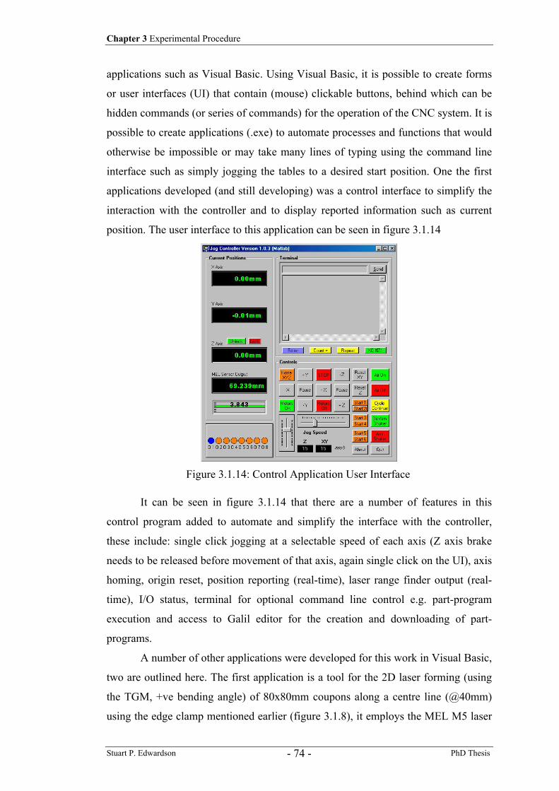
Chapter 3 Experimental Procedure
Stuart P. Edwardson PhD Thesis - 74 -
applications such as Visual Basic. Using Visual Basic, it is possible to create forms
or user interfaces (UI) that contain (mouse) clickable buttons, behind which can be
hidden commands (or series of commands) for the operation of the CNC system. It is
possible to create applications (.exe) to automate processes and functions that would
otherwise be impossible or may take many lines of typing using the command line
interface such as simply jogging the tables to a desired start position. One the first
applications developed (and still developing) was a control interface to simplify the
interaction with the controller and to display reported information such as current
position. The user interface to this application can be seen in figure 3.1.14
It can be seen in figure 3.1.14 that there are a number of features in this
control program added to automate and simplify the interface with the controller,
these include: single click jogging at a selectable speed of each axis (Z axis brake
needs to be released before movement of that axis, again single click on the UI), axis
homing, origin reset, position reporting (real-time), laser range finder output (real-
time), I/O status, terminal for optional command line control e.g. part-program
execution and access to Galil editor for the creation and downloading of part-
programs.
A number of other applications were developed for this work in Visual Basic,
two are outlined here. The first application is a tool for the 2D laser forming (using
the TGM, +ve bending angle) of 80x80mm coupons along a centre line (@40mm)
using the edge clamp mentioned earlier (figure 3.1.8), it employs the MEL M5 laser
Figure 3.1.14: Control Application User Interface
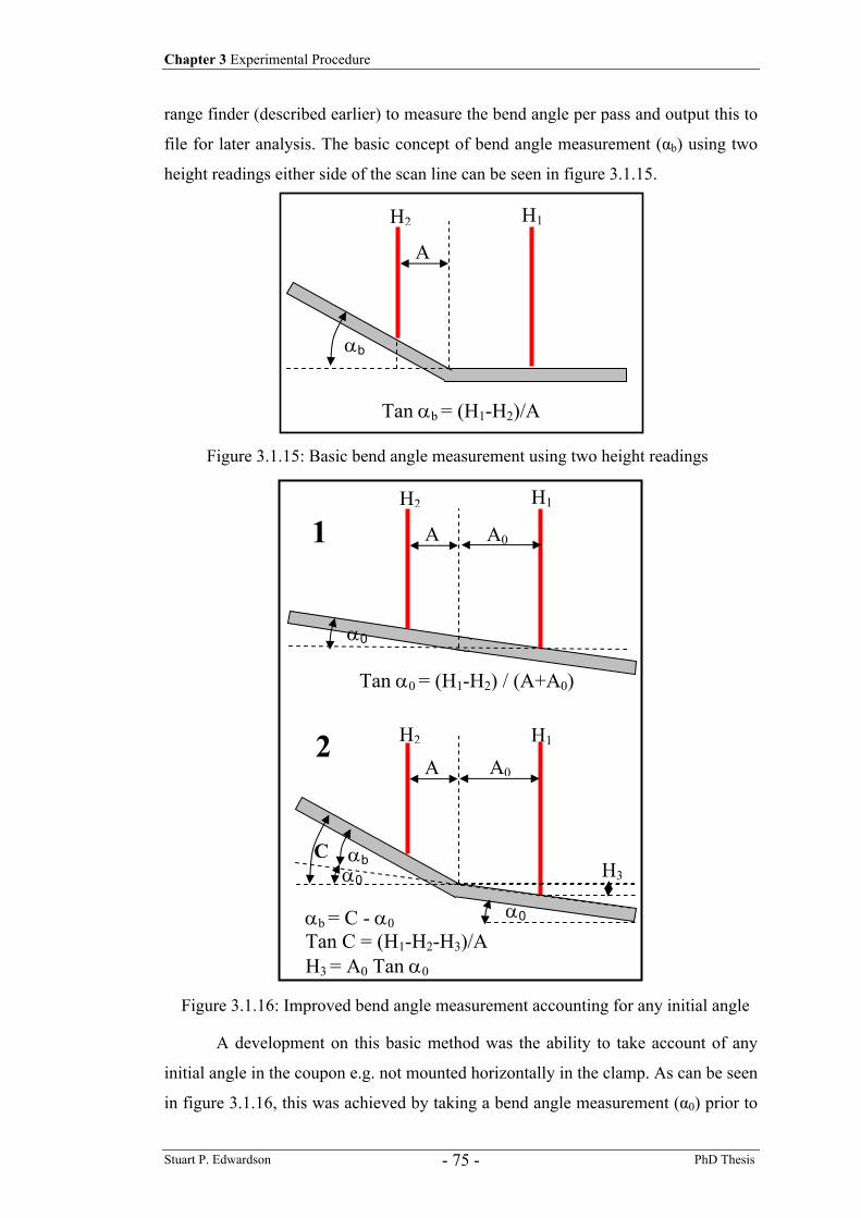
Chapter 3 Experimental Procedure
Stuart P. Edwardson PhD Thesis - 75 -
range finder (described earlier) to measure the bend angle per pass and output this to
file for later analysis. The basic concept of bend angle measurement (αb) using two
height readings either side of the scan line can be seen in figure 3.1.15.
A development on this basic method was the ability to take account of any
initial angle in the coupon e.g. not mounted horizontally in the clamp. As can be seen
in figure 3.1.16, this was achieved by taking a bend angle measurement (α0) prior to
A
H2 H1
αb
Tan αb = (H1-H2)/A
Figure 3.1.15: Basic bend angle measurement using two height readings
Figure 3.1.16: Improved bend angle measurement accounting for any initial angle
A
H2 H1
α0
Tan α0 = (H1-H2) / (A+A0)
A0
AH2 H1
αb
αb = C - α0 Tan C = (H1-H2-H3)/AH3 = A0 Tan α0
α0
A0
C H3
α0
1
2
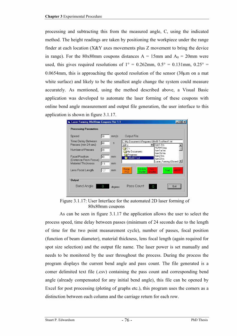
Chapter 3 Experimental Procedure
Stuart P. Edwardson PhD Thesis - 76 -
processing and subtracting this from the measured angle, C, using the indicated
method. The height readings are taken by positioning the workpiece under the range
finder at each location (X&Y axes movements plus Z movement to bring the device
in range). For the 80x80mm coupons distances A = 15mm and A0 = 20mm were
used, this gives required resolutions of 1° = 0.262mm, 0.5° = 0.131mm, 0.25° =
0.0654mm, this is approaching the quoted resolution of the sensor (30µm on a mat
white surface) and likely to be the smallest angle change the system could measure
accurately. As mentioned, using the method described above, a Visual Basic
application was developed to automate the laser forming of these coupons with
online bend angle measurement and output file generation, the user interface to this
application is shown in figure 3.1.17.
As can be seen in figure 3.1.17 the application allows the user to select the
process speed, time delay between passes (minimum of 24 seconds due to the length
of time for the two point measurement cycle), number of passes, focal position
(function of beam diameter), material thickness, lens focal length (again required for
spot size selection) and the output file name. The laser power is set manually and
needs to be monitored by the user throughout the process. During the process the
program displays the current bend angle and pass count. The file generated is a
comer delimited text file (.csv) containing the pass count and corresponding bend
angle (already compensated for any initial bend angle), this file can be opened by
Excel for post processing (ploting of graphs etc.), this program uses the comers as a
distinction between each column and the carriage return for each row.
Figure 3.1.17: User Interface for the automated 2D laser forming of 80x80mm coupons
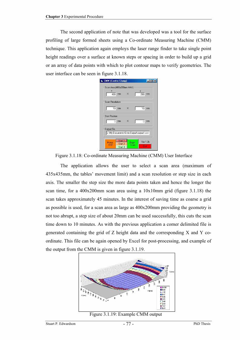
Chapter 3 Experimental Procedure
Stuart P. Edwardson PhD Thesis - 77 -
The second application of note that was developed was a tool for the surface
profiling of large formed sheets using a Co-ordinate Measuring Machine (CMM)
technique. This application again employs the laser range finder to take single point
height readings over a surface at known steps or spacing in order to build up a grid
or an array of data points with which to plot contour maps to verify geometries. The
user interface can be seen in figure 3.1.18.
The application allows the user to select a scan area (maximum of
435x435mm, the tables’ movement limit) and a scan resolution or step size in each
axis. The smaller the step size the more data points taken and hence the longer the
scan time, for a 400x200mm scan area using a 10x10mm grid (figure 3.1.18) the
scan takes approximately 45 minutes. In the interest of saving time as coarse a grid
as possible is used, for a scan area as large as 400x200mm providing the geometry is
not too abrupt, a step size of about 20mm can be used successfully, this cuts the scan
time down to 10 minutes. As with the previous application a comer delimited file is
generated containing the grid of Z height data and the corresponding X and Y co-
ordinate. This file can be again opened by Excel for post-processing, and example of
the output from the CMM is given in figure 3.1.19.
Figure 3.1.18: Co-ordinate Measuring Machine (CMM) User Interface
Figure 3.1.19: Example CMM output
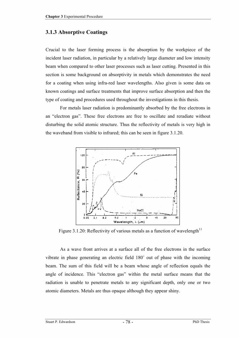
Chapter 3 Experimental Procedure
Stuart P. Edwardson PhD Thesis - 78 -
3.1.3 Absorptive Coatings
Crucial to the laser forming process is the absorption by the workpiece of the
incident laser radiation, in particular by a relatively large diameter and low intensity
beam when compared to other laser processes such as laser cutting. Presented in this
section is some background on absorptivity in metals which demonstrates the need
for a coating when using infra-red laser wavelengths. Also given is some data on
known coatings and surface treatments that improve surface absorption and then the
type of coating and procedures used throughout the investigations in this thesis.
For metals laser radiation is predominantly absorbed by the free electrons in
an “electron gas”. These free electrons are free to oscillate and reradiate without
disturbing the solid atomic structure. Thus the reflectivity of metals is very high in
the waveband from visible to infrared; this can be seen in figure 3.1.20.
As a wave front arrives at a surface all of the free electrons in the surface
vibrate in phase generating an electric field 180˚ out of phase with the incoming
beam. The sum of this field will be a beam whose angle of reflection equals the
angle of incidence. This “electron gas” within the metal surface means that the
radiation is unable to penetrate metals to any significant depth, only one or two
atomic diameters. Metals are thus opaque although they appear shiny.
Figure 3.1.20: Reflectivity of various metals as a function of wavelength11
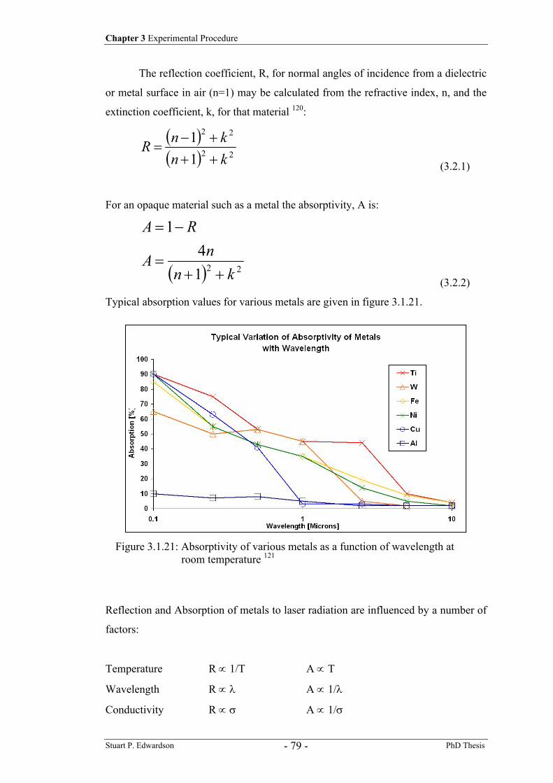
Chapter 3 Experimental Procedure
Stuart P. Edwardson PhD Thesis - 79 -
The reflection coefficient, R, for normal angles of incidence from a dielectric
or metal surface in air (n=1) may be calculated from the refractive index, n, and the
extinction coefficient, k, for that material 120:
( )( ) 22
22
11
knknR
+++−
= (3.2.1)
For an opaque material such as a metal the absorptivity, A is:
( ) 2214
1
knnA
RA
++=
−=
(3.2.2)
Typical absorption values for various metals are given in figure 3.1.21.
Reflection and Absorption of metals to laser radiation are influenced by a number of
factors:
Temperature R ∝ 1/T A ∝ T
Wavelength R ∝ λ A ∝ 1/λ
Conductivity R ∝ σ A ∝ 1/σ
Figure 3.1.21: Absorptivity of various metals as a function of wavelength at room temperature 121
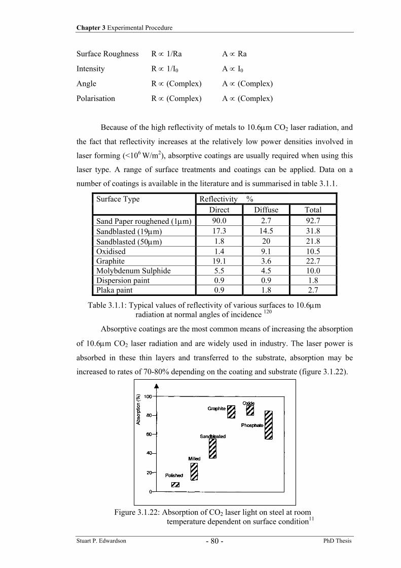
Chapter 3 Experimental Procedure
Stuart P. Edwardson PhD Thesis - 80 -
Surface Roughness R ∝ 1/Ra A ∝ Ra
Intensity R ∝ 1/I0 A ∝ I0
Angle R ∝ (Complex) A ∝ (Complex)
Polarisation R ∝ (Complex) A ∝ (Complex)
Because of the high reflectivity of metals to 10.6µm CO2 laser radiation, and
the fact that reflectivity increases at the relatively low power densities involved in
laser forming (<106 W/m2), absorptive coatings are usually required when using this
laser type. A range of surface treatments and coatings can be applied. Data on a
number of coatings is available in the literature and is summarised in table 3.1.1.
Surface Type Reflectivity % Direct Diffuse Total Sand Paper roughened (1µm) 90.0 2.7 92.7 Sandblasted (19µm) 17.3 14.5 31.8 Sandblasted (50µm) 1.8 20 21.8 Oxidised 1.4 9.1 10.5 Graphite 19.1 3.6 22.7 Molybdenum Sulphide 5.5 4.5 10.0 Dispersion paint 0.9 0.9 1.8 Plaka paint 0.9 1.8 2.7
Absorptive coatings are the most common means of increasing the absorption
of 10.6µm CO2 laser radiation and are widely used in industry. The laser power is
absorbed in these thin layers and transferred to the substrate, absorption may be
increased to rates of 70-80% depending on the coating and substrate (figure 3.1.22).
Table 3.1.1: Typical values of reflectivity of various surfaces to 10.6µm radiation at normal angles of incidence 120
Figure 3.1.22: Absorption of CO2 laser light on steel at room temperature dependent on surface condition11
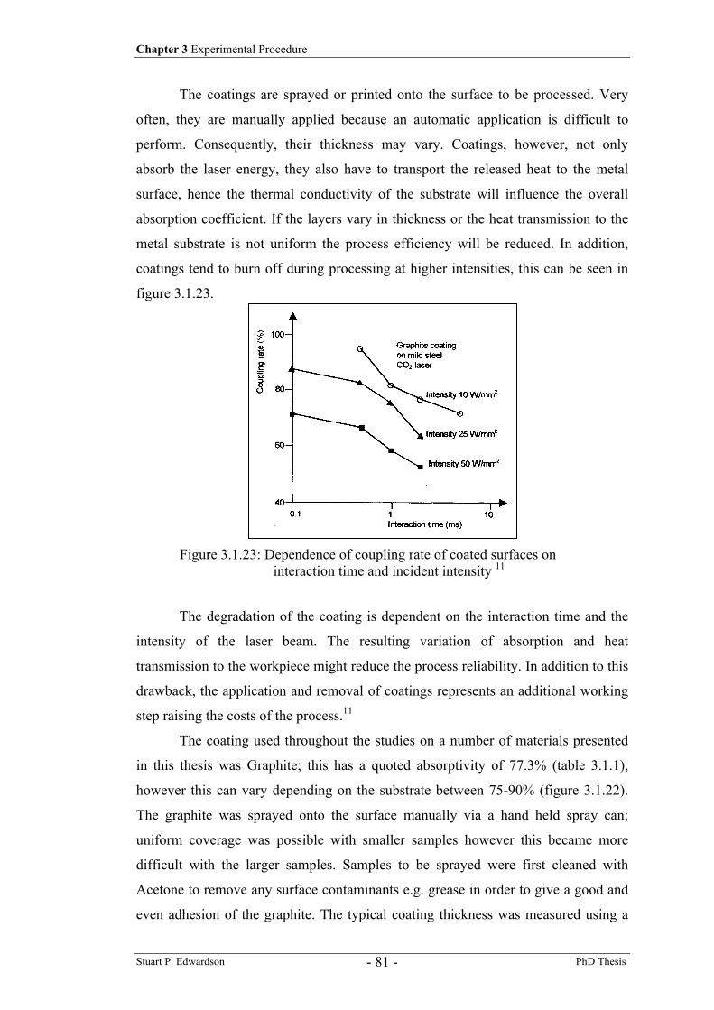
Chapter 3 Experimental Procedure
Stuart P. Edwardson PhD Thesis - 81 -
The coatings are sprayed or printed onto the surface to be processed. Very
often, they are manually applied because an automatic application is difficult to
perform. Consequently, their thickness may vary. Coatings, however, not only
absorb the laser energy, they also have to transport the released heat to the metal
surface, hence the thermal conductivity of the substrate will influence the overall
absorption coefficient. If the layers vary in thickness or the heat transmission to the
metal substrate is not uniform the process efficiency will be reduced. In addition,
coatings tend to burn off during processing at higher intensities, this can be seen in
figure 3.1.23.
The degradation of the coating is dependent on the interaction time and the
intensity of the laser beam. The resulting variation of absorption and heat
transmission to the workpiece might reduce the process reliability. In addition to this
drawback, the application and removal of coatings represents an additional working
step raising the costs of the process.11
The coating used throughout the studies on a number of materials presented
in this thesis was Graphite; this has a quoted absorptivity of 77.3% (table 3.1.1),
however this can vary depending on the substrate between 75-90% (figure 3.1.22).
The graphite was sprayed onto the surface manually via a hand held spray can;
uniform coverage was possible with smaller samples however this became more
difficult with the larger samples. Samples to be sprayed were first cleaned with
Acetone to remove any surface contaminants e.g. grease in order to give a good and
even adhesion of the graphite. The typical coating thickness was measured using a
Figure 3.1.23: Dependence of coupling rate of coated surfaces on interaction time and incident intensity 11
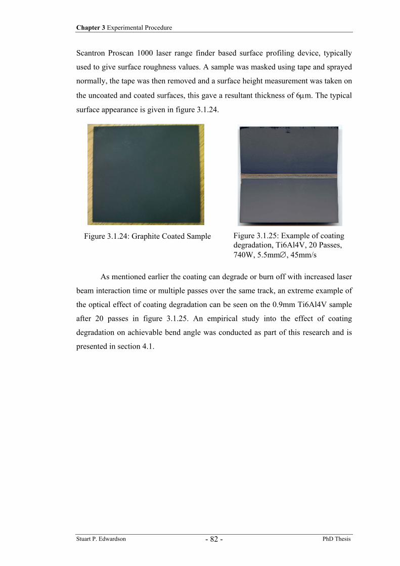
Chapter 3 Experimental Procedure
Stuart P. Edwardson PhD Thesis - 82 -
Scantron Proscan 1000 laser range finder based surface profiling device, typically
used to give surface roughness values. A sample was masked using tape and sprayed
normally, the tape was then removed and a surface height measurement was taken on
the uncoated and coated surfaces, this gave a resultant thickness of 6µm. The typical
surface appearance is given in figure 3.1.24.
As mentioned earlier the coating can degrade or burn off with increased laser
beam interaction time or multiple passes over the same track, an extreme example of
the optical effect of coating degradation can be seen on the 0.9mm Ti6Al4V sample
after 20 passes in figure 3.1.25. An empirical study into the effect of coating
degradation on achievable bend angle was conducted as part of this research and is
presented in section 4.1.
Figure 3.1.24: Graphite Coated Sample Figure 3.1.25: Example of coating degradation, Ti6Al4V, 20 Passes, 740W, 5.5mm∅, 45mm/s
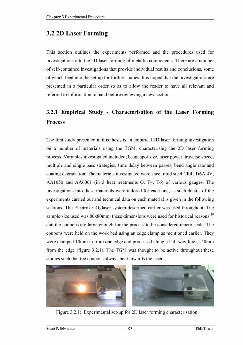
Chapter 3 Experimental Procedure
Stuart P. Edwardson PhD Thesis - 83 -
3.2 2D Laser Forming
This section outlines the experiments performed and the procedures used for
investigations into the 2D laser forming of metallic components. There are a number
of self-contained investigations that provide individual results and conclusions, some
of which feed into the set-up for further studies. It is hoped that the investigations are
presented in a particular order so as to allow the reader to have all relevant and
referred to information to hand before reviewing a new section.
3.2.1 Empirical Study - Characterisation of the Laser Forming
Process
The first study presented in this thesis is an empirical 2D laser forming investigation
on a number of materials using the TGM, characterising the 2D laser forming
process. Variables investigated included; beam spot size, laser power, traverse speed,
multiple and single pass strategies, time delay between passes, bend angle rate and
coating degradation. The materials investigated were sheet mild steel CR4, Ti6Al4V,
AA1050 and AA6061 (in 3 heat treatments O, T4, T6) of various gauges. The
investigations into these materials were tailored for each one, as such details of the
experiments carried out and technical data on each material is given in the following
sections. The Electrox CO2 laser system described earlier was used throughout. The
sample size used was 80x80mm, these dimensions were used for historical reasons 29
and the coupons are large enough for the process to be considered macro scale. The
coupons were held on the work bed using an edge clamp as mentioned earlier. They
were clamped 10mm in from one edge and processed along a half way line at 40mm
from the edge (figure 3.2.1). The TGM was thought to be active throughout these
studies such that the coupons always bent towards the laser.
Figure 3.2.1: Experimental set-up for 2D laser forming characterisation
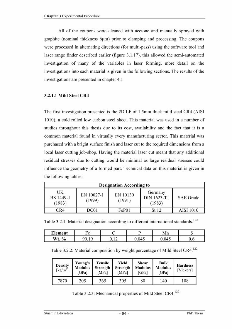
Chapter 3 Experimental Procedure
Stuart P. Edwardson PhD Thesis - 84 -
All of the coupons were cleaned with acetone and manually sprayed with
graphite (nominal thickness 6µm) prior to clamping and processing. The coupons
were processed in alternating directions (for multi-pass) using the software tool and
laser range finder described earlier (figure 3.1.17), this allowed the semi-automated
investigation of many of the variables in laser forming, more detail on the
investigations into each material is given in the following sections. The results of the
investigations are presented in chapter 4.1
3.2.1.1 Mild Steel CR4
The first investigation presented is the 2D LF of 1.5mm thick mild steel CR4 (AISI
1010), a cold rolled low carbon steel sheet. This material was used in a number of
studies throughout this thesis due to its cost, availability and the fact that it is a
common material found in virtually every manufacturing sector. This material was
purchased with a bright surface finish and laser cut to the required dimensions from a
local laser cutting job-shop. Having the material laser cut meant that any additional
residual stresses due to cutting would be minimal as large residual stresses could
influence the geometry of a formed part. Technical data on this material is given in
the following tables:
Designation According to UK
BS 1449-1 (1983)
EN 10027-1 (1999)
EN 10130 (1991)
Germany DIN 1623-T1
(1983) SAE Grade
CR4 DC01 FeP01 St 12 AISI 1010 Table 3.2.1: Material designation according to different international standards.122
Element Fe C P Mn S Wt. % 99.19 0.12 0.045 0.045 0.6
Table 3.2.2: Material composition by weight percentage of Mild Steel CR4.122
Density [kg/m3]
Young’s Modulus
[GPa]
Tensile Strength
[MPa]
Yield Strength
[MPa]
Shear Modulus
[GPa]
Bulk Modulus
[GPa]
Hardness [Vickers]
7870 205 365 305 80 140 108
Table 3.2.3: Mechanical properties of Mild Steel CR4.122
Chapter 3 Experimental Procedure
Stuart P. Edwardson PhD Thesis - 85 -
Melting Point [°C] 1515 Thermal Conductivity [W/m K] 49.8
Coefficient of Thermal Expansion [10-6/K] 20°C 12.2
Coefficient of Thermal Expansion [10-6/K] 250°C 13.5
Coefficient of Thermal Expansion [10-6/K] 500°C 14.2
Specific Heat Capacity [J/kg K] 50-100°C 448
Specific Heat Capacity [J/kg K] 250-300°C 536
Specific Heat Capacity [J/kg K] 400-450°C 649
Specific Heat Capacity [J/kg K] 650-700°C 825
Table 3.2.4: Thermal Properties of Mild Steel CR4.122
The first investigation performed on this material was to determine a process
map or window such that for a given incident power, laser beam spot size and
traverse speed an expected bend angle for a single pass could be known. Due to the
large amount of variable combinations from just these three, it was decided to
investigate only three beam diameters, 3mm, 5.5mm and 8mm, three power levels
per beam diameter (from 500W to 1200W at the surface) and a traverse speed range
of 10mm/s to 90mm/s (comfortable speed range for the X,Y CNC tables). It was
found from initial trails that this range of processing parameters did produce some
forming with no obvious surface damage (smaller beam diameters did however), for
this thickness, type of material and laser beam mode even the larger beam diameters
produced positive bending such that a significant thermal gradient must still be
present (hence TGM). It can be noted that a more complete range of traverse speed
data was collected, this is due to the fact that it was easier to control the traverse
speed via the Galil controller than the other variables. This is significant when
considering closed loop control of the LF process and will be discussed in a later
section.
Once a process map had been determined for each of the beam diameters
investigated, three ideal processing parameter combinations were selected (one for
each beam diameter) for a study into multiple pass LF (over the same irradiation
track; alternating direction). The bend angle and bend angle rate per pass were
analysed up to 30 passes. A further study was conducted into the effect of the time
Chapter 3 Experimental Procedure
Stuart P. Edwardson PhD Thesis - 86 -
delay in between each pass on the bend angle achieved. It was not known as to
whether the heat remaining in the sheet after each pass aided subsequent passes by
reducing the yield stress of the material or if the increase in bulk material
temperature reduced the available thermal gradient on the next pass.
3.2.1.2 Ti6Al4V
An investigation was conducted into the 2D LF of Ti-6Al-4V (Ti64) mill annealed
sheet, an aerospace alloy of titanium. Sheet thicknesses of 0.9mm, 1.4mm, 1.6mm,
2mm and 3.2mm were used. Ti64 is widely used in the aerospace sector due to its
high strength yet low density, excellent resistance to fatigue and crack propagation
and outstanding resistance to corrosion. It is the most widely used titanium alloy.
The atomic structure of titanium undergoes a transformation from a close
packed hexagonal arrangement (alpha or α phase) to a body centred cubic
arrangement (beta or β phase) at 882°C. This transformation can be considerably
modified by the addition of alloying elements to produce alloys that have all α, all β
or α + β structures. Ti64 is an alpha + beta alloy containing 6% aluminium and 4%
vanadium. The aluminium stabilises and strengthens the alpha phase, so raising the
beta-transus temperature (~980°C), as well as reducing the density of the alloy. The
vanadium is a beta stabiliser, and provides a greater amount of the more ductile beta
phase during hot working. On solution treatment high in the alpha + beta field,
followed by rapid cooling to room temperature, the beta phase transforms to a
structure which can be subsequently tempered to a fine dispersion of beta in an alpha
matrix, with consequent strengthening of the alloy. Temperatures up to 700°C are
commonly used in warm-working or forming this alloy conventionally.
This material, supplied by the industrial partners in the larger work
programme which this work formed part of (discussed earlier), was guillotined to the
desired size. Ideally a cutting method that induced less residual stresses would have
been preferred such as laser cutting or EDM, however these were not available or not
possible without additional equipment and expertise. It was felt that this material
would likely be guillotined in a manufacturing environment anyway and that LF
should be studied on the as received material and material conditions. Another factor
in this was the cost and availability of the material, in that there was no room for
error. Titanium, despite being the fourth most abundant structural metals in the
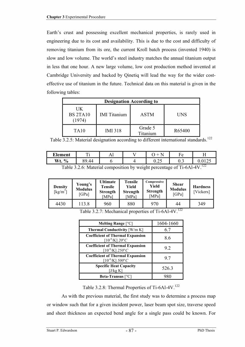
Chapter 3 Experimental Procedure
Stuart P. Edwardson PhD Thesis - 87 -
Earth’s crust and possessing excellent mechanical properties, is rarely used in
engineering due to its cost and availability. This is due to the cost and difficulty of
removing titanium from its ore, the current Kroll batch process (invented 1940) is
slow and low volume. The world’s steel industry matches the annual titanium output
in less that one hour. A new large volume, low cost production method invented at
Cambridge University and backed by Qinetiq will lead the way for the wider cost-
effective use of titanium in the future. Technical data on this material is given in the
following tables:
Designation According to UK
BS 2TA10 (1974)
IMI Titanium ASTM UNS
TA10 IMI 318 Grade 5 Titanium R65400
Table 3.2.5: Material designation according to different international standards.122
Element Ti Al V O + N Fe H Wt. % 89.44 6 4 0.25 0.3 0.0125
Table 3.2.6: Material composition by weight percentage of Ti-6Al-4V.122
Density [kg/m3]
Young’s Modulus
[GPa]
Ultimate Tensile
Strength [MPa]
Tensile Yield
Strength [MPa]
Compressive Yield
Strength [MPa]
Shear Modulus
[GPa]
Hardness [Vickers]
4430 113.8 960 880 970 44 349 Table 3.2.7: Mechanical properties of Ti-6Al-4V.122
Melting Range [°C] 1604-1660 Thermal Conductivity [W/m K] 6.7
Coefficient of Thermal Expansion [10-6/K] 20°C 8.6
Coefficient of Thermal Expansion [10-6/K] 250°C 9.2
Coefficient of Thermal Expansion [10-6/K] 500°C 9.7
Specific Heat Capacity [J/kg K] 526.3
Beta-Transus [°C] 980
Table 3.2.8: Thermal Properties of Ti-6Al-4V.122
As with the previous material, the first study was to determine a process map
or window such that for a given incident power, laser beam spot size, traverse speed
and sheet thickness an expected bend angle for a single pass could be known. For
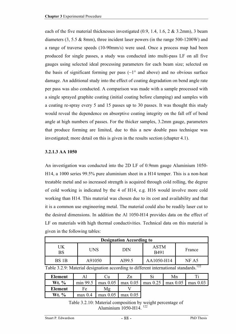
Chapter 3 Experimental Procedure
Stuart P. Edwardson PhD Thesis - 88 -
each of the five material thicknesses investigated (0.9, 1.4, 1.6, 2 & 3.2mm), 3 beam
diameters (3, 5.5 & 8mm), three incident laser powers (in the range 500-1200W) and
a range of traverse speeds (10-90mm/s) were used. Once a process map had been
produced for single passes, a study was conducted into multi-pass LF on all five
gauges using selected ideal processing parameters for each beam size; selected on
the basis of significant forming per pass (~1° and above) and no obvious surface
damage. An additional study into the effect of coating degradation on bend angle rate
per pass was also conducted. A comparison was made with a sample processed with
a single sprayed graphite coating (initial coating before clamping) and samples with
a coating re-spray every 5 and 15 passes up to 30 passes. It was thought this study
would reveal the dependence on absorptive coating integrity on the fall off of bend
angle at high numbers of passes. For the thicker samples, 3.2mm gauge, parameters
that produce forming are limited, due to this a new double pass technique was
investigated; more detail on this is given in the results section (chapter 4.1).
3.2.1.3 AA 1050
An investigation was conducted into the 2D LF of 0.9mm gauge Aluminium 1050-
H14, a 1000 series 99.5% pure aluminium sheet in a H14 temper. This is a non-heat
treatable metal and so increased strength is acquired through cold rolling, the degree
of cold working is indicated by the 4 of H14, e.g. H16 would involve more cold
working than H14. This material was chosen due to its cost and availability and that
it is a common use engineering metal. The material could also be readily laser cut to
the desired dimensions. In addition the Al 1050-H14 provides data on the effect of
LF on materials with high thermal conductivities. Technical data on this material is
given in the following tables:
Designation According to UK BS UNS DIN ASTM
B491 France
BS 1B A91050 Al99.5 AA1050-H14 NF A5 Table 3.2.9: Material designation according to different international standards.122
Element Al Cu Zn Si Mn Ti Wt. % min 99.5 max 0.05 max 0.05 max 0.25 max 0.05 max 0.03
Element Fe Mg V Wt. % max 0.4 max 0.05 max 0.05
Table 3.2.10: Material composition by weight percentage of
Aluminium 1050-H14. 122
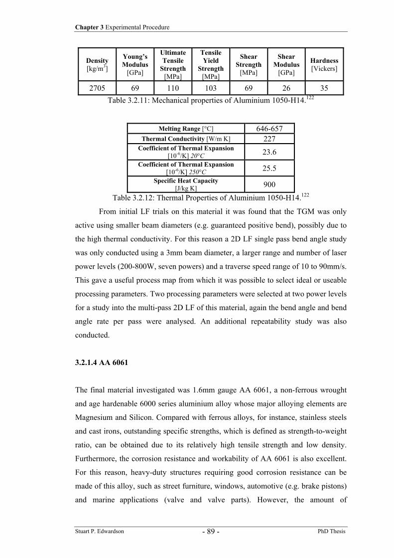
Chapter 3 Experimental Procedure
Stuart P. Edwardson PhD Thesis - 89 -
Density [kg/m3]
Young’s Modulus
[GPa]
Ultimate Tensile
Strength [MPa]
Tensile Yield
Strength [MPa]
Shear Strength
[MPa]
Shear Modulus
[GPa]
Hardness [Vickers]
2705 69 110 103 69 26 35 Table 3.2.11: Mechanical properties of Aluminium 1050-H14.122
Melting Range [°C] 646-657 Thermal Conductivity [W/m K] 227
Coefficient of Thermal Expansion [10-6/K] 20°C 23.6
Coefficient of Thermal Expansion [10-6/K] 250°C 25.5
Specific Heat Capacity [J/kg K] 900
Table 3.2.12: Thermal Properties of Aluminium 1050-H14.122
From initial LF trials on this material it was found that the TGM was only
active using smaller beam diameters (e.g. guaranteed positive bend), possibly due to
the high thermal conductivity. For this reason a 2D LF single pass bend angle study
was only conducted using a 3mm beam diameter, a larger range and number of laser
power levels (200-800W, seven powers) and a traverse speed range of 10 to 90mm/s.
This gave a useful process map from which it was possible to select ideal or useable
processing parameters. Two processing parameters were selected at two power levels
for a study into the multi-pass 2D LF of this material, again the bend angle and bend
angle rate per pass were analysed. An additional repeatability study was also
conducted.
3.2.1.4 AA 6061
The final material investigated was 1.6mm gauge AA 6061, a non-ferrous wrought
and age hardenable 6000 series aluminium alloy whose major alloying elements are
Magnesium and Silicon. Compared with ferrous alloys, for instance, stainless steels
and cast irons, outstanding specific strengths, which is defined as strength-to-weight
ratio, can be obtained due to its relatively high tensile strength and low density.
Furthermore, the corrosion resistance and workability of AA 6061 is also excellent.
For this reason, heavy-duty structures requiring good corrosion resistance can be
made of this alloy, such as street furniture, windows, automotive (e.g. brake pistons)
and marine applications (valve and valve parts). However, the amount of
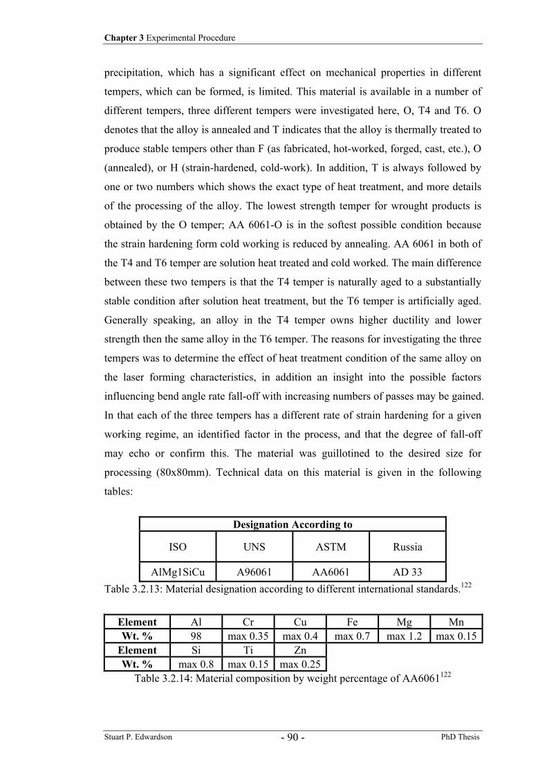
Chapter 3 Experimental Procedure
Stuart P. Edwardson PhD Thesis - 90 -
precipitation, which has a significant effect on mechanical properties in different
tempers, which can be formed, is limited. This material is available in a number of
different tempers, three different tempers were investigated here, O, T4 and T6. O
denotes that the alloy is annealed and T indicates that the alloy is thermally treated to
produce stable tempers other than F (as fabricated, hot-worked, forged, cast, etc.), O
(annealed), or H (strain-hardened, cold-work). In addition, T is always followed by
one or two numbers which shows the exact type of heat treatment, and more details
of the processing of the alloy. The lowest strength temper for wrought products is
obtained by the O temper; AA 6061-O is in the softest possible condition because
the strain hardening form cold working is reduced by annealing. AA 6061 in both of
the T4 and T6 temper are solution heat treated and cold worked. The main difference
between these two tempers is that the T4 temper is naturally aged to a substantially
stable condition after solution heat treatment, but the T6 temper is artificially aged.
Generally speaking, an alloy in the T4 temper owns higher ductility and lower
strength then the same alloy in the T6 temper. The reasons for investigating the three
tempers was to determine the effect of heat treatment condition of the same alloy on
the laser forming characteristics, in addition an insight into the possible factors
influencing bend angle rate fall-off with increasing numbers of passes may be gained.
In that each of the three tempers has a different rate of strain hardening for a given
working regime, an identified factor in the process, and that the degree of fall-off
may echo or confirm this. The material was guillotined to the desired size for
processing (80x80mm). Technical data on this material is given in the following
tables:
Designation According to
ISO UNS ASTM Russia
AlMg1SiCu A96061 AA6061 AD 33 Table 3.2.13: Material designation according to different international standards.122
Element Al Cr Cu Fe Mg Mn Wt. % 98 max 0.35 max 0.4 max 0.7 max 1.2 max 0.15
Element Si Ti Zn Wt. % max 0.8 max 0.15 max 0.25
Table 3.2.14: Material composition by weight percentage of AA6061122
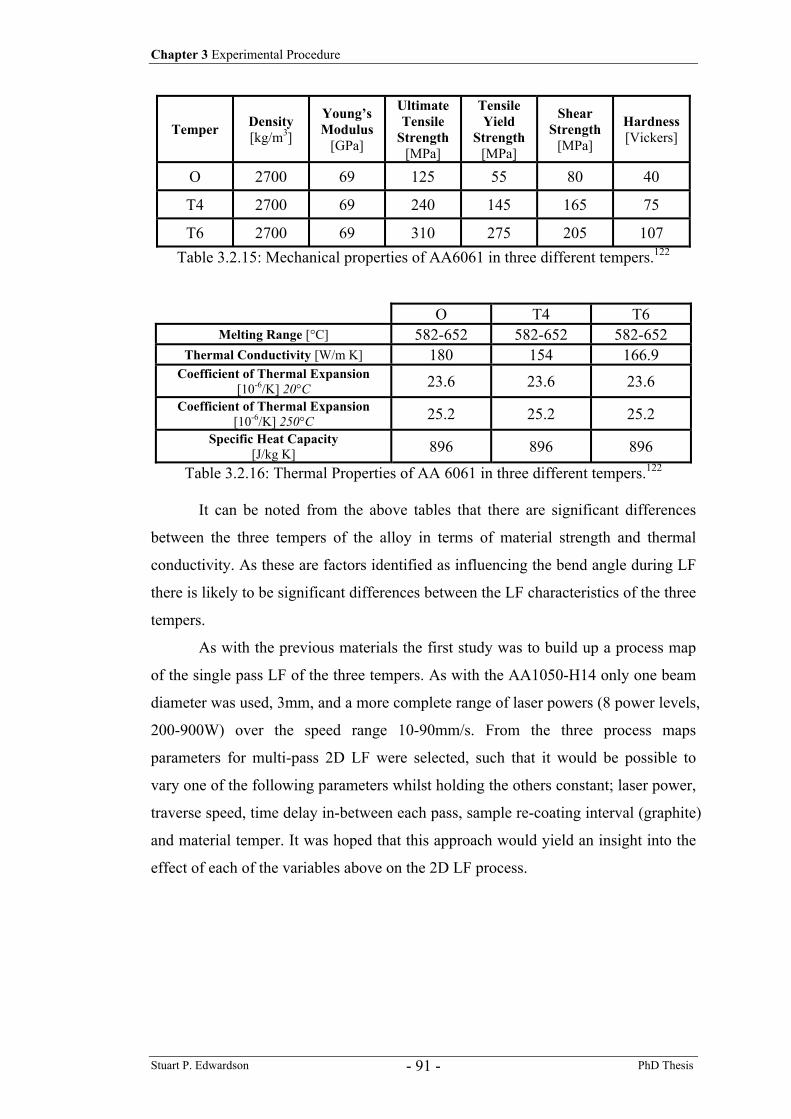
Chapter 3 Experimental Procedure
Stuart P. Edwardson PhD Thesis - 91 -
Temper Density [kg/m3]
Young’s Modulus
[GPa]
Ultimate Tensile
Strength [MPa]
Tensile Yield
Strength [MPa]
Shear Strength
[MPa]
Hardness [Vickers]
O 2700 69 125 55 80 40
T4 2700 69 240 145 165 75
T6 2700 69 310 275 205 107 Table 3.2.15: Mechanical properties of AA6061 in three different tempers.122
O T4 T6 Melting Range [°C] 582-652 582-652 582-652
Thermal Conductivity [W/m K] 180 154 166.9 Coefficient of Thermal Expansion
[10-6/K] 20°C 23.6 23.6 23.6 Coefficient of Thermal Expansion
[10-6/K] 250°C 25.2 25.2 25.2 Specific Heat Capacity
[J/kg K] 896 896 896
Table 3.2.16: Thermal Properties of AA 6061 in three different tempers.122
It can be noted from the above tables that there are significant differences
between the three tempers of the alloy in terms of material strength and thermal
conductivity. As these are factors identified as influencing the bend angle during LF
there is likely to be significant differences between the LF characteristics of the three
tempers.
As with the previous materials the first study was to build up a process map
of the single pass LF of the three tempers. As with the AA1050-H14 only one beam
diameter was used, 3mm, and a more complete range of laser powers (8 power levels,
200-900W) over the speed range 10-90mm/s. From the three process maps
parameters for multi-pass 2D LF were selected, such that it would be possible to
vary one of the following parameters whilst holding the others constant; laser power,
traverse speed, time delay in-between each pass, sample re-coating interval (graphite)
and material temper. It was hoped that this approach would yield an insight into the
effect of each of the variables above on the 2D LF process.
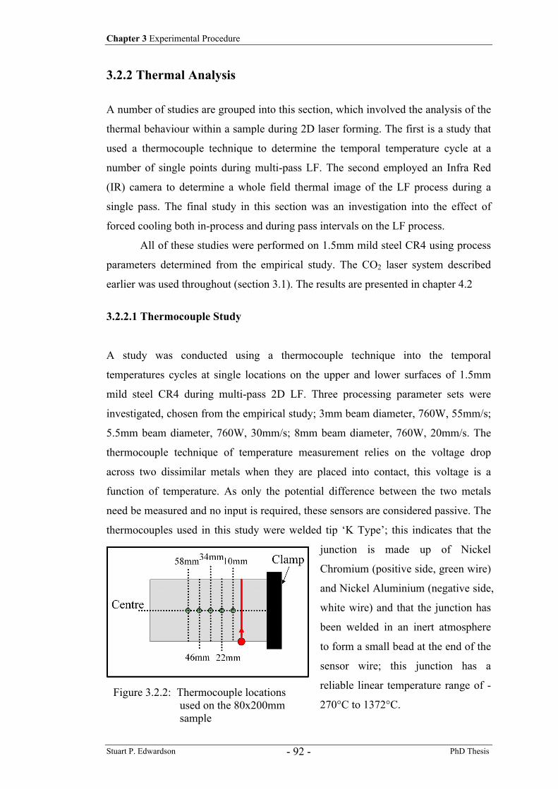
Chapter 3 Experimental Procedure
Stuart P. Edwardson PhD Thesis - 92 -
3.2.2 Thermal Analysis A number of studies are grouped into this section, which involved the analysis of the
thermal behaviour within a sample during 2D laser forming. The first is a study that
used a thermocouple technique to determine the temporal temperature cycle at a
number of single points during multi-pass LF. The second employed an Infra Red
(IR) camera to determine a whole field thermal image of the LF process during a
single pass. The final study in this section was an investigation into the effect of
forced cooling both in-process and during pass intervals on the LF process.
All of these studies were performed on 1.5mm mild steel CR4 using process
parameters determined from the empirical study. The CO2 laser system described
earlier was used throughout (section 3.1). The results are presented in chapter 4.2
3.2.2.1 Thermocouple Study
A study was conducted using a thermocouple technique into the temporal
temperatures cycles at single locations on the upper and lower surfaces of 1.5mm
mild steel CR4 during multi-pass 2D LF. Three processing parameter sets were
investigated, chosen from the empirical study; 3mm beam diameter, 760W, 55mm/s;
5.5mm beam diameter, 760W, 30mm/s; 8mm beam diameter, 760W, 20mm/s. The
thermocouple technique of temperature measurement relies on the voltage drop
across two dissimilar metals when they are placed into contact, this voltage is a
function of temperature. As only the potential difference between the two metals
need be measured and no input is required, these sensors are considered passive. The
thermocouples used in this study were welded tip ‘K Type’; this indicates that the
junction is made up of Nickel
Chromium (positive side, green wire)
and Nickel Aluminium (negative side,
white wire) and that the junction has
been welded in an inert atmosphere
to form a small bead at the end of the
sensor wire; this junction has a
reliable linear temperature range of -
270°C to 1372°C. Figure 3.2.2: Thermocouple locations
used on the 80x200mm sample
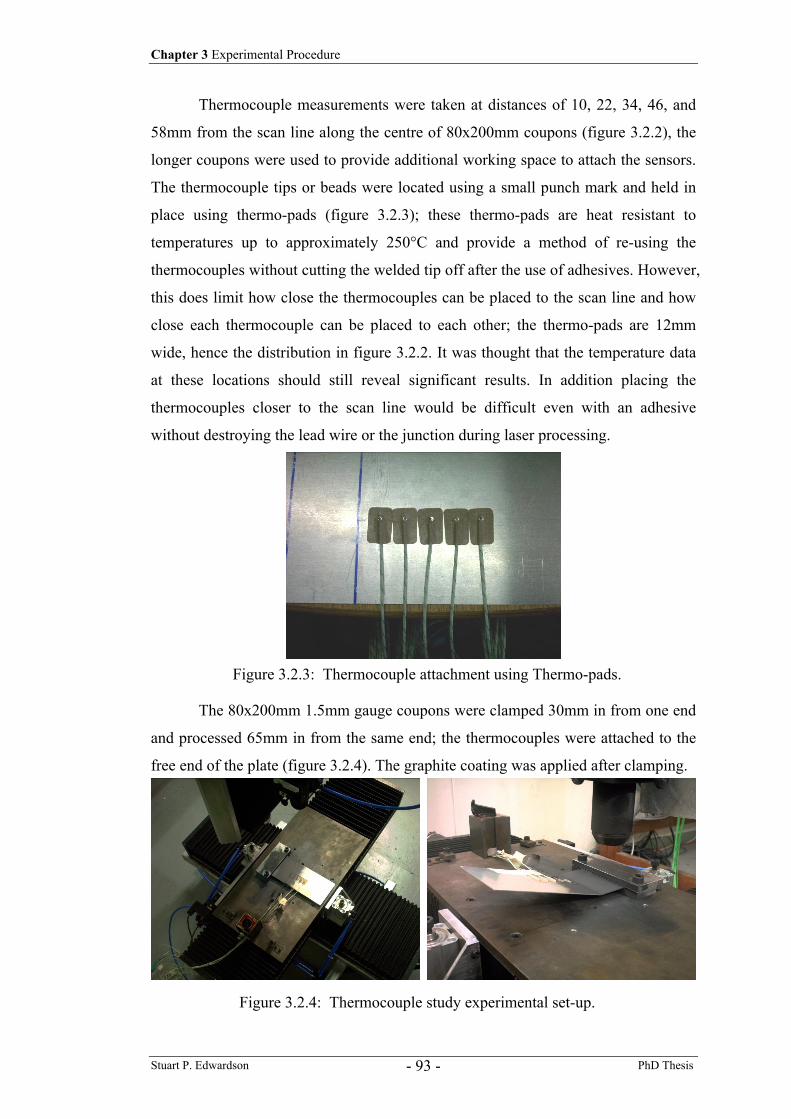
Chapter 3 Experimental Procedure
Stuart P. Edwardson PhD Thesis - 93 -
Thermocouple measurements were taken at distances of 10, 22, 34, 46, and
58mm from the scan line along the centre of 80x200mm coupons (figure 3.2.2), the
longer coupons were used to provide additional working space to attach the sensors.
The thermocouple tips or beads were located using a small punch mark and held in
place using thermo-pads (figure 3.2.3); these thermo-pads are heat resistant to
temperatures up to approximately 250°C and provide a method of re-using the
thermocouples without cutting the welded tip off after the use of adhesives. However,
this does limit how close the thermocouples can be placed to the scan line and how
close each thermocouple can be placed to each other; the thermo-pads are 12mm
wide, hence the distribution in figure 3.2.2. It was thought that the temperature data
at these locations should still reveal significant results. In addition placing the
thermocouples closer to the scan line would be difficult even with an adhesive
without destroying the lead wire or the junction during laser processing.
The 80x200mm 1.5mm gauge coupons were clamped 30mm in from one end
and processed 65mm in from the same end; the thermocouples were attached to the
free end of the plate (figure 3.2.4). The graphite coating was applied after clamping.
Figure 3.2.3: Thermocouple attachment using Thermo-pads.
Figure 3.2.4: Thermocouple study experimental set-up.
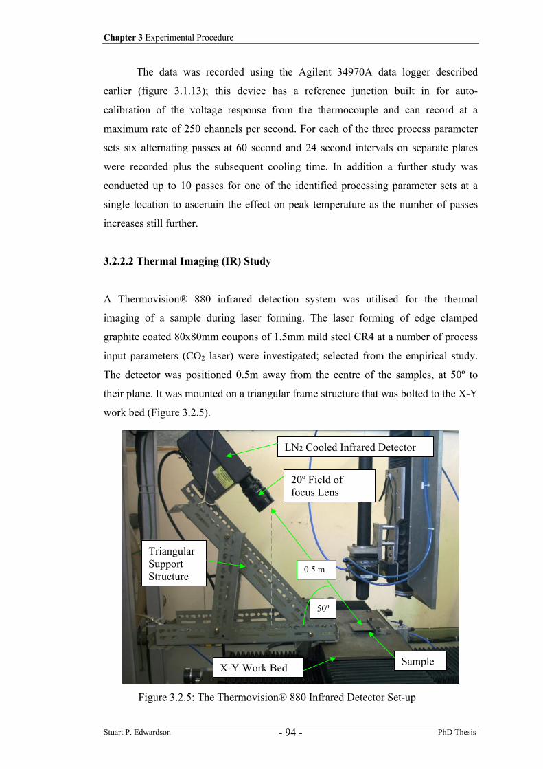
Chapter 3 Experimental Procedure
Stuart P. Edwardson PhD Thesis - 94 -
The data was recorded using the Agilent 34970A data logger described
earlier (figure 3.1.13); this device has a reference junction built in for auto-
calibration of the voltage response from the thermocouple and can record at a
maximum rate of 250 channels per second. For each of the three process parameter
sets six alternating passes at 60 second and 24 second intervals on separate plates
were recorded plus the subsequent cooling time. In addition a further study was
conducted up to 10 passes for one of the identified processing parameter sets at a
single location to ascertain the effect on peak temperature as the number of passes
increases still further.
3.2.2.2 Thermal Imaging (IR) Study
A Thermovision® 880 infrared detection system was utilised for the thermal
imaging of a sample during laser forming. The laser forming of edge clamped
graphite coated 80x80mm coupons of 1.5mm mild steel CR4 at a number of process
input parameters (CO2 laser) were investigated; selected from the empirical study.
The detector was positioned 0.5m away from the centre of the samples, at 50º to
their plane. It was mounted on a triangular frame structure that was bolted to the X-Y
work bed (Figure 3.2.5).
50º
0.5 m
LN2 Cooled Infrared Detector
Sample
Triangular Support Structure
X-Y Work Bed
20º Field of focus Lens
Figure 3.2.5: The Thermovision® 880 Infrared Detector Set-up
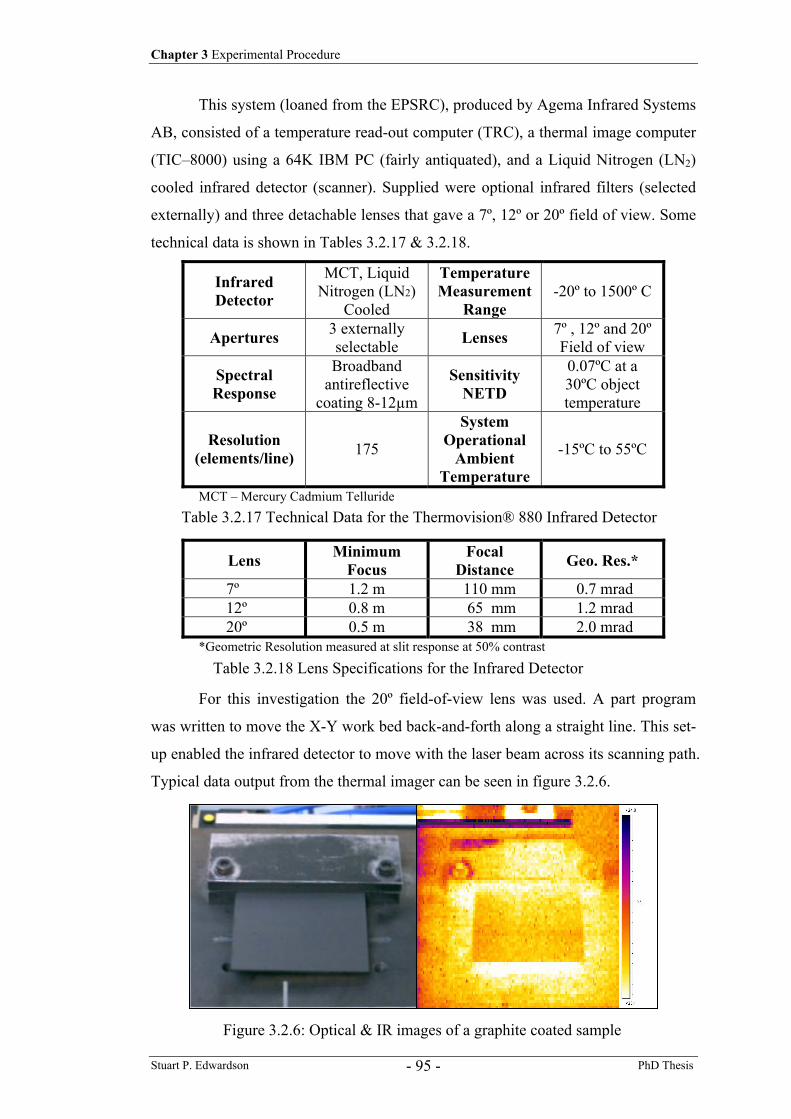
Chapter 3 Experimental Procedure
Stuart P. Edwardson PhD Thesis - 95 -
This system (loaned from the EPSRC), produced by Agema Infrared Systems
AB, consisted of a temperature read-out computer (TRC), a thermal image computer
(TIC–8000) using a 64K IBM PC (fairly antiquated), and a Liquid Nitrogen (LN2)
cooled infrared detector (scanner). Supplied were optional infrared filters (selected
externally) and three detachable lenses that gave a 7º, 12º or 20º field of view. Some
technical data is shown in Tables 3.2.17 & 3.2.18.
Infrared Detector
MCT, Liquid Nitrogen (LN2)
Cooled
Temperature Measurement
Range -20º to 1500º C
Apertures 3 externally selectable Lenses 7º , 12º and 20º
Field of view
Spectral Response
Broadband antireflective
coating 8-12µm
Sensitivity NETD
0.07ºC at a 30ºC object temperature
Resolution (elements/line) 175
System Operational
Ambient Temperature
-15ºC to 55ºC
MCT – Mercury Cadmium Telluride
Lens Minimum Focus
Focal Distance Geo. Res.*
7º 1.2 m 110 mm 0.7 mrad 12º 0.8 m 65 mm 1.2 mrad 20º 0.5 m 38 mm 2.0 mrad
*Geometric Resolution measured at slit response at 50% contrast
For this investigation the 20º field-of-view lens was used. A part program
was written to move the X-Y work bed back-and-forth along a straight line. This set-
up enabled the infrared detector to move with the laser beam across its scanning path.
Typical data output from the thermal imager can be seen in figure 3.2.6.
Table 3.2.17 Technical Data for the Thermovision® 880 Infrared Detector
Table 3.2.18 Lens Specifications for the Infrared Detector
Figure 3.2.6: Optical & IR images of a graphite coated sample
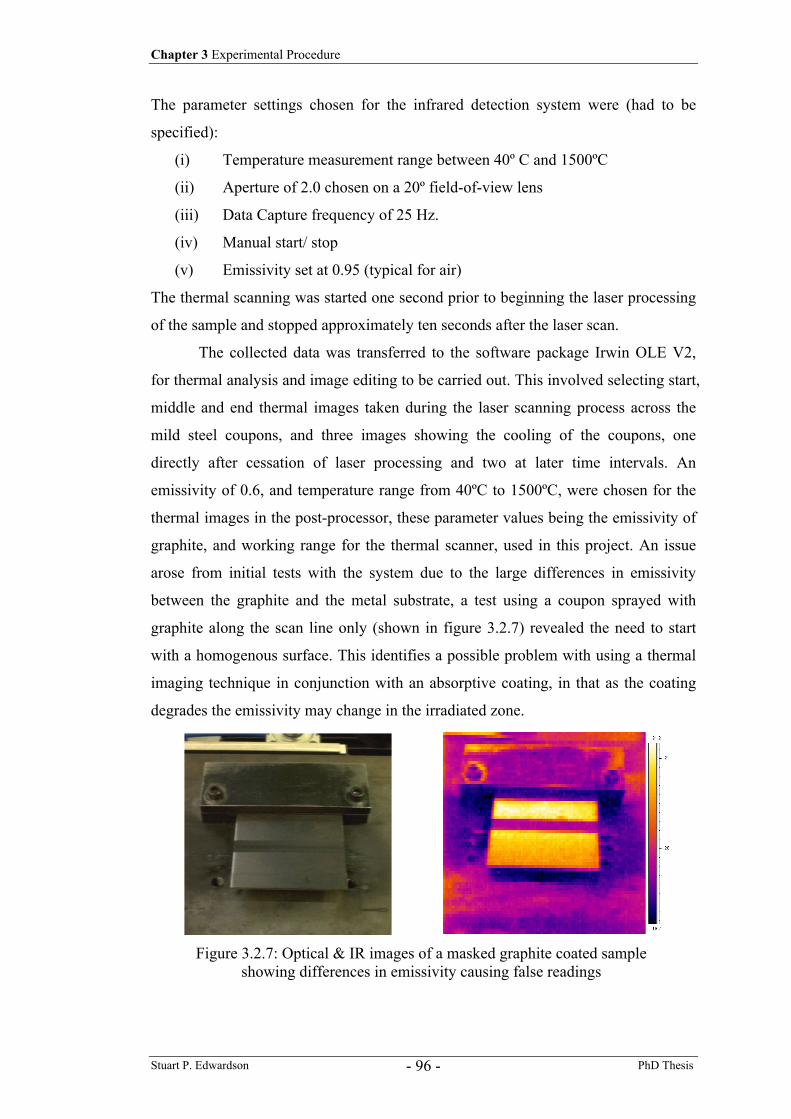
Chapter 3 Experimental Procedure
Stuart P. Edwardson PhD Thesis - 96 -
The parameter settings chosen for the infrared detection system were (had to be
specified):
(i) Temperature measurement range between 40º C and 1500ºC
(ii) Aperture of 2.0 chosen on a 20º field-of-view lens
(iii) Data Capture frequency of 25 Hz.
(iv) Manual start/ stop
(v) Emissivity set at 0.95 (typical for air)
The thermal scanning was started one second prior to beginning the laser processing
of the sample and stopped approximately ten seconds after the laser scan.
The collected data was transferred to the software package Irwin OLE V2,
for thermal analysis and image editing to be carried out. This involved selecting start,
middle and end thermal images taken during the laser scanning process across the
mild steel coupons, and three images showing the cooling of the coupons, one
directly after cessation of laser processing and two at later time intervals. An
emissivity of 0.6, and temperature range from 40ºC to 1500ºC, were chosen for the
thermal images in the post-processor, these parameter values being the emissivity of
graphite, and working range for the thermal scanner, used in this project. An issue
arose from initial tests with the system due to the large differences in emissivity
between the graphite and the metal substrate, a test using a coupon sprayed with
graphite along the scan line only (shown in figure 3.2.7) revealed the need to start
with a homogenous surface. This identifies a possible problem with using a thermal
imaging technique in conjunction with an absorptive coating, in that as the coating
degrades the emissivity may change in the irradiated zone.
Figure 3.2.7: Optical & IR images of a masked graphite coated sample showing differences in emissivity causing false readings
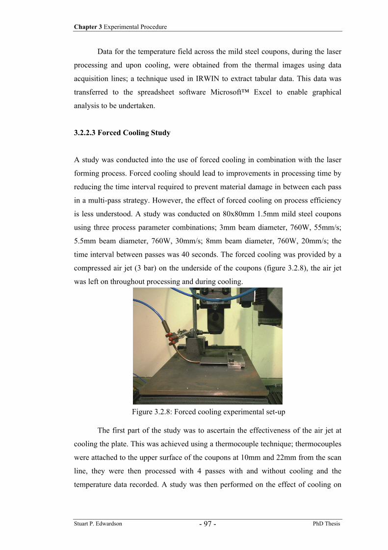
Chapter 3 Experimental Procedure
Stuart P. Edwardson PhD Thesis - 97 -
Data for the temperature field across the mild steel coupons, during the laser
processing and upon cooling, were obtained from the thermal images using data
acquisition lines; a technique used in IRWIN to extract tabular data. This data was
transferred to the spreadsheet software Microsoft™ Excel to enable graphical
analysis to be undertaken.
3.2.2.3 Forced Cooling Study
A study was conducted into the use of forced cooling in combination with the laser
forming process. Forced cooling should lead to improvements in processing time by
reducing the time interval required to prevent material damage in between each pass
in a multi-pass strategy. However, the effect of forced cooling on process efficiency
is less understood. A study was conducted on 80x80mm 1.5mm mild steel coupons
using three process parameter combinations; 3mm beam diameter, 760W, 55mm/s;
5.5mm beam diameter, 760W, 30mm/s; 8mm beam diameter, 760W, 20mm/s; the
time interval between passes was 40 seconds. The forced cooling was provided by a
compressed air jet (3 bar) on the underside of the coupons (figure 3.2.8), the air jet
was left on throughout processing and during cooling.
The first part of the study was to ascertain the effectiveness of the air jet at
cooling the plate. This was achieved using a thermocouple technique; thermocouples
were attached to the upper surface of the coupons at 10mm and 22mm from the scan
line, they were then processed with 4 passes with and without cooling and the
temperature data recorded. A study was then performed on the effect of cooling on
Figure 3.2.8: Forced cooling experimental set-up
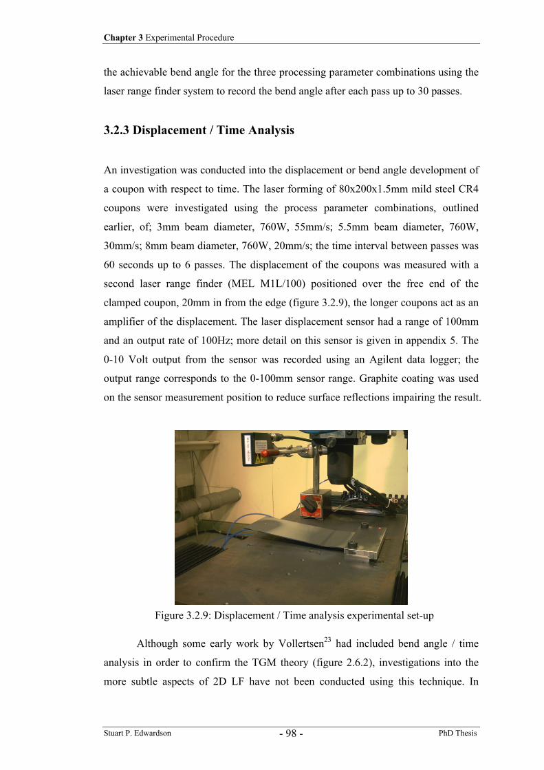
Chapter 3 Experimental Procedure
Stuart P. Edwardson PhD Thesis - 98 -
the achievable bend angle for the three processing parameter combinations using the
laser range finder system to record the bend angle after each pass up to 30 passes.
3.2.3 Displacement / Time Analysis
An investigation was conducted into the displacement or bend angle development of
a coupon with respect to time. The laser forming of 80x200x1.5mm mild steel CR4
coupons were investigated using the process parameter combinations, outlined
earlier, of; 3mm beam diameter, 760W, 55mm/s; 5.5mm beam diameter, 760W,
30mm/s; 8mm beam diameter, 760W, 20mm/s; the time interval between passes was
60 seconds up to 6 passes. The displacement of the coupons was measured with a
second laser range finder (MEL M1L/100) positioned over the free end of the
clamped coupon, 20mm in from the edge (figure 3.2.9), the longer coupons act as an
amplifier of the displacement. The laser displacement sensor had a range of 100mm
and an output rate of 100Hz; more detail on this sensor is given in appendix 5. The
0-10 Volt output from the sensor was recorded using an Agilent data logger; the
output range corresponds to the 0-100mm sensor range. Graphite coating was used
on the sensor measurement position to reduce surface reflections impairing the result.
Although some early work by Vollertsen23 had included bend angle / time
analysis in order to confirm the TGM theory (figure 2.6.2), investigations into the
more subtle aspects of 2D LF have not been conducted using this technique. In
Figure 3.2.9: Displacement / Time analysis experimental set-up
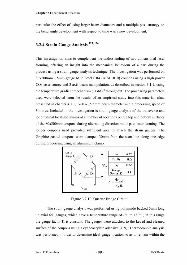
Chapter 3 Experimental Procedure
Stuart P. Edwardson PhD Thesis - 99 -
particular the effect of using larger beam diameters and a multiple pass strategy on
the bend angle development with respect to time was a new development.
3.2.4 Strain Gauge Analysis 123, 124
This investigation aims to complement the understanding of two-dimensional laser
forming, offering an insight into the mechanical behaviour of a part during the
process using a strain gauge analysis technique. The investigation was performed on
80x200mm 1.5mm gauge Mild Steel CR4 (AISI 1010) coupons using a high power
CO2 laser source and 3 axis beam manipulation, as described in section 3.1.1, using
the temperature gradient mechanism (TGM)11 throughout. The processing parameters
used were selected from the results of an empirical study into this material, (data
presented in chapter 4.1.1); 760W, 5.5mm beam diameter and a processing speed of
30mm/s. Included in the investigation is strain gauge analysis of the transverse and
longitudinal localised strains at a number of locations on the top and bottom surfaces
of the 80x200mm coupons during alternating direction multi-pass laser forming. The
longer coupons used provided sufficient area to attach the strain gauges. The
Graphite coated coupons were clamped 30mm from the scan line along one edge
during processing using an aluminium clamp.
The strain gauge analysis was performed using polyimide backed 5mm long
uniaxial foil gauges, which have a temperature range of -30 to 180ºC, in this range
the gauge factor K is constant. The gauges were attached to the keyed and cleaned
surface of the coupons using a cyanoacrylate adhesive (CN). Thermocouple analysis
was performed in order to determine ideal gauge location so as to remain within the
Figure 3.2.10: Quarter Bridge Circuit
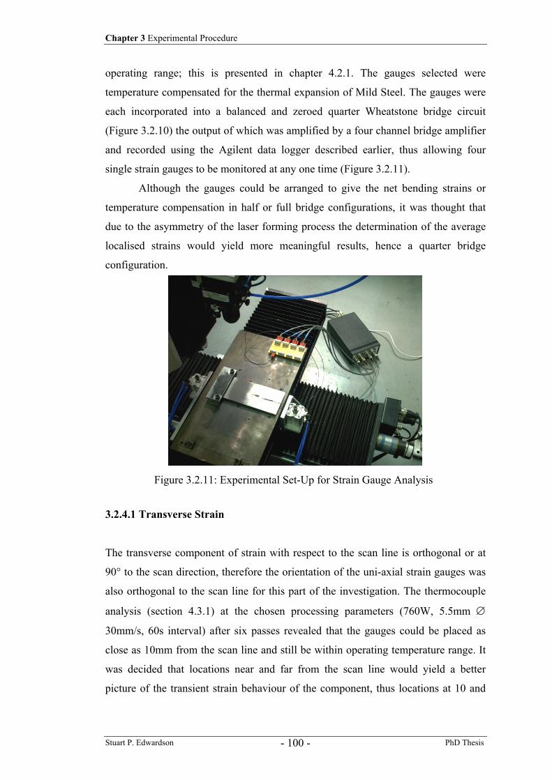
Chapter 3 Experimental Procedure
Stuart P. Edwardson PhD Thesis - 100 -
operating range; this is presented in chapter 4.2.1. The gauges selected were
temperature compensated for the thermal expansion of Mild Steel. The gauges were
each incorporated into a balanced and zeroed quarter Wheatstone bridge circuit
(Figure 3.2.10) the output of which was amplified by a four channel bridge amplifier
and recorded using the Agilent data logger described earlier, thus allowing four
single strain gauges to be monitored at any one time (Figure 3.2.11).
Although the gauges could be arranged to give the net bending strains or
temperature compensation in half or full bridge configurations, it was thought that
due to the asymmetry of the laser forming process the determination of the average
localised strains would yield more meaningful results, hence a quarter bridge
configuration.
3.2.4.1 Transverse Strain
The transverse component of strain with respect to the scan line is orthogonal or at
90° to the scan direction, therefore the orientation of the uni-axial strain gauges was
also orthogonal to the scan line for this part of the investigation. The thermocouple
analysis (section 4.3.1) at the chosen processing parameters (760W, 5.5mm ∅
30mm/s, 60s interval) after six passes revealed that the gauges could be placed as
close as 10mm from the scan line and still be within operating temperature range. It
was decided that locations near and far from the scan line would yield a better
picture of the transient strain behaviour of the component, thus locations at 10 and
Figure 3.2.11: Experimental Set-Up for Strain Gauge Analysis

Chapter 3 Experimental Procedure
Stuart P. Edwardson PhD Thesis - 101 -
46mm from the scan line, close to the centreline and 10mm from the edges of the
upper and lower surfaces, were used. This can be seen in figure 3.2.12.
As the output from only four gauges could be logged at any one time, a
separate coupon was used for each configuration. An assumption was made that the
process conditions were identical for each sample as each coupon was laser cut from
the same mild steel sheet. A prepared sample with four gauges attached can be seen
in figure 3.2.13.
Figure 3.2.12: Schematic Showing Strain Gauge Locations for the Transverse Strain Study
Figure 3.2.13: Strain Gauges Attached to a Coupon
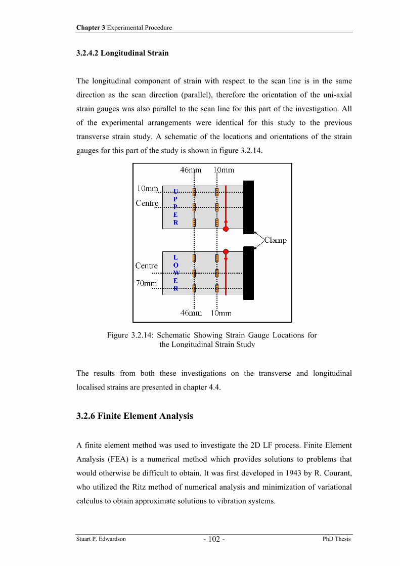
Chapter 3 Experimental Procedure
Stuart P. Edwardson PhD Thesis - 102 -
3.2.4.2 Longitudinal Strain
The longitudinal component of strain with respect to the scan line is in the same
direction as the scan direction (parallel), therefore the orientation of the uni-axial
strain gauges was also parallel to the scan line for this part of the investigation. All
of the experimental arrangements were identical for this study to the previous
transverse strain study. A schematic of the locations and orientations of the strain
gauges for this part of the study is shown in figure 3.2.14.
The results from both these investigations on the transverse and longitudinal
localised strains are presented in chapter 4.4.
3.2.6 Finite Element Analysis
A finite element method was used to investigate the 2D LF process. Finite Element
Analysis (FEA) is a numerical method which provides solutions to problems that
would otherwise be difficult to obtain. It was first developed in 1943 by R. Courant,
who utilized the Ritz method of numerical analysis and minimization of variational
calculus to obtain approximate solutions to vibration systems.
Figure 3.2.14: Schematic Showing Strain Gauge Locations for the Longitudinal Strain Study
Chapter 3 Experimental Procedure
Stuart P. Edwardson PhD Thesis - 103 -
By the early 70's, FEA was limited to expensive mainframe computers
generally owned by the aeronautics, automotive, defence, and nuclear industries.
Since the rapid decline in the cost of computers and the phenomenal increase in
computing power, FEA has been developed to an incredible precision. Present day
computers are now able to produce accurate results for all kinds of parameters.
FEA consists of a computer model of a material or design that is stressed and
analyzed for specific results. It is used in new product design, and existing product
refinement.
FEA uses a complex system of points called nodes which make a grid called
a mesh. This mesh is programmed to contain the material and structural properties
which define how the structure will react to certain loading conditions. Nodes are
assigned at a certain density throughout the material depending on the anticipated
stress levels of a particular area. Regions which will receive large amounts of stress
usually have a higher node density than those which experience little or no stress.
Points of interest may consist of: fracture point of previously tested material, fillets,
corners, complex detail, and high stress areas. The mesh acts like a spider web in that
from each node, there extends a mesh element to each of the adjacent nodes. This
web of vectors is what carries the material properties to the object via the resultant
stiffness matrix, creating many elements.
There are multiple loading conditions which may be applied to an FE model for
analysis:
• Point, pressure, thermal, gravity, and centrifugal static loads
• Thermal loads from the solution of a heat transfer analysis
• Enforced displacements
• Heat flux and convection
• Point, pressure and gravity dynamic loads
There are numerous FEA software packages available ranging from low cost basic
capability up to very flexible and powerful suites of software with a large price tag.
The software used in this investigation was ABAQUS ver.5.8 from Abaqus, Inc., this
is an example of the later type.
ABAQUS© is the world's leading software for advanced finite element
analysis. The ABAQUS software suite has an unsurpassed reputation for technology,
quality and reliability. It has been adopted by many major corporations across all
engineering disciplines as an integral part of their design process. ABAQUS,
Chapter 3 Experimental Procedure
Stuart P. Edwardson PhD Thesis - 104 -
provides superior solutions for linear, non-linear, explicit and multi-body dynamics
problems to deliver a unified finite element analysis environment. The ABAQUS
suite consists of three core products - ABAQUS/Standard, ABAQUS/Explicit and
ABAQUS/CAE.
ABAQUS/Standard provides ABAQUS solver technology to solve traditional
implicit finite element analyses, such as static, dynamic and thermal, all powered
with the widest range of contact and nonlinear material options.
ABAQUS/Explicit provides ABAQUS solver technology focused on
transient dynamics and quasi-static analyses using an explicit approach appropriate
in many applications such as drop test, crushing and many manufacturing processes.
ABAQUS/CAE provides a complete modelling and visualization
environment for ABAQUS solvers, with direct access to CAD models, advanced
meshing and visualization. This is a recent addition to Abaqus and is only available
in versions 6.2 and above.
The program used (Version 5.8 and below) is executed via the command line,
calling a pre-written text file (.inp) which contains the model data, boundary
conditions, loading conditions and step/increment (analysis) data, all defined in the
Abaqus specific syntax. An example of one of the input files used in this
investigation is given in appendix 2.
Reported in this thesis is the development of an FEA model for the single
pass laser forming of 80x80x1.5mm Mild Steel CR4 coupons using a CO2 laser
source and edge clamped boundary conditions. The process parameters investigated
were those obtained from the empirical study; 3mm beam diameter 760W, 55mm/s;
5.5mm beam diameter, 760W, 30mm/s; 8mm beam diameter, 760W, 20mm/s. The
model was developed to ascertain peak temperatures, thermal behaviour, transient
stress/strain conditions, residual stress/strains and displacements during and after
laser forming. The models developed were run in two parts, a purely thermal
analysis which then fed into a coupled thermo-mechanical analysis. The thermal
analysis ran in approximately 2 hours, however the coupled thermo-mechanical
analysis ran in approximately 48 hours. The run time of an FEA model is dependent
on the numbers of nodes and elements used and the complexity of the problem, key
to a usable model is a balance between acceptable run times and complexity of the
mesh in order to give accurate data.
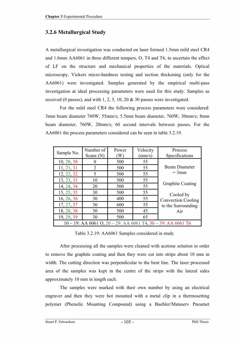
Chapter 3 Experimental Procedure
Stuart P. Edwardson PhD Thesis - 105 -
3.2.6 Metallurgical Study
A metallurgical investigation was conducted on laser formed 1.5mm mild steel CR4
and 1.6mm AA6061 in three different tempers, O, T4 and T6, to ascertain the effect
of LF on the structure and mechanical properties of the materials. Optical
microscopy, Vickers micro-hardness testing and section thickening (only for the
AA6061) were investigated. Samples generated by the empirical multi-pass
investigation at ideal processing parameters were used for this study. Samples as
received (0 passes), and with 1, 2, 5, 10, 20 & 30 passes were investigated.
For the mild steel CR4 the following process parameters were considered:
3mm beam diameter 760W, 55mm/s; 5.5mm beam diameter, 760W, 30mm/s; 8mm
beam diameter, 760W, 20mm/s; 60 second intervals between passes. For the
AA6061 the process parameters considered can be seen in table 3.2.19.
Sample No. Number ofScans (N)
Power (W)
Velocity (mm/s)
Process Specifications
10, 20, 30 0 500 55 11, 21, 31 2 500 55 12, 22, 32 5 500 55 13, 23, 33 10 500 55 14, 24, 34 20 500 55 15, 25, 35 30 500 55 16, 26, 36 30 400 55 17, 27, 37 30 600 55 18, 28, 38 30 500 45 19, 29, 39 30 500 65
Beam Diameter = 3mm
Graphite Coating
Cooled by
Convection Cooling to the Surrounding
Air
10 ~ 19: AA 6061 O, 20 ~ 29: AA 6061 T4, 30 ~ 39: AA 6061 T6
After processing all the samples were cleaned with acetone solution in order
to remove the graphite coating and then they were cut into strips about 10 mm in
width. The cutting direction was perpendicular to the bent line. The laser processed
area of the samples was kept in the centre of the strips with the lateral sides
approximately 10 mm in length each.
The samples were marked with their own number by using an electrical
engraver and then they were hot mounted with a metal clip in a thermosetting
polymer (Phenolic Mounting Compound) using a Buehler/Mataserv Pneumet
Table 3.2.19: AA6061 Samples considered in study
Chapter 3 Experimental Procedure
Stuart P. Edwardson PhD Thesis - 106 -
mounting press. The hot mounting process took about 15 minutes for each sample
and the operation temperature was approximately 150ºC.
After mounting, the specimens were ground using a Struers LabPol-21
grinding machine with water-lubricated silicon carbide (SiC) grinding papers. A 600
grit SiC grinding paper was used as the first stage of grinding in order to remove all
polymer left on the samples fast. However, the quality of the specimen surface was
not satisfactory for photomicrography, particularly on the AA6061 samples, due to
too many scratches left on the surface. Therefore, in order to obtain a fine quality of
specimen, the 1200 and 2500 grinding papers on a Metaserv 2000 Grinder/ Polisher
machine with plenty of water were used. In addition, a polishing cloth with an oil-
based lubricant with 6 and 1 micro diamond particles was used to remove the
grinding scratches. Liquid soap and plenty of water were used to wash the specimens
between the two stages of polishing. The grinding and polishing were done manually;
the specimens were ground and polished for approximately 2 minutes at each stage.
Finally, the specimens were washed well, cleaned with ethanol and dried in hot air.
The samples were then etched. For the mild steel CR4 the etchant used was
“NITAL” which contains 2% HNO3 (nitric acid) and 98% ethanol, the etching time
was approximately 1 minute, until the surface visibly tarnished. For the AA6061
Keller’s reagent was the suggested etchant in order to obtain a clear grain size and
shape through grain contrast. This Keller’s reagent comprises a mixture of 2 ml
hydrofluoric acid (HF, 48%), 3ml of hydrochloric acid (HCL, concentrated), 5 ml of
nitric acid (HNO3) and 190 ml of water. Extra safety precautions must be taken when
using HF acid, this mixture must be mixed in a fume extraction chamber and in a
plastic beaker, HF acid will etch glass (and destroy bone). During etching double
rubber gloves, rubber apron, facial shielding and full face mask were used. The
etching time was 8 to 15 seconds. After etching the samples were washed in stream
of warm water and dried in hot air.
A Leitz Wetzlar optical microscope was used to observe the microstructure
of the etched samples. The magnification lens, including eyepiece and objective,
used were 40, 128, 256, 500, 640, and 1280 times. Both the Leitz Wetzlar optical
microscope and a JVC colour video camera were used with GrandCAM, an image
capture software package, to capture the images of the samples. A comparison of the
section thicknesses was also made from the optical microscopy images and a
measurement using a digital Vernier calliper.
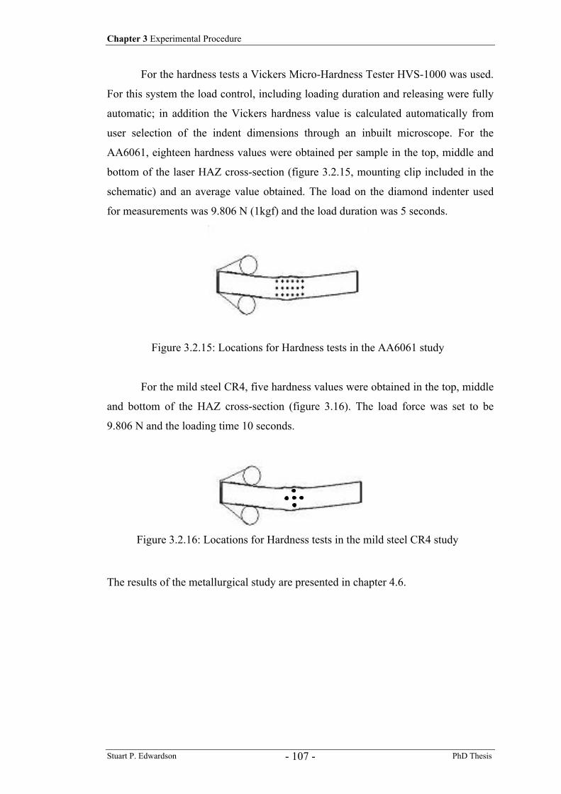
Chapter 3 Experimental Procedure
Stuart P. Edwardson PhD Thesis - 107 -
For the hardness tests a Vickers Micro-Hardness Tester HVS-1000 was used.
For this system the load control, including loading duration and releasing were fully
automatic; in addition the Vickers hardness value is calculated automatically from
user selection of the indent dimensions through an inbuilt microscope. For the
AA6061, eighteen hardness values were obtained per sample in the top, middle and
bottom of the laser HAZ cross-section (figure 3.2.15, mounting clip included in the
schematic) and an average value obtained. The load on the diamond indenter used
for measurements was 9.806 N (1kgf) and the load duration was 5 seconds.
For the mild steel CR4, five hardness values were obtained in the top, middle
and bottom of the HAZ cross-section (figure 3.16). The load force was set to be
9.806 N and the loading time 10 seconds.
The results of the metallurgical study are presented in chapter 4.6.
Figure 3.2.15: Locations for Hardness tests in the AA6061 study
Figure 3.2.16: Locations for Hardness tests in the mild steel CR4 study
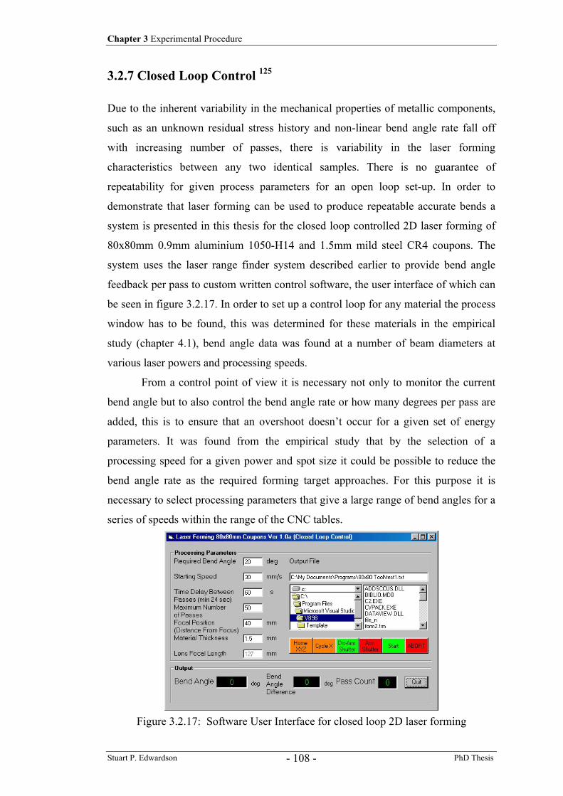
Chapter 3 Experimental Procedure
Stuart P. Edwardson PhD Thesis - 108 -
3.2.7 Closed Loop Control 125
Due to the inherent variability in the mechanical properties of metallic components,
such as an unknown residual stress history and non-linear bend angle rate fall off
with increasing number of passes, there is variability in the laser forming
characteristics between any two identical samples. There is no guarantee of
repeatability for given process parameters for an open loop set-up. In order to
demonstrate that laser forming can be used to produce repeatable accurate bends a
system is presented in this thesis for the closed loop controlled 2D laser forming of
80x80mm 0.9mm aluminium 1050-H14 and 1.5mm mild steel CR4 coupons. The
system uses the laser range finder system described earlier to provide bend angle
feedback per pass to custom written control software, the user interface of which can
be seen in figure 3.2.17. In order to set up a control loop for any material the process
window has to be found, this was determined for these materials in the empirical
study (chapter 4.1), bend angle data was found at a number of beam diameters at
various laser powers and processing speeds.
From a control point of view it is necessary not only to monitor the current
bend angle but to also control the bend angle rate or how many degrees per pass are
added, this is to ensure that an overshoot doesn’t occur for a given set of energy
parameters. It was found from the empirical study that by the selection of a
processing speed for a given power and spot size it could be possible to reduce the
bend angle rate as the required forming target approaches. For this purpose it is
necessary to select processing parameters that give a large range of bend angles for a
series of speeds within the range of the CNC tables.
Figure 3.2.17: Software User Interface for closed loop 2D laser forming
Chapter 3 Experimental Procedure
Stuart P. Edwardson PhD Thesis - 109 -
The control software was developed in Visual Basic to process a coupon
initially at optimum parameters, monitor the bend angle, compare it to the desired
angle and make a prediction of the processing speed for the next pass. It was found
that the traverse speed is the more straightforward and responsive variable to control
as opposed to laser power or beam spot size. As the desired angle approached the
software increases the processing speed per pass according to the determined
calibration graph, so as to reduce the bend angle rate in order to slowly move
towards the desired angle and not overshoot. The user interface for the control
software can be seen in figure 3.2.17; the user can select a target bend angle, the
ideal forming processing parameters and the output file, a maximum number of
passes is also given in order for the control loop to have a way of exiting if the target
angle cannot be achieved. The results of initial trails and final output for the
development of a reliable closed loop control system for these two materials are
presented in chapter 4.7.
3.2.8 Thick Section and Large Area 2D Forming for Ship Building 22
To be relevant to the ship building industry, particularly for the fabrication of hull
components, the laser forming process must be capable of thick section large scale
processing. A number of studies have been made to this end in both 2D and 3D laser
forming of thick section materials 4, 103-106, these studies and others have
demonstrated the potential of the LF process to produce accurately repeatable
geometries.
In this thesis a study is presented on thick section 2D laser forming of mild
steel in order to investigate the factors influencing a scaling of known scan strategies
for thinner section materials, the results of this study are reported here. The study
was conducted on 5 mm thick mild steel using three different laser systems. An
initial study was conducted on an Electrox 1.5kW CO2 laser system, wavelength
10.6µm, run in continuous wave mode, described earlier (figure 3.2.18). A second
study was conducted on an 8kW Ferranti CO2 laser and a 0.9x1.5m Wadkin CNC
table (figure 3.2.19). A third study was conducted at the Lairdside Laser engineering
Centre (LLEC) on a large 5 Axis Laserdyne 890 beam delivery system, employing a
3kW PRC CO2 laser (figure 3.2.20).
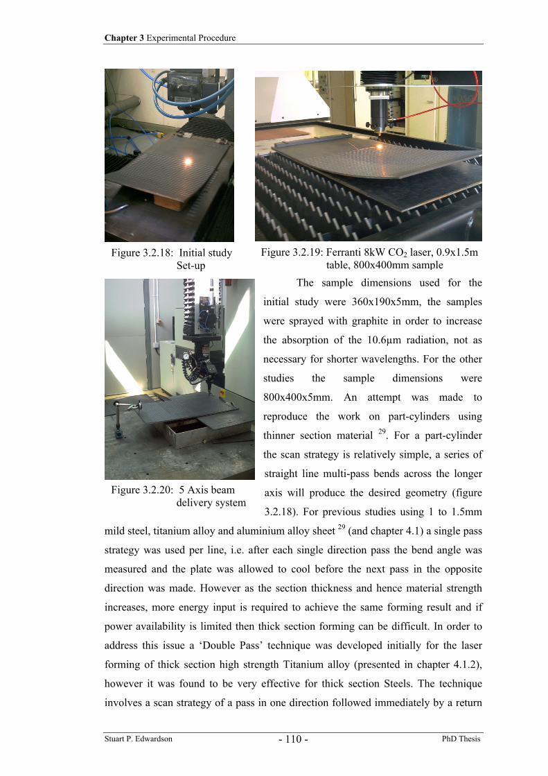
Chapter 3 Experimental Procedure
Stuart P. Edwardson PhD Thesis - 110 -
The sample dimensions used for the
initial study were 360x190x5mm, the samples
were sprayed with graphite in order to increase
the absorption of the 10.6µm radiation, not as
necessary for shorter wavelengths. For the other
studies the sample dimensions were
800x400x5mm. An attempt was made to
reproduce the work on part-cylinders using
thinner section material 29. For a part-cylinder
the scan strategy is relatively simple, a series of
straight line multi-pass bends across the longer
axis will produce the desired geometry (figure
3.2.18). For previous studies using 1 to 1.5mm
mild steel, titanium alloy and aluminium alloy sheet 29 (and chapter 4.1) a single pass
strategy was used per line, i.e. after each single direction pass the bend angle was
measured and the plate was allowed to cool before the next pass in the opposite
direction was made. However as the section thickness and hence material strength
increases, more energy input is required to achieve the same forming result and if
power availability is limited then thick section forming can be difficult. In order to
address this issue a ‘Double Pass’ technique was developed initially for the laser
forming of thick section high strength Titanium alloy (presented in chapter 4.1.2),
however it was found to be very effective for thick section Steels. The technique
involves a scan strategy of a pass in one direction followed immediately by a return
Figure 3.2.18: Initial study Set-up
Figure 3.2.19: Ferranti 8kW CO2 laser, 0.9x1.5m table, 800x400mm sample
Figure 3.2.20: 5 Axis beam delivery system
Chapter 3 Experimental Procedure
Stuart P. Edwardson PhD Thesis - 111 -
pass in the opposite direction; the plate is allowed to cool after each double pass
(forced cooled by air jet to decrease process time). The concept behind this strategy
is that, providing the material surface isn’t damaged on the second pass, the
additional energy input per pass is essentially akin to processing with a much higher
laser power (factor increase dependent on overlapping interaction times); this was
confirmed by thermocouple data. Another factor in this technique is that on the
second pass the heat retained in the irradiated area from the first pass could serve to
produce additional forming by reducing the temperature dependent flow or yield
stress of the material, in that a hot plate is easier to form than a cold one. To produce
the part-cylinder one end of the plate was fixed to the work bed by a bar (figures
3.2.18 – 3.2.20), the laser scans were started at the free end and worked towards the
clamped end, this ensured that the plate would be flat and at the same height for the
next line. The plates were forced cooled by a compressed air jet on the bottom
surface.
For the smaller samples it was possible to confirm the geometry formed
using the CMM software system described earlier. For the larger samples on the
larger workstations (figures 3.2.19 & 3.2.20), a CMM system was not available so
the formed geometries were confirmed by manually taking Z height measurements at
10 and 20mm steps along the edges of the plates and inferring the geometry in the
centre.
Studies were conducted into the 2D LF of part-cylinders along the shorter
axis and the longer axis of the larger plates using a number of laser powers, pass
numbers and step distances. Bends along the longer axis, 800mm long, would
demonstrate the potential of LF for larger scale applications, bends of this length
have not been reported in the literature. A thermocouple study was also conducted on
one of the plates to confirm the double pass strategy and to ascertain the effect of
laser line heating on the rest of the plate. The results from this study on thick section
forming are presented in chapter 4.8.
Chapter 3 Experimental Procedure
Stuart P. Edwardson PhD Thesis - 112 -
3.2.9 Laser Forming of Novel Materials – Metal Laminate
Composite (MLC) Materials 125, 126
The application reported in this work demonstrates how the laser forming process
can be used to form recently developed high strength metal laminate composite
materials. These materials due to their construction and high strength are difficult to
form once constructed using conventional techniques. Metal Laminate Composite
materials (MLC), sometimes referred to as Fibre Metal Laminates (FML), are of
particular interest to the aerospace industry, were the high strength yet lightweight
construction of parts made with these materials offers significant weight reductions
and hence a reduction in operational costs of new large commercial aircraft such as
the Airbus A380 and the proposed ultra-efficient Boeing 7E7. Military applications
are also being considered such as the Joint Strike Fighter (JSF) program.
In the A380 an FML called GLARE (Glass Reinforced Aluminium
Laminate), supplied by Fokker Aerostructures, is to be used in the construction of
the outer skin panels for the upper fuselage at the front and rear of the plane. As
mentioned, it is much lighter than the fully solid monolithic conventional materials
and represents a weight saving of about 500 - 800kg in the construction. The metallic
layers of the panels are pre-formed prior to lay-up and curing with the composite. In
a move away from the traditional rivet-based fixturing, the GLARE panels are
spliced and bonded seamlessly with no break in the fibre reinforcements and the
stringers are adhesively bonded to the panel surface. The required openings for
windows and doors are milled out of the formed panel; a fusion process is not
possible due to the presence of the composite.
Other industries where these materials are of interest include automotive, in
particular the high performance sports car and racing sectors such as formula one. A
more recent application under investigation for these materials is in the construction
of street furniture (e.g. litter bins) and airline cargo containers utilising their
excellent blast resistance capabilities to save lives in the event of terrorism.
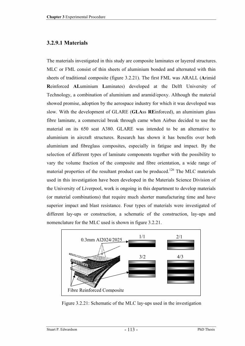
Chapter 3 Experimental Procedure
Stuart P. Edwardson PhD Thesis - 113 -
3.2.9.1 Materials
The materials investigated in this study are composite laminates or layered structures.
MLC or FML consist of thin sheets of aluminium bonded and alternated with thin
sheets of traditional composite (figure 3.2.21). The first FML was ARALL (Arimid
Reinforced ALuminium Laminates) developed at the Delft University of
Technology, a combination of aluminium and aramid/epoxy. Although the material
showed promise, adoption by the aerospace industry for which it was developed was
slow. With the development of GLARE (GLAss REinforced), an aluminium glass
fibre laminate, a commercial break through came when Airbus decided to use the
material on its 650 seat A380. GLARE was intended to be an alternative to
aluminium in aircraft structures. Research has shown it has benefits over both
aluminium and fibreglass composites, especially in fatigue and impact. By the
selection of different types of laminate components together with the possibility to
vary the volume fraction of the composite and fibre orientation, a wide range of
material properties of the resultant product can be produced.126 The MLC materials
used in this investigation have been developed in the Materials Science Division of
the University of Liverpool, work is ongoing in this department to develop materials
(or material combinations) that require much shorter manufacturing time and have
superior impact and blast resistance. Four types of materials were investigated of
different lay-ups or construction, a schematic of the construction, lay-ups and
nomenclature for the MLC used is shown in figure 3.2.21.
1/1 2/1
3/2 4/3
0.3mm Al2024/2025
Fibre Reinforced Composite
Figure 3.2.21: Schematic of the MLC lay-ups used in the investigation
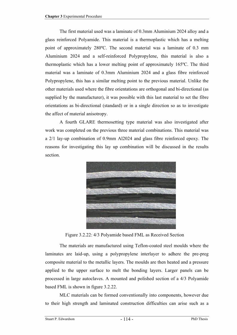
Chapter 3 Experimental Procedure
Stuart P. Edwardson PhD Thesis - 114 -
The first material used was a laminate of 0.3mm Aluminium 2024 alloy and a
glass reinforced Polyamide. This material is a thermoplastic which has a melting
point of approximately 280ºC. The second material was a laminate of 0.3 mm
Aluminium 2024 and a self-reinforced Polypropylene, this material is also a
thermoplastic which has a lower melting point of approximately 165ºC. The third
material was a laminate of 0.3mm Aluminium 2024 and a glass fibre reinforced
Polypropylene, this has a similar melting point to the previous material. Unlike the
other materials used where the fibre orientations are orthogonal and bi-directional (as
supplied by the manufacturer), it was possible with this last material to set the fibre
orientations as bi-directional (standard) or in a single direction so as to investigate
the affect of material anisotropy.
A fourth GLARE thermosetting type material was also investigated after
work was completed on the previous three material combinations. This material was
a 2/1 lay-up combination of 0.9mm Al2024 and glass fibre reinforced epoxy. The
reasons for investigating this lay up combination will be discussed in the results
section.
The materials are manufactured using Teflon-coated steel moulds where the
laminates are laid-up, using a polypropylene interlayer to adhere the pre-preg
composite material to the metallic layers. The moulds are then heated and a pressure
applied to the upper surface to melt the bonding layers. Larger panels can be
processed in large autoclaves. A mounted and polished section of a 4/3 Polyamide
based FML is shown in figure 3.2.22.
MLC materials can be formed conventionally into components, however due
to their high strength and laminated construction difficulties can arise such as a
Figure 3.2.22: 4/3 Polyamide based FML as Received Section
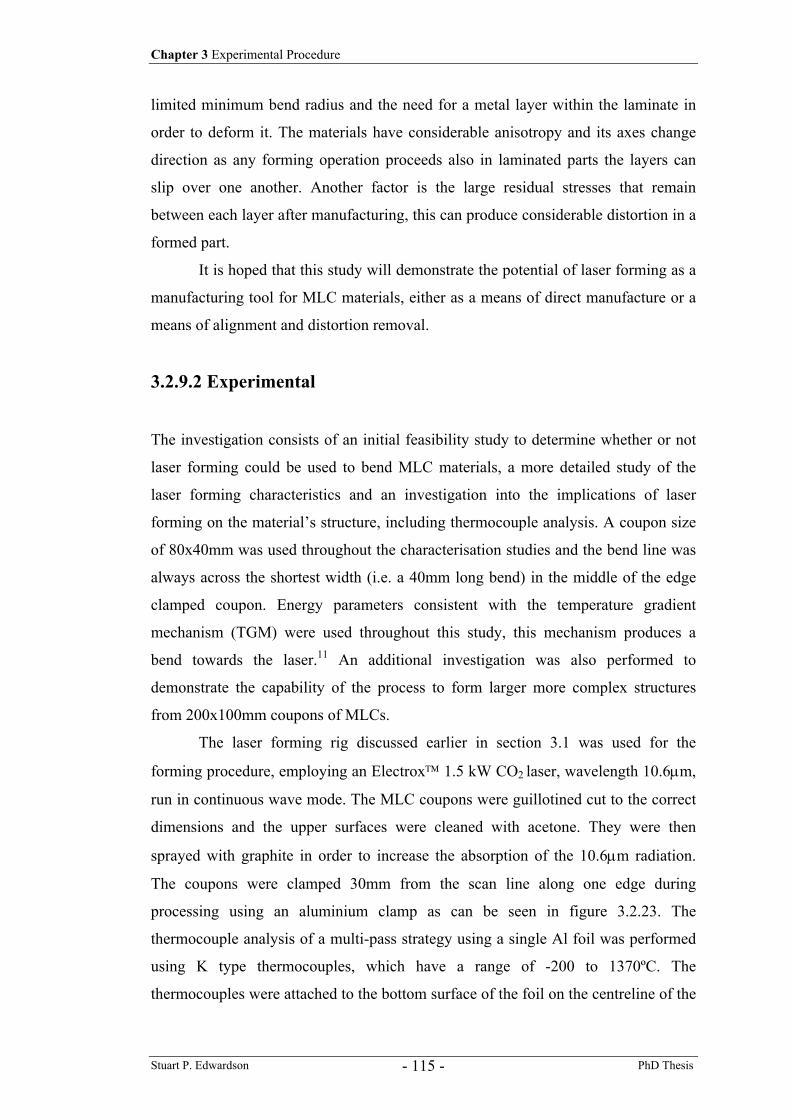
Chapter 3 Experimental Procedure
Stuart P. Edwardson PhD Thesis - 115 -
limited minimum bend radius and the need for a metal layer within the laminate in
order to deform it. The materials have considerable anisotropy and its axes change
direction as any forming operation proceeds also in laminated parts the layers can
slip over one another. Another factor is the large residual stresses that remain
between each layer after manufacturing, this can produce considerable distortion in a
formed part.
It is hoped that this study will demonstrate the potential of laser forming as a
manufacturing tool for MLC materials, either as a means of direct manufacture or a
means of alignment and distortion removal.
3.2.9.2 Experimental
The investigation consists of an initial feasibility study to determine whether or not
laser forming could be used to bend MLC materials, a more detailed study of the
laser forming characteristics and an investigation into the implications of laser
forming on the material’s structure, including thermocouple analysis. A coupon size
of 80x40mm was used throughout the characterisation studies and the bend line was
always across the shortest width (i.e. a 40mm long bend) in the middle of the edge
clamped coupon. Energy parameters consistent with the temperature gradient
mechanism (TGM) were used throughout this study, this mechanism produces a
bend towards the laser.11 An additional investigation was also performed to
demonstrate the capability of the process to form larger more complex structures
from 200x100mm coupons of MLCs.
The laser forming rig discussed earlier in section 3.1 was used for the
forming procedure, employing an Electrox 1.5 kW CO2 laser, wavelength 10.6µm,
run in continuous wave mode. The MLC coupons were guillotined cut to the correct
dimensions and the upper surfaces were cleaned with acetone. They were then
sprayed with graphite in order to increase the absorption of the 10.6µm radiation.
The coupons were clamped 30mm from the scan line along one edge during
processing using an aluminium clamp as can be seen in figure 3.2.23. The
thermocouple analysis of a multi-pass strategy using a single Al foil was performed
using K type thermocouples, which have a range of -200 to 1370ºC. The
thermocouples were attached to the bottom surface of the foil on the centreline of the
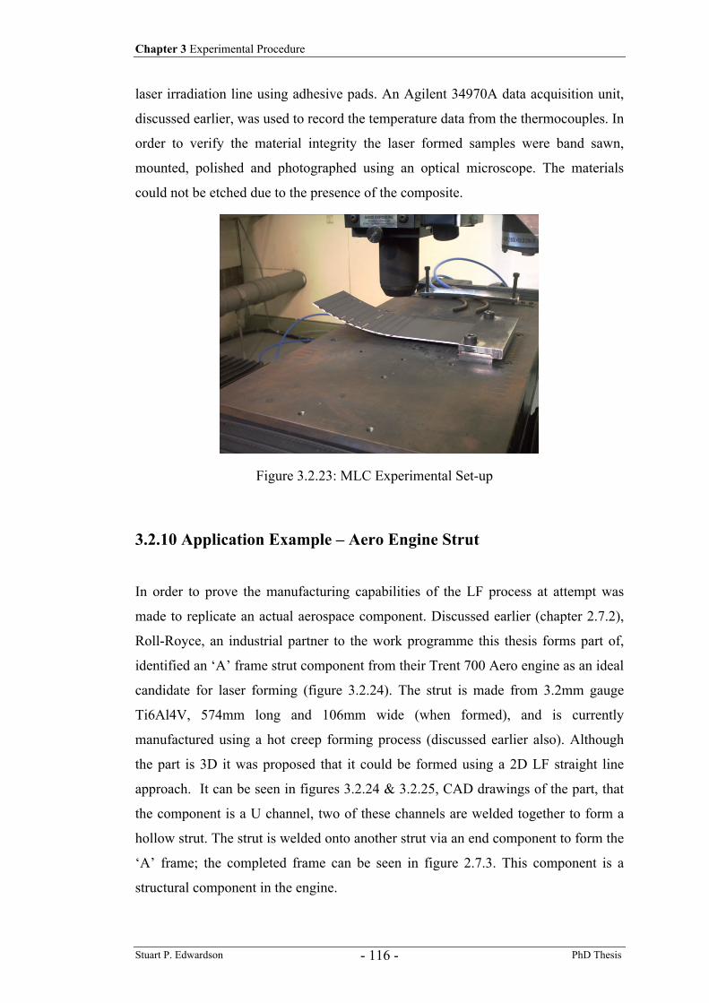
Chapter 3 Experimental Procedure
Stuart P. Edwardson PhD Thesis - 116 -
laser irradiation line using adhesive pads. An Agilent 34970A data acquisition unit,
discussed earlier, was used to record the temperature data from the thermocouples. In
order to verify the material integrity the laser formed samples were band sawn,
mounted, polished and photographed using an optical microscope. The materials
could not be etched due to the presence of the composite.
3.2.10 Application Example – Aero Engine Strut
In order to prove the manufacturing capabilities of the LF process at attempt was
made to replicate an actual aerospace component. Discussed earlier (chapter 2.7.2),
Roll-Royce, an industrial partner to the work programme this thesis forms part of,
identified an ‘A’ frame strut component from their Trent 700 Aero engine as an ideal
candidate for laser forming (figure 3.2.24). The strut is made from 3.2mm gauge
Ti6Al4V, 574mm long and 106mm wide (when formed), and is currently
manufactured using a hot creep forming process (discussed earlier also). Although
the part is 3D it was proposed that it could be formed using a 2D LF straight line
approach. It can be seen in figures 3.2.24 & 3.2.25, CAD drawings of the part, that
the component is a U channel, two of these channels are welded together to form a
hollow strut. The strut is welded onto another strut via an end component to form the
‘A’ frame; the completed frame can be seen in figure 2.7.3. This component is a
structural component in the engine.
Figure 3.2.23: MLC Experimental Set-up
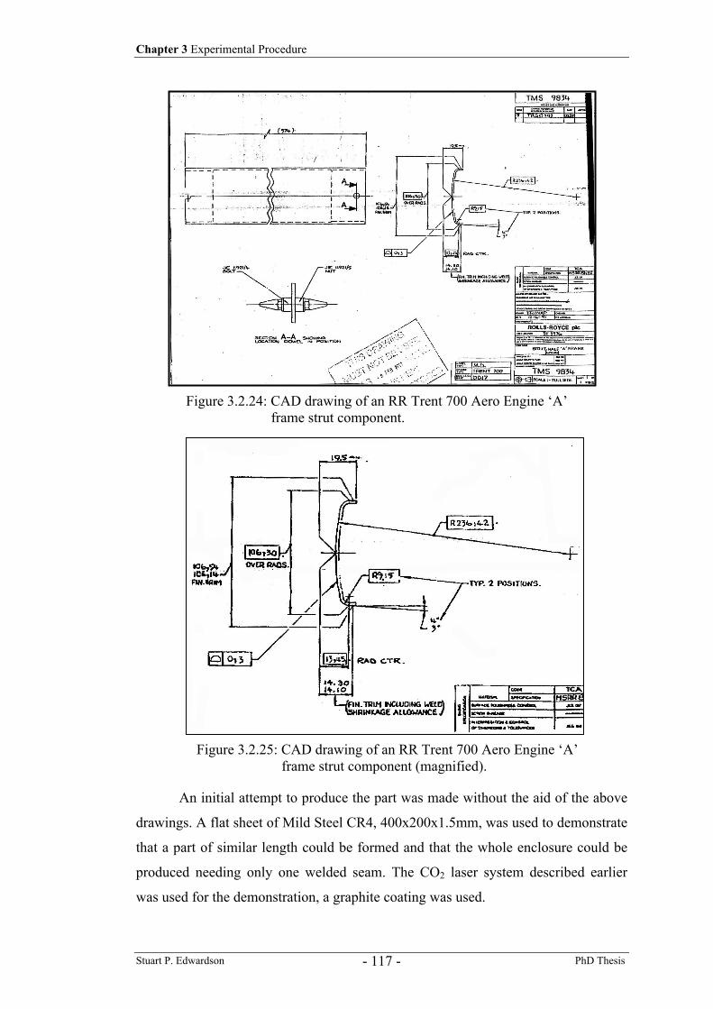
Chapter 3 Experimental Procedure
Stuart P. Edwardson PhD Thesis - 117 -
Figure 3.2.24: CAD drawing of an RR Trent 700 Aero Engine ‘A’ frame strut component.
Figure 3.2.25: CAD drawing of an RR Trent 700 Aero Engine ‘A’ frame strut component (magnified).
An initial attempt to produce the part was made without the aid of the above
drawings. A flat sheet of Mild Steel CR4, 400x200x1.5mm, was used to demonstrate
that a part of similar length could be formed and that the whole enclosure could be
produced needing only one welded seam. The CO2 laser system described earlier
was used for the demonstration, a graphite coating was used.
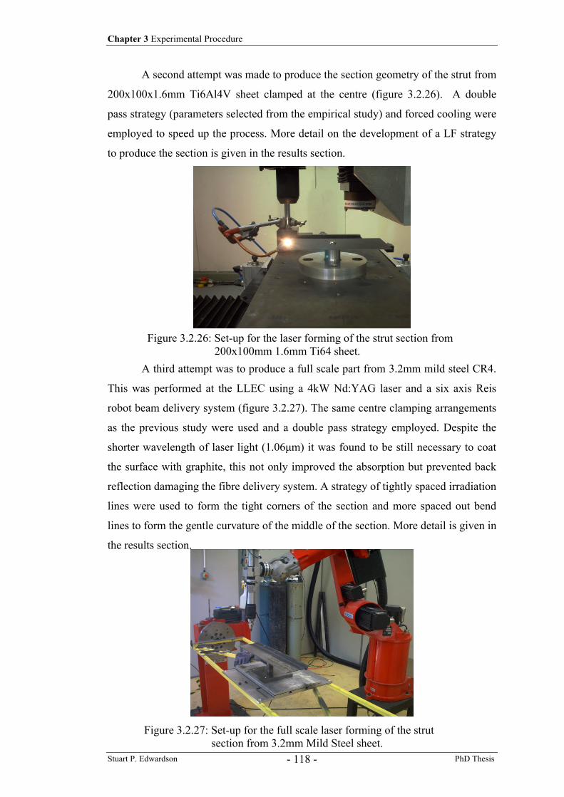
Chapter 3 Experimental Procedure
Stuart P. Edwardson PhD Thesis - 118 -
A second attempt was made to produce the section geometry of the strut from
200x100x1.6mm Ti6Al4V sheet clamped at the centre (figure 3.2.26). A double
pass strategy (parameters selected from the empirical study) and forced cooling were
employed to speed up the process. More detail on the development of a LF strategy
to produce the section is given in the results section.
A third attempt was to produce a full scale part from 3.2mm mild steel CR4.
This was performed at the LLEC using a 4kW Nd:YAG laser and a six axis Reis
robot beam delivery system (figure 3.2.27). The same centre clamping arrangements
as the previous study were used and a double pass strategy employed. Despite the
shorter wavelength of laser light (1.06µm) it was found to be still necessary to coat
the surface with graphite, this not only improved the absorption but prevented back
reflection damaging the fibre delivery system. A strategy of tightly spaced irradiation
lines were used to form the tight corners of the section and more spaced out bend
lines to form the gentle curvature of the middle of the section. More detail is given in
the results section.
Figure 3.2.26: Set-up for the laser forming of the strut section from 200x100mm 1.6mm Ti64 sheet.
Figure 3.2.27: Set-up for the full scale laser forming of the strut section from 3.2mm Mild Steel sheet.
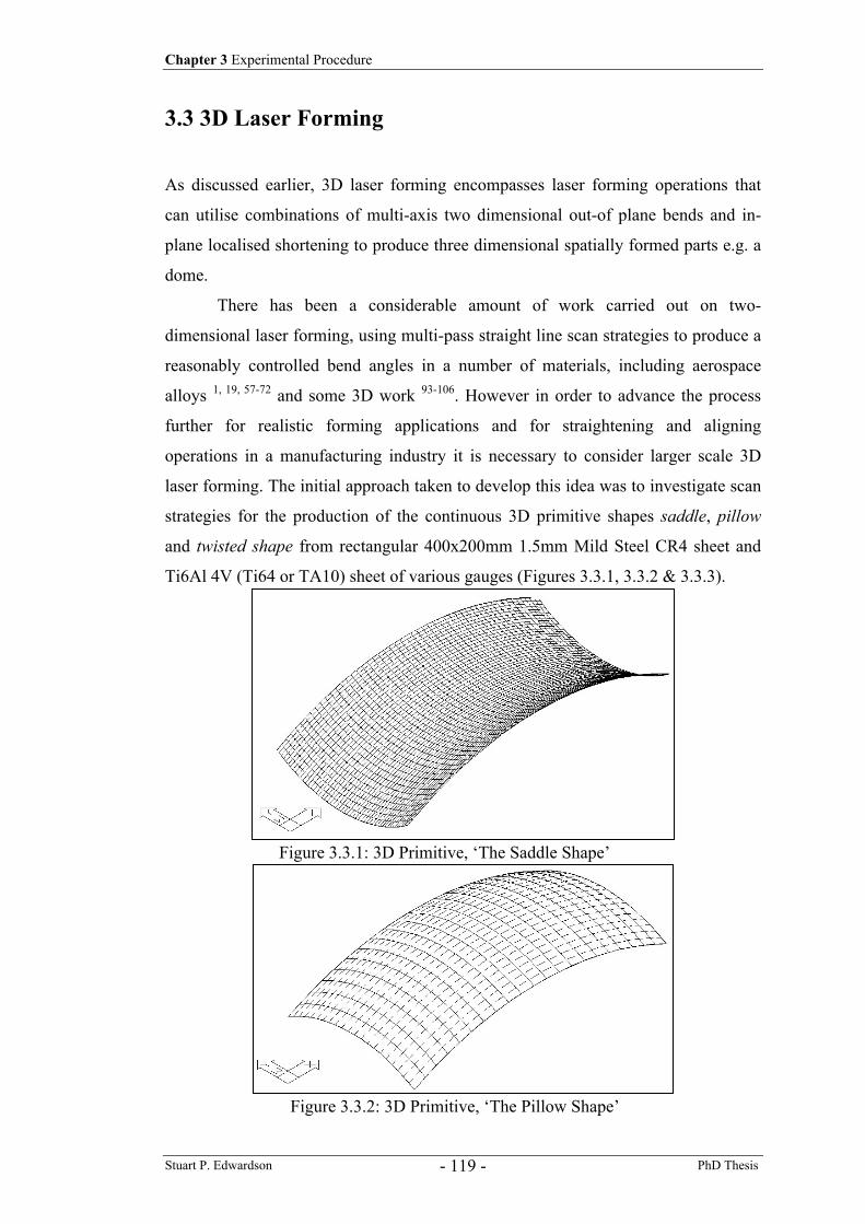
Chapter 3 Experimental Procedure
Stuart P. Edwardson PhD Thesis - 119 -
3.3 3D Laser Forming
As discussed earlier, 3D laser forming encompasses laser forming operations that
can utilise combinations of multi-axis two dimensional out-of plane bends and in-
plane localised shortening to produce three dimensional spatially formed parts e.g. a
dome.
There has been a considerable amount of work carried out on two-
dimensional laser forming, using multi-pass straight line scan strategies to produce a
reasonably controlled bend angles in a number of materials, including aerospace
alloys 1, 19, 57-72 and some 3D work 93-106. However in order to advance the process
further for realistic forming applications and for straightening and aligning
operations in a manufacturing industry it is necessary to consider larger scale 3D
laser forming. The initial approach taken to develop this idea was to investigate scan
strategies for the production of the continuous 3D primitive shapes saddle, pillow
and twisted shape from rectangular 400x200mm 1.5mm Mild Steel CR4 sheet and
Ti6Al 4V (Ti64 or TA10) sheet of various gauges (Figures 3.3.1, 3.3.2 & 3.3.3).
Figure 3.3.2: 3D Primitive, ‘The Pillow Shape’
Figure 3.3.1: 3D Primitive, ‘The Saddle Shape’
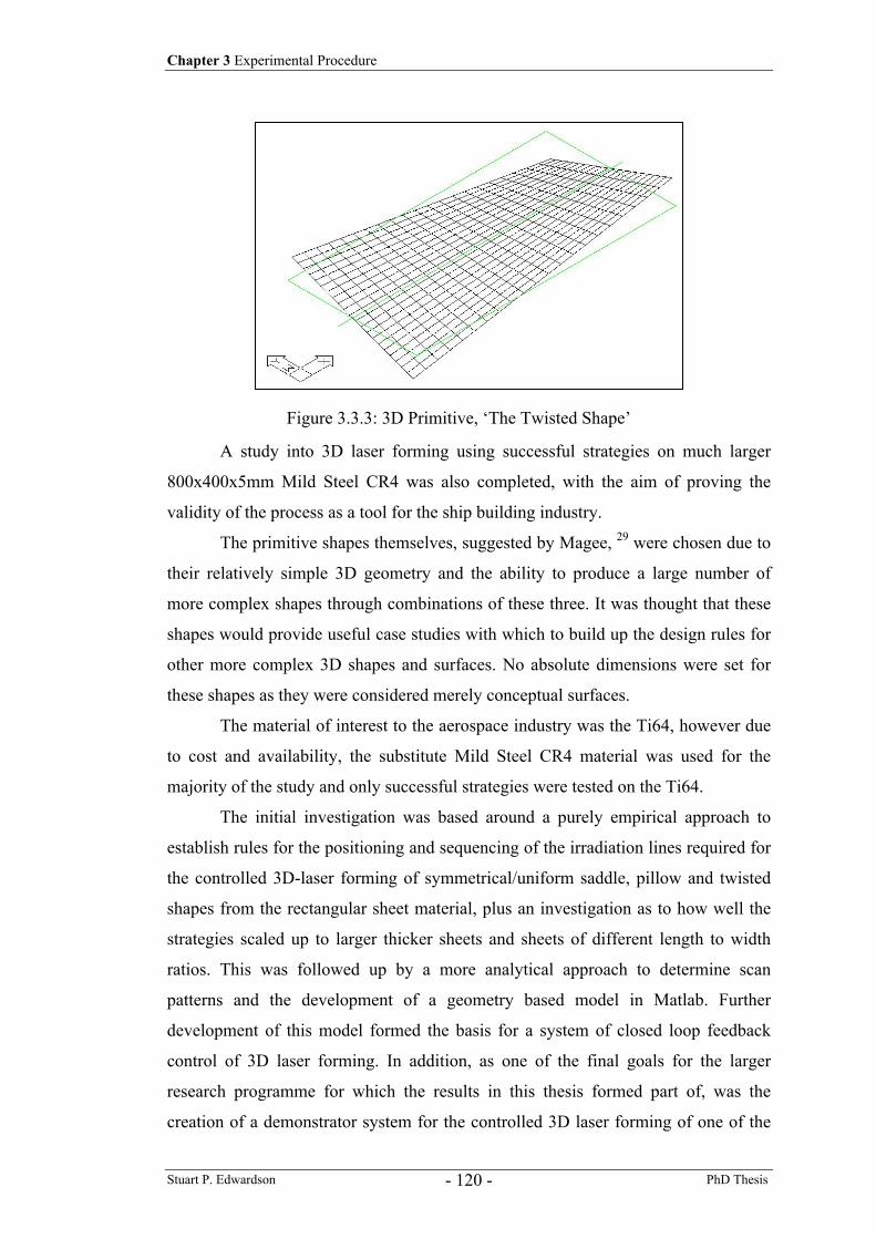
Chapter 3 Experimental Procedure
Stuart P. Edwardson PhD Thesis - 120 -
A study into 3D laser forming using successful strategies on much larger
800x400x5mm Mild Steel CR4 was also completed, with the aim of proving the
validity of the process as a tool for the ship building industry.
The primitive shapes themselves, suggested by Magee, 29 were chosen due to
their relatively simple 3D geometry and the ability to produce a large number of
more complex shapes through combinations of these three. It was thought that these
shapes would provide useful case studies with which to build up the design rules for
other more complex 3D shapes and surfaces. No absolute dimensions were set for
these shapes as they were considered merely conceptual surfaces.
The material of interest to the aerospace industry was the Ti64, however due
to cost and availability, the substitute Mild Steel CR4 material was used for the
majority of the study and only successful strategies were tested on the Ti64.
The initial investigation was based around a purely empirical approach to
establish rules for the positioning and sequencing of the irradiation lines required for
the controlled 3D-laser forming of symmetrical/uniform saddle, pillow and twisted
shapes from the rectangular sheet material, plus an investigation as to how well the
strategies scaled up to larger thicker sheets and sheets of different length to width
ratios. This was followed up by a more analytical approach to determine scan
patterns and the development of a geometry based model in Matlab. Further
development of this model formed the basis for a system of closed loop feedback
control of 3D laser forming. In addition, as one of the final goals for the larger
research programme for which the results in this thesis formed part of, was the
creation of a demonstrator system for the controlled 3D laser forming of one of the
Figure 3.3.3: 3D Primitive, ‘The Twisted Shape’
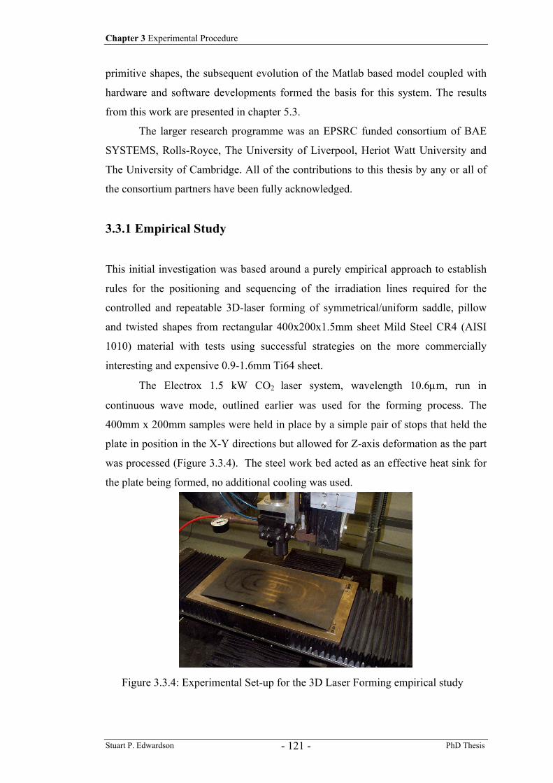
Chapter 3 Experimental Procedure
Stuart P. Edwardson PhD Thesis - 121 -
primitive shapes, the subsequent evolution of the Matlab based model coupled with
hardware and software developments formed the basis for this system. The results
from this work are presented in chapter 5.3.
The larger research programme was an EPSRC funded consortium of BAE
SYSTEMS, Rolls-Royce, The University of Liverpool, Heriot Watt University and
The University of Cambridge. All of the contributions to this thesis by any or all of
the consortium partners have been fully acknowledged.
3.3.1 Empirical Study
This initial investigation was based around a purely empirical approach to establish
rules for the positioning and sequencing of the irradiation lines required for the
controlled and repeatable 3D-laser forming of symmetrical/uniform saddle, pillow
and twisted shapes from rectangular 400x200x1.5mm sheet Mild Steel CR4 (AISI
1010) material with tests using successful strategies on the more commercially
interesting and expensive 0.9-1.6mm Ti64 sheet.
The Electrox 1.5 kW CO2 laser system, wavelength 10.6µm, run in
continuous wave mode, outlined earlier was used for the forming process. The
400mm x 200mm samples were held in place by a simple pair of stops that held the
plate in position in the X-Y directions but allowed for Z-axis deformation as the part
was processed (Figure 3.3.4). The steel work bed acted as an effective heat sink for
the plate being formed, no additional cooling was used.
Figure 3.3.4: Experimental Set-up for the 3D Laser Forming empirical study
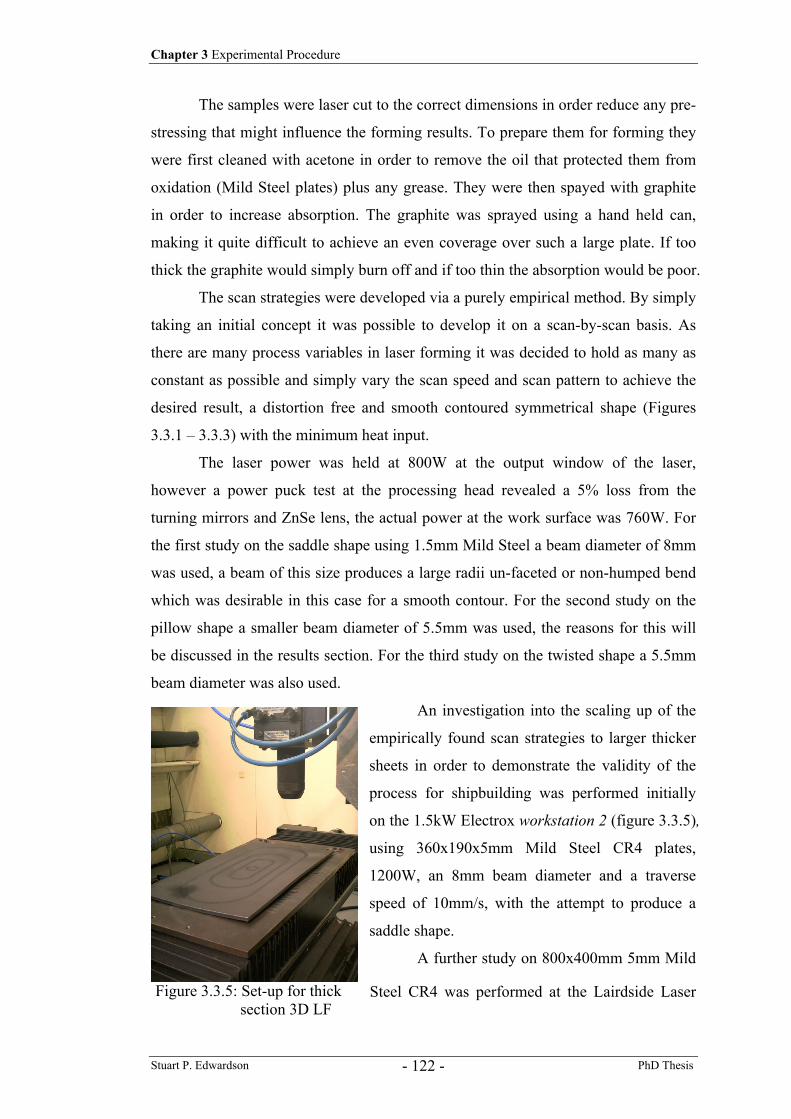
Chapter 3 Experimental Procedure
Stuart P. Edwardson PhD Thesis - 122 -
Figure 3.3.5: Set-up for thick section 3D LF
The samples were laser cut to the correct dimensions in order reduce any pre-
stressing that might influence the forming results. To prepare them for forming they
were first cleaned with acetone in order to remove the oil that protected them from
oxidation (Mild Steel plates) plus any grease. They were then spayed with graphite
in order to increase absorption. The graphite was sprayed using a hand held can,
making it quite difficult to achieve an even coverage over such a large plate. If too
thick the graphite would simply burn off and if too thin the absorption would be poor.
The scan strategies were developed via a purely empirical method. By simply
taking an initial concept it was possible to develop it on a scan-by-scan basis. As
there are many process variables in laser forming it was decided to hold as many as
constant as possible and simply vary the scan speed and scan pattern to achieve the
desired result, a distortion free and smooth contoured symmetrical shape (Figures
3.3.1 – 3.3.3) with the minimum heat input.
The laser power was held at 800W at the output window of the laser,
however a power puck test at the processing head revealed a 5% loss from the
turning mirrors and ZnSe lens, the actual power at the work surface was 760W. For
the first study on the saddle shape using 1.5mm Mild Steel a beam diameter of 8mm
was used, a beam of this size produces a large radii un-faceted or non-humped bend
which was desirable in this case for a smooth contour. For the second study on the
pillow shape a smaller beam diameter of 5.5mm was used, the reasons for this will
be discussed in the results section. For the third study on the twisted shape a 5.5mm
beam diameter was also used.
An investigation into the scaling up of the
empirically found scan strategies to larger thicker
sheets in order to demonstrate the validity of the
process for shipbuilding was performed initially
on the 1.5kW Electrox workstation 2 (figure 3.3.5),
using 360x190x5mm Mild Steel CR4 plates,
1200W, an 8mm beam diameter and a traverse
speed of 10mm/s, with the attempt to produce a
saddle shape.
A further study on 800x400mm 5mm Mild
Steel CR4 was performed at the Lairdside Laser
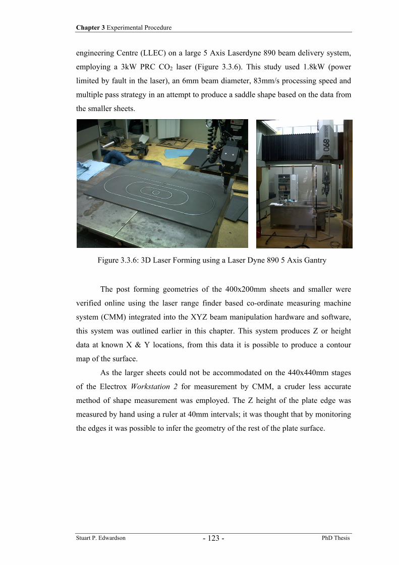
Chapter 3 Experimental Procedure
Stuart P. Edwardson PhD Thesis - 123 -
engineering Centre (LLEC) on a large 5 Axis Laserdyne 890 beam delivery system,
employing a 3kW PRC CO2 laser (Figure 3.3.6). This study used 1.8kW (power
limited by fault in the laser), an 6mm beam diameter, 83mm/s processing speed and
multiple pass strategy in an attempt to produce a saddle shape based on the data from
the smaller sheets.
The post forming geometries of the 400x200mm sheets and smaller were
verified online using the laser range finder based co-ordinate measuring machine
system (CMM) integrated into the XYZ beam manipulation hardware and software,
this system was outlined earlier in this chapter. This system produces Z or height
data at known X & Y locations, from this data it is possible to produce a contour
map of the surface.
As the larger sheets could not be accommodated on the 440x440mm stages
of the Electrox Workstation 2 for measurement by CMM, a cruder less accurate
method of shape measurement was employed. The Z height of the plate edge was
measured by hand using a ruler at 40mm intervals; it was thought that by monitoring
the edges it was possible to infer the geometry of the rest of the plate surface.
Figure 3.3.6: 3D Laser Forming using a Laser Dyne 890 5 Axis Gantry
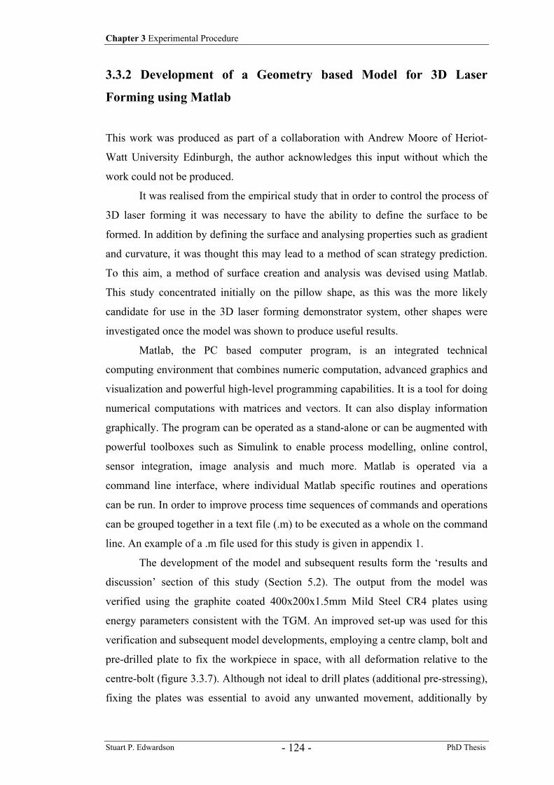
Chapter 3 Experimental Procedure
Stuart P. Edwardson PhD Thesis - 124 -
3.3.2 Development of a Geometry based Model for 3D Laser
Forming using Matlab
This work was produced as part of a collaboration with Andrew Moore of Heriot-
Watt University Edinburgh, the author acknowledges this input without which the
work could not be produced.
It was realised from the empirical study that in order to control the process of
3D laser forming it was necessary to have the ability to define the surface to be
formed. In addition by defining the surface and analysing properties such as gradient
and curvature, it was thought this may lead to a method of scan strategy prediction.
To this aim, a method of surface creation and analysis was devised using Matlab.
This study concentrated initially on the pillow shape, as this was the more likely
candidate for use in the 3D laser forming demonstrator system, other shapes were
investigated once the model was shown to produce useful results.
Matlab, the PC based computer program, is an integrated technical
computing environment that combines numeric computation, advanced graphics and
visualization and powerful high-level programming capabilities. It is a tool for doing
numerical computations with matrices and vectors. It can also display information
graphically. The program can be operated as a stand-alone or can be augmented with
powerful toolboxes such as Simulink to enable process modelling, online control,
sensor integration, image analysis and much more. Matlab is operated via a
command line interface, where individual Matlab specific routines and operations
can be run. In order to improve process time sequences of commands and operations
can be grouped together in a text file (.m) to be executed as a whole on the command
line. An example of a .m file used for this study is given in appendix 1.
The development of the model and subsequent results form the ‘results and
discussion’ section of this study (Section 5.2). The output from the model was
verified using the graphite coated 400x200x1.5mm Mild Steel CR4 plates using
energy parameters consistent with the TGM. An improved set-up was used for this
verification and subsequent model developments, employing a centre clamp, bolt and
pre-drilled plate to fix the workpiece in space, with all deformation relative to the
centre-bolt (figure 3.3.7). Although not ideal to drill plates (additional pre-stressing),
fixing the plates was essential to avoid any unwanted movement, additionally by
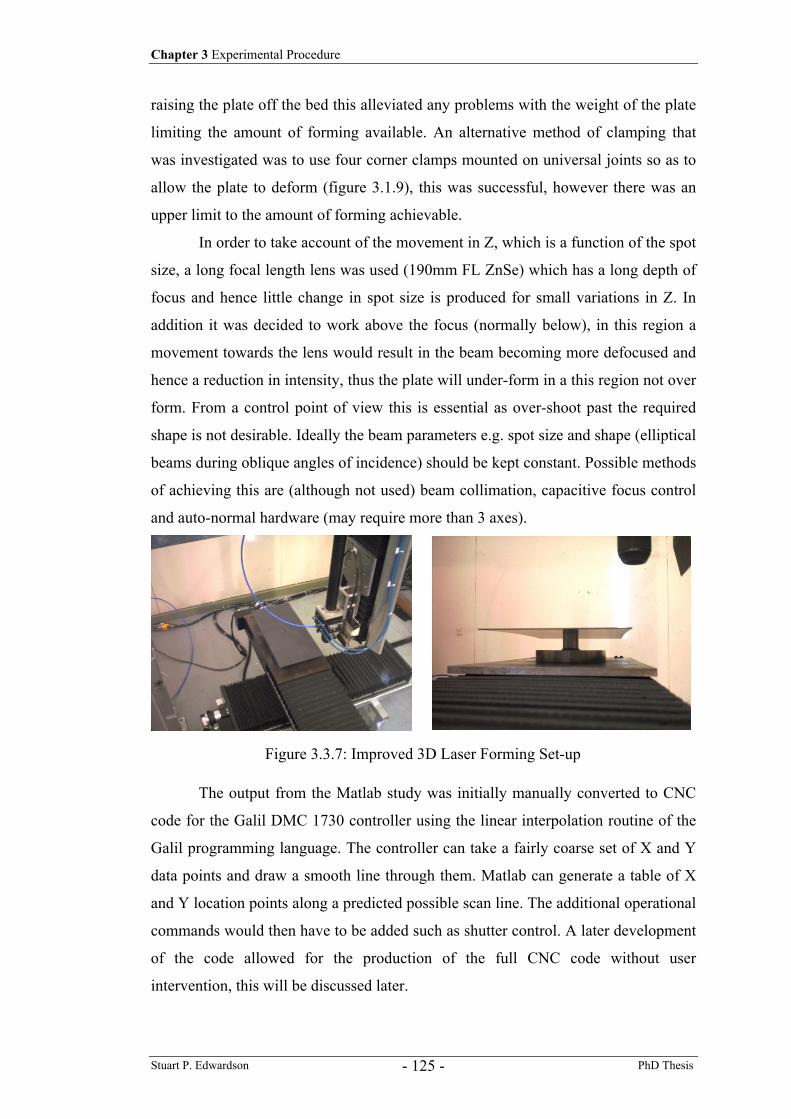
Chapter 3 Experimental Procedure
Stuart P. Edwardson PhD Thesis - 125 -
raising the plate off the bed this alleviated any problems with the weight of the plate
limiting the amount of forming available. An alternative method of clamping that
was investigated was to use four corner clamps mounted on universal joints so as to
allow the plate to deform (figure 3.1.9), this was successful, however there was an
upper limit to the amount of forming achievable.
In order to take account of the movement in Z, which is a function of the spot
size, a long focal length lens was used (190mm FL ZnSe) which has a long depth of
focus and hence little change in spot size is produced for small variations in Z. In
addition it was decided to work above the focus (normally below), in this region a
movement towards the lens would result in the beam becoming more defocused and
hence a reduction in intensity, thus the plate will under-form in a this region not over
form. From a control point of view this is essential as over-shoot past the required
shape is not desirable. Ideally the beam parameters e.g. spot size and shape (elliptical
beams during oblique angles of incidence) should be kept constant. Possible methods
of achieving this are (although not used) beam collimation, capacitive focus control
and auto-normal hardware (may require more than 3 axes).
The output from the Matlab study was initially manually converted to CNC
code for the Galil DMC 1730 controller using the linear interpolation routine of the
Galil programming language. The controller can take a fairly coarse set of X and Y
data points and draw a smooth line through them. Matlab can generate a table of X
and Y location points along a predicted possible scan line. The additional operational
commands would then have to be added such as shutter control. A later development
of the code allowed for the production of the full CNC code without user
intervention, this will be discussed later.
Figure 3.3.7: Improved 3D Laser Forming Set-up
Chapter 3 Experimental Procedure
Stuart P. Edwardson PhD Thesis - 126 -
The geometries of the plates were verified using the laser range finder based
CMM integrated with the XYZ workstation, an improvement to the control software
was made to take account of the new starting location (addition of once touch start
location find buttons) and at a later development the increase in step size (reduce
number of data points taken) to reduce measurement cycle time to 10 minutes from
45 minutes.
The concept and theory behind an in-plane strain approach rather than a
geometry approach to the energy distribution realised on a surface is also given the
in results section for this study (chapter 5.2).
3.3.3 3D Laser Forming Demonstrator System
The 3D laser forming demonstrator system was a development from the work on the
geometry based model using Matlab. Its development and subsequent testing and
output forms the results and discussion section for this study, due to this, only a brief
overview of the procedures and concepts used are given here.
It was found that, although a prediction of a scan pattern could be obtained
either by either empirical or analytical means leading to a ‘single shot’ scan strategy,
from a control point of view this was not desirable. Due to inherent material
variability and unknown residual stress conditions an open loop method of 3D laser
forming based on a look up table of known results would ultimately produce
significant errors. Instead a combined approach was sort, using the predictive
capability of the matlab model to produce an initial scan strategy to be realised, and
then use an adaptive/iterative approach to produce further corrective scan strategies
based on the current geometry when compared to a target geometry, incrementing
slowly towards the desired result scan after scan providing the plate is under-formed
on the first pass. As with closed loop 2D LF the processing speed was used to
control the energy input and hence the rate and magnitude of forming. The difference
in closed loop 3D LF was that the output data from the matlab model called for a
distribution of required distortion (based on geometry and required in-plane strain),
such that the energy input at any point depended on its location on the sheet. This
was realised by varying the traverse speed along any scan line according to the
required deformation at that point (an example of the CNC code through which this
Chapter 3 Experimental Procedure
Stuart P. Edwardson PhD Thesis - 127 -
was achieved can be seen in appendix 6), the required distortion was related to the
traverse speed by calibration data obtained from the 2D LF empirical study, such that
for a given power, spot size and traverse speed a bend angle could be predicted.
After each scan was realised a measurement of the surface geometry was
taken, a comparison was then made to the target geometry and based on the error a
further scan strategy was predicted. In order to control the forming rate to avoid
overshoot, the scan speed range was increased automatically to compensate. The
demonstrator system was set up for the closed loop forming of the pillow shape, an
ideal mathematical surface, an elliptic paraboloid, was used as the target shape, the
pillow shape falls into this class of surfaces. Energy parameters consistent with the
TGM were used throughout (power and spot size held constant), the experimental
set-up remained the same as the previous study with the addition of an air jet
controlled by the Galil system on the underside of the plate to speed cooling after
processing prior to measurement, the air jet was not used during processing.
As the control software was written in Visual Basic and the
predictive/adaptive model run through Matlab, a manual intervention was required to
transfer the surface height data from the CMM system to the Matlab script after each
pass. The script was then executed in order to generate the CNC code for the next
pass. Scans were continued until the error reduced to a desired level. The results
from this study are presented in chapter 5.3.
Chapter 4 2D Laser Forming- Results & Discussion
Stuart P. Edwardson PhD Thesis - 128 -
Chapter 4
2D Laser Forming –
Results and Discussion This chapter contains the results and discussion of experimental and numerical
studies into the 2D laser forming of a number of materials, including mild steel,
aluminium and aluminium alloys, titanium alloy and newly developed Fibre Metal
Laminate materials (FML).
4.1 Empirical Study - Characterisation of the Laser Forming
Process
The first results presented in this thesis are from an empirical 2D laser forming
investigation on a number of materials using the TGM, characterising the 2D laser
forming process. Variables investigated include; beam spot size, laser power,
traverse speed, multiple and single pass strategies, time delay between passes, bend
angle rate and coating degradation. The results for each material investigated are
presented in the following sections.
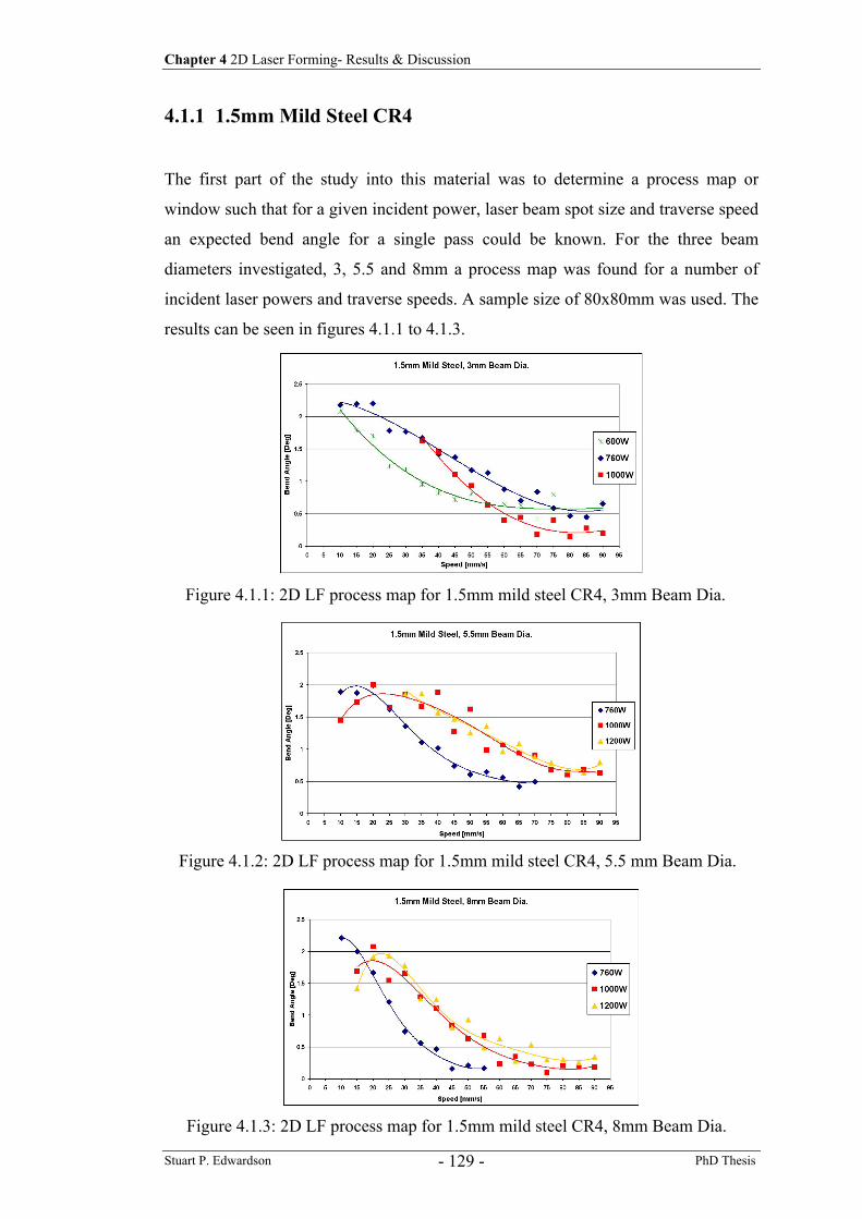
Chapter 4 2D Laser Forming- Results & Discussion
Stuart P. Edwardson PhD Thesis - 129 -
4.1.1 1.5mm Mild Steel CR4
The first part of the study into this material was to determine a process map or
window such that for a given incident power, laser beam spot size and traverse speed
an expected bend angle for a single pass could be known. For the three beam
diameters investigated, 3, 5.5 and 8mm a process map was found for a number of
incident laser powers and traverse speeds. A sample size of 80x80mm was used. The
results can be seen in figures 4.1.1 to 4.1.3.
Figure 4.1.1: 2D LF process map for 1.5mm mild steel CR4, 3mm Beam Dia.
Figure 4.1.2: 2D LF process map for 1.5mm mild steel CR4, 5.5 mm Beam Dia.
Figure 4.1.3: 2D LF process map for 1.5mm mild steel CR4, 8mm Beam Dia.
Chapter 4 2D Laser Forming- Results & Discussion
Stuart P. Edwardson PhD Thesis - 130 -
For the above results, due to the large amount of data, only a single datum
point was taken at each traverse speed and a line of best fit drawn through them
(using a polynomial fit of various orders). It was thought that this would be sufficient
to obtain processing regions were laser forming was possible and that an
approximate speed \ bend angle relationship for a given power and spot size could be
found. In addition due to material and process variability a reliance on obtaining an
exact bend angle only from given process parameters is flawed. This will be
discussed later when considering closed loop control.
It can be seen in figures 4.1.1 to 4.1.3 that for this material there is an
approximately (negative) linear relationship between the bend angle and the traverse
speed for a mid portion of the data for a given power and spot size. At higher
traverse speeds the amount of forming is small and very similar. At a point, as the
speed slows, an activation energy intensity level appears to be reached whereby any
further decrease in speed results in a significant increase in bend angle achieved.
This is consistent with the increasing energy input causing a higher thermal gradient
through the thickness and thus increased forming. This linear increase is arrested at
lower traverse speeds, particularly for the larger 5.5 and 8mm beam diameters,
where a maximum forming level occurs and any further decrease in speed results in a
decrease in bend angle. This could signify a point where the increasing energy input
is detrimental to forming a sufficiently high enough thermal gradient through the
section and thus process efficiency is lost. This could also be a transition point to
another mechanism, in that the bending strains developed are being outweighed by
the in-plane strains as the section becomes uniformly heated and so the shortening
and buckling mechanisms become dominant. For the 3mm beam diameter result
(figure 4.1.1) the fall off at lower traverse speeds is not as apparent. However some
surface melting occurred on samples processed at 20mm/s and below. Thus it is
likely that for the smaller beam diameter at higher intensities a sufficiently high
thermal gradient through the thickness is still maintained.
The effect of the incident laser power on the bend angle response can be seen
in the above figures. As the power increases for a given spot size, the data is shifted
to the right since to achieve the same bend angle the traverse speed must be
increased to compensate for the increased power. This is consistent with obtaining a
similar energy fluence on the sample (energy fluence being the intensity multiplied
by the interaction time, recorded in J/cm2). However, as can be seen in figures 4.1.2
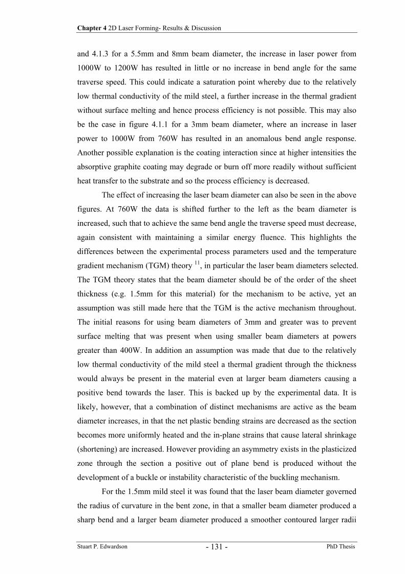
Chapter 4 2D Laser Forming- Results & Discussion
Stuart P. Edwardson PhD Thesis - 131 -
and 4.1.3 for a 5.5mm and 8mm beam diameter, the increase in laser power from
1000W to 1200W has resulted in little or no increase in bend angle for the same
traverse speed. This could indicate a saturation point whereby due to the relatively
low thermal conductivity of the mild steel, a further increase in the thermal gradient
without surface melting and hence process efficiency is not possible. This may also
be the case in figure 4.1.1 for a 3mm beam diameter, where an increase in laser
power to 1000W from 760W has resulted in an anomalous bend angle response.
Another possible explanation is the coating interaction since at higher intensities the
absorptive graphite coating may degrade or burn off more readily without sufficient
heat transfer to the substrate and so the process efficiency is decreased.
The effect of increasing the laser beam diameter can also be seen in the above
figures. At 760W the data is shifted further to the left as the beam diameter is
increased, such that to achieve the same bend angle the traverse speed must decrease,
again consistent with maintaining a similar energy fluence. This highlights the
differences between the experimental process parameters used and the temperature
gradient mechanism (TGM) theory 11, in particular the laser beam diameters selected.
The TGM theory states that the beam diameter should be of the order of the sheet
thickness (e.g. 1.5mm for this material) for the mechanism to be active, yet an
assumption was still made here that the TGM is the active mechanism throughout.
The initial reasons for using beam diameters of 3mm and greater was to prevent
surface melting that was present when using smaller beam diameters at powers
greater than 400W. In addition an assumption was made that due to the relatively
low thermal conductivity of the mild steel a thermal gradient through the thickness
would always be present in the material even at larger beam diameters causing a
positive bend towards the laser. This is backed up by the experimental data. It is
likely, however, that a combination of distinct mechanisms are active as the beam
diameter increases, in that the net plastic bending strains are decreased as the section
becomes more uniformly heated and the in-plane strains that cause lateral shrinkage
(shortening) are increased. However providing an asymmetry exists in the plasticized
zone through the section a positive out of plane bend is produced without the
development of a buckle or instability characteristic of the buckling mechanism.
For the 1.5mm mild steel it was found that the laser beam diameter governed
the radius of curvature in the bent zone, in that a smaller beam diameter produced a
sharp bend and a larger beam diameter produced a smoother contoured larger radii
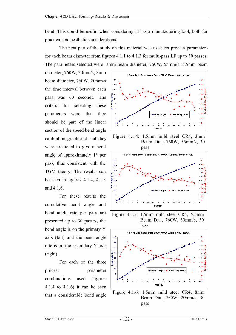
Chapter 4 2D Laser Forming- Results & Discussion
Stuart P. Edwardson PhD Thesis - 132 -
bend. This could be useful when considering LF as a manufacturing tool, both for
practical and aesthetic considerations.
The next part of the study on this material was to select process parameters
for each beam diameter from figures 4.1.1 to 4.1.3 for multi-pass LF up to 30 passes.
The parameters selected were: 3mm beam diameter, 760W, 55mm/s; 5.5mm beam
diameter, 760W, 30mm/s; 8mm
beam diameter, 760W, 20mm/s;
the time interval between each
pass was 60 seconds. The
criteria for selecting these
parameters were that they
should be part of the linear
section of the speed\bend angle
calibration graph and that they
were predicted to give a bend
angle of approximately 1° per
pass, thus consistent with the
TGM theory. The results can
be seen in figures 4.1.4, 4.1.5
and 4.1.6.
For these results the
cumulative bend angle and
bend angle rate per pass are
presented up to 30 passes, the
bend angle is on the primary Y
axis (left) and the bend angle
rate is on the secondary Y axis
(right).
For each of the three
process parameter
combinations used (figures
4.1.4 to 4.1.6) it can be seen
that a considerable bend angle
Figure 4.1.4: 1.5mm mild steel CR4, 3mm Beam Dia., 760W, 55mm/s, 30 pass
Figure 4.1.5: 1.5mm mild steel CR4, 5.5mm Beam Dia., 760W, 30mm/s, 30 pass
Figure 4.1.6: 1.5mm mild steel CR4, 8mm Beam Dia., 760W, 20mm/s, 30 pass
Chapter 4 2D Laser Forming- Results & Discussion
Stuart P. Edwardson PhD Thesis - 133 -
has been produced in each coupon after 30 passes. It can be noted that the bend angle
increase or bend angle rate per pass was not constant for each of the energy
parameters investigated. It can also be noted that the rate falls off at higher numbers
of passes. This is consistent with previously observed data and is attributed to a
number of factors including strain hardening in the HAZ, section thickening and
absorptive coating burn off, discussed earlier. For the data obtained for a 3mm beam
diameter (figure 4.1.4), the expected bend angle rate of ~1° (figure 4.1.1) was
achieved on only the first pass and for each subsequent pass the bend angle rate per
pass generally decreased (somewhat variably) down to a level of ~0.25° per pass.
For the data obtained using 5.5mm and 8mm beam diameters (figures 4.1.5 and 4.1.6)
the bend angle response was similar, this may be due to the similar energy fluence
realised on each coupon. It can be observed in figures 4.1.5 and 4.1.6 that the
expected bend angle rates per pass of ~1.4° and ~1.6° respectively (figures 4.1.2 and
4.1.3) were obtained in the first few passes. It can also be observed that the bend
angle rate increased up to a maximum over the first four passes and then as with the
3mm beam data a general decrease was observed, however in contrast there was still
a considerable forming rate available after 30 passes for these last two forming
parameters. These results demonstrate that the reliance on a given set of processing
parameters to produce a certain bend angle is not practical in an open loop set-up due
to the variable nature of the bend angle rate per pass. They demonstrate that a closed
loop system would need to be considered to increase the reliability and repeatability
of the LF process; the practical implementation of this concept will be demonstrated
in a later section.
Whilst there are a number of theories for the bend angle rate fall off at higher
number of passes (discussed earlier), the distribution of bend angle rates over a
number of passes has not been commented on before in the literature. This is mainly
due the fact that bend angles measurements are rarely taken less than every five
passes (equipment limitations) or that the data was not analysed in the same way. A
possible explanation for the variable nature of the bend angle rate is that it could be
related to the absorptive coating burn off, in that if regions of the coating within the
irradiated track are degraded more than others (possibly due to the manual nature of
coating application causing variation in thickness) the localised absorption
coefficient and hence heat input locally will be different as the laser is traversed
across the coupon. In addition, as an alternating strategy was used throughout (scan
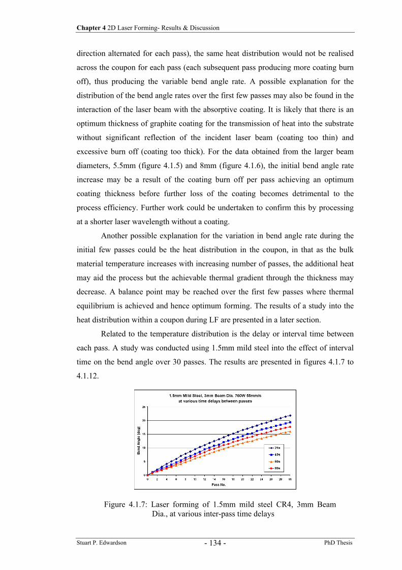
Chapter 4 2D Laser Forming- Results & Discussion
Stuart P. Edwardson PhD Thesis - 134 -
direction alternated for each pass), the same heat distribution would not be realised
across the coupon for each pass (each subsequent pass producing more coating burn
off), thus producing the variable bend angle rate. A possible explanation for the
distribution of the bend angle rates over the first few passes may also be found in the
interaction of the laser beam with the absorptive coating. It is likely that there is an
optimum thickness of graphite coating for the transmission of heat into the substrate
without significant reflection of the incident laser beam (coating too thin) and
excessive burn off (coating too thick). For the data obtained from the larger beam
diameters, 5.5mm (figure 4.1.5) and 8mm (figure 4.1.6), the initial bend angle rate
increase may be a result of the coating burn off per pass achieving an optimum
coating thickness before further loss of the coating becomes detrimental to the
process efficiency. Further work could be undertaken to confirm this by processing
at a shorter laser wavelength without a coating.
Another possible explanation for the variation in bend angle rate during the
initial few passes could be the heat distribution in the coupon, in that as the bulk
material temperature increases with increasing number of passes, the additional heat
may aid the process but the achievable thermal gradient through the thickness may
decrease. A balance point may be reached over the first few passes where thermal
equilibrium is achieved and hence optimum forming. The results of a study into the
heat distribution within a coupon during LF are presented in a later section.
Related to the temperature distribution is the delay or interval time between
each pass. A study was conducted using 1.5mm mild steel into the effect of interval
time on the bend angle over 30 passes. The results are presented in figures 4.1.7 to
4.1.12.
Figure 4.1.7: Laser forming of 1.5mm mild steel CR4, 3mm Beam
Dia., at various inter-pass time delays
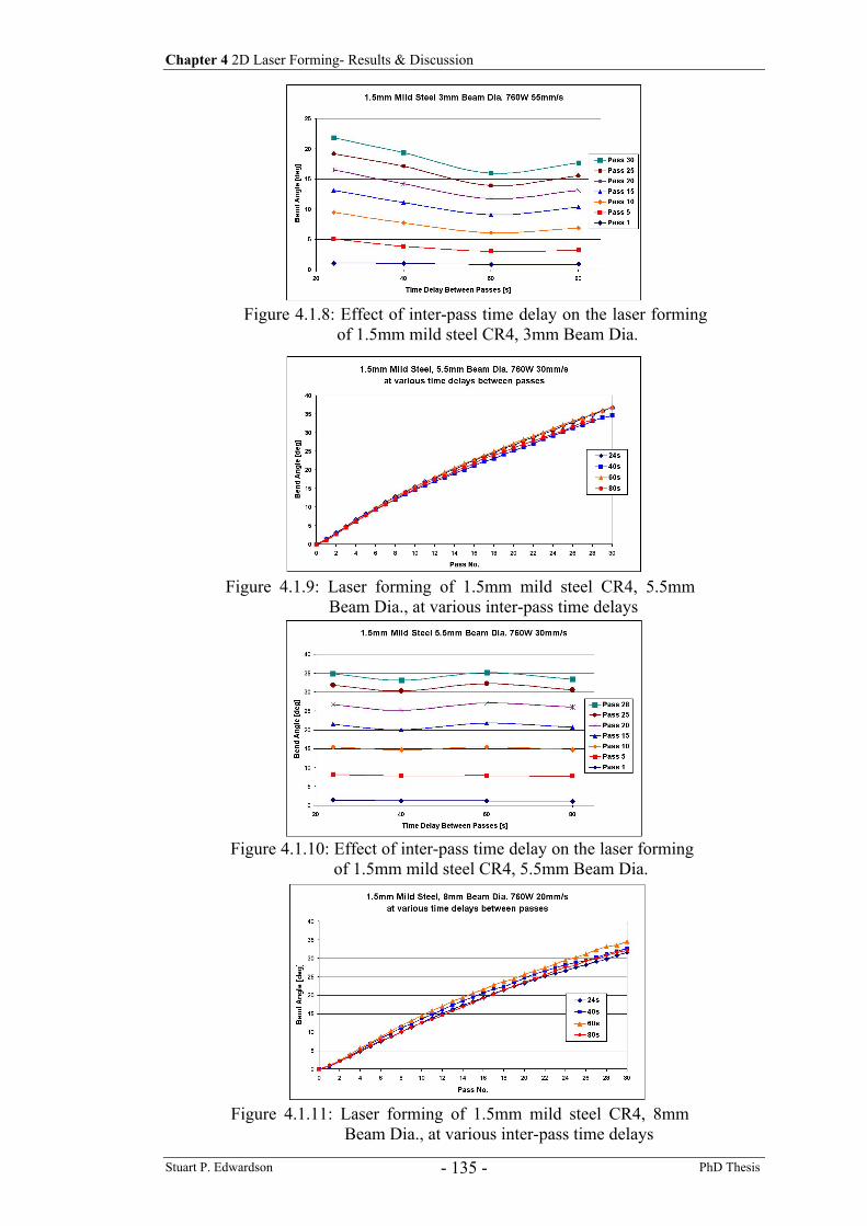
Chapter 4 2D Laser Forming- Results & Discussion
Stuart P. Edwardson PhD Thesis - 135 -
Figure 4.1.8: Effect of inter-pass time delay on the laser forming of 1.5mm mild steel CR4, 3mm Beam Dia.
Figure 4.1.9: Laser forming of 1.5mm mild steel CR4, 5.5mm Beam Dia., at various inter-pass time delays
Figure 4.1.10: Effect of inter-pass time delay on the laser forming of 1.5mm mild steel CR4, 5.5mm Beam Dia.
Figure 4.1.11: Laser forming of 1.5mm mild steel CR4, 8mm Beam Dia., at various inter-pass time delays
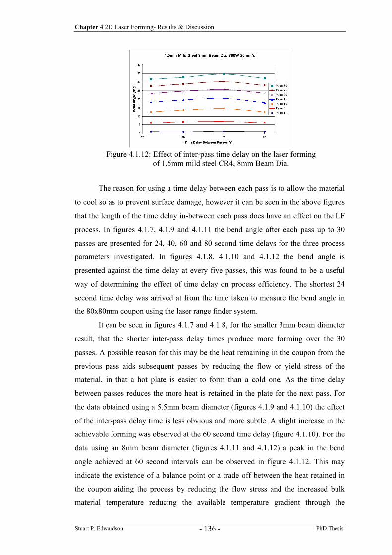
Chapter 4 2D Laser Forming- Results & Discussion
Stuart P. Edwardson PhD Thesis - 136 -
The reason for using a time delay between each pass is to allow the material
to cool so as to prevent surface damage, however it can be seen in the above figures
that the length of the time delay in-between each pass does have an effect on the LF
process. In figures 4.1.7, 4.1.9 and 4.1.11 the bend angle after each pass up to 30
passes are presented for 24, 40, 60 and 80 second time delays for the three process
parameters investigated. In figures 4.1.8, 4.1.10 and 4.1.12 the bend angle is
presented against the time delay at every five passes, this was found to be a useful
way of determining the effect of time delay on process efficiency. The shortest 24
second time delay was arrived at from the time taken to measure the bend angle in
the 80x80mm coupon using the laser range finder system.
It can be seen in figures 4.1.7 and 4.1.8, for the smaller 3mm beam diameter
result, that the shorter inter-pass delay times produce more forming over the 30
passes. A possible reason for this may be the heat remaining in the coupon from the
previous pass aids subsequent passes by reducing the flow or yield stress of the
material, in that a hot plate is easier to form than a cold one. As the time delay
between passes reduces the more heat is retained in the plate for the next pass. For
the data obtained using a 5.5mm beam diameter (figures 4.1.9 and 4.1.10) the effect
of the inter-pass delay time is less obvious and more subtle. A slight increase in the
achievable forming was observed at the 60 second time delay (figure 4.1.10). For the
data using an 8mm beam diameter (figures 4.1.11 and 4.1.12) a peak in the bend
angle achieved at 60 second intervals can be observed in figure 4.1.12. This may
indicate the existence of a balance point or a trade off between the heat retained in
the coupon aiding the process by reducing the flow stress and the increased bulk
material temperature reducing the available temperature gradient through the
Figure 4.1.12: Effect of inter-pass time delay on the laser forming of 1.5mm mild steel CR4, 8mm Beam Dia.
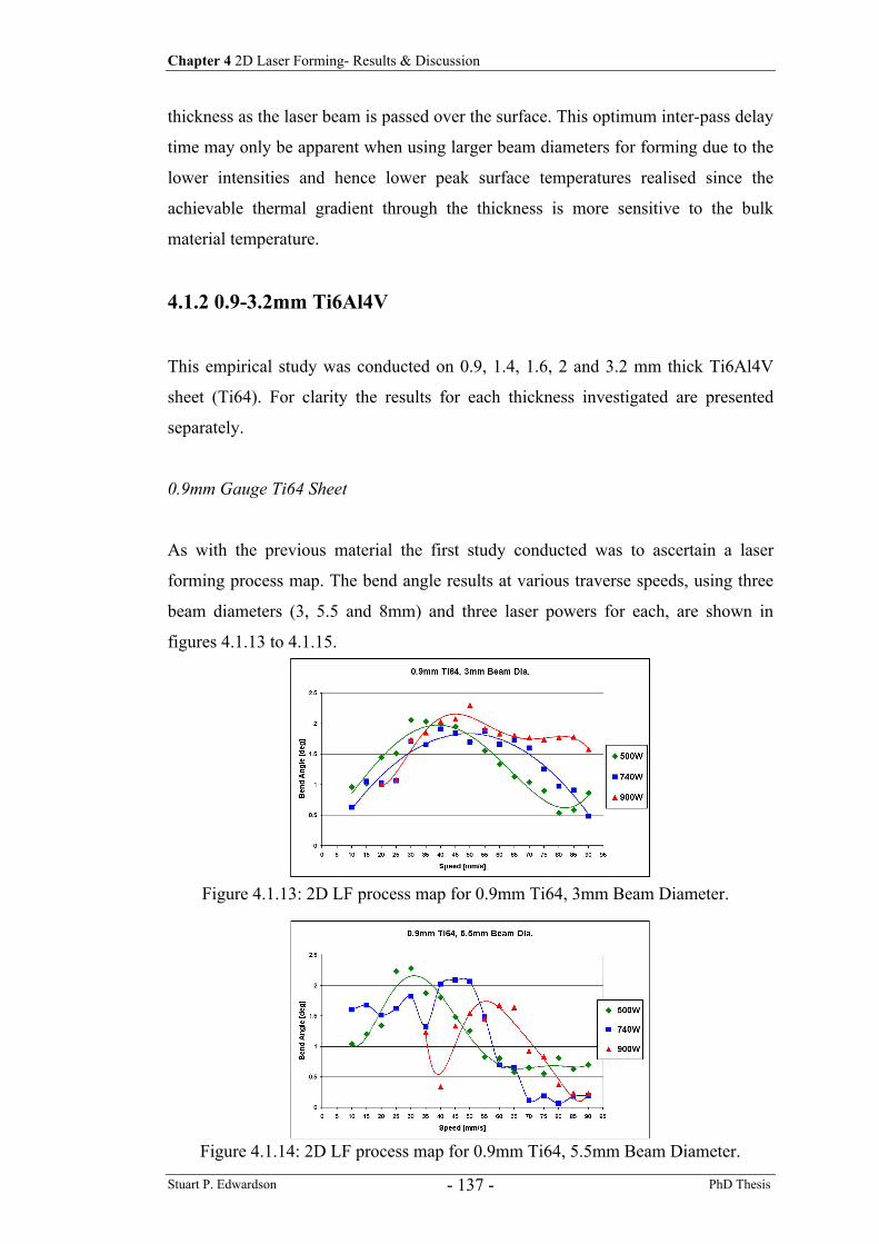
Chapter 4 2D Laser Forming- Results & Discussion
Stuart P. Edwardson PhD Thesis - 137 -
thickness as the laser beam is passed over the surface. This optimum inter-pass delay
time may only be apparent when using larger beam diameters for forming due to the
lower intensities and hence lower peak surface temperatures realised since the
achievable thermal gradient through the thickness is more sensitive to the bulk
material temperature.
4.1.2 0.9-3.2mm Ti6Al4V
This empirical study was conducted on 0.9, 1.4, 1.6, 2 and 3.2 mm thick Ti6Al4V
sheet (Ti64). For clarity the results for each thickness investigated are presented
separately.
0.9mm Gauge Ti64 Sheet
As with the previous material the first study conducted was to ascertain a laser
forming process map. The bend angle results at various traverse speeds, using three
beam diameters (3, 5.5 and 8mm) and three laser powers for each, are shown in
figures 4.1.13 to 4.1.15.
Figure 4.1.13: 2D LF process map for 0.9mm Ti64, 3mm Beam Diameter.
Figure 4.1.14: 2D LF process map for 0.9mm Ti64, 5.5mm Beam Diameter.
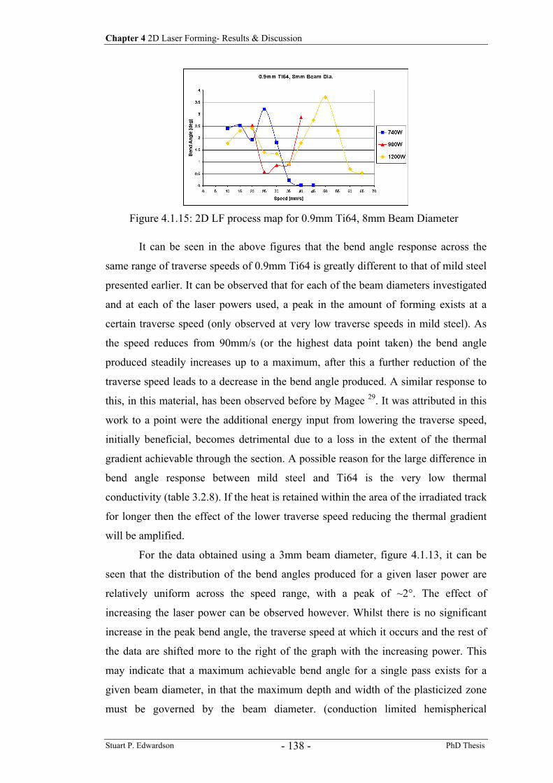
Chapter 4 2D Laser Forming- Results & Discussion
Stuart P. Edwardson PhD Thesis - 138 -
It can be seen in the above figures that the bend angle response across the
same range of traverse speeds of 0.9mm Ti64 is greatly different to that of mild steel
presented earlier. It can be observed that for each of the beam diameters investigated
and at each of the laser powers used, a peak in the amount of forming exists at a
certain traverse speed (only observed at very low traverse speeds in mild steel). As
the speed reduces from 90mm/s (or the highest data point taken) the bend angle
produced steadily increases up to a maximum, after this a further reduction of the
traverse speed leads to a decrease in the bend angle produced. A similar response to
this, in this material, has been observed before by Magee 29. It was attributed in this
work to a point were the additional energy input from lowering the traverse speed,
initially beneficial, becomes detrimental due to a loss in the extent of the thermal
gradient achievable through the section. A possible reason for the large difference in
bend angle response between mild steel and Ti64 is the very low thermal
conductivity (table 3.2.8). If the heat is retained within the area of the irradiated track
for longer then the effect of the lower traverse speed reducing the thermal gradient
will be amplified.
For the data obtained using a 3mm beam diameter, figure 4.1.13, it can be
seen that the distribution of the bend angles produced for a given laser power are
relatively uniform across the speed range, with a peak of ~2°. The effect of
increasing the laser power can be observed however. Whilst there is no significant
increase in the peak bend angle, the traverse speed at which it occurs and the rest of
the data are shifted more to the right of the graph with the increasing power. This
may indicate that a maximum achievable bend angle for a single pass exists for a
given beam diameter, in that the maximum depth and width of the plasticized zone
must be governed by the beam diameter. (conduction limited hemispherical
Figure 4.1.15: 2D LF process map for 0.9mm Ti64, 8mm Beam Diameter
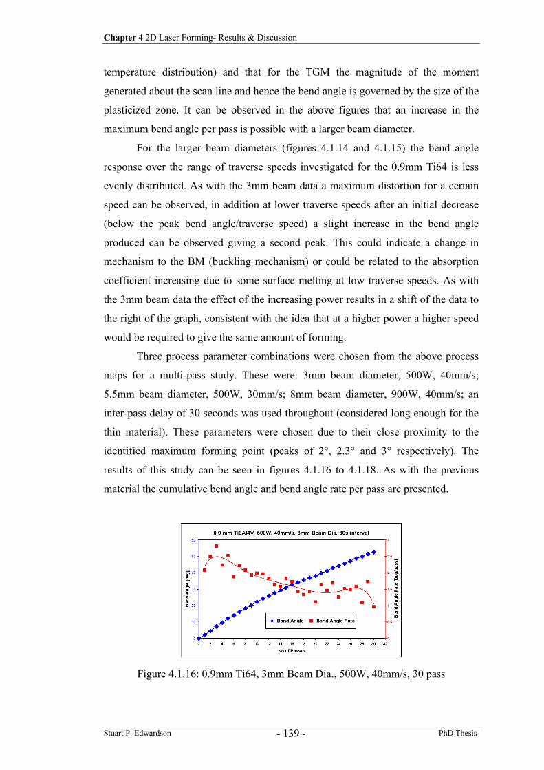
Chapter 4 2D Laser Forming- Results & Discussion
Stuart P. Edwardson PhD Thesis - 139 -
temperature distribution) and that for the TGM the magnitude of the moment
generated about the scan line and hence the bend angle is governed by the size of the
plasticized zone. It can be observed in the above figures that an increase in the
maximum bend angle per pass is possible with a larger beam diameter.
For the larger beam diameters (figures 4.1.14 and 4.1.15) the bend angle
response over the range of traverse speeds investigated for the 0.9mm Ti64 is less
evenly distributed. As with the 3mm beam data a maximum distortion for a certain
speed can be observed, in addition at lower traverse speeds after an initial decrease
(below the peak bend angle/traverse speed) a slight increase in the bend angle
produced can be observed giving a second peak. This could indicate a change in
mechanism to the BM (buckling mechanism) or could be related to the absorption
coefficient increasing due to some surface melting at low traverse speeds. As with
the 3mm beam data the effect of the increasing power results in a shift of the data to
the right of the graph, consistent with the idea that at a higher power a higher speed
would be required to give the same amount of forming.
Three process parameter combinations were chosen from the above process
maps for a multi-pass study. These were: 3mm beam diameter, 500W, 40mm/s;
5.5mm beam diameter, 500W, 30mm/s; 8mm beam diameter, 900W, 40mm/s; an
inter-pass delay of 30 seconds was used throughout (considered long enough for the
thin material). These parameters were chosen due to their close proximity to the
identified maximum forming point (peaks of 2°, 2.3° and 3° respectively). The
results of this study can be seen in figures 4.1.16 to 4.1.18. As with the previous
material the cumulative bend angle and bend angle rate per pass are presented.
Figure 4.1.16: 0.9mm Ti64, 3mm Beam Dia., 500W, 40mm/s, 30 pass
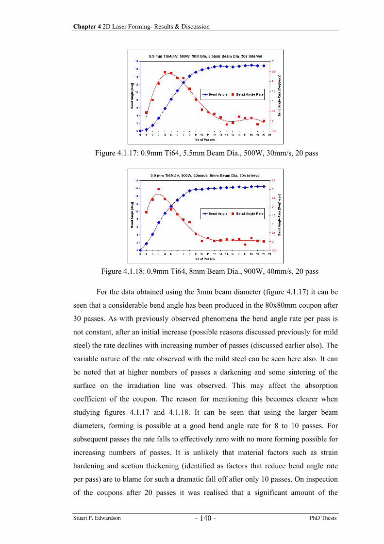
Chapter 4 2D Laser Forming- Results & Discussion
Stuart P. Edwardson PhD Thesis - 140 -
For the data obtained using the 3mm beam diameter (figure 4.1.17) it can be
seen that a considerable bend angle has been produced in the 80x80mm coupon after
30 passes. As with previously observed phenomena the bend angle rate per pass is
not constant, after an initial increase (possible reasons discussed previously for mild
steel) the rate declines with increasing number of passes (discussed earlier also). The
variable nature of the rate observed with the mild steel can be seen here also. It can
be noted that at higher numbers of passes a darkening and some sintering of the
surface on the irradiation line was observed. This may affect the absorption
coefficient of the coupon. The reason for mentioning this becomes clearer when
studying figures 4.1.17 and 4.1.18. It can be seen that using the larger beam
diameters, forming is possible at a good bend angle rate for 8 to 10 passes. For
subsequent passes the rate falls to effectively zero with no more forming possible for
increasing numbers of passes. It is unlikely that material factors such as strain
hardening and section thickening (identified as factors that reduce bend angle rate
per pass) are to blame for such a dramatic fall off after only 10 passes. On inspection
of the coupons after 20 passes it was realised that a significant amount of the
Figure 4.1.17: 0.9mm Ti64, 5.5mm Beam Dia., 500W, 30mm/s, 20 pass
Figure 4.1.18: 0.9mm Ti64, 8mm Beam Dia., 900W, 40mm/s, 20 pass
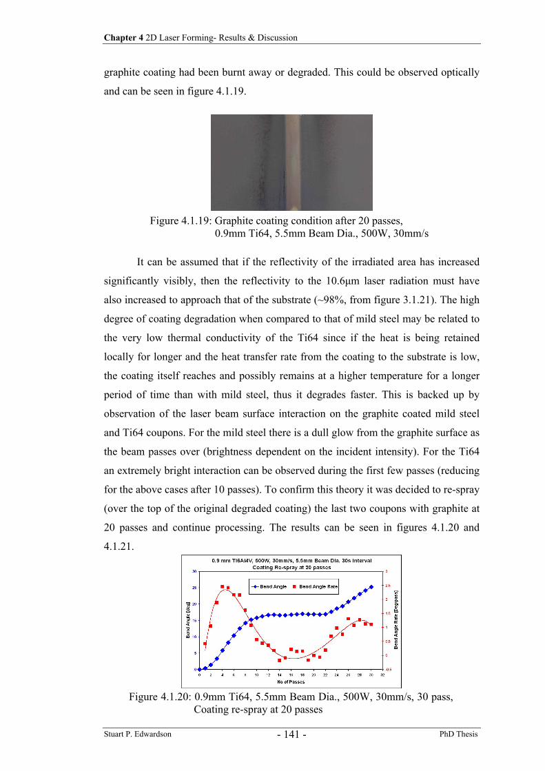
Chapter 4 2D Laser Forming- Results & Discussion
Stuart P. Edwardson PhD Thesis - 141 -
graphite coating had been burnt away or degraded. This could be observed optically
and can be seen in figure 4.1.19.
It can be assumed that if the reflectivity of the irradiated area has increased
significantly visibly, then the reflectivity to the 10.6µm laser radiation must have
also increased to approach that of the substrate (~98%, from figure 3.1.21). The high
degree of coating degradation when compared to that of mild steel may be related to
the very low thermal conductivity of the Ti64 since if the heat is being retained
locally for longer and the heat transfer rate from the coating to the substrate is low,
the coating itself reaches and possibly remains at a higher temperature for a longer
period of time than with mild steel, thus it degrades faster. This is backed up by
observation of the laser beam surface interaction on the graphite coated mild steel
and Ti64 coupons. For the mild steel there is a dull glow from the graphite surface as
the beam passes over (brightness dependent on the incident intensity). For the Ti64
an extremely bright interaction can be observed during the first few passes (reducing
for the above cases after 10 passes). To confirm this theory it was decided to re-spray
(over the top of the original degraded coating) the last two coupons with graphite at
20 passes and continue processing. The results can be seen in figures 4.1.20 and
4.1.21.
Figure 4.1.19: Graphite coating condition after 20 passes, 0.9mm Ti64, 5.5mm Beam Dia., 500W, 30mm/s
Figure 4.1.20: 0.9mm Ti64, 5.5mm Beam Dia., 500W, 30mm/s, 30 pass, Coating re-spray at 20 passes
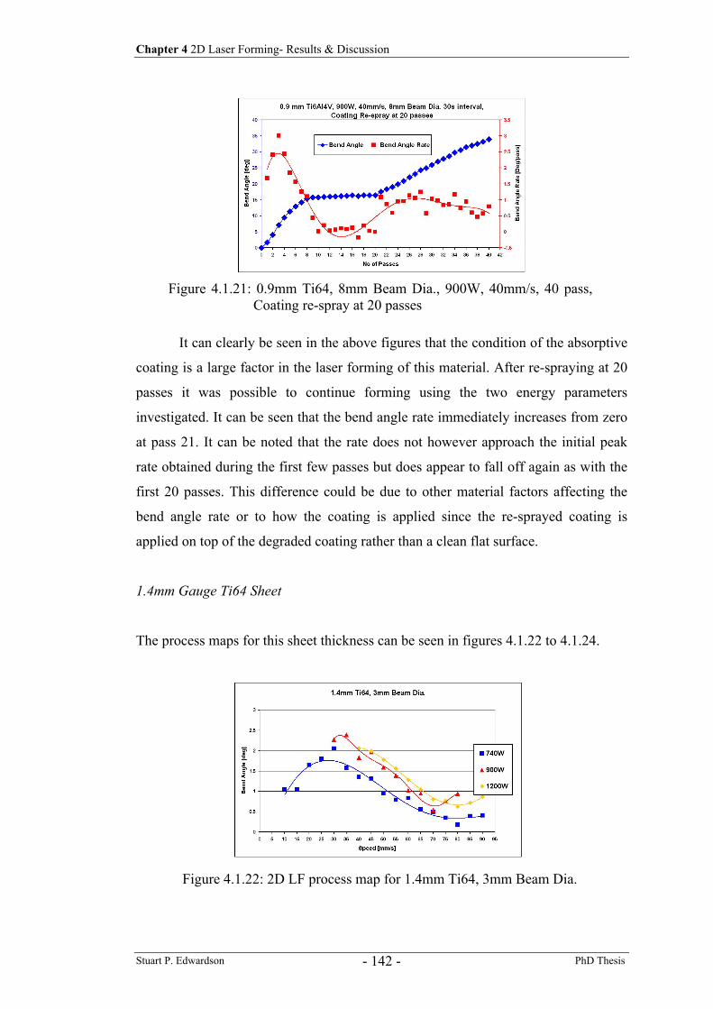
Chapter 4 2D Laser Forming- Results & Discussion
Stuart P. Edwardson PhD Thesis - 142 -
It can clearly be seen in the above figures that the condition of the absorptive
coating is a large factor in the laser forming of this material. After re-spraying at 20
passes it was possible to continue forming using the two energy parameters
investigated. It can be seen that the bend angle rate immediately increases from zero
at pass 21. It can be noted that the rate does not however approach the initial peak
rate obtained during the first few passes but does appear to fall off again as with the
first 20 passes. This difference could be due to other material factors affecting the
bend angle rate or to how the coating is applied since the re-sprayed coating is
applied on top of the degraded coating rather than a clean flat surface.
1.4mm Gauge Ti64 Sheet
The process maps for this sheet thickness can be seen in figures 4.1.22 to 4.1.24.
Figure 4.1.21: 0.9mm Ti64, 8mm Beam Dia., 900W, 40mm/s, 40 pass, Coating re-spray at 20 passes
Figure 4.1.22: 2D LF process map for 1.4mm Ti64, 3mm Beam Dia.
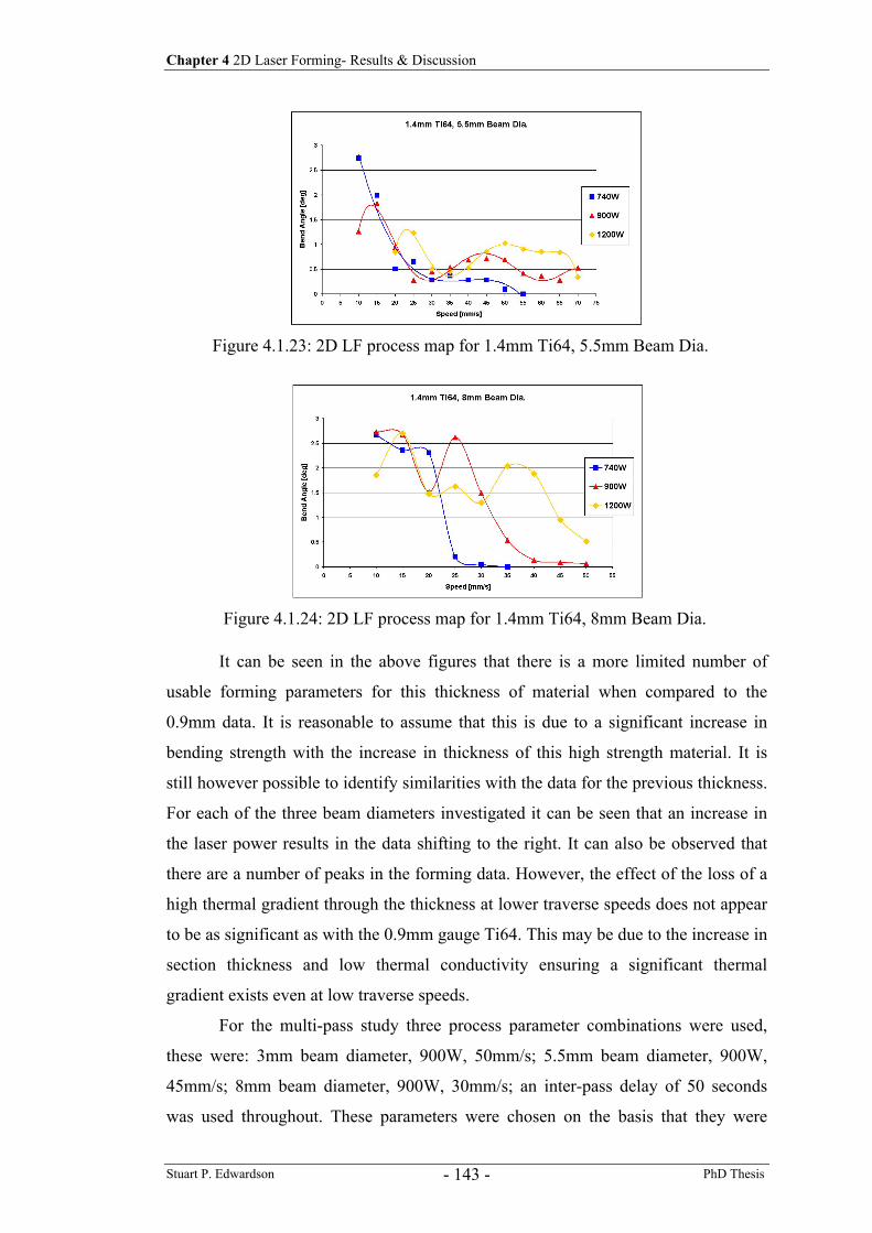
Chapter 4 2D Laser Forming- Results & Discussion
Stuart P. Edwardson PhD Thesis - 143 -
It can be seen in the above figures that there is a more limited number of
usable forming parameters for this thickness of material when compared to the
0.9mm data. It is reasonable to assume that this is due to a significant increase in
bending strength with the increase in thickness of this high strength material. It is
still however possible to identify similarities with the data for the previous thickness.
For each of the three beam diameters investigated it can be seen that an increase in
the laser power results in the data shifting to the right. It can also be observed that
there are a number of peaks in the forming data. However, the effect of the loss of a
high thermal gradient through the thickness at lower traverse speeds does not appear
to be as significant as with the 0.9mm gauge Ti64. This may be due to the increase in
section thickness and low thermal conductivity ensuring a significant thermal
gradient exists even at low traverse speeds.
For the multi-pass study three process parameter combinations were used,
these were: 3mm beam diameter, 900W, 50mm/s; 5.5mm beam diameter, 900W,
45mm/s; 8mm beam diameter, 900W, 30mm/s; an inter-pass delay of 50 seconds
was used throughout. These parameters were chosen on the basis that they were
Figure 4.1.23: 2D LF process map for 1.4mm Ti64, 5.5mm Beam Dia.
Figure 4.1.24: 2D LF process map for 1.4mm Ti64, 8mm Beam Dia.
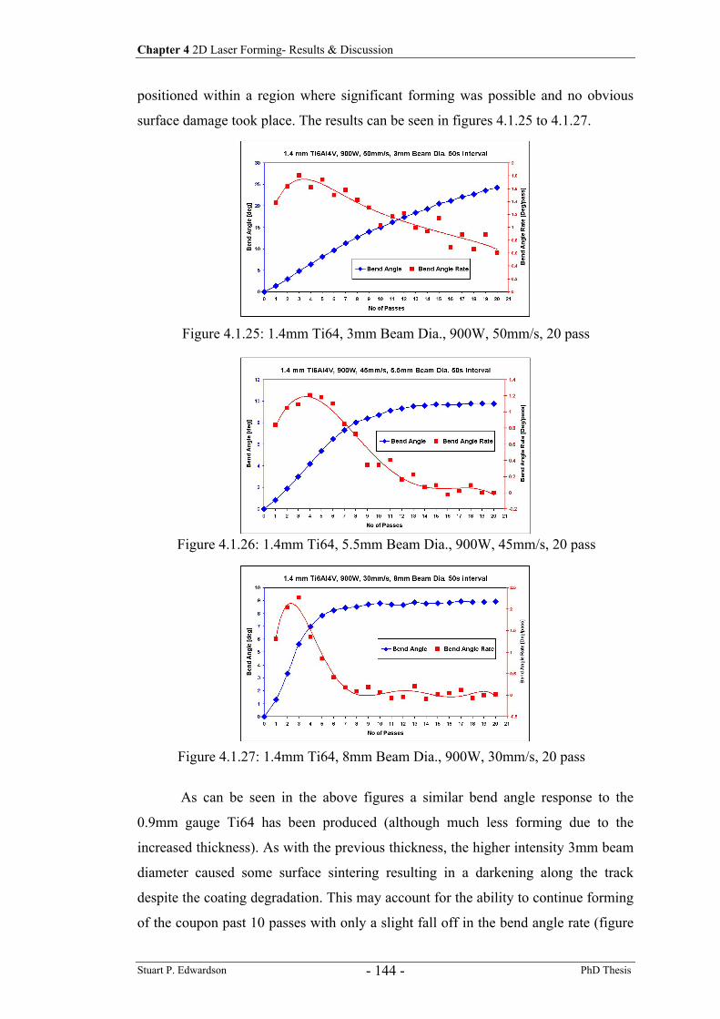
Chapter 4 2D Laser Forming- Results & Discussion
Stuart P. Edwardson PhD Thesis - 144 -
positioned within a region where significant forming was possible and no obvious
surface damage took place. The results can be seen in figures 4.1.25 to 4.1.27.
As can be seen in the above figures a similar bend angle response to the
0.9mm gauge Ti64 has been produced (although much less forming due to the
increased thickness). As with the previous thickness, the higher intensity 3mm beam
diameter caused some surface sintering resulting in a darkening along the track
despite the coating degradation. This may account for the ability to continue forming
of the coupon past 10 passes with only a slight fall off in the bend angle rate (figure
Figure 4.1.25: 1.4mm Ti64, 3mm Beam Dia., 900W, 50mm/s, 20 pass
Figure 4.1.26: 1.4mm Ti64, 5.5mm Beam Dia., 900W, 45mm/s, 20 pass
Figure 4.1.27: 1.4mm Ti64, 8mm Beam Dia., 900W, 30mm/s, 20 pass
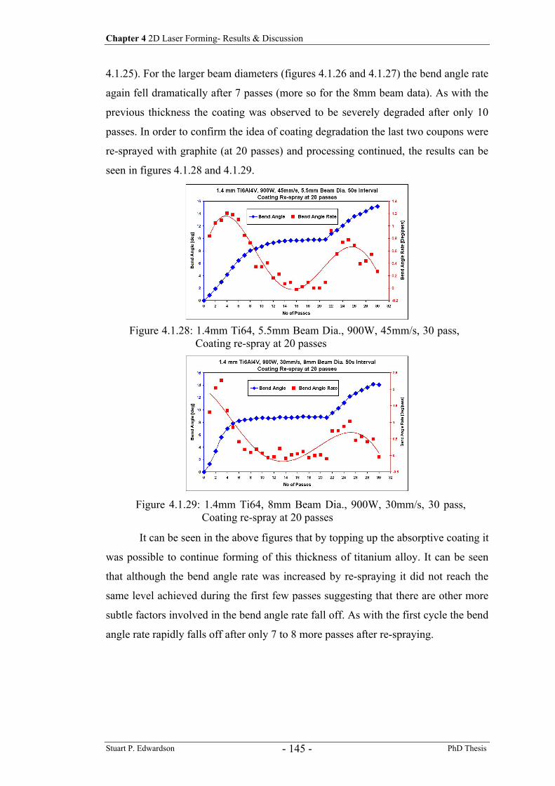
Chapter 4 2D Laser Forming- Results & Discussion
Stuart P. Edwardson PhD Thesis - 145 -
4.1.25). For the larger beam diameters (figures 4.1.26 and 4.1.27) the bend angle rate
again fell dramatically after 7 passes (more so for the 8mm beam data). As with the
previous thickness the coating was observed to be severely degraded after only 10
passes. In order to confirm the idea of coating degradation the last two coupons were
re-sprayed with graphite (at 20 passes) and processing continued, the results can be
seen in figures 4.1.28 and 4.1.29.
It can be seen in the above figures that by topping up the absorptive coating it
was possible to continue forming of this thickness of titanium alloy. It can be seen
that although the bend angle rate was increased by re-spraying it did not reach the
same level achieved during the first few passes suggesting that there are other more
subtle factors involved in the bend angle rate fall off. As with the first cycle the bend
angle rate rapidly falls off after only 7 to 8 more passes after re-spraying.
Figure 4.1.28: 1.4mm Ti64, 5.5mm Beam Dia., 900W, 45mm/s, 30 pass, Coating re-spray at 20 passes
Figure 4.1.29: 1.4mm Ti64, 8mm Beam Dia., 900W, 30mm/s, 30 pass, Coating re-spray at 20 passes
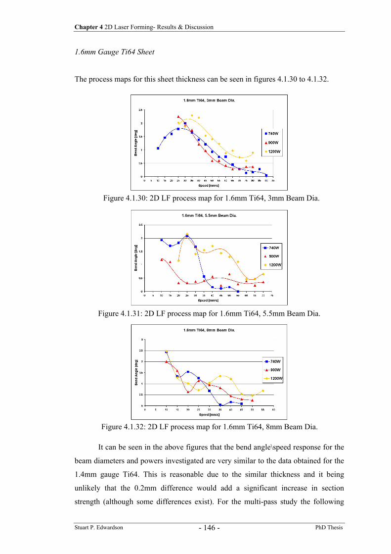
Chapter 4 2D Laser Forming- Results & Discussion
Stuart P. Edwardson PhD Thesis - 146 -
1.6mm Gauge Ti64 Sheet
The process maps for this sheet thickness can be seen in figures 4.1.30 to 4.1.32.
It can be seen in the above figures that the bend angle\speed response for the
beam diameters and powers investigated are very similar to the data obtained for the
1.4mm gauge Ti64. This is reasonable due to the similar thickness and it being
unlikely that the 0.2mm difference would add a significant increase in section
strength (although some differences exist). For the multi-pass study the following
Figure 4.1.30: 2D LF process map for 1.6mm Ti64, 3mm Beam Dia.
Figure 4.1.31: 2D LF process map for 1.6mm Ti64, 5.5mm Beam Dia.
Figure 4.1.32: 2D LF process map for 1.6mm Ti64, 8mm Beam Dia.
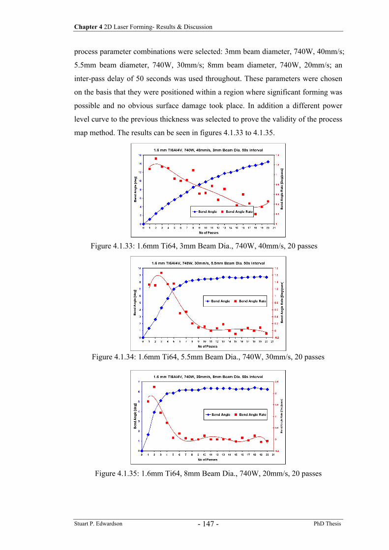
Chapter 4 2D Laser Forming- Results & Discussion
Stuart P. Edwardson PhD Thesis - 147 -
process parameter combinations were selected: 3mm beam diameter, 740W, 40mm/s;
5.5mm beam diameter, 740W, 30mm/s; 8mm beam diameter, 740W, 20mm/s; an
inter-pass delay of 50 seconds was used throughout. These parameters were chosen
on the basis that they were positioned within a region where significant forming was
possible and no obvious surface damage took place. In addition a different power
level curve to the previous thickness was selected to prove the validity of the process
map method. The results can be seen in figures 4.1.33 to 4.1.35.
Figure 4.1.33: 1.6mm Ti64, 3mm Beam Dia., 740W, 40mm/s, 20 passes
Figure 4.1.34: 1.6mm Ti64, 5.5mm Beam Dia., 740W, 30mm/s, 20 passes
Figure 4.1.35: 1.6mm Ti64, 8mm Beam Dia., 740W, 20mm/s, 20 passes
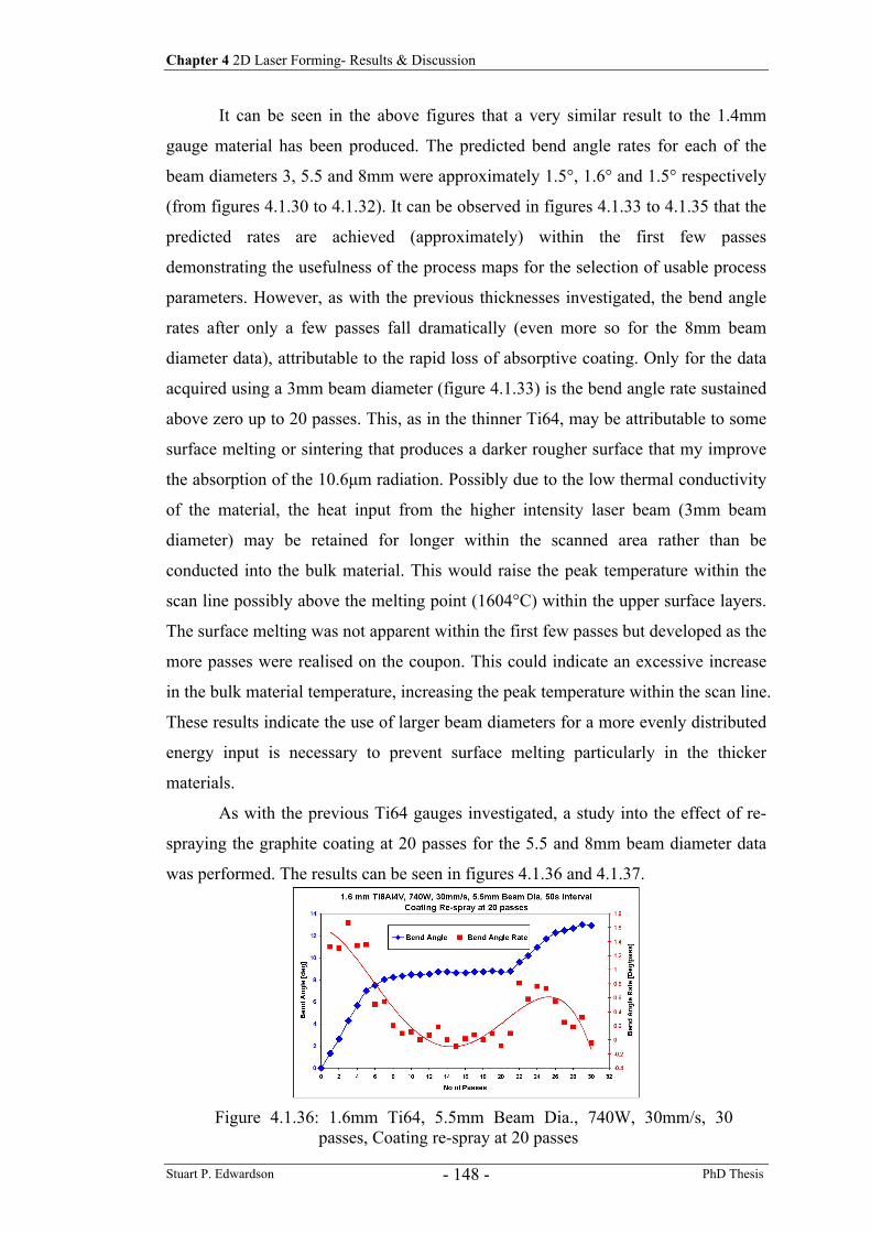
Chapter 4 2D Laser Forming- Results & Discussion
Stuart P. Edwardson PhD Thesis - 148 -
It can be seen in the above figures that a very similar result to the 1.4mm
gauge material has been produced. The predicted bend angle rates for each of the
beam diameters 3, 5.5 and 8mm were approximately 1.5°, 1.6° and 1.5° respectively
(from figures 4.1.30 to 4.1.32). It can be observed in figures 4.1.33 to 4.1.35 that the
predicted rates are achieved (approximately) within the first few passes
demonstrating the usefulness of the process maps for the selection of usable process
parameters. However, as with the previous thicknesses investigated, the bend angle
rates after only a few passes fall dramatically (even more so for the 8mm beam
diameter data), attributable to the rapid loss of absorptive coating. Only for the data
acquired using a 3mm beam diameter (figure 4.1.33) is the bend angle rate sustained
above zero up to 20 passes. This, as in the thinner Ti64, may be attributable to some
surface melting or sintering that produces a darker rougher surface that my improve
the absorption of the 10.6µm radiation. Possibly due to the low thermal conductivity
of the material, the heat input from the higher intensity laser beam (3mm beam
diameter) may be retained for longer within the scanned area rather than be
conducted into the bulk material. This would raise the peak temperature within the
scan line possibly above the melting point (1604°C) within the upper surface layers.
The surface melting was not apparent within the first few passes but developed as the
more passes were realised on the coupon. This could indicate an excessive increase
in the bulk material temperature, increasing the peak temperature within the scan line.
These results indicate the use of larger beam diameters for a more evenly distributed
energy input is necessary to prevent surface melting particularly in the thicker
materials.
As with the previous Ti64 gauges investigated, a study into the effect of re-
spraying the graphite coating at 20 passes for the 5.5 and 8mm beam diameter data
was performed. The results can be seen in figures 4.1.36 and 4.1.37.
Figure 4.1.36: 1.6mm Ti64, 5.5mm Beam Dia., 740W, 30mm/s, 30 passes, Coating re-spray at 20 passes
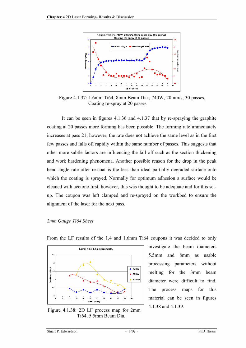
Chapter 4 2D Laser Forming- Results & Discussion
Stuart P. Edwardson PhD Thesis - 149 -
It can be seen in figures 4.1.36 and 4.1.37 that by re-spraying the graphite
coating at 20 passes more forming has been possible. The forming rate immediately
increases at pass 21; however, the rate does not achieve the same level as in the first
few passes and falls off rapidly within the same number of passes. This suggests that
other more subtle factors are influencing the fall off such as the section thickening
and work hardening phenomena. Another possible reason for the drop in the peak
bend angle rate after re-coat is the less than ideal partially degraded surface onto
which the coating is sprayed. Normally for optimum adhesion a surface would be
cleaned with acetone first, however, this was thought to be adequate and for this set-
up. The coupon was left clamped and re-sprayed on the workbed to ensure the
alignment of the laser for the next pass.
2mm Gauge Ti64 Sheet
From the LF results of the 1.4 and 1.6mm Ti64 coupons it was decided to only
investigate the beam diameters
5.5mm and 8mm as usable
processing parameters without
melting for the 3mm beam
diameter were difficult to find.
The process maps for this
material can be seen in figures
4.1.38 and 4.1.39.
Figure 4.1.37: 1.6mm Ti64, 8mm Beam Dia., 740W, 20mm/s, 30 passes, Coating re-spray at 20 passes
Figure 4.1.38: 2D LF process map for 2mm Ti64, 5.5mm Beam Dia.
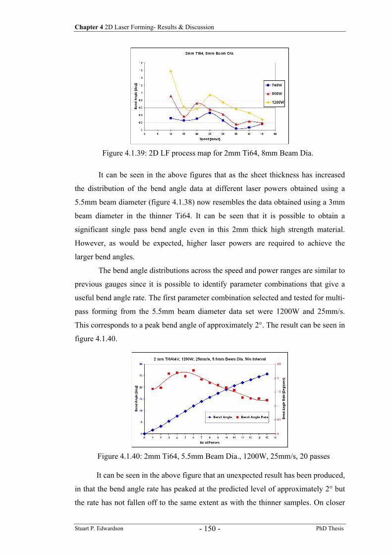
Chapter 4 2D Laser Forming- Results & Discussion
Stuart P. Edwardson PhD Thesis - 150 -
It can be seen in the above figures that as the sheet thickness has increased
the distribution of the bend angle data at different laser powers obtained using a
5.5mm beam diameter (figure 4.1.38) now resembles the data obtained using a 3mm
beam diameter in the thinner Ti64. It can be seen that it is possible to obtain a
significant single pass bend angle even in this 2mm thick high strength material.
However, as would be expected, higher laser powers are required to achieve the
larger bend angles.
The bend angle distributions across the speed and power ranges are similar to
previous gauges since it is possible to identify parameter combinations that give a
useful bend angle rate. The first parameter combination selected and tested for multi-
pass forming from the 5.5mm beam diameter data set were 1200W and 25mm/s.
This corresponds to a peak bend angle of approximately 2°. The result can be seen in
figure 4.1.40.
It can be seen in the above figure that an unexpected result has been produced,
in that the bend angle rate has peaked at the predicted level of approximately 2° but
the rate has not fallen off to the same extent as with the thinner samples. On closer
Figure 4.1.39: 2D LF process map for 2mm Ti64, 8mm Beam Dia.
Figure 4.1.40: 2mm Ti64, 5.5mm Beam Dia., 1200W, 25mm/s, 20 passes
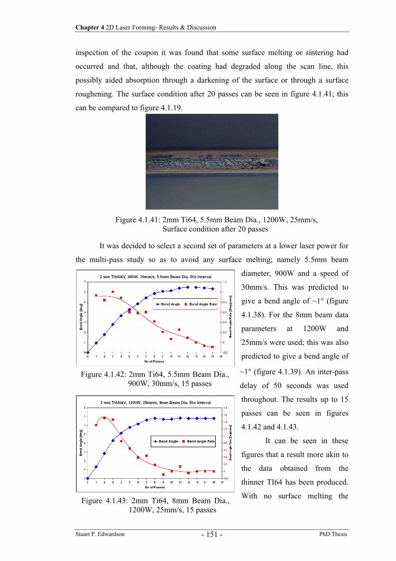
Chapter 4 2D Laser Forming- Results & Discussion
Stuart P. Edwardson PhD Thesis - 151 -
inspection of the coupon it was found that some surface melting or sintering had
occurred and that, although the coating had degraded along the scan line, this
possibly aided absorption through a darkening of the surface or through a surface
roughening. The surface condition after 20 passes can be seen in figure 4.1.41; this
can be compared to figure 4.1.19.
It was decided to select a second set of parameters at a lower laser power for
the multi-pass study so as to avoid any surface melting; namely 5.5mm beam
diameter, 900W and a speed of
30mm/s. This was predicted to
give a bend angle of ~1° (figure
4.1.38). For the 8mm beam data
parameters at 1200W and
25mm/s were used; this was also
predicted to give a bend angle of
~1° (figure 4.1.39). An inter-pass
delay of 50 seconds was used
throughout. The results up to 15
passes can be seen in figures
4.1.42 and 4.1.43.
It can be seen in these
figures that a result more akin to
the data obtained from the
thinner TI64 has been produced.
With no surface melting the
Figure 4.1.41: 2mm Ti64, 5.5mm Beam Dia., 1200W, 25mm/s, Surface condition after 20 passes
Figure 4.1.42: 2mm Ti64, 5.5mm Beam Dia., 900W, 30mm/s, 15 passes
Figure 4.1.43: 2mm Ti64, 8mm Beam Dia., 1200W, 25mm/s, 15 passes
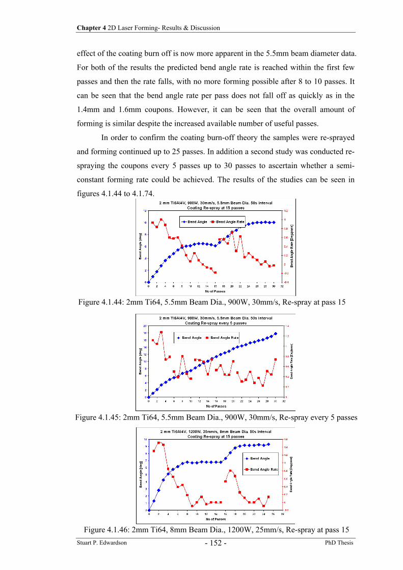
Chapter 4 2D Laser Forming- Results & Discussion
Stuart P. Edwardson PhD Thesis - 152 -
effect of the coating burn off is now more apparent in the 5.5mm beam diameter data.
For both of the results the predicted bend angle rate is reached within the first few
passes and then the rate falls, with no more forming possible after 8 to 10 passes. It
can be seen that the bend angle rate per pass does not fall off as quickly as in the
1.4mm and 1.6mm coupons. However, it can be seen that the overall amount of
forming is similar despite the increased available number of useful passes.
In order to confirm the coating burn-off theory the samples were re-sprayed
and forming continued up to 25 passes. In addition a second study was conducted re-
spraying the coupons every 5 passes up to 30 passes to ascertain whether a semi-
constant forming rate could be achieved. The results of the studies can be seen in
figures 4.1.44 to 4.1.74.
Figure 4.1.44: 2mm Ti64, 5.5mm Beam Dia., 900W, 30mm/s, Re-spray at pass 15
Figure 4.1.45: 2mm Ti64, 5.5mm Beam Dia., 900W, 30mm/s, Re-spray every 5 passes
Figure 4.1.46: 2mm Ti64, 8mm Beam Dia., 1200W, 25mm/s, Re-spray at pass 15
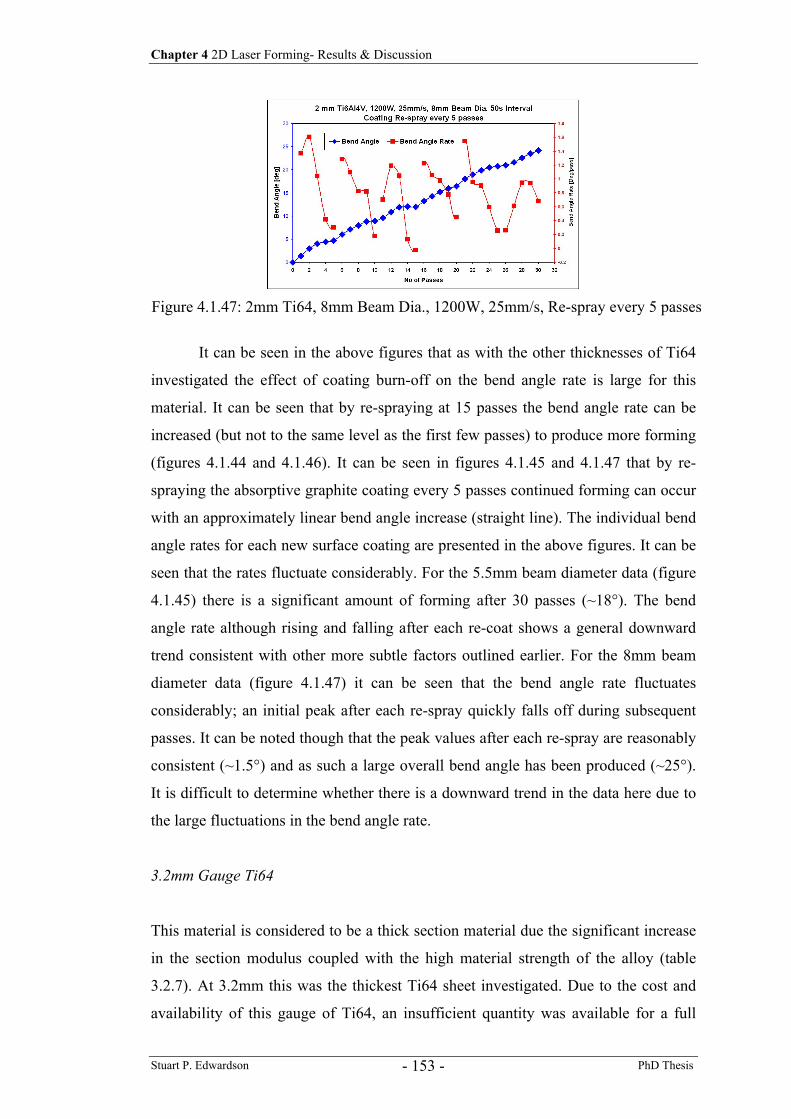
Chapter 4 2D Laser Forming- Results & Discussion
Stuart P. Edwardson PhD Thesis - 153 -
It can be seen in the above figures that as with the other thicknesses of Ti64
investigated the effect of coating burn-off on the bend angle rate is large for this
material. It can be seen that by re-spraying at 15 passes the bend angle rate can be
increased (but not to the same level as the first few passes) to produce more forming
(figures 4.1.44 and 4.1.46). It can be seen in figures 4.1.45 and 4.1.47 that by re-
spraying the absorptive graphite coating every 5 passes continued forming can occur
with an approximately linear bend angle increase (straight line). The individual bend
angle rates for each new surface coating are presented in the above figures. It can be
seen that the rates fluctuate considerably. For the 5.5mm beam diameter data (figure
4.1.45) there is a significant amount of forming after 30 passes (~18°). The bend
angle rate although rising and falling after each re-coat shows a general downward
trend consistent with other more subtle factors outlined earlier. For the 8mm beam
diameter data (figure 4.1.47) it can be seen that the bend angle rate fluctuates
considerably; an initial peak after each re-spray quickly falls off during subsequent
passes. It can be noted though that the peak values after each re-spray are reasonably
consistent (~1.5°) and as such a large overall bend angle has been produced (~25°).
It is difficult to determine whether there is a downward trend in the data here due to
the large fluctuations in the bend angle rate.
3.2mm Gauge Ti64
This material is considered to be a thick section material due the significant increase
in the section modulus coupled with the high material strength of the alloy (table
3.2.7). At 3.2mm this was the thickest Ti64 sheet investigated. Due to the cost and
availability of this gauge of Ti64, an insufficient quantity was available for a full
Figure 4.1.47: 2mm Ti64, 8mm Beam Dia., 1200W, 25mm/s, Re-spray every 5 passes
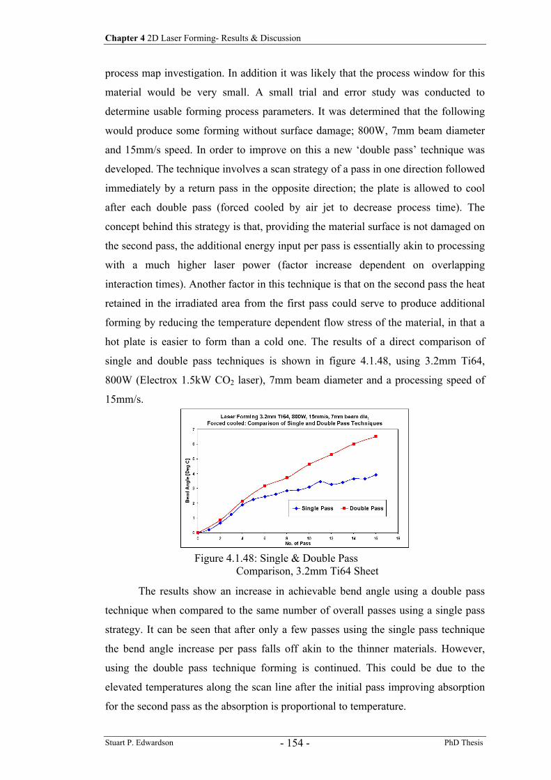
Chapter 4 2D Laser Forming- Results & Discussion
Stuart P. Edwardson PhD Thesis - 154 -
process map investigation. In addition it was likely that the process window for this
material would be very small. A small trial and error study was conducted to
determine usable forming process parameters. It was determined that the following
would produce some forming without surface damage; 800W, 7mm beam diameter
and 15mm/s speed. In order to improve on this a new ‘double pass’ technique was
developed. The technique involves a scan strategy of a pass in one direction followed
immediately by a return pass in the opposite direction; the plate is allowed to cool
after each double pass (forced cooled by air jet to decrease process time). The
concept behind this strategy is that, providing the material surface is not damaged on
the second pass, the additional energy input per pass is essentially akin to processing
with a much higher laser power (factor increase dependent on overlapping
interaction times). Another factor in this technique is that on the second pass the heat
retained in the irradiated area from the first pass could serve to produce additional
forming by reducing the temperature dependent flow stress of the material, in that a
hot plate is easier to form than a cold one. The results of a direct comparison of
single and double pass techniques is shown in figure 4.1.48, using 3.2mm Ti64,
800W (Electrox 1.5kW CO2 laser), 7mm beam diameter and a processing speed of
15mm/s.
The results show an increase in achievable bend angle using a double pass
technique when compared to the same number of overall passes using a single pass
strategy. It can be seen that after only a few passes using the single pass technique
the bend angle increase per pass falls off akin to the thinner materials. However,
using the double pass technique forming is continued. This could be due to the
elevated temperatures along the scan line after the initial pass improving absorption
for the second pass as the absorption is proportional to temperature.
Figure 4.1.48: Single & Double Pass Comparison, 3.2mm Ti64 Sheet
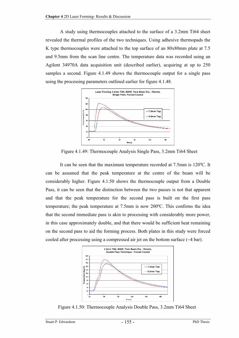
Chapter 4 2D Laser Forming- Results & Discussion
Stuart P. Edwardson PhD Thesis - 155 -
A study using thermocouples attached to the surface of a 3.2mm Ti64 sheet
revealed the thermal profiles of the two techniques. Using adhesive thermopads the
K type thermocouples were attached to the top surface of an 80x80mm plate at 7.5
and 9.5mm from the scan line centre. The temperature data was recorded using an
Agilent 34970A data acquisition unit (described earlier), acquiring at up to 250
samples a second. Figure 4.1.49 shows the thermocouple output for a single pass
using the processing parameters outlined earlier for figure 4.1.48.
It can be seen that the maximum temperature recorded at 7.5mm is 120ºC. It
can be assumed that the peak temperature at the centre of the beam will be
considerably higher. Figure 4.1.50 shows the thermocouple output from a Double
Pass, it can be seen that the distinction between the two passes is not that apparent
and that the peak temperature for the second pass is built on the first pass
temperature; the peak temperature at 7.5mm is now 200ºC. This confirms the idea
that the second immediate pass is akin to processing with considerably more power,
in this case approximately double, and that there would be sufficient heat remaining
on the second pass to aid the forming process. Both plates in this study were forced
cooled after processing using a compressed air jet on the bottom surface (~4 bar).
Figure 4.1.49: Thermocouple Analysis Single Pass, 3.2mm Ti64 Sheet
Figure 4.1.50: Thermocouple Analysis Double Pass, 3.2mm Ti64 Sheet
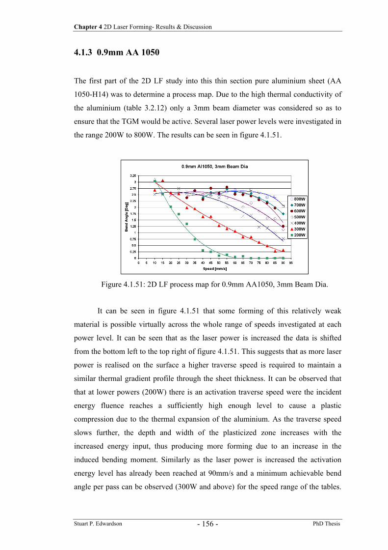
Chapter 4 2D Laser Forming- Results & Discussion
Stuart P. Edwardson PhD Thesis - 156 -
4.1.3 0.9mm AA 1050
The first part of the 2D LF study into this thin section pure aluminium sheet (AA
1050-H14) was to determine a process map. Due to the high thermal conductivity of
the aluminium (table 3.2.12) only a 3mm beam diameter was considered so as to
ensure that the TGM would be active. Several laser power levels were investigated in
the range 200W to 800W. The results can be seen in figure 4.1.51.
It can be seen in figure 4.1.51 that some forming of this relatively weak
material is possible virtually across the whole range of speeds investigated at each
power level. It can be seen that as the laser power is increased the data is shifted
from the bottom left to the top right of figure 4.1.51. This suggests that as more laser
power is realised on the surface a higher traverse speed is required to maintain a
similar thermal gradient profile through the sheet thickness. It can be observed that
that at lower powers (200W) there is an activation traverse speed were the incident
energy fluence reaches a sufficiently high enough level to cause a plastic
compression due to the thermal expansion of the aluminium. As the traverse speed
slows further, the depth and width of the plasticized zone increases with the
increased energy input, thus producing more forming due to an increase in the
induced bending moment. Similarly as the laser power is increased the activation
energy level has already been reached at 90mm/s and a minimum achievable bend
angle per pass can be observed (300W and above) for the speed range of the tables.
Figure 4.1.51: 2D LF process map for 0.9mm AA1050, 3mm Beam Dia.
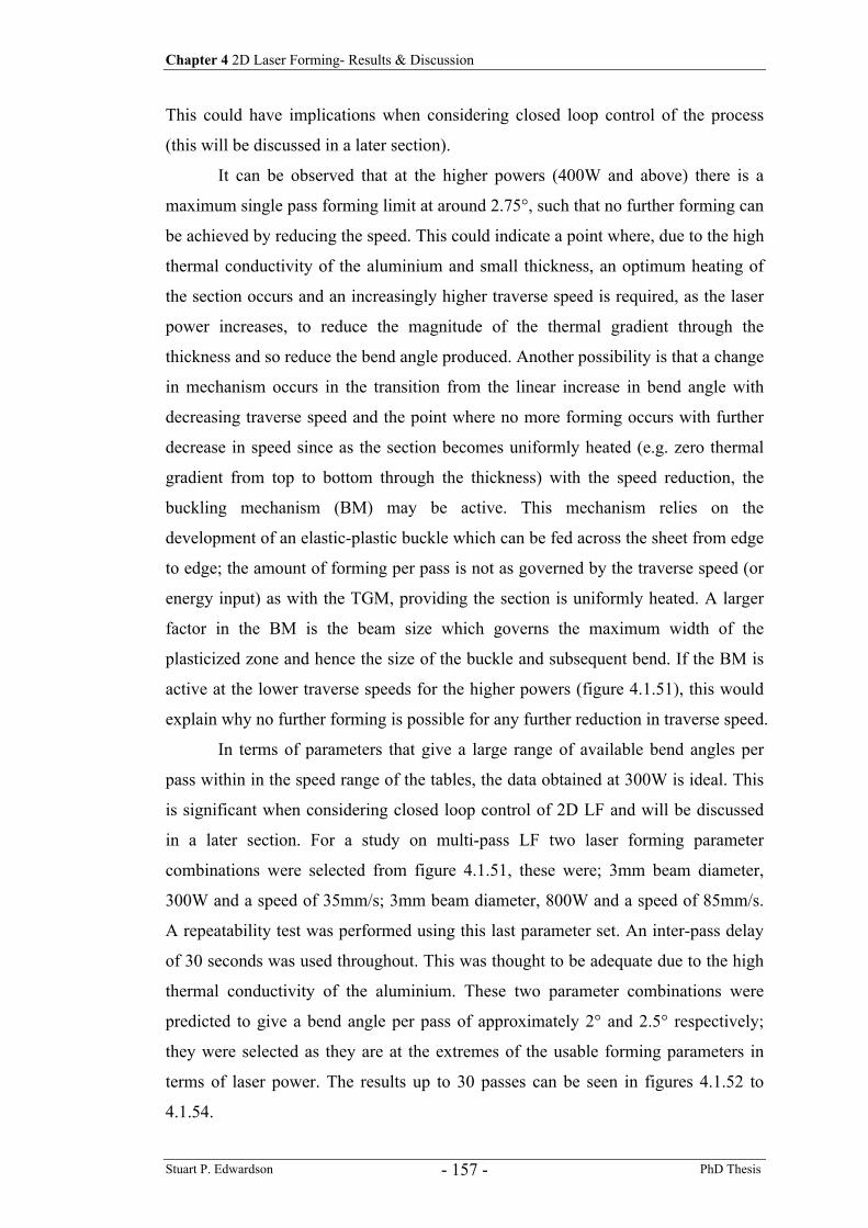
Chapter 4 2D Laser Forming- Results & Discussion
Stuart P. Edwardson PhD Thesis - 157 -
This could have implications when considering closed loop control of the process
(this will be discussed in a later section).
It can be observed that at the higher powers (400W and above) there is a
maximum single pass forming limit at around 2.75°, such that no further forming can
be achieved by reducing the speed. This could indicate a point where, due to the high
thermal conductivity of the aluminium and small thickness, an optimum heating of
the section occurs and an increasingly higher traverse speed is required, as the laser
power increases, to reduce the magnitude of the thermal gradient through the
thickness and so reduce the bend angle produced. Another possibility is that a change
in mechanism occurs in the transition from the linear increase in bend angle with
decreasing traverse speed and the point where no more forming occurs with further
decrease in speed since as the section becomes uniformly heated (e.g. zero thermal
gradient from top to bottom through the thickness) with the speed reduction, the
buckling mechanism (BM) may be active. This mechanism relies on the
development of an elastic-plastic buckle which can be fed across the sheet from edge
to edge; the amount of forming per pass is not as governed by the traverse speed (or
energy input) as with the TGM, providing the section is uniformly heated. A larger
factor in the BM is the beam size which governs the maximum width of the
plasticized zone and hence the size of the buckle and subsequent bend. If the BM is
active at the lower traverse speeds for the higher powers (figure 4.1.51), this would
explain why no further forming is possible for any further reduction in traverse speed.
In terms of parameters that give a large range of available bend angles per
pass within in the speed range of the tables, the data obtained at 300W is ideal. This
is significant when considering closed loop control of 2D LF and will be discussed
in a later section. For a study on multi-pass LF two laser forming parameter
combinations were selected from figure 4.1.51, these were; 3mm beam diameter,
300W and a speed of 35mm/s; 3mm beam diameter, 800W and a speed of 85mm/s.
A repeatability test was performed using this last parameter set. An inter-pass delay
of 30 seconds was used throughout. This was thought to be adequate due to the high
thermal conductivity of the aluminium. These two parameter combinations were
predicted to give a bend angle per pass of approximately 2° and 2.5° respectively;
they were selected as they are at the extremes of the usable forming parameters in
terms of laser power. The results up to 30 passes can be seen in figures 4.1.52 to
4.1.54.
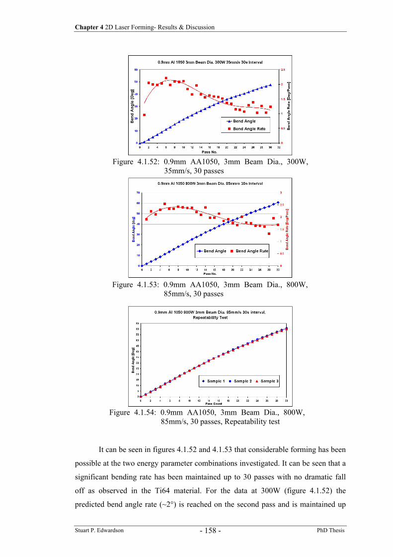
Chapter 4 2D Laser Forming- Results & Discussion
Stuart P. Edwardson PhD Thesis - 158 -
It can be seen in figures 4.1.52 and 4.1.53 that considerable forming has been
possible at the two energy parameter combinations investigated. It can be seen that a
significant bending rate has been maintained up to 30 passes with no dramatic fall
off as observed in the Ti64 material. For the data at 300W (figure 4.1.52) the
predicted bend angle rate (~2°) is reached on the second pass and is maintained up
Figure 4.1.52: 0.9mm AA1050, 3mm Beam Dia., 300W, 35mm/s, 30 passes
Figure 4.1.53: 0.9mm AA1050, 3mm Beam Dia., 800W, 85mm/s, 30 passes
Figure 4.1.54: 0.9mm AA1050, 3mm Beam Dia., 800W, 85mm/s, 30 passes, Repeatability test
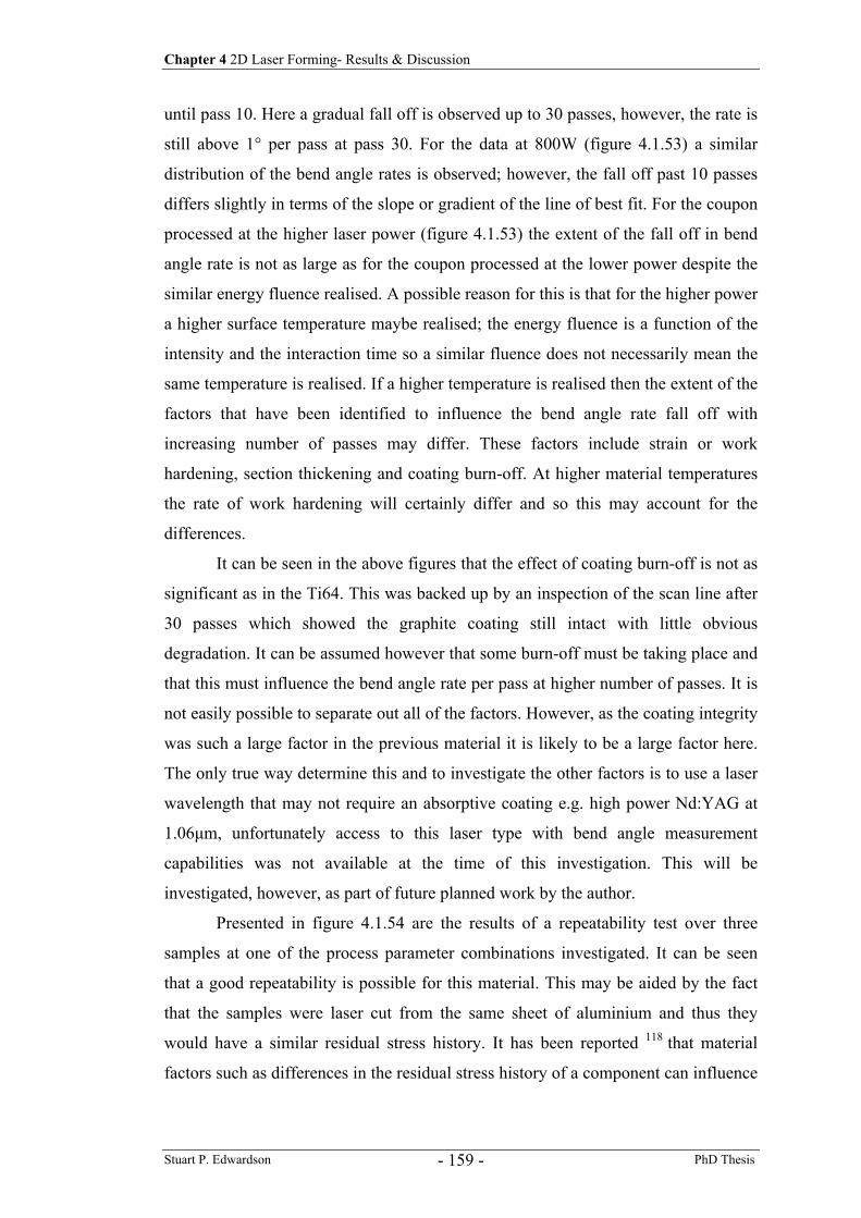
Chapter 4 2D Laser Forming- Results & Discussion
Stuart P. Edwardson PhD Thesis - 159 -
until pass 10. Here a gradual fall off is observed up to 30 passes, however, the rate is
still above 1° per pass at pass 30. For the data at 800W (figure 4.1.53) a similar
distribution of the bend angle rates is observed; however, the fall off past 10 passes
differs slightly in terms of the slope or gradient of the line of best fit. For the coupon
processed at the higher laser power (figure 4.1.53) the extent of the fall off in bend
angle rate is not as large as for the coupon processed at the lower power despite the
similar energy fluence realised. A possible reason for this is that for the higher power
a higher surface temperature maybe realised; the energy fluence is a function of the
intensity and the interaction time so a similar fluence does not necessarily mean the
same temperature is realised. If a higher temperature is realised then the extent of the
factors that have been identified to influence the bend angle rate fall off with
increasing number of passes may differ. These factors include strain or work
hardening, section thickening and coating burn-off. At higher material temperatures
the rate of work hardening will certainly differ and so this may account for the
differences.
It can be seen in the above figures that the effect of coating burn-off is not as
significant as in the Ti64. This was backed up by an inspection of the scan line after
30 passes which showed the graphite coating still intact with little obvious
degradation. It can be assumed however that some burn-off must be taking place and
that this must influence the bend angle rate per pass at higher number of passes. It is
not easily possible to separate out all of the factors. However, as the coating integrity
was such a large factor in the previous material it is likely to be a large factor here.
The only true way determine this and to investigate the other factors is to use a laser
wavelength that may not require an absorptive coating e.g. high power Nd:YAG at
1.06µm, unfortunately access to this laser type with bend angle measurement
capabilities was not available at the time of this investigation. This will be
investigated, however, as part of future planned work by the author.
Presented in figure 4.1.54 are the results of a repeatability test over three
samples at one of the process parameter combinations investigated. It can be seen
that a good repeatability is possible for this material. This may be aided by the fact
that the samples were laser cut from the same sheet of aluminium and thus they
would have a similar residual stress history. It has been reported 118 that material
factors such as differences in the residual stress history of a component can influence
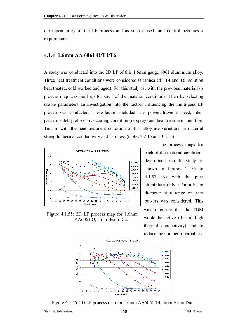
Chapter 4 2D Laser Forming- Results & Discussion
Stuart P. Edwardson PhD Thesis - 160 -
the repeatability of the LF process and as such closed loop control becomes a
requirement.
4.1.4 1.6mm AA 6061 O/T4/T6
A study was conducted into the 2D LF of this 1.6mm gauge 6061 aluminium alloy.
Three heat treatment conditions were considered O (annealed), T4 and T6 (solution
heat treated, cold worked and aged). For this study (as with the previous materials) a
process map was built up for each of the material conditions. Then by selecting
usable parameters an investigation into the factors influencing the multi-pass LF
process was conducted. These factors included laser power, traverse speed, inter-
pass time delay, absorptive coating condition (re-spray) and heat treatment condition.
Tied in with the heat treatment condition of this alloy are variations in material
strength, thermal conductivity and hardness (tables 3.2.15 and 3.2.16).
The process maps for
each of the material conditions
determined from this study are
shown in figures 4.1.55 to
4.1.57. As with the pure
aluminium only a 3mm beam
diameter at a range of laser
powers was considered. This
was to ensure that the TGM
would be active (due to high
thermal conductivity) and to
reduce the number of variables.
Figure 4.1.55: 2D LF process map for 1.6mm AA6061 O, 3mm Beam Dia.
Figure 4.1.56: 2D LF process map for 1.6mm AA6061 T4, 3mm Beam Dia.
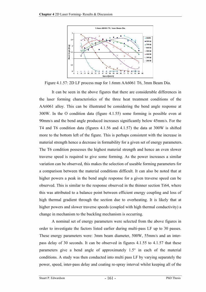
Chapter 4 2D Laser Forming- Results & Discussion
Stuart P. Edwardson PhD Thesis - 161 -
It can be seen in the above figures that there are considerable differences in
the laser forming characteristics of the three heat treatment conditions of the
AA6061 alloy. This can be illustrated be considering the bend angle response at
300W. In the O condition data (figure 4.1.55) some forming is possible even at
90mm/s and the bend angle produced increases significantly below 45mm/s. For the
T4 and T6 condition data (figures 4.1.56 and 4.1.57) the data at 300W is shifted
more to the bottom left of the figure. This is perhaps consistent with the increase in
material strength hence a decrease in formability for a given set of energy parameters.
The T6 condition possesses the highest material strength and hence an even slower
traverse speed is required to give some forming. As the power increases a similar
variation can be observed, this makes the selection of useable forming parameters for
a comparison between the material conditions difficult. It can also be noted that at
higher powers a peak in the bend angle response for a given traverse speed can be
observed. This is similar to the response observed in the thinner section Ti64, where
this was attributed to a balance point between efficient energy coupling and loss of
high thermal gradient through the section due to overheating. It is likely that at
higher powers and slower traverse speeds (coupled with high thermal conductivity) a
change in mechanism to the buckling mechanism is occurring.
A nominal set of energy parameters were selected from the above figures in
order to investigate the factors listed earlier during multi-pass LF up to 30 passes.
These energy parameters were: 3mm beam diameter, 500W, 55mm/s and an inter-
pass delay of 30 seconds. It can be observed in figures 4.1.55 to 4.1.57 that these
parameters give a bend angle of approximately 1.5° in each of the material
conditions. A study was then conducted into multi pass LF by varying separately the
power, speed, inter-pass delay and coating re-spray interval whilst keeping all of the
Figure 4.1.57: 2D LF process map for 1.6mm AA6061 T6, 3mm Beam Dia.
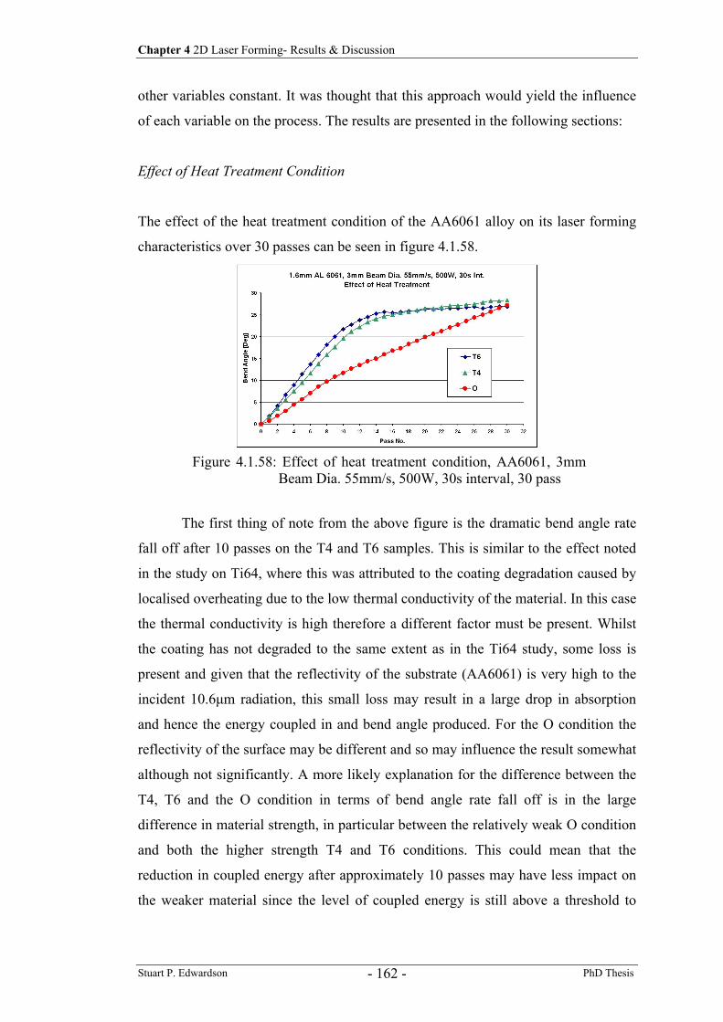
Chapter 4 2D Laser Forming- Results & Discussion
Stuart P. Edwardson PhD Thesis - 162 -
other variables constant. It was thought that this approach would yield the influence
of each variable on the process. The results are presented in the following sections:
Effect of Heat Treatment Condition
The effect of the heat treatment condition of the AA6061 alloy on its laser forming
characteristics over 30 passes can be seen in figure 4.1.58.
The first thing of note from the above figure is the dramatic bend angle rate
fall off after 10 passes on the T4 and T6 samples. This is similar to the effect noted
in the study on Ti64, where this was attributed to the coating degradation caused by
localised overheating due to the low thermal conductivity of the material. In this case
the thermal conductivity is high therefore a different factor must be present. Whilst
the coating has not degraded to the same extent as in the Ti64 study, some loss is
present and given that the reflectivity of the substrate (AA6061) is very high to the
incident 10.6µm radiation, this small loss may result in a large drop in absorption
and hence the energy coupled in and bend angle produced. For the O condition the
reflectivity of the surface may be different and so may influence the result somewhat
although not significantly. A more likely explanation for the difference between the
T4, T6 and the O condition in terms of bend angle rate fall off is in the large
difference in material strength, in particular between the relatively weak O condition
and both the higher strength T4 and T6 conditions. This could mean that the
reduction in coupled energy after approximately 10 passes may have less impact on
the weaker material since the level of coupled energy is still above a threshold to
Figure 4.1.58: Effect of heat treatment condition, AA6061, 3mm Beam Dia. 55mm/s, 500W, 30s interval, 30 pass
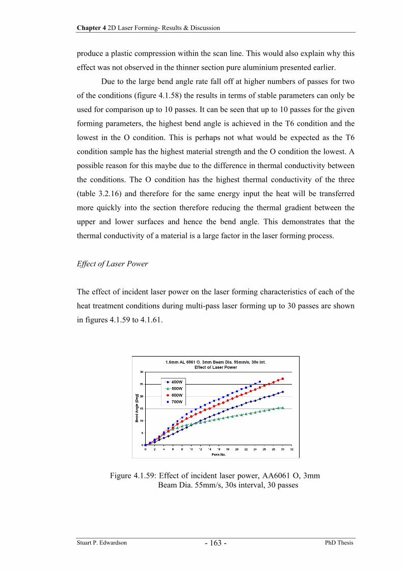
Chapter 4 2D Laser Forming- Results & Discussion
Stuart P. Edwardson PhD Thesis - 163 -
produce a plastic compression within the scan line. This would also explain why this
effect was not observed in the thinner section pure aluminium presented earlier.
Due to the large bend angle rate fall off at higher numbers of passes for two
of the conditions (figure 4.1.58) the results in terms of stable parameters can only be
used for comparison up to 10 passes. It can be seen that up to 10 passes for the given
forming parameters, the highest bend angle is achieved in the T6 condition and the
lowest in the O condition. This is perhaps not what would be expected as the T6
condition sample has the highest material strength and the O condition the lowest. A
possible reason for this maybe due to the difference in thermal conductivity between
the conditions. The O condition has the highest thermal conductivity of the three
(table 3.2.16) and therefore for the same energy input the heat will be transferred
more quickly into the section therefore reducing the thermal gradient between the
upper and lower surfaces and hence the bend angle. This demonstrates that the
thermal conductivity of a material is a large factor in the laser forming process.
Effect of Laser Power
The effect of incident laser power on the laser forming characteristics of each of the
heat treatment conditions during multi-pass laser forming up to 30 passes are shown
in figures 4.1.59 to 4.1.61.
Figure 4.1.59: Effect of incident laser power, AA6061 O, 3mm Beam Dia. 55mm/s, 30s interval, 30 passes
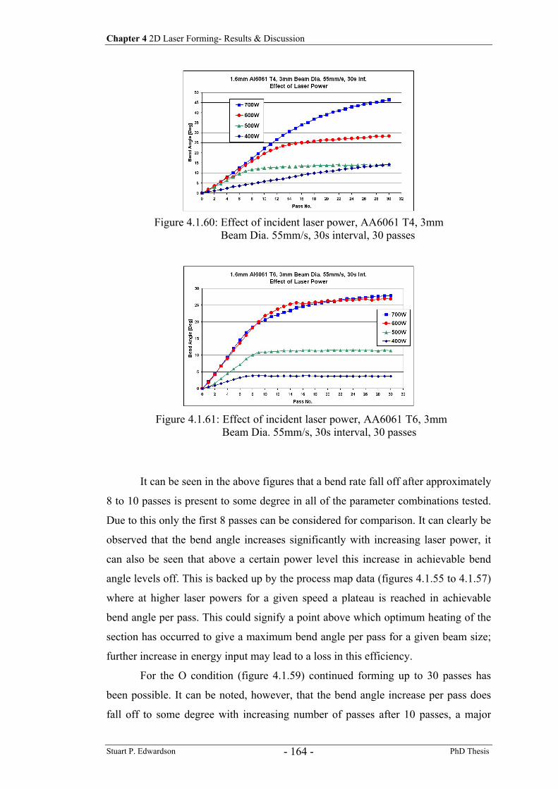
Chapter 4 2D Laser Forming- Results & Discussion
Stuart P. Edwardson PhD Thesis - 164 -
It can be seen in the above figures that a bend rate fall off after approximately
8 to 10 passes is present to some degree in all of the parameter combinations tested.
Due to this only the first 8 passes can be considered for comparison. It can clearly be
observed that the bend angle increases significantly with increasing laser power, it
can also be seen that above a certain power level this increase in achievable bend
angle levels off. This is backed up by the process map data (figures 4.1.55 to 4.1.57)
where at higher laser powers for a given speed a plateau is reached in achievable
bend angle per pass. This could signify a point above which optimum heating of the
section has occurred to give a maximum bend angle per pass for a given beam size;
further increase in energy input may lead to a loss in this efficiency.
For the O condition (figure 4.1.59) continued forming up to 30 passes has
been possible. It can be noted, however, that the bend angle increase per pass does
fall off to some degree with increasing number of passes after 10 passes, a major
Figure 4.1.60: Effect of incident laser power, AA6061 T4, 3mm Beam Dia. 55mm/s, 30s interval, 30 passes
Figure 4.1.61: Effect of incident laser power, AA6061 T6, 3mm Beam Dia. 55mm/s, 30s interval, 30 passes
Chapter 4 2D Laser Forming- Results & Discussion
Stuart P. Edwardson PhD Thesis - 165 -
factor in this is likely to be the coating degradation (given the effect in the other
conditions). The unpredictable nature of this can also be observed in figure 4.1.59,
where the data obtained at 500W shows a very different fall off rate when compared
to the other laser powers tested.
For the data obtained from the T4 condition material (figure 4.1.60), it can be
observed that at 400W a relatively low forming rate can be maintained up to 30
passes with little fall of in bend angle increase per pass. As the power increases a
considerable fall off occurs, this may indicate a threshold energy level above which
significant burn-off of the coating occurs. It can also be noted that, the pass number
the fall off begins at, increases with increasing laser power. This suggests that a
similar amount of coating is lost after approximately 10 passes (i.e. a similar
resultant absorption coefficient) such that a higher laser power would give a higher
coupled energy level and hence continued forming for several passes more.
For the T6 condition (figure 4.1.61) a similar distribution to the T4 condition
can be observed. However, the bend angle rate fall off is more acute. It can be noted
that no power level has been found (of those tested) to give the same small but
consistent bend angle rate as observed in the T4 data for 400W. This could be a
result of the higher material strength of the T6 condition, in that the reduction in the
coupled energy has a significant effect on the bend angle produced.
Comparing the data for all three of the heat treatment conditions it can be
seen that a similar distribution to figure 4.1.58 occurs across the power levels
investigated. Considerably more forming is possible in the higher strength T6 and T4
conditions than in the lower strength O condition using the same energy parameters.
This can be attributed to the considerable differences in the forming characteristics
between the materials (figures 4.1.55 to 4.1.57), metallurgical change or the
difference in thermal conductivity outlined earlier.
Effect of Processing Speed
The effect of processing speed on the laser forming characteristics of each of the heat
treatment conditions during multi-pass laser forming up to 30 passes are shown in
figures 4.1.62 to 4.1.64.
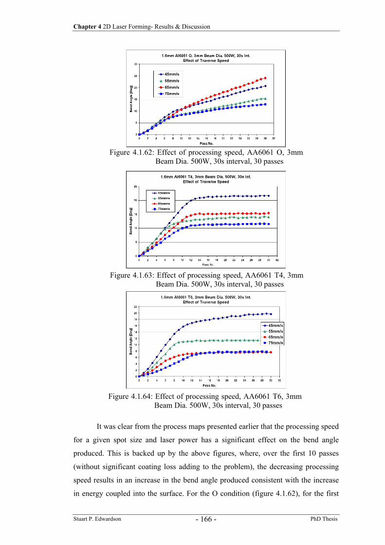
Chapter 4 2D Laser Forming- Results & Discussion
Stuart P. Edwardson PhD Thesis - 166 -
It was clear from the process maps presented earlier that the processing speed
for a given spot size and laser power has a significant effect on the bend angle
produced. This is backed up by the above figures, where, over the first 10 passes
(without significant coating loss adding to the problem), the decreasing processing
speed results in an increase in the bend angle produced consistent with the increase
in energy coupled into the surface. For the O condition (figure 4.1.62), for the first
Figure 4.1.62: Effect of processing speed, AA6061 O, 3mm Beam Dia. 500W, 30s interval, 30 passes
Figure 4.1.63: Effect of processing speed, AA6061 T4, 3mm Beam Dia. 500W, 30s interval, 30 passes
Figure 4.1.64: Effect of processing speed, AA6061 T6, 3mm Beam Dia. 500W, 30s interval, 30 passes
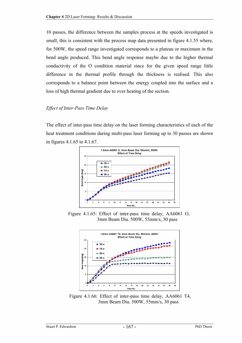
Chapter 4 2D Laser Forming- Results & Discussion
Stuart P. Edwardson PhD Thesis - 167 -
10 passes, the difference between the samples process at the speeds investigated is
small, this is consistent with the process map data presented in figure 4.1.55 where,
for 500W, the speed range investigated corresponds to a plateau or maximum in the
bend angle produced. This bend angle response maybe due to the higher thermal
conductivity of the O condition material since for the given speed range little
difference in the thermal profile through the thickness is realised. This also
corresponds to a balance point between the energy coupled into the surface and a
loss of high thermal gradient due to over heating of the section.
Effect of Inter-Pass Time Delay
The effect of inter-pass time delay on the laser forming characteristics of each of the
heat treatment conditions during multi-pass laser forming up to 30 passes are shown
in figures 4.1.65 to 4.1.67.
Figure 4.1.65: Effect of inter-pass time delay, AA6061 O, 3mm Beam Dia. 500W, 55mm/s, 30 pass
Figure 4.1.66: Effect of inter-pass time delay, AA6061 T4, 3mm Beam Dia. 500W, 55mm/s, 30 pass
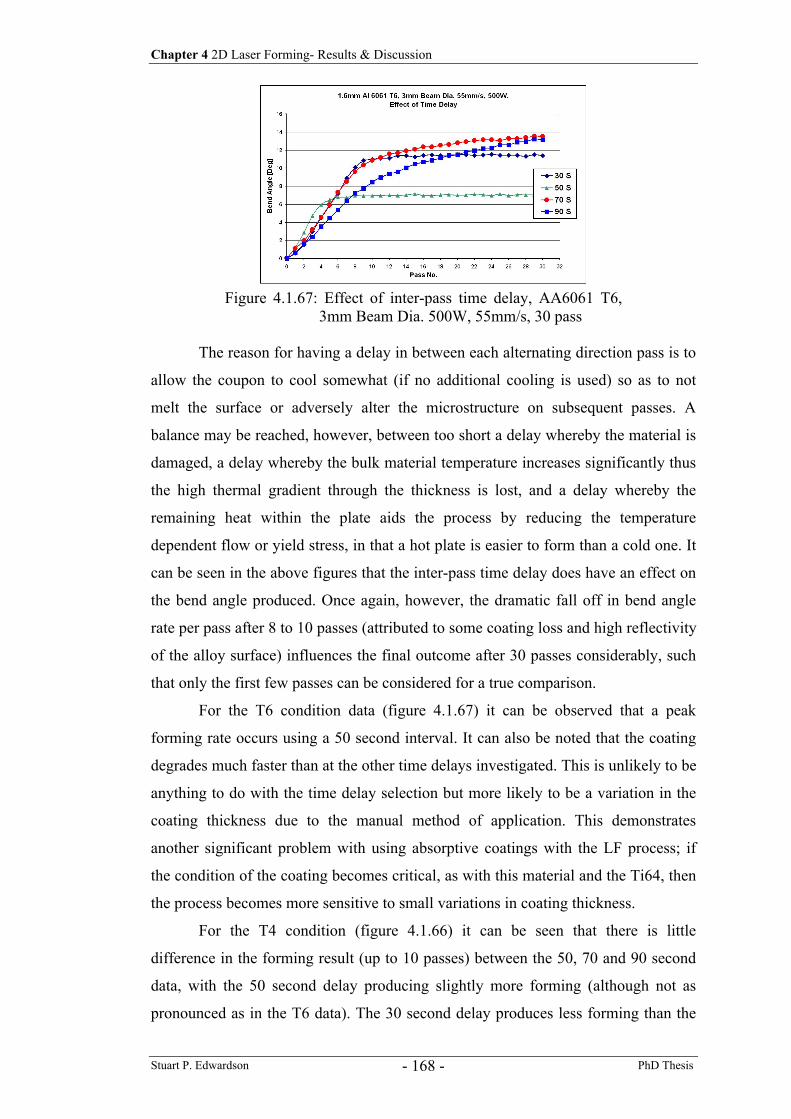
Chapter 4 2D Laser Forming- Results & Discussion
Stuart P. Edwardson PhD Thesis - 168 -
The reason for having a delay in between each alternating direction pass is to
allow the coupon to cool somewhat (if no additional cooling is used) so as to not
melt the surface or adversely alter the microstructure on subsequent passes. A
balance may be reached, however, between too short a delay whereby the material is
damaged, a delay whereby the bulk material temperature increases significantly thus
the high thermal gradient through the thickness is lost, and a delay whereby the
remaining heat within the plate aids the process by reducing the temperature
dependent flow or yield stress, in that a hot plate is easier to form than a cold one. It
can be seen in the above figures that the inter-pass time delay does have an effect on
the bend angle produced. Once again, however, the dramatic fall off in bend angle
rate per pass after 8 to 10 passes (attributed to some coating loss and high reflectivity
of the alloy surface) influences the final outcome after 30 passes considerably, such
that only the first few passes can be considered for a true comparison.
For the T6 condition data (figure 4.1.67) it can be observed that a peak
forming rate occurs using a 50 second interval. It can also be noted that the coating
degrades much faster than at the other time delays investigated. This is unlikely to be
anything to do with the time delay selection but more likely to be a variation in the
coating thickness due to the manual method of application. This demonstrates
another significant problem with using absorptive coatings with the LF process; if
the condition of the coating becomes critical, as with this material and the Ti64, then
the process becomes more sensitive to small variations in coating thickness.
For the T4 condition (figure 4.1.66) it can be seen that there is little
difference in the forming result (up to 10 passes) between the 50, 70 and 90 second
data, with the 50 second delay producing slightly more forming (although not as
pronounced as in the T6 data). The 30 second delay produces less forming than the
Figure 4.1.67: Effect of inter-pass time delay, AA6061 T6, 3mm Beam Dia. 500W, 55mm/s, 30 pass
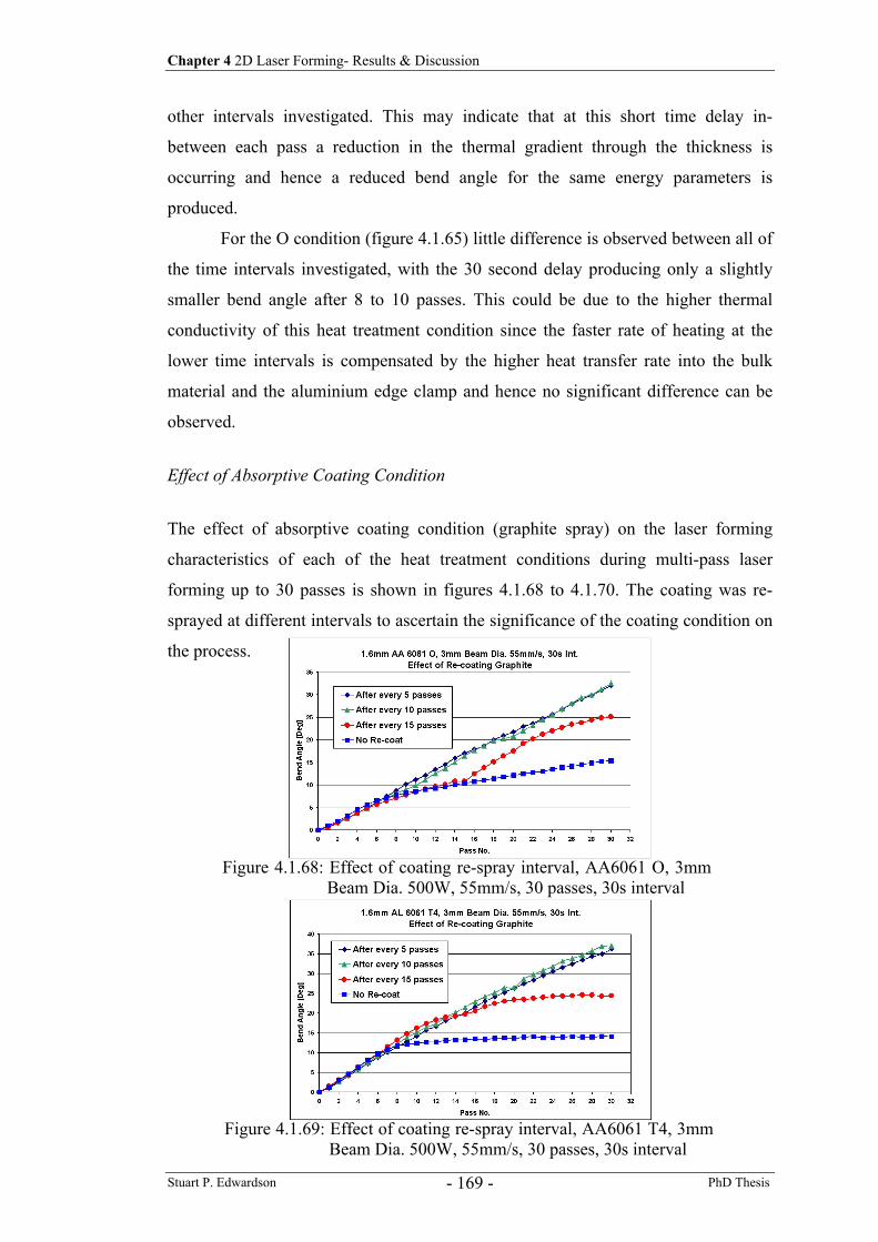
Chapter 4 2D Laser Forming- Results & Discussion
Stuart P. Edwardson PhD Thesis - 169 -
other intervals investigated. This may indicate that at this short time delay in-
between each pass a reduction in the thermal gradient through the thickness is
occurring and hence a reduced bend angle for the same energy parameters is
produced.
For the O condition (figure 4.1.65) little difference is observed between all of
the time intervals investigated, with the 30 second delay producing only a slightly
smaller bend angle after 8 to 10 passes. This could be due to the higher thermal
conductivity of this heat treatment condition since the faster rate of heating at the
lower time intervals is compensated by the higher heat transfer rate into the bulk
material and the aluminium edge clamp and hence no significant difference can be
observed.
Effect of Absorptive Coating Condition
The effect of absorptive coating condition (graphite spray) on the laser forming
characteristics of each of the heat treatment conditions during multi-pass laser
forming up to 30 passes is shown in figures 4.1.68 to 4.1.70. The coating was re-
sprayed at different intervals to ascertain the significance of the coating condition on
the process.
Figure 4.1.68: Effect of coating re-spray interval, AA6061 O, 3mm Beam Dia. 500W, 55mm/s, 30 passes, 30s interval
Figure 4.1.69: Effect of coating re-spray interval, AA6061 T4, 3mm Beam Dia. 500W, 55mm/s, 30 passes, 30s interval
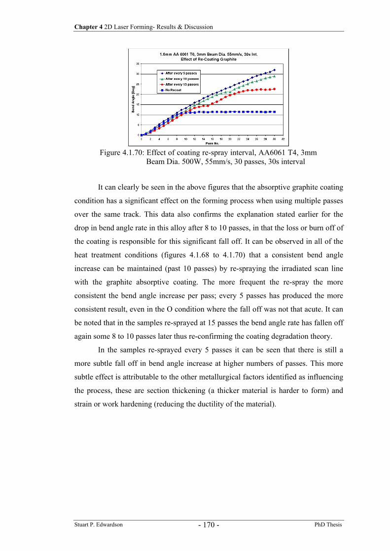
Chapter 4 2D Laser Forming- Results & Discussion
Stuart P. Edwardson PhD Thesis - 170 -
It can clearly be seen in the above figures that the absorptive graphite coating
condition has a significant effect on the forming process when using multiple passes
over the same track. This data also confirms the explanation stated earlier for the
drop in bend angle rate in this alloy after 8 to 10 passes, in that the loss or burn off of
the coating is responsible for this significant fall off. It can be observed in all of the
heat treatment conditions (figures 4.1.68 to 4.1.70) that a consistent bend angle
increase can be maintained (past 10 passes) by re-spraying the irradiated scan line
with the graphite absorptive coating. The more frequent the re-spray the more
consistent the bend angle increase per pass; every 5 passes has produced the more
consistent result, even in the O condition where the fall off was not that acute. It can
be noted that in the samples re-sprayed at 15 passes the bend angle rate has fallen off
again some 8 to 10 passes later thus re-confirming the coating degradation theory.
In the samples re-sprayed every 5 passes it can be seen that there is still a
more subtle fall off in bend angle increase at higher numbers of passes. This more
subtle effect is attributable to the other metallurgical factors identified as influencing
the process, these are section thickening (a thicker material is harder to form) and
strain or work hardening (reducing the ductility of the material).
Figure 4.1.70: Effect of coating re-spray interval, AA6061 T4, 3mm Beam Dia. 500W, 55mm/s, 30 passes, 30s interval
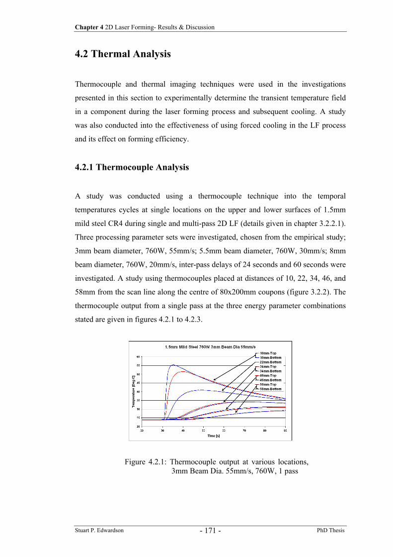
Chapter 4 2D Laser Forming- Results & Discussion
Stuart P. Edwardson PhD Thesis - 171 -
4.2 Thermal Analysis
Thermocouple and thermal imaging techniques were used in the investigations
presented in this section to experimentally determine the transient temperature field
in a component during the laser forming process and subsequent cooling. A study
was also conducted into the effectiveness of using forced cooling in the LF process
and its effect on forming efficiency.
4.2.1 Thermocouple Analysis
A study was conducted using a thermocouple technique into the temporal
temperatures cycles at single locations on the upper and lower surfaces of 1.5mm
mild steel CR4 during single and multi-pass 2D LF (details given in chapter 3.2.2.1).
Three processing parameter sets were investigated, chosen from the empirical study;
3mm beam diameter, 760W, 55mm/s; 5.5mm beam diameter, 760W, 30mm/s; 8mm
beam diameter, 760W, 20mm/s, inter-pass delays of 24 seconds and 60 seconds were
investigated. A study using thermocouples placed at distances of 10, 22, 34, 46, and
58mm from the scan line along the centre of 80x200mm coupons (figure 3.2.2). The
thermocouple output from a single pass at the three energy parameter combinations
stated are given in figures 4.2.1 to 4.2.3.
Figure 4.2.1: Thermocouple output at various locations, 3mm Beam Dia. 55mm/s, 760W, 1 pass
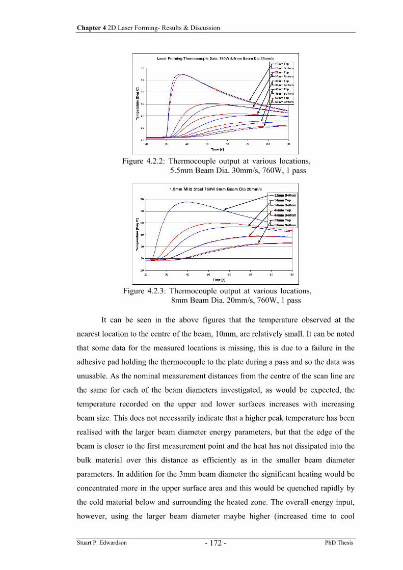
Chapter 4 2D Laser Forming- Results & Discussion
Stuart P. Edwardson PhD Thesis - 172 -
It can be seen in the above figures that the temperature observed at the
nearest location to the centre of the beam, 10mm, are relatively small. It can be noted
that some data for the measured locations is missing, this is due to a failure in the
adhesive pad holding the thermocouple to the plate during a pass and so the data was
unusable. As the nominal measurement distances from the centre of the scan line are
the same for each of the beam diameters investigated, as would be expected, the
temperature recorded on the upper and lower surfaces increases with increasing
beam size. This does not necessarily indicate that a higher peak temperature has been
realised with the larger beam diameter energy parameters, but that the edge of the
beam is closer to the first measurement point and the heat has not dissipated into the
bulk material over this distance as efficiently as in the smaller beam diameter
parameters. In addition for the 3mm beam diameter the significant heating would be
concentrated more in the upper surface area and this would be quenched rapidly by
the cold material below and surrounding the heated zone. The overall energy input,
however, using the larger beam diameter maybe higher (increased time to cool
Figure 4.2.2: Thermocouple output at various locations, 5.5mm Beam Dia. 30mm/s, 760W, 1 pass
Figure 4.2.3: Thermocouple output at various locations, 8mm Beam Dia. 20mm/s, 760W, 1 pass
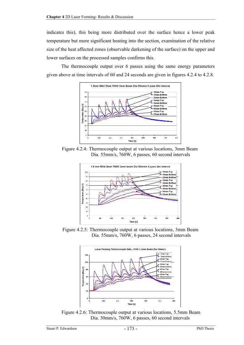
Chapter 4 2D Laser Forming- Results & Discussion
Stuart P. Edwardson PhD Thesis - 173 -
indicates this), this being more distributed over the surface hence a lower peak
temperature but more significant heating into the section, examination of the relative
size of the heat affected zones (observable darkening of the surface) on the upper and
lower surfaces on the processed samples confirms this.
The thermocouple output over 6 passes using the same energy parameters
given above at time intervals of 60 and 24 seconds are given in figures 4.2.4 to 4.2.8.
Figure 4.2.4: Thermocouple output at various locations, 3mm Beam Dia. 55mm/s, 760W, 6 passes, 60 second intervals
Figure 4.2.5: Thermocouple output at various locations, 3mm Beam Dia. 55mm/s, 760W, 6 passes, 24 second intervals
Figure 4.2.6: Thermocouple output at various locations, 5.5mm Beam Dia. 30mm/s, 760W, 6 passes, 60 second intervals
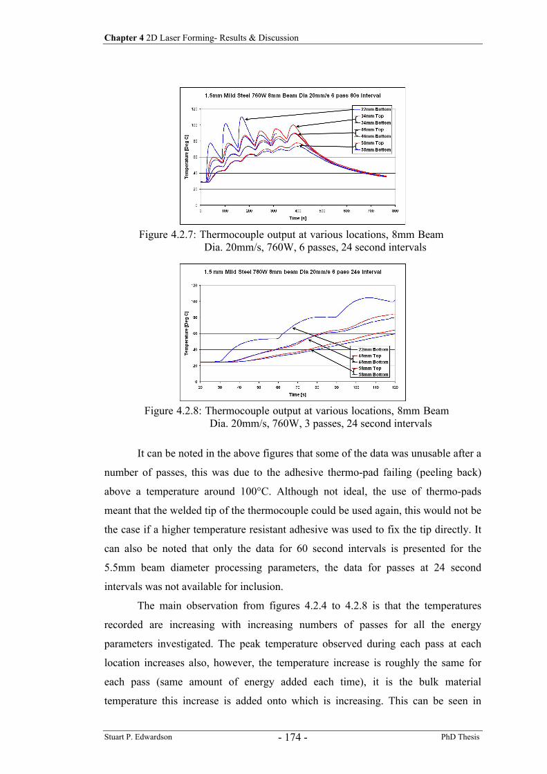
Chapter 4 2D Laser Forming- Results & Discussion
Stuart P. Edwardson PhD Thesis - 174 -
It can be noted in the above figures that some of the data was unusable after a
number of passes, this was due to the adhesive thermo-pad failing (peeling back)
above a temperature around 100°C. Although not ideal, the use of thermo-pads
meant that the welded tip of the thermocouple could be used again, this would not be
the case if a higher temperature resistant adhesive was used to fix the tip directly. It
can also be noted that only the data for 60 second intervals is presented for the
5.5mm beam diameter processing parameters, the data for passes at 24 second
intervals was not available for inclusion.
The main observation from figures 4.2.4 to 4.2.8 is that the temperatures
recorded are increasing with increasing numbers of passes for all the energy
parameters investigated. The peak temperature observed during each pass at each
location increases also, however, the temperature increase is roughly the same for
each pass (same amount of energy added each time), it is the bulk material
temperature this increase is added onto which is increasing. This can be seen in
Figure 4.2.8: Thermocouple output at various locations, 8mm Beam Dia. 20mm/s, 760W, 3 passes, 24 second intervals
Figure 4.2.7: Thermocouple output at various locations, 8mm Beam Dia. 20mm/s, 760W, 6 passes, 24 second intervals
Chapter 4 2D Laser Forming- Results & Discussion
Stuart P. Edwardson PhD Thesis - 175 -
figure 4.2.4 where the data recorded at 58 mm from the scan line, which can be
considered the bulk material temperature (as far as that which influences the scan
line area), is increasing with increasing numbers of passes. This effect may have
implications on the efficiency of the process for subsequent passes, in that if the bulk
material temperature is increasing there maybe a reduction in magnitude of the
thermal gradient through the section directly under the beam (consistent with TGM).
Another factor is the elevated temperatures remaining in the heated area (bulk
material temperature increase) aiding the process by reducing the temperature
dependent flow or yield stress of the material thus making it easier to plastically
deform.
Comparing between the results from the three different beam diameters (60
second intervals) it can be seen that a similar distribution is present here to that
observed earlier for a single pass. The lowest peak temperatures at the locations
investigated are observed in the 3mm beam data (figure 4.2.4) and the highest in the
8mm beam diameter data. As was discussed earlier this does not necessarily mean
that the peak temperatures within the scan line are higher for the larger beam, it is
more likely that this is a factor of the relative beam size to the measurement
locations. The smaller beam diameter is likely to cause a higher peak temperature in
the coupon as the intensity is higher, this should be confirmed by the Finite Element
Analysis (FEA) work presented in a later section.
It can be seen in figures 4.1.5 and 4.1.8 that by decreasing the scan interval to
24 seconds (from 60 seconds) has a significant effect on the temperatures recorded
on the surfaces of the coupons. This significant increase in temperature observed at
the locations investigated must also occur within the scan line. This backs up the
results and discussion presented earlier in the empirical section on this material at
various inter-pass time delays (figures 4.1.7 to 4.1.12), in that it was observed that
the time delay has a significant effect on the final bend angle produced in a multi-
pass strategy. For the 3mm beam diameter processing parameters it was found that a
shorter inter-pass time delay lead to an increase in the amount of forming (24
seconds produced the highest). This is consistent with the thermocouple data
presented in this section (figures 4.2.4 and 4.2.5), where an increase in the
temperature realised in the coupon is apparent when comparing the 60 second and 24
second interval data. If the plate was significantly warmer within the scan line for
subsequent passes at 24 second intervals then the reduction in the flow stress should
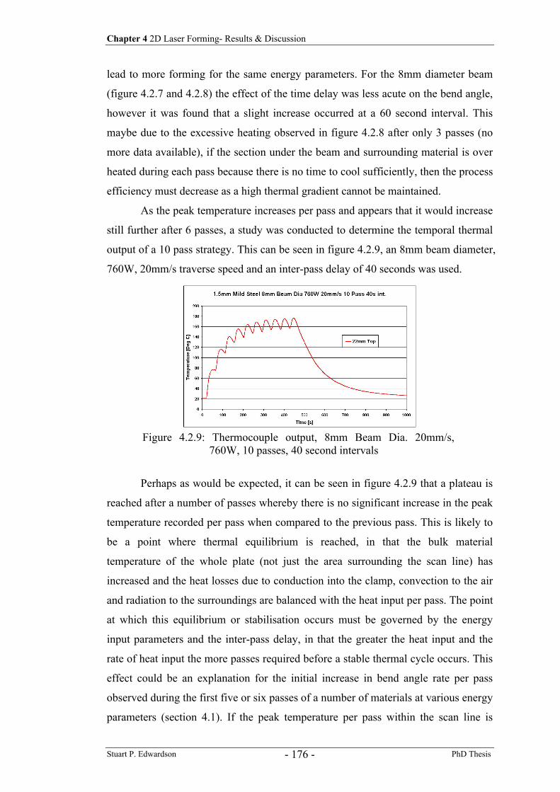
Chapter 4 2D Laser Forming- Results & Discussion
Stuart P. Edwardson PhD Thesis - 176 -
lead to more forming for the same energy parameters. For the 8mm diameter beam
(figure 4.2.7 and 4.2.8) the effect of the time delay was less acute on the bend angle,
however it was found that a slight increase occurred at a 60 second interval. This
maybe due to the excessive heating observed in figure 4.2.8 after only 3 passes (no
more data available), if the section under the beam and surrounding material is over
heated during each pass because there is no time to cool sufficiently, then the process
efficiency must decrease as a high thermal gradient cannot be maintained.
As the peak temperature increases per pass and appears that it would increase
still further after 6 passes, a study was conducted to determine the temporal thermal
output of a 10 pass strategy. This can be seen in figure 4.2.9, an 8mm beam diameter,
760W, 20mm/s traverse speed and an inter-pass delay of 40 seconds was used.
Perhaps as would be expected, it can be seen in figure 4.2.9 that a plateau is
reached after a number of passes whereby there is no significant increase in the peak
temperature recorded per pass when compared to the previous pass. This is likely to
be a point where thermal equilibrium is reached, in that the bulk material
temperature of the whole plate (not just the area surrounding the scan line) has
increased and the heat losses due to conduction into the clamp, convection to the air
and radiation to the surroundings are balanced with the heat input per pass. The point
at which this equilibrium or stabilisation occurs must be governed by the energy
input parameters and the inter-pass delay, in that the greater the heat input and the
rate of heat input the more passes required before a stable thermal cycle occurs. This
effect could be an explanation for the initial increase in bend angle rate per pass
observed during the first five or six passes of a number of materials at various energy
parameters (section 4.1). If the peak temperature per pass within the scan line is
Figure 4.2.9: Thermocouple output, 8mm Beam Dia. 20mm/s, 760W, 10 passes, 40 second intervals
Chapter 4 2D Laser Forming- Results & Discussion
Stuart P. Edwardson PhD Thesis - 177 -
increasing for the first few passes until an equilibrium point is reached then the
amount of forming (governed by the energy input) must also increase for the first
few passes. Once a stable thermal cycle has been established a reasonably consistent
bend angle rate is observed which then drops due to the other factors influencing the
bend angle rate discussed earlier.
4.2.2 Thermal (IR) Imaging Study
The parameter values utilised for this section are given in tables 3.2.17 and 3.2.18.
The images were produced and analysed using the software package Irwin OLE V2.
The emissivity was set at 0.6 (typical for a graphite surface) and the temperature
range given as 40ºC to 1100ºC.
Two-dimensional thermal images of the start, middle and end of the laser
processing and post-processing cooling of the 1.5mm CR4 mild steel coupons, for
each of the beam diameters 3mm, 5.5mm and 8mm, are given in figures 4.2.10,
4.2.11 and 4.2.12, respectively.
The temperature data for analysis was obtained from the laser processing
end-scan image for each beam diameter, using the software post-processor.
Comparisons between the temperature distributions, during laser processing, for the
three process parameter combinations are given in figure 4.2.13. Temperature
distributions for the 3mm, 5.5mm and 8mm diameter laser beams when incident
upon the mild steel coupons are given in figures 4.2.14, 4.2.15 and 4.2.16,
respectively.
The thermal images obtained using the infrared detector all exhibited a
Gaussian-type form and this can be attributed to the distribution of energy within the
beam mode of the CO2 laser utilised in this investigation (figure 3.1.3).
Data acquired using the infrared detector was limited to defined ranges
between -20ºC and 1500ºC. A range of 40ºC to 1100ºC was selected so as to obtain
reasonable heating and cooling temperatures during the laser processing of the
samples. The imaging of the temperature field on the surface of the coupons could
only be considered accurate at positions surrounding the incident laser spot where
the temperatures fell within the detection range.
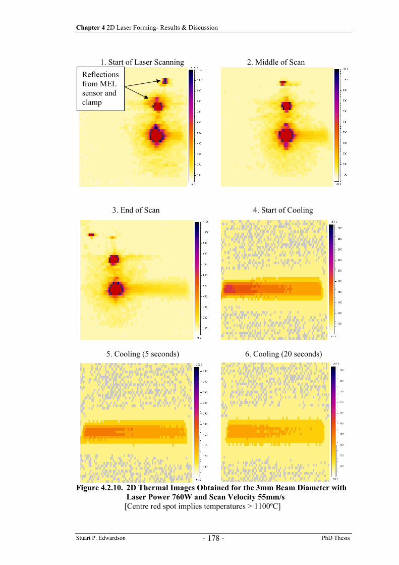
Chapter 4 2D Laser Forming- Results & Discussion
Stuart P. Edwardson PhD Thesis - 178 -
1. Start of Laser Scanning 2. Middle of Scan
3. End of Scan 4. Start of Cooling
5. Cooling (5 seconds) 6. Cooling (20 seconds)
Figure 4.2.10. 2D Thermal Images Obtained for the 3mm Beam Diameter with Laser Power 760W and Scan Velocity 55mm/s [Centre red spot implies temperatures > 1100ºC]
Reflections from MEL sensor and clamp
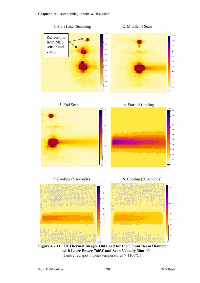
Chapter 4 2D Laser Forming- Results & Discussion
Stuart P. Edwardson PhD Thesis - 179 -
1. Start Laser Scanning 2. Middle of Scan
3. End Scan 4. Start of Cooling
5. Cooling (5 seconds) 6. Cooling (20 seconds)
Figure 4.2.11. 2D Thermal Images Obtained for the 5.5mm Beam Diameter with Laser Power 760W and Scan Velocity 30mm/s [Centre red spot implies temperatures > 1100ºC]
Reflections from MEL sensor and clamp
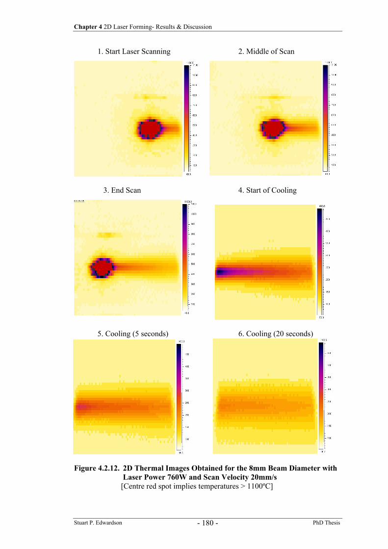
Chapter 4 2D Laser Forming- Results & Discussion
Stuart P. Edwardson PhD Thesis - 180 -
1. Start Laser Scanning 2. Middle of Scan
3. End Scan 4. Start of Cooling
5. Cooling (5 seconds) 6. Cooling (20 seconds)
Figure 4.2.12. 2D Thermal Images Obtained for the 8mm Beam Diameter with
Laser Power 760W and Scan Velocity 20mm/s [Centre red spot implies temperatures > 1100ºC]
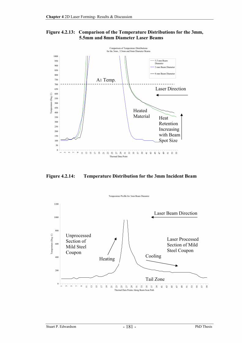
Chapter 4 2D Laser Forming- Results & Discussion
Stuart P. Edwardson PhD Thesis - 181 -
Figure 4.2.13: Comparison of the Temperature Distributions for the 3mm, 5.5mm and 8mm Diameter Laser Beams
Figure 4.2.14: Temperature Distribution for the 3mm Incident Beam
Comparison of Temperature Distributions for the 3mm , 5.5mm and 8mm Diameter Beams
0
50
100
150
200
250
300
350
400
450
500
550
600
650
700
750
800
850
900
950
1000
1 3 5 7 9 11 13 15 17 19 21 23 25 27 29 31 33 35 37 39 41 43 45 47 49 51 53 55
Thermal Data Point
Tem
pera
ture
(Deg
. C)
5.5 mm BeamDiameter3 mm Beam Diameter
8 mm Beam Diameter
Temperature Profile for 3mm Beam Diameter
0
200
400
600
800
1000
1200
1 3 5 7 9 11 13 15 17 19 21 23 25 27 29 31 33 35 37 39 41 43 45 47 49 51 53 55 57 59
Thermal Data Pointa Along Beam Scan Path
Tem
pera
ture
(Deg
. C)
Laser Direction
Heated Material Heat
Retention Increasing with Beam Spot Size
Unprocessed Section of Mild Steel Coupon
Laser Processed Section of Mild Steel Coupon
Laser Beam Direction
Heating Cooling
Tail Zone
A1 Temp.
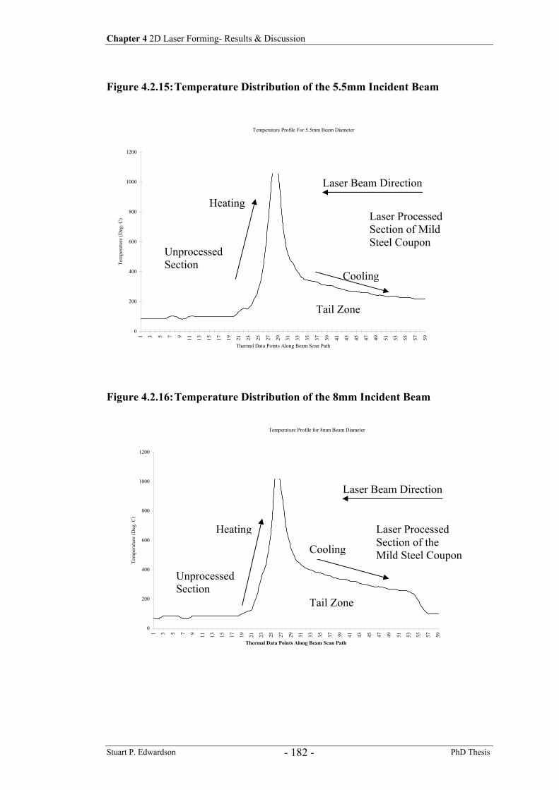
Chapter 4 2D Laser Forming- Results & Discussion
Stuart P. Edwardson PhD Thesis - 182 -
Figure 4.2.15: Temperature Distribution of the 5.5mm Incident Beam
Figure 4.2.16: Temperature Distribution of the 8mm Incident Beam
Temperature Profile For 5.5mm Beam Diameter
0
200
400
600
800
1000
1200
1 3 5 7 9 11 13 15 17 19 21 23 25 27 29 31 33 35 37 39 41 43 45 47 49 51 53 55 57 59
Thermal Data Points Along Beam Scan Path
Tem
pera
ture
(Deg
. C)
Temperature Profile for 8mm Beam Diameter
0
200
400
600
800
1000
1200
1 3 5 7 9 11 13 15 17 19 21 23 25 27 29 31 33 35 37 39 41 43 45 47 49 51 53 55 57 59
Thermal Data Points Along Beam Scan Path
Tem
pera
ture
(Deg
. C)
Laser Beam Direction
Unprocessed Section
Laser Processed Section of Mild Steel Coupon
Unprocessed Section
Laser Processed Section of the Mild Steel Coupon
Laser Beam Direction
Heating
Cooling
Cooling
Heating
Tail Zone
Tail Zone
Chapter 4 2D Laser Forming- Results & Discussion
Stuart P. Edwardson PhD Thesis - 183 -
At the point of incidence between the laser beam and the surface of the
coupons the infrared detector gave measurements that were in excess of 1100ºC
(shown as a centre red spot in the thermal images). This could be due to several
factors:
(i) Correct measurement of a Gaussian-type temperature distribution, with the
temperature being measured at the point on the surface where the energy
distribution of the laser beam was at its maximum.
(ii) Ionisation of the surrounding air above the surface of the mild steel coupons.
(iii) System limitations of the peripheral hardware and software.
(iv) Imaging of the temperature field generated by the graphite coating during
absorption of the laser beam energy.
(v) Incandescence of the graphite coating.
These discussion points are shown, graphically, in figure 4.2.13, which
indicates the temperature distribution, and the temperature measurement overshoot,
for each of the beam diameters. It is likely that the incandescence of the graphite due
to the interaction with the incident laser beam is the cause of the measurement
overshoot, in that it is unlikely that the peak surface temperature in the mild steel
will reach the levels indicated by the IR analysis. This is backed up by observations
during the process where a bright burning can be seen on the graphite surface under
the laser beam. Although the graphite heats up to temperatures in excess of 1100ºC
(possibly much higher), it is the overall heat transfer to the mild steel beneath that
determines the absorption coefficient for the laser type and material. This
demonstrates another problem with using this thermal imaging technique when using
absorptive surface coatings, in that it is not possible to record the peak surface
temperatures realised in the mild steel substrate through the graphite coating when
there are significant differences in temperatures between them.
The time period and surface area over which heat was retained in the mild
steel sheet increased for larger laser beam spot diameters. This can be seen in the
cooling images for each of the beam diameters shown in figures 4.2.10 to 4.2.12.
This was observed in the thermocouple data presented earlier and may have resulted
in the energy absorption being enhanced for larger beam diameters during multiple-
pass scanning regimes due to the increase in the temperature dependent absorption
coefficient. This maybe an additional factor in the initial increase per pass in the bulk
Chapter 4 2D Laser Forming- Results & Discussion
Stuart P. Edwardson PhD Thesis - 184 -
material and peak scan line temperatures and hence bend angle observed during the
first few passes.
Figure 4.2.13 highlights the differences between the temperature distributions
for each of the three beam diameters utilised in this investigation. The mid scan plots
in figures 4.2.14 to 4.2.16 show the effect of heat transfer, with each case showing
that there is a pre-heated zone in front of the laser beam and a tail zone following the
laser beam. From figure 4.2.13 it can be seen that the temperature in the tail zone
increased as the beam diameter was increased, figures 4.2.14 to 4.2.16 also imply
this distribution for tail zone temperatures. This is consistent with the discussion
point raised in the last section from the thermocouple analysis study, whereby the
larger beam diameters showed a higher temperature at the distances recorded and a
longer time to cool, however, it was argued that this does not necessarily indicate
that a higher peak temperature has been realised. It is more likely that for the smaller
beam diameters (3mm) the significant heating (with higher peak temperatures)
would be concentrated more in the upper surface area and this would be quenched
rapidly by the cold material below and surrounding the heated zone thus the heat
retention behind the beam would be less. For the larger beam diameters (8mm) the
overall heat input maybe higher but this is more distributed over the surface and
through the section thus the peak temperature would be less.
The heat distribution on cooling in figures 4.2.10 to 4.2.12 reveals (based on
heat retention after the beam has passed) that a higher temperature is realised at the
end of the scan line when compared to the beginning. This is backed up by
observations of the HAZ at the end of a scan line, where a widening or flaring can be
seen. A possible explanation for this is that the heat from the incident laser beam and
the heat retained behind the beam is flowing into the cold region ahead of the beam,
as the beam reaches the second edge the heat flowing ahead of the beam cannot
travel any further and so a heat build up occurs, hence the increase in temperature at
the second edge. This demonstrates the need for an alternating direction strategy to
even up this temperature distribution along the scan line. In addition the fact that a
higher temperature maybe realised at the end of the scan line means that more
forming maybe realised there, this could be a source of unwanted distortion in the
process (e.g. edge effects) and suggests a need to reduce the energy input near the
edge to account for this heat build up. This could be achieved by varying the traverse
speed along the scan line (e.g. speed up towards the edge).
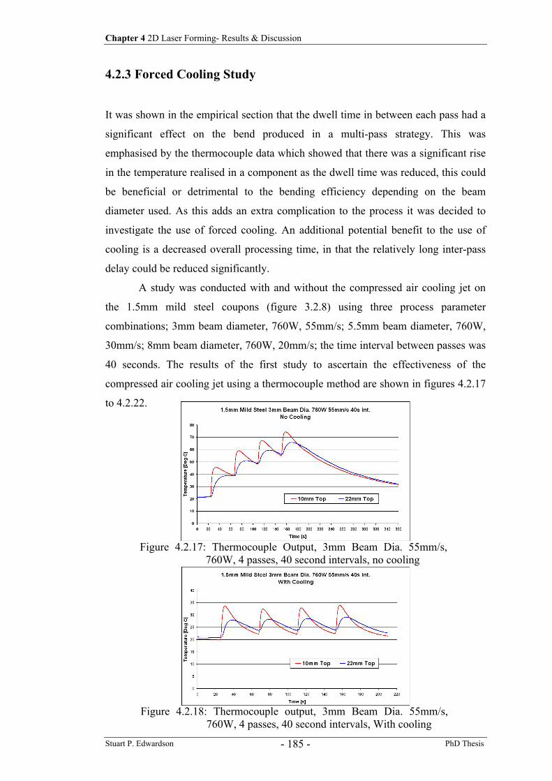
Chapter 4 2D Laser Forming- Results & Discussion
Stuart P. Edwardson PhD Thesis - 185 -
4.2.3 Forced Cooling Study
It was shown in the empirical section that the dwell time in between each pass had a
significant effect on the bend produced in a multi-pass strategy. This was
emphasised by the thermocouple data which showed that there was a significant rise
in the temperature realised in a component as the dwell time was reduced, this could
be beneficial or detrimental to the bending efficiency depending on the beam
diameter used. As this adds an extra complication to the process it was decided to
investigate the use of forced cooling. An additional potential benefit to the use of
cooling is a decreased overall processing time, in that the relatively long inter-pass
delay could be reduced significantly.
A study was conducted with and without the compressed air cooling jet on
the 1.5mm mild steel coupons (figure 3.2.8) using three process parameter
combinations; 3mm beam diameter, 760W, 55mm/s; 5.5mm beam diameter, 760W,
30mm/s; 8mm beam diameter, 760W, 20mm/s; the time interval between passes was
40 seconds. The results of the first study to ascertain the effectiveness of the
compressed air cooling jet using a thermocouple method are shown in figures 4.2.17
to 4.2.22.
Figure 4.2.17: Thermocouple Output, 3mm Beam Dia. 55mm/s, 760W, 4 passes, 40 second intervals, no cooling
Figure 4.2.18: Thermocouple output, 3mm Beam Dia. 55mm/s, 760W, 4 passes, 40 second intervals, With cooling
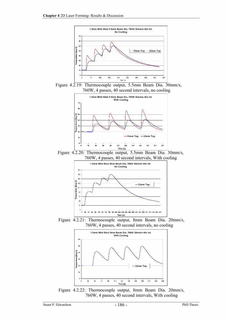
Chapter 4 2D Laser Forming- Results & Discussion
Stuart P. Edwardson PhD Thesis - 186 -
Figure 4.2.19: Thermocouple output, 5.5mm Beam Dia. 30mm/s, 760W, 4 passes, 40 second intervals, no cooling
Figure 4.2.20: Thermocouple output, 5.5mm Beam Dia. 30mm/s, 760W, 4 passes, 40 second intervals, With cooling
Figure 4.2.21: Thermocouple output, 8mm Beam Dia. 20mm/s, 760W, 4 passes, 40 second intervals, no cooling
Figure 4.2.22: Thermocouple output, 8mm Beam Dia. 20mm/s, 760W, 4 passes, 40 second intervals, With cooling
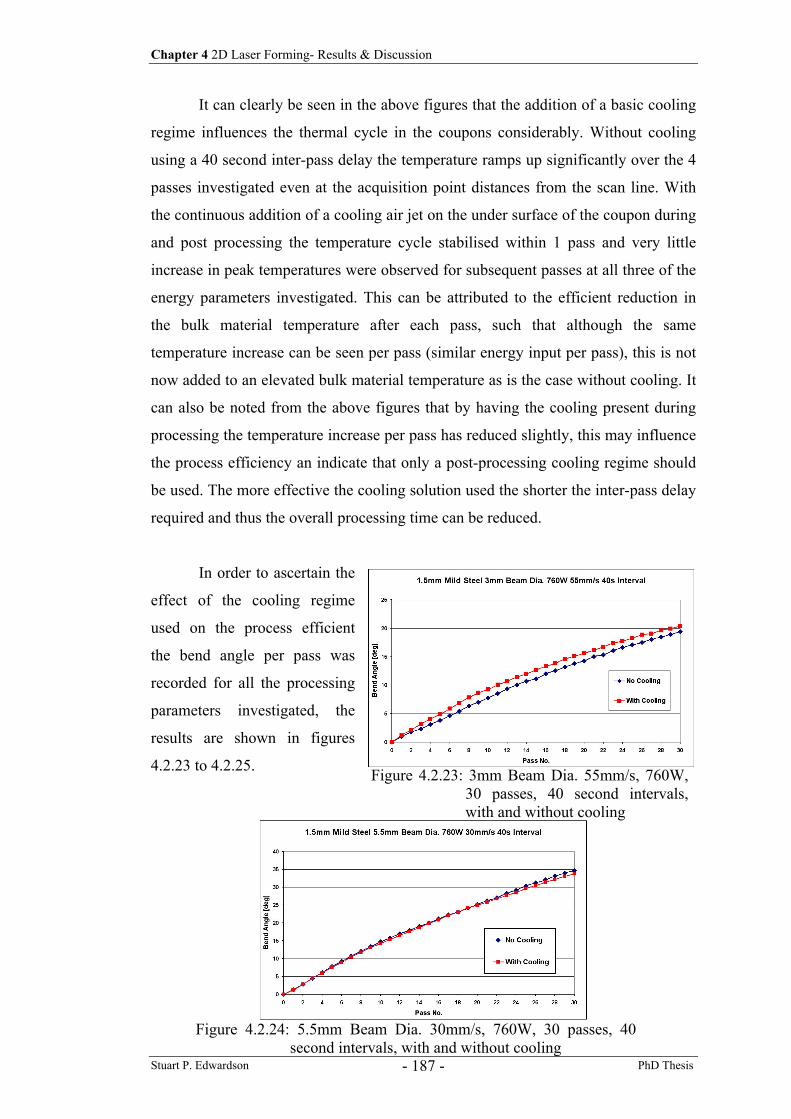
Chapter 4 2D Laser Forming- Results & Discussion
Stuart P. Edwardson PhD Thesis - 187 -
It can clearly be seen in the above figures that the addition of a basic cooling
regime influences the thermal cycle in the coupons considerably. Without cooling
using a 40 second inter-pass delay the temperature ramps up significantly over the 4
passes investigated even at the acquisition point distances from the scan line. With
the continuous addition of a cooling air jet on the under surface of the coupon during
and post processing the temperature cycle stabilised within 1 pass and very little
increase in peak temperatures were observed for subsequent passes at all three of the
energy parameters investigated. This can be attributed to the efficient reduction in
the bulk material temperature after each pass, such that although the same
temperature increase can be seen per pass (similar energy input per pass), this is not
now added to an elevated bulk material temperature as is the case without cooling. It
can also be noted from the above figures that by having the cooling present during
processing the temperature increase per pass has reduced slightly, this may influence
the process efficiency an indicate that only a post-processing cooling regime should
be used. The more effective the cooling solution used the shorter the inter-pass delay
required and thus the overall processing time can be reduced.
In order to ascertain the
effect of the cooling regime
used on the process efficient
the bend angle per pass was
recorded for all the processing
parameters investigated, the
results are shown in figures
4.2.23 to 4.2.25.
Figure 4.2.24: 5.5mm Beam Dia. 30mm/s, 760W, 30 passes, 40
second intervals, with and without cooling
Figure 4.2.23: 3mm Beam Dia. 55mm/s, 760W, 30 passes, 40 second intervals, with and without cooling
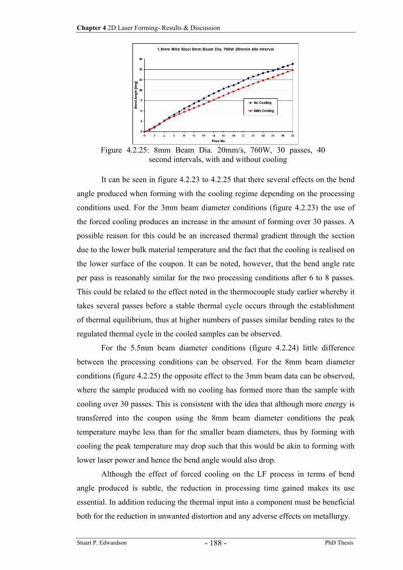
Chapter 4 2D Laser Forming- Results & Discussion
Stuart P. Edwardson PhD Thesis - 188 -
It can be seen in figure 4.2.23 to 4.2.25 that there several effects on the bend
angle produced when forming with the cooling regime depending on the processing
conditions used. For the 3mm beam diameter conditions (figure 4.2.23) the use of
the forced cooling produces an increase in the amount of forming over 30 passes. A
possible reason for this could be an increased thermal gradient through the section
due to the lower bulk material temperature and the fact that the cooling is realised on
the lower surface of the coupon. It can be noted, however, that the bend angle rate
per pass is reasonably similar for the two processing conditions after 6 to 8 passes.
This could be related to the effect noted in the thermocouple study earlier whereby it
takes several passes before a stable thermal cycle occurs through the establishment
of thermal equilibrium, thus at higher numbers of passes similar bending rates to the
regulated thermal cycle in the cooled samples can be observed.
For the 5.5mm beam diameter conditions (figure 4.2.24) little difference
between the processing conditions can be observed. For the 8mm beam diameter
conditions (figure 4.2.25) the opposite effect to the 3mm beam data can be observed,
where the sample produced with no cooling has formed more than the sample with
cooling over 30 passes. This is consistent with the idea that although more energy is
transferred into the coupon using the 8mm beam diameter conditions the peak
temperature maybe less than for the smaller beam diameters, thus by forming with
cooling the peak temperature may drop such that this would be akin to forming with
lower laser power and hence the bend angle would also drop.
Although the effect of forced cooling on the LF process in terms of bend
angle produced is subtle, the reduction in processing time gained makes its use
essential. In addition reducing the thermal input into a component must be beneficial
both for the reduction in unwanted distortion and any adverse effects on metallurgy.
Figure 4.2.25: 8mm Beam Dia. 20mm/s, 760W, 30 passes, 40 second intervals, with and without cooling
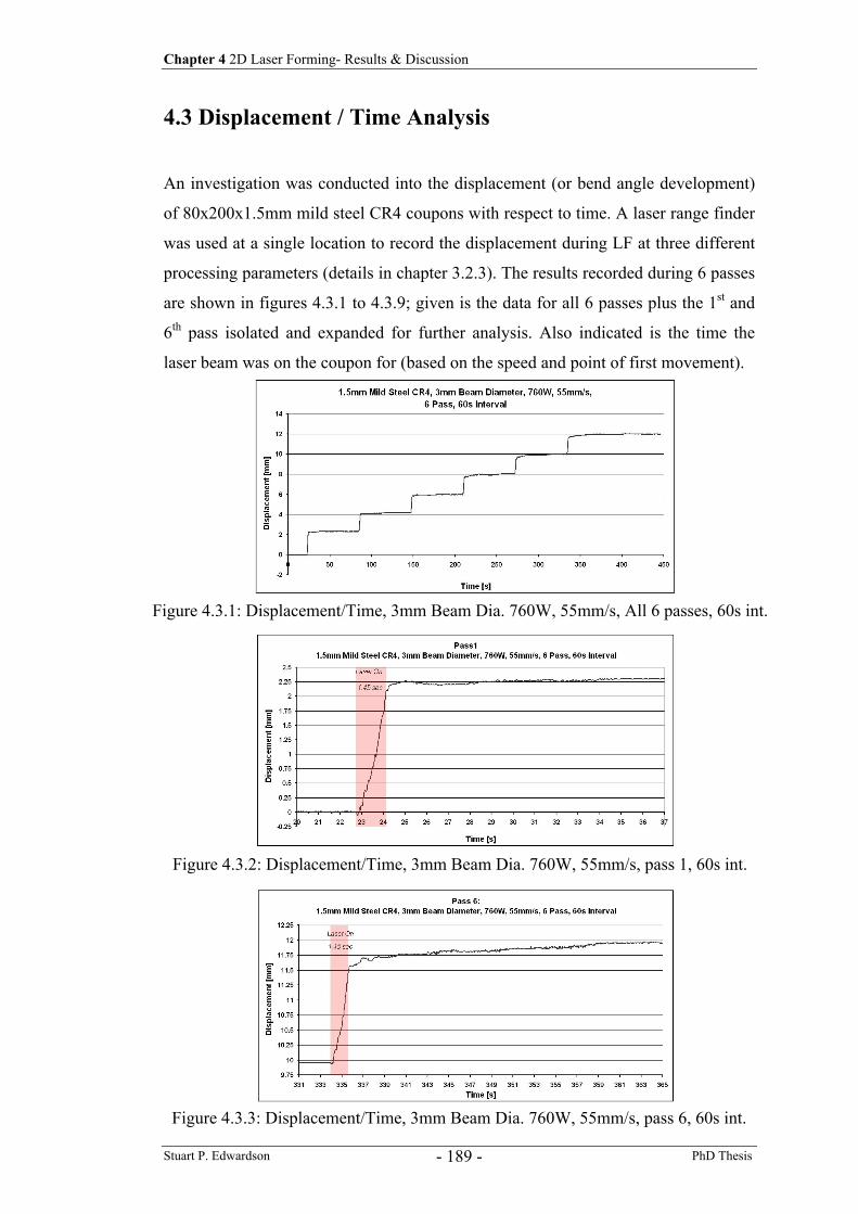
Chapter 4 2D Laser Forming- Results & Discussion
Stuart P. Edwardson PhD Thesis - 189 -
4.3 Displacement / Time Analysis
An investigation was conducted into the displacement (or bend angle development)
of 80x200x1.5mm mild steel CR4 coupons with respect to time. A laser range finder
was used at a single location to record the displacement during LF at three different
processing parameters (details in chapter 3.2.3). The results recorded during 6 passes
are shown in figures 4.3.1 to 4.3.9; given is the data for all 6 passes plus the 1st and
6th pass isolated and expanded for further analysis. Also indicated is the time the
laser beam was on the coupon for (based on the speed and point of first movement).
Figure 4.3.1: Displacement/Time, 3mm Beam Dia. 760W, 55mm/s, All 6 passes, 60s int.
Figure 4.3.2: Displacement/Time, 3mm Beam Dia. 760W, 55mm/s, pass 1, 60s int.
Figure 4.3.3: Displacement/Time, 3mm Beam Dia. 760W, 55mm/s, pass 6, 60s int.
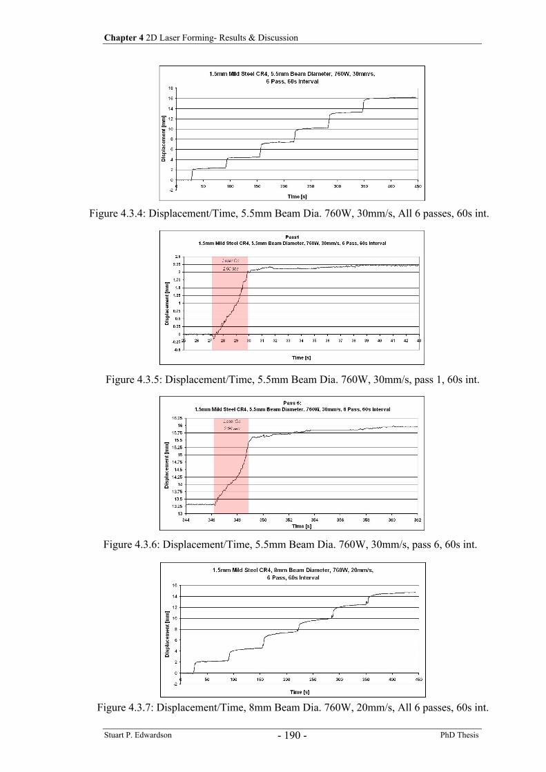
Chapter 4 2D Laser Forming- Results & Discussion
Stuart P. Edwardson PhD Thesis - 190 -
Figure 4.3.4: Displacement/Time, 5.5mm Beam Dia. 760W, 30mm/s, All 6 passes, 60s int.
Figure 4.3.5: Displacement/Time, 5.5mm Beam Dia. 760W, 30mm/s, pass 1, 60s int.
Figure 4.3.6: Displacement/Time, 5.5mm Beam Dia. 760W, 30mm/s, pass 6, 60s int.
Figure 4.3.7: Displacement/Time, 8mm Beam Dia. 760W, 20mm/s, All 6 passes, 60s int.
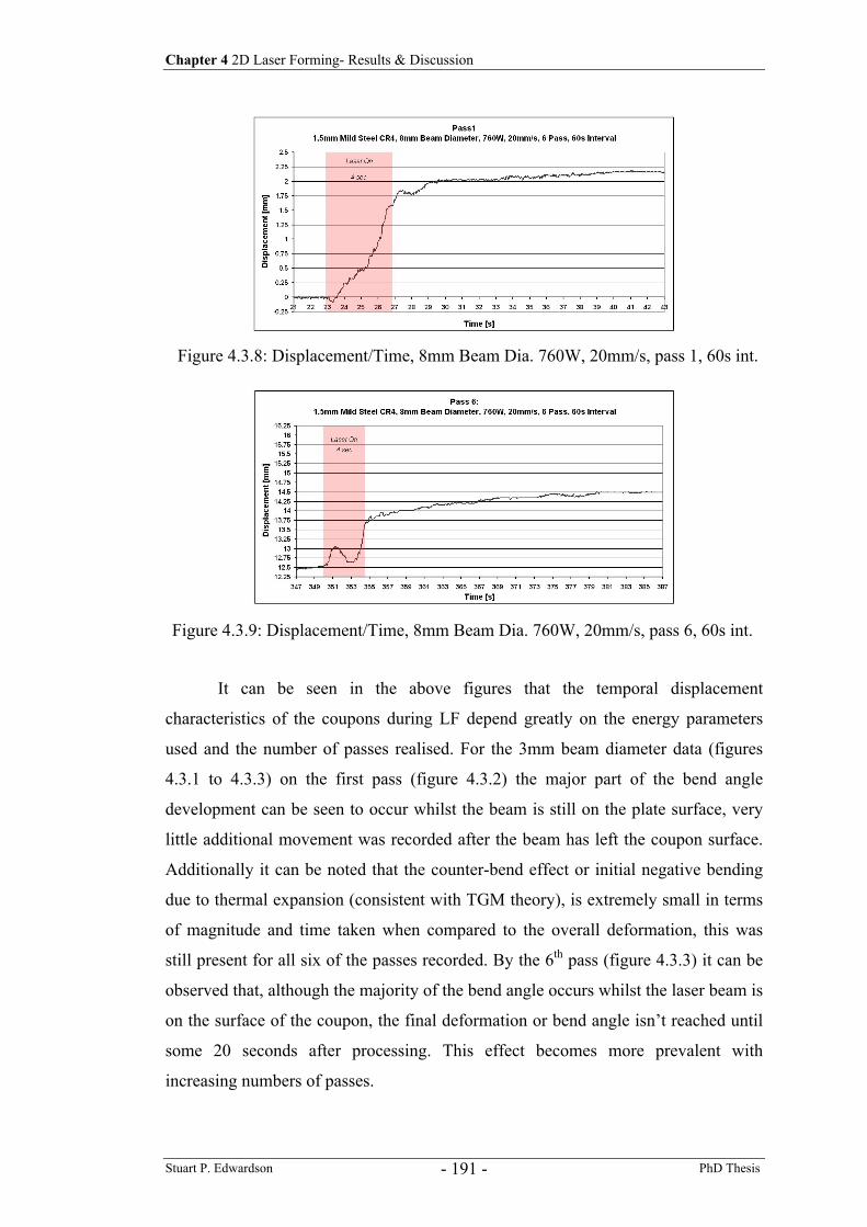
Chapter 4 2D Laser Forming- Results & Discussion
Stuart P. Edwardson PhD Thesis - 191 -
It can be seen in the above figures that the temporal displacement
characteristics of the coupons during LF depend greatly on the energy parameters
used and the number of passes realised. For the 3mm beam diameter data (figures
4.3.1 to 4.3.3) on the first pass (figure 4.3.2) the major part of the bend angle
development can be seen to occur whilst the beam is still on the plate surface, very
little additional movement was recorded after the beam has left the coupon surface.
Additionally it can be noted that the counter-bend effect or initial negative bending
due to thermal expansion (consistent with TGM theory), is extremely small in terms
of magnitude and time taken when compared to the overall deformation, this was
still present for all six of the passes recorded. By the 6th pass (figure 4.3.3) it can be
observed that, although the majority of the bend angle occurs whilst the laser beam is
on the surface of the coupon, the final deformation or bend angle isn’t reached until
some 20 seconds after processing. This effect becomes more prevalent with
increasing numbers of passes.
Figure 4.3.8: Displacement/Time, 8mm Beam Dia. 760W, 20mm/s, pass 1, 60s int.
Figure 4.3.9: Displacement/Time, 8mm Beam Dia. 760W, 20mm/s, pass 6, 60s int.
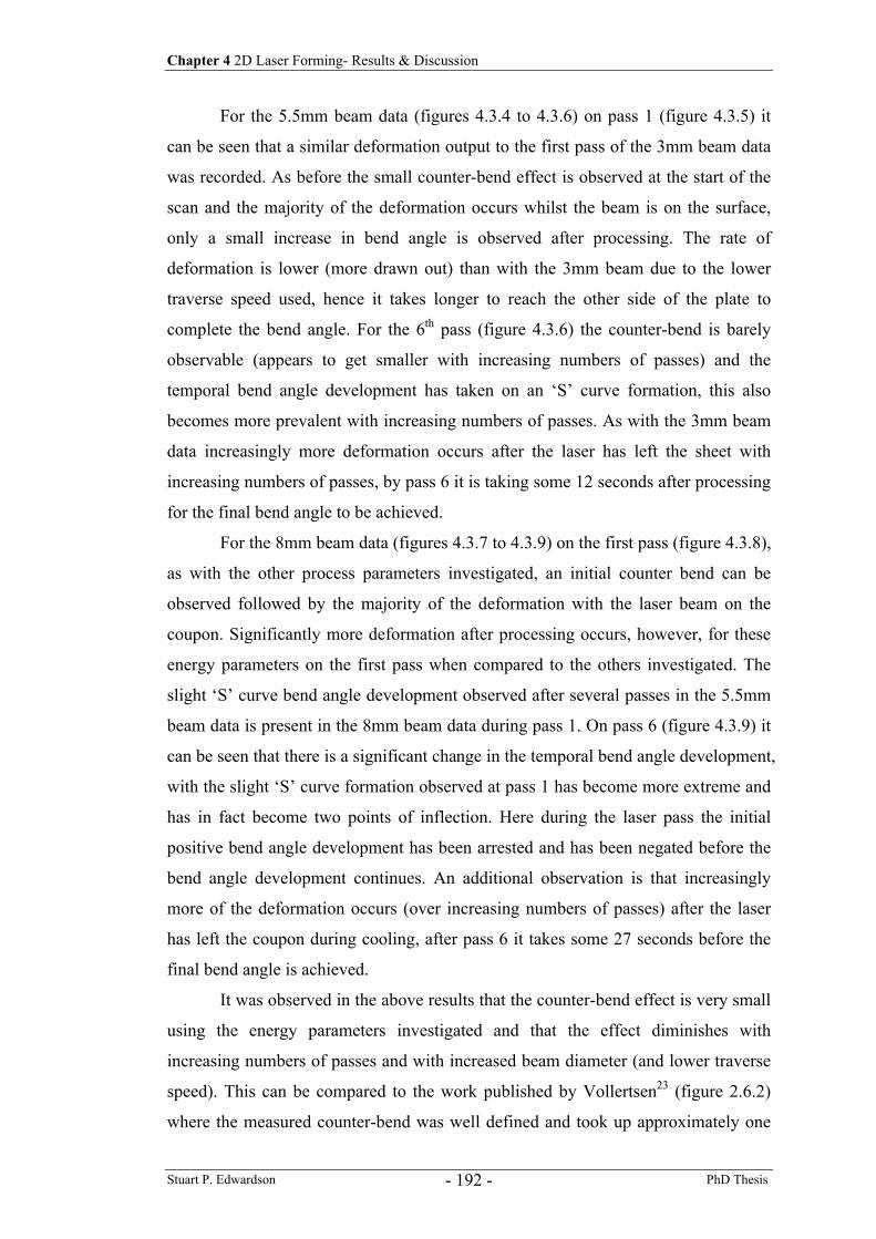
Chapter 4 2D Laser Forming- Results & Discussion
Stuart P. Edwardson PhD Thesis - 192 -
For the 5.5mm beam data (figures 4.3.4 to 4.3.6) on pass 1 (figure 4.3.5) it
can be seen that a similar deformation output to the first pass of the 3mm beam data
was recorded. As before the small counter-bend effect is observed at the start of the
scan and the majority of the deformation occurs whilst the beam is on the surface,
only a small increase in bend angle is observed after processing. The rate of
deformation is lower (more drawn out) than with the 3mm beam due to the lower
traverse speed used, hence it takes longer to reach the other side of the plate to
complete the bend angle. For the 6th pass (figure 4.3.6) the counter-bend is barely
observable (appears to get smaller with increasing numbers of passes) and the
temporal bend angle development has taken on an ‘S’ curve formation, this also
becomes more prevalent with increasing numbers of passes. As with the 3mm beam
data increasingly more deformation occurs after the laser has left the sheet with
increasing numbers of passes, by pass 6 it is taking some 12 seconds after processing
for the final bend angle to be achieved.
For the 8mm beam data (figures 4.3.7 to 4.3.9) on the first pass (figure 4.3.8),
as with the other process parameters investigated, an initial counter bend can be
observed followed by the majority of the deformation with the laser beam on the
coupon. Significantly more deformation after processing occurs, however, for these
energy parameters on the first pass when compared to the others investigated. The
slight ‘S’ curve bend angle development observed after several passes in the 5.5mm
beam data is present in the 8mm beam data during pass 1. On pass 6 (figure 4.3.9) it
can be seen that there is a significant change in the temporal bend angle development,
with the slight ‘S’ curve formation observed at pass 1 has become more extreme and
has in fact become two points of inflection. Here during the laser pass the initial
positive bend angle development has been arrested and has been negated before the
bend angle development continues. An additional observation is that increasingly
more of the deformation occurs (over increasing numbers of passes) after the laser
has left the coupon during cooling, after pass 6 it takes some 27 seconds before the
final bend angle is achieved.
It was observed in the above results that the counter-bend effect is very small
using the energy parameters investigated and that the effect diminishes with
increasing numbers of passes and with increased beam diameter (and lower traverse
speed). This can be compared to the work published by Vollertsen23 (figure 2.6.2)
where the measured counter-bend was well defined and took up approximately one
Chapter 4 2D Laser Forming- Results & Discussion
Stuart P. Edwardson PhD Thesis - 193 -
third of the deformation cycle time. The data recorded in this study would suggest
that the counter-bend is not as significant an event as this during the LF process
using the TGM. A possible reason for this difference is the beam diameter selection
used in this investigation. The TGM theory as proposed by Vollertsen 23 suggests a
beam diameter equal to or of the order of the sheet thickness, i.e. 1.5mm in this case,
it was found in this work, however, that a beam diameter smaller than 3mm caused
excessive surface damage at the power levels used. It was argued (earlier) that the
mechanism works by the setting up of a high thermal gradient through the thickness
such that the generated plastic compression would be asymmetric though the section
and hence a bend towards the laser work occur. This should be still be possible to set
up with larger beam diameters providing the energy input is high and the thermal
conductivity of the material is relatively low, the results presented demonstrate that
this is the case. By using larger beam diameters in conjunction with the TGM
appears to effect the temporal bend angle development, this could be due to the
increased depth of heating present causing a more lateral or in-plane displacement
during the initial thermal expansion rather than significant out of plane displacement
present where the heating is very localised to the upper surface area.
As the number of passes and beam diameter increases the heat retained in the
sample and time to cool increases also. This could be an explanation for the
increased time taken for the final bend angle to be reached observed in the above
results, in that as the purely elastic stresses are relieved during cooling the full extent
of the plastic compression or shrinkage in the upper surface along the scan line is
realised, hence the bend angle increases. Another possible factor in this is the
development of edge effects whereby the bend angle maybe different depending on
the location measured, the results from this study may indicate that the edge effects
develop after the beam has passed during cooling, this is backed up by other work on
the shape measurement of the process 129. If the plate geometry changes during
cooling then this may influence the displacement measurement recorded, multiple
measurement locations would confirm this.
The unusual temporal displacement or ‘S’ curve data observed using the
larger beam diameters at higher numbers of passes could be attributed to a change in
mechanism to the buckling mechanism (BM) or the increased in-plane movement
discussed earlier due to the hybrid TGM conditions, in that as the plate flexes as the
beam is drawn across the scan line there is a mechanical effect ahead and to the rear
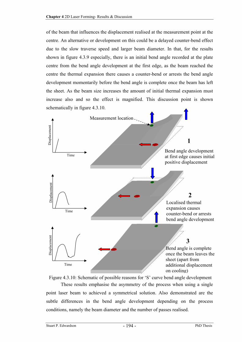
Chapter 4 2D Laser Forming- Results & Discussion
Stuart P. Edwardson PhD Thesis - 194 -
of the beam that influences the displacement realised at the measurement point at the
centre. An alternative or development on this could be a delayed counter-bend effect
due to the slow traverse speed and larger beam diameter. In that, for the results
shown in figure 4.3.9 especially, there is an initial bend angle recorded at the plate
centre from the bend angle development at the first edge, as the beam reached the
centre the thermal expansion there causes a counter-bend or arrests the bend angle
development momentarily before the bend angle is complete once the beam has left
the sheet. As the beam size increases the amount of initial thermal expansion must
increase also and so the effect is magnified. This discussion point is shown
schematically in figure 4.3.10.
These results emphasise the asymmetry of the process when using a single
point laser beam to achieved a symmetrical solution. Also demonstrated are the
subtle differences in the bend angle development depending on the process
conditions, namely the beam diameter and the number of passes realised.
Time
Dis
plac
emen
t
Time
Dis
plac
emen
t
Time
Dis
plac
emen
t
Figure 4.3.10: Schematic of possible reasons for ‘S’ curve bend angle development
1
2
3
Measurement location
Bend angle development at first edge causes initial positive displacement
Localised thermal expansion causes counter-bend or arrests bend angle development
Bend angle is complete once the beam leaves the sheet (apart from additional displacement on cooling)
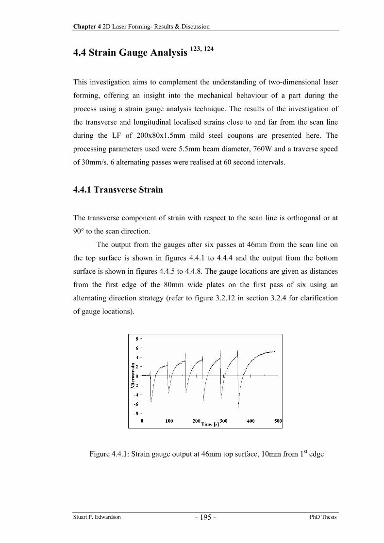
Chapter 4 2D Laser Forming- Results & Discussion
Stuart P. Edwardson PhD Thesis - 195 -
4.4 Strain Gauge Analysis 123, 124
This investigation aims to complement the understanding of two-dimensional laser
forming, offering an insight into the mechanical behaviour of a part during the
process using a strain gauge analysis technique. The results of the investigation of
the transverse and longitudinal localised strains close to and far from the scan line
during the LF of 200x80x1.5mm mild steel coupons are presented here. The
processing parameters used were 5.5mm beam diameter, 760W and a traverse speed
of 30mm/s. 6 alternating passes were realised at 60 second intervals.
4.4.1 Transverse Strain
The transverse component of strain with respect to the scan line is orthogonal or at
90° to the scan direction.
The output from the gauges after six passes at 46mm from the scan line on
the top surface is shown in figures 4.4.1 to 4.4.4 and the output from the bottom
surface is shown in figures 4.4.5 to 4.4.8. The gauge locations are given as distances
from the first edge of the 80mm wide plates on the first pass of six using an
alternating direction strategy (refer to figure 3.2.12 in section 3.2.4 for clarification
of gauge locations).
Figure 4.4.1: Strain gauge output at 46mm top surface, 10mm from 1st edge
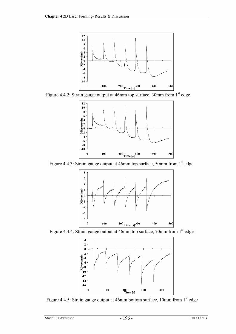
Chapter 4 2D Laser Forming- Results & Discussion
Stuart P. Edwardson PhD Thesis - 196 -
Figure 4.4.2: Strain gauge output at 46mm top surface, 30mm from 1st edge
Figure 4.4.3: Strain gauge output at 46mm top surface, 50mm from 1st edge
Figure 4.4.4: Strain gauge output at 46mm top surface, 70mm from 1st edge
Figure 4.4.5: Strain gauge output at 46mm bottom surface, 10mm from 1st edge
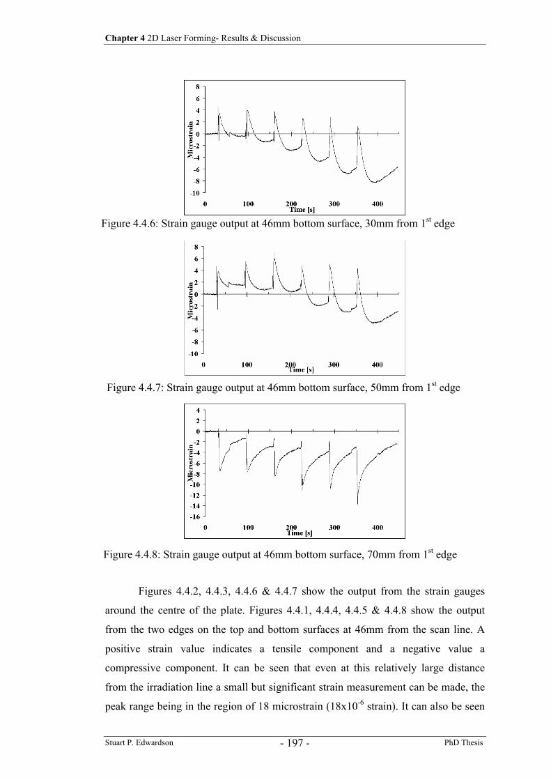
Chapter 4 2D Laser Forming- Results & Discussion
Stuart P. Edwardson PhD Thesis - 197 -
Figures 4.4.2, 4.4.3, 4.4.6 & 4.4.7 show the output from the strain gauges
around the centre of the plate. Figures 4.4.1, 4.4.4, 4.4.5 & 4.4.8 show the output
from the two edges on the top and bottom surfaces at 46mm from the scan line. A
positive strain value indicates a tensile component and a negative value a
compressive component. It can be seen that even at this relatively large distance
from the irradiation line a small but significant strain measurement can be made, the
peak range being in the region of 18 microstrain (18x10-6 strain). It can also be seen
Figure 4.4.6: Strain gauge output at 46mm bottom surface, 30mm from 1st edge
Figure 4.4.7: Strain gauge output at 46mm bottom surface, 50mm from 1st edge
Figure 4.4.8: Strain gauge output at 46mm bottom surface, 70mm from 1st edge
Chapter 4 2D Laser Forming- Results & Discussion
Stuart P. Edwardson PhD Thesis - 198 -
that there is a considerable difference in the strain output at the centre of the plate
compared to the edges. At the centre of the plate on the top surface (figures 4.4.2 &
4.4.3) a tensile component (perhaps due to thermal expansion) is seen during each
pass that recovers initially to a small residual tensile strain. Then, as the number of
passes increases an increasing residual compressive strain is seen, which recovers
somewhat several minutes after processing. At the plate edges on the top surface
(figures 4.4.1 & 4.4.4) an initial tensile component changes to a compressive
component during each pass and a tensile residual strain develops sometime after
processing. On the bottom surface similar strain outputs to the top surface from the
centre (figures 4.4.6 & 4.4.7) to the edges (figures 4.4.5 & 4.4.8) of the plate are seen.
However at the centre the magnitudes of the induced tensile strains are less than the
top surface but there is still a residual compressive strain component after processing.
At the plate edges on the bottom surface the initial tensile component during
processing is less than that at the top surface and the recovery after processing is to
an increasing residual compressive strain. The residual strains on the bottom surface
appear to recover several minutes after processing upon cooling. It can also be noted
in all of the results at a distance of 46mm that the effect of the alternating processing
direction is a variation in the peak values depending on the direction.
To summarise the results at 46mm from the scan line for the 200x80mm
plates, it can be seen that compressive strains are generated near the centre of the
plate and tensile strains at the edges on the top and bottom surfaces during
processing. The residual strain components appear to recover upon cooling, however
a residual tensile component is observed at the edges on the top surface.
These results appear consistent with the observed edge effect 60 or
longitudinal bowing phenomena where it is thought a change in boundary conditions
from the centre to the edge of the plate results in a variation in bend angle from edge
to edge. If a different in-process strain cycle occurs and hence a different residual
transverse strain state exists between the centre and the edge of the plate and top and
bottom surfaces, then this could possibly explain this edge effect distortion. Further
investigation is necessary to determine the longitudinal strains during laser forming,
as this should aid the explanation of the edge effect distortion still further.
The output from the gauges at 10mm from the irradiation line on the top
surface is shown in figures 4.4.9 to 4.4.11 and the output from the bottom surface is
shown in figures 4.4.12 to 4.4.14. As there was a very similar output from the
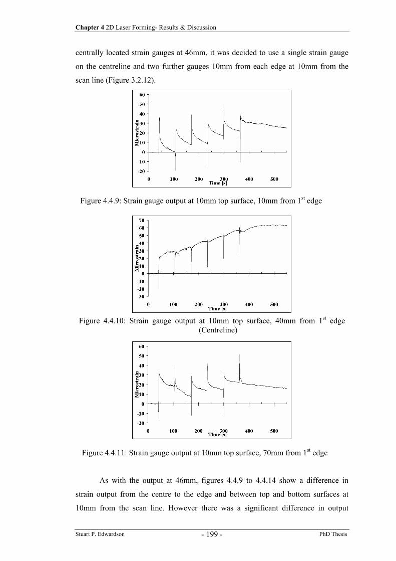
Chapter 4 2D Laser Forming- Results & Discussion
Stuart P. Edwardson PhD Thesis - 199 -
centrally located strain gauges at 46mm, it was decided to use a single strain gauge
on the centreline and two further gauges 10mm from each edge at 10mm from the
scan line (Figure 3.2.12).
As with the output at 46mm, figures 4.4.9 to 4.4.14 show a difference in
strain output from the centre to the edge and between top and bottom surfaces at
10mm from the scan line. However there was a significant difference in output
Figure 4.4.9: Strain gauge output at 10mm top surface, 10mm from 1st edge
Figure 4.4.10: Strain gauge output at 10mm top surface, 40mm from 1st edge (Centreline)
Figure 4.4.11: Strain gauge output at 10mm top surface, 70mm from 1st edge
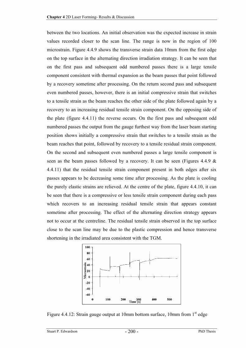
Chapter 4 2D Laser Forming- Results & Discussion
Stuart P. Edwardson PhD Thesis - 200 -
between the two locations. An initial observation was the expected increase in strain
values recorded closer to the scan line. The range is now in the region of 100
microstrain. Figure 4.4.9 shows the transverse strain data 10mm from the first edge
on the top surface in the alternating direction irradiation strategy. It can be seen that
on the first pass and subsequent odd numbered passes there is a large tensile
component consistent with thermal expansion as the beam passes that point followed
by a recovery sometime after processing. On the return second pass and subsequent
even numbered passes, however, there is an initial compressive strain that switches
to a tensile strain as the beam reaches the other side of the plate followed again by a
recovery to an increasing residual tensile strain component. On the opposing side of
the plate (figure 4.4.11) the reverse occurs. On the first pass and subsequent odd
numbered passes the output from the gauge furthest way from the laser beam starting
position shows initially a compressive strain that switches to a tensile strain as the
beam reaches that point, followed by recovery to a tensile residual strain component.
On the second and subsequent even numbered passes a large tensile component is
seen as the beam passes followed by a recovery. It can be seen (Figures 4.4.9 &
4.4.11) that the residual tensile strain component present in both edges after six
passes appears to be decreasing some time after processing. As the plate is cooling
the purely elastic strains are relieved. At the centre of the plate, figure 4.4.10, it can
be seen that there is a compressive or less tensile strain component during each pass
which recovers to an increasing residual tensile strain that appears constant
sometime after processing. The effect of the alternating direction strategy appears
not to occur at the centreline. The residual tensile strain observed in the top surface
close to the scan line may be due to the plastic compression and hence transverse
shortening in the irradiated area consistent with the TGM.
Figure 4.4.12: Strain gauge output at 10mm bottom surface, 10mm from 1st edge
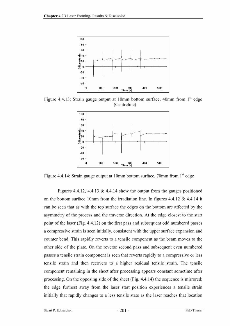
Chapter 4 2D Laser Forming- Results & Discussion
Stuart P. Edwardson PhD Thesis - 201 -
Figures 4.4.12, 4.4.13 & 4.4.14 show the output from the gauges positioned
on the bottom surface 10mm from the irradiation line. In figures 4.4.12 & 4.4.14 it
can be seen that as with the top surface the edges on the bottom are affected by the
asymmetry of the process and the traverse direction. At the edge closest to the start
point of the laser (Fig. 4.4.12) on the first pass and subsequent odd numbered passes
a compressive strain is seen initially, consistent with the upper surface expansion and
counter bend. This rapidly reverts to a tensile component as the beam moves to the
other side of the plate. On the reverse second pass and subsequent even numbered
passes a tensile strain component is seen that reverts rapidly to a compressive or less
tensile strain and then recovers to a higher residual tensile strain. The tensile
component remaining in the sheet after processing appears constant sometime after
processing. On the opposing side of the sheet (Fig. 4.4.14) the sequence is mirrored;
the edge furthest away from the laser start position experiences a tensile strain
initially that rapidly changes to a less tensile state as the laser reaches that location
Figure 4.4.13: Strain gauge output at 10mm bottom surface, 40mm from 1st edge (Centreline)
Figure 4.4.14: Strain gauge output at 10mm bottom surface, 70mm from 1st edge
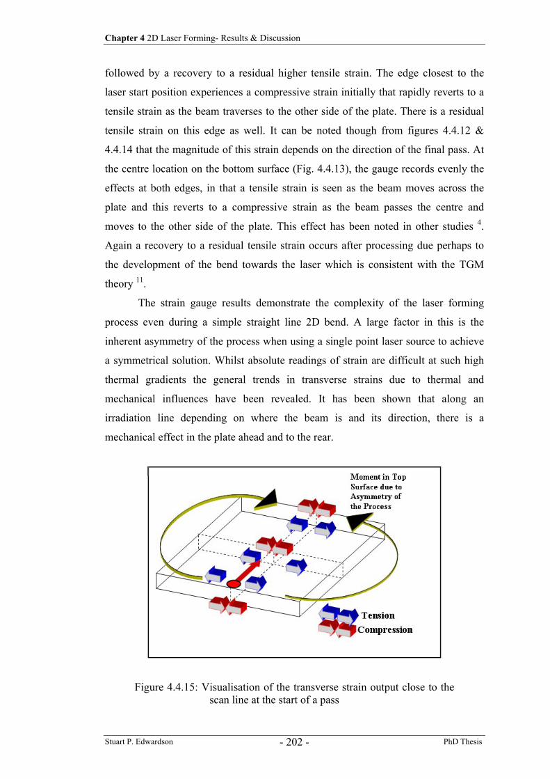
Chapter 4 2D Laser Forming- Results & Discussion
Stuart P. Edwardson PhD Thesis - 202 -
followed by a recovery to a residual higher tensile strain. The edge closest to the
laser start position experiences a compressive strain initially that rapidly reverts to a
tensile strain as the beam traverses to the other side of the plate. There is a residual
tensile strain on this edge as well. It can be noted though from figures 4.4.12 &
4.4.14 that the magnitude of this strain depends on the direction of the final pass. At
the centre location on the bottom surface (Fig. 4.4.13), the gauge records evenly the
effects at both edges, in that a tensile strain is seen as the beam moves across the
plate and this reverts to a compressive strain as the beam passes the centre and
moves to the other side of the plate. This effect has been noted in other studies 4.
Again a recovery to a residual tensile strain occurs after processing due perhaps to
the development of the bend towards the laser which is consistent with the TGM
theory 11.
The strain gauge results demonstrate the complexity of the laser forming
process even during a simple straight line 2D bend. A large factor in this is the
inherent asymmetry of the process when using a single point laser source to achieve
a symmetrical solution. Whilst absolute readings of strain are difficult at such high
thermal gradients the general trends in transverse strains due to thermal and
mechanical influences have been revealed. It has been shown that along an
irradiation line depending on where the beam is and its direction, there is a
mechanical effect in the plate ahead and to the rear.
Figure 4.4.15: Visualisation of the transverse strain output close to the scan line at the start of a pass
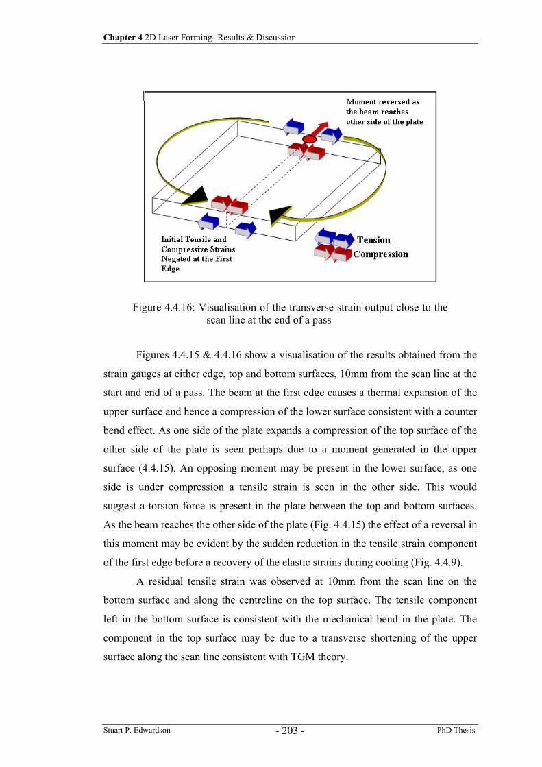
Chapter 4 2D Laser Forming- Results & Discussion
Stuart P. Edwardson PhD Thesis - 203 -
Figures 4.4.15 & 4.4.16 show a visualisation of the results obtained from the
strain gauges at either edge, top and bottom surfaces, 10mm from the scan line at the
start and end of a pass. The beam at the first edge causes a thermal expansion of the
upper surface and hence a compression of the lower surface consistent with a counter
bend effect. As one side of the plate expands a compression of the top surface of the
other side of the plate is seen perhaps due to a moment generated in the upper
surface (4.4.15). An opposing moment may be present in the lower surface, as one
side is under compression a tensile strain is seen in the other side. This would
suggest a torsion force is present in the plate between the top and bottom surfaces.
As the beam reaches the other side of the plate (Fig. 4.4.15) the effect of a reversal in
this moment may be evident by the sudden reduction in the tensile strain component
of the first edge before a recovery of the elastic strains during cooling (Fig. 4.4.9).
A residual tensile strain was observed at 10mm from the scan line on the
bottom surface and along the centreline on the top surface. The tensile component
left in the bottom surface is consistent with the mechanical bend in the plate. The
component in the top surface may be due to a transverse shortening of the upper
surface along the scan line consistent with TGM theory.
Figure 4.4.16: Visualisation of the transverse strain output close to the scan line at the end of a pass
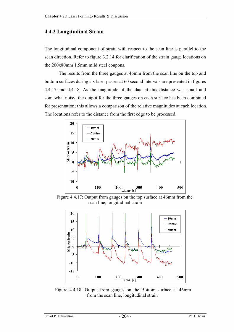
Chapter 4 2D Laser Forming- Results & Discussion
Stuart P. Edwardson PhD Thesis - 204 -
4.4.2 Longitudinal Strain
The longitudinal component of strain with respect to the scan line is parallel to the
scan direction. Refer to figure 3.2.14 for clarification of the strain gauge locations on
the 200x80mm 1.5mm mild steel coupons.
The results from the three gauges at 46mm from the scan line on the top and
bottom surfaces during six laser passes at 60 second intervals are presented in figures
4.4.17 and 4.4.18. As the magnitude of the data at this distance was small and
somewhat noisy, the output for the three gauges on each surface has been combined
for presentation; this allows a comparison of the relative magnitudes at each location.
The locations refer to the distance from the first edge to be processed.
Figure 4.4.17: Output from gauges on the top surface at 46mm from the scan line, longitudinal strain
Figure 4.4.18: Output from gauges on the Bottom surface at 46mm from the scan line, longitudinal strain
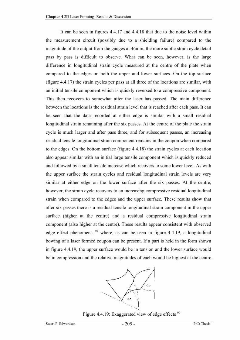
Chapter 4 2D Laser Forming- Results & Discussion
Stuart P. Edwardson PhD Thesis - 205 -
It can be seen in figures 4.4.17 and 4.4.18 that due to the noise level within
the measurement circuit (possibly due to a shielding failure) compared to the
magnitude of the output from the gauges at 46mm, the more subtle strain cycle detail
pass by pass is difficult to observe. What can be seen, however, is the large
difference in longitudinal strain cycle measured at the centre of the plate when
compared to the edges on both the upper and lower surfaces. On the top surface
(figure 4.4.17) the strain cycles per pass at all three of the locations are similar, with
an initial tensile component which is quickly reversed to a compressive component.
This then recovers to somewhat after the laser has passed. The main difference
between the locations is the residual strain level that is reached after each pass. It can
be seen that the data recorded at either edge is similar with a small residual
longitudinal strain remaining after the six passes. At the centre of the plate the strain
cycle is much larger and after pass three, and for subsequent passes, an increasing
residual tensile longitudinal strain component remains in the coupon when compared
to the edges. On the bottom surface (figure 4.4.18) the strain cycles at each location
also appear similar with an initial large tensile component which is quickly reduced
and followed by a small tensile increase which recovers to some lower level. As with
the upper surface the strain cycles and residual longitudinal strain levels are very
similar at either edge on the lower surface after the six passes. At the centre,
however, the strain cycle recovers to an increasing compressive residual longitudinal
strain when compared to the edges and the upper surface. These results show that
after six passes there is a residual tensile longitudinal strain component in the upper
surface (higher at the centre) and a residual compressive longitudinal strain
component (also higher at the centre). These results appear consistent with observed
edge effect phenomena 60 where, as can be seen in figure 4.4.19, a longitudinal
bowing of a laser formed coupon can be present. If a part is held in the form shown
in figure 4.4.19, the upper surface would be in tension and the lower surface would
be in compression and the relative magnitudes of each would be highest at the centre.
Figure 4.4.19: Exaggerated view of edge effects 60
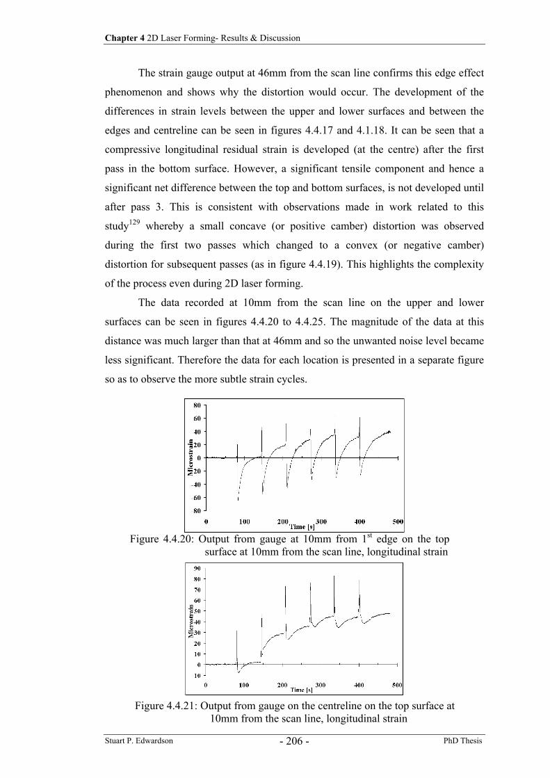
Chapter 4 2D Laser Forming- Results & Discussion
Stuart P. Edwardson PhD Thesis - 206 -
The strain gauge output at 46mm from the scan line confirms this edge effect
phenomenon and shows why the distortion would occur. The development of the
differences in strain levels between the upper and lower surfaces and between the
edges and centreline can be seen in figures 4.4.17 and 4.1.18. It can be seen that a
compressive longitudinal residual strain is developed (at the centre) after the first
pass in the bottom surface. However, a significant tensile component and hence a
significant net difference between the top and bottom surfaces, is not developed until
after pass 3. This is consistent with observations made in work related to this
study129 whereby a small concave (or positive camber) distortion was observed
during the first two passes which changed to a convex (or negative camber)
distortion for subsequent passes (as in figure 4.4.19). This highlights the complexity
of the process even during 2D laser forming.
The data recorded at 10mm from the scan line on the upper and lower
surfaces can be seen in figures 4.4.20 to 4.4.25. The magnitude of the data at this
distance was much larger than that at 46mm and so the unwanted noise level became
less significant. Therefore the data for each location is presented in a separate figure
so as to observe the more subtle strain cycles.
Figure 4.4.20: Output from gauge at 10mm from 1st edge on the top surface at 10mm from the scan line, longitudinal strain
Figure 4.4.21: Output from gauge on the centreline on the top surface at 10mm from the scan line, longitudinal strain
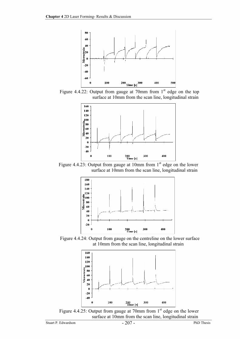
Chapter 4 2D Laser Forming- Results & Discussion
Stuart P. Edwardson PhD Thesis - 207 -
Figure 4.4.22: Output from gauge at 70mm from 1st edge on the top surface at 10mm from the scan line, longitudinal strain
Figure 4.4.23: Output from gauge at 10mm from 1st edge on the lower surface at 10mm from the scan line, longitudinal strain
Figure 4.4.24: Output from gauge on the centreline on the lower surface at 10mm from the scan line, longitudinal strain
Figure 4.4.25: Output from gauge at 70mm from 1st edge on the lower surface at 10mm from the scan line, longitudinal strain
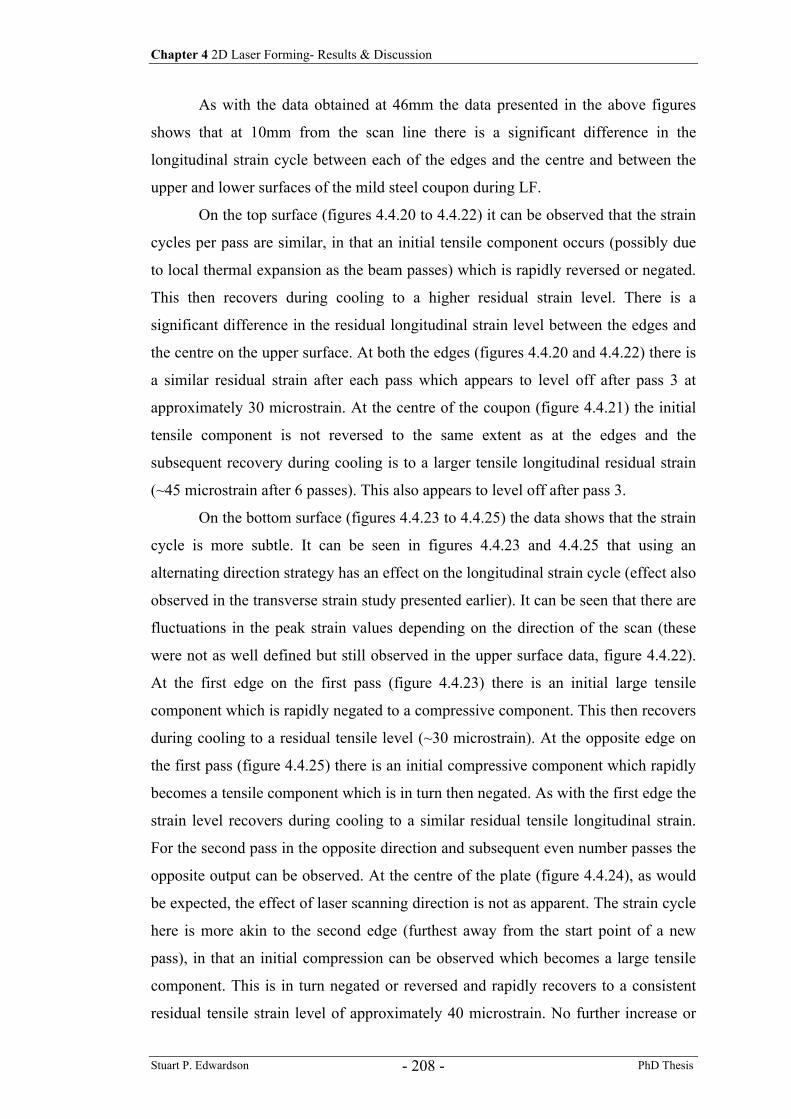
Chapter 4 2D Laser Forming- Results & Discussion
Stuart P. Edwardson PhD Thesis - 208 -
As with the data obtained at 46mm the data presented in the above figures
shows that at 10mm from the scan line there is a significant difference in the
longitudinal strain cycle between each of the edges and the centre and between the
upper and lower surfaces of the mild steel coupon during LF.
On the top surface (figures 4.4.20 to 4.4.22) it can be observed that the strain
cycles per pass are similar, in that an initial tensile component occurs (possibly due
to local thermal expansion as the beam passes) which is rapidly reversed or negated.
This then recovers during cooling to a higher residual strain level. There is a
significant difference in the residual longitudinal strain level between the edges and
the centre on the upper surface. At both the edges (figures 4.4.20 and 4.4.22) there is
a similar residual strain after each pass which appears to level off after pass 3 at
approximately 30 microstrain. At the centre of the coupon (figure 4.4.21) the initial
tensile component is not reversed to the same extent as at the edges and the
subsequent recovery during cooling is to a larger tensile longitudinal residual strain
(~45 microstrain after 6 passes). This also appears to level off after pass 3.
On the bottom surface (figures 4.4.23 to 4.4.25) the data shows that the strain
cycle is more subtle. It can be seen in figures 4.4.23 and 4.4.25 that using an
alternating direction strategy has an effect on the longitudinal strain cycle (effect also
observed in the transverse strain study presented earlier). It can be seen that there are
fluctuations in the peak strain values depending on the direction of the scan (these
were not as well defined but still observed in the upper surface data, figure 4.4.22).
At the first edge on the first pass (figure 4.4.23) there is an initial large tensile
component which is rapidly negated to a compressive component. This then recovers
during cooling to a residual tensile level (~30 microstrain). At the opposite edge on
the first pass (figure 4.4.25) there is an initial compressive component which rapidly
becomes a tensile component which is in turn then negated. As with the first edge the
strain level recovers during cooling to a similar residual tensile longitudinal strain.
For the second pass in the opposite direction and subsequent even number passes the
opposite output can be observed. At the centre of the plate (figure 4.4.24), as would
be expected, the effect of laser scanning direction is not as apparent. The strain cycle
here is more akin to the second edge (furthest away from the start point of a new
pass), in that an initial compression can be observed which becomes a large tensile
component. This is in turn negated or reversed and rapidly recovers to a consistent
residual tensile strain level of approximately 40 microstrain. No further increase or
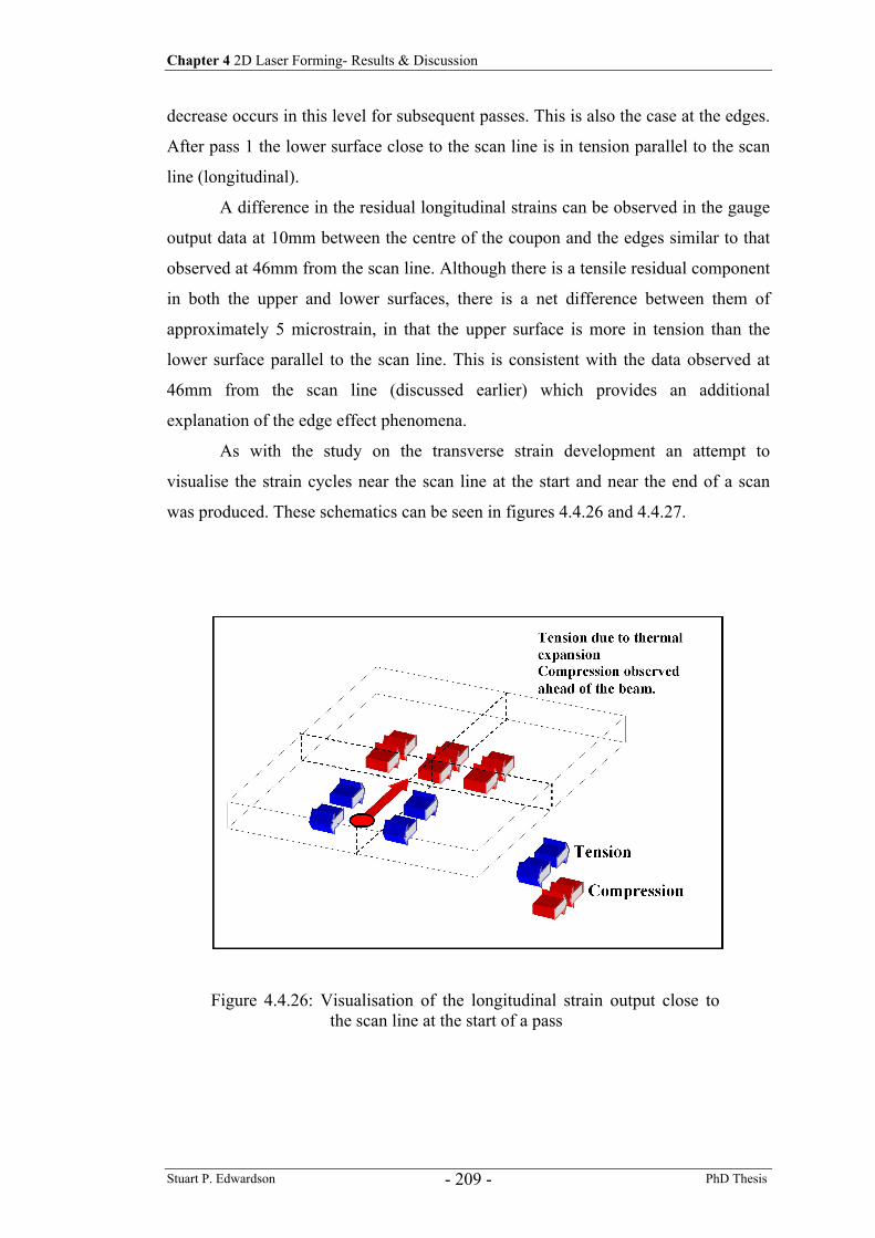
Chapter 4 2D Laser Forming- Results & Discussion
Stuart P. Edwardson PhD Thesis - 209 -
decrease occurs in this level for subsequent passes. This is also the case at the edges.
After pass 1 the lower surface close to the scan line is in tension parallel to the scan
line (longitudinal).
A difference in the residual longitudinal strains can be observed in the gauge
output data at 10mm between the centre of the coupon and the edges similar to that
observed at 46mm from the scan line. Although there is a tensile residual component
in both the upper and lower surfaces, there is a net difference between them of
approximately 5 microstrain, in that the upper surface is more in tension than the
lower surface parallel to the scan line. This is consistent with the data observed at
46mm from the scan line (discussed earlier) which provides an additional
explanation of the edge effect phenomena.
As with the study on the transverse strain development an attempt to
visualise the strain cycles near the scan line at the start and near the end of a scan
was produced. These schematics can be seen in figures 4.4.26 and 4.4.27.
Figure 4.4.26: Visualisation of the longitudinal strain output close to the scan line at the start of a pass
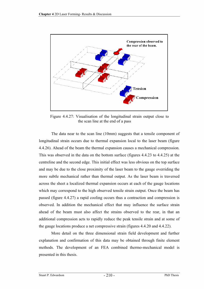
Chapter 4 2D Laser Forming- Results & Discussion
Stuart P. Edwardson PhD Thesis - 210 -
The data near to the scan line (10mm) suggests that a tensile component of
longitudinal strain occurs due to thermal expansion local to the laser beam (figure
4.4.26). Ahead of the beam the thermal expansion causes a mechanical compression.
This was observed in the data on the bottom surface (figures 4.4.23 to 4.4.25) at the
centreline and the second edge. This initial effect was less obvious on the top surface
and may be due to the close proximity of the laser beam to the gauge overriding the
more subtle mechanical rather than thermal output. As the laser beam is traversed
across the sheet a localized thermal expansion occurs at each of the gauge locations
which may correspond to the high observed tensile strain output. Once the beam has
passed (figure 4.4.27) a rapid cooling occurs thus a contraction and compression is
observed. In addition the mechanical effect that may influence the surface strain
ahead of the beam must also affect the strains observed to the rear, in that an
additional compression acts to rapidly reduce the peak tensile strain and at some of
the gauge locations produce a net compressive strain (figures 4.4.20 and 4.4.22).
More detail on the three dimensional strain field development and further
explanation and confirmation of this data may be obtained through finite element
methods. The development of an FEA combined thermo-mechanical model is
presented in this thesis.
Figure 4.4.27: Visualisation of the longitudinal strain output close to the scan line at the end of a pass
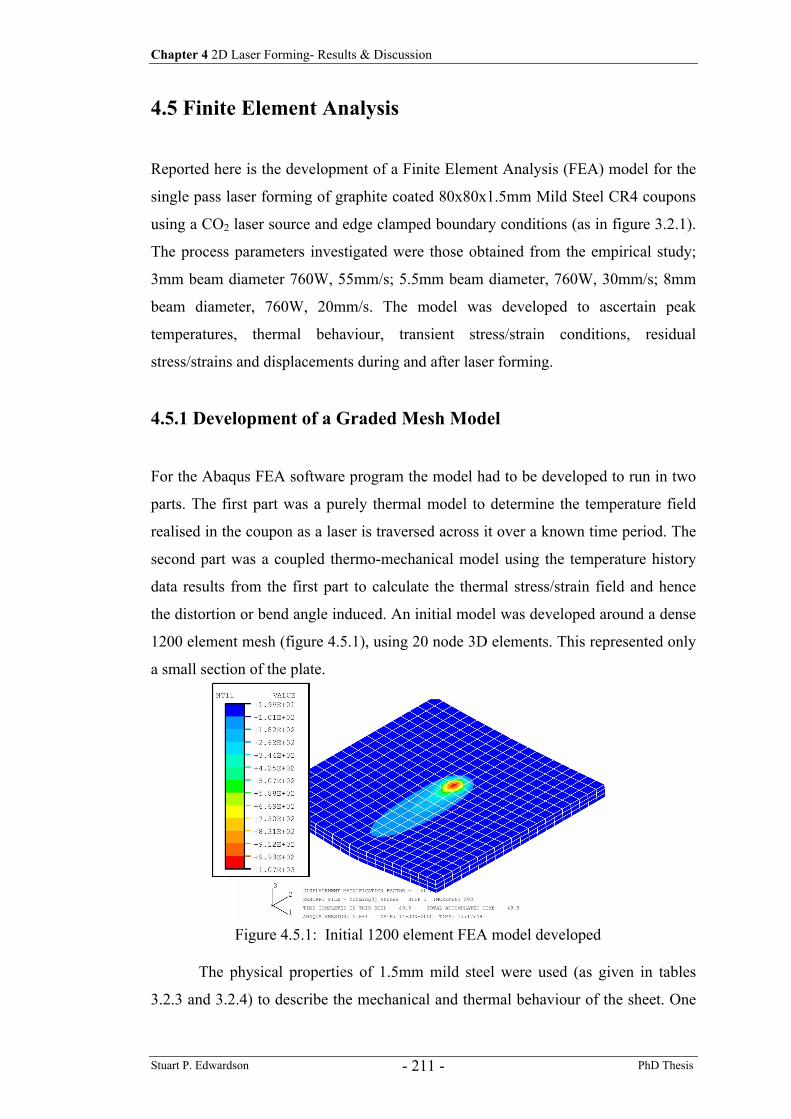
Chapter 4 2D Laser Forming- Results & Discussion
Stuart P. Edwardson PhD Thesis - 211 -
4.5 Finite Element Analysis
Reported here is the development of a Finite Element Analysis (FEA) model for the
single pass laser forming of graphite coated 80x80x1.5mm Mild Steel CR4 coupons
using a CO2 laser source and edge clamped boundary conditions (as in figure 3.2.1).
The process parameters investigated were those obtained from the empirical study;
3mm beam diameter 760W, 55mm/s; 5.5mm beam diameter, 760W, 30mm/s; 8mm
beam diameter, 760W, 20mm/s. The model was developed to ascertain peak
temperatures, thermal behaviour, transient stress/strain conditions, residual
stress/strains and displacements during and after laser forming.
4.5.1 Development of a Graded Mesh Model
For the Abaqus FEA software program the model had to be developed to run in two
parts. The first part was a purely thermal model to determine the temperature field
realised in the coupon as a laser is traversed across it over a known time period. The
second part was a coupled thermo-mechanical model using the temperature history
data results from the first part to calculate the thermal stress/strain field and hence
the distortion or bend angle induced. An initial model was developed around a dense
1200 element mesh (figure 4.5.1), using 20 node 3D elements. This represented only
a small section of the plate.
The physical properties of 1.5mm mild steel were used (as given in tables
3.2.3 and 3.2.4) to describe the mechanical and thermal behaviour of the sheet. One
Figure 4.5.1: Initial 1200 element FEA model developed
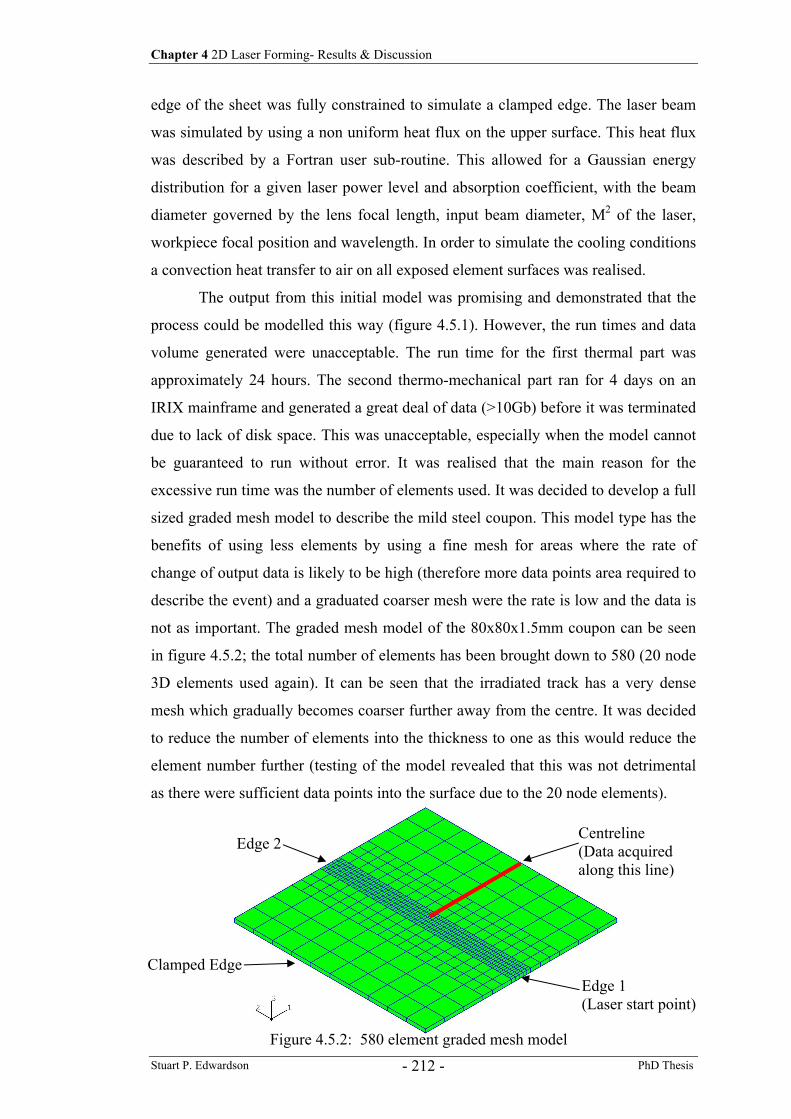
Chapter 4 2D Laser Forming- Results & Discussion
Stuart P. Edwardson PhD Thesis - 212 -
edge of the sheet was fully constrained to simulate a clamped edge. The laser beam
was simulated by using a non uniform heat flux on the upper surface. This heat flux
was described by a Fortran user sub-routine. This allowed for a Gaussian energy
distribution for a given laser power level and absorption coefficient, with the beam
diameter governed by the lens focal length, input beam diameter, M2 of the laser,
workpiece focal position and wavelength. In order to simulate the cooling conditions
a convection heat transfer to air on all exposed element surfaces was realised.
The output from this initial model was promising and demonstrated that the
process could be modelled this way (figure 4.5.1). However, the run times and data
volume generated were unacceptable. The run time for the first thermal part was
approximately 24 hours. The second thermo-mechanical part ran for 4 days on an
IRIX mainframe and generated a great deal of data (>10Gb) before it was terminated
due to lack of disk space. This was unacceptable, especially when the model cannot
be guaranteed to run without error. It was realised that the main reason for the
excessive run time was the number of elements used. It was decided to develop a full
sized graded mesh model to describe the mild steel coupon. This model type has the
benefits of using less elements by using a fine mesh for areas where the rate of
change of output data is likely to be high (therefore more data points area required to
describe the event) and a graduated coarser mesh were the rate is low and the data is
not as important. The graded mesh model of the 80x80x1.5mm coupon can be seen
in figure 4.5.2; the total number of elements has been brought down to 580 (20 node
3D elements used again). It can be seen that the irradiated track has a very dense
mesh which gradually becomes coarser further away from the centre. It was decided
to reduce the number of elements into the thickness to one as this would reduce the
element number further (testing of the model revealed that this was not detrimental
as there were sufficient data points into the surface due to the 20 node elements).
Figure 4.5.2: 580 element graded mesh model
Clamped Edge Edge 1 (Laser start point)
Edge 2 Centreline (Data acquired along this line)
Chapter 4 2D Laser Forming- Results & Discussion
Stuart P. Edwardson PhD Thesis - 213 -
All of the boundary and loading conditions and physical properties developed
for the first model (described earlier) were used for this model as well. The Abaqus
input file that describes this model is given in appendix 2.
The run times for this model were much better, for the first thermal part the
run time was approximately 1 hour and for the more computer intense coupled
thermo-mechanical analysis the run time was approximately 36 hours (depending on
output requirements). A SunOS 5.8 based mainframe was used to run the model.
The output from this FEA model is presented in the following sections; this is
divided into the purely thermal output for the three process parameter combinations
(3, 5.5 and 8mm beam diameters) and the output from the thermo-mechanical model
for the 5.5mm beam diameter process combination.
It is felt that the output from this FEA model will be useful, and whilst some
calibration with real data occurs (described later), the output data cannot be regarded
as absolute (although checks are made to see that the data is realistic). However, the
FEA technique does allow the visualisation of events at any point on the coupon in
real time (such as 3D strain field development) which may aid the further
understanding of the 2D laser forming process.
4.5.2 Thermal Analysis
Key to a usable FEA model is the production of realistic results. A method of
ensuring this is to tune the model to real measured data. This was achieved here by
the use of thermocouple data presented earlier in section 4.2.1. This gave
temperature development with respect to time for locations from 10 to 58mm from
the scan line on the upper and lower surfaces (the closer to the scan line the better).
The absorption coefficient, A, is key to tuning the model to this real data, in that by
varying A, observing the temperature output at 10 and 22mm from the scan line and
then comparing this to the measured data it was possible to achieve a good
agreement in terms of heating rate and peak temperature at these locations. The
cooling rate was tuned to the measured data by varying the convection coefficient to
the surrounding air.
The variation in peak temperature from the model at the centre of the scan
line (on the centreline, upper surface, figure 4.5.2) with absorption coefficient for a
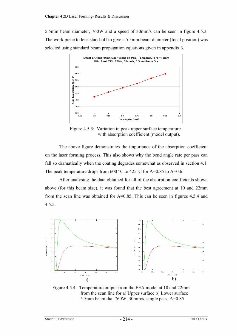
Chapter 4 2D Laser Forming- Results & Discussion
Stuart P. Edwardson PhD Thesis - 214 -
5.5mm beam diameter, 760W and a speed of 30mm/s can be seen in figure 4.5.3.
The work piece to lens stand-off to give a 5.5mm beam diameter (focal position) was
selected using standard beam propagation equations given in appendix 3.
The above figure demonstrates the importance of the absorption coefficient
on the laser forming process. This also shows why the bend angle rate per pass can
fall so dramatically when the coating degrades somewhat as observed in section 4.1.
The peak temperature drops from 600 °C to 425°C for A=0.85 to A=0.6.
After analysing the data obtained for all of the absorption coefficients shown
above (for this beam size), it was found that the best agreement at 10 and 22mm
from the scan line was obtained for A=0.85. This can be seen in figures 4.5.4 and
4.5.5.
Figure 4.5.3: Variation in peak upper surface temperature with absorption coefficient (model output).
Figure 4.5.4: Temperature output from the FEA model at 10 and 22mm from the scan line for a) Upper surface b) Lower surface 5.5mm beam dia. 760W, 30mm/s, single pass, A=0.85
a) b)
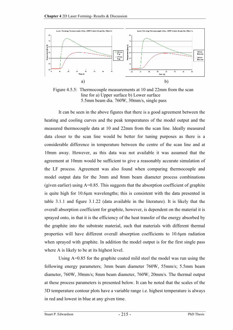
Chapter 4 2D Laser Forming- Results & Discussion
Stuart P. Edwardson PhD Thesis - 215 -
It can be seen in the above figures that there is a good agreement between the
heating and cooling curves and the peak temperatures of the model output and the
measured thermocouple data at 10 and 22mm from the scan line. Ideally measured
data closer to the scan line would be better for tuning purposes as there is a
considerable difference in temperature between the centre of the scan line and at
10mm away. However, as this data was not available it was assumed that the
agreement at 10mm would be sufficient to give a reasonably accurate simulation of
the LF process. Agreement was also found when comparing thermocouple and
model output data for the 3mm and 8mm beam diameter process combinations
(given earlier) using A=0.85. This suggests that the absorption coefficient of graphite
is quite high for 10.6µm wavelengths; this is consistent with the data presented in
table 3.1.1 and figure 3.1.22 (data available in the literature). It is likely that the
overall absorption coefficient for graphite, however, is dependent on the material it is
sprayed onto, in that it is the efficiency of the heat transfer of the energy absorbed by
the graphite into the substrate material, such that materials with different thermal
properties will have different overall absorption coefficients to 10.6µm radiation
when sprayed with graphite. In addition the model output is for the first single pass
where A is likely to be at its highest level.
Using A=0.85 for the graphite coated mild steel the model was run using the
following energy parameters; 3mm beam diameter 760W, 55mm/s; 5.5mm beam
diameter, 760W, 30mm/s; 8mm beam diameter, 760W, 20mm/s. The thermal output
at these process parameters is presented below. It can be noted that the scales of the
3D temperature contour plots have a variable range i.e. highest temperature is always
in red and lowest in blue at any given time.
Figure 4.5.5: Thermocouple measurements at 10 and 22mm from the scan line for a) Upper surface b) Lower surface 5.5mm beam dia. 760W, 30mm/s, single pass
a) b)
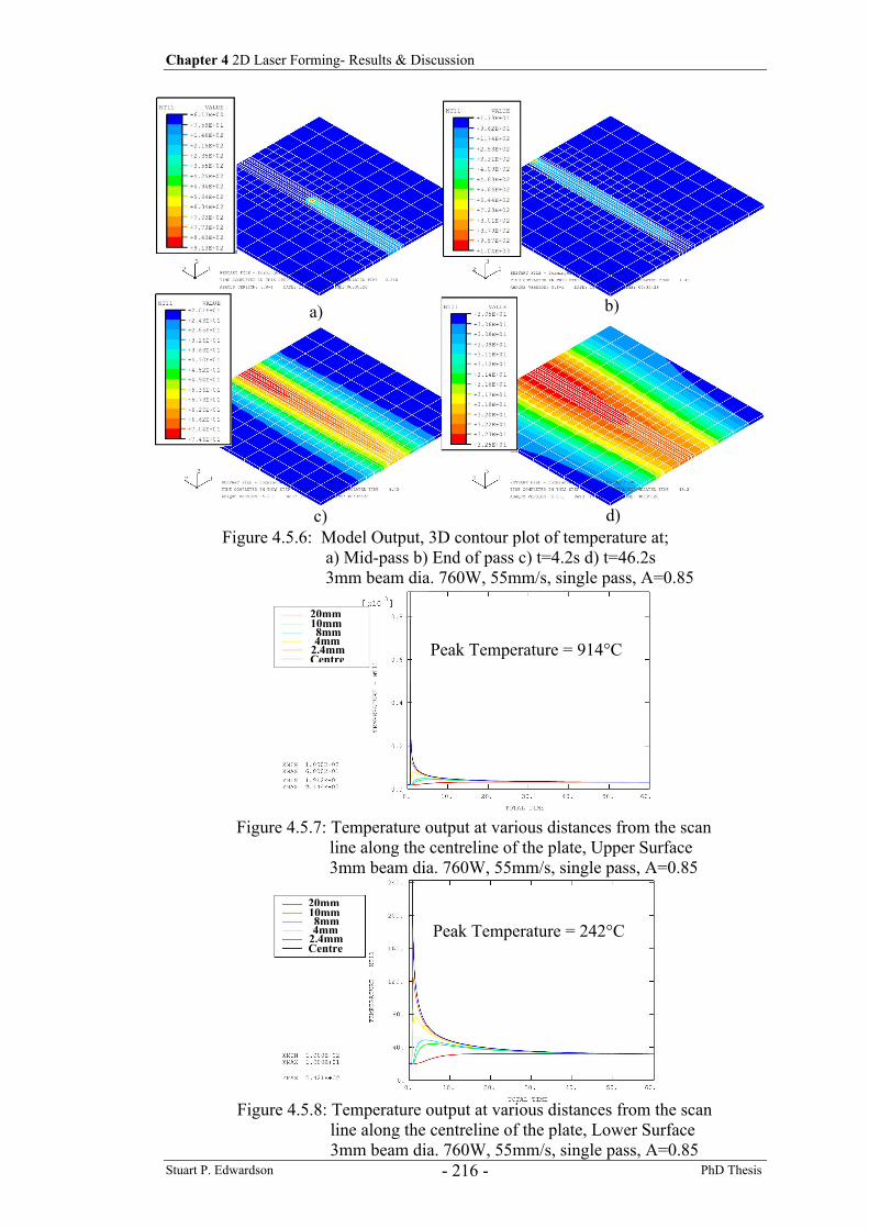
Chapter 4 2D Laser Forming- Results & Discussion
Stuart P. Edwardson PhD Thesis - 216 -
Figure 4.5.6: Model Output, 3D contour plot of temperature at; a) Mid-pass b) End of pass c) t=4.2s d) t=46.2s 3mm beam dia. 760W, 55mm/s, single pass, A=0.85
Figure 4.5.7: Temperature output at various distances from the scan line along the centreline of the plate, Upper Surface 3mm beam dia. 760W, 55mm/s, single pass, A=0.85
Figure 4.5.8: Temperature output at various distances from the scan line along the centreline of the plate, Lower Surface 3mm beam dia. 760W, 55mm/s, single pass, A=0.85
20mm10mm8mm4mm
2.4mmCentre
20mm10mm8mm4mm
2.4mmCentre
Peak Temperature = 914°C
Peak Temperature = 242°C
b) a)
c) d)
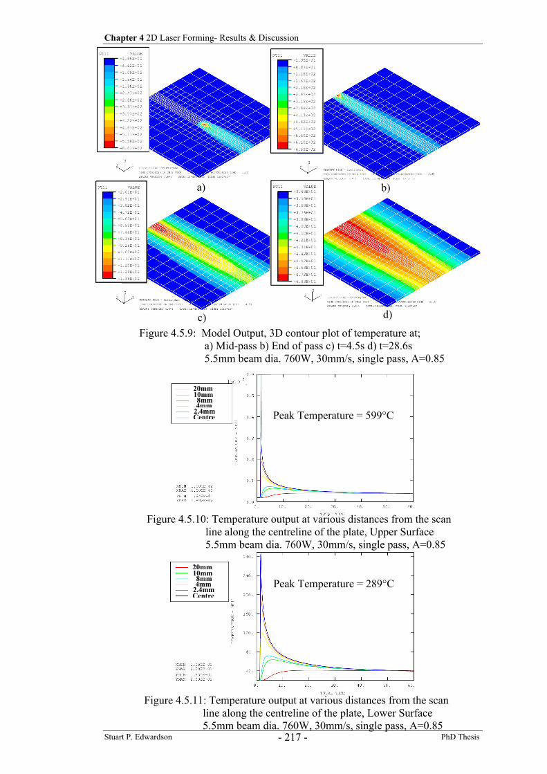
Chapter 4 2D Laser Forming- Results & Discussion
Stuart P. Edwardson PhD Thesis - 217 -
Figure 4.5.9: Model Output, 3D contour plot of temperature at; a) Mid-pass b) End of pass c) t=4.5s d) t=28.6s 5.5mm beam dia. 760W, 30mm/s, single pass, A=0.85
c)
Figure 4.5.11: Temperature output at various distances from the scan line along the centreline of the plate, Lower Surface 5.5mm beam dia. 760W, 30mm/s, single pass, A=0.85
Figure 4.5.10: Temperature output at various distances from the scan line along the centreline of the plate, Upper Surface 5.5mm beam dia. 760W, 30mm/s, single pass, A=0.85
Peak Temperature = 599°C
Peak Temperature = 289°C
20mm10mm8mm4mm
2.4mmCentre
20mm10mm8mm4mm
2.4mmCentre
a) b)
d)
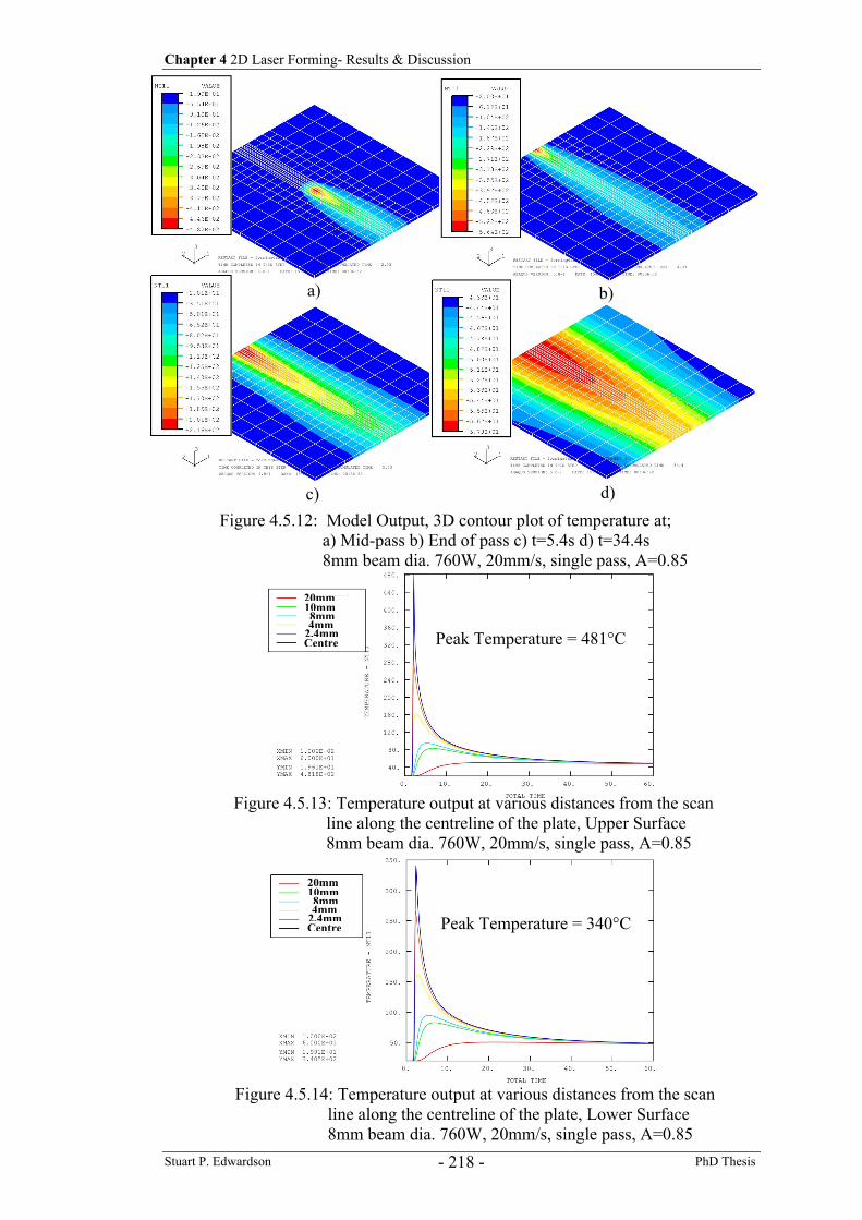
Chapter 4 2D Laser Forming- Results & Discussion
Stuart P. Edwardson PhD Thesis - 218 -
Figure 4.5.12: Model Output, 3D contour plot of temperature at; a) Mid-pass b) End of pass c) t=5.4s d) t=34.4s 8mm beam dia. 760W, 20mm/s, single pass, A=0.85
Figure 4.5.13: Temperature output at various distances from the scan line along the centreline of the plate, Upper Surface 8mm beam dia. 760W, 20mm/s, single pass, A=0.85
Figure 4.5.14: Temperature output at various distances from the scan line along the centreline of the plate, Lower Surface 8mm beam dia. 760W, 20mm/s, single pass, A=0.85
20mm10mm8mm4mm
2.4mmCentre
20mm10mm8mm4mm
2.4mmCentre
Peak Temperature = 481°C
Peak Temperature = 340°C
d) c)
a) b)
Chapter 4 2D Laser Forming- Results & Discussion
Stuart P. Edwardson PhD Thesis - 219 -
It can seen in the above figures that the output from the Abaqus FEA model
can be presented in both X-Y plot form (from many points) and as a 3D contour plot
at any point in the time cycle. In addition an animation of the thermal cycle can be
created. It should be noted that these are the thermal outputs only and so no
deformation was recorded. For the 3D contour plots (figures 4.5.6, 4.5.9 and 4.5.12)
the variable scale can be somewhat confusing; however, this allows the presentation
of the lower temperature data as the plate cools. This would be lost if the scale was
fixed (i.e. 0 to 600°C), instead the highest temperature in the plate at a given time is
assigned the red colour and the lowest blue.
It can be observed in figures 4.5.6, 4.5.9 and 4.5.12 that the modelling of the
incident laser beam on the coupon appears to work well, with the beam size
increasing as the workpiece stand-off is increased. The energy distribution within the
beam can also be observed; although this is not the exact beam mode used, this was
thought to be a reasonable approximation. A problem with the mesh generation can
also be observed in these figures. It was realised that at the interface between the
different densities of mesh a discrepancy between the numbers of nodes has led to
the generation of the unsmooth contours or ripples observed. Although not ideal, it
was felt that in the region of interest along the scan line the data is unaffected and
therefore the analysis should continue. It is intended that this problem will be
rectified in ongoing future work in this field.
In figures 4.5.7, 4.5.10 and 4.5.13 it can be seen that the heating and cooling
curves recorded on the upper surface on the scan line show very high heating and
cooling rates. It can be seen that peak temperatures are only achieved for fractions of
a second before being rapidly quenched by conduction into the surrounding (cold)
bulk material. As would be expected the further away from the centre of the scan line
the lower the peak temperature observed. It can be seen that the peak temperature
increases considerably with decreasing beam diameter, consistent with the increase
in intensity for the same power.
A comparison has been made between the temperatures realised at the same
locations on the upper and lower surfaces. For the 3mm beam diameter data (figures
4.5.7 and 4.5.8) a high peak temperature of 914°C has been predicted at the centre of
the plate on the upper surface. On the lower surface at the same point a peak
temperature of only 242°C has been observed. This is consistent with the TGM
where a high thermal gradient through the thickness is necessary to give the
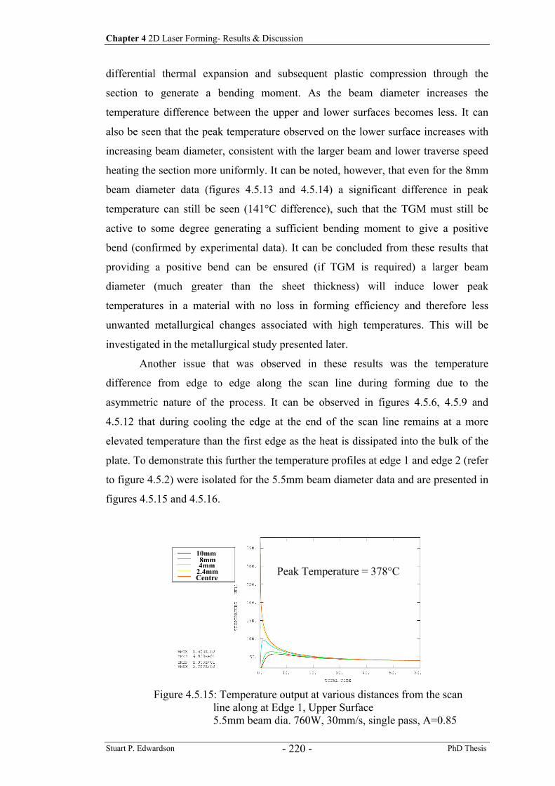
Chapter 4 2D Laser Forming- Results & Discussion
Stuart P. Edwardson PhD Thesis - 220 -
differential thermal expansion and subsequent plastic compression through the
section to generate a bending moment. As the beam diameter increases the
temperature difference between the upper and lower surfaces becomes less. It can
also be seen that the peak temperature observed on the lower surface increases with
increasing beam diameter, consistent with the larger beam and lower traverse speed
heating the section more uniformly. It can be noted, however, that even for the 8mm
beam diameter data (figures 4.5.13 and 4.5.14) a significant difference in peak
temperature can still be seen (141°C difference), such that the TGM must still be
active to some degree generating a sufficient bending moment to give a positive
bend (confirmed by experimental data). It can be concluded from these results that
providing a positive bend can be ensured (if TGM is required) a larger beam
diameter (much greater than the sheet thickness) will induce lower peak
temperatures in a material with no loss in forming efficiency and therefore less
unwanted metallurgical changes associated with high temperatures. This will be
investigated in the metallurgical study presented later.
Another issue that was observed in these results was the temperature
difference from edge to edge along the scan line during forming due to the
asymmetric nature of the process. It can be observed in figures 4.5.6, 4.5.9 and
4.5.12 that during cooling the edge at the end of the scan line remains at a more
elevated temperature than the first edge as the heat is dissipated into the bulk of the
plate. To demonstrate this further the temperature profiles at edge 1 and edge 2 (refer
to figure 4.5.2) were isolated for the 5.5mm beam diameter data and are presented in
figures 4.5.15 and 4.5.16.
Figure 4.5.15: Temperature output at various distances from the scan
line along at Edge 1, Upper Surface 5.5mm beam dia. 760W, 30mm/s, single pass, A=0.85
Peak Temperature = 378°C 10mm
8mm4mm
2.4mmCentre
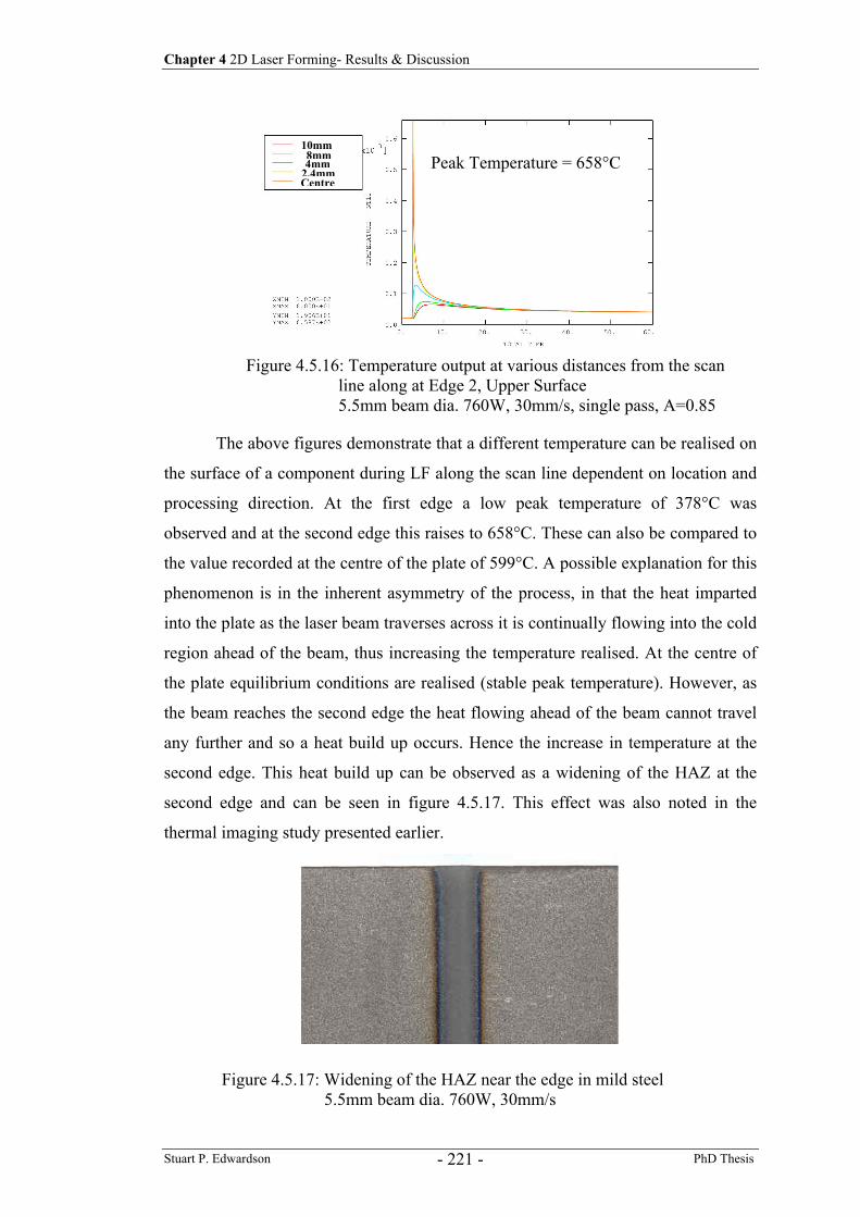
Chapter 4 2D Laser Forming- Results & Discussion
Stuart P. Edwardson PhD Thesis - 221 -
The above figures demonstrate that a different temperature can be realised on
the surface of a component during LF along the scan line dependent on location and
processing direction. At the first edge a low peak temperature of 378°C was
observed and at the second edge this raises to 658°C. These can also be compared to
the value recorded at the centre of the plate of 599°C. A possible explanation for this
phenomenon is in the inherent asymmetry of the process, in that the heat imparted
into the plate as the laser beam traverses across it is continually flowing into the cold
region ahead of the beam, thus increasing the temperature realised. At the centre of
the plate equilibrium conditions are realised (stable peak temperature). However, as
the beam reaches the second edge the heat flowing ahead of the beam cannot travel
any further and so a heat build up occurs. Hence the increase in temperature at the
second edge. This heat build up can be observed as a widening of the HAZ at the
second edge and can be seen in figure 4.5.17. This effect was also noted in the
thermal imaging study presented earlier.
Peak Temperature = 658°C
Figure 4.5.16: Temperature output at various distances from the scan line along at Edge 2, Upper Surface 5.5mm beam dia. 760W, 30mm/s, single pass, A=0.85
10mm8mm4mm
2.4mmCentre
Figure 4.5.17: Widening of the HAZ near the edge in mild steel 5.5mm beam dia. 760W, 30mm/s
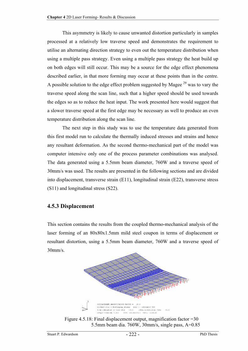
Chapter 4 2D Laser Forming- Results & Discussion
Stuart P. Edwardson PhD Thesis - 222 -
This asymmetry is likely to cause unwanted distortion particularly in samples
processed at a relatively low traverse speed and demonstrates the requirement to
utilise an alternating direction strategy to even out the temperature distribution when
using a multiple pass strategy. Even using a multiple pass strategy the heat build up
on both edges will still occur. This may be a source for the edge effect phenomena
described earlier, in that more forming may occur at these points than in the centre.
A possible solution to the edge effect problem suggested by Magee 29 was to vary the
traverse speed along the scan line, such that a higher speed should be used towards
the edges so as to reduce the heat input. The work presented here would suggest that
a slower traverse speed at the first edge may be necessary as well to produce an even
temperature distribution along the scan line.
The next step in this study was to use the temperature data generated from
this first model run to calculate the thermally induced stresses and strains and hence
any resultant deformation. As the second thermo-mechanical part of the model was
computer intensive only one of the process parameter combinations was analysed.
The data generated using a 5.5mm beam diameter, 760W and a traverse speed of
30mm/s was used. The results are presented in the following sections and are divided
into displacement, transverse strain (E11), longitudinal strain (E22), transverse stress
(S11) and longitudinal stress (S22).
4.5.3 Displacement
This section contains the results from the coupled thermo-mechanical analysis of the
laser forming of an 80x80x1.5mm mild steel coupon in terms of displacement or
resultant distortion, using a 5.5mm beam diameter, 760W and a traverse speed of
30mm/s.
Figure 4.5.18: Final displacement output, magnification factor =30 5.5mm beam dia. 760W, 30mm/s, single pass, A=0.85
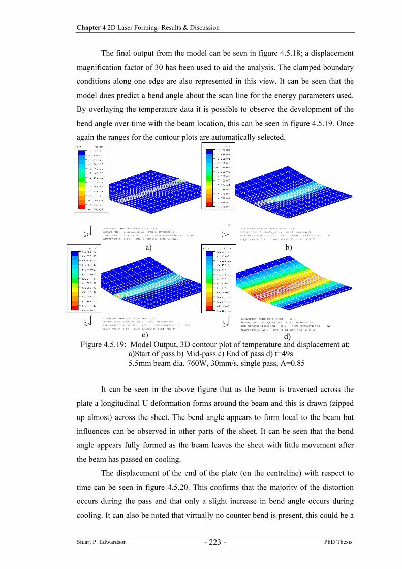
Chapter 4 2D Laser Forming- Results & Discussion
Stuart P. Edwardson PhD Thesis - 223 -
The final output from the model can be seen in figure 4.5.18; a displacement
magnification factor of 30 has been used to aid the analysis. The clamped boundary
conditions along one edge are also represented in this view. It can be seen that the
model does predict a bend angle about the scan line for the energy parameters used.
By overlaying the temperature data it is possible to observe the development of the
bend angle over time with the beam location, this can be seen in figure 4.5.19. Once
again the ranges for the contour plots are automatically selected.
It can be seen in the above figure that as the beam is traversed across the
plate a longitudinal U deformation forms around the beam and this is drawn (zipped
up almost) across the sheet. The bend angle appears to form local to the beam but
influences can be observed in other parts of the sheet. It can be seen that the bend
angle appears fully formed as the beam leaves the sheet with little movement after
the beam has passed on cooling.
The displacement of the end of the plate (on the centreline) with respect to
time can be seen in figure 4.5.20. This confirms that the majority of the distortion
occurs during the pass and that only a slight increase in bend angle occurs during
cooling. It can also be noted that virtually no counter bend is present, this could be a
Figure 4.5.19: Model Output, 3D contour plot of temperature and displacement at; a)Start of pass b) Mid-pass c) End of pass d) t=49s 5.5mm beam dia. 760W, 30mm/s, single pass, A=0.85
a) b)
c) d)
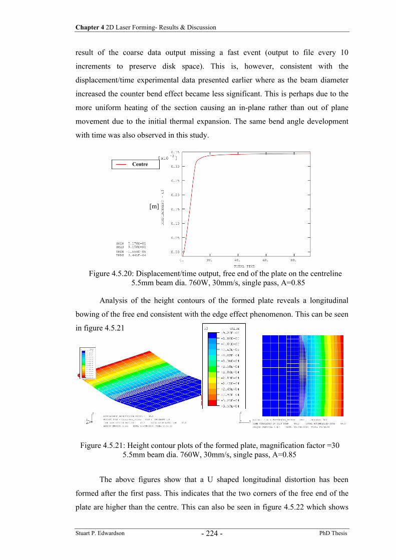
Chapter 4 2D Laser Forming- Results & Discussion
Stuart P. Edwardson PhD Thesis - 224 -
result of the coarse data output missing a fast event (output to file every 10
increments to preserve disk space). This is, however, consistent with the
displacement/time experimental data presented earlier where as the beam diameter
increased the counter bend effect became less significant. This is perhaps due to the
more uniform heating of the section causing an in-plane rather than out of plane
movement due to the initial thermal expansion. The same bend angle development
with time was also observed in this study.
Analysis of the height contours of the formed plate reveals a longitudinal
bowing of the free end consistent with the edge effect phenomenon. This can be seen
in figure 4.5.21
The above figures show that a U shaped longitudinal distortion has been
formed after the first pass. This indicates that the two corners of the free end of the
plate are higher than the centre. This can also be seen in figure 4.5.22 which shows
Figure 4.5.20: Displacement/time output, free end of the plate on the centreline5.5mm beam dia. 760W, 30mm/s, single pass, A=0.85
[m]
Figure 4.5.21: Height contour plots of the formed plate, magnification factor =305.5mm beam dia. 760W, 30mm/s, single pass, A=0.85
Centre
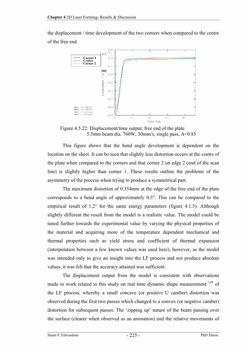
Chapter 4 2D Laser Forming- Results & Discussion
Stuart P. Edwardson PhD Thesis - 225 -
the displacement / time development of the two corners when compared to the centre
of the free end.
This figure shows that the bend angle development is dependent on the
location on the sheet. It can be seen that slightly less distortion occurs at the centre of
the plate when compared to the corners and that corner 2 on edge 2 (end of the scan
line) is slightly higher than corner 1. These results outline the problems of the
asymmetry of the process when trying to produce a symmetrical part.
The maximum distortion of 0.354mm at the edge of the free end of the plate
corresponds to a bend angle of approximately 0.5°. This can be compared to the
empirical result of 1.2° for the same energy parameters (figure 4.1.5). Although
slightly different the result from the model is a realistic value. The model could be
tuned further towards the experimental value by varying the physical properties of
the material and acquiring more of the temperature dependent mechanical and
thermal properties such as yield stress and coefficient of thermal expansion
(interpolation between a few known values was used here), however, as the model
was intended only to give an insight into the LF process and not produce absolute
values, it was felt that the accuracy attained was sufficient.
The displacement output from the model is consistent with observations
made in work related to this study on real time dynamic shape measurement 129 of
the LF process, whereby a small concave (or positive U camber) distortion was
observed during the first two passes which changed to a convex (or negative camber)
distortion for subsequent passes. The ‘zipping up’ nature of the beam passing over
the surface (clearer when observed as an animation) and the relative movements of
Corner 1 CentreCorner 2
Figure 4.5.22: Displacement/time output, free end of the plate 5.5mm beam dia. 760W, 30mm/s, single pass, A=0.85
[m]
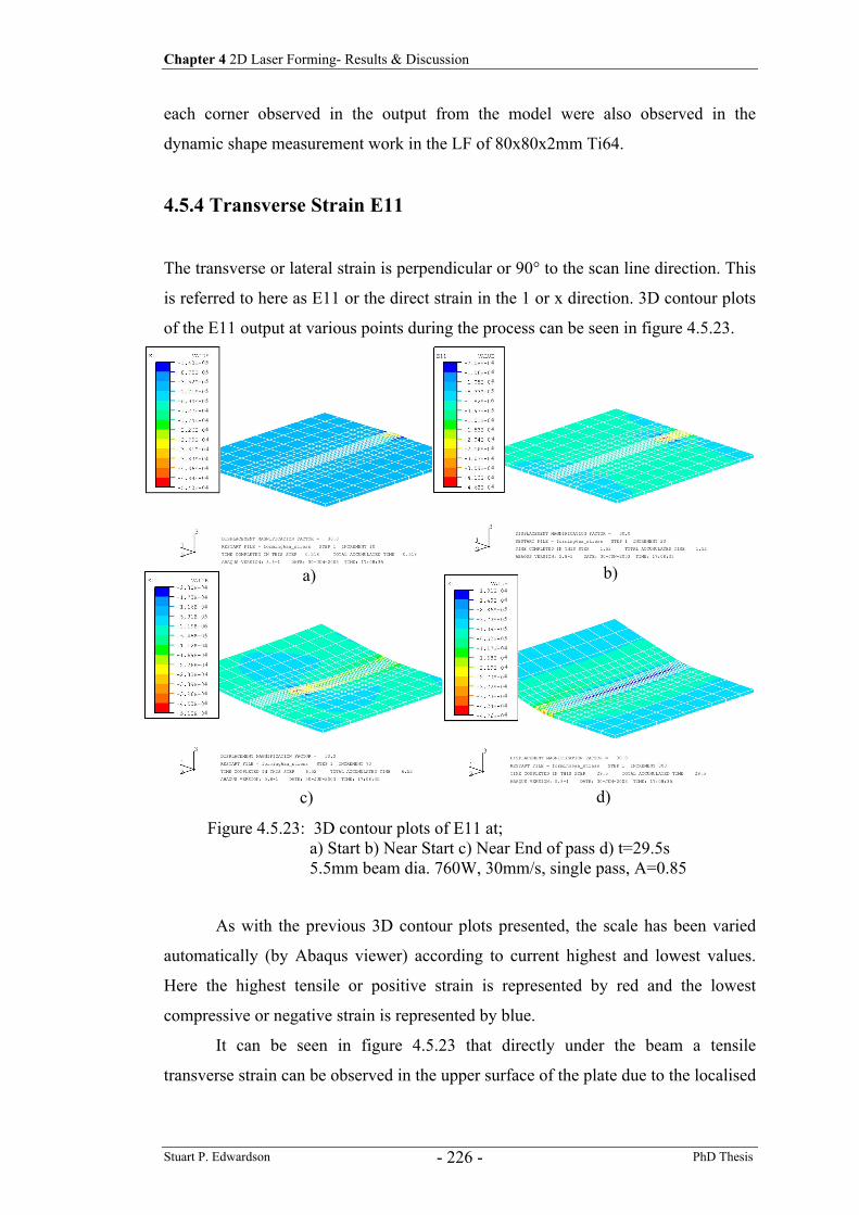
Chapter 4 2D Laser Forming- Results & Discussion
Stuart P. Edwardson PhD Thesis - 226 -
each corner observed in the output from the model were also observed in the
dynamic shape measurement work in the LF of 80x80x2mm Ti64.
4.5.4 Transverse Strain E11
The transverse or lateral strain is perpendicular or 90° to the scan line direction. This
is referred to here as E11 or the direct strain in the 1 or x direction. 3D contour plots
of the E11 output at various points during the process can be seen in figure 4.5.23.
As with the previous 3D contour plots presented, the scale has been varied
automatically (by Abaqus viewer) according to current highest and lowest values.
Here the highest tensile or positive strain is represented by red and the lowest
compressive or negative strain is represented by blue.
It can be seen in figure 4.5.23 that directly under the beam a tensile
transverse strain can be observed in the upper surface of the plate due to the localised
Figure 4.5.23: 3D contour plots of E11 at; a) Start b) Near Start c) Near End of pass d) t=29.5s 5.5mm beam dia. 760W, 30mm/s, single pass, A=0.85
d) c)
b) a)
5
5 5
5
5
4
4 4
4
4
4 4
4
4
444
5
6
5
44
44
44
44
445
5
5
5
44
44
44
44
4
4 4
5
6
5
4 4
4
4
4 4
4
4
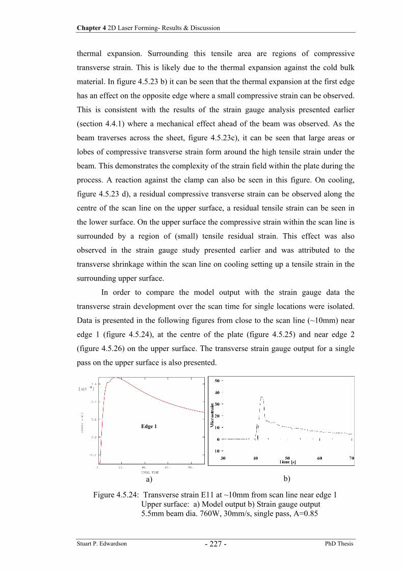
Chapter 4 2D Laser Forming- Results & Discussion
Stuart P. Edwardson PhD Thesis - 227 -
thermal expansion. Surrounding this tensile area are regions of compressive
transverse strain. This is likely due to the thermal expansion against the cold bulk
material. In figure 4.5.23 b) it can be seen that the thermal expansion at the first edge
has an effect on the opposite edge where a small compressive strain can be observed.
This is consistent with the results of the strain gauge analysis presented earlier
(section 4.4.1) where a mechanical effect ahead of the beam was observed. As the
beam traverses across the sheet, figure 4.5.23c), it can be seen that large areas or
lobes of compressive transverse strain form around the high tensile strain under the
beam. This demonstrates the complexity of the strain field within the plate during the
process. A reaction against the clamp can also be seen in this figure. On cooling,
figure 4.5.23 d), a residual compressive transverse strain can be observed along the
centre of the scan line on the upper surface, a residual tensile strain can be seen in
the lower surface. On the upper surface the compressive strain within the scan line is
surrounded by a region of (small) tensile residual strain. This effect was also
observed in the strain gauge study presented earlier and was attributed to the
transverse shrinkage within the scan line on cooling setting up a tensile strain in the
surrounding upper surface.
In order to compare the model output with the strain gauge data the
transverse strain development over the scan time for single locations were isolated.
Data is presented in the following figures from close to the scan line (~10mm) near
edge 1 (figure 4.5.24), at the centre of the plate (figure 4.5.25) and near edge 2
(figure 4.5.26) on the upper surface. The transverse strain gauge output for a single
pass on the upper surface is also presented.
Figure 4.5.24: Transverse strain E11 at ~10mm from scan line near edge 1 Upper surface: a) Model output b) Strain gauge output 5.5mm beam dia. 760W, 30mm/s, single pass, A=0.85
Edge 1
4
a) b)
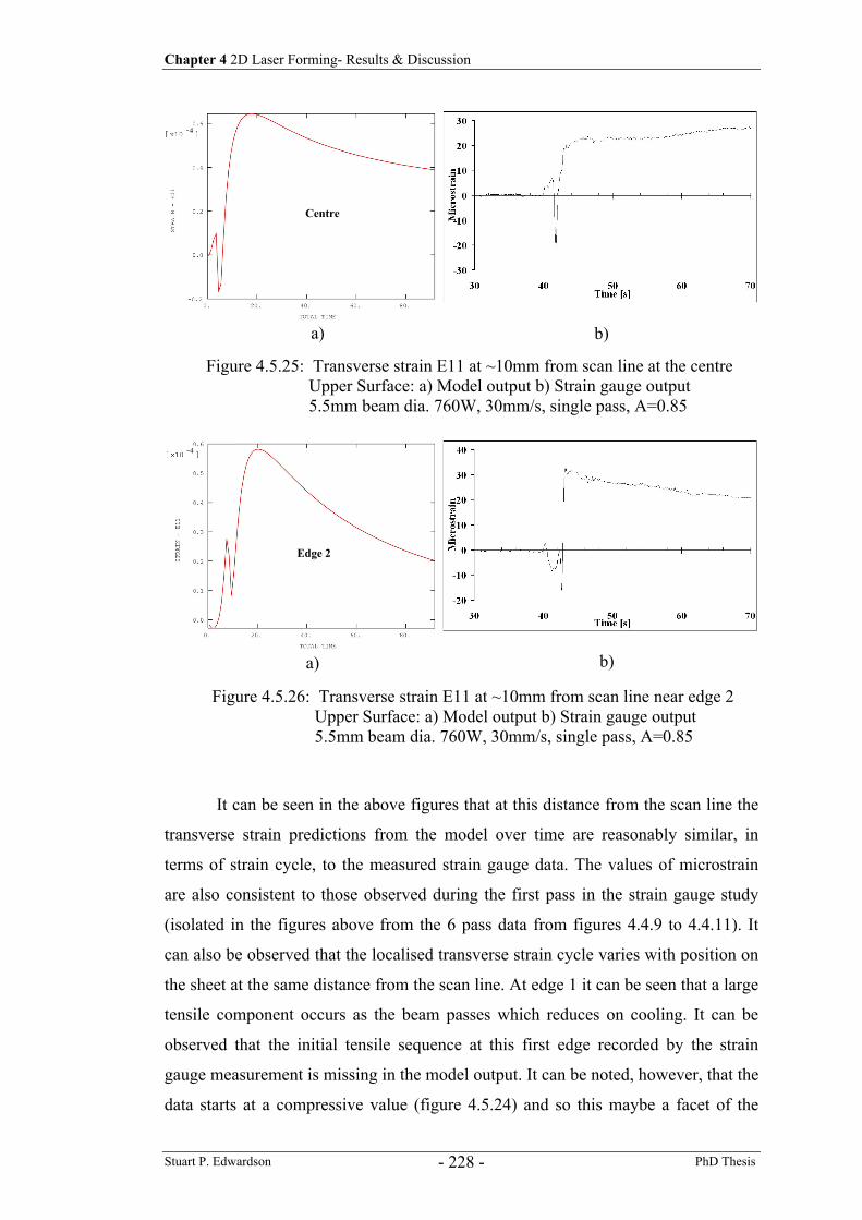
Chapter 4 2D Laser Forming- Results & Discussion
Stuart P. Edwardson PhD Thesis - 228 -
It can be seen in the above figures that at this distance from the scan line the
transverse strain predictions from the model over time are reasonably similar, in
terms of strain cycle, to the measured strain gauge data. The values of microstrain
are also consistent to those observed during the first pass in the strain gauge study
(isolated in the figures above from the 6 pass data from figures 4.4.9 to 4.4.11). It
can also be observed that the localised transverse strain cycle varies with position on
the sheet at the same distance from the scan line. At edge 1 it can be seen that a large
tensile component occurs as the beam passes which reduces on cooling. It can be
observed that the initial tensile sequence at this first edge recorded by the strain
gauge measurement is missing in the model output. It can be noted, however, that the
data starts at a compressive value (figure 4.5.24) and so this maybe a facet of the
Figure 4.5.25: Transverse strain E11 at ~10mm from scan line at the centreUpper Surface: a) Model output b) Strain gauge output 5.5mm beam dia. 760W, 30mm/s, single pass, A=0.85
Figure 4.5.26: Transverse strain E11 at ~10mm from scan line near edge 2 Upper Surface: a) Model output b) Strain gauge output 5.5mm beam dia. 760W, 30mm/s, single pass, A=0.85
Centre
4
Edge 2
4
b)a)
a) b)
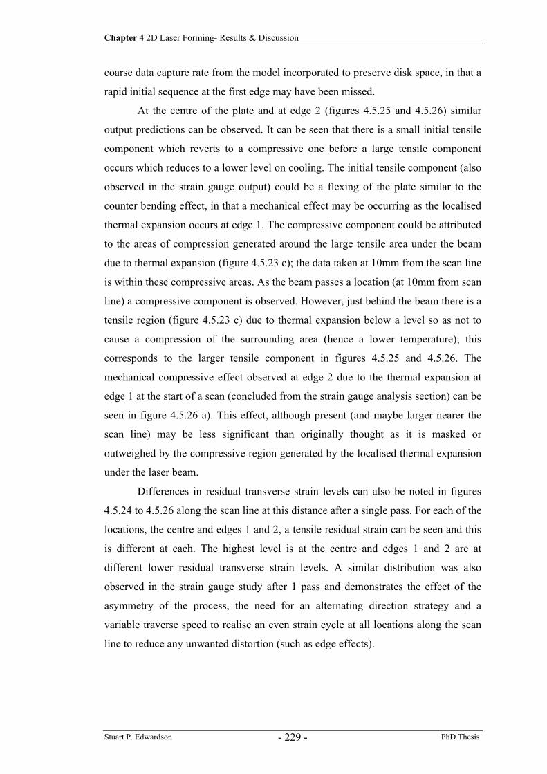
Chapter 4 2D Laser Forming- Results & Discussion
Stuart P. Edwardson PhD Thesis - 229 -
coarse data capture rate from the model incorporated to preserve disk space, in that a
rapid initial sequence at the first edge may have been missed.
At the centre of the plate and at edge 2 (figures 4.5.25 and 4.5.26) similar
output predictions can be observed. It can be seen that there is a small initial tensile
component which reverts to a compressive one before a large tensile component
occurs which reduces to a lower level on cooling. The initial tensile component (also
observed in the strain gauge output) could be a flexing of the plate similar to the
counter bending effect, in that a mechanical effect may be occurring as the localised
thermal expansion occurs at edge 1. The compressive component could be attributed
to the areas of compression generated around the large tensile area under the beam
due to thermal expansion (figure 4.5.23 c); the data taken at 10mm from the scan line
is within these compressive areas. As the beam passes a location (at 10mm from scan
line) a compressive component is observed. However, just behind the beam there is a
tensile region (figure 4.5.23 c) due to thermal expansion below a level so as not to
cause a compression of the surrounding area (hence a lower temperature); this
corresponds to the larger tensile component in figures 4.5.25 and 4.5.26. The
mechanical compressive effect observed at edge 2 due to the thermal expansion at
edge 1 at the start of a scan (concluded from the strain gauge analysis section) can be
seen in figure 4.5.26 a). This effect, although present (and maybe larger nearer the
scan line) may be less significant than originally thought as it is masked or
outweighed by the compressive region generated by the localised thermal expansion
under the laser beam.
Differences in residual transverse strain levels can also be noted in figures
4.5.24 to 4.5.26 along the scan line at this distance after a single pass. For each of the
locations, the centre and edges 1 and 2, a tensile residual strain can be seen and this
is different at each. The highest level is at the centre and edges 1 and 2 are at
different lower residual transverse strain levels. A similar distribution was also
observed in the strain gauge study after 1 pass and demonstrates the effect of the
asymmetry of the process, the need for an alternating direction strategy and a
variable traverse speed to realise an even strain cycle at all locations along the scan
line to reduce any unwanted distortion (such as edge effects).
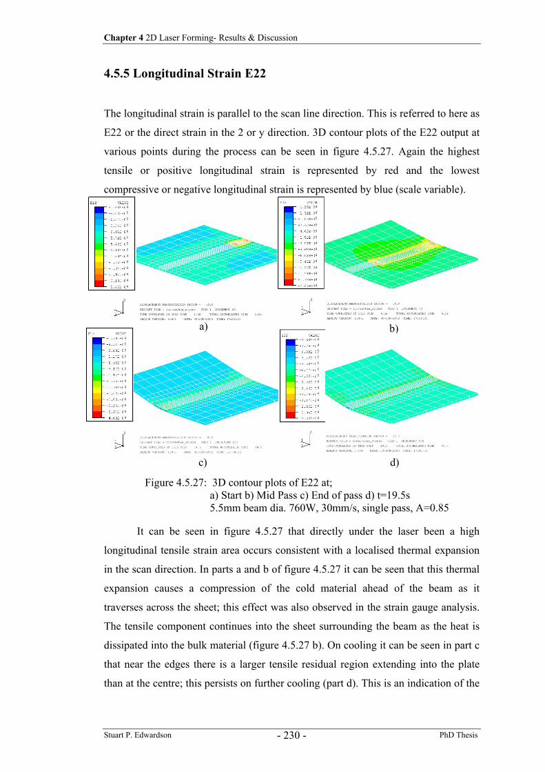
Chapter 4 2D Laser Forming- Results & Discussion
Stuart P. Edwardson PhD Thesis - 230 -
4.5.5 Longitudinal Strain E22
The longitudinal strain is parallel to the scan line direction. This is referred to here as
E22 or the direct strain in the 2 or y direction. 3D contour plots of the E22 output at
various points during the process can be seen in figure 4.5.27. Again the highest
tensile or positive longitudinal strain is represented by red and the lowest
compressive or negative longitudinal strain is represented by blue (scale variable).
It can be seen in figure 4.5.27 that directly under the laser been a high
longitudinal tensile strain area occurs consistent with a localised thermal expansion
in the scan direction. In parts a and b of figure 4.5.27 it can be seen that this thermal
expansion causes a compression of the cold material ahead of the beam as it
traverses across the sheet; this effect was also observed in the strain gauge analysis.
The tensile component continues into the sheet surrounding the beam as the heat is
dissipated into the bulk material (figure 4.5.27 b). On cooling it can be seen in part c
that near the edges there is a larger tensile residual region extending into the plate
than at the centre; this persists on further cooling (part d). This is an indication of the
Figure 4.5.27: 3D contour plots of E22 at; a) Start b) Mid Pass c) End of pass d) t=19.5s 5.5mm beam dia. 760W, 30mm/s, single pass, A=0.85
a) b)
c) d)
4 5
5
5
8
5 5
5
4 4
4
4
4
4
4 5
5
5
5
5 4
4
4 4
4
4
4
4
445
5
5
5
54
44
44
44
445
5
5
544
44
44
44
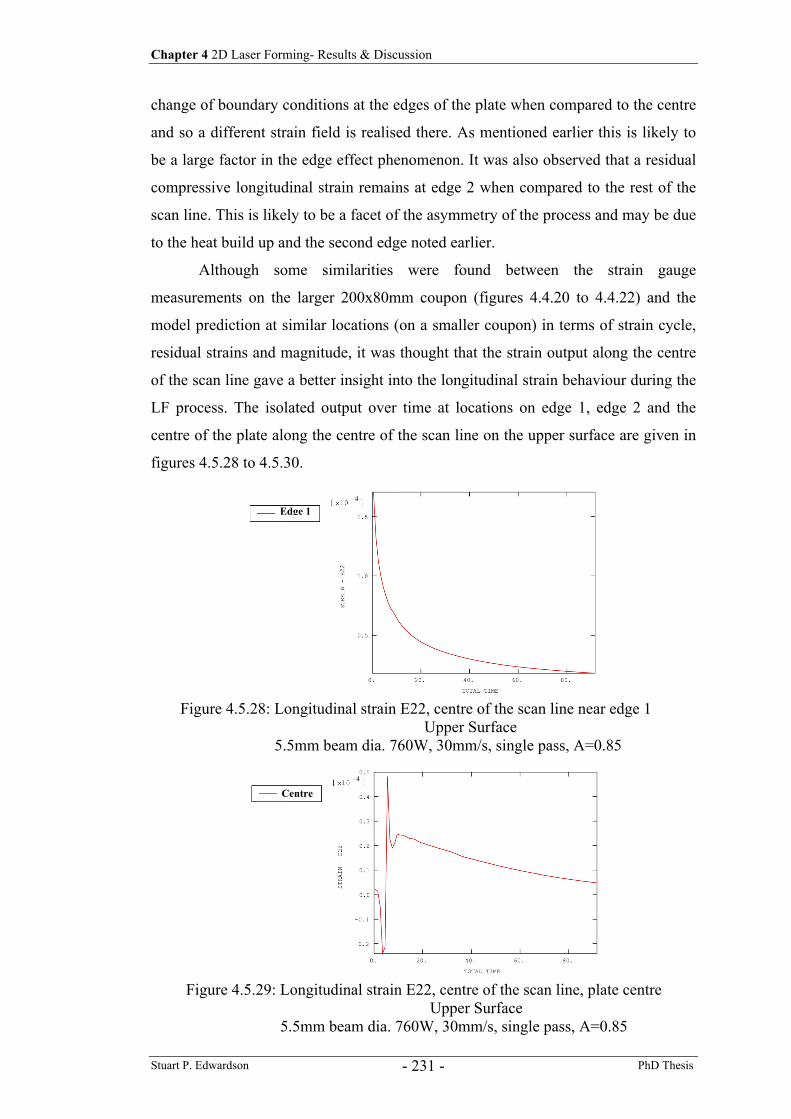
Chapter 4 2D Laser Forming- Results & Discussion
Stuart P. Edwardson PhD Thesis - 231 -
change of boundary conditions at the edges of the plate when compared to the centre
and so a different strain field is realised there. As mentioned earlier this is likely to
be a large factor in the edge effect phenomenon. It was also observed that a residual
compressive longitudinal strain remains at edge 2 when compared to the rest of the
scan line. This is likely to be a facet of the asymmetry of the process and may be due
to the heat build up and the second edge noted earlier.
Although some similarities were found between the strain gauge
measurements on the larger 200x80mm coupon (figures 4.4.20 to 4.4.22) and the
model prediction at similar locations (on a smaller coupon) in terms of strain cycle,
residual strains and magnitude, it was thought that the strain output along the centre
of the scan line gave a better insight into the longitudinal strain behaviour during the
LF process. The isolated output over time at locations on edge 1, edge 2 and the
centre of the plate along the centre of the scan line on the upper surface are given in
figures 4.5.28 to 4.5.30.
Figure 4.5.28: Longitudinal strain E22, centre of the scan line near edge 1 Upper Surface
5.5mm beam dia. 760W, 30mm/s, single pass, A=0.85
Figure 4.5.29: Longitudinal strain E22, centre of the scan line, plate centre Upper Surface
5.5mm beam dia. 760W, 30mm/s, single pass, A=0.85
Edge 1
Centre
4
4
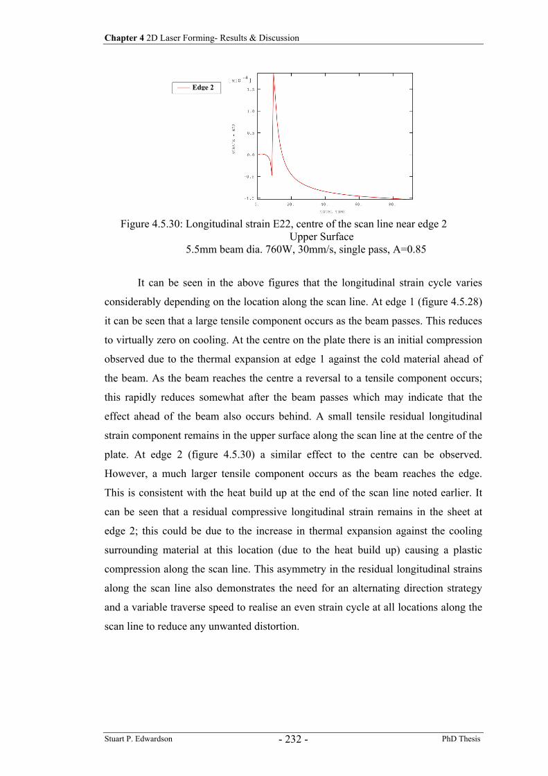
Chapter 4 2D Laser Forming- Results & Discussion
Stuart P. Edwardson PhD Thesis - 232 -
It can be seen in the above figures that the longitudinal strain cycle varies
considerably depending on the location along the scan line. At edge 1 (figure 4.5.28)
it can be seen that a large tensile component occurs as the beam passes. This reduces
to virtually zero on cooling. At the centre on the plate there is an initial compression
observed due to the thermal expansion at edge 1 against the cold material ahead of
the beam. As the beam reaches the centre a reversal to a tensile component occurs;
this rapidly reduces somewhat after the beam passes which may indicate that the
effect ahead of the beam also occurs behind. A small tensile residual longitudinal
strain component remains in the upper surface along the scan line at the centre of the
plate. At edge 2 (figure 4.5.30) a similar effect to the centre can be observed.
However, a much larger tensile component occurs as the beam reaches the edge.
This is consistent with the heat build up at the end of the scan line noted earlier. It
can be seen that a residual compressive longitudinal strain remains in the sheet at
edge 2; this could be due to the increase in thermal expansion against the cooling
surrounding material at this location (due to the heat build up) causing a plastic
compression along the scan line. This asymmetry in the residual longitudinal strains
along the scan line also demonstrates the need for an alternating direction strategy
and a variable traverse speed to realise an even strain cycle at all locations along the
scan line to reduce any unwanted distortion.
Figure 4.5.30: Longitudinal strain E22, centre of the scan line near edge 2 Upper Surface
5.5mm beam dia. 760W, 30mm/s, single pass, A=0.85
Edge 2 4
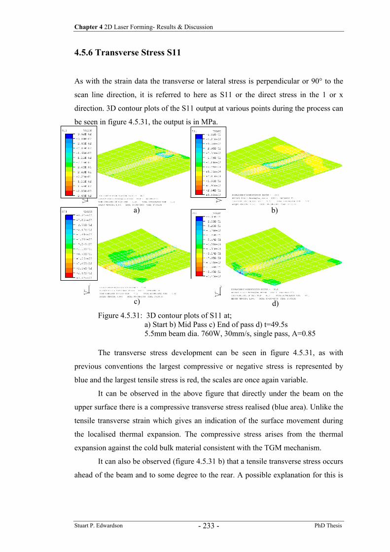
Chapter 4 2D Laser Forming- Results & Discussion
Stuart P. Edwardson PhD Thesis - 233 -
4.5.6 Transverse Stress S11
As with the strain data the transverse or lateral stress is perpendicular or 90° to the
scan line direction, it is referred to here as S11 or the direct stress in the 1 or x
direction. 3D contour plots of the S11 output at various points during the process can
be seen in figure 4.5.31, the output is in MPa.
The transverse stress development can be seen in figure 4.5.31, as with
previous conventions the largest compressive or negative stress is represented by
blue and the largest tensile stress is red, the scales are once again variable.
It can be observed in the above figure that directly under the beam on the
upper surface there is a compressive transverse stress realised (blue area). Unlike the
tensile transverse strain which gives an indication of the surface movement during
the localised thermal expansion. The compressive stress arises from the thermal
expansion against the cold bulk material consistent with the TGM mechanism.
It can also be observed (figure 4.5.31 b) that a tensile transverse stress occurs
ahead of the beam and to some degree to the rear. A possible explanation for this is
Figure 4.5.31: 3D contour plots of S11 at; a) Start b) Mid Pass c) End of pass d) t=49.5s 5.5mm beam dia. 760W, 30mm/s, single pass, A=0.85
a) b)
c) d)
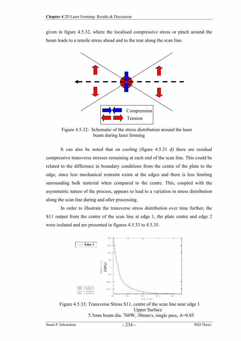
Chapter 4 2D Laser Forming- Results & Discussion
Stuart P. Edwardson PhD Thesis - 234 -
given in figure 4.5.32, where the localised compressive stress or pinch around the
beam leads to a tensile stress ahead and to the rear along the scan line.
It can also be noted that on cooling (figure 4.5.31 d) there are residual
compressive transverse stresses remaining at each end of the scan line. This could be
related to the difference in boundary conditions from the centre of the plate to the
edge, since less mechanical restraint exists at the edges and there is less limiting
surrounding bulk material when compared to the centre. This, coupled with the
asymmetric nature of the process, appears to lead to a variation in stress distribution
along the scan line during and after processing.
In order to illustrate the transverse stress distribution over time further, the
S11 output from the centre of the scan line at edge 1, the plate centre and edge 2
were isolated and are presented in figures 4.5.33 to 4.5.35.
CompressionTension
Figure 4.5.32: Schematic of the stress distribution around the laser beam during laser forming
Edge 1
Figure 4.5.33: Transverse Stress S11, centre of the scan line near edge 1 Upper Surface
5.5mm beam dia. 760W, 30mm/s, single pass, A=0.85
[MPa
]
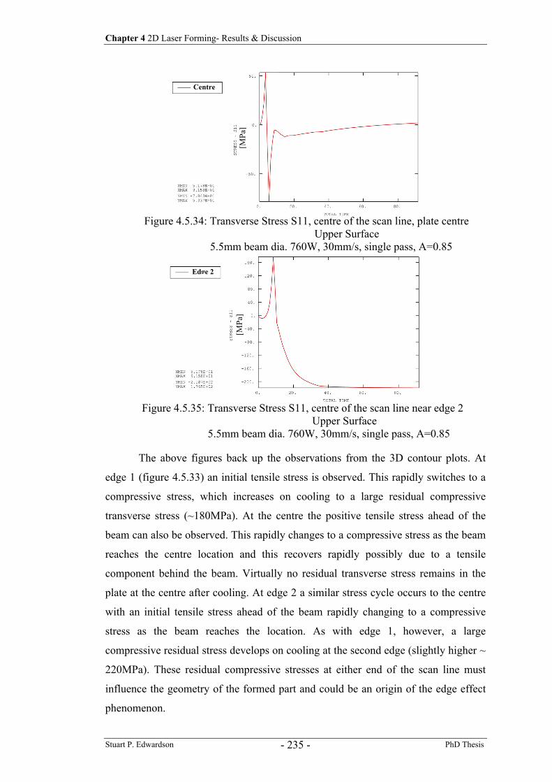
Chapter 4 2D Laser Forming- Results & Discussion
Stuart P. Edwardson PhD Thesis - 235 -
The above figures back up the observations from the 3D contour plots. At
edge 1 (figure 4.5.33) an initial tensile stress is observed. This rapidly switches to a
compressive stress, which increases on cooling to a large residual compressive
transverse stress (~180MPa). At the centre the positive tensile stress ahead of the
beam can also be observed. This rapidly changes to a compressive stress as the beam
reaches the centre location and this recovers rapidly possibly due to a tensile
component behind the beam. Virtually no residual transverse stress remains in the
plate at the centre after cooling. At edge 2 a similar stress cycle occurs to the centre
with an initial tensile stress ahead of the beam rapidly changing to a compressive
stress as the beam reaches the location. As with edge 1, however, a large
compressive residual stress develops on cooling at the second edge (slightly higher ~
220MPa). These residual compressive stresses at either end of the scan line must
influence the geometry of the formed part and could be an origin of the edge effect
phenomenon.
Centre
Edge 2
Figure 4.5.34: Transverse Stress S11, centre of the scan line, plate centre Upper Surface
5.5mm beam dia. 760W, 30mm/s, single pass, A=0.85
Figure 4.5.35: Transverse Stress S11, centre of the scan line near edge 2 Upper Surface
5.5mm beam dia. 760W, 30mm/s, single pass, A=0.85
[MPa
] [M
Pa]
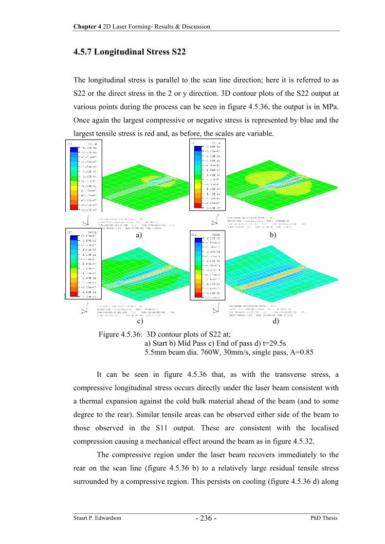
Chapter 4 2D Laser Forming- Results & Discussion
Stuart P. Edwardson PhD Thesis - 236 -
4.5.7 Longitudinal Stress S22
The longitudinal stress is parallel to the scan line direction; here it is referred to as
S22 or the direct stress in the 2 or y direction. 3D contour plots of the S22 output at
various points during the process can be seen in figure 4.5.36, the output is in MPa.
Once again the largest compressive or negative stress is represented by blue and the
largest tensile stress is red and, as before, the scales are variable.
It can be seen in figure 4.5.36 that, as with the transverse stress, a
compressive longitudinal stress occurs directly under the laser beam consistent with
a thermal expansion against the cold bulk material ahead of the beam (and to some
degree to the rear). Similar tensile areas can be observed either side of the beam to
those observed in the S11 output. These are consistent with the localised
compression causing a mechanical effect around the beam as in figure 4.5.32.
The compressive region under the laser beam recovers immediately to the
rear on the scan line (figure 4.5.36 b) to a relatively large residual tensile stress
surrounded by a compressive region. This persists on cooling (figure 4.5.36 d) along
Figure 4.5.36: 3D contour plots of S22 at; a) Start b) Mid Pass c) End of pass d) t=29.5s 5.5mm beam dia. 760W, 30mm/s, single pass, A=0.85
a) b)
c) d)
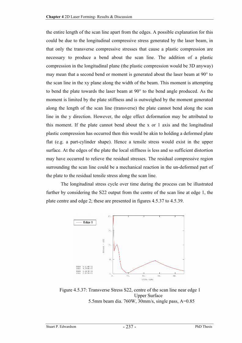
Chapter 4 2D Laser Forming- Results & Discussion
Stuart P. Edwardson PhD Thesis - 237 -
the entire length of the scan line apart from the edges. A possible explanation for this
could be due to the longitudinal compressive stress generated by the laser beam, in
that only the transverse compressive stresses that cause a plastic compression are
necessary to produce a bend about the scan line. The addition of a plastic
compression in the longitudinal plane (the plastic compression would be 3D anyway)
may mean that a second bend or moment is generated about the laser beam at 90° to
the scan line in the xy plane along the width of the beam. This moment is attempting
to bend the plate towards the laser beam at 90° to the bend angle produced. As the
moment is limited by the plate stiffness and is outweighed by the moment generated
along the length of the scan line (transverse) the plate cannot bend along the scan
line in the y direction. However, the edge effect deformation may be attributed to
this moment. If the plate cannot bend about the x or 1 axis and the longitudinal
plastic compression has occurred then this would be akin to holding a deformed plate
flat (e.g. a part-cylinder shape). Hence a tensile stress would exist in the upper
surface. At the edges of the plate the local stiffness is less and so sufficient distortion
may have occurred to relieve the residual stresses. The residual compressive region
surrounding the scan line could be a mechanical reaction in the un-deformed part of
the plate to the residual tensile stress along the scan line.
The longitudinal stress cycle over time during the process can be illustrated
further by considering the S22 output from the centre of the scan line at edge 1, the
plate centre and edge 2; these are presented in figures 4.5.37 to 4.5.39.
Figure 4.5.37: Transverse Stress S22, centre of the scan line near edge 1 Upper Surface
5.5mm beam dia. 760W, 30mm/s, single pass, A=0.85
Edge 1
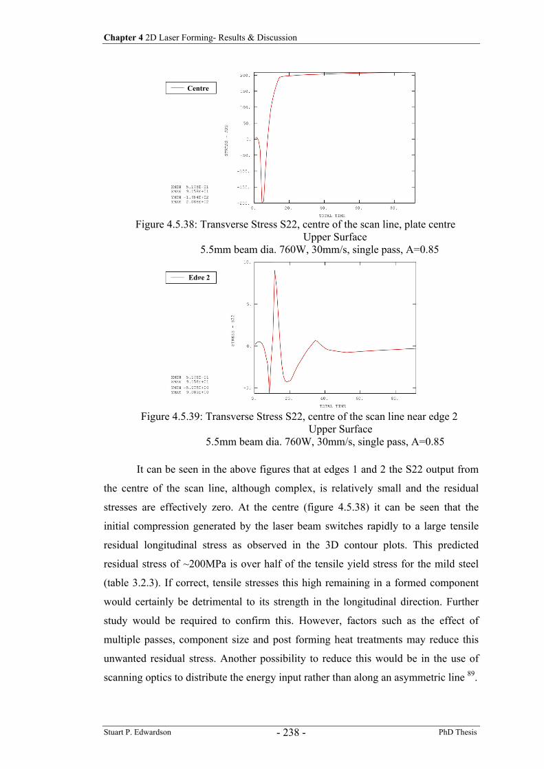
Chapter 4 2D Laser Forming- Results & Discussion
Stuart P. Edwardson PhD Thesis - 238 -
It can be seen in the above figures that at edges 1 and 2 the S22 output from
the centre of the scan line, although complex, is relatively small and the residual
stresses are effectively zero. At the centre (figure 4.5.38) it can be seen that the
initial compression generated by the laser beam switches rapidly to a large tensile
residual longitudinal stress as observed in the 3D contour plots. This predicted
residual stress of ~200MPa is over half of the tensile yield stress for the mild steel
(table 3.2.3). If correct, tensile stresses this high remaining in a formed component
would certainly be detrimental to its strength in the longitudinal direction. Further
study would be required to confirm this. However, factors such as the effect of
multiple passes, component size and post forming heat treatments may reduce this
unwanted residual stress. Another possibility to reduce this would be in the use of
scanning optics to distribute the energy input rather than along an asymmetric line 89.
Figure 4.5.39: Transverse Stress S22, centre of the scan line near edge 2 Upper Surface
5.5mm beam dia. 760W, 30mm/s, single pass, A=0.85
Figure 4.5.38: Transverse Stress S22, centre of the scan line, plate centre Upper Surface
5.5mm beam dia. 760W, 30mm/s, single pass, A=0.85
Centre
Edge 2
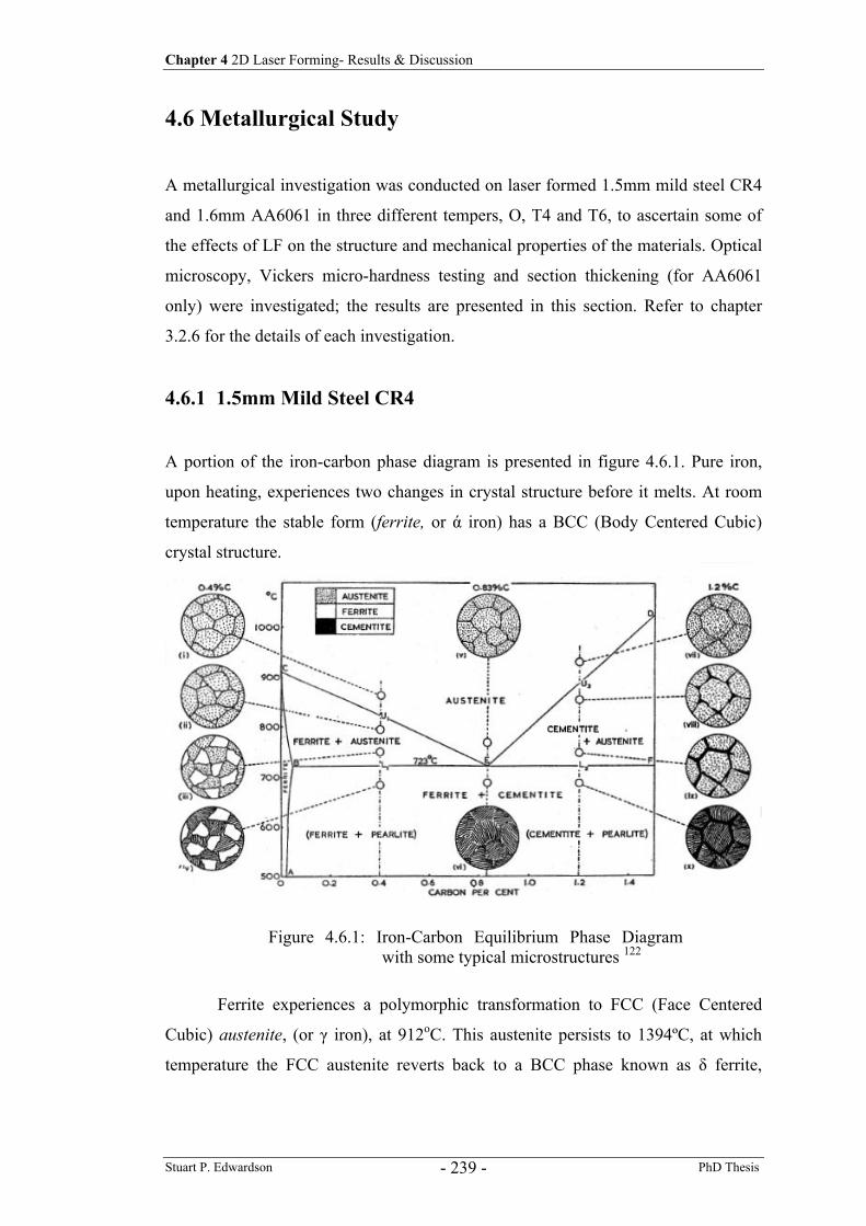
Chapter 4 2D Laser Forming- Results & Discussion
Stuart P. Edwardson PhD Thesis - 239 -
4.6 Metallurgical Study
A metallurgical investigation was conducted on laser formed 1.5mm mild steel CR4
and 1.6mm AA6061 in three different tempers, O, T4 and T6, to ascertain some of
the effects of LF on the structure and mechanical properties of the materials. Optical
microscopy, Vickers micro-hardness testing and section thickening (for AA6061
only) were investigated; the results are presented in this section. Refer to chapter
3.2.6 for the details of each investigation.
4.6.1 1.5mm Mild Steel CR4
A portion of the iron-carbon phase diagram is presented in figure 4.6.1. Pure iron,
upon heating, experiences two changes in crystal structure before it melts. At room
temperature the stable form (ferrite, or ά iron) has a BCC (Body Centered Cubic)
crystal structure.
Ferrite experiences a polymorphic transformation to FCC (Face Centered
Cubic) austenite, (or γ iron), at 912oC. This austenite persists to 1394ºC, at which
temperature the FCC austenite reverts back to a BCC phase known as δ ferrite,
Figure 4.6.1: Iron-Carbon Equilibrium Phase Diagram with some typical microstructures 122
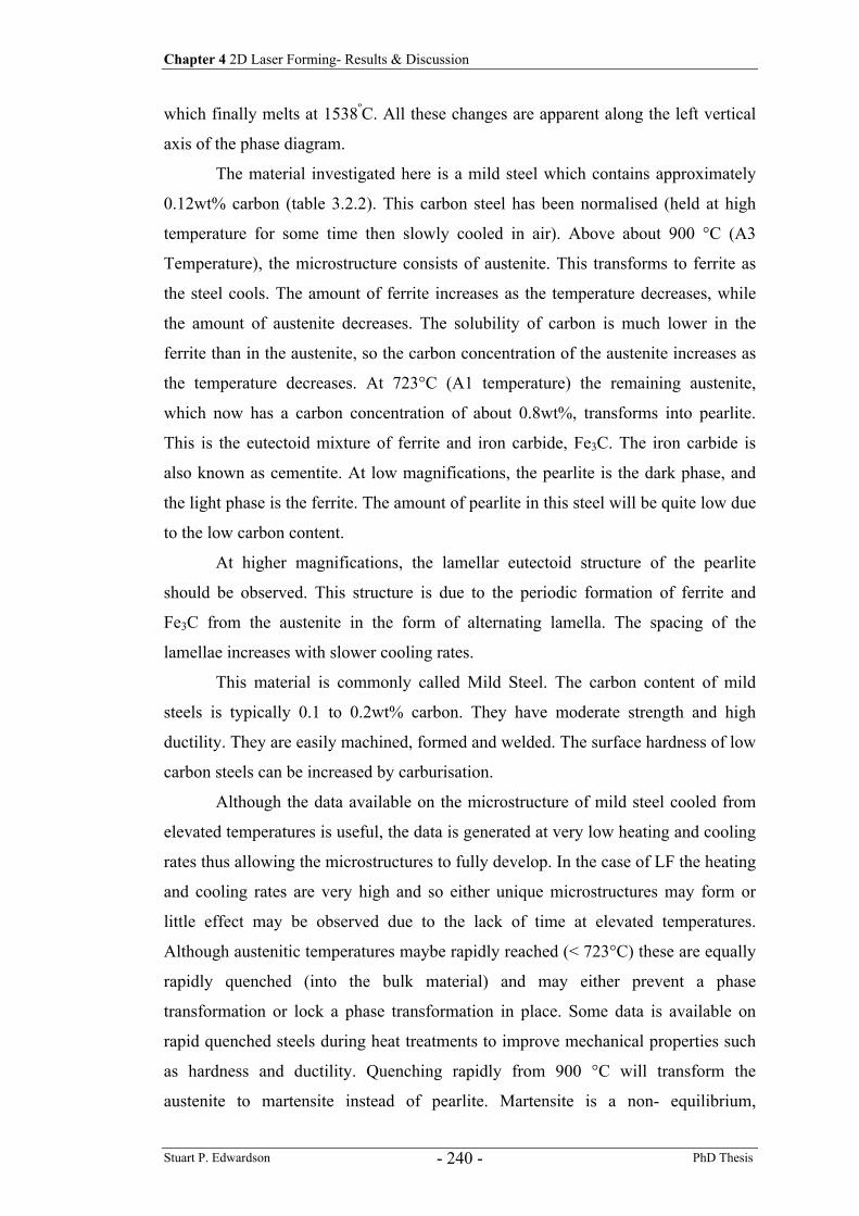
Chapter 4 2D Laser Forming- Results & Discussion
Stuart P. Edwardson PhD Thesis - 240 -
which finally melts at 1538ºC. All these changes are apparent along the left vertical
axis of the phase diagram.
The material investigated here is a mild steel which contains approximately
0.12wt% carbon (table 3.2.2). This carbon steel has been normalised (held at high
temperature for some time then slowly cooled in air). Above about 900 °C (A3
Temperature), the microstructure consists of austenite. This transforms to ferrite as
the steel cools. The amount of ferrite increases as the temperature decreases, while
the amount of austenite decreases. The solubility of carbon is much lower in the
ferrite than in the austenite, so the carbon concentration of the austenite increases as
the temperature decreases. At 723°C (A1 temperature) the remaining austenite,
which now has a carbon concentration of about 0.8wt%, transforms into pearlite.
This is the eutectoid mixture of ferrite and iron carbide, Fe3C. The iron carbide is
also known as cementite. At low magnifications, the pearlite is the dark phase, and
the light phase is the ferrite. The amount of pearlite in this steel will be quite low due
to the low carbon content.
At higher magnifications, the lamellar eutectoid structure of the pearlite
should be observed. This structure is due to the periodic formation of ferrite and
Fe3C from the austenite in the form of alternating lamella. The spacing of the
lamellae increases with slower cooling rates.
This material is commonly called Mild Steel. The carbon content of mild
steels is typically 0.1 to 0.2wt% carbon. They have moderate strength and high
ductility. They are easily machined, formed and welded. The surface hardness of low
carbon steels can be increased by carburisation.
Although the data available on the microstructure of mild steel cooled from
elevated temperatures is useful, the data is generated at very low heating and cooling
rates thus allowing the microstructures to fully develop. In the case of LF the heating
and cooling rates are very high and so either unique microstructures may form or
little effect may be observed due to the lack of time at elevated temperatures.
Although austenitic temperatures maybe rapidly reached (< 723°C) these are equally
rapidly quenched (into the bulk material) and may either prevent a phase
transformation or lock a phase transformation in place. Some data is available on
rapid quenched steels during heat treatments to improve mechanical properties such
as hardness and ductility. Quenching rapidly from 900 °C will transform the
austenite to martensite instead of pearlite. Martensite is a non- equilibrium,
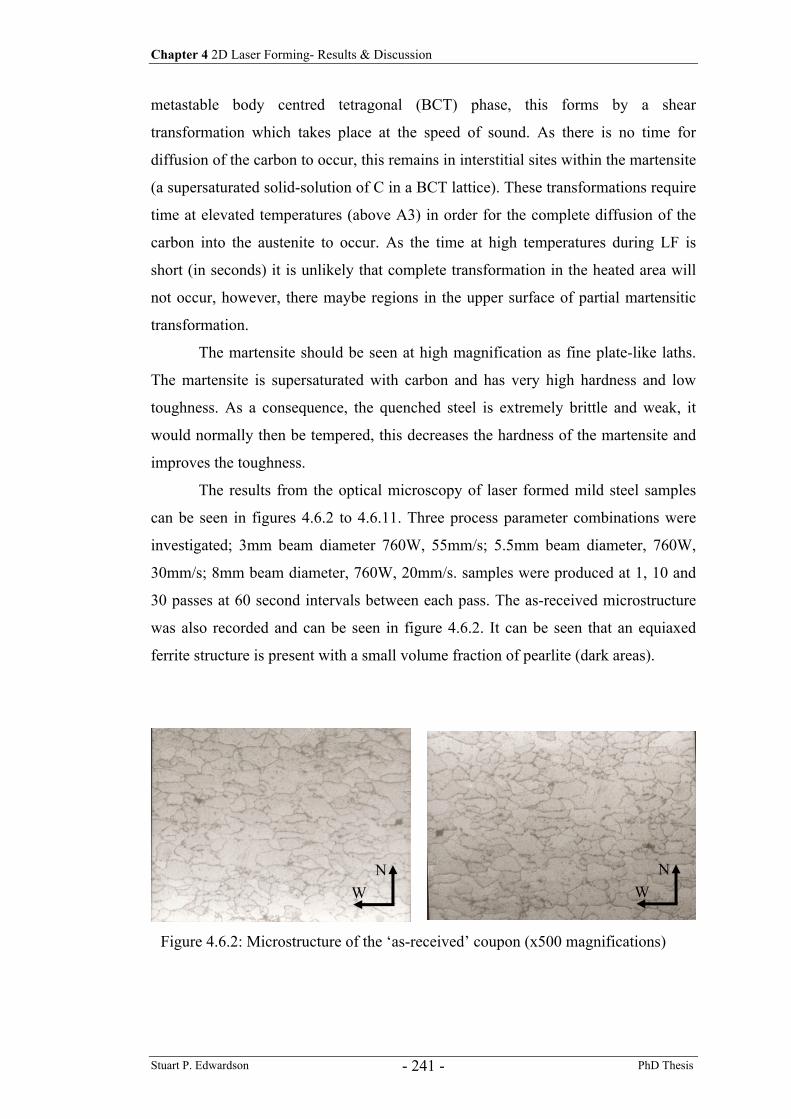
Chapter 4 2D Laser Forming- Results & Discussion
Stuart P. Edwardson PhD Thesis - 241 -
metastable body centred tetragonal (BCT) phase, this forms by a shear
transformation which takes place at the speed of sound. As there is no time for
diffusion of the carbon to occur, this remains in interstitial sites within the martensite
(a supersaturated solid-solution of C in a BCT lattice). These transformations require
time at elevated temperatures (above A3) in order for the complete diffusion of the
carbon into the austenite to occur. As the time at high temperatures during LF is
short (in seconds) it is unlikely that complete transformation in the heated area will
not occur, however, there maybe regions in the upper surface of partial martensitic
transformation.
The martensite should be seen at high magnification as fine plate-like laths.
The martensite is supersaturated with carbon and has very high hardness and low
toughness. As a consequence, the quenched steel is extremely brittle and weak, it
would normally then be tempered, this decreases the hardness of the martensite and
improves the toughness.
The results from the optical microscopy of laser formed mild steel samples
can be seen in figures 4.6.2 to 4.6.11. Three process parameter combinations were
investigated; 3mm beam diameter 760W, 55mm/s; 5.5mm beam diameter, 760W,
30mm/s; 8mm beam diameter, 760W, 20mm/s. samples were produced at 1, 10 and
30 passes at 60 second intervals between each pass. The as-received microstructure
was also recorded and can be seen in figure 4.6.2. It can be seen that an equiaxed
ferrite structure is present with a small volume fraction of pearlite (dark areas).
Figure 4.6.2: Microstructure of the ‘as-received’ coupon (x500 magnifications)
W N
W N
Chapter 4 2D Laser Forming- Results & Discussion
Stuart P. Edwardson PhD Thesis - 242 -
Figure 4.6.3: 1.5mm Mild Steel, 3mm beam diameter 760W, 55mm/s, 1 pass, Top Middle and Bottom of the HAZ section (x500 magnifications)
W N
W N
W N
Top Middle
Bottom
Figure 4.6.4: 1.5mm Mild Steel, 3mm beam diameter 760W, 55mm/s, 10 passes, Top Middle and Bottom of the HAZ section (x500 magnifications)
Top Middle
Bottom
W N
W N
W N
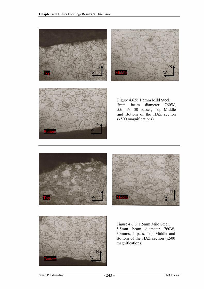
Chapter 4 2D Laser Forming- Results & Discussion
Stuart P. Edwardson PhD Thesis - 243 -
Figure 4.6.5: 1.5mm Mild Steel, 3mm beam diameter 760W, 55mm/s, 30 passes, Top Middle and Bottom of the HAZ section (x500 magnifications)
Bottom
MiddleTop
W N
W N
W N
Figure 4.6.6: 1.5mm Mild Steel, 5.5mm beam diameter 760W, 30mm/s, 1 pass, Top Middle and Bottom of the HAZ section (x500 magnifications)
Bottom
MiddleTop W N
W N
W N
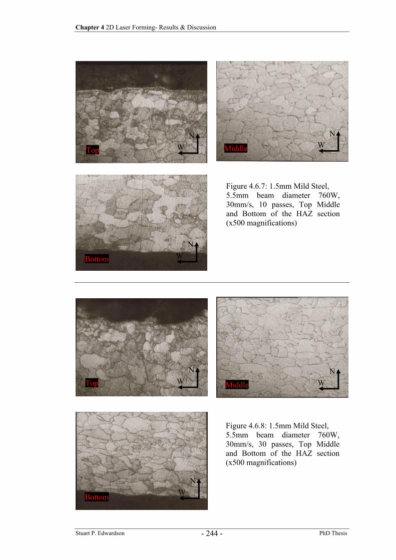
Chapter 4 2D Laser Forming- Results & Discussion
Stuart P. Edwardson PhD Thesis - 244 -
Figure 4.6.7: 1.5mm Mild Steel, 5.5mm beam diameter 760W, 30mm/s, 10 passes, Top Middle and Bottom of the HAZ section (x500 magnifications)
Figure 4.6.8: 1.5mm Mild Steel, 5.5mm beam diameter 760W, 30mm/s, 30 passes, Top Middle and Bottom of the HAZ section (x500 magnifications)
Top
Top Middle
Middle
Bottom
Bottom W N
W N
W N
W N
W N
W N
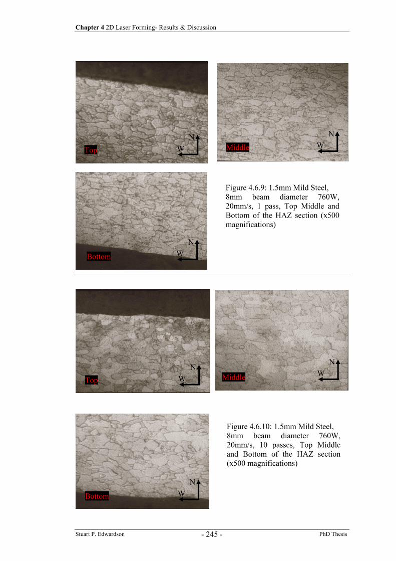
Chapter 4 2D Laser Forming- Results & Discussion
Stuart P. Edwardson PhD Thesis - 245 -
Figure 4.6.9: 1.5mm Mild Steel, 8mm beam diameter 760W, 20mm/s, 1 pass, Top Middle and Bottom of the HAZ section (x500 magnifications)
Figure 4.6.10: 1.5mm Mild Steel, 8mm beam diameter 760W, 20mm/s, 10 passes, Top Middle and Bottom of the HAZ section (x500 magnifications)
Top Middle
Bottom W N
W N
W N
Top Middle
Bottom
W N
W N
W N
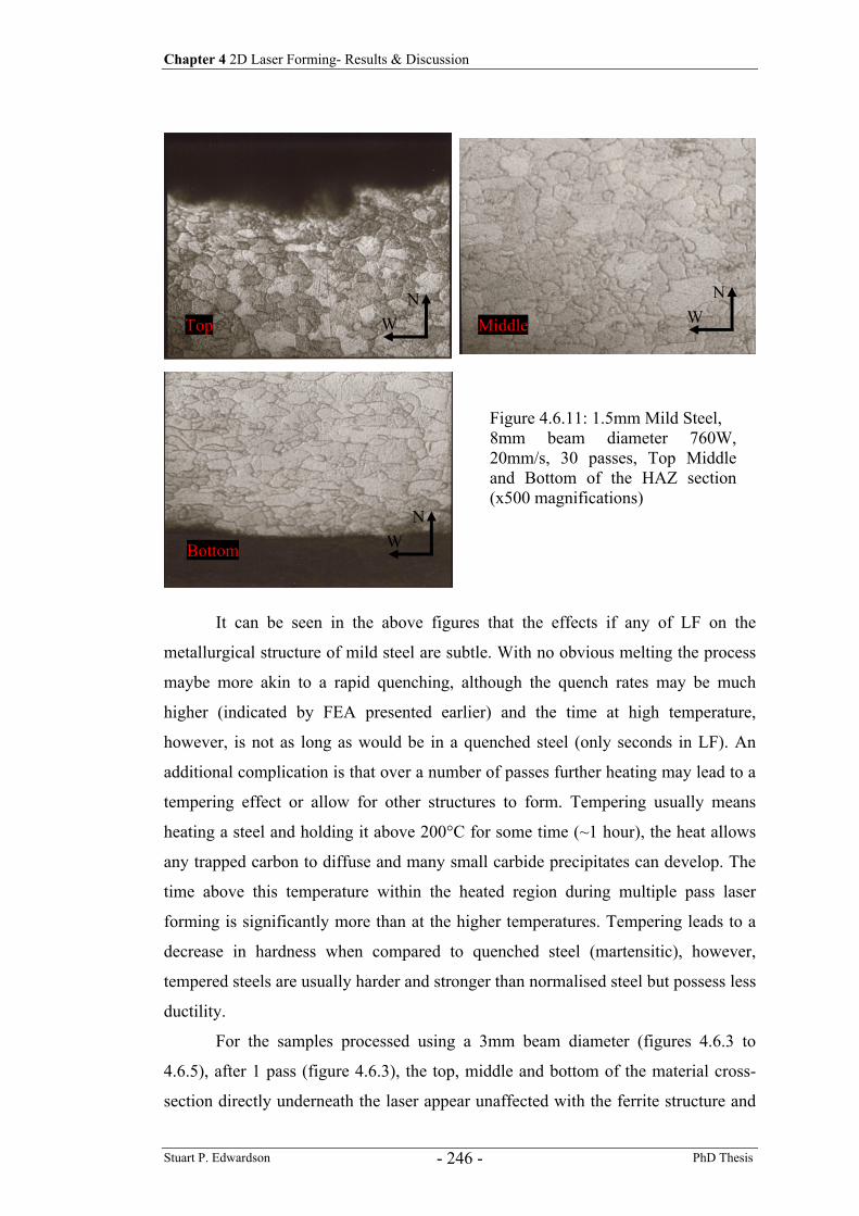
Chapter 4 2D Laser Forming- Results & Discussion
Stuart P. Edwardson PhD Thesis - 246 -
It can be seen in the above figures that the effects if any of LF on the
metallurgical structure of mild steel are subtle. With no obvious melting the process
maybe more akin to a rapid quenching, although the quench rates may be much
higher (indicated by FEA presented earlier) and the time at high temperature,
however, is not as long as would be in a quenched steel (only seconds in LF). An
additional complication is that over a number of passes further heating may lead to a
tempering effect or allow for other structures to form. Tempering usually means
heating a steel and holding it above 200°C for some time (~1 hour), the heat allows
any trapped carbon to diffuse and many small carbide precipitates can develop. The
time above this temperature within the heated region during multiple pass laser
forming is significantly more than at the higher temperatures. Tempering leads to a
decrease in hardness when compared to quenched steel (martensitic), however,
tempered steels are usually harder and stronger than normalised steel but possess less
ductility.
For the samples processed using a 3mm beam diameter (figures 4.6.3 to
4.6.5), after 1 pass (figure 4.6.3), the top, middle and bottom of the material cross-
section directly underneath the laser appear unaffected with the ferrite structure and
Figure 4.6.11: 1.5mm Mild Steel, 8mm beam diameter 760W, 20mm/s, 30 passes, Top Middle and Bottom of the HAZ section (x500 magnifications)
Top Middle
Bottom W N
W N
W N
Chapter 4 2D Laser Forming- Results & Discussion
Stuart P. Edwardson PhD Thesis - 247 -
some pearlite still present. The FEA study presented earlier (figure 4.5.7) predicted
that a temperature above A1 had been reached (723°C, figure 4.6.1) in the upper
surface area during a single pass such that austenite could form, however, the time at
this temperature is possibly too short for any significant change in microstructure to
occur, this is confirmed by the micrographs of the heated area. After 10 and 30
passes (figures 4.6.4 and 4.6.5) the middle and bottom of the section still remain
relatively unaffected (optically). In the upper surface region after 30 passes a
reduction in the average grain size can be observed, this could be consistent with an
ongoing tempering effect by each subsequent laser pass.
For the samples processed using a 5.5mm beam diameter (figures 4.6.6 to
4.6.8), as with the 3mm beam samples after 1 pass, (for the magnifications used)
there appears to be little observable effect in the top, middle and bottom of the
processed section. After 10 and 30 passes (figures 4.6.7 and 4.6.8) the main
observable effect of the LF process is a grain size reduction which again could be
due to a tempering operation, this effect is present to some degree into the depth of
the material probably due to the larger beam diameter causing a larger depth of HAZ.
For the 8mm beam diameter samples (figures 4.6.9 to 4.6.11) the only
observable effect, as seen in the 5.5mm beam samples, is an ongoing grain size
reduction perhaps due to the persistent elevated temperatures (above 200°C) causing
a tempering effect. This effect, however, extends into the depth of the section
implying that a more uniform heating has occurred. Inspection of the visible HAZ on
the upper and lower surfaces confirms that, whilst there is a thermal gradient present,
the larger beam diameter and low traverse speed produce significant heating into the
section.
Whilst the data obtained in this study is useful to give an insight in to the
metallurgy of laser formed parts, observations at higher magnifications and using
different techniques such as SEM or TEM may reveal more about the specific
metallurgy formed. It is encouraging to note that, optically at least, there is little
observable effect on the microstructure of this mild steel from the laser forming
process using the energy parameters investigated.
Another method of determining the effect of LF on the metallurgy and
mechanical properties of the mild steel is through hardness testing. Each of the
samples presented above were tested for hardness using a Vickers micro hardness
testing device (details presented in chapter 3.2.6). Five locations were tested at the
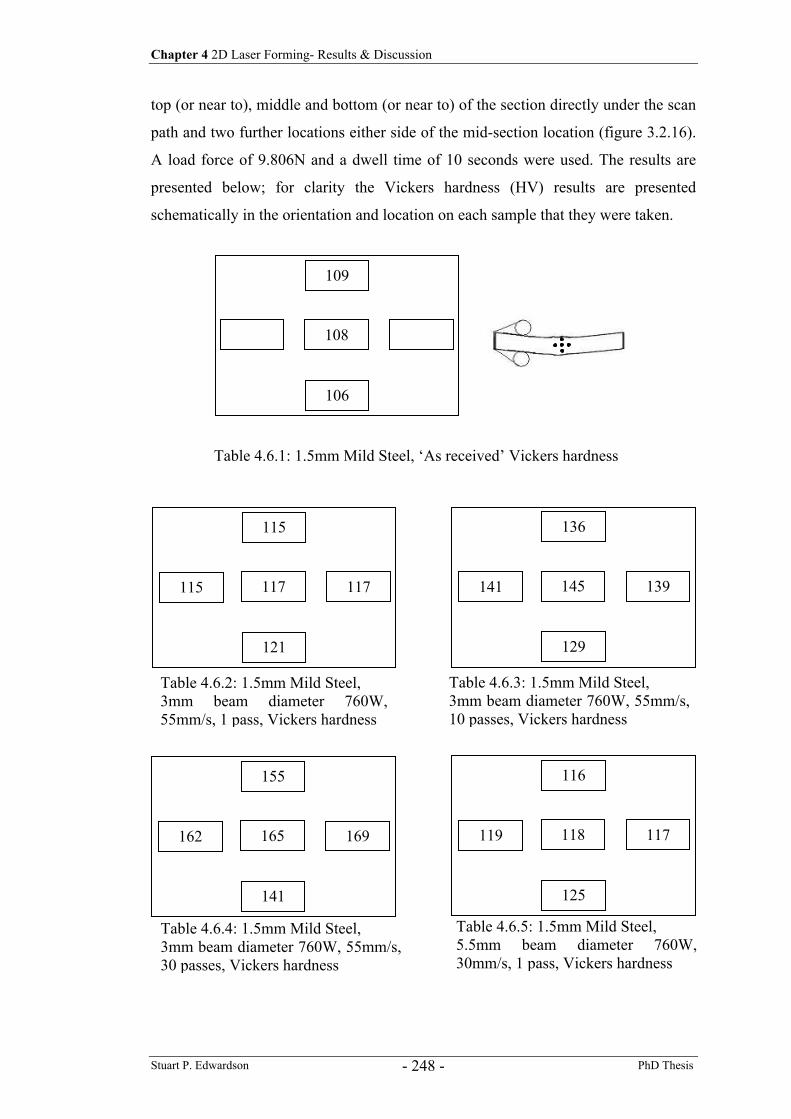
Chapter 4 2D Laser Forming- Results & Discussion
Stuart P. Edwardson PhD Thesis - 248 -
top (or near to), middle and bottom (or near to) of the section directly under the scan
path and two further locations either side of the mid-section location (figure 3.2.16).
A load force of 9.806N and a dwell time of 10 seconds were used. The results are
presented below; for clarity the Vickers hardness (HV) results are presented
schematically in the orientation and location on each sample that they were taken.
109
108
106
115
117
121
115 117
136
145
129
141 139
155
165
141
162 169
116
118
125
119 117
Table 4.6.2: 1.5mm Mild Steel, 3mm beam diameter 760W, 55mm/s, 1 pass, Vickers hardness
Table 4.6.1: 1.5mm Mild Steel, ‘As received’ Vickers hardness
Table 4.6.3: 1.5mm Mild Steel, 3mm beam diameter 760W, 55mm/s,10 passes, Vickers hardness
Table 4.6.4: 1.5mm Mild Steel, 3mm beam diameter 760W, 55mm/s,30 passes, Vickers hardness
Table 4.6.5: 1.5mm Mild Steel, 5.5mm beam diameter 760W, 30mm/s, 1 pass, Vickers hardness
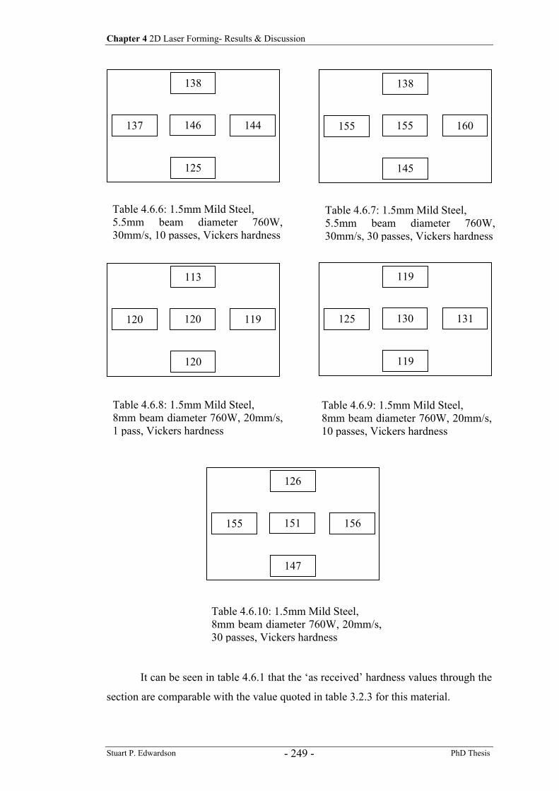
Chapter 4 2D Laser Forming- Results & Discussion
Stuart P. Edwardson PhD Thesis - 249 -
It can be seen in table 4.6.1 that the ‘as received’ hardness values through the
section are comparable with the value quoted in table 3.2.3 for this material.
138
146
125
137 144
138
155
145
155 160
113
120
120
120 119
119
130
119
125 131
126
151
147
155 156
Table 4.6.6: 1.5mm Mild Steel, 5.5mm beam diameter 760W, 30mm/s, 10 passes, Vickers hardness
Table 4.6.7: 1.5mm Mild Steel, 5.5mm beam diameter 760W, 30mm/s, 30 passes, Vickers hardness
Table 4.6.8: 1.5mm Mild Steel, 8mm beam diameter 760W, 20mm/s,1 pass, Vickers hardness
Table 4.6.9: 1.5mm Mild Steel, 8mm beam diameter 760W, 20mm/s,10 passes, Vickers hardness
Table 4.6.10: 1.5mm Mild Steel, 8mm beam diameter 760W, 20mm/s,30 passes, Vickers hardness
Chapter 4 2D Laser Forming- Results & Discussion
Stuart P. Edwardson PhD Thesis - 250 -
For the data obtained from the samples processed using a 3mm beam diameter,
tables 4.6.2 to 4.6.4, it can be seen that the hardness levels through the section have
increased from the nominal un-processed values. After 1 pass a hardness increase is
even observed near the lower surface. As the number of passes increases the
hardness level increases still further, this could be an indication of the development
of a (harder) plastically deformed zone (through compression) in the upper part of
the section (consistent with the TGM mechanism). It can be observed that there is a
distribution of the hardness values through the section, the highest levels appear in
the mid-section of the HAZ after 30 passes. Near the top surface the hardness value
is lower and could be an indication of the possible tempering effect or grain size
reduction by repeated scans of the laser beam observed earlier (figure 4.6.5). Near
the bottom surface after 30 passes (table 4.6.4) there is a comparable increase in
hardness also. As the optical microscopy of this region revealed little or no
microstructural changes in this area indicating that a lower temperature was reached,
the increase in hardness near the bottom surface of the plate could be due to a cold
working or strain hardening effect.
For the data obtained from the samples processed using a 5.5mm beam
diameter (tables 4.6.5 to 4.6.7) a similar result to the previous can be observed. The
hardness values do increase with increasing numbers of passes and the largest
increases can be observed near the mid-section of the plate thickness. Near the upper
surface the HV level has not changed from pass 10 to pass 30, this could also
indicate the microstructural change due to tempering discussed earlier. The
magnitude of the hardness value near the bottom surface after 30 passes is
comparable with the 3mm beam data, this could indicate some cold working or an
increase in the depth of the plastically deformed zone due to the beam diameter
increase.
For the data obtained from the samples processed using an 8mm beam
diameter (tables 4.6.8 to 4.6.10), once again a similar result can be observed in terms
of hardness increase with increasing number of passes and the distribution of
hardness values. Below the softer upper region a more uniform hardness distribution
can be observed, possibly due to the larger beam diameter creating a more uniform
heating of the section and hence increased depth of the plastically deformed zone or
again the result of strain hardening.
Chapter 4 2D Laser Forming- Results & Discussion
Stuart P. Edwardson PhD Thesis - 251 -
The strain hardening phenomena is attributed to the entanglement of
dislocations. Plastic deformation in metals proceeds atomic step by atomic step by
the generation and movement (by external force) of dislocations (or 1D defects or
holes) within the crystal lattice. The area swept by the movement defines a plane, the
glide plane, the movement of a dislocation moves the whole crystal on one side of
the glide plane relative to the other side. During plastic deformation multiple
dislocations created within the lattice interact during movement, as deformation
continues the dislocation density increases and entanglement occurs. This manifest
itself as an increase in hardness and material strength in the region as further plastic
deformation becomes more difficult. Another possible explanation for the lower
hardness in the upper surface compared to the rest of the section after 30 passes
could be the mechanism of dislocation climb. Once a dislocation movement has
taken place (hence plastic deformation) the dislocations are immobile and trapped by
the lattice. The mechanism of dislocation climb, which is strongly influenced by
temperature, makes immobile dislocations mobile again (by circumventing
obstacles), albeit they may move very slowly, thus a reduction in hardness and
material strength would occur. The elevated temperatures in the upper region of the
section during laser forming may allow this phenomenon to take place and hence
provide an explanation as to why the possible strain hardening effect observed in the
mid and lower parts of the heated section are not as apparent in the upper section.
The concept of strain hardening in the heated area of a laser formed
component has been identified in other research 58 as a significant factor in the fall
off of bend angle increase per pass over multiple passes. This is consistent with the
results and discussion above, whereby if significantly more strain hardening occurs
in the lower part of the section of a bend over increasing number of passes, the
bending strength of the section would increase (for a positive bend), and hence the
moment generated by the plastic compression in the upper surface would be less
effective for each subsequent pass.
Chapter 4 2D Laser Forming- Results & Discussion
Stuart P. Edwardson PhD Thesis - 252 -
4.6.2 1.6mm AA 6061 O/T4/T6
This 1.6mm gauge aluminium alloy AA 6061 is a non-ferrous wrought and age
hardenable 6000 series ternary aluminium alloy whose major alloying elements are
magnesium and silicon. The number of alloying elements creates a complex
relationship between phase transformation data, temperature and weight percentage
of each. Because of this, several coherent precipitates form before the final
equilibrium phase is produced in AA 6061.
The 6000 series alloys use precipitation of an intermetallic phase containing
Mg and Si as a strengthening mechanism. In simple ternary Al-Mg-Si alloys (6061)
the precipitation hardening is based on Mg2Si. Achievement of peak strength entails
two stages of heat treatment. First, the material is soaked at a high temperature close
to the melting temperature (the solution heat treatment) to dissolve solutes.
Quenching from the solution temperature creates a supersaturated solution of
alloying ingredients in the Al lattice, and in this condition (the W condition) the
material is soft. Subsequent heat treatment at an intermediate elevated temperature
(the aging heat treatment) facilitates clustering of solute atoms and eventually
formation of ultra-fine semi-coherent precipitates. The maximum hardening is found
for very small precipitates (~4 nm) of non-equilibrium phases. A sequence of
different phases can occur, depending on the composition and aging temperature.
Aging to peak strength is identified as the T6 condition. Excessive aging time or
temperature causes precipitate coarsening with attendant strength loss, commonly
known as over-aging or T7. If the material is left to age naturally at room
temperature after solution heat treatment some incipient solute clustering and
strength increase will occur - this condition is denoted T4. Copper is added to 6000
series alloys to increase the peak aged strength above that achievable with Mg and Si
alone. Sufficient copper changes the main precipitating species from Mg2Si to a
quaternary intermetallic, i.e. AlxMgySizCuw. 122
Due to the complexity of the metallurgy and limited analysis techniques
(optical microscopy only), only a limited study of the microstructure itself was
possible for this work. A typical micrograph of the AA 6061 F (as fabricated, no heat
treatment) microstructure is given in figure 4.6.12.
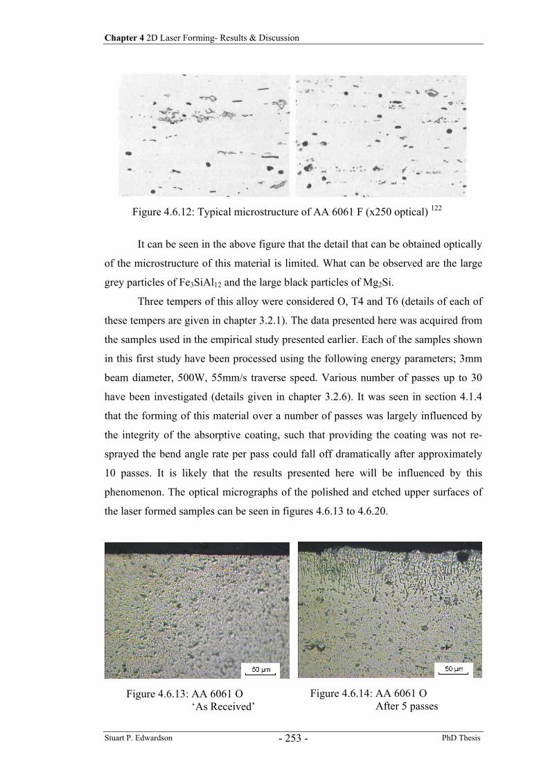
Chapter 4 2D Laser Forming- Results & Discussion
Stuart P. Edwardson PhD Thesis - 253 -
It can be seen in the above figure that the detail that can be obtained optically
of the microstructure of this material is limited. What can be observed are the large
grey particles of Fe3SiAl12 and the large black particles of Mg2Si.
Three tempers of this alloy were considered O, T4 and T6 (details of each of
these tempers are given in chapter 3.2.1). The data presented here was acquired from
the samples used in the empirical study presented earlier. Each of the samples shown
in this first study have been processed using the following energy parameters; 3mm
beam diameter, 500W, 55mm/s traverse speed. Various number of passes up to 30
have been investigated (details given in chapter 3.2.6). It was seen in section 4.1.4
that the forming of this material over a number of passes was largely influenced by
the integrity of the absorptive coating, such that providing the coating was not re-
sprayed the bend angle rate per pass could fall off dramatically after approximately
10 passes. It is likely that the results presented here will be influenced by this
phenomenon. The optical micrographs of the polished and etched upper surfaces of
the laser formed samples can be seen in figures 4.6.13 to 4.6.20.
Figure 4.6.12: Typical microstructure of AA 6061 F (x250 optical) 122
Figure 4.6.13: AA 6061 O ‘As Received’
Figure 4.6.14: AA 6061 O After 5 passes
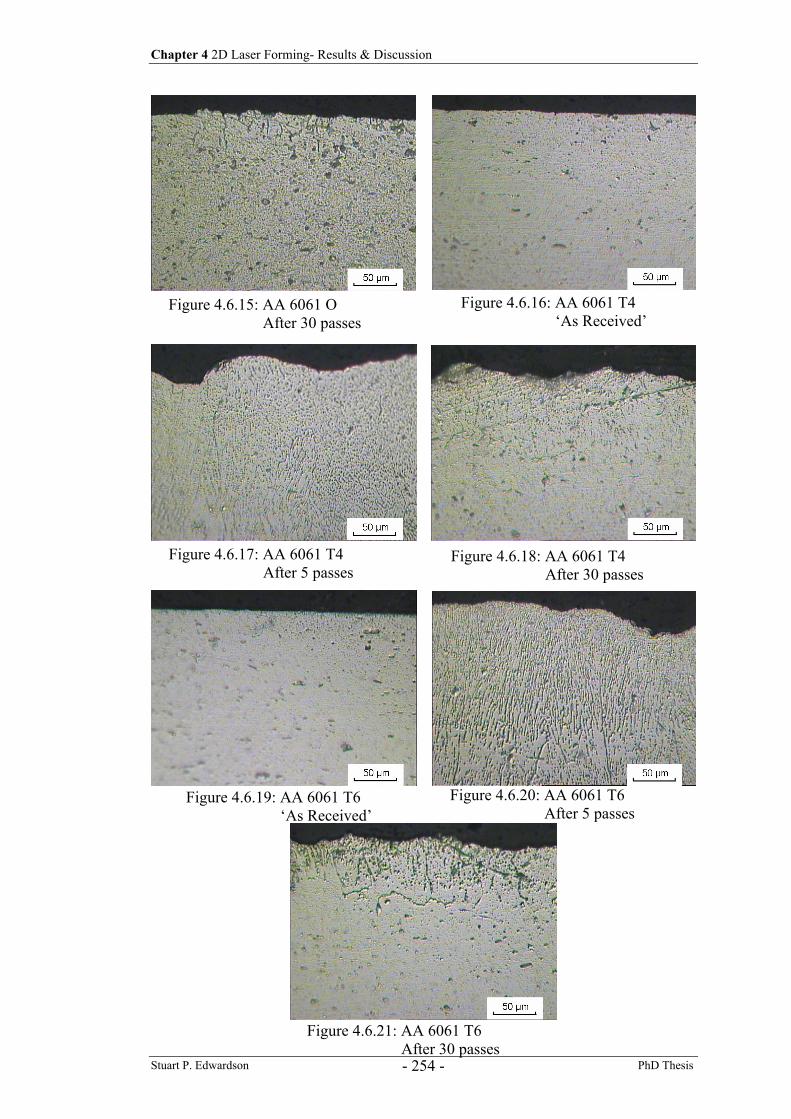
Chapter 4 2D Laser Forming- Results & Discussion
Stuart P. Edwardson PhD Thesis - 254 -
Figure 4.6.16: AA 6061 T4 ‘As Received’
Figure 4.6.19: AA 6061 T6 ‘As Received’
Figure 4.6.15: AA 6061 O After 30 passes
Figure 4.6.17: AA 6061 T4 After 5 passes
Figure 4.6.18: AA 6061 T4 After 30 passes
Figure 4.6.20: AA 6061 T6 After 5 passes
Figure 4.6.21: AA 6061 T6 After 30 passes
Chapter 4 2D Laser Forming- Results & Discussion
Stuart P. Edwardson PhD Thesis - 255 -
It can be seen in the above figures that a number of effects of LF on this
material can be observed. It can be noted firstly that the ‘as received’ microstructure
of the O or annealed condition (figure 4.6.13) appears quite coarse when compared
to the more refined heat treated, cold worked and aged T4 (figure 4.6.16) and T6
(figure 4.6.19) microstructures. Little difference can be observed optically between
the T4 and T6 tempers (T4 naturally aged, T6 artificially aged) the main difference
should be observed in terms of tensile strength and hardness.
After 5 passes a dendritic or coarser structure can be observed near the top
surface in the O condition (figure 4.6.14) and extending deeper into the material in
the T4 (figure 4.6.17) and T6 (figure 4.6.20) samples. The difference between the
samples could be related to the large differences in thermal conductivities between
them (table 3.2.15); in that the O condition has the lowest thermal conductivity and
therefore the elevated temperatures would not extend as far into the material. It can
also be observed that the individual precipitate particles have reduced within this
coarse dendritic formation; this may be consistent with a coarsening of the
precipitates due to excessive heating which may lead to a loss of strength in the heat
affected area. It can be noted that the first 5 passes correspond to a region were a
high bend angle rate was possible and so an efficient coupling of the laser energy
into the surface was possible (section 4.1.4).
After 30 passes in all three of the tempers (figures 4.6.15, 4.6.18, and 4.6.21)
it can be observed that the microstructure appears to be returning to the as received
state, with the coarse dendritic structure observed after 5 passes confined to just the
very upper surface. A possible reason for this could be the coating degradation and
hence bend angle rate fall off after 10 passes observed in the empirical study. This
would mean that the peak temperature experienced by the material will fall off also
for a higher number of passes, and although very little forming occurs due to the
coating loss, there may be sufficient energy coupled into the surface to produce a
heat treatment effect. The elevated temperatures at higher number of passes may
allow for a refinement of the coarse precipitates formed earlier, akin to a post-
forming heat treatment.
Chapter 4 2D Laser Forming- Results & Discussion
Stuart P. Edwardson PhD Thesis - 256 -
The micro hardness testing results can be seen in table 4.6.11. The results
presented are average values for the HAZ taken from 18 tests points (figure 3.2.15).
The data presented are for samples processed at 500W, 55mm/s and a 3mm beam
diameter at various numbers of passes.
Hardness Testing at Different Number of Passes (HV) No. of Passes 0 2 5 10 20 30 AA 6061-O 43.39 (10) 44.18 (11) 42.58 (12) 43.18 (13) 44.98 (14) 45.97 (15)AA 6061-T4 94.03 (20) 89.88 (21) 90.82 (22) 91.43 (23) 94.01 (24) 95.99 (25)AA 6061-T6 108.3 (30) 101.6 (31) 84.40 (32) 85.08 (33) 87.97(34) 89.57 (35)
The number in brackets is the number of the sample from table 3.2.19
It can be seen in table 4.6.11 that the ‘as received’ hardness values are
comparable to those quoted from the literature in table 3.2.15 (AA 6061 T4 slightly
higher though).
For the AA 6061 O it can be seen that there is little change in the hardness
values for increasing number of passes. This is perhaps consistent with the optical
microscopy presented earlier, where any noticeable effect on the material was
confined to the very upper surface (figure 4.6.14) and likely to be missed by the
hardness test. This material is quite soft to start with and any additional hardness
gained from precipitation hardening has not occurred, such that excessive heating
has little effect on the already coarse microstructure.
For the T4 and T6 tempers in can be seen that up to 10 passes there is a
decrease in the average hardness within the heated area. From 10 passes up to 30
passes there is a recovery somewhat in the hardness values. For the T4 temper this
has reached the pre-forming levels after 30 passes. This again is consistent with the
optical microscopy results earlier, in that the possible precipitate coarsening
observed after 5 passes would reduce the hardness within the heated area and the
subsequent heat treatment effects of the poorly coupled laser beam act to restore the
original microstructure and hence the hardness to some degree.
A study into the irradiated section thickening phenomenon was conducted on
these materials. Optical micrographs and measurements of the sheet thickness at the
scan line were taken at various numbers of passes (samples processed at 500W,
55mm/s and a 3mm beam diameter). The results are presented below.
Table 4.6.11: Hardness results for AA 6061 O/T4/T6
Chapter 4 2D Laser Forming- Results & Discussion
Stuart P. Edwardson PhD Thesis - 257 -
Figure 4.6.22: AA 6061 O - a) 0 pass, b) 5 passes c) 30 passes
Figure 4.6.23: AA 6061 T4 - a) 0 pass, b) 5 passes c) 30 passes
Figure 4.6.24: AA 6061 T6 - a) 0 pass, b) 5 passes c) 30 passes
a) b) c)
a)
a)
b)
b) c)
c)
Chapter 4 2D Laser Forming- Results & Discussion
Stuart P. Edwardson PhD Thesis - 258 -
Thickness Measurements At Different Numbers of Passes (mm) No. of Passes 0 2 5 10 20 30 AA 6061-O 1.61 (10) 1.68 (11) 1.73 (12) 1.80 (13) 1.85 (14) 1.84 (15)AA 6061-T4 1.53 (20) 1.58 (21) 1.66 (22) 1.70 (23) 1.73 (24) 1.73 (25)AA 6061-T6 1.55 (30) 1.62 (31) 1.68 (32) 1.71 (33) 1.71 (34) 1.73 (35)
The number in brackets is the number of the sample from table 3.2.19
It can be seen in figures 4.6.22 to 4.6.24 and table 4.6.12 that there is a
significant increase in section thickness with increasing number of passes. It can be
seen in table 4.6.12 that for all three of the tempers the section increase occurs up to
10 passes and then falls off; this is consistent with the dramatic bend angle rate fall
off around 10 passes for these materials. Some further section thickness increase
occurs in the O condition but as can be seen in figure 4.1.58 some additional forming
was possible in this material after 10 passes at these energy parameters.
The fact that the section thickness does increase with increasing number of
passes must influence the bend angle rate at higher number of passes (providing the
absorption can be maintained). This effect has been noted before in other materials 29
and is considered a major factor in the bend angle rate fall off phenomenon. If the
section is thicker then the material will be harder to bend due to the increase in the
section modulus, or alternatively the moment generated about the section for a given
set of energy parameters is less effective. Given the simple beam theory equation for
bending:
zRE
IM σ
== (4.6.1)
Such that:
REIM = (4.6.2)
And:
12
30bsI = (4.6.3)
For a given radius of curvature R the required moment M is governed by the section
thickness S0 cubed. Hence for any increase in thickness the generated moment by LF
must increase by a factor cubed in order to maintain the same radius of curvature.
Table 4.6.12: Irradiated section thickness measurements for AA 6061 O/T4/T6
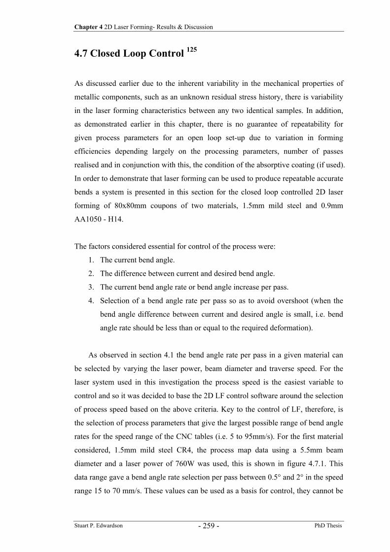
Chapter 4 2D Laser Forming- Results & Discussion
Stuart P. Edwardson PhD Thesis - 259 -
4.7 Closed Loop Control 125
As discussed earlier due to the inherent variability in the mechanical properties of
metallic components, such as an unknown residual stress history, there is variability
in the laser forming characteristics between any two identical samples. In addition,
as demonstrated earlier in this chapter, there is no guarantee of repeatability for
given process parameters for an open loop set-up due to variation in forming
efficiencies depending largely on the processing parameters, number of passes
realised and in conjunction with this, the condition of the absorptive coating (if used).
In order to demonstrate that laser forming can be used to produce repeatable accurate
bends a system is presented in this section for the closed loop controlled 2D laser
forming of 80x80mm coupons of two materials, 1.5mm mild steel and 0.9mm
AA1050 - H14.
The factors considered essential for control of the process were:
1. The current bend angle.
2. The difference between current and desired bend angle.
3. The current bend angle rate or bend angle increase per pass.
4. Selection of a bend angle rate per pass so as to avoid overshoot (when the
bend angle difference between current and desired angle is small, i.e. bend
angle rate should be less than or equal to the required deformation).
As observed in section 4.1 the bend angle rate per pass in a given material can
be selected by varying the laser power, beam diameter and traverse speed. For the
laser system used in this investigation the process speed is the easiest variable to
control and so it was decided to base the 2D LF control software around the selection
of process speed based on the above criteria. Key to the control of LF, therefore, is
the selection of process parameters that give the largest possible range of bend angle
rates for the speed range of the CNC tables (i.e. 5 to 95mm/s). For the first material
considered, 1.5mm mild steel CR4, the process map data using a 5.5mm beam
diameter and a laser power of 760W was used, this is shown in figure 4.7.1. This
data range gave a bend angle rate selection per pass between 0.5° and 2° in the speed
range 15 to 70 mm/s. These values can be used as a basis for control, they cannot be
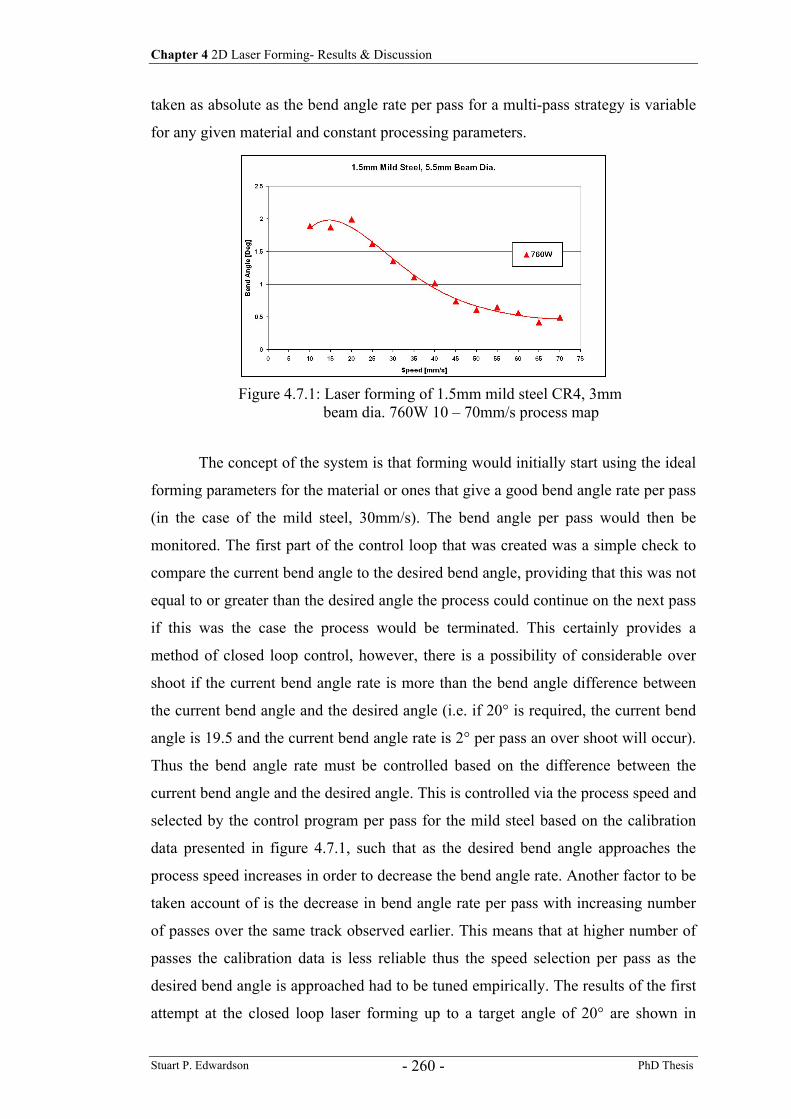
Chapter 4 2D Laser Forming- Results & Discussion
Stuart P. Edwardson PhD Thesis - 260 -
taken as absolute as the bend angle rate per pass for a multi-pass strategy is variable
for any given material and constant processing parameters.
The concept of the system is that forming would initially start using the ideal
forming parameters for the material or ones that give a good bend angle rate per pass
(in the case of the mild steel, 30mm/s). The bend angle per pass would then be
monitored. The first part of the control loop that was created was a simple check to
compare the current bend angle to the desired bend angle, providing that this was not
equal to or greater than the desired angle the process could continue on the next pass
if this was the case the process would be terminated. This certainly provides a
method of closed loop control, however, there is a possibility of considerable over
shoot if the current bend angle rate is more than the bend angle difference between
the current bend angle and the desired angle (i.e. if 20° is required, the current bend
angle is 19.5 and the current bend angle rate is 2° per pass an over shoot will occur).
Thus the bend angle rate must be controlled based on the difference between the
current bend angle and the desired angle. This is controlled via the process speed and
selected by the control program per pass for the mild steel based on the calibration
data presented in figure 4.7.1, such that as the desired bend angle approaches the
process speed increases in order to decrease the bend angle rate. Another factor to be
taken account of is the decrease in bend angle rate per pass with increasing number
of passes over the same track observed earlier. This means that at higher number of
passes the calibration data is less reliable thus the speed selection per pass as the
desired bend angle is approached had to be tuned empirically. The results of the first
attempt at the closed loop laser forming up to a target angle of 20° are shown in
Figure 4.7.1: Laser forming of 1.5mm mild steel CR4, 3mm beam dia. 760W 10 – 70mm/s process map
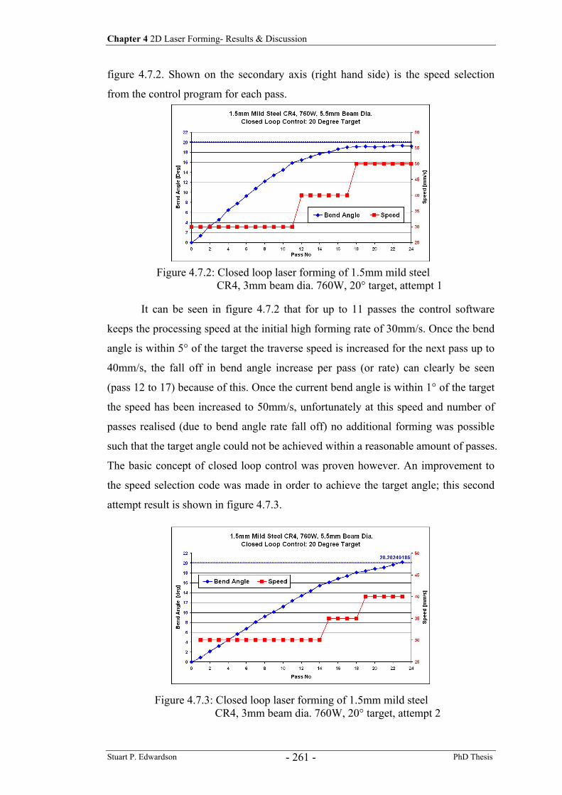
Chapter 4 2D Laser Forming- Results & Discussion
Stuart P. Edwardson PhD Thesis - 261 -
figure 4.7.2. Shown on the secondary axis (right hand side) is the speed selection
from the control program for each pass.
It can be seen in figure 4.7.2 that for up to 11 passes the control software
keeps the processing speed at the initial high forming rate of 30mm/s. Once the bend
angle is within 5° of the target the traverse speed is increased for the next pass up to
40mm/s, the fall off in bend angle increase per pass (or rate) can clearly be seen
(pass 12 to 17) because of this. Once the current bend angle is within 1° of the target
the speed has been increased to 50mm/s, unfortunately at this speed and number of
passes realised (due to bend angle rate fall off) no additional forming was possible
such that the target angle could not be achieved within a reasonable amount of passes.
The basic concept of closed loop control was proven however. An improvement to
the speed selection code was made in order to achieve the target angle; this second
attempt result is shown in figure 4.7.3.
Figure 4.7.2: Closed loop laser forming of 1.5mm mild steel CR4, 3mm beam dia. 760W, 20° target, attempt 1
Figure 4.7.3: Closed loop laser forming of 1.5mm mild steel CR4, 3mm beam dia. 760W, 20° target, attempt 2
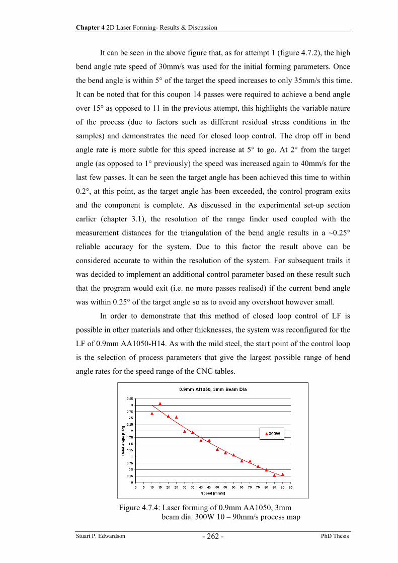
Chapter 4 2D Laser Forming- Results & Discussion
Stuart P. Edwardson PhD Thesis - 262 -
It can be seen in the above figure that, as for attempt 1 (figure 4.7.2), the high
bend angle rate speed of 30mm/s was used for the initial forming parameters. Once
the bend angle is within 5° of the target the speed increases to only 35mm/s this time.
It can be noted that for this coupon 14 passes were required to achieve a bend angle
over 15° as opposed to 11 in the previous attempt, this highlights the variable nature
of the process (due to factors such as different residual stress conditions in the
samples) and demonstrates the need for closed loop control. The drop off in bend
angle rate is more subtle for this speed increase at 5° to go. At 2° from the target
angle (as opposed to 1° previously) the speed was increased again to 40mm/s for the
last few passes. It can be seen the target angle has been achieved this time to within
0.2°, at this point, as the target angle has been exceeded, the control program exits
and the component is complete. As discussed in the experimental set-up section
earlier (chapter 3.1), the resolution of the range finder used coupled with the
measurement distances for the triangulation of the bend angle results in a ~0.25°
reliable accuracy for the system. Due to this factor the result above can be
considered accurate to within the resolution of the system. For subsequent trails it
was decided to implement an additional control parameter based on these result such
that the program would exit (i.e. no more passes realised) if the current bend angle
was within 0.25° of the target angle so as to avoid any overshoot however small.
In order to demonstrate that this method of closed loop control of LF is
possible in other materials and other thicknesses, the system was reconfigured for the
LF of 0.9mm AA1050-H14. As with the mild steel, the start point of the control loop
is the selection of process parameters that give the largest possible range of bend
angle rates for the speed range of the CNC tables.
Figure 4.7.4: Laser forming of 0.9mm AA1050, 3mm beam dia. 300W 10 – 90mm/s process map
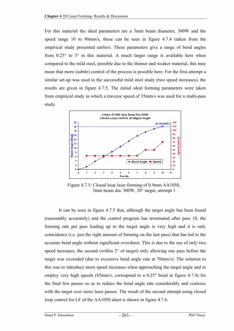
Chapter 4 2D Laser Forming- Results & Discussion
Stuart P. Edwardson PhD Thesis - 263 -
For this material the ideal parameters are a 3mm beam diameter, 300W and the
speed range 10 to 90mm/s, these can be seen in figure 4.7.4 (taken from the
empirical study presented earlier). These parameters give a range of bend angles
from 0.25° to 3° in this material. A much larger range is available here when
compared to the mild steel, possible due to the thinner and weaker material, this may
mean that more (subtle) control of the process is possible here. For the first attempt a
similar set-up was used to the successful mild steel study (two speed increases), the
results are given in figure 4.7.5. The initial ideal forming parameters were taken
from empirical study in which a traverse speed of 35mm/s was used for a multi-pass
study.
It can be seen in figure 4.7.5 that, although the target angle has been found
(reasonably accurately) and the control program has terminated after pass 10, the
forming rate per pass leading up to the target angle is very high and it is only
coincidence (i.e. just the right amount of forming on the last pass) that has led to the
accurate bend angle without significant overshoot. This is due to the use of only two
speed increases, the second (within 2° of target) only allowing one pass before the
target was exceeded (due to excessive bend angle rate at 70mm/s). The solution to
this was to introduce more speed increases when approaching the target angle and to
employ very high speeds (85mm/s, correspond to a 0.25° bend in figure 4.7.4) for
the final few passes so as to reduce the bend angle rate considerably and coalesce
with the target over more laser passes. The result of the second attempt using closed
loop control for LF of the AA1050 sheet is shown in figure 4.7.6.
Figure 4.7.5: Closed loop laser forming of 0.9mm AA1050, 3mm beam dia. 300W, 20° target, attempt 1
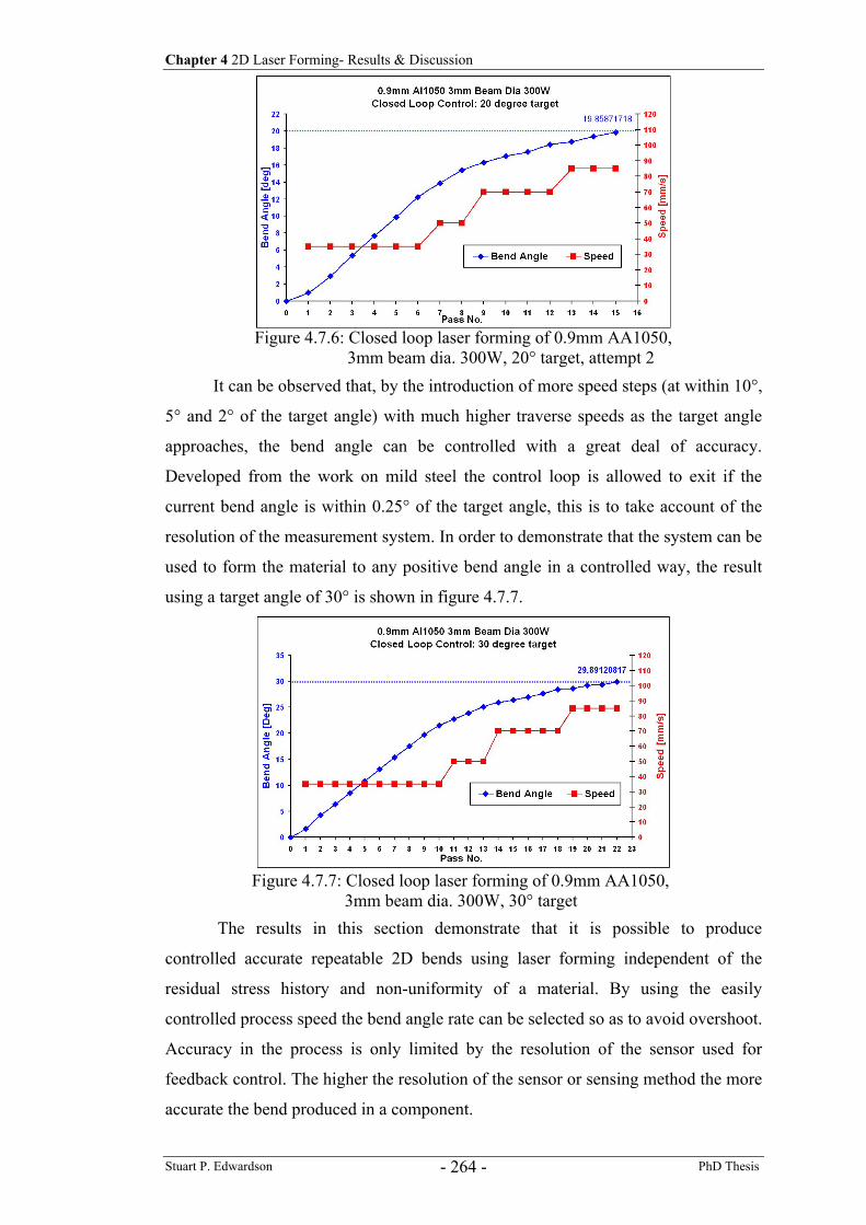
Chapter 4 2D Laser Forming- Results & Discussion
Stuart P. Edwardson PhD Thesis - 264 -
It can be observed that, by the introduction of more speed steps (at within 10°,
5° and 2° of the target angle) with much higher traverse speeds as the target angle
approaches, the bend angle can be controlled with a great deal of accuracy.
Developed from the work on mild steel the control loop is allowed to exit if the
current bend angle is within 0.25° of the target angle, this is to take account of the
resolution of the measurement system. In order to demonstrate that the system can be
used to form the material to any positive bend angle in a controlled way, the result
using a target angle of 30° is shown in figure 4.7.7.
The results in this section demonstrate that it is possible to produce
controlled accurate repeatable 2D bends using laser forming independent of the
residual stress history and non-uniformity of a material. By using the easily
controlled process speed the bend angle rate can be selected so as to avoid overshoot.
Accuracy in the process is only limited by the resolution of the sensor used for
feedback control. The higher the resolution of the sensor or sensing method the more
accurate the bend produced in a component.
Figure 4.7.6: Closed loop laser forming of 0.9mm AA1050, 3mm beam dia. 300W, 20° target, attempt 2
Figure 4.7.7: Closed loop laser forming of 0.9mm AA1050, 3mm beam dia. 300W, 30° target
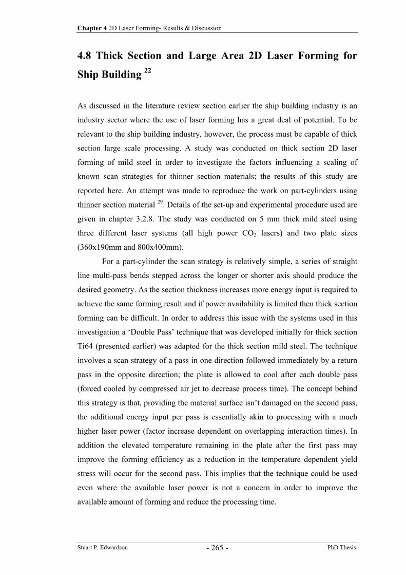
Chapter 4 2D Laser Forming- Results & Discussion
Stuart P. Edwardson PhD Thesis - 265 -
4.8 Thick Section and Large Area 2D Laser Forming for
Ship Building 22
As discussed in the literature review section earlier the ship building industry is an
industry sector where the use of laser forming has a great deal of potential. To be
relevant to the ship building industry, however, the process must be capable of thick
section large scale processing. A study was conducted on thick section 2D laser
forming of mild steel in order to investigate the factors influencing a scaling of
known scan strategies for thinner section materials; the results of this study are
reported here. An attempt was made to reproduce the work on part-cylinders using
thinner section material 29. Details of the set-up and experimental procedure used are
given in chapter 3.2.8. The study was conducted on 5 mm thick mild steel using
three different laser systems (all high power CO2 lasers) and two plate sizes
(360x190mm and 800x400mm).
For a part-cylinder the scan strategy is relatively simple, a series of straight
line multi-pass bends stepped across the longer or shorter axis should produce the
desired geometry. As the section thickness increases more energy input is required to
achieve the same forming result and if power availability is limited then thick section
forming can be difficult. In order to address this issue with the systems used in this
investigation a ‘Double Pass’ technique that was developed initially for thick section
Ti64 (presented earlier) was adapted for the thick section mild steel. The technique
involves a scan strategy of a pass in one direction followed immediately by a return
pass in the opposite direction; the plate is allowed to cool after each double pass
(forced cooled by compressed air jet to decrease process time). The concept behind
this strategy is that, providing the material surface isn’t damaged on the second pass,
the additional energy input per pass is essentially akin to processing with a much
higher laser power (factor increase dependent on overlapping interaction times). In
addition the elevated temperature remaining in the plate after the first pass may
improve the forming efficiency as a reduction in the temperature dependent yield
stress will occur for the second pass. This implies that the technique could be used
even where the available laser power is not a concern in order to improve the
available amount of forming and reduce the processing time.
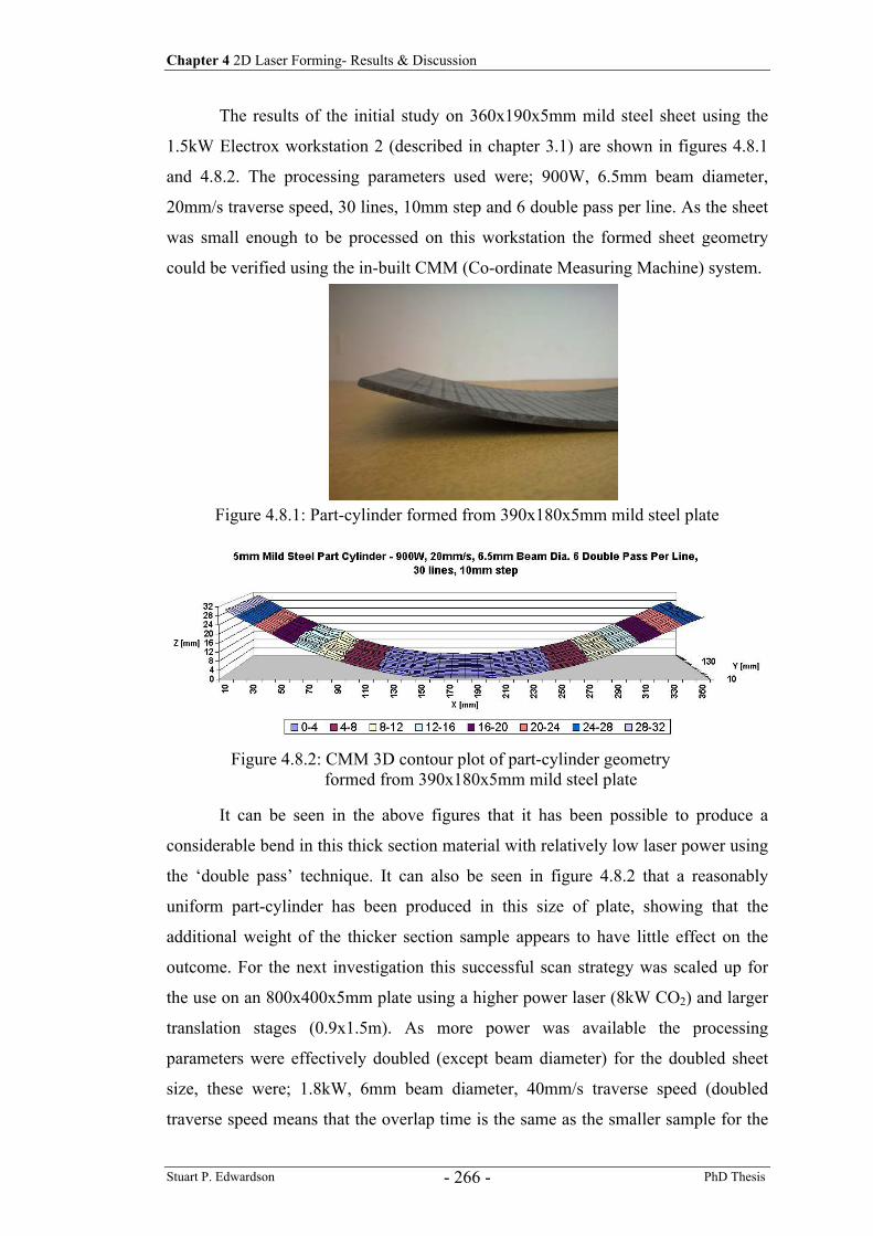
Chapter 4 2D Laser Forming- Results & Discussion
Stuart P. Edwardson PhD Thesis - 266 -
The results of the initial study on 360x190x5mm mild steel sheet using the
1.5kW Electrox workstation 2 (described in chapter 3.1) are shown in figures 4.8.1
and 4.8.2. The processing parameters used were; 900W, 6.5mm beam diameter,
20mm/s traverse speed, 30 lines, 10mm step and 6 double pass per line. As the sheet
was small enough to be processed on this workstation the formed sheet geometry
could be verified using the in-built CMM (Co-ordinate Measuring Machine) system.
It can be seen in the above figures that it has been possible to produce a
considerable bend in this thick section material with relatively low laser power using
the ‘double pass’ technique. It can also be seen in figure 4.8.2 that a reasonably
uniform part-cylinder has been produced in this size of plate, showing that the
additional weight of the thicker section sample appears to have little effect on the
outcome. For the next investigation this successful scan strategy was scaled up for
the use on an 800x400x5mm plate using a higher power laser (8kW CO2) and larger
translation stages (0.9x1.5m). As more power was available the processing
parameters were effectively doubled (except beam diameter) for the doubled sheet
size, these were; 1.8kW, 6mm beam diameter, 40mm/s traverse speed (doubled
traverse speed means that the overlap time is the same as the smaller sample for the
Figure 4.8.1: Part-cylinder formed from 390x180x5mm mild steel plate
Figure 4.8.2: CMM 3D contour plot of part-cylinder geometry formed from 390x180x5mm mild steel plate
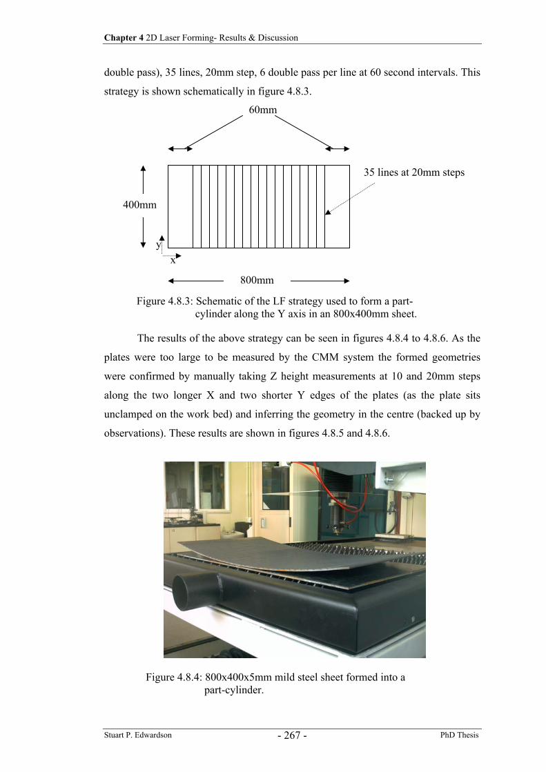
Chapter 4 2D Laser Forming- Results & Discussion
Stuart P. Edwardson PhD Thesis - 267 -
double pass), 35 lines, 20mm step, 6 double pass per line at 60 second intervals. This
strategy is shown schematically in figure 4.8.3.
The results of the above strategy can be seen in figures 4.8.4 to 4.8.6. As the
plates were too large to be measured by the CMM system the formed geometries
were confirmed by manually taking Z height measurements at 10 and 20mm steps
along the two longer X and two shorter Y edges of the plates (as the plate sits
unclamped on the work bed) and inferring the geometry in the centre (backed up by
observations). These results are shown in figures 4.8.5 and 4.8.6.
400mm
800mm
60mm
35 lines at 20mm steps
Figure 4.8.3: Schematic of the LF strategy used to form a part-cylinder along the Y axis in an 800x400mm sheet.
Figure 4.8.4: 800x400x5mm mild steel sheet formed into a part-cylinder.
x y
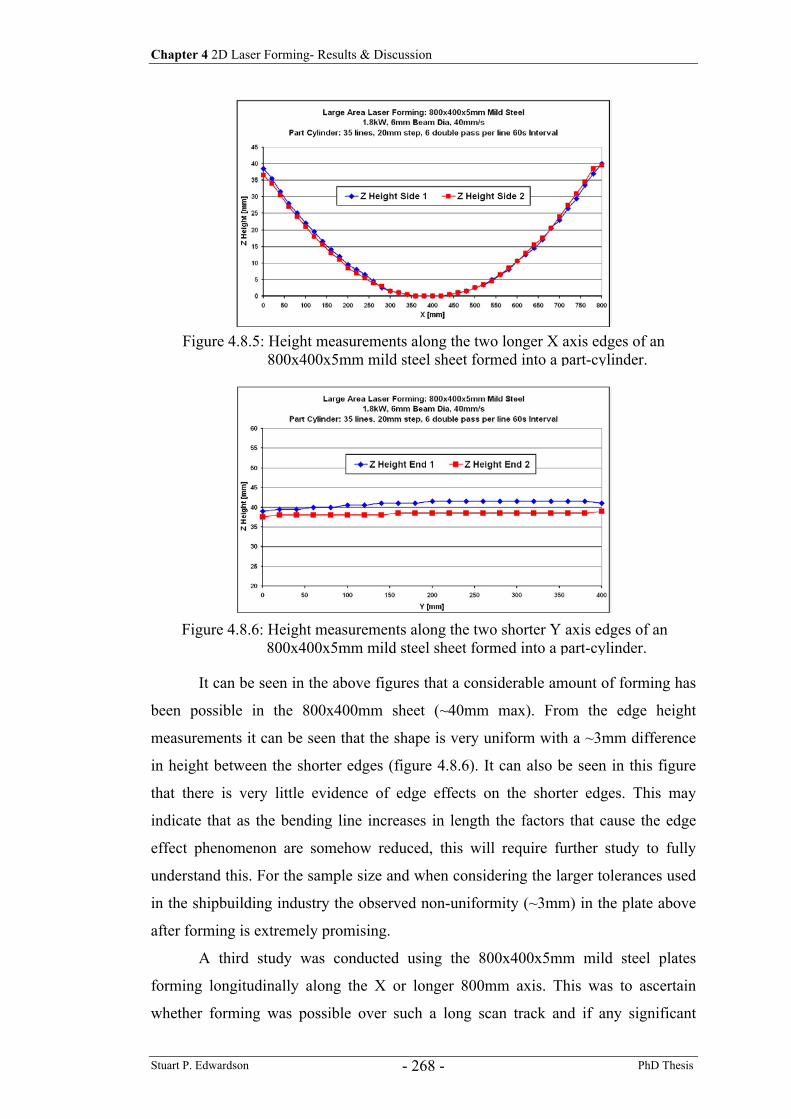
Chapter 4 2D Laser Forming- Results & Discussion
Stuart P. Edwardson PhD Thesis - 268 -
It can be seen in the above figures that a considerable amount of forming has
been possible in the 800x400mm sheet (~40mm max). From the edge height
measurements it can be seen that the shape is very uniform with a ~3mm difference
in height between the shorter edges (figure 4.8.6). It can also be seen in this figure
that there is very little evidence of edge effects on the shorter edges. This may
indicate that as the bending line increases in length the factors that cause the edge
effect phenomenon are somehow reduced, this will require further study to fully
understand this. For the sample size and when considering the larger tolerances used
in the shipbuilding industry the observed non-uniformity (~3mm) in the plate above
after forming is extremely promising.
A third study was conducted using the 800x400x5mm mild steel plates
forming longitudinally along the X or longer 800mm axis. This was to ascertain
whether forming was possible over such a long scan track and if any significant
Figure 4.8.5: Height measurements along the two longer X axis edges of an 800x400x5mm mild steel sheet formed into a part-cylinder.
Figure 4.8.6: Height measurements along the two shorter Y axis edges of an 800x400x5mm mild steel sheet formed into a part-cylinder.
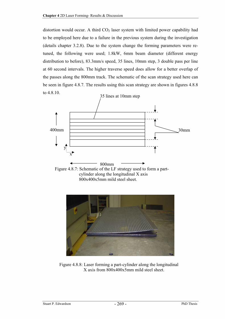
Chapter 4 2D Laser Forming- Results & Discussion
Stuart P. Edwardson PhD Thesis - 269 -
distortion would occur. A third CO2 laser system with limited power capability had
to be employed here due to a failure in the previous system during the investigation
(details chapter 3.2.8). Due to the system change the forming parameters were re-
tuned, the following were used; 1.8kW, 6mm beam diameter (different energy
distribution to before), 83.3mm/s speed, 35 lines, 10mm step, 3 double pass per line
at 60 second intervals. The higher traverse speed does allow for a better overlap of
the passes along the 800mm track. The schematic of the scan strategy used here can
be seen in figure 4.8.7. The results using this scan strategy are shown in figures 4.8.8
to 4.8.10.
400mm
800mm
30mm
35 lines at 10mm step
Figure 4.8.7: Schematic of the LF strategy used to form a part-cylinder along the longitudinal X axis 800x400x5mm mild steel sheet.
x y
Figure 4.8.8: Laser forming a part-cylinder along the longitudinal X axis from 800x400x5mm mild steel sheet.
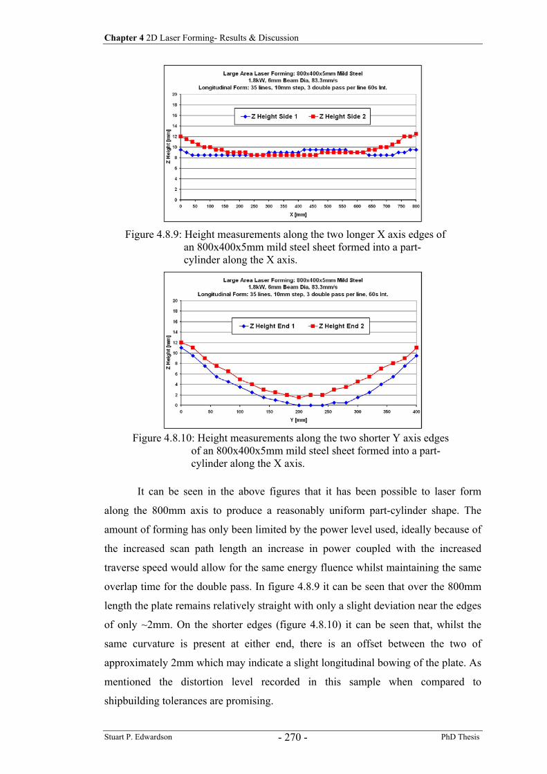
Chapter 4 2D Laser Forming- Results & Discussion
Stuart P. Edwardson PhD Thesis - 270 -
It can be seen in the above figures that it has been possible to laser form
along the 800mm axis to produce a reasonably uniform part-cylinder shape. The
amount of forming has only been limited by the power level used, ideally because of
the increased scan path length an increase in power coupled with the increased
traverse speed would allow for the same energy fluence whilst maintaining the same
overlap time for the double pass. In figure 4.8.9 it can be seen that over the 800mm
length the plate remains relatively straight with only a slight deviation near the edges
of only ~2mm. On the shorter edges (figure 4.8.10) it can be seen that, whilst the
same curvature is present at either end, there is an offset between the two of
approximately 2mm which may indicate a slight longitudinal bowing of the plate. As
mentioned the distortion level recorded in this sample when compared to
shipbuilding tolerances are promising.
Figure 4.8.9: Height measurements along the two longer X axis edges of an 800x400x5mm mild steel sheet formed into a part-cylinder along the X axis.
Figure 4.8.10: Height measurements along the two shorter Y axis edges of an 800x400x5mm mild steel sheet formed into a part-cylinder along the X axis.
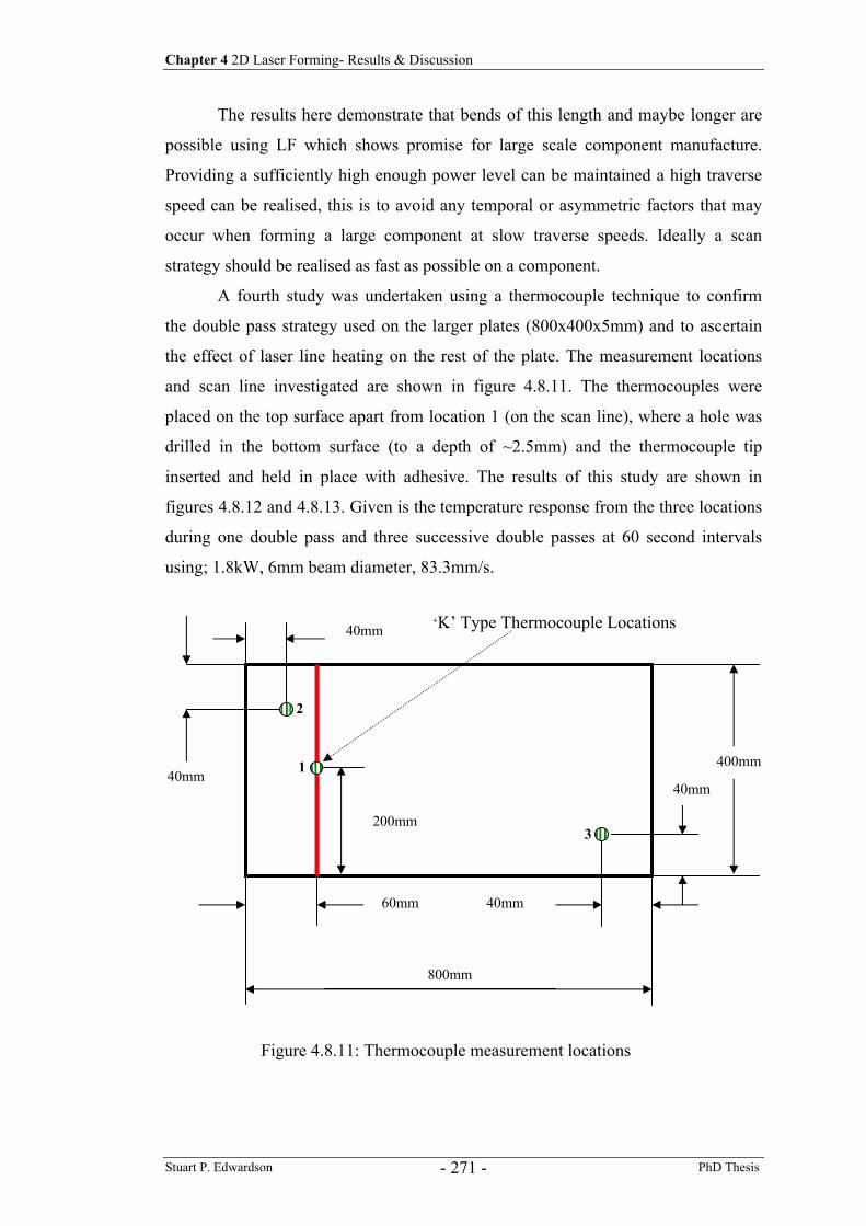
Chapter 4 2D Laser Forming- Results & Discussion
Stuart P. Edwardson PhD Thesis - 271 -
The results here demonstrate that bends of this length and maybe longer are
possible using LF which shows promise for large scale component manufacture.
Providing a sufficiently high enough power level can be maintained a high traverse
speed can be realised, this is to avoid any temporal or asymmetric factors that may
occur when forming a large component at slow traverse speeds. Ideally a scan
strategy should be realised as fast as possible on a component.
A fourth study was undertaken using a thermocouple technique to confirm
the double pass strategy used on the larger plates (800x400x5mm) and to ascertain
the effect of laser line heating on the rest of the plate. The measurement locations
and scan line investigated are shown in figure 4.8.11. The thermocouples were
placed on the top surface apart from location 1 (on the scan line), where a hole was
drilled in the bottom surface (to a depth of ~2.5mm) and the thermocouple tip
inserted and held in place with adhesive. The results of this study are shown in
figures 4.8.12 and 4.8.13. Given is the temperature response from the three locations
during one double pass and three successive double passes at 60 second intervals
using; 1.8kW, 6mm beam diameter, 83.3mm/s.
40mm
40mm
60mm 40mm
40mm
200mm
400mm
800mm
‘K’ Type Thermocouple Locations
1
2
3
Figure 4.8.11: Thermocouple measurement locations
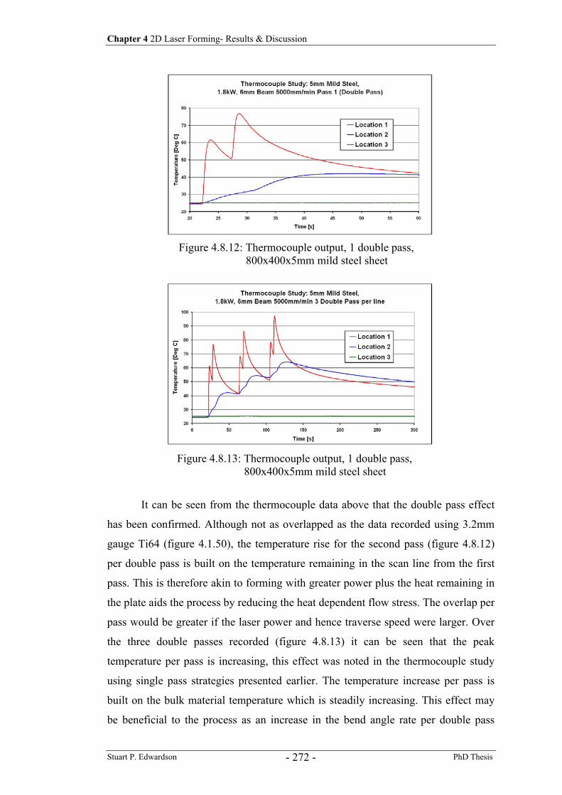
Chapter 4 2D Laser Forming- Results & Discussion
Stuart P. Edwardson PhD Thesis - 272 -
It can be seen from the thermocouple data above that the double pass effect
has been confirmed. Although not as overlapped as the data recorded using 3.2mm
gauge Ti64 (figure 4.1.50), the temperature rise for the second pass (figure 4.8.12)
per double pass is built on the temperature remaining in the scan line from the first
pass. This is therefore akin to forming with greater power plus the heat remaining in
the plate aids the process by reducing the heat dependent flow stress. The overlap per
pass would be greater if the laser power and hence traverse speed were larger. Over
the three double passes recorded (figure 4.8.13) it can be seen that the peak
temperature per pass is increasing, this effect was noted in the thermocouple study
using single pass strategies presented earlier. The temperature increase per pass is
built on the bulk material temperature which is steadily increasing. This effect may
be beneficial to the process as an increase in the bend angle rate per double pass
Figure 4.8.12: Thermocouple output, 1 double pass, 800x400x5mm mild steel sheet
Figure 4.8.13: Thermocouple output, 1 double pass, 800x400x5mm mild steel sheet
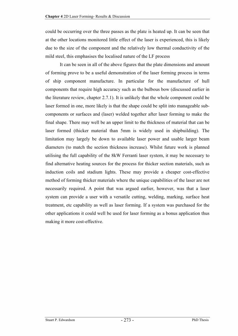
Chapter 4 2D Laser Forming- Results & Discussion
Stuart P. Edwardson PhD Thesis - 273 -
could be occurring over the three passes as the plate is heated up. It can be seen that
at the other locations monitored little effect of the laser is experienced, this is likely
due to the size of the component and the relatively low thermal conductivity of the
mild steel, this emphasises the localised nature of the LF process
It can be seen in all of the above figures that the plate dimensions and amount
of forming prove to be a useful demonstration of the laser forming process in terms
of ship component manufacture. In particular for the manufacture of hull
components that require high accuracy such as the bulbous bow (discussed earlier in
the literature review, chapter 2.7.1). It is unlikely that the whole component could be
laser formed in one, more likely is that the shape could be split into manageable sub-
components or surfaces and (laser) welded together after laser forming to make the
final shape. There may well be an upper limit to the thickness of material that can be
laser formed (thicker material than 5mm is widely used in shipbuilding). The
limitation may largely be down to available laser power and usable larger beam
diameters (to match the section thickness increase). Whilst future work is planned
utilising the full capability of the 8kW Ferranti laser system, it may be necessary to
find alternative heating sources for the process for thicker section materials, such as
induction coils and stadium lights. These may provide a cheaper cost-effective
method of forming thicker materials where the unique capabilities of the laser are not
necessarily required. A point that was argued earlier, however, was that a laser
system can provide a user with a versatile cutting, welding, marking, surface heat
treatment, etc capability as well as laser forming. If a system was purchased for the
other applications it could well be used for laser forming as a bonus application thus
making it more cost-effective.
Chapter 4 2D Laser Forming- Results & Discussion
Stuart P. Edwardson PhD Thesis - 274 -
4.9 Laser Forming of Novel Materials – Metal Laminate
Composite (MLC) Materials 125, 126
The application reported here demonstrates how the laser forming process can be
used to form recently developed high strength metal laminate composite materials
(MLC) or fibre metal laminates (FML). These materials due to their construction and
high strength, are difficult to form once manufactured using conventional techniques.
The aim of this study was to demonstrate the potential of laser forming as a
manufacturing tool for MLC materials, either as a means of direct fabrication or a
means of alignment and distortion removal.
4.9.1 Feasibility Study
The initial concept for the use laser forming with MLC materials was specifically
based around the development of new thermoplastic based fibre reinforced
composites with high melting temperatures. It was considered that it may be possible
to form the material as if it were the equivalent thickness of a metallic solid,
generating a semi-uniform thermal gradient through the thickness (TGM 11) (Figure
4.9.1). Initial tests on 1.38mm thick 2/1 glass reinforced polyamide based MLC
using 800W, a 5mm beam diameter and 80mm/s processing speed produced
excessive melting of the upper 0.3mm Al 2024 layer, with little or no heat transfer
into the lower layers. This led to the perhaps expected conclusion that due to the
extreme differences in thermal properties between each of the layers in a MLC lay-
up it is not possible to set-up a uniform thermal gradient through the thickness.
However, just as the TGM causes a plastic compression of just the upper surface
layers of a solid metallic section, it was thought that by forming by TGM the upper
aluminium layer alone a moment could be generated sufficient to bend the material
section (Figure 4.9.2). Initial tests of this theory found that it was difficult to set up
the TGM across the 0.3mm thickness, the material tended to buckle (Buckling
Mechanism 11) and as the upper layer was constrained the buckle tended to be away
from the laser and hence delamination occurred. Figure 4.9.1 shows the result for a
2/1 polyamide based MLC processed at 300W, 3mm beam diameter and 90mm/s.
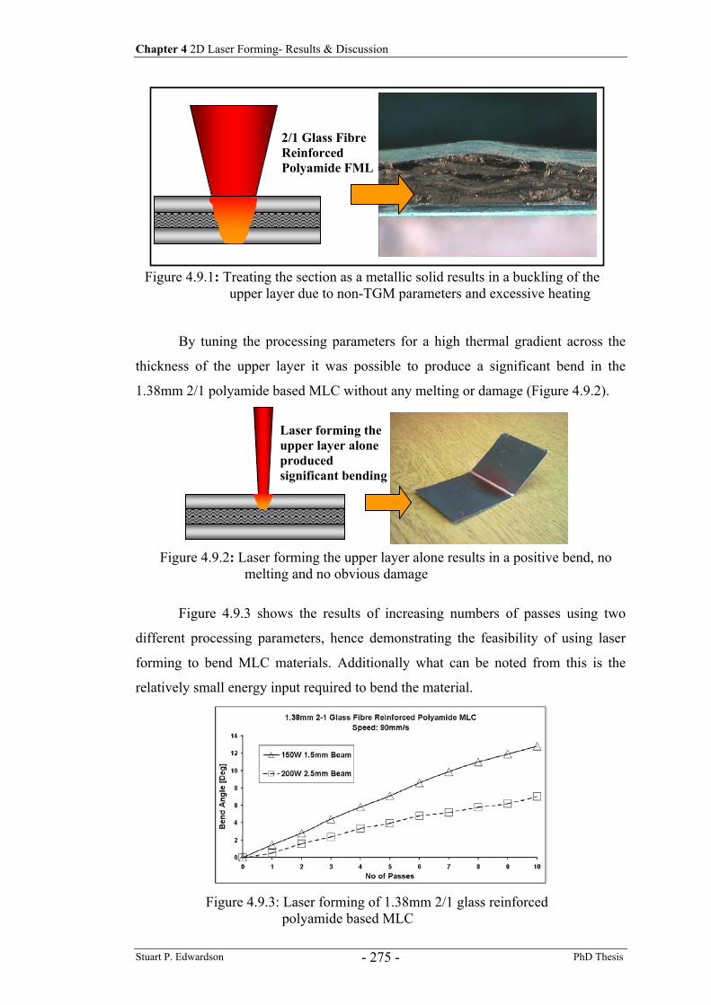
Chapter 4 2D Laser Forming- Results & Discussion
Stuart P. Edwardson PhD Thesis - 275 -
By tuning the processing parameters for a high thermal gradient across the
thickness of the upper layer it was possible to produce a significant bend in the
1.38mm 2/1 polyamide based MLC without any melting or damage (Figure 4.9.2).
Figure 4.9.3 shows the results of increasing numbers of passes using two
different processing parameters, hence demonstrating the feasibility of using laser
forming to bend MLC materials. Additionally what can be noted from this is the
relatively small energy input required to bend the material.
Figure 4.9.1: Treating the section as a metallic solid results in a buckling of the upper layer due to non-TGM parameters and excessive heating
Figure 4.9.3: Laser forming of 1.38mm 2/1 glass reinforced polyamide based MLC
Figure 4.9.2: Laser forming the upper layer alone results in a positive bend, no melting and no obvious damage
Laser forming the upper layer alone produced significant bending
2/1 Glass Fibre Reinforced Polyamide FML
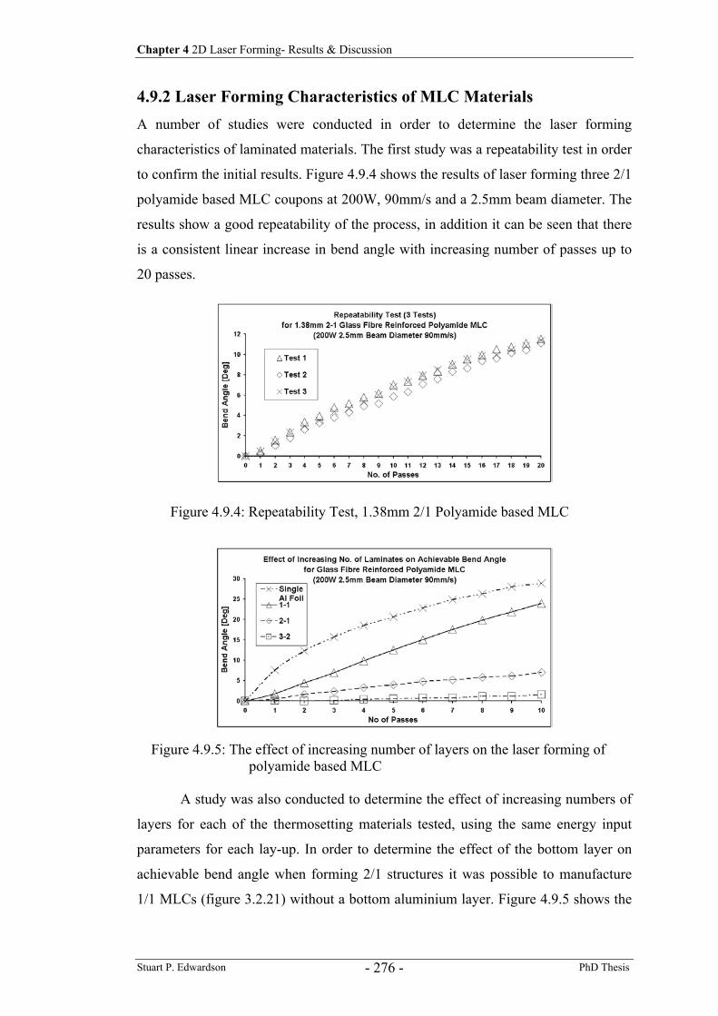
Chapter 4 2D Laser Forming- Results & Discussion
Stuart P. Edwardson PhD Thesis - 276 -
4.9.2 Laser Forming Characteristics of MLC Materials A number of studies were conducted in order to determine the laser forming
characteristics of laminated materials. The first study was a repeatability test in order
to confirm the initial results. Figure 4.9.4 shows the results of laser forming three 2/1
polyamide based MLC coupons at 200W, 90mm/s and a 2.5mm beam diameter. The
results show a good repeatability of the process, in addition it can be seen that there
is a consistent linear increase in bend angle with increasing number of passes up to
20 passes.
A study was also conducted to determine the effect of increasing numbers of
layers for each of the thermosetting materials tested, using the same energy input
parameters for each lay-up. In order to determine the effect of the bottom layer on
achievable bend angle when forming 2/1 structures it was possible to manufacture
1/1 MLCs (figure 3.2.21) without a bottom aluminium layer. Figure 4.9.5 shows the
Figure 4.9.4: Repeatability Test, 1.38mm 2/1 Polyamide based MLC
Figure 4.9.5: The effect of increasing number of layers on the laser forming of polyamide based MLC
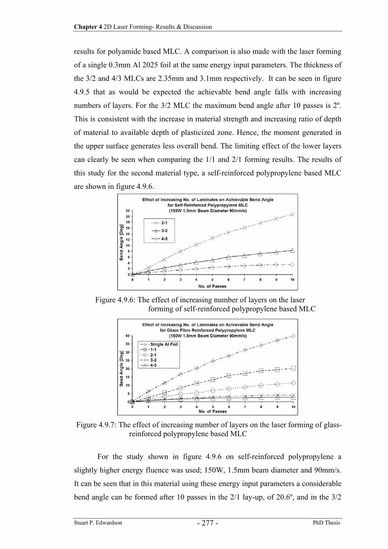
Chapter 4 2D Laser Forming- Results & Discussion
Stuart P. Edwardson PhD Thesis - 277 -
results for polyamide based MLC. A comparison is also made with the laser forming
of a single 0.3mm Al 2025 foil at the same energy input parameters. The thickness of
the 3/2 and 4/3 MLCs are 2.35mm and 3.1mm respectively. It can be seen in figure
4.9.5 that as would be expected the achievable bend angle falls with increasing
numbers of layers. For the 3/2 MLC the maximum bend angle after 10 passes is 2º.
This is consistent with the increase in material strength and increasing ratio of depth
of material to available depth of plasticized zone. Hence, the moment generated in
the upper surface generates less overall bend. The limiting effect of the lower layers
can clearly be seen when comparing the 1/1 and 2/1 forming results. The results of
this study for the second material type, a self-reinforced polypropylene based MLC
are shown in figure 4.9.6.
For the study shown in figure 4.9.6 on self-reinforced polypropylene a
slightly higher energy fluence was used; 150W, 1.5mm beam diameter and 90mm/s.
It can be seen that in this material using these energy input parameters a considerable
bend angle can be formed after 10 passes in the 2/1 lay-up, of 20.6º, and in the 3/2
Figure 4.9.6: The effect of increasing number of layers on the laser forming of self-reinforced polypropylene based MLC
Figure 4.9.7: The effect of increasing number of layers on the laser forming of glass-reinforced polypropylene based MLC
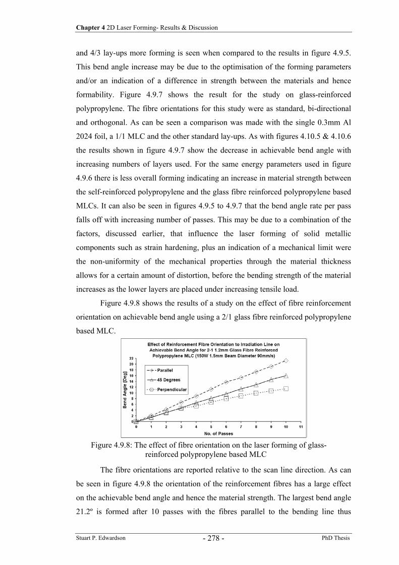
Chapter 4 2D Laser Forming- Results & Discussion
Stuart P. Edwardson PhD Thesis - 278 -
and 4/3 lay-ups more forming is seen when compared to the results in figure 4.9.5.
This bend angle increase may be due to the optimisation of the forming parameters
and/or an indication of a difference in strength between the materials and hence
formability. Figure 4.9.7 shows the result for the study on glass-reinforced
polypropylene. The fibre orientations for this study were as standard, bi-directional
and orthogonal. As can be seen a comparison was made with the single 0.3mm Al
2024 foil, a 1/1 MLC and the other standard lay-ups. As with figures 4.10.5 & 4.10.6
the results shown in figure 4.9.7 show the decrease in achievable bend angle with
increasing numbers of layers used. For the same energy parameters used in figure
4.9.6 there is less overall forming indicating an increase in material strength between
the self-reinforced polypropylene and the glass fibre reinforced polypropylene based
MLCs. It can also be seen in figures 4.9.5 to 4.9.7 that the bend angle rate per pass
falls off with increasing number of passes. This may be due to a combination of the
factors, discussed earlier, that influence the laser forming of solid metallic
components such as strain hardening, plus an indication of a mechanical limit were
the non-uniformity of the mechanical properties through the material thickness
allows for a certain amount of distortion, before the bending strength of the material
increases as the lower layers are placed under increasing tensile load.
Figure 4.9.8 shows the results of a study on the effect of fibre reinforcement
orientation on achievable bend angle using a 2/1 glass fibre reinforced polypropylene
based MLC.
The fibre orientations are reported relative to the scan line direction. As can
be seen in figure 4.9.8 the orientation of the reinforcement fibres has a large effect
on the achievable bend angle and hence the material strength. The largest bend angle
21.2º is formed after 10 passes with the fibres parallel to the bending line thus
Figure 4.9.8: The effect of fibre orientation on the laser forming of glass-reinforced polypropylene based MLC
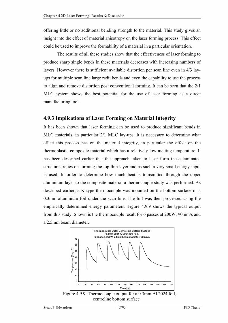
Chapter 4 2D Laser Forming- Results & Discussion
Stuart P. Edwardson PhD Thesis - 279 -
offering little or no additional bending strength to the material. This study gives an
insight into the effect of material anisotropy on the laser forming process. This effect
could be used to improve the formability of a material in a particular orientation.
The results of all these studies show that the effectiveness of laser forming to
produce sharp single bends in these materials decreases with increasing numbers of
layers. However there is sufficient available distortion per scan line even in 4/3 lay-
ups for multiple scan line large radii bends and even the capability to use the process
to align and remove distortion post conventional forming. It can be seen that the 2/1
MLC system shows the best potential for the use of laser forming as a direct
manufacturing tool.
4.9.3 Implications of Laser Forming on Material Integrity It has been shown that laser forming can be used to produce significant bends in
MLC materials, in particular 2/1 MLC lay-ups. It is necessary to determine what
effect this process has on the material integrity, in particular the effect on the
thermoplastic composite material which has a relatively low melting temperature. It
has been described earlier that the approach taken to laser form these laminated
structures relies on forming the top thin layer and as such a very small energy input
is used. In order to determine how much heat is transmitted through the upper
aluminium layer to the composite material a thermocouple study was performed. As
described earlier, a K type thermocouple was mounted on the bottom surface of a
0.3mm aluminium foil under the scan line. The foil was then processed using the
empirically determined energy parameters. Figure 4.9.9 shows the typical output
from this study. Shown is the thermocouple result for 6 passes at 200W, 90mm/s and
a 2.5mm beam diameter.
Figure 4.9.9: Thermocouple output for a 0.3mm Al 2024 foil, centreline bottom surface
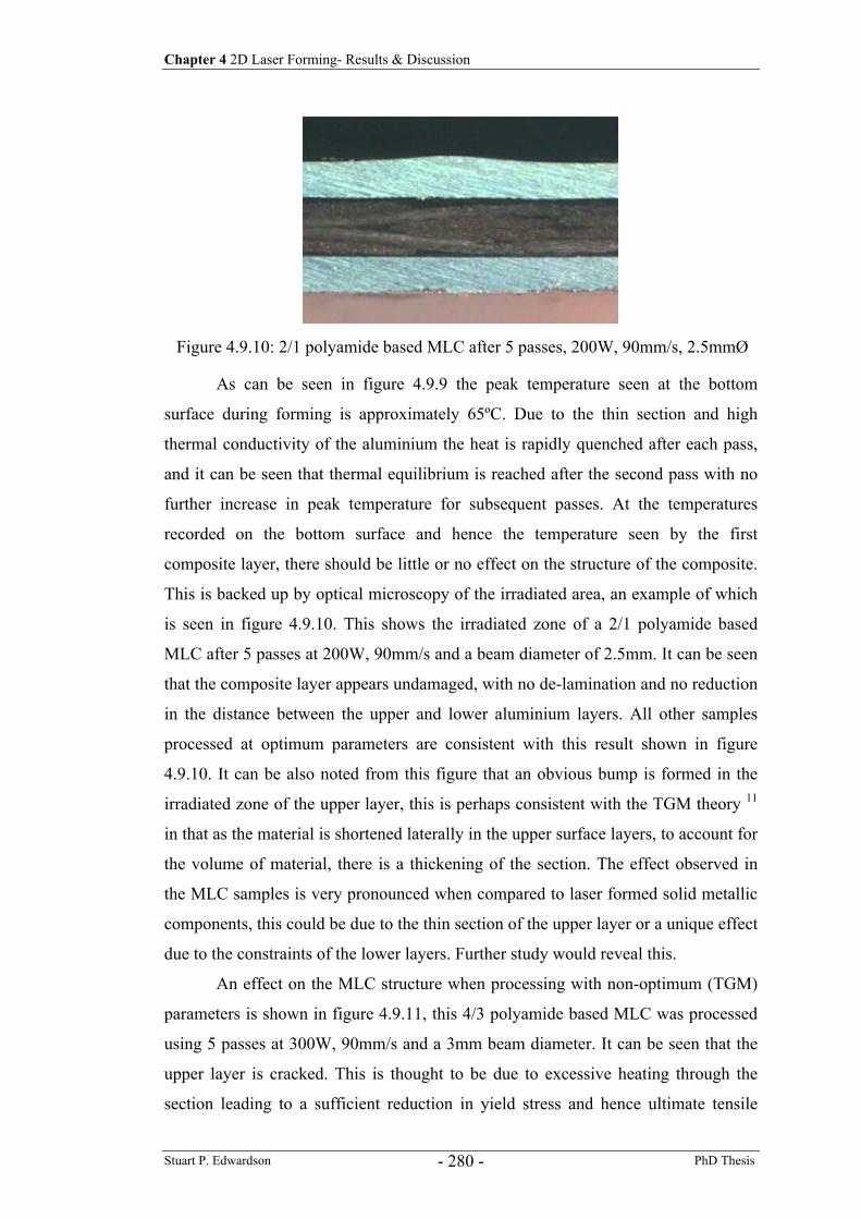
Chapter 4 2D Laser Forming- Results & Discussion
Stuart P. Edwardson PhD Thesis - 280 -
As can be seen in figure 4.9.9 the peak temperature seen at the bottom
surface during forming is approximately 65ºC. Due to the thin section and high
thermal conductivity of the aluminium the heat is rapidly quenched after each pass,
and it can be seen that thermal equilibrium is reached after the second pass with no
further increase in peak temperature for subsequent passes. At the temperatures
recorded on the bottom surface and hence the temperature seen by the first
composite layer, there should be little or no effect on the structure of the composite.
This is backed up by optical microscopy of the irradiated area, an example of which
is seen in figure 4.9.10. This shows the irradiated zone of a 2/1 polyamide based
MLC after 5 passes at 200W, 90mm/s and a beam diameter of 2.5mm. It can be seen
that the composite layer appears undamaged, with no de-lamination and no reduction
in the distance between the upper and lower aluminium layers. All other samples
processed at optimum parameters are consistent with this result shown in figure
4.9.10. It can be also noted from this figure that an obvious bump is formed in the
irradiated zone of the upper layer, this is perhaps consistent with the TGM theory 11
in that as the material is shortened laterally in the upper surface layers, to account for
the volume of material, there is a thickening of the section. The effect observed in
the MLC samples is very pronounced when compared to laser formed solid metallic
components, this could be due to the thin section of the upper layer or a unique effect
due to the constraints of the lower layers. Further study would reveal this.
An effect on the MLC structure when processing with non-optimum (TGM)
parameters is shown in figure 4.9.11, this 4/3 polyamide based MLC was processed
using 5 passes at 300W, 90mm/s and a 3mm beam diameter. It can be seen that the
upper layer is cracked. This is thought to be due to excessive heating through the
section leading to a sufficient reduction in yield stress and hence ultimate tensile
Figure 4.9.10: 2/1 polyamide based MLC after 5 passes, 200W, 90mm/s, 2.5mmØ
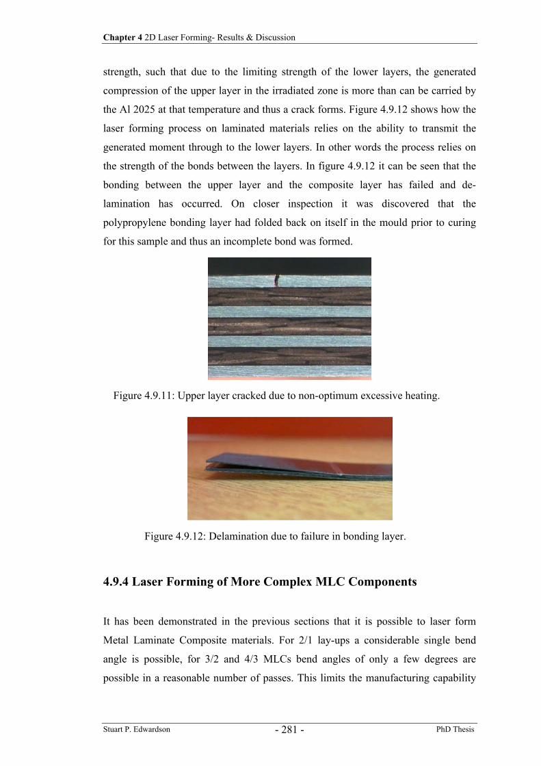
Chapter 4 2D Laser Forming- Results & Discussion
Stuart P. Edwardson PhD Thesis - 281 -
strength, such that due to the limiting strength of the lower layers, the generated
compression of the upper layer in the irradiated zone is more than can be carried by
the Al 2025 at that temperature and thus a crack forms. Figure 4.9.12 shows how the
laser forming process on laminated materials relies on the ability to transmit the
generated moment through to the lower layers. In other words the process relies on
the strength of the bonds between the layers. In figure 4.9.12 it can be seen that the
bonding between the upper layer and the composite layer has failed and de-
lamination has occurred. On closer inspection it was discovered that the
polypropylene bonding layer had folded back on itself in the mould prior to curing
for this sample and thus an incomplete bond was formed.
4.9.4 Laser Forming of More Complex MLC Components
It has been demonstrated in the previous sections that it is possible to laser form
Metal Laminate Composite materials. For 2/1 lay-ups a considerable single bend
angle is possible, for 3/2 and 4/3 MLCs bend angles of only a few degrees are
possible in a reasonable number of passes. This limits the manufacturing capability
Figure 4.9.11: Upper layer cracked due to non-optimum excessive heating.
Figure 4.9.12: Delamination due to failure in bonding layer.
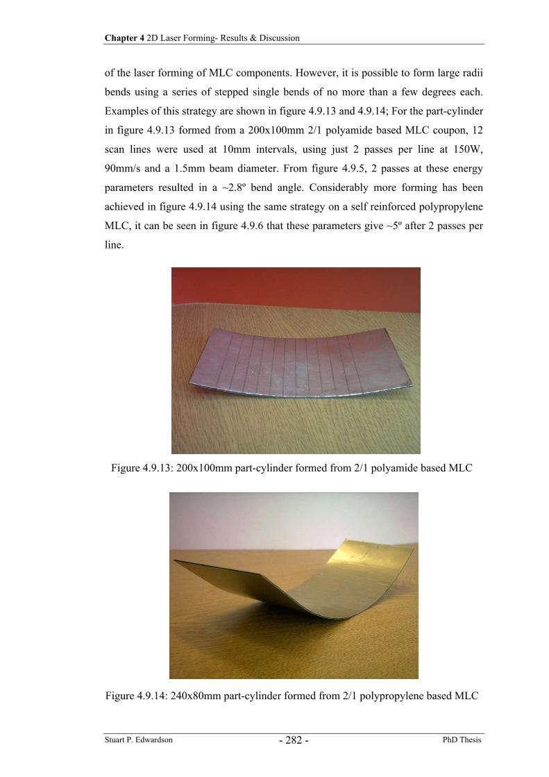
Chapter 4 2D Laser Forming- Results & Discussion
Stuart P. Edwardson PhD Thesis - 282 -
of the laser forming of MLC components. However, it is possible to form large radii
bends using a series of stepped single bends of no more than a few degrees each.
Examples of this strategy are shown in figure 4.9.13 and 4.9.14; For the part-cylinder
in figure 4.9.13 formed from a 200x100mm 2/1 polyamide based MLC coupon, 12
scan lines were used at 10mm intervals, using just 2 passes per line at 150W,
90mm/s and a 1.5mm beam diameter. From figure 4.9.5, 2 passes at these energy
parameters resulted in a ~2.8º bend angle. Considerably more forming has been
achieved in figure 4.9.14 using the same strategy on a self reinforced polypropylene
MLC, it can be seen in figure 4.9.6 that these parameters give ~5º after 2 passes per
line.
Figure 4.9.13: 200x100mm part-cylinder formed from 2/1 polyamide based MLC
Figure 4.9.14: 240x80mm part-cylinder formed from 2/1 polypropylene based MLC
Chapter 4 2D Laser Forming- Results & Discussion
Stuart P. Edwardson PhD Thesis - 283 -
As discussed earlier there is sufficient available distortion per scan line even
in 4/3 lay-ups for this multi-line strategy and even the capability to use the process to
align and remove distortion post-conventional forming. It can be seen however that
the 2/1 MLC system shows the best potential for the use of laser forming as a direct
manufacturing tool. As it has been reported 127 that for conventional forming a metal
layer needs to be within the material to form the material successfully (i.e. a
minimum of a 3/2 lay-up MLC), laser forming offers a useful tool to produce bends
in 2/1 lay-up materials. It may also be possible to use a 3D laser forming approach to
form MLC materials. However, as can be seen in figure 4.10.8 the inherent effect of
material anisotropy may add an unwanted additional complication to a 3D problem.
Work is presented in this thesis on the development of a system that uses predictive
and adaptive approaches to 3D laser form independent of residual stress history and
non-uniform material behaviour, this work is discussed in a later chapter.
4.9.5 Laser Forming Thermosetting MLC Materials
After the success of laser forming the thermoplastic based MLC’s it was decided to
verify the results using a GLARE type material (GLARE 3 127). This material is a
laminate of 2024 aluminium and glass fibre reinforced epoxy, a thermosetting
material.
As shown earlier, the laser forming process when applied to laminate
structures relies on the bending of the upper layer alone. Therefore in order to aid the
process for this study, it was decided to increase the thickness of the Al2024 layers
to 0.9mm, improving the laser formability of the material as it were by increasing the
achievable moment. The material investigated was a 2/1 glass fibre reinforced epoxy
and 0.9mm Al2024 laminate. The fibre directions were bi-directional and orthogonal.
The samples were again 40x80mm.
As with the work presented earlier on the thermoplastic MLC’s an initial
feasibility study was performed. The first energy parameters investigated were taken
from the successful work on the other materials, 150W, 1.5mm beam diameter and a
speed of 90mm/s. As may be expected there was little or no forming, perhaps due to
the increased thickness and hence strength of the upper layer. It was therefore
decided to increase the laser power to 300W and leave the other parameters the same,
Chapter 4 2D Laser Forming- Results & Discussion
Stuart P. Edwardson PhD Thesis - 284 -
this produced a usable result. This result and the result of a repeatability test can be
seen in figure 4.9.15.
It can be seen in figure 4.9.15 that it is possible to laser form this
thermosetting GLARE type material to the same extent as the thermoplastic MLC’s.
A limit can be seen in the data at approximately 6° which corresponds to a point
were some delamination occurs. This is consistent with the problem of a minimum
achievable bend radius for these materials. In addition the energy parameters used
caused some surface melting, therefore it was decided to increase the beam diameter
to 3mm for a further study to establish optimum processing parameters where de-
lamination does not occur. The result of this study at various processing speeds can
be seen in figure 4.9.16.
Figure 4.9.15: Laser forming 2/1 GLARE type materials, initial feasibility test
Figure 4.9.16: Laser forming 2/1 GLARE type materials at various processing speeds
Chapter 4 2D Laser Forming- Results & Discussion
Stuart P. Edwardson PhD Thesis - 285 -
It can be seen in figure 4.9.16 that the rate of forming per pass is governed by
the energy input. The slower the traverse speed for the same power and spot size, the
higher the energy input and hence the higher the bend angle per pass. At 40mm/s it
can be seen that the bend angle data is reasonably linear until approximately 5°. At
this point (pass 5) there is a significant increase in bend angle rate per pass. As with
the previous study (figure 4.9.15) this also corresponds to a point where some
delamination of the upper layer away from the lower layers can be observed in the
sample. In this case the delamination appears to reduce the bending stiffness of the
section as seen by the upper layer, thus allowing more deformation to occur for the
given energy parameters. At approximately 13° (pass 7) the sample fails. The upper
layer was completely delaminated on the free end of the plate (the other end was still
attached and in the edge clamp). The lower layers sprung back flat, as they were only
elastically constrained and the upper Al2024 layer remained bent. Although this
result demonstrates that it is possible to damage the material using laser forming, it
can also be seen that as with the previous sections there is sufficient available
distortion per scan line for multiple scan line large radii bends and even the
capability to use the process to align and remove distortion post-conventional
forming. This was observed at 60mm/s, that providing the plate is not bent to more
than 5° in a single location, no delamination or damage occurs.
Figure 4.9.17: Laser forming a multiple scan line large radii bend, 2/1 GLARE type material, 240x80mm
Chapter 4 2D Laser Forming- Results & Discussion
Stuart P. Edwardson PhD Thesis - 286 -
In order to demonstrate the concept of multiple scan line large radii bends in
this material, a demonstration part was produced. As with the previous section a
240x80mm coupon was used and processed using 300W, 3mm beam diameter, a
processing speed of 40mm/s, 21 lines, 10mm step between the lines and 2 pass per
line. From figure 4.9.16 it can be seen that these energy parameters would give
approximately 2.5° per line, well below the 5° damage threshold. The completed
demonstration part is shown in figures 4.9.17 and 4.9.18. It can be seen that this
technique employing a number of smaller bends can produce a large overall
distortion. One possible drawback with this technique however, is the fact that only
the upper metal layer is plastically deformed. The lower layers are merely elastically
constrained at such a large bending radius, thus adding possible un-wanted residual
stresses between the layers. A solution to this issue and to the problem of a minimum
bend radius maybe the (laser) pre-forming of each metal layer to a near required
shape prior to bonding, then final alignment and adjustment with a laser forming
technique.
Figure 4.9.18: Laser forming a multiple scan line large radii bend, 2/1 GLARE type material, 240x80mm (reverse angle)
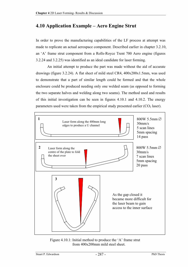
Chapter 4 2D Laser Forming- Results & Discussion
Stuart P. Edwardson PhD Thesis - 287 -
4.10 Application Example – Aero Engine Strut
In order to prove the manufacturing capabilities of the LF process at attempt was
made to replicate an actual aerospace component. Described earlier in chapter 3.2.10,
an ‘A’ frame strut component from a Rolls-Royce Trent 700 Aero engine (figures
3.2.24 and 3.2.25) was identified as an ideal candidate for laser forming.
An initial attempt to produce the part was made without the aid of accurate
drawings (figure 3.2.24). A flat sheet of mild steel CR4, 400x200x1.5mm, was used
to demonstrate that a part of similar length could be formed and that the whole
enclosure could be produced needing only one welded seam (as opposed to forming
the two separate halves and welding along two seams). The method used and results
of this initial investigation can be seen in figures 4.10.1 and 4.10.2. The energy
parameters used were taken from the empirical study presented earlier (CO2 laser).
Laser form along the 400mm long edges to produce a U channel
1
Laser form along the centre of the plate to fold the sheet over
2
3
800W 5.5mm ∅30mm/s 5 scan lines 5mm spacing 14 pass
800W 5.5mm ∅30mm/s 7 scan lines 5mm spacing 20 pass
As the gap closed it became more difficult for the laser beam to gain access to the inner surface
Figure 4.10.1: Initial method to produce the ‘A’ frame strut from 400x200mm mild steel sheet.
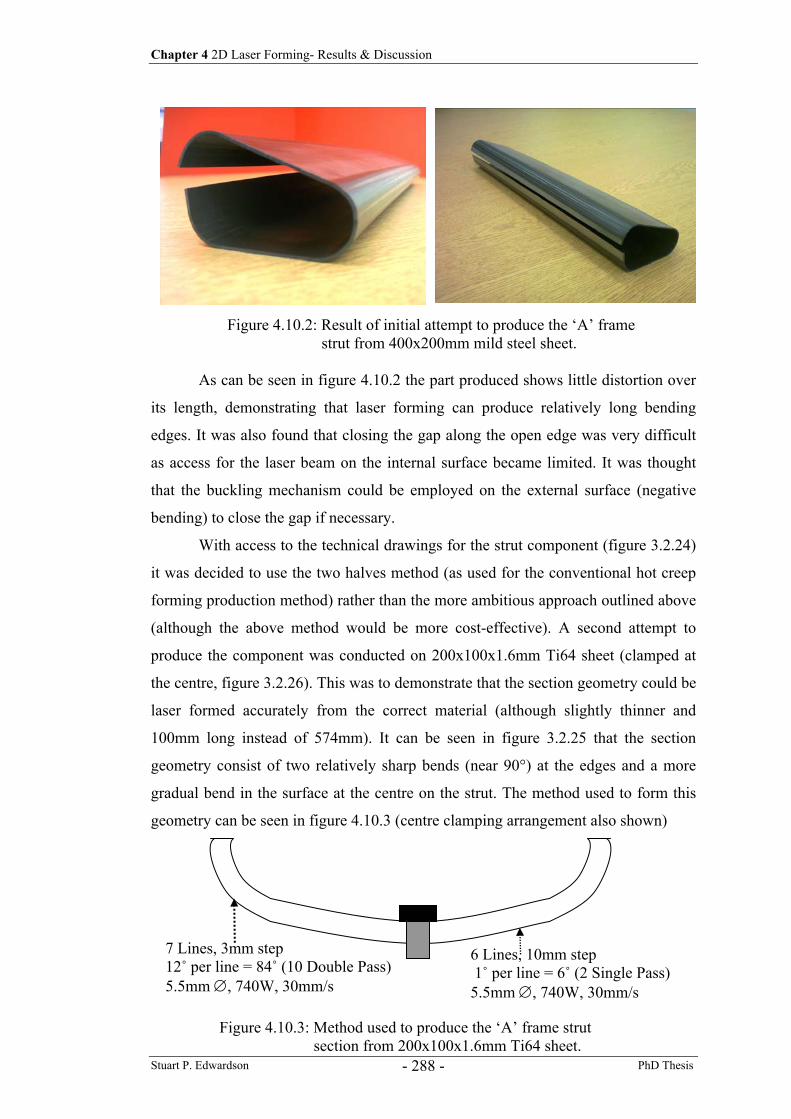
Chapter 4 2D Laser Forming- Results & Discussion
Stuart P. Edwardson PhD Thesis - 288 -
As can be seen in figure 4.10.2 the part produced shows little distortion over
its length, demonstrating that laser forming can produce relatively long bending
edges. It was also found that closing the gap along the open edge was very difficult
as access for the laser beam on the internal surface became limited. It was thought
that the buckling mechanism could be employed on the external surface (negative
bending) to close the gap if necessary.
With access to the technical drawings for the strut component (figure 3.2.24)
it was decided to use the two halves method (as used for the conventional hot creep
forming production method) rather than the more ambitious approach outlined above
(although the above method would be more cost-effective). A second attempt to
produce the component was conducted on 200x100x1.6mm Ti64 sheet (clamped at
the centre, figure 3.2.26). This was to demonstrate that the section geometry could be
laser formed accurately from the correct material (although slightly thinner and
100mm long instead of 574mm). It can be seen in figure 3.2.25 that the section
geometry consist of two relatively sharp bends (near 90°) at the edges and a more
gradual bend in the surface at the centre on the strut. The method used to form this
geometry can be seen in figure 4.10.3 (centre clamping arrangement also shown)
Figure 4.10.2: Result of initial attempt to produce the ‘A’ frame strut from 400x200mm mild steel sheet.
7 Lines, 3mm step 12˚ per line = 84˚ (10 Double Pass) 5.5mm ∅, 740W, 30mm/s
6 Lines, 10mm step 1˚ per line = 6˚ (2 Single Pass) 5.5mm ∅, 740W, 30mm/s
Figure 4.10.3: Method used to produce the ‘A’ frame strut section from 200x100x1.6mm Ti64 sheet.
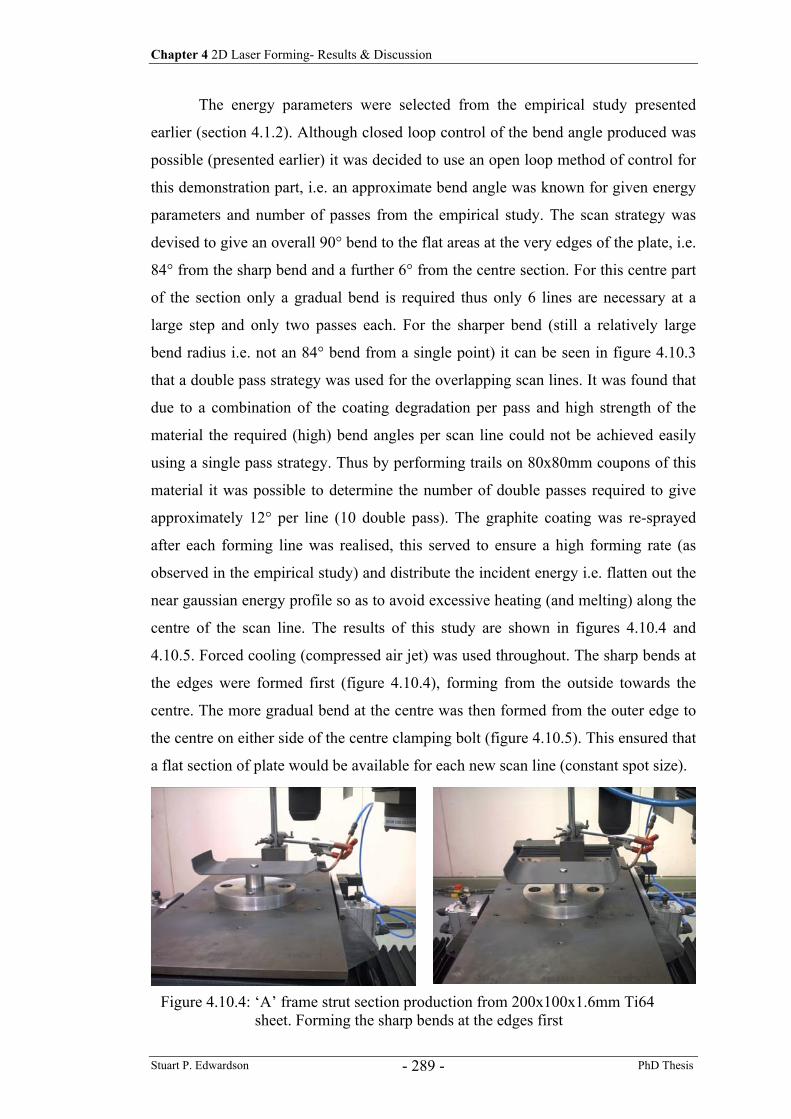
Chapter 4 2D Laser Forming- Results & Discussion
Stuart P. Edwardson PhD Thesis - 289 -
The energy parameters were selected from the empirical study presented
earlier (section 4.1.2). Although closed loop control of the bend angle produced was
possible (presented earlier) it was decided to use an open loop method of control for
this demonstration part, i.e. an approximate bend angle was known for given energy
parameters and number of passes from the empirical study. The scan strategy was
devised to give an overall 90° bend to the flat areas at the very edges of the plate, i.e.
84° from the sharp bend and a further 6° from the centre section. For this centre part
of the section only a gradual bend is required thus only 6 lines are necessary at a
large step and only two passes each. For the sharper bend (still a relatively large
bend radius i.e. not an 84° bend from a single point) it can be seen in figure 4.10.3
that a double pass strategy was used for the overlapping scan lines. It was found that
due to a combination of the coating degradation per pass and high strength of the
material the required (high) bend angles per scan line could not be achieved easily
using a single pass strategy. Thus by performing trails on 80x80mm coupons of this
material it was possible to determine the number of double passes required to give
approximately 12° per line (10 double pass). The graphite coating was re-sprayed
after each forming line was realised, this served to ensure a high forming rate (as
observed in the empirical study) and distribute the incident energy i.e. flatten out the
near gaussian energy profile so as to avoid excessive heating (and melting) along the
centre of the scan line. The results of this study are shown in figures 4.10.4 and
4.10.5. Forced cooling (compressed air jet) was used throughout. The sharp bends at
the edges were formed first (figure 4.10.4), forming from the outside towards the
centre. The more gradual bend at the centre was then formed from the outer edge to
the centre on either side of the centre clamping bolt (figure 4.10.5). This ensured that
a flat section of plate would be available for each new scan line (constant spot size).
Figure 4.10.4: ‘A’ frame strut section production from 200x100x1.6mm Ti64
sheet. Forming the sharp bends at the edges first
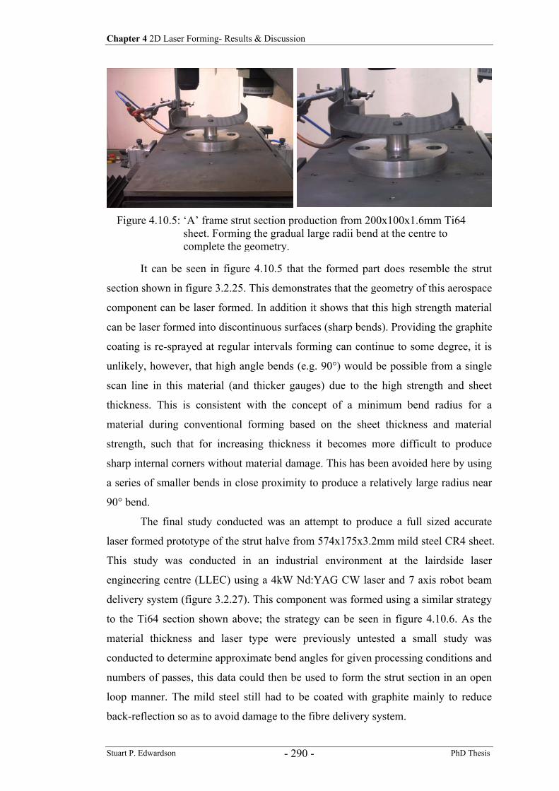
Chapter 4 2D Laser Forming- Results & Discussion
Stuart P. Edwardson PhD Thesis - 290 -
It can be seen in figure 4.10.5 that the formed part does resemble the strut
section shown in figure 3.2.25. This demonstrates that the geometry of this aerospace
component can be laser formed. In addition it shows that this high strength material
can be laser formed into discontinuous surfaces (sharp bends). Providing the graphite
coating is re-sprayed at regular intervals forming can continue to some degree, it is
unlikely, however, that high angle bends (e.g. 90°) would be possible from a single
scan line in this material (and thicker gauges) due to the high strength and sheet
thickness. This is consistent with the concept of a minimum bend radius for a
material during conventional forming based on the sheet thickness and material
strength, such that for increasing thickness it becomes more difficult to produce
sharp internal corners without material damage. This has been avoided here by using
a series of smaller bends in close proximity to produce a relatively large radius near
90° bend.
The final study conducted was an attempt to produce a full sized accurate
laser formed prototype of the strut halve from 574x175x3.2mm mild steel CR4 sheet.
This study was conducted in an industrial environment at the lairdside laser
engineering centre (LLEC) using a 4kW Nd:YAG CW laser and 7 axis robot beam
delivery system (figure 3.2.27). This component was formed using a similar strategy
to the Ti64 section shown above; the strategy can be seen in figure 4.10.6. As the
material thickness and laser type were previously untested a small study was
conducted to determine approximate bend angles for given processing conditions and
numbers of passes, this data could then be used to form the strut section in an open
loop manner. The mild steel still had to be coated with graphite mainly to reduce
back-reflection so as to avoid damage to the fibre delivery system.
Figure 4.10.5: ‘A’ frame strut section production from 200x100x1.6mm Ti64 sheet. Forming the gradual large radii bend at the centre to complete the geometry.
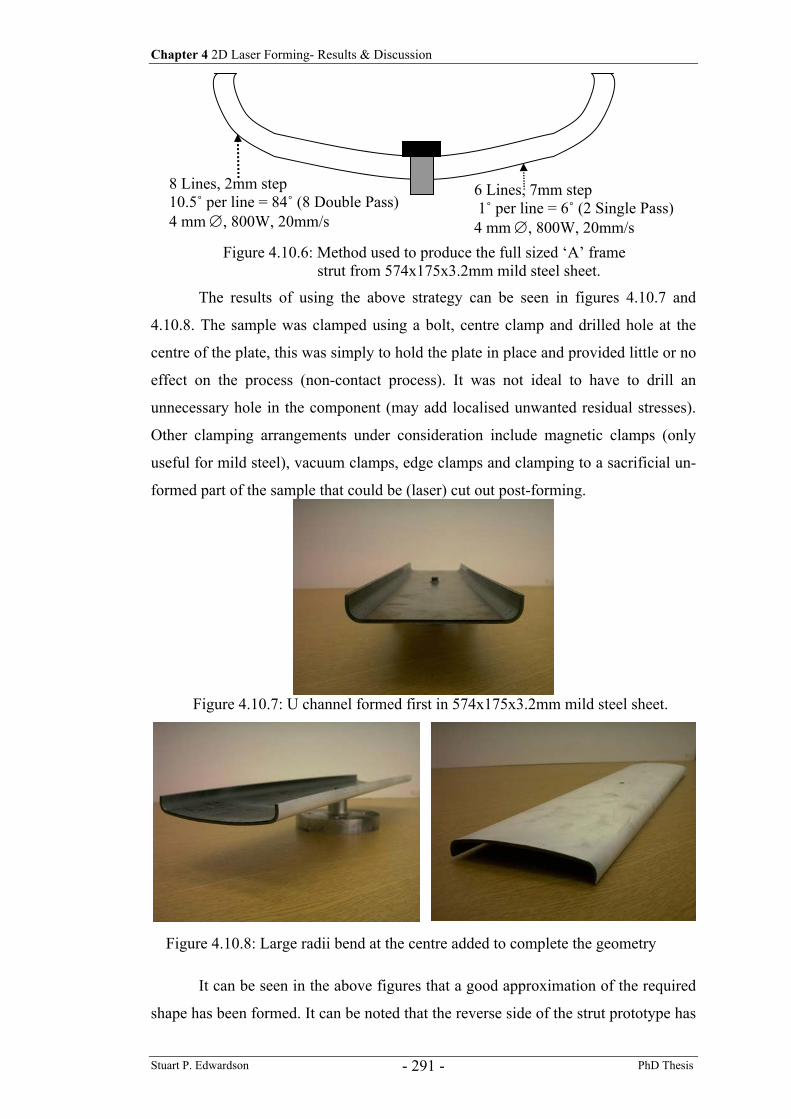
Chapter 4 2D Laser Forming- Results & Discussion
Stuart P. Edwardson PhD Thesis - 291 -
The results of using the above strategy can be seen in figures 4.10.7 and
4.10.8. The sample was clamped using a bolt, centre clamp and drilled hole at the
centre of the plate, this was simply to hold the plate in place and provided little or no
effect on the process (non-contact process). It was not ideal to have to drill an
unnecessary hole in the component (may add localised unwanted residual stresses).
Other clamping arrangements under consideration include magnetic clamps (only
useful for mild steel), vacuum clamps, edge clamps and clamping to a sacrificial un-
formed part of the sample that could be (laser) cut out post-forming.
It can be seen in the above figures that a good approximation of the required
shape has been formed. It can be noted that the reverse side of the strut prototype has
8 Lines, 2mm step 10.5˚ per line = 84˚ (8 Double Pass) 4 mm ∅, 800W, 20mm/s
6 Lines, 7mm step 1˚ per line = 6˚ (2 Single Pass) 4 mm ∅, 800W, 20mm/s
Figure 4.10.6: Method used to produce the full sized ‘A’ frame strut from 574x175x3.2mm mild steel sheet.
Figure 4.10.7: U channel formed first in 574x175x3.2mm mild steel sheet.
Figure 4.10.8: Large radii bend at the centre added to complete the geometry
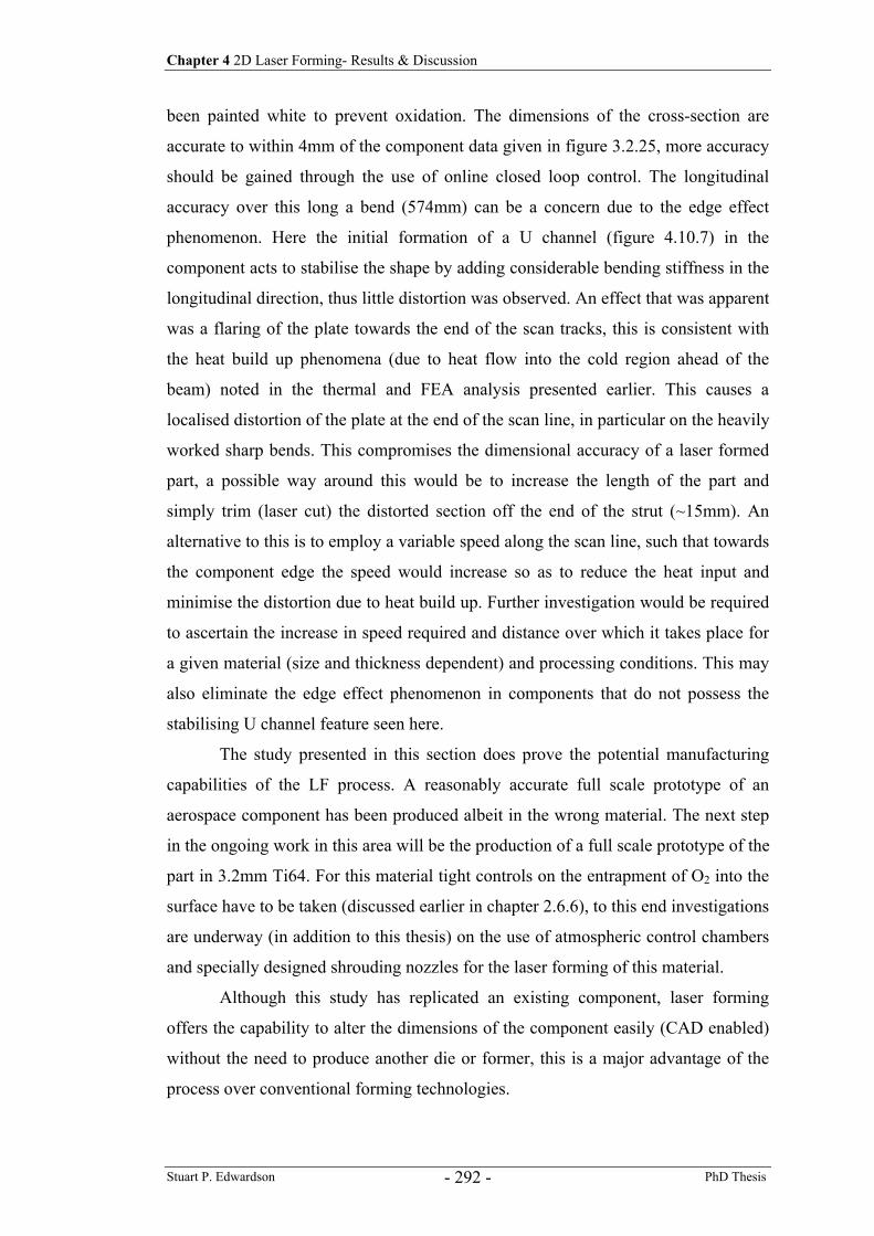
Chapter 4 2D Laser Forming- Results & Discussion
Stuart P. Edwardson PhD Thesis - 292 -
been painted white to prevent oxidation. The dimensions of the cross-section are
accurate to within 4mm of the component data given in figure 3.2.25, more accuracy
should be gained through the use of online closed loop control. The longitudinal
accuracy over this long a bend (574mm) can be a concern due to the edge effect
phenomenon. Here the initial formation of a U channel (figure 4.10.7) in the
component acts to stabilise the shape by adding considerable bending stiffness in the
longitudinal direction, thus little distortion was observed. An effect that was apparent
was a flaring of the plate towards the end of the scan tracks, this is consistent with
the heat build up phenomena (due to heat flow into the cold region ahead of the
beam) noted in the thermal and FEA analysis presented earlier. This causes a
localised distortion of the plate at the end of the scan line, in particular on the heavily
worked sharp bends. This compromises the dimensional accuracy of a laser formed
part, a possible way around this would be to increase the length of the part and
simply trim (laser cut) the distorted section off the end of the strut (~15mm). An
alternative to this is to employ a variable speed along the scan line, such that towards
the component edge the speed would increase so as to reduce the heat input and
minimise the distortion due to heat build up. Further investigation would be required
to ascertain the increase in speed required and distance over which it takes place for
a given material (size and thickness dependent) and processing conditions. This may
also eliminate the edge effect phenomenon in components that do not possess the
stabilising U channel feature seen here.
The study presented in this section does prove the potential manufacturing
capabilities of the LF process. A reasonably accurate full scale prototype of an
aerospace component has been produced albeit in the wrong material. The next step
in the ongoing work in this area will be the production of a full scale prototype of the
part in 3.2mm Ti64. For this material tight controls on the entrapment of O2 into the
surface have to be taken (discussed earlier in chapter 2.6.6), to this end investigations
are underway (in addition to this thesis) on the use of atmospheric control chambers
and specially designed shrouding nozzles for the laser forming of this material.
Although this study has replicated an existing component, laser forming
offers the capability to alter the dimensions of the component easily (CAD enabled)
without the need to produce another die or former, this is a major advantage of the
process over conventional forming technologies.
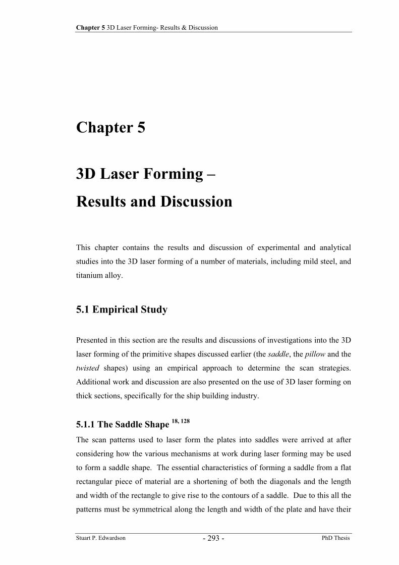
Chapter 5 3D Laser Forming- Results & Discussion
Stuart P. Edwardson PhD Thesis - 293 -
Chapter 5
3D Laser Forming –
Results and Discussion This chapter contains the results and discussion of experimental and analytical
studies into the 3D laser forming of a number of materials, including mild steel, and
titanium alloy.
5.1 Empirical Study
Presented in this section are the results and discussions of investigations into the 3D
laser forming of the primitive shapes discussed earlier (the saddle, the pillow and the
twisted shapes) using an empirical approach to determine the scan strategies.
Additional work and discussion are also presented on the use of 3D laser forming on
thick sections, specifically for the ship building industry.
5.1.1 The Saddle Shape 18, 128 The scan patterns used to laser form the plates into saddles were arrived at after
considering how the various mechanisms at work during laser forming may be used
to form a saddle shape. The essential characteristics of forming a saddle from a flat
rectangular piece of material are a shortening of both the diagonals and the length
and width of the rectangle to give rise to the contours of a saddle. Due to this all the
patterns must be symmetrical along the length and width of the plate and have their
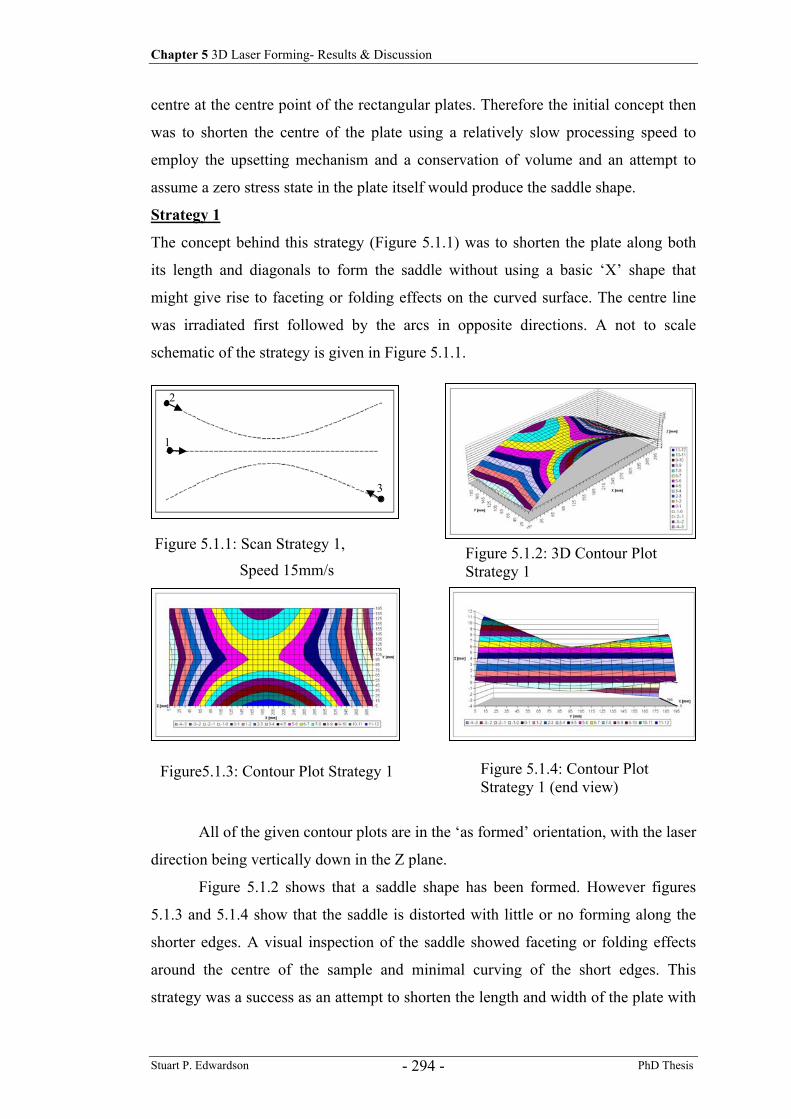
Chapter 5 3D Laser Forming- Results & Discussion
Stuart P. Edwardson PhD Thesis - 294 -
centre at the centre point of the rectangular plates. Therefore the initial concept then
was to shorten the centre of the plate using a relatively slow processing speed to
employ the upsetting mechanism and a conservation of volume and an attempt to
assume a zero stress state in the plate itself would produce the saddle shape.
Strategy 1
The concept behind this strategy (Figure 5.1.1) was to shorten the plate along both
its length and diagonals to form the saddle without using a basic ‘X’ shape that
might give rise to faceting or folding effects on the curved surface. The centre line
was irradiated first followed by the arcs in opposite directions. A not to scale
schematic of the strategy is given in Figure 5.1.1.
All of the given contour plots are in the ‘as formed’ orientation, with the laser
direction being vertically down in the Z plane.
Figure 5.1.2 shows that a saddle shape has been formed. However figures
5.1.3 and 5.1.4 show that the saddle is distorted with little or no forming along the
shorter edges. A visual inspection of the saddle showed faceting or folding effects
around the centre of the sample and minimal curving of the short edges. This
strategy was a success as an attempt to shorten the length and width of the plate with
Figure 5.1.1: Scan Strategy 1,
Speed 15mm/s Figure 5.1.2: 3D Contour Plot Strategy 1
Figure5.1.3: Contour Plot Strategy 1 Figure 5.1.4: Contour Plot Strategy 1 (end view)
2
1
3
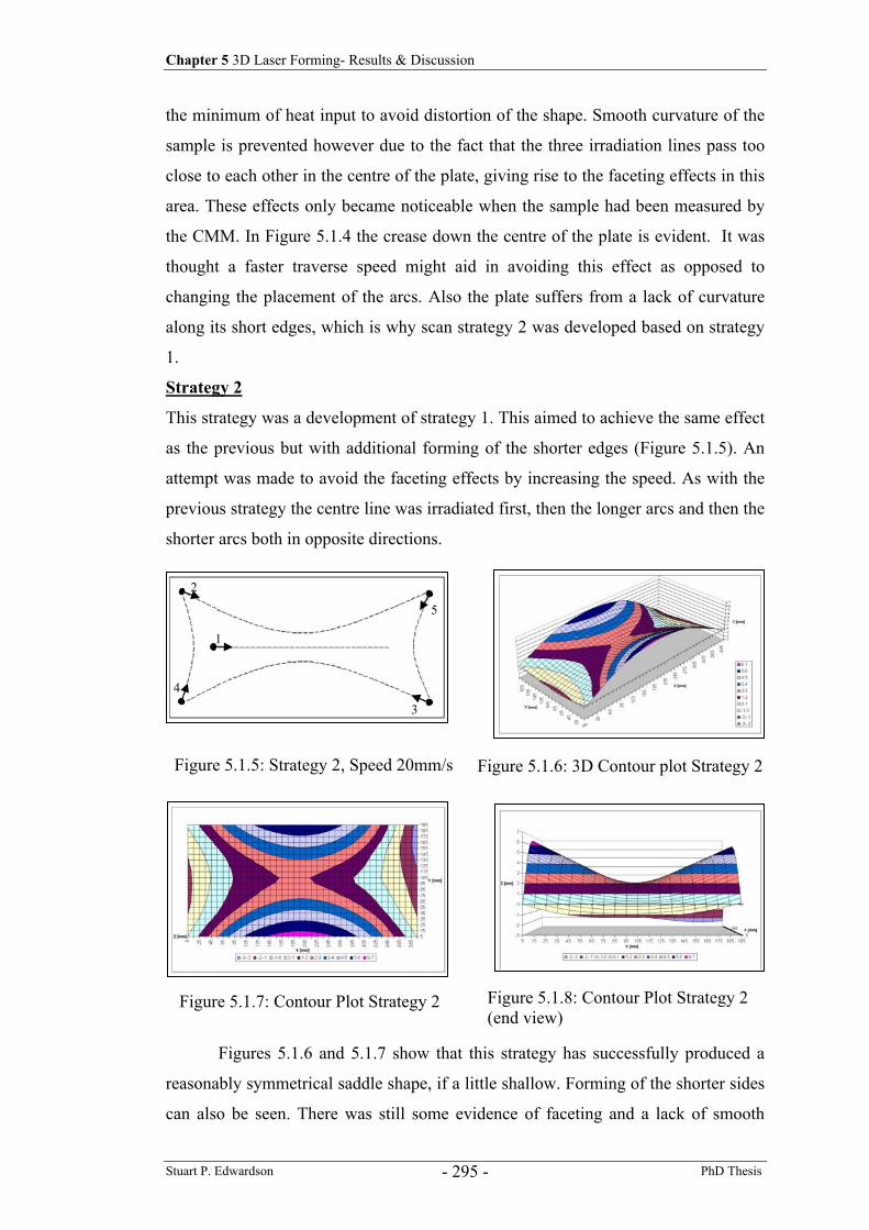
Chapter 5 3D Laser Forming- Results & Discussion
Stuart P. Edwardson PhD Thesis - 295 -
the minimum of heat input to avoid distortion of the shape. Smooth curvature of the
sample is prevented however due to the fact that the three irradiation lines pass too
close to each other in the centre of the plate, giving rise to the faceting effects in this
area. These effects only became noticeable when the sample had been measured by
the CMM. In Figure 5.1.4 the crease down the centre of the plate is evident. It was
thought a faster traverse speed might aid in avoiding this effect as opposed to
changing the placement of the arcs. Also the plate suffers from a lack of curvature
along its short edges, which is why scan strategy 2 was developed based on strategy
1.
Strategy 2
This strategy was a development of strategy 1. This aimed to achieve the same effect
as the previous but with additional forming of the shorter edges (Figure 5.1.5). An
attempt was made to avoid the faceting effects by increasing the speed. As with the
previous strategy the centre line was irradiated first, then the longer arcs and then the
shorter arcs both in opposite directions.
Figures 5.1.6 and 5.1.7 show that this strategy has successfully produced a
reasonably symmetrical saddle shape, if a little shallow. Forming of the shorter sides
can also be seen. There was still some evidence of faceting and a lack of smooth
Figure 5.1.5: Strategy 2, Speed 20mm/s Figure 5.1.6: 3D Contour plot Strategy 2
Figure 5.1.7: Contour Plot Strategy 2 Figure 5.1.8: Contour Plot Strategy 2 (end view)
1
2
3
4
5
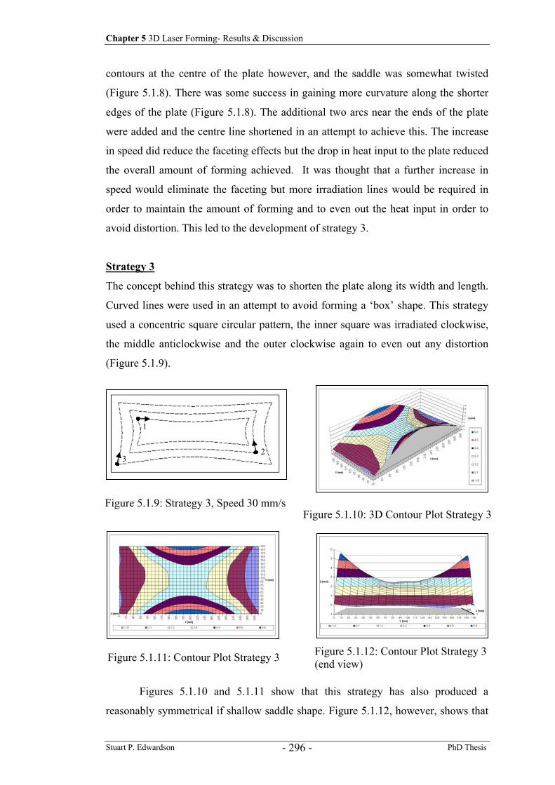
Chapter 5 3D Laser Forming- Results & Discussion
Stuart P. Edwardson PhD Thesis - 296 -
contours at the centre of the plate however, and the saddle was somewhat twisted
(Figure 5.1.8). There was some success in gaining more curvature along the shorter
edges of the plate (Figure 5.1.8). The additional two arcs near the ends of the plate
were added and the centre line shortened in an attempt to achieve this. The increase
in speed did reduce the faceting effects but the drop in heat input to the plate reduced
the overall amount of forming achieved. It was thought that a further increase in
speed would eliminate the faceting but more irradiation lines would be required in
order to maintain the amount of forming and to even out the heat input in order to
avoid distortion. This led to the development of strategy 3.
Strategy 3
The concept behind this strategy was to shorten the plate along its width and length.
Curved lines were used in an attempt to avoid forming a ‘box’ shape. This strategy
used a concentric square circular pattern, the inner square was irradiated clockwise,
the middle anticlockwise and the outer clockwise again to even out any distortion
(Figure 5.1.9).
Figures 5.1.10 and 5.1.11 show that this strategy has also produced a
reasonably symmetrical if shallow saddle shape. Figure 5.1.12, however, shows that
Figure 5.1.9: Strategy 3, Speed 30 mm/sFigure 5.1.10: 3D Contour Plot Strategy 3
Figure 5.1.11: Contour Plot Strategy 3 Figure 5.1.12: Contour Plot Strategy 3 (end view)
1
23
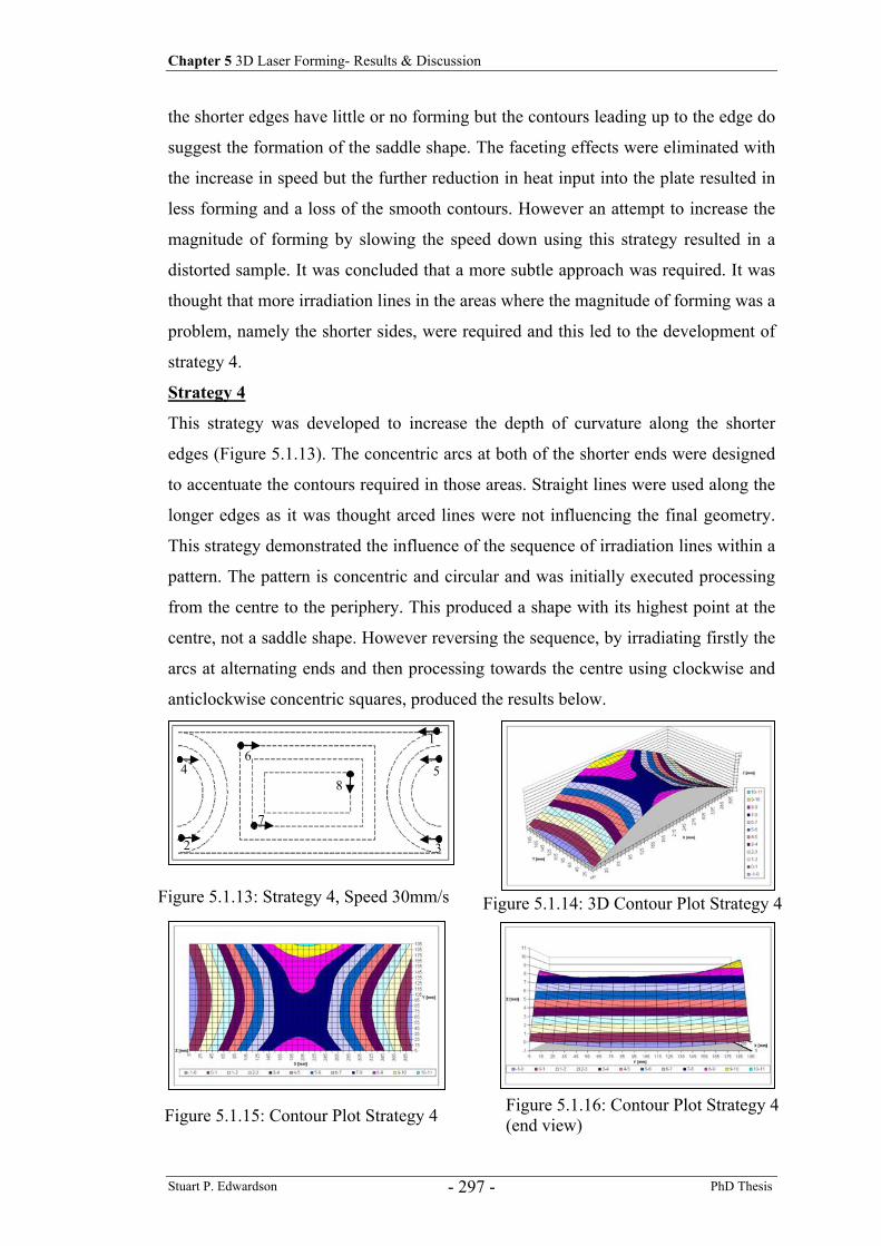
Chapter 5 3D Laser Forming- Results & Discussion
Stuart P. Edwardson PhD Thesis - 297 -
the shorter edges have little or no forming but the contours leading up to the edge do
suggest the formation of the saddle shape. The faceting effects were eliminated with
the increase in speed but the further reduction in heat input into the plate resulted in
less forming and a loss of the smooth contours. However an attempt to increase the
magnitude of forming by slowing the speed down using this strategy resulted in a
distorted sample. It was concluded that a more subtle approach was required. It was
thought that more irradiation lines in the areas where the magnitude of forming was a
problem, namely the shorter sides, were required and this led to the development of
strategy 4.
Strategy 4
This strategy was developed to increase the depth of curvature along the shorter
edges (Figure 5.1.13). The concentric arcs at both of the shorter ends were designed
to accentuate the contours required in those areas. Straight lines were used along the
longer edges as it was thought arced lines were not influencing the final geometry.
This strategy demonstrated the influence of the sequence of irradiation lines within a
pattern. The pattern is concentric and circular and was initially executed processing
from the centre to the periphery. This produced a shape with its highest point at the
centre, not a saddle shape. However reversing the sequence, by irradiating firstly the
arcs at alternating ends and then processing towards the centre using clockwise and
anticlockwise concentric squares, produced the results below.
Figure 5.1.13: Strategy 4, Speed 30mm/s Figure 5.1.14: 3D Contour Plot Strategy 4
Figure 5.1.15: Contour Plot Strategy 4 Figure 5.1.16: Contour Plot Strategy 4 (end view)
1
2 3
4 56
7
8
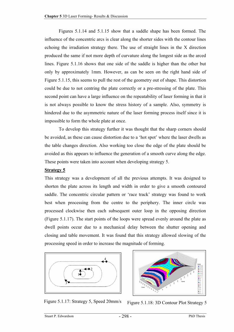
Chapter 5 3D Laser Forming- Results & Discussion
Stuart P. Edwardson PhD Thesis - 298 -
Figures 5.1.14 and 5.1.15 show that a saddle shape has been formed. The
influence of the concentric arcs is clear along the shorter sides with the contour lines
echoing the irradiation strategy there. The use of straight lines in the X direction
produced the same if not more depth of curvature along the longest side as the arced
lines. Figure 5.1.16 shows that one side of the saddle is higher than the other but
only by approximately 1mm. However, as can be seen on the right hand side of
Figure 5.1.15, this seems to pull the rest of the geometry out of shape. This distortion
could be due to not centring the plate correctly or a pre-stressing of the plate. This
second point can have a large influence on the repeatability of laser forming in that it
is not always possible to know the stress history of a sample. Also, symmetry is
hindered due to the asymmetric nature of the laser forming process itself since it is
impossible to form the whole plate at once.
To develop this strategy further it was thought that the sharp corners should
be avoided, as these can cause distortion due to a ‘hot spot’ where the laser dwells as
the table changes direction. Also working too close the edge of the plate should be
avoided as this appears to influence the generation of a smooth curve along the edge.
These points were taken into account when developing strategy 5.
Strategy 5
This strategy was a development of all the previous attempts. It was designed to
shorten the plate across its length and width in order to give a smooth contoured
saddle. The concentric circular pattern or ‘race track’ strategy was found to work
best when processing from the centre to the periphery. The inner circle was
processed clockwise then each subsequent outer loop in the opposing direction
(Figure 5.1.17). The start points of the loops were spread evenly around the plate as
dwell points occur due to a mechanical delay between the shutter opening and
closing and table movement. It was found that this strategy allowed slowing of the
processing speed in order to increase the magnitude of forming.
Figure 5.1.17: Strategy 5, Speed 20mm/s Figure 5.1.18: 3D Contour Plot Strategy 5
1 2
3
4
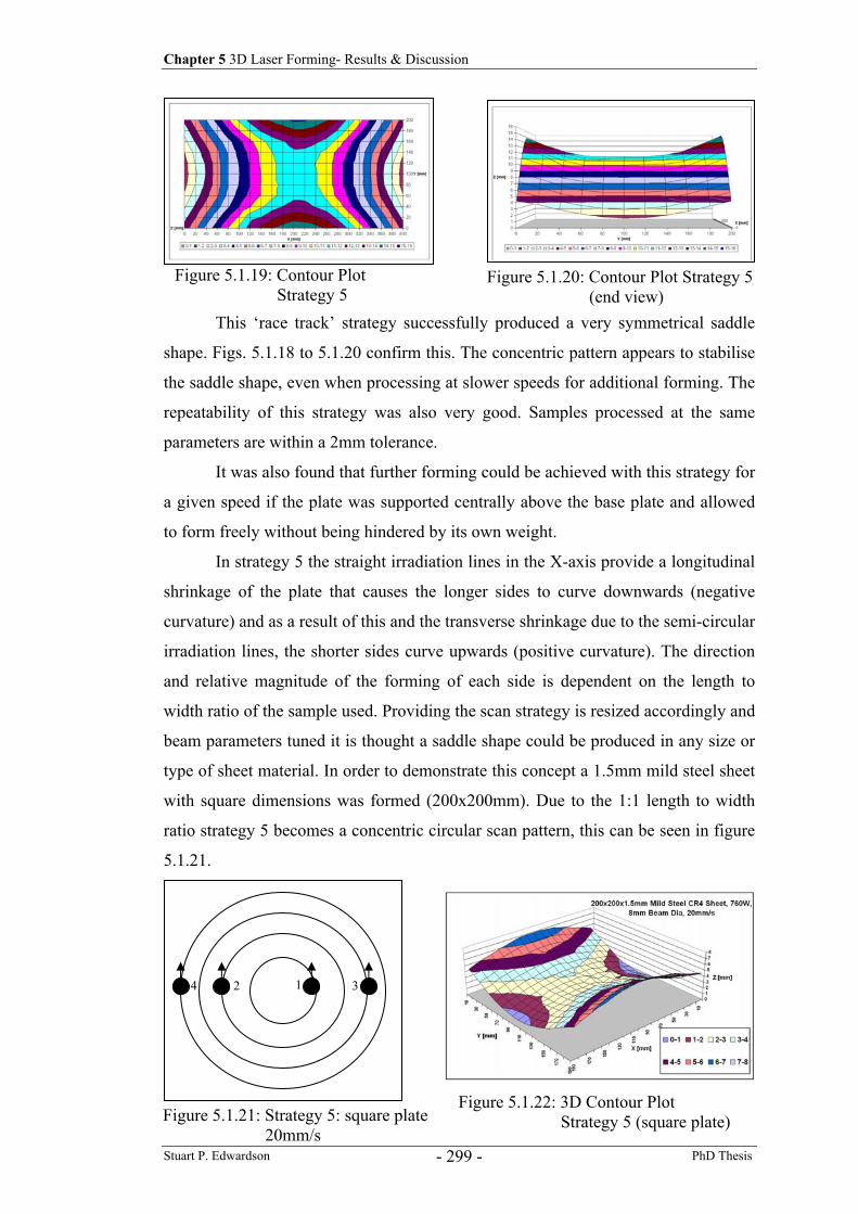
Chapter 5 3D Laser Forming- Results & Discussion
Stuart P. Edwardson PhD Thesis - 299 -
This ‘race track’ strategy successfully produced a very symmetrical saddle
shape. Figs. 5.1.18 to 5.1.20 confirm this. The concentric pattern appears to stabilise
the saddle shape, even when processing at slower speeds for additional forming. The
repeatability of this strategy was also very good. Samples processed at the same
parameters are within a 2mm tolerance.
It was also found that further forming could be achieved with this strategy for
a given speed if the plate was supported centrally above the base plate and allowed
to form freely without being hindered by its own weight.
In strategy 5 the straight irradiation lines in the X-axis provide a longitudinal
shrinkage of the plate that causes the longer sides to curve downwards (negative
curvature) and as a result of this and the transverse shrinkage due to the semi-circular
irradiation lines, the shorter sides curve upwards (positive curvature). The direction
and relative magnitude of the forming of each side is dependent on the length to
width ratio of the sample used. Providing the scan strategy is resized accordingly and
beam parameters tuned it is thought a saddle shape could be produced in any size or
type of sheet material. In order to demonstrate this concept a 1.5mm mild steel sheet
with square dimensions was formed (200x200mm). Due to the 1:1 length to width
ratio strategy 5 becomes a concentric circular scan pattern, this can be seen in figure
5.1.21.
Figure 5.1.19: Contour Plot Strategy 5
Figure 5.1.20: Contour Plot Strategy 5 (end view)
1 2 34
Figure 5.1.21: Strategy 5: square plate 20mm/s
Figure 5.1.22: 3D Contour Plot Strategy 5 (square plate)
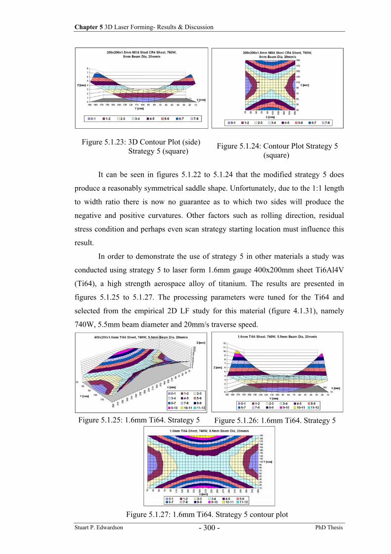
Chapter 5 3D Laser Forming- Results & Discussion
Stuart P. Edwardson PhD Thesis - 300 -
It can be seen in figures 5.1.22 to 5.1.24 that the modified strategy 5 does
produce a reasonably symmetrical saddle shape. Unfortunately, due to the 1:1 length
to width ratio there is now no guarantee as to which two sides will produce the
negative and positive curvatures. Other factors such as rolling direction, residual
stress condition and perhaps even scan strategy starting location must influence this
result.
In order to demonstrate the use of strategy 5 in other materials a study was
conducted using strategy 5 to laser form 1.6mm gauge 400x200mm sheet Ti6Al4V
(Ti64), a high strength aerospace alloy of titanium. The results are presented in
figures 5.1.25 to 5.1.27. The processing parameters were tuned for the Ti64 and
selected from the empirical 2D LF study for this material (figure 4.1.31), namely
740W, 5.5mm beam diameter and 20mm/s traverse speed.
Figure 5.1.23: 3D Contour Plot (side) Strategy 5 (square) Figure 5.1.24: Contour Plot Strategy 5
(square)
Figure 5.1.25: 1.6mm Ti64. Strategy 5 Figure 5.1.26: 1.6mm Ti64. Strategy 5
Figure 5.1.27: 1.6mm Ti64. Strategy 5 contour plot
Chapter 5 3D Laser Forming- Results & Discussion
Stuart P. Edwardson PhD Thesis - 301 -
The above results in 1.6mm Ti64 demonstrate that strategy 5 (‘race track’
strategy) does produce a consistent reasonable symmetrical saddle shape when used
in other materials and that a considerable amount of forming is available even in this
high strength material.
Strategy 6
In order to demonstrate that there may in fact be multiple solutions to any 3D
laser forming problem a sixth strategy was developed for the saddle shape using
1.5mm mild steel. Whilst, as in strategy 5, the concept of producing a shortening in x
and y was used, a different execution was developed. A cross hatch or X scan
strategy was used (figure 5.1.26), this time using energy parameters consistent with
the TGM; namely 760W 5.5mm beam diameter and 40mm/s traverse speed. This
strategy, rather than forming along the x and y axes individually takes the resultant
vector direction to give the diagonal strategy seen in figure 5.1.28. Unlike the
previous strategies a number of complete passes were realised (all 6 scan lines) and
the plate was measured after each. The results after each pass are presented below.
After pass 1 (6 scan lines) it can be seen in figures 5.1.28 to 5.1.31 that a
shallow reasonable symmetrical saddle shape has been formed. As the amount of
1
2
3
4
5
6
Figure 5.1.28: Strategy 6: 5.5mm beam dia. 40mm/s 400x200x1.5mm Mild Steel
Figure 5.1.29: 3D Contour Plot Strategy 6 (pass 1)
Figure 5.1.31: Contour Plot Strategy 6 (pass 1)
Figure 5.1.30: 3D Contour Plot Strategy 6 (pass 1)
Chapter 5 3D Laser Forming- Results & Discussion
Stuart P. Edwardson PhD Thesis - 302 -
forming was small, perhaps due to a reduction in the energy input (40mm/s instead
of 20mm/s previously), a second and third pass was realised to determine if more
forming could be achieved and symmetry could be maintained.
It can be seen in figures 5.1.32 to 5.1.37 that with additional passes it is
possible to produce additional forming (max ~8mm) thus demonstrating the
possibility of incrementing towards a final shape as opposed to a ‘single shot’
strategy. After three passes the shape is still symmetrical and a saddle shape.
However, the effect of the scan lines crossing over at the centre of the plate results in
a flat region (figure 5.1.36). Although this is exaggerated by the contour plot this
effect would not be desirable when forming a continuous surface and may be a result
Figure 5.1.32: 3D Contour Plot Strategy 6 (pass 2)
Figure 5.1.33: 3D Contour Plot Strategy 6 (pass 2)
Figure 5.1.34: Contour Plot Strategy 6 (pass 2)
Figure 5.1.35: 3D Contour Plot Strategy 6 (pass 3)
Figure 5.1.36: 3D Contour Plot Strategy 6 (pass 3)
Figure 5.1.37: Contour Plot Strategy 6 (pass 3)
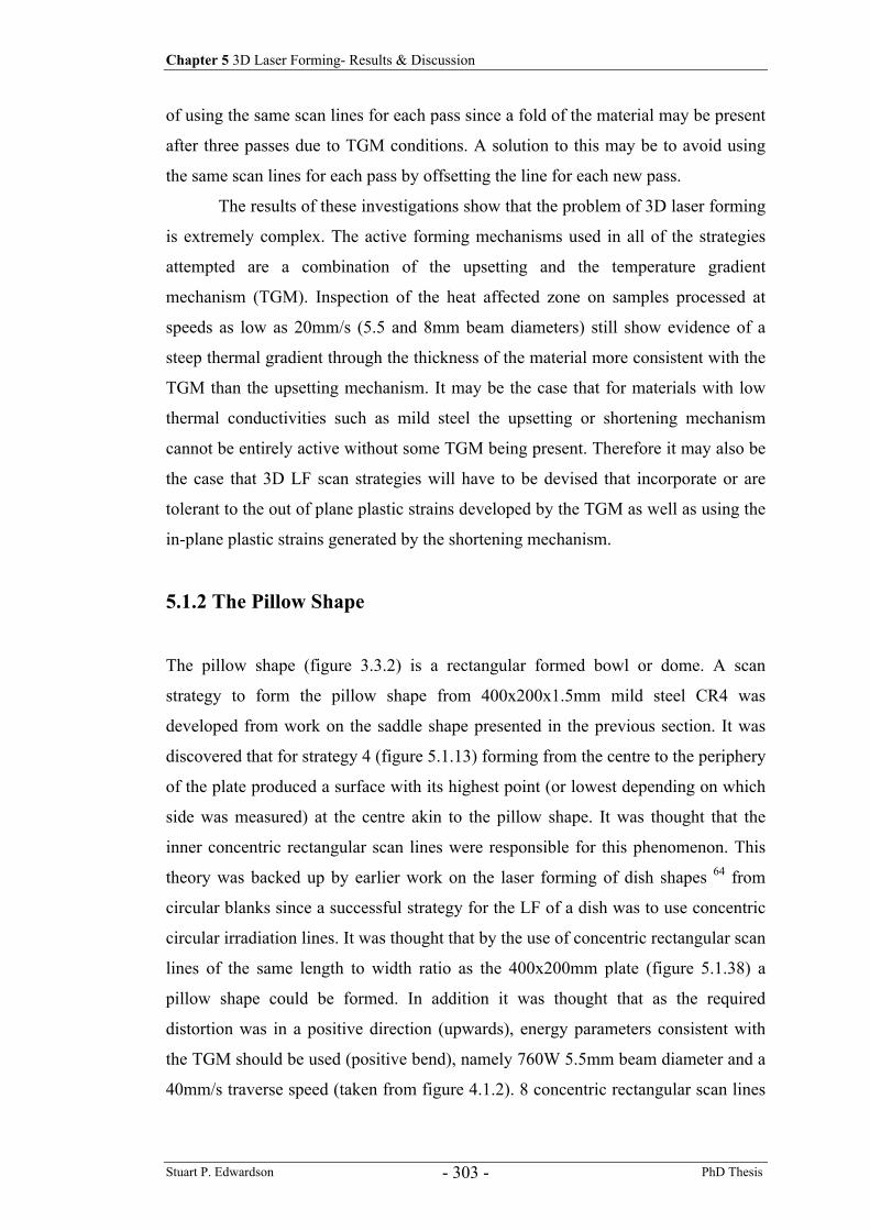
Chapter 5 3D Laser Forming- Results & Discussion
Stuart P. Edwardson PhD Thesis - 303 -
of using the same scan lines for each pass since a fold of the material may be present
after three passes due to TGM conditions. A solution to this may be to avoid using
the same scan lines for each pass by offsetting the line for each new pass.
The results of these investigations show that the problem of 3D laser forming
is extremely complex. The active forming mechanisms used in all of the strategies
attempted are a combination of the upsetting and the temperature gradient
mechanism (TGM). Inspection of the heat affected zone on samples processed at
speeds as low as 20mm/s (5.5 and 8mm beam diameters) still show evidence of a
steep thermal gradient through the thickness of the material more consistent with the
TGM than the upsetting mechanism. It may be the case that for materials with low
thermal conductivities such as mild steel the upsetting or shortening mechanism
cannot be entirely active without some TGM being present. Therefore it may also be
the case that 3D LF scan strategies will have to be devised that incorporate or are
tolerant to the out of plane plastic strains developed by the TGM as well as using the
in-plane plastic strains generated by the shortening mechanism.
5.1.2 The Pillow Shape
The pillow shape (figure 3.3.2) is a rectangular formed bowl or dome. A scan
strategy to form the pillow shape from 400x200x1.5mm mild steel CR4 was
developed from work on the saddle shape presented in the previous section. It was
discovered that for strategy 4 (figure 5.1.13) forming from the centre to the periphery
of the plate produced a surface with its highest point (or lowest depending on which
side was measured) at the centre akin to the pillow shape. It was thought that the
inner concentric rectangular scan lines were responsible for this phenomenon. This
theory was backed up by earlier work on the laser forming of dish shapes 64 from
circular blanks since a successful strategy for the LF of a dish was to use concentric
circular irradiation lines. It was thought that by the use of concentric rectangular scan
lines of the same length to width ratio as the 400x200mm plate (figure 5.1.38) a
pillow shape could be formed. In addition it was thought that as the required
distortion was in a positive direction (upwards), energy parameters consistent with
the TGM should be used (positive bend), namely 760W 5.5mm beam diameter and a
40mm/s traverse speed (taken from figure 4.1.2). 8 concentric rectangular scan lines
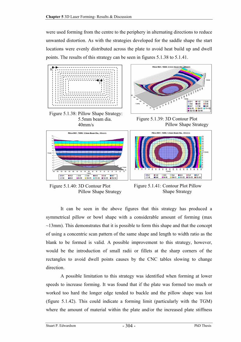
Chapter 5 3D Laser Forming- Results & Discussion
Stuart P. Edwardson PhD Thesis - 304 -
were used forming from the centre to the periphery in alternating directions to reduce
unwanted distortion. As with the strategies developed for the saddle shape the start
locations were evenly distributed across the plate to avoid heat build up and dwell
points. The results of this strategy can be seen in figures 5.1.38 to 5.1.41.
It can be seen in the above figures that this strategy has produced a
symmetrical pillow or bowl shape with a considerable amount of forming (max
~13mm). This demonstrates that it is possible to form this shape and that the concept
of using a concentric scan pattern of the same shape and length to width ratio as the
blank to be formed is valid. A possible improvement to this strategy, however,
would be the introduction of small radii or fillets at the sharp corners of the
rectangles to avoid dwell points causes by the CNC tables slowing to change
direction.
A possible limitation to this strategy was identified when forming at lower
speeds to increase forming. It was found that if the plate was formed too much or
worked too hard the longer edge tended to buckle and the pillow shape was lost
(figure 5.1.42). This could indicate a forming limit (particularly with the TGM)
where the amount of material within the plate and/or the increased plate stiffness
Figure 5.1.39: 3D Contour Plot Pillow Shape Strategy
Figure 5.1.40: 3D Contour Plot Pillow Shape Strategy
Figure 5.1.38: Pillow Shape Strategy: 5.5mm beam dia. 40mm/s
Figure 5.1.41: Contour Plot Pillow Shape Strategy
1
8
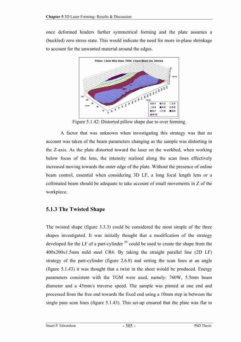
Chapter 5 3D Laser Forming- Results & Discussion
Stuart P. Edwardson PhD Thesis - 305 -
once deformed hinders further symmetrical forming and the plate assumes a
(buckled) zero stress state. This would indicate the need for more in-plane shrinkage
to account for the unwanted material around the edges.
A factor that was unknown when investigating this strategy was that no
account was taken of the beam parameters changing as the sample was distorting in
the Z-axis. As the plate distorted toward the laser on the workbed, when working
below focus of the lens, the intensity realised along the scan lines effectively
increased moving towards the outer edge of the plate. Without the presence of online
beam control, essential when considering 3D LF, a long focal length lens or a
collimated beam should be adequate to take account of small movements in Z of the
workpiece.
5.1.3 The Twisted Shape
The twisted shape (figure 3.3.3) could be considered the most simple of the three
shapes investigated. It was initially thought that a modification of the strategy
developed for the LF of a part-cylinder 29 could be used to create the shape from the
400x200x1.5mm mild steel CR4. By taking the straight parallel line (2D LF)
strategy of the part-cylinder (figure 2.6.8) and setting the scan lines at an angle
(figure 5.1.43) it was thought that a twist in the sheet would be produced. Energy
parameters consistent with the TGM were used, namely: 760W, 5.5mm beam
diameter and a 45mm/s traverse speed. The sample was pinned at one end and
processed from the free end towards the fixed end using a 10mm step in between the
single pass scan lines (figure 5.1.43). This set-up ensured that the plate was flat to
Figure 5.1.42: Distorted pillow shape due to over forming.
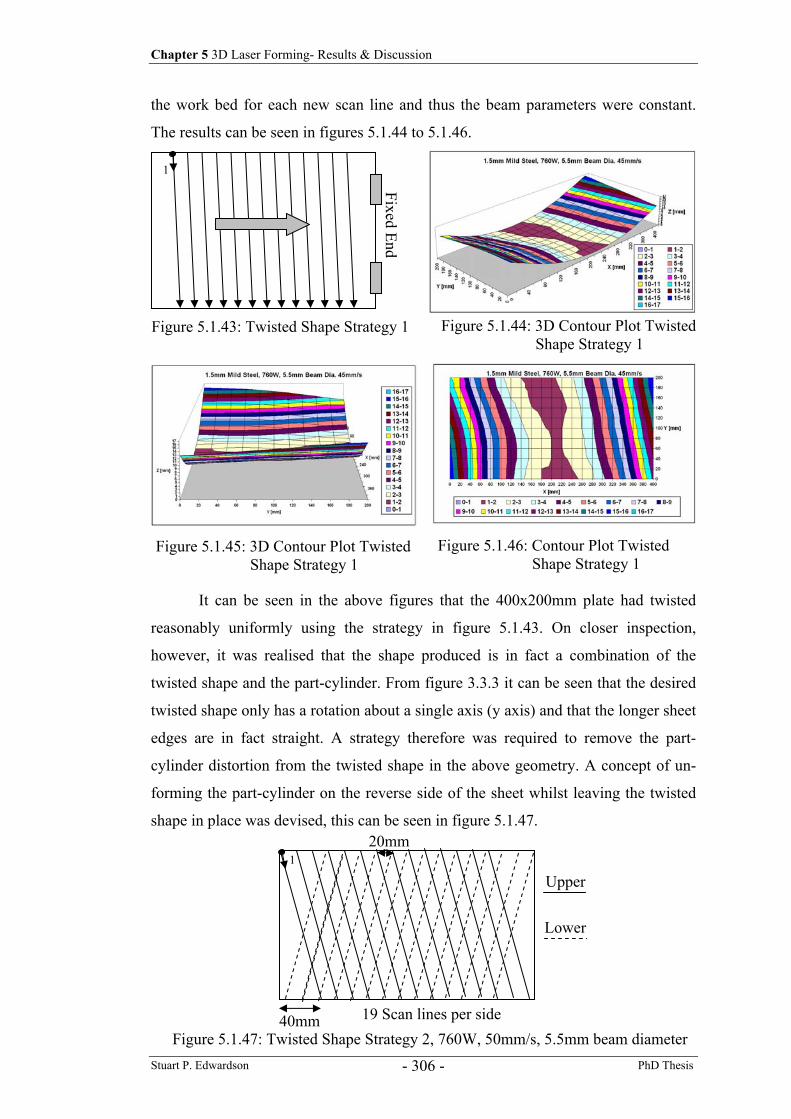
Chapter 5 3D Laser Forming- Results & Discussion
Stuart P. Edwardson PhD Thesis - 306 -
the work bed for each new scan line and thus the beam parameters were constant.
The results can be seen in figures 5.1.44 to 5.1.46.
It can be seen in the above figures that the 400x200mm plate had twisted
reasonably uniformly using the strategy in figure 5.1.43. On closer inspection,
however, it was realised that the shape produced is in fact a combination of the
twisted shape and the part-cylinder. From figure 3.3.3 it can be seen that the desired
twisted shape only has a rotation about a single axis (y axis) and that the longer sheet
edges are in fact straight. A strategy therefore was required to remove the part-
cylinder distortion from the twisted shape in the above geometry. A concept of un-
forming the part-cylinder on the reverse side of the sheet whilst leaving the twisted
shape in place was devised, this can be seen in figure 5.1.47.
Figure 5.1.44: 3D Contour Plot Twisted Shape Strategy 1
Figure 5.1.43: Twisted Shape Strategy 1
Figure 5.1.45: 3D Contour Plot Twisted Shape Strategy 1
Figure 5.1.46: Contour Plot Twisted Shape Strategy 1
Fixed End
1
40mm
20mm
19 Scan lines per side
Upper
Lower
Figure 5.1.47: Twisted Shape Strategy 2, 760W, 50mm/s, 5.5mm beam diameter
1
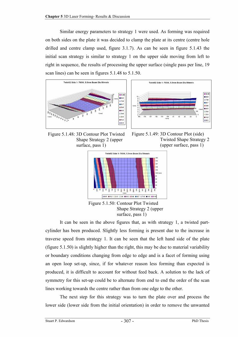
Chapter 5 3D Laser Forming- Results & Discussion
Stuart P. Edwardson PhD Thesis - 307 -
Similar energy parameters to strategy 1 were used. As forming was required
on both sides on the plate it was decided to clamp the plate at its centre (centre hole
drilled and centre clamp used, figure 3.1.7). As can be seen in figure 5.1.43 the
initial scan strategy is similar to strategy 1 on the upper side moving from left to
right in sequence, the results of processing the upper surface (single pass per line, 19
scan lines) can be seen in figures 5.1.48 to 5.1.50.
It can be seen in the above figures that, as with strategy 1, a twisted part-
cylinder has been produced. Slightly less forming is present due to the increase in
traverse speed from strategy 1. It can be seen that the left hand side of the plate
(figure 5.1.50) is slightly higher than the right, this may be due to material variability
or boundary conditions changing from edge to edge and is a facet of forming using
an open loop set-up, since, if for whatever reason less forming than expected is
produced, it is difficult to account for without feed back. A solution to the lack of
symmetry for this set-up could be to alternate from end to end the order of the scan
lines working towards the centre rather than from one edge to the other.
The next step for this strategy was to turn the plate over and process the
lower side (lower side from the initial orientation) in order to remove the unwanted
Figure 5.1.48: 3D Contour Plot Twisted Shape Strategy 2 (upper surface, pass 1)
Figure 5.1.49: 3D Contour Plot (side) Twisted Shape Strategy 2 (upper surface, pass 1)
Figure 5.1.50: Contour Plot Twisted Shape Strategy 2 (upper surface, pass 1)
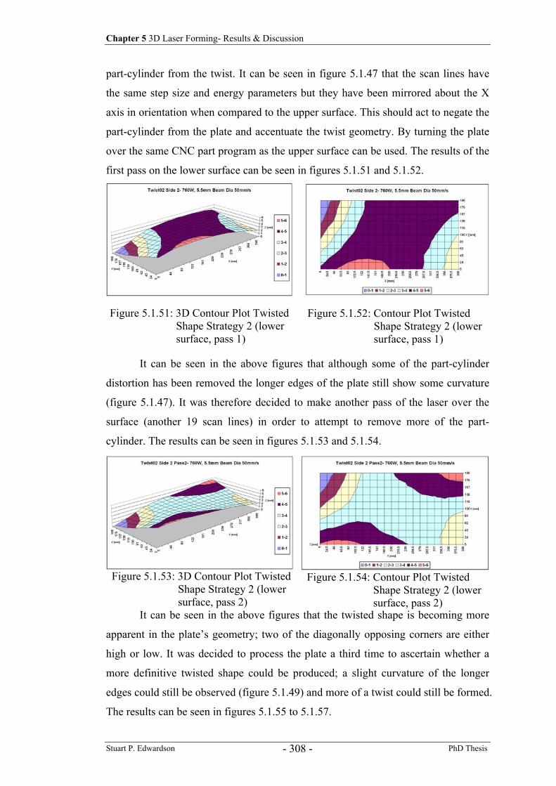
Chapter 5 3D Laser Forming- Results & Discussion
Stuart P. Edwardson PhD Thesis - 308 -
part-cylinder from the twist. It can be seen in figure 5.1.47 that the scan lines have
the same step size and energy parameters but they have been mirrored about the X
axis in orientation when compared to the upper surface. This should act to negate the
part-cylinder from the plate and accentuate the twist geometry. By turning the plate
over the same CNC part program as the upper surface can be used. The results of the
first pass on the lower surface can be seen in figures 5.1.51 and 5.1.52.
It can be seen in the above figures that although some of the part-cylinder
distortion has been removed the longer edges of the plate still show some curvature
(figure 5.1.47). It was therefore decided to make another pass of the laser over the
surface (another 19 scan lines) in order to attempt to remove more of the part-
cylinder. The results can be seen in figures 5.1.53 and 5.1.54.
It can be seen in the above figures that the twisted shape is becoming more
apparent in the plate’s geometry; two of the diagonally opposing corners are either
high or low. It was decided to process the plate a third time to ascertain whether a
more definitive twisted shape could be produced; a slight curvature of the longer
edges could still be observed (figure 5.1.49) and more of a twist could still be formed.
The results can be seen in figures 5.1.55 to 5.1.57.
Figure 5.1.51: 3D Contour Plot Twisted Shape Strategy 2 (lower surface, pass 1)
Figure 5.1.52: Contour Plot Twisted Shape Strategy 2 (lower surface, pass 1)
Figure 5.1.53: 3D Contour Plot Twisted Shape Strategy 2 (lower surface, pass 2)
Figure 5.1.54: Contour Plot Twisted Shape Strategy 2 (lower surface, pass 2)
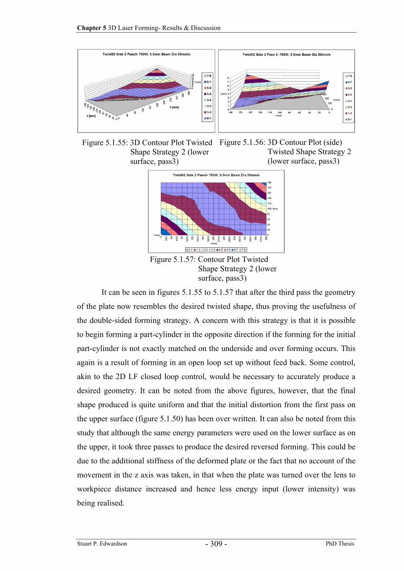
Chapter 5 3D Laser Forming- Results & Discussion
Stuart P. Edwardson PhD Thesis - 309 -
It can be seen in figures 5.1.55 to 5.1.57 that after the third pass the geometry
of the plate now resembles the desired twisted shape, thus proving the usefulness of
the double-sided forming strategy. A concern with this strategy is that it is possible
to begin forming a part-cylinder in the opposite direction if the forming for the initial
part-cylinder is not exactly matched on the underside and over forming occurs. This
again is a result of forming in an open loop set up without feed back. Some control,
akin to the 2D LF closed loop control, would be necessary to accurately produce a
desired geometry. It can be noted from the above figures, however, that the final
shape produced is quite uniform and that the initial distortion from the first pass on
the upper surface (figure 5.1.50) has been over written. It can also be noted from this
study that although the same energy parameters were used on the lower surface as on
the upper, it took three passes to produce the desired reversed forming. This could be
due to the additional stiffness of the deformed plate or the fact that no account of the
movement in the z axis was taken, in that when the plate was turned over the lens to
workpiece distance increased and hence less energy input (lower intensity) was
being realised.
Figure 5.1.55: 3D Contour Plot Twisted Shape Strategy 2 (lower surface, pass3)
Figure 5.1.56: 3D Contour Plot (side) Twisted Shape Strategy 2 (lower surface, pass3)
Figure 5.1.57: Contour Plot Twisted Shape Strategy 2 (lower surface, pass3)
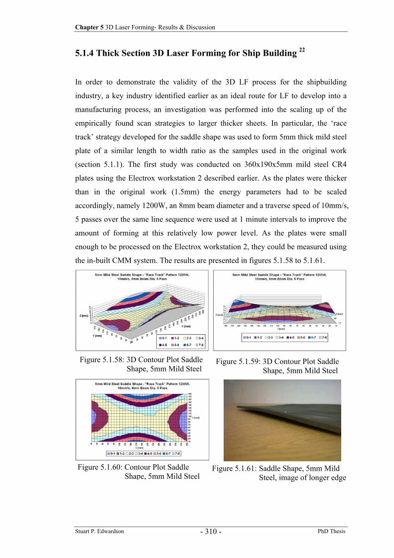
Chapter 5 3D Laser Forming- Results & Discussion
Stuart P. Edwardson PhD Thesis - 310 -
5.1.4 Thick Section 3D Laser Forming for Ship Building 22
In order to demonstrate the validity of the 3D LF process for the shipbuilding
industry, a key industry identified earlier as an ideal route for LF to develop into a
manufacturing process, an investigation was performed into the scaling up of the
empirically found scan strategies to larger thicker sheets. In particular, the ‘race
track’ strategy developed for the saddle shape was used to form 5mm thick mild steel
plate of a similar length to width ratio as the samples used in the original work
(section 5.1.1). The first study was conducted on 360x190x5mm mild steel CR4
plates using the Electrox workstation 2 described earlier. As the plates were thicker
than in the original work (1.5mm) the energy parameters had to be scaled
accordingly, namely 1200W, an 8mm beam diameter and a traverse speed of 10mm/s,
5 passes over the same line sequence were used at 1 minute intervals to improve the
amount of forming at this relatively low power level. As the plates were small
enough to be processed on the Electrox workstation 2, they could be measured using
the in-built CMM system. The results are presented in figures 5.1.58 to 5.1.61.
Figure 5.1.58: 3D Contour Plot Saddle Shape, 5mm Mild Steel
Figure 5.1.59: 3D Contour Plot Saddle Shape, 5mm Mild Steel
Figure 5.1.60: Contour Plot Saddle Shape, 5mm Mild Steel
Figure 5.1.61: Saddle Shape, 5mm Mild Steel, image of longer edge
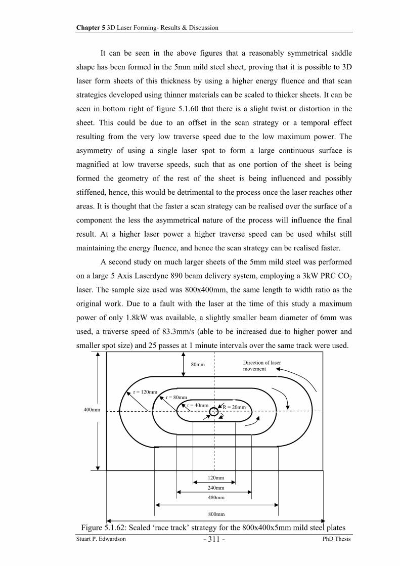
Chapter 5 3D Laser Forming- Results & Discussion
Stuart P. Edwardson PhD Thesis - 311 -
It can be seen in the above figures that a reasonably symmetrical saddle
shape has been formed in the 5mm mild steel sheet, proving that it is possible to 3D
laser form sheets of this thickness by using a higher energy fluence and that scan
strategies developed using thinner materials can be scaled to thicker sheets. It can be
seen in bottom right of figure 5.1.60 that there is a slight twist or distortion in the
sheet. This could be due to an offset in the scan strategy or a temporal effect
resulting from the very low traverse speed due to the low maximum power. The
asymmetry of using a single laser spot to form a large continuous surface is
magnified at low traverse speeds, such that as one portion of the sheet is being
formed the geometry of the rest of the sheet is being influenced and possibly
stiffened, hence, this would be detrimental to the process once the laser reaches other
areas. It is thought that the faster a scan strategy can be realised over the surface of a
component the less the asymmetrical nature of the process will influence the final
result. At a higher laser power a higher traverse speed can be used whilst still
maintaining the energy fluence, and hence the scan strategy can be realised faster.
A second study on much larger sheets of the 5mm mild steel was performed
on a large 5 Axis Laserdyne 890 beam delivery system, employing a 3kW PRC CO2
laser. The sample size used was 800x400mm, the same length to width ratio as the
original work. Due to a fault with the laser at the time of this study a maximum
power of only 1.8kW was available, a slightly smaller beam diameter of 6mm was
used, a traverse speed of 83.3mm/s (able to be increased due to higher power and
smaller spot size) and 25 passes at 1 minute intervals over the same track were used.
r = 40mm r = 80mm
r = 120mm
80mm
120mm
240mm
480mm
800mm
400mm R = 20mm
Direction of laser movement
Figure 5.1.62: Scaled ‘race track’ strategy for the 800x400x5mm mild steel plates
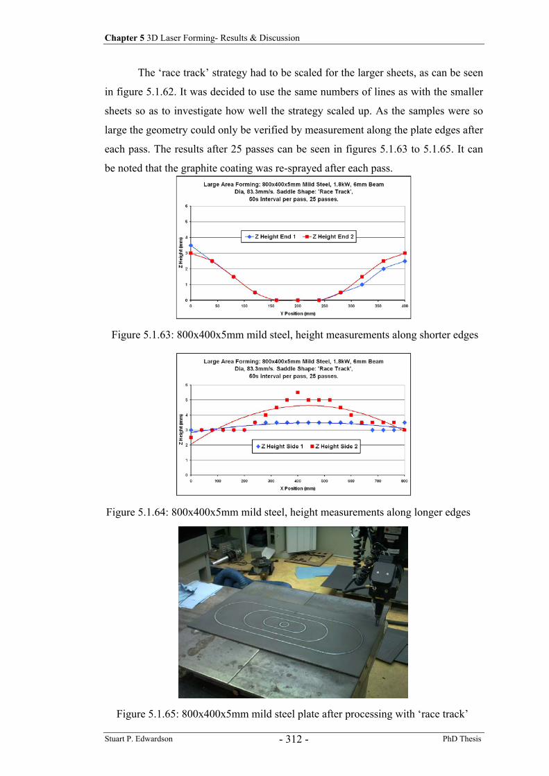
Chapter 5 3D Laser Forming- Results & Discussion
Stuart P. Edwardson PhD Thesis - 312 -
The ‘race track’ strategy had to be scaled for the larger sheets, as can be seen
in figure 5.1.62. It was decided to use the same numbers of lines as with the smaller
sheets so as to investigate how well the strategy scaled up. As the samples were so
large the geometry could only be verified by measurement along the plate edges after
each pass. The results after 25 passes can be seen in figures 5.1.63 to 5.1.65. It can
be noted that the graphite coating was re-sprayed after each pass.
Figure 5.1.63: 800x400x5mm mild steel, height measurements along shorter edges
Figure 5.1.64: 800x400x5mm mild steel, height measurements along longer edges
Figure 5.1.65: 800x400x5mm mild steel plate after processing with ‘race track’

Chapter 5 3D Laser Forming- Results & Discussion
Stuart P. Edwardson PhD Thesis - 313 -
It can be seen in the above figures that a saddle shape has been formed.
Along the shorter edges (400mm, figure 5.1.63) there is a positive curvature and
along the longer edges (figure 5.1.64) there is a negative curvature It can be assumed
from this that a saddle has been formed, this is backed up from observations. It can
be seen that although a saddle has been formed the amount of distortion is very small
compared to the size of the plate (~3mm max). This demonstrates that although the
processing parameters have been scaled (more power could be used however) the
effectiveness of the scaled ‘race track’ pattern has reduced (possibly due to the
increased weight of the plate as well). A solution to this could be to introduce more
scan lines to increase the ratio of the amount of surface area processed to plate
dimensions, to be equal to that used in the 400x200mm plates. As the beam diameter
cannot be scaled (e.g. 8mm to 16mm) and still ensure forming when moving to the
larger plates, more scan lines are needed. Further study is required to confirm this.
However, the potential of the process for shipbuilding applications (outlined earlier)
with the addition of the 2D thick section work (chapter 4.8) has been shown.
As discussed earlier in the literature review the development of an online
monitoring system with predictive distortion correction abilities is a requirement if
any 3D laser forming operation is to be used in a manufacturing environment. The
results of all the empirical studies presented demonstrate the need for such a system
due to the unknowns that can be present when forming in an open loop set-up, such
as residual stresses and variability in the absorption of the incident laser radiation (a
large factor identified from the 2D empirical work). A foreseeable problem with a
system which makes online distortion correction during processing is that, as with
strategies used in this investigation, the final geometry of the part is not reached until
sometime after processing has stopped, when the plate has cooled somewhat and the
elastic stresses have been released leaving a plastically formed part. This suggests
that a strategy of a one off single pass to produce a required geometry would be
extremely difficult to predict and control. A more sensible method of producing a
required geometry would be to increment towards it over a number of passes, taking
surface measurements after each pass so as to have the ability to take account of any
unwanted distortion. The development of a closed loop system for 3D laser forming
based on the recommendations and knowledge gained from the empirical studies is
outlined in the following sections.
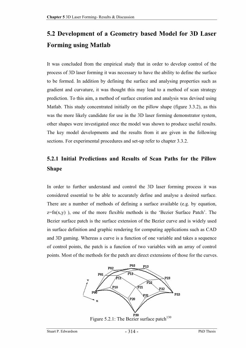
Chapter 5 3D Laser Forming- Results & Discussion
Stuart P. Edwardson PhD Thesis - 314 -
5.2 Development of a Geometry based Model for 3D Laser
Forming using Matlab
It was concluded from the empirical study that in order to develop control of the
process of 3D laser forming it was necessary to have the ability to define the surface
to be formed. In addition by defining the surface and analysing properties such as
gradient and curvature, it was thought this may lead to a method of scan strategy
prediction. To this aim, a method of surface creation and analysis was devised using
Matlab. This study concentrated initially on the pillow shape (figure 3.3.2), as this
was the more likely candidate for use in the 3D laser forming demonstrator system,
other shapes were investigated once the model was shown to produce useful results.
The key model developments and the results from it are given in the following
sections. For experimental procedures and set-up refer to chapter 3.3.2.
5.2.1 Initial Predictions and Results of Scan Paths for the Pillow
Shape
In order to further understand and control the 3D laser forming process it was
considered essential to be able to accurately define and analyse a desired surface.
There are a number of methods of defining a surface available (e.g. by equation,
z=fn(x,y) ), one of the more flexible methods is the ‘Bezier Surface Patch’. The
Bezier surface patch is the surface extension of the Bezier curve and is widely used
in surface definition and graphic rendering for computing applications such as CAD
and 3D gaming. Whereas a curve is a function of one variable and takes a sequence
of control points, the patch is a function of two variables with an array of control
points. Most of the methods for the patch are direct extensions of those for the curves.
Figure 5.2.1: The Bezier surface patch130
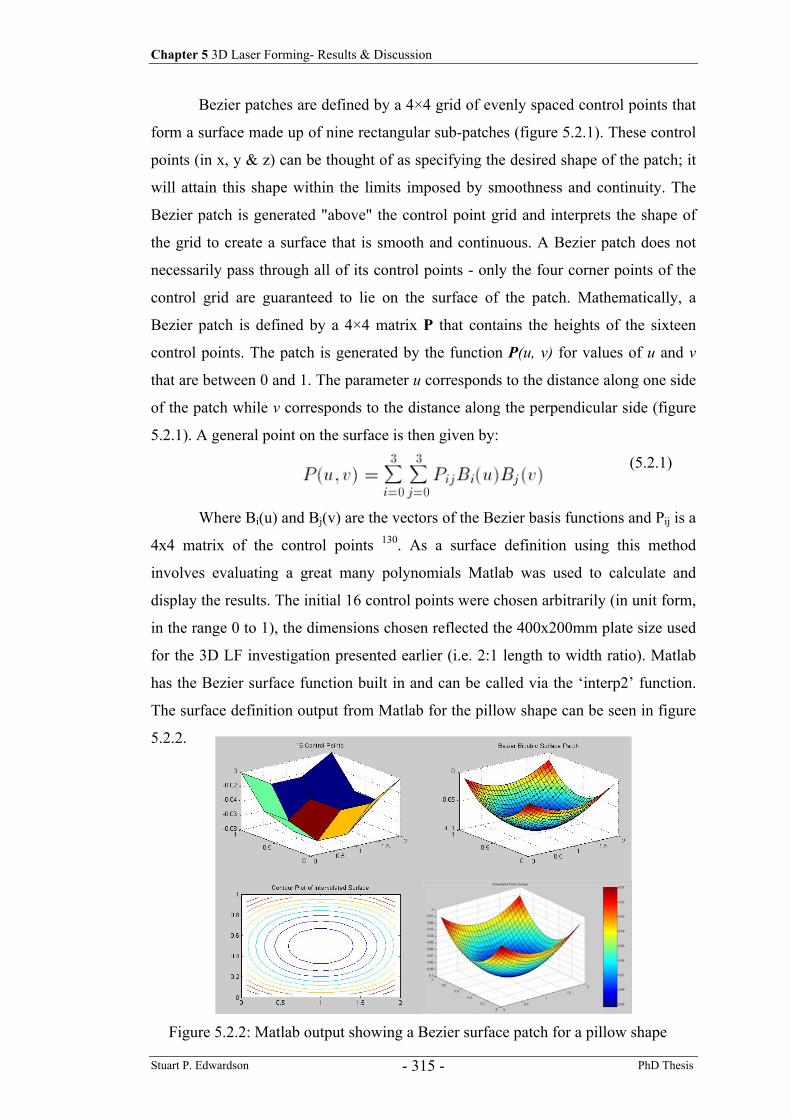
Chapter 5 3D Laser Forming- Results & Discussion
Stuart P. Edwardson PhD Thesis - 315 -
Bezier patches are defined by a 4×4 grid of evenly spaced control points that
form a surface made up of nine rectangular sub-patches (figure 5.2.1). These control
points (in x, y & z) can be thought of as specifying the desired shape of the patch; it
will attain this shape within the limits imposed by smoothness and continuity. The
Bezier patch is generated "above" the control point grid and interprets the shape of
the grid to create a surface that is smooth and continuous. A Bezier patch does not
necessarily pass through all of its control points - only the four corner points of the
control grid are guaranteed to lie on the surface of the patch. Mathematically, a
Bezier patch is defined by a 4×4 matrix P that contains the heights of the sixteen
control points. The patch is generated by the function P(u, v) for values of u and v
that are between 0 and 1. The parameter u corresponds to the distance along one side
of the patch while v corresponds to the distance along the perpendicular side (figure
5.2.1). A general point on the surface is then given by:
(5.2.1)
Where Bi(u) and Bj(v) are the vectors of the Bezier basis functions and Pij is a
4x4 matrix of the control points 130. As a surface definition using this method
involves evaluating a great many polynomials Matlab was used to calculate and
display the results. The initial 16 control points were chosen arbitrarily (in unit form,
in the range 0 to 1), the dimensions chosen reflected the 400x200mm plate size used
for the 3D LF investigation presented earlier (i.e. 2:1 length to width ratio). Matlab
has the Bezier surface function built in and can be called via the ‘interp2’ function.
The surface definition output from Matlab for the pillow shape can be seen in figure
5.2.2.
Figure 5.2.2: Matlab output showing a Bezier surface patch for a pillow shape
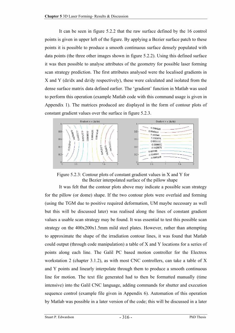
Chapter 5 3D Laser Forming- Results & Discussion
Stuart P. Edwardson PhD Thesis - 316 -
It can be seen in figure 5.2.2 that the raw surface defined by the 16 control
points is given in upper left of the figure. By applying a Bezier surface patch to these
points it is possible to produce a smooth continuous surface densely populated with
data points (the three other images shown in figure 5.2.2). Using this defined surface
it was then possible to analyse attributes of the geometry for possible laser forming
scan strategy prediction. The first attributes analysed were the localised gradients in
X and Y (dz/dx and dz/dy respectively), these were calculated and isolated from the
dense surface matrix data defined earlier. The ‘gradient’ function in Matlab was used
to perform this operation (example Matlab code with this command usage is given in
Appendix 1). The matrices produced are displayed in the form of contour plots of
constant gradient values over the surface in figure 5.2.3.
It was felt that the contour plots above may indicate a possible scan strategy
for the pillow (or dome) shape. If the two contour plots were overlaid and forming
(using the TGM due to positive required deformation, UM maybe necessary as well
but this will be discussed later) was realised along the lines of constant gradient
values a usable scan strategy may be found. It was essential to test this possible scan
strategy on the 400x200x1.5mm mild steel plates. However, rather than attempting
to approximate the shape of the irradiation contour lines, it was found that Matlab
could output (through code manipulation) a table of X and Y locations for a series of
points along each line. The Galil PC based motion controller for the Electrox
workstation 2 (chapter 3.1.2), as with most CNC controllers, can take a table of X
and Y points and linearly interpolate through them to produce a smooth continuous
line for motion. The text file generated had to then be formatted manually (time
intensive) into the Galil CNC language, adding commands for shutter and execution
sequence control (example file given in Appendix 6). Automation of this operation
by Matlab was possible in a later version of the code; this will be discussed in a later
Figure 5.2.3: Contour plots of constant gradient values in X and Y for the Bezier interpolated surface of the pillow shape
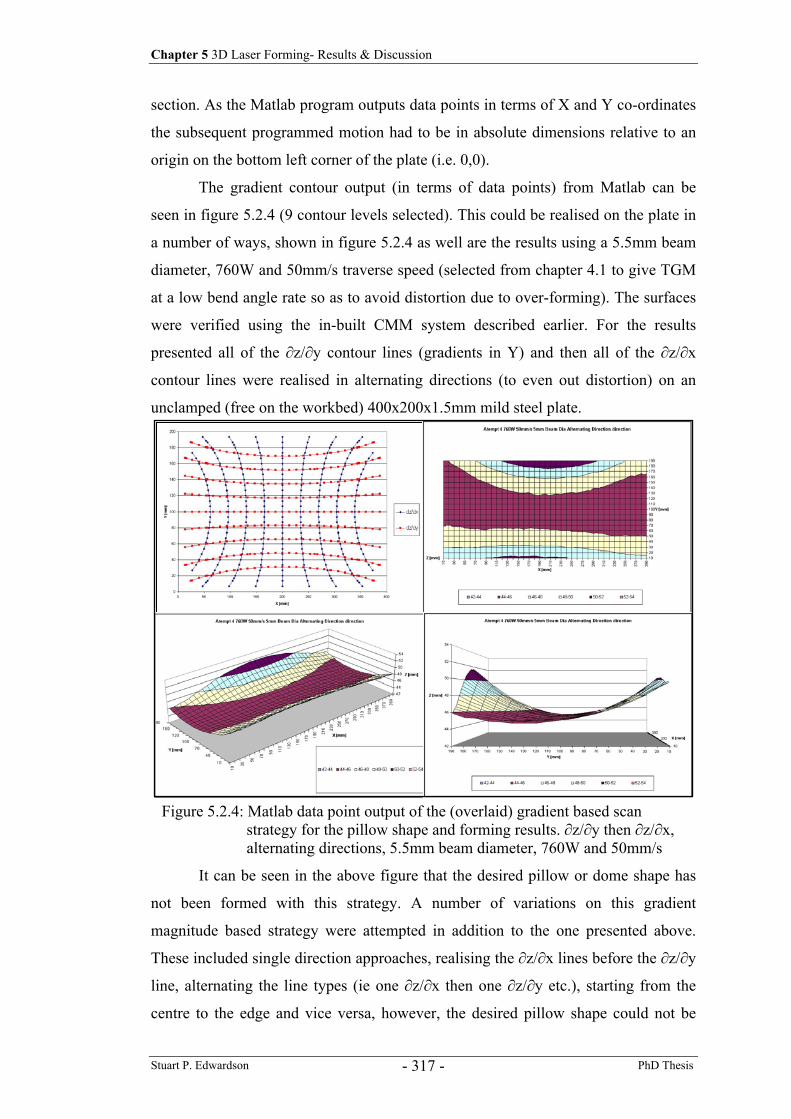
Chapter 5 3D Laser Forming- Results & Discussion
Stuart P. Edwardson PhD Thesis - 317 -
section. As the Matlab program outputs data points in terms of X and Y co-ordinates
the subsequent programmed motion had to be in absolute dimensions relative to an
origin on the bottom left corner of the plate (i.e. 0,0).
The gradient contour output (in terms of data points) from Matlab can be
seen in figure 5.2.4 (9 contour levels selected). This could be realised on the plate in
a number of ways, shown in figure 5.2.4 as well are the results using a 5.5mm beam
diameter, 760W and 50mm/s traverse speed (selected from chapter 4.1 to give TGM
at a low bend angle rate so as to avoid distortion due to over-forming). The surfaces
were verified using the in-built CMM system described earlier. For the results
presented all of the ∂z/∂y contour lines (gradients in Y) and then all of the ∂z/∂x
contour lines were realised in alternating directions (to even out distortion) on an
unclamped (free on the workbed) 400x200x1.5mm mild steel plate.
It can be seen in the above figure that the desired pillow or dome shape has
not been formed with this strategy. A number of variations on this gradient
magnitude based strategy were attempted in addition to the one presented above.
These included single direction approaches, realising the ∂z/∂x lines before the ∂z/∂y
line, alternating the line types (ie one ∂z/∂x then one ∂z/∂y etc.), starting from the
centre to the edge and vice versa, however, the desired pillow shape could not be
Figure 5.2.4: Matlab data point output of the (overlaid) gradient based scan strategy for the pillow shape and forming results. ∂z/∂y then ∂z/∂x, alternating directions, 5.5mm beam diameter, 760W and 50mm/s
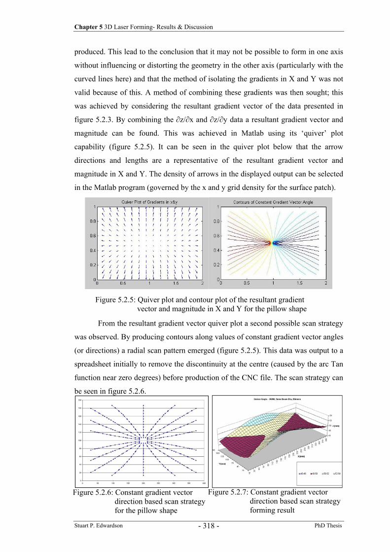
Chapter 5 3D Laser Forming- Results & Discussion
Stuart P. Edwardson PhD Thesis - 318 -
produced. This lead to the conclusion that it may not be possible to form in one axis
without influencing or distorting the geometry in the other axis (particularly with the
curved lines here) and that the method of isolating the gradients in X and Y was not
valid because of this. A method of combining these gradients was then sought; this
was achieved by considering the resultant gradient vector of the data presented in
figure 5.2.3. By combining the ∂z/∂x and ∂z/∂y data a resultant gradient vector and
magnitude can be found. This was achieved in Matlab using its ‘quiver’ plot
capability (figure 5.2.5). It can be seen in the quiver plot below that the arrow
directions and lengths are a representative of the resultant gradient vector and
magnitude in X and Y. The density of arrows in the displayed output can be selected
in the Matlab program (governed by the x and y grid density for the surface patch).
From the resultant gradient vector quiver plot a second possible scan strategy
was observed. By producing contours along values of constant gradient vector angles
(or directions) a radial scan pattern emerged (figure 5.2.5). This data was output to a
spreadsheet initially to remove the discontinuity at the centre (caused by the arc Tan
function near zero degrees) before production of the CNC file. The scan strategy can
be seen in figure 5.2.6.
Figure 5.2.5: Quiver plot and contour plot of the resultant gradient vector and magnitude in X and Y for the pillow shape
Figure 5.2.6: Constant gradient vector direction based scan strategy for the pillow shape
Figure 5.2.7: Constant gradient vector direction based scan strategy forming result
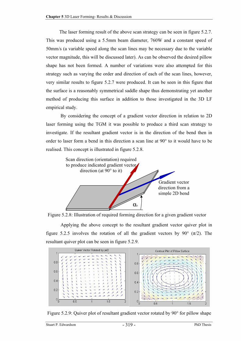
Chapter 5 3D Laser Forming- Results & Discussion
Stuart P. Edwardson PhD Thesis - 319 -
The laser forming result of the above scan strategy can be seen in figure 5.2.7.
This was produced using a 5.5mm beam diameter, 760W and a constant speed of
50mm/s (a variable speed along the scan lines may be necessary due to the variable
vector magnitude, this will be discussed later). As can be observed the desired pillow
shape has not been formed. A number of variations were also attempted for this
strategy such as varying the order and direction of each of the scan lines, however,
very similar results to figure 5.2.7 were produced. It can be seen in this figure that
the surface is a reasonably symmetrical saddle shape thus demonstrating yet another
method of producing this surface in addition to those investigated in the 3D LF
empirical study.
By considering the concept of a gradient vector direction in relation to 2D
laser forming using the TGM it was possible to produce a third scan strategy to
investigate. If the resultant gradient vector is in the direction of the bend then in
order to laser form a bend in this direction a scan line at 90° to it would have to be
realised. This concept is illustrated in figure 5.2.8.
Applying the above concept to the resultant gradient vector quiver plot in
figure 5.2.5 involves the rotation of all the gradient vectors by 90° (π/2). The
resultant quiver plot can be seen in figure 5.2.9.
αb
Scan direction (orientation) required to produce indicated gradient vector
direction (at 90° to it)
Gradient vector direction from a simple 2D bend
Figure 5.2.8: Illustration of required forming direction for a given gradient vector
Figure 5.2.9: Quiver plot of resultant gradient vector rotated by 90° for pillow shape
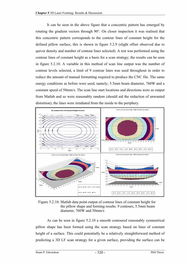
Chapter 5 3D Laser Forming- Results & Discussion
Stuart P. Edwardson PhD Thesis - 320 -
It can be seen in the above figure that a concentric pattern has emerged by
rotating the gradient vectors through 90°. On closer inspection it was realised that
this concentric pattern corresponds to the contour lines of constant height for the
defined pillow surface, this is shown in figure 5.2.9 (slight offset observed due to
quiver density and number of contour lines selected). A test was performed using the
contour lines of constant height as a basis for a scan strategy; the results can be seen
in figure 5.2.10. A variable in this method of scan line output was the number of
contour levels selected, a limit of 9 contour lines was used throughout in order to
reduce the amount of manual formatting required to produce the CNC file. The same
energy conditions as before were used, namely; 5.5mm beam diameter, 760W and a
constant speed of 50mm/s. The scan line start locations and directions were as output
from Matlab and so were reasonably random (should aid the reduction of unwanted
distortion); the lines were irradiated from the inside to the periphery.
As can be seen in figure 5.2.10 a smooth contoured reasonably symmetrical
pillow shape has been formed using the scan strategy based on lines of constant
height of a surface. This could potentially be a relatively straightforward method of
predicting a 3D LF scan strategy for a given surface, providing the surface can be
Figure 5.2.10: Matlab data point output of contour lines of constant height for the pillow shape and forming results. 9 contours, 5.5mm beam diameter, 760W and 50mm/s
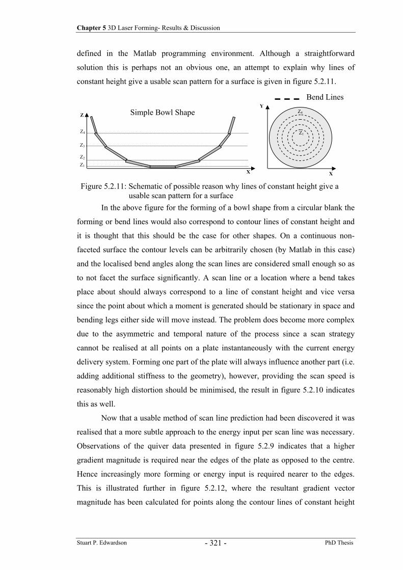
Chapter 5 3D Laser Forming- Results & Discussion
Stuart P. Edwardson PhD Thesis - 321 -
defined in the Matlab programming environment. Although a straightforward
solution this is perhaps not an obvious one, an attempt to explain why lines of
constant height give a usable scan pattern for a surface is given in figure 5.2.11.
In the above figure for the forming of a bowl shape from a circular blank the
forming or bend lines would also correspond to contour lines of constant height and
it is thought that this should be the case for other shapes. On a continuous non-
faceted surface the contour levels can be arbitrarily chosen (by Matlab in this case)
and the localised bend angles along the scan lines are considered small enough so as
to not facet the surface significantly. A scan line or a location where a bend takes
place about should always correspond to a line of constant height and vice versa
since the point about which a moment is generated should be stationary in space and
bending legs either side will move instead. The problem does become more complex
due to the asymmetric and temporal nature of the process since a scan strategy
cannot be realised at all points on a plate instantaneously with the current energy
delivery system. Forming one part of the plate will always influence another part (i.e.
adding additional stiffness to the geometry), however, providing the scan speed is
reasonably high distortion should be minimised, the result in figure 5.2.10 indicates
this as well.
Now that a usable method of scan line prediction had been discovered it was
realised that a more subtle approach to the energy input per scan line was necessary.
Observations of the quiver data presented in figure 5.2.9 indicates that a higher
gradient magnitude is required near the edges of the plate as opposed to the centre.
Hence increasingly more forming or energy input is required nearer to the edges.
This is illustrated further in figure 5.2.12, where the resultant gradient vector
magnitude has been calculated for points along the contour lines of constant height
Z
X
Z4 Z3 Z2 Z1
Y
X
Bend Lines
Simple Bowl Shape
Z1
Z4
Figure 5.2.11: Schematic of possible reason why lines of constant height give a usable scan pattern for a surface
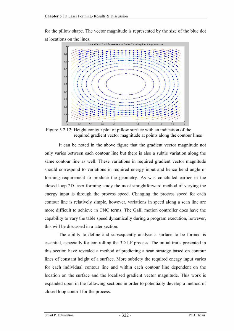
Chapter 5 3D Laser Forming- Results & Discussion
Stuart P. Edwardson PhD Thesis - 322 -
for the pillow shape. The vector magnitude is represented by the size of the blue dot
at locations on the lines.
It can be noted in the above figure that the gradient vector magnitude not
only varies between each contour line but there is also a subtle variation along the
same contour line as well. These variations in required gradient vector magnitude
should correspond to variations in required energy input and hence bend angle or
forming requirement to produce the geometry. As was concluded earlier in the
closed loop 2D laser forming study the most straightforward method of varying the
energy input is through the process speed. Changing the process speed for each
contour line is relatively simple, however, variations in speed along a scan line are
more difficult to achieve in CNC terms. The Galil motion controller does have the
capability to vary the table speed dynamically during a program execution, however,
this will be discussed in a later section.
The ability to define and subsequently analyse a surface to be formed is
essential, especially for controlling the 3D LF process. The initial trails presented in
this section have revealed a method of predicting a scan strategy based on contour
lines of constant height of a surface. More subtlety the required energy input varies
for each individual contour line and within each contour line dependent on the
location on the surface and the localised gradient vector magnitude. This work is
expanded upon in the following sections in order to potentially develop a method of
closed loop control for the process.
Figure 5.2.12: Height contour plot of pillow surface with an indication of the required gradient vector magnitude at points along the contour lines
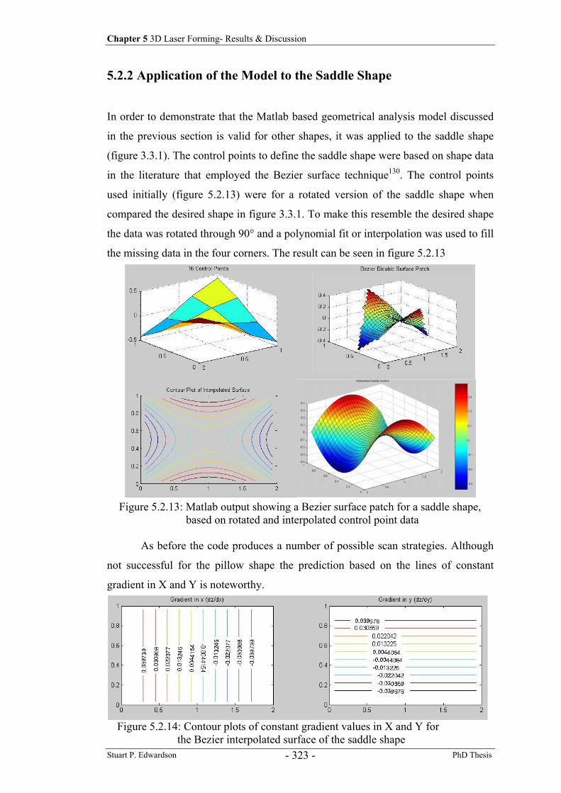
Chapter 5 3D Laser Forming- Results & Discussion
Stuart P. Edwardson PhD Thesis - 323 -
5.2.2 Application of the Model to the Saddle Shape
In order to demonstrate that the Matlab based geometrical analysis model discussed
in the previous section is valid for other shapes, it was applied to the saddle shape
(figure 3.3.1). The control points to define the saddle shape were based on shape data
in the literature that employed the Bezier surface technique130. The control points
used initially (figure 5.2.13) were for a rotated version of the saddle shape when
compared the desired shape in figure 3.3.1. To make this resemble the desired shape
the data was rotated through 90° and a polynomial fit or interpolation was used to fill
the missing data in the four corners. The result can be seen in figure 5.2.13
As before the code produces a number of possible scan strategies. Although
not successful for the pillow shape the prediction based on the lines of constant
gradient in X and Y is noteworthy.
Figure 5.2.13: Matlab output showing a Bezier surface patch for a saddle shape, based on rotated and interpolated control point data
Figure 5.2.14: Contour plots of constant gradient values in X and Y for the Bezier interpolated surface of the saddle shape
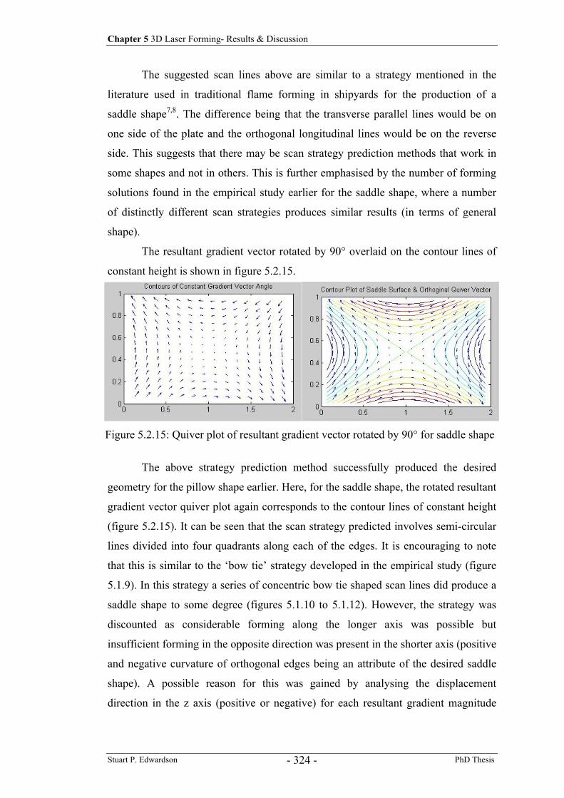
Chapter 5 3D Laser Forming- Results & Discussion
Stuart P. Edwardson PhD Thesis - 324 -
The suggested scan lines above are similar to a strategy mentioned in the
literature used in traditional flame forming in shipyards for the production of a
saddle shape7,8. The difference being that the transverse parallel lines would be on
one side of the plate and the orthogonal longitudinal lines would be on the reverse
side. This suggests that there may be scan strategy prediction methods that work in
some shapes and not in others. This is further emphasised by the number of forming
solutions found in the empirical study earlier for the saddle shape, where a number
of distinctly different scan strategies produces similar results (in terms of general
shape).
The resultant gradient vector rotated by 90° overlaid on the contour lines of
constant height is shown in figure 5.2.15.
The above strategy prediction method successfully produced the desired
geometry for the pillow shape earlier. Here, for the saddle shape, the rotated resultant
gradient vector quiver plot again corresponds to the contour lines of constant height
(figure 5.2.15). It can be seen that the scan strategy predicted involves semi-circular
lines divided into four quadrants along each of the edges. It is encouraging to note
that this is similar to the ‘bow tie’ strategy developed in the empirical study (figure
5.1.9). In this strategy a series of concentric bow tie shaped scan lines did produce a
saddle shape to some degree (figures 5.1.10 to 5.1.12). However, the strategy was
discounted as considerable forming along the longer axis was possible but
insufficient forming in the opposite direction was present in the shorter axis (positive
and negative curvature of orthogonal edges being an attribute of the desired saddle
shape). A possible reason for this was gained by analysing the displacement
direction in the z axis (positive or negative) for each resultant gradient magnitude
Figure 5.2.15: Quiver plot of resultant gradient vector rotated by 90° for saddle shape
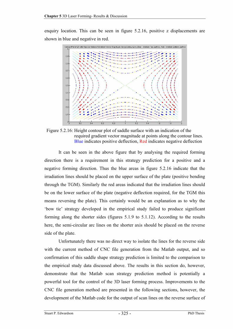
Chapter 5 3D Laser Forming- Results & Discussion
Stuart P. Edwardson PhD Thesis - 325 -
enquiry location. This can be seen in figure 5.2.16, positive z displacements are
shown in blue and negative in red.
It can be seen in the above figure that by analysing the required forming
direction there is a requirement in this strategy prediction for a positive and a
negative forming direction. Thus the blue areas in figure 5.2.16 indicate that the
irradiation lines should be placed on the upper surface of the plate (positive bending
through the TGM). Similarly the red areas indicated that the irradiation lines should
be on the lower surface of the plate (negative deflection required, for the TGM this
means reversing the plate). This certainly would be an explanation as to why the
‘bow tie’ strategy developed in the empirical study failed to produce significant
forming along the shorter sides (figures 5.1.9 to 5.1.12). According to the results
here, the semi-circular arc lines on the shorter axis should be placed on the reverse
side of the plate.
Unfortunately there was no direct way to isolate the lines for the reverse side
with the current method of CNC file generation from the Matlab output, and so
confirmation of this saddle shape strategy prediction is limited to the comparison to
the empirical study data discussed above. The results in this section do, however,
demonstrate that the Matlab scan strategy prediction method is potentially a
powerful tool for the control of the 3D laser forming process. Improvements to the
CNC file generation method are presented in the following sections, however, the
development of the Matlab code for the output of scan lines on the reverse surface of
Figure 5.2.16: Height contour plot of saddle surface with an indication of the required gradient vector magnitude at points along the contour lines. Blue indicates positive deflection, Red indicates negative deflection
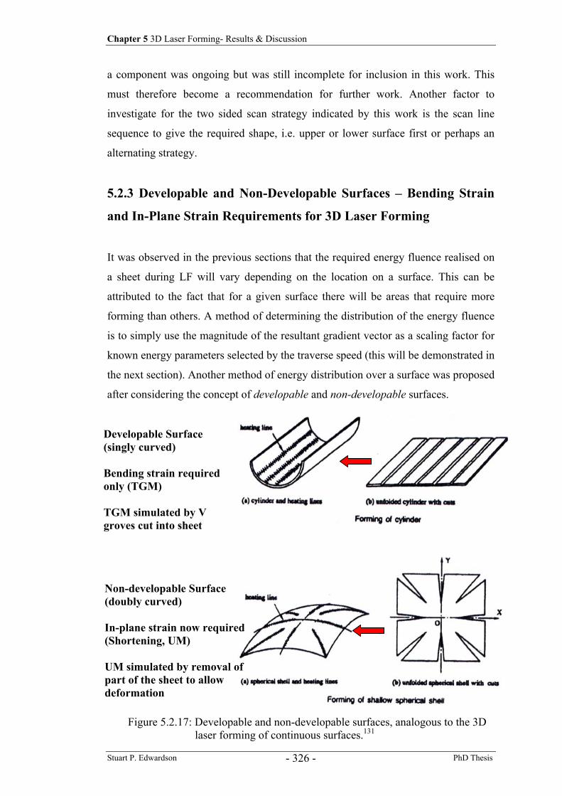
Chapter 5 3D Laser Forming- Results & Discussion
Stuart P. Edwardson PhD Thesis - 326 -
a component was ongoing but was still incomplete for inclusion in this work. This
must therefore become a recommendation for further work. Another factor to
investigate for the two sided scan strategy indicated by this work is the scan line
sequence to give the required shape, i.e. upper or lower surface first or perhaps an
alternating strategy.
5.2.3 Developable and Non-Developable Surfaces – Bending Strain
and In-Plane Strain Requirements for 3D Laser Forming
It was observed in the previous sections that the required energy fluence realised on
a sheet during LF will vary depending on the location on a surface. This can be
attributed to the fact that for a given surface there will be areas that require more
forming than others. A method of determining the distribution of the energy fluence
is to simply use the magnitude of the resultant gradient vector as a scaling factor for
known energy parameters selected by the traverse speed (this will be demonstrated in
the next section). Another method of energy distribution over a surface was proposed
after considering the concept of developable and non-developable surfaces.
Developable Surface (singly curved) Bending strain required only (TGM) TGM simulated by V groves cut into sheet
Non-developable Surface (doubly curved) In-plane strain now required (Shortening, UM) UM simulated by removal of part of the sheet to allow deformation
Figure 5.2.17: Developable and non-developable surfaces, analogous to the 3D laser forming of continuous surfaces.131
Chapter 5 3D Laser Forming- Results & Discussion
Stuart P. Edwardson PhD Thesis - 327 -
The term developable surface comes from mathematics. In mathematics, a
surface is called ‘developable’ if it can be flattened, and it is termed a non-
developable surface if it cannot be flattened. Developable surfaces are special ruled
surfaces which can be unfolded or developed into a plane without stretching or
tearing (or alternatively formed into a surface from a plane without stretching,
tearing or compression). Because of this property, they are of considerable
importance to sheet-metal and plate-metal based industries. Applications include
windshield design, binder surfaces for sheet metal forming processes, aircraft skins,
ship hulls and others 132. The concept of these surfaces is shown schematically in
figure 5.2.17. Given is an example of a developable surface, a part-cylinder, and a
non-developable surface, a dome or pillow shape. An analogy is drawn in figure
5.2.17 to how these surfaces have been formed and what LF mechanism would be
required to form a flat sheet (whole sheet, no cuts) into the two shapes. For a singly
curved developable surface the TGM should be the dominant mechanism used to
produce plastic bending strains and out of plane deformation. For a doubly curved
non-developable surface, material needs to be removed (in-plane) in order to allow
the deformation to take place. This suggests that the shortening mechanism should
be the dominant mechanism when forming this type of surface, the in-plane plastic
shrinkage accounting for the limiting material near the edges (at the expense of the
section thickening). This can be further emphasised by considering the mathematical
analysis of plates during deformation available in the literature 133. From the analysis
of thin plates with small deflections the strain component within a sheet can be
expressed in terms of the deflection of a plate, w. For a developable surface the
strain components at a given location in x and y and the shear strain in the xy plane
(for a plate thickness z) during deformation are given by:
(5.2.1)
(5.2.2)
(5.2.2)
yx
wz
ywz
xwz
xy
y
x
∂∂∂
−=
∂∂
−=
∂∂
−=
2
2
2
2
2
2γ
ε
ε
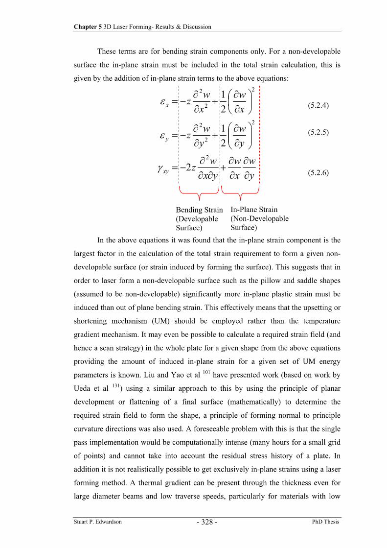
Chapter 5 3D Laser Forming- Results & Discussion
Stuart P. Edwardson PhD Thesis - 328 -
These terms are for bending strain components only. For a non-developable
surface the in-plane strain must be included in the total strain calculation, this is
given by the addition of in-plane strain terms to the above equations:
(5.2.4)
(5.2.5)
(5.2.6)
In the above equations it was found that the in-plane strain component is the
largest factor in the calculation of the total strain requirement to form a given non-
developable surface (or strain induced by forming the surface). This suggests that in
order to laser form a non-developable surface such as the pillow and saddle shapes
(assumed to be non-developable) significantly more in-plane plastic strain must be
induced than out of plane bending strain. This effectively means that the upsetting or
shortening mechanism (UM) should be employed rather than the temperature
gradient mechanism. It may even be possible to calculate a required strain field (and
hence a scan strategy) in the whole plate for a given shape from the above equations
providing the amount of induced in-plane strain for a given set of UM energy
parameters is known. Liu and Yao et al 101 have presented work (based on work by
Ueda et al 131) using a similar approach to this by using the principle of planar
development or flattening of a final surface (mathematically) to determine the
required strain field to form the shape, a principle of forming normal to principle
curvature directions was also used. A foreseeable problem with this is that the single
pass implementation would be computationally intense (many hours for a small grid
of points) and cannot take into account the residual stress history of a plate. In
addition it is not realistically possible to get exclusively in-plane strains using a laser
forming method. A thermal gradient can be present through the thickness even for
large diameter beams and low traverse speeds, particularly for materials with low
yw
xw
yxwz
yw
ywz
xw
xwz
xy
y
x
∂∂
∂∂
+∂∂
∂−=
∂∂
+∂∂
−=
∂∂
+∂∂
−=
2
2
2
2
2
2
2
2
21
21
γ
ε
ε
Bending Strain (Developable Surface)
In-Plane Strain (Non-Developable Surface)
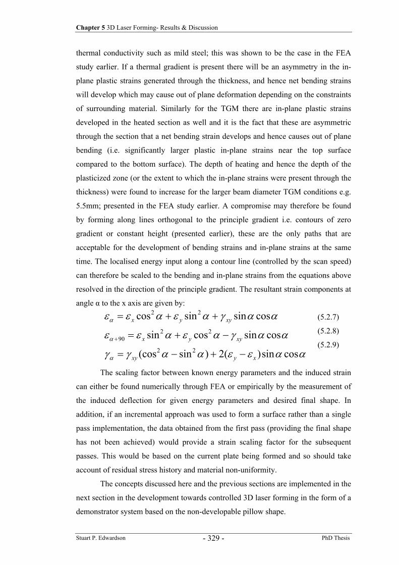
Chapter 5 3D Laser Forming- Results & Discussion
Stuart P. Edwardson PhD Thesis - 329 -
thermal conductivity such as mild steel; this was shown to be the case in the FEA
study earlier. If a thermal gradient is present there will be an asymmetry in the in-
plane plastic strains generated through the thickness, and hence net bending strains
will develop which may cause out of plane deformation depending on the constraints
of surrounding material. Similarly for the TGM there are in-plane plastic strains
developed in the heated section as well and it is the fact that these are asymmetric
through the section that a net bending strain develops and hence causes out of plane
bending (i.e. significantly larger plastic in-plane strains near the top surface
compared to the bottom surface). The depth of heating and hence the depth of the
plasticized zone (or the extent to which the in-plane strains were present through the
thickness) were found to increase for the larger beam diameter TGM conditions e.g.
5.5mm; presented in the FEA study earlier. A compromise may therefore be found
by forming along lines orthogonal to the principle gradient i.e. contours of zero
gradient or constant height (presented earlier), these are the only paths that are
acceptable for the development of bending strains and in-plane strains at the same
time. The localised energy input along a contour line (controlled by the scan speed)
can therefore be scaled to the bending and in-plane strains from the equations above
resolved in the direction of the principle gradient. The resultant strain components at
angle α to the x axis are given by:
(5.2.7)
(5.2.8)
(5.2.9)
The scaling factor between known energy parameters and the induced strain
can either be found numerically through FEA or empirically by the measurement of
the induced deflection for given energy parameters and desired final shape. In
addition, if an incremental approach was used to form a surface rather than a single
pass implementation, the data obtained from the first pass (providing the final shape
has not been achieved) would provide a strain scaling factor for the subsequent
passes. This would be based on the current plate being formed and so should take
account of residual stress history and material non-uniformity.
The concepts discussed here and the previous sections are implemented in the
next section in the development towards controlled 3D laser forming in the form of a
demonstrator system based on the non-developable pillow shape.
ααεεααγγ
ααγαεαεε
ααγαεαεε
α
α
α
cossin)(2)sin(cos
cossincossin
cossinsincos
22
2290
22
xyxy
xyyx
xyyx
−+−=
−+=
++=
+
Chapter 5 3D Laser Forming- Results & Discussion
Stuart P. Edwardson PhD Thesis - 330 -
5.3 3D Laser Forming Demonstrator System
In order to demonstrate the manufacturing capabilities of the 3D laser forming
process, one of the final goals of the EPSRC funded work programme (for the work
at Liverpool, which the research in this thesis forms part of), was the production of a
3D LF demonstrator system for the controlled LF of one of the primitive shapes
(figures 3.3.1 to 3.3.3) from a 400x200x1.5mm mild steel sheet. As discussed in the
literature review (chapter 2.6.5) either predictive or adaptive approaches could be
taken to achieve this (figure 2.6.12).
Intelligent predictive systems, perhaps based on Knowledge-Based Systems
(KBS), neural networks or thermo-mechanical models can achieve predictability
through a knowledge of the material (including its stress history) combined with a
developed, highly tuned process model / control algorithm.
In an adaptive system the use of sensors to provided accurate controlled
feedback coupled with the development of intelligent control software e.g. neural
network, provides an incremental or even real time closed loop method of accurate
3D laser forming, based on the current part characteristics independent of material
variability e.g. residual stress.
For the system developed in this work aspects of both approaches were used
based on the data presented in the previous sections. A potential method of scan
strategy prediction has been developed based on lines of constant height. The energy
distribution within the scan strategy can be given either by the gradient vector
magnitude or the sum of the bending and in-plane strains resolved in the direction of
the principle gradient. This gives a potential predictive capability to a system.
However, as discussed earlier, the single pass implementation of this would be
computationally intense and cannot take into account material non-uniformity and
residual stresses. The system developed here uses the predictive Matlab model to
give an initial scan strategy based on a required geometry. When the geometry is not
formed within one pass (or over formed), an incremental adaptive approach can then
be used for subsequent passes, utilising the error between the current and desired
geometry to give a new scan strategy. Thus any unwanted distortion due to material
variability can be accounted for. The forming rate and distribution of the magnitude
of forming across the surface can be controlled by the process speed based on the
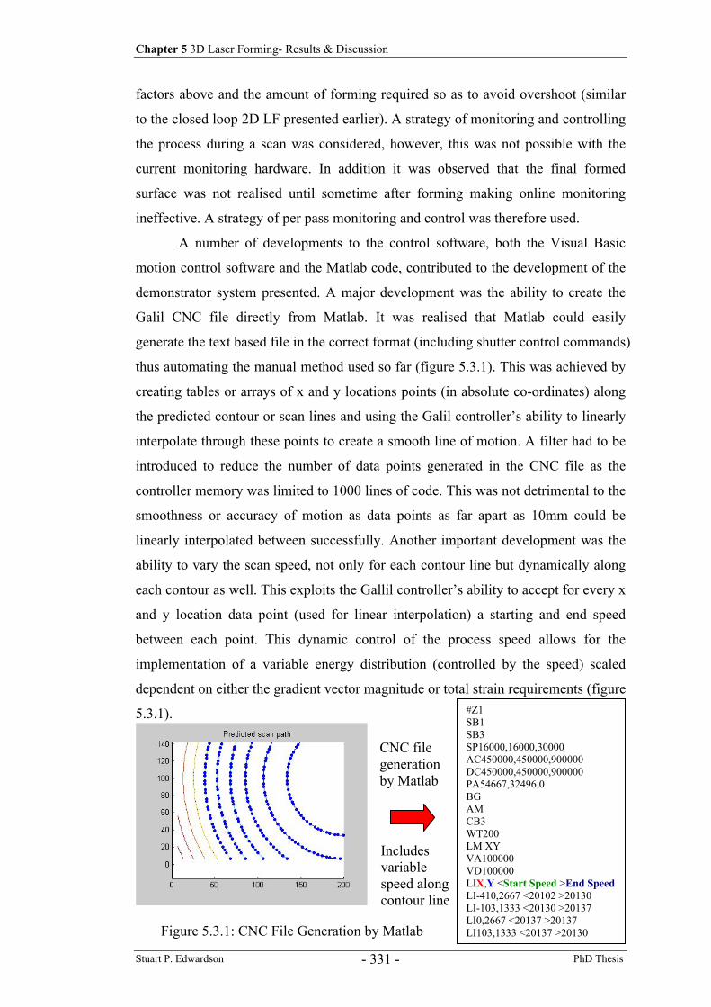
Chapter 5 3D Laser Forming- Results & Discussion
Stuart P. Edwardson PhD Thesis - 331 -
factors above and the amount of forming required so as to avoid overshoot (similar
to the closed loop 2D LF presented earlier). A strategy of monitoring and controlling
the process during a scan was considered, however, this was not possible with the
current monitoring hardware. In addition it was observed that the final formed
surface was not realised until sometime after forming making online monitoring
ineffective. A strategy of per pass monitoring and control was therefore used.
A number of developments to the control software, both the Visual Basic
motion control software and the Matlab code, contributed to the development of the
demonstrator system presented. A major development was the ability to create the
Galil CNC file directly from Matlab. It was realised that Matlab could easily
generate the text based file in the correct format (including shutter control commands)
thus automating the manual method used so far (figure 5.3.1). This was achieved by
creating tables or arrays of x and y locations points (in absolute co-ordinates) along
the predicted contour or scan lines and using the Galil controller’s ability to linearly
interpolate through these points to create a smooth line of motion. A filter had to be
introduced to reduce the number of data points generated in the CNC file as the
controller memory was limited to 1000 lines of code. This was not detrimental to the
smoothness or accuracy of motion as data points as far apart as 10mm could be
linearly interpolated between successfully. Another important development was the
ability to vary the scan speed, not only for each contour line but dynamically along
each contour as well. This exploits the Gallil controller’s ability to accept for every x
and y location data point (used for linear interpolation) a starting and end speed
between each point. This dynamic control of the process speed allows for the
implementation of a variable energy distribution (controlled by the speed) scaled
dependent on either the gradient vector magnitude or total strain requirements (figure
5.3.1).
#Z1 SB1 SB3 SP16000,16000,30000 AC450000,450000,900000 DC450000,450000,900000 PA54667,32496,0 BG AM CB3 WT200 LM XY VA100000 VD100000 LIX,Y <Start Speed >End SpeedLI-410,2667 <20102 >20130 LI-103,1333 <20130 >20137 LI0,2667 <20137 >20137 LI103,1333 <20137 >20130
CNC file generation by Matlab
Includes variable speed along contour line
Figure 5.3.1: CNC File Generation by Matlab
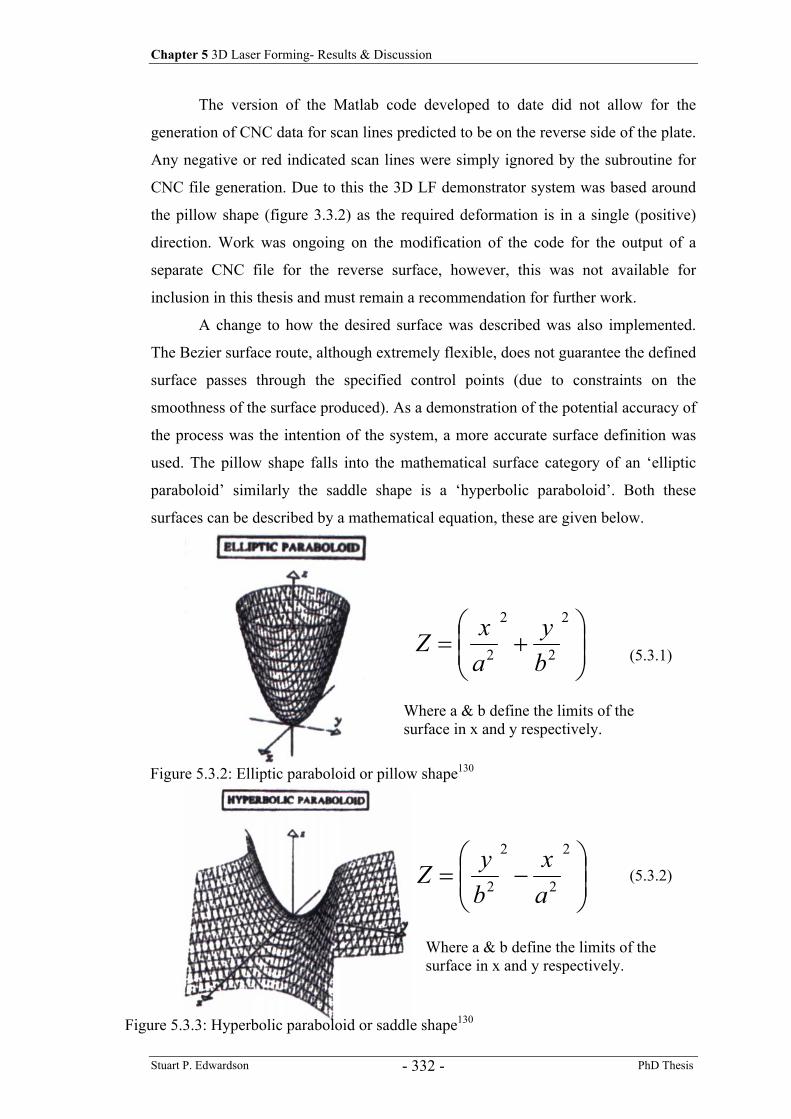
Chapter 5 3D Laser Forming- Results & Discussion
Stuart P. Edwardson PhD Thesis - 332 -
The version of the Matlab code developed to date did not allow for the
generation of CNC data for scan lines predicted to be on the reverse side of the plate.
Any negative or red indicated scan lines were simply ignored by the subroutine for
CNC file generation. Due to this the 3D LF demonstrator system was based around
the pillow shape (figure 3.3.2) as the required deformation is in a single (positive)
direction. Work was ongoing on the modification of the code for the output of a
separate CNC file for the reverse surface, however, this was not available for
inclusion in this thesis and must remain a recommendation for further work.
A change to how the desired surface was described was also implemented.
The Bezier surface route, although extremely flexible, does not guarantee the defined
surface passes through the specified control points (due to constraints on the
smoothness of the surface produced). As a demonstration of the potential accuracy of
the process was the intention of the system, a more accurate surface definition was
used. The pillow shape falls into the mathematical surface category of an ‘elliptic
paraboloid’ similarly the saddle shape is a ‘hyperbolic paraboloid’. Both these
surfaces can be described by a mathematical equation, these are given below.
(5.3.1)
(5.3.2)
+=
2
2
2
2 by
axZ
−=
2
2
2
2 ax
byZ
Figure 5.3.2: Elliptic paraboloid or pillow shape130
Figure 5.3.3: Hyperbolic paraboloid or saddle shape130
Where a & b define the limits of the surface in x and y respectively.
Where a & b define the limits of the surface in x and y respectively.
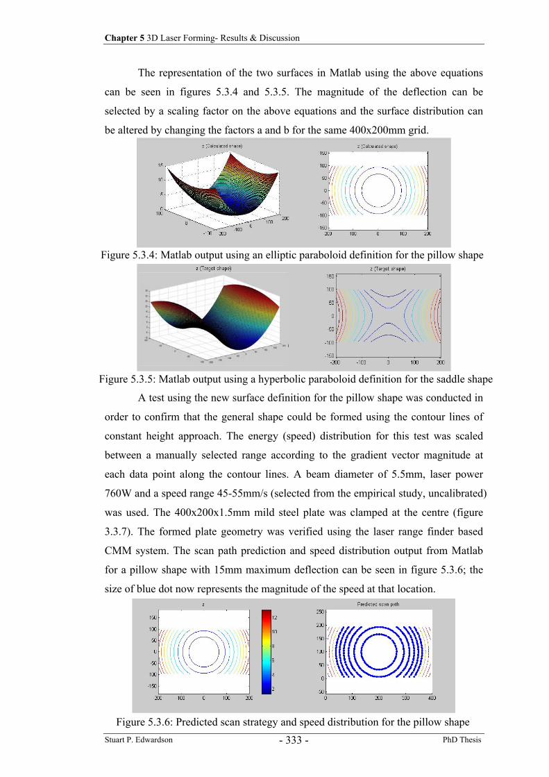
Chapter 5 3D Laser Forming- Results & Discussion
Stuart P. Edwardson PhD Thesis - 333 -
The representation of the two surfaces in Matlab using the above equations
can be seen in figures 5.3.4 and 5.3.5. The magnitude of the deflection can be
selected by a scaling factor on the above equations and the surface distribution can
be altered by changing the factors a and b for the same 400x200mm grid.
A test using the new surface definition for the pillow shape was conducted in
order to confirm that the general shape could be formed using the contour lines of
constant height approach. The energy (speed) distribution for this test was scaled
between a manually selected range according to the gradient vector magnitude at
each data point along the contour lines. A beam diameter of 5.5mm, laser power
760W and a speed range 45-55mm/s (selected from the empirical study, uncalibrated)
was used. The 400x200x1.5mm mild steel plate was clamped at the centre (figure
3.3.7). The formed plate geometry was verified using the laser range finder based
CMM system. The scan path prediction and speed distribution output from Matlab
for a pillow shape with 15mm maximum deflection can be seen in figure 5.3.6; the
size of blue dot now represents the magnitude of the speed at that location.
Figure 5.3.4: Matlab output using an elliptic paraboloid definition for the pillow shape
Figure 5.3.5: Matlab output using a hyperbolic paraboloid definition for the saddle shape
Figure 5.3.6: Predicted scan strategy and speed distribution for the pillow shape
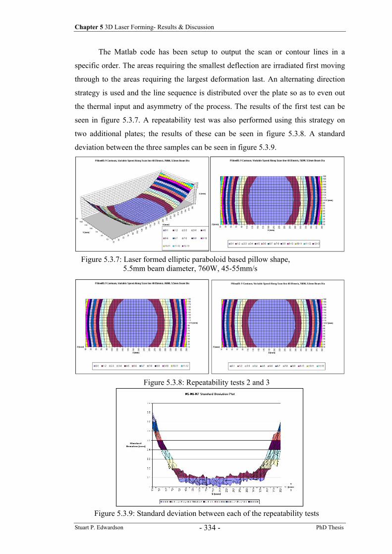
Chapter 5 3D Laser Forming- Results & Discussion
Stuart P. Edwardson PhD Thesis - 334 -
The Matlab code has been setup to output the scan or contour lines in a
specific order. The areas requiring the smallest deflection are irradiated first moving
through to the areas requiring the largest deformation last. An alternating direction
strategy is used and the line sequence is distributed over the plate so as to even out
the thermal input and asymmetry of the process. The results of the first test can be
seen in figure 5.3.7. A repeatability test was also performed using this strategy on
two additional plates; the results of these can be seen in figure 5.3.8. A standard
deviation between the three samples can be seen in figure 5.3.9.
Figure 5.3.9: Standard deviation between each of the repeatability tests
Figure 5.3.7: Laser formed elliptic paraboloid based pillow shape, 5.5mm beam diameter, 760W, 45-55mm/s
Figure 5.3.8: Repeatability tests 2 and 3
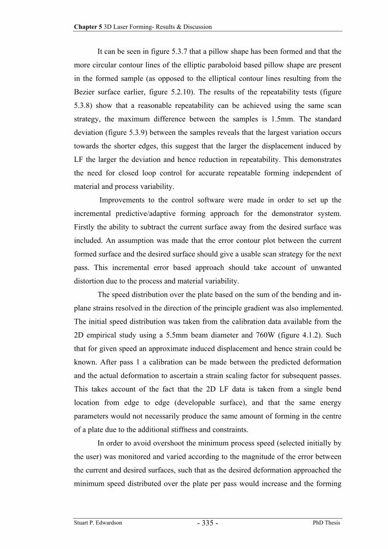
Chapter 5 3D Laser Forming- Results & Discussion
Stuart P. Edwardson PhD Thesis - 335 -
It can be seen in figure 5.3.7 that a pillow shape has been formed and that the
more circular contour lines of the elliptic paraboloid based pillow shape are present
in the formed sample (as opposed to the elliptical contour lines resulting from the
Bezier surface earlier, figure 5.2.10). The results of the repeatability tests (figure
5.3.8) show that a reasonable repeatability can be achieved using the same scan
strategy, the maximum difference between the samples is 1.5mm. The standard
deviation (figure 5.3.9) between the samples reveals that the largest variation occurs
towards the shorter edges, this suggest that the larger the displacement induced by
LF the larger the deviation and hence reduction in repeatability. This demonstrates
the need for closed loop control for accurate repeatable forming independent of
material and process variability.
Improvements to the control software were made in order to set up the
incremental predictive/adaptive forming approach for the demonstrator system.
Firstly the ability to subtract the current surface away from the desired surface was
included. An assumption was made that the error contour plot between the current
formed surface and the desired surface should give a usable scan strategy for the next
pass. This incremental error based approach should take account of unwanted
distortion due to the process and material variability.
The speed distribution over the plate based on the sum of the bending and in-
plane strains resolved in the direction of the principle gradient was also implemented.
The initial speed distribution was taken from the calibration data available from the
2D empirical study using a 5.5mm beam diameter and 760W (figure 4.1.2). Such
that for given speed an approximate induced displacement and hence strain could be
known. After pass 1 a calibration can be made between the predicted deformation
and the actual deformation to ascertain a strain scaling factor for subsequent passes.
This takes account of the fact that the 2D LF data is taken from a single bend
location from edge to edge (developable surface), and that the same energy
parameters would not necessarily produce the same amount of forming in the centre
of a plate due to the additional stiffness and constraints.
In order to avoid overshoot the minimum process speed (selected initially by
the user) was monitored and varied according to the magnitude of the error between
the current and desired surfaces, such that as the desired deformation approached the
minimum speed distributed over the plate per pass would increase and the forming
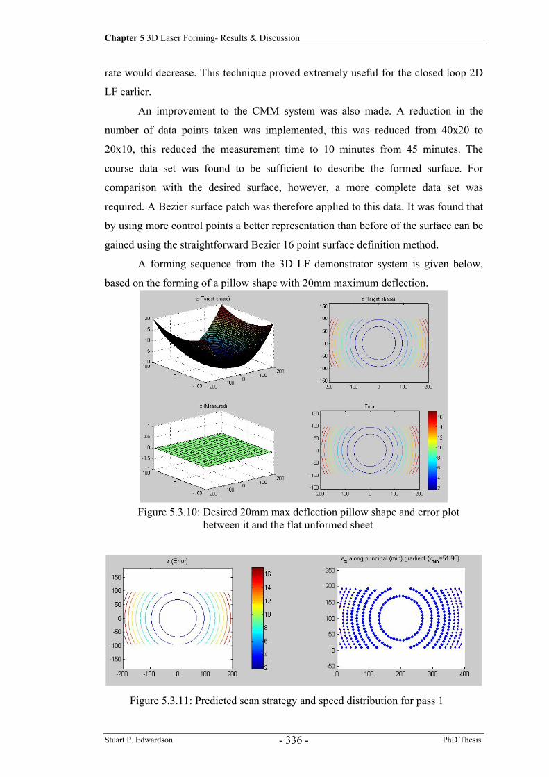
Chapter 5 3D Laser Forming- Results & Discussion
Stuart P. Edwardson PhD Thesis - 336 -
rate would decrease. This technique proved extremely useful for the closed loop 2D
LF earlier.
An improvement to the CMM system was also made. A reduction in the
number of data points taken was implemented, this was reduced from 40x20 to
20x10, this reduced the measurement time to 10 minutes from 45 minutes. The
course data set was found to be sufficient to describe the formed surface. For
comparison with the desired surface, however, a more complete data set was
required. A Bezier surface patch was therefore applied to this data. It was found that
by using more control points a better representation than before of the surface can be
gained using the straightforward Bezier 16 point surface definition method.
A forming sequence from the 3D LF demonstrator system is given below,
based on the forming of a pillow shape with 20mm maximum deflection.
Figure 5.3.10: Desired 20mm max deflection pillow shape and error plot between it and the flat unformed sheet
Figure 5.3.11: Predicted scan strategy and speed distribution for pass 1
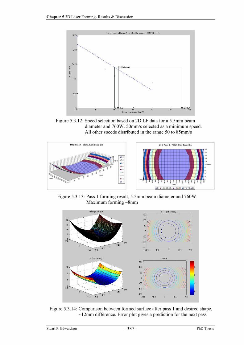
Chapter 5 3D Laser Forming- Results & Discussion
Stuart P. Edwardson PhD Thesis - 337 -
Figure 5.3.12: Speed selection based on 2D LF data for a 5.5mm beam diameter and 760W. 50mm/s selected as a minimum speed. All other speeds distributed in the range 50 to 85mm/s
Figure 5.3.13: Pass 1 forming result, 5.5mm beam diameter and 760W. Maximum forming ~8mm
Figure 5.3.14: Comparison between formed surface after pass 1 and desired shape, ~12mm difference. Error plot gives a prediction for the next pass
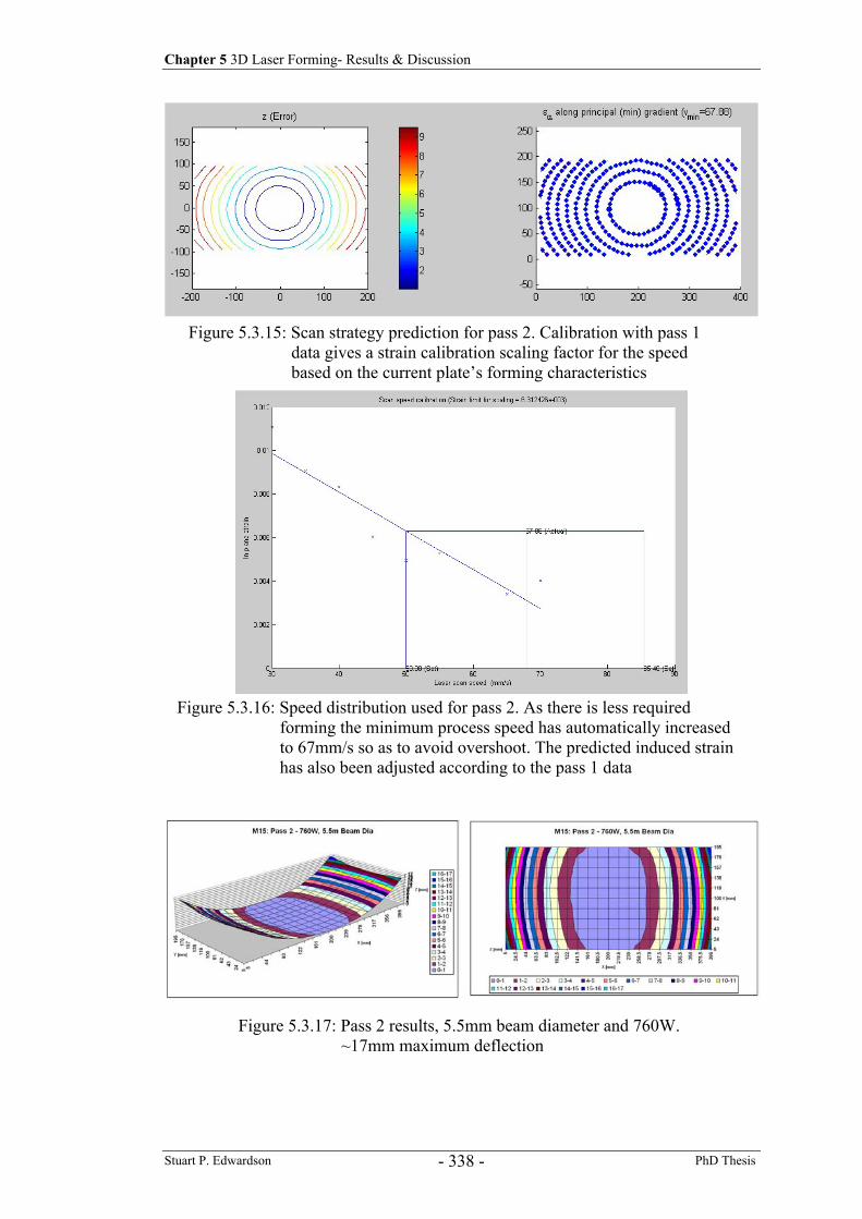
Chapter 5 3D Laser Forming- Results & Discussion
Stuart P. Edwardson PhD Thesis - 338 -
Figure 5.3.15: Scan strategy prediction for pass 2. Calibration with pass 1 data gives a strain calibration scaling factor for the speed based on the current plate’s forming characteristics
Figure 5.3.16: Speed distribution used for pass 2. As there is less required forming the minimum process speed has automatically increased to 67mm/s so as to avoid overshoot. The predicted induced strain has also been adjusted according to the pass 1 data
Figure 5.3.17: Pass 2 results, 5.5mm beam diameter and 760W. ~17mm maximum deflection
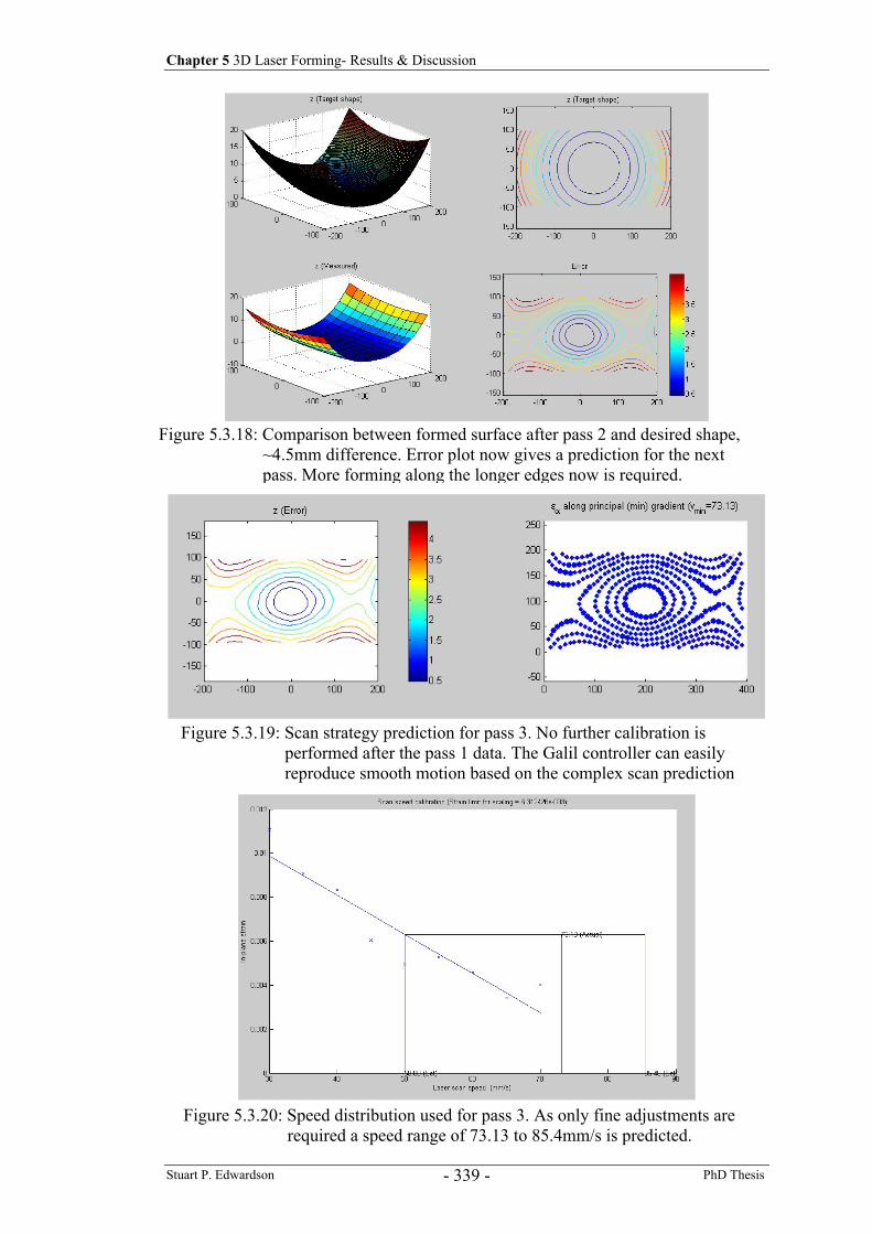
Chapter 5 3D Laser Forming- Results & Discussion
Stuart P. Edwardson PhD Thesis - 339 -
Figure 5.3.18: Comparison between formed surface after pass 2 and desired shape, ~4.5mm difference. Error plot now gives a prediction for the next pass. More forming along the longer edges now is required.
Figure 5.3.19: Scan strategy prediction for pass 3. No further calibration is performed after the pass 1 data. The Galil controller can easily reproduce smooth motion based on the complex scan prediction
Figure 5.3.20: Speed distribution used for pass 3. As only fine adjustments are required a speed range of 73.13 to 85.4mm/s is predicted.
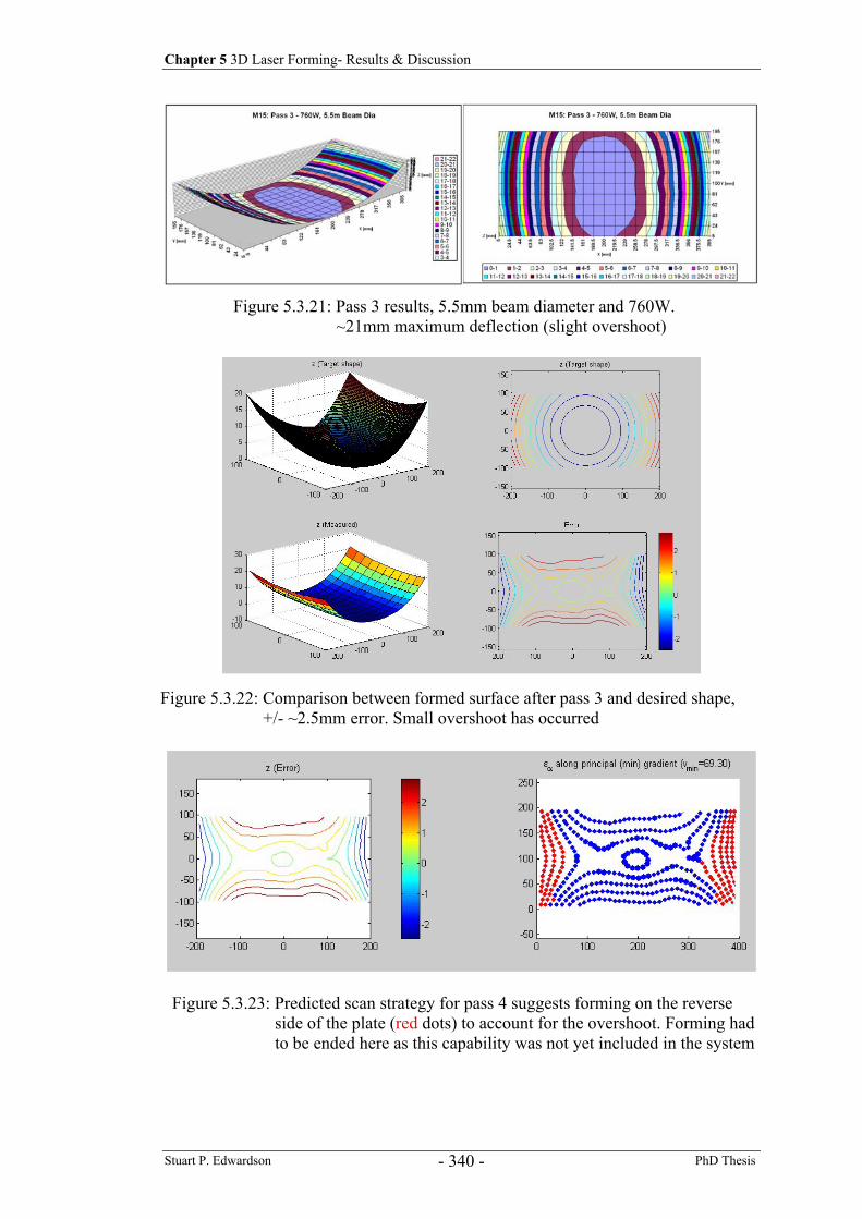
Chapter 5 3D Laser Forming- Results & Discussion
Stuart P. Edwardson PhD Thesis - 340 -
Figure 5.3.21: Pass 3 results, 5.5mm beam diameter and 760W. ~21mm maximum deflection (slight overshoot)
Figure 5.3.22: Comparison between formed surface after pass 3 and desired shape, +/- ~2.5mm error. Small overshoot has occurred
Figure 5.3.23: Predicted scan strategy for pass 4 suggests forming on the reverse side of the plate (red dots) to account for the overshoot. Forming had to be ended here as this capability was not yet included in the system
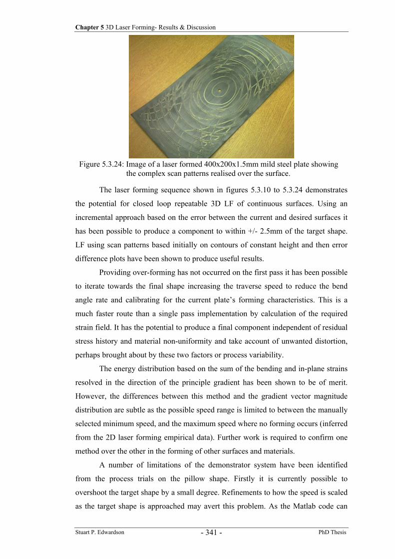
Chapter 5 3D Laser Forming- Results & Discussion
Stuart P. Edwardson PhD Thesis - 341 -
The laser forming sequence shown in figures 5.3.10 to 5.3.24 demonstrates
the potential for closed loop repeatable 3D LF of continuous surfaces. Using an
incremental approach based on the error between the current and desired surfaces it
has been possible to produce a component to within +/- 2.5mm of the target shape.
LF using scan patterns based initially on contours of constant height and then error
difference plots have been shown to produce useful results.
Providing over-forming has not occurred on the first pass it has been possible
to iterate towards the final shape increasing the traverse speed to reduce the bend
angle rate and calibrating for the current plate’s forming characteristics. This is a
much faster route than a single pass implementation by calculation of the required
strain field. It has the potential to produce a final component independent of residual
stress history and material non-uniformity and take account of unwanted distortion,
perhaps brought about by these two factors or process variability.
The energy distribution based on the sum of the bending and in-plane strains
resolved in the direction of the principle gradient has been shown to be of merit.
However, the differences between this method and the gradient vector magnitude
distribution are subtle as the possible speed range is limited to between the manually
selected minimum speed, and the maximum speed where no forming occurs (inferred
from the 2D laser forming empirical data). Further work is required to confirm one
method over the other in the forming of other surfaces and materials.
A number of limitations of the demonstrator system have been identified
from the process trials on the pillow shape. Firstly it is currently possible to
overshoot the target shape by a small degree. Refinements to how the speed is scaled
as the target shape is approached may avert this problem. As the Matlab code can
Figure 5.3.24: Image of a laser formed 400x200x1.5mm mild steel plate showing the complex scan patterns realised over the surface.
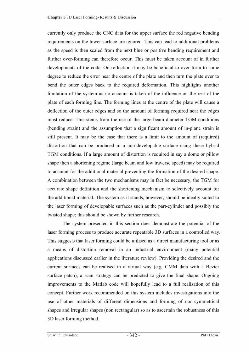
Chapter 5 3D Laser Forming- Results & Discussion
Stuart P. Edwardson PhD Thesis - 342 -
currently only produce the CNC data for the upper surface the red negative bending
requirements on the lower surface are ignored. This can lead to additional problems
as the speed is then scaled from the next blue or positive bending requirement and
further over-forming can therefore occur. This must be taken account of in further
developments of the code. On reflection it may be beneficial to over-form to some
degree to reduce the error near the centre of the plate and then turn the plate over to
bend the outer edges back to the required deformation. This highlights another
limitation of the system as no account is taken of the influence on the rest of the
plate of each forming line. The forming lines at the centre of the plate will cause a
deflection of the outer edges and so the amount of forming required near the edges
must reduce. This stems from the use of the large beam diameter TGM conditions
(bending strain) and the assumption that a significant amount of in-plane strain is
still present. It may be the case that there is a limit to the amount of (required)
distortion that can be produced in a non-developable surface using these hybrid
TGM conditions. If a large amount of distortion is required in say a dome or pillow
shape then a shortening regime (large beam and low traverse speed) may be required
to account for the additional material preventing the formation of the desired shape.
A combination between the two mechanisms may in fact be necessary, the TGM for
accurate shape definition and the shortening mechanism to selectively account for
the additional material. The system as it stands, however, should be ideally suited to
the laser forming of developable surfaces such as the part-cylinder and possibly the
twisted shape; this should be shown by further research.
The system presented in this section does demonstrate the potential of the
laser forming process to produce accurate repeatable 3D surfaces in a controlled way.
This suggests that laser forming could be utilised as a direct manufacturing tool or as
a means of distortion removal in an industrial environment (many potential
applications discussed earlier in the literature review). Providing the desired and the
current surfaces can be realised in a virtual way (e.g. CMM data with a Bezier
surface patch), a scan strategy can be predicted to give the final shape. Ongoing
improvements to the Matlab code will hopefully lead to a full realisation of this
concept. Further work recommended on this system includes investigations into the
use of other materials of different dimensions and forming of non-symmetrical
shapes and irregular shapes (non rectangular) so as to ascertain the robustness of this
3D laser forming method.
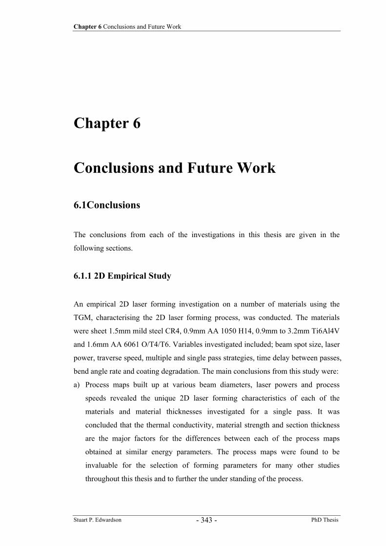
Chapter 6 Conclusions and Future Work
Stuart P. Edwardson PhD Thesis - 343 -
Chapter 6
Conclusions and Future Work
6.1Conclusions
The conclusions from each of the investigations in this thesis are given in the
following sections.
6.1.1 2D Empirical Study
An empirical 2D laser forming investigation on a number of materials using the
TGM, characterising the 2D laser forming process, was conducted. The materials
were sheet 1.5mm mild steel CR4, 0.9mm AA 1050 H14, 0.9mm to 3.2mm Ti6Al4V
and 1.6mm AA 6061 O/T4/T6. Variables investigated included; beam spot size, laser
power, traverse speed, multiple and single pass strategies, time delay between passes,
bend angle rate and coating degradation. The main conclusions from this study were:
a) Process maps built up at various beam diameters, laser powers and process
speeds revealed the unique 2D laser forming characteristics of each of the
materials and material thicknesses investigated for a single pass. It was
concluded that the thermal conductivity, material strength and section thickness
are the major factors for the differences between each of the process maps
obtained at similar energy parameters. The process maps were found to be
invaluable for the selection of forming parameters for many other studies
throughout this thesis and to further the under standing of the process.
Chapter 6 Conclusions and Future Work
Stuart P. Edwardson PhD Thesis - 344 -
b) It was found that beam diameters larger than the sheet thickness had to be used to
induce temperature gradient mechanism conditions. TGM theory would suggest
that a beam diameter of the sheet thickness should be used, however, for realistic
forming operations it was found that beam diameters of this size would cause
significant surface damage.
c) Multiple pass studies using energy parameters selected from the process map
data revealed the 2D laser forming characteristics of each of the materials
investigated during the development of large bend angles of many degrees. By
monitoring the bend angle per pass with custom built hardware and software it
was possible gain further insight into the process. Analysing the bend angle rate
per pass for all the materials and processing conditions used revealed the
subtleties of the process; most notable is that the bend angle rate varies
considerably during a multi-pass strategy. It was found that during the first few
passes there is an initial increase in the bend angle rate per pass thought to be a
result of the absorptive coating burn-off per pass achieving an optimum coating
thickness. An optimum level is reached after a few passes which then begins to
decline after 8 to 10 passes. The extent of this decline was found to depend on
the material and processing conditions used. For the mild steel and pure
aluminium AA 1050 H14, the rate declines slowly over the 30 passes
investigated. This was attributed to the previously determined factors of strain or
work hardening, section thickening and absorptive coating burn-off. For the
Ti6Al4V and AA 6061 the bend angle rate fell dramatically. The major factor for
this was revealed to be the absorptive coating burn-off which was found to be a
larger factor than previously thought. In the case of the Ti6Al4V the high coating
burn off rate was attributed to the low thermal conductivity of the material
preventing adequate conduction of the absorbed heat into the bulk material, thus
overheating the graphite. For the AA6061 the high reflectivity of the substrate
after some graphite burn-off was concluded to be the reason for the dramatic fall
off. This was confirmed by re-spraying the graphite coating on the samples
which gave an immediate increase in the bend angle rate. The other factors were
still present at higher numbers of passes but were overridden by the graphite
coating burn-off. The use of coatings with laser forming, it was concluded from
this study, is not reliable for certain materials. It is therefore recommended that a
Chapter 6 Conclusions and Future Work
Stuart P. Edwardson PhD Thesis - 345 -
shorter laser wavelength should be employed if the process is to be used in an
industrial environment so as to negate the use of absorptive coatings.
d) An investigation to determine the effect of inter-pass time delay on process
efficiency during a multi-pass strategy revealed that there is an optimum delay
for a given set of process parameters. It was concluded that this is due to a
balance point or a trade off between the heat retained in the coupon aiding the
process by reducing the flow stress and the increased bulk material temperature
reducing the available temperature gradient through the thickness as the laser
beam is passed over the surface.
e) A ‘double pass’ technique was developed for thick section materials. The
technique involves a scan strategy of a pass in one direction followed
immediately by a return pass in the opposite direction; the plate is allowed to
cool after each double pass. The concept behind this strategy is that, providing
the material surface is not damaged on the second pass, the additional energy
input per pass is essentially akin to processing with a much higher laser power,
this was confirmed by thermocouple data. Another factor in this technique is that
on the second pass the heat retained in the irradiated area from the first pass
could serve to produce additional forming by reducing the temperature dependent
flow stress of the material, since a hot plate is easier to form than a cold one.
f) A study was conducted into the 2D LF of 1.6mm gauge AA6061 in three heat
treatment conditions O (annealed), T4 and T6 (solution heat treated, cold worked
and aged). It was found that there were considerable differences in the laser
forming characteristics of the three heat treatments of the same alloy. This was
attributed to, apart from the coating burn-off, the considerable differences in
material strength and thermal conductivity between the materials.
6.1.2 Thermal Analysis
Thermocouple and thermal imaging techniques were used in this investigation to
experimentally determine the transient temperature field in 1.5mm gauge mild steel
during the laser forming process and subsequent cooling. A study was also
conducted into the effectiveness of using forced cooling in the LF process and its
effect on forming efficiency. The main conclusions of this study were:
Chapter 6 Conclusions and Future Work
Stuart P. Edwardson PhD Thesis - 346 -
a) The thermocouple study revealed the temporal temperatures cycles at single
locations on the upper and lower surfaces of 1.5mm mild steel CR4 during single
and multi-pass 2D LF. For the multi-pass study the temperatures recorded were
found to increase with increasing numbers of passes for all the energy parameters
investigated. The peak temperature observed during each pass at each location
increased also. However, the temperature increase was roughly the same for each
pass as the same amount of energy is added each time, it was realised that it is
the bulk material temperature this temperature increase per pass is added onto
which is in fact increasing. This effect may have implications on the efficiency of
the process for subsequent passes, since if the bulk material temperature is
increasing there maybe a reduction in magnitude of the thermal gradient through
the section directly under the beam (consistent with TGM). Another factor is that
the elevated temperatures remaining in the heated area may aid the process by
reducing the temperature dependent flow or yield stress of the material thus
making it easier to plastically deform. By reducing the inter-pass time delay it
was found that the peak and bulk material temperatures per pass increase
significantly with increasing numbers of passes. It was found that a plateau is
reached after a number of passes whereby there is no significant increase in the
peak temperature recorded per pass when compared to the previous pass. It was
concluded that this is likely to be a point where thermal equilibrium is reached.
Where the bulk material temperature of the whole plate has stabilised and the
heat losses due to conduction into the clamp, convection to the air and radiation
to the surroundings are balanced with the heat input per pass.
b) A thermal imaging camera revealed the real time heat distribution in a coupon
during a scan using various processing parameters. The graphite was found to be
problematic when used with this measurement technique. It was found that it was
not possible to measure the sample temperature directly within the beam due to
the incandescence of the graphite. The data surrounding the beam revealed that
the time period and surface area over which heat was retained in the mild steel
sheet increased for larger laser beam spot diameters. In addition it was revealed
that a higher temperature is realised at the end of the scan line when compared to
the beginning. This is backed up by observations of the HAZ at the end of a scan
line, where a widening or flaring can be seen. A possible explanation for this is
that the heat from the incident laser beam and the heat retained behind the beam
Chapter 6 Conclusions and Future Work
Stuart P. Edwardson PhD Thesis - 347 -
is flowing into the cold region ahead of the beam, as the beam reaches the second
edge the heat flowing ahead of the beam cannot travel any further and so a heat
build up occurs, hence the increase in temperature at the second edge, this could
be a source of unwanted distortion in the process such as edge effects.
c) In the forced cooling study it was shown that the addition of a basic cooling
regime influences the thermal cycle in the coupons considerably. With the
addition of a cooling air jet on the under surface of a coupon continuously during
and post processing the temperature cycle stabilised within one pass with very
little increase in peak temperature observed for subsequent passes at all three of
the energy parameters investigated. In addition the effect on the LF process in
terms of bend angle produced was shown to be subtle. The use of forced cooling,
it was concluded, has a potential benefit of decreased overall processing time,
since the relatively long inter-pass delay could be reduced significantly; this
makes its use essential. In addition reducing the thermal input into a component
must be beneficial both for the reduction in unwanted distortion and any adverse
effects on metallurgy.
6.1.3 Displacement / Time Analysis
An investigation was conducted into the displacement (or bend angle development)
of 80x200x1.5mm mild steel CR4 coupons with respect to time during LF using
various energy parameters. The conclusions from this study are:
a) It was found that the temporal displacement characteristics of the coupons during
LF depended greatly on the energy parameters used and the number of passes
realised.
b) For the 3mm beam diameter data on the first pass the major part of the bend
angle development was seen to occur whilst the beam is still on the plate surface,
very little additional movement was recorded after the beam has left the coupon
surface. By the sixth pass it was observed that, although the majority of the bend
angle occurs whilst the laser beam is on the surface of the coupon, the final
deformation or bend angle isn’t reached until some 20 seconds after processing.
This effect became more prevalent with increasing numbers of passes and was
attributed to relieving of the purely elastic stresses during cooling.
Chapter 6 Conclusions and Future Work
Stuart P. Edwardson PhD Thesis - 348 -
c) For the larger beam diameters investigated the first pass is similar to the smaller
beam diameter data. For increasing numbers of passes an ‘S’ curve in the
temporal displacement became more apparent. For the 8mm beam diameter this
became two points of inflection where the bend angle was arrested as the beam
was mid way though the plate. This was attributed to a number of factors, a
change in mechanism to the buckling mechanism, increased in-plane movement
due to the large beam TGM conditions and a delayed counter-bend effect due to
the slow traverse speed and larger beam diameter.
d) It was observed that the counter-bend effect was very small using the energy
parameters investigated and that the effect diminishes with increasing numbers of
passes and with increased beam diameter. This suggests that the counter-bend is
not as significant an event during the LF process as given in the TGM theory. A
possible reason for this was thought to be in the use of larger beam diameters
than what was stated in the TGM theory.
6.1.4 Strain Gauge Analysis
An investigation was conducted using a strain gauge technique to determine the
transverse and longitudinal localised strains close to and far from the scan line
during multi-pass LF of 200x80x1.5mm mild steel coupons at various energy
parameters. The conclusions from this study were:
a) The results of the strain gauge analysis investigation demonstrated the
complexity of the laser forming process even during a simple straight line 2D
bend, a large factor in this is the inherent asymmetry of the process when using a
single point laser source to achieve a symmetrical solution.
b) It has been shown that along an irradiation line depending on where the beam is
and its direction, there is a mechanical effect in the plate ahead and to the rear.
c) Whilst absolute readings of strain are difficult at such high thermal gradients the
general trends in transverse and longitudinal localised strains due to thermal and
mechanical influences have been revealed.
d) A significant difference in mid pass and residual strain output was recorded at
the plate edges when compared to the centre on the top and bottom surfaces close
to and distant from the scan line consistent with edge effect phenomenon.
Chapter 6 Conclusions and Future Work
Stuart P. Edwardson PhD Thesis - 349 -
6.1.5 Finite Element Analysis
A Finite Element Analysis (FEA) model for the single pass laser forming of graphite
coated 80x80x1.5mm Mild Steel CR4 coupons using a CO2 laser source a graded
mesh and edge clamped boundary conditions was developed to improve the
understanding of the process. The model was verified with thermocouple and strain
gauge data. The conclusions from the subsequent analysis are given here:
a) The thermal analysis revealed the temporal and peak temperatures realised in a
mild steel coupon during LF using various energy parameters. The peak
temperature was found to be critically dependent on the absorption coefficient
and was cited as a reason as to why the bend angle rate can fall dramatically with
some loss of coating. The heating and cooling rates in LF were found to be
extremely high; these increased with the smaller the beam diameter.
b) It was shown that as the beam diameter increases the temperature difference
between the upper and lower surfaces becomes less. It was also shown that the
peak temperature observed on the lower surface increases with increasing beam
diameter, consistent with a larger beam and lower traverse speed heating the
section more uniformly. It was also observed that there was a temperature
difference from edge to edge along the scan line during forming due to the
asymmetric nature of the process. A higher temperature is realised at the edge at
the end of the scan line than the first edge.
c) Temporal displacement data similar to that recorded in the displacement/time
analysis study was observed in the model. The majority of the bend angle is
produced whilst the beam is still on the plate surface and little or no counter bend
was observed. An edge effect or longitudinal bowing has been recorded
consistent with observations of experimental results.
d) An insight into the temporal 3D strain field development was gained from the
model. The transverse strain was found to be similar to that recorded in the strain
gauge analysis, the results revealing a residual compressive transverse strain
within the irradiated track. Analysis of the longitudinal strains revealed little or
no residual strain in this direction, however a considerable difference in strain
cycle was observed between the first edge, the centre and the second edge
demonstrating the asymmetry of the process.
Chapter 6 Conclusions and Future Work
Stuart P. Edwardson PhD Thesis - 350 -
e) An insight into the temporal 3D stress field development was gained from the
model also. Analysis of the transverse stress reveals that near the centre of the
plate these is no residual stress, however near the edges there is a large
compressive transverse residual stress, this being largest at the second edge.
Analysis of the longitudinal stress reveals that there is a large tensile stress
residual stress on cooling along the scan line surrounded by a compressive zone.
This tensile stress is predicted to be ~200MPa which is over half the yield stress
of the mild steel. If correct, tensile stresses this high remaining in a laser formed
component would certainly be detrimental to its strength in the longitudinal
direction. Further study is necessary to confirm this and to seek methods of
reducing this value such as post forming heat treatments.
6.1.6 Metallurgical Study
A metallurgical investigation was conducted on laser formed 1.5mm mild steel CR4
and 1.6mm AA6061 in three different tempers, O, T4 and T6, to ascertain some of
the effects of LF on the structure and mechanical properties of the materials. Optical
microscopy, Vickers micro-hardness testing and section thickening were investigated.
The main conclusions were:
a) The limited optical microscopy of laser formed mild steel at various energy
parameters and numbers of passes revealed that the effects if any of LF on the
microstructure of mild steel are subtle. With no obvious melting the process
maybe more akin to a rapid quenching, although the quench rates may be much
higher and the time at high temperature is not as long as would be used for a
quenched steel.
b) The hardness tests on the mild steel samples revealed that LF does have an effect
on the metallurgical properties of this material. The hardness values do increase
with increasing numbers of passes and the largest increases were observed near
the mid and lower sections of the plate thickness consistent with a cold working
or strain hardening effect. A lower hardness level was present in the upper
surface of the heated section and was attributed to a possible tempering effect by
subsequent passes of the laser.
Chapter 6 Conclusions and Future Work
Stuart P. Edwardson PhD Thesis - 351 -
c) Similarly to the mild steel data, the optical microscopy of the laser formed AA
6061 in three different tempers revealed only subtle changes to microstructure. A
possible precipitate coarsening was observed in the upper surface area after 5
passes in all of the heat treatments. These reverted back to the original
microstructure after 30 passes. This was attributed to the fact that, due to coating
loss, the amount of energy coupled into the surface reduced significantly after 10
passes. The small amount of heating present after this point may allow for a
refinement of the coarse precipitates formed earlier, akin to a post-forming heat
treatment.
d) Hardness tests on the laser formed AA 6061 samples revealed additional effects
on the metallurgy. For the O condition little effects on the hardness were
observed for increasing numbers of passes, the additional heating has little effect
on the already coarse microstructure. For the T4 and T6 tempers it was observed
that up to 10 passes there was a decrease in the average hardness within the
heated area. From 10 passes up to 30 passes there was a recovery somewhat in
the hardness values. This was consistent with the optical microscopy results,
since the possible precipitate coarsening observed after 5 passes would reduce
the hardness within the heated area, and the subsequent heat treatment effects of
the poorly coupled laser beam act to restore the original microstructure and hence
the hardness to some degree.
6.1.7 2D Closed Loop Control
In order to demonstrate that laser forming can be used to produce repeatable accurate
bends a system was presented for the closed loop controlled 2D laser forming of
80x80mm coupons of two materials, 1.5mm mild steel and 0.9mm AA1050 - H14.
a) The factors considered essential for control of the process were:
1) The current bend angle.
2) The difference between current and desired bend angle.
3) The current bend angle rate or bend angle increase per pass.
4) Selection of a bend angle rate per pass so as to avoid overshoot (when the
bend angle difference between current and desired angle is small, i.e.
bend angle rate should be less than or equal to the required deformation).
Chapter 6 Conclusions and Future Work
Stuart P. Edwardson PhD Thesis - 352 -
b) The bend angle rate per pass was controlled by the easily adjusted process speed
and feedback was given via a laser range finder coupled with control software.
c) Providing a selection of process parameters could be produced that give the
largest possible range of bend angle rates for the speed range of the CNC tables,
closed loop control can be setup for the laser forming of any metallic material
using this method.
d) The controlled laser forming of mild steel and AA 1050 to a number of preset
bend angles was successfully demonstrated
e) The only limit on the accuracy of the system was the resolution of the sensor
used. The higher the resolution of sensor for feedback the more control over the
process there is.
6.1.8 Thick Section and Large Area 2D Forming for Ship Building
A study was conducted on thick section 2D laser forming of mild steel in order to
investigate the factors influencing a scaling of known scan strategies for thinner
section materials, in particular for application in the ship building industry. The
conclusions from this study are:
a) The forming of thick section large area materials has been demonstrated through
the production of part-cylinders from 800x400x5mm thick mild steel on a
number of laser systems.
b) A double pass strategy has been employed throughout to improve the amount of
forming possible with limited laser power.
c) 800mm long bends were successfully produced in this study.
d) Measurement of the formed surfaces revealed a high degree of uniformity for the
size of the component. Little or no effect of the additional weight of the plate was
observed. This is extremely promising for application in the ship building
industry.
e) Thermocouple analysis confirmed the double pass strategy and emphasised the
localised effect of the laser forming process.
Chapter 6 Conclusions and Future Work
Stuart P. Edwardson PhD Thesis - 353 -
6.1.9 Laser Forming of Metal Laminate Composite Materials
An investigation was conducted to demonstrate how the laser forming process can be
used to form recently developed high strength metal laminate composite materials
(MLC) or fibre metal laminates (FML). These materials due to their construction and
high strength are difficult to form once manufactured using conventional techniques.
The conclusions made from this investigation were:
a) It has been shown that it is possible to laser form Fibre Metal Laminate materials
without damage to the material or structure. The process is realised by laser
forming by the TGM the upper aluminium layer alone.
b) The results have shown that the effectiveness of laser forming to produce sharp
single bends in these materials decreases with increasing number of layers.
However, it was shown that there is sufficient available distortion per scan line
even in 4/3 lay-ups for multiple scan line large radii bends and even the
capability to use the process to align and remove distortion post-conventional
forming.
c) It has been shown that the 2/1 lay-up shows the best potential for the use of laser
forming as a direct manufacturing tool. As it is a requirement that a metal layer
needs to be within the material to conventionally form the material successfully
(i.e. a minimum of a 3/2 laminate), laser forming offers a useful tool to produce
bends in 2/1 FML materials.
d) An insight into the effect of material anisotropy on the laser forming process was
also presented. This effect could be used to improve the formability of a material
in a particular orientation.
e) It was also shown that the technique could be used to form thermosetting
GLARE type materials. A large part-cylinder was formed using a series of small
bends. An improvement to the laser formability of the material was made by
increasing the thickness of the metal layers, so as to increase the moment
generated by laser forming the upper layer alone.
Chapter 6 Conclusions and Future Work
Stuart P. Edwardson PhD Thesis - 354 -
6.1.10 Application Example – Aero Engine Strut
In order to prove the manufacturing capabilities of the LF process at attempt was
made to replicate an actual aerospace component. An ‘A’ frame strut component
from a Rolls-Royce Trent 700 Aero engine was identified as an ideal candidate for
laser forming. The conclusions from this work are:
a) An initial attempt to reproduce the strut demonstrated that it may be possible to
form the two halves in one. However, it became difficult to close the gap up as
access to the inner surface became limited. It may be possible to employ the
buckling mechanism on the outer surface for future attempts.
b) An accurate cross-section of the strut was produced in 1.6mm Ti6Al4V sheet
demonstrating that the geometry of this aerospace component can be laser
formed.
c) A full sized accurate laser formed prototype of the strut halve from
574x175x3.2mm mild steel CR4 sheet was also produced. This component was
produce in an industrial environment and demonstrates the manufacturing
capability of the laser forming process to produce real part, whether for actual
use or prototype evaluation. Laser forming also offers the capability to alter the
dimensions of the component easily (CAD enabled) without the need to produce
another die or former, this is a major advantage of the process over conventional
forming technologies.
6.1.11 3D Laser Forming Empirical Study
An investigation was conducted into the 3D laser forming of the primitive shapes,
the saddle, the pillow and the twisted shape using an empirical approach to determine
the scan strategies. Also investigated was the use of 3D laser forming on thick
sections, specifically for the ship building industry.
a) The results of these investigations showed that the problem of 3D laser forming
is extremely complex.
b) For the study on the saddle shape it was found that it was possible to produce a
saddle shape from rectangular sheet Mild Steel CR4 using a concentric ‘race
track’ strategy. This strategy was also found to work in 1.6mm Ti64 and in
Chapter 6 Conclusions and Future Work
Stuart P. Edwardson PhD Thesis - 355 -
square length to width ratio sheets. Another successful strategy was presented
based on a cross-hatch pattern and an incremental route. This demonstrates that
there may be multiple solutions to any 3D laser forming problem.
c) For the pillow shape a concentric rectangular forming strategy was developed for
TGM conditions using rectangles of the same length to width ratio as the sheet to
be formed. A limitation to the amount of symmetrical forming possible with this
strategy was found.
d) For the Twisted shape a strategy of the production of a combination of a twisted
shape and a part-cylinder was developed. The part-cylinder was then un-formed
out of the shape by processing the reverse side of the plate to leave the desired
twisted shape in the sheet.
e) The ‘race track’ strategy for the saddle shape was found to scale up to larger
thicker materials to some degree, however, it was concluded that more forming
lines were required to account for the increased surface area.
f) Any pre-stressing of a work piece was considered a large factor in the magnitude
of forming and any distortion of the final part.
g) Symmetrical laser forming is hindered due to the asymmetric nature of the laser
forming process itself, in that it is not possible to form the whole plate at once. A
solution to this may be scanning optics.
h) Due to material and process variability development of an online monitoring
system with predictive distortion correction capabilities is a requirement if any
3D laser forming operation is required to be used reliably in a manufacturing
environment.
6.1.12 Development of a Geometry based Model for 3D Laser
Forming using Matlab
It was realised from the empirical study that in order to develop control of the
process of 3D laser forming it was necessary to have the ability to define the surface
to be formed. In addition by defining the surface and analysing properties such as
gradient and curvature, it was thought this may lead to a method of scan strategy
prediction. To this aim, a method of surface creation and analysis was devised using
Matlab. The conclusions from this work are given here:
Chapter 6 Conclusions and Future Work
Stuart P. Edwardson PhD Thesis - 356 -
a) A surface definition method using a Bezier surface patch technique proved
crucial in the development of a predictive model for 3D LF.
b) Attributes such as contour lines of constant surface gradient and resultant surface
gradient vector were investigated as possible scan prediction routes. It was
discovered for the pillow shape that by forming orthogonal to the resultant
gradient vector a successful scan strategy was produced. This also corresponded
to the contour lines of constant height of the desired surface.
c) The required amount of forming and hence the localised energy input
requirement was found to vary across the sheet dependent on location. This
observation was based on the resultant gradient vector magnitude across the
sheet. The energy input requirement was found to vary not only per contour line
but within each contour line as well.
d) Application of the model to the saddle shape revealed that forming was required
on the reverse side of the plate to take account of the positive and negative
curvature of the surface. The ability to isolate the contour lines for forming the
reverse side of the plate was not available to test this prediction. It was
encouraging to note however, that a similar scan strategy was developed in the
empirical study that gave a promising result.
e) By considering the concept of developable and non-developable surfaces another
method of energy distribution over a surface was proposed. For a singly curved
developable surface the TGM should be the dominant mechanism used to
produce plastic bending strains and out of plane deformation. For a doubly
curved non-developable surface, material needs to be removed (in-plane) in order
to allow the deformation to take place. This suggests that the shortening
mechanism should be the dominant mechanism when forming this type of
surface, the in-plane plastic shrinkage accounting for the limiting material near
the edges. From the analysis of thin plates with small deflections it was found
that the strain component within a sheet can be expressed in terms of the
deflection. It was found that the in-plane strain component is the largest factor in
the calculation of the total strain requirement to form a given non-developable
surface. A limitation with this finding was that it is not realistically possible to
get exclusively in-plane strains without some bending strains using a laser
forming method. In addition it was argued that a significant amount of in-plane
strain is present anyway in the large beam TGM processing conditions used to
Chapter 6 Conclusions and Future Work
Stuart P. Edwardson PhD Thesis - 357 -
date. As the mechanisms could not be separated effectively, a compromise was
proposed by forming along lines orthogonal to the principle gradient i.e. contours
of zero gradient or constant height. These are the only paths that are acceptable
for the development of bending strains and in-plane strains at the same time. The
energy distribution over the plate could then be given by the sum of bending and
in-plane strains resolved in the direction of the principle gradient.
6.1.13 3D Laser Forming Demonstrator System
In order to demonstrate the manufacturing capabilities of the 3D laser forming
process, one of the final goals of this research was the production of a 3D LF
demonstrator system for the controlled LF of one of the three primitive shapes from
a 400x200x1.5mm mild steel sheet. The conclusions from this work were:
a) A demonstrator system based around the 3D LF of the pillow shape was
presented. Improvements to the Matlab code allowed an automated production of
the CNC code to describe a predicted scan strategy. As the Matlab code could
currently only produce CNC code for a positive forming direction the pillow
shape was the only useable shape. The ability to vary the scan speed per scan line
and within each scan line was included. This allowed the implementation of a
variable energy distribution realised on the plate surface based on either the
gradient vector magnitude or total strain requirements
b) The desired pillow surface was defined in terms of the mathematical equation for
an elliptic paraboloid. The Bezier surface route, although extremely flexible,
does not guarantee the defined surface passes through the specified control points
due to constraints on the smoothness of the surface produced. As a demonstration
of the potential accuracy of the process was the intention of the system, the more
accurate surface definition was used.
c) Using an incremental approach based on the error between the current and
desired surfaces it was possible to produce a component to within +/- 2.5mm of
the target shape.
d) Providing over-forming has not occurred on the first pass it is possible to iterate
towards the final shape increasing the traverse speed to reduce the bend angle
rate and calibrating for the current plate’s forming characteristics. This is a much
Chapter 6 Conclusions and Future Work
Stuart P. Edwardson PhD Thesis - 358 -
faster route than a single pass implementation by calculation of the required
strain field. It has the potential to produce a final component independent of
residual stress history and material non-uniformity and take account of unwanted
distortion, perhaps brought about by these two factors or process variability.
e) The energy distribution based on the sum of the bending and in-plane strains
resolved in the direction of the principle gradient was shown to be of merit.
However, the differences between this method and the gradient vector magnitude
distribution were subtle as the possible speed range is limited to between the
manually selected minimum speed and the maximum speed where no forming
occurs.
f) A number of limitations of the demonstrator system were identified. Firstly it
was currently possible to overshoot the target shape by a small degree. In
addition, as the Matlab code can currently only produce the CNC data for the
upper surface, the red negative bending requirements on the lower surface are
ignored. This can lead to additional problems as the speed is then scaled from the
next blue or positive bending requirement and further over-forming can therefore
occur. No account is taken of the influence on the rest of the plate of each
forming line since the forming lines at the centre of the plate will cause a
deflection of the outer edges and so the amount of forming required near the
edges should be reduced.
g) The system presented did demonstrate the potential of the laser forming process
to produce accurate repeatable 3D surfaces in a controlled way. This suggests
that laser forming could be utilised as a direct manufacturing tool or as a means
of distortion removal in an industrial environment. Providing the desired and the
current surfaces can be realised in a virtual way, a scan strategy can be predicted
to give the final shape.
h) The system as it stands should be ideally suited to the laser forming of
developable surfaces such as the part-cylinder and possibly the twisted shape.
Further development is necessary to the code for non-developable surfaces with
the inclusion of more in-plane strain to account for the additional limiting
material in these surface types.
Chapter 6 Conclusions and Future Work
Stuart P. Edwardson PhD Thesis - 359 -
6.2 Future Work
A number of recommendations for further research have arisen from the work in this
thesis, these are:
1. The use of 2D laser forming closed loop control for the forming of other
materials – In order to demonstrate the robustness of the control method use on
mild steel and pure aluminium in this thesis, it would be beneficial to confirm
this success on other materials such as Ti6Al4V and FMLs. Providing a range of
bend angle rates per pass can be selected via the process speed for a given
material then the system developed here can be used for controlled 2D laser
forming.
2. Closed loop manufacture of a complete component using 2D LF – As a
follow on from the previous recommendation the closed loop control system
could be further developed for the closed loop manufacture of an actual
component such as the aerospace strut section presented in this thesis. This
would truly demonstrate the manufacturing capability of the process and would
certainly interest manufacturing industries.
3. Investigate the use of laser wavelengths that require no absorptive coatings
– The variability of absorptive coatings used in the work in this thesis
demonstrates that they should not be used if possible. In addition the application
and removal of the coatings constitutes additional process steps in an industrial
process and an environmental hazard, by not using them an improvement in
efficiency can be achieved. Research is recommended into the use of shorter
laser wavelengths that do not require absorptive coatings in order to improve the
industrial viability of the process.
4. Investigate the use of a variable scan speed for 2D laser forming – A concern
that was raised in the work in this thesis was the considerable asymmetry of the
LF process even during a simple straight line scan strategy. Differences in the
temporal thermal, stress, strain and displacement characteristics were observed
along a straight scan line. These differences are thought to be responsible for the
edge effect phenomenon observed in laser formed samples. In order to reduce
this asymmetry a variable speed strategy has been suggested to even out the
Chapter 6 Conclusions and Future Work
Stuart P. Edwardson PhD Thesis - 360 -
thermal input along the scan line. Little or no research has been performed,
however, to ascertain the ideal speed distribution along a line to negate the edge
effects.
5. Use of scanning optics to remove the asymmetric nature of the process – As
a follow on from the previous recommendation the use of scanning optics has the
potential to realise a scan strategy in a rapid segmented fashion, offering the
ability to evenly distribute the incident energy rather than a single point source.
This has great potential for 3D laser forming process, particularly for large area
forming were the temporal effects of using a single point source are magnified.
6. Development of faster 3D surface measurement techniques – Key to the
improvement of process efficiency is the development of faster surface
measurement techniques. Single snap shot methods are available, such as fringe
project, to give instantaneous surface profiles. The ability to measure a large
surface mid-process would also be invaluable for the further understanding of LF
and potentially dynamic control could be introduced.
7. 3D laser forming of non-symmetrical surfaces – In order to acertain the limits
and robustness of the Matlab based scan strategy prediction method the laser
forming of non-symmetrical surfaces is recommended e.g a saddle at one end
and a pillow at the other.
8. 3D laser forming of a real component – Similarly to the aero engine strut
section presented in this thesis the controlled 3D laser forming of an actual
component would generate considerable interest in the manufacturing industries.
9. Removal of Distortion – There is considerable interest in the removal of
unwanted distortion from processed components. Processes such as welding,
chemical etching and mechanical forming can produce unwanted distortion in a
component. Research is recommended into the use of laser forming to correct
this distortion. The error based prediction method employed in this research has a
great deal of potential for application in this field.
10. 3D laser forming commercial system development – there is sufficient interest
in laser forming by manufacturing industries as a manufacturing tool. However,
to date there is no commercially available system for closed loop controlled 3D
laser forming. Due to this, production of such a system (or even a part of) would
be lucrative.
References
Stuart P. Edwardson PhD Thesis - 361 -
References
1. J. Magee, K.G. Watkins & W.M. Steen, ‘Advances in Laser Forming’,
Journal of Laser Applications, 10, 6, 1998.
2. K. Wegener & M. Adelhardt, ‘Shipbuilding experiences a revolution’,
Industrial Laser Solutions, Volume 17, Number 12, pp.9-12, Pennwell
Corporation, Tulsa, December 2002 (ISSN 1523-4266)
3. M. Geiger, P. Hoffman, J. Hutfless. ‘Laser Material Processing in Synergy to
Metal Forming’, Production Engineering (Annals of the German Academic
Society for Production Engineering), v.1, p.37, 1993.
4. K. Scully. “Laser Line Heating”, Journal of Ship Production, v.3/4, p.237,
1987.
5. K. Masubuchi, I. Maumoto. “Study on Metal Working by High Power
Lasers”, Proceedings of the 2nd International Conference on BEAM
Technology, v.2, p. 20, 1985.
6. T. Hashimoto, Y. Fujshiro. “An experiment of Line Heating Designed with
the Table Orthogonal Array L32 (281)”, Journal of The Society of Naval
Architects of Japan, v.104, p.201, 1959.
7. M. Araki, N. Inoue, M. Horioka, M. Ando. “On Angular Distortion of Hull
Steel Plates by Line Heating Methods”, Journal of the Society of Naval
Architects of Japan, v.133, p.343, 1973.
8. A. Moshaiov, W. Vorus. The Mechanics of the Flame Bending Process,
Theory and Applications, Journal of Ship Research, Vol. 31 No. 4: December,
1987: pp. 269-281.
9. R.L. Rothman. “Flame Straightening Quenched-and-Tempered Steels in Ship
Construction”, SSC247, Ship Structure Committee, 1974.
10. F. Vollertson. “Mechanisms and Models for Laser Forming”, Proceedings of
Laser Assisted Net shape Engineering Conference (LANE 94), pp. 345-359,
1994.
11. F. Vollertsen. “Forming, Sintering and Rapid Prototyping.” Handbook of the
Eurolaser Academy, Vol. 2. Schuöcker, D (Editor), Chapman & Hall, 1998:
pp. 357-453.
References
Stuart P. Edwardson PhD Thesis - 362 -
12. A.T. Male, Y.W. Chen, C. Pan, Y.M. Zhang. “Rapid prototyping of sheet
metal components by plasma-jet forming” Journal of Materials Processing
Technology 135 (2003) pp. 340–346.
13. W. Hoving, ‘Accurate Manipulation Using Laser Technology’, Proc. of
SPIE, 3097, pp.284-295, 1997.
14. W. Maher, K. Tong, C. Bampton, M. Bright, J. Wooten, C. Rhodes. Laser
Forming of Titanium and Other Metals is Useable Within Metallurgical
Constraints. Proceedings of ICALEO’98, Section E 1998; pp. 121-130.
15. J. Shackel, J. Sidhu, P.B. Prangnell, “The Metallurgical Implications of Laser
Forming Ti-6AL-4V Sheet.” Proceedings of ICALEO’2001, Section D, 2001
16. J. Magee, K.G. Watkins, W.M. Steen. “Laser Bending of High Strength
Alloys.” Journal of Laser Applications, Vol.10 No. 4: 1998; pp. 149-155.
17. J. Magee, K.G. Watkins, W.M. Steen, R.L. Cooke, J. Sidhu. “Development
of an Integrated Laser Forming Demonstrator System for the Aerospace
Industry.” Proceedings of ICALEO’98, Section E, 1998; pp. 141-150.
18. S.P. Edwardson, K.G. Watkins, G. Dearden, J. Magee. “Generation of 3D
Shapes Using a Laser Forming Technique.” Proceedings of ICALEO’2001,
Section D, 2001.
19. K.G. Watkins, S.P. Edwardson, J. Magee, G. Dearden, P. French, R.L. Cooke,
J. Sidhu, N. Calder, “Laser Forming of Aerospace Alloys.” Proceedings of
the SAE Aerospace Manufacturing Technology Conference, 2001, Aerospace
Congress, Seattle, 2001: Paper No. 2001-01-2610
20. A.C. Tam, C.C. Poon & L. Crawforth, ‘Laser Bending of Ceramics and
Application to Manufacture Magnetic Head Sliders in Disk Drives’,
Analytical Sciences, Vol.17 (Special Issue), pp.419-421, The Japan Society
for Analytical Chemistry, April 2001.
21. R. E. Holt, “Flame Straightening Basics,” Welding Engineer, 49-53 (June
1960).
22. G. Dearden, S. P. Edwardson ‘Laser Assisted Forming for Shipbuilding’
Proceeding of the SAIL Conference, 3rd - 5th June 2003, Williamsburg,
Virginia.
23. F. Vollertsen, “Laser forming, Mechanisms, Models, Applications” in LFT
Erlangen monograph (1995).
References
Stuart P. Edwardson PhD Thesis - 363 -
24. F. Vollertsen, “An analytical model for laser bending,” Lasers Eng. 2, 261-
276 (1994).
25. F. Vollertsen, M. Rodle, “Model for the Temperature Gradient Mechanism of
laser Bending,” in Laser Assisted Net Shape Engineering, Proceedings of the
LANE’94, edited by M Geiger and F. Vollertsen, (Meisenbach Bambërg,
Germany, 1994), Vol. I, pp. 371 - 378.
26. Z. Mucha, J. Hoffman, W. Kalita, and S. Mucha, “Laser Forming of Thick
Free Plates”. Laser Assisted Net shape Engineering 2. Proceedings of the
LANE’97, edited by M. Geiger and F. Vollertsen, (Meisenbach Bamberg,
Germany, 1997), Vol. 2, pp. 383-392.
27. M. Geiger, F. Vollertsen, “The Mechanisms of Laser Forming,” CIRP
ANNALS Vol. 42, 1, 301 - 304 (1993).
28. C. L. Yau, K. C Chan, W. B. Lee, “A New Analytical Model for Laser
Bending,” in Laser Assisted Net Shape Engineering 2, Proceedings of the
LANE’97, edited by M. Geiger and F. Vollertsen, (Meisenbach Bamberg,
Ger many, 1997), Vol. 2, pp. 357-366.
29. J. Magee. “Laser Forming of Aerospace Alloys.” PhD Thesis, University of
Liverpool, 1999.
30. F.Vollertsen, I. Komel, and R. Kals, “The laser bending of steel foils for
microparts by the buckling mechanism - A model,” Model. Simul. Mater. Sci.
Eng. 3, 107 - 119 (1995).
31. W. W. Duley, Laser Processing and Analysis of Materials. Plenum Press
(1983).
32. F. Vollertsen, I. Komel, and R. Kals, “The laser bending of steel foils for
microparts by the buckling mechanism - A model,” Model. Simul. Mater. Sci.
Eng. 3, 107 - 119 (1995).
33. J. Kraus, “Basic processes in laser bending of extrusions Using the Upset ting
Mechanism,” in Laser Assisted Net Shape Engineering 2, Proceedings of the
LANE’97, edited by M. Geiger and F. Vollertsen, (Meisenbach Bamberg,
Germany .1997) Vol. 2, pp.43l
34. A. Moshaiov, J. G. Shin, “Modified Strip Model for Analysing the Line
Heating Method (Part 2): Thermo-Elastic-Plastic Plates,” Journal of Ship Re
search, Vol. 35, No. 3, 266-275 (Sept. 1991).
References
Stuart P. Edwardson PhD Thesis - 364 -
35. Y. Iwamura, E. F. Rybicki, “A transient Elastic -Plastic thermal Stress
analysis of flame forming,” Transactions of ASME, Journal of Engineering
for Industry, 163-171 (February 1973).
36. T. Suhara, “Study on Thermo Plastic working: Bending of Beam of
Rectangular Cross Section,” Journal of Zosen Kyokai, Vol. 103, 233-243
(1958).
37. M. Araki, N. Inoue, M. Horioka, M. Ando, “On Angular Distortion of Hull
Steel Plates by Line Heating Methods,” Journal of the Society of Naval
Architects of Japan, Vol. 133, 343-348 (1973).
38. F. Vollertsen, M. Geiger, W. M. Li, “FDM- and FEM- simulation of laser
forming: a comparative study,” Advanced Technology of Plasticity, edited by
Z. R. Wang, Y. He, III, 1793-1798 (1993).
39. M. Geiger, S. Holzer, F. Vollertsen, “Laserstrahlbiegen - Simulation eines 3-
dimensionalen, thermomechanischen Prozesses,” in Metal Forming Process
Simulation in Industry, edited by B. Kropli and, E. Luckey,
Monchengladbach, Germany, 1994, pp. 335 - 352.
40. N. Alberti, L. Fratini, F. Micari, “Numerical simulation of the laser bending
process by a coupled thermal mechanical analysis,” in Laser Assisted Net
Shape Engineering, Proceedings of the LANE’94, edited by M. Geiger and F.
Vollertsen (Me Germany, 1994); Vol. I, pp.: 327 - 336.
41. N. Alberti, L. Fratini, F. Micari, M. Cantello, G. Savant, “Computer Aided
Engineering of a laser assisted bending processes,” in Laser Assisted
NetShape Engineering 2, Proceedings of the LANE’97, edited by M. Geiger
and F. Vollertsen, (Meisenbach Bamberg, Germany, 1997), Vol. 2, pp.375-
382
42. Y-C. Hsiao, H. Shimizu, L. Firth, W. Maher, K. Masabuchi, “Finite Element
Modelling Of Laser Forming,” in Proceedings of the International Congress
On Applications of Lasers and Electro-Optics, (ICALEO97), (San Diego,
U.S.A, 1997), Section A. pp.31-40.
43. H. Holzer, M. Arnet, M. Geiger, “Physical and Numerical modelling of the
Buckling Mechanism,” in Laser Assisted Net Shape Engineering,
Proceedings of the LANE’94, edited by M. Geiger and F. Vollertsen,
( Bamberg, Germany, 1994), Vol. I, pp. 379 - 386.
References
Stuart P. Edwardson PhD Thesis - 365 -
44. G. Yu, K. Masubuchi, T. Maekawa, N. M. Patrikalakis, “Thermomechanics
of laser forming of metal plates” Massachusetts Institute of Technology (MIT)
Fabrication Memorandum 99-1. November 1, 1999.
45. W. Li, Y. L. Yao, “ Effects of Strain Rate in Laser Forming” Proceedings of
ICALEO’99, San Diego CA, Section F, 1998: pp. 107-116
46. W. Li, Y. L. Yao, “Laser Forming with Constant Line Energy” International
Journal of Advanced Manufacturing Technology, Vol. 17 (2001): pp 196-203
47. J. Bao & Y.L. Yao, ‘Analysis and Prediction of Edge Effects in Laser
Bending’, Journal of Manufacturing Science & Engineering, Vol. 123,
ASME, pp.53-61, 2001
48. K. O. Tong, “Analyses on Laser Forming of 0.063” Thick Titainium Sheets”
Proceedings of ICALEO’99, San Diego CA, Section F, 1998: pp. 97-106
49. P. J. Cheng, S. C. Lin, “An Analytical Model for the Temperature Field in
Laser Forming of Sheet Metal” Journal of Materials Processing Technology,
vol. 101 (2000): pp 260-267
50. W. Li, Y. L. Yao, “Numerical and Experimental Investigation of Laser
Induced Tube Bending” Proceedings of ICALEO 2000, Detriot, Section D,
2000: pp. 53-62
51. Z. Hu, M. Labudovic, H. Wang, R. Kovacevic, “Computer Simulation and
Experimental Investigation of Sheet Metal Bending using Laser Beam
Scanning” International Journal of Machine Tools & Manufacture vol. 41
(2001): pp 589-607
52. C. Cosenza, L. Fratini, F. Micari, M. Cantello, M. Penasa, “Explicit Thermo-
Mechanical Analysis of Laser Forming Processes” Laser Assisted Net Shape
Engineering 3, Proceedings of the LANE’2001 Erlangen, Germany, 2001
53. Z. Hu, R. Kovacevic, M. Labudovic, “Experimental and Numerical Modeling
of Buckling Instability of Laser Sheet Forming” International Journal of
Machine Tools & Manufacture vol. 42 (2002): pp 1427-1439
54. W. Shichun, J. Zhong, “FEM Simulation of the Deformation Field during the
Laser Forming of Sheet Metal” Journal of Materials Processing Technology,
vol. 121 (2002): pp 269-275
55. K. C. Lee, J. Lin, “Transient Deformation of Thin Metal Sheets During
Pulsed Laser Forming” Optics & Laser Technology, vol. 34 (2002): pp 639-
648.
References
Stuart P. Edwardson PhD Thesis - 366 -
56. Y. Namba, “Laser Forming in Space”. Proceedings of the International Con
ference on Lasers’85, edited by C. P. Wang, (STS Press, McLean 1986),
pp.403-407.
57. K. Masabuchi. “Studies at M.I.T related to Applications of Laser
Technologies to Metal Fabrication,” in Proceedings of Laser Advanced
Materials Processing (LAMP’92) (Niigata, Japan, 1992), pp. 939 - 946.
58. A. Sprenger, F. Vollertsen, W. M. Steen, and K. G. Watkins, “Influence of
strain hardening on laser bending” Manuf Syst. 24, 215-221 (1995).
59. J. Magee, K. G. Watkins, W. M. Steen, N. Calder, J. Sidhu, J. Kirby, “Laser
Forming of Aerospace Alloys,” Proceedings of ICALEO 97, Vol. 83, Part 2,
section e-156 (1997), pp.156-165.
60. J. Magee, K. G. Watkins, W. M. Steen, N. Calder, J. Sidhu, and J. Kirby,
“Edge effects in laser forming,” in Laser Assisted Net shape Engineering 2.
Proceedings of the LANE’97, edited by M. Geiger and F. Vollertsen,
(Meisenbach Bamberg, Germany, 1997), Vol. 2, pp.399-408.
61. J. Ramos, J. Magee, K.G. Watkins, W.M. Steen, F. Noble. “Microstructure of
laser bent aluminium alloy Alclad 2024-T3.” Proceedings of ICALEO’98,
Section E, 1997: pp. 178-185.
62. J. Ramos, J. Magee, K.G. Watkins. “Microstructure and Microhardness
Study of Laser Bent Al-2024-T3”
63. J. Magee, K.G. Watkins, T. Hennige. “Symmetrical Laser Forming.”
Proceedings of ICALEO’99, San Diego CA, Section F, 1998: pp. 77-86.
64. S.P. Edwardson. “Laser Forming Dish Shapes – A 3D Case Study.”
M.Sc.(Eng.) Thesis, The University of Liverpool, 1999.
65. G. Dearden, S. P. Edwardson "Some Recent Developments in Two- and
Three-Dimensional Laser Forming for ‘Macro’ and ‘Micro’ Applications"
Journal of Optics A: Pure and Applied Optics Vol. 5 No. 4: July 2003; pp.
S8-S15
66. K. C. Chan, C. L. Yau, W. B. Lee, “Laser Bending of Thin Stainless Steel
Sheets” Journal of Laser Applications, vol. 12, No. 6, 2000
67. Z. Mucha, M. Cabaj, R. Gradoń, M. Pawlowski, J. Widlaszewski, “Laser
Forming of Plates by the use of Beam with Circular and Rectangular Cross-
section” Laser Assisted Net Shape Engineering 3, Proceedings of the
LANE’2001 Erlangen, Germany, 2001
References
Stuart P. Edwardson PhD Thesis - 367 -
68. X. F. Wang, J. Takacs, G. Krallics, A. Szilagyi, T Markovits, “ Research on
the Thermo-Physical Process of Laser Bending” Journal of Materials
Processing Technology, vol. 127 (2002): pp 338-391
69. L. Liqun, C. Yanbin, L. Shangyang, G. Dayong, “Characterization of Laser
Bending under Different Cooling Conditions” Proceedings of ICALEO’2002,
Scottsdale, Arizona, 2002.
70. L. Lin, Y. Chen, S. Lin, “ The Characteristics of Laser Forming of
Aluminium Sheet Under Consecutive Irradiations” Proceedings of
ICALEO’2003, Paper 109, Jacksonville, Florida, 2003
71. K.C. Chan, Y. Harada, J. Liang & F. Yoshida, ‘Deformation Behaviour of
Chromium Sheets in Mechanical and Laser Bending’, Journal of Materials
Processing Technology, Vol.122, pp.272-277, 2002.
72. N. Abe, N. Nakagawa, M. Tsukamoto, K. Nakacho, M. Sogabe, S. Miyake,
“Laser Forming of Thick Steel Plates with a High Power Diode Laser”
Proceedings of ICALEO’2001, Jacksonville FL, Section D, 2001
73. J. Magee, L.J. De Vin, ‘Process planning for laser-assisted forming’, Journal
of Materials Processing Technology, Vol.120 (2002), pp.322-326.
74. J. Magee & L.J. De Vin, ‘Combining Forming Tools and Laser Beams’, The
Industrial Laser User, Issue 21, pp.32-34, The UK Association of Industrial
Laser Users (AILU), November 2000.
75. G. Thompson & M. Pridham, ‘A Feedback Control System for Laser
Forming’, Mechatronics, Vol.7, No.5, pp.429-441, 1997.
76. M. Pridham, G. Thompson, “Laser forming: a force for the future,” Materials
World, Vol. 2, (Nov 1994).
77. M. Pridhain, G. Thompson, “Laser forming,” Manufacturing Engineer, p.24
(June 1995).
78. P. J. Cheng, S. C. Lin, “Using Neural Networks to Predict Bending Angle of
Sheet Metal” International Journal of Machine Tools & Manufacture vol. 40
(2000): pp 1185-1197
79. D. E. Peck, G. Jones, “Line Induced Thermal Forming” Proceedings of
ICALEO’2002, Scottsdale, Arizona, 2002.
80. P. O’Hara, “Lasershot Peening of Metals”, The Industrial Laser User, Issue
19, pp.27-29, The UK Association of Industrial Laser Users (AILU), May
2000.
References
Stuart P. Edwardson PhD Thesis - 368 -
81. J. Z. Zhou, J. C. Yang, Y. K. Zhang, M. Zhou, “A Study on Super-Speed
Forming of Metal Sheet by Laser Induced Shockwaves” Journal of Materials
Processing Technology, vol. 129 (2002): pp 241-244
82. W. Hoving, ‘Accurate Manipulation Using Laser Technology’, Proc. of the
3rd International Conference on Laser Assisted Net-shape Engineering
(LANE 2001), Erlangen, Germany, 28-31 August 2001, Eds. M. Geiger & A.
Otto, Meisenbach, Bamberg, Germany, pp.113-124, 2001.
83. B. Müller, “Laser Adjustment - Models for the Design of Actuators” Laser
Assisted Net Shape Engineering 3, Proceedings of the LANE’2001 Erlangen,
Germany, 2001
84. J. Widlaszewski, “Precise laser bending,” in Laser Assisted Net Shape Engi
neering 2, Proceedings of the LANE’97, edited by M. Geiger and F.
Vollertsen, (Meisenbach Bamberg, Germany, 1997), Vol. 2, pp.393
85. J. Widlaszewski, “Thermal Deformation of Multilevel Spatial Structures
Induced by Laser Pulses” Laser Assisted Net Shape Engineering 3,
Proceedings of the LANE’2001 Erlangen, Germany, 2001
86. E. Gaertner, J. Fruehauf & E. Jaensch, ‘Plastic reshaping of silicon
microstructures: process, characterisation and application’, Microsystems
Technologies, Vol.7, pp.155-160, 2001.
87. E. Gaertner, J. Fruehauf, U. Loeschner & H. Exner, ‘Laser bending of etched
silicon microstructures’, Microsystems Technologies, Vol.7, pp.23-26, 2001.
88. Y. Okamoto, Y. Uno, T. Shibata & K-I. Ohta, ‘Precision Laser Forming of
Plastic with YAG Laser’, Proc. 5th International Conference on Progress of
Machine Technology, pp.221-226, 2000.
89. G. Dearden, C. Taylor, K. Bartkowiak, S.P. Edwardson, K.G. Watkins, “An
experimental study of laser micro-forming using a pulsed Nd:YAG laser and
scanning optics” Proceedings of ICALEO’2003, Paper M409, Jacksonville,
Florida, 2003
90. T, Miyazaki, T. Misu, S. Yoshioka, T. Tokunaga, M. Saito, “Forming
Characteristics of Thin Metal Plate with Diode Laser Beam” Proceedings of
ICALEO’2002, Scottsdale, Arizona, 2002.
91. R. Oba, S. Yoshioka, T. Miyazaki, K. Nakamura, “ Laser Forming of Metal
Foil by the Upsetting Mechanism” Proceedings of ICALEO’2002, Scottsdale,
Arizona, 2002.
References
Stuart P. Edwardson PhD Thesis - 369 -
92. S. Yoshioka, T. Miyazki, T. Misu, R. Oba, M. Saito, “ Laser Forming of Thin
Foil by a Newly Developed Sample Holding Method” Journal of Laser
Applications, Vol. 15, No. 2, 2003
93. S. Silve, B. Podschies, W.M. Steen & K.G. Watkins, ‘Laser Forming – A
New Vocabulary for Objects’, Proceedings of the 18th Intl. Congress on
Applications of Lasers & Electro-Optics (ICALEO’99), San Diego, Vol.87,
Section F, pp.87-96, 1999.
94. T. Hennige, “Laser Forming of Spatially Curved Parts”, Laser Assisted Net
Shape Engi neering 2, Proceedings of the LANE’97, edited by M. Geiger and
F. Vollertsen, (Meisenbach Bamberg, Germany, 1997), Vol. 2
95. T. Hennige, “Development of irradiation strategies for 3D-laser forming”
Journal of Materials Processing Technology, Vol. 103 n. 1 (2000): pp 102-
108.
96. M. Otsu, M. Fujii, K. Osakada, “Three-Dimensional Laser Bending of Sheet
Metal” Advanced Technology of Plasticity Vol. II, Proceedings of the 6th
ICTP Sept. 19-24, 1999.
97. G. Casalino, A. D. Ludovico, A. Ancona, P. M. Lugará, “Stainless Steel 3D
Laser Forming for Rapid Prototyping” Proceedings of the 20th International
Congress on Applications of Lasers & Electro-Optics (ICALEO 2001),
Jacksonville, FL, October 2-5, 2001.
98. Vollertsen, F. and Holzer, S., “3D-Thermomechanical Simulation of Laser
Forming”, Simulation of Materials Processing: Theory, Methods and
Applications, Balkema, Rotterdam, p.785, 1995.
99. M. Otsu, K. Osakada & M. Fujii, ‘Controlled Laser Forming of Sheet Metal
with Shape Measurement and Using Database’, Proc. Metal Forming 2000,
Balkerma, pp.433-438, 2000.
100. J. Cheng, Y. L. Yao, “Process Synthesis of Laser Forming by Genetic
Algorithm” Proceedings of the 20th International Congress on Applications of
Lasers & Electro-Optics (ICALEO 2001), Jacksonville, FL, October 2-5,
2001.
101. C. Liu, Y. L. Yao, V. Srinivasan, “Optimal Process Planning for Laser
Forming of Doubly Curved Shapes” Proceedings of ICALEO’2002,
Scottsdale, Arizona, 2002.
References
Stuart P. Edwardson PhD Thesis - 370 -
102. J. Kim, S. Na, “A study on the Laser Forming for Free Curve Generation”
Proceedings of ICALEO’2003, Paper 104, Jacksonville, Florida, 2003
103. R. P. Martukanitz, E. W. Reutzel, R. W. Erskine, S. Nasla, “ Adaptive and
Heuristic Techniques for Laser Assisted Forming of Plate” Proceedings of
ICALEO 2000, Detriot, Section D, 2000: pp. 47-52
104. E.W. Reutzel, R.P. Martukanitz, P. Michaleris, L. Zhang, A.J. Savitz, J.P.
Magnusen, J.U. Aburdene & K.J. Gombotz, ‘Development of a System for
the Laser Assisted Forming of Plate’, Proceedings of the 20th International
Congress on Applications of Lasers & Electro-Optics (ICALEO 2001),
Jacksonville, FL, October 2-5, 2001.
105. E.W. Reutzel, J.U. Aburdene, K.J. Gombotz, , J. P. Magnusen, R.P.
Martukanitz, P. Michaleris, L. Zhang, “Continuing Development of a Laser
Line Forming System” Proceedings of ICALEO’2002, Scottsdale, Arizona,
2002.
106. E.W. Reutzel, K.J. Gombotz, R.P. Martukanitz, P Michaleris, “Path
Planning Strategies for Laser Line Forming” Proceedings of ICALEO’2003,
Paper 106, Jacksonville, Florida, 2003
107. J.E. Jones, V.L. Rhoades, J.C. Jones, A.C. Beck, P. Oberly, P. Sewell, D.D.
Schwemmer, D. Stompro & T. Whipple, ‘Use of the Flexible Laser
Automated Intelligent Real-Time (FLAIR) System for Laser Thermal
Forming’, Proceedings of the International Conference on the Industrial
Applications of Lasers in Manufacturing, Minneapolis, April 1998.
108. G. Thomson, M. Pridham, “Material Property Changes Associated with
Laser Forming of Mild Steel Components” Journal of Materials Processing
Technology, Vol. 118 (2001): pp 40-44.
109. M. Marya, G. R. Edwards, “A Study on the Laser Forming of Near-Alpha
and Meta-stable Beta Titanium Alloy Sheets” Journal of Materials Processing
Technology, Vol. 108 (2001): pp 376-383.
110. M. Marya & G.R. Edwards, ‘Factors Affecting the Laser Bending of Ti-
6Al-2Sn-4Zr-2Mo’, Journal of Laser Applications, Vol.12, Number 4, Laser
Institute of America, pp.149-159, 2000.
111. M. Merklein & M. Geiger, ‘A Comparative Study of Two Different Laser
Forming Mechanisms Regarding the Mechanical Properties of Aluminium
References
Stuart P. Edwardson PhD Thesis - 371 -
Alloys’ Laser Assisted Net Shape Engineering 3, Proceedings of the
LANE’2001 Erlangen, Germany, 2001
112. M. Merklein, T. Hennige, M. Geiger, “Laser Forming of Aluminium and
Aluminium Alloys – Microstructural Investigation” Journal of Materials
Processing Technology, Vol. 115 (2001): pp 159-165.
113. K.C. Chan & J. Liang, ‘Thermal Expansion and Deformation Behaviour of
Aluminium-Matrix Composites in Laser Forming’, Composites Science &
Technology, Vol.61, pp.1265-1270, 2001.
114. K.C. Chan, Y. Harada, J. Liang & F. Yoshida, ‘Deformation Behaviour of
Chromium Sheets in Mechanical and Laser Bending’, Journal of Materials
Processing Technology, Vol.122, pp.272-277, 2002.
115. J, Zhang, D. Pirzada, L. V. Smith, C. Chin, J. G. Cheng, “Fatigue Life
Prediction after Laser Forming” Proceedings of ICALEO’2003, Paper 105,
Jacksonville, Florida, 2003
116. J. Zhang, J. G. Cheng, “Experimental Study and Computer Simulation on
Fracture Toughness of Sheet Metal after Laser Forming” Proceedings of
ICALEO’2003, Paper 108, Jacksonville, Florida, 2003
117. J. A. Ramos, “Creep Behaviour of Thin Metal Sheets during Laser
Bending” Proceedings of the 20th International Congress on Applications of
Lasers & Electro-Optics (ICALEO 2001), Jacksonville, FL, October 2-5,
2001.
118. P. Cheng, Y. L. Yao, “The Influence of Sheet Metal Anisotropy on Laser
Forming Process” Proceedings of ICALEO’2003, Paper 101, Jacksonville,
Florida, 2003
119. J.R. Dydo, H.R. Castner & K. Koppenhoefer, ‘Guidelines for Control of
Distortion in Thin Ship Structures’, EWI Project No. 42372-GDE, Edison
Welding Institute, Columbus, Ohio, October 1999.
120. W.M. Steen, “Laser Materials Processing”, 2nd Edition, Sprenger-Verlag, 1998
121. W. O’Neil, “Laser Cutting Lecture Notes” MSc (Eng) Advanced
Manufacturing with Lasers, The University of Liverpool, 1999.
122. ASM Metals Handbook, ASM International, 10th Ed. 1990
123. S. P. Edwardson, K. G. Watkins, G. Dearden, P. French, J. Magee “Strain
Gauge Analysis of Laser Forming”, Proceedings of the 21st International
References
Stuart P. Edwardson PhD Thesis - 372 -
Congress on Applications of Lasers & Electro-Optics (ICALEO 2002),
Scottsdale, Arizona, October 14-17, 2002.
124. S. P. Edwardson, K. G. Watkins, G. Dearden, P. French, J. Magee "Strain
Gauge Analysis of Laser Forming" Journal of Laser Applications -
November 2003 Volume 15, Issue 4, pp. 225-232
125. S. P. Edwardson, G. Dearden, P. French, K. G. Watkins, W.J. Cantwell,
“Laser Forming of Metal Laminate Composite Materials”, Proceedings of the
22nd International Congress on Applications of Lasers & Electro-Optics
(ICALEO 2003), Jacksonville, Florida, October 13-16, 2003.
126. S. P. Edwardson, G. Dearden, K. G. Watkins, W. J. Cantwell, “A new
forming process for a new material” Laser Industrial Solutions, March 2004.
127. Vlot, A., Gunnink, J. W. Fibre Metal Laminates: An Introduction. Kluwer
Academic Publishers, 2001, ISBN 14020-0038-3.
128. S.P. Edwardson, K.G. Watkins & G. Dearden, “3-D Laser Forming of
Saddle Shapes” Proc. of the 3rd International Conference on Laser Assisted
Net-shape Engineering (LANE 2001), Erlangen, Germany, 28-31 August
2001, Eds. M. Geiger & A. Otto, Meisenbach, Bamberg, Germany, pp.559-
568, 2001, ISBN 3-87525-154-7.
129. M. Reeves, M. D. Stoikou, A. J. Moore, D. P. Hand, J. R. Cho, S. P.
Edwardson, K. G. Watkins, G. Dearden, P. French, J. D.C. Jones. "A system
for Dynamic Shape Measurements During Laser Processing" Proceedings of
ICALEO’2002, Scottsdale, Arizona, 2002.
130. M.E. Mortenson, “Geometric Modelling” Second Edition, Wiley, 1997.
131. K. Ueda, H. Murakawa, A.M. Rashwan, Y. Okumoto, R. Kamichika, 1994,
“Development of computer-aided process planning system for plate bending
by line heating (report 1) – relation between final form of plate and inherent
strain”, Journal of Ship Production, Vol.10 No.1, pp.59-67.
132. M.J. Mancewicz, and Frey, W.H., “Developable surfaces: properties,
representations and methods of design” General Motors R&D Publication
7637 (1992).
133. D. McFarland, B. L. Smith, W. D. Bernhart, “Analysis of plates” Spartan
Books, New York, 1972
A Study into the 2D and 3D Laser Forming of Metallic Components
Stuart P. Edwardson PhD Thesis - 373 -
Publications to Date by the Author
S. P. Edwardson, K. G. Watkins, G. Dearden, J. Magee
“3D Laser Forming of Saddle Shapes”
Laser Assisted Net Shape Engineering, Proceedings of the LANE’2001 Erlangen,
Germany, 2001
S. P. Edwardson, K. G. Watkins, G. Dearden, J. Magee
“Generation of 3D Shapes Using a Laser Forming Technique”
Proceedings of ICALEO’2001, Section D, Jacksonville, Florida, 2001.
K. G. Watkins, S. P. Edwardson, J. Magee, G. Dearden, P. French,
R. L. Cooke, J. Sidhu, N. Calder
“Laser Forming of Aerospace Alloys”
Proceedings of the SAE Aerospace Manufacturing Technology Conference, 2001,
Aerospace Congress, Seattle, 2001: Paper No. 2001-01-2610
S. P. Edwardson, K. G. Watkins, G. Dearden, P. French, J. Magee
"Strain Gauge Analysis of Laser Forming"
Proceedings of ICALEO’2002, Scottsdale, Arizona, 2002.
"Received 3rd Prize in the ICALEO 2002 Student Paper Award"
M. Reeves, M. D. Stoikou, A. J. Moore, D. P. Hand, J. R. Cho,
S. P. Edwardson, K. G. Watkins, G. Dearden, P. French, J. D.C. Jones.
"A system for Dynamic Shape Measurements During Laser Processing"
Proceedings of ICALEO’2002, Scottsdale, Arizona, 2002.
Stuart Edwardson
"High Powered Laser Forming of Metallic Components"
Society of Manufacturing Engineers, Dies and Stamping News Letter, April 2003
Online Publication: http://www.sme.org/dies&stamping/
G. Dearden, S. P. Edwardson
"Laser Assisted Forming for Shipbuilding"
Proceeding of the SAIL Conference, 3rd - 5th June 2003, Williamsburg, Virginia
A Study into the 2D and 3D Laser Forming of Metallic Components
Stuart P. Edwardson PhD Thesis - 374 -
G. Dearden, S. P. Edwardson
"Some Recent Developments in Two- and Three-Dimensional Laser Forming for
'Macro' and 'Micro' Applications"
Journal of Optics A: Pure and Applied Optics Vol. 5 No. 4: July 2003; pp. S8-S15
S. P. Edwardson, G. Dearden, P. French, K. G. Watkins, W. J. Cantwell
“Laser Forming of Metal Laminate Composite Materials”
Proceedings of ICALEO’2003, Paper 107, Jacksonville, Florida, 2003
G. Dearden, C. Taylor, K. Bartkowiak, S.P. Edwardson, K.G. Watkins
“An experimental study of laser micro-forming using a pulsed Nd:YAG laser and
scanning optics”
Proceedings of ICALEO’2003, Paper M409, Jacksonville, Florida, 2003
S. P. Edwardson, K. G. Watkins, G. Dearden, P. French, J. Magee
"Strain Gauge Analysis of Laser Forming"
Journal of Laser Applications - November 2003
Volume 15, Issue 4, pp. 225-232
M. Reeves, A. J. Moore, D. P. Hand, J. D.C. Jones, J. R. Cho, R. C. Reed,
S. P. Edwardson, G. Dearden, P. French, K. G. Watkins
"Dynamic Distortion Measurements during Laser Forming of Ti-6Al-4V and their
comparison with a finite element model"
Proceedings of the Institution of Mechanical Engineers, Part B: Journal of
Engineering Manufacture, December, v 217, n 12, 2003, pp 1685-1696
S. P. Edwardson, P. French, G. Dearden, K. G. Watkins, W. J. Cantwell
“Laser Forming of Fibre Metal Laminates”
Lasers in Engineering (Journal) Submitted January 2004
S. P. Edwardson, G. Dearden, K. G. Watkins, W.J. Cantwell
“Forming a New Material” Industrial Laser Solutions, March 2004
Magazine Article

Appendix
Stuart P. Edwardson PhD Thesis - 375 -
Appendix
A1. Matlab Code I A2. Abaqus Input Files IV A3. Beam Diameter Prediction X A4. Safety Interlocks & System Layout for the Electrox Workstation No. 2 XIII A5. MEL M5 & M1 Laser Range Finder Specifications XV A6. Example Galil CNC code XVIII
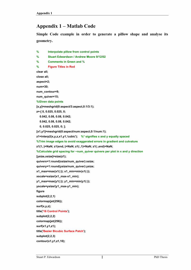
Appendix 1
Stuart P. Edwardson PhD Thesis I
Appendix 1 – Matlab Code Simple Code example in order to generate a pillow shape and analyse its
geometry. % Interpolate pillow from control points % Stuart Edwardson / Andrew Moore 9/12/02 % Comments in Green and % % Figure Titles in Red clear all; close all; aspect=2; num=30; num_contour=9; num_quiver=15; %Given data points [x,y]=meshgrid(0:aspect/3:aspect,0:1/3:1); z=-[ 0, 0.025, 0.025, 0; 0.042, 0.08, 0.08, 0.042; 0.042, 0.08, 0.08, 0.042; 0, 0.025, 0.025, 0; ]; [x1,y1]=meshgrid(0:aspect/num:aspect,0:1/num:1); z1=interp2(x,y,z,x1,y1,'cubic'); %* signifies x and y equally spaced %Trim image edges to avoid exaggerated errors in gradient and cutvature z1(1,:)=NaN; z1(end,:)=NaN; z1(:,1)=NaN; z1(:,end)=NaN; %Calculate grid spacing for ~num_quiver quivers per plot in x and y direction [ysize,xsize]=size(z1); quiverx=1:round(xsize/num_quiver):xsize; quivery=1:round(ysize/num_quiver):ysize; x1_max=max(x1(:)); x1_min=min(x1(:)); xscale=xsize/(x1_max-x1_min); y1_max=max(y1(:)); y1_min=min(y1(:)); yscale=ysize/(y1_max-y1_min); figure subplot(2,2,1) colormap(jet(256)); surf(x,y,z); title('16 Control Points'); subplot(2,2,2) colormap(jet(256)); surf(x1,y1,z1); title('Bezier Bicubic Surface Patch'); subplot(2,2,3) contour(x1,y1,z1,10);
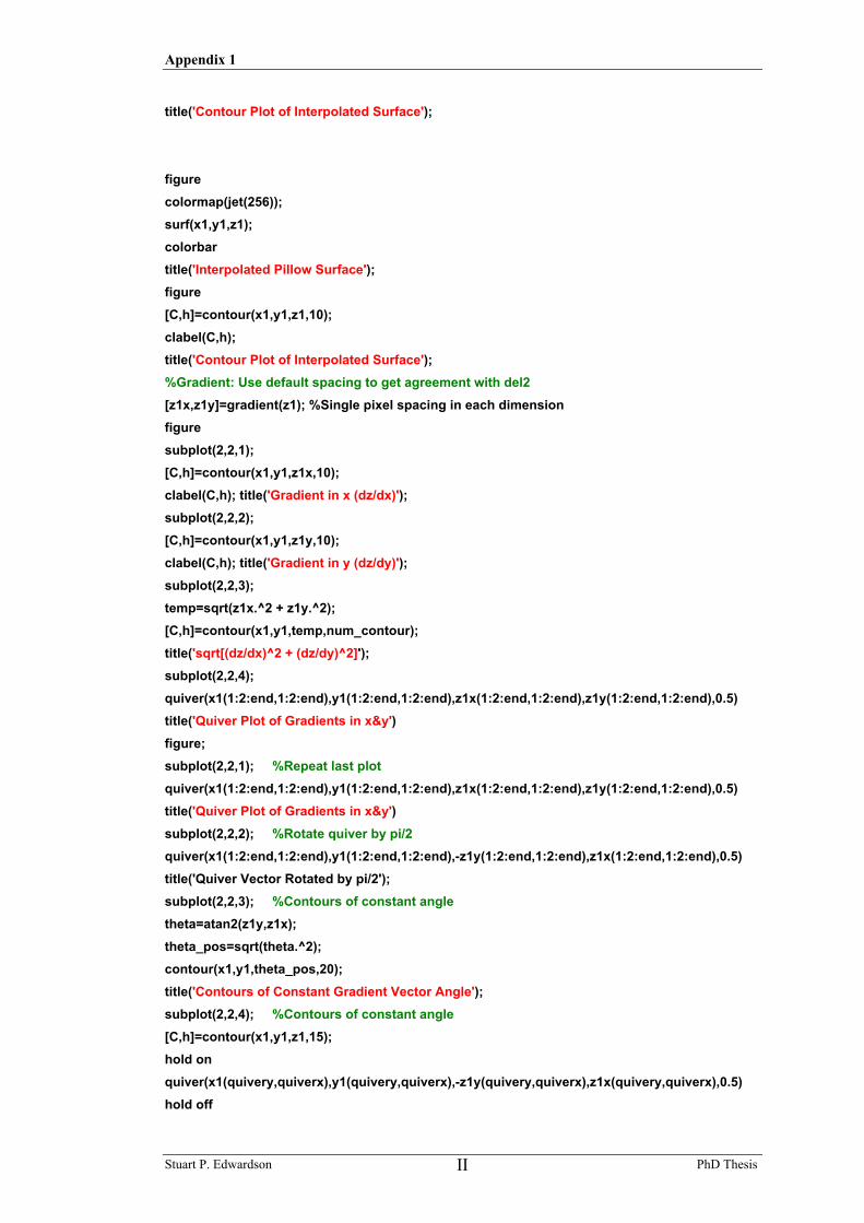
Appendix 1
Stuart P. Edwardson PhD Thesis II
title('Contour Plot of Interpolated Surface'); figure colormap(jet(256)); surf(x1,y1,z1); colorbar title('Interpolated Pillow Surface'); figure [C,h]=contour(x1,y1,z1,10); clabel(C,h); title('Contour Plot of Interpolated Surface'); %Gradient: Use default spacing to get agreement with del2 [z1x,z1y]=gradient(z1); %Single pixel spacing in each dimension figure subplot(2,2,1); [C,h]=contour(x1,y1,z1x,10); clabel(C,h); title('Gradient in x (dz/dx)'); subplot(2,2,2); [C,h]=contour(x1,y1,z1y,10); clabel(C,h); title('Gradient in y (dz/dy)'); subplot(2,2,3); temp=sqrt(z1x.^2 + z1y.^2); [C,h]=contour(x1,y1,temp,num_contour); title('sqrt[(dz/dx)^2 + (dz/dy)^2]'); subplot(2,2,4); quiver(x1(1:2:end,1:2:end),y1(1:2:end,1:2:end),z1x(1:2:end,1:2:end),z1y(1:2:end,1:2:end),0.5) title('Quiver Plot of Gradients in x&y') figure; subplot(2,2,1); %Repeat last plot quiver(x1(1:2:end,1:2:end),y1(1:2:end,1:2:end),z1x(1:2:end,1:2:end),z1y(1:2:end,1:2:end),0.5) title('Quiver Plot of Gradients in x&y') subplot(2,2,2); %Rotate quiver by pi/2 quiver(x1(1:2:end,1:2:end),y1(1:2:end,1:2:end),-z1y(1:2:end,1:2:end),z1x(1:2:end,1:2:end),0.5) title('Quiver Vector Rotated by pi/2'); subplot(2,2,3); %Contours of constant angle theta=atan2(z1y,z1x); theta_pos=sqrt(theta.^2); contour(x1,y1,theta_pos,20); title('Contours of Constant Gradient Vector Angle'); subplot(2,2,4); %Contours of constant angle [C,h]=contour(x1,y1,z1,15); hold on quiver(x1(quivery,quiverx),y1(quivery,quiverx),-z1y(quivery,quiverx),z1x(quivery,quiverx),0.5) hold off

Appendix 1
Stuart P. Edwardson PhD Thesis III
title('Contour Plot of Pillow Surface'); figure hold on [C,h]=contour(x1,y1,z1,15); axis([x1_min,x1_max,y1_min,y1_max]); temp_max=max(temp(:)); temp_min=min(temp(:)); %temp contains sqrt((dz/dx)^2 + (dz/dy)^2) temprange=(temp_max-temp_min); cur_pos=1; %Position in contour matrix C (for structure see help for contourc) for contour=1:size(h,1) %Loop over each contour for point=1:C(2,cur_pos)-1 %Count through each point on contour xi=round( C(1,cur_pos+point)*xscale ); %x values in C(1,:) y in C(2,:) yi=round( C(2,cur_pos+point)*yscale ); %Convert to array pixels sizei=round( 20*( (temp(yi,xi)-temp_min)/temprange ) + 0.5 ); %Scale to size of quiver arrow %+0.5 to avoid 0 (else plot fails) if ~isnan(sizei) if z1(yi,xi)<0 %Scan on other side if deflection negative plot(C(1,cur_pos+point),C(2,cur_pos+point),'.','MarkerSize',sizei,'MarkerEdgeColor','r'); else plot(C(1,cur_pos+point),C(2,cur_pos+point),'.','MarkerSize',sizei,'MarkerEdgeColor','b'); end end end cur_pos=cur_pos+C(2,cur_pos)+1; %Position of next contour end title('Contour Plot of Z1 with Representation of Vector Magnitude Along Contour Line'); hold off
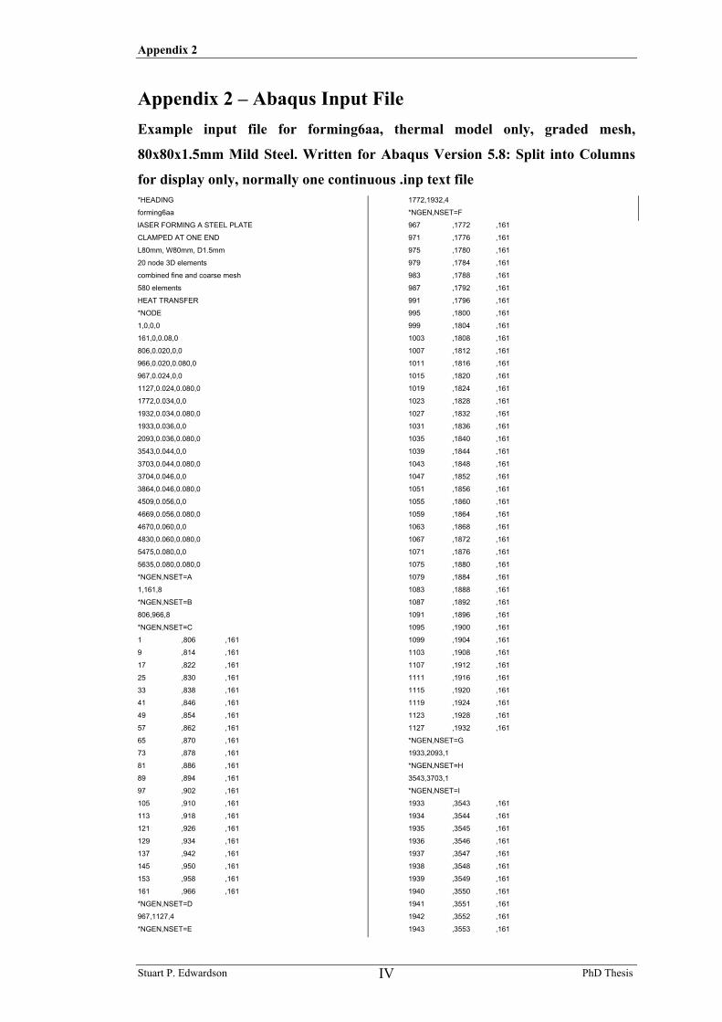
Appendix 2
Stuart P. Edwardson PhD Thesis IV
Appendix 2 – Abaqus Input File Example input file for forming6aa, thermal model only, graded mesh,
80x80x1.5mm Mild Steel. Written for Abaqus Version 5.8: Split into Columns
for display only, normally one continuous .inp text file *HEADING
forming6aa
lASER FORMING A STEEL PLATE
CLAMPED AT ONE END
L80mm, W80mm, D1.5mm
20 node 3D elements
combined fine and coarse mesh
580 elements
HEAT TRANSFER
*NODE
1,0,0,0
161,0,0.08,0
806,0.020,0,0
966,0.020,0.080,0
967,0.024,0,0
1127,0.024,0.080,0
1772,0.034,0,0
1932,0.034,0.080,0
1933,0.036,0,0
2093,0.036,0.080,0
3543,0.044,0,0
3703,0.044,0.080,0
3704,0.046,0,0
3864,0.046,0.080,0
4509,0.056,0,0
4669,0.056,0.080,0
4670,0.060,0,0
4830,0.060,0.080,0
5475,0.080,0,0
5635,0.080,0.080,0
*NGEN,NSET=A
1,161,8
*NGEN,NSET=B
806,966,8
*NGEN,NSET=C
1 ,806 ,161
9 ,814 ,161
17 ,822 ,161
25 ,830 ,161
33 ,838 ,161
41 ,846 ,161
49 ,854 ,161
57 ,862 ,161
65 ,870 ,161
73 ,878 ,161
81 ,886 ,161
89 ,894 ,161
97 ,902 ,161
105 ,910 ,161
113 ,918 ,161
121 ,926 ,161
129 ,934 ,161
137 ,942 ,161
145 ,950 ,161
153 ,958 ,161
161 ,966 ,161
*NGEN,NSET=D
967,1127,4
*NGEN,NSET=E
1772,1932,4
*NGEN,NSET=F
967 ,1772 ,161
971 ,1776 ,161
975 ,1780 ,161
979 ,1784 ,161
983 ,1788 ,161
987 ,1792 ,161
991 ,1796 ,161
995 ,1800 ,161
999 ,1804 ,161
1003 ,1808 ,161
1007 ,1812 ,161
1011 ,1816 ,161
1015 ,1820 ,161
1019 ,1824 ,161
1023 ,1828 ,161
1027 ,1832 ,161
1031 ,1836 ,161
1035 ,1840 ,161
1039 ,1844 ,161
1043 ,1848 ,161
1047 ,1852 ,161
1051 ,1856 ,161
1055 ,1860 ,161
1059 ,1864 ,161
1063 ,1868 ,161
1067 ,1872 ,161
1071 ,1876 ,161
1075 ,1880 ,161
1079 ,1884 ,161
1083 ,1888 ,161
1087 ,1892 ,161
1091 ,1896 ,161
1095 ,1900 ,161
1099 ,1904 ,161
1103 ,1908 ,161
1107 ,1912 ,161
1111 ,1916 ,161
1115 ,1920 ,161
1119 ,1924 ,161
1123 ,1928 ,161
1127 ,1932 ,161
*NGEN,NSET=G
1933,2093,1
*NGEN,NSET=H
3543,3703,1
*NGEN,NSET=I
1933 ,3543 ,161
1934 ,3544 ,161
1935 ,3545 ,161
1936 ,3546 ,161
1937 ,3547 ,161
1938 ,3548 ,161
1939 ,3549 ,161
1940 ,3550 ,161
1941 ,3551 ,161
1942 ,3552 ,161
1943 ,3553 ,161
Appendix 2
Stuart P. Edwardson PhD Thesis V
1944 ,3554 ,161
1945 ,3555 ,161
1946 ,3556 ,161
1947 ,3557 ,161
1948 ,3558 ,161
1949 ,3559 ,161
1950 ,3560 ,161
1951 ,3561 ,161
1952 ,3562 ,161
1953 ,3563 ,161
1954 ,3564 ,161
1955 ,3565 ,161
1956 ,3566 ,161
1957 ,3567 ,161
1958 ,3568 ,161
1959 ,3569 ,161
1960 ,3570 ,161
1961 ,3571 ,161
1962 ,3572 ,161
1963 ,3573 ,161
1964 ,3574 ,161
1965 ,3575 ,161
1966 ,3576 ,161
1967 ,3577 ,161
1968 ,3578 ,161
1969 ,3579 ,161
1970 ,3580 ,161
1971 ,3581 ,161
1972 ,3582 ,161
1973 ,3583 ,161
1974 ,3584 ,161
1975 ,3585 ,161
1976 ,3586 ,161
1977 ,3587 ,161
1978 ,3588 ,161
1979 ,3589 ,161
1980 ,3590 ,161
1981 ,3591 ,161
1982 ,3592 ,161
1983 ,3593 ,161
1984 ,3594 ,161
1985 ,3595 ,161
1986 ,3596 ,161
1987 ,3597 ,161
1988 ,3598 ,161
1989 ,3599 ,161
1990 ,3600 ,161
1991 ,3601 ,161
1992 ,3602 ,161
1993 ,3603 ,161
1994 ,3604 ,161
1995 ,3605 ,161
1996 ,3606 ,161
1997 ,3607 ,161
1998 ,3608 ,161
1999 ,3609 ,161
2000 ,3610 ,161
2001 ,3611 ,161
2002 ,3612 ,161
2003 ,3613 ,161
2004 ,3614 ,161
2005 ,3615 ,161
2006 ,3616 ,161
2007 ,3617 ,161
2008 ,3618 ,161
2009 ,3619 ,161
2010 ,3620 ,161
2011 ,3621 ,161
2012 ,3622 ,161
2013 ,3623 ,161
2014 ,3624 ,161
2015 ,3625 ,161
2016 ,3626 ,161
2017 ,3627 ,161
2018 ,3628 ,161
2019 ,3629 ,161
2020 ,3630 ,161
2021 ,3631 ,161
2022 ,3632 ,161
2023 ,3633 ,161
2024 ,3634 ,161
2025 ,3635 ,161
2026 ,3636 ,161
2027 ,3637 ,161
2028 ,3638 ,161
2029 ,3639 ,161
2030 ,3640 ,161
2031 ,3641 ,161
2032 ,3642 ,161
2033 ,3643 ,161
2034 ,3644 ,161
2035 ,3645 ,161
2036 ,3646 ,161
2037 ,3647 ,161
2038 ,3648 ,161
2039 ,3649 ,161
2040 ,3650 ,161
2041 ,3651 ,161
2042 ,3652 ,161
2043 ,3653 ,161
2044 ,3654 ,161
2045 ,3655 ,161
2046 ,3656 ,161
2047 ,3657 ,161
2048 ,3658 ,161
2049 ,3659 ,161
2050 ,3660 ,161
2051 ,3661 ,161
2052 ,3662 ,161
2053 ,3663 ,161
2054 ,3664 ,161
2055 ,3665 ,161
2056 ,3666 ,161
2057 ,3667 ,161
2058 ,3668 ,161
2059 ,3669 ,161
2060 ,3670 ,161
2061 ,3671 ,161
2062 ,3672 ,161
2063 ,3673 ,161
2064 ,3674 ,161
2065 ,3675 ,161
2066 ,3676 ,161
2067 ,3677 ,161
2068 ,3678 ,161
2069 ,3679 ,161
2070 ,3680 ,161
2071 ,3681 ,161
2072 ,3682 ,161
2073 ,3683 ,161
2074 ,3684 ,161
2075 ,3685 ,161
2076 ,3686 ,161
2077 ,3687 ,161
Appendix 2
Stuart P. Edwardson PhD Thesis VI
2078 ,3688 ,161
2079 ,3689 ,161
2080 ,3690 ,161
2081 ,3691 ,161
2082 ,3692 ,161
2083 ,3693 ,161
2084 ,3694 ,161
2085 ,3695 ,161
2086 ,3696 ,161
2087 ,3697 ,161
2088 ,3698 ,161
2089 ,3699 ,161
2090 ,3700 ,161
2091 ,3701 ,161
2092 ,3702 ,161
2093 ,3703 ,161
*NGEN,NSET=J
3704,3864,4
*NGEN,NSET=K
4509,4669,4
*NGEN,NSET=L
3704 ,4509 ,161
3708 ,4513 ,161
3712 ,4517 ,161
3716 ,4521 ,161
3720 ,4525 ,161
3724 ,4529 ,161
3728 ,4533 ,161
3732 ,4537 ,161
3736 ,4541 ,161
3740 ,4545 ,161
3744 ,4549 ,161
3748 ,4553 ,161
3752 ,4557 ,161
3756 ,4561 ,161
3760 ,4565 ,161
3764 ,4569 ,161
3768 ,4573 ,161
3772 ,4577 ,161
3776 ,4581 ,161
3780 ,4585 ,161
3784 ,4589 ,161
3788 ,4593 ,161
3792 ,4597 ,161
3796 ,4601 ,161
3800 ,4605 ,161
3804 ,4609 ,161
3808 ,4613 ,161
3812 ,4617 ,161
3816 ,4621 ,161
3820 ,4625 ,161
3824 ,4629 ,161
3828 ,4633 ,161
3832 ,4637 ,161
3836 ,4641 ,161
3840 ,4645 ,161
3844 ,4649 ,161
3848 ,4653 ,161
3852 ,4657 ,161
3856 ,4661 ,161
3860 ,4665 ,161
3864 ,4669 ,161
*NGEN,NSET=M
4670,4830,8
*NGEN,NSET=N
5475,5635,8
*NGEN,NSET=O
4670 ,5475 ,161
4678 ,5483 ,161
4686 ,5491 ,161
4694 ,5499 ,161
4702 ,5507 ,161
4710 ,5515 ,161
4718 ,5523 ,161
4726 ,5531 ,161
4734 ,5539 ,161
4742 ,5547 ,161
4750 ,5555 ,161
4758 ,5563 ,161
4766 ,5571 ,161
4774 ,5579 ,161
4782 ,5587 ,161
4790 ,5595 ,161
4798 ,5603 ,161
4806 ,5611 ,161
4814 ,5619 ,161
4822 ,5627 ,161
4830 ,5635 ,161
*NSET,NSET=BOT
A,B,C,D,E,F,G,H,I,J,K,L,M,N,O
*NCOPY,SHIFT,CHANGE NUMBER=10000,OLD SET=BOT,NEW
SET=MID
0.,0.,0.00075
0.,0.,0.,0.,0.,1.,0.
*NCOPY,SHIFT,CHANGE NUMBER=20000,OLD SET=BOT,NEW
SET=TOP
0.,0.,0.0015
0.,0.,0.,0.,0.,1.,0.
*NSET,NSET=ALL
BOT,MID,TOP
*NSET,NSET=ENDA,GENERATE
20001,20161,8
*NSET,NSET=END
ENDA,A
*ELEMENT, TYPE=DC3D20
1,1,323,339,17,20001,20323,20339,20017,162,331,
178,9,20162,20331,20178,20009,
10001,10323,10339,10017
*ELEMENT, TYPE=DC3D20
31,967,1289,1297,975,20967,21289,21297,
20975,1128,1293,1136,971,21128,21293,
21136,20971,10967,11289,11297,10975
*ELEMENT, TYPE=DC3D20
91,1933,2255,2257,1935,21933,22255,22257,21935,
2094,2256,2096,1934,22094,22256,
22096,21934,11933,12255,12257,11935
*ELEMENT, TYPE=DC3D20
491,3543,3865,3873,3551,23543,23865,23873,23551,
3704,3869,3712,3547,23704,23869,23712,
23547,13543,13865,13873,13551
*ELEMENT, TYPE=DC3D20
551,4509,4831,4847,4525,24509,24831,24847,24525,
4670,4839,4686,4517,24670,24839,24686,
24517,14509,14831,14847,14525
*ELGEN,ELSET=L1
1,10,16,1,3,322,10
*ELGEN,ELSET=L2
31,20,8,1,3,322,20
*ELGEN,ELSET=CENTRE
91,80,2,1,5,322,80
*ELGEN,ELSET=R2
491,20,8,1,3,322,20
*ELGEN,ELSET=R1
551,10,16,1,3,322,10
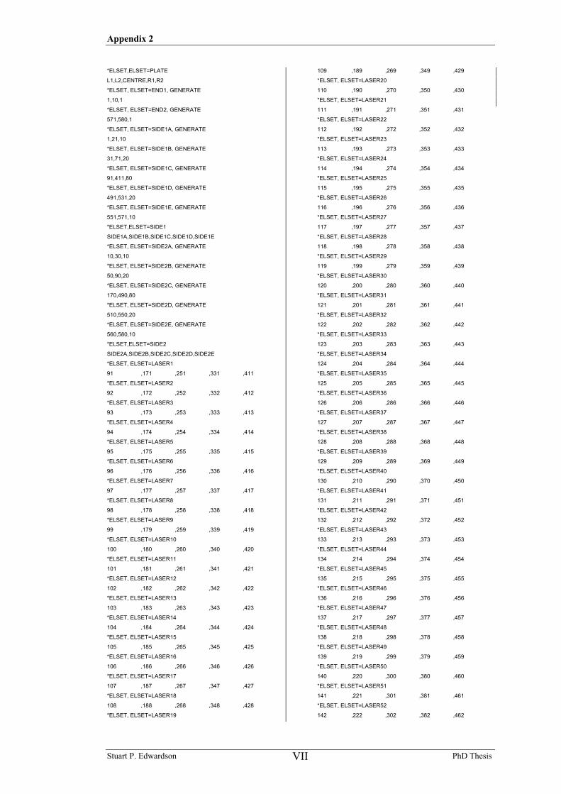
Appendix 2
Stuart P. Edwardson PhD Thesis VII
*ELSET,ELSET=PLATE
L1,L2,CENTRE,R1,R2
*ELSET, ELSET=END1, GENERATE
1,10,1
*ELSET, ELSET=END2, GENERATE
571,580,1
*ELSET, ELSET=SIDE1A, GENERATE
1,21,10
*ELSET, ELSET=SIDE1B, GENERATE
31,71,20
*ELSET, ELSET=SIDE1C, GENERATE
91,411,80
*ELSET, ELSET=SIDE1D, GENERATE
491,531,20
*ELSET, ELSET=SIDE1E, GENERATE
551,571,10
*ELSET,ELSET=SIDE1
SIDE1A,SIDE1B,SIDE1C,SIDE1D,SIDE1E
*ELSET, ELSET=SIDE2A, GENERATE
10,30,10
*ELSET, ELSET=SIDE2B, GENERATE
50,90,20
*ELSET, ELSET=SIDE2C, GENERATE
170,490,80
*ELSET, ELSET=SIDE2D, GENERATE
510,550,20
*ELSET, ELSET=SIDE2E, GENERATE
560,580,10
*ELSET,ELSET=SIDE2
SIDE2A,SIDE2B,SIDE2C,SIDE2D,SIDE2E
*ELSET, ELSET=LASER1
91 ,171 ,251 ,331 ,411
*ELSET, ELSET=LASER2
92 ,172 ,252 ,332 ,412
*ELSET, ELSET=LASER3
93 ,173 ,253 ,333 ,413
*ELSET, ELSET=LASER4
94 ,174 ,254 ,334 ,414
*ELSET, ELSET=LASER5
95 ,175 ,255 ,335 ,415
*ELSET, ELSET=LASER6
96 ,176 ,256 ,336 ,416
*ELSET, ELSET=LASER7
97 ,177 ,257 ,337 ,417
*ELSET, ELSET=LASER8
98 ,178 ,258 ,338 ,418
*ELSET, ELSET=LASER9
99 ,179 ,259 ,339 ,419
*ELSET, ELSET=LASER10
100 ,180 ,260 ,340 ,420
*ELSET, ELSET=LASER11
101 ,181 ,261 ,341 ,421
*ELSET, ELSET=LASER12
102 ,182 ,262 ,342 ,422
*ELSET, ELSET=LASER13
103 ,183 ,263 ,343 ,423
*ELSET, ELSET=LASER14
104 ,184 ,264 ,344 ,424
*ELSET, ELSET=LASER15
105 ,185 ,265 ,345 ,425
*ELSET, ELSET=LASER16
106 ,186 ,266 ,346 ,426
*ELSET, ELSET=LASER17
107 ,187 ,267 ,347 ,427
*ELSET, ELSET=LASER18
108 ,188 ,268 ,348 ,428
*ELSET, ELSET=LASER19
109 ,189 ,269 ,349 ,429
*ELSET, ELSET=LASER20
110 ,190 ,270 ,350 ,430
*ELSET, ELSET=LASER21
111 ,191 ,271 ,351 ,431
*ELSET, ELSET=LASER22
112 ,192 ,272 ,352 ,432
*ELSET, ELSET=LASER23
113 ,193 ,273 ,353 ,433
*ELSET, ELSET=LASER24
114 ,194 ,274 ,354 ,434
*ELSET, ELSET=LASER25
115 ,195 ,275 ,355 ,435
*ELSET, ELSET=LASER26
116 ,196 ,276 ,356 ,436
*ELSET, ELSET=LASER27
117 ,197 ,277 ,357 ,437
*ELSET, ELSET=LASER28
118 ,198 ,278 ,358 ,438
*ELSET, ELSET=LASER29
119 ,199 ,279 ,359 ,439
*ELSET, ELSET=LASER30
120 ,200 ,280 ,360 ,440
*ELSET, ELSET=LASER31
121 ,201 ,281 ,361 ,441
*ELSET, ELSET=LASER32
122 ,202 ,282 ,362 ,442
*ELSET, ELSET=LASER33
123 ,203 ,283 ,363 ,443
*ELSET, ELSET=LASER34
124 ,204 ,284 ,364 ,444
*ELSET, ELSET=LASER35
125 ,205 ,285 ,365 ,445
*ELSET, ELSET=LASER36
126 ,206 ,286 ,366 ,446
*ELSET, ELSET=LASER37
127 ,207 ,287 ,367 ,447
*ELSET, ELSET=LASER38
128 ,208 ,288 ,368 ,448
*ELSET, ELSET=LASER39
129 ,209 ,289 ,369 ,449
*ELSET, ELSET=LASER40
130 ,210 ,290 ,370 ,450
*ELSET, ELSET=LASER41
131 ,211 ,291 ,371 ,451
*ELSET, ELSET=LASER42
132 ,212 ,292 ,372 ,452
*ELSET, ELSET=LASER43
133 ,213 ,293 ,373 ,453
*ELSET, ELSET=LASER44
134 ,214 ,294 ,374 ,454
*ELSET, ELSET=LASER45
135 ,215 ,295 ,375 ,455
*ELSET, ELSET=LASER46
136 ,216 ,296 ,376 ,456
*ELSET, ELSET=LASER47
137 ,217 ,297 ,377 ,457
*ELSET, ELSET=LASER48
138 ,218 ,298 ,378 ,458
*ELSET, ELSET=LASER49
139 ,219 ,299 ,379 ,459
*ELSET, ELSET=LASER50
140 ,220 ,300 ,380 ,460
*ELSET, ELSET=LASER51
141 ,221 ,301 ,381 ,461
*ELSET, ELSET=LASER52
142 ,222 ,302 ,382 ,462
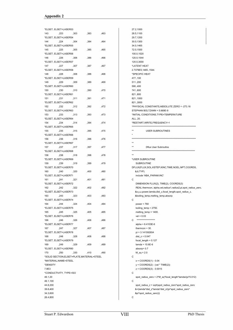
Appendix 2
Stuart P. Edwardson PhD Thesis VIII
*ELSET, ELSET=LASER53
143 ,223 ,303 ,383 ,463
*ELSET, ELSET=LASER54
144 ,224 ,304 ,384 ,464
*ELSET, ELSET=LASER55
145 ,225 ,305 ,385 ,465
*ELSET, ELSET=LASER56
146 ,226 ,306 ,386 ,466
*ELSET, ELSET=LASER57
147 ,227 ,307 ,387 ,467
*ELSET, ELSET=LASER58
148 ,228 ,308 ,388 ,468
*ELSET, ELSET=LASER59
149 ,229 ,309 ,389 ,469
*ELSET, ELSET=LASER60
150 ,230 ,310 ,390 ,470
*ELSET, ELSET=LASER61
151 ,231 ,311 ,391 ,471
*ELSET, ELSET=LASER62
152 ,232 ,312 ,392 ,472
*ELSET, ELSET=LASER63
153 ,233 ,313 ,393 ,473
*ELSET, ELSET=LASER64
154 ,234 ,314 ,394 ,474
*ELSET, ELSET=LASER65
155 ,235 ,315 ,395 ,475
*ELSET, ELSET=LASER66
156 ,236 ,316 ,396 ,476
*ELSET, ELSET=LASER67
157 ,237 ,317 ,397 ,477
*ELSET, ELSET=LASER68
158 ,238 ,318 ,398 ,478
*ELSET, ELSET=LASER69
159 ,239 ,319 ,399 ,479
*ELSET, ELSET=LASER70
160 ,240 ,320 ,400 ,480
*ELSET, ELSET=LASER71
161 ,241 ,321 ,401 ,481
*ELSET, ELSET=LASER72
162 ,242 ,322 ,402 ,482
*ELSET, ELSET=LASER73
163 ,243 ,323 ,403 ,483
*ELSET, ELSET=LASER74
164 ,244 ,324 ,404 ,484
*ELSET, ELSET=LASER75
165 ,245 ,325 ,405 ,485
*ELSET, ELSET=LASER76
166 ,246 ,326 ,406 ,486
*ELSET, ELSET=LASER77
167 ,247 ,327 ,407 ,487
*ELSET, ELSET=LASER78
168 ,248 ,328 ,408 ,488
*ELSET, ELSET=LASER79
169 ,249 ,329 ,409 ,489
*ELSET, ELSET=LASER80
170 ,250 ,330 ,410 ,490
*SOLID SECTION,ELSET=PLATE,MATERIAL=STEEL
*MATERIAL,NAME=STEEL
*DENSITY
7.8E3
*CONDUCTIVITY, TYPE=ISO
46.1,20
46.1,100
44.8,200
39.8,400
34.3,600
26.4,800
27.2,1000
28.5,1100
29.7,1200
30.0,1300
34.0,1465
72.0,1500
100.0,1520
120.0,1544
120.0,3000
*LATENT HEAT
2.7379E5,1465.,1544.
*SPECIFIC HEAT
477.,100
511.,200
590.,400
741.,600
821.,800
821.,1000
821.,3000
*PHYSICAL CONSTANTS,ABSOLUTE ZERO = -273.16
STEPHAN BOLTZANN = 5.669E-9
*INITIAL CONDITIONS,TYPE=TEMPERATURE
ALL, 20.
*RESTART,WRITE,FREQUENCY=1
**********************************************************************
** USER SUBROUTINES
*
**********************************************************************
**
** Dflux User Subroutine
*********************************************************************
**
*USER SUBROUTINE
SUBROUTINE
DFLUX(FLUX,SOL,KSTEP,KINC,TIME,NOEL,NPT,COORDS,
&JLTYP)
include 'ABA_PARAM.INC'
C
DIMENSION FLUX(2), TIME(2), COORDS(3)
REAL thermcon, alpha,vel,radius1,radius2,pi,spot_radius_zero,
&x,y,z,power,lamda,dist_z,focal_length,spot_radius_z,
&boiling_temp,melting_temp,absorp
C
power = 760
boiling_temp = 2750.
melting_temp = 1400.
vel = 0.03
C ********************
alpha = 6.4103E-6
thermcon = 30.
pi = 3.141592654
dist_z = 0.047
focal_length = 0.127
lamda = 10.6E-6
absorp= 0.7
M_sq = 2.0
C
x = COORDS(1) - 0.04
y = COORDS(2) - (vel * TIME(2))
z = COORDS(3) - 0.0015
C
spot_radius_zero = 2*M_sq*focal_length*lamda/(pi*0.012)
C
spot_radius_z = sqrt(spot_radius_zero*spot_radius_zero
&+(lamda*dist_z*lamda*dist_z/(pi*spot_radius_zero*
&pi*spot_radius_zero)))
C
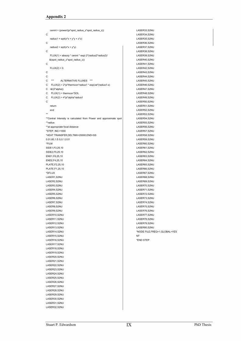
Appendix 2
Stuart P. Edwardson PhD Thesis IX
cenint = (power/(pi*spot_radius_z*spot_radius_z))
C
radius1 = sqrt(x*x + y*y + z*z)
C
radius2 = sqrt(x*x + y*y)
C
FLUX(1) = absorp * cenint * exp(-2*(radius2*radius2)/
&(spot_radius_z*spot_radius_z))
C
FLUX(2) = 0.
C
C
C *** ALTERNATIVE FLUXES ***
C FLUX(2) = 2*pi*thermcon*radius1 * exp(vel*(radius1-x)
C &/(2*alpha))
C FLUX(1) = thermcon*SOL
C FLUX(2) = 4*pi*alpha*radius1
C
return
end
**
**Central Intensity is calculated from Power and approximate spot
**radius
**at appropriate focal distance
*STEP, INC=1000
*HEAT TRANSFER,DELTMX=20000,END=SS
0.01,60,1.E-5,0.1,0.01
*FILM
SIDE1,F3,25,10
SIDE2,F5,25,10
END1,F6,25,10
END2,F4,25,10
PLATE,F2,25,10
PLATE,F1,25,10
*DFLUX
LASER1,S2NU
LASER2,S2NU
LASER3,S2NU
LASER4,S2NU
LASER5,S2NU
LASER6,S2NU
LASER7,S2NU
LASER8,S2NU
LASER9,S2NU
LASER10,S2NU
LASER11,S2NU
LASER12,S2NU
LASER13,S2NU
LASER14,S2NU
LASER15,S2NU
LASER16,S2NU
LASER17,S2NU
LASER18,S2NU
LASER19,S2NU
LASER20,S2NU
LASER21,S2NU
LASER22,S2NU
LASER23,S2NU
LASER24,S2NU
LASER25,S2NU
LASER26,S2NU
LASER27,S2NU
LASER28,S2NU
LASER29,S2NU
LASER30,S2NU
LASER31,S2NU
LASER32,S2NU
LASER33,S2NU
LASER34,S2NU
LASER35,S2NU
LASER36,S2NU
LASER37,S2NU
LASER38,S2NU
LASER39,S2NU
LASER40,S2NU
LASER41,S2NU
LASER42,S2NU
LASER43,S2NU
LASER44,S2NU
LASER45,S2NU
LASER46,S2NU
LASER47,S2NU
LASER48,S2NU
LASER49,S2NU
LASER50,S2NU
LASER51,S2NU
LASER52,S2NU
LASER53,S2NU
LASER54,S2NU
LASER55,S2NU
LASER56,S2NU
LASER57,S2NU
LASER58,S2NU
LASER59,S2NU
LASER60,S2NU
LASER61,S2NU
LASER62,S2NU
LASER63,S2NU
LASER64,S2NU
LASER65,S2NU
LASER66,S2NU
LASER67,S2NU
LASER68,S2NU
LASER69,S2NU
LASER70,S2NU
LASER71,S2NU
LASER72,S2NU
LASER73,S2NU
LASER74,S2NU
LASER75,S2NU
LASER76,S2NU
LASER77,S2NU
LASER78,S2NU
LASER79,S2NU
LASER80,S2NU
*NODE FILE,FREQ=1,GLOBAL=YES
NT
*END STEP
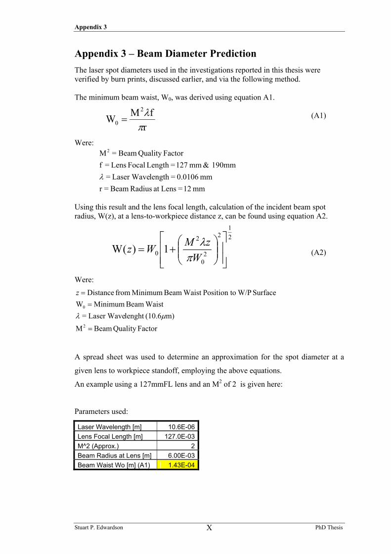
Appendix 3
Stuart P. Edwardson PhD Thesis X
Appendix 3 – Beam Diameter Prediction The laser spot diameters used in the investigations reported in this thesis were verified by burn prints, discussed earlier, and via the following method. The minimum beam waist, W0, was derived using equation A1. (A1)
Were:
mm 12 =Lensat Radius Beam =rmm 0.0106 =length Laser Wave =
190mm & mm 127 =Length Focal Lens =fFactorQuality Beam= M2
λ
Using this result and the lens focal length, calculation of the incident beam spot radius, W(z), at a lens-to-workpiece distance z, can be found using equation A2. (A2) Were:
A spread sheet was used to determine an approximation for the spot diameter at a
given lens to workpiece standoff, employing the above equations.
An example using a 127mmFL lens and an M2 of 2 is given here:
Parameters used:
Laser Wavelength [m] 10.6E-06Lens Focal Length [m] 127.0E-03M^2 (Approx.) 2Beam Radius at Lens [m] 6.00E-03Beam Waist Wo [m] (A1) 1.43E-04
rfMW
2
0 πλ
=
21
2
20
2
0 1)(W
+=
WzMWz
πλ
FactorQuality Beam Mm)(10.6lenght Laser Wave=
Waist Beam MinimumW Surface W/PoPosition t Waist Beam Minimum from Distance
2
0
=
==
µλ
z
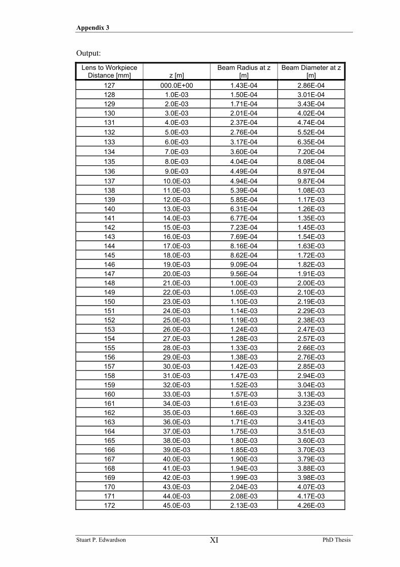
Appendix 3
Stuart P. Edwardson PhD Thesis XI
Output:
Lens to Workpiece Distance [mm] z [m]
Beam Radius at z [m]
Beam Diameter at z [m]
127 000.0E+00 1.43E-04 2.86E-04 128 1.0E-03 1.50E-04 3.01E-04 129 2.0E-03 1.71E-04 3.43E-04 130 3.0E-03 2.01E-04 4.02E-04 131 4.0E-03 2.37E-04 4.74E-04 132 5.0E-03 2.76E-04 5.52E-04 133 6.0E-03 3.17E-04 6.35E-04 134 7.0E-03 3.60E-04 7.20E-04 135 8.0E-03 4.04E-04 8.08E-04 136 9.0E-03 4.49E-04 8.97E-04 137 10.0E-03 4.94E-04 9.87E-04 138 11.0E-03 5.39E-04 1.08E-03 139 12.0E-03 5.85E-04 1.17E-03 140 13.0E-03 6.31E-04 1.26E-03 141 14.0E-03 6.77E-04 1.35E-03 142 15.0E-03 7.23E-04 1.45E-03 143 16.0E-03 7.69E-04 1.54E-03 144 17.0E-03 8.16E-04 1.63E-03 145 18.0E-03 8.62E-04 1.72E-03 146 19.0E-03 9.09E-04 1.82E-03 147 20.0E-03 9.56E-04 1.91E-03 148 21.0E-03 1.00E-03 2.00E-03 149 22.0E-03 1.05E-03 2.10E-03 150 23.0E-03 1.10E-03 2.19E-03 151 24.0E-03 1.14E-03 2.29E-03 152 25.0E-03 1.19E-03 2.38E-03 153 26.0E-03 1.24E-03 2.47E-03 154 27.0E-03 1.28E-03 2.57E-03 155 28.0E-03 1.33E-03 2.66E-03 156 29.0E-03 1.38E-03 2.76E-03 157 30.0E-03 1.42E-03 2.85E-03 158 31.0E-03 1.47E-03 2.94E-03 159 32.0E-03 1.52E-03 3.04E-03 160 33.0E-03 1.57E-03 3.13E-03 161 34.0E-03 1.61E-03 3.23E-03 162 35.0E-03 1.66E-03 3.32E-03 163 36.0E-03 1.71E-03 3.41E-03 164 37.0E-03 1.75E-03 3.51E-03 165 38.0E-03 1.80E-03 3.60E-03 166 39.0E-03 1.85E-03 3.70E-03 167 40.0E-03 1.90E-03 3.79E-03 168 41.0E-03 1.94E-03 3.88E-03 169 42.0E-03 1.99E-03 3.98E-03 170 43.0E-03 2.04E-03 4.07E-03 171 44.0E-03 2.08E-03 4.17E-03 172 45.0E-03 2.13E-03 4.26E-03
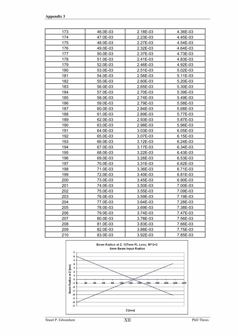
Appendix 3
Stuart P. Edwardson PhD Thesis XII
173 46.0E-03 2.18E-03 4.36E-03 174 47.0E-03 2.23E-03 4.45E-03 175 48.0E-03 2.27E-03 4.54E-03 176 49.0E-03 2.32E-03 4.64E-03 177 50.0E-03 2.37E-03 4.73E-03 178 51.0E-03 2.41E-03 4.83E-03 179 52.0E-03 2.46E-03 4.92E-03 180 53.0E-03 2.51E-03 5.02E-03 181 54.0E-03 2.56E-03 5.11E-03 182 55.0E-03 2.60E-03 5.20E-03 183 56.0E-03 2.65E-03 5.30E-03 184 57.0E-03 2.70E-03 5.39E-03 185 58.0E-03 2.74E-03 5.49E-03 186 59.0E-03 2.79E-03 5.58E-03 187 60.0E-03 2.84E-03 5.68E-03 188 61.0E-03 2.89E-03 5.77E-03 189 62.0E-03 2.93E-03 5.87E-03 190 63.0E-03 2.98E-03 5.96E-03 191 64.0E-03 3.03E-03 6.05E-03 192 65.0E-03 3.07E-03 6.15E-03 193 66.0E-03 3.12E-03 6.24E-03 194 67.0E-03 3.17E-03 6.34E-03 195 68.0E-03 3.22E-03 6.43E-03 196 69.0E-03 3.26E-03 6.53E-03 197 70.0E-03 3.31E-03 6.62E-03 198 71.0E-03 3.36E-03 6.71E-03 199 72.0E-03 3.40E-03 6.81E-03 200 73.0E-03 3.45E-03 6.90E-03 201 74.0E-03 3.50E-03 7.00E-03 202 75.0E-03 3.55E-03 7.09E-03 203 76.0E-03 3.59E-03 7.19E-03 204 77.0E-03 3.64E-03 7.28E-03 205 78.0E-03 3.69E-03 7.38E-03 206 79.0E-03 3.74E-03 7.47E-03 207 80.0E-03 3.78E-03 7.56E-03 208 81.0E-03 3.83E-03 7.66E-03 209 82.0E-03 3.88E-03 7.75E-03 210 83.0E-03 3.92E-03 7.85E-03
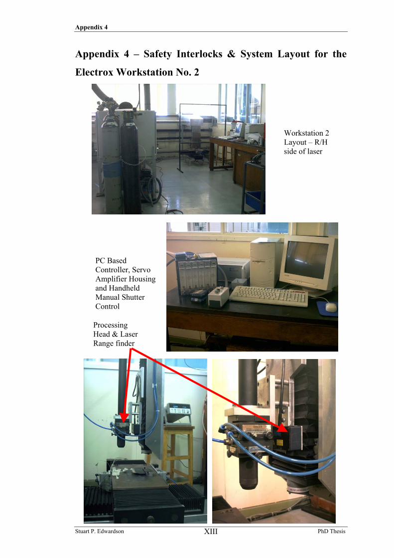
Appendix 4
Stuart P. Edwardson PhD Thesis XIII
Appendix 4 – Safety Interlocks & System Layout for the
Electrox Workstation No. 2
Workstation 2 Layout – R/H side of laser
PC Based Controller, Servo Amplifier Housing and Handheld Manual Shutter Control
Processing Head & Laser Range finder
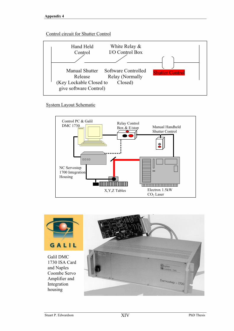
Appendix 4
Stuart P. Edwardson PhD Thesis XIV
Manual Shutter Release
(Key Lockable Closed to give software Control)
Software Controlled Relay (Normally
Closed)
Shutter Control
Hand Held Control
White Relay & I/O Control Box
Control circuit for Shutter Control
Galil DMC 1730 ISA Card and Naples Coombe Servo Amplifier and Integration housing
System Layout Schematic
Control PC & Galil DMC 1730
NC Servostep 1700 Integration Housing
X,Y,Z Tables Electrox 1.5kW CO2 Laser
Manual Handheld Shutter Control
Relay Control Box & E/stop
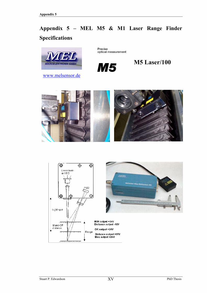
Appendix 5
Stuart P. Edwardson PhD Thesis XV
Appendix 5 – MEL M5 & M1 Laser Range Finder
Specifications
www.melsensor.de
M5 Laser/100
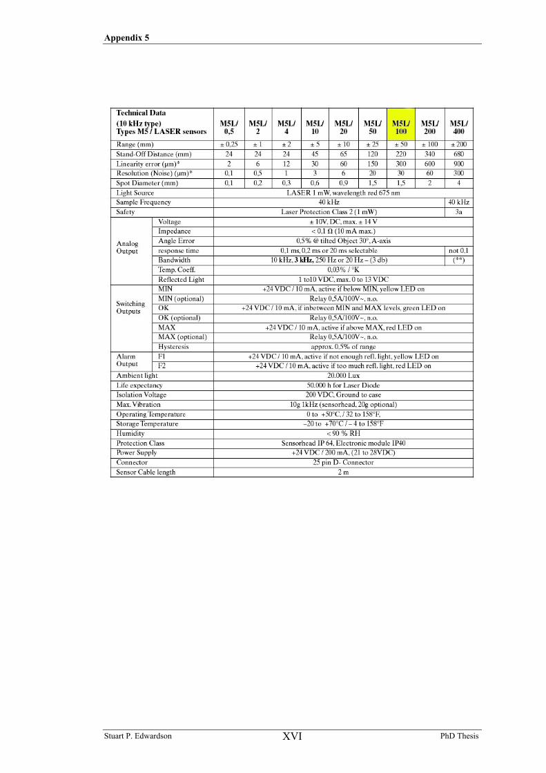
Appendix 5
Stuart P. Edwardson PhD Thesis XVI
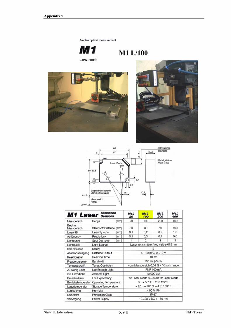
Appendix 5
Stuart P. Edwardson PhD Thesis XVII
M1 L/100

Appendix 6
Stuart P. Edwardson PhD Thesis XVIII
Appendix 6 – Example Galil CNC Code Program to linearly interpolate along three lines that are defined by a series of X & Y points Starting speed and end speed between each point is also specified Values are given as ‘Encoded Counts’ 1mm = 400 counts, Comments are not part of the CNC file #Z1 Internal program name SB1 Unlock Z Axis SB3 Arm Shutter (closed) SP16000,16000,30000 Set general speed X,Y,Z AC450000,450000,900000 Set general acceleration X,Y,Z DC450000,450000,900000 Set general de-acceleration X,Y,Z PA63841,36667,0 Specify an absolute position BG Begin Movement to position AM Wait until movement complete CB3 Open Shutter WT200 Wait 200ms for shutter to open LM XY Specify Linear Interpolation Mode in X&Y VA100000 Vector Acceleration VD100000 Vector De-Acceleration LI2826,-2292 <34162 >34162 Linear Interpolation through these points LI3333,-2470 <34162 >34162 XCo-ordinate,Yco-ordinate,<Starting Speed >End speed LI4000,-1576 <34162 >34162 for each segment LI3333,-700 <34162 >34162 LI4000,-77 <34162 >34162 LI4000,806 <34162 >34162 LI4000,1205 <34162 >34162 LI3333,1793 <34162 >34162 LI3333,2750 <34162 >34162 LI1335,3228 <34162 >34162 LI-1435,4000 <34162 >34162 LI-3234,2059 <34162 >34162 LI-3868,1941 <34162 >34162 LI-3465,1675 <34162 >34162 LI-4000,943 <34162 >34162 LI-4000,-303 <34162 >34162 LI-3759,-982 <34162 >34162 LI-3574,-1550 <34162 >34162 LI-3503,-2450 <34162 >34162 LI-2497,-2059 <34162 >34162 LI-1333,-4280 <34162 >34162 LE Linear Interpolation Mode End BGS Begin Specified Sequence AM SB3 Close Shutter WT500 Wait 500ms for Shutter to close PA18254,76667,0 Specify next start location BG AM CB3 WT200 LM XY VA100000 VD100000 LI2307,-4000 <28457 >29104 LI2105,-3114 <29104 >29971 LI2644,-2886 <29971 >31021 LI3036,-2667 <31021 >31624 LI2986,-2562 <31624 >31891 LI3333,-2445 <31891 >32732 LI3333,-1895 <32732 >33461 LI4000,-1578 <33461 >33803 LI4000,-246 <33803 >33454 LI4000,-246 <33454 >33607 LI4000,-808 <33607 >34162
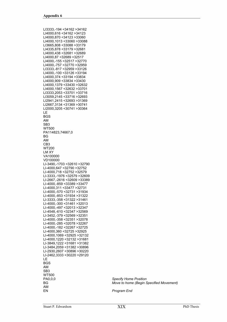
Appendix 6
Stuart P. Edwardson PhD Thesis XIX
LI3333,-194 <34162 >34162 LI4000,616 <34162 >34123 LI4000,870 <34123 >33060 LI4000,1013 <33060 >33088 LI3665,808 <33088 >33179 LI4335,878 <33179 >32681 LI4000,438 <32681 >32689 LI4000,87 <32689 >32517 LI4000,-155 <32517 >32770 LI4000,-757 <32770 >32959 LI3333,-817 <32959 >33126 LI4000,-100 <33126 >33194 LI4000,374 <33194 >33834 LI4000,909 <33834 >33430 LI4000,1379 <33430 >32632 LI4000,1567 <32632 >33701 LI3333,2053 <33701 >33716 LI3059,2145 <33716 >32693 LI2941,2415 <32693 >31369 LI2667,3134 <31369 >30741 LI2000,3205 <30741 >30364 LE BGS AM SB3 WT500 PA114823,74667,0 BG AM CB3 WT200 LM XY VA100000 VD100000 LI-3490,-1703 <32610 >32790 LI-4000,647 <32790 >32752 LI-4000,718 <32752 >32579 LI-3333,-1976 <32579 >32609 LI-2667,-2616 <32609 >33389 LI-4000,-859 <33389 >33477 LI-4000,311 <33477 >32731 LI-4000,-570 <32731 >31934 LI-4000,-853 <31934 >31322 LI-3333,-358 <31322 >31461 LI-4000,-300 <31461 >32013 LI-4000,-497 <32013 >32347 LI-4548,-610 <32347 >32569 LI-3452,-379 <32569 >32351 LI-4000,-358 <32351 >32078 LI-4000,-285 <32078 >32267 LI-4000,-182 <32267 >32725 LI-4000,360 <32725 >32925 LI-4000,1069 <32925 >32132 LI-4000,1220 <32132 >31681 LI-3849,1222 <31681 >31382 LI-3484,2059 <31382 >30896 LI-2930,2607 <30896 >30220 LI-2462,3333 <30220 >29120 LE BGS AM SB3 WT500 PA0,0,0 Specify Home Position BG Move to home (Begin Specified Movement) AM EN Program End


