NONSTANDARD QUANTUM GROUPS – TWISTING CONSTRUCTIONS AND NONCOMMUTATIVE

DIFFERENTIAL GEOMETRY

Andrew D. Jacobs

A Thesis Submitted for the Degree of PhD

at the University of St Andrews

1998

Full metadata for this item is available in St Andrews Research Repository

at: http://research-repository.st-andrews.ac.uk/

Please use this identifier to cite or link to this item: http://hdl.handle.net/10023/13693

This item is protected by original copyright

A thesis presented for the PhD degree at

the University of St. Andrews

N o n s t a n d a r d Q u a n t u m G r o u p s - T w i s t i n g C o n s t r u c t i o n s a n d

N o n c o m m u t a t i v e D i f f e r e n t i a l G e o m e t r y

by

Andrew D. Jacobs

Department of Physics and Astronomy, University of St. Andrews.

April 1998

ProQuest Number: 10167123

All rights reserved

INFORMATION TO ALL USERS The quality of this reproduction is dependent upon the quality of the copy submitted.

In the unlikely event that the author did not send a com p le te manuscript and there are missing pages, these will be noted. Also, if material had to be removed,

a note will indicate the deletion.

uestProQuest 10167123

Published by ProQuest LLO (2017). Copyright of the Dissertation is held by the Author.

All rights reserved.This work is protected against unauthorized copying under Title 17, United States C ode

Microform Edition © ProQuest LLO.

ProQuest LLO.789 East Eisenhower Parkway

P.Q. Box 1346 Ann Arbor, Ml 48106- 1346

I, Andrew Jacobs, hereby certify tha t this thesis has been composed by myself, that it is a record of my own work, and tha t no part of it has been accepted in partial or total fulfilment of any degree or professional qualification.

I hereby certify tha t the candidate has fulfilled the conditions of the resolutions and regulations appropriate to the degree of Doctor of Philosophy.

In presenting this thesis to the University of St. Andrews I understand that I am giving permission for it to be made available for use in accordance with the regulations of the University Library for the time being in force, subject to any copyright vested in the work not being affected thereby. I also understand that the title and abstract will be published, and tha t a copy of the work may be made available to any bona fide library or research worker.

The date of my admission as a research student was October 1992.

To Ruth and my Family

C ontents

Abstract v

Acknowledgements vil

Preface ix

Chapter 1. The Classical Picture 1

1.1. Introduction 1

1.2 . Lie algebras 1

1.3. Complex simple Lie algebras 3

1.4. The universal enveloping algebra 6

1.5. Representation theory of complex simple Lie algebras 7

1.6 . Hopf algebras 8

1.7. Representations of Hopf algebras 9

1.8 . Corepresentations of Hopf algebras 11

1.9. The correspondence between representations and corepresentations for non-degenerately paired Hopf algebras 12

1.10. Enveloping algebras are Hopf algebras 13

1.11. (Co)Module morphisms and matrix coefficient relations 141.12. Tensor product decompositions of the defining representations of the classical

complex simple Lie algebras 14

1.13. Lie groups 181.14. The Classical Lie groups 20

1.15. The algebra of representative functions on a compact group 22

1.16. The Stone-Weierstrass theorem and the algebra of representative functionson the classical Lie groups 23

1.17. The compact real forms of the classical complex Lie algebras and theirrepresentations 25

1.18. Representations of the Classical Lie groups 26

1.19. Complexification of the real classical groups 27

1.20. and C[G] are isomorphic 28

CONTENTS

Chapter 2 . The quantum picture 29

2.1. Introduction 292 .2 . /i-adic topology 30

2.3. Topological Hopf algebras and quantised universal enveloping algebras 33

2.4. Deformations of Hopf algebras 35

2.5. The Drinfeld-Jimbo quantum groups 37

2.6. Representation theory of formal deformations and QUEAs 39

2.7. The necessity of quasi-Hopf algebras 43

2.8. Quantised coordinate rings 45

2.9. The Diamond Lemma 502.10. Application to the Jordanian quantum groups 51

2.11. The rational form of a QUEA 55

2.12. Semiclassical theory — quantum groups at first order 56

2.13. Classical r-matrices 58

2.14. Classification of classical r-matrices 59

2.15. Quasi-Hopf algebras and twisting 61

Chapter 3. Twisting 2-cocycles for the construction of new non-standard quantumgroups 65

3.1. Introduction 65

3.2. Co-quasitriangular Hopf algebras and Reshetikhin twists 67

3.3. A new class of twisting 2-cocycles 733.4. The Cremmer-Gervais problem for GL{i) and beyond 76

3.5. Appendix A; The 3-parameter generalised Cremmer-Gervais R-matrix 79

3.6. Appendix B: The Multiparameter Generalised Fronsdal-Galindo R-matrix 81

Chapter 4. Classification of bicovariant differential calculi on the Jordanian quantumgroups GLh^g{2) and SLh{2) and quantum Lie algebras 85

4.1. Introduction 854.2. The Jordanian quantum groups 87

4.3. Review of Woronowicz’s bicovariant differential calculus 89

4.4. The classification procedure 97

4.5. 4-dimensional bicovariant calculi on GLh^g{2) 1014.6. 3-dimensional bicovariant differential calculi on SLh(2) 113

4.7. The Jordanian quantised universal enveloping algebra 115

4.8. Jordanian quantum Lie algebra from an ad-submodule in t//i(sl2(C)) 1164.9. Jordanian quantum Lie algebra from inverse Clebsch-Gordan coefficients 118

CONTENTS iii

4.10. Conclusion 121

Bibliography 123

CONTENTS

A bstract

The general subject of this thesis is quantum groups. The major original results are obtained in the particular areas of twisting constructions and noncommutative differential geometry.

Chapters 1 and 2 are intended to explain to the reader what are quantum groups. They are written in the form of a series of linked results and definitions. Chapter 1 reviews the theory of Lie algebras and Lie groups, focusing attention in particular on the classical Lie algebras and groups. Though none of the quoted results are due to the author, such a review, aimed specifically at setting up the paradigm which provides essential guidance in the theory of quantum groups, does not seem to have appeared already. In Chapter 2 the elements of the quantum group theory are recalled. Once again, almost none of the results are due to the author, though in Section 2.10, some results concerning the non­standard Jordanian group are presented, by way of a worked example, which have not been published.

Chapter 3 concerns twisting constructions. We introduce a new class of 2-cocycles defined explicitly on the generators of certain multiparameter standard quantum groups. These allow us, through the process of twisting the familiar standard quantum groups, to generate new as well as previously known examples of non-standard quantum groups. In particular we are able to construct generalisations of both the Cremmer-Gervais defor­mation of S'L(3) and the so called esoteric quantum groups of Fronsdal and Galindo in an explicit and straightforward manner.

In Chapter 4 we consider the differential calculus on Hopf algebras as introduced by Woronowicz. We classify all 4-dimensional first order bicovariant calculi on the Jordanian quantum group GLk,g(2) and all 3-dimensional first order bicovariant calculi on the Jorda­nian quantum group SLh{2 ). In both cases we assume that the bicovariant bimodules are generated as left modules by the differentials of the quantum group generators. It is found tha t there are 3 1-parameter families of 4-dimensional bicovariant first order calculi on GLii^g{2) and tha t there is a single, unique, 3-dimensional bicovariant calculus on SLfi{2). This 3-dimensional calculus may be obtained through a classical-like reduction from any one of the three families of 4-dimensional calculi on GLh^g(2). Details of the higher order calculi and also the quantum Lie algebras are presented for all calculi. The quantum Lie algebra obtained from the bicovariant calculus on SLk{2 ) is shown to be isomorphic to the quantum Lie algebra we obtain as an ad-submodule within the Jordanian universal enveloping algebra (A (s[2(C)) and also through a consideration of the decomposition of the tensor product of two copies of the deformed adjoint module. We also obtain the quantum Killing form for this quantum Lie algebra.

ABSTRACT

A cknow ledgem ents

I owe not just a debt of gratitude to Professor Cornwell for his guidance and extreme patience, but also for the singular humanity and support he afforded me throughout the duration of my post graduate studies. Thank you.

ACKNOWLEDGEMENTS

Preface

The theory of quantum groups is a precise mathematical generalisation of many el­ements of classical Lie theory. However, approaching the subject for the first time one could be forgiven for being confused about precisely what classical object corresponds to a particular quantum object. This is probably most acute when it comes to the quantum versions of classical coordinate rings. The fundamental paper of Faddeev, Reshetikhin and Takhtajan[84] in which these objects were originally defined is, at least initially, the most accessible of the early papers on quantum groups. The paper is accessible because it describes an essentially linear algebraic construction for a pair of Hopf algebras start­ing from a matrix R with particular properties. In certain standard cases corresponding to the classical series of Lie groups SLn{C), SOn{^) and 5 p2n(Q the construction is claimed to provide a deformation, or quantisation, of the Hopf algebra of ‘functions on the classical Lie group’ and dually, a quantisation of the universal enveloping algebra of the Lie algebra of the Lie group. In these cases the quantisation of the enveloping algebra is apparently the same as that obtained by Drinfeld and Jimbo. However, there are very many questions raised at this point.

1. W hat exactly is the classical Hopf algebra of ‘functions on the classical Lie group’?2. The FRT Hopf algebras corresponding to the Lie groups 5L„(C), S'On(C) and

Sp 2n{^) are generated in each case by ri generators with relations which look very much like variations of the usual defining properties of matrices in these groups. Why should this be?

3. W hat is the classical relationship between the Hopf algebra of ‘functions on the classical Lie group’ and the universal enveloping algebra of the corresponding Lie algebra?

4. W hat is it reasonable to expect for the relationship between the FRT Hopf algebras and the Drinfeld-Jimbo quantisations of the corresponding enveloping algebras and what exactly has been proved about the actual relationship?

The answers to these questions are peculiarly difficult to extract from the literature and it is the purpose of Chapters 1 and 2 to collect and review the relevant results.

In Chapter 3 we focus our attention on the notion of ‘twisting’ already encountered in Chapter 2. It can be that a pair of quantum groups are both related to the same classical object and yet have radically different Hopf algebraic properties. Very often these quan­tum groups are not homomorphically related but rather are related through the process of twisting. Indeed associated with SLn(C) there are, aside from the standard quantum group of Drinfeld, quantum groups discovered by Fronsdal and Galindo [41], Cremmer and Gervais [22 ] and also some conjectured quantum groups of Gerstenhaber, Giaquinto and Schack [44]. Based on Drinfeld’s fundamental Theorem 2.15.9 which establishes the existence of a kind of universal quantisation for a given Lie group it is one of the outstand­ing problems of quantum group theory to establish the twists which we believe relate these

PREFACE

objects. We have obtained these twists for the Fronsdal-Galindo quantum groups, which includes as a special case the first non-trivial Cremmer-Gervais quantum group. Our construction yields other previously unknown quantum groups when used in conjunction with twists discovered by Engeldinger and Kempf [37]. The twisting construction for the other Cremmer-Gervais quantum groups is still an open problem as is the proof of the Gerstenhaber-Giaquinto-Schack conjecture.

Quantum groups are noncommutative generalisations of algebras of functions on Lie groups. Lie groups are of course differentiable manifolds and there is a well known ‘equiv­alence’ between the algebra of functions on a manifold and the manifold itself. Indeed a good deal of classical differential geometry can be written in terms of the commu­tative algebra of functions on a manifold. Noncommutative geometry as pioneered by Connes [19] is based on the idea that by studying the correct generalisations of these structures for noncommutative algebras we are doing geometry on some generalisation of the manifold itself. In classical differential geom etry Lie groups occupy a position of es­sential importance. It is natural then to investigate the algebraic structures on quantum groups which provide the correct generalisation of differential geometry on Lie groups. Woronowicz [104] developed the relevant theory and it has been intensively studied ever since. A puzzling feature of these calculi soon emerged however. Except for the general linear groups, the calculi were not of the same dimension as their classical counterparts. This has led to some alternative constructions all of which have drawbacks. Very few studies of noncommutive geometry on non-standard quantum groups have been carried out. In Chapter 4 we provide a fairly complete treatment for the non-standard Jordanian quantum group. There we classify Woronowicz type calculi and find that in pleasant contrast to the standard case, there is a single, unique calculus and this has the classical dimension. Furthermore, we consider the analog of a Lie algebra which emerges from this calculus and show that it is isomorphic to that which emerges from a very different dual construction.

CHAPTER 1

T he Classical P icture

1.1. In tro d u c tio n

There is a classical paradigm which provides at the very least the best way of under­standing the interrelations between the many different objects which are called quantum groups. More than this though, the classical theory provides the motivation for key defi­nitions in the most unified and consistent approach to quantum groups, the elements of which are recalled in Chapter 2.

It is the purpose of the present chapter to recall and review the relevant results from the classical theory. We concentrate in particular on the Lie groups 5'L„(C), ROn(C) and Sp 2n{^) and their Lie algebras. There is an issue regarding terminology which the reader should be aware of. Namely, that in Lie theory these Lie groups are called the classical Lie groups, this use of the word classical having nothing to do with the use of the word when distinguishing from quantum objects. From now on, in this chapter, the word classical has the original Lie theory meaning.

In relation to the questions suggested by the FRT paper, Sections 1.12, 1.16, 1.18 and 1,20 are particularly relevant. These sections answer Questions 1 and 3 of the Preface and also provide the relevant framework for the answers to Questions 2 and 4 which will be provided in Chapter 2.

None of the results quoted in this section are new. However we have not found any one source where these results are all presented together. References for this chapter are [21], [14], [92], [91] [16], [101],[43] and [82].

1 .2 . Lie a lgebras

Let us recall the basic definitions.

D e f i n i t i o n 1.2.1. A Lie algebra g, over a field, A;, is a /c-module equipped with a bilinear operation, the Lie bracket, [, ] : 0 G 0 —)• 0 , satisfying

[x,ij] = ~[y,x], (1.2.1)

[.r, [y, z]] 4- [y, [z, x]] -f [z, [æ, y]] = 0, (1.2.2)

for all x , y , z Ç: g. The first of these, (1.2.1), expresses the antisymmetry of the Lie bracket,while (1.2 .2) replaces the associativity condition of associative algebras and is called theJacobi identity.

D e f i n i t i o n 1.2.2. A Lie algebra map 0 between two Lie algebras g and f) is a vector space map such that (/){[x,ij]) = [(^(%), (f){y)] for all x , y e q.

We will only be concerned here with complex or real Lie algebras, in which cases we have A: = C or E respectively.

1. THE CLASSICAL PICTURE

Whenever we have an associative algebra A with a product m : A (g> A —> A, we candefine a Lie bracket on A according to [a, b] ~ m{a 0 b) - m{b 0 a), for all a,b e A. Thisbracket satisfies both (1.2.1) and (1.2 .2) and therefore equips the vector space A with the structure of a Lie algebra which we shall denote L{A).

A typical example of this construction is the following: For any finite-dimensional vector space V the linear transformations of V, g 1(F) = {M : V -> F | M linear}, form a Lie algebra. The bracket is defined by [M, N] = M o N — N o M for all M, N € g 1(F) where o is the usual composition of maps. In particular, if we suppose F to be an n-dimensional complex vector space and choose some basis for it, then the linear transformations become complex valued n x n matrices, and the Lie algebra obtained by this construction is denoted gl„(C) (if we regard this Lie algebra as a real Lie algebra then we denote it gl(n, C)).

We can now define what we mean by a representation of a Lie algebra.

D e f i n i t i o n 1.2.3. A representation of a Lie algebra g is a pair (p, F ), where p is a Lie algebra map p : g —> gl(F). Equivalently, we can emphasise F and talk of a g-module F as a vector space upon which there is defined an action t> such that

[x,y] > V = x> {yt> v) ~ yt> {xt> v), (1.2.3)

for nil x ,y e Q and any v e V .

A submodule of a g-module F is a subspace U Ç V such that x > u ^ U for all a: G g and u G U. We say that a g-module F is simple or irreducible if its only submodules are 0 and F . It is semi-simple or completely reducible if it is a direct sum of simple submodules.

A vector space map ^ : V W between two g-modules F and W is a g-module map if (f){x> v) — x\> (f){v) for all æ G g and u G F . We say that F and W are equivalent g-modules if (j) is also an isomorphism.

There is a useful result which is usually called Schur’s lemma:

T h e o r e m 1.2.4. A g-module map 0 : F -> W between two irreducible g-modules is either 0 or an isomorphism. I f W = F then 4> — Xid for some A G C.

It follows from this tha t the irreducible representations of an Abelian Lie algebra areall 1-dimensional.

The structure of Lie algebras is worked out through a detailed analysis of the adjoint representation. This is the representation (ad, g) where

a.d{x){y) = [x,y] (1.2.4)

for all x ,y e g. In this case the g-module is g itself, the action is provided by the Lie bracket and condition (1.2.3) is just the Jacobi identity.

Of pivotal importance in the theory of Lie algebras is a certain bilinear form.

D e f in it io n 1.2.5. The Killing form, ^ : g 0 g k. is the symmetric A:-bilinear form defined as

^ { x , y) = Tr(ad(a;) o ad(^)) (1.2.5)

for all X-, ?/ G g where Tr denotes the trace.

1.3. COMPLEX SIMPLE LIE ALGEBRAS

The Killing form is ad-invariant, i.e. 93([x, y], z) -f- ^ { y , [x, z]) = 0 for all x ,y e g.

Let us employ the notation

[1) , 1)'] = s p a n j[x ,y ] \ x e ^ , y e (1.2.6)

where [} and ÿ are subsets of a Lie algebra g with the given bracket. Then we say that a Lie algebra g is Abelian if [g,g] = 0 . A subspace I) of a Lie algebra g is a Lie subalgebra of g if [1), [)] Ç f). If a Lie subalgebra f) of g also satisfies [g, f)] Ç 1 then it is called an ideal of g. However, only when b 7 0 and b 7 0 do we regard b as a proper ideal.

1.3. Complex simple Lie algebras

D e f in it io n 1.3.1. A complex simple Lie algebra g is a Lie algebra over C which isnot Abelian and contains no proper ideals.

Such Lie algebras have the following important properties:

T h e o r e m 1.3.2. I f g is a complex simple Lie algebra then the Killing form on g isnon-degenerate and every finite-dimensional g-module is completely reducible.

A key ingredient in the structural analysis which leads to the classification of complex simple Lie algebras is the Cartan subalgebra — a maximal Abelian Lie subalgebra upon which the restriction of the adjoint representation is semi-simple.

T h e o r e m 1.3.3. Every complex simple Lie algebra has at least one Cartan subalgebra. Given two Cartan subalgebras b and b' of g there is an automorphism cr of g such thatb' = < (b)-

The dimensions of all Cartan subalgebras of a given Lie algebra are thus the same, I say, which we define to be the rank of g.

As the simple modules of Abelian Lie algebras are 1-dimensional it follows that having chosen a Cartan subalgebra b, the restriction of the adjoint representation to b splits g into a direct sum of 1-dimensional b-modules. It turns out that except for the I identical modules corresponding to the action of b on b, these modules are mutually inequivalent. Therefore we can define, for some non-zero a G b* which will be called roots, the 1- dimensional root subspaces g« of g by

ga = {x G g I ad(h)(x) = a{h)x for all h G b}- (1.3.1)

Denote by $ the set of all roots, then we have the Cartan decomposition of g

g = b C 0g• (3.3.2)

The roots actually span b* and to every a G # we also have —a G 0 but no other multiple of a. The restriction of the Killing form to b is still non-degenerate, which allows us to introduce elements ha G b corresponding to each root according to %(ha, h) — a{h) for all h G b< A non-degenerate symmetric bilinear form (, ) : b* 0 b* C is then induced on b* by (a, /?) = 93(h^, hp) for all a , /? G <D. In fact, this bilinear form is positive-definite on the real linear span of the roots b® making b® an /-dimensional Euclidian space. For each pair of roots {a, —a}, the single basis elements of g^ and g_a may be chosen to be Ea and E-a respectively such that 93(E^, E_«) = We may also define elements

1, THE CLASSICAL PICTURE

Ha ~ for all a G <D and note that they span fp The Lie brackets for the arbitrary complex simple Lie algebra may then be written in the following Chevalley form:

[Ha,Hp] = 0, (1.3.3)

== (1.3.4)

[Ea,E-a] — Ha, (1.3.5)

where Na,p = ± (p + 1), p being the greatest integer such that /? - p a G (there is analgorithm for determining a consistent choice of signs of the Na,p which is based only onknowledge of 0 ).

Let us note that the numbers can be shown to be integers. Also, in the real Euclidian space spanned by the roots there are reflections Sa, for each a G $, defined by

= /? - (1.3.7)(a , a)W ith multiplication provided by composition of maps, the set of these refiections generate a group, W, called the Weyl group, which leaves invariant.

The pair (<E>, b*) is an example of a reduced root system in b*. That is, 0 is a subset of b* spanning b* such that

1. 0 is finite but does not contain 0;2. for any a G $ there exists an element of b, namely Ha, such that a{Ha) = 2;3. for any a G $ the reflection leaves invariant;4. for all a ,/? G 0 , a(R]g) G Z;5. for each a G 0 , a and —a are the only roots in proportional to a .

Two root systems ($ i, bi) and ($ 2, bg) are isomorphic if there is a vector space iso­morphism (/i : bî -> b2 such that < (0 1 ) = 0 2 and <f){P){H {a)) — /^{Ha) for all a ,P G <l>i. It can be shown that the simplicity of g means that the root system ($ , b*) is irreducible in the sense that we cannot write b = bi ® b2 and — #1 U $2 with 4>i C bi and $2 C 1)2 such that ( $ 1, bi) and ($ 2, bj) are root system s.

A general property of root systems (0, b*) is that there always exists a subset II — {a.i}^_j of $ , called the set of simple roots, which form a basis of b* and in terms of which every other root can be written as a linear combination with either non-negative (in which case we say the root is positive) or non-positive (in which case we say the root is negative) integer coefficients. The set of all roots is therefore divided equally into two subsets, cl) = cl)+ u where and denote the positive and negative roots respectively.

The Weyl group for a root system (<E>, b*) is generated by the I reflections &Rdindeed every root in $ may be obtained through a knowledge of the simple roots alone. Explicitly,

0 = {w(a^) \ w e W and a,; G H}. (1.3.8)Thus, all the information needed to reconstruct the entire root system from the simple roots is encoded in the Cartan matrix, defined as the I x I matrix A with An =

1.3. COMPLEX SIMPLE LIE ALGEBRAS

The choice of fl does not effect the Cartan matrix up to similarity as it can be shown I

tha t any other basis of simple roots IT for a root system (<h, b*) is such that IT = w(II) iwhere w e W and it is a general property of the Weyl group that (iu{a),w{P)} ~ {<y,P) !for any a, P G and w G TV. It follows from this that the root systems reconstructed ;from n and IT are isomorphic. i

In the particular case of the root system of a Lie algebra it can be shown that different choices of Cartan subalgebra lead to isomorphic root systems so we see tha t to any complex simple Lie algebra there corresponds an irreducible root system which is unique up to isomorphism and which is itself specified up to isomorphism by a Cartan matrix. Moreover it may be shown that two Lie algebras are isomorphic if and only if their corresponding root systems are isomorphic.

In the original Lie algebra we can define elements, Hi = Hai, W = and Yi = for each a% G H. These elements actually already generate g according to the following result of J. P. Serre.

T heorem 1.3.4. The complex simple Lie algebra g with Cartan matrix A is isomor­phic to the complex simple Lie algebra generated by the 31 generators V, Hi}\^i subject to the following relations:

[ H i , H j ] = 0 , (1.3.9)= (1.3.10)

[Hi ,Xj ] — A j i X j , [Hi ,Yj] = - A j i Y j , (1.3.11)

= 0, ad(yi)-*i‘+'(y,) = 0, (1.3.12)

where in the last line i ^ j and ad(x)"(p) = [x, [x . . . [x, p ]. . . )] with n nested brackets.

In fact Serre’s result is more general: Given the Cartan matrix of any irreducible root system then Theorem 1.3.4 provides the construction of a complex simple Lie algebra whose root system is that specified by the Cartan matrix.

The basis {Hi,Ea, R -a | / = 1 . . . / , a G of g is called a Cartan- Weyl basis while the generators {Hi, X i , Y i \ i ~ 1 . . . /} are called Chevalley-Serre genei'ators.

We see that the classification of the complex simple Lie algebras is equivalent to the classification of irreducible reduced root systems and that this classification may be carried out through a determination of the possible Cartan matrices.

T heorem 1.3.5. There are four infinite series of finite complex simple Lie algebras, denoted by Ai, Bi+i, C1+2 and respectively, with I > I, together with five exceptional cases which are denoted by Eq, Ej, Eg, F4 and G2. The Cartan matrices are presented, for example, in [21].

The four infinite series of Lie algebras are the classical complex Lie algebras, so called because it can be shown that Ai = sb+i(C), Bi = S02/+i(C), Ci = apgJQ and Di =502/(C) where 5l/+i(C), 502/+i(C), sp2/(C), and S02/(C) are the matrix Lie algebras which arise as the Lie algebras of the classical complex Lie groups (see Section 1.14). They are Lie subalgebras of gQ(C) for particular n. Indeed 5l/+i(C) is the subspace of (/ + 1) x (/ + 1) traceless matrices. The orthogonal Lie algebras 6O2/+] (C) and S02/(C) may be regarded as consisting of skew-symmetric matrices. Equivalently, we can regard S02/+i(C) as consisting

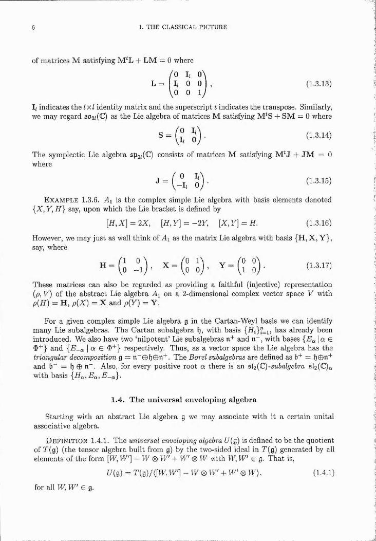
1. THE CLASSICAL PICTURE

of matrices M satisfying M T + LM = 0 where

/O 1/ 0 \L = 1/ 0 0 , (1.3.13)

0 1 /

1/ indicates the Ix l identity matrix and the superscript t indicates the transpose. Similarly,we may regard 502/(C) as the Lie algebra of matrices M satisfying M^S + SM = 0 where

0 1/

1/ 0(1.3.14)

The symplectic Lie algebra 5pgJC) consists of matrices M satisfying M^J + JM = 0 where

f l , o ) • (1.3.15)

E x a m p le 1.3.6. Ai is the complex simple Lie algebra with basis elements denoted [X , Y, H ] say, upon which the Lie bracket is defined by

[R-, X] = 2X, y] = -2 y , [X, y] = R. (1.3.16)

However, we may just as well think of Ai as the matrix Lie algebra with basis {H, X, Y}, say, where

H = ( ; _°i) . X = ( ° J) . Y = Ç . (1.3.17)

These matrices can also be regarded as providing a faithful (injective) representation (p, V) of the abstract Lie algebra Aj on a 2-dimensional complex vector space V with p(R-) = H, p(X) = X and p(y) = Y.

For a given complex simple Lie algebra g in the Cartan-Weyl basis we can identify many Lie subalgebras. The Cartan subalgebra b, with basis has already beenintroduced. We also have two ‘nilpotent’ Lie subalgebras xY and n“ , with bases {Ea | a G

and {E_a \ G 0"^} respectively. Thus, as a vector space the Lie algebra has the triangular decomposition g = n'Sb©^"*^' The Borel subalgebras are defined as and b“ = b ® Also, for every positive root a there is an s[2 {C)-subalgebra 512(C)a with basis {Ha, Ea, E _a}‘

1.4. The universal enveloping algebra

Starting with an abstract Lie algebra g we may associate with it a certain imitai associative algebra.

D e f in it io n 1.4.1. The universal enveloping algebra U(g) is defined to be the quotient of T (g) (the tensor algebra built from g) by the two-sided ideal in T (g) generated by all elements of the form [W, W ] — W 0 W + W 0 W with TT, W G g. That is,

[/(g) = T(g)/([W, IW] - W 0 IW -b IW 0 W), (1.4.1)

for all W, W G g.

1.5. REPRESENTATION THEORY OF COMPLEX SIMPLE LIE ALGEBRAS

Denoting by tt the canonical projection from T(g) to [/(g) and by i the canonical embedding of g in T(g), the composition tt o t is a Lie algebra map from g to [/(g). The adjective ‘universal’ refers to the following property of [/(g): Given any associative algebra, A, and a Lie algebra map / : g L{A) there exists a unique algebra map,(j) : U{g) A such that (j) o [n o c) = f . This universal property means that the representation theories of g and [/(g) are equivalent.

E x a m p le 1.4.2. [ /(512(C)) is the algebra over C generated by the elem ents {%, Y, H } sub jec t to the com m uta to r relations

F /x -X A [ = 2X, / : [ y - y /7 = -2 y , % y - y x = /7. (1.4.2)

(We have suppressed the tensor product here.)

In this example the monomials {Y°‘H^X'^ : a , ^ ,7 G N} form a basis for [/(512(C)). This basis is a particular example of the following general result for universal enveloping algebras of Lie algebras called the Poincare-Birkhoff-Witt (PBW) theorem.

T h e o r e m 1.4.3. I f a finite dimensional Lie algebra, g, has a basis, saij, thenthe set of elements {x^^xÿ . . . x^ | ij G N} form a basis o /[ /(g ) .

Corresponding to the triangular decomposition of g, we have the vector space isomor­phism, [/(g) = [/(n") 0 [/(b) 0 [/(iW).

1.5. Representation theory of complex simple Lie algebras

Roots are a key concept in the classification of complex simple Lie algebras. They are particular examples of a more general concept which is essential for the classification of the irreducible representations of those Lie algebras. We assume our representations to be finite-dimensional and take as understood the equivalence of representations of g andUs)-

D e f in it io n 1.5.1. Suppose V is a g-module and A G b*, then define by,

— {v e V \ h> v = X{h)v for all h G b}- (1.5.1)

When F^ 0 we call it the weight space consisting of weight vectors corresponding to the weight, A, of F . We say that A has multiplicity equal to the dimension of F^.

It turns out that b can be taken to act diagonally on any finite dimensional g-module so that F — 0 aF ^ . Also, given v G V^, then {Ea^v) G for all a G #. In an obvious notation we could also write this as ga t> C F^+°^.

It can be shown that every finite-dimensional g-module contains a certain distinguished kind of weight vector v of weight A say, called a singular vector, such that > u — 0. Then v generates a submodule W = [/(g) > u of F spanned by vectors of the form E^p^EYp.^ - - • E''Ap o v, where v is being acted upon by elements of the PBW-basis of U(n~) (i.e. Pi G and G N). This means that the weights of W arc of the form A — R'iCK/ where G N and the a% are the simple roots. Furthermore we see that A has multiplicity 1 as a weight of W from which it follows that IF is indecomposable and therefore irreducible.

1. THE CLASSICAL PICTURE

D e f i n i t i o n 1.5.2. A singular vector v of weight A of a g-m odule V which is such th a t U{q)>v = V is called a highest weight vector and V is then called a highest weight module w ith highest weight A and w ritten V (A).

D e f i n i t i o n 1.5.3. The I fundamental weights of a Lie algebra g are defined as the elements A(i), A(2) , . . . , Ag) G If such that for I < i j < I.

The fundamental weights (also called the coroots) provide another basis of related to the basis of simple roots by A( ) = The subset of f f , P'^ = NA(*),is then called the set of dominant integral weights, while P ~ is the weightlattice. The root lattice is defined as Q = and it is clear tha t Q C P C f .

The basic theorem classifying finite-dimensional, irreducible g-modules may now be stated.

T h e o re m 1.5.4. I f V is an irreducible Q-module then it contains a highest weight vector, ua, say, of weight A, which is unique up to scalar multiplication and such that A G P'^. Conversely, to every A G P ^ there is an irreducible finite dimensional Q-module y (A) which is unique up to isomorphism and has highest weight A.

E x am p le 1.5.5. The Lie algebra 512(C), with basis { H ,X ,Y } , has rank one so its irreducible representations may be denoted by V{n) = y(nA(i)), with n G N. Each V{n) has dimension n + 1 and a basis may be chosen for it, such that the actions ofthe basis elements of 512(C), are

H t>Vi = ( n ~ 2z)u", (1.5.2)X t> Vi — (n ~ i - \ - (1.5.3)

= + (1.5.4)

In the physics literature, a different basis, e^, where m = ~ j, — j 4 -1 ,... , j — 1, j is used, with the representations being labelled now by the numbers j such tha t 2 j = n

X > é ^ = \ / ( i - m ) ( j+ m + l)e ^ ^ i , (1.5.5)

P^i>e^ = 2me^, (1.5.6)

= \/(7 + rn){j - m + l)e^_ i. (1.5.7)

Two irreducible modules, V{1) and 1/(2), are particularly important. The defining mod­ule 1/(1) is the faithful representation which gives the realisation, which we saw in Exam­ple 1.3.6, of 512(C) as an algebra of 2 x 2 complex traceless matrices. 1/(2) is the adjoint module.

Also for the other classical complex simple Lie algebras, the first fundamental repre­sentations, l/(A(i)), are faithful representations. They are equivalent to the realisations of the abstract Lie algebras in terms of matrices M which satisfy Tr(M ) = 0 in the case of 5l/4-i(C) and M^X -I- X M = 0 with X = L ,S , J in the cases 502(4-1 (C), S02z(C) and sp2/(C) respectively.

1.6. Hopf algebras

We recall the definition of a Hopf algebra.

1.7. REPRESENTATIONS OF HOPF ALGEBRAS

D e f in it io n 1.6.1. A Hopf algebra is a sextuple (A, m, r}, A, e, S) such that A is a C- module (a vector space over C) with C-linear maps m : A(g) A A — the multiplication, ?7 : C —> A — the unit, A : A -A A 0 A — the coproduct, e ; A - a C — the counit and S : A A — the antipode, satisfying the following axioms:

m o (id0m ) = m o (m 0 id), (1.6.1)m o (id07?) = id = 77T o (?y 0 id), (1.6.2)

(id0A ) o A = (A 0 id) o A, (1.6.3)(e 0 id) o A = id = (id 0e) o A, (1.6.4)

m o (id 05') o A = 7 o 6 = m o (5 0 id) o A. (1.6.5)It is further required tha t A and e be algebra maps, which immediately implies tha t m and Ï] are coalgebra maps. The definition of a bialgebra is just that of a Hopf algebra without an antipode.

It follows from the definition that S is both an antialgebra map and an anti-coalgebra map. That is, S{ab) — S{b)S(a) and 5(a(i)) 0 5(a(2)) = 5(a)(2) <0 5(a)(i), where in the second equation we have introduced a version of the Sweedler notation for coproducts [98] in which the summation is suppressed. This notation is extremely useful and will be used from now on. It amounts to writing A (a) = a(i) 0 U(2) with the understanding that theright hand side consists of a summation of the form a (i) 0 0 (2).

A Hopf algebra, A, is said to be commutative if it is commutative as an algebra. It is said to be cocommutative if a(i) 0 a(2) = ci(2) 0 U(i) for all a G A.

D e f in it io n 1.6.2. Two Hopf algebras, U and A, are said to be Hopf algebras in non­degenerate duality, if there exists a bilinear map, ( , ) : C7 0 A C, called a pairing, such that

(æi/,a) = (T,a(i))(2/,a(2)), (a;,a6) = (a;(i),a)(a;(2),6>, (1.6.6)( l ,a ) = e(a), (æ, 1) = 6(æ), {S(x),a) = {x, S(a)), (1.6.7)

which is non-degenerate in the sense that the algebra maps lu : U A* and : A U*, given by iu{x){a) = {x,a) and iA{a){x) = {x,a) respectively, are injective. In this case the maps lu and la constitute embeddings of U and A in A* and U* respectively. A possibly-degenerate pairing between Hopf algebras is called simply a Hopf pairing.

1.7. Representations of Hopf algebras

When we talk about a representation of a Hopf algebra, we mean a representation of its algebra sector. We consider only finite-dimensional representations.

D e f in it io n 1.7.1. If A is a Hopf algebra, then a left A-module is a pair, (>, H), where V is a vector space upon which there is an action, >, of A such that

(ab) >v = a> (b>v), 1a > v = v , (1.7.1)

for all a, 5 G A and v G V7 Equivalently, a representation is a pair (p, V") where p : A - a gl(y) is such that

p{ab)v — p{a)p{b)v, (1.7.2)

for all a,b e A and v G V.

10 1. THE CLASSICAL PICTURE

E x a m p l e 1.7.2. An important example of a left A-module is provided by the left adjoint action of A on A defined as

a> 6 = a(i)65(ü(2)) (1.7.3)for all a,b E A.

A vector space U Ç V is called an A-submoduIe iîaï>U Ç U for all a G A. Reducibility, complete reducibility and irreducibility are then all defined in the obvious way. A map (j) : V W between two A-modules is called an A-module map if (p{at> v) — a> j){v) for all a G A. We have the following ‘Schur’s lemma’ result;

T h e o r e m 1.7.3. An A-module map <f \ V —> W between two irreducible A-modules is either 0 or an isomorphism. I f W = V then ^ = A id for some A G C.

A consequence of this result is that the irreducible representations of any commutative Hopf algebra are 1-dimensional.

If we choose a basis, say, for the vector space, V, of a representation, (p, V),then we obtain a matrix representation, p(a), for all a G A according to, a > Vi =

where p X ) = (/)((%))*;'D e f i n i t i o n 1.7.4. The m,atrix coefficients of a left A-module, E , are the linear forms

p /y : A -y C defined by p^^(a) = a ( a > u) for all a G V* and v G E. The space spanned by the matrix coefficients of all finite-dimensional representations of a Hopf algebra. A, is denoted A° and called the Hopf dual of A.

In all the examples in which we are interested, the Hopf algebra, A say, is infinite dimensional. In this case the dual maps and S* do not provide a Hopfstructure on A*. The problem with A* is that the dual of the multiplication map, m* : A* -A (A 0 A)* is in general taking us out of A* 0 A*, as (A 0 A)* is only isomorphic to A* 0 A* when A is finite and in general is ‘bigger’ than A* 0 A*. The importance of the Hopf dual stems from the fact tha t the restrictions of the dual maps do define a Hopf algebra structure on A°.

The restriction of A* to A*0A* together with e* certainly provides an algebra structure on A*. That this algebra structure closes on A° is guaranteed by certain natural A-module constructions. Indeed, if E and W are A-modules, then so is their direct sum, E 0 W , with the action of A given by a> (u 0 w) = (a,t>u) 0 (aow). This provides an addition for A° — for all CK G E*, G IE*, u G E and w G IE we have p^^ + p j^ = Scalarmultiplication in A° follows from the fact that any constant multiple, cE, of an A-module E is naturally an A-module, so cpg „ = p ^ „ = Pa,cv The Hopf structure of A allows us to construct the tensor product A-module, E 0 TE, given two A-modules, 1/ and W , with the action provided by the coproduct as a > (u 0 re) = (a(i) t> u) 0 (a(2) > w) for any a E A and all u G E and w E W. This provides a multiplication for matrix coefficients, PÏ,vPp ,w — PaSp!v^w’ The counit of A provides the trivial 1-dimensional representation of A, (e, Eg), with a t> = e(a)v^ for any a E A and the single basis element of Denoting by the single basis element of V f such that ^^(uj = 1, then a unit for A° is just pafvc- It is straightforward to check that the multiplication and unit we have defined for A° are simply the restrictions of the dual maps A* : (A 0 A)* -A A* and e* : C —> A* (to be more precise, e*(I)(a) — e{a) = Pa,,uJ.

The details of the full Hopf structure on A° are presented in the following theorem.

1.8. COREPRESENTATIONS OF HOPF ALGEBRAS 11

T h e o r e m 1.7.5. A° is a Hopf algebra. Indeed, for all v E V, w E W , a E V*' and P E W*, where V and W are any pair of left A-modules, we have

Pa,v + P0 ,w ~ Pae0 ,v®ru (1.7.4)

^Pa v Pca,v Pa,cv (1.7.5)where c G C, and

V ® U ) )

7 7 ( 1 ) = e /1 ,

yOLi,V>

(1.7.6)where and {%} are dual bases for V and V* respectively and is the counit in A.

R e m a r k 1.7.6. To understand the expression for the antipode of A° we need to recall that if V is an A-module then so is V* with the action defined as (a>a)(u) = o;(5(a)ou).

R e m a r k 1.7.7. Let us also note here that if U C E is a submodule of E then the matrix coefficients of U are obtained as the subset of matrix coefficients of E such that V E U and a E U*. Also, we can form the quotient space, V/U, which is again an A-module, now with action a o (u + f/) = a o u -f [/. The matrix coefficients of V /U are the subset of matrix coefficients, pa,vi of E for which v ^ U and a E where is the annihilator of U.

For any given n-dimensional representation, (p, E), choosing a basis for E provides us with a m atrix representation and particular examples of matrix coefficients, the matrix elements, {pYj}ij-i, of the representation. The space spanned by the matrix elements of (p, E) is independent of the particular choice of basis and they span the space of matrix coefficients of E.

1.8. Corepresentations of Hopf algebras

We may also consider ‘representations’ of the coalgebra sector.

D e f i n i t i o n 1.8.1. A co-representation is a pair, (Ay, E), where Ay : V —> V 0 A is a linear map such that

(Ay 0 id) o Ay = ( id 0 A ) o Ay, ( id0e) o Ay = i d . (1.8.1)

We say tha t E is a right A-comodule, with A y a right coaction.

E x a m p l e 1.8.2. An important example of a corepresentation of A is provided by the the right adjoint coaction, Adfi, which is defined on any a G A as

Ad^(a) =: G(2) 0 5(ü(i))a(3) (1.8.2)

A vector space U Ç V' such that Ay ([/) C f/ 0 A is called an A-subcornodule. With this notion in place, the definitions of reducibility, complete reducibility and irreducibility are all obvious. A map (j : T'” —> TE between two A-comodules is called an A-comodulc map if {(f) 0 id) o A y = Ay/ o (j). Once again we have a ‘Schur’s lemma’ result.

12 1. THE CLASSICAL PICTURE

T h e o r e m 1.8.3. An A-comodule map </> : E —> W between two irreducible A-comodules is either 0 or an isom.orphism. I f W = V then (/> = A id for some A E C.

It follows from this result is that the irreducible corepresentations of any cocommuta­tive Hopf algebra are 1-dimensional.

D e f i n i t i o n 1.8.4. The matrix coefficients of a co-representation, (Ay, E), of a Hopf algebra A are the elements G A for any u G E and a G V* such that

= (a 0 id) o Ay. (1.8.3)

There is a Sweedleresque notation for coactions, namely A y(u) = U(y) 0 V(a) for all u G E.

We have constructions of comodules analogous to those for modules. Given two A- comodules, E and W , with respective coactions. A y and Ay/, their direct sum is also an A-comodule with coaction Ay@y/(u 0 w) = Ay(u) + Ay/(u') and so is their tensor product, with coaction Ayg,py(u 0 w) = U(y) 0 W(w) 0 V(a)VJ(a) for all u G E and w G W. Once again any constant multiple, cE, of an A-comodule is again an A-comodule, and so is the dual vector space, E*, with coaction, A y. (a) = Of(y.) 0 a(^), such that for any a G E*

0!(y.)(u)a(yi) = a(u(y))5(u(A)) (1.8.4)for all V G E. The trivial 1-dimensional representation this time originates from the unit of A; we denote it by (Ay^, %,). Taking its single basis element to be u,, with a,, G Vf such tha t ajj{vrj) = 1 we have Ay^(u,^) = u,, 0 77(1). Thus the matrix coefficient is just Ta,,,vr, = where 1^ is the unit in A.

Once again there is a Hopf algebra structure on the space of matrix coefficients of all finite dimensional co-representations. This Hopf structure is formally precisely tha t in Theorem 1.7.5, but with p replaced by tt and 77(1) = 1^.

Fixing a particular basis for E , say, there is a uniquely determined family ofelements of A, such that Ay(u^) = 0 7rh. The are called the matrixelements of the corepresentation (A y, E) and span its space of matrix coefficients.

R e m a r k 1.8.5. In fact any Hopf algebra is spanned by the m atrix coefficients of its finite dim ensional corepresentations.

1.9. The correspondence between representations and corepresentations fornon-degenerately paired Hopf algebras

If U and A are Hopf algebras in non-degenerate duality, suppose (Ay, E) is a corep­resentation of A, then choosing a basis for E , {u^}, we can write Ay(u*) = J f j Vj 0 tt^. The Tffi may be identified through the non-degenerate duality with elements of U* and since A (71] ) = 0 '^jk we can define a representation of U, (p, E), according top{X)vi = Y l j 7rji(x)vj for all X G U. Moreover it is clear that (Ay, E) is uniquely spec­ified by this representation. If U{V) denotes the subspace of U* spanned by the matrix coefficients of the [/-module E and A(E) denotes the subspace of A spanned by the ma­trix coefficients of the A-comodule E, then U{V) = A(E) C A. In the other direction, starting with a representation (p, E) of U, p(X)vi — W we can not in general

1.10. ENVELOPING ALGEBRAS ARE HOPF ALGEBRAS 13

associate a corepresentation of A as there is no guaranteed inclusion of 17* in A. Thus we have a one-to-one correspondence between representations (p, V) of U and comodules (Ay, E) of A for all U-modules such that 17(E) C A. This correspondence preserves all the usual representation attributes such as complete reducibility and irreducibility.

1,10. Enveloping algebras are Hopf algebras

For any complex simple Lie algebra, g, the enveloping algebra, U (g), is a Hopf algebra. Here is the precise result.

T h e o r e m 1.10.1. 17(g) is a Hopf algebra with the Hopf maps defined on the generatorsas

A{x) = X ® 1 1 ® X, e{x)=Q, S{x) = —X, (1.10.1)

for X E Q, and extended linearly to the whole o/ 17(g) as algebra, algebra and anti-algebra maps respectively. Moreover, 17(g) is cocommutative, that is, X( i) 0 .T(2) = x^2 ) 0a^{i) for all X E Q.

We may regard g as the subspace of primitive elements of 17(g), i.e. those elements upon which the coproduct has the form in (1.10.1).

E x a m p l e 1.10.2. The adjoint representation of a Lie algebra, g, is the restriction to g of the left adjoint action of 17(g) on 17(g)

xï>y = X(^i)yS{x(2)) = xy - yx. (1 .10 .2 )

As U (g) is cocommutative, all its irreducible corepresentations are 1-dimensional. The irreducible representations of 17(g) were classified in Section 1.5.

The constructions of the previous two sections can now be applied to U (g)-modules. Thus if {p^\V) and {p^^ ,W ) are representations of g then so is 0 VE) with

pV®W(^)(^ 0 to) = p^{x)v 0 tu 4- u 0 p^^\x)w, (1.10.3)

for all V E V, w E W and x E 17(g). The trivial representation of g is just the 1- dimensional ‘highest-weight’ module, E(0), such that a; > u — 0 for all x E 17(g) and V e V . If E is a representation of g then so is E* with (a; t> a) (t;) = a{—x > v).

We will be particularly interested in the Hopf dual of the enveloping algebra, 17(g)°. There is a natural Hopf algebra pairing between t/(g) and l/(g)°. In fact this pairing renders l/(g) and l/(g)° Hopf algebras in non-degenerate duality. On the one hand we have the natural embedding of U{q)° in 17(g)*. Dually we therefore have a linear map t : l/(g) (l/(g)°)* and this shoulcl be injective. If it were not then for all finite 17(g)-modules E we would have some non-zero æ G 17(g) such that pa,v{^) = 0 for any v E E, a e V*. On the contrary, we have the following result due to Harish-Chandra:

T h e o r e m 1.10.3. For any non-zero element, x, of the enveloping algebra, 17(g), of a complex simple Lie algebra, g, there exists a finite di7nensional representation of q , (p, E), such that p{x) ^ 0. Furthermore, in the cases of q a classical complex simple Lie algebra, this representation is constructed as a tensorial power of the defining representation.

We can now deduce immediately that the representation theory of 17(g) is equivalent to the corepresentation theory of 17(g)°.

14 1. THE CLASSICAL PICTURE

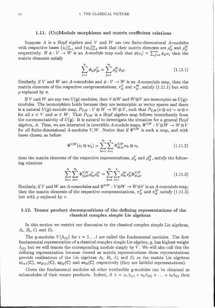
1.11. (Co)M odule morphisms and matrix coefficient relations

Suppose A is a Hopf algebra and V and IE are two finite-dimensional A-modules with respective bases and {wi]fL^ such that their matrix elements are p\j and p-Jrespectively. If r/> ; V —> W is an A-module map such that j){vi) = X ljli 4>jiVj then the matrix elements satisfy

n m( 1 .11 .1)

7=1 7=1

Similarly, if V and PE are A-comodules and <j) : V -A- PE is an A-comodule map, then the matrix elements of the respective corepresentations, ttL and satisfy (1.11.1) but with p replaced by t t .

If V and W are any two [/(g)-modules, then V<S)W and PE0 E are isomorphic as [/(g)- modules. The isomorphism holds because they are isomorphic as vector spaces and there is a natural [/(g)-module map, Pv,w : E 0 PE — PE 0 E, such that Pv,w{v ®w) = w ® v for all V e V and w G PE. That Py,w is a Hopf algebra map follows immediately from the cocommutativity of U{q). It is natural to investigate the situation for a general Hopf algebra, A. Thus, we are interested in invertible A-module maps, 0^'^^ : E 0 PE —> PE0 E for all finite-dimensional A-modules E, TT. Notice that if is such a map, and with bases chosen as before

m n0 Wj) = ^ 0 nf, (1.11.2)

fc=l 1=1

then the matrix elements of the respective representations, pj- and satisfy the follow­ing relations

n m in n(1.11.3)

/=i (=1

Similarly, i î V and PE are A-comodules and 0 ^ '^ : V 0 PE —> PE0 E is an A-comodule map, then the matrix elements of the respective corepresentations, and tt-J satisfy (1.11.3) but with p replaced by t t .

1.12. Tensor product decompositions of the defining representations of theclassical complex simple Lie algebras

In this section we restrict our discussion to the classical complex simple Lie algebras, A(, Bi, Cl and Di.

The g-modules E(A(q) for % = 1 . . . 1 are called the fundamental modules. The first fundamental representation of a classical complex simple Lie algebra, g, has highest weight A(i) but we will denote the corresponding module simply by V. We will also call this the defining representation because viewed as matrix representations these representations provide realisations of the Lie algebras A/, Bi, Q and Di as the matrix Lie algebras 5fi+i(C), so2(+i(C), 5p2((C) and S02((C) respectively (they are faithful representations).

Given the fundamental modules all other irreducible g-modules can be obtained as submodules of their tensor products. Indeed, if A = ;qA(]) -E 742A(2) -f . . . + n/A(q then

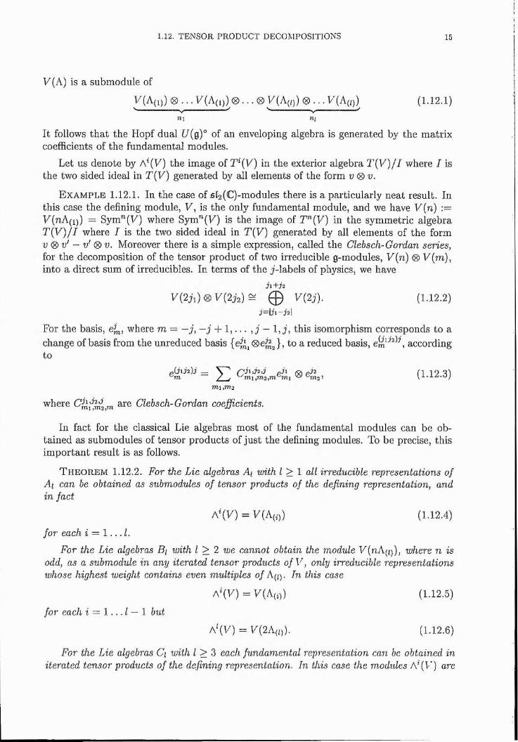
1.12. TENSOR PRODUCT DECOMPOSITIONS 15

V (A) is a submodule of

E(A(i)) 0 . . . E(A(i)) 0 . . . 0 E(A(f)) 0 . . . E(A(o) (1.12.1)V------------- ^ —N/-- "

m niIt follows tha t the Hopf dual U{qY of an enveloping algebra is generated by the matrix coefficients of the fundamental modules.

Let us denote by A*(E) the image of T^{V) in the exterior algebra T { V ) / I where I is the two sided ideal in T (E) generated by all elements of the form u 0 u.

E x a m p l e 1.12.1. In the case of ^^(Q-Piodules there is a particularly neat result. In this case the defining module, V, is the only fundamental module, and we have V(n) := V(nA(i)) = Sym^(E) where Sym” (E) is the image of T^(E) in the symmetric algebra T { V ) / I where I is the two sided ideal in T{V) generated by all elements of the form u 0 u' — u' 0 V. Moreover there is a simple expression, called the Clebsch-Gordan series, for the decomposition of the tensor product of two irreducible g-modules, V{n) 0 E(m ), into a direct sum of irreducibles. In terms of the j-labels of physics, we have

71+72

® 1"(2,72) = 0 V'(2j). (1,12,2)7 = l 7 i - 7 2 |

For the basis, eff, where m = — j, - j + 1, . . . , j - 1, j , this isomorphism corresponds to a change of basis from the unreduced basis to a reduced basis, accordingto

J h h ) j — ^ /771 ,72 ,7 J l ^ p72 (1 1 9

mi,m2

where Clebsch-Gordan coefficients.

In fact for the classical Lie algebras most of the fundamental modules can be ob­tained as submodules of tensor products of just the defining modules. To be precise, this im portant result is as follows.

T h e o r e m 1.12.2. For the Lie algebras A\ with I > 1 all irreducible representations of Ai can be obtained as submodules of tensor products of the defining representation, and in fact

A%V) = !/(% )) (1,12,4)

for each i = 1 .. . 1 .

For the Lie algebras Bi with I > 2 we cannot obtain the module E(nA(/)), where n is odd, as a submodule in any iterated tensor products of V, only irreducible representations whose highest weight contains even multiples of A( ). In this case

A '(y) = E(A(q) (1.12.5)

for each i = 1 .. . 1 — 1 but

a ‘{V) = 1/(2A(„), (1,12,6)

For the Lie algebras Q with I > 3 each fundamental representation can be obtained in iterated tensor products of the defining representation. In this case the modules ) o,ve

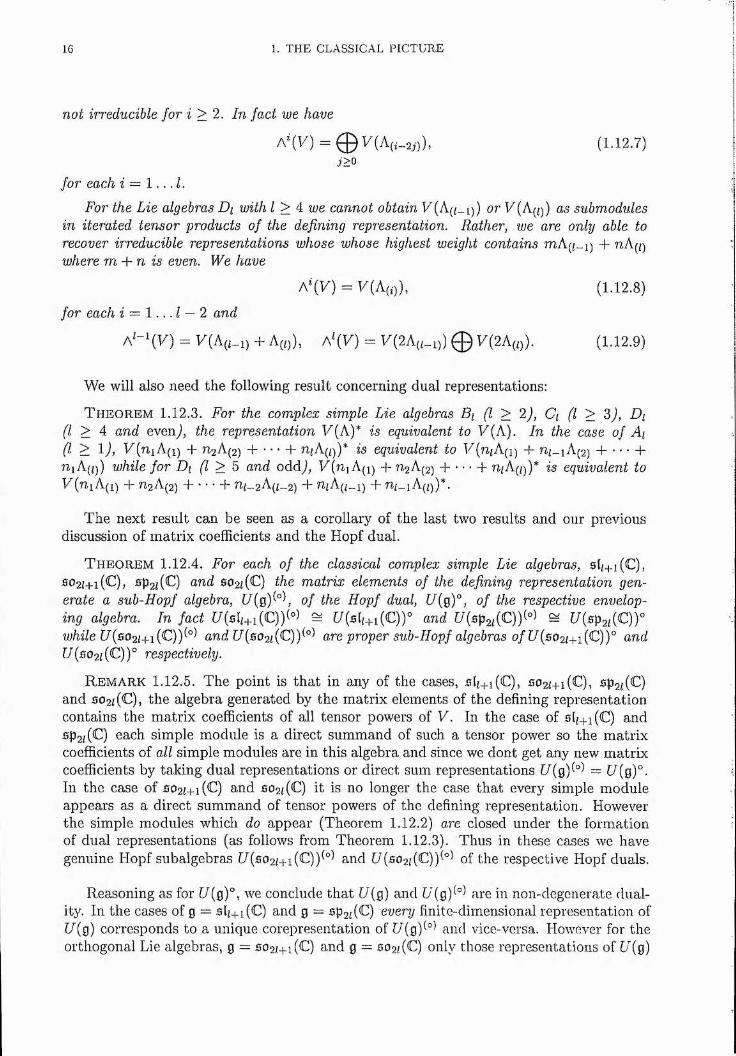
IG 1. THE CLASSICAL PICTURE

not irreducible for i > 2. In fact we have

A*(E) = ^ (1.12.7)7>0

for each 7 = 1. . . / .

For the Lie algebras Di with I > A we cannot obtain V (A(f_i)) or V (Ag)) as submodules in iterated tensor products of the defining representation. Rather, we are onkj able to recover irreducible representations whose whose highest weight contains + ?2A(pwhere m + n is even. We have

A \V ) = T/(A(i)), (1.12.8)for each i — 1 ., . 1 — 2 and

a ‘- \ V ) = V(A(H) + A(„). A '(y) = 1/ ( 2A(,_1,) 0 1/ (2A(„). (1.12.9)

We will also need the following result concerning dual representations:

T h e o re m 1.12.3. For the complex simple Lie algebras Bi (I > 2), Q (I > 3) , Di (I > A and even), the representation E(A)* is equivalent to V{A). In the case of Ai (I > lA E(niA(i) + n2A(2) + • • • + uiAq))* is equivalent to E(nzA(i) + n^_iA(2) + • • • +niA(i)} while for Di (I > b and oddj, E(niA(i) + 712A(2) + ------1- niA^))* is equivalent toE(77iA(i) + 7T.2A(2) + • • • + 7l(_2A((_2) + 72 A(i_i) + 71/_iA(/))*.

The next result can be seen as a corollary of the last two results and our previousdiscussion of matrix coefficients and the Hopf dual.

T h e o re m 1.12.4. For each of the classical complex simple Lie algebras, afi^_i(C), 5021+1 (Q , sp2 ii^) o,nd 5022(C) the matrix elements of the defining representation gen­erate a sub-Hopf algebra, U{qY°\ of the Hopf dual, UIqY, of the respective envelop­ing algebra. In fact [7(5 l/+i(C))^A ^ f/(5b+i(C))° and U(sp2i(C)Y°'^ = U(Bp2i(C))° wWe [7(5022+1 (C))(A 07%d [/(5022(C))(°) are proper sub-Hopf algebras of U{so2i+i{C))° and U{s0 2 i{C)y respectively.

R e m a rk 1.12.5. The point is tha t in any of the cases, 5(/+i(C), 5022+i(C), 5p2i(C) and 5022(C), the algebra generated by the matrix elements of the defining representation contains the matrix coefficients of all tensor powers of V. In the case of sfi+i(C) and 0p22(C) each simple module is a direct summand of such a tensor power so the m atrix coefficients of all simple modules are in this algebra and since we dont get any new matrix coefficients by taking dual representations or direct sum representations [7(g)(°) = [7(g)°. In the case of 5022+1 (C) and 5022(C) it is no longer the case that every simple module appears as a direct summand of tensor powers of the defining representation. However the simple modules which do appear (Theorem 1.12.2) are closed under the formation of dual representations (as follows from Theorem 1.12.3). Thus in these cases we have genuine Hopf subalgebras [/(so22+i(C))^°^ and [/(5022(C))(°) of the respective Hopf duals.

Reasoning as for [7(g)°, we conclude that [/(g) and [7(g)(°) are in non-degenerate dual­ity. In the cases of g = sfi+i(C) and g = sp2f(C) every finite-dimensional representation of [/(g) corresponds to a unique corepresentation of [/(g)(°) and vice-versa. However for the orthogonal Lie algebras, g = 5022+i(C) and g = 5022(C) only those representations of U(q)

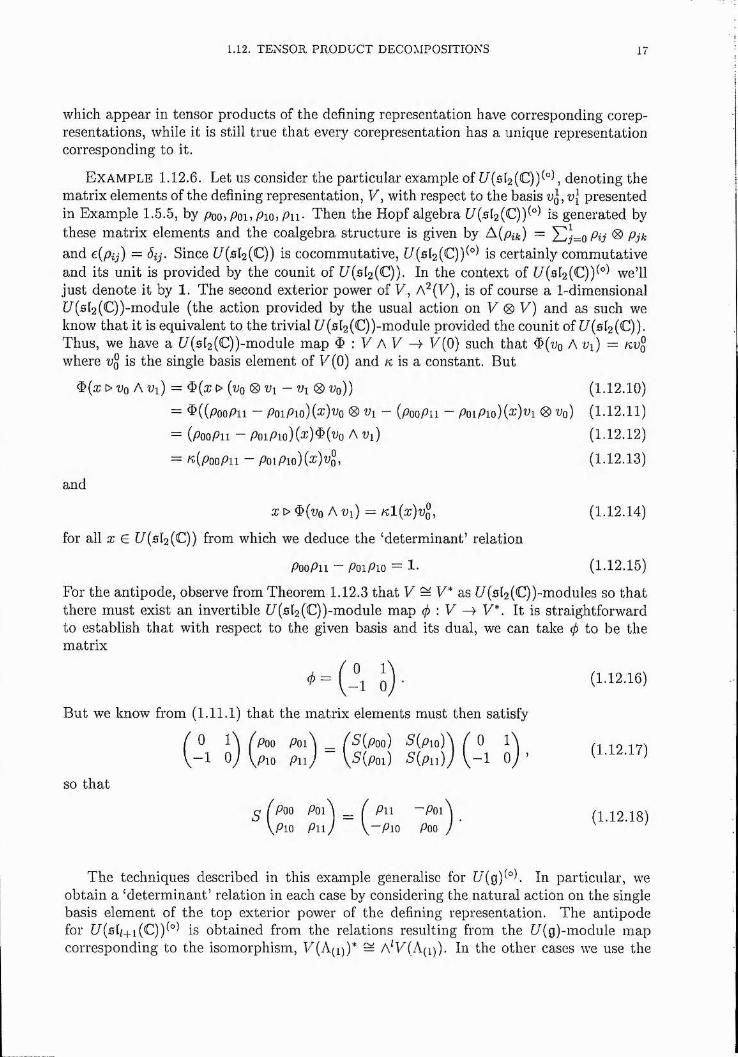
1.12. TENSOR PRODUCT DECOMPOSITIONS 17

which appear in tensor products of the defining representation have corresponding corep­resentations, while it is still true that every corepresentation has a unique representation corresponding to it.

E x a m p le 1.12.6. Let us consider the particular example of [/(512(C))(A, denoting the matrix elements of the defining representation, V, with respect to the basis uj, u} presented in Example 1.5.5, by poo, Poh P101 Pu- Then the Hopf algebra [/(512(C))(°) is generated by these matrix elements and the coalgebra structure is given by A(p fc) = Yl]=oPij 0 Pjk and e{pij) = Sij. Since [/(512(C)) is cocommutative, [/(512(C))(°) is certainly commutative and its unit is provided by the counit of [/(512(C)). In the context of [/(5l2(C))(°) we’ll just denote it by 1. The second exterior power of V, A^(E), is of course a 1-dimensional [/(sl2(C))-module (the action provided by the usual action on E 0 E) and as such we know that it is equivalent to the trivial [/(512(C))-module provided the counit of [/(512(C)). Thus, we have a [/(5l2(C))-module map # : E A E E(0) such that <D(uo A v i) = kvq where Ug is the single basis element of E (0) and K is a constant. But

0(a; i> fg A Ui) = $(a; t> (% 0 - Ui 0 Vq)) (1.12.10)

= ^ ^ ( ( p o o P n - PoiPio)(^)^^o 0 - ( p o o p n - P o iP i o ) C v ) v i 0 Ug) (1.12.11)= (PooPn ~ P o i P i o ) ( ^ ) ^ ^ ( v o A i»i) (1.12.12)

= f<^(PooPii ~~ Poi P io) ( ^ ) v q , (1.12.13)

and

a; 0 $(uo A ui) = al(a:)ug, (1.12.14)

for all X e [/(512(C)) from which we deduce the ‘determinant’ relation

PooPn ~ PoiPio = 1 (1.12.15)

For the antipode, observe from Theorem 1.12.3 that E = E* as [ / (512(C))-modules so that there must exist an invertible [/(s (2(C))-module map : V -> E*. It is straightforward to establish tha t with respect to the given basis and its dual, we can take (/) to be the matrix

■ ^ = ( 1 n V (1.12.16). 1 0

But we know from (1.11.1) that the matrix elements must then satisfy

0 l \ fPoQ PoA _ (S{poo) S{pio)\ / 0 l \ n 19 17T-1 0; P i J - ^,5(poi) ^(P ii)y o j ’ (1.12.17)

5, , Poo Poi\ I Pn - P O I ) (1.12.18)

SO t h a t

s (Pio P n J y —PiQ Poo

The techniques described in this example generalise for [/(g)(°\ In particular, we obtain a ‘determ inant’ relation in each case by considering the natural action on the single basis element of the top exterior power of the defining representation. The antipode for [/(5b+i(C))(°) is obtained from the relations resulting from the [/(g)-module map corresponding to the isomorphism, E(A(i))* = A^E(A(y). In the other cases we use the

18 1. THE CLASSICAL PICTURE

maps corresponding to E(A(i))* = E(A(y). In these cases we actually obtain further relations, namely

p 'X p X -' = 1 , (1.12.19)

where we are using an obvious matrix notation, and X = L ,S , J in the cases S02;+i(C), sû2i(C) and sp2i(C) respectively. Note that with a different choice of basis for E(A(i)) the m atrix elements are changed to some linear combination of the and the matrices X will be different also. Indeed, if in the cases of 502i+i(C) and S02/(C) we took, as wecertainly could, a basis of E(A(i)) in terms of which the Lie algebras were realised asskew-symmetric matrices, then the matrix X in these cases would have been simply theidentity and the extra relations would have looked like

Bq‘ = I, (1.12.20)

where Qij are the matrix elements corresponding to the alternative choice of basis.

1.13. Lie groups

We begin with the basic definitions.

D e f in it io n 1.13.1. A group G which is also a differentiable (infinitely differentiable) manifold is a Lie group if the operations of multiplication and taking inverses are differ­entiable as maps from G x G to G and G to G respectively.

In particular, the left and right translation maps, Lg \ G -A G and Rg : G ^ G given respectively by Lg{h) = gh and Rg{h) = hg are differentiable diffeomorphisms.

D e f in it io n 1.13.2. A differentiable map 4> : G G' between two Lie groups G and G' which is also a group homomorphism is called a Lie group homomorphism.

D e f in it io n 1.13.3. The tangent space at any point, g, of G is denoted Tg(G). It is the real vector space of point derivations of germs of real valued functions at g.

Recall tha t the dimension of a differentiable manifold is the dimension of the Euclidian space which locally approximates the manifold. This is also the dimension of the tangent space Tg{G) at any point g E G.

If V is an element of Tg{G) and / is a real-valued differentiable function on G then on some chart, {Ug,ipg), about g, whose coordinate functions are where d is thedimension of G, we may write

v{ f) = ± vi=l

(1.13.1)

where f = foipg, Abbreviating, an arbitrary tangent vector at g may be written uniquely as V = d/dxi\g.

D e f in it io n 1.13.4. A differentiable vector field on G is a differentiable assignment. X : g —> A|g, of a tangent vector, A|g, to any point g E G.

1.13. LIE GROUPS 19

On a chart {Ug^i/jg), we may express an arbitrary vector field, X , uniquely as

(1.13.2)" ' - 1 4

where Q are difierentiable functions on Ug. If X and Y are two differentiable vector fields then their Lie bracket, [X, Y"], is also a differentiable vector field.

D e f in it io n 1.13.5, If </> : G -4 G' is a differentiable map then there is an induced map dfi, the differential of 0, such tha t for all g E G, d(() \ Tg{G) -4 (G') accordingto

(# (% ;))( /) = ^ ( / o (^), (1.13.3)

for any v E Tg{G).

D e f i n i t i o n 1.13.6. A vector field, X , on a Lie group G is called left-invariant if and only if for all p G G and any h E G

X|g/, = dL g(X |/,). (1.13.4)

The real vector space of all left-invariant vector fields is denoted Sjr,(G).

It may readily be confirmed that the Lie bracket of any two left-invariant vector fields is again left-invariant. The following important theorem tells us tha t the vector space of all left-invariant vector fields is d-dimensional.

T h e o r e m 1.13.7. To any tangent vector v G T^(G), where e E G is the identity of the group, may be associated a left-invariant vector field, X ^ , such that X^|g = c\Lg{v). The map v -4 X^ is a vector space isomorphism between Te{G) and El{G).

D e f i n i t i o n 1.13.8. The Lie algebra of a Lie group G is the vector space Tg(G) equipped with the Lie bracket, [u, w] = [X",X^"]|/ for all v,w E Te(G). It is denotedby g.

Any vector field, X , may be expressed as a sum of the form X = wherethe Q are differentiable functions on G and X^' is the basis of left invariant vector fields corresponding to a basis {vi}f-i of Tg(G).

D e f i n i t i o n 1.13.9. A differentiable curve cj : (a, 5) c M -4 G is an integral curve of a vector field X centred at the identity if <j(0) = / (0 G (a, b)) and dcr(d/d[)|f=g2(a4) = X|o.(g).

For a general differentiable manifold, A4, it is true that to any differentiable vector field X and for any point P in A4, there exists a unique integral curve of X , ap {t), centred at the point P and defined on some interval (a, b) containing 0 such that if s, t and .s -f t are all in {a,b) then cr^x(5)(0 = (s -f t). In the particular case of Lie groups we have the following key result:

T h e o r e m 1.13.10. To every left-invariant vector field X of G there is a unique inte­gral curve centred at the identity with the whole of E as its domain.

If such an integral curve is denoted a^'{t) where v E 7^(G) is such that X |/ = v then cr" : E G is a Lie group homomorphism called a one-parameter subgroup. There is a1-1 correspondence between 7^(G) and one-parameter subgroups.

20 1. THE CLASSICAL PICTURE

D e f in it io n 1.13.11. The exponential map exp : g G is defined as

exp(tn) = cr'’(t), (1.13.5)

for any v E q and t e R.

T h e o r e m 1.13.12. The exponential map exp : g —)■ G zs differentiable and its differ­ential, d e x p : To(g) -4 Tg(G), is the identity map. There is an open neighbourhood, Uq, of g about 0, and an open neighbourhood, Ue, of G about e such that exp : Uq Uc is a diffeomorphism.

E x a m p l e 1.13.13. GL{n, E) is a subset of M (n, E) = , the set of all real matrices,and GL(n, C) is a subset of M (n, C) = E^”^, the set of all complex matrices. Let us just discuss C?L(n, E) and note tha t an analogous discussion holds for GL{n,C). M (n, E) is a differentiable n^-dimensional manifold with a global coordinate system in terms of the single chart, (M (n ,E ),Id ) where Id(M ) = (M u ,M i2, . . . , M„n)for any matrix M E M (n, E). The coordinate functions of this chart are the maps Xij : M (n, E) -4 E where T^j(M) = Mij for i , j — l . . . n . The map det : E"^ -4 E is polynomial and so continuous. Therefore, as {0} is a closed subset of E, {M E M{n, E) | det(M ) = 0} is a closed subset of M (n,E ). But G L(n,E) is just the complement of this subset, so GL(n, E) is an open subset of M{n, E). As such GL(n, E) is also a differentiable manifold and inherits the global coordinate system of M (n, E). That GL(n, E) is indeed a Lie group now follows easily since both multiplication and taking inverses are algebraic and hence differentiable. The tangent space, Tj(GL(n, E)) at the identity in GL(n, E) is spanned by the partial derivatives, {d/dxij)i for i , j = 1 .. .n , and is isomorphic as a vector space to M (n, E). The Lie bracket on Ti(GL(?r, E)) is provided by the matrix commutator, [M, N] = M N — N M , and equipped with this bracket, Ti(GL(n,E)) becomes the real Lie algebra gl(n, E). Actually, it is clear tha t GL(n,E) and GL(n, C) are real analytic manifolds (GL(n, C) may equally be regarded as a complex analytic manifold in which case it will be denoted GLn[C)). It can be shown that the exponential map in both cases is the usual matrix exponential map, i.e.

IVT"'exp(M) = e ^ = l + M + — + (1.13.6)

where M G gl(n, k) and is the matrix exponential function and A: = E or C.

1.14. The Classical Lie groups

Most of the the groups which we are interested in have concrete realisations as matrix subgroups of the matrix groups GL(n, E) or GL{n,C) of respectively real and complex invertible matrices. The groups then inherit their (Hausdorff) topology from the ambient metric spaces E"^ or respectively — the distance being defined by

6(M ,N ) \ y Z (1.14.1)\| +.7 = 1

for any two group elements M and N. In this context the otherwise difficult concepts of closure, boundedness, compactness and connectedness become more tangible. The following result is extremely useful.

1.14. THE CLASSICAL LIE GROUPS 21

T h e o r e m 1.14.1. I f H C G is a subgroup of G which is closed as a topological subspace of G, then H is also a Lie group (a Lie subgroup/ I f and g are the re­spective Lie algebras of H and G, then the differential, dz|/ : 1} -4 g, 0/ the inclu­sion map L : I I -A- G is an isomorphism of f) luith a Lie subalgebra of q. In fact

= {x‘ G g I exp (to) G Hfor all t G R}.

In particular, for any group of matrices, G, which is a closed subgroup of G L(n,k), we deduce that it is a Lie subgroup of GL{n,k). Its Lie algebra, g, is a Lie algebra of matrices with the matrix commutator providing the Lie bracket, the exponential map being the matrix exponential function and so

g = {IVI G gl(?%, k) I G G for all t G E}, (1.14.2)

where M G gl(n, k).

The fact that the exponential map is a diffeomorphism between open neighbourhoods of 0 in g and I in G means that we may coordinatise G as follows. Denote by log, the inverse of the map e. Then ([/i, log) is a chart around I G G. For any other point, M G G, Lm is a diffeomorphism and so Uyi = LmUi is an open neighbourhood of M and defining 0m = lo g o L ^ , ( Z 7 m , 0 m ) is a chart around M. It is clear that these charts fit together differentiably to provide the required differentiable manifold structure. In fact the analyticity of the matrix exponential map ensures that these groups are real analytic Lie groups.

The real classical groups will now be defined.

D e f in it io n 1.14.2. SU{1 + 1), the special unitary group, is the subgroup of GL{1 + 1,C) (/ > 1) consisting of matrices U such that UU* = U*U = I and det(U) = 1 where U* is the hermitian adjoint (i.e. (U*)^j = where z is the complex conjugate of the complex number z).

D e f in it io n 1.14.3. SO(l), the special orthogonal group, is the subgroup of G L(/,E) (/ > 3) consisting of matrices O such tha t OO^ = 0 ^ 0 = I and det(O) = 1 where O* is the transpose of O.

D e f in it io n 1.14.4. Sp{2 l), the symplectic group, is the subgroup of GL{21, C) (A > 2) consisting of matrices U such tha t UU* = U*U = I and UJU* = J where J was given in (1.3.15). (It follows that det{U) = 1.)

It turns out to be necessary to distinguish the special orthogonal groups of the form 5 0 (2 / + 1) and 50 (2 /). W ith the aid of Theorems 1.14.1 and 1.13.12, the following theorem may be established.

T h e o r e m 1.14.5. The classical Lie groups 5 /7 (/ + l ) , 5 0 (2 / 4-1 ) , Sp{2l) and 5 0 ( 2 /) are compact, connected Lie groups of dimensions /(/ + 2), /(2/ T 1), /(2/ + 1) and 1(21 — 1) respectively. Their Lie algebras are denoted by 5 u(l + 1), 5o(2/ + 1), $p(2/) and so(2/) respectively. s u ( / + l ) is the Lie algebra of skew-Hermitian mo,trices of trace zero, so(2/ + l) and s o (2/) are Lie algebras of real sketu-symmetric matrices and sp(2/) is the Lie algebra of skew-Hermitian matrices, T , satisfying T J + JT^ = 0 where J was given in (1.3.15).

22 1. THE CLASSICAL PICTURE

1.15. The algebra of representative functions on a compact group

D e f in it io n 1.15.1. A representation of a compact Lie group G is a pair (vr, V) where 7T : G ^ GL[V) is a continuous group map. We say that V is a G-module with a continuous action, > : G x V V, written as g o v = 7r(g)v for all ^ e G and v E V. This action is understood to be linear on V, but of course the notion of linearity is not present for the group.

D e f i n i t i o n 1.15.2. A representative function on G of a finite dimensional repre­sentation, ( t t , Y), is a continuous function, 7Ta,v : G —> C such tha t for any g E G, '^a,v{g) = c^i9 >v) where v E V and a E V*. The representative functions of all finite­dimensional representations of G are denoted by Gaig(G).

As we assume T to be a finite, n-dimensional complex vector space, i.e. V = C". Choosing a basis, for V results in a matrix representation, t t : G - 4 GL(n, C),and we denote by 7Tij(g) the matrix elements of the representation m atrix 7r(^) of a group element g such tha t g o v i = The continuous, complex valued functionsTTij are representative functions called simply the matrix elements of the representation. The complex conjugate of a matrix element, Wï], is defined by Wïj{g) = TTij(g). The space spanned by the matrix elements of a finite dimensional representation is independent of the choice of basis and indeed the matrix elements span the space of representative functions of the representation.

The notions of submodule, reducibility, complete reducibility and irreducibilty are all defined in the obvious way. As for finite groups, every finite-dimensional representation of a compact Lie group is equivalent to one by unitary matrices. Moreover, we have the following important result concerning their reducibility.

T h e o r e m 1.15.3. All finite dimensional matrix representations of a compact Lie group are completely reducible.

Once again linear algebraic constructions for G-modules are important. Given two G- modules, Y and W , with respective actions, g o v = TT{g)v and gow ~ f[g)v) for all ^ G G and, V E V and w E W , their direct sum is also a G-module with action g o [v ® w) = 'ïï(g)v Arf[g)v} and so is their tensor product, with action go(v® u)) = ('x(g)v) 0 [f,(g)v)) for all u G y and w E W. Any constant multiple, cV of a G-module is again a G-module, and so is the dual vector space, V*, with action, {g o a){v) = a{g~^ o v) for all a E V*. Notice th a t in terms of matrix elements, if and are dual bases of V* and Vand ÏÏ g o a i = ^nd govi = then fij{g) = 7Tji{g~y. Related tothe dual representation is the conjugate representation. This is obtained by introducing the space V defined as the same underlying additive group as R but with the scalar multiplication defined as c o v = cv îov any c G C. If V is a G-module then so is V with g o v i — Since all finite dimensional representations are equivalent torepresentations in terms of unitary matrices we can see that V and V are equivalent as G-modules.

The natural unit for the algebra of continuous functions on G is the identity function, 1 ; G -> M, such tha t 1(g) = 1 for all g E G. It is also a representative function since on any vector space, V, we can define the trivial representation where each group element acts as the identity, i.e. gt>v = v = l(g)v for all v e V .

1.16. STOXE-W EIERSTRASS THEOREM 23

The space of representative functions, Caig(G), which by the previous theorem is spanned by the representative functions of the irreducible representations, forms a sub­algebra of the algebra of all continuous complex-valued functions on G, C(G). In fact Gaig(G) has a Hopf algebra structure which is formally precisely tha t in Theorem 1.7.5, but with p replaced with t t , and 77(1) = 1 . There is actually some further structure on Gaig(G) for which we need the following definition.

D e f i n i t i o n 1.15.4. A 'k-algebra is an algebra over C, (A, 7?t,, 77) say, endowed with a conjugate linear map * : A —> A such that

+ o + = id, 777 o (+0 +) o P = + o ?n, (1.15.1)

where P{a 0 a') = a' 0 a for all a, a' G A. A 4-algebra map, 0 : A -4 A', between two 4-algebras, A and A', is an algebra map which satisfies 0 0 4 = 4 0 0 . Dually, a -k-coalgebra is a coalgebra over C, (C, A, 77) say, equipped with a linear map • : (7 -4 C such that

* o # = id, P o (• 0 •) o A = A o •. (1.15.2)

A Hopf -k-algebra is a Hopf algebra A such that the constituent algebra is a 4-algebra with the coalgebra maps, A and e, 4-algebra maps. The constituent coalgebra is then a 4-coalgebra by the map 4 o 5.

It is usual to denote the 4-map on elements a of a given Hopf 4-algebra as a*. Then on m atrix elements ivij of some representation (tx,V) of G, we define Tr^(^) = 'Xiffg) or, denoting the m atrix coefficients of the conjugate representation V by Wij, 7t*j ~ Wij.

The representation theory of Gaig(G) is of course not particularly interesting as it is a commutative Hopf algebra. However the corepresentation theory corresponds to the representation theory of G and so is extremely interesting. Indeed, given a finite dimen­sional continuous representation (zr, V) of G, we define a corepresentation (Ay, Gaig(G)) by Ay('u)(^) = t(G ) where we are making use of the isomorphism V 0 G(G) = G(G, V) where by G(G, V) we mean the continuous vector-valued functions on G. In the other di­rection, it is clear tha t starting with a corepresentation of Gaig(G) we recover a continuous representation of G. This correspondence preserves the usual representation attributes (i.e. irreducibility etc.). Moreover, there is a natural definition of a unitary corepresenta­tion and with this unitary representations correspond to unitary corepresentations.

1.16. The Stone-Weierstrass theorem and the algebra of representativefunctions on the classical Lie groups

The definitions of the classical Lie groups provide ‘tautological’ faithful matrix rep­resentations which we shall denote by ( 7-, V) (incidentally, these representations are ir­reducible). In each case the group space is a metric space which is moreover compact so G(G) may be equipped with the supremum norm topology provided by the norm I/I = sup{|/(f/)| 1 for all g E G}. The matrix coefficients of the respective defining repre­sentations ‘separate points’ of G in the sense that if two group elements are not the same then there must be a matrix coefficient which distinguishes them. The following theorem of analysis, called the Stone-Weierstrass theorem, is of fundamental importance.

T h e o r e m 1.16.1. Let E be a compact metric space. I f a subalgebra A of the algebra of complex valued functions on E, G{E), contains all complex constants, separates points

24 1. THE CLASSICAL PICTURE

of E and is such that for each f E A the conjugate function f also belongs to A then A is dense in C{E).

Now, for any of the classical Lie groups we can form the polynomial algebra over C, denoted C[G], which is generated by the matrix elements and their complex conjugates, r^. Of course the rij and rff belong to Caig(G) and moreover by the Stone-Weierstrass theorem C[G] is dense in C{G) so we deduce that Gaig(G) is dense in C{G). In the more general context of an arbitrary compact Lie group this result is the celebrated Peter- Weijl theorem. W ith a little further work, the relationship between C[G] and Gaig(G) may be clarified.

T h e o re m 1.16.2. The algebras C[G] a,nd Caig(G) are isomorphic.

In the special cases of the classical Lie groups we can actually make a further refine­ment. In these cases it turns out that C[G] is generated already by the r^j. Denoting by P{r{g)), polynomials in the matrix elements of (r, T) and by I„, the n x n identity matrix, the details in each case are as follows:

1. 5 G WThe first fundamental representation of S U (n) is precisely the (faithful) defining

representation in terms of unitary matrices with determinant 1. Thus for all g E SU{n), each matrix, r{g), in this representation satisfies r{g)r{g)* = r(g)*r{g) — In so r(g)* = r{g)~\ But {r{g)~yij = P{r{g))/det{r{g)) and det(r(^)) = 1 so th a t r{g)ij — P{r{g)). That is, the complex conjugate matrix elements, rfj, are polynomials in the matrix elements r^-.

2. 50(7%)Again, the first fundamental representation of SO(n) is just the (faithful) defin­

ing representation, now in terms of real orthogonal matrices. Thus, in this case it is immediate tha t for all g E G, rij{g) = rij{g), so rij — rij.

3. Sp{2n)Once again, the first fundamental representation of Sp{2 n) is just the (faithful)

defining representation in terms of 2 n x 2 n matrices, r(g), satisfying, in particular, — ^(gYr{g) — l 2n and det{r{g)) = 1 for all g E Sp{2n). By the same

reasoning as for SU(n) we conclude that the complex conjugate matrix elements, rij, are polynomials in the matrix elements tt^.

Since the matrix representations (r, Y), and in particular their matrix elements, are certainly analytic, it now follows that the matrix elements of all finite-dimensional repre­sentations are analytic so indeed the representations themselves are analytic. Also, it is clear that we can view the Hopf algebras C[G] as being generated by the matrix elements of their first fundamental representations of G.

E x a m p l e 1.16.3. Let us consider C[SU{2)]. This commutative Hopf algebra is gen­erated by the matrix elements of the first fundamental representation, rn,?T2, r 2i and T'22 say. We will denote the unit of C[SU{2)] by 1. The coalgebra structure is justA(7Ti/-) = TCi; ^ TTjk and e(7Tij) — ôij. The fact that det(U) = 1 for all U E 51/(2)leads immediately to the corresponding relation

- Fi2'/'21 = 1 (1.16.1)

1.17. THE COMPACT REAL FORMS OF THE CLASSICAL COMPLEX LIE ALGEBRAS 25

for the generators of C[5C/(2)J. In fact we write such a relation also as det(r) = 1. The antipode and 4-structure on C[SU{2)] are similarly obtained immediately by considering the m atrix elements of for any U G 5/7(2)

: /;;■)=ti; :i) ■Compare this Hopf algebra (without 4-structure) with /7(sl2(C))^°l obtained in 1.12.6.

For the other classical Lie groups the Hopf algebra structure of C[G] is just as straight­forward to obtain. In each case we have the determinant condition det(?’) = 1 and for the orthogonal groups also

r / = I (1.16.3)while for the symplectic groups

p*JpJ-^ = 1 . (1.16.4)

Furthermore, the antipode is given by S{rij) — where is the ‘cofactor’ of the element Tij in the ‘m atrix’ r. Finally, the 4-structure is given on the generators by andextended conjugate linearly and homomorphically to the whole of C[G].

1.17. T h e co m p ac t rea l form s of th e classical com plex Lie a lg eb ras a n d th e irrep re se n ta tio n s

The complex simple Lie algebras, 5fi+i(C), 50241(C), 5p2/(C) and 502; (€) are respec­tively complexifications of the real simple Lie algebras gu{1 + 1), so(2/ 4- 1), sp(2/) and 5 0 (2 1 ) according to the following definition:

D e f in it io n 1.17.1. A real Lie algebra is a real form of a complex Lie algebra g if g = C 0R gR. In this case g is called the complexification of gg.

A remarkable theorem due to Weyl says tha t a matrix Lie group G is compact if and only i f the Killing form of its Lie algebra is negative definite. In this case the Lie algebra, g, is said to be compact.

Every complex simple Lie algebra has a real form which is also compact. This is made explicit in the following theorem:

T h e o r e m 1.17.2. In terms of the Cartan-Weyl basis of a complex simple Lie algebra, g, the elements iHi, + E_q, and i(Ea — E_a) form the basis of real simple Lie algebra which is denoted, g^pt, and called the compact real form of q.

The irreducible representations of the four series of classical complex Lie algebras, Ai, Bi, Cl and Di, restrict as irreducible representations to the respective compact real forms, su(/ + 1 ), 50(2/ 4-1), 5p(2l) and 50(2/) respectively. Moreover it is a general result th a t all irreducible representations of simple real Lie algebras whose complexifications are smple arise as the restrictions of the irreducible representations of the complex Lie algebras.

It is worth mentioning that we assume our g-modules to be generic complex vector spaces. However when we regard them as representations of the compact real forms, gcpt, it may be that some are equivalent to real representations. This is true in the particular cases of the first fundamental representations of Bi and Di — as we would expect!

26 1. THE CLASSICAL PICTURE

1.18. Representations of the Classical Lie groups

To every Lie group G there corresponds a unique Lie algebra g. In the other direction, given g there may correspond more than one Lie group. However, amongst the connected Lie groups sharing g there is a distinguished one called the universal covering group and denoted G. This group is simply-connected, unique up to isomorphism and such that every other connected group G whose Lie algebra is g is given by G = G/7ri(G) where 7Ti(G) is the fundamental group of G.

The compact connected groups SU [I -t- 1) and Sp{2l) are simply-connected while 5 0 (2 / 4- 1) and 50(2 /) are not and have universal covering groups Spin{2l 4- 1) and Spin{2l) respectively, with

5 0 (n ) = Spin{n)/Z 2 . (1.18.1)

If (ttg, V) is a continuous representation of some matrix Lie group, G, in terms of matrices, noig), for all g E G, then (vr , H) is a representation of the corresponding Lie algebra, g, in terms of matrices

d7rG(e '') (1.18.2)

i= 0

for all X G g. If (ttl, V) is obtained from (ttg, V) in this way, we say tha t the Lie algebra representation exponentiates to a Lie group representation. As the classical groups are connected, equivalence, irreducibility and complete reducibility are all preserved through both ‘differentiation’ and exponentiation.

The fundamental theorem is the following:

T h e o r e m 1.18.1. I f G\ and Gg are Lie groups (real or complex complex analytic) with Gi simply connected and gi and Q2 ore the corresponding Lie algebras, then a linear map 0 : gi -4 g2 zs the differential d 0 of a Lie group homomorphism ip : G \ ^ G 2 if and only if 0 is a Lie algebra homomorphism.

This result tells us that in the cases of SU(n) and 5p(n), not only is there a Lie algebra representation (tt^, V) corresponding to each group representation, (ttg, T), but tha t every Lie algebra representation arises in this way. In other words, in the cases SU {I 4- 1) and Sp{2l), every Lie algebra representation exponentiates to a Lie group representation.

This is not the case for the Lie groups 5 0 (2 / 4-1) and 50(2 /) as they are not simply- connected. In these cases not all Lie algebra representations exponentiate. That is, there are Lie algebra representations which are not obtained from group representations by differentiating. It is true however that all Lie algebra representations exponentiate to representations of the respective universal covering groups, S p i n ( 2 n 1) and Spin[2n). It is then a question of which of these representations factor through the quotient Z 2. This turns out to be reasonably straightforward to establish. The result is as follows;

T h e o r e m 1.18.2. ® 5 0 ( 2 / 4 -1 ); Of the irreducible representations of so[21 4 -1 ),with highest weight, A = rziA(i) 4- 712A(2) 4- . . . 4- npffi), those that exponentiate to representations of S O {21 -t-1) are such that ui is even.

• 5 0 ( 2 / ) ; Of the irreducible representations of so(2/), with highest weight, A = ?iiA(i) 4- 77,2A(2) 4 - . . . 4- ni.ffi), those that exponentiate to representations of S O (21) are such that 7Z;_i -I- ni is even.

1.19. COMPLEXIFICATION OF THE REAL CLASSICAL GROUPS 27

We see that the irreducible representations of the classical Lie algebras, su(/ + 1), 50(2/ + 1), sp(2/) and so{2l), which exponentiate to representations of the corresponding classical Lie groups SU{1 + 1), 5 0 (2 / + 1), Sp{2l) and 50(2 /) are precisely those that can be obtained in tensor products of the respective defining representaiions. That each irreducible representation of these groups appears in tensor products of the respective defining representations is then an immediate consequence of this Lie algebraic result!

In each of the cases dealt with in the previous theorem, the weights of the representa­tions which exponentiate form additive subgroups, A(0) where G = 5 0 (2 / 4- 1), 50 (2 /), of the respective weight lattices P of the Lie algebras Bi and Di, That is, in each case we have Q C A (0) C P. Remarkably, 7Ti(0 ) = P /A (0 ) and Z{G) = A (0)/Q , results which have precise generalisations.

1.19. C om plex ification of th e rea l classical g roups

For each of the classical compact Lie groups G ~ SU(l 4-1), 5 0 (2 / 4- 1), Sp{2l) and 50 (2 /) , the algebra of representative functions, C[G], carries the structure of a Hopf 4-algebra. Through Tanaka-Krein duality, the respective compact groups may be recon­structed from these Hopf algebras as the set, Hom*_aigebra((L[G], C), of 4-algebra maps from C[G] to C (endowed with the natural group structure coming from the Hopf structure of C[G] and the coarsest topology such tha t the evaluation maps Ag : Hom*.aigebra(QO], C) -4 C given by Ag(0) = 0(s) are all continuous).

If we forget about the 4-structure and denote by G^ the set Homc-aigebra (C[G], C ), then G^ is precisely the affine algebraic variety specified by the coordinate ring C[G] (by the coordinate ring C[G] we will understand C[G] without 4-structure). Indeed, we saw in Section 1.16 tha t for each of the classical compact Lie groups, disregarding the 4-structure, C[G] has the form C[rÿ]/7 where C[?’ÿ] is the polynomial algebra over C in the symbols

h i — 1 • • • 7 , and 7 is a certain ideal (e.g. in the case of SU {14-1) this is just the ideal generated by the expression det(r) — 1). It is then standard that Homoaigebra(C[G], C) is in bijection with the set of common zeros of the polynomials in 7, that is, the affine algebraic variety V{I). Furthermore, recognising G L„(Q as a complex linear algebraic group, the V{I) are clearly subgroups which are moreover specified by polynomial expressions as subsets of GLn{V) and as such are Zariski-closed subgroups and hence complex linear algebraic subgroups. These then are the complexifications of the classical compact Lie groups. Explicitly, the complexifications of SU{1 4-1), 50 (2 /4 -1 ), Sp{2l) and 50(2 /) are 5Li+i(C), 5 0 2 4 1 (C), Sp 2i{C) and SÜ 2 i{C) respectively. They will be called the complex classical Lie groups. They are again matrix groups, which as complexifications can be regarded either as complex linear algebraic groups or as complex analytic groups. Their Lie algebras are precisely the complex simple Lie algebras, sfi+i(C), 50241(C), sp2z(C) and S02i(C) respectively, that is, the complexifications of the Lie algebras of the compact Lie groups.

The coordinate rings C[G] arc precisely the Hopf algebras generated by the matrix elements of the defining representations of the respective complexified groups G^. Fur­thermore, there is a one-to-one correspondence between corepresentations of C[G] and rational representations of G^ (i.e. those representations whose matrix elements are poly­nomial functions on G^).

28 1. THE CLASSICAL PICTURE

Regarding the complex classical groups as complex analytic Lie groups, they are con­nected, with SLi+i{C) and Sp 2i{C) simply connected. The complex orthogonal groups are not simply connected, and we have SOn{C) = Spinn{C)/Z 2 where SpiriniC), the univer­sal covering group of 50„(C ), is the complexification of Spin(n). Each finite dimensional representation of sfi+i(C) and 5p2f(Q exponentiates to a complex analytic representation of the respective groups, SLi+i{C) and Sp 2i{C). The representations of 00241(C) and S0 2 i{C) which exponentiate respectively to complex analytic representations of 5 0 2 4 1 (C) and 502f(C) are precisely those whose restrictions to the compact real forms exponenti­ated to representations of the corresponding compact groups. The defining representations of the complex classical Lie groups (which are irreducible) appear in their very construc­tion and the restriction of these representations to the compact Lie groups within them are precisely the defining representations of the classical compact Lie groups.

In the case of the the real classical Lie groups and their real Lie algebras we were able to deduce, from the tensor structure of the Lie algebra representations together with a knowledge of which representations exponentiated, that every irreducible representation of the classical compact Lie groups appear in tensor products of the respective defining representations. Precisely the same reasoning tells us that for all the classical complex Lie groups, each irreducible complex analytic representation may be obtained within tensor products of the respective defining representations. It follows that the matrix elements of the finite dimensional representations of the classical complex Lie groups are polynomials in the matrix elements of the group elements. This in turn means that every finite complex analytic representation of a classical complex Lie group is a rational representation in the sense of complex linear algebraic groups. Thus we see that there is a one-to-one correspondence between corepresentations of C[G] and complex analytic representations ofGC.

1 .2 0 . f/(g)(°) an d C[G] are isom orphic

Suppose G (we are dropping the superscript C) is the complexification of one of the classical compact Lie groups and g is its Lie algebra.

T h e o r e m 1.20.1. There is a non-degenerate Hopf algebra pairing between the Hopf algebras /7(g) and C[G]. It is given by the action of elements of /7(g) on C[G) as left- invariant differential operators at the identity, explicitly

ak( 1 .20 .1)

tr 1 “ tt 2 -- 1 0(R,XlX2...XA:) = dtidt2 . . . dfA

where P G C[G] and X* G g.

As a consequence of this important theorem, there is an embedding l : C[G] —)■ /7(g)*, of C[G] in /7(g)* as a sub-Hopf algebra. We have already seen that complex analytic representations of G are in one-to-one correspondence with corepresentations of C[G] and in fact tha t C[G] is generated by the matrix elements , of the defining representation of G, (r,V). From Section 1.9 we deduce that the z(rÿ) may be identified with the matrix elements pL of the defining representation of g. It is then a question of which /7(g)- modiiles exponentiate to corresponding G-modules. We have already found the answer to this in Section 1.18 and so can deduce the important isomorphism

C[G] =[/(g)M. (1.20.2)

CHAPTER 2

T he quantum picture

2.1. Introduction

The purpose of this chapter is to provide the reader with an overview, in the form of key definitions and results, of the structural elements of quantum group theory. Again we restrict our discussion to structures associated with complex simple Lie algebras and in places the classical complex simple Lie algebras.

We begin with motivation and discussion of the concepts of fi-adic topology and com­pletion. W ith this mathematical machinery we are then able to formulate in a mathemat­ically rigorous manner the basic definitions and results concerning topological quasitrian- gular Hopf algebras, quantised universal enveloping algebras and their representations.

The quantised enveloping algebras are deformations of classical enveloping algebras. We recall two key cohomology results. The first tells us that there are no non-trivial deformations of universal enveloping algebras as algebras, but they may have non-trivial Hopf algebra deformations. The second tells us that there are no non-trivial deformations of representations of universal enveloping algebras. One consequence of these results is tha t there is a bijective correspondence between representations of the classical U{q) and the quantum Uh[%) such that, for example, Clebsch-Gordan series are preserved. Already these results suggest that there must be a quasitriangular quasi-Hopf algebra associated with Uh(ff) and this is confirmed by a third cohomolgy result.

The least ad-hoc construction of the quantised version of the coordinate rings of clas­sical Lie groups is to define these through the appropriate Hopf dual of the quantised universal enveloping of the corresponding Lie algebra. The classical theory described in Chapter 1 is the motivating model here. There is also a construction due originally to Faddeev, Reshetikhin and Takhtajan (FRT) and later developed by Majid. The FRT construction requires as input only a numerical R-matrix and always provides a bialgebra which can loosely be regarded as some sort of deformation of the classical bialgebra of regular functions on matrices. When the numerical R-matrix is the one obtained in the first fundamental representation from the universal R-matrix of one of the Drinfeld-Jimbo quantised enveloping algebras there is an obvious similarity between the FRT quantum group quantisations of the classical groups 5I/j+i(C), 502n+i(€), 5p2/(C) and 502; (C) and the quantisations defined as the appropriate Hopf dual of the objects [///sfi+i (C)), [//i(00241(C)), % (0p2;(C)) and Uh{so2 i{C)) respectively. Quantum group folk-lore says that these objects are the same though a proof of this in any of the cases other than 57/41 (C) does not seem to have been published.

In a style somewhat analogous to considering the semiclassical Poisson structures of a quantum mechanical system, we investigate the structures which exist within quantum groups at order h in the deformation indeterminate. At this level the relevant objects are

29

30 2. THE QUANTUM PICTURE

Lie bialgebras, for which there is a complete classification. The classification of Lie bialge­bras raises natural questions of existence and uniqueness of corresponding quantisations. The correct mathematical framework for the investigation of such issues is provided by Drinfeld’s notions of quasi-Hopf algebras and twisting. We recall Drinfeld’s famous the­orem. This result together with some more recent work of Etingof and Kazhdan provide the motivation for Chapter 3.

The Jordanian quantum group will be investigated in some detail in Chapter 4. In Section 2.10 we use it to exemplify some of the discussion of the chapter.

The references for this section are first and foremost the four excellent books on quantum groups by Chari and Pressley [17], Kassel [60], Jantzen [54] and in particular Cuichardet [46]. Drinfeld’s original papers of course provide inspiration, fi-adic topology is discussed in some detail in [6], The definition of quantised coordinate rings for the groups SOn{C) in terms of representations of quantised enveloping algebras is difficult to find in the literature. It seems to be well known amongst researchers but I was only able to find it explicitly statecl in the work of Hodges [51] and less explicitly in the thesis of Dijkhuizen [28].

2.2. /i-adic topology

The quintessential example of a quantum group, (012(C)), first appeared as an algebra in the work of Kulish and Reshetikhin [64]. Its full Hopf algebra structure was worked out later by Skylanin in [93]. In [64] a ‘deformation’ of [/(012(C)) appeared as the algebra with generators { X ,Y ,H } and commutator relations

[R,X] = 2X, [R ,y ] = -2Y ,

A question immediately arises as to the interpretation of the right hand side in (2.2.1). In particular how should we understand an object such as where a is an element of some algebra A. Splitting it up into partial, finite sums, s„ = each Sn iswell defined. W hat we need is a topological setting in which there is an equivalent of the usual Cauchy criterion of analysis, and in which = limn_^oo5n-

D e f in it io n 2.2.1. The ring of formal power series, C[[/i]], is the ring (which may also be regarded as an algebra over C) consisting of all formal objects of the form Y];=o...oo If a, 6 G C[[/i]] such that â = Yln>o and 6 = then

a + b = y^ (a„ + 6„)/i", ab = Y . ( Y , (2.2.2)n>0 n>0 p-i-q=n

C[[fi]] can be understood in topological terms such that formal objects like à are interpreted as limits of the corresponding partial sums. We consider the truncations C[[/il]//r” C[[/7,]]. Denoting by Sn the natural projection 5» : C[[fi]] -4 C[[/i]]/fi” C[[fi]] we write the image of à under 5» as à mod lY . Note that à G C[[h]] is invertible if and only if à mod Y 0- The algebras C[[/i]]//ff C[[/z]], for all n > 1 of polyno­mials in h of order up to n — 1 can be linked chain-like by the natural projections Pn : defined

2,2. 4A D IC TOPOLOGY 31

The family {C[[h]]/h^C[[h]],Pn) is an example of an inverse system of algebras, that is, a family {An,Pn) for all > 0 or > 1 of algebras A„ together with maps Pn : A^ -4 An-i-

D e f in it io n 2.2.2. The inverse limit, A = limA,i, of an inverse system of algebras is the set

limA,i = G An I Pn{0"ii) — 0,, —1}, (2.2.3)n>0

endowed with the usual componentwise addition and multiplication inherited from nn>o We define the map tt/. : lmiA„ -4 Ak to be the restriction to Im /R of the natural projec­tion from [%7%>o to Ak, then Pn o yr» = ttu- i -

A useful and easily derived result on inverse limits is the following:

T h e o r e m 2.2.3. Given an algebra B, an inverse system of algebras {An,Pn) ond a family of algebra maps (/„ : -4 An) such that pn o fn ~ /„_i for all n > 0, there existsan algebra map

/ : B -4 limAn (2.2.4)such that 7T„ o f — fn for all > 0.

Using this result it is not difficult to check that C[[h]] = lmC[[/z]]//z^^€[[/%]]. Also, we find tha t the quotient of an inverse limit is again an inverse limit.

T h e o r e m 2.2.4. If(An,Pn) is an inverse system of algebras with A = lm A ,i and I is a two-sided ideal in A then

A/7 ^ l^(A ,t/7 ,,), (2.2.5)

where In — ^^(7) and 7r„ is the natural algebra map 7T„ : A -4 A„.

The topology with which we promised to endow C[[/z]] is the so-called inverse limit topology. It is obtained generally, for any inverse limit liniA„, by giving each algebra An the discrete topology, An the induced product topology and then restricting to ImAn- A basis of open sets of ImiAn is then provided by the sets {7r~^(/7n)} where Un is an open set of An. In the particular case of C[[/r]], open neighbourhoods of 0 in C[[h]] are the sets h'^C[[h]] for all n > 0 and the topology is translation invariant in tha t 7T“ ^(a) = a + h^C[[h]] where a is any element of C[h]/{IY). This topology is also called the h-adic topology.

Actually, the fi-adic topology is a metric topology. For any a G C[[/i]] define Vh(a) to be the largest nonnegative integer n such that à G h^C[[h]].

T h e o r e m 2.2.5. C[[h]] is a metric space with a distance d{à,b) defined for any pair of elements a,h E C[[/i]] as d{a, b) =

D e f in it io n 2.2.6. A sequence {sn} in C[[/?J] is called a Cauchy sequence if given some P there exists an N such that for all m, n > N. Sm — Sn G !ffiC[[h]].

In particular, the partial sums Sn = J2i^o...n form a Cauchy sequence, and we can see that they converge in C[[/r]] to à = Z*=o...oo so giving ‘meaning' to the infinite sum. Moreover it is not difficult to check that every Cauchy sequence converges in C[[h]] so that C[[h]] is complete in this fi-adic topology.

32 2. THE QUANTUM PICTURE

More generally, for any C[[/z]]-modnle M we can construct the inverse limit of the /%]]-modules M / h^M to obtain the completion, M, of M in the /z-adic topology. In M,

the open neighbourhoods of 0 are the sets /z”M, and we may consider elements of the form X j^o...oo TTZt/z* where m* € M. M is a metric space with d(m, m') — wherenow Vh{m) is the largest non-negative integer n such that m G lYM . It is important to note tha t a completed C[[/z]]-module is both separated (Hausdorff) and complete.

In particular for algebras A over C[[/i]] objects like with a G A are well defined in the /z-adic completion of A, A. Notice also that is invertible in this context as g/io ijiod /z = 1.

If a and h are elements of some algebra A over C[[/zJ], then is not well de­fined in A 0c[[/ij] A. Generally if M and N are C[[/z]]-modules we need the /z-adic com­pletion, Mé>N, of M 0c[[/i]] N, obtained as the inverse limit of the modules (M 0c[[/i]] 7V)//z"(M0c[Mj N).

The most important class of C[[/z]]-modules for us are topologically free C[[/z]]-modules. Starting with a complex vector space V we construct V[[h]] as the C[[/z]]-module consisting of formal power series Ei=o...oo^%^*) with the C[[/z]]-action given by the natural extension of the algebra structure of C[[/z]]. Just as for C[[/z]], V[[h]] is separated and complete in the /z-adic topology. In fact H([/z]] is precisely the /z-adic completion of Y 0 C[[/z]].

D e f in it io n 2.2.7. A C[[/z]]-module will be called topologically free if it is of the form V[[h]] for some complex vector space V.

A C[[/z]]-module M is said to be torsion free if for any rn G M hm = 0 m = 0. Notice tha t any topologically free module is torsion free and that if M and N are isomorphic C[[/z]] modules then M is torsion free if and only if N is torsion free. Combined with the following result, this gives an important means of identifying topologically free modules.

T h e o r e m 2.2.8. A C[[h]]-module M is topologically free if and only if M is separated, complete and torsion free.

In particular, suppose we have two topologically free modules, V[[/z]] and kH[[/z]], then it is standard that their direct sum Y[[/t)]@H/[[/z]] is separated and complete, furthermore we can easily demonstrate that V[[h]] 0 kH[[/z]) = (H 0 H/)[[/z]] as C[[/z]]-modiiles so that as (V”[[/z]] 0 kY[[/z]]) mod /z can be identified with V 0 W we can write Y[[/z]] 0 IT[[/z]] = (V 0kÙ )[[/%]]. A similar statement applies for the completed tensor product Y[[/z]]0TT[[/z]]. It is by definition a completion and so separated and complete. It is then a standard procedure to demonstrate that Y[[/7]]0lT[[/z]) = {V 0 lT)[[/z]] as C[[/z]]-modules so that we can identify V[[h]](S>W[[h]] = {V 0 lT)[[/z]].

These and further desirable properties of topologically free modules are collected in the following theorem.

T h e o r e m 2.2.9. Suppose U, and Iff are complex vector spaces. Then

ft)

Homq[,])(B[[/z]), Y[[/z]]) ^ Hom(C H)[[/z]]. (2.2.6)

2.3. TOPOLOGICAL HOFF ALGEBRAS AND QUANTISED UNIVERSAL ENVELOPING ALGEBRAS3

50 that for any f e ([/[[/%]], ^ [[ /z j] ) we identify f M- J ]n > o where fn eHom([/, y ) for all n > 0 and

À E = E ( E (2.2.7)n>0 n>0 p+q=n

where 2n>o € C/[[/ïJ]. We write f = (/„).

M W ]ey[M ] = (c /ey )[W ]. (2 .2 .8)

(Hi)

c/[W]®y[M] = ([/ ® y)[M]. (2 .2 .9)

W

V[[h]]-, W[[h]]) ^ Homq[,.„((U ® F)([/i)l, W[[/i])) (2.2.10)

so that for any f e F[[?j]]; VK[[/î]]) we identify f H- X)„>o fJ i" where

/ ( E E = E ( E fr{'»'p,vf))hP', (2.2.11)p>0 q n>0 p+q+r—n

where fn G Hom^^^(C/, V"; W) for all n > 0.

If is a basis for a complex vector space y , then the C[[/i]]-moduIe generated bythese basis elements is dense in V[[h]] and we call {vi}i^j a topological basis for y [[/%]]. When y is finite dimensional, y[[/i]] is said to be of finite rank and indeed is precisely the C[[/i]]“inodule generated by the finite basis {oi}.

Sometimes we are interested in the quotient of a topologically free module V[[h]] bythe closure Î of some sub-module /. y[[h]]// inherits the metric space topology of y[[h]]and is complete since we quotient by the closure of I. For V[[h]]/Î to be topologically free it is then necessary and sufficient that it be torsion free, that is for any Vh G V[[h]] hvfi G / =4> v/i G / .

2.3. Topological Hopf algebras and quantised universal enveloping algebras

The topological setting of the previous section requires a modified definition of the notion of a Hopf algebra.

D e f i n i t i o n 2.3.1. A topological Hopf algebra, is a sextuple = (A,*, m, f). A, e, S) such tha t Ah is a C[[h]]-module with C[[h]]-linear maps, m : Ah®Ah Ah, i) : C[[h\] -4- Ah, A : -4 Ah®Ah, è : A/i -4 €[[/%]] and S : Ah —> Ah satisfying the same relationsas (1.6.5) but with the tensor products replaced by completed tensor products.

Very many examples of what are called quantum groups are examples of the following structure, invented by Drinfeld.

34 2. THE QUANTUM PICTURE

D e f in it io n 2.3.2. A topological quasitriangular Hopf algebra {Ah, 01) is a topological Hopf algebra Ah together with an invertible element 01 of the completed tensor product, Ah®Ah, such that

= (2.3.1)

( A® id) (3 ) = 3^13%, (2.3.2)(id®A)(3l) = 0^13%, (2.3.3)

where A°P(a) = a(2)0 a(i) and if CR = Ri®R'i then for example CR13 = i?i0 l(g)i?J. In this case

^ 121 131 23 — ^23^13^12- (2.3.4)which is the celebrated quantum Yang-Baxter equation (QYBE).

If our topological quasitriangular Hopf algebra {Ah, 01) is such that Ah is topologically free as a C[[/i]]-module, then the underlying vector space is {AfJhAh)[[h]] and we can legitimately think about the topological Hopf and quasitriangular structures in terms of formal power series. Thus the Hopf maps m, fj, Â, ë and S may be treated (in view of Theorem 2.2.9) in terms of the corresponding families of C-linear maps (m„), {r]n), {An), {cn) and {Sn)- In particular, the coproduct A is determined by its action on elements a G Ah/hAh as A (a) = 53„>oAn(a)h^ where the A» are C-linear maps such that An : Ah/hAh -4 {Ah/hAh) ® {AhJhAh) and the universal /^-matrix may be written as CR = where the Oin are elements of {Ah/hAh) ® {Ah/hAh). This makes fora considerable conceptual simplification so it is rather fortunate that quantum groups are indeed topologically free!

D e f in it io n 2.3.3. A quantised universal enveloping algebra (QUEA) corresponding to a Lie algebra g is a topological Hopf algebra H/i(g) such tha t {Uh{^)/ hUh{Q)) = U{q) as Hopf algebras, we can identify Uh{ô) with f/(g)[[A]] as C[[/i]]-modules and = 0 and €n = 0 for all n > 0. Thus we denote a QUEA by Uh{o) = {U{Q)[[h]],m,r], A,e, S). A quasitriangular QUEA is a QUEA which is also a topological quasitriangular Hopf algebra such tha t 0 = 1 (g) 1 mod h.

R e m a r k 2.3.4. Notice that the unit and counit maps of a QUEA corresponding to g are just the C[[/i]]-linear extensions of the corresponding maps of U{q). In this case we will denote them simply as 77 and e respectively. We will see an ‘explanation’ of this fact in the following section.

Two basic constructions will be the following:

D e f in it io n 2.3.5. Denote by C{AT} the usual C-algebra freely generated by the sym­bols X — {Ai, A 2, . . . An,}. Then the topologically free algebra generated by the symbols A is (C (A ))[M ].

D e f in it io n 2.3.6. An algebra Ah is topologically generated by the symbols A subject to the relations U if Ah — (C (A))[[/i]]/7 where / is the closure in the h-adic topology of the ideal in (C(A))[[/i]] corresponding to the relations A.

R e m a r k 2.3.7. By factoring out the closure of I we ensure that infinite sums, ..00 with all ai ^ I are not left in the quotient. If they were then the zero Cauchy sequence (5,1) + I where Sn — E*=o...R would converge to 0 and Yli=o...oo^hh^ + 7 so that the resulting algebra would not be complete.

2.4. DEFORMATIONS OF HOPF ALGEBRAS 35

2.4. Deformations of Hopf algebras

Quantised universal enveloping algebras are formal deformations of the classical uni­versal enveloping algebras according to the following definition.

D e f i n i t i o n 2.4.1. A formal deformation of a Hopf algebra A ~ {A, m, 77, A, e, S) over C, is a topological Hopf algebra over C[[h]], Ah = {A[[h]],m,fi, À ,ë, S). As indicated, Ah is the topologically free C[[/i]]-module A[[A]| but we must also have m = rh mod h and A = Â mod h.

Recalling the identification / = (/„), a formal deformation Ah is said to have a trivial algebra structure if rUn = 0 for all 7% > 0 (777.0 = rn) and a trival coalgebra structure if A„ = 0 for all 77 > 0 (Aq = A). If a formal deformation has both a trivial algebra structure and a trivial coalgebra structure then it is called simply a trivial deformation.

If Ah and A% are two formal deformations of a Hopf algebra A then they are said to be equivalent if there exists an isomorphism of Hopf algebras ^ : Ah ^ A% such that 0 = id mod/i.

T h e o r e m 2.4.2. Any formal deformation of a Hopf algebra A is equivalent to one whose unit fj and counit ë are such that rjn — 0 and Cn = 0 for all 77 > 0 . Any formal deformation of a Hopf algebra treated as a bialgebra is a topological Hopf algebra.

Let us recall th a t if A is an algebra over C and M is an A-bimodule w ith left and right actions > and < respectively, then by an n-cochain, we mean an 77-linear m ap / : A®" - 4 M. We define the coboundary of an 77-cochain / to be the (77 -t- l)-cochain d'^f given by

d " / ( a i , Û2, , . . . , an+i) = n i t> / ( o 2 , . . . , Un+i) (2.4.1)n

-f ^ ^ ( —1)V(^D • ■ • , . . . , ün+i) (2.4.2)i=l

+ (- l)" '" V (G i,.. . ,nn)<a»+i, (2.4.3)

so th a t o d" = 0. An n-cocycle is then an 77-cochain such th a t dAf — 0 whilst an n-coboundary is an ?7-cochain of the form d""^^ for some (77 — l)-cochain g. Denoting the set of all ?7-cocycles by Z"(A, M) and the set of all 77-coboundaries by B^^{A, M), the quotient space

AT"(A,M) = Z "(A ,M )/B "(A ,M ) (2.4.4)

is called the n-th Hochschild cohomology group.Given an arbitrary Hopf algebra A, the deformed multiplication, fh, and coproduct,

À, are restricted by the requirements that in any extant deformation of A they must be respectively associative and co-associative and also compatible in the sense that  is an algebra map. For the multiplication this means that for all a, 5, c G A

777(777(8,6), c) = ih(a,ni{b.c)), (2.4.5)

so that

= n7p(8.77iq(5,c)))h", (2.4.6)n>0 p+q=n ji>0 p+q~n

36 2. THE QUANTUM PICTURE

and we obtain an infinite number of constraints on the C-linear maps (m„)

Y ] rnp(mq{a,b),c) = Y c)), (2.4.7)p+q~n p+q=n

for all n > 0. Similarly we derive constraints on the A„ from coassociativity and con­straints on the interrelations between the nin and A„, from the compatibility condition.

In particular, for the multiplication, at order h {n = 1) we have

mi{a,b)c + rrii{ab,c) = ?ni(a, 6c) H-am i(6, c), (2.4.8)

and this is precisely the condition for mi to be a 2-cocycle in Z^(A, A) for the Hochschild cohomology theory of the algebra A. From the co-associativity condition we find that A% must be a 2-cocycle in a ‘dualised’ Hochschild cohomology theory for the coalgebra A. In combination with the compatibility condition, we have the condition that (mi, A^) be a2-cocycle in the Gerstenhaber-Schack cohomology theory of A as a bialgebra.

We must identify equivalent deformations A^ and A} . If the isomorphism is given by 0 then we obtain, for the multiplication, the system of constraints

^ mp((^g(a),<^r(6))= Y^(j6p(mg(8,6)) (2.4.9)p+q+r—n p+q=n

for all 8,6 G A and n > 0. To order h {n = I) this gives us

mi (a, 6) — m[{a, 6) — (f)i{a)b 4- a(f)i{b) - cj)i(ah), (2.4.10)

which tells us that for equivalent deformations, m% and m} differ by a 2-coboundary in B^(A, A) in the Hochschild cohomology theory of A as an algebra. Again we obtain similar results for the coproduct, relevant in the context of the Gerstenhaber-Schack cohomology.

Thus the space of inequivalent deformations of A, to order h, treated as an algebra, is precisely the second Hochschild cohomology group H ‘ (A,A) = %^(A, A)/B^(A, A). Simi­larly we find that the space of inequivalent deformations of A to order h as a coalgebra is the second dualised Hochschild cohomology group H^^^^(A, A) and the space of bialgebra deformations of H to order h is the second order Gerstenhaber-Schack cohomology group Ff^s(A,A).

T h e o r e m 2.4.3. I f Ff^(A, A) = 0 then every formal deformation of A is equivalent to one which has a trivial algebra structure. I f A) = 0 then every formal defor­mation of A is equivalent to one that has a trivial coalgebra structure. I f H^s{A, A) = 0 then every formal deformation of A is equivalent to a trivial one.

The following result is one of two key cohomological results for the subject of quantum groups. It tells us that for the universal enveloping algebras, U{q), of complex semi-simple Lie algebras, g, there are no non-trivial deformations of [/(g) as an algebra but there may be Hopf algebra deformations.

T h e o r e m 2.4.4. For any complex simple Lie algebra g

;^'(f7(g), [/(g)) = 0, H^,<[/(g), L(g)) = A^(g). (2.4.11)

This result leads directly to the following theorem.

2.0. THE DRINFELD-JIMBO QUANTUM GROUPS 37

T h e o r e m 2.4,5. Let q be a complex simple Lie algebra and corresponding to it a QUEA Uh{Q) = (t/(g)[[/7]], ?Ti, ?7, À, e, 5). Then there is an isomorphism of Hopf algebras, 4> : Uh{Q) -> U}i{q)^ such that ^ — idm odh, where

Uh(g)^ = (U(Q)[[h]],m,r],À^,r],S^) (2.4.12)

is a topological Hopf algebra on [/(g) [[/%]] with trivial multiplication and

Âÿ = (( lÈÿ) o A o ( -1 (2.4.13)

and

~ Y S o (2,4.14)

When f//i(g) is quasitriangular with universal R-matrix Ul, so is [A(g)ÿ '^Hh universal R-matrix SU" = (00^) (IR).

R e m a r k 2.4.6. Theorem 2.4.4 tells us tha t [//i(g) must be isomorphic as an algebra to a deformation of [/(g) which is trivial as an algebra. This isomorphism, is then used to define the coalgebra structures on [/(g) [[h]] such that the algebra isomorphism extends to a Hopf algebra isomorphism. Note that it is not obvious that e o = e. However this may be proved using a relatively simple cohomological argument.

Dually, a similar result holds for the cohomology groups associated with deformations of the coordinate rings of simple complex linear algebraic groups. In this case however the roles of algebra and coalgebra are reversed and there may again be Hopf algebra deformations but there can be no non-trivial deformations of C[G] as a coalgebra.

We should note that these cohomology theory results inform us of the possibility of deformations. They do not tell us how many (if any) of the first order deformations extend to full formal deformations. We say that a structure is rigid with respect to deformations if the cohomology theory tells us that no formal deformations are possible.

2.5. The Drinfeld-Jimbo quantum groups

For any complex simple Lie algebra g of rank I we define integers d i,d 2, . . . ,di as follows. In the cases Ai, Di, Eq, Ej, Es A = 1 for all i. When q = Bi, di = 1 for 1 < — I and di — 2. When g = Q , set A = 2 for 1 < z < [ - 1 and di = 1. ForF4, di = d2 ~ I and ds ~ d^ = 2 while for G2, d\ = 3 and CÎ2 = 1. Also, for any positive integers m > n, define

[ ]<7 ~ E r r ’ W<7- — ['n]g[n — 1]<7 • ■ • [l]ç, (2.5.1)

\m\

<7

We can now state the fundamental definition

n]f.[m - n]f.(2 .5 .2)

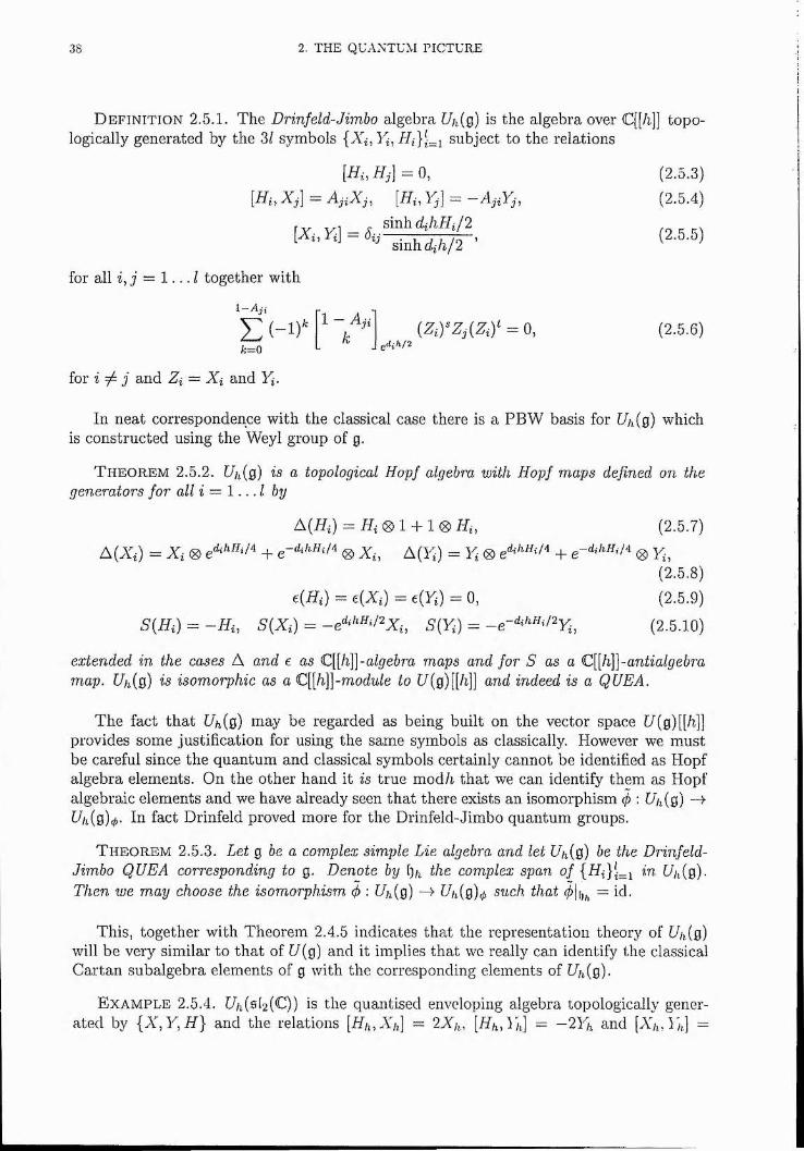
38 2. THE QUANTUM PICTURE

D e f in it io n 2.5.1. The Drinfeld-Jimbo algebra U/Xo) is the algebra over C[[/i]] topo­logically generated by the 3/ symbols {A^, subject to the relations

[Wi,iTj] = 0, (2.5.3)[Hi,Xj] = AjiXj, [Hi,Yj] = -A jiY j, (2.5.4)

for all i , j = l . . . l together with

1 —

E ( -1 ) 'fc=0

for i ^ j and Zi — Xi and Y{.

1 - (Zi)'Zj(A^)' = 0, (2.5.6)éihtl

In neat correspondence with the classical case there is a PBW basis for f//i(g) which is constructed using the Weyl group of g.

T h e o r e m 2.5.2. /7/i(g) is a topological Hopf algebra with Hopf maps defined on the generators for a lii — 1 .. A by

A{Hi) Hi, (2.5.7)

A(Xi) = Xi ® ® Xi, A(Ki) = Kj ® ® Yu(2.5.8)

^{Hi) = e(Xi) = e(Fj) = 0, (2.5.9)

S{Hi) = -Hu S{Xi) = - e “‘>‘ ‘/^Xu S(Yi) = -e-'‘‘'‘''<l+u (2.5.10)

extended in the cases A and e as C[[/7]]-a/^e6ra maps and for S as a C[[h]]~antialgebra map. Uii(q) is isomorphic as a C[[h]]-module to f/(g)[[/%]] and indeed is a QUEA.

The fact tha t Uh{o) may be regarded as being built on the vector space [/(g)[[/7]] provides some justification for using the same symbols as classically. However we must be careful since the quantum and classical symbols certainly cannot be identified as Hopf algebra elements. On the other hand it is true mod/i that we can identify them as Hopfalgebraic elements and we have already seen that there exists an isomorphism f) : f//i(g) ->t//i(g)^. In fact Drinfeld proved more for the Drinfeld-Jimbo quantum groups.

T h e o r e m 2.5.3. Let q he a complex simple Lie algebra and let f//i(g) be the Drinfeld- Jimbo QUEA corresponding to g. Denote by Ipi the complex span of in U/fio).Then we may choose the isomorphism ^ : Uifig) -A [//^(g)^ such that = id.

This, together with Theorem 2.4.5 indicates that the representation theory of Uh(Q) will be very similar to that of U (g) and it implies that we really can identify the classical Cartan subalgebra elements of g with the corresponding elements of Uh{o).

E x a m p l e 2.5.4. Uh{sl2 {C)) is the quantised enveloping algebra topologically gener­ated by { X ,Y ,H } and the relations [Hh,Xh] ~ 2AY, [77/ , and [A/ , =

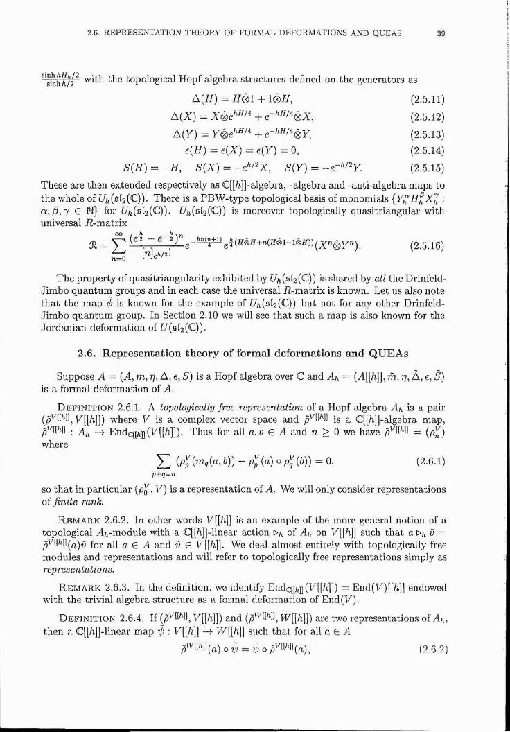
2.0. REPRESENTATION THEOR'i’ OF FORMAL DEFORMATIONS AND QUEAS 39

‘"s'mhh/f with the topological Hopf algebra structures defined on the generators as

A (ff) = ifd il + (2.5.11)

A(X) = Xdie'*"/'' + (2.5.12)

A (V ) = y® e'‘"/'' + e - '‘" /“®y, (2.5.13)e(ff) = e(X) = e(V) = 0, (2.5.14)

S ( f f ) = - H , S ( X) = - e ' ‘/^X, S (y ) = (2.5.15)

These are then extended respectively as C[[/i]]-algebra, -algebra and -anti-algebra maps to the whole of UhishiC)). There is a PBW-type topological basis of monomials {T/f 77f :a , ^ ,7 G N} for t//i(s[2(C)). is moreover topologically quasitriangular withuniversal 77-matrix

oo / h — — \n^ (e. - e J) (2,5.16)

^ Nck/z!n=0

The property of quasitriangularity exhibited by 12(C)) is shared by all the Drinfeld- Jimbo quantum groups and in each case the universal 77-matrix is known. Let us also note that the map 4> is known for the example of [^(^^(C )) but not for any other Drinfeld- Jimbo quantum group. In Section 2.10 we will see that such a map is also known for the Jordanian deformation of [/(512(C)).

2.6. Representation theory of formal deformations and QUE As

Suppose A = {A, m, r], A, e, S) is a Hopf algebra over C and A^ = (A[[/i]], 771, 77, À, e, S) is a formal deformation of A.

D e f in it io n 2.6.1. A topologically free representation of a Hopf algebra Ah is a pair where V is a complex vector space and ig a C[[h]]-algebra map,

pF[[/i]] . Endq[/i]](y[[/7]]). Thus for all a,b e A and 77 > 0 we have = (p^)where

(Pp (n%q(n, 6)) - Pp (a) o (6)) = 0, (2.6.1)p+q—n

so that in particular {pQ , V) is a representation of A. We will only consider representations of finite rank.

R e m a r k 2.6.2. In other words V[[h]] is an example of the more general notion of a topological A^-module with a C[[/7]]-linear action \>h of on y[[h]] such that a>h^ = pYM(^d)y for all a G A and v G y[[h]]. We deal almost entirely with topologically free modules and representations and will refer to topologically free representations simply as representations.

R e m a r k 2.6.3. In the definition, we identify Endc[[/i]](y[[/7]]) = E n d (y )[[/%]] endowed with the trivial algebra structure as a formal deformation of End(y).

D e f in it io n 2.6.4. If y [[/%]]) and W [[/%]]) are two representations of Ah,then a C[[h]]-linear map : V[[h]] iy[}h]] such that for all a G A

pnq[/i]](^) Q Ü o (2.6.2)

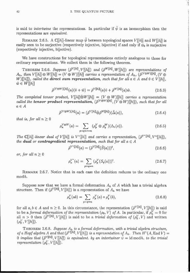
40 2. THE QUANTUM PICTURE

is said to intertwine the representations. In particu la r if ijj is an isom orphism then the represen tations are equivalent

R e m a r k 2.6.5. A C[[/i]]-linear m ap f) between topological spaces V[[h]] and IVff/i]] is easily seen to be surjective (respectively injective, bijective) if and only if is surjective (respectively injective, bijective).

We have constructions for topological representations entirely analogous to those for ord inary representations. We collect them in the following theorem .

T h e o r e m 2.6.6. Suppose y[[/ï]]) and W[[/7]{) are representations ofAh, then V[[h]] © W[[h]] = {V © W)[[h)] carries a representation of Ah, (y ©W)[[/7]]), called the direct sum representation, such that for alia E A and v G y[[/i]],w G W[[h\]

+ w) = p^"^"(8)fi + p'^[[''"(8)w. (2.6.3)

The completed tensor product, y[[/^]]®iy[[/i]] = (y ® iy)[W] carries a representation called the ten sor product representation, (y 0W)[[/7]]), such that for all8 G /I

= (p^[M l0pi'^M )(A (8)), (2.6.4)

that is, for all n > 0

E ( p ;® p f ) ( A , . ( a ) ) . (2.6.5)p+q+r=n

The C[[/i]]-[mear dual ofV[[h]] is y*[[h]] and carries a representation, (p^dW)^ y*[[N]); the dual or contragredient representation, such that for all a Q. A

/* [W ](8 ) = ( /[M ]( ,§ (8 ) ) ) \ (2.6.6)

or, for all n > 0

p r u ) = E (2-6.7)p+q=n

R e m a r k 2.6.7. Notice that in each case the definition reduces to the ordinary one mod/7.

Suppose now th a t we have a form al deform ation Ah of A which has a triv ia l algebrastruc tu re . T hen if y }[/%]]) is a representation of Ah we have

p+q=nfor all 8 ,6 G A and n > 0. In th is circum stance, the representation y[[h)l) is saidto be a formal deformation of the representation (po, y ) of A. In particu la r, if p]( = 0 forall 77 > 0 th en [g said to be a trivial deformation of (Pq ,V ) and w ritten( p ; \ n M i ) .

T h e o r e m 2.6.8. Suppose Ah is a formal deformation, with a trivial algebra structure, of a Hopf algebra A and that (p^ y[[/7]]) is a representation of Ah- Then (A, E nd V) =0 implies that y[[/7]]) is equivalent, by an intertwiner ip — id mod/7, to the trivialrepresentation (pj , y[[/7]]).

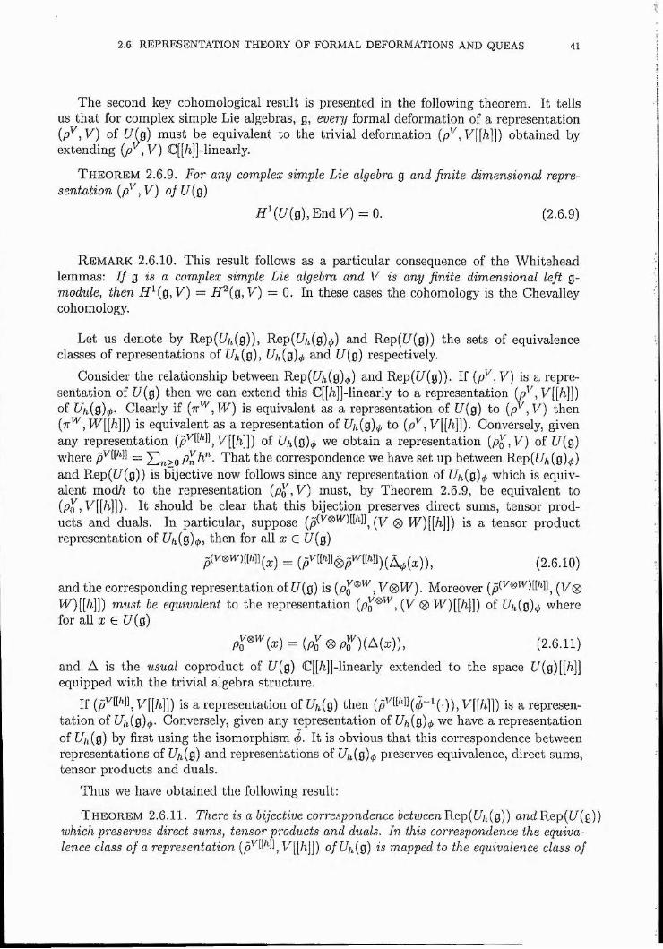
2.6. REPRESENTATION THEORY OF FORMAL DEFORMATIONS AND QUEAS 41

The second key cohomological result is presented in the following theorem. It tells us tha t for complex simple Lie algebras, g, every formal deformation of a representation {p^yV) of [/(g) must be equivalent to the trivial deformation ip^,V[[h]]) obtained by extending (p^, y ) C[[h]]-linearly.

T h e o r e m 2.6.9. For any complex simple Lie algebra g and finite dimensional repre­sentation (p ^ ,y ) 0/ [/(g)

7 /X [/(g ),E n d y ) = 0 . (2.6.9)

R e m a r k 2.6.10. This result follows as a particular consequence of the Whitehead lemmas: I f q is a complex simple Lie algebra and V is any finite dimensional left g- module, then = 0. In these cases the cohomology is the Chevalleycohomology.

Let us denote by Rep(% (g)), Rep([//t(g)^) and Rep([/(g)) the sets of equivalence classes of representations of Uifig), [//^(g)^ and [/(g) respectively.

Consider the relationship between Rep([//Xg)ÿ) and Rep([/(g)). If {p^,V) is a repre­sentation of [/(g) then we can extend this C[[/i]]-linearly to a representation (p^^,V[[h]\) of [//i(g)ÿ. Clearly if { n ^ ,W ) is equivalent as a representation of [/(g) to (p^ ,V ) then (tt^ , W[[/7]]) is equivalent as a representation of [//i(g)^ to (p^, y[[/7]]). Conversely, given any representation (p ^ ‘1, y[[/7)]) of [//i(g)t^ we obtain a representation (p^, L) of [/(g) where p^^M = Pn That the correspondence we have set up between Rep([//i(g),^) and Rep([/(g)) is bijective now follows since any representation of [//i(g)< which is equiv­alent mod/7 to the representation (p^, V) must, by Theorem 2.6.9, be equivalent to (Po'", y[[/i]]). It should be clear tha t this bijection preserves direct sums, tensor prod­ucts and duals. In particular, suppose {pW®^)[Mfiy 0 W)[[/7]]) is a tensor product representation of [//i(g)< , then for all x e U{q)

= (p"'[W]Ôp^"''«)(Â^(a;)), (2.6.10)

and the corresponding representation of U (g) is (p^®^, V ®W). Moreover ( y ^k y )[[/7 ]]) must be equivalent to the representation {pq®^,{V 0 kL )[[/7]]) of [/,i(g ) ,^ where for all X e U(q)

p^®^(æ) = (p^ 0pg^)(A(æ)), (2.6.11)

and A is the usual coproduct of [/(g) C[[/7]]-linearly extended to the space [/(g)[[h-]] equipped with the trivial algebra structure.

If y[[/7]]) is a representation of Uh{g) then is a represen­tation of Uh{g)(f,. Conversely, given any representation of Uh(g)(p we have a representation of [//i(g) by first using the isomorphism 0. It is obvious that this correspondence between representations of Uifig) and representations of [//^(g)^ preserves equivalence, direct sums, tensor products and duals.

Thus we have obtained the following result:

T h e o r e m 2.6.11. There is a bijective correspondence between Rep([//^(g)) and Rep([/(g)) which preserves direct sums, tensor products and duals. In this correspondence the equiva­lence class of a representation y[[/7]]) ofUifig) is mapped to the equivalence class of

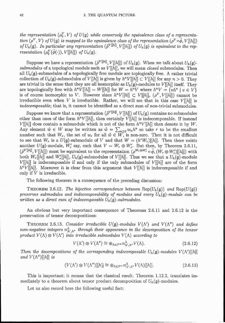
42 2. THE QUANTUM PICTURE

the representation {Pq ,V ) ofU{g) while conversely the equivalence class of a representa­tion (p^, V) ofU{g) is mapped to the equivalence class of the representation (p^o<^, y [[A]]) ofU}i{g). In particular any representation y[[/7]]) ofUifig) is equivalent to the rep­resentation {po iH-))y^[W]) ofUh(Q).

Suppose we have a representation y[[/7]|) of Uh{g). When we talk about Uh{g)-submodules of a topological module such as y[[/i]], we will mean closed submodules. Then all [//i(g)-submodules of a topologically free module are toplogically free. A rather trivial collection of [//j(g)-submodules of V[[h]] is given by /7’ y[[h]] C y[[h]) for any n > 0. They are trivial in the sense that they are all isomorphic as [//i(g)-modules to V[[h]] itself. They are topologically free with h^V[[h\] = W[[A]] for W ~ hlW where h^V = {vlF | u G y} is of course isomorphic to V. However since IFVWh]] C y [[A]], (p^,y[[/i]]) cannot be irreducible even when V is irreducible. Rather, we will see that in this case V[[h]] is indecomposable-, that is, it cannot be identified as a direct sum of non-trivial submodules.

Suppose we know that a representation y [[/i]]) of [4(g) contains no submodulesother than ones of the form h^V[[h]\, then certainly V[[h]] is indecomposable. If instead y [[A]] does contain a submodule which is not of the form A’W [[/%]] then denote it by W. Any element w e W may be written as w = En>o so take r to be the smallest number such that HA, the set of w,. for all w e W , is non-zero. Then it is not difficult to see tha t HA is a [/(g)-submodule of V and that W = {h^Wr)[[h]]. Then there exists another [/(g)-module, Wj say, such that y = HA © HA'. But then, by Theorem 2 .6.11, (pF[[/i]] y[[/^]j) must be equivalent to the representation (HA © kIA)[[A]]) withboth HA[M] and HA'[[/i]], [//i(0)-submodules of V[[h]]. Thus we see that a [//^(g)-module V[[h]] is indecomposable if and only if the only submodules of V[[h]] are of the form h^V[[h]]. Moreover it is clear from this argument that V[[h]] is indecomposable if and only if y is irreducible.

The following theorem is a consequence of the preceding discussion;

T h e o r e m 2.6.12. The bijective correspondence between Rep([//j(g)) and R ep([/(g )) preserves submodules and indecomposability of modules and every Uifig)-module can be written as a direct sum of indecomposable Uffig)-submodules.

An obvious but very important consequence of Theorems 2.6.11 and 2.6.12 is the preservation of tensor decompositions:

T h e o re m 2.6.13. Consider irreducible U{g)-modules y (A') and y (A") and define non-negative integers through their appearance in the decomposition of the tensorproduct V (A) 0 y (A') into irreducible submodules V (A) according to

V{A') ® y (A") ^ ®Agp+n;(,_^„y(A). (2.6,12)

Then the decompositions of the corresponding indecomposable Uh(g)-modules y (A') [[/%]] and y(A")[[/7]] is

(y(A ') ® V{A")[[h]] ^ ®A£P+R:(,,A„y(A)[[A]]. (2.6.13)

This is important; it means that the classical result. Theorem 1.12.2, translates im­mediately to a theorem about tensor product decomposition of [//^(g)-modules.

Let us also record here the following useful fact:

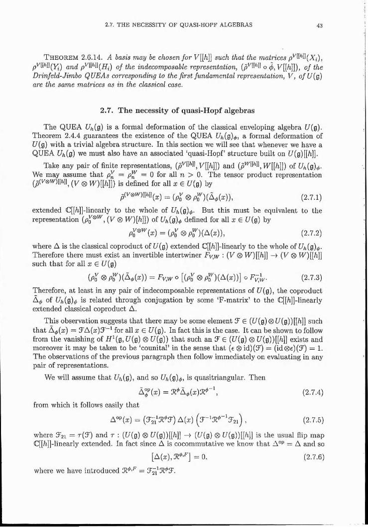
2.7. THE NECESSITY OF QUASFHOPF ALGEBRAS 43

T h e o r e m 2.6.14. A basis may be chosen for V[[h]] such that the matricesand of the indecomposable representation, o of the

Drinfeld-Jimbo QUE As corresponding to the first fundamental representation, V, ofU(g) are the same matrices as in the classical case.

2.7. The necessity of quasi-Hopf algebras

The QUEA Uh{g) is a formal deformation of the classical enveloping algebra [/(g). Theorem 2.4.4 guarantees the existence of the QUEA U/fig)^, a formal deformation of [/(g) with a trivial algebra structure. In this section we will see that whenever we have a QUEA Ufiio) we must also have an associated ‘quasi-Hopf’ structure built on [/(g)[[/%]].

Take any pair of finite representations, U[[/7]]) and of Uh{g)(i,-We may assume that p^ = p ^ = 0 for all n > 0. The tensor product representationp(V(g)W)[[/i]] ( y 0 W) [[/%]]) is defined for all a; E [/(g) by

(2.7.1)

extended C[[/i]]-linearly to the whole of [//i(0)0- But this must be equivalent to therepresentation (p^®^% (V 0 W)[h]]) of [^(g)^ defined for all x G U{g) by

Po P D (^ M ), (2.7.2)

where A is the classical coproduct of [/(g) extended C[[/7]]-linearly to the whole of [//^(g)^. Therefore there must exist an invertible intertwiner Fy,w ' {V ® W)[[h]] (V 0 W) [[h]] such that for all x G U (g)

(p^ 0 pg^)(A^(a;)) = o [(/? 0 pg^)(A(a;))] o (2.7.3)

Therefore, at least in any pair of indecomposable representations of [/(g), the coproduct of Uh{g)(j) is related through conjugation by some ‘F-matrix’ to the C[[/i]]-linearly

extended classical coproduct A.

This observation suggests that there may be some element T G ([/(g )0 [/(g))[}h]) such that A(p{x) = TA(a:)T~^ for all a; G [/(g). In fact this is the case. It can be shown to follow from the vanishing of H^(g,U{g) 0 [/(g)) that such an T G ([/(g) 0 [/(g))[[h]] exists and moreover it may be taken to be ‘counital’ in the sense that (e 0 id) (T) = (id0 e)(T) = 1. The observations of the previous paragraph then follow immediately on evaluating in any pair of representations.

We will assume that Uh[g), and so [//i(g)</„ is quasitriangular. Then

À“'’(æ) = K^À*(a:)X^“ ‘, (2.7.4)

from which it follows easily that

A“p(.t) = A(z) , (2.7.5)

where T21 = p(T) and r : ([/(g) 0 [/(g))[[/%]] -A- ([/(g) 0 [/(g))[[h]j is the usual flip mapC[[/7]]-linearly extended. In fact since A is cocommutative we know that A“* = A and so

[A(a;),07' ' ] = 0 , (2.7.6)

where we have introduced 07" ' =

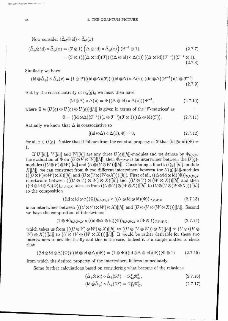
44 2. THE QUANTUM PICTURE

Now consider ( id) o À^(a;),

( * ® id )o  * M = (S'® 1) A ® id) O À.ÿ(æ)) ( S - ‘ ® 1), (2.7.7)

= (S ® 1)((A ® id)(S)) ((A ® id) o A(æ)) ((A ® id )(S -‘) ) (S - ' ® 1).(2.7.8)

Similarly we have

(id®A^) o À^(æ) = (1 ® S)((id® A )(S)) ((id®A) o A(x)) ((id® A )(S -‘))(l ® S"*)(2.7.9)

But by the coassociativity of % (0)ÿ we must then have

(id0A ) o A(æ) = ((A 0 id) o A(a;))) (2.7.10)

where # G (f/(g) 0 f/(g) 0 [/(g))[[/i]] is given in terms of the ‘F-m atrices’ as

$ = ((id 0 A )(T -^ ))(l 0 3 '-^ )(T 0 1)((A 0 id)(T)). (2.7.11)

Actually we know that A is coassociative so

[(id 0 A ) o A(æ), # ) = 0, (2.7.12)

for all X G U{g). Notice that it follows from the counital property of T that (id 0e id)(4>) = 1 .

If U[[h]], V[[h]] and W [[/%)] are any three [/(g)[[/z]]-modules and we denote by ^u,v,w the evaluation of i on {U ® V ® W) [[/%]], then is an intertwiner between the [/(g)-modules (([/0y)0W)[[/t]] and ([/0 (y0W ))[[/i]]. Considering a fourth [I(g)[[/7]]-module AT [[/ill, we can construct from # two different intertwiners between the [/(g)[[/7]]-modules ((([/0y)0W)0X)[W) and ([/0(y0(W0%)))[M]. First of all, ((A0id0id)($))[/,y,ty,% intertwines between ((([/ 0 Ù) 0 W ) 0 Y)[[h]j and (([/ 0 V) 0 {W 0 %))[[&]] and then ((id 0 i d 0 A ) ( $ ) ) [ / , takes us from (([/0y)0(T H 0A ))[[/i]] to ( [ /0(y0(kF0AT)))[[h]) so the composition

((id 0 id 0A)($))[/,y,w,A o ((A 0 id 0 id)($))n,y,w,x (2.7.13)

is an intertw iner between ( ( ( [ /0 V ) 0 W ) 0 % ) [[h]] and ( [ / 0 ( V 0 { W 0%)))[[/%]]. Second we have the composition of intertwiners

(1 0 $)[/,v,w,x o ((id0 A 0 id)( $ ) ) ( / , ° (^ 0 l)f/,y,w,Au (2.7.14)

which takes us from ((([/ 0 V ) 0 W ) 0 AT)[[/?.]] to (([/ 0 (U 0 kF)) 0 A‘)[[h]] to ([/ 0 ((V 0VF) 0 Ar))[[/7]j to ([/ 0 (y 0 (VF 0 A')))[[/i]]. It would be rather desirable for these twointertw iners to act identically and this is the case. Indeed it is a simple m atter to check th a t

((id0id0A )(^))((id0id0A )(<^)) = (1 0 $)((id0A 0 id)($))($ 0 1) (2.7.16)

from which the desired property of the intertwiners follows immediately.

Some further calculations based on considering what become of the relations

(Â * â id) o Â^(3l*) = (2-7.16)

(id® À *) o A,j(3J^) = KfjKfz. (2.7.17)

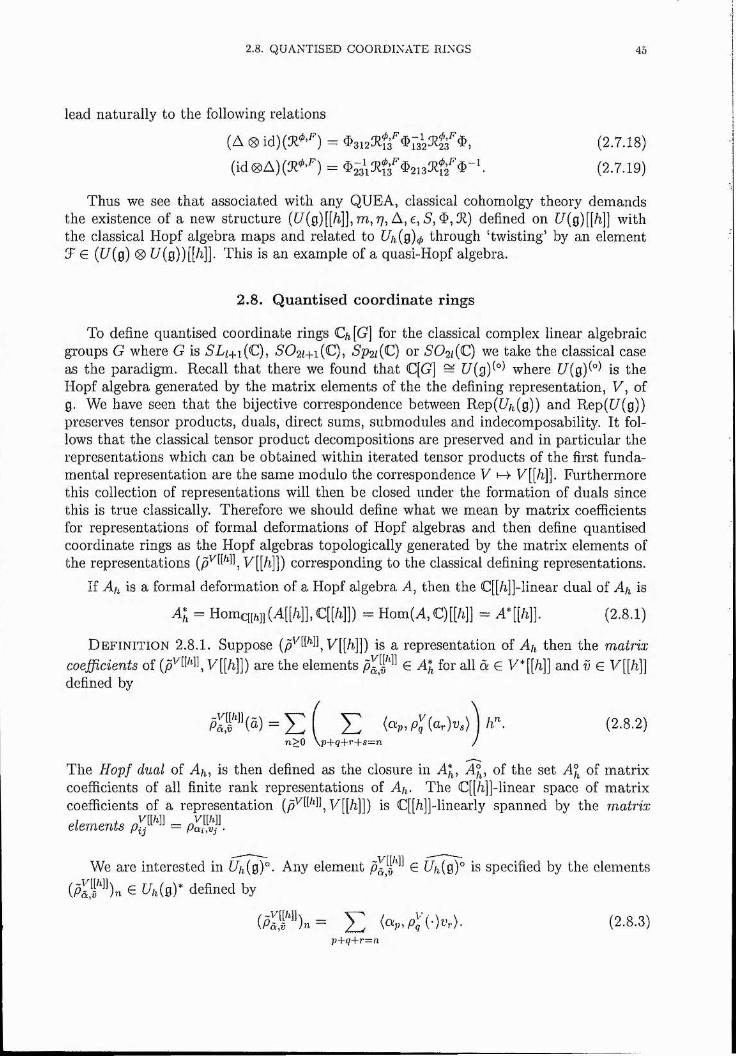
2.8. QUANTISED COORDINATE RINGS 45

lead naturally to the following relations

(A ® (2.7.18)

(id®A)(3?^-'") = $2-3\aiff ®2i33îff <E>-‘. (2.7.19)

Thus we see that associated with any QUEA, classical cohomolgy theory demands the existence of a new structure ([/(g)[[/ij], m, 77, A, e, 5, <&, 97) defined on U(g)[[/i]] with the classical Hopf algebra maps and related to C4(g)< through ‘twisting’ by an element T G (U(g) 0 [/(g))[M]. This is an example of a quasi-Hopf algebra.

2.8. Quantised coordinate rings

To define quantised coordinate rings C/JG] for the classical complex linear algebraic groups G where G is SLi^i[C), 502i+i(C), Sp 2i{C) or S 0 2 i{C) we take the classical case as the paradigm. Recall tha t there we found that C[G] = U(g)(°) where [/(g)(°) is the Hopf algebra generated by the matrix elements of the the defining representation, V, of g. We have seen tha t the bijective correspondence between Rep([//i(g)) and Rep([/(g)) preserves tensor products, duals, direct sums, submodules and indecomposability. It fol­lows that the classical tensor product decompositions are preserved and in particular the representations which can be obtained within iterated tensor products of the first funda­mental representation are the same modulo the correspondence V !-> U [[/%]]. Furthermore this collection of representations will then be closed under the formation of duals since this is true classically. Therefore we should define what we mean by matrix coefficients for representations of formal deformations of Hopf algebras and then define quantised coordinate rings as the Hopf algebras topologically generated by the matrix elements of the representations corresponding to the classical defining representations.

If Ah is a formal deformation of a Hopf algebra /I, then the C[[h]]-linear dual of Ah is

= HomqM](4H],C[[fi]]) = Hom(A,C)[W] = (2.8.1)

D e f in it io n 2.8.1. Suppose (p ' CW], y[[h]]) is a representation of Ah then the matrix coefficients of U[[/i]]) are the elements G A* for all à G V*[[h]] and v G V[[h]]defined by

K f^"(ô) = Y ] ( (2.8.2)n>0 \p+q+r-|-s=n /

The Hopf dual of Ah, is then defined as the closure in A^, A \, of the set A° of matrixcoefficients of all finite rank representations of Ah. The C[[h)]-linear space of matrixcoefficients of a representation U [[/%]]) is C[[/i]]-linearly spanned by the matrixelements = PaS?-

We are interested in [//^(g)°. Any element G U/i(g)° is specified by the elements iP&T^^)n G Uh(gY defined by

(pw ) " = E K . P i (2.8.3)p+q+r=n

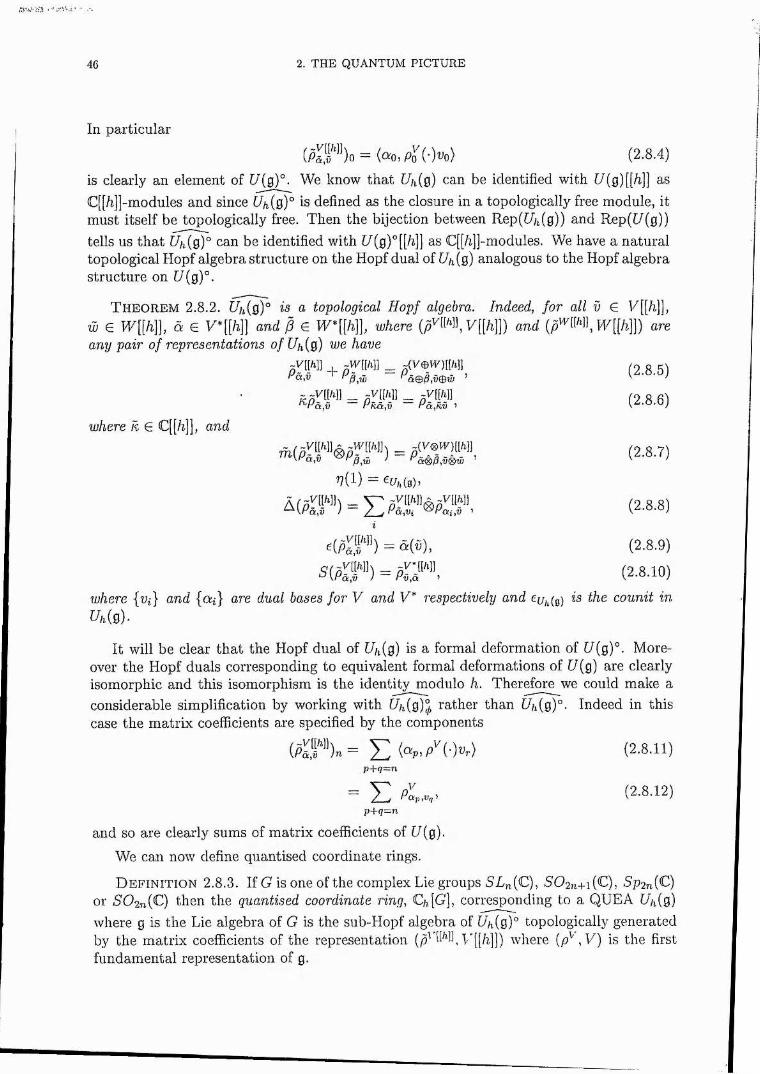
46 2. THE QUANTUM PICTURE

In particular

= (G!o, (-)i;o) (2.8.4)is clearly an element of [/(g)°. We know that Uifig) can be identified with [/(g)[[h]] asC[[/il]-modules and since Uh{g)° is defined as the closure in a topologically free module, it must itself be topologically free. Then the bijection between Rep(C4(g)) and Rep([/(g))tells us tha t Uh{g)° can be identified with [/(g)"[[/%]] as C[[/7]]-modules. We have a natural topological Hopf algebra structure on the Hopf dual of Uh {g) analogous to the Hopf algebra structure on //(g)".

T h e o r e m 2.8.2. Uk{g)° is a topological Hopf algebra. Indeed, for all v G w G VF[[/i]), à G y*[[hj] and G VF*[[h]], where !/[[/%]]) and {p^^^^^^\W[[h]]) areany pair of representations o/ [4(g) we have

where k G C[[/z]], and

g,w

= A i ' - (2.8.6)

77(1) =

À ( A i ) - E A i ' ® A i - (2.8.8)i

e ( A i ' ) = * (")- (2.8.9)

g ( A i ' ) = A ? " ' (2.8.10)where {ui} and {a^} are dual bases for V and V* respectively and eUf,{Q) is the counit in[4 (g).

It will be clear that the Hopf dual of Uk{g) is a formal deformation of [/(g)". More­over the Hopf duals corresponding to equivalent formal deformations of U (g) are clearlyisomorphic and this isomorphism is the identity modulo h. Therefore we could make aconsiderable simplification by working with [//i(g)J rather than Uh{g)°. Indeed in this case the matrix coefficients are specified by the components

( A , i ' ) n = E (2.8.11)p+q=n

~ E (2.8.12)p+q=n

and so are clearly sums of matrix coefficients of [/(g).We can now define quantised coordinate rings.

D e f in it io n 2.8.3. If G is one of the complex Lie groups STn(C), 5'02n+i(C), Sp 2n{^) or S02n(C) then the quantised coordinate ring, C/,.[G], corresponding to a QUEA Uh{g)where g is the Lie algebra of G is the sub-Hopf algebra of [//i(g)° topologically generated by the matrix coefficients of the representation V'[[h]]) where {p^\V) is the firstfundamental representation of g.

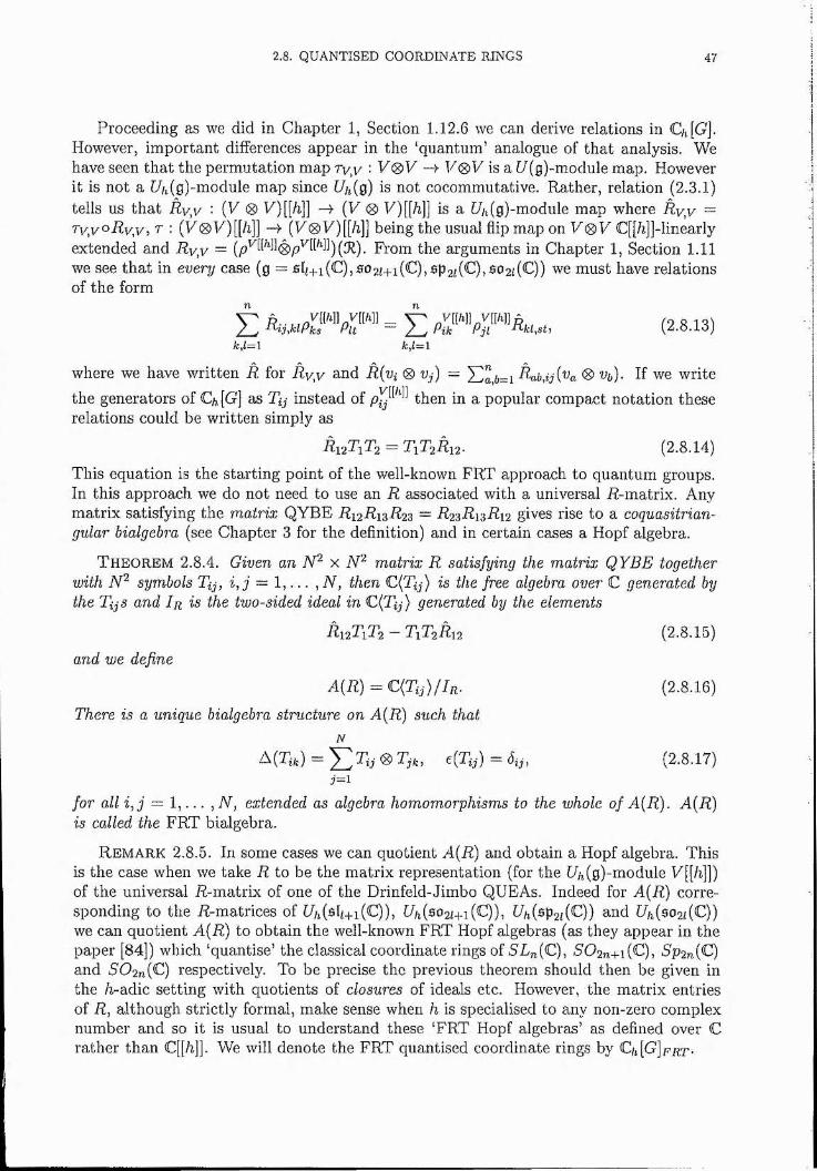
2.8. QUANTISED COORDINATE RINGS 47

Proceeding as we did in Chapter 1, Section 1.12.6 we can derive relations in C/JGJ. However, important differences appear in the ‘quantum’ analogue of that analysis. We have seen that the permutation map Tyy ' V ® V -> V® V is a [/(g)-module map. However it is not a Uifig)-module map since Uh{ô) is not cocommutative. Rather, relation (2.3.1) tells us th a t Rv,v : (U 0 y)[[h]] {V 0 y)[[h]] is a Uh{g)-modu\e map where Rv,v = T v y o R v y , T : ( y 0 l/)[[h]] -> ( y 0 y)[[/t]j being the usual flip map on V ® V C[[/i]]-linearly extended and R y y — (p^(W]0 p [H]])(g )_ From the arguments in Chapter 1, Section 1.11 we see tha t in every case (g = 5h+i (C), go 2f+i ( Q , ap (Q , eo 2z (C)) we must have relations of the form

È = E (2.8.13)k,l=\ k,l—l

where we have written R for R y y and R{vi 0 Vj) ~ ^ ^ 6=1 ^abiji^a 0 Vb). If we write

Gthe generators of C/ [G] as Tij instead of fken in a popular compact notation these relations could be written simply as

-R12T1T2 = T\T2 R \ 2 - (2.8.14)This equation is the starting point of the well-known FRT approach to quantum groups. In this approach we do not need to use an R associated with a universal R-matrix. Any m atrix satisfying the matrix QYBE R 12R 13R23 — R23R 13R 12 gives rise to a coquasitrian- gular bialgebra (see Chapter 3 for the definition) and in certain cases a Hopf algebra.

T h e o r e m 2.8.4. Given an x matrix R satisfying the matrix QYBE together with symbols Tij, i , j = l , . . . ,N , then ) is the free algebra over C generated by the TijS and In is the two-sided ideal in C{Tij) generated by the elements

R 12T1T2 — T1T2 R 12 (2.8.15)and we define

= (2 .8 .16)

There is a unique bialgebra structure on A{R) such thatN

A(îii-) = E ® = Sij, (2.8.17)

for all Î, j = 1, . . . ,N , extended as algebra homomorphisms to the whole of A(R). A{R) is called the FRT bialgebra.

R e m a r k 2.8.5. In some cases we can quotient A{R) and obtain a Hopf algebra. This is the case when we take R to be the matrix representation (for the [//4g)-module l/[[h]]) of the universal R-matrix of one of the Drinfeld-Jimbo QUE As. Indeed for A{R) corre­sponding to the R-matrices of [7/i(slz+i(C)), Uk{502i+i(C}), Uh{sp2i (Q ) and Uh{so2i(C}) we can quotient A{R) to obtain the well-known FRT Hopf algebras (as they appear in the paper [84]) which ‘quantise’ the classical coordinate rings of 5L„(C), S'02n+i(Q , Rp2n(C) and 502n(Q respectively. To be precise the previous theorem should then be given in the /i-adic setting with quotients of closures of ideals etc. However, the m atrix entries of R, although strictly formal, make sense when h is specialised to any non-zero complex number and so it is usual to understand these ‘FRT Hopf algebras’ as defined over C rather than C[[/i]j. We will denote the FRT quantised coordinate rings by C/i[G]i?Rr-

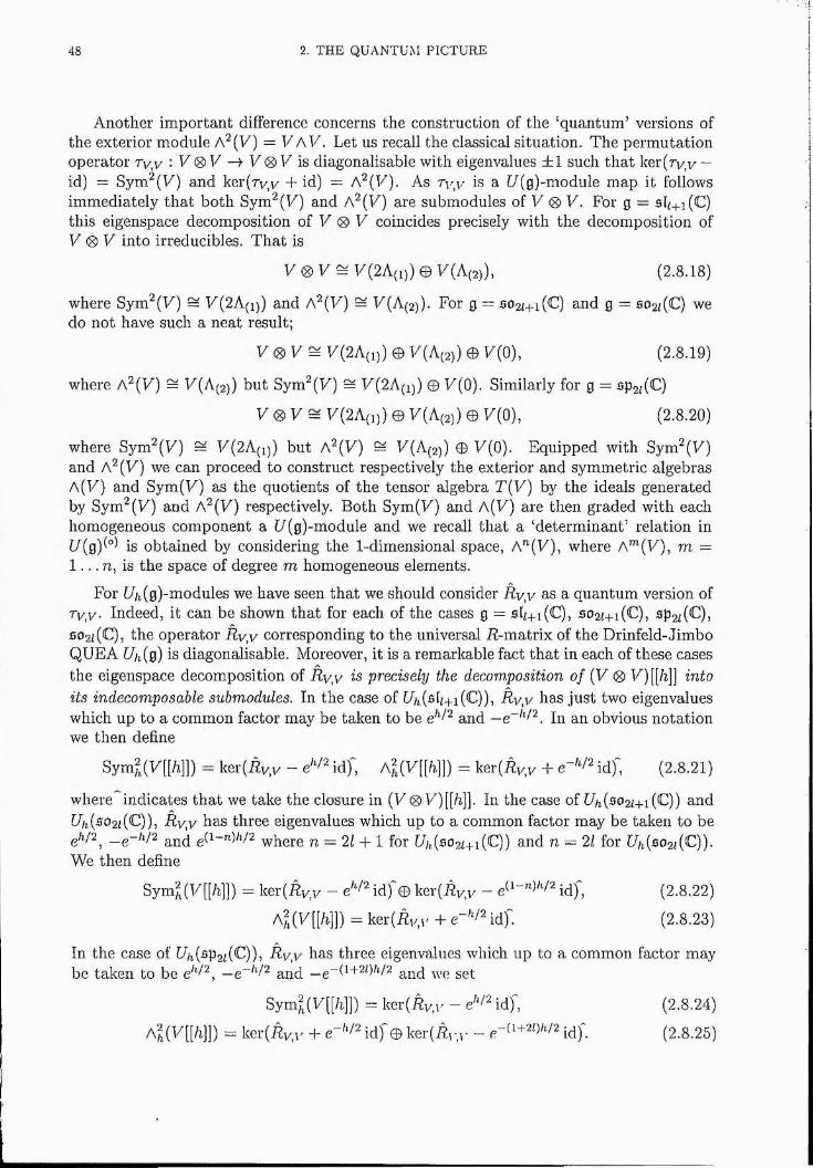
48 2. THE QUANTUM PICTURE

Another important difference concerns the construction of the ‘quantum’ versions of the exterior module A^(V) = V a V. Let us recall the classical situation. The permutation operator r y y : U 0 L V ® V is diagonalisable with eigenvalues ±1 such that ker(Ty,y —id) = Sym^(y) and ker{ryy + id) = A^(U). As ryy is a [/(g)-module map it follows immediately that both Sym^(y) and A^(U) are submodules of V 0 V. For g = s[/+i(C) this eigenspace decomposition of y 0 y coincides precisely with the decomposition of y 0 y into irreducibles. That is

y 0 y ^ y ( 2A(i)) e y(A(2)), (2 .8 .I8)

where Sym^(y) = y(2A(q) and A^(y) = y(A(2)). For g = 502z+i(Q and g = 502;(C) we do not have such a neat result;

y 0 y ^ y ( 2A(i)) ® y(A(2)) © y(o), (2.8 .19)

where A^(y) = y(A(2)) but Sym^(y) = y(2A(q) © y(0). Similarly for g = sp2i(Q

y 0 y ^ y ( 2A(i)) © y(A(2)) © y(o), (2.8.20)

where Sym^(y) = y(2A(q) but A^(y) = y(A(2)) © y(0). Equipped with Sym^(y) and A^(y) we can proceed to construct respectively the exterior and symmetric algebras A(y) and Sym (y) as the quotients of the tensor algebra T{V) by the ideals generated by Sym^(y) and A^{V) respectively. Both Sym(y) and A(y) are then graded with each homogeneous component a [/(g)-module and we recall that a ‘determinant’ relation in C/(g)V) is obtained by considering the 1-dimensional space, A"'(y), where A"^(y), m =1 . . . n, is the space of degree m homogeneous elements.

For [//i(g)-modules we have seen that we should consider R y y as a quantum version of Tyy. Indeed, it can be shown that for each of the cases g = 5lz+i(C), so2i+i(C), 5p2((Q, ^02! (C), the operator R y y corresponding to the universal R-matrix of the Drinfeld-Jimbo QUEA Ufi{g) is diagonalisable. Moreover, it is a remarkable fact that in each of these cases the eigenspace decomposition of R y y is precisely the decomposition of {V 0 y)[[h]] into its indecomposable submodules. In the case of [//i(5li+i(C)), R y y has just two eigenvalues which up to a common factor may be taken to be and — In an obvious notation we then define

Sym ^(y [[/%]]) = ker(Ry,y - id), A^(y[[A]]) = ker(Ryy 4- id ), (2.8.21)

where indicates that we take the closure in ( V 0y)[[h]]. In the case of Uh{so2i+i{C}) and Ufi{so2i{C)), R y y has three eigenvalues which up to a common factor may be taken to be g/i/2, and where n = 2/ -I-1 for Uh{so2i+i(C)) and n = 2l for Uh(so2i{C)).We then define

Sym^(y[[A]]) = ker(Ryy — id) © ker(Ry,y - (2.8.22)

AA(^[WI) = ker(Ry,y -k id): (2.8.23)

In the case of Uh(sp2 ii^))y R v y has three eigenvalues which up to a common factor may be taken to be e’ R, —e"V2 a,nd —e"B+2bW2 g id we set

Sym^(y [[/%]]) = ker(Ry,v' - id), (2.8.24)

A?i(y[Wl) = ker(Ry,r 4- id) © ker(Rr,r ~ g-B+2()/i/2 (2.8.25)

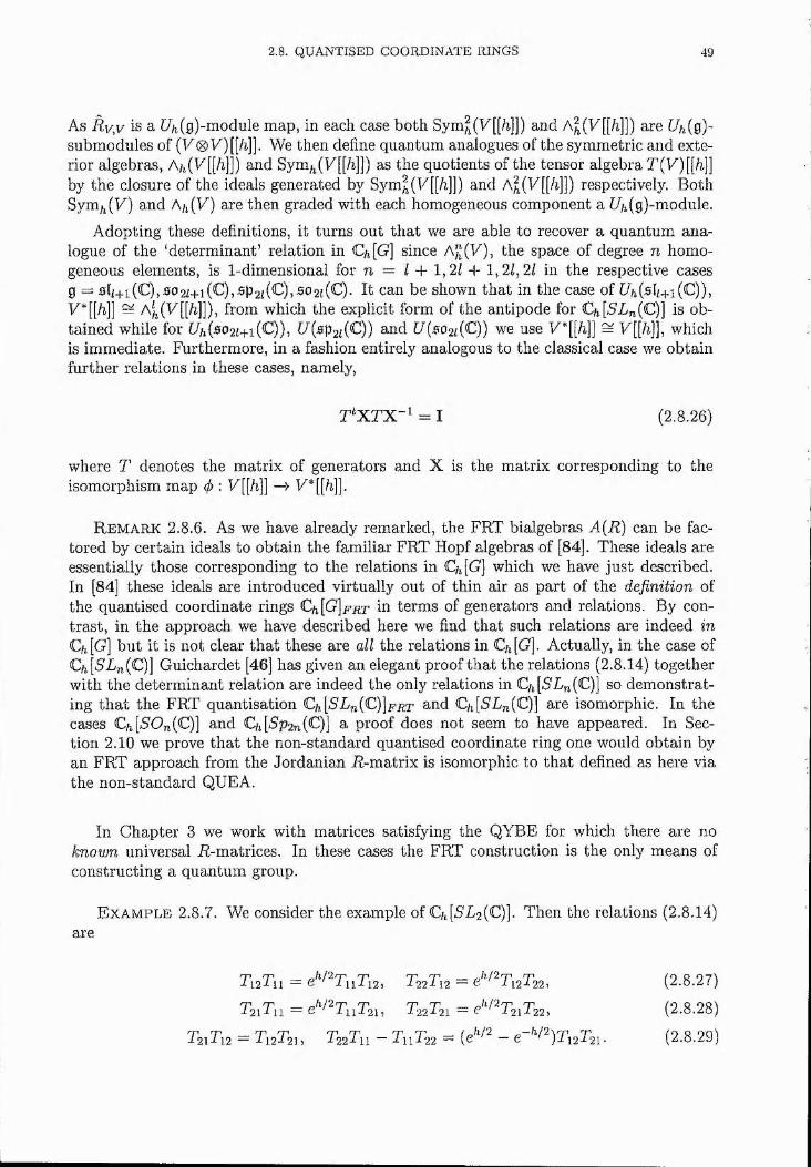
2.8. QUANTISED COORDINATE RINGS 49

As R y y is a [//i(g)-module map, in each case both Sym^(y[[h]]) and A^(y[[/i]]) are Uh{g)- submodules of {V0y)[[/^]]. We then define quantum analogues of the symmetric and exte­rior algebras, A/i(y[[/i]]) and Sym,^(y[[A])) as the quotients of the tensor algebra T{V)[[h]] by the closure of the ideals generated by Sym^(y[[/z]]) and A^(y[[/i]]) respectively. Both SymifiV) and AifiV) are then graded with each homogeneous component a [//4g)-module.

Adopting these definitions, it turns out that we are able to recover a quantum ana­logue of the ‘determinant’ relation in Qi[G] since Ag(y), the space of degree n homo­geneous elements, is 1-dimensional for n = / 4- 1,2/ -f- 1,2/, 2/ in the respective cases g = fî[/+i(C),502f+i(C),5p2/(C),fî02i(Q- It can be shown that in the case of y*[[/i]] ^ A}j(y[[/i]]), from which the explicit form of the antipode for Ch[SLn{C)] is ob­tained while for f//i(so2i+i(C)), //(Bp2i(Q ) nnd /7(502z(Q) we use V*[[h]] = whichis immediate. Furthermore, in a fashion entirely analogous to the classical case we obtain further relations in these cases, namely,

r^X TX "^ = I (2.8.26)

where T denotes the matrix of generators and X is the matrix corresponding to the isomorphism map (j) : V[[h]]

R em ark 2.8.6. As we have already remarked, the FRT bialgebras A{R) can be fac­tored by certain ideals to obtain the familiar FRT Hopf algebras of [84]. These ideals are essentially those corresponding to the relations in C/JG] which we have just described. In [84] these ideals are introduced virtually out of thin air as part of the definition of the quantised coordinate rings C /JG ]frt in terms of generators and relations. By con­trast, in the approach we have described here we find that such relations are indeed in C/i[G) but it is not clear that these are all the relations in C/i[G]. Actually, in the case of C/i[S'Ln(C)] Guichardet [46] has given an elegant proof that the relations (2.8.14) together with the determinant relation are indeed the only relations in C/i[5An(Q] so demonstrat­ing tha t the FRT quantisation C/J5Ln(Q]FRT and C/i[5L„,(C)] are isomorphic. In the cases C/i[S'G„(C)] and C/i[5p2n(G)] a proof does not seem to have appeared. In Sec­tion 2.10 we prove that the non-standard quantised coordinate ring one would obtain by an FRT approach from the Jordanian R-matrix is isomorphic to tha t defined as here via the non-standard QUEA.

In Chapter 3 we work with matrices satisfying the QYBE for which there are no known universal R-matrices. In these cases the FRT construction is the only means of constructing a quantum group.

areE x a m p l e 2.8.7. We consider the example of C/i[S'L2(C)]. Then the relations (2.8.14)

TizTu = +''^TnTn, (2.8.27)

TjiTn = e''/^TnT2 u ^ 2 X2 , = (2.8.28)

T2 1 T 12 = T 12T2 1 , T2 2 T,, - T n T 22 = (£'*/■' - e-"/")Ti2 T2 i. (2.8.29)

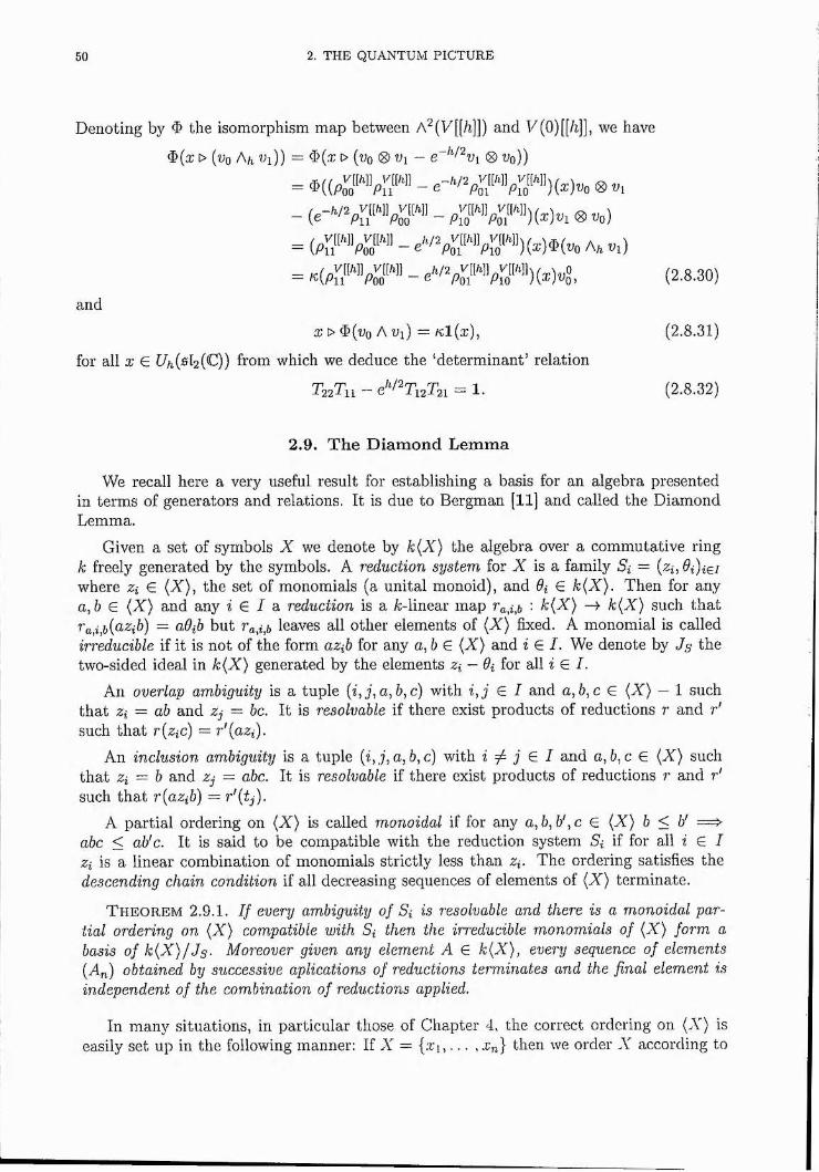
50 2. THE QUANTUM PICTURE

Denoting by the isomorphism map between A^(y[[/i]]) and y(0)[[/i]], we have

4 > ( a ; 0 ( vq A / i V i ) ) = 0 ( a ; t> ( vq 0 V i - 0 Vq) )

= ® Vi

- - Pro"po."'‘")(^)-i ® vo)= Aft «1)

= . ( p t ^ 'G r » - e''/=AA"p5'"") W "S, (2.8.30)and

a; > $(% A fi) = Kl(æ), (2.8.31)

for all X G [//i(sÏ2(C)) from which we deduce the ‘determinant’ relation

= 1. (2.8.32)

2.9. The Diamond Lemma

We recall here a very useful result for establishing a basis for an algebra presented in terms of generators and relations. It is due to Bergman [11] and called the Diamond Lemma.

Given a set of symbols X we denote by k{X) the algebra over a commutative ring k freely generated by the symbols. A reduction system for X is a family Si ~ {zi, Oi)i^i where Zi G (X), the set of monomials (a unital monoid), and &i G k{X). Then for any a, 6 G (X) and any 2 G I a reduction is a /c-linear map ra,i,b ' h(X) -+ k{X) such that ' 'a,i,b{azih) = aOib but leaves all other elements of (X) fixed. A monomial is called irreducible if it is not of the form azib for any a, b G (X) and i G / . We denote by J g the two-sided ideal in k{X) generated by the elements Zi — Oi for all % G /.

An overlap ambiguity is a tuple (i,j ,a ,b ,c) with i , j G / and a, 6, c G (X) — 1 such that Zi — ab and Zj = be. It is resolvable if there exist products of reductions r and r ' such that r{zic) = r'{azi).

An inclusion ambiguity is a tuple (i, j , a, 6, c) with i ^ j G I and a,b,c G (X) such that Zi — b and Zj = abc. It is resolvable if there exist products of reductions r and r ' such tha t r{azib) = r'{tj).

A partial ordering on (X) is called rnonoidal if for any a,b,b',c G (X) b < b' abc < ah'c. It is said to be compatible with the reduction system Si if for all / G / Zi is a linear combination of monomials strictly less than z*. The ordering satisfies the descending chain condition if all decreasing sequences of elements of (X) terminate.

T h e o r e m 2.9.1. I f every ambiguity of Si is resolvable and there is a rnonoidal par­tial ordering on (X) compatible with Si then the irreducible monomials of (X) form a basis of k{X)/Js- Moreover given any element A G k{X), every sequence of elements (A„) obtained by successive aplications of reductions terminates and the final element is independent of the combination of reductions applied.

In many situations, in particular those of Chapter 4, the correct ordering on (X) is easily set up in the following manner: If X = {.x'l, Vn] then we order X according to

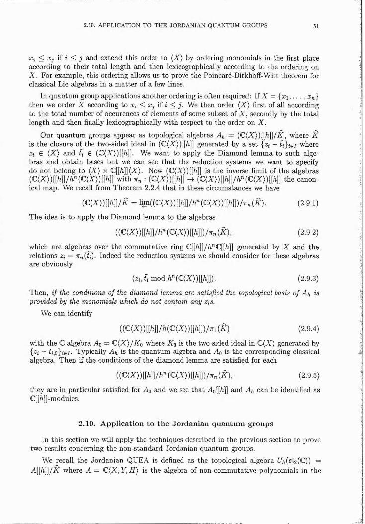
2.10. APPLICATION TO THE JORDANIAN QUANTUM GROUPS 51

Xi < Xj if i < j and extend this order to {X) by ordering monomials in the first place according to their total length and then lexicographically according to the ordering on X, For example, this ordering allows us to prove the Poincare-Birkhoff-Witt theorem for classical Lie algebras in a m atter of a few lines.

In quantum group applications another ordering is often required: If X = {xi , . . . , Xn} then we order X according to xi < Xj if z < j . We then order (X) first of all according to the total number of occurences of elements of some subset of X , secondly by the total length and then finally lexicographically with respect to the order on X .

Our quantum groups appear as topological algebras Ah — (C(X))[[A]]/X, where K is the closure of the two-sided ideal in (C(X))[[/i]] generated by a set {zi — where Zi G (X) and U G (C(X))[[/i]J. We want to apply the Diamond lemma to such alge­bras and obtain bases but we can see that the reduction systems we want to specify do not belong to (X) x C[[/i]](X). Now (C(X))[[/i]J is the inverse limit of the algebras (C(X))[M]//z"(C(X))[W] with : (C(X»[M] -k (C(X))[M]//t''(C(X»[M] the canon- ical map. We recall from Theorem 2.2.4 that in these circumstances we have

(C{X))[[h]]/K = lim((C(X»[[ft]]//j'*(C{X»[[ft]])/,r„(i?). (2.9.1)

The idea is to apply the Diamond lemma to the algebras

((C(X))[[/ill//i’*(C(X))[[/ijl)/7r„(X), (2.9.2)

which are algebras over the commutative ring C[[/i]]//z” C[[h]] generated by X and the relations Zi = 7Tn{ii). Indeed the reduction systems we should consider for these algebras are obviously

{zi, ii mod A” (C(X))[[/z]]). (2.9.3)

Then, if the conditions of the diamond lemma are satisfied the topological basis of Ah is provided by the monomials which do not contain any Zis,

We can identify

((C<X))[[/i]]/;i(C(X))[[/i]])/7ri(X) (2.9.4)

with the C-algebra A q = C (X)/Xo where K q is the two-sided ideal in C(X) generated by Typically Ah is the quantum algebra and A q is the corresponding classical

algebra. Then if the conditions of the diamond lemma are satisfied for each

((C(X))[M]/h"(C(X))[M])/7T,,(X), (2.9.5)

they are in particular satisfied for A q and we see that Ao[[/i]] and Ah can be identified as hll-modules.

2.10. Application to the Jordanian quantum groups

In this section we will apply the techniques described in the previous section to prove two results concerning the non-standard Jordanian quantum groups.

We recall the Jordanian QUEA is defined as the topological algebra [/&(512(C)) — A[[/z]]/X where A = C {X ,Y ,H ) is the algebra of non-commutative polynomials in the

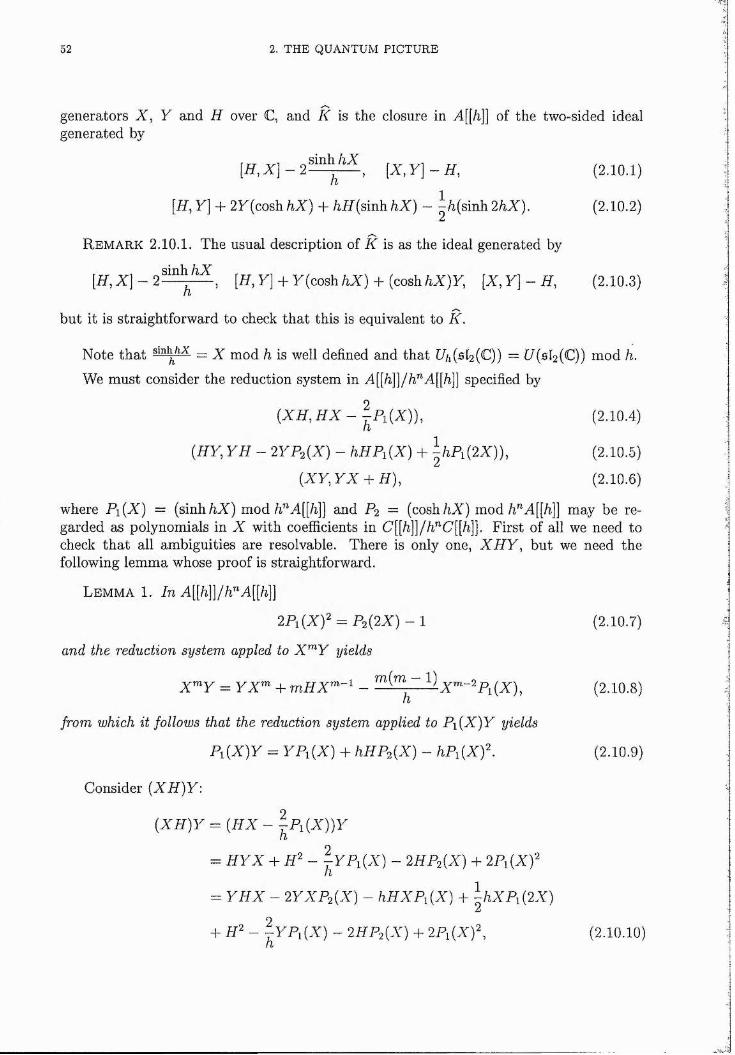
52 2. THE QUANTUM PICTURE

generators X , Y and H over C, and K is the closure in T[[/i]] of the two-sided ideal generated by

[ X , Y] - H, (2.10.1)

[H,Y\+2Y{coshhX) + hH{sia]ihX) - ]-h(smh.2hX). (2 . 10.2)

R e m a r k 2.10.1. The usual description of K is as the ideal generated by

[H,Y] + Y(coshhX) + {coshhX)Y, [ X , Y] - H, (2.10.3)

but it is straightforward to check that this is equivalent to K,

Note tha t ^ mod h is well defined and that Uh{sl2 {C}) = U{5 l2 {C)) mod h.We must consider the reduction system in A[[/z]]//z”A[[/i]] specified by

{XH, H X - Ip i(X )) , (2.10.4)

(HY, YH - 2YP2{X) - hHPi(X) + A p i { 2 X ) ) , (2.10.5)

(X Y , YX + H), (2.10.6)

where P i(X ) = (sinhhX) modh'^A[[h]] and P2 — (cosh AX) mod h^A[[h]] may be re­garded as polynomials in X with coefficients in C[[h]]/h”'C[[h]). First of all we need tocheck tha t all ambiguities are resolvable. There is only one, X H Y , but we need thefollowing lemma whose proof is straightforward.

L em m a 1. In A[[h\]lhAA[[h]]

2fi(X )^ = P2(2X) - 1 (2.10.7)

and the reduction system appled to X '^ Y yields

= Y X ”' + m H X ”'-' - A + x 2 1 x ”'-^P i{X), (2.10.8)

from which it follows that the reduction system applied to P i (X )Y yields

P i ( x ) y = y P i ( x ) 4- h P P 2(x ) - fiP i(x)^. (2 .10.9)

Consider {XH )Y:

{XH) Y = {HX - |P i(X ))K

= H Y X + H^ ~ /y P i(X ) - 2HP2(X) + 2P,{Xf

= Y H X - 2YXP2(X) - hHXP,{X) + A x P , { 2 X )

+ W - f y P i i X ) - 2HP2(X) + 2 P i{X ) \ (2.10.10)

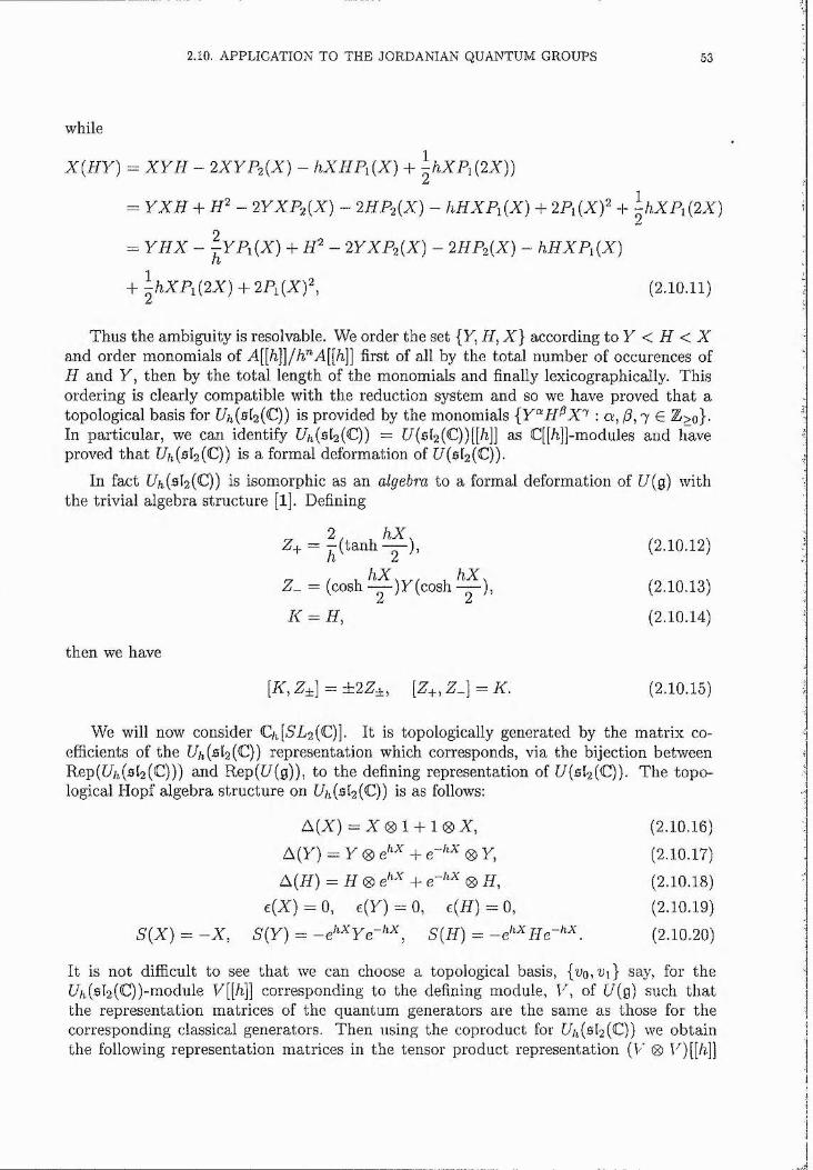
2.10. APPLICATION TO THE JORDANIAN QUANTUM GROUPS 53

while

X { HY ] = X Y H - 2 X Y P 2 {X) - hXHPi { X) + h x P , { 2 X ) )

= Y X H + H ^ - 2YXP2{X) - 2HP2(X) - hHXP, {X) + 2 P i ( X f + A x p y x )

= Y H X - \ y P i { X ) + - 2YXP2{X) - 2HP2{X) - hHXP, { X)

+ h . X P , ( 2 X ) + 2 P i { Xf , (2 ,10.11)

Thus the ambiguity is resolvable. We order the set {T, H , X ) according t o Y < H < Xand order monomials of A[[/i]]//z"'A[[/i]] first of all by the total number of occurences of H and Y , then by the total length of the monomials and finally lexicographically. This ordering is clearly compatible with the reduction system and so we have proved that a topological basis for (512(C)) is provided by the monomials {Y°'H^X'^ : a , /3,7 G Z>o}. In particular, we can identify [//»(512(C)) = [/(512(C))[[A]] as C[[A]]-modules and have proved tha t [// (512(C)) is a formal deformation of [/(512(C)).

In fact [//i (512(C)) is isomorphic as an algebra to a formal deformation of [/(g) with the trivial algebra structure [1]. Defining

2 h \= - ( t a n h - ^ ) , (2.10.12)

= (cosh ^ ^ ) y (cosh - ^ ) , (2.10.13)

A = R, (2.10.14)

then we have

[K, Z±] = dz2Z±, [Z+, Z-] = K. (2.10.15)

We will now consider C/i[5L2(C)]. It is topologically generated by the matrix co­efficients of the [//i (512(C)) representation which corresponds, via the bijection between Rep([//i(512(C))) and Rep([/(g)), to the defining representation of [/(512(C)). The topo­logical Hopf algebra structure on [//i (512(C)) is as follows:

A(X) = X 0 1 -k 1 0 X, (2.10.16)

A(y) = y 0 -k 0 y, (2.10.17)A(R) = R 0 -k 0 R, (2.10.18)

e(X) = 0, c(y) = 0, €(P) = 0, (2.10.19)

R(X) = - X , S (y ) = -e^^ye-^^ , S(R) = (2.10.20)

It is not difficult to see that we can choose a topological basis, {uo,ui} say, for the [//i(5l2(C))-module V[[h]] corresponding to the defining module, V, of [/(g) such that the representation matrices of the quantum generators are the same as those for the corresponding classical generators. Then using the coproduct for [//i(512(C)) we obtain the following representation matrices in the tensor product representation (V' 0 V") [[/?-]]

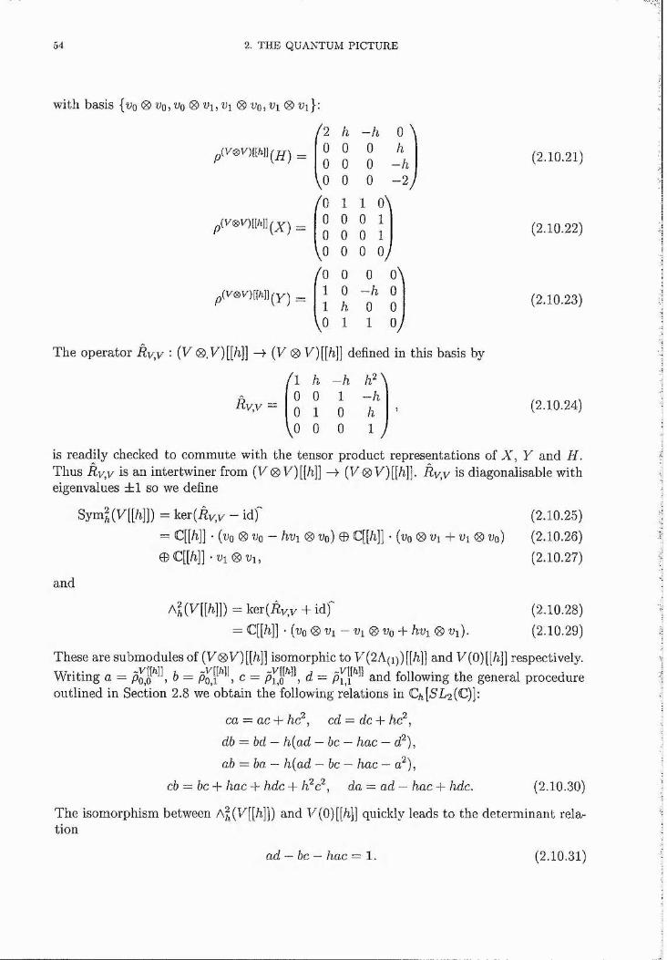
54 2. THE QUANTUM PICTURE

with basis {uq 0 Uq, vq ®Vi,Vi 0 uq, Vi 0 Ui}:

The operator R y y : {V 0.U )[[/%)] —> (y 0 y)[[A]) defined in this basis by

(2 h - h 0 \0 0 0 h0 0 0 —h

VO 0 0 - V/o 1 1 0\

0 0 0 10 0 0 1

lo 0 0 Qj

fo 0 0 o\1 0 —h 01 h 0 0

lo 1 1 V

(2 .10 .21)

(2 .10 .22)

(2.10.23)

Ry,y

( l h 0 0 0 1

\0 0

- h \ 1 —h 0 h 0 1 /

(2.10.24)

is readily checked to commute with the tensor product representations of X , Y and H. Thus R y y is an intertwiner from ( V 0y)[[A]] -4- {V®V)[[h]]. R y y is diagonalisable with eigenvalues dbl so we define

Sym^(y[W]) =: ker(Ry,y - id)= c[[h]] • (uo 0 U o - hvi 0 Vq) © C[[h]] • (% 0 Ui + Ui 0 U o )

h]] • ui 0 t»i,

and

A^(y[[/t]]) = kev{Rv,v + id)'= C[[h]] • (uo 0 Ui - Ui 0 uo + hvi 0 Ui).

(2.10.25)(2.10.26)(2.10.27)

(2.10.28) (2.10.29)

These are submodules of (y0y)[[h]] isomorphic to y(2A(i))[[h]] and y (0)[[/?.]] respectively.Writing a = b = c = pJ^PP d = p^^P^ and following the general procedureoutlined in Section 2.8 we obtain the following relations in C/i[5L2(C)]:

cb

ca = ac + hc^, cd = dc + hc^,

db = bd — h(ad — be — hac — d^), ab = ba — h{ad — be — hae — a^),

be + hae + hde + d a ~ ad — hae + hde. (2.10.30)

The isomorphism between A|(y[[/i]]) and y(0)[[h]] quickly leads to the determinant rela­tion

ad — be — hae = 1. (2.10.31)

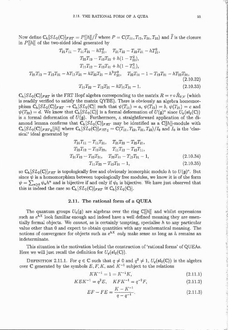
2.11. THE RATIONAL FORM OF A QUEA

Now define Q [ 5'L2(C )]fr t = f where P = C(Tii,T i2, T22) and I is the closure in P[[/z]] of the two-sided ideal generated by

T 2 1T 11 — T 1 1T 21 — h T 2 i , T 2 1 T 2 2 — T 2 2 T 2 1 — I1 T 2 1 ,

T22Ti2-Ti2T22 + d (l-T & ),TiiTi2 - T i 2Tn + / i ( l - T f i ) ,

T 2 1 T 1 2 — T 1 2 T 2 1 — h T i \ T 2 i — /1 T 22T 21 — T 2 2 T 1 1 — 1 — T 1 2 T 2 1 — /1 Î 2 2 T 2 1 ,

(2.10.32)T 11T22 — T12T21 — hTiiT2 i — 1. (2.10.33)

Ch[SL2 {C)\FRT is the FRT Hopf algebra corresponding to the matrix R ~ t o R y y (whichis readily verified to satisfy the matrix QYBE). There is obviously an algebra homomor­phism Ch[SL2 {C)]FET -> Qi[*5L2(C)] such that i/j{Tii) = a, -ipiTu) — 6, '0 (^2i) = c and 2(^22) = d. We know that Ch[SL2 {C)] is a formal deformation of [/(g)" since [//i(sl2(C))

is a formal deformation of [/(g). Furthermore, a straightforward application of the di­amond lemma confirms that C/JS'I/2(C )]frt may be identified as a C[[/z]]-module with C/i[5I/2(C)]ffto[[^11 where C/i[*S'Z/2(C)]f.^to = C(Tii, I 12, T21, 722)/do and Iq is the ‘clas­sical’ ideal generated by

Ti rp 'T ' n~' rp T" nn nn21J 11 — 11-/21, J-2 1 J-22 — J-2 2 J-2 1 ,T i rp T n~’ p /p p p22^12 — ^ 12 22, -111412 — 412411,

T21T12 — T12T21, T2 2T 11 — T 12T21 — 1, (2.10.34)T11T22 — T12T21 — 1, (2.10.35)

so C/i[S'L2(C )]ff t is topologically free and obviously isomorphic modulo h to [/(g)". But since ip is & homomorphism between topologically free modules, we know it is of the form Ip — Yln>o and is bijective if and only if ipo is bijective. We have just observed that this is indeed the case so Ch[SL2 {C)]frt = C/J5 L2(C)].

2.11. The rational form of a QUEA

The quantum groups [//^(g) are algebras over the ring C[[h]] and whilst expressions such as look familiar enough and indeed have a well defined meaning they are essen­tially formal objects. We cannot, as is certainly tempting, specialise h to any particular value other than 0 and expect to obtain quantities with any mathematical meaning. The notions of convergence for objects such as only make sense as long as h remains an indeterminate.

This situation is the motivation behind the construction of ‘rational forms’ of QUE As. Here we will just recall the definition for [/g(512(C)).

D e f in it io n 2.11,1. For ç G C such tha t g 7 0 and 7 1, [/g(sl2(C)) is the algebra over C generated by the symbols E ,F ,K , and subject to the relations

= 1 = A -Q Q (2.11.1)AFA-^ = g'^F, (2.11.2)A -

F F - F F = ----------------------------------------------- (2.11.3)

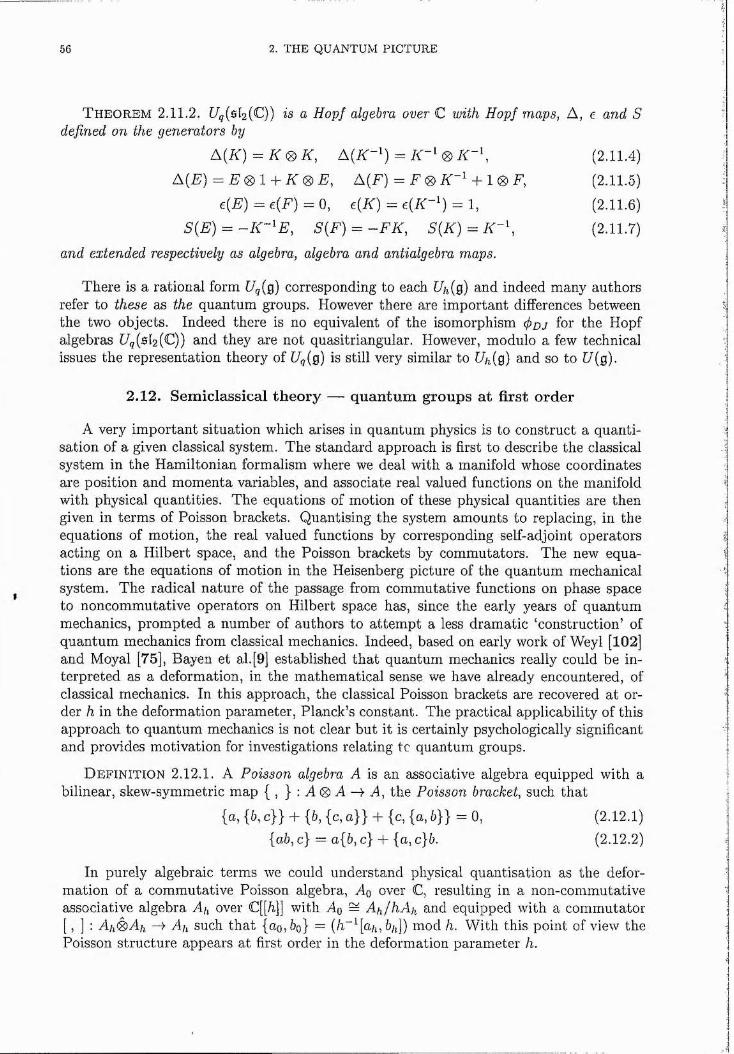
56 2. THE QUANTUM PICTURE

T h e o re m 2.11.2. Rg(512(C)) is a Hopf algebra over C with Hopf maps, A, e and S defined on the generators by

A(A) = A 0 A, A(A-^) = A-^ 0 A " \ (2.11.4)

A(E) = E 0 1 + A 0 E, A(E) = E 0 A'^ + 1 0 E, (2.11.5)

e(E) = 6(E) = 0, g(A) = e(A-^) = 1, (2.11.6)E(E) = -A -^ E , E(E) = -E A , R ( A ) = A - \ (2.11.7)

and extended respectively as algebra, algebra and antialgebra maps.

There is a rational form Eg(g) corresponding to each Uh{Q) and indeed many authors refer to these as the quantum groups. However there are important differences between the two objects. Indeed there is no equivalent of the isomorphism (poj for the Hopf algebras Eg (512(C)) and they are not quasitriangular. However, modulo a few technical issues the representation theory of Eg(g) is still very similar to E/i(g) and so to E(g).

2.12. Semiclassical theory — quantum groups at first order

A very important situation which arises in quantum physics is to construct a quanti­sation of a given classical system. The standard approach is first to describe the classical system in the Hamiltonian formalism where we deal with a manifold whose coordinates are position and momenta variables, and associate real valued functions on the manifold with physical quantities. The equations of motion of these physical quantities are then given in terms of Poisson brackets. Quantising the system amounts to replacing, in the equations of motion, the real valued functions by corresponding self-adjoint operators acting on a Hilbert space, and the Poisson brackets by commutators. The new equa­tions are the equations of motion in the Heisenberg picture of the quantum mechanical system. The radical nature of the passage from commutative functions on phase space to noncommutative operators on Hilbert space has, since the early years of quantum mechanics, prompted a number of authors to attem pt a less dramatic ‘construction’ of quantum mechanics from classical mechanics. Indeed, based on early work of Weyl [102] and Moyal [75], Bayen et al. [9] established that quantum mechanics really could be in­terpreted as a deformation, in the mathematical sense we have already encountered, of classical mechanics. In this approach, the classical Poisson brackets are recovered at or­der h in the deformation parameter, Planck’s constant. The practical applicability of this approach to quantum mechanics is not clear but it is certainly psychologically significant and provides motivation for investigations relating tc quantum groups.

D e f in it io n 2.12.1. A Poisson algebra A is an associative algebra equipped w ith a bilinear, skew -sym m etric m ap { , } : A ® A -+ A, th e Poisson bracket, such th a t

{a, {6, c}} -k {b, {c, a}} -k {c, {a, 6}} = 0, (2.12.1){ab, c} — a[b, c} -k (a, c}b. (2.12.2)

In purely algebraic terms we could understand physical quantisation as the defor­mation of a commutative Poisson algebra, Aq over C, resulting in a non-commutative associative algebra A^ over C[[h]] with Aq = Ah/hAh and equipped with a commutator [, ] : Ah®Ah -4 Ah such that {ao,6o} = (h"%d/i, 5/,]) mod h. With this point of view the Poisson structure appears at first order in the deformation parameter h.

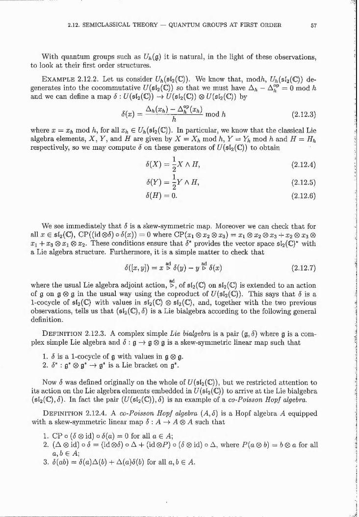
2.12. SEMICLASSICAL THEORY — QUANTUM GROUPS AT FIRST ORDER 57

W ith quantum groups such as E%(g) it is natural, in the light of these observations, to look at their first order structures.

E xam ple 2.12.2. Let us consider Ea(5L(C)). We know that, mod/?,, E/t(5L(C)) de­generates into the cocommutative E(5l2(Q) so that we must have A/i - = 0 mod hand we can define a map ô : E (5[2(C)) -> //(^^(C)) 0 E(5l2(C)) by

<5(æ) = ,4 , /.) ft (2.12.3)

where x = x^ mod h, for all x^ G (512(C)). In particular, we know that the classical Lie algebra elements, X , Y, and H are given by X = X/j mod h, Y ~ Yh mod h and H — Hh respectively, so we may compute 6 on these generators of E(5l2(C)) to obtain

5{X) = i x A H, (2.12.4)

<5(y) = l F A H , (2.12.5)

6 { H) = 0. (2.12.6)

We see immediately tha t <5 is a skew-symmetric map. Moreover we can check that for all X G 512(C), CP ((id 0 6 ) o 6 {x)) = 0 where CP(æi 0 3:2 0 2 :3) = x\ ®X 2 ®xq-{-X2 ®Xs® xi + ^ 3 0 X1 0 X2. These conditions ensure that 6 * provides the vector space 512(C)* with a Lie algebra structure. Furthermore, it is a simple matter to check that

J([x,y]) = X ^ J(i/) - y ^ J(x) (2.12.7)

3;dwhere the usual Lie algebra adjoint action, >, of 5L(C) on 512(C) is extended to an action of 0 on 0 0 g in the usual way using the coproduct of E(5L(C)). This says that J is a 1-cocycle of 5[2(C) with values in 512(C) 0 5(2(C), and, together with the two previous observations, tells us tha t (512(C), J) is a Lie bialgebra according to the following general definition.

D e f in it io n 2.12.3. A complex simple Lie bialgebra is a pair (g, ô) where g is a com­plex simple Lie algebra and ( 5 : g - > g 0 g i s a skew-symmetric linear map such that

1. (5 is a 1-cocycle of g with values in g 0 g.2. 6* : g* 0 g* -4 g* is a Lie bracket on g*.

Now (5 was defined originally on the whole of E(5l2(C)), but we restricted attention to its action on the Lie algebra elements embedded in E (512(C)) to arrive at the Lie bialgebra (512(C), J). In fact the pair (E(5l2(C)),<5) is an example of a co-Poisson Hopf algebra.

D e f in it io n 2.12.4. A co-Poisson Hopf algebra (A, 6) is a Hopf algebra A equipped with a skew-symmetric linear map 6 : A -+ A ® A such that

1. CP o ((5 0 id) o 6(a) = 0 for all a G A;2. (A 0 id) o J = (id0(5) o A 4- ( id 0 P ) o { 6 ® id) o A, where P{a ® b) = b® a for all

a, 6 G A;3. ô(ab) — 6 (a) A{b) 4- A{a)ô{b) for all a, 5 G A.

58 2. THE QUANTUM PICTURE

As we would expect there is close relationship between co-Poisson Hopf algebras built on enveloping algebras U{q) and Lie bialgebras.

T heorem 2.12.5. Given a co-Poisson Hopf algebra (/7(g), 5) then (g,^|g) is a Lie bialgebra. Conversely, starting with any Lie bialgebra (g, <5) the cocommutator ô extends uniquely to provide U (g) with the structure of a co-Poisson Hopf algebra.

The observation that L/i(sl2(C)) has a Lie bialgebra structure ‘built in’ at first order in h is not peculiar to C4 (s[2(C)).

T h e o r e m 2.12.6. IfUhiQ) QUEA — whether a standard Drinfeld-Jimbo oneor not — then with 6 defined as

S{x) = -■ ‘7'*) ~ mod h, (2,12.8)

where x — Xh mod h, U{q,6 ) is a co-Poisson Hopf algebra and consequently (g, ( |g) is a Lie bialgebra.

We can now formulate an alternative ‘bottom up’ definition of a QUEA.

D efinition 2.12.7. A quantisation of a Lie bialgebra (g,5), as a quantised universal enveloping algebra, t4(g), is a deformation of the Hopf algebra U{q) such that that the cocommutator 6 of (g, 5) is given by the restriction to g of that defined in (2.12.8).

2.13. Classical r~matrices

A first step towards classifying QUEAs of complex simple Lie algebras is clearly a classification of the complex simple Lie bialgebras. The cocommutator ô in each case is a 1-cocycle of g with values in g 0 g. But applying Whitehead’s Lemma with M = g ® g we see tha t every 1-cocycle must be a 1-coboundary. That is, the cocommutator must beof the form 6 {x) — x > r for all T E g where r is some element of g 0 g. In order that (g, 5) be a Lie bialgebra, it then follows tha t r must be such that

1- 0 E> (ri2 + ^21) = 0.2 . g > ([[r, r]]) = 0 where [[r, r]] = [r^, ria] + r^s] + [ris, ^23]-

Up to scalar multiplication there is only one g-invariant element of g 0 g. This is the Casimir element C corresponding to the Killing form % of g, so we deduce that

^i2 + ^2i = /^C, (2.13.1)

where k is some scalar. This means that we can write r in the form r = l ( r j2 — ^21) + |C .

But from 6(æ) = æ ^ it follows th a t r' = | ( r i 2 —r’21) defines the same bialgebra structure as r = |( t ’i2 — T2i) + fC so we can concentrate on antisymmetric ?’-matrices.

Supposing r to be antisymmetric, it can be shown that [[r, r]] G A^g and furthermore tha t the g-invariant subspace of A^g is 1-dimensional and spanned by [[C, C]].

If r is skew and s is g-invariant then [[r -I- s, r 4- s]] = [[r, r]] -f [[s, s]]. Thus we arrive at the following result through which we define the notion of a classical r-matrix.

2.14. CLASSIFICATION OF CLASSICAL r-MATRICES 59

T h e o r e m 2.13.1. Evei'y complex simple Lie bialgebra is coboundary and specified by an element r G g 0 g which may be written as r = + kC where r^ is an element ofg A g and k, is a scalar such that r satisfies the classical Yang-Baxter equation [[r, r]] = 0. Such an element r is then called a classical r-matrix.

We may now reflect that in Example 2.12.2 we ignored the quasitriangularity of U/i(s(2(C)) when we considered its semi-classical limit. If we had taken it into account, then the definition of the co-commutator could have been written as

S(x) = - -A ") ~ (2.13.2)

from which we would have obtained the results,

^(X) = X > r, (2.13.3)

(5(F) = F > r, (2.13.4)

S(H) = JÎ > r, (2.13.5)

where r G 512(C) 0 512(C) appears in the expansion S l— l-^-hr mod h?.

By virtue of the fact that Dl obeys the quantum Yang-Baxter equation, r obeys the classical Yang-Baxter equation. Explicitly, it is given by

r = ^ H ® H + X ® Y , (2.13.6)

and borrowing terminology from the quantum case we say that r defines (512(C), 5) as a quasitriangular Lie bialgebra. Indeed we have just seen that every complex simple Lie bialgebra is quasitriangular which in a sense ‘explains’ the quasitriangularity of the standard QUEAs.

A subset of topological quasitriangular Hopf algebras is the topological triangular Hopf algebras. These have universal i?-matrices which satisfy — 3 where J = 101. At the semi-classical level this is also a useful sub-division. The complex simple triangular Lie bialgebras are precisely those whose r-matrices are given by r =

2.14. Classification of classical r-matrices

We have already seen tha t there are standard quasitriangular QUEAs associated with all complex simple Lie algebras. The corresponding standard Lie bialgebras are de­scribed in terms of the so-called Drinfeld-Jimbo classical r-matrices, r^^. These are non-triangular solutions of the classical Yang-Baxter equation. If I) is the Cartan subal­gebra of g, we denote by Cq the restriction of the Casimir to 6 0 [3. Then we can choose a basis element E^ for each root subspace g^ such that the Drinfeld-Jimbo r-matrices are given by

= iC o + ^ 0 E.„. (2.14.1)qSA+

These are by no means the only classical r-matrices for complex simple Lie algebras — there are many ‘nonstandard’ examples. The complete classification consists of two distinct classifications for the non-triangular and triangular cases respectively.

60 2. THE QUANTUM PICTURE

In the case of the non-triangular r-matrices the classification is due to Belavin and Drinfeld. To state their result we need a preliminary definition.

D e f in it io n 2.14.1. A quadrup le (H o,H i,r , s ) where IIo and IIi are subsets of the set n of sim ple roots, r : Ho —> IIi a one-to-one m apping and s e b A 1r is said to be admissible if it satisfies the following three conditions:

1. (r((a),r(/5)) = (a,/?) for all a ,/? G Hq.2. For every ck G Ho, there is an n such that a , r(o ;),. . . , G Ilo but r^{a) ^ Hq.3. (t(q;) 0 l)(|(7o + s) + (1 0 ci')(^Co + s) = 0 for all œ G fig.

Let us also introduce an ordering of the positive roots such that a < (3 if = r'^(a) for some m > 0 (r is extended linearly). The result of Belavin and Drinfeld may now be stated:

T h e o r e m 2.14.2. / /(I Io , H i, r, s) is an admissible quadruple then a Cartan- Weyl basis of the root subspaces of g can be chosen such that

r = r^"^ -f- s + Ea A Ep (2.14.2)a , 0 e A + , 0 < a

is a non-triangular classical r-matrix and moreover every non-triangular classical r-matrix is equivalent via a Lie algebra automorphism to one of this form.

For 512(C) we see that the only non-triangular r-matrix is the Drinfeld-Jimbo solution. Somewhat more interesting is the situation for 5(3 (C). In this case there is also a non­standard non-triangular r-matrix. For reasons which should become clear in Chapter 3 we call it the Cremmer-Gervais r-m atrix and denote it by r^^ . Explicitly

= + I hc,AH/} + E ^ A E . h, (2.14.3)

where a , are the simple roots and the notation for the Lie algebra elements is tha t of Chapter 1.

It is worth setting this result beside the following observation. For any quasitriangular Lie bialgebra, (g, r), and given any element / G g 0 g satisfying

[[/21 — / 12, /21 - / 12I] + [[/21 — / 12, f']] + [[a /21 — / 12I] = 0 (2.14.4)

(g ,r 4- /21 — / 12) is also a quasitriangular Lie bialgebra. We say tha t (g,r 4- j '21 — / 12) is related to (g, r) through a semiclassical twist by / . Notice that it follows that every quasitriangular Lie bialgebra is related via such a twisting to the trivial quasitriangular Lie bialgebra (g, 0), so that in fact all the quasitriangular Lie bialgebras associated with a given Lie algebra are related amongst themselves through semiclassical twists. In par­ticular, in the case of the Cremmer-Gervais r-m atrix for 5(3(0 ), we know that r^'^ and r ^ ^ are related through a semiclassical twist / = ^ H a 0 / / / ? 4 - E g 0 E ^ p . Of course these observations are rather trivial. We mention them because the quantum counterparts of these twists are far from trivial, and indeed are far from being completely understood. One of the main results of Chapter 3 is actually a construction of a ‘quantisation’ of this twist.

The classification of the triangular solutions of the classical Yang-Baxter equation was achieved some time after the Belavin-Drinfeld result bv Stolin. For details we refer the

2.15. QUASI-HOPF ALGEBRAS AND TWISTING 61

reader to the original papers [94]. Here we will just mention that for 5[2(C) there is a single triangular r-matrix, r'^,

r" = X A / / (2.14.5)which defines co-commutators

(^(%) = 0, (2.14.6)< (y) = 2X AY, (2.14.7)(^(//) = 2% A/f. (2.14.8)

There is a known quantisation of (512(C), r" ) as a triangular QUEA, which is oftencalled the Jordanian quantised universal enveloping algebra (hence the superscript). The Hopf algebra structure was discovered independently by Ohn [81] and Lazarev and Mov- shev [66] with the triangular universal A-matrix worked out subsequently by Ballesteros et al [7] and Abdesselam et al [1]. It will be described explicitly in Chapter 4, where we classify the bicovariant differential calculi on the corresponding quantised coordinate rings, [ % ( € ) ] and C ^[% (C )].

Given the classification of the semiclassical structures it is now a question of whether or not there is a QUEA corresponding to each complex simple Lie bialgebra which contains the Lie bialgebra in its semi-classical limit. There is an early result of Drinfeld which establishes the existence and uniqueness up to ‘quantum’ twists of a triangular QUEA quantising every triangular Lie bialgebra. The existence problem in the non-triangular case has only been resolved quite recently by Etingof and Kahzdan [38]. The correct mathematical framework for discussing such issues is provided by Drinfeld’s notion of quasi-Hopf algebras. Uniqueness does not seem to have been established for any but the standard Drinfeld-Jimbo quantum groups.

2.15. Q uasi-H opf a lgebras an d tw is tin g

Given a topological quasitriangular Hopf algebra ([//i(g),IR) and a %(g)-module, y[[A]], the form of the universal i7-matrix ensures that Ik is a well defined operator on {V 0 y)[[fi]]. In fact this is clear in the case of (512(C)) with Ik as defined in (2.5.16) since by Theorem 2.6.14 the elements X and Y act nilpotently on U[[fi]]. The same reasoning applies in the general case.

E x am p le 2.15.1. Choose V to be the first fundamental representation of [/(512(C)) and take {uq, ui} as a basis for V[[h]] as in Theorem 2.6.14 so that

{uo 0 uo,uo 0 VuVi 0 uo,Ui 0 Ui} (2.15.1)

is a basis of {V 0 U)[[fi]]. On {V 0 V)[[h]] the universal /[-matrix of U/t(512(C)), Ik, then acts as the matrix R y y where

Rv y

/gV2 0 0 0 \0 1 gW2 _ g-/t/2 00 0 1 0V 0 0 0 g/i/2 (2.15.2)

In this example R y y is a C[[fi]]-linear automorphism of {V 0 U)[[fi]]. This is the case generally when we denote by Rv,v the universal /[-matrix interpreted as an operator on (U 0 y)[[A]] where V[[h]] is a [//i(g)-module since Ik is by definition invertible. Moreover,

62 2. THE QUANTUM PICTURE

defining R y y = T y y o R y y where Tyy : ( V 0U)[[fi]] is the C[[/i]]-linear permutation map such tha t Tyy{v®w) = W0U for all v ,w Ç. K[[/i]], the QYBE implies that R y y satisfies the braid relation

{ R y y é id) o (id 0 R y y ) o {Ryyé> id) = (id <S)Ryy) o ( R y y ^ id) o (id (^Ryy). (2.15.3)

Let us now recall the definition of the braid group.

D e f in i t io n 2,15.2. The braid group on n strands Bn is the group generated by then — 1 symbols a i, (72,... , (Jn-i such that aicrj = <7(7* if |% - > 1 and

~ (2.15.4)

for all 2, / = 1 . . . n — 1.

Given the formal similarity between (2.15.3) and (2.15.4) it is not surprising that there is a simple construction which turns the operators R y y into C[[fi]]-linear representations of the braid group Indeed defining operators 6% on Y®"'[[/i]] for z — 1 . . . n — 1 by

I/iv,’l/G>idy®(n-2)pj] Z = 1,idi;/®(<-i)j /, jj 0 jR y,v0 idy®(n-i-i[p^]] 1 < i < n — 1, (2.15.5)

idy®(n-2)[[/l]] ®Hyy,

then we have precisely bfij = bjbi if |z — > 1 and

(2.15.6)

for all z, j = 1 . . . n — 1.

Apparently many ‘mathematical-physics-miles’ from the discussion to this point are Wess-Zumino-Witten (WZW) theories in conformai field theory and the Knizhnik-Zamol- odchikov (KZ) equations. In fact there is a KZ system of equations associated with any pair (g, t) where g is a complex simple Lie algebra and t is a symmetric g-invariant element of g 0 g together with a parameter h an integer ?z > 1 and a g-module V. Moreover, through a classical construction of the monodromy of the the KZ equations is obtained a representation of the braid group Bn called the monodromy representation which, for n = 2, has the form r y y o

Kohno and Drinfeld independently obtained the following remarkable result:

T h e o r e m 2.15.3. Let g be a complex simple Lie algebra and V an irreducible g- module. Then the monodromy representation of the braid group Bn on y®” [[/z]] from the K Z equations is equivalent to the C[[h]]-linear representations of the braid group de­termined by the universal IR of the Drinfeld-Jimbo QUEA Uh{g).

In a series of fundamental works [33, 35 , 36] Drinfeld simultaneously proved this theorem, introduced new mathematical structures generalising his earlier innovation of quasitriangular Hopf algebras, and set up the correct framework for questions of existence and uniqueness of quantum groups. His new mathematical structures will now be defined.

D e fin it io n 2.15.4. A topological quasi-Hopf algebra over C[[/z]] is a a topological algebra, (A, m, ?]), together with C[[/z]]-linear maps A : A —> A0A, e : A —> C[[/z]] and

2.15. QUASI-HOPF ALGEBRAS AND TWISTING 63

S : A ^ A called the coproduct, counit and antipode respectively and an invertible element 0 G A 0A 0A called the Drinfeld associator such that

(id 0 A ) o A (a) = <L“ ^((A(8) id) o A(a))<I>, (2,15.7)

( ( A 0 id 0 id) (#)) ( (id 0 id 0 A) (0) ) — (# 0 l) ( ( id 0 A0 id )($ ))(l0 $), (2.15.8)

(e0 id) o A = id = (id0 e) o A, (2.15.9)

( id 6 0 id ) (0 ) = 1, (2.15.10)

5 (a(i))o;a(2) = e(a)o;, a(i)/?5 (a(2)) = e(a)//, (2.15.11)

= = 1, (2,15.12)

for all a G A where A(a) = O(i)0 (Z(2) is a Sweedler notation for the coproduct, 1 is the unit in A, <D = ^ (/>00'0</>" and

D e f in it io n 2.15.5. A topological quasitriangular quasi-Hopf algebra (QTQHA) is a tuple ( A , m, 77, A,e, 5 ,ex,//, <&,Ik) where (A, m,ry. A,e, 5, ex,d>) is a quasi-Hopf algebra and Ik is invertible and called the universal /[-matrix such that

A°P(u) = Ik A (a )9 [- \ (2.15.13)

(A® id) (31) = 4>ÿi31i3‘ï-i323l234r23, (2.15.14)(id® A) (31) = (&31231i3$213^12' 123 (2.15.15)

for all a G A,

These definitions are imposing to say the least and do not suggest that any conceptual simplification will be obtained by working with QTQHAs rather than quasitriangular Hopf algebras. However the QTQHAs have a truly fundamental property which is not in general shared by the quasitriangular Hopf algebras. They admit twists according to the following theorem:

T h e o r e m 2.15.6. Let (A, m, 77, A, e, S, cx, //, 0, Ik) be a QTQHA and suppose T G A0 A is invertible and such that

(€ 0 id )(T ) = 1 = ( id 0 6 )(T ); (2.15.16)

then T is called a universal twisting matrix and (A g r , m, 77, A j , e, 5, cx, //, <I>j, k g r ) where,

A ?(o) = T A ( a ) T - \ (2.15.17)

% = T2iIkT7/, (2.15.18)

= T i2 ( (A 0 id ) (T ) )$ ( ( id 0 A )(T ) ) -^ % ^ (2.15.19)

M G QTQ//A.

Observe that any topological (quasitriangular) Hopf algebra is a (QT)QHA for which the Drinfeld associator is just 10101. Also, it is of course the case that the definitionsand twisting result apply equally well if the objects are defined over a field such as Crather than the ring C[[/i]].

The twisting result may be specialised to the interesting case of twisting from and to a quasitriangular Hopf algebra. Such twists (or rather their duals) will be the subject of Chapter 3.

64 2. THE QUANTUM PICTURE

D e f i n i t i o n 2.15.7. A quasi-Hopf quantised universal enveloping algebra (QHQUEA) associated to a complex simple Lie algebra g is a QHA (A, m, rj, A, e, 5, a , (5, $) such that A fh A = [/(g) as quasi-Hopf algebras and A = U(q)[[Ji]] as C[[/i]]-modules and cp = 1 0 1 0 1 mod iP. A quasitriangular QHQUEA is a QHQUEA which is also a topological quasitriangular quasi Hopf algebra with Ik = 1 0 1 mod h.

D e f i n i t i o n 2.15.8. The classical limit of a quasitriangular QHQUEA (A, 0 , Ik) is the pair (g,t) where t = — 1 0 1) mod h. A quasitriangular QHQUEA with (g,[)as its classical limit is then called a quantisation of (g, /).

Drinfeld’s fundamental result is the following;

T h e o r e m 2.15.9. Given any Lie algebra, q, together with a symmetric g-invariant element, t, there exists a quantisation of the universal enveloping algebra, [/(g), as a quasitriangular quasi-Hopf quantised universal enveloping algebra, ([/(g)[[/z]], and this quantisation is unique amongst quantisations of (g, t) up to twisting.

An immediate consequence of this result is that the standard quantisation of U (s[/+i(C)), ([//i(sli+i(C)), Ik^), is twist equivalent as a quasitriangular quasi-Hopf algebra to the ‘uni­versal’ quantisation ([/(5lf+i(C))[[A]], We consider the relevance of this result inrelation to the Belavin-Drinfeld classification of classical r-matrices and recent work of Etingof and Kazhdan in Chapter 3.

CHAPTER 3

T w istin g 2-cocycles for th e construction of new non-standard quantum groups

3.1. Introduction

Originally there were two clearly defined types of quantum groups [32, 55, 84]. They were single-parameter quantisations, C4(g) and Qi[G] respectively, of dual classical ob­jects: the universal enveloping algebras of simple Lie algebras, [/(g), and the coordinate rings of simple Lie groups, C[G]. W ith their universal /[-matrices, 7k, these Uh{g) are the standard examples of quasitriangular Hopf algebras, while the C/j[G], together with the corresponding numerical /[-matrices, are the standard examples of what we call co- quasitriangular Hopf algebras [29, 30]. It soon became apparent that there were a num­ber of multiparameter generalisations [26, 95, 99] of these standard quantum groups and through the work of Drinfeld [33], followed by Reshetikhin [83], an interpretation emerged: all the multiparameter quantum groups corresponding to a particular standard quantum group were related, amongst themselves and with the standard quantum group, through Drinfeld’s important process of twisting. In fact the original works of Drinfeld and Reshetikhin were concerned only with quasitriangular Hopf algebras, but their con­structions dualise immediately to the case of co-quasitriangular Hopf algebras. Since the twists act only as similarity transformations on the so called R-matrices [84], the differ­ent standard quantum groups corresponding to different classical Lie groups cannot be related to each other by twisting. The picture then is of a number of distinct ‘twist equiv­alence classes’. Later, Kempf and Engeldinger [61, 37] (see also the work of Khoroshkin and Tolstoy [62]) refined Reshetikhin’s work slightly and showed that there were other interesting quantum groups related, through Reshetikhin-type twists, with the standard ones.

From time to time there appeared genuinely non-standard quantum groups, usually de­fined in terms of non-standard numerical /[-matrices. It is natural to investigate whether these define new twist equivalence classes or whether they belong to classes already defined by the standard /[-matrices. We will be particularly concerned in this article with the non-standard quantum groups of Cremmer and Gervais [22] and Fronsdal and Galindo [41, 42] which for general theoretical reasons (see Section 4) may be expected to be twist-equivalent to the standard SL(n) quantum groups. However, let us be clear that no twist of the Reshetikhin type is suitable in these cases. As we explain later, the relevant twisting structures are counital 2-cocycles on the quantum groups. The problem then is to find the appropriate twisting 2-cocycles, defined on the standard co-quasitriangular Hopf algebra, C/i[S'L(n)], which twist this quantum group into the Cremmer-Gervais and Fronsdal-Galindo quantum groups.

65

66 3. TW ISTING 2-COCYCLES

Recently, Hodges has made significant progress in this area [50], drawing on previous work of his contained in a series of important papers [51, 52, 53]. These covered many as­pects of quantum group theory from a ring theoretic perspective. We should mention [52] in particular, where some remarkable aspects of the algebraic structure of Cremmer- Gervais quantum groups were revealed. In [50] Hodges starts from a particular, standard, multiparameter quantised enveloping algebra Up{Q) (this is a multiparameter version of a rational form Uq{g) of % (g)). He then identifies a pair of commuting sub-Hopf algebras, t/p(b]f) and Up(b^), associated with certain Belavin-Drinfeld triples [10]. This gives rise to a Hopf algebra homomorphism, cj) : Dp(bf) 0 Up(bJ) —)■ Dp(g), through the usual mul­tiplication map. Attention then shifts to the dual map, (j)* : (^[G] -4 Cp[Bf] 0 Cp[Rf]. Hodges proceeds to identify lm(0*), in a series of precise and subtle steps, with the image of the tensor product of a pair of ‘extended’ Borel subalgebra-like objects, between which there is a skew pairing. This skew pairing lifts to the tensor components of Im(</>*). It is well known that such a pairing gives rise to a 2-cocycle, the quintessential example appear­ing in the twisting interpretation of the quantum double [30, 71], and a 2-cocycle is then induced on the quantised function algebra Cp[G]. Hodges claims tha t in the particular case of 513(C) the 2-cocycle coming from his construction generates the Cremmer-Gervais deformation of C[S'L(3)]. More generally, he claims that it should also be possible to reach the esoteric quantum groups of Fronsdal and Galindo [41, 42). However, Hodges’ approach is rather technical and does not readily yield 2-cocycles defined explicitly on the familiar T-matrix generators of standard quantum groups. We are able to remedy this situation here.

Our approach is actually quite distinct from that of Hodges. We work entirely within the framework of co-quasitriangular Hopf algebras coming from solutions of the matrix quantum Yang-Baxter equation (QYBE). Since we are working with quantum groups coming from the FRT construction and are not concerned with their relationship with QUEAs we do not need to work in a topological setting. Indeed from now on we denote the quantised coordinate rings coming from the FRT construction by Cq [G] where q is an element of some base field k and in particular (standard) cases can be taken to be

In Section 2 we recall the definition of a co-quasitriangular Hopf algebra and the basic result on twisting by 2-cocycles. A good reference for this theory, and much more besides, is the book by Majid [71], from which much of our notation is borrowed. Other good references are the paper by Larson and Towber [65] and the papers of Doi and Takeuchi [29, 30]. Majid calls co-quasitriangular Hopf algebras, ‘dual quasitriangular Hopf algebras’, but our terminology comes from [29, 30]. We go on to describe the well known class of 2-cocycles which appears as the dual of the Reshetikhin-type twists. They originate from particular solutions of the QYBE. The ‘parameterization’ twists originally considered by Reshetikhin [83] may be regarded as examples in this class, and using such a twist we have obtained a new 3-parameter generalised Cremmer-Gervais R-matrix, presented here, which includes as a special case the 2-parameter R-matrix considered by Hodges in [52]. Details of the derivation of this new R-matrix are given in Appendix A. The sub-Hopf-algebra-induced twists considered by Engeldinger and Kempf [61, 37] also belong to this general class of 2-cocycles, and are recalled here.

Section 3 contains our main new results. We present there a new class of 2-cocycles which no longer emanate from solutions of the matrix QYBE. Instead, they arise from matrices satisfying a new, and remarkably simple, system of equations. A number of

3.2. CO-QUASITRIANGULAR HOPF ALGEBRAS AND RESHETIKHIN TWISTS 67

explicit 2-cocycles belonging to our new class are presented, along with the following results:

® It is shown explicitly that the new 3-parameter generalised Cremmer-Gervais quan­tum group corresponding to GR(3), already given in Section 2, is obtained from a particular multiparameter standard quantum group through twisting.

• The 2-CO cycle used to obtain the generalised Cremmer-Gervais deformation of GL{3) is an example of a general class of simple root 2-cocycles which themselves belong to a more general class of composite simple root 2-cocycles. These 2-cocycles may all be defined on certain standard, multiparameter, deformations of GL{n), and consequently generate new non-standard quantum groups.

® A 2-cocycle which can be used to twist a certain multiparameter standard deforma­tion of C[GL{2 N — 1)] to obtain a generalisation of the quantum groups of Fronsdal and Galindo is presented. For N = 2 this 2-cocycle is just the one used to obtain the generalised Cremmer-Gervais GL(3) quantum group.

Note tha t the R-matrix considered by Fronsdal and Galindo is already ‘multiparameter’, involving N parameters, but we obtain, in Appendix B, an R-matrix which depends on (1 -f- — ! ) ( / / + 2)) parameters. Let us also note that, as was already suggested inHodges work [50], starting from the original standard quantum groups, Cq[SL{n)], we need a combination of the Reshetikhin-type parameterisation twists with our new twists to obtain the Fronsdal-Galindo quantum groups.

In Section 4, we collect some information about the semi-classical objects correspond­ing to the R-matrices which we have been considering in this chapter, namely the classical r-matrices. We also recall the background, in Drinfeld’s fundamental work, which serves as the on-going motivation in the quest for interesting twists. We end by pointing out a particular problem involved in constructing the Cremmer-Gervais quantum group corre­sponding to GR(4), and describe an interesting phenomenon involving sub-Hopf-algebra- induced twists. Starting from the standard multiparameter quantum group, Cq,p[GL(4)], we twist, first of all, using a sub-Hopf-algebra-induced twist. The resulting quantum group may reasonably be called ‘weakly non-standard’ and can be twisted further using a2-cocycle from our construction. The new, non-standard, R-matrix obtained through this double twist involves a pair of non-standard off-diagonal elements which could not have been added to the original R-matrix directly, but which do appear in the Cremmer-Gervais R-matrix for GL(4).

3.2. Co-quasitriangular Hopf algebras and Reshetikhin twists

We begin with some basic definitions.

D e f in it io n 3.2.1. A bialgebra A is called co-quasitriangular if there exists a bilinear form cr on A, which we will call an R-form, such that

1. cr is invertible with respect to the convolution product, *, that is, there is another bilinear form cr” such that

(;(&(!), = Cr"'XG(i),6(i))(T(a(2),6(2)), (3.2.1)2. (j * m = * (7, i.e.

0"(G(1), 6(1))U(2)5(2) = 5(l)G(l)f7(a(2),6(2)), (3.2.2)

68 3. TWISTING 2-COCYCLES

3. a{m 0 id) = dig * agg, i.e.

(7(^6, c) = 0-(a, C(i))cr(6, C(2)), (3.2.3)

4. C7(id0m) = (713 * (712, i.e.

(7(&, 6c) = (7(G(1), c)(7(G(2), 6). (3.2.4)

R e m a r k 3.2.2. We are employing here a slightly simplified version of the Sweedler notation for coproducts: A(a) = G(i) 0 a(2), with the summation suppressed.

R e m a r k 3.2.3. It may be useful to briefiy recall how we arrive at this definition. Suppose th a t {H, 7k) is a quasitriangular bialgebra, with 7k G 7/ 0 7/ the universal R- matrix obeying Drinfeld’s familiar axioms

(A 0 id)(7k) = 7ki37k23, (id0A)(7k) = 7ki37ki2, (3.2.5)A°P(/z) = 7koA( f i )o7k - \ VfiGR. (3.2:6)

In fact, we may be regard 7k as a map A: -A 7/ 0 7/, where k is the ground field. Whenformulating the dual notion of co-quasitriangular bialgebra, we then need to consider an77-form a which is now a map A 0 A —> where A can be thought of as dual to H. To formulate the dual axioms, involving a instead of 7k, we require the algebra structure on Hom(A 0 A, A:). This is the convolution algebra provided by the natural tensor product coalgebra structure of A 0 A. Explicitly then, let us give the details for a particular example,

((713 * (723)(a 0) 6 <0 c) = (713(G(1) 0 6(i) 0 C(i))(723(G(2) <0 (>(2) <0 C(2))= (7(G(i),C(i))e(6(i))(7(6(2),C(2))c(G(2))= (7(a,C(i))(7(6, C(2)).

For more on this process of ‘dualising’ we refer the reader to Majid’s book [71], and his paper [69].

From the definition it is readily seen that the QYBE now manifests itself as

(712 * (7lg * (723 — (723 * (7l3 * (7i2- (3.2.7)When A is actually a Hopf algebra, with antipode 5, we call it a co-quasitriangular Hopfalgebra. It can then be shown that S is always invertible, and a~^{a,b) = a{S{a),b) andcr(a, b) = a~^(a, S{b)).

The FRT bialgebras A(R), introduced by the Leningrad school [84] and developed by Majid [70], where R is any matrix solution of the QYBE, fit into the co-quasitriangular bialgebra framework. Indeed, we define the 77-form on the generators T /, as

= (3.2.8)

or in the useful ‘matrix notation’, as

(7(T%, T2) = 7Îi2, (3.2.9)

and then extend its domain of definition to the whole of A(77) by setting

(7(TiT2,Tg) = (7(Ti,T3)(7(7^,7k) = 77i3R23, (3.2.10)(7(Ti,T2T3) = (7(Ti,l^)(7(Ti,72) = 77i37[i2. (3.2.11)

The QYBE then guarantees consistency with the product relation (3.2.2).

3.2. CO-QUASITRIANGULAR HOPF ALGEBRAS AND RESHETIKHIN TW ISTS 69

R e m a r k 3.2.4. To remove any possible doub t abou t the no ta tion being employed here, let us present (3.2.10) explicitly, in term s of the generators, as

o (T ? T lT l ) = a ( T p T T ) a ( T l r j =

where the summation convention is being assumed.

D e f in it io n 3.2.5. A bilinear form % on a bialgebra A is called a counital 2-cocycle on A if it is invertible in the convolution product, and

X (l,a) = €(a) = x(G ,l), (3.2.12)

and

%i2 * %(m 0 id) = %23 * %(id <0 m). (3.2.13)

R e m a r k 3.2.6. It is a simple m atter to show that any R-form is a counital 2-cocycle. We also note that for any Hopf algebra on which we can define such a 2-cocycle, which moreover intertwines the multiplication as in (3.2.2), the antipode is necessarily invertible.

R e m a r k 3.2.7. In the more familiar dual version of this definition, we consider an invertible element IF of R 0 R . Then (3.2.12) and (3.2.13) correspond respectively to

(c 0 id)(JF) = 1 = (id0e)(JF), (3.2.14)

and

IFi2(A 0 id)(IF) = .R23(id0A)(IF). (3.2.15)

An element T satisfying these conditions is then called a counital 2-cocycle for R.

R e m a r k 3.2.8. For a general discussion of cocycles for and on Hopf algebras we refer the reader to Section 2.3 of Majid’s book [71].

The property of co-quasitriangular Hopf algebras which is of particular interest to us is that, given one, we may generate others using these counital 2-cocycles. This important process of twisting is the dual of Drinfeld’s original quasitriangular quasi-Hopf algebra twist [33], restricted to the special case of twisting from and to co-quasitriangular Hopf algebras. It is not difficult to dualise Drinfeld’s original quasitriangular quasi-Hopf algebra axioms, and his result on twisting. This was probably first carried out explicitly byMajid [69]. We obtain the axioms for a co-quasitriangular co-quasi-Hopf algebra and onspecialising the twisting result, we obtain the following important theorem.

T h e o r e m 3.2.9. Let (A, m , 77, A, e, cr) be a co-quasitriangular bialgebra and let % 6e a counital 2 -cocycle on A, then there is a new co-quasitriangular bialgebra (A^, cr ) obtained by twisting the product and R-form of (A, cr) as

— (3. 2. 16)

= X21 * - (3.2.17)

I f A is moreover a Hopf algebra with antipode S, then A^ is also a Hopf algebra with twisted antipode given by

S . = (3.2.18)

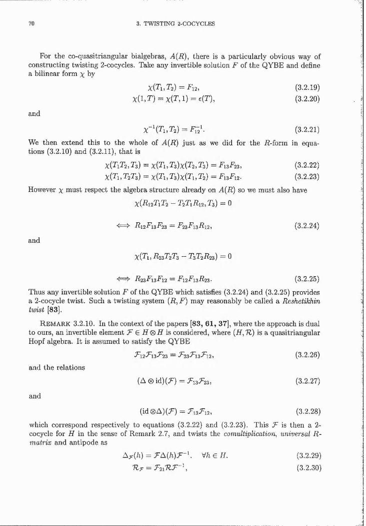
70 3. TWISTING 2-COCYCLBS

For the co-quasitriangular bialgebras, A(R), there is a particularly obvious way of constructing twisting 2-cocycles. Take any invertible solution F of the QYBE and define a bilinear form % by

x T i . î s ) = F i2, (3.2.19)X(1,T) = x { T , l ) = e(T), (3.2.20)

and

(3.2.21)

We then extend this to the whole of A(R) just as we did for the R-form in equa­tions (3.2.10) and (3.2.11), that is

x(TiT2,T3) = x(Ti,T3)x(T2,T3) = F13F23, (3.2.22)x(Ti,T2T3) = x(Ti,T3)x(Ti,T2) = F13F 12. (3.2.23)

However % must respect the algebra structure already on A(R) so we must also have

x { E i 2T i T 2 — T 2T 1R 12, T g) — 0

4=^ R 12R13R23 = 7 237 13/^12, (3.2.24)

and

x ( T i ,R 2 3 T 2 T 3 — T 3Y 2 R 23) = 0

<=> R237 137 12 — 7 127 13R23- (3.2.25)

Thus any invertible solution F of the QYBE which satisfies (3.2.24) and (3.2.25) provides a 2-cocycle twist. Such a twisting system (R, F) may reasonably be called a Reshetikhin twist [83].

R e m a r k 3.2.10. In the context of the papers [83, 61 , 37], where the approach is dualto ours, an invertible element .F E 7/ 0 7/ is considered, where (7/, 7k) is a quasitriangularHopf algebra. It is assumed to satisfy the QYBE

= E 2zR\2,F\2 , (3.2.26)

and the relations

(A 0 id )(.F ) = F'i3F'23, (3.2.27)

and

(id 0 A )(/:) = Fi3^i2, (3.2.28)

which correspond respectively to equations (3.2.22) and (3.2.23). This F is then a 2- cocycle for 7/ in the sense of Remark 2.7, and twists the comultiplicaMon, universal R- matrix and antipode as

A;r(fi) = .F A (f i)F - \ Vfi G 7/. (3.2.29)7k;r = IF2i7k/^-\ (3.2.30)

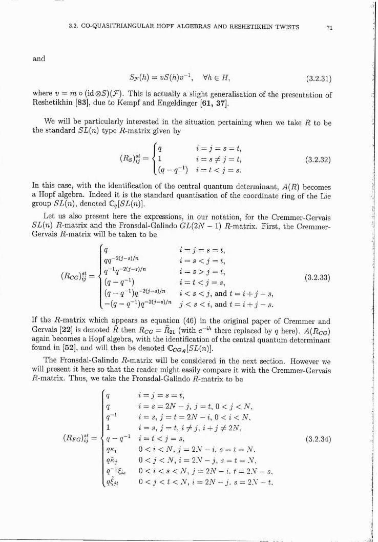
3.2. CO-QUASITRIANGULAR HOPF ALGEBRAS AND RESHETIKHIN TWISTS 71

and

(3.2.31)

where v = m o (id05)(F*). This is actually a slight generalisation of the presentation of Reshetikhin [83], due to Kempf and Engeldinger [61, 37].

We will be particularly interested in the situation pertaining when we take R to be the standard SL{n) type R-matrix given by

q i — . j — s —

1 i — s j = t,{q - q~^) i = t < j ^ s .

(3.2.32)

In this case, with the identification of the central quantum determinant, A(R) becomes a Hopf algebra. Indeed it is the standard quantisation of the coordinate ring of the Lie group 5L(n), denoted C^[5 L(n)].

Let us also present here the expressions, in our notation, for the Cremmer-Gervais SL[n) R-matrix and the Fronsdal-Galindo GL[2 N - 1) R-matrix. First, the Cremmer- Gervais R-matrix will be taken to be

q - i q - 2 { j ~ s ) / n

( g —

- ( ? -

(3.2,33)

i =2 j = s = t, z = g < j i — s ^ j — [, z = it < / = g,i < s < j , and t = i j - s,j < s < z, and t = i y j - s.

If the R-matrix which appears as equation (46) in the original paper of Cremmer and Gervais [22 ] is denoted R then R cg = R21 (with there replaced by q here). A [R cg) again becomes a Hopf algebra, with the identification of the central quantum determinant found in [52], and will then be denoted CcG,g[RR(?z)].

The Fronsdal-Galindo R-matrix will be considered in the next section. However we will present it here so that the reader might easily compare it with the Cremmer-Gervais R-matrix. Thus, we take the Fronsdal-Galindo R-matrix to be

/

{ R f g )% — <

(-1 i ~ j ~ s =q i = s = 2N — j , j = t, 0 < j < R,

i — s, j — t = 2N — z, 0 < z < R,1 Z = g, J = t, Z 2 + ; ^ 2R,9 - z = t < / = g.

0 < z < R , j = 2R — z, g = t = R.0 < / < R , z = 2R — J, s = t = R,0 < z < g < R , j — 2N - i. f = 2R - s.0 < j < t < R , z = 2R - J . g = 2R - L

(3.2.34)

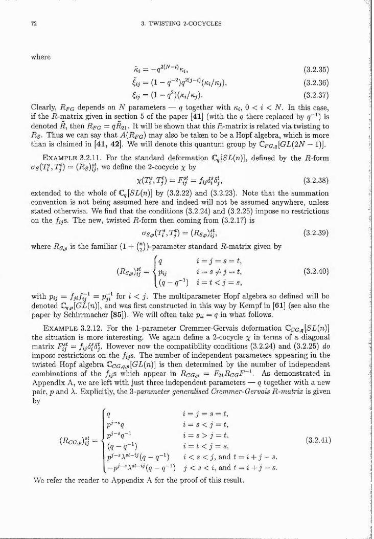
72 3. TWISTING 2-COCYCLES

where

Ki = (3.2.35)

4 = (1 - (3.2.36)

U = (1 - 4 ) («;/«,)• (3.2.37)Clearly, R pc depends on N parameters — q together with K,i, 0 < i < N. In this case, if the R-matrix given in section 5 of the paper [41] (with the q there replaced by isdenoted R, then R pc — qR2 i- It will be shown that this R-matrix is related via twisting toRs- Thus we can say tha t A (Rfg) may also be taken to be a Hopf algebra, which is more than is claimed in [41, 42], We will denote this quantum group by CpG,q[GE{2N — 1)].

E x a m p l e 3.2.11. For the standard deformation C^[5R(n)], defined by the R-form a s{T f,T j) = {RsYij, we define the 2-cocycle % by

= = (3.2.38)

extended to the whole of Cg[5L(n)] by (3.2.22) and (3.2.23). Note that the summation convention is not being assumed here and indeed will not be assumed anywhere, unless stated otherwise. We find that the conditions (3.2.24) and (3.2.25) impose no restrictions on the fijS. The new, twisted R-form then coming from (3.2.17) is

(7s,p(:^\T;) = (Rg,p)g, (3.2.39)

where Rs,p is the familiar (1 + (J) )-parameter standard R-matrix given by

I q i — j — s — t,Pij i = s = t, (3.2.40)

{q - q~^) z = t < / = g,

with Pij = = P jl for i < j . The multiparameter Hopf algebra so defined will bedenoted Cq^p[GL{n)], and was first constructed in this way by Kempf in [61] (see also the paper by Schirrmacher [85]). We will often take pa = q in what follows.

E x a m p l e 3.2.12. For the 1-parameter Cremmer-Gervais deformation CcG,q[SL(n)] the situation is more interesting. We again define a 2-cocycle % in terms of a diagonal matrix Ffj — fijôfôy However now the compatibility conditions (3.2.24) and (3.2.25) do impose restrictions on the /^s. The number of independent parameters appearing in the twisted Hopf algebra CcG,q,p[GL{n)] is then determined by the number of independent combinations of the /^ s which appear in Rcg,p = F2 \RcgE"^. As demonstrated in Appendix A, we are left with just three independent parameters — q together with a new pair, p and A. Explicitly, the 3-parameter generalised Cremmer-Gervais R-matrix is given

byq z = j = g = t,p" ~ q i ~ s < j — t,pl~^q~^ i = s > j — C(g - 9"^) % = ( < / =pi-s\st-tj(^q _ q-i^ z < g < J, and t — i j — ,s,

— q~Y j < s < i, and t = i j — s.We refer the reader to Appendix A for the proof of this result.

{Hcg,p) (3.2.41)

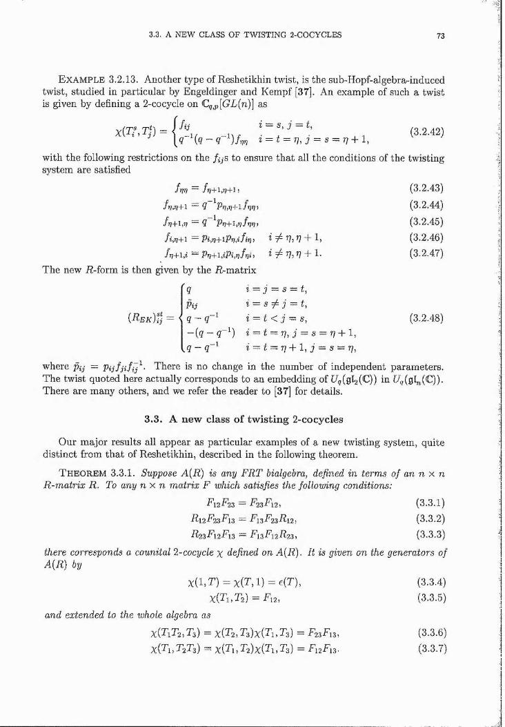
3.3. A NEW CLASS OF TWISTING 2-COCYCLES 73

E x a m p l e 3.2.13. Another type of Reshetikhin twist, is the sub-Hopf-algebra-induced twist, studied in particular by Engeldinger and Kempf [37]. An example of such a twist is given by defining a 2-cocycle on Cq^p[GL{n)] as

with the following restrictions on the fijS to ensure that all the conditions of the twisting system are satisfied

f r jT ) — /?7+l,r7+l) (3.2.43)fï},r)+l — q (3.2.44)

fî]+i,7] — q Pr]+i,Tifr]T] (3.2.45)fi,T)+l — Pi,’n+lPrj,ifir} 'I PiP F Ij (3.2.46)frj+lfi PT}+l,iPi,7]fT)i Vi P 1. (3.2.47)

The new R-form is then given by the R-matrix

{REK)ij

q i = j z=2 s ■= t,pij i — s ^ j = t .1

q - q~^ i = t < j = s, (3.2.48)~ { q ~ q ~ Y i = t = 7], j = s = rj+ 1 ,

. q - q ~ ^ i = t = rj-}-l, j = s = T],

where pij — Pijfjifîj^’ There is no change in the number of independent parameters. The twist quoted here actually corresponds to an embedding of Uq{Ql2 {C}) in [/g(gl^^(C)). There are many others, and we refer the reader to [37] for details.

3.3. A new class of tw is tin g 2-cocycles

Our major results all appear as particular examples of a new twisting system, quite distinct from that of Reshetikhin, described in the following theorem.

T h e o r e m 3.3.1. Suppose A{R) is any FRT bialgebra, defined in terms of an n x n R-matrix R. To any n x n matrix F which satisfies the following conditions:

F 12F 23 = R23F 12, (3.3.1)R12R23F 13 = R13E23R 12, (3.3.2)R23R12R13 = R13R12R23, (3.3.3)

there corresponds a counital 2-cocycle % defined on A(R). It is given on the generators of A(R) 6?/

x ( l,T ) = x (T ,l) = €(T), (3.3.4)x(Ti,T2) = Ri2, (3.3.5)

and extended to the whole algebra as

x(TiT2,T3) = x(T2,T3)x(Ti,T3) = F23F13, (3.3.6)x(Ti,T2T3) = x(Ti,T2)x(Ti,T3) = F12F 13. (3.3.7)

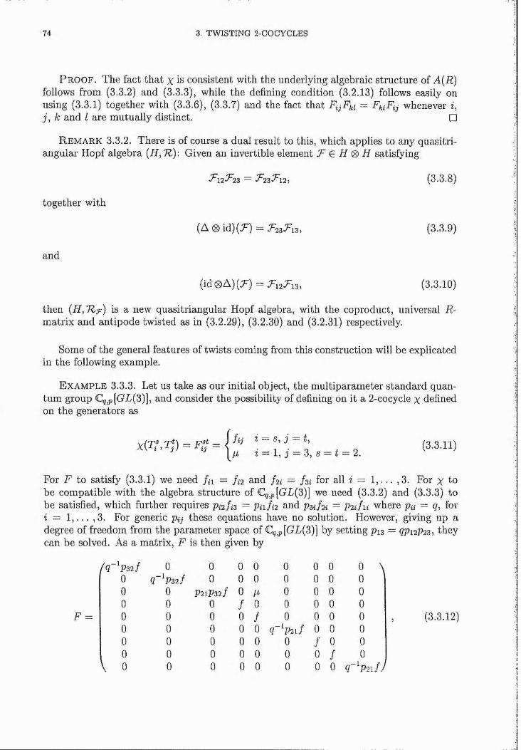
74 3. TWISTING 2-COCYCLES

P r o o f . T he fact th a t % is consistent w ith the underlying algebraic s tru c tu re of A[R) follows from (3.3.2) and (3.3.3), while the defining condition (3.2.13) follows easily on using (3.3.1) together w ith (3.3.6), (3.3.7) and the fact th a t FijF^i — FkiFi j whenever z, j , k and I are m utually d istinct. □

R e m a r k 3.3.2. There is of course a dual result to this, which applies to any quasitri­angular Hopf algebra (R, 7k): Given an invertible element F e H 0 H satisfying

F\2.Fo% ~ Foojr.23. 12, (3.3.8)

together with

(A 0 id)(F) = F 23F]13, (3.3.9)

and

(id0A )(F ') = F'i2Fi3, (3.3.10)

then (R, 7kj-) is a new quasitriangular Hopf algebra, with the coproduct, universal R- matrix and antipode twisted as in (3.2.29), (3.2.30) and (3.2.31) respectively.

Some of the general features of twists coming from this construction will be explicated in the following example.

E x a m p l e 3.3.3. Let us take as our initial object, the multiparameter standard quan­tum group Cq^p[GL{3)], and consider the possibility of defining on it a 2-cocycle % defined on the generators as

t = 2.(3.3.11)

For F to satisfy (3.3.1) we need fn = /*2 and f 2i = fu for all z = 1, . . . , 3. For % to be compatible with the algebra structure of Cg,p[GT(3)] we need (3.3.2) and (3.3.3) to be satisfied, which further requires Pi2 f i3 = Pnfi2 and p u f 2i — P2i fu where pu = q, for i = 1 , . . . ,3. For generic Pij these equations have no solution. However, giving up a degree of freedom from the parameter space of Cç,p[GL(3)] by setting pi^ — ÇP12P23, they can be solved. As a matrix, F is then given by

0 0 0 0 0 0 0 0 \0 0 0 0 0 0 0 00 0 P21P32/ 0 M 0 0 0 00 0 0 / 0 0 0 0 00 0 0 0 / 0 0 0 00 0 0 0 0 g"^P2i/ 0 0 00 0 0 0 0 0 / 0 00 0 0 0 0 0 0 / 00 0 0 0 0 0 0 0 7“ P2i/ /

(3.3.12)

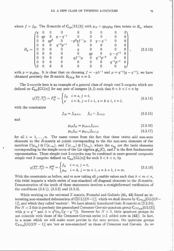
3.3. A NEW CLASS OF TWISTING 2-COCYCLES 75

where / = f 2 2 - The R-matrix of Cg,p[5L(3)] with p i3 = ÇP12P23 then twists to Ry, where

fq 0 0 0 0 0 0 00 0 0 0 0 0 00 0 0 0 0 00 0 0 0 0 0 0 00 0 0 0 q 0 0 0 00 0 0 0 0 9P 0 q - q - ^ 00 0 0 0 0 0 00 0 0 0 0 0 0 0

\o 0 0 0 0 0 0 0 q)

(3.3.13)

with p = pi2p2 3 - It is clear that on choosing / = obtained precisely the R-matrix Rcg,p for n = 3.

-pX and n == q ^(q — q Q, we have

The 2-cocycle here is an example of a general class of simple root 2-cocydes which are defined on C..q^p[GL{n)] for any pair of integers (k, I) such that 0 < A: < / < n by

fijx { T i ,T ‘) = F ^ =

with the constraints

and

i — s, j — A,i=zk, j = l- \- l , s = k + l , t = l,

fi,k — fi,k+li fl,i —

Pi,kfi,l — Pi,k+lfi,l+li

Pl,ifk,i — Pl+l,ifk+l,ii

(3.3.14)

(3.3.15)

(3.3.16)(3.3.17)

for all z = 1, . . . ,n. The name comes from the fact that these twists add non-zero elements to the R-matrix at points corresponding to the the non-zero elements of the matrices r(ca^) 0 r ( e _ a j , and r ( e _ a j 0 r(ea^), where the are the basis elements corresponding to the simple roots of the Lie algebra gf„(C), and T is the first fundamental representation. These simple root 2-cocycles may be combined in more general composite simple root 2-cocycles defined on Cq^p[GL{n)] for each 0 < A; < n, by

-iZ\ zrist } fijMm

z — s, j — A, i = k, j = m - { - l , s A: -f 1, A — m.

(3.3.18)

W ith the constraints as before, and m now taking all possible values such that k < m < n, this twist imparts a whole series of non-standard off-diagonal elements to the R-matrix. Demonstration of the tru th of these statements involves a straightforward verification of the conditions (3.3.1), (3.3.2) and (3.3.3).

While working on the universal T-matrix, Fronsdal and Galindo [41, 42] found an in­teresting non-standard deformation of C[GL(2R —1)], which we shall denote by [GT(2R- 1)], and which they called ‘esoteric’. We have already introduced their R-matrix in (3.2.34). For N = 2 this is precisely the generalised Cremmer-Gervais quantum group Ccg,(?,p[GT(3)] with p — q~^ and A = q^[i^il{q — q~^))- However for N > 2 , their quantum groups do not coincide with those of the Cremmer-Gervais series (c.f. added note in [42]). In fact, in a sense which we will make more precise in the next section, the quantum groups F>FG,q[GL{2 N — 1)] are ‘not as non-standard’ as those of Cremmer and Gervais. As we

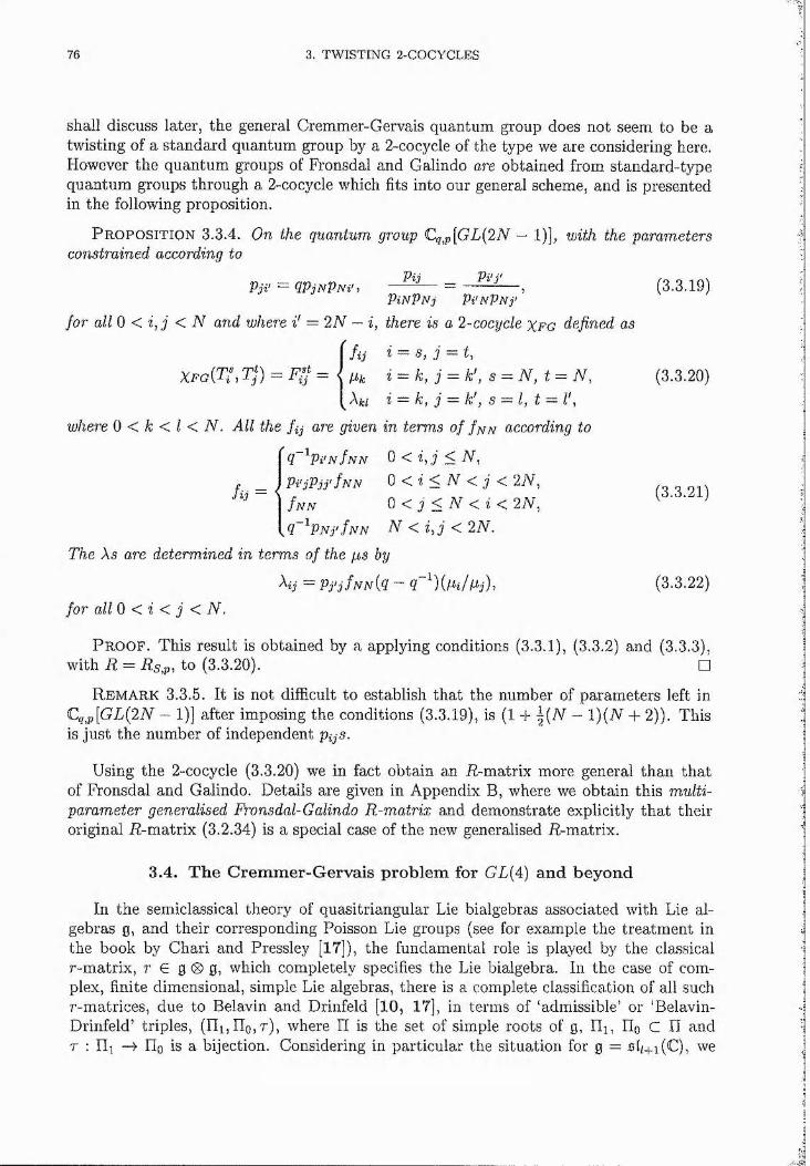
76 3. TWISTING 2-COCYCLES

shall discuss later, the general Cremmer-Gervais quantum group does not seem to be a twisting of a standard quantum group by a 2-cocycle of the type we are considering here. However the quantum groups of Fronsdal and Galindo are obtained from standard-type quantum groups through a 2-cocycle which fits into our general scheme, and is presented in the following proposition.

P r o p o s it io n 3 .3.4. On the quantum group Cq^p[GL(2 N - 1)], with the parameters constrained according to

Pj i ' — q P j N P N i ' i —— — = , (3.3.19)P i N P N j P i ' N P N j '

for all 0 < i , j < N and where i' = 2N - i, there is a 2-cocycle x f g defined as

I fij i = s, j — t,Pk i ~ k , i = k ' , s = N , t — TV, (3.3.20)

^ki i — k, j — k , s — I, t ~ I , where 0 < k < I < N . All the fij are given in terms of fj^pj according to

q~^Pi'NfNN 0 < < R,P i ’j P j j ' f N N 0 < z < R < j < 2R,

/vN 0 < / < R < z < 2R,F~^PNj'Inn N < i , j < 2R.The As are determined in terms of the pLS by

X i j — P j ' j f N N i S l q ) { p i / P j ) i (3.3.22)for alio < i < j < N .

(3.3.21)

P r o o f . This result is obtained by a applying conditions (3.3.1), (3.3.2) and (3.3.3), with R — Rs,pi to (3.3.20). □

R em ar k 3.3.5. It is not difficult to establish that the number of parameters left in Cq^p[GL{2N - 1)] after imposing the conditions (3.3.19), is (1 -I- | ( R — 1)(R 4- 2)). This is just the number of independent p^s.

Using the 2-cocycle (3.3.20) we in fact obtain an R-matrix more general than that of Fronsdal and Galindo. Details are given in Appendix B, where we obtain this multi­parameter generalised Fronsdal-Galindo R-matrix and demonstrate explicitly tha t their original R-matrix (3.2.34) is a special case of the new generalised R-matrix.

3.4. T h e C rem m er-G erv ais p ro b lem for GL(4) an d beyo n d

In the semiclassical theory of quasitriangular Lie bialgebras associated with Lie al­gebras 0 , and their corresponding Poisson Lie groups (see for example the treatm ent in the book by Chari and Pressley [17]), the fundamental role is played by the classical r-m atrix, r G g 0 g, which completely specifies the Lie bialgebra. In the case of com­plex, finite dimensional, simple Lie algebras, there is a complete classification of all such r-matrices, due to Belavin and Drinfeld [10 , 17], in terms of ‘admissible’ or ‘Belavin- Drinfeld’ triples, (Hi ,Hg,r) , where H is the set of simple roots of g, Hi, Hq C H and r : H i -A H q is a bijection. Considering in particular the situation for g = 5lf+i(C), we

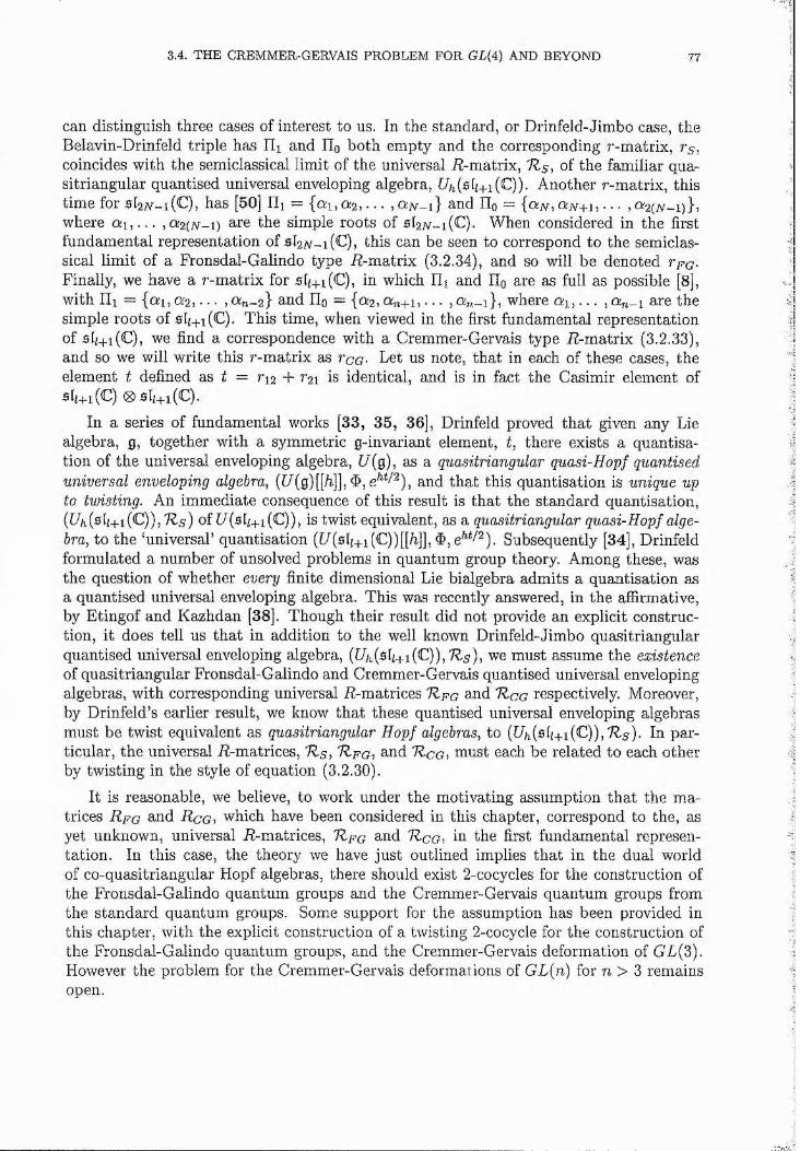
3.4. THE CREMMER-GERVAIS PROBLEM FOR GL{A) AND BEYOND 77

can distinguish three cases of interest to us. In the standard, or Drinfeld-Jimbo case, the Belavin-Drinfeld triple has Hi and Hq both empty and the corresponding r-matrix, rg, coincides with the semiclassical limit of the universal R-matrix, 7kg, of the familiar qua­sitriangular quantised universal enveloping algebra, Uh{sk+i{C)). Another r-matrix, this time for s12N-i(U), has [50] Hi = {cKi, Ck2, . . . , a^v-i} and IIo = {cKv, Av-n, • • • > ck2(n-i)}? where « i , . . . , 0!2(iv-i) are the simple roots of st2 _i(C). When considered in the first fundamental representation of 5f2iv-i(Q, this can be seen to correspond to the semiclas­sical limit of a Fronsdal-Galindo type R-matrix (3.2.34), and so will be denoted rpg- Finally, we have a r-m atrix for 5fz+i(C), in which Hi and Hq are as full as possible [8], with Hi = {cKi, Ck2, . . . , a n - 2 } and Ho = {0:2, ttn+i, • • • , where « i , . . . , an-\ are thesimple roots of 5f/+i(C). This time, when viewed in the first fundamental representation of 5ff_|_i(C), we find a correspondence with a Cremmer-Gervais type R-matrix (3.2.33), and so we will write this r-m atrix as Vcg- Let us note, that in each of these cases, the element t defined as t = r i2 + r 2i is identical, and is in fact the Casimir element of 5(i+l(C) 0Sf;+i(C).

In a series of fundamental works [33, 35, 36], Drinfeld proved tha t given any Lie algebra, g, together with a symmetric g-invariant element, t, there exists a quantisa­tion of the universal enveloping algebra, R(g), as a quasitriangular quasi-Hopf quantised universal enveloping algebra, ([/(g)[[fi]], e^*/^), and that this quantisation is unique upto twisting. An immediate consequence of this result is that the standard quantisation, (U/i(sfi+i(C)), 7kg) of [7(5[i4-i(C)), is twist equivalent, as a quasitriangular quasi-Hopf alge­bra, to the ‘universal’ quantisation (R(sfi+i(C))[[/i]], Subsequently [34], Drinfeldformulated a number of unsolved problems in quantum group theory. Among these, was the question of whether every finite dimensional Lie bialgebra admits a quantisation as a quantised universal enveloping algebra. This was recently answered, in the affirmative, by Etingof and Kazhdan [38]. Though their result did not provide an explicit construc­tion, it does tell us that in addition to the well known Drinfeld-Jimbo quasitriangular quantised universal enveloping algebra, { U h { s i i + i { C ) ) , T Z s ) , we must assume the existence of quasitriangular Fronsdal-Galindo and Cremmer-Gervais quantised universal enveloping algebras, with corresponding universal R-matrices IZpG and TZcg respectively. Moreover, by Drinfeld’s earlier result, we know that these quantised universal enveloping algebras must be twist equivalent as quasitriangular Hopf algebras, to (R/i(5 4.1(C)), 7kg). In par­ticular, the universal R-matrices, 7kg, TZfgi and 7kcG, must each be related to each other by twisting in the style of equation (3.2.30).

It is reasonable, we believe, to work under the motivating assumption that the ma­trices R fg and R qgi which have been considered in this chapter, correspond to the, as yet unknown, universal R-matrices, TZfg and TZcgi m the first fundamental represen­tation. In this case, the theory we have just outlined implies that in the dual world of co-quasitriangular Hopf algebras, there should exist 2-cocycles for the construction of the Fronsdal-Galindo quantum groups and the Cremmer-Gervais quantum groups from the standard quantum groups. Some support for the assumption has been provided in this chapter, with the explicit construction of a twisting 2-cocycle for the construction of the Fronsdal-Galindo quantum groups, and the Cremmer-Gervais deformation of GL(3). However the problem for the Cremmer-Gervais deformations of GL(n) for n > 3 remains open.

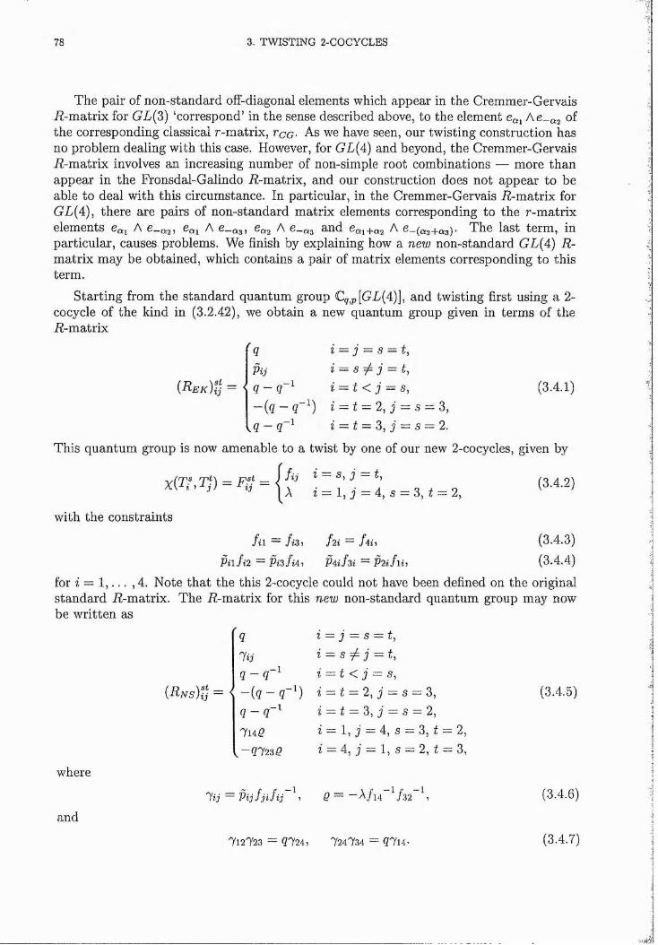
78 3. TWISTING 2-COCYCLES

The pair of non-standard off-diagonal elements which appear in the Cremmer-Gervais R-matrix for GL{3) ‘correspond’ in the sense described above, to the element ofthe corresponding classical r-matrix, Tcg- As we have seen, our twisting construction has no problem dealing with this case. However, for GL[A) and beyond, the Cremmer-Gervais R-matrix involves an increasing number of non-simple root combinations — more than appear in the Fronsdal-Galindo R-matrix, and our construction does not appear to be able to deal with this circumstance. In particular, in the Cremmer-Gervais R-matrix for GL(4), there are pairs of non-standard matrix elements corresponding to the r-m atrix elements A 6 - ^ 2 1 ^ai A 6-^35 A e_Qg and Can-ag A e_(ag4.a3). The last term, in particular, causes problems. We finish by explaining how a new non-standard GL(A) R- m atrix may be obtained, which contains a pair of matrix elements corresponding to this term.

Starting from the standard quantum group C^,p[GL(4)], and twisting first using a 2~ cocycle of the kind in (3.2.42), we obtain a new quantum group given in terms of the R-matrix

Kq

i = j = s = t, i = s ^ j — t, i = t < j = s, i = t — 2, j — s — 3, iz=zt — 3, j — s ~ 2 .

(3.4.1)

This quantum group is now amenable to a twist by one of our new 2-cocycles, given by

X(T’,T}) = pst _ j fijA - \ a

— ^1 j — Lz = 1, j = 4, g = 3, [ = 2,

(3.4.2)

with the constraints

fil — fiZi fli ~ fiii (3.4.3)

= Pi3/t4, pAifzi = P2iflh (3.4.4)

for z = 1, . . . ,4. Note that the this 2-cocycle could not have been defined on the originalstandard R-matrix. The R-matrix for this new non-standard quantum group may nowbe written as

'qlijq - q~^

i = j = s = t, i = s ^ j = t, i = t < j = s.

- { q - q ^ Yq - q - ^7l4g

,-97239

i — t ~ 2 , j = s = 3, z = t = 3, j = s = 2, z = 1, j = 4, g = 3, t = 2, z = 4, / — 1, g = 2, i = 3,

(3.4.5)

where

= Pijfjifij 1 9 = —A/1.4 \/'32 \ (3.4.6)

and

7l2?23 = 9724, 724734 = 9714. (3.4.7)

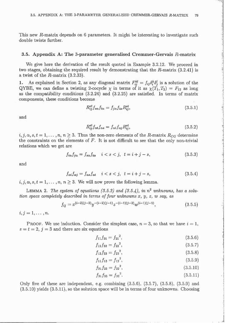
3.5. A PPENDIX A: THE 3-PARAMETER GENERALISED CREMMER-GERVAIS R-MATRIX 79

This new R-matrix depends on 6 parameters. It might be interesting to investigate suchdouble twists further.

3.5. Appendix A: The 3-parameter generalised Cremmer-Gervais R-matrix

We give here the derivation of the result quoted in Example 3.2,12. We proceed in two stages, obtaining the required result by demonstrating that the R-matrix (3.2.41) is a twist of the R-matrix (3.2.33).

1. As explained in Section 2, as any diagonal matrix ~ is a solution of theQYBE, we can define a twisting 2-cocycle % in terms of it as %(Ti, Tg) = Fu as long as the compatibility conditions (3.2.24) and (3.2.25) are satisfied. In terms of matrix components, these conditions become

Rijfsafta — fjafiaR'iji (3.5.1)

and

Hfjfatfas — faifajRiji (3.5.2)

i, j, a , s, t = 1, . . . , n, n > 3. Thus the non-zero elements of the R-matrix R cg determinethe constraints on the elements of F. It is not difficult to see that the only non-trivialrelations which we get are

fiafja ~ fsafta S < J, t = i Ar j 5, (3.5.3)

and

faifaj ~ fas fat S <C J, t i j S , (3.5.4)

i , j , a , s, t — 1, . . . ,n, n > 3 . We will now prove the following lemma.

L em m a 2. The system of equations (3.5.3) and (3.5.4)f unknowns, has a solu­tion space completely described in terms of four unknowns x, y, z, w say, as

i, j ~ 1, . . . , 77.

P r o o f . We use induction. Consider the simplest case, n = 3, so that we have i = 1, s — t = 2, j = 3 and there are six equations

/ l l / s i = / 21^, (3.5.6)

/ 1 2 / 3 2 = / 22^5 (3.5.7)

/ 1 3 / 3 3 = / 23^, (3.5.8)

/ 1 1 / 1 3 = / l 2 ^. (3.5.9)

/ 2 1 / 2 3 — ./22^, (3.5.10)

/ 3 1 / 3 3 = fzY ■ (3.5.11)

Only five of these are independent, e.g. combining (3.5.6), (3.5.7), (3.5.8), (3.5.9) and(3.5.10) yields (3.5.11), so the solution space will be in terms of four unknowns. Choosing

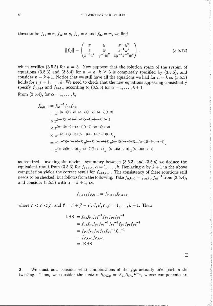
80 3. TWISTING 2-COCYCLES

these to be f n ~ x, f u — y, /21 = z and /gg = w, we find

nul l = z w z I , (3.5.12)\x~ ^z ‘ y~^uF xy~‘ z~‘w'^

which verifies (3.5.5) for n = 3. Now suppose that the solution space of the system of equations (3.5.3) and (3.5.4) for n — k, k > 3 is completely specified by (3.5.5), and consider n = A: + 1. Notice tha t we still have all the equations we had for n = A; so (3.5.5) holds for z ,/ = 1, . . . , k. We need to check that the new equations appearing consistently specify fa,k+i and fk+i,a according to (3.5.5) for a = 1, . . . , /c + 1.From (3.5.4), for a = 1, . . . , k,

-(Q-2)(i-2)+(Q-2)(s-2)H-(a-2)(t-2)f a , k + l f a i f a s f a t i

^ -(a-2)(i-2)Hy (ci—2)(ii—1)—(a—2)(s—1)-(q—2)(i—1)y (a—l)(i—2)—(a—l)(s—2)—(o!—l)(t—2)y .j -(a-l)(i-l)+(Q-l)(s-l)+(Q-l)(Z-l)

— , j , i a — 2 ) { — i + s + t — 2 ) y { a — 2 ) { i — s — t + l ) (a—l)(i—s—i+2) (Q—1}(—i-|-s+Z—1)^ ^ { a - 2 ) ( k + l - 2 ) y - { a - 2 ) i k + l - l ) ^ - { a - l ) i k + l - 2 ) ^ { a ~ l ) { k + l - l ) ^

as required. Invoking the obvious symmetry between (3.5.3) and (3.5.4) we deduce the equivalent result from (3.5.3) for fk+i,ai a = 1, . . . ,k. Replacing a by A: + 1 in the above computation yields the correct result for fk+i,k+i- The consistency of these solutions still needs to be checked, but follows from the following. Take fa,k+i — fasfatfai~^ from (3.5.4), and consider (3.5.3) with a — k A-1, i.e.

f i ' yk-\ -7 f j ' , k - \ - \ f s ' , k - { ~ ^ f t \ k - \ ~ l i 1

where i' < s' < / , and t' = i' + j ' - s', i', s', = , A: + 1. Then

LHS = J y z / y r '

f s ' , k - \ - l f t ' , k - h 7

= RHS

□

2. We must now consider what combinations of the fijS actually take part in the twisting. Thus, we consider the matrix Rco,p = / 2iR c g F “ \ whose components are

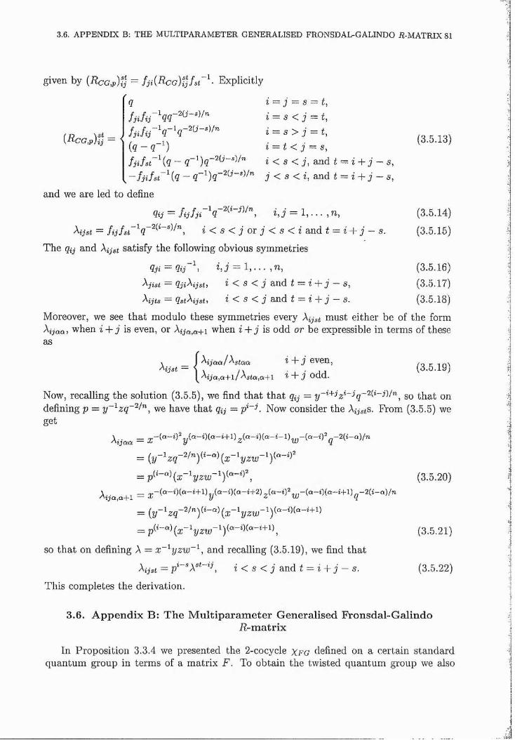
3.6. APPEND IX B: THE MULTIPARAMETER GENERALISED FRONSDAL-GALINDO R-MATRIX 81

given by Explicitly

= j 2= S = t,= g < / = ,

i ~ s > j = t,= t < / = g, (3.5.13)

(3.5.14)

(3.5.15)

{q - q~^)f j i f s t~ \q “ q-^)q-Aj-^)/n 2 < g < ; , and t = z + / - g,

, - / j iA z 'X ? - gr-i)g-2(j'-«)/" j < g < 2, and t = z + / - g,

and we are led to define

9v = z,/ = 1, . . . , ?z,

z < g < / or / < g < z and t = z + j - g.

The qij and Xijst satisfy the following obvious symmetries

qji ~ Qij i  J “ 1, . . . ,?7, (3.5.16)Xjist ~ QjiXijsti i s <j. j and t — i j g, (3.5.1 /)Xijts — QstXijsti i s j and t ~ i j s. (3.5.18)

Moreover, we see that modulo these symmetries every Xijst must either be of the form^ijaai when z + / is even, or Xija,a+i when i + j is odd or be expressible in terms of these as

Xijst — ^ijaa/ Xstaa z + j even,AijQ!,a-t-l/A5to,a:-f 1 T / odd.

(3.5.19)

Now, recalling the solution (3.5.5), we find that that qij — y '^q 7)/» so that ondefining p — y~^zq~‘ /^, we have that qij = p^~U Now consider the A^s/S. From (3.5.5) we get

= {y~^ zq~‘^'^Y''~°'\x~^yzw~Y^^~^^'^

Atja,o:-|-l — X ''' 'y '' '''' ' Z'' ' w

so that on defining A — x~^yzw~^, and recalling (3.5.19), we find that

hjst = i < s < j and t = z + / - g.

This completes the derivation.

(3.5.20)

(3.5.21)

(3.5.22)

3.6. Appendix B; The Multiparameter Generalised Fronsdal-GalindoR-matrix

In Proposition 3.3.4 we presented the 2-cocycle xfg defined on a certain standard quantum group in terms of a matrix F. To obtain the twisted quantum group we also

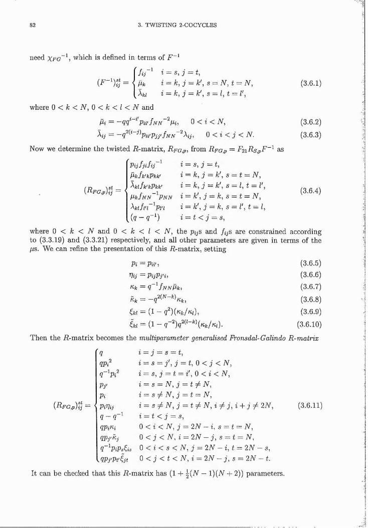
82 3. TWISTING 2-COCYCLES

need xfg \ which is defined in terms of F ^

Pk Xkl

where 0 < A ; < R , 0 < A : < / < i Y and

— l\st _i = s, j = t,i = k, j — k ' , s = N , t = N, i ~ k, j = k' , s — I, t — I',

Fi = 0 < z < R,

Âÿ = —9 * ^'^Pii'Pjj'fNN "^Xij, 0 < z < j < R .

Now we determine the twisted R-matrix, R f g ,pi from R f g ,p = F2 \Rs,pF~^ as

(3.6.1)

(3.6.2)

(3.6.3)

Pij fjifi j z = g, / = t.Pkfk'kPkk' i = k, j = k ' , s = t = N,\lfk'kVkk' i — k, j — k , g — Z, t — I ,PkÎNN ^Pn N i = k ' , j = k, s = t — N,^klfl'F^Pl'l i = k', j = k, s = I', t ~ I,(9 - 9"^) i = t < j = s,

(3.6.4)

where 0 < k < N and 0 < k < I < N , the pijS and /^ s are constrained according to (3.3.19) and (3.3.21) respectively, and all other parameters are given in terms of the IIS. We can refine the presentation of this R-matrix, setting

P i = P w 1 (3.6.5)Pi j = P i j P j ' i , (3.6.6)

Kt = In N P k i (3.6.7)

(3.6.8)

= (1 - 9^)(K*/N), (3.6.9)

& = (1 - 9"')9'(^"*=\Kt//{(). (3.6.10)

Then the R-matrix becomes the multiparameter generalised Fronsdal-Galindo R-matrix

{RFG,pYij = <

9 i 222 j — S — t,9P:^ i = s = j ' , j ^ t , 0 < j < R ,

i = s , j = t = i \ Q < i < N ,

Pj' i — s ~ N , j = t ^ N ,Pi i = sj t 2 N , j = t = N,

2 = g ^ R , j = ÿ ^ R , 2 ^ j , 2 + j ^ 2R,q - q ~ ^ i = t < j = s,9PiK* 0 < z < R , j = 2R - z, g = ( = R ,9PfKj 0 < / < R , z = 2R — J, g = t = R ,

0 < z < g < R , j — 2R — i, t — 2R — g..9PyPf'&( 0 < j < [ < R , z = 2R — j, g = 2R — t.

(3.6.11)

It can be checked that this R-matrix has (1 -t- | ( R — 1)(R + 2)) parameters.

3.6. A PPENDIX B; THE MULTIPARAMETER GENERALISED FRONSDAL-GALINDO R-MATRIX 83

To identify the i?-matrix originally discussed by Fronsdal and Galindo (3.2.34), as a special case of this E-matrix, consider the particular solution of (3.3.19) given by setting pij = 1 for 0 < î ^ j / < A ^ , 0 < z < A ^ < j < 2 N and N < i ^ j < 2N.

84 3. TWISTING 2-COCYCLES

CHAPTER 4

C lassification o f bicovariant differential calculi on th e Jordanian quantum groups GLh g{2) and SLh{2) and quantum Lie algebras

4.1. Introduction

The program of noncommutative geometry pioneered by Connes [19, 20] is based on fundamental results in the field of abstract analysis discovered in the first half of this cen­tury by Gelfand, Kolmogoroff, Naimark, Stone and others (a useful historical overview can be found in I. Segal’s review [90] of Connes’ book [19]). In particular, Gelfand and Kol­mogoroff showed that for a locally compact space, the algebra of continuous functions on the space is essentially equivalent to the space itself. The algebra of continuous functions is of course commutative, and in fact a C*-algebra. We can then reasonably consider the study of noncommutative C*-algebras as some form of noncommutative geometry. Thus the essential idea is to express the formalism of classical geometry as far as possible in the language of commutative algebra, and then use this as the paradigm for generalising to the noncommutative setting.

An implementation of this program has been developed by Dubois-Violette and co­workers (see the book by Madore [68], and the references therein). They generalize an elegant algebraic approach to the differential geometry of a smooth manifold introduced by Koszul [63] to the case where the commutative algebra of smooth functions on the manifold is replaced by the noncommutative algebra of matrices over some field.

In another direction, quantum groups provide natural candidates for noncommuta­tive generalizations of the algebras of smooth functions on classical compact Lie groups. Classically the algebra of representative functions is a dense subalgebra of the algebra of all smooth complex valued functions on the group and carries the structure of a ir-Hopf algebra. Dropping the 4r-structure we obtain the coordinate rings of the corresponding complex Lie groups, SLn{C)^ SOn(C) and Sp 2n{C). These coordinate rings are gener­ated already by the matrix elements of the defining representations of these groups (for GLn{C) we should adjoin (det(t))“ where t is the matrix of matrix element functions). Corresponding to these classical groups are the well known FRT Hopf algebras A(E), introduced by Faddeev, Reshetikhin and Takhtajan in [84]. They are ‘quantisations’ of the classical coordinate rings. It is these structures upon which we should try to develop some sort of noncommutative Lie group geometry. The pioneering works here are those of Woronowicz [103, 104]. In particular, in [104] Woronowicz set out a formalism in terms of bicovariant bimodules which has been studied intensively by very many authors since. Let us note that the classical differential calculus on Lie groups is bicovariant.

There is a well known ‘problem’ with the bicovariant calculi associated with the stan­dard FRT quantum groups other than G L q ( n ) : Their dimensions do not agree with the corresponding classical calculi. In the particular case of S L q { n ) the bicovariant calculus of Woronowicz is n^-dimensional while the classical calculus is of dimension — 1 (the

85

86 4. BICOVARIANT DIFFERENTIAL CALCULI ON JORDANIAN QUANTUM GROUPS

dimension being the dimension of the vector space of left-invariant 1-forms). This prob­lem has stimulated some authors to consider alternative approaches to the development of differential geometry on quantum groups. For example, in [87] Schmiidgen and Schuler consider left-covariant bimodules (developing Woronowicz’s original approach [103]) on SLq{n). They obtain first order calculi with the classical dimension; however for n > 4 the higher order calculi do not have the correct dimension. Another interesting approach was initiated by Faddeev and Pyatov[39]. They considered, for the particular case of SLq{n), the consequences of relaxing the condition of the classical Leibniz rule which is present in the bicovariant Woronowicz approach. They obtained bicovariant calculi of the correct classical dimension at all orders. However, subsequent work by Arutyunov, Isaev and Popowicz[5] suggests that a similar approach cannot be employed for the other simple quantum groups SOq{n) and Spq{n).

In this chapter we consider the original Woronowicz bicovariant calculus, but we ex­amine such calculi on the non-standard quantum groups GL^,/i(2) and SLh(2) — the so-called Jordanian quantum groups. In [58, 59], Karimipour initiated the study of bi­covariant calculi associated with SLh(2). Here we perform a complete classification of all first order bicovariant calculi on the quantum groups GLh^g{2) and SLh{2). Furthermore we consider the higher order calculi and the corresponding quantum Lie algebras. Let us summarise our main classification results:

• There are three 1-parameter families of 4-dimensional first order bicovariant differ­ential calculi on GLh,g{2 ) whose bimodules of forms are generated as left GLh^g[2 )- modules by the differentials of the quantum group generators.

• For one value of the parameter, the calculi in the three families are the same. This parameter value coincides with the value required for a ‘classical-like’ reduction to a 3-dimensional first order bicovariant calculus on SLh{2) which is shown to be unique.

• For all the calculi the relations in the exterior algebra are obtained and are shown to lead to exterior calculi whose dimension is classical at all orders.

• For all the calculi the relations in the enveloping algebra of the quantum Lie algebra are obtained and are shown to lead to PBW-type bases.

Classically, the Lie algebra of a Lie group is obtained as the vector space of tangent vectors at the identity equipped with a Lie bracket defined in terms of the left-invariant vector fields on the group manifold. The formalism of Woronowicz’s bicovariant calculus has a natural construction for a ‘quantum Lie algebra’ generalising the classical construc­tion to the abstract Hopf algebra setting. However, for all standard quantum groups the quantum Lie algebras so obtained have the ‘wrong’ dimension. This has prompted authors such as Sudbery and Delius to look for alternative constructions for quantum Lie algebras [67, 23, 24]. Two different approaches are described in their work. Recall that classically the Lie algebra g is an ad-submodule of the classical adjoint [/(g)-module, U (g), and its Lie bracket is the restriction of this classical adjoint action to g. This motivates the first approach [67, 23], A p proach 1, in which we look for an ad-submodule within the quantised universal enveloping algebra Eg(g) which has the correct dimension and upon which the restriction of the adjoint action of H^(g) closes. Lyubashenko and Sudbery employed a result of Joseph and Letzter and obtained a quantum Lie algebra in the cases [/ç(sli+i(C)) such that the coproduct of U q ( s i i + i { C ) ) applied to the basis of their quantum Lie algebra is of a particularly neat form. The other approach[24], A p p ro ach 2, (see also

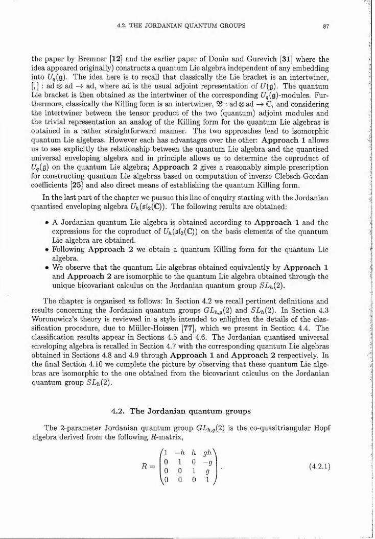
4.2. THE JORDANIAN QUANTUM GROUPS 87

the paper by Bremner [12] and the earlier paper of Donin and Gurevich [31] where the idea appeared originally) constructs a quantum Lie algebra independent of any embedding into C/q(g). The idea here is to recall that classically the Lie bracket is an intertwiner, [, ] : ad (gi ad —>• ad, where ad is the usual adjoint representation of [/(g). The quantum Lie bracket is then obtained as the intertwiner of the corresponding [7g(g)-modules. Fur­thermore, classically the Killing form is an intertwiner, 0 : ad g ad -4- C, and considering the intertwiner between the tensor product of the two (quantum) adjoint modules and the trivial representation an analog of the Killing form for the quantum Lie algebras is obtained in a rather straightforward manner. The two approaches lead to isomorphic quantum Lie algebras. However each has advantages over the other; A p p ro ach 1 allows us to see explicitly the relationship between the quantum Lie algebra and the quantised universal enveloping algebra and in principle allows us to determine the coproduct of Uq{g) on the quantum Lie algebra; A p p ro ach 2 gives a reasonably simple prescription for constructing quantum Lie algebras based on computation of inverse Clebsch-Gordan coefficients [25] and also direct means of establishing the quantum Killing form.

In the last part of the chapter we pursue this line of enquiry starting with the Jordanian quantised enveloping algebra [//i(012(C)). The following results are obtained:

® A Jordanian quantum Lie algebra is obtained according to A p p ro ach 1 and the expressions for the coproduct of [//i (012(C)) on the basis elements of the quantum Lie algebra are obtained.

• Following A p p ro ach 2 we obtain a quantum Killing form for the quantum Lie algebra.

• We observe that the quantum Lie algebras obtained equivalently by A p p ro ach 1 and A p p ro ach 2 are isomorphic to the quantum Lie algebra obtained through the unique bicovariant calculus on the Jordanian quantum group SLh{2).

The chapter is organised as follows: In Section 4.2 we recall pertinent definitions and results concerning the Jordanian quantum groups GLh^g{2 ) and SLh{2). In Section 4.3 Woronowicz’s theory is reviewed in a style intended to enlighten the details of the clas­sification procedure, due to Mfiller-Hoissen [77], which we present in Section 4.4. The classification results appear in Sections 4.5 and 4.6. The Jordanian quantised universal enveloping algebra is recalled in Section 4.7 with the corresponding quantum Lie algebras obtained in Sections 4.8 and 4.9 through A p proach 1 and A p p ro ach 2 respectively. In the final Section 4.10 we complete the picture by observing that these quantum Lie alge­bras are isomorphic to the one obtained from the bicovariant calculus on the Jordanian quantum group SLh{2 ).

4.2. T h e Jo rd a n ia n q u a n tu m groups

The 2-parameter Jordanian quantum group GLh^g{2) is the co-quasitriangular Hopf algebra derived from the following E-matrix,

R =

f l - h h0 1 00 0 1 g

VO 0 0 V

(4.2.1)

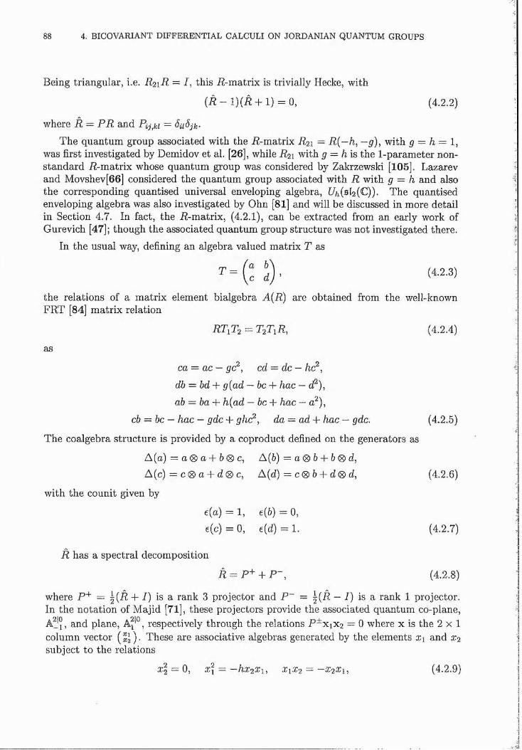
88 4. BICOVARIANT DIFFERENTIAL CALCULI ON JORDANIAN QUANTUM GROUPS

Being triangular, i.e. R 2 1 R = / , this E-matrix is trivially Hecke, with

(Ê - 1 )(E -h 1) = 0, (4.2.2)

where R ~ P R and Pij^ki =The quantum group associated with the E-matrix E 21 = E ( - / i , —g), with g — h = 1 ,

was first investigated by Demidov et al. [26], while E 21 with g = h is the 1-parameter non­standard E-matrix whose quantum group was considered by Zakrzewski [105]. Lazarev and Movshev[66] considered the quantum group associated with E with g = h and also the corresponding quantised universal enveloping algebra, E/i (012(C)). The quantised enveloping algebra was also investigated by Ohn [81] and will be discussed in more detail in Section 4.7. In fact, the E-matrix, (4.2.1), can be extracted from an early work of Gurevich [47]; though the associated quantum group structure was not investigated there.

In the usual way, defining an algebra valued matrix T as

^ = ( c 5 ) - (4,2.3)

the relations of a matrix element bialgebra A{R) are obtained from the well-known FRT [84] matrix relation

ET1T2 = TzTiE, (4.2.4)

as

ca — ac — gc^^ cd = dc —

db = b d p g { a d — be-\- h a c — d^),

ab ~ b a p h { a d — be P h a c — a f ) ,

cb = be — h a c — g d c P gh(?^ d a — a d p h a c — gdc. (4.2.5)

The coalgebra structure is provided by a coproduct defined on the generators as

A(a) — a < ^ a P b < S > c , A(5) = a < S > b P b ® d ,

A{c) — c<S> a P d® c, A(d) = c® b P d 0 d, (4.2.6)

with the counit given by

e(a) = 1, e{b) = 0,e(c) = 0, e{d) = 1. (4.2.7)

E has a spectral decomposition

Ê = E + - b E - , (4.2.8)

where P ^ = ^ { R p I) is a rank 3 projector and P~ — | ( E — J) is a rank 1 projector. In the notation of Majid [71], these projectors provide the associated quantum co-plane, A^5, and plane, respectively through the relations E ^ x p ^ = 0 where x is the 2 x 1 column vector (%%). These are associative algebras generated by the elements x\ and X2

subject to the relations

xl = 0, xl = —hx 2 X\, X1X2 = - X 2 X1 , (4.2.9)

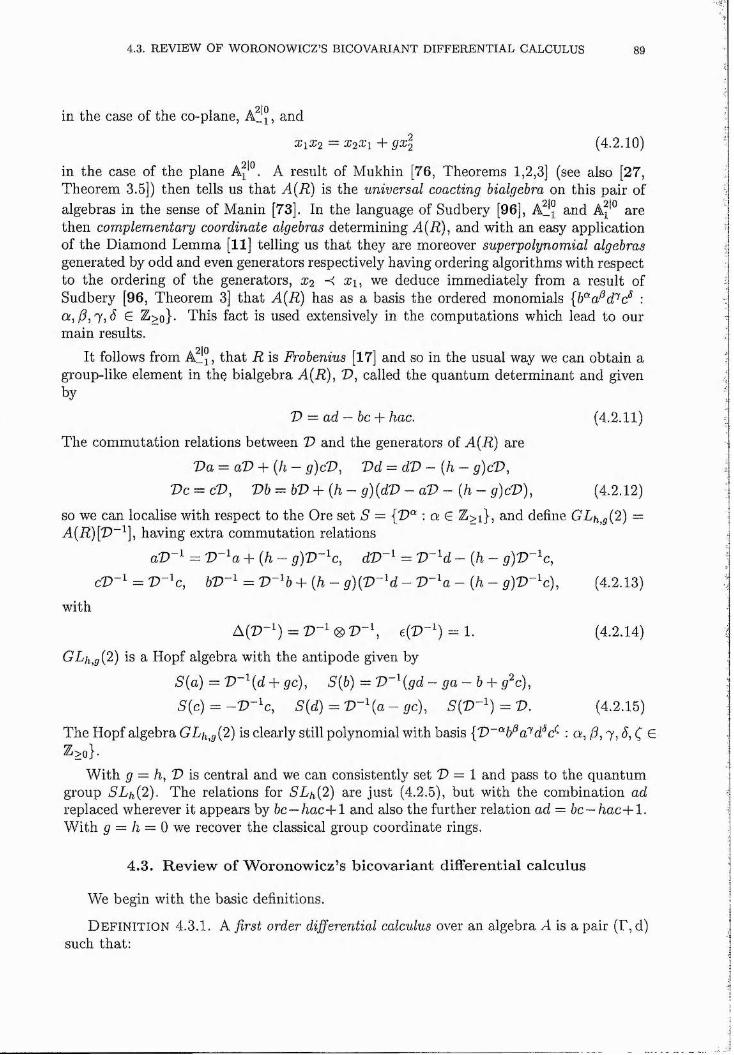
4.3. REVIEW OF WORONOWICZ’S BICOVARIANT DIFFERENTIAL CALCULUS 89

in the case of the co-plane, J , and

2:13:2 = 3:22:1 -h ^2:2 (4.2.10)

in the case of the plane Ai'°. A result of Mukhin [76, Theorems 1,2,3] (see also [27, Theorem 3.5]) then tells us that A{R) is the universal coacting hialgebra on this pair of algebras in the sense of Manin [73]. In the language of Sudbery [96], A^J and A *° are then complementary coordinate algebras determining A(E), and with an easy application of the Diamond Lemma [11] telling us tha t they are moreover superpolynomial algebras generated by odd and even generators respectively having ordering algorithms with respect to the ordering of the generators, 2:2 -< 2:1, we deduce immediately from a result of Sudbery [96, Theorem 3] tha t A(E) has as a basis the ordered monomials :a,j3 ,p ,ô e Z>o}. This fact is used extensively in the computations which lead to our main results.

It follows from A^J, that R is Frobenius [17] and so in the usual way we can obtain a group-like element in the bialgebra A(E), V, called the quantum determinant and given by

V — ad — be P hac. (4.2.11)

The commutation relations between V and the generators of A(R) are

V a = aV P {h — g)cV, V d = dV - {h — g)cV,Dc = cD, m = 6D + (A - ^)(dD - nD - (/t - g)cT>), (4.2.12)

so we can localise with respect to the Ore set S = : a € Z>i}, and define GLh,g{2 ) =A{R)[V~^]^ having extra commutation relations

0%)- = + (/t - g)D-^c, - (/t - p)D-^c,

= D-^c, + (/t - ^)(D-^d - - (/t - ^)l)-^c), (4.2.13)with

A (l)-^) = (g, e(D-^) = 1. (4.2.14)

GLh^g{2 ) is a Hopf algebra with the antipode given by

S{a) — V~^(d + gc), S(b) — V~^(gd ~ ga — h P g^c),

E(c) = E(d) = - pc), E(%)-^) = D. (4.2.15)

The Hopf algebra GLh^g[2) is clearly still polynomial with basis {V~^b^a?d^c^ : a , /?, y, 6, ( 6 ^>o}-

W ith g — h ^ V is central and we can consistently set X> = 1 and pass to the quantum group SLfi{2). The relations for SLh{2) are just (4.2.5), but with the combination ad replaced wherever it appears by hc—hacP l and also the further relation ad — b c ~ h a cp l . W ith g = h — 0 we recover the classical group coordinate rings.

4.3. R ev iew of W oronow icz’s b icovarian t diflTerential calculus

We begin with the basic definitions.

D e f in i t io n 4.3.1. A first order differential calculus over an algebra A is a pair (F,d) such that:

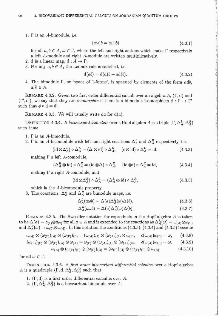
90 4. BICOVARIANT DIFFERENTIAL CALCULI ON JORDANIAN QUANTUM GROUPS

1. r is an A-bimodule, i.e.

[auj)h — a(u)b) (4.3.1)

for all Q, 6 € A, w € r , where the left and right actions which make F respectively a left A-module and right A-module are written multiplicatively.

2. d is a linear map, d : A -> F.3. For any a, 6 G A, the Leibniz rule is satisfied, i.e.

d(a6) = d(a)6 + ad(b). (4.3.2)

4. The bimodule F, or ‘space of 1-forms’, is spanned by elements of the form adb, (2,6 G A.

R e m a r k 4.3.2. Given two first order differential calculi over an algebra A, (F, d) and (F ',d '), we say tha t they are isomorphic if there is a bimodule isomorphism cj) : F —> F' such tha t ^ o d = dh

R e m a r k 4.3.3. We will usually w rite da for d(a).

D e f in it io n 4.3.4. A bicovariant himodule over a Hopf algebra A is a triple (F, A ^, A ^) such that:

1. F is an A-bimodule.2. F is an A-bicomodule with left and right coactions A^ and A j respectively, i.e.

(id 0 A ^) o A^ = (A (g) id) o A^, (eg) id) o A^ = id, (4.3.3)

making F a left A-comodule,

(A j 0 id) o A J = (id 0A ) o A^, (id Ge) o A f = id, (4.3,4)

making F a right A-comodule, and

(id ®A^) o A^ = (A^ (g) id) o A^, (4.3.5)

which is the A-bicomodule property.3. The coactions, A j and A j are bimodule maps, i.e.

A^(aw6) = A(n)A^((j)A(6), (4.3,6)

A^{acob) = A(n)A^(w)A(6). (4.3.7)

R e m a r k 4.3.5. The 8weedier notation for coproducts in the Hopf algebra A is taken to be A(a) = n(i)G)U(2) for all a G A and is extended to the coactions as A^(w) = and A^(w) = W(r)0W(yt). In this notation the conditions (4.3.3), (4.3.4) and (4.3.5) become

0 (ü;(r))(A) 0 M r)) (r ) = M A))(i) 0 ((^(A))(2) 0 ^ (r), c(w(yi))w(r) = w, (4.3.8)

(<^(r))(r) 0 { ^ { T ) ) { A ) 0(V(A) — ^(r) 0 (^(a))(i) 0 (w(A))(2), ^(^(A))^(r) = w, (4.3.9)

<X{A) 0 (w(r))(D 0 (w(r))(A) = (^(p))(a) 0 (<V(r))(r) 0 a;(A), (4 .3 .10)

for all w G F.

D e f in it io n 4.3.6. A first order bicovariant differential calculus over a Hopf algebra A is a quadruple (F, d, A^, A j) such that:

1. (F, d) is a first order differential calculus over A.2. (F, A a , A J) is a bicovariant bimodule over A.

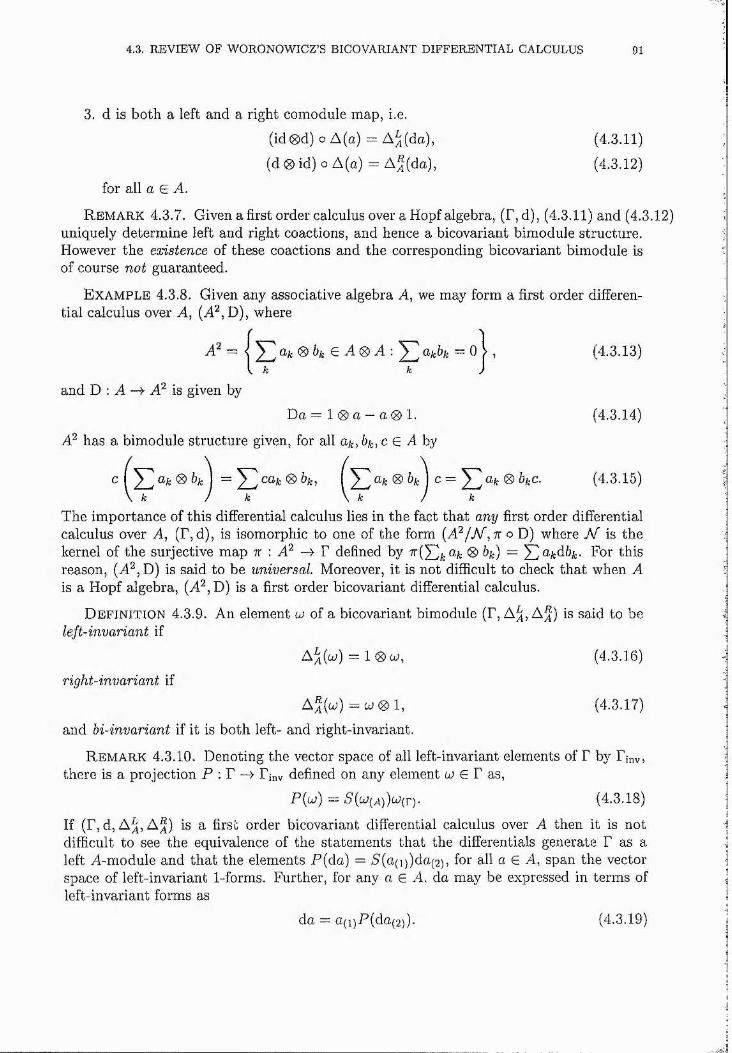
4.3. REVIEW OF WORONOWICZ’S BICOVARIANT DIFFERENTIAL CALCULUS 91

3. d is both a left and a right comodule map, i.e.

(id0d) o A(a) = A^(da), (4.3.11)

(d 0 id) o A(g) = AA(da), (4.3.12)

for all a e A.

R e m a r k 4.3.7. Given a first order calculus over a Hopf algebra, (F, d), (4.3.11) and (4.3.12) uniquely determine left and right coactions, and hence a bicovariant bimodule structure. However the existence of these coactions and the corresponding bicovariant bimodule is of course not guaranteed.

E x a m p l e 4.3.8. Given any associative algebra A, we may form a first order differen­tial calculus over A, (A^,D), where

and D : A -4 is given by

< ^ Gft 0 e A 0 A ; ^ a/cbk = 0 > , (4.3.13)[ k k )

D a — 1 0 a —a ® 1. (4.3.14)

A has a bimodule structure given, for all a/-, 6 ;, c G A by

C I 0 I = 0 6fc, I 0 &A: I c = 0 &f c C. (4.3.15)\ A : / k \ k / k

The importance of this differential calculus lies in the fact that any first order differential calculus over A, (F, d), is isomorphic to one of the form (A^/A/, tt o D) where A f is the kernel of the surjective map tt : A -> F defined by a* 0 h ) — j^^kdibk. For this reason, (A^, D) is said to be universal Moreover, it is not difficult to check tha t when A is a Hopf algebra, (A^,D) is a first order bicovariant differential calculus.

D e f in it io n 4.3.9. An element cj of a bicovariant bimodule (F, A^, A j) is said to be left-invariant if

A^(w) = l 0 w , (4.3.16)right-invariant if

A^(cj) =CJ0 1, (4.3.17)and bi-invariant if it is both left- and right-invariant.

R e m a r k 4.3.10. Denoting the vector space of all left-invariant elements of F by F,nv, there is a projection E : F F^v defined on any element w G F as,

E(w) = S'(aj(A))cJ(r). (4.3.18)

If (F, d, A^, A j) is a first order bicovariant differential calculus over A then it is not difficult to see the equivalence of the statements that the differentials generate F as a left A-module and tha t the elements E(da) = S'(a(i))da(2), for all a G A, span the vector space of left-invariant 1-forms. Further, for any a G A, da may be expressed in terms of left-invariant forms as

da = a(i)E(da(2)). (4.3.19)

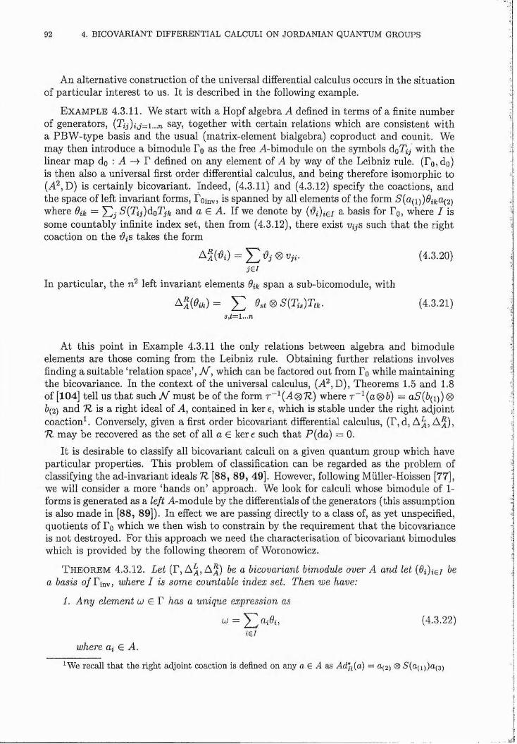
92 4. BICOVARIANT DIFFERENTIAL CALCULI ON JORDANIAN QUANTUM GROUPS

An alternative construction of the universal differential calculus occurs in the situation of particular interest to us. It is described in the following example.

E x a m p l e 4.3.11. We start with a Hopf algebra A defined in terms of a finite number of generators, say, together with certain relations which are consistent witha PBW -type basis and the usual (matrix-element bialgebra) coproduct and counit. We may then introduce a bimodule Pq as the free A-bimodule on the symbols doTij with the linear map do : A -> P defined on any element of A by way of the Leibniz rule. (Pg, do) is then also a universal first order differential calculus, and being therefore isomorphic to (A^,D) is certainly bicovariant. Indeed, (4.3.11) and (4.3.12) specify the coactions, and the space of left invariant forms, Poinv; is spanned by all elements of the form S{a(^i))9 ika^2 ) where 9ik = E(7^j)do% and a G A. If we denote by {'9i)i^i a basis for P q, where I issome countably infinite index set, then from (4.3.12), there exist VijS such that the right coaction on the takes the form

= (4,3.20)jel

In particular, the left invariant elements 9ik span a sub-bicomodule, with

A3(%t) = Y . ^s t0S{T i,)T a . (4,3,21)

At this point in Example 4.3.11 the only relations between algebra and bimodule elements are those coming from the Leibniz rule. Obtaining further relations involves finding a suitable ‘relation space’, A/", which can be factored out from Pq while maintaining the bicovariance. In the context of the universal calculus, (A^,D), Theorems 1.5 and 1.8 of [104] tell us tha t such A/" must be of the form r~^(A077) where r~^{a0 b) = aS{b(^i) ) 0

6(2) and 77 is a right ideal of A, contained in ker e, which is stable under the right adjoint coactionL Conversely, given a first order bicovariant differential calculus, (P, d, A^, A j) , 77 may be recovered as the set of all a G ker e such that P{da) = 0.

It is desirable to classify all bicovariant calculi on a given quantum group which have particular properties. This problem of classification can be regarded as the problem of classifying the ad-invariant ideals 77 [8 8 , 89, 49]. However, following Miiller-Hoissen [77], we will consider a more ‘hands on’ approach. We look for calculi whose bimodule of 1- forms is generated as a left A-module by the differentials of the generators (this assumption is also made in [8 8 , 89]). In effect we are passing directly to a class of, as yet unspecified,quotients of Fg which we then wish to constrain by the requirement that the bicovarianceis not destroyed. For this approach we need the characterisation of bicovariant bimodules which is provided by the following theorem of Woronowicz.

T h e o r e m 4.3.12. Let (F, A ^, A ^) be a bicovariant bimodule over A and let {9i)i^i be a basis o/Finv? where I is some countable index set. Then we have:

1. Any element cj G F has a unique expression as

CJ --- a j d j , (4.3.22)iei

where av G A.

^ W e r e c a l l t h a t t h e r i g h t a d j o i n t c o a c t i o n i s d e f i n e d o n a n y o G .4 a s Ad*ji{a) = a(2) ® 5(a(i))a(3)

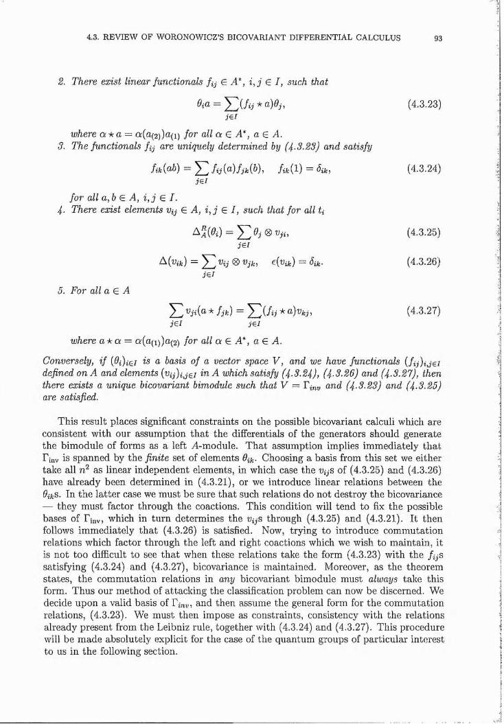
4.3. REVIEW OF WORONOWICZ’S BICOVARIANT DIFFERENTIAL CALCULUS 93

2. There exist linear functionals fij G A*, G I, such that

diU = 'y^^ifij * (4.3.23)

where a-ka = a{a^2 })( (i) for all a G A*, a e A.3. The functionals fij are uniquely determined by (4.3.23) and satisfy

At(a6) = Aj(a)/;'jk(6), A t(l) = (4.3.24)jei

for all a,b £ A, i , j G I.4 . There exist elements Vij G A, i^j G I , such that for all ti

A^(^i) = ^ 9j 0 Vji, (4.3.25)jei

^ Ojj 0 c{Viif) — Ôifç. (4.3.26)jei

5. For all a E A

^ V 'OjijO' fjk) — ^ ^ { f i j o)vkj, (4.3.27)jei jei

where a A a = a(ci(i))a(2) for all a G A*, a E A.

Conversely, if {9i)i^i is a basis of a vector space V, and we have functionals {fij)ijeidefined on A and elements (%)i,jG/ in A which satisfy (4.3.24), (4-3.26) and (4-3.27), thenthere exists a unique bicovariant bimodule such that V = Finv and (4-3.23) and (4-3.25) are satisfied.

This result places significant constraints on the possible bicovariant calculi which are consistent with our assumption that the differentials of the generators should generate the bimodule of forms as a left A-module. That assumption implies immediately that Finv is spanned by the finite set of elements 9ik- Choosing a basis from this set we either take all as linear independent elements, in which case the VijS of (4.3.25) and (4.3.26)have already been determined in (4.3.21), or we introduce linear relations between the9ik?>. In the latter case we must be sure that such relations do not destroy the bicovariance — they must factor through the coactions. This condition will tend to fix the possible bases of Finv, which in turn determines the VijS through (4.3.25) and (4.3.21). It then follows immediately that (4.3.26) is satisfied. Now, trying to introduce commutation relations which factor through the left and right coactions which we wish to maintain, it is not too difficult to see that when these relations take the form (4.3.23) with the /^ s satisfying (4.3.24) and (4.3.27), bicovariance is maintained. Moreover, as the theorem states, the commutation relations in any bicovariant bimodule must always take this form. Thus our method of attacking the classification problem can now be discerned. We decide upon a valid basis of F^u, and then assume the general form for the commutation relations, (4.3.23). We must then impose as constraints, consistency with the relations already present from the Leibniz rule, together with (4.3.24) and (4.3.27). This procedure will be made absolutely explicit for the case of the quantum groups of particular interest to us in the following section.

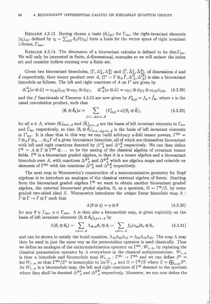
94 4. BICOVARIANT DIFFERENTIAL CALCULI ON JORDANIAN QUANTUM GROUPS

R e m a r k 4.3.13. Having chosen a basis (9i)i^i for Finv, the righ t-invarian t elem ents {gdia defined by % = form a basis for the vector space of right invariant1-forms, Frinv

R e m a r k 4.3.14. The dimension of a bicovariant calculus is defined to be dim Finv We will only be interested in finite, d-dimensional, examples so we will eschew the index set and consider indices running over a finite set.

Given two bicovariant bimodules, (F, A^, A j) and (f, Â^, A j) , of dimensions d and d respectively, their tensor product over A, (F' = F 0 a f , A '^, A 'J) is also a bicovariant bimodule as follows. The left and right coactions of A on F' are given by

A^a((^ 0 cj) — cJ(a)D(a) 0 cJ(r) 0 cJ(r), A'^(cj 0 cj) = cj(p) 0 W(p) 0 cJ(a)CJ(A), (4.3.28)

and the / functionals of Theorem 4.3.12 are now given by = fij * where * is the usual convolution product, such that

{&i®êk)a= Y Pkji*o.){$j<S>e,), (4.3,29)

for all a e A, where (0i)j=i...rf and (^i)i=i.„j are the bases of left invariant elements in Fjnv and finv respectively, so that {9i 0 is the basis of left invariant elementsin F'inv It is clear that in this way we can build arbitrary n-fold tensor powers, F®" = F 0 A F 0 A.. . 0A F of a given bicovariant bimodule, all of which are themselves bicovariant with left and right coactions denoted by A’ a &nd A"^ respectively. We can then define F® = A 0 F © F® 0 . . . to be the analog of the classical algebra of covariant tensor fields. F® is a bicovariant graded algebra, in that it is a tensor algebra and a bicovariant bimodule over A, with coactions A®^ and A®a which are algebra maps and coincide on elements of F®" with the coactions A”^ and A” J respectively.

The next step in Woronowicz’s construction of a noncommutative geometry for Hopf algebras is to introduce an analogue of the classical external algebra of forms. Starting from the bicovariant graded algebra F® we want to obtain another bicovariant graded algebra, the external bicovariant graded algebra, Q, as a quotient, fl ~ F®/5, by some graded two-sided ideal S. Woronowicz introduces the unique linear bimodule map A : F 0 F -4 F 0 F such that

A (g0 ??) =77 0 6) (4.3.30)

for any ^ G F;nv, G Frinv A is then also a bicomodule map, is given explicitly on the basis of left invariant elements {9i 0 9k)i j=i...d by

A(9i 0 9k) = Aik stOs <^9t= ^ fit[vsk)Os 0 Ot, (4.3.31)

and can be shown to satisfy the braid equation, A12A23A12 = A23A12A23. The map A may then be used in just the same way as the permutation operator is used classically. Thus we define an analogue of the antisymmetrisation operator on F®", PFi...n, by replacing the classical permutation operator by A everywhere in the classical antisymmetriser. W\...n is then a bimodule and bicomodule map : F®" -4 F®" and we can define E" =ker HA...n so that r® "/S" is isomorphic to ImT'Fi...„ and Q = F®/5 where S — E".As Wi„_n is a bicomodule map, the left and right coactions of F® descend to the quotient where they shall be denoted A^^ and A ^a respectively. Moreover, we can now define the

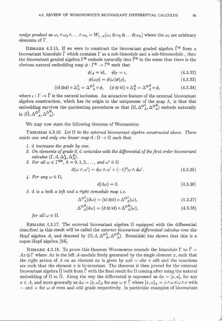
4.3. REVIEW OF WORONOWICZ’S BICOVARIANT DIFFERENTIAL CALCULUS 95

wedge product as cji A tJ2 A . . . A 0 W2 0 . . . where th e are a rb itra ryelem ents of F.

R e m a r k 4.3.15. If we were to construct the bicovariant graded algebra f® from a b icovariant b im odule f which contains F as a sub-bim odule and a sub-bicom odule , then the b icovariant graded algebra F® em beds na tu ra lly into f® in the sense th a t there is the obvious n a tu ra l em bedding m ap 0 ; F® -4 f® such th a t

= id, ( Ir = (4.3.32)

< (wp) = i (w)< (/?), (4.3.33)

(id 0 çi) o A a = A®^ o (^, ( 0 0 id) o A J = A ® a o (4.3.34)

where t : F -4 f is the n a tu ra l inclusion. An a ttrac tiv e feature of the ex ternal bicovariant algebra construction , which has its origin in the uniqueness of the m ap A, is th a t th is em bedding survives the quotien ting procedures so th a t (f2, A^a> A.^a) em beds n a tu ra lly

in (fl, A ^a^ A ^a)-

We m ay now s ta te the following theorem of Woronowicz:

T h e o r e m 4.3.16. Let fl be the external bicovariant algebra constructed above. There exists one and only one linear map d : fl -4 fl such that:

1. d increases the grade by one.2. On elements of grade 0, d coincides with the differential of the first order bicovariant

calculus (F, d, A ^ , A j ) .3. For all w G F® ', A: — 0 , 1 , 2 , . . . , and w' G fl

d(w A c j ' ) = dcj A cj' 4- ( - l)^ c j A dcj'. (4.3.35)

4. For any c j G fl,

d(dcj) = 0. (4.3.36)

5. d is a both a left and a right comodule map i.e.

A"^(dw) = (id ®d) o A"^(w), (4.3.37)

A"^(dw) = (d ® id) o A “ “ (w), (4.3.38)

for all CJ G fl.

R e m a r k 4.3.17. T he ex ternal bicovariant algebra f2 equipped w ith the differential described in th is resu lt will be called the exterior bicovariant differential calculus over the H opf a lgebra A, and denoted by (fl, d, A^ a j Brzezihski has shown th a t th is is asuper-H opf algebra [15].

R e m a r k 4.3.18. To prove th is theorem W oronowicz extends the bim odule F to f = A x © F where Ax is the left A -m odule freely generated by the single elem ent x, such th a t the righ t action of A on an elem ent ax is given by axb = abx + adb and the coactionsare such th a t the elem ent x is bi-invariant. T he theorem is then proved for the ex ternalb icovariant a lgebra Ù bu ilt from f w ith the final result for fl coming after using the n a tu ra l em bedding of fl in Q. Along the way the differential is expressed as d a = [x,a], for any a G A, and m ore generally as dcj — [x,cj]q: for any cj G F where [x,cj]:p = xAcj©cjA.x w ith — and + for c j of even and odd grade respectively. In particu la r exam ples of bicovariant

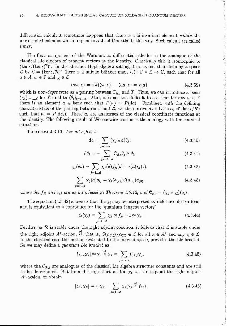
96 4. BICOVARIANT DIFFERENTIAL CALCULI ON JORDANIAN QUANTUM GROUPS

differential calculi it sometimes happens that there is a bi-invariant element within the unextended calculus which implements the differential in this way. Such calculi are called inner.

The final component of the Woronowicz differential calculus is the analogue of the classical Lie algebra of tangent vectors at the identity. Classically this is isomorphic to (ker e/(kere)^)*. In the abstract Hopf algebra setting it turns out tha t defining a space C h y C — (ker e/77)* there is a unique bilinear map, (, ) : T x £ -4 C, such that for all a e A, ÜJ e T and % G £

(ow,x) = e(a)(w,x), (da,x) = x(a), (4.3.39)which is non-degenerate as a pairing between Tinv and T. Thus, we can introduce a basis (x$)i=i...d for £ dual to (0i)i=i,..rf. Also, it is not too difficult to see that for any cj G T there is an element a G ker e such that E ( cj) = P(da). Combined with the defining characteristics of the pairing between T and £ , we then arrive at a basis ai of (ker e/77) such tha t 9i = E(da^). These a* are analogues of the classical coordinate functions at the identity. The following result of Woronowicz continues the analogy with the classical situation.

T h e o r e m 4.3.19. For all a,b E A

j=l,..d(4.3.40)

d9i = — A 9i, j,l= ...d

(4.3.41)

X i(a6)= ^ Xj(o)/ji(f)) + <a)x^(6), (4.3.42)

^ Xj(a)% = Xi(a(2))'S'(o(i))a(3), (4.3.43)

as introduced in Theorem ^.S.IZ, and = (Xj *X()(a%).

The equation (4.3.42) shows us that the Xi may be interpreted as ‘deformed derivations’ and is equivalent to a coproduct for the ‘quantum tangent vectors’

^ ^ X j 0 f j i + 1 0 Xi- (4.3.44)j = l . . . d

Further, as 77 is stable under the right adjoint coaction, it follows that £ is stable underthe right adjoint A*-action, <3, that is, S'(ck(i))xû;(2) G £ for all a E A* and any % G £. In the classical case this action, restricted to the tangent space, provides the Lie bracket. So we may define a quantum Lie bracket as

[Xi, Xfc] ~ X i X k — Ci k^j Xj ) (4.3.45)j = l . . . d

where the Cik,j are analogues of the classical Lie algebra structure constants and are still to be determined. But from the coproduct on the Xi we can expand the right adjoint A*-action, to obtain

[Xî,XA:] ~ X i X k ^ Xs(Xi ^ f s k ) - (4.3.46).s=l...d

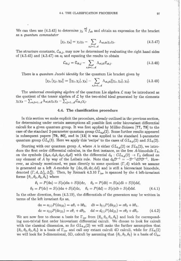
4.4. THE CLASSIFICATION PROCEDURE 97

We can then use (4.3.43) to determine Xi ^ fsk and obtain an expression for the bracket as a quantum commutator

[XuXt] = ^ (4.3.47)s , t=l . . .d

The structure constants, Q&j, may now be determined by evaluating the right hand sides of (4.3.45) and (4.3.47) on ai and equating the results to obtain

Gk,j — ^ik,j ~ Ast,ik^stJ• (4.3.48)s, t~l . . .d

There is a quantum Jacobi identity for the quantum Lie bracket given by

[Xi,[Xj)Xfc]] [[Xi, Xi]> X/j] ~ ^ "I X.î]) Xt]- (4.3.49)

The universal enveloping algebra of the quantum Lie algebra £ may be introduced as the quotient of the tensor algebra of £ by the two-sided ideal generated by the elements XtXk - Aat.tkXsXt -

4.4. The classification procedure

In this section we make explicit the procedure, already outlined in the previous section, for determining under certain assumptions all possible first order bicovariant differential calculi for a given quantum group. It was first applied by Miiller-Hoissen [77, 78] to the case of the standard 2-parameter quantum group GLq^p{2 ). Some further results appeared in subsequent papers [79, 80], and in [13] it was applied to the standard 1-parameter quantum group GLg(3). Here we apply this ‘recipe’ to the cases of GL/,,,g(2) and SLh{2 ).

Starting with our quantum group A, where A is either GL/i,^(2) or EL/,, (2), we intro­duce the first order differential calculus, in the first instance, as the free A-bimodule To, on the symbols {dga, do6, dgc, dgd} with the differential do : GLh,g{2 ) —> Tq defined on any element of A by way of the Leibniz rule. Note that dgD'^ = How­ever, as already mentioned, we pass directly to some quotient (T, d) which we assume is generated as a left A-module by {da, d6, dc, dd} and is still a bicovariant bimodule, denoted (F, d, A^, A j) . Then, by Remark 4.3.10 Fmv is spanned by the 4 left-invariant forms {(9i, ^2, ^3, ^4} where

9i — P{da) = S'(a)da + S{b)dc, 6 2 = P{db) = S{a)db P S{b)dd,^3 = E(dc) = E(c)da + E(d)dc, ^4 = R(dd) = 5'(c)d6 + S(d)dd. (4.4.1)

In the other direction, from (4.3.19), the differentials of the generators may be written in terms of the left invariant 9iS as,

da = a(i)P(da(2)) = affi + 6^3, d6 = 6(i)P(d6(2)) = a^2 + 6^4,dc = C(i)P(dc(2)) = c9i 4- dOs, dd = d(i)P(dd(2)) = c^2 + d^4- (4.4.2)

We are now free to choose a basis for F^v from (ffi, ^2, ^3, 04} and look for correspond­ing non-trivial first order bicovariant differential calculi. We choose to look for calculi with the classical dimension, so for GLh,g(2) we will make the further assumption that{^1, ^2, 3, ^4} is a basis of Fmv and call any extant calculi 4D calculi, while for SLh{2)we will look for 3-dimensional, 3D, calculi by assuming that {^1,^2, ^3} is a basis of Gmv

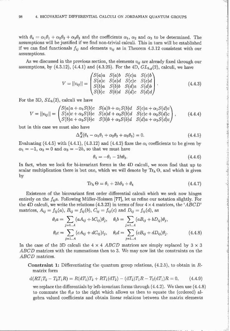
98 4. BICOVARIANT DIFFERENTIAL CALCULI ON JORDANIAN QUANTUM GROUPS

with 6 4 = ai9i + 0:2^2 + 0:3^3 and the coefficients ai, Q'2 and to be determined. The assumptions will be justified if we find non-trivial calculi. This in turn will be established if we can find functionals fij and elements Vij as in Theorem 4.3.12 consistent with our assumptions.

As we discussed in the previous section, the elements are already fixed through our assumptions, by (4.3.12), (4.4.1) and (4.3.25). For the 4D, GLh^g{2), calculi, we have

(S{a)a S{a)b S{c)a E(c)6^T / _ l l , , . | | _ ■?(«)= S(a)d S{c)c S(c)d , .' - " " ‘j I I - S{b)a S{b)b S{d)a S{d)h '

\S{b)c S(b)d S{d)c S{d)d)For the 3D, SLh{2), calculi we have

f S[a) aP 0iiS{b)c S{a)h P aiS(b)d S(c)a P a iS{d )c \ y = ||%H = I S{a)cP a 2 S{b)c S{a) dP a 2 S{b)d 5(c)c + o;25(d)c ] , (4.4.4)

\ S { b ) a P a 3 S(b)c S{b)b P asS(b)d S(d)a P a.3 S{d)cJ

but in this case we must also have

~ + 0(202 p 0(303) — 0. (4.4.5)

Evaluating (4.4.5) with (4.4.1), (4.3.12) and (4.4.2) fixes the coefficients to be given by 0(1 = —1, 0:2 — 0 and 0:3 = —2 h, so that we must have

04 = —01 — 2/203. (4.4.6)

In fact, when we look for bi-invariant forms in the 4D calculi, we soon find tha t up toscalar multiplication there is but one, which we will denote by Tr/ 0 , and which is givenby

Tr/ 0 = 01 + 2/203 T 04 (4.4.7)

Existence of the bicovariant first order differential calculi which we seek now hinges entirely on the f i j S . Following Miiller-Hoissen [77], let us refine our notation slightly. For the 4D calculi, we write the relations (4.3.23) in terms of four 4 x 4 matrices, the 'ABCD^ matrices, Aij = fij {a), Bij = fij{b), Cij = fij{c) and Dij = fij{d), as

9ia = {aAij P bCij)9j, 0 6 = {aBij P bDij)9j,j —l ..A j = 1 . . . 4

9iC ~ (oAjj P dCjj)tj, 9id = {oBjj + dDjj)9j. (4.4.8)J — 1 , , , 4

In the case of the 3D calculi the 4 x 4 ABCD matrices are simply replaced by 3 x 3 A B C D matrices with the summations then to 3. We may now list the constraints on the A BC D matrices.

C o n s tra in t 1: Differentiating the quantum group relations, (4.2.5), to obtain in R~ matrix form

d ( E T i T 2 - T 2 T i E ) = E ( d T i ) T 2 + R T i ( d T 2 ) - ( d T 2 ) T i E - T 2 ( d T i ) E = 0 , ( 4 . 4 . 9 )

we replace the differentials by left-invariant forms through (4.4.2). We then use (4.4.8) to commute the 0 s to the right which allows us then to equate the (ordered) al­gebra valued coefficients and obtain linear relations between the matrix elements

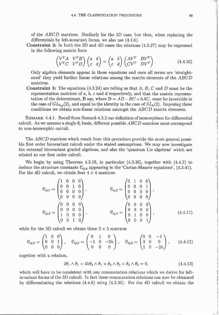
4.4. THE CLASSIFICATION PROCEDURE 99

of the A B C D matrices. Similarly for the 3D case, but then, when replacing the differentials by left-invariant forms, we also use (4.4.6).

C o n s tra in t 2: In both the 3D and 4D cases the relations (4.3.27) may be expressed in the following matrix form

(4.4.10)

Only algebra elements appear in these equations and once all terms are ‘straight­ened’ they yield further linear relations among the matrix elements of the A B C D matrices.

C o n s tra in t 3: The equations (4.3.24) are telling us that A, B, C and D must be the representation matrices of a, b, c and d respectively, and that the matrix represen­tation of the determinant, D say, where P — AD — B C P hA C , must be invertible in the case of GLh^g{2), and equal to the identity in the case of SL}fi2). Imposing these conditions we obtain non-linear relations amongst the A B C D matrix elements.

R e m a r k 4.4.1. Recall from Remark 4.3.2 our definition of isomorphism for differential calculi. As we assume a single 0* basis, different possible A B C D matrices must correspond to non-isomorphic calculi.

The A B C D matrices which result from this procedure provide the most general possi­ble first order bicovariant calculi under the stated assumptions. We may now investigate the external bicovariant graded algebras, and also the ‘quantum Lie algebras’ which are related to our first order calculi.

We begin by using Theorem 4.3.16, in particular (4.3.36), together with (4.4.2) to deduce the structure constants 6^,^ appearing in the ‘Cartan-Maurer equations’, (4.3.41). For the 4D calculi, we obtain four 4 x 4 matrices

e,U,1

A 0 0 o \ 0 0 1 0 0 0 0 0

\o 0 0 oy

/o 0 0 o \ 0 0 0 0 1 0 0 0

\0 0 1 0 /

G,-,-ü,2

e U ,4

/O 1 0 o \0 0 0 1 0 0 0 0

\0 0 0 0 /

/O 0 0 o \ 0 0 0 0 0 1 0 0

\o 0 0 ly

(4.4.11)

while for the 3D calculi we obtain three 3 x 3 matrices

1 0 O' = 1 0 0 1

0 0 0

0= I - 1

0e U ,3

together with a relation,

201 A 0 % 4- 4 /2 0 3 A 01 -T 02 A 03 -j- 03 A 02 = 0 ,

(4.4.12)

(4.4.13)

which will have to be consistent with any commutation relations which we derive for left- invariant forms of the 3D calculi. In fact these commutation relations can now be obtained by differentiating the relations (4.4.8) using (4.3.35). For the 4D calculi we obtain the

J

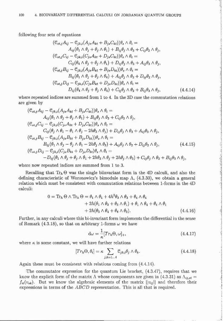
100 4. BICOVARIANT DIFFERENTIAL CALCULI ON JORDANIAN QUANTUM GROUPS

following four sets of equations

(GgtjAÿ Qjk^i{AjsAkt T BjsCkt))9s 9i ~A i j { 9 \ A 9 j P 9j f \ 9 \ ) P B i j 9 j A 0 3 -i- Gÿ-02 A 9 j ,

(GgtjQj — ^ j k , i { C j s A k t P D j s C k t ) ) d s A 0t =( 0 4 A 9 j + 9 j A 0i) + D i j 9 j A 0 3 + A i j 9 ^ A 0j,

— G j k , i { A j s B k t P B j s D k t ) ) 9 s A 0 =Pÿ(0i A 0j + 9 j A 0 4 ) + A i j 9 j A 0 2 + D i j 9 2 A 0 ,

i ^ s t j D i j — G j k f f C j s B f c t + D j s D k t ) ) 9 s A 0t =Dy ( 0 4 A 0j + 0j A 0 4 ) + Gÿ0j A 0 2 + Pij0 3 A 0j, (4.4.14)

where repeated indices are summed from 1 to 4. In the 3D case the commutation relations are given by

(GgijAjj Q j k ^ i { A j s A k t T B j g C k t ) ) 9 s A 0 =Aij ( 0 1 A 0j + 0j A 0i) + Pij0j A 0 3 + Gij0 2 A 0j,

(GgijGij G j k f f C j s A k t P DjgGfct))0g A 0fc =Gij(0j A 0 1 — 0 1 A 9 j — 2 A0 3 A 0j) + D i j 9 j A 0 3 4- Aij0 3 A 0j,

(GgijPij — G j k , i { A j s B f c t 4- B j s D k t ) ) 9 s A 0t =P ij ( 0 1 A 0j — 0j A 0 1 — 2h9j A 0 3 ) 4- Aij0j A 0 2 4- P ij0 2 A 0j, (4.4,15)

(GgijPij — G j k f f C j s B k t + D j s D k t ) 9 s A 0( =—Pij ( 0 1 A 0j 4“ 0j A 0 1 4“ 2 A0 3 A 0j 4- 2h9j A 0 3 ) 4- Gij0j A 0 2 4- Pij0 3 A 0j,

where now repeated indices are summed from 1 to 3.

Recalling that Tr , 0 was the single biinvariant form in the 4D calculi, and also the defining characteristic of Woronowicz’s bimodule map A, (4.3.30), we obtain a general relation which must be consistent with commutation relations between 1-forms in the 4D calculi:

0 = Tr/j © A Ti’/i 0 = 0 1 A 0 1 4~ 4 /2 ^ 0 3 A 0 3 4- 0 4 A 0 4

4” 2 /2 ( 0 1 A 0 3 4 - 0 3 A 0 1 ) 4- 0 1 A 0 4 4- 0 4 A 0 1

4“ 2 /2 ( 0 3 A 0 4 4- 0 4 A 0 3 ). (4.4.16)

Further, in any calculi where this bi-invariant form implements the differential in the sense of Remark (4.3.18), so that on arbitrary 1-forms u we have

dw = -[Tr/i©,a;]+, (4.4.17)

where k is some constant, we will have further relations

[Tr/1 0 , 0 ;] = K ^ GjA:J0jA0fe. (4.4.18)j , f c = 1...4

Again these must be consistent with relations coming from (4.4.14).

The commutator expression for the quantum Lie bracket, (4.3.47), requires tha t we know the explicit form of the matrix A whose components are given in (4.3.31) as Aij,st =f i t ( ' Osk) - But we know the algebraic elements of the matrix ||uij|| and therefore theirexpressions in terms of the A B C D representation. This is all that is required.

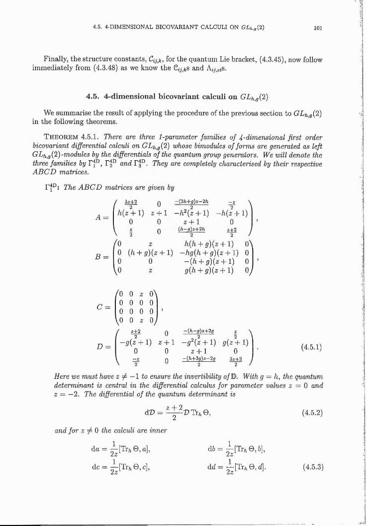
4.5. 4-DIMENSIONAL BICOVARIANT CALCULI ON GLh,g{2) 101

Finally, the structure constants, for the quantum Lie bracket, (4.3.45), now follow immediately from (4.3.48) as we know the 6%j,&s and Aij^st .

4.5. 4-dimensional bicovariant calculi on GLh^g{2)

We summarise the result of applying the procedure of the previous section to GLh^g{2) in the following theorems.

T h e o r e m 4.5.1. There are three 1-parameter families of f-dimensional first order bicovariant differential calculi on GLh^g{2) whose bimodules of forms are generated as left GLfi,g{2)-modules by the differentials of the quantum group generators. We will denote the three families by Fg^ and Fg^. They are completely characterised by their respective A B C D matrices.

Fi^: The A B C D matrices are given by

A =

B

C

D

/ 32+2’ 2 0

d(z 4“ 1) z P 10 0

I 0/ o z

0 {h + g){z + 1)0 0

z

/O 0 z 0 \0 0 0 00 0 0 0 1

\ o 0 z oy/ z+2

, 2 0- g { z P l ) z + 1

0 0

V ? 0

-{Zh+g)z—2h

-h'^iz + l)z p 1

{h—g)z+2h2

\h{z -I-1)

0z + 2 I 2 /

h(^h T g){z + 1) 0 \■hg[h P g){z P 1) 0~ { h P g ) { z P l ) 0g(/2 + ^ )(z + i) oy

-{h~g)z+2g 2

^^(z + 1) g(z;-H )z + 1

—(/t+3g)z—2g 2 2

(4.5.1)

Here we must have z ^ —1 to ensure the invertibility o/D, With g — h, the quantum determinant is central in the differential calculus for parameter values z = 0 and z = —2. The differential of the quantum determinant is

d ü = l l ^ D T r f t e , (4.5.2)

and for z ^ 0 the calculi are inner

1da = — [Tr/,0,a],

^ |T r / ,0 ,c ] ,

d 6 = ^ [ % 0 , 6 ] ,

dd = “ [Tr/i 0 , d]. (4.5.3)

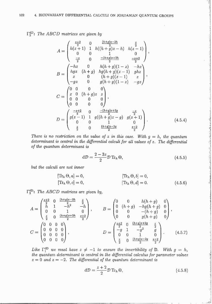
102 4. BICOVARIANT DIFFERENTIAL CALCULI ON JORDANIAN QUANTUM GROUPS

The A B C D matrices are given by

A==

B =

C =

D

£ ± 22 0

{h+g)z—2h2 1 \

l l (Z + 1 ) 1 /%((/%' P g ) z — f f h{ z - l )0 0 1 0

— 2 2 0

—{h+g)z+2h2

-Z+2 j 2 /

( - h z 0 h { h P g ) ( l - z) ~ h z \hgz { h P g ) h g { h + g ) { z - - 1 ) gr/tZ

z 0 (h + 9)G ~ ~ 1 ) Z

\ - 0 g { h P g ) { l - 4/o 0 0 o\

Z 0 (A + ^)z z0 0 0 0 ’

VO 0 0 V/ - 2 + 2

2 0~{h+g)z+2g

2 ? \0(^- 1 ) 1 g(z + 1 )

0 0 1 0V 2 0{h+g)z-2g

22+ 2 i

2 /

(4.5.4)

There is no restriction on the value of z in this case. With g — h, the quantum determinant is central in the differential calculi for all values of z. The differential of the quantum determinant is

é V = ^ - ^

but the calculi are not inner

[Tr/j 0 , a] = 0,[ % 0 ,c ] = O,

Fg^: The A B C D matrices are given by,

(4.5.5)

[% 0 ,6 ]= O ,[Tr/i 0 , d] - 0. (4.5.6)

A

/ z+2 ' 2

h

C

0 1

0 0 \ | 0/o 0 0 o \

0 0 0 0 0 0 0 0

\0 0 0 0 /

{h+g)z—2h

-h1 0

{h+g)z+2h z+2B

D =

/O 0 0

Vo

-9 0

VI

0(fi + g)

00

h{h + g) -h g {h + g)

~ { h P g )

o \000 /

{h+g)z+2g

{h+g)z—2g2

2902 + 22

(4.5.7)

Like F{^ we must have z to ensure the invertibility of D. With g = h,the quantum determinant is central in the differential calculus for parameter values z = 0 and z = —2. The differential of the quantum determinant is

dî> = L t H p T r , .e , (4.5.8)

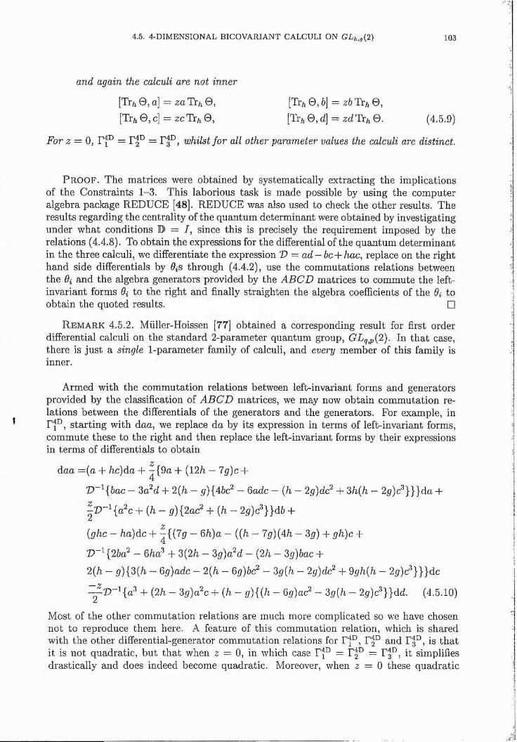
4.5. 4-DIMENSIONAL BICOVARIANT CALCULI ON GLk,g{2) 103

and again the calculi are not inner

[Tr/i 0 , a] = za 0 , [Tr/j 0 ,6 ] = z6 Tr/i 0 ,

[Tr/i0,c] = zcT r/i0 , [Tr/j 0 , d] = zdTi/j 0 . (4.5.9)

For z = 0, whilst for all other parameter values the calculi are distinct.

P r o o f . The matrices were obtained by systematically extracting the implications of the Constraints 1-3. This laborious task is made possible by using the computer algebra package REDUCE [48]. REDUCE was also used to check the other results. The results regarding the centrality of the quantum determinant were obtained by investigating under what conditions 3 = 1, since this is precisely the requirement imposed by the relations (4.4.8). To obtain the expressions for the differential of the quantum determinant in the three calculi, we differentiate the expression V = ad —bcPhac, replace on the right hand side differentials by 0*s through (4.4.2), use the commutations relations between the 9i and the algebra generators provided by the A B C D matrices to commute the left- invariant forms 9i to the right and finally straighten the algebra coefficients of the 9{ to obtain the quoted results. □

R e m a rk 4.5.2. Miiller-Hoissen [77] obtained a corresponding result for first order differential calculi on the standard 2-parameter quantum group, GLg^p{2). In that case, there is just a single 1-parameter family of calculi, and every member of this family is inner.

Armed with the commutation relations between left-invariant forms and generators provided by the classification of A B C D matrices, we may now obtain commutation re­lations between the differentials of the generators and the generators. For example, in

starting with daa, we replace da by its expression in terms of left-invariant forms, commute these to the right and then replace the left-invariant forms by their expressions in terms of differentials to obtain

daa = (a -f- /%c)da 4- — (9a 4- (12/i — 7g)c 4-

V~^{bac — 3a^d 4- 2{h — g){4bc^ — 6adc — {h — 2g)d(? 4- 3h(A - 2g)c^}}]da 4-

4- (h - g){2a(? P ( h - 2g)c^}}db P

(ghc - ha)dc 4- ^{(7p - 6h)a - {{h — 7g){4h - 3g) 4- gh)c 4-

V (26a^ — Qha P 3(26, — 3g)a^d — (26 — 3g)bac 4-

2(6 — p){3(6 — Qg)adc — 2(6 — Qg)bc — 3^(6 — 2g)dc^ 4- 9g6(6 - 2g)c^}}}dc

P {a^ 4- (26 — 3g)a'^c 4- (6 — ^ ){(6 — Qg)ac^ — 3g{h — 2g)c^}}dd. (4 .5 .10)

Most of the other commutation relations are much more complicated so we have chosen not to reproduce them here. A feature of this commutation relation, which is shared with the other differential-generator commutation relations for F{^, Fg^ and F |° , is that it is not quadratic, but that when z = 0, in which case F'J^ = Fg® = Fg^, it simplifies drastically and does indeed become quadratic. Moreover, when z = 0 these quadratic

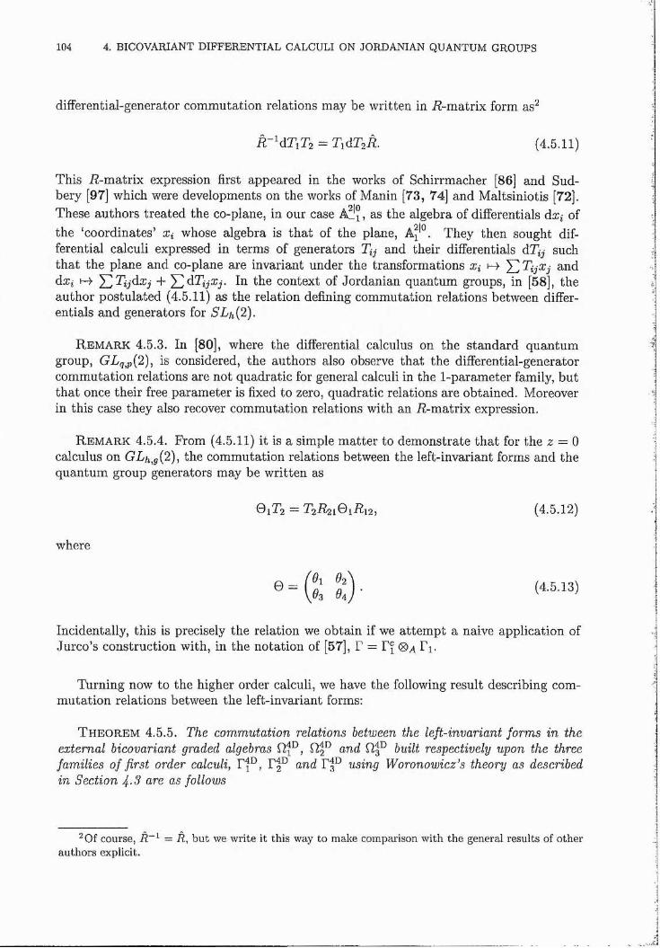
104 4. BICOVARIANT DIFFERENTIAL CALCULI ON JORDANIAN QUANTUM GROUPS

differentiai-generator commutation relations may be written in E-matrix form as^

R - A T 1T2 = TidTafi. (4.5.11)

This E-m atrix expression first appeared in the works of Schirrmacher [86] and Sud­bery [97] which were developments on the works of Manin [73, 74] and Maltsiniotis [72]. These authors treated the co-plane, in our case as the algebra of differentials dx, of the ‘coordinates’ x% whose algebra is that of the plane, They then sought dif­ferential calculi expressed in terms of generators and their differentials dTij such that the plane and co-plane are invariant under the transformations x* (-->■ ^ TljXj and dxt X^Tÿdxj + J^dTijXj. In the context of Jordanian quantum groups, in [58], the author postulated (4.5.11) as the relation defining commutation relations between differ­entials and generators for 5L/J2).

R e m a r k 4.5.3. In [80], where the differential calculus on the standard quantum group, GEg,p(2), is considered, the authors also observe that the differential-generator commutation relations are not quadratic for general calculi in the 1-parameter family, but that once their free parameter is fixed to zero, quadratic relations are obtained. Moreover in this case they also recover commutation relations with an E-matrix expression.

R e m a r k 4.5.4. From (4.5.11) it is a simple m atter to demonstrate tha t for the z = 0 calculus on GLh,g{2), the commutation relations between the left-invariant forms and the quantum group generators may be written as

Q1T2 = T2 R 2 1 O 1R 1 2 , (4.5.12)

where

Incidentally, this is precisely the relation we obtain if we attem pt a naive application of Jurco’s construction with, in the notation of [57], F = F^ 0/^ Fi.

Turning now to the higher order calculi, we have the following result describing com­mutation relations between the left-invariant forms:

T h e o r e m 4.5.5. The commutation relations between the left-invariant forms in the external bicovariant graded algebras and built respectively upon the threefamilies of first order calculi, F |^ , F |^ and F | ’ using Woronowicz^s theory as described in Section 4-3 are as follows

"Of course, R = R , but we write it this way to make comparison with the general results of other authors explicit.

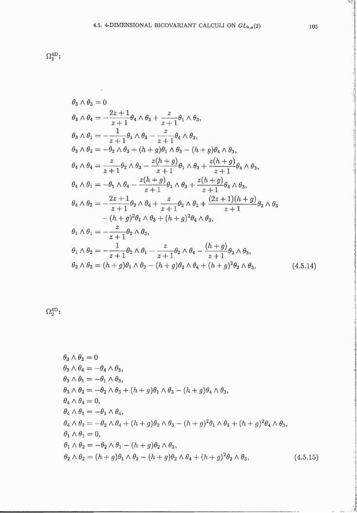
4.5. 4-DIMENSIONAL BICOVARIANT CALCULI ON % ,g (2 ) 105

03 A 03 = 0_ L 1 ^

03 A 04 = --------q-04 A 03 4------— 01 A 03,z + 1 z + 1

03 A 01 = ------— 01 A 0 3 --------— 4 A 03,z + 1 z + 1

03 A 02 ~ —02 A 03 + (6 + 5')0i A 03 — (6 + g)94 A 03,

= Y - 9 2 a % - A % + A %,Z + i Z + 1 Z + 1

04 A = - 0 , A 04 - P f f e, A 03 + + r i + 0 4 A 03,Z + 1 z + 1

04 A 03 = - ^ ^ 0 2 A 04 + A 0 1+ + + h ( ^ » + g )g ^ 0Z + 1 z + 1 z + 1

— (6 + gY9\ A 03 + (6 + p)^04 A 03,

01 A 01 = ------ — 02 A 03,z + 1

01 A 02 = -----—T02 A 0 1 -------— 02 A 04 — — 02 A 03,z + 1 z + 1 z + 1

02 A 02 = (6 + g)9\ A 02 — (6 + p)02 A 04 + (6 + (/)^02 A 03, (4 .5 .14)

0 3 A 0 3 = 0

0 3 A 0 4 = — 0 4 A 0 3 ,

03 A 01 = —01 A 0 3 ,

0 3 A 0 2 = — 0 2 A 0 3 + ( 6 + f / ) 0 i A 0 3 — ( 6 + g)9i A 0 3 ,

0 4 A 0 4 = 0,04 A 0 1 = — 0 1 A 0 4 ,

0 4 A 0 2 = — 0 2 A 0 4 + ( 6 + g)9‘2 A 0 3 — ( / i + g)‘9i A 0 3 + ( 6 + g )^94 A 0 3 ,

01 A 01 = 0,

01 A 02 = —02 A 01 — ( 6 + ^ )0 2 A 0 3 ,

0 2 A 0 2 = ( 6 + <?)0 i A 0 2 — ( 6 + g ' ) 0 2 A 0 4 + [h + ( / ) ^ 0 2 A 0 3 , (4.5.15)

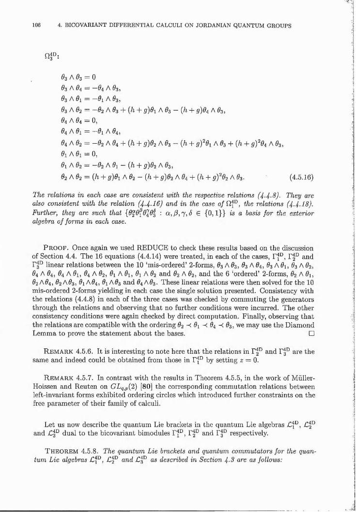
106 4. BICOVARIANT DIFFERENTIAL CALCULI ON JORDANIAN QUANTUM GROUPS

03 A 03 -= 0

03 A 04 == — 0 4 A 0 3 ,0 3 A 01 == — 0 1 A 0 3 ,

03 A &2 == — 0 2 A 0 3 + (6 + 0)01 A 03 —(6 + 0 ) 0 4 A 0 3 ,04 A 04 == 0,

04 A 01 == — 0 1 A 0 4 ,

04 A 02 == — 0 2 A 0 4 + (6 + 0)02 A 03 —(6 + 0 ) ^ 0 1 A 0 3 + ( 6 + 0 ) ^ 0 4

01 A 0 1 == 0,

01 A 02 == —02 A 01 —{h + 0)02 A 0 3 ,

02 A 02 == (6 + g ) O i A 02 - (6 + 0)02 A 04 + (6 + 0 ) ^ 0 2 A 0 3 . (4.5.16)

The relations in each case are consistent with the respective relations (4-4-8). They are also consistent with the relation (4 .4^6) and in the case o f ü f ^ , the relations (4-4.18). Further, they are such that : a, (8,^,5 € {0,1}} is a basis for the exterioralgebra of forms in each case.

P r o o f . Once again we used REDUCE to check these results based on the discussion of Section 4.4. The 16 equations (4.4.14) were treated, in each of the cases, andF |^ linear relations between the 10 ‘mis-ordered’ 2-forms, 03 A 03, 03 A 04, 03 A 01, 03 A 02, 04 A 04, 04 A 01, 04 A 02, 01 A 01, 01 A 02 and 02 A 02, and the 6 ‘ordered’ 2-forms, 02 A 01, 02 A 04, 02 A 03, 01A 04, 01A 03 and 04 A 03. These linear relations were then solved for the 10 mis-ordered 2-forms yielding in each case the single solution presented. Consistency with the relations (4.4.8) in each of the three cases was checked by commuting the generators through the relations and observing tha t no further conditions were incurred. The other consistency conditions were again checked by direct computation. Finally, observing that the relations are compatible with the ordering 02 -A 01 + 04 + 03, we may use the Diamond Lemma to prove the statement about the bases. □

R e m a r k 4.5.6. It is interesting to note here that the relations in F |^ and Fg° are the same and indeed could be obtained from those in F |° by setting z = 0.

R e m a r k 4.5.7. In contrast with the results in Theorem 4.5.5, in the work of Miiller- Hoissen and Reuten on GLg,p(2) [80] the corresponding commutation relations between left-invariant forms exhibited ordering circles which introduced further constraints on the free parameter of their family of calculi.

Let us now describe the quantum Lie brackets in the quantum Lie algebras and £ 3 dual to the bicovariant bimodules F 'p , Fg^ and F |^ respectively.

T h e o r e m 4.5.8. The quantum Lie brackets and quantum commutator's for the quan­tum Lie algebras Cff’, Cip and £ 3 as described in Section 4-3 are as follows:

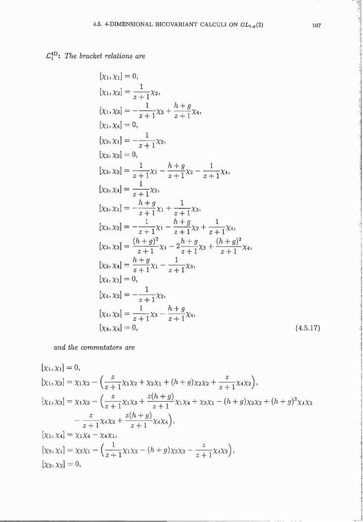
4.5. 4-DIMENSIONAL BICO VARIANT CALCULI ON GLh,g{2) 107

C f^ i The bracket relations are

k u x i l

[XuXa]

[xi

[xi

k

1

[X2

[X2

[X2

[%3

[%3

[X3

[%3

[X4

[%4

[x.

[x

X3}

X4]

X l ]

X2]

Xs]

X4]

X l ]

X2]

Xs]

X4]

X l ]

X2]

X3]

X4]

z + 1 1

X2 ,

z + 1 X 3 +h P g z + 1 X4)

0,

z + 1 X2,

0,

■Xl6 + 0

-X2Z + 1 z + 1 z + 1

1

h + g 1

X4)

Xi +z + 1 ' z + 11 6 + 0

z + 1Xl z + 1

X3,

X2 +1

Z + 1 X4,

Z + 1 6 + 0

z + 1 z + 11

z + 1 0,

1

X l z + 1XSî

1 6 + 0z + 1 z + 1 0,

X4,

and the commutators are

[Xi.Xi] = 0,

[Xl, X2] = X1X2 - |X lX 2 + X2X1 + (fi + g ) X2X 2 + ^X4X2 1

^ ( f i ■+■ 0 )

(4.5.17)

[Xi,X3] = X1X3z + 1

X1X3 +z + 1

X1X4 + X s X l ~ (fi 0 ) X 3 X 2 + (fi + 0 ) X4X2

z z ( 6 + 0 )

[Xi, X4] == X1X4 — X4X1,

[x2, Xl] = X2X1 “ ( — —7X1X2 — (fi + g)x2X2 - "-7-7X4X2 ] )z + 1 + 1

[X2,X2] = 0 ,

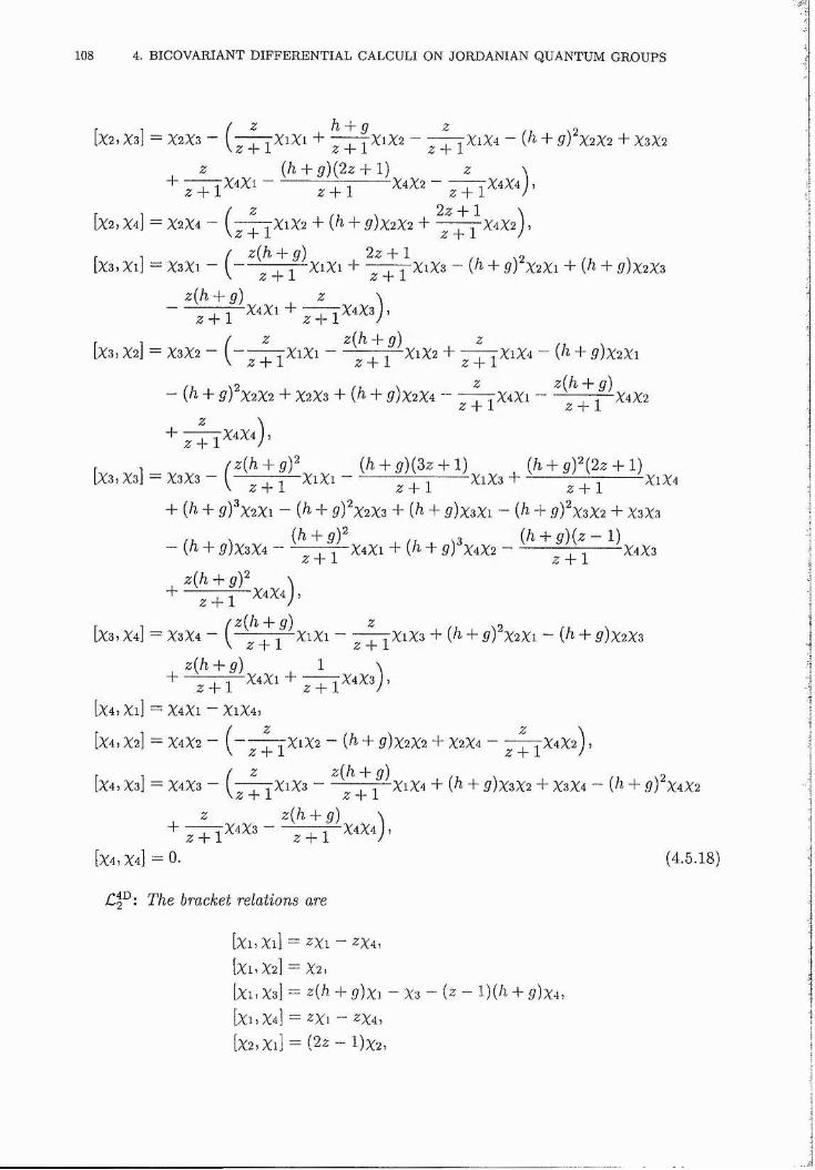
108 4. BICOVARIANT DIFFERENTIAL CALCULI ON JORDANIAN QUANTUM GROUPS

[%2 ,Xs] - X2X3 - 1 %1%1 + — T-rXiX2 - TT7% iX 4 - (/t + g)^X2X2 + X3X24 - i Z + I z + i

, { h g ) { 2 z 1) z \+ T T i

[ X 2 , X 4 ] = X 2 X 4 - jX lX 2 + { h + g ) X 2 X 2 + ^ J X4X2 ) ,

r I / g) 2z + 1 , ,0 / N[X3, Xi] = XsXi - ( ------- —T -% 1%1 + T i Xi%3 - (/ + ^ ) X2X1 4- (/i + P)X2X3\ Z -r 1 Z -r i.

z(h + g) Z \- - ^ : ^ x 4 X i + j : ^ X 4 X 2 ) ,

r 1 / z z (h-hg) z ,1X3 , X2] — X3X2 — I r r X i X i 1— X1X2 4— —7rXiX4 ~ (/^ 4- g)x2Xi\ z i- z + L Z + L

— {h-\- gŸX2X2 4- X2X3 4- {h + ^)X2X4----- - 7 X4X1 --------——:|^X4X2Z + I Z -{- Lz

4- YX4X4) ,

[X3,X31 = X3X3 - ( ^ ^ ^ X i x , - ^ ^ ^ i f Ç f i^ x .X 3 + ^ ^ i ^ Ç ^ x a 4\ z -p 1 Z -f- I Z -j- I4- {h + g)^X2Xi — { h- h g Y x 2X 3 4- (h 4- g ) X i X i ~ {h + g)^X3X2 4- XsXs

- (/t 4- p)X3X4 - f : 4Xl 4- (/t + p)^X4X2 - ^ X 4X3Z i Z -T i

Z 1

[X3, X4] = XsX4 — (" " ^ Ip ^ X iX i — jXiXa + {h 4- gYx2Xi ~~ (h + g )x 2Xs

z{h-\-g) 1 \+ ^ : ^ X 4 X i 4 - — x4X3j,

[X4, Xl] = X4X1 - X1X4 ,

[X4: X2] = X4X2 — ( —7 X1X2 — (h 4- g)X2X2 4- X2X4 7TX4X2) ,\ z 4- i z -r X. /

[X4, Xa] = X4X3 — _|_ ^ X iX a y 7 ^ X i X 4 4- 4- g)xzX2 4- XaX4 ~ + ^)^X4X2

z z{h + g) \

[X4, X4] — O' (4.5.18)

Ck^: The bracket relations are

[Xl 5Xl] = z x i -

b (i, X2] = X2,

[Xi, Xa] = z{h 4- 5')Xi

[Xu X4 ] = -z Xi - .ZX4,

L%2, Xl] = (2z - 1)X2

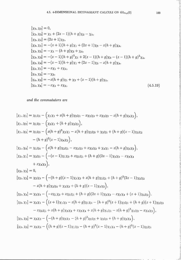
4.5. 4-DIMENSIONAL BICOVARIANT CALCULI ON GLh,g{2) 109

[%2, X2] = 0,

[%2, Xs] = Xl + (2z — l ) {h + g)x2 ~ X4,

[X2,X4] — (2z + 1)X2,[X3, Xl] = —(^ + l) ( /i + g)xi + {2z 4- 1)X3 — ^{h 4- p )x 4 ,

[Xa, X2] = —Xl - (^ 4- ^)X2 4- X4,

[X3,X3| = l)(/t4-^)^Xi + 2 ( z - l)(/t + ^ )X3 - l)(/t4-^^)^X4,[X3, X4] = -(^ - 4- p)xi + (2z - 1)%3 - 4- p)x4,[X4,Xi] = - % + % ,[X4j X2] = —X2 ,[X4> Xa] = —z (h 4- ^ )x i 4- Xa 4- (z — l ) ( h 4- 5’)X4,

[X4j X4] — —z x i 4- ZX4, (4.5.19)

and the commutators are

[Xi,Xi] — XiXi ~ (x iX i + 4- p)X2Xi - X2Xa 4- zxaX2 — z{h 4- )X4X2 ,

[Xi, X2] — X1X2 - (x2Xi + + P)X2X2 )

[Xi, Xs] = X1X3 - 4- p) X2Xi - 4- p)X2Xa 4- XsXi + (/ 4- p)(z - 1)X3X2

— 4- gŸ{z — i ) x 4X2^ ,

[xi, X4] = XiX4 - 4- p)x2Xi - ;%X2X3 4- ZX3X2 4- X4X1 - 4- !7)X4X2),

[X2 , Xl] — X2X1 — ( “ (^ “ l)X iX 2 4- ZX2X1 4- (/i 4- 5^)(2z — 1)X2X2 ~ ^X2X4

4- ^X4X2^ j

[X2,X2] = 0,

[X2, Xa] = X2X3 — (^~{h 4- p )(z — l)x iX 2 4- z{h 4- g)X2Xi 4- {h 4- g Ÿ ( 2 z — l ) x 2X2

— z ( h + g)X2X4 4- XaX2 (h-h g){z — 1)X4X2^,

[X2 , X4] = X2X4 — { j - z X i X 2 4- ZX2X1 4- (/i 4- g)(2z 4- 1)X2X2 — ^X2X4 4- (z 4- 1)X4X2^ ^

[X3, Xl] — XaXi — 4- l)x iX a — z (h 4- (?)xiX4 — (/i 4- g Ÿ ( z + l)% 2Xi 4- (h 4- g) (z 4- 1)X2X:

— %Xi 4- z(/i + g)xaX2 + ZX3X4 4- z(A 4- (?)X4Xi - 4- (/) X4X2 - %Xa),

[X3i X2] = X3X2 — (j~{h 4- g)X2 Xi ~ {h 4- g Y x 2 X2 4- X2X3 4- (h 4- g)X2X4^,

[Xa, Xa] = XaXa - ((/i 4- p)(z - l)x iX a - (/i + !7) (z - l)x iX 4 - (/i 4- ) (z - l ) x 2Xi

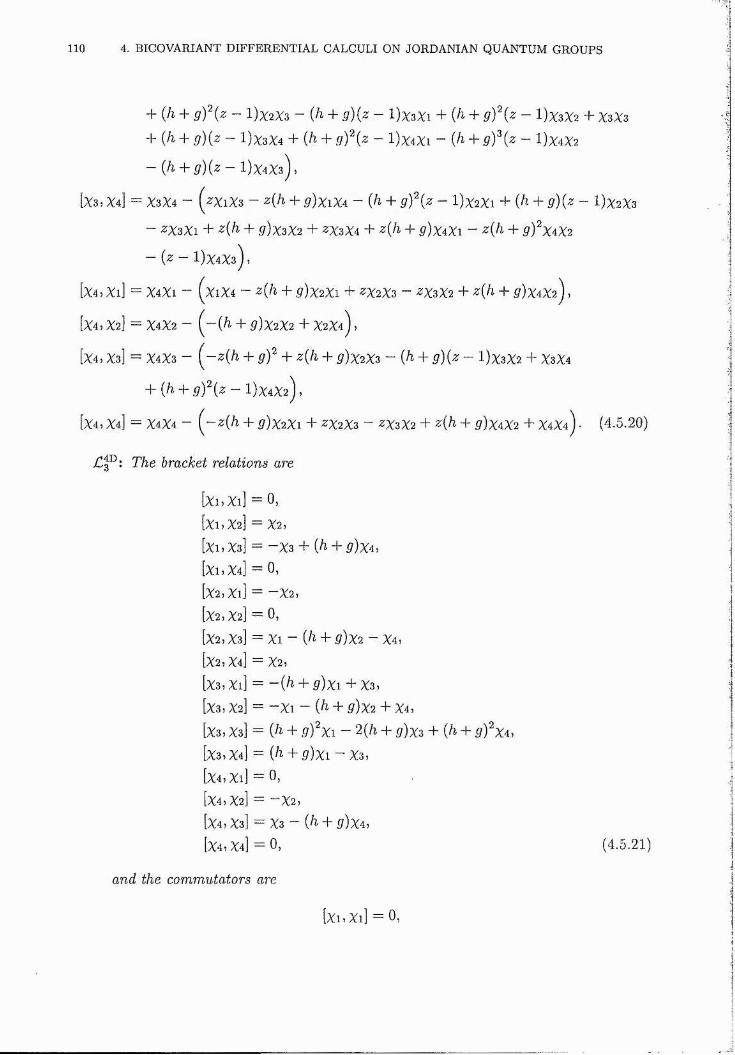
110 4. BICOVARIANT DIFFERENTIAL CALCULI ON JORDANIAN QUANTUM GROUPS

+ (^ + gŸ{z - 1)%2%3 - {h + g){z — + g)‘ {z — l)x sX 2 + XsXs

+ (^ + g){^ — 1)X3%4 + (h 4- g)^{z - l)x4X i - (h 4- g)^{z — 1)%4%2

- ( / l4 - ^ f ) ( z - 1)%4%3),

[%3, %4] = X3%4 - (^%1%3 - ;z(/t 4- ^)Xl%4 - (/l 4- p)^(z - 1)%2%1 4" (& 4" ^ )(z - 1)X2%3

- % X l 4- z(/l 4- ^)X3%2 4- Z%3%4 4- z(/l 4- p)%4%l - 4- ^)^X4%2

- - 1)X4%3) ,

[X4 , Xl] = X4X1 - (x iX 4 - 4- ^)X2Xi 4- ZX2X3 - % X 2 4- z(/i 4- p)X4X2 l ,

[X4, X2] = X4X2 — 4- g)X2X2 4- X2X4 ) 5

[X4 j Xa] = X4X3 — 4- g)‘ 4- z{h 4- 5')X2X3 — {h-\- g)(z ~ l)xaX 2 4- XaX4

4 - ( / t4 - p ) ^ ( z - l ) X 4 X 2 ) ,

[X4, X4] = X4X4 - ^ -z (A 4- p)X2Xi 4- ZX2X3 - % X 2 4- z(/i 4- 5r)X4X2 4- X4X4 ) . (4.5.20)

£ 3^ : The bracket relations are

[XuXi] = 0,

[xu X2] = X2 ,

[Xi, Xa] = —Xa 4- {h 4- (?)X4,

[X1,X4] = 0,

[X2,Xl] = -X 2 ,

[X2 , X2] = 0,

[X2 j Xa] = Xl “ {h 4- g ) x 2 — X4,

1X2, X4] = X2 ,

|X3,Xi] = - ( /^ 4 -p )x i4 -X 3 ,

[Xa, X2] = —Xl — 4- g ) x 2 4- %4,

[Xa, Xa] = {h 4- g^Xi — 2(/i 4- f/)xa 4- {h 4- (/)^X4 ,

[xa, X4] = {h 4- g)xi ~ Xa,

[X4, Xl] = 0,

[X4,X2] = -X 2 ,

[X4,Xa] = Xa - (/t4-5f)x4,[X4,X4] = 0, (4.5.21)

and the commutators are

[Xi, Xl] — 0,

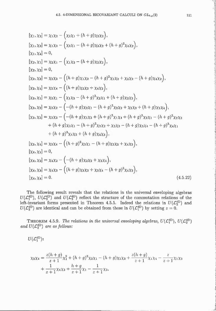
4.5. 4-DIMENSIONAL BICOVARIANT CALCULI ON GLH,g{2) n i

[%1, X2] = %1%2 - (X2%1 + (A + p)X2X2) ,

[xi, Xa] = XiXa - (xaXi - (/ + ^)XaX2 + (/i + ^)^X4X2),

[Xi,X4] = 0 ,

1x 2 ; Xl] = X2X1 - (xiX2 — { h + g)X2 X2 ^ ,

[X2 ,X 2] = 0 ,

[X2; Xa] = X2X3 - + 5')xiX 2 — { h - \ - g Ÿ X 2 X 2 + XaX2 ~ { h +

[X2, X4] = X2X4 — + P)X2X2 + X4X2) ;

[Xa, Xl] = XaXi - (xiXa - (/& + p)^X2Xi + + p)X2Xa),

[Xa, X2] = X3X2 — + ^)X2Xi “ + g Y x 2 X 2 + X2X3 + (/i +

[Xa, Xa] — XaXa — {^~{h + g)xiXz + (/i + ^)^XiX4 + (h + g Ÿ x 2 Xi ~ + p)^X2Xa

+ ( h + p)xaXi ~ { h + g Ÿ X 3 X 2 + XaXa ” [ h + <7)XaX4 ~ {k. + p)^X4Xi

+ (^ + p)^X4X2 + (/i + p)x 4X a),

[Xa, X4] = XaX4 - { [ h + g Ÿ x 2 Xi — [ h + g)x 2 Xs + X4X a),

[X4 ,Xi] = 0 ,

[X4 ; X2] = X4X2 — ^ - ( / l + g)X2X2 + X2X4) ;

[X4 ; Xa] = X4X3 — ( { k , + ^)xaX2 + XaX4 — { h H- 5’)^X4X2^ ,

[X4 ,X 4] = 0 . (4 .5 .2 2 )

The following result reveals tha t the relations in the universal enveloping algebras U{Cf^) and U{Cf^) reflect the structure of the commutation relations of the

left-invariant forms presented in Theorem 4.5.5. Indeed the relations in U{Cf^) and U(jCf^) are identical and can be obtained from those in U{Cf^) by setting z — 0.

T h e o r e m 4 .5 .9 . The relations in the universal enveloping algebras, U (C f^ ) , U{jC,2^) and U{Cf^ ) are as follows:

f/(£ t^ ):

z{h-\-g) 9 , z(h-i-g) zXaX4 — ---- —;— Xl + ( h + o ) X2X1 “ + g ) x . 2 X 3 H--- ——j—XiX' 4 ----- — rXiXaZ-t-i Z-|-i Z-+-1

1 h-h g 1+ + jip Y X i - 7:;:^X3.

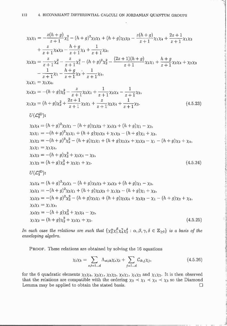
112 4. BICOVARIANT DIFFERENTIAL CALCULI ON JORDANIAN QUANTUM GROUPS

z { h g ) 2 /1 , \ 2 /, \ z ( ^ h g ) 2z + 1XaXi — :"T' I Xl - {h + g) X2X1 + + g)X2X3------ —V—X1X4 4-------—7X1X3z -f-i z + l z 4 - i

z h g 1+ ^ X 4 X 3 - ^ X i + j ; ^ X 3 ,

z 2 z 2 / L , \2 2 (2z 4* l)(/i 4“ 5') ^4 "^X3X2 - gqjyX4 “ JljTYXi ~ (^ + i?) X2 -------- ------------- X2X1 + j —■■ X2X4 4- X2X3

1 h-\- g ‘ 1Xl “ — 77X2--H-----t t X4jz 4- 1 z 4- 1 z 4 - l

X4Xl = X1X4,2 Z 1 1

X4X2 — 4- g)x 2 ~ ^ _j_ ^X2Xi + ^ ^X2X4 - ^ ^X2,

/ 7 \ 2 2 z 4" 1 z 1X1X2 = \h 4- g)x2 + "7 7 4 X2X1 4— —7X2X4 4— 7-7X2- (4.5.23)

z - r i Z -T 1 Z - r i

X3X4 = (/t 4- ^)^X2Xl - (/t 4- p)X2X3 4- X4X3 4- (A + ^)%1 - %3,

XsXi = — 4- p)^X2Xi 4- (h. + g)X2X3 4- X1X3 — (^ 4- p )x i 4- Xa,

XaX2 = — (/i 4- (7)^X2 ” (^ 4- ^)X 2Xi 4- {h + p)x2X4 4- X2X3 ~ Xi ~ (^ 4- p )x 2 4- X4,

X4X1 = X1X4,

X4X2 = - ( / i 4- p)x2 + X2X4 - X2,X1X2 = (/!- 4- p ) x 2 4- X2X1 4- X2 - (4.5.24)

XaX4 = {h + g Y x 2 Xi — (/i 4- p)x2X3 4- X4Xa 4- (/i 4- p)xi — Xa,

XaXi = “ (^ + 5')^X2Xi 4- (/i 4- p)x2Xa 4- XiXa “ (/i 4- g)xi 4- Xa,

X3X2 = — (/i 4- 5')^X2 - 4- ^)X2Xi 4- [h + g)X2 XA 4- X2Xa “ Xi ~ {h + .g)x2 4- X4,X4X1 = X1X4,X4X2 = ~ [ h + g )x 2 4- X2X4 — X2,

X1X2 = (/t 4- g ) x 2 4- X2 X1 4- X2 - (4.5.25)

In each case the relations are such that {xfX?X 4 X2 • 7 ,^ G Z>o} is a basis of theenveloping algebra.

P r o o f . These relations are obtained by solving the 16 equations

XiXk — ^st.ikXsXt ^ ^ Qk jX j , (4.0.26)s,i=l...d j=l.,.d

for th e 6 q u a d ra tic e lem en ts xaX 4 , XaXi, XaX2 , X4Xi, X4 X2 a n d X1X2 . I t is th e n observedtha t the relations are compatible with the ordering X2 Xi ^ X4 ^ Xa so the DiamondLemma may be applied to obtain the stated basis. □

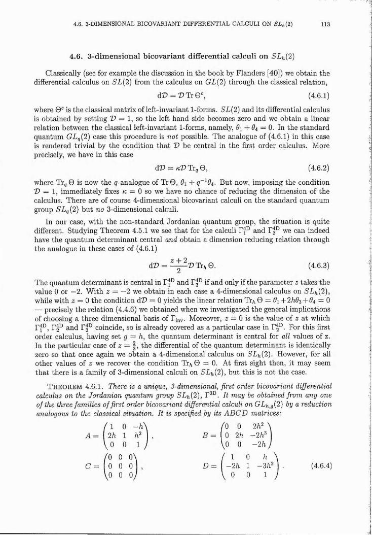
4.6. 3 -DIMENSIONAL BICOVARIANT DIFFERENTIAL CALCULI ON SLk{2) 113

4.6. 3 -d im ensional b icovarian t d ifferen tia l calculi on SLk{2)

Classically (see for example the discussion in the book by Flanders [40]) we obtain the differential calculus on SL(2) from the calculus on GL(2) through the classical relation,

d D ^ D T rG ': , (4.6.1)

where is the classical matrix of left-invariant 1-forms. SL(2) and its differential calculus is obtained by setting I> = 1, so the left hand side becomes zero and we obtain a linear relation between the classical left-invariant 1-forms, namely, 4- ^4 = 0. In the standard quantum GLq{2) case this procedure is not possible. The analogue of (4.6.1) in this caseis rendered trivial by the condition that V be central in the first order calculus. Moreprecisely, we have in this case

d£> = KDTrg0, (4.6.2)

where Tr^ 0 is now the g-analogue of Tr 0 , 9i 4- q~^0 4 . But now, imposing the condition V = 1, immediately fixes K = 0 so we have no chance of reducing the dimension of the calculus. There are of course 4-dimensional bicovariant calculi on the standard quantum group SLq{2) but no 3-dimensional calculi.

In our case, with the non-standard Jordanian quantum group, the situation is quite different. Studying Theorem 4.5.1 we see that for the calculi and we can indeed have the quantum determinant central and obtain a dimension reducing relation through the analogue in these cases of (4.6.1)

dV = ^ ^ V T T , , e . (4.6.3)

The quantum determinant is central in F |^ and F |^ if and only if the parameter z takes the value 0 or —2. W ith z = —2 we obtain in each case a 4-dimensional calculus on 5I//i(2), while with z = 0 the condition dV = 0 yields the linear relation Ti'h 0 = 9i 4-2 % 4-^4 — 0 — precisely the relation (4.4.6) we obtained when we investigated the general implications of choosing a three dimensional basis of Finv Moreover, z = 0 is the value of z at which F |d , p 4D p 4D coincide, so is already covered as a particular case in F^^. For this first order calculus, having set g = h, the quantum determinant is central for all values of z. In the particular case of z = | , the differential of the quantum determinant is identically zero so tha t once again we obtain a 4-dimensional calculus on SLh{2). However, for all other values of z we recover the condition Ti^ 0 = 0 . At first sight then, it may seem that there is a family of 3-dimensional calculi on SLh{2), but this is not the case.

T h e o r e m 4.6.1. There is a unique, 3~dimensional, first order bicovariant differential calculus on the Jordanian quantum group SLh{2), F^^. It may be obtained from any one of the three families of first order bicovariant dijferential calculi on GLh,g(2) by a reduction analogous to the classical situation. It is specified by its A B C D matrices:

0 0 0

0 0 00 0 0 , D = \ -2 h 1 - 3/1 . (4.6.4)

0 0 2fi \0 2h -2JA I0 0 -2 fi y

1 0 h-2h 1 -3fi^0 0 1

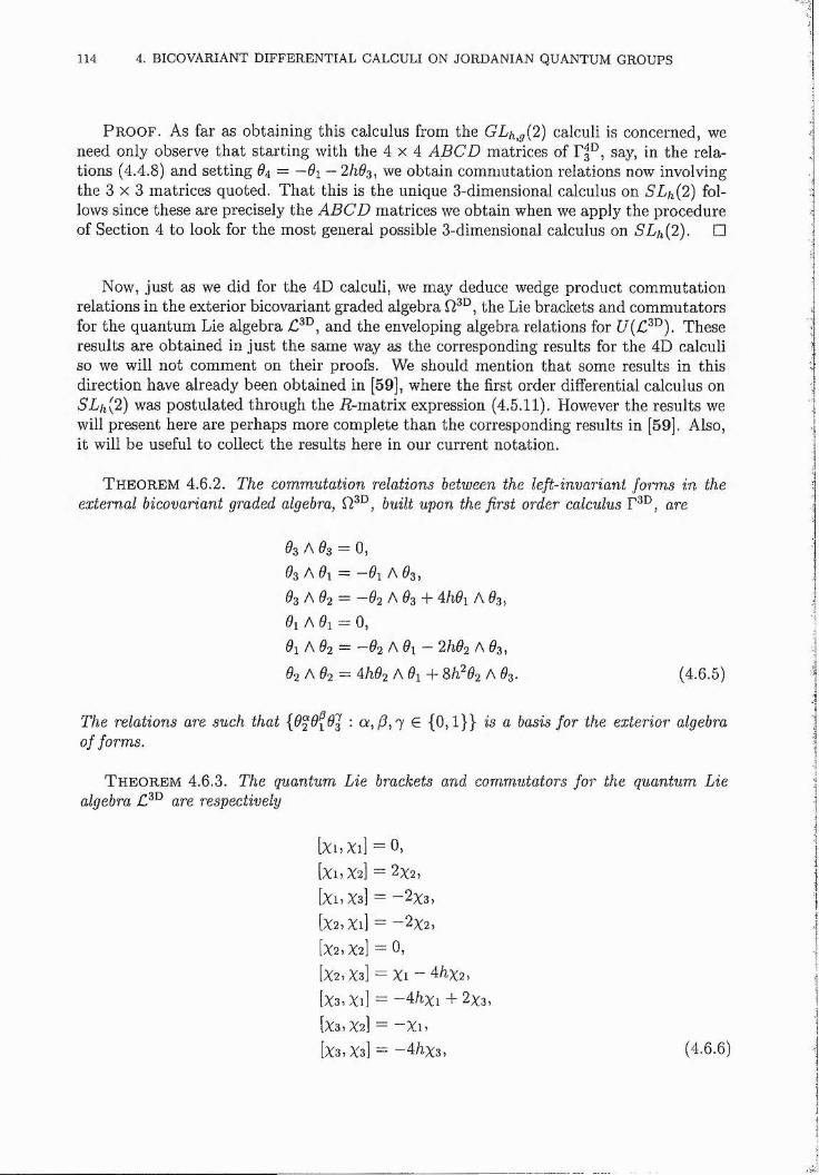
114 4. BICO VARIANT DIFFERENTIAL CALCULI ON JORDANIAN QUANTUM GROUPS

P r o o f . A s far as obtaining this calculus from the GLh^g{2 ) calculi is concerned, we need only observe tha t starting with the 4 x 4 A B C D matrices of Pg^, say, in the rela­tions (4.4.8) and setting Ô4 = ~ 6 i - 2 % , we obtain commutation relations now involving the 3 x 3 matrices quoted. That this is the unique 3-dimensional calculus on SLh(2 ) fol­lows since these are precisely the AB G D matrices we obtain when we apply the procedure of Section 4 to look for the most general possible 3-dimensional calculus on SLh(2 ). □

Now, just as we did for the 4D calculi, we may deduce wedge product commutation relations in the exterior bicovariant graded algebra the Lie brackets and commutators for the quantum Lie algebra and the enveloping algebra relations for Theseresults are obtained in just the same way as the corresponding results for the 4D calculi so we will not comment on their proofs. We should mention tha t some results in this direction have already been obtained in [59], where the first order differential calculus on 5L/i(2) was postulated through the i?-matrix expression (4.5.11). However the results we will present here are perhaps more complete than the corresponding results in [59]. Also, it will be useful to collect the results here in our current notation.

T h e o r e m 4.6.2. The commutation relations between the left-invariant forms in the external bicovariant graded algebra, built upon the first order calculus are

6*3 A ^ 3 = 0,^ 3 A 6^1 = —9\ A 3 ,^ 3 A ^2 = —02 A ^ 3 -T Ah9\ A 3 ,

A 6^1 = 0,9\ f\ 02 ~ ~~02 A 0\ — 2h02 A 3 ,02 02 — 4/1 2 A -(- Sh‘02 A 0' . (4.6.5)

The relations are such that ■ ck,/5,7 G {0,1}} is a basis for the exterior algebraof forms.

T h e o r e m 4.6.3. The quantum Lie brackets and commutators for the quantum Lie algebra are respectively

[Xij Xl] — 0,[XuXz] = 2x2,

[Xi,Xs] = -2 X 3 ,

[X2, Xl] = —2X2,

[X2, X2] = 0,[X2,Xs] = Xl - 4fiX2,

[X3,Xi] = —4 fix i + 2x3,

[X3,X2| = - X l ,

[X3,X3] = -4 fiX 3 , (4.6.6)

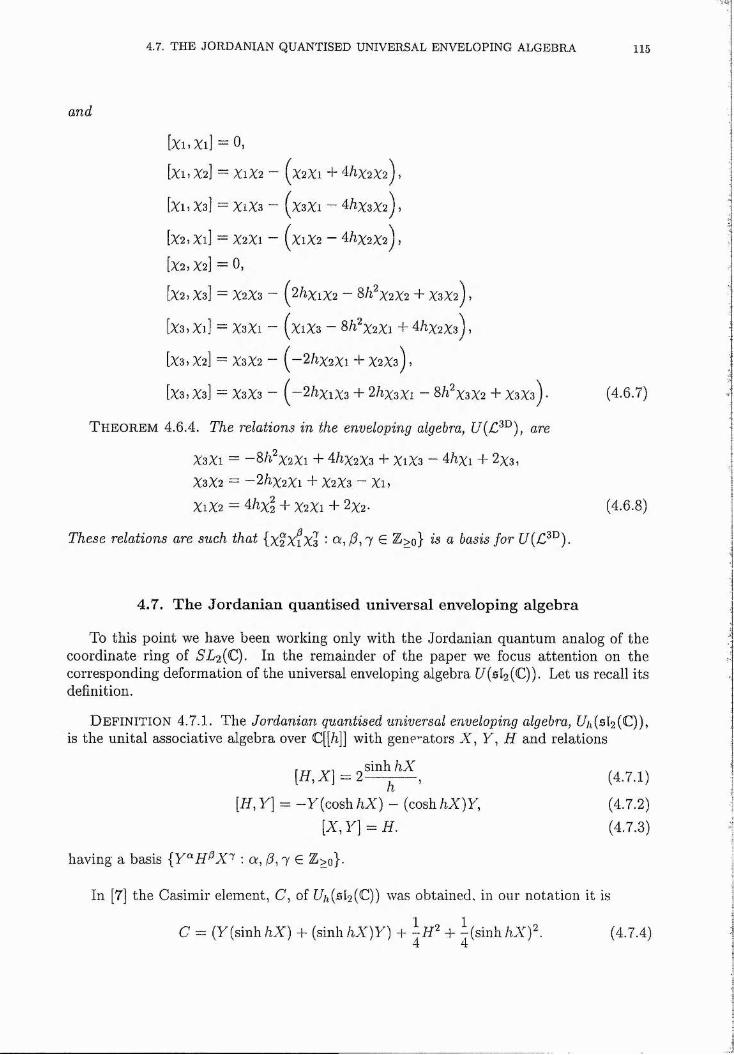
4.7. THE JORDANIAN QUANTISED UNIVERSAL ENVELOPING ALGEBRA 115

and

[%i,Xi] = 0,

[Xi, X2] = X1X2 —

[Xi, Xsl = X1X3 —

[X2,Xl] =X 2X i -

[X2,X2| = 0,

[X2 , Xs] = X2X3 —

[X3,Xl] =X 3X i -

[X3, X2] = X3X2 -

[X3, X3] — X3X3 —

X2X1 +4fiX2X2j,

X3X1 — 4AX3X2),

X1X2 - 4/1X2X2)

2A%1%2 — 8/i^X2X2 + X3X2) ,

X1X3 - 8A^X2Xi + 4/1X2X3) ,

—2/1X2X1 + X2X3),

~2Ax iX3 + 2/%X3Xi — 8A^XsX2 + XsX3

T h e o r e m 4.6.4. The relations in the enveloping algebra, are

XsXi = —8fi^X2Xi + 4/1X2X3 + X1X3 — 4/%Xi + 2x 3,X3X2 = - 2 AX2X1 + X2 X3 - Xl,

X1X2 = 4 /1x 2 + X2X1 + 2x2-

These relations are such that {X2 X1X3 : E %>o} is a basis for U{C^^).

(4.6.7)

(4.6.8)

4.7. T h e Jo rd a n ia n q u an tised un iversa l enveloping a lg eb ra

To this point we have been working only with the Jordanian quantum analog of the coordinate ring of 5 L2(C). In the remainder of the paper we focus attention on the corresponding deformation of the universal enveloping algebra U(sl2 {C)). Let us recall its definition.

D e f in it io n 4.7.1. The Jordanian quantised universal enveloping algebra, f//i(sl2(C)), is the unital associative algebra over C[[h]] with generators X , Y , H and relations

^sinh/iX ' I

= -y (co sh /i% ) - (cosh/tX)y,

having a basis ; a, /?, 7 G Z>o}.

(4.7.1)

(4.7.2)(4.7.3)

In [7] the Casimir element, C, of Uh(si2 {C)) was obtained, in our notation it is

C = (y(sinh/jX ) + (sinhftX )y) + + bsinhAAO^ (4.7.4)

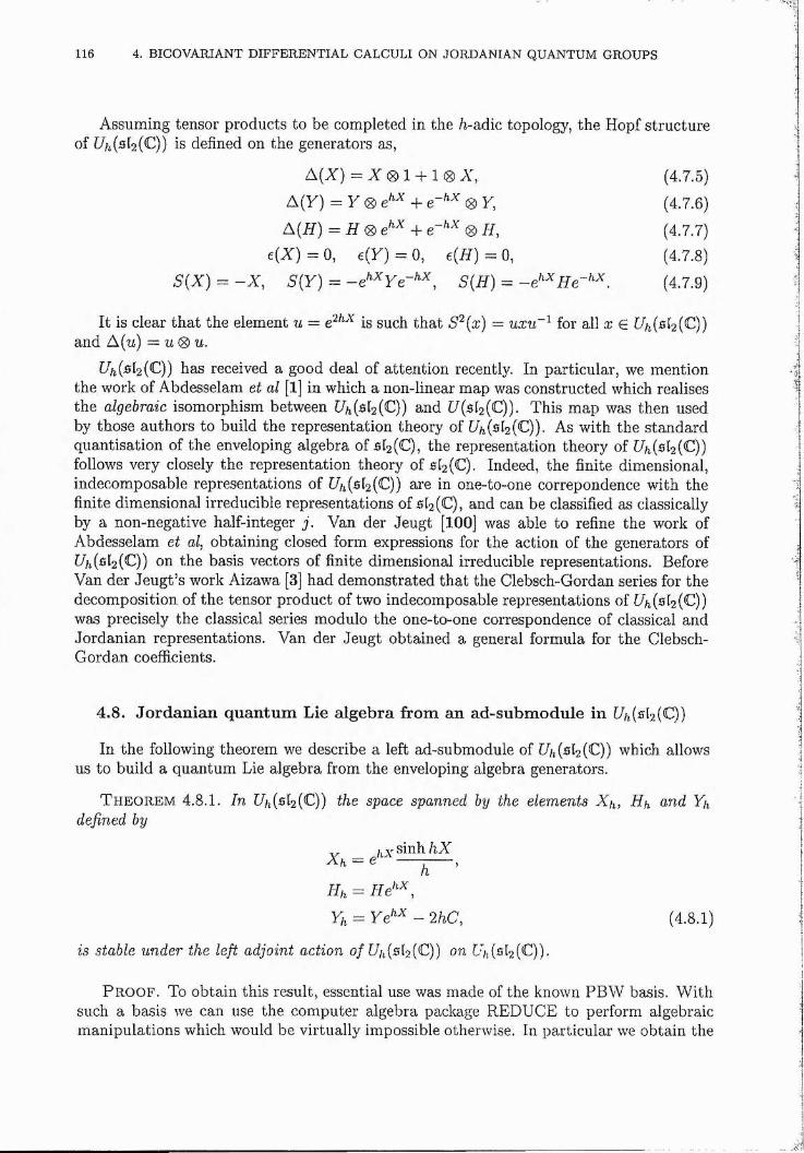
116 4. BICOVARIANT DIFFERENTIAL CALCULI ON JORDANIAN QUANTUM GROUPS

Assuming tensor products to be completed in the /i-adic topology, the Hopf structure of f//i(Af2(C)) is defined on the generators as,

A(% ) = % ® 1 + 1 ® AT, (4.7.5)

A (y ) = y ® 4 - 0 y, (4.7.6)

A(77) = Ff ® 4- ® 77, (4.7.7)e (% )= 0 , e(y) = 0, e(77)=0, (4.7.8)

5 (X ) = - X , S (y ) = -e ^ ^ y e -^ ^ , S(77) = (4.7.9)

It is clear tha t the element u = is such that S'^{x) — uxu~^ for all x G f4 (Af2(C)) and X[u) ~ u ® u.

Uh{^h{^)) has received a good deal of attention recently. In particular, we mention the work of Abdesselam et al [1] in which a non-linear map was constructed which realises the algebraic isomorphism between t4 (5 l2(Q ) and t/(sf2(C)). This map was then used by those authors to build the representation theory of UhlskiC)). As with the standard quantisation of the enveloping algebra of 512(C), the representation theory of Uh{sl2{C)) follows very closely the representation theory of 512(C). Indeed, the finite dimensional, indecomposable representations of (512(C)) are in one-to-one correpondence with the finite dimensional irreducible representations of 512(C), and can be classified as classically by a non-negative half-integer j . Van der Jeugt [100] was able to refine the work of Abdesselam et al, obtaining closed form expressions for the action of the generators of (A (^ 12(C)) on the basis vectors of finite dimensional irreducible representations. Before Van der Jeugt’s work Aizawa [3] had demonstrated that the Clebsch-Gordan series for the decomposition of the tensor product of two indecomposable representations of [4 .(512(C)) was precisely the classical series modulo the one-to-one correspondence of classical and Jordanian representations. Van der Jeugt obtained a general formula for the Clebsch- Gordan coefficients.

4.8. Jordanian quantum Lie algebra from an ad-submodule in L4(512(C))

In the following theorem we describe a left ad-submodule of V/i(5l2(C)) which allows us to build a quantum Lie algebra from the enveloping algebra generators.

T h e o r e m 4.8.1. In V/i(512(C)) the space spanned by the elements X^, Hh and 14 defined by

V sinh h XXu =h

k =14 = yg/^^ _ (4.8.1)

is stable under the left adjoint action 0/ f//i(sl2 (C)) on L4 (sl2 (C)).

P r o o f . T o obtain this result, essential use was made of the known PBW basis. W ith such a basis we can use the computer algebra package REDUCE to perform algebraic manipulations which would be virtually impossible otherwise. In particular we obtain the

M

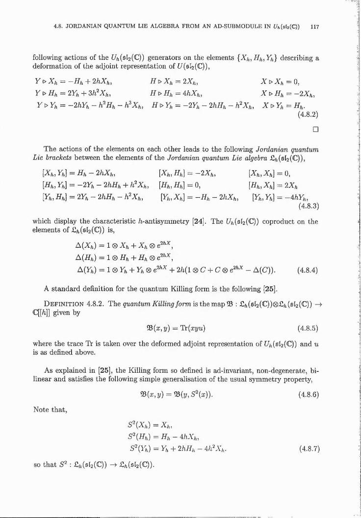
4.8. JORDANIAN QUANTUM LIE ALGEBRA PROM AN AD-SUBMODULE IN %(5[a(C)) 117

following actions of the t//^(sl2(C)) generators on the elements {X/j,/7/i, 14} describing a deformation of the adjoint representation of [/(512(C)),

Y o Xfi = —Hh + 2hXh, H o Xh = 2X^, X > Xh — 0,y > H i, = 2Y„ + H > H „ = AhX,„ % > % = -2A /„

y t> î'/i = ~ 2hYf, — Xh, H >Yh = ~ 2Yj, — 2hHh — fi'^Xh, X >Yh = Hh.(4.8.2)

□

The actions of the elements on each other leads to the following Jordanian quantum Lie brackets between the elements of the Jordanian quantum Lie algebra (512(C)),

[%/,, 14] = - 2% , [%/,, 7//,] = - 2%A, %/,] = 0 ,{Hu,Yh\ = -2 Y h -2 h H h + h^Xh, [Hh,Hh]^d, [ Hh , Xh]^2Xh[Yh, Hh] = 2y„ - 2hHh - h?Xh, [Yh, Xh] = - % - 2hXh, [Yh, Yh] = -AKYh,

(4.8.3)

which display the characteristic A-antisymmetry [24]. The [//i(s 12(C)) coproduct on the elements of (512(C)) is,

C\(Xh) = l ® X h + Xh®e^'^^,

X{Hh) = l ® H h + Hh®e^''^,

X[Yh) = + + 2h{l ® C + C ® - A(C)). (4.8.4)

A standard definition for the quantum Killing form is the following [25].

D e f i n i t i o n 4.8.2. quantum Killing form is : Ca(512 (C))® (512 (C)) —>C[[fi]] given by

Q3(a:, 2/) = YT{xyu) (4.8.5)

where the trace Tr is taken over the deformed adjoint representation of [// (512(C)) and uis as defined above.

As explained in [25], the Killing form so defined is ad-invariant, non-degenerate, bi­linear and satisfies the following simple generalisation of the usual symmetry property,

lB(a;, ?/) = 93(2/, '9^(a;)). (4.8.6)

Note that,

S^(A,.) = Xh,

S \ H h ) = Hh - ihXh,

S'^iYh) = Yh + 2hHh - 4/(^V,.. (4.8.7)

so tha t (512(C)) £/, (512(C)).

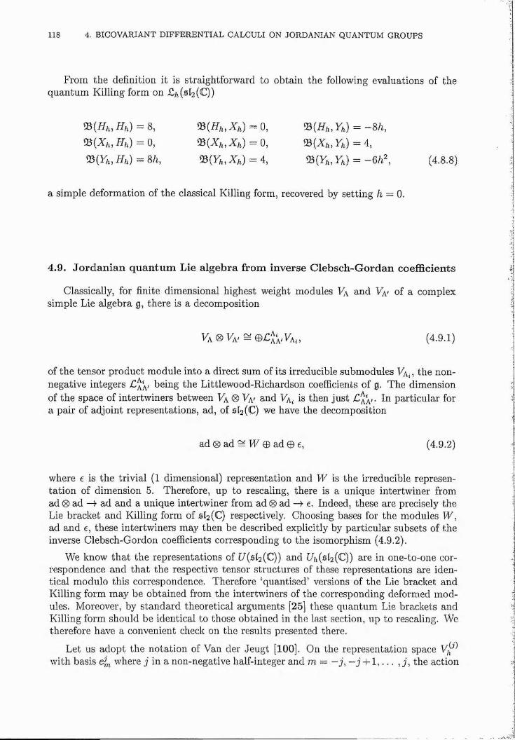
118 4. BICOVARIANT DIFFERENTIAL CALCULI ON JORDANIAN QUANTUM GROUPS

From the definition it is straightforward to obtain the following evaluations of the quantum Killing form on £/i(sl2(C))

77/,) = 8, 93(77/,, X/,) = 0, 0(77/,, 14) = -8fi,0(X /,, 77/,) = 0, 0(X/,, %/,) = 0, 0(X/,, y,) = 4,0(}4, -[f/i) = 8/z, 0(14, %/,) = 4, 0(14,14) = -6/t", (4.8.8)

a simple deformation of the classical Killing form, recovered by setting h — 0.

4.9. Jordanian quantum Lie algebra from inverse Clebsch-Gordan coefficients

Classically, for finite dimensional highest weight modules Fa and of a complex simple Lie algebra g, there is a decomposition

14 ® Va'= (4,9.1)

of the tensor product module into a direct sum of its irreducible submodules ^4., the non­negative integers being the Littlewood-Richardson coefficients of g. The dimension of the space of intertwiners between Va ® Va' and Va is then just In particular for a pair of adjoint representations, ad, of 512(C) we have the decomposition

ad 0 ad = 0 ad 0 e, (4.9.2)

where e is the trivial (1 dimensional) representation and W is the irreducible represen­tation of dimension 5. Therefore, up to rescaling, there is a unique intertwiner fromad 0 ad ^ ad and a unique intertwiner from ad 0 ad e. Indeed, these are precisely the Lie bracket and Killing form of 5(2(C) respectively. Choosing bases for the modules W , ad and e, these intertwiners may then be described explicitly by particular subsets of the inverse Clebsch-Gordon coefficients corresponding to the isomorphism (4.9.2).

We know that the representations of [ / (512(C)) and U/,(512(C)) are in one-to-one cor­respondence and that the respective tensor structures of these representations are iden­tical modulo this correspondence. Therefore ‘quantised’ versions of the Lie bracket and Killing form may be obtained from the intertwiners of the corresponding deformed mod­ules. Moreover, by standard theoretical arguments [25] these quantum Lie brackets and Killing form should be identical to those obtained in the last section, up to rescaling. We therefore have a convenient check on the results presented there.

Let us adopt the notation of Van der Jeugt [100]. On the representation space with basis where j in a non-negative half-integer and m ~ - j , ~ j + 1 , . . . , j , the action

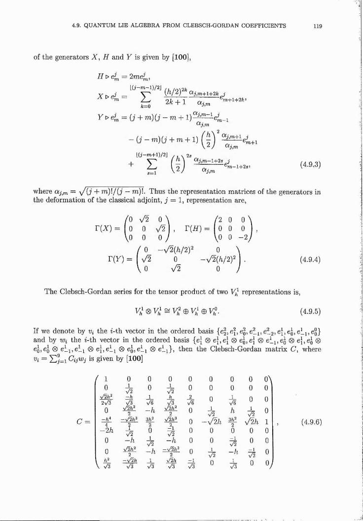
4.9. QUANTUM LIE ALGEBRA FROM CLEBSCH-GORDAN COEFFICIENTS 119

of the generators X , H and Y is given by [100],

77 > = 2me^,[ Q - m - l ) / 2 J

^ > 4 = EA:=:0

y [> e4 = {j + m )(7 - m + 1)a j , m

' m - 1

2k'X (Xj rn+l j

[G-m-M)/2j / , X 2s ^_ 1 l+2s jO I rv- ^rn-l+2s^5-1 \ ^ /

(4.9,3)

where ~ i / ( j + m)l /{ j — m)!. Thus the representation matrices of the generators in the deformation of the classical adjoint, j = 1, representation are,

/O \/2 0 \ /2 0 0r ( x ) = 0 0 x/2 , r(77) = 0 0 o

Vo 0 0 / Vo 0 - 2

r ( y ) = V 20 -\/2 (/i/2 )^ 0 \

0V2

(4.9.4)

The Clebsch-Gordan series for the tensor product of two Vfl representations is,

(4.9.5)

If we denote by V{ the 2-th vector in the ordered basis {€2, cf,Cq,e?_i, eig,e}, ej, e[_i, Cq}and by Wi the F th vector in the ordered basis {e\4 ) 4 ® e l l , e l l ® 6i, e l l G» eg, e l i 0 e li} , then the Clebsch-Gordan matrix C, where

= U L i CijWj is given by [100]

C =

/ 1 0

Y21Y2 \/3

0

4-2 fi

00

\ V3

0 0 0 0 0 0 0 0 \ J1

V2 0 1J 2 0 0 0 0 0

1~ h 1 h

x/32

\/6 0 1

\ / 60 0 '!

V2h22 —h V2k2

2 0 1V2 h 1

\/2 0 i-%/2/i3

?v/2

3/i22 2, 0

3 22 \/2h 1 (4.9.6) 1

0 -1vT 0 0 0 0 0

1

—h 1\/2 — h 0 0 - 1

V2 0 0ti\/2/l2 —h -%/2 /i2

0 1 —h - 1 0 12 2 \/2 vT !

- V 2 hx/3

1n/3 x/3

- 1\/3 0 1

x/3 0 oy

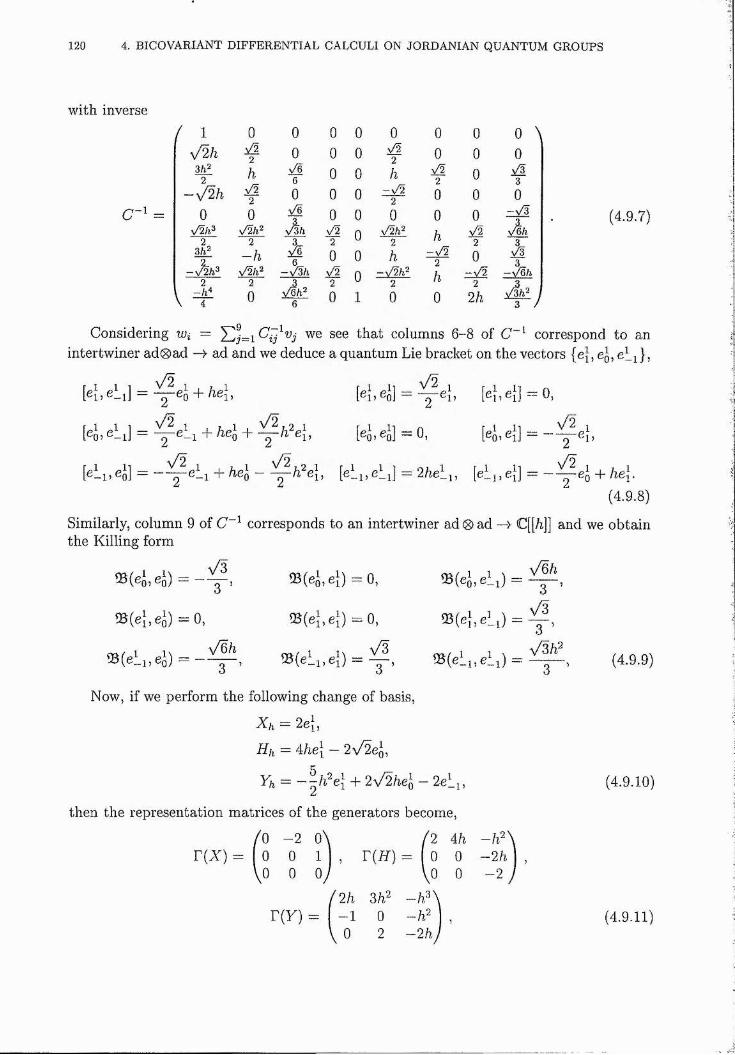
120 4. BICOVARIANT DIFFERENTIAL CALCULI ON JORDANIAN QUANTUM GROUPS

with inverse

- 1

1 0 0 0 0 0 0 0 0 \v/2ft :/2

2 0 0 0 2 0 0 03 22 h V6

6 0 0 h 2 0 s/33

-h/2 h V22 0 0 0 -s/2

2 0 0 00 0 0 0 0 0 0 -V3

V2h2 2 3

v/22 0 s/2h'

2 h s/ 22 3

-v%/i3—h

-V3A0s/ 2

001

h— \/5/l2

c A2h0

0-s/2

v/3 — s/Eli

-à"4

20 6

20

20

22 h j

3 /

(4.9.7)

Considering wi = we see that columns 6-8 of C~^ correspond to anintertwiner ad®ad —> ad and we deduce a quantum Lie bracket on the vectors {e}, ej, e li} ,

el, e 1 , , 1 — ej + /îei,

[ o>

[e ll, ®J] = —- ^ e l i + / l e j ----

0) o] ~ 0,

1'D [ci, e j — 0,

[ej, e{] = —\/2 1

2

■1) ‘--IJ 2Aeli, [ e l] ,4 l = - ^ « 0 + M -(4.9.8)

Similarly, column 9 of C corresponds to an intertwiner ad 0 ad -->■ C[[/i]] and we obtain the Killing form

® ( 4 ) 4 ) =

0 (e} ,e j) = 0,

0 ( e l i , e j ) =

3 ’

\/6 /i

0 (eo ,e i) = 0,

0(e},e{) = 0,

^ ( e l i , e[) =

^ ( 4 , e i i ) =

^ ( 4 , 4 i ) =

0 ( e l i , e l i ) =

Now, if we perform the following change of basis,

X h = 2e]

0 )

/t — ‘ ' 1)Hh = 4he\ — 2\/2eJ

Yh = + 2\/2he\ — 2eli,

then the representation matrices of the generators become.

0 - 2 /2 4/10 0 i ' b r(77) = 0 00 0 V \o 0

/2 h 3&:r ( F ) nr: - 1 0 ,

\ o 2 -2 A /

(4.9.9)

(4.9.10)

(4.9.11)

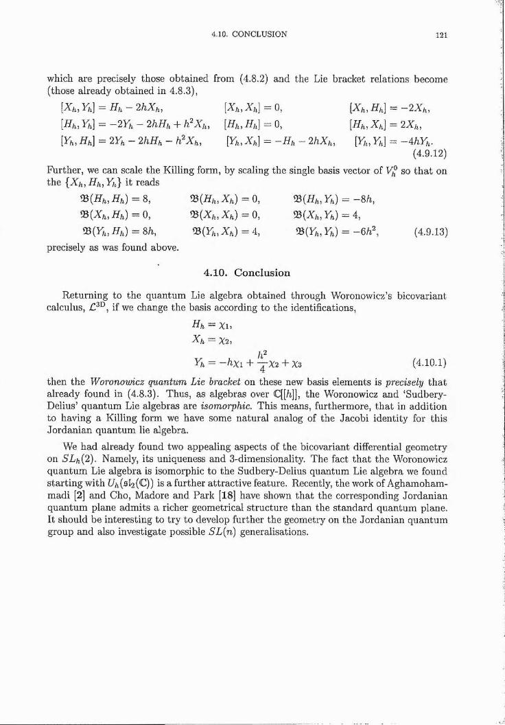
4.10. CONCLUSION 121

which are precisely those obtained from (4.8.2) and the Lie bracket relations become (those already obtained in 4.8.3),

= 0 , = - 2%A,[Hhi Yh] = “ 2F/1 — 2hHh + hf [Hh, Hh] = 0, [Hh, Xh] = 2Xh,[}%, 77/,] = 2F, - 2/177/, - /i^X/,, [Yk, %h] = -77k - 2/iX/,, F,] = -4 /iF ,.

(4.9.12)Further, we can scale the Killing form, by scaling the single basis vector of so tha t on the {Xh, Hh, Yh} it reads

^ { H h , H h ) = 8, 93(77/1, X h ) = 0, 0(77/,, Y h ) = -8 /i,0(X/,,77/,) = O, 0(X /,,X /,) = O, 0 (% /,,% = 4,

0 (y ,, 77/,) = 8/1, 0 (y;„ X/,) = 4, 0 (y ,, y^) = - 6 / i \ (4 .9 .13)precisely as was found above.

4.10. Conclusion

Returning to the quantum Lie algebra obtained through Woronowicz’s bicovariantcalculus, if we change the basis according to the identifications,

Hh = Xl,

X h = X2,

Yh — —h x i + — X2 + Xs (4.10.1)

then the Woronowicz quantum Lie bracket on these new basis elements is precisely thatalready found in (4.8.3). Thus, as algebras over C[[/ij], the Woronowicz and ‘Sudbery- Delius’ quantum Lie algebras are isomorphic. This means, furthermore, tha t in addition to having a Killing form we have some natural analog of the Jacobi identity for this Jordanian quantum lie algebra.

We had already found two appealing aspects of the bicovariant differential geometry on SLh{2). Namely, its uniqueness and 3-dimensionality. The fact tha t the Woronowicz quantum Lie algebra is isomorphic to the Sudbery-Delius quantum Lie algebra we found starting with Uh{sl2 {C)) is a further attractive feature. Recently, the work of Aghamoham- madi [2] and Cho, Madore and Park [18] have shown that the corresponding Jordanian quantum plane admits a richer geometrical structure than the standard quantum plane. It should be interesting to try to develop further the geometry on the Jordanian quantum group and also investigate possible S L {n ) generalisations.

122 4. BICOVARIANT DIFFERENTIAL CALCULI ON JORDANIAN QUANTUM GROUPS

Bibliography

[1] B. Abdesselam , A, Chakrabarti and R. Chakrabarti, Irreducible representations of Jordanian quan­tum algebra U h{sl{2)) via a nonlinear map, Mod. Phys. Lett. A, 11 (1996), 2883-2891.

[2[3[4

[5

[6

[7[8

[9

[10

[11[12[13

[14

[15

[16

[17

[18

[19

[20[21

[22

[23

[24

[25

A. Aghamohammadi, S L h {2)-sym m etric torsionless connections, Lett. Math. Phys. 40 (1997), 95. N. Aizawa, preprint q-alg/9701022B. L. Aneva, V. K. Dobrev and S. G. Mihov, D uality fo r the Jordanian M atrix Quantum Group GLg^h{2), INRNE preprint, IN R N E -T H /3/97, q - a lg / (1997).G. E. Arutuynov, A. P. Isaev and Z. Popowicz, Poincare-B itkhoff-W itt property for bicovariant algebras on sim ple quantum groups, Steklov preprint, q -a lg /9 5 0 2 0 0 2 (1995).M. F. Atiyah and I. G. MacDonald, Introduction to Com mutative Algebra, Addison-Wesley, Reading, Mass., 1969.A. Ballesteros, F. J. Herranz, M. A. del Olmo and M. Santander, J. Phys. A, 28 (1995), 7113.J. Balog, L. Dabrowski and L. Feher, Non-standard quantum group in Toda and W ZN W theories, in Nonperturbative m ethods in low dimensional quantum field theories, World Scientific, 279-293(1991).F. Bayen, M. Flato, M, C. Fronsdal, A. Lichnerowicz and D. Sternheimer, D eform ation theory and quantisation I. D eform ations of sym plectic structures, Ann. Phys. I l l (1978), 61-110.A. A. Belavin and V. G. Drinfeld, Triangle equations and simple Lie algebras, in M athematical Physics Reviews, edited by S. P. Novikov, Harwood, New York, 93-166 (1984).G. Bergman, The diamond lemma for ring theory. Advances in Mathematics 29 (1978), 178-218.M. Bremner, Quantum deformations of sim ple Lie algebras, Canad. Math. Bull. 40 (1997), 143-148. K. Bresser, All bicovariant differential calculi on GLq{3,C) and SLq{3,C), J. Phys. A Math Gen.,28 (1995), 2545-2562.T. Brocker and T. tom Dieck, Representations of Compact Lie Croups, Graduate Texts in M athe­m atics, vol. 98, Springer-Verlag, New York, 1985.T. Brzezihski, Remarks on bicovariant differential calculi and exterior Hopf algebras, Lett. Math. Phys., 2 7 (1993), 287.R. Carter, G. Segal and I. MacDonald, Lectures on Lie Croups and Lie algebras, London M athe­m atical Society Student Texts, vol. 32, Cambridge University Press, Cambridge, 1995.V. Chari and A. Pressley, A guide to quantum groups, Cambridge University Press, Cambridge(1994).S. Cho, J. Madore and K. S. Park, Noncom m utative Geometry of the h-deform ed Quantum Plane, Semyung preprint, SMHEP 9 7 /8 , q -a lg /9 7 0 9 0 0 7 (1997).A. Connes, N on-Com m utative Differential Geometry, Publications of Inst, des Hautes Etudes Scien­tifiques, 62 (1986), 257.A. Connes, N on-Com m utative Geometry, Academic Press, 1994.J. F. Cornwell, Croup Theory in Physics, Volume 2, Techniques in Physics, vol. 7, Academic Press, London, 1984.E. Cremmer and J.-L. Gervais, The quantum group structure associated with non-linearly extended Virasoro algebras, Comm. Math. Phys., 134 , 619-632 (1990).G. W. Delius and A. Hüffmann, On quantum Lie algebras and quantum root system s, J. Phys. A,29 (1996), 1703.G. W . Delius and M. D. Gould, Quantum Lie algebras, their existence, uniqueness and q- antisym m etry, Commun. Math. Phys. 185 (1997), 709-722.G. W. Delius, C. Gardner and M. D. Gould, The structure of quantum Lie algebras for the classical series B i, Ci and D i, KCL preprint, q -a lg /9 7 0 6 0 2 9 (1996).

123

124 BIBLIOGRAPHY

[26

[27

[28

[29[30

[31

[32

[33[34

[35

[36

[37

[38[39

[40

[41[42

[43

[44

[45

[46

[47

[48

[49

[50

[51

[52

B. E. Dem idov, Yu. I. Manin, E. E. Mukhin and D. V. Zhdanovich, N on-standard quantum defor­m ations of G L(n) and constant solutions of the Yang-Baxter equation, Progr. Theor. Phys. Suppl., 102 (1990), 203-218.E. E. Dem idov, Some aspects of the theory of quantum groups, Russian Math. Surveys, 48 (1993), 41-79.M. S. Dijkhuizen, On Com pact Quantum Groups and Homogeneous Spaces, PhD thesis. University of Amsterdam, Amsterdam (1994).Y. Doi, Braided bialgebras and quadratic bialgebras, Comm. Alg. 21, 1731-1749 (1993).Y. Doi and M. Takeuchi, M ultiplication alteration by two-cocycles - the quantum version. Comm. Alg., 22 , 5715-5732 (1994).J. Donin and D. Gurevich, Braiding of the Lie algebra s^CC), Amer. Math. Soc. Transi. (2) 167 (1995), 23-26.V. G. Drinfeld, Quantum groups, in Proceedings of the International Congress of Mathematicians, Berkeley, 1986, edited by A. M. Gleason, American Mathematical Society, Providence, 798-820 (1987)V. G. Drinfeld, Quasi-Hopf algebras, Leningrad Math. J., 1, 1419-1457 (1990).V . G. Drinfeld, On som e unsolved problems in quantum group theory, in Quantum Groups, Pro­ceedings of Workshops held in the Euler International M athematical Institute, 1990, edited by P. P. Kulish, Lect. Notes Math. 1510 , 1-8 (1992).V. G. Drinfeld, On quasitriangular quasi-Hopf algebras and a group closely connected with G a/(Q /Q ), Leningrad Math. J. 2, 829-860 (1991).V. G. Drinfeld, On the structure of quasitriangular quasi-Hopf algebras, Funct. Anal. Appl. 26, 63-65 (1992).R. A. Engeldinger and A. Kempf, Sub-Hopf-algebra-induced tw ists o f quantum enveloping algebras, J. Math. Phys. 35 , 1931-1938 (1994).P. E tingof and D. Kazhdan, Quantisation of Lie bialgebras, I, preprint, Harvard University, (1996). L. D. Faddeev and P. N. Pyatov, The Differential Calculus on Quantum Linear Groups, Amer. Math. Soc. Transi. 175 (1996) 35-47.H. Flanders, Differential Forms with Applications to the Physical Sciences, Dover Publications, New York (1989).C. Fronsdal and A. Galindo, The Universal T -m atrix , Contemp. Math., 175 , 73-88 (1994).C. Fronsdal and A. Galindo, D eform ations of M ultiparameter Quantum gl{n ), Lett. Math. Phys., 34 , 25-36 (1995).W . Fulton and J. Harris, Representation Theory, A First Course, Graduate Texts in M athem atics, vol. 129, Springer-Verlag, New York, 1991.M. Gerstenhaber, A. Giaquinto and S. D. Schack, Construction of quantum groups from Belavin- D rinfeld infinitesim als, in Quantum Deformations of Algebras and their Representations, edited by A. Joseph and S. Shnider, Israel Math. Conf. Series 7, Bar-Ilan Univ., 45-64 (1993).A. Guichardet, On the Definitions of the Quantum Group U h{sl{2 ,k)) and the R estricted Dual of U ii(s l{n ,k )), in Noncompact Lie Groups and Some of Their Applications, edited by E. A. Tanner and R. W ilson, Kluwer Academic Publishers, Netherlands, 413-422 (1994).A. Guichardet, Groupes quantiques, Introduction au point de vue formel, Intereditions, CNRS, Paris(1995).D. I. Gurevich, Hecke sym m etries and quantum determ inants, Dokl. Akad. Nauk. SSSR, 303 (1988), 542-546 (Russian); English transi, in Soviet Math. Dokl., 38 (1989), 555-559.A. C. Hearn and J. P. Fitch (ed.), RE D U C E U ser’s Manual 3.6, Konrad-Zuse-Zentrum für Infor- m ationstechnik Berlin, Berlin (1995).I. Heckenberger and K. Schmüdgen, Classification of Bicovariant Differential Calculi on the Quantum Groups S L q { n 4-1) and Spq{2n), Leipzig preprint (1997), q - a lg /T. J. Hodges, Nonstandard quantum groups associated to certain Belavin-Drinfeld triples, Contemp. M ath., to appear.T. J. Hodges, T. Levasseur and M. Toro, Algebraic structure of m ulti-param eter quantum groups, Advances in M ath., to appear.T. J. Hodges, On the Crem m er-Gervais quantisations of S L {n ), Internat. Math. Res. Notices, 10, 465-481 (1995).

BIBLIOGRAPHY 125

[53] T. J. Hodges, Double quantum groups and Iwasawa decomposition, J. Algebra, to appear.[54] J. C. Jantzen, Lectures on Quantum Groups, Graduate Studies in M athematics, vol. 6, American

M athem atical Society, Rhode Island, 1996.[55] M. Jimbo, A q-analogue of U{g l{N + 1)), Hecke algebra and the Yang-Baxter equation, Lett. Math.

Phys. 11 , 247-252 (1986).[56] B. Jurco, D ifferential calculus on quantised simple Lie groups, Lett. Math. Phys., 22 (1991), 177-186.[57] B. Jurco, Differential Calculus on Quantum Groups: Constructive Procedure, CERN preprint,

h ep -th /9408179 (1994).[58] V. Karimipour, The Quantum De Rham Complexes Associated with S L h { 2 ) , Lett. Math. Phys., 30

(1994), 87-98.[59] V. Karimipour, Bicovariant differential geom etry of the quantum group S L h { 2 ) , Lett. Math. Phys.,

35 (1995), 303-311.[60] C. Kassel, Quantum Groups, Graduate Texts in M athematics, vol. 155, Springer-Verlag, New York,

1995.[61] A. Kempf, M ultiparam eter R -m atrices, Sub-Quantum-Groups and Generalised Twisting Method, in

Proceedings of the X X th International Conference on Differential Geometric M ethods in Theoretical Physics, World Scientific, Singapore, 546 (1991).

[62] S. M. Khoroshkin and V. N. Tolstoy, Twisting of quantum (super j algebras. Connection of D rin feld ’.s and C artan-W eyl realizations fo r quantum affine algebras, Bonn preprint M PI/94-23 (1994).

[63] J. L. Koszul, Lectures on Fibre Bundles and Differential Geometry, Tata Institute of Fundamental Research, Bombay.

[64] P. P. Kulish and N. Reshetikhin, Quantum linear problem for the sine-Gordan equation and higher representations. Zap. Nauchn. Sem. Leningrad. Otdel. Mat. Inst. Steklov. (LOMI) 101 (1981), 101- 110.

[65] R. G. Larson and J. Towber, Two dual classes of bialgebras related to the concept of quantum group and quantum Lie algebra. Comm. Alg. 19, 3295-3345 (1991).

[66] A. Yu. Lazarev and M. V. Movshev, On the quantisation of certain Lie groups and Lie algebras,Russ. Math. Surveys, 46:6 (1991), 225-226.

[67] V. Lyubashenko and A. Sudbery, Quantum Lie algebras of type A„, University of York preprint, q -a lg /9 5 1 0 0 0 4 (1995).

[68] J. Madore, An Introduction to Noncom m utative Differential Geometry and its Physiacl Applications,Cambridge University Press, Cambridge 1995.

[69] S. Majid, Tanaka-Krein theorem for quasi-Hopf algebras and other results, Contemp. Math. 134,219-232 (1992).

[70] S. M ajid, Q uasitriangular H opf algebras and Yang-Baxter equations, Int. J. Mod. Phys. A, 5, 1-91 (1990).

[71] S. M ajid, Foundations of quantum group theory, Cambridge University Press, Cambridge (1995).[72] G. M altsiniotis, Calcul différentiel sur le groupe linéaire quantique, C. R. Acad. Sci. Sér. I, 311

(1990), 831.[73] Yu. I. Manin, Quantum Groups and Noncom m utative Geometry, Centre de Recherche

M athém atiques, Montréal (1988).[74] Yu. I. Manin, N otes on quantum groups and quantum de Rham complexes, Teor. Mat. Fiz., 92 (1992),

425.[75] J. E. Moyal, Quantum mechanics as a statistical theory, Proc. Camb. Phil. Soc. 45 (1949), 99-T24.[76] E. E. Mukhin, Yang-Baxter operators and the non-commutative de Rham complex, Russ. Math.

Surveys, 46 :4 (1991), 192-193.[77] F. Müller Hoissen, Differential calculi on the quantum group GLp^q{2), J. Phys. A Math. Gen., 25

(1992), 1703-1734. j[78] F. Müller Hoissen, Noncom m utative differential calculus, quantum groups, and computer algebra, in i

G. Jacobs et al. (eds), Proc. Int. IMACS Symposium on Symbolic Computation, Lab. d’informatique IFondamentale, Lille (1993). I

[79] F. Müller Hoissen, D ifferential Calculi on quantum (sub-) groups and their classical lim it, in Proc. IInt. Symposium on Generalised Symmetries in Physics, ASI, Clausthal (1993). |

[80] F. Müller Hoissen and C. Reuten, Bicovariant differential calculi on GLp,,(2) and quantum subgroups, IJ. Phys. A Math. Gen., 26 (1993), 2955-2975. I

126 BIBLIOGRAPHY

[81] C. Ohn, A ^-product on SL(2) and the corresponding nonstandard quantum U(sl(2)), Lett. Math. Phys., 25 (1992), 85-88.

[82] .1. L. Onishchik and E. B. \ ’inberg. Lie Groups and Algebrou- Groups, Springer Series in Sovief M athematics, Springer \erlag , Berlin (1990).

[83] N. Y. Reshetikhin, M ulti-parameter quantum groups and twisted quasi-triangular Hopf algebras, Lett. Math. Phys., 20, 331-335 (1990).

[84] N. Yu. Reshetikhin, L. A. Takhtajan, and L. D. Faddeev, Quantisation of Lie groups and Lie algebras, Leningrad Math. J., 1, 193-225 (1990).

[85] A. Schirrmacher, M ultiparameter R-m atrices and their quantum groups, J. Phys. A. 24. L1249-L1258(1991).

[86] A. Schirrmacher, Remarks on the use of R-m atrices, in R. Gierlak et al. (eds), Quantum Groups and Related Topics, Kluwer, Dordrecht (1992), 55-66.

[87] K. Schmüdgen and A. Schuler, Covariant differential calculi on quantum spaces and on quantum groups, C. R. Acad. Sci Paris, 316 (1993), 1155-1160.

[88] K. Schmüdgen and A. Schiller, Classification of Bicovariant Differential Calculi on Quantum Groups of Type A , B , C and D , Commun. Math. Phys., 167 (1995), 635-670.

[89] K. Schmüdgen and A. Schüler, Classification of Bicovariant Differential Calculi on Quantum Groups, Commun. Math. Phys., 170 (1995), 315-335.

[90] I. Segal, Review of “Noncommutative G eom etry” by Alain Connes. Bull. Amer. Math. Sue. 33 (1996) 459-465.

[91] I. R. Shafarevich, Basic Notions of Algebra, Springer-\ erlag, Berlin, 1997.[92] B. Simon, Representations of Finite and Compact Groups, Graduate Studies in Mathematics, vol. 10.

American M athematical Society, Rhode Island, 1996.[93] E. K. Sklyanin, On an algebra generated by quadratic relations, Uspekhi Mat. Xauk 40 (1985). 214.

(Russian)[94] A. Stolin, On rational solutions of the classical Yang-Baxter equation, Thesis, Matcmatiska Institu-

tionen, Stockholms Universitet.[95] A. Sudbery, Consistent multi-parameter quantisation of GL(n). J. Phys. A, 23, L697 -L701 (1990).[96] A. Sudbery, M atrix element bialgebras determined by quadratic co-ordinate algebras, J. .Algebra, 158

(1994), 375-399.[97] A. Sudbery, Canonical differential calculus on quantum general linear groups and .supergroups, Phys.

Lett. B, 284 (1992), 61-65.[98] M. Sweedier, Hopf Algebras, W. A. Benjamin, Inc. New York (1969)[99] M. Takeuchi, A two-parameter quantisation of GL^ (Summary), Proc. Japan Acad. Ser. A Math.

Sci. 66 , 112-114 (1990).[100] J. Van der Jeugt, Representations and Clebsch-Gordan coefficients for the Jordanian quantum al­

gebra U k{sl{2)), Gent preprint, q -aIg /9 7 0 3 0 1 1 (1997).[101] E. B. Vinberg, Linear Representations of Groups, Easier Lehrbücher, Birkhauser \ erlag, Basel

(1989).[102] H. Weyl, Quantenmechanik und Gruppentheorie, Z. Phys. 46 (1927) 1-46.[103] S. L. Woronowicz, Twisted SU(2) Group. An exam.ple of a N on-Com mutative DiffermJinl Calculus.

Publ. RIMS, Kyoto Univ.. 23 (1987), 117.[104] S. L. Woronowicz, Differential Calculus on Compact Matrix Pseudogroups ((Jinnitum Groups),

Commun. Math. Phys., 122 (1989). 125-170.[105] S. Zakrzewski, .4 Hopf star-nlgebra of polynomials on the quantum S L v l . P ) for a -unitary" R-

matrix, Lett. Math. Phvs. 22 (1091), 287-298.