Embed Size (px)
Citation preview
Petroleum Refining and Petrochemical Industry Integration and Coordination under
Uncertainty
by
Khalid Y. Al-Qahtani
A thesis
presented to the University of Waterloo
in fulfillment of the
thesis requirement for the degree of
Doctor of Philosophy
in
Chemical Engineering
Waterloo, Ontario, Canada, 2009
©Khalid Y. Al-Qahtani 2009

ii
I hereby declare that I am the sole author of this thesis. This is a true copy of the thesis, including any required final revisions, as accepted by my examiners. I understand that my thesis may be made electronically available to the public. Khalid Yahya Al-Qahtani
iii
Abstract
Petroleum refining and the petrochemical industry account for a major share in the world
energy and industrial market. In many situations, they represent the economy back-bone of
industrial countries. Today, the volatile environment of the market and the continuous
change in customer requirements lead to constant pressure to seek opportunities that properly
align and coordinate the different components of the industry. In particular, petroleum
refining and petrochemical industry coordination and integration is gaining a great deal of
interest. However, previous research in the field either studied the two systems in isolation
or assumed limited interactions between them.
The aim of this thesis is to provide a framework for the planning, integration and
coordination of multisite refinery and petrochemical networks using proper deterministic,
stochastic and robust optimization techniques. The contributions of this dissertation fall into
three categories; namely, a) Multisite refinery planning, b) Petrochemical industry planning,
and c) Integration and coordination of multisite refinery and petrochemical networks.
The first part of this thesis tackles the integration and coordination of a multisite refinery
network. We first address the design and analysis of multisite integration and coordination
strategies within a network of petroleum refineries through a mixed-integer linear
programming (MILP) technique. The integrated network design specifically addresses
intermediate material transfer between processing units at each site. The proposed model is
then extended to account for model uncertainty by means of two-stage stochastic
programming. Parameter uncertainty was considered and included coefficients of the
objective function and right-hand-side parameters in the inequality constraints. Robustness is
analyzed based on both model robustness and solution robustness, where each measure is
assigned a scaling factor to analyze the sensitivity of the refinery plan and the integration
network due to variations. The proposed technique makes use of the sample average
approximation (SAA) method with statistical bounding techniques to give an insight on the
sample size required to give adequate approximation of the problem.
The second part of the thesis addresses the strategic planning, design and optimization of
a network of petrochemical processes. We first set up and give an overview of the
iv
deterministic version of the petrochemical industry planning model adopted in this thesis.
Then we extend the model to address the strategic planning, design and optimization of a
network of petrochemical processes under uncertainty and robust considerations. Similar to
the previous part, robustness is analyzed based on both model robustness and solution
robustness. Parameter uncertainty considered in this part includes process yield, raw material
and product prices, and lower product market demand. The Expected Value of Perfect
Information (EVPI) and Value of the Stochastic Solution (VSS) are also investigated to
numerically illustrate the value of including the randomness of the different model
parameters.
The final part of this dissertation addresses the integration between the multisite refinery
system and the petrochemical industry. We first develop a framework for the design and
analysis of possible integration and coordination strategies of multisite refinery and
petrochemical networks to satisfy given petroleum and chemical product demand. The main
feature of the work is the development of a methodology for the simultaneous analysis of
process network integration within a multisite refinery and petrochemical system. Then we
extend the petroleum refinery and petrochemical industry integration problem to consider
different sources of uncertainties in model parameters. Parameter uncertainty considered
includes imported crude oil price, refinery product price, petrochemical product price,
refinery market demand, and petrochemical lower level product demand. We apply the
sample average approximation (SAA) method within an iterative scheme to generate the
required scenarios and provide solution quality by measuring the optimality gap of the final
solution.

v
Acknowledgement
All praise be to Allah, Lord of the worlds, who guided me though out this research and
beyond.
I am deeply indebted to my supervisor Prof. Ali Elkamel whose support, continuous
encouragement and precious advices made this dissertation possible. I would also like to
express my gratitude and appreciations to my supervisory board members: Prof. Hamid
Noori, Prof. David Fuller, Prof. Hector Budman and Prof. William Epling for their helpful
comments and suggestions.
A special thank to all my professors, colleagues and friends for the valuable discussions we
had though out this work. I want to mention, in particular, Dr. Kumaraswamy
Ponnambalam, Dr. Ibrahim Alhajri , Dr. Yousef Saif and Dr. Mohammed Bashammkh.
I gratefully acknowledge financial support from Saudi Aramco, my employer, for sponsoring
my studies and giving me the opportunity to enhance my experience and education.
Last but not the least, my deepest thanks and greatest love go to my father, Yahya and
mother, Haya. You have always been the ideal example I look up to. Whatever I do in life, I
would never achieve what you have accomplished. My true love also goes to my wife,
Hussa, daughter, Atheer, and son, Waleed, for their support, encouragement and forbearance
of this seemingly never ending task. You have been the joy of my life.
vi
Table of Contents
List of Figures ....................................................................................................................................... ix
List of Tables.......................................................................................................................................... x
Nomenclature .......................................................................................................................................xii
Acronyms ............................................................................................................................................. xx
Chapter 1 Introduction............................................................................................................................ 1
1.1 Motivation............................................................................................................................. 1
1.2 Contributions......................................................................................................................... 3
Chapter 2 Refining and Petrochemical Industry Background ................................................................ 8
2.1 Production Planning and Scheduling .................................................................................... 8
2.2 Petroleum Refining ............................................................................................................. 10
2.2.1 Overview ........................................................................................................................ 10
2.2.2 Refinery Configuration................................................................................................... 13
2.3 Petrochemical Industry ....................................................................................................... 16
2.3.1 Overview ........................................................................................................................ 16
2.3.2 Petrochemical Feedstock ................................................................................................ 18
2.4 Refinery and Petrochemical Synergy Benefits ................................................................... 21
2.4.1 Process Integration ......................................................................................................... 21
2.4.2 Utilities Integration (heat/hydrogen/steam/power) ......................................................... 23
2.4.3 Fuel Gas Upgrade ........................................................................................................... 24
2.5 Production Planning under Uncertainty .............................................................................. 25
2.5.1 Stochastic Programming................................................................................................. 26
2.5.2 Chance Constrained Programming ................................................................................. 28
2.5.3 Robust Optimization....................................................................................................... 29
Chapter 3 Optimization of Multisite Refinery Network: Integration and Coordination ...................... 31
3.1 Introduction......................................................................................................................... 31
3.2 Literature Review................................................................................................................ 34
3.3 Problem Statement .............................................................................................................. 39
3.4 Model Formulation ............................................................................................................. 41
3.4.1 Material Balance............................................................................................................. 43
3.4.2 Product Quality............................................................................................................... 45
3.4.3 Capacity Limitation and Expansion................................................................................ 46
vii
3.4.4 Product Demand ............................................................................................................. 47
3.4.5 Import Constraint............................................................................................................ 47
3.4.6 Objective Function.......................................................................................................... 47
3.5 Illustrative Case Study ........................................................................................................ 48
3.5.1 Single Refinery Planning................................................................................................ 49
3.5.2 Multisite Refinery Planning............................................................................................ 52
3.6 Conclusion .......................................................................................................................... 63
Chapter 4 Robust Optimization of Multisite Refinery Network: Integration and Coordination .......... 65
4.1 Introduction......................................................................................................................... 65
4.2 Literature Review................................................................................................................ 66
4.3 Model Formulation ............................................................................................................. 70
4.3.1 Stochastic Model ............................................................................................................ 70
4.3.2 Robust Model ................................................................................................................. 73
4.4 Sample Average Approximation (SAA) ............................................................................. 75
4.4.1 SAA Method................................................................................................................... 75
4.4.2 SAA Procedure ............................................................................................................... 77
4.5 Illustrative Case Study ........................................................................................................ 79
4.5.1 Single Refinery Planning................................................................................................ 80
4.5.2 Multisite Refinery Planning............................................................................................ 87
4.6 Conclusion .......................................................................................................................... 93
Chapter 5 Optimization of Petrochemical Networks: Deterministic Approach ................................... 94
5.1 Introduction......................................................................................................................... 94
5.2 Literature Review................................................................................................................ 95
5.3 Model Formulation ............................................................................................................. 97
5.4 Illustrative Case Study ........................................................................................................ 99
5.5 Conclusion ........................................................................................................................ 102
Chapter 6 Robust Optimization for Petrochemical Networks: Design under Uncertainty................. 104
6.1 Introduction....................................................................................................................... 104
6.2 Model Formulation ........................................................................................................... 105
6.2.1 Two-Stage Stochastic Model ........................................................................................ 105
6.2.2 Robust Optimization..................................................................................................... 107
6.3 Value to Information and Stochastic Solution .................................................................. 110
6.4 Illustrative Case Study ...................................................................................................... 111
6.4.1 Solution of Stochastic Model........................................................................................ 112
viii
6.4.2 Solution of Robust Model............................................................................................. 115
6.5 Conclusion ........................................................................................................................ 117
Chapter 7 Multisite Refinery and Petrochemical Network Design: Optimal Integration and
Coordination....................................................................................................................................... 119
7.1 Introduction....................................................................................................................... 119
7.2 Problem Statement ............................................................................................................ 122
7.3 Model Formulation ........................................................................................................... 125
7.4 Illustrative Case Study ...................................................................................................... 131
7.5 Conclusion ........................................................................................................................ 139
Chapter 8 Integration and Coordination of Multisite Refinery and Petrochemical Networks under
Uncertainty ......................................................................................................................................... 141
8.1 Introduction....................................................................................................................... 141
8.2 Model Formulation ........................................................................................................... 142
8.3 Scenario Generation.......................................................................................................... 146
8.4 Illustrative Case Study ...................................................................................................... 147
8.5 Conclusion ........................................................................................................................ 151
Chapter 9 Conclusion ......................................................................................................................... 153
9.1 Key Contributions ............................................................................................................. 153
9.2 Future Research................................................................................................................. 155
Appendix ............................................................................................................................................ 158
References .......................................................................................................................................... 159
Curriculum Vitae ................................................................................................................................ 170
ix
List of Figures
Figure 2.1 Process operations hierarchy. (Shah, 1998) ......................................................................... 9
Figure 2.2 A simplified process flow diagram for a typical refinery. (Khor, 2007)............................ 12
Figure 2.3 Schematic diagram of standard refining configuration. ..................................................... 13
Figure 2.4 A Single Route of petroleum feedstock to petrochemical products. (Bell, 1990).............. 17
Figure 3.1 Refinery supply chain with process network integration. .................................................. 32
Figure 3.2 Refinery 1 layout using SEN representation. ..................................................................... 50
Figure 3.3 Refinery 2 layout using SEN representation. ..................................................................... 54
Figure 3.4 Refinery 3 layout using SEN representation. ..................................................................... 55
Figure 4.1 SEN representation of multiple refineries integration network. ........................................81
Figure 4.2 Single refinery planning optimality gap variations with sample size. ............................... 85
Figure 4.3 Cost variation with different values of 1θ and 2θ for single refinery planning. ............... 86
Figure 4.4 Tradeoff between cost and risk at different 2θ values while varying 1θ for single refinery planning. ............................................................................................................................................... 87
Figure 4.5 Multisite refinery planning optimality gap variations with sample size. ........................... 90
Figure 4.6 Cost variation with different values of 1θ and 2θ for multisite refinery planning. .......... 92
Figure 4.7 Tradeoff between cost and risk at different 2θ values while varying 1θ for multisite refinery planning. ................................................................................................................................. 92
Figure 5.1 A simplified network of processes in the model. ............................................................. 101
Figure 6.1 Profit variation with different values of 1θ and 2θ . ........................................................ 116
Figure 6.2 Tradeoff between profit and risk at different 2θ values while varying 1θ ...................... 117
Figure 7.1 Refinery and petrochemical industry supply chain. ......................................................... 120
Figure 7.2 SEN representation of the refinery integration network. ................................................. 135
Figure 7.3 SEN representation of the PVC petrochemical complex possible routes. ....................... 136
x
List of Tables
Table 2.1 Petrochemical alternative use of refinery streams. (Anon, 1998) ....................................... 22
Table 3.1 Major refinery capacity constraints for single refinery planning ........................................ 51
Table 3.2 Model results and comparison of single refinery planning ................................................. 52
Table 3.3 Major refineries capacity constraints for multisite refinery planning , Scenario-1&2 ........ 56
Table 3.4 Model results of multisite refinery planning; Scenario-1.................................................... 57
Table 3.5 Model results of multisite refinery planning; Scenario-2.................................................... 58
Table 3.6 Model results of multisite refinery planning; Scenario-3.................................................... 59
Table 3.7 Major refineries capacity constraints for multisite refinery planning, Scenario-4 .............. 61
Table 3.8 Model results of multisite refinery planning; Scenario-4.................................................... 62
Table 4.1 Major capacity constraints of single refinery planning .......................................................83
Table 4.2 Computational results with SAA of single refinery planning ............................................. 84
Table 4.3 Model results of single refinery planning............................................................................ 85
Table 4.4 Major refineries capacity constraints for multisite refinery planning ................................. 88
Table 4.5 Computational results with SAA of the multisite refinery planning ................................... 89
Table 4.6 Model results of the multisite refinery planning ................................................................. 91
Table 5.1 A list of chemicals included in the model ......................................................................... 100
Table 5.2 Deterministic model solution ............................................................................................ 102
Table 6.1 Stochastic model solution.................................................................................................. 113
Table 7.1 Major refinery network capacity constraints ..................................................................... 132
Table 7.2 Major products and process technologies in the petrochemical complex ......................... 136
Table 7.3 Model results of multirefinery network............................................................................. 137
Table 7.4 Deterministic model results of refinery and petrochemical networks ............................... 138
Table 8.1 Major refinery network capacity constraints ..................................................................... 148
Table 8.2 Major products and process technologies in the petrochemical complex ......................... 149

xi
Table 8.3 Computational results with SAA for the stochastic model................................................ 150
Table 8.4 Stochastic model results of refinery and petrochemical networks .................................... 151
xii
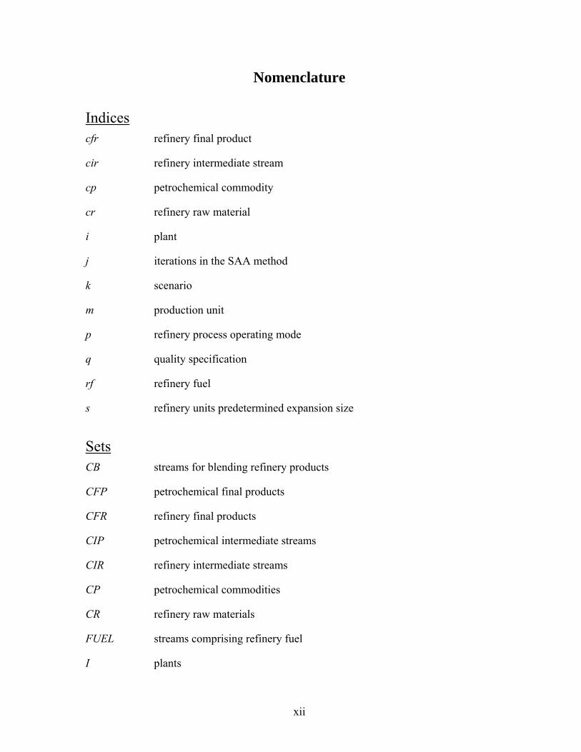
Nomenclature
Indices cfr refinery final product
cir refinery intermediate stream
cp petrochemical commodity
cr refinery raw material
i plant
j iterations in the SAA method
k scenario
m production unit
p refinery process operating mode
q quality specification
rf refinery fuel
s refinery units predetermined expansion size
Sets CB streams for blending refinery products
CFP petrochemical final products
CFR refinery final products
CIP petrochemical intermediate streams
CIR refinery intermediate streams
CP petrochemical commodities
CR refinery raw materials
FUEL streams comprising refinery fuel
I plants
xiii
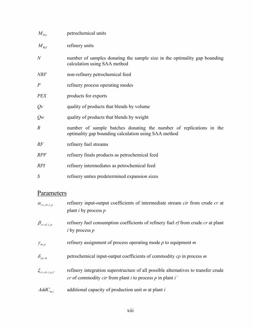
PetM petrochemical units
RefM refinery units
N number of samples donating the sample size in the optimality gap bounding calculation using SAA method
NRF non-refinery petrochemical feed
P refinery process operating modes
PEX products for exports
Qv quality of products that blends by volume
Qw quality of products that blends by weight
R number of sample batches donating the number of replications in the optimality gap bounding calculation using SAA method
RF refinery fuel streams
RPF refinery finals products as petrochemical feed
RPI refinery intermediates as petrochemical feed
S refinery unties predetermined expansion sizes
Parameters picircr ,,,α refinery input-output coefficients of intermediate stream cir from crude cr at
plant i by process p
pirfcr ,,,β refinery fuel consumption coefficients of refinery fuel rf from crude cr at plant i by process p
pm,γ refinery assignment of process operating mode p to equipment m
mcp,δ petrochemical input-output coefficients of commodity cp in process m
',,,, ipicircrξ refinery integration superstructure of all possible alternatives to transfer crude cr of commodity cir from plant i to process p in plant i’
imAddC , additional capacity of production unit m at plant i
xiv
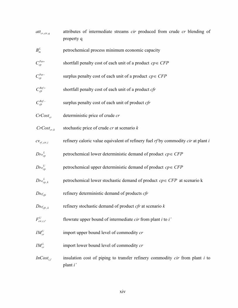
qcircratt ,, attributes of intermediate streams cir produced from crude cr blending of property q
LmB petrochemical process minimum economic capacity
+PetcpC shortfall penalty cost of each unit of a product CFPcp∈
−PetcpC surplus penalty cost of each unit of a product CFPcp∈
+RefcfrC shortfall penalty cost of each unit of a product cfr
−RefcfrC surplus penalty cost of each unit of product cfr
crCrCost deterministic price of crude cr
kcrCrCost , stochastic price of crude cr at scenario k
icirrfcv ,, refinery caloric value equivalent of refinery fuel rf by commodity cir at plant i
LcpPetD petrochemical lower deterministic demand of product CFPcp∈
UcpPetD petrochemical upper deterministic demand of product CFPcp∈
LkcpPetD , petrochemical lower stochastic demand of product CFPcp∈ at scenario k
cfrRefD refinery deterministic demand of products cfr
kcfrRefD , refinery stochastic demand of product cfr at scenario k
UiicirF ',, flowrate upper bound of intermediate cir from plant i to i’
UcrIM import upper bound level of commodity cr
LcrIM import lower bound level of commodity cr
',iiInCost insulation cost of piping to transfer refinery commodity cir from plant i to plant i’
xv
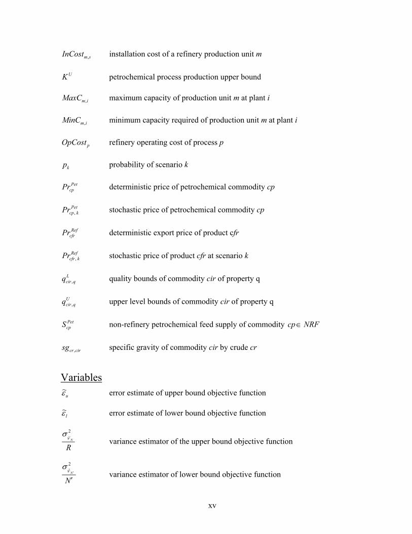
smInCost , installation cost of a refinery production unit m
UK petrochemical process production upper bound
imMaxC , maximum capacity of production unit m at plant i
imMinC , minimum capacity required of production unit m at plant i
pOpCost refinery operating cost of process p
kp probability of scenario k
PetcpPr deterministic price of petrochemical commodity cp
PetkcpPr , stochastic price of petrochemical commodity cp
RefcfrPr deterministic export price of product cfr
RefkcfrPr , stochastic price of product cfr at scenario k
Lqcirq , quality bounds of commodity cir of property q
Uqcirq , upper level bounds of commodity cir of property q
PetcpS non-refinery petrochemical feed supply of commodity NRFcp∈
circrsg , specific gravity of commodity cir by crude cr
Variables uε
~ error estimate of upper bound objective function
lε~ error estimate of lower bound objective function
RN
2ν
σ variance estimator of the upper bound objective function
NN
′′
2ν̂
σ variance estimator of lower bound objective function
xvi
jNν objective function value of each iteration j with a sample size N
Nν objective function upper bound estimator over a sample size N
N ′ν̂ objective function lower bound estimator (point estimator) over a sample size N
Reficfre ,' refinery exports of final product PEXcfr∈ from refinery i
PeticpcrFf ,, petrochemical feed from refinery final product CPRPFcfr ∈∈ from plant i
PeticpcrFi ,, petrochemical feed from refinery intermediates CPRPIcir ∈∈ form plant i
PetcpFn petrochemical feed from non-refinery commodity cp
ReficrS , refinery supply of raw material cr to refinery i
+RefkcfrV , shortfall of product cfr at scenario k
−RefkcfrV , surplus of product cfr at scenario k
+PetkcpV , shortfall of product CFPcp∈ at scenario k
−PetkcpV , surplus of product CFPcp∈ at scenario k
icfrcircrw ,,, blending levels of crude cr that produces intermediate cir to yield a product cfr at plant i
Petmx mass flowrate of petrochemical production unit m
Refcfr,ix mass flowrate of refinery final product cfr by refinery i
Petcpxi mass flow rate of petrochemical intermediate stream CIPcp∈
Refipicircrxi ',,,, refinery transshipment level of crude cr of commodity cir from plant i to
process p at plant i’
Reficfrxv , volumetric flowrate of refinery final product cfr by refinery i
Refsimexpy ,, binary variable representing refinery expansions of production unit m at plant
i for a specific expansion size s
xvii
Refcir,i,i'pipey binary variable representing transshipment of refinery commodity cir from
plant i to plant i’
Petmprocy binary variable representing petrochemical selection of unit m
ipcrz ,, process input flowrate of crude cr to process p at plant i
Processing Unit DATK Desulfurization of aviation turbine kerosene
DCG Desulfurization of cycle gas oil
DCK Delayed coker
DGO Desulfurization of gas oil
CDU Crude distillation
DIST Desulfurization of delayed coker distillates
FCC1 Fluid catalytic cracker (gasoline mode)
FCC2 Fluid catalytic cracker (gas oil mode)
HCU Hydrocracker
ISOM Isomerization
REF1 Reformer (95% severity)
REF2 Reformer (100% severity)
Stream 100 Reformate at 100% severity
95 Reformate at 95% severity
ATK Aviation turbine kerosene intermediates
ATKP Aviation turbine kerosene product
C-4 C-4 fractions (mixed butanes, -enes, etc.)
CGO Cycle gas oil
xviii
Cl Chlorine
CN Fluid catalytic cracker gasoline
CoGO Coker gas oil
Coke Petroleum coke
CR Crude oil
DCGO Desulfurized cycle gas oil
Diesl Petroleum diesel product
DIST Distillate
DSATK Desulfurized aviation turbine kerosene
DSDIST Desulfurized distillate
DSGO Desulfurized gas oil
E Ethylene
EDC Ethylene dichloride
GO Gas oil
GO6 No.6 gas oil
GSLN Petrochemical gasoline
HCI Hydrochloric acid
HFO Petroleum heating fuel oil
HN Heavy naphtha
ISO Isomerate
JP4 No.4 jet fuel
KE Kerosene
LN Light naphtha
LPG Liquefied petroleum gas
NaOH Sodium hydroxide
xix
P Propylene
PFG Petrochemical fuel gas
PFO Petrochemical fuel oil
PG95 Refinery gasoline with 95 octane number
PG98 Refinery gasoline with 98 octane number
PVA polyvinyl alcohol
PVC Polyvinyl chloride
RF Refinery fuel
RG Refinery gas
T Toluene
UCO Unconverted gas oil
VCM Vinyl chloride monomer
VGO Vacuum gas oil
VRSD Desulfurized vacuum residue
xx
Acronyms
ATKP Military Jet Fuel
BMCI Bureau of Mines Correlation Index
BTX Benzene-Toluene-Xylene
CVaR Conditional Value-at-Risk
Des Desulfurization
EEV Expectation of Expected Value
EV Expected Value
EVPI Expected Value of Perfect Information
FCC Fluid Catalytic Cracker
GAMS General Algebraic Modeling System
GTI Gas Turbine Integration
LP Linear Programming
LSR light Straight-Run
MAP Method of Approximation Programming
MILP Mixed-Integer Linear Programming
MINLP Mixed-Integer Non-Linear Programming
MV Mean-Variance
NLP Non-Linear Programming
OTOE One Task-One Equipment
Paygas Pyrolysis Gasoline
PIMS Process Industry Modeling System
RPMS Refinery and Petrochemical Modeling System
SAA Sample Average Approximation
xxi
SEN State-Equipment Network
SLP Successive Linear Programming
SRI Stanford Research Institute
SS Stochastic Solution
STN State-Task Network
UPM Upper Partial Mean
VaR Value-at-Risk
VSS Value of Stochastic Solution
VTE Variable-Task Equipment
WS Wait-and-See
1
Chapter 1
Introduction
1.1 Motivation
Petroleum refining and the petrochemical industry play a paramount role in the current world
economy. They provide the platform to transform raw materials into many essential products
in our life, ranging from transportation and industrial fuels to basic components for plastics,
synthetic rubbers and many other useful chemical products. The economic growth and
increasing populations will keep global demand for such products high for the foreseeable
future. According to the International Energy Agency (IEA, 2006), petroleum makes up
42.3% of the total energy consumption in the world. One half of the petroleum consumption
over the period of 2003 to 2030 will be in the transportation sector. The industrial sector, on
the other hand, accounts for a 39% of the projected increase in world oil consumption,
mostly in chemical and petrochemical processes (EIA, 2006). Meeting such demand will
require large investments and proper optimization tools for the strategic planning of these
industries.
The competition in the market place is another pressing motive for firms to pursue
strategies in order to gain a competitive edge, including the search for opportunities to
improve their coordination and synergy. Bhatnagar et al. (1993) defined two levels of
coordination, namely: “general coordination” and “multiplant coordination”. The first class
considers the problem of integrating different activities of the supply, production and
2
distribution. The second class, ‘multiplant coordination”, mainly addresses production
planning problems. They stressed the importance and need to further develop and design
general and clear frameworks for multiplant coordination. The benefits projected from the
coordination of multiple sites are not only in terms of expenses but also in terms of market
effectiveness and responsiveness (Shah, 1998). Most of the previous strategic planning
studies have focused mainly on restricted defined supply chain networks and have not
provided a thorough analysis of an enterprise as a whole (Shapiro, 2004). Furthermore, they
focused on the coordination of the multiple system echelons of a firm where less attention
was given to providing a framework for the coordination of the same planning level at
multiple sites via process network integration.
However, considering such high level planning decisions, especially with the current
volatile market environment, requires knowledge of uncertainties impact. In production
planning, sources of system uncertainties can be categorized as short-term or long-term
depending on the extent of time horizon (Subrahmanyam et al., 1994). The short-term
uncertainties mainly refer to operational variations, equipment failure, etc. Whereas, long-
term uncertainty may include supply and demand rate variability and price fluctuations, on a
longer time horizon (Shah, 1998). Technological uncertainty in the left-hand-side
coefficients which can be viewed in the context of production planning as the variation in
process yields is another important uncertainty factor. Reklaitis (1991), Rippin (1993), Shah
(1998), and Grossmann (2005) reviewed the development of the general planning and
scheduling problems and summarized the main future challenges as 1) Development of
effective integration and coordination of different planning and scheduling models on single
and multisite systems, 2) Modeling uncertainty through adequate stochastic models, and 3)
3
Development of efficient and general purpose algorithms tailored to provide proper solution
techniques for planning and scheduling problems.
All the above mentioned challenges stimulated the main thrust of this thesis with an
ultimate objective of addressing the planning, integration and coordination of multisite
refinery and petrochemical systems.
1.2 Contributions
The aim of this dissertation is to provide a framework for the planning, integration and
coordination of multisite refinery and petrochemical networks using proper deterministic,
stochastic and robust techniques. The contributions of this thesis are organized into three
parts, addressing different components of the system and advance to achieve the overall
thesis objective.
Multisite Refinery Planning
Currently, the petroleum industry is facing pressures to reduce their product fuel prices, in
spite of the soaring oil prices, while maintaining a high profit margin. With this market
environment, oil companies strive to seek opportunities to increase their resources utilization
and profit. This requires appropriate decision-making tools to utilize all available resources
not only on a single facility scale, but in the more comprehensive outlook of an enterprise-
wide scale. Most of the pervious studies focused on the coordination between the different
functions of an enterprise without exploiting integration alternatives within the same
planning level across multiple sites.
4
The aim of this part of the thesis (Chapter 3) is to address the design and analysis of
multisite integration and coordination strategies within a network of petroleum refineries
using different crude combination alternatives. In addition, account for production capacity
expansion requirements as needed. The main feature of this work is the development of a
methodology for simultaneous analysis of process network integration alternatives in a
multisite refining system through a mixed-integer linear programming (MILP) with the
overall objective of minimizing total annualized cost. The network design specifically
addresses intermediate material transfer between processing units at each site. The
performance of the proposed model is tested on several industrial-scale examples to illustrate
the economic potential and trade-offs involved in the optimization of the network. Although
the methodology is applied on a network of refineries, it can be readily extended to cover
other networks of continuous chemical processes.
In the next phase (Chapter 4), we consider the problem of multisite integration and
coordination within a network of petroleum refineries under uncertainty and using robust
optimization techniques. The framework of the simultaneous analysis of process network
integration, proposed in Chapter 3, is extended to account for uncertainty in model
parameters. Robustness is analyzed based on both model robustness and solution robustness,
where each measure is assigned a scaling factor to analyze the sensitivity of the refinery plan
and the integration network due to variations. The stochastic model is formulated as a two-
stage stochastic MILP problem whereas the robust optimization is formulated as an MINLP
problem with nonlinearity arising from modeling the risk components. Parameters
uncertainty considered include coefficients of the objective function in terms of crude and
final products prices as well as the right-hand-side parameters in the inequality constraints in
5
terms of demand. The proposed method makes use of the sample average approximation
(SAA) method with statistical bounding techniques. The proposed model is tested on two
industrial-scale studies of a single refinery and a network of complex refineries. Modeling
uncertainty in the process parameters provided a practical perspective of this type of problem
in the chemical industry where benefits not only appear in terms of economic considerations,
but also in terms of improved resource utilization.
Petrochemical Industry Planning
The Petrochemical industry is a network of highly integrated production processes where
products of one plant may have an end use or may also represent raw materials for other
processes. This multiplicity gives rise to a highly complex structure which requires proper
planning tools and consideration of the different alternatives for future developments.
Consideration of uncertainty in such decisions is of a great deal of importance and interest by
both the private companies and governments. Previous studies in the field have mainly
considered the problem under deterministic assumptions or considered only part of the
uncertainty in the process parameters.
In this part, we first set up and give an overview of the deterministic version of the
petrochemical planning model (Chapter 5). Then we extend it to address the strategic
planning, design and optimization of a network of petrochemical processes under uncertainty
and robust considerations (Chapter 6). Robustness is analyzed based on both model
robustness and solution robustness, where each measure is assigned a scaling factor to
analyze the sensitivity each component. The stochastic model is formulated as a two-stage
stochastic MILP problem whereas the robust optimization is formulated as an MINLP
6
problem with nonlinearity arising from modeling the risk components. Parameter uncertainty
considered in this part includes process yield, raw material and product prices, and lower
product market demand. The study shows that the final petrochemical network bears more
sensitivity to variations in product prices as apposed to variations in market demand and
process yields for scaling values that maintain the final petrochemical structure obtained
form the stochastic model. The concept of Expected Value of Perfect Information (EVPI)
and Value of the Stochastic Solution (VSS) are also investigated to numerically illustrate the
value of including the randomness of the different model parameters.
Integration and Coordination of Multisite Refinery and Petrochemical Networks
The integration of petroleum refining and petrochemical industries is attracting a whole lot of
interest among many companies and governments. Pervious research in the field assumed
either no limitations on refinery feedstock to the petrochemical industry or fixed the refinery
production levels assuming an optimal operation while optimizing the petrochemical system.
In this part of the thesis (Chapter 7), we address the design of optimal integration and
coordination of multisite refinery and petrochemical networks to satisfy given petroleum and
chemical products demand. The refinery and petrochemical systems were modeled as
mixed-integer problem with the objective of minimizing the annualized cost over a given
time horizon among the refineries and maximizing the added value of the petrochemical
network. The main feature of the work is the development of a methodology for the
simultaneous analysis of process network integration within a multisite refinery and
petrochemical system. This approach provides a proper planning tool across the petroleum
7
refining and petrochemical industry systems and achieves an optimal production strategy by
allowing trade offs between the refinery and the downstream petrochemical market. The
proposed methodology not only devises the integration network in the refineries and
synthesizes the petrochemical industry, but also provides refinery expansion requirements,
production and blending levels.
In the final phase of this dissertation (Chapter 8), we extend the petroleum refinery and
petrochemical industry integration problem to consider different sources of uncertainties in
the problem. Uncertainties in the model included imported crude oil price, refinery product
price, petrochemical product price, refinery market demand, and petrochemical lower level
product demand. The problem is modeled as an MILP two-stochastic problem. Furthermore,
we apply the sample average approximation (SAA) method within an iterative scheme to
generate the required scenarios. The solution quality is then statistically evaluated by
measuring the optimality gap of the final solution. This optimization approach for the
petroleum refining and petrochemical industry provides an appropriate scheme for handling
what is considered as a backbone of many countries’ economies.
8
Chapter 2
Refining and Petrochemical Industry Background
2.1 Production Planning and Scheduling
Planning and scheduling can be defined as developing strategies for the allocation of
equipment, utility or labor resources over time to execute specific tasks in order to produce
single or several products (Grossmann et al., 2001). In most research dealing with planning
and scheduling, there seems to be no clear cut between the two. Hartmann (1998) and
Grossmann et al. (2001) pointed out some of the differences between a planning model and a
scheduling model. In a general sense, process manufacturing planning models consider high
level decisions such as investment on longer time horizons. Scheduling models, on the other
hand, are concerned more with the feasibility of the operations to accomplish a given number
and order of tasks.
Planning problems can mainly be distinguished as strategic, tactical or operational, based
on the decisions involved and the time horizon considered (Grossmann et al., 2001). The
strategic level planning considers a time span of more than one year and covers a whole
width of an organization. At this level, approximate and/or aggregate models are adequate
and mainly consider future investment decisions. Tactical level planning typically involves a
midterm horizon of few months to a year where the decisions usually include production,
inventory and distribution. Operational level covers shorter periods of time spanning from
9
one week to three months where the decisions involve actual production and allocation of
resources. For a general process operations hierarchy, planning is the highest level of
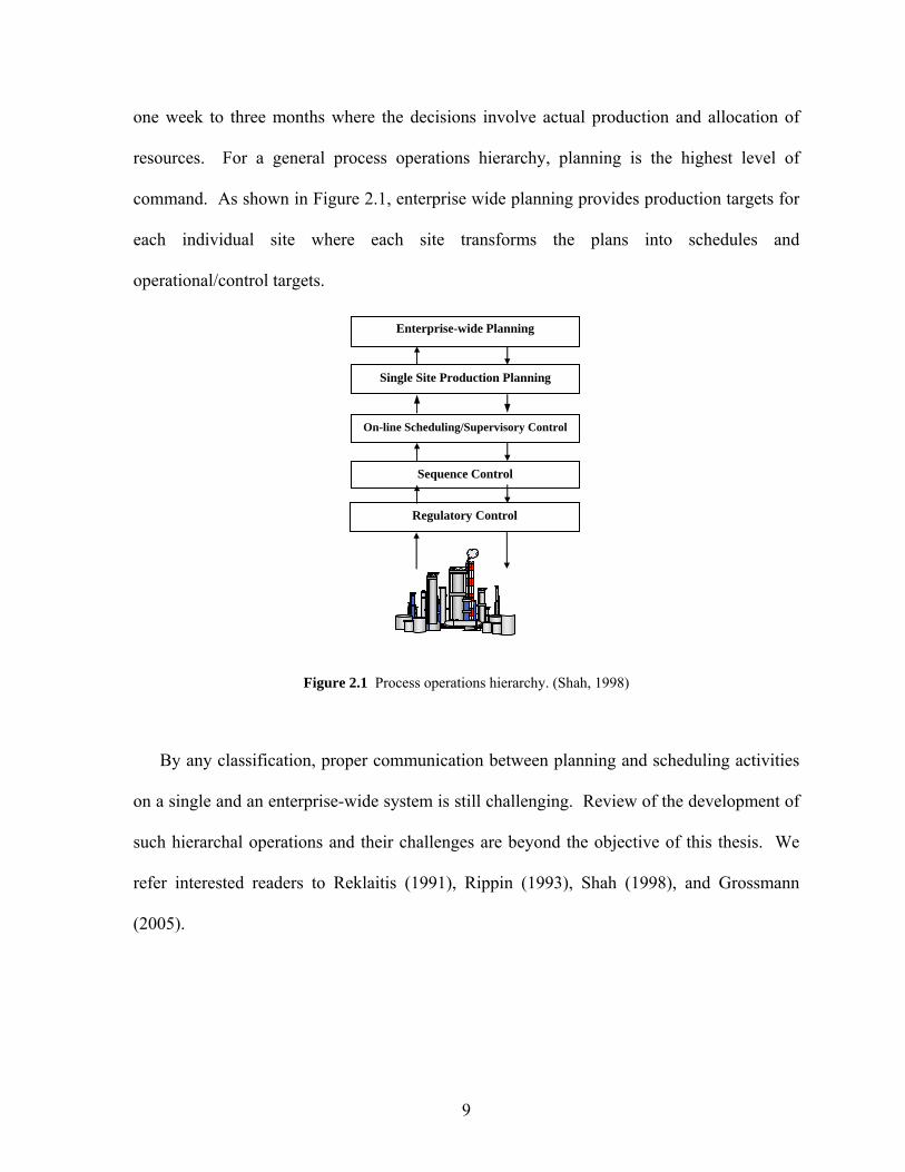
command. As shown in Figure 2.1, enterprise wide planning provides production targets for
each individual site where each site transforms the plans into schedules and
operational/control targets.
Figure 2.1 Process operations hierarchy. (Shah, 1998)
By any classification, proper communication between planning and scheduling activities
on a single and an enterprise-wide system is still challenging. Review of the development of
such hierarchal operations and their challenges are beyond the objective of this thesis. We
refer interested readers to Reklaitis (1991), Rippin (1993), Shah (1998), and Grossmann
(2005).
On-line Scheduling/Supervisory Control
Single Site Production Planning
Enterprise-wide Planning
Regulatory Control
Sequence Control
10
2.2 Petroleum Refining
2.2.1 Overview
The first refinery was built in Titusville, Pennsylvania in 1860 at a cost of $15,000 (Nelson,
1958). This refinery and other refineries at that time only used batch distillation to separate
kerosene and heating oils from other crude fractions. During the early years, refining
separation was performed using batch processing. However, with the increase in petroleum
product demands, continuous refining became a necessity. The first widely recognized
continuous refinery plants emerged around 1912 (Nelson, 1958). With the diversity and
complexity of petroleum products demand, the refining industry has developed from a few
simple processing units to very complex production systems. For a detailed history on the
evolution of refining technologies, we refer the reader to Nelson (1958) and Wilson (1997).
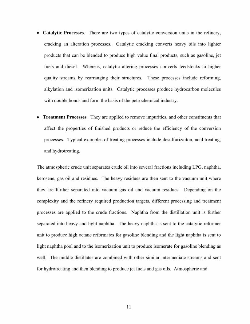
A simplified process flow diagram of a typical modern refinery is shown in Figure 2.2.
The refining processes can be divided into four main systems (OSHA, 2003):
♦ Distillation Processes. They are used to separate oil into fractions by distillation
according to their boiling points. Distillation is usually divided into two steps,
atmospheric and vacuum fractionation. This is done in order to achieve higher separation
efficiencies at a lower cost.
♦ Coking and Thermal Processes. They convert heavy feedstocks, usually from
distillation processes, to produce more desirable and valuable products that are suitable
feeds to other refinery units. Such units include coking and visbreaking.
11
♦ Catalytic Processes. There are two types of catalytic conversion units in the refinery,
cracking an alteration processes. Catalytic cracking converts heavy oils into lighter
products that can be blended to produce high value final products, such as gasoline, jet
fuels and diesel. Whereas, catalytic altering processes converts feedstocks to higher
quality streams by rearranging their structures. These processes include reforming,
alkylation and isomerization units. Catalytic processes produce hydrocarbon molecules
with double bonds and form the basis of the petrochemical industry.
♦ Treatment Processes. They are applied to remove impurities, and other constituents that
affect the properties of finished products or reduce the efficiency of the conversion
processes. Typical examples of treating processes include desulfurizaiton, acid treating,
and hydrotreating.
The atmospheric crude unit separates crude oil into several fractions including LPG, naphtha,
kerosene, gas oil and residues. The heavy residues are then sent to the vacuum unit where
they are further separated into vacuum gas oil and vacuum residues. Depending on the
complexity and the refinery required production targets, different processing and treatment
processes are applied to the crude fractions. Naphtha from the distillation unit is further
separated into heavy and light naphtha. The heavy naphtha is sent to the catalytic reformer
unit to produce high octane reformates for gasoline blending and the light naphtha is sent to
light naphtha pool and to the isomerization unit to produce isomerate for gasoline blending as
well. The middle distillates are combined with other similar intermediate streams and sent
for hydrotreating and then blending to produce jet fuels and gas oils. Atmospheric and
12
Figure 2.2 A simplified process flow diagram for a typical refinery. (Khor, 2007)
13
vacuum gas oils are further treated by catalytic cracking and in other cases by hydrocracking,
or both, in order to increase the gasoline and distillate yields. In some refineries, vacuum
residues are further treated using coking and thermal processes to increase light products
yields. The above mentioned processes are highly complicated and involve different
processing mechanisms. We refer the reader to standard petroleum refining textbooks, Gary
and Handwerk (1994) for instance, for more details and process analysis.
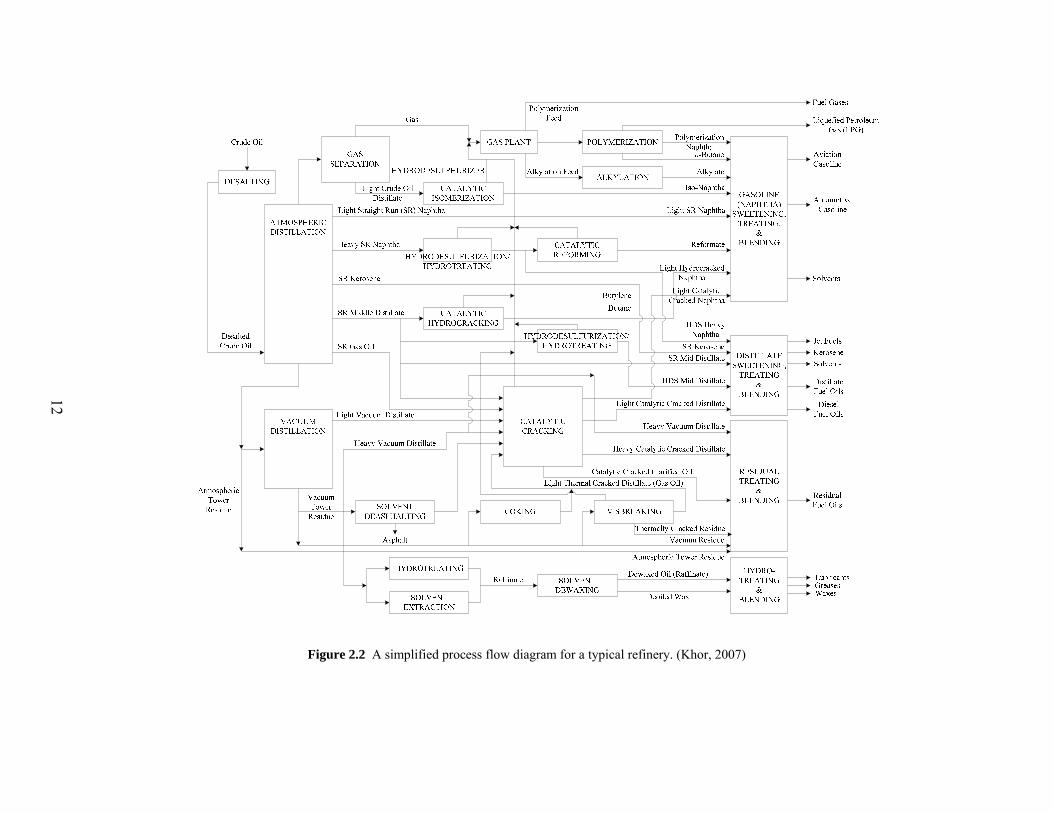
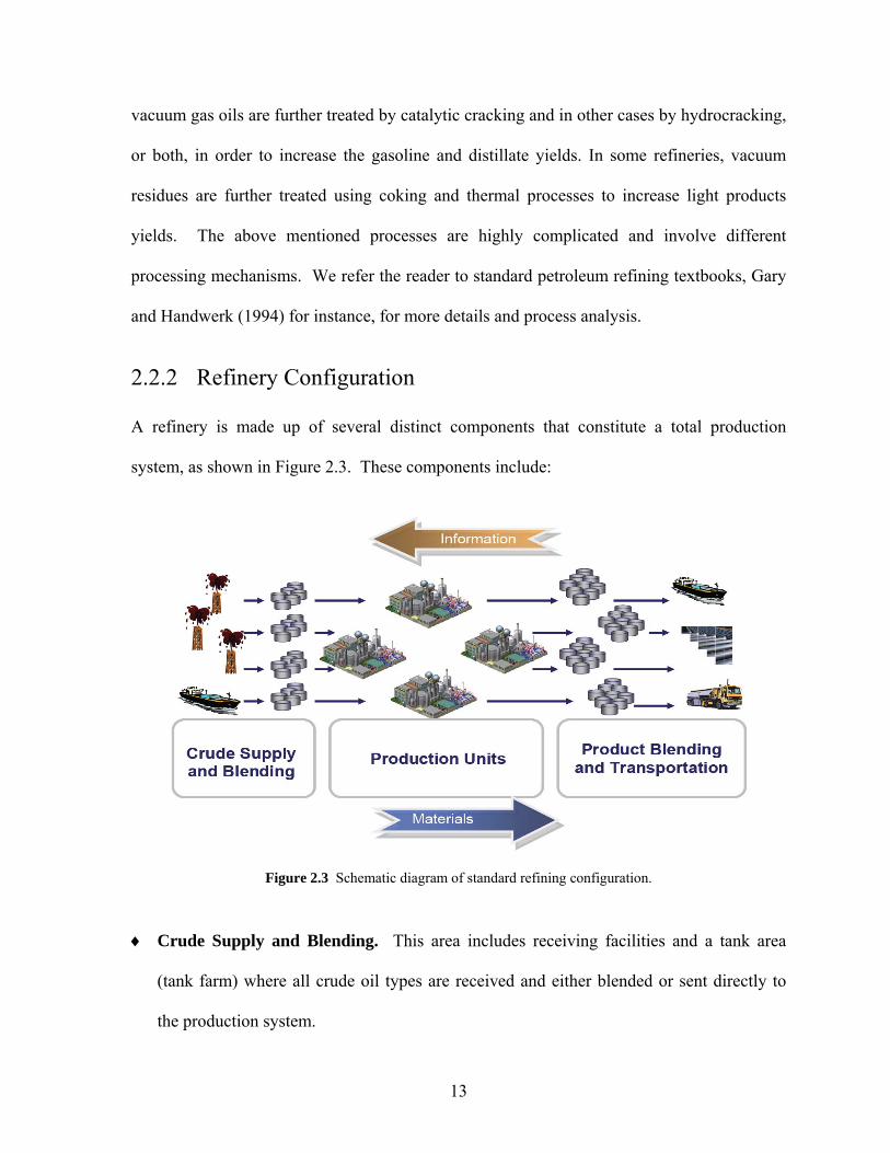
2.2.2 Refinery Configuration
A refinery is made up of several distinct components that constitute a total production
system, as shown in Figure 2.3. These components include:
Figure 2.3 Schematic diagram of standard refining configuration.
♦ Crude Supply and Blending. This area includes receiving facilities and a tank area
(tank farm) where all crude oil types are received and either blended or sent directly to
the production system.
14
♦ Production Units. Production units separate crude oil into different fractions or cuts,
upgrade and purify some of these cuts, and convert heavy fractions to light, more useful
fractions. It also includes the utilities which provide the refinery with fuel, flaring
capability, electricity, steam, cooling water, fire water, sweet water, compressed air,
nitrogen, etc, all of which are necessary for the refinery’s safe operation.
♦ Product Blending and Transportation. In this area final products are processed
according to either a predetermined recipes and/or to a certain product specifications.
This area also includes the dispatch (terminals) of finished products to the different
customers.
The petroleum industry has long leveraged the use of mathematical programming and its
different applications. The invention of both the simplex algorithm by Dantzig in 1947 and
digital computers was the main driver for the wide spread use of linear programming (LP)
applications in the industry (Bodington & Baker, 1990). Since then, many early applications
followed in the area of refinery planning (Symonds, 1955; Manne, 1958; Charnes and
Cooper, 1961; Wagner, 1969; Adams & Griffin, 1972) and distribution planning (Zierer et
al., 1976).
One of the main challenges that inspired more research in the area of refining was the
blending or pooling problem (Bodington & Baker, 1990). The inaccurate and inconsistent
results from the use of linear blending relations led to the development of many techniques to
handle nonlinearities. The nonlinearities arise mainly because product properties, such as
octane number and vapor pressure assume a nonlinear relationship of quantities and
properties of each blending component (Lasdon & Waren, 1983). In this context, we will
15
describe two commonly used approaches in industry and commercial planning softwares to
tackle this problem. They are linear blending indices and successive linear programming
(SLP).
Linear blending indices are dimensionless numerical figures that were developed to
represent true physical properties of mixtures on either a volume or weight average basis
(Bodington & Baker, 1990). They can be used directly in the LP model and span the most
important properties in petroleum products, including octane number, pour point, freezing
point, viscosity sulfur content, and vapor pressure. Many refineries and researchers use this
approximation. Blending indices tables and graphs can often be found in petroleum refining
books such as Gary and Handwerk (1994) or can be proprietarily developed by refining
companies for their own use.
Successive linear programming (SLP), on the other hand, is a more sophisticated method
to linearize blending nonlinearities in the pooling problem. The idea of SLP was first
introduced by Griffith and Stewart (1961) of Shell Oil company where it was named the
method of approximation programming (MAP). They utilized the idea of a Taylor series
expansion to remove nonlinearities in the objective function and constraints then solving the
resulting linear model repeatedly. Every LP solution is used as an initial solution point for
the next model iteration until a satisfying criterion is reached. Bounding constraints were
added to ensure the new model feasibility. Following their work, many improvement
heuristics and solution algorithms were developed to accommodate bigger and more complex
problems (Lasdon & Waren, 1980). Most commercial blending softwares and computational
tools nowadays are based on SLP, such as RPMS by Honeywell Process Solutions
(previously Booner & Moore, 1979) and PIMS by Aspen Technology (previously Bechtel
16
Corp., 1993). However, such commercial tools are not built to support studies on capacity
expansion alternatives, design of plants integration and stochastic modeling and analysis.
All in all, the petroleum industry has invested considerable effort in developing
sophisticated mathematical programming models to help planners provide overall planning
schemes for refinery operations, crude oil evaluation, and other related tasks.
2.3 Petrochemical Industry
2.3.1 Overview
The Petrochemical industry is a network of highly integrated production processes. The
products of one plant may have an end use but may also represent raw materials for another
process. Most chemicals can be produced by many different sequences of reactions and
production processes. This multiplicity of production schemes offers the sense of switching
between production methods and raw materials utilization.
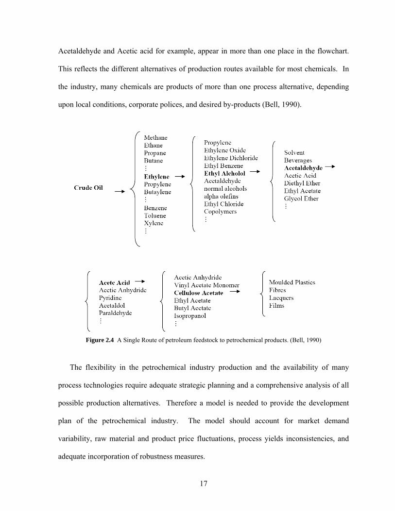
Petroleum feedstock, natural gas and tar represent the main production chain drivers for
the petrochemical industry (Bell, 1990). From these, many important petrochemical
intermediates are produced including ethylene, propylene, butylenes, butadiene, benzene,
toluene, and xylene. These essential intermediates are then converted to many other
intermediates and final petrochemical products constructing a complex petrochemical
network. Figure 2.4 depicts a portion of the petrochemical alternative routs to produce
cellulous acetate.
Figure 2.4 is in fact a small extraction of much larger and comprehensive flow diagrams
found in Stanford Research Institute (SRI) reports. Note that certain chemicals,
17
Acetaldehyde and Acetic acid for example, appear in more than one place in the flowchart.
This reflects the different alternatives of production routes available for most chemicals. In
the industry, many chemicals are products of more than one process alternative, depending
upon local conditions, corporate polices, and desired by-products (Bell, 1990).
Figure 2.4 A Single Route of petroleum feedstock to petrochemical products. (Bell, 1990)
The flexibility in the petrochemical industry production and the availability of many
process technologies require adequate strategic planning and a comprehensive analysis of all
possible production alternatives. Therefore a model is needed to provide the development
plan of the petrochemical industry. The model should account for market demand
variability, raw material and product price fluctuations, process yields inconsistencies, and
adequate incorporation of robustness measures.
18
The realization of the petrochemical planning need and importance has inspired a great
deal of research in order to devise different models to account for the overall system
optimization. Optimization models include continuous and mixed-integer programming
under deterministic or parameter uncertainty considerations. Related literature is reviewed at
a later stage of this thesis based on the chapter topic.
2.3.2 Petrochemical Feedstock
The preparation of intermediate petrochemical streams requires different processing
alternatives depending on the feedstock quality. In our classification of petrochemical
feedstocks we closely follow the one by Gary and Handwerk (1994) consisting of aromatics,
olefins, and paraffins/cyclo-paraffins compounds. The classification of petrochemical
feedstocks into these clusters helps identify the different sources in the refinery that provide
suitable feedstock and therefore better recognize areas of synergy between the refinery and
petrochemical systems.
2.3.2.1 Aromatics
Aromatics are hydrocarbons containing a benzene ring which is a stable and saturated
compound. Aromatics used by the petrochemical industry are mainly benzene, toluene,
xylene (BTX) as well as ethylbenzene and are produced by catalytic reforming where their
yield would increase with the increase of reforming severity (Gary & Handwerk, 1994).
Extractive distillation by different solvents, depending on the chosen technology, is used to
recover such compounds. BTX recovery consists of an extraction using solvents that
enhances the relative volatilities of the preferred compound followed by a separation process
based on the products’ boiling points. Further processing of xylenes using
19
isomerization/separation processes is commonly required to produce o-, m-, and p-xylene
mixtures depending on market requirements. Benzene, in particular, is a source to a wide
variety of chemical products. It is often converted to ethylbenzene, cumene, cyclohexane,
and nitrobenzene which in turn are further processed to other chemicals including styrene,
phenol, and aniline (Rudd et al., 1981). Toluene production, on the other hand, is mainly
driven by benzene and mixed xylenes demand. Mixed xylene, particularly in Asia, is used
for producing para-xylene and polyester (Balaraman, 2006).
The other source of aromatics is the pyrolysis gasoline (pygas) which is a byproduct of
naphtha or gas oil steam cracking. This presents an excellent synergistic opportunity
between refinery, BTX complex and stream cracking for olefins production.
2.3.2.2 Olefins
Olefins are hydrocarbon compounds with at least two carbon atoms having a double bond
where their unstable nature and tendency to polymerize makes them one of the very
important building blocks for the chemical and petrochemical industry (Gary & Handwerk,
1994). Although olefins are produced by fluid catalytic cracking in refineries, the main
production source is through steam cracking of liquefied petroleum gas (LPG), naphtha or
gas oils.
The selection of steam cracker feedstock is mainly driven by market demand as different
feedstocks qualities produce different olefins yields. One of the commonly used feed quality
assessment methods in practice is the Bureau of Mines Correlation Index (BMCI) (Gonzalo
et al., 2004). This index is a function of average boiling point and specific gravity of a
particular feedstock. The steam cracker feed quality improves with a decrease in the BMCI
20
value. For instance, vacuum gas oil (VGO) has a high value of BMCI and therefore is not an
attractive steam cracker feed. The commonly used feedstocks in industry are naphtha and
gas oil.
Steam cracking plays an instrumental role in the petrochemical industry in terms of
providing the main petrochemical intermediates for the down stream industry. The steam
cracker olefin production includes ethylene, propylene, butylene and benzene. These
intermediates are further processed into a wide range of polymers (plastics), solvents, fibres,
detergents, ammonia and other synthetic organic compounds for general use in the chemical
industry (Rudd et al., 1981). In a situation where worldwide demand for these basic olefins
is soaring, more studies are being conducted to maximize steam cracking efficiency (Ren et
al., 2006). An alternative strategy would be to seek integration possibilities with the refinery
as they both share feedstocks and products that can be utilized to maximize profit and
processing efficiency.
2.3.2.3 Normal Paraffins and cyclo-paraffins
Paraffin hydrocarbon compounds contain only single bonded carbon atoms which give them
higher stability characteristics. Normal paraffin compounds are abundantly present in
petroleum fractions but are mostly recovered from light straight-run (LSR) naphtha and
kerosene. However, the non-normal hydrocarbon components of LSR naphtha are of a
higher octane number and therefore are preferred for gasoline blending (Meyers, 1997). For
this reason, new technologies have been developed to further separate LSR naphtha into
higher octane products that can be used in the gasoline pool and normal paraffins that is used
as steam cracker feedstock (e.g. UOP IsoSivTM Process). The normal paraffins recovered
21
from kerosene, on the other hand, are mostly used in biodegradable detergents
manufacturing.
Cyclo-paraffins, also referred to as naphthenes, are mainly produced by dehydrogenation
of their equivalent aromatic compounds; such as the production of cyclo-hexane by
dehydrogenation of benzene. Cyclo-hexane is mostly used for the production of adipic acid
and nylon manufacturing (Rudd et al., 1981).
2.4 Refinery and Petrochemical Synergy Benefits
Process integration in the refining and petrochemical industry include many intuitively
recognized benefits of processing higher quality feedstocks, improving value of byproducts,
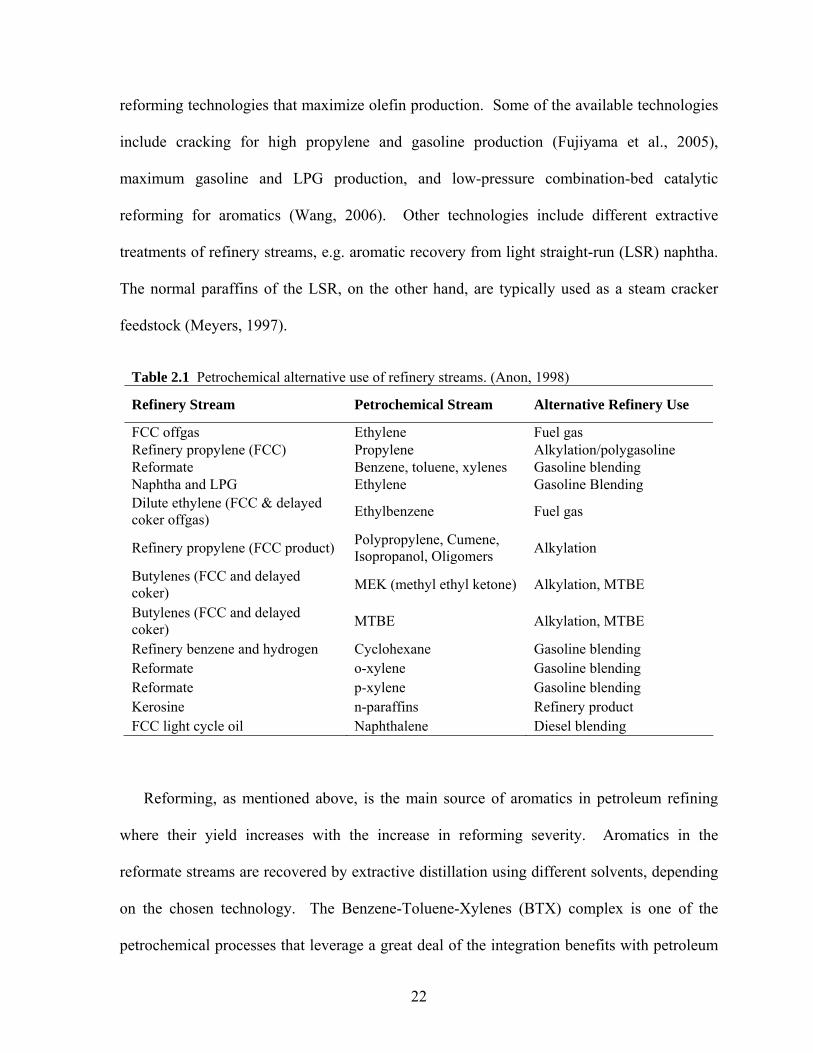
and achieving better efficiencies through sharing of resources. Table 2.1 illustrates different
refinery streams that can be of superior quality when used in the petrochemical industry. The
potential integration alternatives for refining and petrochemical industries can be classified
into three main categories; 1) process integration, 2) utilities integration, and 3) fuel gas
upgrade. The integration opportunities discussed below are for a general refinery and a
petrochemical complex. Further details and analysis about the system requirements can be
developed based on the actual system infrastructure, market demand, and product and energy
prices.
2.4.1 Process Integration
The innovative design of different refinery processes while considering downstream
petrochemical industry is an illustration of the realization of refining and petrochemical
integration benefits. This is demonstrated by the wide varieties of refinery cracking and
22
reforming technologies that maximize olefin production. Some of the available technologies
include cracking for high propylene and gasoline production (Fujiyama et al., 2005),
maximum gasoline and LPG production, and low-pressure combination-bed catalytic
reforming for aromatics (Wang, 2006). Other technologies include different extractive
treatments of refinery streams, e.g. aromatic recovery from light straight-run (LSR) naphtha.
The normal paraffins of the LSR, on the other hand, are typically used as a steam cracker
feedstock (Meyers, 1997).
Table 2.1 Petrochemical alternative use of refinery streams. (Anon, 1998)
Refinery Stream Petrochemical Stream Alternative Refinery Use
FCC offgas Ethylene Fuel gas Refinery propylene (FCC) Propylene Alkylation/polygasoline Reformate Benzene, toluene, xylenes Gasoline blending Naphtha and LPG Ethylene Gasoline Blending Dilute ethylene (FCC & delayed coker offgas) Ethylbenzene Fuel gas
Refinery propylene (FCC product) Polypropylene, Cumene, Isopropanol, Oligomers Alkylation
Butylenes (FCC and delayed coker) MEK (methyl ethyl ketone) Alkylation, MTBE
Butylenes (FCC and delayed coker) MTBE Alkylation, MTBE
Refinery benzene and hydrogen Cyclohexane Gasoline blending Reformate o-xylene Gasoline blending Reformate p-xylene Gasoline blending Kerosine n-paraffins Refinery product FCC light cycle oil Naphthalene Diesel blending
Reforming, as mentioned above, is the main source of aromatics in petroleum refining
where their yield increases with the increase in reforming severity. Aromatics in the
reformate streams are recovered by extractive distillation using different solvents, depending
on the chosen technology. The Benzene-Toluene-Xylenes (BTX) complex is one of the
petrochemical processes that leverage a great deal of the integration benefits with petroleum
23
refining. The integration benefits are not only limited to the process side but extend to the
utilities as will be explained in the following section.
Pyrolysis gasoline (pygas), a byproduct of stream cracking, can be further processed in
the BTX complex to recover the aromatic compounds and the raffinate after extraction can be
blended in the gasoline or naphtha pool (Balaraman, 2006). If there is no existing aromatics
complex to further process the pygas, it could alternatively be routed to the reformer feed for
further processing (Philpot, 2007). However this alternative may not be viable in general as
most reformers run on maximum capacity. Pygas from steam cracking contains large
amounts of diolefins which are undesirable due to their instability and tendency to
polymerize yielding filter plugging compounds. For this reason, hydrogenation of pygas is
usually recommended prior to further processing.
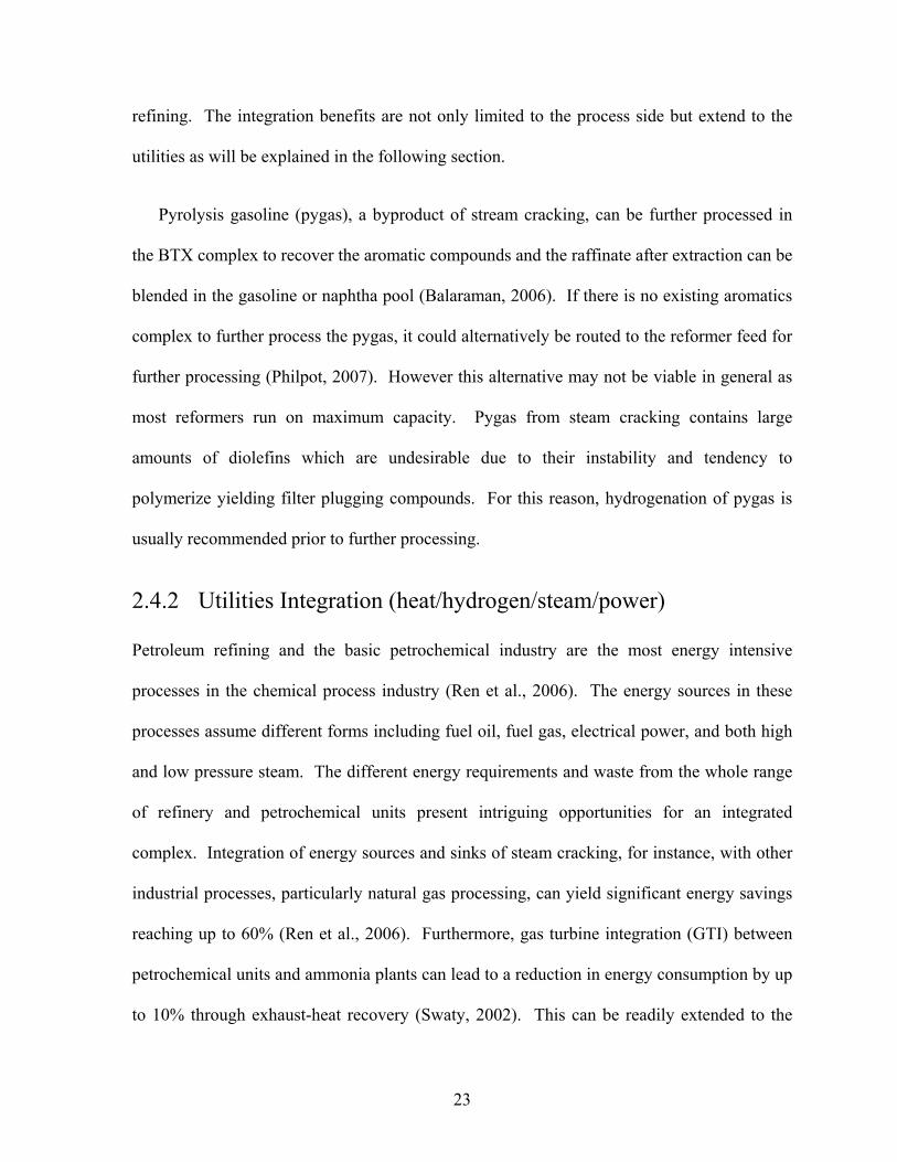
2.4.2 Utilities Integration (heat/hydrogen/steam/power)
Petroleum refining and the basic petrochemical industry are the most energy intensive
processes in the chemical process industry (Ren et al., 2006). The energy sources in these
processes assume different forms including fuel oil, fuel gas, electrical power, and both high
and low pressure steam. The different energy requirements and waste from the whole range
of refinery and petrochemical units present intriguing opportunities for an integrated
complex. Integration of energy sources and sinks of steam cracking, for instance, with other
industrial processes, particularly natural gas processing, can yield significant energy savings
reaching up to 60% (Ren et al., 2006). Furthermore, gas turbine integration (GTI) between
petrochemical units and ammonia plants can lead to a reduction in energy consumption by up
to 10% through exhaust-heat recovery (Swaty, 2002). This can be readily extended to the
24
refinery processing units which span a wide variety of distillation, cracking, reforming, and
isomerization processes.
Hydrogen is another crucial utility that is receiving more attention recently mainly due to
the stricter environmental regulations on sulfur emissions. Reduction of sulfur emissions is
typically achieved by deeper desulfurization of petroleum fuels which in turn requires
additional hydrogen production (Crawford et al., 2002). A less capital intensive alternative
to alleviate hydrogen shortage is to operate the catalytic reformer at higher severity.
However, higher severity reforming increases the production of BTX aromatics which
consequently affect the gasoline pool aromatics specification. Therefore, the BTX extraction
process becomes a more viable alternative for the sake of aromatics recovery as well as
maintaining the gasoline pool within specification (Crawford et al., 2002). The capital cost
for the implementation of such a project would generally be lower as the BTX complex and
refinery would share both process and utilities streams.
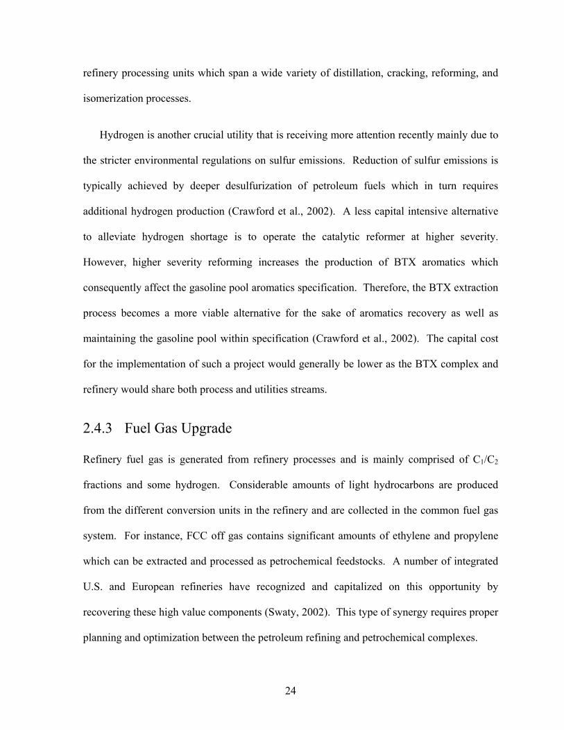
2.4.3 Fuel Gas Upgrade
Refinery fuel gas is generated from refinery processes and is mainly comprised of C1/C2
fractions and some hydrogen. Considerable amounts of light hydrocarbons are produced
from the different conversion units in the refinery and are collected in the common fuel gas
system. For instance, FCC off gas contains significant amounts of ethylene and propylene
which can be extracted and processed as petrochemical feedstocks. A number of integrated
U.S. and European refineries have recognized and capitalized on this opportunity by
recovering these high value components (Swaty, 2002). This type of synergy requires proper
planning and optimization between the petroleum refining and petrochemical complexes.
25
The other major component is hydrogen where it typically accounts for 50-80 % of the
refinery fuel gas (Patel et al., 2003). This substantial amount of hydrogen is disposed to the
fuel gas system from different sources in the refinery. The most significant source, however,
is the catalytic reforming. Hydrogen recovery using economically attractive technologies is
of a great benefit to both refineries and petrochemical systems especially with the increasing
strict environmental regulations on fuels.
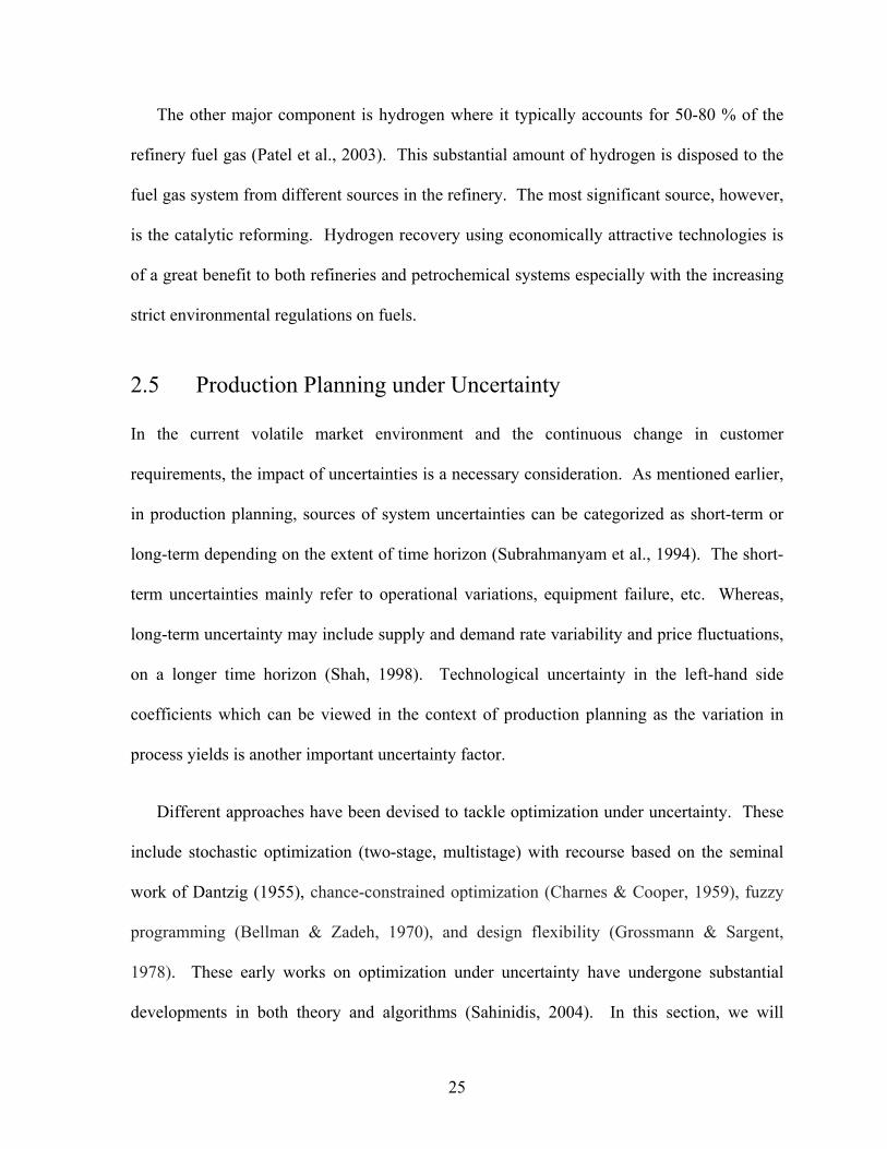
2.5 Production Planning under Uncertainty
In the current volatile market environment and the continuous change in customer
requirements, the impact of uncertainties is a necessary consideration. As mentioned earlier,
in production planning, sources of system uncertainties can be categorized as short-term or
long-term depending on the extent of time horizon (Subrahmanyam et al., 1994). The short-
term uncertainties mainly refer to operational variations, equipment failure, etc. Whereas,
long-term uncertainty may include supply and demand rate variability and price fluctuations,
on a longer time horizon (Shah, 1998). Technological uncertainty in the left-hand side
coefficients which can be viewed in the context of production planning as the variation in
process yields is another important uncertainty factor.
Different approaches have been devised to tackle optimization under uncertainty. These
include stochastic optimization (two-stage, multistage) with recourse based on the seminal
work of Dantzig (1955), chance-constrained optimization (Charnes & Cooper, 1959), fuzzy
programming (Bellman & Zadeh, 1970), and design flexibility (Grossmann & Sargent,
1978). These early works on optimization under uncertainty have undergone substantial
developments in both theory and algorithms (Sahinidis, 2004). In this section, we will
26
mainly concentrate on stochastic, chance-constrained (probabilistic) optimization, and robust
optimization. For additional details and information, the interested reader is invited to pursue
references such as Dempster (1980), Sahinidis (2004) and the recent textbooks of Kall and
Wallace (1994) and Ruszczyński and Shapiro (2003).
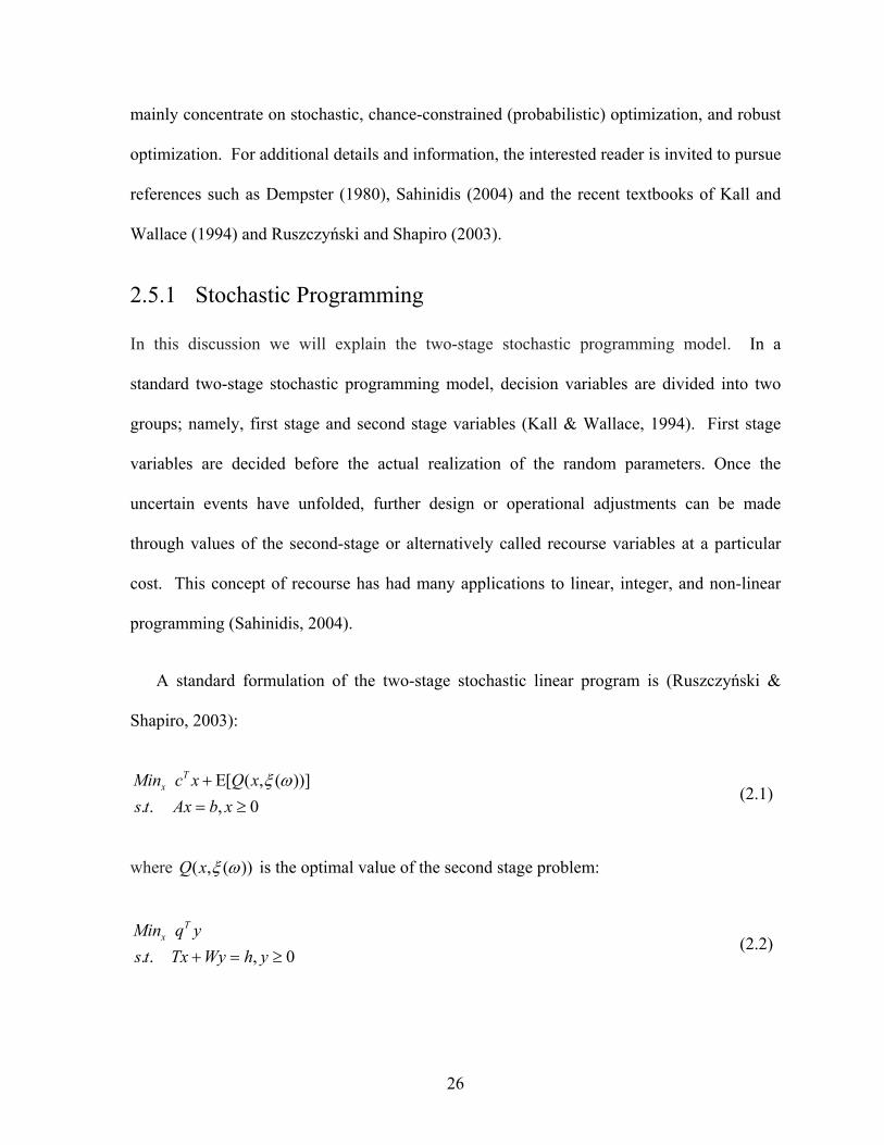
2.5.1 Stochastic Programming
In this discussion we will explain the two-stage stochastic programming model. In a
standard two-stage stochastic programming model, decision variables are divided into two
groups; namely, first stage and second stage variables (Kall & Wallace, 1994). First stage
variables are decided before the actual realization of the random parameters. Once the
uncertain events have unfolded, further design or operational adjustments can be made
through values of the second-stage or alternatively called recourse variables at a particular
cost. This concept of recourse has had many applications to linear, integer, and non-linear
programming (Sahinidis, 2004).
A standard formulation of the two-stage stochastic linear program is (Ruszczyński &
Shapiro, 2003):
0,..))](,([
≥=Ε+
xbAxtsxQxcMin T
x ωξ (2.1)
where ))(,( ωξxQ is the optimal value of the second stage problem:
0,.. ≥=+ yhWyTxtsyqMin T
x (2.2)
27
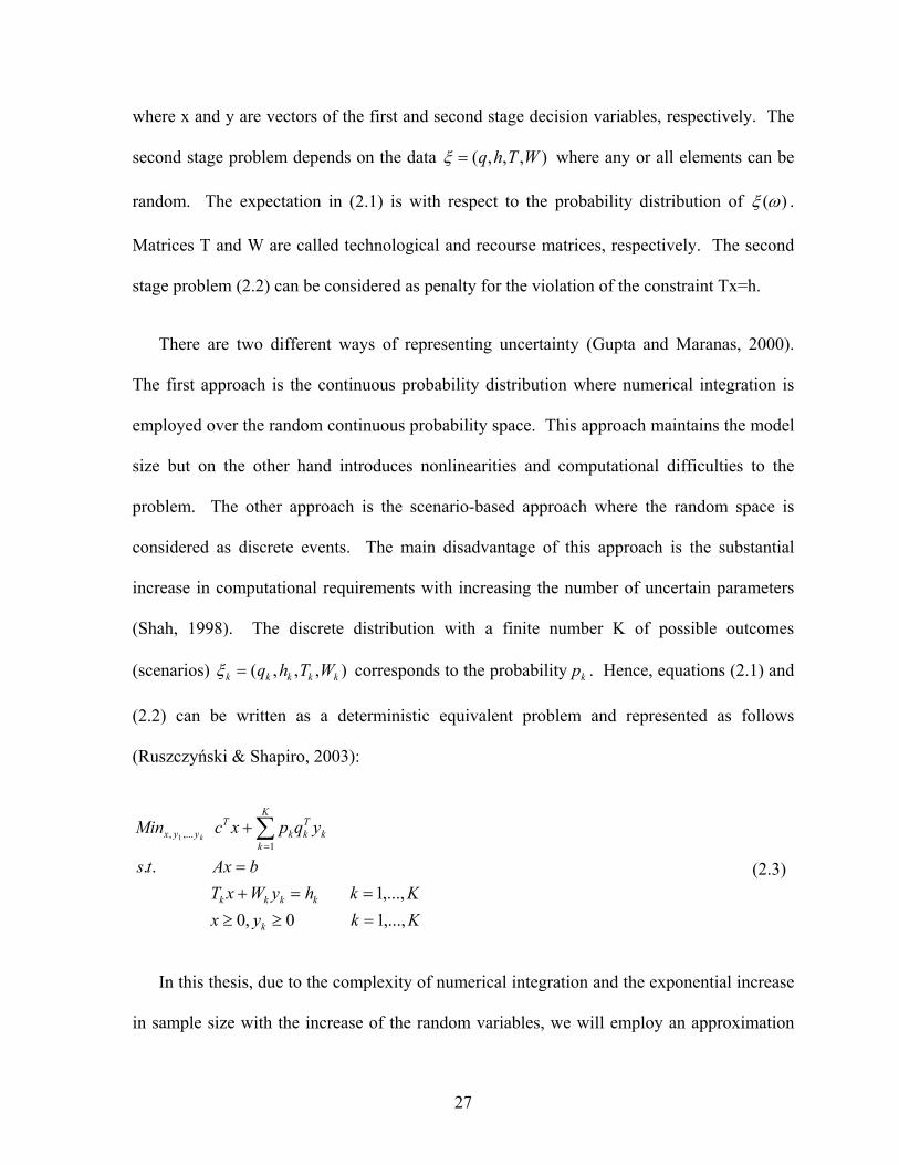
where x and y are vectors of the first and second stage decision variables, respectively. The
second stage problem depends on the data ),,,( WThq=ξ where any or all elements can be
random. The expectation in (2.1) is with respect to the probability distribution of )(ωξ .
Matrices T and W are called technological and recourse matrices, respectively. The second
stage problem (2.2) can be considered as penalty for the violation of the constraint Tx=h.
There are two different ways of representing uncertainty (Gupta and Maranas, 2000).
The first approach is the continuous probability distribution where numerical integration is
employed over the random continuous probability space. This approach maintains the model
size but on the other hand introduces nonlinearities and computational difficulties to the
problem. The other approach is the scenario-based approach where the random space is
considered as discrete events. The main disadvantage of this approach is the substantial
increase in computational requirements with increasing the number of uncertain parameters
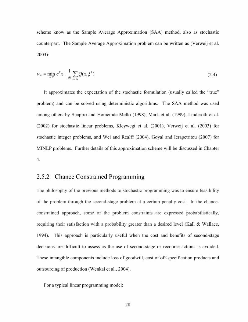
(Shah, 1998). The discrete distribution with a finite number K of possible outcomes
(scenarios) ),,,( kkkkk WThq=ξ corresponds to the probability kp . Hence, equations (2.1) and
(2.2) can be written as a deterministic equivalent problem and represented as follows
(Ruszczyński & Shapiro, 2003):
KkyxKkhyWxT
bAxts
yqpxcMin
k
kkkk
K
kk
Tkk
Tyyx k
,...,10,0,...,1
..1
,..., 1
=≥≥==+
=
+∑=
(2.3)
In this thesis, due to the complexity of numerical integration and the exponential increase
in sample size with the increase of the random variables, we will employ an approximation
28
scheme know as the Sample Average Approximation (SAA) method, also as stochastic
counterpart. The Sample Average Approximation problem can be written as (Verweij et al.
2003):
∑∈
∈+=
Nk
kT
XxN xQN
xc ),(1min ξν (2.4)
It approximates the expectation of the stochastic formulation (usually called the “true”
problem) and can be solved using deterministic algorithms. The SAA method was used
among others by Shapiro and Homemde-Mello (1998), Mark et al. (1999), Linderoth et al.
(2002) for stochastic linear problems, Kleywegt et al. (2001), Verweij et al. (2003) for
stochastic integer problems, and Wei and Realff (2004), Goyal and Ierapetritou (2007) for
MINLP problems. Further details of this approximation scheme will be discussed in Chapter
4.
2.5.2 Chance Constrained Programming
The philosophy of the previous methods to stochastic programming was to ensure feasibility
of the problem through the second-stage problem at a certain penalty cost. In the chance-
constrained approach, some of the problem constraints are expressed probabilistically,
requiring their satisfaction with a probability greater than a desired level (Kall & Wallace,
1994). This approach is particularly useful when the cost and benefits of second-stage
decisions are difficult to assess as the use of second-stage or recourse actions is avoided.
These intangible components include loss of goodwill, cost of off-specification products and
outsourcing of production (Wenkai et al., 2004).
For a typical linear programming model:
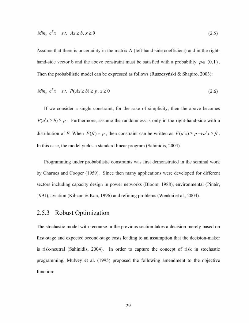
29
0,.. ≥≥ xbAxtsxcMin Tx (2.5)
Assume that there is uncertainty in the matrix A (left-hand-side coefficient) and in the right-
hand-side vector b and the above constraint must be satisfied with a probability ∈p )1,0( .
Then the probabilistic model can be expressed as follows (Ruszczyński & Shapiro, 2003):
0,)(.. ≥≥≥ xpbAxPtsxcMin Tx (2.6)
If we consider a single constraint, for the sake of simplicity, then the above becomes
pbxaP t ≥≥ )( . Furthermore, assume the randomness is only in the right-hand-side with a
distribution of F. When pF =)(β , then constraint can be written as β≥→≥ xapxaF tt )( .
In this case, the model yields a standard linear program (Sahinidis, 2004).
Programming under probabilistic constraints was first demonstrated in the seminal work
by Charnes and Cooper (1959). Since then many applications were developed for different
sectors including capacity design in power networks (Bloom, 1988), environmental (Pintér,
1991), aviation (Kibzun & Kan, 1996) and refining problems (Wenkai et al., 2004).
2.5.3 Robust Optimization
The stochastic model with recourse in the previous section takes a decision merely based on
first-stage and expected second-stage costs leading to an assumption that the decision-maker
is risk-neutral (Sahinidis, 2004). In order to capture the concept of risk in stochastic
programming, Mulvey et al. (1995) proposed the following amendment to the objective
function:
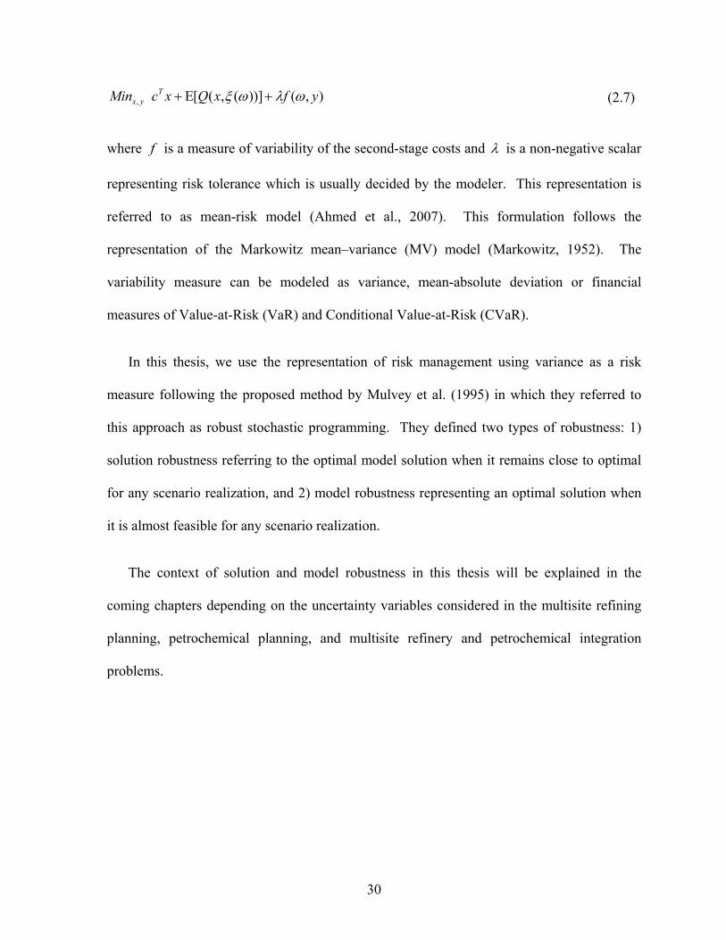
30
),())](,([, yfxQxcMin Tyx ωλωξ +Ε+ (2.7)
where f is a measure of variability of the second-stage costs and λ is a non-negative scalar
representing risk tolerance which is usually decided by the modeler. This representation is
referred to as mean-risk model (Ahmed et al., 2007). This formulation follows the
representation of the Markowitz mean–variance (MV) model (Markowitz, 1952). The
variability measure can be modeled as variance, mean-absolute deviation or financial
measures of Value-at-Risk (VaR) and Conditional Value-at-Risk (CVaR).
In this thesis, we use the representation of risk management using variance as a risk
measure following the proposed method by Mulvey et al. (1995) in which they referred to
this approach as robust stochastic programming. They defined two types of robustness: 1)
solution robustness referring to the optimal model solution when it remains close to optimal
for any scenario realization, and 2) model robustness representing an optimal solution when
it is almost feasible for any scenario realization.
The context of solution and model robustness in this thesis will be explained in the
coming chapters depending on the uncertainty variables considered in the multisite refining
planning, petrochemical planning, and multisite refinery and petrochemical integration
problems.
31
Chapter 3
Optimization of Multisite Refinery Network: Integration and Coordination
3.1 Introduction
With the current situation of high crude oil prices and the everlasting pressure to reduce
prices of final petroleum products, refiners are faced with a very challenging situation. This
nature of petroleum economic environment is a pressing motive for refineries to operate at an
optimal level and continue to seek opportunities to increase their profit margin. This requires
appropriate high level decision-making to utilize all available resources not only on a single
facility scale, but in a more comprehensive outlook of an enterprise-wide scale. Such
approach provides an enhanced coordination and objectives alliance towards achieving a
global optimal production strategy (Chopra & Meindl, 2004). The benefits projected from
the coordination of multiple sites are not only in terms of expenses but also in terms of
market effectiveness and responsiveness (Shah, 1998). Most of the time, there will be some
necessity for a degree of independent management at each operating entity. However, the
need for a coordinated response and the desire to minimize costs, imply that the various
entities should be treated as parts of one large production system (Wilkinson, 1996).
Planning for this system should be carried out centrally, allowing proper interactions between
all operating facilities and consequently an efficient utilization of available resources. The
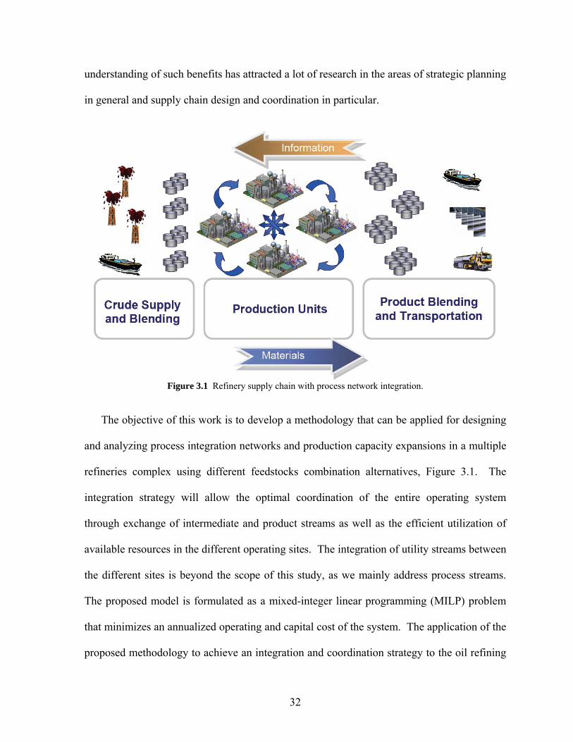
32
understanding of such benefits has attracted a lot of research in the areas of strategic planning
in general and supply chain design and coordination in particular.
Figure 3.1 Refinery supply chain with process network integration.
The objective of this work is to develop a methodology that can be applied for designing
and analyzing process integration networks and production capacity expansions in a multiple
refineries complex using different feedstocks combination alternatives, Figure 3.1. The
integration strategy will allow the optimal coordination of the entire operating system
through exchange of intermediate and product streams as well as the efficient utilization of
available resources in the different operating sites. The integration of utility streams between
the different sites is beyond the scope of this study, as we mainly address process streams.
The proposed model is formulated as a mixed-integer linear programming (MILP) problem
that minimizes an annualized operating and capital cost of the system. The application of the
proposed methodology to achieve an integration and coordination strategy to the oil refining
33
industry adds more complications and challenges. This is due to the fact that refining is one
of the most complex chemical industries which comprises complicated processes and various
configurations and structural alternatives. Although the MILP model was developed and
applied to the refining industry in this study, it can be extended to any network of chemical
processes. Since the decisions in this study are of a long-term planning horizon, a linear
model formulation is adequate to capture the required details of refinery processes (Zhang &
Zhu, 2006). All capital cost investments were discounted over a time horizon in order to
support a net present worth analysis.
Bok et al. (2000) explained a classification of chemical process networks and
characterized them as either dedicated or flexible processes. Dedicated processes operate at
one mode and for high volume products whereas flexible processes operate at different
modes and produce different products at different times. In our formulation, we account for
different operating modes. This should not be confused with flexible processes as the
different modes in this study represent different product yields and do not require any set up
costs or changeover times.
The remainder of Chapter 3 is organized as follows. In the following section we will
provide a literature review on process expansions and multisite planning and coordination
studies in the chemical process industry. Then we will explain the problem statement and
proposed model formulation in section 3.3 and 3.4, respectively. In section 3.5, we will
illustrate the performance of the model through various industrial-scale refinery examples
and scenarios. The Chapter ends with some concluding remarks in section 3.6.
34
3.2 Literature Review
There has been quite a large stream of research concerned with capacity expansions and
retrofit problems in the chemical and operations research literature. In this section, however,
we will concentrate on expansion and strategic multisite planning studies. Single site short-
term and mid-term planning and scheduling studies are beyond the scope of this thesis and
the interested reader is referred to the work by Bodington and Baker (1990), Pinto and Moro
(2000), and Kallrath (2005).
One of the early attempts in the operations research literature that considered multiple
echelons and sites seems to be that of Williams (1981). Williams investigated different
heuristic techniques of varying sophistication for production-distribution scheduling.
Although he used simplifying assumptions, his work is one of the early attempts in the
operations research literature in the use of coordinated planning across multiple echelons and
sites. In the process systems engineering community, large scale multisite planning and
coordination models had a bigger share just recently.
Many earlier studies tackled different expansion problems in the chemical industry
including the NLP formulation by Himmelblau and Bickel (1980) and multiperiod MILP
model by Grossmann and Santibanez (1980) and the recursive MILP model by Jimenez and
Rudd (1987). A common drawback among these studies was their limitation of problem size
due to computational burden. Other papers on capacity expansions can be found in Roberts
(1964), Manne (1967) and Florian et al. (1980) where discussions of how relevant these
problems are to the industry are also provided. More recently, Sahinidis et al. (1989)
developed a multiperiod MILP model for strategic planning in terms of selection and
35
expansion of processes given forecasted demands and prices. In their study, they
investigated several solution strategies to reduce model computational burden. The strategies
included branch and bound, integer cuts, cutting planes, Benders decomposition and other
heuristics. This model was later reformulated by Sahinidis and Grossmann (1991a, 1992) by
identifying a lot sizing problem structure within the long-range problem formulation. The
new reformulation improved the solution efficiency through tighter linear relaxation to the
MILP model. The model was expanded to include continuous and batch flexible and
dedicated processes (Sahinidis & Grossmann, 1991b). Along the same lines, Norton and
Grossmann (1994) extended the work by Sahinidis et al. (1989) to account for dedicated and
flexible processes in terms of feedstocks, products and the combination of continuous and
batch processes. They illustrated their example on a petrochemical complex.
Wilkinson et al. (1996) proposed an approach that integrates production and distribution
in multisite facilities using the resource task network representation proposed by Pantelides
(1994). They applied this technique to an industrial case across a whole continent that
involved the production and distribution planning among different factories and markets. In
a similar problem, McDonald and Karimi (1997) studied multiple semicontinuous facilities in
a number of geographically distributed customers. The aim was to find an optimal
allocation of recourses to tasks to meet a certain demand over a time horizon. They included
a number of additional supply chain type constraints such as single sourcing, internal
sourcing, and transportation times.
Iyer and Grossmann (1998) revisited the work by Sahinidis et al. (1989) and used a
bilevel decomposition approach to reduce the computational complexity of the problem with
the objective of solving larger scenarios. In a similar effort, Bok et al. (2000) extended the
36
work by Norton and Grossmann (1994) to incorporate operational decisions over a short term
horizon such as inventory profile, changeover cost, and intermittent supplies over multiple
operating sites. They also used a bilevel decomposition approach to reduce computational
time and illustrated their approach on several examples dealing with a petrochemical
complex. Their model addressed short term operating decisions and provided no insight on
designing or retrofitting the process network.
Shah (1998) presented a review of the production planning and scheduling in single and
multiple facilities. He pointed out that multisite problems have received little attention and
are potential candidates for future research. Bunch et al. (1998) developed MILP model to
find the lowest cost alternative among existing geographically distributed pharmaceutical
facilities to satisfy a given demand. The model was used to find optimal assignment of
products to facilities and production quantities over a time horizon. They used a commercial
scheduling software (VirtECS) for both problem representation and solution. In their study,
there was no clear underlying structure of the problem or a systematic approach for the
model formulation. Furthermore, the solution approach did not guarantee optimality.
Timpe and Kallrath (2000) developed a multi-period MILP model for a complete supply
chain management of a multisite production network. The problem was formulated and
applied to the food industry. The model concentrated on the coordination of the different
echelons of the food supply chain and did not cover developing an integration scheme for the
multiste facilities. Swaty (2002) studied the possibility of integrating a refinery and an
ethylene plant through the exchange of process intermediate streams. The analysis was based
on a linear programming (LP) model for each plant and profit marginal analysis of possible
intermediate plant exchange. The study was implemented on a real life application in
37
western Japan. Jackson and Grossmann (2003) proposed a multiperiod nonlinear
programming model for production planning and distribution over multisite facilities. They
used a temporal decomposition technique to reduce the scale of the problem.
Lasschuit and Thijssen (2004) pointed out the importance of developing integrated
supply chain planning models on both strategic and tactical levels in the petroleum and
chemical industry. They also stressed on the issues that need to be accounted for when
formulating these models. Neiro and Pinto (2004) proposed a general framework for
modeling operational planning of the petroleum supply chain. They developed MINLP
model for the planning of multiple existing refineries, terminals and pipeline networks.
Decisions included the selection of oil types and scheduling plan to the refineries subject to
quality constraints as well as processing units, operating variables, product distribution, and
inventory management. The model was applied to an industrial case in Brazil. Due to the
high computational burden, the model was only solved for two time periods. The authors
suggested that decomposition methods should be applied to yield a smaller MINLP or MILP
model. Their approach did not consider the design problem of a network of operating
facilities as their formulation addressed only operational type decisions.
Ryu and Pistikopoulos (2005) presented MILP model for the design of enterprise-wide
supply chains in the chemical industry. They investigated three different operating policies,
namely, competition, cooperation and coordination. Their model was based on the
assumption that plants will always have much larger capacities than demand. Furthermore,
their work was mainly concerned with optimizing the operating policies among the different
echelons of the supply chain and did not account for designing an integration policy between
the multisite production facilities.
38
Khogeer (2005) developed a LP model for multiple refinery coordination. He developed
different scenarios to experiment with the effect of catastrophic failure and different
environmental regulation changes on the refineries performance. This work was developed
using commercial planning software (Aspen PIMS). In his study, there was no model
representation of the refineries systems or clear simultaneous representation of optimization
objective functions. Such an approach deprives the study from its generalities and limits the
scope to a narrow application. Furthermore, no process integration or capacity expansions
were considered.
Another stream of research tackled modeling uncertainty in capacity expansion and
supply chain studies in the process industry. Ierapetritou and Pistikopoulos (1994) developed
a two-stage stochastic programming model for short to long-term planning problems. They
proposed a decomposition method based on the generalized Benders decomposition
algorithm where they used a Gaussian quadrature to estimate the expectation of the objective
function. Liu and Sahinidis (1995; 1996; 1997) studied design uncertainty in process
expansion through sensitivity analysis, stochastic programming and fuzzy programming,
respectively. In their stochastic model, they used Monte Carlo sampling to calculate the
expected objective function values. Their comparison over the different methodology of
including uncertainty was in favor of stochastic models when random parameters
distributions are not available.
On a larger scale, Tsiakis et al. (2001) developed a supply chain design for multiple
markets and plants of steady-state continuous processes. Similarly, Ryu et al. (2004)
presented a bilevel framework for planning an enterprise-wide network under uncertainty of
some product demands plant and warehouse capacities as well as resource availability. They
39
considered the hierarchy of the supply chain and allowed for optimizing different levels of
the chain individually.
The above discussion clearly points out the importance of multisite planning and
indicates that such a problem is attracting a great deal of interest as the realizations of the
coordinated benefits became more vivid. However, to the best of our knowledge, no
previous work has tackled developing a general framework for designing a network between
multiple refineries in terms of material exchange. The aim of this study is to provide a
methodology of the design of an integration and coordination policy of multiple refineries to
explore potential synergies and efficient utilization of resources across an enterprise or
multiple enterprises. The expansions of the facilities and the construction of the integration
network are assumed to be implemented simultaneously in a single time horizon in order to
minimize future process interruptions. Although our discussion will consistently refer to a
network of refineries, the methodology that we will present can be readily extended to other
chemical process networks.
3.3 Problem Statement
The optimization of refining processes involves a broad range of aspects varying from
economical analysis and strategic expansions to crude oil selection, process levels targets,
operating modes, etc. The focus of this study is the development of a methodology for
designing an integrated network and production expansion across multiple refineries as well
as the establishment of an operating policy that sets feedstock combinations, process levels
and operating mode preferences to satisfy a given demand. Such integration will provide
40
appropriate means for improving the coordination across the whole network production
system.
The general integration problem can be defined as:
A set of products CFRcfr∈ to be produced at multiple refinery sites Ii∈ is given. Each
refinery consists of different production units RefMm∈ that can operate at different
operating modes Pp∈ . An optimal feedstock from different available crudes CRcr∈ is
desired. Furthermore, the process network across the multiple refineries is connected in a
finite number of ways and an integration superstructure is defined. Market product prices,
operating cost at each refinery, as well as product demands are assumed to be known.
The problem consists of determining the optimal integration for the overall network and
associated coordination strategies across the refinery facilities as well as establishing an
optimal overall production and determining the operating levels for each refinery site. The
objective is to minimize the annualized cost over a given time horizon by improving the
coordination and utilization of excess capacities in each facility. Expansion requirements to
improve production flexibility and reliability are also considered.
For all refinery processes within the network we assume that all material balances are
expressed in terms of linear yield vectors. Even though this might sound to be restrictive as
most if not all refinery processes are inherently nonlinear, this practice is commonly applied
in the petroleum refining business. Moreover, the decisions in this study are of a strategic
level in which such linear formulation is adequate to address the required level of details
involved at this stage. It is also assumed that processes have fixed capacities and the
41
operating cost of each process and production mode is proportional to the process inlet flow.
In the case of product blending, quality blending indices are used to maintain model linearity.
Blending indices tables and graphs can often be found in petroleum refining books such as
Gary and Handwerk (1994) or can be proprietarily developed by refining companies for their
own use. It is also assumed that all products that are in excess of the local demand can be
exported to a global market. Piping and pumping installation costs to transport intermediate
streams as well as the operating costs of the new system were lumped into one fixed-charge
cost. All costs are discounted over a 20 years time horizon and with an interest rate of 7%.
No inventories will be considered since the model is addressing strategic decisions which
usually cover a long period of time. We also assume perfect mixing and that the properties
of each crude type are decided by specific key components. Properties of the oil mixture,
such as viscosity, do not affect the strategic decisions of network design immensely and are
therefore not considered in the model. Such considerations renders the model unnecessary
complicated and are even tolerable on studies of operational planning and scheduling level
(Lee et al., 1996; Jia & Ierapetritou, 2003, 2004).
3.4 Model Formulation
The model is formulated based on the State Equipment Network (SEN) representation
(Yeomans & Grossmann, 1999). The general characterization of this representation includes
three elements: state, task and equipment. A State includes all streams in a process and is
characterized by either quantitative or qualitative attributes or both. The quantitative
characteristics include flowrate, temperature and pressure whereas the qualitative
characteristics include other attributes such as the phase(s) of the streams. A task, on the
other hand, represents the physical and chemical transformations that occur between
42
consecutive states. Equipment provides the physical devices that execute a given task (e.g.
reactor, absorber, heat exchanger).
The state equipment network (SEN) allows for two types of task to equipment
assignment: The first type is one task-one equipment (OTOE) assignment where tasks are
assigned to equipment a priori. This type of assignment yields an identical representation to
the state task network (STN) by Kondili et al. (1993). The second type is the variable task
equipment assignment where the actual assignment of tasks to equipment is considered as
part of the optimization problem. The use of this representation provides a consistent
modeling strategy and an explicit handling of units that operate under different modes, which
is common in the refining industry.
In treating stream mixing, the mixing device was defined as part of the designated
refinery operation itself. This approach was also undertaken by Zhang and Zhu (2006).
Therefore the only mixers considered are where the final blending takes place. This
approach distinguishes the contribution of each feedstock to the final product. With this type
of formulation, all variables and attributes of intermediate streams will depend on the crude
type.
The problem is formulated as an MILP model where binary variables are used for
designing the process integration network between the refineries and deciding on the
production unit expansion alternatives. Linearity in the model was achieved by defining
component flows instead of individual flows and associated fractions. The planning problem
formulation is as follows.
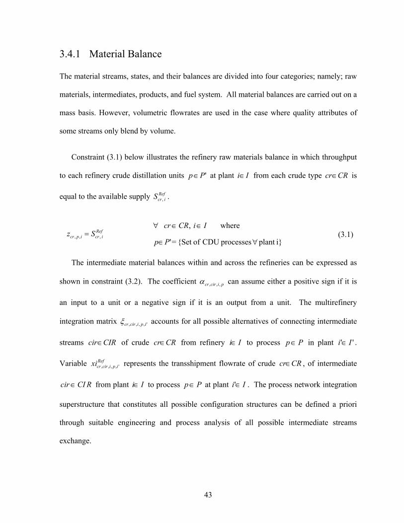
43
3.4.1 Material Balance
The material streams, states, and their balances are divided into four categories; namely; raw
materials, intermediates, products, and fuel system. All material balances are carried out on a
mass basis. However, volumetric flowrates are used in the case where quality attributes of
some streams only blend by volume.
Constraint (3.1) below illustrates the refinery raw materials balance in which throughput
to each refinery crude distillation units 'Pp∈ at plant Ii∈ from each crude type CRcr∈ is
equal to the available supply ReficrS , .
Reficripcr Sz ,,, =
∀ IiCRcr ∈∈ , where
i}plant processes CDU of{Set =' ∀∈Pp (3.1)
The intermediate material balances within and across the refineries can be expressed as
shown in constraint (3.2). The coefficient picircr ,,,α can assume either a positive sign if it is
an input to a unit or a negative sign if it is an output from a unit. The multirefinery
integration matrix ',,,, ipicircrξ accounts for all possible alternatives of connecting intermediate
streams CIRcir∈ of crude CRcr∈ from refinery Ii∈ to process Pp∈ in plant '' Ii∈ .
Variable Refipicircrxi ',,,, represents the transshipment flowrate of crude CRcr∈ , of intermediate
RCIcir∈ from plant Ii∈ to process Pp∈ at plant Ii∈' . The process network integration
superstructure that constitutes all possible configuration structures can be defined a priori
through suitable engineering and process analysis of all possible intermediate streams
exchange.
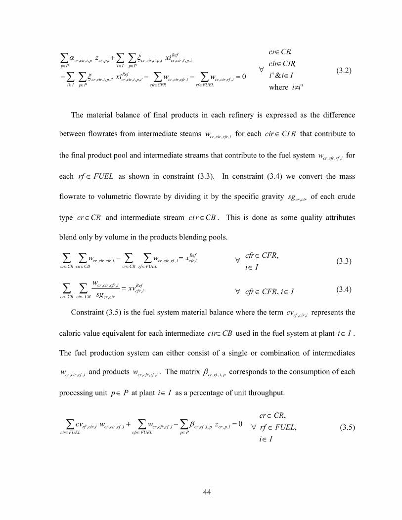
44
0,,,,,,',,,,'
',,,,
,,',,'
,,',,,,,,,
=−−−
+
∑∑∑ ∑
∑ ∑∑
∈∈∈ ∈
∈ ∈∈
FUELrfirfcircr
CFRcfricfrcircr
Refipicircr
Ii Ppipicircr
Refipicircr
Ii Ppipicircr
Ppipcrpicircr
wwxi
xiz
ξ
ξα ∀
'where&'
,,
iiIii
CIRcirCRcr
≠∈
∈∈
(3.2)
The material balance of final products in each refinery is expressed as the difference
between flowrates from intermediate steams icfrcircrw ,,, for each RCIcir∈ that contribute to
the final product pool and intermediate streams that contribute to the fuel system irfcfrcrw ,,, for
each FUELrf ∈ as shown in constraint (3.3). In constraint (3.4) we convert the mass
flowrate to volumetric flowrate by dividing it by the specific gravity circrsg , of each crude
type CRcr∈ and intermediate stream CBrci ∈ . This is done as some quality attributes
blend only by volume in the products blending pools.
∑ ∑ ∑∑∈ ∈ ∈∈
=−CRcr
Refcfr,i
CRcr FUELrfirfcfrcr
CBciricfrcircr xww ,,,,,, ∀
IiCFRcfr
∈∈ , (3.3)
∑ ∑∈ ∈
=CRcr
Reficfr
CBcir circr
icfrcircr xvsg
w,
,
,,, ∀ IiCFRcfr ∈∈ , (3.4)
Constraint (3.5) is the fuel system material balance where the term icirrfcv ,, represents the
caloric value equivalent for each intermediate CBrci ∈ used in the fuel system at plant Ii∈ .
The fuel production system can either consist of a single or combination of intermediates
irfcircrw ,,, and products irfcfrcrw ,,, . The matrix pirfcr ,,,β corresponds to the consumption of each
processing unit Pp∈ at plant Ii∈ as a percentage of unit throughput.
∑∑∑∈∈∈
=−+Pp
ipcrpirfcrFUELcfr
irfcfrcrFUELcir
irfcircricirrf zwwcv 0,,,,,,,,,,,,, β ∀Ii
FUELrfCRcr
∈∈∈
,,
(3.5)
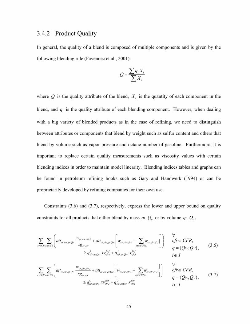
45
3.4.2 Product Quality
In general, the quality of a blend is composed of multiple components and is given by the
following blending rule (Favennec et al., 2001):
∑∑=
i
ii
XXq
Q
where Q is the quality attribute of the blend, iX is the quantity of each component in the
blend, and iq is the quality attribute of each blending component. However, when dealing
with a big variety of blended products as in the case of refining, we need to distinguish
between attributes or components that blend by weight such as sulfur content and others that
blend by volume such as vapor pressure and octane number of gasoline. Furthermore, it is
important to replace certain quality measurements such as viscosity values with certain
blending indices in order to maintain model linearity. Blending indices tables and graphs can
be found in petroleum refining books such as Gary and Handwerk (1994) or can be
proprietarily developed by refining companies for their own use.
Constraints (3.6) and (3.7), respectively, express the lower and upper bound on quality
constraints for all products that either blend by mass wQq∈ or by volume vQq∈ .
Refcfr,i
LQwqcfr
Reficfr
LQvqcfr
CRcr CBcir FUELrfirfcfrcricfrcircrQwqcircr
circr
icfrcircrQvqcircr
xqxvq
wwattsg
watt
∈∈
∈ ∈ ∈∈∈
+≥
⎟⎟⎠
⎞⎜⎜⎝
⎛⎥⎦
⎤⎢⎣
⎡−+∑ ∑ ∑
,,,
,,,,,,,,,
,,,,,
∀
IiQvQwq
CFRcfr
∈=∈
},,{,
(3.6)
Refcfr,i
UQwqcfr
Reficfr
UQvqcfr
CRcr CBcir FUELrfirfcfrcricfrcircrQwqcircr
circr
icfrcircrQvqcircr
xqxvq
wwattsg
watt
∈∈
∈ ∈ ∈∈∈
+≤
⎟⎟⎠
⎞⎜⎜⎝
⎛⎥⎦
⎤⎢⎣
⎡−+∑ ∑ ∑
,,,
,,,,,,,,,
,,,,,
∀
IiQvQwq
CFRcfr
∈=∈
},,{,
(3.7)
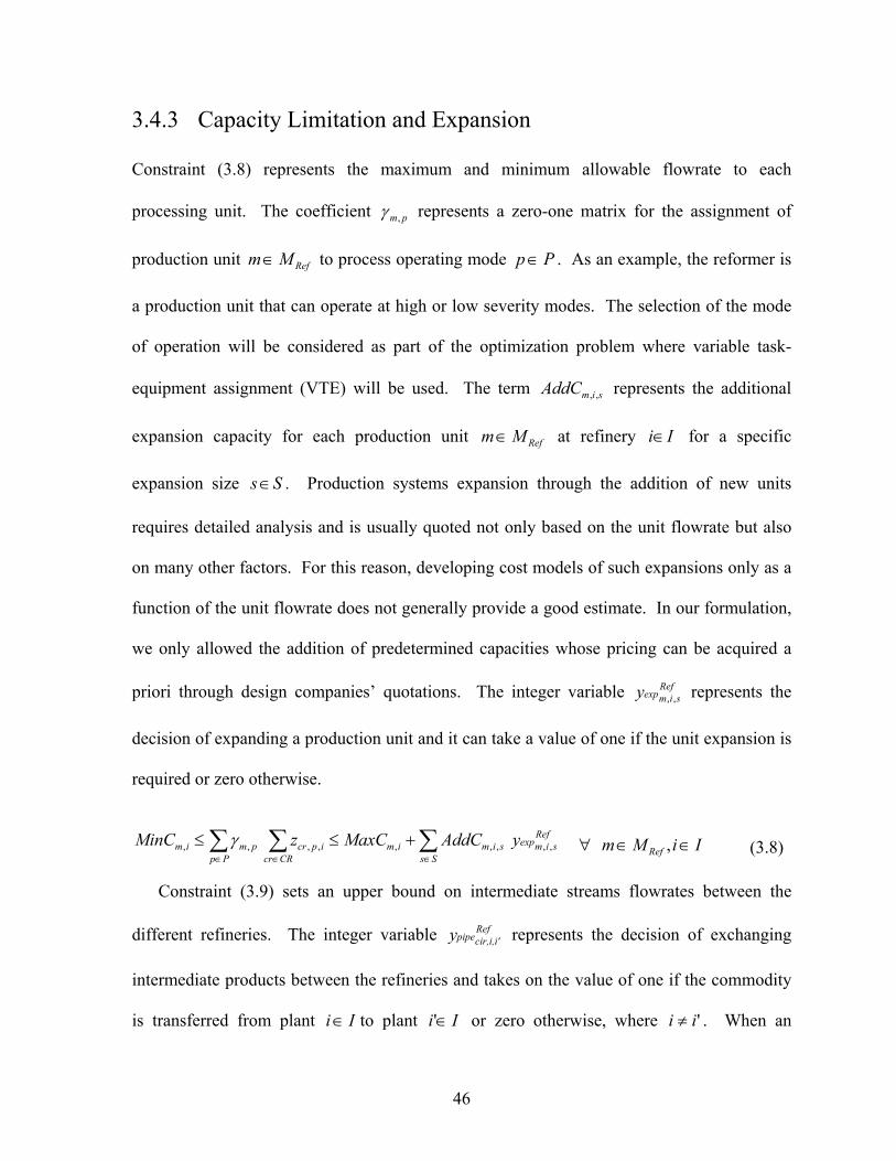
46
3.4.3 Capacity Limitation and Expansion
Constraint (3.8) represents the maximum and minimum allowable flowrate to each
processing unit. The coefficient pm,γ represents a zero-one matrix for the assignment of
production unit RefMm∈ to process operating mode Pp∈ . As an example, the reformer is
a production unit that can operate at high or low severity modes. The selection of the mode
of operation will be considered as part of the optimization problem where variable task-
equipment assignment (VTE) will be used. The term simAddC ,, represents the additional
expansion capacity for each production unit RefMm∈ at refinery Ii∈ for a specific
expansion size Ss∈ . Production systems expansion through the addition of new units
requires detailed analysis and is usually quoted not only based on the unit flowrate but also
on many other factors. For this reason, developing cost models of such expansions only as a
function of the unit flowrate does not generally provide a good estimate. In our formulation,
we only allowed the addition of predetermined capacities whose pricing can be acquired a
priori through design companies’ quotations. The integer variable Refsimexpy ,, represents the
decision of expanding a production unit and it can take a value of one if the unit expansion is
required or zero otherwise.
∑∑ ∑∈∈ ∈
+≤≤Ss
Refsimexpsim
Ppim
CRcripcrpmim yAddCMaxCzMinC ,,,,,,,,, γ ∀ IiMm Ref ∈∈ , (3.8)
Constraint (3.9) sets an upper bound on intermediate streams flowrates between the
different refineries. The integer variable Refcir,i,i'pipey represents the decision of exchanging
intermediate products between the refineries and takes on the value of one if the commodity
is transferred from plant Ii∈ to plant Ii∈' or zero otherwise, where 'ii ≠ . When an
47
intermediate stream is selected to be exchanged between two refineries, its flowrate must be
below the transferring pipeline capacity UiicirF ',, .
∑ ∑∈ ∈
≤CRcr
Refcir,i,i'pipe
Uiicir
Pp
Refipicircripicircr yFxi ',,',,,,',,,,ξ ∀
'where&',
iiIiiCIRcir
≠∈∈
(3.9)
3.4.4 Product Demand
Constraint (3.10) stipulates that the final products from each refinery Refcfr,ix less the amount
exported Reficfre ,' for each exportable product PEXcfr ∈' from each plant Ii∈ must satisfy the
domestic demand cfrRefD .
( ) cfrRefIi
Reficfr
Refcfr,i Dex ≥−∑
∈', ∀
PEXcfrCFRcfrcfrcfr
∈∈ ',where'&
(3.10)
3.4.5 Import Constraint
The imports or resources constraint (3.11) imposes upper and lower bounds on the available
feedstock CRcr∈ to the refineries. The lower bound constraint might be useful in the cases
where there are protocol agreements to exchange or supply crude oil between countries.
∑∈
≤≤Ii
Ucr
Reficr
Lcr IMSIM , CRcr∈∀ (3.11)
3.4.6 Objective Function
The objective function considered in this study is given by:
48
Reficfr
PEXcfr Ii
Refcfr
Ii Mm Ss
Refsimexpsm
CIRcir Ii
Refcir,i,i'pipe
Iiii
CRcr Iiipcr
Ppp
Reficr
CRcr Iicr
ePr
yInCost
yInCost
zOpCost
SCrCostMin
Ref
,
,,,
'',
,,
,
∑ ∑
∑ ∑ ∑
∑ ∑∑
∑ ∑∑
∑ ∑
∈ ∈
∈ ∈ ∈
∈ ∈ ∈
∈ ∈∈
∈ ∈
−
+
+
+
'where ii ≠ (3.12)
The above objective represents a minimization of the annualized cost which comprises of
crude oil cost, refineries operating cost, refineries intermediate exchange piping cost,
production system expansion cost, and export revenue. The operating cost of each process is
assumed to be proportional to the process inlet flow and is expressed on a yearly basis.
3.5 Illustrative Case Study
In this section, we present two examples with different scenarios. The first example
illustrates the performance of the model on a single site total refinery planning problem
where we compare the results of the model to an industrial scale study from Favennec et al.
(2001). This example serves to validate our model and to make any necessary adjustments.
The second example extends the scale of the model application to cover three complex
refineries in which we demonstrate the different aspects of the model. The refineries
considered are of large industrial-scale refineries and actually mimic a general set up of many
areas around the world. The decisions in this example include the selection of crude blend
combination, design of process integration network between the three refineries, and
decisions on production units’ expansion options and operating levels.
49
The modeling system GAMS (Brooke et al., 1996) was used for setting up the
optimization models and the problems are solved by BDMLP 1.3 on a Pentium M processor
2.13 GHz.
3.5.1 Single Refinery Planning
Figure 3.2 provides a SEN representation of the refinery considered in this example. The
planning horizon was set to one month in order to compare the model results to those of
Favennec et al. (2001). As shown in Figure 3.2, the refinery uses two different feedstocks
(e.g. Arabian light and Kuwait crudes) where the optimum blend is used to feed the
atmospheric crude unit. The atmospheric crude unit separates crude oil into several fractions
including LPG, naphtha, kerosene, gas oil and residues. The heavy residues are then sent to
the vacuum unit where they are further separated into vacuum gas oil and vacuum residues.
Depending on the production targets, different processing and treatment processes are
applied to the crude fractions. In this example, the naphtha is further separated into heavy
and light naphtha. Heavy naphtha is sent to the catalytic reformer unit to produce high
octane reformates for gasoline blending and light naphtha is sent to light naphtha pool and to
an isomerization unit to produce isomerate for gasoline blending too. The middle distillates
are combined with other similar intermediate streams and sent for hydrotreating and then for
blending to produce jet fuels and gas oils. Atmospheric and vacuum gas oils are further
treated by catalytic cracking and in other cases by hydrocracking or both to increase the
gasoline and distillate yields. In some refineries, vacuum residues are further treated using
cooking and thermal processes to increase light products yields. The final products in
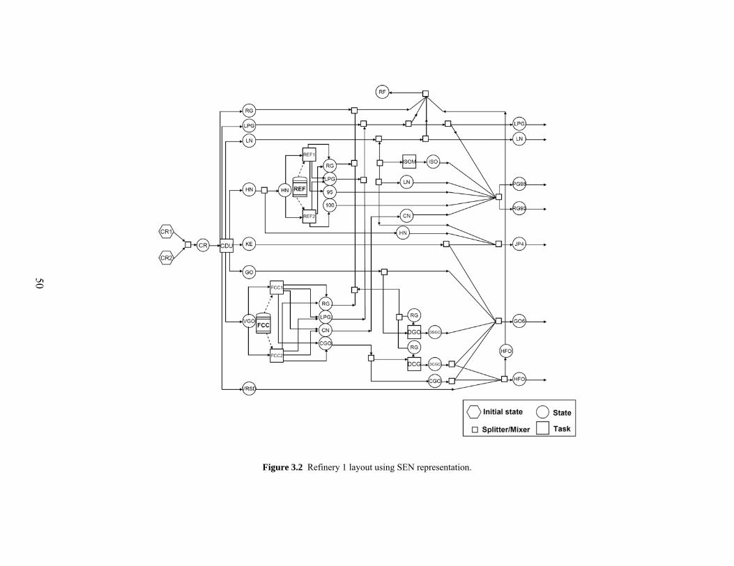
50
Figure 3.2 Refinery 1 layout using SEN representation.
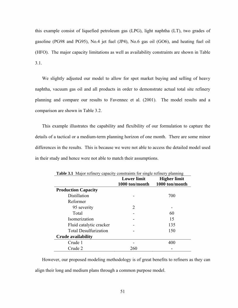
51
this example consist of liquefied petroleum gas (LPG), light naphtha (LT), two grades of
gasoline (PG98 and PG95), No.4 jet fuel (JP4), No.6 gas oil (GO6), and heating fuel oil
(HFO). The major capacity limitations as well as availability constraints are shown in Table
3.1.
We slightly adjusted our model to allow for spot market buying and selling of heavy
naphtha, vacuum gas oil and all products in order to demonstrate actual total site refinery
planning and compare our results to Favennec et al. (2001). The model results and a
comparison are shown in Table 3.2.
This example illustrates the capability and flexibility of our formulation to capture the
details of a tactical or a medium-term planning horizon of one month. There are some minor
differences in the results. This is because we were not able to access the detailed model used
in their study and hence were not able to match their assumptions.
Table 3.1 Major refinery capacity constraints for single refinery planning Lower limit
1000 ton/month Higher limit
1000 ton/month Production Capacity
Distillation - 700 Reformer 95 severity 2 - Total - 60 Isomerization - 15 Fluid catalytic cracker - 135 Total Desulfurization - 150
Crude availability Crude 1 - 400 Crude 2 260 -
However, our proposed modeling methodology is of great benefits to refiners as they can
align their long and medium plans through a common purpose model.
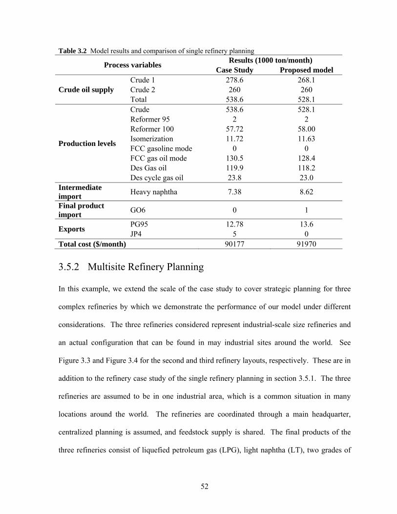
52
Table 3.2 Model results and comparison of single refinery planning Results (1000 ton/month) Process variables Case Study Proposed model
Crude 1 278.6 268.1 Crude 2 260 260 Crude oil supply Total 538.6 528.1 Crude 538.6 528.1 Reformer 95 2 2 Reformer 100 57.72 58.00 Isomerization 11.72 11.63 FCC gasoline mode 0 0 FCC gas oil mode 130.5 128.4 Des Gas oil 119.9 118.2
Production levels
Des cycle gas oil 23.8 23.0 Intermediate import Heavy naphtha 7.38 8.62
Final product import GO6 0 1
PG95 12.78 13.6 Exports JP4 5 0 Total cost ($/month) 90177 91970
3.5.2 Multisite Refinery Planning
In this example, we extend the scale of the case study to cover strategic planning for three
complex refineries by which we demonstrate the performance of our model under different
considerations. The three refineries considered represent industrial-scale size refineries and
an actual configuration that can be found in may industrial sites around the world. See
Figure 3.3 and Figure 3.4 for the second and third refinery layouts, respectively. These are in
addition to the refinery case study of the single refinery planning in section 3.5.1. The three
refineries are assumed to be in one industrial area, which is a common situation in many
locations around the world. The refineries are coordinated through a main headquarter,
centralized planning is assumed, and feedstock supply is shared. The final products of the
three refineries consist of liquefied petroleum gas (LPG), light naphtha (LT), two grades of
53
gasoline (PG98 and PG95), No. 4 jet fuel (JP4), military jet fuel (ATKP), No.6 gas oil
(GO6), diesel fuel (Diesel), heating fuel oil (HFO), and petroleum coke (coke). We will now
consider several practical scenarios to demonstrate the advantage of the proposed integration
model and its robustness under different considerations.
Scenario-1: single feedstock, multiple refineries with no integration. In this scenario,
the three refineries are using a single feedstock type, Arabian Light, and operate centrally
with no network integration alternatives. The major model constraints and results are shown
in Table 3.3 and Table 3.4, respectively. The three refineries collaborate to satisfy a given
local market demand where the model provides the production and blending level targets for
the individual sites. Products that exceeded local market demand are either sold in the spot
market or exported. The annual production cost across the facilities was found to be
$7,118,000.
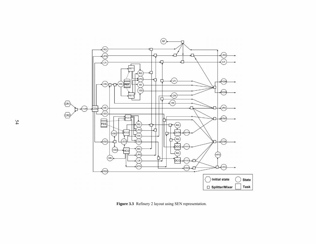
54
Figure 3.3 Refinery 2 layout using SEN representation.
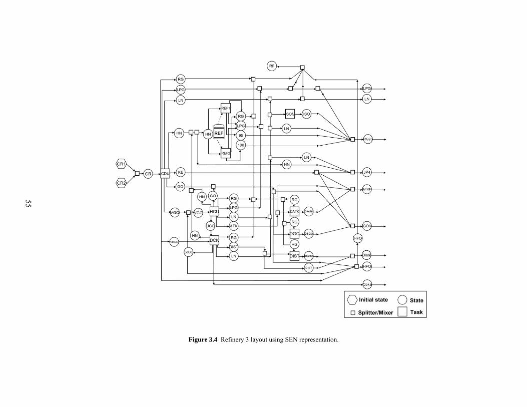
55
Figure 3.4 Refinery 3 layout using SEN representation.
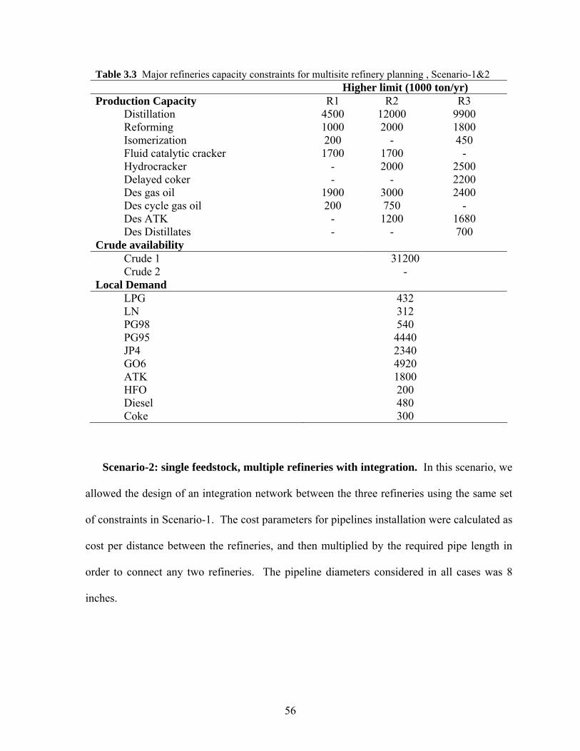
56
Table 3.3 Major refineries capacity constraints for multisite refinery planning , Scenario-1&2 Higher limit (1000 ton/yr) Production Capacity R1 R2 R3
Distillation 4500 12000 9900 Reforming 1000 2000 1800 Isomerization 200 - 450 Fluid catalytic cracker 1700 1700 - Hydrocracker - 2000 2500 Delayed coker - - 2200 Des gas oil 1900 3000 2400 Des cycle gas oil 200 750 - Des ATK - 1200 1680 Des Distillates - - 700
Crude availability Crude 1 31200 Crude 2 -
Local Demand LPG 432 LN 312 PG98 540 PG95 4440 JP4 2340 GO6 4920 ATK 1800 HFO 200 Diesel 480 Coke 300
Scenario-2: single feedstock, multiple refineries with integration. In this scenario, we
allowed the design of an integration network between the three refineries using the same set
of constraints in Scenario-1. The cost parameters for pipelines installation were calculated as
cost per distance between the refineries, and then multiplied by the required pipe length in
order to connect any two refineries. The pipeline diameters considered in all cases was 8
inches.
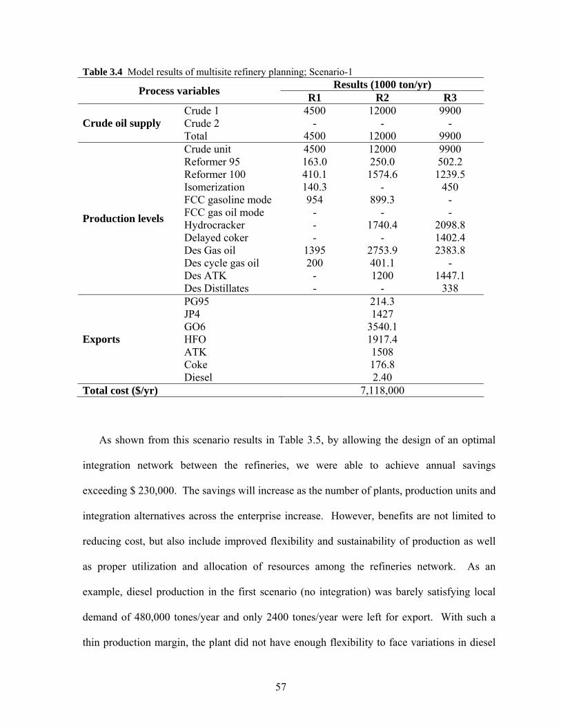
57
Table 3.4 Model results of multisite refinery planning; Scenario-1 Results (1000 ton/yr) Process variables R1 R2 R3
Crude 1 4500 12000 9900 Crude 2 - - - Crude oil supply Total 4500 12000 9900 Crude unit 4500 12000 9900 Reformer 95 163.0 250.0 502.2 Reformer 100 410.1 1574.6 1239.5 Isomerization 140.3 - 450 FCC gasoline mode 954 899.3 - FCC gas oil mode - - - Hydrocracker - 1740.4 2098.8 Delayed coker - - 1402.4 Des Gas oil 1395 2753.9 2383.8 Des cycle gas oil 200 401.1 - Des ATK - 1200 1447.1
Production levels
Des Distillates - - 338 PG95 214.3 JP4 1427 GO6 3540.1 HFO 1917.4 ATK 1508 Coke 176.8
Exports
Diesel 2.40 Total cost ($/yr) 7,118,000
As shown from this scenario results in Table 3.5, by allowing the design of an optimal
integration network between the refineries, we were able to achieve annual savings
exceeding $ 230,000. The savings will increase as the number of plants, production units and
integration alternatives across the enterprise increase. However, benefits are not limited to
reducing cost, but also include improved flexibility and sustainability of production as well
as proper utilization and allocation of resources among the refineries network. As an
example, diesel production in the first scenario (no integration) was barely satisfying local
demand of 480,000 tones/year and only 2400 tones/year were left for export. With such a
thin production margin, the plant did not have enough flexibility to face variations in diesel
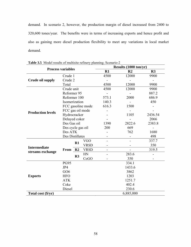
58
demand. In scenario 2, however, the production margin of diesel increased from 2400 to
320,600 tones/year. The benefits were in terms of increasing exports and hence profit and
also as gaining more diesel production flexibility to meet any variations in local market
demand.
Table 3.5 Model results of multisite refinery planning; Scenario-2 Results (1000 ton/yr) Process variables R1 R2 R3
Crude 1 4500 12000 9900 Crude 2 - - - Crude oil supply Total 4500 12000 9900 Crude unit 4500 12000 9900 Reformer 95 - - 887.2 Reformer 100 573.1 2000 686.9 Isomerization 140.3 - 450 FCC gasoline mode 616.3 1500 - FCC gas oil mode - - - Hydrocracker - 1105 2436.54 Delayed coker - - 2066 Des Gas oil 1390 2822.6 2383.8 Des cycle gas oil 200 669 - Des ATK - 762 1680
Production levels
Des Distillates - - 498 VGO - - 337.7 R1 VRSD - - 350
R2 VRSD - - 319.5 HN - 283.6 -
Intermediate streams exchange From
R3 CoGO - 350 - PG95 334.1 JP4 1433.6 GO6 3862 HFO 1203 ATK 1251.7 Coke 402.4
Exports
Diesel 230.6 Total cost ($/yr) 6,885,000
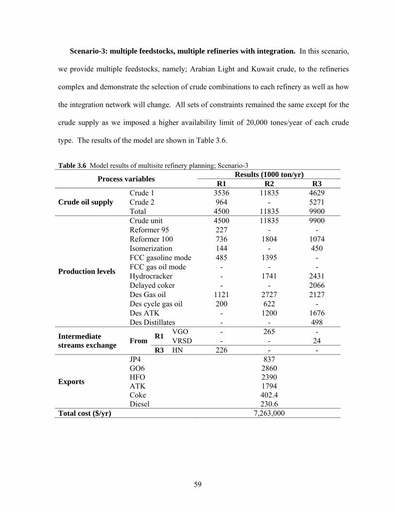
59
Scenario-3: multiple feedstocks, multiple refineries with integration. In this scenario,
we provide multiple feedstocks, namely; Arabian Light and Kuwait crude, to the refineries
complex and demonstrate the selection of crude combinations to each refinery as well as how
the integration network will change. All sets of constraints remained the same except for the
crude supply as we imposed a higher availability limit of 20,000 tones/year of each crude
type. The results of the model are shown in Table 3.6.
Table 3.6 Model results of multisite refinery planning; Scenario-3 Results (1000 ton/yr) Process variables R1 R2 R3
Crude 1 3536 11835 4629 Crude 2 964 - 5271 Crude oil supply Total 4500 11835 9900 Crude unit 4500 11835 9900 Reformer 95 227 - - Reformer 100 736 1804 1074 Isomerization 144 - 450 FCC gasoline mode 485 1395 - FCC gas oil mode - - - Hydrocracker - 1741 2431 Delayed coker - - 2066 Des Gas oil 1121 2727 2127 Des cycle gas oil 200 622 - Des ATK - 1200 1676
Production levels
Des Distillates - - 498 VGO - 265 - R1 VRSD - - 24 Intermediate
streams exchange From R3 HN 226 - -
JP4 837 GO6 2860 HFO 2390 ATK 1794 Coke 402.4
Exports
Diesel 230.6 Total cost ($/yr) 7,263,000
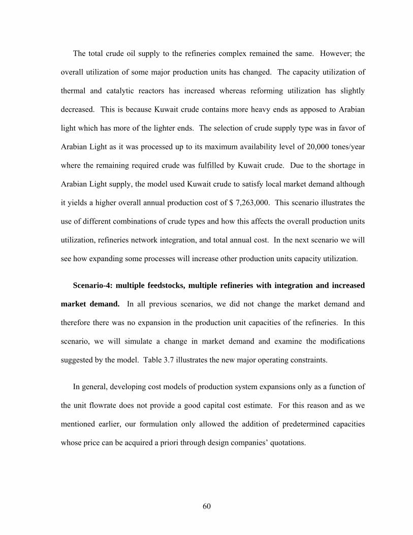
60
The total crude oil supply to the refineries complex remained the same. However; the
overall utilization of some major production units has changed. The capacity utilization of
thermal and catalytic reactors has increased whereas reforming utilization has slightly
decreased. This is because Kuwait crude contains more heavy ends as apposed to Arabian
light which has more of the lighter ends. The selection of crude supply type was in favor of
Arabian Light as it was processed up to its maximum availability level of 20,000 tones/year
where the remaining required crude was fulfilled by Kuwait crude. Due to the shortage in
Arabian Light supply, the model used Kuwait crude to satisfy local market demand although
it yields a higher overall annual production cost of $ 7,263,000. This scenario illustrates the
use of different combinations of crude types and how this affects the overall production units
utilization, refineries network integration, and total annual cost. In the next scenario we will
see how expanding some processes will increase other production units capacity utilization.
Scenario-4: multiple feedstocks, multiple refineries with integration and increased
market demand. In all previous scenarios, we did not change the market demand and
therefore there was no expansion in the production unit capacities of the refineries. In this
scenario, we will simulate a change in market demand and examine the modifications
suggested by the model. Table 3.7 illustrates the new major operating constraints.
In general, developing cost models of production system expansions only as a function of
the unit flowrate does not provide a good capital cost estimate. For this reason and as we
mentioned earlier, our formulation only allowed the addition of predetermined capacities
whose price can be acquired a priori through design companies’ quotations.
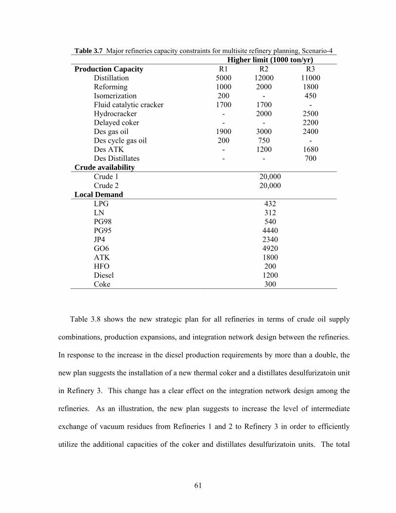
61
Table 3.7 Major refineries capacity constraints for multisite refinery planning, Scenario-4 Higher limit (1000 ton/yr) Production Capacity R1 R2 R3
Distillation 5000 12000 11000 Reforming 1000 2000 1800 Isomerization 200 - 450 Fluid catalytic cracker 1700 1700 - Hydrocracker - 2000 2500 Delayed coker - - 2200 Des gas oil 1900 3000 2400 Des cycle gas oil 200 750 - Des ATK - 1200 1680 Des Distillates - - 700
Crude availability Crude 1 20,000 Crude 2 20,000
Local Demand LPG 432 LN 312 PG98 540 PG95 4440 JP4 2340 GO6 4920 ATK 1800 HFO 200 Diesel 1200 Coke 300
Table 3.8 shows the new strategic plan for all refineries in terms of crude oil supply
combinations, production expansions, and integration network design between the refineries.
In response to the increase in the diesel production requirements by more than a double, the
new plan suggests the installation of a new thermal coker and a distillates desulfurizatoin unit
in Refinery 3. This change has a clear effect on the integration network design among the
refineries. As an illustration, the new plan suggests to increase the level of intermediate
exchange of vacuum residues from Refineries 1 and 2 to Refinery 3 in order to efficiently
utilize the additional capacities of the coker and distillates desulfurizatoin units. The total
62
annual cost has increased to $ 21,463,000 due to the additional units’ capital and operating
costs.
Table 3.8 Model results of multisite refinery planning; Scenario-4 Results (1000 ton/yr) Process variables R1 R2 R3
Crude 1 3077 8293 6059 Crude 2 1923 1333 4420 Crude oil supply Total 5000 9626 10479 Crude unit 5000 9626 10479 Reformer 95 276 - 19 Reformer 100 724 2000 610 Isomerization 163 - 450 FCC gasoline mode 751 1595 - FCC gas oil mode - - - Hydrocracker - 1065 2500 Delayed coker - - 3490 Des Gas oil 1900 3000 1089 Des cycle gas oil 200 712 - Des ATK - 1200 1258
Production levels
Des Distillates - - 841 GO - 52 - VGO - 216 - R1 VRSD - - 400
R2 VRSD - - 400 HN 242 332 - GO 400 400 - ATK - 240 -
Intermediate streams exchange From
R3
UCO - 23 - Delayed Coker - - 1380 Process
Expansions Des Distillates - - 600 JP4 543 GO6 2655 HFO 1217 ATK 1272 Coke 886
Exports
Diesel - Total cost ($/yr) 21,463,000
63
3.6 Conclusion
A mixed-integer programming model for minimizing cost in the strategic planning of
multirefineries network was presented. The objective was to develop a methodology for
designing a process integration network and production capacity expansions in a multiple
refinery complex using different feedstock alternatives. Two examples with multiple
scenarios of large-scale refineries were solved to illustrate the performance of the proposed
design methodology and to show the economic potential and trade-offs involved in the
optimization of such systems. The integration specifically addressed intermediate material
transfer between processing units at each site. In the formulation, bilinear mixing equations
were avoided by introducing individual component flows in order to maintain linearity.
Petroleum refining is a central and crucial link in the oil supply chain and has received
extensive attention over the last decades. However, despite all the progress that has been
made in developing planning and scheduling models a general purpose model is still a target
(Grossmann, 2005). A general model that can be used for different planning levels, short,
medium and long range will be of great benefit in terms of seamless interactions of these
functions. In this work we showed the capability of the proposed model in capturing all
details required for medium-range and tactical planning as illustrated by Example 1. This is
a step forward in achieving such vertical integration among all planning hierarchies.
In our study, all parameters were assumed to be deterministic. However, the current
situation of fluctuating petroleum crude oil prices and demands is an indication that markets
and industries everywhere are impacted by uncertainties. For example, source and
availability of crude oils as the raw material; prices of feedstock, chemicals, and
64
commodities; production costs; and future market demand for finished products will have a
direct impact on final decisions. Thus, acknowledging the shortcomings of deterministic
models, the next phase of our investigation will be considering uncertainties in the design
problem.
65
Chapter 4
Robust Optimization of Multisite Refinery Network: Integration and Coordination
4.1 Introduction
Today the petroleum refining industry is facing a challenging task to remain competitive in a
globalized market. High crude oil prices and growing stringent international protocols and
regulations force petroleum companies to embrace every opportunity that increases their
profit margin. A common solution is to seek integration alternatives not only within a single
facility but also on an enterprise-wide scale. This will provide enhanced utilization of
resources and improved coordination and therefore achieve a global optimal production
strategy within the network. However, considering such highly strategic planning decisions,
particularly in the current volatile market and the ever changing customer requirements,
uncertainties play a paramount role in the final decision making.
The remainder of Chapter 4 is organized as follows. In the following section we will
give a review of the related literature. Section 4.3 will discuss the proposed model
formulation for petroleum refining multisite network planning under uncertainty and using
robust optimization. Then we will briefly explain the sample average approximation (SAA)
method in section 4.4. In section 4.5, we will present computational results and the
performance of the proposed approach on industrial case studies consisting of a single
66
refinery and a network of petroleum refineries. The chapter ends with concluding remarks in
section 4.6.
4.2 Literature Review
Different approaches have been devised to tackle optimization under uncertainty including
stochastic optimization (two-stage, multistage) with recourse based on the seminal work of
Dantzig (1955), chance-constrained optimization (Charnes & Cooper, 1959), fuzzy
programming (Bellman & Zadeh, 1970), and design flexibility (Grossmann and Sargent,
1978). These early works on optimization under uncertainty have undergone substantial
developments in both theory and algorithms (Sahinidis, 2004). In this thesis, we employ
stochastic programming with recourse which deals with problems with uncertain parameters
of a given discrete or continuous probability distribution. The most common formulation of
stochastic programming models for planning problems is the two-stage stochastic program.
In a two-stage stochastic programming model, decision variables are cast into two groups:
first stage and second stage variables. The first stage variables are decided prior to the actual
realization of the random parameters. Once the uncertain events have unfolded, further
design or operational adjustments can be made through values of the second-stage
(alternatively called recourse variables at a particular cost). Stochastic programming with
recourse commonly gives rise to large-scale models that require the use of decomposition
methods and proper approximation techniques due to the high number of samples
encountered (Liu & Sahinidis, 1996). However, recent developments in sampling techniques
may help maintain the stochastic program to a manageable size.
67
More recent applications and developments in the chemical engineering arena include the
work by Ierapetritou and Pistikopoulos (1994) who proposed an algorithm for a two-stage
stochastic linear planning model. The algorithm is based on design flexibility by finding a
feasible subspace of the probability region instead of enumerating all possible uncertainty
realizations. They also developed a Benders decomposition scheme for solving the problem
without a priori discretization of the random space parameters. This was achieved by means
of Gaussian quadrature numerical integration of the continuous density function. In a similar
production planning problem, Clay and Grossmann (1996) developed a successive
disaggregation algorithm for the solution of two-stage stochastic linear models with discrete
uncertainty. Liu and Sahinidis (1995; 1996; 1997) studied the design uncertainty in process
expansion using sensitivity analysis, stochastic programming and fuzzy programming,
respectively. In their stochastic model, they used Monte Carlo sampling to calculate the
expected objective function values. Their comparison over the different methodologies was
in favor of stochastic models when random the parameter distributions are not available.
Ahmed et al. (2000) proposed a modification to the decomposition algorithm of Ierapetritou
and Pistikopoulos (1994). They were able to avoid solving the feasibility subproblems and
instead of imposing constraints on the random space, they developed feasibility cuts on the
master problem of their decomposition algorithm. The modification mitigates suboptimal
solutions and develops a more accurate comparison to cost and flexibility. Nerio and Pinto
(2005) developed a multiperiod MINLP model for production planning of refinery operations
under uncertain petroleum and product prices and demand. They were able to solve the
model for 19 periods and five scenarios.
68
Another stream of research considered risk and robust optimization. The representation
of risk management using variance as a risk measure was proposed by Mulvey et al. (1995)
in which they referred to this approach as robust stochastic programming. They defined two
types of robustness: a) solution robustness referring to the optimal model solution when it
remains close to optimal for any scenario realization, and b) model robustness representing
an optimal solution when it is almost feasible for any scenario realization. Ahmed and
Sahinidis (1998) proposed the use of an upper partial mean (UPM) as an alternative measure
of variability with the aim of eliminating nonlinearities introduced by using variance. In
addition to avoiding nonlinearity of the problem, UPM presents an asymmetric measure of
risk, as apposed to variance, by penalizing unfavorable risk cases. Bok et al. (1998)
proposed a multiperiod robust optimization model for chemical process networks with
demand uncertainty and applied it to the petrochemical industry in South Korea. They
adopted the robust optimization framework by Mulvey et al. (1995) where they defined
solution robustness as the model solution when it remains close to optimal for any demand
realization, and model robustness when it has almost no excess capacity and unmet demand.
More recently, Barbaro and Bagajewicz (2004) proposed a new risk metric to manage
financial risk. They defined risk as the probability of not meeting a certain target profit, in
the case of maximization, or cost, in the case of minimization. Additional binary variables
are then defined for each scenario where each variable assumes a value of 1 in the case of not
meeting the required target level; either profit or cost, and zero otherwise. Accordingly,
appropriate penalty levels are assigned in the objective function. This approach mitigates the
shortcomings of the symmetric penalization in the case of using variance, but on the other
hand, adds computational burden through additional binary variables. Lin et al. (2004)
69
proposed a robust optimization approach based on min-max framework where they consider
bounded uncertainty without known probability distribution. The uncertainty considered was
both in the objective function coefficients and right-hand-side of the inequality constraints
and was then applied to a set of MILP problems. This approach allowed the violation of
stochastic inequality constraints with a certain probability and uncertainty parameters were
estimated from their nominal values through random perturbations. This approach, however,
could result in large infeasibilities in some of the constraints when the nominal data values
are slightly changed. This work was then extended by Janak et al. (2007) to cover known
probability distributions and mitigate the big violations of constraints in Lin et al. (2004) via
bounding the infeasibility of constraints and finding “better” nominal values of the uncertain
parameters. It is worth mentioning that both Lin et al. (2004) and Janak et al. (2007) work is
based on infeasibility/optimality analysis and does not consider recourse actions. For recent
reviews on scheduling problems under uncertainty, we refer the interested reader to Janak, et
al. (2007) and for reviews on single and multisite planning and coordination see Chapter 3.
In this chapter, we extend the deterministic modeling for the design and analysis of
multisite integration and coordination within a network of petroleum refineries proposed in
Chapter 3 to consider uncertainty in raw materials and final product prices as well as
products demand. This work also accounts for both model robustness and solution
robustness, following the Mulvey et al. (1995) approach. The stochastic model is formulated
as a two-stage stochastic MILP problem whereas the robust optimization is formulated as an
MINLP problem with nonlinearity arising from modeling the risk components. The
proposed approach tackles parameters uncertainty in the coefficients of the objective function
and the right-hand-side of inequality constraints. Furthermore, we apply the sample average
70
approximation (SAA) method within an iterative scheme to generate the required samples.
The solution quality is then statistically assessed by measuring the optimality gap of the final
solution. The proposed approach was applied to industrial scale case studies of a single
petroleum refinery and a network of refineries.
4.3 Model Formulation
4.3.1 Stochastic Model
The formulation addresses the problem of determining an optimal integration strategy across
multiple refineries and establishing an overall production and operating plan for each
individual site. The deterministic model was explained in Chapter 3. In this study,
uncertainty is accounted for using two-stage stochastic programming with recourse.
Parameters uncertainties considered in this study include uncertainties in the imported crude
oil price crCrCost , product price RefcfrPr , (uncertainties in the coefficients of the objective
function) and the market demand cfrRefD (uncertainties in the right hand side of inequality
constraints). Uncertainty is modeled through the use of mutually exclusive scenarios of the
model parameters with a finite number N of outcomes. For each kξ = ( kcrCrCost , , RefkcfrPr , ,
kcfrRefD , ) where Nk ,...,2,1= , there corresponds a probability kp . The generation of the
scenarios as well as model statistical bounding will be explained in a later section. The
stochastic model is given by:
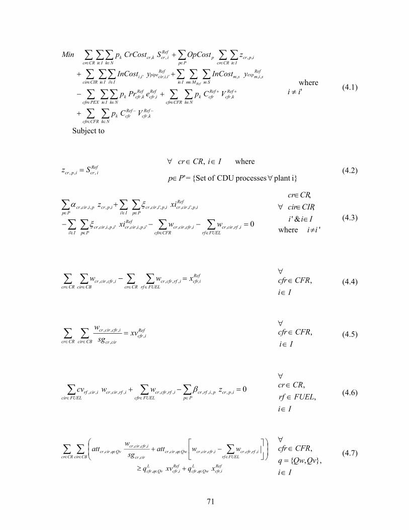
71
∑ ∑
∑ ∑∑ ∑∑
∑ ∑ ∑∑ ∑∑
∑ ∑∑∑ ∑∑
∈ ∈
−−
∈ ∈
++
∈ ∈ ∈
∈ ∈ ∈∈ ∈ ∈
∈ ∈∈∈ ∈ ∈
+
+−
++
+
CFRcfr Nk
Refkcfr
Refcfrk
CFRcfr Nk
Refkcfr
Refcfrk
PEXcfr Ii Nk
Reficfr
Refkcfrk
Ii Mm Ss
Refsimexpsm
CIRcir Ii
Refcir,i,i'pipe
Iiii
CRcr Iiipcr
Ppp
CRcr Ii Nk
Reficrkcrk
VCp
VCpePrp
yInCostyInCost
zOpCostSCrCostpMin
Ref
,
,,,
,,,'
',
,,,,
where 'ii ≠ (4.1)
Subject to
Reficripcr Sz ,,, =
∀ IiCRcr ∈∈ , where
i}plant processes CDU of{Set =' ∀∈Pp (4.2)
0,,,,,,',,,,'
',,,,
,,',,'
,,',,,,,,,
=−−−
+
∑∑∑ ∑
∑ ∑∑
∈∈∈ ∈
∈ ∈∈
FUELrfirfcircr
CFRcfricfrcircr
Refipicircr
Ii Ppipicircr
Refipicircr
Ii Ppipicircr
Ppipcrpicircr
wwxi
xiz
ξ
ξα
∀ Iii
CIRcirCRcr
∈∈∈
&',
,
'where ii≠
(4.3)
∑ ∑ ∑∑∈ ∈ ∈∈
=−CRcr
Refcfr,i
CRcr FUELrfirfcfrcr
CBciricfrcircr xww ,,,,,,
∀
IiCFRcfr
∈∈ , (4.4)
∑ ∑∈ ∈
=CRcr
Reficfr
CBcir circr
icfrcircr xvsg
w,
,
,,, ∀
IiCFRcfr
∈∈ ,
(4.5)
∑∑∑∈∈∈
=−+Pp
ipcrpirfcrFUELcfr
irfcfrcrFUELcir
irfcircricirrf zwwcv 0,,,,,,,,,,,,, β ∀
IiFUELrfCRcr
∈∈∈
,,
(4.6)
Refcfr,i
LQwqcfr
Reficfr
LQvqcfr
CRcr CBcir FUELrfirfcfrcricfrcircrQwqcircr
circr
icfrcircrQvqcircr
xqxvq
wwattsg
watt
∈∈
∈ ∈ ∈∈∈
+≥
⎟⎟⎠
⎞⎜⎜⎝
⎛⎥⎦
⎤⎢⎣
⎡−+∑ ∑ ∑
,,,
,,,,,,,,,
,,,,,
∀
IiQvQwq
CFRcfr
∈=∈
},,{, (4.7)
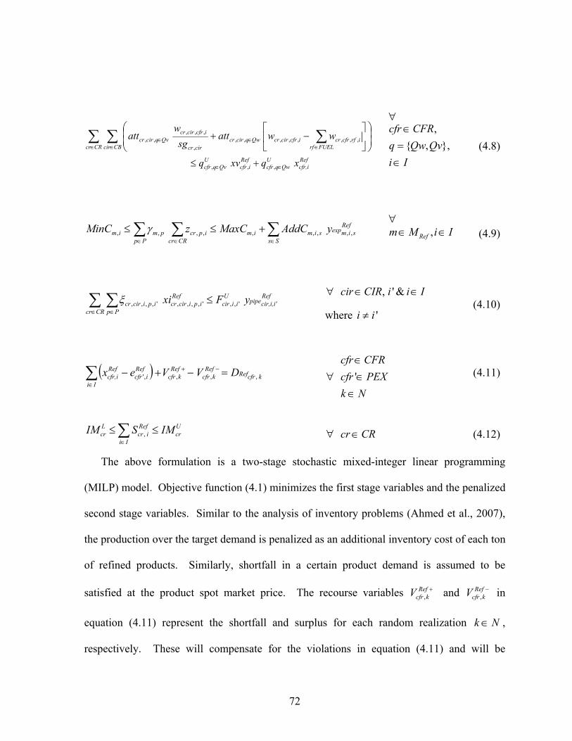
72
Refcfr,i
UQwqcfr
Reficfr
UQvqcfr
CRcr CBcir FUELrfirfcfrcricfrcircrQwqcircr
circr
icfrcircrQvqcircr
xqxvq
wwattsg
watt
∈∈
∈ ∈ ∈∈∈
+≤
⎟⎟⎠
⎞⎜⎜⎝
⎛⎥⎦
⎤⎢⎣
⎡−+∑ ∑ ∑
,,,
,,,,,,,,,
,,,,,
∀
IiQvQwq
CFRcfr
∈=∈
},,{,
(4.8)
∑∑ ∑∈∈ ∈
+≤≤Ss
Refsimexpsim
Ppim
CRcripcrpmim yAddCMaxCzMinC ,,,,,,,,, γ
∀ IiMm Ref ∈∈ ,
(4.9)
∑ ∑∈ ∈
≤CRcr
Refcir,i,i'pipe
Uiicir
Pp
Refipicircripicircr yFxi ',,',,,,',,,,ξ
∀ IiiCIRcir ∈∈ &',
where 'ii ≠ (4.10)
( ) kcfrRefRef
kcfrRef
kcfrIi
Reficfr
Refcfr,i DVVex ,,,,' =−+− −+
∈∑ ∀
NkPEXcfrCFRcfr
∈∈∈' (4.11)
∑∈
≤≤Ii
Ucr
Reficr
Lcr IMSIM , ∀ CRcr∈ (4.12)
The above formulation is a two-stage stochastic mixed-integer linear programming
(MILP) model. Objective function (4.1) minimizes the first stage variables and the penalized
second stage variables. Similar to the analysis of inventory problems (Ahmed et al., 2007),
the production over the target demand is penalized as an additional inventory cost of each ton
of refined products. Similarly, shortfall in a certain product demand is assumed to be
satisfied at the product spot market price. The recourse variables +RefkcfrV , and −Ref
kcfrV , in
equation (4.11) represent the shortfall and surplus for each random realization Nk ∈ ,
respectively. These will compensate for the violations in equation (4.11) and will be
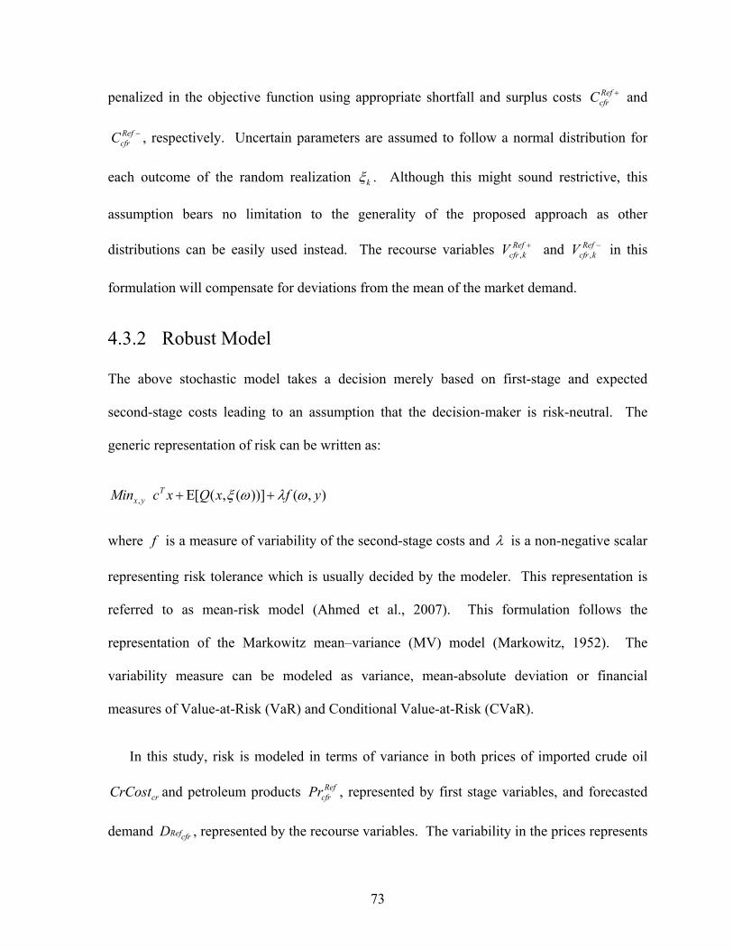
73
penalized in the objective function using appropriate shortfall and surplus costs +RefcfrC and
−RefcfrC , respectively. Uncertain parameters are assumed to follow a normal distribution for
each outcome of the random realization kξ . Although this might sound restrictive, this
assumption bears no limitation to the generality of the proposed approach as other
distributions can be easily used instead. The recourse variables +RefkcfrV , and −Ref
kcfrV , in this
formulation will compensate for deviations from the mean of the market demand.
4.3.2 Robust Model
The above stochastic model takes a decision merely based on first-stage and expected
second-stage costs leading to an assumption that the decision-maker is risk-neutral. The
generic representation of risk can be written as:
),())](,([, yfxQxcMin Tyx ωλωξ +Ε+
where f is a measure of variability of the second-stage costs and λ is a non-negative scalar
representing risk tolerance which is usually decided by the modeler. This representation is
referred to as mean-risk model (Ahmed et al., 2007). This formulation follows the
representation of the Markowitz mean–variance (MV) model (Markowitz, 1952). The
variability measure can be modeled as variance, mean-absolute deviation or financial
measures of Value-at-Risk (VaR) and Conditional Value-at-Risk (CVaR).
In this study, risk is modeled in terms of variance in both prices of imported crude oil
crCrCost and petroleum products RefcfrPr , represented by first stage variables, and forecasted
demand cfrRefD , represented by the recourse variables. The variability in the prices represents
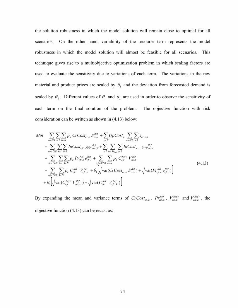
74
the solution robustness in which the model solution will remain close to optimal for all
scenarios. On the other hand, variability of the recourse term represents the model
robustness in which the model solution will almost be feasible for all scenarios. This
technique gives rise to a multiobjective optimization problem in which scaling factors are
used to evaluate the sensitivity due to variations of each term. The variations in the raw
material and product prices are scaled by 1θ and the deviation from forecasted demand is
scaled by 2θ . Different values of 1θ and 2θ are used in order to observe the sensitivity of
each term on the final solution of the problem. The objective function with risk
consideration can be written as shown in (4.13) below:
[ ][ ])var()var(
)var()var(
,,2
,,,,1,
,,,
,,,'
',
,,,,
−−++
∈ ∈
−−
∈ ∈
++
∈ ∈ ∈
∈ ∈ ∈∈ ∈ ∈
∈ ∈∈∈ ∈ ∈
++
+++
+−
++
+
∑ ∑
∑ ∑∑ ∑∑
∑ ∑ ∑∑ ∑∑
∑ ∑∑∑ ∑∑
Refkcfr
Refcfr
Refkcfr
Refcfr
Reficfr
Refkcfr
Reficrkcr
CFRcfr Nk
Refkcfr
Refcfrk
CFRcfr Nk
Refkcfr
Refcfrk
PEXcfr Ii Nk
Reficfr
Refkcfrk
Ii Mm Ss
Refsimexpsm
CIRcir Ii
Refcir,i,i'pipe
Iiii
CRcr Iiipcr
Ppp
CRcr Ii Nk
Reficrkcrk
VCVC
ePrSCrCostVCp
VCpePrp
yInCostyInCost
zOpCostSCrCostpMin
Ref
θ
θ
(4.13)
By expanding the mean and variance terms of kcrCrCost , , RefkcfrPr , , +Ref
kcfrV , and −RefkcfrV , , the
objective function (4.13) can be recast as:
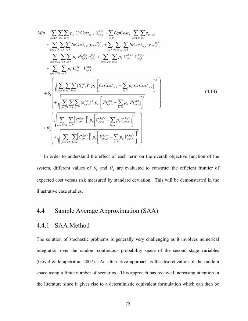
75
[ ]
[ ] ⎟⎟⎟⎟⎟⎟
⎠
⎞
⎜⎜⎜⎜⎜⎜
⎝
⎛
⎥⎦
⎤⎢⎣
⎡−+
⎥⎦
⎤⎢⎣
⎡−
+
⎟⎟⎟⎟⎟⎟
⎠
⎞
⎜⎜⎜⎜⎜⎜
⎝
⎛
⎥⎦
⎤⎢⎣
⎡−+
⎥⎦
⎤⎢⎣
⎡−
+
+
+−
++
+
∑ ∑ ∑
∑ ∑ ∑
∑ ∑∑ ∑
∑ ∑∑ ∑
∑ ∑
∑ ∑∑ ∑∑
∑ ∑ ∑∑ ∑∑
∑ ∑∑∑ ∑∑
∈ ∈ ∈
−−−
∈ ∈ ∈
+++
∈ ∈ ∈ ∈
∈ ∈ ∈ ∈
∈ ∈
−−
∈ ∈
++
∈ ∈ ∈
∈ ∈ ∈∈ ∈ ∈
∈ ∈∈∈ ∈ ∈
CFRcfr Nk Nk
Refkcfrk
Refkcfrk
Refcfr
CFRcfr Nk Nk
Refkcfrk
Refkcfrk
Refcfr
CRcr Ii Nk Nk
Refkcfrk
Refkcfrk
Reficfr
CRcr Ii Nk Nkkcrkkcrk
Reficr
CFRcfr Nk
Refkcfr
Refcfrk
CFRcfr Nk
Refkcfr
Refcfrk
PEXcfr Ii Nk
Reficfr
Refkcfrk
Ii Mm Ss
Refsimexpsm
CIRcir Ii
Refcir,i,i'pipe
Iiii
CRcr Iiipcr
Ppp
CRcr Ii Nk
Reficrkcrk
VpVpC
VpVpC
PrpPrpe
CrCostpCrCostpS
VCp
VCpePrp
yInCostyInCost
zOpCostSCrCostpMin
Ref
2
,,2
2
,,2
2
2
,,2
,
2
,,2
,
1
,
,,,
,,,'
',
,,,,
)(
)(
θ
θ
(4.14)
In order to understand the effect of each term on the overall objective function of the
system, different values of 1θ and 2θ are evaluated to construct the efficient frontier of
expected cost versus risk measured by standard deviation. This will be demonstrated in the
illustrative case studies.
4.4 Sample Average Approximation (SAA)
4.4.1 SAA Method
The solution of stochastic problems is generally very challenging as it involves numerical
integration over the random continuous probability space of the second stage variables
(Goyal & Ierapetritou, 2007). An alternative approach is the discretization of the random
space using a finite number of scenarios. This approach has received increasing attention in
the literature since it gives rise to a deterministic equivalent formulation which can then be
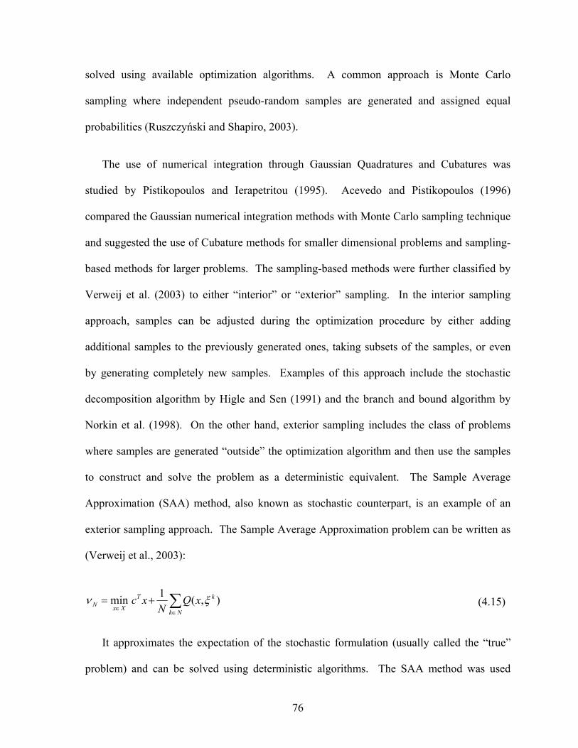
76
solved using available optimization algorithms. A common approach is Monte Carlo
sampling where independent pseudo-random samples are generated and assigned equal
probabilities (Ruszczyński and Shapiro, 2003).
The use of numerical integration through Gaussian Quadratures and Cubatures was
studied by Pistikopoulos and Ierapetritou (1995). Acevedo and Pistikopoulos (1996)
compared the Gaussian numerical integration methods with Monte Carlo sampling technique
and suggested the use of Cubature methods for smaller dimensional problems and sampling-
based methods for larger problems. The sampling-based methods were further classified by
Verweij et al. (2003) to either “interior” or “exterior” sampling. In the interior sampling
approach, samples can be adjusted during the optimization procedure by either adding
additional samples to the previously generated ones, taking subsets of the samples, or even
by generating completely new samples. Examples of this approach include the stochastic
decomposition algorithm by Higle and Sen (1991) and the branch and bound algorithm by
Norkin et al. (1998). On the other hand, exterior sampling includes the class of problems
where samples are generated “outside” the optimization algorithm and then use the samples
to construct and solve the problem as a deterministic equivalent. The Sample Average
Approximation (SAA) method, also known as stochastic counterpart, is an example of an
exterior sampling approach. The Sample Average Approximation problem can be written as
(Verweij et al., 2003):
∑∈
∈+=
Nk
kT
XxN xQN
xc ),(1min ξν (4.15)
It approximates the expectation of the stochastic formulation (usually called the “true”
problem) and can be solved using deterministic algorithms. The SAA method was used
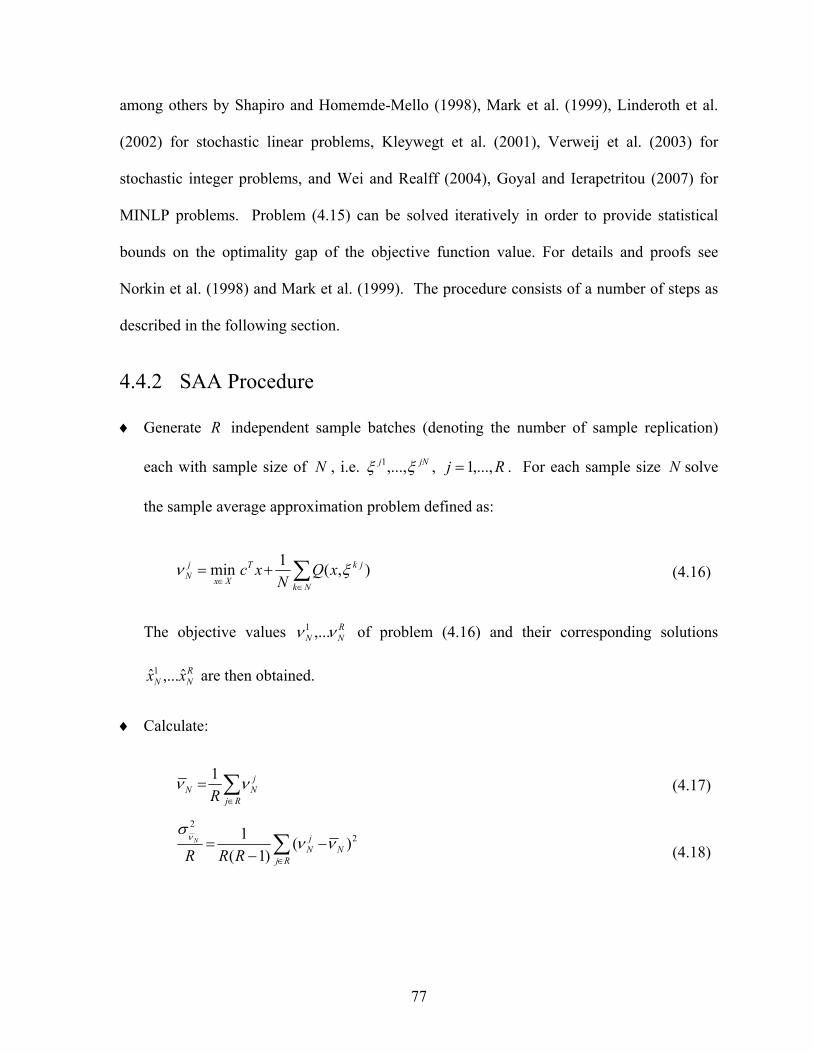
77
among others by Shapiro and Homemde-Mello (1998), Mark et al. (1999), Linderoth et al.
(2002) for stochastic linear problems, Kleywegt et al. (2001), Verweij et al. (2003) for
stochastic integer problems, and Wei and Realff (2004), Goyal and Ierapetritou (2007) for
MINLP problems. Problem (4.15) can be solved iteratively in order to provide statistical
bounds on the optimality gap of the objective function value. For details and proofs see
Norkin et al. (1998) and Mark et al. (1999). The procedure consists of a number of steps as
described in the following section.
4.4.2 SAA Procedure
♦ Generate R independent sample batches (denoting the number of sample replication)
each with sample size of N , i.e. jNj ξξ ,...,1 , Rj ,...,1= . For each sample size N solve
the sample average approximation problem defined as:
∑∈
∈+=
Nk
jkT
Xx
jN xQ
Nxc ),(1min ξν (4.16)
The objective values RNN νν ,...1 of problem (4.16) and their corresponding solutions
RNN xx ˆ,...ˆ1 are then obtained.
♦ Calculate:
∑∈
=Rj
jNN R
νν 1 (4.17)
22
)()1(
1N
Rj
jNRRR
N ννσν ∑
∈
−−
= (4.18)
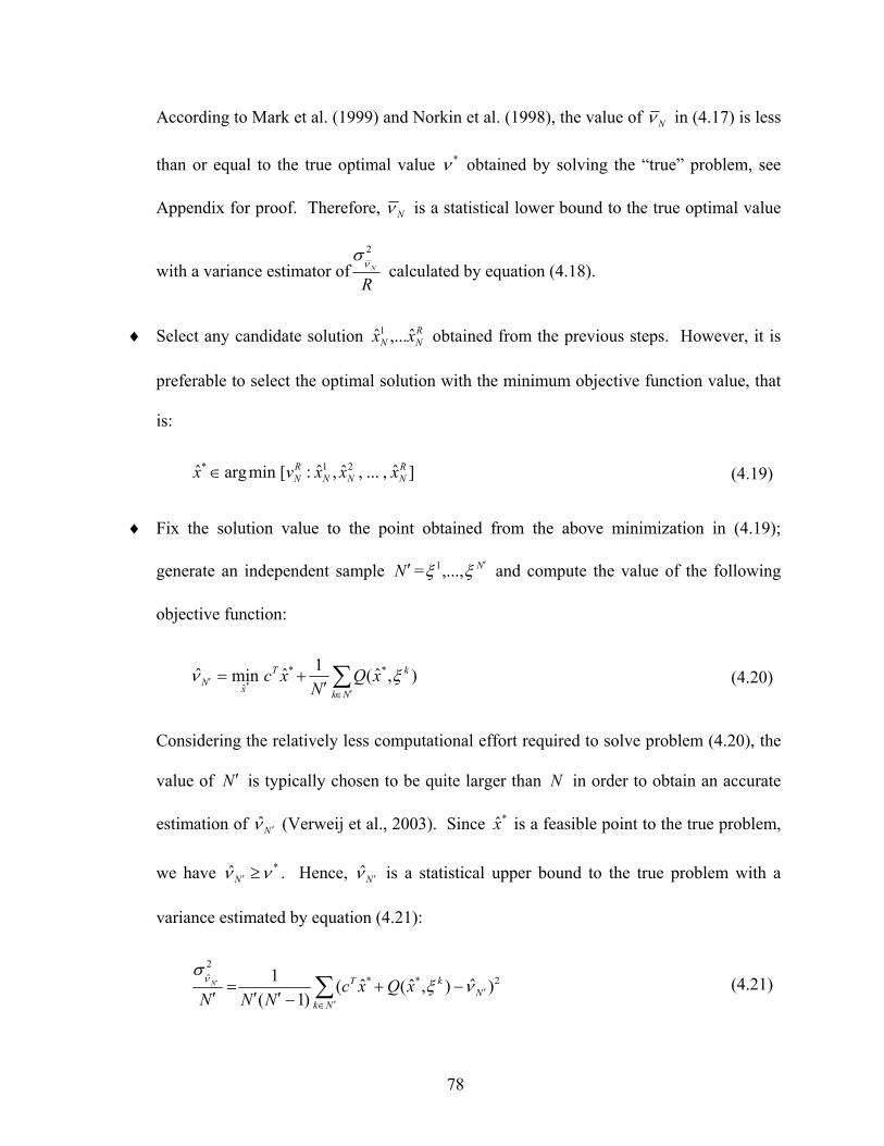
78
According to Mark et al. (1999) and Norkin et al. (1998), the value of Nν in (4.17) is less
than or equal to the true optimal value *ν obtained by solving the “true” problem, see
Appendix for proof. Therefore, Nν is a statistical lower bound to the true optimal value
with a variance estimator ofR
N
2ν
σ calculated by equation (4.18).
♦ Select any candidate solution RNN xx ˆ,...ˆ1 obtained from the previous steps. However, it is
preferable to select the optimal solution with the minimum objective function value, that
is:
]ˆ,...,ˆ,ˆ:[minargˆ 21* RNNN
RN xxxvx ∈ (4.19)
♦ Fix the solution value to the point obtained from the above minimization in (4.19);
generate an independent sample N ′= N ′ξξ ,...,1 and compute the value of the following
objective function:
),ˆ(1ˆminˆ **
ˆ* ∑′∈
′ ′+=
Nk
kT
xN xQN
xc ξν (4.20)
Considering the relatively less computational effort required to solve problem (4.20), the
value of N ′ is typically chosen to be quite larger than N in order to obtain an accurate
estimation of N ′ν̂ (Verweij et al., 2003). Since *x̂ is a feasible point to the true problem,
we have *ˆ νν ≥′N . Hence, N ′ν̂ is a statistical upper bound to the true problem with a
variance estimated by equation (4.21):
2**
2ˆ )ˆ),ˆ(ˆ(
)1(1
NNk
kT xQxcNNN
N′
′∈
−+−′′
=′ ∑′ νξ
σν (4.21)
79
♦ From the above procedure, we can estimate the )1( α− confidence interval of the optimal
gap. For a given 2/,1 α−nt where t is critical value of the t-distribution with )1( −n degrees
of freedom, the following can be estimated:
Rt N
nlν
α
σε 2/,1~
−= and N
t Nnu ′
= ′−
να
σε ˆ
2/,1~
♦ Then, the optimality gap can be constructed as:
]~~}ˆ{,0[ luNN εενν ++− +′ where )0,(max}{ yy ≡+ . (4.22)
Note that due to sampling error we may find that NN νν <′ˆ . For this reason the
confidence interval obtained by (4.22) provides a more conservative bounding. The
above procedure for the validation of a candidate solution was originally suggested by
Norkin et al. (1998) and further developed by Mark et al. (1999).
4.5 Illustrative Case Study
This section presents computational results of the models and the sampling scheme proposed
in this chapter. The refinery examples considered represent industrial-scale size refineries
and an actual configuration that can be found in may industrial sites around the world. In the
presentation of the results, we focus on demonstrating the sample average approximation
computational results as we vary the sample sizes and compare their solution accuracy and
the CPU time required for solving the models.
The modeling system GAMS (Brooke et al., 1996) is used for setting up the optimization
models. The computational tests were carried out on a Pentium M processor 2.13 GHz. The
models were solved with DICOPT (Viswanathan & Grossmann, 1990). The NLP
80
subproblems were solved with CONOPT2 (Drud, 1994), while the MILP master problems
were solved with CPLEX (CPLEX Optimization Inc, 1993).
4.5.1 Single Refinery Planning
This example illustrates the performance of the proposed approach on a single site total
refinery planning problem. The refinery scale, capacity and configuration mimic an existing
refinery in the Middle East. Figure 4.1 is a state equipment network (SEN) representation of
multiple refineries network, where in this example we will study Refinery 1. The refinery
uses a single feedstock (Arabian Light) to feed the atmospheric crude unit where it separates
crude oil into several fractions including LPG, naphtha, kerosene, gas oil and residues. The
heavy residues are then sent to the vacuum unit where they are further separated into vacuum
gas oil and vacuum residues. In general, depending on the production targets, different
processing and treatment processes are applied to the crude fractions. In our case, the
naphtha is further separated into heavy and light naphtha. Heavy naphtha is sent to the
catalytic reformer unit to produce high octane reformates for gasoline blending and light
naphtha is sent to light naphtha pool and to an isomerization unit to produce isomerate for
gasoline blending too.
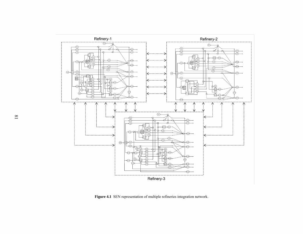
81
Figure 4.1 SEN representation of multiple refineries integration network.
82
The middle distillates are combined with other similar intermediate streams and sent for
hydrotreating and then for blending to produce jet fuels and gas oils. Atmospheric and
vacuum gas oils are further treated by either fluid catalytic cracking (FCC) or hydrocracking
(HC) in order to increase the gasoline and distillate yields. These distillates from both FCC
and HC are desulfurized in the cycle gas oil desulfurization and ATK desulfurization
processes. The final products in this example consist of liquefied petroleum gas (LPG), light
naphtha (LT), two grades of gasoline (PG98 and PG95), No.4 jet fuel (JP4), military jet fuel
(ATKP), No.6 gas oil (GO6), and heating fuel oil (HFO).
The major capacity limitations as well as the availability constraints are shown in Table
4.1. Raw materials, product prices, and demand uncertainty were assumed to follow a
normal distribution. However, this assumption bears no restriction to the generality of the
proposed modeling approach as other sampling distributions can be easily used instead.
Prices of crude oil and refined products reflect the current market prices and assume a
standard deviation of $10 US. The problem is formulated as an LP since there is no
integration or capacity expansion requirement in this case study.
Table 4.2 and Figure 4.2 show different confidence interval values of the optimality gap
when changing the sample sizes of N and 'N , while fixing the number of replications R to
30. The replication number R need not be very large since usually 5 to 7 replications are
sufficient to get an idea about the variability of Nν (Qian & Shapiro, 2006). It can be seen
that the increase of the sample size N has more weight on reducing the optimality gap and
therefore the variability of the objective function as compared to 'N .
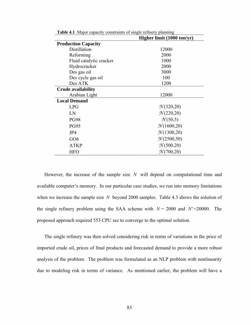
83
Table 4.1 Major capacity constraints of single refinery planning Higher limit (1000 ton/yr) Production Capacity
Distillation 12000 Reforming 2000 Fluid catalytic cracker 1000 Hydrocracker 2000 Des gas oil 3000 Des cycle gas oil 100 Des ATK 1200
Crude availability Arabian Light 12000
Local Demand LPG N (320,20) LN N (220,20) PG98 N (50,5) PG95 N (1600,20) JP4 N (1300,20) GO6 N (2500,50) ATKP N (500,20) HFO N (700,20)
However, the increase of the sample size N will depend on computational time and
available computer’s memory. In our particular case studies, we run into memory limitations
when we increase the sample size N beyond 2000 samples. Table 4.3 shows the solution of
the single refinery problem using the SAA scheme with N = 2000 and 'N =20000. The
proposed approach required 553 CPU sec to converge to the optimal solution.
The single refinery was then solved considering risk in terms of variations in the price of
imported crude oil, prices of final products and forecasted demand to provide a more robust
analysis of the problem. The problem was formulated as an NLP problem with nonlinearity
due to modeling risk in terms of variance. As mentioned earlier, the problem will have a
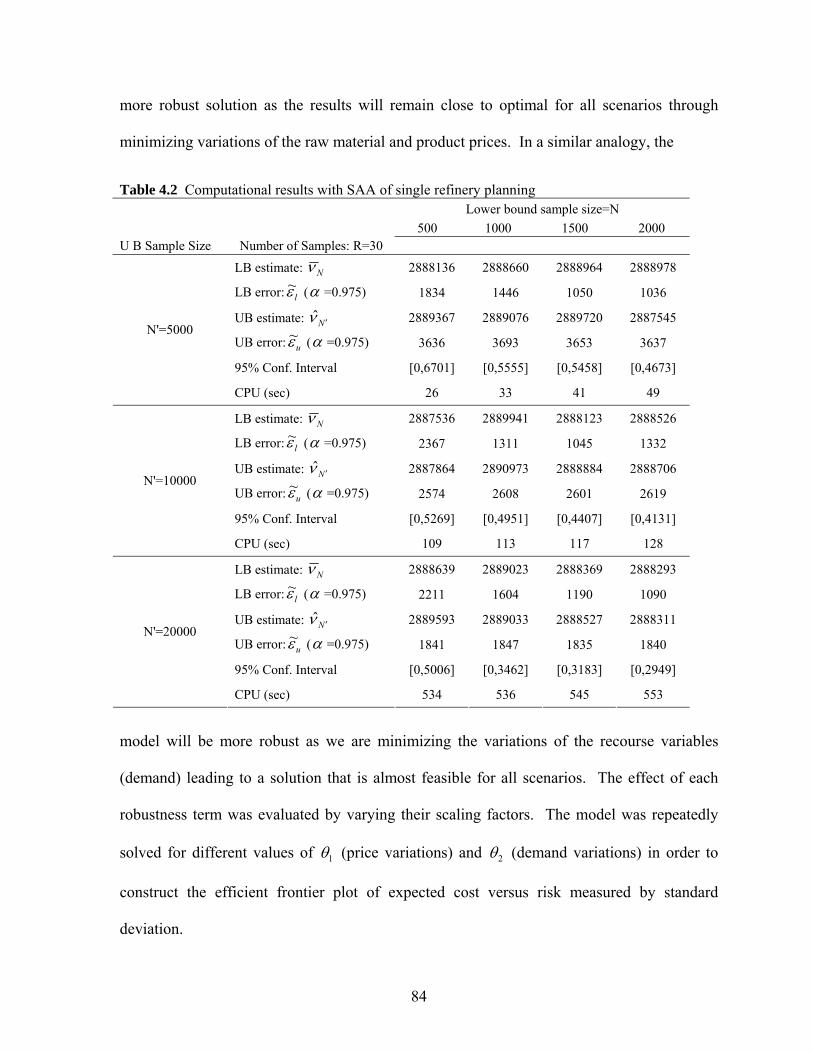
84
more robust solution as the results will remain close to optimal for all scenarios through
minimizing variations of the raw material and product prices. In a similar analogy, the
Table 4.2 Computational results with SAA of single refinery planning Lower bound sample size=N 500 1000 1500 2000 U B Sample Size Number of Samples: R=30
LB estimate: Nν 2888136 2888660 2888964 2888978
LB error: lε~ (α =0.975) 1834 1446 1050 1036
UB estimate: N ′ν̂ 2889367 2889076 2889720 2887545
UB error: uε~ (α =0.975) 3636 3693 3653 3637
95% Conf. Interval [0,6701] [0,5555] [0,5458] [0,4673]
N'=5000
CPU (sec) 26 33 41 49
LB estimate: Nν 2887536 2889941 2888123 2888526
LB error: lε~ (α =0.975) 2367 1311 1045 1332
UB estimate: N ′ν̂ 2887864 2890973 2888884 2888706
UB error: uε~ (α =0.975) 2574 2608 2601 2619
95% Conf. Interval [0,5269] [0,4951] [0,4407] [0,4131]
N'=10000
CPU (sec) 109 113 117 128
LB estimate: Nν 2888639 2889023 2888369 2888293
LB error: lε~ (α =0.975) 2211 1604 1190 1090
UB estimate: N ′ν̂ 2889593 2889033 2888527 2888311
UB error: uε~ (α =0.975) 1841 1847 1835 1840
95% Conf. Interval [0,5006] [0,3462] [0,3183] [0,2949]
N'=20000
CPU (sec) 534 536 545 553
model will be more robust as we are minimizing the variations of the recourse variables
(demand) leading to a solution that is almost feasible for all scenarios. The effect of each
robustness term was evaluated by varying their scaling factors. The model was repeatedly
solved for different values of 1θ (price variations) and 2θ (demand variations) in order to
construct the efficient frontier plot of expected cost versus risk measured by standard
deviation.
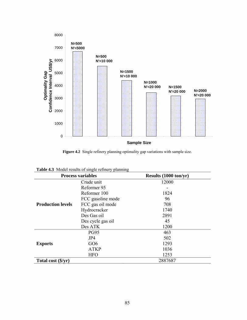
85
0
1000
2000
3000
4000
5000
6000
7000
8000
Sample Size
Opt
imal
ity G
ap
Con
fiden
ce In
terv
al U
S$/y
r
N=1500N'=20 000
N=500N'=5000
N=500N'=10 000
N=1500N'=10 000
N=1000N'=20 000
N=2000N'=20 000
Figure 4.2 Single refinery planning optimality gap variations with sample size.
Table 4.3 Model results of single refinery planning
Process variables Results (1000 ton/yr) Crude unit 12000 Reformer 95 - Reformer 100 1824 FCC gasoline mode 96 FCC gas oil mode 708 Hydrocracker 1740 Des Gas oil 2891 Des cycle gas oil 45
Production levels
Des ATK 1200 PG95 463 JP4 502 GO6 1293 ATKP 1036
Exports
HFO 1253 Total cost ($/yr) 2887687
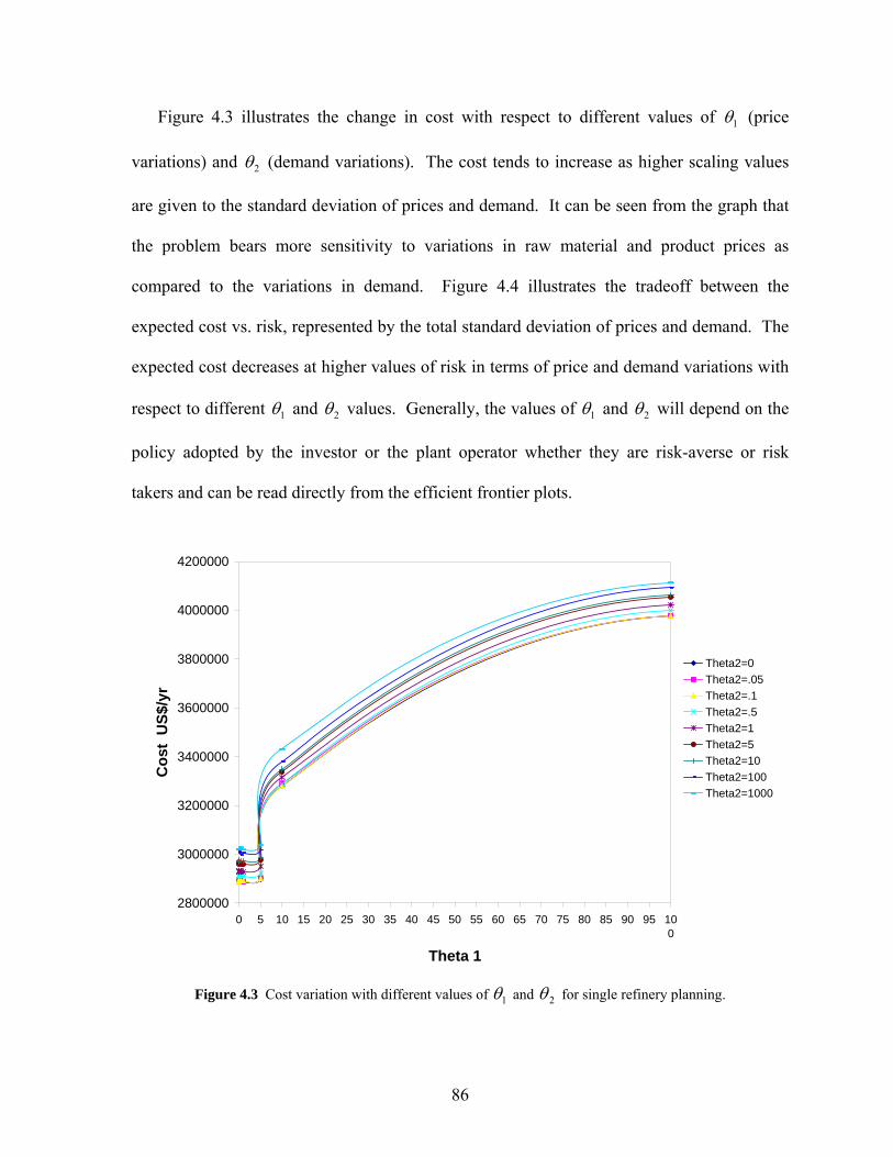
86
Figure 4.3 illustrates the change in cost with respect to different values of 1θ (price
variations) and 2θ (demand variations). The cost tends to increase as higher scaling values
are given to the standard deviation of prices and demand. It can be seen from the graph that
the problem bears more sensitivity to variations in raw material and product prices as
compared to the variations in demand. Figure 4.4 illustrates the tradeoff between the
expected cost vs. risk, represented by the total standard deviation of prices and demand. The
expected cost decreases at higher values of risk in terms of price and demand variations with
respect to different 1θ and 2θ values. Generally, the values of 1θ and 2θ will depend on the
policy adopted by the investor or the plant operator whether they are risk-averse or risk
takers and can be read directly from the efficient frontier plots.
2800000
3000000
3200000
3400000
3600000
3800000
4000000
4200000
0 5 10 15 20 25 30 35 40 45 50 55 60 65 70 75 80 85 90 95 100
Theta 1
Cos
t U
S$/y
r
Theta2=0Theta2=.05Theta2=.1Theta2=.5Theta2=1Theta2=5Theta2=10Theta2=100Theta2=1000
Figure 4.3 Cost variation with different values of 1θ and 2θ for single refinery planning.
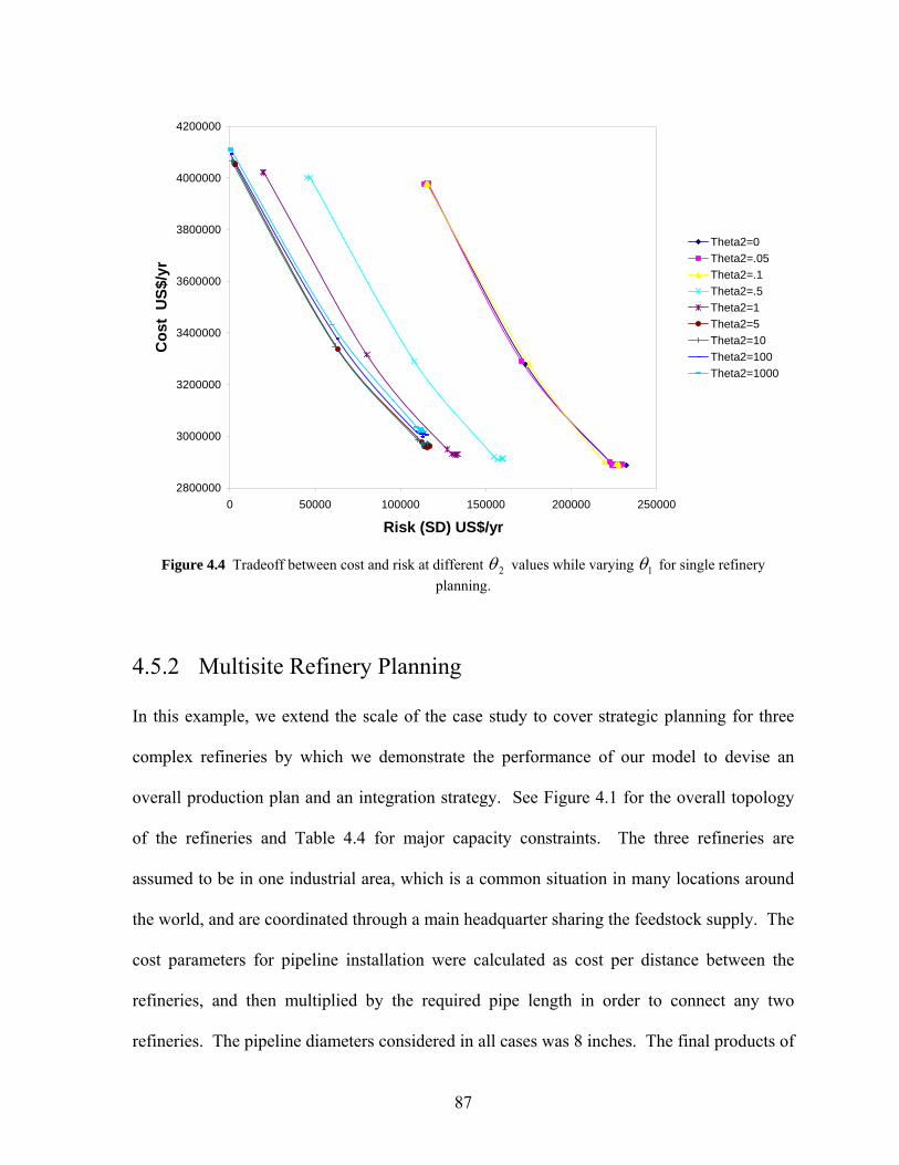
87
2800000
3000000
3200000
3400000
3600000
3800000
4000000
4200000
0 50000 100000 150000 200000 250000
Risk (SD) US$/yr
Cos
t U
S$/y
r
Theta2=0Theta2=.05Theta2=.1Theta2=.5Theta2=1Theta2=5Theta2=10Theta2=100Theta2=1000
Figure 4.4 Tradeoff between cost and risk at different 2θ values while varying 1θ for single refinery
planning.
4.5.2 Multisite Refinery Planning
In this example, we extend the scale of the case study to cover strategic planning for three
complex refineries by which we demonstrate the performance of our model to devise an
overall production plan and an integration strategy. See Figure 4.1 for the overall topology
of the refineries and Table 4.4 for major capacity constraints. The three refineries are
assumed to be in one industrial area, which is a common situation in many locations around
the world, and are coordinated through a main headquarter sharing the feedstock supply. The
cost parameters for pipeline installation were calculated as cost per distance between the
refineries, and then multiplied by the required pipe length in order to connect any two
refineries. The pipeline diameters considered in all cases was 8 inches. The final products of
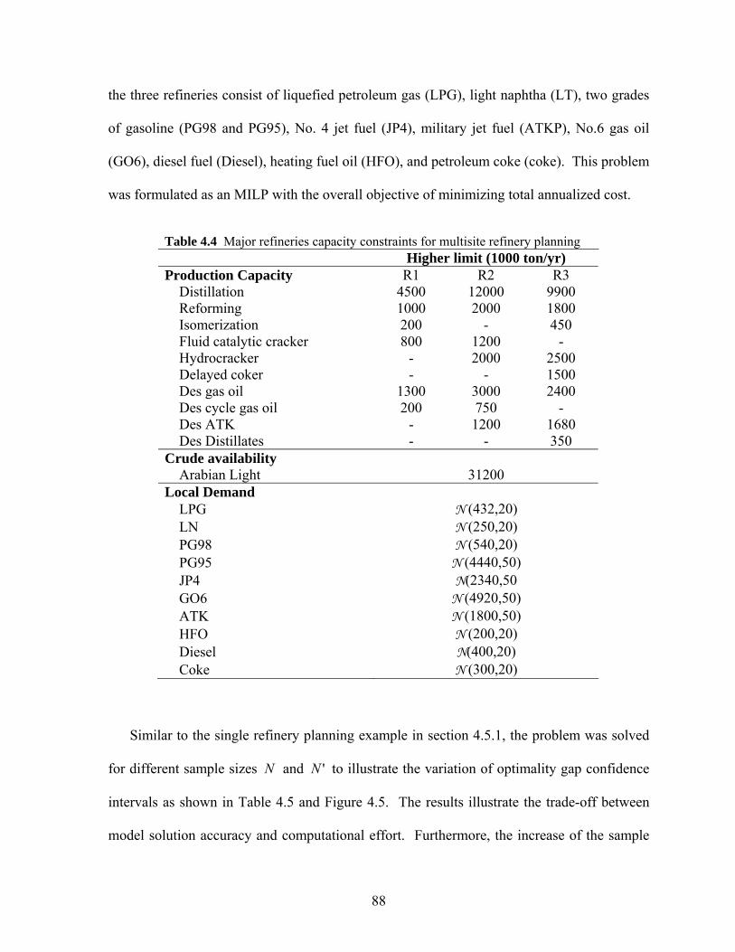
88
the three refineries consist of liquefied petroleum gas (LPG), light naphtha (LT), two grades
of gasoline (PG98 and PG95), No. 4 jet fuel (JP4), military jet fuel (ATKP), No.6 gas oil
(GO6), diesel fuel (Diesel), heating fuel oil (HFO), and petroleum coke (coke). This problem
was formulated as an MILP with the overall objective of minimizing total annualized cost.
Table 4.4 Major refineries capacity constraints for multisite refinery planning Higher limit (1000 ton/yr) Production Capacity R1 R2 R3 Distillation 4500 12000 9900 Reforming 1000 2000 1800 Isomerization 200 - 450 Fluid catalytic cracker 800 1200 - Hydrocracker - 2000 2500 Delayed coker - - 1500 Des gas oil 1300 3000 2400 Des cycle gas oil 200 750 - Des ATK - 1200 1680 Des Distillates - - 350 Crude availability Arabian Light 31200 Local Demand LPG N (432,20) LN N (250,20) PG98 N (540,20) PG95 N (4440,50) JP4 N(2340,50 GO6 N (4920,50) ATK N (1800,50) HFO N (200,20) Diesel N(400,20) Coke N (300,20)
Similar to the single refinery planning example in section 4.5.1, the problem was solved
for different sample sizes N and 'N to illustrate the variation of optimality gap confidence
intervals as shown in Table 4.5 and Figure 4.5. The results illustrate the trade-off between
model solution accuracy and computational effort. Furthermore, the increase of the sample
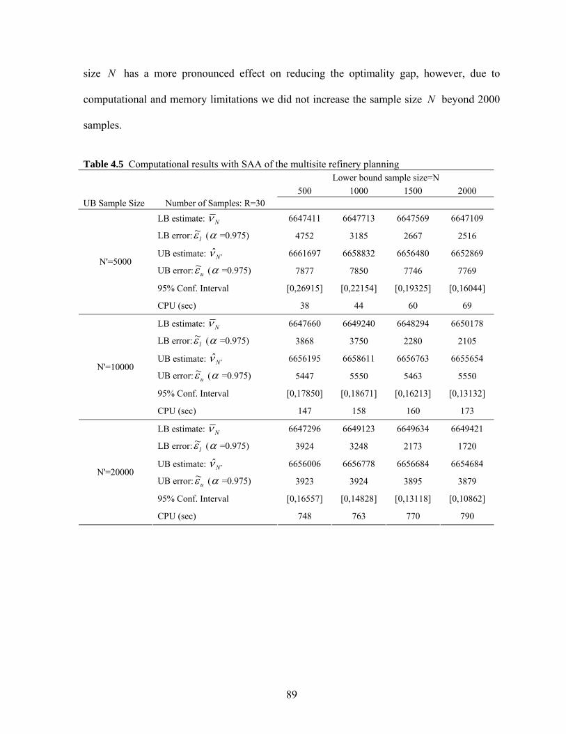
89
size N has a more pronounced effect on reducing the optimality gap, however, due to
computational and memory limitations we did not increase the sample size N beyond 2000
samples.
Table 4.5 Computational results with SAA of the multisite refinery planning Lower bound sample size=N 500 1000 1500 2000 UB Sample Size Number of Samples: R=30
LB estimate: Nν 6647411 6647713 6647569 6647109
LB error: lε~ (α =0.975) 4752 3185 2667 2516
UB estimate: N ′ν̂ 6661697 6658832 6656480 6652869
UB error: uε~ (α =0.975) 7877 7850 7746 7769
95% Conf. Interval [0,26915] [0,22154] [0,19325] [0,16044]
N'=5000
CPU (sec) 38 44 60 69
LB estimate: Nν 6647660 6649240 6648294 6650178
LB error: lε~ (α =0.975) 3868 3750 2280 2105
UB estimate: N ′ν̂ 6656195 6658611 6656763 6655654
UB error: uε~ (α =0.975) 5447 5550 5463 5550
95% Conf. Interval [0,17850] [0,18671] [0,16213] [0,13132]
N'=10000
CPU (sec) 147 158 160 173
LB estimate: Nν 6647296 6649123 6649634 6649421
LB error: lε~ (α =0.975) 3924 3248 2173 1720
UB estimate: N ′ν̂ 6656006 6656778 6656684 6654684
UB error: uε~ (α =0.975) 3923 3924 3895 3879
95% Conf. Interval [0,16557] [0,14828] [0,13118] [0,10862]
N'=20000
CPU (sec) 748 763 770 790
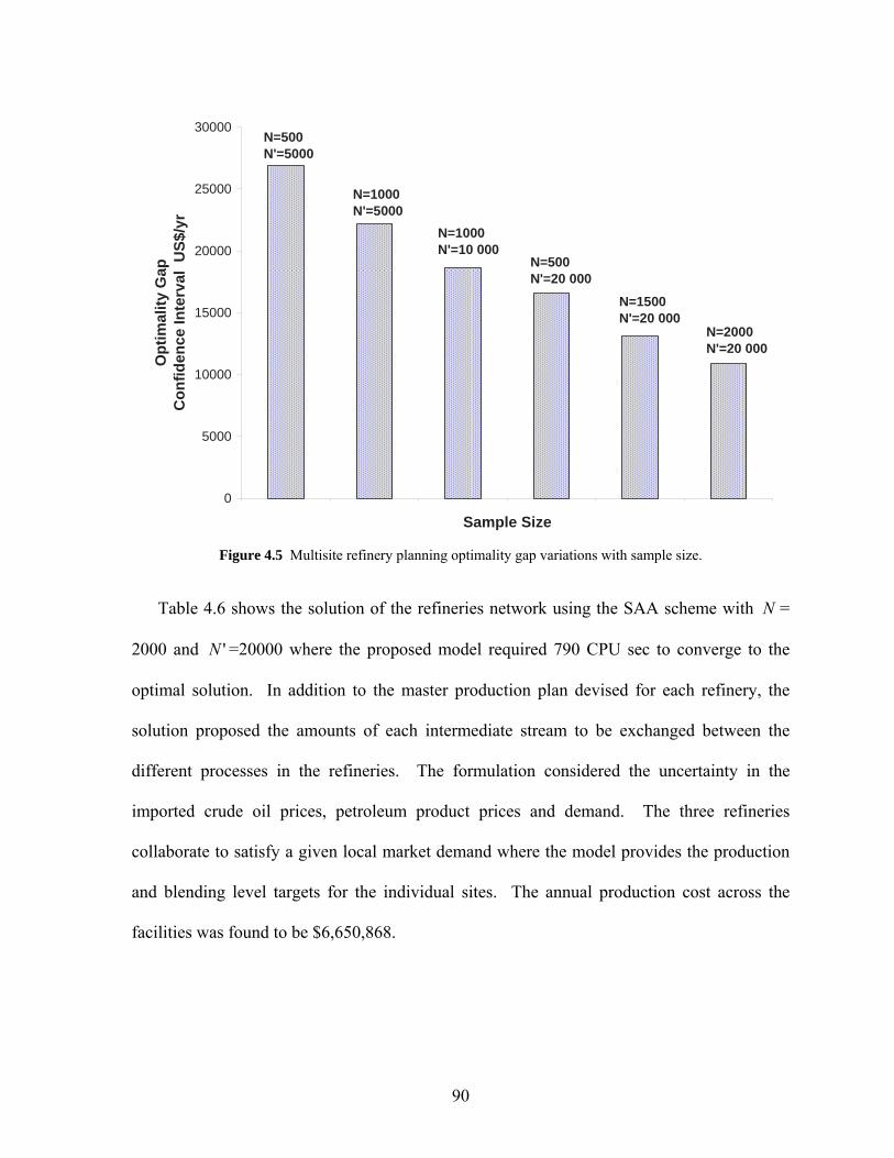
90
0
5000
10000
15000
20000
25000
30000
Sample Size
Opt
imal
ity G
ap
Con
fiden
ce In
terv
al U
S$/y
r
N=1500N'=20 000
N=500N'=5000
N=1000N'=5000
N=1000N'=10 000
N=500N'=20 000
N=2000N'=20 000
Figure 4.5 Multisite refinery planning optimality gap variations with sample size.
Table 4.6 shows the solution of the refineries network using the SAA scheme with N =
2000 and 'N =20000 where the proposed model required 790 CPU sec to converge to the
optimal solution. In addition to the master production plan devised for each refinery, the
solution proposed the amounts of each intermediate stream to be exchanged between the
different processes in the refineries. The formulation considered the uncertainty in the
imported crude oil prices, petroleum product prices and demand. The three refineries
collaborate to satisfy a given local market demand where the model provides the production
and blending level targets for the individual sites. The annual production cost across the
facilities was found to be $6,650,868.
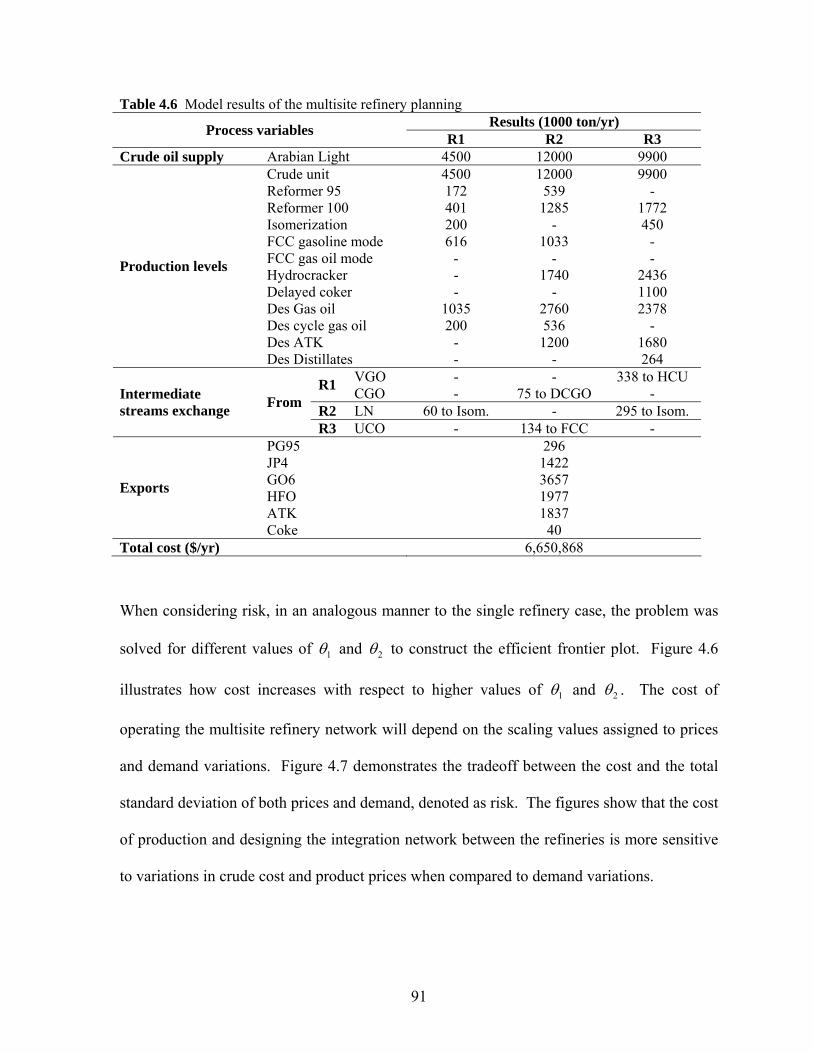
91
Table 4.6 Model results of the multisite refinery planning Results (1000 ton/yr) Process variables R1 R2 R3
Crude oil supply Arabian Light 4500 12000 9900 Crude unit 4500 12000 9900 Reformer 95 172 539 - Reformer 100 401 1285 1772 Isomerization 200 - 450 FCC gasoline mode 616 1033 - FCC gas oil mode - - - Hydrocracker - 1740 2436 Delayed coker - - 1100 Des Gas oil 1035 2760 2378 Des cycle gas oil 200 536 - Des ATK - 1200 1680
Production levels
Des Distillates - - 264 VGO - - 338 to HCU R1 CGO - 75 to DCGO -
R2 LN 60 to Isom. - 295 to Isom. Intermediate streams exchange From
R3 UCO - 134 to FCC - PG95 296 JP4 1422 GO6 3657 HFO 1977 ATK 1837
Exports
Coke 40 Total cost ($/yr) 6,650,868
When considering risk, in an analogous manner to the single refinery case, the problem was
solved for different values of 1θ and 2θ to construct the efficient frontier plot. Figure 4.6
illustrates how cost increases with respect to higher values of 1θ and 2θ . The cost of
operating the multisite refinery network will depend on the scaling values assigned to prices
and demand variations. Figure 4.7 demonstrates the tradeoff between the cost and the total
standard deviation of both prices and demand, denoted as risk. The figures show that the cost
of production and designing the integration network between the refineries is more sensitive
to variations in crude cost and product prices when compared to demand variations.
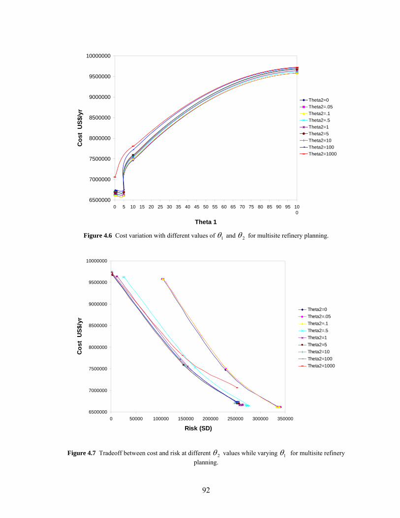
92
6500000
7000000
7500000
8000000
8500000
9000000
9500000
10000000
0 5 10 15 20 25 30 35 40 45 50 55 60 65 70 75 80 85 90 95 100
Theta 1
Cos
t U
S$/y
r
Theta2=0Theta2=.05Theta2=.1Theta2=.5Theta2=1Theta2=5Theta2=10Theta2=100Theta2=1000
Figure 4.6 Cost variation with different values of 1θ and 2θ for multisite refinery planning.
6500000
7000000
7500000
8000000
8500000
9000000
9500000
10000000
0 50000 100000 150000 200000 250000 300000 350000
Risk (SD)
Cos
t U
S$/y
r
Theta2=0Theta2=.05Theta2=.1Theta2=.5Theta2=1Theta2=5Theta2=10Theta2=100Theta2=1000
Figure 4.7 Tradeoff between cost and risk at different 2θ values while varying 1θ for multisite refinery planning.
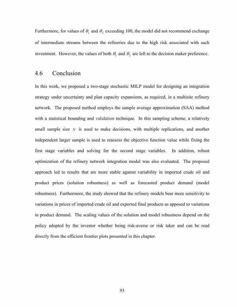
93
Furthermore, for values of 1θ and 2θ exceeding 100, the model did not recommend exchange
of intermediate streams between the refineries due to the high risk associated with such
investment. However, the values of both 1θ and 2θ are left to the decision maker preference.
4.6 Conclusion
In this work, we proposed a two-stage stochastic MILP model for designing an integration
strategy under uncertainty and plan capacity expansions, as required, in a multisite refinery
network. The proposed method employs the sample average approximation (SAA) method
with a statistical bounding and validation technique. In this sampling scheme, a relatively
small sample size N is used to make decisions, with multiple replications, and another
independent larger sample is used to reassess the objective function value while fixing the
first stage variables and solving for the second stage variables. In addition, robust
optimization of the refinery network integration model was also evaluated. The proposed
approach led to results that are more stable against variability in imported crude oil and
product prices (solution robustness) as well as forecasted product demand (model
robustness). Furthermore, the study showed that the refinery models bear more sensitivity to
variations in prices of imported crude oil and exported final products as apposed to variations
in product demand. The scaling values of the solution and model robustness depend on the
policy adopted by the investor whether being risk-averse or risk taker and can be read
directly from the efficient frontier plots presented in this chapter.
94
Chapter 5
Optimization of Petrochemical Networks: Deterministic Approach
5.1 Introduction
The petrochemical industry is a network of highly integrated production processes where
products of one plant may have an end use or may also represent raw materials for other
processes. This flexibility in petrochemical products production and the availability of many
process technologies offer the sense of switching between production methods and raw
materials utilization. The world economic growth and increasing populations will keep
global demand for transportation fuels and petrochemical products growing rapidly for the
foreseeable future. One half of the petroleum consumption over the period of 2003 to 2030
will be in the transportation sector, whereas the industrial sector accounts for a 39-percent of
the projected increase in world oil consumption, mostly for chemical and petrochemical
processes (EIA, 2006). Meeting this demand will require large investments and proper
strategic planning for the petrochemical industry.
The objective of this chapter is to give an overview on the optimization of petrochemical
networks and set up the deterministic model which will be used in the analysis of parameter
uncertainties in Chapter 6.
95
The remainder of Chapter 5 is organized as follows. In the following section we will
review the related literature in the area of petrochemical planning. Then, we will discuss the
deterministic model formulation for the petrochemical network planning and illustrate its
performance through an industrial case study in section 5.3 and 5.4, respectively. The
chapter ends with concluding remarks in section 5.5.
5.2 Literature Review
The realization of the petrochemical planning needs along with its important impact has
inspired a great deal of research in order to devise different modeling frameworks and
algorithms. These include optimization models with continuous and mixed-integer
programming under both deterministic and uncertainty considerations.
The seminal work of Stadtherr and Rudd (1976, 1978) defined the petrochemical industry
as a network of chemical process systems with linear chemical transformations and material
interactions. They showed that the model provided a good representation of the
petrochemical industry and can be used as a tool for estimating the relative effectiveness of
available and new technologies and their impact on the overall industry. Their objective was
to minimize feedstock consumptions. A similar LP modeling approach was adapted by Sokic
and Stevancevic (1983). Sophos et al. (1980) presented a model that minimizes feedstock
consumption and entropy creation (lost work). Fathi-Afshar and Yang (1985) devised a
multiobjective model of minimizing cost and gross toxicity emissions. Modeling the
petrochemical industry using linear programming may have showed its ability to provide
relatively reliable results through different technology structures. However, the need for
approximating non-linear objective functions or the restriction of process technology
96
combination alternatives mandated different modeling techniques involving mixed-integer
programming.
Some of the first mixed-integer programming models that tackled this problem were
proposed by Jimenez et al. (1982) and Jimenez and Rudd (1987) for the development of the
Mexican petrochemical industry. The proposed models were used to plan the installation of
new plants with profitable levels as opposed to importing chemical products. However, there
were no capacity limitations constraints on the processes. Al-Amir et al. (1998) developed
an MILP model for the development of Saudi Arabia’s petrochemical industry maximizing
profit. The model included minimum economic production quantity for the different
processes and accounted for domestic consumption and global market exports. This model
was further extended by Alfares and Al-Amir (2002) to include four main product categories:
propylene, ethylene, synthesis gas and aromatics and their derivatives. They devised a non-
linear objective function of production investment cost at different production levels and
derived a linear representation of the function through piece-wise linear approximation. Al-
Sharrah et al. (2001, 2002) presented MILP models that took sustainability and strategic
technology selection into consideration. The models included a constraint to limit the
selection of one technology to produce a chemical achieving a long term financial stability
and an environmental consideration through a suitability objective. Sustainability was
quantified by a health index of the chemicals and increasing profit was represented by the
added value of each process in the network. This work was later extended by Al-Sharrah et
al. (2003) with the aim of identifying long-range and short-range disturbances that affect
planning of the petrochemical industry. Al-Sharrah et al. (2006) further developed their
petrochemical planning framework into a multiobjective model accounting for economic gain
97
and risk from plant accidents. The above body of research did not account for parameter
uncertainties.
The above discussion points out the importance of petrochemical network planning in
process system engineering studies. In this chapter we develop a deterministic strategic
planning model of a network of petrochemical processes. The problem is formulated as a
mixed-integer linear programming (MILP) model with the objective of maximizing the
added value of the overall petrochemical network.
5.3 Model Formulation
The optimization of petrochemical network design involves a broad range of aspects varying
from economical and environmental analysis, strategic selection of processes and production
capacities. The deterministic model presented in this study is slightly modified from that of
Al-Sharrah et al. (2001, 2006). A set of CP number of chemicals involved in the operation
of petM processes is assumed to be given. Let Petmx be the annual level of production of
process petMm∈ , PetcpF the amount of chemical CPcp∈ as a feedstock, and mcp,δ the input-
output coefficient matrix of material cp in process petMm∈ , and LcpPetD and U
cpPetD represent
the lower and upper level of demand for product CPcp∈ , respectively. Then, the material
balance that governs the operation of the petrochemical network can be expressed as shown
in constraints (5.1) and (5.2):
∑∈
≥+PetMm
LcpPet
Petmmcp
Petcp DxF ,δ ∀ CPcp∈ (5.1)
98
For a given subset of chemicals where CPcp∈ , these constraints control the production
of different processes based on final products upper and lower demands of the petrochemical
market. In constraint (5.3), defining the binary variables Petmprocy for each process petMm∈
is required for the process selection requirement as Petmprocy will equal 1 only if process m is
selected or zero otherwise. Furthermore, if only process m is selected, its production level
must be at least equal to the process minimum economic capacity LmB for each petMm∈ ,
where UK is a valid upper bound.. This can be written for each process m as follows:
Petmproc
UPetm
Petmproc
Lm yKxyB ≤≤ ∀ PetMm∈ (5.3)
In the case where it is preferred or to choose only one process technology to produce a
single chemical, constraints (5.4) and (5.5) can be included for each intermediate and product
chemical type, respectively:
∑∈
≤CIPcp
Petmprocy 1 ∀ PetMm∈ that produces
CIPcp∈ (intermediate) (5.4)
∑∈
≤CFPcp
Petmprocy 1 ∀ PetMm∈ that produces
CFPcp∈ (final) (5.5)
Finally, we can specify limitations on the supply of feedstock PetcpS for each chemical
type cp though constraint (5.6) as follows:
Petcp
Petcp SF ≤ ∀ CPcp∈ (5.6)
∑∈
≤+PetMm
UcpPet
Petmmcp
Petcp DxF ,δ ∀ CPcp∈ (5.2)
99
The economic objective in the model can either be represented as operating cost
minimization or added-value maximization. In the case of added-value maximization,
products prices are subtracted from the cost of feedstocks for each process. If PetcpPr is the
price of chemical cp , the added-value objective function can be represented as:
∑ ∑∈ ∈CPcp Mm
Petmmcp
Petcp
Pet
xPrMax ,δ (5.7)
5.4 Illustrative Case Study
The case study presented in this thesis is based on Al-Sharrah et al. (2006). The
petrochemical network included 81 processes connecting the production and consumption of
65 chemicals. A simplified network of processes and chemicals included in the
petrochemical network are given in Figure 5.1 and Table 5.1; respectively. The chemicals
are classified according to their function as follows:
a) Primary raw material (PR)
b) Secondary raw material (SR)
c) Intermediate (I)
d) Primary final product (PF)
e) Secondary final product (SF)
PR chemicals are derived from petroleum and natural gas and other basic feedstocks,
whereas the SR chemicals are those needed as additives or in small quantities.
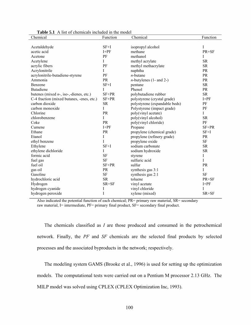
100
Table 5.1 A list of chemicals included in the model Chemical Function Chemical Function
Acetaldehyde SF+I acetic acid I+PF Acetone PF Acetylene I acrylic fibers PF Acrylonitrile I acrylonitrile-butadiene-styrene PF Ammonia PR Benzene SF+I Butadiene I butenes (mixed n-, iso-,-dienes, etc.) SF+PR C-4 fraction (mixed butanes, -enes, etc.) SF+PR carbon dioxide SR carbon monoxide I Chlorine PR chlorobenzene I Coke PR Cumene I+PF Ethane PR Etanol I ethyl benzene I Ethylene SF+I ethylene dichloride I formic acid SF fuel gas SF fuel oil SF+PR gas oil PR Gasoline SF hydrochloric acid SR Hydrogen SR+SF hydrogen cyanide I hydrogen peroxide I
isopropyl alcohol I methane PR+SF methanol I methyl acrylate SR methyl methacrylate SR naphtha PR n-butane PR n-butylenes (1- and 2-) PR pentane SR Phenol PR polybutadiene rubber SR polystyrene (crystal grade) I+PF polystyrene (expandable beds) PF Polystyrene (impact grade) PF poly(vinyl acetate) I poly(vinyl alcohol) SR poly(vinyl chloride) PF Propane SF+PR propylene (chemical grade) SF+I propylene (refinery grade) PR propylene oxide SF sodium carbonate SR sodium hydroxide SR styrene I sulfuric acid I sulfur PR synthesis gas 3:1 I synthesis gas 2:1 SF toluene PR+SF vinyl acetate I+PF vinyl chloride I xylene (mixed) SR+SF
Also indicated the potential function of each chemical; PR= primary raw material, SR= secondary raw material, I= intermediate, PF= primary final product, SF= secondary final product.
The chemicals classified as I are those produced and consumed in the petrochemical
network. Finally, the PF and SF chemicals are the selected final products by selected
processes and the associated byproducts in the network; respectively.
The modeling system GAMS (Brooke et al., 1996) is used for setting up the optimization
models. The computational tests were carried out on a Pentium M processor 2.13 GHz. The
MILP model was solved using CPLEX (CPLEX Optimization Inc, 1993).
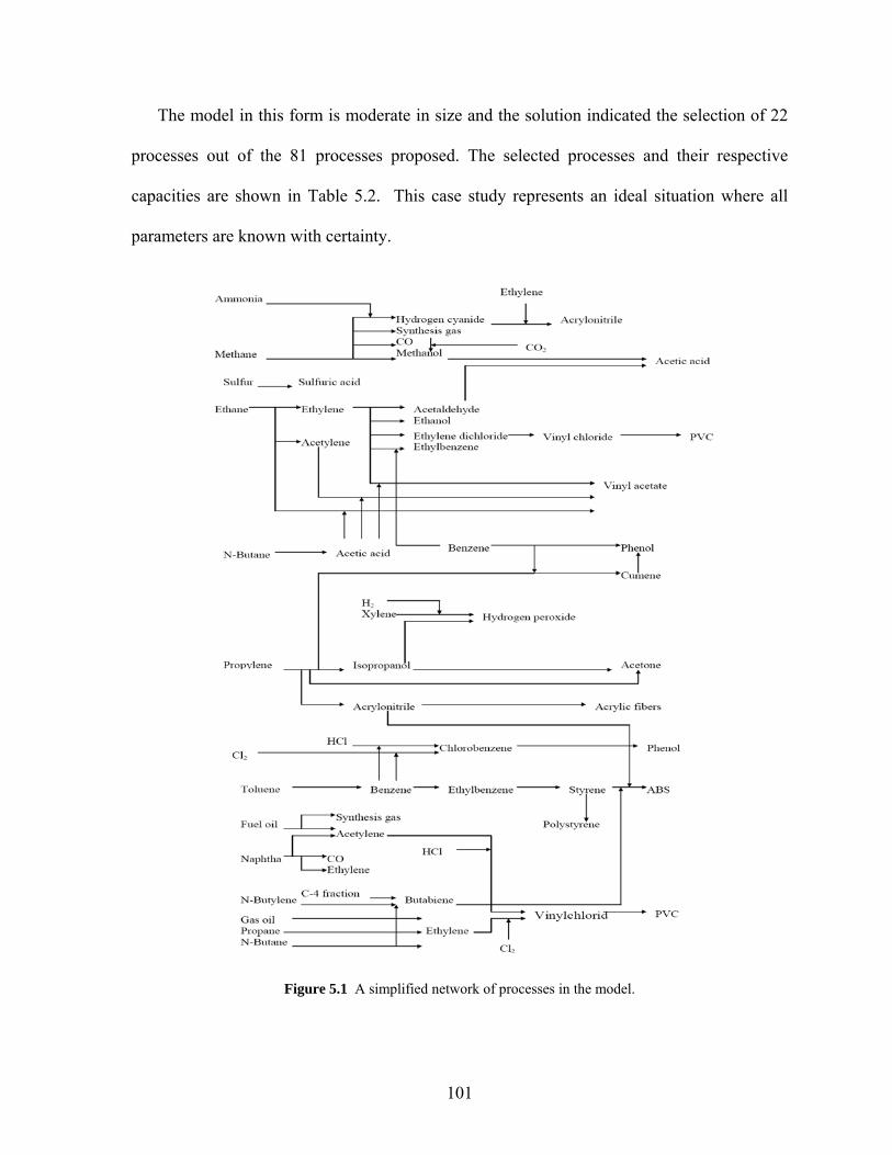
101
The model in this form is moderate in size and the solution indicated the selection of 22
processes out of the 81 processes proposed. The selected processes and their respective
capacities are shown in Table 5.2. This case study represents an ideal situation where all
parameters are known with certainty.
Figure 5.1 A simplified network of processes in the model.
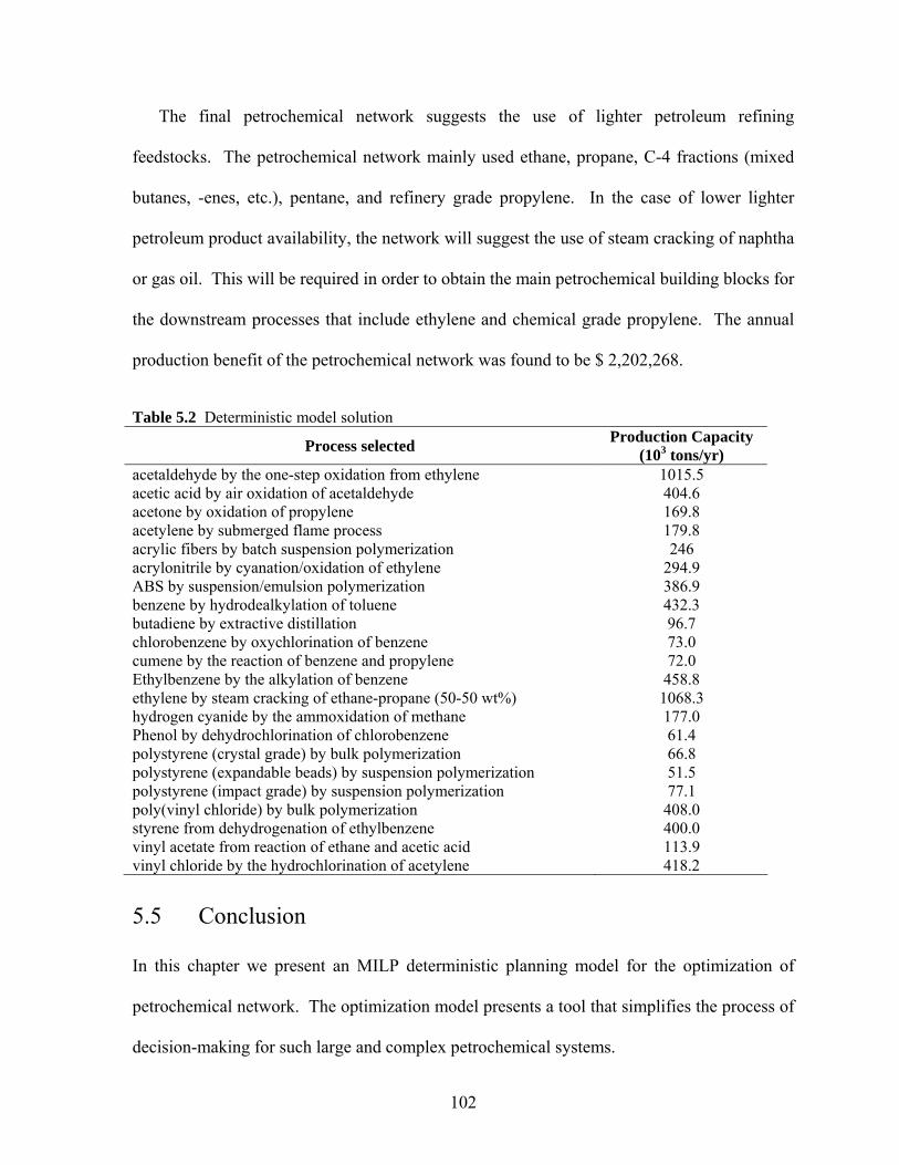
102
The final petrochemical network suggests the use of lighter petroleum refining
feedstocks. The petrochemical network mainly used ethane, propane, C-4 fractions (mixed
butanes, -enes, etc.), pentane, and refinery grade propylene. In the case of lower lighter
petroleum product availability, the network will suggest the use of steam cracking of naphtha
or gas oil. This will be required in order to obtain the main petrochemical building blocks for
the downstream processes that include ethylene and chemical grade propylene. The annual
production benefit of the petrochemical network was found to be $ 2,202,268.
Table 5.2 Deterministic model solution
Process selected Production Capacity (103 tons/yr)
acetaldehyde by the one-step oxidation from ethylene 1015.5 acetic acid by air oxidation of acetaldehyde 404.6 acetone by oxidation of propylene 169.8 acetylene by submerged flame process 179.8 acrylic fibers by batch suspension polymerization 246 acrylonitrile by cyanation/oxidation of ethylene 294.9 ABS by suspension/emulsion polymerization 386.9 benzene by hydrodealkylation of toluene 432.3 butadiene by extractive distillation 96.7 chlorobenzene by oxychlorination of benzene 73.0 cumene by the reaction of benzene and propylene 72.0 Ethylbenzene by the alkylation of benzene 458.8 ethylene by steam cracking of ethane-propane (50-50 wt%) 1068.3 hydrogen cyanide by the ammoxidation of methane 177.0 Phenol by dehydrochlorination of chlorobenzene 61.4 polystyrene (crystal grade) by bulk polymerization 66.8 polystyrene (expandable beads) by suspension polymerization 51.5 polystyrene (impact grade) by suspension polymerization 77.1 poly(vinyl chloride) by bulk polymerization 408.0 styrene from dehydrogenation of ethylbenzene 400.0 vinyl acetate from reaction of ethane and acetic acid 113.9 vinyl chloride by the hydrochlorination of acetylene 418.2
5.5 Conclusion
In this chapter we present an MILP deterministic planning model for the optimization of
petrochemical network. The optimization model presents a tool that simplifies the process of
decision-making for such large and complex petrochemical systems.
103
However, considering this type of high level strategic planning model, especially with the
current volatile market environment and the continuous change in customer requirements, the
impact of uncertainties is inevitable. In fact, ignoring uncertainty of key parameters in
decision problems can yield non-optimal and infeasible decisions (Birge, 1995). For that
reason, the scope of the following chapter is to extend the deterministic petrochemical
planning model to account for uncertainties in model parameters and include the risk notion
in decision-making using proper robust optimization techniques.
104
Chapter 6
Robust Optimization for Petrochemical Networks: Design under Uncertainty
6.1 Introduction
The discussion on planning under uncertainty in Chapter 4 and planning in the petrochemical
networks in Chapter 5 underline the importance of modeling uncertainty and considering risk
in process system engineering studies. In this chapter, we extend the model presented in
Chapter 5 to address the strategic planning, design and optimization of a network of
petrochemical processes under uncertainty and robust considerations. Robustness is
analyzed based on both model robustness and solution robustness, where each measure is
assigned a scaling factor to analyze the sensitivity of the refinery plan and integration
network due to variations. For each term, a different scaling factor was used to analyze the
sensitivity of the petrochemical network due to variations of each component. The stochastic
model is formulated as a two-stage stochastic MILP problem whereas the robust optimization
is formulated as an MINLP problem with nonlinearity arising from modeling the risk
components. Both endogenous uncertainty, represented by uncertainty in the process yield
and exogenous uncertainty, represented by uncertainty in raw material and product prices,
and lower product market demand were considered. The concept of Expected Value of
Perfect Information (EVPI) and Value of the Stochastic Solution (VSS) are also investigated
to numerically illustrate the value of including the randomness of the different model
105
parameters. The considerations of uncertainty in these parameters provided a more robust
and practical analysis of the problem especially at a time when fluctuations in petroleum and
petrochemical products prices and demands are soaring. For a literature review on planning
of petrochemical networks, planning under uncertainty, and modeling risk, we refer the
reader to Chapter 4 and 5.
The remainder of Chapter 6 is organized as follows. In the following section we will
explain the proposed model formulation for the petrochemical network planning under
uncertainty and with uncertainty and risk consideration, referred to as robust optimization.
Then we will briefly explain the concept of value of information and stochastic solution, in
section 6.3. In section 6.4, we will illustrate the performance of the model through an
industrial case study. The chapter ends with concluding remarks in section 6.5.
6.2 Model Formulation
6.2.1 Two-Stage Stochastic Model
This formulation is an extension to the deterministic model presented in Chapter 5. In the
previous chapter, all parameters of the model were assumed to be known with certainty.
However, the current situation of fluctuating high petroleum crude oil and petrochemical
product prices and demands is an indication of the high market and industry volatility.
Acknowledging the shortcomings of deterministic models, parameter uncertainty is
considered in the process yield mcp,δ , raw material and product prices PetcpPr , and lower
product demand LcpPetD . The problem is formulated as a two-stage stochastic programming
model. The uncertainty is considered through discrete distribution of the random parameters
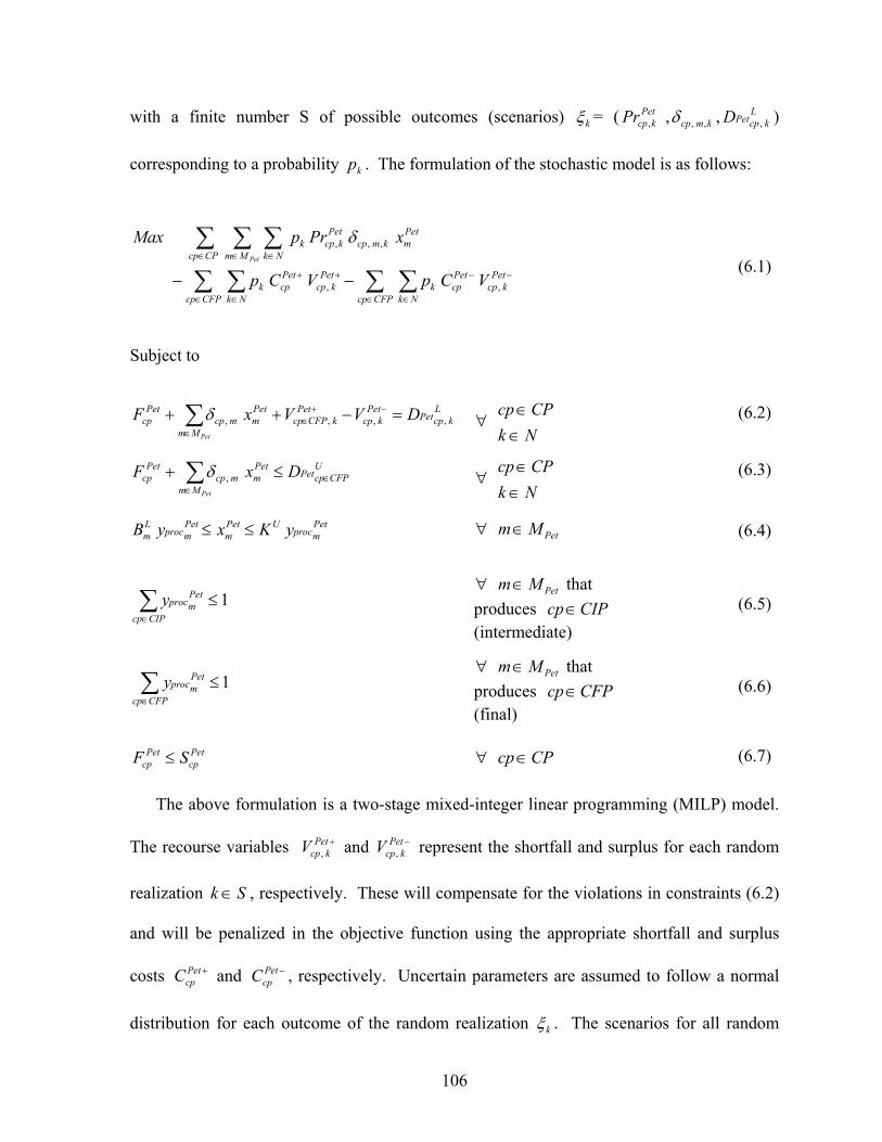
106
with a finite number S of possible outcomes (scenarios) kξ = ( PetkcpPr , , kmcp ,,δ , L
kcpPetD , )
corresponding to a probability kp . The formulation of the stochastic model is as follows:
∑ ∑∑ ∑
∑ ∑ ∑
∈ ∈
−−
∈ ∈
++
∈ ∈ ∈
−−CFPcp Nk
Petkcp
Petcpk
CFPcp Nk
Petkcp
Petcpk
CPcp Mm Nk
Petmkmcp
Petkcpk
VCpVCp
xPrpMaxPet
,,
,,, δ (6.1)
Subject to
∑∈
−+∈ =−++
PetMm
LkcpPet
Petkcp
PetkCFPcp
Petmmcp
Petcp DVVxF ,,,,δ ∀
NkCPcp
∈∈
(6.2)
UCFPcpPet
Mm
Petmmcp
Petcp DxF
Pet
∈∈
≤+ ∑ ,δ ∀ NkCPcp
∈∈
(6.3)
Petmproc
UPetm
Petmproc
Lm yKxyB ≤≤ ∀ PetMm∈ (6.4)
∑∈
≤CIPcp
Petmprocy 1
∀ PetMm∈ that produces CIPcp∈ (intermediate)
(6.5)
∑∈
≤CFPcp
Petmprocy 1
∀ PetMm∈ that produces CFPcp∈ (final)
(6.6)
Petcp
Petcp SF ≤ ∀ CPcp∈ (6.7)
The above formulation is a two-stage mixed-integer linear programming (MILP) model.
The recourse variables +PetkcpV , and −Pet
kcpV , represent the shortfall and surplus for each random
realization Sk ∈ , respectively. These will compensate for the violations in constraints (6.2)
and will be penalized in the objective function using the appropriate shortfall and surplus
costs +PetcpC and −Pet
cpC , respectively. Uncertain parameters are assumed to follow a normal
distribution for each outcome of the random realization kξ . The scenarios for all random
107
parameters are generated simultaneously. The recourse variables +PetkcpV , and −Pet
kcpV , in this
formulation will compensate for deviations from the mean of the lower market demands
LcpPetD and process yield mcp,δ . In that way, the use of an independent recourse action and
compensation for the violation in the constraint due to process yield uncertainty alone was
avoided. Although this may not allow an explicit analysis for process yield uncertainty, it
instead circumvents the complication of treating these types endogenous uncertainty.
6.2.2 Robust Optimization
The stochastic model with recourse in the previous section takes a decision merely based on
first-stage and expected second-stage costs leading to an assumption that the decision-maker
is risk-neutral (Sahinidis, 2004). In order to capture the concept of risk in stochastic
programming, Mulvey et al. (1995) proposed the following amendment to the objective
function:
),())](,([, yfxQxcMin Tyx ωλωξ +Ε+
where ))](,([ ωξxQΕ is the fixed recourse, f is a measure of variability (i.e. second
moment) of the second-stage costs, and λ is a non-negative scalar representing risk tolerance.
The representation through risk management using variance as a risk measure is often
referred to as robust stochastic programming (Mulvey et al., 1995). This is also a typical risk
measure following the Markowitz mean–variance (MV) model (Markowitz, 1952). The
robustness is incorporated through the consideration of higher moments (variance) of the
random parameter distribution kξ in the objective function and hence measuring the
tradeoffs between mean value and variability.
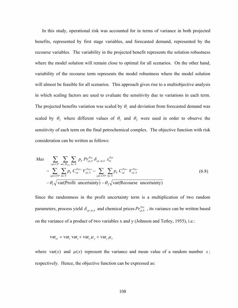
108
In this study, operational risk was accounted for in terms of variance in both projected
benefits, represented by first stage variables, and forecasted demand, represented by the
recourse variables. The variability in the projected benefit represents the solution robustness
where the model solution will remain close to optimal for all scenarios. On the other hand,
variability of the recourse term represents the model robustness where the model solution
will almost be feasible for all scenarios. This approach gives rise to a multiobjective analysis
in which scaling factors are used to evaluate the sensitivity due to variations in each term.
The projected benefits variation was scaled by 1θ and deviation from forecasted demand was
scaled by 2θ where different values of 1θ and 2θ were used in order to observe the
sensitivity of each term on the final petrochemical complex. The objective function with risk
consideration can be written as follows:
)yuncertaintRecoursevar()yuncertaintProfitvar( 21
,,
,,,
θθ
δ
−−
−− ∑ ∑∑ ∑
∑ ∑ ∑
∈ ∈
−−
∈ ∈
++
∈ ∈ ∈
CFPcp Nk
Petkcp
Petcpk
CFPcp Nk
Petkcp
Petcpk
CPcp Mm Nk
Petmkmcp
Petkcpk
VCpVCp
xPrpMaxPet
(6.8)
Since the randomness in the profit uncertainty term is a multiplication of two random
parameters, process yield kmcp ,,δ and chemical prices PetkcpPr , , its variance can be written based
on the variance of a product of two variables x and y (Johnson and Tetley, 1955), i.e.:
xyyxyxxy μμ varvarvarvarvar ++=
where )var(x and )(xμ represent the variance and mean value of a random number x ;
respectively. Hence, the objective function can be expressed as:
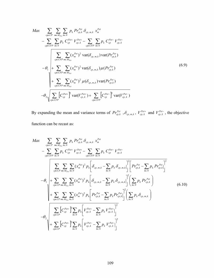
109
[ ] [ ]∑ ∑
∑ ∑
∑ ∑
∑ ∑
∑ ∑∑ ∑
∑ ∑ ∑
∈ ∈
−−++
∈ ∈
∈ ∈
∈ ∈
∈ ∈
−−
∈ ∈
++
∈ ∈ ∈
+−
+
+−
−−
CFPcp CFPcp
Petkcp
Petcp
Petkcp
Petcp
CFPcp Mm
Petkcpkmcp
Petm
CFPcp Mm
Petkcpkmcp
Petm
CFPcp Mm
Petkcpkmcp
Petm
CFPcp Nk
Petkcp
Petcpk
CFPcp Nk
Petkcp
Petcpk
CPcp Mm Nk
Petmkmcp
Petkcpk
VCVC
Prx
Prx
Prx
VCpVCp
xPrpMax
Pet
Pet
Pet
Pet
)var()var(
)var()()(
)()var()(
)var()var()(
,2
,2
2
,,,2
,,,2
,,,2
1
,,
,,,
θ
δμ
μδ
δ
θ
δ
(6.9)
By expanding the mean and variance terms of PetkcpPr , , kmcp ,,δ , +Pet
kcpV , and −PetkcpV , , the objective
function can be recast as:
[ ]
[ ]∑ ∑ ∑
∑ ∑ ∑
∑ ∑ ∑ ∑∑
∑ ∑ ∑ ∑∑
∑ ∑ ∑ ∑∑
∑ ∑∑ ∑
∑ ∑ ∑
∈ ∈ ∈
−−−
∈ ∈ ∈
+++
∈ ∈ ∈ ∈∈
∈ ∈ ∈ ∈∈
∈ ∈ ∈ ∈∈
∈ ∈
−−
∈ ∈
++
∈ ∈ ∈
⎥⎦
⎤⎢⎣
⎡−+
⎥⎦
⎤⎢⎣
⎡−
−
⎟⎟⎠
⎞⎜⎜⎝
⎛⎥⎦
⎤⎢⎣
⎡−+
⎟⎟⎠
⎞⎜⎜⎝
⎛⎥⎦
⎤⎢⎣
⎡−+
⎥⎦
⎤⎢⎣
⎡−⎥
⎦
⎤⎢⎣
⎡−
−
−−
CPcp Nk Nk
Petkcpk
Petkcpk
Petcp
CPcp Nk Nk
Petkcpk
Petkcpk
Petcp
CPcp Mm Nk Nkkmcpk
Nk
Petkcpk
Petkcpk
Petm
CPcp Mm Nk Nk
Petkcpk
Nkkmcpkkmcpk
Petm
CPcp Mm Nk Nk
Petkcpk
Petkcp
Nkkmcpkkmcpk
Petm
CFPcp Nk
Petkcp
Petcpk
CFPcp Nk
Petkcp
Petcpk
CPcp Mm Nk
Petmkmcp
Petkcpk
VpVpC
VpVpC
pPrpPrpx
Prpppx
PrpPrppx
VCpVCp
xPrpMax
Pet
Pet
Pet
Pet
2
,,2
2
,,2
2
,,
2
,,2
,
2
,,,,2
2
,,
2
,,,,2
1
,,
,,,
)(
)(
)(
θ
δ
δδ
δδ
θ
δ
(6.10)
110
In order to understand the effect of each term on the overall objective function of the
petrochemical network, different values of 1θ and 2θ should be evaluated as will be shown in
the illustrative case study.
6.3 Value to Information and Stochastic Solution
Since stochastic programming adds computational burden on practical problems, it is
desirable to quantify the benefits of considering uncertainty. In order to address this point,
there are generally two values of interest. One is expected value of perfect information
(EVPI) which measures the maximum amount the decision maker is willing to pay in order
to get accurate information on the future. The second is value of stochastic solution (VSS)
which is the difference in the objective function between the solutions of mean value
problem (replacing random events with their means) and the stochastic solution (SS). (Birge,
1982)
A solution based on perfect information would yield optimal first stage decisions for each
realization of the random parameters ξ . Then the expected value of these decisions, known
as “wait-and-see” (WS) can be written as (Madansky, 1960):
)],([ ξξ xzMinEWS =
However, since our objective is profit maximization, the expected value of perfect
information (EVPI) can be calculated as:
SSWSEVPI −= (6.11)
111
The other quantity of interest is the value of stochastic solution (VSS). In order to
quantify it, we first need to solve the mean value problem, also referred to as the expected
value problem (EV). This can be defined as ])[,( ξExzMin where ξξ =][E (Birge, 1982).
The solution of the EV problem provides the first stage decisions variables evaluated at
expectation of the random realizations. The expectation of the EV problem, evaluated at
different realization of the random parameters, is then defined as (Birge, 1982):
)]),(([ ξξξ xzMinEEEV =
where )(ξx is evaluated from the EV model, allowing the optimization problem to choose
second stage variables with respect to ξ . Similarly since our objective is profit
maximization, the value of stochastic solution can be expressed as:
EEVSSVSS −= (6.12)
The value of stochastic solution can also be evaluated as the cost of ignoring uncertainty
in the problem. These concepts will be evaluated in our case study.
6.4 Illustrative Case Study
A number of case studies were developed to demonstrate the performance of the optimization
models and illustrate the effect of process yield, raw material and product prices, and lower
product market demand variations. The case study in this chapter is based on Al-Sharrah et
al. (2006) and is the same as the example presented in Chapter 5. The petrochemical network
included 81 processes connecting the production and consumption of 65 chemicals which
gave rise to 5265 uncertain process yield parameters. In addition, the model included 11
112
uncertain product demand parameters and 65 uncertain parameters representing raw materials
and product prices. This gives a total of 5341 uncertain parameters which were modeled
with a total number of 200 scenarios for each random parameter. Due to the high number of
uncertain parameters and that fact that these type of data are generally stored in spreadsheets,
all scenarios where generated in Excel spreadsheets using a pseudo random number
generator. The input data was then imported to GAMS using the GAMS-Excel interface.
All uncertain parameters were assumed to have a normal distribution. However, this
assumption bears no restriction to the generality of the proposed modeling approach as other
sampling distributions can be easily used instead.
The modeling system GAMS (Brooke et al., 1996) is used for setting up the optimization
models. The computational tests were carried out on a Pentium M processor 2.13 GHz. The
models were solved with DICOPT (Viswanathan & Grossmann, 1990). The NLP
subproblems were solved with CONOPT2 (Drud, 1994), while the MILP master problems
were solved with CPLEX (CPLEX Optimization Inc, 1993).
6.4.1 Solution of Stochastic Model
The two-stage mixed-integer stochastic program with recourse that includes a total number of
200 scenarios for each random parameter is considered in this section. All random
parameters were assumed to follow a normal distribution and the scenarios for all random
parameters were generated simultaneously. Therefore, the recourse variables account for the
deviation from a given scenario as opposed to the deviation from a particular random number
realization.
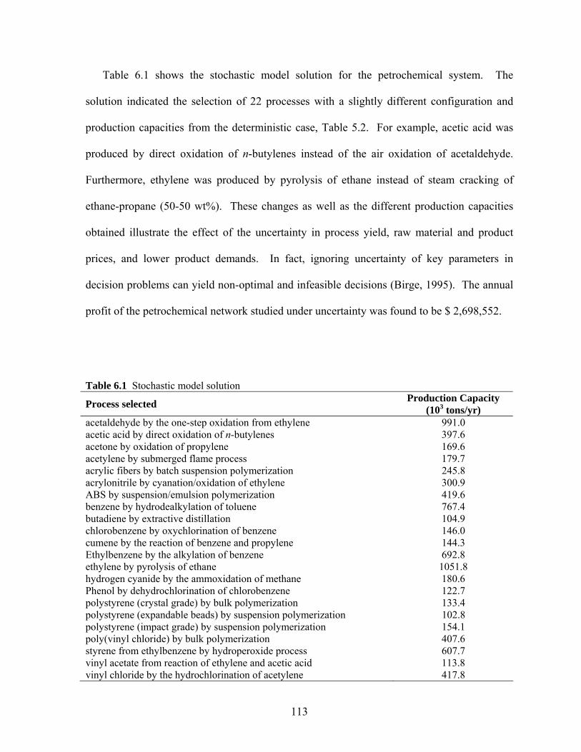
113
Table 6.1 shows the stochastic model solution for the petrochemical system. The
solution indicated the selection of 22 processes with a slightly different configuration and
production capacities from the deterministic case, Table 5.2. For example, acetic acid was
produced by direct oxidation of n-butylenes instead of the air oxidation of acetaldehyde.
Furthermore, ethylene was produced by pyrolysis of ethane instead of steam cracking of
ethane-propane (50-50 wt%). These changes as well as the different production capacities
obtained illustrate the effect of the uncertainty in process yield, raw material and product
prices, and lower product demands. In fact, ignoring uncertainty of key parameters in
decision problems can yield non-optimal and infeasible decisions (Birge, 1995). The annual
profit of the petrochemical network studied under uncertainty was found to be $ 2,698,552.
Table 6.1 Stochastic model solution
Process selected Production Capacity (103 tons/yr)
acetaldehyde by the one-step oxidation from ethylene 991.0 acetic acid by direct oxidation of n-butylenes 397.6 acetone by oxidation of propylene 169.6 acetylene by submerged flame process 179.7 acrylic fibers by batch suspension polymerization 245.8 acrylonitrile by cyanation/oxidation of ethylene 300.9 ABS by suspension/emulsion polymerization 419.6 benzene by hydrodealkylation of toluene 767.4 butadiene by extractive distillation 104.9 chlorobenzene by oxychlorination of benzene 146.0 cumene by the reaction of benzene and propylene 144.3 Ethylbenzene by the alkylation of benzene 692.8 ethylene by pyrolysis of ethane 1051.8 hydrogen cyanide by the ammoxidation of methane 180.6 Phenol by dehydrochlorination of chlorobenzene 122.7 polystyrene (crystal grade) by bulk polymerization 133.4 polystyrene (expandable beads) by suspension polymerization 102.8 polystyrene (impact grade) by suspension polymerization 154.1 poly(vinyl chloride) by bulk polymerization 407.6 styrene from ethylbenzene by hydroperoxide process 607.7 vinyl acetate from reaction of ethylene and acetic acid 113.8 vinyl chloride by the hydrochlorination of acetylene 417.8
114
However, in order to properly evaluate the added-value of including uncertainty of the
problem parameters, we will investigate both the expected value of perfect information
(EVPI) and the value of stochastic solution (VSS).
In order to evaluate the value of stochastic solution (VSS) we first solved the
deterministic problem, as illustrated in the previous section, and fixed the petrochemical
network and the production rate of the processes. We then solved the EEV problem by
allowing the optimization problem to choose second stage variables with respect to the
realization of the uncertain parameters ξ . From (6.12), the VSS is:
622,513930,184,2552,698,2
==
−=
VSSEEV
EEVVSS
This indicates that the benefit of incorporating uncertainty in the different model parameters
for the petrochemical network investment is $ 513,622. On the other hand, the expected
value of perfect information (EVPI) can be evaluated by first finding the “wait-and-see”
(WS) solution. The latter can be obtained by taking the expectation for the optimal first stage
decisions evaluated at each realization ξ . From (6.11), the EVPI is:
488,25040,724,2
552,698,2
==
−=
EVPIWS
WSEVPI
This implies that if it were possible to know the future realization of the demand, prices and
yield perfectly, the profit would have been $2,724,040 instead of $2,698,552, yielding
savings of $25,488. However, since acquiring perfect information is not viable, we will
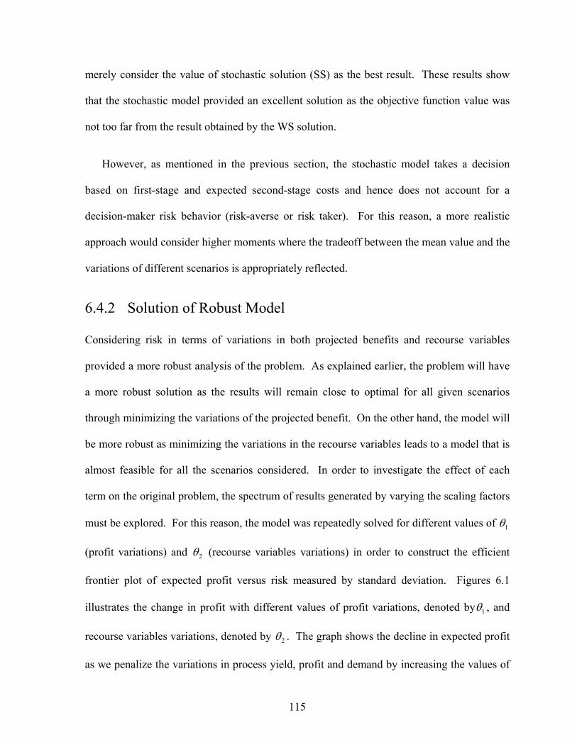
115
merely consider the value of stochastic solution (SS) as the best result. These results show
that the stochastic model provided an excellent solution as the objective function value was
not too far from the result obtained by the WS solution.
However, as mentioned in the previous section, the stochastic model takes a decision
based on first-stage and expected second-stage costs and hence does not account for a
decision-maker risk behavior (risk-averse or risk taker). For this reason, a more realistic
approach would consider higher moments where the tradeoff between the mean value and the
variations of different scenarios is appropriately reflected.
6.4.2 Solution of Robust Model
Considering risk in terms of variations in both projected benefits and recourse variables
provided a more robust analysis of the problem. As explained earlier, the problem will have
a more robust solution as the results will remain close to optimal for all given scenarios
through minimizing the variations of the projected benefit. On the other hand, the model will
be more robust as minimizing the variations in the recourse variables leads to a model that is
almost feasible for all the scenarios considered. In order to investigate the effect of each
term on the original problem, the spectrum of results generated by varying the scaling factors
must be explored. For this reason, the model was repeatedly solved for different values of 1θ
(profit variations) and 2θ (recourse variables variations) in order to construct the efficient
frontier plot of expected profit versus risk measured by standard deviation. Figures 6.1
illustrates the change in profit with different values of profit variations, denoted by 1θ , and
recourse variables variations, denoted by 2θ . The graph shows the decline in expected profit
as we penalize the variations in process yield, profit and demand by increasing the values of
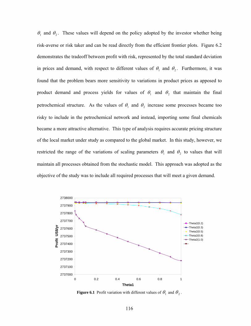
116
1θ and 2θ . These values will depend on the policy adopted by the investor whether being
risk-averse or risk taker and can be read directly from the efficient frontier plots. Figure 6.2
demonstrates the tradeoff between profit with risk, represented by the total standard deviation
in prices and demand, with respect to different values of 1θ and 2θ . Furthermore, it was
found that the problem bears more sensitivity to variations in product prices as apposed to
product demand and process yields for values of 1θ and 2θ that maintain the final
petrochemical structure. As the values of 1θ and 2θ increase some processes became too
risky to include in the petrochemical network and instead, importing some final chemicals
became a more attractive alternative. This type of analysis requires accurate pricing structure
of the local market under study as compared to the global market. In this study, however, we
restricted the range of the variations of scaling parameters 1θ and 2θ to values that will
maintain all processes obtained from the stochastic model. This approach was adopted as the
objective of the study was to include all required processes that will meet a given demand.
2737000
2737100
2737200
2737300
2737400
2737500
2737600
2737700
2737800
2737900
2738000
0 0.2 0.4 0.6 0.8 1
Theta1
Prof
it U
S$/y
r Theta2(0.2)Theta2(0.3)Theta2(0.5)Theta2(0.8)Theta2(1.0)
Figure 6.1 Profit variation with different values of 1θ and 2θ .
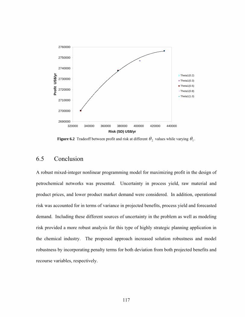
117
2690000
2700000
2710000
2720000
2730000
2740000
2750000
2760000
320000 340000 360000 380000 400000 420000 440000
Risk (SD) US$/yr
Prof
it U
S$/y
r
Theta1(0.2)
Theta1(0.3)
Theta1(0.5)
Theta1(0.8)
Theta1(1.0)
Figure 6.2 Tradeoff between profit and risk at different 2θ values while varying 1θ .
6.5 Conclusion
A robust mixed-integer nonlinear programming model for maximizing profit in the design of
petrochemical networks was presented. Uncertainty in process yield, raw material and
product prices, and lower product market demand were considered. In addition, operational
risk was accounted for in terms of variance in projected benefits, process yield and forecasted
demand. Including these different sources of uncertainty in the problem as well as modeling
risk provided a more robust analysis for this type of highly strategic planning application in
the chemical industry. The proposed approach increased solution robustness and model
robustness by incorporating penalty terms for both deviation from both projected benefits and
recourse variables, respectively.
118
The results of the model studied under uncertainty and with risk consideration, as one can
intuitively anticipate, yielded different petrochemical network configurations and plant
capacities when compared to the deterministic model results. The concepts of Expected
Value of Perfect Information (EVPI) and Value of the Stochastic Solution (VSS) were
introduced and numerically illustrated. The results obtained from the stochastic model
provided good results as the objective function value was not too far from the results
obtained using the wait-and-see approach. Furthermore, the study showed that the final
petrochemical network bears more sensitivity to variations in product prices as apposed to
variation in market demand and process yields when the values of 1θ and 2θ were selected to
maintain the final petrochemical structure.
119
Chapter 7
Multisite Refinery and Petrochemical Network Design: Optimal Integration and Coordination
7.1 Introduction
In view of the current situation of high oil prices and the increasing consciousness and
implementation of strict environmental regulations, petroleum refiners and petrochemical
companies started seeking opportunities for mergers and integration. This is evident in the
current projects around the world for building integrated refineries and the development of
complex petrochemical industries that are aligned through advanced integration platforms.
Figure 7.1 illustrates a typical refining and petrochemical industry supply chain. The
realization of coordination and objective alignment benefits across the enterprise has been the
main driver of such efforts (Sahinidis et al., 1989; Shah, 1998).
Despite the fact that petroleum refining and petrochemical companies have recently
engaged in more integration projects, relatively little research in the open literature has been
reported, mostly due to confidentiality reasons. Such concerns render the development of a
systematic framework of network integration and coordination difficult. The studies
published in the open literature were mainly developed by consulting and design firms, as
well as the operating companies, and generally lack a structured methodology for evaluating
the projects feasibility. Just to mention a few of the studies published, Swaty (2002) studied
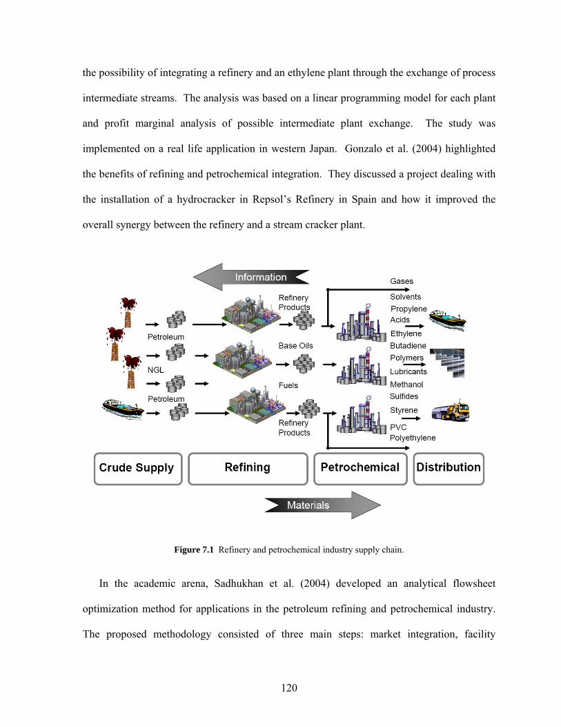
120
the possibility of integrating a refinery and an ethylene plant through the exchange of process
intermediate streams. The analysis was based on a linear programming model for each plant
and profit marginal analysis of possible intermediate plant exchange. The study was
implemented on a real life application in western Japan. Gonzalo et al. (2004) highlighted
the benefits of refining and petrochemical integration. They discussed a project dealing with
the installation of a hydrocracker in Repsol’s Refinery in Spain and how it improved the
overall synergy between the refinery and a stream cracker plant.
Figure 7.1 Refinery and petrochemical industry supply chain.
In the academic arena, Sadhukhan et al. (2004) developed an analytical flowsheet
optimization method for applications in the petroleum refining and petrochemical industry.
The proposed methodology consisted of three main steps: market integration, facility
121
network optimization through economic margin analysis and load shifting, and elimination of
less profitable processes. They demonstrated their method on two case studies: a single site
refinery and a petrochemical complex. Li et al. (2006) proposed a Linear Programming (LP)
model for the integration of a refinery and an ethylene cracker. They evaluated different
schemes iteratively for different crude types to optimize the refinery and ethylene cracker
operations. The best scheme was selected based on the highest profit from the cases studied.
More recently, Kuo and Chang (2008) developed a short term multi-period planning model
for a benzene-toluene-xylene (BTX) complex. They modeled the system as a mixed integer
linear programming (MILP) model with binary variables mainly for mode switching and
inventory control (backlog and surplus indication). They divided the processing units into
two sets, 1) reaction processes: reforming, isomerization units and tatory units, and 2)
separation processes: aromatics extraction units, xylene fractionation units and the parex
units. Optimization of the other refinery units, blending levels and olefin cracking process
were not considered. The decisions in their study mainly included the optimal throughput
and operation mode of each production unit, inventory levels and feedstock supplies. For
more details on strategic multisite planning studies, multisite refinery optimization, and
petrochemical industry planning the interested reader is referred to the previous chapters and
the references given herein.
Petroleum refining and petrochemical plants integration is gaining a great deal of interest
with the realization of coordination and vertical integration benefits. Previous research in the
field assumed either no limitations on refinery feedstock availability for the petrochemical
planning problem or fixed the refinery production levels assuming an optimal operation.
However, in this chapter we present a mathematical model for the determination of the
122
optimal integration and coordination strategy for a refinery network and synthesize the
optimal petrochemical network required to satisfy a given demand from any set of available
technologies. Therefore, achieving a global optimal production strategy by allowing
appropriate trade offs between the refinery and the downstream petrochemical markets. The
refinery and petrochemical systems were modeled as MILP problems that will also lead to
overall refinery and petrochemical process production levels and detailed blending levels at
each refinery site. The objective function is a minimization of the annualized cost over a
given time horizon among the refineries by improving the coordination and utilization of
excess capacities in each facility and maximization of the added value in the petrochemical
system. Expansion requirements to improve production flexibility and reliability in the
refineries are also considered.
The remainder of Chapter 7 is organized as follows. In the following section, we explain
the problem statement of the petroleum refinery and petrochemical integration. Then, we
discuss the proposed model formulation in section 7.3. In section 7.4, we illustrate the
performance of the model through an industrial-scale case study. The chapter ends with
some concluding remarks in section 7.5.
7.2 Problem Statement
The optimization of refining and petrochemical processes involves a wide range of aspects
varying from economical analysis and strategic expansions to crude oil selection, process
levels targets, operating modes, etc. The focus of this study is to develop a mathematical
programming tool for the simultaneous design of an integrated network of refineries and
petrochemical processes. On the refinery side, the model provides the optimal network
123
integration between the refineries, process expansion requirements, operating policy based on
different feedstock combination alternatives, process levels and operating modes. On the
petrochemical side, the model establishes the design of an optimal petrochemical process
network from a range of process technologies to satisfy a given demand. The simultaneous
network design and optimization of the refining and petrochemical industry provides
appropriate means for improving the coordination across the industrial system and is prone to
develop an overall optimal production strategy across the petroleum chain.
The general problem under study can be defined as follows:
A set of refinery products CFRcfr∈ produced at multiple refinery sites Ii∈ and a set of
petrochemical products CFPcp∈ is given. Each refinery consists of different production
units RefMm∈ that can operate at different modes Pp∈ while a set of wide range
petrochemical and chemical process technologies PefMm∈ is available for selection.
Furthermore, different crude oil slates CRcr∈ are available and given. The petrochemical
network selects its feedstock from three main sources; namely, refinery intermediate streams
PeticircrFi ,, of an intermediate product RPIcir∈ , refinery final products Pet
icfrcrFf ,, of a final
product RPFcfr∈ , and non-refinery streams PetcpFn of a chemical NRFcp∈ . The process
network across the refineries and petrochemical system is connected in a finite number of
ways. An integration superstructure between the refinery processes is defined in order to
allow exchanging intermediate streams. Market product prices, operating cost at each
refinery and petrochemical system, as well as product demands are assumed to be known.
124
The problem consists of determining the optimal integration and coordination strategy for
the overall refinery network and designing the optimal petrochemical network required to
satisfy a given demand from the available process technologies. The proposed approach will
also provide overall refinery and petrochemical process production levels and detailed
blending levels at each refinery site. The objective function is a minimization of the
annualized cost over a given time horizon among the refineries by improving the
coordination and utilization of excess capacities in each facility and maximization of the
added value in the petrochemical system. Expansion requirements to improve production
flexibility and reliability in the refineries are also considered.
For all refinery and petrochemical processes within the network we assume that all
material balances are expressed in terms of linear yield vectors. Even though this might
sound restrictive as most if not all refinery and petrochemical processes are inherently
nonlinear, this practice is commonly applied with such large scale systems. Moreover, the
decisions in this study are of a strategic level in which such linear formulation is adequate to
address the required level of details involved at this stage. It is also assumed that processes
have fixed capacities and the operating cost of each process and production mode is
proportional to the process inlet flow. In the case of refinery product blending, quality
blending indices are used to maintain model linearity. It is also assumed that all products
that are in excess of the local demand can be exported to a global market. Piping and
pumping installation costs to transport refinery intermediate streams between the different
refinery sites as well as the operating costs of the new system are lumped into one fixed-
charge cost. All costs are discounted over a 20 years time horizon and with an interest rate of
7%. No inventories will be considered since the model is addressing strategic decisions
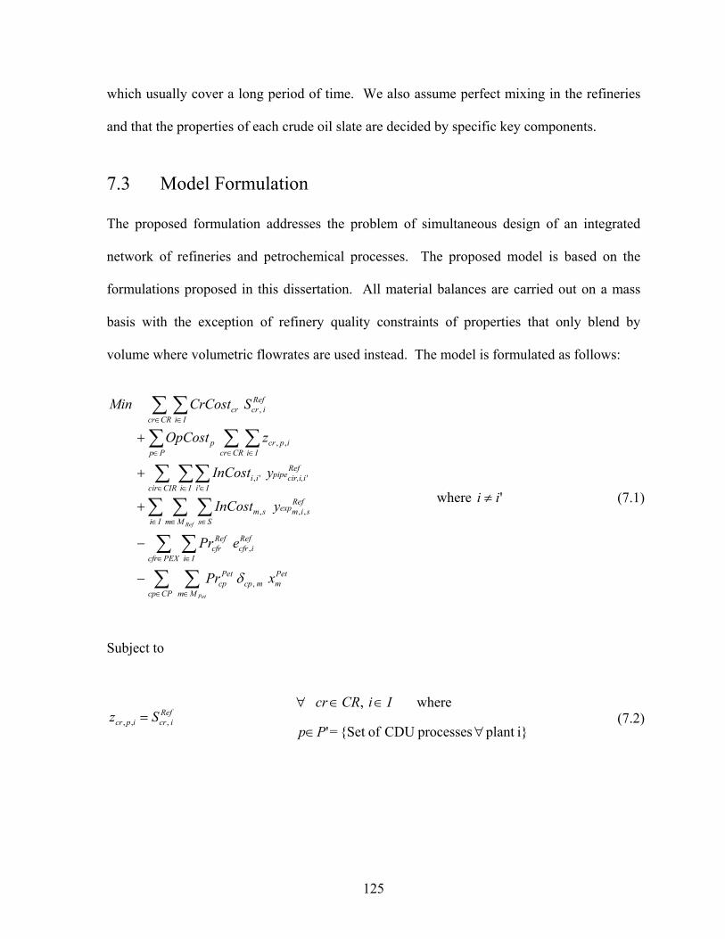
125
which usually cover a long period of time. We also assume perfect mixing in the refineries
and that the properties of each crude oil slate are decided by specific key components.
7.3 Model Formulation
The proposed formulation addresses the problem of simultaneous design of an integrated
network of refineries and petrochemical processes. The proposed model is based on the
formulations proposed in this dissertation. All material balances are carried out on a mass
basis with the exception of refinery quality constraints of properties that only blend by
volume where volumetric flowrates are used instead. The model is formulated as follows:
∑ ∑
∑ ∑
∑ ∑ ∑
∑ ∑∑
∑ ∑∑
∑ ∑
∈ ∈
∈ ∈
∈ ∈ ∈
∈ ∈ ∈
∈ ∈∈
∈ ∈
−
−
+
+
+
CPcp Mm
Petmmcp
Petcp
Reficfr
PEXcfr Ii
Refcfr
Ii Mm Ss
Refsimexpsm
CIRcir Ii
Refcir,i,i'pipe
Iiii
CRcr Iiipcr
Ppp
Reficr
CRcr Iicr
Pet
Ref
xPr
ePr
yInCost
yInCost
zOpCost
SCrCostMin
,
,
,,,
'',
,,
,
δ
where 'ii ≠ (7.1)
Subject to
Reficripcr Sz ,,, =
∀ IiCRcr ∈∈ , where
i}plant processes CDU of{Set =' ∀∈Pp (7.2)
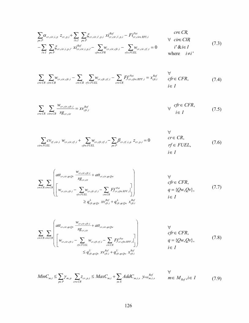
126
0,,,,,,',,,,'
',,,,
,,,,',,'
,,',,,,,,,
=−−−
−+
∑∑∑ ∑
∑ ∑∑
∈∈∈ ∈
∈∈ ∈∈
FUELrfirfcircr
CFRcfricfrcircr
Refipicircr
Ii Ppipicircr
PetiRPIcircr
Refipicircr
Ii Ppipicircr
Ppipcrpicircr
wwxi
Fixiz
ξ
ξα
∀ Iii
CIRcirCRcr
∈∈∈
&',
,
'where ii≠
(7.3)
∑ ∑∑ ∑∑∈
∈∈∈ ∈∈
=−−CRcr
Refcfr,i
PetiRPFcfrcr
CRcrCRcr FUELrfirfcfrcr
CBciricfrcircr xFfww ,,,,,,,,
∀
IiCFRcfr
∈∈ , (7.4)
∑ ∑∈ ∈
=CRcr
Reficfr
CBcir circr
icfrcircr xvsg
w,
,
,,, ∀ IiCFRcfr
∈∈ ,
(7.5)
∑∑∑∈∈∈
=−+Pp
ipcrpirfcrFUELcfr
irfcfrcrFUELcir
irfcircricirrf zwwcv 0,,,,,,,,,,,,, β ∀
IiFUELrfCRcr
∈∈∈
,,
(7.6)
Refcfr,i
LQwqcfr
Reficfr
LQvqcfr
CRcr CBcir PetiRPFcfrcr
CRcrFUELrfirfcfrcricfrcircr
Qwqcircrcircr
icfrcircrQvqcircr
xqxvq
Ffww
attsg
watt
∈∈
∈ ∈∈
∈∈
∈∈
+≥
⎟⎟⎟⎟⎟
⎠
⎞
⎜⎜⎜⎜⎜
⎝
⎛
⎥⎦
⎤⎢⎣
⎡−−
+
∑ ∑∑∑
,,,
,,,,,,,,
,,,
,,,,,
∀
IiQvQwq
CFRcfr
∈=∈
},,{,
(7.7)
Refcfr,i
UQwqcfr
Reficfr
UQvqcfr
CRcr CBcir
FUELrf
PetiRPFcfrcr
CRcrirfcfrcricfrcircr
Qwqcircrcircr
icfrcircrQvqcircr
xqxvq
Ffww
attsg
watt
∈∈
∈ ∈
∈∈
∈
∈∈
+≤
⎟⎟⎟⎟⎟
⎠
⎞
⎜⎜⎜⎜⎜
⎝
⎛
⎥⎦
⎤⎢⎣
⎡−−
+
∑ ∑∑ ∑
,,,
,,,,,,,,
,,,
,,,,,
∀
IiQvQwq
CFRcfr
∈=∈
},,{,
(7.8)
∑∑ ∑∈∈ ∈
+≤≤Ss
Refsimexpsim
Ppim
CRcripcrpmim yAddCMaxCzMinC ,,,,,,,,, γ
∀IiMm Ref ∈∈ ,
(7.9)
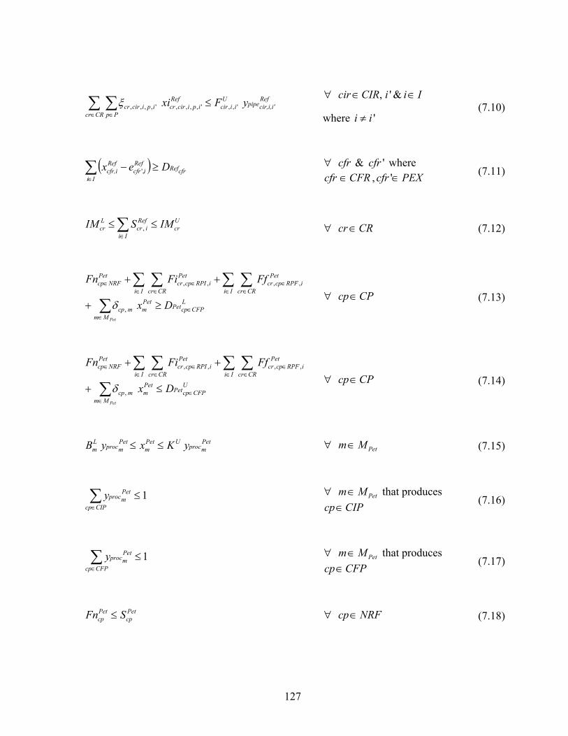
127
∑ ∑∈ ∈
≤CRcr
Refcir,i,i'pipe
Uiicir
Pp
Refipicircripicircr yFxi ',,',,,,',,,,ξ
∀ IiiCIRcir ∈∈ &',
where 'ii ≠ (7.10)
( ) cfrRefIi
Reficfr
Refcfr,i Dex ≥−∑
∈', ∀ '& cfrcfr where
CFRcfr ∈ , PEXcfr ∈' (7.11)
∑∈
≤≤Ii
Ucr
Reficr
Lcr IMSIM , ∀ CRcr∈ (7.12)
∑
∑ ∑∑ ∑
∈∈
∈∈
∈∈∈
∈∈
≥+
++
PetMm
LCFPcpPet
Petmmcp
Ii
PetiRPFcpcr
CRcrIi
PetiRPIcpcr
CRcr
PetNRFcp
Dx
FfFiFn
,
,,,,
δ ∀ CPcp∈ (7.13)
∑
∑ ∑∑ ∑
∈∈
∈∈
∈∈∈
∈∈
≤+
++
PetMm
UCFPcpPet
Petmmcp
Ii
PetiRPFcpcr
CRcrIi
PetiRPIcpcr
CRcr
PetNRFcp
Dx
FfFiFn
,
,,,,
δ ∀ CPcp∈ (7.14)
Petmproc
UPetm
Petmproc
Lm yKxyB ≤≤ ∀ PetMm∈ (7.15)
∑∈
≤CIPcp
Petmprocy 1 ∀ PetMm∈ that produces
CIPcp∈ (7.16)
∑∈
≤CFPcp
Petmprocy 1 ∀ PetMm∈ that produces
CFPcp∈ (7.17)
Petcp
Petcp SFn ≤ ∀ NRFcp∈ (7.18)
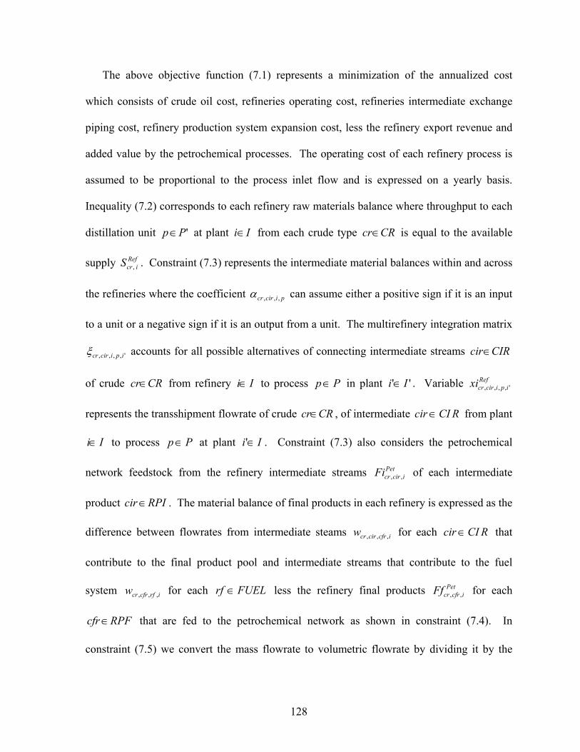
128
The above objective function (7.1) represents a minimization of the annualized cost
which consists of crude oil cost, refineries operating cost, refineries intermediate exchange
piping cost, refinery production system expansion cost, less the refinery export revenue and
added value by the petrochemical processes. The operating cost of each refinery process is
assumed to be proportional to the process inlet flow and is expressed on a yearly basis.
Inequality (7.2) corresponds to each refinery raw materials balance where throughput to each
distillation unit 'Pp∈ at plant Ii∈ from each crude type CRcr∈ is equal to the available
supply ReficrS , . Constraint (7.3) represents the intermediate material balances within and across
the refineries where the coefficient picircr ,,,α can assume either a positive sign if it is an input
to a unit or a negative sign if it is an output from a unit. The multirefinery integration matrix
',,,, ipicircrξ accounts for all possible alternatives of connecting intermediate streams CIRcir∈
of crude CRcr∈ from refinery Ii∈ to process Pp∈ in plant '' Ii∈ . Variable Refipicircrxi ',,,,
represents the transshipment flowrate of crude CRcr∈ , of intermediate RCIcir∈ from plant
Ii∈ to process Pp∈ at plant Ii∈' . Constraint (7.3) also considers the petrochemical
network feedstock from the refinery intermediate streams PeticircrFi ,, of each intermediate
product RPIcir∈ . The material balance of final products in each refinery is expressed as the
difference between flowrates from intermediate steams icfrcircrw ,,, for each RCIcir∈ that
contribute to the final product pool and intermediate streams that contribute to the fuel
system irfcfrcrw ,,, for each FUELrf ∈ less the refinery final products PeticfrcrFf ,, for each
RPFcfr∈ that are fed to the petrochemical network as shown in constraint (7.4). In
constraint (7.5) we convert the mass flowrate to volumetric flowrate by dividing it by the
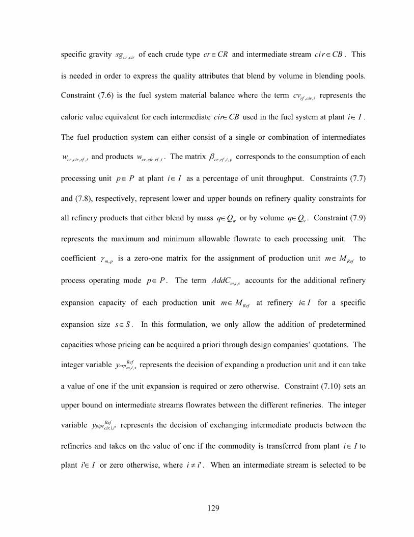
129
specific gravity circrsg , of each crude type CRcr∈ and intermediate stream CBrci ∈ . This
is needed in order to express the quality attributes that blend by volume in blending pools.
Constraint (7.6) is the fuel system material balance where the term icirrfcv ,, represents the
caloric value equivalent for each intermediate CBrci ∈ used in the fuel system at plant Ii∈ .
The fuel production system can either consist of a single or combination of intermediates
irfcircrw ,,, and products irfcfrcrw ,,, . The matrix pirfcr ,,,β corresponds to the consumption of each
processing unit Pp∈ at plant Ii∈ as a percentage of unit throughput. Constraints (7.7)
and (7.8), respectively, represent lower and upper bounds on refinery quality constraints for
all refinery products that either blend by mass wQq∈ or by volume vQq∈ . Constraint (7.9)
represents the maximum and minimum allowable flowrate to each processing unit. The
coefficient pm,γ is a zero-one matrix for the assignment of production unit RefMm∈ to
process operating mode Pp∈ . The term simAddC ,, accounts for the additional refinery
expansion capacity of each production unit RefMm∈ at refinery Ii∈ for a specific
expansion size Ss∈ . In this formulation, we only allow the addition of predetermined
capacities whose pricing can be acquired a priori through design companies’ quotations. The
integer variable Refsimexpy ,, represents the decision of expanding a production unit and it can take
a value of one if the unit expansion is required or zero otherwise. Constraint (7.10) sets an
upper bound on intermediate streams flowrates between the different refineries. The integer
variable Refcir,i,i'pipey represents the decision of exchanging intermediate products between the
refineries and takes on the value of one if the commodity is transferred from plant Ii∈ to
plant Ii∈' or zero otherwise, where 'ii ≠ . When an intermediate stream is selected to be
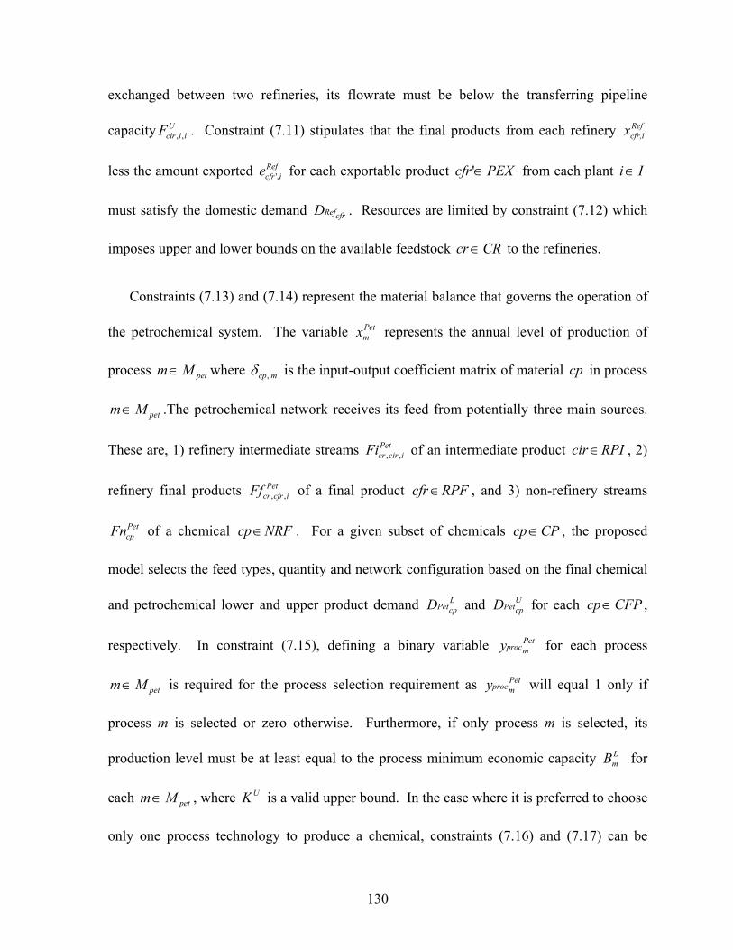
130
exchanged between two refineries, its flowrate must be below the transferring pipeline
capacity UiicirF ',, . Constraint (7.11) stipulates that the final products from each refinery Ref
cfr,ix
less the amount exported Reficfre ,' for each exportable product PEXcfr ∈' from each plant Ii∈
must satisfy the domestic demand cfrRefD . Resources are limited by constraint (7.12) which
imposes upper and lower bounds on the available feedstock CRcr∈ to the refineries.
Constraints (7.13) and (7.14) represent the material balance that governs the operation of
the petrochemical system. The variable Petmx represents the annual level of production of
process petMm∈ where mcp,δ is the input-output coefficient matrix of material cp in process
petMm∈ .The petrochemical network receives its feed from potentially three main sources.
These are, 1) refinery intermediate streams PeticircrFi ,, of an intermediate product RPIcir∈ , 2)
refinery final products PeticfrcrFf ,, of a final product RPFcfr∈ , and 3) non-refinery streams
PetcpFn of a chemical NRFcp∈ . For a given subset of chemicals CPcp∈ , the proposed
model selects the feed types, quantity and network configuration based on the final chemical
and petrochemical lower and upper product demand LcpPetD and U
cpPetD for each CFPcp∈ ,
respectively. In constraint (7.15), defining a binary variable Petmprocy for each process
petMm∈ is required for the process selection requirement as Petmprocy will equal 1 only if
process m is selected or zero otherwise. Furthermore, if only process m is selected, its
production level must be at least equal to the process minimum economic capacity LmB for
each petMm∈ , where UK is a valid upper bound. In the case where it is preferred to choose
only one process technology to produce a chemical, constraints (7.16) and (7.17) can be
131
included for each intermediate product CIPcp∈ and final product CFPcp∈ , respectively.
Finally, we can specify limitations on the supply of feedstock PetcpFn for each chemical type
NRFcp∈ though constraint (7.18). Bear in mind that the limitations on the refinery
intermediate product PeticircrFi ,, and final product Pet
icfrcrFf ,, that are fed to the petrochemical
network are dictated by the model based on both refinery and petrochemical demand and
price structure.
7.4 Illustrative Case Study
In this section we demonstrate the performance of the proposed model on an industrial-scale
case study. Instead of considering the full scale petrochemical network which may have
limited application, we consider a special case of the integration problem. Although the
proposed formulation covers the full scale refinery network and petrochemical systems, the
case study will consider the integration of a petrochemical complex for the production of
polyvinyl chloride (PVC) with a multirefinery network. PVC is one of the major ethylene
derivatives that has many important applications and uses including pipe fittings, automobile
bumpers, toys, bottles and many others (Rudd et al., 1981).
Direct integration of refining and ethylene cracking is considered as the essential building
block in achieving the total petrochemical integration (Joly et al., 2002; Li et al., 2006). This
problem has received more attention lately due to soaring motor gasoline prices and the
directly related prices of ethylene feedstocks (Lippe, 2007). This kind of volatility in prices
has prompted a shift in ethylene feedstock selection and economics to either lighter or
heavier refinery product slates (Lippe, 2008). Shifting from one feedstock to another will
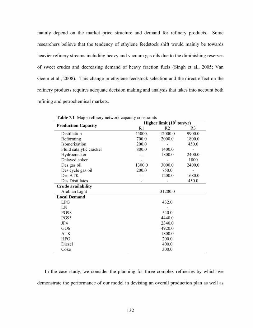
132
mainly depend on the market price structure and demand for refinery products. Some
researchers believe that the tendency of ethylene feedstock shift would mainly be towards
heavier refinery streams including heavy and vacuum gas oils due to the diminishing reserves
of sweet crudes and decreasing demand of heavy fraction fuels (Singh et al., 2005; Van
Geem et al., 2008). This change in ethylene feedstock selection and the direct effect on the
refinery products requires adequate decision making and analysis that takes into account both
refining and petrochemical markets.
Table 7.1 Major refinery network capacity constraints Higher limit (103 ton/yr)
Production Capacity R1 R2 R3 Distillation 45000. 12000.0 9900.0 Reforming 700.0 2000.0 1800.0 Isomerization 200.0 - 450.0 Fluid catalytic cracker 800.0 1400.0 - Hydrocracker - 1800.0 2400.0 Delayed coker - - 1800 Des gas oil 1300.0 3000.0 2400.0 Des cycle gas oil 200.0 750.0 - Des ATK - 1200.0 1680.0 Des Distillates - - 450.0 Crude availability Arabian Light 31200.0 Local Demand LPG 432.0 LN - PG98 540.0 PG95 4440.0 JP4 2340.0 GO6 4920.0 ATK 1800.0 HFO 200.0 Diesel 400.0 Coke 300.0
In the case study, we consider the planning for three complex refineries by which we
demonstrate the performance of our model in devising an overall production plan as well as
133
an integration strategy among the refineries. The state equipment network (SEN)
representation for the overall topology of the refineries network is given in Figure 7.2.
The atmospheric crude unit separates crude oil into several fractions including LPG,
naphtha, kerosene, gas oil and residues. The heavy residues are then sent to the vacuum unit
where they are further separated into vacuum gas oil and vacuum residues. Depending on the
production targets, different processing and treatment processes are applied to the crude
fractions. In this example, the naphtha is further separated into heavy and light naphtha.
Heavy naphtha is sent to the catalytic reformer unit to produce high octane reformates for
gasoline blending and light naphtha is sent to the light naphtha pool and to an isomerization
unit to produce isomerate for gasoline blending too, as in refineries 2&3. The middle
distillates are combined with other similar intermediate streams and sent for hydrotreating
and then for blending to produce jet fuels and gas oils. Atmospheric and vacuum gas oils are
further treated by catalytic cracking, as in refinery 2, or by hydrocracking, as in refinery 3, or
by both, as in refinery 1, to increase the gasoline and distillate yields. In refinery 3, vacuum
residues are further treated using coking and thermal processes to increase light products
yields. The final products of the three refineries network consists of liquefied petroleum gas
(LPG), light naphtha (LT), two grades of gasoline (PG98 and PG95), No. 4 jet fuel (JP4),
military jet fuel (ATKP), No.6 gas oil (GO6), diesel fuel (Diesel), heating fuel oil (HFO), and
petroleum coke (coke). The major capacity constraints for the refinery network are given in
Table 7.1. Furthermore, the three refineries are assumed to be in one industrial area, which is
a common situation in many locations around the world, and are coordinated through a main
headquarter sharing the feedstock supply. The cost parameters for pipelines installation were
calculated as cost per distance between the refineries, and then multiplied by the required
134
pipe length in order to connect any two refineries. The pipeline diameter considered in all
cases was 8 inches.
The petrochemical complex for the production of PVC starts with the production of
ethylene from the refineries feedstocks. The main feedstocks to the ethylene plant in our
study are light naphtha (LN) and gas oil (GO). The selection of the feedstocks and hence the
process technologies are decided based on the optimal balance and trade-off between the
refinery and petrochemical markets. The process technologies considered in this study for
the production of PVC are list in Table 7.2. The overall topology of all petrochemical
technologies for the PVC production is shown in Figure 7.3.
From the refinery side, the proposed model will provide the optimal network integration
between the refineries, process expansion requirements, operating policy based on different
feedstock combination alternatives, process levels and operating modes. On the
petrochemical side, the model will establish the design of an optimal petrochemical process
network for the production of PVC from the range of process technologies and feedstocks
available to satisfy a given demand. This problem was formulated as an MILP with the
overall objective of minimizing total annualized cost of the refinery and maximizing the
added value from the PVC petrochemical network. Maximizing the added value of the
petrochemical network is appropriate since the feedstocks costs contribute to the majority of
the total cost. For instance, the feedstock cost of ethylene plant contributes to more than 87%
of the total cost when naphtha is used and 84% and 74% when propane and ethane are used,
respectively (NBK MENA Equity Research, 2007).
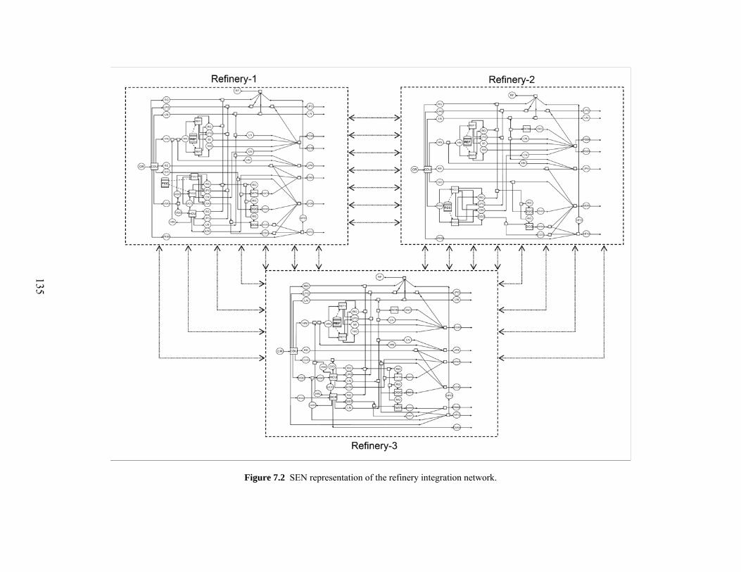
135
Figure 7.2 SEN representation of the refinery integration network.

136
Table 7.2 Major products and process technologies in the petrochemical complex Product Sale Price
($/ton)* Process Technology Process
Index Min Econ.
Prod. (103 ton/yr)
` Pyrolysis of naphtha (low
severity) 1 250
Pyrolysis of gas oil (low severity)
2 250
Steam cracking of naphtha (high severity)
3 250
Ethylene (E) 1570
Steam cracking of gas oil (high severity)
4 250
Chlorination of ethylene 5 180 Ethylene Dichloride (EDC)
378 Oxychlorination of ethylene 6 180 Chlorination and
Oxychlorination of ethylene 7 250 Vinyl chloride
monomer (VCM) 1230
Dehydrochlorination of ethylene dichloride
8 125
Bulk polymerization 9 50 Polyvinyl chloride (PVC)
1600 Suspension polymerization 10 90
* All chemical prices in this study were obtained from latest CW Price Reports in the chemical week journal.
The modeling system GAMS (Brooke et al., 1996) is used for setting up the optimization
models. The computational tests were carried out on a Pentium M processor 2.13 GHz and
the MILP problems were solved with CPLEX (CPLEX Optimization Inc, 1993).
3
4
LN
DSGO
E
7
8
5
6
9
10
E
E
EDC
VCM
VCM
VCM
PVC
NaOH
NaOH
GSLN
P
PFO
C-4
GSLN
P
PFO
C-4
Cl
NaOH
Cl
HCI
NaOH
HCI
T
PVA
NaOH
1
2
PFG
GSLN
P
PFO
C-4
PFG
GSLN
P
PFO
C-4
PFG
3
4
LN
DSGO
E
7
8
5
6
9
10
E
E
EDC
VCM
VCM
VCM
PVC
NaOH
NaOH
GSLN
P
PFO
C-4
GSLN
P
PFO
C-4
Cl
NaOH
Cl
HCI
NaOH
HCI
T
PVA
NaOH
1
2
PFG
GSLN
P
PFO
C-4
PFG
GSLN
P
PFO
C-4
PFG
GSLN
P
PFO
C-4
PFG
GSLN
P
PFO
C-4
PFG
Figure 7.3 SEN representation of the PVC petrochemical complex possible routes.
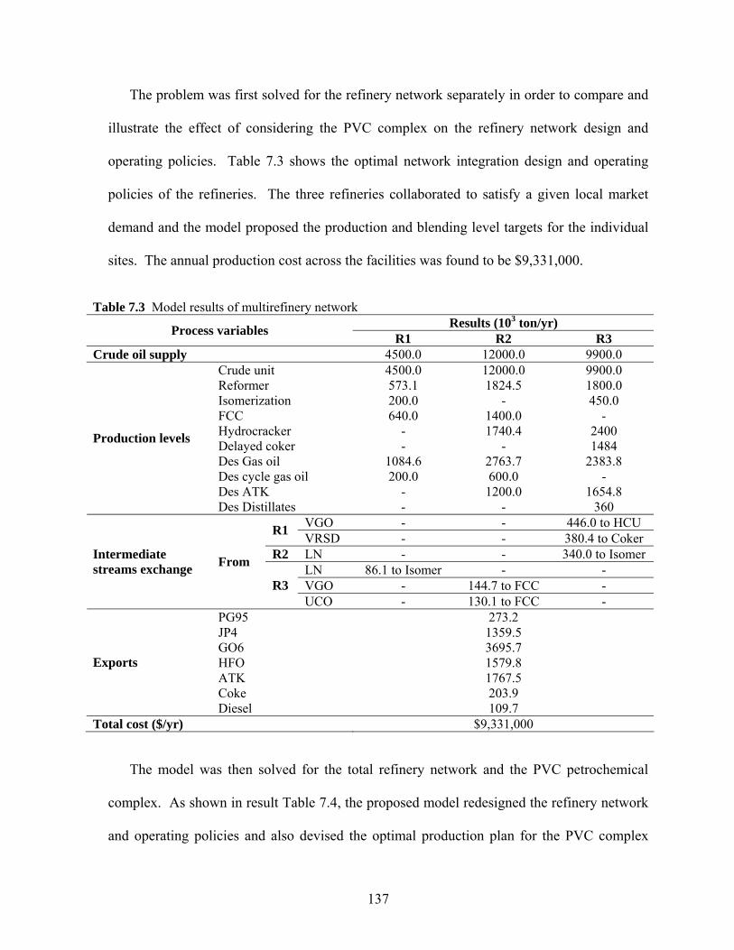
137
The problem was first solved for the refinery network separately in order to compare and
illustrate the effect of considering the PVC complex on the refinery network design and
operating policies. Table 7.3 shows the optimal network integration design and operating
policies of the refineries. The three refineries collaborated to satisfy a given local market
demand and the model proposed the production and blending level targets for the individual
sites. The annual production cost across the facilities was found to be $9,331,000.
Table 7.3 Model results of multirefinery network Results (103 ton/yr) Process variables R1 R2 R3
Crude oil supply 4500.0 12000.0 9900.0 Crude unit 4500.0 12000.0 9900.0 Reformer 573.1 1824.5 1800.0 Isomerization 200.0 - 450.0 FCC 640.0 1400.0 - Hydrocracker - 1740.4 2400 Delayed coker - - 1484 Des Gas oil 1084.6 2763.7 2383.8 Des cycle gas oil 200.0 600.0 - Des ATK - 1200.0 1654.8
Production levels
Des Distillates - - 360 VGO - - 446.0 to HCU R1 VRSD - - 380.4 to Coker
R2 LN - - 340.0 to Isomer LN 86.1 to Isomer - - VGO - 144.7 to FCC -
Intermediate streams exchange From
R3 UCO - 130.1 to FCC -
PG95 273.2 JP4 1359.5 GO6 3695.7 HFO 1579.8 ATK 1767.5 Coke 203.9
Exports
Diesel 109.7 Total cost ($/yr) $9,331,000
The model was then solved for the total refinery network and the PVC petrochemical
complex. As shown in result Table 7.4, the proposed model redesigned the refinery network
and operating policies and also devised the optimal production plan for the PVC complex
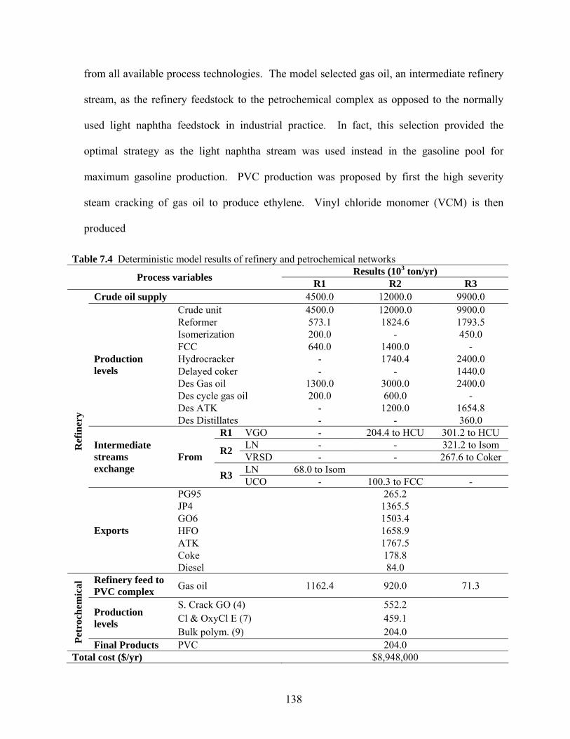
138
from all available process technologies. The model selected gas oil, an intermediate refinery
stream, as the refinery feedstock to the petrochemical complex as opposed to the normally
used light naphtha feedstock in industrial practice. In fact, this selection provided the
optimal strategy as the light naphtha stream was used instead in the gasoline pool for
maximum gasoline production. PVC production was proposed by first the high severity
steam cracking of gas oil to produce ethylene. Vinyl chloride monomer (VCM) is then
produced
Table 7.4 Deterministic model results of refinery and petrochemical networks Results (103 ton/yr) Process variables R1 R2 R3
Crude oil supply 4500.0 12000.0 9900.0 Crude unit 4500.0 12000.0 9900.0 Reformer 573.1 1824.6 1793.5 Isomerization 200.0 - 450.0 FCC 640.0 1400.0 - Hydrocracker - 1740.4 2400.0 Delayed coker - - 1440.0 Des Gas oil 1300.0 3000.0 2400.0 Des cycle gas oil 200.0 600.0 - Des ATK - 1200.0 1654.8
Production levels
Des Distillates - - 360.0 R1 VGO - 204.4 to HCU 301.2 to HCU
LN - - 321.2 to Isom R2 VRSD - - 267.6 to Coker LN 68.0 to Isom
Intermediate streams exchange
From
R3 UCO - 100.3 to FCC - PG95 265.2 JP4 1365.5 GO6 1503.4 HFO 1658.9 ATK 1767.5 Coke 178.8
Ref
iner
y
Exports
Diesel 84.0 Refinery feed to PVC complex Gas oil 1162.4 920.0 71.3
S. Crack GO (4) 552.2 Cl & OxyCl E (7) 459.1 Production
levels Bulk polym. (9) 204.0
Petr
oche
mic
al
Final Products PVC 204.0 Total cost ($/yr) $8,948,000
139
through the chlorination and oxychlorination of ethylene and finally, VCM is converted to
PVC by bulk polymerization. The simultaneous optimization of the refinery and
petrochemical network had an impact on both the refinery intermediate exchange network
and production levels, as shown in Tables 7.3 and 7.4. For example, the capacity utilization
of the desulfurization of gas oil process increased from 83%, 92%, 99% in refineries 1, 2, and
3, respectively, to 100% in all refineries when the petrochemical network was considered in
the model. The annual production cost across the facilities was found to be $8,948,000.
7.5 Conclusion
A mixed-integer programming model for designing an integration and coordination policy
among multiple refineries and a petrochemical network was presented. The objective was to
develop a simultaneous methodology for designing a process integration network between
petroleum refining and the petrochemical industry. A large-scale three refinery network and
a PVC petrochemical complex were integrated to illustrate the performance of the proposed
design methodology and to show the economic potential and trade-offs involved in the
optimization of such systems. The study showed that the optimization of the downstream
petrochemical industry has an impact on the multirefinery network integration and
coordination strategies. This result emphasizes the importance of developed methodology.
In our study, however, all parameters were assumed to be known with certainty.
Nevertheless, the current situation of fluctuating and high petroleum crude oil prices, changes
in demand, and the direct effect this can have on the downstream petrochemical system
underlines the importance of considering uncertainties. For example, the availability of

140
crude oils, feedstock and chemicals prices, and market demands for finished products will
have a direct impact on the output of the highly strategic decisions involved in our study.
Acknowledging the shortcomings of deterministic models, the next phase of our investigation
will be the consideration of uncertainties in the integration problem.
141
Chapter 8
Integration and Coordination of Multisite Refinery and Petrochemical Networks under Uncertainty
8.1 Introduction
In this final chapter, we study the multisite refinery and petrochemical integration problem,
explained in Chapter 7, under uncertainty. The randomness considered includes both the
objective function and right-hand side parameters of inequality constraints. As pointed out in
the previous chapters, considering such strategic planning decisions requires proper handling
of uncertainties as they play a major role in the final decision making.
The main focus of this study is to develop a mathematical programming tool for
simultaneous design of an integrated network of refineries and petrochemical processes
under uncertainty. The proposed model not only addresses the integration between the
multiple refineries and devises their detailed plans, but also establishes the design of an
optimal petrochemical network from a range of process technologies to satisfy a given
demand. In this study we treat parameter uncertainty in terms of imported crude oil price,
refinery product price, petrochemical product price, refinery market demand, and
petrochemical lower level product demand. The problem is modeled as an MILP two-stage
stochastic model with recourse. Furthermore, we apply the sample average approximation
(SAA) method within an iterative scheme to generate the required scenarios. The solution
142
quality is then statistically evaluated by measuring the optimality gap of the final solution.
The objective function is a minimization of the annualized cost over a given time horizon
among the refineries by improving the coordination and utilization of excess capacities in
each facility and maximization of the added value in the petrochemical system. The
proposed formulation was applied to an integrated industrial scale case study of a
petrochemical complex for the production of polyvinyl chloride (PVC) and a network of
petroleum refineries.
The remainder of Chapter 8 is organized as follows. In the following section we will
explain the proposed model formulation for the refinery and petrochemical integration
problem under uncertainty. Then we will explain the scenario generation methodology
adopted, in section 8.3. In section 8.4, we present the computational results and the
performance of the proposed approach on an industrial scale case study. The chapter ends
with concluding remarks in section 8.5.
8.2 Model Formulation
The proposed formulation addresses the problem of planning an integrated network of
refineries and petrochemical processes. The proposed model is based on the formulation
proposed in the previous chapters of this thesis. The general problem under study was
defined in the previous chapter. In this study, uncertainty was accounted for by using two-
stage stochastic programming with recourse approach. Parameters uncertainties considered
in this study included uncertainties in the imported crude oil price crCrCost , refinery product
price RefcfrPr , petrochemical product price Pet
cpPr , refinery market demand cfrRefD , and
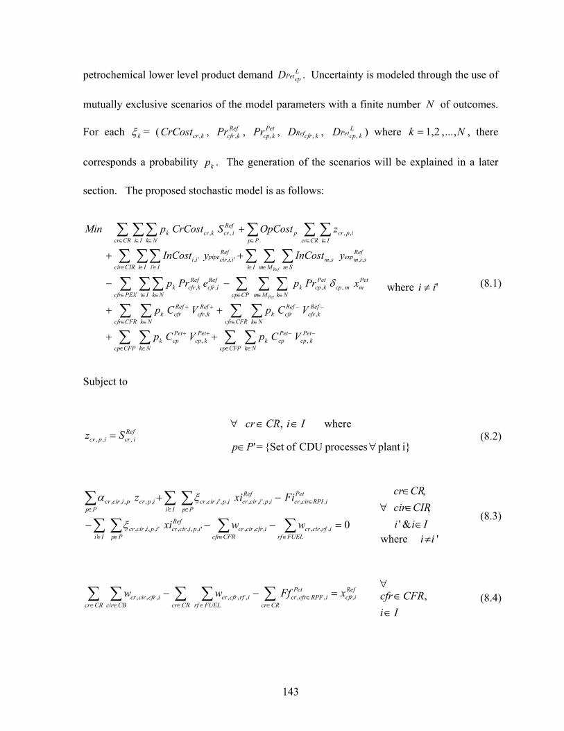
143
petrochemical lower level product demand LcpPetD . Uncertainty is modeled through the use of
mutually exclusive scenarios of the model parameters with a finite number N of outcomes.
For each kξ = ( kcrCrCost , , RefkcfrPr , , Pet
kcpPr , , kcfrRefD , , LkcpPetD , ) where Nk ,...,2,1= , there
corresponds a probability kp . The generation of the scenarios will be explained in a later
section. The proposed stochastic model is as follows:
∑ ∑∑ ∑
∑ ∑∑ ∑
∑ ∑ ∑∑ ∑∑
∑ ∑ ∑∑ ∑∑
∑ ∑∑∑ ∑∑
∈ ∈
−−
∈ ∈
++
∈ ∈
−−
∈ ∈
++
∈ ∈ ∈∈ ∈ ∈
∈ ∈ ∈∈ ∈ ∈
∈ ∈∈∈ ∈ ∈
++
++
−−
++
+
CFPcp Nk
Petkcp
Petcpk
CFPcp Nk
Petkcp
Petcpk
CFRcfr Nk
Refkcfr
Refcfrk
CFRcfr Nk
Refkcfr
Refcfrk
CPcp Mm Nk
Petmmcp
Petkcpk
PEXcfr Ii Nk
Reficfr
Refkcfrk
Ii Mm Ss
Refsimexpsm
CIRcir Ii
Refcir,i,i'pipe
Iiii
CRcr Iiipcr
Ppp
CRcr Ii Nk
Reficrkcrk
VCpVCp
VCpVCp
xPrpePrp
yInCostyInCost
zOpCostSCrCostpMin
Pet
Ref
,,
,,
,,,,
,,,'
',
,,,,
δ where 'ii ≠ (8.1)
Subject to
Reficripcr Sz ,,, =
∀ IiCRcr ∈∈ , where
i}plant processes CDU of{Set =' ∀∈Pp (8.2)
0,,,,,,',,,,'
',,,,
,,,',,,'
,',,,,,,,,
=−−−
−+
∑∑∑ ∑
∑ ∑∑
∈∈∈ ∈
∈∈ ∈∈
FUELrfirfcircr
CFRcfricfrcircr
Refipicircr
Ii Ppipicircr
PetiRPIcircr
Refipicircr
Ii Ppipicircr
Ppipcrpicircr
wwxi
Fixiz
ξ
ξα
∀ Iii
CIRcirCRcr
∈∈∈
&',
,
'where ii≠
(8.3)
∑ ∑∑ ∑∑∈
∈∈∈ ∈∈
=−−CRcr
Refcfr,i
PetiRPFcfrcr
CRcrCRcr FUELrfirfcfrcr
CBciricfrcircr xFfww ,,,,,,,,
∀
IiCFRcfr
∈∈ , (8.4)
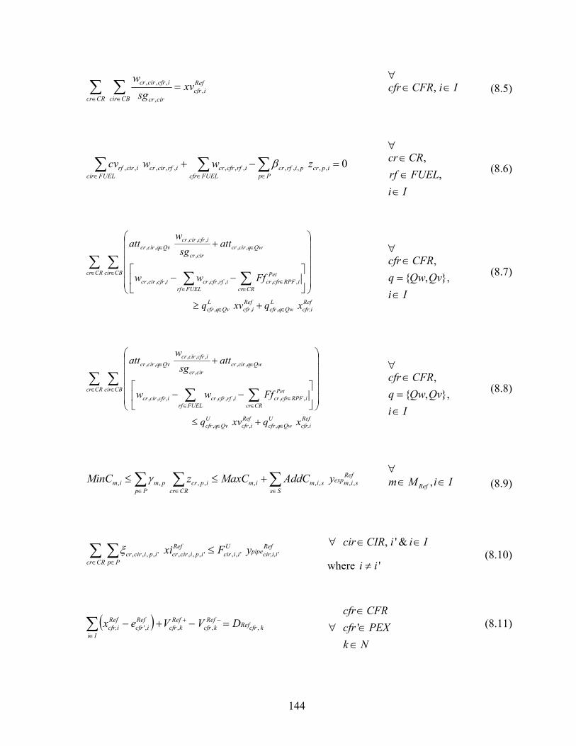
144
∑ ∑∈ ∈
=CRcr
Reficfr
CBcir circr
icfrcircr xvsg
w,
,
,,, ∀
IiCFRcfr ∈∈ ,
(8.5)
∑∑∑∈∈∈
=−+Pp
ipcrpirfcrFUELcfr
irfcfrcrFUELcir
irfcircricirrf zwwcv 0,,,,,,,,,,,,, β ∀
IiFUELrfCRcr
∈∈∈
,,
(8.6)
Refcfr,i
LQwqcfr
Reficfr
LQvqcfr
CRcr CBcir PetiRPFcfrcr
CRcrFUELrfirfcfrcricfrcircr
Qwqcircrcircr
icfrcircrQvqcircr
xqxvq
Ffww
attsg
watt
∈∈
∈ ∈∈
∈∈
∈∈
+≥
⎟⎟⎟⎟⎟
⎠
⎞
⎜⎜⎜⎜⎜
⎝
⎛
⎥⎦
⎤⎢⎣
⎡−−
+
∑ ∑∑∑
,,,
,,,,,,,,
,,,
,,,,,
∀
IiQvQwq
CFRcfr
∈=∈
},,{,
(8.7)
Refcfr,i
UQwqcfr
Reficfr
UQvqcfr
CRcr CBcir
FUELrf
PetiRPFcfrcr
CRcrirfcfrcricfrcircr
Qwqcircrcircr
icfrcircrQvqcircr
xqxvq
Ffww
attsg
watt
∈∈
∈ ∈
∈∈
∈
∈∈
+≤
⎟⎟⎟⎟⎟
⎠
⎞
⎜⎜⎜⎜⎜
⎝
⎛
⎥⎦
⎤⎢⎣
⎡−−
+
∑ ∑∑ ∑
,,,
,,,,,,,,
,,,
,,,,,
∀
IiQvQwq
CFRcfr
∈=∈
},,{,
(8.8)
∑∑ ∑∈∈ ∈
+≤≤Ss
Refsimexpsim
Ppim
CRcripcrpmim yAddCMaxCzMinC ,,,,,,,,, γ
∀ IiMm Ref ∈∈ ,
(8.9)
∑ ∑∈ ∈
≤CRcr
Refcir,i,i'pipe
Uiicir
Pp
Refipicircripicircr yFxi ',,',,,,',,,,ξ
∀ IiiCIRcir ∈∈ &',
where 'ii ≠ (8.10)
( ) kcfrRefRef
kcfrRef
kcfrIi
Reficfr
Refcfr,i DVVex ,,,,' =−+− −+
∈∑ ∀
NkPEXcfrCFRcfr
∈∈∈' (8.11)
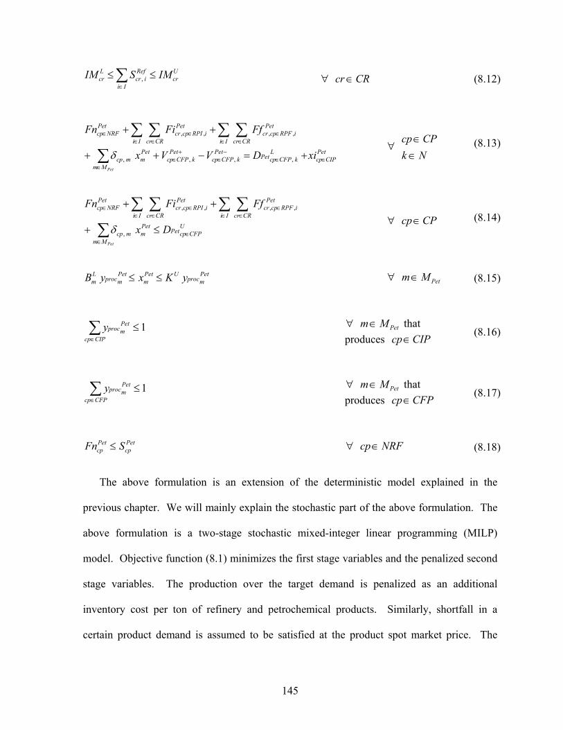
145
∑∈
≤≤Ii
Ucr
Reficr
Lcr IMSIM , ∀ CRcr∈ (8.12)
PetCIPcp
Mm
LkCFPcpPet
PetkCFPcp
PetkCFPcp
Petmmcp
Ii
PetiRPFcpcr
CRcrIi
PetiRPIcpcr
CRcr
PetNRFcp
xiDVVx
FfFiFn
Pet
∈∈
∈−
∈+
∈
∈∈
∈∈∈
∈∈
+=−++
++
∑
∑ ∑∑ ∑
,,,,
,,,,
δ ∀
NkCPcp
∈∈
(8.13)
UCFPcpPet
Mm
Petmmcp
Ii
PetiRPFcpcr
CRcrIi
PetiRPIcpcr
CRcr
PetNRFcp
Dx
FfFiFn
Pet
∈∈
∈∈
∈∈∈
∈∈
≤+
++
∑
∑ ∑∑ ∑
,
,,,,
δ ∀ CPcp∈ (8.14)
Petmproc
UPetm
Petmproc
Lm yKxyB ≤≤ ∀ PetMm∈ (8.15)
∑∈
≤CIPcp
Petmprocy 1 ∀ PetMm∈ that
produces CIPcp∈ (8.16)
∑∈
≤CFPcp
Petmprocy 1 ∀ PetMm∈ that
produces CFPcp∈ (8.17)
Petcp
Petcp SFn ≤ ∀ NRFcp∈ (8.18)
The above formulation is an extension of the deterministic model explained in the
previous chapter. We will mainly explain the stochastic part of the above formulation. The
above formulation is a two-stage stochastic mixed-integer linear programming (MILP)
model. Objective function (8.1) minimizes the first stage variables and the penalized second
stage variables. The production over the target demand is penalized as an additional
inventory cost per ton of refinery and petrochemical products. Similarly, shortfall in a
certain product demand is assumed to be satisfied at the product spot market price. The
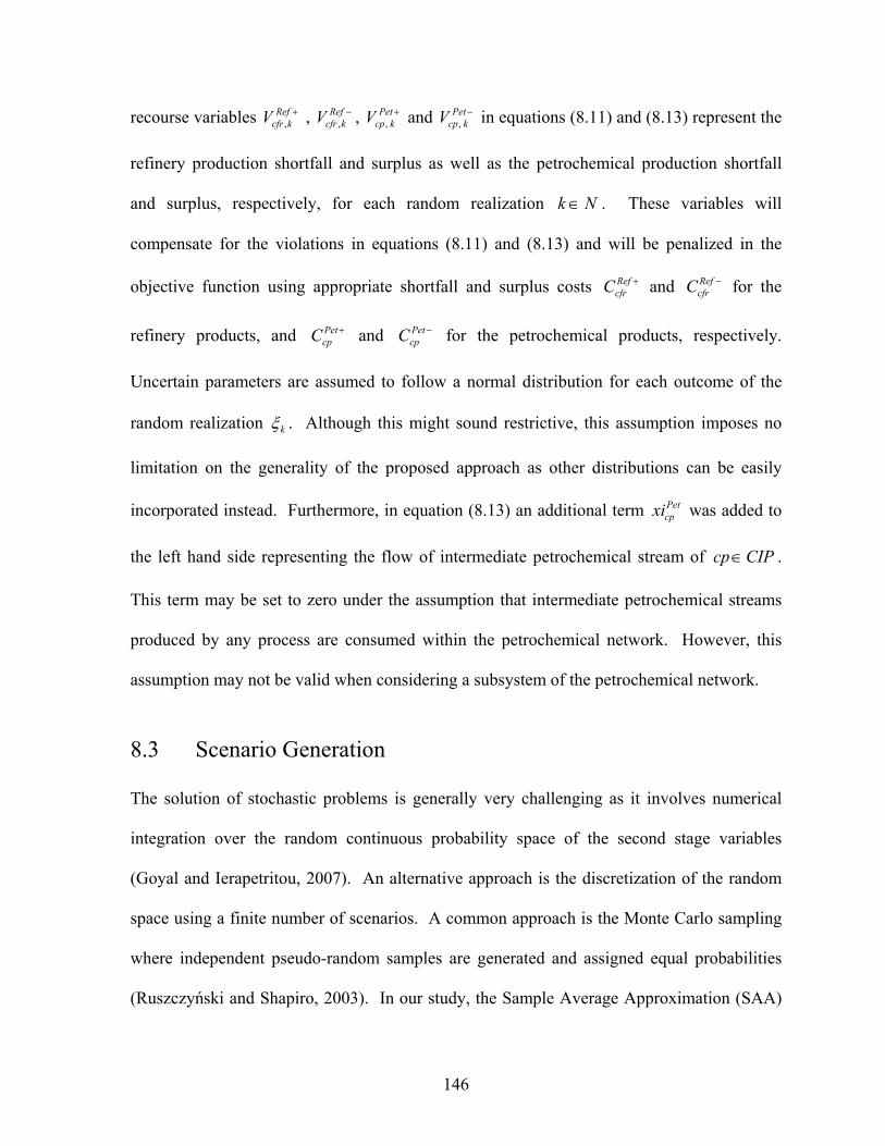
146
recourse variables +RefkcfrV , , −Ref
kcfrV , , +PetkcpV , and −Pet
kcpV , in equations (8.11) and (8.13) represent the
refinery production shortfall and surplus as well as the petrochemical production shortfall
and surplus, respectively, for each random realization Nk ∈ . These variables will
compensate for the violations in equations (8.11) and (8.13) and will be penalized in the
objective function using appropriate shortfall and surplus costs +RefcfrC and −Ref
cfrC for the
refinery products, and +PetcpC and −Pet
cpC for the petrochemical products, respectively.
Uncertain parameters are assumed to follow a normal distribution for each outcome of the
random realization kξ . Although this might sound restrictive, this assumption imposes no
limitation on the generality of the proposed approach as other distributions can be easily
incorporated instead. Furthermore, in equation (8.13) an additional term Petcpxi was added to
the left hand side representing the flow of intermediate petrochemical stream of CIPcp∈ .
This term may be set to zero under the assumption that intermediate petrochemical streams
produced by any process are consumed within the petrochemical network. However, this
assumption may not be valid when considering a subsystem of the petrochemical network.
8.3 Scenario Generation
The solution of stochastic problems is generally very challenging as it involves numerical
integration over the random continuous probability space of the second stage variables
(Goyal and Ierapetritou, 2007). An alternative approach is the discretization of the random
space using a finite number of scenarios. A common approach is the Monte Carlo sampling
where independent pseudo-random samples are generated and assigned equal probabilities
(Ruszczyński and Shapiro, 2003). In our study, the Sample Average Approximation (SAA)
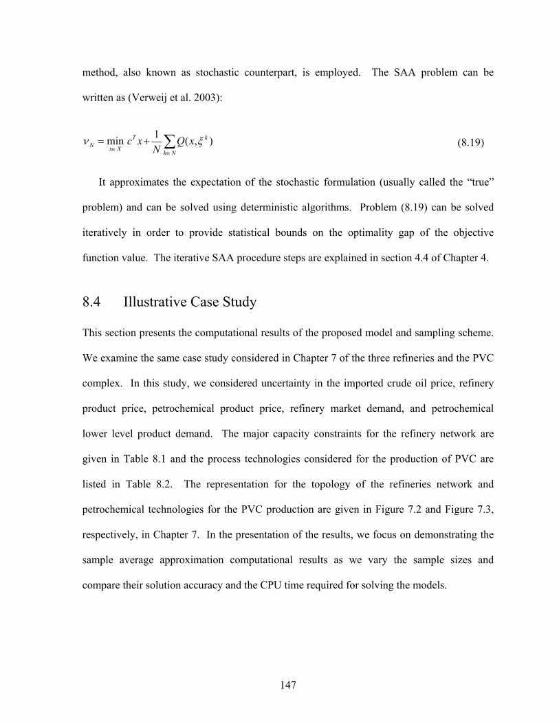
147
method, also known as stochastic counterpart, is employed. The SAA problem can be
written as (Verweij et al. 2003):
∑∈
∈+=
Nk
kT
XxN xQN
xc ),(1min ξν (8.19)
It approximates the expectation of the stochastic formulation (usually called the “true”
problem) and can be solved using deterministic algorithms. Problem (8.19) can be solved
iteratively in order to provide statistical bounds on the optimality gap of the objective
function value. The iterative SAA procedure steps are explained in section 4.4 of Chapter 4.
8.4 Illustrative Case Study
This section presents the computational results of the proposed model and sampling scheme.
We examine the same case study considered in Chapter 7 of the three refineries and the PVC
complex. In this study, we considered uncertainty in the imported crude oil price, refinery
product price, petrochemical product price, refinery market demand, and petrochemical
lower level product demand. The major capacity constraints for the refinery network are
given in Table 8.1 and the process technologies considered for the production of PVC are
listed in Table 8.2. The representation for the topology of the refineries network and
petrochemical technologies for the PVC production are given in Figure 7.2 and Figure 7.3,
respectively, in Chapter 7. In the presentation of the results, we focus on demonstrating the
sample average approximation computational results as we vary the sample sizes and
compare their solution accuracy and the CPU time required for solving the models.
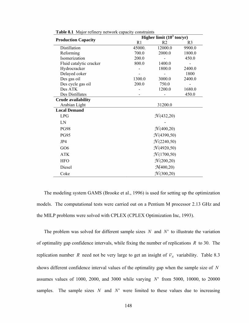
148
Table 8.1 Major refinery network capacity constraints Higher limit (103 ton/yr)
Production Capacity R1 R2 R3 Distillation 45000. 12000.0 9900.0 Reforming 700.0 2000.0 1800.0 Isomerization 200.0 - 450.0 Fluid catalytic cracker 800.0 1400.0 - Hydrocracker - 1800.0 2400.0 Delayed coker - - 1800 Des gas oil 1300.0 3000.0 2400.0 Des cycle gas oil 200.0 750.0 - Des ATK - 1200.0 1680.0 Des Distillates - - 450.0 Crude availability Arabian Light 31200.0 Local Demand LPG N (432,20) LN - PG98 N (400,20) PG95 N (4390,50) JP4 N (2240,50) GO6 N (4920,50) ATK N (1700,50) HFO N (200,20) Diesel N(400,20) Coke N (300,20)
The modeling system GAMS (Brooke et al., 1996) is used for setting up the optimization
models. The computational tests were carried out on a Pentium M processor 2.13 GHz and
the MILP problems were solved with CPLEX (CPLEX Optimization Inc, 1993).
The problem was solved for different sample sizes N and 'N to illustrate the variation
of optimality gap confidence intervals, while fixing the number of replications R to 30. The
replication number R need not be very large to get an insight of Nν variability. Table 8.3
shows different confidence interval values of the optimality gap when the sample size of N
assumes values of 1000, 2000, and 3000 while varying 'N from 5000, 10000, to 20000
samples. The sample sizes N and 'N were limited to these values due to increasing
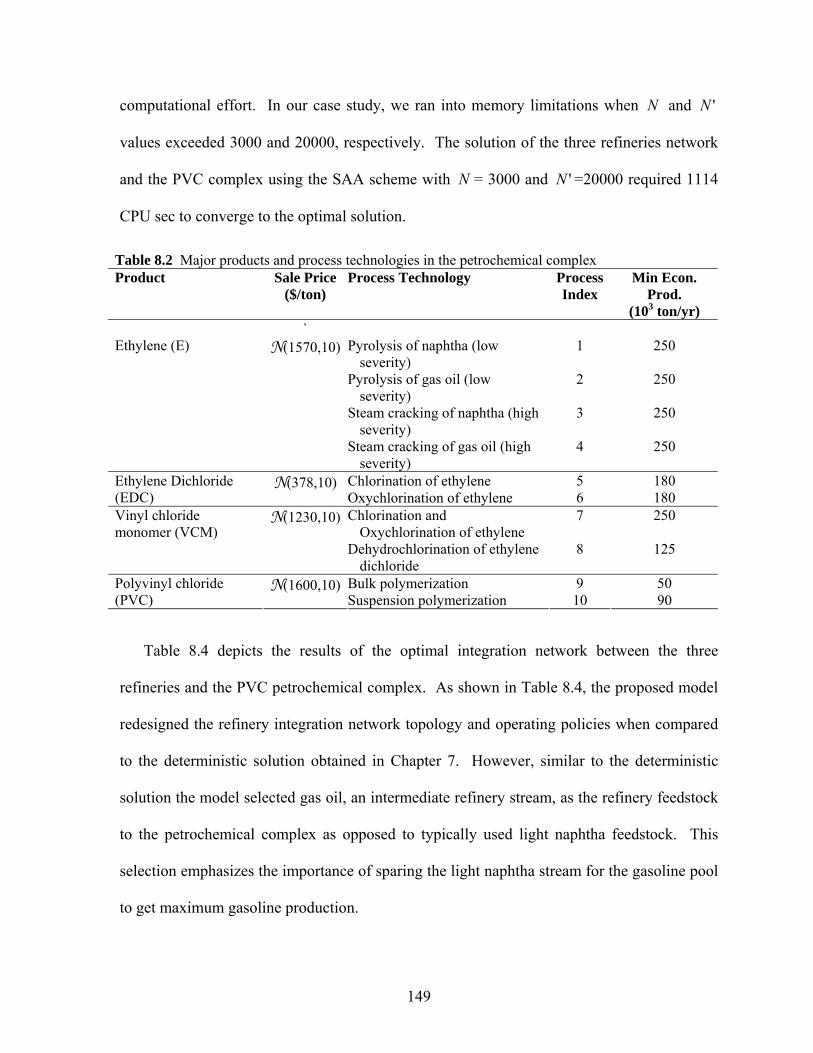
149
computational effort. In our case study, we ran into memory limitations when N and 'N
values exceeded 3000 and 20000, respectively. The solution of the three refineries network
and the PVC complex using the SAA scheme with N = 3000 and 'N =20000 required 1114
CPU sec to converge to the optimal solution.
Table 8.2 Major products and process technologies in the petrochemical complex Product Sale Price
($/ton) Process Technology Process
Index Min Econ.
Prod. (103 ton/yr)
` Pyrolysis of naphtha (low
severity) 1 250
Pyrolysis of gas oil (low severity)
2 250
Steam cracking of naphtha (high severity)
3 250
Ethylene (E) N(1570,10)
Steam cracking of gas oil (high severity)
4 250
Chlorination of ethylene 5 180 Ethylene Dichloride (EDC)
N(378,10) Oxychlorination of ethylene 6 180 Chlorination and
Oxychlorination of ethylene 7 250 Vinyl chloride
monomer (VCM) N(1230,10)
Dehydrochlorination of ethylene dichloride
8 125
Bulk polymerization 9 50 Polyvinyl chloride (PVC)
N(1600,10)Suspension polymerization 10 90
Table 8.4 depicts the results of the optimal integration network between the three
refineries and the PVC petrochemical complex. As shown in Table 8.4, the proposed model
redesigned the refinery integration network topology and operating policies when compared
to the deterministic solution obtained in Chapter 7. However, similar to the deterministic
solution the model selected gas oil, an intermediate refinery stream, as the refinery feedstock
to the petrochemical complex as opposed to typically used light naphtha feedstock. This
selection emphasizes the importance of sparing the light naphtha stream for the gasoline pool
to get maximum gasoline production.
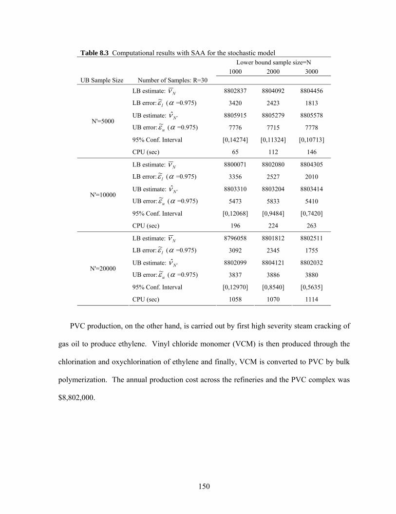
150
Table 8.3 Computational results with SAA for the stochastic model Lower bound sample size=N 1000 2000 3000 UB Sample Size Number of Samples: R=30
LB estimate: Nν 8802837 8804092 8804456
LB error: lε~ (α =0.975) 3420 2423 1813
UB estimate: N ′ν̂ 8805915 8805279 8805578
UB error: uε~ (α =0.975) 7776 7715 7778
95% Conf. Interval [0,14274] [0,11324] [0,10713]
N'=5000
CPU (sec) 65 112 146
LB estimate: Nν 8800071 8802080 8804305
LB error: lε~ (α =0.975) 3356 2527 2010
UB estimate: N ′ν̂ 8803310 8803204 8803414
UB error: uε~ (α =0.975) 5473 5833 5410
95% Conf. Interval [0,12068] [0,9484] [0,7420]
N'=10000
CPU (sec) 196 224 263
LB estimate: Nν 8796058 8801812 8802511
LB error: lε~ (α =0.975) 3092 2345 1755
UB estimate: N ′ν̂ 8802099 8804121 8802032
UB error: uε~ (α =0.975) 3837 3886 3880
95% Conf. Interval [0,12970] [0,8540] [0,5635]
N'=20000
CPU (sec) 1058 1070 1114
PVC production, on the other hand, is carried out by first high severity steam cracking of
gas oil to produce ethylene. Vinyl chloride monomer (VCM) is then produced through the
chlorination and oxychlorination of ethylene and finally, VCM is converted to PVC by bulk
polymerization. The annual production cost across the refineries and the PVC complex was
$8,802,000.
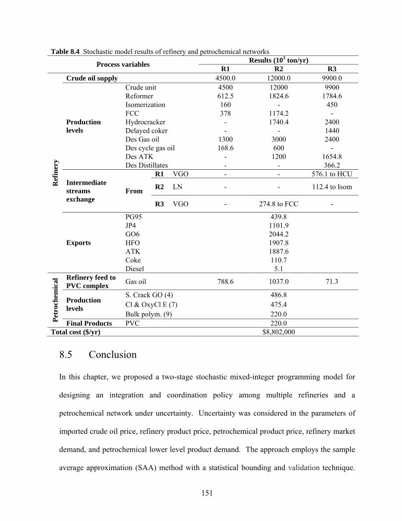
151
Table 8.4 Stochastic model results of refinery and petrochemical networks Results (103 ton/yr) Process variables R1 R2 R3
Crude oil supply 4500.0 12000.0 9900.0 Crude unit 4500 12000 9900 Reformer 612.5 1824.6 1784.6 Isomerization 160 - 450 FCC 378 1174.2 - Hydrocracker - 1740.4 2400 Delayed coker - - 1440 Des Gas oil 1300 3000 2400 Des cycle gas oil 168.6 600 - Des ATK - 1200 1654.8
Production levels
Des Distillates - - 366.2 R1 VGO - - 576.1 to HCU
R2 LN - - 112.4 to Isom Intermediate streams exchange
From
R3 VGO - 274.8 to FCC -
PG95 439.8 JP4 1101.9 GO6 2044.2 HFO 1907.8 ATK 1887.6 Coke 110.7
Ref
iner
y
Exports
Diesel 5.1 Refinery feed to PVC complex Gas oil 788.6 1037.0 71.3
S. Crack GO (4) 486.8 Cl & OxyCl E (7) 475.4 Production
levels Bulk polym. (9) 220.0
Petr
oche
mic
al
Final Products PVC 220.0 Total cost ($/yr) $8,802,000
8.5 Conclusion
In this chapter, we proposed a two-stage stochastic mixed-integer programming model for
designing an integration and coordination policy among multiple refineries and a
petrochemical network under uncertainty. Uncertainty was considered in the parameters of
imported crude oil price, refinery product price, petrochemical product price, refinery market
demand, and petrochemical lower level product demand. The approach employs the sample
average approximation (SAA) method with a statistical bounding and validation technique.
152
In this sampling scheme, a relatively small sample size N is used to make decisions, with
multiple replications, and another independent larger sample is used to reassess the objective
function value while fixing the first stage variables. The proposed model performance was
illustrated on a network of three large-scale refineries and a PVC petrochemical complex.
The formulation captured the simultaneous design of both the refinery and petrochemical
networks and illustrated the economic potential and trade-offs. The consideration of
uncertainties in this type of high level strategic planning model, especially with the current
volatile market environment, presented an adequate treatment of the problem and a proper
optimization tool.
153
Chapter 9
Conclusion
In this chapter we highlight the key contributions of this dissertation and provide some
recommendations for possible research extensions.
9.1 Key Contributions
Multisite Refinery Planning
♦ Developed a framework for the design and analysis of multisite integration and
coordination strategies within a network of petroleum refineries through a mixed-integer
linear programming (MILP) technique.
♦ Extended the proposed model to account for model uncertainty by means of two-stage
stochastic programming. Parameters uncertainty considered include coefficients of the
objective function and right-hand-side parameters in the inequality constraints.
♦ The proposed stochastic model makes use of the sample average approximation (SAA)
method with statistical bounding techniques to give an insight on the sample size required
to give adequate approximation of the problem.
154
♦ Applied a robust optimization technique to investigate both model robustness and
solution robustness, where each measure is assigned a scaling factor to analyze the
sensitivity of the refinery plan and integration network due to variations.
Petrochemical Industry Planning
♦ Proposed a two-stage stochastic programming model to address the strategic planning,
design and optimization of a network of petrochemical processes under uncertainty.
Parameter uncertainty considered in this part includes process yield, raw material and
product prices, and lower product market demand.
♦ The Expected Value of Perfect Information (EVPI) and Value of the Stochastic Solution
(VSS) were investigated to numerically illustrate the value of including the randomness
of the different model parameters.
♦ Applied a robust optimization technique to investigate both model robustness and
solution robustness, where each measure is assigned a scaling factor to analyze the
sensitivity of the petrochemical network.
Integration and Coordination of Multisite Refinery and Petrochemical Networks
♦ Proposed a formulation that addresses the design of optimal integration and coordination
strategy of multisite refinery and petrochemical networks. The proposed model provided
a proper planning tool for the petroleum refining and petrochemical industry. The
155
optimal production strategy was achieved by allowing trade offs between the refinery and
the downstream petrochemical markets.
♦ Extended the proposed model in this dissertation to account for various parameter
uncertainties using two-stage stochastic programming.
♦ The proposed approach uses the sample average approximation (SAA) method with
statistical bounding techniques to give an insight on the sample size requirement and
optimality gap estimation.
9.2 Future Research
The following recommendations emerged as a result of the work presented and the objectives
pursued in this thesis. Future work on these recommendations can extend and improve the
work developed in this dissertation.
Multisite Refinery Planning
♦ The integrated network design presented in this thesis specifically addresses intermediate
material transfer between processing units at each site. However, utilities integration of
all forms including fuel oil, fuel gas, hydrogen, electrical power, and steam, is of great
importance. As discussed in Chapter 2, the benefits of including the utilities in the
integration problem can yield significant energy savings. More work is needed to
properly capture such benefits.
♦ The objective function considered in this dissertation merely considered economics in
terms of cost and profit. However, with the increasingly strict regulations on
156
environmental standards, emission control on various pollutants and green house gases
should be considered. Future work in this area should take into account different
mitigation alternatives for dealing with such emission sources in the refinery.
♦ The framework presented assumes the prior knowledge of the available sets of states,
tasks, and requirement. However, defining these sets based on the available supply,
demand and market prices remains a problem that requires further investigation.
Petrochemical Industry Planning
♦ The model proposed in this dissertation presented the overall optimal network of the
petrochemical processes based on the available supply demand market prices. The
implementation of such highly capital intensive projects would normally be phased based
on the market demand shifts and budget constraints. In order to properly address these
issues, a multiperiod optimization model is required in addition to considering
uncertainty in each forecasted period. Further research towards this objective needs to be
developed.
♦ Similar to the point mentioned earlier, future research needs to account for environmental
regulations and the selection of emissions control alternatives.
Integration and Coordination of Multisite Refinery and Petrochemical Networks
♦ In this dissertation we merely considered the uncertainty in the model parameters without
including robustness measures. This is due to the fact that modeling robustness using
157
variance as shown in the multisite refinery and petrochemical systems renders the
problem nonlinear. Solving such large scale MINLP models might lead to complications
that can be avoided if a different measure is used to capture the risk notion in the
problem. More recently introduced financial risk measures, including the Value-at-Risk
(VaR) and Conditional Value-at-Risk (CVaR), should be pursued.
158
Appendix
SAA Optimal Solution Bounding
Here we present a proof of the SAA lower bound on the true optimal solution of the
stochastic problem. The proof is rather intuitive, but for more details we refer the reader to
Mark et al. (1999).
Proposition 1. For any R independent and identically distributed sample batches (denoting
the number of sample replication) each with sample size of N , i.e. jNj ξξ ,...,1 , Rj ,...,1= ,
the *]E[ νν ≤jN is always valid.
Proof.
For any feasible point 'x that belongs to the solution set X , the inequality below is valid:
)(ˆmin)(ˆ xfxf NXxN ∈≥′
By taking the expectations of both sides and minimizing the left hand side, we get:
)](ˆ[min)](ˆ[min xfxf NXx
NXx ∈∈Ε≥Ε
Since )()](ˆ[ xfxfN =Ε , it follows that ]E[* jNνν ≥ .
159
References
Acevedo, J., & Pistikopoulos, E. N. (1996). Computational studies of stochastic optimization algorithms for process synthesis under uncertainty. Computers & Chemical Engineering, 20, S1.
Addams, F. G., & Griffin, J. M. (1972). Economic-Linear Programming Model of the U.S. petroleum Refining Industry. Journal of American Statistics Association, 67, 542.
Ahmed, S., & Sahinidis, N. V. (1998). Robust process planning under uncertainty. Industrial & Engineering Chemistry Research, 37, 1883.
Ahmed, S., Çakman, U. & Shapiro, A. (2007) Coherent risk measure in inventory problems. European Journal of Operational Research, 182, 226.
Ahmed, S., Sahinidis, N. V., & Pistikopoulos, E. N. (2000). An improved decomposition algorithm for optimization under uncertainty. Computers & Chemical Engineering, 23, 1589.
Al-Amir, A. M. J., Al-Fares, H., & Rahman, F. (1998). Towards Modeling the Development of the Petrochemical Industry in the Kingdom of Saudi Arabia. Arabian Journal of Science & Engineering, 23, 113.
Al-Fares, H. K., & Al-Amir, A. M. (2002). An Optimization Model for Guiding the Petrochemical Industry Development in Saudi Arabia. Engineering Optimization, 34, 671.
Al-Sharrah, G. K., Alatiqi, I., & Elkamel, A. (2002). Planning an Integrated Petrochemical Business Portfolio for Long-Range Financial Stability. Industrial & Engineering Chemistry Research, 41, 2798.
Al-Sharrah, G. K., Alatiqi, I., & Elkamel, A. (2003). Modeling and Identification of Economic Disturbances in the Planning of the Petrochemical Industry. Industrial & Engineering Chemistry Research, 42, 4678.
Al-Sharrah, G. K., Alatiqi, I., Elkamel, A.; & Alper, E. (2001). Planning an Integrated Petrochemical Industry with an Environmental Objective. Industrial & Engineering Chemistry Research, 40, 2103.
Al-Sharrah, G. K., Hankinson G., & Elkamel A. (2006). Decision-making for petrochemical planning using multiobjective and strategic tools. Chemical Engineering Research and Design, 84(A11), 1019.
Anon. (1998). Petrochem complex shields refining profits. Oil & Gas Journal; 96 31.
160
Balaraman, K. S. (2006). Maximizing Hydrocarbon Value Chain by Innovative Concepts. Journal of the Petrotech Society, 3, 26.
Barbaro, A., & Bagajewicz, M. J. (2004). Managing financial risk in planning under uncertainty. AIChE Journal, 5, 963.
Bechtel Corp. (1993). PIMS (Process Industry Modeling System). User’s manual, version 6.0. Houston, TX.
Bell, J. T. (1990). Modeling of the Global Petrochemical Industry. Ph.D. Thesis. University of Wisconsin-Madison.
Bellman, R., & Zadeh, L. A. (1970). Decision-making in a fuzzy environment. Management Science, 17, 141.
Bhatnagar, R., Chandra, P., & Goyal, S.K. (1993). Models for multi-plant coordination. European Journal of Operational Research, 67, 141.
Birge, J. R. (1982). Stochastic linear programs with fixed recourse. Mathematical Programming, 24, 314.
Birge, J. R. (1995). Models and model value in stochastic programming. Annals of Operations Research, 59, 1.
Bloom, J. A. (1988). Solving and electricity generating capacity expansion planning problem by generalized Benders’ Decomposition. Operations Research, 31, 84.
Bodington, C. E., & Baker, T. E. (1990). A History of Mathematical Programming in the Petroleum Industry. Interfaces, 20, 117.
Bok, J. K., Grossmann I. E., & Park S. (2000). Supply chain optimization in continuous flexible processes. Industrial & Engineering Chemistry Research, 39, 1279.
Bok, J., Lee, H., & Park, S. (1998). Robust investment model for long-range capacity expansion of chemical processing networks under uncertain demand forecast scenarios. Computers & Chemical Engineering, 22, 1037.
Booner & Moore Management Science. (1979). RPMS (Refinery and Petrochemical Modeling System): A system description. Houston, TX.
Brooke, A., Kendrick, D., & Meeraus, A., Raman, R. (1996). GAMS—A User’s Guide, Washington DC: GAMS Development Corporation.
Bunch, P.R., Rowe, R.L., & Zentner, M.G. (1998). Large Scale Multi-Facility Planning using mathematical programming methods. AIChE Symposium Series: Proceedings of the Third International Conference of the Foundations of Computer-Aided Process Operations. Snowbird, Utah, USA, July 5–10, 94, 249.
161
Charnes, A., & Cooper, W. (1959). Chance-constrained programming. Management Science, 6, 73.
Charnes, A., & Cooper, W. (1961). Management Models and Industrial Applications of Linear Programming. New York: John Wiley and Sons.
Chopra, S., & Meindl, P. (2004). Supply Chain Management: Strategy, Planning, and Operations 2nd. New Jersey: Pearson Education.
Clay, R. L., & Grossmann, I. E. (1997). A disaggregation algorithm for the optimization of stochastic planning models. Computers & Chemical Engineering, 21, 751.
CPLEX Optimization, Inc. (1993). Using the CPLEX Callable Library and CPLEX Mixed Integer Library. Incline Village, NV: CPLEX Optimization Inc.
Crawford, C. D., Bharvani, R. R., & Chapel. D. G. (2002). Integrating Petrochemicals into the Refinery. Hydrocarbon Engineering, 7, 35.
Dantzig, G. B. (1955). Linear programming under uncertainty. Management Science, 1,197.
Dempster, M. A. H. (1980). Introduction to stochastic programming. New York: Academic Press.
Drud, A. S. (1994). CONOPT: a large scale GRG code. ORSA Journal of Computing, 6, 207.
Energy Information Administration (EIA). (2006). International Energy Outlook. http://www.eia.doe.gov/oiaf/ieo/index.html, accessed on October 20, 2006.
Fathi-Afshar, S., & Yang, J. (1985). Designing the Optimal Structure of the Petrochemical Industry for Minimum Cost and Least Gross Toxicity of Chemical Production. Chemical Engineering Science, 40, 781.
Favennec, J., Coiffard J., Babusiaux, D., & Trescazes, C. (2001). Refinery Operation and Management (Volume 6). Paris: Editions Technip.
Florian, M. K., Lenstra, J. K., & Rinnooy Khan, A. H. (1980). Deterministic production planning: Algorithms and complexity. Management science, 26, 669.
Fujiyama, Y., Redhwi, H. H., Aitani, A. M., Saeed, M. R., & Dean, C. F. (2005). Demonstration plant for new FCC technology yields increased propylene. Oil & Gas Journal; 103, 54.
Gary, J. H., & Handwerk, G. E. (1994). Petroleum Refining: Technology and Economics. New York: Marcel Dekker Inc.
Gonzalo, M. F., Balseyro, I. G., Bonnardot, J., Morel, F., & Sarrazin, P. (2004). Consider integrating refining and petrochemical operations. Hydrocarbon Processing, 83, 61.
162
Goyal, V., Ierapetritou, M. G. (2007). Stochastic MINLP optimization using simplicial approximation. Computers and Chemical Engineering, 31, 1081.
Griffith, R. E., & Stewart, R. A. (1961). A nonlinear programming technique for the optimization of continuous processes. Management Science, 7, 379.
Grossmann, I. E. (2005). Enterprise-wide optimization: a new frontier in process systems engineering. AIChE Journal, 51, 1846.
Grossmann, I. E., & Santibanez, J. (1980). Application of mixed-integer linear programming in process synthesis. Computers & Chemical Engineering, 4, 205.
Grossmann, I. E., & Sargent, R. W. H. (1978) Optimum design of chemical plants with uncertain parameters. AIChE Journal, 24, 1021.
Grossmann, I. E., van den Heever, S. A., & Harjunkoski, I. (2001). Discrete optimization methods and their role in the integration of planning and scheduling. Proceedings of Chemical Process Control Conference 6 at Tucson, 2001. http://egon.cheme.cmu.edu/papers.html, accessed on June 20, 2006.
Gruse, W.A. (1960). Chemical Technology of Petroleum, 3rd Edition. New York: McGraw-Hill Book Company.
Gupta, A., & Maranas, C. D. (2000). A two-stage modeling and solution framework for multisite midterm planning under demand uncertainty. Industrial & Engineering Chemistry Research, 39, 3799.
Hartmann, J. C. (1998). M. Distinguish between scheduling and planning models. Hydrocarbon Processing, 77, 5.
Hengstebeck, R. J. (1959). Petroleum Processing. New York: McGraw-Hill Book Company INC.
Higle, J. L., & Sen, S. (1991). Stochastic decomposition: An algorithm for two stage linear programs with recourse. Mathematics of Operations Research, 16, 650.
Himmelblau D. M., & Bickel, T. C. (1980). Optimal expansion of a hydrodesulfurization process. Computers & Chemical Engineering, 4, 101.
Ierapetritou, M. G., & Pistikopoulos, E. N. (1994). Novel Optimization Approach of Stochastic Planning Models. Industrial & Engineering Chemistry Research, 33, 1930.
International Energy Agency (IEA). (2006). Key world Energy Statistics: 2006 Edition. http://www.iea.org, accessed on September 25, 2006.
163
Iyer, R. R., & Grossmann I. E. (1998). A bilevel decomposition algorithm for long-range planning of process networks. Industrial & Engineering Chemistry Research, 37, 474.
Jackson, J. R., & Grossmann, I. E. (2003). Temporal Decomposition Scheme for Nonlinear Multisite Production Planning and Distribution Models. Industrial & Engineering Chemistry Research, 42, 3045.
Janak S. L., Lin, X., & Floudas, C. A. (2007). A new robust optimization approach for scheduling under uncertainty: II. Uncertainty with known probability distribution. Computers & chemical Engineering, 31, 171.
Jia, Z., & Ierapetritou, M. (2003). Refinery Short-Term Scheduling Using Continuous Time Formulation: Crude-Oil Operations. Industrial & Engineering Chemistry Research, 42, 3085.
Jia, Z., & Ierapetritou, M. (2004). Efficient short-term scheduling of refinery operations based on a continuous time formulation. Computers & Chemical Engineering, 28, 1001.
Jimenez, A., Rudd, D. F., & Meyer, R. R. (1982). Study of the Development of Mexican Petrochemical Industry using Mixed- Integer Programming. Computers & Chemical Engineering, 6, 219.
Jimenez, G. A., & Rudd, D. F. (1987). Use of a recursive mixed-integer programming model to detect an optimal integration sequence for the Mexican petrochemical industry. Computers & Chemical Engineering, 11, 291.
Johnson, N. L., & Tetley, H. (1955). Statistics, vol. I. Cambridge University Press.
Joly, M., Moro, .L.F.L, & Pinto, J.M. (2002). Planning and scheduling for petroleum refineries using mathematical programming. Brazilian Journal of Chemical Engineering, 19, 207.
Kall, P., & Wallace, S. W. (1994). Stochastic programming. New York, NY: Wiley.
Kallrath, J. (2005). Solving Planning and Design Problems in the Process Industry Using Mixed Integer and Global Optimization. Annals of Operations Research, 140, 339.
Khogeer, A. S. (2005). Multiobjective multirefinery optimization with environmental and catastrophic failure effects objectives. Ph.D. Thesis. Colorado State University.
Khor, C. S. (2007). A hybrid of stochastic programming approaches for decision-making in petroleum refinery production-operations under uncertainty. MASc Thesis. University of Waterloo.
164
Kibzun, A. I., & Kan, Y. S. (1996). Stochastic Programming Problems with Probability and Quantile Functions. New York: Wiley
Kleywegt, A. J., Shapiro, A., & Homem-De-Mello, T. (2001). The sample average approximation method for stochastic discrete optimization. SIAM Journal on Optimization, 12, 479.
Kondili, E., Pantelides, C. C., & Sargent, R. W. H. (1993). A general algorithm for short-term scheduling of batch operations-I. MILP formulation. Computers & Chemical Engineering, 17, 211.
Kuo, T., & Chang, T. (2008). Optimal planning strategy for the supply chains of light aromatic compounds in petrochemical industries. Computers & Chemical Engineering, 32, 1147.
Lasdon, L. S., & Waren, A. D. (1980). Survey of Nonlinear Programming Applications. Operations Research, 28, 1029.
Lasdon, L. S., & Waren, A. D. (1983). Large scale nonlinear programming. Computers & Chemical Engineering, 7, 595.
Lasschuit, W., & Thijssen, N. (2003). Supporting supply chain planning and scheduling decisions in the oil & chemical industry. In I. E. Grossmann & C. M. McDonald (Eds.), Proceedings of fourth international conference on foundations of computer-aided process operations. Coral Springs, CAChE. 37.
Lee, H., Pinto, J. M., Grossmann, I. E., & Park, S. (1996). Mixed-Integer Linear Programming Model for Refinery Short-Term scheduling of Crude Oil Unloading with Inventory Management. Industrial & Engineering Chemistry Research, 35, 1630.
Li, C., He, X., Chen, B., Chen, B., Gong, Z., & Quan, L. (2006). Integrative optimization of refining and petrochemical plants. Proceedings of the 16th European Symposium on Computer Aided Process Engineering and 9th International Symposium on Process Systems Engineering; Garmisch-Partenkirchen, Germany, July 9-13, 21.
Lin, X., Janak, S. L., & Floudas, C. A. (2004). A new robust optimization approach for scheduling under uncertainty: I. Bounded uncertainty. Computers & Chemical Engineering, 28, 1069.
Linderoth, J., Shapiro, A., & Wright, S. (2002). The empirical behavior of sampling methods for stochastic programming. http://www.optimization-online.org/DB HTML/2002/01/424.html accessed on October 12, 2007.
Lippe, D. (2007). Gasoline price spike shifts ethylene feeds. Oil & Gas Journal, 105, 56.
Lippe, D. (2008). US olefins see improving feed economics, demand. Oil & Gas Journal, 106, 56.
165
Liu, M. L., & Sahinidis, N. V. (1995). Computational Trends and Effects of Approximations in an MILP Model for Process Planning. Industrial & Engineering Chemistry Research, 34, 1662.
Liu, M. L., & Sahinidis, N. V. (1996). Optimization in Process Planning under Uncertainty. Industrial & Engineering Chemistry Research, 35, 4154.
Liu, M. L., & Sahinidis, N. V. (1997). Process Planning in a Fuzzy Environment. European Journal of Operational Research, 100, 142.
Madansky, A. (1960). Inequalities for stochastic linear programming problems. Management science, 6,197.
Malcolm, S. A., & Zenios, S. A. (1994). Robust optimization of power systems capacity expansion under uncertainty. Journal of the Operational Research Society, 45, 1040.
Manne, A. (1958). A linear programming model of the US petroleum refining industry. Econometrica, 26, 67.
Manne, A. S. (1967). Investment for capacity expansion problems. Cambridge, MA: MIT Press.
Mark, W. K., Morton, D. P., &Wood, R. K. (1999). Monte Carlo bounding techniques for determining solution quality in stochastic programs. Operational Research Letters, 24, 47.
Markowitz, H. M. (1952). Portfolio selection. Journal of Finance, 7, 77.
McDonald, C. M., & Karimi, I. A. (1997). Planning and scheduling of parallel semicontinuous processes. 1. Production planning. Industrial & Engineering Chemistry Research, 36, 2691.
Meyers, R. A. (1997). Handbook of Petroleum Refining processes: 2nd Ed. USA: The McGraw-Hill Companies Inc.
Moro, L. F. L., Zanin, A. C., & Pinto, J. M. (1998). A Planning Model for Refinery Diesel Production. Computer & Chemical Engineering, 22, S1039.
Mulvey, J. M., Vanderbei, R. J., & Zenios, S. A. (1995). Robust optimization of large-scale systems. Operations Research, 43, 264.
NBK MENA Equity Research. (2007). Petrochemical Primer. http://cm2.zawya.com/researchreports/nbk/20070923_NBK_105729.pdf, accessed on March 20, 2008.
166
Neiro, S. M. S., & Pinto J. M. (2004). A general modeling framework for the operational planning of petroleum supply chains. Computers & Chemical Engineering, 28, 871.
Neiro, S. M. S., & Pinto, J. M. (2005). Multiperiod optimization for production planning of petroleum refineries. Chemical Engineering Communications, 192, 62.
Nelson, W. L. (1958). Petroleum Refinery Engineering, 4th Edition. New York: McGraw-Hill Book Company.
Norkin, W. I., Pflug, G. Ch., & Ruszczysk, A. (1998). A branch and bound method for stochastic global optimization. Mathematical Programming, 83, 425.
Norton, L. C., & Grossmann, I. E. (1994). Strategic planning model for complete process flexibility. Industrial & Engineering Chemistry Research, 33, 69.
Occupational Safety and Health Administration of the United States of America (OSHA). (2003). Technical Manual: Petroleum Refining Processes. http://www.osha.gov/dts/osta/otm/otm_iv/otm_iv_2.html, accessed on April 20, 2006.
Pantelides, C. C. (1994). Unified Frameworks for Optimal Process Planning and Scheduling. Proceeding of the Second Conference on Foundations of Computer-Aided Operations. CAChE Publications, 253.
Patel, N., Baade, W., Fong, L. W., & Khurana, V. (2003). Creating Value Through Refinery Hydrogen Management. http://www.h2alliance.com/pdf/CreatingValue.pdf, accessed on February 27, 2008.
Philpot, J. 2007. Integration Profitability. ( 2007) Hydrocarbon Engineering, 12, 41.
Pintér, J. (1991). Stochastic modeling and optimization of environmental management. Annals of Operations Research, 31,527.
Pinto, J. M., Joly, M., & Moro, L .F. L. (2000). Planning and scheduling models for refinery operations. Computers & Chemical Engineering, 24, 2259.
Pistikopoulos, E. N., & Ierapetritou, M. G. (1995). Novel approach for optimal process design under uncertainty. Computers & Chemical Engineering, 19, 1089.
Qian, Z., & Shapiro, A. (2006). Simulation-based approach to estimation of latent variable models. Computational Statistics & Data Analysis, 51, 1243.
Reklaitis, G. V. (1991). Perspectives on Scheduling and Planning of Process Operations. Proceedings of the fourth International symposium of Process System Engineering, Montebello, Canada.
167
Ren, T., Patel, M., & Blok, K. (2006). Olefins from conventional and heavy feedstocks: Energy use in steam cracking and alternative processes. Energy, 31, 425.
Rippin, D. W. T. (1993). Batch Process Systems Engineering: a Retrospective and Prospective Review. Computers & Chemical Engineering, S13, S1.
Roberts, S. M. (1964). Dynamic Programming in Chemical Engineering and Process Control. New York: Academic Press.
Rudd, D. F., Fathi-Afshar, S., Trevino, A. A. , & Statherr, M. A. (1981). Petrochemical Technology Assessment. New York: John Wiley & Sons.
Ruszczyński, R., & Shapiro, A. (2003). Handbooks in Operations Research and Management Science-Volume 10: Stochastic Programming. Amsterdam, Netherlands: Elsevier Science.
Ryu, J., & Pistikopoulos, E. N. (2005). Design and Operation of an Enterprise-wide Process Network Using Operation Policies. 1. Design. Industrial & Engineering Chemistry Research, 44, 2174.
Ryu, J., Dua V., & Pistikopoulos, E. N. (2004). A bilevel programming framework for enterprise-wide process networks under uncertainty. Computers & Chemical Engineering, 28 1121.
Sadhukhan, J., Zhang, N., & Zhu X. X. (2004). Analytical optimization of industrial systems and applications to refineries, petrochemicals. Chemical Engineering Science, 59, 4169.
Sahinidis, N. V. (2004). Optimization under uncertainty: state-of-the-art and opportunities. Computers & Chemical Engineering, 28, 971.
Sahinidis, N. V., & Grossmann, I. E. (1991a). Reformulation of multiperiod MILP models for planning and scheduling of chemical processes. Computers & Chemical Engineering, 15, 255.
Sahinidis, N. V., & Grossmann, I. E. (1991b). Multiperiod investment model for processing networks with dedicated and flexible plants. Industrial & Engineering Chemistry Research, 30, 1165.
Sahinidis, N. V., & Grossmann, I. E. (1992). Reformulation of multi-period MILP model for planning and scheduling of chemical processes. Operations Research, 40, S127.
Sahinidis, N. V., Grossmann, I. E., Fornari, R.E., & Chathrathi, M. (1989). Optimization model for long range planning in chemical industry. Computers & Chemical Engineering, 13, 1049.
Shah, N. (1998). Single- and multisite planning and scheduling: current status and future challenges. AIChE Symposium Series: Proceedings of the Third International
168
Conference of the Foundations of Computer-Aided Process Operations, Snowbird, Utah, USA, July 5–10, 94, 75.
Shapiro, A. & Homem-de-Mello, T. (1998). A simulation-based approach to two stage stochastic programming with recourse. Mathematical Programming, 81, 301.
Shapiro, J. F. (2004). Challenges of strategic supply chain planning and modeling. Computers & Chemical Engineering, 28, 855.
Singh J., Kumar M.M., Saxena A.K., & Kumar S. (2005). Reaction pathways and product yields in mild thermal cracking of vacuum residues: A multi-lump kinetic model, Chemical Engineering Journal, 108, 239.
Sokic, M., & Stevancevic, D. (1983). The Optimal Structure of the Petrochemical Industry. Chemical Engineering Science, 38, 265.
Sophos, A., Rotstein, E., & Stephanopoulos, G. (1980). Multiobjective Analysis in Modeling the Petrochemical Industry. Chemical Engineering Science, 38, 2415.
Stadtherr, M. A., & Rudd, D. F. (1976). Systems study of the Petrochemical Industry. Chemical Engineering Science, 31, 1019.
Stadtherr, M. A., & Rudd, D. F. (1978). Resource Use by the Petrochemical Industry. Chemical Engineering Science, 33, 923.
Subrahmanyam, S., Pekny, J., & Reklaitis, G.V. (1994). Design of batch chemical plants under market uncertainty. Industrial & Engineering Chemistry Research, 33, 2688.
Swaty, T. E. (2002). Consider over-the-fence product stream swapping to raise profitability. Hydrocarbon Processing, 81, 37.
Symonds, G. H. (1955). Linear Programming- The Solution of Refinery Problems. New York: Esso Standard Oil Company.
Timpe, C. H., & Kallrath, J. (2000). Optimal planning in large multisite production networks. European Journal of Operational Research, 126, 422-435.
Tsiakis, P., Shah, N., & Pantelides, C. C. (2001). Design of multiechelon supply chain networks under demand uncertainty. Industrial & Engineering Chemistry Research, 40, 3585.
Van Geem, K.M., Reyniers and, M.F., & Marin, G.B. (2008). Challenges of Modeling Steam Cracking of Heavy Feedstocks. Oil & Gas Science & Technology, 63, 79.
Verweij, B., Ahmed, S., Kleywegt, A. J., Nemhauser, G., & Shapiro, A. (2003). The sample average approximation method applied to stochastic routing problems: A computational study. Computational Optimization & Applications, 24, 289.
169
Viswanathan, J., & Grossmann, I. E. (1990). A combined penalty function and outer-approximation method for MINLP optimization. Computers & Chemical Engineering, 14, 769.
Wagner, H. (1969). Principles of Operations Research with Applications to Managerial Decision. New Jersey: Prentice-Hall Inc.
Wang, J. (2006). China’s Petrochemical Technologies. Chemistry International, May-Jun 2006.
Wei, J., & Realff, M. J. (2004). Sample average approximation methods for stochastic MINLPs. Computers & Chemical Engineering, 28, 336.
Wenkai, L., Hui C., Li, P., & Li, A. (2004). Refinery Planning under Uncertainty. Industrial & Engineering Chemistry Research, 43, 6742.
Wilkinson, S. (1996). Aggregate Formulation for Large-Scale Processing Scheduling Problems. Ph.D. Thesis. Imperial College.
Wilkinson, S., Shah N., & Pantelides C.C. (1996). Integrated production and Distribution shedueling on a Europe-Wide Basis. Computers & Chemical Engineering, S20, S1275.
Williams, J. F. (1981). Heuristic Techniques for Simultaneous Scheduling of Production and Distribution in Multi-Echelon Structures. Management Science. 27, 336.
Wilson, J. W. (1997). Fluid Catalytic Cracking-Technology and Operation. Tulsa, OK: PennWell Publishing Company.
Yeomans, H., & Grossmann, I.E. (1999). A systematic modeling framework of superstructure optimization in process synthesis. Computers & Chemical Engineering, 23, 709.
Zhang, J., Zhu, X.X., & Towler, G.P. (2001). A Simultaneous Optimization Strategy for Overall Integration in Refinery Planning. Industrial & Engineering Chemistry Research, 40, 2640.
Zhang, N., & Zhu, X.X. (2006). Novel modeling and decomposition strategy for total site optimization. Computers & Chemical Engineering, 30, 765.
Zierer, T. K., Mitchell, W. A., & White, T. R. (1976). Practical Applications of Linear Programming to Shell’s Distribution Problems. Interfaces, 6, 13.
170
Khalid Y. Al-Qahtani
Curriculum Vitae
Education
2005 ― 2008 Ph.D. Chemical Engineering, University of Waterloo
2008 Diploma in Operational Research, University of Waterloo
1994 ― 1999 B.S. Chemical Engineering, King Fahd University of Petroleum & Minerals
Publication
Referred Journals publications
Al-Qahtani, K., & Elkamel, A. 2008. Multisite Facility Network Integration Design and Coordination: An Application to the Refining Industry. Computers & Chemical Engineering, 32, 2198.
Al-Qahtani, K., Elkamel, A. & Ponnambalam, K. 2008. Robust Optimization for Petrochemical Network Design under Uncertainty, Industrial & Engineering Chemistry Research, 47, 3912.
Al-Ali, H., Al-Qahtani, K. & Elkamel, A. 2008. A Mathematical Programming Model for Achieving Total Emission Control in the Petroleum Refining Industry. International Journal of Oil, Gas and Coal Technology, 1, 444.
Al-Qahtani, K., & Elkamel, A. 2009. Multisite refinery and petrochemical network design: optional integration and coordination strategies. Industrial & Engineering Chemistry Research, 48, 814.
Al-Qahtani, K., & Elkamel, A. 2008. Robust Planning of Multisite Refinery Networks: Optimization under Uncertainty. Computers & Chemical Engineering, submitted.
Al-Qahtani, K., & Elkamel, A. 2008. Integration and Coordination of Multisite Refinery and Petrochemical Networks under Uncertainty. Chemical Engineering Science, submitted.
171
Refereed Conference publication
Al-Qahtani, K., Elkamel, A., & Ponnambalam, k. 2007. Robust MINLP Optimization Model for Petrochemical Network Design using a Hybrid Stochastic - Probabilistic Approach. The 6th European Congress of Chemical Engineering (ECCE-6), Copenhagen, September 16-20, 2007, 1, 605.
Al-Qahtani, K., & Elkamel, A. 2008. Integration and Coordination of Multirefinery Networks: A Robust Optimization Approach. The 19th IASTED International Conference on Modeling and Simulation, Quebec City, May 26-28, 2008, 620-14, 1.
Conference Presentations and Seminars
Al-Qahtani, K., & Elkamel, A. 2006. Multirefinery integration and coordination using mathematical programming. The 56th Canadian Chemical Engineering Conference, Sherbrooke, Quebec, October 15-18, 2006.
Al-Qahtani, K., & Elkamel, A. 2007. An Extended MILP Model for the Network Design and Process Capacity Expansion Plans of Multiple Refineries. The 49th Annual Canadian Operational Research Society (CORS) Conference, London, Ontario, May 14-16, 2007.
Al-Qahtani, K., Elkamel, A., & Ponnambalam, K. 2007. Robust Planning of Petrochemical Networks: Design under Uncertainty. Presented at the South Western Ontario Operational Research Day (SWORD), University of Waterloo, Waterloo, Ontario, October 12, 2007.
Al-Qahtani, K., & Elkamel, A. 2008. Integration and Coordination of Multirefinery Networks: A Robust Optimization Approach. Applied Statistics, Control & Optimization Meeting, Ecole Polytechnique, Montreal, May 20-21, 2008.


