Path Properties of Multigenerational Samples

from Branching Processes

Jim Kuelbs

Department of Mathematics

University of Wisconsin

Madison, WI 53706-1388

Anand N. Vidyashankar?

Department of Statistical Science

Cornell University

Ithaca, NY 14853-4201

Abstract

This paper is concerned with the study of functional limit theorems constructed using data

from multiple generations of a supercritical branching process. These results arise naturally

when samples are obtained from several successive generations of a supercritical branching

process, and one is interested in the joint asymptotic behavior of various statistical functionals

constructed from the data. More precisely, let Zn : n ≥ 0 be a supercritical branching

process and set Rn = Z−1n−1Zn. Also let, Rn,r(n) = (Rn, Rn−1, · · · , Rn−r(n)+1). Since the

number of generations sampled may increase without limit, to formulate our results it is natural

to embed Rn,r(n) in R∞, and its related functional forms in infinite products of continuous

function spaces. The limit theorems we consider include various forms of the functional law of

large numbers (consistency) and also a functional central limit theorem (asymptotic normality)

under minimal moment conditions. The limiting process in our functional limit theorem is an

infinite dimensional Brownian motion in the infinite product space (C0[0, 1])∞, with the product

topology. In order to study rates of convergence in these results, we also include related infinite

dimensional functional laws of the iterated logarithm of Strassen and Chung-Wichura type in

the space (C0[0, 1])∞. Connections to various statistical issues involving PCR and other related

data are discussed.

? Research Supported in part by a grant from NSF DMS 000-03-07057 and also by grants from

the NDCHealth Corporation

Key Words: Branching processes, Functional equation, Large deviations, Strassen law of the it-

erated logarithm, Chung-Wichura law of the iterated logarithm, Harmonic Moments, Small-ball

problems, Polymerase Chain Reaction Experiments, Uniform Consistency, Joint Asymptotic

Normality

AMS 1991 Subject Classification: 60J80 60F10

Short title: Path Properties for Multigenerational Samples

1

1 Introduction

The primary focus of this paper is the study of path properties of various functionals constructedfrom data sampled successively from multiple generations of a supercritical branching process initi-ated by a single ancestor at time 0. The functionals that we study include ratios of generation sizes,the maxima of partial sums of the nth generation population, and natural functional forms relatedto such quantities. A number of factors motivated this study. First, in several scientific experiments,samples are obtained from the nth generation to perform inferences on the mean and variance pa-rameter of a branching process. The choice of n is somewhat adhoc and varies between scientistsand lab technicians. One of the goals of this paper is to study, from an asymptotic perspective,the joint behavior of such estimates, when one samples from successive generations. Second, from aprobabilistic perspective, we wanted to understand the analogues of classical functional limit theo-rems for the stochastic processes involving multiple generations of supercritical branching processesthat arise in this setting.

An example of the first motivation arises in the study of Polymerase Chain Reaction (PCR)experiments. In such an experiment, an initial amount of DNA is amplified for use in variousbiological experiments. The PCR experiment evolves in three phases; an exponential phase, a linearphase, and a pleateau phase. Branching processes and their variants have been used to model datafrom PCR experiments during the exponential phase ([17], pp. 231). The mean of the branchingprocess is related to the quantity called the efficiency of the PCR. One of the goals of the PCRexperiments is to ”quantitate” the initial number of DNA molecules in a sample or equivalently,estimate the number of ancestors in a branching process ([20]). In an end point assay, data areobtained from the last two cycles (generations) corresponding to the end of the exponential phase,and these are used to estimate the mean of the branching process. The statistical estimate of theinitial number of ancestors is a function of the estimate of the mean of the branching process ([20]).Since the cycle(generation) corresponding to the end of exponential phase is somewhat arbitrary andvaries betweens labs and the technicians involved, a natural question is if two different technicianswith different choices for the end of the exponential phase obtain consistent results for the sameexperiment. The results of this paper help answer this question in the affirmative in the sense thatour results imply joint convergence of a broad array of multigenerational samples from the branchingprocess. For instance, our central limit theorem enables an experimenter to construct confidenceregions for the ”mean vector” using the asymptotic independence of the components, see Corollary2, Remark 3-Remark 6, and Appendix B. For further work in the area relating branching processesand PCR consult [27], [28] and [25] while for statistical problems involving mutation rates see [9].

We begin with a brief description of the branching process. We denote by Zn : n ≥ 0 theGalton-Watson process initited by a single ancestor Z0 ≡ 1 defined on a probability space (Ω,F , P ).Let ξn,j, j ≥ 1, n ≥ 1 denote a double array of integer valued i.i.d. random variables withprobability distribution pj : j ≥ 0, i.e.

P (ξ1,1 = k) = pk. (1.1)

The random variable ξn,j is interpreted as the number of children produced by the jth parent in the(n − 1)thgeneration. The branching process Zn : n ≥ 1 is iteratively defined as follows: for n ≥ 1

Zn =Zn−1∑

j=1

ξn,j. (1.2)

2

Let m = E(Z1). It is well known that if m > 1 (i.e. the process is supercritical), then Zn → ∞with positive probability and that the probability that the process becomes extinct, namely q, isless than one. Furthermore, q satisfies the functional equation

f(q) = q, (1.3)

where for 0 ≤ s ≤ 1,f(s) =

∑

j≥0

sjpj . (1.4)

Also, q = 0 if and only if p0 = 0. We will assume in our paper that 1 < m < ∞.Let us denote by Fn the σ−field generated by the sequence Z0, Z1, · · · , Zn. Let Wn = Zn

mn .Then it is known that (Wn,Fn) : n ≥ 0 is a non-negative martingale sequence, and an importantclassical result due to Kesten and Stigum is that it converges to a non-degenerate limitW if and onlyif E(Z1 logZ1) < ∞, see, for example, [2], Theorem 1, page 24. Furthermore, as can be seen from[2], Corollary 4, p.36, almost surely on the survival set S we have 0 < W <∞. If E(Z1 logZ1) = ∞,then there exists a sequence of constants cn such that the normalized sequence WSH

n = Zn

cnhas a

non-degenerate limit. The constants cn are called the Senata constants, and we denote the almostsure limit of WSH

n by WSH . Furthermore, Theorem 3, p. 30, and Corollary 1, p.52, of [2] imply thatalmost surely on the survival set, 0 < WSH < ∞. We have indexed the random variables in thislast setting by SH, as Heyde showed the almost sure convergence in Seneta’s earlier result, whichprovided only convergence in distribution.

The quantity Rn = Z−1n−1Zn is known as Nagaev’s estimator of the mean m, and it has been

shown in [16] to be the maximum likelihood estimator when only (Zn−1, Zn) are observed. Thelaw of large numbers (consistency) and the central limit theorem (asymptotic normality) associatedwith Rn have previously been studied under the first and second moment, respectively. The lawof the iterated logarithm associated with Rn was also known under the assumption of finite (2 +δ) moments for the offspring distribution (see, for instance, [18] [19]). Now consider the vectorRn,r(n) ≡ (Rn, Rn−1, · · · , Rn−r(n)+1). When r(n) is independent of n, then Rn,r(n) is a vectorof fixed length, and the law of large numbers for the vector can be obtained by looking at thecomponents individually. However, when r(n) ∞ various difficulties emerge, but we obtain anumber of strong law results for Rn,r(n), and hence also Rn, via continuity theorems applied toour functional limit theorems. Furthermore, we study the conditional and unconditional completeconvergence of these functional law of large numbers.

The central limit theorem for the multigenerational process is somewhat surprising. For instance,if r(n) = 2, we show that the limit distribution of (

√Zn−1(Rn−m),

√Zn−2(Rn−1−m)) is bivariate

normal with mean vector 0 and covariance matrix σ2I2, where I2 is the identity matrix of order2; that is the components are asymptotically independent. The problem is more complex whenr(n) ∞, but the asymptotic independence of different components exists even in this setting. Wealso establish the functional version of such a result when r(n) ∞ under no hypothesis other thanthe finiteness of the second moment.

The rate of convergence in the classical central limit theorem based on an independent and iden-tically distributed (i.i.d.) sequence of centered random variables is given by the law of the iteratedlogarithm(LIL). In particular, the LIL studies the almost sure large values of the normalized partialsums, and the factor (log logn)

12 in the denominator is required to provide a finite and nonzero

3

limsup. The functional version of the classical LIL is due to Strassen in [32], and represents a land-mark in the study of limit theorems in probability. In the so-called other LIL, namely Chung’s LIL([5]) for centered partial sums, the emphasis is not on large values for the normalized partial sums,but rather on their small values and the rate of escape from zero. Chung’s result also contains thefactor (log logn)

12 , but now it appears in the numerator and one needs small deviation probabilities

at the functional level to do the analysis. The functional version of Chung’s result appeared in theimportant paper [34].

The classical LIL has a long history, which we will not repeat here, as it is fairly well known, andStrassen’s LIL is also a widely known result. However, since Chung’s LIL and its functional versiondue to Wichura are perhaps less well known, we include a few remarks and references in this area.These are far from comprehensive, but are intended to motivate the statements of Theorems 5 and6 in Section 2 which generalize Wichura’s result to multiple generations of the branching processZn : n ≥ 0.

We begin with Chung’s law in the context of a sequence of i.i.d. random variables Xj : j ≥ 1.Let Sk =

∑kj=1Xj and set Mn = max1≤k≤n |Sk| where E(X1) = 0, 0 < σ2 = E(X2

1 ) < ∞. Thedistributional behavior of Mn was given by Erdos and Kac in [14], where they established that

Mn

n12σ

d→ V, (1.5)

with

P (V ≤ x) =4π

∑

i≥0

(−1)i

2i + 1exp(− (2i + 1)π2

8x2). (1.6)

Chung ([5]), under a finite third moment assumption, established a law of the iterated logarithmfor the convergence in (1.5). More precisely, Chung proved that ifE|X1|3 < ∞, then with probabilityone

lim infn→∞

√log lognnσ2

Mn =π√8. (1.7)

In his proof, Chung used the Erdos-Kac result, and it is no small coincidence that the constant π√8

in (1.7) is the square root of the constant in the exponent of the i = 0 term in the series givenin (1.6). This is the constant determining the asymptotics of x−2 logP (V ≤ x) as x ↓ 0, and isthe small ball constant in this setting. It determines the constant in (1.7), because it is the cutoffpoint for the convergence or divergence in the Borel-Cantelli arguments used in this situation. It isalso the so-called small ball constant for Wiener measure since the distribution in (1.6) is also thedistribution of the norm of Brownian motion when time is restricted to [0, 1].

Pakshirajan ([30]) established the above result under a (2 + δ) moment assumption, and inChung’s review of this paper he raised the question as to whether the result was true under a finitesecond moment assumption. Jain and Pruitt ([21]) answered Chung’s question affirmatively, andsomewhat later in [8], the analogue of (1.7) was established for i.i.d. finite dimensional randomvectors with only two moments. Furthermore, the rate of escape constant was also shown to bethe small ball constant of the related limiting Brownian motion. However, the main task in thepaper [8] was not to establish these results alone, but rather the more refined idea to use thesesmall deviation probability estimates to obtain an extension of Chung’s LIL which provides a speedof convergence result refining Strassen’s LIL. This is a very elegant result, and certainly deserves

4

more discussion, but we mention it here only to further motivate the fact that small ball constant’sand small deviation probabilities appear in a variety of ways. Of course, they appeared in Chung’soriginal work as well, but there three moments were assumed for the proof, and it was unknown if thelimiting constant in this setting existed with fewer moments, and also whether it was independentof the moment condition.

Wichura ([34]), still working under slightly more than two moments, established the functionalform of (1.7) and also obtained the related result for the Brownian motion. This result has recentlybeen generalized to a number of different settings. These include [6], which deals with such resultsfor symmetric stable processes having stationary independent increments, [23] which studies thefractional Brownian motion case, and [24], where Wichura’s FLIL is generalized to certain stochasticintegrals. Again, a central feature in these results is that the small ball probability constant andthe rate of escape constant are equal. Of course, in view of the invariance principle, the smalldeviation probabilities for Brownian motion can be obtained via a series expansion in (1.6),but forother processes far less is known about such probabilities. In fact, a challenging step to extendingthe Wichura FLIL to other processes, or classes of processes, is usually to determine the necessarysmall deviation probability estimates required. In this paper this is accomplished using known ratesof convergence of the Prokhorov metric for the invariance principle. The use of Prokhorov’s metricin connection with the LIL appeared earlier in a result in [22], and also works here to overcomethe additional difficulties imposed when working with partial sums from successive generations of abranching process, rather than partial sums from a fixed i.i.d. sequence of random variables.

In the context of branching processes, set

Mn,Zn−1 = max1≤k≤Zn−1

|k∑

j=1

(ξn,j −m)√σ2k

|, (1.8)

where σ2 = var(Z1). Let us also define Mn ≡ (Mn,Zn−1 ,Mn−1,Zn−2, · · ·Mn−r(n)+1,Zn−r(n), 0, 0, · · ·).

Theorems 5 and 6 in Section 2 present the functional version of (1.7) for the sequence Mn andMn,Zn−1.

The (log logn)12 factor in the classical LIL, and also Strassen’s FLIL, is a consequence of two facts.

Roughly speaking they are as follows. First, to look at almost sure limit theorems for the maximumof the partial sums, it is sufficient to look along geometric subsequences of the partial sums. Thistakes care of one of the logarithms, and the second is eliminated through various comparisions, whichone can hope will allow one to exploit the large deviations of the Gaussian limit distribution in theCLT for these partial sums. A similar comment applies to Chung’s LIL and Wichura’s functionalgeneralization, except now it is the exponential tail behavior of the small deviation probabilities forthe sup-norm of Brownian motion given by (1.6) that eliminate the second logarithm. However, inthe branching process setup we are working with a triangular array of random variables and hencethere is no fixed sequence of random variables from which one can extract geometric subsequences.As a result, our analogue of Strassen’s functional LIL and Wichura’s functional LIL will only involvea factor of (logn)

12 and not an iterated logarithm. Hence, we speak of Strassen’s functional law of

the logarithm and Wichura’s functional law of the logarithm, even though we may some times referto such laws as LIL’s. Heyde ([19]) established an analogue of the classical LIL for the partial sumsassociated with Rn, and here we establish functional versions of Strassen [32] and Chung-Wichura[34] type for statistics built from vectors Rn,r(n) in R∞. Finally, it is perhaps worth mentioningthat one might think that the factor (logn)

12 in our results is natural since the sample size in each

5

generation is Zn, and log logZn behaves likes logn for supercritical processes when the process doesnot die out. However, this reasoning is incorrect, since similar results hold as stated for triangulararrays of centered i.i.d. random variables with third moments, as long as the nth row has n8+δ

terms, i.e. the papers [29], [12], and [13] can be consulted for suitable rates of convergence of theProkhorov metric in the invariance principle under a variety of moment conditions. In particular,(1.7) of [13] implies suitable rates for our purposes for uniformly bounded i.i.d. triangular arrays ifthe row lengths are shortened to n2+δ terms.

Finally, one can view these results as a first step in obtaining detailed limit theorems for triangulararrays of correlated random variables when functionals are constructed from successive rows. A keytechnical tool that proves very useful to achieve this, in this context, concerns the harmonic momentsof logarithms of generation sizes. This, along with Lemma 8, allows us to establish the ”almost sureresults” obtained here under fairly sharp moment conditions. We also are then able to study multiplegenerations simultaneously using an iterative approach which is also new as far as we are aware. Thekey is to get sharp estimates for functionals defined on the sucessive generations. The feasibility ofextending these tools to other models used in such areas like clinical trials is under investigation.

The paper is organized as follows: Section 2 develops the basic notation and states the mainresults of the paper. Section 3 contains the proofs of the laws of large numbers. Section 4 is devotedto the proof of the functional central limit theorem, while Section 5 deals with the functional versionsof Strassen’s law of the logarithm. Section 6 is devoted to the proof of the Chung-Wichura law ofthe logarithm. Section 7 is an appendix, which contains a useful result on the harmonic moment of(LZn)r for r > 0, and Section 8 contains a few simulation results.

2 Notation, Assumptions, and Main Results

In this section, we state the main results of the paper. Our goal is to obtain functional limit theoremsfor supercritical branching processes based on r(n)-generations, where 1 ≤ r(n) ≤ n. In particular,the integer sequence r(n) may approach infinity as n goes to infinity, and these functional limittheorems will enable the study of the random vector Rn,r(n) ≡ (Rn, Rn−1, . . . , Rn−r(n)+1, 0, 0, . . .) ∈R∞ as n → ∞. We begin by describing the processes in which we embed Rn,r(n). On the setZn−1 > 0, and for 0 ≤ t ≤ 1, we define

Yn,Zn−1(t) =1

Zn−1

btZn−1c∑

j=1

(ξn,j −m) + (tZn−1 − btZn−1c)1

Zn−1(ξn,btZn−1c+1 −m), (2.1)

and on the set Zn−1 = 0 we define Yn,Zn−1(t) = 0, 0 ≤ t ≤ 1. We view each Yn,Zn−1(·) as anelement of the set of all continuous functions on [0,1] that vanish at 0, which we denote by C0[0, 1].Then C0[0, 1] is a Banach space with the usual supremum norm, and we want to study the asymptoticbehavior of the r(n)-dimensional random vector (Yn,Zn−1 (·), Yn−1,Zn−2(·), . . . , Yn−r(n)+1,Zn−r(n)

) asn → ∞. Since r(n) may well converge to infinity, it is useful for these purposes to define

Yn,r(n)(·) = (Yn,Zn−1(·), Yn−1,Zn−2(·), . . . , Yn−r(n)+1,Zn−r(n)(·), 0, 0, . . .), (2.2)

where the zeros in the previous vector are the zero function in C0[0, 1]. Hence Yn,r(n)(·) is an elementof (C0[0, 1])∞, where

(C0[0, 1])∞ ≡∏

C0[0, 1] (2.3)

6

is the infinite cartesian product of C0[0, 1] with the product topology. Since the product topologyis metrizable with the metric

d∞(x,y) =∑

k≥1

12k

||xk − yk||1 + ||xk − yk||

, (2.4)

where || · || is the supremum norm on C0[0, 1], it is sufficient to study the convergence in the d∞metric. We now state our result concerning the functional law of large numbers. Let S denote thesurvival set of the process, and Sc its complement.

Theorem 1. Assume that E(Z1) <∞ and that 1 ≤ r(n) ≤ n. Then,

limn→∞

d∞(Yn,r(n),0) = 0 a.s. , (2.5)

where 0 = (0, 0, · · ·) and 0 is the constant function identically equal to 0.

Our next result concerns the strong law of large numbers where the sense of convergence is moredemanding, and requires the uniform convergence of Yn,r(n) to zero in (C0[0, 1])∞. More precisely,we define the non-negative function

maxYn,r(n) ≡ max1≤j≤r(n)

||Yn−j+1,Zn−j ||, (2.6)

where as above || · || is the supremum norm on C0[0, 1]. Then we show the random quantitymaxYn,r(n) converges completely to zero. That is, if

J(ε) =∑

n≥1

P (maxYn,r(n) > ε), (2.7)

and J(ε) < ∞ for all ε > 0, then we say maxYn,r(n) converges completely to zero. Of course, an easyapplication of the Borel-Cantelli then immediately implies we also have convergence of maxYn,r(n)

to zero with probability one.

Theorem 2. Let 1 ≤ r(n) ≤ n, and assume n − r(n) ≥ (logn)h(n), where h(n) → ∞. Then thefollowing hold:

(a) If E(Zr1) < ∞ for some r > 1, then maxYn,r(n) converges completely to zero. In particular,

with probability one

limn→∞

maxYn,r(n) = 0. (2.8)

(b) If E(Z1(LZ1)r) < ∞ for some r > 1 and r(n) also satisfies∑

n≥1

r(n)(loge n)r(n− r(n))−r < ∞, (2.9)

then maxYn,r(n) converges completely to zero and (2.8) holds with probabiity one.

Remark 1. Let mn,r(n) denote the vector in R∞ whose first r(n) entries are all m, with the rest beingzero. Then the quantity Rn,r(n) = Yn,r(n)(1) + mn,r(n) has an interesting statistical interpretation.Indeed, for 1 ≤ j ≤ r(n), the jth component of Yn,r(n)(1)+mn,r(n) is the non-parametric maximumlikelihood estimator (MLE) of the sample mean when the observation process is (Zn−j , Zn−j+1) [16].Consider a statistical experiment in which generation sizes are observed at r(n) generations by r(n)

7

individuals working backwards from the nth generation. Then each individual estimates the samplemean using the MLE, and hence the first r(n) coordinates of Rn,r(n) represents these estimates.Our Theorems 1 and 2 help us understand the consistency property of these sample estimates. Forexample, if m denotes the vector in R∞ all of whose entries are m, then on the survival set STheorem 1 with r(n) → ∞ implies the random vector Rn,r(n) is a consistent estimator of bothmn,r(n) and m in the product topology. This is immediate, since convergence in the product topologyrequires only that each coordinate converges. Furthermore, on the survival set S, Theorem 2 impliesthat Rn,r(n) is also a consistent estimator of both mn,r(n) and m, when we ask that consistency forb = (b1, b2, . . .) ∈ R∞ to mean

max(Rn,r(n) − b) ≡ max1≤j≤r(n)

|Yn−j+1,Zn−j(1) +m− bj| (2.10)

converges to zero almost surely on S. Of course, (2.10) is most interesting when r(n) → ∞, butif we change the definition of max(Rn,r(n) − b) to be supj≥1 |Yn−j+1,Zn−j(1) + m − bj| for b =(b1, b2, . . .) ∈ R∞, where we assume Yk,Zk−1(1) = 0 for k < 0, then Rn,r(n) is no longer consistentfor m. Therefore Theorem 1 and Theorem 2 imply consistency results for the estimator Rn,r(n), andthose from Theorem 1 involving the product topology one might call strong joint consistency, whereasthose from Theorem 2 using

max(Rn,r(n) − b) ≡ max1≤j≤r(n)

|Yn−j+1,Zn−j(1) +m− bj| (2.11)

would then be called uniform strong joint consistency. Of course, if one uses the above notions ofconsistency as given in Theorems 1 and 2 with r(n) → ∞, then it is clear that uniform strong jointconsistency always implies the strong joint consistency.

Our next corollary summarizes the consistency of the vector of mles. Its proof is immediate bysetting t = 1

Corollary 1. Under the conditions of Theorem 1 and 2 with r(n) → ∞, the mles of the populationmeans based on r(n) successive generations satisfy strong joint consistency and uniform strong jointconsistency on the survival set of the process.

We now move on to study the functional central limit theorem (FCLT) associated with thesequence Rn,r(n). We first define the scaled version of the vector Yn,r(n) and denote it by Xn,r(n).More precisely, let σ2 = V ar(Z1) < ∞ denote the offspring variance. Let 0 ≤ t ≤ 1, and on the setZn−1 > 0 define

Xn,Zn−1(t) =1

σ√Zn−1

btZn−1c∑

j=1

(ξn,j −m) + (tZn−1 − btZn−1c))(ξn,btZn−1c+1 −m), (2.12)

and on the set Zn−1 = 0 define Xn,Zn−1(t) = 0. Note that Xn,Zn−1(t) =√

Zn−1σ2 Yn,Zn−1(t). Let

Xn,r(n)(t) ≡ (Xn,Zn−1(t), Xn−1,Zn−2(t), · · ·Xn−r(n)+1,Zn−r(n)(t), 0, 0, · · · , ). (2.13)

We will use ⇒ to denote the weak convergence. We are now ready to state the functional centrallimit theorem for the stochastic process Xn,r(n)(·).

8

Theorem 3. Assume that (i) E(Z21 ) < ∞, (ii) 1 ≤ r(n) ≤ n, and (iii) limn→∞ r(n) = ∞. Then,

in the product topology on (C0[0, 1])∞, as n → ∞

L(Xn,r(n)|Zn−1 > 0) ⇒ L(B1, B2, · · · ), (2.14)

where the Bi’s are independent standard Brownian motions.

Remark 2. The fact that the limit law in our CLT is that given by an infinite product of i.i.d.Brownian motions implies that each coordinate, unless one decides to scale down the coordinates, hasa limit law of equal significance. Hence without such scalings, the product topology is in some sensethe natural topology for these theorems. More precisely, as in the case of the law of large numbers,by evaluating the functional Xn,r(n)(·) at 1, we can deduce distributional results concerning thecentered version of Rn,r(n) from those on Xn,r(n). In particular, we can deduce the joint asymptoticdistribution of the centered MLEs. Since this result has consequences in inference for branchingprocesses, we state this result as a corollary. Recall that,

σXn,r(n)(1) = (√Zn−1(Rn −m),

√Zn−2(Rn−1 −m), · · ·

√Zn−r(n)(Rn−r(n)+1 −m), · · · )I[Zn−1>0].

(2.15)

Corollary 2. Let r(n) ≡ l. Then under the condition that E(Z21 ) < ∞, as n→ ∞,

L(Xn,r(n))(1)|Zn−1 > 0) ⇒ (N1, N2, · · ·Nl, 0, 0, · · ·), (2.16)

where Ni for 1 ≤ i ≤ l , are independent normal random variables with mean 0 and variance 1. Ofcourse, if 1 ≤ r(n) ≤ n and limn→∞ r(n) = ∞, then as n → ∞ we have

L(Xn,r(n))(1)|Zn−1 > 0) ⇒ (N1, N2, · · ·Nl, Nl+1, · · ·), (2.17)

where Ni for all i ≤ 1 , are independent normal random variables with mean 0 and variance 1.

Remark 3. Returning to the PCR example mentioned in the introduction, in a real time PCRassay, data are available for every cycle during the entire experiment. One of the important questionsexperimentally is to statistically identify the end of the exponential phase. This corresponds to thechange in the dynamics of the PCR process, namely from supercritical to critical. One approachto estimate the change point is to use data from k consecutive cycles to construct the confidenceregion for the k−dimensional vector (m,m, · · ·m). Using Corollary 2, this confidence region canbe approximated by the product of the one-dimensional confidence intervals. Then, the end of theexponential phase can be estimated by the cycle corresponding to the first time the confidence regionincludes the k−vector (1, 1, · · · , 1). The method of identifying the change point using k > 1 shouldbe more reliable than k = 1 as explained below.

Remark 4. We performed simulations to evaluate the role of k, the number of confidence intervalsthat include 1, in correctly identifying the end of the exponential phase in a PCR experiment. Todescribe the simulation experiment, we first briefly describe the branching process model for PCRdata. The branching process model for the PCR data has an offspring distribution with support on1, 2. Let P (Z1 = 2) = p. Then, m = 1 + p. We consider two distinct cases. First, we study whenp changes from positve to 0 at a particular generation. We call this a discontinuous change point.Second, we study when p decreases ”smoothly” to 0. We call this the continuous change point. Sincein both the cases, p changes to 0 either smoothly or discontinuously, we will write p(n) for p. Wenote that the linear phase was not included in our simulations.

9

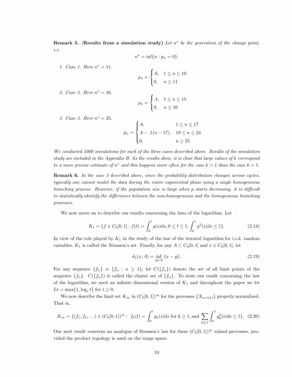
Remark 5. (Results from a simulation study) Let n? be the generation of the change point,i.e.

n? = infn : pn = 0.

1. Case 1. Here n? = 11.

pn =

.6, 1 ≤ n ≤ 10

0, n ≥ 11

2. Case 2. Here n? = 16.

pn =

.4, 1 ≤ n ≤ 15

0, n ≥ 16

3. Case 3. Here n? = 25.

pn =

.8, 1 ≤ n ≤ 17

.8− .1(n− 17), 18 ≤ n ≤ 24

0, n ≥ 25

We conducted 1000 simulations for each of the three cases described above. Results of the simulationstudy are included in the Appendix B. As the results show, it is clear that large values of k correspondto a more precise estimate of n? and this happens more often for the case k > 1 than the case k = 1.

Remark 6. In the case 3 described above, since the probability distribution changes across cycles,typically one cannot model the data during the entire exponential phase using a single homogeneousbranching process. However, if the population size is large when p starts decreasing, it is difficultto statistically identify the differences between the non-homogeneous and the homogeneous branchingprocesses.

We now move on to describe our results concerning the laws of the logarithm. Let

K1 = f ∈ C0[0, 1] : f(t) =∫ t

0

g(s)ds, 0 ≤ t ≤ 1,∫ 1

0

g2(s)ds ≤ 1. (2.18)

In view of the role played by K1 in the study of the law of the iterated logarithm for i.i.d. randomvariables, K1 is called the Strassen’s set. Finally, for any A ⊂ C0[0, 1] and x ∈ C0[0, 1], let

d1(x,A) = infy∈A

||x− y||. (2.19)

For any sequence fn ≡ fn : n ≥ 1, let C(fn) denote the set of all limit points of thesequence fn. C(fn) is called the cluster set of fn. To state our result concerning the lawof the logarithm, we need an infinite dimensional version of K1 and throughout the paper we letLt = max1, loge t for t ≥ 0.

We now describe the limit set K∞ in (C0[0, 1])∞ for the processes Xn,r(n) properly normalized.That is,

K∞ = (f1, f2, . . .) ∈ (C0[0, 1])∞ : fk(t) =∫ t

0

gk(s)ds for k ≥ 1, and∑

k≥1

∫ 1

0

g2k(s)ds ≤ 1. (2.20)

Our next result concerns an analogue of Strassen’s law for these (C0[0, 1])∞ valued processes, pro-vided the product topology is used on the range space.

10

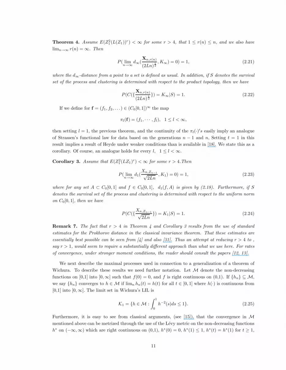
Theorem 4. Assume E(Z21 (L(Z1))r) < ∞ for some r > 4, that 1 ≤ r(n) ≤ n, and we also have

limn→∞ r(n) = ∞. Then

P ( limn→∞

d∞(Xn,r(n)

(2Ln)12,K∞) = 0) = 1, (2.21)

where the d∞-distance from a point to a set is defined as usual. In addition, if S denotes the survivalset of the process and clustering is determined with respect to the product topology, then we have

P (C(Xn,r(n)

(2Ln)12) = K∞|S) = 1. (2.22)

If we define for f = (f1, f2, . . .) ∈ (C0[0, 1])∞ the map

πl(f ) = (f1, · · · , fl), 1 ≤ l < ∞,

then setting l = 1, the previous theorem, and the continuity of the πl(·)′s easily imply an analogueof Strassen’s functional law for data based on the generations n − 1 and n, Setting t = 1 in thisresult implies a result of Heyde under weaker conditions than is available in [18]. We state this as acorollary. Of course, an analogue holds for every l, 1 ≤ l < ∞.

Corollary 3. Assume that E(Z21 (LZ1)r) < ∞ for some r > 4.Then

P ( limn→∞

d1(Xn,Zn−1√

2Ln,K1) = 0) = 1, (2.23)

where for any set A ⊂ C0[0, 1] and f ∈ C0[0, 1], d1(f,A) is given by (2.18). Furthermore, if Sdenotes the survival set of the process and clustering is determined with respect to the uniform normon C0[0, 1], then we have

P (C(Xn,Zn−1√

2Ln) = K1|S) = 1. (2.24)

Remark 7. The fact that r > 4 in Theorem 4 and Corollary 3 results from the use of standardestimates for the Prokhorov distance in the classical invariance theorem. That these estimates areessentially best possible can be seen from [4] and also [31]. Thus an attempt at reducing r > 4 to ,say r > 1, would seem to require a substantially different approach than what we use here. For ratesof convergence, under stronger moment conditions, the reader should consult the papers [12, 13].

We next describe the maximal processes used in connection to a generalization of a theorem ofWichura. To describe these results we need further notation. Let M denote the non-decreasingfunctions on [0,1] into [0,∞] such that f(0) = 0, and f is right continuous on (0,1). If hn ⊆ M,we say hn converges to h ∈ M if limn hn(t) = h(t) for all t ∈ [0, 1] where h(·) is continuous from[0,1] into [0,∞]. The limit set in Wichura’s LIL is

K1 = h ∈ M :∫ 1

0

h−2(s)ds ≤ 1. (2.25)

Furthermore, it is easy to see from classical arguments, (see [15]), that the convergence in Mmentioned above can be metrized through the use of the Levy metric on the non-decreasing functionsh∗ on (−∞,∞) which are right continuous on (0,1), h∗(0) = 0, h∗(1) ≤ 1, h∗(t) = h∗(1) for t ≥ 1,

11

and such that h∗(t) = h∗(0) for t < 0. That is, if λ(s) = s/(1 + s) for 0 ≤ s ≤ ∞, then the metric ρon M, which is of interest, is given by

ρ(h, g) = dL(h∗, g∗), (2.26)

where

h∗(s) = λ(h(s)), 0 ≤ s ≤ 1, (2.27)

and dL is Levy’s metric. Of course, for given h ∈ M the function h∗ used in (2.26) is assumed tobe such that h∗(s) = 0 for s < 0, h∗(s) = h∗(1) for s > 1, and given by (2.27) on [0,1]. (M, ρ) isalso separable since the subprobabilities on [0,1] are separable in Levy’s metric. We also define themaximal process related to Xn,Zn−1(·) by

Mn,Zn−1(t) = sup0≤s≤t

|Xn,Zn−1(s)|, 0 ≤ t ≤ 1. (2.28)

We are, of course, interested in the infinite dimensional version of the maximal processes. Tothis end, we first define the vector maximal process Mn,r(n) analogous to (2.28) as follows:

Mn,r(n)(t) = (Mn,Zn−1(t),Mn−1,Zn−2(t), · · · ,Mn−rn+1,Zn−r(n) (t), 0, 0, · · ·). (2.29)

The infinite dimensional Chung-Wichura limit set is as follows:

K∞ = (h1, h2, . . . , ) ∈ M∞ :∞∑

k=1

∫ 1

0

h−2k (s)ds ≤ 1, (2.30)

where M∞ is the infinite cartesian product of M. The topology on M∞ is the product topologywhich is complete and separable in the topology given by the metric

ρ∞(f ,g) =∑

k≥1

12k

ρ(fk, gk)1 + ρ(fk , gk)

, (2.31)

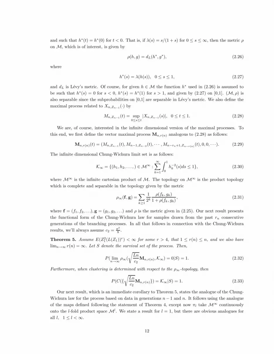
where f = (f1, f2, . . .),g = (g1, g2, . . .) and ρ is the metric given in (2.25). Our next result presentsthe functional form of the Chung-Wichura law for samples drawn from the past rn consecutivegenerations of the branching processes. In all that follows in connection with the Chung-Wichuraresults, we’ll always assume c2 = π2

8 .

Theorem 5. Assume E(Z21 (L(Z1))r) < ∞ for some r > 4, that 1 ≤ r(n) ≤ n, and we also have

limn→∞ r(n) = ∞. Let S denote the survival set of the process. Then,

P ( limn→∞

ρ∞(√Ln

c2Mn,r(n),K∞) = 0|S) = 1. (2.32)

Furthermore, when clustering is determined with respect to the ρ∞-topology, then

P (C(√Ln

c2Mn,r(n)) = K∞|S) = 1. (2.33)

Our next result, which is an immediate corollary to Theorem 5, states the analogue of the Chung-Wichura law for the process based on data in generations n− 1 and n. It follows using the analogueof the maps defined following the statement of Theorem 4, except now πl take M∞ continuouslyonto the l-fold product space Ml. We state a result for l = 1, but there are obvious analogues forall l, 1 ≤ l < ∞.

12

Theorem 6. Assume that E(Z21 (LZ1)r) < ∞ for some r > 4. Let S denote the survival set of the

process. Then

P ( limn→∞

ρ(√Ln

c2Mn,Zn−1 ,K1) = 0|S) = 1. (2.34)

Furthermore, when clustering is determined with respect to the ρ-topology, then

P (C(√Ln

c2Mn,Zn−1) = K1|S) = 1. (2.35)

3 Functional Laws of Large Numbers

In this section we provide proofs of the functional strong laws of large numbers in Theorems 1 and2. We start with the proof of Theorem 1, which we split into several lemmas.

Lemma 1. Let ε > 0. Then there exists r0 = r0(ε) such that for all r ≥ r0(ε) and all n ≥ 1

P ( max1≤k≤r

|k∑

j=1

(ξn,j −m)| > 2rε) ≤ 2P (|r∑

j=1

(ξn,j −m)| > rε). (3.1)

Proof. If ε > 0 is given, then E(ξn,1) < ∞ and the weak law of large numbers implies thereexists a k0(ε) such that for all k ≥ k0(ε) and n ≥ 1 we have

P (|k∑

j=1

(ξn,j −m)| > kε) <12. (3.2)

Thus for r ≥ k0(ε) we have for all n ≥ 1 that

max1≤k≤r

P (|k∑

j=1

(ξn,j −m)| ≥ rε) ≤ max(1/2, max1≤k≤k0(ε)

P (|k∑

j=1

(ξn,j −m)| ≥ rε)). (3.3)

Now taking r0(ε) ≥ k0(ε) sufficiently large, we have for all n ≥ 1 that

max1≤k≤r

P (|k∑

j=1

(ξn,j −m)| ≥ rε) ≤ 1/2. (3.4)

Thus by Ottaviani’s inequality, ([7]), we have (3.1), and the lemma is proven.Our next lemma establishes the almost sure convergence of Yn(1), and is a straight forward

consequence of the Senata-Heyde result ([2], page 30).

Lemma 2. limn→∞ Yn,Zn−1(1) = 0 a.s.

Proof: Let S denote the survival set of the process and Sc its complement. Then on Sc, bydefinition, there exists an n0(ω) such that Zn−1 = 0 for all n ≥ n0(ω). Hence, by definition of theprocess, Yn,Zn−1(1) = 0 on Sc. We now deal with the set S. Note that on S, Zn > 0 for all n ≥ 1almost surely. Hence,

Zn

Zn−1= (

Znc−1n

Zn−1c−1n−1

)cncn−1

(3.5)

13

Now, by Theorem 3 of [2]

limn→∞

(Znc

−1n

Zn−1c−1n−1

) =W (ω)W (ω)

= 1, (3.6)

where the last equality follows from W (ω) > 0 a.s. on S. Also, again from [2],

limn→∞

cncn−1

= m. (3.7)

Hence, Yn,Zn−1(1) → 0 a.s. on S, completing the proof of the lemma.An interesting consequence of Lemma 2 is the following estimate of Zn on a set S0 (defined

below) of probability 1 − q. Define,

S0 = ω : limn→∞

Zn(ω)Zn−1(ω)

= m. (3.8)

Then, from the proof of Lemma 2, it follows that P (S∆S0) = 0 and Sc ∩S0 = φ. Also, on S0 thefollowing hold: for every 1 < β < m, and all ω ∈ S0, there is a n0(ω) such that for all n ≥ n0(ω) + 1

Zn(ω) > βZn−1(ω) > Zn−1(ω) (3.9)

and

Zn(ω) ≥ maxZ0(ω), · · · , Zn−1(ω). (3.10)

Thus (3.9) and (3.10) imply that for all ω ∈ S0 and n ≥ n0(ω),

Zn(ω) ≥ βn−n0Zn0(ω), (3.11)

where n0 = n0(ω).Let us denote by F0 the trivial σ−field, i.e. F0 = φ,Ω, and for n ≥ 1 let

Fn = σ(ξk,j : j ≥ 1 : 1 ≤ k ≤ n). (3.12)

Furthermore, let

Bn(ε) = sup1≤k≤Zn−1

|k∑

j=1

(ξn,j −m)| > 2Zn−1ε. (3.13)

Our next lemma is one way to express the role of the branching property of Zn : n ≥ 0, andallows us to complete the proof of Theorem 1. It also is used in the study of complete convergencein Theorem 2.

Lemma 3. Let ε > 0 and let ξ, ξn : n ≥ 1 be an i.i.d. sequence defined on the probabilityspace (Ω1,G, Q), which is different from (Ω,F , P ), the probability space supporting Zn : n ≥ 0.Furthermore, assume that L(ξ) = L(Z1). Then there exists a finite random variable n0 on (Ω,F , P )such that for all n ≥ n0(ω) we have with P-probability one that

P (Bn(ε)|Fn−1)(ω) ≤ 2Q(|Zn−1(ω)∑

j=1

(ξj −m))| ≥ εZn−1(ω)) (3.14)

= 2P (|Zn−1∑

j=1

(ξj −m)| ≥ εZn−1|Zn−1)(ω). (3.15)

Of course, all terms in (3.14-15) are understood to be zero if Zn−1(ω) = 0.

14

Proof. By the Markov property of Zn : n ≥ 0, it follows that

P (Bn(ε)|Fn−1) = P (Bn(ε)|Zn−1). (3.16)

If ω ∈ Sc, then eventually Zn−1(ω) = 0 and by definition of the Yn,Zn−1 process, both the LHS andRHS of (3.14) are then zero. Hence for ω ∈ Sc we set n0(ω) = mink ≥ 1 : Zk(ω) = 0. Thus,it is remains to establish the validity of the lemma on S0 since P (S∆S0) = 0. To this end, letω ∈ S0 and r0 = r0(ε) be as in Lemma 1. Then there exists an n0 = n0(ω) such that for all n ≥ n0,Zn−1(ω) > r0(ε). Hence first by (3.16) and the branching property, and then by Lemma 1 and thebranching property, we have

P (Bn(ε)|Fn−1)(ω) = Q( sup1≤k≤Zn−1(ω)

|k∑

j=1

(ξj −m)| > 2Zn−1(ω)ε) (3.17)

≤ 2Q(|Zn−1(ω)∑

j=1

(ξj −m)| > εZn−1(ω)) (3.18)

= 2P (|Zn−1∑

j=1

(ξj −m)| > εZn−1|Zn−1)(ω), (3.19)

yielding the lemma.Proof of Theorem 1. First we will show that with probability one

limn→∞

||Yn,Zn−1|| = 0. (3.20)

If ω ∈ Sc then Zn−1 = 0 for some n ≥ n0 and hence on Sc we have

limn→∞

||Yn,Zn−1|| = 0. (3.21)

If ω ∈ S, then by the conditional Borel-Cantelli Lemma, it is sufficient to show that∑

n≥1

P (||Yn,Zn−1|| > ε|Fn−1) < ∞. (3.22)

Using Lemma 3 and that Bn(ε) = ||Yn,Zn−1|| > ε, Lemma 1 implies it is sufficient to show that

∑

n≥1

P (|Zn−1∑

j=1

(ξj −m) > εZn−1|Fn−1) < ∞ a.s. (3.23)

on S. Now, by Lemma 2

P (ω : | Zn

Zn−1−m| > ε i.o ∩ S) = 0, (3.24)

which by the conditional Borel-Cantelli Lemma is equivalent to the finiteness of the LHS of (3.23)a.s. on S. Thus we have established (3.20), and the theorem follows as the convergence in the metricin (2.4) requires only coordinatewise convergence for finitely many coordinates with probability one.

Proof of Theorem 2. The proof will again proceed with several lemmas, some of which willalso be of use for later proofs. The first lemma is essentially Theorem 3 of [AN, p.41].

15

Lemma 4. Let Zn : n ≥ 0 be a supercritical Galton-Watson process with Z0 = 1. Then thereexists a constant γ ∈ (0, 1) such that

limn→∞

P (Zn = k)/γn = νk, (3.25)

where 0 ≤ νk < ∞ for all k ≥ 1.

Proof. If p1 = P (Z1 = 1) 6= 0, then f ′(q) = p1, and since the process is supercritical we havef ′(q) ∈ (0, 1). Thus with γ = f ′(q), Theorem 3.1 of [AN, p. 41] implies the lemma. When p1 = 0there are two cases to consider, namely p0 = 0 and p0 6= 0. If p0 = 0, then Zn ≥ 2n and henceeventually for any fixed k we have P (Zn = k) = 0. Thus the lemma also holds in this case with γ

any number in (0, 1) and νk = 0.Hence there remains the case p0 6= 0, p1 = 0. In this last case, since the process is supercritical,

we have 0 < q < 1, and again we have 0 < f ′(q) < 1, so the result in [AN] cited above implies thelemma.

Our next lemma provides estimates which are useful in connection with the complete convergencein Theorem 2. We use the notation of Lemma 3, where ξ, ξj : j ≥ 1 are i.i.d random variables onthe probability space (Ω1,G, Q).

Lemma 5. Let Tk =∑k

j=1(ξj − m). Then there exists a k0(ε,L(ξ)), where L(ξ) is the law of ξ,such that for all k ≥ k0

Q(|Tk| > kε

2) ≤ 16ε−2k−1E((ξ −m)2I(|ξ −m| ≤ k)) + kQ(|ξ −m| ≥ k). (3.26)

Proof. Let

Tk =k∑

j=1

(ξj −m)I(|ξj −m| ≤ k) for all k ≥ 1. (3.27)

Now observe that

Q(|Tk| >kε

2) ≤ Q(|Tk| >

kε

2) +Q(|Tk − Tk| > 0). (3.28)

Now,

Q(|Tk − Tk| > 0) ≤ kQ(|ξ −m| ≥ k), (3.29)

and it remains to estimate Q(|Tk| > kε2 ). Observe that, since E(ξ−m) = 0, there exists a k0(ε) such

that k ≥ k0(ε) implies |E(ξ −m)I(|ξ −m| ≤ k))| ≤ ε4. Hence,

Q(|Tk| >kε

2) ≤ Q(|Tk − E(Tk)| > kε

4) (3.30)

≤ 16ε−2k−1E((ξ −m)2I(|ξ −m| ≤ k)). (3.31)

Thus (3.26) holds for all k ≥ k0.

To finish the proof of Theorem 2, we first note that

P ( sup1≤j≤r(n)

||Yn−j+1,Zn−j || > ε) ≤r(n)∑

j=1

P (||Yn−j+1,Zn−j|| > ε) (3.32)

=r(n)∑

j=1

P (||Yn−j+1,Zn−j|| > ε Zn−j > 0) (3.33)

= In + IIn, (3.34)

16

where

In =r(n)∑

j=1

n0(ε)∑

k=1

P (||Yn−j+1,Zn−j|| > ε Zn−j = k) (3.35)

≤r(n)∑

j=1

n0(ε)∑

k=1

P (Zn−j = k), (3.36)

and

IIn =r(n)∑

j=1

∑

k≥n0(ε)+1

P (||Yn−j+1,Zn−j || > ε Zn−j = k). (3.37)

We will first study In. By Lemma 4 above, there exists 0 < M < ∞, 0 ≤ νk < ∞, and 0 < γ < 1such that

P (Zn−j = k) ≤ M (νk + 1)γn−j (3.38)

for 1 ≤ k ≤ n0(ε) and all n > j. Note that M may need to be large, but the set of k′s wherethe inequality holds is finite, and hence M < ∞ is possible. Since r(n) ≥ (logn)(h(n) wherelimn→∞ h(n) = ∞ in both parts of the theorem, we have easily have

∑

n≥1

r(n)γn−r(n) < ∞, (3.39)

and hence for all n0(ε) < ∞ we have

∑

n≥1

In ≤ M∑

n≥1

n0(ε)∑

k=1

(νk + 1)r(n)γn−r(n) < ∞. (3.40)

Thus it remains to deal with IIn. The first case we consider is when the assumptions in part-ahold. Since the conclusions of part-a do not involve r and we have r > 1, it suffices to assume1 < r ≤ 2 when we write the proof. Thus by a result of von Bahr and Esseen in [33] we have

E(|k∑

j=1

(ξj −m)/k|r) ≤ BrE(|ξ −m)|r)k−(r−1), (3.41)

for an absolute constant Br . Now we also have

P (||Yn−j+1,Zn−j || > ε Zn−j = k) = Q( max1≤l≤k

|l∑

j=1

(ξj −m)| > kε)P (Zn−j = k), (3.42)

and applying Lemma 1 and Markov’s inequality (3.41) and (3.42) combine to imply∑

n≥1 IIn < ∞provided

∑

n≥r(n)+1

r(n)∑

j=1

∑

k≥n0(ε)+1

k−(r−1)P (Zn−j = k) ≤∑

n≥r(n)+1

r(n)∑

j=1

E(Z−(r−1)n−j I(Zn−j > 0)) < ∞. (3.43)

Since r − 1 ≤ 1 and the process is supercritical, the proof of (4) in Theorem 2 of [19] implies

E(Z−(r−1)n−j I(Zn−j > 0)) ≤ (γn−j

HB )r−1, (3.44)

17

where 0 < γHB < 1. Combining (3.43-44) we thus have∑

n≥1 IIn < ∞ since

∑

n≥1

r(n)∑

j=1

(γn−jHB )r−1 ≤

∑

n≥1

r(n)(γn−r(n)HB )r−1 <∞ (3.45)

when r > 1, 0 < γHB < 1, 1 ≤ r(n) ≤ n and n − r(n) ≥ (logn)h(n) with limn→∞ h(n) = ∞. Thuspart-a is proven.

Turning to part-b and using the notation of Lemma 3 we see that

P (||Yn−j+1,Zn−j || > ε Zn−j = k) = Q( max1≤l≤k

|l∑

j=1

(ξj −m)| > kε)P (Zn−j = k). (3.46)

Now taking n0(ε) ≥ max(r0( ε2), k0(ε)), where r0(·) is defined as in Lemma 1, and k0(ε) is as in

Lemma 5, we have for k ≥ n0(ε) + 1,

P (||Yn−j+1,Zn−j || > ε Zn−j = k) ≤ 2Q(|k∑

j=1

(ξj −m)| > kε)P (Zn−j = k). (3.47)

Thus,∑

n≥1 IIn < ∞ if

∑

n≥r(n)+1

r(n)−1∑

j=1

∑

k≥n0(ε)+1

(E(k−1(ξ −m)2I(|ξ −m| ≤ k)) + kQ(|ξ −m| ≥ k))P (Zn−j = k) < ∞.

(3.48)

Now, by Markov’s inequality,

kQ(|ξ −m| ≥ k) ≤ E(φ(|ξ −m|))(Lk)r

, (3.49)

where φ(t) = t(L(t))r for t ≥ 0. We now deal with the other term inside the sum in (3.48). Letc0 ≥ ee be sufficiently large that

E(k−1(ξ −m)2I(|ξ −m| ≤ k)) ≤ IIn(A) + IIn(B) + IIn(C), (3.50)

where

IIn(A) = E(k−1(ξ −m)2I(|ξ −m| ≤ c0)) ≤ c20k−1, (3.51)

IIn(B) = E(k−1(ξ −m)2I(c0 ≤ |ξ −m| ≤ k(Lk)−r)) ≤ E(|ξ −m|)(Lk)−r , (3.52)

and

IIn(C) = E(k−1(ξ −m)2I(c0 ≤ k(Lk)−r ≤ |ξ −m| ≤ k)) (3.53)

≤ E(|ξ −m|(L(|ξ −m|)r)(L(k(Lk)−r))−rI(k≥c0)). (3.54)

The last inequality holds if c0 > ee and t ≥ c0 is sufficiently large so that we have Lt− rLLt ≥ 12Lt.

Combining (3.48),(3.49), and the estimates in (3.50-54) we see that

∑

n≥r(n)+1

IIn ≤ C∑

n≥r(n)+1

r(n)−1∑

j=0

E(LZ−rn−j(Zn−j > 0)), (3.55)

18

where C is a finite positive constant. Now using the harmonic moment results for LZn from AppendixA, we see that

∑

n≥1

IIn ≤ C∑

n≥1

r(n)(loge n)r

(n − r(n))r< ∞ (3.56)

where C is a possibly different finite positive constant and the last series converges by assumption.This completes the proof of Theorem 2.

Using our Theorems 1 and 2 one can study limit theorems for the uncentered version of Yn,Zn−1 ,scaled by constants cn−1 instead of Zn−1. In particular, if 1 < E(Z1) = m <∞ the Senata constantsmentioned in section one can be used for cn, and if we also have E(Z1LZ1) < ∞, then we can takecn = mn. To this end, we define the appropriately modified processes

Y mn,cn−1

(t) =1

cn−1

btZn−1c∑

j=1

ξn,j + (tZn−1 − btZn−1c)1

cn−1(ξbtZn−1c+1). (3.57)

Then, under the asssumption that 1 < m < ∞, for every fixed t, as n→ ∞, Y mn,cn−1

(t) → mtV a.s.,where V is a non-degenerate random variable. Indeed, V = W if E(Z1LZ1) < ∞ and V = WSH ifE(Z1LZ1) = ∞. Of course, the limit is non-zero only on the survival set S. Furthermore, one alsothen has that ||Yn,cn−1|| converges almost surely to mV as n → ∞. Our next result, a corollary ofTheorem 1, shows that in the product topology the stochastic process

Ymn = (Y m

n,cn−1(t), Y m

n−1,cn−2(t), · · · , Y m

n−r(n)+1,cn−r(n)(t), 0, 0, · · ·) (3.58)

converges to an appropriate limit almost surely.

Proposition 1. Assume that E(Z1) < ∞ and 1 ≤ r(n) ≤ n with limn→∞ r(n) = ∞. Let

L = (mtV,mtV, · · · , ). (3.59)

where V = W if E(Z1LZ1) <∞ and V = WSH if E(Z1LZ1) = ∞. Then,

limn→∞

d∞(Ymn ,L) = 0 a.s.. (3.60)

Furthermore, the limit L is strictly positive and finite almost surely only on the non-extinction setS and is zero almost surely on Sc.

Remark 8. The previous proposition is a functional generalization of a classical limit theorem fora supercritical Galton-Watson process.

Proof. Let

Nn(t) =btZn−1c∑

j=1

ξn,j + (tZn−1 − btZn−1c)(ξbtZn−1c+1), 0 ≤ t ≤ 1. (3.61)

Then with the constants cn defined as above we have

Y mn,cn−1

(t) = Nn(t)/cn−1, 0 ≤ t ≤ 1, (3.62)

and

Yn,Zn−1(t) = Nn(t)/Zn−1 −mt, 0 ≤ t ≤ 1. (3.63)

19

Since we are asking for almost sure convergence in the product topology in Proposition 1, it iseasy to see that it suffices to show that

limn→∞

sup0≤t≤1

|Y mn,cn−1

(t) −mtV | = 0 (3.64)

with probability one. Now this limit is immediate almost surely on the complement of the survivalset S, since Y m

n,cn−1(·), for all large n, and V both equal zero almost surely there. On the set S we

have Zn−1 > 0 and

sup0≤t≤1

|Y mn,cn−1

(t) −mtV | = sup0≤t≤1

|Nn(t)cn−1

−mtV | (3.65)

≤ sup0≤t≤1

[|Nn(t)cn−1

−mtZn−1

cn−1| +mt|Zn−1

cn−1− V |] (3.66)

≤ Zn−1

cn−1sup

0≤t≤1|Nn(t)Zn−1

−mt| +m|Zn−1

cn−1− V | (3.67)

=Zn−1

cn−1||Yn,Zn−1|| +m|Zn−1

cn−1− V |. (3.68)

Letting n → ∞ in the above, and applying Theorem 1 and the Seneta-Heyde and Kesten-Stigumresults as explained in the introduction, the proposition is proved.

4 Functional Central Limit Theorem

In this section we provide a proof of the functional central limit theorem. The proof is based ona lemma for weak convergence in infinite product spaces. It seems such a lemma should be inthe literature, but we could not find it. Hence we include it for completeness and its independentinterest. We begin with a bit of notation. Let (S, d) be a complete separable metric space and µ bea Borel probability measure on (S, d) and π : S → S be Borel measurable. Define,

µπ(A) = µ(π−1(A)) (4.1)

for all Borel sets A of (S, d). Let S∞ denote the infinite product space with a typical point s =(s1, s2, · · · ). The product topology on S∞ is metrizable with metric

d∞(s, t) =∑

j≥1

12j

d(sj , tj)1 + d(sj , tj)

, (4.2)

where s, t ∈ S∞. If q = (q1, q2, · · · , ) is a point in S, we define the mapping πl : S∞ → S∞, forl ≥ 1, by

πl(s) = (s1, s2, · · · , sl, ql+1, ql+2, · · · , ). (4.3)

We now state a lemma concerning weak convergence in product spaces. A proof is provided for thesake of completeness.

Lemma 6. Let µn : n ≥ 1 and µ∞ be Borel probability measures on (S∞, d∞). Then µn : n ≥ 1converges weakly to µ∞ if and only if µπl

n converges weakly to µπl∞ for all l ≥ 1.

20

Proof. To prove weak convergence, we need to verify that ( see, for example, [11])

limn→∞

∫

S∞fdµn =

∫

S∞fdµ∞ (4.4)

for f : S∞ → S∞ satisfying ||f |BL ≤ 1, where

||f ||BL = sups∈S∞

|f(s)| + sups 6=t∈S∞

|f(s) − f(t)|d(s, t)

. (4.5)

First note that the mappings πl : l ≥ 1 are continuous and hence Borel measurable. Then forl ≥ 1 we have,

∫

S∞f(s)dµn −

∫

S∞f(s)dµ∞ = I1 + I2 + I3, (4.6)

where

I1 =∫

S∞(f(s) − f(πl(s))dµn, (4.7)

I2 =∫

S∞f(πl(s))d(µn − µ∞), (4.8)

and

I3 =∫

S∞(f(πl(s)) − f(s))dµ∞. (4.9)

Let ε > 0 and l0(ε) > 0 be such that∑

j≥l0(ε)2−j ≤ ε

2 . This implies that for l ≥ l0(ε),

d(s, πl(s)) =∑

j≥n0(ε)+1

12j

d(sj , qj)1 + d(sj , qj)

≤ ε

2; (4.10)

thus, for ||f ||BL ≤ 1, we have

lim sup |∫

S∞fd(µn − µ∞)| ≤ ε

2+ lim sup

n→∞|∫

S∞f(πl(s)d(µn − µ∞)| + ε

2. (4.11)

Since ε > 0 is arbitrary, the asserted weak convergence follows. Finally, if µn ⇒ µ∞, then sinceπl : l ≥ 1 are continuous, by the continuous mapping theorem µπl

n ⇒ µπl∞.

Proof of Theorem 3. Let µ denote Wiener measure on C0[0, 1] and µ∞ be the infinite productmeasure formed by µ on (C0[0, 1])∞. Also let µn denote the law of Xn,r(n) when Zn−1 is conditionedto be stricty positive,i.e. for A a Borel subset of (C0[0, 1[)∞ we have

µn(A) = P (Xn,r(n) ∈ A|Zn−1 > 0).

By Lemma 6 with S = C0[0, 1] and q the zero vector in (C0[0, 1])∞, it is sufficient to establish, foreach l ≥ 1, the weak convergence of µπl

n to µπl∞. If we identify the range space of πl with (C0[0, 1])l

in the obvious way, then it suffices to show that on (C0[0, 1])l we have that

λn = L(Xn,Zn−1 , Xn−1,Zn−2 , · · · , Xn−l+1,Zn−l |Zn−1 > 0)

converges weakly to (µ)l, the l-fold product of µ on that space.

21

To establish weak convergence of λn to (µ)l, it is sufficient, by Theorem 3.1 of Billingsley ([3]),to show for arbitrary continuity sets Ei of the Wiener measure on C0[0, 1] that

limn→∞

λn(E1 ×E2 × · · · × El) =l∏

j=1

µ(Ej). (4.12)

We will now verify (4.12). To this end, set

θn = (P (Zn−1 > 0))λn(l∏

j=1

Ej). (4.13)

Then,

θn = E(l∏

j=1

IAn,j ), (4.14)

where

An,j = Xn−j+1,Zn−j ∈ Ej, Zn−j > 0 (4.15)

for 1 ≤ j ≤ l. Let F0 = φ,Ω and Fn = σ(ξk,j : j ≥ 1 : 1 ≤ k ≤ n) for n ≥ 1. Also, to simplifythe notation, write An,j = Aj , for 1 ≤ j ≤ l. Now,

θn = E(E(l∏

j=1

IAj |Fn−1)) (4.16)

= E(E(IA1 |Fn−1)l∏

j=2

IAj ). (4.17)

Now, setting βn ≡ E(IA1 |Fn−1), we have

βn = ∆n + µ(E1), (4.18)

where ∆n = E(IA1 |Fn−1) − µ(E1). Thus,

θn = µ(E1)E(l∏

j=2

(IAj ) + en, (4.19)

where

en = E(l∏

j=2

IAj ∆n). (4.20)

We will now show that limn→∞ en = 0. To this end, let ε > 0 and note that

lim supn→∞

en ≤ lim supn→∞

E(|∆n|IZn−2>0) (4.21)

≤ I + II, (4.22)

where

I = lim supn→∞

E(|P (A1|Fn−1) − µ(E1)|I(Zn−1>0, Zn−2>0)), (4.23)

22

and

II = lim supn→∞

E(|P (A1|Fn−1) − µ(E1)|I(Zn−1=0, Zn−2=0)). (4.24)

Now observe that,

P (A1|Zn−1 = j) = P (Xn,Zn−1 ∈ E1|Zn−1 = j) = P (Xn,j ∈ E1). (4.25)

Hence, given ε > 0, and that E1 is a µ-continuity set, Donsker’s invariance principle implies

|P (Xn,j ∈ E1) − µ(E1)| ≤ ε (4.26)

for j ≥ j0(ε, E1) independent of n, since ξn,j, j ≥ 1 are i.i.d. with E(ξ1,1) = 0 and E(ξ21,1) < ∞.Now, using the Markov property of Zn, we have

I = lim supn→∞

E(|P (A1|Fn−1) − µ(E1)|I(Zn−1>0 Zn−2>0)) (4.27)

≤ lim supn→∞

E(|P (A1|Zn−1) − µ(E1)|I(Zn−1>0 Zn−2>0)) (4.28)

≤ limn→∞

(Σ1,n + Σ2,n), (4.29)

where

Σ1,n =∑

j1≤j0

∑

j2≥1

|P (A1|Zn−1 = j1) − µ(E1)|P (Zn−1 = j1, Zn−2 = j2), (4.30)

Σ2,n =∑

j1≥j0+1

∑

j2≥1

|P (A1|Zn−1 = j1) − µ(E1)|P (Zn−1 = j1, Zn−2 = j2). (4.31)

Thus,

I ≤ lim supn→∞

[2P (1 ≤ Zn−1 ≤ j0) + ε] = ε, (4.32)

where we used Lemma 4 to show that limn→∞ P (1 ≤ Zn−1 ≤ j0) = 0. As for II, observe that

II ≤ 2 lim supn→∞

∑

j≥1

P (Zn−2 = j, Zn−1 = 0) (4.33)

≤ lim supn→∞

∑

j≥1

pj0P (Zn−2 = j) (4.34)

≡ lim supn→∞

[fn−2(p0) − fn−2(0)] (4.35)

= 0, (4.36)

since fn−2(p0) and fn−2(0) both converge to q. Since en ≥ 0, this implies limn→∞ en = 0.Now returning to (4.19) and iterating we get,

θn ≡l−1∏

j=1

µ(Ej)E(IAl) +l−2∑

j=0

µ(Ej)en−j , (4.37)

where E0 = C0[0, 1] and en−j = E(∏l

k=2+j IAj∆n−j). Now, using an argument similar to the oneused to prove en → 0, one can show that limn→∞ en−j = 0.

23

Finally, note that

E(IAl ) = P (Xn−l+1,Zn−l ∈ El, Zn−l > 0) (4.38)

=∑

j≥1

P (Xn−l+1,j) ∈ El)P (Zn−l = j) (4.39)

= In + IIn + IIIn, (4.40)

where

In =j0(ε,El)∑

j=1

P (Xn−l+1,j ∈ El)P (Zn−l = j). (4.41)

IIn =∑

j>j0(ε,El)

(P (Xn−l+1,j ∈ El) − µ(El))P (Zn−l = j), (4.42)

and

IIIn = µ(El)P (Zn−l > j0(ε, El)); (4.43)

and j0(ε, El) is such that for all j ≥ j0(ε, El)

|P (Xn−l+1,j ∈ El) − µ(El)| < ε. (4.44)

Existence of such a j0(ε, El) follows by Donsker’s invariance principle since ξn,j : j ≥ 1 are all i.i.d.with E(ξn,1 = 0 and E(ξ2n,1) < ∞. Using Lemma 4 we have limn→∞ P (1 ≤ Zn−l ≤ j0(ε, El)) = 0,and hence it follows that In → 0 as n → ∞. Furthermore, using (4.44) and that P (Zn−l >

j0(ε, El)) → (1 − q) it follows that lim supn→∞ IIn ≤ ε(1 − q). Finally, IIIn → µ(El)(1 − q). Thus,limn→∞E(IAl) = µ(El)(1 − q), which implies limn→∞ θn = (1 − q)

∏lj=1 µ(Ej), and hence from

(4.13) we have limn→∞ λn =∏l

j=1 µ(Ej). Thus the theorem is proven.

5 Strassen’s Functional Laws of the Logarithm

In this section we establish Strassen’s law of the logarithm for supercritical Galton-Watson processesin the multiple generation setting. We begin with a general outline of the method of proof. As a firststep, we will show with probability one that Xn,r(n)/(2Ln)1/2 is relatively compact with respectto the product topology on (C0[0, 1])∞. The next step will be to show that if f /∈ K∞, then withprobability one f is not in the cluster set C(Xn,r(n)/(2Ln)1/2). Finally, conditioning on the suvivalset, we show with probability one that every point ofK∞ is in the cluster set C(Xn,r(n)/(2Ln)1/2).Throughout, the topology on the range space (C0[0, 1])∞ is the product topology, which is separableand metric.

We begin with some notation that we will use extensively. For any subset A of a metric spaceM with metric d, Aδ is defined to be the set

Aδ = y ∈M |d(x, y) < δ for some x ∈ A. (5.1)

In order not to cause confusion with this notation, we will henceforth usually write the complementof a typical set A as A′, rather than Ac, as used earlier in connection with the survival set S. However,allowing abuse of this principle, we will continue to write the complement of S as before.

Our first lemma yields compactness of the cluster set K∞.

24

Lemma 7. K∞ is a compact subset of ((C0[0, 1])∞, d∞).

Proof. Let K∞ denote the countably infinite product set∏K1, where in each coordinate

K1 = f ∈ C0[0, 1] : f ∈ AC[0, 1], ||f ||2µ ≤ 1. (5.2)

Here we write AC[0, 1] to denote the absolutely continuous functions in C0[0, 1], and set ||f ||2µ =∫ 1

0(f ′(s))2ds for f ∈ AC[0, 1] such that f ′ is square integrable on [0, 1]. Furthermore, we define

||f ||2µ = ∞ elsewhere on C0[0, 1]. Then it is well known that K1 is a compact subset of (C0[0, 1], || ·||), see, for example, Strassen [32] or Lemma 2.1 of Kuelbs ([22]), and hence Tychnoff’s Theoremimmediately implies K∞ is compact in ((C0[0, 1])∞, d∞). Since K∞ ⊆ K∞, it is therefore enoughto show that K∞ is closed in ((C0[0, 1])∞, d∞).

Let fn ∈ K∞ ⊆ (C0[0, 1])∞ and assume that

limn→∞

d∞(fn, f ) = 0 (5.3)

for some f ∈ (C0[0, 1])∞. Assume fn = (fn,1, fn,2, · · · ) and f = (f1, f2, · · ·). Then for each N ≥ 1,we have

limn→∞

sup1≤j≤N

||fn,j − fj || = 0, (5.4)

and the sequence (fn,1, fn,2, · · ·fn,N ) : n ≥ 1 is contained in

KN = (h1, · · ·hN ) :N∑

j=1

||hj||2µ ≤ 1, hj ∈ AC[0, 1], 1≤ j ≤ N. (5.5)

NowKN is compact in (C0[0, 1])N for allN ≥ 1 since it is the limit set for Strassen’s LIL for standardBrownian Motion on RN . Thus (f1, · · ·fN ) ∈ KN for all N ≥ 1, which implies

∑j≥1 ||fj||2µ ≤ 1 and

also that fj ∈ AC[0, 1] for all j ≥ 1 by definition of KN and that KN is closed in (C0[0, 1])N . Thus,f ∈ K∞ and hence K∞ is closed and compact. This completes the proof of the lemma.

The next lemma is useful in our calculations several times.

Lemma 8. Suppose φ(t) = t2(Lt)r where r > 0, t ≥ 0, and as before Lt = max1, loge t. IfE(φ(Z1)) < ∞, m = E(Z1), and L(ξ) = L(Z1), where ξ is independent of Zn−1, then there existsa finite positive constant c(ξ, r), depending only on r > 0 and the law L(ξ) = L(Z1), such that

Zn−1P (|ξ −m| ≥ Z1/2n−1|Zn−1)I(Zn−1 > 0) ≤ c(r, ξ)/(LZn−1)r , (5.6)

and

Zn−1E(|η/Z1/2n−1|3|Zn−1)I(Zn−1 > 0) ≤ c(r, ξ)/(LZn−1)r, (5.7)

where

η = (ξ −m)I(|ξ −m| ≤ Z1/2n−1) − µn,Zn−1 , (5.8)

and

µn,Zn−1 = E((ξ −m)I(|ξ −m| ≤ Z1/2n−1)|Zn−1). (5.9)

25

Proof. Since the terms to be dominated in (5.6) and (5.7) are all zero when Zn−1 = 0, andLt ≥ 1 for all t ≥ 0, the result holds in this situation. Hence it suffices to prove the result when weassume Zn−1 > 0.

To simplify notation, let ρ = ξ − m. Then, since φ(t) is increasing for t ≥ 0, we have by theconditional Markov inequality that

Zn−1P (|ρ| ≥ Z1/2n−1|Zn−1)I(Zn−1 > 0) ≤ Zn−1E(|ρ|I(|ρ| ≥ Z

1/2n−1)|Zn−1)/φ(Z1/2

n−1) (5.10)

=∫ ∞

Z1/2n−1

t2(Lt)rdF|ρ|(t)/(LZ1/2n−1)

r (5.11)

≤ E(φ(|ρ|))/(LZ1/2n−1)

r (5.12)

≤ 2rE(φ(|ρ|))/(LZn−1)r , (5.13)

where in the last inequality we have used that (Lt1/2)r ≥ (Lt)r/2r for t ≥ 0 and r > 0. Thus (5.6)holds with c(r, ξ) ≥ 2rE(φ(|ξ −m|)).

To verify (5.7) observe that

Zn−1E(|η/Z1/2n−1|3|Zn−1)I(Zn−1 > 0) ≤ Z

−1/2n−1 E(|ρI(|ρ| ≤ Z

1/2n−1) − µn,Zn−1 |3|Zn−1) (5.14)

≤ Z−1/2n−1 a1,n + a2,n, (5.15)

wherea1,n = E(|ρI(|ρ| ≤ Z

1/2n−1) − µn,Zn−1 |2|ρ|I(|ρ| ≤ Z

1/2n−1)|Zn−1),

anda2,n = E(|ρI(|ρ| ≤ Z

1/2n−1) − µn,Zn−1 |2|µn,Zn−1||Zn−1).

Recalling µn,Zn−1 is σ(Zn−1) measurable, we have

a1,n ≤ 2E(|ξ −m|3I(|ξ −m| ≤ Z1/2n−1)|Zn−1) + 2µ2

n,Zn−1E(|ξ −m|),

and we also easily see thata2,n ≤ |µn,Zn−1 |E((ξ −m)2).

Thus

Zn−1E(|η/Z1/2n−1|3|Zn−1)I(Zn−1 > 0) ≤ Z

−1/2n−1 a3,n + a4,n +E((ξ −m)2)|µn,Zn−1|,

where a3,n = 2E(|ξ−m|3I(|ξ−m| ≤ Z1/2n−1)|Zn−1) and a4,n = 2µ2

n,Zn−1E(|ξ−m|). Since |µn,Zn−1 | ≤

E(|ξ −m|) we see that

Z−1/2n−1 a2,n + a4,n ≤ c(r, ξ)/(LZn−1)r , (5.16)

where c(r, ξ) is a finite positve constant depending only on r > 0 and L(ξ).Hence (5.7) will hold, and the lemma will be proved, if we show

Z−1/2n−1 a3,n = 2Z−1/2

n−1 E(|ξ −m|3I(|ξ −m| ≤ Z1/2n−1)|Zn−1) ≤ c(r, ξ)/(LZn−1)r , (5.17)

where again c(r, ξ) is a finite positve constant depending only on r > 0 and L(ξ). To verify (5.17)take c0 = c0(r) such that c0 ≥ ee and if t ≥ c0, then loge t−2r loge(loge t) > (loge t)/2. If c0 > Zn−1,then

Z−1/2n−1 a3,n ≤ 2c0E(|ξ −m|2)/Z1/2

n−1,

26

and again (5.7) will hold for a sufficiently large constant c(r, ξ). Hence it remains to consider thecase where c0 ≤ Zn−1. Thus we observe that

Z−1/2n−1 a3,n ≤ 2(A1,n +A2,n),

where

A1,n = E(|ξ −m|2|ξ −m|Z−1/2n−1 I(0 < |ξ −m| ≤ Z

1/2n−1/(LZn−1)r)|Zn−1) (5.18)

≤ E(|ξ −m|2)/(LZn−1)r , (5.19)

and

A2,n = E(|ξ −m|2|ξ −m|Z−1/2n−1 I(Z

1/2n−1/(LZn−1)r) ≤ |ξ −m| ≤ Z

1/2n−1)|Zn−1) (5.20)

≤ E(φ(|ξ −m|))/L(Z1/2n−1/(LZn−1)r)r . (5.21)

Since c0 ≤ Zn−1, our choice of c0 now allows us to complete the proof.Our next lemma gives some elementary properties of the set K1 in C0[0, 1] with respect to the

sup-norm || · ||, which will be useful later in proving our version of Strassen’s theorem.

Lemma 9. If λ ≥ 1 and 0 < β ≤ δ/2, then

((λ(K1)δ)′)β = (λ(Kδ1 )

′)β ⊆ λ(Kδ/2

1 )′.

Proof. The set equality is obvious since multipling by λ ≥ 1 is a one-to-one mapping. Hence weturn to the set inclusion. Now if x ∈ (λ(Kδ

1 )′)β, then there exists y ∈ (Kδ

1 )′such that ||λy−x|| < β.

We want x to be in λ(Kδ/21 )

′, so assume it is in the complement, i.e. x ∈ λ(Kδ/2

1 ) since λ 6= 0.Hence if x ∈ λ(Kδ/2

1 ) then x = λz where z ∈ Kδ/21 , so there exists k ∈ K1 with ||z−k|| < δ/2. Thus

from the above we have

||y − k|| ≤ ||y − x/λ||+ ||x/λ− k|| ≤ β/λ + ||z − k|| < δ,

provided β < δ/2 and λ ≥ 1. This is a contradiction since y ∈ (Kδ1 )

′and k ∈ K impies ||y− k|| ≥ δ.

Thus the lemma holds.Before we state our next lemma, we recall from (2.13) that

Xn,r(n) = (Xn,Zn−1 , Xn−1,Zn−2, · · · , Xn−r(n)+1,Zn−r(n), 0, 0, · · ·), (5.22)

and for later use we define

Xn,l = (Xn,Zn−1 , Xn−1,Zn−2 , · · · , Xn−l+1,Zn−l , 0, 0, . . .). (5.23)

Our next lemma concerns the relative compactness of the sequence Xn,r(n)/(2Ln)1/2 in the metricspace ((C0[0, 1])∞, d∞).

Lemma 10. P (Xn,r(n)/(2Ln)1/2 is relatively compact in (C0[0, 1])∞) = 1.

Proof. Since ((C0[0, 1])∞, d∞) is separable, and K∞ is a compact subset, it is sufficient toestablish that for each s > 0 we have

∑

n≥1

P (Xn,r(n)/(2Ln)1/2 /∈ (K∞)s) <∞. (5.24)

27

Let s > 0 be arbitrary but fixed. Let α > 0 be such that 2α = s/2(l + 1), where∑

k≥l 2−k < s/2.

Then

P (Xn,r(n)/(2Ln)1/2 /∈ (K∞)s) ≤ P (Xn,l/(2Ln)1/2 /∈∏

(K1)2α) (5.25)

≤l−1∑

j=0

P (Xn−j,Zn−j−1/(2Ln)1/2 /∈ (K1)2α). (5.26)

Thus, to establish (5.24), it is sufficient to establish

∑

n≥1

P (Xn,Zn−1

(2Ln)12/∈ (K1)2α) < ∞. (5.27)

Now, since Xn,Zn−1 = 0 when Zn−1 = 0, it follows that

P (Xn,Zn−1

(2Ln) 12/∈ (K1)2α) = P (

Xn,Zn−1

(2Ln) 12/∈ (K1)2α, Zn−1 > 0) (5.28)

Define

An,α = Xn,Zn−1

(2Ln)12/∈ (K1)2α, (5.29)

and with c(r, ξ) as in Lemma 8 and cE = c5(3, 1) from Corollary 2 of [12] we also define

Bn,α = cE [c(r, ξ)/(LZn−1)r ]1/4 <α

4, Zn−1 ≥ a0, (5.30)

a ≥ a0 ≥ e implies that

σ2a =

∫ a

−a

t2dF(ξ−m)(t) − (∫ a

−a

tdF(ξ−m)(t))2 (5.31)

≥ σ2/4. (5.32)

When a =√Zn−1, we will abuse the notation and denote σ2√

Zn−1by σ2

n. Observe that, σ2a ≤ σ2,

and hence for√Zn−1 ≥ a0, we have 1 ≤ σ

σn≤ 2. Thus

P (An,α ∩ Zn−1 > 0) = P (An,α ∩Bn,α) + P (An,α ∩ Zn−1 > 0 ∩B′n,α). (5.33)

Now,

P (An,α ∩B′n,α) ≤ P (B′

n,α) (5.34)

≤ P (0 < Zn−1 ≤ max(a0, bΛc), (5.35)

where bΛc = 1 + exp16c4Ec(r, ξ)α−4. Now, since Lemma 4 implies

∑

n≥1

P (Zn ≤ J) < ∞ (5.36)

for every J < ∞, it follows that∑

n≥1

P (An,α ∩ Zn−1 > 0 ∩B′n,α) < ∞. (5.37)

28

Thus to complete the proof, we need to establish∑

n≥1

P (An,α ∩Bn,α) < ∞. (5.38)

To this end, define the truncated version of the Xn,Zn−1 process as follows. If Zn−1 > 0, define fort = k

Zn−1and 1 ≤ k ≤ Zn−1,

Tn(t) = (σ2Zn−1)−1/2k∑

j=1

((ξn,j −m)I(|ξn,j −m| ≤√Zn−1) − µn,Zn−1); (5.39)

the function is linearly interpolated for other values of t with Tn(0) = 0; furthermore,

µn,Zn−1 = E((ξ −m)I(|(ξ −m)| ≤ Z12n−1|Zn−1)); (5.40)

if Zn−1 = 0 then set Tn(t) = 0 for all t ∈ [0, 1]. Now, returning to (5.38)

P (An,α ∩Bn,α) = P (Xn,Zn−1

(2Ln) 12/∈ K2α ∩Bn,α) (5.41)

≤ In + IIn, (5.42)

where

In = P ( Tn

(2Ln)12/∈ Kα ∩Bn,α), (5.43)

and

IIn = P (||Xn,Zn−1 − Tn|| ≥ α((2Ln)12 ) ∩Bn,α). (5.44)

We will first deal with IIn. Since α(2Ln)12 > 0, we have

IIn ≤ P (||Xn,Zn−1 − Tn|| ≥ α((2Ln)12 ) ∩Bn,α) (5.45)

≤ P ( sup1≤k≤Zn−1

(σ2Zn−1)−1/2|k∑

j=1

(ξn,j −m)I(|(ξ −m)| > Z12n−1)| >

α

2(2Ln)

12 ), (5.46)

where the last inequality follows because Zn−1 > 0 on Bn,α implies

Zn−1|µn,Zn−1|

Z12n−1

= Z12n−1|

∫ Z12n−1

−Z12

n−1

tdF(ξ−m)(t)| (5.47)

≤ Z12n−1

∫ ∞

Z12n−1

tdF|ξ−m|(t) (5.48)

≤ limn→∞

∫ ∞

Z12n−1

t2dF(ξ−m)(t) +∫ −Z

12

n−1

−∞t2dF(ξ−m)(t) (5.49)

≤ σ2 ≤ α

2(2Ln)

12 (5.50)

for all n sufficiently large. Thus,

IIn ≤ P ( max1≤j≤Zn−1

|ξn,j −m| ≥ Z12n−1) (5.51)

≤∫

Zn−1>0

Zn−1P (|ξ −m| ≥ Z12n−1|Zn−1)dP (5.52)

≤ c(r, ξ)E((LZn−1)−rI(Zn−1 > 0)), (5.53)

29

where the last inequality follows from (5.6) of Lemma 8. Thus∑∞

n=1 IIn < ∞ by using the harmonicmoments result for LZn obtained in Appendix A.

We now deal with In. Since 1 ≤ σσn

≤ 2 on Bn,α and λKα ⊇ Kα for all λ ≥ 1 we have

In ≤ P ( σσn

Tn

(2Ln) 12/∈ Kα ∩Bn,α). (5.54)

Hence since Bn,α is Fn−1 measurable, the Markov property for Zn implies

In ≤∫

Bn.α

P ( σσn

Tn

(2Ln)12/∈ Kα|Fn−1)dP =

∫

Bn,α

P ( σσnTn /∈ (2Ln)1/2Kα|Zn−1)dP

Therefore, we have

In ≤∫

Bn,α

[P (B /∈ ((2Ln)1/2Kα)2bn) + 2bn]dP,

where bn denotes the Prokhorov metric distance between the law of Tn conditioned on Zn−1, andthe law of Wiener measure on C0[0, 1], which we denote by writing

bn = ρ(L(σ

σnTn|Zn−1),L(B)).

Now on Bn,α we have Zn−1 > 0, and if 2bn < α2 on Bn,α, then Lemma 9 implies

In ≤∫

Zn−1>0(P (

B

(2Ln) 12/∈ K

α2 ) + 2bn)dP. (5.55)

To verify this last inequality we apply (5.7) of Lemma 8 and Corollary 2 of [12], with cE = c5(3, 1),to obtain

bn ≤ cE [c(r, ξ)/(LZn−1)r]1/4, (5.56)

and hence 2bn < α/2 on Bn,α as required. Thus,∑

n≥1 In < ∞ if

∑

n≥1

P (B

(2Ln) 12/∈ K

α2 ) <∞, (5.57)

and∑

n≥1

E((LZn−1)−r/4I(Zn−1 > 0)) < ∞. (5.58)

To prove (5.57) we use Schilder’s Theorem for Wiener measure ([10]), which implies for any δ > 0and n ≥ n(δ) that

logP (B /∈ (2 logn)12K

α2 ) ≤ −2 lognΛ((K

α2 )′)(1 − δ),

where

Λ(A) = inf||f ||2µ

2: f ∈ A, A ⊂ C0[0, 1].

Now, note that Λ((Kα2 )′) > (1+β)

2 for some β > 0. Hence, for n ≥ n(δ)

logP (B /∈ (2 logn)12K

α2 ) ≤ −(1 + β)(1 + δ) logn.

Now, choosing δ > 0 such that (1 + β)(1 − δ) > 1 + β2, (5.57) holds. Finally, (5.58) follows by the

harmonic moments result for LZn in Appendix A, and that r/4 > 1 in the above. This completesthe proof of the lemma.

Before we move on to establish (6.91) we introduce one more bit of a notation.

30

Definition 1. Let h ∈ (C0[0, 1])∞ and define

||h||2µ∞=

∑

j≥1

||hj||2µ, (5.59)

where h = (h1, h2, , h3, · · ·);also set

J(f , δ) = inf||h||2µ∞ : h ∈ (C0[0, 1])∞, d∞(f ,h) < δ. (5.60)

Note that ||h||2µ∞ = ∞ on a dense subset of (C0[0, 1])∞, but that J(f , δ) < ∞ for all f ∈(C0[0, 1])∞ and all δ > 0. Also, f ∈ (C0[0, 1])∞ implies f(0) = (0, 0, · · ·). Our next lemma is a keytechnical lemma needed in the proof of (6.91).

Lemma 11. Let f ∈ (C0[0, 1])∞ and assume that f /∈ K∞. Then there exists a δ > 0 and anη(δ) > 0 such that

d∞(f ,K∞) > 3δ, (5.61)

and

J(f , 2δ) > 1 + 2η. (5.62)

Proof. Note that since K∞ is closed, and f /∈ K∞ (5.61) is obvious. Now, suppose (5.62) fails.Then, there exists a sequence hn : n ≥ 1 ∈ (C0[0, 1])∞ such that d∞(hn, f ) < 2δ for all n ≥ 1 and

limn→∞

||hn||2µ∞≤ 1. (5.63)

This implies that for every ε > 0 there exists an N (ε) such that

supn≥N(ε)

||hn||2µ∞≤ 1 + ε, (5.64)

and hence hn : n ≥ N (ε) ⊂ (1+ε)K∞ . Now, since (1+ε)K∞ is compact, and (C0[0, 1])∞ is separa-ble, there exists a subsequence hnk : k ≥ 1 and g ∈ (C0[0, 1])∞ such that limk→∞ d∞(hnk ,g) = 0.Furthermore, g ∈ (1 + ε)K∞ for all ε > 0, by (5.64) and the fact that (1 + ε)K∞ is closed in(C0[0, 1])∞. This implies, g ∈ K∞. This is a contradiction to limn→∞ d∞(hnk,g) = 0 since we havelim supn→∞ d∞(hn, f ) ≤ 2δ with δ > 0 and d∞(f ,K∞) > 3δ.

Our next lemma establishes (6.91).

Lemma 12. Under the conditions of the Theorem we have

P ( limn→∞

d∞(Xn,r(n)

(2Ln) 12,K∞) = 0) = 1. (5.65)

Proof. By Lemma 9, the sequence Xn,r(n)

(2Ln)12 is relatively compact in the complete separable

metric space ((C0[0, 1])∞, d∞) with probability one. Thus, to prove (5.65) it is sufficient to show thatfor each f /∈ K∞, there exists an open subset V of (C0[0, 1])∞ containing 0 such that (f+V )∩K∞ = φ

and

P (Xn,r(n)

(2Ln) 12∈ f + V i.o.) = 0. (5.66)

31

Hence we turn to the proof of (5.66). Fix f /∈ K∞ and take δ > 0, η > 0 as in Lemma 11. Thenset V =

∏Vj , where Vj = αU and U = f ∈ C0[0, 1] : ||f || < 1 for 1 ≤ j ≤ l, Vj = C0[0, 1] for

j ≥ (l + 1), and l, α are chosen to satisfy

3lα+ 3∑

j≥l+1

2−j < δ. (5.67)

Then,

f + 3V ⊂ g : d∞(g, f ) < 2δ (5.68)

and by our choice of δ > 0, η > 0 we have by Lemma 10 that

J(f , δ) = inf||h||2µ∞ : h ∈ f + 3V > 1 + 2η. (5.69)

Also observe that (5.61) implies that the closure of f + V does not intersect K∞.Let S denote the survival set and S0 be the set as defined in (3.8). Furthermore, since Xn,Zn−1 = 0

eventually on Sc, we have that

P (Xn,r(n)

(2Ln)1/2∈ f + V i.o. ∩ Sc) = 0. (5.70)

Hence (5.66) holds from (5.70) and that P (S∆S0) = 0 if we show that

P (Xn,r(n)

(2Ln)12∈ f + V i.o. ∩ S0) = 0. (5.71)

Now, by definition of V , that (f + V )∩K∞ = φ, and that eventually r(n) > l, we see (5.71) holds if

P ( Xn,l

(2Ln)12∈ (f1, · · · , fl) + (V1 × V2 × · · · × Vl) i.o. ∩ S0) = 0. (5.72)

Let F0 = φ,Ω and Fn = σ(Z1, · · · , Zn) for n ≥ 1. Let

Gn,k = Fnl+k, k = 0, 1, 2 · · · l − 1, n ≥ 0, (5.73)

and

En = ∩l−1j=0An,j,α, (5.74)

where

An,j,α = Xn−j,Zn−j−1

(2Ln)12

∈ fj+1 + Vj+1 (5.75)

for j = 0, 1, 2, · · · l − 1. Then Enl+k is Gn,k measurable and (5.72) holds by the conditional Borel-Cantelli lemma if we show that

∑

n≥1

P (Enl+k|Gn−1,k) < ∞ (5.76)

a.s. on S0 for each k = 0, 1, · · · l − 1. That is, since En i.o. ∩ S0 is the event in (5.72) and

En i.o ∩ S0 ⊆ ∪l−1k=0Enl+k i.o. in n ∩ S0, (5.77)

32

the conditional Borel-Cantelli lemma and (5.76) implies

P (Enl+k i.o. in n ∩ S0) = 0. (5.78)

Hence, (5.76) holding a.s. on S0 for k = 0, 1, 2, · · ·l−1 and (5.77) and (5.78) combine to prove (5.72).We will prove (5.76) for k = 0 and observe that the other cases are exactly the same. Furthermore,to simplify out notation we will let Hn = Gn,0 = Fnl for n = 0, 1, · · · . Hence, we must show that

∑

n≥1

P (Enl|Hn−1) < ∞ (5.79)

a.s. on S0.To this end, since on S0 we eventually have Zn > βn for some 1 < β < m (see [1]), then for

sufficiently large n we have

P (Enl|Hn−1) = P (∩l−1j=0Anl,j,α|Hn−1)I(Z(n−1)l > β(n−1)l) (5.80)

= P (∩l−1j=0Anl,j,α ∩ Z(n−1)l > β(n−1)l)|Hn−1), (5.81)

where the second equality holds since Z(n−1)l is Hn−1 measurable. Thus, for all n sufficiently large,on S0 we have

P (Enl|Hn−1) = E(I(∩l−1j=1Anl,j,α ∩ Z(n−1)l > β(n−1)l) · Tn,l,α|Hn−1) (5.82)

= θn,1 + θn,2, (5.83)

where

Tn,l,α = E(I(Anl,0,α)|Fnl−1), (5.84)

θn,1 = E[I(∩l−1j=1Anl,j,α ∩ Z(n−1)l > β(n−1)) · Tn,l,α,1|Hn−1], (5.85)

θn,2 = E[I(∩l−1j=1Anl,j,α ∩ Z(n−1)l > β(n−1)) · Tn,l,α,2|Hn−1], (5.86)

Tn,l,α,1 = E(I(Anl,0,α ∩Bn,α)|Fnl−1), (5.87)

Tn,l,α,2 = E(I(Anl,0,α ∩B′n,α)|Fnl−1), (5.88)

and

Bn,α = cE [c(r, ξ)

(Znl−1)r]1/4 < ρ0, Znl−1 > r0(f1, · · ·fl;α) ≥ 1. (5.89)

Here cE is the constant from Corollary 2 of [12], c(r, ξ) is given as in Lemma 8, and Zk >

r0(f1, · · ·fl+1;α) implies σσk

(fj + 2αU ) ⊂ (fj + 52αU ) for j = 1, 2, · · · l, where σ2

k = σ2Zk

is given asin (5.31). Note that the set Bn,α defined here is different from the one used previously, but it servesthe same purpose in our calculation. Now

θn,2 ≤ P (B′n,α|Hn−1) (5.90)

33

and hence∑

n≥1

E(θn,2) ≤∑

n≥1

P (B′n,α) <∞ (5.91)

as in the argument yielding (5.36-37). Thus,∑

n≥1 θn,2 converges with probability 1.We now deal with θn,1. If Zn−1 > 0, define Tn(t) as in (5.39), and let Tn(t) = 0 for 0 ≤ t ≤ 1

when Zn−1 = 0. Then recalling V1 = αU , we have

P (Anl,0,α ∩Bn,α|Fnl−1) = P (Xnl,Znl−1

(2Lnl)12

∈ f1 + V1 ∩Bn,α|Fnl−1) (5.92)

≤ In + IIn, (5.93)

where

In = P ( Tnl

(2Lnl) 12∈ (f1 + 2αU ) ∩Bn,α|Fnl−1), (5.94)

and

IIn = P (||Xnl,Znl−1 − Tnl|| > α(2Lnl)12 ∩Bn,α|Fnl−1). (5.95)

Thus,

θn,1 ≤ E(I(∩l−1j=1Anl,j,α ∩ Z(n−1)l > β(n−1)) · (In + IIn)|Hn−1) (5.96)

≤ E(I(∩l−1j=1Anl,j,α ∩ Z(n−1)l > β(n−1)) · In|Hn−1 +E(IIn|Hn−1). (5.97)

We first deal with the second term. Arguing as we did following (5.44-45) and applying Lemma8 we have

IIn ≤ Znl−1P (|ξ −m| ≥ Z12nl−1|Znl−1)I(Znl−1>0) (5.98)

≤ c(r, ξ)(LZnl−1)−rI(Znl−1 > 0). (5.99)

Thus by the harmonic moment results in Appendix A, we have∑

n≥1E(IIn|Hn−1) < ∞ a.s. on Ω.We now turn to estimate In. To simplify writing, let

Gn = ∩l−1j=1Anl,j,α ∩ Z(n−1)l > β(n−1)l. (5.100)

Hence on S0 with Znl−1 ≥ r0(f1 · · ·fl;α), we have σσnl

(f1 + 2αU ) ⊂ f1 + 52αU . Hence,

In = P (Tnl

(2Lnl)12∈ f1 + 2αU ∩Bn,α|Fnl−1) (5.101)

≤ P ( σ

σnl

Tnl

(2Lnl)12∈ (f1 +

52αU ∩Bn,α|Fnl−1) (5.102)

≤ P (B

(2Lnl)12∈ f1 + 3αU ) + bnI(Zn−1 > 0), (5.103)

where the last inequality follows as in the argument used to obtain (5.55). That is, by definition ofthe Prokhorov metric ρ(·, ·), Corollary 2 of Einmahl, ([12]), and Lemma 8 we have

bn = ρ(L(σ

σnlTnl|Znl−1),L(B)) (5.104)

≤ cE [c(r, ξ)

(LZnl−1)r]1/4 < ρ0 (5.105)

34

on Bnα. Here L(B) is the law of the standard Brownian motion on C0[0, 1], and we assume thatr0(f1, · · · , fl;α) is sufficiently large to insure that ρ0 above can be taken small enough that ρ0 < α/2,which then implies for λ ≥ 1 that (λ(fj + 5

2αU ))ρ0 ⊂ λ(fj + 3αU ) for j = 1, 2, · · · , l. Thus,

θn,1 ≤ ψn,1 + ψn,2 + IIn, (5.106)

where

ψn,1 = E(I(Gn|Hn−1)P (B

(2Lnl)12∈ (f1 + 3αU )) (5.107)

and

ψn,2 = cEc(r, ξ)1/4E(I(Gn ∩Bn,α)(LZnl−1)−r/4|Hn−1). (5.108)

Now,∑

n≥1

E(ψn,2) ≤∑

n≥1

E((LZnl−1)−r/4I(Znl−1>0)) < ∞ (5.109)

by the harmonic moment results of Appendix A and that r > 4. Hence∑

n≥1ψn,2 converges withprobability one and on S0 we have

P (Enl|Hn−1) ≤ ψn,1 + ψn,3, (5.110)

where

ψn,3 = θn,2 + ψn,2 + IIn (5.111)

and θn,2 , ψn,2, and IIn are summable with probability one. Now, recalling that Gn involves oneless of the sets Anl,j,α, we iterate the above argument l − 1 more times, starting at (5.80-83) withsubsequent analogues of Bn,α, to obtain

P (Enl|Hn−1) ≤ l−1∏

j=0

P (B

(2Lnl) 12∈ fj + 3αU )I(Z(n−1)l > β(n−1)l) + ψn,4 (5.112)

where∑

n≥1ψn,4 < ∞. Now, using Schilder’s large deviation estimate for Wiener measure as in [10],and our choice of α in forming the open set V , Lemma 11 implies for γ > 0 and for all sufficientlylarge n that

P (Enl|Hn−1) ≤ exp− loge(nl)(1 − γ)(1 + 2η)I(Z(n−1)l > β(n−1)l) + ψn,4. (5.113)

The above estimate follows similarly to the proof of (5.57), where we now use lower bounds for theopen set involved. Now taking γ sufficiently small so that (1 − γ)(1 + 2η) > 1, we have a.s. on S0

that∑

n≥1

P (Enl|Hn−1) < ∞. (5.114)

The proof of the lemma now follows as indicated in (5.77), since the other l−1 cases are completelysimilar.

35

Combining Lemmas 10 and 12, we see that with probability one we have

C(Xn,r(n)

(2Ln)12) ⊆ K∞,

when we use the product topology on (C0[0, 1])∞. Our next lemma establishes that in the producttopology the cluster set C(Xn,r(n)

(2Ln)12) is actually K∞ when we condition on non-extinction.

Lemma 13. Under the assumptions of the Theorem, we have a.s. on S0 that

C(Xn,r(n)

(2Ln) 12) = K∞. (5.115)

In particular, we have

P (C(Xn,r(n)

(2Ln)12) = K∞|S0) = 1.

Proof. Since the cluster set of a sequence of points in ((C0[0, 1])∞, d∞) is closed, and thetopological space ((C0[0, 1])∞, d∞) is separable, it is easy to see that it is sufficient to show that foran arbitrary point f ∈ K∞ with ||f ||µ∞ < 1, we have a.s. on S0 that

Xn,r(n)

(2Ln) 12∈ f + V i.o. (5.116)

where V is an arbitrary open set containing 0 of the form V =∏

j≥1 Vj as above. The fact thatwe need not be concerned about points f ∈ K∞ with ||f ||µ∞ = 1 follows since for such f we have||(n− 1)f/n||µ∞ < 1 and lim→∞ d∞(f , (n− 1)f/n) = 0.

Thus by the conditional Borel Cantelli lemma it suffices to show that∑

n≥1

P (Enl|Hn−1) = ∞ (5.117)

where Enl and Hn−1 are as before, except now f ∈ K∞ with ||f ||µ∞ < 1, and l and α are arbitrarybut fixed in our argument. Also let Gn be as given in (5.100). Then to verify (5.115), observe thatfor all n sufficiently large, on S0

P (Enl|Hn−1) = E(E(I(Anl,0,α|Fnl−1)I(Gn)|Hn−1) (5.118)

> θn,1 − θn,2, (5.119)

where

θn,1 = E(I(Gn)E(I(Anl,0,α ∩Bn,α|Fnl−1)|Hn−1), (5.120)

θn,2 ≤ P (B′n,α|Hn−1), (5.121)

and

Bn,α = cE [c(r, ξ)(LZnl−1)−r ]1/4 < ρ0, Znl−1 > r0(f1, · · ·fl;α) > 1, (5.122)

where cE and c(r, ξ) are defined as above. Also, here we take r0(f1, · · ·fl, α) such that Zk >

r0(f1, · · ·fl, α) implies

σ

σk(fj +

34αU ) ⊃ (fj +

α

2U ) (5.123)

36

for j = 1, 2, · · · , l. From (5.90) and (5.91),∑

n≥1 θn,2 < ∞ a.s. on Ω, and arguing as in (5.92-95)and that V1 = αU ,

P (Anl,0,α ∩Bn,α|Fnl−1) = P (Xnl,Znl−1/(2Lnl)12 ∈ (f1 + αU ) ∩Bn,α|Fnl−1) (5.124)

≥ In − IIn, (5.125)

where

In = P ( Tnl

(2Ln)12∈ f1 +

34αU ∩Bn,α|Fnl−1), (5.126)

and

IIn = P (||Xnl,Znl−1 − Tnl|| >α

4((2Lnl)

12 ) ∩Bn,α|Fnl−1). (5.127)

Hence,

θn,1 ≥ E(I(Gn)(In − IIn)|Hn−1) (5.128)

≥ E(I(Gn)In|Hn−1) − E(IIn|Hn−1), (5.129)

where as in (5.98-99), we have∑

n≥1E(IIn|Hn−1) < ∞with probability one. Recalling the definitionof Bn,α in this setting, we see that Znl−1 > r0(f1, f2, · · ·fl ;α) implies

σ

σnl(fj +

34αU ) ⊇ (fj +

α

2U ), (5.130)

and hence

In = P ( Tnl

(2Lnl)12∈ f1 +

34αU ∩Bn,α|Fnl−1) (5.131)

≥ P (σ

σnl

Tnl

(2Lnl)12∈ f1 +

12αU |Fnl−1)I(Bn,α) (5.132)

≥ (P (B

((2Lnl)12 )

∈ f1 +α

4U ) − bn)I(Bn,α). (5.133)

Here the second inequality follows from Einmahl([12]) and Lemma 8, with bn the Prokhorov distancebetween the conditional law L( σ

σnlTnl|Znl−1>0) and the law of standard Brownian motion on C0[0, 1].

Furthermore, as before on Bn,α we have

bn ≤ cE [c(r, ξ)(LZnl−1)−r]1/4 ≤ ρ0. (5.134)

and for λ ≥ 1 that (λ(f1 + α4U ))ρ0 ⊆ λ(f1 + α

2U ) provided ρ0 is sufficiently small that ρ0 < α/4.

Now∑

n≥1E(bnI(Bn,α)|Hn−1) < ∞ a.s. on Ω by the harmonic moment results of Appendix A ;i.e. bn < ρ0 implies Znl−1 > 0, and we also have

∑n≥1 θn,2 < ∞ a.s. on Ω. Thus (5.128-133) imply

that it suffices to show∑

n≥1

P (Gn ∩Bn,α|Hn−1)P (B

(2Lnl)12∈ (f1 +

α

4U )) = ∞ (5.135)

a.s. on S0. Now,

P (Gn ∩Bn,α|Hn−1) = P (Gn|Hn−1) − P (B′n,α|Hn−1) (5.136)

37

and since∑

n≥1P (B′n,α|Hn−1) < ∞ with probability one by what we did earlier, (5.117) will follow

if we show that a.s. on S0

∑

n≥1

P (Gn|Hn−1)P (B

(2Lnl)12∈ (f1 +

α

4U )) = ∞. (5.137)

Iterating the previous argument l − 1 more times we see that it suffices to show that a.s. on S0

∑

n≥1

l∏

j=1

P (B

(2Lnl) 12∈ (fj +

α

4U ))I(Z(n−1)l > β(n−1)l) = ∞. (5.138)

Since

P (Z(n−1)l > β(n−1)l eventually ∩ S0) = P (S0), (5.139)

it is sufficient to show that

∑

n≥1

l∏

j=1

P (B

(2Lnl)12∈ (fj +

α

4U )) = ∞. (5.140)

Now by Schilder’s large deviation estimate for Wiener measure as in (5.113), for γ > 0

l∏

j=1

P (B

(2Lnl)12∈ (fj +

α

4U )) ≥ exp−2Lnl

l∑

j=1

||fj||2µ(12(1 − γ

2), (5.141)

provided n ≥ n(γ) for some finite constant n(γ). Thus for l fixed, by taking n > n(γ) sufficientlylarge we have

l∏

j=1

P (B

(2Lnl)12∈ (fj +

α

4U )) ≥ exp−Ln

l∑

j=1

||fj||2µ(1 − γ). (5.142)

Since in this case ||f ||2µ∞ < 1, we have∑l

j=1 ||fj||2µ < 1, and we can choose γ > 0 sufficiently small

so that∑(l)

j=1 ||fj||2µ(1 − γ) < 1. Hence for all sufficiently large n we have,

l∏

j=1

P (B

(2Lnl)12∈ (fj +

α

4U )) ≥ 1

n(5.143)

yielding (5.117). This proves (5.115) and the lemma is proven.Proof of Theorem 5. The proof of Theorem 5 follows by combining Lemma 10, Lemma 12

and Lemma 13.Replacing the normalizer Zn−1 in the denominator of the definition of Xn,Zn−1 (t) in (2.12) by

mn−1 suggests the possibility that a result similar to Proposition 1 on the LLN might hold for ouranalogue of Strassen’s theorem. For these purposes we define the C0[0, 1]-valued process

Xn,Zn−1,mn−1 (t) = (Zn−1

mn−1)

12Xn,Zn−1(t), 0 ≤ t ≤ 1, (5.144)

and also the (C0[0, 1])∞-valued process on [0, 1] given by

Xn,r(n),mn−1(t) = (Xn,Zn−1,mn−1 (t), · · · , Xn−r(n)+1,Zn−r(n),mn−r(n) (t), 0, 0. . . .). (5.145)

Then the following holds.

38

Proposition 2. Assume E(Z21 (L(Z1))r) <∞ for some r > 4, that 1 ≤ r(n) ≤ n, and limn→∞ r(n) =

∞. Let W be given as in Proposition 1. Then

P ( limn→∞

d∞(Xn,r(n),mn−1

(2Ln) 12

,W12K∞) = 0) = 1, (5.146)

where the d∞-distance from a point to a set is defined as usual. In addition, if S denotes the survivalset of the process and clustering is determined with respect to the product topology, then we have

P (C(Xn,r(n),mn−1

(2Ln) 12

) = W12K∞|S) = 1. (5.147)

Proof. First of all observe that

Xn,r(n),mn−1 (t) = ((Zn−1

mn−1)

12Xn,Zn−1(t), · · · , (

Zn−r(n)

mn−r(n))

12Xn−r(n)+1,Zn−r(n)

(t), 0, 0, . . .), (5.148)

and Theorem 4 implies with probability one that

limn→∞

d∞(Xn,r(n)

(2Ln)12,K∞) = 0. (5.149)

Now recall that on Sc we have Xn,Zn−1 (·) = 0 for all sufficiently large n and that (0, 0, · · ·) ∈ K∞.Hence it suffices to to show almost surely on S that

limn→∞

d∞(Xn,r(n),mn−1

(2Ln)12

,W12K∞) = 0 (5.150)

Letting E = ω ∈ S : limn→∞Zn−1mn−1 (ω) = W (ω) < ∞, we have P (E4S) = 0. Now fix ω ∈ E

such that (5.149) holds. Then the relative compactness of Lemma 10, or that K∞ is compact and(5.149) holds, implies for every subsequence n′ of the integers there exists a further subsequence n′′

and k(·, ω) = (k1(·, ω), k1(·, ω), k1(·, ω), · · · ) ∈ K∞ such that

limn′′→∞

d∞(Xn′′,r(n′′)(·, ω)

(2Ln′′)12

,k(·, ω)) = 0, (5.151)

which implies

limn′′→∞

||Xn′′−j+1,Zn′′−j

(·, ω)

(2Ln′′) 12

− kj(·, ω)|| = 0 (5.152)

for all j ≥ 1. Furthermore, since ω ∈ E, we also have

limn→∞

Zn−1(ω)mn−1

= W (ω) < ∞. (5.153)

Now

limn→∞

d∞(Xn,r(n),mn−1 (·, ω)

(2Ln) 12

,W12 (ω)K∞) = 0 (5.154)

if and only if for each subsequence n′ of the integers there is a further subsequence n′′ and h(·, ω) ∈K∞ such that

limn′′→∞

d∞(Xn′′,r(n′′),mn′′−1 (·, ω)

(2Ln′′) 12

,W12 (ω)h(·, ω)) = 0, (5.155)

39

Furthermore, (5.155) holds if and only if for all j ≥ 1

limn′′→∞

||Xn′′−j+1,Zn′′−j ,mn′′−j (·, ω)

(2Ln′′)12

−W12 (ω)hj(·, ω)|| = 0. (5.156)

Hence for ω ∈ E such that (5.149) holds, take a subsequence n′ of the integers. Now take a furthersubsequence n′′ and k(·, ω) ∈ K∞ such that (5.151) holds. Also set h(·, ω) = k(·, ω), where k(·, ω)is as in (5.151). Then

||Xn′′−j+1,Zn′′−j ,mn′′−j (·, ω)

(2Ln′′)12

−W12 (ω)kj(·, ω)|| ≤ An′′ +Bn′′ , (5.157)

where

An′′,j,ω = ||( Zn′′−j

mn′′−j)

12 [Xn′′−j+1,Zn′′−j

(·, ω)

(2Ln′′)12

− kj(·, ω)]||, (5.158)

and

Bn′′,j,ω = ||kj(ω)[(Zn′′−j

mn′′−j)

12 −W

12 (ω)]||. (5.159)

Given (5.152) for all j ≥ 1, we thus have limn′′→∞An′′,j,ω = 0 and limn′′→∞ Bn′′,j,ω = 0 for allj ≥ 1 and ω ∈ E, and hence (5.156) holds for all j ≥ 1. Hence (5.155) holds with h = k, and (5.146)is proven.

To finish the proof of Proposition 2 one proves (5.147) by repeating the argument above arguingalong suitable subsequences. That is, if k is in the cluster set

C(Xn,r(n)

(2Ln)12), (5.160)

and ω ∈ E, then W12 (ω)k is in the cluster set

C(Xn,r(n),mn−1

(2Ln)12

). (5.161)

Hence almost surely on S we have C(Xn,r(n),mn−1

(2Ln)12

) = W12K∞, and Proposition 2 is proven.

6 The Chung-Wichura Functional Law of the Logarithm

Now we turn to the proof of the multiple generation functional law of Chung-Wichura type given inTheorem 5. Of course, Theorem 6 is a simple consequence of Theorem 5 by taking r(n) = 1, so werestrict our attention to Theorem 5.

The basic outline of the proof is much the same as for our version of Strassen’s result obtainedin Theorem 4, but the details are quite different. An immediate simplification in this case is thatthe infinite product space (M∞, ρ∞) is a compact metric space. This follows since the metric ρ∞gives the product topology on M∞, and by the definition (2.25) the space (M, ρ) itself is a compactmetric space, i.e. (M, ρ) is homeomorphic to the space of sub-probabilities on [0, 1] under the Levymetric, which is a compact metric space. Hence in order to prove Theorem 6 it suffices obtainanalogues of Lemmas 12 and 13.

First, however, we show the limit set K∞ is a compact subset of (M∞, ρ∞).

40

Lemma 14. K∞ is a compact subset of the space (M∞, ρ∞).

Proof. Since (M∞, ρ∞) is compact, it suffices to show K∞ is a closed subset of (M∞, ρ∞). Hencelet fn be a sequence in K∞, and f ∈ M∞ such that fn = (fn,1, fn,2, · · · ) and f = (f1, f2, · · · ). Then,since ρ∞ gives the product topology on M∞, we have limn→∞ ρ∞(fn, f ) =0 iff limn→∞ ρ(fn,j , fj) = 0for every j ≥ 1. Furthermore, (2.25-26) and the classical facts regarding convergence in Levy’smetric, see [15], pp 32-37, imply that limn→∞ ρ(fn,j , fj) = 0 iff limn→∞ fn,j(t) = fj(t) for all t ∈ [0, 1]which are continuity points of the limit function fj . Hence it is immediate that limn→∞ ρ∞(fn, f ) = 0iff for all j ≥ 1 we have

limn→∞

fn,j(t) = fj(t),

except possibly for countably many t ∈ [0, 1].Hence let fn be sequence in K∞ with limn→∞ ρ∞(fn, f ) = 0. Then for every integer n ≥ 1 the

above implies we have that

N∑

j=1

∫ 1

0

f−2j (s)ds =

N∑

j=1

∫ 1

0

limn→∞

f−2n,j(s)ds (6.1)

≤ lim infn→∞

N∑

j=1

∫ 1

0

f−2n,j(s)ds (6.2)

≤ 1, (6.3)

where the first inequality above is Fatou’s lemma and the second because fn ∈ K∞. Since N isarbitrary, this implies f ∈ K∞, so we have K∞ is closed. Thus the lemma is proven.

Now we introduce some further notation, which will yield a useful open neighborhood base forthe topological space (M, ρ).

Definition. If f ∈ M, then we set t∗f = supt : 0 ≤ t ≤ 1, f(t) < ∞ and note that t∗f = 1 bydefault if f(1) < ∞. If

0 = t0 < t1, t2, · · · , tr < t∗f ≤ tr+1 < · · · < tr+s ≤ 1

is an arbitrary partition of the interval [0, 1], we often will abbreviate the partition by P withoutexplicitly displaying the points of the partition, or the number of points in the partition, which isalso arbitrary. If f ∈ M, α, β > 0, and P is the partition

0 = t0 < t1 < t2 < · · · < tr < t∗f ≤ tr+1 < · · · < tr+s ≤ 1

we define the neighborhood

N (f, t1, t2, · · · , tr+s, α, β) = N (1)(f, t1, t2, · · · , tr, α) ∩N (2)(f, tr+1, tr+2 , · · · , tr+s, β), (6.4)

where

N (1)(f, t1, t2, · · · , tr, α) = g ∈ M : f(tj) − α < g(tj) < f(tj) + α, j = 1, · · · , r

andN (2)(f, tr+1, tr+2 , · · · , tr+s, β) = g ∈ M : g(tr+k) > β, k = 1, · · · , s.

41

When the partition P and α, β are understood we will sometimes simply write N (f), N (f,P), orN (f,P, α, β). If the partition P contains only points from [0, t∗f ), then we will use N (f,P, α) todenote

g ∈ M : f(tj) − α < g(tj) < f(tj) + α, j = 1, · · · , r.

Finally, if tf = 1, f(1) < ∞, and t = 1 is a continuity point of f, then we will allow t = 1 in partitionsof the form N (f,P, α).

Our next lemma justifies the neighborhood terminology we use for the sets N (f). Since (M, ρ) ishomeomorphic to the space of sub-probabilities on [0, 1] metrized by Levy’s metric, and convergencein Levy’s metric is equivalent to pointwise convergence at all points where the limit function iscontinuous, the same holds for ρ convergence on M by definition of ρ in (2.26). Hence the followinglemma is hardly surprising, but we include the details for completeness.

Lemma 15. The collection of sets N (f,P, α, β), as P varies over all possible partitions of continuitypoints of f in [0, 1] and we also allow α, β > 0 to be arbitrary, forms an open neighborhood base atthe point f ∈ M. That is, given

N (f, t1, t2, · · · , tr+s, α, β) = N (1)(f, t1, t2, · · · , tr, α) ∩N (2)(f, tr+1, tr+2 , · · · , tr+s, β),

there is an ε > 0 and open neighborhood

H(f) = g ∈ M : ρ(f, g) < ε

such that H(f) ⊆ N (f, t1, t2, · · · , tr+s, α, β), and for each such H(f) there is an α, β > 0 and apartition P such that N (f,P, α, β) ⊆ H(f). Moreover, if f(1) < ∞, then the sets N (f,P, α), asP varies over all finite partitions of continuity points of f and α > 0 is arbitrary, form an openneighborhood base at f .

Proof Once we prove the above set inclusions, the fact that sets N (f) are actually open followsimmediately since the inequalities that define N (f) as per (6.4) are strict inequalities.

Hence we now show the set inclusions, starting with

N (f) = N (1)(f, t1, t2, · · · , tr, α)∩N (2)(f, tr+1, tr+2, · · · , tr+k, β)

as in (6.4) and finding ε > 0 so that H(f) ⊆ N (f). Thus it suffices to take ε > 0 sufficiently smallso that

ρ(f, g) = dL(f∗, g∗) < ε

implies g ∈ Nf , i.e. |g(tj) − f(tj )| < α for 1 ≤ j ≤ r, and g(tr+k) > β for k = 1, · · · , s.Since f ∈ M is finite on [0, t∗f ), then under the conditions on f imposed here, and 0 = t0 <

t1 < · · · < tr < t∗f , we have f is uniformly bounded on [0, T ) by f(T ), where tr < T < t∗f . Next weobserve that if h(s) = s/(1 + s) for 0 ≤ s < ∞, then h is continuous, strictly increasing, and hasrange [0, 1). Hence h has an inverse h−1 which is continuous on [0, 1). In particular, this impliesthat if |h(b) − h(c)| ≤ θ for 0 ≤ b, c ≤ f(T ) + 1, then for θ = θ(α) > 0 sufficiently small we have|b− c| < α. This is just the uniform continuity of h−1 on [0,M/(1 +M )], where M = f(T ) + 1.

Now f∗(ti) = f(ti)/(1 + f(ti) ∈ [0, f(tr)/(1 + f(tr)] ⊆ [0,M/(1 +M )) for all i = 1, · · · , r, andthus uniformly in ti, 1, . . . , r if |f∗(ti) − g∗(ti)| < θ and 0 ≤ f∗(ti), g∗(ti) ≤ M/(1 + M ) we have|f(ti) − g(ti)| < α. Since α, β > 0 are fixed we thus fix θ = θ(α, β) > 0 so that the above holds,0 < θ = θ(α) < M/(1 +M ) − f(T )/(1 + f(T ))/2, and also such that (1 − θ)/θ > β.

42

Using the continuity of f at each ti we now choose ε > 0 sufficiently small so that

f∗(ti + ε) − f∗(ti − ε) + 2ε < θ

uniformly for i = 1, · · · , r. Here we recall that the f∗ is defined to be zero on (−∞, 0] and f∗(1) on[1,∞). Then d(f, g) = dL(f∗, g∗) < ε implies

f∗(ti − ε) − ε < g∗(ti) < f∗(ti + ε) + ε, 1 ≤ i ≤ r + s.

Hence since f∗ is non-decreasing, f∗(ti − ε) ≤ f∗(ti) ≤ f∗(ti + ε), which implies

|f∗(ti) − g∗(ti)| < f∗(ti + ε) − f∗(ti − ε) + 2ε < θ

for i = 1, · · · , r + s and 0 ≤ f∗(ti), g∗(ti) ≤ M/(1 + M ). Thus by our choice of θ, we have g ∈N (1)(f, t1, t2, · · · , tr, α) = g ∈ M : f(tj) − α < g(tj) < f(tj) + α, j = 1, · · · , r. In addition, sincef∗(tr + k) = 1 for k = 1, · · · , s, then g∗(tr+k) > 1 − ε > 1 − θ by our choice of ε, and this impliesg(tr+k) > β for k = 1, · · · , s. Thus we also have g ∈ N (2)(f, tr+1, tr+2 , · · · , tr+s, β) = g ∈ M :g(tr+k) > β, k = 1, · · · , s, and hence g ∈ N (f), which is what we want. Furthermore, speaking ofNf as a neighborhood of f is suitable terminology.

Next we fix H(f) = g ∈ M : ρ(f, g) < ε = g ∈ M : dL(f∗, g∗) < ε. Thus

−ε +f(t − ε)

1 + f(t − ε)<

g(t)1 + g(t)

<f(t + ε)

1 + f(t + ε)+ ε, (6.5)

for t ≥ 0, where it is understood here that f(t) = 0 for t ≤ 0 and f(t) = f(1) for t ≥ 1 when f ∈ M.Now we define suitable N (f,P, α, β). To do this we take the partition P to be 0 = t0 < t1 <

t2 < · · · , tr < t∗f ≤ tr+1, · · · , tr+s such that the points of the partition are all continuity points of fand max1≤j≤r+s(tj − tj−1) < ε/2. Next we choose α such that 0 < α < ε/2 and β > (1 − ε)/ε.

Then since h(s) = s/(1 + s) satisfies |h(s) − h(t)| ≤ |s − t| for s, t ∈ [0,∞], we thus have that|f(t) − g(t)| < α implies |f∗(t) − g(t∗)| < ε/2 for all t ∈ [0,∞]. Hence if g ∈ N (f,P, α, β) andtj−1 ≤ t ≤ tj , 1 ≤ j ≤ r, then

g(t)1 + g(t)

≤ g(tj)1 + g(tj)

≤ f(tj )1 + f(tj )

+ ε/2 ≤ f(t + ε)1 + f(t + ε)

+ ε, (6.6)

where the first and third inequalities are due to the fact that h(s) = s/(1+ s) is increasing on [0,∞]and the second follows since |f(tj) − g(tj)| < α implies |f∗(tj) − g∗(tj)| < ε/2. An exactly similarargument implies

g(t)1 + g(t)

≥ g(tj−1)1 + g(tj−1)

≥ f(tj−1)1 + f(tj−1)

− ε/2 ≥ f(t − ε)1 + f(t − ε)

− ε. (6.7)

Similarly, if tr ≤ t ≤ t∗f ≤ tr+1, then t+ ε > t∗f and hence we have

g(t)1 + g(t)

≤ 1 ≤f(t + ε)

1 + f(t + ε)+ ε, (6.8)

and also as in (6.7) that

g(t)1 + g(t)

≥ g(tr)1 + g(tr)

≥ f(tr )1 + f(tr)

− ε/2 ≥ f(t − ε)1 + f(t − ε)

− ε. (6.9)

43

Finally, if tj−1 ≤ t ≤ tj for j ≥ r + 2, then the inequality (6.8) is still valid, and we also have that

g(t)1 + g(t)

≥ g(tj−1)1 + g(tj−1)

>β

1 + β> 1 − ε >

f(t − ε)1 + f(t − ε)

− ε.

Thus we have for g in this N (f,P, α, β), that dL(f∗, g∗) < ε, and hence N (f,P, α, β) ⊆ H(f)as required. Of course, if f(1) < ∞, then the above shows there is an N (f,P, α) ⊆ H(f).Thus thelemma is proven.

Another elementary lemma involving the spaces (M, ρ) and (M∞, ρ∞) is as follows.

Lemma 16. Let f ∈ M and for n ≥ 1, M > 0 define

hn(t) =n+ 1n

f(t) and f(M)(t) = f(t) ∧ M, 0 ≤ t ≤ 1.

Thenρ(hn, f) ≤ 1/n and ρ(f (M), f) ≤ 1/(M + 1).

Moreover, if f ∈ K, then∫ 1

0

h−2n (s)ds = (n/(n+ 1))2

∫ 1

0

f−2(s)ds < 1.

Furthermore, if f = (f1, f2, · · · ) ∈ K∞, hn = n+1n f , f (M) = (f (M)

1 , f(M)2 , · · · ), then

ρ∞(hn, f ) ≤ 1/n and ρ∞(f (M), f ) ≤ 1/(M + 1),

and∞∑

j=1

∫ 1

0

h−2n (s)ds ≤ (

n

n+ 1)2 < 1.

Proof. First observe that

ρ(hn, f) = dL(h∗n, f∗) ≤ ||h∗n − f∗||,

where the equality is by definition of the ρ-metric, and the inequality follows since the sup-normdominates the Levy metric. However, h∗n(t) − f∗(t) = 0 if t ≥ t∗f or t = 0, and for 0 < t < t∗f

h∗n(t) − f∗(t) =f(t)/n

(1 + f(t))2≤ 1/n.

Thus ||hn − f || ≤ 1/n, which implies ρ(hn, f) ≤ 1/n as indicated. Similarly, f∗(t) − (f (M))∗(t) = 0if 0 ≤ f(t) ≤ M and for M < f(t)

f∗(t) − (f (M))∗(t) =f(t)

1 + f(t)− M

1 +M≤ 1 − M

1 +M=

11 +M

.

Thus ρ(f (M), f) ≤ 1/(M + 1) as indicated. The remainder of the proof is now immediate.To prove Theorem 5 we next prove a lemma which allows us to transfer estimates on Xn,Zn−1

being close to B in law, to estimates on Mn,Zn−1 being close to

MB(t) = sup0≤s≤t

|B(s)|, 0 ≤ t ≤ 1 (6.10)

in law.

44

Lemma 17. Let Λ : C[0, 1] → C[0, 1] be defined by

(Λf)(t) = sup0≤s≤t

|f(s)|, 0 ≤ t ≤ 1,

and for any Borel probability measure µ on C[0, 1] define µΛ(A) = µ(Λ−1(A)) for Borel sets A.If ρ(µ, ν) is the Prokhorov metric for probability measures on C[0, 1] when we use the sup-normdistance on C[0, 1], then

ρ(µΛ, νΛ) ≤ ρ(µ, ν). (6.11)

Proof. Take δ > ρ(µ, ν) and A an arbitrary Borel subset of C[0, 1]. Then we have

µΛ(A) = µ(Λ−1(A)) ≤ ν((Λ−1(A))δ) + δ ≤ ν(Λ−1(Aδ)) + δ = νΛ(Aδ) + δ. (6.12)

In the above, the second inequality follows from the fact that Λ is a Lip-1 map with Lipshitz constantone, and hence (Λ−1(A))δ ⊆ Λ−1(Aδ) for every A and δ > 0. That is, if f ∈ (Λ−1(A))δ , then thereexists g ∈ Λ−1(A) with ||f − g||∞ < δ. Hence Λ(g) ∈ A and since ||Λ(f)−Λ(g)||∞ ≤ ||f − g||∞, thisimplies Λ(f) ∈ Aδ and hence f ∈ Λ−1(Aδ). The proof that ||Λ(f) − Λ(g)||∞ ≤ ||f − g||∞ followseasily from the triangle inequality. Finally (6.12) for arbitrary A and δ > ρ(µ, ν) implies the lemma.

Our next lemma proves convergence to the set K∞ on the survival set S.

Lemma 18. Let S denote the survival set of the process and set c2 = π2/8. Then, under theconditions of the theorem we have

P ( limn→∞

ρ∞((Ln/c2)1/2Mn,r(n),K∞) = 0 ∩ S) = P (S). (6.13)

Proof. To simplify notation we let

ηn(t) = (Ln/c2)1/2Mn,Zn−1(t), 0 ≤ t ≤ 1, n ≥ 1. (6.14)

We also define the vector valued processes

ηn,l(t) = (Ln/c2)1/2(Mn,Zn−1 (t), · · · ,Mn−l+1,Zn−l(t)), 0 ≤ t ≤ 1, n ≥ 1, l ≥ 1, (6.15)

and

ηn,r(n)(t) = (Ln/c2)1/2(Mn,Zn−1 (t), · · · ,Mn−r(n)+1,Zn−r(n)(t), 0, 0, · · ·), 0 ≤ t ≤ 1, n ≥ 1. (6.16)

Since (M∞, ρ∞) is a compact metric space, it is separable. Hence K∞ closed implies that (6.13)will follow if we show for every f /∈ K∞ there exists an open set V containing f such that V ∩K∞ = φ

and V satisfies

P (ηn,r(n) ∈ V i.o. ∩ S) = 0. (6.17)

Letting S0 be defined as in (3.8), we have P (S4S0) = 0, and hence it suffices to show

P (ηn,r(n) ∈ V i.o. ∩ S0) = 0. (6.18)

for each f /∈ K∞ and suitable open set V disjoint from K∞ containing f .

45

If f = (f1, f2. . . . ) /∈ K∞, then∑

j≥1

∫ 1

0f−2

j (s)ds > 1. Hence there exists an integer l ≥ 1 andδ > 0 such that

l∑

j=1

∫ 1

0

f−2j (s)ds > 1 + δ.

Furthermore, since the f ′js are nondecreasing on [0, 1], there exist finite partitions Pj of [0, t∗fj)

consisting of continuity points of fj and α > 0 such that

l∑

j=1

∑

tk∈Pj

(fj(tk) + 4α)−2(tk − tk−1) > 1 + δ. (6.19)

Here the reader should note that we need not take any points in the partition Pj which are in [tf∗j, 1]

since∫ 1

tf∗j

f−2j (s)ds = 0. In particular, if tf∗

j= 0 we will not form a partition, but rather define

Vj = M, to be used as indicated below. That is, if V =∏∞

j=1 Vj, where Vj = N (fj ,Pj, α), orVj = M should tf∗

j= 1, for 1 ≤ j ≤ l, and Vj = M for j ≥ l + 1, then for g = (g1, g2, · · · ) ∈ V we

have

∑

j≥1

∫ 1

0

g−2j (s)ds ≥

l∑

j=1

∑

tk∈Pj

(fj(tk) + α)−2(tk − tk−1) > 1 + δ. (6.20)

Of course, if tf∗j

= 0 for some j, 1 ≤ j ≤ l, then those terms do not need to appear in (6.20), but tosimplify the notation we write the proof as if all tf∗

j> 0 for j = 1, · · · , l.

In particular, we now have f ∈ V and V ∩K∞ = φ. Furthermore, since Vj = M for all j ≥ l+ 1and eventually r(n) > l, we have

ηn,r(n) ∈ V = ηn,l ∈l−1∏

j=0

Vj+1 =l−1⋂

j=0

ηn−j,Zn−j−1 ∈ Vj+1. (6.21)

Hence (6.18) will follow if we show

P (ηn,l ∈l−1∏

j=0

Vj+1 i.o. ∩ S0) = 0. (6.22)

Letting F0 = φ,Ω and Fn = σ(Z1, · · · , Zn) for n ≥ 1, we define

Gn,k = Fnl+k, k = 0, 1, 2 · · · l − 1, n ≥ 0, (6.23)

and

En =l−1⋂

j=0

An,j,α, (6.24)

where

An,j,α = ηn−j,Zn−j−1 ∈ Vj+1 = N (fj+1,Pj+1, α) (6.25)

for j = 0, 1, 2, · · · l − 1. Strictly speaking these sets also involve δ through (6.19), but we supressthat as our choice of α implies (6.19).

46

Then Enl+k is Gn,k measurable and (6.22) holds by the conditional Borel-Cantelli lemma if weshow that

∑

n≥1

P (Enl+k|Gn−1,k) < ∞ (6.26)

a.s. on S0 for each k = 0, 1, · · · l − 1. That is, since En i.o. ∩ S0 is the event in (6.22) and

En i.o ∩ S0 ⊆ ∪l−1k=0Enl+k i.o. in n ∩ S0, (6.27)

the conditional Borel-Cantelli lemma and (6.26) implies

P (Enl+k i.o. in n ∩ S0) = 0. (6.28)

Hence, (6.26) holding a.s. on S0 for k = 0, 1, 2, · · ·l−1 and (6.27) and (6.28) combine to prove (6.22).We will prove (6.26) for k = 0 and observe that the other cases are exactly the same. Furthermore,to simplify out notation we will let Hn = Gn,0 = Fnl for n = 0, 1, · · · . Hence, we must show that

∑

n≥1

P (Enl|Hn−1) <∞ (6.29)

a.s. on S0.To this end, notice that on S0 we have Zn > βn for some 1 < β < m (see [1]). Then for

sufficiently large n we have that

P (Enl|Hn−1) = P (∩l−1j=0Anl,j,α|Hn−1)I(Z(n−1)l > β(n−1)l) (6.30)

= P (∩l−1j=0Anl,j,α ∩ Z(n−1)l > β(n−1)l)|Hn−1), (6.31)

since Z(n−1)l is Hn−1 measurable. Thus, for all n sufficiently large, on S0 we have

P (Enl|Hn−1) = E(I(∩l−1j=1Anl,j,α ∩ Z(n−1)l > β(n−1)l) · Tn,l,α|Hn−1) (6.32)

= θn,1 + θn,2, (6.33)

where

Tn,l,α = E(I(Anl,0,α)|Fnl−1), (6.34)

θn,1 = E[I(∩l−1j=1Anl,j,α ∩ Z(n−1)l > β(n−1)) · Tn,l,α,1|Hn−1], (6.35)

θn,2 = E[I(∩l−1j=1Anl,j,α ∩ Z(n−1)l > β(n−1)) · Tn,l,α,2|Hn−1], (6.36)

Tn,l,α,1 = E(I(Anl,0,α ∩Bn,α)|Fnl−1), (6.37)

Tn,l,α,2 = E(I(Anl,0,α ∩B′n,α)|Fnl−1), (6.38)

and

Bn,α = cE [c(r, ξ)

(Znl−1)r]1/4 < ρ0, Znl−1 > r0(f1, · · ·fl;α) ≥ 1. (6.39)

47

Here cE is the constant from Corollary 2 of [12], c(r, ξ) is given as in Lemma 8, and Zk >

r0(f1, · · ·fl+1;α) implies σσkN (fj ,Pj, 2α) ⊆ N (fj ,Pj,

52α) for j = 1, 2, · · · l, where σ2

k = σ2Zk

isgiven as in (5.31). Note that the set Bn,α defined here is different from the one used previously, butit serves the same purpose in our calculation. Now

θn,2 ≤ P (B′n,α|Hn−1) (6.40)

and hence∑

n≥1

E(θn,2) ≤∑

n≥1

P (B′n,α) < ∞ (6.41)

as in the argument yielding (5.36-37). Thus∑

n≥1 θn,2 converges with probability 1.We now deal with θn,1. If Zn−1 > 0, define Tn(t) as in (5.39), and let Tn(t) = 0 for 0 ≤ t ≤ 1

when Zn−1 = 0. Then recalling V1 = N (f1,P1, α) and the map Λ from Lemma 17, we have

P (Anl,0,α ∩Bn,α|Fnl−1) = P (ηnl,Znl−1 ∈ V1 ∩Bn,α|Fnl−1) (6.42)

≤ In + IIn, (6.43)

where

In = P ((L(nl)/c2)1/2Λ(Tnl) ∈ N (f1,P1, 2α) ∩Bn,α|Fnl−1), (6.44)

and

IIn = P (||ηnl,Znl−1 − (L(nl)/c2)1/2Λ(Tnl)|| > α/2 ∩Bn,α|Fnl−1). (6.45)

Thus,

θn,1 ≤ E(I(∩l−1j=1Anl,j,α ∩ Z(n−1)l > β(n−1)) · (In + IIn)|Hn−1) (6.46)

≤ E(I(∩l−1j=1Anl,j,α ∩ Z(n−1)l > β(n−1)) · In|Hn−1 + Γn, (6.47)

where Γn = E(I(Z(n−1)l > β(n−1))IIn|Hn−1).We first deal with the second term Γn. First we observe that

I(Z(n−1)l > β(n−1))IIn ≤ αn + βn,

where

αn = P ((L(nl)c2

)12 sup

1≤k≤Znl−1

|k∑

j=1

(ξn,j −m)I(|ξn,j −m| > Z12nl−1)| > 0|Fnl−1),

and

βn = P ((L(nl)c2

)12Znl−1|µn,Znl−1|/Z

12nl−1 > α/2 ∩Bn,α ∩ Z(n−1)l > β(n−1)|Fnl−1).

Applying Lemma 8 we thus have

αn ≤ Znl−1P (|ξ −m| ≥ Z12nl−1|Znl−1)I(Znl−1>0) (6.48)

≤ c(r, ξ)(LZnl−1)−rI(Znl−1 > 0). (6.49)

Thus by the harmonic moment results in Appendix A, we have∑

n≥1E(αn|Hn−1) < ∞ a.s. on Ω.

48

We now turn to an estimate of βn. When Znl−1 > 0, arguing as in (5.47-50) we see

Znl−1|µn,Znl−1 |/Z12nl−1 ≤

∫ ∞

Z12

nl−1

t2(Lt)rdF|ξ−m|(t)/(LZnl−1)r ≤ c

(LZnl−1)r

for some finite constant c since E(ξ2(Lξ)r) < ∞. Hence

βn ≤ P ((L(nl)c2

)12

c

(LZnl−1)r> α/2 ∩ Znl−1 > 3 ∩ Z(n−1)l > β(n−1)|Fnl−1),

which implies

βn ≤ P (3 ≤ Znl−1 ≤ expu(L(nl))12r ∩ Z(n−1)l > β(n−1)|Fnl−1),

where u is a finite positive constant depending only on α, c, r, c2. Letting Hn = 3 ≤ Znl−1 ≤expu(L(nl))

12r and Bk = Z(n−1)l = k for k = 0, 1, 2, · · · , then since these sets are Fnl−1

measurable we haveβn ≤ I(Hn)I(Z(n−1)l > β(n−1)).

Using the Markov property we have

E(βn|Hn−1) ≤ E(I(Hn)|Z(n−1)l)I(Z(n−1)l > β(n−1)).

Now

E(I(Hn)|Z(n−1)l)I(Z(n−1)l > β(n−1)) =∑

k≥0

∫BkI(Hn)dPP (Bk)

I(Bk)I(Z(n−1)l > β(n−1))

=∑

k≥[β(n−1)l ]+1

I(Bk)P (Z(n−1)l = k ∩Hn)

P (Bk)

=∑

k≥[β(n−1)l ]+1

I(Bk)P (Hn|Z(n−1)l = k),

and hence we have

E(βn|Hn−1) ≤∑

k≥[β(n−1)l ]+1

P (3 <k∑

j=1

Zl−1,j < expu(L(nl))12r ),

where L(Zl−1,j) = L(Zl−1) are independent for j ≥ 1. Hence

E(βn|Hn−1) ≤∑

k≥[β(n−1)l ]+1

P (exp−k∑

j=1

Zl−1,j ≥ exp− expu(L(nl))12r ) ≤,

and Markov’s inequality therefore implies

E(βn|Hn−1) ≤∑

k≥[β(n−1)l ]+1

expexpu(L(nl))12r (E(exp−Zl−1))k)

=∑

k≥[β(n−1)l ]+1

expexpu(L(nl))12r γk = expexpu(L(nl))

12r γ

[β(n−1)l ]+1

1 − γ,

49

where γ = E(exp−Zl−1) < 1 since p0 < 1. Since r > 4 we have 1/2r < 1, and thus for large n wehave

expexpu(L(nl))12r γ

[β(n−1)l ]+1

1 − γ≤ γ

12 β(n−1)l

.

Thus for such n we haveE(βn|Hn−1) ≤ γ

12 β(n−1)l

,

and hence∑

n≥1E(βn|Hn−1) < ∞ almost surely, which implies∑

n≥1 Γn =∑

n≥1E(αn+βn|Hn−1)converges with probability one on Ω.

We now turn to estimating In. To simplify writing, let

Gn = ∩l−1j=1Anl,j,α ∩ Z(n−1)l > β(n−1)l. (6.50)

Hence on S0 with Znl−1 ≥ r0(f1 · · ·fl;α), we have σσnl

N (f1,P1, 2α) ⊂ N (f1,P1,52α). Hence,

In = P (Λ(Tnl) ∈ (c2/L(nl))1/2N (f1,P1, 2α) ∩Bn,α|Fnl−1) (6.51)

≤ P (Λ(σ

σnlTnl) ∈ (c2/L(nl))1/2N (f1,P1,

52α) ∩Bn,α|Fnl−1) (6.52)

≤ P (MB ∈ [(c2/L(nl))1/2N (f1,P1,52α)]2bn) + 2bnI(Bn,α), (6.53)

where the last inequality follows as in the argument used to obtain (5.55), Lemma 17, MB is asdefined in (6.10), and bn denotes the Prokhorov distance ρ(L( σ

σnlTnl|Znl−1),L(B)). Furthermore,

Corollary 2 of Einmahl, ([12]), and Lemma 8 implies we have

bn = ρ(L(σ

σnlTnl|Znl−1),L(B)) (6.54)

≤ cE [c(r, ξ)

(LZnl−1)r]1/4I(Znl−1 > 0) (6.55)

on Bnα. Of course, L(B) is the law of the standard Brownian motion on C0[0, 1]. Now eventuallyon S0 we have Zn > βn for 1 < β < m and hence almost surely on S0 eventually we have that theProkhorov distance bn is less than 1/n. Thus limn→∞ bn(L(nl))1/2 = 0 there, and almost surely onS0 we have eventually in n that

P (MB ∈ [(c2/L(nl))1/2N (f1,P1,52α)]2bn) ≤ P (MB ∈ (c2/L(nl))1/2N (f1,P1, 3α)),

where the probability inequality follows from simple set inclusion. Hence on S0 we have eventuallyin n that

θn,1 ≤ ψn,1 + ψn,2 + IIn, (6.56)

where

ψn,1 = E(I(Gn|Hn−1)P (MB ∈ (c2/L(nl))1/2N (f1,P1, 3α)) (6.57)

and

ψn,2 = cEc(r, ξ)1/4E(I(Gn ∩Bn,α)(LZnl−1)−r/4|Hn−1). (6.58)

50

Now,∑

n≥1

E(ψn,2) ≤∑

n≥1

E((LZnl−1)−r/4I(Znl−1>0)) < ∞ (6.59)

by the harmonic moment results of Appendix A and that r > 4. Hence∑

n≥1ψn,2 converges withprobability one and on S0 we have

P (Enl|Hn−1) ≤ ψn,1 + ψn,3, (6.60)

where

ψn,3 = θn,2 + ψn,2 + IIn (6.61)

and θn,2 , ψn,2, and IIn are summable with probability one. Furthermore, since the term

P (MB ∈ (c2/L(nl))1/2N (f1,P1, 3α))

in (6.57) is deterministic, we have∑

n≥1ψn,1 <∞ almost surely on S0 if

∑

n≥1

E(I(Gn|Hn−1)P (MB ∈ (c2/L(nl))1/2N (f1,P1, 3α)) < ∞

almost surely on S0. Hence we need to study this last series, and recalling that Gn involves oneless of the sets Anl,j,α, we iterate the above argument l − 1 more times, starting at (6.30-33) withsubsequent analogues of Bn,α, to obtain on S0 for all sufficiently large n that

P (Enl|Hn−1) ≤ l∏

j=1

P (MB ∈ (c2/L(nl))1/2N (fj,Pj, 3α)I(Z(n−1)l > β(n−1)l) + ψn,4 (6.62)

where∑

n≥1ψn,4 < ∞. Now we apply Proposition 2.2 of [6] for Wiener measure, which holds evenif the a′js and b′js mentioned there merely satisfy aj < bj for 1 ≤ j ≤ m and b1 ≤ b2 ≤, · · · ≤ bm.Thus our choice of α in forming the open set V as in (6.19) implies for γ > 0 and for all sufficientlylarge n that

P (Enl|Hn−1) ≤ exp− loge(nl)(1 − γ)(1 + δ)I(Z(n−1)l > β(n−1)l). (6.63)

Now taking γ sufficiently small so that (1 − γ)(1 + δ) > 1, we have a.s. on S0 that∑

n≥1

P (Enl|Hn−1) < ∞. (6.64)

The proof of the lemma now follows as indicated from (6.27), since the other l−1 cases are completelysimilar.

Hence from this last lemma we have almost surely on the survival set S that

C((Ln/c2)1/2Mn,r(n)) ⊆ K∞,

when we use the product topology on (C0[0, 1])∞. Our next lemma establishes that in this settingthe cluster set C((Ln/c2)1/2Mn,r(n)) is actually K∞ almost surely on S.

51

Lemma 19. Let S denote the survival set of the process and set c2 = π2/8. Then, under theconditions of the theorem we have

P (C((Ln/c2)1/2Mn,r(n)) = K∞ ∩ S) = P (S). (6.65)

Proof. Since the cluster set of a sequence of points in ((C0[0, 1])∞, ρ∞) is closed, and thetopological space ((C0[0, 1])∞, ρ∞) is separable, it is sufficient to show that for an arbitrary pointf ∈ K∞ with

∑j≥1

∫ 1

0 f−2j (s)ds ≤ 1, we have a.s. on S0 that

(Ln/c2)1/2Mn,r(n) ∈ V i.o. (6.66)

where V is an arbitrarily small open set containing f . Furthermore, if

K0 = f = (f1, f2, · · · ) ∈ K∞ : fj(1) < ∞ for all j ≥ 1,∑

j≥1

∫ 1

0

f−2j (s)ds < 1,

then by Lemma 16 we see K0 is dense in K∞. Hence it suffices to show that almost surely on S0

(6.66) holds for each f ∈ K0, when V =∏∞

j=1 Vj is an open set containing f of the form in Lemma18. That is, since fj(1) < ∞ for all j ≥ 1 when f = (f,f2, · · · ) ∈ K0, then by Lemma 15 it sufficesto take l an arbitrary positive integer, partitions Pj of continuity points of fj for 1 ≤ j ≤ l, and asingle α > 0 arbitrarily small with

Vj = N (fj ,Pj, α), 1 ≤ j ≤ l,

and Vj ∈ M for j ≥ l + 1. Moreover, by replacing f = (f1, f2, · · · ) ∈ K0 by f = (f1, f2, · · · ) where

fj(t) = fj(t) +εt

2j, 0 ≤ t ≤ 1,

and ε > 0 is arbitrarily small, there is no loss in generality in assuming that each fj is strictlyincreasing on [0, 1]. Thus we also assume this holds for our f ∈ K0.

By the conditional Borel Cantelli lemma it suffices to show that∑

n≥1

P (Enl|Hn−1) = ∞ (6.67)

where Enl and Hn−1 are as before in Lemma 18, except now f = (f1, f2, · · · ) ∈ K0 so we also have∑j≥1

∫ 1

0 f−2j (s)ds < 1, and l and α are arbitrary but fixed in our argument. Thus to verify (6.67),

observe that for all n sufficiently large, on S0

P (Enl|Hn−1) = E(E(I(Anl,0,α|Fnl−1)I(Gn)|Hn−1) (6.68)

> θn,1 − θn,2, (6.69)

where

θn,1 = E(I(Gn)E(I(Anl,0,α ∩Bn,α|Fnl−1)|Hn−1), (6.70)

θn,2 ≤ P (B′n,α|Hn−1), (6.71)

and

Bn,α = cE [c(r, ξ)(LZnl−1)−r ]1/4 < ρ0, Znl−1 > r0(f1, · · ·fl;α) > 1, (6.72)

52

where cE and c(r, ξ) are defined as above. Of course, here Gn is as in (6.50) with the sets Anl,j,α

defined as before except that now they are defined in terms of the sets N (fj ,Pj, α). Also, here wetake r0(f1, · · ·fl, α) such that Zk > r0(f1, · · ·fl, α) implies

σ

σkN (fj ,Pj,

34α) ⊇ N (fj ,Pj,

α

2) (6.73)

for j = 1, 2, · · · , l. From (5.90) and (5.91),∑

n≥1 θn,2 < ∞ a.s. on Ω, and arguing as in (5.92-95)and recalling that V1 = N (f1,P1, α),

P (Anl,0,α ∩Bn,α|Fnl−1) = P (ηnl,Znl−1 ∈ V1 = N (f1,P1, α) ∩Bn,α|Fnl−1) (6.74)

≥ In − IIn, (6.75)

where

In = P ((L(nl)/c2)1/2Λ(Tnl) ∈ N (f1,P1,34α ∩Bn,α|Fnl−1), (6.76)

and

IIn = P (||ηnl,Znl−1 − (L(nl)/c2)1/2Λ(Tnl)|| >α

4 ∩Bn,α|Fnl−1). (6.77)

Hence,

θn,1 ≥ E(I(Gn)(In − IIn)|Hn−1) (6.78)

≥ E(I(Gn)In|Hn−1) −E(IInI(Z(n−1)l > β(n−1)l)|Hn−1), (6.79)

where as in (6.45-50), we have∑

n≥1E(IInI(Z(n−1)l > β(n−1)l)|Hn−1) <∞ with probability one.Recalling the definition of Bn,α in this setting, we see that Znl−1 > r0(f1, f2, · · ·fl;α) implies

σ

σkN (fj ,Pj,

34α) ⊇ N (fj ,Pj,

α

2),

and we also have thatP (MB ∈ (c2/L(nl))1/2N (f1,P1,

α

4))I(Bn,α)

≤ P (Λ(σ

σnlTnl) ∈ [(c2/L(nl))1/2N (f1,P1,

α

4)]2bn ∩Bn,α|Fnl−1) + 2bnI(Bn,α),

where bn denotes the Prokorov distance

ρ(L(σ

σnlTnl|Znl−1 > 0),L(B)).

Furthermore, Corollary 2 of Einmahl, ([12]), and Lemma 8 implies we have on Bn,α that

bn ≤ cE [c(r, ξ)(LZnl−1)−r]1/4 ≤ ρ0.

In addition, limn→∞ bn(L(nl))12 on S0 and bn < ρ0 on Bn,α. Hence if ρ0 < α/12 the above implies

for all n sufficiently large that

P (MB ∈ (c2/L(nl))1/2N (f1,P1,α

4))I(Bn,α)

≤ P (Λ(σ

σnlTnl) ∈ [(c2/L(nl))1/2N (f1,P1,

α

4)]2bn ∩Bn,α|Fnl−1) + 2bnI(Bn,α)

53

≤ P (Λ(σ

σnlTnl) ∈ (c2/L(nl))1/2N (f1,P1,

α

2) ∩Bn,α|Fnl−1) + 2bnI(Bn,α)

≤ P (Λ(Tnl) ∈ (c2/L(nl))1/2N (f1,P1,34α) ∩Bn,α|Fnl−1) + 2bnI(Bn,α),

where Lemma 17 is used in the first inequality andMB is as defined in (6.10). Now∑

n≥1E(bnI(Bn,α)|Hn−1) <∞ a.s. on Ω by the harmonic moment results of Appendix A ; i.e. bn < ρ0 implies Znl−1 > 0. Inaddition, we also have

∑n≥1 θn,2 <∞ a.s. on Ω. Thus the above shows it suffices to verify

∑

n≥1

P (Gn ∩Bn,α|Hn−1)P (MB ∈ (c2/L(nl))1/2N (f1,P1,α

4)) = ∞ (6.80)

a.s. on S0. Now,

P (Gn ∩Bn,α|Hn−1) = P (Gn|Hn−1) − P (B′n,α|Hn−1) (6.81)

and since∑

n≥1P (B′n,α|Hn−1) < ∞ with probability one by what we did earlier, (6.80) will follow

if we show that a.s. on S0

∑

n≥1

P (Gn|Hn−1)P (MB ∈ (c2/L(nl))1/2N (f1,P1,α

4)) = ∞. (6.82)

Iterating the previous argument l − 1 more times we see as before that since the quantities

P (MB ∈ (c2/L(nl))1/2N (fj,Pj,α

4))

are deterministic, it suffices to show that a.s. on S0

∑

n≥1

l∏

j=1

P (MB ∈ (c2/L(nl))1/2N (fj ,Pj,α

4))I(Z(n−1)l > β(n−1)l) = ∞. (6.83)

Since

P (Z(n−1)l > β(n−1)l eventually ∩ S0) = P (S0), (6.84)

it is therefore sufficient to show that

∑

n≥1

l∏

j=1

P (MB ∈ (c2/L(nl))1/2N (fj,Pj,α

4)) = ∞. (6.85)

Now we apply Proposition 2.4 of ([6]) for Brownian motion, which implies for γ > 0 and j = 1, · · · , lthat

P (MB ∈ (c2/L(nl))1/2N (fj ,Pj,α

4)) ≥ exp−(1 + γ)L(nl)

∑

tk∈Pj

(tk − tk−1)/(fj(tk) +α

4)2 (6.86)

provided n ≥ n(γ). Since the f ′js are increasing we have

l∑

j=1

∑

tk∈Pj

(tk − tk−1)/(fj(tk) +α

4)2 ≤

l∑

j=1

∫ 1

0

f−2j (s)ds,

and since ∑

j≥1

∫ 1

0

f−2j (s)ds < 1,

54

there exists γ > 0 sufficiently small so that for n ≥ n(γ) we have

l∏

j=1

P (MB ∈ (c2/L(nl))1/2N (fj ,Pj,α

4)) ≥ exp−Ln. (6.87)

Thus we can choose γ > 0 sufficiently small so that for all n sufficiently large

l∏

j=1

P (MB ∈ (c2/L(nl))1/2N (fj ,Pj,α

4)) ≥

1n

(6.88)

yielding (6.85). This proves (6.67) and the lemma.Replacing the normalizer Zn−1 in the denominator of the definition of Xn,Zn−1 (t) in (2.12) by

mn−1 suggests the possibility that a result similar to Proposition 2 might hold for our analogue ofthe Chung-Wichura theorem. For these purposes we define the processes on [0, 1] given by

Mn,Zn−1,mn−1 (t) = (Zn−1

mn−1)

12Mn,Zn−1(t), 0 ≤ t ≤ 1, (6.89)

and

Mn,r(n),mn−1 (t) = (Mn,Zn−1,mn−1 (t), · · · ,Mn−r(n)+1,Zn−r(n),mn−r(n) (t), 0, 0. . . .). (6.90)

Then the following holds.

Proposition 3. Assume E(Z21 (L(Z1))r) <∞ for some r > 4, that 1 ≤ r(n) ≤ n, and limn→∞ r(n) =

∞. Let W be given as in Proposition 1, and S the survival set of the process Zn : n ≥ 0. Then

P ( limn→∞

ρ∞(√Ln

c2Mn,r(n),mn−1 ,W

12K∞) = 0|S) = 1, (6.91)

where the ρ∞-distance from a point to a set is defined as usual. In addition, if clustering is deter-mined with respect to the product topology on M∞, then we have

P (C(√Ln

c2Mn,r(n),mn−1) = W

12K∞|S) = 1. (6.92)

Proof. First of all observe that

Mn,r(n),mn−1 (t) = ((Zn−1

mn−1)

12Mn,Zn−1) (t), · · · , (

Zn−r(n)

mn−r(n))

12Mn−r(n)+1,Zn−r(n)

(t), 0, 0, . . .), (6.93)

and Theorem 5 implies almost everywhere on S that

limn→∞

ρ∞(√Ln

c2Mn,r(n),K∞) = 0. (6.94)

Letting E = ω ∈ S : limn→∞Zn−1mn−1 (ω) = W (ω) < ∞, we have P (E4S) = 0. Now fix ω ∈ E

such that (6.94) holds. Then the relative compactness of M∞, or that K∞ is compact and (6.94)holds, implies for every subsequence n′ of the integers there is a further subsequence n′′, possiblydepending on ω, and k(·, ω) = (k1(·, ω), k1(·, ω), k1(·, ω), · · ·) ∈ K∞ such that

limn′′→∞

ρ∞(√Ln′′

c2Mn′′,r(n′′)(·, ω),k(·, ω)) = 0, (6.95)

55

which implies

limn′′→∞

ρ(√Ln′′

c2Mn′′−j+1,Zn′′−j

(·, ω), kj(·, ω)) = 0 (6.96)

for all j ≥ 1. Furthermore, since ω ∈ E, we also have

limn→∞

Zn−1(ω)mn−1

= W (ω) < ∞. (6.97)

Now

limn→∞

ρ∞(√Ln

c2Mn,r(n),mn−1(·, ω),W

12 (ω)K∞) = 0 (6.98)

if and only if for each subsequence n′ of the integers, there is a further subsequence n′′, possiblydepending on ω, and h(·, ω) ∈ K∞ such that

limn′′→∞

ρ∞(√Ln′′

c2Mn′′,r(n′′),mn′′−1 (·, ω),W

12 (ω)h(·, ω)∞) = 0. (6.99)

Furthermore, (6.99) holds if and only if for all j ≥ 1

limn′′→∞

ρ(√Ln′′

c2Mn′′−j+1,Zn′′−j ,mn′′−j (·, ω),W

12 (ω)hj(·, ω)) = 0. (6.100)

Hence for ω ∈ E such that (6.94) holds, take a subsequence n′ of the integers. Now take a furthersubsequence n′′ and k(·, ω) ∈ K∞ such that (6.95) holds . Also let h(·, ω) = k(·, ω), where k(·, ω)is as in (6.95). Now (6.100) holds for each j ≥ 1 if for each t ∈ [0, 1] which is a continuity point ofkj(·, ω) we have

limn′′→∞

√Ln′′

c2Mn′′−j+1,Zn′′−j ,mn′′−j (t, ω) = W

12 (ω)kj(t, ω). (6.101)

However,√Ln

c2Mn−j+1,Zn−j ,mn−j (t, ω) = (

Zn−1

mn−1)

12

√Ln

c2Mn−j+1,Zn−j (t, ω), (6.102)

and hence whenever ω ∈ E and (6.96) holds for all j ≥ 1, we have (6.101) holding for all j ≥ 1.Thus (6.91) is proven.

To finish the proof of Proposition 3 one proves (6.92) by repeating the argument above arguingalong suitable subsequences. That is, if k is in the cluster set

C(√Ln

c2Mn,r(n)), (6.103)

and ω ∈ E, then W12 (ω)k is in the cluster set

C(√Ln

c2Mn,r(n),mn−1). (6.104)

Hence almost surely on S we have C(√

Lnc2

Mn,r(n),mn−1) = W12K∞, and (6.92) holds.

56

7 Appendix A

In this section we will establish the rate of convergence of the harmonic moment of (LZn)r. Recallthat Lt = max1, loge t) for t ≥ 0. The method of investigation involves the integral representationof (LZn)r used in the study of the harmonic moments of Zr

n [26]. Useful facts to aid in the proof ofthe harmonic moments of LZn result are contained in the following two lemmas.

Lemma 20. Let 0 < b < 1/2 and suppose r > 0.Then there exists c(r) < ∞ such that

I(r, b) =∫ ∞

1

bxxr−1dx ≤ c(r)b/ loge(1/b). (7.1)

Proof. When 0 < r ≤ 1, then xr−1 is decreasing in x and hence

I(r, b) ≤∫ ∞

1

bxdx = b/ loge(1/b),

so the lemma holds when 0 < r ≤ 1 with c(r) = 1. When r > 1, by integrating by parts, it followsthat

I(r, b) =b

loge(1b)

+(r − 1)loge(

1b)I(r − 1, b). (7.2)

If 0 < r − 1 ≤ 1, then xr−2 is decreasing in x, and as in the previous case we see

I(r − 1, b) ≤ b/ loge(1/b).

Thus by combining the previous two inequalities we again see the result holds with c(r) = 1 + (r −1)/ loge 2 for 1 < r ≤ 2. If r − 1 > 2, by iterating the above, the lemma follows.

Lemma 21. Let 0 < b < 1 and suppose r > 1. Furthermore, let 0 < τ < 1 and define

J1(r, b) =∫ τ

0

bxxr−1dx,

and

J2(r, b) =∫ 1

τ

bxxr−1dx.

Then J1(r, b) and J2(r, b) are increasing in b for 0 < b < 1,

J1(r, b) ≤ τ r/r, (7.3)

and

J2(r, b) ≤ bτ/ loge(1/b). (7.4)

Proof. That these functions increase in b is obvious. Furthermore, since bx ≤ 1 for x > 0, wehave

J1(b, r) ≤∫ τ

0

xr−1dx = τ r/r,

and hence the estimate for J1(r, b) is immediate. Now r ≥ 1 implies xr−1 ≤ 1 on [τ, 1], and hence

J2(r, b) ≤∫ 1

τ

bxdx ≤ bτ/ loge(1/b).

Thus the lemma is proven.

57

Theorem 7. Let r > 0, and assume Zn : n ≥ 0 is a Galton-Watson branching process with1 < m = E(Z1) < ∞. Then

lim supn→∞

nrE((LZn)−rI(Zn > 0))/(loge n)r < ∞. (7.5)

Proof. Let β(n) be an arbitrary sequence of real numbers such that limn→∞ β(n) = ∞. Thenwe will prove that

lim supn→∞

nrE((LZn)−rI(Zn > 0))/(β(n) loge n)r = 0. (7.6)

Of course, since the sequence β(n) converges to infinity as slowly as we wish, this suffices to prove(7.5). Hence it remains to verify (7.6).

Since Lt = 1 for 0 ≤ t ≤ e we first observe that

E((LZn)−rI(Zn > 0)) = P (1 ≤ Zn ≤ 2) + E((LZn)−rI(Zn ≥ 3)).

Using Lemma 4 it follows thatlim

n→∞nrP (1 ≤ Zn ≤ 2) = 0,

and hence it suffices to show

limn→∞

nrE((LZn)−rI(Zn ≥ 3))/(β(n) loge n)r = 0.

Now the definition of the gamma function implies we have for every y > 0 that

1yr

=1

Γ(r)

∫ ∞

0

exp(−θy)θr−1dθ,

and hence by replacing y by (LZn), we get

(LZn)−rI(Zn ≥ 3) =1

Γ(r)

∫ ∞

0

exp(−θ(LZn))θr−1dθI(Zn ≥ 3) (7.7)

=1

Γ(r)

∫ ∞

0

Z−θn θr−1dθI(Zn ≥ 3). (7.8)

Then Tonelli’s Theorem implies

E((LZn)−rI(Zn ≥ 3)) =1

Γ(r)

∫ ∞

0

E(Z−θn I(Zn ≥ 3))θr−1dθ (7.9)

= An +Bn, (7.10)

where Jensen’s inequality implies

An ≤ 1Γ(r)

∫ 1

0

[E(Z−1n I(Zn ≥ 3))]θθr−1dθ,

andBn =

1Γ(r)

∫ ∞

1

E(Z−θn I(Zn ≥ 3))θr−1dθ.

Our next concern is to show limn→∞ nrBn = 0. To check this observe that

Bn =1

Γ(r)

∫ ∞

1

∑

j≥3

∫ ∞

1

j−xP (Zn = j)xr−1dx,

58

and by Tonelli’s Theorem, and applying (7.1) of Lemma 14 with b = j−1, we see that

Bn =1

Γ(r)

∑

j≥3

c(r)(j loge j)−1P (Zn = j) ≤ c(r)

Γ(r)E(Z−1

n I(Zn ≥ 1)).

Thus by applying (21),(23), and (25) in the proof of (4) in Theorem 2 of [19], there exists 0 < γHB < 1such that

E(Z−1n I(Zn ≥ 3)) ≤ γn

HB , (7.11)

and hence we havelim

n→∞nrBn ≤ c(r)

Γ(r)lim

n→∞nrγn

HB = 0.

To finish the proof, it thus suffice to show

limn→∞

nrAn/(β(n) loge n)r = 0.

Again, by applying (4) in Theorem 2 of [19] we have (7.11), and hence for 0 < τ < 1

Γ(r)An ≤ J1(τ, γnHB ) + J2(τ, γn

HB )).

Taking β(n) → ∞ slowly enough that 0 < τ ≡ β12 (n)(loge n)/n < 1 we see from Lemma 15 that

Γ(r)An ≤ 1r(β

12 (n)(loge n)/n)r + (γn

HB )β12 (n)(loge n)/n/ loge(γ

nHB).

Thus limn→∞ nrAn/(β(n) loge n)r = 0 as required, and the theorem is proved.

8 Appendix B

The table below reports the average estimate of the change point and the fraction of iterations wherethe estimate was correct, i.e. where the estimate equalled n?. Recall, from Remark 3-Remark 6 inSection 2, that k denotes the number of consecutive confidence intervals used to identify the changepoint.

59

Case 1, n? = 11k = 1 k = 2 k = 3 k = 4 k = 5 k = 6 k = 7 k = 8

fraction correct 0.162 0.587 0.866 0.952 0.987 0.996 0.998 0.998average 3.145 7.248 9.778 10.556 10.873 10.96 10.996 10.996

Case 2, n? = 16k = 1 k = 2 k = 3 k = 4 k = 5 k = 6 k = 7 k = 8 k = 9 k = 10

fraction correct 0.014 0.158 0.431 0.638 0.775 0.888 0.943 0.965 0.976 0.981average 1.723 4.199 8.147 11.036 12.907 14.468 15.242 15.57 15.764 15.85

Case 3, n? = 25k = 1 k = 2 k = 3 k = 4 k = 5

fraction correct 0.519 0.926 0.991 0.999 1average 13.781 23.272 24.787 24.976 25

Acknowledgements: The authors would like to thank Bret Hanlon for help with simulations.Mr. Hanlon is a student of the second author.

60

References

[1] Asmussen, S. and Hering H. (1983). Branching Processes, Progress in Probability Vol. 3,Birkhauser, Boston.

[2] Athreya, K.B. and Ney, P.E. (1972). Branching Processes, Springer-Verlag, Berlin.

[3] Billingsley, P. (1999). Weak Convergence of Probability Measures, John Wiley & Sons, Inc.,New York.

[4] Borovkov, A.A. (1973). On the rate of convergence for the invariance principle, Theory ofProbababilty and its Applications 18, 207-225.

[5] Chung, K.L. (1948). On the maximum partial sums of sequences of independent random vari-ables, Transactions of the American Mathematical Society, 2, 205-233.

[6] Chen, X, Kuelbs, J. and Li, W.V. (2000). A functional LIL for symmetric stable processes, TheAnnals of Probability, 28, 258-276.

[7] Chow, Y.S. and Teicher, H. (1988). Probability Theory: Independence, Interchangeability, Mar-tingales, Springer Verlag, Berlin.

[8] de Acosta, A. (1983). Small deviations in the functional central limit theorem with applicationsto functional laws of the iterated logarithm, Annals of Probability, 11, 78-101.

[9] Deepali, S., Lai, Y., Sun, F., Arnheim, N. (2003). Taq DNA polymerase slippage mutationrates measured by PCR and quasi-likelihood analysis:(CA/GT)n and (A/T)n microsatellites,Nucleic Acid Research, Vol. 31, 3, 974-980.

[10] Dembo, A. and Zeitouni, O. (1993). Large Deviation Techniques and Applications, Jones andBartlett Publishers, Boston.

[11] Dudley, R.M. (1989). Real Analysis and Probability, Wadsworth and Brook-Cole, Pacific Grove,CA.

[12] Einmahl, U. (1987). A useful estimate in the multidimensional invariance principle, ProbabilityTheory and Related Fields, 76, 81-101.

[13] Einmahl, U. (1989). Extensions of results of Komlos, Major, and Tusnady to the multivariatecase, Journal of Multivariate Analysis, 28, 20-68.

[14] Erdos, P. and Kac, M. (1946). On certain limit theorems of the theory of probability, Bulletinof the American Mathematical Society, 52, 292-302.

[15] Gnedenko, B.V. and Kolmogorov, A.N. (1954). Limit distributions for sums of independentrandom variables, Addison-Wesley, Reading.

[16] Guttorp, P.(1991). Statistical Inference for Branching Processes. John Wiley & Sons, New York.

[17] Haccou, P., Jagers, P. and Vatutin, V.A. (2005). Branching Processes- variation, Growth, andExtinction of Populations, Cambridge University Press, Cambridge.

61

[18] Heyde, C.C. (1971). Some almost sure convergence theorems for branching processes, Z.Wahrscheinlichleitstheor. Verw. Geb., 20, 189-192.

[19] Heyde, C.C. and Brown, B.M.(1971). An invariance principle and some convergence rate resultsfor branching processes, Z. Wahrscheinlichleitstheor. Verw. Geb., 20, 271-278.

[20] Jacob, C. and Peccoud, J. (1998). Estimation of the parameters of a Branching Process fromMigrating Binomial Observations, Advances in Applied Probability, 30, 948-967.

[21] Jain, N.C. and Pruitt, W.E. (1975). The other law of the iterated logarithm, The Annals ofProbability, 6, 1046-1049.

[22] Kuelbs, J. (1976). A strong convergence theorem for Banach space valued random variables,The Annals of Probability, 4, 744-771.

[23] Kuelbs, J. and Li, W.V. (2002). A functional LIL and some weighted occupation measure resultsfor fractional Brownian motion, Journal of Theoretical Probability, 15, 1007-1030.

[24] Kuelbs, J. and Li, W.V. (2005). A functional LIL for stochastic integrals and the Levy areaprocess, Journal of Theoretical Probability, 18, 261-290.

[25] Lalam, N.,Jacob, C., and Jagers, P.(2004). Modelling the PCR amplification process by a size-dependent branching process and estimation of the efficiency, Advances in Applied probability,36, 602-615.

[26] Ney, P.E. and Vidyashankar, A.N. (2003). Harmonic moments and large deviation rates forsupercritical branching processes, Annals of Applied Probability, 13, 475-489.

[27] Piau, D. (2004). Immortal branching Markov processes: Averaging properties and PCR appli-cations, The Annals of probability, 32, 337-364.

[28] Piau, D. (2005). Confidence intervals for nonhomogeneous branching processes and polymerasechain reactions, The Annals of Probability, 33, 674-702.

[29] Prokhorov, J. V. (1956). Convergence of random processes and limit theorems in probability,Theory of Probability and its Applications, 1, 157-214.

[30] Pakshirajan (1959). On the maximum partial sums of sequences of independent random vari-ables, Theory of Probability and Applications, 4, 398-404.

[31] Sahanenko, A.I. (1974). Estimates of the rate of convergence in the invariance principle, Dokl.Akad. Nauk SSSR, 219, 1752-55

[32] Strassen,V. (1964). An invariance principle for the law of the iterated logarithm, Z. Wahrschein-lichkeitstheorie und Verw. Gebiete, 3, 211-226.

[33] von Bahr,B. and Esseen, C.G. (1965). Inequalities for the rth absolute moment of a sum ofrandom variables, 1 ≤ r ≤ 2, Annals of Mathemaical Statistics,36, 299-303.

[34] Wichura, M. (1973). A functional form of Chung’s law of the iterated logarithm for maximumabsolute partial sums, unpublished manuscript.

62