Embed Size (px)
Citation preview

AD-A275 125 0DTICELECTE 1 PARAMETER ESTIMATION FOR ARMA MODELS
"JAN 3 11994 f WITH INFINITE VARIANCE INNOVATIONS
Cby
Thomas Mikosch', Tamar Gadrich, Claudia Kliippelberg, and Robert J. Adler2
Victoria University Wellington, Technion Haifa,
ETH Zurich, Technion Haifa.
Abstract
We consider a standard ARMA process of the form f(B)Xt = e(B)Zt, where the
*eee innovations Zt belong to the domain of attraction of a stable law, so that neither
the Zt nor the Xt have a finite variance. Our aim is to estimate the coefficients of
t and E. Since maximum likelihood estimation is not a viable possibility (due to
the unknown form of the marginal density of the innovation sequence) we adopt the
so-called "Whittle estimator", based on the sample periodogram of the X sequence.
Despite the fact that the periodogram does not, a priori, seem like a logical object
to study in this non-C2 situation, we show that our estimators are consistent, obtain
their asymptotic distributions, and show that they converge to the true values faster
than in the usual £2 case.
December 30, 1993
1. Research supported in part by New Zealand FRST Grant (93-VIC-36-039).
2. Research supported in part by US-Israel Binational Science Foundation grant
(89-298) and by ONR grant N00014/89/J/1870.
AMS 1980 Subject Classifications:
Primary 62M10, 62M15; Secondary 62E20, 62F10
Key words and phrases: Stable innovations, ARMA process, periodogram, Whittle
estimator, parameter estimation.
Short title: Infinite variance ARMA.
Appro• ac :0. P;',IC releasel
S94-02813
i27 045

Estimation for infinite variance ARMA models I
1. Introduction
This paper considers two closely related, but distinct, subjects. We commencewith the discrete moving average process
00
j=-0o
where (Zt)tez is a noise sequence of iid random variables (r.v.'s) having not nec-
essarily a finite variance. Two preceding papers by Kliippelberg and Mikosch
(1991), (1992), studied the asymptotic behaviour of periodogram-type estima-
tors for the process (Xt)tZ under the condition that Z, is in the domain of
normal attraction of an a-stable law for some a E (0, 2]. In Kliippelberg and
Mikosch (1992) it was shown that the normalized periodogram
"I.,x( A) = I Xt -A12 X2, -ir < A < v,t=1 t=1
converges in distribution to
I~k(A)12 &2(A) + 2(A)
$=00where •(A) = E•-o @Ye-A is the transfer function, •L2 __ E &• and the
vector (a(A), (A), y2) has a mixed stable distribution such that (a(A),fi(A))
are jointly a-stable and f2 is positive a/2-stable. Furthermore, the vectorof different periodograrn ordinates (74x (Aoi)) converges weakly, and
the components of the limit vector have exponentially fast decreasing tails and
are uncorrelated. Smoothed versions of the normalized periodogram were also
studied, and their weak convergence to the normalized power transfer function
Jo(A)12/0 2 established.In this paper we weaken the above assumptions on ZI considerably: we only
require that E ,Z ,Id <o ofor some d> 0 and that(fz?) satisfies somet=1 n>1
tightness condition. Under such general conditions one cannot expect to de-rive distributional limits for J,,,x(A); but we prove weak convergence for the
smoothed normalized periodogram to Ii(A)12 / 02 for a large class of smooth-
ing filters (Section 3). In Section 4 we obtain under the same mild condi-
Estimation for infinite variance ARMA models 2
tions on the noise variables weak convergence of the sample autocorrelations
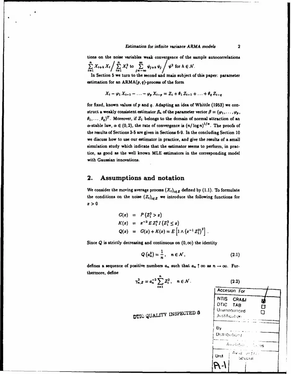
t=1 + /=f j=-00gIn Section 5 we turn to the second and main subject of this paper: parameter
estimation for an ARMA(p, q)-process of the form
Xt - V 1- I ..- o Xt-P = Zt + 61 Z-,I +... + o, z
for fixed, known values of p and q. Adapting an idea of Whittle (1953) we con-struct a weakly consistent estimator & of the parameter vector P = (j0,,. .. , oP,
0..9 ) Moreover, if Z, belongs to the domain of normal attraction of ana-stable law, a E (0,2), the rate of convergence is (n/log n)l*/. The proofs of
the results of Sections 3-5 are given in Sections 6-9. In the concluding Section 10
we discuss how to use our estimator in practice, and give the results of a small
simulation study which indicate that the estimator seems to perform, in prac-tice, as good as the well known MLE estimators in the corresponding modelwith Gaussian innovations.
2. Assumptions and notation
We consider the moving average process (Xg)tz defined by (1.1). To formulate
the conditions on the noise (Zt)t 6 _ we introduce the following functions for
s>0
C(s) = p(4>z)
K(s) = IE I (Z?<s)
Q(x) = C(s) + K(s) = E A (X- I)]V
Since Q is strictly decreasing and continuous on (0, oo) the identity
1Q (a) = -, nE A(, (2.1)n
defines a sequence of positive numbers a, such that an T oo as n -+ oo. Fur-thermore, define
7n2,z = a-2 n Z,, n E'. (2.2):--* Accesion For
NTIS CRA&IOTIC TAB 0
U1Wannoj!iced oDTIQ Ljj&ATry INSpECT J jS14cT Cf
D is v ): , i1
I -) S ______ - --'V
u~s1

Estimation for infinite variance ARMA models 3
For the moving average process as in (1.1) we introduce the following assump-
tions: There exists some d > 0 such that
(AI) EIZ lI' < o;
(A2) E I, < oo for 6=lAd;j=-oo
(A3) n/ar --o0, n--.oo, for 6=lAd;
(A4) lir limsup P (-y2,z < z) = 0.
Remarks. 1) (Al) and (A2) imply absolute a.s. convergence of the series (1.1)
for every t E Z. This is a consequence of the three-series theorem.
2) (A2) is obviously satisfied for every ARMA(p, q)-process. In this case the ikj
decrease exponentially.3) The conditions E Z2 < co, (A3) and (A4) cannot hold together, since (A3)
and the SLLN imply that 7-,z " 0 contradicting (A4).4) (A4) is a stochastic compactness condition on 7-,z. A necessary and sufficient
condition for 7y,z to be stochastically compact is
liminf K(z)/G(z) > 0.
[e.g. Mailer (1981)]. Furthermore, if iz2 is stochastically compact, then there
exists some constant c > 0 such that for all n E Nf
P(n,z < z)< cz, X>0,
[Griffin (1983)] which implies (A4).A natural class of noise variables to satisfy conditions (Al), (A3) and (A4)
is the domain of attraction of an a-stable random variable, which we denote
by DA(a). For the definition and properties of o-stable r.v.'s, their domain of
attraction and regularly and slowly varying functions see e.g. Feller (1971) or
Bingham, Goldie and Teugels (1987).
Now if Z, E DA(a) for some a E (0, 2), then Z4 E DA(a/2) and
lim G(z)/K(z) = (4- *)/a,
Then G is a regularly varying function and the norming constants in (2.2) can
be chosen as
a2 G- (n-') = inf {z;G(z) < n-}

Estimation for infinite variance ARMA models 4
i.e. G- is the generalized inverse of G. This implies that a! = n2/aL(n) where L
is a slowly varying function and y.,z d y2 for some positive &/2-stable r.v. 92.Furthermore, E JZI Id < oo for d < a. In the following lemma we summarize
these relations.
Lemma 2.1. Suppose Zi E DA(a) for some a E (0,2), then (AI), (AS) and(A4) hold for some d > 0 and a2 = n2/OL(n) where L is a slowly varying func-
tion. 0
The following notation will be used throughout the paper: For any sequence of
r.v.'s (At)SEZ and a sequence of positive constants (an),,)E we introduce
n2,~ = a-2 At2
2
I,,,A(.) = a; 2 At e-,-t ,-X E (-i_,v],
11/2
At= a-' Atl/7nA= At /(A,)
, )= h.,A(A)/ 7,A = A I e-" , A (-E ,-i.
3. Consistency of the smoothed normalized pe-
riodogram
Kliippelberg and Mikoech (1991) considered Z1 in the domain of normal attrac-tion of an a-stable r.v. (Z1 E DNA(a)), a E (0,2); this means that Zi E DA(a)with norming constants a! = n2/1 . In that case both the periodogram I,,,x (A)
and the normalized periodogram T',x(A) converge in distribution for everyA E (-i, ir. A common technique to obtain consistency is to apply some smooth-
ing operation, and for I.,x(A) this provides a consistent estimator for the nor-
malized power transfer function Io(A)I 2/0 2 .

Estimation for infinite variance ARMA models 5
Now we shall show consistency of the smoothed normalized periodogram
Ihl<_,,m
under less restrictive conditions. Here W.(k) are nonnegative weights at points
Al = A + k/n, IkI 1 m, n E M/, satisfying
m = mn--.oo, mn/n--.O, n---oo, (3.1a)
W,,(k) = W,,(-k), Jkl< m, (3.1b)
F W. (k) = 1, (3.1c)
SW,2(k) = o(1), n-. oo. (3.1d)
If A& = A + k/n 0 (-,•w,] the term n.,x (A•) in Tn,x((A) will be evaluated by
defining ln,x to have period 2r. The same convention will be used to define
O(N), A (
Theorem 3.1. Suppose (Xt),Ez satisfies (AI)-(A4) and (3.1) holds. Then
!fn,x(A) £' I,/(,X)I 2/ 2 n, - oo. 0
4. Consistency of the sample autocorrelation
function
For h E Z define
jn,x(h) = .f.,x(h)/ht2.,x
j(h) = .t(h)/02
where
n-lih
-Y.,x(h) = a;2 F, XX,+Ihlt=-1
"y(h) = F, 4,j ',+I,,.j= -00

Estimation for infinite variance ARMA models 6
Obviously, if E Z2 < co, j,,x(h) is a consistent estimator of the autocorrelation
function 5(h) of (X)tdez. One of the results of Davis and Resnick (1986) is the
following: For Z, E DNA(a), a E (0, 2), Z, symmetric
((n/log-n)/" (5..,x(h) -5(h))) h=1... -"
( (j +h) - j(j - h) - 2-(j) 5(h)) KL ) (4.1)
where Y0, Y1,Y2 .... are independent r.v.'s, Yo is positive a/2-stable and (Y)je•g
are iid standard a-stable. (4.1) implies that 5,,x(h) is weakly consistent with
limit j(h) and the rate of convergence is faster than in the finite variance cae.
Under our more general conditions (A1)-(A4) a precise result as (4.1) cannot
be expected but we prove weak consistency.
Proposition 4.1. Suppose (Xi),Cz satisfies (AI)-(A4), then
5,,x(h) -# 5(h), hEK, n--oo. 0
As shown in the appendix by replacing conditions (A3) and (A4) by a slightly
more restrictive con'1ition it is possible to obtain a.s. convergence of 5,,x(h) to5(h) along some known subsequence. In particular, this condition is satisfied
for Z1 E DA(a), a E (0, 2). Moreover, we give an example to show that a.s.
convergence need not hold in general under (A1)-(A4).
5. Parameter estimation for ARMA(p, q)
processes
We consider a causal invertible ARMA(p,q) process (X:),ez satisfying for ev-
ery t the ARMA equations
Xt - (p, Xt-I - .. -- oeF Xt-P = Zt + $I zt-I + ...- + of Zt-f
for lid (Zt)tez. Denote
jo(z) = 1-jolz-...-joPzp
O(z) = l+01z+...+eq

Estimation for infinite variance ARMA models 7
and
# = ( so 9,. . . , 1P , 0 9,. . . ,0 )T
Then in the infinite moving average representaion of our process we have that
We introduce the parameter set
C = {jE7&P+;,p;p $ O,0, #O,,p(z) and P(z) have no common zeros,
(z) O(z) 0 for zl _< 1}.
Denote by g(Q, f) the power transfer function corresponding to 6 E C; i.e.
and define
1,(8 - A n- l'A,;(6)
where the sum is taken over all Fourier frequencies
n
Clearly, as n -- oo, the sum and the integral should converge to the same limit.Suppose lo E C is the true, but unknown parameter vector. Then two natural
estimators of i0 are given by
On= argmain -7nj3) 4n. = argmnin &n(,).
Given the assumption that o',(6) - 82(0), it seems reasonable to assume,as is in fact the case, that fl - &, and that therefore the two estimators are
asymptotically equivalent. It is clear that, in practice, & is the only applicable
estimator, since the integral defining u.(f) will always have to be evaluatedby an approximating sum. Nevertheless, throughout this paper we shall give
proofs of convergence for the estimator based on q.2(0), since here the notation
is much lighter.The choice of these estimators is motivated by the fact that the functionfr g A 0
Estimation for infinite variance ARMA models 8
has its absolute minimum at 6 = $o in C. [cf. Brockwell and Davis (1991),
Proposition 10.8.1.). Moreover, by Theorem 3.1., Imx(A) can be applied to
estimate g (A, fo)/ 4'P (,0o), where 0,2 (flo) is the quantity tO2 corresponding to 0-.
For Gaussian (X,),Ez the estimator A, is closely related to least squares and
maximum likelihood estimators and it is a standard estimator for ARMA pro-
ceases with finite variance. The idea goes back to Whittle (1953), see also Dzha-
paridze (1986), Fox and Taqqu (1986) and Dahlhaus (1989). It is well-known
that in the classical case &,, is consistent and asymptotically normal [cf. Brock-
well and Davis (1991)]. We show that & is also for ARMA processes with
infinite variance a weakly consistent estimator for the true parameter vector fi0.
Theorem 5.1. Suppose (XI),6z is a causal invertible ARMA(pq) process and
conditions (AI)-(A4) hold. Then
. - 4 #o and o-.(On)-+2 (O n- oo.
Furthermore, the same limit relationships hold also for &, and &2. 0
As shown in the Appendix, it is possible to obtain a.s. convergence along
some specified subsequence under more restrictive conditions which hold e.g.
for Zi E DA(c), a E (0, 2).
For ARMA(p,q) processes with finite variance O, is asymptotically normal
with rate of convergence of order n- 1/2. An analogous result gives in our case
a rate of convergence of order (n/log n)-l/a :i.e. the convergence is considerably
faster (since a < 2).
To obtain a representation of the limit vector we restrict ourselves to sym-
metric Zi E DNA(a) for a E (0, 2) such thatft . )
t=1
where Y is a-stable.
Recall that a random variable Y is said to have a stable distribution (Y
S(o,,,6,p)) if there are parameters 0 < a < 2, a > 0, -1 <_ 1, and p real
such that its characteristic function has the form:
* exp {-a,*110 (1 - ifl(signe) tan M) + ipe} ifa 1,E ety {pf-aO (I + M~(sign 8) In 181)2+ if a =i1&

Estimation for infinite variance ARMA models 9
If P = p = 0 then Y is symmetric and we say that Y has a "symmetric a stable"
distribution, denoted by Y 4 SaS.
For later use, let C. be the constant defined by
a=I __ -a fa
Car= F(2-o)c i'fa) (5.2)
Theorem 5.2. Suppose (X,)tz ui an ARMA(p,q) process and (Z1)tEz are iid
symmetric such that (5.1) holds. Then
- ) "' Il
0)CO((On - 160) 41r W-' (AD) E YN, (
where Yo,Y 1,Y2 ,... are independent r.v.'s, Yo __ S0 2(C2/0,1,0) is positive
a12-stable, (Yt),Eg, are iid SaS with scale parameter a = C.1/, W- 1 ( io) s
the inverse ofthe matrix
W t A) 8lng(A,flo) o9 Ilng (A, flo)l T A
and, for k E X', b4 is the vector1 ;t,k 0g-' (A,i, 0)
bk e-ik (A, 00 dA.
Furthermore, (5.3) holds also with •,, replaced by On 0
The limit vector in (5.3) is the ratio of an a-stable (p + q)-dimensional vector
over a positive a/2-stable r.v. It is not difficult to see that for AR(p) processes
fin is just the formal analogue of the Yule-Walker estimates. Their weak limit
behaviour was derived by Davis and Resnick (1986) using time domain methods.
In closing we note that "more rapid than Gaussian" rates of convergence for
estimators in heavy tailed problems seems to be the norm rather than the excep-
tion. For example, Feigin and Resnick (1992, 1993) study parameter estimation
for autoregressive processes with positive, heavy tailed innovations, and obtain
rates of convergence for their estimator of the same order as ours, but with-
out the logarithmic term. Their estimators, however, are different to ours both
in spirit and detail, and involve the numerical solution of a non-trivial linear
programming problem.
Estimation for infinite variance ARMA models 10
6. Auxiliary results
We shall frequently make use of the following decomposition of the periodogram.Its proof is given in Proposition 2.1 of Klippelberg and Mikoech (1991).
Proposition 6.1. Suppose (X),)Ez is a moving average process as in (1.1) and
(A..), (A.2) are satisfied. Then
In.x(A) = Ii¢(A)I 2 In,z(A) + R.(A), -w < A <
where
Rn(A) = €(A) J.(A) Y.(-A) + O(-A) J.(-A) Yn(A) + IY.(A)I 2
Jn(A) = an-'jZtCe"tt=1
Yn(A) = an' E' 0iei'j'Un(A)j=-ooY..(•) n j•' ~(•
Uq(A) E Z e-'\' - z, e-',\. Dt~l--j1=1
The following Lemma is similar to Davis and Resnick (1986), p. 549, see alsoLemma 5.1 of Kliippelberg and Mikosch (1992).
Lemma 6.2. Suppose (Xt),ez satisfies (A1)-(A4), then
7!,x = p2 722,z(l + op(l)), n - oo.
Proof.
t=1 j=-oo 9=1 iij
="V1 + V2 •
Then the triangle inequality gives
ELY21 <a-2 n (I~dI¢',)' EIZJ Z2I -. 0
n. , (j. I 110i I) E JZI Z2 0
Estimation for infinite variance ARMA models 11
and
6/2
2 y2,ZIA</ E< 2 OJ (z z')"00
j=-,0
Lemma 6.3. Let (Z,),ez be a sequence of iid r.v. '. Then the following rda-
tions hold for n -- oo:
(a)
E Z1i2 = 0 (nO-2) (6.1a)
(b) If (A1), (AS) and (A4) hold, then
EZ1 Z2 = o(n') , (6.1b)
E 9Z2'Z 22 3 = o (n- 2 ), (6.1c)
EZ1 Z 2 Z3 Z 4 = o(n- 2) (6.1d)
(c) If (Al) and (A3) hold, then
n-h-2 p 0, h E A~o
a,, Zt Z:+h -* 0 he .s=1
Proof.
(a)
I 2
n(n -1)E 22Z 2 442(Z
(c)
E -- h 26
E a;2E Z Zt+h < a; 2 6(n - h) E IZI Z2 1- 0.t=1

Estimation for infinite variance ARMA models 12
(b) By Hblder's inequality, l •+i iel, n E Xv, thus the sequence
Sz1 ) nE÷I X is uniformly integrable.
Part (c) and (A4) imply that
n-i tn-I
~nZe na-1 Z, a;~Zi,+, 0t.
Hencen-i
C=I
This proves (6.1b). The proofs of (6.1c) and (6.1d) are similar; we only prove
(6.1d):
([n/21 - 1)(n - [n/2] - 1) IE Z1 Z2 2 3 z41
[n/21-1 n-i [n/2) ]
•_,~ ~ Z,2 +,+ 2 12 ,,+t= 1 Z+ s=n~~ 9=1 t~n/2J+1 J
[n/21-1i-
t=/1 E (~n12]+i
=1 t=[n/21+i
by (6.1c). 0
7. Proof of Theorem 3.1.
As a structural part of n,x (A) we define
,. := E W.(k)coxýC(t-s)Ikl_<m
and prove some asymptotic relations for n -- oo.
Lemma 7.1.

Estimation for infinite variance ARMA models 13
(a)
= 0(1),
(b)n IS
(C)
ctt,. =0o(n), Cgs.C. = 0(72), C,, C.. =0 (n2)
Proof. (a)
EZcs = W.(k) ECoSA(t,-S)II IklI<m t,
m W.(k) { (E ZC ,At + ( sin)At =010).
(b) ' c# -C c2 +n, and the result follows from equation (6.2) of Kliippelberg
and Mikosch (1992).
(c) Using trigonometric sum formulas we obtain
Scgs Ctr~ E W. W(k 1 ) W. (k2) ~COS Ak (t- S) CoS'\ 2 Q-r)Itd,&,l< I'J'r
< W. (k1) W. (kc2)Ik ,I 21t & r
" J+ COS Ak t sin k E C iAk, Si sin Akrt
"+ I~sinAk~tsin Ak~t ~sin AL.,s F sin~k2 r

Estimation for infinite variance ARMA models 14
+ l~ i~~cskt~nAS CBA~t 8 t
for some constant do > 0. Furthermore, there exist constants d1 , d2 , d3
such that by (a) and (b)
E •,CisCt = E C,. Cr+ di '2,+d2 EC,, C,'+ d3E .it•Jor t,s,r t t'r t,4
= E csc, +din+d2 EC,+4sE¢C2
ts,r t1, ? 9's
0 o(n2).
That the sum ct, c,. = 0 (n 2 ) follows similarly. 0
We apply Proposition 6.1. and Lemma 6.2. to T,,x and obtain
Z.,x(A) = E W.(k) ,x (Ak)JkI<m
= {,o-2 F, Wnk)l•C(Ak)l2 T.,Z(A,) (7.1)IkI_<m
+ k-2 y-,2%,Z E Wn (k) Rn (Ak) 1 (1 +I op(1)) .
Since max jk - A[ - 0 as n - oo and Ii(A)12 is uniformly continuous,IkI<M
Ikl_<mm
Thus we conclude that
E W.(k)l (A)1l2 In,Z(Ak) = (1+o(j))I4'(A)1 2 E Wn(k) I.,z(A,)
bItm Ihkl<m
= (1 + o(j))I,•(A)I 2 ( I + .(A))(7.2)
wheren
Ikl~m ,-

Estimation for infinite variance ARMA models 15
7 (A) -- 0, n 'o.
Proof. We prove E (&(A)) -- 0 as n --. oo: There exist constants d1 , d2, d3
such that
&2(A) = di c22292+d c,. c,, ,2Z.2,.n tsa
+ d3 E C'. C'1 , ZZ Z.,
and the result follows from Lemmas 6.3. and 7.1. 0In view of (7.1), (7.2) and Lemnma 7.2. it remains to prove that
.Y.,2 E W.(k) &. (,k) P 0.
By the decomposition of Proposition 6.1. and by H61der's inequality, we have
for some constant c > 0
E W. (k) Rn(A.)
~~1/212_W. • k+•,IJ.>, ,,,) W ,,.(k)IY.(,X.)2 + ": W.(,k)IY••(k)2}
I\tlam IlM
By (7.2) and Lemma 7.2.,-2•,.,2 F w.(k) JJ. (-Xk)12 = w().,z (Ak) =op(1),
1kI:5m ILhI:5
hence it suffices to show that
"',z E w.(/k)I.(,I 0 (7.3)
By the decomposition of Proposition 6.1. we have
IYn (Ak,)12 < 2 (AIL. + A2k)
where
21 2
Alk = a- e'' U., (A)It'>"

Estimation for infinite variance ARMA models 16
A2k = a.- 2 , -'•' U, (- ) .Isn
Lemma 7.3. -2
Proof. We have for some c < 00
E W.(k) Alk < (VI + V2 )
IhS-m
where
V, = a; 2 T W(k) M p, e-"b Z, Ze-e''Ill<m I91>n r=I-t
2
V2 = a- 2 M w5 (k) Pt, C-iAth'Iz (A).IkHS- I~t~
Note that
",,Z v2< :5 '', Wn(k)'f,(•)o()
By (A4), it remains to show that V1 P-, 0. We restrict ourselves to prove that
V, 1 = a; 2 W(k) ,o, -cA#l E z. e-iAjr
a;2 E W ZS e-ixAt x: 4, -' P 0Iki:m r=(n+-)A
We have for some positive c
I V 1 l I ' 2 < a ; ' E n W .( k ) I =,I1( 1 l 1,) 2 1 6 / 2
1Ikl<"= (M=-00 r=(n+I)^(I-t)

Estimation for infinite variance ARMA models 17
c aCO
n 'E lo I' f II -1t-O r=(m+i)^(i-*)
t=-Go
and an application of Markov's inequality proves V1 , - 0. O
Lemma 7.4. t-2 W,(k) A2k 0.
Proof. In view of (A4) it suffices to show that 1 Wn(k) A2k P' 0. We restrictIklhS,
ourselves to show that
v3= a 2 • w,~(k) •, e-'•' U,. A•3= a- < W-(k) It =2
IkI~n 2IJ.l<_m = X=1-1 I=n-t+l
We have for some positive c
E IV3'1/2 < a-S EL=lb 1 tl• Z,1+t= IxZtl)[
a.) Eft00
Markov's inequality proves V3 - 4 0. 0
Finally we combine Lemmas 7.3. and 7.4. which gives (7.3); this proves The-
orem 3.1. 0

Estimation for infinite variance ARMA models 18
8. Proof of Proposition 4.1.
We mimic the proof of Davis and Resnick (1986), pp. 548-550. For any h E XS[
we have
SX, Xt,+% - j(h) X,' = ji(~&-(h) Oj) Zt.. ZI-,t= =1 t=1 i~ (8.1)
+ E • v, (Oi,+ - 5(h) 0,) (Ztý_, - Z,) =:V, + V2
f=1 i
where we used the fact that Oi, (Ob+4q - 7 (h) 4') = 0. By (AI)-(A3) we obtain
for some ci > 0, i = 1,2,3,4.
E1a; 2 V,I 1 _< cn .a;26-EjO,(O~j+,&-j(h)Oi~jjl
< c 2 na n -2 0,
and
E Ia;'4 V2/1' < c a-' 10i (,.+,, - 5(h) oi)l112 Iil
< c4Gb -. 0.
By Markov's inequality this implies
< 2 (VI + V 2 ) -P* 0. (8.2)
Furthermore, by Lenma 6.2.
7.2,x = + (1+o(1))
This, (8.1), (8.2) and (A4) imply that
II n
II~l t=1 t=nt hl-/-5,,x(h) - j(h) = (n-
SE---S
t=1 t=1
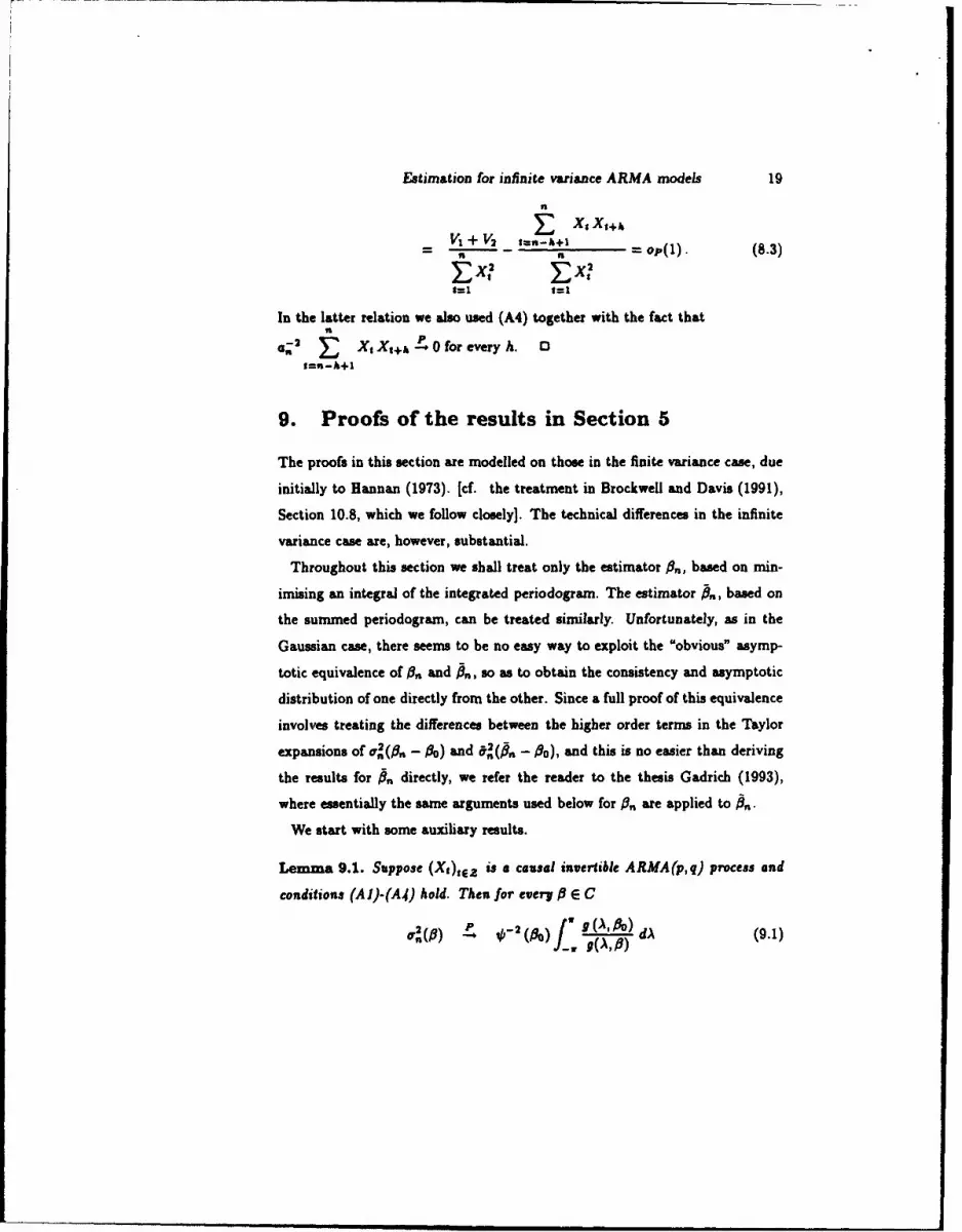
Estimation for infinite variance ARMA models 19
___+_V I=n-h+1= op(l). (8.3)
t=1 t=1
In the latter relation we also used (A4) together with the fact that
G-2 1 X,Xl+-,.P 0foreveryh. 03tn-h+1
9. Proofs of the results in Section 5
The proofs in this section are modelled on those in the finite variance case, due
initially to Hannan (1973). [cf. the treatment in Brockwell and Davis (1991),
Section 10.8, which we follow closely]. The technical differences in the infinite
variance case are, however, substantial.
Throughout this section we shall treat only the estimator fl, based on min-
imising an integral of the integrated periodogram. The estimator A, based on
the summed periodogram, can be treated similarly. Unfortunately, as in the
Gaussian case, there seems to be no easy way to exploit the "obvious" asymp-
totic equivalence of & and A., so as to obtain the consistency and asymptotic
distribution of one directly from the other. Since a full proof of this equivalence
involves treating the differences between the higher order terms in the Taylor
expansions of Ur(•f - .o) and •(•n - lo), and this is no easier than deriving
the results for & directly, we refer the reader to the thesis Gadrich (1993),
where essentially the same arguments used below for j% are applied to •.
We start with some auxiliary results.
Lemma 9.1. Suppose (Xt),Ez i a causal invertible ARMA(p,q) process and
conditions (A1)-(A4) hold. Then for every 6 E C
0,)2 2(6-2 ( pi•)0_( )

Estimation for infinite variance ARMA models 20
gnd for ewery 6 > 0
up0..(6 0-2,60)j O(A .oA)dA (9.2)
tohere 6 1 (e-'•)r 2 + 6
I,(,) = i(e..,,,)IT
and
Proof. We restrict ourselves to prove that (9.2) is satisfied. The proof of (9.1) is
analogous. We adopt the proof of Proposition 10.8.2 in Brockwell, Davis (1991).
We defineIM1 eixk k ~
qm(A,-) = E b ei k = b (- be- L -',m j=o Ikl<_J J'l<M
where
bl,= jeiAg(o- ) d.
Fix c > 0. Then there exists some m E Ar such that
q,,(,' -) - g.'(A,, )I < c/(4r)
for all (A,#) E [-w, r] x Z!. Hence
qo(f,•-) -, (-A d-%G'- ) r-/2, V,6 EV
Hence for fixed e
P, (SUi jo'p.2Sfl) _ ,k2(po)L 901AD)dA >
P up 2rII i,X(h)q (1 L)dA - h 0-2(AD)f ' 9(A, D)dAjŽ; )
m 9,(P) - 2)

Estimation for infinite variance ARMA models 21
II ,h,s5P up 2v (i-,X~a) - (h))(1_ L ) bl
+P (;up 121 Yi(h) (I jh" bt 0- 2(46a) 000 dAj >
The first summand on the rhs converges to zero in view of Proposition 4.1.
and because the bh are uniformly bounded for 0 E' and m fixed. The second
summand is zero provided m is chosen sufficiently large ( see p.379 in Brockwell,
Davis (1991)). 0
Proof of Theorem 5.1. We adapt the proof of Theorem 10.8.1 in Brockwell and
Davis (1991). We suppose that 6,, does not converge in probability to 00. We
have by Lemma 9.1. that
P(-7.2(On.) :5 t) > P(o,.(/6o) <_ t) -- P(2wO -2(/po) _< t). (9.3)
for every t. By the Helly-Bray theorem and the compactness of ? there exists a
non-random subsequence nk such that #., converges in distribution to a random
variable 6 which is different from 00 on a set of positive probability. The
functional F(f, z) = f(z) mapping C(U) x C to R is continuous where C(C) is
the space of continuous functions on U equipped with the supnorm. According
to Lemma . converges in probability to 0-2(po) f.W xl.*_., Hence
,6 is tight. Since P3, . the sequence#,,, is tight as well. Thus (o,,6,,)
is tight in C(C) x V and there exists a further subsequence (we use nk for the ease
of notation) such that (o.,,f .. ) converges in distribution. By the continuous
mapping theorem we conclude that
F(aj,,On.) = .2j ,,(fl..) d+ g(A, •)•(
Thus we have
P(o,.2,(fl.)5 _t )5 _<p(o..,j,(..)5 _t )
Estimation for infinite variance ARMA models 22
..g6( 013)
pP(O-2(1o)" (AADo) < t,o = Po) +f. 96,01) -
+P(,-,(,,o) f gA,1 0)dA <t g(A 60) dA > 2w,,606)#(A,l)fl)+P(_ 2 _lo)_. g6( Ag A
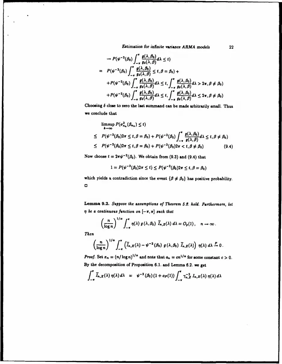
Choosing 6 close to zero the last suumnand can be made arbitrarily small. Thus
we conclude that
]im Sup p(,7.2.(6..) :5 t)
k-oo
< p(O- 2(flo)2,r < t", = po) + p(-O2 (1) wI g(A)' 3 )d, < t,,6 # A0)f -g(A, #) -
5< P(p- 2 (13o)2r <1t,# = #O) + P(-32 (0o)2r < t,0 $ P3o) (9.4)
Now choose t = 2wo- 2(,6o). We obtain from (9.3) and (9.4) that
1 = P(O- 2 (.8o)21r < t) _5 P(•,- 2(.8o)2w < t,,6 = flo)
which yields a contradiction since the event {13 #• 1o} has positive probability.
0
Lemma 9.2. Suppose the assumptions of Theorem 5.2. hold. Furthermore, let
17 be a continuous function on [-w, r] such that
log-) n Ij (.A)g(A, Po) Jn,z(A) dA = Op(l), n -# o.
Then
(12) 1cu (7nX(A) _ -2 ('60) g(,A,&3) 7nZ(A)) 17(,X) dA 0.
Proof. Set x. = (n/log n)'l* and note that a,, = cfl/° for some constant c > 0.
By the decomposition of Proposition 6.1. and Lemma 6.2. we get
j ) d ,x(IA) i7(A) dA

Estimation for infinite variance ARMA models 23
= 2- (ao) (1+ OP(1)) _".,z(A) g (A, Po) 7(A) dA
+k- (no) (1 + op(1)) R j'. P,(A) 7(A) dA
By the assumptions it suffices to show that
z j R,1(A) ,7(A) dA = op(l).
We apply Holder's inequality and obtain for some c > 0
Thus it remains to show that
z IY-(A)I dA -* 0.
We have
- 2(.\,,(12 dA <en- 2/a C-i. Z_, e-'a dA
I _<
+ [,_, f- n Z , 2- dZ e+ I n Z, - 12
d=A tl--
"" 20j e2i'j Zt •-iAt dA
=: -2/* (VI + V2 + V3 + V4).
It suffices to show that the Vi are stochastically bounded. We will show this for
V1. The other estimates are similar. Note that V, = fw, IQ(A)12 dA where
-1 0
"" -- t=(n+1 )0-j)
It uffcesto howtha th Var tochsial one.Wewl hwti

Estimation for infinite variance ARMA models 24
Let B, and B2 be two independent Brownian motions on I-v, wj and suppose
that they are independent of (Zt). Then
Ee (E.( (Q(•))dBQ(A)+ J".r(Q(())dB.(A))
~E (E , N 2)r/2
=E (E (s'N.f: Q2+mQ (EA)))2)d A) N (dA)') (Z)
E (E(e VOf:)~d
e'Ee- V.
Here N1 , N 2 are i.i.d. standard Gaussian r.v.'s independent of (Zt).
In order to show stochastic boundedness of V, it thus suffices to prove that the
real and the imaginary parts of f., Q(A)dB1 (A) are stochastically bounded. We
restrict ourselves to the real part.
We introduce the gauge function A. for any r.v. A by
A.(A) =sup t* P(JAJ > t))
Then for any sequence (a)iC", of real numbers we have for some constant c. > 0
n
a, Z < c , I* A* (Zo)i=1
[see e.g. Kliippelberg and Mikosch (1991), Lemma 3.4]. Then for fixed e > 0
-f Re (() A)e1-i2))!dB 1 ) >8)B 1))
:5C*E (E(.up sP (fz t=R+)A1-) -t \'!)B(\I,)B)

Estimation for infinite variance ARMA models 25
< c.A:(Zo) E E j , Re (e 0+j)) dB1 (A)
= c.A:(Zo) • EINj 0 I ,,Ij=-o \l=(n+1)A(^-j) /
-0
Here (Nj) is a sequence of identically distributed (but dependent) Gaussian
r.v.'s and c is a positive constant. In the last step we made use of condition
(A2). This proves the stochastic boundedness of V1 . 0
Lemma 9.3. Suppose the assumptions of Theorem 5.2. hold. Furthermore, let
ij be an odd continuous function on [-w,iw] and the Fourier coefficients 1k,
Z, of i1(A) g(A, 0o) satisfy F, IfkI' < c for some p E (0,1 Aa). Then
k=-00l
(n) 1 ]' ,x( i7(A) dA -d* 00-2 ('6) E.j 1k
where Yo, Y1, Y2,... are independent r.v. 's, Yo is positive a/2-stable and (Yt),)E
are iid symmetric a-stable with ch.f. Ee"Y = e-cI-tl', t E R.
Proof. We adapt the proof of Proposition 10.8.6 of Brockwell and Davis (1991).
In view of Lemma 9.2. it suffices to show that
zXJ Tnz(A) 170) g (A, ,o) dA --+ 4w E , A
where zn = (n/log n)1/*. Set
and
Xm(A) = f 1 e4k with fk = x(A) dA.2l<m J-

Estimation for infinite variance ARMA models 26
The assumptions on (fk) imply that uniformly in A~
k=-oo
Moreover, fo = 0. We show that for all c > 0
urn limsup P (zn PI.,z(A) (X(A) -x.(nX)) dA > e =0. (9.5)M-0n-c o J-W
For n E K and h E Z we setn-IhI
'T.,z(h) = T.,z(ihI) E I ZI Zt+Il/t z
9=1t=
and y = (n log n)i"* . Then for n > m there exists some ci > 0
VI= Xn t Tn z(X) (X(A) - x. (A)) dA
= n f'(Zn.z(h) e-1Ah F f&%
= x.~ 2v F ,~()m<IhI<n
- 2 n-i f n-h= C I I; ZY; 1 F, F, Z'S Z,+,,
Ih~m+i t= J
n-n-i n4-t
= Z c7,Y1 j E t A t)
1=1 h~m+i
n-rn-i n
= Z c Y,,2 4 Z, Z' fh-t Zh1=1 h=m+t+i
Since -f2, -+72 for some positive ck/2-stable r.v. 9for (9.5) it suffices to show
that for every C > 0
iMlim IiSUP P (IV21 > ) = 0rn-ca ncao

Estimation for infinite variance ARMA models 27
An application of Theorem 3.1 of Rosinski and Woyczynski (1987) yields for
some C2 > 01 n-nInI+lgP(JV21 > ) -5 IC2-In + log4 •
1=1 h=m+t+l
Note that for x E (0, 1),
ZO (1 + log+ )_< to
where p E (0, 1 A a). Hence for constants c2 , c3 > 0
P(I V21 > C) !5 C2 1_ : llh-,l"j
t=1 h=m+t+l
n 0< c.3-F (n - ) IftlI'< c3 E IftlI/=m~l =m+l
and, by the assumptions, the rhs converges to 0 as m -- oo. This proves (9.5).
Now it remains to show (cf. Proposition 6.3.9 in Brockwell and Davis (1991))
that
V3 = zX/_ In,(.) x,(AX) d) - 21 E hk L. (9.6)SIkI<m YO
For n > m we have
V3= nf ( j, 2 (h) ei"h ~jfk e i') dA
= Zn 21 1_ in,z(h) f,
[ ( -Ihl Z
= 21'r., If , fi, Fl, Z t+hlhl< t=
Theorem 3.3 of Davis and Resnick (1986) gives for h > 0
n-I n-h
(vi,.z, y E z'zs,+,,... " E z' z,+h) (YO,Y1,...,Yh).t=1 t----

Estimation for infinite variancc ARMA models 28
The specific scaling constants in the statement of the lernma, and in Theorem
5.2, then follow from the representation of the Y. given in Davis and Resnick
(1986) and the results of Le Page (1980).
This together with the continuous mapping theorem proves (9.6). D
Proof of Theorem 5.2. We adapt the proof of Theorem 10.8.2 of Brockwell and
Davis (1991). A Taylor expansion gives
,90.2 (#o) L90,. (fl.,) _(R. -flo) L92• 0,.20,8 - 08# 082
0,82L92 02 (#:,)S (fl. -#o) 0,82
for some 6,*, with 11,6 - ,11 < 11. - ,BoI where 11 1i denotes the Euclidean
norm. Now- -8 ('6 I) n,x(A ,62) dA
0,82 = ,82
Pand since,8* -+ #o similar arguments as in the proof of Lemmas 9.1. yield that
0,20 2i82gI- 0, 02a32" (• p •- 2 (0o) fWg (A, 0o) -92 dA.
Following the lines of the proof in Brockwell and Davis (1991) after (10.8.39)
the same arguments lead to
,9,6 p-('6) W(8o) ,
Hence it suffices to show that
8f,2 o.a(00) d 4zrO-2(#O) 0= oY, b
k=1
where bk is defined in Theorem 5.2., or, equivalently, by the Cramir-Wold device
that for all vectors c E PP+9
z. ¢C9 0u. (0o) d 4 2 (po) E kTbZ. CT41O = k b

Estimation for infinite variance ARMA models 29
We have
C9. = 2T fT_. 8,-) (A,3°) d,-
8 =: i- I.,x(A) 8()fW T.x (A I(A dA
where 17(,) = C T '0-9 0, 00)
is an odd continuous function. Furthermore, it is not difficult to see that the
Fourier coefficients of q(A)g(A,flo) satisfy the conditions of Lemma 9.3. An
application of this lemma implies that
xn f TI,x(A) q\(A) dA _. 4# 0-2(1o) L oo fJrk=1
where fk are the Fourier coefficients of ri(A) g (A, ,o); i.e.
=ý _- e-ikA T '9- (C'\,8 ) g(A,o) dA.
Thus
XnCT 84'rp-2(0) _( ') Yk 1 e iXk CT 8g- (A, g(),60)dA
C 8 4 ( 13 Yo 2 , 813=
for all c E ZP+q. This implies that
80,. (#3o) d4 1~(3) 'b
k=1
where bk is the vector
If _' e_,ik 8g0(9 ,1 o0) g(A,\,o) dA. 3
10. An application to simulated data
To get some idea of how the Whittle estimator behaves in the heavy tailed
situation, we ran a small simulation study. Before describing the results, we
make some comments about the application of the estimator.

Estimation for infinite variance ARMA models 30
As noted earlier, in application it is the estimator &,,, based on the summed
periodogram, that is used. In fact, whereas until now we worked with the self-
normalized sample periodogram Y.,X, in practice it makes more sense to work
with the regular periodogram I,,x(A) defined by
2
f.,x(A) = n- 1 Xe'A# , -V < A < T.
In this case, it is immediate from the definition of A. that it could have also
been defined as the minimiser of
&. (,) A)(-j (10.1)
where the sum, as before, is taken over all Fourier frequencies. (The difference
between &2 and 872 lies in factors of n and the normalization , X2, neither of
which affect the minimisation.)
It should be emphasised that minimisation of (10.1) requires knowledge of
neither the stability parameter a nor the scale parameter a of the data. (This,
of course, is not true if one wants to determine the convergence rate of the
estimator.) This fact has two important consequences. The first is that although
there exist methods for estimating stable exponents (e.g. Dzhaparidze (1986),
Hahn and Weiner (1991), Hsing (1991) and Koutrouvelis (1980)] none of these
have very good small sample behaviour, and so it extremely comforting to have
an estimator that is a independent.
The second consequence is that since it is well known that the Whittle esti-
mator is asymptotically equivalent to the MLE in the Gaussian case, the fact
that in the stable case the Whittle estimator is an identical function of the data
implies a robustness property for both the Whittle and maximum likelihood
estimators in the Gaussian case as well.
The following table includes the result of a small scale simulation study. We
generated 100 observations from each of the models
1. Xt-O0.4 Xtl = Zt

Estimation for infinite variance ARMA models 31
2. Xt = Zt + 0.S Zt_•
3. Xt - 0.4 X,_ l = Z, + 0.8 Z,_-,
where the innovations sequence {Z,) was either iid a-stable with a = 1.5 and
scale parameter equal to 2.0, or, for comparison purposes, N(0,2). (In the
stable case we relied on the algorithm given by Chambers, Mallows and Stuck
(1976) for generation of the innovation process.) We ran 1,000 such simulations
for each model. In the stable example we estimated the ARMA parameters via
the estimator A., and in the Gaussian case via the usual MLE estimator. The
results were as follows:
Model True Whittle estimate Maximum-likelihood
No. values mean st. dev. mean st. dev.
I V = 0.4 0.384 0.093 0.394 0.102
2 e = 0.8 0.782 0.097 0.831 0.099
3 p = 0.4 0.397 0.100 0.385 0.106
e = 0.8 0.736 0.124 0.815 0.082
TAble I0.1: Estimating the parameters of stable and normal ARMA
processes via Whittle and MLE estimates.
We shall not attempt to interpret these results for the reader, but merely
point out that the accuracy of the Whittle estimator in the stable case seems
indistinguishable from that of the MLE in the Gaussian case.
Finally, a comment about estimating p, q, a and the scale parameter of the
stable innovations. We have assumed throughout, including in the simulation
above, that p and q are known. When this is not that case, Bhansali (1984,
1988) has proposed a technique for estimating p and q that seems to work well

Estimation for infinite variance ARMA models 32
in practice. Estimation of a can be done either from the raw data, or from
the residuals calculated after parameter estimation. Limited experience with
simulations indicates that it is best done on the (supposedly lid) residuals.
Appendix
In Theorem 5.1. we proved weak convergence of the estimated coefficient vec-
tor 8, to its true value Oo. In the finite variance case this holds even almost
surely. In the infinite variance case (which is e.g. satisfied for Zi E DA(a),
a E (0, 2)) we obtain a.s. convergence under a more restrictive condition if we
take the limit along a well-specified sequence in X. We introduce the following
condition:
(AS) There exists a sequence of positive numbers e. such thatn
liminf e;- = 1 as. (AP.I)n-00
where the norming constants e. satisfy the following conditions: There ex-
ist some d > 0 and v E M such that for nk = kV, k E X, F, (nk e -21 + e;') < 0o,
for 6 = 1 A d, and (e,/e..) is bounded away from 0 and oo uniformly for
n E [nk, nk+i] for all k E K.
A survey of results of type (AP.1) can be found in Pruitt (1990, p. 1149).
Fristedt and Pruitt (1971) proved under the restriction E IZiI' < oo for some
d > 0 that (AP.1) holds with
2= log logn (AP.2).=(C log log n/n)
for some constant f > 1 where 9 (.)= (-logEe--Z2).
If Z, e DA(a) for a E (0, 2) we deduce from (AP.2) the following Lemma.
Lemmaa 1 Suppose F E DA(a), a E (0,2). Then (A5) is satisfied for d < a
and e2 = ni2/ Z(n) for some slowly varying function L. The number v in (A5)
can be chosen to satisfy v > a/( 2 6 - a) V (a/6) provided 6 > a/2. 0

Estimation for infinite variance ARMA models 33
The following result complements Proposition 4.1.
Proposition 2 Suppose (Xt),ez satisfies (Al), (AS) and (A5). Then
--.x~h "(h), hEar, n.-,oo.
Proof. We use the decomposition of (8.1) and obtain
max IVIK <2 ,max ,Vl 1P -l,(oj+,,- j(h) j))l I Z,_, Z,_•lInenhlItlt~l l=1 ,$*j
By (AI), (A2) and (A5) we obtain for all z > 0
p max lVii> e> ) <2 c, e21E max lVii'.1n..n.+ 1ci F, ne[nb il.<
k=1 k=1
&=I
for some cl, c2 > 0. A Borel-Cantelli argument yields
lir max IVIen 2 =0 a.S.k-ca n5nknf.+j)j
Now to estimate V2 set
fi = • (0j+h - "7(h) j) .
Then
n2 nV2 = Es •(z,!- _Z;) s E(zL,-Z;)i>O t=1 i<0 t=1
= V3 +V 4 .
We restrict ourselves to show that ira e-%Va = 0 a.s., the proof for e;2V4 is
similar. We haven-i n 0 a
v, = >2s, >2z._,- fs, Fz? + s Z,_ E ft > 4i>n tl--i i=n t=1 l:i<n fl-i l<i<n V=n-i-!
= 5 v- vO+ v,-vs.-

Estimation for infinite variance ARMA models 34
We restrict ourselves to show that lim e• V7 = 0 a.s., the proof for V5 , V6 and
VS is analogous. Again by (AI), (A2) and (A5) we have
lE-e2' V71" < c, e-' E Ifi, JiJ < ook=1 k=1 i>O
and a Borel-Cantelli argument yields the desired result. Similar arguments show
that
e- 2X Ie;. 2 p Z, + o(X) a.st=1 t=1
So we obtain as in (8.3) that
7..,x(h)- (,) -. o a.s. 0
A result similar to Proposition 2 for Zi E DA(p) was obtained by Bhansali
(1988). The following example shows that Proposition 2 is in general not valid
if the subsequence (nh) is replaced by (n).
Ezample. Consider the MA(1) process
X 1=Z,+OZt-i, tEXt, 101<1,
for a symmetric Z, E DNA(a) for some a E (0, 2). Then as mentioned in Sec-
tion 2 (AI)-(A4) and (AS) are satisfied where (e.) can be chosen as
en = nll/ (loglogn)( 1 -/ 2 )/.
Now consider""n-I
Z_, (Z, + 19 z_,) ( z,+ I + 9 Z4 +z,)-2=1
rn--i n--I n-I n-I
x z~z,+ E +DEZ,,Z,+I +9Ez;+ E Z,_Zt=1 t=1 t=1 2=1
z;2 +9 2 , z_, + 20F z,_2 Z,-- --=1 t=1

Estimation for infinite variance ARMA models 35
Rosinski and Woyczynski (1987) have shown that for some c > 0
P (ZIZ2 > z)<5Cz-' (l+Io09+ Z-').
Similar arguments as in the proof of Heyde's SLLN [see Stout (1974)] and the
fact that00
SP (Z Z 2 >2) <c0h-=1
imply that
n-I
e-2 E (Z Zt+l + g Z Z, _,_Z + 0 Z,_, Z,+1 )
lim =-- 0 a.s.n--00 n--
Thus
7nX(l) " 0 + o(I) a.s. (AP.3)
e2 + I + Z,/ýý Z,+o(0)
We shall show that
limsup Z2, Z2 = oo a.s. (AP.4)
n-co
Define
A_ {= Z2> en 2Il} Bn :{Z.2 < n2/a}
then for every c > 0
p zF)'~ P (An r) Bn i-o.).
Note that P (An) = oo and liminf P (Bn) > 0. Since An and {BI, B 2,..., Bn}n-0o
are independent for each n > 1, an application of a standard Borel-Cantelli
lemma [e.g. Petrov (1975), Lemma 5, Section IX.2] yields P(A, n Bn i.o.) > 0,
hence
4i
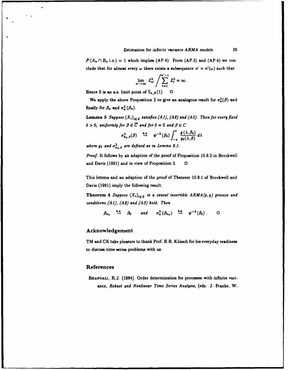
Estimation for infinite variance ARMA models 36
P(A,, n B,, i.o.) = I which implies (AP.4). From (AP.3) and (AP.4) we con-
clude that for almost every w there exists a subsequence n' = n'(w) such that
tim Z 'n 00*Z•=o.
Hence 0 is an a.s. limit point of 5n,x(1). 0
We apply the above Proposition 2 to give an analogous result for o,2(,) and
finally for ft and o'2 (f,,).
Lemma 3 Suppose (X,),tz satisfies (Al), (At) and (A5). Then for every fized
6 > 0, uniformly for 6 E Z! and for 6 = 0 andfl E C
Cob5(.) 0- 2(po) 0(~) dg.0(A,•0) d
where ga and o'2n ,6 are defined as in Lemma 9.1.
Proof. It follows by an adaption of the proof of Proposition 10.8.2 in Brockwell
and Davis (1991) and in view of Proposition 2. 0
This lemma and an adaption of the proof of Theorem 10.8.1 of Brockwell and
Davis (1991) imply the following result.
Theorem 4 Suppose (X,)tez is a causal invertible ARMA(p,q) process and
conditions (A,1), (Al) and (A5) hold. Then
--- /o and on ('.6) 0- -2('8) 0
Acknowledgement
TM and CK take pleasure to thank Prof. H.R. Kiinsch for his everyday readiness
to discuss time series problems with us.
References
BHANSALI, R.J. (1984). Order determination for processes with infinite vari-
ance, Robust and Nonlinear Time Series Analysis, (eds. J. Franke, W.

Estimation for infinite variance ARMA models 37
Hardle and D. Martin), pp. 17-25, New-York: Springer.
BHANSALI, R.J. (1988). Consistent order determination for processes with
infinite variance. J. Roy. Statist. Soc. Series B 50, 46-60.
BINGHAM, N.H., GOLDIE, C.M. AND TEUGELS, J.L (1987). Regular Varia-
tion. Cambridge University Press.
BROCKWELL, P.J. AND DAVIS, R.A. (1991). Time Series: Theory and Meth-
ods, 2nd ed., Springer, Berlin.
CHAMBERS, J.M. MALLOWS, C.L. AND STUCK, B.W. (1976). A method for
simulating stable random variables, Journal of the American Statistical
Association, 71, 340-344.
DAHLHAUS, R. (1989). Efficient parameter estimation for self-similar pro-
cesses. Ann. Statist. 17, 1749-1766.
DAVIS, R.A. AND RESNICK, S.I. (1986). Limit theory for the sample co-
variance and correlation functions of moving averages. Ann. Statist. 14,
533-558.
DZHAPARIDZE, K. (1986). Parameter Estimation and Hypothesis Testing in
Spectral Analysis of Stationay Time Series. Springer, New York.
FELLER, W. (1971). An Introduction to Probability Theory and Its Applica-
tions. Vol. II, 2nd ed., Wiley, New York.
FEIGIN, P. AND RESNICK, S. (1992). Estimation for autoregressive processes
with positive innovations. Stochastic Models 8, 479-498.
FEIGIN, P. AND RESNICK, S. (1993). Limit distributions for linear program-
ming time series estimators. Preprint.
Fox, R. AND TAQQU, M.S. (1986). Large sample properties of parameter
estimates for strongly dependent stationary Gaussian time series. Ann.
Statist. 14, 517-532.

Estimation for infinite variance ARMA models 38
FRISTEDT, B.E. AND PRUITT, W.E. (1971). Lower functions for increasing
random walks and subordinators. Z. Wahrsch. verw. Gebiete 18,167-182.
GADRICH, T. (1993). Parameter Estimation for ARMA Processes with Sym-
metric Stable Innovations, D.Sc. Thesis, Technion. (In Hebrew)
GRIFFIN, P.S. (1983). Probability estimates for the small deviations of d-di-
mensional random walk. Ann. Probab. 11, 939-952.
HANNAN, E.J. (1973). The asymptotic theory of linear time-series models, J.
Appi. Prob., 10, 130-145.
HAHN, M.G. AND WEINER, D.C. (1991). On joint estimation of an exponent
of regular variation and an asymmetry parameter for tail distributions,
in Sums, trimmed sums and eztremes. M.G. Hahn, D.M. Mason, D.C.
Weiner (Eds.) Progress in Probability, 23, Birkhauser.
HSING, T. (1991). On tail index estimation using dependent data, Ann.
Statist., 19, 1547-1569.
KOUTROUVELIS, I.A. (1980). Regression-type estimation of the parameters of
stable laws J. Amer. Stat. Assoc. 75, 918-928.
KLbPPELBERG, C. AND MIICOSCH, T. (1991). Spectral estimates and stable
processes. Stoch. Proc. Appi. (to appear).
KLUPPELBERG, C. AND MIKOSCH, T. (1992). Some limit theory for the
normalized periodogram of p-stable moving average processes. Technical
Report, Departement Mathematik, ETH Ziirich.
LE PAGE, R. (1980). Multidimensional infinitely divisible variables and pro-
cesses. Part I: Stable case. Preprint.
MALLER., R.A. (1981). Some properties of stochastic compactness. J. Austrul.
Math. Soc. (Series A) 30, 264-277.

Estimation for infinite variance ARMA models 39
PETROV, V.V. (1975). Sums of Independent Random Variables. Springer,
New York.
PRUITT, W.E. (1990). The rate of escape of random walk. Ann. Probab. 18,
1417-1461.
ROSINSKI, J. AND WOYCZYNSKI, W.A. (1987). Multilinear forms in Pareto-
like random variables and product random measures. Colloquium Mathe-
maticum, Vol. 51, 303-313.
STOUT (1974). Almost Sure Convergence. Academic Press, New York.
WHITTLE, P. (1953). Estimation and information in stationary time series.
Ark. Mat. 2, 423-434.
Claudia Kluppelberg Thomas MikoschDepartement Mathematik Institute of Statistics and Operations ResearchETH Zuirich Victoria UniversityCH - 8092 Ziirich WellingtonSWITZERLAND NEW ZEALAND
Tamar Gadrich and Robert J. AdlerFaculty of Industrial Engineering & ManagementTechnion - Israel Institute of TechnologyHaifa, 32000ISRAEL


