Embed Size (px)
Citation preview
arX
iv:1
101.
5790
v3 [
mat
h.PR
] 3
Aug
201
3
Parameter estimation for α-fractional bridges
Khalifa Es-Sebaiy∗ and Ivan Nourdin†‡
Université de Bourgogne and Université Nancy 1
Abstract: Let α, T > 0. We study the asymptotic properties of a least squares estimator for theparameter α of a fractional bridge defined as dXt = −α Xt
T−t dt + dBt, 0 6 t < T , where B is a
fractional Brownian motion of Hurst parameter H > 12 . Depending on the value of α, we prove that
we may have strong consistency or not as t → T . When we have consistency, we obtain the rate ofthis convergence as well. Also, we compare our results to the (known) case where B is replaced by astandard Brownian motion W .
It is great pleasure for us to dedicate this paper to our friend David Nualart, in celebration of his60th birthday and with all our admiration.
1 Introduction
Let W be a standard Brownian motion and let α be a non-negative real parameter. In recent years,the study of various problems related to the (so-called) α-Wiener bridge, that is, to the solution X to
X0 = 0; dXt = −αXt
T − tdt+ dWt, 0 6 t < T, (1)
has attracted interest. For a motivation and further references, we refer the reader to Barczy and Pap[2, 3], as well as Mansuy [6]. Because (1) is linear, it is immediate to solve it explicitely; one then getsthe following formula:
Xt = (T − t)α∫ t
0
(T − s)−αdWs, t ∈ [0, T ),
the integral with respect to W being a Wiener integral.An example of interesting problem related to X is the statistical estimation of α when one observes
the whole trajectory of X . A natural candidate is the maximum likelihood estimator (MLE), whichcan be easily computed for this model, due to the specific form of (1): one gets
αt = −
(∫ t
0
Xu
T − udXu
)/(∫ t
0
X2u
(T − u)2du
), t < T. (2)
In (2), the integral with respect to X must of course be understood in the Itô sense. On the otherhand, at this stage it is worth noticing that αt coincides with a least squares estimator (LSE) as well;indeed, αt (formally) minimizes
α 7→
∫ t
0
∣∣∣∣Xu + αXu
T − u
∣∣∣∣2
du.
Also, it is worth bearing in mind an alternative formula for αt, which is more easily amenable toanalysis and which is immediately shown thanks to (1):
α− αt =
(∫ t
0
Xu
T − udWu
)/(∫ t
0
X2u
(T − u)2du
). (3)
∗Institut de Mathématiques de Bourgogne, Université de Bourgogne, Dijon, France. Email:[email protected]
†Institut Élie Cartan, Université Henri Poincaré, BP 239, 54506 Vandoeuvre-lès-Nancy, France. Email:[email protected]
‡Supported in part by the (french) ANR grant ‘Exploration des Chemins Rugueux’
1
When dealing with (3) by means of a semimartingale approach, it is not very difficult to check thatαt is indeed a strongly consistent estimator of α. The next step generally consists in studying thesecond-order approximation. Let us describe what is known about this problem: as t→ T ,
• if 0 < α < 12 then
(T − t)α−12
(α− αt
) law−→ Tα− 1
2 (1 − 2α)× C(1), (4)
with C(1) the standard Cauchy distribution, see [4, Theorem 2.8];
• if α = 12 then
| log(T − t)|(α− αt
) law−→
∫ T
0WsdWs∫ T
0 W 2s ds
, (5)
see [4, Theorem 2.5];
• if α > 12 then √
| log(T − t)|(α− αt
) law−→ N (0, 2α− 1), (6)
see [4, Theorem 2.11].
Thus, we have the full picture for the asymptotic behavior of the MLE/LSE associated to α-Wienerbridges.
In the present paper, our goal is to investigate what happens when, in (1), the standard Brownianmotion W is replaced by a fractional Brownian motion B. More precisely, suppose from now on thatX = Xtt∈[0,T ) is the solution to
X0 = 0; dXt = −αXt
T − tdt+ dBt, 0 6 t < T, (7)
where B is a fractional Brownian motion with known parameter H , whereas α > 0 is considered asan unknown parameter. Although X could have been defined for all H in (0, 1), for technical reasonsand in order to keep the length of our paper within bounds we restrict ourself to the case H ∈ (12 , 1)in the sequel.
In order to estimate the unknown parameter α when the whole trajectory of X is observed, wecontinue to consider the estimator αt given by (2). (It is no longer the MLE, but it is still a LSE.)Nevertheless, there is a major difference with respect to the standard Brownian motion case. Indeed,the process X being no longer a semimartingale, in (2) one cannot utilize the Itô integral to integratewith respect to it. However, because X has§ γ-Hölder continuous paths on [0, t] for all γ ∈ (12 , H) andall t ∈ [0, T ), one can choose, instead, the Young integral (see Section 2.3 for the main properties ofthis integral, notably its chain rule (17) and how (18) relies it Skorohod integral).
Let us now describe the results we prove in the present paper. First, in Theorem 1 we show that the(strong) consistency of αt as t→ T holds true if and only if α 6
12 . Then, depending on the precise value
of α ∈ (0, 12 ], we derive the asymptotic behavior of the error αt−α. It turns out that, once adequatelyrenormalized, this error converges either in law or almost surely, to a limit that we are able to computeexplicitely. More specifically, we show in Theorem 2 the following convergences (below and throughout
the paper, C(1) always stands for the standard Cauchy distribution and β(a, b) =∫ 1
0 xa−1(1−x)b−1dx
for the usual Beta function): as t→ T ,
• if 0 < α < 1−H then
(T − t)α−H(α− αt
) law−→ Tα−H(1− 2α)
√(H − α)β(2 − 2H − α, 2H − 1)
(1−H − α)β(1 − α, 2H − 1)× C(1); (8)
§More precisely, we assume throughout the paper that we work with a suitable γ-Hölder continuous versionof X, which is easily shown to exist by the Kolmogorov-Centsov theorem.
2
• if α = 1−H then
(T − t)1−2H
√| log(T − t)|
(α− αt
) law−→ T 1−2H(2H − 1)
32
√2 β(1−H, 2H − 1)
β(H, 2H − 1)× C(1); (9)
• if 1−H < α < 12 then
(T − t)2α−1(α− αt
) a.s.−→ (1− 2α)
∫ T
0
dBu
(T − u)1−α
∫ u
0
dBs
(T − s)α
/(∫ T
0
dBs
(T − s)α
)2
; (10)
• if α = 12 then
| log(T − t)|(α− αt
) a.s.−→
1
2. (11)
When comparing the convergences (8) to (11) with those arising in the standard Brownian motioncase (that is, (4) to (6)), we observe a new and interesting phenomenom when the parameter α rangesfrom 1−H to 1
2 (of course, this case is immaterial in the standard Brownian motion case).We hope our proofs of (8) to (11) to be elementary. Indeed, except maybe the link (18) between
Young and Skorohod integrals, they only involve soft arguments, often based on the mere derivationof suitable equivalent for some integrals. In particular, unlike the classical approach (as used, e.g., in[4]) we stress that, here, we use no tool coming from the semimartingale realm.
Before to conclude this introduction, we would like to mention the recent paper [5] by Hu andNualart, which has been a valuable source of inspiration. More specifically, the authors of [5] studythe estimation of the parameter α > 0 arising in the fractional Ornstein-Uhlenbeck model, defined asdXt = −αXtdt + dBt, t > 0, where B is a fractional Brownian motion of (known) index H ∈ (12 ,
34 ).
They show the strong consistency of a least squares estimator αt as t → ∞ (with, however, a majordifference with respect to us: they are forced to use Skorohod integral rather than Young integral todefine αt, otherwise αt 6→ α as t → ∞; unfortunately, this leads to an impossible-to-simulate estima-tor, and this is why they introduce an alternative estimator for α.) They then derive the associatedrate of convergence as well, by exhibiting a central limit theorem. Their calculations are of completelydifferent nature than ours because, to achieve their goal, the authors of [5] make use of the fourthmoment theorem of Nualart and Peccati [8].
The rest of our paper is organized as follows. In Section 2 we introduce the needed material forour study, whereas Section 3 contains the precise statements and proofs of our results.
2 Basic notions for fractional Brownian motion
In this section, we briefly recall some basic facts concerning stochastic calculus with respect tofractional Brownian motion; we refer to [7] for further details. Let B = Btt∈[0,T ] be a fractionalBrownian motion with Hurst parameterH ∈ (0, 1), defined on some probability space (Ω,F , P ). (Here,and throughout the text, we do assume that F is the sigma-field generated by B.) This means thatB is a centered Gaussian process with the covariance function E[BsBt] = RH(s, t), where
RH(s, t) =1
2
(t2H + s2H − |t− s|2H
). (12)
If H = 12 , then B is a Brownian motion. From (12), one can easily see that E
[|Bt −Bs|2
]= |t− s|2H ,
so B has γ−Hölder continuous paths for any γ ∈ (0, H) thanks to the Kolmogorov-Centsov theorem.
3
2.1 Space of deterministic integrands
We denote by E the set of step R−valued functions on [0,T ]. Let H be the Hilbert space defined asthe closure of E with respect to the scalar product
⟨1[0,t],1[0,s]
⟩H = RH(t, s).
We denote by | · |H the associated norm. The mapping 1[0,t] 7→ Bt can be extended to an isometrybetween H and the Gaussian space associated with B. We denote this isometry by
ϕ 7→ B(ϕ) =
∫ T
0
ϕ(s)dBs. (13)
When H ∈ (12 , 1), it follows from [9] that the elements of H may not be functions but distributionsof negative order. It will be more convenient to work with a subspace of H which contains onlyfunctions. Such a space is the set |H| of all measurable functions ϕ on [0, T ] such that
|ϕ|2|H| := H(2H − 1)
∫ T
0
∫ T
0
|ϕ(u)||ϕ(v)||u − v|2H−2dudv <∞.
If ϕ, ψ ∈ |H| then
E[B(ϕ)B(ψ)
]= H(2H − 1)
∫ T
0
∫ T
0
ϕ(u)ψ(v)|u − v|2H−2dudv. (14)
We know that (|H|, 〈·, ·〉|H|) is a Banach space, but that (|H|, 〈·, ·〉H) is not complete (see, e.g., [9]).
We have the dense inclusions L2([0, T ]) ⊂ L1H ([0, T ]) ⊂ |H| ⊂ H.
2.2 Malliavin derivative and Skorohod integral
Let S be the set of all smooth cylindrical random variables, which can be expressed as F =f(B(φ1), . . . , B(φn)) where n > 1, f : Rn → R is a C∞-function such that f and all its derivativeshave at most polynomial growth, and φi ∈ H, i = 1, . . . , n. The Malliavin derivative of F with respectto B is the element of L2(Ω,H) defined by
DsF =
n∑
i=1
∂f
∂xi(B(φ1), . . . , B(φn))φi(s), s ∈ [0, T ].
In particular DsBt = 1[0,t](s). As usual, D1,2 denotes the closure of the set of smooth random variableswith respect to the norm
‖F‖21,2 = E[F 2] + E[|DF |2H
].
The Malliavin derivative D verifies the chain rule: if ϕ : Rn → R is C1b and if (Fi)i=1,...,n is a sequence
of elements of D1,2, then ϕ(F1, . . . , Fn) ∈ D1,2 and we have, for any s ∈ [0, T ],
Dsϕ(F1, . . . , Fn) =
n∑
i=1
∂ϕ
∂xi(F1, . . . , Fn)DsFi.
The Skorohod integral δ is the adjoint of the derivative operator D. If a random variable u ∈ L2(Ω,H)belongs to the domain of the Skorohod integral (denoted by domδ), that is, if it verifies
|E〈DF, u〉H| 6 cu√E[F 2] for any F ∈ S,
then δ(u) is defined by the duality relationship
E[Fδ(u)] = E[〈DF, u〉H
],
4
for every F ∈ D1,2. In the sequel, when t ∈ [0, T ] and u ∈ domδ, we shall sometimes write
∫ t
0 usδBs
instead of δ(u1[0,t]). If h ∈ H, notice moreover that∫ T
0hsδBs = δ(h) = B(h).
For every q > 1, let Hq be the qth Wiener chaos of B, that is, the closed linear subspace of L2(Ω)generated by the random variables Hq (B (h)) , h ∈ H, ‖h‖H = 1, where Hq is the qth Hermitepolynomial. The mapping Iq(h
⊗q) = Hq (B (h)) provides a linear isometry between the symmetrictensor product H⊙q (equipped with the modified norm ‖ · ‖H⊙q = 1√
q!‖ · ‖H⊗q) and Hq. Specifically,
for all f, g ∈ H⊙q and q > 1, one has
E[Iq(f)Iq(g)
]= q!〈f, g〉H⊗q . (15)
On the other hand, it is well-known that any random variable Z belonging to L2(Ω) admits thefollowing chaotic expansion:
Z = E[Z] +
∞∑
q=1
Iq(fq), (16)
where the series converges in L2(Ω) and the kernels fq, belonging to H⊙q, are uniquely determined byZ.
2.3 Young integral
For any γ ∈ [0, 1], we denote by C γ([0, T ]) the set of γ-Hölder continuous functions, that is, the setof functions f : [0, T ] → R such that
|f |γ := sup06s<t6T
|f(t)− f(s)|
(t− s)γ<∞.
(Notice the calligraphic difference between a space C of Hölder continuous functions, and a space Cof continuously differentiable functions!). We also set |f |∞ = supt∈[0,T ] |f(t)|, and we equip C γ([0, T ])with the norm
‖f‖γ := |f |γ + |f |∞.
Let f ∈ C γ([0, T ]), and consider the operator Tf : C1([0, T ]) → C0([0, T ]) defined as
Tf(g)(t) =
∫ t
0
f(u)g′(u)du, t ∈ [0, T ].
It can be shown (see, e.g., [10, Section 2.2]) that, for any β ∈ (1 − γ, 1), there exists a constantCγ,β,T > 0 depending only on γ, β and T such that, for any g ∈ C β([0, T ]),
∥∥∥∥∫ ·
0
f(u)g′(u)du
∥∥∥∥β
6 Cγ,β,T‖f‖γ‖g‖β.
We deduce that, for any γ ∈ (0, 1), any f ∈ C γ([0, T ]) and any β ∈ (1 − γ, 1), the linear operatorTf : C1([0, T ]) ⊂ C β([0, T ]) → C β([0, T ]), defined as Tf(g) =
∫ ·0 f(u)g
′(u)du, is continuous with
respect to the norm ‖ · ‖β. By density, it extends (in an unique way) to an operator defined on C β . Asconsequence, if f ∈ C γ([0, T ]), if g ∈ C β([0, T ]) and if γ + β > 1, then the (so-called) Young integral∫ ·0 f(u)dg(u) is (well) defined as being Tf (g).
The Young integral obeys the following chain rule. Let φ : R2 → R be a C2 function, and letf, g ∈ C γ([0, T ]) with γ > 1
2 . Then∫ ·0
∂φ∂f (f(u), g(u))df(u) and
∫ ·0
∂φ∂g (f(u), g(u))dg(u) are well-defined
as Young integrals. Moreover, for all t ∈ [0, T ],
φ(f(t), g(t)) = φ(f(0), g(0)) +
∫ t
0
∂φ
∂f(f(u), g(u))df(u) +
∫ t
0
∂φ
∂g(f(u), g(u))dg(u). (17)
5
2.4 Link between Young and Skorohod integrals
Assume H > 12 , and let u = (ut)t∈[0,T ] be a process with paths in C γ([0, T ]) for some fixed γ > 1−H .
Then, according to the previous section, the integral∫ T
0 usdBs exists pathwise in the Young sense.Suppose moreover that ut belongs to D
1,2 for all t ∈ [0, T ], and that u satisfies
P
(∫ T
0
∫ T
0
|Dsut||t− s|2H−2dsdt <∞
)= 1.
Then u ∈ domδ, and we have (see [1]), for all t ∈ [0, T ]:
∫ t
0
usdBs =
∫ t
0
usδBs +H(2H − 1)
∫ t
0
∫ t
0
Dsux|x− s|2H−2dsdx. (18)
In particular, notice that ∫ T
0
ϕsdBs =
∫ T
0
ϕsδBs = B(ϕ) (19)
when ϕ is non-random.
3 Statement and proofs of our main results
In all this section, we fix a fractional Brownian motion B of Hurst index H ∈ (12 , 1), as well asa parameter α > 0. Let us consider the solution X to (7). It is readily checked that we have thefollowing explicit expression for Xt:
Xt = (T − t)α∫ t
0
(T − s)−αdBs, t ∈ [0, T ), (20)
where the integral can be understood either in the Young sense, or in the Skorohod sense, see indeed(19).
For convenience, and because it will play an important role in the forthcoming computations, weintroduce the following two processes related to X : for t ∈ [0, T ],
ξt =
∫ t
0
(T − s)−αdBs; (21)
ηt =
∫ t
0
dBu(T − u)α−1
∫ u
0
dBs(T − s)−α =
∫ t
0
(T − u)α−1ξudBu. (22)
In particular, we observe that
Xt = (T − t)αξt and
∫ t
0
Xu
T − udBu = ηt for t ∈ [0, T ). (23)
When α is between 0 and H (resp. 1 − H and H), in Lemma 4 (resp. Lemma 5) we shall actuallyshow that the process ξ (resp. η) is well-defined on the whole interval [0, T ] (notice that we could havehad a problem at t = T ), and that it admits a continuous modification. This is why we may and willassume in the sequel, without loss of generality, that ξ (resp. η) is continuous when 0 < α < H (resp.1−H < α < H).
Recall the definition (2) of αt. By using (7) and then (23), as well as the definitions (21) and (22),we arrive to the following formula:
α− αt =
∫ t
0Xu(T − u)−1dBu∫ t
0 X2u(T − u)−2ds
=ηt∫ t
0 (T − u)2α−2ξ2udu.
6
Thus, in order to prove the convergences (8) to (11) of the introduction (that is, our main result!),
we are left to study the (joint) asymptotic behaviors of ηt and∫ t
0 (T − u)2α−2ξ2udu as t → T . The
asymptotic behavior of∫ t
0 (T − u)2α−2ξ2udu is rather easy to derive (see Lemma 9), because it looks
like a convergence à la Cesàro when α 612 . In contrast, the asymptotic behavior of ηt is more difficult
to obtain, and will depend on the relative position of α with respect to 1 − H . It is actually thecombination of Lemmas 3, 5, 6, 7, 8 that will allow to derive it for the full range of values of α.
We are now in position to prove our two main results, that we restate here as theorems forconvenience.
Theorem 1 We have αtprob.−→ α∧ 1
2 as t→ T . When α < H we have almost sure convergence as well.
As a corollary, we find that αt is a strong consistent estimator of α if and only if α 6 12 . The next
result precises the associated rate of convergence in this case.
Theorem 2 Let G ∼ N (0, 1) be independent of B, let C(1) stand for the standard Cauchy distribution,
and let β(a, b) =∫ 1
0xa−1(1− x)b−1dx denote the usual Beta function.
1. Assume α ∈ (0, 1−H). Then, as t→ T ,
(T − t)α−H(α− αt
) law−→ (1 − 2α)
√H(2H − 1)
β(2− α− 2H, 2H − 1)
1−H − α×G
ξT
law= Tα−H(1 − 2α)
√(H − α)β(2 − 2H − α, 2H − 1)
(1−H − α)β(1 − α, 2H − 1)× C(1).
2. Assume α = 1−H. Then, as t→ T ,
(T − t)1−2H
√| log(T − t)|
(α− αt
) law−→ (2H − 1)
32
√2H β(1 −H, 2H − 1)×
G
ξT
law= T 1−2H(2H − 1)
32
√2 β(1−H, 2H − 1)
β(H, 2H − 1)× C(1).
3. Assume α ∈(1−H, 12
). Then, as t→ T ,
(T − t)2α−1(α− αt
) a.s.−→
(1− 2α) ηT(ξT )2
.
4. Assume α = 12 . Then, as t→ T ,
| log(T − t)|(α− αt
) a.s.−→
1
2.
The rest of this section is devoted to the proofs of Theorems 1 and 2. Before to be in position todo so, we need to state and prove some auxiliary lemmas. In what follows we use the same symbol cfor all constants whose precise value is not important for our consideration.
Lemma 3 Let α, β ∈ (0, 1) be such that α+ β < 2H. Then, for all T > 0,
∫ T
0
ds (T − s)−β
∫ T
0
dr (T − r)−α|s− r|2H−2 =
∫ T
0
ds s−β
∫ T
0
dr r−α|s− r|2H−2 <∞.
7
Proof. By homogeneity, we first notice that
∫ T
0
ds s−β
∫ T
0
dr r−α|s− r|2H−2 = T 2H−α−β
∫ 1
0
ds s−β
∫ 1
0
dr r−α|s− r|2H−2,
so that it is not a loss of generality to assume in the proof that T = 1. If α + 1 < 2H then∫ 1/s
0r−α|1− r|2H−2dr 6 cs−2H+1+α, implying in turn
∫ 1
0
ds s−β
∫ 1
0
dr r−α|s− r|2H−2 =
∫ 1
0
ds s2H−α−β−1
∫ 1/s
0
dr r−α|1− r|2H−26 c
∫ 1
0
s−βds <∞.
If α+ 1 = 2H , then∫ 1/s
0r1−2H |1− r|2H−2dr 6 c(1 + | log s|), implying in turn
∫ 1
0
ds s−β
∫ 1
0
dr r−α|s− r|2H−2 =
∫ 1
0
ds s−β
∫ 1
0
dr r1−2H |s− r|2H−2
=
∫ 1
0
ds s−β
∫ 1/s
0
dr r1−2H |1− r|2H−26 c
∫ 1
0
s−β(1 + | log s|
)ds <∞.
Finally, if α+ 1 > 2H , then
∫ 1
0
ds s−β
∫ 1
0
dr r−α|s− r|2H−2 =
∫ 1
0
ds s2H−α−β−1
∫ 1/s
0
dr r−α|1− r|2H−2
6
∫ 1
0
s2H−α−β−1ds×
∫ ∞
0
r−α|1− r|2H−2dr <∞.
Lemma 4 Assume α ∈ (0, H). Recall the definition (21) of ξt. Then ξT := limt→T ξt exists in L2.Moreover, for all ε ∈ (0, H −α), the process ξtt∈[0,T ] admits a modification with (H −α− ε)-Höldercontinuous paths, still denoted ξ in the sequel. In particular, ξt → ξT almost surely as t→ T .
Proof. Because α < H , by Lemma 3 we have that∫ T
0 ds s−α∫ T
0 du u−α|s − u|2H−2 < ∞. For alls 6 t < T , we thus have, using (14) to get the first equality,
E[(ξt − ξs)
2]
= H(2H − 1)
∫ t
s
du(T − u)−α
∫ t
s
dv(T − v)−α|v − u|2H−2
= H(2H − 1)
∫ T−s
T−t
du u−α
∫ T−s
T−t
dv v−α|v − u|2H−2
= H(2H − 1)
∫ t−s
0
du (u+ T − t)−α
∫ t−s
0
dv (v + T − t)−α|v − u|2H−2
6 H(2H − 1)
∫ t−s
0
du u−α
∫ t−s
0
dv v−α|v − u|2H−2
= H(2H − 1)(t− s)2H−2α
∫ 1
0
du u−α
∫ 1
0
dv v−α|v − u|2H−2 = c(t− s)2H−2α.
By the Cauchy criterion, we deduce that ξT := limt→T ξt exists in L2. Moreover, because the process ξis centered and Gaussian, the Kolmogorov-Centsov theorem applies as well, thus leading to the desiredconclusion.
Lemma 5 Assume α ∈ (1 −H,H). Recall the definition (22) of ηt. Then ηT := limt→T ηt exists inL2. Moreover, there exists γ > 0 such that ηtt∈[0,T ] admits a modification with γ-Hölder continuouspaths, still denoted η in the sequel. In particular, ηt → ηT almost surely as t→ T .
8
Proof. As a first step, fix β1, β2 ∈ (1 −H,H) and let us show that there exists ε = ε(β1, β2, H) > 0and c = c(β1, β2, H) > 0 such that, for all 0 6 s 6 t 6 T ,
∫
[0,t]×[s,t]
(T − u)−β1(T − v)−β2 |u− v|2H−2dudv 6 c(t− s)ε. (24)
Indeed, we have
∫
[0,t]×[s,t]
(T − u)−β1(T − v)−β2 |u− v|2H−2dudv =
∫ T
T−t
du u−β1
∫ T−s
T−t
dv v−β2 |u− v|2H−2
=
∫ t
0
du(u+ T − t)−β1
∫ t−s
0
dv(v + T − t)−β2 |u− v|2H−26
∫ t
0
du u−β1
∫ t−s
0
dv v−β2 |u− v|2H−2
=
∫ t−s
0
du u−β1
∫ t−s
0
dv v−β2 |u− v|2H−2 +
∫ t
t−s
du u−β1
∫ t−s
0
dv v−β2(u− v)2H−2
= (t− s)2H−β1−β2
∫ 1
0
du u−β1
∫ 1
0
dv v−β2 |u− v|2H−2 +
∫ t
t−s
du u−β1−β2+2H−1
∫ (t−s)/u
0
dv v−β2(1− v)2H−2
6 c(t− s)2H−β1−β2 + c(t− s)1−β2
∫ t
t−s
du u−β1(u− t+ s)2H−2 (see Lemma 3 for the first integral and
use 1− v > 1− t−su for the second one)
6 c(t− s)2H−β1−β2
(1 +
∫ s/(t−s)
0
(w + 1)−β1w2H−2dw
)
= c(t− s)2H−β1−β2 ×
1 if β1 > 2H − 1
1 + | log(t− s)| if β1 = 2H − 1
(t− s)−2H+1+β1 if β1 < 2H − 1
6 c(t− s)ε for some ε ∈ (0, 1 ∧ (2H − β1)− β2),
hence (24) is shown.Now, let t < T . Using (18), we can write
ηt =
∫ t
0
ξu(T − u)α−1δBu +H(2H − 1)
∫ t
0
du(T − u)α−1
∫ u
0
dv(T − v)−α(u− v)2H−2. (25)
(To have the right to write (25), according to Section 2.4 we must check that: (i) u→ (T − u)α−1ξu
belongs almost surely to C γ([0, t]) for some γ > 1 − H ; (ii) ξu ∈ D1,2 for all u ∈ [0, t], and (iii)∫
[0,t]2(T − u)α−1|Dvξu| |u − v|2H−2dudv < ∞ almost surely. To keep the length of this paper within
bounds, we will do it completely here, and this will serve as a basis for the proof of the other instanceswhere a similar verification should have been made as well. The main reason why (i) to (iii) are easyto check is because we are integrating on the compact interval [0, t] with t strictly less than T .
Proof of (i). Firstly, u → (T − u)α−1 is C∞ and bounded on [0, t]. Secondly, for u, v ∈ [0, t] with,say, u < v, we have
E[(ξu − ξv)2] = H(2H − 1)
∫ v
u
dx(T − x)−α
∫ v
u
dy(T − y)−α|y − x|2H−2
6 (T − t)−2αH(2H − 1)
∫ v
u
dx
∫ v
u
dy|y − x|2H−2 = (T − t)−2α|v − u|2H .
Hence, by combining the Kolmogorov-Centsov theorem with the fact that ξ is Gaussian, we get that(almost) all the sample paths of ξ are θ-Hölderian on [0, t] for any θ ∈ (0, H). Consequently, bychoosing γ ∈ (1−H,H) (which is possible since H > 1/2), the proof of (i) is concluded.
9
Proof of (ii). This is evident, using the representation (21) of ξ as well as the fact that s →(T − s)−α
1[0,t](s) ∈ |H|, see Section 2.1.Proof of (iii). Here again, it is easy: indeed, we have Dvξu = (T − v)−α
1[0,u](v), so∫
[0,t]2(T − u)α−1|Dvξu| |u− v|2H−2dudv =
∫
[0,t]2(T − u)α−1(T − v)−α |u− v|2H−2dudv <∞.
)
Let us go back to the proof. We deduce from (25), after setting
ϕt(u, v) =1
2(T − u ∨ v)α−1(T − u ∧ v)−α
1[0,t]2(u, v),
that
ηt = I2(ϕt) +H(2H − 1)
∫ t
0
du(T − u)α−1
∫ u
0
dv(T − v)−α(u − v)2H−2.
Hence, because of (15),
E[(ηt − ηs)
2]
= 2‖ϕt − ϕs‖2H⊗2 +H2(2H − 1)2
(∫ t
s
du(T − u)α−1
∫ u
0
dv(T − v)−α(u − v)2H−2
)2
.
(26)
We have, by observing that ϕt − ϕs ∈ |H|⊙2,
‖ϕt − ϕs‖2H⊗2
= H2(2H − 1)2∫
[0,T ]4
[ϕt(u, v)− ϕs(u, v)
][ϕt(x, y)− ϕs(x, y)
]|u− x|2H−2||v − y|2H−2dudvdxdy
=1
4H2(2H − 1)2
∫
([0,t]2\[0,s]2)2(T − u ∨ v)α−1(T − x ∨ y)α−1(T − u ∧ v)−α(T − x ∧ y)−α
×|u− x|2H−2||v − y|2H−2dudvdxdy.
Taking into account the form of the domain in the previous integral and using that ϕt−ϕs is symmetric,we easily show that ‖ϕt−ϕs‖2H⊗2 is upper bounded (up to constant, and without seeking for sharpness)by a sum of integrals of the type
∫
[0,t]×[s,t]×[0,T ]2(T − u)−β1(T − v)−β2(T − x)−β3(T − y)−β4 |u− x|2H−2|v − y|2H−2dudvdxdy,
with β1, β2, β3, β4 ∈ α, 1 − α. Hence, combining Lemma 3 with (24), we deduce that there existsε > 0 small enough and c > 0 such that, for all s, t ∈ [0, T ],
‖ϕt − ϕs‖2H⊗2 6 c|t− s|ε. (27)
On the other hand, we can write, for all s 6 t < T ,∫ t
s
du(T − u)α−1
∫ u
0
dv(T − v)−α(u− v)2H−2
=
∫ T−s
T−t
du uα−1
∫ T
u
dv v−α(v − u)2H−2
=
∫ t−s
0
du(u+ T − t)α−1
∫ t
u
dv(v + T − t)−α(v − u)2H−2
6
∫ t−s
0
du uα−1
∫ T
u
dv v−α(v − u)2H−2
= (t− s)2H−1
∫ 1
0
du uα−1
∫ Tt−s
u
dv v−α(v − u)2H−2
= (t− s)2H−1
∫ 1
0
du u2H−2
∫ T(t−s)u
1
dv v−α(v − 1)2H−2. (28)
10
Let us consider three cases. Assume first that α > 2H − 1: in this case,
∫ T(t−s)u
1
v−α(v − 1)2H−2dv 6
∫ ∞
1
v−α(v − 1)2H−2dv <∞;
leading, thanks to (28), to
∫ t
s
du(T − u)α−1
∫ u
0
dv(T − v)−α(u− v)2H−26 c(t− s)2H−1.
The second case is when α = 2H − 1: we then have
∫ T(t−s)u
1
v−α(v − 1)2H−2dv 6 c(1 + | log(t− s)|+ | log u|
)
so that, by (28),
∫ t
s
du(T − u)α−1
∫ u
0
dv(T − v)−α(u− v)2H−26 c(t− s)2H−1
(1 + | log(t− s)|
).
Finally, the third case is when α < 2H − 1: in this case,
∫ T(t−s)u
1
v−α(v − 1)2H−2dv 6 c(t− s)α−2H+1uα−2H+1;
so that, by (28), ∫ t
s
du(T − u)α−1
∫ u
0
dv(T − v)−α(u− v)2H−26 c(t− s)α.
To summarize, we have shown that there exists c > 0 such that, for all s, t ∈ [0, T ],
∫ t
s
du(T − u)α−1
∫ u
0
dv(T − v)−α(u− v)2H−26 c(1 + | log(|t− s|)|1α=2H−1
)|t− s|(2H−1)∧α. (29)
By inserting (27) and (29) into (26), we finally get that there exists ε > 0 small enough and c > 0such that, for all s, t ∈ [0, T ],
E[(ηt − ηs)
2]6 c|t− s|ε.
By the Cauchy criterion, we deduce that ηT := limt→T ηt exists in L2. Moreover, because ηt − ηs −E[ηt] + E[ηs] belongs to the second Wiener chaos of B (where all the Lp norms are equivalent), theKolmogorov-Centsov theorem applies as well, thus leading to the desired conclusion.
Lemma 6 Recall the definition (22) of ηt. For any t ∈ [0, T ), we have
ηt =
∫ t
0
(T − u)α−1dBu ×
∫ t
0
(T − s)−αdBs −
∫ t
0
δBs (T − s)−α
∫ s
0
δBu (T − u)α−1
−H(2H − 1)
∫ t
0
ds (T − s)−α
∫ s
0
du (T − u)α−1(s− u)2H−2.
Proof. Fix t ∈ [0, T ). Applying the change of variable formula (17) to the right-hand side of the firstequality in (22) leads to
ηt =
∫ t
0
(T − u)α−1dBu ×
∫ t
0
(T − s)−αdBs −
∫ t
0
dBs (T − s)−α
∫ s
0
dBu (T − u)α−1. (30)
11
On the other hand, by (18) we have that
∫ t
0
dBs (T − s)−α
∫ s
0
dBu (T − u)α−1 (31)
=
∫ t
0
δBs (T − s)−α
∫ s
0
δBu (T − u)α−1 +H(2H − 1)
∫ t
0
ds(T − s)−α
∫ s
0
du(T − u)α−1(s− u)2H−2.
The desired conclusion follows. (We omit the justification of (30) and (31) because it suffices to proceedas in the proof (25).)
Lemma 7 Let β(a, b) =∫ 1
0 xa−1(1 − x)b−1dx denote the usual Beta function, let Z be any σB-
measurable random variable satisfying P (Z <∞) = 1, and let G ∼ N (0, 1) be independent of B.
1. Assume α ∈ (0, 1−H). Then, as t→ T ,
(Z, (T − t)1−H−α
∫ t
0
(T − u)α−1dBu
)law−→
(Z,
√H(2H − 1)
β(2− α− 2H, 2H − 1)
1−H − αG
).
(32)
2. Assume α = 1−H. Then, as t→ T ,(Z,
1√| log(T − t)|
∫ t
0
(T − u)−HdBu
)law−→
(Z,√2H(2H − 1)β(1 −H, 2H − 1)G
). (33)
Proof. By a standard approximation procedure, we first notice that it is not a loss of generality toassume that Z belongs to L2(Ω) (using e.g. that Z 1|Z|6n
a.s.−→ Z as n→ ∞).
1. Set N =√H(2H − 1)β(2−α−2H,2H−1)
1−H−α G. For any d > 1 and any s1, . . . , sd ∈ [0, T ), we shall
prove that(Bs1 , . . . , Bsd , (T − t)1−H−α
∫ t
0
(T − u)α−1dBu
)law−→
(Bs1 , . . . , Bsd , N
)as t→ T . (34)
Suppose for a moment that (34) has been shown, and let us proceed with the proof of (32). By thevery construction of H and by reasoning by approximation, we deduce that, for any l > 1 and anyh1, . . . , hl ∈ H with unit norms,
(B(h1), . . . , B(hl), (T − t)1−H−α
∫ t
0
(T − u)α−1dBu
)law−→
(B(h1), . . . , B(hl), N
)as t→ T .
This implies that, for any l > 1, any h1, . . . , hl ∈ H with unit norms and any integers q1, . . . , ql > 0,(Hq1(B(h1)), . . . , Hql(B(hl)), (T − t)1−H−α
∫ t
0
(T − u)α−1dBu
)
law−→
(Hq1(B(h1)), . . . , Hql(B(hl)), N
)as t→ T ,
with Hq the qth Hermite polynomial. Using now the very definition of the Wiener chaoses and byreasoning by approximation once again, we deduce that, for any l > 1, any integers q1, . . . , ql > 0 andany f1 ∈ H⊙q1 , . . . , fl ∈ H⊙ql ,(Iq1(f1), . . . , Iql(fl), (T − t)1−H−α
∫ t
0
(T − u)α−1dBu
)law−→
(Iq1 (f1), . . . , Iql(fl), N
)as t→ T .
Thus, for any random variable F ∈ L2(Ω) with a finite chaotic decomposition, we have(F, (T − t)1−H−α
∫ t
0
(T − u)α−1dBu
)law−→
(F,N
)as t→ T . (35)
12

To conclude, let us consider the chaotic decomposition (16) of Z. By applying (35) to F = E[Z] +∑nq=1 Iq(fq) and then letting n→ ∞, we finally deduce that (32) holds true.Now, let us proceed with the proof of (34). Because the left-hand side of (34) is a Gaussian vector,
to get (34) it is sufficient to check the convergence of covariance matrices. Let us first compute the
limiting variance of (T − t)1−H−α∫ t
0 (T − u)α−1dBu as t→ T . By (14), for any t ∈ [0, T ) we have
E
[((T − t)1−H−α
∫ t
0
(T − u)α−1dBu
)2]
= H(2H − 1)(T − t)2−2H−2α
∫ t
0
ds(T − s)α−1
∫ t
0
du(T − u)α−1|s− u|2H−2
= H(2H − 1)(T − t)2−2H−2α
∫ T
T−t
ds sα−1
∫ T
T−t
du uα−1|s− u|2H−2
= H(2H − 1)
∫ TT−t
1
ds sα−1
∫ TT−t
1
du uα−1|s− u|2H−2
→ H(2H − 1)
∫ ∞
1
ds sα−1
∫ ∞
1
du uα−1|s− u|2H−2 as t→ T ,
with∫ ∞
1
ds sα−1
∫ ∞
1
du uα−1|s− u|2H−2 =
∫ ∞
1
ds s2α+2H−3
∫ ∞
1/s
du uα−1|1− u|2H−2
=
∫ ∞
1
s2α+2H−3ds
∫ ∞
1
uα−1(u− 1)2H−2du+
∫ ∞
1
ds s2α+2H−3
∫ 1
1/s
du uα−1(1− u)2H−2
=β(2 − α− 2H, 2H − 1)
2(1−H − α)+
∫ 1
0
du uα−1(1− u)2H−2
∫ ∞
1/u
ds s2α+2H−3
=β(2 − α− 2H, 2H − 1)
1−H − α.
Thus,
limt→T
E
[((T − t)1−H−α
∫ t
0
(T − u)α−1dBu
)2]=H(2H − 1)
1 −H − αβ(2− α− 2H, 2H − 1).
On the other hand, by (14) we have, for any v < t < T ,
E
[Bv × (T − t)1−H−α
∫ t
0
(T − u)α−1dBu
]
= H(2H − 1)(T − t)1−H−α
∫ t
0
du (T − u)α−1
∫ v
0
ds |u− s|2H−2
= H(T − t)1−H−α
∫ t
0
(T − u)α−1(u2H−1 + sign(v − u)× |v − u|2H−1
)du
→ 0 as t→ T ,
because∫ T
0 (T − u)α−1(u2H−1 + sign(v − u)× |v − u|2H−1
)du <∞. Convergence (34) is then shown,
and (32) follows.
13
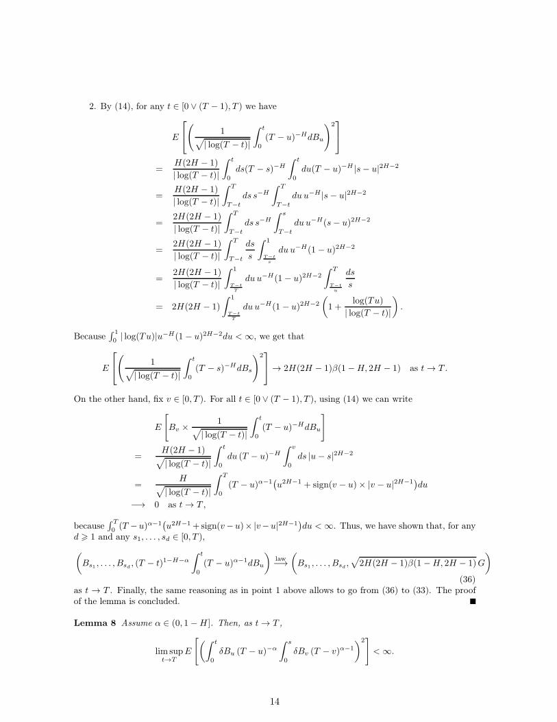
2. By (14), for any t ∈ [0 ∨ (T − 1), T ) we have
E
(
1√| log(T − t)|
∫ t
0
(T − u)−HdBu
)2
=H(2H − 1)
| log(T − t)|
∫ t
0
ds(T − s)−H
∫ t
0
du(T − u)−H |s− u|2H−2
=H(2H − 1)
| log(T − t)|
∫ T
T−t
ds s−H
∫ T
T−t
du u−H |s− u|2H−2
=2H(2H − 1)
| log(T − t)|
∫ T
T−t
ds s−H
∫ s
T−t
du u−H(s− u)2H−2
=2H(2H − 1)
| log(T − t)|
∫ T
T−t
ds
s
∫ 1
T−ts
du u−H(1− u)2H−2
=2H(2H − 1)
| log(T − t)|
∫ 1
T−tT
du u−H(1− u)2H−2
∫ T
T−tu
ds
s
= 2H(2H − 1)
∫ 1
T−tT
du u−H(1− u)2H−2
(1 +
log(Tu)
| log(T − t)|
).
Because∫ 1
0 | log(Tu)|u−H(1− u)2H−2du <∞, we get that
E
(
1√| log(T − t)|
∫ t
0
(T − s)−HdBs
)2→ 2H(2H − 1)β(1−H, 2H − 1) as t→ T .
On the other hand, fix v ∈ [0, T ). For all t ∈ [0 ∨ (T − 1), T ), using (14) we can write
E
[Bv ×
1√| log(T − t)|
∫ t
0
(T − u)−HdBu
]
=H(2H − 1)√| log(T − t)|
∫ t
0
du (T − u)−H
∫ v
0
ds |u− s|2H−2
=H√
| log(T − t)|
∫ T
0
(T − u)α−1(u2H−1 + sign(v − u)× |v − u|2H−1
)du
−→ 0 as t→ T ,
because∫ T
0 (T −u)α−1(u2H−1+sign(v−u)× |v−u|2H−1
)du <∞. Thus, we have shown that, for any
d > 1 and any s1, . . . , sd ∈ [0, T ),
(Bs1 , . . . , Bsd , (T − t)1−H−α
∫ t
0
(T − u)α−1dBu
)law−→
(Bs1 , . . . , Bsd ,
√2H(2H − 1)β(1 −H, 2H − 1)G
)
(36)as t → T . Finally, the same reasoning as in point 1 above allows to go from (36) to (33). The proofof the lemma is concluded.
Lemma 8 Assume α ∈ (0, 1−H ]. Then, as t→ T ,
lim supt→T
E
[(∫ t
0
δBu (T − u)−α
∫ s
0
δBv (T − v)α−1
)2]<∞.
14
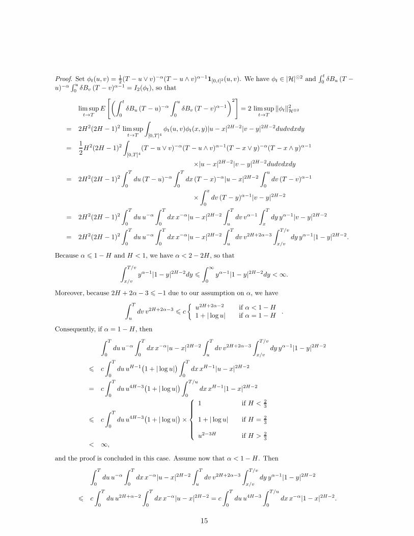
Proof. Set φt(u, v) =12 (T − u ∨ v)−α(T − u ∧ v)α−1
1[0,t]2(u, v). We have φt ∈ |H|⊙2 and∫ t
0 δBu (T −
u)−α∫ u
0 δBv (T − v)α−1 = I2(φt), so that
lim supt→T
E
[(∫ t
0
δBu (T − u)−α
∫ u
0
δBv (T − v)α−1
)2]= 2 lim sup
t→T‖φt‖
2H⊗2
= 2H2(2H − 1)2 lim supt→T
∫
[0,T ]4φt(u, v)φt(x, y)|u − x|2H−2|v − y|2H−2dudvdxdy
=1
2H2(2H − 1)2
∫
[0,T ]4(T − u ∨ v)−α(T − u ∧ v)α−1(T − x ∨ y)−α(T − x ∧ y)α−1
×|u− x|2H−2|v − y|2H−2dudvdxdy
= 2H2(2H − 1)2∫ T
0
du (T − u)−α
∫ T
0
dx (T − x)−α|u− x|2H−2
∫ u
0
dv (T − v)α−1
×
∫ x
0
dv (T − y)α−1|v − y|2H−2
= 2H2(2H − 1)2∫ T
0
du u−α
∫ T
0
dxx−α|u− x|2H−2
∫ T
u
dv vα−1
∫ T
x
dy yα−1|v − y|2H−2
= 2H2(2H − 1)2∫ T
0
du u−α
∫ T
0
dxx−α|u− x|2H−2
∫ T
u
dv v2H+2α−3
∫ T/v
x/v
dy yα−1|1− y|2H−2.
Because α 6 1−H and H < 1, we have α < 2− 2H , so that
∫ T/v
x/v
yα−1|1− y|2H−2dy 6
∫ ∞
0
yα−1|1− y|2H−2dy <∞.
Moreover, because 2H + 2α− 3 6 −1 due to our assumption on α, we have
∫ T
u
dv v2H+2α−36 c
u2H+2α−2 if α < 1−H1 + | log u| if α = 1−H
.
Consequently, if α = 1−H , then
∫ T
0
du u−α
∫ T
0
dxx−α|u− x|2H−2
∫ T
u
dv v2H+2α−3
∫ T/v
x/v
dy yα−1|1− y|2H−2
6 c
∫ T
0
du uH−1(1 + | log u|
) ∫ T
0
dxxH−1|u− x|2H−2
= c
∫ T
0
du u4H−3(1 + | log u|
) ∫ T/u
0
dxxH−1|1− x|2H−2
6 c
∫ T
0
du u4H−3(1 + | log u|
)×
1 if H < 23
1 + | log u| if H = 23
u2−3H if H > 23
< ∞,
and the proof is concluded in this case. Assume now that α < 1−H . Then
∫ T
0
du u−α
∫ T
0
dxx−α|u− x|2H−2
∫ T
u
dv v2H+2α−3
∫ T/v
x/v
dy yα−1|1− y|2H−2
6 c
∫ T
0
du u2H+α−2
∫ T
0
dxx−α|u− x|2H−2 = c
∫ T
0
du u4H−3
∫ T/u
0
dxx−α|1− x|2H−2.
15

Let us distinguish three different cases. First, if α < 2H − 1 then
∫ T
0
du u4H−3
∫ T/u
0
dxx−α|1− x|2H−26 c
∫ T
0
u2H−2+αdu <∞.
Second, if α = 2H − 1 then
∫ T
0
du u4H−3
∫ T/u
0
dxx−α|1− x|2H−2 =
∫ T
0
du u4H−3
∫ T/u
0
dxx1−2H |1− x|2H−2
6 c
∫ T
0
u4H−3(1 + | log u|
)du <∞.
Third, if α > 2H − 1 then
∫ T
0
du u4H−3
∫ T/u
0
dxx−α|1− x|2H−26
∫ T
0
u4H−3du
∫ ∞
0
x−α|1− x|2H−2dx <∞.
Thus, in all the possible cases we see that lim supt→T E
[(∫ t
0 δBu (T − u)−α∫ u
0 δBv (T − v)α−1)2]
is
finite, and the proof of the lemma is done.
Lemma 9 Assume α ∈ (0, H), and recall the definition (21) of ξt. Then, as t→ T :
1. if 0 < α < 12 , then
(T − t)1−2α
∫ t
0
ξ2s (T − s)2α−2 dsa.s.→
ξ2T1− 2α
;
2. if α = 12 , then
1
| log(T − t)|
∫ t
0
ξ2sT − s
dsa.s.→ ξ2T ;
3. if 12 < α < H, then
∫ t
0
ξ2s (T − s)2α−2 dsa.s.→
∫ T
0
ξ2s (T − s)2α−2 ds <∞.
Proof. 1. Using the(H2 − α
2
)-Hölderianity of ξ (Lemma 4), we can write
∣∣∣∣(T − t)1−2α
∫ t
0
ξ2s (T − s)2α−2 ds−ξ2T
1− 2α
∣∣∣∣
6 (T − t)1−2α
∫ t
0
∣∣ξ2s − ξ2T∣∣(T − s)2α−2 ds+ (T − t)1−2α T
2α−1
1− 2αξ2T
6 c|ξ|∞(T − t)1−2α
∫ t
0
(T − s)H2 + 3α
2 −2 ds+ (T − t)1−2α T2α−1
1− 2αξ2T
6 c|ξ|∞((T − t)
H2 −α
2 + (T − t)1−2αTH2 + 3α
2 −1)+ (T − t)1−2α T
2α−1
1− 2αξ2T
→ 0 almost surely as t → T .
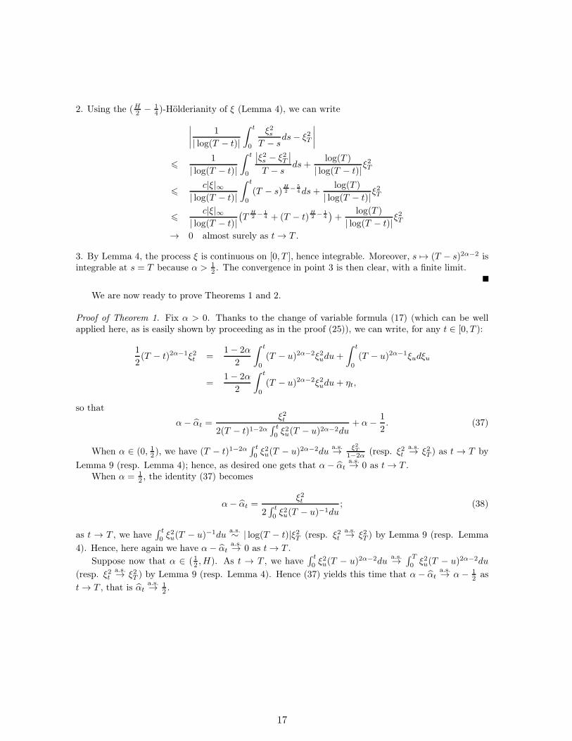
16
2. Using the (H2 − 14 )-Hölderianity of ξ (Lemma 4), we can write
∣∣∣∣1
| log(T − t)|
∫ t
0
ξ2sT − s
ds− ξ2T
∣∣∣∣
61
| log(T − t)|
∫ t
0
∣∣ξ2s − ξ2T∣∣
T − sds+
log(T )
| log(T − t)|ξ2T
6c|ξ|∞
| log(T − t)|
∫ t
0
(T − s)H2 − 5
4 ds+log(T )
| log(T − t)|ξ2T
6c|ξ|∞
| log(T − t)|
(T
H2 − 1
4 + (T − t)H2 − 1
4
)+
log(T )
| log(T − t)|ξ2T
→ 0 almost surely as t→ T .
3. By Lemma 4, the process ξ is continuous on [0, T ], hence integrable. Moreover, s 7→ (T − s)2α−2 isintegrable at s = T because α > 1
2 . The convergence in point 3 is then clear, with a finite limit.
We are now ready to prove Theorems 1 and 2.
Proof of Theorem 1. Fix α > 0. Thanks to the change of variable formula (17) (which can be wellapplied here, as is easily shown by proceeding as in the proof (25)), we can write, for any t ∈ [0, T ):
1
2(T − t)2α−1ξ2t =
1− 2α
2
∫ t
0
(T − u)2α−2ξ2udu+
∫ t
0
(T − u)2α−1ξudξu
=1− 2α
2
∫ t
0
(T − u)2α−2ξ2udu+ ηt,
so that
α− αt =ξ2t
2(T − t)1−2α∫ t
0ξ2u(T − u)2α−2du
+ α−1
2. (37)
When α ∈ (0, 12 ), we have (T − t)1−2α∫ t
0 ξ2u(T − u)2α−2du
a.s.→ ξ2T
1−2α (resp. ξ2ta.s.→ ξ2T ) as t → T by
Lemma 9 (resp. Lemma 4); hence, as desired one gets that α− αta.s.→ 0 as t→ T .
When α = 12 , the identity (37) becomes
α− αt =ξ2t
2∫ t
0ξ2u(T − u)−1du
; (38)
as t → T , we have∫ t
0ξ2u(T − u)−1du
a.s.∼ | log(T − t)|ξ2T (resp. ξ2t
a.s.→ ξ2T ) by Lemma 9 (resp. Lemma
4). Hence, here again we have α− αta.s.→ 0 as t→ T .
Suppose now that α ∈ (12 , H). As t → T , we have∫ t
0 ξ2u(T − u)2α−2du
a.s.→∫ T
0 ξ2u(T − u)2α−2du
(resp. ξ2ta.s.→ ξ2T ) by Lemma 9 (resp. Lemma 4). Hence (37) yields this time that α − αt
a.s.→ α− 1
2 as
t→ T , that is αta.s.→ 1
2 .
17
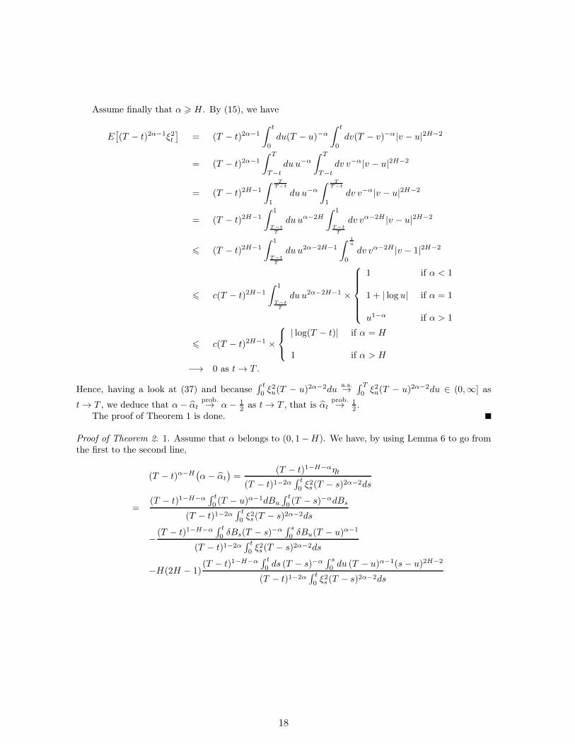
Assume finally that α > H . By (15), we have
E[(T − t)2α−1ξ2t
]= (T − t)2α−1
∫ t
0
du(T − u)−α
∫ t
0
dv(T − v)−α|v − u|2H−2
= (T − t)2α−1
∫ T
T−t
du u−α
∫ T
T−t
dv v−α|v − u|2H−2
= (T − t)2H−1
∫ TT−t
1
du u−α
∫ TT−t
1
dv v−α|v − u|2H−2
= (T − t)2H−1
∫ 1
T−tT
du uα−2H
∫ 1
T−tT
dv vα−2H |v − u|2H−2
6 (T − t)2H−1
∫ 1
T−tT
du u2α−2H−1
∫ 1u
0
dv vα−2H |v − 1|2H−2
6 c(T − t)2H−1
∫ 1
T−tT
du u2α−2H−1 ×
1 if α < 1
1 + | log u| if α = 1
u1−α if α > 1
6 c(T − t)2H−1 ×
| log(T − t)| if α = H
1 if α > H
−→ 0 as t→ T .
Hence, having a look at (37) and because∫ t
0 ξ2u(T − u)2α−2du
a.s.→∫ T
0 ξ2u(T − u)2α−2du ∈ (0,∞] as
t→ T , we deduce that α− αtprob.→ α− 1
2 as t→ T , that is αtprob.→ 1
2 .The proof of Theorem 1 is done.
Proof of Theorem 2. 1. Assume that α belongs to (0, 1−H). We have, by using Lemma 6 to go fromthe first to the second line,
(T − t)α−H(α− αt
)=
(T − t)1−H−αηt
(T − t)1−2α∫ t
0ξ2s (T − s)2α−2ds
=(T − t)1−H−α
∫ t
0 (T − u)α−1dBu
∫ t
0 (T − s)−αdBs
(T − t)1−2α∫ t
0 ξ2s (T − s)2α−2ds
−(T − t)1−H−α
∫ t
0 δBs(T − s)−α∫ s
0 δBu(T − u)α−1
(T − t)1−2α∫ t
0ξ2s (T − s)2α−2ds
−H(2H − 1)(T − t)1−H−α
∫ t
0ds (T − s)−α
∫ s
0du (T − u)α−1(s− u)2H−2
(T − t)1−2α∫ t
0ξ2s (T − s)2α−2ds
18
=1− 2α
ξT(T − t)1−H−α
∫ t
0
(T − u)α−1dBu
×
∫ t
0(T − s)−αdBs
ξT×
ξ2T
(1− 2α)(T − t)1−2α∫ t
0ξ2s (T − s)2α−2ds
−(T − t)1−H−α
∫ t
0δBs(T − s)−α
∫ s
0δBu(T − u)α−1
(T − t)1−2α∫ t
0 ξ2s (T − s)2α−2ds
−H(2H − 1)(T − t)1−H−α
∫ t
0 ds (T − s)−α∫ s
0 du (T − u)α−1(s− u)2H−2
(T − t)1−2α∫ t
0 ξ2s (T − s)2α−2ds
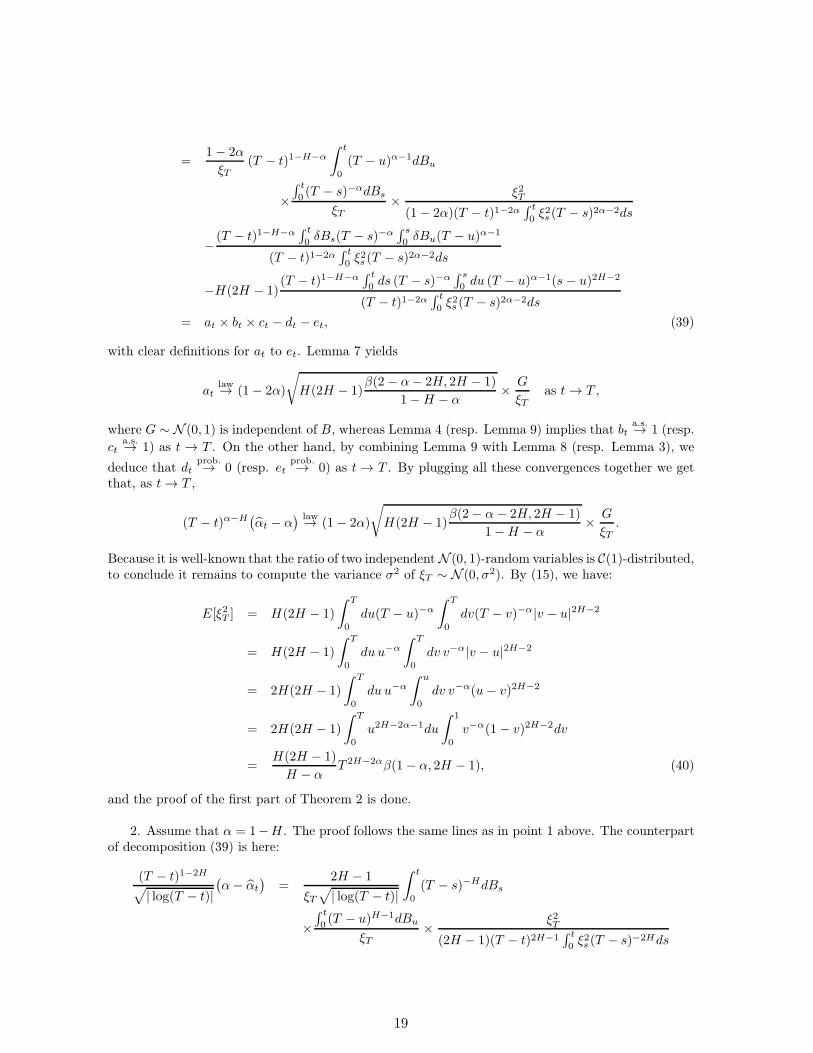
= at × bt × ct − dt − et, (39)
with clear definitions for at to et. Lemma 7 yields
atlaw→ (1− 2α)
√H(2H − 1)
β(2 − α− 2H, 2H − 1)
1−H − α×G
ξTas t → T ,
where G ∼ N (0, 1) is independent of B, whereas Lemma 4 (resp. Lemma 9) implies that bta.s.→ 1 (resp.
cta.s.→ 1) as t → T . On the other hand, by combining Lemma 9 with Lemma 8 (resp. Lemma 3), we
deduce that dtprob.→ 0 (resp. et
prob.→ 0) as t → T . By plugging all these convergences together we get
that, as t→ T ,
(T − t)α−H(αt − α
) law→ (1− 2α)
√H(2H − 1)
β(2 − α− 2H, 2H − 1)
1−H − α×G
ξT.
Because it is well-known that the ratio of two independent N (0, 1)-random variables is C(1)-distributed,to conclude it remains to compute the variance σ2 of ξT ∼ N (0, σ2). By (15), we have:
E[ξ2T ] = H(2H − 1)
∫ T
0
du(T − u)−α
∫ T
0
dv(T − v)−α|v − u|2H−2
= H(2H − 1)
∫ T
0
du u−α
∫ T
0
dv v−α|v − u|2H−2
= 2H(2H − 1)
∫ T
0
du u−α
∫ u
0
dv v−α(u− v)2H−2
= 2H(2H − 1)
∫ T
0
u2H−2α−1du
∫ 1
0
v−α(1− v)2H−2dv
=H(2H − 1)
H − αT 2H−2αβ(1− α, 2H − 1), (40)
and the proof of the first part of Theorem 2 is done.
2. Assume that α = 1−H . The proof follows the same lines as in point 1 above. The counterpartof decomposition (39) is here:
(T − t)1−2H
√| log(T − t)|
(α− αt
)=
2H − 1
ξT√| log(T − t)|
∫ t
0
(T − s)−HdBs
×
∫ t
0(T − u)H−1dBu
ξT×
ξ2T
(2H − 1)(T − t)2H−1∫ t
0ξ2s (T − s)−2Hds
19
−
∫ t
0δBs(T − s)H−1
∫ s
0δBu(T − u)−H
√| log(T − t)|(T − t)2H−1
∫ t
0ξ2s (T − s)−2Hds
−H(2H − 1)
∫ t
0 ds (T − s)H−1∫ s
0 du (T − u)−H(s− u)2H−2
√| log(T − t)|(T − t)2H−1
∫ t
0 ξ2s (T − s)−2Hds
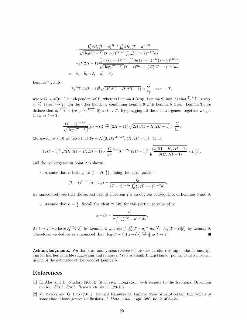
= at × bt × ct − dt − et.
Lemma 7 yields
atlaw→ (2H − 1)
32
√2H β(1−H, 2H − 1)×
G
ξTas t→ T ,
where G ∼ N (0, 1) is independent of B, whereas Lemma 4 (resp. Lemma 9) implies that bta.s.→ 1 (resp.
cta.s.→ 1) as t → T . On the other hand, by combining Lemma 9 with Lemma 8 (resp. Lemma 3), we
deduce that dtprob.→ 0 (resp. et
prob.→ 0) as t → T . By plugging all these convergences together we get
that, as t→ T ,
(T − t)1−2H
√| log(T − t)|
(αt − α
) law→ (2H − 1)
32
√2H β(1 −H, 2H − 1)×
G
ξT.
Moreover, by (40) we have that ξT ∼ N(0, HT 4H−2β(H, 2H − 1)
). Thus,
(2H − 1)32
√2H β(1−H, 2H − 1)×
G
ξT
law= T 1−2H(2H − 1)
32
√2 β(1−H, 2H − 1)
β(H, 2H − 1)× C(1),
and the convergence in point 2 is shown.
3. Assume that α belongs to (1 −H, 12 ). Using the decomposition
(T − t)2α−1(α− αt
)=
ηt
(T − t)1−2α∫ t
0ξ2u(T − u)2α−2du
,
we immediately see that the second part of Theorem 2 is an obvious consequence of Lemmas 5 and 9.
4. Assume that α = 12 . Recall the identity (38) for this particular value of α:
α− αt =ξ2t
2∫ t
0 ξ2u(T − u)−1du
.
As t → T , we have ξ2ta.s.→ ξ2T by Lemma 4, whereas
∫ t
0ξ2u(T − u)−1du
a.s.∼ | log(T − t)|ξ2T by Lemma 9.
Therefore, we deduce as announced that | log(T − t)|(α− αt
) a.s.→ 1
2 as t→ T .
Acknowledgments. We thank an anonymous referee for his/her careful reading of the manuscriptand for his/her valuable suggestions and remarks. We also thank Jingqi Han for pointing out a misprintin one of the estimates of the proof of Lemma 5.
References
[1] E. Alòs and D. Nualart (2003): Stochastic integration with respect to the fractional Brownianmotion. Stoch. Stoch. Reports 75, no. 3, 129-152.
[2] M. Barczy and G. Pap (2011): Explicit formulas for Laplace transforms of certain functionals ofsome time inhomogeneous diffusions. J. Math. Anal. Appl. 380, no. 2, 405-424.
20
[3] M. Barczy and G. Pap (2010): α-Wiener bridges: singularity of induced measures and sample pathproperties. Stoch. Anal. Appl. 28, no. 3, 447-466.
[4] M. Barczy and G. Pap (2010): Asymptotic behavior of maximum likelihood estimator for timeinhomogeneous diffusion processes. J. Statist. Plan. Infer. 140, no. 6, 1576-1593.
[5] Y. Hu and D. Nualart (2010): Parameter estimation for fractional Ornstein-Uhlenbeck processes.Statist. Probab. Lett. 80, 1030-1038.
[6] R. Mansuy (2004): On a one-parameter generalization of the Brownian bridge and associatedquadratic functionals. J. Theoret. Probab. 17, no. 4, 1021-1029.
[7] D. Nualart (2006): The Malliavin calculus and related topics. Springer-Verlag, Berlin, secondedition.
[8] D. Nualart and G. Peccati (2005). Central limit theorems for sequences of multiple stochasticintegrals. Ann. Probab. 33 (1), 177–193.
[9] V. Pipiras and M.S. Taqqu (2000): Integration questions related to fractional Brownian motionProbab. Theory Rel. Fields 118, no. 2, 251-291.
[10] F. Russo and P. Vallois (2007): Elements of stochastic calculus via regularization. Séminaire deProbabilités XL, 147-185. Lecture Notes in Math. 1899, Springer, Berlin.
21


