P1-conservative solution interpolation on unstructured triangular meshes

INTERNATIONAL JOURNAL FOR NUMERICAL METHODS IN ENGINEERINGInt. J. Numer. Meth. Engng 2000; 00:1–6 Prepared using nmeauth.cls [Version: 2002/09/18 v2.02]

P1-conservative solution interpolation on unstructured triangularmeshes

F. Alauzet1,∗ and M. Mehrenberger2

1INRIA, Projet Gamma, Domaine de Voluceau, Rocquencourt, BP 105, 78153 Le Chesnay Cedex, France.2IRMA, Universite Louis-Pasteur, UMR CNRS 7501, 7 rue Rene Descartes, 67084 Strasbourg, France.

SUMMARY

This document presents an interpolation operator on unstructured triangular meshes that verifiesthe properties of mass conservation, P1-exactness (order 2) and maximum principle. This operator isimportant for the resolution of the conservation laws in CFD by means of mesh adaptation methods asthe conservation properties is not verified throughout the computation. Indeed, the mass preservationcan be crucial for the simulation accuracy. The conservation properties is achieved by local meshintersection and quadrature formulae. Derivatives reconstruction are used to obtain an order 2 method.Algorithmically, our goal is to design a method which is robust and efficient. The robustness ismandatory to apply the operator to highly anisotropic meshes. The efficiency will permit the extensionof the method to dimension three. Several numerical examples are presented to illustrate the efficiencyof the approach. Copyright c© 2000 John Wiley & Sons, Ltd.

key words: Solution interpolation, conservative interpolation, localization algorithm, unstructured

mesh, mesh adaptation, conservation laws

1. INTRODUCTION

Solution interpolation or solution transfer is an important stage for several applications inscientific computing. For instance, it is an essential component of the Arbitrary Lagrangian-Eulerian (ALE) methods. In such a context this stage is generally named remapping orrezoning. An accurate remapping has to verify some properties such as conservation, high orderaccuracy, bound preserving, ... Numerous works have addressed such remapping strategies, seefor instance [1, 2, 3]. In these approaches, the mesh is considered with a fixed topology, i.e.,the number of vertices, elements and the connectivities remain unchanged. However, some ofthem have been extended to also handle meshes with changing topology as [4, 5].

Solution interpolation is also a key point in mesh adaptation for Eulerian simulations. Indeed,it links the mesh generation and the numerical flow solver, and it allows the simulation to be

∗Correspondence to: INRIA, Projet Gamma, Domaine de Voluceau, Rocquencourt, BP 105, 78153 Le ChesnayCedex, France.

Received 21 January 2009Copyright c© 2000 John Wiley & Sons, Ltd. Revised 18 September 2009

2 F. ALAUZET AND M. MEHRENBERGER

restarted from the previous state. More precisely, after generating a new (possibly adapted)mesh, called current mesh, the aim is to recover the previous solution field defined on the oldmesh, called background mesh on this new mesh to pursue the computation. This recurrentstage in adaptive simulations is crucial for time-dependent problems as the errors introducedby the interpolation procedure accumulate throughout the computations. The impact of sucherrors on the solution accuracy was pointed out in [6] where standard linear interpolation isapplied.

In this paper, we consider the solution interpolation in the context of anisotropically adaptedtriangular meshes where the background and the current meshes are distinct, in the sense thatthe number of entities and the connectivities are completely different. Flows are modeled bythe conservative compressible Euler equations and resolved by a second order finite volumescheme. Therefore, to obtain a consistent mesh adaptation loop, the proposed interpolationscheme must satisfy the following properties:

• mass conservation• P1 exactness implying an order 2 for the method• maximum principle.

Moreover, this method has to be algorithmically very robust as we deal with highly stretchedelements and it has to be very efficient to be extensible to 3D. The word efficient signifies thatit requires low memory storage and that the cpu time over cost with respect to the standardlinear interpolation is acceptable.

The mass conservation property of the interpolation operator is achieved by local meshintersection, i.e., intersections are performed at the element level. The use of mesh intersectionfor conservative interpolation seems natural for unconnected meshes and has already beenalluded in [7] or applied in [5] for order 1 reconstruction. The locality is primordial for theefficiency and the robustness. Once again for efficiency purposes, the proposed intersectionalgorithm is especially designed for simplicial meshes. Then, the idea is to compute theintersection between two simplexes and to mesh this intersection in order to use quadratureformulae to exactly compute the transfered mass.

The high-order accuracy is obtained by a solution gradient reconstruction from the discretedata and the use of Taylor formulae. This high-order interpolation can lead to loss ofmonotonicity. The maximum principle is then enforced by correcting the interpolated solution.Notice that much care has been taken while designing the localization algorithm as it is alsocritical for efficiency.

The proposed P1-conservative interpolation operator is suitable for solutions defined atelements or vertices.

The paper is outlined as follows. Section 2 introduces the main definitions and Section 3presents the localization algorithm. The standard linear interpolation is recalled in Section 4.Then in Section 5, the proposed P1-conservative interpolation operator is described. First, themesh intersection algorithm is given and at a second stage, P1-conservative reconstruction isdiscussed. In Section 6, we provide pseudo-conservative interpolation schemes based on high-order quadrature formulae or a Lagrangian approach. Finally, the efficiency of the proposedapproach is emphasized on analytical examples in Section 7 and adaptive numerical simulationsin Section 8. Some concluding remarks close the paper.

Copyright c© 2000 John Wiley & Sons, Ltd. Int. J. Numer. Meth. Engng 2000; 00:1–6Prepared using nmeauth.cls

P1-CONSERVATIVE SOLUTION INTERPOLATION 3

2. DEFINITIONS AND NOTATIONS

In this section, we provide the reader with notations, definitions and conventions used in thepaper. Let us consider a bounded domain Ω ∈ R2 and let ∂Ω be its boundary. We like tointroduce a triangular mesh H =

⋃Ki of domain Ω composed with triangles. A triangle in

R2 is defined by the list of its vertices which are locally numbered in a convenient way. Thislist, enriched with some conventions, provides the complete definition of the related element,including the definition of its edges and neighbors, together with an orientation. Indeed, in ourapplications we strictly require an orientation of the elements of the mesh. In particular, theoriented local numbering of the triangle vertices enables us to compute its surface area whilegiving a sense to its sign. It also enables directional normals to be evaluated for each edge.

Formally speaking, the local numbering of vertices, edges and neighboring triangles is pre-defined in such a way that some properties are implicitly induced. This definition is only aconvenient convention resulting in implicit properties. In the case of a triangle with vertices[P0, P1, P2] in this order, the first vertex having been chosen, the numbering of the others isdeduced counter-clockwise, see Figure 1 (left). This orientation provides us with positive signwhile computing the triangle surface area. Then, the topology can now be well defined thanksto the edges definition: ~e0 =

−−−→P1P2, ~e1 =

−−−→P2P0 and ~e2 =

−−−→P0P1. This numeration is such that

the index of the edge is the index of the viewing vertex, i.e., the opposite vertex. Regardingthe neighboring triangles, we denote by Ki the neighbor viewing vertex Pi through edge ~ei,see Figure 1 (left).

In the rest of the paper all the indices in square bracket are given modulo 3 : [i] = i mod(3).With all these notations, we now give some definitions utilized in all the paper algorithms.

Let K = [P0, P1, P2] be a triangle, its signed (surface) area AK is given by:

AK =12

∣∣∣∣∣∣x0 y0 1x1 y1 1x2 y2 1

∣∣∣∣∣∣ =12

∣∣∣∣ x1 − x0 x2 − x0

y1 − y0 y2 − y0

∣∣∣∣ .

P0P1

P2

!e0!e1

!e2

K0K1

K2

K

P0P1

P2

K

+ + +

! + +

!! +

! + !

+ !!

+ ! +

+ + !

Figure 1. Left, definition of a triangle K and its three neighbors Ki. Vertices indices are orderedcounter-clockwise and the entities numeration is the same as the viewing vertices. Right, the sevenregions defined by the signs of the three barycentric coordinates of a point P with respect to an element

K.



This area is positive if the triangle is numerated counter-clockwise which is our conventionon the mesh orientation. The signed area is also given by one half of the z-component of−−−→P0P1 ∧

−−−→P0P2.

Let P be a point, we denote by Ki the virtual triangle where vertex Pi is substituted by P .The signed areas AKi , for i = 0 . . . 2, are called the barycentrics of P . The three associatedbarycentric coordinates are given by:

βi =AKi

AKfor i = 0 . . . 2 .

The sign of the three barycentric coordinates or barycentrics defines explicitly seven regions ofthe plane where point P can be located with respect to element K. The possible combinationsare given in Figure 1 (right).

Finally, we introduce a definition of the distance of a point P with respect to an edge of atriangle K = [P0, P1, P2]. The signed distance, also called power, of point P with respectto edge ~ei =

−−−−−−−−→P[i+1] P[i+2], for i = 0 . . . 2, is given by:

P(P,~ei) =−−−−→P[i+1]P .

−→N ei

=−−−−→P[i+2]P .

−→N ei

,

where−→N ei

is the inward unit normal (for the element) of edge ~ei. Notice that the barycentricsand the powers are linked by the relation:

AKi =12||~ei|| P(P,~ei) .

From these relations, we deduce the coordinates of the orthogonal projection X of P on theline defined by edge ~ei =

−−−−−−−−→P[i+1] P[i+2]:

X = P[i+1] +~ei .−−−−→P[i+1]P

‖~ei ‖2~ei = P[i+2] +

~ei .−−−−→P[i+2]P

‖~ei ‖2~ei .

Finally, we recall some definitions relative to the interpolation schemes. Let u be a solutiondefined on a mesh H1 of a domain Ω. The mass of the solution over the mesh is simplym =

∫H1 u. We deduce the notion of mass on an element K given by mK =

∫Ku.

An interpolation scheme is said to be conservative if it preserves the mass when transferringthe solution field u from a mesh H1 to another H2. Formally speaking, if we denote by Πu theinterpolated field on H2, then such scheme verifies∫

H1u =

∫H2

Πu .

A scheme is said to be Pk-exact if it is exact for polynomial solutions of degree lower thanor equal to k. Finally, a Pk-conservative interpolation scheme is a scheme satisfying bothproperties.

3. LOCALIZATION ALGORITHM

The localization problem or research of point location consists in identifying the element ofa simplicial mesh containing a given point. The localization of a given point in a mesh is a



frequent issue that arises in various situations. As regards interpolation methods, we initiallyhave a mesh with a field, here the solution, that we call background mesh, denoted Hback.We aim at transferring or interpolating the field onto another mesh called current mesh ornew mesh, denoted Hnew. Therefore, the algorithm consists in finding which elements of thebackground mesh contain the vertices of the new mesh in order to apply an interpolationscheme.

Here, we consider the simplified problem where the background and the new meshes arediscretizations of the same domain Ω. This problem has to be dealt with care in the case ofsimplicial meshes to handle difficult configurations. Indeed, background and current meshescan be non-convex and can contain holes. It is also possible that the overlapping of the currentmesh does not coincide with the background mesh since their boundary discretization candiffer. Consequently, some vertices of the current mesh can be outside of the background meshand conversely. Moreover, efficient localization algorithms have to be implemented to avoidthe naive quadratic scheme in O(Nnew

ver ×N backtri ) where Nnew

ver is the number of vertices of Hnewand N back

tri the number of triangles of Hback.

The localization can be solved efficiently by traversing the background mesh using itstopology, i.e., the neighboring elements of each element, thanks to a barycentric coordinates-based algorithm [8, 9]. More precisely, in two dimensions, let P be a vertex of the new mesh,K = [P0, P1, P2] a triangle of the background mesh. From the signs of the three barycentriccoordinates βii=0,2, three possible cases arise (see Figure 2):

• all barycentric coordinates are positive then vertex P is located inside element K• one barycentric coordinate is negative then it indicates the direction for the next move.

For instance, if barycentric βi is negative then we move to neighboring element Ki sharingedge ~ei with K. We say that P is viewed by edge ~ei

• two barycentric coordinates are negative then two neighboring triangles are possible forthe next move. A random choice or a geometric one is used.

Starting from an initial element K0 of the background mesh, we apply the previous test.According to the signs of the barycentric coordinates, we pass through the correspondingneighbor of K0 and we repeat this process until the three barycentric coordinates are positivemeaning that the visited triangle contains P . With this algorithm, we follow a path in thebackground mesh to locate vertex P as shown in Figure 3 (left). This algorithm complexity isin O(n×Nnew

ver ) where n is the average number of visited triangles for each path.

P0 P1

P2

K

P+ + +

P0P1

P2

K

! + +P

K0

P0

P1

P2

K

P ! + !

K0

K2

Figure 2. Illustration of the three possible cases depending on the signs of the three barycentriccoordinates of vertex P with respect to triangle K when moving inside the background mesh.



However, cyclic or closed paths can occur. The element containing the vertex is missed andan infinite loop is obtained. In this case, the path leads us to an already tested element, aspresented in Figure 3 (right). In this academic example, starting from K0, triangles K1, K2,K3, K4 and K5 are visited bringing us back to K0. A color algorithm, to mark already visitedelements, is used to avoid this problem allowing us to choose another direction when severalchoices reoccur. Another way to solve this problem is to consider a random choice when severalpossibilities occur.

Another difficulty arises when the path is stuck by the geometry of domain Ω. Startingelement K0 and vertex P are separated by a hole (Figure 4, left) or by a non-convex domain(Figure 4, right). The path demands to pass through the hole or the boundary to reach theelement containing vertex P . A simple, but inefficient, way to remedy this problem is to makean exhaustive search, i.e., for such a vertex all elements of the background mesh are tested.Besides, a more challenging solution is to follow a path on the boundary in order to bypassthe obstacle.

K0

P

K5

K4

K3

K2

K1

K0

P

Figure 3. Left, a possible path to locate the vertex P of the new mesh starting from the triangle K0 ofthe background mesh. Right, cyclic path leading us to an already checked element. Starting from K0,

triangles K1, K2, K3, K4 and K5 are visited bringing us back to K0.

K0

P

K0

P

Figure 4. Starting element K0 and vertex P are separated by a hole (left) or the non-convex domain(right). The path demands to pass through the hole or the boundary to reach the element containing

vertex P .



Localization coupled with a grid structure. The previous algorithm can be very timeconsuming if a large number of elements (e.g. n is large) needs to be visited between triangleK0 and the solution triangle. This can result in a large number of area computations. Thismajor drawback leads us to consider a more local approach which aims at combining thealgorithm with a grid structure (a tree-like structure can be considered). This facilitates andspeeds up the localization process. A grid enclosing the mesh is constructed and, for each gridcell, one element of the background mesh located in it, if any, is recorded. Then, to locatea new vertex in the background mesh, the cell containing the vertex is first identified andthen the localization scheme starts from the element associated with this cell. In this way, thenumber of visited triangles is reduced and the number of necessary computations decreasesas well. In the case where we are stuck by the boundary, because of a hole or a non-convexdomain, the grid structure helps us to bypass the obstacle. Indeed, elements associated withgrid neighboring cells of the current one are considered as new initial guesses for the searchingalgorithm. The localization is restarted from one of these new elements.

Remark 3.1. Note that the grid (or the tree-like structure) could be defined in various waysdepending on the nature of the data set. In this respect, for a grid, the number of cells and thusthe occupation of the cells are parameters that clearly affect the efficiency of the whole process.

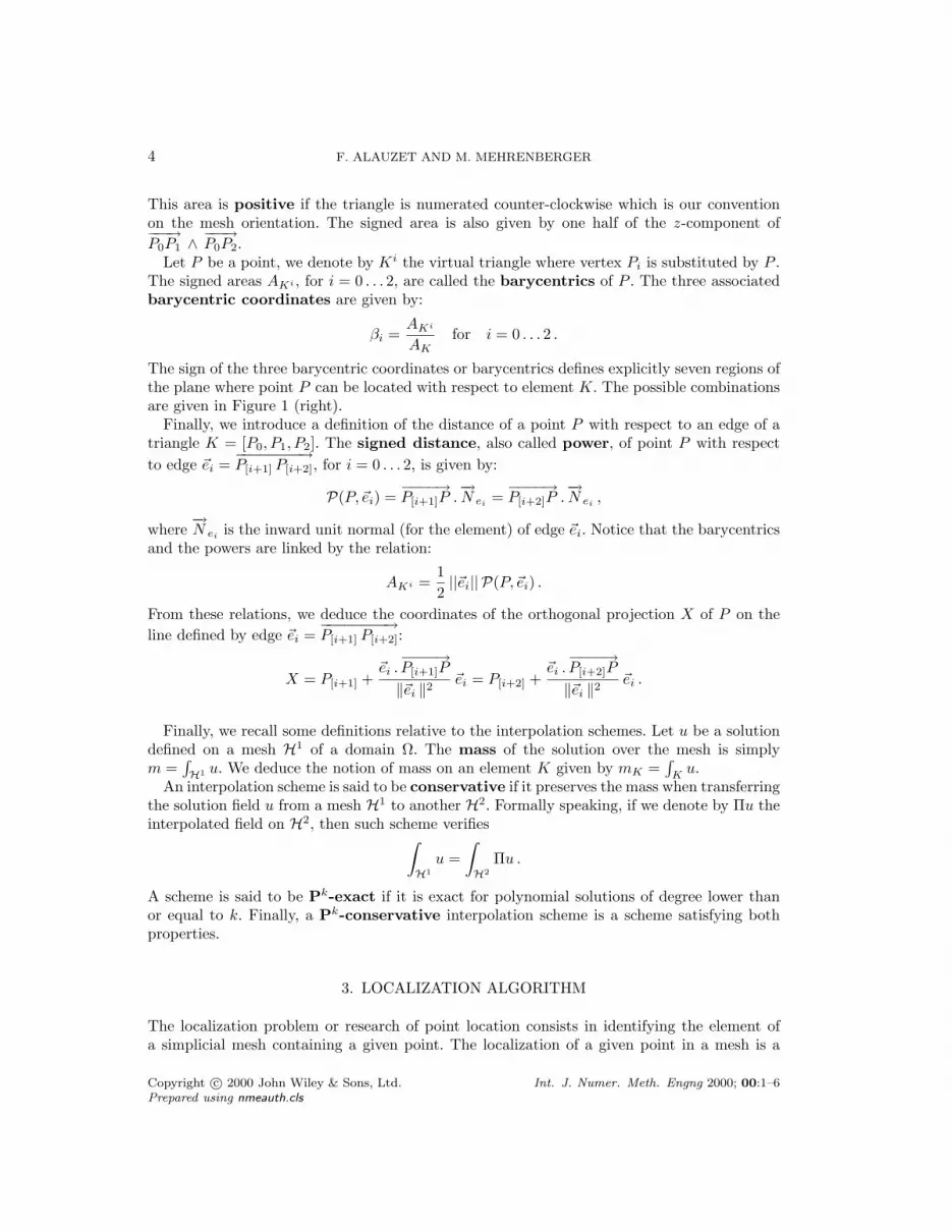
Localization using the topology of both meshes. We can even improve the locality ofthe localization scheme by using the topology of both meshes. Such scheme tends to minimize nthe number of elements visited when locating new vertices. Instead of determining the locationof the new vertices in their data (or storage) order, the idea is that once a vertex P has beenlocated in a background element K, then we handle the set of vertices Qii=1,m of the ball ofP , i.e., the set of vertices that are connected to P by an edge. For the vertices Qii=1,m, weset as starting element of the localization process the triangle K that contains P , see Figure 5.Consequently, the number of visited triangles is drastically reduced as in this algorithm theinitial guess of the searching process is at the element (or connectivity) level. Moreover, withthis approach, the scheme does not depend on any parameters.

Another advantage of this approach is that this scheme avoids the problem where the processis stuck by a hole or a non-convex boundary as vertices Qii=1,m are connected to P in thenew mesh. This algorithm is also in O(n × Nnew

ver ) where n is the average number of visitedtriangles and here n tends to be optimal. Indeed, in practice the number of visited triangles ison average less than 3. In fact n is of the order of the number of elements of the backgroundmesh that are overlapped by an element of the current mesh.

Handling the ”fork” problem. We assume that vertex P is inside the backgrounddiscretized domain. When the path reaches a geometrical fork or a crossroads with multiplechoices for the next move, the presented algorithm could make the wrong choice and ask toprocess in the wrong direction, see Figure 6. Then, we are no more able to locate vertex P aswe are stuck by the boundary. Special treatment has to be considered to solve this problem.To this end, we require to have for each boundary edge:

• the list of its two neighboring boundary edges• the unique triangle sharing this edge. This element will be used as initial element guess

to localize P .



P Q0

Q1

Q2

Q3

Q4

Q5

K

Figure 5. Reducing the number of visited triangles in the localization scheme by using the topology ofboth meshes. Vertex P has been located in element K. Then, the set of vertices Qii=1,m connected

to P uses element K as initial guess for the localization scheme.

When the ”fork” problem occurs, the algorithm is stuck in an element Kstuck for which Pis seen by a boundary edge e. To localize vertex P , an iterative algorithm is considered. Itconsists in applying the localization process starting each time from a new triangle given by aboundary edge neighboring the current one to which we are stuck, this until vertex P is found.More precisely, at the first step, we consider as initial guess for the localization algorithmthe triangles denoted Kstep1 associated with the two boundary edges neighbors of e, i.e., theneighboring edges of order 1 of the current edge, see Figure 6 (right). If P is not found, thenwe consider the neighboring edges of order 2, the neighboring edges of the neighboring edges.We start from the elements denoted Kstep2. If P is still not located, then we consider the nextorder of neighbors and so on until convergence of the algorithm. Notice that in two dimensions,at each new iteration, only two new edges are considered, since the other ones have alreadybeen checked. At worst all boundary edges are checked.

Figure 6, right, illustrates this algorithm. The localization process bring us to Kstuck. Weapply the localization process starting from the two triangles denoted Kstep1 and we are stillblocked. Then, we consider Kstep2. If the algorithm still fails, we consider Kstep3 and P islocalized.

Handling boundary problems. However, none of these algorithms are able to handlethe case of vertices localized outside of the background discretized domain. Special treatmentfor this kind of vertices must be designed. We consider the simplified problem where thebackground and the new meshes are discretizations of the same domain Ω, when a vertex isoutside of the background mesh its distance to the mesh is of the order of the boundary meshtolerance (i.e., the gap between the boundary discretization and the exact geometry). Thiswill be used to set the tolerance ε to say if P is close or not to the boundary.

In this case, the aim is to find the ”closest” triangle to vertex P which is the unique triangleassociated with the ”closest” boundary edge to vertex P . A boundary edge is considered asthe closest boundary edge if two properties are verified :

(i) the power of vertex P with respect to the boundary edge e is lower than the giventhreshold ε:

P(P, e) < ε,



K0

P

e

Kstuck

K0

P

Kstep1

Kstep1

Kstep2

Kstep3

Kstep4

Kstuck

e

Figure 6. Two illustrations of the ”fork” problem when the algorithm has made the wrong choice. Weare stuck in triangle Kstuck where P is viewed by boundary edge e. The figure on the right illustratesthe process to remedy this problem by restarting the localization from new triangles. At first step, we

choose triangles Kstep1 as initial guess. Then, Kstep2 if P has not been found. And so on.

(ii) the orthogonal projection X of P on the line defined by e lies inside the edge e = [Q0, Q1],mathematically speaking:

0 < ~e.−−→Q0P < ‖~e‖2.

The meaning of each condition is exemplified in Figure 7. The condition (i) is not verified onthe left, whereas the condition (ii) is not fulfilled on the right.

Practically, we have no warranty that the localization scheme finds directly the correctboundary edge. If the scheme does not succeed then we apply the same algorithm as in the”fork” problem. The localization process restarts each time from a new triangle given by aboundary edge neighboring the current one where the process has been stuck, this until the”closest” triangle is found.

At worst, it is always possible to perform an exhaustive search. All boundary edges arechecked and we select the closest one.

K0

P

e

eK

Kstuck

K0

P

e

eK

Kstuck

Figure 7. Illustration of the possible cases when a vertex is outside of the domain. The localizationalgorithm ends in triangle Kstuck. The condition (i) (resp. (ii)) is not fulfilled for edge eK on the left

(resp. right) figure. We have to move to edge e to find the ”closest” triangle.



4. CLASSICAL LINEAR INTERPOLATION

In this section, we present the classical linear interpolation scheme which is not conservative.In this paper, the provided solution is considered to be piecewise linear by element. In the caseof a nodal value representation of the solution, we get an implicit continuous piecewise linearsolution by element.

Let P be a vertex of the current mesh, K = [P0, P1, P2] be a triangle of the backgroundmesh containing P and βi, for i = 0, ..., 2, be the barycentric coordinates of P with respectto K. We denote by Pk the set of polynomials of degree less or equal than k and by Pr theset of polynomials where the solution given by the interpolation scheme lies. The classical P1

interpolation scheme reads:

Π1u(P ) =2∑i=0

βi(P )u(Pi) .

where the interpolation operator has been denoted Π1. This scheme is P1 exact, we havePr = P1 and it is thus of order 2. This scheme is monotone and satisfies the maximum principle.However, this scheme does not conserve the mass. Indeed, if an edge between two triangles isswapped then this interpolation keeps the solution at the triangles vertices unchanged whereasthe mass of the solution has effectively changed.

Remark 4.1. The interpolation operator Π1 is independent of the mesh topology. Therefore,it can be applied to any points of the domain.

5. P1-CONSERVATIVE INTERPOLATION

In this section, we present a P1-conservative interpolation scheme. The provided solution isconsidered to be piecewise linear by element. The piecewise representation can be continuousor discontinuous.

The idea of the conservative interpolation is to compute the mass of each element of the newmesh Hnew knowing the mass of each element of the background mesh Hback. To this end, alocal mesh intersection algorithm is utilized. Then, in the case of vertex-centered solution, thesolution is transferred accurately and conservatively to vertices using the mass of the elementsof its ball. More precisely, the algorithm is decomposed in the following steps:

1. localize the vertices of Hnew in Hback2. set mass for all Kback ∈ Hback3. for all Knew ∈ Hnew compute its intersection with all Kback

j ∈ Hback that it overlaps4. mesh the intersection polygon of each couple of elements (Knew,Kback

j )5. get the mass and the gradient mass on Knew. A piecewise discontinuous reconstruction

is obtained6. correct the reconstruction to enforce the maximum principle7. set the solution values to vertices by averaging for nodal values solution

The mesh intersection procedure corresponding to step 3 and 4 is exposed in Section 5.1and the conservative reconstruction, step 5 to 7, is described in Section 5.2.



5.1. Mesh intersection algorithm

The mesh intersection algorithm consists in intersecting each triangle of the current mesh withall the background mesh triangles that it overlaps and in meshing the intersection region. In thefollowing, we first describe our generic intersection algorithm between any pair of triangles andhow we discretize the polygon of intersection (Section 5.1.2). The core of this algorithm is theedge-edge intersection procedure (Section 5.1.1). Secondly, in the context of the conservativeinterpolation, the scheme to locate all background triangles that are overlapped by the currentelement and the way the intersections are handled are presented (Section 5.1.3).

5.1.1. Edge-edge intersection Let eP = [P0P1] and eQ = [Q0Q1] be two edges of the plane,cf. Figure 8. We denote by

−→N eP

and−→N eQ

their counter-clockwise oriented unit normals,respectively. Assuming we are not in a degenerated case, i.e., all powers are not zero, thenthere is intersection of the two edges if and only if:

P(P0, eQ)P(P1, eQ) < 0 and P(Q0, eP )P(Q1, eP ) < 0 .

Then, the intersection point of the two edges X is simply expressed in terms of powers by therelation:

X = P0 +‖−−→P0X‖

‖−−→P0X‖+ ‖

−−→P1X‖

−−−→P0P1 = P0 +

P(P0, eQ)P(P0, eQ)− P(P1, eQ)

−−−→P0P1 ,

or

X = P0 +P(P0, eQ)−→N eQ

.−−−→P1P0

−−−→P0P1 . (1)

There are three degenerated cases to handle with care:

• only one power is zero: for instance P(P0, eQ) = 0, then there is intersection if and onlyif P(Q0, eP )P(Q1, eP ) < 0 and X = P0 (see Figure 8, right)

• two powers are zero, one for each edge: for instance P(P0, eQ) and P(Q0, eP ), then thereis intersection and X = P0 = Q0

• all powers are zero, then the two edges are aligned (see Figure 8, right). There isintersection if and only if the edges overlap each other. There are two sub-cases:

– one intersection point that is the common point of the two edges– two intersection points that are the end-points of the edge included in the other

one or one end-point of each edge in the other case, cf. Figure 8, right.

Several edge-edge intersection cases are depicted in Figure 8.

5.1.2. Triangle-triangle intersection The triangle-triangle intersection procedure computesthe intersection of two triangles and meshes the intersection region if it is not empty. Noticethat if the intersection exists, the intersection region of two triangles is always a convex polygongiven by the convex hull of the intersection points.

In the aim of applying the conservative interpolation to the three-dimensional case, it iscrucial to propose a general intersection process that extends immediately to tetrahedron-tetrahedron intersection. Consequently, all the procedures assuming, for instance, that the



Q1

Q0

P0

P1 Q1

Q0

P0

P1

Q1Q0P0

P1

Q0 Q1

Q1Q0 P1P0

P0 P1

Figure 8. Edge-edge intersection cases: an intersection (left), no intersection (middle) and severaldegenerated cases (right).

intersection points are ordered and use this property to connect them are not considered. Forinstance, algorithms going through the element edges in the trigonometric order to computethe intersections are ignored. Indeed, such order does not exist in three dimensions.

One can also try to enumerate and classify all the possible configurations and designpredefined meshes of the intersection region corresponding to each case. Each combinationof vertices power signs describes explicitly an overlap configuration for any pair of triangles.In two dimensions, there are 18 possible cases. Nonetheless, this approach is too difficult toextend to 3D as the number of cases increases exponentially.

Therefore, the proposed approach must be generic and must not require any orders to beextensible to higher dimensions. To this end, a meshing technique, which extends to 3D, isproposed to obtain the mesh of the intersection region. It is a two steps process.

First, for the given pair of triangles, the list of the nine possible couple of edges, one foreach triangle, is formed. The edge-edge intersection procedure is applied for each pair of edges.If an intersection occurs, then the intersection point is evaluated with Relation (1). Theseintersections result in a cloud of points. In degenerated cases, the number of cloud points isstrictly less than 3. In non degenerated cases, the cloud of points contains between 3 and 6points. In this case, the convex hull of this cloud of points forms a convex polygon representingthe region of intersection of the triangles pair.

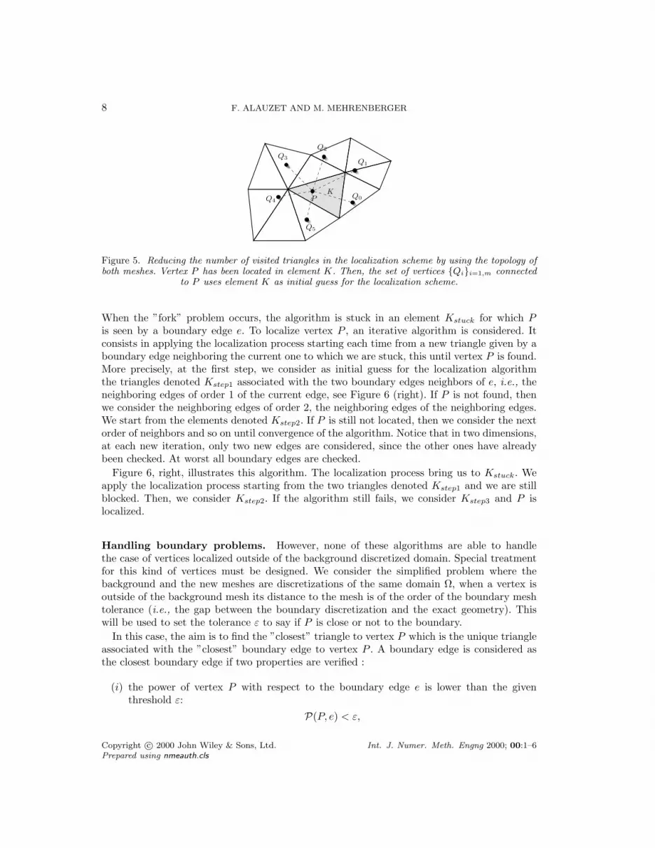
Second, this convex polygon is meshed by primarily constructing an oriented triangle withthree points chosen randomly. Notice that the three points cannot be aligned by construction.Then, a new point is selected and the unique triangle edge which is viewing this point islooked for, i.e., the only edge for which the barycentric coordinate is negative. A new orientedtriangle is built by connecting the point to this edge. The process is iterated until all pointsare inserted by only checking edges forming the boundary of the current polygon (i.e., edgeswhich are not shared by two triangles). Notice that, at each iteration, as the current polygon isconvex, there is only one boundary edge that views the selected point. A mesh of the polygonis then obtained. This process for five points is illustrated in Figure 9.

Remark 5.1. This meshing procedure is just an application of the incremental Delaunaymethod to triangulate a cloud of points, i.e., the Delaunay kernel, in our particular case [7].



Remark 5.2. This method is extensible to three dimensions even if it is slightly morecomplicated, notably four points can be coplanar.

No intersection criteria. When the triangles intersect, the proposed algorithmautomatically detects it and meshes it whatever the configuration. But, three possibledegenerated cases can occur during the process which are assimilated to no intersection:

• 0 intersecting point are found meaning an empty intersection,• 1 intersecting point is found implying that the intersection of the triangles is a vertex,• 2 intersecting points are found signifying that triangles intersect on a edge.

In such configurations, the algorithm has to make the distinction between the case where onetriangle is included in the other one, meaning that the intersection is this triangle, and thecase where the intersection is empty. We propose two criteria to discriminate these cases. LetKP = [P0, P1, P2] and KQ = [Q0, Q1, Q2] be two triangles. We denote by ePj = [P[j+1] P[j+2]]and eQj = [Q[j+1]Q[j+2]] for j = 0, .., 2 the edges of KP and KQ, respectively.

Proposition 5.1. KP is included inside KQ if and only if for all Pi, i = 0, .., 2 and for alleQj , j = 0, .., 2, we have P(Pi, e

Qj ) ≥ 0. In other words, all powers of KP are positives signifying

that all the vertices of KP are included inside KQ.

Proposition 5.2. The intersection between KP and KQ is empty if and only if there existePj or eQj such that for all Qi or Pi we have P(Qi, ePj ) < 0 or P(Pi, e

Qj ) < 0. In other words,

each triangle lies in a half-plane separated by the edge ePj or eQj

As regards the triangle-triangle intersection procedure, the algorithm computes the 9possible edge-edge intersections. It requires the evaluation of the 18 possible vertices powerswith respect to an edge. Actually, only their signs are needed. Consequently, the triangleinclusion case can be immediately checked. Then, if the intersection algorithm returns 0, 1 or2 intersection point(s), it implies that no intersection occurs. Notwithstanding, Proposition 5.2could be used to faster discriminate the non-intersection case.

1 1

23

Figure 9. Left, five intersection points have been computed for the triangle-triangle intersection.Middle, the first three points define the first triangle. Then right, the fourth point is connected tothe vertices of the edge of triangle 1 viewing it. It creates triangle 2. Similarly, the triangle 3 is formed

with the fifth point.



5.1.3. Overlapped elements detection Now, in the context of the conservative interpolation,the method consists in computing for each triangle Knew of the current mesh Hnew itsintersection with all triangles Kback

j of the background mesh Hback that it overlaps. We presenthow this list of background elements is determined and the way the intersections are handled.

First of all, all vertices of the new mesh Hnew are localized in the background mesh Hbackusing the algorithm presented in Section 3. Then, for each triangle Knew of Hnew, the initiallist of background triangles overlapped is given by the elements containing the vertices ofKnew. In degenerated cases where a vertex lies on an edge or on a background vertex, weadd to the initial list both triangles sharing the edge or the ball of the background vertex,respectively.

Then, the intersections between Knew and the triangles of the initial list are computed.Then, new triangles are added to the list during the intersection procedure as follows:

• if an edge ej of Kback is intersected by Knew (i.e., it exists an edge of Knew for whichthe intersection occurs) then we add the neighbor Kback

j of Kback sharing the edge ej tothe list,

• if a vertex of Kback has all its powers positive with respect to the edges of Knew (i.e., itlies inside Knew) then we add the ball of this vertex to the list.

With this simple procedure, all overlapped elements are automatically detected whilecomputing intersections. The process is depicted in Figure 10. Overlapped elements aredetected without any additional cost as powers and edge-edge intersections are alreadycomputed in the triangle-triangle intersection process.

As regards degenerated cases, when the edge-edge intersection results in an edge, then westill add the neighboring triangle. When it results in a vertex, we add the vertex ball to thelist.

1

1

1

2

2

2

2

2

22

2

2

22

1

1

1

2

2

2

2

2

22

2

2 3

3

3

3 3

3

4

44

4

Figure 10. Illustration of the overlapped elements detection process. First, the list of the backgroundelements to which the vertices of Knew belong are detected: they are tagged 1. Then, the other elementsare iteratively detected while computing intersections. The tag number represents the intersection step.

Two steps are sufficient for the left case, whereas the right case requires four steps.

5.2. P1-conservative reconstruction

In this section, we describe the P1-conservative solution reconstruction process. We considera bounded domain Ω of R2 and two triangular meshes of this domain Hback =

⋃Kbacki



and Hnew =⋃Knewi . For sake of simplicity, we first make the assumption that the discrete

boundaries of both meshes are the same, i.e., both meshes are discretization of the samepolygonal domain Ωh: |Hback| = |Hnew| where |H| =

∫Ωhdx. The case of non-matching discrete

boundaries is addressed in Section 5.2.3. For each mesh, a dual partition of the domain isdefined by associating to each vertex of a mesh a control volume or cell (which is defined bysome rules): Hback =

⋃Cbacki and Hnew =

⋃Cnewi . A P1 discrete solution field u is given on

the background mesh Hback.

Now, we have to define a projection operator Πc1 from Hback to Hnew with the following

properties:

• Πc1 is conservative:

∫Hback

u =∫Hnew

Πc1u

• Πc1 is P1 exact: if u is affine then Πc

1u = u.

In the following, we define the projection operator for solutions defined at elements andsolutions defined at vertices.

5.2.1. Solution defined at elements In this case, the solution is piecewise linear by elementsand can be discontinuous. We have for each background triangle Kback:

• the mass mKback =∫Kback u = |Kback|u(G), where G is the barycenter of the triangle

• the constant gradient ∇uKback .

For each triangle Knew of the current mesh, we compute the intersection with all trianglesof the background mesh Kback

j it overlaps as described in the previous section. Each coupleof triangles Knew and Kback

j provides a simplicial mesh of their intersection region denoted

Tj = Knew ∩Kbackj . The integrals

∫Tj

u and∫Tj

∇u are then computed exactly using Gauss

quadrature formulae. Consequently, we obtain for each triangle of the current mesh the massand the gradient:

mKnew =∫Knew

Πc1u =

∑j

∫Tj

u and (∇Πc1u)|Knew =

∑j

∫Tj∇u

|Knew|.

This reconstruction is conservative and P1 exact. It gives a P1 by element discontinuoussolution. A specific treatment of the reconstruction is carried out to verify the maximumprinciple.

Verifying the maximum principle. Let K be a triangle of the new mesh. In the following,for clarity we denote by uK the P1-conservative interpolated solution Πc

1u on K. The value atthe barycenter and the gradient of the interpolated solution on K are given by:

uK(GK) =1|K|

∫K

u and ∇uK =1|K|

∫K

∇uK .

Consequently, for each vertex Pi of the new mesh, we get a value of the solution using Taylorexpansion for each element K of its ball:

uK(Pi) = uK(GK) +∇uK ·−−−→GKPi . (2)



A correction is applied to the linear representation of the solution on each element in orderto verify the maximum principle. To this end, let K be the set of elements of the backgroundmesh that K overlaps, see Figure 10, and let Q be the set of vertices of K:

K = Kbackj |K ∩Kback

j 6= ∅ and Q = Qj |Qj ∈ Kback such that Kback ∈ K .Then, for each vertex Pi of each element K of the new mesh, the nodal value uK(Pi) verifythe maximum principle if:

umin = minQ∈Q

u(Q) ≤ uK(Pi) ≤ maxQ∈Q

u(Q) = umax .

Notice that uK(GK) satisfies the maximum principle. If a vertex does not verify the maximumprinciple on an element K then the gradient value of this element is corrected. Two approachesare proposed. One is based on the notion of limiter used in numerical schemes and the otherone results from a minimization problem.

A first correction with limiters (I). For each element K, the limited vertex reconstruction isgiven by:

uIK(Pi) = uK(GK) + ΦK ∇uK ·

−−−→GKPi = uK(GK) + ΦK(uK(Pi)− uK(GK)) ,

where ΦK ∈ [0, 1] is defined by ΦK = mini=0,1,2

φK(Pi), with

φK(Pi) =

min

(1,

umax − uK(GK)uK(Pi)− uK(GK)

)if uK(Pi)− uK(GK) > 0

min(

1,umin − uK(GK)uK(Pi)− uK(GK)

)if uK(Pi)− uK(GK) < 0

1 if uK(Pi)− uK(GK) = 0 .

Another correction (II). We first reorder the indices such that uK(P0) ≤ uK(P1) ≤ uK(P2).We then set

uMK (P2) = min(uK(P2), umax)

uMK (P1) = min(uK(P1) +12

max(0, uK(P2)− umax), umax)

uMK (P0) = 3uK(G)− uMK (P1)− uMK (P2),

and

uK(P0) = max(uMK (P0), umin)

uK(P1) = max(uMK (P1)− 12

max(0, umin − uMK (P0)), umin)

uK(P2) = 3uK(G)− uK(P0)− uK(P1).

These new nodal values uK(Pi) define the corrected linear representation of the solution onK. For any points X included in K, its solution value is then given by:

uIIK(X) =

2∑i=0

βi(X)uK(Pi) ,

where βi(X) are the barycentric coordinates of X with respect to K. The final interpolatedsolution verifies all required properties:



Proposition 5.3. Let S ∈ I,II. The reconstruction uSK satisfies the maximum principle, islinear preserving and is conservative. Moreover, we have:

uK(P0) ≤ uK(P1) ≤ uK(P2) =⇒ uSK(P0) ≤ uSK(P1) ≤ uSK(P2)

and

umin ≤ uK(Pi) ≤ umax for i = 0, 1, 2 =⇒ uSK(Pi) = uK(Pi) for i = 0, 1, 2.

Notice that the reconstruction II comes from a minimization problem. Indeed, we have

Proposition 5.4. Suppose that uK(P0) ≤ uK(P1) ≤ uK(P2) and that umax < uK(P2). Then,we have

2∑i=0

|uK(Pi)− uMK (Pi)|2 ≤2∑i=0

|uK(Pi)− vK(Pi)|2

for all the linear reconstructions vK satisfying vK(P2) = umax, vK(Pi) ≤ umax for i = 0, 1 and∫KvK =

∫KuK .

The proofs of these propositions are given in the Appendix.

5.2.2. Solution defined at vertices When the solution is given at vertices of the backgroundmesh, i.e., nodal values are provided, it defines implicitly a piecewise linear continuousrepresentation of the solution at the elements. Therefore, the P1-conservative interpolationdefined in the previous section can be applied. A piecewise linear solution by elements, whichis generally discontinuous, is then obtained on the new mesh. Now, one more stage is requiredto retrieve a solution at vertices of the new mesh. This solution transferred from elements tovertices must preserve the properties of the interpolation scheme.

The solution is simply re-distributed to each vertex P of the new mesh by averaging:

uS(P ) =

∑Knew

i 3P |Knewi |uSKnew

i(P )∑

Knewi 3P |Ki|

,

where S ∈ I,II depends on the chosen reconstruction and u is the interpolated solutionon the new mesh. Notice that after re-distribution to vertices the interpolated solution stillsatisfies the maximum principle, is linear preserving and is conservative.

Remark 5.3. As the mass of the solution is linked to the topology of the mesh, the P1-conservative interpolation operator Πc

1 depends on the mesh topology on which it is applied. Inconsequence, it cannot be applied to interpolate solution at any points of a given domain.

5.2.3. Non-matching discrete boundaries Let Ω be a bounded domain of R2 and Hback andHnew two meshes of Ω. We consider the case where the discrete boundaries of Hback and Hnewdo not match. In other words, Hback and Hnew are meshes of two different polygonal domainsΩbackh and Ωnewh the boundary of which differs: Γbackh 6= Γnewh . Therefore, the volume of eachmesh differs: |Hback| 6= |Hnew|.

In the conservative interpolation, the non-matching discrete boundaries are handled differentlydepending on the solution behavior. We consider the following specific cases:



1. if the solution is constant or linear, we require to keep a constant or linear solution tosatisfy the P1-exactness property. If an uniform field is given as initial set, we want toreturn an uniform solution set. In this case, the conservation principle is violated.

2. else, if the solution does not vary linearly, then we verify the conservation principle bymodifying the solution.

6. PSEUDO-CONSERVATIVE INTERPOLATION

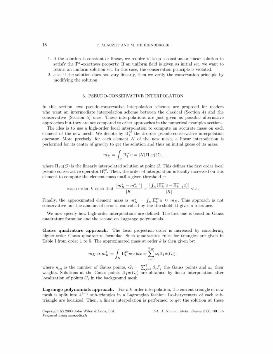
In this section, two pseudo-conservative interpolation schemes are proposed for readerswho want an intermediate interpolation scheme between the classical (Section 4) and theconservative (Section 5) ones. These interpolations are just given as possible alternativeapproaches but they are not compared to other approaches in the numerical examples sections.

The idea is to use a high-order local interpolation to compute an accurate mass on eachelement of the new mesh. We denote by Πpc

k the k-order pseudo-conservative interpolationoperator. More precisely, for each element K of the new mesh, a linear interpolation isperformed for its center of gravity to get the solution and thus an initial guess of its mass:

m1K =

∫K

Πpc1 u = |K|Π1u(G) ,

where Π1u(G) is the linearly interpolated solution at point G. This defines the first order localpseudo conservative operator Πpc

1 . Then, the order of interpolation is locally increased on thiselement to compute the element mass until a given threshold ε:

reach order k such that|mk

K −mk−1K |

|K|=|∫K

(Πpck u−Πpc

k−1u)||K|

< ε .

Finally, the approximated element mass is mkK =

∫K

Πpck u ≈ mK . This approach is not

conservative but the amount of error is controlled by the threshold. It gives a tolerance.

We now specify how high-order interpolations are defined. The first one is based on Gaussquadrature formulae and the second on Lagrange polynomials.

Gauss quadrature approach. The local projection order is increased by consideringhigher-order Gauss quadrature formulae. Such quadratures rules for triangles are given inTable I from order 1 to 5. The approximated mass at order k is then given by:

mK ≈ mkK =

∫K

Πpck u(x)dx =

ngp∑i=1

ωiΠ1u(Gi) ,

where npg is the number of Gauss points, Gi =∑3j=1 βjPj the Gauss points and ωi their

weights. Solutions at the Gauss points Π1u(Gi) are obtained by linear interpolation afterlocalization of points Gi in the background mesh.

Lagrange polynomials approach. For a k-order interpolation, the current triangle of newmesh is split into 4k−1 sub-triangles in a Lagrangian fashion. Iso-barycenters of each sub-triangle are localized. Then, a linear interpolation is performed to get the solution at these



centers of gravity. The approximated mass at order k is given by:

mK ≈ mkK =

∫K

Πpck (x)dx =

4k−1∑i=1

|K|4k−1

Π1u(Gi) .

The weakness of this approach is to have 64 points to localize and interpolate at order 4 andeven more after. Consequently, it becomes rapidly time consuming.

7. ACCURACY AND CONVERGENCE STUDY ON ANALYTICAL FUNCTIONS

In this section, the behavior of the P1-conservative interpolation is analyzed on four analyticalfunctions defined on the domain [−1, 1] which are representative of several physical phenomenaencountered in computational fluid dynamics (CFD). The P1-conservative interpolation iscompared to the linear interpolation, in particular the mass conservation and the convergenceorder of the schemes are studied.

To perform this analysis, two meshes H11 and H2

1, composed respectively of 631 and 611vertices, are considered. These meshes are completely different and unconnected. They aredepicted in Figure 11. In order to study the methods convergence order, each mesh spans aseries of embedded meshes denoted (H1

i )i=1...5 and (H2i )i=1...5. At each time, the mesh Hji+1

Opg npg βj multiplicity weight ωi

1 1 ( 13 ,

13 ,

13 ) 1 |K|

2 3 ( 16 ,

16 ,

23 ) 3 1

3 |K|

3 4 ( 13 ,

13 ,

13 ) 1 − 9

16 |K|

( 15 ,

15 ,

35 ) 3 25

48 |K|

4 6 (ai, ai, 1− 2 ai) for i = 1, 2 3

a1 = 0.445948490915965 0.223381589678010 |K|

a2 = 0.091576213509771 0.109951743655322 |K|

5 7 ( 13 ,

13 ,

13 ) 1 9

40 |K|

(ai, ai, 1− 2 ai) for i = 1, 2 3

a1 = 6−√

1521

155−√

151200 |K|

a2 = 6+√

1521

155+√

151200 |K|

Table I. Gauss quadrature formulae for triangles from [10]. Opg is the quadrature order, npg is thenumber of Gauss points, βi are the barycentric coordinates that define the Gauss points and ωi their

associated weights.



Step # vertices H1i # vertices H2

i

1 631 6112 2, 444 2, 3663 9, 619 9, 3114 38, 165 36, 9415 152, 041 147, 161

Table II. Mesh sizes of the series of embedded mesh (H1i )i=1...5 and (H2

i )i=1...5.

is deduced from Hji by splitting each triangle into four triangles in a Lagrangian fashion, i.e.,in a isoparametric way. These series of meshes are summarized in Table II.

For each case, the function is applied on H1i providing a solution field u1

i . This solution fieldis transfered from H1

i to H2i , we get Πu2

i . This solution transfer is called transfer H1i → H2

i .The error is computed by comparing the interpolated solution Πu2

i with the function appliedon H2

i , i.e., u2i , in L2-norm:

ε2i =

∫H2

i(u2i −Πu2

i )2∫

H2i(u2i )2

,

where the integrals are computed using a 5-order Gaussian quadrature. The series of errorsenable a convergence study.

We have also analyzed the error when the solution field is re-interpolated back to H1i . That

is to say, the function is applied on H1i giving u1

i , then it is interpolated on H2i giving Πu2

i

and finally Πu2i is interpolated from H2

i to H1i and we obtain Πu1

i . The error εi is obtained bycomputing the gap in L2-norm between u1

i and Πu1i on H1

i . This double solution transfer iscalled transfer H1

i → H2i → H1

i .

Figure 11. Uniform unstructured triangular meshes used to compare interpolation schemes. Left, H11

containing 631 vertices, and right, H21 containing 611 vertices.



For each analytical function, a figure is given providing:

• top left, a three-dimensionnal representation of the function• top right, the mass variation for the solution transfer H1

i → H2i

• bottom left, the error εi for the solution transfer H1i → H2

i

• and bottom right, the error εi for the solution transfer H1i → H2

i → H1i .

The linear interpolation scheme is represented by the red lines and the P1-conservativeinterpolation is represented by the blue lines.

A Gaussian function. The first analytical function is a gaussian given by:

f1(x, y) = exp(−30 (x2 + y2)) .

This function is smooth and is representative of the vortices encountered in CFD, Figure 12.The mass variation with the classical linear interpolation converges toward zero. It has a

variation lower than 10−5 for meshes with more than 35, 000 vertices. Conversely, the mass

Figure 12. Gaussian analytical function f1. Top left, a three-dimensionnal representation of thefunction. Top right, the mass variation for the transfer H1

i → H2i . Bottom left, the error εi for

the transfer H1i → H2

i . Bottom right, the error εi for the transfer H1i → H2

i → H1i .



variation with the P1-conservative interpolation is of the order of the numerical zero (≈ 10−10)for all interpolation steps.

As regards the accuracy and the convergence order, both interpolation scheme are convergingat order 2 for solution transfers H1

i → H2i and H1

i → H2i → H1

i . This fits to the theory. Wenotice that the P1-conservative interpolation is more accurate than the linear one in bothcases. The difference in accuracy varies between 2 and 3 for the solution transfer H1

i → H2i

and between 3 and 12 for the transfer H1i → H2

i → H1i .

A continuous sinusoidal shock. This analytical function represents a continuous modelof a shock which can be assimilated to the numerical capture of a shock with a dissipative flowsolver, i.e., the solver captures the shock on several mesh elements. This smooth function isgiven by:

f2(x, y) = tanh(100 (y + 0.3 sin(−2x))) .

Figure 13. Continuous sinusoidal shock analytical function f2. Top left, a three-dimensionnalrepresentation of the function. Top right, the mass variation for the transfer H1

i → H2i . Bottom left,

the error εi for the transfer H1i → H2


i → H1i .



It contains two quasi-constant regions that are separated by a sinusoidal region in which astrong gradient variation occurs continuously.

As previously, the mass variation with the P1-conservative interpolation is of the orderof the numerical zero (≈ 10−9) for all interpolation steps. For the linear interpolation themass variation decreases when mesh accuracy increases. The mass variation is almost 10−5 formeshes with more than one hundred thousand vertices. Notice that for coarser meshes (thefirst two steps) the mass variation is between 0.3 and 0.6% for just one solution transfer.

The P1-conservative interpolation achieves an order 2 of convergence for solution transfersH1i → H2

i and H1i → H2

i → H1i whereas the linear interpolation has a convergence order less

than 2. The convergence order is almost 1.6 in both cases. Actually, meshes are not fine enoughto reach the asymptotical mesh convergence order for the linear interpolation. As regards theaccuracy, the P1-conservative interpolation is more accurate than the linear one in all casesand the difference increases while meshes are refined.

Figure 14. Multi-scales smooth analytical function f3. Top left, a three-dimensionnal representationof the function. Top right, the mass variation for the transfer H1

i → H2i . Bottom left, the error εi for

the transfer H1i → H2


i → H1i .



A multi-scales smooth function. This function presents smooth sinusoidal variations butat different scales. There are two order of magnitudes between small and large scales variations.This function reads:

f3(x, y) =

0.01 sin(50x y) if x y ≤ −π

50

sin(50x y) if−π50

< xy ≤ 2π50

0.01 sin(50x y) if2π50

< xy

.

The mass variation with the P1-conservative interpolation is still of the order of thenumerical zero (≈ 10−10) for all interpolation steps. For the linear interpolation, the massvariation is large from 1% for step 1 to 0.01% for step 5 for only one solution transfer. However,the mass variation still converges toward zero while the mesh size converges toward zero.

For this smooth case, the two approaches reach an order 2 of convergence for solutiontransfers H1

i → H2i and H1

i → H2i → H1

i . Concerning the accuracy, the conclusions are the

Figure 15. Discontinuous analytical function f4. Top left, a three-dimensionnal representation of thefunction. Top right, the mass variation for the transfer H1

i → H2i . Bottom left, the error εi for the

transfer H1i → H2


i → H1i .



same as in the previous cases. The P1-conservative interpolation achieves better accuracythan the standard linear interpolation and even more for the solution transfer H1

i → H2i → H1

i

where the error is reduced by an order of magnitude for the finest meshes (step 4 and 5).

A discontinuous function. The final function is discontinuous and represents four steps:

f4(x, y) =

1 if x ≥ 0 and y ≥ 02 if x ≥ 0 and y < 03 if x < 0 and y ≥ 04 if x < 0 and y < 0

.

The solution is constant in four squared regions and it is discontinuous at the interface of eachregion.

The mass variation with the P1-conservative interpolation, in this case too, is of the orderof the numerical zero for all the interpolation steps. For the linear interpolation, the massvariation is large from 1% for step 1 to 0.01% for step 5 for only one solution transfer. However,it still converges toward zero while the size approaches zero.

Even if the mass is preserved, while transferring the solution from a mesh to a finer one,i.e., the solution transfer H1

i → H2i , the same accuracy is obtained for both approaches.

Nevertheless, for the solution transfer H1i → H2

i → H1i the P1-conservative interpolation

performs better than the classical linear approach.

Conclusions. For all those analytical cases, while preserving the mass, the P1-conservativeinterpolation achieves better accuracy than the classical linear interpolation and for some casesit converges at a faster rate.

8. APPLICATION TO MESH ADAPTATION

Mesh adaptation provides a way of controlling the accuracy of the numerical solution bymodifying the domain discretization according to size and directional constraints. It is wellknown that mesh adaptation captures accurately physical phenomena in the computationaldomain while reducing significantly the cpu time, see [6, 11, 12].

8.1. Unsteady mesh adaptation scheme

Anisotropic mesh adaptation is a non-linear problem. Therefore, an iterative procedure isrequired to solve this problem. For stationary simulations, an adaptive computation is carriedout via a mesh adaptation loop inside which an algorithmic convergence of the mesh-solutioncouple is sought.

At each stage, a numerical solution is computed on the current mesh with a flow solverand has to be analyzed by means of an error estimate. The considered error estimate aims atminimizing the global interpolation error in norm Lp, thus it is independent of the problemat hand. From the multi-scales metric theory in [13] and [12], an analytical expression of theoptimal metric is exhibited in two dimensions that minimizes the interpolation error in norm



Lp:

MLp = DLp (det |Hu|)−1

2p+2 R−1u |Λ|Ru with DLp = 2 ε−1

(∫Ω

(det |Hu|)p

2p+2

) 1p

, (3)

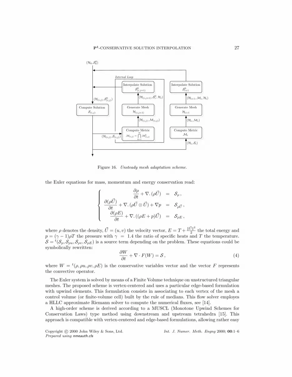
where ε is the prescribed error threshold. This anisotropic metric is a function of the Hessian ofthe solution which is reconstructed from the numerical solution by a double L2 projection. Thismetric will replace the Euclidean one modifying the scalar product that underlies the notion ofdistance used in mesh generation algorithms. Next, an adapted mesh is generated with respectto this metric where the aim is to generate a mesh such that all its edges have a length of (orclose to) one in the prescribed metric and such that all its elements are almost regular. Sucha mesh is called a unit mesh. Here, the mesh is adapted by local mesh modifications of theprevious mesh (the mesh is not regenerated) using classical mesh operations: vertex insertion,edge and face swap, collapse and node displacement [8]. Finally, the solution is interpolated onthe new mesh using one of the interpolation schemes presented in this paper. This procedureis repeated until the convergence of the solution and of the mesh is achieved. This algorithmis represented by the external loop of the mesh adaptation scheme in Figure 16.

To solve the non-linear problem of mesh adaptation for unsteady simulation, a new algorithmgeneralizing the mesh adaptation scheme coupled with a metric intersection in time procedurehas been proposed in [6]. This procedure, based on the resolution of a transient fixed pointproblem for the couple mesh-solution at each iteration of the mesh adaptation loop, predicts thesolution evolution in the computational domain. Knowing then the solution evolution duringa short period of time, the mesh is suitably adapted in all the regions where the solutionprogresses so as to preserve its accuracy.

This iterative algorithm consists of two steps: the main adaptation loop and an internal loopin which the transient fixed point problem is solved. At each iteration of the main adaptationloop, we consider a time period [t, t + ∆t] in which the solution evolves. During this period,we try to algorithmically converge to the solution at t + ∆t and to the associated adaptedmesh. In other words, from the solution at time t, we compute the solution to time t + ∆t,and the computation is iterated via the internal loop until the desired accuracy is obtainedfor the solution at t + ∆t. Similarly, we algorithmically converge toward the correspondinginvariant mesh adapted to this period [t, t+∆t] throughout a sequence of consecutively adaptedmeshes. The solution behavior is thus predicted in all the regions of the domain where thesolution evolves. To take into account the solution progression, a metric is defined by meansof an intersection procedure in time. More precisely, metrics associated to several solutionsthroughout the time period [t, t+ ∆t] are evaluated and intersected into a unique one. Then, anew mesh is generated according to this metric field. Finally, the initial solution of this periodis interpolated and the computation is resumed. This scheme, illustrated in Figure 16, controlsthe spatial and the time error during the whole computation.

8.1.1. Flow solver In all the examples, the flow is modeled by the conservative Eulerequations. Assuming that the gas is perfect, inviscid and that there is no thermal diffusion,



Internal Loop

Interpolate Solution Interpolate Solution

Generate Mesh Generate Mesh

Compute Metric Compute Metric

Compute SolutionS(i,j)

S0(i,j+1)

H(i,j+1)

(H(i,j),M(i,j))

(H(i,j+1),S0i ,Hi)(H(i,j),S0

(i,j))

(H(i,j),S(i,j))

(H0,S00 )

Hi+1

S0i+1

Mi

(Hi,Si)

(Hi,Mi)

(Hi+1,Mi,Hi)

M(i,j) =m!

k=1

Mk(i,j)

Figure 16. Unsteady mesh adaptation scheme.

the Euler equations for mass, momentum and energy conservation read:

∂ρ

∂t+∇. (ρ~U) = Sρ ,

∂(ρ~U)∂t

+∇. (ρ~U ⊗ ~U) +∇p = Sρ~U ,

∂(ρE)∂t

+∇. ((ρE + p)~U) = SρE ,

where ρ denotes the density, ~U = (u, v) the velocity vector, E = T + ‖~U‖22 the total energy and

p = (γ − 1)ρT the pressure with γ = 1.4 the ratio of specific heats and T the temperature.S = t(Sρ,Sρu,Sρv,SρE) is a source term depending on the problem. These equations could besymbolically rewritten:

∂W

∂t+∇ · F (W ) = S , (4)

where W = t(ρ, ρu, ρv, ρE) is the conservative variables vector and the vector F representsthe convective operator.

The Euler system is solved by means of a Finite Volume technique on unstructured triangularmeshes. The proposed scheme is vertex-centered and uses a particular edge-based formulationwith upwind elements. This formulation consists in associating to each vertex of the mesh acontrol volume (or finite-volume cell) built by the rule of medians. This flow solver employesa HLLC approximate Riemann solver to compute the numerical fluxes, see [14].

A high-order scheme is derived according to a MUSCL (Monotone Upwind Schemes forConservation Laws) type method using downstream and upstream tetrahedra [15]. Thisapproach is compatible with vertex-centered and edge-based formulations, allowing rather easy



and, importantly, inexpensive higher-order extensions of monotone upwind schemes. The fluxintegration based on the edges and their corresponding upwind elements (crossed by the edge)is a key-feature in order to preserve the positivity of the density for vertex-centered formulationas demonstrated in [16]. Appropriate β-schemes are used for the variable extrapolation whichgives us a third-order space-accurate scheme for the linear advection on cartesian triangularmeshes, see [17]. This approach provides low diffusion second-order space-accurate schemein the non-linear case. The MUSCL type method is combined with a generalization of theSuperbee limiter with three entries to guarantee the TVD (Total Variation Diminishing)property of the scheme [16].

An explicit time stepping algorithm is used by means of a 4-stage, 3-order strong-stability-preserving (SSP) Runge-Kutta scheme which allows us to use a CFL coefficient up to 2 [18].Such time discretization methods have non linear stability properties which are particularlysuitable for the integration of system of hyperbolic conservation laws where discontinuitiesappear. These schemes verify the TVD property. In practice, we consider a CFL equal to 1.8.

More details can be found in [19].

8.2. Spherical blast

This example is a spherical Riemann problem between two parallel walls simulating a blastproposed by Langseth and LeVeque [20]. Initially, the gas is at rest with density ρout = 1 andpressure pout = 1 everywhere except in a sphere centered at (0, 0, 0.4) with radius 0.2. Insidethe sphere the parameters are ρin = 1 and pin = 5. For both regions, we have γ = 1.4. Asmentioned in [20], the initial pressure jump results in a strong outward moving shock wave,an outward contact discontinuity and an inward moving rarefaction wave. The main featureof the solution are the interactions between these waves. Another significant feature is thedevelopment of a low density region in the center of the domain with the development ofinstabilities along the contact discontinuity.

As the solution remains cylindrically symmetric throughout the simulation, it is possible toformulate it as a two-dimensional problem with a source term where S is given by:

S = − sign(x)r

t(ρu, ρu2, ρuv, u(ρE + p)

),

where r =√x2 + (y − 0.4)2 represents the distance to the center of the sphere. The sign of x is

considered in the source term as we solve the problem on the entire domain [−1.5, 1.5]× [0, 1].The solution is computed until a-dimensioned time t = 0.7.

Error threshold E P1 P1-conservative0.05 6, 360 7, 7020.04 10, 424 12, 1020.03 19, 003 24, 2970.02 65, 740 78, 0990.015 118, 929 158, 121

Table III. Number of vertices of the final adapted meshes obtained with the unsteady mesh adaptationalgorithm for the P1 and the P1-conservative interpolation for several error thresholds.



For this problem, the L2-norm of the density interpolation error is controlled. The globalsimulation is split into 20 time periods of time length ∆t = 0.035 for which a transientfixed-point problem is solved throughout 5 internal loop iterations. This simulation has beenperformed for five error thresholds, ranging from ε = 0.05 to ε = 0.015. The number of metricintersections in time varies between 10 and 20 depending on the error threshold. Two seriesof adaptations have been performed: one with the classic P1 interpolation and the other onewith the P1-conservative interpolation scheme. The statistics of the final (t = 0.7) adaptedmeshes are given in Table III.

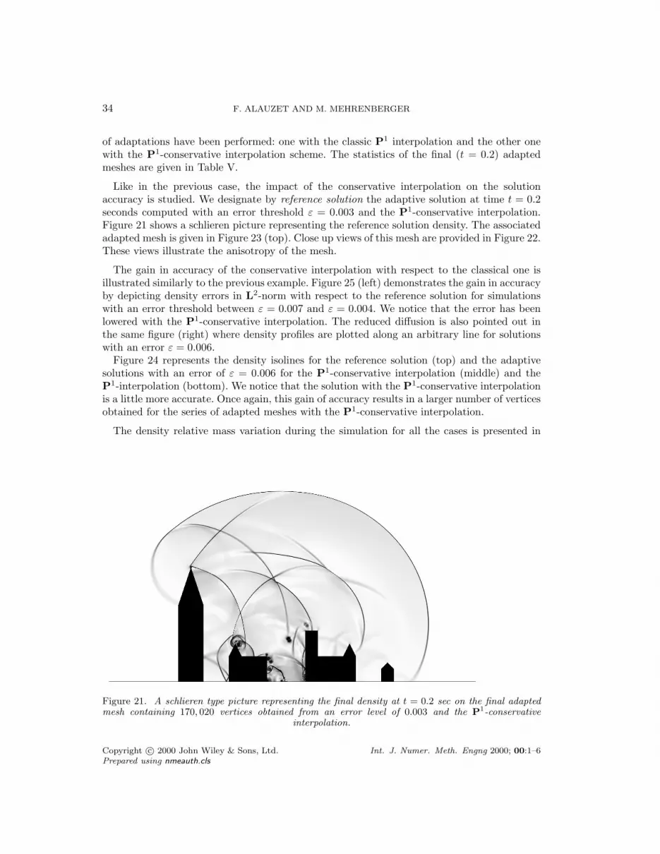
In the following, we will analyze the impact of the conservative interpolation on the solutionaccuracy. We designate by reference solution the adaptive solution at time t = 0.7 computedwith an error threshold ε = 0.015 and the P1-conservative interpolation. Figure 17 shows aschlieren picture representing the reference solution density at t = 0.7. This picture imitatesa photographic technique used in physical experiments. The final adapted mesh at t = 0.7associated to the reference solution is depicted in Figure 18 (top). A close up view of theadapted mesh in a region where instabilities occur is given in Figure 20 (right). Notice that insome regions the accuracy of the mesh attains h = 2. e−4.

Several items illustrate the gain in accuracy of the conservative interpolation with respectto the classical one. These items point out that the solution has been less diffused during theinterpolation stage and it thus results in a more accurate solution.

The gain in accuracy is demonstrated in Figure 20 (left) where the density errors in L2-normwith respect to the reference solution are drawn for the adaptive simulations with an errorthreshold from ε = 0.05 to ε = 0.02 for the conservative and the classical interpolations. Wenotice that the error has been lowered with the conservative interpolation.

This is also illustrated in Figure 19 where the pressure isolines are represented for thereference solution (top) and the adaptive solutions with an error of ε = 0.03 for the P1-conservative interpolation (middle) and the P1-interpolation (bottom). The solution with theP1-conservative interpolation is slightly more detailed showing that it is less dissipative.

This impact is also emphasized by the mesh size of the final adapted of each simulation.For a given error threshold, we remark that using the P1-conservative interpolation results

Figure 17. A schlieren type picture representing the final density at t = 0.7 on the final adapted meshcontaining 158, 121 vertices obtained from an error level of 0.015 and the P1-conservative interpolation.



in a larger final mesh. As the solution is less dissipated during the interpolation stage, moredetails (phenomena) of the solution are preserved and thus the adaptive process generateslarger meshes.

Notice that for this example, it is impossible to examine the impact on the mass conservationdue to the source term that modifies the mass of each variable at each iteration.

As regards the cpu time, both interpolation schemes have been compared on several couplesof meshes on a Intel Core 2 at 2.8 GHz. All the cases are summarized in Table IV. It follows thatthe P1-conservative interpolation is approximately 5 times slower than the P1 interpolation.Nevertheless, the cost of the interpolation stage (a few seconds) is always negligible as comparedto the solver cpu time.

# vertices Hbacki # vertices Hnewi P1-cons cpu time in sec. P1 cpu time in sec. ratio7, 682 7, 702 0.235 0.046 5.111, 789 12, 102 0.298 0.061 4.922, 964 24, 297 0.564 0.104 5.471, 735 78, 099 2.192 0.293 7.5140, 603 158, 121 4.839 0.971 5.0

Table IV. Cpu time comparison between the P1-conservative interpolation and the P1 interpolationon several couples of meshes on a Intel Core 2 at 2.8 GHz. The cpu time is expressed in seconds.



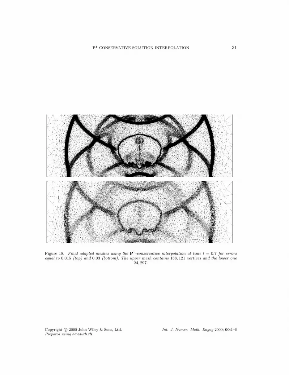
Figure 18. Final adapted meshes using the P1-conservative interpolation at time t = 0.7 for errorsequal to 0.015 (top) and 0.03 (bottom). The upper mesh contains 158, 121 vertices and the lower one

24, 297.



Figure 19. Pressure isolines from 0.715 to 1.695 with an increment of 0.0245 at time t = 0.7. Top,the reference solution, i.e., ε = 0.015 and the P1-conservative interpolation. Middle, adapted solutionobtained for ε = 0.03 with the P1-conservative interpolation. Bottom, adapted solution obtained for

ε = 0.03 with the P1-interpolation.



Figure 20. Left, L2-norm error of the density with respect to the reference solution for adaptivesimulations for ε from 0.05 to 0.02. In red, adaptive simulations with the P1-conservative interpolationand, in green, with the P1 interpolation. Right, a close up view of the adapted mesh of Figure 18 (top)

in a region where instabilities occur.

8.3. A blast in a town

The second example is a blast in a geometry representing a city plaza that has been proposedin [6]. This simulation is a multi-dimensional generalization of the Sod Riemann problem [21]in a geometry. The main feature of this problem is related to the random character of theshock wave propagation due to a large number of waves reflexions on the geometry and ofshock waves interactions.

The computational domain size is 150 × 90 m2. Initially, the gas representing the ambientair is at rest with a density ρout = 0.125 and pout = 0.1. To simulate the blast, a high pressureand density region is introduced in a quarter-circle centered at (6.5, 0) with a radius 0.25. Inthis region, the relevant parameters are ρin = 1, pin = 1 and uin = vin = 0. For both regions,we have γ = 1.4. The solution is computed until physical time t = 0.2 seconds.

For this problem too, the L2-norm of the density interpolation error is controlled. Theglobal simulation is split into 30 time periods of time length ∆t = 0.0066 for which a transientfixed-point problem is solved throughout 5 internal loop iterations. This simulation has beenperformed for five error thresholds, from ε = 0.007 to ε = 0.003. The number of metricintersections in time varies between 10 and 20 depending on the error threshold. Two series

Error threshold E P1 P1-conservative0.007 15, 532 17, 7950.006 21, 343 23, 7670.005 43, 001 51, 1040.004 73, 219 84, 0490.003 152, 503 170, 020

Table V. Number of vertices of the final adapted meshes obtained with the unsteady mesh adaptationalgorithm for the P1 and the P1-conservative interpolation for several error thresholds.



of adaptations have been performed: one with the classic P1 interpolation and the other onewith the P1-conservative interpolation scheme. The statistics of the final (t = 0.2) adaptedmeshes are given in Table V.

Like in the previous case, the impact of the conservative interpolation on the solutionaccuracy is studied. We designate by reference solution the adaptive solution at time t = 0.2seconds computed with an error threshold ε = 0.003 and the P1-conservative interpolation.Figure 21 shows a schlieren picture representing the reference solution density. The associatedadapted mesh is given in Figure 23 (top). Close up views of this mesh are provided in Figure 22.These views illustrate the anisotropy of the mesh.

The gain in accuracy of the conservative interpolation with respect to the classical one isillustrated similarly to the previous example. Figure 25 (left) demonstrates the gain in accuracyby depicting density errors in L2-norm with respect to the reference solution for simulationswith an error threshold between ε = 0.007 and ε = 0.004. We notice that the error has beenlowered with the P1-conservative interpolation. The reduced diffusion is also pointed out inthe same figure (right) where density profiles are plotted along an arbitrary line for solutionswith an error ε = 0.006.

Figure 24 represents the density isolines for the reference solution (top) and the adaptivesolutions with an error of ε = 0.006 for the P1-conservative interpolation (middle) and theP1-interpolation (bottom). We notice that the solution with the P1-conservative interpolationis a little more accurate. Once again, this gain of accuracy results in a larger number of verticesobtained for the series of adapted meshes with the P1-conservative interpolation.

The density relative mass variation during the simulation for all the cases is presented in

Figure 21. A schlieren type picture representing the final density at t = 0.2 sec on the final adaptedmesh containing 170, 020 vertices obtained from an error level of 0.003 and the P1-conservative

interpolation.



Figure 26. For the P1 interpolation, the mass has varied of almost 0.01% at the end of thesimulation. We remark that the mass variation increases during the simulation and that itdecreases with the adapted mesh accuracy. We also notice that the mass variation is small ascompared to the one obtained for the analytical examples. This is due to the use of adaptedmeshes.

Concerning the P1-conservative interpolation, the mass variation is very low: 10−7 at theend of the simulation. It increases during the simulation. Notice that this growth is to someextent due to small variations of the domain area while remeshing the domain during thecomputation.

As regards the cpu time, both interpolation schemes have been compared on several couplesof meshes on a Intel Core 2 at 2.8 GHz. All the cases are summarized in Table VI. It followsthat the P1-conservative interpolation is, in this case too, approximately 5 times slower thanthe P1 interpolation. Nevertheless, the cost of the interpolation stage (a few seconds) is stillnegligible comparing to the solver cpu time.

Figure 22. Close up views of the final adapted mesh containing 170, 020. These views illustrate thatall the regions where shock waves progress during a given period are anisotropically refined.



Figure 23. Final adapted meshes using the P1-conservative interpolation at time t = 0.2 seconds forerrors equal to 0.003 (top) and 0.006 (bottom). The upper mesh contains 170, 020 vertices and the

lower one 23, 767.



Figure 24. Density isolines from 0.085 to 0.19 with an increment of 2.65 e−3 at time t = 0.2 seconds.Top, the reference solution, i.e., ε = 0.003 and the P1-conservative interpolation. Middle, adaptedsolution obtained for ε = 0.006 with the P1-conservative interpolation. Bottom, adapted solution

obtained for ε = 0.006 with the P1-interpolation.



Figure 25. Left, L2-norm error of the density with respect to the reference solution for adaptivesimulations for ε from 0.007 to 0.004. In red, adaptive simulations with the P1-conservativeinterpolation and, in green, with the P1 interpolation. Right, comparison of the density profile attime t = 0.2 seconds along the line of equation y = 3.07692x− 17.4615 for the solutions obtained with

an error threshold ε = 0.006.

Figure 26. Density relative mass variation during the simulation for all cases. The abscissae representthe iterations of the mesh adaptation algorithm. Left, mass variation for the P1 interpolation. Right,

mass variation for the P1-conservative interpolation.



# vertices Hbacki # vertices Hnewi P1-cons cpu time in sec. P1 cpu time in sec. ratio17, 180 17, 795 0.468 0.114 4.122, 384 23, 767 0.630 0.126 5.047, 232 51, 104 1.295 0.243 5.375, 104 84, 049 2.103 0.328 6.4153, 502 170, 020 4.463 1.225 3.6

Table VI. Cpu time comparison between the P1-conservative interpolation and the P1 interpolationon several couples of meshes on a Intel Core 2 at 2.8 GHz. The cpu time is expressed in seconds.

8.4. Some remarks about the numerical results

In all the presented examples, the benefits due to the conservative interpolation have beenillustrated. Analytical examples have clearly demonstrated the advantages of the conservativeinterpolation. However, for the two blast simulations, the gain in accuracy seems to be small asregards the cost. But, it is important to note that the number of mesh adaptations, and thusof interpolations, that have been performed in both simulations is small (less than 30). Morecomplex problem or problem with a long time will require to perform more adaptations andtherefore the difference between the P 1-interpolation and the P 1-conservative interpolationshould be more significative. Moreover, we have to remember that the conservation propertycan be mandatory for some applications.

9. CONCLUSION

In this work, we have proposed a P1-conservative interpolation operator that satisfies themaximum principle. This operator is based on local mesh intersections and local operationsthat make it efficient in terms of cpu time and memory requirement. Numerical examplesshow that it is approximately 5 times slower than the classical linear interpolation. Theproperties of this new operator have been verified numerically on analytical examples andadaptive simulations. These examples also point out a better accuracy of the conservativeinterpolation compared to the classical one.

The proposed conservative interpolation scheme extends easily to P k-representation of thesolution if solutions are defined at the elements. However, the extension to P k-representationof the solution defined at vertices requires more work and is under consideration at the time.

Finally, the proposed algorithm is extendable to three dimensions even if the meshintersection is more difficult to handle. This version is under development.



Appendix

We give here the proof of Propositions 5.3 and 5.4.

Proposition 5.3. Let S ∈ I,II. The reconstruction uSK satisfies the maximum principle, islinear preserving and is conservative. Moreover, we have:

uK(P0) ≤ uK(P1) ≤ uK(P2) =⇒ uSK(P0) ≤ uSK(P1) ≤ uSK(P2)

and

umin ≤ uK(Pi) ≤ umax for i = 0, 1, 2 =⇒ uSK(Pi) = uK(Pi) for i = 0, 1, 2.

Proof of Proposition 5.3.• We first consider the case where S = I.

From the definition of uK(G), we have umin ≤ uK(G) ≤ umax where G is the barycenter ofthe triangle. Now, it suffices to prove that umin ≤ uIK(Pi) ≤ umax, for i = 0, 1, 2. We have atfirst 0 ≤ ϕK(Pi), since umin ≤ uK(G) ≤ umax. If uK(Pi)− uK(G) > 0, we then get

0 ≤ uIK(Pi)− uK(G) ≤ ϕK(Pi)|uK(Pi)− uK(G)| ≤ umax − uK(G).

On the other hand, if uK(Pi)− uK(G) < 0, we have

0 ≥ uIK(Pi)− uK(G) ≥ −ϕK(Pi)|uK(Pi)− uK(G)| ≥ umin − uK(G).

Finally, if uK(Pi) = uK(G), we have uIK(Pi) = uK(G).Consequently, for all the cases, we have umin ≤ uIK(Pi) ≤ umax and therefore umin ≤

uI(Pi) ≤ umax. This proves the maximum principle.

Now, we suppose that u is affine. We have to prove that uIK(Pi) = u(Pi), for i = 0, 1, 2.Since u is affine, we have umin ≤ u(P ) = uK(P ) ≤ umax and thus ϕK(Pi) = 1 for i = 0, 1, 2.We then have uIK(Pi) = uK(G) +∇uK ·

−−→GPi = uK(Pi) = u(Pi).

Since∫K

−−→GPdP = 0, we obtain that

∫KuIK =

∫Ku. We then have∑

K

∫K

u =∑K

|K|uIK(P0) + uIK(P1) + uIK(P2)

3=∑P

∑Ki3P

|Ki|uIKi(P )

=∑P

(∑Ki3P

|Ki|)uI(P ) =∑K

|K|uI(P0) + uI(P1) + uI(P2)

3

=∑K

∫K

uI ,

and thus the reconstruction is conservative.

For the last two properties, as we have

uK(P0) ≤ uK(P1) ≤ uK(P2)⇔ ∇uK ·−−→GP0 ≤ ∇uK ·

−−→GP1 ≤ ∇uK ·

−−→GP2,



and since ϕK(Pi) ≥ 0, we have the first result. If umin ≤ uK(Pi) ≤ umax, we get ϕK(Pi) = 1and thus the last property is also true.

• Now, we consider the case where S = II.

We first prove thatuMK (P0) ≤ uMK (P1) ≤ uMK (P2) ≤ umax.

If uK(P2) ≤ umax, we have uMK (Pi) = uK(Pi), i = 0, 1, 2, and thus have the inequality.Otherwise, we have uMK (P2) = umax and uMK (P1) = min(uK(P1) + uK(P2)−umax

2 , umax).Therefore, if 2uK(P1)+uK(P2) ≤ 3umax, we have uMK (Pi) = uK(Pi)+ uK(P2)−umax

2 , for i = 0, 1and we get the result.Finally, if 2uK(P1) + uK(P2) > 3umax, we have uMK (P1) = umax and uMK (P0) = 3uK(G) −2umax ≤ umax and we obtain also the desired inequality.

We can similarly prove that

umin ≤ uIIK (P0) ≤ uIIK (P1) ≤ uIIK (P2).

It remains to prove that uIIK (P2) ≤ umax. We already know that uMK (P2) ≤ umax. IfuMK (P0) ≥ umin, we have it. Otherwise, if 2uMK (P1) + uMK (P0) ≥ 3umin, we have

uIIK (P2) = uMK (P2) +uMK (P0)− umin

2≤ uMK (P2) ≤ umax .

And in the other case, we have uIIK (P2) = 3uK(G) − 2umin ≤ umax. It finishes to prove themaximum principle.

If u is affine, we have uK(P0) = umin and uK(P2) = umax. We then get uMK (Pi) = uK(Pi)and uIIK (Pi) = uK(Pi), for i = 0, 1, 2 that provide the P1-exactness.

Since uIIK (P2) = 3uK(G)− uIIK (P0)− uIIK (P1), we obtain the conservation:∫KuIIK =

∫Ku.

The last properties can be checked from the formulae.

Proposition 5.4. Suppose that uK(P0) ≤ uK(P1) ≤ uK(P2) and that umax < uK(P2).Then, we have

2∑i=0

|uK(Pi)− uMK (Pi)|2 ≤2∑i=0

|uK(Pi)− vK(Pi)|2

for all the linear reconstructions vK satisfying vK(P2) = umax, vK(Pi) ≤ umax for i = 0, 1 and∫KvK =

∫KuK .

Proof of Proposition 5.4. We set εi = vK(Pi) − uK(Pi), for i = 0, 1, 2. Since we have∫KvK =

∫Ku, we deduce that ε0 + ε1 + ε2 = 0. On the other hand ε2 = umax − uK(P2),

and εi ≤ umax − uK(Pi) for i = 0, 1. We thus have to minimize ε20 + ε2

1, for all the numbers



ε0, ε1 satisfying εi ≤ umax − uK(Pi) for i = 0, 1, and ε0 + ε1 = uK(P2)− umax.By setting ε0 = 1

2 (uK(P2)− umax) + η, we have to minimize

(12

(uK(P2)− umax) + η)2 + (12

(uK(P2)− umax)− η)2,

for η belonging to the interval

I = [uK(P1)− umax +12

(uK(P2)− umax), umax − uK(P0)− 12

(uK(P2)− umax)].

The minimum is given for η = 0, if 0 ∈ I or for one bound of I otherwise. Notice that 0 ∈ Iif and only if 2uK(P1) + uK(P2) ≤ 3umax. Thus, if 2uK(P1) + uK(P2) ≤ 3umax, we check thatfor η = 0, vK(P1) = uMK (P1). On the other hand, if 2uK(P1) + uK(P2) > 3umax, we can checkthat

(umax − uK(P1))2 + (uK(P2)− 2umax + uK(P1))2

≤ (umax − uK(P0))2 + (uK(P2)− 2umax + uK(P0))2,

so that the minimum is given for the left bound and we get for this value of η thatvK(P1) = uMK (P1). Thus, in all cases, we have vK(P1) = uMK (P1), and this concludes theproof.

REFERENCES

1. Dukowicz J, Kodis J. Accurate conservative remapping (rezoning) for arbitrary Lagrangian - Euleriancomputations. SIAM J. Sci. Statist. Comput. 1987; 8(3):305–321.

2. Garimella R, Kucharik M, Shashkov M. An efficient linearity and bound preserving conservativeinterpolation (remapping) on polyhedral meshes. Comput. & Fluids 2007; 36(2):224–237.

3. Margolin L, Shashkov M. Second-order sign-preserving conservative interpolation (remapping) on generalgrids. J. Comp. Phys. 2003; 184(1):266–298.

4. Cheng J, Shu CW. A high order accurate conservative remapping method on staggered meshes. Appl.Numer. Math. 2008; 58(7):1042–1060.

5. Grandy J. Conservative remapping and regions overlays by intersecting polyhedra. J. Comp. Phys. 1999;148(2):433–466.

6. Alauzet F, Frey P, George PL, Mohammadi B. 3D transient fixed point mesh adaptation for time-dependent problems: Application to CFD simulations. J. Comp. Phys. 2007; 222:592–623.

7. George PL, Borouchaki H. Delaunay triangulation and meshing. Application to finite elements. Herms:Paris, 1998.

8. Frey P, George PL. Mesh generation. Application to finite elements. 2nd edn., ISTE Ltd and John Wiley& Sons, 2008.

9. Lohner R. Applied CFD techniques. An introduction based on finite element methods. John Wiley & Sons,Ltd: New York, 2001.

10. Ern A, Guermond JL. Theory and Practice of Finite Elements, Applied Mathematical Series, vol. 159.Springer: New York, 2004.

11. Frey P, Alauzet F. Anisotropic mesh adaptation for CFD computations. Comput. Methods Appl. Mech.Engrg. 2005; 194(48-49):5068–5082.

12. Loseille A, Dervieux A, Frey P, Alauzet F. Achievement of global second-order mesh convergence fordiscontinuous flows with adapted unstructured meshes. AIAA paper 2007; 2007-4186.

13. Leservoisier D, George PL, Dervieux A. Metrique continue et optimisation de maillage. RR-4172, INRIAApr 2001. (in French).

14. Batten P, Clarke N, Lambert C, Causon D. On the choice of wavespeeds for the HLLC riemann solver.SIAM J. Sci. Comput. 1997; 18(6):1553–1570.



15. Stoufflet B, Periaux J, Fezoui L, Dervieux A. Numerical simulation of 3-D hypersonic Euler flows aroundspace vehicles using adapted finite element. AIAA Paper 1987; 87-0560.

16. Cournede PH, Koobus B, Dervieux A. Positivity statements for a Mixed-Element-Volume scheme on fixedand moving grids. European Journal of Computational Mechanics 2006; 15(7-8):767–798.

17. Debiez C, Dervieux A. Mixed-Element-Volume MUSCL methods with weak viscosity for steady andunsteady flow calculations. Computer & Fluids 2000; 29:89–118.

18. Spiteri R, Ruuth S. A new class of optimal high-order strong-stability-preserving time discretizationmethods. SIAM J. Numer. Anal. 2002; 40(2):469–491.

19. Alauzet F. Adaptive sonic boom sensitivity analysis. Proc. of ECCOMAS CFD, 2006.20. Langseth J, LeVeque RJ. A wave propagation method for three-dimensional hyperbolic conservation laws.

J. Comp. Phys. 2000; 165:126–166.21. Sod G. A survey of several finite difference methods for systems of nonlinear hyperbolic conservation laws.

J. Comput. Phys. 1978; 27:1–31.


Documents

P1-conservative solution interpolation on unstructured triangular meshes