Output gap and Neutral interest measures for Colombia

- Bogotá - Colombia - Bogotá - Colombia - Bogotá - Colombia - Bogotá - Colombia - Bogotá - Colombia - Bogotá - Colombia - Bogotá - Colombia - Bogotá - Colombia - Bogotá -

mtriansa

Cuadro de texto

Output gap and Neutral interest measures for Colombia Por:Andrés González, Sergio Ocampo, Julián Pérez y Diego Rodríguez Núm. 726 2012

Output gap and Neutral interest measures forColombia∗

Andrés González†

[email protected] Ocampo‡

[email protected]án Pérez§

[email protected]

Diego Rodríguez¶

[email protected]

Abstract

In this paper two new measures of the Colombian output gap and the real neutral interest rate are proposed.Instead of relying only on statistical filters, the proposed measures use semi-structural New-Keynesian models,adapted for a small open economy. The output gap measures presented are in line with previous works forColombia and capture all the turning points of the Colombian business cycle, as measured by Alfonso et al.(2011). They are also strongly correlated with inflation and precede its movements along the sample. Theneutral interest rate computed indicates that the monetary policy stance has been overall countercyclical, buthas failed to anticipate the output gap’s movements, or at least react strongly enough to them.

Keywords: Output Gap, New-keynesian model, Neutral interest rate.JEL Classification: E23, E32, E43.

The conduct of monetary policy requires information on the current state of the economy anda measure of the monetary stance. This information is crucial for policy makers but is by natureunobservable, and thus subject to great uncertainty, implying the need for methodologies capable toaccount for both things (Taylor (1999) and Woodford (2003)). This document uses semi-structuralNew Keynesian models to obtain such information for the Colombian economy in the 1994-2011 period.

The state of the economy is summarized in the output gap, defined as the difference betweenobserved and potential output, the latter understood as the level of economic activity in absence ofinflationary pressures. The output gap is therefore an indicator of inflation pressures and the dynamicsof the aggregate demand.

The monetary policy stance is measured by the difference between the real interest rate and theneutral interest rate (Blinder, 1999), defined as an interest rate level at which the monetary authorityexerts no influence over the behavior of the aggregate demand, in other words: “Any higher real interestrate constitutes “tight money” and will eventually imply falling inflation; and any lower real rate is“easy money” and signals eventually rising inflation” (Blinder, 1999, pp 33). Note that the neutral rate∗A previous version of this paper was presented as a thesis to obtain a master’s degree in economics from the Pontificia

Universidad Javeriana. Many people have improved substantially the contents of this document with suggestions anddiscussions, special thanks are in order to Hernando Vargas, Carlos Huertas, Adolfo Cobo, Andrés Giraldo, ChristianBustamante and Angelo Gutierrez. Of course, any remaining errors are the sole responsability of the authors. Theresults and opinions expressed in this document do not compromise in any way the Banco de la República, its board ofgovernors or the Inter-American Development Bank.†Macroeconomic Modeling Department, Banco de la República‡Research Department, Inter-American Development Bank.§Inflation and Programing Department, Banco de la República¶Macroeconomic Modeling Department, Banco de la República

1

1 Models 2

is not equal to the natural rate of interest, for the latter is, “the real rate of interest required to keepaggregate demand equal at all times to the natural rate of output” (Woodford, 2003, pp 248). Thenatural rate is interpreted as a desirable level for the real interest rate, whereas the neutral rate onlyindicates the effect of the real interest rate over the output gap.

The output gap and the neutral interest rate must be inferred from the macroeconomic informationavailable. For the output gap, the techniques to do so rely on the use of statistical tools such as filters,VARs, factor models, among others, that allow the decomposition of output in its trend component(associated with the potential output) and its cyclical component (associated with the output gap).1The neutral interest rate is more difficult to extract because its value is not necessarily related to atrend or smooth component of the real interest rate, moreover, this last variable is also unobservable,for it depends on the agents’ inflation expectations.

In order to jointly estimate the desired variables it is necessary to account for the structuralrelationships between them and other variables as the inflation rate, as well as variables that affecta small open economy, as the real exchange rate, the foreign interest rate, etc. Because of this, weexpand a statistical model, the local linear trend model, with a New-Keynesian model adapted for asmall open economy. Two alternative specifications of the model, which differ in the way expectationsare formed, are considered. This is done in order to present different measures of the output gap andthe monetary stance, recognizing that its measurement is subject to model uncertainty (Orphanidesand Williams, 2002).

In the first specification of the model, agents are assumed to follow pre-determined rules whenforming expectations. These rules are a function of current and lagged values of the variable overwhich the expectation is formed. In this way the model has a direct state space representation andthe output gap can be extracted by means of the Kalman filter. In the second specification, agents areassumed to have rational expectations about the future, taking into account all information available.In order to extract the output gap, the solution to the rational expectations equilibrium of the modelhas to be computed, and then the state space representation can be formulated.

The approach taken here is similar to the previous work of Echavarría et al. (2007) and Berget al. (2006), and seeks to complement a literature already existing for Colombia, noting the worksof González et al. (2010), Torres (2007), Rodríguez et al. (2006), Gómez and Julio (1998) and Cobo(2004) among many others. It is also closely related to various articles that seek to jointly estimate thedynamics of the output gap and the natural interest rate. This is the case of Laubach and Williams(2003), Garnier and Wilhelmsen (2009), Mesonnier and Renne (2007) and Castillo et al. (2006).

The description of the models is covered in Section 1. Both models are estimated with Colombiandata, this is described in Sections 2 and 3. Afterward both models are used to extract the output gapmeasures for Colombia, this is discussed in Section 4. Finally, results for neutral interest rate estimatesare presented in Section 5.

1 Models

Two models are used to extract information about the output gap and the natural interest rate forColombia in the 1994-2011 period. Both models are built on top of a local linear trend model, introduc-ing the neutral interest rate, and a more elaborate definition of the output gap, using a semi-structuralNew-Keynesian model for a small open economy. One of the models has adaptative expectations andthe second one rational expectations. The gap is extracted using the Kalman filter. The idea is to giveeconomic structure to the output gap, and introduce the notion of a neutral interest rate, as opposedto the use of a purely statistical model. This allows to extract information from series other than theGDP when computing the output gap, and infer the dynamics of the neutral rate. This same strategywas used by González et al. (2010) for computing a measure of the Colombian natural interest rate,showing the differences between purely statistical and macroeconomic models. Appendix A presents

1 Most of this techniques imply unwanted results over the relations of output’s permanent and transitory component,making them completely correlated or orthogonal, depending on the method (Canova, 2007, Ch 3).

1 Models 3

the equations for each model.

1.1 Local Linear Trend ModelThe local linear model will be used as a base for building the more elaborate macroeconomic models thatare shown below. It is a purely statistical model that decomposes output (y) into a trend componentwith an stochastic drift (yt) and the output gap (yt).

The output gap is given by:yt = yt − yt (1.1)

The output trend component is assumed to follow a random walk with a stochastic drift:

yt = yt−1 + gt + εyt (1.2)

The drift is the growth rate of the trend component of output and is given by:

gt = (1− τ) gss + τgt−1 + εgt (1.3)

both εyt and εgt are iid Gaussian disturbances. The shocks’ variances(σ2y, σ

2g

)and τ are parameters to

be estimated.Note that εyt and εgt account for permanent shocks to the level of potential output, providing an

explanation for movements in that variable. This feature allows to use data on the GDP level whenestimating the output gap. However, the local linear model does not give any economic structure tothe output gap, and does not include other variables, also relevant for monetary policy. Because ofthat, this model is complemented with economic structural relationships as described in the adaptativeand rational expectations models.

1.2 Adaptative Expectations Semi-Structural ModelThe model consists in equations (1.1), (1.2), (1.3), an IS curve, a Phillips curve, a UIP condition, andequations for the dynamics of the real interest rate and the real exchange rate.

The IS curve is given by:

yt = β1yt−1 − β2 (rt−1 − rt−1) + β3qt−1 + zyt (1.4)

According to this representation, the output gap depends on its past value, the real interest rategap (being rt the neutral rate of interest), the real exchange rate gap (qt) and an exogenous variablezyt that stands for the effects of demand shocks in the IS curve. zyt is assumed to follow an AR(1)process:

zyt = ρyzyt−1 + εyt (1.5)

Note that when the real interest rate rt is equal to rt the term of the IS curve involving the realinterest rate is canceled, thus eliminating the effect of the real interest rate over the output gap. Thisis why the variable rt is taken as the neutral interest rate.

The Phillips curve for the annualized quarterly inflation rate, is given by:

πt = πet+1|t + λ2yt + λ3 (qt − qt−1) + zπt (1.6)

where πet+1|t denotes the period t expectations over period t+ 1 inflation, qt is the real exchange ratelevel, and zπt is an exogenous variable that stands for the effects of supply shocks over the Phillipscurve. As before, zπt is assumed to follow an AR(1) process:

zπt = ρπzπt−1 + επt (1.7)

1 Models 4

Inflation expectations are defined as an average between the inflation target (π) and lagged annualinflation (π4,t−1), this is:

πet+1|t = λ1π + (1− λ1)π4,t−1 (1.8)

as for the annual inflation (π4,t) it follows from the definition of πt that:

π4,t =1

4(πt + πt−1 + πt−2 + πt−3) (1.9)

The model is complemented by three sets of equations characterizing the dynamics of the realinterest rate, the foreign real interest rate and the real exchange rate.

The real interest rate must satisfy two equations. The Fisher equation (1.10), and an uncoveredinterest parity condition (1.11):

rt = it − πet+1|t (1.10)

rt − r?t = (rt − r?t ) + 4(qet+1|t − qt

)+ εrt (1.11)

where r?t is the foreign real interest rate, r?t its neutral value at period t, and qet+1|t is the one periodahead expected value of the real exchange rate.

The neutral interest rate is assumed to follow an AR(1) process, this means that it is an exogenousfactor for the model, nevertheless its value can be extracted from the model, since the relation betweenthe neutral rate and other variables is well defined by IS curve (1.4), and the UIP condition (1.11).Since all equations operate simultaneously in the equilibrium, the value of the neutral rate dependsimplicitly on the foreign interest rate, the real exchange rate and the overall state of the economy.2

rt = ρr rt−1 + (1− ρr) rss + εrt (1.12)

The real exchange rate gap is defined as the difference between its realized and its trend value:

qt = qt − qt (1.13)

its trend is assumed to follow a random walk:

qt = qt−1 + εqt (1.14)

and the expected real exchange rate is assumed to be an average between the trend, and the laggedvalue of the exchange rate:

qet+1|t = ϕqt + (1− ϕ) qt−1 (1.15)

Finally, the nominal interest rate responds to a contemporaneous Taylor rule,3 the rule’s interceptis given by the neutral interest rate plus the inflation target, following Taylor (1993) and Woodford(2003), and it is assumed that the foreign neutral interest rate and the foreign interest rate gap evolveexogenously following AR(1) processes:

it = γ1it−1 + (1− γ1) ((rt + π) + γ2 (π4,t − π) + γ3yt) + εit (1.16)

r?t = ρr? r?t−1 + (1− ρr?) r?ss + εr

?

t (1.17)

r?t − r?t = κ(r?t−1 − r?t−1

)+ εr

?

t (1.18)2 The relation between the neutral interest rate and the potential output’s growth rate (gt) is not included explicitly,

as is done by Laubach and Williams (2003), Mesonnier and Renne (2007) and Echavarría et al. (2007). Nevertheless,an extra exercise was carried out modifying the definition of the neutral interest rate. The potential output’s growthrate recovered was very stable and implied little changes over the neutral rate, with respect to the results presented inSection 5.

3 As in Laubach and Williams (2003) and Mesonnier and Renne (2007) the equilibrium is well defined in the absenceof a Taylor rule, and the nominal interest rate can be taken as a exogenous variable. The Taylor rule is included forcomparison with the rational expectations model, where it plays a crucial role for equilibrium determinacy (see Taylor(1999) and Woodford (2003)).

2 Data 5

All εj variables, with j ∈ {y, π, r, q, r, r?, r?}, are assumed to be iid Gaussian disturbances withmean zero and constant variance.

1.3 Rational Expectations Semi-Structural ModelThe second model is built on top of the adaptative expectations model and differs from it in the wayinflation and real exchange rate expectations are formed, and in the dynamics of the nominal interestrate, for which it is now possible to assume a forward looking Taylor rule. Additionally a forwardlooking component is introduced into the IS curve.

The IS curve (1.4) is modified and is given by:

yt = β1yt−1 − β2 (rt−1 − rt−1) + β3qt−1 + β4Et {yt+1}+ zyt (1.19)

Inflation expectations (1.8) are also modified and are now given by the average between expectedand lagged annual inflation:

πet+1|t = λ1Et {π4,t+4}+ (1− λ1)π4,t−1 (1.20)

Exchange rate expectations formulation is also modified, and is the average between expected andlagged exchange rate. The relative importance of each component is given by the parameter ϕ. Theequation that characterizes the expectations is:

qet|t+1 = ϕEt {qt+1}+ (1− ϕ) qt−1 (1.21)

The Fisher equation (1.10) is defined in terms of the expected inflation corresponding to rationalexpectations:

rt = it − Et {πt+1} (1.22)

Finally, the Taylor rule is modified to include the 4-periods expected value of inflation, taking intoaccount the lagged effect of monetary policy:

it = γ1it−1 + (1− γ1) ((rt + π) + γ2Et (π4,t+4 − π) + γ3yt) + εit (1.23)

2 Data

A set of 5 macroeconomic variables is used for the estimation and filtering process. All variables areused in quarterly frequency with a sample that ranges from the first quarter of 1994 to the last quarterof 2011, thus the sample has 72 observations.

The series used are the natural logarithm of the seasonally adjusted GDP, total CPI inflation(seasonally adjusted), and the nominal interest rate, taken as the average rate of the 90 days certificateof deposit (CDT). As for foreign variables, the real interest rate is taken as the 90 days certificate ofdeposit rate for the US,4 and the real exchange rate corresponds to the bilateral exchange rate betweenColombia and the US, computed with the average bilateral nominal exchange rate and the CPI indexesfor both countries (all items included).

Two things are worthwhile mentioning. The first is that, as in Mesonnier and Renne (2007), the realinterest rate is computed in-model, in a way consistent with the models’ inflation expectations. Thesecond is that the Colombian economy experienced a disinflation period in the 2000’s, with a decreasinginflation target. Since the models take the nominal series as stationary, I shall work with the domesticinflation and nominal interest rate series relative to the inflation target, this eliminates the trendfrom the series and makes them compatible with the models definitions. Two parallel exercises wereconducted incorporating a time varying inflation target, assuming AR(1) and random walk dynamics,the results are robust to this changes.

4 The real rate is computed ex-post with the US CPI inflation, the CPI is seasonally adjusted and all items areincluded.

3 Parametrization 6

3 Parametrization

The parameters are divided in two sets. One is fixed and is composed mainly by those of the steadystate, and the other one is to be estimated. The estimation is done by means of bayesian techniques.

3.1 Fixed ParametersThe parameters that determine the long run values of the variables in the models are fixed accordingto the characteristics of Colombian data. The long run rate of output growth is fixed at 4% in annualterms (gss = 0.04). The inflation target is set at 3% (π = 0.03) accordingly to the mid point of the longrun target band for inflation of the Banco de la República. Since Colombia is a small open economy,its real interest rate is given in the long run by the foreign interest rate, hence the domestic and foreignreal interest rates are set to 2.5% in the steady state (rss = r?ss = 0.025). This fact along with theabsence of drift in the equilibrium exchange rate process imply that there is no depreciation in steadystate.

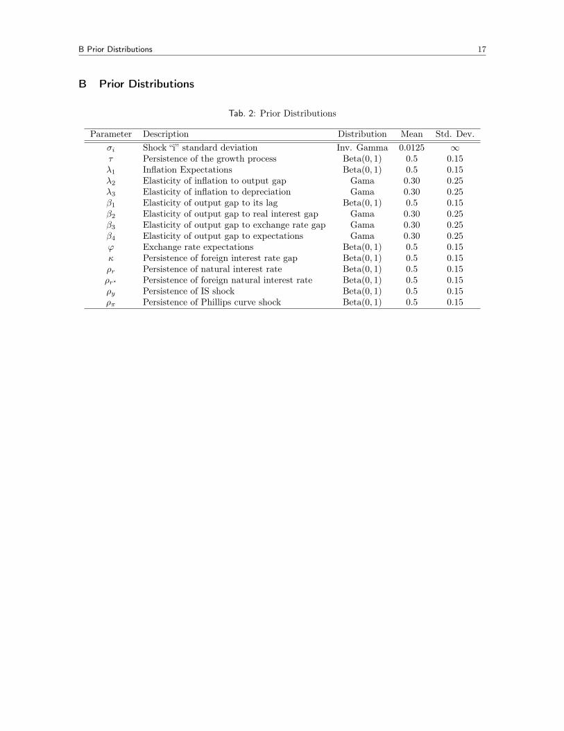
3.2 EstimationParameters that are not fixed are estimated by means of bayesian techniques, combining prior infor-mation with the model’s likelihood function (computed with the Kalman filter). Two chains of 100.000draws are used when computing the parameters’ posterior distributions. There are three types of priordistributions used. For bounded parameters (between 0 and 1) a Beta distribution is used, the meanis set to the mid point of the interval. For unbounded parameters a Gamma distribution is used, themean is set to 0.3 in accordance to previous estimations of semi-structural models. Finally the shocks’variances are all associated with an Inverse-Gamma prior distribution. Appendix B summarizes theprior distributions used for the estimation of the models. The results of the estimation procedure foreach model are presented in Appendices C and D respectively. The estimation was made using theDynare software (Adjemian et al., 2011).

4 The Output Gap

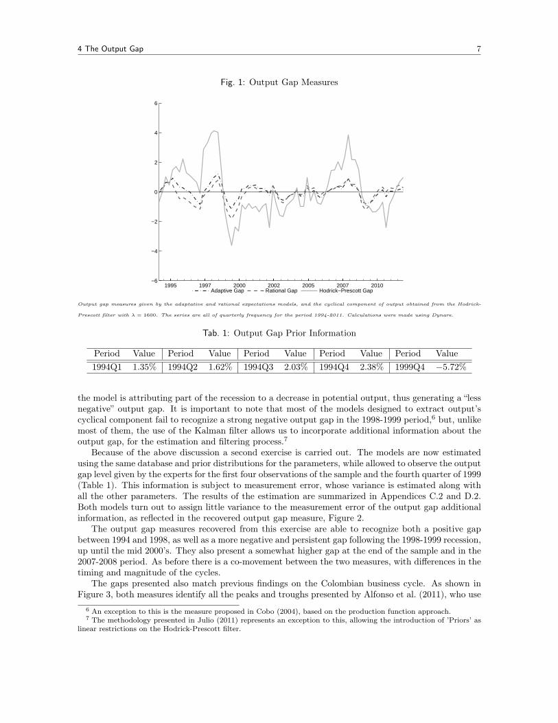
After the estimation the parameters are set to their posterior mode values. Then each model is usedto extract the output gap from the data. The output gap measure that is proposed is obtained withthe Kalman smoother for variable y in each model. Since the Hodrick-Prescott filter (henceforth HPfilter) can be represented as a special case of the local linear trend model it is used as a benchmarkfor the results (see Harvey and Jaeger (1993) and Canova (2007)). Figure 1 presents the resultsfor both models. Note that, although all three measures co-move they are not equal, showing thatthe economic models have additional information when compared to the statistical filter. The mostnotorious differences are in the 2000-2004 and 2006-2009 periods. In the first period the models identifya closed output gap whereas the HP filter still has a negative cyclical component. In the second periodthe models, specially the adaptative expectations model, fail to recognize a great increase in the outputgap, as opposed to the HP filter, which identifies a strong positive cycle.

Besides the differences between the proposed measures for the output gap and the one given bythe HP filter, there are also differences between those measures and the consensus among the experts.According to them, the gap should have been positive at the beginning of the sample and more negativeat the 1998-1999 recession. The models fail to reproduce these facts because of two reasons. First,the Kalman filter is initialized at an arbitrary point, that does not necessarily reflect the true value ofthe states. In the previous exercise the filter was initialized as if the gap was equal to zero -its steadystate value- in 1994Q1.5 Second, the local linear trend model, on top of which the proposed modelsare built, understands the data in the 1998-1999 period as a change in output’s trend, this means that

5 In Figure 1 the output gap is not equal to zero at the first period because the gap measure is given by the Kalmanfilter smoother, which takes into account the whole sample for determining the gap value at each period.

4 The Output Gap 7

Fig. 1: Output Gap Measures

1995 1997 2000 2002 2005 2007 2010−6

−4

−2

0

2

4

6

Adaptive Gap Rational Gap Hodrick−Prescott Gap

Output gap measures given by the adaptative and rational expectations models, and the cyclical component of output obtained from the Hodrick-

Prescott filter with λ = 1600. The series are all of quarterly frequency for the period 1994-2011. Calculations were made using Dynare.

Tab. 1: Output Gap Prior Information

Period Value Period Value Period Value Period Value Period Value1994Q1 1.35% 1994Q2 1.62% 1994Q3 2.03% 1994Q4 2.38% 1999Q4 −5.72%

the model is attributing part of the recession to a decrease in potential output, thus generating a “lessnegative” output gap. It is important to note that most of the models designed to extract output’scyclical component fail to recognize a strong negative output gap in the 1998-1999 period,6 but, unlikemost of them, the use of the Kalman filter allows us to incorporate additional information about theoutput gap, for the estimation and filtering process.7

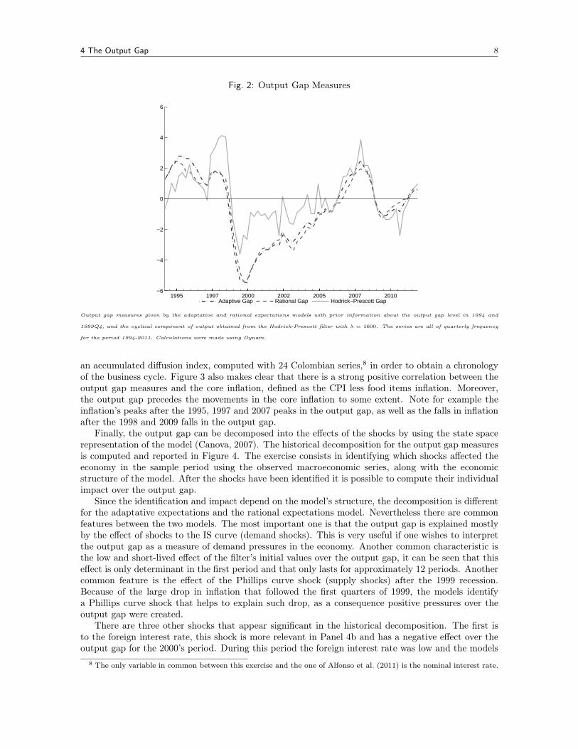
Because of the above discussion a second exercise is carried out. The models are now estimatedusing the same database and prior distributions for the parameters, while allowed to observe the outputgap level given by the experts for the first four observations of the sample and the fourth quarter of 1999(Table 1). This information is subject to measurement error, whose variance is estimated along withall the other parameters. The results of the estimation are summarized in Appendices C.2 and D.2.Both models turn out to assign little variance to the measurement error of the output gap additionalinformation, as reflected in the recovered output gap measure, Figure 2.

The output gap measures recovered from this exercise are able to recognize both a positive gapbetween 1994 and 1998, as well as a more negative and persistent gap following the 1998-1999 recession,up until the mid 2000’s. They also present a somewhat higher gap at the end of the sample and in the2007-2008 period. As before there is a co-movement between the two measures, with differences in thetiming and magnitude of the cycles.

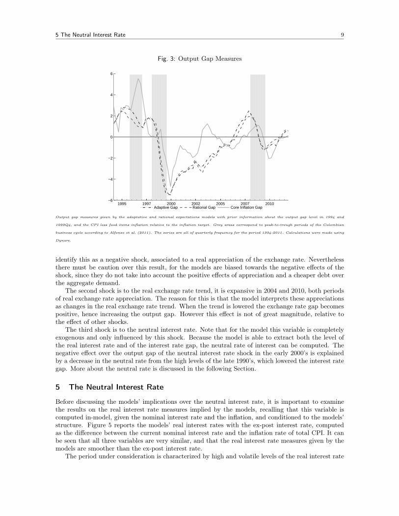
The gaps presented also match previous findings on the Colombian business cycle. As shown inFigure 3, both measures identify all the peaks and troughs presented by Alfonso et al. (2011), who use

6 An exception to this is the measure proposed in Cobo (2004), based on the production function approach.7 The methodology presented in Julio (2011) represents an exception to this, allowing the introduction of ’Priors’ as

linear restrictions on the Hodrick-Prescott filter.

4 The Output Gap 8


1995 1997 2000 2002 2005 2007 2010−6

−4

−2

0

2

4

6

Adaptive Gap Rational Gap Hodrick−Prescott Gap

Output gap measures given by the adaptative and rational expectations models with prior information about the output gap level in 1994 and

1999Q4, and the cyclical component of output obtained from the Hodrick-Prescott filter with λ = 1600. The series are all of quarterly frequency

for the period 1994-2011. Calculations were made using Dynare.

an accumulated diffusion index, computed with 24 Colombian series,8 in order to obtain a chronologyof the business cycle. Figure 3 also makes clear that there is a strong positive correlation between theoutput gap measures and the core inflation, defined as the CPI less food items inflation. Moreover,the output gap precedes the movements in the core inflation to some extent. Note for example theinflation’s peaks after the 1995, 1997 and 2007 peaks in the output gap, as well as the falls in inflationafter the 1998 and 2009 falls in the output gap.

Finally, the output gap can be decomposed into the effects of the shocks by using the state spacerepresentation of the model (Canova, 2007). The historical decomposition for the output gap measuresis computed and reported in Figure 4. The exercise consists in identifying which shocks affected theeconomy in the sample period using the observed macroeconomic series, along with the economicstructure of the model. After the shocks have been identified it is possible to compute their individualimpact over the output gap.

Since the identification and impact depend on the model’s structure, the decomposition is differentfor the adaptative expectations and the rational expectations model. Nevertheless there are commonfeatures between the two models. The most important one is that the output gap is explained mostlyby the effect of shocks to the IS curve (demand shocks). This is very useful if one wishes to interpretthe output gap as a measure of demand pressures in the economy. Another common characteristic isthe low and short-lived effect of the filter’s initial values over the output gap, it can be seen that thiseffect is only determinant in the first period and that only lasts for approximately 12 periods. Anothercommon feature is the effect of the Phillips curve shock (supply shocks) after the 1999 recession.Because of the large drop in inflation that followed the first quarters of 1999, the models identifya Phillips curve shock that helps to explain such drop, as a consequence positive pressures over theoutput gap were created.

There are three other shocks that appear significant in the historical decomposition. The first isto the foreign interest rate, this shock is more relevant in Panel 4b and has a negative effect over theoutput gap for the 2000’s period. During this period the foreign interest rate was low and the models

8 The only variable in common between this exercise and the one of Alfonso et al. (2011) is the nominal interest rate.

5 The Neutral Interest Rate 9


1995 1997 2000 2002 2005 2007 2010−6

−4

−2

0

2

4

6

Adaptive Gap Rational Gap Core Inflation Gap

Output gap measures given by the adaptative and rational expectations models with prior information about the output gap level in 1994 and

1999Q4, and the CPI less food items inflation relative to the inflation target. Grey areas correspond to peak-to-trough periods of the Colombian

business cycle according to Alfonso et al. (2011). The series are all of quarterly frequency for the period 1994-2011. Calculations were made using

Dynare.

identify this as a negative shock, associated to a real appreciation of the exchange rate. Neverthelessthere must be caution over this result, for the models are biased towards the negative effects of theshock, since they do not take into account the positive effects of appreciation and a cheaper debt overthe aggregate demand.

The second shock is to the real exchange rate trend, it is expansive in 2004 and 2010, both periodsof real exchange rate appreciation. The reason for this is that the model interprets these appreciationsas changes in the real exchange rate trend. When the trend is lowered the exchange rate gap becomespositive, hence increasing the output gap. However this effect is not of great magnitude, relative tothe effect of other shocks.

The third shock is to the neutral interest rate. Note that for the model this variable is completelyexogenous and only influenced by this shock. Because the model is able to extract both the level ofthe real interest rate and of the interest rate gap, the neutral rate of interest can be computed. Thenegative effect over the output gap of the neutral interest rate shock in the early 2000’s is explainedby a decrease in the neutral rate from the high levels of the late 1990’s, which lowered the interest rategap. More about the neutral rate is discussed in the following Section.

5 The Neutral Interest Rate

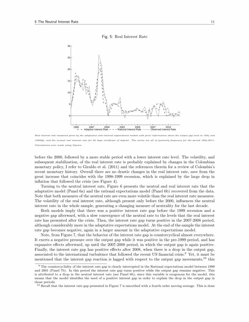
Before discussing the models’ implications over the neutral interest rate, it is important to examinethe results on the real interest rate measures implied by the models, recalling that this variable iscomputed in-model, given the nominal interest rate and the inflation, and conditioned to the models’structure. Figure 5 reports the models’ real interest rates with the ex-post interest rate, computedas the difference between the current nominal interest rate and the inflation rate of total CPI. It canbe seen that all three variables are very similar, and that the real interest rate measures given by themodels are smoother than the ex-post interest rate.

The period under consideration is characterized by high and volatile levels of the real interest rate


Fig. 4: Output Gap Historical Decomposition

(a) Adaptative Model

1995 2000 2005 2010−0.06

−0.05

−0.04

−0.03

−0.02

−0.01

0

0.01

0.02

0.03

IS ShockPot. Out. ShockGrowth ShockPhillips ShockTaylor ShockEx. Rate ShockUIP ShockN. Int. ShockF. Eq. Int. ShockF. Int. ShockInitial Values

(b) Rational Model

1995 2000 2005 2010−0.06

−0.05

−0.04

−0.03

−0.02

−0.01

0

0.01

0.02

0.03

IS ShockPot. Out. ShockGrowth ShockPhillips ShockTaylor ShockEx. Rate ShockUIP ShockN. Int. ShockF. Eq. Int. ShockF. Int. ShockInitial Values

Output gap historical decomposition in shocks given by the adaptative and rational expectations models with prior information about the output

gap level in 1994 and 1999Q4. The series are all of quarterly frequency for the period 1994-2011. Calculations were made using Dynare.


Fig. 5: Real Interest Rate

1995 1997 2000 2002 2005 2007 2010

0

5

10

15

20

25

30

Adaptive Interest Rate Rational Interest Rate Observed Interest Rate

Real interest rate measures given by the adaptative and rational expectations models with prior information about the output gap level in 1994 and

1999Q4, and the ex-post real interest rate for 90 days certificate of deposit. The series are all of quarterly frequency for the period 1994-2011.

Calculations were made using Dynare.

before the 2000, followed by a more stable period with a lower interest rate level. The volatility, andsubsequent stabilization, of the real interest rate is probably explained by changes in the Colombianmonetary policy, I refer to Giraldo et al. (2011) and the references therein for a review of Colombia’srecent monetary history. Overall there are no drastic changes in the real interest rate, save from thegreat increase that coincides with the 1998-1999 recession, which is explained by the large drop ininflation that followed the crisis (see Figure 4).

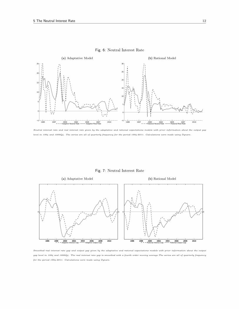
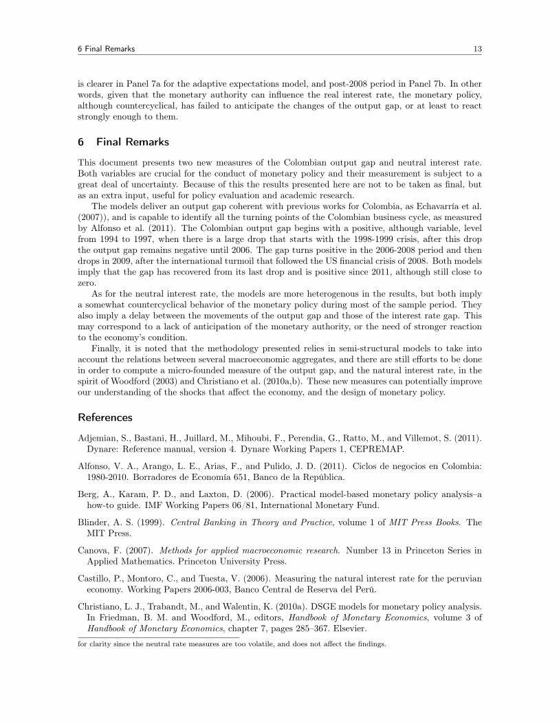
Turning to the neutral interest rate, Figure 6 presents the neutral and real interest rate that theadaptative model (Panel 6a) and the rational expectations model (Panel 6b) recovered from the data.Note that both measures of the neutral rate are even more volatile than the real interest rate measures.The volatility of the real interest rate, although present only before the 2000, influences the neutralinterest rate in the whole sample, generating a changing measure of neutrality for the last decade.

Both models imply that there was a positive interest rate gap before the 1999 recession and anegative gap afterward, with a slow convergence of the neutral rate to the levels that the real interestrate has presented after the crisis. Then, the interest rate gap turns positive in the 2007-2008 period,although considerably more in the adaptative expectations model. At the end of the sample the interestrate gap becomes negative, again in a larger amount in the adaptative expectations model.

Note, from Figure 7, that the behavior of the interest rate gap is countercyclical almost everywhere.It exerts a negative pressure over the output gap while it was positive in the pre-1999 period, and hasexpansive effects afterward, up until the 2007-2008 period, in which the output gap is again positive.Finally, the interest rate gap has positive effects after 2008, when there is a drop in the output gap,associated to the international turbulence that followed the recent US financial crisis.9 Yet, it must bementioned that the interest gap reaction is lagged with respect to the output gap movements,10 this

9 The countercyclality of the interest rate gap is clearly interrupted in the Rational expectations model between 1999and 2001 (Panel 7b). In this period the interest rate gap turns positive while the output gap remains negative. Thisis attributed to a drop in the neutral interest rate (see Panel 6b), since this variable is exogenous for the model, thismeans that the model identifies the need of a positive interest gap in order to explain the drop in the output gap inthose periods.

10 Recall that the interest rate gap presented in Figure 7 is smoothed with a fourth order moving average. This is done


Fig. 6: Neutral Interest Rate


1995 1997 2000 2002 2005 2007 2010−5

0

5

10

15

20

25

Adaptive Neutral Rate Adaptive Real Rate

(b) Rational Model

1995 1997 2000 2002 2005 2007 2010−5

0

5

10

15

20

25

30

Rational Neutral Rate Rational Real Rate

Neutral interest rate and real interest rate given by the adaptative and rational expectations models with prior information about the output gap

level in 1994 and 1999Q4. The series are all of quarterly frequency for the period 1994-2011. Calculations were made using Dynare.

Fig. 7: Neutral Interest Rate


1996 1998 2000 2002 2004 2006 2008 2010

0

1996 1998 2000 2002 2004 2006 2008 2010

0

Adaptive Interest Gap Adaptive Output Gap

(b) Rational Model

1996 1998 2000 2002 2004 2006 2008 2010

0

1996 1998 2000 2002 2004 2006 2008 2010

0

Rational Interest Gap Rational Output Gap

Smoothed real interest rate gap and output gap given by the adaptative and rational expectations models with prior information about the output

gap level in 1994 and 1999Q4. The real interest rate gap is smoothed with a fourth order moving average.The series are all of quarterly frequency

for the period 1994-2011. Calculations were made using Dynare.

6 Final Remarks 13

is clearer in Panel 7a for the adaptive expectations model, and post-2008 period in Panel 7b. In otherwords, given that the monetary authority can influence the real interest rate, the monetary policy,although countercyclical, has failed to anticipate the changes of the output gap, or at least to reactstrongly enough to them.

6 Final Remarks

This document presents two new measures of the Colombian output gap and neutral interest rate.Both variables are crucial for the conduct of monetary policy and their measurement is subject to agreat deal of uncertainty. Because of this the results presented here are not to be taken as final, butas an extra input, useful for policy evaluation and academic research.

The models deliver an output gap coherent with previous works for Colombia, as Echavarría et al.(2007)), and is capable to identify all the turning points of the Colombian business cycle, as measuredby Alfonso et al. (2011). The Colombian output gap begins with a positive, although variable, levelfrom 1994 to 1997, when there is a large drop that starts with the 1998-1999 crisis, after this dropthe output gap remains negative until 2006. The gap turns positive in the 2006-2008 period and thendrops in 2009, after the international turmoil that followed the US financial crisis of 2008. Both modelsimply that the gap has recovered from its last drop and is positive since 2011, although still close tozero.

As for the neutral interest rate, the models are more heterogenous in the results, but both implya somewhat countercyclical behavior of the monetary policy during most of the sample period. Theyalso imply a delay between the movements of the output gap and those of the interest rate gap. Thismay correspond to a lack of anticipation of the monetary authority, or the need of stronger reactionto the economy’s condition.

Finally, it is noted that the methodology presented relies in semi-structural models to take intoaccount the relations between several macroeconomic aggregates, and there are still efforts to be donein order to compute a micro-founded measure of the output gap, and the natural interest rate, in thespirit of Woodford (2003) and Christiano et al. (2010a,b). These new measures can potentially improveour understanding of the shocks that affect the economy, and the design of monetary policy.

References

Adjemian, S., Bastani, H., Juillard, M., Mihoubi, F., Perendia, G., Ratto, M., and Villemot, S. (2011).Dynare: Reference manual, version 4. Dynare Working Papers 1, CEPREMAP.

Alfonso, V. A., Arango, L. E., Arias, F., and Pulido, J. D. (2011). Ciclos de negocios en Colombia:1980-2010. Borradores de Economía 651, Banco de la República.

Berg, A., Karam, P. D., and Laxton, D. (2006). Practical model-based monetary policy analysis–ahow-to guide. IMF Working Papers 06/81, International Monetary Fund.

Blinder, A. S. (1999). Central Banking in Theory and Practice, volume 1 of MIT Press Books. TheMIT Press.

Canova, F. (2007). Methods for applied macroeconomic research. Number 13 in Princeton Series inApplied Mathematics. Princeton University Press.

Castillo, P., Montoro, C., and Tuesta, V. (2006). Measuring the natural interest rate for the peruvianeconomy. Working Papers 2006-003, Banco Central de Reserva del Perú.

Christiano, L. J., Trabandt, M., and Walentin, K. (2010a). DSGE models for monetary policy analysis.In Friedman, B. M. and Woodford, M., editors, Handbook of Monetary Economics, volume 3 ofHandbook of Monetary Economics, chapter 7, pages 285–367. Elsevier.

for clarity since the neutral rate measures are too volatile, and does not affect the findings.

6 Final Remarks 14

Christiano, L. J., Trabandt, M., and Walentin, K. (2010b). Involuntary unemployment and the businesscycle. NBER Working Papers 15801, National Bureau of Economic Research, Inc.

Cobo, A. (2004). Output gap in Colombia: An eclectic aproach. Borradores de Economía 327, Bancode la República.

Echavarría, J. J., López, E., Misas, M., Téllez, J., and Parra, J. C. (2007). La tasa de interés naturalen Colombia. Ensayos sobre política económica, 25(54):44–89.

Garnier, J. and Wilhelmsen, B.-R. (2009). The natural rate of interest and the output gap in the euroarea: a joint estimation. Empirical Economics, 36(2):297–319.

Giraldo, A., Misas, M., and Villa, E. (2011). Reconstructing the recent monetary policy history ofColombia from 1990 to 2010. Vniversitas Económica 008860, Pontificia Universidad Javeriana -Bogotá.

Gómez, J. and Julio, J. M. (1998). Output gap estimation, estimation uncertainty and its effect onpolicy rules. Ensayos sobre política económica, (34):89–117.

González, E., Melo, L. F., Rojas, L. E., and Rojas, B. (2010). Estimations of the natural rate ofinterest in Colombia. Borradores de Economía 626, Banco de la República.

Harvey, A. C. and Jaeger, A. (1993). Detrending, stylized facts and the business cycle. Journal ofApplied Econometrics, 8(3):231–47.

Julio, J. M. (2011). The hodrick-prescott filter with priors: linear restrictions on hp filters. MPRAPaper 34202, University Library of Munich, Germany.

Laubach, T. and Williams, J. C. (2003). Measuring the natural rate of interest. The Review ofEconomics and Statistics, 85(4):1063–1070.

Mesonnier, J.-S. and Renne, J.-P. (2007). A time-varying "natural" rate of interest for theeuro area. European Economic Review, 51(7):1768–1784.

Orphanides, A. and Williams, J. C. (2002). Robust monetary policy rules with unknown natural rates.Brookings Papers on Economic Activity, 33(2):63–146.

Rodríguez, N., Torres, J. L., and Velasco, A. (2006). Estimating an output gap indicator using businesssurveys and real data. Borradores de Economía 392I, Banco de la República.

Taylor, J. B. (1993). Discretion versus policy rules in practice. Carnegie-Rochester Conference Serieson Public Policy, 39(1):195–214.

Taylor, J. B. (1999). Monetary Policy Rules. Number tayl99-1 in NBER Books. National Bureau ofEconomic Research, Inc.

Torres, J. L. (2007). La estimación de la brecha del producto en Colombia. Borradores de Economía462, Banco de la República.

Woodford, M. (2003). Interest and Prices: Foundations of a Theory of Monetary Policy. PrincetonUniversity Press.

A Equations 15

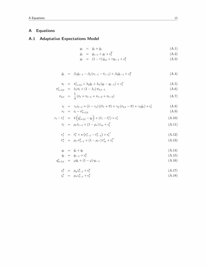
A Equations

A.1 Adaptative Expectations Model

yt = yt + yt (A.1)

yt = yt−1 + gt + εyt (A.2)gt = (1− τ) gss + τgt−1 + εgt (A.3)

yt = β1yt−1 − β2 (rt−1 − rt−1) + β3qt−1 + zyt (A.4)

πt = πet+1|t + λ2yt + λ3 (qt − qt−1) + zπt (A.5)πet+1|t = λ1πt + (1− λ1)π4,t−1 (A.6)

π4,t =1

4(πt + πt−1 + πt−2 + πt−3) (A.7)

it = γ1it−1 + (1− γ1) ((rt + π) + γ2 (π4,t − π) + γ3yt) + εit (A.8)rt = it − πet+1|t (A.9)

rt − r?t = 4(qet+1|t − qt

)+ (rt − r?t ) + εrt (A.10)

rt = ρr rt−1 + (1− ρr) rss + εrt (A.11)

r?t = r?t + κ(r?t−1 − r?t−1

)+ εr

?

t (A.12)

r?t = ρr? r?t−1 + (1− ρr?) r?ss + εr

?

t (A.13)

qt = qt + qt (A.14)qt = qt−1 + εqt (A.15)

qet+1|t = ϕqt + (1− ϕ) qt−1 (A.16)

zyt = ρyzyt−1 + εyt (A.17)

zπt = ρπzπt−1 + επt (A.18)

A Equations 16

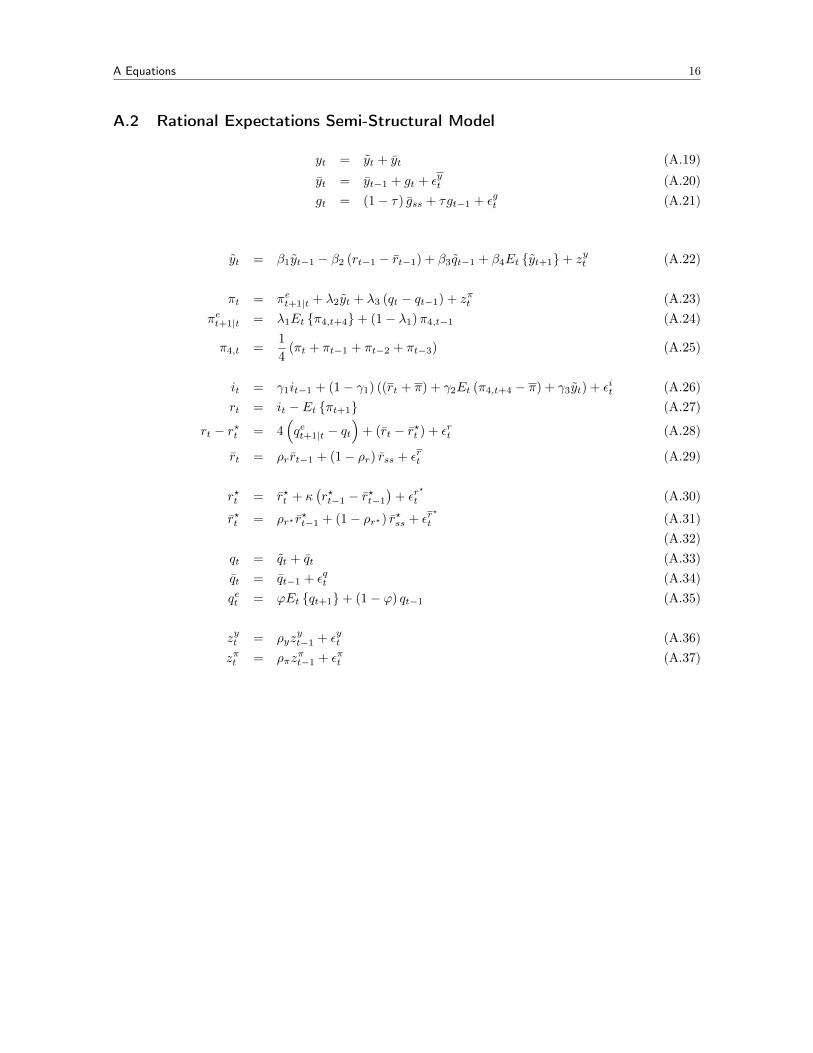
A.2 Rational Expectations Semi-Structural Model

yt = yt + yt (A.19)

yt = yt−1 + gt + εyt (A.20)gt = (1− τ) gss + τgt−1 + εgt (A.21)

yt = β1yt−1 − β2 (rt−1 − rt−1) + β3qt−1 + β4Et {yt+1}+ zyt (A.22)

πt = πet+1|t + λ2yt + λ3 (qt − qt−1) + zπt (A.23)πet+1|t = λ1Et {π4,t+4}+ (1− λ1)π4,t−1 (A.24)

π4,t =1

4(πt + πt−1 + πt−2 + πt−3) (A.25)

it = γ1it−1 + (1− γ1) ((rt + π) + γ2Et (π4,t+4 − π) + γ3yt) + εit (A.26)rt = it − Et {πt+1} (A.27)

rt − r?t = 4(qet+1|t − qt

)+ (rt − r?t ) + εrt (A.28)

rt = ρr rt−1 + (1− ρr) rss + εrt (A.29)

r?t = r?t + κ(r?t−1 − r?t−1

)+ εr

?

t (A.30)

r?t = ρr? r?t−1 + (1− ρr?) r?ss + εr

?

t (A.31)(A.32)

qt = qt + qt (A.33)qt = qt−1 + εqt (A.34)qet = ϕEt {qt+1}+ (1− ϕ) qt−1 (A.35)

zyt = ρyzyt−1 + εyt (A.36)

zπt = ρπzπt−1 + επt (A.37)

B Prior Distributions 17

B Prior Distributions

Tab. 2: Prior Distributions

Parameter Description Distribution Mean Std. Dev.σi Shock “i” standard deviation Inv. Gamma 0.0125 ∞τ Persistence of the growth process Beta(0, 1) 0.5 0.15λ1 Inflation Expectations Beta(0, 1) 0.5 0.15λ2 Elasticity of inflation to output gap Gama 0.30 0.25λ3 Elasticity of inflation to depreciation Gama 0.30 0.25β1 Elasticity of output gap to its lag Beta(0, 1) 0.5 0.15β2 Elasticity of output gap to real interest gap Gama 0.30 0.25β3 Elasticity of output gap to exchange rate gap Gama 0.30 0.25β4 Elasticity of output gap to expectations Gama 0.30 0.25ϕ Exchange rate expectations Beta(0, 1) 0.5 0.15κ Persistence of foreign interest rate gap Beta(0, 1) 0.5 0.15ρr Persistence of natural interest rate Beta(0, 1) 0.5 0.15ρr? Persistence of foreign natural interest rate Beta(0, 1) 0.5 0.15ρy Persistence of IS shock Beta(0, 1) 0.5 0.15ρπ Persistence of Phillips curve shock Beta(0, 1) 0.5 0.15

C Estimation Results - Adaptative Expectations Model 18

C Estimation Results - Adaptative Expectations Model

C.1 Unconditioned Estimation

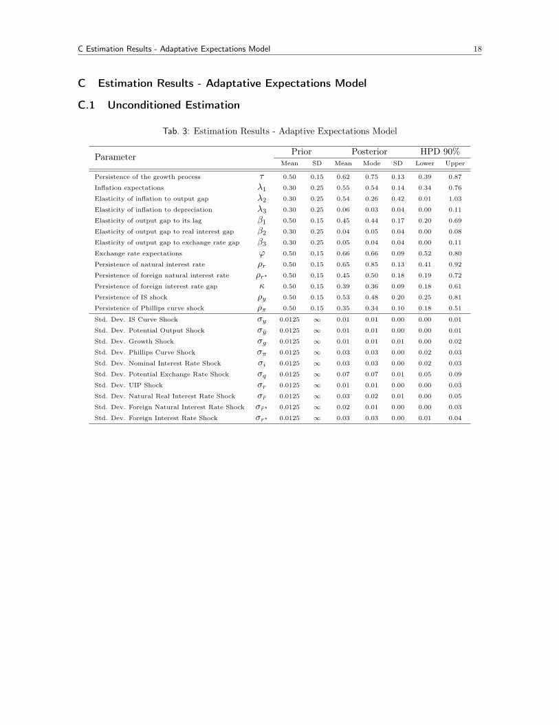
Tab. 3: Estimation Results - Adaptive Expectations Model

Parameter Prior Posterior HPD 90%Mean SD Mean Mode SD Lower Upper

Persistence of the growth process τ 0.50 0.15 0.62 0.75 0.13 0.39 0.87

Inflation expectations λ1 0.30 0.25 0.55 0.54 0.14 0.34 0.76

Elasticity of inflation to output gap λ2 0.30 0.25 0.54 0.26 0.42 0.01 1.03

Elasticity of inflation to depreciation λ3 0.30 0.25 0.06 0.03 0.04 0.00 0.11

Elasticity of output gap to its lag β1 0.50 0.15 0.45 0.44 0.17 0.20 0.69

Elasticity of output gap to real interest gap β2 0.30 0.25 0.04 0.05 0.04 0.00 0.08

Elasticity of output gap to exchange rate gap β3 0.30 0.25 0.05 0.04 0.04 0.00 0.11

Exchange rate expectations ϕ 0.50 0.15 0.66 0.66 0.09 0.52 0.80

Persistence of natural interest rate ρr 0.50 0.15 0.65 0.85 0.13 0.41 0.92

Persistence of foreign natural interest rate ρr? 0.50 0.15 0.45 0.50 0.18 0.19 0.72

Persistence of foreign interest rate gap κ 0.50 0.15 0.39 0.36 0.09 0.18 0.61

Persistence of IS shock ρy 0.50 0.15 0.53 0.48 0.20 0.25 0.81

Persistence of Phillips curve shock ρπ 0.50 0.15 0.35 0.34 0.10 0.18 0.51

Std. Dev. IS Curve Shock σy 0.0125 ∞ 0.01 0.01 0.00 0.00 0.01

Std. Dev. Potential Output Shock σy 0.0125 ∞ 0.01 0.01 0.00 0.00 0.01

Std. Dev. Growth Shock σg 0.0125 ∞ 0.01 0.01 0.01 0.00 0.02

Std. Dev. Phillips Curve Shock σπ 0.0125 ∞ 0.03 0.03 0.00 0.02 0.03

Std. Dev. Nominal Interest Rate Shock σi 0.0125 ∞ 0.03 0.03 0.00 0.02 0.03

Std. Dev. Potential Exchange Rate Shock σq 0.0125 ∞ 0.07 0.07 0.01 0.05 0.09

Std. Dev. UIP Shock σr 0.0125 ∞ 0.01 0.01 0.00 0.00 0.03

Std. Dev. Natural Real Interest Rate Shock σr 0.0125 ∞ 0.03 0.02 0.01 0.00 0.05

Std. Dev. Foreign Natural Interest Rate Shock σr? 0.0125 ∞ 0.02 0.01 0.00 0.00 0.03

Std. Dev. Foreign Interest Rate Shock σr? 0.0125 ∞ 0.03 0.03 0.00 0.01 0.04


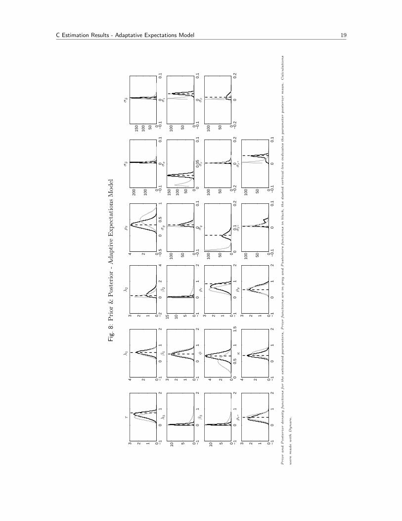
Fig.

8:Prior

&Posterior

-Ada

ptiveExp

ectation

sMod

el

−1

01

20123

τ

−1

01

2024

λ1

−2

02

40123

λ2

−1

01

20510

λ3

−1

01

20123

β1

−1

01

2051015

β2

−1

01

20510

β3

00.

51

1.5

024

φ

−1

01

20123

ρ r

−1

01

20123

ρ r∗

−1

01

2024

κ

−1

01

20123

ρ y

−0.

50

0.5

1024

ρ π

−0.

10

0.1

0

100

200

σy

−0.

10

0.1

050100

150

σy

−0.

10

0.1

050100

σg

00.

050.

1050100

150

σπ

−0.

10

0.1

050100

σi

00.

10.

2050100

σq

−0.

20

0.2

050100

σr

−0.

20

0.2

050100

σr

−0.

10

0.1

050100

σr∗

−0.

10

0.1

050100

σr∗

PriorandPosteriordensity

functionsfortheestim

atedparameters,Priorfunctionsare

ingrayandPosteriors

functionsin

black,thedashed

verticallineindicatestheparameterposteriormean.Calculations

were

madewithDynare.


C.2 Conditioned Estimation

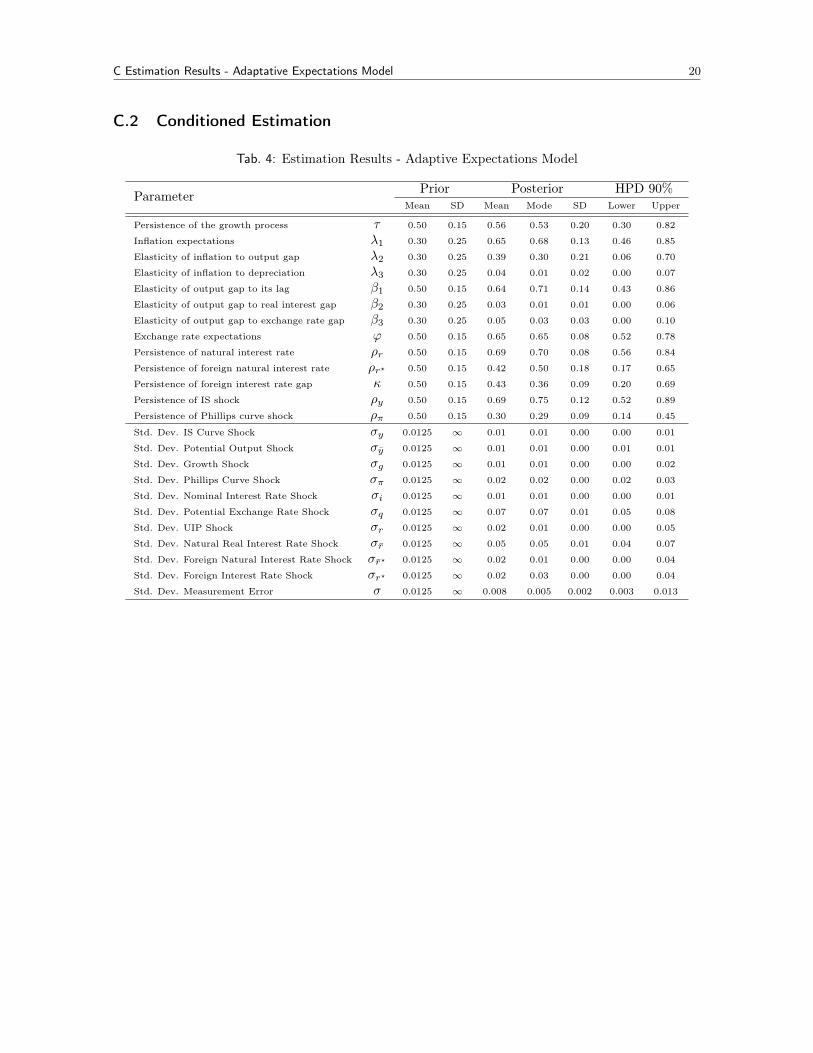
Tab. 4: Estimation Results - Adaptive Expectations Model

























Std. Dev. Measurement Error σ 0.0125 ∞ 0.008 0.005 0.002 0.003 0.013


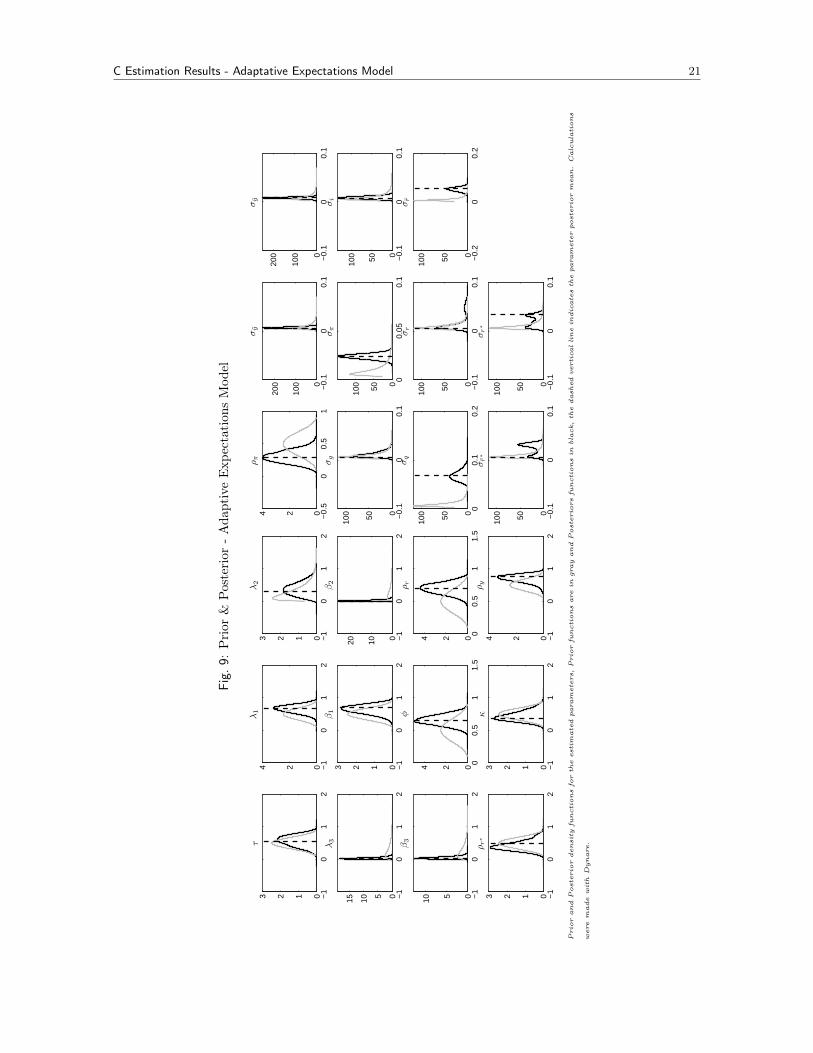
Fig.

9:Prior

&Posterior

-Ada

ptiveExp

ectation

sMod

el

−1

01

20123

τ

−1

01

2024

λ1

−1

01

20123

λ2

−1

01

2051015

λ3

−1

01

20123

β1

−1

01

201020

β2

−1

01

20510

β3

00.

51

1.5

024

φ

00.

51

1.5

024

ρ r

−1

01

20123

ρ r∗

−1

01

20123

κ

−1

01

2024

ρ y

−0.

50

0.5

1024

ρ π

−0.

10

0.1

0

100

200

σy

−0.

10

0.1

0

100

200

σy

−0.

10

0.1

050100

σg

00.

050.

1050100

σπ

−0.

10

0.1

050100

σi

00.

10.

2050100

σq

−0.

10

0.1

050100

σr

−0.

20

0.2

050100

σr

−0.

10

0.1

050100

σr∗

−0.

10

0.1

050100

σr∗




ingrayandPosteriors

functionsin

black,thedashed


were

madewithDynare.

D Estimation Results - Rational Expectations Model 22

D Estimation Results - Rational Expectations Model

D.1 Unconditioned Estimation

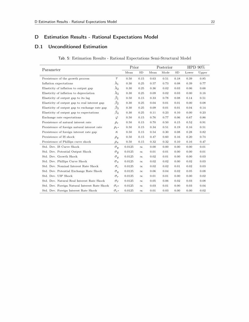
Tab. 5: Estimation Results - Rational Expectations Semi-Structural Model









Elasticity of output gap to expectations β4 0.30 0.25 0.11 0.23 0.10 0.00 0.23


















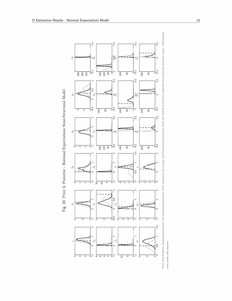
Fig.

10:Prior

&Posterior

-Rationa

lExp

ectation

sSemi-S

truc

turalM

odel

−1

01

20123

τ

−1

01

2024

λ1

−1

01

20123

λ2

−1

01

202468

λ3

−0.

50

0.5

1024

β1

−1

01

2051015

β2

−1

01

20510

β3

−1

01

20246

β4

00.

51

1.5

0246

φ

00.

51

1.5

024ρ r

−1

01

2024

ρ r∗

−1

01

20123

κ

−1

01

20123

ρ y

−0.

50

0.5

1024

ρ π

−0.

10

0.1

0

100

200

300

σy

−0.

10

0.1

050100

150

σy

−0.

10

0.1

050100

σg

00.

050.

1050100

150

σπ

−0.

10

0.1

050100

σi

00.

10.

2050100

σq

−0.

10

0.1

050100

σr

−0.

20

0.2

050100

σr

−0.

10

0.1

050100

σr∗

−0.

10

0.1

050100

σr∗




ingrayandPosteriors

functionsin

black,thedashed


were

madewithDynare.


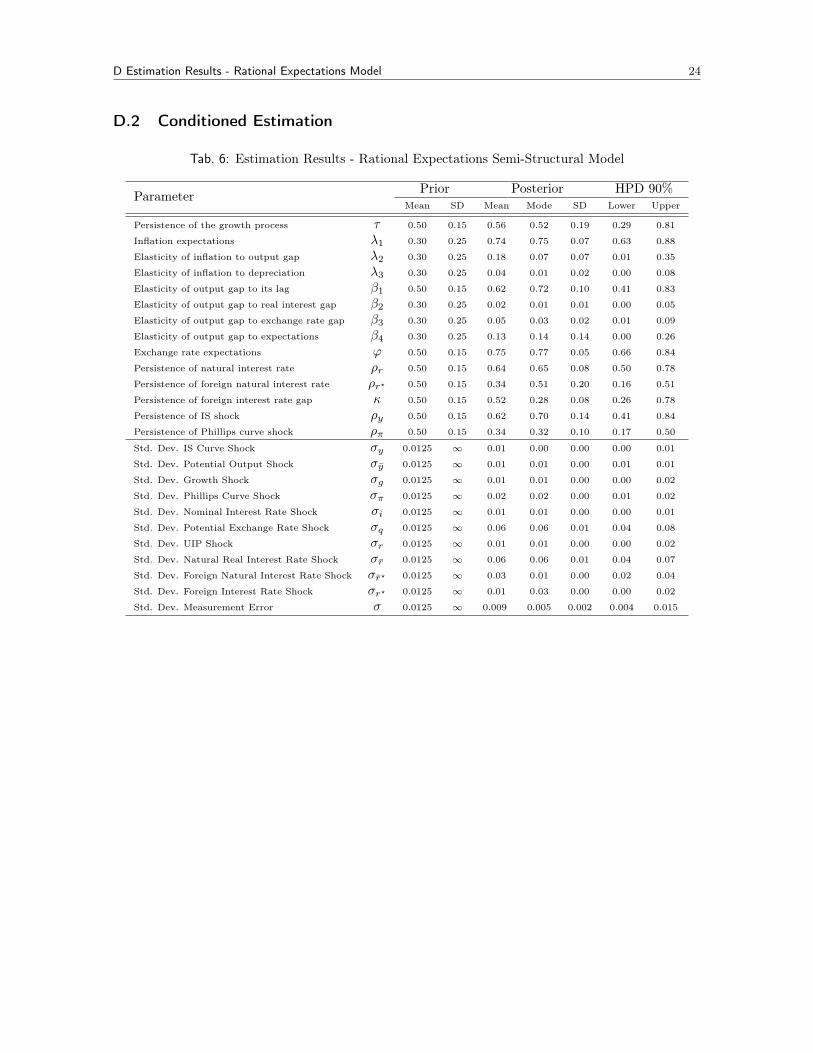
D.2 Conditioned Estimation

Tab. 6: Estimation Results - Rational Expectations Semi-Structural Model









Elasticity of output gap to expectations β4 0.30 0.25 0.13 0.14 0.14 0.00 0.26

















Std. Dev. Measurement Error σ 0.0125 ∞ 0.009 0.005 0.002 0.004 0.015


Fig.

11:Prior

&Posterior

-Rationa

lExp

ectation

sSemi-S

truc

turalM

odel

−1

01

20123

τ

−1

01

2024

λ1

−1

01

20123

λ2

−1

01

202468

λ3

−0.

50

0.5

1024

β1

−1

01

2051015

β2

−1

01

20510

β3

−1

01

20246

β4

00.

51

1.5

0246

φ

00.

51

1.5

024ρ r

−1

01

2024

ρ r∗

−1

01

20123

κ

−1

01

20123

ρ y

−0.

50

0.5

1024

ρ π

−0.

10

0.1

0

100

200

300

σy

−0.

10

0.1

050100

150

σy

−0.

10

0.1

050100

σg

00.

050.

1050100

150

σπ

−0.

10

0.1

050100

σi

00.

10.

2050100

σq

−0.

10

0.1

050100

σr

−0.

20

0.2

050100

σr

−0.

10

0.1

050100

σr∗

−0.

10

0.1

050100

σr∗




ingrayandPosteriors

functionsin

black,thedashed


were

madewithDynare.

Documents

Output gap and Neutral interest measures for Colombia