OPTION PRICING IN NON-COMPETITIVE MARKETS

HAI ZHANG

A DISSERTATION SUBMITTED TOTHE FACULTY OF GRADUATE STUDIES

IN PARTIAL FULFILMENT OF THE REQUIREMENTSFOR THE DEGREE OF

DOCTOR OF PHILOSOPHY

GRADUATE PROGRAM IN MATHEMATICS AND STATISTICSYORK UNIVERSITY

TORONTO, ONTARIO

April 2017

c©Hai Zhang 2017

Abstract

In the classic option pricing theory, the market is assumed to be competitive. The relax-

ation of the competitive market assumption introduces two features: liquidity cost and

feedback effect. In our study, investors in non-competitive markets are divided into two

categories: small investors and large investors. Small investors encounter liquidity cost

while large investors face both liquidity cost and feedback effect. For small investors, liq-

uidity cost could be modelled by a supply curve function. For large investors, liquidity cost

could be modelled via trading speed and a trading action is assumed to have a feedback

effect on underlying asset price. Chapter 2 and chapter 3 are dedicated to investigate the

option pricing for small investors. In chapter 2, how to perfectly hedge options (including

vanilla options and exotic options) under the supply curve model in a geometric Brownian

motion model was studied. In Chapter 3,local risk minimization method was used to price

European options with liquidity cost in a jump-diffusion model. In chapter 4, the utility

indifference pricing method was applied to price European options for large investors.

ii

Acknowledgements

I would like to express my very great appreciation to my supervisor Professor Hyejin Ku

for the time investing into me and the help during my PhD study at York University. I

am grateful to my thesis committee: Professor Huaiping Zhu and Dr. Ping Wu for their

support and suggestions.

iii

Table of Contents

Abstract ii

Acknowledgements iii

Table of Contents iv

List of Tables vii

List of Figures ix

1 Introduction 1

1.1 Dissertation Objective . . . . . . . . . . . . . . . . . . . . . . . . . . . . 1

1.2 Background . . . . . . . . . . . . . . . . . . . . . . . . . . . . . . . . . 1

1.3 Option pricing in a perfect market . . . . . . . . . . . . . . . . . . . . . 3

1.4 Option pricing in non-competitive markets . . . . . . . . . . . . . . . . . 4

1.5 Chapter Breakdown . . . . . . . . . . . . . . . . . . . . . . . . . . . . . 11

iv

2 Options Pricing and Hedging for Small Investors 13

2.1 Introduction . . . . . . . . . . . . . . . . . . . . . . . . . . . . . . . . . 13

2.2 The supply curve model . . . . . . . . . . . . . . . . . . . . . . . . . . . 15

2.3 European options . . . . . . . . . . . . . . . . . . . . . . . . . . . . . . 19

2.4 Upper bound and lower bound of option prices . . . . . . . . . . . . . . 26

2.4.1 Asymptotic Expansion . . . . . . . . . . . . . . . . . . . . . . . 30

2.4.2 Numerical results of European options . . . . . . . . . . . . . . 36

2.5 American options . . . . . . . . . . . . . . . . . . . . . . . . . . . . . . 42

2.5.1 Numerical results . . . . . . . . . . . . . . . . . . . . . . . . . . 45

2.6 Exotic options . . . . . . . . . . . . . . . . . . . . . . . . . . . . . . . . 46

2.6.1 Barrier options . . . . . . . . . . . . . . . . . . . . . . . . . . . 47

2.6.2 Asian options . . . . . . . . . . . . . . . . . . . . . . . . . . . . 48

3 Option Pricing with Liquidity Risk in a Jump-diffusion Model 54

3.1 Introduction . . . . . . . . . . . . . . . . . . . . . . . . . . . . . . . . . 54

3.2 Local risk minimization in a jump-diffusion model . . . . . . . . . . . . 56

3.3 Approximate a jump-diffusion process with a discrete-time model . . . . 60

3.4 Supply curve model and Local risk minimization considering liquidity risk 65

3.5 Numerical results . . . . . . . . . . . . . . . . . . . . . . . . . . . . . . 69

v

4 Utility Indifference Pricing for Large Investors 73

4.1 Introduction . . . . . . . . . . . . . . . . . . . . . . . . . . . . . . . . . 73

4.2 The Model . . . . . . . . . . . . . . . . . . . . . . . . . . . . . . . . . . 75

4.2.1 Permanent price impact modelling . . . . . . . . . . . . . . . . . 75

4.2.2 Liquidity risk modelling . . . . . . . . . . . . . . . . . . . . . . 77

4.2.3 No arbitrage under large investor model . . . . . . . . . . . . . . 78

4.3 Utility indifference price for European options . . . . . . . . . . . . . . 84

4.3.1 An example of utility indifference pricing . . . . . . . . . . . . . 84

4.3.2 Utility indifference pricing for European options . . . . . . . . . 85

4.4 Existence and uniqueness of the solution of the HJB equation . . . . . . . 88

4.5 Example and numerical experiments . . . . . . . . . . . . . . . . . . . . 103

4.5.1 Example of the trading speed model and the feedback effects model 103

4.5.2 Numerical results . . . . . . . . . . . . . . . . . . . . . . . . . . 108

4.5.3 An extended large investor model . . . . . . . . . . . . . . . . . 112

5 Conclusions and Future Work 114

Bibliography 117

vi

List of Tables

1.1 Different models with respect to liquidity cost and feedback effects . . . . 9

2.1 Seller’s and Buyer’s replication costs with different Strikes and liquidity

parameters when T = 1. . . . . . . . . . . . . . . . . . . . . . . . . . . . 37

2.2 Buyer’s and Seller’s replication costs with different Strikes and liquidity

parameters when T = 0.5. . . . . . . . . . . . . . . . . . . . . . . . . . . 38

2.3 Option seller’ prices comparison of PDE method and approximation formula 40

2.4 Monte Carlo simulation of hedging error. . . . . . . . . . . . . . . . . . 42

2.5 American option’s replication costs with different Strikes and liquidity pa-

rameters. . . . . . . . . . . . . . . . . . . . . . . . . . . . . . . . . . . . 46

2.6 Barrier option’s replication costs with different Strikes and liquidity pa-

rameters. . . . . . . . . . . . . . . . . . . . . . . . . . . . . . . . . . . . 49

2.7 Asian option’s replication costs with different Strikes and liquidity param-

eters. . . . . . . . . . . . . . . . . . . . . . . . . . . . . . . . . . . . . . 53

vii

3.1 Option prices with different Strikes and volatility . . . . . . . . . . . . . 71

3.2 Option prices with different values of λ1 and λ2 . . . . . . . . . . . . . . 72

3.3 Comparison of results of three hedging strategies when σ = 0.2 and T = 1 72

3.4 Comparison of results of three hedging strategies when σ = 0.3 and T = 1 72

4.1 Utility indifference price with different α and β. . . . . . . . . . . . . . . 108

4.2 Utility indifference price with different α and β when M = 5. . . . . . . . 109

4.3 Utility indifference price with different α and β when M = 100. . . . . . 109

4.4 Utility indifference price with different α and β when M = 500. . . . . . 110

4.5 Utility indifference price with different α and β when M = 1000. . . . . . 110

4.6 Utility indifference price when γ = 5 × 10−8 with different α and β . . . . 113

viii

List of Figures

2.1 Traded stock price under supply curve model . . . . . . . . . . . . . . . 16

2.2 Buyer’s and seller’s prices with varying Strikes . . . . . . . . . . . . . . 38

2.3 Buyer’s and seller’s prices with varying f’(0) . . . . . . . . . . . . . . . 39

2.4 Option seller’ prices comparison of PDE method and approximation formula 40

3.1 3 periods trinomial model to approximate a jump-diffusion model . . . . 62

4.1 Optimal Trading Speed at Fixed Time . . . . . . . . . . . . . . . . . . . 111

ix

1 Introduction

1.1 Dissertation Objective

The objective of this dissertation is to study how to price options in non-competitive mar-

kets. Based on new features of non-competitive markets, liquidity cost and feedback ef-

fects, market participants are divided into two categories: small investors and large in-

vestors. Different pricing models are proposed for both small and large investors.

1.2 Background

As financial markets grow, derivatives have become more and more important for specu-

lating and hedging purposes. Derivatives are financial contracts whose value depends on

underlying variables. Futures, options, swaps, and forwards are the main categories of

derivatives. The valuation of derivatives poses one of the most important challenges in

mathematical finance. The Black-Scholes option pricing model proved a breakthrough in

pricing derivatives. Its main insight is that options can be replicated by two primary assets:

1

the underlying stock and the bank account. The option’s price is simply the value of the

portfolio consisting of the underlying asset and the bank account.

It is well known, however, that the Black-Scholes option pricing model was built on ex-

cessively restrictive assumptions on market conditions and asset processes. The following

assumptions provide an ideal world for deriving the Black-Scholes equation:

1. There are no transaction costs (including taxes) and no restrictions on trading (e.g.

short sale constraints). These two conditions contribute to a frictionless market.

2. An investor can buy or sell unlimited quantities of the stock without changing the

stock price. This assumption contributes to a competitive market.

3. The interest rate is constant, and the stock price follows a geometric Brownian mo-

tion with constant drift and volatility. These conditions forms a complete market.

A market satisfying both assumptions (1) and (2) is considered to be a perfect market. It

is important to distinguish complete market from perfect market. Note that a market could

be complete but imperfect. If there are transaction costs in the market, but the interest

rate is constant and the stock price follows a geometric Brownian motion, the market is

imperfect but complete. A market could also be incomplete but perfect, for instance, a

jump-diffusion model without transaction cost. In a Black-Scholes world, it satisfies all

the three assumptions above, so the market is both perfect and complete. The options

2

become redundant securities and can be replicated by the stock and the bank account

(Merton (1976)). Therefore, the replication cost is the unique option price.

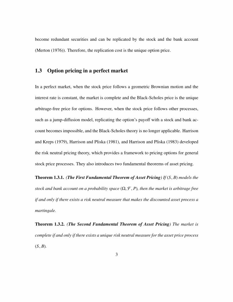
1.3 Option pricing in a perfect market

In a perfect market, when the stock price follows a geometric Brownian motion and the

interest rate is constant, the market is complete and the Black-Scholes price is the unique

arbitrage-free price for options. However, when the stock price follows other processes,

such as a jump-diffusion model, replicating the option’s payoff with a stock and bank ac-

count becomes impossible, and the Black-Scholes theory is no longer applicable. Harrison

and Kreps (1979), Harrison and Pliska (1981), and Harrison and Pliska (1983) developed

the risk neutral pricing theory, which provides a framework to pricing options for general

stock price processes. They also introduces two fundamental theorems of asset pricing.

Theorem 1.3.1. (The First Fundamental Theorem of Asset Pricing) If (S , B) models the

stock and bank account on a probability space (Ω,F , P), then the market is arbitrage free

if and only if there exists a risk neutral measure that makes the discounted asset process a

martingale.

Theorem 1.3.2. (The Second Fundamental Theorem of Asset Pricing) The market is

complete if and only if there exists a unique risk neutral measure for the asset price process

(S , B).

3

Risk neutral pricing is a general pricing method and can be used to price options in

general asset price models. Let V(t, S t) denote the option price at time t with the stock

price S t, and the payoff of the option (S T − K)+ at the time of maturity T . In a perfect and

arbitrage free market, the value of a European option is the discounted expectation of its

payoff under a risk neutral measure Q:

V(t, S t) = EQt

[e−r(T−t) (S T − K)+

]where r is the constant interest rate. If the stock price S t follows a geometric Brownian

motion model with constant volatility, the risk neutral measure is unique. However, in

more general cases, such as a jump-diffusion model (Kou (2002)) or a stochastic volatility

model (Heston (1993)), more than one risk neutral measure exists. A particular risk neutral

measure is chosen to price options in general asset price models.

1.4 Option pricing in non-competitive markets

When the market is perfect, risk neutral valuation provides a general approach to value op-

tions. Pricing options is simplified to the calculation of expectations of discounted options

payoff under the risk neutral measure. The market, however, is imperfect; more precisely,

it is neither frictionless nor fully competitive. Risk neutral valuation collapses when the

market is imperfect. Much research has been devoted to extending the option pricing the-

ory to imperfect markets, including markets with friction (transaction costs or short sell

4

constraints) and non-competitive markets (markets with liquidity risk or feedback effects).

When the frictionless market assumption was relaxed, transaction costs were intro-

duced and option pricing with transaction costs was extensively studied. Leland (1985)

proposed a Black-Scholes type equation with modified volatility to characterize the op-

tion price, which shows that transaction costs add extra cost to the option writer, resulting

in higher prices for options. Boyle and Vorst (1992) investigated the option pricing with

transaction costs in a binomial model, and a simple Black-Scholes approximation formula

was derived for the option prices. Unlike the perfect continuous delta hedging with fi-

nite initial cost in the Black-Scholes model, replication of options with transaction costs

in continuous time will incur infinite transaction costs. By replacing the perfect hedging

with a super hedging strategy, Edirisinghe et al. (1993) and Bensaid et al. (1992) showed

that it is cheaper to dominate a contingent claim than to replicate it. Later, Soner et al.

(1995)proved that the minimal cost to hedge a European call option with transactions cost-

s is just trivial hedging. Also, there is considerable literature focusing on options pricing

with short sell constraints. Related results can be found in Cvitanic and Karatzas (1993),

Jouini and Kallal (1995), and Pham (2000).

Compared to markets with friction, there has been much less attention paid to inves-

tigating options pricing in non-competitive markets. The relaxation of the competitive

market assumption has a twofold impact on the market. First, it brings liquidity risk to the

5

market. Liquidity risk is the risk that due to the timing and size of a trade, a given security

or asset cannot be traded quickly enough to meet the short term financial demands of the

holder. The source of liquidity risk is demand pressure. Demand pressure arises because

not all investors are present in the market at the same time, meaning that if an investor

needs to sell a security quickly, then bid limit orders will be consumed by the investor’s

sell market order, forcing the price the investor receives to be less than the market price.

In order words, liquidity risk leads quick selling at a price less than the market price and

quick buying at a price higher than the market price. Liquidity risk is considered to be the

most significant risk in addition to market risk and credit risk. In a market with liquidi-

ty risk, investors cannot buy or sell large quantities of security at the given market price.

As the market for a security becomes less liquid, investors are more likely to take losses

because of the bigger Bid-Ask spread. Liquidity risk results an extra cost associated with

buying or selling a given security. We regard this newly incurred cost as liquidity cost. The

average liquidity cost is dependent upon both the securities market price and the trading

volume or trading speed.

Liquidity risk is a critical consideration in derivative pricing. When the market is liq-

uid for a derivative, the trader has no difficulty in doing the daily hedging to maintain the

delta neutrality. However, for some securities, the market is not liquid, which means the

liquidity risk needs to be considered when pricing and hedging derivatives on this under-

6

lying security. One approach, proposed by Cetin et al. (2004), is to introduce a supply

curve to model the security price as a function of market price and trading volume. This

supply curve function is a non-decreasing function of trading volume: buying more shares

of stock means paying higher price per share, which is natural. In Cetin et al. (2004), the

option price under the supply curve function is the same as the Black-Scholes price, which

means that there is no liquidity premium. On the other hand, the option pricing model

with liquidity cost in Cetin and Rogers (2007) produces a nonzero liquidity premium for

options when considered in discrete time. Motivated by the lack of liquidity premium

in the continuous time model, a super hedging European option under the supply curve

function in continuous time was studied by Cetin et al. (2010). They studied the super

replication problem under the supply curve function with the additional constraint on the

boundedness of the quadratic variation and the absolute continuous parts of the portfolio

processes. A dynamic programming equation is used to characterize the minimal hedging

cost of European options with liquidity risk. The equations shows that a nonzero liquidity

premium in continuous-time for a set of appropriately defined admissible strategies could

be generated. Gokay and Soner (2012) considered the super hedging of European options

in a binomial model, and it led the same liquidity premium as the continuous time lim-

it mentioned in Cetin et al. (2010). Also, Ku et al. (2012) derived a partial differential

equation that provided discrete time delta hedging strategies, concluding that the expect-

7

ed hedging errors approach zero almost surely as the length of the revision interval goes

to zero. All these approaches provided us with new insights on European option pricing

with liquidity risk, but it is difficult to apply them to pricing American options and exotic

options. A general method for pricing different options with liquidity risk is still lacking.

In addition, the relaxation of the competitive market assumption raises another prob-

lem: feedback effects. In non-competitive markets, feedback effects refer to the price

effects that trading actions by investors place on the security’s future price evolution. A

security’s future price becomes dependent on an investor’s trading action. Some investors

could take advantage of making a profit by choosing an optimal trading strategy to influ-

ence a security’s future price. Investors whose trading has a feedback effect on a security’s

price evolution are considered to be large investors. Regarding large investors’ hedging

strategies in asset pricing, Frey and Stremme (1997) , Platen and Schweizer (1998), and

Schied and Schoneborn (2009) followed a microeconomic equilibrium approach to study

the feedback effects from such hedging strategies. Frey and Stremme (1997) investigated

the impact of dynamic hedging on the price process in a general discrete time economy

with the equilibrium model. Ronnie Sircar and Papanicolaou (1998) analysed the increas-

es in market volatility of asset prices. Following an equilibrium analysis, they derived

a nonlinear partial differential equation for the derivative price and the hedging strategy.

They observed that the increase in volatility can be attributed to the feedback effect of

8

Liquidity cost No liquidity cost

Feedback effects Large investor model Not investigated

No feedback effects Small investor model Black-Scholes model

Table 1.1: Different models with respect to liquidity cost and feedback effects

Black-Scholes hedging strategies.

Another approach to investigating the feedback effects is to study the coefficients of the

price process relying exogenously on the large trader’s trading strategy. Kraft and Kuhn

(2011) modelled the permanent price impact by making the expected returns dependent

on the stock position of a large investor. Jarrow (1994) studied option pricing when large

investors are manipulating the market through their trading strategies. Cvitanic and Ma

(1996) and Cuoco and Cvitanic (1998) assumed that the large trader has a price impact

on the expected return through the investor’s stock holdings. Almgren (2003), Schied and

Schoneborn (2009) and Forsyth (2011) modelled the permanent price impact of the stock

price from the size of the transaction and the speed of change of the position in the stock.

However, how to price and hedge the option for large investors considering both liquidity

cost and feedback effects is still not answered.

In this dissertation, I addressed the option pricing problem with liquidity cost and feed-

back effects in a unified framework. In non-competitive markets, the new features—liquidity

9

cost and feedback effects—violate the perfect market assumption. When considering the

market participants in a non-competitive market, the market participants are divided into

two categories: small investors and large investors. Small investors are associated with

liquidity cost while large investors in a market are associated with both liquidity cost and

feedback effects. The criteria for characterizing an investor are not only determined by the

investor’s wealthy but also on the security the investor is trading. A specific investor who

owns 10, 000 shares in Apple might not be able to influence Apple’s stock price. Some

small companies, trading 10, 000 shares, however, might influence and even manipulate

the small company’s stock price. Therefore, for big companies, this investor is a relatively

small investor, while for small companies, this investor becomes a large investor. Table

1.1 provides a big picture of different models for pricing and hedging options in different

market assumptions. In this study, I propose different pricing methods for two types of

investors.

Small investors do not have the market power to change the security’s future price. But

liquidity cost is unavoidable, and it will add extra cost to hedging options. In Cetin et al.

(2010) and Ku et al. (2012), investors are assumed to be small investors, and their hedging

strategy does not affect the price evolution. Only liquidity cost needs to be considered

when studying option pricing for small investors, and feedback effects are not taken into

consideration. As for large investors, their market power to influence security price evolu-

10

tion could be a great advantage to the large investors and cannot be ignored. Both liquidity

cost and feedback effects need to be considered when pricing options for large investors.

1.5 Chapter Breakdown

Chapter 2 and Chapter 3 are devoted to the study of options pricing for small investors.

Small investors in non-competitive markets face a liquidity cost, which is modelled by a

supply curve function. Chapter 2 will show the existence of a perfect hedging of options

for small investors when the stock price follows a geometric Brownian motion. There

are perfect hedging strategies for the party writing the options and the party buying the

options. Partial differential equations used to characterize the perfect hedging cost for

vanilla and exotic options are presented. The chapter will also show that the hedging cost

for the party writing the options forms an upper bound for the option price and the hedging

cost for the party buying the options forms a lower bound.

Chapter 3 will show how to apply local risk minimization to price European options

in a jump-diffusion model for small investors. The jump-diffusion model is approximated

by discrete time models, and local risk minimization is used to price and hedge European

options in the discrete time model. When the time interval in the discrete time model goes

to zero, the option price obtained from the discrete time model converges to the option

price in a jump-diffusion model.

11

Chapter 4 will study option pricing for European options for large investors. Large

investors face both liquidity cost and feedback effects in the non-competitive market. In

this chapter, the utility indifference price method will be applied to price options for large

investors in a non-competitive market, since the utility indifference pricing approach has

been proven to be a good pricing methodology to price options for large investors. HJB

equations to characterize the value function will be derived. The existence and uniqueness

of viscosity solution of HJB equations will also be proved.

12

2 Options Pricing and Hedging for Small Investors

2.1 Introduction

In a perfect market, risk neutral valuation provides a general framework for pricing op-

tions. Liquidity risk and feedback effects exist in a non-competitive market, causing the

market to be imperfect, and risk neutral valuation is no longer applicable. This dissertation

will attempt to develop new methods for pricing and hedging options in a non-competitive

market. Generally, the market participants could be divided into two categories: small

investors and large investors. Small investors are defined as investors who do not have

the market power to change a security’s future price; feedback effects are not taken into

consideration when pricing and hedging options for small investors. Liquidity risk is un-

avoidable for small investors, however, adding a liquidity cost for hedging options. The

question is how to price and hedge options for small investors with liquidity cost. The

first step toward an answer involves modelling liquidity risk and characterizing the liq-

uidity cost. Cetin et al. (2004) introduced a supply curve to model the security price as

13

a function of market price and trading volume. Based on the supply curve model, Cetin

et al. (2010) studied a super hedging European option in continuous time. Gokay and

Soner (2012) considered the super hedging problem in a binomial model. Ku et al. (2012)

derived a partial differential equation that provided discrete time delta hedging strategies

whose expected hedging errors approach zero almost as surely as the length of the revision

interval goes to zero. All these approaches are limited to pricing European options with

liquidity risk, but it seems quite difficult to generalize them to pricing American options

and exotic options.

This chapter proposes a general method for pricing different options with liquidity

risk. Adapting the Black-Scholes’ replication idea, this chapter will show the existence of

perfect replication for European options with liquidity risk, and will derive a partial differ-

ential equation to characterize the replication cost. Perfect replication of American options

and exotic options (Barrier options and Asian options) will then be presented and the cor-

responding partial differential equations to characterize the replication cost will be derived.

My approach could be applied to pricing other exotic options and early exercise option-

s,e.g. Lookback options and Bermudan options. For simplicity, this chapter will limit its

coverage to European options, American options, Barrier options, and Asian options. For

each kind of option, there exists a buyer’s replication cost and a seller’s replication cost.

The buyer’s and the seller’s replication costs can then be considered the lower bound and

14

the upper bound, respectively, for the option price for small investors in a non-competitive

market.

2.2 The supply curve model

Let us consider a financial market that consists of a risk-free bank account and a risky

stock. The interest rate is r and the bank account Bt is given by:

dBt = rBtdt, t ∈ [0, T ]. (2.1)

The stock price is defined on a probability space (Ω,F , P) with the filtration Ft : t ≥ 0

generated by a one-dimensional Brownian motion Wt. The stock price S t follows the

stochastic differential equation:

dS t = µS tdt + σS tdWt, t ∈ [0, T ] (2.2)

where µ is the drift rate and σ is the volatility.

An investor who writes an option needs to construct a portfolio consisting of the un-

derlying stock and the bank account to hedge the option. During the hedging process, the

hedging portfolio needs to be adjusted frequently to reflect the change of the value of the

options. In a non-competitive market, the market is not fully liquid and liquidity risk ex-

ists. Investors cannot buy or sell a large volume of stock at the given quoted price. Cetin

et al. (2004) introduced a supply curve function to model the liquidity risk. A supply curve

15

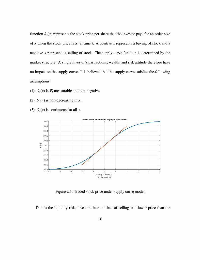
function S t(x) represents the stock price per share that the investor pays for an order size

of x when the stock price is S t at time t. A positive x represents a buying of stock and a

negative x represents a selling of stock. The supply curve function is determined by the

market structure. A single investor’s past actions, wealth, and risk attitude therefore have

no impact on the supply curve. It is believed that the supply curve satisfies the following

assumptions:

(1): S t(x) is Ft measurable and non-negative.

(2): S t(x) is non-decreasing in x.

(3): S t(x) is continuous for all x.

-5 -4 -3 -2 -1 0 1 2 3 4 5

trading volume k (in thousands)

99.5

99.6

99.7

99.8

99.9

100

100.1

100.2

100.3

100.4

100.5

St(k

)

Traded Stock Price under Supply Curve Model

Figure 2.1: Traded stock price under supply curve model

Due to the liquidity risk, investors face the fact of selling at a lower price than the

16

market quoted price and buying at a higher price than the market quoted price; liquidity

risk therefore adds extra cost for trading. An example could be found in Figure 2.1. In

respect to the general form of a supply curve function, Ku et al. (2012) applied a separable

form of supply curve function, which is given by:

S t(x) = f (x)S t, (2.3)

where f (·) is a twice differential non-decreasing function with f (0) = 1. This chapter will

use the above separable form of supply curve function.

A trading strategy is defined by a pair of (Bt, Pt), where Bt denotes the wealth in the

bank account and Pt is the number of stock at time t. We restrict Pt to the form:

Pt = P0 +

∫ t

0αsds +

∫ t

0βsdWs, (2.4)

where αs and βs are two progressively Fs measurable processes and both E[∫ t

0|αs|ds

]and

E[∫ t

0β2

sds]

are finite for every t ∈ [0,T ]. Pt is a continuous process, which has finite

quadratic variation and infinite variation. The differential form of Pt will be

dPt = αtdt + βtdWt. (2.5)

The quadratic term of Pt is

(dPt)2 = β2t dt. (2.6)

In a fully liquid market, there is no liquidity risk, and the cost to change the stock position

from Pt to Pt+dt during [t, t + dt] is dPt × S t. When liquidity risk exists and the traded

17

price of the stock is given by a supply curve function S t(x) = f (x)S t, the cost becomes

dPt ×S t(dPt). The liquidity cost incurred from [t, t + dt] is the extra cost introduced by the

supply curve function. It is defined as:

dPt × S t(dPt) − dPt × S t. (2.7)

From (2.7) and the Taylor expansion of f (Pt), it follows that:

dPt × S t(dPt) − dPt × S t = dPt( f (dPt) − 1)S t

= dPt

(f ′(0)dPt +

f ′′(0)2

dPt2)

S t. (2.8)

Substituting (dPt)2 = β2t dt into (2.8), we obtain the result

dPt × S t(dPt) − dPt × S t = f ′(0)β2t S tdt. (2.9)

The portfolio’s value is defined by

Λt = PtS t + Bt.

Under the supply curve model, a trading strategy (Pt, Bt) is self-financing when

PtS t + Bt = P0S 0 + B0 +

∫ t

0PudS u +

∫ t

0rBudu −

∫ t

0f ′(0)β2

uS udu, (2.10)

where P0S 0 + B0 is the value of the initial portfolio,∫ t

0PudS u is the capital gain from

the stock,∫ t

0rBudu is the gain from bank account and

∫ t

0f ′(0)β2

uS udu is the accumulated

liquidity cost. Under self-financing condition, the differential form of Λt is

dΛt = PtdS t − f ′(0)S tβ2t dt + rBtdt. (2.11)

18

Compared with the self-financing condition in the Black-Scholes model, the self-financing

condition with liquidity cost has an extra term f ′(0)S tβ2t dt to account for the liquidity cost

incurred during the trading.

2.3 European options

An investor who writes one call option (S T −K)+ needs to set a hedging portfolio to hedge

the option. It is assumed that the option is covered, which means the option writer already

owns P0 position of the stock. Therefore, there is no liquidity cost for constructing the

initial hedging portfolio (P0, B0). The investor continuously adjust the hedging position Pt

during the hedging, and under the supply curve model, the value of the hedging portfolio

at time T is

PT S T + BT = P0S 0 + B0 +

∫ T

0PudS u +

∫ t

0rBudu −

∫ T

0f ′(0)β2

uS udu.

In this study, replicating the option means the market value of the option writer’s hedging

portfolio at maturity T equals the option’s payoff. In other words, this study does not

consider the liquidity cost of delivering the option’s payoff at maturity. The option could

then be replicated by a self-financing portfolio:

(S T − K)+ = PT S T + BT ,

19

and the replication cost for the option seller is P0S 0 + B0. Symmetrically, there exists a

replication strategy from the option buyer. When an investor buys one option, the investor

shorts a portfolio to hedge the option. Assuming the short portfolio is (−P0,−B0) and the

option buyer can replicate the option at time T , we have the following equations:

−(S T − K)+ = −PT S T − BT = −P0S 0 − B0 +

∫ T

0(−Pu)dS u −

∫ t

0rBudu−

∫ T

0f ′(0)β2

uS udu

and

(S T − K)+ = PT S T + BT = P0S 0 + B0 +

∫ T

0PudS u +

∫ t

0rBudu +

∫ T

0f ′(0)β2

uS udu.

The replication cost for option buyer is P0S 0 + B0. The replication cost for the option seller

and buyer will be different. This chapter shall show that the seller’s replication cost will

be greater than buyer’ replication cost.

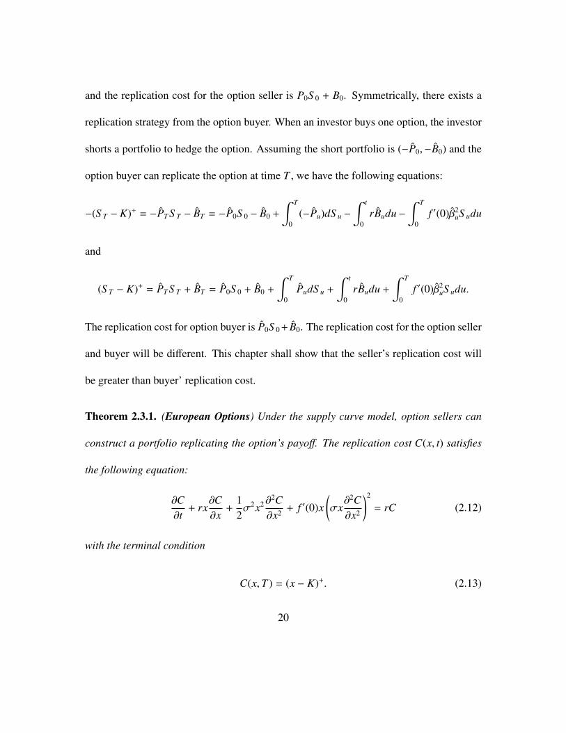
Theorem 2.3.1. (European Options) Under the supply curve model, option sellers can

construct a portfolio replicating the option’s payoff. The replication cost C(x, t) satisfies

the following equation:

∂C∂t

+ rx∂C∂x

+12σ2x2∂

2C∂x2 + f ′(0)x

(σx

∂2C∂x2

)2

= rC (2.12)

with the terminal condition

C(x,T ) = (x − K)+. (2.13)

20

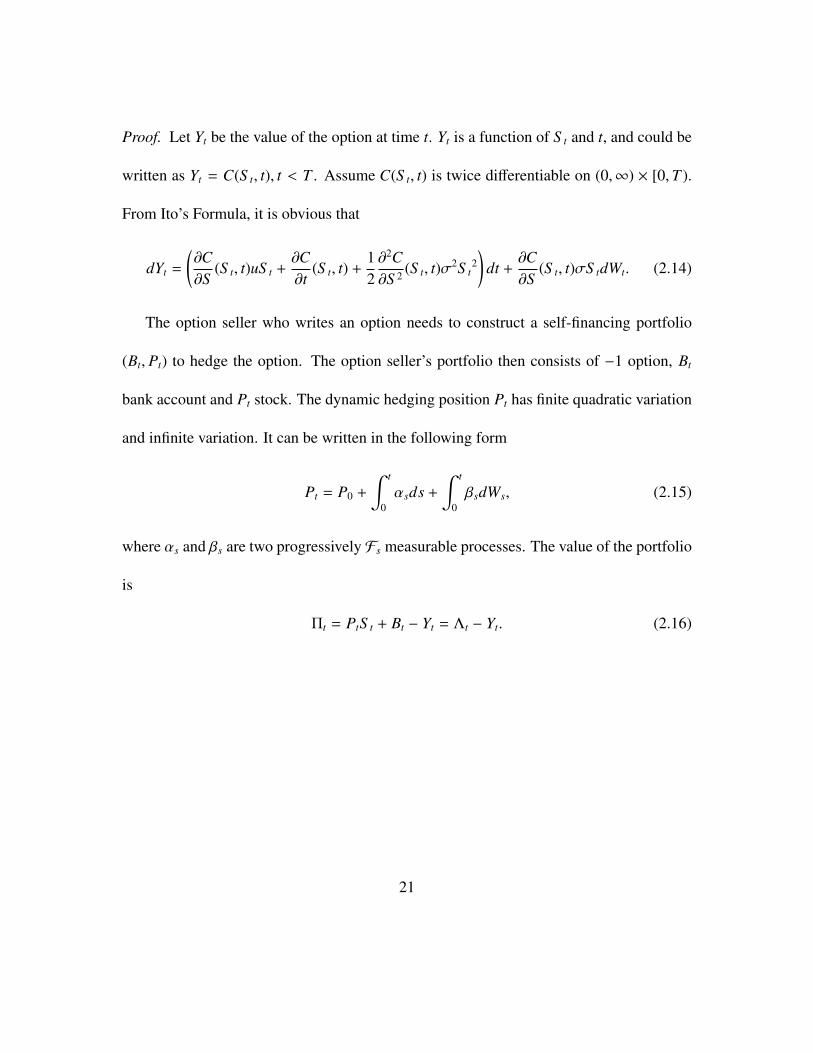
Proof. Let Yt be the value of the option at time t. Yt is a function of S t and t, and could be

written as Yt = C(S t, t), t < T . Assume C(S t, t) is twice differentiable on (0,∞) × [0,T ).

From Ito’s Formula, it is obvious that

dYt =

(∂C∂S

(S t, t)uS t +∂C∂t

(S t, t) +12∂2C∂S 2 (S t, t)σ2S t

2)

dt +∂C∂S

(S t, t)σS tdWt. (2.14)

The option seller who writes an option needs to construct a self-financing portfolio

(Bt, Pt) to hedge the option. The option seller’s portfolio then consists of −1 option, Bt

bank account and Pt stock. The dynamic hedging position Pt has finite quadratic variation

and infinite variation. It can be written in the following form

Pt = P0 +

∫ t

0αsds +

∫ t

0βsdWs, (2.15)

where αs and βs are two progressively Fs measurable processes. The value of the portfolio

is

Πt = PtS t + Bt − Yt = Λt − Yt. (2.16)

21

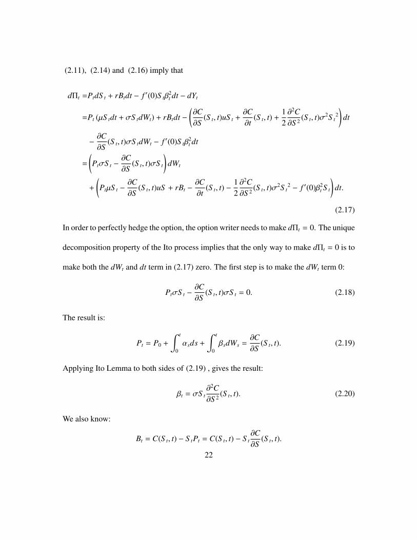
(2.11), (2.14) and (2.16) imply that

dΠt =PtdS t + rBtdt − f ′(0)S tβ2t dt − dYt

=Pt (µS tdt + σS tdWt) + rBtdt −(∂C∂S

(S t, t)uS t +∂C∂t

(S t, t) +12∂2C∂S 2 (S t, t)σ2S t

2)

dt

−∂C∂S

(S t, t)σS tdWt − f ′(0)S tβ2t dt

=

(PtσS t −

∂C∂S

(S t, t)σS t

)dWt

+

(PtµS t −

∂C∂S

(S t, t)uS + rBt −∂C∂t

(S t, t) −12∂2C∂S 2 (S t, t)σ2S t

2 − f ′(0)β2t S t

)dt.

(2.17)

In order to perfectly hedge the option, the option writer needs to make dΠt = 0. The unique

decomposition property of the Ito process implies that the only way to make dΠt = 0 is to

make both the dWt and dt term in (2.17) zero. The first step is to make the dWt term 0:

PtσS t −∂C∂S

(S t, t)σS t = 0. (2.18)

The result is:

Pt = P0 +

∫ t

0αsds +

∫ t

0βsdWs =

∂C∂S

(S t, t). (2.19)

Applying Ito Lemma to both sides of (2.19) , gives the result:

βt = σS t∂2C∂S 2 (S t, t). (2.20)

We also know:

Bt = C(S t, t) − S tPt = C(S t, t) − S t∂C∂S

(S t, t).

22

Then, we make the dt term of (2.17) to be 0:

PtµS t −∂C∂S

(S t, t)uS t + rBt −∂C∂t

(S t, t) −12σ2S t

2∂2C∂S 2 (S t, t) − f ′(0)S tβ

2t = 0. (2.21)

Substituting βt = σS t∂2C∂S 2 (S t, t), Bt = C(S t, t) − S t

∂C∂S (S t, t) and Pt = ∂C

∂S (S t, t) into (2.21),

we obtain

∂C∂t

(S t, t) + rS t∂C∂S t

+12σ2S 2

t∂2C∂S 2

t(S t, t) + f ′(0)σ2S 3

t

(∂2C∂S 2

t(S t, t)

)2

= rC(S t, t). (2.22)

Replacing S t with dummy variable x, the replication cost of European options satisfies the

following equation

∂C∂t

+ rx∂C∂x

+12σ2x2∂

2C∂x2 + f ′(0)x

(σx

∂2C∂x2

)2

= rC, (2.23)

with the terminal condition:

C(x,T ) = (x − K)+. (2.24)

Similarly, we can characterize the replication cost for option buyers.

Theorem 2.3.2. Under the supply curve model, option buyers can construct a portfolio

replicating the option’s payoff. The replication cost C(x, t) satisfies the following equation:

∂C∂t

+ rx∂C∂x

+12σ2x2∂

2C∂x2 − f ′(0)x

(σx

∂2C∂x2

)2

= rC (2.25)

23

with the terminal condition:

C(x,T ) = (x − K)+. (2.26)

From the fundamental theorem of asset pricing, we can perfectly hedge derivatives

when the market is perfect and complete. In a market with transaction costs or short

selling constraints, perfect hedging does not exist in a continuous time model. People tend

to agree that perfect hedging is impossible in an imperfect market in a continuous time

model. Surprisingly, we achieve continuous perfect hedging in a market with liquidity risk.

In other words, we have found an example where continuous perfect hedging exists in an

imperfect market. What’s the difference between our liquidity risk model and a transaction

costs model? Why is perfect hedging possible in our model when it is impossible in a

transaction costs model?

In both the proportional transaction costs model and our liquidity cost model, we need

to adopt a dynamic hedging strategy to hedge the option to replicate the option’s payoff.

When the stock price follows a geometric Brownian motion, the dynamic hedging position

Pt usually has the following form:

Pt = P0 +

∫ t

0αudu +

∫ t

0βudWu, (2.27)

which has finite quadratic variation and infinite variation. The incurred proportional trans-

24

action costs during [0, T ] is

∫ T

0kS t |dPt| =

∫ T

0kS t |αtdt + βtdWt| ,

where k is the parameter of transaction costs proportion. When βt is not 0,

∫ T

0kS t |αtdt + βtdWt|

will be infinite because of the infinite variation of the Brownian motion. This means that

under a continuous hedging strategy, the incurred transaction costs will go to infinity if

we adopt a continuous time hedging strategy. This is the reason we cannot replicate an

option’s payoff with finite initial cost in the transaction costs model.

In the liquidity cost model, however, the liquidity cost is:

∫ T

0f ′(0)S tβ

2t dt.

The fundamental difference between the transaction costs model and our liquidity cost

model is that under a continuous hedging strategy, the transaction costs will go to infinity

while the liquidity cost will be finite, which is why we can replicate options in the liquidity

cost model.

25

2.4 Upper bound and lower bound of option prices

We denote the option seller’s replication cost by C+(x, t). From the option seller’s side, the

replication cost C+(x, t) is determined by

∂C+

∂t(x, t) + rx

∂C+

∂x+

12σ2x2∂

2C+

∂x2 (x, t) + f ′(0)x(σx

∂2C+

∂x2 (x, t))2

= rC+(x, t) (2.28)

with C+(x,T ) = (x − K)+, C+(0, t) = 0, and limx→+∞

C(x, t) = +∞. The Black-Scholes price

C(x, t) satisfies

∂C∂t

(x, t) + rx∂C∂x

+12σ2x2∂

2C∂x2 (x, t) = rC(x, t) (2.29)

with C(x,T ) = (x − K)+, C(0, t) = 0, and limx→+∞

C(x, t) = +∞.

Theorem 2.4.1. When f ′(0) ≥ 0, suppose C+(x, t) is a classical solution to

∂C+

∂t(x, t) + rx

∂C+

∂x+

12σ2x2∂

2C+

∂x2 (x, t) + f ′(0)x(σx

∂2C+

∂x2 (x, t))2

= rC+(x, t) (2.30)

and C(x, t) is a classical solution to

∂C∂t

(x, t) + rx∂C∂x

+12σ2x2∂

2C∂x2 (x, t) = rC(x, t) (2.31)

on (0,+∞) × [0,T ). If we have C+(x,T ) = C(x,T ), C+(0, t) = C(0, t) and limx→+∞

C+(x, t) =

limx→+∞

C(x, t), then C+(x, t) ≥ C(x, t) on (0,+∞) × [0,T ].

Proof. Denote D(x, t) = C+(x, t) −C(x, t), then we have

D(x,T ) = 0,D(0, t) = 0 and limx→+∞

D(x, t) = 0.

26

Differentiating D(x, t) = C+(x, t) −C(x, t) w.r.t t and x, we have:

∂D∂t

(x, t) =∂C+

∂t(x, t) −

∂C∂t

(x, t) (2.32)

∂D∂x

(x, t) =∂C+

∂x(x, t) −

∂C∂x

(x, t) (2.33)

and

12σ2x2∂

2D∂x2 (x, t) =

12σ2x2∂

2C+

∂x2 (x, t) −12σ2x2∂

2C∂x2 (x, t). (2.34)

Subtracting (2.31) from (2.30), we obtain

∂C+

∂t(x, t) −

∂C∂t

(x, t) + rx∂C+

∂t(x, t) − rx

∂C∂t

(x, t) +12σ2x2∂

2C+

∂x2 (x, t) (2.35)

−12σ2x2∂

2C∂x2 (x, t) + f ′(0)x

(∂2C+

∂x2 (x, t)σx)2

= rC+(x, t) − rC(x, t). (2.36)

Substituting (2.33) and (2.34) into (2.35), we obtain

∂D∂t

(x, t) + rx∂D∂x

(x, t) +12σ2x2∂

2D∂x2 (x, t) − rD(x, t) = − f ′(0)x

(∂2C+

∂x2 (x, t)σx)2

. (2.37)

We denote

F(x, t) = − f ′(0)x(∂2C+

∂x2 (x, t)σx)2

,

so we have F(x, t) ≤ 0 and

∂D∂t

(x, t) + rx∂D∂x

(x, t) +12σ2x2∂

2D∂x2 (x, t) − rD(x, t) = F(x, t). (2.38)

27

Suppose D(x, t) has a negative local minimum at some point (x∗, t∗) in (0,∞)× (0,T ] , then

we have

D(x∗, t∗) < 0. (2.39)

The necessary condition for local minimum implies

∂D∂t

(x∗, t∗) =∂D∂x

(x∗, t∗) = 0. (2.40)

The scale function h(x) = D(x, t∗) has its minimum at x∗, thus

h′′(x∗) =∂2D∂x2 (x∗, t∗) ≥ 0. (2.41)

From (2.38), we know

∂D∂t

(x∗, t∗) + rx∗∂D∂x

(x∗, t∗) +12σ2x∗2

∂2D∂x2 (x∗, t∗)− rD(x∗, t∗) = − f ′(0)x∗

(∂2C+

∂x2 (x∗, t∗)σx∗)2

(2.42)

From (2.40), we have

12∂2D∂x2 (x∗, t∗)σ2x∗2 − rD(x∗, t∗) = − f ′(0)x∗

(∂2C+

∂x2 (x∗, t∗)σx∗)2

(2.43)

which implies

rD(x∗, t∗) ≥ 0 (2.44)

Because r ≥ 0, (2.44) is contrast to

D(x∗, t∗) < 0.

28

By now, we can conclude

D(x, t) ≥ 0

and

C+(x, t) ≥ C(x, t), when (t, x) ∈ [0,+∞) × [0,T ].

We denote the option buyer’s replication cost by C−(x, t). From the option buyer’s side,

the replication cost C−(x, t) is determined by

∂C−

∂t+ rx

∂C−

∂x+

12σ2x2∂

2C−

∂x2 − f ′(0)x(σx

∂2C−

∂x2

)2

= rC− (2.45)

with C−(x,T ) = (x − K)+, C−(0, t) = 0, and limx→+∞

C−(x, t) = +∞. Applying the same

argument, we can prove

C−(x, t) ≤ C(x, t), when (t, x) ∈ [0,+∞) × [0,T ].

So, we can conclude that

C−(x, t) ≤ C+(x, t).

Under the supply curve model, any price above C+(x, t) will lead to arbitrage for the option

seller and below C−(x, t) will lead to arbitrage for the option buyer. We can consider

C+(x, t) as the upper bound for option price, and C−(x, t) as lower bound. So the quoted

option price Cp in the market with liquidity risk should satisfy

C−(x, t) ≤ Cp ≤ C+(x, t).

29

The price of the option satisfies the differential equation

∂C∂t

+ rx∂C∂x

+12σ2x2∂

2C∂x2 + f ′(0)x

(∂2C∂x2 σx

)2

= rC (2.46)

Since Θ = ∂C∂t , ∆ = ∂C

∂x , Γ = ∂2C∂x2 it follows that

Θ + rx∆ +12σ2x2Γ + f ′(0)σ2x3Γ2 = rC (2.47)

Hedging options with a large absolute value of Γ will lead to a large liquidity cost, which

is reflected in the term f ′(0)σ2x3Γ2. Intuitively, a large Γ means frequent trading of stocks,

and frequent trading leads to a large liquidity cost. Imagine that if one option has Γ = 0,

which means there is no need to change the stock position in the hedging portfolio, then

the liquidity risk will be zero. The option price in the market with liquidity risk will be the

Black-Scholes price. The option price is also reflected in the equation (2.47).

2.4.1 Asymptotic Expansion

In this section, we analyze the solution of equation (2.46) with an asymptotic expansion

method, the idea that can be tracked to Ku et al. (2012). In this section, we present an

approximation formula for equation (2.46).

When f ′(0) is sufficiently small, the solution can be approximated by the form

C(x, t) = C0(x, t) + f ′(0)C1(x, t) + O( f ′(0)2).

30

The C0(x, t) term is determined by the Black-Scholes equation:

∂C0

∂t+ rx

∂C0

∂x+

12σ2x2∂

2C0

∂x2 = rC0 (2.48)

with Boundary condition C0(x,T ) = (x − K)+. In the order of O( f ′(0)), we have C1(x, t)

determined by

∂C1

∂t+ rx

∂C1

∂x+

12σ2x2∂

2C1

∂x2 + σ2x3(∂2C0

∂x2 + f ′(0)∂2C1

∂x2

)2

= rC1 (2.49)

with C1(x,T ) = 0.

The explicit solution is the Black-Scholes formula

C0(x, t) = xN(d1) − Ke−rT N(d2) (2.50)

where

d1 =ln(x/k) + (r + σ2/2)(T − t)

σ√

T − t, d2 = d1 − σ

√T − t.

For the European call option, the gamma, ∂2C0∂x2 is given by

∂2C0

∂x2 =1

xσ√

T − t

1√

2πe−

12 d2

1 .

Substituting the formula of ∂2C0∂x2 into equation (2.49) and simplifying it, we obtain

∂C1

∂t+ rx

∂C1

∂x+

12σ2x2∂

2C1

∂x2 +x

2π(T − t)e−d2

1 = rC1 (2.51)

Please note that the f ′(0)∂2C1∂x2 in equation(2.49) is ignored in deriving equation(2.51) be-

cause it is in the order term of O( f ′(0)). In order to derive the explicit solution of equation

31

(2.51), we make the following variables transformations to transform equation (2.51) into

a standard boundary value problem for the heat equation:

x = ey, t = T −2τσ2

C1(x, t) = v(y, τ) = v(ln(x),

σ2(T − t)2

)The partial derivative of C1(x, t) with respect to x and t expressed in terms of partial deriva-

tives of v in terms of y and τ are:

∂C1

∂t= −

σ2

2∂v∂τ

(2.52)

∂C1

∂x=

1x∂v∂y

(2.53)

∂2C1

∂x2 = −1x2

∂v∂y

+1x2

∂2v∂y2 (2.54)

Substituting (2.52), (2.53) and (2.54) into equation (2.51), we obtain:

−σ2

2∂v∂τ

+ rx1x∂v∂y

+12σ2x2(−

1x2

∂v∂y

+1x2

∂2v∂y2 ) +

x2π(T − t)

e−d21 = rv.

After we rearrange the equation of v(y, τ) and simplify it, we get:

∂v∂τ

=∂2v∂y2 +

(2rσ2 − 1

)∂v∂y−

2rσ2 v +

2σ2 g(y, τ) (2.55)

where

g(y, τ) =x

2π(T − t)e−d2

1 =ey

2π( 2τσ2 )

e−d21 =

σ2

4πτey−

(ln (ey/K)+(r+σ

22 ) 2τ

σ2

)22τ .

For further reference, we denote

a =σ2 − 2r

2σ2 , b = −

(σ2 + 2r

2σ2

)2

.

32

We set v(y, τ) = eay+bτw(y, τ). Computing the partials of v in terms of y and τ, we have

∂v∂τ

= beay+bτw + eay+bτ∂w∂τ

∂v∂y

= aeay+bτw + eay+bτ∂w∂y

∂2v∂y2 = a2eay+bτw + 2aeay+bτ∂w

∂y+ eay+bτ∂

2w∂y2 .

Substituting them into equation (2.55) and simplifying it, we obtain

bw +∂w∂τ

= a2w + 2a∂w∂y

+∂2w∂y2 +

(2rσ2 − 1

) (aw +

∂w∂y

)−

2rσ2 w +

2σ2eay+bτg(y, τ). (2.56)

We denote

a =σ2 − 2r

2σ2 , b = −

(σ2 + 2r

2σ2

)2

and simplifying equation (2.56) by substituting a, b and g(y, τ), we have:

∂w∂τ

=∂2w∂y2 +

12πτ

ey−ay−bτ−

(ln (ey/K)+(r+σ

22 ) 2τ

σ2

)22τ (2.57)

The initial condition for (2.57) is w(y, 0) = 0. The solution w(y, τ) is solved using

Duhamel’s principle:

w(y, τ) =

∫ τ

0

∫ ∞

−∞

12πu

eξ−aξ−bu−

(ln (eξ/K)+(r+σ

22 ) 2u

σ2

)22u

12√π(τ − u)

e−(y−ξ)24(τ−u) dξdu. (2.58)

33

Equation (2.58) is a double integration with respect to ξ and u.

∫1

2πueξ−aξ−bu−

(ln (eξ/K)+(r+σ

22 ) 2u

σ2

)22u

12√π(τ − u)

e−(y−ξ)24(τ−u) dξ

=K

2rσ2 +1e

(4τu−4u2)(σ2(uy+u2−τu)+r(2u2−2τu)+ln(K)σ2(2τ−2u))2

4σ4(2τ−u)(2τu−2u2)2 +y2

4u−4τ−ruσ2 −

r2uσ4 −

u4−

ln2(K)2u

4π√τ − uu

√u−2τ

u(u−τ)

·

erf

√

u−2τu(u−τ)ξ

2−σ2

(uy + u2 − τu

)+ r

(2u2 − 2τu

)+ ln (K)σ2 (2τ − 2u)

σ2 (2τu − 2u2) √

u−2τu(u−τ)

where

erf (x) =

∫ x

−x

e−v2

√π

dv

When ξ → +∞,

erf

√

u−2τu(u−τ)ξ

2−σ2

(uy + u2 − τu

)+ r

(2u2 − 2τu

)+ ln (K)σ2 (2τ − 2u)

σ2 (2τu − 2u2) √

u−2τu(u−τ)

→ 1.

and when ξ → −∞,

erf

√

u−2τu(u−τ)ξ

2−σ2

(uy + u2 − τu

)+ r

(2u2 − 2τu

)+ ln (K)σ2 (2τ − 2u)

σ2 (2τu − 2u2) √

u−2τu(u−τ)

→ −1.

Therefore, the integration with respect to ξ could be written in an explicit form:

∫ ∞

−∞

12πu

eξ−aξ−bu−

(ln (eξ/K)+(r+σ

22 ) 2u

σ2

)22u

12√π(τ − u)

e−(y−ξ)24(τ−u) dξ

=K

2rσ2 +1e

(4τu−4u2)(σ2(uy+u2−τu)+r(2u2−2τu)+ln(K)σ2(2τ−2u))2

4σ4(2τ−u)(2τu−2u2)2 +y2

4u−4τ−ruσ2 −

r2uσ4 −

u4−

ln2(K)2u

2π√τ − uu

√u−2τ

u(u−τ)

. (2.59)

34

Then w(y, τ) could be written as:

w(y, τ) =

∫ τ

0

K2rσ2 +1e

(4τu−4u2)(σ2(uy+u2−τu)+r(2u2−2τu)+ln(K)σ2(2τ−2u))2

4σ4(2τ−u)(2τu−2u2)2 +y2

4u−4τ−ruσ2 −

r2uσ4 −

u4−

ln2(K)2u

2π√τ − uu

√u−2τ

u(u−τ)

du.

We know

C1(x, t) = v(y, τ) = eay+bτw(y, τ) (2.60)

Substituting

y = ln(x), τ =σ2

2(T − t)

into equation (2.60), we have

C1(x, t) = eσ2−2r

2σ2 ln(x)−(σ2+2r

2σ2

)212σ

2(T−t)×

∫ 12σ

2(T−t)

0

K2rσ2 +1e

(2σ2(T−t)u−4u2)(σ2(u ln(x)+u2−( 12σ

2(T−t))u)+r(2u2−σ2(T−t)u)+ln(K)σ2(σ2(T−t)−2u))2

4σ4(σ2(T−t)−u)(σ2(T−t)u−2u2)2 +ln2(x)

4u−2σ2(T−t)− ruσ2 −

r2uσ4 −

u4−

ln2(K)2u

2πu√

12σ

2(T − t) − u√

u−σ2(T−t)u(u− 1

2σ2(T−t))

du.

The solution C(x, t) is approximated by

C(x, t) ≈ C0(x, t) + f ′(0)C1(x, t). (2.61)

Therefore, the European call option price with liquidity cost could be approximated by

C(x, t) = xN(d1) − Ke−rT N(d2) + f ′(0)eσ2−2r

2σ2 ln(x)−(σ2+2r

2σ2

)212σ

2(T−t)×

∫ 12σ

2(T−t)

0

K2rσ2 +1e

(2σ2(T−t)u−4u2)(σ2(u ln(x)+u2−( 12σ

2(T−t))u)+r(2u2−σ2(T−t)u)+ln(K)σ2(σ2(T−t)−2u))2

4σ4(σ2(T−t)−u)(σ2(T−t)u−2u2)2 +ln2(x)

4u−2σ2(T−t)− ruσ2 −

r2uσ4 −

u4−

ln2(K)2u

2πu√

12σ

2(T − t) − u√

u−σ2(T−t)u(u− 1

2σ2(T−t))

du

35

where

d1 =ln(x/K) + (r + σ2/2)(T − t)

σ√

T − t, d2 = d1 − σ

√T − t.

The liquidity premium is

f ′(0)eσ2−2r

2σ2 ln(x)−(σ2+2r

2σ2

)212σ

2(T−t)×

∫ 12σ

2(T−t)

0

K2rσ2 +1e

(2σ2(T−t)u−4u2)(σ2(u ln(x)+u2−( 12σ

2(T−t))u)+r(2u2−σ2(T−t)u)+ln(K)σ2(σ2(T−t)−2u))2

4σ4(σ2(T−t)−u)(σ2(T−t)u−2u2)2 +ln2(x)

4u−2σ2(T−t)− ruσ2 −

r2uσ4 −

u4−

ln2(K)2u

2πu√

12σ

2(T − t) − u√

u−σ2(T−t)u(u− 1

2σ2(T−t))

du.

The liquidity premium is positive and is a linear function of liquidity parameter f ′(0).

When the liquidity parameter f ′(0) is sufficiently small, the liquidity premium increases

linearly with respect to f ′(0). In the next section, we will present the numerical results of

option prices with the approximation formula.

2.4.2 Numerical results of European options

In this section, we present some numerical results of European options. There are two

ways to calculate the option prices: using the finite difference method to solve the PDE

numerically and by using the approximation formula. We will present and compare the

option prices using the two methods. Also, numerical simulation of the hedging strategy

and hedging error will be shown to illustrate the perfect hedging of the option with liquidity

cost.

Compared to the Black-Scholes equation, the PDE of the option price with liquidity

36

risk

∂C∂t

+ rx∂C∂x

+12σ2x2∂

2C∂x2 ± f ′(0)x

(σx

∂2C∂x2

)2

= rC, (2.62)

has a nonlinear term ∂2C∂S 2 (S , t)2, which makes the PDE fully nonlinear.

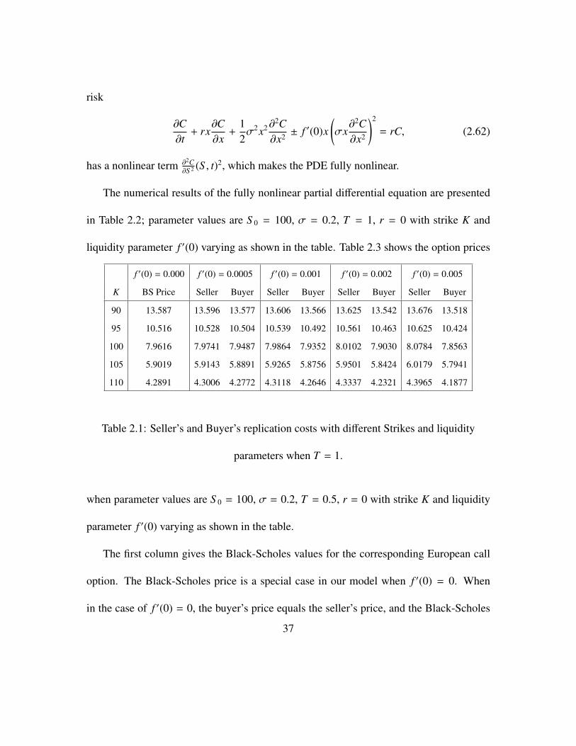
The numerical results of the fully nonlinear partial differential equation are presented

in Table 2.2; parameter values are S 0 = 100, σ = 0.2, T = 1, r = 0 with strike K and

liquidity parameter f ′(0) varying as shown in the table. Table 2.3 shows the option prices

f ′(0) = 0.000 f ′(0) = 0.0005 f ′(0) = 0.001 f ′(0) = 0.002 f ′(0) = 0.005

K BS Price Seller Buyer Seller Buyer Seller Buyer Seller Buyer

90 13.587 13.596 13.577 13.606 13.566 13.625 13.542 13.676 13.518

95 10.516 10.528 10.504 10.539 10.492 10.561 10.463 10.625 10.424

100 7.9616 7.9741 7.9487 7.9864 7.9352 8.0102 7.9030 8.0784 7.8563

105 5.9019 5.9143 5.8891 5.9265 5.8756 5.9501 5.8424 6.0179 5.7941

110 4.2891 4.3006 4.2772 4.3118 4.2646 4.3337 4.2321 4.3965 4.1877

Table 2.1: Seller’s and Buyer’s replication costs with different Strikes and liquidity

parameters when T = 1.

when parameter values are S 0 = 100, σ = 0.2, T = 0.5, r = 0 with strike K and liquidity

parameter f ′(0) varying as shown in the table.

The first column gives the Black-Scholes values for the corresponding European call

option. The Black-Scholes price is a special case in our model when f ′(0) = 0. When

in the case of f ′(0) = 0, the buyer’s price equals the seller’s price, and the Black-Scholes

37

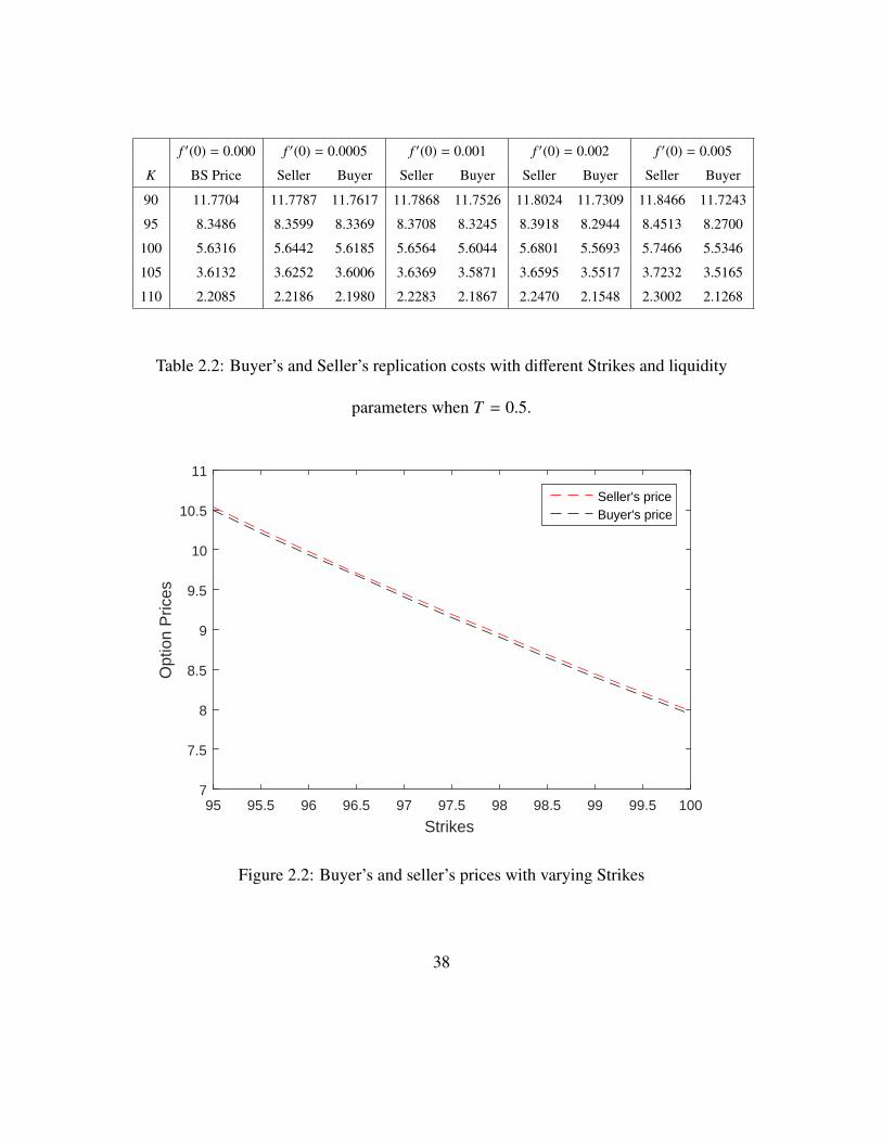
f ′(0) = 0.000 f ′(0) = 0.0005 f ′(0) = 0.001 f ′(0) = 0.002 f ′(0) = 0.005

K BS Price Seller Buyer Seller Buyer Seller Buyer Seller Buyer

90 11.7704 11.7787 11.7617 11.7868 11.7526 11.8024 11.7309 11.8466 11.7243

95 8.3486 8.3599 8.3369 8.3708 8.3245 8.3918 8.2944 8.4513 8.2700

100 5.6316 5.6442 5.6185 5.6564 5.6044 5.6801 5.5693 5.7466 5.5346

105 3.6132 3.6252 3.6006 3.6369 3.5871 3.6595 3.5517 3.7232 3.5165

110 2.2085 2.2186 2.1980 2.2283 2.1867 2.2470 2.1548 2.3002 2.1268

Table 2.2: Buyer’s and Seller’s replication costs with different Strikes and liquidity

parameters when T = 0.5.

95 95.5 96 96.5 97 97.5 98 98.5 99 99.5 100

Strikes

7

7.5

8

8.5

9

9.5

10

10.5

11

Opt

ion

Pric

es

Seller's priceBuyer's price

Figure 2.2: Buyer’s and seller’s prices with varying Strikes

38

0 0.5 1 1.5 2 2.5 3 3.5 4 4.5 5

Liquidity parameter f'(0) ×10-3

5

6

7

8

9

10O

ptio

n pr

ices

Buyer's priceSeller's price

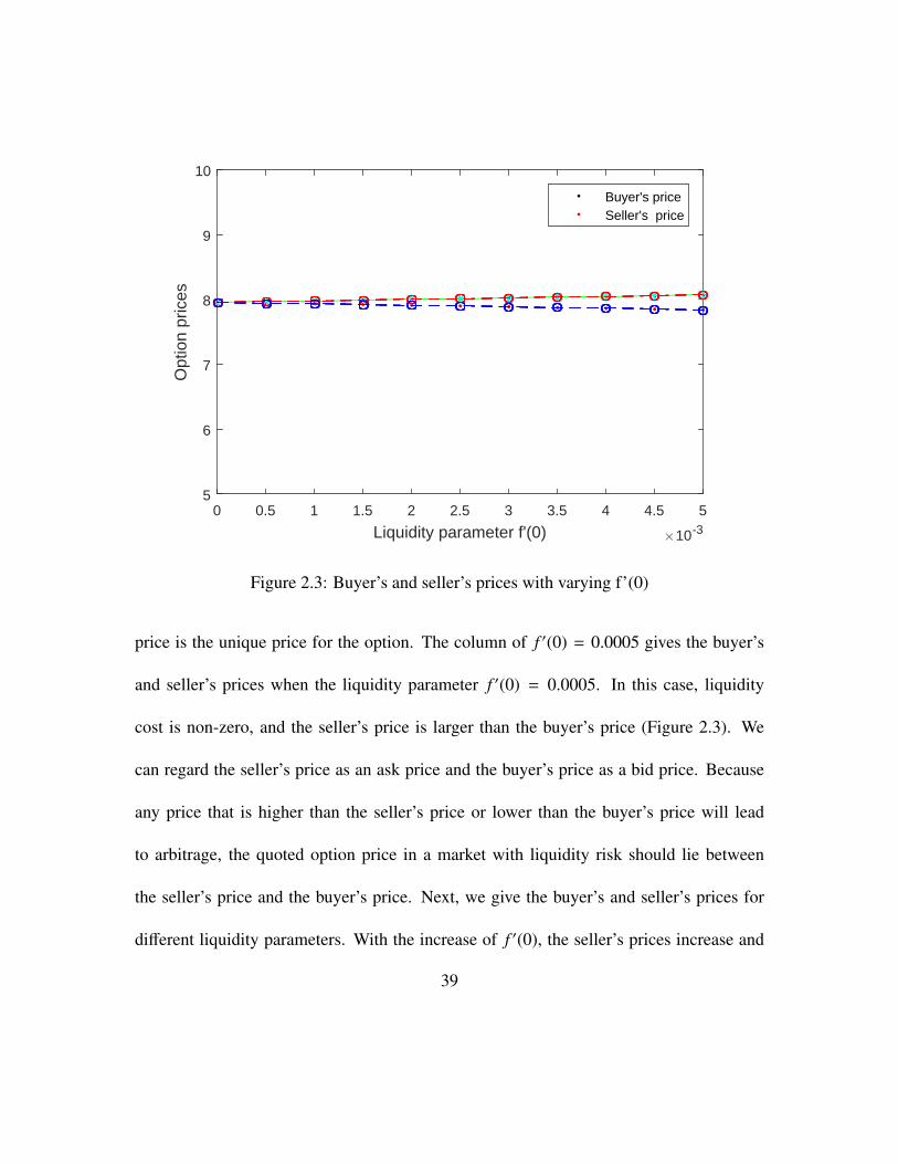
Figure 2.3: Buyer’s and seller’s prices with varying f’(0)

price is the unique price for the option. The column of f ′(0) = 0.0005 gives the buyer’s

and seller’s prices when the liquidity parameter f ′(0) = 0.0005. In this case, liquidity

cost is non-zero, and the seller’s price is larger than the buyer’s price (Figure 2.3). We

can regard the seller’s price as an ask price and the buyer’s price as a bid price. Because

any price that is higher than the seller’s price or lower than the buyer’s price will lead

to arbitrage, the quoted option price in a market with liquidity risk should lie between

the seller’s price and the buyer’s price. Next, we give the buyer’s and seller’s prices for

different liquidity parameters. With the increase of f ′(0), the seller’s prices increase and

39

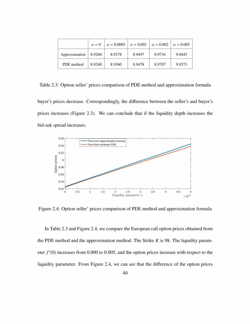
α = 0 α = 0.0005 α = 0.001 α = 0.002 α = 0.005

Approximation 8.9260 8.9378 8.9497 8.9734 9.0445

PDE method 8.9240 8.9360 8.9478 8.9707 9.0373

Table 2.3: Option seller’ prices comparison of PDE method and approximation formula

buyer’s prices decrease. Correspondingly, the difference between the seller’s and buyer’s

prices increases (Figure 2.3). We can conclude that if the liquidity depth increases the

bid-ask spread increases.

0 0.5 1 1.5 2 2.5 3 3.5 4 4.5 5

10-3

8.92

8.94

8.96

8.98

9

9.02

9.04

9.06

Opt

ion

pric

es

Price from Approximation formulaPrice from nonlinear PDE

Figure 2.4: Option seller’ prices comparison of PDE method and approximation formula

In Table 2.3 and Figure 2.4, we compare the European call option prices obtained from

the PDE method and the approximation method. The Strike K is 98. The liquidity param-

eter f ′(0) increases from 0.000 to 0.005, and the option prices increase with respect to the

liquidity parameter. From Figure 2.4, we can see that the difference of the option prices

40

from the two methods are extremely small. We can conclude that when liquidity parameter

f ′(0) is sufficiently small, the asymptotic approximation method is quite accurate.

We analyse the hedging error of our model. The hedging error HT is defined to be

HT = (PT S T + BT ) − (S T − K)+.

In theory, we can perfectly hedge the option with a self-financing portfolio in continuous

time, which means the hedging error is zero almost surely. In practice, we can apply

discrete time hedging, so we can not perfectly replicate the option. When our hedging

period goes to zero, however, the hedging error will converge to zero. We did the Monte

Carlo simulation to compute the mean and variance of the hedging error. Table 2.4 presents

the Monte Carlo simulation results for the option seller with Strike K = 100 and varying

liquidity parameter f ′(0). There are 10, 000 paths used in the simulation, with 100 time

steps in each simulation. The mean row shows the mean hedging error. The mean and

variance of the hedging error do not vary too much with different liquidity parameter

f ′(0). Moreover, the mean and variance of the hedging error with f ′(0) > 0 are almost

the same as the mean and variance of the hedging error of the Black-Scholes case (when

f ′(0) = 0).

41

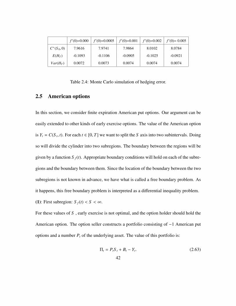
f ′(0)=0.000 f ′(0)=0.0005 f ′(0)=0.001 f ′(0)=0.002 f ′(0)= 0.005

C+(S 0, 0) 7.9616 7.9741 7.9864 8.0102 8.0784

E(HT ) -0.1093 -0.1106 -0.0905 -0.1025 -0.0921

Var(HT ) 0.0072 0.0073 0.0074 0.0074 0.0074

Table 2.4: Monte Carlo simulation of hedging error.

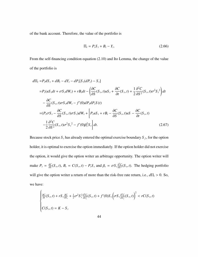
2.5 American options

In this section, we consider finite expiration American put options. Our argument can be

easily extended to other kinds of early exercise options. The value of the American option

is Yt = C(S t, t). For each t ∈ [0,T ] we want to split the S axis into two subintervals. Doing

so will divide the cylinder into two subregions. The boundary between the regions will be

given by a function S f (t). Appropriate boundary conditions will hold on each of the subre-

gions and the boundary between them. Since the location of the boundary between the two

subregions is not known in advance, we have what is called a free boundary problem. As

it happens, this free boundary problem is interpreted as a differential inequality problem.

(1): First subregion: S f (t) < S < ∞.

For these values of S , early exercise is not optimal, and the option holder should hold the

American option. The option seller constructs a portfolio consisting of −1 American put

options and a number Pt of the underlying asset. The value of this portfolio is:

Πt = PtS t + Bt − Yt. (2.63)

42

From the self-financing condition (2.10) and Ito Lemma, the change of the value of the

portfolio is

dΠt =PtdS t + dBt − dYt − dPt[S t(dPt) − S t]

=Pt(uS tdt + σS tdWt) + rBtdt −(∂C∂S

(S t, t)uS t +∂C∂t

(S t, t) +12∂2C∂S 2 (S t, t)σ2S t

2)

dt

−∂C∂S

(S t, t)σS tdWt − f ′(0)dPtdPtS (t)

=

(PtσS t −

∂C∂S

(S t, t)σS t

)dWt + rBtdt +

[PtuS t −

∂C∂S t

(S t, t)uS −∂C∂t

(S t, t)

−12∂2C∂S 2 (S t, t)σ2S t

2 − f ′(0)β2t S t

]dt. (2.64)

Because stock price S t has not reached optimal exercise boundary S f , for the option hold-

er, it is optimal to continue holding the option. The option writer will make Pt = ∂C∂S (S t, t).

Applying Ito Lemma to Pt = ∂C∂S (S t, t) gives us

βt = σS t∂2C∂S 2 (S t, t). (2.65)

The change in the hedging portfolio will be dΠt = 0. Substituting Pt = ∂C∂S (S t, t), Bt =

C(S t, t) − PtS t and (2.65) into (2.64), we have∂C∂t (S t, t) + rS t

∂C∂S t

+ 12σ

2S 2t∂2C∂S 2

t(S t, t) + f ′(0)S t

(σS t

∂2C∂S 2

t(S t, t)

)2= rC(S t, t)

C(S t, t) > K − S t

(2): Second subregion: 0 ≤ S < S f (t).

For these values of S , early exercise is optimal. The option writer constructs a portfolio

consisting of −1 American put option and a number Pt of the underlying asset and Bt units

43

of the bank account. Therefore, the value of the portfolio is

Πt = PtS t + Bt − Yt. (2.66)

From the self-financing condition equation (2.10) and Ito Lemma, the change of the value

of the portfolio is

dΠt =PtdS t + dBt − dYt − dPt[S t(dPt) − S t]

=Pt(uS tdt + σS tdWt) + rBtdt −(∂C∂S

(S t, t)uS t +∂C∂t

(S t, t) +12∂2C∂S 2 (S t, t)σ2S t

2)

dt

−∂C∂S

(S t, t)σS tdWt − f ′(0)dPtdPtS (t)

=(PtσS t −∂C∂S

(S t, t)σS t)dWt +

[PtuS t + rBt −

∂C∂S

(S t, t)uS −∂C∂t

(S t, t)

−12∂2C∂S 2 (S t, t)σ2S t

2 − f ′(0)β2t S t

]dt. (2.67)

Because stock price S t has already entered the optimal exercise boundary S f , for the option

holder, it is optimal to exercise the option immediately. If the option holder did not exercise

the option, it would give the option writer an arbitrage opportunity. The option writer will

make Pt = ∂C∂S (S t, t), Bt = C(S t, t) − PtS t and βt = σS t

∂2C∂S 2 (S t, t). The hedging portfolio

will give the option writer a return of more than the risk-free rate return, i.e., dΠt > 0. So,

we have:∂C∂t (S t, t) + rS t

∂C∂S t

+ 12σ

2S 2t∂2C∂S 2

t(S t, t) + f ′(0)S t

(σS t

∂2C∂S 2

t(S t, t)

)2< rC(S t, t)

C(S t, t) = K − S t

44

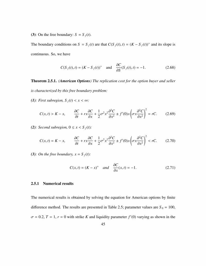
(3): On the free boundary: S = S f (t).

The boundary conditions on S = S f (t) are that C(S f (t), t) = (K − S f (t))+ and its slope is

continuous. So, we have

C(S f (t), t) = (K − S f (t))+ and∂C∂S

(S f (t), t) = −1. (2.68)

Theorem 2.5.1. (American Options) The replication cost for the option buyer and seller

is characterized by this free boundary problem:

(1): First subregion, S f (t) < x < ∞:

C(x, t) > K − x,∂C∂t

+ rx∂C∂x

+12σ2x2∂

2C∂x2 ± f ′(0)x

(σx

∂2C∂x2

)2

= rC. (2.69)

(2): Second subregion, 0 ≤ x < S f (t):

C(x, t) = K − x,∂C∂t

+ rx∂C∂x

+12σ2x2∂

2C∂x2 ± f ′(0)x

(σx

∂2C∂x2

)2

< rC. (2.70)

(3): On the free boundary, x = S f (t):

C(x, t) = (K − x)+ and∂C∂x

(x, t) = −1. (2.71)

2.5.1 Numerical results

The numerical results is obtained by solving the equation for American options by finite

difference method. The results are presented in Table 2.5; parameter values are S 0 = 100,

σ = 0.2, T = 1, r = 0 with strike K and liquidity parameter f ′(0) varying as shown in the

45

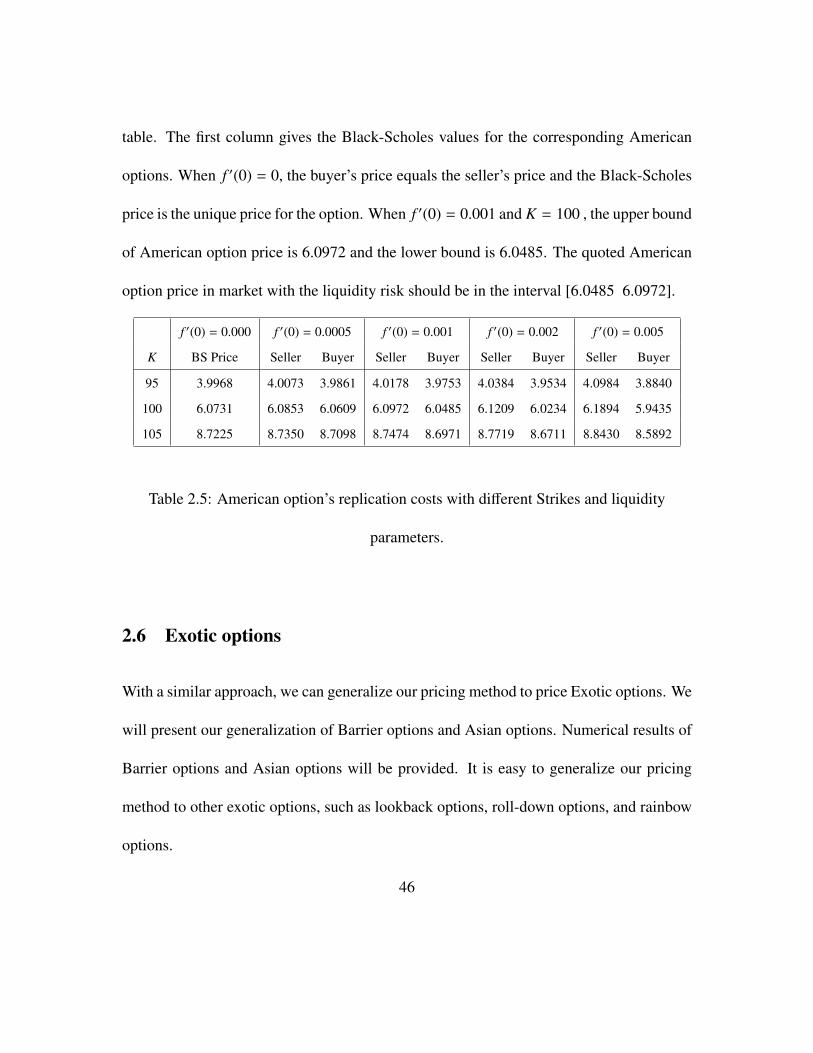
table. The first column gives the Black-Scholes values for the corresponding American

options. When f ′(0) = 0, the buyer’s price equals the seller’s price and the Black-Scholes

price is the unique price for the option. When f ′(0) = 0.001 and K = 100 , the upper bound

of American option price is 6.0972 and the lower bound is 6.0485. The quoted American

option price in market with the liquidity risk should be in the interval [6.0485 6.0972].

f ′(0) = 0.000 f ′(0) = 0.0005 f ′(0) = 0.001 f ′(0) = 0.002 f ′(0) = 0.005

K BS Price Seller Buyer Seller Buyer Seller Buyer Seller Buyer

95 3.9968 4.0073 3.9861 4.0178 3.9753 4.0384 3.9534 4.0984 3.8840

100 6.0731 6.0853 6.0609 6.0972 6.0485 6.1209 6.0234 6.1894 5.9435

105 8.7225 8.7350 8.7098 8.7474 8.6971 8.7719 8.6711 8.8430 8.5892

Table 2.5: American option’s replication costs with different Strikes and liquidity

parameters.

2.6 Exotic options

With a similar approach, we can generalize our pricing method to price Exotic options. We

will present our generalization of Barrier options and Asian options. Numerical results of

Barrier options and Asian options will be provided. It is easy to generalize our pricing

method to other exotic options, such as lookback options, roll-down options, and rainbow

options.

46

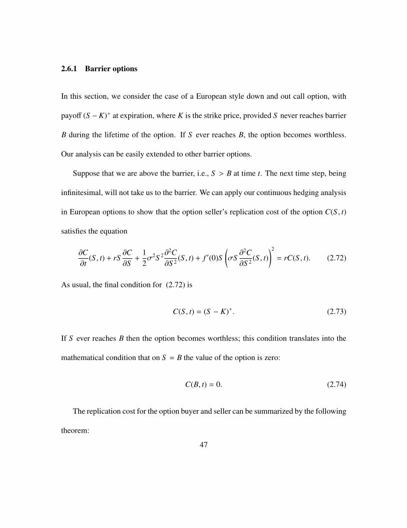
2.6.1 Barrier options

In this section, we consider the case of a European style down and out call option, with

payoff (S −K)+ at expiration, where K is the strike price, provided S never reaches barrier

B during the lifetime of the option. If S ever reaches B, the option becomes worthless.

Our analysis can be easily extended to other barrier options.

Suppose that we are above the barrier, i.e., S > B at time t. The next time step, being

infinitesimal, will not take us to the barrier. We can apply our continuous hedging analysis

in European options to show that the option seller’s replication cost of the option C(S , t)

satisfies the equation

∂C∂t

(S , t) + rS∂C∂S

+12σ2S 2∂

2C∂S 2 (S , t) + f ′(0)S

(σS

∂2C∂S 2 (S , t)

)2

= rC(S , t). (2.72)

As usual, the final condition for (2.72) is

C(S , t) = (S − K)+. (2.73)

If S ever reaches B then the option becomes worthless; this condition translates into the

mathematical condition that on S = B the value of the option is zero:

C(B, t) = 0. (2.74)

The replication cost for the option buyer and seller can be summarized by the following

theorem:

47

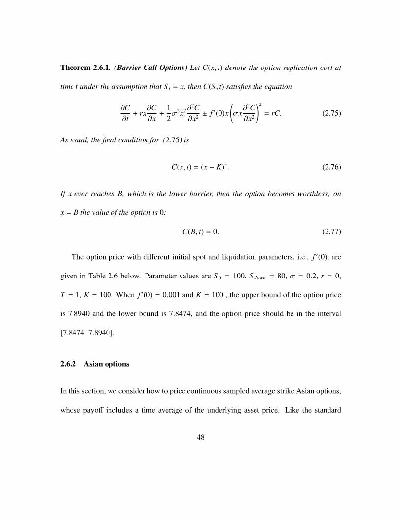
Theorem 2.6.1. (Barrier Call Options) Let C(x, t) denote the option replication cost at

time t under the assumption that S t = x, then C(S , t) satisfies the equation

∂C∂t

+ rx∂C∂x

+12σ2x2∂

2C∂x2 ± f ′(0)x

(σx

∂2C∂x2

)2

= rC. (2.75)

As usual, the final condition for (2.75) is

C(x, t) = (x − K)+. (2.76)

If x ever reaches B, which is the lower barrier, then the option becomes worthless; on

x = B the value of the option is 0:

C(B, t) = 0. (2.77)

The option price with different initial spot and liquidation parameters, i.e., f ′(0), are

given in Table 2.6 below. Parameter values are S 0 = 100, S down = 80, σ = 0.2, r = 0,

T = 1, K = 100. When f ′(0) = 0.001 and K = 100 , the upper bound of the option price

is 7.8940 and the lower bound is 7.8474, and the option price should be in the interval

[7.8474 7.8940].

2.6.2 Asian options

In this section, we consider how to price continuous sampled average strike Asian options,

whose payoff includes a time average of the underlying asset price. Like the standard

48

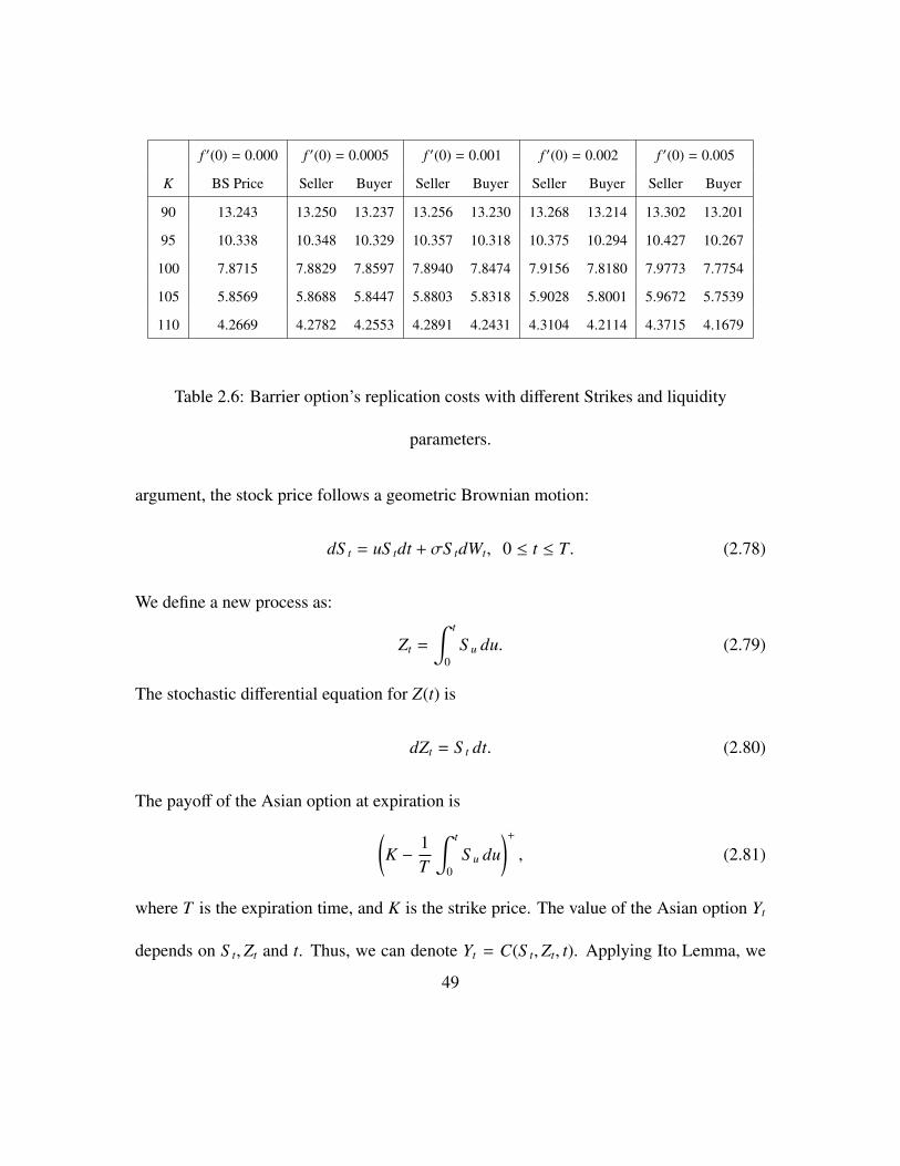
f ′(0) = 0.000 f ′(0) = 0.0005 f ′(0) = 0.001 f ′(0) = 0.002 f ′(0) = 0.005

K BS Price Seller Buyer Seller Buyer Seller Buyer Seller Buyer

90 13.243 13.250 13.237 13.256 13.230 13.268 13.214 13.302 13.201

95 10.338 10.348 10.329 10.357 10.318 10.375 10.294 10.427 10.267

100 7.8715 7.8829 7.8597 7.8940 7.8474 7.9156 7.8180 7.9773 7.7754

105 5.8569 5.8688 5.8447 5.8803 5.8318 5.9028 5.8001 5.9672 5.7539

110 4.2669 4.2782 4.2553 4.2891 4.2431 4.3104 4.2114 4.3715 4.1679

Table 2.6: Barrier option’s replication costs with different Strikes and liquidity

parameters.

argument, the stock price follows a geometric Brownian motion:

dS t = uS tdt + σS tdWt, 0 ≤ t ≤ T. (2.78)

We define a new process as:

Zt =

∫ t

0S u du. (2.79)

The stochastic differential equation for Z(t) is

dZt = S t dt. (2.80)

The payoff of the Asian option at expiration is(K −

1T

∫ t

0S u du

)+

, (2.81)

where T is the expiration time, and K is the strike price. The value of the Asian option Yt

depends on S t,Zt and t. Thus, we can denote Yt = C(S t,Zt, t). Applying Ito Lemma, we

49

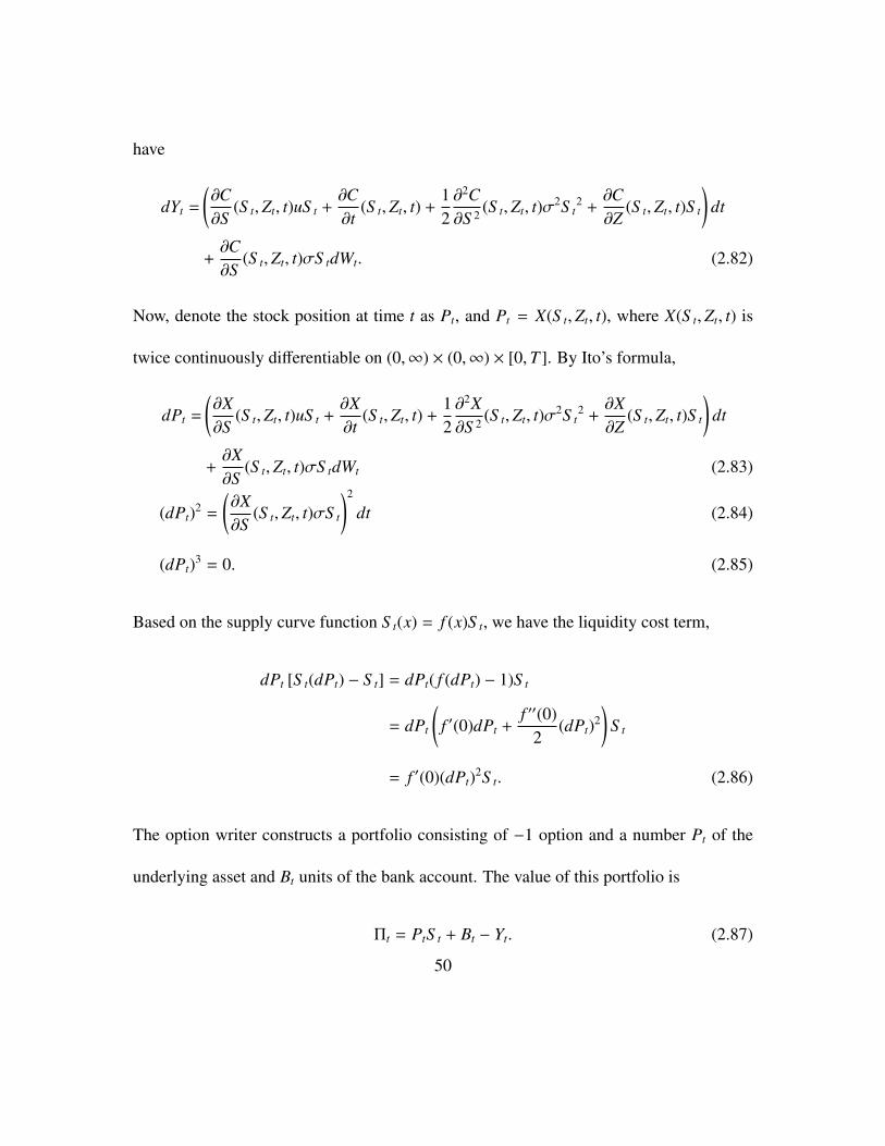
have

dYt =

(∂C∂S

(S t,Zt, t)uS t +∂C∂t

(S t,Zt, t) +12∂2C∂S 2 (S t,Zt, t)σ2S t

2 +∂C∂Z

(S t,Zt, t)S t

)dt

+∂C∂S

(S t,Zt, t)σS tdWt. (2.82)

Now, denote the stock position at time t as Pt, and Pt = X(S t,Zt, t), where X(S t,Zt, t) is

twice continuously differentiable on (0,∞) × (0,∞) × [0,T ]. By Ito’s formula,

dPt =

(∂X∂S

(S t,Zt, t)uS t +∂X∂t

(S t,Zt, t) +12∂2X∂S 2 (S t,Zt, t)σ2S t

2 +∂X∂Z

(S t,Zt, t)S t

)dt

+∂X∂S

(S t,Zt, t)σS tdWt (2.83)

(dPt)2 =

(∂X∂S

(S t,Zt, t)σS t

)2

dt (2.84)

(dPt)3 = 0. (2.85)

Based on the supply curve function S t(x) = f (x)S t, we have the liquidity cost term,

dPt [S t(dPt) − S t] = dPt( f (dPt) − 1)S t

= dPt

(f ′(0)dPt +

f ′′(0)2

(dPt)2)

S t

= f ′(0)(dPt)2S t. (2.86)

The option writer constructs a portfolio consisting of −1 option and a number Pt of the

underlying asset and Bt units of the bank account. The value of this portfolio is

Πt = PtS t + Bt − Yt. (2.87)

50

The change of the value of the portfolio in the time t to t + dt is

dΠt =PtdS t + rBtdt − dYt − dPt [S t(dPt) − S t]

=PtdS t + rBtdt −(∂C∂S

(S t, t)uS t +∂C∂t

(S t, t) +12∂2C∂S 2 (S t, t)σ2S t

2)

dt

+∂C∂S

(S t, t)σS tdWt + rBtdt − dPt[S (t, dPt) − S (t, 0)]

=Pt (uS tdt + σS tdWt) −∂C∂S

(S t,Zt, t)σS tdWt − f ′(0)(dPt)2S (t, 0)

−

(∂C∂S

(S t,Zt, t)uS t +∂C∂t

(S t,Zt, t) +12∂2C∂S 2 (S t,Zt, t)σ2S t

2 +∂C∂Z

(S t,Zt, t)S t

)dt

=

(PtσS t −

∂C∂S

(S t,Zt, t)σS t

)dWt + rBtdt +

[PtuS t −

∂C∂S

(S t,Zt, t)uS t −∂C∂t

(S t,Zt, t)

−12∂2C∂S 2 (S t,Zt, t)σ2S t

2 −∂C∂Z

(S t,Zt, t)S t − f ′(0)S t

(∂X∂S

(S t,Zt, t)σS t

)2 dt. (2.88)

In order to fully hedge the option, the option writer needs to make dΠt = 0. By making

dBt and dt terms to 0, we have Pt = ∂C∂S (S t,Zt, t), Bt = C(S t,Zt, t) − PtS t and ∂X

∂S (S t,Zt, t) =

∂2C∂S 2 (S t,Zt, t). Substituting them into (2.88), we deduce from dΠt = 0 that

∂C∂t

(S t,Zt, t) + rS t∂C∂S t

+12∂2C∂S 2 (S t,Zt, t)σ2S t

2 +∂C∂Z

(S t,Zt, t)S t (2.89)

+ f ′(0)S t

(∂2C∂S 2 (S t,Zt, t)σS t

)2

= rC(S t,Zt, t). (2.90)

Replacing S t with dummy variable x, and Zt by the dummy variable y, we obtain

∂C∂t

(x, y, t) + rx∂C∂x

(x, y, t) +12∂2C∂x2 (x, y, t)σ2x2 +

∂C∂y

(x, y, t)x

+ f ′(0)x(σx

∂2C∂x2 (x, y, t)

)2

= rC(x, y, t). (2.91)

51

The boundary conditions for continuous average Asian put options are

C(x,KT, t) = 0, 0 ≤ t ≤ T, x ≥ 0,

C(x, y,T ) = (K −yT

)+, x ≥ 0, 0 ≤ y ≤ KT,

C(0, y, t) = (K −yT

)+, 0 ≤ t ≤ T, 0 ≤ y ≤ KT,

C(xmax, y, t) = (K −y + (T − t)xmax

T)+, 0 ≤ t ≤ T, 0 ≤ y ≤ KT.

For other kinds of Asian options, we have different boundary conditions and the PDE

remains the same. For the option buyer’s side, following the same analysis, it can be

easily known that the replication cost is characterized by:

∂C∂t

+ rx∂C∂x

+12σ2x2∂

2C∂x2 + x

∂C∂y− f ′(0)x

(σx

∂2C∂x2

)2

= rC. (2.92)

Theorem 2.6.2. (Asian Options) Let C(x, y, t) denote the option replication cost at time t

under the assumption that S t = x and Yt = y, such that Yt =∫ t

0S u du, we have

∂C∂t

+ rx∂C∂x

+12σ2x2∂

2C∂x2 + x

∂C∂y± f ′(0)x

(σx

∂2C∂x2

)2

= rC, (2.93)

and the boundary conditions

C(x,KT, t) = 0, 0 ≤ t ≤ T, x ≥ 0,

C(x, y,T ) = (K −yT

)+, x ≥ 0, 0 ≤ y ≤ KT,

C(0, y, t) = (K −yT

)+, 0 ≤ t ≤ T, 0 ≤ y ≤ KT,

C(xmax, y, t) = (K −y + (T − t)xmax

T)+, 0 ≤ t ≤ T, 0 ≤ y ≤ KT.

52

f ′(0) = 0.000 f ′(0) = 0.0005 f ′(0) = 0.001 f ′(0) = 0.002 f ′(0) = 0.005

K BS Price Seller Buyer Seller Buyer Seller Buyer Seller Buyer

95 2.4967 2.5011 2.4922 2.5056 2.4876 2.5145 2.4786 2.5409 2.4510

100 4.7046 4.7100 4.6993 4.7153 4.6939 4.7259 4.6830 4.7573 4.6500

Table 2.7: Asian option’s replication costs with different Strikes and liquidity parameters.

We provide some numerical results for Asian options. Parameter values are S 0 = 100,

r = 0, σ = 0.2, T = 1 with varying strike K in Table 2.7. When f ′(0) = 0.001 and

K = 100 , the upper bound of the option price is 4.7153 and the lower bound is 4.6939.

The quoted Asian option price in the market with liquidity risk should be in the interval

[4.6939, 4.7153].

53

3 Option Pricing with Liquidity Risk in a

Jump-diffusion Model

3.1 Introduction

In this chapter, we will investigate option pricing with liquidity risk in a jump-diffusion

model. in Chapter 2, we showed the existence of a perfect hedging of vanilla and exotic op-

tions in a non-competitive market for small investors when stock price follows a geometric

Brownian motion. However, empirical studies (Jorion (1988), Andersen et al. (2002) and

Bates (2000)) suggest that there are jumps in the stock price. Jumps in the stock price is

modeled by a jump-diffusion model. Option pricing in a jump-diffusion model was first

considered in Merton (1976). Numerous pricing approaches have since been proposed for

pricing derivatives in a jump-diffusion model: super hedging, mean variance hedging (Lim

(2005)), and local risk minimization hedging (Follmer and Schweizer (1991)). Jumps in

stock price bring jump risk, and it is known that liquidity risk and jump risk are not in-

54

dependent but correlated. Specifically, the liquidity risk for options becomes much more

critical when there are jumps in the underlying security. For example, in a financial crisis,

it is common that an underlying asset price exhibits jumps, leading investors in the market

to change their position on the underlying asset quickly to hedge derivatives, which caus-

es a significant liquidity problem. This motivates us to study the pricing and hedging of

options in a jump-diffusion model with liquidity risk.

When the underlying stock price follows a jump-diffusion model, the market becomes

incomplete, which makes perfect hedging impossible. Other pricing methods have been

developed for hedging options. Local risk minimization has been proven to be an easily

applicable pricing method to price options in incomplete markets. Options can be priced

by the local risk minimization method for a jump-diffusion model in the continuous time

setting (without liquidity risk), giving us a partial differential equation to characterize the

hedging cost. It is natural to ask whether a modified partial differential equation can be

derived to describe the local risk minimization hedging cost of options in a market with

liquidity risk. It doesn’t seem possible to derive such a partial differential equation due to

the complexity introduced by liquidity risk. In order to value options with liquidity risk in

a jump-diffusion model, we turn to a discrete-time model.

A jump-diffusion model could be approximated by a discrete-time process (Amin

(1993)). Local risk minimization is easily applicable in discrete-time (see Coleman et al.

55

(2007)). In this chapter, we apply local risk minimization to price options with liquidity

risk for a discrete-time Markov process. The discrete-time Markov process converges to a

continuous jump-diffusion process as the time step goes to zero. By letting the length of

the time intervals go to zero, the option price obtained from the discrete-time model ap-

proaches the option price in the jump-diffusion model. Therefore, the method we suggest

is useful for pricing and hedging options in a jump-diffusion model with the presence of

liquidity costs.

3.2 Local risk minimization in a jump-diffusion model

We consider a financial market that consists of one bank account and one stock. The

interest rate is r and the bank account Bt is given by:

dBt = rBtdt, t ∈ [0, T ]. (3.1)

Without loss of generality, it is assumed that r = 0. The stock price is defined on a

probability space (Ω,F ,P) with the filtration Ft : t ≥ 0 generated by a one-dimensional

Brownian motion Wt and a Poisson process Nt with intensity λ. The stock price S t is

modeled by a jump-diffusion process and follows the stochastic differential equation

dS t = µS tdt + σS tdWt + (Vi − 1)S tdNt, t ∈ [0, T ] (3.2)

56

where σ is the volatility, µ is the drift term of the stock, and Vi is the jump size where

P Vi = eq j = p j 1 ≤ j ≤ m (3.3)

and

p1 + p1 + ... + pm = 1.

The solution of the stochastic differential equation (3.2) is written as

S t = S 0 exp

(µ −12σ2)t + σWt

N(t)∏i=1

Vi. (3.4)

Assume that an investor writes an option with maturity T . In order to hedge the option,

the investor needs to construct a portfolio (Pt, Bt) to hedge both the diffusion and the jump

risk, where Pt stands for the number of shares of the stock and Bt is the amount of the bank

account. Let C(t, S t) denote the option price at time t when the stock price is S t. Since the

interest rate r = 0, the change in the portfolio value during time interval [t, t + dt] will be

PtdS t = Pt[µS tdt + σS tdWt + (V − 1)S td Nt

]. (3.5)

The change of the option price will be

dC(t, S t) =∂C∂t

dt +∂C∂S

µS tdt +∂C∂S

σS tdWt +12∂2C∂S 2σ

2S 2t dt

+ [C(t,V × S t) −C(t, S t)]dNt. (3.6)

In order to make the model simple, we assume P(V = elog(1+q) = 1+q) = 1 and E(V) = 1+q.

We can extend the above analysis to cases with multiple jumps. The market is incomplete

57

in a jump-diffusion model, since there are multiple sources of randomness, a derivative

cannot be fully hedged with the underlying stock and bank account. If we try to hedge the

jump risk and make dNt terms in both (3.4) and (3.6), we get

qS tPt = C(t, (1 + q)S t) −C(t, S t), (3.7)

which means

Pt =C(t, (1 + q)S t) −C(t, S t)

qS t.

On the other hand, if we try to hedge the diffusion risk and make dWt terms in both (3.4)

and (3.6), we get

µS tPt =∂C∂S

µS t, (3.8)

which leads to

Pt =∂C∂S

.

As expected, we cannot eliminate the jump risk and diffusion risk simultaneously. There-

fore, we need to find a compromise in hedging the two risks.

When the two risks cannot be hedged completely and the hedging error is not zero, the

local risk minimization approach could be used to minimize the variance of the hedging

error caused by the diffusion risk and jump risk. This hedging strategy is a compromise

between hedging the jump risk and hedging diffusion risk. In the local risk minimization

approach, we make the expected hedging error equal zero, and minimize the variance of

58

the hedging error. Let Mt = Nt − λt, then Mt is a martingale. The change of the portfolio

becomes

PtdS t = Pt[(µ + λq) S tdt + σS tdWt + qS td Mt

]. (3.9)

From Ito’s formula of jump-diffusion processes, it can be shown

dC(t, S t) =∂C∂t

dt +∂C∂S

µS tdt +12∂2C∂S 2σ

2S 2t dt + λ

[C(t, (1 + q)S t) −C(t, S t)

]dt

+∂C∂S

σS tdWt +[C(t, (1 + q)S t) −C(t, S t)

]dMt. (3.10)

The hedging error is defied as PtdS t − dC(t, S t). Notice that in order to make the expected

hedging error equal zero, we must set the dt term of (3.9) and (3.10) to equal

∂C∂t

dt+∂C∂S

µS tdt+12∂2C∂S 2σ

2S 2t dt+λ

[C(t, (q + 1)S t) −C(t, S t)

]dt = Pt(µ+λq)S tdt. (3.11)

The variance of the hedging error is

Var [PtdS t − dC(t, S t)] = PtqS t − [C(t, (q + 1)S t) −C(t, S t)]2 λdt,

+

(PtσS t −

∂C∂S

σS t

)2

dt, (3.12)

which is minimized by

Pt =∂C∂S

σ2

σ2 + λq2 +C(t, (q + 1)S t) −C(t, S t)

qS t

λq2

σ2 + λq2 .

Then Pt represents the stock position of the local risk minimization hedging strategy. Sub-

59

stituting Pt into (3.11), we have the pricing equation for C(t, S )

∂C∂t− q

(λσ2 − quσ2 + λq2

)∂C∂S

S +

(λσ2 − quσ2 + λq2

) [C(t, (q + 1)S ) −C(t, S t)

]+

12∂2C∂S 2σ

2S 2 = 0. (3.13)

for 0 ≤ t < T . Equation (3.13) characterizes the option’s hedging cost under local mini-

mization hedging strategy.

3.3 Approximate a jump-diffusion process with a discrete-time model

It is well known that a geometric Brownian motion can be approximated by a binomial

model. If the jump size takes finite values, a jump-diffusion process could be approximated

by a discrete-time process (Figure 3.1). We can approximate the jump-diffusion process

(3.2) in the following way. For any t ∈ [0, T ], we have n stages over time horizon [0, t],

denoted by 0 = t0 < t1 < · · · < tN = t with ∆t = tN . Given S k the stock price at time tk and

60

time step ∆t, there are m + 2 possible values for S k+1 at time k + 1:

S k+1 =

S ke(µ− 12σ

2)∆t+σ√

∆t, if S k goes up;

S ke(µ− 12σ

2)∆t−σ√

∆t, if S k goes down;

eq1S k, if S k jumps to eq1S k;

...

eqmS k, if S k jumps to eqmS k.

The relation of S k+1 and S k is S k+1 = S kξk+1, where

ξk+1 =

e(µ− 12σ

2)∆t+σ√

∆t, with probability 1−λ∆t2 ;

e(µ− 12σ

2)∆t−σ√

∆t, with probability 1−λ∆tt2 ;

eq1 , with probability p1λ∆t;

...

eqm , with probability pmλ∆t.

Theorem 3.3.1. As N → ∞, (S k)k=0,1,...,N is convergent to the following jump-diffusion

process in distribution

S t = S 0 exp

(µ −12σ2)t + σW(t)

N(t)∏i=1

Vi, (3.14)

61

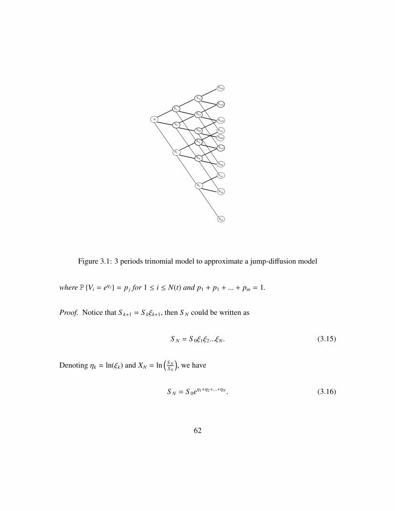
Sd

Sj

Suu

Sud

Suj

Sdd

Sdj

Sjj

Suuu

Suud

Sudd

Sujd

Sddd

Suuj

Sujj

Sdjj

Sjjj

Sddj

S

Su

Figure 3.1: 3 periods trinomial model to approximate a jump-diffusion model

where P Vi = eq j = p j for 1 ≤ i ≤ N(t) and p1 + p1 + ... + pm = 1.

Proof. Notice that S k+1 = S kξk+1, then S N could be written as

S N = S 0ξ1ξ2...ξN . (3.15)

Denoting ηk = ln(ξk) and XN = ln(

S NS 0

), we have

S N = S 0eη1+η2+...+ηN . (3.16)

62

For the discrete-time model, the log return XN has the form

XN = η1 + η2 + ... + ηN , (3.17)

where η1, η2, ...ηN are independent and identically distributed.

For the continuous time jump-diffusion model, the log return Xt = ln(

S tS 0

)is expressed

as

Xt =

(µ −

12σ2

)t + σWt +

N(t)∑i=1

Ui, (3.18)

where Ui = ln(Vi). The generating function of Xt is

GXt(θ) = E[eθXt

]= E

[eθ[(µ−

12σ

2)t+σWt+∑N(t)

i=1 Ui]]

= eθ(µ−12σ

2)tE[eθσWt

]E

[eθ

∑N(t)i=1 Ui

]. (3.19)

From iterated conditional expectation, we have

E[eθ

∑N(t)i=1 Ui

]= E

E

[eθ

∑N(t)i=1 Ui |N(t)

]= E

[(p1eq1θ + p2eq2θ + ... + pmeqmθ

)N(t)]

=

∞∑k=1

(p1eq1θ + p2eq2θ + ... + pmeqmθ

)k (λt)ke−λt

k!

= expλ(p1eq1θ + p2eq2θ + ... + pmeqmθ − 1

)t. (3.20)

Also, we know

E[eθσWt

]= exp

(12σ2θ2t

). (3.21)

63

Together with (3.20) and (3.21), the moment generating function of GXt(θ) could be ex-

pressed as

GXt(θ) = expθ

(µ −

12σ2

)t +

12σ2θ2t + λ

(p1eq1θ + p2eq2θ + ... + pmeqmθ − 1

)t. (3.22)

The moment generating function of XN is GXN (θ) = E[eθXN ] and it could be written as

GXN (θ)

=[Gηk(θ)

]N

=

1 − λ∆t

2eθ[(µ−

12σ

2)∆t+σ√

∆t] +1 − λ∆t

2eθ[(µ−

12σ

2)∆t−σ√

∆t] + p1λ∆teθq1 + ... + pmλ∆teθqm

N

=

1 − λ∆t

2

[1 + (µ −

12σ2)∆tθ + σ

√∆tθ +

12σ2∆tθ2 + O(∆t)3/2

]+

1 − λ∆t2

[1 + (µ −

12σ2)∆tθ − σ

√∆tθ +

12σ2∆tθ2 + O(∆t)

]+ p1λ∆teθq1 + ... + pmλ∆teθqm

N

=

1 + (µ −

12σ2)θ∆t +

12σ2θ2∆t + λ(p1eθq1 + p2eθq2 + ...pmeθqm − 1)θ∆t + O(∆t)3/2

N

=

1 +

[θ(µ −

12σ2) +

12σ2θ2 + λ(p1eq1θ + p2eq2θ + ... + pmeqmθ − 1)

]∆t + O(∆t)3/2

N

.

We know N = t∆t , and as N → ∞ we have

limN→∞

1 +

[θ(µ −

12σ2) +

12σ2θ2 + λ(p1eq1θ + p2eq2θ + ... + pmeqmθ − 1)

]∆t + O(∆t)3/2

N

= lim∆t→0

1 +

[θ(µ −

12σ2) +

12σ2θ2 + λ(p1eq1θ + p2eq2θ + ... + pmeqmθ − 1)

]∆t + O(∆t)3/2

t∆t

= expθ(µ −

12σ2)t +

12σ2θ2t + λ(p1eq1θ + p2eq2θ + ... + pmeqmθ − 1)t

,

which is exactly the generating function of Xt. We proved the moment generating function

64

of XN converges to the moment generating function of Xt. From the convergence in distri-

bution theorem, we have XN is convergent to Xt in distribution and S N = S 0eXN converges

to S t = S 0eXt in distribution.

3.4 Supply curve model and Local risk minimization considering liq-

uidity risk

Liquidity risk is modeled by the supply curve model. A supply curve function S t(z) repre-

sents the stock price per share that the investor pays for an order size of z given the stock

price is S t at time t. A positive z represents a buying of stock and a negative x represents

a selling of stock. In the discrete-time model, separable form of supply curve function has

the following form:

S k(z) = f (z)S k. (3.23)

Since we can approximate a jump-diffusion process by using a discrete-time model,

pricing and hedging options in a jump-diffusion process could de addressed in the discrete-

time model that approximates the jump-diffusion model. When the time interval tN goes

to zero, the option price obtained from the discrete-time model will converge to the option

price with liquidity risk in the jump-diffusion model.

Assume that we are going to hedge a European call option with maturity tN and payoff

HN = (S N − K)+ that is FtN measurable. A trading strategy is given by two stochastic

65

processes as (xk)k=0,1,...,N and (yk)k=0,1,...,N , where xk stands for the number of shares and yk

is the bank account amount at time tk. Both xk and yk are Ftk measurable for 0 ≤ k ≤ N.

The portfolio is the combination of the stock and the bank account given by the trading

strategy. The value of portfolio at time tk is given by:

Vk = xkS k + yk. (3.24)

The liquidity cost incurred from t1 to tk is defined by

Lk =

k−1∑i=1

[f (xi+1 − xi) − 1

]S i+1(xi+1 − xi). (3.25)

Since the interest rate r is assumed to be 0, the accumulated gain Gk is given by

Gk =

k−1∑i=0

xi(S i+1 − S i) −k−1∑i=0

[f (xi+1 − xi) − 1

]S i+1(xi+1 − xi), (3.26)

and G0 = 0. Indeed, the accumulated gain in the market with liquidity cost equals the

accumulated gain from the stock minus the liquidity cost of dynamic hedging.

The accumulated cost at time tk is defined by

Ck = Vk −Gk. (3.27)

A strategy is self-financing if the accumulated cost process (Ck)k=0,1,...,N is a constant over

time. The self-financing strategy means:

Ck+1 −Ck =(Vk+1 −Gk+1) − (Vk −Gk) (3.28)

=xk+1S k+1 + yk+1 +[f (xi+1 − xi) − 1

]S i+1(xi+1 − xi) − xkS k+1 − yk = 0. (3.29)

66

The value of a self-financing portfolio is given by Vk = V0 + Gk for 0 ≤ k ≤ N. If the

market is complete and perfect, such as in the binomial model, there is a self-financing

strategy with VN = HN a.s. But if the market is incomplete, for example, if there is a

jump risk of the stock price and a contingent claim is non-attainable, the cost process

(Ck)k=1,2,...,N cannot be constant and a hedging strategy has to be chosen based on some

optimality criterion.

We apply a local risk minimization hedging method to hedge options in the discrete-

time model. First, we impose VN = HN . Local risk minimization requires the cost pro-

cess (Ck)k=1,2,...,N be a martingale and the variance of incremental cost process (Ck+1 −

Ck)k=0,1,...,N−1 be minimal. The traditional criterion for local risk minimization is the quadrat-

ic criterion, i.e.,

min Var[(Ck+1 −Ck)|Fk] (3.30)

Subject to: E[Ck+1 −Ck|Fk] = 0. (3.31)

It is equivalent to minimize

E[(Ck+1 −Ck)2|Fk]. (3.32)

In our discrete-time model, given the payoff at maturity of the option HN , we set VN =

xNS N + yN = HN . By the local risk minimization method, the trading strategy (x∗N−1, y∗N−1)

67

at tN−1 is

(x∗N−1, y∗N−1) = arg min

xN−1,yN−1E[(HN − xN−1S N − yN−1)2|Fk]. (3.33)

For 0 ≤ k < N, when we know (x∗k+1, y∗k+1), we want to minimize E[(Ck+1 − Ck)2|Fk] to

deduce (x∗k, y∗k). It can be done by minimizing the following optimization problem:

(x∗k, y∗k) = arg min

xk ,ykE[(x∗k+1S k+1 + y∗k+1 +

[f (x∗k+1 − xk) − 1

]S k+1(x∗k+1 − xk) − xkS k+1 − yk)2|Fk].

(3.34)

By the backward deduction, accordingly we can have (x∗N−1, y∗N−1), (x∗N−2, y

∗N−2)...,(x∗1, y

∗1),

(x∗0, y∗0). Then the initial option price at time t0 is determined is x∗0S 0 + y∗0, and (x∗N−1, y

∗N−1),

(x∗N−2, y∗N−2)...,(x∗1, y

∗1), (x∗0, y

∗0) provide the local risk minimization hedging strategies. As

N goes to infinity, the discrete-time model is convergent to the jump-diffusion model. The

option price and hedging strategy obtained from the discrete time model give a good ap-

proximation of the corresponding price and hedging strategy in the jump-diffusion model.

The discrete-time model we just presented can be viewed as an extension of the clas-

sic binomial model. When the liquidity parameter is 0 (the supply curve function is flat

everywhere), our approach coincides with the discrete-time model of a jump-diffusion pro-

cess with local risk minimization hedging. Also, when the jump parameter λ = 0 (there

are no jumps), our model is reduced to the binomial model with liquidity costs, which is

a discrete-time version of a continuous perfect replication model. It is obvious that our

model becomes the classic binomial model when both parameters are zero.

68

3.5 Numerical results

In this section, we present compare results of numerical studies of three hedging strategies:

delta hedging, traditional local risk minimization hedging (local risk minimization with-

out liquidity risk), and modified local risk minimization hedging (local risk minimization

considering liquidity risk). First we describe the discrete model used to approximate the

jump-diffusion model.

The jump-diffusion model we are going to approximate is given by

dS t = µS tdt + σS tdWt + (Vi − 1)S tdNt, t ∈ [0, T ] (3.35)

where σ = 0.2, µ = 0.2, Nt is a Poisson process with intensity λ1 + λ2 and Vi is the jump

size with

P Vi = 0.9 =λ1

λ1 + λ2and P Vi = 1.12 =

λ2

λ1 + λ2.

The discrete-time model used to approximate the jump-diffusion model has N periods with

time interval ∆t = TN . If the stock price is S k at period k in the discrete-time model, then

the stock price at period k + 1 has four scenarios: goes up, goes down, jumps down, and

jumps up. The probability distribution for S k+1 are:

69

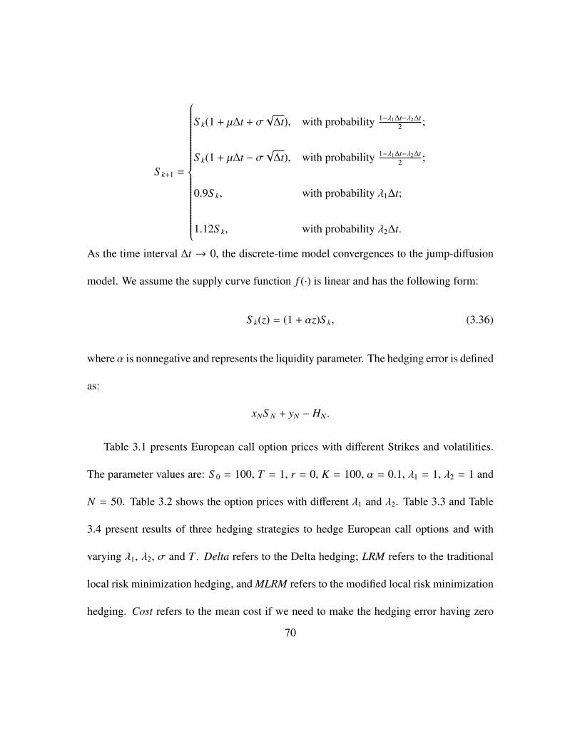
S k+1 =

S k(1 + µ∆t + σ√

∆t), with probability 1−λ1∆t−λ2∆t2 ;

S k(1 + µ∆t − σ√

∆t), with probability 1−λ1∆t−λ2∆t2 ;

0.9S k, with probability λ1∆t;

1.12S k, with probability λ2∆t.

As the time interval ∆t → 0, the discrete-time model convergences to the jump-diffusion

model. We assume the supply curve function f (·) is linear and has the following form:

S k(z) = (1 + αz)S k, (3.36)

where α is nonnegative and represents the liquidity parameter. The hedging error is defined

as:

xNS N + yN − HN .

Table 3.1 presents European call option prices with different Strikes and volatilities.

The parameter values are: S 0 = 100, T = 1, r = 0, K = 100, α = 0.1, λ1 = 1, λ2 = 1 and

N = 50. Table 3.2 shows the option prices with different λ1 and λ2. Table 3.3 and Table

3.4 present results of three hedging strategies to hedge European call options and with

varying λ1, λ2, σ and T . Delta refers to the Delta hedging; LRM refers to the traditional

local risk minimization hedging, and MLRM refers to the modified local risk minimization

hedging. Cost refers to the mean cost if we need to make the hedging error having zero

70

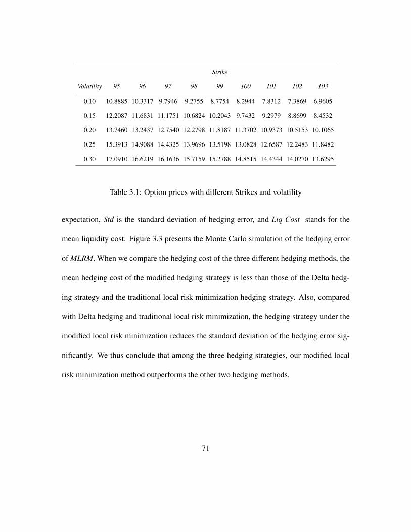
Strike

Volatility 95 96 97 98 99 100 101 102 103

0.10 10.8885 10.3317 9.7946 9.2755 8.7754 8.2944 7.8312 7.3869 6.9605

0.15 12.2087 11.6831 11.1751 10.6824 10.2043 9.7432 9.2979 8.8699 8.4532

0.20 13.7460 13.2437 12.7540 12.2798 11.8187 11.3702 10.9373 10.5153 10.1065

0.25 15.3913 14.9088 14.4325 13.9696 13.5198 13.0828 12.6587 12.2483 11.8482

0.30 17.0910 16.6219 16.1636 15.7159 15.2788 14.8515 14.4344 14.0270 13.6295

Table 3.1: Option prices with different Strikes and volatility

expectation, Std is the standard deviation of hedging error, and Liq Cost stands for the

mean liquidity cost. Figure 3.3 presents the Monte Carlo simulation of the hedging error

of MLRM. When we compare the hedging cost of the three different hedging methods, the

mean hedging cost of the modified hedging strategy is less than those of the Delta hedg-

ing strategy and the traditional local risk minimization hedging strategy. Also, compared

with Delta hedging and traditional local risk minimization, the hedging strategy under the

modified local risk minimization reduces the standard deviation of the hedging error sig-

nificantly. We thus conclude that among the three hedging strategies, our modified local

risk minimization method outperforms the other two hedging methods.

71

@@@@@

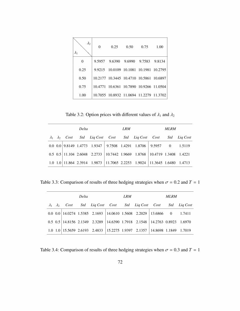
λ1

λ20 0.25 0.50 0.75 1.00

0 9.5957 9.6390 9.6990 9.7583 9.8134

0.25 9.9215 10.0109 10.1081 10.1981 10.2795

0.50 10.2177 10.3445 10.4710 10.5861 10.6897

0.75 10.4771 10.6361 10.7890 10.9266 11.0504

1.00 10.7055 10.8932 11.0694 11.2279 11.3702

Table 3.2: Option prices with different values of λ1 and λ2

Delta LRM MLRM

λ1 λ2 Cost Std Liq Cost Cost Std Liq Cost Cost Std Liq Cost

0.0 0.0 9.8149 1.4773 1.9347 9.7508 1.4291 1.8706 9.5957 0 1.5119

0.5 0.5 11.104 2.6048 2.2733 10.7442 1.9669 1.8768 10.4719 1.3408 1.4221

1.0 1.0 11.864 2.3914 1.9873 11.7065 2.2253 1.9024 11.3645 1.6480 1.4713

Table 3.3: Comparison of results of three hedging strategies when σ = 0.2 and T = 1

Delta LRM MLRM

λ1 λ2 Cost Std Liq Cost Cost Std Liq Cost Cost Std Liq Cost

0.0 0.0 14.0274 1.5385 2.1693 14.0610 1.5608 2.2029 13.6866 0 1.7411

0.5 0.5 14.8156 2.1349 2.3289 14.6390 1.7918 2.1548 14.2763 0.8923 1.6970

1.0 1.0 15.5659 2.6193 2.4833 15.2275 1.9397 2.1357 14.8698 1.1849 1.7019

Table 3.4: Comparison of results of three hedging strategies when σ = 0.3 and T = 1

72

4 Utility Indifference Pricing for Large Investors

4.1 Introduction

We considered option pricing with liquidity risk for small investors in Chapters 2 and 3.

For large investors, liquidity risk is extremely important and cannot be neglected. Large

investors will face liquidity costs when trying to trade especially fast. Rogers and Singh

(2010), and Forsyth (2011) assumed that the effect of liquidity costs is dependent on the

speed of trades. In optimal liquidation of a large position of assets (see Almgren and Chriss

(2001), and Almgren (2003)), the liquidity cost is also modelled through the trading speed.

Generally, it is assumed that the liquidity cost depends on the rate of change of holding,

and that the faster the large investors trade, the more liquidity costs they will incur.

Liquidity risk adds liquidity cost for options hedging for large investors. However,

their market power to influence security price evolution could be a great advantage. The

price impact could be regarded as feedback effects of large investors. Many reserchers

have studited the feedback effects of large investors. In Frey and Stremme (1997), nonlin-

73

ear partial differential equations are derived for the replication prices of path-independent

European contingent claims.. Also, see Jarrow (1994), Frey (1998), Platen and Schweizer

(1998), and Bank and Baum (2004). These papers assume trading actions have a lasting

effect on the stock price evolution. The feedback effects of large investors are often con-

sidered in optimal liquidation of a large position of assets. For the literature on optimal

liquidation in which the aim is to unwind an initial position by some fixed time horizon,

we refer to Almgren and Chriss (2001), Almgren (2003), and Forsyth (2011). These pa-

pers try to liquidate a given initial position optimally by some fixed time. Longstaff (2001)

considered the optimal portfolio choices in an illiquid market, where the trading strategies

were assumed to be of bounded variation. The paper by Avellaneda et al. (2003) dis-

cussed stock pinning on option expiration date and the price impact of delta-hedging. In

a non-competitive market, the large investor is defined as the investor who can influence

or manipulate an underlying asset’s price. Therefore, we assume that the drift term of the

underlying asset’s price depends on the large investor’s trading speed.

In this chapter, we investigate the option pricing and hedging problem for a large in-

vestor considering both liquidity risk and feedback effects. Specifically, we assume illiq-

uidity will pose some kind of nonlinear transaction cost on trading and a trading action

will have a lasting impact on the stock price evolution. An investor will face costs in try-

ing to trade rapidly. Thus, the effect of illiquidity costs depends on the rate of the change

74

of holding, rather than the size of the change of holding. We use the utility based approach

to price European options in a market with liquidity risk. Utility indifference pricing has

been proven to be a powerful method in pricing options in markets with frictions, such as

markets with transaction costs in Hodges and Neuberger (1989) and Davis et al. (1993),

or markets with non-traded assets in Henderson (2002). We apply the utility indifference

approach to price European options for large investors in non-competitive markets. We

study the large investor’s utility maximization problems with writing options and without

writing options, and derive two Hamilton-Jacobi-Bellman equations to characterize the

value functions for two optimal control problems. The option price is defined as the differ-

ence between the initial wealth of two utility maximization problems achieving the same

expected utility. We use viscosity solutions to characterize HJB equations and prove the

existence and uniqueness of solutions of the HJB equations. An example incorporating

liquidity risk and feedback effects is presented to illustrate our model.

4.2 The Model

4.2.1 Permanent price impact modelling

We consider a financial market that consists of one bank account and one stock on a given

probability space (Ω,F ,F, P) where F = Ft : t ≥ 0 is the filtration generated by one-

dimensional Brownian motion Wt. The interest rate is r and the bank account Bt is given

75

by

dBt = rBtdt, t ∈ [0, T ]. (4.1)

We define the set of trading strategies to be the set of all Ft adapted processes with left

continuous paths that have right limits. We let Pt be the number of shares of stock held at

time t. We shall assume that Pt to be a finite-variation process, where Pt =∫ t

0vξ dξ and vξ

is uniformly bounded by M < ∞. Trading speed can be defined by

vt =dPt

dt.

We restrict the set of trading strategies available to the investor with one condition: that

the changes in the number of shares of stock held over any time interval never exceed

M-multiple of the length of the time interval. We note that M might be determined by

market conditions such as the daily trading volume of the asset. We also assume that a

trading strategy is allowed if it keeps the wealth (mark-to-market value) bounded below,

which ensures that an investor cannot take advantage of certain pathological varieties of

arbitrage, such as doubling strategies. We denote by Γ = vt : 0 ≤ t ≤ T the set of

admissible trading strategies available to the investor.

The feedback effects can be modelled by imposing a function of trading speed into the

drift term of the stock price. Then, with trading speed vt, the stock price evolves in the

following way

dS t = (µ + g(vt))S tdt + σS tdWt, t ∈ [0, T ] (4.2)

76

where g(·) is the function describing feedback effects and it is a nondecreasing function

with g(0) = 0. The symbol vt > 0 means the large investor is buying, and this buying

action will drive the stock price up. So, the drift term will increase and g(vt) > 0. The

same idea applies to the case when vt < 0.

Another approach to modelling the permanent price impact is by making the expected

returns dependent on the stock position of such a large investor (Kraft and Kuhn (2011)):

dS t = (µ + µ1θt)S tdt + σS tdWt, t ∈ [0, T ] (4.3)

where µ1 is the parameter to characterize feedback effects and θt represents the value of

the stock position.

This model falls into the class of models suggested by Cuoco and Cvitanic (1998) who

studied stock dynamics of

dS t = µ(θt)S tdt + σ(θt)S tdWt, t ∈ [0, T ] (4.4)

where µ and σ are functions of θt. In those two models, the large investor’s position will

pose lasting feedback effects on the stock price evolution, even thought the large investor

may not change the stock position in the future.

4.2.2 Liquidity risk modelling

The non-competitive market provides different prices for buying and selling stock, de-

pending on how many shares a large investor wants to trade, or how rapidly the investor

77

wants to change the position. Let S (t, vt, ω) be the stock price per share at time t ∈ [0,T ]

that an investor pays/receives for a trading speed vt ∈ R. The actual execution price of

the stock to be paid/received is different from the price initially quoted. In practice, if an

investor wants to change the holding with speed vt the actual traded price S (t, vt, ω) will

not be equal to the market price S t due to the effect of illiquidity. More specifically, when

vt > 0, the stock is purchased and the buying price will be greater than S t. When vt < 0,

the stock is sold and the selling price will be less than S t. We assume the (stochastic)

traded price of stock is given by

S (t, vt, ω) = f (vt)S t, − M ≤ vt ≤ M (4.5)

where f (·) is a positive and nondecreasing function with f (0) = 1. We assume S (t, vt, ω)

increases as vt increases, which is consistent with intuition. The faster the buying speed,

the higher the average paid price per share. The quicker the selling speed, the lower the

average received price per share of stock.

4.2.3 No arbitrage under large investor model

In a non-competitive market, the large investor will incur liquidity cost during the trading,

and at the same time, the trading action will place a feedback effects on stock price evolu-

tion. We consider the model combining liquidity risk and feedback effects as large investor

model. Before we apply a utility indifference pricing method to price European options,

78

we need to verify that the large investor model is arbitrage free. Assume that at time 0,

the stock price is S 0 and a large investor holds B0 units of bank account and P0 shares of

stock. The large investor tries to make an arbitrage at time T . In our large investor model,

if we can prove that in order to have PT S T + BT ≥ 0 P − a.s. at time T , where S T is the

stock price at time T , PT is the stock position and BT is the unit of bank account, we must

have P0S 0 + B0 ≥ 0 at time 0, then we can conclude the large investor model is arbitrage

free.

We know Pt is the stock position and S t is the stock price. Denote the portfolio value

by Yt and is defined as

Yt = PtS t + Bt.

Let us first investigate the evolution of the portfolio’s value. If the trading speed between

[t, t + h] is v, the the stock position at time t + h will be Pt+h = Pt + vh. By the principle

of a self-financing condition, the stock purchase must be financed by the sale of the bank

account. Therefore, the bank account at time t + h will be Bt+h = Bt(1 + rh) − f (v)S tvh.

The portfolio value at time t + h will be:

Yt+h = Pt+hS t+h + Bt+h.

79

The increase of the the portfolio’s value is

Yt+h − Yt = (Pt+hS t+h + Bt+h) − (PtS t + Bt) (4.6)

= (Pt + vh)(S t + S t+h − S t) +[Bt(1 + rh) − f (v)S tvh

]− PtS t − Bt (4.7)

= vS th + Pt(S t+h − S t) + rBth − f (vt)S tvth (4.8)

= Pt(S t+h − S t) + rBth + [1 − f (vt)]S tvth. (4.9)

In the large investor model, when the trading strategy is self-financing, the portfolio value

Yt satisfies

dYt = PtdS t + rBtdt + [1 − f (vt)]S tvtdt. (4.10)

Under self-financing condition, the dynamics of (Pt, S t, Bt) are

dPt = vtdt (4.11)

dS t = (µ + g(vt))S tdt + σS tdWt (4.12)

dBt = rBtdt − f (vt)S tvtdt. (4.13)

Theorem 4.2.1. (No arbitrage in the large trader model) When S t is given as dS t =

(µ + g(vt))S tdt + σS tdWt and Yt is given as dYt = PtdS t + rBtdt + [1 − f (vt)]S tvtdt, the

model is arbitrage-free.

Proof. When S t is given as

dS t = (µ + g(vt))S tdt + σS tdWt

80

and Yt is given by

dYt = PtdS t + rBtdt + [1 − f (vt)]S tvtdt,

the evolution of the discounted stock price and portfolio’s value are

d(e−rtS t) = (µ + g(vt) − r)e−rtS tdt + σe−rtS tddWt,

and

d(e−rtYt) = Ptd(e−rtS t) + [1 − f (vt)]e−rtS tvtdt.

Let vt be the trading speed corresponding to an admissible trading strategy (Pt, Bt). Since

g(vt) is bounded, it is obvious that

Eexp

∫ T

0

(µ + g(vt) − r

σ

)2

dt < ∞,

therefore the Novikov condition is satisfied. By Girsanov’s theorem, there exists an equiv-

alent probability measure Q under which the process

Wt = Wt +

∫ t

0

µ + g(vs) − rσ

dt, t ∈ [0,T ]

is a Brownian motion. The Radon-Nikodym derivative reads

dQdP

= exp−∫ T

0

µ + g(vt) − rσ

dWt −12

∫ T

0

(µ + g(vt) − r

σ

)2

dt.

Under the probability measure Q, we have

d(e−rtS t) = σe−rtS tdWt

81

and

d(e−rtYt) = Ptσe−rtS tdWt + [1 − f (vt)]e−rtS tvtdt.

We therefore further have:

e−rT YT = Y0 +

∫ T

0Ptσe−rtS tdWt +

∫ T

0[1 − f (vt)]e−rtS tvtdt.

Since f (·) is a nondecreasing function with f (0) = 1, we have

[1 − f (vt)]e−rtS tvt ≤ 0.

Suppose there exits an arbitrage strategy with Y0 ≤ 0 and

P(YT ≥ 0) = 1 and P(YT > 0) > 0 (4.14)

then

P(YT < 0) = 0.

By the equivalence of P and Q, we have

PQ(YT < 0) = 0. (4.15)

We also have

EQ

[∫ T

0

(Ptσe−rtS t

)2 dt]≤ EQ

[∫ T

0σ2 supP2

t (e−rtS t

)2 dt]

≤ σ2 supP2t

∫ T

0EQ

[(e−rtS t

)2]

dt

= supP2t S

20(eσ

2T − 1).

82

and

EQ

[∫ T

0

∣∣∣[1 − f (vt)]e−rtS tvt

∣∣∣ dt]≤ EQ

[∫ T

0M × sup |[1 − f (vt)]vt|e−rtS tdt

]≤ M × sup |1 − f (vt)|

[∫ T

0EQ(e−rtS t)dt

]= M × sup|1 − f (vt)|S 0T

From the above conditions, we know∫ T

0Ptσe−rtS tdWt

is a martingale and ∫ T

0[1 − f (vt)]e−rtS tvtdt

is well defined. Taking the expectation of e−rT YT , from

[1 − f (vt)]e−rtS tvt ≤ 0,

we then have

EQ[e−rT YT

]= Y0 + EQ

[∫ T

0[1 − f (vt)]e−rtS tvtdt

]≤ Y0 ≤ 0 (4.16)

From (4.15) and (4.16), we have

PQ(YT > 0) = 0.

By the equivalence of P and Q, it implies

P(YT > 0) = 0,

which contradicts (4.14). Therefore, we can conclude that the model is arbitrage-free.

83

4.3 Utility indifference price for European options

4.3.1 An example of utility indifference pricing

The idea of applying the utility maximization approach to pricing European options is as

follows. The utility indifference price for a European option is the price at which the large

investor’s utility is indifferent between paying nothing at time T , and receiving v to pay

the option’s payoff C(S T ) at time T .

Given a utility function U and an option CT with known payoffs at some terminal time

T , then we let the function V : R × R→ R be defined by

V(x, k) = supXT∈A(x)

E [U (XT + kCT )]

where x is the initial endowment, A(x) is the set of all self-financing portfolios at time T

starting with endowment x, and k is the number of options to be sold. The indifference

price v(k) for k units of CT is the solution of V(x + v(k), k) = V(x, 0).

Consider a market with a risk free asset B with B0 = 100 and BT = 110, and a risky

asset S with S 0 = 100 and S T ∈ 90, 110, 130 each with probability 1/3. Let the utility

function be given by U(x) = 1 − exp(−x/10). To find the indifference price for a single

84

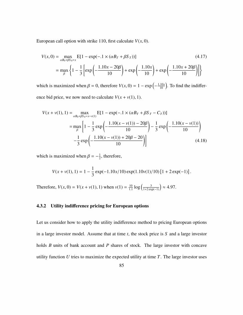
European call option with strike 110, first calculate V(x, 0).

V(x, 0) = maxαB0+βS 0=x

E[1 − exp(−.1 × (αBT + βS T ))] (4.17)

= maxβ

1 −

13

[exp

(−

1.10x − 20β10

)+ exp

(−

1.10x10

)+ exp

(−

1.10x + 20β10

)]

which is maximized when β = 0, therefore V(x, 0) = 1 − exp(−1.10x

10

). To find the indiffer-

ence bid price, we now need to calculate V(x + v(1), 1).

V(x + v(1), 1) = maxαB0+βS 0=x−v(1)

E[1 − exp(−.1 × (αBT + βS T −CT ))]

= maxβ

[1 −

13

exp(−

1.10(x − v(1)) − 20β10

)−

13

exp(−

1.10(x − v(1))10

)−

13

exp(−

1.10(x − v(1)) + 20β − 2010

)](4.18)

which is maximized when β = −12 , therefore,

V(x + v(1), 1) = 1 −13

exp(−1.10x/10) exp(1.10v(1)/10)[1 + 2 exp(−1)

].

Therefore, V(x, 0) = V(x + v(1), 1) when v(1) = 101.1 log

(3

1+2 exp(−1)

)≈ 4.97.

4.3.2 Utility indifference pricing for European options

Let us consider how to apply the utility indifference method to pricing European options

in a large investor model. Assume that at time t, the stock price is S and a large investor

holds B units of bank account and P shares of stock. The large investor with concave

utility function U tries to maximize the expected utility at time T . The large investor uses

85

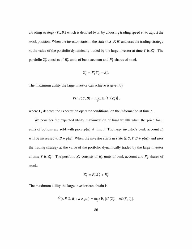
a trading strategy (Pt, Bt) which is denoted by π, by choosing trading speed vt, to adjust the

stock position. When the investor starts in the state (t, S , P, B) and uses the trading strategy

π, the value of the portfolio dynamically traded by the large investor at time T is ZπT . The

portfolio ZπT consists of Bπ

T units of bank account and PπT shares of stock

ZπT = Pπ

T S πT + Bπ

T .

The maximum utility the large investor can achieve is given by

V(t, P, S , B) = maxπ

Et[U

(Zπ

T)],

where Et denotes the expectation operator conditional on the information at time t .

We consider the expected utility maximization of final wealth when the price for n

units of options are sold with price p(n) at time t. The large investor’s bank account Bt

will be increased to B + p(n). When the investor starts in state (t, S , P, B + p(n)) and uses

the trading strategy π, the value of the portfolio dynamically traded by the large investor

at time T is ZπT . The portfolio Zπ

T consists of BπT units of bank account and Pπ

T shares of

stock.

ZπT = Pπ

T S πT + Bπ

T

The maximum utility the large investor can obtain is

V(t, P, S , B + n × pw) = maxπ

Et[U

(Zπ

T − nC(S T ))],

86

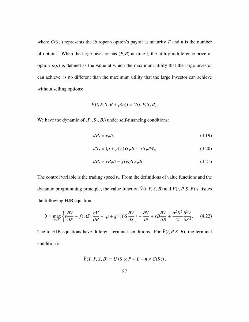
where C(S T ) represents the European option’s payoff at maturity T and n is the number

of options. When the large investor has (P, B) at time t, the utility indifference price of

option p(n) is defined as the value at which the maximum utility that the large investor

can achieve, is no different than the maximum utility that the large investor can achieve

without selling options:

V(t, P, S , B + p(n)) = V(t, P, S , B).

We have the dynamic of (Pt, S t, Bt) under self-financing conditions:

dPt = vtdt, (4.19)

dS t = (µ + g(vt))S tdt + σS tdWt, (4.20)

dBt = rBtdt − f (vt)S tvtdt. (4.21)

The control variable is the trading speed vt. From the definitions of value functions and the

dynamic programming principle, the value function V(t, P, S , B) and V(t, P, S , B) satisfies

the following HJB equation:

0 = maxv∈K

v∂V∂P− f (v)S v

∂V∂B

+ (µ + g(vt))S∂V∂S

+∂V∂t

+ rB∂V∂B

+σ2S 2

2∂2V∂S 2 . (4.22)

The to HJB equations have different terminal conditions. For V(t, P, S , B), the terminal

condition is

V(T, P, S , B) = U (S × P + B − n ×C(S )) .

87

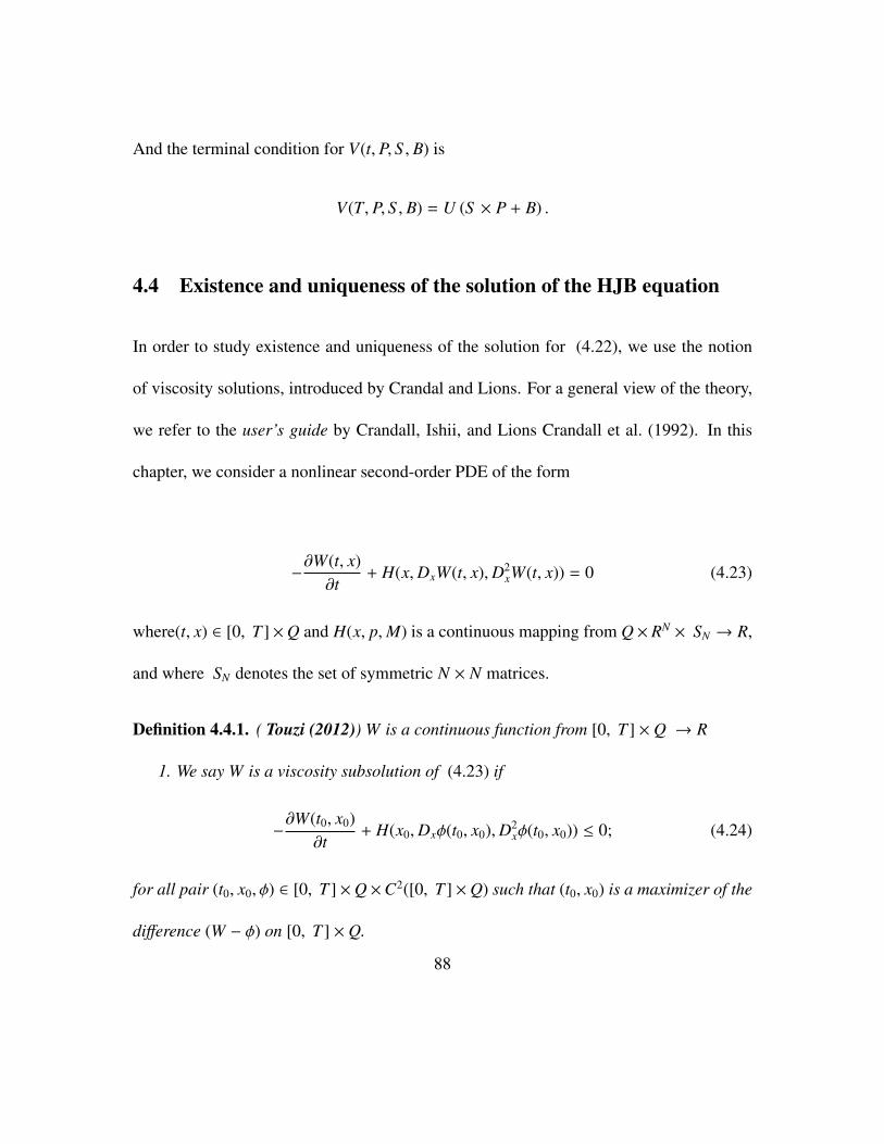
And the terminal condition for V(t, P, S , B) is

V(T, P, S , B) = U (S × P + B) .

4.4 Existence and uniqueness of the solution of the HJB equation

In order to study existence and uniqueness of the solution for (4.22), we use the notion

of viscosity solutions, introduced by Crandal and Lions. For a general view of the theory,

we refer to the user’s guide by Crandall, Ishii, and Lions Crandall et al. (1992). In this

chapter, we consider a nonlinear second-order PDE of the form

−∂W(t, x)

∂t+ H(x,DxW(t, x),D2

xW(t, x)) = 0 (4.23)

where(t, x) ∈ [0, T ]×Q and H(x, p,M) is a continuous mapping from Q× RN × SN → R,

and where SN denotes the set of symmetric N × N matrices.

Definition 4.4.1. ( Touzi (2012)) W is a continuous function from [0, T ] × Q → R

1. We say W is a viscosity subsolution of (4.23) if

−∂W(t0, x0)

∂t+ H(x0,Dxφ(t0, x0),D2

xφ(t0, x0)) ≤ 0; (4.24)

for all pair (t0, x0, φ) ∈ [0, T ] ×Q ×C2([0, T ] ×Q) such that (t0, x0) is a maximizer of the

difference (W − φ) on [0, T ] × Q.

88

2. We say W is a viscosity supersolution of (4.23) if

−∂W(t0, x0)

∂t+ H(x0,Dxφ(t0, x0),D2

xφ(t0, x0)) ≥ 0. (4.25)

for all pair (t0, x0, φ) ∈ [0, T ] × Q ×C2([0, T ] × Q) such that (t0, x0) is a minimizer of the

difference (W − φ) on [0, T ] × Q.

3. We say W is a viscosity solution of (4.23) if it is both a viscosity supersolution and

subsolution of (4.23).

For the PDE in this chapter, H(x, p, X) has the following specific form:

H(x, p,M) = −maxv∈K

[v, (µ + g(v))x2,−v f (v)x2 − rx3

]· [p1, p2, p3]T

−σ2

2(0, x2, 0)M(0, x2, 0)T (4.26)

where x = (x1, x2, x3) ∈ Q, p = (p1, p2, p3) ∈ R3, and M ∈ S3.

Theorem 4.4.1. The value function W(t, P, S , B) is a viscosity solution of

−∂W∂t−max

v∈K

v∂W∂P− f (v)S v

∂W∂B− rB

∂W∂B

+ (µ + g(vt))S∂W∂S

−σ2S 2

2∂2W∂S 2 = 0 (4.27)

on (0 T ) × Q.

Proof. (1): Let X = (P, S , B). We first need to prove W(t, X) is a viscosity subsolution of

(4.27) on (0, T ) × Q. To do so, we need to show that for all smooth function φ(t, X), such

that W(t, X)−φ(t, X) has a local maximum at (t0, X0) ∈ (0, T )×Q, the following inequality

89

holds:

−∂φ(t0, X0)

∂t−max

v∈K

v∂φ(t0, X0)

∂P− ( f (v)S t0v + rBt0)

∂φ(t0, X0)∂B

+ (µ + g(v))S t0∂φ(t0, X0)

∂S

−σ2S 2

t0

2∂2φ(t0, X0)

∂S 2 ≤ 0. (4.28)

Without loss of generality, we assume that W(t0, X0) = φ(t0, X0), and W ≤ φ on (0, T )×

Q. Suppose that, on the contrary, there exists a function φ and a control variable v0 ∈ Γ,

where Γ is the set of all the admissible controls, satisfying the property that there exists an

open set B(t0, X0) containing (t0, X0) such that φ(t0, X0) = W(t0, X0) and φ(t, X) ≥ W(t, X)

for all (t, X) ∈ B(t0, X0). Then there exits θ > 0 such that

−∂φ(t, X)∂t

−maxv∈K

v∂φ(t, X)∂P

− ( f (v)S v + rB)∂φ(t, X)∂B

+ (µ + g(v))S∂φ(t, X)∂S

−σ2S 2

2∂2φ(t, X)∂S 2 > θ. (4.29)

for all (t, X) ∈ B(t0, X0). Let τ be the stopping time

τ = inf t ∈ [t0, T ], (t, X) < B(t0, X0)

such that for t0 ≤ t ≤ τ, (t, X) ∈ B(t0, X0). For t0 ≤ t ≤ τ and fixed v ∈ Γ, when the value

function is J(t0, Pt0 , S t0 , Bt0 , v), we have

J(t0, Pt0 , S t0 , Bt0 , v) ≤ Et0 [W(τ, S τ, Pτ, Bτ)] ≤ Et0[φ(tτ, S τ, Pτ, Bτ)

].

90

By Dynkin’s formula (see Øksendal (2003)), we have

E[φ(tτ, Pτ, S τ, Bτ)

]=φ(t0, Pt0 , S t0 , Bt0) + Et0

[∫ τ

t0

∂φ(t, X)∂t

+ v∂φ(t, X)∂P

−( f (v)S v + rB)∂φ(t, X)∂B

+ (µ + g(v))S∂φ(t, X)∂S

+σ2S 2

2∂2φ(t, X)∂S 2 dt

]≤ φ(t0, Pt0 , S t0 , Bt0) − Et0

[∫ τ

t0θdt

]. (4.30)

Taking the supremum over all admissible control v ∈ Γ, we have

φ(t0, Pt0 , S t0 , Bt0) =W(t0, Pt0 , S t0 , Bt0) (4.31)

= maxv∈Γ

J(t0, Pt0 , S t0 , Bt0 , v) (4.32)

≤φ(t0, Pt0 , S t0 , Bt0) − Et0

[∫ τ

t0θdt

]. (4.33)

This contradicts the fact that θ > 0. Therefore, W(t, P, S , B) is a viscosity subsolution.

(2): Next, we prove W(t, X) is a viscosity supersolution of (4.27) on (0 T )×Q. Given

(t0, Pt0 , S t0 , Bt0) ∈ (0, T ) × Q, let φ(t, X) ∈ C1,2((0, T ) × Q) such that W(t, X) − φ(t, X)

has a local minimum in B(t0, X0). Without loss of generality, we assume that W(t0, X0) =

φ(t0, X0) and W(t, X) ≥ φ(t, X) on B(t0, X0). Let τ be the stopping time

τ = inf t ∈ [t0, T ], (t, X) < B(t0, X0) .

Given t0 < t1 < τ, consider the control variable vt = v ∈ Γ, where v is a constant for

t ∈ [t0, t1]. From the dynamic programming principle, we have

W(t0, Pt0 , S t0 , Bt0) ≥ Et0[W(t1, Pt1 , S t1 , Bt1)

].

91

Also, we know

W(t1, Pt1 , S t1 , Bt1) ≥ φ(t1, Pt1 , S t1 , Bt1).

From Dynkin’s formula

E[φ(t1, Pt1 , S t1 , Bt1)

]=φ(t0, Pt0 , S t0 , Bt0) + Et0

[∫ t1

t0

∂φ(t, X)∂t

+ v∂φ(t, X)∂P

−( f (v)S v + rB)∂φ(t, X)∂B

+ (µ + g(v))S∂φ(t, X)∂S

+σ2S 2

2∂2φ(t, X)∂S 2 dt

].

(4.34)

From the fact that

W(t0, Pt0 , S t0 , Bt0) ≥ Et0[W(t1, Pt1 , S t1 , Bt1)

]≥ Et0

[φ(t1, Pt1 , S t1 , Bt1)

](4.35)

and W(t0, Pt0 , S t0 , Bt0) = φ(t0, Pt0 , S t0 , Bt0), we obtain

Et0

[∫ t1

t0

∂φ(t, X)∂t

+ v∂φ(t, X)∂P

− ( f (v)S v + rB)∂φ(t, X)∂B

+ (µ + g(v))S∂φ(t, X)∂S

+σ2S 2

2∂2φ(t, X)∂S 2 dt

]≤ 0. (4.36)

Letting t1 → t0, we have

∂φ(t0, X0)∂t

+ v∂φ(t0, X0)

∂P− ( f (v)S v + rB0)

∂φ(t0, X0)∂B

+(µ + g(v))S∂φ(t0, X0)

∂S+σ2S 2

2∂2φ(t0, X0)

∂S 2 ≤ 0. (4.37)

92

Taking the supremum over v ∈ K, we can conclude

−∂φ(t0, X0)

∂t−max

v∈K

v∂φ(t0, X0)

∂P− ( f (v)S v + rB0)

∂φ(t0, X0)∂B

+ (µ + g(v))S∂φ(t0, X0)

∂S

−σ2S 2

2∂2φ(t0, X0)

∂S 2 ≥ 0.

(4.38)

Thus, W(t, P, S , B) is a viscosity supersolution of (4.27).

From (1) and (2), W(t, P, S , B) is both a viscosity supersolution and subsolution of (4.27)

and the proof is completed.

By now, we can conclude V(t, P, S , B) is a viscosity solution of

0 = maxv∈K

v∂W∂P− f (v)S v

∂W∂B

+ (µ + g(vt))S∂W∂S

+∂W∂t

+ rB∂W∂B

+σ2S 2

2∂2W∂S 2 , (4.39)

with the terminal condition

W(t = T, P, S , B) = U (S × P + B − N ×CT )

and V(t, P, S , B) is a viscosity solution of

0 = maxv∈K

v∂W∂P− f (v)S v

∂W∂B

+ (µ + g(vt))S∂W∂S

+∂W∂t

+ rB∂W∂B

+σ2S 2

2∂2W∂S 2 , (4.40)

with the terminal condition

W(t = T, P, S , B) = U (S × P + B) .

Next, we show the value function is the unique viscosity solution of (4.27).

93

In order to prove uniqueness of the viscosity solution, we need the following maximum

principle for semicontinuous function, which is stated in a suitable form for our applica-

tion. For the convenience of the reader we restate the relevant theorem from Crandall et al.

(1992) without proofs, thus making our exposition self-contained.

Theorem 4.4.2. (Crandall, Lions and Ishii ) For i = 1, 2, let Qi be locally compact subsets

ofRN , and Q = Q1×Q2, let ui be upper semicontinuous in (0,T )×Qi, and J2,+(0,T )×Qi

ui(t, x) the

parabolic superjet of ui(t, x), and φ be twice continuously differentiable in a neighborhood

of (0,T ) × Q.

Set

ω(t, x1, x2) = u1(t, x1) + u2(t, x2)

for (t, x1, x2) ∈ (0,T ) × Q, and suppose (t, x1, x2) is a local maximum of ω − φ relative to

(0,T ) × Q. Moreover let us assume that, there is an r > 0 such that for every M > 0 there

exists a C such that for i = 1, 2

bi ≤ C whenever (bi, qi, Xi) ∈ J2,+[0,T ]×Qi

ui(t, x)

|xi − xi| + |t − t| ≤ r and |ui(t, xi)| + |qi| + ‖Xi‖ ≤ M

Then for each ε > 0 there exists Xi ∈ S (N) such that

1.

(bi,Dxiφ(t, x), Xi) ∈ J2,+(0,T )×Qi

ui(t, x) f or i = 1, 2

94

2.

−(1ε

+ ‖D2φ(x)‖)I ≤

X1 0

0 X2

≤ D2φ(x) + ε(D2φ(x))2

3.

b1 + b2 =∂φ(t, x, y)

∂t

where for a symmetric matrix A, ‖A‖ := supξT Aξ : |ξ| ≤ 1.

Now we present the following comparison principle in our case.

Theorem 4.4.3. (Comparison Principle) Suppose V1(t, x) and V2(t, x) are continuous in

(t, x) and are respectively viscosity subsolution and supersolution of (4.64), with at most

a linear growth Vi(t, x) ≤ K(1 + |x|) i = 1, 2. If V1(t, x) ≤ V2(t, x) for x ∈ Q and V1(T, x) ≤

V2(T, x) for 0 < t ≤ T and x ∈ ∂Q, then V1(t, x) ≤ V2(t, x) for all (t, x) ∈ (0,T ] × Q.

Proof. (1): We can rewrite the equation in the following form:

−∂W(t, x)

∂t+ H(x,DxW(t, x),D2

xW(t, x)) = 0 (4.41)

where

H(x, p,M) = −maxv∈K

[v, (µ + g(v))x2,−v f (v)x2 − rx3] · [p1, p2, p3]T

−σ2

2(0, x2, 0)M(0, x2, 0)T . (4.42)

95

Denote

H(x, p) = −maxv∈K

[v, (µ + g(v))x2,−v f (v)x2 − rx3] · [p1, p2, p3]T

. (4.43)

Let V1(t, x) be a viscosity subsolution of (4.41). For ρ > 0, define

Vρ1 (t, x) = V1(t, x) −

ρ

t + T, (t, x) ∈ (0,T ] × Q.

We have

ddt

(−ρ

t + T) =

ρ

(t + T )2 > 0.

We can therefore claim that Vρ1 (t, x) is a viscosity subsolution of (4.41). In fact,

−∂Vρ

1 (t, x)∂t

+ H(x,DxVρ1 (t, x),D2

xVρ1 (t, x)) ≤ −

ρ

(t + T )2 ≤ −ρ

4T 2 . (4.44)

(2): For any 0 < δ < 1 and 0 < γ < 1, define

Φ(t, x, y) = Vρ1 (t, x) − V2(t, y) −

1δ|x − y|2 − γeT−t(x2 + y2) (4.45)

and

φ(t, x, y) =1δ|x − y|2 + γeT−t(x2 + y2).

We know V1(t, x) and V2(t, x) satisfy the linear growth. We the have

lim|x|+|y|→∞

Φ(t, x, y) = −∞

and Φ(t, x, y) is continuous in (t, x, y). Therefore, Φ(t, x, y) has a global maximum at a

point (tδ, xδ, yδ). Note that

Φ(tδ, xδ, yδ) = Vρ1 (tδ, xδ) − V2(tδ, yδ) −

1δ|xδ − yδ|2 − γeT−tδ(x2

δ + y2δ).

96

In particular,

Φ(tδ, xδ, xδ) + Φ(tδ, yδ, yδ) ≤ 2Φ(tδ, xδ, yδ)

which means

Vρ1 (tδ, xδ) − V2(tδ, xδ) − γeT−tδ(x2

δ + x2δ)

+Vρ1 (tδ, yδ) − V2(tδ, yδ) − γeT−tδ(y2

δ + y2δ)

≤2Vρ1 (tδ, xδ) − 2V2(tδ, yδ) −

2δ|xδ − yδ|2 − 2γeT−tδ(x2

δ + y2δ).

Thus, we have

2δ|xδ − yδ|2 ≤

[Vρ

1 (tδ, xδ) − Vρ1 (tδ, yδ)

]+ [V2(tδ, yδ) − V2(tδ, yδ)]. (4.46)

By the linear growth condition, there exists K1, K2 such that Vρ1 (t, x) ≤ K1(1 + |x|) and

V2(t, x) ≤ K2(1 + |x|). So, there exists C such that

2δ|xδ − yδ|2 ≤ C(1 + |xδ| + |yδ|). (4.47)

We know Φ(tδ, 0, 0) ≤ Φ(tδ, xδ, xδ), which implies

Φ(tδ, 0, 0) ≤ Vρ1 (tδ, xδ) − V2(tδ, yδ) −

1δ|xδ − yδ|2 − γeT−tδ(x2

δ + y2δ).

So, we have

γeT−tδ(x2δ + y2

δ) ≤ Vρ1 (tδ, xδ) − V2(tδ, yδ) −

1δ|xδ + yδ|2 − Φ(tδ, 0, 0) ≤ 3C(1 + |xδ| + |yδ|)

97

and

γeT−tδ(x2δ + y2

δ)1 + |xδ| + |yδ|

≤ 3C.

Therefore, there exists Cγ such that

|xδ| + |yδ| ≤ Cγ.

The result implies that (xδ, yδ) is bounded by Cγ and there exists subsequence (tδ, xδ, yδ)

that are convergent to some (t0, x0, y0). From (4.47), we can conclude

limδ→0

xδ = x0 = y0 = limδ→0

yδ and limδ→0

tδ = t0.

(3): Suppose that there exists (t, x) ∈ (0,T ] × Q satisfying

V1(t, x) ≥ V2(t, x).

Then ∃ τ > 0

V1(t, x) − V2(t, x) = 2τ.

Equation (4.46) and the semicontinuities of Uρ(t, x) and V2(t, x) give us

limδ→0

2δ|xδ − yδ|2 = 0.

Letting δ→ 0, we have

limδ→0

Φ(tδ, xδ, yδ) ≤ limδ→0

(Vρ1 (tδ, xδ) − V2(tδ, yδ))

≤ limδ→0

sup(Vρ1 (tδ, xδ) − lim

δ→0inf(V2(tδ, yδ))

≤ Vρ1 (t0, x0) − V2(t0, x0) (4.48)

98

also

Φ(tδ, xδ, yδ) ≥ Φ(t, x, x)

≥ Vρ1 (t, x) − V2(t, x) − γeT−t(x2 + x2)

≥ V1(t, x) − V2(t, x) −ρ

t + T− γeT−t(x2 + x2)

≥ 2τ −ρ

t + T− γeT−t(x2 + x2).

When γ and ρ are small enough, we have

2τ −ρ

t + T− γeT−t(x2 + x2) ≥ τ. (4.49)

So, we can claim

τ ≤ Φ(tδ, xδ, yδ)

and

τ ≤ limδ→0

Φ(tδ, xδ, yδ) ≤ Vρ1 (t0, x0) − V2(t0, x0).

From V1 ≤ V2 on ∂([0,T ] × Q), we have

Vρ1 = V1 −

ρ

t + T≤ V1 on (T × Q) ∪ ((0,T ] × ∂Q).

So (t0, x0, y0) < (T × Q) ∪ ((0,T ] × ∂Q) and (tδ, xδ, yδ) is a local maximizer of Φ(t, x, y).

(4): By Theorem 4.4.2, for ε > 0 there exists b1δ, b2δ, Xδ,Yδ such that

(b1δ,2δ

(xδ − yδ) + 2γeT−tδ xδ, Xδ) ∈ J2,+(0,T )×QVρ

1 (tδ, xδ), (4.50)

(b2δ,2δ

(xδ − yδ) − 2γeT−tδyδ,Yδ) ∈ J2,−(0,T )×QV2(tδ, yδ), (4.51)

99

and

b1δ − b2δ =∂φ(tδ, xδ, yδ)

∂t= −γeT−tδ(x2

δ + y2δ).

Equations (4.44) and (4.50) imply that there exists c > 0 making

−b1δ + H(xδ,2δ

(xδ − yδ) + 2γeT−tδ xδ, Xδ) ≤ −c (4.52)

and equation (4.51) implies

−b2δ + H(yδ,2δ

(xδ − yδ) − 2γeT−tδyδ,Yδ) ≥ 0. (4.53)

From equations (4.52) and (4.53)

b1δ − b2δ + H(yδ,2δ

(xδ − yδ)− 2γeT−tδyδ,Yδ)−H(xδ,2δ

(xδ − yδ) + 2γeT−tδ xδ, Xδ) ≥ c. (4.54)

By the maximum principle, we have

−

1ε

+ ‖D2φ(tδ, xδ, yδ)‖

I ≤

Xδ 0

0 −Yδ

≤ D2φ(tδ, xδ, yδ) + ε(D2φ(tδ, xδ, yδ))2

D2φ(tδ, xδ, yδ) =2δ

I3 −I3

−I3 I3

+ 2γeT−tδ

I3 0

0 I3

and

(D2φ(x))2 =8δ2

I3 −I3

−I3 I3

+8γeT−tδ

δ

I3 −I3

−I3 I3

+ 4γe2(T−tδ)

I3 0

0 I3

.100

We can rewrite

xδXδxTδ − yδYδyT

δ = (xδ, yδ)

Xδ 0

0 −Yδ

(xδyδ

)(4.55)

≤ (xδ, yδ)

2δ

I3 −I3

−I3 I3

+ (2γeT−tδ + 4εγ2e2(T−tδ))

I3 0

0 I3

+ ε

8 + 8γδeT−tδ

δ2

I3 −I3

−I3 I3

(xδyδ

). (4.56)

Letting γ → 0 and ε = δ4 , we have

xδXδxTδ − yδYδyT

δ ≤δ

4(xδ − yδ)2, (4.57)

yδYδyTδ − xδXδxT

δ ≥ −4δ

(xδ − yδ)2. (4.58)

We can have the following (4.54)

H(yδ,2δ

(xδ − yδ) + 2γeT−tδyδ,Yδ) − H(xδ,2δ

(xδ − yδ) + 2γeT−tδ xδ, Xδ) ≥ b2δ − b1δ + c

(4.59)

We can deduce from (4.59) that

H(yδ,2δ

(xδ − yδ) − 2γeT−tδyδ) − H(xδ,2δ

(xδ − yδ) + 2γeT−tδ xδ)

≥ (b2δ − b1δ) +σ2

2(yδYδyT

δ − xδXδxTδ ) + c

≥ γeT−tδ(x2δ + y2

δ) −4σ2

2δ(xδ − yδ)2 + c (4.60)

101

Letting γ −→ 0

H(yδ,2δ

(xδ − yδ)) − H(xδ,2δ

(xδ − yδ)) ≥ −4σ2

2δ(xδ − yδ)2 + c. (4.61)

We have limδ→02δ|xδ − yδ|2 = 0 and from the continuity of H, and limδ→0 xδ = x0 =

limδ→0 yδ, we have

0 = limδ→0

[H(yδ,

2δ

(xδ − yδ)) − H(xδ,2δ

(xδ − yδ))]≥ c (4.62)

which is a contradiction.

The uniqueness of the viscosity solution follows from the comparison theorem because

any viscosity solution is both supersolution and subsolution.

Theorem 4.4.4. The value function V(t, P, S , B) is the unique viscosity solution of

0 = maxv∈K

v∂W∂P− f (v)S v

∂W∂B

+ (µ + g(vt))S∂W∂S

+∂W∂t

+ rB∂W∂B

+σ2S 2

2∂2W∂S 2 , (4.63)

with the terminal condition W(T, P, S , B) = U (S × P + B − N ×CT ) and the boundary

condition W(t, P, 0, B) = U(er(T−t)B

). The value function V(t, P, S , B) is the unique viscos-

ity solution of

0 = maxv∈K

v∂W∂P− f (v)S v

∂W∂B

+ (µ + g(vt))S∂W∂S

+∂W∂t

+ rB∂W∂B

+σ2S 2

2∂2W∂S 2 , (4.64)

with the terminal condition W(T, P, S , B) = U (S × P + B) and boundary condition W(t, P, 0, B) =

U(er(T−t)B

).

102

4.5 Example and numerical experiments

4.5.1 Example of the trading speed model and the feedback effects model

To illustrate our model, we provide a simple example that is interesting enough to give

us an explicit solution. Consider the functions of trading speed vt, f (vt) = 1 + αvt and

g(vt) = βvt, with α > 0 and β > 0. We then have the following SDE for market price and

actual traded price:

dS t = (µ + βvt)S tdt + σS tdBt,

S t(vt) = (1 + αvt)S t, − M ≤ vt ≤ M.

α is positive and indicates the depth of illiquidity (the parameter for liquidity costs). β is

also positive and indicates the feedback effects factor.

Applying Ito’s formula to log(S t), we have

d log(S t) = (µ + g(vt) −12σ2)dt + σdWt.

Integrating both sides, we get

log(S T ) − log(S 0) =

∫ T

0(µ −

12σ2)dt +

∫ T

0g(vt)dt +

∫ T

0σdWt

A trade is considered to be a round trip trade when∫ T

0vtdt = 0. When g(vt) = βvt, a round

trip will not affect the stock price at time T . Indeed,

log(S T )−log(S 0) =

∫ T

0(µ−

12σ2)dt+

∫ T

0βvtdt+

∫ T

0σdWt =

∫ T

0(µ−

12σ2)dt+

∫ T

0σdWt.

103

We substitute f (vt) = 1 + αvt and g(vt) = βvt to (4.64). With a little analysis, we have

0 = maxv∈K

−αS

∂W∂B

v2 +

(∂W∂P

+ βS∂W∂S− S

∂W∂B

)v

+ µS∂W∂S

+∂W∂t

+ rB∂W∂B

+σ2S 2

2∂2W∂S 2 .

(4.65)

Note that−αS ∂W

∂B v2 +(∂W∂P + βS ∂W

∂S − S ∂W∂B

)v

is a quadratic function of v. Since W(t, P, S , B)

is monotone increasing with respect to B, ∂W∂B > 0. Also, the fact that S > 0 and α > 0 gets

−αS∂W∂B

< 0.

Therefore, the maximum of− αS ∂W

∂B v2 +(∂W∂P + βS ∂W

∂S − S ∂W∂B

)v

is achieved when

v∗ =

1S∂W∂P + β∂W

∂S −∂W∂B

2α∂W∂B

.

Since the term 2α∂W∂B is always nonnegative, the sign of v∗ is determined by 1

S∂W∂P +β∂W

∂S −∂W∂B .

There are three possible cases:

Case (1):

∂W∂B

>1S∂W∂P

+ β∂W∂S

;

the optimal solution v∗ < 0 where the maximum is achieved by selling the stock and

increasing the holdings on the bank account. Marginal utility per dollar of stock holding

plus marginal utility on stock price caused by the feedback effects factor is less than the

marginal utility per dollar on the bank account. To maximize the utility, it is recommended

that the wealth transferred from from the stocks to the bank account.

104

Case (2):

∂W∂B

<1S∂W∂P

+ β∂W∂S

;

the optimal solution v∗ > 0 where the maximum is achieved by buying the stock and

decreasing our holdings on the bank account. Marginal utility per dollar of the stock

holding plus marginal utility on the stock price caused by the permanent price impact

factor is greater than the marginal utility per dollar on the bank account. To maximize the

utility, it is recommended that wealth be transferred from the bank account to the stocks.

Case (3):

∂W∂B

=1S∂W∂P

+ β∂W∂S

;

the optimal solution v∗ = 0, where the maximum is achieved by doing nothing. Marginal

utility per dollar of the stock holding plus marginal utility on the stock price caused by

the feedback effects factor is equal to the marginal utility per dollar on the bank account.

There is no transaction needed.

At a fixed time t, the above result suggests that the state space can be divided into

buying and selling regions by a surface. On the surface, the trading speed is 0 and there is

no transaction. The buy region is characterized by

∂W∂B

<1S∂W∂P

+ β∂W∂S

105

and the selling region is characterized by

∂W∂B

>1S∂W∂P

+ β∂W∂S

.

We consider the exponential utility function given by

U(x) = 1 − exp(−λx)

where the index of risk aversion is −U′′

(x)U′(x) = λ, which is independent of the investors

wealth. The integral version of state variable BT is written as

BT = Bt exp(r(T − t)

)−

∫ T

tf (vu)S uvudu

Then

V(t, P, S , B)

= maxv∈Γ

Et1 − exp (−λ (PT S T + BT ))

=1 −min

v∈ΓEt

exp

(−λ

(PT S T + B exp (r(T − t)) −

∫ T

tf (vu)S uvudu

))=1 − exp

(−λB exp (r(T − t))

)minv∈Γ

Et

exp

(−λ

(PT S T −

∫ T

tf (vu)S uvudu

))=1 − exp

(−λB exp (r(T − t))

)Q(t, P, S )

where Q(t, P, S ) is a continuous function in P and S , and can be defined by Q(t, P, S ) =

1 − V(t, P, S , 0). With a little analysis, we have

0 = maxv∈K

−αSλ exp(r(T − t))Q(t, P, S )v2 +

(∂Q∂P

+ βS∂Q∂S− Sλ exp(r(T − t))Q(t, P, S )

)v

+ µS∂Q∂S

+∂Q∂t− λB exp(r(T − t))r + rBλ exp(r(T − t))Q(t, P, S )

∂Q∂B

+σ2S 2

2∂2Q∂S 2 .

106

with terminal condition

Q(T, P, S ) = 1 − exp(S × P)

Note the term in the above PDE

−αSλ exp(r(T − t))Q(t, P, S )v2 +

(∂Q∂P

+ βS∂Q∂S− Sλ exp(r(T − t))Q(t, P, S )

)v

is a quadratic function of v. The maximum of the quadratic term is achieved when

v∗ =

∂Q∂P + βS ∂Q

∂S − Sλ exp(r(T − t))Q(t, P, S )2αSλ exp(r(T − t))Q(t, P, S )

which means the optimal trading speed v∗ is independent of B. The utility indifference

price for n units of options p(n) at time 0 is defined by the equation

V(t = 0, P0, S 0, B + p(n)) = V(t = 0, P0, S 0, B0) (4.66)

Assuming P0 = 0, we have the following explicit formula for the utility indifference price

p(n):

p(n) =1

−λ exp(rT )log

Q(0, 0, S )Q(0, 0, S )

.

At time 0, the large investor’s initial wealth is B units of the bank account. The utility

indifference price p(n) at time 0 is independent of B, which means the utility indifference

price p(n) is independent of the large investor’s initial wealth.

107

4.5.2 Numerical results

In this section, we discuss the numerical solution to the example and present some results.

We compute the utility indifference price of a European call option with strike 100 and

observe interesting properties. In the numerical experiments, the parameter values that we

used are initial stock price S 0 = 100, µ = 0.05, σ = 0.2, r = 0 and T = 0.1. We assume

λ = 0.00001 and n = 1000. Table 4.1 provides a comparison of the option prices for

α = 0.00001 α = 0.00005 α = 0.00010β n = 500 n = 1000 n = 2000 n = 500 n = 1000 n = 2000 n = 500 n = 1000 n = 2000

0.00000 2.8180 2.8584 2.9452 2.8200 2.8616 2.9484 2.8202 2.8621 2.94880.00001 2.8144 2.8580 2.9388 2.8192 2.8615 2.9472 2.8198 2.8620 2.94820.00002 2.8112 2.8369 2.8863 2.8188 2.8576 2.9373 2.8196 2.8600 2.94330.00005 2.7182 2.6186 2.4406 2.8024 2.8200 2.8553 2.8116 2.8416 2.9028

Table 4.1: Utility indifference price with different α and β.

different α, β and number n of the options written by the investor. We have observed when

α increases (the depth of illiquidity increases) for a fixed β, the option price increases.

But when β increases (the depth of feedback effects increases) for a fixed α, the option

price decreases. When β is large, a large investor has more influence on the stock price

evolution. We can conclude that the investor may have the power to manipulate the stock

price, to some extent, to maximize the investor’s utility.

When α is relatively small compared to β, with the increase of n, the option price

108

α = 0.00001 α = 0.00005 α = 0.00010β n = 500 n = 1000 n = 2000 n = 500 n = 1000 n = 2000 n = 500 n = 1000 n = 2000

0.00000 2.8240 2.8659 2.9527 2.8240 2.8659 2.9527 2.8240 2.8660 2.95270.00001 2.8240 2.8660 2.9526 2.8240 2.8660 2.9526 2.8242 2.8660 2.95260.00002 2.8240 2.8657 2.9523 2.8240 2.8657 2.9523 2.8240 2.8657 2.95230.00005 2.8232 2.8649 2.9515 2.8232 2.8649 2.9515 2.8232 2.8649 2.9515

Table 4.2: Utility indifference price with different α and β when M = 5.

α = 0.00001 α = 0.00005 α = 0.00010β n = 500 n = 1000 n = 2000 n = 500 n = 1000 n = 2000 n = 500 n = 1000 n = 2000

0.00000 2.8200 2.8634 2.9508 2.8230 2.8652 2.9520 2.8236 2.8657 2.95240.00001 2.8222 2.8641 2.9498 2.8238 2.8653 2.9510 2.8240 2.8657 2.95180.00002 2.8198 2.8592 2.9441 2.8224 2.8619 2.9458 2.8234 2.8637 2.94760.00005 2.8040 2.8424 2.9268 2.8102 2.8459 2.9286 2.8154 2.8499 2.9308

Table 4.3: Utility indifference price with different α and β when M = 100.

decreases. And when β is relatively small compared to α, with the increase of n, the option

price increases. The explanation is that when α is relatively small compared to β, the

advantage of feedback effects outweighs the liquidity cost, so the more options the large

investor sells, the more benefits the large investor can gain from feedback effects on stock

price, and the average hedging cost per unit of an option for the large investor decreases.

But when β is relatively small compared to α, the liquidity cost cannot be overturned by

the advantage brought by the feedback effects. So, the more options the large investor

sells, the larger the liquidity cost the large investor will incur, and the average hedging

cost per unit of option for a large investor will increase.

109

α = 0.00001 α = 0.00005 α = 0.00010β n = 500 n = 1000 n = 2000 n = 500 n = 1000 n = 2000 n = 500 n = 1000 n = 2000

0.00000 2.8180 2.8617 2.9488 2.8230 2.8652 2.9520 2.8236 2.8657 2.95240.00001 2.8218 2.8622 2.9437 2.8238 2.8653 2.9508 2.8240 2.8657 2.95180.00002 2.8150 2.8444 2.9173 2.8224 2.8613 2.9409 2.8234 2.8637 2.94690.00005 2.7490 2.7628 2.8313 2.8062 2.8237 2.8726 2.8154 2.8453 2.9063

Table 4.4: Utility indifference price with different α and β when M = 500.

α = 0.00001 α = 0.00005 α = 0.00010β n = 500 n = 1000 n = 2000 n = 500 n = 1000 n = 2000 n = 500 n = 1000 n = 2000

0.00000 2.8180 2.8617 2.9488 2.8230 2.8652 2.9520 2.8236 2.8657 2.95240.00001 2.8218 2.8622 2.9424 2.8238 2.8653 2.9508 2.8240 2.8657 2.95180.00002 2.8150 2.8407 2.8992 2.8224 2.8613 2.9409 2.8234 2.8637 2.94690.00005 2.7222 2.6946 2.7309 2.8062 2.8237 2.8588 2.8154 2.8453 2.9063

Table 4.5: Utility indifference price with different α and β when M = 1000.

For a fixed time, we know that the optimal trading speed is independent of B in the

case of exponential utility. We have the optimal trading speed at a fixed time in Figure 4.1.

Knowing the optimal trading speed, we can define the trading region. The trading region

is divided by a smooth surface into a buying region and a selling region. On the curve, the

trading speed is 0, and there is no transaction. Above the curve,

∂Q∂P

+ βS∂Q∂S

< SλQ(t, P, S )

it belongs to the buying region. And below the curve

∂Q∂P

+ βS∂Q∂S

> SλQ(t, P, S )

110

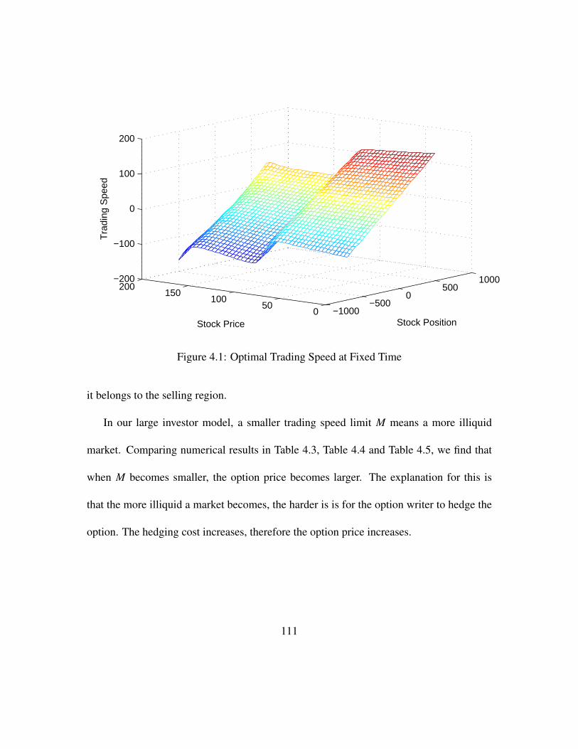
−1000−500

0500

1000

050

100150

200−200

−100

0

100

200

Stock PositionStock Price

Tra

ding

Spe

ed

Figure 4.1: Optimal Trading Speed at Fixed Time

it belongs to the selling region.

In our large investor model, a smaller trading speed limit M means a more illiquid

market. Comparing numerical results in Table 4.3, Table 4.4 and Table 4.5, we find that

when M becomes smaller, the option price becomes larger. The explanation for this is

that the more illiquid a market becomes, the harder is is for the option writer to hedge the

option. The hedging cost increases, therefore the option price increases.

111

4.5.3 An extended large investor model

In our large investor model, above, we assumed that the trading speed would have an

effect on the drift term of the stock price. We can extend the large investor’s model to state

that the trading speed places an effect on both the drift term and the volatility term of the

stock price evolution. Usually, trading action (including both buying and selling) increases

the volatility of trading assets. Volatility of the asset increases with the increase of |vt|.

Consider a simple trading speed model f (vt) = 1+αvt, g(vt) = βvt and σ(vt) =√σ2 + γv2

t ,

with α > 0, β > 0 and γ > 0. Then

dS t = (µ + βvt)S tdt +

√σ2 + γv2

t S tdBt,

S t(vt) = (1 + αvt)S t, − M ≤ vt ≤ M,

where α > 0 and indicates the depth of illiquidity. β > 0 and it indicates the feedback

effects index. With a little analysis, we have

0 = maxv∈K

− αS

∂W∂B

v2 +

(∂W∂P

+ βS∂W∂S− S

∂W∂B

)v +

γv2S 2

2∂2W∂S 2

+ µS

∂W∂S

+σ2S 2

2∂2W∂S 2 +

∂W∂t

+ rB∂W∂B

. (4.67)

Table 4.6 shows the option price when γ = 5 × 10−8. Compared with the case a large

investor does not influence the stock price’s volatility, and option prices are relatively

higher when a large investor has an influence on the stock price’s volatility. This result is

illustrated by a comparison between Table 4.1 and Table 4.6.

112

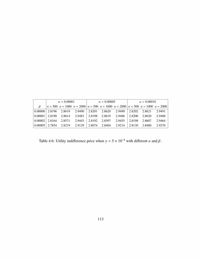
α = 0.00001 α = 0.00005 α = 0.00010β n = 500 n = 1000 n = 2000 n = 500 n = 1000 n = 2000 n = 500 n = 1000 n = 2000

0.00000 2.8196 2.8619 2.9490 2.8201 2.8620 2.9490 2.8202 2.8621 2.94910.00001 2.8190 2.8614 2.9483 2.8198 2.8619 2.9486 2.8200 2.8620 2.94880.00002 2.8164 2.8571 2.9443 2.8192 2.8597 2.9455 2.8198 2.8607 2.94640.00005 2.7854 2.8219 2.9129 2.8074 2.8404 2.9214 2.8130 2.8480 2.9276

Table 4.6: Utility indifference price when γ = 5 × 10−8 with different α and β .

113

5 Conclusions and Future Work

In this dissertation, we studied option pricing and hedging in a non-competitive market.

The non-competitive market is characterized by liquidity risk and feedback effects. Based

on an investor’s market power to have feedback effects on an underlying security price,

market participants in a non-competitive market are divided into small investors and large

investors. Different pricing models were proposed for both small and large investors.

In chapter 2, we investigated how to price and hedge options for small investors in a

non-competitive market. Based on the supply curve model, partial differential equations

were presented to characterize the replication cost for options. We showed that the repli-

cation cost from the seller party was greater than the replication cost from the buyer party.

In a non-competitive market, we regard the replication cost from the seller party as the

upper bound for option price, and the replication cost from buyer’s party as a lower bound.

Our model boasts several advantages over other models. First, it provides a general frame-

work for pricing different options, including path-dependent options. Second, our model

is an extension of the Black-Scholes model; in the case f ′(0) = 0, our model returns to

114

the Black-Scholes model. Third, we only introduced one parameter f ′(0) to incorporate

liquidity risk, which makes our model relatively simple.

In chapter 3, we approximated a jump-diffusion process by a discrete-time Markov

process and applied the local risk minimization method incorporating liquidity risk to

price European options in the discrete-time model with liquidity costs. Numerical results

showed that the proposed hedging strategies reduce the standard deviation of the hedging

error as well as the mean hedging cost, which confirmed that our modified local risk min-

imization method performs better than other existing hedging strategies. Therefore, when

the underlying asset price is assumed to follow a jump-diffusion process in a market with

liquidity risk, our method is useful for option valuation and hedging under liquidity risk.

In chapter 4, we investigated option valuation based on utility maximization for a large

investor in a market with liquidity risk. We considered two effects of a non-competitive

market: liquidity risk and feedback effects of large investors. In non-competitive markets,

trading action will incur liquidity costs, but at the same time, the investor can have an

influence on the stock price evolution and gain benefits from the permanent price impact by

choosing the optimal strategy. Thus, the option price, in some sense, is determined by these

two contradicting phenomena. When both the permanent impact function and the liquidity

cost function are linear in the trading speed, the optimal solution is computed explicitly,

and the state space can be characterized and divided into the buy and sell regions.

115

Our work provides a new understanding of option pricing theory in non-competitive

markets, yet some interesting and important questions remain. We have only an approxi-

mate European option price by approximating a jump diffusion model by a discrete time

model. More effort is required to develop a method to determine the precise option price

in a jump diffusion model. Another issue is that we modelled the feedback effects of large

investors by imposing a function of trading speed to the drift term of underlying stock

price without justification from market microstructure. A deep study of limit order book

dynamic could help us understand the modelling of feedback effects.

116

Bibliography

Robert Almgren and Neil Chriss. Optimal execution of portfolio transactions. Journal ofRisk, 3:5–40, 2001.

Robert F Almgren. Optimal execution with nonlinear impact functions and trading-enhanced risk. Applied mathematical finance, 10(1):1–18, 2003.

Kaushik I Amin. Jump diffusion option valuation in discrete time. The journal of finance,48(5):1833–1863, 1993.

Torben G Andersen, Luca Benzoni, and Jesper Lund. An empirical investigation ofcontinuous-time equity return models. The Journal of Finance, 57(3):1239–1284, 2002.

Marco Avellaneda, Michael D Lipkin, et al. A market-induced mechanism for stock pin-ning. Quantitative Finance, 3(6):417–425, 2003.

Peter Bank and Dietmar Baum. Hedging and portfolio optimization in financial marketswith a large trader. Mathematical Finance, 14(1):1–18, 2004.

David S Bates. Post-’87 crash fears in the s&p 500 futures option market. Journal ofEconometrics, 94(1):181–238, 2000.

Bernard Bensaid, Jean-Philippe Lesne, Jose Scheinkman, et al. Derivative asset pricingwith transaction costs1. Mathematical Finance, 2(2):63–86, 1992.

Phelim P Boyle and Ton Vorst. Option replication in discrete time with transaction costs.The Journal of Finance, 47(1):271–293, 1992.

Umut Cetin and LCG Rogers. Modeling liquidity effects in discrete time. MathematicalFinance, 17(1):15–29, 2007.

Umut Cetin, Robert A Jarrow, and Philip Protter. Liquidity risk and arbitrage pricingtheory. Finance and stochastics, 8(3):311–341, 2004.

117

Umut Cetin, H Mete Soner, and Nizar Touzi. Option hedging for small investors underliquidity costs. Finance and Stochastics, 14(3):317–341, 2010.

Thomas F Coleman, Yuying Li, and Maria-Cristina Patron. Total risk minimization usingmonte carlo simulations. Handbooks in Operations Research and Management Science,15:593–635, 2007.

Michael G Crandall, Hitoshi Ishii, and Pierre-Louis Lions. Users guide to viscosity solu-tions of second order partial differential equations. Bulletin of the American Mathemat-ical Society, 27(1):1–67, 1992.

Domenico Cuoco and Jaksa Cvitanic. Optimal consumption choices for a investor. Journalof Economic Dynamics and Control, 22(3):401–436, 1998.

Jaksa Cvitanic and Ioannis Karatzas. Hedging contingent claims with constrained portfo-lios. The Annals of Applied Probability, pages 652–681, 1993.

Jaksa Cvitanic and Jin Ma. Hedging options for a large investor and forward-backwardsde’s. The annals of applied probability, 6(2):370–398, 1996.

Mark HA Davis, Vassilios G Panas, and Thaleia Zariphopoulou. European option pricingwith transaction costs. SIAM Journal on Control and Optimization, 31(2):470–493,1993.

Chanaka Edirisinghe, Vasanttilak Naik, and Raman Uppal. Optimal replication of optionswith transactions costs and trading restrictions. Journal of Financial and QuantitativeAnalysis, 28(01):117–138, 1993.

Hans Follmer and Martin Schweizer. Hedging of contingent claims. Applied stochasticanalysis, 5:389, 1991.

Peter A Forsyth. A hamilton–jacobi–bellman approach to optimal trade execution. Appliednumerical mathematics, 61(2):241–265, 2011.

Rudiger Frey. Perfect option hedging for a large trader. Finance and Stochastics, 2(2):115–141, 1998.

Rudiger Frey and Alexander Stremme. Market volatility and feedback effects from dy-namic hedging. Mathematical finance, 7(4):351–374, 1997.

Selim Gokay and Halil Mete Soner. Liquidity in a binomial market. Mathematical Fi-nance, 22(2):250–276, 2012.

118

J Michael Harrison and David M Kreps. Martingales and arbitrage in multiperiod securi-ties markets. Journal of Economic theory, 20(3):381–408, 1979.

J Michael Harrison and Stanley R Pliska. Martingales and stochastic integrals in the the-ory of continuous trading. Stochastic processes and their applications, 11(3):215–260,1981.

J Michael Harrison and Stanley R Pliska. A stochastic calculus model of continuoustrading: complete markets. Stochastic processes and their applications, 15(3):313–316,1983.

Vicky Henderson. Valuation of claims on nontraded assets using utility maximization.Mathematical Finance, 12(4):351–373, 2002.

Steven L Heston. A closed-form solution for options with stochastic volatility with appli-cations to bond and currency options. Review of financial studies, 6(2):327–343, 1993.

Stewart D Hodges and Anthony Neuberger. Optimal replication of contingent claims undertransaction costs. Review of futures markets, 8(2):222–239, 1989.

Robert A Jarrow. Derivative security markets, market manipulation, and option pricingtheory. Journal of Financial and Quantitative Analysis, 29(02):241–261, 1994.

Philippe Jorion. On jump processes in the foreign exchange and stock markets. Review ofFinancial Studies, 1(4):427–445, 1988.

Elyegs Jouini and Hedi Kallal. Arbitrage in securities markets with short-sales constraints.Mathematical finance, 5(3):197–232, 1995.

Steven G Kou. A jump-diffusion model for option pricing. Management science, 48(8):1086–1101, 2002.

Holger Kraft and Christoph Kuhn. Large traders and illiquid options: Hedging vs. manip-ulation. Journal of Economic Dynamics and Control, 35(11):1898–1915, 2011.

Hyejin Ku, Kiseop Lee, and Huaiping Zhu. Discrete time hedging with liquidity risk.Finance Research Letters, 9(3):135–143, 2012.

Hayne E Leland. Option pricing and replication with transactions costs. The journal offinance, 40(5):1283–1301, 1985.

Andrew EB Lim. Mean-variance hedging when there are jumps. SIAM Journal on Controland Optimization, 44(5):1893–1922, 2005.

119

Francis A Longstaff. Optimal portfolio choice and the valuation of illiquid securities.Review of financial studies, 14(2):407–431, 2001.

Robert C Merton. Option pricing when underlying stock returns are discontinuous. Jour-nal of financial economics, 3(1):125–144, 1976.

Bernt Øksendal. Stochastic differential equations. Springer, 2003.

Huyen Pham. Dynamic l p-hedging in discrete time under cone constraints. SIAM Journalon Control and Optimization, 38(3):665–682, 2000.

Eckhard Platen and Martin Schweizer. On feedback effects from hedging derivatives.Mathematical Finance, 8(1):67–84, 1998.

Leonard CG Rogers and Surbjeet Singh. The cost of illiquidity and its effects on hedging.Mathematical Finance, 20(4):597–615, 2010.

K Ronnie Sircar and George Papanicolaou. General black-scholes models accounting forincreased market volatility from hedging strategies. Applied Mathematical Finance, 5(1):45–82, 1998.

Alexander Schied and Torsten Schoneborn. Risk aversion and the dynamics of optimal liq-uidation strategies in illiquid markets. Finance and Stochastics, 13(2):181–204, 2009.

Halil M Soner, Steven E Shreve, and J Cvitanic. There is no nontrivial hedging portfoliofor option pricing with transaction costs. The Annals of Applied Probability, pages327–355, 1995.

Nizar Touzi. Optimal stochastic control, stochastic target problems, and backward SDE,volume 29. Springer, 2012.

120