Optimization of Taxiway Routing and Runway

Scheduling

Gillian Clare∗ and Arthur Richards†

University of Bristol, Bristol, UK

Abstract

This paper describes a Mixed Integer Linear Programming (MILP) optimization method for

the coupled problems of airport taxiway routing and runway scheduling. The Receding Horizon

(RH) formulation and use of iteration in the avoidance constraints allows the scalability of

the baseline algorithm presented to be illustrated, with examples based on Heathrow airport

containing up to 240 aircraft. The results show that average taxi times can be reduced by

55% when compared to a First Come First Serve (FCFS) approach. The main advantage is

seen with the departure aircraft flow. Comparative testing demonstrates that iteration reduces

the computational demand of the required separation constraints whilst introducing no loss

in performance. RH formulation enables near real-time operation as the computation is spread

between horizons preventing unnecessarily detailed plans being calculated for the distant future.

The conversion to RH does however result in an approximation to the globally optimal solution,

although this is shown to be relatively small.

Manuscript received

∗Ph.D. Candidate, Department of Aerospace Engineering, University of Bristol, Queens Building, University Walk,Bristol BS8 1TR; gk2661@bristol.ac.uk, Student Member AIAA.

†Lecturer, Department of Aerospace Engineering, University of Bristol, Queens Building, University Walk, BristolBS8 1TR; Arthur.Richards@bristol.ac.uk, Member AIAA.

1

Key words: Optimization, Mixed-integer Programming, Taxi Routing, Runway

Nomenclature

a, b, c Identify Aircraft

aL(n) The last aircraft to visit node n prior to current horizon

ax Auxiliary aircraft

A Set of all active aircraft

Aarr Set of all arriving aircraft

Adep Set of all departing aircraft

Ax Set of all auxiliary aircraft

C(n,m) Absolute binary connectivity matrix

Ca(n,m) Binary connectivity matrix for aircraft a

dt(a, b, n) Temporal separation required between aircraft a and b at node n

DSE Binary Variable

DOT Binary Variable

DHO Binary Variable

FCFS First Come First Serve

gSE Binary Ordering Switch for Separation conflict

gCO Binary Ordering Switch for Cross-Over conflict

gRO Binary Ordering Switch for Runway conflict

k, j Identify planning periods

G Set of all gate nodes

L(n,m) Topology distances

2

Ltaxi(a) Distance taxied previous to current problem

M Large number

n,m Identify nodes (intersections) on the taxiways

n0(a) Origin node of aircraft a

nD(a) Destination node of aircraft a

nF (a) Final node in aircraft a’s detailed plan

nRa Arrival runway node

nRd Departure runway node

nv(a) Virtual node introduced by aircraft a

Na Number of aircraft in the problem

Nn Number of nodes in the airport graph structure

Nk Number of planning periods in the problem

N Set of all nodes in the airport graph structure

CO, COi, COdet Set of crossover conflicts: all, those enforced in iteration i, those detected

rST (n,m) Shortest path through the airport graph structure between nodes n and m

R(a, k) Routing variable recording the node at which aircraft a begins planning period k

RH Receding Horizon

RO Set of all possible departure runway conflicts

SE ,SEi,SEdet Set of separation conflicts: all, those enforced in iteration i, those detected

tD(a) Destination time for aircraft a’s

tstart(a) Universal time at which aircraft a started taxiing

t0(a) Origin time of aircraft a

T (a, k) Time at which aircraft a passes the node in it’s kth planning period

3

TL(n) Time at which node n was last visited prior to current horizon

Tt(a) Time aircraft a taxied prior to current horizon

V (a) Maximum speed of aircraft a

wi Weightings in the objective function

X(a, n,m, p) Binary representation of aircraft movement plans

1 Introduction

Meeting the increasing air traffic demand, which is expected to more than double between 2005

and 2020 [1], within the current air traffic system requires improvements in all areas of Air Traffic

Management (ATM). Significant improvements in en-route ATM are shifting the system bottle

neck to the limited airport capacity. Congestion on the airport surface is a major constraint to the

available capacity of the air transport system. Economically, congestion reduces the turnaround

efficiency, while environmentally the increase in both air pollutant and noise emissions impact neg-

atively upon the local region. Furthermore, congestion causes concerns for controller workload [2]

and increased risk of runway incursion [3]. The practical difficulties of increasing capacity through

airport expansion introduces the desire for enhanced airport ground movement efficiency by intel-

ligent use of the existing resources. Projects such as Eurocontrol’s Advanced-Surface Movement,

Guidance and Control Systems (A-SMGCS) [4], and the European Commission’s European airport

Movement Management by A-SMGCS (EMMA) [5] have begun the development of new technology

and systems of operation to improve upon current practices.

Optimization of airport ground operations is an important topic in modern transportation

4

research and several approaches have been investigated. Surface movement research has mainly

focussed on subsets of the problem which can be classified as: arrival and departure management,

including runway sequencing and scheduling [6–9]; stand allocation [10]; and taxi planning, includ-

ing route allocation followed by local deconfliction [11], and route scheduling [12]. Ref.13 introduces

three separate yet interacting schedulers for the runway, ramp and taxiway system. Ref.14 performs

both routing and timing optimization, although using discrete time steps and not including take-off

separation on the runway. In contrast this paper considers the problem in continuous time, which

prevents conservative rounding, considered to be beneficial [15] and incorporates departure runway

scheduling, as this has been identified as the key flow constraint to surface movement [16].

This paper describes an automated tool for airport taxiway routing and runway scheduling

which applies non-convex optimization to the surface movement problem. The key features of this

work are coupled routing and timing optimization, incorporation of runway scheduling, and the

implementation in continuous time. This combines discrete decisions, choosing among predeter-

mined taxiways, with continuous decisions, relating to the timing of the planned movement. The

method in this paper adopts Mixed Integer Linear Programming (MILP) optimization, known to

be suited to such hybrid problems [17]. MILP has previously been successfully used in Air Traffic

Management optimizers for both en-route [18] and ground [11,12] traffic. This type of formulation

can be solved using efficient, commercial software, such as CPLEX [19], generating globally optimal

solutions.

Airport surface movement optimization is NP-hard [20] due to the dynamic traffic assignment

when the coupled non-convex decisions of routing and timing are simultaneously optimized. There

are many individual constraints such as push-back times, taxiway layouts, and runway separations

all requiring consideration. The runway operations alone are constrained by both wake vortex

5

separations and downstream flight path, or Standard Instrument Departure (SID) separations [21].

This level of complexity results in computationally demanding optimizations. The dynamic nature

of the problem, with aircraft entering and leaving, and the possibility of unexpected events, requires

plans to be updated regularly. These factors motivate a formulation with reduced computational

demand. This was achieved by the RH formulation and use of iteration in the avoidance constraints

in the baseline algorithm presented.

RH schemes have been used extensively before in trajectory planning [22,23] as the framework is

well suited to such problems. The optimization combines detailed near-term planning over a finite

period called the planning horizon with coarse far-term approximations beyond this; this plan is

then implemented up to a shorter ‘execution’ horizon, before re-planning occurs, with inputs from

the state that has been reached during execution. The continuous nature of traffic at airports is

well modelled by the continuation of one horizon to the next, as this allows for inclusion of a rolling

window [9,12]. Practically this introduced scalability, as the optimizer considers only a ‘window’ of

the aircraft from the entire problem in and given horizon, with aircraft able to enter and leave the

problem between the optimizations for each horizon. As a result, computation is spread between

horizons preventing unnecessarily detailed plans being calculated for the distant future. However,

this approach results in an approximation to the overall optimization problem solution.

Iteration has previously been demonstrated to be an effective tool for reducing computation

with no loss in performance when many constraints are redundant [24, 25]. In this work it is done

with respect to the avoidance constraints. Instead of solving the full problem from the beginning,

all of the avoidance constraints are initially relaxed. When a solution is found, avoidance violations

are identified, and constraints are re-applied to the problem and the MILP is solved again. This

process is repeated until a solution with no constraint violation is found.

6

The structure of the paper is as follows: Section 2 presents the statement of the problem to be

tackled, including the iteration, Section 3 describes the formulation in MILP. The results of a large

scale problem are presented in Section 4.2, and comparative testing in Section 4.3 demonstrates

how the RH and iterative features of the baseline algorithm contribute to the computation. Finally,

performance comparisons from the comparative testing are discussed in Section 4.4.

2 General Problem Statement

This section presents the general problem formulation, beginning with the optimization struc-

ture and progressing through the basic parameters, constraints and objective. Further details of

the MILP implementation of equations is presented in Section 3. The notation is developed in the

text, but to improve readability, the following standards for indices are used throughout: a, b and

c represent aircraft; n and m represent nodes; and i, j and k represent planning periods.

2.1 Optimization Structure

The optimization scheme is formulated in a Receding Horizon(RH) framework, meaning that a

single large planning problem is approximated as a sequence of smaller problems. The active

taxiing aircraft plan for a number, Nk, of planning periods, or planning horizon, this plan is then

carried out over a shorter execution horizon before replanning occurs. As the aircraft may not reach

their destination nodes in the finite planning horizon, an approximate cost-to-go for the remaining

travel to their destination nodes is incorporated. This allows computation to be spread over time,

and ensures that computational effort is not wasted on detailed plans for the distant future, which

are likely to be revised multiple times before execution. It also results in an approximation to

7

Figure 1: Optimizer System Diagram

the overall problem solution. However, our previous results have shown that the effects of this

approximation are insignificant whereas the computation saving is large [26].

Planning for problem instances which span periods of time much longer than the planning and

execution horizons are naturally handled with a rolling window of aircraft. The idea is that aircraft

are able to enter and leave the problem between plans, meaning the optimization is only ever looking

at a ‘window’ of the total number of aircraft in the global problem. This is especially well suited

to the continuous nature of traffic at airports, with aircraft continuously arriving and departing.

Aircraft are considered to be ‘active’ in the optimization for a horizon if they are already taxiing

or their earliest possible taxi start time is within the execution horizon. When the aircraft take off,

they are removed from the active set before the next horizon is optimized.

The planning solution for each horizon is provided by an optimizer which iterates on the conflict

prevention constraints, this idea is similar to that presented by Earl and d’Andrea [24]. Initially

no constraints are included to prevent conflict on the airport surface. Once the problem is solved,

the solution is checked for any conflicts between aircraft. If conflicts are detected, constraints to

8

prevent these are added to the problem and it is re-solved. This is repeated until the solution is

conflict free, as shown by the system diagram in Fig. 1. The formulation of this iterative optimizer

is described in the remainder of this section. A simulator is used to predict the new state of each

aircraft at the end of the current execution horizon, defining the inputs for the optimization at the

next planning step. In this paper the simulator assumes that all aircraft behave perfectly, and no

variability is introduced. The RH formulation introduces feedback, meaning that the method can

in principal compensate for uncertainty.

2.2 Input parameters

2.2.1 Airport

The airport surface is modelled as a graph (see Fig. 3) containing a set of Nn nodes denoted N ,

each representing a junction or intersection of taxiways. A base binary connectivity matrix C is

defined such that C(n,m) = 1 if and only if there is a direct taxiway connection from node n to

node m on the airport surface. A similarly defined aircraft specific connectivity matrix Ca allows

for variations in allowable taxiways between aircraft. The distance matrix L is defined such that

L(n,m) represents the distance along the taxiway between adjacent nodes n and m. The shortest

taxiway distance from node n to any other node m is defined as rST (n,m). This quantity is pre-

calculated outside the optimization using a rapid graph search algorithm. A set of ‘gate entry’

nodes G ⊂ {n : n ∈ N} are defined, these represent gateways beyond which are apron areas with

the parking positions: we do not model the apron area in detail. Designate the departure runway

node as nRd ∈ N and the arrival runway node as nRa ∈ N . At present mixed mode runways

(including the runway crossing mode) are not being considered.

9

2.2.2 Aircraft

The set A contains all Na active aircraft in the problem, as explained, those which can taxi within

the execution horizon. A is composed of an active arriving aircraft set Aarr ⊂ A, and an active

departing aircraft set Adep ⊂ A where Aarr = A \ (Adep). Active aircraft are modelled as points

moving along the arcs, subject to a maximum speed limit V (a). Each active aircraft a ∈ A is

required to move from its specified origin node n0(a) ∈ N for the horizon to its final destination

node nD(a) ∈ N . No aircraft is permitted to move until after its origin time t0(a). In their initial

horizon this is earliest push-back for departing aircraft and landing time for arriving aircraft,

whereas in any subsequent horizon the horizon start time is used. Consideration is not given in this

paper to scheduling of the arrival runway, hence the landing times of arriving aircraft are currently

assumed to be fixed inputs.

2.2.3 Separation Rules

The matrix dt ∈ <Na×Na×Nn encodes the temporal separation limits during taxiing and on the

departure runway, such that the time from aircraft a to that of aircraft b at a node n must be no

less than dt(a, b, n). For the runway this includes wake vortex separation limits and the downstream

Standard Instrument Departure (SID) routes separation requirements [21]. Some work [12, 27] on

the timing of predetermined routes have encoded the temporal separation as a variable, depending

on the speeds of the aircraft to be separated. In this paper we consider it to depend only on the

weight classes of the aircraft, their planned flight paths, and whether the node in question is a

runway.

10

2.3 Decision Variables

The optimization divides the movement of all aircraft into a sequence of Nk moves. Note that the

actual time length of these vary from one planning period to another, and also between aircraft,

so moves are not required to be synchronised. This variability means that in a planning horizon

which consists of Nk planning periods, each aircraft’s plan is for a different length of time. This

introduces challenges in setting an execution horizon that is lower than the planning horizons of

each aircraft, in this paper we consider a small fixed execution horizon of 40 seconds, although

investigation of variable execution horizons is of interest for future work.

The variable R ∈ <Na×Nk defines the routing of each aircraft a. R(a, k) is the node at which

aircraft a begins it’s k’th move. The second key decision variable T ∈ <Na×Nk is then defined such

that T (a, k) is the time at which aircraft a starts its k’th move. Together, R and T completely

specify each aircraft’s motion from start to finish.

2.4 Constraints

2.4.1 Initial Conditions

Constraints on the initial planning step of the optimization are:

R(a, 1) = n0(a) ∀a ∈ A (1)

T (a, 1) ≥ t0(a) ∀a ∈ A (2)

Equation (1) ensures that every aircraft’s initial position is its origin node for the current

horizon. Equation (2) ensures that the all aircraft do not plan to begin moving before their origin

time in any given horizon. As we are assuming fixed landing times, Equation (3) is needed to ensure

11

that the arriving aircraft comply with their given origin time in their initial horizon:

∀a ∈ Aarr

T (a, 1) = t0(a) (3)

Note that terminal conditions, defining where the aircraft should end up and when, are not

enforced as constraints. Instead, these are represented by the terms of the objective function

explained later in this section.

2.4.2 Virtual Nodes

The formulation requires all aircraft a to have an origin node, n0(a) within each horizon. As within

the RH environment aircraft may end an execution horizon between two nodes n and m (see Fig. 2-

A), virtual nodes nv(a) are employed. These are nodes which are temporarily introduced into the

airport topology model at the terminal locations of aircraft from the preceding execution horizon,

as in Fig. 2-B. The virtual node nv(a) introduced by aircraft a is then its origin node n0(a) in the

next planning horizon.

The aircraft specific connectivity matrices, Ca(n,m) incorporate the virtual nodes in each hori-

zon, before being restored to the base matrix C(n,m) after the optimization. In order to prevent

reversing immediately occurring in the next horizons plan, the link directly behind each aircraft

a is considered to be one-way in the individual connectivity matrix Ca(n,m) of that aircraft, as

shown in Fig. 2-C.

In some cases a virtual node is very close to the next node, as demonstrated by the distance f

from node m in Fig. 2-D. It is considered that any aircraft at a virtual node nv within this distance

12

Figure 2: Virtual Nodes: A) A case where a virtual node is required B) How the virtual nodeamends the graph C) Directional arcs to prevent immediate reversing in proceeding horizon D)Virtual node placement too close to original node causing a ‘blockage’

would block the original node m. In this situation the aircraft is considered to have carried out

its original plan through to the next planned node m, and this is set as the origin n0 in the next

horizon with it’s earliest movement time t0 restricted to be after the planned time at node m from

the previous horizon.

2.4.3 Routing Constraints

The following constraint ensures that the routes recorded by the variable R are valid for the taxiway

structures defined in connectivity matrices Ca.

Ca(R(a, k − 1), R(a, k)) = 1 ∀a ∈ A, k ∈ {2, . . . , Nk} (4)

Note all nodes apart from destination nodes are not considered to be linked to themselves,

preventing repeated nodes in the plan. Repeats of the destination node are allowed if required to

fill the planning periods, the associated times are constrained by Equation (5) to being the same,

preventing any confusion for runway scheduling constraints. Doubling back, for example the route

13

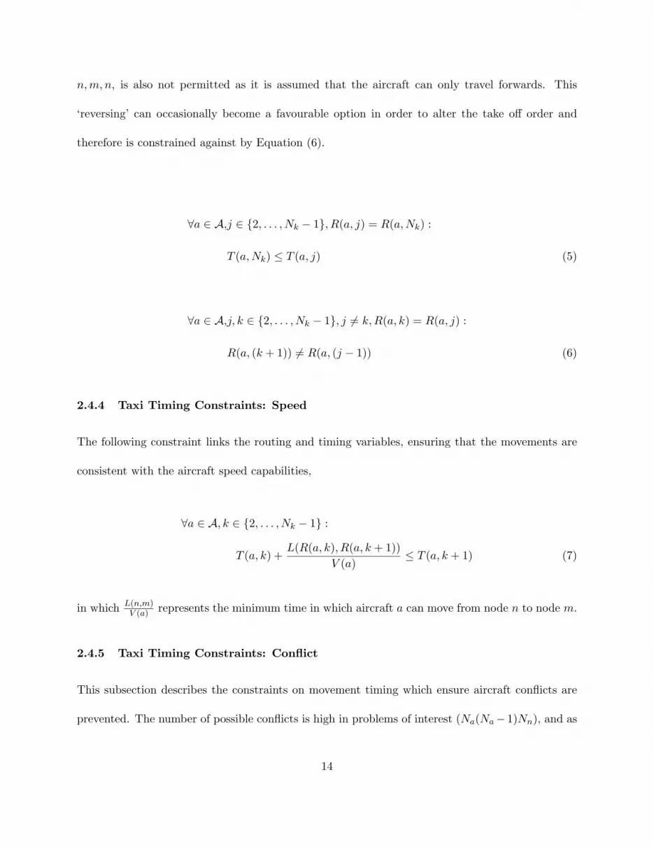
n,m, n, is also not permitted as it is assumed that the aircraft can only travel forwards. This

‘reversing’ can occasionally become a favourable option in order to alter the take off order and

therefore is constrained against by Equation (6).

∀a ∈ A,j ∈ {2, . . . , Nk − 1}, R(a, j) = R(a,Nk) :

T (a,Nk) ≤ T (a, j) (5)

∀a ∈ A,j, k ∈ {2, . . . , Nk − 1}, j 6= k,R(a, k) = R(a, j) :

R(a, (k + 1)) 6= R(a, (j − 1)) (6)

2.4.4 Taxi Timing Constraints: Speed

The following constraint links the routing and timing variables, ensuring that the movements are

consistent with the aircraft speed capabilities,

∀a ∈ A, k ∈ {2, . . . , Nk − 1} :

T (a, k) +L(R(a, k), R(a, k + 1))

V (a)≤ T (a, k + 1) (7)

in which L(n,m)V (a) represents the minimum time in which aircraft a can move from node n to node m.

2.4.5 Taxi Timing Constraints: Conflict

This subsection describes the constraints on movement timing which ensure aircraft conflicts are

prevented. The number of possible conflicts is high in problems of interest (Na(Na− 1)Nn), and as

14

a result fully constrained problems are computationally demanding. However the number of actual

conflicts which would occur if not constrained against is typically much lower. Conflict constraints

are therefore well suited to an iterative framework which aims to improve solution efficiency by

solving a series of less-constrained problems instead of the full problem [24].

SE = {{a, b, n} : a, b ∈ 1 . . . Na, a 6= b, n ∈ N} is a set of all instances of possible separation

conflict between two aircraft a and b at a node n. Similarly CO = {{a, b, n,m} : a, b ∈ 1 . . . Na, a 6=

b, n,m ∈ N , n 6= m} contains the lists of all possible crossover (overtaking and head-on) conflicts

between two aircraft a and b between two nodes n and m.

Subsets of these: SE i ⊆ SE and COi ⊆ CO are needed for the iterative procedure, these are

augmented from one iteration, i to the next, i + 1. The conflict constraints (11-17) are initially

fully relaxed by including no instances of possible conflict in the subsets:

SE0 = CO0 = ∅ (8)

Note for solution of the fully constrained problem it is considered that in the initial iteration the

subset represents the full set, SE0 = SE and CO0 = CO. After each iterations MILP solution the

plan is checked for conflicts, if any occur they are added to the detected sets for that iteration

SEdet(i) or COdet(i) which are then used to augment the subsets, using Equations (9-10), and the

problem is re-solved. This process is repeated until no conflicts are present in the solution.

SE i = SE i−1 ∪ SEdet(i− 1) (9)

COi = COi−1 ∪ COdet(i− 1) (10)

This iterative procedure still results in the globally optimal solution whilst reducing computational

15

effort by avoiding the application of redundant constraints. The rationale behind this comes from

the non-linear increase in solve times with problem size, meaning solving four problems of size 1

can be quicker than solving one problem of size 4.

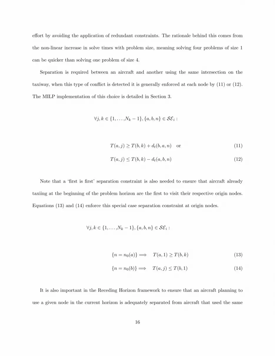
Separation is required between an aircraft and another using the same intersection on the

taxiway, when this type of conflict is detected it is generally enforced at each node by (11) or (12).

The MILP implementation of this choice is detailed in Section 3.

∀j, k ∈ {1, . . . ,Nk − 1}, {a, b, n} ∈ SE i :

T (a, j) ≥ T (b, k) + dt(b, a, n) or (11)

T (a, j) ≤ T (b, k)− dt(a, b, n) (12)

Note that a ‘first is first’ separation constraint is also needed to ensure that aircraft already

taxiing at the beginning of the problem horizon are the first to visit their respective origin nodes.

Equations (13) and (14) enforce this special case separation constraint at origin nodes.

∀j, k ∈ {1, . . . ,Nk − 1}, {a, b, n} ∈ SE i :

{n = n0(a)} =⇒ T (a, 1) ≥ T (b, k) (13)

{n = n0(b)} =⇒ T (a, j) ≤ T (b, 1) (14)

It is also important in the Receding Horizon framework to ensure that an aircraft planning to

use a given node in the current horizon is adequately separated from aircraft that used the same

16

node in the previous horizon. This is accounted for by Equation (15):

∀a ∈ {1, . . . ,Na}, k ∈ {1, . . . , Nk} :

T (a, k) > TL(R(a, k)) + dt(a, aL(R(a, k)), R(a, k)) (15)

where TL(n) is the last time that node n was visited prior to the current horizon, and aL(n) is the

last aircraft to use the node n. Since separation is only enforced at nodes, it is necessary to be able

to constrain against crossover conflicts occurring on the arcs in between nodes, such as overtaking

and head on situations. Equations (16)-(17) constrain against detected conflicts of this type.

∀k, j ∈ {1, . . . , Nk − 1}, {a, b, n,m} ∈ COi :

T (a, j) ≥ T (b, k) + dt(b, a, n) and

T (a, j + 1) ≥ T (b, k + 1) + dt(b, a,m)

(16)

orT (a, j) ≤ T (b, k)− dt(a, b, n) and

T (a, j + 1) ≤ T (b, k + 1)− dt(a, b,m)

(17)

2.4.6 Cost-to-go

A cost-to-go is used to represent the approximate plan beyond the detailed planning horizon dis-

cussed in Section 2.1. This is based on the shortest taxiway distance, rST (nF , nD), from the

terminal node nF of the detailed plan to the destination node nD (runway or gate entry), traversed

17

at the maximum speed of the aircraft, Va.

∀a ∈ A :

tD(a) = T (a,Nk) +rST (nF (a), nD(a))

Va(18)

Equation (18) ensures that the auxiliary variable tD(a), encoding the absolute planned time at

which aircraft a reaches its destination node, complies with the approximate plan from the planned

terminal position.

2.4.7 Runway Scheduling

Studies have shown that the runway is a major bottle neck in the airport surface [16], and Atkin

at al [6] identified that the downstream separation constraints beyond the runway were of great

importance. This motivates the inclusion of runway scheduling in a ground movement optimizer.

As mentioned already, arrival runway scheduling is not being considered in this paper, and the

predetermined landing times and order are fixed. This leaves the departure runway scheduling.

As the aircraft are not guaranteed to reach their destination in the planning horizon the runway

scheduling has to be dealt with in a different way to the general separation. Each aircraft a has an

absolute planned destination (or take-off for departures) time tD(a) which is used in (19) or (20)

18

to create a valid schedule which meets the separation constraints.

∀a, b ∈Adep ∪ Ax :

tD(a) ≥ tD(b) + dt(b, a, nR) or (19)

tD(a) ≤ tD(b)− dt(a, b, nR) (20)

where the separation limits on the runway, represented by dt, include both the wake vortex and

downstream SID separation requirements. Also Ax is a set of auxiliary aircraft, a concept discussed

in the next section. Note that the last take off time from executed horizons is also recorded and

used to constrain the first take off in the current plan.

2.4.8 Departure Runway Planning Foresight

As discussed, it is natural to operate the RH planner in a ‘Rolling Window’ fashion, considering

only a subset of the aircraft. Under this formulation it was observed that the introduction of

new aircraft could cause considerable shuffling in the take-off queue. This leads to undesirable

behaviour, as taxiing aircraft may slow down considerably, lengthening the taxi time, and also

increasing the need for acceleration and deceleration. This effect is similar to ‘churning’ seen in

other assignment and routing optimizers [28].

In order to combat this effect, the scheduler is allowed greater ‘foresight’, in terms of departing

aircraft. The set, Ax of auxiliary departure aircraft, ax is defined. These aircraft are those whose

earliest push-back time t0(ax) is within the foresight horizon Tf beyond the current execution

horizon. This set of aircraft is not included in the routing optimizer, and they are used for the

19

purposes of runway scheduling only. Auxiliary aircraft do not have a detailed plan: instead the

shortest path approximation is used to determine the time at which they are expected to start

taxiing tstart, and a take off time on the runway tD only.

The lists of departing aircraft, Adep and auxiliary input aircraft, Ax are combined for use

in (20). The following equations are the equivalent to (18) for auxiliary aircraft, the distinction

being the use of a variable value of tstart. The shortest taxiway distance to the destination node

rST (n0(ax), nD(ax)) for auxiliary input aircraft is also included, measured from the origin node, n0

due to their lack of detailed plan.

∀ax ∈ Ax :

tD(ax) = tstart(ax) +rST (no(ax), nD(ax))

Vax

(21)

tstart(ax) ≥ to(ax) (22)

Equation (21) ensures that estimated take off times comply with the rough plan to the runway from

the origin position. Equation (22) ensures that auxiliary aircraft ax does not plan to start taxiing

before its earliest push-back time. The foresight is set to 300 seconds, preliminary experiments

suggested that a foresight horizon of around 400 seconds could offer a reduction in the overall

taxied time of approximately 2% over the case where the optimizer has no foresight. Larger values

of foresight inevitably result in higher computation times, hence 300 seconds was used in this case,

reducing computation whilst still accessing the benefits of foresight. Readers are directed to [26]

for thorough discussion.

20

2.5 Objective Function

The objective that is minimized in a given horizon, h, is a weighted combination of the last time

on the take-off runway amongst all active and auxiliary aircraft, the total taxi time of all the active

aircraft and their total taxi distance,

Jh =w0tend

+w1

Na∑a=1

(tD(a)− tstart(a))︸ ︷︷ ︸Taxi time for a

(23)

+w2

Na∑a=1

(Nk)∑k=2

L(R(a, k − 1), R(a, k)) + rST (nF (a), nD(a))︸ ︷︷ ︸Distance travelled by a

The coefficients w0, w1 and w2 are non-negative weightings with initial values in this paper of 25,5

and 3 respectively, and tend represents the last time on the take off runway motivating throughput.

tend ≥ TD(a) ∀a ∈ A ∪Ax (24)

The absolute time that aircraft a starts to taxi is represented by tstart(a). This value is fixed

for aircraft already taxiing at the beginning of the problem, but variable for those who have yet to

begin taxiing, being equal to T (a, 1) in this case. Beyond the horizon, the cost-to-go assumes the

aircraft use the shortest possible path to the destination rST (nF (a), nD), where nF (a) is the final

node in aircraft a’s detailed plan.

The inclusion of the approximation values beyond the detailed plan acts as a terminal penalty.

Also aircraft are prevented from ‘putting off’ making a detailed plan in favour of a rough repre-

21

sentation of their whole plan by only allowing destination nodes to be repeated in the detailed

plan.

3 MILP Implementation

3.1 Introduction

This Section describes the MILP formulation of the contraints presented in Section 2. A linear

program is a mathematical formulation of a minimization or maximization of a linear function,

f(x), subject to linear constraints. A Mixed Integer Linear Programming (MILP) problem is a

subset of linear programs in which a specified subset of the variables are required to take on integer

values as in (25), meaning that both discrete and continuous decisions can be represented. Solving

such problems is NP-hard.

Min : f(x) = cTx + dTy

Subject to :

Ax+By = b

Gx+ Fy ≤ g

x ∈ Z

(25)

Representation of the taxiway routing and runway scheduling problem defined in Section 2

as a MILP problem requires the introduction of binary decision variables, and reformulation of

constraints. The remainder of this Section presents these amendments.

22

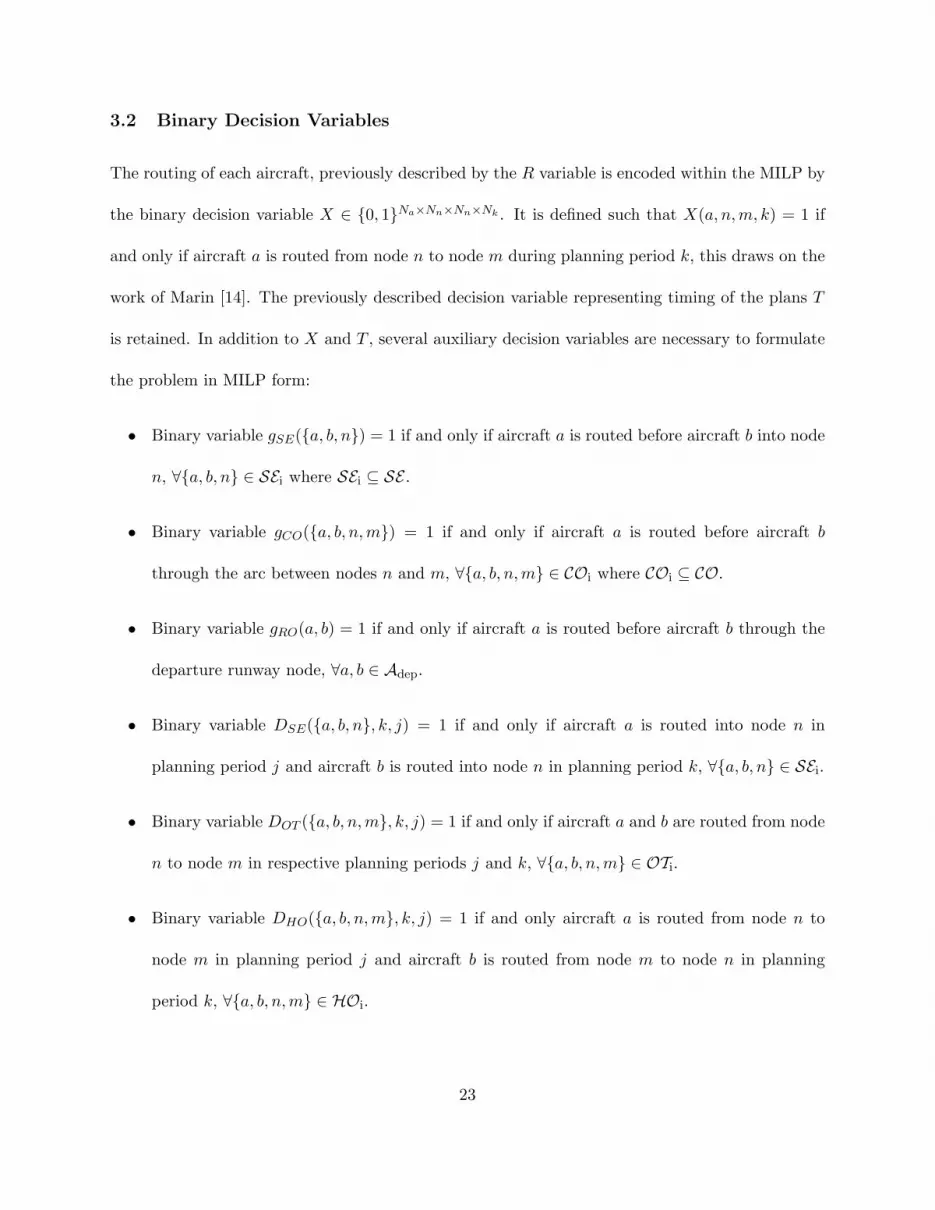
3.2 Binary Decision Variables

The routing of each aircraft, previously described by the R variable is encoded within the MILP by

the binary decision variable X ∈ {0, 1}Na×Nn×Nn×Nk . It is defined such that X(a, n,m, k) = 1 if

and only if aircraft a is routed from node n to node m during planning period k, this draws on the

work of Marin [14]. The previously described decision variable representing timing of the plans T

is retained. In addition to X and T , several auxiliary decision variables are necessary to formulate

the problem in MILP form:

• Binary variable gSE({a, b, n}) = 1 if and only if aircraft a is routed before aircraft b into node

n, ∀{a, b, n} ∈ SEi where SEi ⊆ SE .

• Binary variable gCO({a, b, n,m}) = 1 if and only if aircraft a is routed before aircraft b

through the arc between nodes n and m, ∀{a, b, n,m} ∈ COi where COi ⊆ CO.

• Binary variable gRO(a, b) = 1 if and only if aircraft a is routed before aircraft b through the

departure runway node, ∀a, b ∈ Adep.

• Binary variable DSE({a, b, n}, k, j) = 1 if and only if aircraft a is routed into node n in

planning period j and aircraft b is routed into node n in planning period k, ∀{a, b, n} ∈ SEi.

• Binary variable DOT ({a, b, n,m}, k, j) = 1 if and only if aircraft a and b are routed from node

n to node m in respective planning periods j and k, ∀{a, b, n,m} ∈ OTi.

• Binary variable DHO({a, b, n,m}, k, j) = 1 if and only aircraft a is routed from node n to

node m in planning period j and aircraft b is routed from node m to node n in planning

period k, ∀{a, b, n,m} ∈ HOi.

23

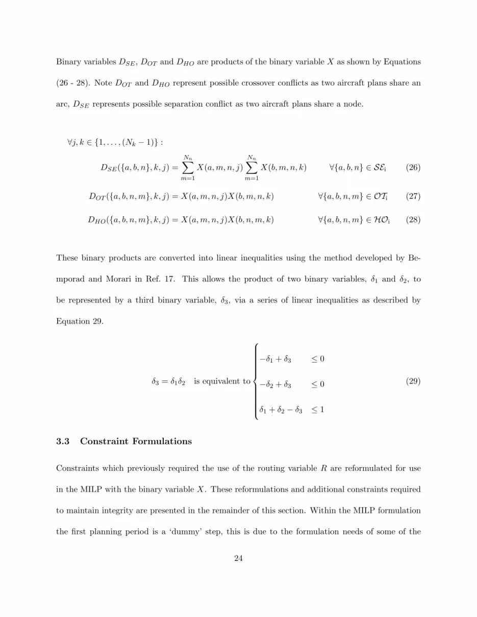
Binary variables DSE , DOT and DHO are products of the binary variable X as shown by Equations

(26 - 28). Note DOT and DHO represent possible crossover conflicts as two aircraft plans share an

arc, DSE represents possible separation conflict as two aircraft plans share a node.

∀j, k ∈ {1, . . . , (Nk − 1)} :

DSE({a, b, n}, k, j) =Nn∑

m=1

X(a,m, n, j)Nn∑

m=1

X(b,m, n, k) ∀{a, b, n} ∈ SEi (26)

DOT ({a, b, n,m}, k, j) = X(a,m, n, j)X(b,m, n, k) ∀{a, b, n,m} ∈ OTi (27)

DHO({a, b, n,m}, k, j) = X(a,m, n, j)X(b, n,m, k) ∀{a, b, n,m} ∈ HOi (28)

These binary products are converted into linear inequalities using the method developed by Be-

mporad and Morari in Ref. 17. This allows the product of two binary variables, δ1 and δ2, to

be represented by a third binary variable, δ3, via a series of linear inequalities as described by

Equation 29.

δ3 = δ1δ2 is equivalent to

−δ1 + δ3 ≤ 0

−δ2 + δ3 ≤ 0

δ1 + δ2 − δ3 ≤ 1

(29)

3.3 Constraint Formulations

Constraints which previously required the use of the routing variable R are reformulated for use

in the MILP with the binary variable X. These reformulations and additional constraints required

to maintain integrity are presented in the remainder of this section. Within the MILP formulation

the first planning period is a ‘dummy’ step, this is due to the formulation needs of some of the

24

constraints which require summations in the binary routing variable X. This first step is used to

enforce the initial position and time constraints:

X(a, n0(a), n0(a), 1) = 1 ∀a ∈ A (30)

T (a, 1) = T (a, 2) ∀a ∈ A (31)

The following constraints are introduced to ensure that the variable X encodes a valid routing

through the taxiways:

∀a ∈ A, n ∈ N :

X(a, n,m, k) ≤ C(n,m) ∀m ∈ N , k ∈ {2, . . . , Nk − 1} (32)

Nn∑m=1

X(a, n,m, k) =Nn∑

m=1

X(a,m, n, k − 1) ∀k ∈ {2, . . . , Nk − 1} (33)

Nn∑n=1

Nn∑m=1

X(a, n,m, k) = 1 ∀k ∈ {1, . . . , Nk − 1} (34)

Equation (32) constrains the aircraft’s movements to follow the rules of connectivity of the graph

structure. Continuity is assured by Equation (33), meaning that if an aircraft moves to node n in

period k − 1, it must move from node n in period k. Equation (34) forces each aircraft to have a

plan for each period.

Equations (5) and (6) are respectively emulated in MILP by the following Equations:

25

∀a ∈ A,j ∈ {2, . . . , Nk − 1} :

T (a,Nk) ≤ T (a, j) +M ∗ (1−Nn∑

m=1

X(a,m, nD(a), (j − 1))) (35)

∀a ∈ A,n ∈ {1, . . . , Nn − 1},m ∈ {(n+ 1), . . . , Nn} :

(Nk−1)∑k=1

X(a, n,m, k) +(Nk−1)∑

j=1

X(a,m, n, j) ≤ 1 (36)

where M is an arbitrary large number greater than the largest scale in the problem. The speed

constraint is translated into that shown in Equation (37)

∀a ∈ A,k ∈ {2, . . . , Nk − 1} :

T (a, k) +∑Nn

n=1

∑Nnm=1 L(n,m)X(a, n,m, k)

V (a)≤ T (a, k + 1) (37)

The iterated constraints on movement timing which ensure aircraft conflicts are prevented are

reformulated as follows:

∀{a, b, n} ∈ SEi, n 6= n0(a) ∪ n0(b), k ∈ {2, . . . , Nk − 1} :

gSE({a, b, n}) ≥ −M (1−DSE({a, b, n}, j, 1)) + 0.5 (38)

gSE({a, b, n}) ≤ +M (1−DSE({a, b, n}, 1, k)) + 0.5 (39)

Equations (38) and (39) represent the first is first rule, ensuring that if a node, apart from the

26

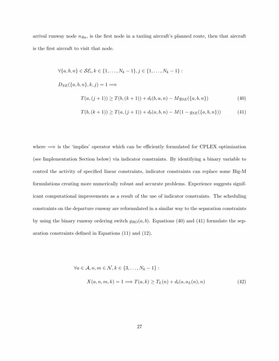
arrival runway node nRa, is the first node in a taxiing aircraft’s planned route, then that aircraft

is the first aircraft to visit that node.

∀{a, b, n} ∈ SEi, k ∈ {1, . . . , Nk − 1}, j ∈ {1, . . . , Nk − 1} :

DSE({a, b, n}, k, j) = 1 =⇒

T (a, (j + 1)) ≥ T (b, (k + 1)) + dt(b, a, n)−MgSE({a, b, n}) (40)

T (b, (k + 1)) ≥ T (a, (j + 1)) + dt(a, b, n)−M(1− gSE({a, b, n})) (41)

where =⇒ is the ‘implies’ operator which can be efficiently formulated for CPLEX optimization

(see Implementation Section below) via indicator constraints. By identifying a binary variable to

control the activity of specified linear constraints, indicator constraints can replace some Big-M

formulations creating more numerically robust and accurate problems. Experience suggests signif-

icant computational improvements as a result of the use of indicator constraints. The scheduling

constraints on the departure runway are reformulated in a similar way to the separation constraints

by using the binary runway ordering switch gRO(a, b). Equations (40) and (41) formulate the sep-

aration constraints defined in Equations (11) and (12).

∀a ∈ A, n,m ∈ N , k ∈ {3, . . . , Nk − 1} :

X(a, n,m, k) = 1 =⇒ T (a, k) ≥ TL(n) + dt(a, aL(n), n) (42)

27

∀a ∈ Adep :

if Tt > 0 then T (a, 1) ≥ TL(n0(a)) + dt(a, aL(n0(a)), n0(a))

if Tt = 0 then T (a, 1) ≥ 0

(43)

The consideration of aircraft from previous horizons demonstrated by Equation (15), is split into

the two Equations (42-43), respectively dealing with the departure runway / taxiways and the

aircraft departing their gates. Tt is the time an aircraft has already spent taxiing prior to the

current horizon, and indicates whether it is leaving from the gate, or a position already on the

taxiways. The choice in Equation (43) can be formulated as Tt is an input parameter.

∀{a, b, n,m} ∈ COi, k ∈ {1, . . . , Nk − 1}, j ∈ {1, . . . , Nk − 1} :

DOT ({a, b, n,m}, k, j) ∪DHO({a, b, n,m}, k, j) = 1 =⇒

T (a, j) + dt(a, b, n) ≤ T (b, k) +M(1− gCO({a, b, n,m})) (44)

T (a, (j + 1)) + dt(a, b,m) ≤ T (b, (k + 1)) +M(1− gCO({a, b, n,m}))(45)

T (b, k) + dt(b, a, n) ≤ T (a, j) +MgCO({a, b, n,m}) (46)

T (b, (k + 1)) + dt(b, a,m) ≤ T (a, (j + 1)) +MgCO({a, b, n,m}) (47)

Equations (44 - 47) prevent overtaking on the taxiways and head-on conflicts on the taxiways,

28

emulating Equations (16) and (17). To summarize the objective is formulated as:

Jh =w0tend

+w1

Na∑a=1

(tD(a)− tstart(a))︸ ︷︷ ︸Taxi time for a

(48)

+w2

Na∑a=1

(Nk−1)∑k=2

Nn∑n=1

Nn∑m=1

L(n,m)X(a, n,m, k) + rST (m, a)X(a, n,m, (Nk − 1))︸ ︷︷ ︸Distance travelled by a

this is to be minimized subject to Equations (2,3,18,21,22, and 30-47).

4 Results

4.1 Implementation

The optimization was translated into the AMPL modelling language [29]. An AMPL model file

contains the constraint forms for all instances, while the data is written to an AMPL data file by a

Matlab script. CPLEX 11.1.0 parallel optimization software [19] is used on a 3GHz dual core PC

with 2GB of RAM to solve all problems.

4.2 Large-Scale Heathrow Problem

4.2.1 Problem Set-Up

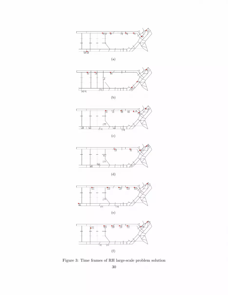
To illustrate the potential of the approach the baseline optimization scheme developed was used

on a large-scale problem using the Heathrow layout represented by the 126-node graph structure

shown in Fig. 3(a). Basic departure and arrival board data collected from the Heathrow website [30]

on Wednesday 26th August 2009 between 9 am and 12 noon, was used. This included 240 aircraft,

29

(a)

(b)

(c)

(d)

(e)

(f)

Figure 3: Time frames of RH large-scale problem solution

30

122 of which were arrivals. Gate assignments, SID routes and aircraft weight classes have been

assigned arbitrarily as these details were not publicly available. The graph structure used does not

incorporate Terminal 4, as very few flights used this terminal. Terminal 4 arrivals are assumed to

taxi south of the arrival runway and hence do not form part of the problem. Terminal 4 departures

were assumed to enter the problem at the bottom right-hand node, having already passed to the

East of the arrival runway.

The RH framework had a planning horizon ofNk = 6 planning periods with replanning occurring

every 40 seconds. The departure foresight window used was 300 seconds. The weightings used in

the objective (48), were set as follows: w0 = 25, w1 = 5, w3 = 3.

4.2.2 FCFS Comparisons and Analysis

The problem described above was solved using both the RH optimization scheme and a FCFS ap-

proach. The resulting RH plan was found to improve upon FCFS by 55% when comparing the total

taxiing time across all aircraft, going from an average of 13.2 minutes per aircraft to 5.89 minutes

per aircraft. Fig. 4 shows the direct comparison of taxi times for each arrival and departure aircraft

in the problem. This shows a distinct difference between arrivals and departures, indicating the

MILP optimization offers little improvement over FCFS for arrivals, whereas significant improve-

ments can be made in the departure plans. This may be due to the lack of downstream constraints

on arrivals as actions beyond the gate entry are not considered. It is also noted that many arrivals

had short journeys to Terminal 5, which were largely unimpeded by departure aircraft flow, and

that due to the layout of Heathrow, all aircraft follow the same general circulation pattern across

the surface (North-East in the example presented). Although slight, the deviations that some ar-

rivals do show from FCFS indicate interactions with departures, with the slightly longer taxi times

31

0 500 1000 1500 2000 25000

100

200

300

400

500

600

700

800

FCFS Taxi Time (s)

RH

Tax

i Tim

e (s

)

DepartureArrival1:1

Figure 4: Comparison of individual aircraft taxiing times between RH and FCFS approaches

suggesting they may have accepted some delay to increase global gains.

It was observed that some departure aircraft wait at their gate in order to begin their taxi later.

This was seen to be a good strategy in recent work by Simaiakis and Balakrishnan [31] in which it

was demonstrated that a saturation limit to the number of departure aircraft taxiing exists. Below

the limit, increasing the number of departing aircraft increases take off rate; beyond it, the runway

becomes the defining capacity constraint, and increasing the number of departure aircraft simply

adds to congestion on the surface. However, in the solution produced by the RH scheme, 10% of

the departure aircraft and 50% of the arrival aircraft also took routes which were different to the

shortest paths used in FCFS, and as the simple demonstrations in our previous work [32] showed,

allowing re-routing can be beneficial to the problem solution.

Fig. 5(a) shows a comparison of the departure aircraft take-off times between the FCFS and

RH solutions, with the dashed, light and heavier lines respectively highlighting an earlier take-

off, no change, and a later take-off under the RH scheme. It can be seen from Fig. 5(a) that

the majority of aircraft have earlier take-off times under the RH optimization. Also, although

considerable reordering takes place, it occurs in a relatively localised fashion, meaning no one

32

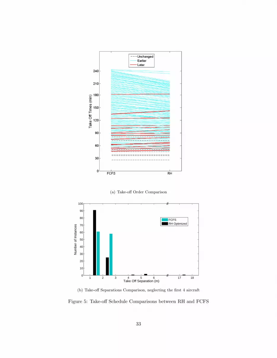
(a) Take-off Order Comparison

1 2 3 4 5 6 17 180

10

20

30

40

50

60

70

80

90

100

//

//

//

//

Take Off Separation (m)

Num

ber

of In

stan

ces

FCFSRH Optimized

(b) Take-off Separations Comparison, neglecting the first 4 aircraft

Figure 5: Take-off Schedule Comparisons between RH and FCFS

33

0

50

100

150

200

250

300

3500 20 40 60 80 100 120

Hor

izon

Num

ber

Solve Time (s)

Figure 6: Solve times for individual horizons using RH

aircraft is unreasonably delayed for the global good. By observing the change in the distribution

of separation times between take offs, shown in Fig. 5(b), it is clear that the throughput capacity

of the departure runway would be improved by the RH scheme, as it creates a 17 minute gap in

runway usage in which up to 17 additional aircraft could potentially take off.

Stills from the RH solution are shown in Fig. 3. Within these shaded aircraft represent de-

partures and unshaded arrivals. Interactions between the arrival and departure paths around the

airport surface can be seen clearly in still (a), still (b) and still (c). Note that in still (c), departure

aircraft number 107 departs from the gate in a timely fashion allowing it to slip into the departure

queue between aircraft number 90 and aircraft number 88, as shown by still (d). The departure

runway order and spacing are seen to be well formed on the taxiways in still (e) and still (f).

The complete simulation took just under 4 hours to run. Fig. 6 shows the solve times of each

individual horizon within the problem, from this it can be seen that all of the horizons solved

within 120 seconds with many horizons solving in under a minute. Although slightly slower than

34

real time, as the replanning occurs every 40 seconds, the difference is small enough to suggest that

with increased computing power, real time operation will be practical. The issue of computational

efficiency is discussed further in the next section.

4.3 Computation

In order to investigate the efficiency of the baseline algorithm presented here, we consider the

effect of moving away from it by first the removing the RH framework and then also removing the

constraint iteration.

Solving airport problems of the scale of that described in Section 4.2 without a receding horizon

means expecting all aircraft to plan their entire route, to allow computation of the global optimal.

This would require a longer planning horizon of around 30 planning periods, as the largest value of

RST from gate to runway in the graph model of Heathrow is 25 nodes in length. Even considering

a rolling window in aircraft memory issues become a problem. In a typical day more than 1200

aircraft pass through Heathrow [30]. The RH element of the baseline scheme is necessary to allow

solution of problems of this scale, although it does introduce some approximations into the solution.

We have found that it is possible, without RH, to solve small instances of the taxi problem

on a small section of the Heathrow lay-out for up to 8 aircraft taxiing simultaneously where the

aircraft only need to plan up to 10 moves. Therefore, comparison tests were completed using a

19-node section representing the area around the holding point of Heathrow’s North runway. Only

departing aircraft were considered and 64 different instances of a 3 aircraft problem were posed.

The same was done for cases involving 4, 5, 6, 7 and 8 aircraft. The weights used in the objective

function for these problems were also: w0 = 25, w1 = 5 and w2 = 3.

The problems were solved using the baseline algorithm: as presented - ‘RH’; without the RH

35

3 4 5 6 7 810

0

101

102

103

104

105

Number of Aircraft in Problem

Sol

ve T

ime

(s)

RH − Single HorizonRH − Total ProblemIterativeFully Constrained

1 Hour

1 Min

1 Sec

Figure 7: Solve Time Comparison of 3, 4, 5, 6, 7 and 8 aircraft problems, 64 permutations of each,solved using Fully Constrained, Iterative, and Receding-Horizon methods

framework - ‘Iterative’; and without RH or constraint iteration - ‘Fully Constrained’. Fig. 7 shows

the solve times of these problems, including both the full problem solved by the baseline RH scheme,

‘RH - Total Problem’, and a single horizon within that, ‘RH - Single Horizon’. Note the lack of

results for the fully constrained case for problems involving more than 5 aircraft. Beyond this the

algorithm consistently ran out of memory to complete the optimization, or reached the 10 hour

restriction on solve time without finding an integer solution.

The results show that constraint iteration reduces the solve time considerably, although the solve

times still increase at an exponential rate with respect to problem size. The spread of Iterative

solve times also increases significantly with problem size, consistent with the results of previous

works [24]. The more constraints that have to be added back into the problem, the longer the

iterative method takes. However in all cases presented here the solve time saving is significant due

36

to the large number of inactive constraints, and no approximations are introduced so the solution

is still the global optimal.

Considering the RH framework, it can be seen that the single horizon computation times are

at the lowest end of the range of Iterative solve times if not below. The solve time saving available

from adopting the RH approach becomes more pronounced as the number of aircraft in the problem

increases. The ‘RH - Total Problem’ solve time is a summation of the solve times of the individual

horizons needed to complete the entire problem. This shows much less variability than iterative

scheme for larger problems and is observed to be much more scalable in the number of aircraft,

being almost linear, suggesting that for bigger problems the computational saving will become even

more significant. The ability of the RH, rolling window scheme to spread the computation between

horizons, and hence over time, also becomes more significant in larger problems which span longer

periods of time on the airport surface (≥ 1 hour), allowing the optimizer to concentrate on the near

future, using approximations for the distant future.

4.4 Performance

As already stated constraint iteration does not effect the solution quality, meaning that the Iterative

solution is identical to that of the Fully-Constrained problem. However, the introduction of the

RH framework results in a plan which is an approximation to the global optimal solution. Figure 8

shows comparisons of RH solution performance to both the non-RH (Iterative/Fully Constrained)

and FCFS with points representing each of the problems described above and a line indicating

the 1:1. Figures 8(a) and 8(b) show comparisons of the total taxi time performance of RH against

Iterative/Fully Constrained and FCFS respectively. From these figures it can be seen that, as would

be expected, in general the RH-scheme has equivalent or longer taxi times than the Iterative/Fully

37

0 500 1000 1500 20000

200

400

600

800

1000

1200

1400

1600

1800

2000

Iterative Total Taxi Time (s)

RH

Tot

al T

axi T

ime

(s)

IterativeBetter

RHBetter

(a) Total Taxi Time Comparison, RH v Iterative

0 1000 2000 3000 40000

500

1000

1500

2000

2500

3000

3500

4000

FCFS Total Taxi Time (s)

RH

Tot

al T

axi T

ime

(s)

RHBetter

FCFSBetter

(b) Total Taxi Time Comparison, RH v FCFS

0 1000 2000 3000 4000 5000 6000 70000

1000

2000

3000

4000

5000

6000

7000

Iterative Total Taxi Distance (m)

RH

Tot

al T

axi D

ista

nce

(m)

IterativeBetter

RHBetter

(c) Total Taxi Distance Comparison, RH v Iterative

0 1000 2000 3000 4000 5000 6000 70000

1000

2000

3000

4000

5000

6000

7000

FCFS Total Taxi Distance (m)

RH

Tot

al T

axi D

ista

nce

(m)

FCFSBetter

RHBetter

(d) Total Taxi Distance Comparison, RH v FCFS

0 200 400 600 8000

100

200

300

400

500

600

700

800

Iterative tend

(s)

RH

Ten

d (s)

IterativeBetter

RHBetter

(e) tend, Comparison, RH v Iterative

0 200 400 600 800 10000

100

200

300

400

500

600

700

800

900

1000

FCFS tend

(s)

RH

Ten

d (s)

FCFSBetter

RHBetter

(f) tend, Comparison, RH v FCFS

Figure 8: Performance Comparisons38

Constrained schemes, and shorter taxi times than the FCFS approach. Figs. 8(c) and 8(d) show

the same comparison for the total taxi distance performance. The RH scheme plans are shown to

have similar total taxi distances to the Iterative/Fully Constrained plans. As would be expected

due to the FCFS approach’s use of the shortest path to runway, the RH plans are shown to have

longer total taxi distances than the FCFS, due to the key re-routing behaviour of the coupled

routing-timing scheme.

Figs. 8(e) and 8(f) show comparisons of the last time on runway or tend performance, a measure

of throughput, of RH against Iterative/Fully Constrained and FCFS respectively. The RH scheme

is shown in many cases to match the Iterative/Fully Constrained last time on runway (note it

never improves on this due to the relatively high weighting on destination times tD), and improve

upon or match FCFS. In some cases the RH plan has a higher tend, than both the non-RH and

the FCFS approaches. This is a symptom of the close proximity of the problem within the 19-

node structure. The ‘rough plan’ part of the RH scheme does not take into account physical

infeasibility of reordering when computing the runway schedule. In larger problems this is not

prevalent, although further refinement of the rough plan is a consideration for future work.

5 Conclusions and Further Work

In this paper we have presented a novel method combining in one optimization the taxiway op-

erations and runway scheduling elements of airport surface movement in a continuous time en-

vironment. Additionally this is implemented in a receding horizon, iterative manner to improve

scalability of computation.

The potential of the algorithm has been illustrated using a 240-aircraft example of ground

39

movement operations at Heathrow airport. Results demonstrated that the optimization scheme

presented offers the potential for significant savings (over 50% on average) in total taxiing time

over a FCFS approach.

Our simulation shows that the behaviour of arrivals differs little between FCFS and optimized

operations. No significant improvement in taxiing time was observed in any arrival aircraft. It is

speculated that this differentiation in the improvement between arrivals and departures is due to

the lack of downstream constraints on arrivals.

Comparative tests broke down the contributions of each feature of the baseline algorithm to the

computation achieved. We have shown that use of iteration of the conflict constraints can reduce

solve times significantly, while maintaining globally optimal solutions. The RH formulation has

been shown to significantly increases the scope of problems which can be handled by the optimizer.

This is because not only does it allow faster computation of the same problems, but also allows

easy transition to the continuous solution of problems in a rolling window sense.

Future work will concentrate on further studies of the large-scale heathrow airport problem in

order to learn more about how the arrival and departure aircraft interact on the airport surface.

This should include restricting the taxiway system, and introduction of enforced push-back times.

Also comparative results with heuristic approaches to taxi planning are of interest.

Acknowledgements

This research is supported by Airbus Operations Ltd, the Knowledge Transfer Network for In-

dustrial Mathematics (managed by the Smith Institute) and the Engineering and Physical Sciences

40

Research Council (EPSRC). The support of Sanjiv Sharma and Mick Dunne as well as useful dis-

cussions with Jason Atkin and Edmund Burke are gratefully acknowledged.

References

[1] SESAR, “Definition Phase 1: Deliverable 1,” Tech. rep., Eurocontrol, 2006.

[2] Sniffen, M. J., “Air Controllers say Staffing too Short,” The Associated Press, Online, available

at http://ap.google.com/article/ALeqM5hi4BgcTtGM7dM2ETypQdZIzSra7gD8U2N4NO1, 10

January 2008.

[3] “National Civil Aviation Safety Committee Sub-Committee on Runway Incursions: Final Re-

port,” Tech. Rep. TP 13795E, Transport Canada, Ottawa, September 2000.

[4] Eurocontrol, “Advanced-Surface Movement, Guidance and Contol Systems (A-SMGCS),” web-

site available at http://www.eurocontrol.int/airports/public/standard_page/APR1_

Projects_ASMGCS.html, 2002-2006.

[5] Commission, E., “European airport Movement Management by A-SMGCS (EMMA),” web-

site available at http://www.transport-research.info/web/projects/project_details.

cfm?ID=20372, 2004-2006.

[6] Atkin, J., Burke, E., Greenwood, J., and Reeson, D., “Hybrid Metaheuristics to Aid Runway

Scheduling at London Heathrow Airport,” Transportation Science, Vol. 41, No. 1, 2007, pp. 90–

106.

41

[7] Anagnostakis, I. and Clarke, J.-P., “Runway Operations Planning: a two-stage solution

methodology,” Proceedings of the 36th Annual Hawaii International Conference on System

Sciences, 2003.

[8] van Leeuwen, P., Hesselink, H., and Rohling, J., “Scheduling Aircraft Using Constraint Satis-

faction,” Electronic Notes in Theoretical Computer Science, Vol. 76, 2002, pp. 252 – 268.

[9] Atkin, J., Burke, E., Greenwood, J., and Reeson, D., “The Effect of the Planning Horizon and

the Freezing Time on Take-off Sequencing,” Proceedings of the 2nd International Conference

on Research in Air Transportation, 2006.

[10] Bolat, A., “Models and a genetic algorithm for a static aircraft-gate assignment problem,”

Journal of the Operations Research Society , Vol. 52, 2001, pp. 1107–1120.

[11] Visser, H. and Roling, P., “Optimal Airport Surface Traffic Planning using Mixed Integer

Linear Programming,” AIAA’s 3rd Annual Aviation Technology, Integration, and Operations

(ATIO) Tech, Vol. November, 2003, pp. 17–19.

[12] Smeltink, J. W., Soomer, M. J., de Waal, P. R., and van der Mei, R. D., “An Optimisation

Model for Airport Taxi Scheduling,” Elsevier Science, Vol. n/a, 2004, pp. n/a.

[13] Balakrishnan, H. and Jung, Y., “A Framework for Coordinated Surface Operations Planning

at Dallas-Fort Worth International Airport,” AIAA Guidance, Navigation and Control Con-

ference and Exibit , 2007.

[14] Marin, A., “Airport Management: Taxi Planning,” Annual of Operations Research, Vol. 143,

2006, pp. 191–202.

42

[15] van Ham, F., “Development of a Taxi Planning Tool using Genetic Optimization,” Tech. rep.,

Delft University of Technology, 1999.

[16] Idris, H. R., Delcaire, B., Anagnostakis, I., Hall, W. D., Pujet, N., Feron, E., Hansman, R. J.,

Clarke, J. P., and Odoni, A. R., “Identification of Flow Contstraints and Contol Points in

Departure Operations at Airport Systems,” Proceedings of the AIAA Guidance, Navigation

and Control Conference, 1998.

[17] Bemporad, A. and Morari, M., “Control of Systems integrating Logic Dynamics and Con-

straints,” Automatica, Vol. 35, No. 3, 1999, pp. 407–427.

[18] Bertsimas, D. and Stock-Patterson, S., “The Air Traffic Flow Management Problem with

Enroute Capacities,” Operations Research, Vol. 46,3, 1998, pp. 406–422.

[19] ILOG CPLEX Website, http://www.ilog.com/products/cplex/, visited July 2005.

[20] Reif, J. H., “Complexity of the Movers Problem and Generalizations,” 20th IEEE Symposium

on the Foundations of Computer Science, 1979, pp. 421–427.

[21] “CAP493: Manual of Air Traffic Services Part 1,” Civil Aviation Authority,, November 2007,

available at http://www.caa.co.uk/docs/33/CAP493Part1.pdf.

[22] Bellingham, J., Kuwata, Y., and How, J., “Stable Receding Horizon Trajectory Control for

Complex Environments,” Proceedings of the AIAA Guidance, Navigation and Control Confer-

ence, 2003.

[23] Kuwata, Y., Richards, A., Schouwenaars, T., and How, J., “Distributed Robust Receding Hori-

zon Control for Multi-vehicle Guidance,” IEEE Transactions on Control Systems Technology ,

Vol. 15, 2007, pp. 627–641.

43

[24] Earl, M. and D’Andrea, R., “Iterative MILP Methods for Vehicle Control Problems,” IEEE

TRANSACTIONS ON ROBOTICS , Vol. 21, 2005, pp. 1158.

[25] Keith, G., Tait, J., and Richards, A., “Efficient Path Optimization with Terrain Avoidance,”

Proceedings of the AIAA Guidance, Navigation and Control Conference, 2007.

[26] Clare, G. and Richards, A., “Receding Horizon, Iterative Optimization of Taxiway Routing and

Runway Scheduling,” Proceedings of the AIAA Guidance, Navigation and Control Conference,

2009.

[27] Rathinam, S., Montoya, J., and Jung, Y., “An Optimization Model for Reducing Aircraft Taxi

Times at the Dallas Fort Worth International Airport,” Proceedings of the 26th International

Congress of the Aeronautical Sciences, 2008.

[28] Schumacher, C., Chandler, P. R., and Rasmussen, S. R., “TASK ALLOCATION FOR WIDE

AREA SEARCH MUNITIONS,” Proceedings of the American Control Conference, 2002.

[29] Fourer, R., Gay, D. M., and Kernighan, B. W., AMPL - A Modeling Language for Mathmatical

Programming , Thomson, Brooks/Cole, 2003.

[30] Heathrow, B., “Official Airport Website,” BAA Heathrow: Official Airport Website, http:

//www.heathrowairport.com/, January 2008.

[31] Simaiakis, I. and Balakrishnan, H., “Queuing Models of Airport Departure Proces for Emis-

sions Reduction,” AIAA Guidance Navigation and Control Conference, 2009.

[32] Keith, G. and Richards, A., “Optimization of Taxiway Routing and Runway Scheduling,”

Proceedings of the AIAA Guidance, Navigation and Control Conference, 2008.

44