Optimal Movement of Two Factory Cranes

Ionut. Arona, Latife Genc-Kayab, Iiro Harjunkoskic, Samid Hodab,J. N. Hooker∗,b

aCura Capital Management, 1270 Avenue of the Americas, New York, NY 10020, USAbTepper School of Business, Carnegie Mellon University, Pittsburgh, PA 15213, USAcABB Corporate Research Center, Wallstadter Str. 59, 68526 Ladenburg, Germany

Abstract

We study the problem of finding optimal space-time trajectories for two fac-

tory cranes or hoists that move along a single overhead track. Each crane is

assigned a sequence of pickups and deliveries at specified locations that must

be performed within given time windows. The cranes must be operated so as

not to interfere with each other, although one crane may need to yield to an-

other. The objective is generally to follow a production schedule as closely as

possible. We show that only certain types of trajectories need be considered

to obtain an optimal solution. This simplifies the operation of the cranes and

enhances safety, because the cranes move according to predictable patterns. We

present a specialized dynamic programming algorithm that solves the problem

and accommodates a wide variety of constraints that typically arise in such

problems. To control the state space size we use an innovative state space rep-

resentation based on a cartesian product of intervals of states and an array of

two-dimensional circular queues. The algorithm solves medium-sized instances

of the problem to optimality and can be used to create benchmarks for tuning

heuristic algorithms that solve larger instances.

Key words: crane scheduling, dynamic programming

∗Corresponding author.Email addresses: ionut.aron@gmail.com (Ionut. Aron), lgenc@andrew.cmu.edu (Latife

Genc-Kaya), Iiro.Harjunkoski@de.abb.com (Iiro Harjunkoski), shoda@andrew.cmu.edu(Samid Hoda), john@hooker.tepper.cmu.edu (J. N. Hooker)

Preprint submitted to Elsevier April 18, 2010

1. Introduction

Manufacturing facilities frequently rely on track-mounted cranes to move

in-process materials or equipment from one location to another. A typical ar-

rangement, and the type studied here, allows one or more hoists to move along

a single horizontal track that is normally mounted on the ceiling. Each hoist

may be mounted on a crossbar that permits lateral movement as the crossbar

itself moves longitudinally along the track. A cable suspended from the crossbar

raises and lowers a lifting hook or other device.

When a production schedule for the plant is drawn up, cranes must be avail-

able to move materials from one processing unit to another at the desired times.

The cranes may also transport cleaning or maintenance equipment. Because the

cranes operate on a single track, they must be scheduled so as not to interfere

with each other. One crane may be required to yield (move out of the way) to

permit another crane to pick up or deliver its load.

The problem is combinatorial in nature because one must not only compute

a space-time trajectory for each crane, but must decide which crane yields to an-

other and when. A decision made at one point may create a bottleneck that has

unforeseen repercussions much later in the schedule. Production planners may

put together a schedule that seems to allow ample time for crane movements,

only to find that the crane operators cannot keep up with the schedule.

In this paper we analyze the problem of scheduling two cranes and describe

an exact algorithm, based on dynamic programming, to solve it. We assume

that each crane has been pre-assigned a sequence of jobs to perform. We selected

a dynamic programming approach because it accommodates a wide variety of

constraints that typically arise in problems of this kind. A crane may be required

to carry out multiple tasks at various locations before completing a job, and each

job may specify a different set of tasks. Time windows may be given for the job

as a whole and/or the tasks within a job. Precedence relations may be imposed

between jobs, or between tasks in different jobs. A crane may be allowed to

pause, or yield to the other crane, between certain tasks but not others. Many

2

linear and nonlinear objective functions are possible, although in practice the

objective is normally to follow the production schedule as closely as possible.

This research is part of a larger project in which both heuristic and exact al-

gorithms have been developed for use in crane scheduling software. The heuristic

method makes crane assignment and sequencing decisions as well as computing

space-time trajectories, and it is fast enough to accommodate large problems in-

volving several cranes. However, once the assignments and sequencing are given,

the heuristic method may fail to find feasible trajectories when they exist and

reject good solutions as a result. We therefore found it important to solve the

trajectory problem exactly for a given assignment and sequencing, as a check

on the heuristic method. The exact algorithm has practical value in its own

right, because two-crane problems are common in industry, and the algorithm

solves instances of respectable size within a minute or so. Yet it has an equally

important role in the creation of benchmarks against which heuristic methods

can be tested and tuned for best performance.

We begin by deriving structural results for the two-crane problem that

restrict the trajectories that must be considered. This makes the problem

tractable for dynamic programming by reducing the state space. It also simpli-

fies the operation of the cranes, and enhances safety, by restricting the crane

movements to certain predictable patterns.

We then describe a dynamic programming algorithm for the optimal trajec-

tory problem. The state space is large, due to the fine space-time granularity

with which the problem must be solved, as well as the necessity of keeping up

with which task a crane is performing and how long it has been processing that

task. To deal with these complications we introduce a novel state space descrip-

tion that represents many states implicitly as a cartesian product of intervals.

The state space is efficiently stored and updated in a data structure that uses

an array of two-dimensional circular queues. These enhancements accelerate

solution by at least an order of magnitude and allow us to solve problems of

realistic size within a reasonable time. The paper concludes with computational

results and directions for further research.

3

2. Previous Work

The literature on crane scheduling tends to cluster around two types of prob-

lems: movement of materials from one tank to another in an electroplating or

similar process (normally referred to as hoist scheduling problems), and loading

and unloading of container ships in a port.

A classification scheme for hoist scheduling problems appears in Manier and

Bloch (2003). These problems typically require a cyclic schedule involving one

or more types of parts, where parts of each type must visit specified tanks in a

fixed sequence. The most common objective is to minimize cycle time.

Much research in this area deals with the single-hoist cyclic scheduling prob-

lem (e.g., Phillips and Unger (1976); Armstrong et al. (1994); Liu et al. (2002)).

Even this restricted problem is NP-complete (Lei and Wang, 1989).

Several papers address cyclic two-hoist and multi-hoist problems. One ap-

proach partitions the tanks into contiguous subsets, assigns a hoist to each

subset, and schedules each hoist within its partition (Lei and Wang, 1991; Zhou

and Li, 2008). A better solution can generally be obtained, however, by allowing

a tank to be served by more than one hoist. Models that address this problem

assign transfer operations to hoists and determine when each operation should

begin and end. A transfer operation typically consists of removing a part from

one tank and moving it to the next tank in the sequence for that part type. The

empty hoist then travels to the starting location of another transfer operation.

A hoist typically moves directly to the delivery point when loaded, but depend-

ing on the model, may yield to another hoist when empty. These models do

not explicitly compute space-time trajectories but avoid collisions by selecting

departure and arrival times that allow hoists to make the necessary movements

without interference (Lei et al., 1993; Varnier et al., 1997; Rodosek and Wallace,

1998; Manier et al., 2000; Yang et al., 2001; Riera and Yorke-Smith, 2002; Leung

and Zhang, 2003; Che and Chu, 2004; Leung et al., 2004; Leung and Levner,

2006).

Our problem differs from the typical hoist scheduling problem in several

4

respects. The schedule is not cyclic. The problem is given as a set of jobs rather

than parts to be processed. Each crane is assigned a sequence of jobs rather

than transfer operations. A job may consist of several tasks to be performed

consecutively by one crane in a specified order. The jobs may all be different.

Both loaded and empty cranes may be allowed to pause or yield, and permission

to do so may depend on which task is being executed. There may also be

precedence constraints and a wide variety of objective functions.

Port cranes are generally classified as quay cranes and yard cranes. Quay

cranes may be mounted on a single track, as are factory cranes, but the schedul-

ing problem differs in several respects. The cranes load (or unload) containers

into ships rather than transferring items from one location on the track to an-

other. A given crane can reach several ships, or several holds in a single ship,

either by rotating its arm or perhaps by moving laterally along the track. The

problem is to assign cranes to loading (unloading) tasks, and schedule the tasks,

so that the cranes do not interfere with each other (e.g., Daganzo (1989); Moc-

chia et al. (2005); Kim and Park (2004)).

Yard cranes are typically mounted on wheels and can follow certain paths

in the dockyard to move containers from one location to another (Zhang et al.,

2002; Ng, 2005).

In an early study of factory crane scheduling, Lieberman and Turksen (1982)

present heuristic algorithms that obtain noninterfering solutions only under cer-

tain conditions. A worst-case bound is derived for makespan in the two-crane

case, but no computational results are reported.

3. The Optimal Trajectory Problem

As noted above, we define a crane scheduling problem to consist of a number

of jobs, each of which specifies several tasks to be performed consecutively. For

example, a job may require that a crane pick up a ladle at one location, fill

the ladle with molten metal at a second location, deliver the metal to a third

location, and then return the ladle. Tasks may also involve maintenance and

5

cleaning activities. The same crane must perform all the tasks in a job and

must remain stationary at the appropriate location while processing each task.

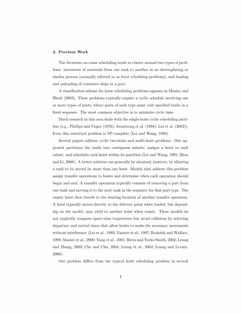
The location and processing time for each task are given (Fig.1), as are

release times and deadlines. Each crane is pre-assigned a sequence of jobs.

Each job must finish before the next job assigned to that crane begins.

In this study we explicitly account only for the longitudinal movements of

the crane along the track. We assume that the crane has time to make the

necessary lateral and vertical movements as it moves from one task location to

another. This results in little loss of generality, because any additional time

necessary for lateral or vertical motion can be built into the processing time for

the task.

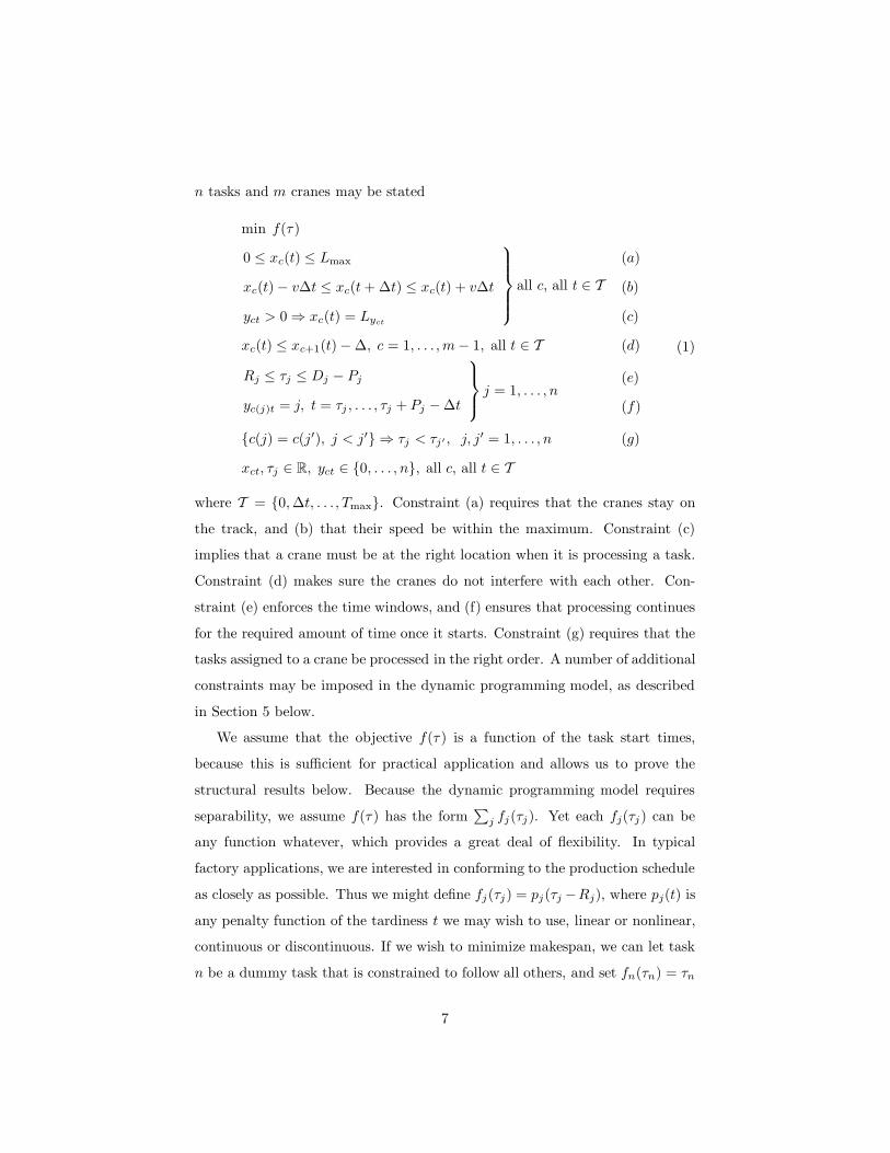
The problem data are:

Rj, Tj, Pj = release time, deadline, and processing time of task j

Lj = processing location (stop) for task j

c(j) = crane assigned to task j

v, Lmax = maximum crane speed and track length

∆ = minimum crane separation

Note that we refer to the processing location of a task as a stop.

We suppose for generality that there are cranes 1, . . . , m, where crane 1 is

the left crane and crane m the right crane, although we solve the problem only

for m = 2. Tmax is the length of the time horizon. The problem variables are:

xc(t) = position of crane c at time t

yct = task being processed by crane c at time t (0 if none)

τj = time at which task j starts processing

Task j therefore finishes processing at time τj + Pj. We assume that the tasks

are indexed so that tasks assigned to a given crane are processed in order of

increasing indices.

If we measure time in discrete intervals of length ∆t, the basic problem with

6

n tasks and m cranes may be stated

min f(τ )

0 ≤ xc(t) ≤ Lmax

xc(t) − v∆t ≤ xc(t + ∆t) ≤ xc(t) + v∆t

yct > 0 ⇒ xc(t) = Lyct

all c, all t ∈ T

(a)

(b)

(c)

xc(t) ≤ xc+1(t) − ∆, c = 1, . . . , m − 1, all t ∈ T (d)

Rj ≤ τj ≤ Dj − Pj

yc(j)t = j, t = τj , . . . , τj + Pj − ∆t

j = 1, . . . , n(e)

(f)

{c(j) = c(j′), j < j′} ⇒ τj < τj′ , j, j′ = 1, . . . , n (g)

xct, τj ∈ R, yct ∈ {0, . . . , n}, all c, all t ∈ T

(1)

where T = {0, ∆t, . . ., Tmax}. Constraint (a) requires that the cranes stay on

the track, and (b) that their speed be within the maximum. Constraint (c)

implies that a crane must be at the right location when it is processing a task.

Constraint (d) makes sure the cranes do not interfere with each other. Con-

straint (e) enforces the time windows, and (f) ensures that processing continues

for the required amount of time once it starts. Constraint (g) requires that the

tasks assigned to a crane be processed in the right order. A number of additional

constraints may be imposed in the dynamic programming model, as described

in Section 5 below.

We assume that the objective f(τ ) is a function of the task start times,

because this is sufficient for practical application and allows us to prove the

structural results below. Because the dynamic programming model requires

separability, we assume f(τ ) has the form∑

j fj(τj). Yet each fj(τj) can be

any function whatever, which provides a great deal of flexibility. In typical

factory applications, we are interested in conforming to the production schedule

as closely as possible. Thus we might define fj(τj) = pj(τj −Rj), where pj(t) is

any penalty function of the tardiness t we may wish to use, linear or nonlinear,

continuous or discontinuous. If we wish to minimize makespan, we can let task

n be a dummy task that is constrained to follow all others, and set fn(τn) = τn

7

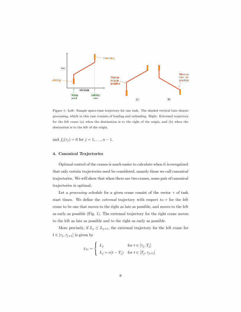
Figure 1: Left: Sample space-time trajectory for one task. The shaded vertical bars denote

processing, which in this case consists of loading and unloading. Right: Extremal trajectory

for the left crane (a) when the destination is to the right of the origin, and (b) when the

destination is to the left of the origin.

and fj(τj) = 0 for j = 1, . . . , n− 1.

4. Canonical Trajectories

Optimal control of the cranes is much easier to calculate when it is recognized

that only certain trajectories need be considered, namely those we call canonical

trajectories. We will show that when there are two cranes, some pair of canonical

trajectories is optimal.

Let a processing schedule for a given crane consist of the vector τ of task

start times. We define the extremal trajectory with respect to τ for the left

crane to be one that moves to the right as late as possible, and moves to the left

as early as possible (Fig. 1). The extremal trajectory for the right crane moves

to the left as late as possible and to the right as early as possible.

More precisely, if Lj ≤ Lj+1, the extremal trajectory for the left crane for

t ∈ [τj, τj+1] is given by

x1t =

Lj for t ∈ [τj , Tj]

Lj + v(t − Tj) for t ∈ [Tj , τj+1]

8

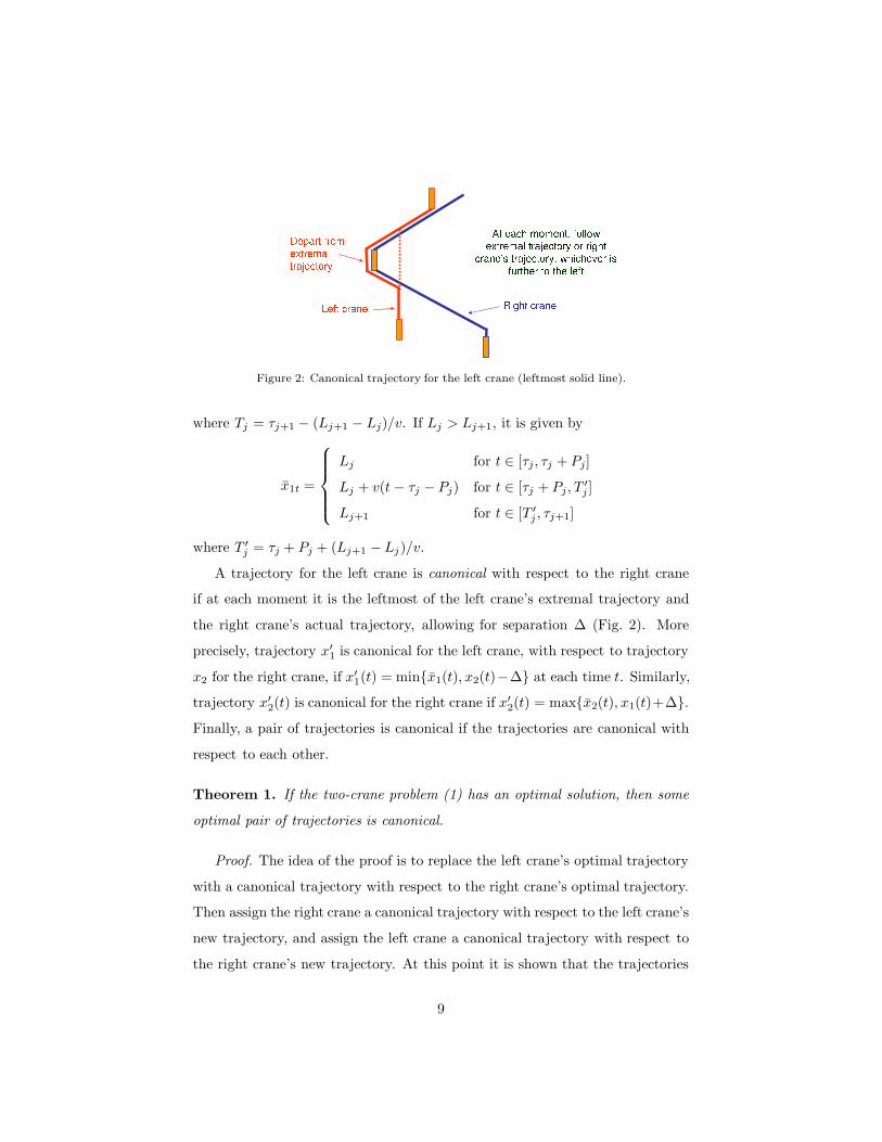
Figure 2: Canonical trajectory for the left crane (leftmost solid line).

where Tj = τj+1 − (Lj+1 − Lj)/v. If Lj > Lj+1, it is given by

x1t =

Lj for t ∈ [τj, τj + Pj]

Lj + v(t − τj − Pj) for t ∈ [τj + Pj, T′j ]

Lj+1 for t ∈ [T ′j , τj+1]

where T ′j = τj + Pj + (Lj+1 − Lj)/v.

A trajectory for the left crane is canonical with respect to the right crane

if at each moment it is the leftmost of the left crane’s extremal trajectory and

the right crane’s actual trajectory, allowing for separation ∆ (Fig. 2). More

precisely, trajectory x′1 is canonical for the left crane, with respect to trajectory

x2 for the right crane, if x′1(t) = min{x1(t), x2(t)−∆} at each time t. Similarly,

trajectory x′2(t) is canonical for the right crane if x′

2(t) = max{x2(t), x1(t)+∆}.

Finally, a pair of trajectories is canonical if the trajectories are canonical with

respect to each other.

Theorem 1. If the two-crane problem (1) has an optimal solution, then some

optimal pair of trajectories is canonical.

Proof. The idea of the proof is to replace the left crane’s optimal trajectory

with a canonical trajectory with respect to the right crane’s optimal trajectory.

Then assign the right crane a canonical trajectory with respect to the left crane’s

new trajectory, and assign the left crane a canonical trajectory with respect to

the right crane’s new trajectory. At this point it is shown that the trajectories

9

are canonical with respect to each other. We will see that these replacements

can be made without changing the objective function value, which means the

canonical trajectories are optimal, and the theorem follows.

Thus let x∗ = (x∗1, x∗

2) be a pair of optimal trajectories for a two-crane

problem. Let x1, x2 be extremal trajectories for the left and right cranes with

respect to the processing schedules in the optimal trajectories. By definition,

the extremal trajectories have the same processing schedules as the original

trajectories.

Consider the canonical trajectory x′1 for the left crane with respect to x∗

2,

which is given by x′1(t) = min{x1(t), x∗

2(t) − ∆}. We claim that (x′1, x

∗2) is

optimal. First note that x1(t) = x∗1(t) if the left crane is processing at time t,

by definition of x1. Thus x1(t) = x∗1(t) ≤ x∗

2(t)−∆ for all such t, because x∗1, x

∗2

is a feasible schedule. This implies that x′1(t) = x∗

1(t) at all times t when the left

crane is processing. The left crane can therefore retain its original processing

schedule. Because the objective function value does not change, (x′1, x

∗2) is

optimal if it is feasible.

Furthermore, (x′1, x

∗2) is feasible because the cranes do not interfere with

each other, and the speed of the left crane is never greater than v. The cranes

do not interfere with each other because x′1(t) ≤ x∗

2(t) − ∆ for all t, from the

defintion of x′1(t). To show that the speed of the left crane is never more than v

it suffices to show that the average speed in the left-to-right direction between

any pair of time points t1, t2 is never more than v, and similarly for the average

speed in the right-to-left direction. The former is

x′1(t2) − x′

1(t1)t2 − t1

=min{x1(t2), x∗

2(t2) − ∆} − min{x1(t1), x∗1(t1) − ∆}

t2 − t1

≤ max{

x1(t2) − x1(t1)t2 − t1

,x∗

2(t2) − x∗2(t1)

t2 − t1

}≤ v

where the first inequality is due to the fact that

min{a, b} − min{c, d} ≤ max{a− c, b− d}

for any a, b, c, d, and the second inequality due to the fact that x1 and x∗2 are fea-

sible trajectories. The speed in the right-to-left direction is similarly bounded.

10

Now consider the canonical trajectory x′2 for the right crane with respect to

x′1, given by x′

2(t) = max{x2(t), x′1(t) + ∆}. It can be shown as above that the

right crane can retain its processing schedule, and (x′1, x

′2) is therefore optimal.

Finally, let x′′1 be the canonical trajectory for the left crane with respect to

x′2, given by x′′

1(t) = min{x1(t), x′2(t)−∆}. Again (x′′

1 , x′2) is optimal. Since x′′

1

is canonical with respect to x′2, to prove the theorem it suffices to show that x′

2

is canonical with respect to x′′1 ; that is, max{x2(t), x′′

1(t) + ∆} = x′2(t) for all t.

To show this we consider four cases for each time t.

Case 1: x1(t) + ∆ ≤ x2(t). We first show that

(x′′1 (t), x′

2(t)) = (x1(t), x2(t)) (2)

Because x′1(t) = min{x1(t), x∗

2(t) − ∆}, x′1(t) is equal to x1(t) or x∗

2(t) − ∆. In

the latter case, we have

x′2(t) = max{x2(t), x′

1(t) + ∆} = max{x2(t), x∗2(t)} = x2(t)

and

x′′1(t) = min{x1, x

′2(t) − ∆} = min{x1, x2(t) − ∆} = x1(t)

If, on the other hand, x′1(t) = x1(t), we have x′

2(t) = max{x2(t), x1(t) + ∆} =

x2(t) and again x′′1(t) = x1(t). Now from (2) we have

max{x2(t), x′′1(t) + ∆} = max{x2(t), x1(t) + ∆} = x2(t) = x′

2(t)

as claimed.

The remaining cases suppose x2(t) < x1(t) + ∆ and consider the situations

in which x∗2(t) is less than or equal to x2(t), between x2(t) and x1(t) + ∆, and

greater than x1(t) + ∆.

Case 2: x∗2(t) ≤ x2(t) < x1(t) + ∆. It can be checked that (x′′

1(t), x′2(t)) =

(x2(t) − ∆, x2(t)) and max{x2(t), x′′1(t) + ∆} = max{x2(t), x2(t)} = x2(t) =

x′2(t), as claimed.

Case 3: x2(t) < x∗2(t) ≤ x1(t) + ∆. Here (x′′

1(t), x′2(t)) = (x∗

2(t) − ∆, x∗2(t))

and max{x2(t), x′′1(t) + ∆} = max{x2(t), x∗

2(t)} = x∗2(t) = x′

2(t).

11

Case 4: x2(t) < x1(t) + ∆ < x∗2(t). Here (x′′

1(t), x′2(t)) = (x1(t), x1(t) + ∆)

and max{x2(t), x′′1(t) + ∆} = max{x2(t), x1(t) + ∆} = x1(t) + ∆ = x′

2(t). This

completes the proof.

The properties of canonical trajectories allow us to consider a very restricted

subset of trajectories when computing the optimum.

Corollary 2. If the two-crane problem has an optimal solution, then there is

an optimal solution with the following characteristics:

(a) While not processing a task, the left (right) crane is never to the right (left)

of both the previous and the next stop.

(b) While not processing a task, the left (right) crane is moving in a direction

toward its next stop if it is to the right (left) of the previous or next stop.

(c) A crane never moves in the direction away from its next stop unless it is

adjacent to the other crane at all times during such motion.

(d) While not processing a task, the left (right) crane can be stationary only if

it is (i) at the previous or the next stop, whichever is further to the left

(right), or (ii) adjacent to the other crane.

Proof.

(a) If crane 1 (the left crane) is to the right of both its previous and next stop

at some time t, then x1(t) > x1(t). This is impossible in a canonical trajectory,

in which x1(t) = min{x1(t), x2(t) − ∆}. The argument is similar for crane 2.

(b) Suppose crane 1 is to the right of its previous stop. Due to (a), it is not

to the right of its next stop, which must therefore be to the right of the previous

stop. We cannot have x1(t) > x1(t) as in (a), and we cannot have x1(t) < x1(t),

since this means the crane cannot reach its next stop in time. So crane 1 is

on its canonical trajectory, which means that it is moving toward its next stop.

The argument is similar if crane is to the right of the next stop.

(c) From (a) and (b), at a given time t crane 1 can be moving in the direction

opposite its next stop only if it is at or to the left of both the previous and next

12

stops. This means that it will be to the left of both at time t + ∆t, so that

x1(t + ∆t) < x1(t + ∆t). But since

x1(t + ∆t) = min{x1(t + ∆t), x2(t + ∆t) − ∆}

this means x1(t + ∆t) = x2(t + ∆t) − ∆, and crane 1 is adjacent to the other

crane. Since crane 1 is moving left between t and t + ∆t, it must be adjacent

to the other crane at time t as well.

(d) From (a) and (b), a stationary crane 1 must be at or to the left both the

previous and the next stop. If it is at one of them, then (i) applies. If it is to

the left of both, then x1(t) < x1(t), which again implies that x1(t) = x2(t)−∆,

and (ii) holds.

5. Dynamic Programming Recursion

The optimal control problem for the cranes is not simply a matter of com-

puting an optimal space-time trajectory. It is complicated by three factors: (a)

each crane must perform tasks in a certain order; (b) each task must be per-

formed at a certain location for a certain amount of time; and (c) the cranes

must not interfere with each other. Dynamic programming has the flexibility

to deal with these and other constraints while preserving optimality (up to the

precision allowed by the space and time granularity). The drawback is a po-

tentially exploding state space, but we will show how to keep it under control

for problems of reasonable size. To simplify notation, we assume from here out

that ∆t = 1.

There are three state variables for each crane. One is the crane location

xct as defined in model (1). The second is the task yct assigned to crane c at

time t. This the task currently being processed, or if the crane is not currently

processing, the next task to be processd by crane c. This differs from yct in the

model (1) in that we no longer set yct = 0 when crane c is not processing. The

13

third state variable is

uct =

amount of time crane c will have been processing at time t + 1

(0 if the crane is neither processing nor starts processing at time t)

In principle the recursion is straightforward, although a practical implemen-

tation requires careful management of state transitions and data structures.

Let xt = (x1t, x2t), and similarly for yt and ut. Also let zt = (xt, yt, ut). It is

convenient to use a forward recursion:

gt+1(zt+1) = minzt∈S−1(zt+1)

{h(t, yt, ut) + gt(zt)} (3)

where gt(zt) is the cost of an optimal trajectory between the initial state and

state zt at time t, h(t, yt, ut) is the cost incurred at time t, and S−1(zt+1) is the

set of states at time t from which the system can move to state zt+1 at time

t + 1.

Because the objective function is f(τ ) =∑

j fj(τj) as specified earlier, we

incur cost fj(t) when the crane c assigned task j starts task j at time t (i.e.,

yct = j and uct = 1). Thus h(t, yt, ut) =∑

c hc(t, yt, ut), where

hc(t, yt, ut) =

fyct (t) if uct = 1

0 otherwise

The boundary condition is g0(z0) = 0, where z0 is the initial state. The

optimal cost is gTmax(zTmax), where zTmax is the desired terminal state.

By a suitable definition of S−1(zt+1), we can impose any constraint that can

be defined in terms of the current state. For example, we can require the crane

c processing task j to start moving to the next task j′ as soon as processing is

finished. This is possible because the state at time t tells us whether crane c is

processing task j (yct = j) and will be finished at time t + 1 (uct = Pj). The

set S−1(zt+1) is defined by formulating the constraint in reverse: if crane c is

assigned task j′ at time t + 1 (yc,t+1 = j′) and is still in the same location as

task j (xc,t+1 = Lj), then there is no feasible predecessor for the current state

(S−1(zt+1) = ∅). Similarly, we can prohibit crane c from yielding (moving away

from its next stop) after it finishes processing task j. A variety of precedence

14

constraints can also be implemented. For example, we can require that the right

crane start processing task j′ only after the left crane finishes task j. At any

given time t, we can determine whether the left crane has finished task j by

checking whether y1t > j, and if so we allow the right crane to start task j′.

Finally, the can impose bounds on the processing time rather than specify it

exactly, because state variable uct indicates how long the current task has been

processed so far.

For each state zt+1 the recursion (3) computes the minimum gt+1(zt+1) and

the state zt = s−1t+1(zt+1) that achieves the minimum. Thus s−1

t+1(zt+1) points

to the state that would precede zt+1 in the optimal trajectory if zt+1 were in

the optimal trajectory. For a basic recursion, the cost table gt+1(·) is stored

in memory until gt+2(·) is computed, and then released (this is modified in the

next section). Thus only two consecutive cost tables need be stored in memory

at any one time. The table s−1t+1(·) of pointers is stored offline. Then if zT is

the final state, we can retrace the optimal solution in reverse order by reading

the tables s−1t+1(·) into memory one at a time and setting zt = s−1

t+1(zt+1) for

t = N − 1, N − 2, . . . , 0.

6. Reduction of the State Space

We can substantially reduce the size of the state space if we observe that in

practical problems, the cranes spend much more time processing than moving.

The typical processing time for a state ranges from two to five minutes (some-

times much longer), while the typical transit time to the next location is well

under a minute. Furthermore, the state variables representing location and task

assignment (xct and yct) cannot change while the crane is processing.

These facts suggests that the processing time state variable uct should be

replaced by an interval Uct = [uloct, u

hict ] = {ulo

ct, uloct + 1, . . . , uhi

ct} of consecutive

processing times, where uloct ≥ 0 and uhi

ct ≤ Pyct . A single “state” (xt, yt, Uct) =

(xt, yt, (U1t, U2t)) now represents a set of states, namely the Cartesian product

{(xt, yt, (i, j)) | i ∈ U1t, j ∈ U2t}

15

The possible state transitions for either crane c are shown in Table 1. The

transitions in the table are feasible only if they satisfy other constraints in the

problem, including those based on time windows, the physical length of the

track, and interactions with the other crane. The transitions can be explained,

line by line, as follows:

1. Because the processing time interval is the singleton [0, 0], the crane can be

in motion and can in particular move to either adjacent location. When it

arrives at the next location, the currently assigned task can start process-

ing if the crane is in the correct position, in which case the state interval

is Uct = [0, 1] to represent two possible states: one in which the task does

not start processing at time t + 1, and one in which it does (the interval

is [1, 1] if the deadline forces the task to start processing at t + 1). If the

crane is in the wrong location for the task, the state remains [0, 0].

2. None of the states in the interval [0, u2] allow processing to finish at time

t+1. So all of the processing time states advance by one—except possibly

the zero state, in which processing has not yet started and can be delayed

yet again if the deadline permits it.

3. The last state in the interval [0, Pyct] allows processing to finish at time t+

1. This state splits off from the interval and assumes one of the processing

state intervals in line 1. The other states evolve as in line 2.

4. Because the task is underway in all states, all processing times advance

by one.

5. This is similar to line 3 except that there is no zero state.

There is no need to store a pointer s−1t+1(xt, yt, (i, j)) for every state (xt, yt, (i, j))

in (xt, yt, Ut). This is because when uct ≥ 2, the state of crane c preceding

(xct, yct, uct) must be (xct, yct, uct − 1). Thus we store s−1t+1(xt, yt, (i, j)) only

when i ≤ 1 or j ≤ 1.

However, we must store the cost gt+1(xt, yt, (i, j)) for every (i, j), because

it is potentially different for every (i, j). Fortunately, it is not necessary to

update this entire table at each time period, because most of the costs evolve

16

in a predictable fashion. If i, j ≥ 2, then

gt+1(xy, yt, (i, j)) = gt(xt, yt, (i − 1, j − 1))

So for each pair of tasks (y, y′) we maintain a two-dimensional circular queue

Qyy′(·, ·) in which the cost

gt+1((Ly, Ly′), (y, y′), (i, j)) (4)

for i, j ≥ 2 is stored at location

Qyy′((t + i − 2) mod M, (t + j − 2) mod M )

where M is the size of the array Qyy′(·, ·) (i.e., the longest possible processing

time). In each period we insert the cost (4) into Q only for pairs (i, j) in which

i = 2 or j = 2; the costs for other pairs with i, j ≥ 2 were computed in previous

periods. Thus only one row and one column of the Q array are altered in each

time period, which substantially reduces computation time. When i ≤ 1 or

j ≤ 1, the cost (4) is stored as a table entry gt+1(xt, yt, (i, j)) that is updated

at every time period, as with pointers.

The array Qyy′(·, ·) is created when the state ((Ly, Ly′), (y, y′), (i, j)) is first

encountered with i, j ≥ 2. The array is kept in memory over multiple periods

until it is no longer updated, at which time it is deleted.

7. Experimental results

We report computational tests on a representative problem that is based

on an actual industry scheduling situation. There are 60 jobs, each of which

contains from two to eight tasks. We obtain smaller instances by scheduling

only some of the jobs, namely the first ten (in order of release time), the first

twenty, and so forth. Results on other problems we have examined are similar.

In particular, we found that the computation time depends primarily on the

width of the time windows, regardless of the problem solved.

Release times were obtained from the production schedule, but no deadlines

were given. Because of the sensitivity of computation time to time windows, we

17

initially set the deadline of each job to be 40 minutes after each release time,

with the expectation that these may have to be relaxed to obtain a feasible

solution.

We divided the 108.5-meter track into ten equal segments, so that each dis-

tance unit represents 10.85 meters. Each crane can traverse the length of the

track in about one minute. Because we want the crane to move one distance

unit for each time unit, we set the time unit at six seconds. The 60-job schedule

requires about four hours to complete, which means that the dynamic program-

ming procedure has about Tmax = 2400 time stages.

Table 2 shows computation times obtained on a desktop PC running Win-

dows XP with a Pentium D processor 820 (2.8 GHz). The assignment and

sequencing of jobs used in each instance is the best one that was obtained by a

heuristic procedure. Feasible solutions were found for all the instances except

the full 60-job problem. To obtain a feasible solution of this problem, we were

obliged to enlarge the time windows from 40 to 95 minutes by postponing the

deadlines. This illustrates the combinatorial nature of the problem, because

the addition of only ten jobs created new bottlenecks that delayed at least one

job nearly 95 minutes beyond its release time. Wider time windows result in a

larger state space and thus greater computation time. Nonetheless, the 60-job

problem with 95-minute windows was solved in well under a minute.

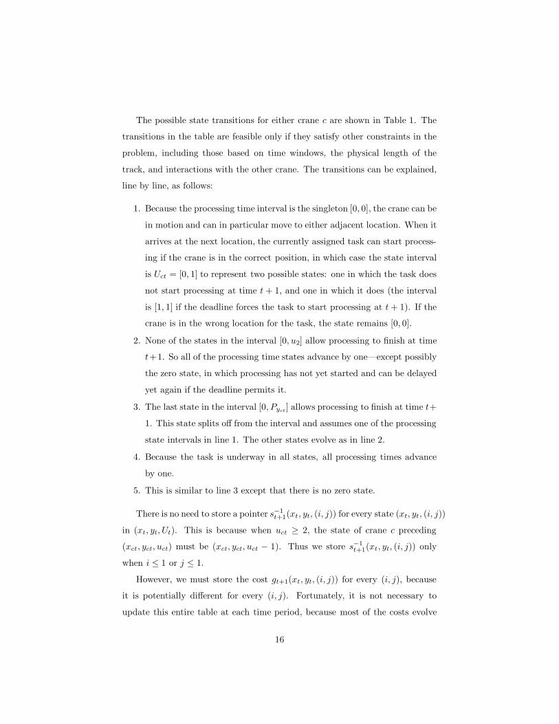
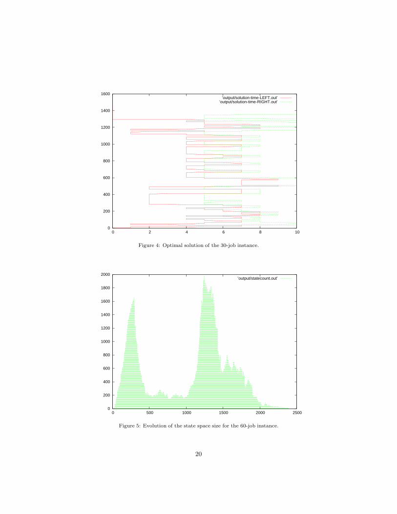
The optimal trajectories for two selected instances appear in Figs. 3 and 4.

The horizontal axis represents distance along the track in 10.85-meter units.

The vertical axis represents time in 6-second units. Thus the schedule for the

30-job problem spans about 1350 time units, or 135 minutes. The space-time

trajectory of the left crane appears as a solid line, and as a dashed line for

the right crane. The left crane begins and ends at the leftmost position, and

analogously for the right crane. Note that the cranes are at rest most of the

time. The trajectories are canonical trajectories as defined above, which ensures

a certain consistency in the way the two cranes interact.

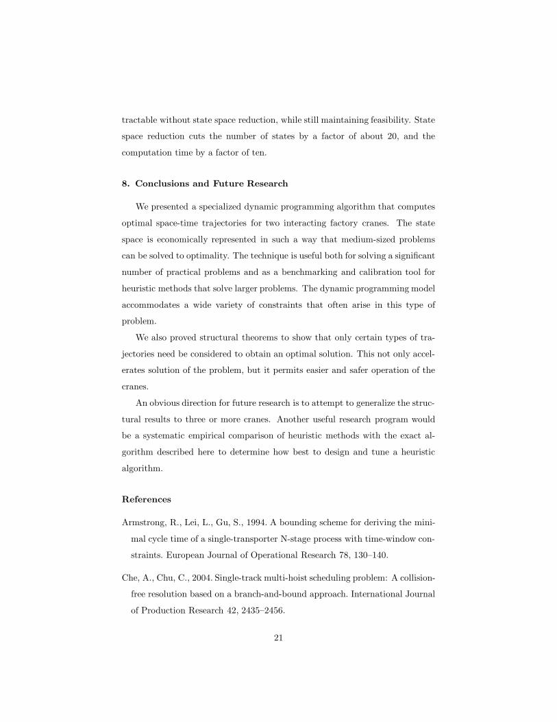
The number of states was always less than 500 for the 10-job instance, less

than 1000 for 30 jobs, and less than 2000 for 60 jobs—even though the theoretical

18

0

50

100

150

200

250

300

350

400

450

0 2 4 6 8 10

’output/solution-time-LEFT.out’’output/solution-time-RIGHT.out’

Figure 3: Optimal solution of the 10-job instance.

maximum is astronomical. Figure 5 tracks the evolution of state space size over

time for the 60-job problem. The horizontal axis corresponds to time stages,

which again are separated by six seconds. The vertical axis is the number of

states at each time stage.

Typically, only a few time windows must be wide to allow a feasible solution,

because only a few jobs must be delayed. Yet it is difficult or impossible to

predict which are the critical jobs. It is therefore necessary to be able to solve

problems in which all of the time windows are wide, perhaps on the order of 90

minutes as in the 60-job instance. It was to accommodate wide time windows

that we developed the state space reduction techniques of Section 6.

Table 3 reveals the critical importance of these techniques. For each of the

three problem instances, the table shows the average time and state space size

required to compute the optimal trajectories for ten different job assignments

and sequencings. Without the state space reduction technique, the dynamic

programming algorithm could scale up to only 30 jobs, and even then only for

narrow time windows. The time windows were reduced to make the problem

19

0

200

400

600

800

1000

1200

1400

1600

0 2 4 6 8 10

’output/solution-time-LEFT.out’’output/solution-time-RIGHT.out’

Figure 4: Optimal solution of the 30-job instance.

0

200

400

600

800

1000

1200

1400

1600

1800

2000

0 500 1000 1500 2000 2500

’output/statecount.out’

Figure 5: Evolution of the state space size for the 60-job instance.

20

tractable without state space reduction, while still maintaining feasibility. State

space reduction cuts the number of states by a factor of about 20, and the

computation time by a factor of ten.

8. Conclusions and Future Research

We presented a specialized dynamic programming algorithm that computes

optimal space-time trajectories for two interacting factory cranes. The state

space is economically represented in such a way that medium-sized problems

can be solved to optimality. The technique is useful both for solving a significant

number of practical problems and as a benchmarking and calibration tool for

heuristic methods that solve larger problems. The dynamic programming model

accommodates a wide variety of constraints that often arise in this type of

problem.

We also proved structural theorems to show that only certain types of tra-

jectories need be considered to obtain an optimal solution. This not only accel-

erates solution of the problem, but it permits easier and safer operation of the

cranes.

An obvious direction for future research is to attempt to generalize the struc-

tural results to three or more cranes. Another useful research program would

be a systematic empirical comparison of heuristic methods with the exact al-

gorithm described here to determine how best to design and tune a heuristic

algorithm.

References

Armstrong, R., Lei, L., Gu, S., 1994. A bounding scheme for deriving the mini-

mal cycle time of a single-transporter N-stage process with time-window con-

straints. European Journal of Operational Research 78, 130–140.

Che, A., Chu, C., 2004. Single-track multi-hoist scheduling problem: A collision-

free resolution based on a branch-and-bound approach. International Journal

of Production Research 42, 2435–2456.

21

Daganzo, C. F., 1989. The crane scheduling problem. Transportation Research

Part B 23, 159–175.

Kim, K. H., Park, Y.-M., 2004. A crane scheduling method for port container

terminals. European Journal of Operational Research 156, 752–768.

Lei, L., Armstrong, R., Gu, S., 1993. Minimizing the fleet size with dependent

time-window and single-track constraints. Operations Research Letters 14,

91–98.

Lei, L., Wang, T. J., 1989. A proof: The cyclic hoist scheduling problem is

NP-complete. Working paper, Rutgers University.

Lei, L., Wang, T. J., 1991. The minimum common-cycle algorithm for cycle

scheduling of two material handling hoists with time window constraints.

Management Science 37, 1629–1639.

Leung, J., Levner, E., 2006. An efficient algorithm for multi-hoist cyclic schedul-

ing with fixed processing times. Operations Research Letters 34, 465–472.

Leung, J., Zhang, G., 2003. Optimal cyclic scheduling for printed circuit board

production lines with multiple hoists and general processing sequence. IEEE

Transactions on Robotics and Automation 19, 480–484.

Leung, J. M. Y., Zhang, G., Yang, X., Mak, R., Lam, K., 2004. Optimal cyclic

multi-hoist scheduling: A mixed integer programming approach. Operations

Research 52, 965–976.

Lieberman, R. W., Turksen, I. B., 1982. Two operation crane scheduling prob-

lems. IIE Transactions 14, 147–155.

Liu, J., Jiang, Y., Zhou, Z., 2002. Cyclic scheduling of a single hoist in ex-

tended electroplating lines: A comprehensive integer programming solution.

IIE Transactions 34, 905–914.

Manier, M.-A., Bloch, C., 2003. A classification for hoist schedling problems.

International Journal of Flexible Manufacturing Systems 15, 37–55.

22

Manier, M.-A., Varnier, C., Baptiste, P., 2000. Constraint-base model for the

cyclic multi-hoists scheduling problem. Production Planning and Control 11,

244–257.

Mocchia, L., Cordeau, J.-F., Gaudioso, M., Laporte, G., 2005. A branch-and-

cut algorithm for the quay crane scheduling problem in a container terminal.

Naval Research Logistics 53, 45–59.

Ng, W. C., 2005. Crane scheduling in container yards with inter-crane interfer-

ence. European Journal of Operational Research 164, 64–78.

Phillips, L. W., Unger, P. S., 1976. Mathematical programming solution of a

hoist scheduling problem. AIIE Transactions 8, 219–321.

Riera, D., Yorke-Smith, N., 2002. An improved hybrid model for the generic

hoist scheduling problem. Annals of Operations Research 115, 173–191.

Rodosek, R., Wallace, M., 1998. A generic model and hybrid algorithm for

hoist scheduling problems. In: Maher, M., Puget, J.-F. (Eds.), Principle and

Practice of Constraint Programming (CP 1998). Vol. 1520. Springer, Pisa.

Varnier, C., Bachelu, A., Baptiste, P., 1997. Resolution of the cyclic multi-hoists

scheduling problem with overlapping partitions. INFOR 35, 309–324.

Yang, G., Ju, D. P., Zheng, W. M., Lam, K., 2001. Solving multiple hoist

scheduling problems by use of simulated annealing. Transportation Research

Part B 36, 537–555.

Zhang, C., Wan, Y.-W., Liu, J., Linn, R. J., 2002. Dynamic crane deployment in

container storage yards. Ruan Jian Xue Bao (Journal of Software) 12, 11–17.

Zhou, Z., Li, L., 2008. A solution for cyclic scheduling of multi-hoists without

overlapping. Annals of Operations Research (online).

23

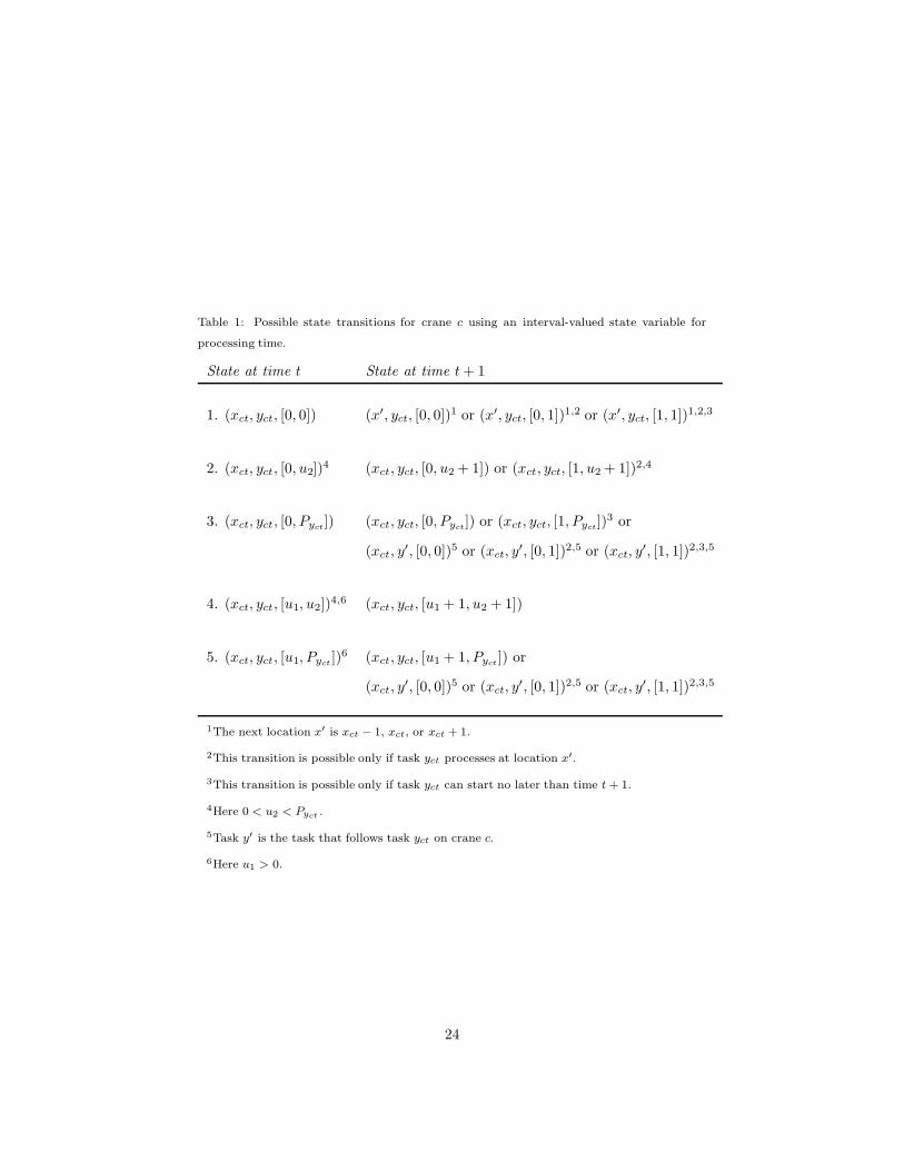
Table 1: Possible state transitions for crane c using an interval-valued state variable for

processing time.

State at time t State at time t + 1

1. (xct, yct, [0, 0]) (x′, yct, [0, 0])1 or (x′, yct, [0, 1])1,2 or (x′, yct, [1, 1])1,2,3

2. (xct, yct, [0, u2])4 (xct, yct, [0, u2 + 1]) or (xct, yct, [1, u2 + 1])2,4

3. (xct, yct, [0, Pyct]) (xct, yct, [0, Pyct]) or (xct, yct, [1, Pyct])3 or

(xct, y′, [0, 0])5 or (xct, y

′, [0, 1])2,5 or (xct, y′, [1, 1])2,3,5

4. (xct, yct, [u1, u2])4,6 (xct, yct, [u1 + 1, u2 + 1])

5. (xct, yct, [u1, Pyct])6 (xct, yct, [u1 + 1, Pyct]) or

(xct, y′, [0, 0])5 or (xct, y

′, [0, 1])2,5 or (xct, y′, [1, 1])2,3,5

1The next location x′ is xct − 1, xct, or xct + 1.

2This transition is possible only if task yct processes at location x′.

3This transition is possible only if task yct can start no later than time t + 1.

4Here 0 < u2 < Pyct .

5Task y′ is the task that follows task yct on crane c.

6Here u1 > 0.

24

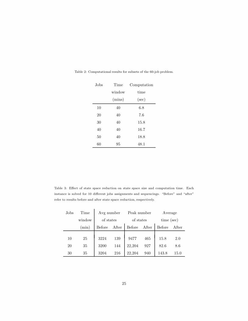
Table 2: Computational results for subsets of the 60-job problem.

Jobs Time Computation

window time

(mins) (sec)

10 40 6.8

20 40 7.6

30 40 15.8

40 40 16.7

50 40 18.8

60 95 48.1

Table 3: Effect of state space reduction on state space size and computation time. Each

instance is solved for 10 different jobs assignments and sequencings. “Before” and “after”

refer to results before and after state space reduction, respectively.

Jobs Time Avg number Peak number Average

window of states of states time (sec)

(min) Before After Before After Before After

10 25 3224 139 9477 465 15.8 2.0

20 35 3200 144 22,204 927 82.6 8.6

30 35 3204 216 22,204 940 143.8 15.0

25