Optimal Income Taxation: MirrleesMeets Ramsey∗

Jonathan Heathcote

Federal Reserve Bank of Minneapolis

Hitoshi Tsujiyama

Goethe University Frankfurt

Dec, 2013

Preliminary and Incomplete

1 Introduction

In this paper we revisit a classic question in public finance: what structure of

labor earnings taxation can maximize the social benefits of redistribution and

public insurance while minimizing the social harm associated with distorting

the allocation of labor input. There are two approaches to this question

in the literature. The Mirrlees approach is to look for tax systems that

maximize social welfare subject to the constraint that the planner cannot

observe the relative contributions of individual productivity versus individual

labor input in producing observed individual earnings. This approach is

attractive because it places no constraints on the shape of the tax schedule,

and because the implied allocations are constrained effi cient.

∗The views expressed herein are those of the authors and not necessarily those of theinstitutions with whom we are affi liated.

1

The alternative Ramsey approach is to restrict the planner to choose a

tax schedule within a parametric class —for example, to restrict taxes to be

a linear function of earnings. While there are no theoretical foundations for

imposing ad hoc restrictions on the design of the tax schedule, the practical

advantage of doing so is that one can then consider tax design in richer

models.

In this paper we do two things. First, we build on the Mirrlees tradi-

tion but extend the framework in three directions that, in our view, allow us

to provide quantitatively more relevant guidance on the welfare-maximizing

shape of the tax function. Second, we show that constrained effi cient allo-

cations can be approximately implemented via very simple parametric tax

functions, and thus that in practice the Mirrlees and Ramsey approaches to

tax design can yield very similar prescriptions.

The standard Mirrlees approach is to set up a planner’s problem where

the planner maximizes a social welfare function subject to resource feasibility,

and subject to incentive constraints such that individuals have incentives to

truthfully reveal their productivity types. Given a solution to this problem,

a tax schedule can then be inferred, such that the same allocations are decen-

tralized as a competitive equilibrium given those taxes. Note that according

to this decentralization, the government is providing all the insurance in the

economy.

The first way in which we extend the standard Mirrlees environment is to

assume that agents are able to privately insure a share of idiosyncratic labor

productivity risk. We assume that the planner cannot directly observe these

insurable shocks, or the associated insurance transfers. Given this hidden

private insurance, the planner cannot make individual income or consump-

tion a function of insurable shocks. Thus our environment contains distinct

roles for both public and private insurance. For the purposes of practical tax

design, the more risk agents are able to insure privately, the smaller is the role

of the government in providing social insurance, and the less redistributive

2

will be the resulting tax schedule.

Our second extension is to assume that individual labor productivity has

a component that is observable by the planner, in addition to a component

that the planner cannot observe directly. The logic is that wages vary sys-

tematically by observables such as age, gender, race, and education level. To

the extent that the planner has some information about workers’productiv-

ities, a constrained effi cient tax system should explicitly index taxes to these

observables (see, e.g., Weinzierl (2011)).

The shape of the optimal tax schedule in any social insurance problem is

inevitably sensitive to the assumed social welfare function. For example, in

the simplest static Mirrlees problem, one can construct a social welfare func-

tion in which Pareto weights increase with productivity at a rate such that

the planner has no desire to redistribute, and thus (absent public expendi-

ture) no desire to tax. Alternatively, a Rawlsian welfare objective that puts

weight only on the least well-off agent in the economy will typically call for

a highly progressive tax schedule. Our third innovation relative to previous

work in the Mirrlees tradition is to construct a social welfare function moti-

vated by the tax system observed in US data. The logic is that the degree of

progressivity built into the US tax and transfer system is informative about

the government’s taste for redistribution. We show that a summary statistic

for the amount of progressivity embedded in the US system borrowed from

Benabou (2000) and Heathcote, Storesletten, and Violante (2013) can be

mapped parametrically into a summary statistic for the preference for redis-

tribution in the planner’s social welfare function. This empirically-motivated

social welfare function will serve as our baseline objective function.

The environment in which we compare alternative tax systems is a simple

model in which agents are heterogeneous only with respect to labor produc-

tivity. There are three orthogonal components to idiosyncratic labor pro-

ductivity: log(w) = α + κ + ε. When individuals first enter the economy

they draw two fixed effects. The first (α) is private information to the agent

3

and cannot be privately insured —the standard Mirrlees assumptions. The

second (κ) is observed by the planner, and captures differences in wages re-

lated to observables like age and education. Again, because this component

is drawn before the agent can trade in financial markets, it cannot be insured

privately. Agents then purchase explicit private insurance indexed to a third

component of the wage (ε). The goal of the planner is to design a tax system

that specifies the net taxes to be paid each agent, recognizing that agents will

be privately insuring ε shocks in the background. The planner only observes

κ and total individual income, which comprises labor earnings plus private

insurance income.

Because the goal of the paper is to deliver quantitatively realistic pre-

scriptions, we are carefully to replicate observed dispersion in US wages, and

to decompose the overall variance of wages into the three model components

described above. First, we set the variance of the observable fixed effect to

reflect the amount of wage dispersion that can be accounted for by standard

observables in a Mincer regression. Second, we set the variance of privately

insurable shocks to the variance of wage shocks estimated to be privately

insurable by Heathcote, Storesletten, and Violante (forthcoming).

After laying out the environment, and describing the program that defines

constrained effi cient allocations, we describe the general form of Ramsey

problems in which the planner is forced to choose tax systems that belong

to a particular parametric class — for example, affi ne tax schedules. We

then describe how to use a particular ad hoc tax schedule —the power form

considered by Heathcote, Storesletten, and Violante (2013) —to construct a

mapping from observed progressivity to an implied social welfare function.

Given this empirically-motivated welfare function we then tackle the Mirrlees

optimal tax problem, and measure the potential welfare gains that could be

attained by moving to a constrained effi cient tax system. Our key findings

are as follows.

First, in the conventional Mirrlees model, where α is the only component

4

of wages and the planner maximizes a utilitarian social welfare function, there

are very large welfare gains from tax reform: the gain from an effi cient tax

reform is equivalent to a 5.75 percent increase in all agents’consumption.

At the same time, the tax system that decentralizes effi cient allocations re-

duces hours worked and output by over 10 percent relative to the current tax

schedule. The effi cient tax schedule features large lump-sum transfers equal

to around one quarter of per capita output.

The nature of optimal taxation changes dramatically when we extend

the model to incorporate our alternative empirically-motivated social welfare

function or to incorporate privately insurable shocks (ε). With the same

simple model for wages —log(w) = α —but the empirically-motivated social

welfare function, the welfare gain from tax reform shrinks from 5.75 to 0.09

percent of consumption. Thus, the current tax system does not appear to

be particularly ineffi cient. Introducing insurable shocks to wages reduces

quite dramatically effi cient marginal tax rates: from 54% to 43%, assuming

a utilitarian welfare objective.

When we explore how nearly we can decentralize effi cient allocations with

simple parametric tax schedules, we compare two alternative ways to redis-

tribute: an affi ne tax system in which marginal tax rates are constant, and

all agents receive a lump-sum transfer, and a power system (a la Benabou

(2000)) in which there are no lump-sum transfers, but where marginal tax

rates increase with income.1 The best system in the affi ne class system does

not do particularly well. For example, in the model with a utilitarian planner

and uninsurable and insurable shocks, the optimal tax system in the affi ne

class delivers less than one third of the welfare gains from moving to the

fully non-parametric income tax schedule that delivers effi cient allocations.

Moreover, our comparison of alternative tax functions indicates that it is

more important to have marginal rates increase with income than to provide

1These are both two parameter functions. Taxes paid as a function of income accordingto the two systems are, respectively, T (y) = τ0 + τ1y and T (y) = y − λy1−τ .

5

universal lump-sum transfers. These findings contrast with much of the ex-

isting literature which has argued that affi ne tax schedules can approximately

decentralize effi cient allocations.

In the next part of the paper we introduce the observable component of

wages (κ). We find that if the planner can condition taxes on the observ-

able component of labor productivity it can generate large welfare gains, in

part because it translates into lower marginal rates on average. Under an

affi ne system with two observable types (think college versus high school),

the type with higher observable productivity (college graduates) should face

higher marginal tax rates, and receive smaller lump-sum transfers. Higher

marginal rates on the more productive type allow the planner to redistribute

across types, while smaller lump-sum transfers offset the disincentive effects

of higher marginal tax rates on labor supply.

2 Environment

A unit mass of agents have identical preferences over consumption c, and

work effort h. The utility function is separable between consumption and

work effort and takes the form

u(c, h) =c1−γ

1− γ −h1+σ

1 + σ(1)

Given this functional form, the Frisch elasticity of labor supply is 1/σ.

Agents differ only with respect to labor productivity θ. Individual labor

productivity has three orthogonal components

log θ = α + κ+ ε (2)

These three idiosyncratic components differ with respect to whether or not

they can be insured privately, and whether or not they are publicly observ-

able. We assume that α ∈ A ⊂ R+ and κ ∈ K ⊂ R+ represent shocks that

6

cannot be insured privately, while perfect private insurance exists against

shocks to ε ∈ E ⊂ R+. We assume that κ is publicly observable while α andε are not observed by the tax authority. We let the vector (α, κ, ε) denote

an individual’s type, and F (α), F (κ) and F (ε) denote the distributions for

the three components.

The timing of events is as follows. Agents first draw α and κ. They then

trade in a market in which they can purchase private insurance at actuarially

fair prices against ε. Then each individual draws an ε, insurance pays out,

and individuals choose how much to work. Finally, a government assesses

taxes, and income less net taxes is consumed.

The price of insurance claims that will pay one unit of consumption if and

only if ε ∈ E ⊂ E isQ(E) =∫EdF (ε). In the first stage of the period, prior to

drawing ε, the budget constraint for an agent with uninsurable components

α and κ is ∫B(ε;α, κ)Q(ε)dε = 0 (3)

where B(x;α, κ) denotes the quantity (positive of negative) of insurance

claims purchased that pay a unit of consumption if and only if the second

stage draw for the insurable shock is x.

In the second stage of the period, income before taxes y(α, κ, ε) is the

sum of labor earnings plus insurance payouts

y(α, κ, ε) = exp(α + κ+ ε)h(α, κ, ε) +B(ε;α, κ) (4)

The tax authority observes only two individual level variables: the observ-

able component of productivity κ, and total end of period income y(α, κ, ε).

The tax authority does not directly observe α or ε, does not observe hours

worked, and does not observe any of the trades B(·;α, κ) associated withprivate insurance against ε. Taxes must be functions of observables. We let

T (y;κ) denote the income tax schedule, which may be indexed to κ. Given

that it observes income taxes collected the planner also effectively observes

7

consumption, since

c(α, κ, ε) = y(α, κ, ε)− T (y(α, κ, ε);κ) (5)

One interpretation for the differential insurance assumption for α and κ

versus ε is that α and κ represent fixed effects that are drawn before agents

can participate in insurance markets. An alternative interpretation is that

ε represents shocks that can be pooled within a family or other risk-sharing

group, while α and κ are common across all members of the group but differ

across groups.

One interpretation for the differential observability assumption for α and

ε versus κ is that α and ε reflect components of productivity that are pri-

vate information, while κ reflects the impact of observable characteristics on

productivity, such as age, education, and gender.

While the model we describe is static it would be straightforward to de-

velop a dynamic extension in which agents draw new values for the insurable

shock ε in each period and in which the observable component κ evolves over

time. A much more challenging extension would be to allow for persistent

shocks to the unobservable non-insurable component of productivity α.

Aggregate output in the economy is simply aggregate effective labor sup-

ply

Y =

∫ ∫ ∫exp(α + κ+ ε)h(α, κ, ε)dF (α)dF (κ)dF (ε) (6)

where h(α, κ, ε) denotes hours worked by an individual of type (α, κ, ε).

Aggregate output is divided between private consumption and a publicly-

provided good that is allocated equally across all agents.

Y =

∫ ∫ ∫c(α, κ, ε)dF (α)dF (κ)dF (ε) +G (7)

The government must run a balanced budget, and thus the budget con-

8

straint is ∫ ∫ ∫T (y(α, κ, ε);κ)dF (α)dF (κ)dF (ε) = G (8)

3 Constrained Effi cient Allocations

In the Mirrlees formulation of the program that determines constrained effi -

cient allocations, rather than thinking of the planner choosing taxes, we will

instead think of the planner as choosing both consumption c(α, κ, ε) and in-

come y(α, κ, ε) as functions of the individual types (α, κ, ε). It is clear that, by

choosing taxes, the tax authority can choose the difference between income

and consumption. It is less obvious that the planner can also dictate income

levels as a function of type. To achieve this, the Mirrlees formulation of the

planner’s problem includes incentive constraints that guarantee that for each

and every type (α, κ, ε) an agent of that type weakly prefer to deliver to

the planner the value for income y(α, κ, ε) the planner intends for that type,

thereby receiving (after-taxes) the value for consumption c(α, κ, ε), rather

than delivering any alternative level of income. It is easiest to formulate the

Mirrlees problem with the planner inviting agents to report their unobserv-

able characteristics α and ε, and then assigning the agent an allocation for

income y(α, κ, ε) and consumption c(α, κ, ε) on the basis of their reports α

and ε (recall that the planner observes κ directly). But since the planner

is offering agents a choice between a menu of alternative pairs for income

and consumption, it is clear that an alternative way to think about what the

planner does is that it offers a mapping from any possible value for income

to consumption. Such a schedule can be decentralized via a tax schedule on

income y of the form T (y;κ) that defines how rapidly consumption grows

with income.2

2Note that some values for income might not feature in the menu offered by the Mirrleesplanner. Those values will not be chosen in decentralization with income taxes as long asincome at those values is taxed suffi ciently heavily. For example, suppose the lowest valuefor income in the Mirrlees solution is y, with corresponding consumption value c. Lower

9

The planner maximizes a social welfare function,W (α, κ, ε), with weights

that potentially vary with α, κ and ε.3 The timing with the period is as

follows. In the first stage, agents draw (α, κ). They make a report α(α, κ) to

the planner where the reporting function α : A×K → A. At the same time,agents buy private insurance against ε, B(·;α, κ, α). In the second stage,agents draw ε, and insurance pays out. Agents make a report ε(α, κ, ε) to

the planner where the second stage reporting function ε : A×K × E → E .Finally, agents work suffi cient hours to deliver y(α(α, κ), κ, ε(α, κ, ε)), and

receive consumption c(α(α, κ), κ, ε(α, κ, ε)).

3.1 Second stage agent’s problem

As a first step towards characterizing effi cient allocations, we start with the

agent’s problem in the final stage, given generic reporting strategies α and

ε. Let α = α(α, κ). Agents choose insurance purchases and labor supply to

solve the following problem

maxh(α,κ,·,α;ε),B(·;α,κ,α;ε)

∫u(α, κ, ε, α; ε)dF (ε) (9)

where

u(α, κ, ε, α; ε) =c(α, κ, ε(α, κ, ε))1−γ

1− γ − h(α, κ, ε, α, ε(α, κ, ε))1+σ

1 + σ

income values can be ruled in the competitive equilibrium by assuming that marginal taxrates are 100% for income below y and that conditional on delivering at least y agentsreceive a lump-sum transfer equal to c.

3We will show later that the planner will be unable to offer contracts in which incomeor consumption vary with ε, and given that result we will focus on a social welfare functionin which weights do not vary with ε.

10

subject to ∫B(ε;α, κ, α; ε)Q(ε)dε = 0 (10)

exp(α + κ+ ε)h(α, κ, ε, α, ε(α, κ, ε)) +B(ε;α, κ, α; ε) = y(α, κ, ε(α, κ, ε))

Let v(α, κ, ε, α, ε(α, κ, ε)) denote maximum utility after drawing ε given

reports α and ε(α, κ, ε).

3.2 First stage planner’s problem

The planner maximizes W (α, κ, ε) subject to the resource constraint, and

incentive constraints that ensure that utility from reporting α and ε truthfully

and receiving the associated allocation is weakly larger than expected welfare

from any alternative report and associated allocation. Formally. the planner

solves

max{c(α,κ,ε),y(α,κ,ε)}

∫ ∫ ∫W (α, κ, ε)v(α, κ, ε, α, ε)dF (α)dF (κ)dF (ε) (11)

subject to∫ ∫ ∫c(α, κ, ε)dF (α)dF (κ)dF (ε)+G =

∫ ∫ ∫y(α, κ, ε)dF (α)dF (κ)dF (ε)

(12)

and subject to allocations being incentive compatible.∫v(α, κ, ε, α, ε)dF (ε) ≥

∫v(α, κ, ε, α, ε)dF (ε) ∀α, κ and ∀α (13)

v(α, κ, ε, α, ε) ≥ v(α, κ, ε, α, ε) ∀α, κ, ε, α and ∀ε (14)

where v(α, κ, ε, α, ε) is the utility achieved by an agent who follows reporting

strategies α and ε, who draws (α, κ, ε), and who makes reports α = α(α, κ)

and ε = ε(α, κ, ε).

The second set of incentive constraints (14) imposes that agents weakly

11

prefer to report ε truthfully for any report α in the first stage. This ensures

that truth-telling ε(α, κ, ε) = ε is incentive compatible for any first stage

strategy α. The first set of incentive constraints (13) impose that agents

weakly prefer to report α truthfully, assuming truthful reporting in the second

stage. Thus truth-telling α(α, κ) = α is incentive compatible at the first

stage.

3.3 Preliminary result: allocations cannot be condi-

tioned on ε

We start by assuming agents follow arbitrary reporting strategies and com-

pute the implied equilibrium allocations and utility. We show that for any

reporting strategies, hours worked are not a function of the report ε. It fol-

lows that a truth-telling reporting strategy is incentive compatible if and

only if consumption is also independent of the report ε. It follows further

that there is nothing to be gained from the planner asking agents to report

ε —since neither component of individual welfare (and hence social welfare)

can be made contingent on those reports.

Let λ(α, κ, α; ε) denote the multiplier on the first constraint in the agent’s

problem (maximize 9 subject to 10), where α = α(α, κ). This multiplier

cannot be a function of ε because the constraint applies before ε is drawn.

Let ρ(α, κ, ε, α, ε) denote the multiplier on the second constraint given a draw

ε, where ε = ε(α, κ, ε). The first-order conditions imply

h(α, κ, ε, α) = [exp(α + κ+ ε)λ(α, κ, α; ε)]1σ (15)

The crucial thing to note here is that hours are independent of the report

ε = ε(α, κ, ε). The logic for this result is that agents exploit insurance markets

to deliver target income y(α, κ, ε) at minimum cost in terms of labor effort.

That implies that they choose hours as a function of the draw for ε to make

marginal disutility of hours h(α, κ, ε, α)σ proportional to the wage exp(α+κ+

12

ε), —a familiar complete markets result. The wage is obviously independent

of ε and the constant of proportionality is too —it is the multiplier on the

insurance purchases constraint, which applies prior to ε and thus ε being

realized.

Consider an agent of type (α, κ, ε) who is following an arbitrary reporting

strategy in the first stage, so that α = α(α, κ). In the second stage, after

drawing ε, this agent will want to report the value ε whose associated contract

{c(α, κ, ε), y(α, κ, ε)} maximizes utility. Because hours worked, and thus

disutility from hours, are independent of ε, it follows that the agent will

choose whichever contract offers the highest value for c(α, κ, ε). Thus truth

telling is incentive compatible if and only if consumption is independent of

the individual report ε. Thus neither consumption nor hours can be made

contingent on the report of ε in any truth-telling allocation. Thus contracts

must be of the form {c(α, κ), y(a, κ)} . Since these contracts are independentof ε we can envision these contracts being offered prior to ε being revealed.

Note that because neither consumption nor income depend on ε in the

constrained effi cient allocation, the income or consumption tax system that

decentralizes effi cient allocations is also independent of ε. We have derived

this result endogenously, given the assumption that the planner cannot ob-

serve ε. An alternative approach that gives the same outcome

3.4 Restatement of Mirrlees problem

We now apply this result to produce a much simpler representation of the

program that defines constrained effi cient allocations. We will drop the de-

pendence of consumption and income on the insurable shock. In addition,

because the planner weights do not vary with ε, and because we do not need

to worry about the second set of incentive constraints (14), we can also dis-

pense with keeping track of private insurance markets altogether, and work

with expected utility (conditional on α and κ) prior to drawing ε.

From the agent’s budget constraint we can solve for the multiplier on

13

the insurance purchases constraint, λ(α, κ, α), and thus simplify the expres-

sion for hours h(α, κ, ε, α). Substituting (4) into (3) and then using (15) to

substitute for hours gives

λ(α, κ, α) =

(y(α, κ)∫

exp(α + κ+ ε)1+σσ dF (ε)

)σ

Substituting this into (15) gives

h(α, κ, ε, α) = exp(α + κ+ ε)1σ

y(α, κ)∫exp(α + κ+ ε)

1+σσ dF (ε)

Thus utility, given type (α, κ, ε) and report α, is

v(α, κ, ε, α) =c(α, κ, α)1−γ

1− γ − 1

1 + σ

(exp(α + κ+ ε)

1σ y(α, κ)∫

exp(α + κ+ ε)1+σσ dF (ε)

)1+σ

Expected utility, prior to drawing ε, is

∫v(α, κ, ε, α)dF (ε) =

∫ c(α, κ, α)1−γ1− γ − 1

1 + σ

(exp(α + κ+ ε)

1σ y(α, κ)∫

exp(α + κ+ ε)1+σσ dF (ε)

)1+σ dF (ε)

=c(α, κ, α)1−γ

1− γ −

(∫exp(ε)

1+σσ dF (ε)

)−σ1 + σ

(y(α, κ)

exp(α + κ)

)1+σLet U(α, κ, α) =

∫v(α, κ, ε, α)dF (ε) . We can now restate the planner’s

problem that defines constrained effi cient allocations.

max{c(α,κ),y(α,κ)}

∫ ∫W (α, κ)U(α, κ, α)dF (α)dF (κ) (16)

subject to∫ ∫c(α, κ)dF (α)dF (κ) +G =

∫ ∫y(α, κ)dF (α)dF (κ) (17)

14

and

U(α, κ, α) ≥ U(α, κ, α) ∀α, κ and ∀α (18)

Note that ε no longer appears anywhere in this problem, and nor does the

second stage agent’s problem. The problem is identical to a standard static

Mirrlees type problem, where the planner faces a distribution of agents with

heterogeneous unobserved productivity α.We will solve this problem numer-

ically. Note, however, that the period utility function for each agent in this

problem is not identical to the utility function we started with in the underly-

ing problem, since the weight on hours worked is now(∫exp(ε)

1+σσ dF (ε)

)−σ.

3.5 First Best

If the planner can observe α directly, the welfare maximization problem is

identical to the one described above, except that there are no incentive com-

patibility constraints.

4 Ramsey Policies

We will compare outcomes and welfare under the solution to the Mirrlees

described above to those under alternative ad hoc tax systems. One compar-

ison of particular interest will be the US tax system. We will consider taxes

based on individual earnings, and taxes based on income.

Consider a decentralized economy with income taxes T (y;κ) and private

insurance markets against ε shocks. Knowing α and κ, but before drawing

ε, agents solve

maxc(α,κ,ε),h(α,κ,ε),B(α,κ,ε)

∫ (c(α, κ, ε)1−γ

1− γ − h(α, κ, ε)1+σ

1 + σ

)dF (ε) (19)

subject to equations (3), (5) and (4).

15

The first-order conditions are

c(α, κ, ε)−γ [1− T ′ (y(α, κ, ε);κ)] exp(α + κ+ ε) = h(α, κ, ε)σ

c(α, κ, ε)−γ [1− T ′ (y(α, κ, ε);κ)] = λ(α, κ) (20)

where λ(α, κ) is the multiplier on the insurance purchases constraint.

Proposition. Assume that the tax function satisfies

T ′′(y;κ) > −γ (1− T′(y;κ))

(y − T (y;κ))

for all feasible y. Then income, taxes and consumption are independent of

ε.4

Note that this condition is automatically satisfied for any affi ne tax sched-

ule. Suppose the condition is satisfied. Then the first-order condition for

labor supply can be written as

h(α, κ, ε) = [y(α, κ)− T (y(α, κ);κ)]−γ [1− T ′(y(α, κ);κ)] exp(α + κ+ ε)1σ

where y(α, κ) can be solved for from the budget constraint∫B(α, κ, ε)dF (ε) =

∫[y(α, κ)− exp(α + κ+ ε)h(α, κ, ε)] dF (ε) = 0

4Proof. Subsituting ?? into 20 gives

[y(α, κ, ε)− T (y(α, κ, ε);κ)]−γ [1− T ′(y(α, κ, ε);κ)] = λ(α, κ)

The derivative of the left-hand side of this equation with respect to the insurable shock εis, by the Chain Rule((y − T (y;κ))−γ (1− T ′(y;κ))

)=

(−γ (y − T (y;κ))−γ−1 (1− T ′(y;κ)) (1− T ′(y;κ))− (y − T (y;κ))−γ (1− T ′(y;κ))T ′′(y;κ)

) ∂y∂ε

=(−γ (y − T (y;κ))−1 (1− T ′(y;κ))− T ′′(y;κ)

) ∂y∂ε

The first term is strictly negative iff the condition is satisfied, which immediately impliesthat ∂y∂ε = 0.

16

4.1 Earnings taxes

Let x(α, κ, ε) = exp(α + κ + ε)h(α, κ, ε) denote labor earnings. Consider

a decentralized economy with earnings taxes T (x(α, κ, ε);κ) and private in-

surance markets against ε shocks. Knowing α and κ, but before drawing ε,

agents solve a very similar problem to the one described above with income

taxes.

The first order conditions are

c(α, κ, ε)−γ [1− T ′(x(α, κ, ε);κ] exp(α + κ+ ε) = h(α, κ, ε)σ (21)

c(α, κ, ε)−γ = µ(α, κ)

In this case it is immediate from the second first-order condition that

consumption is independent of ε. Hours worked are implicitly given by

h(α, κ, ε) = c(α, κ)−γ exp(α + κ+ ε) [1− T ′ (exp(α + κ+ ε)h(α, κ, ε);κ)]1σ

while the budget constraints can be combined to give

c(α, κ) =

∫[exp(α + κ+ ε)h(α, κ, ε)− T (exp(α + κ+ ε)h(α, κ, ε);κ)] dF (ε) = 0

4.1.1 Affi ne taxes

Given an affi ne tax schedule, it is possible to characterize equilibrium allo-

cations more sharply. Suppose earnings taxes are affi ne, with (potentially)

κ−contingent intercept and slope, so that

T (x;κ) = τ 0(κ) + τ 1(κ)x

Then we have an explicit solution for hours worked, as a function of the wage

and consumption.

h(α, κ, ε) =[c(α, κ)−γ exp(α + κ+ ε) (1− τ 1(ε))

] 1σ

17

Note that under an affi ne tax structure, equilibrium allocations for consump-

tion and hours worked are identical for income versus earnings taxes, assum-

ing the coeffi cients τ 0(κ) and τ 1(κ) are the same in the two systems. The

logic is that the only difference between the corresponding intra-temporal

FOCs is that in one case the relevant marginal tax rate is the rate on income

while in the other it is the rate on earnings.

4.2 Decentralization of constrained effi cient allocations

Let c∗(α, κ) and y∗(α, κ) denote consumption and income in the constrained

effi cient allocation and let h∗(α, κ, ε) denote the constrained effi cient alloca-

tion rule for hours (all given a particular social welfare function W (α, κ)):

h∗(α, κ, ε) =y∗(α, κ)

exp(α + κ)∫exp(ε)

1+σσ dF (ε)

exp(ε)1σ

Substituting constrained effi cient allocations into the competitive equilib-

rium first-order condition for hours worked in the economy with income taxes

(20) implicitly defines the marginal tax rates that decentralize constrained

effi cient allocations:

1− T ′(y∗(α, κ);κ) = y∗(α, κ)σ

c∗(α, κ)−γ exp(α + κ)1+σ(∫exp(ε)

1+σσ dF (ε)

)σNote that marginal tax rates do not vary with ε because income (including

insurance payouts) does not vary with ε. Note also that while the decentral-

ization above is based on income taxes, it is clear that the Mirrlees solution

could equivalently be decentralized using consumption taxes. In that case

we would get

1 + T ′(c∗(α, κ);κ) =c∗(α, κ)−γ exp(α + κ)1+σ

(∫exp(ε)

1+σσ dF (ε)

)σy∗(α, κ)σ

18

Note, finally, that we cannot decentralize the Mirrlees solution using taxes

on individual earnings, because in the competitive equilibrium individual

earnings —and thus taxes —vary with ε, while in the solution to the Mir-

rlees planner taxes paid (which are equal to income minus consumption) are

independent of ε and vary only with the components α and κ.

5 Social Welfare Function

We now describe our methodology for using the degree of progressivity built

into the actual tax system to infer social preferences. We will assume the

social welfare function takes the form

W (α, κ) =exp(−ω (α + κ))∫ ∫

exp(−ω (α + κ))dF (α)dF (κ)(22)

where the parameter ω controls the extent to which the planner puts rela-

tively more or less weight or relatively high productivity workers. We im-

plicitly assume that the planner puts equal weight on agents with different

realizations for ε. The logic for this is that, as explained above, constrained ef-

ficient allocations cannot be made to vary with ε.One motivation for choosing

a social welfare function that treats the components α and κ symmetrically

is that for any non-κ contingent tax system based on individual earnings or

income, only the total uninsurable component of productivity (i.e. α+ κ) is

relevant for individual choices and individual welfare.

Heathcote, Storesletten, and Violante (2013) argue that the following

earnings tax function offers a reasonable approximation to the US tax and

transfer system

T (y) = y − λy1−τ (23)

Thus the marginal tax rate on individual income is given by

T ′(y) = 1− λ(1− τ)(y)−τ

19

Suppose the US government is solving the following Ramsey problem

maxT (y(α,κ,ε);κ)

∫ ∫W (α, κ)

(∫u (c(α, κ, ε), h(α, κ, ε)) dF (ε)

)dF (α)dF (κ)

subject to

1. c(α, κ, ε) and h(α, κ, ε) are solutions to the household’s problem ??given the tax function T (y(α, κ, ε);κ).

2. The government budget constraint is satisfied given an exogenous value

for public expenditure G∫ ∫ ∫T (y(α, κ, ε);κ)dF (ε)dF (α)dF (κ) = G.

3. The tax function is in the two-parameter class described by 23.

4. The social welfare function takes the form described by 22.

Note that while in principle the government chooses two tax parameters,

λ and τ , because it has to respect the government budget constraint, the

government effectively has a single choice variable, τ . Let τ ∗(ω) denote the

welfare maximizing choice for τ given a social welfare function indexed by ω.

The logic underlying our empirically-motivated social welfare function

is that while we do not directly observe ω, we do observe the degree of

progressivity chosen by the US political system. Let τUS denote that value

for τ . We then infer that US social preferences ωUS must satisfy

τ ∗(ωUS) = τUS (24)

and use this equation to reverse engineer ωUS and thus a social welfare func-

tion.

We now describe how we operationalize this.

20

Substituting the tax function 23 into the first-order conditions for an

economy with earnings taxes (20) gives

h(α, κ, ε) =[c(α, κ)−γ−

τ1−τ exp(α + κ+ ε)(1− τ)λ

11−τ

] 1σ

(25)

The budget constraint is

c(α, κ) = λy(α, κ, ε)1−τ

Since this applies for every ε,

c(α, κ)1

1−τ =

∫λ

11−τ y(α, κ, ε)dF (ε)

which, using the definition for income y(α, κ, ε) and substituting in the ex-

pression for hours, can be expressed as

c(α, κ) = λ1+σ

σ+τ+γ(1−τ) (1−τ)1−τ

σ+τ+γ(1−τ) exp

((1 + σ) (1− τ)σ + τ + γ(1− τ)(α + κ)

)[∫exp

(1 + σ

σε

)dF (ε)

] σ(1−τ)σ+τ+γ(1−τ)

(26)

Given expressions 25 and 26, and using the government budget constraint

to solve for λ, we can compute social welfare for any values for τ and ω.

When we calibrate the model we will search numerically for a value for ω

that satisfies equation 24.

It is instructive to consider a special case, in which the function τ ∗(ω) can

be characterized in closed form. Consider the special case in which utility is

logarithmic in consumption, so γ = 1.Assume, in addition, that all shocks are

normally distributed: α˜N(−vα/2, vα), κ˜N(−vα/2, vα) and ε˜N(−vα/2, vα)is normally distributed with variance vε and mean −vε/2.

21

Then

c(α, κ;λ, τ) = λ(1− τ)1−τ1+σ exp((1− τ) (α + κ)) exp

((1− τ)

(1− 2τ − τσ

σ + τ

)vε2

)h(α, κ, ε; τ) = (1− τ)

11+σ exp

(−(1− τ)σ + τ

(1− 2τ − στ

σ + τ

)vε2

)exp

(1− τσ + τ

ε

)

λ =(1− τ)

11+σ exp

((1−τ)(σ+τ)2

(σ + 2τ + στ) vε2

)−G

(1− τ)1−τ1+σ exp

((1− τ)

(1−2τ−τσσ+τ

)vε2

) ∫ ∫exp ((1− τ)(α + κ)) dF (α)dF (κ)

We can substitute these expressions into the planner’s objective function,

to give an unconstrained optimization problem with one choice variable, τ .

Given the social welfare function 22 the planner’s problem is

maxτ

{∫ ∫exp(−ω (α + κ))∫ ∫

exp(−ω (α + κ))dF (α)dF (κ)

(log (c(α, κ; τ))−

∫h(α, κ, ε; τ)1+σ

1 + σdF (ε)

)dF (α)dF (κ)

}Substituting in the expressions above for c(α, κ;λ, τ), h(α, κ, ε; τ) and

λ(τ) and differentiating with respect to τ gives a first-order condition that

maps ω and G into the optimal choice for τ . In the appendix we show that

the first order condition is

1

1− g(G, τ)−1

(1 + σ)(1− τ) + (vα + vκ) (1 + ω − τ) + 1

1 + σ= 0

where g(G, τ) = G× Y (τ) and Y (τ) denotes aggregate output.Let ∗’s denote observed variables. If the US political system is solving

this problem, we can use this first-order condition in conjunction with the

observed choices for G and τ to infer ω. In particular, since g(G∗, τ ∗) =

G∗ × Y (τ ∗) = g∗ we infer that

ω∗ = − (1− τ ∗) + 1

vα + vκ

1

1 + σ

[1

(1− g∗) (1− τ ∗) − 1]

Note that ω∗is increasing in τ ∗, as expected. Thus if we observe more

22

progressive taxation, we can infer that the social planner puts less weight on

higher wage individuals. Holding fixed observed τ ∗, ∂ω∗

∂vα< 0 and ∂ω∗

∂vκ< 0.

Thus more uninsurable risk but the same tax progressivity means we can

infer the planner has less desire to redistribute. Similarly, holding fixed

observed τ ∗, ∂ω∗

∂σ< 0, meaning that for the same observed τ , the less elastic

we think labor supply is (and thus the smaller the distortions associated

with progressive taxation) the less desire to redistribute we should attribute

to the planner. Finally ∂ω∗

∂g∗ > 0, meaning that, holding fixed progressivity,

the larger the share of output devoted to public goods, the more the planner

wants to redistribute. The logic here is that tax progressivity tends to reduce

labor supply, making it more diffi cult to finance public goods, so governments

that need to finance large expenditure will tend to choose less progressivity

—unless they have a strong desire to redistribute.

6 Calibration

This section illustrates the calibration of this economy.

6.1 Preference

The agents’utility is given by

u(c, h) =c1−γ

1− γ −h1+σ

1 + σ

As a baseline parametrization, we assume the relative risk aversion being

unity γ = 1, i.e., log preference for consumption. We choose σ = 2 so that

the Frisch elasticity is 0.5.

23

Figure 1: Fit of HSV tax function

8.5

99.

510

10.5

1111

.512

12.5

13Lo

g of

pos

t−go

vern

men

t inc

ome

8.5 9 9.5 10 10.5 11 11.5 12 12.5 13Log of pre−government income

6.2 Tax System and Government Expenditure

We regard the U.S. income tax system is well-represented by a particular tax

function

T (y;λ, τ) = y − λy1−τ

which is first introduced by Benabou (2000). Heathcote, Storesletten, and

Violante (2013) estimate the progressivity parameter in this baseline tax

function as τ = 0.151. Figure 1 shows log of the pre- and post-government

income of the U.S. households and one can see it fits the actual tax system

fairly well. The remaining parameter λ is pinned down by the resource

feasibility. We call this tax function as the HSV tax function.

The government consumption and investment constitute 18.8% of GDP

in 2005 in the U.S., and hence we set government spending G such that

G/Y = 0.188.

24

6.3 Wage distribution

The baseline model has three independent shocks, α, ε and κ. We need to

estimate the variance of these shocks.

The variance of insurable shocks vε is given by 0.193, the estimate from

Heathcote, Storesletten, and Violante (forthcoming). Carefully taking into

account the measurement errors, they also estimate the total variance of

wages to be 0.466.

For the variance of observable shocks vκ, we use the estimate in Heathcote,

Perri, and Violante (2010) who estimate the variance of cross sectional wage

dispersion attributable to observables to be 0.108. We can therefore estimate

the variance of uninsurable shocks which are not observable as the residual

and is then given by vα = 0.165.

The bounds for α are given by

exp(α) ∈[5.15/2

19.60,2, 138.16

19.60

].

Specifically, we assume the minimum productivity level is the half of the

Federal minimum wage $5.15 in 2005. Taking into account the fat right

tail of the wage distribution (Saez (2001)), we assume the maximum level

of the productivity is given by $2,138.16, the earnings per hour at 99.99th

percentile of 2005 earnings distribution from Piketty and Saez (2003). We

assume annual hours worked are 2000 to calculate this number. Both bounds

are normalized by $19.60, the average hourly earnings in 2005 taken from BLS

data.

Saez (2001) argues that the wage distribution has a thick right tail and

is well-approximated by a Pareto distribution. We address this issue by

assuming that the distribution being log-normal for exp(α) ≤ x and being

Pareto for exp(α) > x where x = 1.77 so that 95% of the population lie

in the log-normal range and 5% lie in the Pareto range. This value for x

corresponds to about $34.6. For the Pareto parameter, we use 2.0, estimated

25

from Piketty and Saez (2003). The shape of the wage distribution is found

in Figure 2.

We assume two-point equal-weight distribution for κ. This gives exp(κhigh)/ exp(κlow) =

1.93. We also assume that the uninsurable shocks ε are drawn from a con-

tinuous normal distribution N(−vε2, vε).

We use 10,000 evenly spaced grid points in the baseline.

6.4 Social Welfare

We estimate the empirically motivated social welfare function. Specifically,

we estimate the welfare parameter ω∗ described in Section 5 using the U.S.

tax data. The resulting weight is illustrated in Figure 3. It shows that the

relative weights are increasing in wage, which might be intuitive given the

low marginal weight in the U.S. economy.

7 Quantitative Analysis

In this section, we compare outcomes and welfare under the solution to the

Mirrlees described above to those under alternative ad hoc tax systems. One

comparison of particular interest is with the US tax system. Welfare measure

we use here is the consumption equivalent variation.

We are interested in computing the welfare gains in moving to tax policies

that are optimal when we restrict the tax code to take a simple functional

form. In particular, we consider the HSV income tax as our baseline economy.

We also consider polynomial tax schedules, starting with affi ne tax schedules,

and then moving to add quadratic and cubic terms. For each functional form

we consider, we search for welfare-maximizing values for the parameters that

define the tax schedule5. We consider both tax schedules that explicitly

5For higher order polynomial tax functions, we impose a restriction that marginalrates become constant above ten times of average income. This cutoff value correspondsto 99.5th percentile of income distribution. This is for computational purpose and does

26

Figure 2: Wage Distribution

0 1 2 3 4 5 6 7 80

1

2

3

4

5

6

x 10-4

Hourly Wages

Den

sity

27

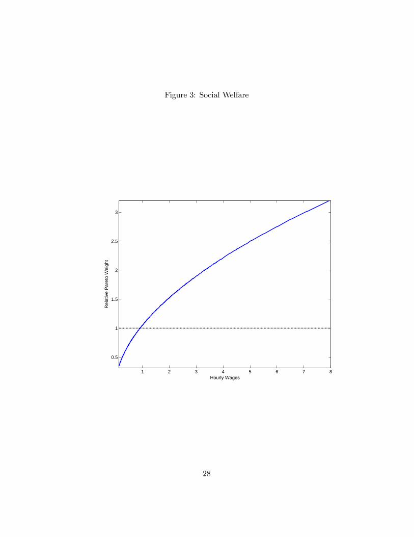
Figure 3: Social Welfare

1 2 3 4 5 6 7 8

0.5

1

1.5

2

2.5

3

Hourly Wages

Rel

ativ

e P

aret

o W

eigh

t

28

condition on the observable characteristic κ, as well as tax schedules that do

not.

7.1 Impact of Insurable Risks and Social Welfare Func-

tion

We consider the impact of insurable shocks and welfare function. In all the

exercises, we keep the total variance of the wage shocks constant.

We start with the "standard" Mirrlees model in which Utilitarian planner

provides all the insurance in the economy. In this case, all the wage vari-

ance comes from the variation in uninsurable and unobservable shocks, i.e.,

logw = α.

The top panel of Table 1 compares optimal tax systems under this econ-

omy. There are large welfare gains from moving to the second best allocation

(5.74% of the consumption) and significant output losses (more than 10% of

GDP). The marginal tax rates are very high and more than 50% on average.

The gains from the second best allocation are approximated well with the

affi ne tax system that displays sizable lump-sum transfers, which appears

in the column TR/Y , whereas the HSV tax system is worse than the affi ne

tax. The intuition of this well-known result in the literature (e.g., Mirrlees

(1971)) is the following. In this economy, the variance of uninsurable shocks

is large and the planner provides all the insurance. Because she has a strong

preference for redistribution, she needs a large amount of transfers from pro-

ductive agents to unproductive ones. The HSV tax has no lump-sum feature

by its nature and cannot come close to the second best.

Next, we introduce insurable shocks in the "standard" Mirrlees model.

The planner still has a taste for redistribution, but the variance of uninsurable

shocks is smaller because agents have access to private insurance markets.

The marginal tax rates are then reduced to 43% and the size of the welfare

not change the results quantitatively.

29

gains is much smaller. This is intuitive given that the role of the planner

is relatively small. Perhaps surprisingly, the HSV tax dominates the affi ne

tax unlike the previous case. The reason is because there is a relatively

small number of people who receive adverse uninsurable shocks and hence

the redistribution effects from the lump-sum transfer is much weaker. The

planner wants to redistribute resources to poor agents, but because the target

population is small, she does so by having increasing marginal tax rates

instead.

The same result appears when we switch to the empirical motivated Social

Welfare Function. Note that now the Ramsey HSV tax is our benchmark and

the current U.S. tax code is the optimal HSV tax system by construction. The

variance of underlying shocks is as large as the "standard" Mirrlees model,

but the planner has less incentive to redistribute resources to unproductive

agents. The last column shows that the transfers are now very small and

hence the marginal tax rates decline to even around 30%. As in the previous

case, switching from the HSV tax to the optimal affi ne tax exhibits welfare

losses.

The last panel of Table 1 is the economy with insurable shocks and empir-

ical motivated SWF, which is our benchmark. It shows that the marginal tax

is further reduced and is around 30%. The second best allocation displays

both welfare gains and output gains. This is because the planner raises the

tax revenue more effi ciently in this economy.

7.2 Richer Tax Functions

In this section, we consider richer tax schemes in our benchmark economy.

Specifically, we compare the baseline HSV tax to polynomial tax systems.

As we saw in the previous section, Table 2 shows that the affi ne tax system

is worse than the baseline HSV tax. However, the quadratic term delivers

gains relative to the affi ne tax and the overall welfare is comparable with the

baseline HSV tax. The size of the transfers is smaller than the affi ne tax, but

30

Table 1: Impact of Insurable Risks and Social Welfare FunctionWages SWF Tax Parameters Outcomes

welfare Y mar. tax TR/Y

logw = α UtilitarianAffi ne Tax τ 0 : −0.280 τ 1 : 0.541 5.04 −10.57 0.541 0.293HSV Tax λ : 0.805 τ : 0.377 4.32 −9.79 0.507 0.110Mirrlees Tax 5.74 −10.67 0.542 0.248

logw = α + ε UtilitarianAffi ne Tax τ 0 : −0.228 τ 1 : 0.445 0.47 −6.11 0.445 0.210HSV Tax λ : 0.821 τ : 0.289 1.25 −5.75 0.431 0.066Mirrlees Tax 1.60 −5.86 0.434 0.167

logw = α EmpiricalAffi ne Tax τ 0 : −0.120 τ 1 : 0.315 −0.44 −0.04 0.315 0.096

HSV Tax (baseline) λ : 0.842 τ : 0.151 − − 0.311 0.020Mirrlees Tax 0.09 −0.04 0.312 0.047

logw = α + ε EmpiricalAffi ne Tax τ 0 : −0.113 τ 1 : 0.300 −0.60 0.57 0.300 0.083

HSV Tax (baseline) λ : 0.835 τ : 0.151 − − 0.311 0.018Mirrlees Tax 0.20 0.91 0.285 0.033

31

Table 2: No Type-Contingent TaxesTax System Outcomes

HSV λ τ welfare Y mar. tax G/Y TR/Y0.835 0.151 - - 0.311 0.188 0.018

τ 0 τ 1 τ 2 τ 3- 0.178 - - -1.32 5.61 0.178 0.178 -0.023

-0.113 0.300 - - -0.60 0.57 0.300 0.187 0.083-0.069 0.213 0.022 - 0.01 0.72 0.292 0.187 0.045-0.032 0.126 0.063 -0.003 0.14 0.80 0.288 0.187 0.015

Second Best (Mirrlees) 0.20 0.91 0.285 0.186 0.033First Best 9.14 16.03 0 0.162 0.221

the marginal tax rates are also lower on average. This means the higher order

term is important to raise the revenue effi ciently and it effectively reduces

the tax distortion.

The third order term adds more gains and delivers almost 75% of the gains

of the second best allocation. This tells us that the increasing marginal tax

rates are more important than the universal lump-sum transfers.

One interesting observation of this benchmark case is that additional

gains from switching to Mirrlees tax are tiny (0.2% of consumption). Under

the empirically motivated social welfare function, the current tax system

performs very well and hence there are not much room for welfare improving

tax reforms. In the next section, we see that this is not the case once we

introduce the observable types and consider type contingent tax systems.

We plot decision rules and the optimal tax schedule for each tax system

in Figure 4 to 6. For each figure, we take log hourly wages in the x-axis.

Figure 4 compares the baseline HSV tax with the Mirrlees second best

allocation and taxes. The optimal marginal tax, the dashed line in the bot-

tom left figure, displays the usual zero tax result at the bottom and top of

the distribution. However, it also shows high non linearity in the middle.

32

The tax schedule starts at a very low rate around 20% in the area where

most people are located, and then sharply increases in the right half of the

wage distribution, especially the range where the uninsurable shock follows

the Pareto distribution. The planner has a strong incentive to keep the rates

low where most people are affected, but wants to increase it to raise enough

revenue once the number of people affected decreases. The baseline HSV

Ramsey tax scheme captures this increase, while the optimal tax exhibits

higher non-linearity.

Figure 5 compares the affi ne tax with the Mirrlees tax. This reveals the

reason why the Ramsey affi ne tax is worse than the baseline HSV tax. The

marginal tax rate is flat in this case, because it is simply given by τ 1. Thus

it hardly captures the increasing pattern of the Mirrlees tax. This creates a

large gap in the average tax, which is found in the bottom right figure.

Figure 6 compares the cubic tax with the Mirrlees tax. The marginal tax

of the Ramsey policy in this case captures not only the increasing pattern

but the convex shape of the optimal tax rates. Thus it approximates the

optimal average tax and hence delivers most of the welfare gains.

7.3 Type-Contingent Taxes

In this section, we consider κ−type contingent taxation, the full model con-sidered in the model section.

Table 3 shows the results. We find significant welfare gains relative to non-

contingent taxes. For example, the Mirrlees second best tax brings the gains

of 1.74% of consumption. By conditioning on observables, the planner can

raise the tax revenue more effi ciently and the marginal tax rates decreases to

the level less than 25%. In contrast to the literature, the optimal tax system

also creates significant output gains.

The result that the HSV tax performs better than the affi ne tax survives

in this class of taxes. Even though the affi ne tax schedule effectively delivers

33

Figure 4: Baseline HSV Tax System

-2 0 2 4

-4

-2

0

2

4

6

Log

Con

sum

ptio

n

Log Hourly Wages

-2 0 2 4

0.4

0.6

0.8

1

1.2

Hou

rs W

orke

d

Log Hourly Wages

-2 0 2 4

0

0.1

0.2

0.3

0.4

0.5

0.6

Mar

gina

l Tax

Rat

e

Log Hourly Wages-2 0 2 4

-1

-0.5

0

0.5

1

Ave

rage

Tax

Rat

e

Log Hourly Wages

MirrleesRamsey

34

Figure 5: Affi ne Tax System

-2 0 2 4

-4

-2

0

2

4

6

Log

Con

sum

ptio

n

Log Hourly Wages

-2 0 2 4

0.4

0.6

0.8

1

1.2

Hou

rs W

orke

d

Log Hourly Wages

-2 0 2 4

0

0.1

0.2

0.3

0.4

0.5

0.6

Mar

gina

l Tax

Rat

e

Log Hourly Wages-2 0 2 4

-1

-0.5

0

0.5

1

Ave

rage

Tax

Rat

e

Log Hourly Wages

MirrleesRamsey

35

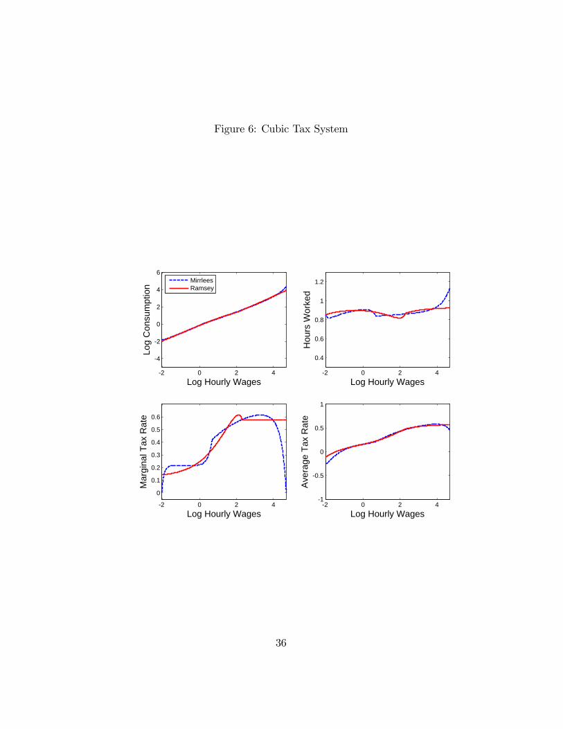
Figure 6: Cubic Tax System

-2 0 2 4

-4

-2

0

2

4

6

Log

Con

sum

ptio

n

Log Hourly Wages

-2 0 2 4

0.4

0.6

0.8

1

1.2

Hou

rs W

orke

d

Log Hourly Wages

-2 0 2 4

0

0.1

0.2

0.3

0.4

0.5

0.6

Mar

gina

l Tax

Rat

e

Log Hourly Wages-2 0 2 4

-1

-0.5

0

0.5

1

Ave

rage

Tax

Rat

e

Log Hourly Wages

MirrleesRamsey

36

the transfers to low κ-type and sets the marginal tax rates differently for

each κ type, it delivers less than 50% of the welfare gains of the second best.

Thus the linear tax is again not a good approximation of the optimal tax. On

the other hand, the type-specific HSV schedule delivers much larger welfare

gains. This fact tells us that the lump-sum transfers are not so important to

mimic the optimal allocation and, rather, the increasing marginal tax rates

are crucial.

However, this does not mean that we need a complex highly non-linear

tax system. It turns out that the second best optimal allocation can be

approximately implemented with the type-specific cubic tax and this simple

tax scheme delivers 94% of the welfare gain of the second best.

8 Conclusions

There has been a long debate on the structure of labor income taxation in

and out of the academia. This paper addresses its main question: how to

balance redistribution versus distortions to labor supply. When doing so,

we emphase that it is important to measure the gap in terms of allocations

and welfare, not in terms of marginal tax rates. The first finding is that

Ramsey and Mirrlees tax schemes not far apart in terms of welfare: we can

approximately decentralize the second best constrained effi cient allocation

with a simple tax scheme. We find that increasing marginal tax systems are

crutial, but universal lump-sum transfers might not be so important. In the

same vein, we find that the current tax scheme might actually be close to

Mirrlees. This means that there are not much room for welfare improving

tax reforms. However, there will be potential large welfare gains from type-

contingent taxes, and to acheive them, we need to condition both transfers

and tax rates on observables.

37

Table 3: Type-Contingent TaxesHSV λ τ welfare Y mar. tax TR/Ybaseline 0.833 0.151 - - 0.311 0.018

0.9780.715

0.2360.042

1.06 1.53 0.2850.063-0.041

τ 0 τ 1 τ 2 τ 3-0.048 0.157 0.054 -0.002 0.12 0.49 0.297 0.035

--0.0090.275

- - 0.06 5.61 0.1780.001-0.048

-0.2110.075

0.248 - - 0.75 3.29 0.2480.193-0.127

-0.0790.1110.338

- - 0.33 2.26 0.2620.0700.028

-0.1880.052

0.2030.269

- - 0.79 3.34 0.2480.172-0.105

-0.1290.234

0.0230.003

0.0970.081

-0.005-0.003

1.64 3.86 0.2260.123-0.235

Second Best (Mirrlees) 1.74 4.01 0.2210.128-0.144

38

References

Benabou, R. (2000): “Unequal Societies: Income Distribution and the

Social Contract,”American Economic Review, 90(1), 96—129.

Heathcote, J., F. Perri, and G. L. Violante (2010): “Unequal We

Stand: An Empirical Analysis of Economic Inequality in the United States:

1967-2006,”Review of Economic Dynamics, 13(1), 15—51.

Heathcote, J., K. Storesletten, and G. Violante (2013): “Redis-

tributive Taxation in a Partial-Insurance Economy,”mimeo.

(forthcoming): “Consumption and Labor Supply with Partial In-

surance: An Analytical Framework,”American Economic Review.

Mirrlees, J. A. (1971): “An Exploration in the Theory of Optimum In-

come Taxation,”Review of Economic Studies, 38(114), 175—208.

Piketty, T., and E. Saez (2003): “Income Inequality In The United

States, 1913-1998,”The Quarterly Journal of Economics, 118(1), 1—39.

Saez, E. (2001): “Using Elasticities to Derive Optimal Income Tax Rates,”

Review of Economic Studies, 68(1), 205—29.

Weinzierl, M. (2011): “The Surprising Power of Age-Dependent Taxes,”

Review of Economic Studies, 78(4), 1490—1518.

39