Embed Size (px)
Citation preview

© 2017 V. Marinca and R.-D. Ene, published by De Gruyter Open.This work is licensed under the Creative Commons Attribution-NonCommercial-NoDerivs 3.0 License.
Open Phys. 2017; 15:42–57
Research Article Open Access
Vasile Marinca and Remus-Daniel Ene*
Optimal homotopy perturbation method fornonlinear differential equations governing MHDJeffery-Hamel flow with heat transfer problemDOI 10.1515/phys-2017-0006Received Aug 29, 2016; accepted Dec 06, 2016
Abstract: In this paper, the Optimal Homotopy Perturba-tion Method (OHPM) is employed to determine an analyticapproximate solution for thenonlinearMHD Jeffery-Hamelflow and heat transfer problem. The Navier-Stokes equa-tions, taking into account Maxwell’s electromagnetismand heat transfer, lead to two nonlinear ordinary differ-ential equations. The results obtained by means of OHPMshow very good agreement with numerical results andwith Homotopy Perturbation Method (HPM) results.
Keywords: optimal homotopy perturbation method;Jeffery-Hamel; nonlinear ordinary differential equations
PACS: 02.60.-x, 47.11.-j, 47.50.-d
1 IntroductionIncompressible fluid flow with heat transfer is one of themost applicable cases in various fields of engineering dueto its industrial applications. The problem of a viscousfluid between two nonparallel walls meeting at a vertexand with a source or sink at the vertex was pioneeredby Jeffery [1] and Hamel [2]. Since then, the Jeffery-Hamelproblem has been studied by several researchers and dis-cussed in many textbooks and articles. A stationary prob-lem with a finite number of “outlets” to infinity in theformof infinite sectors is considered byRivkind andSolon-nikov [3]. The problem of steady viscous flow in a conver-gent channel is analyzed analytically and numerically for
*Corresponding Author: Remus-Daniel Ene: University Po-litehnica Timisoara, Department of Mathematics, Timisoara,300006, Romania; Email: [email protected] Marinca: University Politehnica Timisoara, Department ofMechanics and Vibration, Timisoara, 300222, Romania; Departmentof Electromechanics and Vibration, Center for Advanced and Funda-mental Technical Research, Romania Academy, Timisoara, 300223,Romania
small,moderately large and asymptotically largeReynoldsnumbers over the entire range of allowed convergence an-gles by Akulenko, et al. [4]. The MHD Jeffery-Hamel prob-lem is solved by Makinde and Mhone [5] using a spe-cial type of Hermite-Padé approximation semi-numericalapproach and by Esmaili et al. [6] by applying the Ado-mian decomposition method. The classical Jeffery-Hamelflow problem is solved by Ganji et al. [7] by means of thevariational iteration andhomotopyperturbationmethods,and by Joneidi et al. [8] by the differential transformationmethod, Homotopy Perturbation Method and HomotopyAnalysis Method. The classical Jeffery-Hamel problemwasextended in [9] to include the effects of external magneticfield in a conducting fluid. The optimal homotopy asymp-totic method is applied by Marinca and Herişanu [10] andby Esmaeilpour and Ganji [11]. The effect of magnetic fieldand nanoparticles on the Jeffery-Hamel flow are studiedin [12, 13]. A numerical treatment using stochastic algo-rithms is applied by Raja and Samar [14].
During recent years, several methods have been usedfor solving different problems such as the traveling-wave transformation method [15], the Cole-Hopf transfor-mation method [16], the optimal homotopy asymptoticmethod [17] and the generalized boundary element ap-proach [18].
In general, the problems of Jeffery-Hamel flows andother fluid mechanics problems are inherently nonlin-ear. Excepting a limited number of these problems, mostdo not have analytical solutions. The aim of this paperis to propose an accurate approach to the MHD Jeffery-Hamel flow with heat transfer problem using an analyt-ical technique, namely the Optimal Homotopy Perturba-tion Method (OHPM) [19–21]. Our approach does not re-quire a small or large parameter in the governing equa-tions, and is based on the construction and determinationof some auxiliary functions combined with a convenientway to optimally control the convergence of the solution.

MHD Jeffery-Hamel flow with heat transfer problem: OHPM solutions | 43
2 Problem statement andgoverning equations
We consider a system of cylindrical coordinates with asteady flow of an incompressible conducting viscous fluidfrom a source or sink at channel walls lying in planes, withangle 2α, taking into account the effect of electromagneticinduction, as shown in Fig. 1, and heat transfer.
The continuity equation, the Navier-Stokes equationsand energy equation in cylindrical coordinates canbewrit-ten as [22–25]:
1r∂∂r (rur) +
1r∂∂r (ruφ) = 0, (1)
ur∂ur∂r + uφr
∂ur∂φ −
u2φr = −1ρ
∂P∂r (2)
+ ν[1r∂(rεrr)∂r + 1
r∂εrφ∂r − εrφr − σB
20
ρr2 ur],
ur∂uφ∂r + uφr
∂uφ∂φ − uφurr = − 1
ρr∂P∂φ (3)
+ ν[1r2∂(rεrφ)∂r + 1
r∂εφφ∂φ − εrφr − σB
20
ρr2 uφ],
ur∂T∂r = k
ρcp
(∇2T
)(4)
+ νcp
[2((
∂ur∂r
)2+(urr
)2)+(1r∂ur∂r
)2]+ σB
20
ρr2 u2r ,
where ρ is the fluid density, P is the pressure, ν is thekinematic viscosity, T is the temperature, k is the thermalconductivity, cp is the specific heat at constant pressure,σ is the electrical conductivity, B0 is the inducedmagneticfield and the stress components are defined as
εrr = 2∂ur∂r −23divu, (5)
εφφ =2r∂uφ∂φ + 2ur
r − 23divu, (6)
εrφ =2r∂ur∂φ + 2 ∂∂r
(uφr
). (7)
By considering the velocity field as only along the ra-dial direction, i.e., uφ = 0 and substituting Eqs. (5)-(7) intoEqs. (2) and (3), the continuity, Navier-Stokes and energyequations become:
1r∂∂r (rur) = 0, (8)
ur∂ur∂r = −1ρ
∂P∂r + ν
(∇2ur −
urr2 −
σB20ρr2 ur
), (9)
− 1ρr∂P∂φ + 2ν
r2∂ur∂φ = 0. (10)
The relevant boundary conditions, due to the symme-try assumption at the channel centerline, are as follows:
∂ur∂φ = ∂T
∂φ = 0, ur =ucr at φ = 0, (11)
and at the plates making the body of the channel:
ur = 0, T = Tcr2 at φ = α, (12)
where uc and Tc are the centerline rate of movement andthe constant wall temperature, respectively.
From the continuity equation (8), one can get
rur = f (φ), (13)
where f (φ) is an arbitrary function of φ only.By integrating Eq. (10), it holds that
P(r, φ) = 2ρνr2 f (φ) + ρg(r), (14)
in which g(r) is an arbitrary function of r only.Now, we define the dimensionless parameters:
η = φα , F(η) = f (φ)uc, θ(η) = r2 TTc
, (15)
where Tc is the ambient temperature, and substitutingthese into Eqs. (4) and (9) and then eliminating the pres-sure term, one can put
F′′′ + 2αReFF′ + (4 − H)α2F′ = 0, (16)
θ′′ + 2α (2α + RePrF) θ (17)
+ βPr[(H + 4α2
)F2 + F′2
]= 0,
subject to the boundary conditions
F(0) = 1, F′(0) = 0, F(1) = 0, (18)
θ(1) = 0, θ′(0) = 0, (19)
where Re = αucν is the Reynolds number, H =
√σB20ρν is the
Hartmann number, Pr = νcpkρ , β = uc
cp and prime denotesderivative with respect to η.
44 | V. Marinca and R.-D. Ene
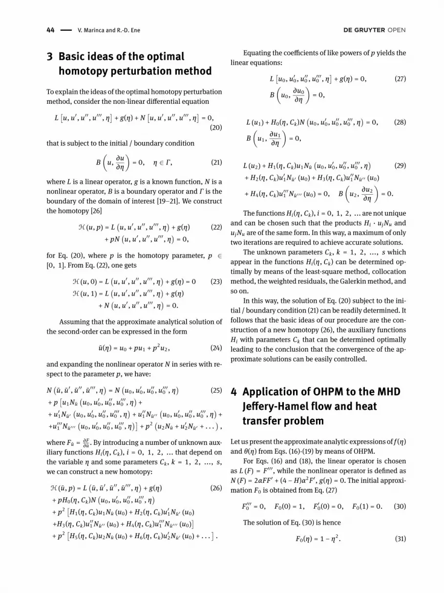
3 Basic ideas of the optimalhomotopy perturbation method
To explain the ideas of the optimal homotopy perturbationmethod, consider the non-linear differential equation
L[u, u′, u′′, u′′′, η
]+ g(η) + N
[u, u′, u′′, u′′′, η
]= 0,
(20)
that is subject to the initial / boundary condition
B(u, ∂u∂η
)= 0, η ∈ Γ , (21)
where L is a linear operator, g is a known function, N is anonlinear operator, B is a boundary operator and Γ is theboundary of the domain of interest [19–21]. We constructthe homotopy [26]
H (u, p) = L(u, u′, u′′, u′′′, η
)+ g(η) (22)
+ pN(u, u′, u′′, u′′′, η
)= 0,
for Eq. (20), where p is the homotopy parameter, p ∈[0, 1]. From Eq. (22), one gets
H (u, 0) = L(u, u′, u′′, u′′′, η
)+ g(η) = 0 (23)
H (u, 1) = L(u, u′, u′′, u′′′, η
)+ g(η)
+ N(u, u′, u′′, u′′′, η
)= 0.
Assuming that the approximate analytical solution ofthe second-order can be expressed in the form
u(η) = u0 + pu1 + p2u2, (24)
and expanding the nonlinear operator N in series with re-spect to the parameter p, we have:
N(u, u′, u′′, u′′′, η
)= N
(u0, u′0, u′′0 , u′′′0 , η
)(25)
+ p[u1Nu
(u0, u′0, u′′0 , u′′′0 , η
)+
+ u′1Nu′(u0, u′0, u′′0 , u′′′0 , η
)+ u′′1Nu′′
(u0, u′0, u′′0 , u′′′0 , η
)+
+u′′′1 Nu′′′(u0, u′0, u′′0 , u′′′0 , η
)]+ p2
(u2Nu + u′2Nu′ + . . .
),
where Fu = ∂F∂u . By introducing a number of unknown aux-
iliary functions Hi(η, Ck), i = 0, 1, 2, ... that depend onthe variable η and some parameters Ck, k = 1, 2, ..., s,we can construct a new homotopy:
H (u, p) = L(u, u′, u′′, u′′′, η
)+ g(η) (26)
+ pH0(η, Ck)N(u0, u′0, u′′0 , u′′′0 , η
)+ p2
[H1(η, Ck)u1Nu (u0) + H2(η, Ck)u′1Nu′ (u0)
+H3(η, Ck)u′′1Nu′′ (u0) + H4(η, Ck)u′′′1 Nu′′′ (u0)]
+ p2[H5(η, Ck)u2Nu (u0) + H6(η, Ck)u′2Nu′ (u0) + . . .
].
Equating the coefficients of like powers of p yields thelinear equations:
L[u0, u′0, u′′0 , u′′′0 , η
]+ g(η) = 0, (27)
B(u0,
∂u0∂η
)= 0,
L (u1) + H0(η, Ck)N(u0, u′0, u′′0 , u′′′0 , η
)= 0, (28)
B(u1,
∂u1∂η
)= 0,
L (u2) + H1(η, Ck)u1Nu(u0, u′0, u′′0 , u′′′0 , η
)(29)
+ H2(η, Ck)u′1Nu′ (u0) + H3(η, Ck)u′′1Nu′′ (u0)
+ H4(η, Ck)u′′′1 Nu′′′ (u0) = 0, B(u2,
∂u2∂η
)= 0.
The functionsHi(η, Ck), i = 0, 1, 2, ... are not uniqueand can be chosen such that the products Hi · ujNu andujNu are of the same form. In this way, a maximum of onlytwo iterations are required to achieve accurate solutions.
The unknown parameters Ck, k = 1, 2, ..., s whichappear in the functions Hi(η, Ck) can be determined op-timally by means of the least-square method, collocationmethod, theweighted residuals, the Galerkinmethod, andso on.
In this way, the solution of Eq. (20) subject to the ini-tial / boundary condition (21) can be readily determined. Itfollows that the basic ideas of our procedure are the con-struction of a new homotopy (26), the auxiliary functionsHi with parameters Ck that can be determined optimallyleading to the conclusion that the convergence of the ap-proximate solutions can be easily controlled.
4 Application of OHPM to the MHDJeffery-Hamel flow and heattransfer problem
Let uspresent the approximate analytic expressions of f (η)and θ(η) from Eqs. (16)-(19) by means of OHPM.
For Eqs. (16) and (18), the linear operator is chosenas L (F) = F′′′, while the nonlinear operator is defined asN (F) = 2αFF′ + (4 − H)α2F′, g(η) = 0. The initial approxi-mation F0 is obtained from Eq. (27)
F′′′0 = 0, F0(0) = 1, F′0(0) = 0, F0(1) = 0. (30)
The solution of Eq. (30) is hence
F0(η) = 1 − η2. (31)

MHD Jeffery-Hamel flow with heat transfer problem: OHPM solutions | 45
On the other hand, from Eq. (16), one obtains
NF (F) = 2αReF′, NF′ (F) = 2αReF + (4 − H)α2. (32)
By substituting Eq. (31) into the nonlinear operator Nand into Eq. (32), one retrieves
N (F0) = 2Aη2 − 2(A + B)η, NF (F0) = −2Aη, (33)NF′ (F0) = −Aη2 + A + B,
where A = 2αRe, B = (4 − H)α2.Eq. (28) becomes
F′′′1 + H0(η, Ck)[2Aη2 − 2(A + B)η
]= 0, (34)
F1(0) = F′1(0) = F1(1) = 0.
We choose H0(η, Ck) = −60C1 where C1 is an un-known parameter and from Eq. (34) we obtain
F1(η) = 2AC1η5 − 5(A + B)C1η4 + (3A + 5B)C1η2. (35)
Eq. (29) can be written in the form
F′′′2 + H1(η, Ck)(−2Aη)F1 (36)+ H2(η, Ck)(−Aη2 + A + B)F′1 = 0F2(0) = F′2(0) = F2(1) = 0.
In this case we choose
H1(η, Ck) =12A
(C2η2 + C3η + C4 +
C5η
),
H2(η, Ck) =C62 + C7η ,
such that the solution of Eq. (36) is given by
F2(η) =AC1C2495
η11 +2AC1C3 − 5(A + B)C1C2
720η10 (37)
+2AC1C4 − 5(A + B)C1C3 + 5A2C1C6
504η9
+(3A + 5B)C1C2 − 5(A + B)C1C4 + 2AC1C5 − 10(A2 + AB)C1C6
336η8
+(3A + 5B)C1C3 − 5(A + B)C1C5 − 5(A2 + AB)C1C6 + 2AC1C7
210η7
+(3A + 5B)C1C4 + (13A2 + 25AB + 10B2)C1C6 − 5(A + B)C1C7
120η6
+(3A + 5B)C1C5
60η5 −
(3A2 + 8AB + 5B2)C1C6 + (3A + 5B)C1C724
η4
+ Mη2 ,
where
M = −C1C2[(
1495 −
1144 + 1
112
)A +
(5
336 −1
144
)B]
− C1C3[(
1360 −
5504 + 1
70
)A +
(142 −
5504
)B]
− C1C7(13A140 + B6
)
− C1C4[(
1252 −
5336 + 1
40
)A +
(124 −
5336
)B]
− C1C5(9A280 + 5B
84
)− C1C6
[(5
504 −5
168 −5
210 −160
)A2
−(
5168 + 5
210 + 18
)AB − 1
8B2].
For p = 1 in Eq. (24), we obtain the second-order ap-proximate solution, using Eqs. (31), (35) and (37):
F(η) = F0(η) + F1(η) + F2(η) =AC1C2495
η11 (38)
+2AC1C3 − 5(A + B)C1C2
720η10
+2AC1C4 − 5(A + B)C1C3 + 5A2C1C6
504η9
+(3A + 5B)C1C2 − 5(A + B)C1C4 + 2AC1C5 − 10(A2 + AB)C1C6
336η8
+(3A + 5B)C1C3 − 5(A + B)C1C5 − 5(A2 + AB)C1C6 + 2AC1C7
210η7
+(3A + 5B)C1C4 + (13A2 + 25AB + 10B2)C1C6 − 5(A + B)C1C7
120η6
+(2AC1 +
(3A + 5B)60
C1C5)η5
−[(3A2 + 8AB + 5B2)C1C6 + (3A + 5B)C1C7
24+ (5A + 5B)C1
]η4
+ [(3A + 5B) + M − 1] η2 .
Now, we present the approximate analytic solution forEqs. (17) and (19). The linear and nonlinear operators andthe function g are, respectively,
L(θ) = θ′′, g(η) = −1, (39)
N(θ) = 1 + 4α2θ + 2αRePrFθ + βPr[(H + 4α2)F2 + F′2
].
Eq. (27) becomes
θ′′0 − 1 = 0, θ0(1) = 0, θ′0(0) = 0. (40)
Eq. (40) has the solution
θ0(η) =12(1 − η
2). (41)
From Eq. (39) it follows that
Nθ(θ) = 4α2 + 2αRePrF, Nθ′ (θ) = 0. (42)
By substitutingEq. (41) into Eqs. (39) and (42), one getsrespectively
N(θ0) = C − 2Dη2 + Eη4, Nθ(θ0) = L + Kη2, (43)
where
C = 1 + 2α2 + αRePr + 4βα2Pr + PrHβ (44)
46 | V. Marinca and R.-D. Ene
D = α2 + 2αRePr + 2βPr(2α2 − 1) + PrHβE = αRePr + 4βα2Pr + PrHβL = 4α2 + 2αRePr, K = −2αRePr.
Eq. (28) can be written
θ′′1 + h0(η, C8)(C − 2Dη2 + Eη4) = 0, (45)θ1(1) = θ′1(0) = 0.
Choosing h0(η, C8) = −30C8 in Eq. (45), one obtains
θ1(η) = C8[15C(η2 − 1) − 5D(η4 − 1) + E(η6 − 1)
]. (46)
Eq. (29) can be written in the form
θ′′2 + h1(η, Ck)(L + Kη2)θ1 = 0, θ2(1) = θ′2(0) = 0, (47)
and therefore it is natural to choose the auxiliary functionh1 as
h1(η, Ck) =1C8
(C9 + C10η + C11η2 + C12η3 + C13η4
).
From Eq. (47), it can shown that
θ2(η) = −L(15C − 5D + E) (48)
·[12C9(η
2 − 1) + 16C10(η
3 − 1)]
+[15LCC9 − (15C − 5D + E)(KC9 + LC11)
] η4 − 112
+[15LCC10 − (15C − 5D + E)(KC10 + LC12)
] η5 − 120
+[(15CK − 5DK)C9 + 15LCC11
−(15C − 5D + E)(KC11 + LC13)] η6 − 1
30+[(15CK − 5DL)C10 + 15LCC12 − K(15C − 5D + E)C12
]· η
7 − 142
+[(LE − 5DK)C9 + (15CK − 5DL)C11 + 15LCC13−
−K(15C − 5D + E)C13] η8 − 1
56
+[(LE − 5DK)C10 + (15CK − 5DL)C12
] η9 − 172
+[EKC9 + (LE − 5DK)C11 + (15CK − 5DL)C13
] η10 − 190
+[EKC11 + (LE − 5DK)C13
] η12 − 1132 + EKC12
η13 − 1156
+ EKC13η14 − 1182 .
The second-order approximate solution of Eqs. (17)and (19) is
θ(η) = θ0(η) + θ1(η) + θ2(η), (49)
where θ0, θ1 and θ2 are given by Eqs. (41), (46) and(48), respectively.
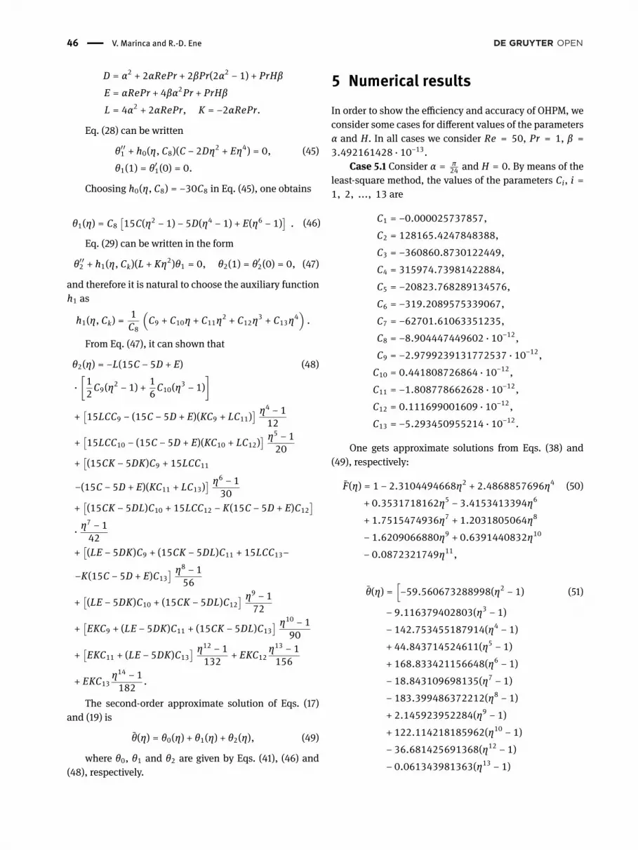
5 Numerical resultsIn order to show the efficiency and accuracy of OHPM, weconsider some cases for different values of the parametersα and H. In all cases we consider Re = 50, Pr = 1, β =3.492161428 · 10−13.
Case 5.1 Consider α = π24 and H = 0. By means of the
least-square method, the values of the parameters Ci, i =1, 2, ..., 13 are
C1 = −0.000025737857,C2 = 128165.4247848388,C3 = −360860.8730122449,C4 = 315974.73981422884,C5 = −20823.768289134576,C6 = −319.2089575339067,C7 = −62701.61063351235,C8 = −8.904447449602 · 10−12,C9 = −2.9799239131772537 · 10−12,C10 = 0.441808726864 · 10−12,C11 = −1.808778662628 · 10−12,C12 = 0.111699001609 · 10−12,C13 = −5.293450955214 · 10−12.
One gets approximate solutions from Eqs. (38) and(49), respectively:
F(η) = 1 − 2.3104494668η2 + 2.4868857696η4 (50)+ 0.3531718162η5 − 3.4153413394η6
+ 1.7515474936η7 + 1.2031805064η8
− 1.6209066880η9 + 0.6391440832η10
− 0.0872321749η11,
θ(η) =[−59.560673288998(η2 − 1) (51)
− 9.116379402803(η3 − 1)− 142.753455187914(η4 − 1)+ 44.843714524611(η5 − 1)+ 168.833421156648(η6 − 1)− 18.843109698135(η7 − 1)− 183.399486372212(η8 − 1)+ 2.145923952284(η9 − 1)+ 122.114218185962(η10 − 1)− 36.681425691368(η12 − 1)− 0.061343981363(η13 − 1)
MHD Jeffery-Hamel flow with heat transfer problem: OHPM solutions | 47
+2.491809125293(η14 − 1)]· 10−12.
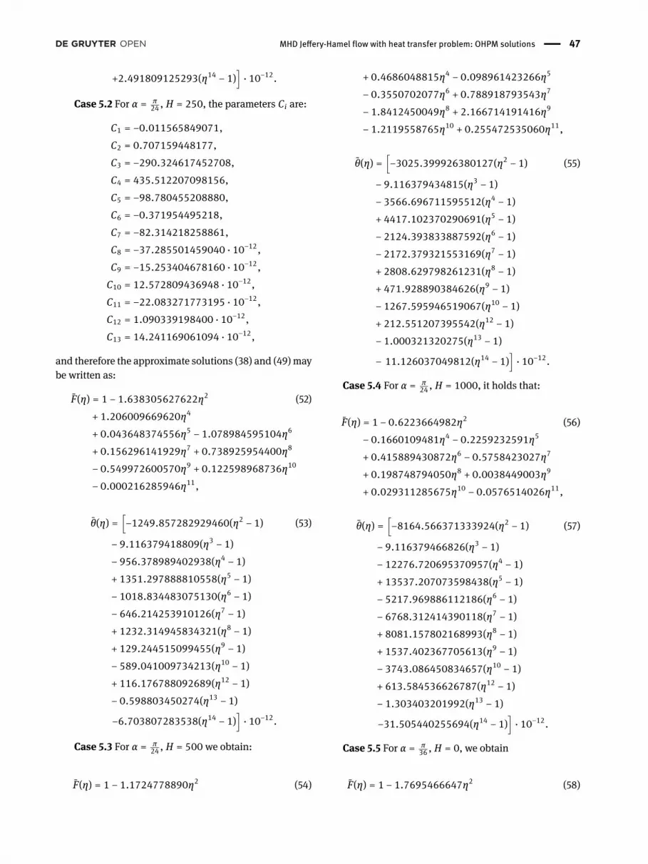
Case 5.2 For α = π24 , H = 250, the parameters Ci are:
C1 = −0.011565849071,C2 = 0.707159448177,C3 = −290.324617452708,C4 = 435.512207098156,C5 = −98.780455208880,C6 = −0.371954495218,C7 = −82.314218258861,C8 = −37.285501459040 · 10−12,C9 = −15.253404678160 · 10−12,C10 = 12.572809436948 · 10−12,C11 = −22.083271773195 · 10−12,C12 = 1.090339198400 · 10−12,C13 = 14.241169061094 · 10−12,
and therefore the approximate solutions (38) and (49)maybe written as:
F(η) = 1 − 1.638305627622η2 (52)+ 1.206009669620η4
+ 0.043648374556η5 − 1.078984595104η6
+ 0.156296141929η7 + 0.738925954400η8
− 0.549972600570η9 + 0.122598968736η10
− 0.000216285946η11,
θ(η) =[−1249.857282929460(η2 − 1) (53)
− 9.116379418809(η3 − 1)− 956.378989402938(η4 − 1)+ 1351.297888810558(η5 − 1)− 1018.834483075130(η6 − 1)− 646.214253910126(η7 − 1)+ 1232.314945834321(η8 − 1)+ 129.244515099455(η9 − 1)− 589.041009734213(η10 − 1)+ 116.176788092689(η12 − 1)− 0.598803450274(η13 − 1)
−6.703807283538(η14 − 1)]· 10−12.
Case 5.3 For α = π24 , H = 500 we obtain:
F(η) = 1 − 1.1724778890η2 (54)
+ 0.4686048815η4 − 0.098961423266η5
− 0.3550702077η6 + 0.788918793543η7
− 1.8412450049η8 + 2.166714191416η9
− 1.2119558765η10 + 0.255472535060η11,
θ(η) =[−3025.399926380127(η2 − 1) (55)
− 9.116379434815(η3 − 1)− 3566.696711595512(η4 − 1)+ 4417.102370290691(η5 − 1)− 2124.393833887592(η6 − 1)− 2172.379321553169(η7 − 1)+ 2808.629798261231(η8 − 1)+ 471.928890384626(η9 − 1)− 1267.595946519067(η10 − 1)+ 212.551207395542(η12 − 1)− 1.000321320275(η13 − 1)
− 11.126037049812(η14 − 1)]· 10−12.
Case 5.4 For α = π24 , H = 1000, it holds that:
F(η) = 1 − 0.6223664982η2 (56)− 0.1660109481η4 − 0.2259232591η5
+ 0.415889430872η6 − 0.5758423027η7
+ 0.198748794050η8 + 0.0038449003η9
+ 0.029311285675η10 − 0.0576514026η11,
θ(η) =[−8164.566371333924(η2 − 1) (57)
− 9.116379466826(η3 − 1)− 12276.720695370957(η4 − 1)+ 13537.207073598438(η5 − 1)− 5217.969886112186(η6 − 1)− 6768.312414390118(η7 − 1)+ 8081.157802168993(η8 − 1)+ 1537.402367705613(η9 − 1)− 3743.086450834657(η10 − 1)+ 613.584536626787(η12 − 1)− 1.303403201992(η13 − 1)
−31.505440255694(η14 − 1)]· 10−12.
Case 5.5 For α = π36 , H = 0, we obtain
F(η) = 1 − 1.7695466647η2 (58)

48 | V. Marinca and R.-D. Ene
+ 1.2754140854η4 + 0.1103023597η5
− 1.1550256736η6 + 0.4434051824η7
+ 0.3358564399η8 − 0.3325192185η9
+ 0.1045556849η10 − 0.0124421957η11,
θ(η) =[−111.208165621670(η2 − 1) (59)
− 6.895054111348(η3 − 1)− 219.101666428999(η4 − 1)+ 112.000412353392(η5 − 1)+ 120.895605108821(η6 − 1)− 47.637714830801(η7 − 1)− 104.355375516421(η8 − 1)+ 6.984672282609(η9 − 1)+ 75.737792150272(η10 − 1)− 24.982664253556(η12 − 1)− 0.097447216002(η13 − 1)
+1.768576986049(η14 − 1)]· 10−12.
Case 5.6 If α = π36 , H = 250 then
F(η) = 1 − 1.5111014276η2 (60)+ 0.8612876996η4 + 0.0128407190η5
− 0.5668759509η6 + 0.0367598458η7
+ 0.3198667899η8 − 0.1656253347η9
+ 0.0019977968η10 + 0.0108498620η11,
θ(η) =[−5094.867741624686(η2 − 1) (61)
− 6.895054147361(η3 − 1)− 4500.773385702808(η4 − 1)+ 6249.12145418685(η5 − 1)− 4283.444052831423(η6 − 1)− 2834.31757828637(η7 − 1)+ 5102.615992457279(η8 − 1)+ 528.701361603855(η9 − 1)− 2382.96513866767(η10 − 1)+ 460.279590044557(η12 − 1)− 2.850139405026(η13 − 1)
−26.598784857626(η14 − 1)]· 10−12.
Case 5.7 For α = π36 , H = 500 the approximate solu-
tions are
F(η) = 1 − 1.2942214724η2 (62)
+ 0.5334630869η4 + 0.0019708504η5
− 0.3330602404η6 − 0.0197377497η7
+ 0.2108709627η8 − 0.1151093836η9
+ 0.0147650020η10 + 0.0010589440η11,
θ(η) =[−10479.441564298402(η2 − 1) (63)
− 6.895054183374(η3 − 1)− 9629.602717192312(η4 − 1)+ 12532.057010176612(η5 − 1)− 7708.77471180501(η6 − 1)− 5687.792565325205(η7 − 1)+ 9313.682156269786(η8 − 1)+ 1063.274966246270(η9 − 1)− 4206.734533154069(η10 − 1)+ 761.164805945711(η12 − 1)− 5.659649234867(η13 − 1)
−42.382058179415(η14 − 1)]· 10−12.
Case 5.8 If α = π36 , H = 1000 then
F(η) = 1 − 0.9581900583η2 (64)+ 0.0913634769η4 + 0.0030073285η5
− 0.1611067985η6 + 0.0668486226η7
− 0.0696973759η8 + 0.0454374262η9
− 0.0111066789η10 − 0.0065559425η11,
θ(η) =[−22457.262743604428(η2 − 1) (65)
− 6.895054255400(η3 − 1)− 22247.17539598977(η4 − 1)+ 26605.166448464304(η5 − 1)− 14220.534699997283(η6 − 1)− 12131.493178637833(η7 − 1)+ 17921.197074275697(η8 − 1)+ 2301.819882082563(η9 − 1)− 7836.564793794578(η10 − 1)+ 1301.948445444968(η12 − 1)− 11.186604132870(η13 − 1)
−68.576887703688(η14 − 1)]· 10−12.
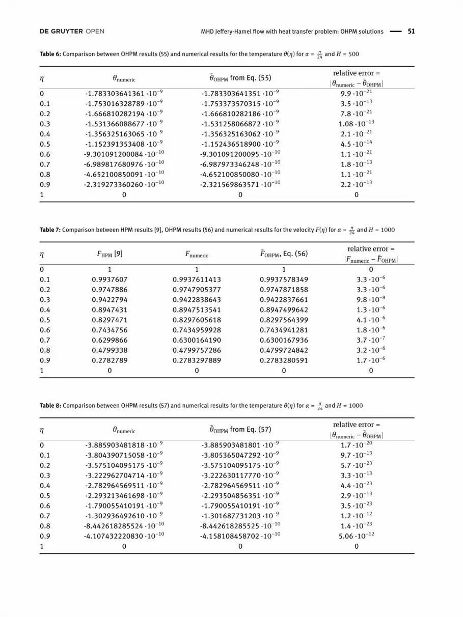
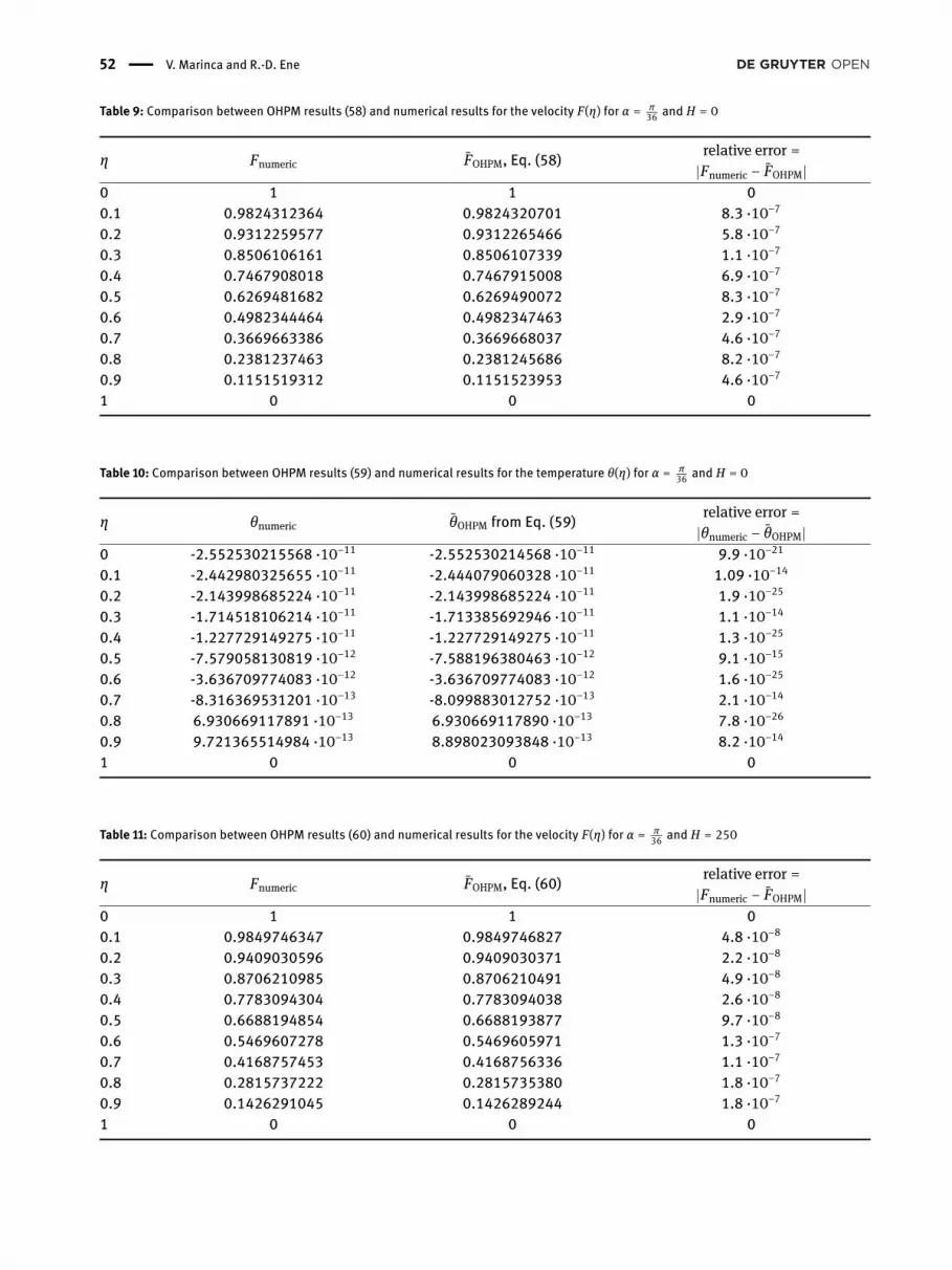
From Tables 1–16, it is obvious that the second-orderapproximate solutions obtained by OHPM are of a highaccuracy in comparison with the homotopy perturbationmethod and with numerical solution obtained by means

MHD Jeffery-Hamel flow with heat transfer problem: OHPM solutions | 49
Table 1: Comparison between HPM results [9], OHPM results (50) and numerical results for the velocity F(η) for α = π24 and H = 0
η FHPM [9] Fnumeric FOHPM, Eq. (50)relative error =
|Fnumeric − FOHPM|0 1 1 1 00.1 0.9770711 0.9771426047 0.9771444959 1.8 ·10−6
0.2 0.9112020 0.9114792278 0.9114802054 9.7 ·10−7
0.3 0.8104115 0.8110052403 0.8110054657 2.2 ·10−7
0.4 0.6859230 0.6869148220 0.6869163034 1.4 ·10−6
0.5 0.5498427 0.5512883212 0.5512895302 1.2 ·10−6
0.6 0.4131698 0.4151088947 0.4151091740 2.7 ·10−7
0.7 0.2846024 0.2870546320 0.2870554998 8.6 ·10−7
0.8 0.1702791 0.1731221390 0.1731231521 1.01 ·10−6
0.9 0.0744232 0.0768715756 0.0768721058 5.3 ·10−7
1 0 0 0 0
Table 2: Comparison between OHPM results (51) and numerical results for the temperature θ(η) for α = π24 and H = 0
η θnumeric θOHPM from Eq. (51) relative error =|θnumeric − θOHPM|
0 -9.134405103300 ·10−12 -9.134559900000 ·10−12 1.5 ·10−16
0.1 -8.553981690585 ·10−12 -8.561731325450 ·10−12 7.7 ·10−15
0.2 -7.029011445513 ·10−12 -7.029011445531 ·10−12 1.7 ·10−23
0.3 -4.968059593695 ·10−12 -4.959904647105 ·10−12 8.1 ·10−15
0.4 -2.830354806908 ·10−12 -2.830354806921 ·10−12 1.3 ·10−23
0.5 -1.003581673783 ·10−12 -1.015625108634 ·10−12 1.2 ·10−14
0.6 2.755715234490 ·10−13 2.755715234410 ·10−13 7.9 ·10−24
0.7 9.398183452650 ·10−13 9.682947296376 ·10−13 2.8 ·10−14
0.8 1.062337244632 ·10−12 1.062337244629 ·10−12 3.3 ·10−24
0.9 7.684282928672 ·10−13 6.524090716991 ·10−13 1.1 ·10−13
1 0 0 0
B0
B0
2 Αj
r,uSource
or sink
Figure 1: Geometry of the MHD Jeffery-Hamel problem.
of a fourth-order Runge-Kuttamethod in combinationwiththe shootingmethod usingWolframMathematica 6.0 soft-ware.
In Figs. 2 and 3 are presented the effect of the Hart-mann number on the velocity profile for Re = 50 andα = π
24 and α =π36 , respectively. It is observed that velocity
increases with increase of the Hartmann number for anyvalue of α. The same effect of Hartmann number on thethermal profile are presented in Figs. 4 and 5 for α = π
24and α = π
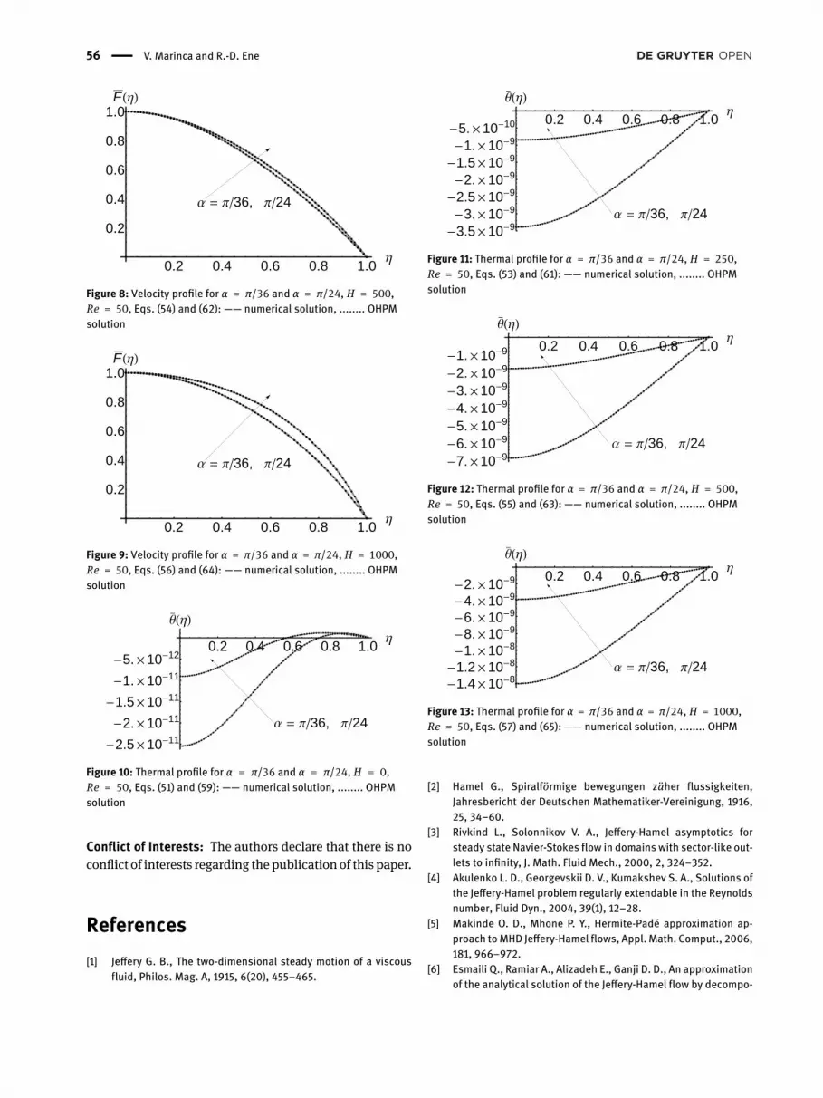
36 , respectively. In this case, the temperaturedecreases with increase of the Hartmann number in bothcases. The effect of the half angle α on the velocity profileis presented in Figs. 6–9. With increasing value of α, ve-locity decreases for H = 0 and H = 250, but increases forH = 500 and H = 1000. From Figs. 10–13, it is interestingto remark that the temperature increases as the half angleα increases. In all cases, themaximum temperature occursnear thewalls forH = 0 and precisely at thewall forH = 0,while the minimum occurs near the channel axis.
50 | V. Marinca and R.-D. Ene
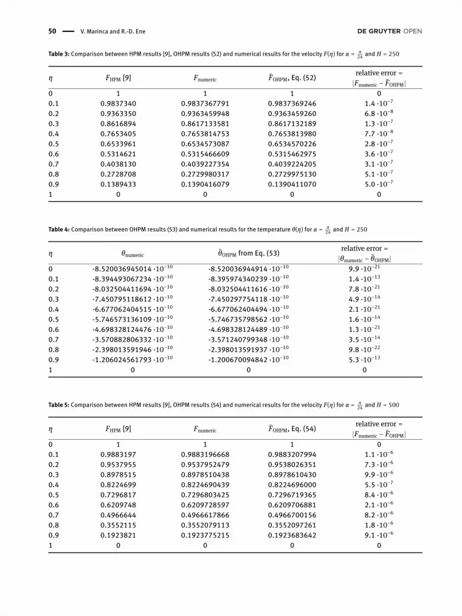
Table 3: Comparison between HPM results [9], OHPM results (52) and numerical results for the velocity F(η) for α = π24 and H = 250
η FHPM [9] Fnumeric FOHPM, Eq. (52)relative error =
|Fnumeric − FOHPM|0 1 1 1 00.1 0.9837340 0.9837367791 0.9837369246 1.4 ·10−7
0.2 0.9363350 0.9363459948 0.9363459260 6.8 ·10−8
0.3 0.8616894 0.8617133581 0.8617132189 1.3 ·10−7
0.4 0.7653405 0.7653814753 0.7653813980 7.7 ·10−8
0.5 0.6533961 0.6534573087 0.6534570226 2.8 ·10−7
0.6 0.5314621 0.5315466609 0.5315462975 3.6 ·10−7
0.7 0.4038130 0.4039227354 0.4039224205 3.1 ·10−7
0.8 0.2728708 0.2729980317 0.2729975130 5.1 ·10−7
0.9 0.1389433 0.1390416079 0.1390411070 5.0 ·10−7
1 0 0 0 0
Table 4: Comparison between OHPM results (53) and numerical results for the temperature θ(η) for α = π24 and H = 250
η θnumeric θOHPM from Eq. (53) relative error =|θnumeric − θOHPM|
0 -8.520036945014 ·10−10 -8.520036944914 ·10−10 9.9 ·10−21
0.1 -8.394493067234 ·10−10 -8.395974340239 ·10−10 1.4 ·10−13
0.2 -8.032504411694 ·10−10 -8.032504411616 ·10−10 7.8 ·10−21
0.3 -7.450795118612 ·10−10 -7.450297754118 ·10−10 4.9 ·10−14
0.4 -6.677062404515 ·10−10 -6.677062404494 ·10−10 2.1 ·10−21
0.5 -5.746573136109 ·10−10 -5.746735798562 ·10−10 1.6 ·10−14
0.6 -4.698328124476 ·10−10 -4.698328124489 ·10−10 1.3 ·10−21
0.7 -3.570882806332 ·10−10 -3.571240799348 ·10−10 3.5 ·10−14
0.8 -2.398013591946 ·10−10 -2.398013591937 ·10−10 9.8 ·10−22
0.9 -1.206024561793 ·10−10 -1.200670094842 ·10−10 5.3 ·10−13
1 0 0 0
Table 5: Comparison between HPM results [9], OHPM results (54) and numerical results for the velocity F(η) for α = π24 and H = 500
η FHPM [9] Fnumeric FOHPM, Eq. (54)relative error =
|Fnumeric − FOHPM|0 1 1 1 00.1 0.9883197 0.9883196668 0.9883207994 1.1 ·10−6
0.2 0.9537955 0.9537952479 0.9538026351 7.3 ·10−6
0.3 0.8978515 0.8978510438 0.8978610430 9.9 ·10−6
0.4 0.8224699 0.8224690439 0.8224696000 5.5 ·10−7
0.5 0.7296817 0.7296803425 0.7296719365 8.4 ·10−6
0.6 0.6209748 0.6209728597 0.6209706881 2.1 ·10−6
0.7 0.4966644 0.4966617866 0.4966700156 8.2 ·10−6
0.8 0.3552115 0.3552079113 0.3552097261 1.8 ·10−6
0.9 0.1923821 0.1923775215 0.1923683642 9.1 ·10−6
1 0 0 0 0
MHD Jeffery-Hamel flow with heat transfer problem: OHPM solutions | 51
Table 6: Comparison between OHPM results (55) and numerical results for the temperature θ(η) for α = π24 and H = 500
η θnumeric θOHPM from Eq. (55) relative error =|θnumeric − θOHPM|
0 -1.783303641361 ·10−9 -1.783303641351 ·10−9 9.9 ·10−21
0.1 -1.753016328789 ·10−9 -1.753373570315 ·10−9 3.5 ·10−13
0.2 -1.666810282194 ·10−9 -1.666810282186 ·10−9 7.8 ·10−21
0.3 -1.531366088677 ·10−9 -1.531258066872 ·10−9 1.08 ·10−13
0.4 -1.356325163065 ·10−9 -1.356325163062 ·10−9 2.1 ·10−21
0.5 -1.152391353408 ·10−9 -1.152436518900 ·10−9 4.5 ·10−14
0.6 -9.301091200084 ·10−10 -9.301091200095 ·10−10 1.1 ·10−21
0.7 -6.989817680976 ·10−10 -6.987973346248 ·10−10 1.8 ·10−13
0.8 -4.652100850091 ·10−10 -4.652100850080 ·10−10 1.1 ·10−21
0.9 -2.319273360260 ·10−10 -2.321569863571 ·10−10 2.2 ·10−13
1 0 0 0
Table 7: Comparison between HPM results [9], OHPM results (56) and numerical results for the velocity F(η) for α = π24 and H = 1000
η FHPM [9] Fnumeric FOHPM, Eq. (56)relative error =
|Fnumeric − FOHPM|0 1 1 1 00.1 0.9937607 0.9937611413 0.9937578349 3.3 ·10−6
0.2 0.9747886 0.9747905377 0.9747871858 3.3 ·10−6
0.3 0.9422794 0.9422838643 0.9422837661 9.8 ·10−8
0.4 0.8947431 0.8947513541 0.8947499642 1.3 ·10−6
0.5 0.8297471 0.8297605618 0.8297564399 4.1 ·10−6
0.6 0.7434756 0.7434959928 0.7434941281 1.8 ·10−6
0.7 0.6299866 0.6300164190 0.6300167936 3.7 ·10−7
0.8 0.4799338 0.4799757286 0.4799724842 3.2 ·10−6
0.9 0.2782789 0.2783297889 0.2783280591 1.7 ·10−6
1 0 0 0 0
Table 8: Comparison between OHPM results (57) and numerical results for the temperature θ(η) for α = π24 and H = 1000
η θnumeric θOHPM from Eq. (57) relative error =|θnumeric − θOHPM|
0 -3.885903481818 ·10−9 -3.885903481801 ·10−9 1.7 ·10−20
0.1 -3.804390715058 ·10−9 -3.805365047292 ·10−9 9.7 ·10−13
0.2 -3.575104095175 ·10−9 -3.575104095175 ·10−9 5.7 ·10−23
0.3 -3.222962704714 ·10−9 -3.222630117770 ·10−9 3.3 ·10−13
0.4 -2.782964569511 ·10−9 -2.782964569511 ·10−9 4.4 ·10−23
0.5 -2.293213461698 ·10−9 -2.293504856351 ·10−9 2.9 ·10−13
0.6 -1.790055410191 ·10−9 -1.790055410191 ·10−9 3.5 ·10−23
0.7 -1.302936492610 ·10−9 -1.301687731203 ·10−9 1.2 ·10−12
0.8 -8.442618285524 ·10−10 -8.442618285525 ·10−10 1.4 ·10−23
0.9 -4.107432220830 ·10−10 -4.158108458702 ·10−10 5.06 ·10−12
1 0 0 0
52 | V. Marinca and R.-D. Ene
Table 9: Comparison between OHPM results (58) and numerical results for the velocity F(η) for α = π36 and H = 0
η Fnumeric FOHPM, Eq. (58)relative error =
|Fnumeric − FOHPM|0 1 1 00.1 0.9824312364 0.9824320701 8.3 ·10−7
0.2 0.9312259577 0.9312265466 5.8 ·10−7
0.3 0.8506106161 0.8506107339 1.1 ·10−7
0.4 0.7467908018 0.7467915008 6.9 ·10−7
0.5 0.6269481682 0.6269490072 8.3 ·10−7
0.6 0.4982344464 0.4982347463 2.9 ·10−7
0.7 0.3669663386 0.3669668037 4.6 ·10−7
0.8 0.2381237463 0.2381245686 8.2 ·10−7
0.9 0.1151519312 0.1151523953 4.6 ·10−7
1 0 0 0
Table 10: Comparison between OHPM results (59) and numerical results for the temperature θ(η) for α = π36 and H = 0
η θnumeric θOHPM from Eq. (59) relative error =|θnumeric − θOHPM|
0 -2.552530215568 ·10−11 -2.552530214568 ·10−11 9.9 ·10−21
0.1 -2.442980325655 ·10−11 -2.444079060328 ·10−11 1.09 ·10−14
0.2 -2.143998685224 ·10−11 -2.143998685224 ·10−11 1.9 ·10−25
0.3 -1.714518106214 ·10−11 -1.713385692946 ·10−11 1.1 ·10−14
0.4 -1.227729149275 ·10−11 -1.227729149275 ·10−11 1.3 ·10−25
0.5 -7.579058130819 ·10−12 -7.588196380463 ·10−12 9.1 ·10−15
0.6 -3.636709774083 ·10−12 -3.636709774083 ·10−12 1.6 ·10−25
0.7 -8.316369531201 ·10−13 -8.099883012752 ·10−13 2.1 ·10−14
0.8 6.930669117891 ·10−13 6.930669117890 ·10−13 7.8 ·10−26
0.9 9.721365514984 ·10−13 8.898023093848 ·10−13 8.2 ·10−14
1 0 0 0
Table 11: Comparison between OHPM results (60) and numerical results for the velocity F(η) for α = π36 and H = 250
η Fnumeric FOHPM, Eq. (60)relative error =
|Fnumeric − FOHPM|0 1 1 00.1 0.9849746347 0.9849746827 4.8 ·10−8
0.2 0.9409030596 0.9409030371 2.2 ·10−8
0.3 0.8706210985 0.8706210491 4.9 ·10−8
0.4 0.7783094304 0.7783094038 2.6 ·10−8
0.5 0.6688194854 0.6688193877 9.7 ·10−8
0.6 0.5469607278 0.5469605971 1.3 ·10−7
0.7 0.4168757453 0.4168756336 1.1 ·10−7
0.8 0.2815737222 0.2815735380 1.8 ·10−7
0.9 0.1426291045 0.1426289244 1.8 ·10−7
1 0 0 0

MHD Jeffery-Hamel flow with heat transfer problem: OHPM solutions | 53
Table 12: Comparison between OHPM results (61) and numerical results for the temperature θ(η) for α = π36 and H = 250
η θnumeric θOHPM from Eq. (61) relative error =|θnumeric − θOHPM|
0 -3.397742006028 ·10−9 -3.397742006018 ·10−9 9.9 ·10−21
0.1 -3.346638363267 ·10−9 -3.347192325339 ·10−9 5.5 ·10−13
0.2 -3.199501303768 ·10−9 -3.199501303768 ·10−9 1.9 ·10−22
0.3 -2.964278501171 ·10−9 -2.964072110215 ·10−9 2.06 ·10−13
0.4 -2.653181572584 ·10−9 -2.653181572584 ·10−9 6.7 ·10−23
0.5 -2.281170448213 ·10−9 -2.281224162207 ·10−9 5.3 ·10−14
0.6 -1.864037686164 ·10−9 -1.864037686164 ·10−9 1.4 ·10−23
0.7 -1.416766717489 ·10−9 -1.416988166987 ·10−9 2.2 ·10−13
0.8 -9.521674889800 ·10−10 -9.521674889800 ·10−10 2.8 ·10−24
0.9 -4.798620033623 ·10−10 -4.772452449206 ·10−10 2.6 ·10−12
1 0 0 0
Table 13: Comparison between OHPM results (62) and numerical results for the velocity F(η) for α = π36 and H = 500
η Fnumeric FOHPM, Eq. (62)relative error =
|Fnumeric − FOHPM|0 1 1 00.1 0.9871108049 0.9871108182 1.3 ·10−8
0.2 0.9490642316 0.9490642266 5.0 ·10−9
0.3 0.8876104540 0.8876104486 5.3 ·10−9
0.4 0.8053144512 0.8053144616 1.03 ·10−8
0.5 0.7051032297 0.7051032241 5.5 ·10−9
0.6 0.5897534597 0.5897534552 4.4 ·10−9
0.7 0.4613867287 0.4613867398 1.1 ·10−8
0.8 0.3210064088 0.3210063961 1.2 ·10−8
0.9 0.1680649652 0.1680649814 1.6 ·10−8
1 0 0 0
Table 14: Comparison between OHPM results (63) and numerical results for the temperature θ(η) for α = π36 and H = 500
η θnumeric θOHPM from Eq. (63) relative error =|θnumeric − θOHPM|
0 -6.861779213872 ·10−9 -6.861779213862 ·10−9 9.9 ·10−21
0.1 -6.756689795935 ·10−9 -6.757837516749 ·10−9 1.1 ·10−12
0.2 -6.454596023395 ·10−9 -6.454596023395 ·10−9 1.4 ·10−23
0.3 -5.973076729675 ·10−9 -5.972618579646 ·10−9 4.5 ·10−13
0.4 -5.338639377096 ·10−9 -5.338639377096 ·10−9 5.7 ·10−24
0.5 -4.583265280198 ·10−9 -4.583356882876 ·10−9 9.1 ·10−14
0.6 -3.739726496008 ·10−9 -3.739726496008 ·10−9 6.6 ·10−24
0.7 -2.838920429095 ·10−9 -2.839180849233 ·10−9 2.6 ·10−13
0.8 -1.906149341683 ·10−9 -1.906149341683 ·10−9 5.7 ·10−24
0.9 -9.597066242185 ·10−10 -9.553857275377 ·10−10 4.3 ·10−12
1 0 0 0

54 | V. Marinca and R.-D. Ene
Table 15: Comparison between OHPM results (64) and numericalresults for the velocity F(η) for α = π
36 and H = 1000
η Fnumeric FOHPM, Eq. (64)relative error =
|Fnumeric − FOHPM|0 1 1 00.1 0.9904272110 0.9904271107 1.003 ·10−7
0.2 0.9618100677 0.9618099299 1.3 ·10−7
0.3 0.9144036356 0.9144036639 2.8 ·10−8
0.4 0.8484736891 0.8484737167 2.7 ·10−8
0.5 0.7640642211 0.7640640849 1.3 ·10−7
0.6 0.6606772356 0.6606771839 5.1 ·10−8
0.7 0.5368520578 0.5368521821 1.2 ·10−7
0.8 0.3896018441 0.3896017829 6.1 ·10−8
0.9 0.2136111325 0.2136111294 3.1 ·10−9
1 0 0 0
Table 16: Comparison between OHPM results (65) and numericalresults for the temperature θ(η) for α = π
36 and H = 1000
η θnumeric θOHPM from Eq. (65) relative error =|θnumeric − θOHPM|
0 -1.406496797937 ·10−8 -1.406496797936 ·10−8 9.9 ·10−21
0.1 -1.383991714524 ·10−8 -1.384237616580 ·10−8 2.4 ·10−12
0.2 -1.319483359510 ·10−8 -1.319483359510 ·10−8 8.2 ·10−24
0.3 -1.217244871718 ·10−8 -1.217139646331 ·10−8 1.05 ·10−12
0.4 -1.083591345359 ·10−8 -1.083591345359 ·10−8 1.1 ·10−23
0.5 -9.260353523538 ·10−9 -9.260364501045 ·10−9 1.09 ·10−14
0.6 -7.519751014022 ·10−9 -7.519751014022 ·10−9 4.9 ·10−24
0.7 -5.683228753360 ·10−9 -5.683311365697 ·10−9 8.2 ·10−14
0.8 -3.802282135607 ·10−9 -3.802282135607 ·10−9 3.3 ·10−24
0.9 -1.908111552553 ·10−9 -1.902733734257 ·10−9 5.3 ·10−12
1 0 0 0
MHD Jeffery-Hamel flow with heat transfer problem: OHPM solutions | 55
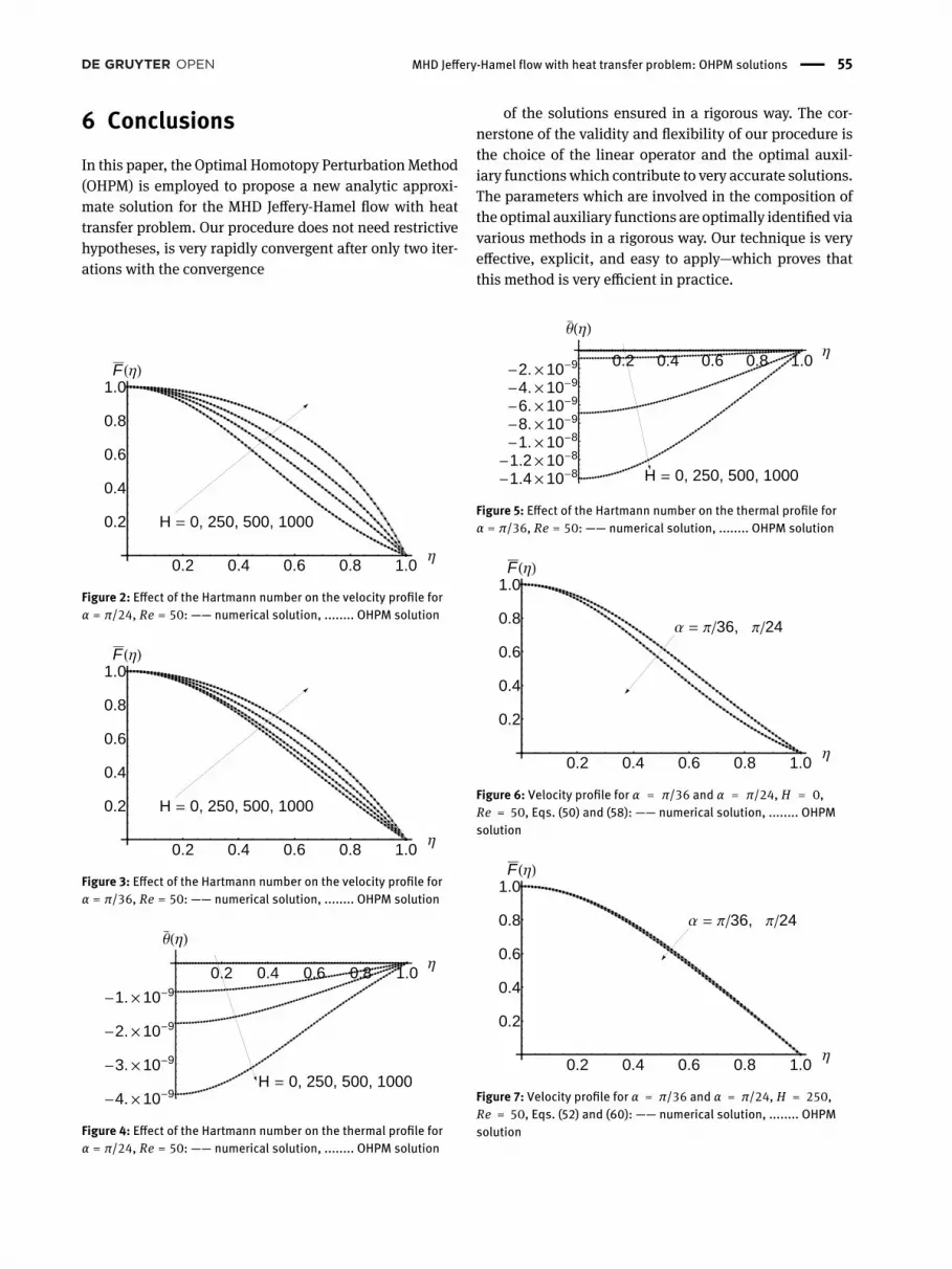
6 ConclusionsIn this paper, the Optimal Homotopy PerturbationMethod(OHPM) is employed to propose a new analytic approxi-mate solution for the MHD Jeffery-Hamel flow with heattransfer problem. Our procedure does not need restrictivehypotheses, is very rapidly convergent after only two iter-ations with the convergence
H = 0, 250, 500, 1000
0.2 0.4 0.6 0.8 1.0Η
0.2
0.4
0.6
0.8
1.0FHΗL
Figure 2: Effect of the Hartmann number on the velocity profile forα = π/24, Re = 50: —— numerical solution, ........ OHPM solution
H = 0, 250, 500, 1000
0.2 0.4 0.6 0.8 1.0Η
0.2
0.4
0.6
0.8
1.0FHΗL
Figure 3: Effect of the Hartmann number on the velocity profile forα = π/36, Re = 50: —— numerical solution, ........ OHPM solution
H = 0, 250, 500, 1000
0.2 0.4 0.6 0.8 1.0Η
-4.´10-9
-3.´10-9
-2.´10-9
-1.´10-9
Θ�HΗL
Figure 4: Effect of the Hartmann number on the thermal profile forα = π/24, Re = 50: —— numerical solution, ........ OHPM solution
of the solutions ensured in a rigorous way. The cor-nerstone of the validity and flexibility of our procedure isthe choice of the linear operator and the optimal auxil-iary functionswhich contribute to very accurate solutions.The parameters which are involved in the composition ofthe optimal auxiliary functions are optimally identified viavarious methods in a rigorous way. Our technique is veryeffective, explicit, and easy to apply—which proves thatthis method is very efficient in practice.
H = 0, 250, 500, 1000
0.2 0.4 0.6 0.8 1.0Η
-1.4´10-8-1.2´10-8-1.´10-8-8.´10-9-6.´10-9-4.´10-9-2.´10-9
Θ�HΗL
Figure 5: Effect of the Hartmann number on the thermal profile forα = π/36, Re = 50: —— numerical solution, ........ OHPM solution
Α = Π�36, Π�24
0.2 0.4 0.6 0.8 1.0Η
0.2
0.4
0.6
0.8
1.0FHΗL
Figure 6: Velocity profile for α = π/36 and α = π/24, H = 0,Re = 50, Eqs. (50) and (58): —— numerical solution, ........ OHPMsolution
Α = Π�36, Π�24
0.2 0.4 0.6 0.8 1.0Η
0.2
0.4
0.6
0.8
1.0FHΗL
Figure 7: Velocity profile for α = π/36 and α = π/24, H = 250,Re = 50, Eqs. (52) and (60): —— numerical solution, ........ OHPMsolution
56 | V. Marinca and R.-D. Ene
Α = Π�36, Π�24
0.2 0.4 0.6 0.8 1.0Η
0.2
0.4
0.6
0.8
1.0FHΗL
Figure 8: Velocity profile for α = π/36 and α = π/24, H = 500,Re = 50, Eqs. (54) and (62): —— numerical solution, ........ OHPMsolution
Α = Π�36, Π�24
0.2 0.4 0.6 0.8 1.0Η
0.2
0.4
0.6
0.8
1.0FHΗL
Figure 9: Velocity profile for α = π/36 and α = π/24, H = 1000,Re = 50, Eqs. (56) and (64): —— numerical solution, ........ OHPMsolution
Α = Π�36, Π�24
0.2 0.4 0.6 0.8 1.0Η
-2.5´10-11
-2.´10-11
-1.5´10-11
-1.´10-11
-5.´10-12
Θ�HΗL
Figure 10: Thermal profile for α = π/36 and α = π/24, H = 0,Re = 50, Eqs. (51) and (59): —— numerical solution, ........ OHPMsolution
Conflict of Interests: The authors declare that there is noconflict of interests regarding the publication of this paper.
References[1] Jeffery G. B., The two-dimensional steady motion of a viscous
fluid, Philos. Mag. A, 1915, 6(20), 455–465.
Α = Π�36, Π�24
0.2 0.4 0.6 0.8 1.0Η
-3.5´10-9
-3.´10-9
-2.5´10-9
-2.´10-9
-1.5´10-9
-1.´10-9
-5.´10-10
Θ�HΗL
Figure 11: Thermal profile for α = π/36 and α = π/24, H = 250,Re = 50, Eqs. (53) and (61): —— numerical solution, ........ OHPMsolution
Α = Π�36, Π�24
0.2 0.4 0.6 0.8 1.0Η
-7.´10-9
-6.´10-9
-5.´10-9
-4.´10-9
-3.´10-9
-2.´10-9
-1.´10-9
Θ�HΗL
Figure 12: Thermal profile for α = π/36 and α = π/24, H = 500,Re = 50, Eqs. (55) and (63): —— numerical solution, ........ OHPMsolution
Α = Π�36, Π�24
0.2 0.4 0.6 0.8 1.0Η
-1.4´10-8
-1.2´10-8
-1.´10-8
-8.´10-9
-6.´10-9
-4.´10-9
-2.´10-9
Θ�HΗL
Figure 13: Thermal profile for α = π/36 and α = π/24, H = 1000,Re = 50, Eqs. (57) and (65): —— numerical solution, ........ OHPMsolution
[2] Hamel G., Spiralformige bewegungen zaher flussigkeiten,Jahresbericht der Deutschen Mathematiker-Vereinigung, 1916,25, 34–60.
[3] Rivkind L., Solonnikov V. A., Jeffery-Hamel asymptotics forsteady state Navier-Stokes flow in domains with sector-like out-lets to infinity, J. Math. Fluid Mech., 2000, 2, 324–352.
[4] Akulenko L. D., Georgevskii D. V., Kumakshev S. A., Solutions ofthe Jeffery-Hamel problem regularly extendable in the Reynoldsnumber, Fluid Dyn., 2004, 39(1), 12–28.
[5] Makinde O. D., Mhone P. Y., Hermite-Padé approximation ap-proach toMHD Jeffery-Hamel flows, Appl. Math. Comput., 2006,181, 966–972.
[6] Esmaili Q., Ramiar A., Alizadeh E., Ganji D. D., An approximationof the analytical solution of the Jeffery-Hamel flow by decompo-

MHD Jeffery-Hamel flow with heat transfer problem: OHPM solutions | 57
sition method, Phys. Lett., 2008, 372, 3434–3439.[7] Ganji Z. Z., Ganji D. D., Esmaeilpour M., Study of nonlinear
Jeffery-Hamel flow by He’s semi-analytical methods and com-parison with numerical results, Comput. Math. Appl., 2009, 58,2107–2116.
[8] Joneidi A. A., Domairry G., Babaelahi M., Three analytical meth-ods applied to Jeffery-Hamel flow, Commun. Nonlinear Sci. Nu-mer. Simul., 2010, 15, 3423–3434.
[9] Moghimi S. M., Ganji D. D., Bararnia H., Hosseini M., JalbalM., Homotopy perturbation method for nonlinear MHD Jeffery-Hamel problem, Comput. Math. Appl., 2011, 61, 2213–2216.
[10] Marinca V., Herisanu N., An optimal homotopy asymptotic ap-proach applied to nonlinear MHD Jeffery-Hamel flow, Math.Probl. Eng., 2011, Article ID 169056, 16 pages.
[11] Esmaeilpour M., Ganji D. D., Solution of the Jeffery-Hamel flowproblem by optimal homotopy asymptotic method, Comput.Math. Appl., 2010, 59, 3405–3411.
[12] Sheikholeshami M., Ganji D. D., Ashorynejad H. R., RokniH. B., Analytical investigation of Jeffery-Hamel flow with highmagnetic fiwld and nanoparticle by Adomian decompositionmethod, Appl. Math. Mech.-Engl., 2012, 33(1), 25–36.
[13] Rostami A. K., Akbari M. R., Ganji D. D., Heydari S., InvestigatingJeffery-Hamel flow with high-magnetic field and nanoparticlesby HPM and AGM, Cent. Eur. J. Eng., 2014, 4(4), 357–370.
[14] Raja M. A. Z., Samar R., Numerical treatment of nonlinear MHDJeffery-Hamel problems using stochastic algorithms, Comput.Fluids, 2014, 91, 111–115.
[15] Yang X.-J., Tenreiro Machado J. A., Baleanu D., Cattani C., Onexact traveling-wave solutions for local fractional Korteweg-deVries equation, Chaos, 2016, 26, Article ID 084312.
[16] Yang X.-J., Tenreiro Machado J. A., Hristov J., Nonlinear dynam-ics for local fractional Burgers’ equation arising in frctal flow,Nonlinear Dynam., 2016, 84, 3–7.
[17] Jafari H., Ghorbani M., Ebadattalab E., Moallem R., Baleanu D.,Optimal homotopy asymptotic method - a tool for solving fuzzydifferential equations, J. Comput. Complex. Appl., 2016, 2(4),112–123.
[18] Kakuda K., Tosaka N., The generalized boundary element ap-proach to Burgers’ equation, Int. J. Numer. Meth. Eng., 1990,29(2), 245–261.
[19] Marinca V., Herişanu N., Nonlinear Dynamical Systems in Engi-neering - Some Approximate Approaches, Springer Verlag, Hei-delberg, 2011.
[20] Marinca V., Herişanu N., Nonlinear dynamic analysis of an elec-trical machine rotor-bearing system by the optimal homotopyperturbation method, Comput. Math. Appl., 2011, 61, 2019–2024.
[21] Herişanu N., Marinca V., Optimal homotopy perturbationmethod for a non-conservative dynamical system of a rotatingelectrical machine, Z. Naturforsch A, 2012, 67a, 509–516.
[22] Schlichting H., Boundary-layer theory, Mc Graw-Hill Book Com-pany, 1979.
[23] Ali F.M., Nazar R., ArifinN.M., Pop I.,MHD stagnation-point flowand heat transfer towards a stretching sheet with induced mag-netic field, Appl. Math. Mech.-Engl., 2011, 32, 409–418.
[24] Choi S. H., Wilhelm H.-E., Incompressible magnetohydrody-namic flow with heat transfer between inclined walls, Phys. Flu-ids, 1979, 22, 1073–1078.
[25] Turkylmazoglu M., Extending the traditional Jeffery-Hamel flowto strechable convergent / divergent channels, Comput. Fluids,2014, 100, 196–203.
[26] He J. H., A coupling method of homotopy technique and pertur-bation technique for nonlinear problems, Int. J. Nonlin. Mech.,2000, 35, 37–43.


