Optimal Design for a Study of Butadiene Toxicokinetics in Humans

Frederic Y. Bois,*,1 Thomas J. Smith,† Andrew Gelman,‡ Ho-Yuan Chang,† and Andrew E. Smith†

*Lawrence Berkeley National Laboratory, Berkeley, California;†Harvard School of Public Health, Boston, Massachusetts; and ‡Statistics Department,Columbia University, New York, New York

Received September 4, 1998; accepted February 28, 1999

The derivation of the optimal design for an upcoming toxicoki-netic study of butadiene in humans is presented. The specific goalof the planned study is to obtain a precise estimate of butadienemetabolic clearance for each study subject, together with a goodcharacterization of its population variance. We used a two-com-partment toxicokinetic model, imbedded in a hierarchical popu-lation model of variability, in conjunction with a preliminary set ofbutadiene kinetic data in humans, as a basis for design optimiza-tion. Optimization was performed using Monte Carlo simulations.Candidate designs differed in the number and timing of exhaledair samples to be collected. Simulations indicated that only 10 airsamples should be necessary to obtain a coefficient of variation of15% for the estimated clearance rate, if the timing of those samplesis properly chosen. Optimal sampling times were found to closelybracket the end of exposure. This efficient design will allow therecruitment of more subjects in the study, in particular to matchprescribed levels of accuracy in the estimate of the populationvariance of the butadiene metabolic rate constant. The techniquespresented here have general applicability to the design of humanand animal toxicology studies.

Key Words: butadiene population toxicokinetics; human inha-lation experiments; Markov chain Monte Carlo simulations; opti-mal experimental design.

An individual’s risk from exposure to a metabolicallyactivated or detoxified agent is defined by the intensity andduration of internal exposure in combination with physio-logic and genetic factors that control metabolic enzymeactivity. Individuals with the highest exposure intensityandthe highest rate of activation and/or the slowest deactivationrates will have the highest levels of the active metabolite,and over time the highest risk. Consequently, the averagerisk per unit of exposure for epidemiologic studies willdepend in part on the population’s distribution of metabolicphenotypes. Thus, knowledge of human metabolic rates canbe critical to the estimation of risk from occupational andenvironmental exposures, and for extrapolating risk fromone population to another. Unfortunately, in most cases,

these data are unavailable. Animal bioassay data are com-monly used to estimate the quantitative risks of chemicalexposures and fill the gaps in human data. Animal risks canbe extrapolated to humans using a variety of toxicologicapproaches, most recently physiologic-pharmacokinetic(PBPK) modeling (National Research Council (NRC), 1994;Ramsey and Andersen, 1984; Reitzet al., 1988). The com-mon approach is to “scale-up” rodent models to humans,making some allowance for species differences in metabolicrates on the basis ofin vitro data (when available). How-ever, because of differences in metabolism, there can beconsiderable interspecies variation in potency in animalbioassays, which prevents simple extrapolations to humans.Without human data, it is impossible to determine whetherhumans are similar to the most sensitive species, or not.Consequently, it is important to obtain human metabolicdata to characterize human risks of exposure for prevalenthazards.

Timed sets of samples of exhaled breath, urine, or bloodduring and after a measured exposure are useful to estimatehuman metabolic rates. These data can potentially be obtainedby 3 strategies: evaluation of environmentally or occupation-ally exposed subjects, or laboratory exposures of volunteers.The first 2 approaches are conceptually possible, but highlyimpractical. In the field, it is rarely possible to obtain a tem-poral control of exposure, or to collect precisely timed series ofbiological samples. Properly executed laboratory studies ofbrief, low-level exposures can produce high quality data toestimate apparent metabolic rates and intersubject variability.These studies must use protocols approved by a human-sub-jects review committee to insure that risks for the subjects areminimal. Study approval is possible if several conditions aremet: (1) environmental and occupational exposures to the agentare common, (2) the lifetime risk of the lab exposure is lessthan one per million using standard, most-sensitive species riskassessment procedures (California Environmental ProtectionAgency Air Resources Board, 1992), and (3) volunteers arefully informed that the exposure may produce a small increasein their lifetime risk of a health effect.

Our primary goal in this work was to define an efficienttesting protocol for assessing 1,3-butadiene metabolic clear-ance in human volunteers.

1 To whom correspondence should be sent at B3E–INSERM U444, Faculte´de Medecine St. Antoine, 27 rue Chaligny, 75012 Paris, France. Fax: 011 331 44 73 84 62. E-mail: fbois@diana.lbl.gov.

TOXICOLOGICAL SCIENCES49, 213–224 (1999)Copyright © 1999 by the Society of Toxicology

213

1,3-Butadiene as a Model Compound

Environmental and occupational exposures to butadiene arecommon, because it is a component of urban air pollution(0.001 ppm) (Mullins, 1990; U.S. Environmental ProtectionAgency, 1989), cigarette smoke (2 ppm) (Brunnemannet al.,1990), and gasoline vapors (0.01 ppm) (Rappaportet al.,1987), while occupational exposures range from 0.01 ppm to300 ppm (Fajenet al., 1990). The cumulative exposures rangefrom 8.8 ppm3 h (i.e., 8.8 ppm for 1 h or 4.4 ppm for 2 hetc.)per year for urban air pollution to 2,000 ppm3 h per year fora 1 ppm average occupational exposure.

Considerable data have been accumulated to suggest thatbutadiene is an animal carcinogen, and may be a humancarcinogen. The U.S. EPA classified 1,3-butadiene as a “prob-able human carcinogen” (Group 2B) on the basis of 2 rodentinhalation studies, where the rodent exposures ranged from18,000 to 750,000 ppm3 h accumulated in daily exposuresover a year or more (U.S. Environmental Protection Agency,1985). The International Agency for Research on Cancer(IARC, 1992) has given 1,3-butadiene a rating of 2A, which is“probably carcinogenic in humans.” This determination wasbased on both animal and epidemiologic studies. Recently,IARC has re-examined the epidemiologic evidence on buta-diene and concluded that it was not possible to separate po-tential effects of styrene and other exposures from those ofbutadiene, so the classification was left at 2A. The U.S. Occu-pational Safety and Health Administration (OSHA) recentlyreduced the allowable daily occupational exposure to 2.0 ppmfor 8 h (16 ppm3 h) for butadiene. There is considerableinterest in the human risks of butadiene exposures.

The California EPA (1992) performed a population riskassessment assuming a continuous 1 ppm exposure for 70 years(6.13 105 ppm3 h) based on tumor rates for mice, which arethe most sensitive species. The lifetime risk of cancer rangedfrom 1.43 10–4 to 0.8. However, if the rat tumor rates are usedinstead of the mouse, the lifetime risks are orders of magnitudelower because of differences in rat and mouse metabolism ofbutadiene. Based onin vitro metabolism measurements onmouse, rat, and human tissue samples, it appears that humansmay be more like rats than mice (Bondet al., 1996; Csanadyet al., 1992; Johanson and Filser, 1996). Thus, it is importantto measure human metabolic rates to assess human risks.

Optimizing Design of Volunteer Exposures to Butadiene

The purpose of the study reported here was to help developa human testing protocol that would maximize the precision ofestimates for butadiene metabolic rate and its population vari-ance, while minimizing the number of breath samples taken(and specifying their optimal timing). As we sought to exposethe subjects to a minimal risk of toxicity, exposure concentra-tion and length were not optimized but set, according to criteriaof risk and feasibility. Preliminary experiments in Dr. Chang’slaboratory, using an approved human subjects protocol, used

inhalation exposures of 5.0 ppm for 2 h, 10 ppm3 h, equiv-alent to about one day of occupational exposure allowed underOSHA rules. These data, whose collection is described below,were used as a training set for our analysis. Taking advantageof improved analytical sensitivity, the exposure protocol forthe planned experiments has been set to 2.0 ppm for 20 min(i.e., 0.67 ppm3 h). We were left with defining the numberand timing of breath samples for these future experiments. Tothat effect, we present a new method for experimental designoptimization, based on Monte Carlo simulations. Our methodhas the advantage of following naturally from the Markovchain Monte Carlo techniques applicable to population phar-macokinetic models (Boiset al., 1996a,b; Gelmanet al., 1996;Wakefield, 1996).

MATERIALS AND METHODS

Preliminary data. Eight human volunteers were recruited and tested in Dr.Chang’s laboratory at the National Cheng Kung University, College of Med-icine, in Taiwan, Taiwan. The tests were conducted, under informed consent,with an Institutional Review Board-approved human subjects protocol. Theconsent form clearly indicated that 1,3-butadiene is a suspected human car-cinogen and that exposure to it may cause a small increase in the subject’slifetime risk of cancer. An inhalation exposure of 5 ppm for 2 h, (i.e.,10 ppm3hr, equivalent to about one day of occupational exposure allowed under OSHArules), was chosen. That exposure was the minimum that could be preciselymeasured, and was well below Taiwan’s allowable occupational exposure of10 ppm per 8-h work day for a working lifetime. The exposure was generatedusing a permeation tube, dynamic calibration apparatus (Metronics Assoc. Inc.,Palo Alto, CA) that is designed to produce parts-per-million concentrations. Inthis apparatus, a liquefied calibration gas slowly permeates through the wallsof a Teflon tube, which is sealed with double stainless steel balls at either end(O’Keefe and Ortman, 1966). The operating temperature is tightly controlled,so the permeation tube releases gas at a fixed low rate, and can be used as aprimary standard by periodically weighing the tube. After testing the minuteventilation rate of each subject before experiment, the default flow rate was setat 11.50 L/min, which included the flow rate of the permeation apparatus (0.18L/min) and a dilution flow rate of 11.32 L/min. Three permeation tubes wereused in the permeation chamber of the standard gas generator and eachgenerated 42.5mg/min at the flow rate of 0.18 L/min. Together with thedilution flow this gives a final concentration of 5.0 ppm of butadiene. This gasflowed into a reservoir Tedlart bag, which provided sufficient capacity to meetthe cyclic demand of the subject’s breathing. To accommodate differences inthe basic ventilation rate of each subject, a bypass was also included to releaseexcess gas flow before it entered the reservoir bag. The flow rates out of thestandard gas generator and for the dilution system are critical determinants ofthe accuracy of the butadiene concentration generated; therefore, the flow rateswere calibrated and measured before and after each exposure experiment.Additionally, before and after each exposure, an air sample was collected fromthe exposure system to measure, by gas chromatography (GC) analysis, theexact concentration of butadiene being produced. This is a very safe exposuresystem, which has little risk of overexposure from errors in dilution oraccidental releases.

Subjects were evaluated by a physician to verify their health and absence ofmedical problems that might affect their metabolism, and to verify that theyunderstood the possible cancer risk. Body weight (Bw) was recorded (Table 1).No specific dietary information was collected at the time of testing. Subjectswere seated and exposed by facemask. A one-way valve in the mask allowedthe subjects to draw in breathing air with butadiene and to exhale into either ahood or a 15 L. Tedlart breath-collection bag. At most, 41 timed one-minbreath samples were collected: 11 during the 2-h exposure (every 10 min); and

214 BOIS ET AL.

30 during the 57-min post-exposure period (every min for the first 10 min,every 2 min for the next 20 min, then every 3 min for the remaining 27 min).Some subjects had less than 41 samples collected (a few sample times weremissed), the lowest number of samples collected was 32. To avoid residualcontamination, different masks were used during exposure and after exposure.Minute ventilation (Kin) was estimated for each subject by measuring thevolume of breath collected in the breath samples (Table 1). Replicate deter-minations ofKin had a coefficient of variation (CV) of 2%. Immediately aftercollection, the breath was drawn from the bag through a tributyl catechol(TBC, to prevent self-polymerization) treated charcoal tube at 100 ml/min.Butadiene adsorbed on the charcoal tubes was desorbed with heptane andanalyzed by GC using a flame ionization detector and a 50 m, 0.32 mm, ODfused silica porous layer open tubular column previously coated with Al2O3/KCl. The limit of detection was 0.01 ppm in a 10 L breath sample and thecoefficient of variation (mean/SD) was 5.6% for replicate samples.

For each subject, the butadiene blood/air partition coefficient,Pba, wasmeasured (Table 1) with a method developed by Dr. Chang. A measuredvolume of venous blood (approximately 20 ml) was added to a flask with aseptum, two side arms, and a valve in the bottom. A known amount of purebutadiene was added through a septum, and the flask was equilibrated withoccasional shaking for 30 min at 37°C. Approximately 90% of the blood wasremoved and the volume determined. The remaining butadiene was flushedfrom the flask with nitrogen, into a TBC-treated charcoal tube, under a flow of50 ml/min for 40 min. The butadiene collected was measured by the GCmethod described above. The partition coefficient was calculated from themass of butadiene added (Madded), the measured mass of butadiene flushed fromthe air and residual blood in the flask (Ma1r), the volume of the flask (Vflask), andthe volumes of blood added (VBadded) and removed (VBrm). The mass ofbutadiene in the blood removed isMb 5 Madded – Ma1r, and the volume of airin the flask isVair 5 Vflask – VBadded. The formula used is:

Pba 5Mb /VBrm

SMa1r 2 MbSVBadded

VBrm2 1DD /Vair

Replicate determinations ofPba had a CV of 16%. No compensation wasattempted for variations in blood lipids associated with meals consumed beforethe testing was performed. However, the normal Taiwanese diet is a low fatdiet, so the change in blood lipids is likely to have been small.

Toxicokinetic/statistical model. A standard two-compartment toxicoki-netic model was selected to describe the above data and conduct the designoptimization. Preliminary work (not reported) had shown that a two-compart-ment model in which metabolism took place in the peripheral compartment ledto the same estimates of metabolic rate; that model was therefore not consid-ered here. In addition, a one-compartment model was unable to correctlydescribe the data (this was assessed using the statistical techniques described

below). We chose the simplest compartmental model able to correctly describethe data at hand. A discussion of the possible physiological meaning of the 2compartments is not in order,a priori, and will be presented in the Resultssection, on the basis of the posterior parameter values obtained. The modeladopted here assumes that metabolic elimination takes place in the centralcompartment (Fig. 1). It corresponds to the following set of differentialequations:

5­Qcentral

­t5 KinCinhaled 1

Kcp

Ppc

Qperiph

Vp2 SKcp 1

Kin

PcaDQcentral

Vc2 KmetQcentral

­Qperiph

­t5 Kcp

Qcentral

Vc2

Kcp

Ppc

Qperiph

Vp

­Qmetab

­t5 KmetQcentral (1)

where Qcentral and Qperiph are the quantities of butadiene in the central andperipheral compartments, respectively (in mmoles).Cinhaled is the inhalationconcentration (in mmoles/L);Kin is the minute ventilation rate (in L/min);Kcp

is the rate constant for distribution from the central to the peripheral compart-ment (in L/min);Ppc is the peripheral over central partition coefficient (dimen-sionless);Vc and Vp are the volumes (in L) of the central and peripheralcompartments, respectively;Pca is the central over air partition coefficient(dimensionless);Kmet is the butadiene metabolic rate constant (in min–1), whichhere is the parameter of primary interest. The concentration of butadiene inexhaled air (in mmol/L) was given by the algebraic equation:

Cexhaled50.7 z Qcentral

Pa z Vc1 0.3 z Cinhaled (2)

which assumes a physiological pulmonary dead space of 30%.Central volume was scaled to body weight,Bw (in kg), and its scaling

coefficient,sc_Vc, was the parameter actually estimated:

Vc 5 sc_Vc 3 Bw (3)

It can be noticed, in Equation 1 thatPpc andVp are not separately identifiable,and therefore their product was defined as one parameter,PpcVp.

The above equations were coded for the MCSim simulation software and

FIG. 1. Schematic representation of the toxicokinetic 2-compartmentmodel used. The model parameters are first order rate constants, partitioncoefficients and volumes (see text).

TABLE 1Physiological Characteristics Measured for Each of the Eight

Human Subjects Studied in Preliminary Experiments

Subject IDBody weight

(Bw, kg)Minute ventilationrate (Kin, L/min)

Blood/air partitioncoefficient (Pba)

A 71 8.4 1.5B 68 7.1 1.8C 60 6.0 0.9D 50 4.5 1.3E 67.5 7.8 1.4F 70 7.8 1.3G 64 7.6 1.1H 48 5.0 1.3

215OPTIMAL DESIGN OF TOXICOKINETIC STUDIES

solved with the Lsodes integrator (Bois and Maszle, 1997; Maszle and Bois,1993).

The 2-compartment toxicokinetic model was imbedded in a hierarchicalpopulation model (Fig. 2) to describe the various levels of variability presentin the data, according to a population toxicokinetic approach (Boiset al.,1996b). At the individual level, for each subject, the data (y) consisted ofexhaled air concentrations of butadiene, blood to air partition coefficients, (Pba,used to estimatePca), and minute ventilation rate,Kin, all measured experi-mentally with uncertainty. Body weight,Bw, relatively precisely measured,was considered as a covariate. The expected values of the exhaled air concen-trations are a function (ƒ) of exposure level (E), time (t), a set of physiologicalparameters ofa priori unknown values (u, which includessc_Vc, Kcp, PpcVp,Kmet, Kin, andPca), andBw. E, t, u, andBw were subject-specific. The functionƒ was the toxicokinetic model described above. The data collected were alsoaffected by measurement and modeling errors, which were assumed, as usual,to be independent and log-normally distributed, with mean of zero and vari-ances2 (on the log scale). The variance vectors2 had three components:s2

1

for butadiene exhaled air concentrations,s22 for blood over air partition

coefficients, ands23 for minute ventilation rates.

At the population level, the individual parameters,u, were assumed to bedistributed normally (in log-space) around a population meanm, with popu-lation varianceS2.

The hierarchical population model is symbolically illustrated by Figure 2.Three types of nodes are featured in the figure: square nodes representvariables for which the values are known by observation, such asy or Bw, orwere fixed by us, such asE andt, or the priors ons2, m andS2; circular nodesrepresent variables with unknown values, such asu, s2, m, or S2; the trianglerepresents the deterministic compartmental model ƒ.

An arrow between two nodes indicates a direct statistical dependencebetween the variables of those nodes.

The model ƒ was non-physiological and we had no prior information on itsparametersu. Therefore, uniform (i.e., non informative) prior distributionswere used for the population meansm. For the population variancesS2,inverse-gamma priors were used; inverse-gamma priors are standard referencepriors for unknown variances (Bernardo and Smith, 1994). Their shape pa-rameters were set to 1, and their scales were chosen to correspond to 20% CVfor all parameters, except forKmet. CVs of about 20% have been found fordistribution parameters in other studies (Boiset al., 1996a; Gelmanet al.,1996). ForKmet, the scale corresponded to 100% CV, because we expectedapriori the population variability for this parameter to be higher than for theothers, and a factor 2 variability is commensurate with values found in theliterature on variability of metabolic parameters (Boiset al., 1996b). Fors2

1,we used the standard non-informative prior distributionP(s2

1) ˜ s21. The

experimental variancess22 ands2

3 were knowna priori (see Preliminary Datasection, above) and set to the corresponding values.

From Bayes’ theorem, the joint posterior distribution of the parameters toestimate,P(u, s2, m, S2 | y, Bw, E, t) is proportional to the likelihood of thedata multiplied by the parameters’ priors:

P~u, s 2, m, S 2y, Bw, E, t ! , P~yu, s 2, Bw, E, t !

z P~um, S 2! z P~s 2! z P~m! z P~S 2!. (4)

where:P(u, s2, m, S2 | y, Bw, E, t) is the joint posterior distribution,P(y | u, s2, Bw, E, t) is the likelihood of the data,P(u u m, S2) is the conditional distribution ofu, given m andS2,P(s2), P(m), andP(S2) are the prior distributions (as specified above) for

s2, m, andS2, respectively.The likelihood term was given by the lognormal measurement model:

log~y! ; 1~log f ~u, Bw, E, t !, s 2! (5)

Current standard practice in Bayesian statistics is to summarize a compli-cated high-dimensional posterior distribution (such as that given by Eq. 4) byrandom draws from the conditional distribution of each individual modelparameter, given the other parameters (Smith and Roberts, 1993). This can beshown equivalent, at equilibrium, to random draws from their joint posteriordistribution (Smith and Roberts, 1993). By conditional independence argu-ments, the conditional distributions of individual model components are sim-pler than Equation 4:

P~us 2, m, S 2, y, Bw, E, t ! , P~yu, s 2, Bw, E, t ! z P~um, S 2! (6)

P~mu, s 2, S 2, y, Bw, E, t ! , P~um, S 2! z P~m! (7)

P~S 2u, s 2, m, y, Bw, E, t ! , P~u, m, S 2! z P~S 2! (8)

P~s 2u, m, S 2, y, Bw, E, t ! , P~yu, s 2, Bw, E, t ! z P~s 2! (9)

Each term on the right can be numerically evaluated, given the distributionalassumptions listed above. We used Metropolis-Hasting sampling to updateeach parameter in its turn (using Eqs. 6–9), therefore performing a randomwalk through the posterior distribution. This iterative sampling belongs to aclass of Markov chain Monte Carlo (MCMC) techniques that has recentlyreceived much interest (Gelfand and Smith, 1990; Gelman, 1992; Gelman andRubin, 1996; Gilkset al., 1996; Wakefieldet al., 1994). Two independentMarkov chain Monte Carlo runs were performed for each computation. Con-vergence was monitored using the method of Gelman and Rubin (1992). Oncea posterior sample of parameter values is obtained, further simulations can thenbe performed to compute, under specified conditions, posterior distributions ofestimands of interest (e.g., a total quantity of metabolites formed).

FIG. 2. Graph of the hierarchical statistical model describing dependen-cies between groups of variables. Symbols are:P, prior distributions;m: meanpopulation parameters;S2, variances of the parameters in the population;E,butadiene exposure concentrations;t, experimental sampling times;u, un-known physiological parameters;Bw, body weight, exactly measured; ƒ, PBPKmodel; y, measured butadiene concentration (in exhaled air) and measuredvalues ofKin andPba; s2, variances of the experimental measurements. Squarenodes represent variables of known value; circular nodes represent unknownvariables; the triangle represents the deterministic physiological model.

216 BOIS ET AL.

Optimal design determination. The Harvard School of Public HealthInstitutional Review Board has approved, for our planned study, a protocolsimilar to the one used for preliminary experiments. The planned exposurelevel was reduced to 2 ppm for 20 min (instead of the 5 ppm for a 2-h exposure,used here). This exposure represents an inhalation dose similar to that receivedduring everyday life from exposure to urban air pollution, passive cigarettesmoke, gasoline vapors, and automobile exhaust. Subjects will be paid anominal amount (equal to 6 h of alaboratory technician’s salary) to compen-sate for the discomfort of the procedure, time required, and any travel ex-penses. The study has been approved by the Institutional Review Boardbecause (1) the planned exposures will be in the range of everyday ambientinhalation doses, (2) they will be below the allowable occupational exposures,(3) the subjects will be well informed about the carcinogenic potential of1,3-butadiene and its resulting risk (less than 1/106 based on California EPAmethodology, extrapolating from the mouse, the most sensitive species), and(4) data about human metabolism of 1,3-butadiene are critically needed forpopulation risk assessments of ambient and occupational exposures.

We were faced with the problem of defining the number and timing of breathsamples for the planned experiments. The method used to optimize that part ofthe design is based on decision theory, as presented for example by Mu¨ller andParmigiani (1995): the goal of collecting and analyzing data is to makedecisions. Such decisions may range from addressing an estimation problemunder squared error loss (the usual least-square estimation) to recommendinga certain treatment in clinical settings. Each decision has a payoff, and anyrational decision-maker should take the decision leading to maximum payoff.That payoff depends on some set of unknown quantities,u, taking values in aset of possibilitiesQ and havinga priori distributionP. In our case, one canthink of the payoff as ”being right about the value ofKmet,” of the decision as“publishing thatKmet is equal to 0.1,” and ofu as being the true value ofKmet.In scientific research, experiments are typically conducted to gain additionalknowledge ofu. The usual sequence of actions in an experiment is:

1. Choose a designe among all possible experiments;2. Conduct the experiment and observe datay*. The data are assumed to

have as probability model (i.e., error model) ƒe(y*/u);3. Make a final decisiond, knowingy*, to reportur as value foru, so as to

maximize the payoffU(e, d, u). The payoff can be, for example, inverselyproportional to the square of the difference betweenur andu.

In addition, recruiting subjects and collecting data involve costs, which maydepend on the design, as well as onu or y*. The cost function is C(e, y*, u).From a theoretical point of view, consistent with the expected utility principle(Bernardo and Smith, 1994), the optimal experiment is that which maximizesthe function:

U~e! 5 Ey,Q

@U~e, d, u! 2 C~e, y*, u!#dPe~u, y*! (10)

wherePe is the joint distribution ofy* andu. The interpretation ofU(e) is quitesimple: it is the expected value, over all possible parameter values and dataoutcomes (i.e. future observations) of the net utility (cost subtracted) ofperforming experimente.

Cost depends on the number of recruited subjects and on the number ofmeasurements made. We chose here to neglect costs because we wanted tofocus on the scientific question of precisely identifyingKmet. As a utilityfunction we chose:

U~e, d, u! 5 2 ~log Kmet 2 E@log Kmetu#! 2 (11)

whereE(z) denotes mathematical expectation. This corresponds to measuringutility by the opposite of the variance of the parameter of interest,Kmet (i.e., thesmaller the variance ofKmet the greater the utility of the design). We evaluatedthe expected utilityU(e) in Equation 10 by averaging over the distribution ofu giveny* and averaging over the distribution ofy* givene andu. We did theaveraging by simulation (randomly sampling from the distributions and form-

ing the sample averages). The analysis of the preliminary data by MCMCsimulations provided us with a set of parameter vectors sampled from theirjoint posterior distribution. Those vectors were used to simulate datasets for therange of possible future experiments. Using each dataset, we then obtained anupdated posterior variance forKmet. Finally the averageKmet variance, over alldatasets (according to Eq. 10), was used to select the most informativeexperiment,i.e. the one leading to the smallest estimation variance.

More precisely,N parameter sets (u*) (corresponding to ”individuals”) weregenerated by sampling one random parameter vector from1(m,S2), for each ofN pairs ofm andS2 obtained by the MCMC sampling. Half ofN u* vectorswere then used as input to the model to create as many predicted datasets (y9).Each dataset included the same numberM of data points, obtained along a gridof time values (tj, j 5 1 … M). Simulated experimental noise was added to thepredictions data as specified by the measurement error model (Eq. 5) andN/2estimates of experimental variance, obtained by MCMC sampling.

Even along a small grid of design points, the number of possible combina-tions can be enormous (e.g., there are 1,099,511,627,776 possibilities with 40points). To avoid searching the entire design space, our algorithm proceededheuristically, along 2 directions: forward or backward (Atkinson and Donev,1992). In the “forward” mode, the algorithm started with no points in thedesign,i.e. from the prior knowledge. The criterion variances2 (variance ofKmet) was directly obtained fromu* since Kmet was included inu* (if thevariance of a model prediction were of interest, the model should first be usedto compute those predictions for eachu9). At the next step, each possibleposition,j, of a design point along the time-grid was examined for its potentialat reducing the criterion variance. For each design pointj and each datasety9,the variance estimate was computed by importance reweighting (Bernardo andSmith, 1994), given the corresponding datumy9 j. The reweighted estimate ofvariance for any variablef (model parameter or prediction) is given by:

s2 5 Oi

N

r i~w i 2 w# ! 2 (12)

where the average is:

w# 5 Oi

N

r iw i (13)

the importance weights are:

r i 5 Li /Oi

N

Li (14)

where Li is the likelihood of the datumy9 j given u9 i, under the lognormalmeasurement model (Eq. 5). The variance estimates obtained were averagedover all N/2 datasets, according to Equation 10. The point giving the lowestvariance forKmet was selected and definitely included in the design, closing thatstep. The algorithm then went on to determine the best time point for a secondposition and so on, iteratively, until all candidate design points were included.In the ”backward” mode, all time points were included at start and thealgorithm removed sequentially the least informative points, until the nulldesign was reached.

The MCSim software (Bois and Maszle, 1997; Maszle and Bois, 1993), hasbeen extended to perform the above calculations and was used throughout.

RESULTS

Adjustment of the Population Model to Butadiene Data

To parameterize the butadiene population pharmacokineticmodel, two Markov chains of 50,000 iterations each were run.

217OPTIMAL DESIGN OF TOXICOKINETIC STUDIES

After 10,000 iterations, the trajectory of each parameter startedto oscillate randomly around a mean value, and these oscilla-tions had stabilized to a stationary distribution. The Gelman-Rubin convergence diagnostic less than 1.01 for all parameters,meaning that we would have expected to achieve at most 1%reduction in variance by continuing the simulations. One in 40of the last 40,000 simulations of 2 chains were recorded,yielding 2,000 sets of parameter values from which the infer-ences and predictions presented in the following were made.

Figure 3 presents, for an individual (subject A), the model-predicted time course of butadiene exhaled air concentration,overlaid with the measured values. Predictions were made withthe parameter set of highest posterior density, and with 10parameter sets randomly sampled from their joint posterior.The fit was excellent, and the same was observed for allsubjects. The residuals appeared evenly spread in log-space,indicating that the log-normal error model was reasonable andthat little modeling error was present (observed and predicteddata values differ on average by only 6%, and at most by 25%).Visual inspection of the residuals did not show any evidence ofautocorrelation between them. In this extended design, datasampling was thorough and left little room for model uncer-tainty. A two-compartment model appeared sufficient to de-scribe those data. The posterior geometric mean of the mea-surement SD for butadiene concentrations,s1, was 1.077(6 0.0036), corresponding to a CV of 7.7%. That estimate wasclose to the reported assay error of 5.6%.

Posterior Parameter Distributions

The joint distribution of all population and individual pa-rameters was obtained in output of the MCMC simulations.

This allowed consideration of marginal distributions (distribu-tions of the parameters considered individually), but also ofcorrelations of any order. Summary statistics for the populationparameters means,m, and geometric standard deviations,S, arepresented in Table 2. The volume of the central compartmentrepresented only 8% of the body weight on average. This wasclose to volume of blood in the body. Distribution to theperipheral compartment was fast (corresponding to a half-lifeof 0.6 minutes). It is difficult to comment on the productPpcVp

because of its composite nature; given its value (about 30), theperipheral compartment might correspond to the extra-vascularspace, with large volume, partition coefficient lower than 1 anda fast exchange rate with blood. The metabolic elimination rateconstant corresponded to a half-life of about 3 min. Variabilityacross the 8 individuals was estimated to be 17% CV forsc_Vc

andKcp, 15% forPpcVp, and 50% forKmet. Table 3 presents theposterior distribution ofKmet for each subject (distributions forthe other parameters are not presented). TheseKmet valuescorrespond to clearances of about 1.4 L/min (95% confidenceinterval: 0.45 – 4.1). For all model parameters, individual

FIG. 3. Evolution in time of butadiene concentration in exhaled air forsubject 3 (preliminary experiments). Exposure was to 5 ppm for 2 h. The solidlines correspond to the maximum posterior probability fit and to 10 other fitsfrom randomly-sampled parameter sets. The data are represented by circles.

TABLE 2Summary Statistics for the Posterior Distributions of the Pop-

ulation Geometric Means, m, and Geometric Standard Deviations,S (See Fig. 2 and Corresponding Text), Derived from Analysis ofthe Preliminary Experiments

Model parametera mb Sb

sc_Vc 0.0813 (1.09) [0.0693, 0.0983] 1.17 (1.05) [1.09, 1.33]Kcp 1.21 (1.08) [1.03, 1.42] 1.17 (1.05) [1.09, 1.30]PpcVp 31.5 (1.08) [27.4, 36.6] 1.15 (1.04) [1.09, 1.27]Kmet 0.239 (1.20) [0.165, 0.350] 1.63 (1.14) [1.35, 2.26]Kin 0.373 (1.06) [0.330, 0.423] 1.18 (1.05) [1.11, 1.33]Pca 1.24 (1.10) [1.03, 1.51] 1.25 (1.07) [1.13, 1.46]

a Units: see text.b Summary statistics given: geometric mean (geometric standard deviation)

[2.5th percentile, 97.5th percentile].

TABLE 3Summary Statistics of the Posterior Distributions for Individual

Kmet Values, in Min–1 (Determined from the Preliminary Experi-ments)

SubjectGeometric

meanGeometric

SD2.5th

percentile97.5th

percentile

A 0.284 1.12 0.223 0.350B 0.200 1.13 0.154 0.252C 0.198 1.26 0.121 0.292D 0.249 1.13 0.194 0.317E 0.206 1.16 0.153 0.270F 0.194 1.22 0.125 0.267G 0.270 1.14 0.204 0.346H 0.273 1.12 0.219 0.340

218 BOIS ET AL.

estimates were clustered around the corresponding populationvalues, without “outliers”. Uncertainties (in terms of CV)amounted to 2% to 25% approximately, most of the CVs beingclose to 10%. Parameter estimates were therefore quite precisewith such an extended design. There were however, very largecorrelations between parameter estimates for any given indi-vidual (correlation coefficients ranging in absolute value from0.52 to 0.94 were found betweensc_Vc, Kcp, PpcVp, andPca).However,Kmet, estimates were not strongly correlated to otherparameters (correlation coefficients ranging from –0.07 to0.32).

Optimal Design of the Butadiene Experiments

Our interest resided in optimizing the design of butadieneexposure experiments. The optimization criterion chosen wasminimization of the expected posterior variance of the param-eter Kmet (in log space), for a random individual. Butadieneexposure length and concentration were set to 20 minutes, and2 ppm, respectively. These choices were dictated by safetyreasons (subjects have no benefits in being exposed to buta-diene) and analytical considerations (resulting concentrationsin exhaled air must be detectable).

A prior sample of 1,000 parameter vectors, describing ”fu-ture” individuals, was obtained by sampling from 1,000 pairsof m andS population parameters drawn by MCMC sampling(see above). Body weights were randomly drawn from a log-normal distribution with geometric mean 70 kg and geometricstandard deviation 1.2, truncated at62 SDs. This prior samplerepresents our knowledge of the population before the new(coming) experiments.

We discretized experimental time along a grid of 20 possiblevalues. Time points were at 2, 5, 10, 15, 19, 21, 22, 24, 26, 28,32, 38, 44, 50, 56, 62, 68, 80, 92, and 104 minutes after startof exposure. The final time was set with regard to the detectionlimit of the analytical method. Predictive datasets were ob-tained using half of the prior parameter vectors. Each of thesedatasets represents a possible response of new individuals inthe future study. This allowed us to assess whether the optimaldesign was stable across subjects. Experimental noise wassimulated according to a lognormal distribution, using a geo-metric SD of 1.077, as estimated by MCMC sampling (seeabove).

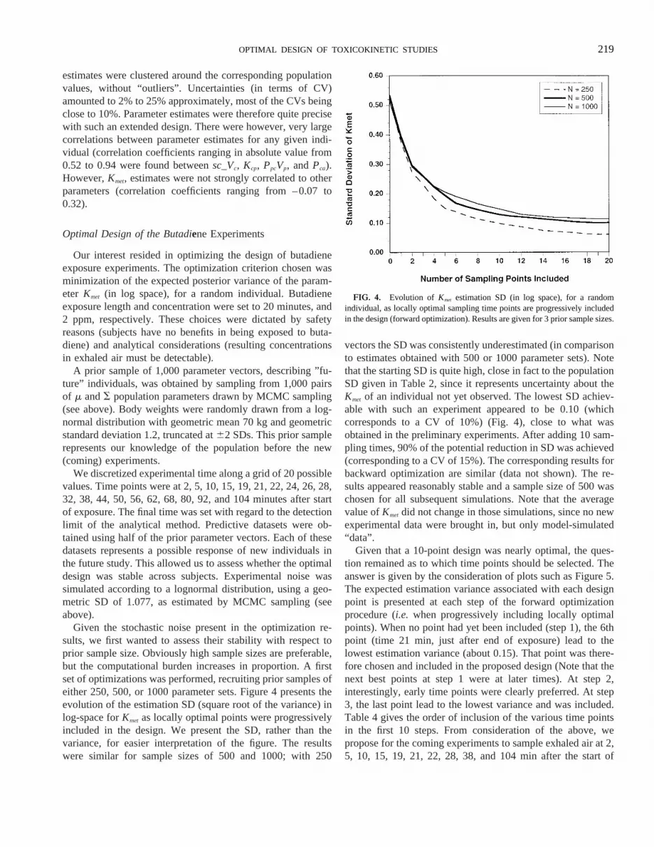
Given the stochastic noise present in the optimization re-sults, we first wanted to assess their stability with respect toprior sample size. Obviously high sample sizes are preferable,but the computational burden increases in proportion. A firstset of optimizations was performed, recruiting prior samples ofeither 250, 500, or 1000 parameter sets. Figure 4 presents theevolution of the estimation SD (square root of the variance) inlog-space forKmet as locally optimal points were progressivelyincluded in the design. We present the SD, rather than thevariance, for easier interpretation of the figure. The resultswere similar for sample sizes of 500 and 1000; with 250

vectors the SD was consistently underestimated (in comparisonto estimates obtained with 500 or 1000 parameter sets). Notethat the starting SD is quite high, close in fact to the populationSD given in Table 2, since it represents uncertainty about theKmet of an individual not yet observed. The lowest SD achiev-able with such an experiment appeared to be 0.10 (whichcorresponds to a CV of 10%) (Fig. 4), close to what wasobtained in the preliminary experiments. After adding 10 sam-pling times, 90% of the potential reduction in SD was achieved(corresponding to a CV of 15%). The corresponding results forbackward optimization are similar (data not shown). The re-sults appeared reasonably stable and a sample size of 500 waschosen for all subsequent simulations. Note that the averagevalue ofKmet did not change in those simulations, since no newexperimental data were brought in, but only model-simulated“data”.

Given that a 10-point design was nearly optimal, the ques-tion remained as to which time points should be selected. Theanswer is given by the consideration of plots such as Figure 5.The expected estimation variance associated with each designpoint is presented at each step of the forward optimizationprocedure (i.e. when progressively including locally optimalpoints). When no point had yet been included (step 1), the 6thpoint (time 21 min, just after end of exposure) lead to thelowest estimation variance (about 0.15). That point was there-fore chosen and included in the proposed design (Note that thenext best points at step 1 were at later times). At step 2,interestingly, early time points were clearly preferred. At step3, the last point lead to the lowest variance and was included.Table 4 gives the order of inclusion of the various time pointsin the first 10 steps. From consideration of the above, wepropose for the coming experiments to sample exhaled air at 2,5, 10, 15, 19, 21, 22, 28, 38, and 104 min after the start of

FIG. 4. Evolution of Kmet estimation SD (in log space), for a randomindividual, as locally optimal sampling time points are progressively includedin the design (forward optimization). Results are given for 3 prior sample sizes.

219OPTIMAL DESIGN OF TOXICOKINETIC STUDIES

exposure. This design, which should lead to an estimation CVof 15%, is about evenly distributed in time; the times brack-eting the end of exposure are definitely needed and samplingduring exposure should be very informative.

The proposed sampling schedule was tested by simulatingexperimental data at the specified time points and fitting the

toxicokinetic model using MCMC sampling. The aim of thesesimulations was to check if, under realistic conditions, theestimation SDs ofKmet for future subjects would indeed be low(or at least close to those obtained with a dense samplingschedule in preliminary experiments). Data for several ”normalsubjects” were simulated as above, as well as data for “patho-logical subjects,” with metabolic rates twice as high as for thenormal subjects. All simulated subjects were introduced in thepopulation model, together with the 8 subjects of the prelimi-nary experiments. Figure 6 presents for the 8 actual subjects,10 ”normal” and 10 “pathological” simulated subjects, theresultingKmet estimates. The optimal 10-point sampling sched-ule lead to estimation SDs comparable to those obtained usingthe preliminary 40-point sampling schedule (which lead to CVsof about 15% forKmet). Note thatKmet for ”pathological sub-jects” (fast metabolizers) had lower SD than for “normal sub-jects” (low metabolizers). For the simulated subjects the figurealso indicates the position of the ”true” value ofKmet (the valueused to simulate the subjects). The estimate was usually closeto the true value, except for the 2 subjects whoseKmet is farlower than those for the rest of the population (a conditionwhich, we just mentioned, leads to a low precision of esti-mates).

Figure 7 presents expected sample-based estimates of theCV of the population variance ofKmet (in log-space) togetherwith an analytical approximation: Given the distributional as-sumptions of our population model, if theKmet values of indi-viduals were known perfectly, the posterior density of the

FIG. 5. Expected estimation variance associated with each design timepoint, for the first 10 steps of the forward optimization algorithm (at each step,the optimal time point is included in the proposed design). Gaps correspond toalready included points.

TABLE 4Order of Inclusion of Candidate Time Points by Forward

Optimization of Planned Butadiene Experiments

Step Included time point (min) Resulting variance Resulting SD

1 21 0.158 0.3972 19 0.0878 0.2963 104 0.0679 0.2614 5 0.0501 0.2245 38 0.0375 0.1946 2 0.0279 0.1677 15 0.0241 0.1558 10 0.0211 0.1459 22 0.0186 0.136

10 28 0.0165 0.128

FIG. 6. Estimates (circles) of loge(Kmet) obtained by MCMC sampling, forthe 8 actual subjects of preliminary experiments (40-point sampling schedule),and simulated subjects (10-points optimal sampling schedule). All subjectswere included in the same population model. Data for simulated normalsubjects were drawn using estimates of population parameters for actualsubjects (i.e., they mimic actual subjects’ data). Data for simulated patholog-ical subjects were drawn using a doubled value ofKmet. True values ofKmet areindicated by crosses. Error bars represent estimation SDs. An optimal 10-pointsampling schedule leads to estimation SDs comparable to those obtained usingthe 40-point sampling schedule.

220 BOIS ET AL.

population variance ofKmet (in log-space) would follow aninverse-gamma distribution with a CV of 1/În/211, n beingthe number of subjects recruited. A “1” appears in the denom-inator because we are setting to 1 the shape parameter of theprior distributions for population variances (corresponding tovague prior distributions). In fact, the subjects’Kmet are af-fected by uncertainty, but the approximation is reasonablewithin the range presented, even if slightly underestimating.According to the figure, with 40 subjects a CV of 25% shouldbe achieved. One hundred subjects would bring this valuedown to 20%. The CV of the corresponding SD forKmet, inlog-space, would be about half of that value, and hence closeto 10%.

DISCUSSION

In the introductory section, it was noted that knowledge ofhuman metabolic rates is critical to the estimation of risk fromoccupational and environmental exposures, and for extrapolat-ing risk from one population to another. We are interested inmore than just an estimate of the average human metabolicrate. There is evidence for butadiene that both formation anddeactivation of epoxy metabolites are mediated by enzymeswhose activity is determined by the individual’s genotype(Carriereet al., 1996; Hassettet al., 1994). Thus, the averagerisk per unit-of-exposure for epidemiologic studies of petro-chemical workers will depend on the population’s distributionof metabolic genotypes.

It is not straightforward to obtainin vivo human metabolicdata for both ethical and practical reasons. An alternativeapproach could bein vitro studies of enzyme activity in tissue

slices, microsomes, or short-term cell cultures. These are suit-able for performing comparisons when differences are large,such as cross-species differences in microsomal and cytosolicenzyme activities (Csanadyet al., 1992). However, as noted byGuengerich (1996), allin vitro approaches have limitations inreplicating in vivo metabolism. Metabolism depends on boththe intrinsic reaction rate(s) of the enzyme(s) involved and onthe amount of enzyme protein. Humans have a variety ofintrinsic, genetically-determined enzyme rate capabilities. Anindividual’s basic genetic capability is further modified byconcurrent intake of alcohol, drugs, or foods, etc. The occur-rence of such modifications in a population is difficult toevaluate byin vitro tests. A population-based collection oftissue samples would be necessary to characterize this varia-tion, which is impractical and would not provide good esti-mates of the total rates. Since we wish to estimate the distri-bution of human metabolic rates to project population risksfrom exposure, it seems most appropriate to conduct efficient,short-duration laboratory exposures on a relatively large num-ber of subjects. It is important that human testing be as efficientas possible, so that the risk to the volunteers is minimized. Thismeans that the smallest possible exposure is used in the tests,the smallest number of subjects are tested, and the smallestnumber of sample time points is used that will efficientlyestimate individual metabolic rates. Resolution of these con-siderations depends on the pharmacokinetics of the agent,measurement capabilities, and statistical factors.

The Bayesian approach with Monte Carlo simulation is anideal means to optimize a measurement strategy to assess anyone of the parameters of a pharmacokinetic model of humanexposure to an environmental agent. Pilot data, with oversam-pling of time points during and after exposure, provided theinput information for both the prior estimates of the modelparameters and a test of the model’s predictive capability. Inparticular, this work brings together for the first time, to ourknowledge, a Bayesian population toxicokinetic analysis, and asimulation-based approach to optimal design. The populationapproach enables an easy summarizing of the population, thestraightforward generation of simulated individuals, and theassessment of the behavior of precision in variance estimates(Boiset al., 1996a,b; Fanninget al., 1997; Gelmanet al., 1996;Jonssonet al., 1997; Wakefieldet al., 1994). It is easy in thisframework to account for the uncertainty about measured co-variates, such as minute ventilation or blood to air partitioncoefficient. Their measurements were treated as data, withknown measurement SDs. The fits obtained with a 2-compart-ment model are excellent (among the best we have seen).Advantage of the 2-compartment model are obvious: it issimple, scientifically economical, quickly computed, and givesestimates of total metabolic clearance. This 2-compartmentmodel does not describe a terminal elimination phase whichwould be controlled by the slow release of butadiene from thefat, but this phase would start beyond the measurements ana-lyzed here. By not explicitly considering butadiene redistribu-

FIG. 7. Relationship between the planned study sample size and the CV ofthe population varianceKmet (in log-space). The circles are estimates obtainedby MCMC sampling of simulated experiments; the solid line is an analyticalapproximation.

221OPTIMAL DESIGN OF TOXICOKINETIC STUDIES

tion to body fat, we may have slightly overestimated metabo-lism. However, this potential bias is expected to be smallbecause blood flow to the fat represents only a few percent ofcardiac output and there was no observable slow-compartmentcontribution to the washout. Given a relative blood flow of 6:1for the liver versus the fat, and a high extraction for butadiene,the metabolic rate might be at most overestimated by about17%. Arguably, retention in fat could bear more on the totalamount butadiene metabolized, independently of metabolicrate, and should be considered if cancer risk assessment, forexample, was the objective of the analysis. We purposefullylimited ourselves to the estimation of metabolic clearance,given the data at hand, which was our research objective. Wealso did not need to extrapolate to other species, other routes ofexposure, or another dose range. Would that be the case, aPBPK model could be used for optimal design determination.Some approaches require linearized models (Mentre´ et al.,1997), in contrast, our method would still be applicable in thecase of a complex nonlinear model.

Classical approaches to design tend to be the exclusive realmof biostatisticians and specialized software (Beatty and Piegor-sch, 1997). We hope to make the technique more widelyaccessible, in particular to toxicologists interested in modeling.Our method is strongly model-based rather than databased.Model-based approaches (Atkinsonet al., 1993; Bursteinet al.,1997; D’Argenio, 1981, 1990; Kashubaet al., 1996; Palmerand Muller, 1998) are very flexible, because they allow thepredictive design of experiments; preliminary data are neededto define a reasonable model, but it is then possible to optimizethe design of any experiment susceptible to be simulated by themodel. On the other hand, data-based approaches (Mager andGoller, 1998; Mahmood, 1998; Paiet al., 1996; Tse andNedelman, 1996) trim down already-performed experimentsthrough bootstrap or similar techniques; they are less sensitiveto modeling errors, but also less powerful. Note that not onlytimes, but also doses, or exposure length could be optimized byour method. In the case presented here, those variables were setbased on safety considerations. Note also that the reduction invariance of a ”useful prediction” could have been chosen asoptimization criterion, instead of the variance of a crucialmodel parameter (Kmet). Such a prediction, relevant to cancerrisk, could be the amount of metabolites formed during the lasth of an 8-h exposure. We could also have computed a globalcriterion, such as Shannon information (Merle´ and Mentre´,1995; Polson, 1992). The choice of criterion should be dictatedby the ultimate goal of the planned studies. In addition, in thisanalysis the balancing of costs and benefits was done infor-mally. We did not need to formally put costs and benefits on acommon utility scale. A complete cost function could be spec-ified if formal cost minimization or more sophisticated decisionmaking was requested (Wakefield and Racine-Poon, 1995).Cost functions could be used in particular if the simultaneouslysampling optimization of several output variables (e.g., ex-haled air, venous blood, and urine) was sought. A valuable

aspect of optimal design might actually be the opportunity itgives to think about sophisticated utility functions: consider-ing, for example, balancing the cost of the planned experi-ments, the expected benefits to society, and the potential riskincurred to the study subjects…

The forward and backward optimizations used here areheuristic approaches and are not guaranteed to give the verybest results. A global optimization on all possible time pointcombinations would be required for that, but the resolution ofsuch large problems is still an open question, and in any casevery difficult (Atkinson and Donev, 1992). Forward and back-ward optimizations gave the same results in our problem,which reassures us that the results are reasonable and close tooptimal. One of the drawbacks of our approach is the noiseinduced by the stochastic nature of the algorithm. Conse-quently, points offering an almost equal reduction of varianceat a given step can be chosen quite randomly. The path leadingto an optimal design might be missed in some cases. However,the size of the sample used can always be increased as com-puting power expands. In fact, there should be a set of nearoptimal designs to choose from, and the path to them does notneed to be unique. It might actually be better to think in termsof informative design “regions,” as the examination of varianceprofiles as in Figure 5 reveals. In the case studied, the mostinformative region for the elimination rate appears to be thediscontinuity at the end of exposure. The early exposure periodand the final portion of the elimination phase come next. Ofthose 3 periods, only the last one is usually considered asuseful, on the basis of simple sensitivity analysis. Our approachtakes into account the entire statistical framework used toderive estimates of the metabolic elimination rate constant (inparticular the strong estimation covariances) and leads tosomewhat different results. It should be noted that the form ofthe error distribution is of importance in determining the op-timal design, since points determined with precision will tendto be preferred. We used a log-normal error model here, whichfits the preliminary data very well. It is possible that a refinedmodel, with a constant error term added (implying a detectionlimit), would be slightly better suited to the prediction of thelow-concentration, short-exposure experiments envisioned.Using alternative error distributions can easily be accommo-dated by our approach.

An important finding from these simulations is the descrip-tion of the diminishing returns for increasing the number ofsampling time points. As expected, large increases in numbersare needed to reduce the coefficient of variation of the esti-mated metabolic rate constant below 10%. This value is closeto what is expected given the estimation covariances andpractical limits to measurements. However, until this study, thequantitative relationship between number of samples and pre-cision was not known, because it is not determined by thesimple 1/=n expression. The data presented here showed thatrelatively small numbers of data points, about 10, can provideprecise estimates (i.e., with a 13% CV) of the apparent first

222 BOIS ET AL.

order metabolic rate for butadiene oxidation. Actually, addi-tional simulations (data not shown) indicated that if higherprecision were needed, a design with two 10 min exposureperiods and 30 sampling times can achieve an estimationCV 9%.

Analysis of the pilot data gave an indication of the variabil-ity among individuals to be expected in butadiene metabolismfor an ethnic Chinese group. This variability amounts to a 50%CV. Broader populations including other ethnic backgroundsmay be expected to show more variation as a result of differ-ences in enzyme genotypes. With genotypic data, it becomespossible to define the characteristic population rate parameterfor a genotype, and to determine if rates are significantlydifferent between different genotypes or ethnic groups (Jon-sson et al., 1997). At this point, it will be useful to takeadvantage of PBPK modeling to compensate for differences inbody size, body fat, inhalation rates, and blood partition coef-ficients.

It is tempting to take advantage of the proposed reduction incost of individual experiments to include more subjects in thestudy, with the aim of increasing the precision of the popula-tion estimate ofKmet. Our results show that, with up to ahundred subjects in the study, a 20% CV can be obtained onthe population variance ofKmet (this is a 10% CV for theestimation SD). Recruitment of about 50 subjects would yielda CV already close to those values. Again, given the limit to theprecision of individualKmet estimates, there should be a lowerlimit to the precision achievable for the estimate of popula-tion’s variability. We did not formally optimize the design withthe objective of precision of population variance, but insteaddecoupled the optimization of design for individual-specificKmet and their population variance. This decoupling shouldhave little implications here. However, a global approachwould be more elegant, and we need to explore ways toimplement the full population approach in simulation-baseddesign optimization.

Many issues in designs routinely used in toxicology (air-chamber or gavage experiments) remain to be investigated. Itwould be interesting to see if some aspects of the optimaldesign for butadiene carry for other compounds, or to ask, forexample, whether exhaled air sampling can replace blood-sampling altogether. Many experimenters are performing manysimilar experiments in animals and humans and all shouldbenefit from the availability of a simple, almost automaticmethod for design optimization.

ACKNOWLEDGMENTS

This work has been primarily supported by Grant ES07581 from the Na-tional Institutes of Health. F. Bois is also supported by grant R 824755–01–0from the U.S. Environmental Protection Agency and by the Association pourla Recherche contre le Cancer. T. Smith also is partially supported by theNational Institute for Environmental Health Sciences research grant ES07586and the center grant ES000002. We thank the reviewers for their thoroughreviews and very helpful comments.

REFERENCES

Atkinson, A. C., Chaloner, K., Herzberg, A. M., and Juritz, J. (1993). Optimumexperimental designs for properties of a compartmental model.Biometrics49, 325–337.

Atkinson, A. C., and Donev, A. N. (1992).Optimum Experimental Designs.Oxford, New-York.

Beatty, D. A., and Piegorsch, W. W. (1997). Optimal statistical design fortoxicokinetic studies.Stat. Methods Med. Res.6, 359–376.

Bernardo, J. M., and Smith, A. F. M. (1994).Bayesian Theory. Wiley, NewYork.

Bois, F. Y., Gelman, A., Jiang, J., Maszle, D., Zeise, L., and Alexeef, G.(1996b). Population toxicokinetics of tetrachloroethylene.Arch. Toxicol.70,347–355.

Bois, F., Jackson, E., Pekari, K., and Smith, M. (1996a). Population toxico-kinetics of benzene.Environ. Health Perspect.104(suppl. 6), 1405–1411.

Bois, F. Y., and Maszle, D. (1997). MCSim: a simulation program.J. Stat.Software2, http://www.stat.ucla.edu/journals/jss/v02/i09.

Bond, J. A., Himmelstein, M. W., and Medinsky, M. A. (1996). The use oftoxicologic data in mechanistic risk assessment: 1,3-butadiene as a casestudy.Int. Arch. Occup. Environ. Health68, 415–420.

Brunnemann, K. D., Kagan, M. R., Cox, J. E., and Hoffmann, D. (1990).Analysis of 1,3-butadiene and other selected gas-phase components incigarette mainstream and sidestream smoke by gas chromatography-massselective detection.Carcinogenesis11, 1863–1868.

Burstein, A. H., Gal, P., and Forrest, A. (1997). Evaluation of a sparsesampling strategy for determining vancomycin pharmacokinetics in pretermneonates: application of optimal sampling theory.The Ann. Pharmacother-apy 31, 980–983.

California Environmental Protection Agency Air Resources Board (1992).Proposed Identification of 1,3-Butadiene as a Toxic Air Contaminant. Sta-tionery Source Division, Sacramento, CA.

Carriere, V., Berthou, F., Baird, S., Belloc, C., Beaune, P., and de Waziers, I.(1996). Human cytochrome P450 2E1 (CYP2E1): from genotype to pheno-type.Pharmacogenetics6, 203–211.

Csanady, G. A., Guengerich, F. P., and Bond, J. A. (1992). Comparison of thebiotransformation of 1,3-butadiene and its metabolite, butadiene monep-oxide, by hepatic and pulmonary tissues from humans, rats, and mice.Carcinogenesis13, 1143–1153.

D’Argenio, D. Z. (1981). Optimal sampling times for pharmacokinetic exper-iments.J. Pharmacok. Biopharm.9, 739–756.

D’Argenio, D. Z. (1990). Incorporating prior parameter uncertainty in thedesign of sampling schedules for pharmacokinetic parameter estimationexperiments.Math. Biosci.99, 105–118.

Fajen, J. M., Roberts, D. R., Ungers, L. J. and Krishnan, E. R. (1990).Occupational exposure of workers to 1,3 butadiene.Environ. Health Per-spect.86, 11–18.

Fanning, E., Bois, F. Y., Rothman, N., Bechtold, B., Li, G., Hayes, R., andSmith, M. (1997). Population toxicokinetics of benzene and its metabolites.Toxicol. Appl. Pharmacol.(suppl.), 164.

Gelfand, A. E., and Smith, A. F. M. (1990). Sampling-based approaches tocalculating marginal densities.J. Am. Stat. Assoc.85, 398–409.

Gelman, A. (1992). Iterative and non-iterative simulation algorithms.Comput.Sci. Stat.24, 433–438.

Gelman, A., Bois, F., and Jiang, J. (1996). Physiological pharmacokineticanalysis using population modeling and informative prior distributions.J. Am. Stat. Assoc.91, 1400–1412.

Gelman, A., and Rubin, D. B. (1992). Inference from iterative simulation,using multiple sequences (with discussion).Stat. Sci.7, 457–511.

223OPTIMAL DESIGN OF TOXICOKINETIC STUDIES

Gelman, A., and Rubin, D. B. (1996). Markov chain Monte Carlo methods inbiostatistics.Stat. Methods Med. Res.5, 339–355.

Gilks, W. R., Richardson, S., and Spiegelhalter, D. J. (1996).Markov ChainMonte Carlo in Practice. Chapman & Hall, London.

Guengerich, F. P. (1996).In vitro techniques for studying drug metabolism.J. Pharmacok. Biopharm.24, 521–533.

Hassett, C., Aicher, L., Sidhu, J. S., and Omiecinski, C. J. (1994). Humanmicrosomal epoxide hydrolase: genetic polymorphism and functional ex-pressionin vitro of amino acid variants.Hum. Mol. Genet.3, 421–428.

International Agency for Research on Cancer (IARC) (1992).OccupationalExposures to Mists and Vapours from Strong Inorganic Acids and OtherIndustrial Chemicals. International Agency for Research on Cancer, Lyon,France.

Johanson, G. and Filser, J. G. (1996). PBPK model for butadiene metabolismto epoxides: Quantitative species differences in metabolism.Toxicology113, 40–47.

Jonsson, F., Johanson, G., and Bois, F. Y. (1997). A new approach to estimatepopulation variability in target dose based on genetic polymorphism dataand PBTK modeling.Toxicol. Appl. Pharmacol.(suppl.), 34.

Kashuba, A. D. M., Ballow, C. H., and Forrest, A. (1996). Development andevaluation of a Bayesian pharmacokinetic estimator and optimal, sparsesampling strategies for ceftazidime.Antimicrob. Agents Chemother.40,1860–1865.

Mager, H., and Go¨ller, G. (1998). Resampling methods in sparse samplingsituations in preclinical pharmacokinetic studies.J. Pharm. Sci.87, 372–378.

Mahmood, I. (1998). A limited sampling approach in pharmacokinetic studies:experience with the antiepilepsy drug tiagabine.Br.J. Clin. Pharmacol.38,324–330.

Maszle, D., and Bois, F. Y. (1993).Program MCSim—User Manual. Avail-able from the authors, or at ftp://sparky.berkeley.edu/pub/mcsim and http://sparky.berkeley.edu/users/fbois.

Mentre, F., Mallet, A., and Baccar, D. (1997). Optimal design in random-effects regression models.Biometrika84, 429–442.

Merle, Y., and Mentre´, F. (1995). Bayesian design criteria: computation,comparison, and application to a pharmacokinetic and a pharmacodynamicmodel.J. Pharmacokinet. Biopharm.23, 101–125.

Muller, P., and Parmigiani, G. (1995). Optimal design via curve fitting ofMonte Carlo experiments.J. Am. Stat. Assoc.90, 1322–1330.

Mullins, J. A. (1990). Industrial emissions of 1,3-butadiene.Environ. HealthPerspect.86, 9–10.

National Research Council (NRC) (1994).Science and Judgement in RiskAssessment. National Academy Press, Washington, DC.

O’Keefe, A. E., and Ortman, G. O. (1966). Primary standards for trace gasanalysis.Anal. Chem.38, 760–763.

Pai, S. M., Fettner, S. H., Hajian, G., Cayen, M. N., and Batra, V. K. (1996).Characterization of AUCs from sparsely sampled populations in toxicologystudies.Pharm. Res.13, 1283–1290.

Palmer, J. L., and Mu¨ller, P. (1998). Bayesian optimal design in populationmodels for haematologic data.Stat. Med.17, 1613–1622.

Polson, N. G. (1992). On the expected amount of information from a non-linear model.J. Roy. Statist. Soc. B54, 889–895.

Ramsey, J. C., and Andersen, M. (1984). A physiologically based descriptionof the inhalation pharmacokinetics of styrene in rats and humans.Toxicol.Appl. Pharmacol.73, 159–175.

Rappaport, S. M., Selvin, S., and Waters, M. A. (1987). Exposures to hydro-carbon components of gasoline in the petroleum industry.Appl. Ind. Hyg.2,148–154.

Reitz, R. H., MacDougal, J. N., Himmelstein, M. W., Nolan, R. J., andSchumann, A. M. (1988). Physiologically based pharmacokinetic modelingwith methylchloroform: implications for interspecies, high dose/low dose,and dose route extrapolations.Toxicol. Appl. Pharmacol.95, 185–199.

Smith, A. F. M., and Roberts, G. O. (1993). Bayesian computation via theGibbs sampler and related Markov chain Monte Carlo methods.J. Roy.Statist. Soc. B55, 3–23.

Tse, F. L. S., and Nedelman, J. R. (1996). Serial versus sparse sampling intoxicokinetic studies.Pharm. Res.13, 1105–1108.

U.S. Environmental Protection Agency (1985).Mutagenticity and Carcinoge-nicity Assessment of 1,3-Butadiene, Publication No. EPA/600/8–85/004F.Office of Health Effects and Environmental Assessment, Washington, DC.

U.S. Environmental Protection Agency (1989).Revised Draft Final Report:Locating and Estimating Air Emissions for Sources of 1,3-Butadiene. Non-criteria Pollutant Programs Branch, Air Quality Management Division,Research Triangle Park, NC.

Wakefield, J. C. (1996). The Bayesian analysis of population pharmacokineticmodels.J. Am. Stat. Assoc.91, 62–75.

Wakefield, J. C., and Racine-Poon, A. (1995). An application of Bayesianpopulation pharmacokinetic pharmacodynamic models to dose recommen-dation.Stat. Med.14, 971–986.

Wakefield, J. C., Smith, A. F. M., Racine-Poon, A., and Gelfand, A. E. (1994).Bayesian analysis of linear and non-linear population models using theGibbs sampler.Appl. Statist.– J. Roy. Statist. Soc. C43, 201–221.

224 BOIS ET AL.