Optimal boundary control of dynamics responses of piezo actuating micro-beams

Applied Mathematical Modelling 33 (2009) 3343–3353

Contents lists available at ScienceDirect

Applied Mathematical Modelling

journal homepage: www.elsevier .com/locate /apm

Optimal boundary control of dynamics responses of piezo actuatingmicro-beams

Ibrahim Sadek a, Ismail Kucuk a,*, Eiman Zeini b, Sarp Adali c

a Department of Mathematics and Statistics, American University of Sharjah, P.O. Box 26666, Sharjah, United Arab Emiratesb Department of Mathematics, Alexandria University, Alexandria, Egyptc School of Mechanical Engineering, University of KwaZulu-Natal, Durban, South Africa

a r t i c l e i n f o a b s t r a c t

Article history:Received 19 September 2007Received in revised form 31 October 2008Accepted 3 November 2008Available online 21 November 2008

Keywords:Micro-beamsPiezoceramicsMaximum principleOptimal boundary controlEigenfunction expansions technique

0307-904X/$ - see front matter � 2008 Elsevier Incdoi:10.1016/j.apm.2008.11.009

* Corresponding author.E-mail addresses: [email protected] (I. Sadek), ikuc

Optimal control theory is formulated and applied to damp out the vibrations of micro-beams where the control action is implemented using piezoceramic actuators. The useof piezoceramic actuators such as PZT in vibration control is preferable because of theirlarge bandwidth, their mechanical simplicity and their mechanical power to produce con-trolling forces. The objective function is specified as a weighted quadratic functional ofthe dynamic responses of the micro-beam which is to be minimized at a specified termi-nal time using continuous piezoelectric actuators. The expenditure of the control forces isincluded in the objective function as a penalty term. The optimal control law for themicro-beam is derived using a maximum principle developed by Sloss et al. [J.M. Sloss,J.C. Bruch Jr., I.S. Sadek, S. Adali, Maximum principle for optimal boundary control ofvibrating structures with applications to beams, Dynamics and Control: An InternationalJournal 8 (1998) 355–375; J.M. Sloss, I.S. Sadek, J.C. Bruch Jr., S. Adali, Optimal control ofstructural dynamic systems in one space dimension using a maximum principle, Journalof Vibration and Control 11 (2005) 245–261] for one-dimensional structures where thecontrol functions appear in the boundary conditions in the form of moments. The derivedmaximum principle involves a Hamiltonian expressed in terms of an adjoint variable aswell as admissible control functions. The state and adjoint variables are linked by termi-nal conditions leading to a boundary-initial-terminal value problem. The explicit solutionof the problem is developed for the micro-beam using eigenfunction expansions of thestate and adjoint variables. The numerical results are given to assess the effectivenessand the capabilities of piezo actuation by means of moments to damp out the vibrationof the micro-beam with a minimum level of voltage applied on the piezo actuators.

� 2008 Elsevier Inc. All rights reserved.

1. Introduction

Active control of vibrations in flexible structures through the smart structure concept is a developing area of researchand has numerous applications, especially in the vibration control of structures (such as beams, plates, shells), in aero-space engineering, flexible robot manipulators, antennas, active noise control, shape control and in earthquake resistantstructures. Due to the increase of high structural requirements in the performance and control of flexible structures,applications of smart structures technologies are expanding rapidly. Among various smart effects encountered in a widerange of engineering applications are piezoelectric, electro and magnetostriction, shape memory and other technologies. In

. All rights reserved.

[email protected] (I. Kucuk), [email protected] (E. Zeini), [email protected] (S. Adali).

mailto:[email protected]




http://www.sciencedirect.com/science/journal/0307904X

http://www.elsevier.com/locate/apm

3344 I. Sadek et al. / Applied Mathematical Modelling 33 (2009) 3343–3353

particular, piezoelectric materials belong to a class of materials which are being used as distributed sensors or activedampers of vibrations, i.e., for sensing and actuation. Presently one of the most widely used piezo materials in active con-trol is piezoceramics such as PZT for their large bandwidth, their mechanical simplicity and their mechanical power toproduce controlling forces. The books by Preumont [1] and Banks et al. [2] provide an overview of these materials andthe related control techniques.

Modeling of the direct and the reverse effects of a distributed piezoelectric layer has been studied in [2–7]. Feedback con-trol algorithms such as rate feedback, independent modal space control and coupled mode control can be used in the vibra-tion control of distributed structures [8–12]. However, the feedback control strategies lead to active damping with adamping ratio that can reach 20% on the first modes of the investigated structure without any modification. Such resultsare of interest for many engineering application [1,3,5]. Similar remarks can be made concerning the application of feedfor-ward strategies which have been applied to acoustic control in [13,14] and to vibration control of beams in [15–17]. In thefeedforward control strategies, the quantity to be controlled, i.e., wave propagation, velocity, etc., is measured downstreamfrom the control location and this quantity is minimized by using control forces. Both feedback and feedforward controls areclosed-loop control strategies requiring information on the state variables which can be measured upstream (feedback) ordownstream (feedforward) of the control location by means of sensors. The present approach implements an open-loop con-trol strategy as opposed to closed-loop ones and as such a control law is formulated as part of the solution. The control lawformulated in this way is optimal in the sense that it gives the best control for the given objective function and the constraintwhich involves the functionals of the state and control variables. A distinct difference between the closed and open controlsis the use of sensors whereby the information used in the feed (closed-loop control) is obtained via sensors which are notneeded in the open-loop control since the control law is formulated independently of any information of the system inoperation.

Feedback control algorithms have been used almost exclusively for the control of intelligent structures and the imple-mentation of this approach to vibration control can be found in [18–22]. However, time delays in the implementation ofa feedback control may cause to lose the robustness of structures [23] and in fact may destabilize the structure in certaincases [24]. An example of open-loop boundary control of a long vibrating rod was studied in [25], where the optimal controllaw was derived by using a maximum principle. Boundary control of beams has been studied by active constrained layer in[26] and those of plates by smart modal sensors in [27]. Main application area of piezoelectric control is suppression of vibra-tions of structural components used in many branches of engineering [18,28–30]. Piezo control is also used for acoustic con-trol [19] and to suppress and control flutter of lifting surfaces [31,32].

The micro electro mechanical systems (MEMS) seem to be of interest in improving the mechanical efficiency of structuralactive control. They can effectively present a good approach for a large class of problems such as the control of waves [33]and control of the mechanical interaction or the stabilization of a micro system such as those described in [34]. In the presentstudy, the control of a micro-beam totally covered by a piezoelectric, PZT, film is studied. In this system, it is possible to coverthe entire structure with piezoelectric material, which is not possible on large structures.

In this context, the open-loop control results are obtained using a recently developed maximum principle for the opti-mal boundary of one-dimensional structures [35]. For this purpose, the piezo-control problem is formulated as an optimalboundary control problem using the applied voltage as the control function to damp out the vibrations of the micro-beam.The boundary control is an economic method for controlling the distributed parameter system (DPS) since it does not re-quire the attachment of sensors or actuators to the control system with distributed control forces. The objective functionis specified as a weighted functional of the dynamic responses of the micro-beam which is to be minimized at a specificterminal time using continuous piezoelectric actuators. The continuous piezoelectric actuators are the open-loop controlfunctions that appeared in the boundary conditions in the form of moments. The optimal control law for the micro-beamis derived by introducing the adjoint problem and the related Hamiltonian in the form of a maximum principle [35,36].The maximum principle gives a relationship between the optimal control force and the adjoint variable, which is com-bined with the state variable through terminal conditions. Thus, the control problem is formulated as a boundary-ini-tial-terminal value problem. Explicit solutions are obtained by the use of eigenfunction expansions for the state andadjoint variables for a simply supported beam with continuous piezoceramic actuators. This approach has been appliedto damp out the vibrations of a cantilever beam where the control action is implemented using piezoceramic actuators[37].

The effectiveness of the proposed control system is illustrated numerically by plotting the courses of the deflection andvelocity against time. These results indicate that the vibrations of the beam can be reduced substantially at a given terminaltime by exercising open-loop piezo control. Furthermore, the reductions in displacement and velocity depend on the mag-nitude of the control moment which depends on the expenditure of control energy.

2. Equation of motion for a piezoelectric beam

Consider a micro-beam of length L, width b and height of the beam hs covered by the layers of piezoelectric materials eachof having thickness hp. The dynamical equilibrium of the Euler–Bernoulli beam described in Fig. 1 is defined in the followingequation [34]:

�qwtt þ Eco Ico wxxxx ¼ 0; 0 < x < L;0 < t < tf ; ð1Þ

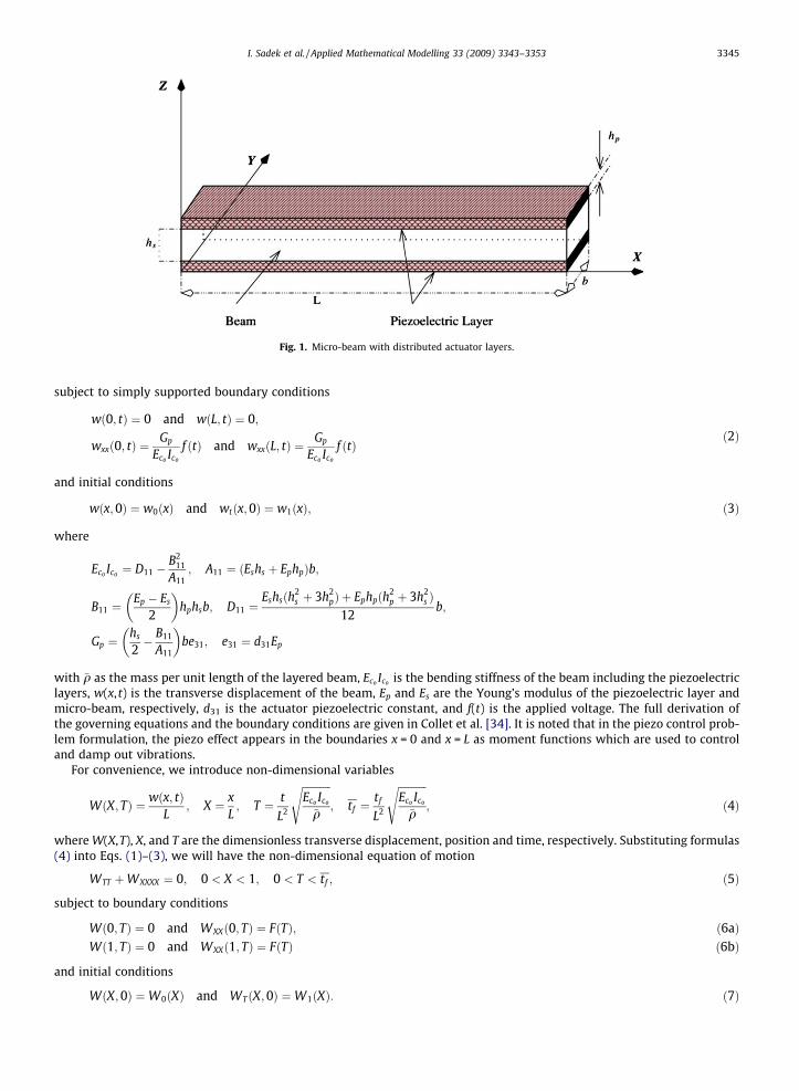
Fig. 1. Micro-beam with distributed actuator layers.

I. Sadek et al. / Applied Mathematical Modelling 33 (2009) 3343–3353 3345

subject to simply supported boundary conditions

wð0; tÞ ¼ 0 and wðL; tÞ ¼ 0;

wxxð0; tÞ ¼Gp

Eco Ico

f ðtÞ and wxxðL; tÞ ¼Gp

Eco Ico

f ðtÞð2Þ

and initial conditions

wðx; 0Þ ¼ w0ðxÞ and wtðx;0Þ ¼ w1ðxÞ; ð3Þ

where

Eco Ico ¼ D11 �B2

11

A11; A11 ¼ ðEshs þ EphpÞb;

B11 ¼Ep � Es

2

� �hphsb; D11 ¼

Eshsðh2s þ 3h2

pÞ þ Ephpðh2p þ 3h2

s Þ12

b;

Gp ¼hs

2� B11

A11

� �be31; e31 ¼ d31Ep

with �q as the mass per unit length of the layered beam, Eco Ico is the bending stiffness of the beam including the piezoelectriclayers, w(x, t) is the transverse displacement of the beam, Ep and Es are the Young’s modulus of the piezoelectric layer andmicro-beam, respectively, d31 is the actuator piezoelectric constant, and f(t) is the applied voltage. The full derivation ofthe governing equations and the boundary conditions are given in Collet et al. [34]. It is noted that in the piezo control prob-lem formulation, the piezo effect appears in the boundaries x = 0 and x = L as moment functions which are used to controland damp out vibrations.

For convenience, we introduce non-dimensional variables

WðX; TÞ ¼ wðx; tÞL

; X ¼ xL; T ¼ t

L2

ffiffiffiffiffiffiffiffiffiffiffiEco Ico

�q

s; tf ¼

tf

L2

ffiffiffiffiffiffiffiffiffiffiffiEco Ico

�q

s; ð4Þ

where W(X,T), X, and T are the dimensionless transverse displacement, position and time, respectively. Substituting formulas(4) into Eqs. (1)–(3), we will have the non-dimensional equation of motion

WTT þWXXXX ¼ 0; 0 < X < 1; 0 < T < tf ; ð5Þ

subject to boundary conditions

Wð0; TÞ ¼ 0 and WXXð0; TÞ ¼ FðTÞ; ð6aÞWð1; TÞ ¼ 0 and WXXð1; TÞ ¼ FðTÞ ð6bÞ


WðX;0Þ ¼W0ðXÞ and WTðX;0Þ ¼W1ðXÞ: ð7Þ


3. Optimal control problem

In this section, the objective of the control problem is to find the minimum applied force F(T), which minimizes the mea-sure of displacement and velocity over a given period of time with minimum expenditure of the control. Among all admis-sible control functions,

FðTÞ 2 Uad ¼ fF : F 2 L2ð0; tf Þg, the particular control function Fo(T) 2 Uad (the optimal control) is sought to minimize thefollowing cost functionals:

J1ðFÞ ¼Z 1

0l1W2ðX; tf Þh i

dX; J2ðFÞ ¼Z 1

0l2W2

TðX; tf Þh i

dX;

J3ðFÞ ¼Z tf

0l3F2ðTÞdT:

The index of performance J(F) is obtained by combining the multiple objectives in a weighted sum given by

JðFÞ ¼X3

i¼1

liJiðFÞ; ð8Þ

where l1, l2, and l3 > 0 are weight constants which reflect the relative weighting attached to minimize Ji(F) with l1 + l2 > 0and l3 – 0. The last term in Eq. (8) is a penalty term on control energy.

The optimal boundary control of the micro-beam can now expressed as

JðFoÞ ¼ minF2Uad

JðFÞ ð9Þ

with W(X,T) subject to Eqs. (5) and (6).The proof of uniqueness of the optimal control (9) follows easily from the convexity of the performance. Assuming that an

optimal control exists, our main objective is to derive a maximum principle that can be used to determine the optimalcontrol.

4. Boundary control characterization

To apply the maximum principle theory [25] to solve the control problem (9), we need to introduce an adjoint problemwith the adjoint variable V(X,T) satisfying the differential equation

VTT þ VXXXX ¼ 0; 0 < X < 1; 0 < T < tf ð10Þ

with boundary conditions

Vð0; TÞ ¼ 0 and VXXð0; TÞ ¼ 0; ð11aÞVð1; TÞ ¼ 0 and VXXð1; TÞ ¼ 0 ð11bÞ

and the terminal conditions

VTðX; tf Þ ¼ 2l1WðX; tf Þ;VðX; tf Þ ¼ �2l2WTðX; tf Þ: ð12Þ

For F(T) 2 Uad, let W(X,T) = W(X,T;F) satisfy Eq. (5) with boundary conditions and initial conditions (6) and (7), respec-tively. For Fo(T) 2 Uad, let Wo(X,T) = W(X,T;Fo) and let Vo(X,T) = V(X,T;Fo) be the corresponding adjoint variable satisfy Eq.(10) with boundary conditions and terminal conditions (11) and (12), respectively. The maximum principle can now be sta-ted as follows:

Theorem 1 (Maximum principle). If the optimal control Fo(T) 2 Uad satisfies the maximum problem

maxF2Uad

HðT; V ; FÞ ¼ HðT; V0; FoÞ; ð13Þ

where the Hamiltonian is given by the equation

HðT; V ; FÞ ¼ RðTÞFðTÞ þ l3F2ðTÞ ð14Þ

in which

RðTÞ ¼ VXð0; TÞ � VXð1; TÞ

then

JðFoÞ 6 JðFÞ: ð15Þ


Proof. We start the proof by introducing the operator

WðWÞ ¼WTT þWXXXX : ð16Þ

If

DW ¼WðX; TÞ �WoðX; TÞ;DF ¼ FðX; TÞ � FoðX; TÞ

ð17Þ

then

WðDWÞ � DF ¼ 0 ð18Þ

with the boundary conditions (6) becoming

DWð0; TÞ ¼ 0 and DWðL; TÞ ¼ 0;DWXXð0; TÞ ¼ DFðTÞ and DWXXðL; TÞ ¼ DFðTÞ

ð19Þ

and the initial conditions (7) becoming

DWðX;0Þ ¼ 0; DWtðX; 0Þ ¼ 0: ð20Þ

Consider the form
Z 1
0

Z tf

0fDWWðVÞ � VWðDWÞgdT dX ¼

Z 1

0

Z tf

0DWðVTT þ VXXXXÞ � VðDWTT þ DWXXXXÞdT dX

¼Z 1

0

Z tf

0ðDWVTT � VDWTTÞdT dXþ|fflfflfflfflfflfflfflfflfflfflfflfflfflfflfflfflfflfflfflfflfflfflfflfflfflfflfflfflfflfflfflffl{zfflfflfflfflfflfflfflfflfflfflfflfflfflfflfflfflfflfflfflfflfflfflfflfflfflfflfflfflfflfflfflffl}

I

Z 1

0

Z tf

0ðDWVXXXX � VDWXXXXÞdT dX|fflfflfflfflfflfflfflfflfflfflfflfflfflfflfflfflfflfflfflfflfflfflfflfflfflfflfflfflfflfflfflfflfflfflffl{zfflfflfflfflfflfflfflfflfflfflfflfflfflfflfflfflfflfflfflfflfflfflfflfflfflfflfflfflfflfflfflfflfflfflffl}

II

¼ 0:

ð21Þ

Integration by parts of I in (21) gives

I ¼Z 1

0fDWðX; tf ÞVtðX; tf Þ � DWðX;0ÞVTðX;0Þ � VðX; tf ÞDWTðX; tf Þ þ VðX; 0ÞDWTðX;0ÞgdX

¼Z 1

0fDWðX; tf ÞVTðX; tf Þ � VðX; tf ÞDWTðX; tf ÞgdX: ð22Þ

Similarly, twice integration by parts of II and applying the boundary conditions (11) and (19) will lead to

II ¼Z tf

0DWðX; TÞVXXXðX; TÞj10 �

Z 1

0DWXVXXXdX � VðX; TÞDWXXXðX; TÞj10 þ

Z 1

0VXDWXXXdX

� �dT

¼Z tf

0VXð1; TÞDWXXð1; TÞ � VXð0; TÞDWXXð0; TÞf gdT: ð23Þ

Replacing (22) and (23) into (21) observes the following:
Z 1
0fDWðX; tf ÞVTðX; tf Þ � VðX; tf ÞDWTðX; tf ÞgdX þ

Z tf

0fVXðL; TÞDWXXð1; TÞ � VXð0; TÞDWXXð0; TÞgdT ¼ 0

or
Z 1
0fDWðX; tf ÞVTðX; tf Þ � VðX; tf ÞDWTðX; tf ÞgdX ¼

Z tf

0fVXð0; TÞDWXXð0; TÞ � VXð1; TÞDWXXð1; TÞgdT:

From terminal conditions (12) in the adjoint variable and the boundary conditions (11) and (19), we obtain
Z 1
0f2l1DWðX; tf ÞWðX; tf Þ þ 2l2WTðX; tf ÞDWTðX; tf ÞgdX ¼

Z tf

0fVXð0; TÞ � VXð1; TÞgDf ðTÞdT: ð24Þ

Now, consider the performance index

DJðFÞ ¼ JðFÞ � JðFoÞ

¼Z 1

0l1 W2ðX; tf Þ �Wo2 ðX; tf Þh i

þ l2 W2TðX; tf Þ �Wo2

T ðX; tf Þh in o

dX þ l3

Z tf

0½F2ðTÞ � Fo2 ðTÞ�dT: ð25Þ

Expanding the terms W2ðX; tf Þ and W2TðX; tf Þ by using Taylor series about WoðX; tf Þ and Wo

TðX; tf Þ, respectively, in (25), weobtain


W2ðX; tf Þ �Wo2 ðX; tf Þ ¼ 2WoðX; TÞDWðX; tf Þ þ r1;

W2TðX; tf Þ �Wo2

T ðX; tf Þ ¼ 2WoTðX; TÞDWTðX; tf Þ þ r2;

ð26Þ

where

r1 ¼ 2ðDWÞ2 þ � � � > 0; r2 ¼ 2ðDWTÞ2 þ � � � > 0: ð27Þ

Substituting (26) into the right-hand side of Eq. (25), we have

DJðFÞ ¼Z 1

02l1 WoðX; tf ÞDWoðX; tf Þ þ r1

� þ 2l2 Wo

TðX; tf ÞDWoTðX; tf Þ þ r2

� �dX þ l3

Z tf

0½F2ðTÞ � Fo2 ðTÞ�dT: ð28Þ

Since l1 P 0, l2 P 0, l3 > 0 and 2l1r1 + 2l2 r2 P 0, we obtain

DJðFÞPZ tf

0fVXð0; TÞ � VXðL; TÞgDFðTÞdT þ l3

Z tf

0fF2ðTÞ � Fo2 ðTÞgdT: ð30Þ

Let us introduce R(T) in (30)

RðTÞ ¼ VXð0; TÞ � VXðL; TÞ

so that (30) becomes

DJðFÞPZ tf

0ðRðTÞFðTÞ þ l3F2ðTÞÞ � ðRðTÞF0ðTÞ þ l3Fo2 ðTÞÞn o

dT: ð31Þ

By the hypothesis of the maximum principle Eq. (14), it immediately follows that:

RðTÞFoðTÞ þ l3Fo2 ðTÞP RðTÞFðTÞ þ l3F2ðTÞ: ð32Þ

In view of the inequalities (31) and (32)

DJðFÞP 0 implies that JðFoÞ 6 JðFÞ:

Thus, Fo(t) is indeed the optimal control and this completes the proof of the theorem. h

The optimal control function in (13) is therefore given by

FoðTÞ ¼ �12l3½VXð0; TÞ � VXð1; TÞ�: ð33Þ

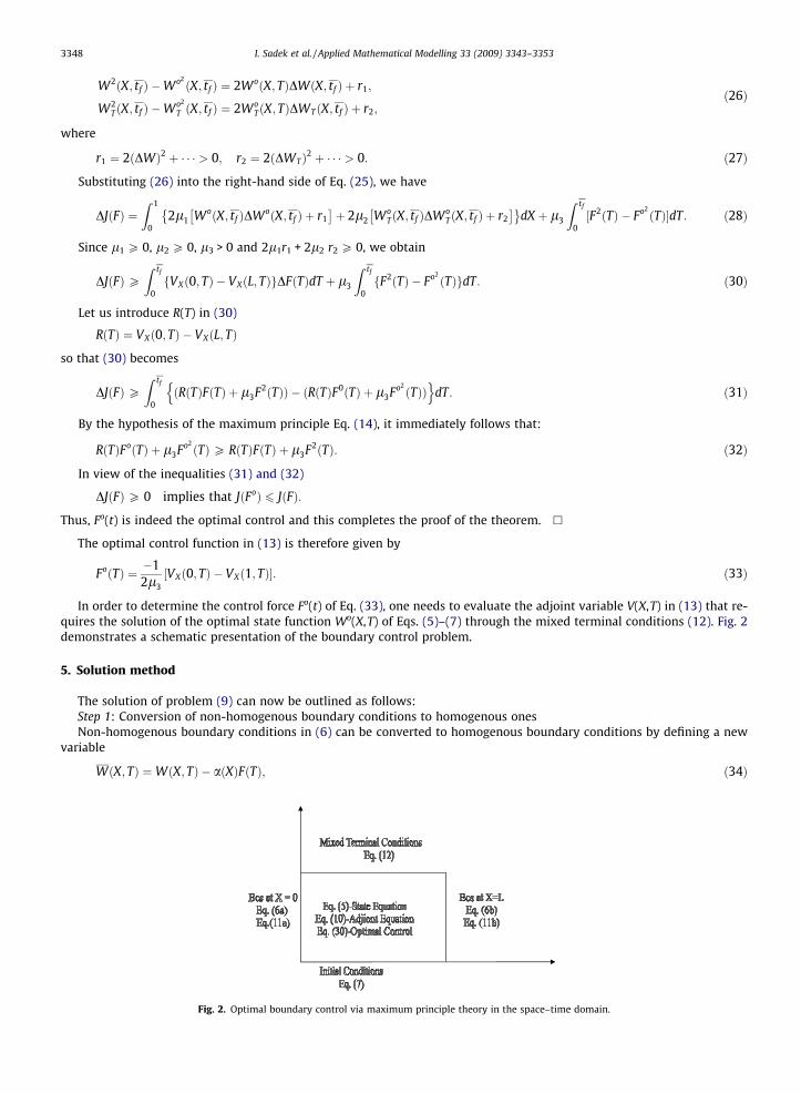
In order to determine the control force Fo(t) of Eq. (33), one needs to evaluate the adjoint variable V(X,T) in (13) that re-quires the solution of the optimal state function Wo(X,T) of Eqs. (5)–(7) through the mixed terminal conditions (12). Fig. 2demonstrates a schematic presentation of the boundary control problem.

5. Solution method

The solution of problem (9) can now be outlined as follows:Step 1: Conversion of non-homogenous boundary conditions to homogenous onesNon-homogenous boundary conditions in (6) can be converted to homogenous boundary conditions by defining a new

variable

WðX; TÞ ¼WðX; TÞ � aðXÞFðTÞ; ð34Þ

Fig. 2. Optimal boundary control via maximum principle theory in the space–time domain.


where

aðXÞ ¼ 12ðX2 � XÞ:

Then, the partial differential equation in (5) becomes

WTTðX; TÞ þWXXXXðX; TÞ ¼ �aðXÞF 00ðTÞ; 0 < X < 1; 0 < T < tf ð35Þ

with the new boundary conditions defined as

Wð0; TÞ ¼ 0 and Wð1; TÞ ¼ 0;

WXXð0; TÞ ¼ 0 and WXXð1; TÞ ¼ 0 ð36Þ


WðX; 0Þ ¼WoðXÞ � aðXÞFð0Þ;WTðX;0Þ ¼W1ðXÞ � aðXÞF 0ð0Þ:

ð37Þ

Step 2: Approximating the solution of adjoint system.Solve the distributed parameter adjoint system (10) and (11) by approximating in terms of Nth-terms of sine Fourier

series

VoðX; TÞ ¼XN

n¼1

Q nðTÞ sin knX; ð38Þ

where

Q nðTÞ ¼ d1n cos k2nT þ d2n sin k2

nT: ð39Þ

Thus (38) becomes

VoxðX; TÞ ¼

XN

n¼1

kn d1n cos k2nT þ d2n sin k2

nT�

cos knX ð40Þ

in which kn = np/L.Step 3: Computing the optimal control force Fo(t).Substituting Eq. (38) into Eq. (33), one obtains

FoðTÞ ¼ �12l3

XN

n¼1

kn½1� ð�1Þn� d1n cos k2nT þ d2n sin k2

nT�

: ð41Þ

Step 4: Solve the distributed parameter state system (35) and (36)Similarly, the solution of Eq. (32) can be obtained by using the Nth-terms of sine Fourier series

WðX; TÞ ¼XN

n¼1

ZnðTÞ sin knX ð42Þ

with kn = np.Substituting Eq. (42) in Eq. (35), one obtains

XN

n¼1

Z00nðTÞ þ k4nZnðTÞ

�sin knX ¼ �aðXÞF 00ðTÞ: ð43Þ

By applying the orthogonality of the Fourier sine series in Eq. (43), this leads to

Z00nðTÞ þ k4nZnðTÞ ¼ �2gnF 00ðTÞ ð44Þ

with Z
gn ¼
1

0aðXÞ sin knXdX:

The solution of Eq. (44) is

ZnðTÞ ¼ c1n cos k2nT þ c2n sin k2

nT þ � 2k2

n

gn

!Z T

0sin k2

nðT � sÞF 00ðsÞds; ð45Þ

where the constants c1n and c2n can be determined by the initial conditions (19), i.e.,

c1n ¼ 2Z 1

0fWoðXÞ � aðXÞFð0Þg sin knXdX


and

c2n ¼2k4

n

Z 1

0fW1ðXÞ � aðXÞF 0ð0Þg sin knXdX:

In view of Eq. (41), Eq. (45) becomes

ZnðTÞ ¼ c1n cos k2nT þ c2n sin k2

nT þ gn

k2nl3

!Z T

0sin k2

nðt � sÞXM

m¼1

k5m½ð�1Þm � 1� d1m cos k2

msþ d2m sin k2ms

� " #ds; ð46Þ

where d1n and d2n are constants to be computed by the terminal conditions (12).Step 5: Finding the undermined constants d1n and d2n.Inserting the expansions (38) and (42) into the mixed terminal conditions (12) leads to a system of linear modal equations

ddT

Qnðtf ; d1n; d2nÞ ¼ 2l1Znðtf ; d1n;d2nÞ;

Q nðtf ; d1n;d2nÞ ¼ �2l2d

dTZnðtf ; d1n;d2nÞ:

ð47Þ

Substituting the modal time solutions (39) and (45) into the lumped parameter system (44) leads to two linear equationsin d1n and d2n. Solving for d1n and d2n, the adjoint function Vo(X,T) is determined from Eq. (38), the optimal control Fo(t) isgiven explicitly by Eq. (41) and finally the optimal response of the micro-beam is obtained explicitly

WoðX; TÞ ¼WoðX; TÞ þ aðXÞFoðTÞ ð48Þ

and optimal performance index is expressed by

JðFoÞ ¼Z 1

0l1Wo2 ðX; tf Þ þ l2Wo2

T ðX; tf Þh i

dX þZ tf

0l3Fo2 ðTÞdT: ð49Þ

6. Numerical results

Numerical results are given to show the effectiveness of piezo actuation in controlling the system and damping out thevibration of the micro-beam with a minimal level of voltage applied on the piezo actuators at the given terminal timetf ¼ 15:0 subject to the initial impact conditions

WðX;0Þ ¼ 0 and WTðX;0Þ ¼ sinðknXÞ; ð50Þ

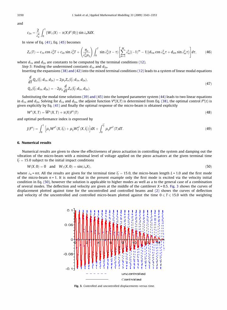
where kn = np. All the results are given for the terminal time tf ¼ 15:0, the micro-beam length L = 1.0 and the first modeof the micro-beam n = 1. It is noted that in the present example only the first mode is excited via the velocity initialcondition in Eq. (50), however the solution is applicable to higher modes as well as a to the general case of a combinationof several modes. The deflection and velocity are given at the middle of the cantilever X = 0.5. Fig. 3 shows the curves ofdisplacement plotted against time for the uncontrolled and controlled beams and (2) shows the curves of deflectionand velocity of the uncontrolled and controlled micro-beam plotted against the time 0 6 T 6 15.0 with the weighting

Fig. 3. Controlled and uncontrolled displacements versus time.


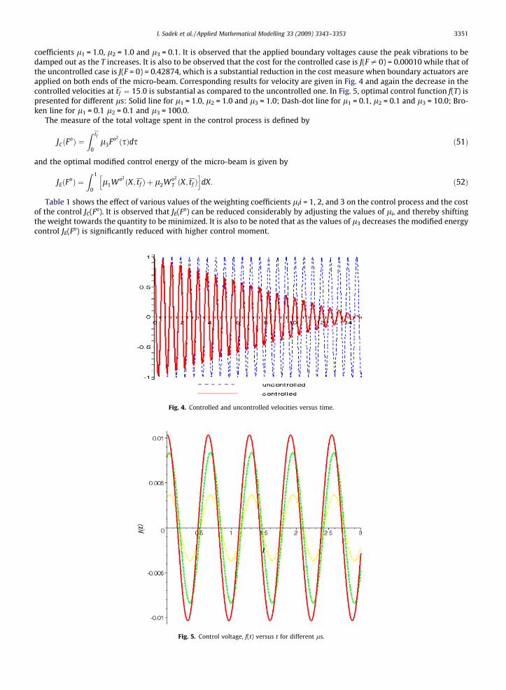
coefficients l1 = 1.0, l2 = 1.0 and l3 = 0.1. It is observed that the applied boundary voltages cause the peak vibrations to bedamped out as the T increases. It is also to be observed that the cost for the controlled case is J(F – 0) = 0.00010 while that ofthe uncontrolled case is J(F = 0) = 0.42874, which is a substantial reduction in the cost measure when boundary actuators areapplied on both ends of the micro-beam. Corresponding results for velocity are given in Fig. 4 and again the decrease in thecontrolled velocities at tf ¼ 15:0 is substantial as compared to the uncontrolled one. In Fig. 5, optimal control function f(T) ispresented for different ls: Solid line for l1 = 1.0, l2 = 1.0 and l3 = 1.0; Dash-dot line for l1 = 0.1, l2 = 0.1 and l3 = 10.0; Bro-ken line for l1 = 0.1 l2 = 0.1 and l3 = 100.0.

The measure of the total voltage spent in the control process is defined by

JCðFoÞ ¼

Z tf

0l3Fo2 ðsÞds ð51Þ

and the optimal modified control energy of the micro-beam is given by

JEðFoÞ ¼

Z 1

0l1Wo2 ðX; tf Þ þ l2Wo2

T ðX; tf Þh i

dX: ð52Þ

Table 1 shows the effect of various values of the weighting coefficients lii = 1, 2, and 3 on the control process and the costof the control JC(Fo). It is observed that JE(Fo) can be reduced considerably by adjusting the values of li, and thereby shiftingthe weight towards the quantity to be minimized. It is also to be noted that as the values of l3 decreases the modified energycontrol JE(Fo) is significantly reduced with higher control moment.

Fig. 4. Controlled and uncontrolled velocities versus time.

Fig. 5. Control voltage, f(t) versus t for different ls.

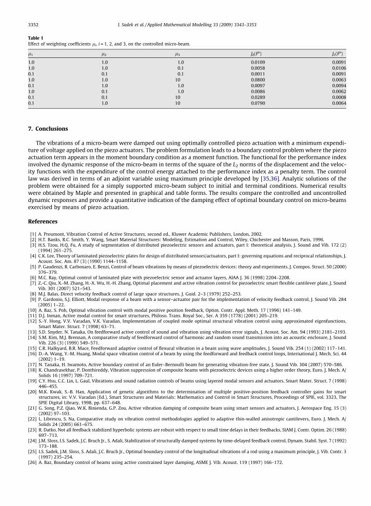
Table 1Effect of weighting coefficients li, i = 1, 2, and 3, on the controlled micro-beam.

l1 l2 l3 JE(Fo) JC(Fo)

1.0 1.0 1.0 0.0109 0.00911.0 1.0 0.1 0.0058 0.01060.1 0.1 0.1 0.0011 0.00911.0 1.0 10 0.0800 0.00630.1 1.0 1.0 0.0097 0.00941.0 0.1 1.0 0.0086 0.00620.1 0.1 10 0.0289 0.00080.1 1.0 10 0.0790 0.0064


7. Conclusions

The vibrations of a micro-beam were damped out using optimally controlled piezo actuation with a minimum expendi-ture of voltage applied on the piezo actuators. The problem formulation leads to a boundary control problem where the piezoactuation term appears in the moment boundary condition as a moment function. The functional for the performance indexinvolved the dynamic response of the micro-beam in terms of the square of the L2 norms of the displacement and the veloc-ity functions with the expenditure of the control energy attached to the performance index as a penalty term. The controllaw was derived in terms of an adjoint variable using maximum principle developed by [35,36]. Analytic solutions of theproblem were obtained for a simply supported micro-beam subject to initial and terminal conditions. Numerical resultswere obtained by Maple and presented in graphical and table forms. The results compare the controlled and uncontrolleddynamic responses and provide a quantitative indication of the damping effect of optimal boundary control on micro-beamsexercised by means of piezo actuation.

References

[1] A. Preumont, Vibration Control of Active Structures, second ed., Kluwer Academic Publishers, London, 2002.[2] H.T. Banks, R.C. Smith, Y. Wang, Smart Material Structures: Modeling, Estimation and Control, Wiley, Chichester and Masson, Paris, 1996.[3] H.S. Tzou, H.Q. Fu, A study of segmentation of distributed piezoelectric sensors and actuators, part I: theoretical analysis, J. Sound and Vib. 172 (2)

(1994) 261–275.[4] C.K. Lee, Theory of laminated piezoelectric plates for design of distributed sensors/actuators, part I: governing equations and reciprocal relationships, J.

Acoust. Soc. Am. 87 (3) (1990) 1144–1158.[5] P. Gaudenzi, R. Carbonaro, E. Benzi, Control of beam vibrations by means of piezoelectric devices: theory and experiments, J. Compos. Struct. 50 (2000)

376–379.[6] M.C. Ray, Optimal control of laminated plate with piezoelectric sensor and actuator layers, AIAA J. 36 (1998) 2204–2208.[7] Z.-C. Qiu, X.-M. Zhang, H.-X. Wu, H.-H. Zhang, Optimal placement and active vibration control for piezoelectric smart flexible cantilever plate, J. Sound

Vib. 301 (2007) 521–543.[8] M.J. Balas, Direct velocity feedback control of large space structures, J. Guid. 2–3 (1979) 252–253.[9] P. Gardonio, S.J. Elliott, Modal response of a beam with a sensor–actuator pair for the implementation of velocity feedback control, J. Sound Vib. 284

(2005) 1–22.[10] A. Baz, S. Poh, Optimal vibration control with modal positive position feedback, Optim. Contr. Appl. Meth. 17 (1996) 141–149.[11] D.J. Inman, Active modal control for smart structures, Philoso. Trans. Royal Soc., Ser. A 359 (1778) (2001) 205–219.[12] S.-Y. Hong, V.V. Varadan, V.K. Varadan, Implementation of coupled mode optimal structural vibration control using approximated eigenfunctions,

Smart Mater. Struct. 7 (1998) 63–71.[13] S.D. Snyder, N. Tanaka, On feedforward active control of sound and vibration using vibration error signals, J. Acoust. Soc. Am. 94 (1993) 2181–2193.[14] S.M. Kim, M.J. Brennan, A comparative study of feedforward control of harmonic and random sound transmission into an acoustic enclosure, J. Sound

Vib. 226 (3) (1999) 549–571.[15] C.R. Halkyard, B.R. Mace, Feedforward adaptive control of flexural vibration in a beam using wave amplitudes, J. Sound Vib. 254 (1) (2002) 117–141.[16] D.-A. Wang, Y.-M. Huang, Modal space vibration control of a beam by using the feedforward and feedback control loops, International J. Mech. Sci. 44

(2002) 1–19.[17] N. Tanaka, H. Iwamoto, Active boundary control of an Euler–Bernoulli beam for generating vibration-free state, J. Sound Vib. 304 (2007) 570–586.[18] K. Chandrasekhar, P. Donthireddy, Vibration suppression of composite beams with piezoelectric devices using a higher order theory, Euro. J. Mech. A/

Solids 16 (1997) 709–721.[19] C.Y. Hsu, C.C. Lin, L. Gaul, Vibrations and sound radiation controls of beams using layered modal sensors and actuators, Smart Mater. Struct. 7 (1998)

446–455.[20] M.K. Kwak, S.-B. Han, Application of genetic algorithms to the determination of multiple positive-position feedback controller gains for smart

structures, in: V.V. Varadan (Ed.), Smart Structures and Materials: Mathematics and Control in Smart Structures, Proceedings of SPIE, vol. 3323, TheSPIE Digital Library, 1998, pp. 637–648.

[21] G. Song, P.Z. Qiao, W.K. Binienda, G.P. Zou, Active vibration damping of composite beam using smart sensors and actuators, J. Aerospace Eng. 15 (3)(2002) 97–103.

[22] L. Librescu, S. Na, Comparative study on vibration control methodologies applied to adaptive thin-walled anisotropic cantilevers, Euro. J. Mech. A/Solids 24 (2005) 661–675.

[23] R. Datko, Not all feedback stabilized hyperbolic systems are robust with respect to small time delays in their feedbacks, SIAM J. Contr. Optim. 26 (1988)697–713.

[24] J.M. Sloss, I.S. Sadek, J.C. Bruch Jr., S. Adali, Stabilization of structurally damped systems by time-delayed feedback control, Dynam. Stabil. Syst. 7 (1992)173–188.

[25] I.S. Sadek, J.M. Sloss, S. Adali, J.C. Bruch Jr., Optimal boundary control of the longitudinal vibrations of a rod using a maximum principle, J. Vib. Contr. 3(1997) 235–254.

[26] A. Baz, Boundary control of beams using active constrained layer damping, ASME J. Vib. Acoust. 119 (1997) 166–172.


[27] T. Kaizuka, Active boundary control of a rectangular plate using smart modal sensors, Smart Mater. Struct. 15 (2006) 1395–1403.[28] C. Hwu, W.C. Chang, H.S. Gai, Vibration suppression of composite sandwich beams, J. Sound Vib. 272 (2004) 1–20.[29] B.P. Baillargeon, S.S. Vel, Active vibration suppression of sandwich beams using piezoelectric shear actuators: experiments and numerical simulations,

Journal of Intelligent Mater. Sys. Struct. 16 (2005) 517–530.[30] G.E. Stavroulakis, G. Foutsitzi, E. Hadjigeorgiou, D. Marinova, C.C. Baniotopoulos, Design and robust optimal control of smart beams with application on

vibrations suppression, Adv. Eng. Software 36 (2005) 806–813.[31] S. Raja, A.A. Pashilkar, R. Sreedeep, J.V. Kamesh, Flutter control of a composite plate with piezoelectric multilayered actuators, Aerospace Sci. Technol.

10 (5) (2006) 435–441.[32] J.-H. Han, J. Tani, J. Qiu, Active flutter suppression of a lifting surface using piezoelectric actuation and modern control theory, J. Sound Vib. 291 (3–5)

(2006) 706–722.[33] M.O.M. Carvalho, M. Zindeluk, Active control of waves in a Timoshenko beam, Int. J. Solids Struct. 38 (2001) 1749–1764.[34] M. Collet, V. Walter, P. Delobelle, Active damping of a micro-cantilever piezo-composite beam, J. Sound Vib. 260 (3) (2003) 453–476.[35] J.M. Sloss, J.C. Bruch Jr., I.S. Sadek, S. Adali, Maximum principle for optimal boundary control of vibrating structures with applications to beams, Dynam.

Contr.: An Int. J. 8 (1998) 355–375.[36] J.M. Sloss, I.S. Sadek, J.C. Bruch Jr., S. Adali, Optimal control of structural dynamic systems in one space dimension using a maximum principle, J. Vib.

Contr. 11 (2005) 245–261.[37] A. Lara, J.M. Sloss, J.C. Bruch Jr., I.S. Sadek, S. Adali, Vibration damping in beams via piezo actuation using optimal boundary control, Int. J. Solids Struct.

37 (2000) 6537–6554.

Documents

Optimal boundary control of dynamics responses of piezo actuating micro-beams