UNIT I INTRODUCTION TO OPTICALFIBERS

Prepared by

T.DINESH KUMARAssistant Professor

ECE, SCSVMV

OPTICALCOMMUNICATION

AIM & OBJECTIVES

To learn the basic elements of optical fiber transmission link, fiber modesconfigurations and structures.

To understand the different kind of losses, signal distortion, SM fibers. To learn the various optical sources, materials and fiber splicing. To learn the fiber optical receivers and noise performance in photo detector. To explore link budget, WDM, solitons and SONET/SDH network.

PRE TEST-MCQ TYPE

1. Which equations are best suited for the study of electromagnetic wave propagation?a) Maxwell’s equationsb) Allen-Cahn equationsc) Avrami equationsd) Boltzmann’s equations

2. When λ is the optical wavelength in vacuum, k is given by k=2Π/λ. What does k stand for inthe above equation?a) Phase propagation constantb) Dielectric constantc) Boltzmann’s constantd) Free-space constant

3. When light is described as an electromagnetic wave, it consists of a periodically varyingelectric E and magnetic field H which are oriented at an angle?a) 90 degree to each otherb) Less than 90 degreec) Greater than 90 degreed) 180 degree apart

4. Which is the most important velocity in the study of transmission characteristics of opticalfiber?a) Phase velocityb) Group velocityc) Normalized velocityd) Average velocity

UNIT I INTRODUCTION TO OPTICAL FIBERS

Evolution of fiber optic system- Element of an Optical Fiber Transmission link- Total internalReflection- Acceptance angle –Numerical aperture – Skew rays Ray Optics-Optical FiberModes and Configurations- Mode theory of Circular Wave guides- Overview of Modes-KeyModal concepts- Linearly Polarized Modes -Single Mode Fibers-Graded Index fiber structure

THEORY

Introduction

Fiber-optic communication is a method of transmitting information from one place toanother by sending pulses of light through an optical fiber. The light forms anelectromagnetic carrier wave that is modulated to carry information. Fiber is preferred overelectrical cabling when high bandwidth, long distance, or immunity to electromagneticinterference are required. This type of communication can transmit voice, video, andtelemetry through local area networks, computer networks, or across long distances.

Optical fiber is used by many telecommunications companies to transmit telephone signals,Internet communication, and cable television signals. Researchers at Bell Labs have reachedinternet speeds of over 100 peta bit ×kilometer per second using fiber-optic communication.The process of communicating using fiber-optics involves the following basic steps:

1. Creating the optical signal involving the use of a transmitter, usually from an electricalsignal

2. Relaying the signal along the fiber, ensuring that the signal does not become too distortedor weak

3. Receiving the optical signal

4. Converting it into an electrical signal

Historical Development

First developed in the 1970s, fiber-optics have revolutionized the telecommunicationsindustry and have played a major role in the advent of the Information Age. Becauseof its advantages over electrical transmission, optical fibers have largely replacedcopper wire communications in core networks in the developed world.

In 1880 Alexander Graham Bell and his assistant Charles Sumner Tainter created avery early precursor to fiber-optic communications, the Photophone, at Bell'snewly established Volta Laboratory in Washington, D.C. Bell considered it his mostimportant invention. The device allowed for the transmission of sound on a beam of light.On June 3, 1880, Bell conducted the world's first wireless telephone transmission betweentwo buildings, some 213 meters apart. Due to its use of an atmospheric transmissionmedium, the Photophone would not prove practical until advances in laser and optical fibertechnologies permitted the secure transport of light. The Photophone's first practical use camein military communication systems many decades later.

In 1954 Harold Hopkins and Narinder Singh Kapany showed that rolled fiber glass allowedlight to be transmitted. Initially it was considered that the light can traverse in only straightmedium. Jun-ichi Nishizawa, a Japanese scientist at Tohoku University, proposed theuse of optical fibers for communications in 1963. Nishizawa invented the PIN diode andthe static induction transistor, both of which contributed to the development of optical fibercommunications.

In 1966 Charles K. Kao and George Hockham at STC Laboratories (STL) showed thatthe losses of 1,000 dB/km in existing glass (compared to 5–10 dB/km in coaxial cable)were due to contaminants which could potentially be removed.

Optical fiber was successfully developed in 1970 by Corning Glass Works, withattenuation low enough for communication purposes (about 20 dB/km) and at the sametime GaAs semiconductor lasers were developed that were compact and therefore suitablefor transmitting light through fiber optic cables for long distances. In 1973, Optelecom, Inc.,co-founded by the inventor of the laser, Gordon Gould, received a contract from APA for thefirst optical communication systems. Developed for Army Missile Command in Huntsville,Alabama, it was a laser on the ground and a spout of optical fiber played out by missile totransmit a modulated signal over five kilometers.

After a period of research starting from 1975, the first commercial fiber-opticcommunications system was developed which operated at a wavelength around 0.8 μm andused GaAs semiconductor lasers. This first-generation system operated at a bit rate of 45Mbit/s with repeater spacing of up to 10 km. Soon on 22 April 1977, General Telephone andElectronics sent the first live telephone traffic through fiber optics at a 6 Mbit/s throughput inLong Beach, California.

In October 1973, Corning Glass signed a development contract with CSELT and Pirelliaimed to test fiber optics in an urban environment: in September 1977, the second cable inthis test series, named COS-2, was experimentally deployed in two lines (9 km) in Turin,for the first time in a big city, at a speed of 140 Mbit/s.

The second generation of fiber-optic communication was developed for commercial use inthe early 1980s, operated at 1.3 μm and used InGaAsP semiconductor lasers. These earlysystems were initially limited by multi mode fiber dispersion, and in 1981 the single-modefiber was revealed to greatly improve system performance, however practical connectorscapable of working with single mode fiber proved difficult to develop. Canadian serviceprovider SaskTel had completed construction of what was then the world's longestcommercial fiber optic network, which covered 3,268 km (2,031 mi) and linked 52communities. By 1987, these systems were operating at bit rates of up to 1.7 Gb/s withrepeater spacing up to 50 km (31 mi). The first transatlantic telephone cable to use opticalfiber was TAT-8, based on Desurvire optimised laser amplification technology. It went intooperation in 1988.

Third-generation fiber-optic systems operated at 1.55 μm and had losses of about 0.2dB/km. This development was spurred by the discovery of Indium gallium arsenide and thedevelopment of the Indium Gallium Arsenide photodiode by Pearsall. Engineers overcameearlier difficulties with pulse- spreading at that wavelength using conventional InGaAsPsemiconductor lasers. Scientists overcame this difficulty by using dispersion-shifted fibersdesigned to have minimal dispersion at 1.55 μm or by limiting the laser spectrum to a singlelongitudinal mode. These developments eventually allowed third-generation systems tooperate commercially at 2.5 Gbit/s with repeater spacing in excess of 100 km (62 mi).

The fourth generation of fiber-optic communication systems used optical amplification toreduce the need for repeaters and wavelength-division multiplexing to increase datacapacity. These two improvements caused a revolution that resulted in the doubling ofsystem capacity every six months starting in 1992 until a bit rate of 10 Tb/s was reached by2001. In 2006 a bit-rate of 14 Tbit/s was reached over a single 160 km (99 mi) line usingoptical amplifiers.

The focus of development for the fifth generation of fiber-optic communications is onextending the wavelength range over which a WDM system can operate. Theconventional wavelength window, known as the C band, covers the wavelength range1.53–1.57 μm, and dry fiber has a low-loss window promising an extension of thatrange to 1.30–1.65 μm. Other developments include the concept of "optical solutions",pulses that preserve their shape by counteracting the effects of dispersion with the nonlineareffects of the fiber by using pulses of a specific shape.

In the late 1990s through 2000, industry promoters, and research companies such as KMI, andRHK predicted massive increases in demand for communications bandwidth due toincreased use of the Internet, and commercialization of various bandwidth-intensiveconsumer services, such as video on demand. Internet protocol data traffic wasincreasing exponentially, at a faster rate than integrated circuit complexity hadincreased under Moore's Law. From the bust of the dot-com bubble through 2006,however, the main trend in the industry has been consolidation of firms and offshoring of manufacturing to reduce costs.

Advantages of Fiber Optic Transmission

Optical fibers have largely replaced copper wire communications in core networks in thedeveloped world, because of its advantages over electrical transmission. Here are the mainadvantages of fiber optic transmission.

Extremely High Bandwidth: No other cable-based data transmission medium offers thebandwidth that fiber does. The volume of data that fiber optic cables transmit per unit time isfar great than copper cables.

Longer Distance: in fiber optic transmission, optical cables are capable of providing lowpower loss, which enables signals can be transmitted to a longer distance than copper cables.

Resistance to Electromagnetic Interference: in practical cable deployment, it’s inevitableto meet environments like power substations, heating, ventilating and otherindustrial sources of interference. However, fiber has a very low rate of bit error (10 EXP-13), as a result of fiber being so resistant to electromagnetic interference. Fiber optictransmission is virtually noise free.

Low Security Risk: the growth of the fiber optic communication market is mainly driven byincreasing awareness about data security concerns and use of the alternative raw material.Data or signals are transmitted via light in fiber optic transmission. Therefore there is no wayto detect the data being transmitted by "listening in" to the electromagnetic energy"leaking" through the cable, which ensures the absolute security of information.

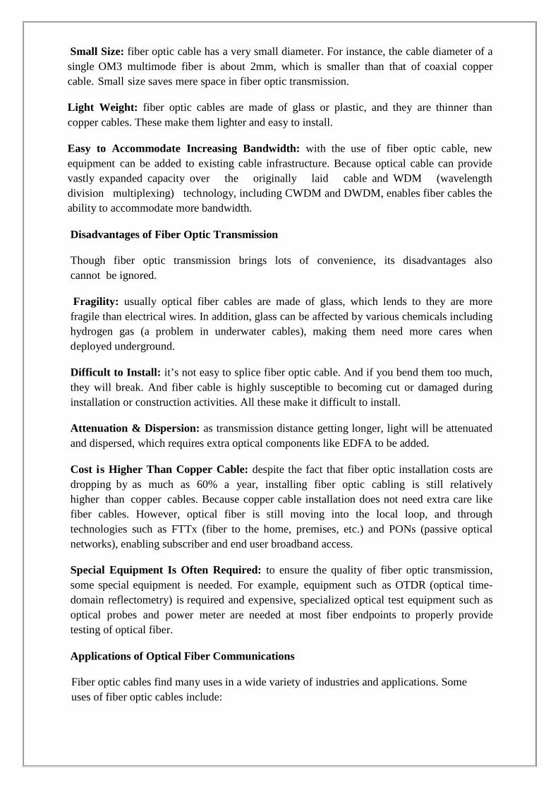
Small Size: fiber optic cable has a very small diameter. For instance, the cable diameter of asingle OM3 multimode fiber is about 2mm, which is smaller than that of coaxial coppercable. Small size saves mere space in fiber optic transmission.

Light Weight: fiber optic cables are made of glass or plastic, and they are thinner thancopper cables. These make them lighter and easy to install.

Easy to Accommodate Increasing Bandwidth: with the use of fiber optic cable, newequipment can be added to existing cable infrastructure. Because optical cable can providevastly expanded capacity over the originally laid cable and WDM (wavelengthdivision multiplexing) technology, including CWDM and DWDM, enables fiber cables theability to accommodate more bandwidth.

Disadvantages of Fiber Optic Transmission

Though fiber optic transmission brings lots of convenience, its disadvantages alsocannot be ignored.

Fragility: usually optical fiber cables are made of glass, which lends to they are morefragile than electrical wires. In addition, glass can be affected by various chemicals includinghydrogen gas (a problem in underwater cables), making them need more cares whendeployed underground.

Difficult to Install: it’s not easy to splice fiber optic cable. And if you bend them too much,they will break. And fiber cable is highly susceptible to becoming cut or damaged duringinstallation or construction activities. All these make it difficult to install.

Attenuation & Dispersion: as transmission distance getting longer, light will be attenuatedand dispersed, which requires extra optical components like EDFA to be added.

Cost is Higher Than Copper Cable: despite the fact that fiber optic installation costs aredropping by as much as 60% a year, installing fiber optic cabling is still relativelyhigher than copper cables. Because copper cable installation does not need extra care likefiber cables. However, optical fiber is still moving into the local loop, and throughtechnologies such as FTTx (fiber to the home, premises, etc.) and PONs (passive opticalnetworks), enabling subscriber and end user broadband access.

Special Equipment Is Often Required: to ensure the quality of fiber optic transmission,some special equipment is needed. For example, equipment such as OTDR (optical time-domain reflectometry) is required and expensive, specialized optical test equipment such asoptical probes and power meter are needed at most fiber endpoints to properly providetesting of optical fiber.

Applications of Optical Fiber Communications

Fiber optic cables find many uses in a wide variety of industries and applications. Someuses of fiber optic cables include:

Medical -Used as light guides, imaging tools and also as lasers for surgeries

Defense/Government-Used as hydrophones for seismic waves and SONAR , as wiring inaircraft, submarines and other vehicles and also for field networking

Data Storage- Used for data transmission

Telecommunications- Fiber is laid and used for transmitting and receiving purposes

Networking- Used to connect users and servers in a variety of network settings and helpincrease the speed and accuracy of data transmission

Industrial/Commercial- Used for imaging in hard to reach areas, as wiring where EMI is anissue, as sensory devices to make temperature, pressure and other measurements, and aswiring in automobiles and in industrial settings.

Broadcast/CATV-Broadcast/cable companies are using fiber optic cables for wiring CATV,HDTV, internet, video on- demand and other applications. Fiber optic cables are used forlighting and imaging and as sensors to measure and monitor a vast array of variables. Fiberoptic cables are also used in research and development and testing across all the abovementioned industries

The optical fibers have many applications. Some of them are as follows

Used in telephone systems

Used in sub-marine cable networks

Used in data link for computer networks, CATV Systems

Used in CCTV surveillance cameras

Used for connecting fire, police, and other emergency services.

Used in hospitals, schools, and traffic management systems.

They have many industrial uses and also used for in heavy duty constructions.

Block Diagram of Optical Fiber Communication System

Block Diagram of Optical Fiber Communication System

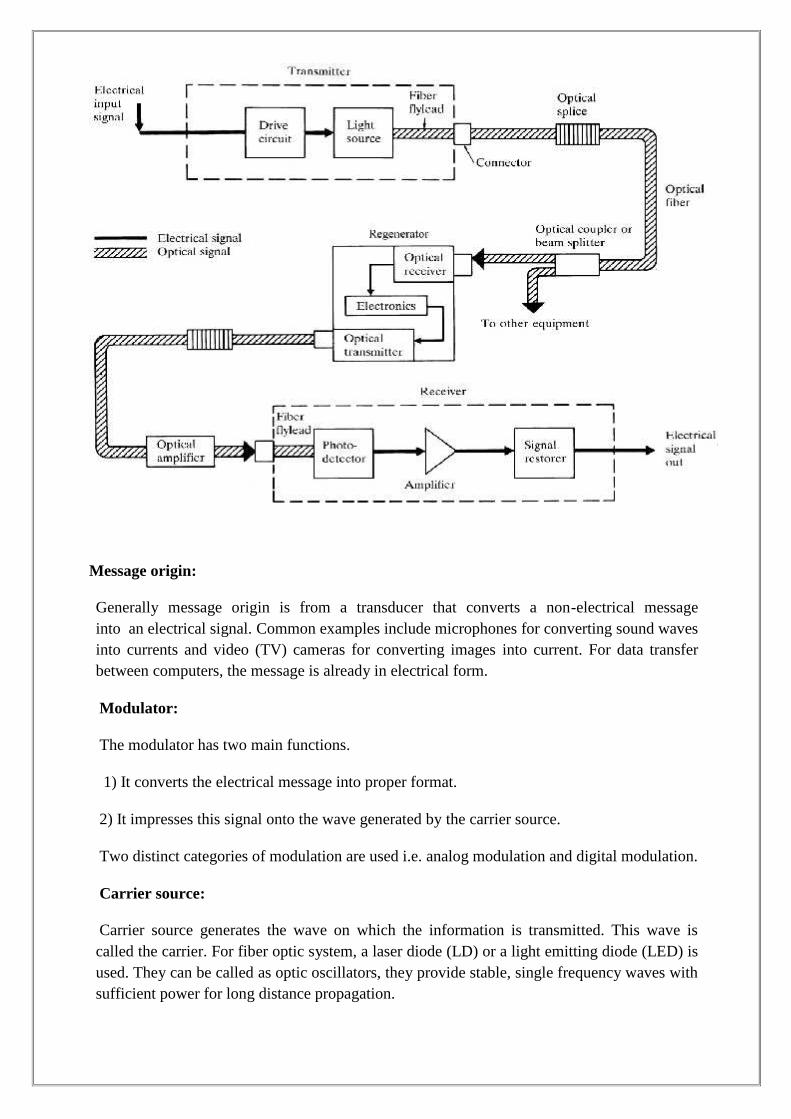
Message origin:

Generally message origin is from a transducer that converts a non-electrical messageinto an electrical signal. Common examples include microphones for converting sound wavesinto currents and video (TV) cameras for converting images into current. For data transferbetween computers, the message is already in electrical form.

Modulator:

The modulator has two main functions.

1) It converts the electrical message into proper format.

2) It impresses this signal onto the wave generated by the carrier source.

Two distinct categories of modulation are used i.e. analog modulation and digital modulation.

Carrier source:

Carrier source generates the wave on which the information is transmitted. This wave iscalled the carrier. For fiber optic system, a laser diode (LD) or a light emitting diode (LED) isused. They can be called as optic oscillators, they provide stable, single frequency waves withsufficient power for long distance propagation.

Channel coupler:

Coupler feeds the power into information channel. For an atmospheric optic system, thechannel coupler is a lens used for collimating the light emitted by the source and directing thislight towards the receiver. The coupler must efficiently transfer the modulated light beamfrom the source to the optic fiber. The channel coupler design is an important part of fibersystem because of possibility of high losses.

Information channel:

The information channel is the path between the transmitter and receiver. In fiberoptic communications, a glass or plastic fiber is the channel. Desirable characteristics of theinformation channel include low attenuation and large light acceptance cone angle. Opticalamplifiers boost the power levels of weak signals. Amplifiers are needed in very long links toprovide sufficient power to the receiver. Repeaters can be used only for digital systems. Theyconvert weak and distorted optical signals to electrical ones and then regenerate the originaldigital pulse trains for further transmission.

Another important property of the information channel is the propagation time of thewaves travelling along it. A signal propagating along a fiber normally contains a range offiber optic frequencies and divides its power along several ray paths. This results in adistortion of the propagation signal. In a digital system, this distortion appears as a spreadingand deforming of the pulses. The spreading is so great that adjacent pulses begin to overlapand become unrecognizable as separate bits of information.

Optical detector:

The information begin transmitted is detected by detector. In the fiber system the optic waveis converted into an electric current by a photodetector. The current developed by the detectoris proportional to the power in the incident optic wave. Detector output current containsthe transmitted information. This detector output is then filtered to remove the constant biasand then amplified. The important properties of photodetectors are small size, economy,long life, low power consumption, high sensitivity to optic signals and fast response toquick variations in the optic power. Signal processing includes filtering, amplification. Properfiltering maximizes the ratio of signal to unwanted power. For a digital system decisioncircuit is an additional block. The bit error rate (BER) should be very small for qualitycommunications.

Signal processing:

Signal processing includes filtering, amplification. Proper filtering maximizes the ratio ofsignal to unwanted power. For a digital syst5em decision circuit is an additional block. Thebit error rate (BER) should be very small for quality communications.

Message output:

The electrical form of the message emerging from the signal processor is transformed into asound wave or visual image. Sometimes these signals are directly usable when computers orother machines are connected through a fiber system.

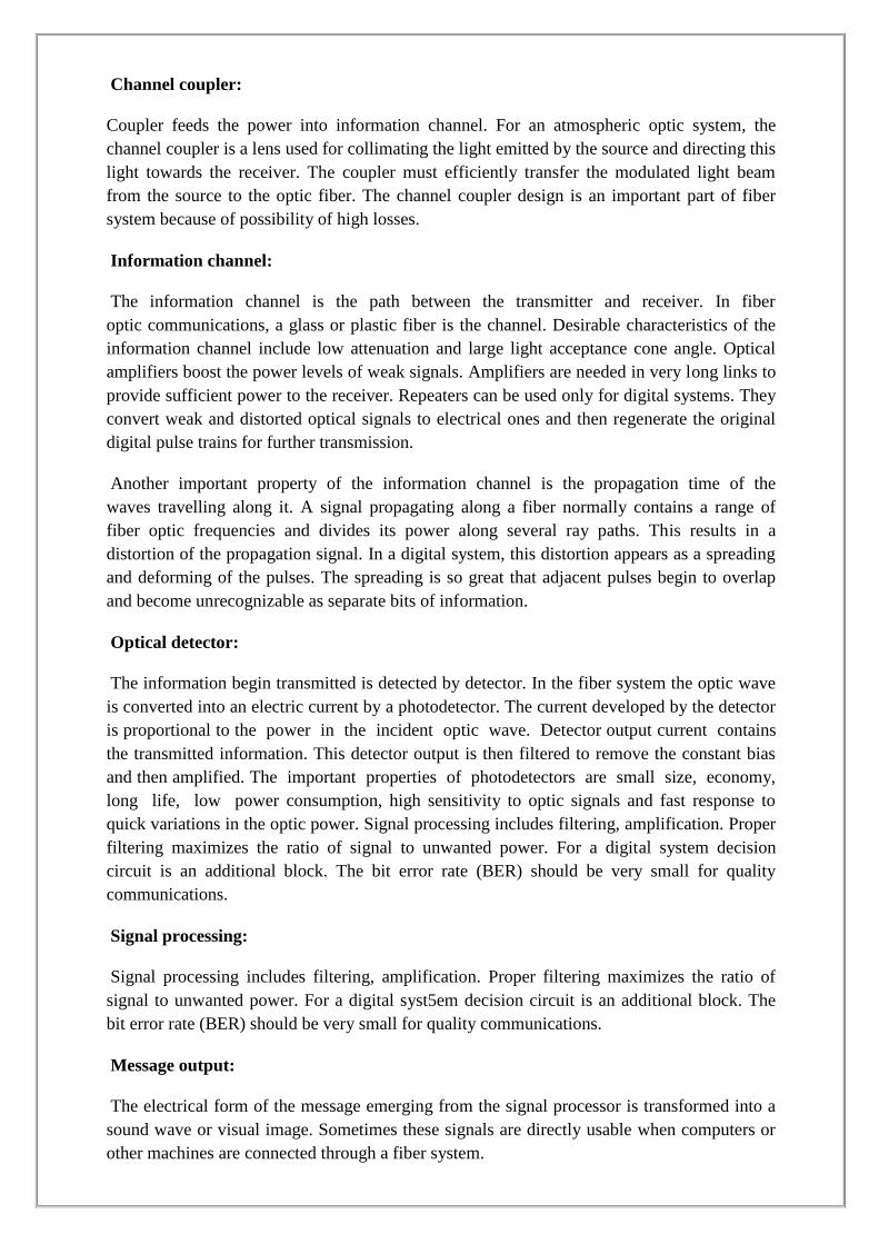
Electromagnetic Spectrum

The radio waves and light are electromagnetic waves. The rate at which they alternate inpolarity is called their frequency (f) measured in hertz (Hz). The speed of electromagneticwave (c) in free space is approximately 3 x 108 m/sec. The distance travelled during eachcycle is called as wavelength (λ)

In fiber optics, it is more convenient to use the wavelength of light instead of the frequencywith light frequencies; wavelength is often stated in microns or nanometers.

1 micron (µ) = 1 Micrometre (1 x 10-6) ;1 nano (n) = 10-9 meter

Fiber optics uses visible and infrared light. Infrared light covers a fairly wide range ofwavelengths and is generally used for all fiber optic communications. Visible light isnormally used for very short range transmission using a plastic fiber

Electromagnetic Spectrum

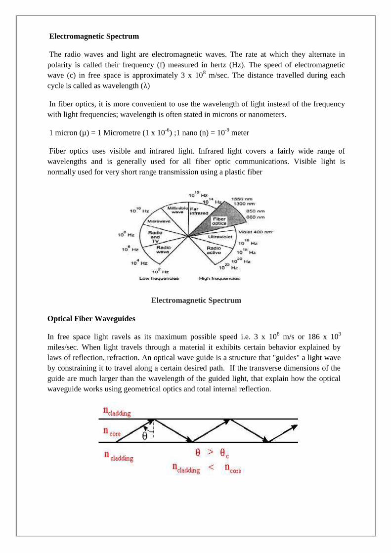
Optical Fiber Waveguides

In free space light ravels as its maximum possible speed i.e. 3 x 108 m/s or 186 x 103

miles/sec. When light travels through a material it exhibits certain behavior explained bylaws of reflection, refraction. An optical wave guide is a structure that "guides" a light waveby constraining it to travel along a certain desired path. If the transverse dimensions of theguide are much larger than the wavelength of the guided light, that explain how the opticalwaveguide works using geometrical optics and total internal reflection.

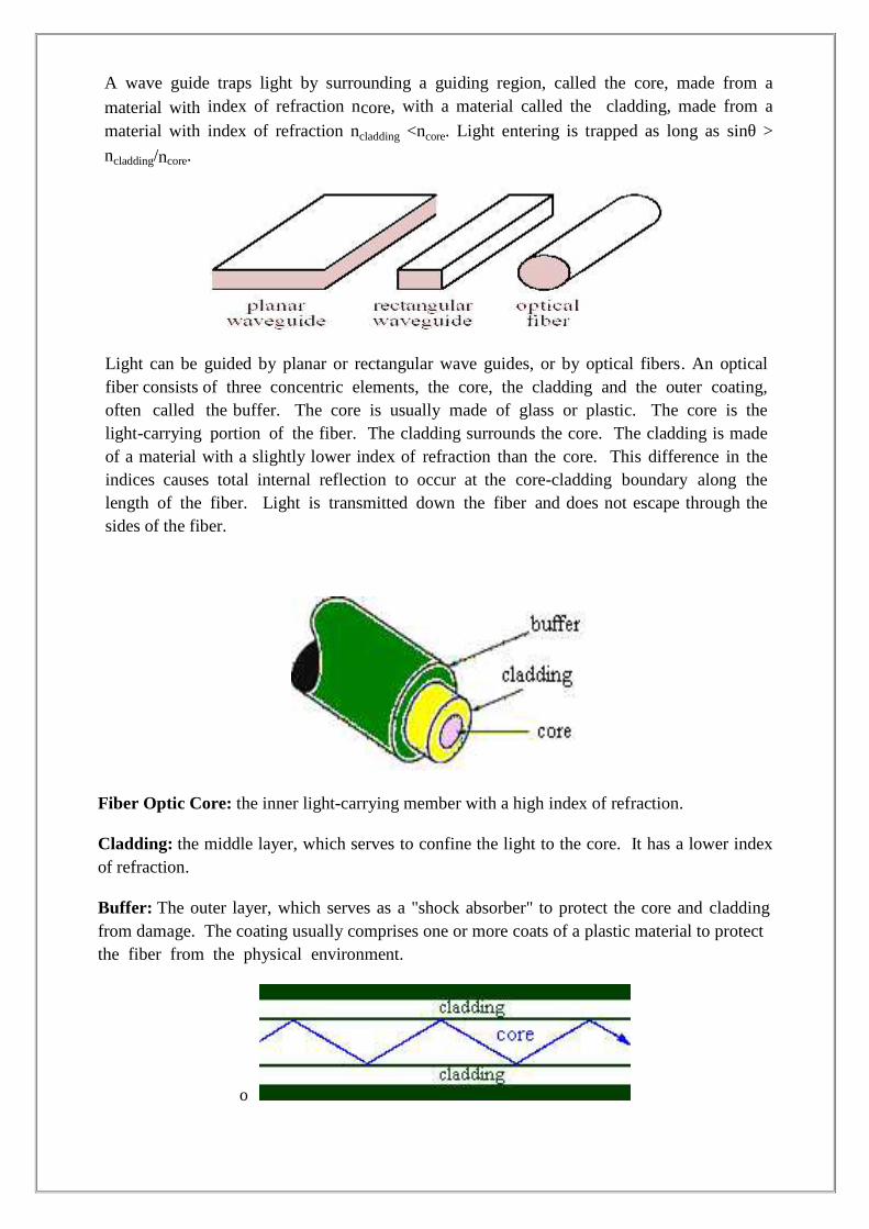
A wave guide traps light by surrounding a guiding region, called the core, made from a

material with index of refraction ncore, with a material called the cladding, made from a

material with index of refraction ncladding <ncore. Light entering is trapped as long as sinθ >ncladding/ncore.

Light can be guided by planar or rectangular wave guides, or by optical fibers. An opticalfiber consists of three concentric elements, the core, the cladding and the outer coating,often called the buffer. The core is usually made of glass or plastic. The core is thelight-carrying portion of the fiber. The cladding surrounds the core. The cladding is madeof a material with a slightly lower index of refraction than the core. This difference in theindices causes total internal reflection to occur at the core-cladding boundary along thelength of the fiber. Light is transmitted down the fiber and does not escape through thesides of the fiber.

Fiber Optic Core: the inner light-carrying member with a high index of refraction.

Cladding: the middle layer, which serves to confine the light to the core. It has a lower indexof refraction.

Buffer: The outer layer, which serves as a "shock absorber" to protect the core and claddingfrom damage. The coating usually comprises one or more coats of a plastic material to protectthe fiber from the physical environment.

o

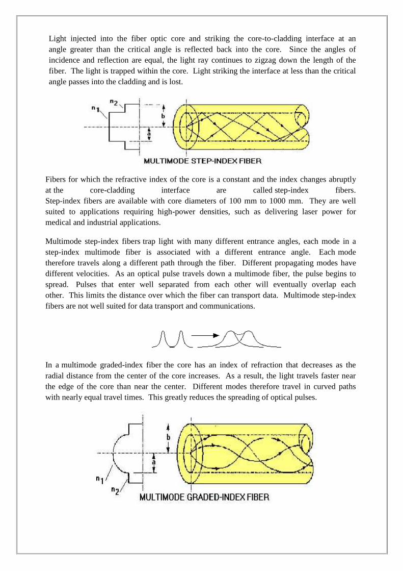
Light injected into the fiber optic core and striking the core-to-cladding interface at anangle greater than the critical angle is reflected back into the core. Since the angles ofincidence and reflection are equal, the light ray continues to zigzag down the length of thefiber. The light is trapped within the core. Light striking the interface at less than the criticalangle passes into the cladding and is lost.

Fibers for which the refractive index of the core is a constant and the index changes abruptlyat the core-cladding interface are called step-index fibers.Step-index fibers are available with core diameters of 100 mm to 1000 mm. They are wellsuited to applications requiring high-power densities, such as delivering laser power formedical and industrial applications.

Multimode step-index fibers trap light with many different entrance angles, each mode in astep-index multimode fiber is associated with a different entrance angle. Each modetherefore travels along a different path through the fiber. Different propagating modes havedifferent velocities. As an optical pulse travels down a multimode fiber, the pulse begins tospread. Pulses that enter well separated from each other will eventually overlap eachother. This limits the distance over which the fiber can transport data. Multimode step-indexfibers are not well suited for data transport and communications.

In a multimode graded-index fiber the core has an index of refraction that decreases as theradial distance from the center of the core increases. As a result, the light travels faster nearthe edge of the core than near the center. Different modes therefore travel in curved pathswith nearly equal travel times. This greatly reduces the spreading of optical pulses.

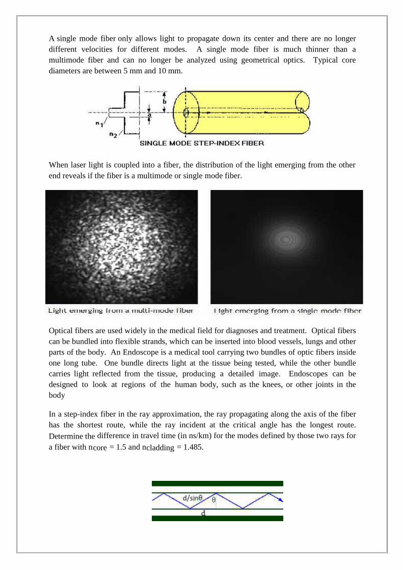
A single mode fiber only allows light to propagate down its center and there are no longerdifferent velocities for different modes. A single mode fiber is much thinner than amultimode fiber and can no longer be analyzed using geometrical optics. Typical corediameters are between 5 mm and 10 mm.

When laser light is coupled into a fiber, the distribution of the light emerging from the otherend reveals if the fiber is a multimode or single mode fiber.

Optical fibers are used widely in the medical field for diagnoses and treatment. Optical fiberscan be bundled into flexible strands, which can be inserted into blood vessels, lungs and otherparts of the body. An Endoscope is a medical tool carrying two bundles of optic fibers insideone long tube. One bundle directs light at the tissue being tested, while the other bundlecarries light reflected from the tissue, producing a detailed image. Endoscopes can bedesigned to look at regions of the human body, such as the knees, or other joints in thebody

In a step-index fiber in the ray approximation, the ray propagating along the axis of the fiberhas the shortest route, while the ray incident at the critical angle has the longest route.

Determine the difference in travel time (in ns/km) for the modes defined by those two rays for

a fiber with ncore = 1.5 and ncladding = 1.485.

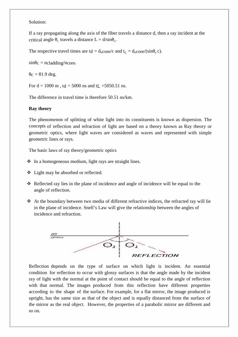
Solution:

If a ray propagating along the axis of the fiber travels a distance d, then a ray incident at the

critical angle θc travels a distance L = d/sinθc.

The respective travel times are td = dncore/c and tL = dncore/(sinθc c).

sinθc = ncladding/ncore.

θc = 81.9 deg.

For d = 1000 m , td = 5000 ns and tL =5050.51 ns.

The difference in travel time is therefore 50.51 ns/km.

Ray theory

The phenomenon of splitting of white light into its constituents is known as dispersion. Theconcepts of reflection and refraction of light are based on a theory known as Ray theory orgeometric optics, where light waves are considered as waves and represented with simplegeometric lines or rays.

The basic laws of ray theory/geometric optics

In a homogeneous medium, light rays are straight lines.

Light may be absorbed or reflected.

Reflected ray lies in the plane of incidence and angle of incidence will be equal to theangle of reflection.

At the boundary between two media of different refractive indices, the refracted ray will liein the plane of incidence. Snell’s Law will give the relationship between the angles ofincidence and refraction.

Reflection depends on the type of surface on which light is incident. An essentialcondition for reflection to occur with glossy surfaces is that the angle made by the incidentray of light with the normal at the point of contact should be equal to the angle of reflectionwith that normal. The images produced from this reflection have different propertiesaccording to the shape of the surface. For example, for a flat mirror, the image produced isupright, has the same size as that of the object and is equally distanced from the surface ofthe mirror as the real object. However, the properties of a parabolic mirror are different andso on.

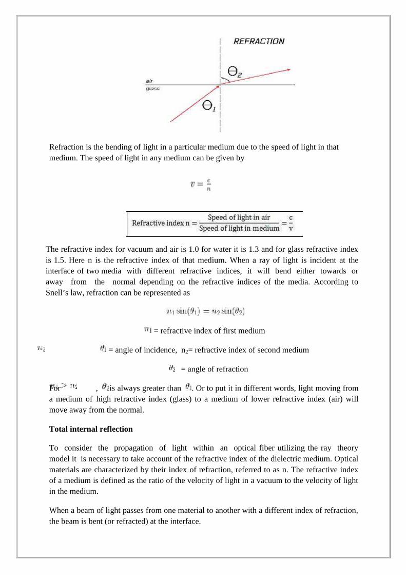
Refraction is the bending of light in a particular medium due to the speed of light in thatmedium. The speed of light in any medium can be given by

The refractive index for vacuum and air is 1.0 for water it is 1.3 and for glass refractive indexis 1.5. Here n is the refractive index of that medium. When a ray of light is incident at theinterface of two media with different refractive indices, it will bend either towards oraway from the normal depending on the refractive indices of the media. According toSnell’s law, refraction can be represented as

= refractive index of first medium

= angle of incidence, n2= refractive index of second medium

= angle of refraction

For , is always greater than . Or to put it in different words, light moving froma medium of high refractive index (glass) to a medium of lower refractive index (air) willmove away from the normal.

Total internal reflection

To consider the propagation of light within an optical fiber utilizing the ray theorymodel it is necessary to take account of the refractive index of the dielectric medium. Opticalmaterials are characterized by their index of refraction, referred to as n. The refractive indexof a medium is defined as the ratio of the velocity of light in a vacuum to the velocity of lightin the medium.

When a beam of light passes from one material to another with a different index of refraction,the beam is bent (or refracted) at the interface.

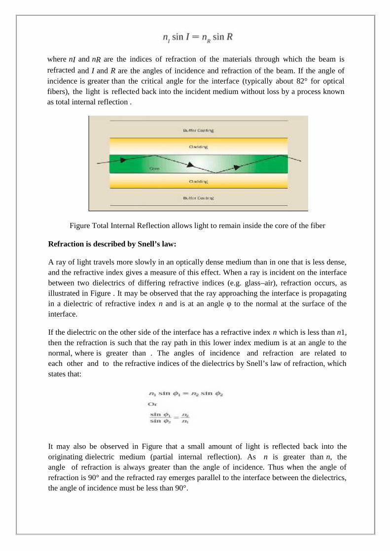
where nI and nR are the indices of refraction of the materials through which the beam is

refracted and I and R are the angles of incidence and refraction of the beam. If the angle ofincidence is greater than the critical angle for the interface (typically about 82° for opticalfibers), the light is reflected back into the incident medium without loss by a process knownas total internal reflection .

Figure Total Internal Reflection allows light to remain inside the core of the fiber

Refraction is described by Snell’s law:

A ray of light travels more slowly in an optically dense medium than in one that is less dense,and the refractive index gives a measure of this effect. When a ray is incident on the interfacebetween two dielectrics of differing refractive indices (e.g. glass–air), refraction occurs, asillustrated in Figure . It may be observed that the ray approaching the interface is propagatingin a dielectric of refractive index n and is at an angle φ to the normal at the surface of theinterface.

If the dielectric on the other side of the interface has a refractive index n which is less than n1,then the refraction is such that the ray path in this lower index medium is at an angle to thenormal, where is greater than . The angles of incidence and refraction are related toeach other and to the refractive indices of the dielectrics by Snell’s law of refraction, whichstates that:

It may also be observed in Figure that a small amount of light is reflected back into theoriginating dielectric medium (partial internal reflection). As n is greater than n, theangle of refraction is always greater than the angle of incidence. Thus when the angle ofrefraction is 90° and the refracted ray emerges parallel to the interface between the dielectrics,the angle of incidence must be less than 90°.

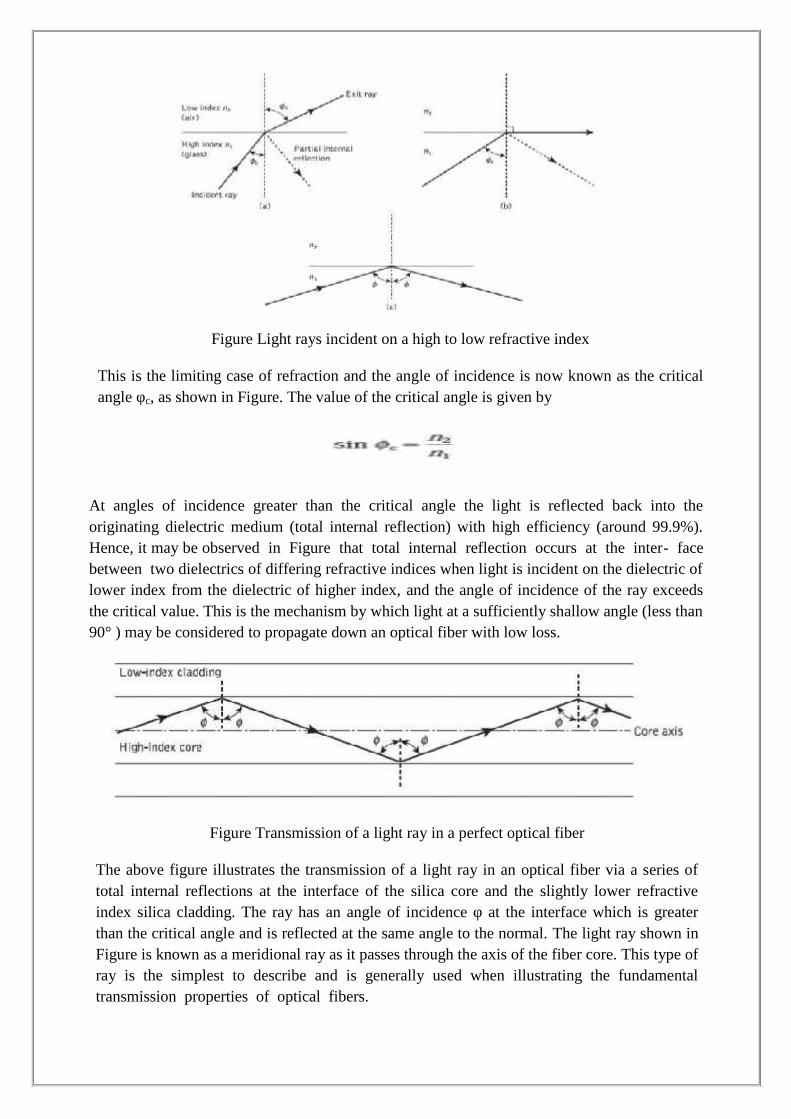
Figure Light rays incident on a high to low refractive index

This is the limiting case of refraction and the angle of incidence is now known as the criticalangle φc, as shown in Figure. The value of the critical angle is given by

At angles of incidence greater than the critical angle the light is reflected back into theoriginating dielectric medium (total internal reflection) with high efficiency (around 99.9%).Hence, it may be observed in Figure that total internal reflection occurs at the inter- facebetween two dielectrics of differing refractive indices when light is incident on the dielectric oflower index from the dielectric of higher index, and the angle of incidence of the ray exceedsthe critical value. This is the mechanism by which light at a sufficiently shallow angle (less than90° ) may be considered to propagate down an optical fiber with low loss.

Figure Transmission of a light ray in a perfect optical fiber

The above figure illustrates the transmission of a light ray in an optical fiber via a series oftotal internal reflections at the interface of the silica core and the slightly lower refractiveindex silica cladding. The ray has an angle of incidence φ at the interface which is greaterthan the critical angle and is reflected at the same angle to the normal. The light ray shown inFigure is known as a meridional ray as it passes through the axis of the fiber core. This type ofray is the simplest to describe and is generally used when illustrating the fundamentaltransmission properties of optical fibers.

It must also be noted that the light transmission illustrated in Figure assumes a perfectfiber, and that any discontinuities or imperfections at the core–cladding interface wouldprobably result in refraction rather than total internal reflection, with the subsequent loss ofthe light ray into the cladding.

Critical Angle

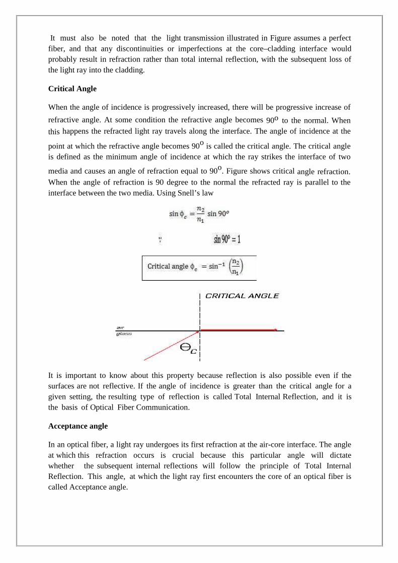
When the angle of incidence is progressively increased, there will be progressive increase of

refractive angle. At some condition the refractive angle becomes 90o to the normal. When

this happens the refracted light ray travels along the interface. The angle of incidence at the

point at which the refractive angle becomes 90o is called the critical angle. The critical angleis defined as the minimum angle of incidence at which the ray strikes the interface of two

media and causes an angle of refraction equal to 90o. Figure shows critical angle refraction.When the angle of refraction is 90 degree to the normal the refracted ray is parallel to theinterface between the two media. Using Snell’s law

It is important to know about this property because reflection is also possible even if thesurfaces are not reflective. If the angle of incidence is greater than the critical angle for agiven setting, the resulting type of reflection is called Total Internal Reflection, and it isthe basis of Optical Fiber Communication.

Acceptance angle

In an optical fiber, a light ray undergoes its first refraction at the air-core interface. The angleat which this refraction occurs is crucial because this particular angle will dictatewhether the subsequent internal reflections will follow the principle of Total InternalReflection. This angle, at which the light ray first encounters the core of an optical fiber iscalled Acceptance angle.

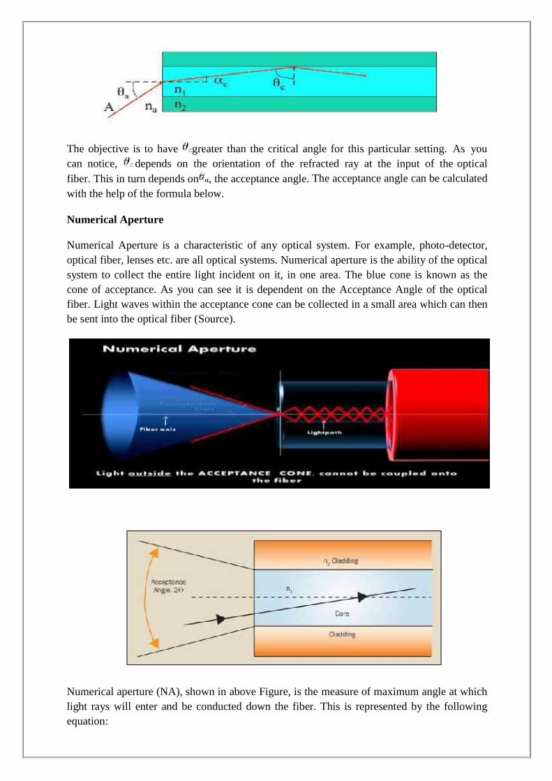
The objective is to have greater than the critical angle for this particular setting. As youcan notice, depends on the orientation of the refracted ray at the input of the opticalfiber. This in turn depends on , the acceptance angle. The acceptance angle can be calculatedwith the help of the formula below.

Numerical Aperture

Numerical Aperture is a characteristic of any optical system. For example, photo-detector,optical fiber, lenses etc. are all optical systems. Numerical aperture is the ability of the opticalsystem to collect the entire light incident on it, in one area. The blue cone is known as thecone of acceptance. As you can see it is dependent on the Acceptance Angle of the opticalfiber. Light waves within the acceptance cone can be collected in a small area which can thenbe sent into the optical fiber (Source).

Numerical aperture (NA), shown in above Figure, is the measure of maximum angle at whichlight rays will enter and be conducted down the fiber. This is represented by the followingequation:

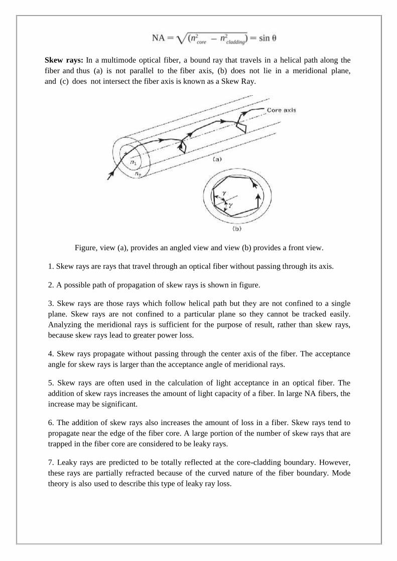
Skew rays: In a multimode optical fiber, a bound ray that travels in a helical path along thefiber and thus (a) is not parallel to the fiber axis, (b) does not lie in a meridional plane,and (c) does not intersect the fiber axis is known as a Skew Ray.

Figure, view (a), provides an angled view and view (b) provides a front view.

1. Skew rays are rays that travel through an optical fiber without passing through its axis.

2. A possible path of propagation of skew rays is shown in figure.

3. Skew rays are those rays which follow helical path but they are not confined to a singleplane. Skew rays are not confined to a particular plane so they cannot be tracked easily.Analyzing the meridional rays is sufficient for the purpose of result, rather than skew rays,because skew rays lead to greater power loss.

4. Skew rays propagate without passing through the center axis of the fiber. The acceptanceangle for skew rays is larger than the acceptance angle of meridional rays.

5. Skew rays are often used in the calculation of light acceptance in an optical fiber. Theaddition of skew rays increases the amount of light capacity of a fiber. In large NA fibers, theincrease may be significant.

6. The addition of skew rays also increases the amount of loss in a fiber. Skew rays tend topropagate near the edge of the fiber core. A large portion of the number of skew rays that aretrapped in the fiber core are considered to be leaky rays.

7. Leaky rays are predicted to be totally reflected at the core-cladding boundary. However,these rays are partially refracted because of the curved nature of the fiber boundary. Modetheory is also used to describe this type of leaky ray loss.

Cylindrical fiber

1. Modes

When light is guided down a fiber (as microwaves are guided down a waveguide), phaseshifts occur at every reflective boundary. There is a finite discrete number of paths down theoptical fiber (known as modes) that produce constructive (in phase and therefore additive)phase shifts that reinforce the transmission. Because each mode occurs at a different angle tothe fiber axis as the beam travels along the length, each one travels a different length throughthe fiber from the input to the output. Only one mode, the zero-order mode, travels the lengthof the fiber without reflections from the sidewalls. This is known as a single-mode fiber. Theactual number of modes that can be propagated in a given optical fiber is determined by thewavelength of light and the diameter and index of refraction of the core of the fiber.

The exact solution of Maxwell’s equations for a cylindrical homogeneous core dielectricwaveguide* involves much algebra and yields a complex result. Although the presentation ofthis mathematics is beyond the scope of this text, it is useful to consider the resulting modalfields. In common with the planar guide TE (where Ez = 0) and TM (where Hz = 0) modesare obtained within the dielectric cylinder. The cylindrical waveguide, however, isbounded in two dimensions rather than one. Thus two integers, l and m, are necessary inorder to specify the modes, in contrast to the single integer (m) required for the planar guide.

For the cylindrical waveguide, therefore refer to TElm and TMlm modes. These modescorrespond to meridional rays traveling within the fiber. However, hybrid modeswhere Ez and Hz are nonzero also occur within the cylindrical waveguide.

These modes, which result from skew ray propagation within the fiber, are designatedHElm and EHlm depending upon whether the components of H or E make the largercontribution to the transverse (to the fiber axis) field. Thus an exact description of the modalfields in a step index fiber proves somewhat complicated.

Fortunately, the analysis may be simplified when considering optical fibers forcommunication purposes. These fibers satisfy the weakly guiding approximation where therelative index difference Δ1. This corresponds to small grazing angles θ. In fact is usuallyless than 0.03 (3%) for optical communications fibers. For weakly guiding structures withdominant forward propagation, mode theory gives dominant transverse field components.Hence approximate solutions for the full set of HE, EH, TE and TM modes may be given bytwo linearly polarized components.

These linearly polarized (LP) modes are not exact modes of the fiber except for thefundamental (lowest order) mode. However, as in weakly guiding fibers is very small, thenHE– EH mode pairs occur which have almost identical propagation constants. Such modes aresaid to be degenerate. The superposition of these degenerating modes characterized by acommon propagation constant correspond to particular LP modes regardless of their HE, EH,TE or TM field configurations. This linear combination of degenerate modes obtained fromthe exact solution produces a useful simplification in the analysis of weakly guiding fibers.

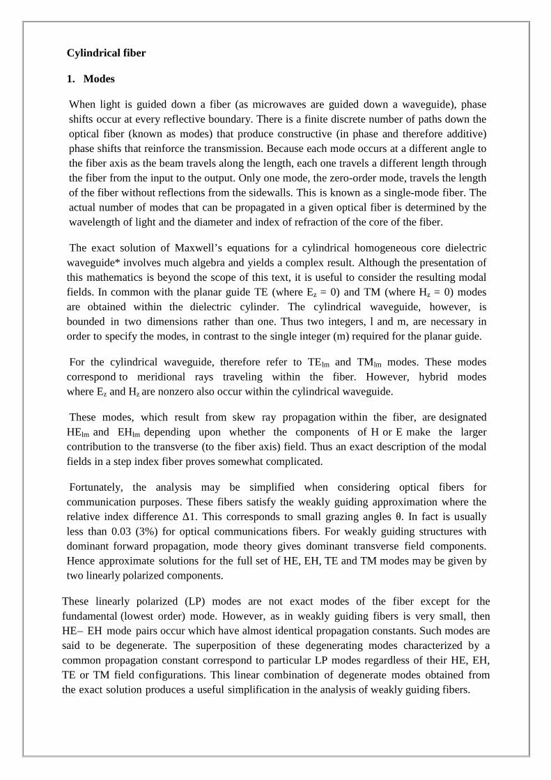
The relationship between the traditional HE, EH, TE and TM mode designations and theLPlm mode designations is shown in Table. The mode subscripts l and m are related tothe electric field intensity profile for a particular LP mode. There are in general 2l fieldmaxima around the circumference of the fiber core and m field maxima along a radiusvector. Furthermore, it may be observed from Table 1.1 that the notation for labeling theHE and EH modes has changed from that specified for the exact solution in the cylindricalwaveguide mentioned previously.

2. Mode coupling

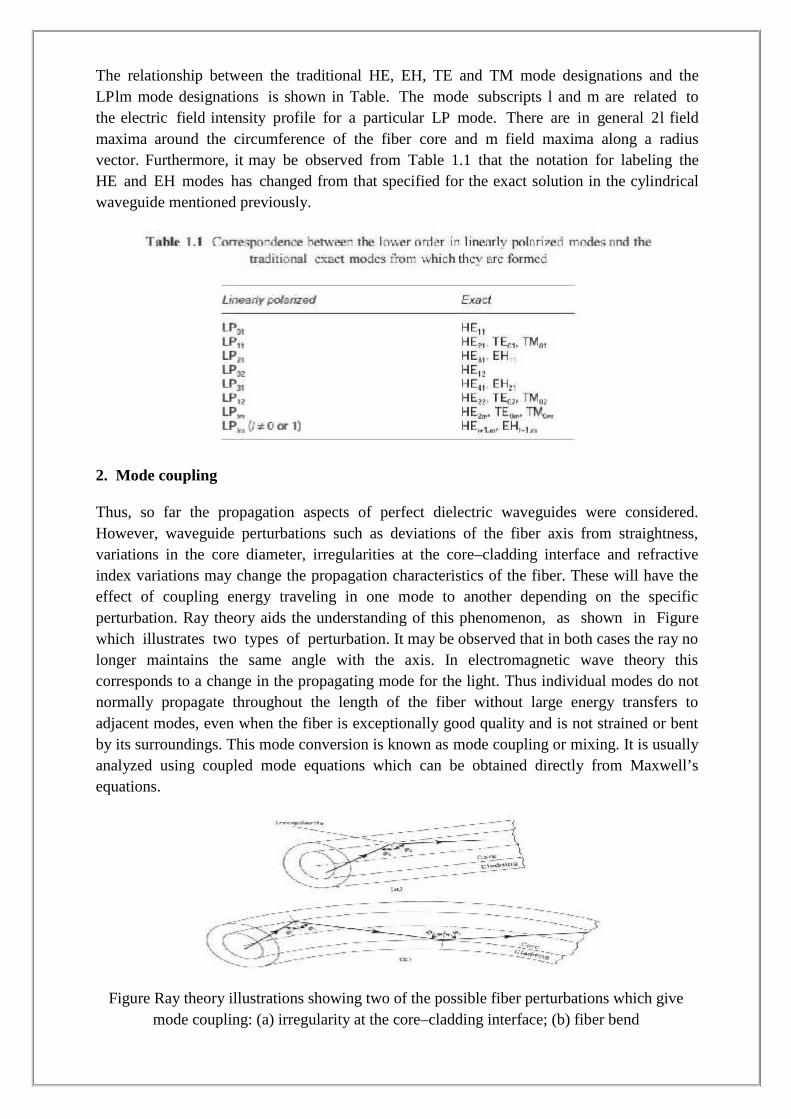
Thus, so far the propagation aspects of perfect dielectric waveguides were considered.However, waveguide perturbations such as deviations of the fiber axis from straightness,variations in the core diameter, irregularities at the core–cladding interface and refractiveindex variations may change the propagation characteristics of the fiber. These will have theeffect of coupling energy traveling in one mode to another depending on the specificperturbation. Ray theory aids the understanding of this phenomenon, as shown in Figurewhich illustrates two types of perturbation. It may be observed that in both cases the ray nolonger maintains the same angle with the axis. In electromagnetic wave theory thiscorresponds to a change in the propagating mode for the light. Thus individual modes do notnormally propagate throughout the length of the fiber without large energy transfers toadjacent modes, even when the fiber is exceptionally good quality and is not strained or bentby its surroundings. This mode conversion is known as mode coupling or mixing. It is usuallyanalyzed using coupled mode equations which can be obtained directly from Maxwell’sequations.

Figure Ray theory illustrations showing two of the possible fiber perturbations which givemode coupling: (a) irregularity at the core–cladding interface; (b) fiber bend

3. Step index fibers

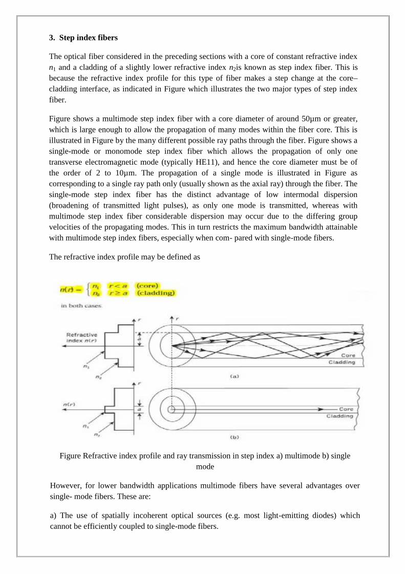
The optical fiber considered in the preceding sections with a core of constant refractive indexn1 and a cladding of a slightly lower refractive index n2is known as step index fiber. This isbecause the refractive index profile for this type of fiber makes a step change at the core–cladding interface, as indicated in Figure which illustrates the two major types of step indexfiber.

Figure shows a multimode step index fiber with a core diameter of around 50µm or greater,which is large enough to allow the propagation of many modes within the fiber core. This isillustrated in Figure by the many different possible ray paths through the fiber. Figure shows asingle-mode or monomode step index fiber which allows the propagation of only onetransverse electromagnetic mode (typically HE11), and hence the core diameter must be ofthe order of 2 to 10µm. The propagation of a single mode is illustrated in Figure ascorresponding to a single ray path only (usually shown as the axial ray) through the fiber. Thesingle-mode step index fiber has the distinct advantage of low intermodal dispersion(broadening of transmitted light pulses), as only one mode is transmitted, whereas withmultimode step index fiber considerable dispersion may occur due to the differing groupvelocities of the propagating modes. This in turn restricts the maximum bandwidth attainablewith multimode step index fibers, especially when com- pared with single-mode fibers.

The refractive index profile may be defined as

Figure Refractive index profile and ray transmission in step index a) multimode b) singlemode

However, for lower bandwidth applications multimode fibers have several advantages oversingle- mode fibers. These are:

a) The use of spatially incoherent optical sources (e.g. most light-emitting diodes) whichcannot be efficiently coupled to single-mode fibers.

b) Larger numerical apertures, as well as core diameters, facilitating easier coupling tooptical sources

c) Lower tolerance requirements on fiber connectors

Multimode step index fibers allow the propagation of a finite number of guided modes alongthe channel. The number of guided modes is dependent upon the physical parameters (i.e.relative refractive index difference, core radius) of the fiber and the wavelengths of thetransmitted light which are included in the normalized frequency V for the fiber.

Mode propagation does not entirely cease below cutoff. Modes may propagate as unguided orleaky modes which can travel considerable distances along the fiber. Nevertheless, it is theguided modes which are of paramount importance in optical fiber communications as theseare confined to the fiber over its full length. The total number of guided modes or modevolume Ms for a step index fiber is related to the V value for the fiber by the approximateexpression that allows an estimate of the number of guided modes propagating in a particularmultimode step index fiber.

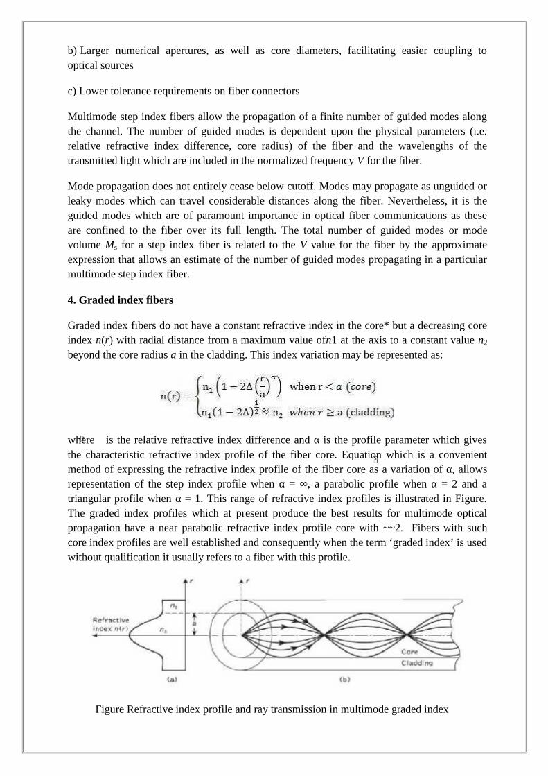
4. Graded index fibers

Graded index fibers do not have a constant refractive index in the core* but a decreasing coreindex n(r) with radial distance from a maximum value ofn1 at the axis to a constant value n2

beyond the core radius a in the cladding. This index variation may be represented as:

where is the relative refractive index difference and α is the profile parameter which givesthe characteristic refractive index profile of the fiber core. Equation which is a convenientmethod of expressing the refractive index profile of the fiber core as a variation of α, allowsrepresentation of the step index profile when α = ∞, a parabolic profile when α = 2 and atriangular profile when α = 1. This range of refractive index profiles is illustrated in Figure.The graded index profiles which at present produce the best results for multimode opticalpropagation have a near parabolic refractive index profile core with ~~2. Fibers with suchcore index profiles are well established and consequently when the term ‘graded index’ is usedwithout qualification it usually refers to a fiber with this profile.

Figure Refractive index profile and ray transmission in multimode graded index

Where, r = Radial distance from fiber axis, a = Core radius, n1= Refractive index of core, n2 =

Refractive index of cladding, α = Shape of index profile.

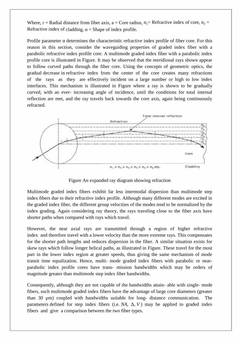
Profile parameter α determines the characteristic refractive index profile of fiber core. For thisreason in this section, consider the waveguiding properties of graded index fiber with aparabolic refractive index profile core. A multimode graded index fiber with a parabolic indexprofile core is illustrated in Figure. It may be observed that the meridional rays shown appearto follow curved paths through the fiber core. Using the concepts of geometric optics, thegradual decrease in refractive index from the center of the core creates many refractionsof the rays as they are effectively incident on a large number or high to low indexinterfaces. This mechanism is illustrated in Figure where a ray is shown to be graduallycurved, with an ever- increasing angle of incidence, until the conditions for total internalreflection are met, and the ray travels back towards the core axis, again being continuouslyrefracted.

Figure An expanded ray diagram showing refraction

Multimode graded index fibers exhibit far less intermodal dispersion than multimode stepindex fibers due to their refractive index profile. Although many different modes are excited inthe graded index fiber, the different group velocities of the modes tend to be normalized by theindex grading. Again considering ray theory, the rays traveling close to the fiber axis haveshorter paths when compared with rays which travel.

However, the near axial rays are transmitted through a region of higher refractiveindex and therefore travel with a lower velocity than the more extreme rays. This compensatesfor the shorter path lengths and reduces dispersion in the fiber. A similar situation exists forskew rays which follow longer helical paths, as illustrated in Figure. These travel for the mostpart in the lower index region at greater speeds, thus giving the same mechanism of modetransit time equalization. Hence, multi- mode graded index fibers with parabolic or near-parabolic index profile cores have trans- mission bandwidths which may be orders ofmagnitude greater than multimode step index fiber bandwidths.

Consequently, although they are not capable of the bandwidths attain- able with single- modefibers, such multimode graded index fibers have the advantage of large core diameters (greaterthan 30 µm) coupled with bandwidths suitable for long- distance communication. Theparameters defined for step index fibers (i.e. NA, Δ, V ) may be applied to graded indexfibers and give a comparison between the two fiber types.

However, it must be noted that for graded index fibers the situation is more complicated sincethe numerical aperture is a function of the radial distance from the fiber axis. Graded indexfibers, therefore, accept less light than corresponding step index fibers with the same relativerefractive index difference.

Single-mode fiber

The advantage of the propagation of a single mode within an optical fiber is that the signaldispersion caused by the delay differences between different modes in a multimode fiber maybe avoided. Multimode step index fibers do not lend themselves to the propagation of a singlemode due to the difficulties of maintaining single-mode operation within the fiber whenmode conversion (i.e. coupling) to other guided modes takes place at both input mismatchesand fiber imperfections. Hence, for the transmission of a single mode the fiber must bedesigned to allow propagation of only one mode, while all other modes are attenuated byleakage or absorption. Following the preceding discussion of multimode fibers, this may beachieved through choice of a suitable normalized frequency for the fiber. For single-modeoperation, only the fundamental LP01 mode can exist. Hence the limit of single-modeoperation depends on the lower limit of guided propagation for the LP11 mode. Thecutoff normalized frequency for the LP11 mode in step index fibers occurs at Vc = 2.405. Thussingle-mode propagation of the LP01 mode in step index fibers is possible over the range:

As there is no cutoff for the fundamental mode. It must be noted that there are in fact twomodes with orthogonal polarization over this range, and the term single-mode applies topropagation of light of a particular polarization. Also, it is apparent that the normalizedfrequency for the fiber may be adjusted to within the range given in Equation by reduction ofthe core radius.

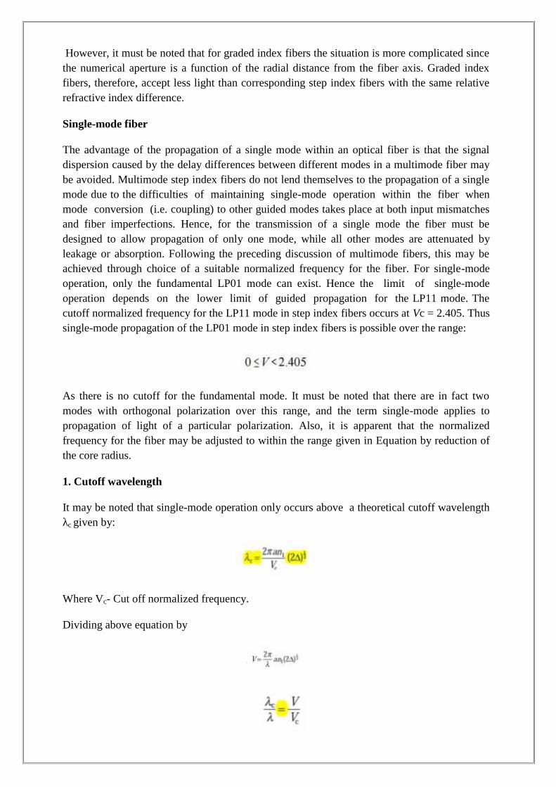
1. Cutoff wavelength

It may be noted that single-mode operation only occurs above a theoretical cutoff wavelengthλc given by:

Where Vc- Cut off normalized frequency.

Dividing above equation by

Thus for step index fiber where Vc=2.405, the cut-off wavelength is given by

An effective cutoff wavelength has been defined by the ITU-T which is obtained from a 2 mlength of fiber containing a single 14 cm radius loop. This definition was produced becausethe first higher order LP11 mode is strongly affected by fiber length and curvature near cutoff.Recommended cutoff wavelength values for primary coated fiber range from 1.1 to 1.28 µmfor single-mode fiber designed for operation in the 1.3µm wavelength region in order to avoidmodal noise and dispersion problems. Moreover, practical transmission systems are generallyoperated close to the effective cutoff wave- length in order to enhance the fundamental modeconfinement, but sufficiently distant from cutoff so that no power is transmitted in the second-order LP11 mode.

2. Mode-field diameter and spot size

Many properties of the fundamental mode are determined by the radial extent of itselectromagnetic field including losses at launching and jointing, micro bend losses, waveguidedispersion and the width of the radiation pattern. Therefore, the MFD is an importantparameter for characterizing single-mode fiber properties which takes into account thewavelength-dependent field penetration into the fiber cladding. In this context it is a bettermeasure of the functional properties of single- mode fiber than the core diameter. For stepindex and graded (near parabolic profile) single-mode fibers operating near the cutoffwavelength λc, the field is well approximated by a Gaussian distribution. In this case the MFDis generally taken as the distance between the opposite 1/e = 0.37 field amplitude points andthe power 1/e2 = 0.135 points in relation to the corresponding values on the fiber axis.Another parameter which is directly related to the MFD of a single-mode fiber is the spot size(or mode-field radius) ω0. Hence MFD = 2ω0, where ω0 is the nominal half width of the inputexcitation.

The MFD can therefore be regarded as the single- mode analog of the fiber core diameter inmultimode fibers. However, for many refractive index profiles and at typical operatingwavelengths the MFD is slightly larger than the single-mode fiber core diameter. Often, forreal fibers and those with arbitrary refractive index profiles, the radial field distribution is notstrictly Gaussian and hence alternative techniques have been proposed. However, the problemof defining the MFD and spot size for non-Gaussian field distributions is difficult one and atleast eight definitions exist.

3. Effective refractive index

The rate of change of phase of the fundamental LP01 mode propagating along a straight fiberis determined by the phase propagation constant. It is directly related to the wavelength of theLP01 mode λ01 by the factor 2π, since β gives the increase in phase angle per unitlength. Hence:

Morever, it is convenient to define an effective refractive index for single mode fiber,sometimes referred to as a phase index or normalized phase change coefficient neff by the ratioof the propagation constant of the fundamental mode to that of the vaccum propagationconstant.

Hence, the wavelength of the fundamental mode is smaller than the vaccum wave by thefactor 1/ neff ,where

It should be noted that the fundamental mode propagates in a medium with a refractive indexn(r) which is dependent on the distance r from the fiber axis. The effective refractive index cantherefore be considered as an average over the refractive index of this medium. Within anormally clad fiber, not depressed-cladded fibers, at long wavelengths (i.e. small V values) theMFD is large compared to the core diameter and hence the electric field extends far into thecladding region. In this case the propagation constant β will be approximately equal to n2k(i.e. the cladding wave number) and the effective index will be similar to the refractiveindex of the cladding n2. Physically, most of the power is transmitted in the claddingmaterial. At short wavelengths, however, the field is concentrated in the core region and thepropagation constant β approximates to the maximum wave number nlk. Following thisdiscussion, and as indicated previously, then the propagation constant in single-mode fibervaries over the interval n2k< β <n1k. Hence, the effective refractive index will vary over therange n2<neff<n1.

4. Group delay and mode delay factor

The transit time or group delay τg for a light pulse propagating along a unit length of fiber isthe inverse of the group velocity, υg

The group index of a uniform plane wave propagating in a homogenous medium has beenidentified as

However, for a single mode fiber, it is usual to define an effective group index by

Hence, where υg is considered to be the group velocity of the fundamental fiber mode. Hence,the specific group delay of the fundamental fiber mode becomes:

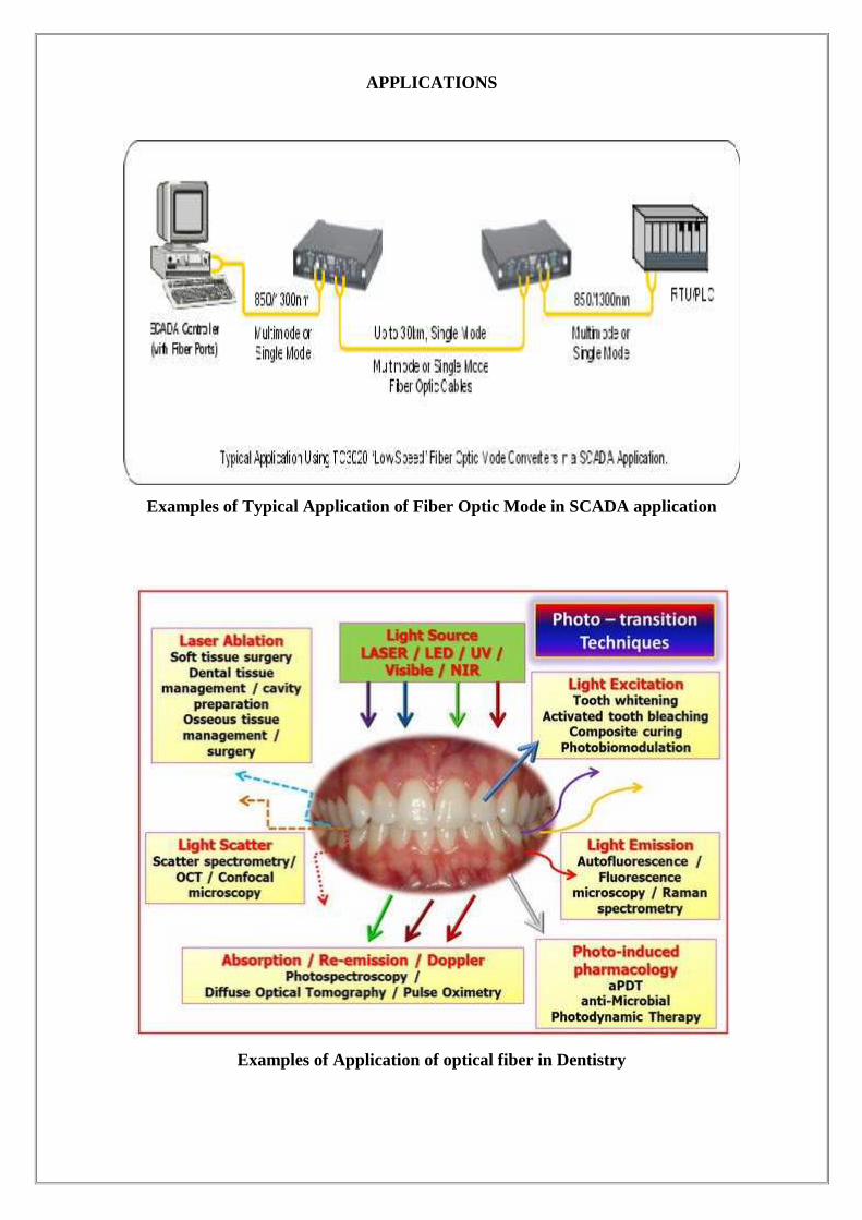
APPLICATIONS

Examples of Typical Application of Fiber Optic Mode in SCADA application

Examples of Application of optical fiber in Dentistry

POST TEST-MCQ TYPE

1. What is refraction?a) Bending of light wavesb) Reflection of light wavesc) Diffusion of light wavesd) Scattering of light waves

2. The phenomenon which occurs when an incident wave strikes an interface at an anglegreater than the critical angle with respect to the normal to the surface is called asa) Refractionb) Partial internal reflectionc) Total internal reflectiond) Limiting case of refraction

3. A monochromatic wave propagates along a waveguide in z direction. These points ofconstant phase travel in constant phase travel at a phase velocity Vp is given by?a) Vp=ω/βb) Vp=ω/cc) Vp=C/Nd) Vp=mass/acceleration

4. Which law gives the relationship between refractive index of the dielectric?a) Law of reflectionb) Law of refraction (Snell’s Law)c) Millman’s Lawd) Huygen’s Law

5. The light sources used in fibre optics communication area) LED’s and Lasersb) Phototransistorsc) Xenon lightsd) Incandescent

6. Which ray passes through the axis of the fiber core?a) Reflectedb) Refractedc) Meridionald) Skew

7. Light incident on fibers of angles___the acceptance angle do not propagate into the fiber.a) Less thanb) Greater thanc) Equal tod) Less than and equal to

8. The ratio of speed of light in air to the speed of light in another medium is called asa) Speed factorb) Dielectric constantc) Reflection indexd) Refraction index

9. When a ray of light enters one medium from another medium, which quality will notchange?a) Directionb) Frequencyc) Speedd) Wavelength

10. What is the numerical aperture of the fiber if the angle of acceptance is 16 degree?a) 0.50b) 0.36c) 0.20d) 0.27

11. For lower bandwidth applicationsa) Single mode fiber is advantageousb) Photonic crystal fibers are advantageousc) Coaxial cables are advantageousd) Multimode fiber is advantageous

12. Meridional rays in graded index fibers followa) Straight path along the axisb) Curved path along the axisc) Path where rays changes angles at core-cladding interfaced) Helical path

13. Skew rays follow aa) Hyperbolic path along the axisb) Parabolic path along the axisc) Helical pathd) Path where rays changes angles at core-cladding interface

14. What is needed to predict the performance characteristics of single mode fibers?a) The intermodal delay effectb) Geometric distribution of light in a propagating modec) Fractional power flow in the cladding of fiberd) Normalized frequency

15. Which equation is used to calculate MFD?a) Maxwell’s equationsb) Peterman equationsc) Allen Cahn equationsd) Boltzmann’s equations

16. he difference between the modes’ refractive indices is called asa) Polarizationb) Cutoffc) Fiber birefringenced) Fiber splicing

17. How many propagation modes are present in single mode fibers?a) Oneb) Twoc) Threed) Five

18. A device that reduces the intensity of light in optical fiber communications isa) Compressorb) Optical attenuatorc) Barometerd) Reducer

19. The core of an optical fiber has aa) Lower refracted index than airb) Lower refractive index than the claddingc) Higher refractive index than the claddingd) Similar refractive index with the cladding

20. One of the following materials is sensitive to light. Identify it.a) Photoresistb) Photosensitivec) Light Sensitived) Maser

21. If a mirror is used to reflect light, the reflected light angle is ____ as the incident anglea) Smallerb) Largerc) The samed) Independent

22. This is not a part of the optical spectrum. Identify it.a) infraredb) ultravioletc) visible colord) x-rays

23. Which type of fiber has the highest modal dispersion.a) Step-index multimodeb) Graded index multimodec) Step-index single moded) Graded index mode

24. What is a specific path the light takes in an optical fiber corresponding to a certain angleand number of reflection?a) Modeb) Gradec) Numerical Apertured) Dispersion

CONCLUSION

In this unit, an understanding of optical fiber communication link, structure, propagation and

transmission properties of an optical fiber and the Estimate the losses and analyze the

propagation characteristics of an optical signal in different types of fibers was done. The

Introduction to Optical Fibers, its types and applications were discussed.

REFERENCES

1. Gerd Keiser, “Optical Fiber Communication” McGraw-Hill International,4th Edition. 2010.

2. John M. Senior, “Optical Fiber Communication”, Second Edition, Pearson Education, 2007.

3. Ramaswami, Sivarajan and Sasaki “Optical Networks”, Morgan Kaufmann, 2009.

4. J.Senior, Optical Communication, Principles and Practice, Prentice Hall of India, 3rd

Edition, 2008.

5. J.Gower, “Optical Communication System”, Prentice Hall of India, 2001.

ASSIGNMENT

1. Describe the Ray theory transmission.

2. Describe Single-mode fiber and its mode field diameter.

3. Describe in detail the Classification of fibers or Compare the structure and characteristics of

step index and graded index fiber structures.

4. Derive the expression for linearly polarized modes in optical fibers and obtain the

expression for normalized frequency.

5. A step index multimode fiber with a numerical aperture of 0.2 support approximately 1000

modes at 850 nm wavelength. What is the diameter of its core? How many modes does the

fiber support at 850 nm and 1550 nm.

6. Draw the block diagram of optical fiber transmission link and explain.

UNIT II SIGNAL DEGRADATIONOPTICAL FIBERS

Prepared by

T.DINESH KUMARAssistant Professor

ECE, SCSVMV

OPTICALCOMMUNICATION

AIM & OBJECTIVES

To learn the basic elements of optical fiber transmission link, fiber modesconfigurations and structures.

To understand the different kind of losses, signal distortion, SM fibers. To learn the various optical sources, materials and fiber splicing. To learn the fiber optical receivers and noise performance in photo detector.

PRE TEST-MCQ TYPE

1. What does ISI stand for in optical fiber communication?a) Invisible size interferenceb) Infrared size interferencec) Inter-symbol interferenced) Inter-shape interference

2. 3dB optical bandwidth is always ___________ the 3dB electrical bandwidth.a) Smaller thanb) Larger thanc) Negligible thand) Equal to

3. In waveguide dispersion, refractive index is independent ofa) Bit rateb) Index differencec) Velocity of mediumd) Wavelength

4. After Total Internal Reflection the Meridional raya) Makes an angle equal to acceptance angle with the axial rayb) Makes an angle equal to critical angle with the axial rayc) Travels parallel equal to critical angle with the axial rayd) Makes an angle equal to critical angle with the axial ray

5. How many mechanisms are there which causes absorption?a) Oneb) Threec) Twod) Four

UNIT II SIGNAL DEGRADATION OPTICAL FIBERS

Attenuation - Absorption losses, Scattering losses, Bending Losses, Core and Cladding losses,Signal Distortion in Optical Waveguides-Information Capacity determination -Group Delay-Material Dispersion, Wave guide Dispersion, Signal distortion in SM fibers-Polarization Modedispersion, Intermodal dispersion, Pulse Broadening in GI fibers-Mode Coupling -DesignOptimization of SM fibers- RI profile and cut-off wavelength

THEORY

Introduction

One of the important property of optical fiber is signal attenuation. It is also known as fiberloss or signal loss. The signal attenuation of fiber determines the maximum distancebetween transmitter and receiver. The attenuation also determines the number of repeatersrequired, maintaining repeater is a costly affair. Another important property of optical fiber isdistortion mechanism. As the signal pulse travels along the fiber length it becomes morebroader. After sufficient length the broad pulses starts overlapping with adjacent pulses. Thiscreates error in the receiver. Hence the distortion limits the information carrying capacity offiber.

Attenuation

Attenuation is a measure of decay of signal strength or loss of light power that occurs as lightpulses propagate through the length of the fiber. In optical fibers the attenuation is mainlycaused by two physical factors absorption and scattering losses. Absorption is because of fibermaterial and scattering due to structural imperfection within the fiber. Nearly 90% of totalattenuation is caused by Rayleigh scattering only. Microbending of optical fiber alsocontributes to the attenuation of signal.

The rate at which light is absorbed is dependent on the wavelength of the light and thecharacteristics of particular glass. Glass is a silicon compound, by adding different additionalchemicals to the basic silicon dioxide the optical properties of the glass can be changed.

The Rayleigh scattering is wavelength dependent and reduces rapidly as the wavelength of theincident radiation increases. The attenuation of fiber is governed by the materials fromwhich it is fabricated, the manufacturing process and the refractive index profile chosen.Attenuation loss is measured in dB/km.

Attenuation Units

As attenuation leads to a loss of power along the fiber, the output power is significantly lessthan the couples power. Let the couples optical power is p(0) i.e. at origin (z = 0). Then thepower at distance z is given by,

where, αp is fiber attenuation constant (per km).

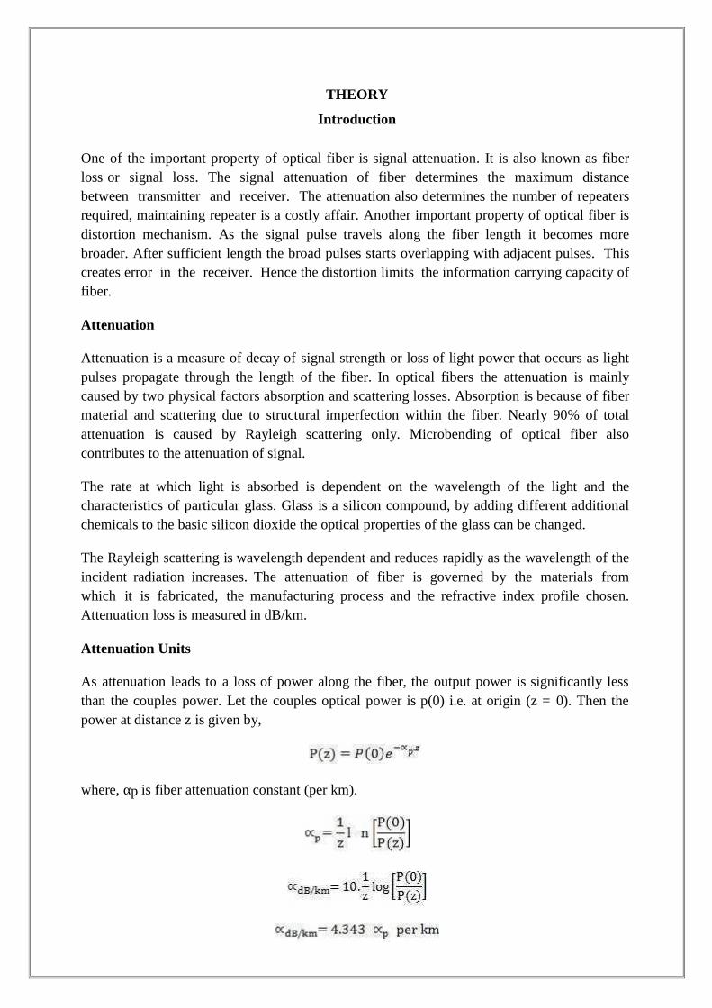
This parameter is known as fiber loss or fiber attenuation. Attenuation is also a function ofwavelength. Optical fiber wavelength as a function of wavelength is shown in Figure.

Figure Optical fiber wavelength as a function of wavelength

Absorption

Absorption loss is related to the material composition and fabrication process of fiber.Absorption loss results in dissipation of some optical power as hear in the fiber cable.Although glass fibers are extremely pure, some impurities still remain as residue afterpurification. The amount of absorption by these impurities depends on their concentration andlight wavelength.

Absorption in optical fiber is caused by these three mechanisms.

1. Absorption by atomic defects in the glass composition

2. Extrinsic absorption by impurity atoms in the glass material

3. Intrinsic absorption by the basic constituent atoms of the fiber material.

Absorption by Atomic Defects

Atomic defects are imperfections in the atomic structure of the fiber materials such as missingmolecules, high density clusters of atom groups. These absorption losses are negligiblecompared with intrinsic and extrinsic losses.

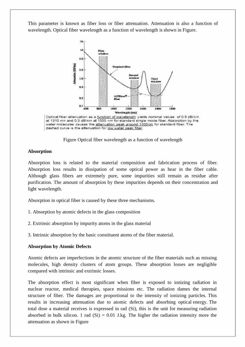
The absorption effect is most significant when fiber is exposed to ionizing radiation innuclear reactor, medical therapies, space missions etc. The radiation dames the internalstructure of fiber. The damages are proportional to the intensity of ionizing particles. Thisresults in increasing attenuation due to atomic defects and absorbing optical energy. Thetotal dose a material receives is expressed in rad (Si), this is the unit for measuring radiationabsorbed in bulk silicon. 1 rad (Si) = 0.01 J.kg. The higher the radiation intensity more theattenuation as shown in Figure

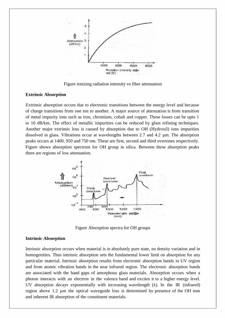
Figure ionizing radiation intensity vs fiber attenuation

Extrinsic Absorption

Extrinsic absorption occurs due to electronic transitions between the energy level and becauseof charge transitions from one ion to another. A major source of attenuation is from transitionof metal impurity ions such as iron, chromium, cobalt and copper. These losses can be upto 1to 10 dB/km. The effect of metallic impurities can be reduced by glass refining techniques.Another major extrinsic loss is caused by absorption due to OH (Hydroxil) ions impuritiesdissolved in glass. Vibrations occur at wavelengths between 2.7 and 4.2 µm. The absorptionpeaks occurs at 1400, 950 and 750 nm. These are first, second and third overtones respectively.Figure shows absorption spectrum for OH group in silica. Between these absorption peaksthere are regions of low attenuation.

Figure Absorption spectra for OH groups

Intrinsic Absorption

Intrinsic absorption occurs when material is in absolutely pure state, no density variation and inhomogenities. Thus intrinsic absorption sets the fundamental lower limit on absorption for anyparticular material. Intrinsic absorption results from electronic absorption bands in UV regionand from atomic vibration bands in the near infrared region. The electronic absorption bandsare associated with the band gaps of amorphous glass materials. Absorption occurs when aphoton interacts with an electron in the valence band and excites it to a higher energy level.UV absorption decays exponentially with increasing wavelength (λ). In the IR (infrared)region above 1.2 µm the optical waveguide loss is determined by presence of the OH ionsand inherent IR absorption of the constituent materials.

The inherent IR absorption is due to interaction between the vibrating band and theelectromagnetic field of optical signal this results in transfer of energy from field to the band,thereby giving rise to absorption, this absorption is strong because of many bonds present inthe fiber. The ultraviolet loss at any wavelength is expressed as,

where, x is mole fraction of GeO2. λ is operating wavelength. αuv is in dB/km.

The loss in infrared (IR) region (above 1.2 µm) is given by expression

The expression is derived for GeO2-SiO2 glass fiber.

Rayleigh Scattering Losses

Scattering losses exists in optical fibers because of microscopic variations in the materialdensity and composition. As glass is composed by randomly connected network of molecules

and several oxides (e.g. SiO2, GeO2 and P2O5), these are the major cause of compositional

structure fluctuation. These two effects results to variation in refractive index and Rayleightype scattering of light.

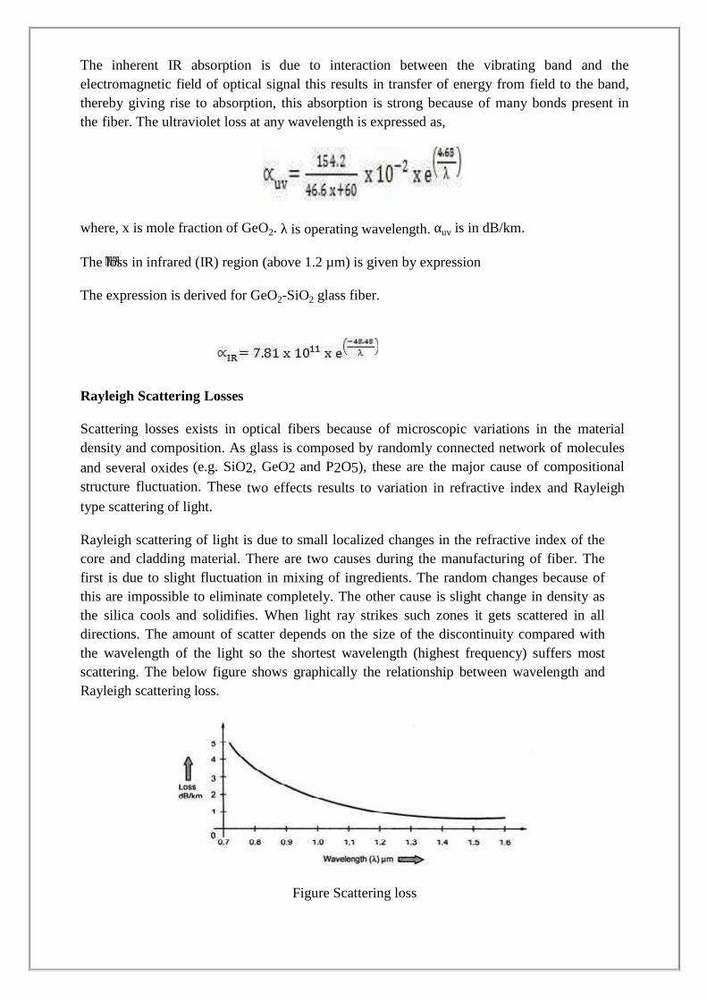
Rayleigh scattering of light is due to small localized changes in the refractive index of thecore and cladding material. There are two causes during the manufacturing of fiber. Thefirst is due to slight fluctuation in mixing of ingredients. The random changes because ofthis are impossible to eliminate completely. The other cause is slight change in density asthe silica cools and solidifies. When light ray strikes such zones it gets scattered in alldirections. The amount of scatter depends on the size of the discontinuity compared withthe wavelength of the light so the shortest wavelength (highest frequency) suffers mostscattering. The below figure shows graphically the relationship between wavelength andRayleigh scattering loss.

Figure Scattering loss

Scattering loss for single component glass is given by,

where, n = Refractive index, B = Boltzmann’s constant, βT = Isothermal compressibility of

material, Tf = Temperature at which density fluctuations are frozen into the glass as it solidifies(fictive temperature)

Another form of equation is

where, P = Photoelastic coefficient

where, = Mean square refractive index fluctuation

= Volume of fiber

Multimode fibers have higher dopant concentrations and greater compositional fluctuations.The overall losses in these fibers are more as compared to single mode fibers.

Mie Scattering

Linear scattering also occurs at in homogenities and these arise from imperfections in thefiber’s geometry, irregularities in the refractive index and the presence of bubbles etc. causedduring manufacture. Careful control of manufacturing process can reduce Mie scattering toinsignificant levels.

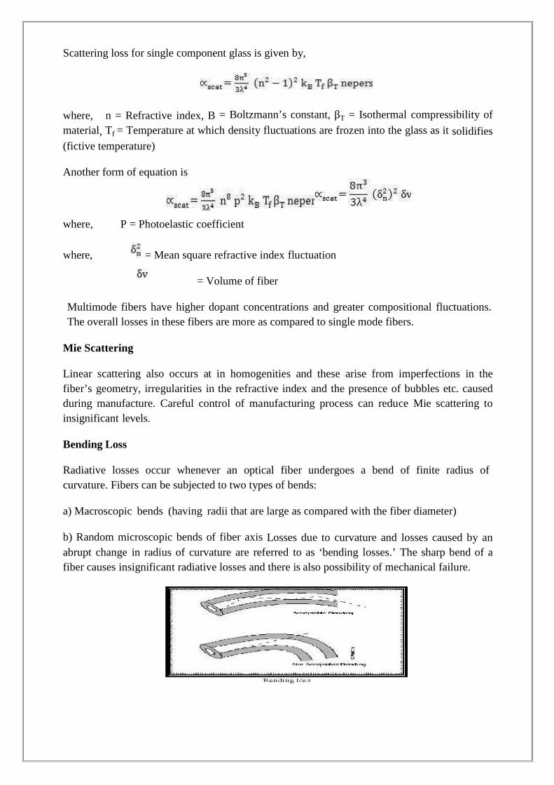
Bending Loss

Radiative losses occur whenever an optical fiber undergoes a bend of finite radius ofcurvature. Fibers can be subjected to two types of bends:

a) Macroscopic bends (having radii that are large as compared with the fiber diameter)

b) Random microscopic bends of fiber axis Losses due to curvature and losses caused by anabrupt change in radius of curvature are referred to as ‘bending losses.’ The sharp bend of afiber causes insignificant radiative losses and there is also possibility of mechanical failure.

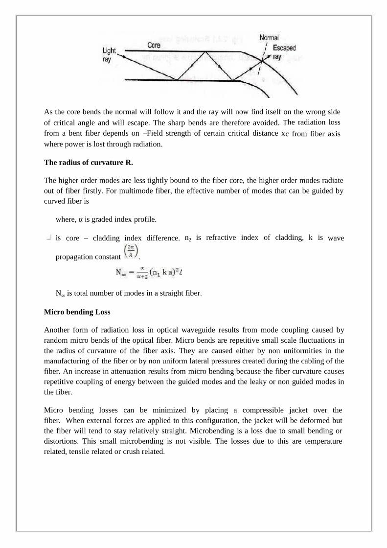
As the core bends the normal will follow it and the ray will now find itself on the wrong side

of critical angle and will escape. The sharp bends are therefore avoided. The radiation loss

from a bent fiber depends on –Field strength of certain critical distance xc from fiber axiswhere power is lost through radiation.

The radius of curvature R.

The higher order modes are less tightly bound to the fiber core, the higher order modes radiateout of fiber firstly. For multimode fiber, the effective number of modes that can be guided bycurved fiber is

where, α is graded index profile.

is core – cladding index difference. n2 is refractive index of cladding, k is wave

propagation constant .

N∞ is total number of modes in a straight fiber.

Micro bending Loss

Another form of radiation loss in optical waveguide results from mode coupling caused byrandom micro bends of the optical fiber. Micro bends are repetitive small scale fluctuations inthe radius of curvature of the fiber axis. They are caused either by non uniformities in themanufacturing of the fiber or by non uniform lateral pressures created during the cabling of thefiber. An increase in attenuation results from micro bending because the fiber curvature causesrepetitive coupling of energy between the guided modes and the leaky or non guided modes inthe fiber.

Micro bending losses can be minimized by placing a compressible jacket over thefiber. When external forces are applied to this configuration, the jacket will be deformed butthe fiber will tend to stay relatively straight. Microbending is a loss due to small bending ordistortions. This small microbending is not visible. The losses due to this are temperaturerelated, tensile related or crush related.

ng on wavelength) to a series of periodic peaks and trou

on curve. These effects can be minimized during insta

lustrates microbening.

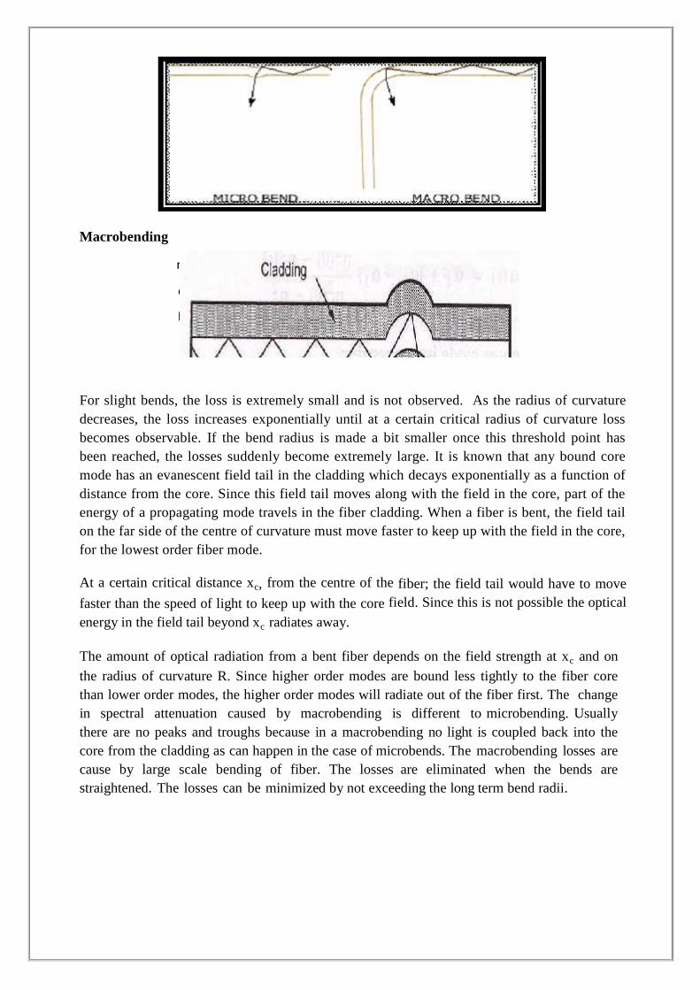
Macrobending

For slight bends, the loss is extremely small and is not observed. As the radius of curvaturedecreases, the loss increases exponentially until at a certain critical radius of curvature lossbecomes observable. If the bend radius is made a bit smaller once this threshold point hasbeen reached, the losses suddenly become extremely large. It is known that any bound coremode has an evanescent field tail in the cladding which decays exponentially as a function ofdistance from the core. Since this field tail moves along with the field in the core, part of theenergy of a propagating mode travels in the fiber cladding. When a fiber is bent, the field tailon the far side of the centre of curvature must move faster to keep up with the field in the core,for the lowest order fiber mode.

At a certain critical distance xc, from the centre of the fiber; the field tail would have to move

faster than the speed of light to keep up with the core field. Since this is not possible the optical

energy in the field tail beyond xc radiates away.

The amount of optical radiation from a bent fiber depends on the field strength at xc and on

the radius of curvature R. Since higher order modes are bound less tightly to the fiber corethan lower order modes, the higher order modes will radiate out of the fiber first. The changein spectral attenuation caused by macrobending is different to microbending. Usuallythere are no peaks and troughs because in a macrobending no light is coupled back into thecore from the cladding as can happen in the case of microbends. The macrobending losses arecause by large scale bending of fiber. The losses are eliminated when the bends arestraightened. The losses can be minimized by not exceeding the long term bend radii.

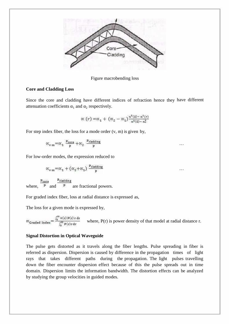
Figure macrobending loss

Core and Cladding Loss

Since the core and cladding have different indices of refraction hence they have different

attenuation coefficients α1 and α2 respectively.

For step index fiber, the loss for a mode order (v, m) is given by,

…

For low-order modes, the expression reduced to

…

where, and are fractional powers.

For graded index fiber, loss at radial distance is expressed as,

The loss for a given mode is expressed by,

where, P(r) is power density of that model at radial distance r.

Signal Distortion in Optical Waveguide

The pulse gets distorted as it travels along the fiber lengths. Pulse spreading in fiber isreferred as dispersion. Dispersion is caused by difference in the propagation times of lightrays that takes different paths during the propagation. The light pulses travellingdown the fiber encounter dispersion effect because of this the pulse spreads out in timedomain. Dispersion limits the information bandwidth. The distortion effects can be analyzedby studying the group velocities in guided modes.

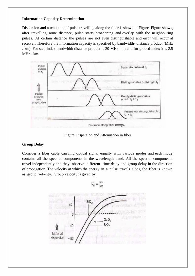
Information Capacity Determination

Dispersion and attenuation of pulse travelling along the fiber is shown in Figure. Figure shows,after travelling some distance, pulse starts broadening and overlap with the neighbouringpulses. At certain distance the pulses are not even distinguishable and error will occur atreceiver. Therefore the information capacity is specified by bandwidth- distance product (MHz. km). For step index bandwidth distance product is 20 MHz .km and for graded index it is 2.5MHz . km.

Figure Dispersion and Attenuation in fiber

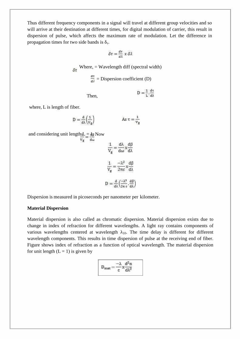
Group Delay

Consider a fiber cable carrying optical signal equally with various modes and each modecontains all the spectral components in the wavelength band. All the spectral componentstravel independently and they observe different time delay and group delay in the directionof propagation. The velocity at which the energy in a pulse travels along the fiber is knownas group velocity. Group velocity is given by,

Thus different frequency components in a signal will travel at different group velocities and sowill arrive at their destination at different times, for digital modulation of carrier, this result indispersion of pulse, which affects the maximum rate of modulation. Let the difference inpropagation times for two side bands is δτ.

Where, = Wavelength diff (spectral width)

= Dispersion coefficient (D)

Then,

where, L is length of fiber.

and considering unit length L = 1. Now

Dispersion is measured in picoseconds per nanometer per kilometer.

Material Dispersion

Material dispersion is also called as chromatic dispersion. Material dispersion exists due tochange in index of refraction for different wavelengths. A light ray contains components ofvarious wavelengths centered at wavelength λ10. The time delay is different for differentwavelength components. This results in time dispersion of pulse at the receiving end of fiber.Figure shows index of refraction as a function of optical wavelength. The material dispersionfor unit length (L = 1) is given by

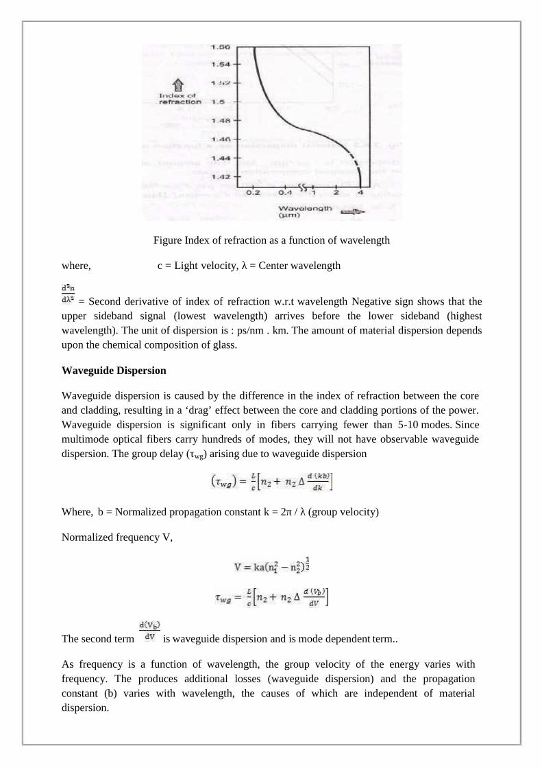
Figure Index of refraction as a function of wavelength

where, c = Light velocity, λ = Center wavelength

= Second derivative of index of refraction w.r.t wavelength Negative sign shows that theupper sideband signal (lowest wavelength) arrives before the lower sideband (highestwavelength). The unit of dispersion is : ps/nm . km. The amount of material dispersion dependsupon the chemical composition of glass.

Waveguide Dispersion

Waveguide dispersion is caused by the difference in the index of refraction between the coreand cladding, resulting in a ‘drag’ effect between the core and cladding portions of the power.Waveguide dispersion is significant only in fibers carrying fewer than 5-10 modes. Sincemultimode optical fibers carry hundreds of modes, they will not have observable waveguidedispersion. The group delay (τwg) arising due to waveguide dispersion

Where, b = Normalized propagation constant k = 2π / λ (group velocity)

Normalized frequency V,

The second term is waveguide dispersion and is mode dependent term..

As frequency is a function of wavelength, the group velocity of the energy varies withfrequency. The produces additional losses (waveguide dispersion) and the propagationconstant (b) varies with wavelength, the causes of which are independent of materialdispersion.

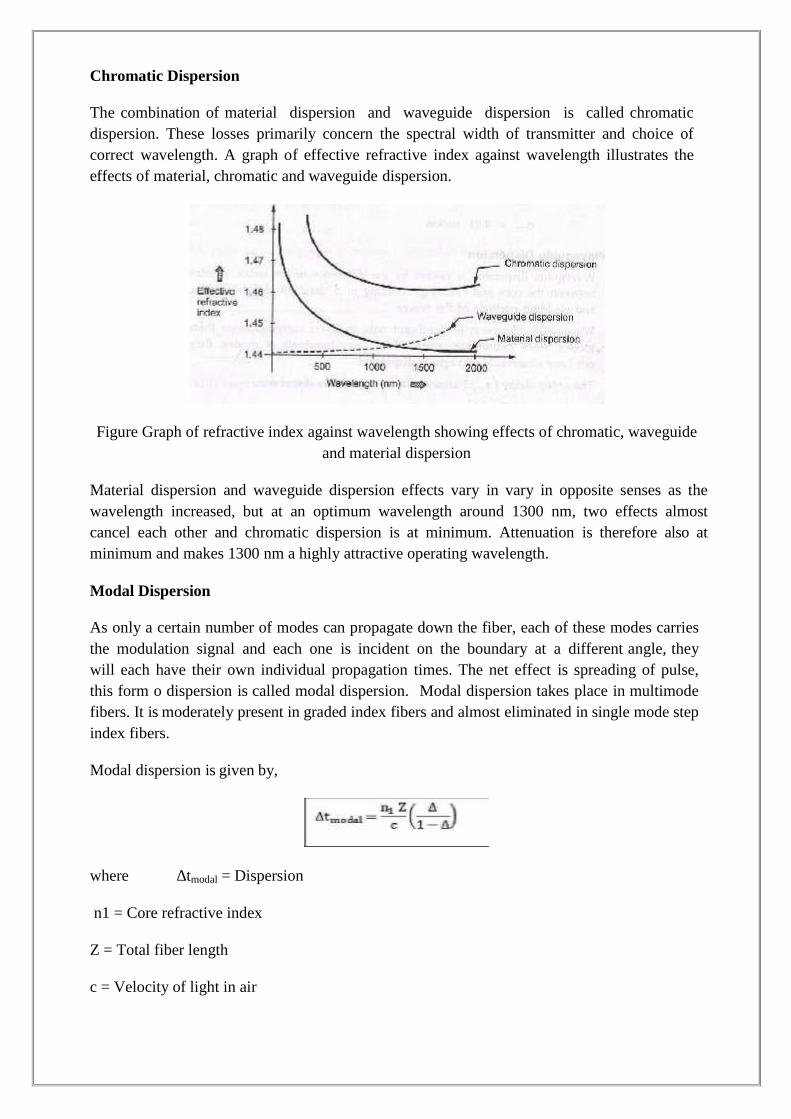
Chromatic Dispersion

The combination of material dispersion and waveguide dispersion is called chromaticdispersion. These losses primarily concern the spectral width of transmitter and choice ofcorrect wavelength. A graph of effective refractive index against wavelength illustrates theeffects of material, chromatic and waveguide dispersion.

Figure Graph of refractive index against wavelength showing effects of chromatic, waveguideand material dispersion

Material dispersion and waveguide dispersion effects vary in vary in opposite senses as thewavelength increased, but at an optimum wavelength around 1300 nm, two effects almostcancel each other and chromatic dispersion is at minimum. Attenuation is therefore also atminimum and makes 1300 nm a highly attractive operating wavelength.

Modal Dispersion

As only a certain number of modes can propagate down the fiber, each of these modes carriesthe modulation signal and each one is incident on the boundary at a different angle, theywill each have their own individual propagation times. The net effect is spreading of pulse,this form o dispersion is called modal dispersion. Modal dispersion takes place in multimodefibers. It is moderately present in graded index fibers and almost eliminated in single mode stepindex fibers.

Modal dispersion is given by,

where ∆tmodal = Dispersion

n1 = Core refractive index

Z = Total fiber length

c = Velocity of light in air

Fractional refractive index

Polarization Mode Dispersion (PMD)

Different frequency component of a pulse acquires different polarization state (such as linearpolarization and circular polarization). This result in pulse broadening is known as polarizationmode dispersion (PMD). PMD is the limiting factor for optical communication system at highdata rates. The effects of PMD must be compensated.

Pulse Broadening in GI Fibers

The core refractive index varies radially in case of graded index fibers, hence it supportsmultimode propagation with a low intermodal delay distortion and high data rate over longdistance is possible. The higher order modes travelling in outer regions of the core, willtravel faster than the lower order modes travelling in high refractive index region. If theindex profile is carefully controlled, then the transit times of the individual modes will beidentical, so eliminating modal dispersion. The r.m.s pulse broadening is given as:

where, σintermodal – R.M.S pulse width due to intermodal delay distortion., σintermodal – R.M.S

pulse width resulting from pulse broadening within each mode.

The intermodal delay and pulse broadening are related by expression given byPersonick.

Where τg is group delay.From this the expression for intermodal pulse broadening is given as:

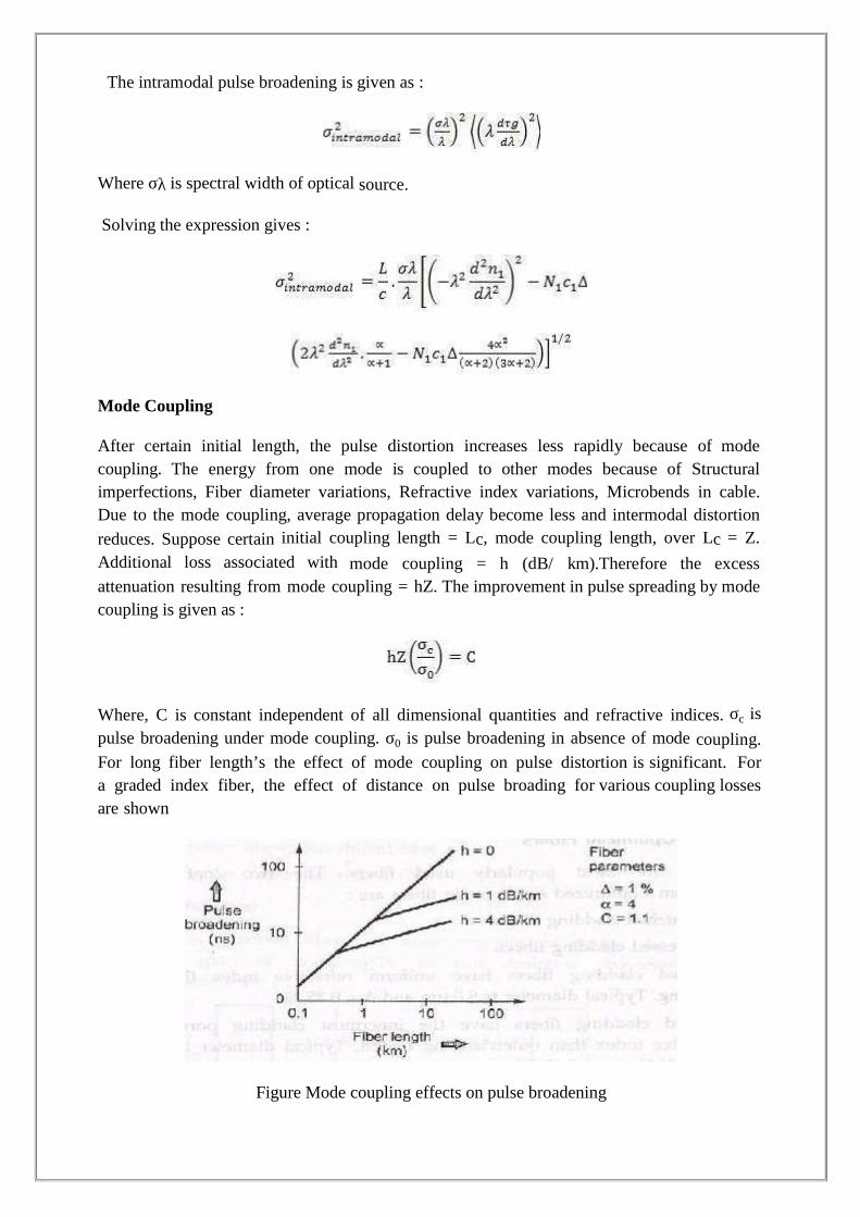
The intramodal pulse broadening is given as :

Where σλ is spectral width of optical source.

Solving the expression gives :

Mode Coupling

After certain initial length, the pulse distortion increases less rapidly because of modecoupling. The energy from one mode is coupled to other modes because of Structuralimperfections, Fiber diameter variations, Refractive index variations, Microbends in cable.Due to the mode coupling, average propagation delay become less and intermodal distortion

reduces. Suppose certain initial coupling length = Lc, mode coupling length, over Lc = Z.

Additional loss associated with mode coupling = h (dB/ km).Therefore the excessattenuation resulting from mode coupling = hZ. The improvement in pulse spreading by modecoupling is given as :

Where, C is constant independent of all dimensional quantities and refractive indices. σc is

pulse broadening under mode coupling. σ0 is pulse broadening in absence of mode coupling.For long fiber length’s the effect of mode coupling on pulse distortion is significant. Fora graded index fiber, the effect of distance on pulse broading for various coupling lossesare shown

Figure Mode coupling effects on pulse broadening

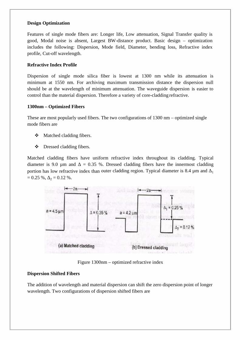
Design Optimization

Features of single mode fibers are: Longer life, Low attenuation, Signal Transfer quality isgood, Modal noise is absent, Largest BW-distance product. Basic design – optimizationincludes the following: Dispersion, Mode field, Diameter, bending loss, Refractive indexprofile, Cut-off wavelength.

Refractive Index Profile

Dispersion of single mode silica fiber is lowest at 1300 nm while its attenuation isminimum at 1550 nm. For archiving maximum transmission distance the dispersion nullshould be at the wavelength of minimum attenuation. The waveguide dispersion is easier tocontrol than the material dispersion. Therefore a variety of core-cladding refractive.

1300nm – Optimized Fibers

These are most popularly used fibers. The two configurations of 1300 nm – optimized singlemode fibers are

Matched cladding fibers.

Dressed cladding fibers.

Matched cladding fibers have uniform refractive index throughout its cladding. Typicaldiameter is 9.0 µm and ∆ = 0.35 %. Dressed cladding fibers have the innermost cladding

portion has low refractive index than outer cladding region. Typical diameter is 8.4 µm and ∆1

= 0.25 %, ∆2 = 0.12 %.

Figure 1300nm – optimized refractive index

Dispersion Shifted Fibers

The addition of wavelength and material dispersion can shift the zero dispersion point of longerwavelength. Two configurations of dispersion shifted fibers are

Figure Dispersion shifted fibers

Dispersion Flattened

Dispersion flattened fibers are more complex to design. It offers much broader span ofwavelengths to suit desirable characteristics. Two configurations are:

Figure Dispersion Flattened

Figure Total resultant dispersion

Dispersion Calculations

The total dispersion consists of material and waveguide dispersions. The resultantintermodal dispersion is given as,

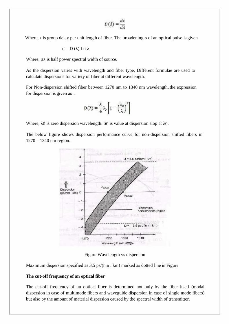
Where, τ is group delay per unit length of fiber. The broadening σ of an optical pulse is given

σ = D (λ) Lσ λ

Where, σλ is half power spectral width of source.

As the dispersion varies with wavelength and fiber type, Different formulae are used tocalculate dispersions for variety of fiber at different wavelength.

For Non-dispersion shifted fiber between 1270 nm to 1340 nm wavelength, the expressionfor dispersion is given as :

Where, λ0 is zero dispersion wavelength. S0 is value at dispersion slop at λ0.

The below figure shows dispersion performance curve for non-dispersion shifted fibers in1270 – 1340 nm region.

Figure Wavelength vs dispersion

Maximum dispersion specified as 3.5 ps/(nm . km) marked as dotted line in Figure

The cut-off frequency of an optical fiber

The cut-off frequency of an optical fiber is determined not only by the fiber itself (modaldispersion in case of multimode fibers and waveguide dispersion in case of single mode fibers)but also by the amount of material dispersion caused by the spectral width of transmitter.

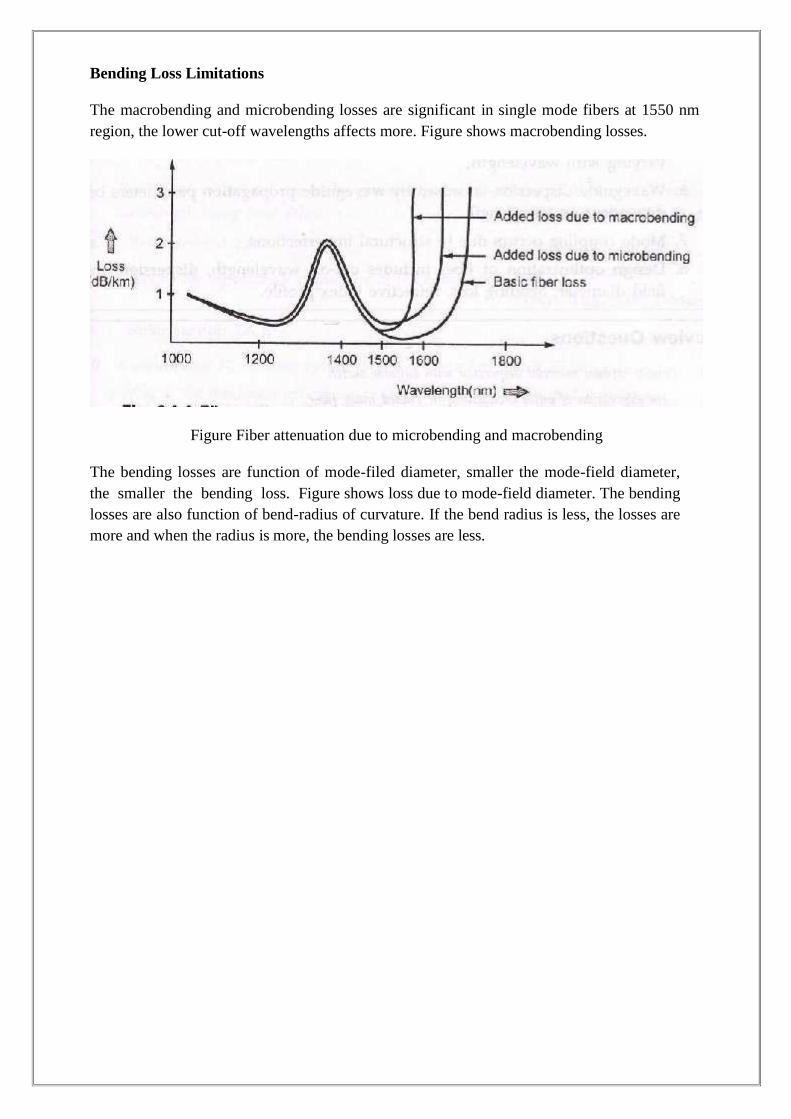
Bending Loss Limitations

The macrobending and microbending losses are significant in single mode fibers at 1550 nmregion, the lower cut-off wavelengths affects more. Figure shows macrobending losses.

Figure Fiber attenuation due to microbending and macrobending

The bending losses are function of mode-filed diameter, smaller the mode-field diameter,the smaller the bending loss. Figure shows loss due to mode-field diameter. The bendinglosses are also function of bend-radius of curvature. If the bend radius is less, the losses aremore and when the radius is more, the bending losses are less.

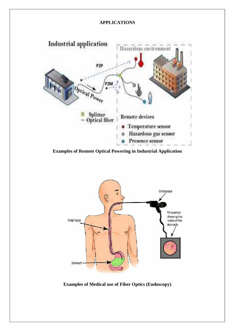
APPLICATIONS

Examples of Remote Optical Powering in Industrial Application

Examples of Medical use of Fiber Optics (Endoscopy)

POST TEST-MCQ TYPE

1. Which of the following statements best explain the concept of material absorption?a) A loss mechanism related to the material composition and fabrication of fiberb) A transmission loss for optical fibersc) Results in attenuation of transmitted lightd) Causes of transfer of optical power

2. Polarization modal noise can _________ the performance of communication system.a) Degradeb) Improvec) Reduced) Attenuate

3. Absorption losses due to atomic defects mainly includea) Radiationb) Missing molecules, oxygen defects in glassc) Impurities in fiber materiald) Interaction with other components of core

4. The effects of intrinsic absorption can be minimized bya) Ionizationb) Radiationc) Suitable choice of core and cladding componentsd) Melting

5. Which of the following is not a metallic impurity found in glass in extrinsic absorption?a) Fe2+

b) Fe3+

c) Cud) Si

6. A multimode fiber has refractive indices n1 = 1.15, n2 = 1.11 and an operatingwavelength of 0.7μm. Find the radius of curvature?

a) 8.60μm

b) 9.30μm

c) 9.1μm

d) 10.2μm

7. A single mode fiber has refractive indices n1=1.50, n2 = 2.23, core diameter of 8μm,wavelength = 1.5μm cutoff wavelength = 1.214μm. Find the radius of curvature?a) 12 mmb) 20 mmc) 34 mmd) 36 mm

8. How the potential macro bending losses can be reduced in case of multimode fiber?a) By designing fibers with large relative refractive index differencesb) By maintaining direction of propagationc) By reducing the bendd) By operating at larger wavelengths

9. Rayleigh scattering and Mie scattering are the types ofa) Linear scattering lossesb) Non-linear scattering lossesc) Fiber bends lossesd) Splicing losses

10. Dominant intrinsic loss mechanism in low absorption window between ultraviolet andinfrared absorption tails isa) Mie scatteringb) Rayleigh scatteringc) Stimulated Raman scatteringd) Stimulated Brillouin scattering

11. The scattering resulting from fiber imperfections like core-cladding RI differences,diameter fluctuations, strains, and bubbles is?a) Rayleigh scatteringb) Mie scatteringc) Stimulated Brillouin scatteringd) Stimulated Raman scattering

12. Mie scattering has in-homogeneities mainly ina) Forward directionb) Backward directionc) All directiond) Core-cladding interface

13. Raman and Brillouin scattering are usually observed ata) Low optical power densitiesb) Medium optical power densitiesc) High optical power densitiesd) Threshold power densities

14. Stimulated Brillouin scattering is mainly aa) Forward processb) Backward processc) Upward processd) Downward process

15. Stimulated Raman scattering occur ina) Forward directionb) Backward directionc) Upward directiond) Forward and backward direction

16. Stimulated Raman scattering may have an optical power threshold of may be threeorders of magnitudea) Lower than Brillouin thresholdb) Higher than Brillouin thresholdc) Same as Brillouin thresholdd) Higher than Rayleigh threshold

17. What is dispersion in optical fiber communication?a) Compression of light pulsesb) Broadening of transmitted light pulses along the channelc) Overlapping of light pulses on compressiond) Absorption of light pulses

18. For no overlapping of light pulses down on an optical fiber link, the digital bit rate BTmust bea) Less than the reciprocal of broadened pulse durationb) More than the reciprocal of broadened pulse durationc) Same as that of than the reciprocal of broadened pulse durationd) Negligible

19. What is pulse dispersion per unit length if for a graded index fiber, 0.1μs pulsebroadening is seen over a distance of 13 km?a) 6.12ns/kmb) 7.69ns/kmc) 10.29ns/kmd) 8.23ns/km

20. The optical source used in a fiber is an injection laser with a relative spectral width σλ/λof 0.0011 at a wavelength of 0.70μm. Estimate the RMS spectral width.a) 1.2 nmb) 1.3 nmc) 0.77 nmd) 0.98 nm

21. Intermodal dispersion occurring in a large amount in multimode step index fiber resultsina) Propagation of the fiberb) Propagating through the fiberc) Pulse broadening at outputd) Attenuation of waves

22. Consider a single mode fiber having core refractive index n1= 1.5. The fiber length is12m. Find the time taken by the axial ray to travel along the fiber.a) 1.00μsecb) 0.06μsecc) 0.90μsecd) 0.30μsec

23. A 4 km optical link consists of multimode step index fiber with core refractive index of1.3 and a relative refractive index difference of 1%. Find the delay difference between theslowest and fastest modes at the fiber output.a) 0.173 μsecb) 0.152 μsecc) 0.96 μsecd) 0.121 μsec

24. The modal noise can be reduced bya) Decreasing width of signal longitudinal modeb) Increasing coherence timec) Decreasing number of longitudinal modesd) Using fiber with large numerical aperture

25. Disturbance along the fiber such as vibrations, discontinuities, connectors, splices,source/detectors coupling result ina) Modal noiseb) Inter-symbol interferencec) Infrared interferenced) Pulse broadening

26. Practical pulse broadening value for graded index fiber lies in the range ofa) 0.9 to 1.2 ns/kmb) 0.2 to 1 ns/kmc) 0.23 to 5 ns/kmd) 0.45 to 8 ns/km

27. Dispersion-shifted single mode fibers are created bya) Increasing fiber core diameter and decreasing fractional index differenceb) Decreasing fiber core diameter and decreasing fractional index differencec) Decreasing fiber core diameter and increasing fractional index differenced) Increasing fiber core diameter and increasing fractional index difference

28. he fibers which relax the spectral requirements for optical sources and allow flexiblewavelength division multiplying are known asa) Dispersion-flattened single mode fiberb) Dispersion-enhanced single mode fiberc) Dispersion-compressed single mode fiberd) Dispersion-standardized single mode fiber

29. The variant of non-zero-dispersion-shifted fiber is called asa) Dispersion flattened fiberb) Zero-dispersion fiberc) Positive-dispersion fiberd) Negative-dispersion fiber

30. The optical source used for detection of optical signal isa) IR sensorsb) Photodiodesc) Zener diodesd) Transistors

31. An optical fiber behaves as a birefringence medium due to differences ina) Effective R-I and core geometryb) Core-cladding symmetryc) Transmission/propagation time of wavesd) Refractive indices of glass and silica

CONCLUSION

In this unit, the different kind of losses, signal distortion, Single mode fibers were discussed.

The estimation of the losses and analyzing the propagation characteristics of an optical signal in

different types of fibers were dealt in this unit.

REFERENCES

1. Gerd Keiser, “Optical Fiber Communication” McGraw-Hill International,4th Edition. 2010.

2. John M. Senior, “Optical Fiber Communication”, Second Edition, Pearson Education, 2007.

3. Ramaswami, Sivarajan and Sasaki “Optical Networks”, Morgan Kaufmann, 2009.

4. J.Senior, Optical Communication, Principles and Practice,Prentice Hall of India, 3rd

Edition, 2008.

5. J.Gower, “Optical Communication System”, Prentice Hall of India, 2001.

ASSIGNMENT

1. Explain the scattering and bending losses that occur in an optical fiber with relevant

diagrams and expressions.

2. Write a brief note on design optimization of single mode fibers.

3. With diagram, explain intra and inter modal dispersion.

4. Discuss the attenuation encountered in optical fiber communication due to Bending,

Scattering and Absorption.

5. What are the losses on signal attenuation mechanisms in a fiber? Explain in detail.

6. Discuss polarization mode dispersion and its limitations

UNIT III FIBER OPTICALSOURCES AND COUPLING

Prepared by

T.DINESH KUMAR

Assistant Professor

ECE, SCSVMV

OPTICALCOMMUNICATION

AIM & OBJECTIVES

To learn the basic elements of optical fiber transmission link, fiber modes configurationsand structures.

To understand the different kind of losses, signal distortion, SM fibers. To learn the various optical sources, materials and fiber splicing. To learn the fiber optical receivers and noise performance in photo detector.

PRE TEST-MCQ TYPE

1. How many types of sources of optical light are available?a) Oneb) Twoc) Threed) Four

2. Which process gives the laser its special properties as an optical source?a) Dispersionb) Stimulated absorptionc) Spontaneous emissiond) Stimulated emission

3. A device which converts electrical energy in the form of a current into optical energy is called asa) Optical sourceb) Optical couplerc) Optical isolatord) Circulator

4. The majority of the carriers in a p-type semiconductor are __________a) Holesb) Electronsc) Photonsd) Neutrons

5. The hole concentration in extrinsic materials is _________ electron concentration.a) much greater thanb) lesser thanc) equal tod) negligible difference with

UNIT III FIBER OPTICAL SOURCES AND COUPLING

Direct and indirect Band gap Materials -LED structures -Light source materials -Quantumefficiency and LED power, Modulation of a LED, lasers Diodes-Modes and Threshold condition –Rate equations-External Quantum efficiency -Resonant frequencies -Laser Diodes, Temperatureeffects, Introduction to Quantum laser, Fiber amplifiers- Power Launching and coupling, Lencingschemes, Fiber -to- Fiber joints, Fiber splicing-Signal to Noise ratio , Detector response time.

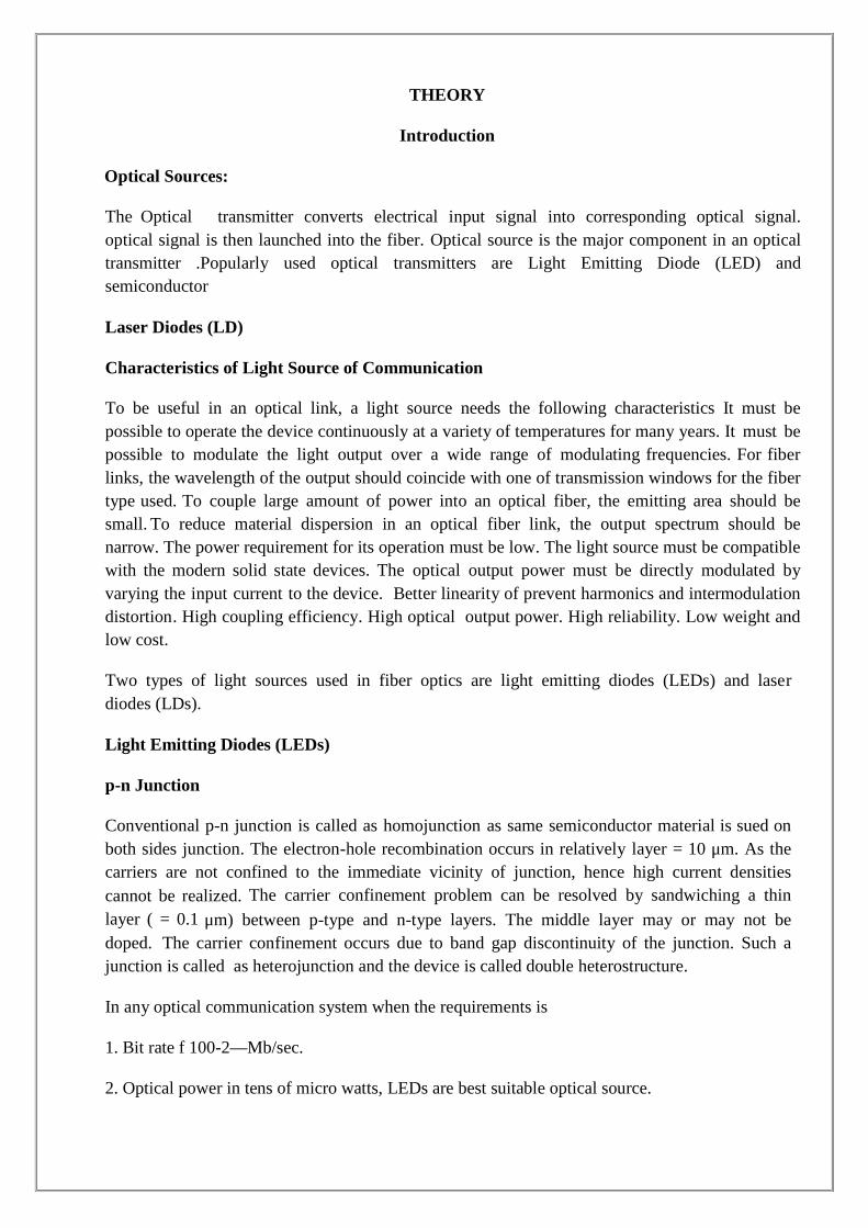
THEORY

Introduction

Optical Sources:

The Optical transmitter converts electrical input signal into corresponding optical signal.optical signal is then launched into the fiber. Optical source is the major component in an opticaltransmitter .Popularly used optical transmitters are Light Emitting Diode (LED) andsemiconductor

Laser Diodes (LD)

Characteristics of Light Source of Communication

To be useful in an optical link, a light source needs the following characteristics It must bepossible to operate the device continuously at a variety of temperatures for many years. It must bepossible to modulate the light output over a wide range of modulating frequencies. For fiberlinks, the wavelength of the output should coincide with one of transmission windows for the fibertype used. To couple large amount of power into an optical fiber, the emitting area should besmall. To reduce material dispersion in an optical fiber link, the output spectrum should benarrow. The power requirement for its operation must be low. The light source must be compatiblewith the modern solid state devices. The optical output power must be directly modulated byvarying the input current to the device. Better linearity of prevent harmonics and intermodulationdistortion. High coupling efficiency. High optical output power. High reliability. Low weight andlow cost.

Two types of light sources used in fiber optics are light emitting diodes (LEDs) and laserdiodes (LDs).

Light Emitting Diodes (LEDs)

p-n Junction

Conventional p-n junction is called as homojunction as same semiconductor material is sued onboth sides junction. The electron-hole recombination occurs in relatively layer = 10 μm. As thecarriers are not confined to the immediate vicinity of junction, hence high current densitiescannot be realized. The carrier confinement problem can be resolved by sandwiching a thinlayer ( = 0.1 μm) between p-type and n-type layers. The middle layer may or may not bedoped. The carrier confinement occurs due to band gap discontinuity of the junction. Such ajunction is called as heterojunction and the device is called double heterostructure.

In any optical communication system when the requirements is

1. Bit rate f 100-2—Mb/sec.

2. Optical power in tens of micro watts, LEDs are best suitable optical source.

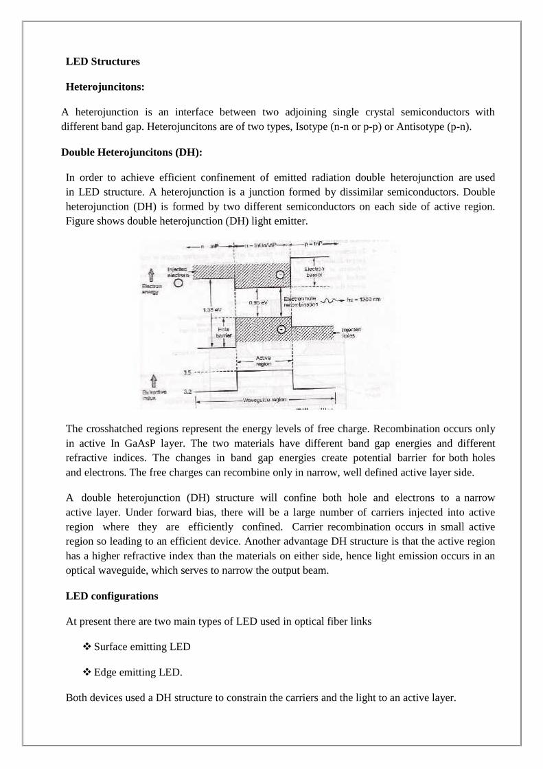
LED Structures

Heterojuncitons:

A heterojunction is an interface between two adjoining single crystal semiconductors withdifferent band gap. Heterojuncitons are of two types, Isotype (n-n or p-p) or Antisotype (p-n).

Double Heterojuncitons (DH):

In order to achieve efficient confinement of emitted radiation double heterojunction are usedin LED structure. A heterojunction is a junction formed by dissimilar semiconductors. Doubleheterojunction (DH) is formed by two different semiconductors on each side of active region.Figure shows double heterojunction (DH) light emitter.

The crosshatched regions represent the energy levels of free charge. Recombination occurs onlyin active In GaAsP layer. The two materials have different band gap energies and differentrefractive indices. The changes in band gap energies create potential barrier for both holesand electrons. The free charges can recombine only in narrow, well defined active layer side.

A double heterojunction (DH) structure will confine both hole and electrons to a narrowactive layer. Under forward bias, there will be a large number of carriers injected into activeregion where they are efficiently confined. Carrier recombination occurs in small activeregion so leading to an efficient device. Another advantage DH structure is that the active regionhas a higher refractive index than the materials on either side, hence light emission occurs in anoptical waveguide, which serves to narrow the output beam.

LED configurations

At present there are two main types of LED used in optical fiber links

Surface emitting LED

Edge emitting LED.

Both devices used a DH structure to constrain the carriers and the light to an active layer.

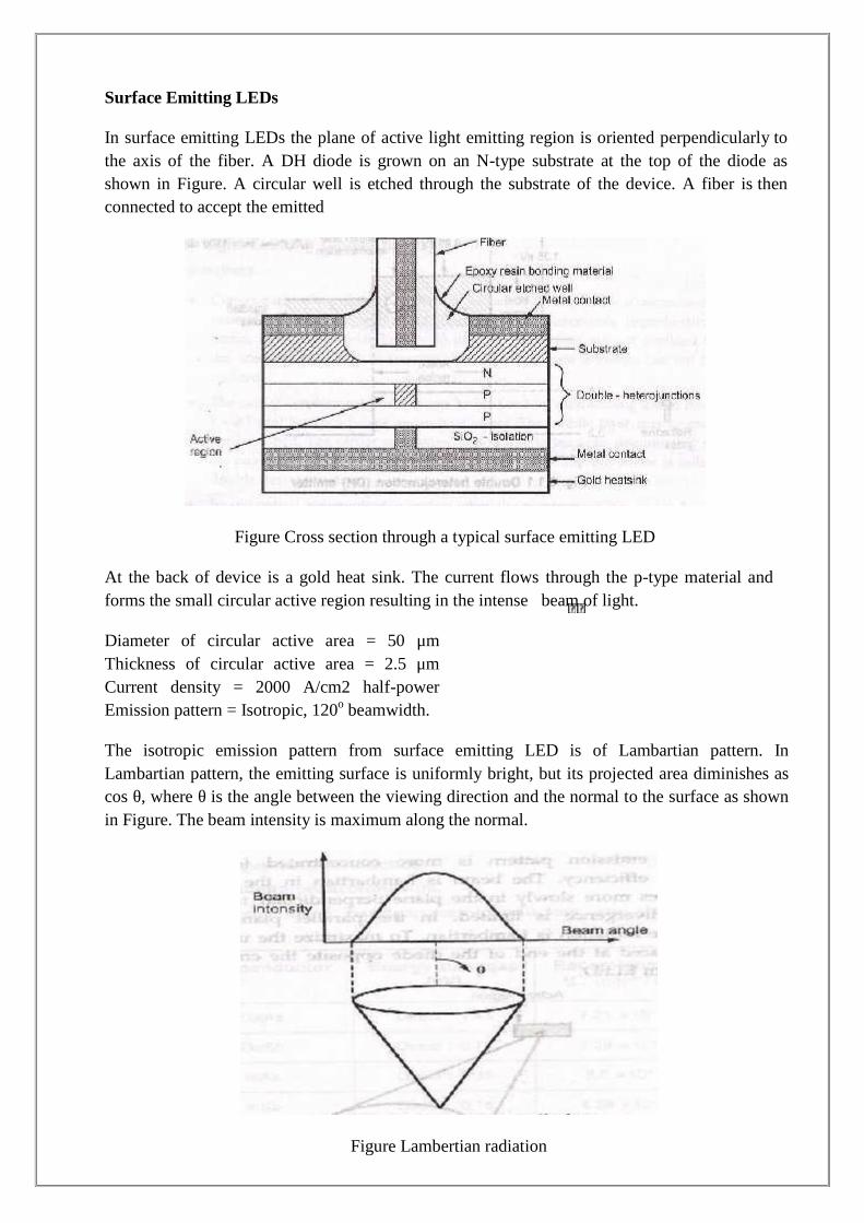
Surface Emitting LEDs

In surface emitting LEDs the plane of active light emitting region is oriented perpendicularly tothe axis of the fiber. A DH diode is grown on an N-type substrate at the top of the diode asshown in Figure. A circular well is etched through the substrate of the device. A fiber is thenconnected to accept the emitted

Figure Cross section through a typical surface emitting LED

At the back of device is a gold heat sink. The current flows through the p-type material andforms the small circular active region resulting in the intense beam of light.

Diameter of circular active area = 50 μmThickness of circular active area = 2.5 μmCurrent density = 2000 A/cm2 half-powerEmission pattern = Isotropic, 120o beamwidth.

The isotropic emission pattern from surface emitting LED is of Lambartian pattern. InLambartian pattern, the emitting surface is uniformly bright, but its projected area diminishes ascos θ, where θ is the angle between the viewing direction and the normal to the surface as shownin Figure. The beam intensity is maximum along the normal.

Figure Lambertian radiation

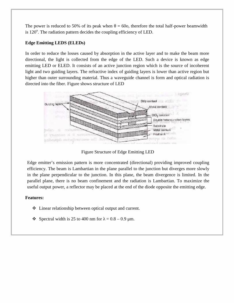
The power is reduced to 50% of its peak when θ = 60o, therefore the total half-power beamwidthis 120o. The radiation pattern decides the coupling efficiency of LED.

Edge Emitting LEDS (ELEDs)

In order to reduce the losses caused by absorption in the active layer and to make the beam moredirectional, the light is collected from the edge of the LED. Such a device is known as edgeemitting LED or ELED. It consists of an active junction region which is the source of incoherentlight and two guiding layers. The refractive index of guiding layers is lower than active region buthigher than outer surrounding material. Thus a waveguide channel is form and optical radiation isdirected into the fiber. Figure shows structure of LED

Figure Structure of Edge Emitting LED

Edge emitter’s emission pattern is more concentrated (directional) providing improved couplingefficiency. The beam is Lambartian in the plane parallel to the junction but diverges more slowlyin the plane perpendicular to the junction. In this plane, the beam divergence is limited. In theparallel plane, there is no beam confinement and the radiation is Lambartian. To maximize theuseful output power, a reflector may be placed at the end of the diode opposite the emitting edge.

Features:

Linear relationship between optical output and current.

Spectral width is 25 to 400 nm for λ = 0.8 – 0.9 μm.

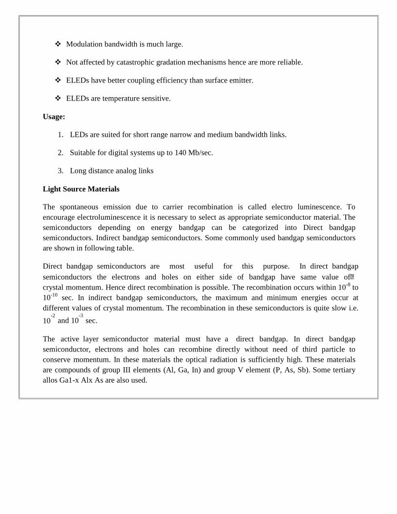
Modulation bandwidth is much large.

Not affected by catastrophic gradation mechanisms hence are more reliable.

ELEDs have better coupling efficiency than surface emitter.

ELEDs are temperature sensitive.

Usage:

1. LEDs are suited for short range narrow and medium bandwidth links.

2. Suitable for digital systems up to 140 Mb/sec.

3. Long distance analog links

Light Source Materials

The spontaneous emission due to carrier recombination is called electro luminescence. Toencourage electroluminescence it is necessary to select as appropriate semiconductor material. Thesemiconductors depending on energy bandgap can be categorized into Direct bandgapsemiconductors. Indirect bandgap semiconductors. Some commonly used bandgap semiconductorsare shown in following table.

Direct bandgap semiconductors are most useful for this purpose. In direct bandgapsemiconductors the electrons and holes on either side of bandgap have same value ofcrystal momentum. Hence direct recombination is possible. The recombination occurs within 10-8 to10-10 sec. In indirect bandgap semiconductors, the maximum and minimum energies occur atdifferent values of crystal momentum. The recombination in these semiconductors is quite slow i.e.

10-2

and 10-3

sec.

The active layer semiconductor material must have a direct bandgap. In direct bandgapsemiconductor, electrons and holes can recombine directly without need of third particle toconserve momentum. In these materials the optical radiation is sufficiently high. These materialsare compounds of group III elements (Al, Ga, In) and group V element (P, As, Sb). Some tertiaryallos Ga1-x Alx As are also used.

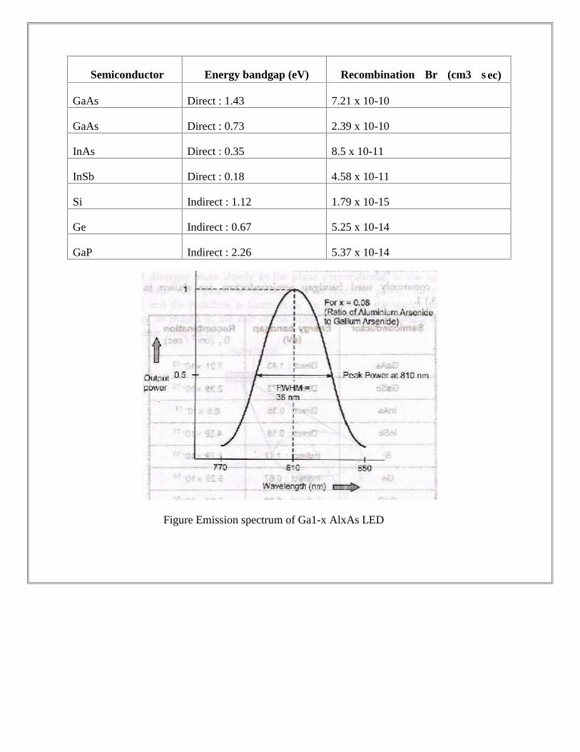
Semiconductor Energy bandgap (eV) Recombination Br (cm3 s ec)

GaAs Direct : 1.43 7.21 x 10-10

GaAs Direct : 0.73 2.39 x 10-10

InAs Direct : 0.35 8.5 x 10-11

InSb Direct : 0.18 4.58 x 10-11

Si Indirect : 1.12 1.79 x 10-15

Ge Indirect : 0.67 5.25 x 10-14

GaP Indirect : 2.26 5.37 x 10-14

Figure Emission spectrum of Ga1-x AlxAs LED

The peak output power is obtained at 810 nm. The width of emission spectrum at half power (0.5)is referred as full width half maximum (FWHM) spectral width. For the given LED FWHM is 36nm. The fundamental quantum mechanical relationship between gap energy E and frequency v isgiven as

Where, energy (E) is in joules and wavelength (λ) is in meters. Expressing the gap energy (Eg)in electron volts and wavelength (λ) in micrometers for this application.

Different materials and alloys have different band gap energies. The bandgap energy (Eg) can becontrolled by two compositional parameters x and y, within direct bandgap region. Thequaternary alloy In1-x Gax Asy P1-y is the principal material sued in such LEDs. Two expressionrelating Eg and x,y are

Quantum Efficiency and Power

The internal quantum efficiency (ηint) is defined as the ratio of radiative recombination rate tothe total recombination rate.

Where, Rr is radiative recombination rate.

Rnr is non-radiative recombination rate.

If n are the excess carriers, then radiative life time, and non-radiative life time,

The internal quantum efficiency is given and the recombination time of carriers in active region is τ

It is also known as bulk recombination life time.

Therefore internal quantum efficiency is given as

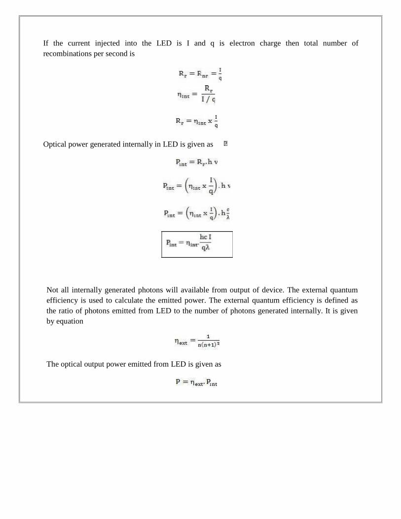
If the current injected into the LED is I and q is electron charge then total number ofrecombinations per second is

Optical power generated internally in LED is given as

Not all internally generated photons will available from output of device. The external quantumefficiency is used to calculate the emitted power. The external quantum efficiency is defined asthe ratio of photons emitted from LED to the number of photons generated internally. It is givenby equation

The optical output power emitted from LED is given as

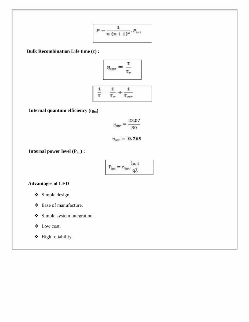
Bulk Recombination Life time (τ) :

Internal quantum efficiency (ηint)

Internal power level (Pint) :

Advantages of LED

Simple design.

Ease of manufacture.

Simple system integration.

Low cost.

High reliability.

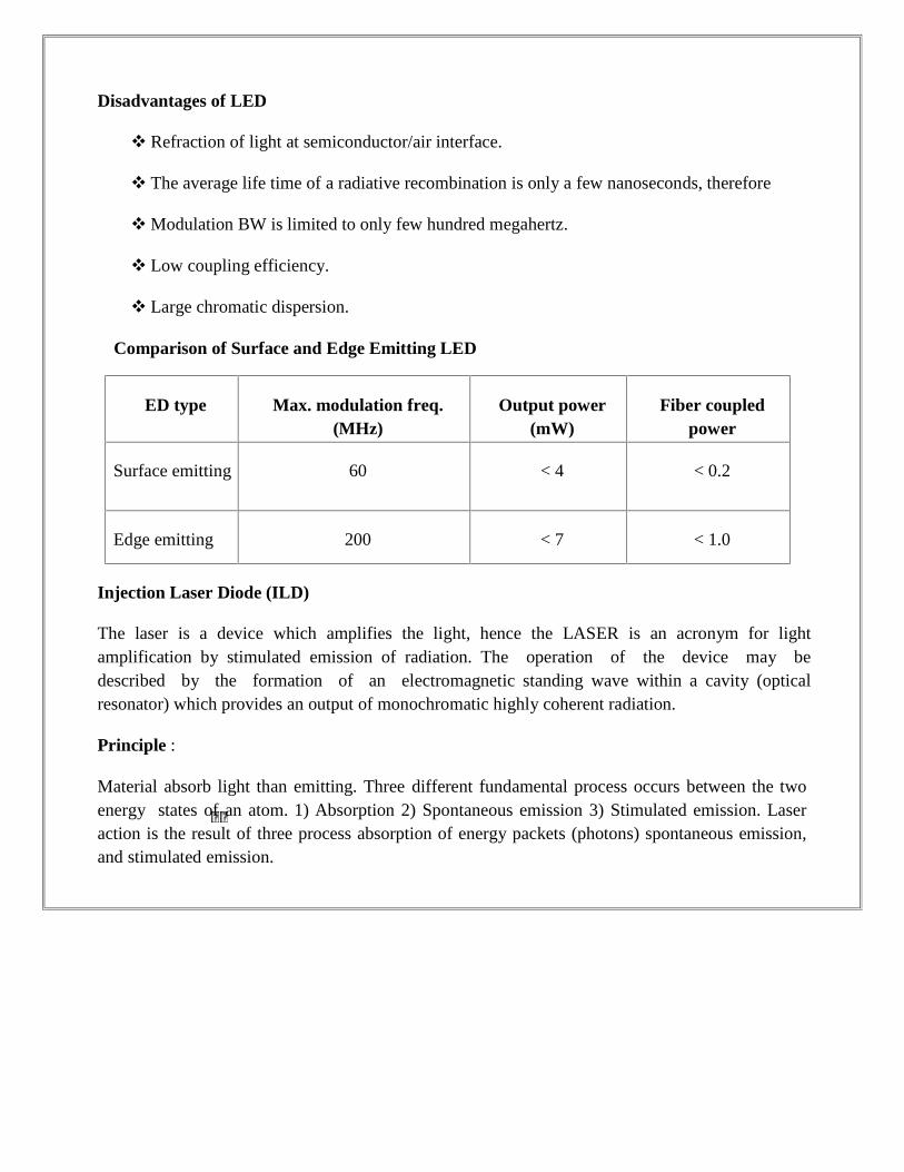
Disadvantages of LED

Refraction of light at semiconductor/air interface.

The average life time of a radiative recombination is only a few nanoseconds, therefore

Modulation BW is limited to only few hundred megahertz.

Low coupling efficiency.

Large chromatic dispersion.

Comparison of Surface and Edge Emitting LED

ED type Max. modulation freq.(MHz)

Output power(mW)

Fiber coupledpower

Surface emitting 60 < 4 < 0.2

Edge emitting 200 < 7 < 1.0

Injection Laser Diode (ILD)

The laser is a device which amplifies the light, hence the LASER is an acronym for lightamplification by stimulated emission of radiation. The operation of the device may bedescribed by the formation of an electromagnetic standing wave within a cavity (opticalresonator) which provides an output of monochromatic highly coherent radiation.

Principle :

Material absorb light than emitting. Three different fundamental process occurs between the twoenergy states of an atom. 1) Absorption 2) Spontaneous emission 3) Stimulated emission. Laseraction is the result of three process absorption of energy packets (photons) spontaneous emission,and stimulated emission.

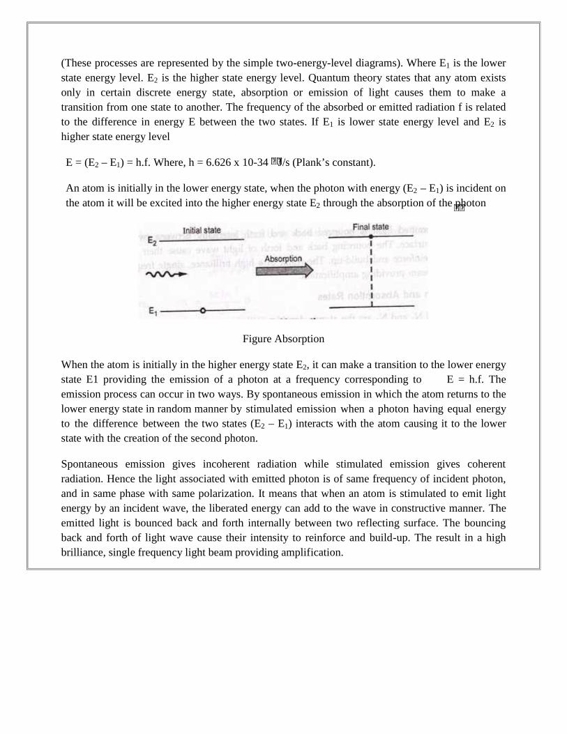
(These processes are represented by the simple two-energy-level diagrams). Where E1 is the lowerstate energy level. E2 is the higher state energy level. Quantum theory states that any atom existsonly in certain discrete energy state, absorption or emission of light causes them to make atransition from one state to another. The frequency of the absorbed or emitted radiation f is relatedto the difference in energy E between the two states. If E1 is lower state energy level and E2 ishigher state energy level

E = (E2 – E1) = h.f. Where, h = 6.626 x 10-34 J/s (Plank’s constant).

An atom is initially in the lower energy state, when the photon with energy (E2 – E1) is incident onthe atom it will be excited into the higher energy state E2 through the absorption of the photon

Figure Absorption

When the atom is initially in the higher energy state E2, it can make a transition to the lower energystate E1 providing the emission of a photon at a frequency corresponding to E = h.f. Theemission process can occur in two ways. By spontaneous emission in which the atom returns to thelower energy state in random manner by stimulated emission when a photon having equal energyto the difference between the two states (E2 – E1) interacts with the atom causing it to the lowerstate with the creation of the second photon.

Spontaneous emission gives incoherent radiation while stimulated emission gives coherentradiation. Hence the light associated with emitted photon is of same frequency of incident photon,and in same phase with same polarization. It means that when an atom is stimulated to emit lightenergy by an incident wave, the liberated energy can add to the wave in constructive manner. Theemitted light is bounced back and forth internally between two reflecting surface. The bouncingback and forth of light wave cause their intensity to reinforce and build-up. The result in a highbrilliance, single frequency light beam providing amplification.

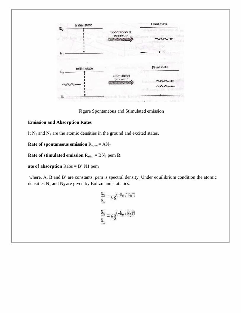
Figure Spontaneous and Stimulated emission

Emission and Absorption Rates

It N1 and N2 are the atomic densities in the ground and excited states.

Rate of spontaneous emission Rspon = AN2

Rate of stimulated emission Rstim = BN2 ρem R

ate of absorption Rabs = B’ N1 ρem

where, A, B and B’ are constants. ρem is spectral density. Under equilibrium condition the atomicdensities N1 and N2 are given by Boltzmann statistics.

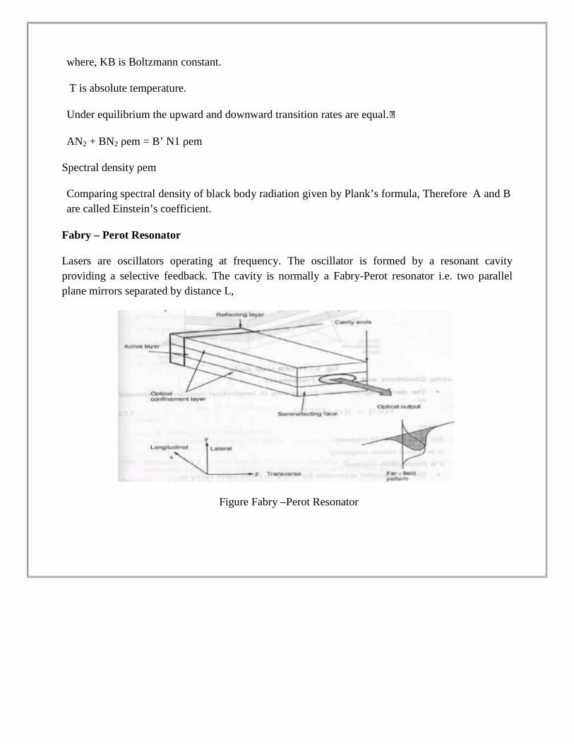
where, KB is Boltzmann constant.

T is absolute temperature.

Under equilibrium the upward and downward transition rates are equal.

AN2 + BN2 ρem = B’ N1 ρem

Spectral density ρem

Comparing spectral density of black body radiation given by Plank’s formula, Therefore A and Bare called Einstein’s coefficient.

Fabry – Perot Resonator

Lasers are oscillators operating at frequency. The oscillator is formed by a resonant cavityproviding a selective feedback. The cavity is normally a Fabry-Perot resonator i.e. two parallelplane mirrors separated by distance L,

Figure Fabry –Perot Resonator

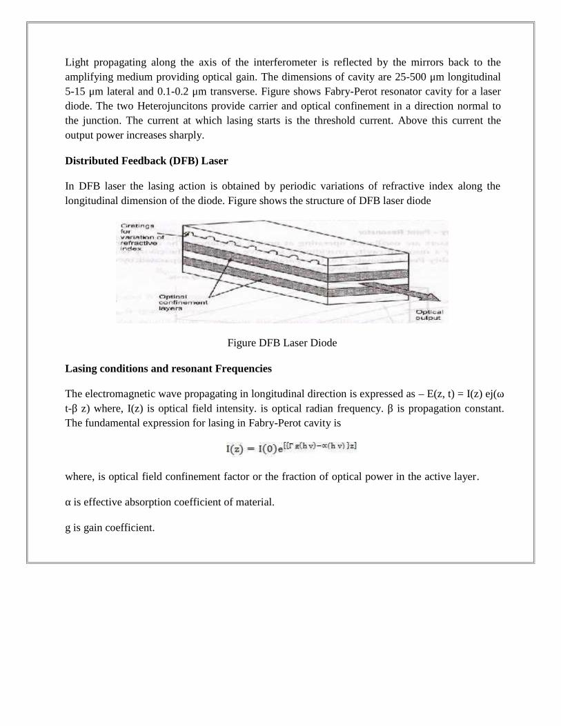
Light propagating along the axis of the interferometer is reflected by the mirrors back to theamplifying medium providing optical gain. The dimensions of cavity are 25-500 μm longitudinal5-15 μm lateral and 0.1-0.2 μm transverse. Figure shows Fabry-Perot resonator cavity for a laserdiode. The two Heterojuncitons provide carrier and optical confinement in a direction normal tothe junction. The current at which lasing starts is the threshold current. Above this current theoutput power increases sharply.

Distributed Feedback (DFB) Laser

In DFB laser the lasing action is obtained by periodic variations of refractive index along thelongitudinal dimension of the diode. Figure shows the structure of DFB laser diode

Figure DFB Laser Diode

Lasing conditions and resonant Frequencies

The electromagnetic wave propagating in longitudinal direction is expressed as – E(z, t) = I(z) ej(ωt-β z) where, I(z) is optical field intensity. is optical radian frequency. β is propagation constant.The fundamental expression for lasing in Fabry-Perot cavity is

where, is optical field confinement factor or the fraction of optical power in the active layer.

α is effective absorption coefficient of material.

g is gain coefficient.

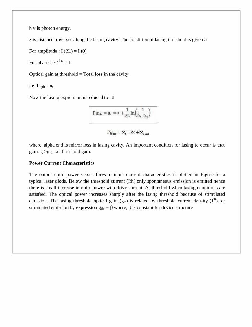
h v is photon energy.

z is distance traverses along the lasing cavity. The condition of lasing threshold is given as

For amplitude : I (2L) = I (0)

For phase : e-j2β L = 1

Optical gain at threshold = Total loss in the cavity.

i.e. Γ gth = αt

Now the lasing expression is reduced to –

where, alpha end is mirror loss in lasing cavity. An important condition for lasing to occur is thatgain, g ≥g th i.e. threshold gain.

Power Current Characteristics

The output optic power versus forward input current characteristics is plotted in Figure for atypical laser diode. Below the threshold current (Ith) only spontaneous emission is emitted hencethere is small increase in optic power with drive current. At threshold when lasing conditions aresatisfied. The optical power increases sharply after the lasing threshold because of stimulatedemission. The lasing threshold optical gain (gth) is related by threshold current density (Jth) forstimulated emission by expression gth = β where, β is constant for device structure

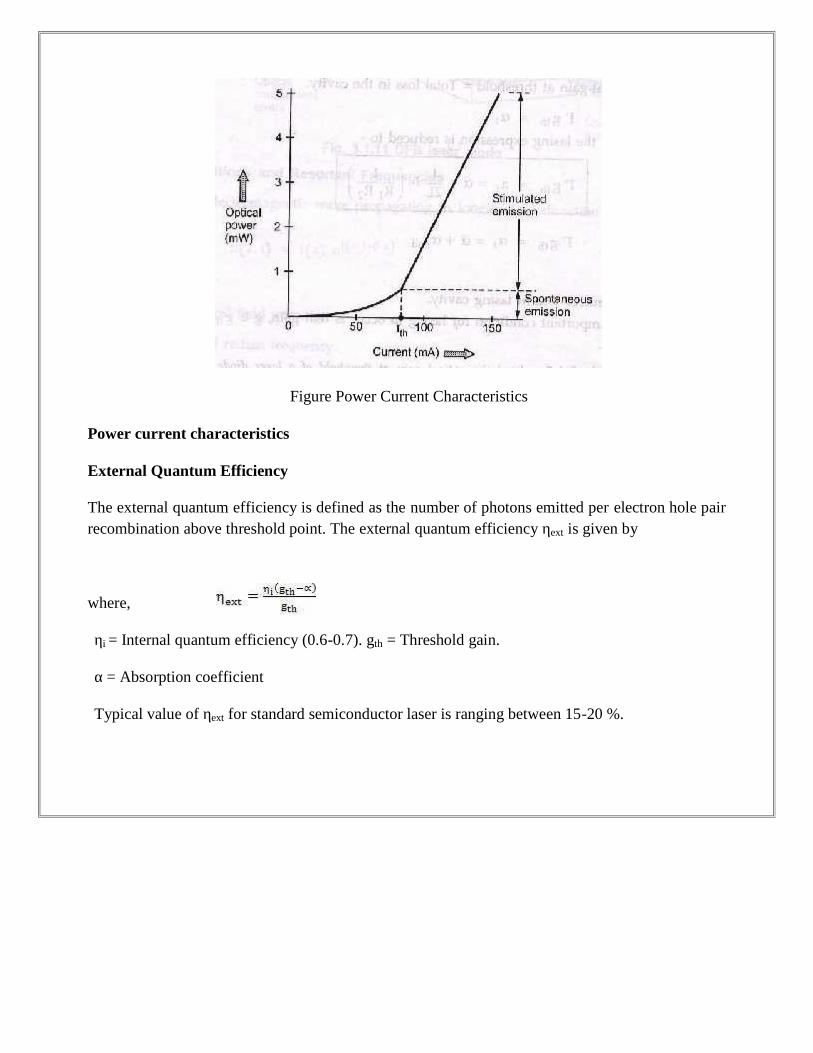
Figure Power Current Characteristics

Power current characteristics

External Quantum Efficiency

The external quantum efficiency is defined as the number of photons emitted per electron hole pairrecombination above threshold point. The external quantum efficiency ηext is given by

where,

ηi = Internal quantum efficiency (0.6-0.7). gth = Threshold gain.

α = Absorption coefficient

Typical value of ηext for standard semiconductor laser is ranging between 15-20 %.

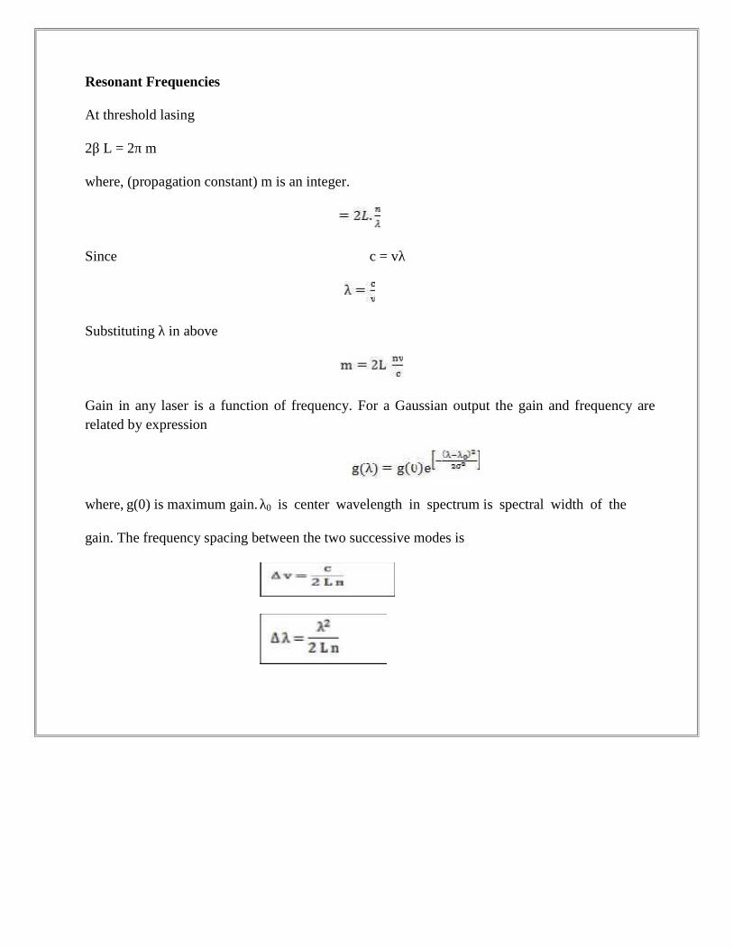
Resonant Frequencies

At threshold lasing

2β L = 2π m

where, (propagation constant) m is an integer.

Since c = vλ

Substituting λ in above

Gain in any laser is a function of frequency. For a Gaussian output the gain and frequency arerelated by expression

where, g(0) is maximum gain.λ0 is center wavelength in spectrum is spectral width of the

gain. The frequency spacing between the two successive modes is

Advantages of Laser Diode

Simple economic design.

High optical power.

Production of light can be precisely controlled.

Can be used at high temperatures.

Better modulation capability.

High coupling efficiency.

Low spectral width (3.5 nm)

Ability to transmit optical output powers between 5 and 10 mW.

Ability to maintain the intrinsic layer characteristics over long periods.

Disadvantages of Laser Diode

At the end of fiber, a speckle pattern appears as two coherent light beams add orsubtract their electric field depending upon their relative phases.

Laser diode is extremely sensitive to overload currents and at high transmissionrates, when laser is required to operate continuously the use of large drive currentproduces unfavourable thermal characteristics and necessitates the use of coolingand power stabilization.

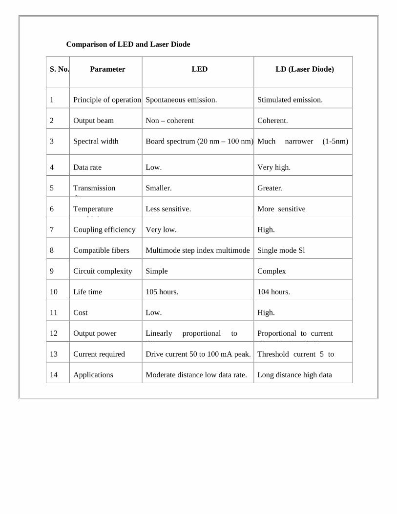
Comparison of LED and Laser Diode

S. No. Parameter LED LD (Laser Diode)

1 Principle of operation Spontaneous emission. Stimulated emission.

2 Output beam Non – coherent Coherent.

3 Spectral width Board spectrum (20 nm – 100 nm) Much narrower (1-5nm)

nm).4 Data rate Low. Very high.

5 Transmissiondistance

Smaller. Greater.

6 Temperaturesensitivity

Less sensitive. More sensitivetemperature

7 Coupling efficiency Very low. High.

8 Compatible fibers Multimode step index multimode

GRIN

Single mode Sl

Multimode GRIN

9 Circuit complexity Simple Complex

10 Life time 105 hours. 104 hours.

11 Cost Low. High.

12 Output power Linearly proportional todrive current

Proportional to currentabove the threshold

13 Current required Drive current 50 to 100 mA peak. Threshold current 5 to

40 ma

14 Applications Moderate distance low data rate. Long distance high data

rates.

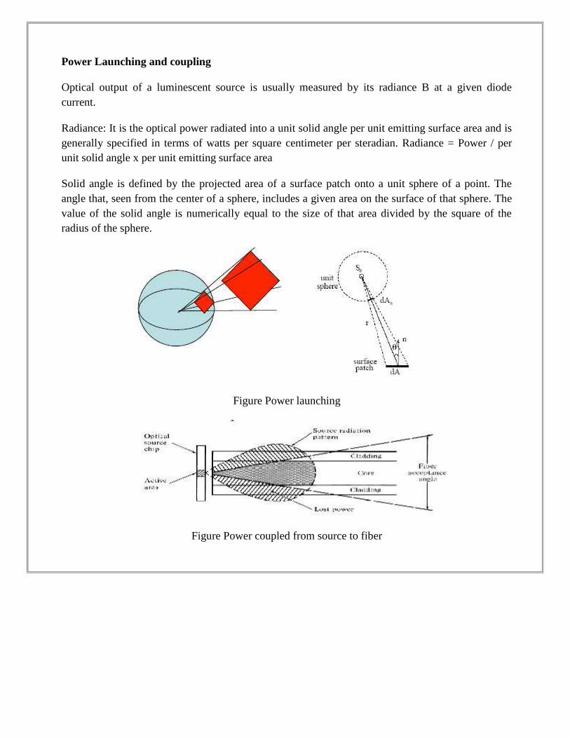
Power Launching and coupling

Optical output of a luminescent source is usually measured by its radiance B at a given diodecurrent.

Radiance: It is the optical power radiated into a unit solid angle per unit emitting surface area and isgenerally specified in terms of watts per square centimeter per steradian. Radiance = Power / perunit solid angle x per unit emitting surface area

Solid angle is defined by the projected area of a surface patch onto a unit sphere of a point. Theangle that, seen from the center of a sphere, includes a given area on the surface of that sphere. Thevalue of the solid angle is numerically equal to the size of that area divided by the square of theradius of the sphere.

Figure Power launching

Figure Power coupled from source to fiber

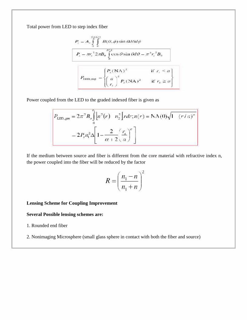
Total power from LED to step index fiber

Power coupled from the LED to the graded indexed fiber is given as

If the medium between source and fiber is different from the core material with refractive index n,the power coupled into the fiber will be reduced by the factor

Lensing Scheme for Coupling Improvement

Several Possible lensing schemes are:

1. Rounded end fiber

2. Nonimaging Microsphere (small glass sphere in contact with both the fiber and source)

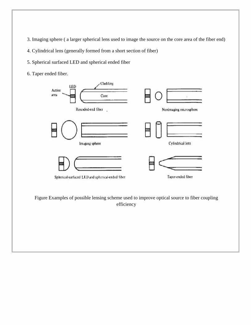
3. Imaging sphere ( a larger spherical lens used to image the source on the core area of the fiber end)

4. Cylindrical lens (generally formed from a short section of fiber)

5. Spherical surfaced LED and spherical ended fiber

6. Taper ended fiber.

Figure Examples of possible lensing scheme used to improve optical source to fiber couplingefficiency

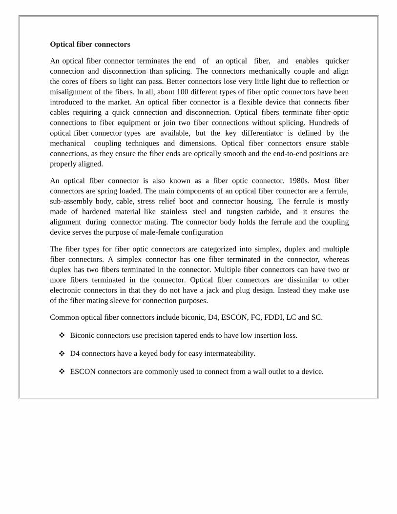
Optical fiber connectors

An optical fiber connector terminates the end of an optical fiber, and enables quickerconnection and disconnection than splicing. The connectors mechanically couple and alignthe cores of fibers so light can pass. Better connectors lose very little light due to reflection ormisalignment of the fibers. In all, about 100 different types of fiber optic connectors have beenintroduced to the market. An optical fiber connector is a flexible device that connects fibercables requiring a quick connection and disconnection. Optical fibers terminate fiber-opticconnections to fiber equipment or join two fiber connections without splicing. Hundreds ofoptical fiber connector types are available, but the key differentiator is defined by themechanical coupling techniques and dimensions. Optical fiber connectors ensure stableconnections, as they ensure the fiber ends are optically smooth and the end-to-end positions areproperly aligned.

An optical fiber connector is also known as a fiber optic connector. 1980s. Most fiberconnectors are spring loaded. The main components of an optical fiber connector are a ferrule,sub-assembly body, cable, stress relief boot and connector housing. The ferrule is mostlymade of hardened material like stainless steel and tungsten carbide, and it ensures thealignment during connector mating. The connector body holds the ferrule and the couplingdevice serves the purpose of male-female configuration

The fiber types for fiber optic connectors are categorized into simplex, duplex and multiplefiber connectors. A simplex connector has one fiber terminated in the connector, whereasduplex has two fibers terminated in the connector. Multiple fiber connectors can have two ormore fibers terminated in the connector. Optical fiber connectors are dissimilar to otherelectronic connectors in that they do not have a jack and plug design. Instead they make useof the fiber mating sleeve for connection purposes.

Common optical fiber connectors include biconic, D4, ESCON, FC, FDDI, LC and SC.

Biconic connectors use precision tapered ends to have low insertion loss.

D4 connectors have a keyed body for easy intermateability.

ESCON connectors are commonly used to connect from a wall outlet to a device.

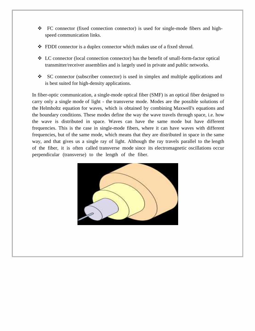
FC connector (fixed connection connector) is used for single-mode fibers and high-speed communication links.

FDDI connector is a duplex connector which makes use of a fixed shroud.

LC connector (local connection connector) has the benefit of small-form-factor opticaltransmitter/receiver assemblies and is largely used in private and public networks.

SC connector (subscriber connector) is used in simplex and multiple applications andis best suited for high-density applications.

In fiber-optic communication, a single-mode optical fiber (SMF) is an optical fiber designed tocarry only a single mode of light - the transverse mode. Modes are the possible solutions ofthe Helmholtz equation for waves, which is obtained by combining Maxwell's equations andthe boundary conditions. These modes define the way the wave travels through space, i.e. howthe wave is distributed in space. Waves can have the same mode but have differentfrequencies. This is the case in single-mode fibers, where it can have waves with differentfrequencies, but of the same mode, which means that they are distributed in space in the sameway, and that gives us a single ray of light. Although the ray travels parallel to the lengthof the fiber, it is often called transverse mode since its electromagnetic oscillations occurperpendicular (transverse) to the length of the fiber.

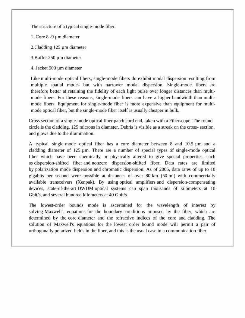
The structure of a typical single-mode fiber.

1. Core 8 -9 µm diameter

2.Cladding 125 µm diameter

3.Buffer 250 µm diameter

4. Jacket 900 µm diameter

Like multi-mode optical fibers, single-mode fibers do exhibit modal dispersion resulting frommultiple spatial modes but with narrower modal dispersion. Single-mode fibers aretherefore better at retaining the fidelity of each light pulse over longer distances than multi-mode fibers. For these reasons, single-mode fibers can have a higher bandwidth than multi-mode fibers. Equipment for single-mode fiber is more expensive than equipment for multi-mode optical fiber, but the single-mode fiber itself is usually cheaper in bulk.

Cross section of a single-mode optical fiber patch cord end, taken with a Fiberscope. The roundcircle is the cladding, 125 microns in diameter. Debris is visible as a streak on the cross- section,and glows due to the illumination.

A typical single-mode optical fiber has a core diameter between 8 and 10.5 µm and acladding diameter of 125 µm. There are a number of special types of single-mode opticalfiber which have been chemically or physically altered to give special properties, suchas dispersion-shifted fiber and nonzero dispersion-shifted fiber. Data rates are limitedby polarization mode dispersion and chromatic dispersion. As of 2005, data rates of up to 10gigabits per second were possible at distances of over 80 km (50 mi) with commerciallyavailable transceivers (Xenpak). By using optical amplifiers and dispersion-compensatingdevices, state-of-the-art DWDM optical systems can span thousands of kilometers at 10Gbit/s, and several hundred kilometers at 40 Gbit/s

The lowest-order bounds mode is ascertained for the wavelength of interest bysolving Maxwell's equations for the boundary conditions imposed by the fiber, which aredetermined by the core diameter and the refractive indices of the core and cladding. Thesolution of Maxwell's equations for the lowest order bound mode will permit a pair oforthogonally polarized fields in the fiber, and this is the usual case in a communication fiber.

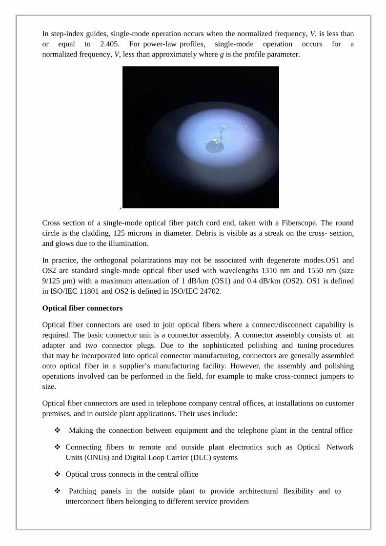
In step-index guides, single-mode operation occurs when the normalized frequency, V, is less thanor equal to 2.405. For power-law profiles, single-mode operation occurs for anormalized frequency, V, less than approximately where g is the profile parameter.

,

Cross section of a single-mode optical fiber patch cord end, taken with a Fiberscope. The roundcircle is the cladding, 125 microns in diameter. Debris is visible as a streak on the cross- section,and glows due to the illumination.

In practice, the orthogonal polarizations may not be associated with degenerate modes.OS1 andOS2 are standard single-mode optical fiber used with wavelengths 1310 nm and 1550 nm (size9/125 µm) with a maximum attenuation of 1 dB/km (OS1) and 0.4 dB/km (OS2). OS1 is definedin ISO/IEC 11801 and OS2 is defined in ISO/IEC 24702.

Optical fiber connectors

Optical fiber connectors are used to join optical fibers where a connect/disconnect capability isrequired. The basic connector unit is a connector assembly. A connector assembly consists of anadapter and two connector plugs. Due to the sophisticated polishing and tuning proceduresthat may be incorporated into optical connector manufacturing, connectors are generally assembledonto optical fiber in a supplier’s manufacturing facility. However, the assembly and polishingoperations involved can be performed in the field, for example to make cross-connect jumpers tosize.

Optical fiber connectors are used in telephone company central offices, at installations on customerpremises, and in outside plant applications. Their uses include:

Making the connection between equipment and the telephone plant in the central office

Connecting fibers to remote and outside plant electronics such as Optical NetworkUnits (ONUs) and Digital Loop Carrier (DLC) systems

Optical cross connects in the central office

Patching panels in the outside plant to provide architectural flexibility and tointerconnect fibers belonging to different service providers

Connecting couplers, splitters, and Wavelength Division Multiplexers (WDMs) tooptical fibers

Connecting optical test equipment to fibers for testing and maintenance.

Outside plant applications may involve locating connectors underground in subsurface enclosuresthat may be subject to flooding, on outdoor walls, or on utility poles. The closures that enclosethem may be hermetic, or may be “free-breathing.” Hermetic closures will prevent the connectorswithin being subjected to temperature swings unless they are breached. Free-breathing enclosureswill subject them to temperature and humidity swings, and possibly to condensation and biologicalaction from airborne bacteria, insects, etc. Connectors in the underground plant may be subjected togroundwater immersion if the closures containing them are breached or improperly assembled.

The latest industry requirements for optical fiber connectors are in Telcordia GR-326, GenericRequirements for Single mode Optical Connectors and Jumper Assemblies. A multi-fiber opticalconnector is designed to simultaneously join multiple optical fibers together, with eachoptical fiber being joined to only one other optical fiber. The last part of the definition is includedso as not to confuse multi-fiber connectors with a branching component, such as a coupler.

The latter joins one optical fiber to two or more other optical fibers. Multi-fiber opticalconnectors are designed to be used wherever quick and/or repetitive connects and disconnects of agroup of fibers are needed. Applications include telecommunications companies’ Central Offices(COs), installations on customer premises, and Outside Plant (OSP) applications. The multi-fiberoptical connector can be used in the creation of a low-cost switch for use in fiber optical testing.Another application is in cables delivered to a user with pre- terminated multi-fiber jumpers. Thiswould reduce the need for field splicing, which could greatly reduce the number of hoursnecessary for placing an optical fiber cable in a telecommunications network. This, in turn,would result in savings for the installer of such cable.

The return loss RL is a measure of the portion of light that is reflected back to the source at thejunction. It is expressed in decibel. The higher the RL value in decibels, the lower is thereflections. Typical RL values lie between 35 and 50 dB for PC, 60 to 90 dB for APC and 20 to40 dB for multimode fibres. In the early days of fibre-optic plug-in connectors, the abutting endfaces were polished to an angle of 90° to the fibre axis, while current standards require PC(Physical Contact) polishing or APC (Angled Physical Contact) polishing. The term HRL (HighReturn Loss) is frequently used, but it has the same meaning as APC.

In PC polishing, the ferrule is polished to a convex end to ensure that the fibre cores touch at theirhighest point. This reduces the occurrence of reflections at the junction. A furtherimprovement in return loss is achieved by using the APC polishing technique. Here, theconvex end surfaces of the ferrules are polished to an angle (8°) relative to the fibre axis. SCconnectors are also sold with a 9° angle. They possess IL and RL values identical to 8°versions, and for this reason they have not established themselves worldwide.

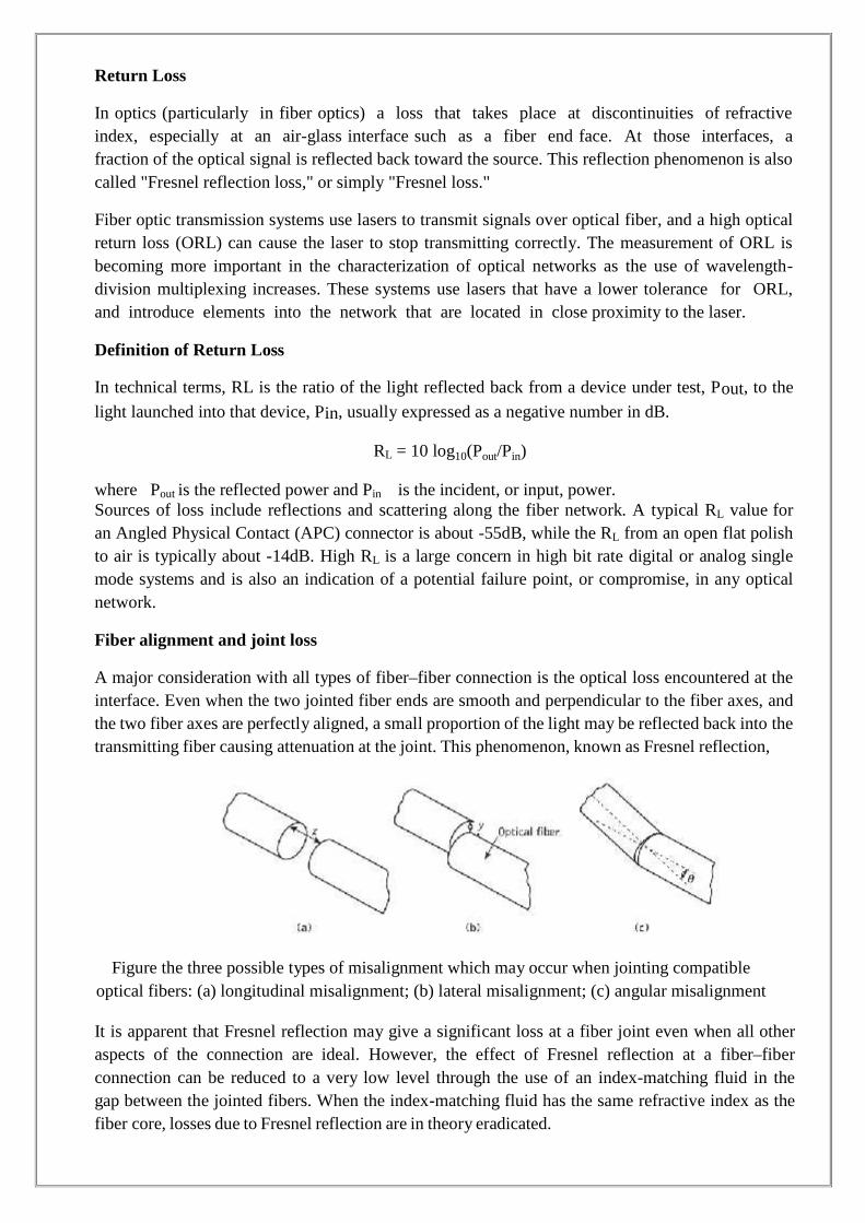
Return Loss

In optics (particularly in fiber optics) a loss that takes place at discontinuities of refractiveindex, especially at an air-glass interface such as a fiber end face. At those interfaces, afraction of the optical signal is reflected back toward the source. This reflection phenomenon is alsocalled "Fresnel reflection loss," or simply "Fresnel loss."

Fiber optic transmission systems use lasers to transmit signals over optical fiber, and a high opticalreturn loss (ORL) can cause the laser to stop transmitting correctly. The measurement of ORL isbecoming more important in the characterization of optical networks as the use of wavelength-division multiplexing increases. These systems use lasers that have a lower tolerance for ORL,and introduce elements into the network that are located in close proximity to the laser.

Definition of Return Loss

In technical terms, RL is the ratio of the light reflected back from a device under test, Pout, to the

light launched into that device, Pin, usually expressed as a negative number in dB.

RL = 10 log10(Pout/Pin)

where Pout is the reflected power and Pin is the incident, or input, power.Sources of loss include reflections and scattering along the fiber network. A typical RL value foran Angled Physical Contact (APC) connector is about -55dB, while the RL from an open flat polishto air is typically about -14dB. High RL is a large concern in high bit rate digital or analog singlemode systems and is also an indication of a potential failure point, or compromise, in any opticalnetwork.

Fiber alignment and joint loss

A major consideration with all types of fiber–fiber connection is the optical loss encountered at theinterface. Even when the two jointed fiber ends are smooth and perpendicular to the fiber axes, andthe two fiber axes are perfectly aligned, a small proportion of the light may be reflected back into thetransmitting fiber causing attenuation at the joint. This phenomenon, known as Fresnel reflection,

Figure the three possible types of misalignment which may occur when jointing compatibleoptical fibers: (a) longitudinal misalignment; (b) lateral misalignment; (c) angular misalignment

It is apparent that Fresnel reflection may give a significant loss at a fiber joint even when all otheraspects of the connection are ideal. However, the effect of Fresnel reflection at a fiber–fiberconnection can be reduced to a very low level through the use of an index-matching fluid in thegap between the jointed fibers. When the index-matching fluid has the same refractive index as thefiber core, losses due to Fresnel reflection are in theory eradicated.

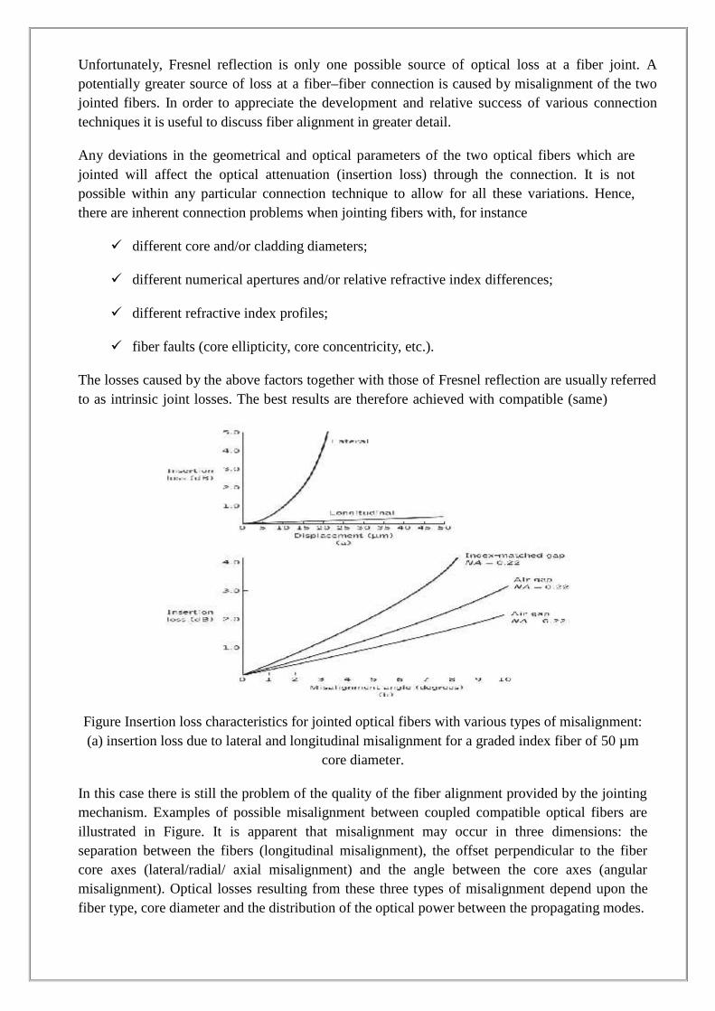
Unfortunately, Fresnel reflection is only one possible source of optical loss at a fiber joint. Apotentially greater source of loss at a fiber–fiber connection is caused by misalignment of the twojointed fibers. In order to appreciate the development and relative success of various connectiontechniques it is useful to discuss fiber alignment in greater detail.

Any deviations in the geometrical and optical parameters of the two optical fibers which arejointed will affect the optical attenuation (insertion loss) through the connection. It is notpossible within any particular connection technique to allow for all these variations. Hence,there are inherent connection problems when jointing fibers with, for instance

different core and/or cladding diameters;

different numerical apertures and/or relative refractive index differences;

different refractive index profiles;

fiber faults (core ellipticity, core concentricity, etc.).

The losses caused by the above factors together with those of Fresnel reflection are usually referredto as intrinsic joint losses. The best results are therefore achieved with compatible (same)

Figure Insertion loss characteristics for jointed optical fibers with various types of misalignment:(a) insertion loss due to lateral and longitudinal misalignment for a graded index fiber of 50 µm

core diameter.

In this case there is still the problem of the quality of the fiber alignment provided by the jointingmechanism. Examples of possible misalignment between coupled compatible optical fibers areillustrated in Figure. It is apparent that misalignment may occur in three dimensions: theseparation between the fibers (longitudinal misalignment), the offset perpendicular to the fibercore axes (lateral/radial/ axial misalignment) and the angle between the core axes (angularmisalignment). Optical losses resulting from these three types of misalignment depend upon thefiber type, core diameter and the distribution of the optical power between the propagating modes.

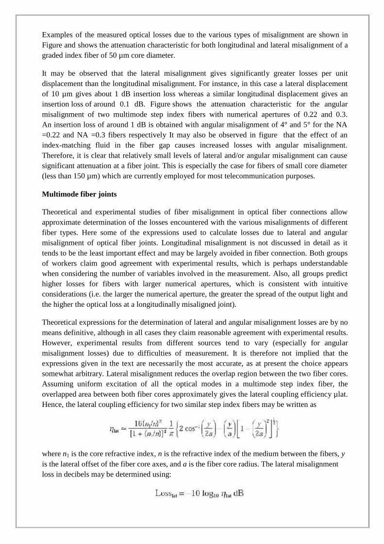
Examples of the measured optical losses due to the various types of misalignment are shown inFigure and shows the attenuation characteristic for both longitudinal and lateral misalignment of agraded index fiber of 50 µm core diameter.

It may be observed that the lateral misalignment gives significantly greater losses per unitdisplacement than the longitudinal misalignment. For instance, in this case a lateral displacementof 10 µm gives about 1 dB insertion loss whereas a similar longitudinal displacement gives aninsertion loss of around 0.1 dB. Figure shows the attenuation characteristic for the angularmisalignment of two multimode step index fibers with numerical apertures of 0.22 and 0.3.An insertion loss of around 1 dB is obtained with angular misalignment of 4° and 5° for the NA=0.22 and NA =0.3 fibers respectively It may also be observed in figure that the effect of anindex-matching fluid in the fiber gap causes increased losses with angular misalignment.Therefore, it is clear that relatively small levels of lateral and/or angular misalignment can causesignificant attenuation at a fiber joint. This is especially the case for fibers of small core diameter(less than 150 µm) which are currently employed for most telecommunication purposes.

Multimode fiber joints

Theoretical and experimental studies of fiber misalignment in optical fiber connections allowapproximate determination of the losses encountered with the various misalignments of differentfiber types. Here some of the expressions used to calculate losses due to lateral and angularmisalignment of optical fiber joints. Longitudinal misalignment is not discussed in detail as ittends to be the least important effect and may be largely avoided in fiber connection. Both groupsof workers claim good agreement with experimental results, which is perhaps understandablewhen considering the number of variables involved in the measurement. Also, all groups predicthigher losses for fibers with larger numerical apertures, which is consistent with intuitiveconsiderations (i.e. the larger the numerical aperture, the greater the spread of the output light andthe higher the optical loss at a longitudinally misaligned joint).

Theoretical expressions for the determination of lateral and angular misalignment losses are by nomeans definitive, although in all cases they claim reasonable agreement with experimental results.However, experimental results from different sources tend to vary (especially for angularmisalignment losses) due to difficulties of measurement. It is therefore not implied that theexpressions given in the text are necessarily the most accurate, as at present the choice appearssomewhat arbitrary. Lateral misalignment reduces the overlap region between the two fiber cores.Assuming uniform excitation of all the optical modes in a multimode step index fiber, theoverlapped area between both fiber cores approximately gives the lateral coupling efficiency µlat.Hence, the lateral coupling efficiency for two similar step index fibers may be written as

where n1 is the core refractive index, n is the refractive index of the medium between the fibers, yis the lateral offset of the fiber core axes, and a is the fiber core radius. The lateral misalignmentloss in decibels may be determined using:

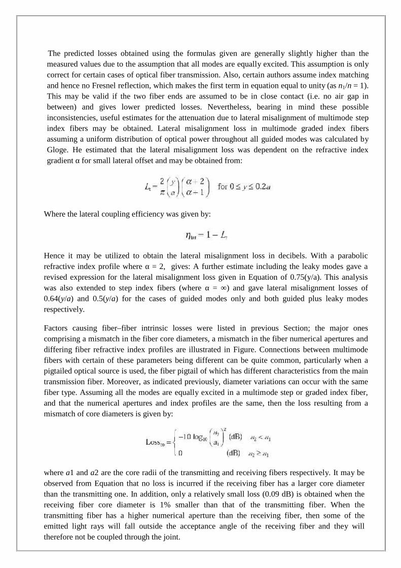
The predicted losses obtained using the formulas given are generally slightly higher than themeasured values due to the assumption that all modes are equally excited. This assumption is onlycorrect for certain cases of optical fiber transmission. Also, certain authors assume index matchingand hence no Fresnel reflection, which makes the first term in equation equal to unity (as n1/n = 1).This may be valid if the two fiber ends are assumed to be in close contact (i.e. no air gap inbetween) and gives lower predicted losses. Nevertheless, bearing in mind these possibleinconsistencies, useful estimates for the attenuation due to lateral misalignment of multimode stepindex fibers may be obtained. Lateral misalignment loss in multimode graded index fibersassuming a uniform distribution of optical power throughout all guided modes was calculated byGloge. He estimated that the lateral misalignment loss was dependent on the refractive indexgradient α for small lateral offset and may be obtained from:

Where the lateral coupling efficiency was given by:

Hence it may be utilized to obtain the lateral misalignment loss in decibels. With a parabolicrefractive index profile where α = 2, gives: A further estimate including the leaky modes gave arevised expression for the lateral misalignment loss given in Equation of 0.75(y/a). This analysiswas also extended to step index fibers (where α = ∞) and gave lateral misalignment losses of0.64(y/a) and 0.5(y/a) for the cases of guided modes only and both guided plus leaky modesrespectively.

Factors causing fiber–fiber intrinsic losses were listed in previous Section; the major onescomprising a mismatch in the fiber core diameters, a mismatch in the fiber numerical apertures anddiffering fiber refractive index profiles are illustrated in Figure. Connections between multimodefibers with certain of these parameters being different can be quite common, particularly when apigtailed optical source is used, the fiber pigtail of which has different characteristics from the maintransmission fiber. Moreover, as indicated previously, diameter variations can occur with the samefiber type. Assuming all the modes are equally excited in a multimode step or graded index fiber,and that the numerical apertures and index profiles are the same, then the loss resulting from amismatch of core diameters is given by:

where a1 and a2 are the core radii of the transmitting and receiving fibers respectively. It may beobserved from Equation that no loss is incurred if the receiving fiber has a larger core diameterthan the transmitting one. In addition, only a relatively small loss (0.09 dB) is obtained when thereceiving fiber core diameter is 1% smaller than that of the transmitting fiber. When thetransmitting fiber has a higher numerical aperture than the receiving fiber, then some of theemitted light rays will fall outside the acceptance angle of the receiving fiber and they willtherefore not be coupled through the joint.

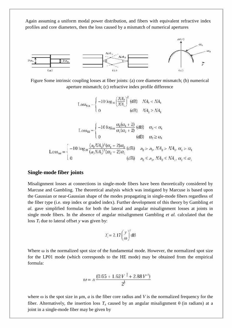
Again assuming a uniform modal power distribution, and fibers with equivalent refractive indexprofiles and core diameters, then the loss caused by a mismatch of numerical apertures

Figure Some intrinsic coupling losses at fiber joints: (a) core diameter mismatch; (b) numericalaperture mismatch; (c) refractive index profile difference

Single-mode fiber joints

Misalignment losses at connections in single-mode fibers have been theoretically considered byMarcuse and Gambling. The theoretical analysis which was instigated by Marcuse is based uponthe Gaussian or near-Gaussian shape of the modes propagating in single-mode fibers regardless ofthe fiber type (i.e. step index or graded index). Further development of this theory by Gambling etal. gave simplified formulas for both the lateral and angular misalignment losses at joints insingle mode fibers. In the absence of angular misalignment Gambling et al. calculated that theloss Tl due to lateral offset y was given by:

Where ω is the normalized spot size of the fundamental mode. However, the normalized spot sizefor the LP01 mode (which corresponds to the HE mode) may be obtained from the empiricalformula:

where is the spot size in μm, a is the fiber core radius and V is the normalized frequency for the

fiber. Alternatively, the insertion loss Ta caused by an angular misalignment (in radians) at ajoint in a single-mode fiber may be given by

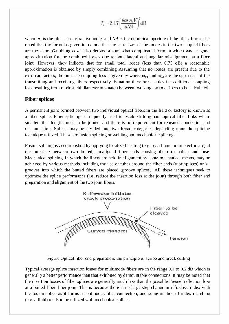
where n1 is the fiber core refractive index and NA is the numerical aperture of the fiber. It must benoted that the formulas given in assume that the spot sizes of the modes in the two coupled fibersare the same. Gambling et al. also derived a somewhat complicated formula which gave a goodapproximation for the combined losses due to both lateral and angular misalignment at a fiberjoint. However, they indicate that for small total losses (less than 0.75 dB) a reasonableapproximation is obtained by simply combining Assuming that no losses are present due to theextrinsic factors, the intrinsic coupling loss is given by where 01 and 02 are the spot sizes of thetransmitting and receiving fibers respectively. Equation therefore enables the additional couplingloss resulting from mode-field diameter mismatch between two single-mode fibers to be calculated.

Fiber splices

A permanent joint formed between two individual optical fibers in the field or factory is known asa fiber splice. Fiber splicing is frequently used to establish long-haul optical fiber links wheresmaller fiber lengths need to be joined, and there is no requirement for repeated connection anddisconnection. Splices may be divided into two broad categories depending upon the splicingtechnique utilized. These are fusion splicing or welding and mechanical splicing.

Fusion splicing is accomplished by applying localized heating (e.g. by a flame or an electric arc) atthe interface between two butted, prealigned fiber ends causing them to soften and fuse.Mechanical splicing, in which the fibers are held in alignment by some mechanical means, may beachieved by various methods including the use of tubes around the fiber ends (tube splices) or V-grooves into which the butted fibers are placed (groove splices). All these techniques seek tooptimize the splice performance (i.e. reduce the insertion loss at the joint) through both fiber endpreparation and alignment of the two joint fibers.

Figure Optical fiber end preparation: the principle of scribe and break cutting

Typical average splice insertion losses for multimode fibers are in the range 0.1 to 0.2 dB which isgenerally a better performance than that exhibited by demountable connections. It may be noted thatthe insertion losses of fiber splices are generally much less than the possible Fresnel reflection lossat a butted fiber–fiber joint. This is because there is no large step change in refractive index withthe fusion splice as it forms a continuous fiber connection, and some method of index matching(e.g. a fluid) tends to be utilized with mechanical splices.

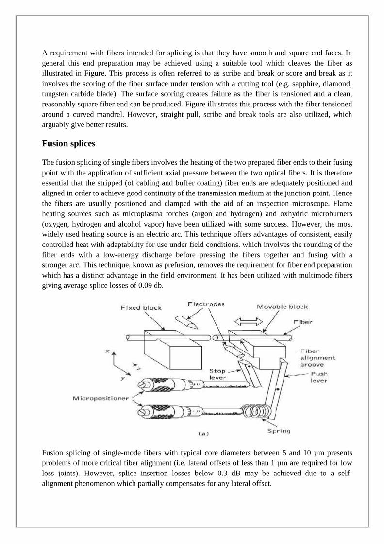
A requirement with fibers intended for splicing is that they have smooth and square end faces. Ingeneral this end preparation may be achieved using a suitable tool which cleaves the fiber asillustrated in Figure. This process is often referred to as scribe and break or score and break as itinvolves the scoring of the fiber surface under tension with a cutting tool (e.g. sapphire, diamond,tungsten carbide blade). The surface scoring creates failure as the fiber is tensioned and a clean,reasonably square fiber end can be produced. Figure illustrates this process with the fiber tensionedaround a curved mandrel. However, straight pull, scribe and break tools are also utilized, whicharguably give better results.

Fusion splices

The fusion splicing of single fibers involves the heating of the two prepared fiber ends to their fusingpoint with the application of sufficient axial pressure between the two optical fibers. It is thereforeessential that the stripped (of cabling and buffer coating) fiber ends are adequately positioned andaligned in order to achieve good continuity of the transmission medium at the junction point. Hencethe fibers are usually positioned and clamped with the aid of an inspection microscope. Flameheating sources such as microplasma torches (argon and hydrogen) and oxhydric microburners(oxygen, hydrogen and alcohol vapor) have been utilized with some success. However, the mostwidely used heating source is an electric arc. This technique offers advantages of consistent, easilycontrolled heat with adaptability for use under field conditions. which involves the rounding of thefiber ends with a low-energy discharge before pressing the fibers together and fusing with astronger arc. This technique, known as prefusion, removes the requirement for fiber end preparationwhich has a distinct advantage in the field environment. It has been utilized with multimode fibersgiving average splice losses of 0.09 db.

Fusion splicing of single-mode fibers with typical core diameters between 5 and 10 µm presentsproblems of more critical fiber alignment (i.e. lateral offsets of less than 1 µm are required for lowloss joints). However, splice insertion losses below 0.3 dB may be achieved due to a self-alignment phenomenon which partially compensates for any lateral offset.

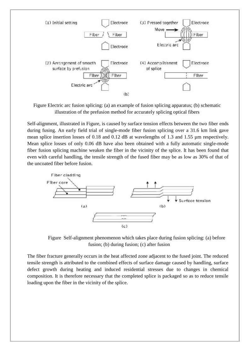
Figure Electric arc fusion splicing: (a) an example of fusion splicing apparatus; (b) schematicillustration of the prefusion method for accurately splicing optical fibers

Self-alignment, illustrated in Figure, is caused by surface tension effects between the two fiber endsduring fusing. An early field trial of single-mode fiber fusion splicing over a 31.6 km link gavemean splice insertion losses of 0.18 and 0.12 dB at wavelengths of 1.3 and 1.55 µm respectively.Mean splice losses of only 0.06 dB have also been obtained with a fully automatic single-modefiber fusion splicing machine weaken the fiber in the vicinity of the splice. It has been found thateven with careful handling, the tensile strength of the fused fiber may be as low as 30% of that ofthe uncoated fiber before fusion.

Figure Self-alignment phenomenon which takes place during fusion splicing: (a) beforefusion; (b) during fusion; (c) after fusion

The fiber fracture generally occurs in the heat affected zone adjacent to the fused joint. The reducedtensile strength is attributed to the combined effects of surface damage caused by handling, surfacedefect growth during heating and induced residential stresses due to changes in chemicalcomposition. It is therefore necessary that the completed splice is packaged so as to reduce tensileloading upon the fiber in the vicinity of the splice.

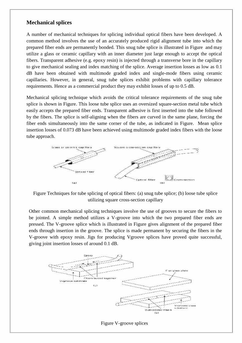
Mechanical splices

A number of mechanical techniques for splicing individual optical fibers have been developed. Acommon method involves the use of an accurately produced rigid alignment tube into which theprepared fiber ends are permanently bonded. This snug tube splice is illustrated in Figure and mayutilize a glass or ceramic capillary with an inner diameter just large enough to accept the opticalfibers. Transparent adhesive (e.g. epoxy resin) is injected through a transverse bore in the capillaryto give mechanical sealing and index matching of the splice. Average insertion losses as low as 0.1dB have been obtained with multimode graded index and single-mode fibers using ceramiccapillaries. However, in general, snug tube splices exhibit problems with capillary tolerancerequirements. Hence as a commercial product they may exhibit losses of up to 0.5 dB.

Mechanical splicing technique which avoids the critical tolerance requirements of the snug tubesplice is shown in Figure. This loose tube splice uses an oversized square-section metal tube whicheasily accepts the prepared fiber ends. Transparent adhesive is first inserted into the tube followedby the fibers. The splice is self-aligning when the fibers are curved in the same plane, forcing thefiber ends simultaneously into the same corner of the tube, as indicated in Figure. Mean spliceinsertion losses of 0.073 dB have been achieved using multimode graded index fibers with the loosetube approach.

Figure Techniques for tube splicing of optical fibers: (a) snug tube splice; (b) loose tube spliceutilizing square cross-section capillary

Other common mechanical splicing techniques involve the use of grooves to secure the fibers tobe jointed. A simple method utilizes a V-groove into which the two prepared fiber ends arepressed. The V-groove splice which is illustrated in Figure gives alignment of the prepared fiberends through insertion in the groove. The splice is made permanent by securing the fibers in theV-groove with epoxy resin. Jigs for producing Vgroove splices have proved quite successful,giving joint insertion losses of around 0.1 dB.

Figure V-groove splices

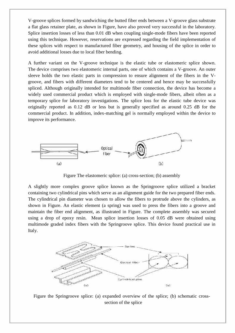
V-groove splices formed by sandwiching the butted fiber ends between a V-groove glass substratea flat glass retainer plate, as shown in Figure, have also proved very successful in the laboratory.Splice insertion losses of less than 0.01 dB when coupling single-mode fibers have been reportedusing this technique. However, reservations are expressed regarding the field implementation ofthese splices with respect to manufactured fiber geometry, and housing of the splice in order toavoid additional losses due to local fiber bending.

A further variant on the V-groove technique is the elastic tube or elastomeric splice shown.The device comprises two elastomeric internal parts, one of which contains a V-groove. An outersleeve holds the two elastic parts in compression to ensure alignment of the fibers in the V-groove, and fibers with different diameters tend to be centered and hence may be successfullyspliced. Although originally intended for multimode fiber connection, the device has become awidely used commercial product which is employed with single-mode fibers, albeit often as atemporary splice for laboratory investigations. The splice loss for the elastic tube device wasoriginally reported as 0.12 dB or less but is generally specified as around 0.25 dB for thecommercial product. In addition, index-matching gel is normally employed within the device toimprove its performance.

Figure The elastomeric splice: (a) cross-section; (b) assembly

A slightly more complex groove splice known as the Springroove splice utilized a bracketcontaining two cylindrical pins which serve as an alignment guide for the two prepared fiber ends.The cylindrical pin diameter was chosen to allow the fibers to protrude above the cylinders, asshown in Figure. An elastic element (a spring) was used to press the fibers into a groove andmaintain the fiber end alignment, as illustrated in Figure. The complete assembly was securedusing a drop of epoxy resin. Mean splice insertion losses of 0.05 dB were obtained usingmultimode graded index fibers with the Springroove splice. This device found practical use inItaly.

Figure the Springroove splice: (a) expanded overview of the splice; (b) schematic cross-section of the splice

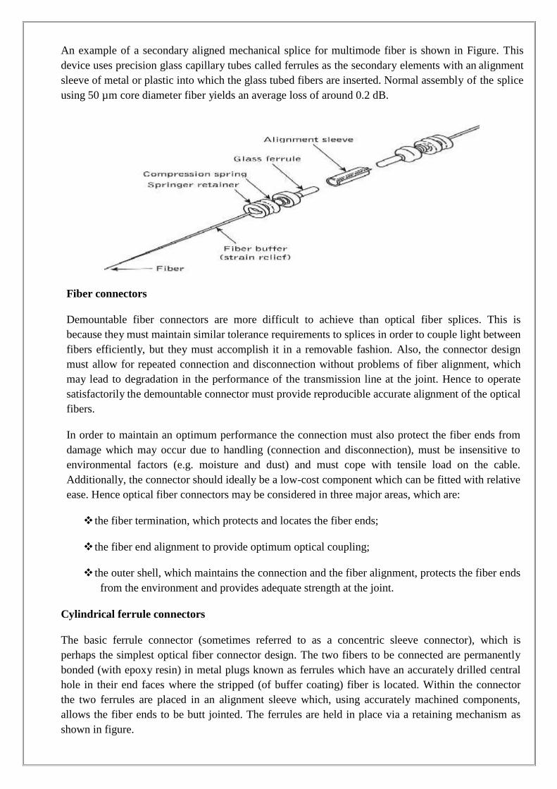
An example of a secondary aligned mechanical splice for multimode fiber is shown in Figure. Thisdevice uses precision glass capillary tubes called ferrules as the secondary elements with an alignmentsleeve of metal or plastic into which the glass tubed fibers are inserted. Normal assembly of the spliceusing 50 µm core diameter fiber yields an average loss of around 0.2 dB.

Fiber connectors

Demountable fiber connectors are more difficult to achieve than optical fiber splices. This isbecause they must maintain similar tolerance requirements to splices in order to couple light betweenfibers efficiently, but they must accomplish it in a removable fashion. Also, the connector designmust allow for repeated connection and disconnection without problems of fiber alignment, whichmay lead to degradation in the performance of the transmission line at the joint. Hence to operatesatisfactorily the demountable connector must provide reproducible accurate alignment of the opticalfibers.

In order to maintain an optimum performance the connection must also protect the fiber ends fromdamage which may occur due to handling (connection and disconnection), must be insensitive toenvironmental factors (e.g. moisture and dust) and must cope with tensile load on the cable.Additionally, the connector should ideally be a low-cost component which can be fitted with relativeease. Hence optical fiber connectors may be considered in three major areas, which are:

the fiber termination, which protects and locates the fiber ends;

the fiber end alignment to provide optimum optical coupling;

the outer shell, which maintains the connection and the fiber alignment, protects the fiber endsfrom the environment and provides adequate strength at the joint.

Cylindrical ferrule connectors

The basic ferrule connector (sometimes referred to as a concentric sleeve connector), which isperhaps the simplest optical fiber connector design. The two fibers to be connected are permanentlybonded (with epoxy resin) in metal plugs known as ferrules which have an accurately drilled centralhole in their end faces where the stripped (of buffer coating) fiber is located. Within the connectorthe two ferrules are placed in an alignment sleeve which, using accurately machined components,allows the fiber ends to be butt jointed. The ferrules are held in place via a retaining mechanism asshown in figure.

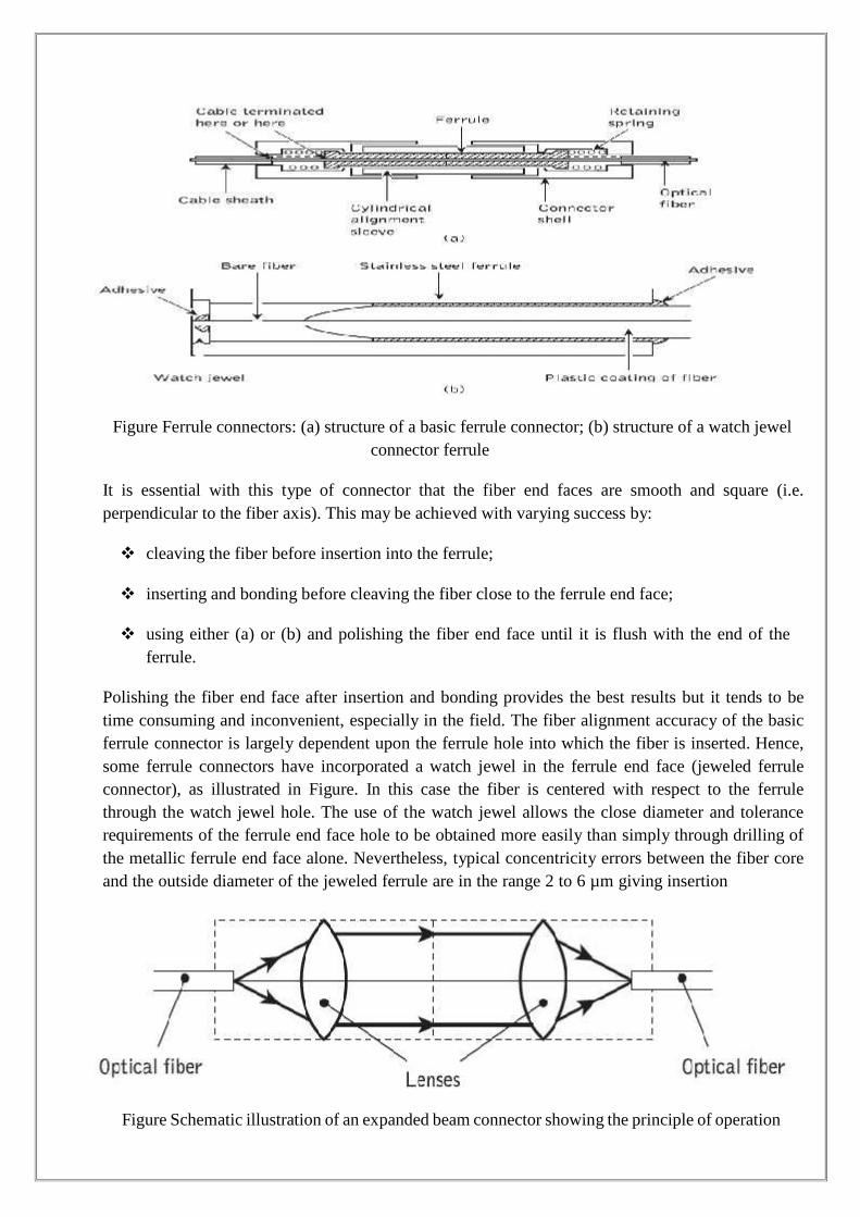
Figure Ferrule connectors: (a) structure of a basic ferrule connector; (b) structure of a watch jewelconnector ferrule

It is essential with this type of connector that the fiber end faces are smooth and square (i.e.perpendicular to the fiber axis). This may be achieved with varying success by:

cleaving the fiber before insertion into the ferrule;

inserting and bonding before cleaving the fiber close to the ferrule end face;

using either (a) or (b) and polishing the fiber end face until it is flush with the end of theferrule.

Polishing the fiber end face after insertion and bonding provides the best results but it tends to betime consuming and inconvenient, especially in the field. The fiber alignment accuracy of the basicferrule connector is largely dependent upon the ferrule hole into which the fiber is inserted. Hence,some ferrule connectors have incorporated a watch jewel in the ferrule end face (jeweled ferruleconnector), as illustrated in Figure. In this case the fiber is centered with respect to the ferrulethrough the watch jewel hole. The use of the watch jewel allows the close diameter and tolerancerequirements of the ferrule end face hole to be obtained more easily than simply through drilling ofthe metallic ferrule end face alone. Nevertheless, typical concentricity errors between the fiber coreand the outside diameter of the jeweled ferrule are in the range 2 to 6 µm giving insertion

Figure Schematic illustration of an expanded beam connector showing the principle of operation

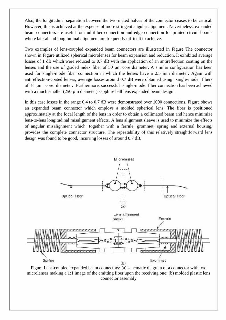
Also, the longitudinal separation between the two mated halves of the connector ceases to be critical.However, this is achieved at the expense of more stringent angular alignment. Nevertheless, expandedbeam connectors are useful for multifiber connection and edge connection for printed circuit boardswhere lateral and longitudinal alignment are frequently difficult to achieve.

Two examples of lens-coupled expanded beam connectors are illustrated in Figure The connectorshown in Figure utilized spherical microlenses for beam expansion and reduction. It exhibited averagelosses of 1 dB which were reduced to 0.7 dB with the application of an antireflection coating on thelenses and the use of graded index fiber of 50 µm core diameter. A similar configuration has beenused for single-mode fiber connection in which the lenses have a 2.5 mm diameter. Again withantireflection-coated lenses, average losses around 0.7 dB were obtained using single-mode fibersof 8 µm core diameter. Furthermore, successful single-mode fiber connection has been achievedwith a much smaller (250 µm diameter) sapphire ball lens expanded beam design.

In this case losses in the range 0.4 to 0.7 dB were demonstrated over 1000 connections. Figure showsan expanded beam connector which employs a molded spherical lens. The fiber is positionedapproximately at the focal length of the lens in order to obtain a collimated beam and hence minimizelens-to-lens longitudinal misalignment effects. A lens alignment sleeve is used to minimize the effectsof angular misalignment which, together with a ferrule, grommet, spring and external housing,provides the complete connector structure. The repeatability of this relatively straightforward lensdesign was found to be good, incurring losses of around 0.7 dB.

Figure Lens-coupled expanded beam connectors: (a) schematic diagram of a connector with twomicrolenses making a 1:1 image of the emitting fiber upon the receiving one; (b) molded plastic lens

connector assembly

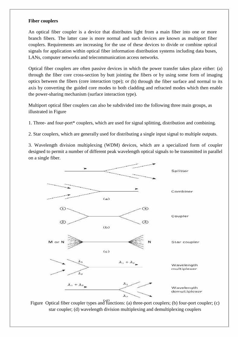
Fiber couplers

An optical fiber coupler is a device that distributes light from a main fiber into one or morebranch fibers. The latter case is more normal and such devices are known as multiport fibercouplers. Requirements are increasing for the use of these devices to divide or combine opticalsignals for application within optical fiber information distribution systems including data buses,LANs, computer networks and telecommunication access networks.

Optical fiber couplers are often passive devices in which the power transfer takes place either: (a)through the fiber core cross-section by butt jointing the fibers or by using some form of imagingoptics between the fibers (core interaction type); or (b) through the fiber surface and normal to itsaxis by converting the guided core modes to both cladding and refracted modes which then enablethe power-sharing mechanism (surface interaction type).

Multiport optical fiber couplers can also be subdivided into the following three main groups, asillustrated in Figure

1. Three- and four-port* couplers, which are used for signal splitting, distribution and combining.

2. Star couplers, which are generally used for distributing a single input signal to multiple outputs.

3. Wavelength division multiplexing (WDM) devices, which are a specialized form of couplerdesigned to permit a number of different peak wavelength optical signals to be transmitted in parallelon a single fiber.

Figure Optical fiber coupler types and functions: (a) three-port couplers; (b) four-port coupler; (c)star coupler; (d) wavelength division multiplexing and demultiplexing couplers

In this context WDM couplers either combine the different wavelength optical signal onto thefiber (i.e. multiplex) or separate the different wavelength optical signals output from the fiber(i.e. demultiplex). Ideal fiber couplers should distribute light among the branch fibers with noscattering loss† or the generation of noise, and they should function with complete insensitivityto factors including the distribution of light between the fiber modes, as well as the state ofpolarization of the light. Unfortunately, in practice passive fiber couplers do not display all ofthe above properties and hence the characteristics of the devices affect the performance ofoptical fiber networks.

This technique, which can provide a bidirectional coupling capability, is well suited for usewith multimode step index fibers but may incur higher excess losses than other methods as allthe input light cannot be coupled into the output fibers. Another coupling technique is toincorporate a beam splitter element between the fibers. The semitransparent mirror methodprovides an ingenious way to accomplish such a fiber coupler, as shown in Figure. A partiallyreflecting surface can be applied directly to the fiber end face cut at an angle of 45° to form athin-film beam splitter.

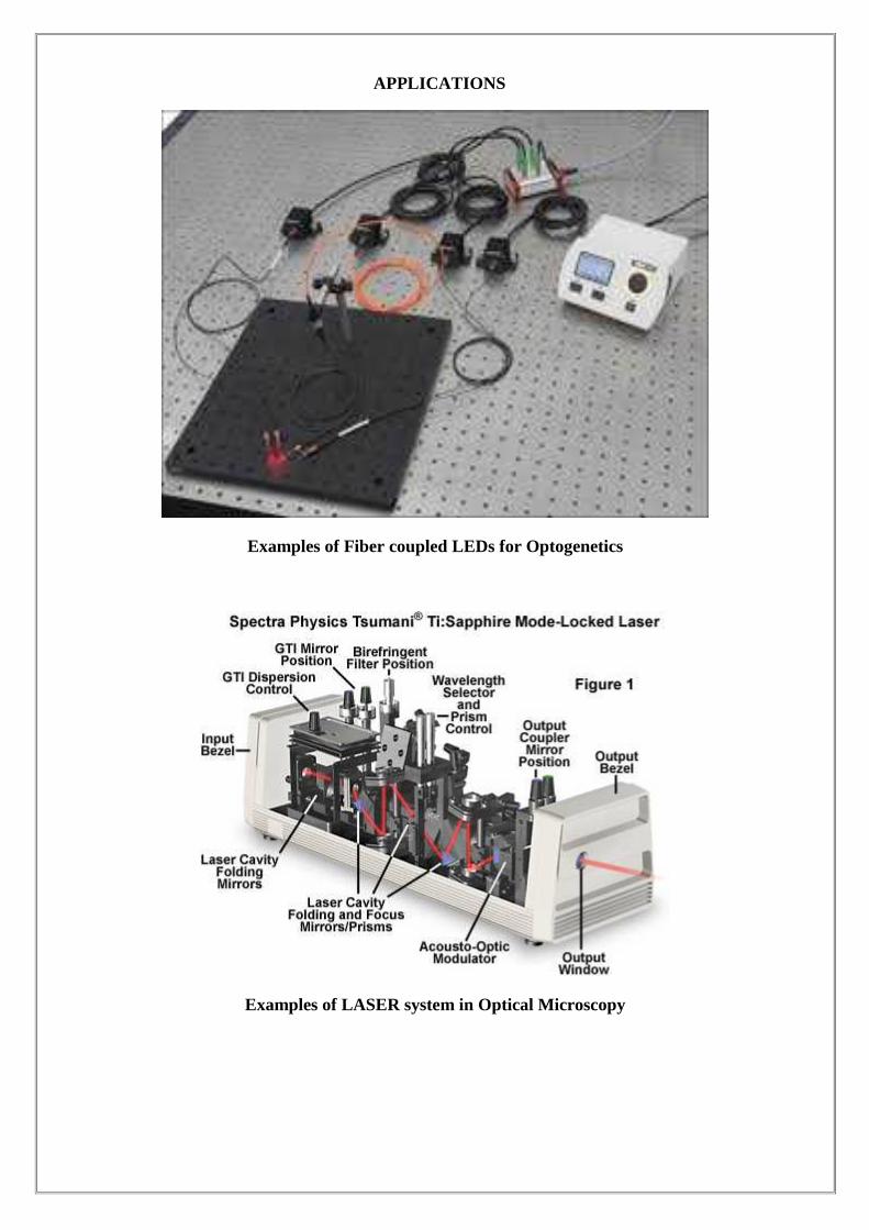
APPLICATIONS

Examples of Fiber coupled LEDs for Optogenetics

Examples of LASER system in Optical Microscopy

POST TEST-MCQ TYPE

1. The radiation emission process (emission of a proton at frequency) can occur in howmany ways.a) Twob) Threec) Fourd) One

2. The lower energy level contains more atoms than upper level under the conditions ofa) Isothermal packagingb) Population inversionc) Thermal equilibriumd) Pumping

3. Which of the following in the laser occurs when photon colliding with an excited atomcauses the stimulated emission of a second photon.a) Light amplificationb) Attenuationc) Dispersiond) Population inversion

4. Which of the following factors does not cause divergence of the collimated beam from aGRIN-rod lens?a) Lens cut lengthb) Size of fiber corec) Refractive index profiled) Chromatic aberration5. Which is used when the optical emission results from the application of electric field.a) Radiationb) Efficiencyc) Electro-luminescenced) Magnetron oscillator

6. Population inversion is obtained at a p-n junction bya) Heavy doping of p-type materialb) Heavy doping of n-type materialc) Light doping of p-type materiald) Heavy doping of both p-type and n-type material

7. The absence of _______________ in LEDs limits the internal quantum efficiency.a) Proper semiconductorb) Adequate power supplyc) Optical amplification through stimulated emissiond) Optical amplification through spontaneous emission

8. What is the use of interposed optics in expanded beam connectors?a) To achieve lateral alignment less critical than a butt-joined fiber connectorb) To make a fiber loss freec) To make a fiber dispersived) For index-matching

9. Determine the internal quantum efficiency generated within a device when it has aradiative recombination lifetime of 80 ns and total carrier recombination lifetime of 40 ns.a) 20 %b) 80 %c) 30 %d) 40 %

10. The Lambertian intensity distribution __________ the external power efficiency bysome percent.a) Reducesb) Does not affectsc) Increasesd) Have a negligible effect

11. Determine coupling efficiency into the fiber when GaAs LED is in close proximity tofiber core having numerical aperture of 0.3.a) 0.9b) 0.3c) 0.6d) 0.12

12. The amount of radiance in planer type of LED structures isa) Lowb) Highc) Zerod) Negligible

13. In surface emitter LEDs, more advantage can be obtained by usinga) BH structuresb) QC structuresc) DH structuresd) Gain-guided structure

14. In a multimode fiber, much of light coupled in the fiber from an LED isa) Increasedb) Reducedc) Lostd) Unaffected

15. The InGaAsP is emitting LEDs are realized in terms of restricted area) Length strip geometryb) Radiancec) Current spreadingd) Coupled optical power

16. The internal quantum efficiency of LEDs decreasing _______________ with________________ temperature.a) Exponentially, decreasingb) Exponentially, increasingc) Linearly, increasingd) Linearly, decreasing

17. The optical 3 dB point occurs when currents ratio is equal toa) 8/3b) 2/2c) 1/2d) 3/4

18. Laser modes are generally separated by fewa) Tenths of micrometerb) Tenths of nanometerc) Tenths of Pico-meterd) Tenths of millimeter

19. The spectral width of emission from the single mode device isa) Smaller than broadened transition line-widthb) Larger than broadened transition line-widthc) Equal the broadened transition line-widthd) Cannot be determined

20. Gain guided laser structure area) Chemical laserb) Gas laserc) DH injection laserd) Quantum well laser

21. In a DH laser, the sides of cavity are formed bya) Cutting the edges of deviceb) Roughening the edges of devicec) Softening the edges of deviced) Covering the sides with ceramics

22. In Buried hetero-junction (BH) lasers, the optical field is confined withina) Transverse directionb) Lateral directionc) Outside the stripd) Both transverse and lateral direction

23. Quantum well lasers are also known asa) BH lasersb) DH lasersc) Chemical lasersd) Gain-guided lasers

24. Better confinement of optical mode is obtained ina) Multi Quantum well lasersb) Single Quantum well lasersc) Gain guided lasersd) BH lasers

25. The phenomenon resulting in the electrons to jump from one state to another each timeemitting of photon is known asa) Inter-valence band absorptionb) Mode hoppingc) Quantum cascadingd) Quantum confinement

26. Which lasers are presently the major laser source for optical fiber communications?a) Semiconductorb) Non-Semiconductorc) Injectiond) Solid-state

27. It is a resonant cavity formed by two parallel reflecting mirrors separated by a mirrorseparated by a medium such as air or gas is?a) Optical cavityb) Wheatstone’s bridgec) Oscillatord) Fabry-perot resonator

28. Which of the following co-dopant is NOT employed by neodymium and erbium dopedsilica fiber lasers?a) Phosphorus pent oxideb) Germaniac) Nitrogend) Alumina

29. Dopants levels in glass fiber lasers are generallya) Lowb) Highc) Same as that of GRIN rod lens laserd) Same as that of semiconductor laser

30. The lasing output of the basic Fabry-perot cavity fiber is restricted to betweena) 1 and 2 nmb) 5 and 10 nmc) 3 and 6 nmd) 15 and 30 nm

31. In Fabry-perot laser, the lower threshold is obtained bya) Increasing the refractive indexb) Decreasing the refractive indexc) Reducing the slope efficiencyd) Increasing the slope efficiency

32. Y3Al5 O12 is a molecular formula fora) Ytterbium aluminateb) Yttrium oxidec) Ytterbium oxy-aluminated) Yttrium-aluminum garnet

33. A measure of amount of optical fiber emitted from source that can be coupled into afiber is termed asa) Radianceb) Angular power distributionc) Coupling efficiencyd) Power-launching

34. How many types of misalignments occur when joining compatible fiber?a) Oneb) Twoc) Fived) Three

35. Losses caused by factors such as core-cladding diameter, numerical aperture, relativerefractive index differences, different refractive index profiles, fiber faults are known asa) Intrinsic joint lossesb) Extrinsic lossesc) Insertion lossesd) Coupling losses

36. A permanent joint formed between two different optical fibers in the field is known as aa) Fiber spliceb) Fiber connectorc) Fiber attenuatord) Fiber dispersion

37. How many types of fiber splices are available?a) Oneb) Twoc) Threed) Four

38. What is the main requirement with the fibers that are intended for splicing?a) Smooth and oval end facesb) Smooth and square end facesc) Rough edge facesd) Large core diameter

39. In score and break process, which of the following is NOT used as a cutting tool?a) Diamondb) Sapphirec) Tungsten carbided) Copper

40. The heating of the two prepared fiber ends to their fusing point with the application ofrequired axial pressure between the two optical fibers is called asa) Mechanical splicingb) Fusion splicingc) Meltingd) Diffusion

41. Which of the following is not used as a flame heating source in fusion splicing?a) Microprocessor torchesb) Ox hydric burnersc) Electric arcd) Gas burner

42. Which is caused by surface tension effects between the two fiber ends during fusing.a) Pre-fusionb) Diffusionc) Self-alignmentd) Splicing

43. What are formed by sandwiching the butted fiber ends between a V-groove glasssubstrate and a flat glass retainer plate.a) Springroove splicesb) V-groove splicesc) Elastic splicesd) Fusion splices

44. What is the use of an index-matching material in the connector between the two jointedfibers?a) To decrease the light transmission through the connectionb) To increase the light transmission through the connectionc) To induce losses in the fiberd) To make a fiber dispersive

45. How many categories of fiber connectors exist?a) Oneb) Threec) Twod) Four

46. What is the use of watch jewel in cylindrical ferrule connector?a) To obtain the diameter and tolerance requirements of the ferruleb) For polishing purposesc) Cleaving the fiberd) To disperse a fiber

47. In connectors, the fiber ends are separated by some gap. This gap ranges froma) 0.040 to 0.045 mmb) 0.025 to 0.10 mmc) 0.12 to 0.16 mmd) 0.030 to 0.2mm

CONCLUSION

In this unit, the various optical sources, materials and fiber splicing were learnt. The principlesof different optical sources and power launching-coupling methods were described in detailed.

REFERENCES

1. Gerd Keiser, “Optical Fiber Communication” McGraw-Hill International,4th Edition. 2010.

2. John M. Senior, “Optical Fiber Communication”, Second Edition, Pearson Education, 2007.

3. Ramaswami, Sivarajan and Sasaki “Optical Networks”, Morgan Kaufmann, 2009.

4. J.Senior, Optical Communication, Principles and Practice,Prentice Hall of India, 3rd

Edition, 2008.

5. J.Gower, “Optical Communication System”, Prentice Hall of India, 2001.

ASSIGNMENT

1. Draw and explain the LED structures based Double Heterostucture configuration

2. Discuss the principle of operation of LASER diodes.

3. What are the effects of temperature on the performance of a LASER diode?

4. Explain the lensing schemes used to improve optical source - to- fiber coupling efficiency.

5. What are the advantages of Quantum well LASERS?

6. Explain briefly the three key processes involved in the laser action.

7. Describe for a fabry-perot resonator laser diode, modes and threshold conditions. Obtain itsrate equations for steady state output.

8. Describe various fiber splicing techniques with their diagrams.

9. Describe the various types of fiber connectors and couplers.

10. Explain mechanical splices with neat diagrams.

UNIT IV FIBER OPTIC RECEIVER ANDMEASUREMENTS

Prepared by

T.DINESH KUMARAssistant Professor

ECE, SCSVMV

OPTICALCOMMUNICATION

AIM & OBJECTIVES

To learn the basic elements of optical fiber transmission link, fiber modesconfigurations and structures.

To understand the different kind of losses, signal distortion, SM fibers. To learn the various optical sources, materials and fiber splicing. To learn the fiber optical receivers and noise performance in photo detector. To explore link budget, WDM, solitons and SONET/SDH network.

PRE TEST-MCQ TYPE

1. How many design considerations are considered while determining the receiverperformance?a) Threeb) Twoc) Oned) Four

2. Which circuits extends the dynamic range of the receiver?a) Monolithicb) Trans-impedancec) Automatic Error Control (AEC)d) Automatic Gain Control (AGC)

3. The sensitivity of the low-impedance configuration is ____________a) Goodb) Poorc) Greatd) Same as that of high-impedance configuration

4. What is generally used to determine the receiver performance characteristics?a) Noiseb) Resistorc) Dynamic range & sensitivity characteristicsd) Impedance

UNIT IV FIBER OPTIC RECEIVER AND MEASUREMENTS

Fundamental receiver operation, Pre-amplifiers, Error sources – Receiver Configuration –Probability of Error – Quantum limit, Fiber Attenuation measurements- Dispersionmeasurements-Fiber Refractive index profile measurements – Fiber cut- off Wave lengthMeasurements – Fiber Numerical Aperture Measurements – Fiber diameter measurements

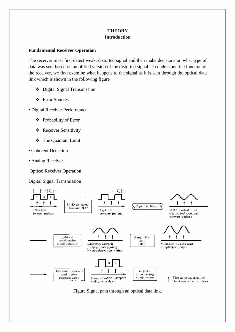
THEORYIntroduction

Fundamental Receiver Operation

The receiver must first detect weak, distorted signal and then make decisions on what type ofdata was sent based on amplified version of the distorted signal. To understand the function ofthe receiver, we first examine what happens to the signal as it is sent through the optical datalink which is shown in the following figure

Digital Signal Transmission

Error Sources

• Digital Receiver Performance

Probability of Error

Receiver Sensitivity

The Quantum Limit

• Coherent Detection

• Analog Receiver

Optical Receiver Operation

Digital Signal Transmission

Figure Signal path through an optical data link.

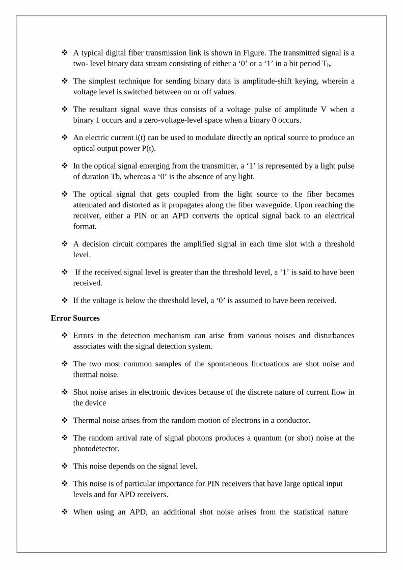
A typical digital fiber transmission link is shown in Figure. The transmitted signal is atwo- level binary data stream consisting of either a ‘0’ or a ‘1’ in a bit period Tb.

The simplest technique for sending binary data is amplitude-shift keying, wherein avoltage level is switched between on or off values.

The resultant signal wave thus consists of a voltage pulse of amplitude V when abinary 1 occurs and a zero-voltage-level space when a binary 0 occurs.

An electric current i(t) can be used to modulate directly an optical source to produce anoptical output power P(t).

In the optical signal emerging from the transmitter, a ‘1’ is represented by a light pulseof duration Tb, whereas a ‘0’ is the absence of any light.

The optical signal that gets coupled from the light source to the fiber becomesattenuated and distorted as it propagates along the fiber waveguide. Upon reaching thereceiver, either a PIN or an APD converts the optical signal back to an electricalformat.

A decision circuit compares the amplified signal in each time slot with a thresholdlevel.

If the received signal level is greater than the threshold level, a ‘1’ is said to have beenreceived.

If the voltage is below the threshold level, a ‘0’ is assumed to have been received.

Error Sources

Errors in the detection mechanism can arise from various noises and disturbancesassociates with the signal detection system.

The two most common samples of the spontaneous fluctuations are shot noise andthermal noise.

Shot noise arises in electronic devices because of the discrete nature of current flow inthe device

Thermal noise arises from the random motion of electrons in a conductor.

The random arrival rate of signal photons produces a quantum (or shot) noise at thephotodetector.

This noise depends on the signal level.

This noise is of particular importance for PIN receivers that have large optical inputlevels and for APD receivers.

When using an APD, an additional shot noise arises from the statistical nature

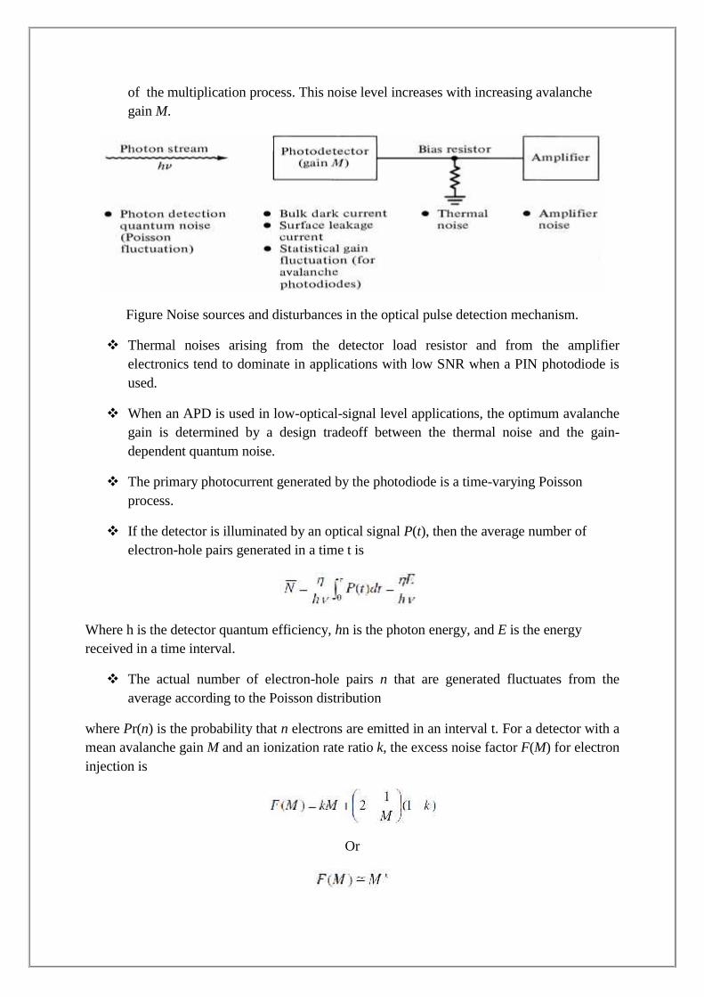
of the multiplication process. This noise level increases with increasing avalanchegain M.

Figure Noise sources and disturbances in the optical pulse detection mechanism.

Thermal noises arising from the detector load resistor and from the amplifierelectronics tend to dominate in applications with low SNR when a PIN photodiode isused.

When an APD is used in low-optical-signal level applications, the optimum avalanchegain is determined by a design tradeoff between the thermal noise and the gain-dependent quantum noise.

The primary photocurrent generated by the photodiode is a time-varying Poissonprocess.

If the detector is illuminated by an optical signal P(t), then the average number ofelectron-hole pairs generated in a time t is

Where h is the detector quantum efficiency, hn is the photon energy, and E is the energyreceived in a time interval.

The actual number of electron-hole pairs n that are generated fluctuates from theaverage according to the Poisson distribution

where Pr(n) is the probability that n electrons are emitted in an interval t. For a detector with amean avalanche gain M and an ionization rate ratio k, the excess noise factor F(M) for electroninjection is

Or

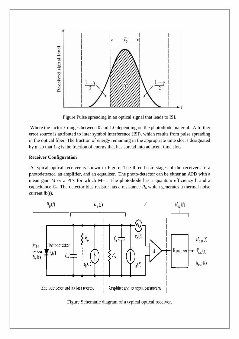
Figure Pulse spreading in an optical signal that leads to ISI.

Where the factor x ranges between 0 and 1.0 depending on the photodiode material. A furthererror source is attributed to inter symbol interference (ISI), which results from pulse spreadingin the optical fiber. The fraction of energy remaining in the appropriate time slot is designatedby g, so that 1-g is the fraction of energy that has spread into adjacent time slots.

Receiver Configuration

A typical optical receiver is shown in Figure. The three basic stages of the receiver are aphotodetector, an amplifier, and an equalizer. The photo-detector can be either an APD with amean gain M or a PIN for which M=1. The photodiode has a quantum efficiency h and acapacitance Cd. The detector bias resistor has a resistance Rb which generates a thermal noisecurrent ib(t).

Figure Schematic diagram of a typical optical receiver.

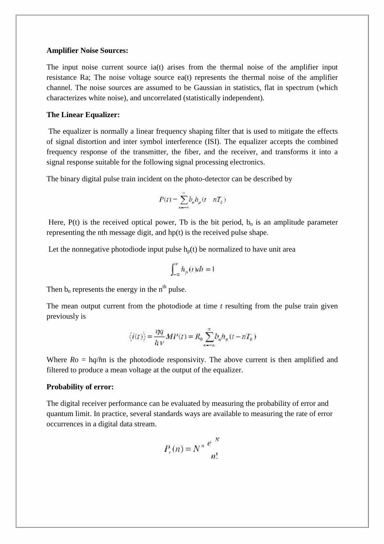
Amplifier Noise Sources:

The input noise current source ia(t) arises from the thermal noise of the amplifier inputresistance Ra; The noise voltage source ea(t) represents the thermal noise of the amplifierchannel. The noise sources are assumed to be Gaussian in statistics, flat in spectrum (whichcharacterizes white noise), and uncorrelated (statistically independent).

The Linear Equalizer:

The equalizer is normally a linear frequency shaping filter that is used to mitigate the effectsof signal distortion and inter symbol interference (ISI). The equalizer accepts the combinedfrequency response of the transmitter, the fiber, and the receiver, and transforms it into asignal response suitable for the following signal processing electronics.

The binary digital pulse train incident on the photo-detector can be described by

Here, P(t) is the received optical power, Tb is the bit period, bn is an amplitude parameterrepresenting the nth message digit, and hp(t) is the received pulse shape.

Let the nonnegative photodiode input pulse hp(t) be normalized to have unit area

Then bn represents the energy in the nth pulse.

The mean output current from the photodiode at time t resulting from the pulse train givenpreviously is

Where Ro = hq/hn is the photodiode responsivity. The above current is then amplified andfiltered to produce a mean voltage at the output of the equalizer.

Probability of error:

The digital receiver performance can be evaluated by measuring the probability of error andquantum limit. In practice, several standards ways are available to measuring the rate of erroroccurrences in a digital data stream.

The Quantum Limit:

Consider an ideal photodetector which has unity quantum efficiency and which produces nodark current that is no electron hole pairs are generated in the absence of an optical pulse.

With this condition it is possible to find the minimum received optical power required for aspecific bit error rate performance in a digital system. This minimum received power level isknown as the quantum limit, since all system parameters are assumed ideal and theperformance is only limited by the photodetection statistics.

Assume that an optical pulse of energy E falls on the photodetector in a time interval τ. Thiscan only be interpreted by the receiver as a 0 pulse if no electron hole pairs are generated withthe pulse present. The probability that n=0 electrons are emitted in a time interval τ is

Thus for a given error probability Pr(0), we can find the minimum energy E required at aspecific wavelength λ.

Preamplifier:

Front End

The front end of a receiver consists of a photodiode followed by a preamplifier. The opticalsignal is coupled onto the photodiode by using a coupling scheme similar to that used foroptical transmitters but coupling is often used in practice. The photodiode converts the opticalbit stream into an electrical time-varying signal. The role of the preamplifier is to amplify theelectrical signal for further processing. The design of the front end requires a trade-offbetween speed and sensitivity. Since the input voltage to the preamplifier can be increased byusing a large load resistor R L, a high-impedance front end is often used. Furthermore, asdiscussed, a large RL reduces the thermal noise and improves the receiver sensitivity.

The main drawback of high-impedance front end is its low bandwidth given by Δf = (2πRLCT

)−1, where Rs _RL is assumed and CT =Cp+CA is the total capacitance, which includes thecontributions from the photodiode (Cp) and the transistor used for amplification (CA). Thereceiver bandwidth is limited by its slowest component. A high-impedance front end cannot beused if Δf is considerably less than the bit rate. An equalizer is sometimes used to increase thebandwidth. The equalizer acts as a filter that attenuates low-frequency components of thesignal more than the high-frequency components, thereby effectively increasing the front-endbandwidth. If the receiver sensitivity is not of concern, one can simply decrease RL to increasethe bandwidth, resulting in a low-impedance front end. Transimpedance front ends provide aconfiguration that has high sensitivity together with a large bandwidth. Its dynamic range isalso improved compared with high-impedance front ends. As seen in Figure the load resistor isconnected as a feedback resistor around an inverting amplifier.

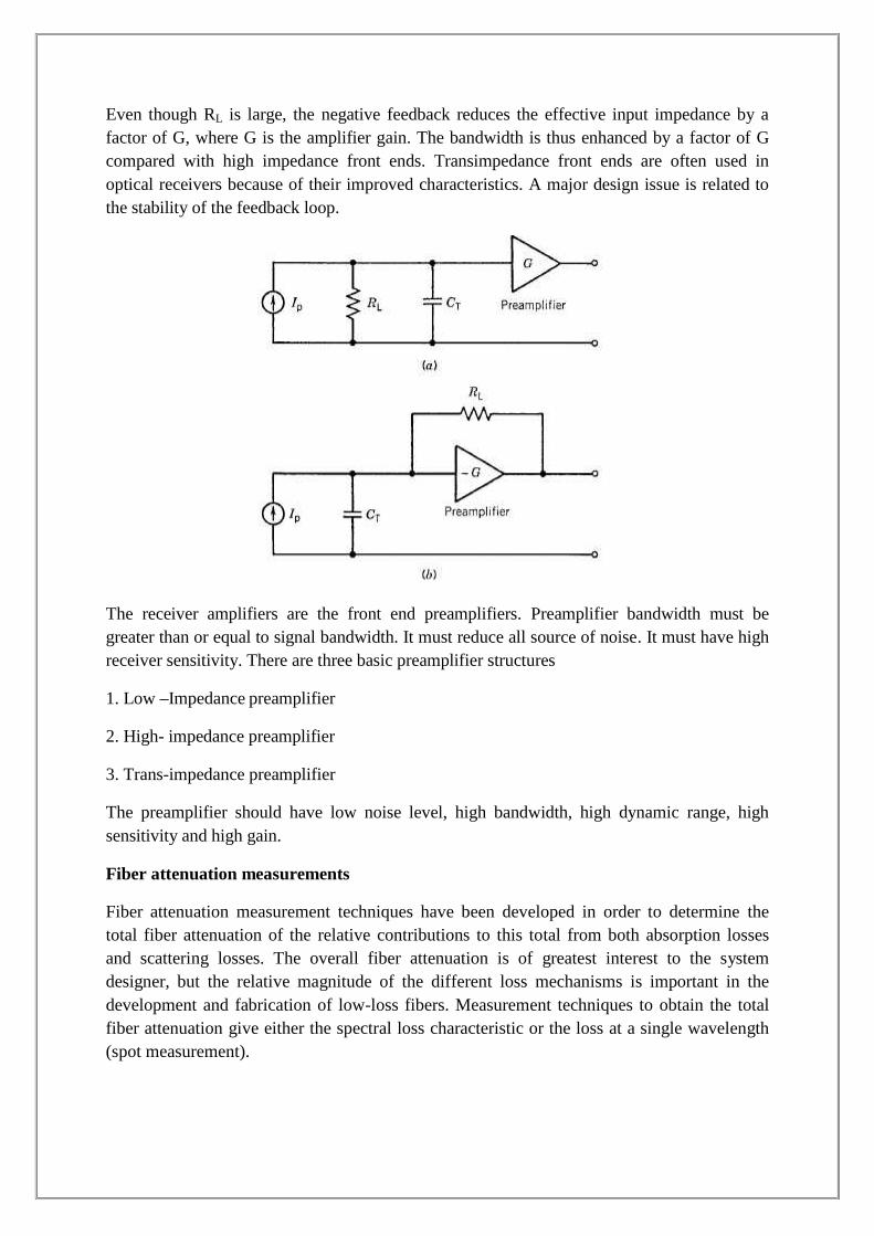
Even though RL is large, the negative feedback reduces the effective input impedance by afactor of G, where G is the amplifier gain. The bandwidth is thus enhanced by a factor of Gcompared with high impedance front ends. Transimpedance front ends are often used inoptical receivers because of their improved characteristics. A major design issue is related tothe stability of the feedback loop.

The receiver amplifiers are the front end preamplifiers. Preamplifier bandwidth must begreater than or equal to signal bandwidth. It must reduce all source of noise. It must have highreceiver sensitivity. There are three basic preamplifier structures

1. Low –Impedance preamplifier

2. High- impedance preamplifier

3. Trans-impedance preamplifier

The preamplifier should have low noise level, high bandwidth, high dynamic range, highsensitivity and high gain.

Fiber attenuation measurements

Fiber attenuation measurement techniques have been developed in order to determine thetotal fiber attenuation of the relative contributions to this total from both absorption lossesand scattering losses. The overall fiber attenuation is of greatest interest to the systemdesigner, but the relative magnitude of the different loss mechanisms is important in thedevelopment and fabrication of low-loss fibers. Measurement techniques to obtain the totalfiber attenuation give either the spectral loss characteristic or the loss at a single wavelength(spot measurement).

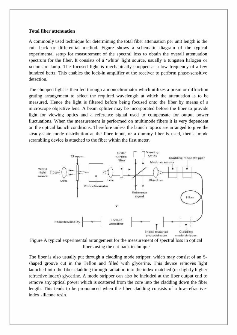
Total fiber attenuation

A commonly used technique for determining the total fiber attenuation per unit length is thecut- back or differential method. Figure shows a schematic diagram of the typicalexperimental setup for measurement of the spectral loss to obtain the overall attenuationspectrum for the fiber. It consists of a ‘white’ light source, usually a tungsten halogen orxenon are lamp. The focused light is mechanically chopped at a low frequency of a fewhundred hertz. This enables the lock-in amplifier at the receiver to perform phase-sensitivedetection.

The chopped light is then fed through a monochromator which utilizes a prism or diffractiongrating arrangement to select the required wavelength at which the attenuation is to bemeasured. Hence the light is filtered before being focused onto the fiber by means of amicroscope objective lens. A beam splitter may be incorporated before the fiber to providelight for viewing optics and a reference signal used to compensate for output powerfluctuations. When the measurement is performed on multimode fibers it is very dependenton the optical launch conditions. Therefore unless the launch optics are arranged to give thesteady-state mode distribution at the fiber input, or a dummy fiber is used, then a modescrambling device is attached to the fiber within the first meter.

Figure A typical experimental arrangement for the measurement of spectral loss in opticalfibers using the cut-back technique

The fiber is also usually put through a cladding mode stripper, which may consist of an S-shaped groove cut in the Teflon and filled with glycerine. This device removes lightlaunched into the fiber cladding through radiation into the index-matched (or slightly higherrefractive index) glycerine. A mode stripper can also be included at the fiber output end toremove any optical power which is scattered from the core into the cladding down the fiberlength. This tends to be pronounced when the fiber cladding consists of a low-refractive-index silicone resin.

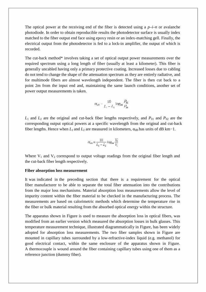
The optical power at the receiving end of the fiber is detected using a p–i–n or avalanchephotodiode. In order to obtain reproducible results the photodetector surface is usually indexmatched to the fiber output end face using epoxy resin or an index-matching gell. Finally, theelectrical output from the photodetector is fed to a lock-in amplifier, the output of which isrecorded.

The cut-back method* involves taking a set of optical output power measurements over therequired spectrum using a long length of fiber (usually at least a kilometer). This fiber isgenerally uncabled having only a primary protective coating. Increased losses due to cablingdo not tend to change the shape of the attenuation spectrum as they are entirely radiative, andfor multimode fibers are almost wavelength independent. The fiber is then cut back to apoint 2m from the input end and, maintaining the same launch conditions, another set ofpower output measurements is taken.

L1 and L2 are the original and cut-back fiber lengths respectively, and P01 and P02 are thecorresponding output optical powers at a specific wavelength from the original and cut-backfiber lengths. Hence when L1 and L2 are measured in kilometers, αdB has units of dB km−1.

Where V1 and V2 correspond to output voltage readings from the original fiber length andthe cut-back fiber length respectively.

Fiber absorption loss measurement

It was indicated in the preceding section that there is a requirement for the opticalfiber manufacturer to be able to separate the total fiber attenuation into the contributionsfrom the major loss mechanisms. Material absorption loss measurements allow the level ofimpurity content within the fiber material to be checked in the manufacturing process. Themeasurements are based on calorimetric methods which determine the temperature rise inthe fiber or bulk material resulting from the absorbed optical energy within the structure.

The apparatus shown in Figure is used to measure the absorption loss in optical fibers, wasmodified from an earlier version which measured the absorption losses in bulk glasses. Thistemperature measurement technique, illustrated diagrammatically in Figure, has been widelyadopted for absorption loss measurements. The two fiber samples shown in Figure aremounted in capillary tubes surrounded by a low-refractive-index liquid (e.g. methanol) forgood electrical contact, within the same enclosure of the apparatus shown in Figure.A thermocouple is wound around the fiber containing capillary tubes using one of them as areference junction (dummy fiber).

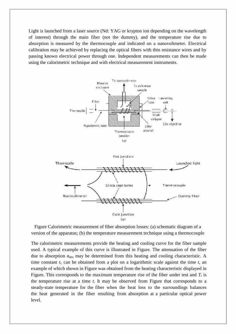
Light is launched from a laser source (Nd: YAG or krypton ion depending on the wavelengthof interest) through the main fiber (not the dummy), and the temperature rise due toabsorption is measured by the thermocouple and indicated on a nanovoltmeter. Electricalcalibration may be achieved by replacing the optical fibers with thin resistance wires and bypassing known electrical power through one. Independent measurements can then be madeusing the calorimetric technique and with electrical measurement instruments.

Figure Calorimetric measurement of fiber absorption losses: (a) schematic diagram of aversion of the apparatus; (b) the temperature measurement technique using a thermocouple

The calorimetric measurements provide the heating and cooling curve for the fiber sampleused. A typical example of this curve is illustrated in Figure. The attenuation of the fiberdue to absorption αabs may be determined from this heating and cooling characteristic. Atime constant tc can be obtained from a plot on a logarithmic scale against the time t, anexample of which shown in Figure was obtained from the heating characteristic displayed inFigure. This corresponds to the maximum temperature rise of the fiber under test and Tt isthe temperature rise at a time t. It may be observed from Figure that corresponds to asteady-state temperature for the fiber when the heat loss to the surroundings balancesthe heat generated in the fiber resulting from absorption at a particular optical powerlevel.

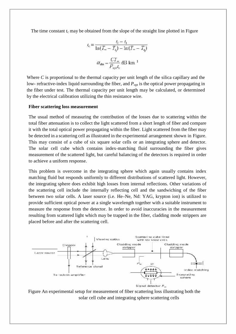
The time constant tc may be obtained from the slope of the straight line plotted in Figure

Where C is proportional to the thermal capacity per unit length of the silica capillary and thelow- refractive-index liquid surrounding the fiber, and Popt is the optical power propagating inthe fiber under test. The thermal capacity per unit length may be calculated, or determinedby the electrical calibration utilizing the thin resistance wire.

Fiber scattering loss measurement

The usual method of measuring the contribution of the losses due to scattering within thetotal fiber attenuation is to collect the light scattered from a short length of fiber and compareit with the total optical power propagating within the fiber. Light scattered from the fiber maybe detected in a scattering cell as illustrated in the experimental arrangement shown in Figure.This may consist of a cube of six square solar cells or an integrating sphere and detector.The solar cell cube which contains index-matching fluid surrounding the fiber givesmeasurement of the scattered light, but careful balancing of the detectors is required in orderto achieve a uniform response.

This problem is overcome in the integrating sphere which again usually contains indexmatching fluid but responds uniformly to different distributions of scattered light. However,the integrating sphere does exhibit high losses from internal reflections. Other variations ofthe scattering cell include the internally reflecting cell and the sandwiching of the fiberbetween two solar cells. A laser source (i.e. He–Ne, Nd: YAG, krypton ion) is utilized toprovide sufficient optical power at a single wavelength together with a suitable instrument tomeasure the response from the detector. In order to avoid inaccuracies in the measurementresulting from scattered light which may be trapped in the fiber, cladding mode strippers areplaced before and after the scattering cell.

Figure An experimental setup for measurement of fiber scattering loss illustrating both thesolar cell cube and integrating sphere scattering cells

These devices remove the light propagating in the cladding so that the measurements aretaken only using the light guided by the fiber core. Also, to avoid reflections contributing tothe optical signal within the cell, the output fiber end is index matched using either a fluid orsuitable surface.

The loss due to scattering αsc is given by:

where l(km) is the length of the fiber contained within the scattering cell, Popt is the opticalpower propagating within the fiber at the cell and Psc is the optical power scattered from theshort length of fiber l within the cell. As Popt >> Psc, then the logarithm in equation may beexpanded to give:

Since the measurements of length are generally in centimeters and the optical power isnormally registered in volts, Equation can be written as:

Where Vsc and Vopt are the voltage readings corresponding to the scattered optical power andthe total optical power within the fiber at the cell. The relative experimental accuracy (i.e.repeatability) for scatter loss measurements is in the range ±0.2 dB using the solar cell cubeand around 5% with the integrating sphere. However, it must be noted that the absoluteaccuracy of the measurements is somewhat poorer, being dependent on the calibration of thescattering cell and the mode distribution within a multimode fiber.

Fiber dispersion measurements

Dispersion measurements give an indication of the distortion to optical signals as theypropagate down optical fibers. The delay distortion which, for example, leads to thebroadening of transmitted light pulses limits the information-carrying capacity of the fiber.The measurement of dispersion allows the bandwidth of the fiber to be determined. Therefore,besides attenuation, dispersion is the most important transmission characteristic of anoptical fiber. As discussed, there are three major mechanisms which produce dispersion inoptical fibers (material dispersion, waveguide dispersion and intermodal dispersion). Theimportance of these different mechanisms to the total fiber dispersion is dictated by the fibertype. For instance, in multimode fibers (especially step index), intermodal dispersion tends tobe the dominant mechanism, whereas in single-mode fibers intermodal dispersion isnonexistent as only a single mode is allowed to propagate. In the single-mode case thedominant dispersion mechanism is chromatic. The dominance of intermodal dispersion inmultimode fibers makes it essential that dispersion measurements on these fibers areperformed only when the equilibrium mode distribution has been established within the fiber,otherwise inconsistent results will be obtained. Therefore devices such as mode scramblersor filters must be utilized in order to simulate the steady state mode distribution.

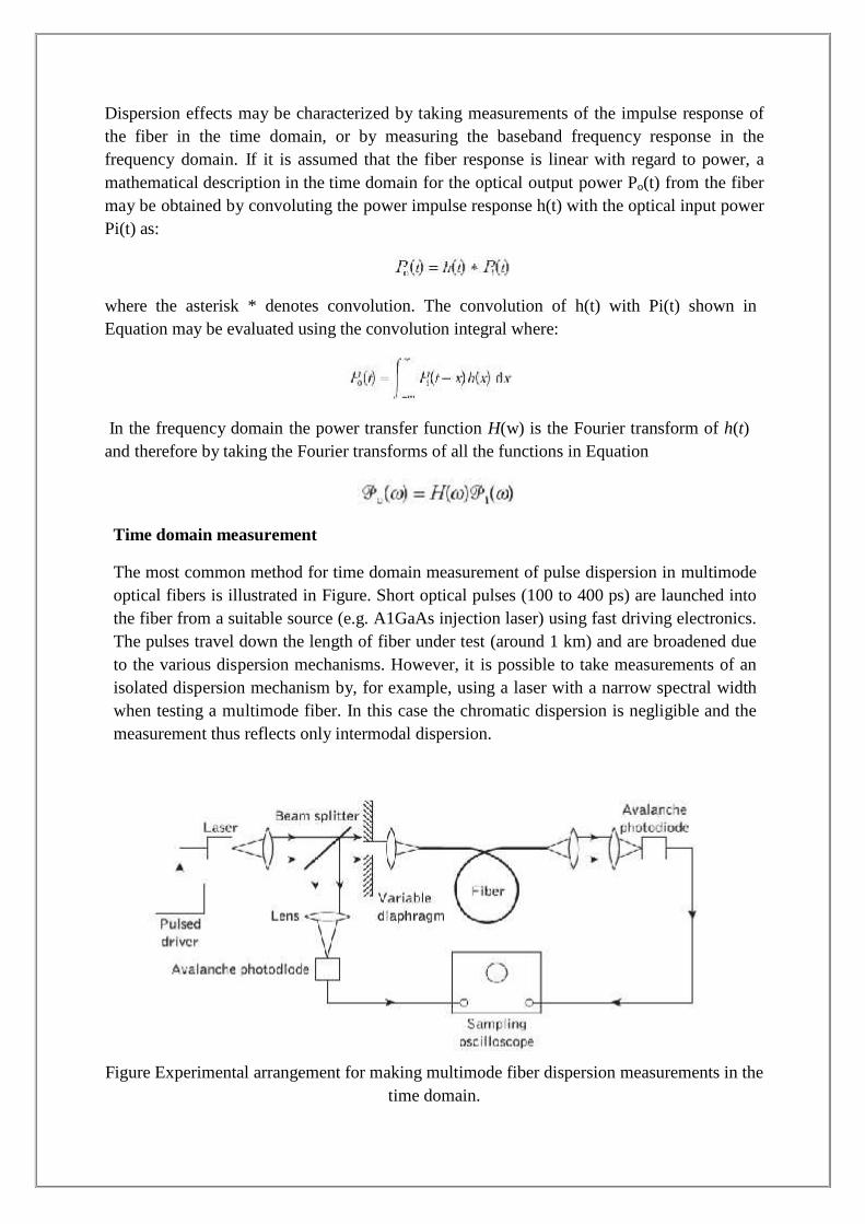
Dispersion effects may be characterized by taking measurements of the impulse response ofthe fiber in the time domain, or by measuring the baseband frequency response in thefrequency domain. If it is assumed that the fiber response is linear with regard to power, amathematical description in the time domain for the optical output power Po(t) from the fibermay be obtained by convoluting the power impulse response h(t) with the optical input powerPi(t) as:

where the asterisk * denotes convolution. The convolution of h(t) with Pi(t) shown inEquation may be evaluated using the convolution integral where:

In the frequency domain the power transfer function H(w) is the Fourier transform of h(t)and therefore by taking the Fourier transforms of all the functions in Equation

Time domain measurement

The most common method for time domain measurement of pulse dispersion in multimodeoptical fibers is illustrated in Figure. Short optical pulses (100 to 400 ps) are launched intothe fiber from a suitable source (e.g. A1GaAs injection laser) using fast driving electronics.The pulses travel down the length of fiber under test (around 1 km) and are broadened dueto the various dispersion mechanisms. However, it is possible to take measurements of anisolated dispersion mechanism by, for example, using a laser with a narrow spectral widthwhen testing a multimode fiber. In this case the chromatic dispersion is negligible and themeasurement thus reflects only intermodal dispersion.

Figure Experimental arrangement for making multimode fiber dispersion measurements in thetime domain.

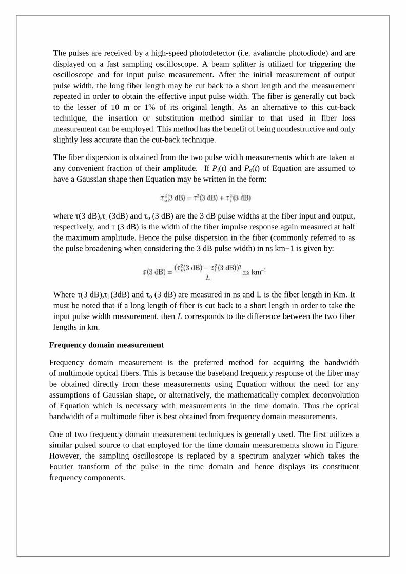
The pulses are received by a high-speed photodetector (i.e. avalanche photodiode) and aredisplayed on a fast sampling oscilloscope. A beam splitter is utilized for triggering theoscilloscope and for input pulse measurement. After the initial measurement of outputpulse width, the long fiber length may be cut back to a short length and the measurementrepeated in order to obtain the effective input pulse width. The fiber is generally cut backto the lesser of 10 m or 1% of its original length. As an alternative to this cut-backtechnique, the insertion or substitution method similar to that used in fiber lossmeasurement can be employed. This method has the benefit of being nondestructive and onlyslightly less accurate than the cut-back technique.

The fiber dispersion is obtained from the two pulse width measurements which are taken atany convenient fraction of their amplitude. If Pi(t) and Po(t) of Equation are assumed tohave a Gaussian shape then Equation may be written in the form:

where τ(3 dB),τi (3dB) and τo (3 dB) are the 3 dB pulse widths at the fiber input and output,respectively, and τ (3 dB) is the width of the fiber impulse response again measured at halfthe maximum amplitude. Hence the pulse dispersion in the fiber (commonly referred to asthe pulse broadening when considering the 3 dB pulse width) in ns km−1 is given by:

Where τ(3 dB),τi (3dB) and τo (3 dB) are measured in ns and L is the fiber length in Km. Itmust be noted that if a long length of fiber is cut back to a short length in order to take theinput pulse width measurement, then L corresponds to the difference between the two fiberlengths in km.

Frequency domain measurement

Frequency domain measurement is the preferred method for acquiring the bandwidthof multimode optical fibers. This is because the baseband frequency response of the fiber maybe obtained directly from these measurements using Equation without the need for anyassumptions of Gaussian shape, or alternatively, the mathematically complex deconvolutionof Equation which is necessary with measurements in the time domain. Thus the opticalbandwidth of a multimode fiber is best obtained from frequency domain measurements.

One of two frequency domain measurement techniques is generally used. The first utilizes asimilar pulsed source to that employed for the time domain measurements shown in Figure.However, the sampling oscilloscope is replaced by a spectrum analyzer which takes theFourier transform of the pulse in the time domain and hence displays its constituentfrequency components.

Figure Experimental setup for making fiber dispersion measurements in the frequencydomain using a pulsed laser source

The experimental arrangement is illustrated in Figure. Comparison of the spectrum at thefiber output Po(w) with the spectrum at the fiber input Pi(w) provides the basebandfrequency response for the fiber under test where:

The second technique involves launching a sinusoidally modulated optical signal atdifferent selected frequencies using a sweep oscillator. Therefore the signal energy isconcentrated in a very narrow frequency band in the baseband region, unlike the pulsemeasurement method where the signal energy is spread over the entire baseband region.

Fiber refractive index profile measurements

The refractive index profile of the fiber core plays an important role in characterizing theproperties of optical fibers. It allows determination of the fiber’s numerical aperture and thenumber of modes propagating within the fiber core, while largely defining any intermodaland/or profile dispersion caused by the fiber. Hence a detailed knowledge of the refractiveindex profile enables the impulse response of the fiber to be predicted.

Also, as the impulse response and consequently the information-carrying capacity of thefiber is strongly dependent on the refractive index profile, it is essential that the fibermanufacturer is able to produce particular profiles with great accuracy, especially in the caseof graded index fibers (i.e. optimum profile). There is therefore a requirement for accuratemeasurement of the refractive index profile. These measurements may be performed usinga number of different techniques each of which exhibit certain advantages and drawbacks.

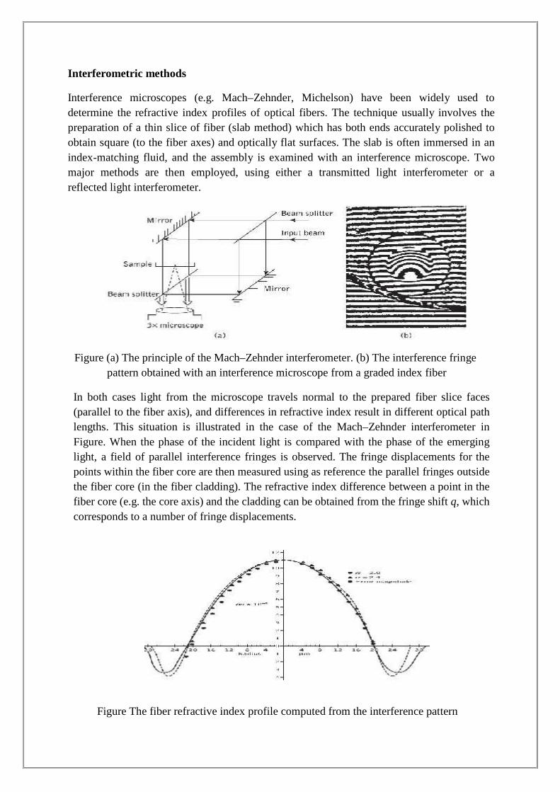
Interferometric methods

Interference microscopes (e.g. Mach–Zehnder, Michelson) have been widely used todetermine the refractive index profiles of optical fibers. The technique usually involves thepreparation of a thin slice of fiber (slab method) which has both ends accurately polished toobtain square (to the fiber axes) and optically flat surfaces. The slab is often immersed in anindex-matching fluid, and the assembly is examined with an interference microscope. Twomajor methods are then employed, using either a transmitted light interferometer or areflected light interferometer.

Figure (a) The principle of the Mach–Zehnder interferometer. (b) The interference fringepattern obtained with an interference microscope from a graded index fiber

In both cases light from the microscope travels normal to the prepared fiber slice faces(parallel to the fiber axis), and differences in refractive index result in different optical pathlengths. This situation is illustrated in the case of the Mach–Zehnder interferometer inFigure. When the phase of the incident light is compared with the phase of the emerginglight, a field of parallel interference fringes is observed. The fringe displacements for thepoints within the fiber core are then measured using as reference the parallel fringes outsidethe fiber core (in the fiber cladding). The refractive index difference between a point in thefiber core (e.g. the core axis) and the cladding can be obtained from the fringe shift q, whichcorresponds to a number of fringe displacements.

Figure The fiber refractive index profile computed from the interference pattern

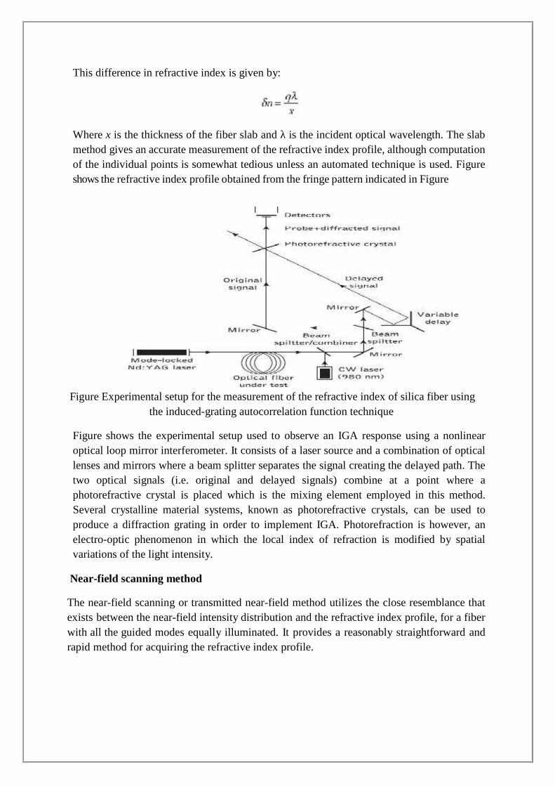
This difference in refractive index is given by:

Where x is the thickness of the fiber slab and λ is the incident optical wavelength. The slabmethod gives an accurate measurement of the refractive index profile, although computationof the individual points is somewhat tedious unless an automated technique is used. Figureshows the refractive index profile obtained from the fringe pattern indicated in Figure

Figure Experimental setup for the measurement of the refractive index of silica fiber usingthe induced-grating autocorrelation function technique

Figure shows the experimental setup used to observe an IGA response using a nonlinearoptical loop mirror interferometer. It consists of a laser source and a combination of opticallenses and mirrors where a beam splitter separates the signal creating the delayed path. Thetwo optical signals (i.e. original and delayed signals) combine at a point where aphotorefractive crystal is placed which is the mixing element employed in this method.Several crystalline material systems, known as photorefractive crystals, can be used toproduce a diffraction grating in order to implement IGA. Photorefraction is however, anelectro-optic phenomenon in which the local index of refraction is modified by spatialvariations of the light intensity.

Near-field scanning method

The near-field scanning or transmitted near-field method utilizes the close resemblance thatexists between the near-field intensity distribution and the refractive index profile, for a fiberwith all the guided modes equally illuminated. It provides a reasonably straightforward andrapid method for acquiring the refractive index profile.

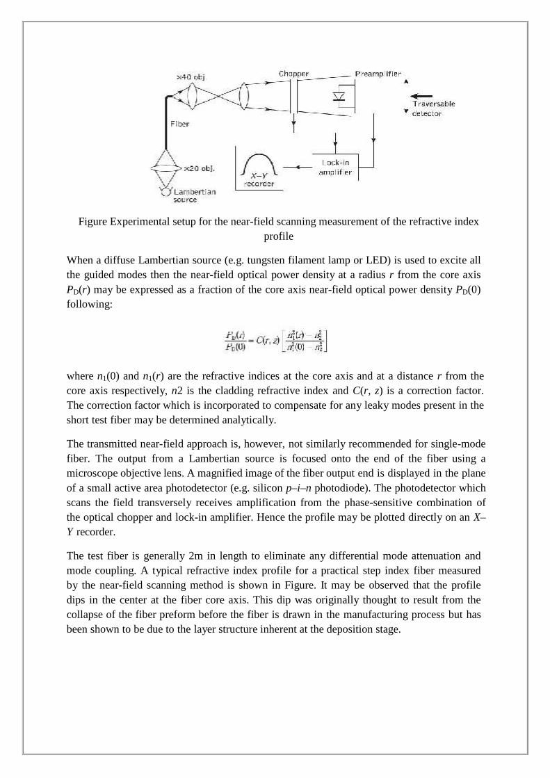
Figure Experimental setup for the near-field scanning measurement of the refractive indexprofile

When a diffuse Lambertian source (e.g. tungsten filament lamp or LED) is used to excite allthe guided modes then the near-field optical power density at a radius r from the core axisPD(r) may be expressed as a fraction of the core axis near-field optical power density PD(0)following:

where n1(0) and n1(r) are the refractive indices at the core axis and at a distance r from thecore axis respectively, n2 is the cladding refractive index and C(r, z) is a correction factor.The correction factor which is incorporated to compensate for any leaky modes present in theshort test fiber may be determined analytically.

The transmitted near-field approach is, however, not similarly recommended for single-modefiber. The output from a Lambertian source is focused onto the end of the fiber using amicroscope objective lens. A magnified image of the fiber output end is displayed in the planeof a small active area photodetector (e.g. silicon p–i–n photodiode). The photodetector whichscans the field transversely receives amplification from the phase-sensitive combination ofthe optical chopper and lock-in amplifier. Hence the profile may be plotted directly on an X–Y recorder.

The test fiber is generally 2m in length to eliminate any differential mode attenuation andmode coupling. A typical refractive index profile for a practical step index fiber measuredby the near-field scanning method is shown in Figure. It may be observed that the profiledips in the center at the fiber core axis. This dip was originally thought to result from thecollapse of the fiber preform before the fiber is drawn in the manufacturing process but hasbeen shown to be due to the layer structure inherent at the deposition stage.

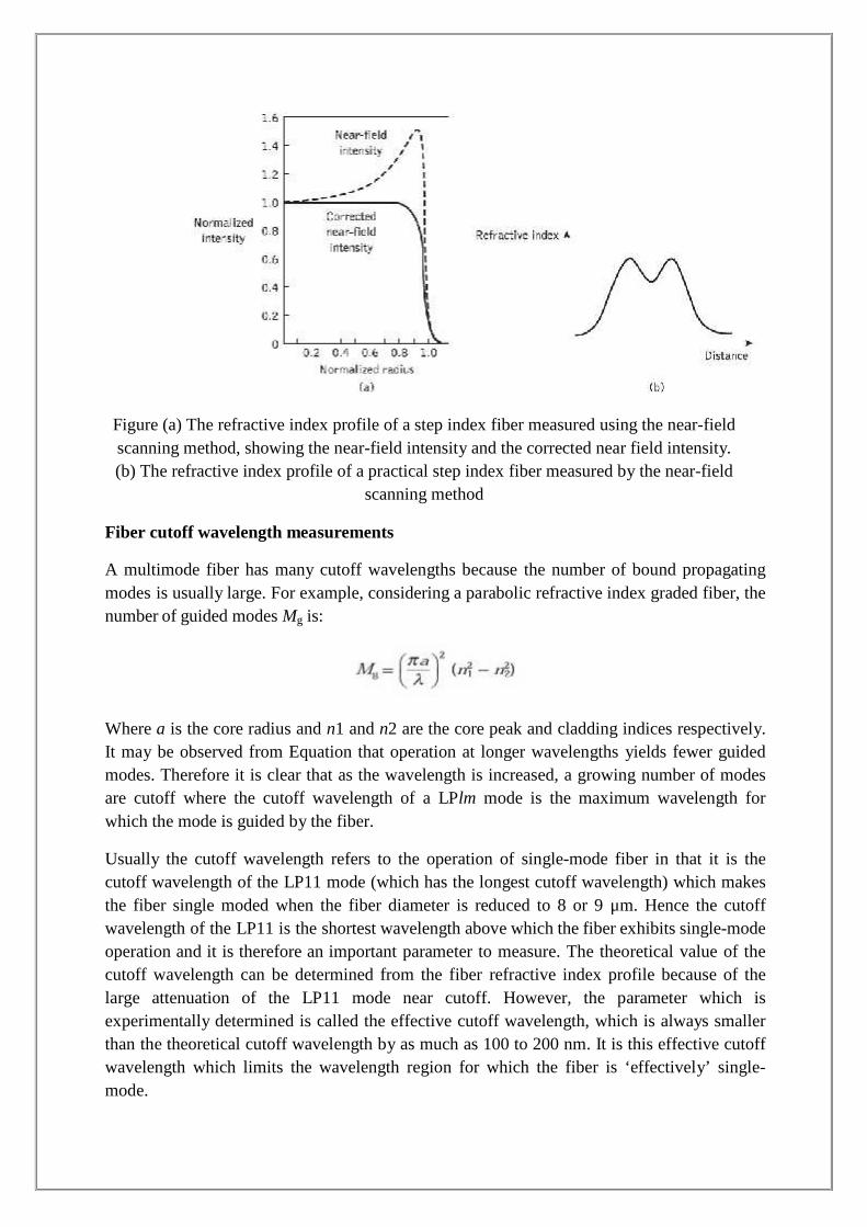
Figure (a) The refractive index profile of a step index fiber measured using the near-fieldscanning method, showing the near-field intensity and the corrected near field intensity.(b) The refractive index profile of a practical step index fiber measured by the near-field

scanning method

Fiber cutoff wavelength measurements

A multimode fiber has many cutoff wavelengths because the number of bound propagatingmodes is usually large. For example, considering a parabolic refractive index graded fiber, thenumber of guided modes Mg is:

Where a is the core radius and n1 and n2 are the core peak and cladding indices respectively.It may be observed from Equation that operation at longer wavelengths yields fewer guidedmodes. Therefore it is clear that as the wavelength is increased, a growing number of modesare cutoff where the cutoff wavelength of a LPlm mode is the maximum wavelength forwhich the mode is guided by the fiber.

Usually the cutoff wavelength refers to the operation of single-mode fiber in that it is thecutoff wavelength of the LP11 mode (which has the longest cutoff wavelength) which makesthe fiber single moded when the fiber diameter is reduced to 8 or 9 μm. Hence the cutoffwavelength of the LP11 is the shortest wavelength above which the fiber exhibits single-modeoperation and it is therefore an important parameter to measure. The theoretical value of thecutoff wavelength can be determined from the fiber refractive index profile because of thelarge attenuation of the LP11 mode near cutoff. However, the parameter which isexperimentally determined is called the effective cutoff wavelength, which is always smallerthan the theoretical cutoff wavelength by as much as 100 to 200 nm. It is this effective cutoffwavelength which limits the wavelength region for which the fiber is ‘effectively’ single-mode.

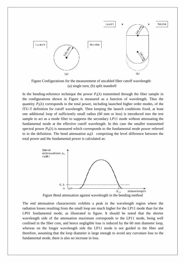
Figure Configurations for the measurement of uncabled fiber cutoff wavelength:(a) single turn; (b) split mandrell

In the bending-reference technique the power Ps(λ) transmitted through the fiber sample inthe configurations shown in Figure is measured as a function of wavelength. Thus thequantity Ps(λ) corresponds to the total power, including launched higher order modes, of theITU-T definition for cutoff wavelength. Then keeping the launch conditions fixed, at leastone additional loop of sufficiently small radius (60 mm or less) is introduced into the testsample to act as a mode filter to suppress the secondary LP11 mode without attenuating thefundamental mode at the effective cutoff wavelength. In this case the smaller transmittedspectral power Pb(λ) is measured which corresponds to the fundamental mode power referredto in the definition. The bend attenuation ab(λ comprising the level difference between thetotal power and the fundamental power is calculated as:

Figure Bend attenuation against wavelength in the bending method

The end attenuation characteristic exhibits a peak in the wavelength region where theradiation losses resulting from the small loop are much higher for the LP11 mode than for theLP01 fundamental mode, as illustrated in figure. It should be noted that the shorterwavelength side of the attenuation maximum corresponds to the LP11 mode, being wellconfined in the fiber core, and hence negligible loss is induced by the 60 mm diameter loop,whereas on the longer wavelength side the LP11 mode is not guided in the fiber andtherefore, assuming that the loop diameter is large enough to avoid any curvature loss to thefundamental mode, there is also no increase in loss.

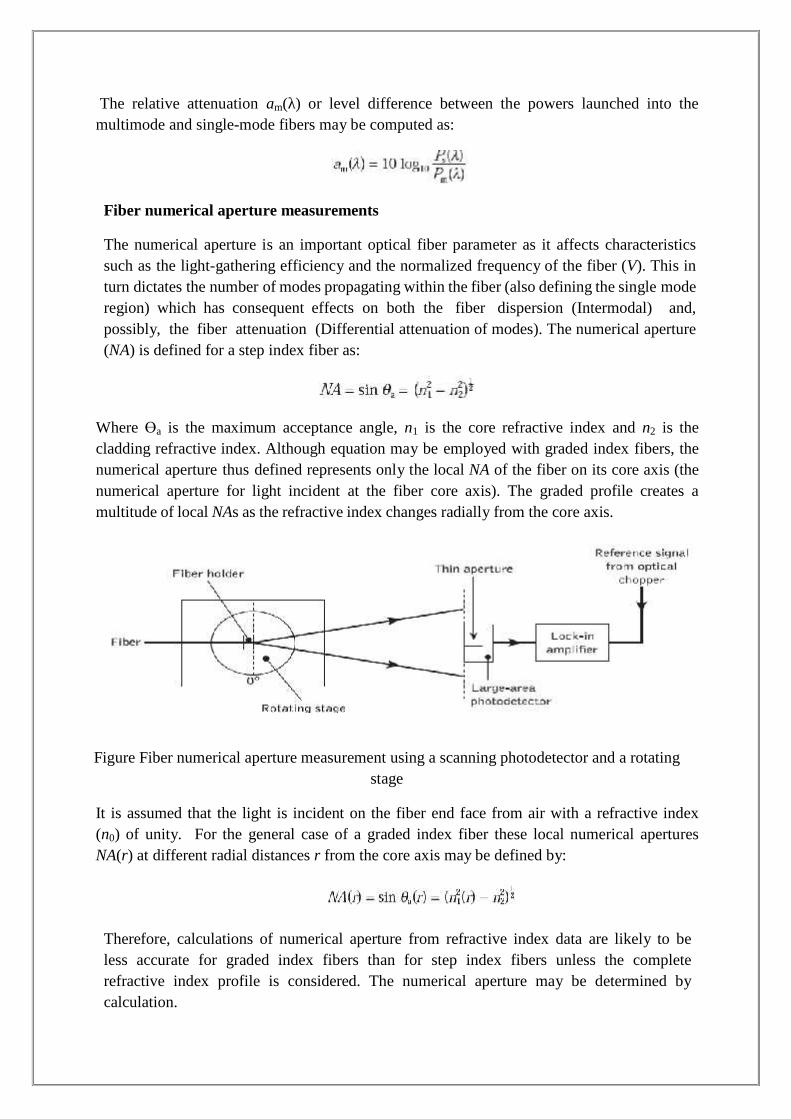
The relative attenuation am(λ) or level difference between the powers launched into themultimode and single-mode fibers may be computed as:

Fiber numerical aperture measurements

The numerical aperture is an important optical fiber parameter as it affects characteristicssuch as the light-gathering efficiency and the normalized frequency of the fiber (V). This inturn dictates the number of modes propagating within the fiber (also defining the single moderegion) which has consequent effects on both the fiber dispersion (Intermodal) and,possibly, the fiber attenuation (Differential attenuation of modes). The numerical aperture(NA) is defined for a step index fiber as:

Where ϴa is the maximum acceptance angle, n1 is the core refractive index and n2 is thecladding refractive index. Although equation may be employed with graded index fibers, thenumerical aperture thus defined represents only the local NA of the fiber on its core axis (thenumerical aperture for light incident at the fiber core axis). The graded profile creates amultitude of local NAs as the refractive index changes radially from the core axis.

Figure Fiber numerical aperture measurement using a scanning photodetector and a rotatingstage

It is assumed that the light is incident on the fiber end face from air with a refractive index(n0) of unity. For the general case of a graded index fiber these local numerical aperturesNA(r) at different radial distances r from the core axis may be defined by:

Therefore, calculations of numerical aperture from refractive index data are likely to beless accurate for graded index fibers than for step index fibers unless the completerefractive index profile is considered. The numerical aperture may be determined bycalculation.

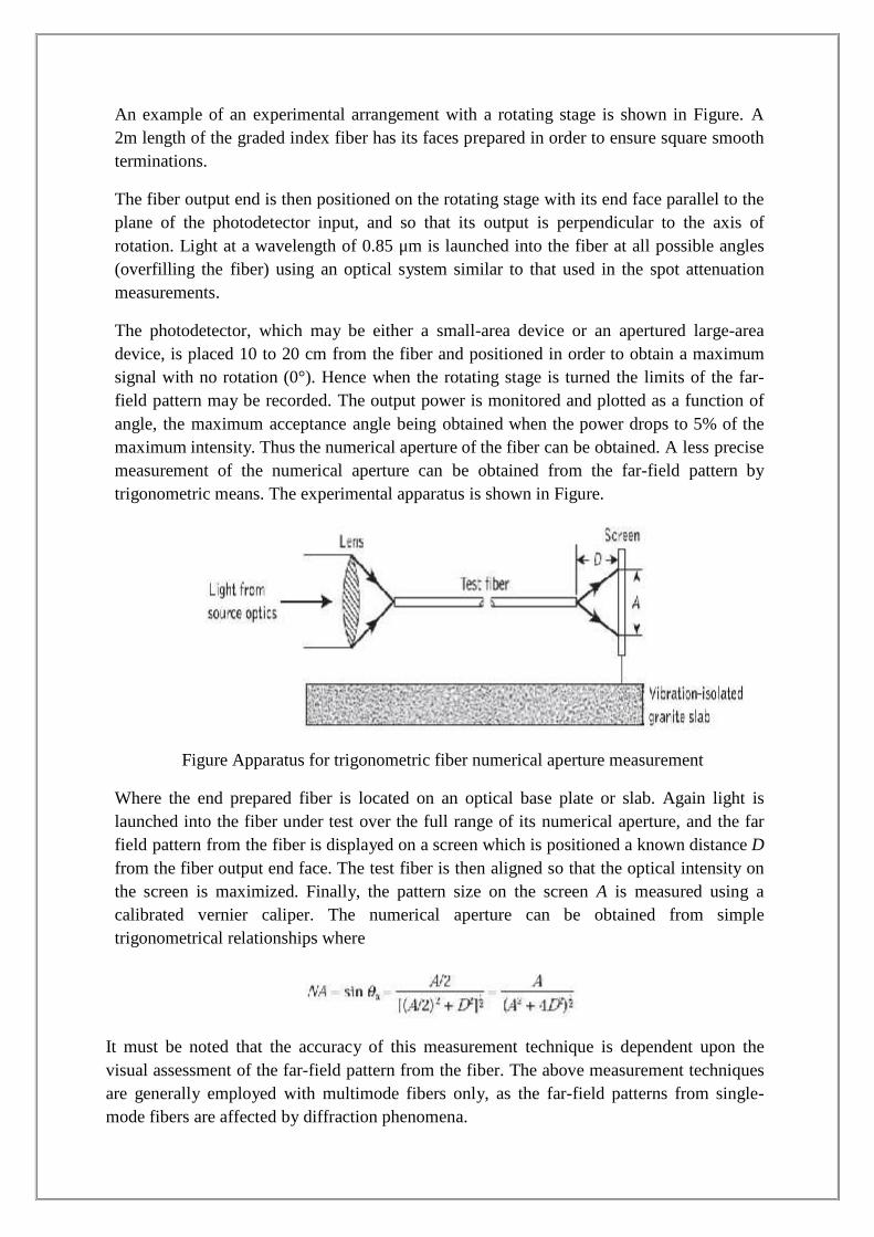
An example of an experimental arrangement with a rotating stage is shown in Figure. A2m length of the graded index fiber has its faces prepared in order to ensure square smoothterminations.

The fiber output end is then positioned on the rotating stage with its end face parallel to theplane of the photodetector input, and so that its output is perpendicular to the axis ofrotation. Light at a wavelength of 0.85 μm is launched into the fiber at all possible angles(overfilling the fiber) using an optical system similar to that used in the spot attenuationmeasurements.

The photodetector, which may be either a small-area device or an apertured large-areadevice, is placed 10 to 20 cm from the fiber and positioned in order to obtain a maximumsignal with no rotation (0°). Hence when the rotating stage is turned the limits of the far-field pattern may be recorded. The output power is monitored and plotted as a function ofangle, the maximum acceptance angle being obtained when the power drops to 5% of themaximum intensity. Thus the numerical aperture of the fiber can be obtained. A less precisemeasurement of the numerical aperture can be obtained from the far-field pattern bytrigonometric means. The experimental apparatus is shown in Figure.

Figure Apparatus for trigonometric fiber numerical aperture measurement

Where the end prepared fiber is located on an optical base plate or slab. Again light islaunched into the fiber under test over the full range of its numerical aperture, and the farfield pattern from the fiber is displayed on a screen which is positioned a known distance Dfrom the fiber output end face. The test fiber is then aligned so that the optical intensity onthe screen is maximized. Finally, the pattern size on the screen A is measured using acalibrated vernier caliper. The numerical aperture can be obtained from simpletrigonometrical relationships where

It must be noted that the accuracy of this measurement technique is dependent upon thevisual assessment of the far-field pattern from the fiber. The above measurement techniquesare generally employed with multimode fibers only, as the far-field patterns from single-mode fibers are affected by diffraction phenomena.

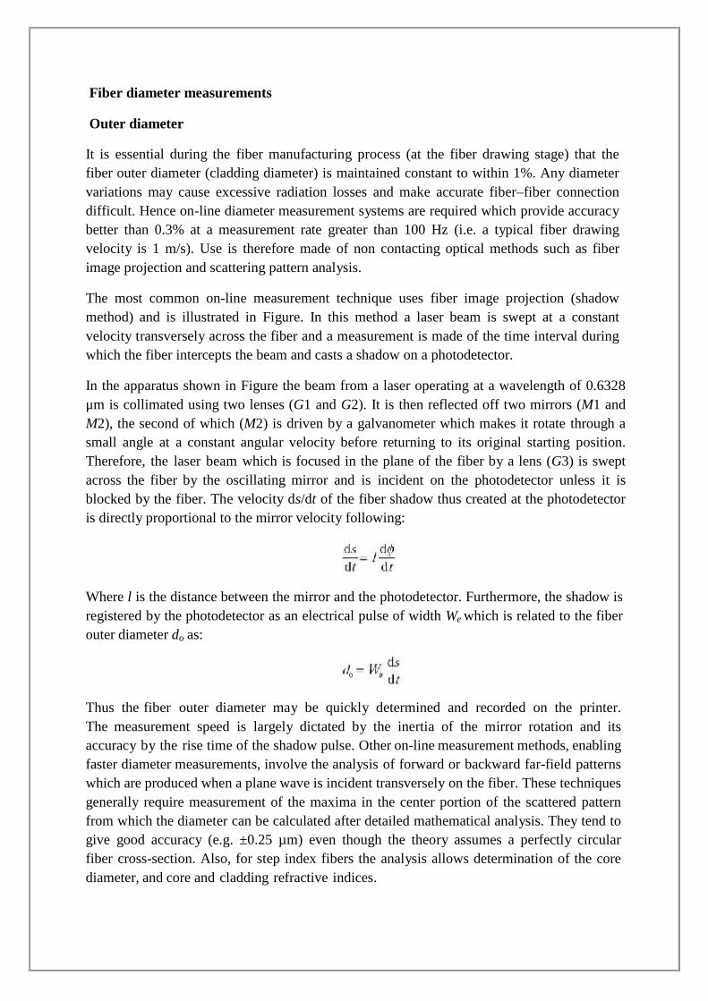
Fiber diameter measurements

Outer diameter

It is essential during the fiber manufacturing process (at the fiber drawing stage) that thefiber outer diameter (cladding diameter) is maintained constant to within 1%. Any diametervariations may cause excessive radiation losses and make accurate fiber–fiber connectiondifficult. Hence on-line diameter measurement systems are required which provide accuracybetter than 0.3% at a measurement rate greater than 100 Hz (i.e. a typical fiber drawingvelocity is 1 m/s). Use is therefore made of non contacting optical methods such as fiberimage projection and scattering pattern analysis.

The most common on-line measurement technique uses fiber image projection (shadowmethod) and is illustrated in Figure. In this method a laser beam is swept at a constantvelocity transversely across the fiber and a measurement is made of the time interval duringwhich the fiber intercepts the beam and casts a shadow on a photodetector.

In the apparatus shown in Figure the beam from a laser operating at a wavelength of 0.6328μm is collimated using two lenses (G1 and G2). It is then reflected off two mirrors (M1 andM2), the second of which (M2) is driven by a galvanometer which makes it rotate through asmall angle at a constant angular velocity before returning to its original starting position.Therefore, the laser beam which is focused in the plane of the fiber by a lens (G3) is sweptacross the fiber by the oscillating mirror and is incident on the photodetector unless it isblocked by the fiber. The velocity ds/dt of the fiber shadow thus created at the photodetectoris directly proportional to the mirror velocity following:

Where l is the distance between the mirror and the photodetector. Furthermore, the shadow isregistered by the photodetector as an electrical pulse of width We which is related to the fiberouter diameter do as:

Thus the fiber outer diameter may be quickly determined and recorded on the printer.The measurement speed is largely dictated by the inertia of the mirror rotation and itsaccuracy by the rise time of the shadow pulse. Other on-line measurement methods, enablingfaster diameter measurements, involve the analysis of forward or backward far-field patternswhich are produced when a plane wave is incident transversely on the fiber. These techniquesgenerally require measurement of the maxima in the center portion of the scattered patternfrom which the diameter can be calculated after detailed mathematical analysis. They tend togive good accuracy (e.g. ±0.25 µm) even though the theory assumes a perfectly circularfiber cross-section. Also, for step index fibers the analysis allows determination of the corediameter, and core and cladding refractive indices.

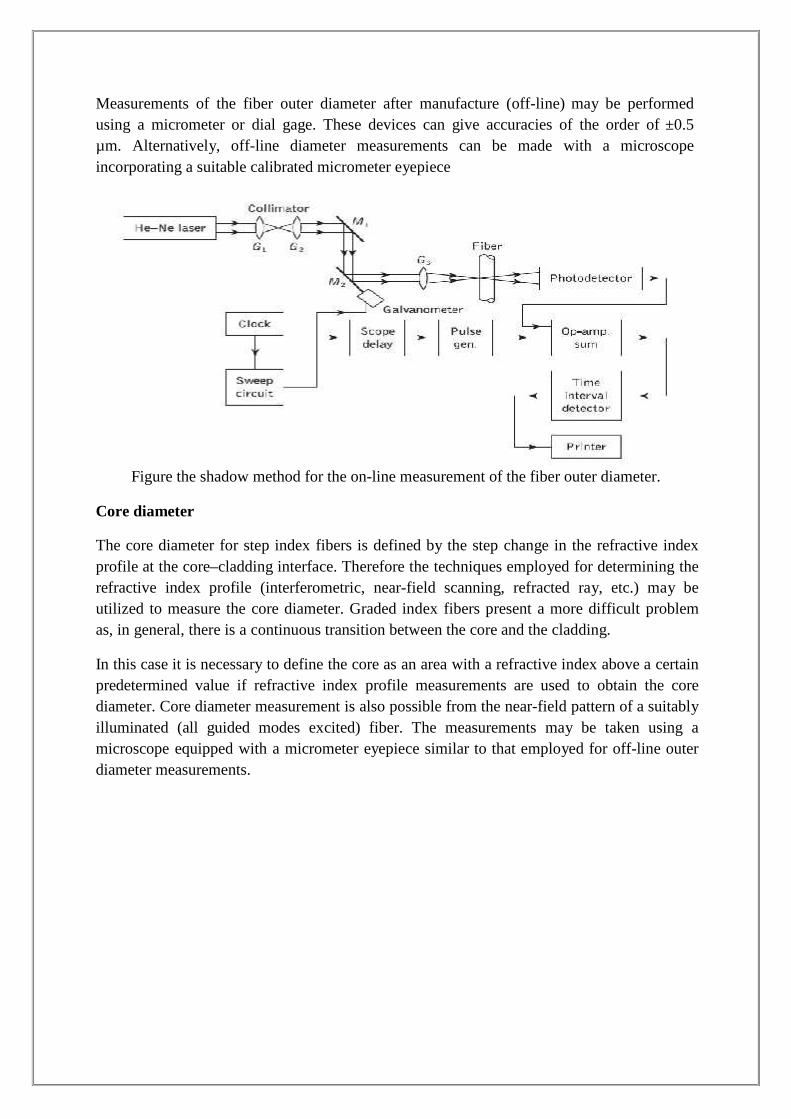
Measurements of the fiber outer diameter after manufacture (off-line) may be performedusing a micrometer or dial gage. These devices can give accuracies of the order of ±0.5µm. Alternatively, off-line diameter measurements can be made with a microscopeincorporating a suitable calibrated micrometer eyepiece

Figure the shadow method for the on-line measurement of the fiber outer diameter.

Core diameter

The core diameter for step index fibers is defined by the step change in the refractive indexprofile at the core–cladding interface. Therefore the techniques employed for determining therefractive index profile (interferometric, near-field scanning, refracted ray, etc.) may beutilized to measure the core diameter. Graded index fibers present a more difficult problemas, in general, there is a continuous transition between the core and the cladding.

In this case it is necessary to define the core as an area with a refractive index above a certainpredetermined value if refractive index profile measurements are used to obtain the corediameter. Core diameter measurement is also possible from the near-field pattern of a suitablyilluminated (all guided modes excited) fiber. The measurements may be taken using amicroscope equipped with a micrometer eyepiece similar to that employed for off-line outerdiameter measurements.

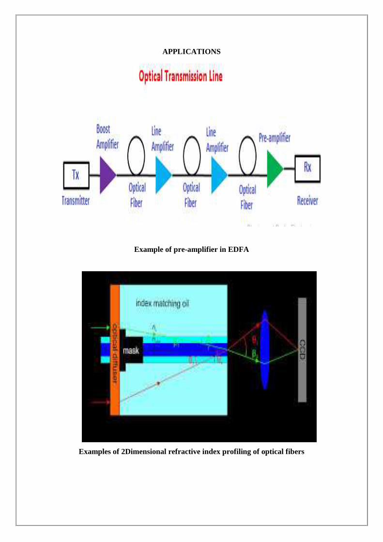
APPLICATIONS

Example of pre-amplifier in EDFA

Examples of 2Dimensional refractive index profiling of optical fibers

POST TEST-MCQ TYPE

1. Which refers to any spurious or undesired disturbances that mask the received signal ina communication system?a) Attenuationb) Noisec) Dispersiond) Bandwidth

2. How many types of noise are observed because of the spontaneous fluctuations inoptical fiber communication systems?a) Oneb) Fourc) Twod) Three

3.Which is caused due to thermal interaction between the free electrons and the vibratingions in the conduction medium.a) Thermal noiseb) Dark noisec) Quantum noised) Gaussian noise

4. The minimum pulse energy needed to maintain a given bit-error-rate (BER) which anypractical receiver must satisfy is known asa) Minimal energyb) Quantum limitc) Point of reversedd) Binary signaling

5. Which is used in the specification of optical detectors.a) Noise equivalent powerb) Polarizationc) Sensitivityd) Electron movement

6. Which of the following APDs are recognized for their high gain-bandwidth products?a) GaAsb) Alloy-madec) Germaniumd) Silicon

7. How many circuits are present in an equivalent circuit for the digital optical fiberreceiver?a) Fourb) Onec) Threed) Two

8. Which compensates for distortion of the signal due to the combined transmitter,medium and receiver characteristics?a) Amplificationb) Distortionc) Equalizationd) Dispersion

9. The phase frequency response of the system should be ____________ in order tominimize inter-symbol interference.a) Non-Linearb) Linearc) Mored) Less

10. How many amplifier configurations are frequently used in optional fibercommunication receivers?a) Oneb) Twoc) Threed) Four

12. The major advantage of the trans-impedance configuration over the high-impedancefront end isa) Greater bandwidthb) Less bandwidthc) Greater dynamic ranged) Less dynamic range

13. The trans-impedance front end configuration operates as a __________ with negativefeedback.a) Current mode amplifierb) Voltage amplifierc) Attenuatord) Resonator

14. Which is the lowest noise amplifier device?a) Silicon FETb) Amplifier-Ac) Attenuatord) Resonator-B

15. FET device has extremely high input impedance greater thana) 107 Ohms and less than 108

b) 106 Ohms and less than 107

c) 1014 Ohmsd) 1023 Ohms

16. High-performance microwave FETs are fabricated froma) Siliconb) Germaniumc) Gallium arsenided) Zinc

17. Which receiver can be fabricated using PIN-FET hybrid approach?a) Trans-impedance front end receiverb) Gallium arsenide receiverc) High-impedance front-endd) Low-impedance front-end

18. What is usually required by FETs to optimize the figure of merit?a) Attenuation of barrierb) Matching with the depletion regionc) Dispersion of the gate regiond) Matching with the detector

19. A technique used for determining the total fiber attenuation per unit length is________ method.a) Frankb) Cut-offc) cut-backd) Erlangen

20. The system designer finds greatest interest in thea) Overall fiber attenuationb) Fiber dispersionc) Latitude of the fiberd) Durability

21. How many parameters are usually worked upon by the measurement techniques inattenuation?a) Threeb) Twoc) Oned) Five

22. What type of light source is usually present in the cut-back method?a) Tungsten or xenonb) LEDc) Laserd) Photo-sensor

23. The device used to remove any scattered optical power from the core isa) Mode setup terminatorb) Nodal spectrumc) Mode stripperd) Attenuator

24. What is the unit of measurement of the optical attenuation per unit length?a) dB-kmb) dB/kmc) km/dBd) V

25. What are used to allow measurements at a selection of different wavelengths?a) Diaphragmsb) Spot attenuatorsc) Beltsd) Interference filters

26. Which technology is used by the backscatter measurement method?a) Refractionb) Francis flat recoveryc) Optical time domain reflectometryd) Optical frequency

27. Which measurements checks the impurity level in the manufacturing process?a) Material reflectometryb) Material absorption lossc) Material attenuation lossd) Calorimetric loss

28. Which removes the light propagating in the cladding?a) Cladding mode strippersb) Core strippersc) Mode enhancersd) Attenuators

29. Which measurements give an indication of the distortion to the optical signals as theypropagate down optical fibers?a) Attenuationb) Dispersionc) Encapsulationd) Frequency

30. The measurement of dispersion allows the _________ of the fiber to be determined.a) Capacityb) Frequencyc) Bandwidthd) Power

31. How many types of mechanisms are present which produce dispersion in opticalfibers?a) Threeb) Twoc) Oned) Four

32. Intermodal dispersion is nonexistent in ________ fibers.a) Multimodeb) Single modec) Step index- multimoded) Al-GU

33. In the single mode fibers, the dominant dispersion mechanism isa) Intermodal dispersionb) Frequency distributionc) Material dispersiond) Intra-modal dispersion

34. How many domains support the measurements of fiber dispersion?a) Oneb) Threec) Fourd) Two

35. The time domain dispersion measurement setup involves _____________ as the photodetector.a) Avalanche photodiodeb) Oscilloscopec) Circulatord) Gyrator

36. The detailed knowledge of the refractive index profile predicts the __________ of thefiber.a) Nodal responseb) Variation in frequencyc) Impulse responsed) Amplitude

37. Which of the fiber is strongly dependent on the refractive index profile?a) Amplitudeb) Tuning frequencyc) Diameterd) Information carrying capacity

38. What is required in case of graded index fibers?a) High amplitudeb) High frequencyc) High impulse responsed) Optimum profile

39. Which of the following have been widely used to determine the refractive indexprofiles of optical fibers?a) Interference microscopesb) Gyro metersc) Mode-diameter deviced) Tunable microscopes

40. Which of the following is the main drawback of the slab technique?a) Efficiencyb) Amplitudec) Time requiredd) Accuracy

41. What does ‘a’ stands for in the given equation?Mg=(πa/λ)2(n1

2 - n22)

a) Radius of the coreb) Constantc) Coefficient of refractiond) Density

42. What is the name of the test used to determine the efficient values of the effectivecutoff wavelength?a) Round robin testb) Mandarin testc) Hough Werner testd) Fulton test43. How many bend effects are produced in the fiber?a) Oneb) Threec) Twod) Four

44. Which method is the most commonly used method for the determination of the fiberrefractive index profile?a) Refracted near-field methodb) Bending-referencec) Power step methodd) Alternative test method45. The numerical aperture for a step index fiber is sine angle of thea) Efficient angleb) Aperturec) Acceptance angled) Attenuation

46. Far field pattern measurements with regard to multimode fibers are dependent on the_____________ of the fiber.a) Amplitudeb) Frequencyc) Diameterd) Length

47. Which of the following is a non-contacting optical method of on-line diametermeasurement?a) Brussels’s methodb) Velocity differentiator methodc) Photo detector methodd) Image projection method

48. Which affects both the fiber attenuation and dispersion?a) Refractive indexb) Micro-bendingc) Connectorsd) Splices

49. Which of the following is not included in the optical fiber link measurement test?a) Attenuation measurementb) Dispersion measurementc) Splice loss measurementd) Receiver sensitivity

50. The handheld optical power meter has a measurement accuracy of ________a) 0.01 dBb) 0.25 dBc) 0.8 dBd) 1 dB

51. Which may be used for measurement of the absolute optical attenuation on a fiberlink?a) Silicon photodiodesb) InGaAsP photodiodesc) Optical power metersd) Gyrators

52. During the fiber drawing process, the fiber outer diameter is maintained constant towithina) 2%b) 1%c) 5%d) 10%

53. What is the minimum value of accuracy in diameter is needed to avoid radiationlosses in the fiber?a) 0.1%b) 0.2%c) 0.3%d) 0.03%

54. Which of the following is a non-contacting optical method of on-line diametermeasurement?a) Brussels’s methodb) Velocity differentiator methodc) Photo detector methodd) Image projection method

CONCLUSION

In this unit, the characteristics of fiber optic receivers were discussed. The Fiber Attenuation

measurements, Dispersion measurements, Fiber Refractive index profile measurements, Fiber

cut- off Wave length Measurements, Fiber Numerical Aperture Measurements, Fiber

diameter measurements and their techniques were learnt.

REFERENCES

1. Gerd Keiser, “Optical Fiber Communication” McGraw-Hill International,4th Edition.

2010.

2. John M. Senior, “Optical Fiber Communication”, Second Edition, Pearson Education,

2007.

3. Ramaswami, Sivarajan and Sasaki “Optical Networks”, Morgan Kaufmann, 2009.

4. J.Senior, Optical Communication, Principles and Practice,Prentice Hall of India, 3rd

Edition, 2008.

5. J.Gower, “Optical Communication System”, Prentice Hall of India, 2001.

ASSIGNMENT

1. With diagram explain the measurement of Cutoff wavelength of optical fiber?

2. With diagram explain the measurement of numerical aperture of a fiber andmeasurement of refractive index fiber?

3. Explain detail in fiber attenuation measurement and Dispersion measurements.

4. Explain the error sources and device the Probability of error for fiber optic system?

5. Explain the fiber optic receiver operation?

6. Write short notes on quantum limit?

UNIT V OPTICAL NETWORKS ANDSYSTEM TRANSMISSION

Prepared by

T.DINESH KUMAR

Assistant Professor

ECE, SCSVMV

OPTICALCOMMUNICATION

AIM & OBJECTIVES

To learn the basic elements of optical fiber transmission link, fiber modesconfigurations and structures.

To understand the different kind of losses, signal distortion, SM fibers. To learn the various optical sources, materials and fiber splicing. To learn the fiber optical receivers and noise performance in photo detector. To explore link budget, WDM, solitons and SONET/SDH network.

PRE TEST-MCQ TYPE

1. The network structure formed due to the interconnectivity patterns is known as aa) Networkb) Struckc) Topologyd) D-pattern

2. In the __________ topology, the data generally circulates bi-directionally.a) Meshb) Busc) Stard) Ring

3. The ring and star topologies are combined in a ________ configuration.a) Meshb) Fringec) Datad) Singular

4. Packet switching is also called asa) Frame switchingb) Cell switchingc) Trans-switchingd) Buffer switching

5. A _______________ is a series of logical connections between the source and destinationnodes.a) Cell circuitb) Attenuation circuitc) Virtual circuitd) Switched network

UNIT V OPTICAL NETWORKS AND SYSTEM TRANSMISSIONBasic Networks – SONET / SDH – Broadcast – and –select WDM Networks –WavelengthRouted Networks – Non linear effects on Network performance –Link Power budget -Risetime budget- Noise Effects on System Performance-Operational Principles of WDMPerformance of WDM + EDFA system – Solutions – Optical CDMA – Solitons in OpticalFiber -Ultra High Capacity Networks.

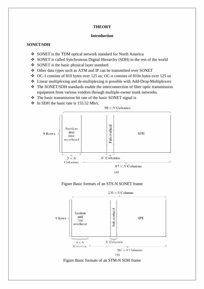
THEORY

Introduction

SONET/SDH

SONET is the TDM optical network standard for North America SONET is called Synchronous Digital Hierarchy (SDH) in the rest of the world SONET is the basic physical layer standard Other data types such as ATM and IP can be transmitted over SONET OC-1 consists of 810 bytes over 125 us; OC-n consists of 810n bytes over 125 us Linear multiplexing and de-multiplexing is possible with Add-Drop-Multiplexers The SONET/SDH standards enable the interconnection of fiber optic transmission

equipment from various vendors through multiple-owner trunk networks. The basic transmission bit rate of the basic SONET signal is In SDH the basic rate is 155.52 Mb/s.

Figure Basic formats of an STS-N SONET frame

Figure Basic formats of an STM-N SDH frame

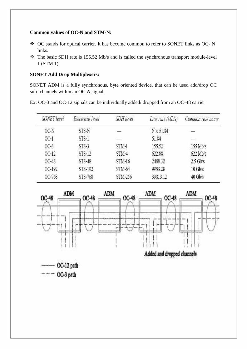
Common values of OC-N and STM-N:

OC stands for optical carrier. It has become common to refer to SONET links as OC- Nlinks.

The basic SDH rate is 155.52 Mb/s and is called the synchronous transport module-level1 (STM 1).

SONET Add Drop Multiplexers:

SONET ADM is a fully synchronous, byte oriented device, that can be used add/drop OCsub- channels within an OC-N signal

Ex: OC-3 and OC-12 signals can be individually added/ dropped from an OC-48 carrier

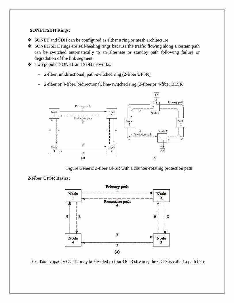
SONET/SDH Rings:

SONET and SDH can be configured as either a ring or mesh architecture SONET/SDH rings are self-healing rings because the traffic flowing along a certain path

can be switched automatically to an alternate or standby path following failure ordegradation of the link segment

Two popular SONET and SDH networks:

– 2-fiber, unidirectional, path-switched ring (2-fiber UPSR)

– 2-fiber or 4-fiber, bidirectional, line-switched ring (2-fiber or 4-fiber BLSR)

Figure Generic 2-fiber UPSR with a counter-rotating protection path

2-Fiber UPSR Basics:

Ex: Total capacity OC-12 may be divided to four OC-3 streams, the OC-3 is called a path here

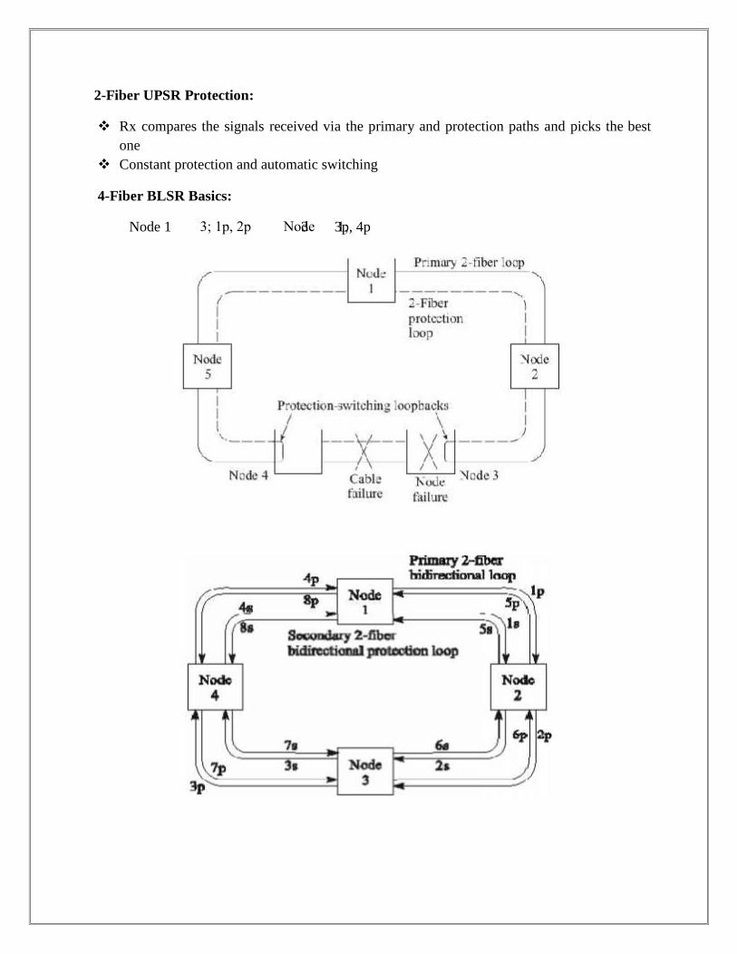
2-Fiber UPSR Protection:

Rx compares the signals received via the primary and protection paths and picks the bestone

Constant protection and automatic switching

4-Fiber BLSR Basics:

Node 13; 1p, 2p Node31;3p, 4p

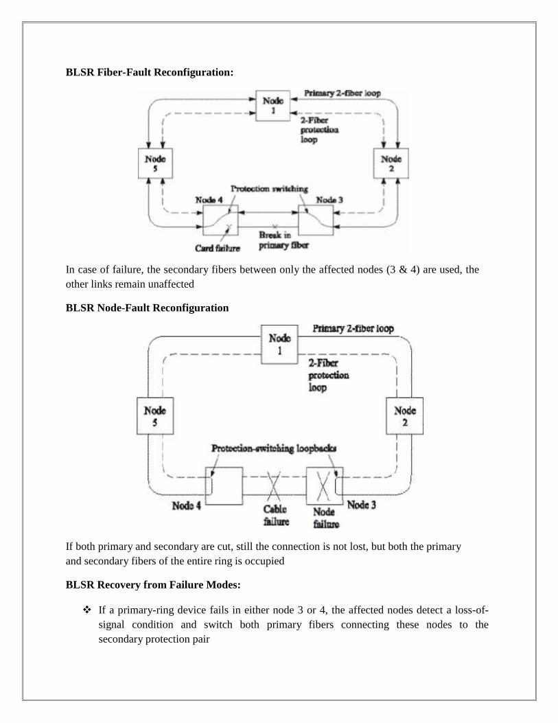
BLSR Fiber-Fault Reconfiguration:

In case of failure, the secondary fibers between only the affected nodes (3 & 4) are used, theother links remain unaffected

BLSR Node-Fault Reconfiguration

If both primary and secondary are cut, still the connection is not lost, but both the primaryand secondary fibers of the entire ring is occupied

BLSR Recovery from Failure Modes:

If a primary-ring device fails in either node 3 or 4, the affected nodes detect a loss-of-signal condition and switch both primary fibers connecting these nodes to thesecondary protection pair

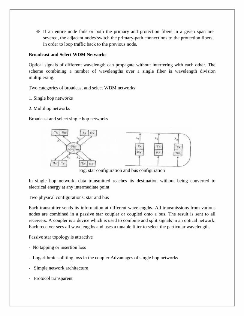
If an entire node fails or both the primary and protection fibers in a given span aresevered, the adjacent nodes switch the primary-path connections to the protection fibers,in order to loop traffic back to the previous node.

Broadcast and Select WDM Networks

Optical signals of different wavelength can propagate without interfering with each other. Thescheme combining a number of wavelengths over a single fiber is wavelength divisionmultiplexing.

Two categories of broadcast and select WDM networks

1. Single hop networks

2. Multihop networks

Broadcast and select single hop networks

Fig: star configuration and bus configuration

In single hop network, data transmitted reaches its destination without being converted toelectrical energy at any intermediate point

Two physical configurations: star and bus

Each transmitter sends its information at different wavelengths. All transmissions from variousnodes are combined in a passive star coupler or coupled onto a bus. The result is sent to allreceivers. A coupler is a device which is used to combine and split signals in an optical network.Each receiver sees all wavelengths and uses a tunable filter to select the particular wavelength.

Passive star topology is attractive

- No tapping or insertion loss

- Logarithmic splitting loss in the coupler Advantages of single hop networks

- Simple network architecture

- Protocol transparent

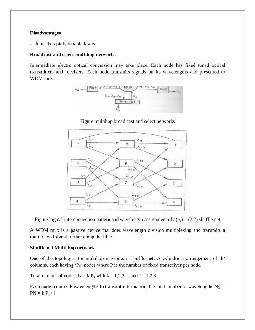
Disadvantages

- It needs rapidly tunable lasers

Broadcast and select multihop networks

Intermediate electro optical conversion may take place. Each node has fixed tuned opticaltransmitters and receivers. Each node transmits signals on its wavelengths and presented toWDM mux.

Figure multihop broad cast and select networks

Figure logical interconnection pattern and wavelength assignment of a(p,) = (2,2) shuffle net

A WDM mux is a passive device that does wavelength division multiplexing and transmits amultiplexed signal further along the fiber

Shuffle net Multi hop network

One of the topologies for multihop networks is shuffle net. A cylindrical arrangement of ‘k’columns, each having ‘Pk’ nodes where P is the number of fixed transceiver per node.

Total number of nodes, N = k Pk with k = 1,2,3… and P =1,2,3..

Each node requires P wavelengths to transmit information, the total number of wavelengths Nλ =PN = k Pk+1

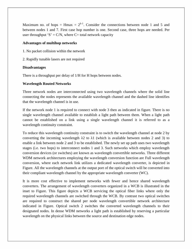
Maximum no. of hops = Hmax = 2k-1. Consider the connections between node 1 and 5 andbetween nodes 1 and 7. First case hop number is one. Second case, three hops are needed. Peruser throughput ‘S’ = C/N, where C= total network capacity

Advantages of multihop networks

1. No packet collision within the network

2. Rapidly tunable lasers are not required

Disadvantages

There is a throughput per delay of 1/H for H hops between nodes.

Wavelength Routed Networks

Three network nodes are interconnected using two wavelength channels where the solid lineconnecting the nodes represents the available wavelength channel and the dashed line identifiesthat the wavelength channel is in use.

If the network node 1 is required to connect with node 3 then as indicated in figure. There is nosingle wavelength channel available to establish a light path between them. When a light pathcannot be established on a link using a single wavelength channel it is referred to as awavelength continuity constraint.

To reduce this wavelength continuity constraint is to switch the wavelength channel at node 2 byconverting the incoming wavelength λ2 to λ1 (which is available between nodes 2 and 3) toenable a link between node 2 and 3 to be established. The newly set up path uses two wavelengthstages (i.e. two hops) to interconnect nodes 1 and 3. Such networks which employ wavelengthconversion devices (or switches) are known as wavelength convertible networks. Three differentWDM network architectures employing the wavelength conversion function are Full wavelengthconversion, where each network link utilizes a dedicated wavelength converter, is depicted inFigure. All the wavelength channels at the output port of the optical switch will be converted intotheir compliant wavelength channel by the appropriate wavelength converter (WC).

It is more cost effective to implement networks with fewer and hence shared wavelengthconverters. The arrangement of wavelength converters organized in a WCB is illustrated in theinset to Figure. This figure depicts a WCB servicing the optical fiber links where only therequired wavelength channels are switched through the WCB. By contrast two optical switchesare required to construct the shared per node wavelength convertible network architectureindicated in Figure. Optical switch 2 switches the converted wavelength channels to theirdesignated nodes. In dense WDM networks a light path is established by reserving a particularwavelength on the physical links between the source and destination edge nodes.

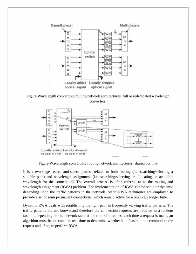
Figure Wavelength convertible routing network architectures: full or rededicated wavelengthconverters;

Figure Wavelength convertible routing network architectures: shared per link

It is a two-stage search and-select process related to both routing (i.e. searching/selecting asuitable path) and wavelength assignment (i.e. searching/selecting or allocating an availablewavelength for the connection). The overall process is often referred to as the routing andwavelength assignment (RWA) problem. The implementation of RWA can be static or dynamicdepending upon the traffic patterns in the network. Static RWA techniques are employed toprovide a set of semi permanent connections, which remain active for a relatively longer time.

Dynamic RWA deals with establishing the light path in frequently varying traffic patterns. Thetraffic patterns are not known and therefore the connection requests are initiated in a randomfashion, depending on the network state at the time of a request each time a request is made, analgorithm must be executed in real time to determine whether it is feasible to accommodate therequest and, if so, to perform RWA.

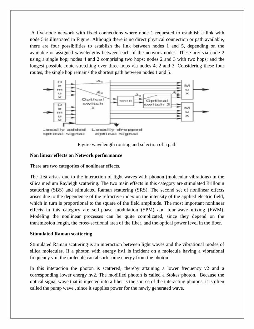
A five-node network with fixed connections where node 1 requested to establish a link withnode 5 is illustrated in Figure. Although there is no direct physical connection or path available,there are four possibilities to establish the link between nodes 1 and 5, depending on theavailable or assigned wavelengths between each of the network nodes. These are: via node 2using a single hop; nodes 4 and 2 comprising two hops; nodes 2 and 3 with two hops; and thelongest possible route stretching over three hops via nodes 4, 2 and 3. Considering these fourroutes, the single hop remains the shortest path between nodes 1 and 5.

Figure wavelength routing and selection of a path

Non linear effects on Network performance

There are two categories of nonlinear effects.

The first arises due to the interaction of light waves with phonon (molecular vibrations) in thesilica medium Rayleigh scattering. The two main effects in this category are stimulated Brillouinscattering (SBS) and stimulated Raman scattering (SRS). The second set of nonlinear effectsarises due to the dependence of the refractive index on the intensity of the applied electric field,which in turn is proportional to the square of the field amplitude. The most important nonlineareffects in this category are self-phase modulation (SPM) and four-wave mixing (FWM).Modeling the nonlinear processes can be quite complicated, since they depend on thetransmission length, the cross-sectional area of the fiber, and the optical power level in the fiber.

Stimulated Raman scattering

Stimulated Raman scattering is an interaction between light waves and the vibrational modes ofsilica molecules. If a photon with energy hv1 is incident on a molecule having a vibrationalfrequency vm, the molecule can absorb some energy from the photon.

In this interaction the photon is scattered, thereby attaining a lower frequency v2 and acorresponding lower energy hv2. The modified photon is called a Stokes photon. Because theoptical signal wave that is injected into a fiber is the source of the interacting photons, it is oftencalled the pump wave , since it supplies power for the newly generated wave.

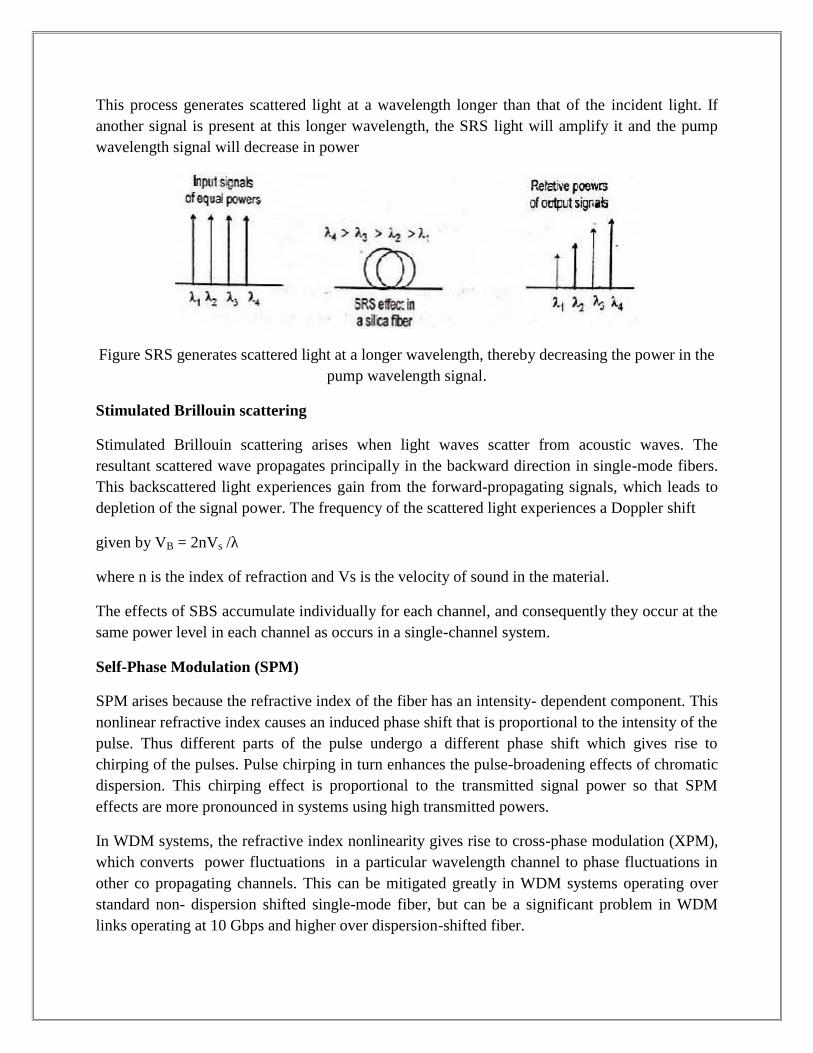
This process generates scattered light at a wavelength longer than that of the incident light. Ifanother signal is present at this longer wavelength, the SRS light will amplify it and the pumpwavelength signal will decrease in power

Figure SRS generates scattered light at a longer wavelength, thereby decreasing the power in thepump wavelength signal.

Stimulated Brillouin scattering

Stimulated Brillouin scattering arises when light waves scatter from acoustic waves. Theresultant scattered wave propagates principally in the backward direction in single-mode fibers.This backscattered light experiences gain from the forward-propagating signals, which leads todepletion of the signal power. The frequency of the scattered light experiences a Doppler shift

given by VB = 2nVs /λ

where n is the index of refraction and Vs is the velocity of sound in the material.

The effects of SBS accumulate individually for each channel, and consequently they occur at thesame power level in each channel as occurs in a single-channel system.

Self-Phase Modulation (SPM)

SPM arises because the refractive index of the fiber has an intensity- dependent component. Thisnonlinear refractive index causes an induced phase shift that is proportional to the intensity of thepulse. Thus different parts of the pulse undergo a different phase shift which gives rise tochirping of the pulses. Pulse chirping in turn enhances the pulse-broadening effects of chromaticdispersion. This chirping effect is proportional to the transmitted signal power so that SPMeffects are more pronounced in systems using high transmitted powers.

In WDM systems, the refractive index nonlinearity gives rise to cross-phase modulation (XPM),which converts power fluctuations in a particular wavelength channel to phase fluctuations inother co propagating channels. This can be mitigated greatly in WDM systems operating overstandard non- dispersion shifted single-mode fiber, but can be a significant problem in WDMlinks operating at 10 Gbps and higher over dispersion-shifted fiber.

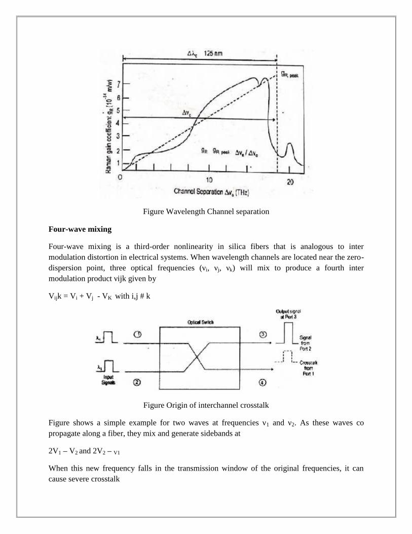
Figure Wavelength Channel separation

Four-wave mixing

Four-wave mixing is a third-order nonlinearity in silica fibers that is analogous to intermodulation distortion in electrical systems. When wavelength channels are located near the zero-dispersion point, three optical frequencies (νi, νj, νk) will mix to produce a fourth intermodulation product νijk given by

Vijk = Vi + Vj - VK with i,j # k

Figure Origin of interchannel crosstalk

Figure shows a simple example for two waves at frequencies ν1 and ν2. As these waves copropagate along a fiber, they mix and generate sidebands at

2V1 – V2 and 2V2 – V1

When this new frequency falls in the transmission window of the original frequencies, it cancause severe crosstalk

LINK POWER BUDGET:

For optimizing link power budget an optical power loss model is to be studied as shown inFigure. Let

lc denotes the losses occur at connector.

Lsp denotes the losses occur at splices.

αf denotes the losses occur in fiber.

Figure Link power budget

All the losses from source to detector comprises the total loss (PT) in the system. Link powermargin considers the losses due to component aging and temperature fluctuations.

Usually a link margin of 6-8 dB is considered while estimating link power budget. Total opticalloss = Connector loss + (Splicing loss + Fiber attenuation) + System margin (Pm)

PT = 2lc + αfL + System margin (Pm)

Where, L is transmission distance.

Rise Time Budget

Rise time gives important information for initial system design. Rise-time budget analysisdetermines the dispersion limitation of an optical fiber link. Total rise time of a fiber link is theroot-sum-square of rise time of each contributor to the pulse rise time degradation.

The link components must be switched fast enough and the fiber dispersion must be lowenough to meet the bandwidth requirements of the application adequate bandwidth for asystem can be assured by developing a rise time budget. As the light sources and detectorshas a finite response time to inputs. The device does not turn-on or turn-off instantaneously.Rise time and fall time determines the overall response time and hence the resultingbandwidth.

Connectors, couplers and splices do not affect system speed, they need not be accounted in risetime budget but they appear in the link power budget. Four basic elements that contributes tothe rise-time are, Transmitter rise-time (ttx)

Group Velocity Dispersion (GVD) rise time (tGVD) Modal dispersion rise time of fiber (tmod)

Receiver rise time (trx) Where,

Rise time due to modal dispersion is given as

Where,

BM is bandwidth (MHz) L is length of fiber (km)

q Is a parameter ranging between 0.5 and 1.

B0 is bandwidth of 1 km length fiber

Rise time due to group velocity dispersion is

Where, D is dispersion [ns/(nm.km)] Σλ is half-power spectral width of source L is length of

fiber

Receiver front end rise-time in nanoseconds is

Brx is 3 dB – bW of receiver (MHz).

Equation can be written as

WDM

WDM (Wavelength-division Multiplexing) is the technology of combing a number of wavelengthsonto the same fiber simultaneously. A powerful aspect of WDM is that each optical channel cancarry any transmission format. WDW increases the capacity of a fiber network dramatically. Thus itis recognized as the Layer 1 transport technology in all tiers of the network. The purpose of thisarticle is to give a brief overview of WDM technology and its applications.

NEED OF WDM

Due to the rapid growth in telecommunication links, high capacity and faster data transmission ratesover farther distances are required. To meet these demands, network managers are relying more andmore on fiber optics. Typically, there are three methods for expanding capacity: installing morecables, increasing system bit rate to multiplex more signals and wavelength division multiplexing.The first method, installing more cables, will be preferred in many cases, especially inmetropolitan areas, since fiber has become incredibly inexpensive and installation methods moreefficient. But when conduit space is not available or major construction is necessary, this may not bethe most cost-effective.

Another way for capacity expansion is to increase system bit rate to multiplex more signals. Butincreasing system bit rate may not prove cost effective either. Since many systems are alreadyrunning at SONET OC-48 rates (2.5 GB/s) and upgrading to OC-192 (10 GB/s) isexpensive, requires changing out all the electronics in a network, and adds 4 times the capacity, maynot be necessary. Thirdly, the WDM has been proved to be the more cost-effective technology. Itdoes not only support current electronics and fibers but also can share fibers by transmittingchannels at different wavelengths (colors) of light. Besides, systems are already using fiber opticamplifiers as repeaters also do not require upgrading for most WDM.

From the above comparison of three methods for expanding capacity, it can easily draw a conclusionthat WDM is the best solution to meet the demand for more capacity and faster data transmissionrates. Actually, it is not difficult to understand the operating principle of WDM. Consider the factthat you can see many different colors of light: red, green, yellow, blue, etc. The colors aretransmitted through the air together and may mix, but they can be easily separated by using a simpledevice like a prism. It’s like separating the “white” light from the sun into a spectrum of colors withthe prism. WDM is equivalent to the prism in the operating principle. A WDM system uses amultiplexer at the transmitter to joint the several signals together. At the same time, it uses ademultiplexer at the receiver to split them apart, as shown in the following diagram. With the righttype of fiber, it is possible to function as an optical add-drop multiplexer.

This technique was originally demonstrated with optical fiber in the early 80s. The first WDMsystems combined only two signals. Modern systems can handle up to 160 signals and can thusexpand a basic 10 Gbit/s system over a single fiber pair to over 1.6 Tbit/s.

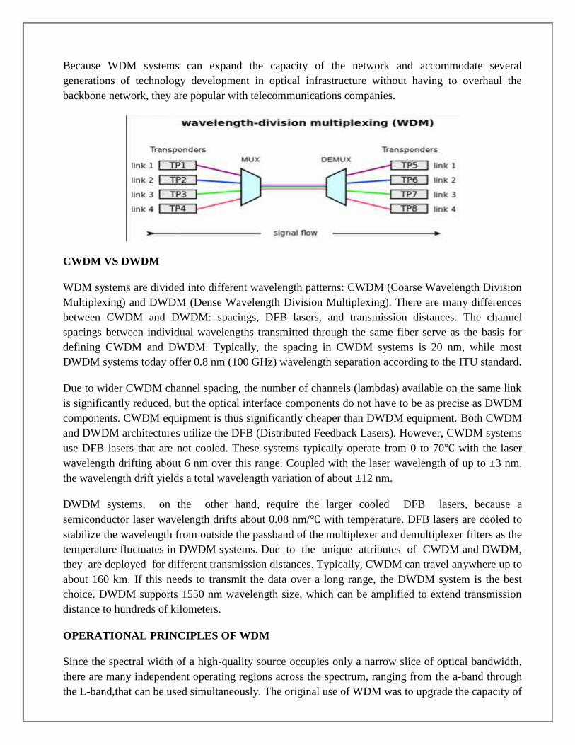
Because WDM systems can expand the capacity of the network and accommodate severalgenerations of technology development in optical infrastructure without having to overhaul thebackbone network, they are popular with telecommunications companies.

CWDM VS DWDM

WDM systems are divided into different wavelength patterns: CWDM (Coarse Wavelength DivisionMultiplexing) and DWDM (Dense Wavelength Division Multiplexing). There are many differencesbetween CWDM and DWDM: spacings, DFB lasers, and transmission distances. The channelspacings between individual wavelengths transmitted through the same fiber serve as the basis fordefining CWDM and DWDM. Typically, the spacing in CWDM systems is 20 nm, while mostDWDM systems today offer 0.8 nm (100 GHz) wavelength separation according to the ITU standard.

Due to wider CWDM channel spacing, the number of channels (lambdas) available on the same linkis significantly reduced, but the optical interface components do not have to be as precise as DWDMcomponents. CWDM equipment is thus significantly cheaper than DWDM equipment. Both CWDMand DWDM architectures utilize the DFB (Distributed Feedback Lasers). However, CWDM systemsuse DFB lasers that are not cooled. These systems typically operate from 0 to 70℃ with the laserwavelength drifting about 6 nm over this range. Coupled with the laser wavelength of up to ±3 nm,the wavelength drift yields a total wavelength variation of about ±12 nm.

DWDM systems, on the other hand, require the larger cooled DFB lasers, because asemiconductor laser wavelength drifts about 0.08 nm/℃ with temperature. DFB lasers are cooled tostabilize the wavelength from outside the passband of the multiplexer and demultiplexer filters as thetemperature fluctuates in DWDM systems. Due to the unique attributes of CWDM and DWDM,they are deployed for different transmission distances. Typically, CWDM can travel anywhere up toabout 160 km. If this needs to transmit the data over a long range, the DWDM system is the bestchoice. DWDM supports 1550 nm wavelength size, which can be amplified to extend transmissiondistance to hundreds of kilometers.

OPERATIONAL PRINCIPLES OF WDM

Since the spectral width of a high-quality source occupies only a narrow slice of optical bandwidth,there are many independent operating regions across the spectrum, ranging from the a-band throughthe L-band,that can be used simultaneously. The original use of WDM was to upgrade the capacity of

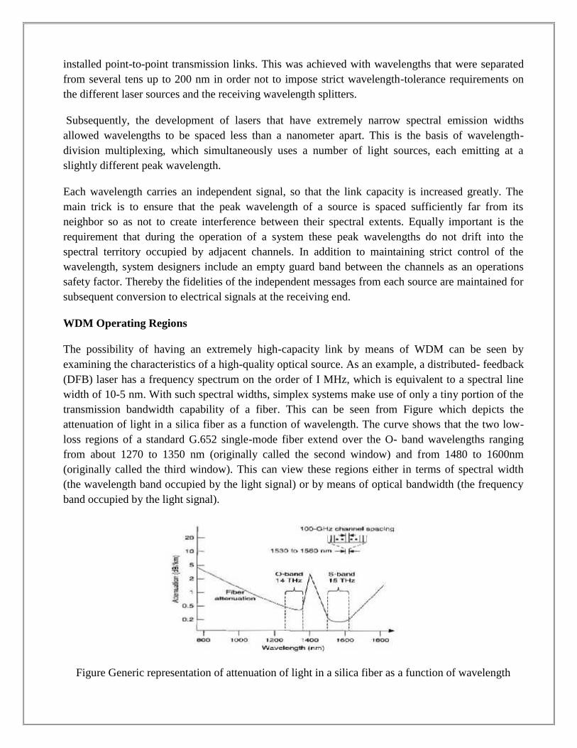
installed point-to-point transmission links. This was achieved with wavelengths that were separatedfrom several tens up to 200 nm in order not to impose strict wavelength-tolerance requirements onthe different laser sources and the receiving wavelength splitters.

Subsequently, the development of lasers that have extremely narrow spectral emission widthsallowed wavelengths to be spaced less than a nanometer apart. This is the basis of wavelength-division multiplexing, which simultaneously uses a number of light sources, each emitting at aslightly different peak wavelength.

Each wavelength carries an independent signal, so that the link capacity is increased greatly. Themain trick is to ensure that the peak wavelength of a source is spaced sufficiently far from itsneighbor so as not to create interference between their spectral extents. Equally important is therequirement that during the operation of a system these peak wavelengths do not drift into thespectral territory occupied by adjacent channels. In addition to maintaining strict control of thewavelength, system designers include an empty guard band between the channels as an operationssafety factor. Thereby the fidelities of the independent messages from each source are maintained forsubsequent conversion to electrical signals at the receiving end.

WDM Operating Regions

The possibility of having an extremely high-capacity link by means of WDM can be seen byexamining the characteristics of a high-quality optical source. As an example, a distributed- feedback(DFB) laser has a frequency spectrum on the order of I MHz, which is equivalent to a spectral linewidth of 10-5 nm. With such spectral widths, simplex systems make use of only a tiny portion of thetransmission bandwidth capability of a fiber. This can be seen from Figure which depicts theattenuation of light in a silica fiber as a function of wavelength. The curve shows that the two low-loss regions of a standard G.652 single-mode fiber extend over the O- band wavelengths rangingfrom about 1270 to 1350 nm (originally called the second window) and from 1480 to 1600nm(originally called the third window). This can view these regions either in terms of spectral width(the wavelength band occupied by the light signal) or by means of optical bandwidth (the frequencyband occupied by the light signal).

Figure Generic representation of attenuation of light in a silica fiber as a function of wavelength

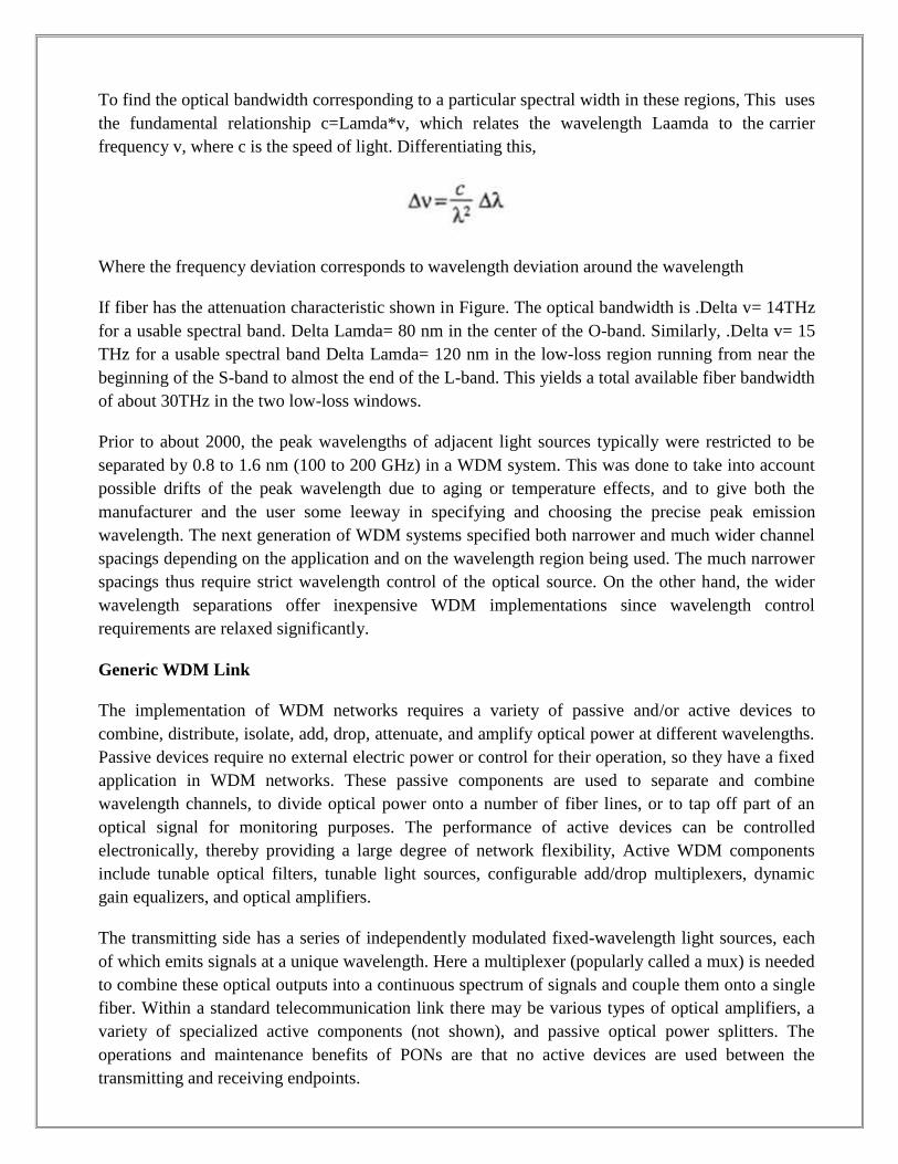
To find the optical bandwidth corresponding to a particular spectral width in these regions, This usesthe fundamental relationship c=Lamda*v, which relates the wavelength Laamda to the carrierfrequency v, where c is the speed of light. Differentiating this,

Where the frequency deviation corresponds to wavelength deviation around the wavelength

If fiber has the attenuation characteristic shown in Figure. The optical bandwidth is .Delta v= 14THzfor a usable spectral band. Delta Lamda= 80 nm in the center of the O-band. Similarly, .Delta v= 15THz for a usable spectral band Delta Lamda= 120 nm in the low-loss region running from near thebeginning of the S-band to almost the end of the L-band. This yields a total available fiber bandwidthof about 30THz in the two low-loss windows.

Prior to about 2000, the peak wavelengths of adjacent light sources typically were restricted to beseparated by 0.8 to 1.6 nm (100 to 200 GHz) in a WDM system. This was done to take into accountpossible drifts of the peak wavelength due to aging or temperature effects, and to give both themanufacturer and the user some leeway in specifying and choosing the precise peak emissionwavelength. The next generation of WDM systems specified both narrower and much wider channelspacings depending on the application and on the wavelength region being used. The much narrowerspacings thus require strict wavelength control of the optical source. On the other hand, the widerwavelength separations offer inexpensive WDM implementations since wavelength controlrequirements are relaxed significantly.

Generic WDM Link

The implementation of WDM networks requires a variety of passive and/or active devices tocombine, distribute, isolate, add, drop, attenuate, and amplify optical power at different wavelengths.Passive devices require no external electric power or control for their operation, so they have a fixedapplication in WDM networks. These passive components are used to separate and combinewavelength channels, to divide optical power onto a number of fiber lines, or to tap off part of anoptical signal for monitoring purposes. The performance of active devices can be controlledelectronically, thereby providing a large degree of network flexibility, Active WDM componentsinclude tunable optical filters, tunable light sources, configurable add/drop multiplexers, dynamicgain equalizers, and optical amplifiers.

The transmitting side has a series of independently modulated fixed-wavelength light sources, eachof which emits signals at a unique wavelength. Here a multiplexer (popularly called a mux) is neededto combine these optical outputs into a continuous spectrum of signals and couple them onto a singlefiber. Within a standard telecommunication link there may be various types of optical amplifiers, avariety of specialized active components (not shown), and passive optical power splitters. Theoperations and maintenance benefits of PONs are that no active devices are used between thetransmitting and receiving endpoints.

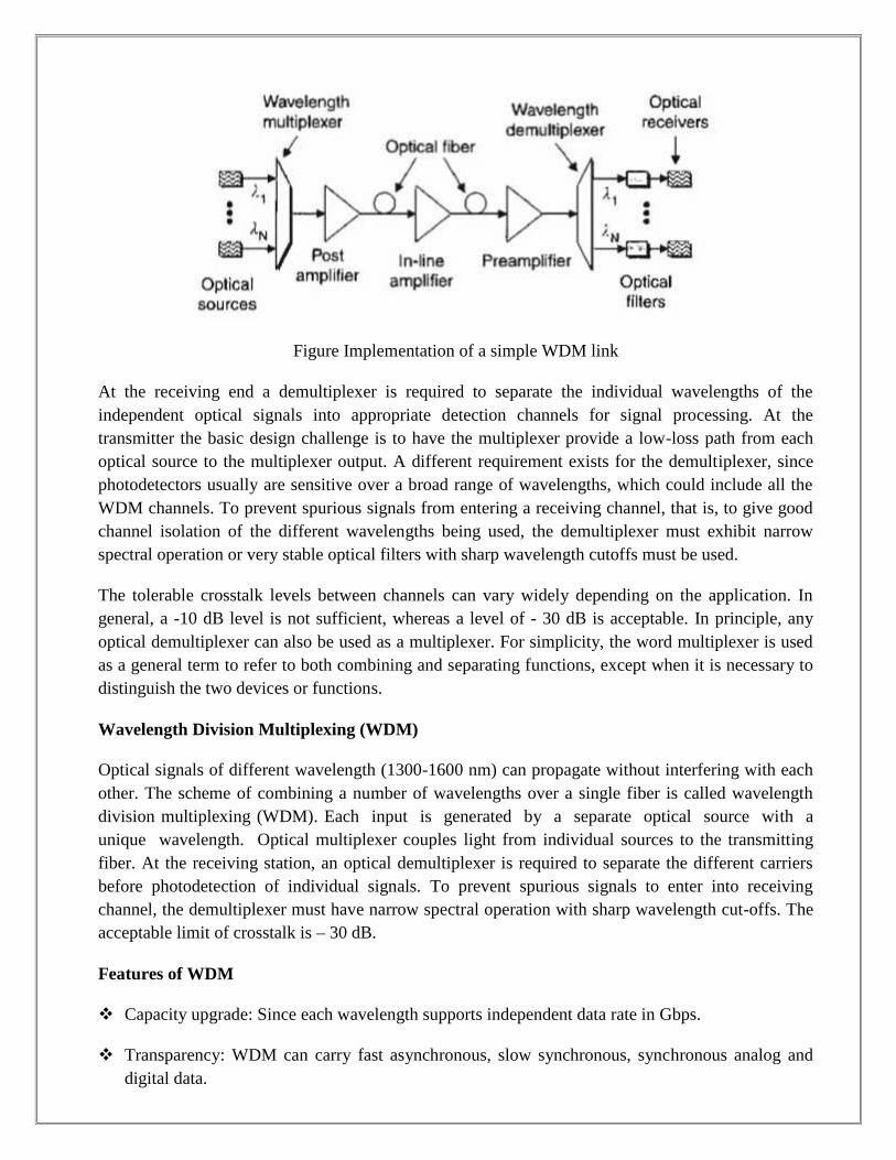
Figure Implementation of a simple WDM link

At the receiving end a demultiplexer is required to separate the individual wavelengths of theindependent optical signals into appropriate detection channels for signal processing. At thetransmitter the basic design challenge is to have the multiplexer provide a low-loss path from eachoptical source to the multiplexer output. A different requirement exists for the demultiplexer, sincephotodetectors usually are sensitive over a broad range of wavelengths, which could include all theWDM channels. To prevent spurious signals from entering a receiving channel, that is, to give goodchannel isolation of the different wavelengths being used, the demultiplexer must exhibit narrowspectral operation or very stable optical filters with sharp wavelength cutoffs must be used.

The tolerable crosstalk levels between channels can vary widely depending on the application. Ingeneral, a -10 dB level is not sufficient, whereas a level of - 30 dB is acceptable. In principle, anyoptical demultiplexer can also be used as a multiplexer. For simplicity, the word multiplexer is usedas a general term to refer to both combining and separating functions, except when it is necessary todistinguish the two devices or functions.

Wavelength Division Multiplexing (WDM)

Optical signals of different wavelength (1300-1600 nm) can propagate without interfering with eachother. The scheme of combining a number of wavelengths over a single fiber is called wavelengthdivision multiplexing (WDM). Each input is generated by a separate optical source with aunique wavelength. Optical multiplexer couples light from individual sources to the transmittingfiber. At the receiving station, an optical demultiplexer is required to separate the different carriersbefore photodetection of individual signals. To prevent spurious signals to enter into receivingchannel, the demultiplexer must have narrow spectral operation with sharp wavelength cut-offs. Theacceptable limit of crosstalk is – 30 dB.

Features of WDM

Capacity upgrade: Since each wavelength supports independent data rate in Gbps.

Transparency: WDM can carry fast asynchronous, slow synchronous, synchronous analog anddigital data.

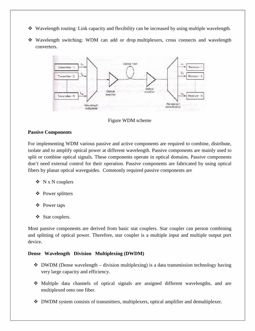
Wavelength routing: Link capacity and flexibility can be increased by using multiple wavelength.

Wavelength switching: WDM can add or drop multiplexers, cross connects and wavelengthconverters.

Figure WDM scheme

Passive Components

For implementing WDM various passive and active components are required to combine, distribute,isolate and to amplify optical power at different wavelength. Passive components are mainly used tosplit or combine optical signals. These components operate in optical domains. Passive componentsdon’t need external control for their operation. Passive components are fabricated by using opticalfibers by planar optical waveguides. Commonly required passive components are

N x N couplers

Power splitters

Power taps

Star couplers.

Most passive components are derived from basic stat couplers. Star coupler can person combiningand splitting of optical power. Therefore, star coupler is a multiple input and multiple output portdevice.

Dense Wavelength Division Multiplexing (DWDM)

DWDM (Dense wavelength – division multiplexing) is a data transmission technology havingvery large capacity and efficiency.

Multiple data channels of optical signals are assigned different wavelengths, and aremultiplexed onto one fiber.

DWDM system consists of transmitters, multiplexers, optical amplifier and demultiplexer.

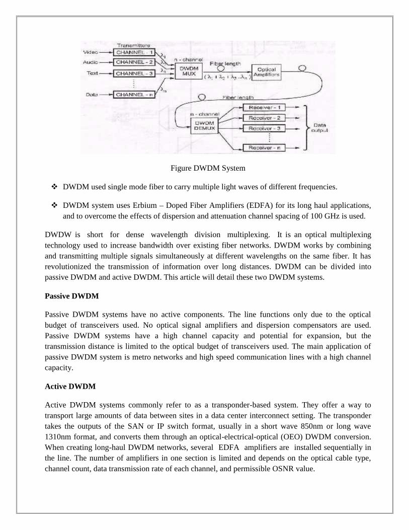
Figure DWDM System

DWDM used single mode fiber to carry multiple light waves of different frequencies.

DWDM system uses Erbium – Doped Fiber Amplifiers (EDFA) for its long haul applications,and to overcome the effects of dispersion and attenuation channel spacing of 100 GHz is used.

DWDW is short for dense wavelength division multiplexing. It is an optical multiplexingtechnology used to increase bandwidth over existing fiber networks. DWDM works by combiningand transmitting multiple signals simultaneously at different wavelengths on the same fiber. It hasrevolutionized the transmission of information over long distances. DWDM can be divided intopassive DWDM and active DWDM. This article will detail these two DWDM systems.

Passive DWDM

Passive DWDM systems have no active components. The line functions only due to the opticalbudget of transceivers used. No optical signal amplifiers and dispersion compensators are used.Passive DWDM systems have a high channel capacity and potential for expansion, but thetransmission distance is limited to the optical budget of transceivers used. The main application ofpassive DWDM system is metro networks and high speed communication lines with a high channelcapacity.

Active DWDM

Active DWDM systems commonly refer to as a transponder-based system. They offer a way totransport large amounts of data between sites in a data center interconnect setting. The transpondertakes the outputs of the SAN or IP switch format, usually in a short wave 850nm or long wave1310nm format, and converts them through an optical-electrical-optical (OEO) DWDM conversion.When creating long-haul DWDM networks, several EDFA amplifiers are installed sequentially inthe line. The number of amplifiers in one section is limited and depends on the optical cable type,channel count, data transmission rate of each channel, and permissible OSNR value.

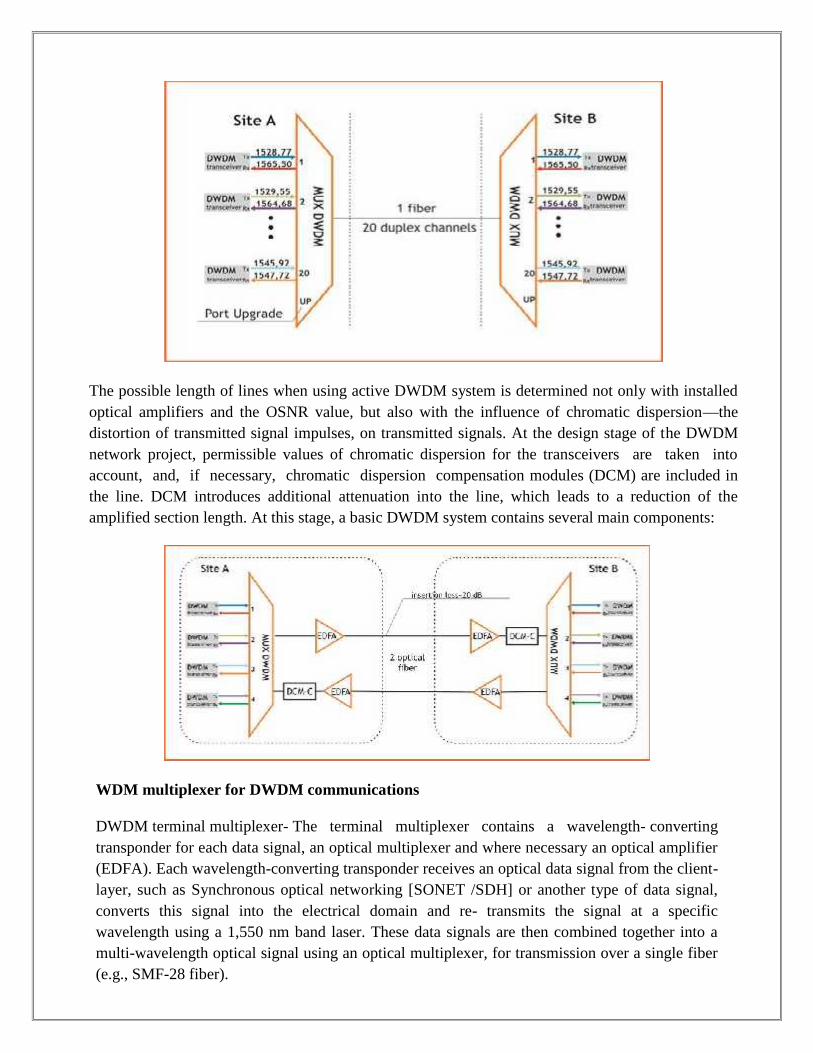
The possible length of lines when using active DWDM system is determined not only with installedoptical amplifiers and the OSNR value, but also with the influence of chromatic dispersion—thedistortion of transmitted signal impulses, on transmitted signals. At the design stage of the DWDMnetwork project, permissible values of chromatic dispersion for the transceivers are taken intoaccount, and, if necessary, chromatic dispersion compensation modules (DCM) are included inthe line. DCM introduces additional attenuation into the line, which leads to a reduction of theamplified section length. At this stage, a basic DWDM system contains several main components:

WDM multiplexer for DWDM communications

DWDM terminal multiplexer- The terminal multiplexer contains a wavelength- convertingtransponder for each data signal, an optical multiplexer and where necessary an optical amplifier(EDFA). Each wavelength-converting transponder receives an optical data signal from the client-layer, such as Synchronous optical networking [SONET /SDH] or another type of data signal,converts this signal into the electrical domain and re- transmits the signal at a specificwavelength using a 1,550 nm band laser. These data signals are then combined together into amulti-wavelength optical signal using an optical multiplexer, for transmission over a single fiber(e.g., SMF-28 fiber).

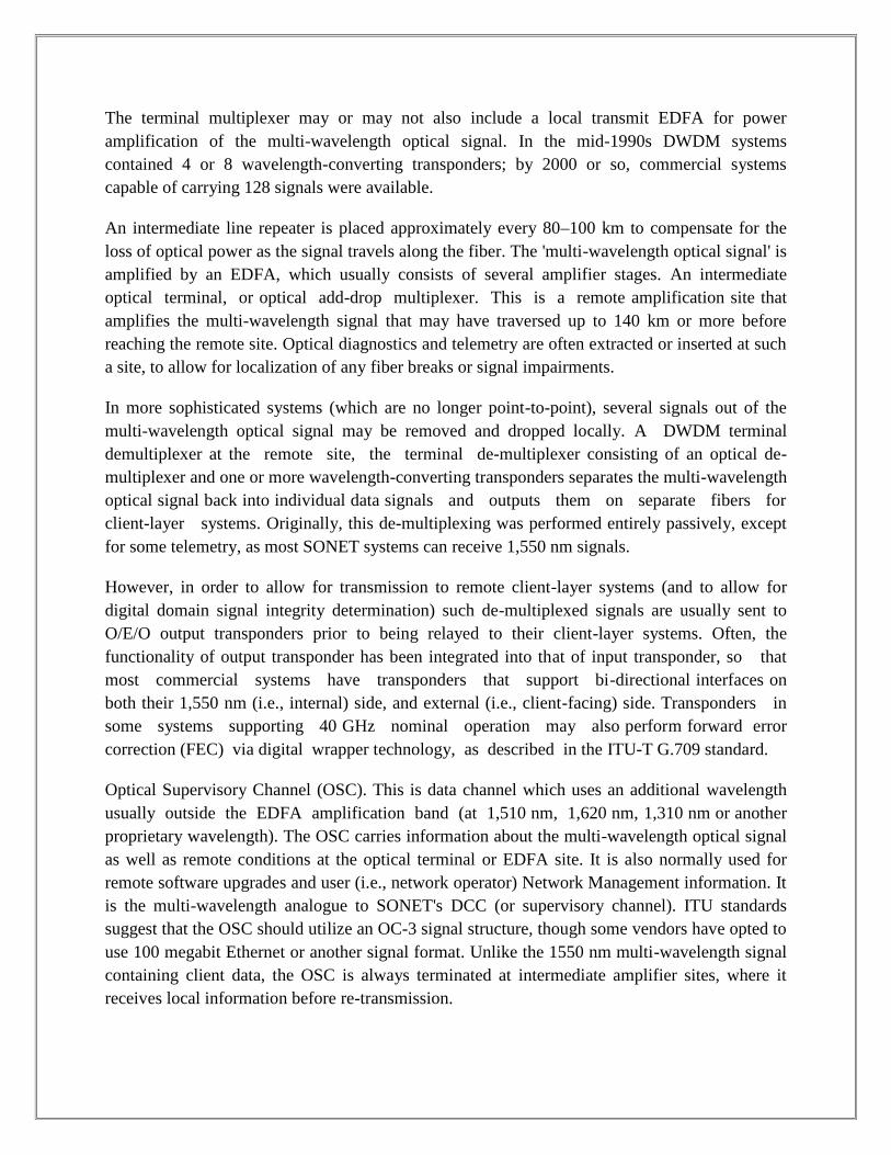
The terminal multiplexer may or may not also include a local transmit EDFA for poweramplification of the multi-wavelength optical signal. In the mid-1990s DWDM systemscontained 4 or 8 wavelength-converting transponders; by 2000 or so, commercial systemscapable of carrying 128 signals were available.

An intermediate line repeater is placed approximately every 80–100 km to compensate for theloss of optical power as the signal travels along the fiber. The 'multi-wavelength optical signal' isamplified by an EDFA, which usually consists of several amplifier stages. An intermediateoptical terminal, or optical add-drop multiplexer. This is a remote amplification site thatamplifies the multi-wavelength signal that may have traversed up to 140 km or more beforereaching the remote site. Optical diagnostics and telemetry are often extracted or inserted at sucha site, to allow for localization of any fiber breaks or signal impairments.

In more sophisticated systems (which are no longer point-to-point), several signals out of themulti-wavelength optical signal may be removed and dropped locally. A DWDM terminaldemultiplexer at the remote site, the terminal de-multiplexer consisting of an optical de-multiplexer and one or more wavelength-converting transponders separates the multi-wavelengthoptical signal back into individual data signals and outputs them on separate fibers forclient-layer systems. Originally, this de-multiplexing was performed entirely passively, exceptfor some telemetry, as most SONET systems can receive 1,550 nm signals.

However, in order to allow for transmission to remote client-layer systems (and to allow fordigital domain signal integrity determination) such de-multiplexed signals are usually sent toO/E/O output transponders prior to being relayed to their client-layer systems. Often, thefunctionality of output transponder has been integrated into that of input transponder, so thatmost commercial systems have transponders that support bi-directional interfaces onboth their 1,550 nm (i.e., internal) side, and external (i.e., client-facing) side. Transponders insome systems supporting 40 GHz nominal operation may also perform forward errorcorrection (FEC) via digital wrapper technology, as described in the ITU-T G.709 standard.

Optical Supervisory Channel (OSC). This is data channel which uses an additional wavelengthusually outside the EDFA amplification band (at 1,510 nm, 1,620 nm, 1,310 nm or anotherproprietary wavelength). The OSC carries information about the multi-wavelength optical signalas well as remote conditions at the optical terminal or EDFA site. It is also normally used forremote software upgrades and user (i.e., network operator) Network Management information. Itis the multi-wavelength analogue to SONET's DCC (or supervisory channel). ITU standardssuggest that the OSC should utilize an OC-3 signal structure, though some vendors have opted touse 100 megabit Ethernet or another signal format. Unlike the 1550 nm multi-wavelength signalcontaining client data, the OSC is always terminated at intermediate amplifier sites, where itreceives local information before re-transmission.

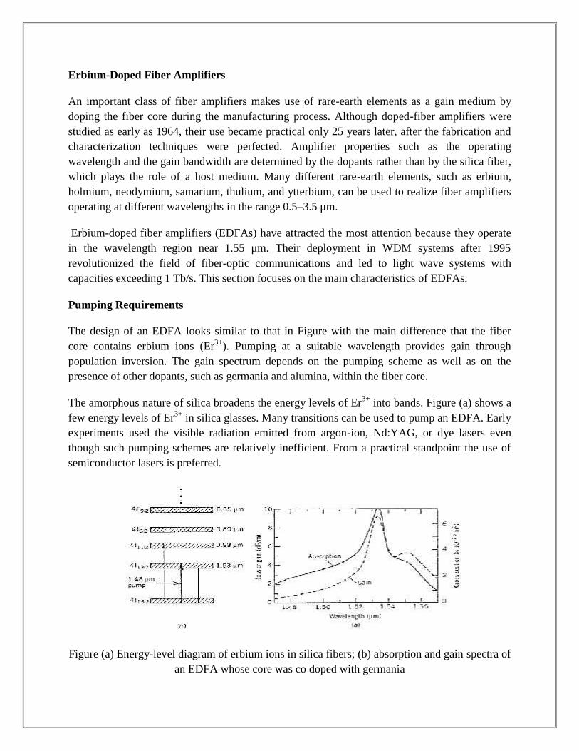
Erbium-Doped Fiber Amplifiers

An important class of fiber amplifiers makes use of rare-earth elements as a gain medium bydoping the fiber core during the manufacturing process. Although doped-fiber amplifiers werestudied as early as 1964, their use became practical only 25 years later, after the fabrication andcharacterization techniques were perfected. Amplifier properties such as the operatingwavelength and the gain bandwidth are determined by the dopants rather than by the silica fiber,which plays the role of a host medium. Many different rare-earth elements, such as erbium,holmium, neodymium, samarium, thulium, and ytterbium, can be used to realize fiber amplifiersoperating at different wavelengths in the range 0.5–3.5 μm.

Erbium-doped fiber amplifiers (EDFAs) have attracted the most attention because they operatein the wavelength region near 1.55 μm. Their deployment in WDM systems after 1995revolutionized the field of fiber-optic communications and led to light wave systems withcapacities exceeding 1 Tb/s. This section focuses on the main characteristics of EDFAs.

Pumping Requirements

The design of an EDFA looks similar to that in Figure with the main difference that the fibercore contains erbium ions (Er3+). Pumping at a suitable wavelength provides gain throughpopulation inversion. The gain spectrum depends on the pumping scheme as well as on thepresence of other dopants, such as germania and alumina, within the fiber core.

The amorphous nature of silica broadens the energy levels of Er3+ into bands. Figure (a) shows afew energy levels of Er3+ in silica glasses. Many transitions can be used to pump an EDFA. Earlyexperiments used the visible radiation emitted from argon-ion, Nd:YAG, or dye lasers eventhough such pumping schemes are relatively inefficient. From a practical standpoint the use ofsemiconductor lasers is preferred.

Figure (a) Energy-level diagram of erbium ions in silica fibers; (b) absorption and gain spectra ofan EDFA whose core was co doped with germania

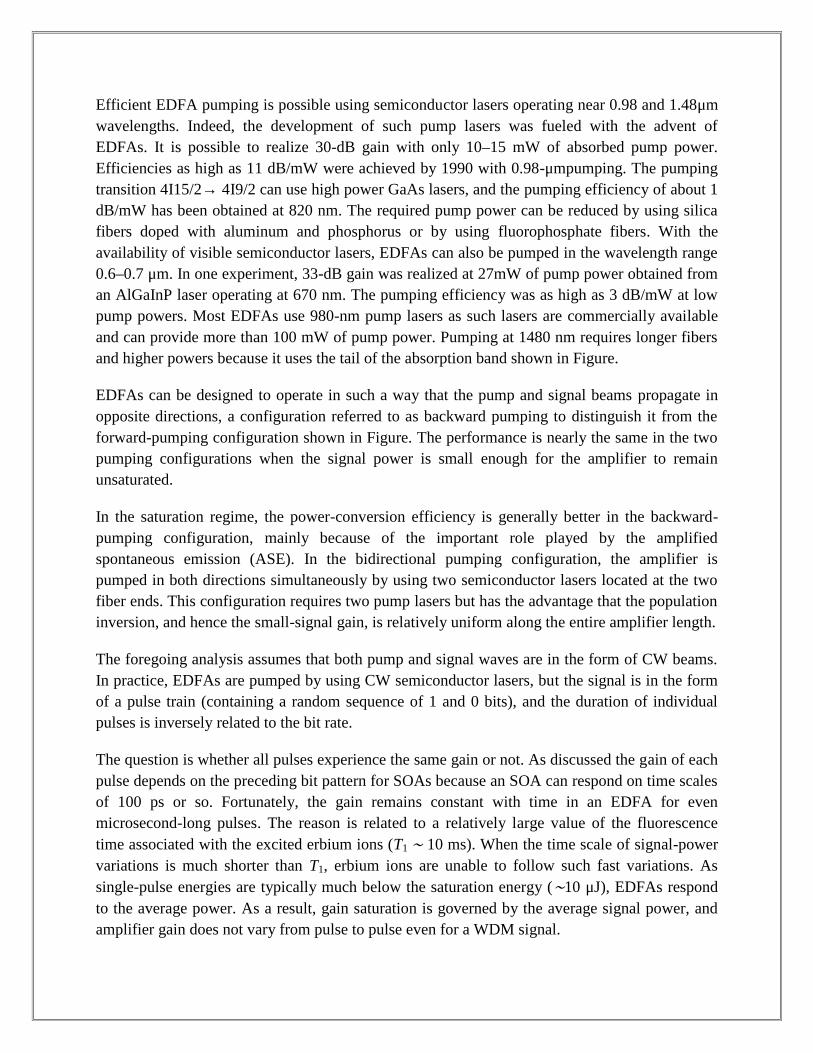
Efficient EDFA pumping is possible using semiconductor lasers operating near 0.98 and 1.48μmwavelengths. Indeed, the development of such pump lasers was fueled with the advent ofEDFAs. It is possible to realize 30-dB gain with only 10–15 mW of absorbed pump power.Efficiencies as high as 11 dB/mW were achieved by 1990 with 0.98-μmpumping. The pumpingtransition 4I15/2→ 4I9/2 can use high power GaAs lasers, and the pumping efficiency of about 1dB/mW has been obtained at 820 nm. The required pump power can be reduced by using silicafibers doped with aluminum and phosphorus or by using fluorophosphate fibers. With theavailability of visible semiconductor lasers, EDFAs can also be pumped in the wavelength range0.6–0.7 μm. In one experiment, 33-dB gain was realized at 27mW of pump power obtained froman AlGaInP laser operating at 670 nm. The pumping efficiency was as high as 3 dB/mW at lowpump powers. Most EDFAs use 980-nm pump lasers as such lasers are commercially availableand can provide more than 100 mW of pump power. Pumping at 1480 nm requires longer fibersand higher powers because it uses the tail of the absorption band shown in Figure.

EDFAs can be designed to operate in such a way that the pump and signal beams propagate inopposite directions, a configuration referred to as backward pumping to distinguish it from theforward-pumping configuration shown in Figure. The performance is nearly the same in the twopumping configurations when the signal power is small enough for the amplifier to remainunsaturated.

In the saturation regime, the power-conversion efficiency is generally better in the backward-pumping configuration, mainly because of the important role played by the amplifiedspontaneous emission (ASE). In the bidirectional pumping configuration, the amplifier ispumped in both directions simultaneously by using two semiconductor lasers located at the twofiber ends. This configuration requires two pump lasers but has the advantage that the populationinversion, and hence the small-signal gain, is relatively uniform along the entire amplifier length.

The foregoing analysis assumes that both pump and signal waves are in the form of CW beams.In practice, EDFAs are pumped by using CW semiconductor lasers, but the signal is in the formof a pulse train (containing a random sequence of 1 and 0 bits), and the duration of individualpulses is inversely related to the bit rate.

The question is whether all pulses experience the same gain or not. As discussed the gain of eachpulse depends on the preceding bit pattern for SOAs because an SOA can respond on time scalesof 100 ps or so. Fortunately, the gain remains constant with time in an EDFA for evenmicrosecond-long pulses. The reason is related to a relatively large value of the fluorescencetime associated with the excited erbium ions (T1 ∼ 10 ms). When the time scale of signal-powervariations is much shorter than T1, erbium ions are unable to follow such fast variations. Assingle-pulse energies are typically much below the saturation energy (∼10 μJ), EDFAs respondto the average power. As a result, gain saturation is governed by the average signal power, andamplifier gain does not vary from pulse to pulse even for a WDM signal.

In some applications such as packet-switched networks, signal power may vary on a time scalecomparable to T1. Amplifier gain in that case is likely to become time dependent, an undesirablefeature from the standpoint of system performance. A gain control mechanism that keeps theamplifier gain pinned at a constant value consists of making the EDFA oscillate at a controlledwavelength outside the range of interest (typically below 1.5 μm). Since the gain remainsclamped at the threshold value for a laser, the signal is amplified by the same factor despitevariations in the signal power. In one implementation of this scheme, an EDFA was forced tooscillate at 1.48 μm by fabricating two fiber Bragg gratings acting as high-reflectivity mirrors atthe two ends of the amplifier.

Multichannel Amplification

The bandwidth of EDFAs is large enough that they have proven to be the optical amplifier ofchoice for WDM applications. The gain provided by them is nearly polarization insensitive.Moreover, the interchannel crosstalk that cripples SOAs because of the carrier-densitymodulation occurring at the channel spacing does not occur in EDFAs. The reason is related tothe relatively large value of T1 (about 10 ms) compared with the carrier lifetime in SOAs (<1ns). The sluggish response of EDFAs ensures that the gain cannot be modulated at frequenciesmuch larger than 10 kHz.

A second source of interchannel crosstalk is cross-gain saturation occurring because the gain of aspecific channel is saturated not only by its own power (self saturation) but also by the power ofneighboring channels. This mechanism of crosstalk is common to all optical amplifiers includingEDFAs. It can be avoided by operating the amplifier in the unsaturated regime. Experimentalresults support this conclusion. In a 1989 experiment negligible power penalty was observedwhen an EDFA was used to amplify two channels operating at 2 Gb/s and separated by 2 nm aslong as the channel powers were low enough to avoid the gain saturation. The main practicallimitation of an EDFA stems from the spectral non uniformity of the amplifier gain. Even thoughthe gain spectrum of an EDFA is relatively broad, as seen in Figure, the gain is far from uniform(or flat) over a wide wavelength range. As a result, different channels of a WDM signal areamplified by different amounts.

This problem becomes quite severe in long-haul systems employing a cascaded chain of EDFAs.The reason is that small variations in the amplifier gain for individual channels growexponentially over a chain of in-line amplifiers if the gain spectrum is the same for all amplifiers.Even a 0.2-dB gain difference grows to 20 dB over a chain of 100 in-line amplifiers, makingchannel powers vary by a factor of 100, an unacceptable variation range in practice. To amplifyall channels by nearly the same amount, the double-peak nature of the EDFA gain spectrumforces one to pack all channels near one of the gain peaks. In a simple approach, input powers ofdifferent channels were adjusted to reduce power variations at the receiver to an acceptable level.

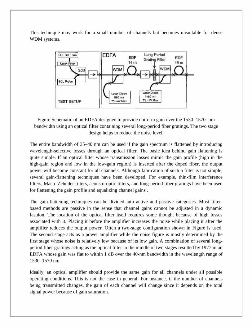
This technique may work for a small number of channels but becomes unsuitable for denseWDM systems.

Figure Schematic of an EDFA designed to provide uniform gain over the 1530–1570- nmbandwidth using an optical filter containing several long-period fiber gratings. The two stage

design helps to reduce the noise level.

The entire bandwidth of 35–40 nm can be used if the gain spectrum is flattened by introducingwavelength-selective losses through an optical filter. The basic idea behind gain flattening isquite simple. If an optical filter whose transmission losses mimic the gain profile (high in thehigh-gain region and low in the low-gain region) is inserted after the doped fiber, the outputpower will become constant for all channels. Although fabrication of such a filter is not simple,several gain-flattening techniques have been developed. For example, thin-film interferencefilters, Mach–Zehnder filters, acousto-optic filters, and long-period fiber gratings have been usedfor flattening the gain profile and equalizing channel gains .

The gain-flattening techniques can be divided into active and passive categories. Most filter-based methods are passive in the sense that channel gains cannot be adjusted in a dynamicfashion. The location of the optical filter itself requires some thought because of high lossesassociated with it. Placing it before the amplifier increases the noise while placing it after theamplifier reduces the output power. Often a two-stage configuration shown in Figure is used.The second stage acts as a power amplifier while the noise figure is mostly determined by thefirst stage whose noise is relatively low because of its low gain. A combination of several long-period fiber gratings acting as the optical filter in the middle of two stages resulted by 1977 in anEDFA whose gain was flat to within 1 dB over the 40-nm bandwidth in the wavelength range of1530–1570 nm.

Ideally, an optical amplifier should provide the same gain for all channels under all possibleoperating conditions. This is not the case in general. For instance, if the number of channelsbeing transmitted changes, the gain of each channel will change since it depends on the totalsignal power because of gain saturation.

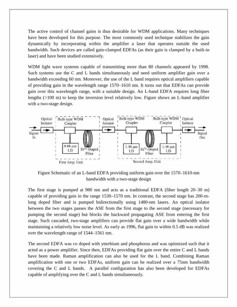
The active control of channel gains is thus desirable for WDM applications. Many techniqueshave been developed for this purpose. The most commonly used technique stabilizes the gaindynamically by incorporating within the amplifier a laser that operates outside the usedbandwidth. Such devices are called gain-clamped EDFAs (as their gain is clamped by a built-inlaser) and have been studied extensively.

WDM light wave systems capable of transmitting more than 80 channels appeared by 1998.Such systems use the C and L bands simultaneously and need uniform amplifier gain over abandwidth exceeding 60 nm. Moreover, the use of the L band requires optical amplifiers capableof providing gain in the wavelength range 1570–1610 nm. It turns out that EDFAs can providegain over this wavelength range, with a suitable design. An L-band EDFA requires long fiberlengths (>100 m) to keep the inversion level relatively low. Figure shows an L-band amplifierwith a two-stage design.

Figure Schematic of an L-band EDFA providing uniform gain over the 1570–1610-nmbandwidth with a two-stage design

The first stage is pumped at 980 nm and acts as a traditional EDFA (fiber length 20–30 m)capable of providing gain in the range 1530–1570 nm. In contrast, the second stage has 200-m-long doped fiber and is pumped bidirectionally using 1480-nm lasers. An optical isolatorbetween the two stages passes the ASE from the first stage to the second stage (necessary forpumping the second stage) but blocks the backward propagating ASE from entering the firststage. Such cascaded, two-stage amplifiers can provide flat gain over a wide bandwidth whilemaintaining a relatively low noise level. As early as 1996, flat gain to within 0.5 dB was realizedover the wavelength range of 1544–1561 nm.

The second EDFA was co doped with ytterbium and phosphorus and was optimized such that itacted as a power amplifier. Since then, EDFAs providing flat gain over the entire C and L bandshave been made. Raman amplification can also be used for the L band. Combining Ramanamplification with one or two EDFAs, uniform gain can be realized over a 75nm bandwidthcovering the C and L bands. A parallel configuration has also been developed for EDFAscapable of amplifying over the C and L bands simultaneously.

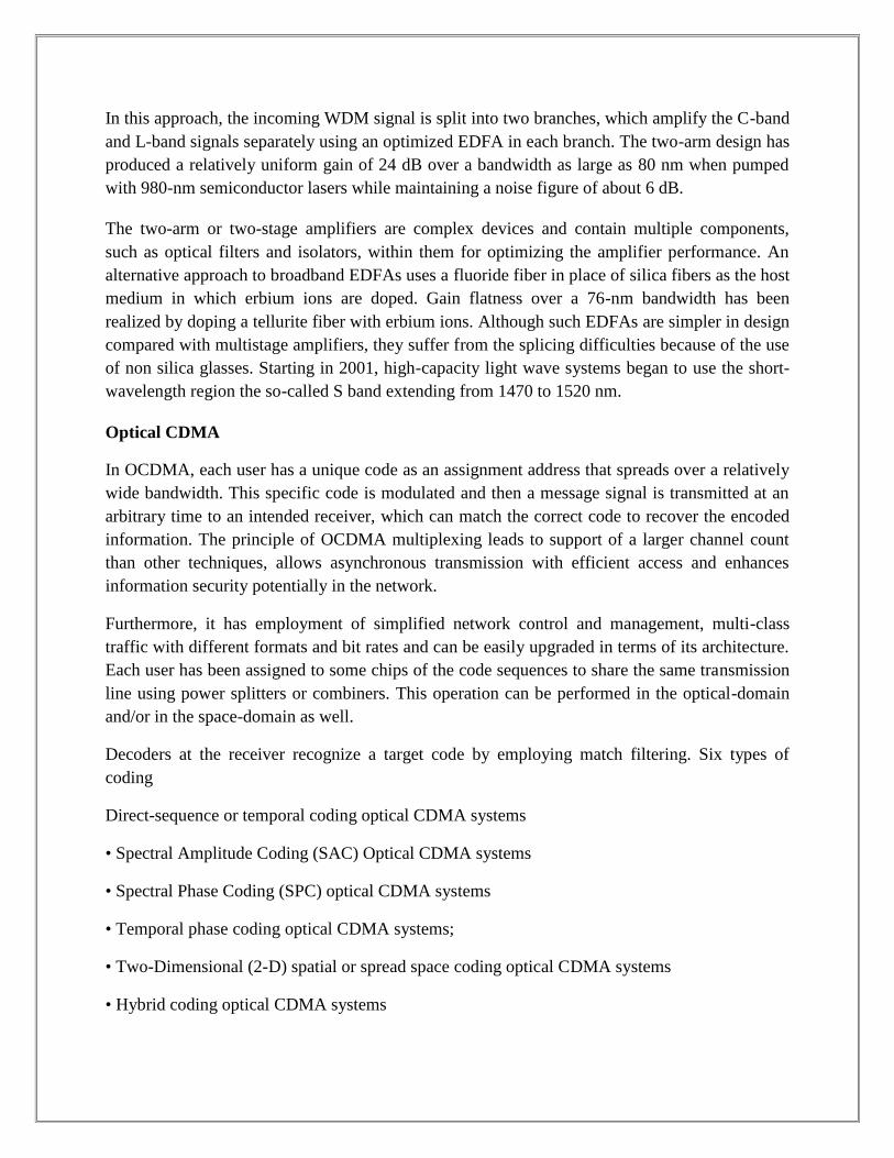
In this approach, the incoming WDM signal is split into two branches, which amplify the C-bandand L-band signals separately using an optimized EDFA in each branch. The two-arm design hasproduced a relatively uniform gain of 24 dB over a bandwidth as large as 80 nm when pumpedwith 980-nm semiconductor lasers while maintaining a noise figure of about 6 dB.

The two-arm or two-stage amplifiers are complex devices and contain multiple components,such as optical filters and isolators, within them for optimizing the amplifier performance. Analternative approach to broadband EDFAs uses a fluoride fiber in place of silica fibers as the hostmedium in which erbium ions are doped. Gain flatness over a 76-nm bandwidth has beenrealized by doping a tellurite fiber with erbium ions. Although such EDFAs are simpler in designcompared with multistage amplifiers, they suffer from the splicing difficulties because of the useof non silica glasses. Starting in 2001, high-capacity light wave systems began to use the short-wavelength region the so-called S band extending from 1470 to 1520 nm.

Optical CDMA

In OCDMA, each user has a unique code as an assignment address that spreads over a relativelywide bandwidth. This specific code is modulated and then a message signal is transmitted at anarbitrary time to an intended receiver, which can match the correct code to recover the encodedinformation. The principle of OCDMA multiplexing leads to support of a larger channel countthan other techniques, allows asynchronous transmission with efficient access and enhancesinformation security potentially in the network.

Furthermore, it has employment of simplified network control and management, multi-classtraffic with different formats and bit rates and can be easily upgraded in terms of its architecture.Each user has been assigned to some chips of the code sequences to share the same transmissionline using power splitters or combiners. This operation can be performed in the optical-domainand/or in the space-domain as well.

Decoders at the receiver recognize a target code by employing match filtering. Six types ofcoding

Direct-sequence or temporal coding optical CDMA systems

• Spectral Amplitude Coding (SAC) Optical CDMA systems

• Spectral Phase Coding (SPC) optical CDMA systems

• Temporal phase coding optical CDMA systems;

• Two-Dimensional (2-D) spatial or spread space coding optical CDMA systems

• Hybrid coding optical CDMA systems

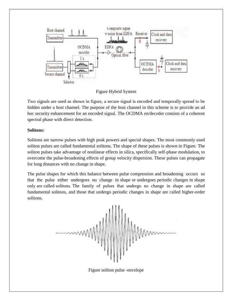
Figure Hybrid System

Two signals are used as shown in figure, a secure signal is encoded and temporally spread to behidden under a host channel. The purpose of the host channel in this scheme is to provide an adhoc security enhancement for an encoded signal. The OCDMA en/decoder consists of a coherentspectral phase with direct detection.

Solitons:

Solitons are narrow pulses with high peak powers and special shapes. The most commonly usedsoliton pulses are called fundamental solitons. The shape of these pulses is shown in Figure. Thesoliton pulses take advantage of nonlinear effects in silica, specifically self-phase modulation, toovercome the pulse-broadening effects of group velocity dispersion. These pulses can propagatefor long distances with no change in shape.

The pulse shapes for which this balance between pulse compression and broadening occurs sothat the pulse either undergoes no change in shape or undergoes periodic changes in shapeonly are called solitons. The family of pulses that undergo no change in shape are calledfundamental solitons, and those that undergo periodic changes in shape are called higher-ordersolitons.

Figure soliton pulse -envelope

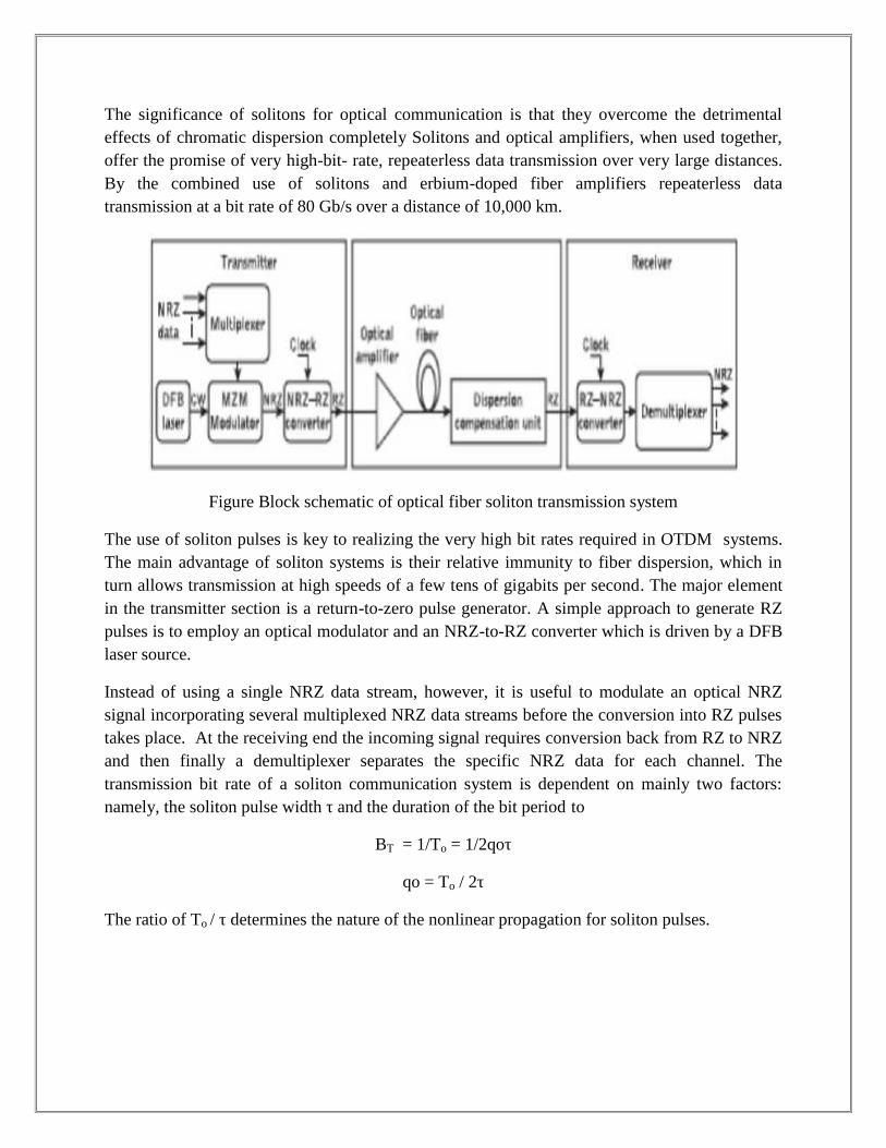
The significance of solitons for optical communication is that they overcome the detrimentaleffects of chromatic dispersion completely Solitons and optical amplifiers, when used together,offer the promise of very high-bit- rate, repeaterless data transmission over very large distances.By the combined use of solitons and erbium-doped fiber amplifiers repeaterless datatransmission at a bit rate of 80 Gb/s over a distance of 10,000 km.

Figure Block schematic of optical fiber soliton transmission system

The use of soliton pulses is key to realizing the very high bit rates required in OTDM systems.The main advantage of soliton systems is their relative immunity to fiber dispersion, which inturn allows transmission at high speeds of a few tens of gigabits per second. The major elementin the transmitter section is a return-to-zero pulse generator. A simple approach to generate RZpulses is to employ an optical modulator and an NRZ-to-RZ converter which is driven by a DFBlaser source.

Instead of using a single NRZ data stream, however, it is useful to modulate an optical NRZsignal incorporating several multiplexed NRZ data streams before the conversion into RZ pulsestakes place. At the receiving end the incoming signal requires conversion back from RZ to NRZand then finally a demultiplexer separates the specific NRZ data for each channel. Thetransmission bit rate of a soliton communication system is dependent on mainly two factors:namely, the soliton pulse width τ and the duration of the bit period to

BT = 1/To = 1/2qoτ

qo = To / 2τ

The ratio of To / τ determines the nature of the nonlinear propagation for soliton pulses.

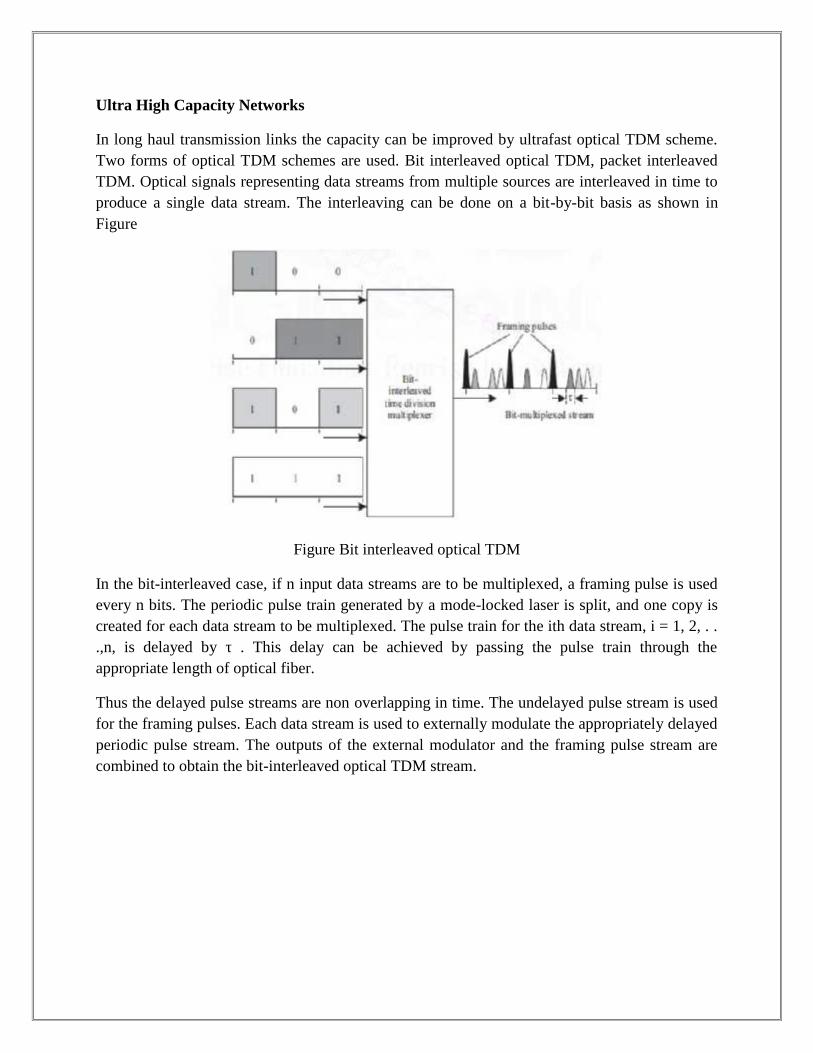
Ultra High Capacity Networks

In long haul transmission links the capacity can be improved by ultrafast optical TDM scheme.Two forms of optical TDM schemes are used. Bit interleaved optical TDM, packet interleavedTDM. Optical signals representing data streams from multiple sources are interleaved in time toproduce a single data stream. The interleaving can be done on a bit-by-bit basis as shown inFigure

Figure Bit interleaved optical TDM

In the bit-interleaved case, if n input data streams are to be multiplexed, a framing pulse is usedevery n bits. The periodic pulse train generated by a mode-locked laser is split, and one copy iscreated for each data stream to be multiplexed. The pulse train for the ith data stream, i = 1, 2, . ..,n, is delayed by τ . This delay can be achieved by passing the pulse train through theappropriate length of optical fiber.

Thus the delayed pulse streams are non overlapping in time. The undelayed pulse stream is usedfor the framing pulses. Each data stream is used to externally modulate the appropriately delayedperiodic pulse stream. The outputs of the external modulator and the framing pulse stream arecombined to obtain the bit-interleaved optical TDM stream.

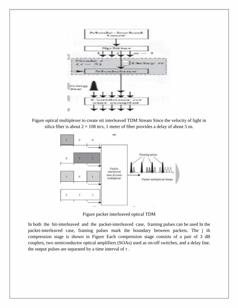
Figure optical multiplexer to create nit interleaved TDM Stream Since the velocity of light insilica fiber is about 2 × 108 m/s, 1 meter of fiber provides a delay of about 5 ns.

Figure packet interleaved optical TDM

In both the bit-interleaved and the packet-interleaved case, framing pulses can be used In thepacket-interleaved case, framing pulses mark the boundary between packets. The j thcompression stage is shown in Figure Each compression stage consists of a pair of 3 dBcouplers, two semiconductor optical amplifiers (SOAs) used as on-off switches, and a delay line.the output pulses are separated by a time interval of τ .

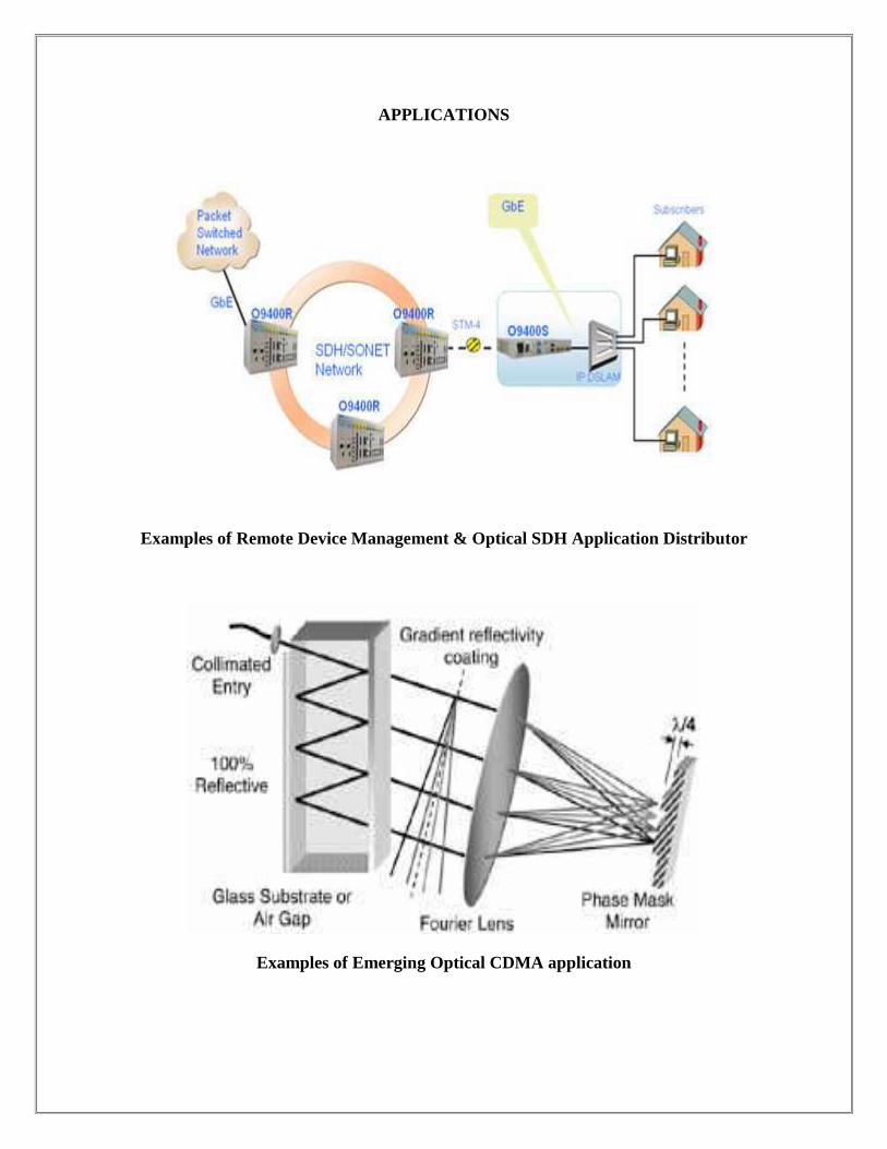
APPLICATIONS

Examples of Remote Device Management & Optical SDH Application Distributor

Examples of Emerging Optical CDMA application

POST TEST-MCQ TYPE

1. Each stage of information transfer is required to follow the fundamentals ofa) Optical interconnectionb) Optical hibernationc) Optical networkingd) Optical regeneration

2. What is a multi-functional element of optical network?a) Hopb) Optical nodec) Wavelengthd) Optical attenuation

3. A signal carried on a dedicated wavelength from source to destination node is known as aa) Light pathb) Light wavec) Light noded) Light source

4. The fundamentals of optical networking are divided into _______ areas.a) Twob) Onec) Fourd) Three

5. The optical networking fundamentals are _____________ of the transmission techniques.a) Dependentb) Independentc) Similard) Dissimilar

6. What are the array of switches which forms circuit switching fabrics?a) Packet arraysb) Optical cross connectsc) Circuit arraysd) Optical networks

7. Which of the following is an example of a static circuit-switched network?a) OXCb) Circuit regeneratorc) Packet resolverd) SDH/SONET

8. What is the main disadvantage of OCS?a) Regenerating mechanismb) Optical sessionc) Time permitd) Disability to handle burst traffic

9. Optical electro-conversions takes place in _________________ networks.a) Sessionalb) Optical packet-switchedc) Optical circuit-switchedd) Circular

10. How many functions are performed by an optical packet switch?a) Fourb) Threec) Twod) One

11. Which provides data storage for packets to resolve contention problems?a) Switchingb) Routingc) Bufferingd) Reversing

12. What is usually required by a packet to ensure that the data is not overwritten?a) Headerb) Footerc) Guard bandd) Payload

13. Which of the following provides efficient designation, routing, forwarding, switching oftraffic through an optical packet-switched network?a) Label correlationb) Multiprotocol label switchingc) Optical correlationd) Routing

14. Electrical devices in optical network are basically used for _____________a) Signal degradationb) Node transferc) Signal controld) Amplification

15. A ____________ digital hierarchy was required to enable the internationalcommunications network to evolve in the optical fiber era.a) Asynchronousb) Dedicatedc) Seismicd) Synchronous

16. Which is a packetized multiplexing and switching technique which combines the benefitsof circuit and packet switching?a) Synchronous modeb) Asynchronous transfer modec) Circuit packetd) Homogeneous mode

17. An advanced type of reconfigurable OTN is referred to as an _______________a) Automatic OTNb) Auto-generated photonc) Automatically switched optical networkd) Optical reimbursement

18. The mapping of IP frames in SDH/SONET is accomplished in ___________ stages.a) Fourb) Twoc) Threed) One

19. Which supports a great number of wavelength channels and reduces the number ofswitches within the optical network?a) Waveband switchingb) Optical remunerationc) Optical genesisd) Wavelength multiplexing

20. The routing and wavelength assignment problem addresses the core issue ofa) Traffic patterns in a networkb) Wavelength adjustmentc) Wavelength continuity constraintd) Design problem

21. How many techniques of implementation are there for routing wavelength assignment(RWA)?a) Twob) Sixc) Threed) Four

22. The ___________ provides information about the physical path and wavelengthassignment for all active light paths.a) Network stateb) RWAc) LAN topologyd) Secluded communication protocol

23. Which is a network that connects several regional or national networks together?a) Long-haul networkb) Domain networkc) Short-haul networkd) Erbium network

24. What is the range of transmission of extended long haul network?a) 200-400 kmb) 600-1000 kmc) 1000-2000 kmd) 2000-4000 km

25. What is the range of transmission of ultra-long haul network?a) 200-400 kmb) 600-1000 kmc) 1000-2000 kmd) 2000-4000 km

26. Which feature plays an important role in making the longer haul networks feasible?a) Channelingb) Forward error controlc) Backward error controld) Interconnection

27. Which of the following is not an element of a submerged cable system?a) Repeaterb) Branching unitc) Gain equalizerd) Attenuator

28. Which provides interconnection between the United States and European countries?a) TATb) WTEc) PFEd) POP

29. A single fiber in TAT-14 can carry _________ wavelength channels.a) Oneb) Twelvec) Sixteend) Ten

30. Optical MAN’S are usually structured in _______ topologies.a) Ringb) Busc) Meshd) Star

31. What is the exception in the similarities between the optical Ethernet and the EthernetLAN?a) Physical layerb) Data-link layerc) Refractive indexd) Attenuation mechanism

32. Which technology is used by optical Ethernet?a) GP-technologyb) HJ-technologyc) IP-technologyd) GB-technology

33. Optical Ethernet can operate at the transmission rates as low asa) 10 M bits per secondb) 40 M bits per secondc) 100 M bits per secondd) 1000 M bits per second

34. How many types of optical Ethernet connections are developed?a) Twob) Onec) Fourd) Three

35. Which type of connection can be used as an Ethernet switch?a) Point-to-pointb) Multipoint-to-multipointc) Multipoint-to-pointd) Point-to-multipoint

36. The _______________ provides point-to-point access to a bidirectional single-modeoptical fiber.a) Optical regeneratorb) Optical sessionc) Optical distribution noded) Optical buffer

37. The ___________ protocol is not used when the Ethernet connections are configured fora full duplex operation.a) TCP/IPb) MACc) CSMA/CDd) DTH

38. Optical Ethernet provides switching capabilities in layersa) 1 and 2b) 2 and 3c) 3 and 4d) 1 and 4

39. The more advantages optical amplifier isa) Fiber amplifierb) Semiconductor amplifierc) Repeatersd) Mode hooping amplifier

40. Which of the following cannot be used for wideband amplification?a) Semiconductor optical amplifierb) Erbium-doped fiber amplifierc) Raman fiber amplifierd) Brillouin fiber amplifier

41. Which of the following is used preferably for channel selection in a WDM system?a) Semiconductor optical amplifierb) Erbium-doped fiber amplifierc) Raman fiber amplifierd) Brillouin fiber amplifier

42. For used in single-mode fiber __________ are used preferably.a) Semiconductor optical amplifierb) Erbium-doped fiber amplifierc) Raman fiber amplifierd) Brillouin fiber amplifier

43. _______________ is superior as compared to _________________a) TWA, FPAb) FPA, TWAc) EDFA, FPAd) FPA, EDFA

44. Signal amplification is obtained ina) Erbium-doped fluoro-zir-carbonate fiber multimodeb) Rare-earth-doped fiber amplifiersc) Raman fiber systemsd) Brillouin fiber amplifier

45. Which is constructed using erbium-doped glass?a) Erbium-based micro fiber amplifierb) Rare-earth-doped fiber amplifiersc) Raman fiber systemsd) Brillouin fiber amplifier

46. In _____________ Rayleigh scattering can be reduced.a) An erbium-based micro fiber amplifierb) Rare-earth-doped fiber amplifiersc) Raman fiber systemsd) Distributed Raman amplification

47. Which is defined as a process by which the wavelength of the transmitted signal ischanged without altering the data carried by the signal?a) Wavelength conversionb) Attenuationc) Sigma managementd) Wavelength dispersion

48. The device which is used to perform wavelength conversion is called asa) Attenuatorb) Wavelength Gyratorc) Wavelength Circulatord) Wavelength translator

49. The ___________ converters cannot process different modulation formats.a) Shiftingb) Optoelectronic wavelengthc) Opt-circulard) Magnetic simulating

50. Which of the following is NOT an application of optical amplifier?a) Power amplifierb) In-line repeater amplifierc) Demodulatord) Preamplifier

51. What is the typical range of the noise figure?a) 1 – 2 dBb) 3 – 5 dBc) 7 – 11 dBd) 12 – 14 dB

52. A major attribute of coherent optical transmission was its ability to provide_______________ for future multicarrier systems and networks.a) Attenuationb) Dispersionc) Frequency selectivityd) Noisy carriers

53. A multicarrier modulation format in which there has been growing interest to compensatefor impairments in optical fiber transmission systems isa) OFDMb) EDMc) WDMd) ADM

54. WDM stands for?a) Wave division multiplexingb) Wavelength division multiplexingc) Wavelength dependent multiplexingd) Wave dependent multiplexing

55. A technique that can be a solution to the problem of synchronizing data sources.a) framingb) data link controlc) full link controld) pulse stuffing

56. Wavelength Division Multiplexing (WDM) is an analog multiplexing technique tocombinea) magnetic signalsb) electromagnetic signalsc) digital signalsd) optical signals

57. EDFAs generally operate in the wavelength region neara) 1550 nm and can offer capacities exceeding 1000 Gbps.b) 850 nm and can offer capacities around 100 Gbps.c) 1150 nm and can offer capacities around 1000 Gbps.d) 1550 nm and can offer capacities around 100 Gbps.

58. Which wavelength is the most appropriate one for pumping an EDFA?a) 850 nmb) 980 nmc) 1300 nmd) 1550 nm

59. The main difference between an SOA and an EDFA is thata) An SOA operates in the electrical domain, whereas the EDFA operates in the optical

domain.b) An SOA is pumped electrically, whereas the EDFA is pumped optically.c) An SOA is pumped optically, whereas the EDFA is pumped electrically.d) An SOA amplifies 1300 nm wavelength, whereas the EDFA amplifies 1550 nm.

60. Which band specifies the operation of EDFA?a) O bandb) X bandc) C bandd) S band

61. Basically, Solitons are pulses which propagate through the fiber without showing anyvariation ina) Amplitudeb) Shapec) Velocityd) All of the above

62. DWDM stands fora) Digital Wavelength-Division Modulationb) Dense Wavelength-Division Modulationc) Double Wavelength-Division Modulationd) Dense Wavelength-Division Multiplexing

63. In SONET, OC-1 stands fora) Optical Carrier level oneb) Optical Coupler unidirectionalc) Optical Channel oned) Optical Cable type 1

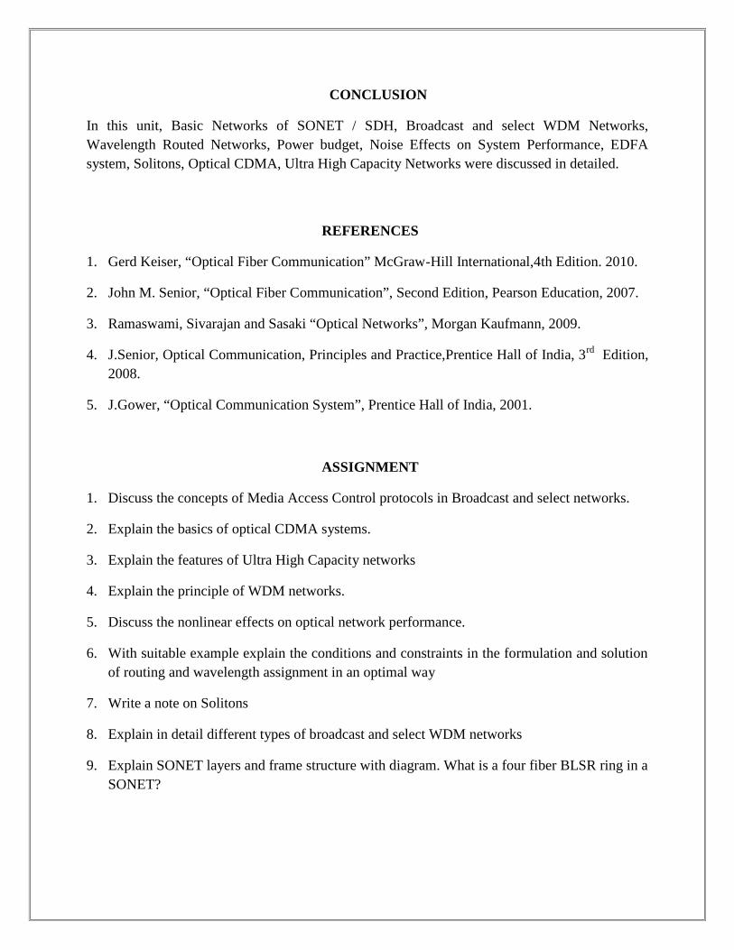
CONCLUSION

In this unit, Basic Networks of SONET / SDH, Broadcast and select WDM Networks,Wavelength Routed Networks, Power budget, Noise Effects on System Performance, EDFAsystem, Solitons, Optical CDMA, Ultra High Capacity Networks were discussed in detailed.

REFERENCES

1. Gerd Keiser, “Optical Fiber Communication” McGraw-Hill International,4th Edition. 2010.

2. John M. Senior, “Optical Fiber Communication”, Second Edition, Pearson Education, 2007.

3. Ramaswami, Sivarajan and Sasaki “Optical Networks”, Morgan Kaufmann, 2009.

4. J.Senior, Optical Communication, Principles and Practice,Prentice Hall of India, 3rd Edition,2008.

5. J.Gower, “Optical Communication System”, Prentice Hall of India, 2001.

ASSIGNMENT

1. Discuss the concepts of Media Access Control protocols in Broadcast and select networks.

2. Explain the basics of optical CDMA systems.

3. Explain the features of Ultra High Capacity networks

4. Explain the principle of WDM networks.

5. Discuss the nonlinear effects on optical network performance.

6. With suitable example explain the conditions and constraints in the formulation and solutionof routing and wavelength assignment in an optimal way

7. Write a note on Solitons

8. Explain in detail different types of broadcast and select WDM networks

9. Explain SONET layers and frame structure with diagram. What is a four fiber BLSR ring in aSONET?