Embed Size (px)
Citation preview
Advanced Optical Wireless Communication Systems
Optical wireless communications is a dynamic area of research and development. Com-bining fundamental theory with a broad overview, this book is an ideal reference for any-one working in the field, as well as a valuable guide for self-study. It begins by describingimportant issues in optical wireless theory, including coding and modulation techniquesfor optical wireless, wireless optical CDMA communication systems, equalization andMarkov chains in cloud channels, and optical MIMO systems, as well as explainingkey issues in information theory for optical wireless channels. The next part describesunique channels that could be found in optical wireless applications, such as NLOS UVatmospheric scattering channels, underwater communication links, and a combinationof hybrid RF/optical wireless systems. The final part describes applications of opticalwireless technology, such as quantum encryption, visible light communication, IR links,and sensor networks, with step-by-step guidelines to help reduce design time and cost.
Shlomi Arnon is an Associate Professor at the Department of Electrical and ComputerEngineering at Ben-Gurion University (BGU), Israel, and the Principal Investigator ofIsrael Partnership with NASA LUNAR Science Institute. In addition to research, Pro-fessor Arnon and his students work on many challenging engineering projects withemphasis on the humanitarian dimension, such as developing a system to detect humansurvival after earthquakes, or an infant respiration monitoring system to prevent cardiacarrest and apnea.
John R. Barry is a Professor of Telecommunications in the School of Electrical andComputer Engineering at the Georgia Institute of Technology. He is a coauthor of Dig-ital Communication (2004), and Iterative Timing Recovery: A Per-Survivor Approach(VDM, 2009), and he is the author of Wireless Infrared Communications (1994).
George K. Karagiannidis is an Associate Professor of Digital Communications Systemsin the Electrical and Computer Engineering Department, and Head of the Telecommu-nications Systems and Networks Laboratory, at Aristotle University of Thessaloniki. Heis co-recipient of the Best Paper Award of the Wireless Communications Symposium(WCS) in the IEEE International Conference on Communications (ICC’07).
Robert Schober is a Professor and Canada Research Chair in Wireless Communica-tions at the University of British Columbia (UBC), Vancouver, Canada. He has receivednumerous awards, including best paper awards from the German Information Technol-ogy Society (ITG), the European Association for Signal, Speech and Image Processing(EURASIP), IEEE ICUWB 2006, the International Zurich Seminar on BroadbandCommunications, and European Wireless 2000.
Murat Uysal is an Associate Professor at Özyegin University, Istanbul, where he leadsthe Communication Theory and Technologies (CT&T) Research Group. Dr. Uysal is therecipient of several awards including the NSERC Discovery Accelerator SupplementAward, University of Waterloo Engineering Research Excellence Award, and the TUBADistinguished Young Scientist Award.

Advanced Optical WirelessCommunication Systems
Edited by
SHLOMI ARNONBen-Gurion University (BGU), Israel
JOHN R. BARRYGeorgia Institute of Technology, USA
GEORGE K. KARAGIANNID ISAristotle University of Thessaloniki, Greece
ROBERT SCHOBERUniversity of British Columbia (UBC), Canada
MURAT UYSALÖzyegin University, Turkey

C A M B R I D G E U N I V E R S I T Y P R E S S
Cambridge, New York, Melbourne, Madrid, Cape TownSingapore, São Paulo, Delhi, Mexico City
Cambridge University PressThe Edinburgh Building, Cambridge CB2 8RU, UK
Published in the United States of America by Cambridge University Press, New York
www.cambridge.orgInformation on this title: www.cambridge.org/9780521197878
c© Cambridge University Press 2012
This publication is in copyright. Subject to statutory exceptionand to the provisions of relevant collective licensing agreements,no reproduction of any part may take place without the writtenpermission of Cambridge University Press.
First published 2012
Printed in the United Kingdom at the University Press, Cambridge
A catalog record for this publication is available from the British Library
ISBN 978-0-521-19787-8 hardback
Cambridge University Press has no responsibility for the persistence oraccuracy of URLs for external or third-party internet websites referred toin this publication, and does not guarantee that any content on suchwebsites is, or will remain, accurate or appropriate.
Contents
List of contributors page x
Part I Outlook 1
1 Introduction 3Shlomi Arnon, John Barry, George Karagiannidis, Robert Schober, and Murat Uysal
Part II Optical wireless communication theory 9
2 Coded modulation techniques for optical wireless channels 11Ivan B. Djordjevic
2.1 Atmospheric turbulence channel modeling 122.2 Codes on graphs 132.3 Coded-MIMO free-space optical communication 192.4 Raptor codes for temporally correlated FSO channels 262.5 Adaptive modulation and coding (AMC) for FSO
communications 292.6 Multidimensional coded modulation for FSO communications 352.7 Free-space optical OFDM communication 382.8 Heterogeneous optical networks (HONs) 432.9 Summary 48Acknowledgments 49References 49
3 Wireless optical CDMA communication systems 54Jawad A. Salehi, Babak M. Ghaffari, and Mehdi D. Matinfar
3.1 Introduction 543.2 OCDMA system description 553.3 Indoor wireless optical CDMA LAN 593.4 Free-space optical CDMA systems 683.5 Modulation 753.6 Experimental prototypes 81
vi Contents
Acknowledgment 84References 84
4 Pointing error statistics 87Shlomi Arnon
References 89
5 Equalization and Markov chains in cloud channel 90Mohsen Kavehrad
5.1 Introduction 915.2 Channel propagation modeling 925.3 Modeling results and eigen analyses 995.4 Equalization related issues 1035.5 Summary and conclusions 112Acknowledgment 113References 113
6 Multiple-input multiple-output techniques for indoor optical wirelesscommunications 116Steve Hranilovic
6.1 Indoor OW MIMO channel characteristics 1176.2 MIMO for diffuse OW channels 1196.3 Spot-diffusing OW MIMO systems 1236.4 Point-to-Point OW MIMO communications 1276.5 Future directions 138References 139
7 Channel capacity 146Amos Lapidoth, Stefan M. Moser, and Michèle Wigger
7.1 Introduction and channel models 1467.2 Capacity results 1507.3 Proof techniques 163References 172
Part III Unique channels 175
8 Modeling and characterization of ultraviolet scattering communication channels 177Haipeng Ding, Brian M. Sadler, Gang Chen, and Zhengyuan Xu
8.1 Introduction 1778.2 Single scattering models 181
Contents vii
8.3 Multiple scattering models 1838.4 NLOS UV channel measurement systems 1898.5 Numerical and experimental results 1928.6 Summary 198References 199
9 Free-space optical communications underwater 201Brandon Cochenour and Linda Mullen
9.1 Introduction: towards a link equation 2019.2 Introduction to ocean optics 2029.3 Channel characterization: theory 2139.4 Experimental research in wireless optical communications underwater 2189.5 System design for uFSO links 2289.6 Summary 236References 237
10 The optical wireless channel 240Roger Green and Mark Leeson
10.1 Introduction 24010.2 System configurations 24110.3 Optical sources 24210.4 Optical detectors 24410.5 Optical filters 24510.6 Nature of the optical wireless channel 24710.7 Interference sources 24810.8 Impact of interference on BER 25110.9 Channel impulse response 25310.10 Hardware aspects of the receiver-amplifier in the
indoor channel environment 25510.11 Modulation schemes for optical wireless 26310.12 Optics for optical wireless 26710.13 Concluding remarks 268References 269
11 Hybrid RF/FSO communications 273Nick Letzepis and Albert Guillén i Fàbregas
11.1 Introduction 27311.2 Channel model 27511.3 Information-theoretic preliminaries 28111.4 Uniform power allocation 28711.5 Power allocation 29211.6 Conclusions and summary 295
viii Contents
Appendix A Kullback–Leibler divergence between Poisson and Gaussiandistributions 297
Appendix B Derivative of the mutual information for discrete-input Poissonchannels 297
Acknowledgments 299References 299
Part IV Applications 303
12 Quantum key distribution 305Rupert Ursin, Nathan Langford and Andreas Poppe
12.1 Motivation 30512.2 Security considerations of QKD 30612.3 QKD protocols 30812.4 Technical implementation of a free-space setup 31212.5 QKD networks 319References 326
13 Optical modulating retro-reflectors 328William Rabinovich
13.1 Introduction 32813.2 Modulating retro-reflector link budgets 33013.3 The optical retro-reflector 33213.4 The optical modulator 33413.5 Modulating retro-reflector applications and field demonstrations 34113.6 Conclusion 347References 347
14 Visible-light communications 351Kang Tae-Gyu
14.1 VLC principle 35114.2 VLC standards 35414.3 VLC research and development 35914.4 VLC applications 36114.5 Future work 367References 367
15 Optical wireless in sensor networks 369Dominic C. O’Brien and Sashigaran Sivathasan
15.1 Introduction 36915.2 Free-space optical (FSO) sensor network 371

Contents ix
15.3 Radio frequency/Free-space optical (RF/FSO) sensor network system 37815.4 Conclusions 38315.5 Acknowledgments 384References 384
Index 388

Contributors
Shlomi ArnonBen Gurion University of the Negev, Israel
John R. BarryGeorgia Institute of Technology
Gang ChenUniversity of California
Brandon CochenourNaval Air Systems Command (NAVAIR), USA
Haipeng DingUniversity of California
Ivan DjordjevicUniversity of Arizona
Babak M. GhaffariSharif University of Technology, Iran
Roger GreenUniversity of Warwick
Steve HranilovicMcMaster University, Canada
Albert G. i FàbregasUniversity of Cambridge
Mohsen KavehradPennsylvania State University
George K. KaragiannidisAristotle University of Thessaloniki, Greece
Nathan LangfordUniversity of Oxford
Amos LapidothETH Zurich
List of contributors xi
Nick LetzepisDefence Science and Technology Organisation, Australia
Mark LeesonUniversity of Warwick
Mehdi D. MatinfarSharif University of Technology, Iran
Stefan M. MoserNational Chiao Tung University, Taiwan
Linda MullenNaval Air Systems Command (NAVAIR), USA
Dominic O’BrienUniversity of Oxford
Andreas PoppeAIT Austrian Institute of Technology GmbH
William RabinovichUS Naval Research Laboratory
Brian M. SadlerArmy Research Laboratory, USA
Jawad A. SalehiSharif University of Technology, Iran
Robert SchoberUniversity of British Columbia, Canada
Sashigaran SivathasanCurtin University of Technology, Malaysia
Rupert UrsinInstitute for Quantum Optics and Quantum Information (IQOQI),Austrian Academy of Sciences
Kang Tae-GyuElectronics and Telecommunications Research Institute (ETRI), South Korea
Murat UysalÖzyegin University, Turkey
Michèle WiggerTélécom ParisTech, France
Zhengyuan XuUniversity of California


Part I
Outlook

1 IntroductionShlomi Arnon, John Barry, George Karagiannidis, Robert Schober,and Murat Uysal
Optical wireless communication is an emerging and dynamic research and developmentarea that has generated a vast number of interesting solutions to very complicatedcommunication challenges. For example, high data rate, high capacity and minimuminterference links for short-range communication for inter-building communication,computer-to-computer communication, or sensor networks. At the opposite extreme isa long-range link in the order of millions of kilometers in the new mission to Marsand other solar system planets. It is important to mention that optical wireless com-munication is one of the oldest methods that humanity has used for communication. Inprehistoric times humans used fire and smoke to communicate; later in history, Romanoptical heliographs and Sumerians signalling towers were the communication systemsof these empires. An analogous technology was used by Napoleonic Signalling Towersand “recently” by the light photo-phone of Alexander Graham Bell back in the 1880s.
Obviously, the data rate, quality of service delivered, and transceiver technologiesemployed have improved greatly from those early optical wireless technologies. In itsmany applications, optical wireless communication links have already succeeded inbecoming part of our everyday lives at our homes and offices. Optical wireless productsare already well familiar, ranging from visible-light communication (VLC), TV remotecontrol to IrDA ports that currently have a worldwide installed base of hundreds of mil-lion of units with tens of percent annual growth. Optical wireless is also widely availableon personal computers, peripherals, embedded systems and devices of all types, terres-trial and in-building optical wireless LANs, network of sensors, and inter-satellite linkapplications.
The book includes three main parts: Part II Optical wireless communication theory,Part III Unique channels, and Part IV Applications.
Part II describes important issues in optical wireless theory starting with Chap-ter 2 about coding and modulation techniques for optical wireless channels by IvanB. Djordjevic. The author explains that the communication over the FSO channel isachieved through the line-of-sight (LOS) between two distant transceivers. An opti-cal wave propagating over the FSO channel experiences fluctuations in amplitude andphase due to atmospheric turbulence, which represents a fundamental problem presenteven under clear sky conditions. In this chapter, several coded modulation concepts
Advanced Optical Wireless Communication Systems, ed. Shlomi Arnon, John R. Barry, George K.Karagiannidis, Robert Schober, and Murat Uysal. Published by Cambridge University Press.c© Cambridge University Press 2012.
4 S. Arnon, J. Barry, G. Karagiannidis, R. Schober, and M. Uysal
enabling communication over strong atmospheric turbulence channels are described:(i) coded-multiple-input multiple-output (MIMO), (ii) raptor coding, (iii) adaptivemodulation and coding (AMC), (iv) multidimensional coded modulation, and (v) coded-orthogonal frequency division multiplexing (OFDM). Furthermore, the concept ofheterogeneous optical networking is discussed. Chapter 3 titled “Wireless opticalCDMA communication systems” by Jawad A. Salehi, Babak M. Ghaffari, and MehdiD. Matinfar, describes a particular and advanced form of optical wireless communica-tion systems, namely optical code-division multiple-access (OCDMA), in the context ofwireless optical systems. As wireless optical communication systems gets more matureand become viable for multi-user communication systems, advanced multiple-accesstechniques become more important and attractive in such systems. Among all multiple-access techniques in optical domain, OCDMA is of utmost interest because of itsflexibility, ease of implementation, no need for synchronization among many users andsoft traffic handling capability. The deployment of OCDMA communication systems inboth indoor and outdoor free-space optical links is also analyzed. Chapter 4 is “Pointingerror statistics” by Shlomi Arnon. In this chapter the author presents a simple modelthat describes the effect of the statistic of the pointing error on the performance of com-munication systems. Chapter 5 is “Equalization and Markov chains in cloud channel”by M. Kavehrad. The focus of this chapter is on investigating the possibility of simpli-fying the task of calculating the performances in cloud channel by a direct extraction ofstate transition matrices associated with standard Markov modeling from the MCRTcomputer simulations programs. Chapter 6 by Steve Hranilovic considers multiple-input multiple-output (MIMO) techniques employing a number of optical sources astransmitters and a collection of photodiodes as receivers for indoor optical wireless(OW) channels. The OW MIMO systems discussed in this chapter differ fundamen-tally from those used in radio channels. In particular, the signalling constraints imposedby intensity-modulated/direct-detection (IM/DD) systems limit the direct application oftheory from radio channels. Nonetheless, MIMO techniques can be applied to OW chan-nels to yield improvements in reliability and to improve data rates. This chapter startswith a brief overview of the characteristics of indoor OW MIMO systems. Given that theapplication and available gains depend on channel architecture, the balance of the chap-ter considers the use of MIMO techniques in three main OW channel topologies: diffuse,spot-diffusing, and point-to-point. The last chapter in this part, Chapter 7 by AmosLapidoth, Stefan M. Moser, Michèle Wigger, describes the basics of channel capacity.In this chapter the authors focus on communication systems that employ pulse ampli-tude modulation (PAM), which in the case of optical communication is called pulseintensity modulation. In such systems the transmitter modulates the information bitsonto continuous-time pulses of duration T , and the receiver preprocesses the incomingcontinuous-time signal by integrating it over nonoverlapping intervals of length T . Suchcontinuous-time systems can be modeled as discrete-time channels where the (discrete)time k input and output correspond to the integrals of the continuous-time transmittedand received signals (i.e., optical intensities) from kT to (k + 1)T . Note that for suchdiscrete-time systems, the achieved data rate is not measured in bits (or nats) per sec-ond, but in bits (or nats) per channel use. They discuss three different discrete-time, pulse
Introduction 5
intensity modulated, optical channel models: the discrete-time Poisson channel, the free-space optical intensity channel, and the optical intensity channel with input-dependentGaussian noise.
Part III describes unique channels that could be found in optical wireless applications.Chapter 8: “Modeling and characterization of wireless ultraviolet scattering communi-cation channels” by Zhengyuan Xu, Brian M. Sadler, Gang Chen, and Haipeng Ding,describes the modeling and characterization issues that arise from short-range communi-cations over non-line-of-sight (NLOS) ultraviolet (UV) atmospheric scattering channels.The chapter starts by presenting the unique channel properties and history of NLOSUV communications, and introducing outdoor NLOS UV scattering link geometries.Both single and multiple scattering effects are considered, including channel impulseresponse and link path loss. Analysis and Monte Carlo simulation are employed toinvestigate the UV channel properties. The authors also report on experimental outdoorchannel measurements, and compare with theoretical predictions. Chapter 9 titled “Freespace optical communications underwater” by Brandon Cochenour and Linda Mullen,serves as both an introduction to the field of light propagation underwater, as well as asurvey of current literature pertaining to underwater free-space optics (uFSO) or under-water optical wireless communication. The authors begin with a simple examination ofa link budget equation. Next, they present an introduction of ocean optics in order togain an appreciation for the challenges involved with implementing free-space opticallinks underwater. They then discuss state-of-the-art theoretical and experimental meth-ods for predicting beam propagation in seawater. Finally, they present some commonuFSO link types, and discuss the system-level design issues associated with each. Chap-ter 10 by Roger Green and Mark Leeson deals with Indoor IR communication channel.Infrared (IR) indoor optical wireless (OW) potentially combines the high bandwidthavailability of optical communications with the mobility found in radio frequency (RF)wireless communication systems. So although IR is currently overshadowed by a mul-titude of home and office RF wireless networking schemes, it has significant potentialwhen bandwidth demand is high. Compared to an RF system, OW offers the advan-tageous opportunity for high-speed medium- to short-range communications operatingwithin a virtually unlimited and unregulated bandwidth spectrum using lower-cost com-ponents. Thus, the first sections of the chapter provide a brief overview of the systemconfigurations, sources, detectors and filters used for OW followed by considerationof bit error rate (BER) performance in typical indoor scenarios. The third chapter inthis part, Chapter 11, describes the concept of hybrid RF/optical wireless systems chan-nel. The authors of this chapter are Nick Letzepis and Albert G. i Fàbregas. The authorsremind us that in free-space optical (FSO) communication an optical carrier is employedto convey information wirelessly. FSO systems have the potential to provide fiber-like data rates with the advantages of quick deployment times, high security, and nofrequency regulations. Unfortunately such links are highly susceptible to atmosphericeffects. Scintillation induced by atmospheric turbulence causes random fluctuations inthe received irradiance of the optical laser beam. Numerous studies have shown that per-formance degradation caused by scintillation can be significantly reduced through theuse of multiple-lasers and multiple-apertures, creating the well-known multiple-input
6 S. Arnon, J. Barry, G. Karagiannidis, R. Schober, and M. Uysal
multiple-output (MIMO) channel. However, it is the large attenuating effects of cloudand fog that pose the most formidable challenge. Extreme low-visibility fog can causesignal attenuation on the order of hundreds of decibels per kilometre. One method toimprove the reliability in these circumstances is to introduce a radio frequency (RF) linkto create a hybrid FSO/RF communication system. When the FSO link is blocked bycloud or fog, the RF link maintains reliable communications, albeit at a reduced datarate. Typically a millimetre wavelength carrier is selected for the RF link to achievedata rates comparable to that of the FSO link. At these wavelengths, the RF link is alsosubject to atmospheric effects, including rain and scintillation, but less affected by fog.The two channels are therefore complementary: the FSO signal is severely attenuatedby fog, whereas the RF signal is not; and the RF signal is severely attenuated by rain,whereas the FSO is not. Both, however, are affected by scintillation. They propose achannel model for hybrid FSO/RF communications based on the well-known parallelchannel, that takes into account the differences in signaling rate, and the atmosphericfading effects present in both the FSO and RF links. These fading effects are slow com-pared to typical data rates and, as such, each channel is based on a block-fading channelmode.
Part IV covers applications based on optical wireless communication. It begins withChapter 12 about quantum encryption by Rupert Ursin, Nathan Langford, and AndreasPoppe. In this chapter the authors explain that the ability to guarantee security and pri-vacy in communication are critical factors in encouraging people to accept and trustnew tools and methods for today’s information-based society (e.g. eCommerce, eHealth)and for future services (e.g. eGovernment, eVoting). The trend towards faster electron-ics provides the ability to handle longer keys, thus providing better security, but alsoincreases the possibility of breaking keys in state-of-the-art cryptosystems. Neverthelessmodern quantum cryptography has created a new paradigm for cryptographic commu-nication, which provides strong security and incontrovertible evidence of any attemptedeavesdropping which is based on theoretically and experimentally proven laws of nature.This technique, called quantum key distribution (QKD), generates a symmetrical clas-sical bit string using the correlations of measurements on quantum systems and hasalready developed into a mature technology providing products capable of everydayuse. The main hurdle for quantum communication is that, with present fiber and detec-tor technologies, terrestrial QKD links are limited to distances of just over 100 km,well within reach of how far someone could travel in a short time to simply deliverthe information in person. In the future, however, it will be possible to extend the dis-tances spanned by individual fiber-based QKD links by using repeater nodes. Theseindividual QKD links could then be combined to create larger and more complex QKDnetworks which will allow many different combinations of users to be connected overthe same infrastructure. The economic benefits of such an interlinking network approachto QKD will be most apparent in a typical metropolitan scenario, where many poten-tial users are likely to be located in a relatively small area, each wanting to be ableto communicate securely with many different partners. Chapter 13 covers modulatingretro-reflectors by William Rabinovich. In this chapter the author make it clear thatdirect FSO links with active terminals on both ends have many good applications. There
Introduction 7
are, however, other applications in which the two ends of the link have different payloadand power capabilities. Some examples include: unattended sensors, small unmannedaerial vehicles (UAVs) and small, tele-operated robots. For these applications a mod-ulating retro-reflector (MRR) may be an appropriate solution. The MRR imposes amodulation on the interrogating beam and passively retro-reflects it back to the inter-rogator. The passive retro-reflector will generally have a large field of view over whichincident light will be reflected back to its source, thus eliminating, or greatly reduc-ing, pointing requirements on this end of the link. Despite this, the retro-reflected beamdivergence can be very small, preserving the desirable features of direct FSO such assecurity and non-interference. Chapter 14 by Kang Tae-Gyu describes the emergingtechnology of visible-light communication. Visible-light communications is the namegiven to a wireless communication system that conveys information by modulating lightthat is visible to the human eye. Communications may not be the primary purpose of thelight; in many applications the light primarily serves as a source of illumination. Interestin VLC has grown rapidly with the growth of visible-light light emitting diodes (LEDs)for illumination. The motivation is clear: When a room is illuminated by LEDs, why notexploit it to provide communications as well as illumination? This sharing of resourcescan save electric power and raw materials.
Chapter 15 targets the area of sensor networks and is written by Dominic C. O’Brienand Sashigaran Sivathasan In this chapter two architectures that use retro-reflectors aredescribed, based on the use of retro-reflecting links for sensor network application. Inthe first optical links provide all the communications of the system, and in the secondthis is augmented by the use of short-range RF links. These are given as representativeexamples only, and are not meant to represent any “best” approach to using opticalwireless in sensor networks. However, they do illustrate some of the challenges andpotential advantages of using this technique.
The combination of the different chapters within the book provides a uniquedatabase and a wide base of knowledge. The aspiration is to serve as a textbook fora graduate-level course for students in electrical engineering, electro optics engineering,communication engineering, and physics. It is also intend to serve as a source for self-study and as a reference book for senior engineers involved in the design of wirelesscommunication systems. The background required for this book includes good know-ledge in the areas of generating and detection of optical signal, probability and stochasticprocess, and communication theory. Part of this information and additional readingcould be found in the books: Applied Aspects of Optical Communication and LIDARby N. Blaunstein, S. Arnon, N. Kopeika, A. Zilberman, and Optical CommunicationSecond Edition, by R. Gagliardi and S. Karp; and in the optical wireless communicationspecial issues in OSA/JON 2006 and IEEE /JSAC 2009.

Part II
Optical wireless communicationtheory

2 Coded modulation techniques foroptical wireless channelsIvan B. Djordjevic
The transport capabilities of optical communication systems have increasedtremendously in the past two decades, primarily due to advances in optical devicesand technologies, and have enabled the Internet as we know it today with all itsimpacts on the modern society. Future internet technologies should be able to supporta wide range of services containing a large amount of multimedia over different net-work types at high transmission speeds. The future optical networks should allow theinteroperability of radio frequency (RF), fiber-optic and free-space optical (FSO) tech-nologies. However, the incompatibility of RF/microwave and fiber-optics technologiesis an important limiting factor in efforts to further increase future transport capabilitiesof such hybrid networks. Because of its flexibility, FSO communication is a technologythat can potentially solve the incompatibility problems between RF and optical tech-nologies. Moreover, FSO technologies can address any type of connectivity needs inoptical networks. To elaborate, in metropolitan area networks (MANs), FSO commu-nications can be used to extend the existing MAN rings; in enterprise networks, FSOcan be used to enable local area network (LAN)-to-LAN connectivity and intercampusconnectivity; and, last but not the least, FSO is an excellent candidate for the last-mileconnectivity. FSO links are considered as a viable solution for various applications listedabove because of the following properties [1]–[15]: (i) the high-directivity of the opticalbeam provides high power efficiency and spatial isolation from other potential interfer-ers, a property not inherent in RF/microwave communications, (ii) FSO transmissionis unlicensed, (iii) the large fractional-bandwidth coupled with high optical gain usingmoderate powers permits very high data rate transmission, (iv) the state-of-the-art fiber-optics communications employ intensity modulation with direct detection (IM/DD), andthe components for IM/DD are widely available, and (v) FSO links are relatively easyto install and easily accessible for repositioning when necessary.
The communication over the FSO channel is achieved through the line-of-sight (LOS)between two distant transceivers. An optical wave propagating over the FSO chan-nel experiences fluctuations in amplitude and phase due to atmospheric turbulence,which represents a fundamental problem present even under clear sky conditions. Inthis chapter, we describe several coded modulation concepts enabling communicationover strong atmospheric turbulence channels: (i) coded-multiple-input multiple-output
Advanced Optical Wireless Communication Systems, ed. Shlomi Arnon, John R. Barry, George K.Karagiannidis, Robert Schober, and Murat Uysal. Published by Cambridge University Press.c© Cambridge University Press 2012.
12 Ivan B. Djordjevic
(MIMO), (ii) raptor coding, (iii) adaptive modulation and coding (AMC), (iv) multidi-mensional coded modulation, and (v) coded-orthogonal frequency division multiplexing(OFDM). We also discuss the concept of heterogeneous optical networking. This chap-ter is organized as follows. The FSO channel model is introduced in Section 2.1. Thecodes on graphs suitable for use in FSO communications are described in Section 2.2.The concept of coded-MIMO is introduced in Section 2.3. The raptor coding conceptfor temporally correlated FSO channels is described in Section 2.4. The AMC concept isintroduced in Section 2.5. We consider both feed-back AMC and hybrid FSO-RF com-munication scenarios. The multidimensional coded modulation concept is introducedin Section 2.6. The concept of FSO-OFDM transmission is introduced in Section 2.7.The heterogeneous optical networking concept is introduced in Section 2.8. Finally,Section 2.9 summarizes this chapter.
2.1 Atmospheric turbulence channel modeling
A commonly used turbulence model assumes that the variations of the medium canbe understood as individual cells of air or eddies of different diameters and refractiveindices. In the context of geometrical optics, these eddies may be observed as lensesthat randomly refract the optical wavefront, generating a distorted intensity profile atthe receiver of a communication system. The intensity fluctuation is known as scintilla-tion, and represents one of the most important factors that limit the performance of anatmospheric FSO communication link. The most widely accepted theory of turbulenceis due to Kolmogorov [1]. This theory assumes that kinetic energy from large turbulenteddies, characterized by the parameter known as outer scale L0, is transferred withoutloss to the eddies of decreasing size down to sizes of a few millimeters characterizedby the inner scale parameter l0. The inner scale represents the cell size at which energyis dissipated by viscosity. The refractive index varies randomly across the different tur-bulent eddies and causes phase and amplitude variations to the wavefront. Turbulencecan also cause the random drifts of optical beams – a phenomenon usually referred to aswandering – and can induce beam focusing.
The outer scale is assumed to be infinite in this chapter. Understanding the turbulenceeffects under zero inner scale is important as it represents a physical bound for theoptical atmospheric channel and as such it has been of interest to researchers [1]. Toaccount for the strength of turbulence we use the unitless Rytov variance, given by [1]
σ 2R = 1.23 C2
n k7/6L11/6, (2.1)
where k = 2π/λ is the wave number, λ is the wavelength, L is the propagation distance,and C2
n denotes the refractive index structure parameter, which is constant for horizontalpaths. Weak fluctuations are associated with σ 2
R < 1, strong fluctuations with σ 2R > 1,
and the saturation regime is defined by σ 2R →∞ [1].
To characterize the FSO channel from a communication theory point of view, it is use-ful to give a statistical representation of scintillation. The reliability of a communicationlink can be determined if we use a good probabilistic model for the turbulence. Several
Coded modulation techniques for OW channels 13
probability density functions (PDFs) have been proposed for the intensity variations atthe receiver of an optical link [6]–[11]. Al-Habash et al. [12] proposed a statistical modelthat factorizes the irradiance as the product of two independent random processes eachwith a Gamma probability density function (PDF). The PDF of the intensity fluctuationis therefore
f (I) = 2(αβ)(α+β)/2
�(α)�(β)I(α+β)/2−1Kα−β
(2√αβ I
), I > 0, (2.2)
where I is the signal intensity, α and β are parameters of the PDF, �(·) is the Gammafunction, and Kα−β (·) is the modified Bessel function of the second kind of order α−β.
The parameters α and β of the PDF that predicts the scintillation experienced by planewaves in the case of l0 = 0, are given by the expressions [4],[5]
α =(
exp
[0.49σ 2
R
(1+ 1.11σ 12/5R )7/6
]− 1
)−1
and
β =(
exp
[0.51σ 2
R
(1+ 0.69σ 12/5R )5/6
]− 1
)−1
, (2.3)
where σ 2R is the Rytov variance as given in Eq. (2.1). This is a very interesting
expression, because the PDF of the intensity fluctuations at the receiver can be pre-dicted from the physical turbulence conditions. The predicted distribution matchesvery well the distributions obtained from numerical propagation simulations andexperiments [1],[6].
2.2 Codes on graphs
The codes on graphs of interest in optical communications include turbo codes, turbo-product codes, and LDPC codes. Turbo codes [25],[26] can be considered as thegeneralization of the concatenated codes, where during iterative decoding the decodersexchange the soft messages for a certain number of times. Turbo codes can approachchannel capacity closely in the region of interest for wireless communications. How-ever, they exhibit strong error floors in the region of interest for optical communications;therefore, alternative iterative soft decoding approaches are to be sought. As recentlyshown in [16]–[24], turbo-product codes and LDPC codes can provide excellent codinggains and, when properly designed, do not exhibit an error floor in the region of interestfor optical communications.
A turbo-product code (TPC) is an (n1n2, k1k2, d1d2) code in which codewords forman n1 × n2 array such that each row is a codeword from an (n1, k1, d1) code C1, andeach column is a codeword from an (n2, k2, d2) code C2. With ni, ki and di (i = 1, 2)we denoted the codeword length, dimension, and minimum distance, respectively, ofthe ith component code. The soft bit reliabilities are iterated between decoders for C1
and C2. In optical communications, TPCs based on BCH component codes have beenintensively studied, e.g. [25],[26].
14 Ivan B. Djordjevic
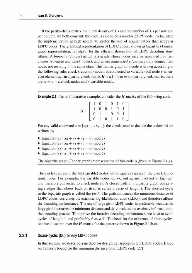
If the parity-check matrix has a low density of 1’s and the number of 1’s per row andper column are both constant, the code is said to be a regular LDPC code. To facilitatethe implementation at high speed, we prefer the use of regular rather than irregularLDPC codes. The graphical representation of LDPC codes, known as bipartite (Tanner)graph representation, is helpful for the efficient description of LDPC decoding algo-rithms. A bipartite (Tanner) graph is a graph whose nodes may be separated into twoclasses (variable and check nodes), and where undirected edges may only connect twonodes not residing in the same class. The Tanner graph of a code is drawn according tothe following rule: check (function) node c is connected to variable (bit) node v when-ever element hcv in a parity-check matrix H is a 1. In an m×n parity-check matrix, thereare m = n− k check nodes and n variable nodes.
Example 2.1: As an illustrative example, consider the H-matrix of the following code
H =
⎡⎢⎢⎣
1 0 1 0 1 01 0 0 1 0 10 1 1 0 0 10 1 0 1 1 0
⎤⎥⎥⎦ .
For any valid codeword x = [x0x1 . . . xn−1], the checks used to decode the codeword arewritten as,
● Equation (c0): x0 + x2 + x4 = 0 (mod 2)● Equation (c1): x0 + x3 + x5 = 0 (mod 2)● Equation (c2): x1 + x2 + x5 = 0 (mod 2)● Equation (c3): x1 + x3 + x4 = 0 (mod 2)
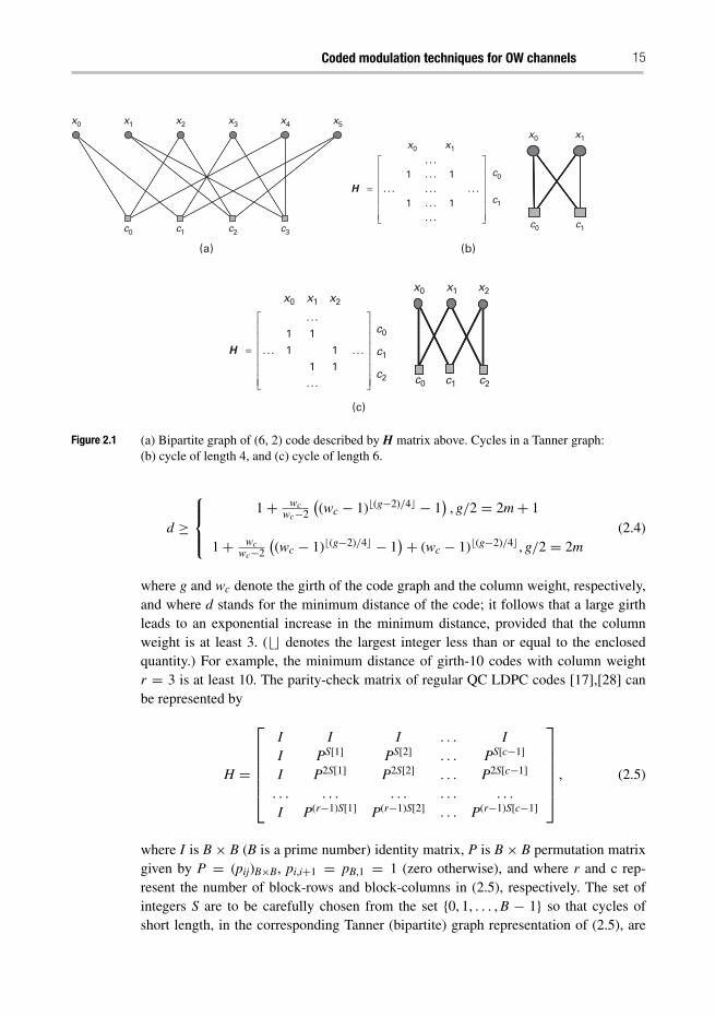
The bipartite graph (Tanner graph) representation of this code is given in Figure 2.1(a).
The circles represent the bit (variable) nodes while squares represent the check (func-tion) nodes. For example, the variable nodes x0, x2, and x4 are involved in Eq. (c0),and therefore connected to check node c0. A closed path in a bipartite graph compris-ing l edges that closes back on itself is called a cycle of length l. The shortest cyclein the bipartite graph is called the girth. The girth influences the minimum distance ofLDPC codes, correlates the extrinsic log-likelihood ratios (LLRs), and therefore affectsthe decoding performance. The use of large girth LDPC codes is preferable because thelarge girth increases the minimum distance and de-correlates the extrinsic information inthe decoding process. To improve the iterative decoding performance, we have to avoidcycles of length 4, and preferably 6 as well. To check for the existence of short cycles,one has to search over the H-matrix for the patterns shown in Figure 2.1(b,c).
2.2.1 Quasi-cyclic (QC) binary LDPC codes
In this section, we describe a method for designing large-girth QC LDPC codes. Basedon Tanner’s bound for the minimum distance of an LDPC code [27]
Coded modulation techniques for OW channels 15
x0
c0 c1 c2 c3
x1 x2 x3 x4 x5
c0
c0 c1
c1
x0 x1
x0 x1
. . .
. . .. . .
. . .
. . .
. . .
. . .1 1
1 1
⎡ ⎤⎢ ⎥⎢ ⎥⎢ ⎥=⎢ ⎥⎢ ⎥⎢ ⎥⎣ ⎦
H
(a) (b)
⎥
(c)
c0
c0
c1
c1
c2c2
x0 x1 x2x0 x1 x2
. . .
1 1
1 1
1 1
⎡ ⎤⎢ ⎥⎢ ⎥⎢=⎢ ⎥⎢ ⎥⎢ ⎥⎣ ⎦
H
. . .
. . . . . .
Figure 2.1 (a) Bipartite graph of (6, 2) code described by H matrix above. Cycles in a Tanner graph:(b) cycle of length 4, and (c) cycle of length 6.
d ≥
⎧⎪⎨⎪⎩
1+ wcwc−2
((wc − 1)�(g−2)/4� − 1
), g/2 = 2m+ 1
1+ wcwc−2
((wc − 1)�(g−2)/4� − 1
)+ (wc − 1)�(g−2)/4�, g/2 = 2m(2.4)
where g and wc denote the girth of the code graph and the column weight, respectively,and where d stands for the minimum distance of the code; it follows that a large girthleads to an exponential increase in the minimum distance, provided that the columnweight is at least 3. (�� denotes the largest integer less than or equal to the enclosedquantity.) For example, the minimum distance of girth-10 codes with column weightr = 3 is at least 10. The parity-check matrix of regular QC LDPC codes [17],[28] canbe represented by
H =
⎡⎢⎢⎢⎢⎢⎣
I I I . . . II PS[1] PS[2] . . . PS[c−1]
I P2S[1] P2S[2] . . . P2S[c−1]
. . . . . . . . . . . . . . .
I P(r−1)S[1] P(r−1)S[2] . . . P(r−1)S[c−1]
⎤⎥⎥⎥⎥⎥⎦ , (2.5)
where I is B × B (B is a prime number) identity matrix, P is B × B permutation matrixgiven by P = (pij)B×B, pi,i+1 = pB,1 = 1 (zero otherwise), and where r and c rep-resent the number of block-rows and block-columns in (2.5), respectively. The set ofintegers S are to be carefully chosen from the set {0, 1, . . . , B − 1} so that cycles ofshort length, in the corresponding Tanner (bipartite) graph representation of (2.5), are
16 Ivan B. Djordjevic
avoided. According to Theorem 2.1 in [28], we have to avoid the cycles of length 2k(k = 3 or 4) defined by the following equation
S[i1]j1 + S[i2]j2 + · · · S[ik]jk = S[i1]j2 + S[i2]j3 + · · · S[ik]j1 mod B, (2.6)
where the closed path is defined by (i1, j1), (i1, j2), (i2, j2), (i2, j3), . . ., (ik, jk), (ik, j1) withthe pair of indices denoting row-column indices of permutation-blocks in (2.5) such thatlm �= lm+1, lk �= l1 (m = 1, 2, .., k; l ∈ {i, j}). Therefore, we have to identify the sequenceof integers S[i] ∈ {0, 1, . . . , B − 1} (i = 0, 1, . . . , r − 1; r < B) not satisfying Equa-tion (2.6), which can be done either by computer search or in a combinatorial fashion.For example, to design the QC LDPC codes in [23], we introduced the concept of thecyclic-invariant difference set (CIDS). The CIDS-based codes come naturally as girth-6codes, and to increase the girth we had to selectively remove certain elements from aCIDS. The design of LDPC codes of rate above 0.8, column weight 3 and girth g ≥ 10using the CIDS approach is very challenging and is still an open problem. Instead, inour recent paper [29] (see also [17]), we solved this problem by developing an efficientcomputer search algorithm. We add an integer at a time from the set {0, 1, . . . , B − 1}(not used before) to the initial set S and check if the Equation (2.6) is satisfied. If Equa-tion (2.6) is satisfied, we remove that integer from the set S and continue our searchwith another integer from set {0, 1, . . . , B − 1} until we exploit all the elements from{0, 1, . . . , B− 1}. The code rate of these QC codes, R, is lower-bounded by
R ≥ |S|B− rB
|S|B = 1− r/|S|, (2.7)
and the codeword length is |S|B, where |S| denotes the cardinality of set S. For a givencode rate R0, the number of elements from S to be used is �r/(1 − R0)�. With thisalgorithm, LDPC codes of arbitrary code rate can be designed.
Example 2.2: By setting B = 2311, the set of integers to be used in (2.5) is obtained asS = {1, 2, 7, 14, 30, 51, 78, 104, 129, 212, 223, 318, 427, 600, 808}. The correspondingLDPC code has rate R0 = 1−3/15 = 0.8, column weight 3, girth-10 and length |S|B =15 · 2311 = 34665. In the example above, the initial set of integers was S = {1, 2, 7},and the set of rows to be used in (2.5) is {1,3,6}. The use of a different initial set willresult in a different set from that obtained above.
Example 2.3: By setting B = 269, the set S is obtained as S = {0, 2, 3, 5, 9, 11, 12,14, 27, 29, 30, 32, 36, 38, 39, 41, 81, 83, 84, 86, 90, 92, 93, 95, 108, 110, 111, 113,117, 119, 120, 122}. If 30 integers are used, the corresponding LDPC code has rateR0 = 1− 3/30 = 0.9, column weight 3, girth-8 and length 30 · 269 = 8070.
Coded modulation techniques for OW channels 17
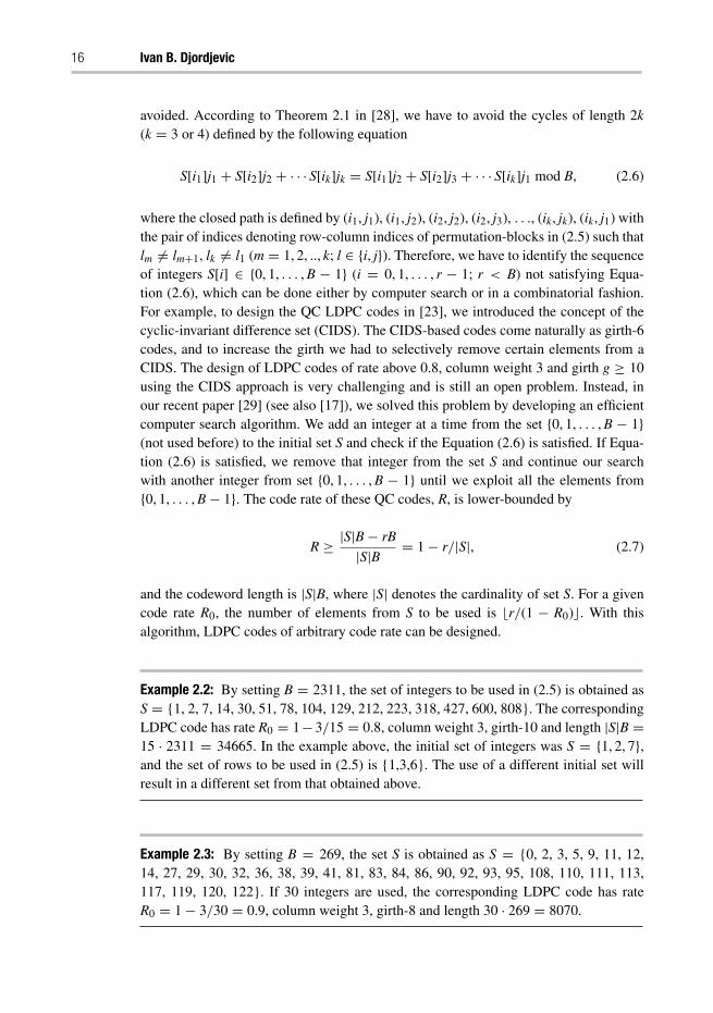
2.2.2 Decoding of LDPC codes
In this section, we describe the min-sum-with-correction-term algorithm [30] (see also[17]). It is a simplified version of the original algorithm proposed by Gallager [31].Gallager proposed a near optimal iterative decoding algorithm for LDPC codes thatcomputes the distributions of the variables in order to calculate the a posteriori prob-ability (APP) of a bit vi of a codeword v = [v0 v1 . . . vn−1] to be equal to 1 given areceived vector y = [y0 y1 . . . yn−1]. This iterative decoding scheme involves passingthe extrinsic information back and forth among the c-nodes and the v-nodes over theedges to update the distribution estimation. Each iteration in this scheme is composedof two half-iterations. In Figure 2.2, we illustrate both the first and the second halvesof an iteration of the algorithm. As an example, in Figure 2.2(a), we show the messagesent from v-node vi to c-node cj. The vi-node collects the information from the chan-nel (yi sample), in addition to extrinsic information from other c-nodes connected tothe vi-node, processes them and sends the extrinsic information (not already availableinformation) to cj. This extrinsic information contains the information about the proba-bility Pr(ci = b|yi), where b ∈ {0, 1}. This is performed in all c-nodes connected to thevi-node. On the other hand, Figure 2.2(b) shows the extrinsic information sent fromc-node ci to the v-node vj, which contains the information about Pr(ci equation is satis-fied |y). This is done repeatedly for all the c-nodes connected to the vi-node. After thisintuitive description, we describe the min-sum-with-correction-term algorithm in moredetail because of its simplicity and suitability for high-speed implementation. Generally,we can either compute the APP Pr(vi|y) or the APP ratio l(vi) = Pr(vi = 0|y)/Pr(vi =1|y), which is also referred to as the likelihood ratio. In the log-domain version of thesum-product algorithm, we replace these likelihood ratios with log-likelihood ratios(LLRs) due to the fact that the probability domain includes many multiplications whichleads to numerical instabilities, whereas the computation using LLRs involves additiononly. Moreover, the log-domain representation is more suitable for finite precision rep-resentation. Thus, we compute the LLRs by L(vi) = log[Pr(vi = 0|y)/Pr(vi = 1|y)]. Forthe final decision, if L(vi) > 0, we decide in favor of 0 and if L(vi) < 0, we decide infavor of 1. To further explain the algorithm, we introduce the following notations due toMacKay [32]:
vi
viyi (channel sample)
cj
cjqij (b)
qij (b)
rji (b)
rji (b)
(a) (b)
Figure 2.2 Illustration of the half-iterations of the sum-product algorithm: (a) first half-iteration: extrinsicinformation sent from v-nodes to c-nodes, and (b) second half-iteration: extrinsic informationsent from c-nodes to v-nodes.
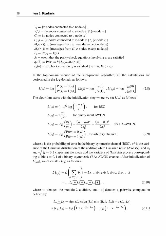
18 Ivan B. Djordjevic
Vj = {v-nodes connected to c-node cj}Vj\i = {v-nodes connected to c-node cj}\{v-node vi}Ci = {c-nodes connected to v-node vi}Ci\j = {c-nodes connected to v-node vi} \ {c-node cj}Mv(∼ i) = {messages from all v-nodes except node vi}Mc(∼ j) = {messages from all c-nodes except node cj}Pi = Pr(vi = 1|yi)Si = event that the parity-check equations involving ci are satisfiedqij(b) = Pr(vi = b | Si, yi, Mc(∼ j))rji(b) = Pr(check equation cj is satisfied | vi = b, Mv(∼ i))
In the log-domain version of the sum-product algorithm, all the calculations areperformed in the log-domain as follows:
L(vi) = log
[Pr(vi = 0|yi)
Pr(vi = 1|yi)
], L(rji) = log
[rji(0)
rji(1)
], L(qji) = log
[qji(0)
qji(1)
]. (2.8)
The algorithm starts with the initialization step where we set L(vi) as follows:
L(vi) = (−1)yi log
(1− ε
ε
), for BSC
L(vi) = 2yi
σ 2, for binary input AWGN
L(vi) = log
(σ1
σ0
)− (yi − μ0)2
2σ 20
+ (yi − μ1)2
2σ 21
, for BA-AWGN
L(vi) = log
(Pr(vi = 0|yi)
Pr(vi = 1|yi)
), for arbitrary channel (2.9)
where ε is the probability of error in the binary symmetric channel (BSC), σ2 is the vari-ance of the Gaussian distribution of the additive white Gaussian noise (AWGN), and μj
and σ 2j (j = 0, 1) represent the mean and the variance of Gaussian process correspond-
ing to bits j = 0, 1 of a binary asymmetric (BA)-AWGN channel. After initialization ofL(qij), we calculate L(rji) as follows:
L(rji) = L
⎛⎝ ∑
i′∈Vj\ib′j
⎞⎠ = L (. . .⊕ bk ⊕ bl ⊕ bm ⊕ bn . . .)
= . . . Lk + Ll + Lm + Ln + . . . (2.10)
where ⊕ denotes the modulo-2 addition, and + denotes a pairwise computationdefined by
La + Lb = sign (La) sign (Lb)min (|La|, |Lb|)+ s (La, Lb)
s (La, Lb) = log(
1+ e−|La+Lb|)− log
(1+ e−|La−Lb|
). (2.11)
Coded modulation techniques for OW channels 19
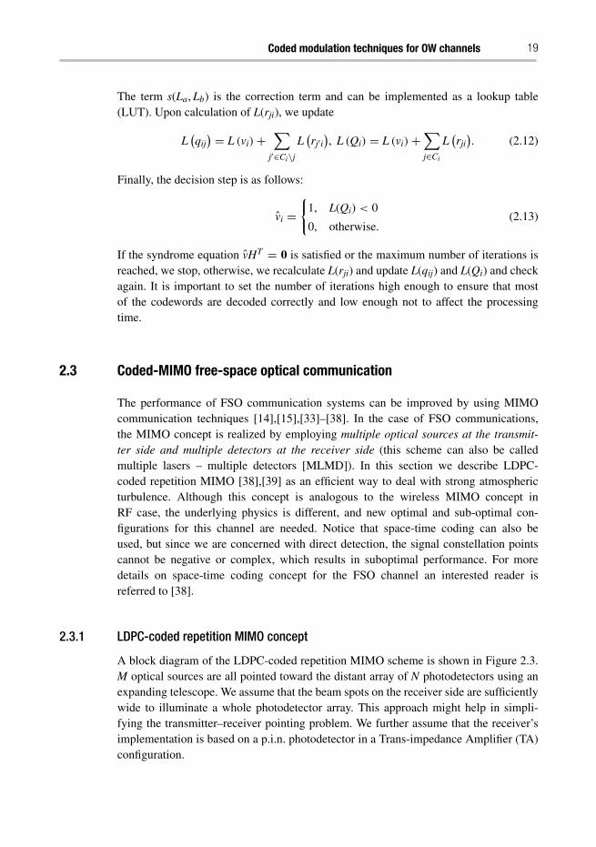
The term s(La, Lb) is the correction term and can be implemented as a lookup table(LUT). Upon calculation of L(rji), we update
L(qij
) = L (vi)+∑
j′∈Ci\jL(rj′i
), L (Qi) = L (vi)+
∑j∈Ci
L(rji). (2.12)
Finally, the decision step is as follows:
vi ={
1, L(Qi) < 0
0, otherwise.(2.13)
If the syndrome equation vHT = 0 is satisfied or the maximum number of iterations isreached, we stop, otherwise, we recalculate L(rji) and update L(qij) and L(Qi) and checkagain. It is important to set the number of iterations high enough to ensure that mostof the codewords are decoded correctly and low enough not to affect the processingtime.
2.3 Coded-MIMO free-space optical communication
The performance of FSO communication systems can be improved by using MIMOcommunication techniques [14],[15],[33]–[38]. In the case of FSO communications,the MIMO concept is realized by employing multiple optical sources at the transmit-ter side and multiple detectors at the receiver side (this scheme can also be calledmultiple lasers – multiple detectors [MLMD]). In this section we describe LDPC-coded repetition MIMO [38],[39] as an efficient way to deal with strong atmosphericturbulence. Although this concept is analogous to the wireless MIMO concept inRF case, the underlying physics is different, and new optimal and sub-optimal con-figurations for this channel are needed. Notice that space-time coding can also beused, but since we are concerned with direct detection, the signal constellation pointscannot be negative or complex, which results in suboptimal performance. For moredetails on space-time coding concept for the FSO channel an interested reader isreferred to [38].
2.3.1 LDPC-coded repetition MIMO concept
A block diagram of the LDPC-coded repetition MIMO scheme is shown in Figure 2.3.M optical sources are all pointed toward the distant array of N photodetectors using anexpanding telescope. We assume that the beam spots on the receiver side are sufficientlywide to illuminate a whole photodetector array. This approach might help in simpli-fying the transmitter–receiver pointing problem. We further assume that the receiver’simplementation is based on a p.i.n. photodetector in a Trans-impedance Amplifier (TA)configuration.
20 Ivan B. Djordjevic
Sourcebits
Transmitter 1
. . .
Transmitter M
LDPCencoder
Receiver 1
.
.
.
Receiver N
Pro
cessor
bits
Atmospheric turbulencechannel
(a)
Light beamthrough
turbulentchannel
opticalamp.
Expandingtelescope
Detector 1
Fiber
Collimatinglens
TA amplifier
Opticalsource
mth Transmitter
Receiver array
Detector N
…
(b)
Bit LLRscalculator
LDPC decoderFrom FSO link Receiver
array
ProcessorDetected bits
(c)
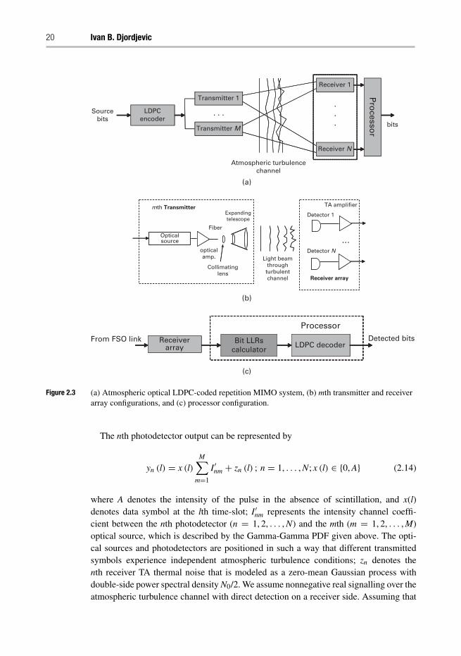
Figure 2.3 (a) Atmospheric optical LDPC-coded repetition MIMO system, (b) mth transmitter and receiverarray configurations, and (c) processor configuration.
The nth photodetector output can be represented by
yn (l) = x (l)M∑
m=1
I′nm + zn (l) ; n = 1, . . . , N; x (l) ∈ {0, A} (2.14)
where A denotes the intensity of the pulse in the absence of scintillation, and x(l)denotes data symbol at the lth time-slot; I′nm represents the intensity channel coeffi-cient between the nth photodetector (n = 1, 2, . . . , N) and the mth (m = 1, 2, . . . , M)optical source, which is described by the Gamma-Gamma PDF given above. The opti-cal sources and photodetectors are positioned in such a way that different transmittedsymbols experience independent atmospheric turbulence conditions; zn denotes thenth receiver TA thermal noise that is modeled as a zero-mean Gaussian process withdouble-side power spectral density N0/2. We assume nonnegative real signalling over theatmospheric turbulence channel with direct detection on a receiver side. Assuming that
Coded modulation techniques for OW channels 21
the receiver TA thermal noise is white-Gaussian with a double-side-power spectral den-sity N0/2, the LLR of a symbol x(l) (at the lth time-slot) for a binary repetition MIMOtransmission is determined by
L (x (l)) = log
⎧⎪⎪⎪⎪⎪⎪⎪⎪⎪⎪⎪⎨⎪⎪⎪⎪⎪⎪⎪⎪⎪⎪⎪⎩
N∏n=1
1√2π√
N0/2exp
[− yn(l)2
2N0/2
]
1√2π√
N0/2exp
⎡⎢⎢⎣−
(yn(l)−
M∑m=1
Inm
)2
N0
⎤⎥⎥⎦
⎫⎪⎪⎪⎪⎪⎪⎪⎪⎪⎪⎪⎬⎪⎪⎪⎪⎪⎪⎪⎪⎪⎪⎪⎭
=N∑
n=1
⎧⎪⎪⎪⎪⎨⎪⎪⎪⎪⎩−yn (l)2
N0+
(yn (l)−
M∑m=1
Inm
)2
N0
⎫⎪⎪⎪⎪⎬⎪⎪⎪⎪⎭
. (2.15)
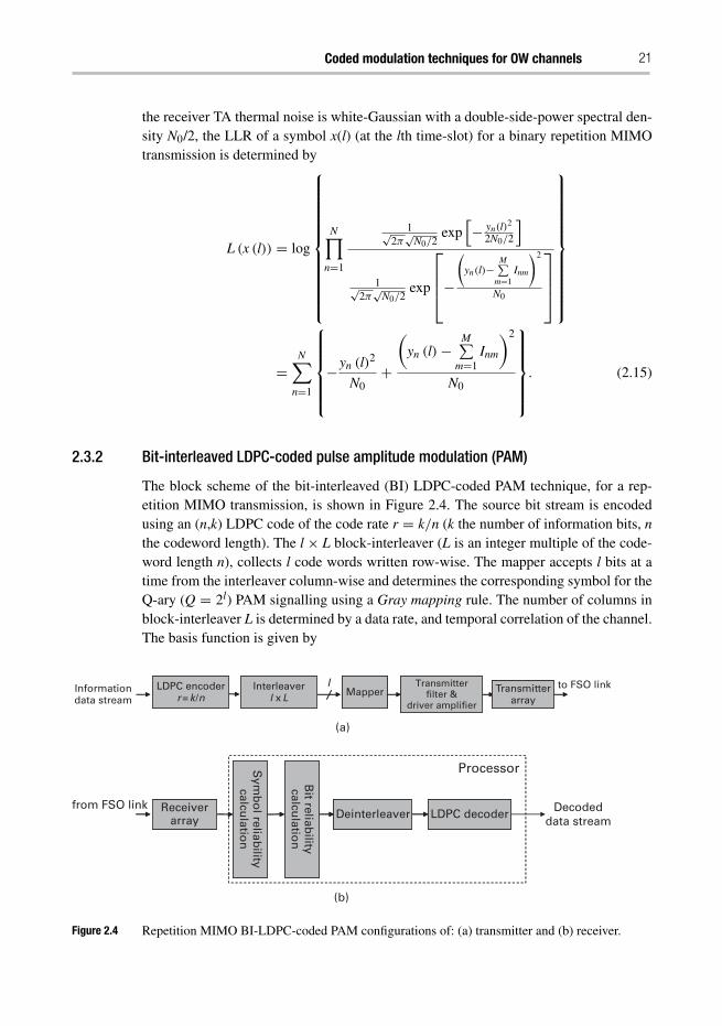
2.3.2 Bit-interleaved LDPC-coded pulse amplitude modulation (PAM)
The block scheme of the bit-interleaved (BI) LDPC-coded PAM technique, for a rep-etition MIMO transmission, is shown in Figure 2.4. The source bit stream is encodedusing an (n,k) LDPC code of the code rate r = k/n (k the number of information bits, nthe codeword length). The l× L block-interleaver (L is an integer multiple of the code-word length n), collects l code words written row-wise. The mapper accepts l bits at atime from the interleaver column-wise and determines the corresponding symbol for theQ-ary (Q = 2l) PAM signalling using a Gray mapping rule. The number of columns inblock-interleaver L is determined by a data rate, and temporal correlation of the channel.The basis function is given by
Informationdata stream
LDPC encoderr = k /n
Transmitterarray
Interleaverl x L Mapper
l Transmitterfilter &
driver amplifier
to FSO link
(a)
Sym
bo
l reliability
calculatio
n
Bit reliab
ilitycalcu
lation
Deinterleaver LDPC decoder Decodeddata stream
from FSO link Receiverarray
Processor
(b)
Figure 2.4 Repetition MIMO BI-LDPC-coded PAM configurations of: (a) transmitter and (b) receiver.
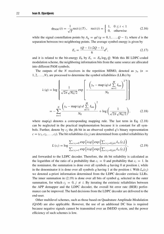
22 Ivan B. Djordjevic
φPAM (t) = 1√T
rect (t/T) , rect (t) ={
1, 0 ≤ t < 10, otherwise
(2.16)
while the signal constellation points by Aq = qd (q = 0, 1, . . . , Q − 1), where d is theseparation between two neighboring points. The average symbol energy is given by
Es = (Q− 1) (2Q− 1)
6d2, (2.17)
and it is related to the bit-energy Eb by Es = Eb log2 Q. With this BI LDPC-codedmodulation scheme, the neighboring information bits from the same source are allocatedinto different PAM symbols.
The outputs of the N receivers in the repetition MIMO, denoted as yn (n =1, 2, . . . , N), are processed to determine the symbol reliabilities (LLRs) by
λ (q) = log
⎧⎪⎪⎪⎪⎨⎪⎪⎪⎪⎩
1√2π√
N0/2exp
⎡⎢⎢⎢⎢⎣−
(yn −map (q) d
M∑m=1
Inm
)2
N0
⎤⎥⎥⎥⎥⎦
⎫⎪⎪⎪⎪⎬⎪⎪⎪⎪⎭
= −N∑
n=1
(yn −map (q) d
M∑m=1
Inm
)2
N0+ log
(1√
2π√
N0/2
), (2.18)
where map(q) denotes a corresponding mapping rule. The last term in Eq. (2.18)can be neglected in the practical implementation because it is constant for all sym-bols. Further, denote by cj the jth bit in an observed symbol q’s binary representationc = (c1, c2, . . . , cl). The bit reliabilities L(cj) are determined from symbol reliabilities by
L (ci) = log
∑c:ci=0 exp
[λ(q)
]exp
(∑c:cj=0,j�=i La
(cj))
∑c:ci=1 exp
[λ(q)
]exp
(∑c:cj=0,j�=i La
(cj)) , (2.19)
and forwarded to the LDPC decoder. Therefore, the ith bit reliability is calculated asthe logarithm of the ratio of a probability that ci = 0 and probability that ci = 1. Inthe nominator, the summation is done over all symbols q having 0 at position i, whilein the denominator it is done over all symbols q having 1 at the position i. With La(cj)we denoted a-priori information determined from the LDPC decoder extrinsic LLRs.The inner summation in (2.19) is done over all bits of symbol q, selected in the outersummation, for which cj = 0, j �= i. By iterating the extrinsic reliabilities betweenthe APP demapper and the LDPC decoder, the overall bit error rate (BER) perfor-mance can be improved. The hard decisions from the LDPC decoder are delivered to theend-user.
Other multilevel schemes, such as those based on Quadrature Amplitude-Modulation(QAM) are also applicable. However, the use of an additional DC bias is requiredbecause negative signals cannot be transmitted over an IM/DD system, and the powerefficiency of such schemes is low.
Coded modulation techniques for OW channels 23
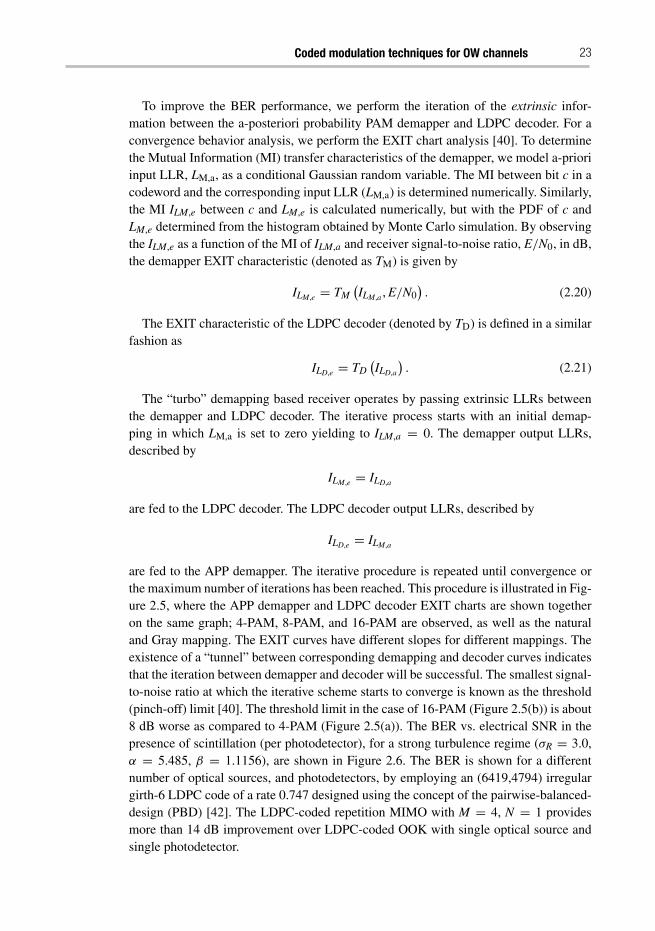
To improve the BER performance, we perform the iteration of the extrinsic infor-mation between the a-posteriori probability PAM demapper and LDPC decoder. For aconvergence behavior analysis, we perform the EXIT chart analysis [40]. To determinethe Mutual Information (MI) transfer characteristics of the demapper, we model a-prioriinput LLR, LM,a, as a conditional Gaussian random variable. The MI between bit c in acodeword and the corresponding input LLR (LM,a) is determined numerically. Similarly,the MI ILM,e between c and LM,e is calculated numerically, but with the PDF of c andLM,e determined from the histogram obtained by Monte Carlo simulation. By observingthe ILM,e as a function of the MI of ILM,a and receiver signal-to-noise ratio, E/N0, in dB,the demapper EXIT characteristic (denoted as TM) is given by
ILM,e = TM(ILM,a , E/N0
). (2.20)
The EXIT characteristic of the LDPC decoder (denoted by TD) is defined in a similarfashion as
ILD,e = TD(ILD,a
). (2.21)
The “turbo” demapping based receiver operates by passing extrinsic LLRs betweenthe demapper and LDPC decoder. The iterative process starts with an initial demap-ping in which LM,a is set to zero yielding to ILM,a = 0. The demapper output LLRs,described by
ILM,e = ILD,a
are fed to the LDPC decoder. The LDPC decoder output LLRs, described by
ILD,e = ILM,a
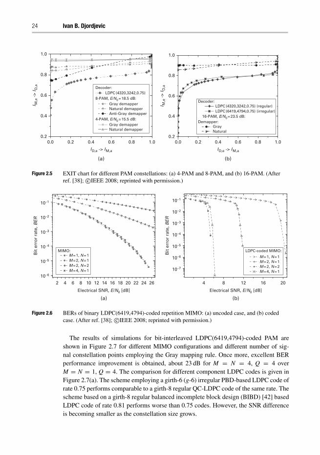
are fed to the APP demapper. The iterative procedure is repeated until convergence orthe maximum number of iterations has been reached. This procedure is illustrated in Fig-ure 2.5, where the APP demapper and LDPC decoder EXIT charts are shown togetheron the same graph; 4-PAM, 8-PAM, and 16-PAM are observed, as well as the naturaland Gray mapping. The EXIT curves have different slopes for different mappings. Theexistence of a “tunnel” between corresponding demapping and decoder curves indicatesthat the iteration between demapper and decoder will be successful. The smallest signal-to-noise ratio at which the iterative scheme starts to converge is known as the threshold(pinch-off) limit [40]. The threshold limit in the case of 16-PAM (Figure 2.5(b)) is about8 dB worse as compared to 4-PAM (Figure 2.5(a)). The BER vs. electrical SNR in thepresence of scintillation (per photodetector), for a strong turbulence regime (σR = 3.0,α = 5.485, β = 1.1156), are shown in Figure 2.6. The BER is shown for a differentnumber of optical sources, and photodetectors, by employing an (6419,4794) irregulargirth-6 LDPC code of a rate 0.747 designed using the concept of the pairwise-balanced-design (PBD) [42]. The LDPC-coded repetition MIMO with M = 4, N = 1 providesmore than 14 dB improvement over LDPC-coded OOK with single optical source andsingle photodetector.
24 Ivan B. Djordjevic
0.0 0.2 0.4 0.6 0.8 1.00.2
0.4
0.6
0.8
1.0
I M,e
->
I D,a
I M,e
->
I D,a
I D,e -> I M,a I D,e -> I M,a
0.0 0.2 0.4 0.6 0.8 1.0
Decoder:LDPC (4320,3242,0.75)
8-PAM, E/N0 = 18.5 dB:Gray demapperNatural demapperAnti-Gray demapper
4-PAM, E/N0 = 15.5 dB:Gray demapperNatural demapper
0.2
0.4
0.6
0.8
1.0
Decoder:LDPC (4320,3242,0.75) (regular)LDPC (6419,4794,0.75) (irregular)
16-PAM, E/N0 = 23.5 dB:Demapper:
GrayNatural
(a) (b)
Figure 2.5 EXIT chart for different PAM constellations: (a) 4-PAM and 8-PAM, and (b) 16-PAM. (Afterref. [38]; c©IEEE 2008; reprinted with permission.)
2 4 6 8 10 12 14 16 18 20 4 8 12 16 2022 24 26
10−1
10−2
10−3
10−4
10−5
10−6
10−1
10−2
10−3
10−4
10−5
10−6
10−7
Bit
err
or
rate
, BE
R
Bit
err
or
rate
, BE
R
Electrical SNR, E/N0 [dB]
MIMO:M = 1, N = 1M = 2, N = 1M = 2, N = 2M = 4, N = 1
LDPC-coded MIMO:
M = 1, N = 1M = 2, N = 1M = 2, N = 2M = 4, N = 1
(a)
Electrical SNR, E/N0 [dB]
(b)
Figure 2.6 BERs of binary LDPC(6419,4794)-coded repetition MIMO: (a) uncoded case, and (b) codedcase. (After ref. [38]; c©IEEE 2008; reprinted with permission.)
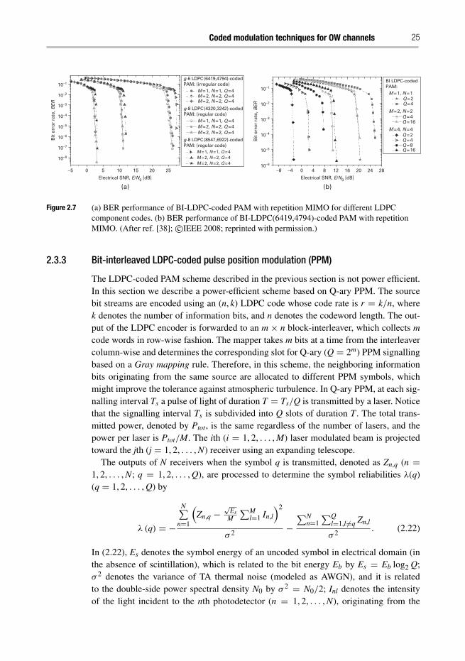
The results of simulations for bit-interleaved LDPC(6419,4794)-coded PAM areshown in Figure 2.7 for different MIMO configurations and different number of sig-nal constellation points employing the Gray mapping rule. Once more, excellent BERperformance improvement is obtained, about 23 dB for M = N = 4, Q = 4 overM = N = 1, Q = 4. The comparison for different component LDPC codes is given inFigure 2.7(a). The scheme employing a girth-6 (g-6) irregular PBD-based LDPC code ofrate 0.75 performs comparable to a girth-8 regular QC-LDPC code of the same rate. Thescheme based on a girth-8 regular balanced incomplete block design (BIBD) [42] basedLDPC code of rate 0.81 performs worse than 0.75 codes. However, the SNR differenceis becoming smaller as the constellation size grows.
Coded modulation techniques for OW channels 25
−5 0 5 10 15 20 25
10−1
10−2
10−3
10−4
10−5
10−6
10−7
10−8
Bit
err
or
rate
, BE
R
10−1
10−2
10−3
10−4
10−5
10−6
Bit
err
or
rate
, BE
R
Electrical SNR, E/N0 [dB]
g-6 LDPC (6419,4794)-codedPAM: (irregular code)
M = 1, N = 1, Q = 4 M = 2, N = 2, Q = 4M = 2, N = 2, Q = 4
g-8 LDPC (4320,3242)-codedPAM: (regular code)
M = 1, N = 1, Q = 4 M = 2, N = 2, Q = 4M = 2, N = 2, Q = 4
g-8 LDPC (8547,6922)-codedPAM: (regular code)
M = 1, N = 1, Q = 4 M = 2, N = 2, Q = 4M = 2, N = 2, Q = 4
−8 −4 0 4 8 12 16 20 24 28
BI LDPC-codedPAM:
M = 1, N = 1Q = 2Q = 4
M = 2, N = 2Q = 4Q = 16
M = 4, N = 4 Q = 2Q = 4Q = 8Q = 16
(a)Electrical SNR, E/N0 [dB]
(b)
Figure 2.7 (a) BER performance of BI-LDPC-coded PAM with repetition MIMO for different LDPCcomponent codes. (b) BER performance of BI-LDPC(6419,4794)-coded PAM with repetitionMIMO. (After ref. [38]; c©IEEE 2008; reprinted with permission.)
2.3.3 Bit-interleaved LDPC-coded pulse position modulation (PPM)
The LDPC-coded PAM scheme described in the previous section is not power efficient.In this section we describe a power-efficient scheme based on Q-ary PPM. The sourcebit streams are encoded using an (n, k) LDPC code whose code rate is r = k/n, wherek denotes the number of information bits, and n denotes the codeword length. The out-put of the LDPC encoder is forwarded to an m × n block-interleaver, which collects mcode words in row-wise fashion. The mapper takes m bits at a time from the interleavercolumn-wise and determines the corresponding slot for Q-ary (Q = 2m) PPM signallingbased on a Gray mapping rule. Therefore, in this scheme, the neighboring informationbits originating from the same source are allocated to different PPM symbols, whichmight improve the tolerance against atmospheric turbulence. In Q-ary PPM, at each sig-nalling interval Ts a pulse of light of duration T = Ts/Q is transmitted by a laser. Noticethat the signalling interval Ts is subdivided into Q slots of duration T . The total trans-mitted power, denoted by Ptot, is the same regardless of the number of lasers, and thepower per laser is Ptot/M. The ith (i = 1, 2, . . . , M) laser modulated beam is projectedtoward the jth (j = 1, 2, . . . , N) receiver using an expanding telescope.
The outputs of N receivers when the symbol q is transmitted, denoted as Zn,q (n =1, 2, . . . , N; q = 1, 2, . . . , Q), are processed to determine the symbol reliabilities λ(q)(q = 1, 2, . . . , Q) by
λ (q) = −
N∑n=1
(Zn,q −
√Es
M
∑Ml=1 In,l
)2
σ 2−
∑Nn=1
∑Ql=1,l �=q Zn,l
σ 2. (2.22)
In (2.22), Es denotes the symbol energy of an uncoded symbol in electrical domain (inthe absence of scintillation), which is related to the bit energy Eb by Es = Eb log2 Q;σ 2 denotes the variance of TA thermal noise (modeled as AWGN), and it is relatedto the double-side power spectral density N0 by σ 2 = N0/2; Inl denotes the intensityof the light incident to the nth photodetector (n = 1, 2, . . . , N), originating from the
26 Ivan B. Djordjevic
0 4 8 12 16 20 24
Bit
err
or
rate
, BE
R
Electrical SNR, Eb/N0 [dB]
Uncoded:M = 1, N = 1:
Q = 2
Q = 2
Q = 2
Q = 4
Q = 4
Q = 4
Q = 8
Q = 8
Q = 8
M = 2, N = 2:
M = 2, N = 4:
LDPC (6419,4794,0.747)-coded:BICM:
M = 1, N = 1, Q =2 M = 2, N = 2, Q = 4M = 2, N = 4, Q = 4 M = 2, N = 4, Q = 8
MLC:M = 2, N = 4, Q = 4 (1.194 bits/symbol)M = 2, N = 4, Q = 8 (2.241 bits/symbol)
10−1
10−2
10−3
10−4
10−5
10−6
10−7
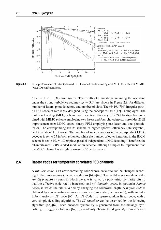
Figure 2.8 BER performance of bit-interleaved LDPC-coded modulation against MLC for different MIMO(MLMD) configurations.
lth (l = 1, 2, . . . , M) laser source. The results of simulations assuming the operationunder the strong turbulence regime (σR = 3.0) are shown in Figure 2.8, for differentnumber of lasers, photodetectors, and number of slots. The (6419,4794) irregular girth-6 LDPC code of rate 0.747 designed using the concept of PBD [42], is employed. Themultilevel coding (MLC) scheme with spectral efficiency of 2.241 bits/symbol com-bined with MIMO scheme employing two lasers and four photodetectors provides 21dBimprovement over LDPC-coded binary PPM employing one laser and one photode-tector. The corresponding BICM scheme of higher spectral efficiency (3bits/symbol)performs about 1 dB worse. The number of inner iterations in the sum-product LDPCdecoder is set to 25 in both schemes, while the number of outer iterations in the BICMscheme is set to 10. MLC employs parallel independent LDPC decoding. Therefore, thebit-interleaved LDPC-coded modulation scheme, although simpler to implement thanthe MLC scheme has a slightly worse BER performance.
2.4 Raptor codes for temporally correlated FSO channels
A rate-less code is an error-correcting code whose code-rate can be changed accord-ing to the time-varying channel conditions [64]–[67]. The well-known rate-less codesare: (i) punctured codes, in which the rate is varied by puncturing the parity bits sothat the effective code rate is increased; and (ii) fountain codes, in particular Raptorcodes, in which the rate is varied by changing the codeword length. A Raptor code isobtained by concatenating an inner error-correcting code (the pre-code), with an outerLuby-transform (LT) code [65]. An LT Code is a sparse random linear code, with avery simple decoding algorithm. The LT encoding can be described by the followingalgorithm [65],[67]. Each encoded symbol xn is generated from the message sym-bols s1, . . . , sK,LT as follows [67]: (i) randomly choose the degree dn from a degree
Coded modulation techniques for OW channels 27
distribution Ω(x), and (ii) choose uniformly at random dn distinct input symbols, andset xn equal to the bitwise sum, modulo 2, of those dn symbols. LT decoding can bedescribed by the following algorithm. The decoder’s task is to recover s from x = sG,where G is the matrix associated with the graph (of the pseudorandom matrix) by usingthe sum-product algorithm [67]:
1. Find a check node xn that is connected to only one source symbol sk
(a) Set sk = xn.(b) Add sk to all checks xn
′ that are connected to sk:xn′ := xn + sk for all n’ such that Gnk = 1.
(c) Remove all the edges connected to the source symbol sk.2. Repeat (1) until all sk are determined.
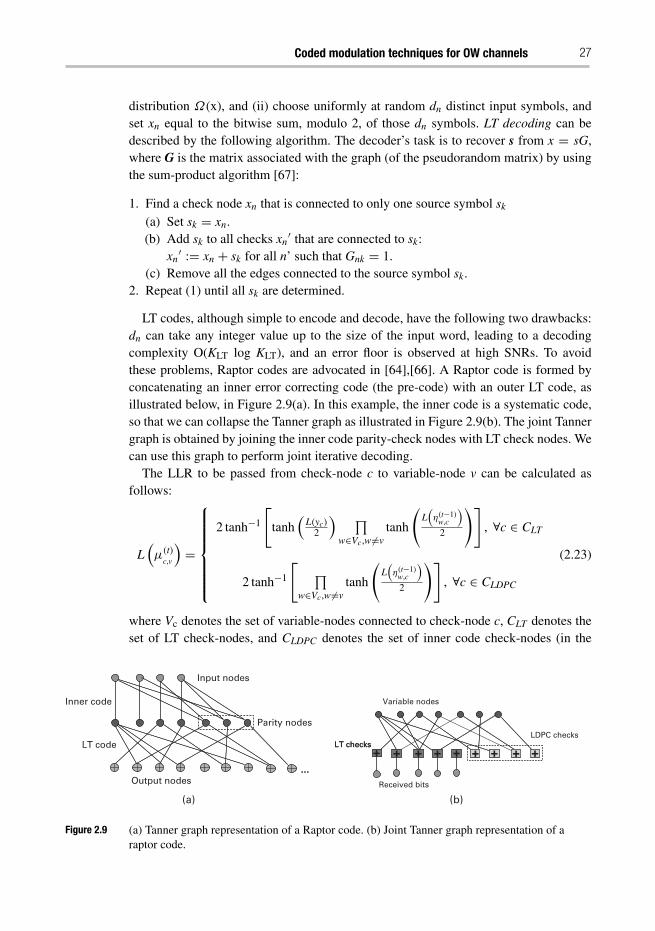
LT codes, although simple to encode and decode, have the following two drawbacks:dn can take any integer value up to the size of the input word, leading to a decodingcomplexity O(KLT log KLT), and an error floor is observed at high SNRs. To avoidthese problems, Raptor codes are advocated in [64],[66]. A Raptor code is formed byconcatenating an inner error correcting code (the pre-code) with an outer LT code, asillustrated below, in Figure 2.9(a). In this example, the inner code is a systematic code,so that we can collapse the Tanner graph as illustrated in Figure 2.9(b). The joint Tannergraph is obtained by joining the inner code parity-check nodes with LT check nodes. Wecan use this graph to perform joint iterative decoding.
The LLR to be passed from check-node c to variable-node v can be calculated asfollows:
L(μ(t)
c,v
)=
⎧⎪⎪⎪⎪⎪⎪⎨⎪⎪⎪⎪⎪⎪⎩
2 tanh−1
[tanh
(L(yc)
2
) ∏w∈Vc,w�=v
tanh
(L(η(t−1)
w,c
)2
)], ∀c ∈ CLT
2 tanh−1
[ ∏w∈Vc,w�=v
tanh
(L(η(t−1)
w,c
)2
)], ∀c ∈ CLDPC
(2.23)
where Vc denotes the set of variable-nodes connected to check-node c, CLT denotes theset of LT check-nodes, and CLDPC denotes the set of inner code check-nodes (in the
…
LT code
Inner code
Input nodes
Output nodes…
Parity nodes
LT checks
Variable nodes
LDPC checksLT checks
Received bits
+ + + + + ++ ++
(a) (b)
Figure 2.9 (a) Tanner graph representation of a Raptor code. (b) Joint Tanner graph representation of araptor code.
28 Ivan B. Djordjevic
example above the inner code is an LDPC code). In (2.23), we use the character μ todenote the passage of messages from c-nodes to v-nodes, and the character η to denotethe passage of messages in the opposite direction. The superscript t is used to denote thecurrent iteration, and (t−1) denotes the previous one; yc is the sample that corresponds totransmitted codeword bit xv. The LLR to be passed from variable-node v to check-nodec can be calculated as follows:
L(η(t)
v,c
)=
⎧⎪⎪⎨⎪⎪⎩
∑d∈Cv,d �=c
L(μ(t−1)
d,v
), ∀c ∈ CLT
L(x(t)
v
)+ ∑d∈Cv,d �=c
L(μ(t−1)
d,v
), ∀c ∈ CLDPC
. (2.24)
The variable-node v LLR-update rule is given by
L(
x(t)v
)=
∑c∈Cv
L(μ(t)
c,v
). (2.25)
Finally, the decision step is as follows:
xv ={
1, L(x(t)
v
)< 0
0, otherwise. (2.26)
If the syndrome equation xHT = 0 (x denotes the codeword and H is the joint parity-check matrix) is satisfied or the maximum number of iterations is reached, we stop,otherwise, we recalculate (2.23)–(2.26) and check again.
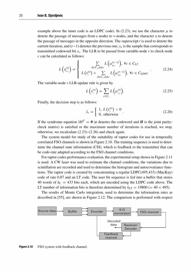
The system model for study of the suitability of raptor codes for use in temporallycorrelated FSO channels is shown in Figure 2.10. The training sequence is used to deter-mine the channel state information (CSI), which is feedback to the transmitter that canbe code-rate adapted according to the FSO channel conditions.
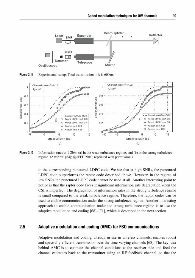
For raptor codes performance evaluation, the experimental setup shown in Figure 2.11is used. A CW laser was used to estimate the channel conditions, the variations due toscintillation are recorded and used to determine the histogram and autocovariance func-tions. The raptor code is created by concatenating a regular LDPC(495,433) (MacKay)code of rate 0.87 and an LT code. The user bit sequence is fed into a buffer that stores40 words of kC = 433 bits each, which are encoded using the LDPC code above. TheLT number of information bits is therefore determined by kLT = 19800 (= 40× 495).
The results of Monte Carlo integration, used to determine the information rates asdescribed in [55], are shown in Figure 2.12. The comparison is performed with respect
Source data Buffer EncoderE-Oconversion FSO channel
Receivr/Decoder
Feedchannelbackchannel
Source data Buffer Encoder E-Oconversion FSO channel
Receiver/Decoder
Decodeddata
Feedbackchannel
Figure 2.10 FSO system with feedback channel.
Coded modulation techniques for OW channels 29
Laser SMFReflector
Beam splitter
Mirror
Expander
Telescope
MMF
DetectorOscilloscope
Figure 2.11 Experimental setup. Total transmission link is 600 m.
(a) (b)
0
Bit
s/ch
ann
el u
se
Bit
s/ch
ann
el u
se
0.2
−5 0 5
Effective SNR [dB]
10
Capacity AWGN−OOKPunct. LDPC, perf. CSI
Punct. LDPC, imp. CSI
Raptor, perf. CSI
Raptor, imp. CSI
Capacity AWGN−OOK
Punct. LDPC, perf. CSI
Punct. LDPC, imp. CSI
Raptor, perf. CSI
Raptor, imp. CSI
15 −5−10 0 5
Effective SNR [dB]
10 15
0.4
0.6
0.8
1 Tb = 105
0
0.2
0.4
0.6
0.8
12 2
Tb = 105
Channel case σ I = 0.12 Channel case σ I = 1.02
Figure 2.12 Information rates at 1 Gb/s: (a) in the weak turbulence regime, and (b) in the strong turbulenceregime. (After ref. [64]; c©IEEE 2010; reprinted with permission.)
to the corresponding punctured LDPC code. We see that at high SNRs, the puncturedLDPC code outperforms the raptor code described above. However, in the regime oflow SNRs the punctured LDPC code cannot be used at all. Another interesting point tonotice is that the raptor code faces insignificant information rate degradation when theCSI is imperfect. The degradation of information rates in the strong turbulence regimeis small compared to the weak turbulence regime. Therefore, the raptor codes can beused to enable communication under the strong turbulence regime. Another interestingapproach to enable communication under the strong turbulence regime is to use theadaptive modulation and coding [68]–[71], which is described in the next section.
2.5 Adaptive modulation and coding (AMC) for FSO communications
Adaptive modulation and coding, already in use in wireless channels, enables robustand spectrally efficient transmission over the time-varying channels [68]. The key ideabehind AMC is to estimate the channel conditions at the receiver side and feed thechannel estimates back to the transmitter using an RF feedback channel, so that the
30 Ivan B. Djordjevic
DetectorDirect modulated
laser diode
Expandingtelescope
Compressingtelescope
LDPCencoder
Inputdata
Outputdata
Extrinsic LLRs
RF feedbackchannel
FSO channelestimate
Powercontrol
Buffer MapperLDPC
decoderAPP
demapperInterleaver Deinterleaver
Interleaver
(a)
(b)
RF feedbackchannel
FSO channelestimate
Powercontrol
Outputdata
RF TxRF mapper& modulator
LDPCencoder
Inputdata
S/P
Buffer
Buffer
RF Powercontrol
RF Rx
RF channelestimate
ADC
ADC
Buffer
BufferP/S LDPC
decoder
MUXMapper
APPdemapper
Extrinsic LLRs
Detector
Expandingtelescope
Compressingtelescope
Direct modulatedlaser diode
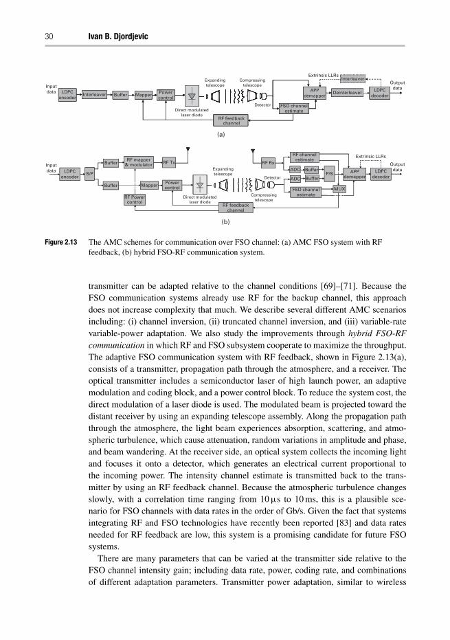
Figure 2.13 The AMC schemes for communication over FSO channel: (a) AMC FSO system with RFfeedback, (b) hybrid FSO-RF communication system.
transmitter can be adapted relative to the channel conditions [69]–[71]. Because theFSO communication systems already use RF for the backup channel, this approachdoes not increase complexity that much. We describe several different AMC scenariosincluding: (i) channel inversion, (ii) truncated channel inversion, and (iii) variable-ratevariable-power adaptation. We also study the improvements through hybrid FSO-RFcommunication in which RF and FSO subsystem cooperate to maximize the throughput.The adaptive FSO communication system with RF feedback, shown in Figure 2.13(a),consists of a transmitter, propagation path through the atmosphere, and a receiver. Theoptical transmitter includes a semiconductor laser of high launch power, an adaptivemodulation and coding block, and a power control block. To reduce the system cost, thedirect modulation of a laser diode is used. The modulated beam is projected toward thedistant receiver by using an expanding telescope assembly. Along the propagation paththrough the atmosphere, the light beam experiences absorption, scattering, and atmo-spheric turbulence, which cause attenuation, random variations in amplitude and phase,and beam wandering. At the receiver side, an optical system collects the incoming lightand focuses it onto a detector, which generates an electrical current proportional tothe incoming power. The intensity channel estimate is transmitted back to the trans-mitter by using an RF feedback channel. Because the atmospheric turbulence changesslowly, with a correlation time ranging from 10 μs to 10 ms, this is a plausible sce-nario for FSO channels with data rates in the order of Gb/s. Given the fact that systemsintegrating RF and FSO technologies have recently been reported [83] and data ratesneeded for RF feedback are low, this system is a promising candidate for future FSOsystems.
There are many parameters that can be varied at the transmitter side relative to theFSO channel intensity gain; including data rate, power, coding rate, and combinationsof different adaptation parameters. Transmitter power adaptation, similar to wireless
Coded modulation techniques for OW channels 31
communications, can be used to compensate for SNR variation due to atmosphericturbulence, with the aim to maintain a desired BER. The power adaptation therefore“inverts” the FSO channel scintillation so that the FSO channel behaves similarly as anAWGN channel to the receiver. The power adaptation policy for FSO channel inversionis similar to that for wireless links [68], and is defined by
P (it) = C/i2t , (2.27)
where C = P/E[1/i2t ] and it is the irradiance at time instance t; P(it) is the instanta-neous power, and P is the average power. The FSO channel, upon channel inversion,appears to the transmitter as a standard AWGN channel with SNR = �0/E[1/i2t ], where�0 = Es/N0 is the signal-to-noise ratio in the absence of scintillation, with Es being thesymbol energy and N0/2 being the double-side power spectral density of AWGN relatedto variance by σ2 = N0/2.
The channel inversion can be detrimental when it → 0 because the factor E[1/i2t ]tends to infinity. To avoid this problem the truncated channel inversion policy from wire-less communications [68] can be adopted, in which the channel inversion is performedonly when the irradiance is above the certain threshold itsh > 0; that is
P (it) ={
C/i2t , it ≥ itsh
0, it < itsh. (2.28)
The threshold irradiance is to be chosen in such a way to maximize channel capacity. Invariable data-rate adaptation, we change the signal constellation size for the fixed sym-bol rate depending on FSO channel conditions. When the FSO channel conditions arefavorable we increase the constellation size, decrease it when channel conditions are notfavorable, and do not transmit at all when the intensity channel coefficients are belowthe irradiance threshold. In the optimum power-variable data-rate adaptive scheme, weadapt the launch power and data rate so that the spectral efficiency is maximized. Withthis adaptation policy, more power and higher data rates are transmitted when FSOchannel conditions are good, less power and lower data rates are transmitted whenFSO channel is bad, and nothing is transmitted when the FSO irradiance falls belowthe threshold. For more details on optimum adaptation scheme an interested reader isreferred to [71].
The second AMC scheme, the adaptive hybrid FSO-RF communication system,shown in Figure 2.13(b), consists of two parallel FSO and RF channels. The LDPCencoded data stream is partially transmitted over FSO and partially over RF channel.The operating symbol rate of the FSO channel is commonly many times higher than thatof the RF channel. The FSO channel comprises an FSO transmitter, propagation paththrough the atmosphere, and an FSO receiver. The optical transmitter includes a semi-conductor laser of high launch power, an adaptive mapper, and a power control block. Toreduce the system cost, direct modulation of laser diode is used. The modulated beam isprojected toward the distant receiver by using an expanding telescope assembly. Alongthe propagation path through the atmosphere, the light beam experiences absorption,scattering, and atmospheric turbulence, which cause attenuation, and random variationsin amplitude and phase. The RF channel comprises adaptive RF mapper, RF power
32 Ivan B. Djordjevic
control, RF transmitter (Tx), transmitting antenna, wireless propagation path, receiverantenna, and RF receiver (Rx). The RF channel estimates and FSO irradiance estimatesare transmitted back to transmitters using the same RF feedback channel. The data ratesand powers in both channels are varied in accordance with the channel conditions. Thesymbol rates on both channels are kept fixed while the signal constellation sizes arevaried based on channel conditions. When the FSO (RF) channel condition is favorablelarger constellation size is used, when the FSO (RF) channel condition is poor, smallerconstellation sizes are used, and when the FSO (RF) channel SNR falls below thresholdthe signal is not transmitted at all. Both the subsystems (FSO and RF) are designed toachieve the same target bit error probability (Pb). The optimum power adaptation policyfor hybrid RF-FSO channel is the water-filling policy [70]:
KFSOPFSO (it)
P=
{1
�tsh− 1
�FSO , �FSO ≥ �tsh
0, �FSO < �tsh, �FSO = �FSO
0 i2t
KRFPRF (h)
P=
{1
�tsh− 1
�RF , �RF ≥ �tsh
0, �RF < �tsh, �RF = �RF
0 h2
(2.29)
where �tsh is the threshold SNR, which is common to both channels; KFSO =−1.85\ ln (5Pb), KRF = −1.5\ ln (5Pb) (with Pb being the target BER) and h is theRF fading coefficient; PFSO (PRF) denotes the portion of the power allocated to the FSO(RF) channel. Equation (2.29) allows us optimally to allocate the powers between FSOand RF channels depending on channel conditions.
In Figure 2.14, which is related to the FSO with RF feedback system, we show spec-tral efficiencies that can be achieved using optimum power and rate adaptation andM-ary pulse-amplitude modulation (MPAM) for different target bit error probabilities,and both: (a) weak turbulence regime (σR = 0.2, α = 51.913, β = 49.113), and(b) strong turbulence regime (σR = 2, α = 4.3407, β = 1.3088). For example, thespectral efficiency R/B of 2 bits/s/Hz at Pb = 10−9 is achieved for symbol SNR of23.3 dB in weak turbulence regime, and 26.2 dB in strong turbulence regime. In thesame figure, we also report spectral efficiencies that can be achieved by employing thesimple channel inversion power adaptation scheme. Interestingly, in the weak turbu-lence regime (Figure 2.14(a)) this performs comparable to the optimum adaptive-poweradaptive-rate scheme. However, in the strong turbulence regime (see Figure 2.14(b))this scheme faces significant performance degradation. Therefore, in the strong turbu-lence regime we have to employ the truncated channel inversion scheme, instead. InFigure 2.14, we also report spectral efficiencies that can be achieved by employing thetruncated channel inversion. This scheme performs comparable to the optimum adap-tation scheme in the weak turbulence regime, while at Pb = 10−9 and for spectralefficiency of 2 bits/s/Hz it performs 3.7 dB worse, but significantly better than the simplechannel inversion scheme.
By using trellis coded modulation (TCM), introduced by Ungerboeck [72], in com-bination with convolutional codes or by using coset codes, introduced by Forney [73],in combination with block codes, we can separate the encoding and modulation process(see [68] for more details). However, to keep the complexity of this approach reasonably
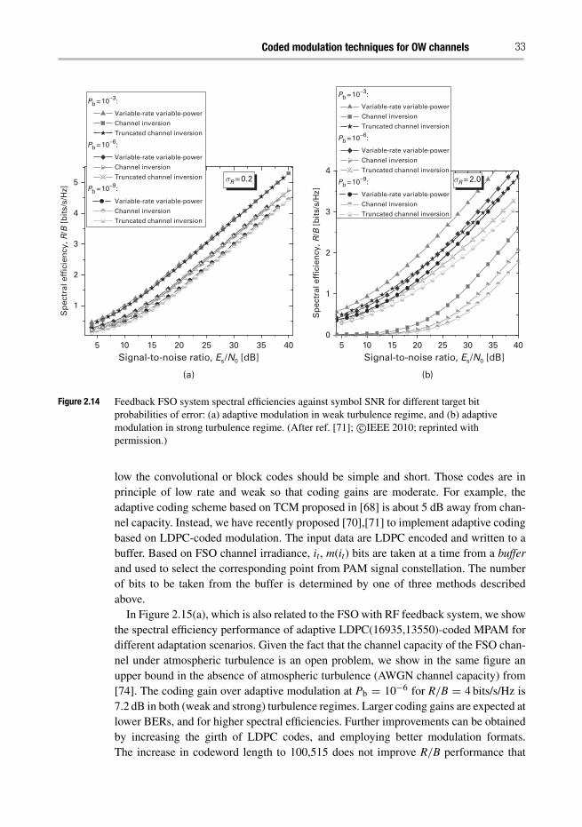
Coded modulation techniques for OW channels 33
5 10 15 20 25 30 35 40
1
2
3
4
5 σR = 0.2
Sp
ectr
al e
ffic
ien
cy, R
/B [
bit
s/s/
Hz]
Sp
ectr
al e
ffic
ien
cy, R
/B [
bit
s/s/
Hz]
Signal-to-noise ratio, Es /N0 [dB]5 10 15 20 25 30 35 40
Signal-to-noise ratio, Es /N0 [dB]
Pb = 10−3:
Pb = 10−6:
Pb = 10−9:
Variable-rate variable-power
Channel inversion
Truncated channel inversion
Variable-rate variable-power
Channel inversion
Truncated channel inversion
Variable-rate variable-power
Channel inversion
Truncated channel inversion
(a)
0
1
2
3
4
(b)
σR = 2.0
Pb = 10−3:
Pb = 10−6:
Pb = 10−9:
Variable-rate variable-power
Channel inversion
Truncated channel inversion
Variable-rate variable-power
Channel inversion
Truncated channel inversion
Variable-rate variable-power
Channel inversion
Truncated channel inversion
Figure 2.14 Feedback FSO system spectral efficiencies against symbol SNR for different target bitprobabilities of error: (a) adaptive modulation in weak turbulence regime, and (b) adaptivemodulation in strong turbulence regime. (After ref. [71]; c©IEEE 2010; reprinted withpermission.)
low the convolutional or block codes should be simple and short. Those codes are inprinciple of low rate and weak so that coding gains are moderate. For example, theadaptive coding scheme based on TCM proposed in [68] is about 5 dB away from chan-nel capacity. Instead, we have recently proposed [70],[71] to implement adaptive codingbased on LDPC-coded modulation. The input data are LDPC encoded and written to abuffer. Based on FSO channel irradiance, it, m(it) bits are taken at a time from a bufferand used to select the corresponding point from PAM signal constellation. The numberof bits to be taken from the buffer is determined by one of three methods describedabove.
In Figure 2.15(a), which is also related to the FSO with RF feedback system, we showthe spectral efficiency performance of adaptive LDPC(16935,13550)-coded MPAM fordifferent adaptation scenarios. Given the fact that the channel capacity of the FSO chan-nel under atmospheric turbulence is an open problem, we show in the same figure anupper bound in the absence of atmospheric turbulence (AWGN channel capacity) from[74]. The coding gain over adaptive modulation at Pb = 10−6 for R/B = 4 bits/s/Hz is7.2 dB in both (weak and strong) turbulence regimes. Larger coding gains are expected atlower BERs, and for higher spectral efficiencies. Further improvements can be obtainedby increasing the girth of LDPC codes, and employing better modulation formats.The increase in codeword length to 100,515 does not improve R/B performance that
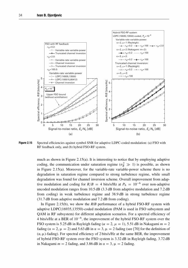
34 Ivan B. Djordjevic
0 5 10 15 20 25 300
1
2
3
4
5
Sp
ectr
al e
ffic
ien
cy, R
/B [
bit
s/s/
Hz]
Sp
ectr
al e
ffic
ien
cy, R
/B [
bit
s/s/
Hz]
Signal-to-noise ratio, Es /N0 [dB]5 10 15 20 25 30
Signal-to-noise ratio, Es /N0 [dB]
FSO with RF feedback:σR = 0.2:
Variable-rate variable-powerTruncated channel inversion
σR = 2.0:
Variable-rate variable-powerChannel inversionTruncated channel inversion
σR = 100.0:
Variable-rate variable-powerLDPC (16935,13550)LDPC (100515,80412)Channel inversion
Pb = 10−6
Upper FSO bound(without scintillation)
(a)
1
2
3
4
5
(b)
Hybrid FSO-RF system
LDPC (16935,13550)-coded, Pb = 10−6
Variable-rate variable-power:α = 2, μ = 1 (Rayleigh):
σR = 100
σR = 0.2 σR = 100 σR = 2.0
α = 2, μ = 2 (Nakagami m = 2):σR = 0.2 σR = 100
α = 3, μ = 2: σR = 0.2 σR = 100
Truncated channel inversion: α = 2, μ = 1 (Rayleigh):
σR = 0.2 σR = 100
α = 3, μ = 2:
Figure 2.15 Spectral efficiencies against symbol SNR for adaptive LDPC-coded modulation: (a) FSO withRF feedback only, and (b) hybrid FSO-RF system.
much as shown in Figure 2.15(a). It is interesting to notice that by employing adaptivecoding, the communication under saturation regime (σ 2
R � 1) is possible, as shownin Figure 2.15(a). Moreover, for the variable-rate variable-power scheme there is nodegradation in saturation regime compared to strong turbulence regime, while smalldegradation was found for channel inversion scheme. Overall improvement from adap-tive modulation and coding for R/B = 4 bits/s/Hz at Pb = 10−6 over non-adaptiveuncoded modulation ranges from 10.5 dB (3.3 dB from adaptive modulation and 7.2 dBfrom coding) in weak turbulence regime and 38.9 dB in strong turbulence regime(31.7 dB from adaptive modulation and 7.2 dB from coding).
In Figure 2.15(b), we show the R/B performance of a hybrid FSO-RF system withadaptive LDPC(16935,13550)-coded modulation (PAM is used in FSO subsystem andQAM in RF subsystem) for different adaptation scenarios. For a spectral efficiency of4 bits/s/Hz at a BER of 10−6, the improvement of the hybrid FSO-RF system over theFSO system is 5.25 dB in Rayleigh fading (α = 2, μ = 1), 5.51 dB in Nakagami m = 2fading (α = 2, μ = 2) and 5.63 dB in α = 3, μ = 2 fading (see [70] for the definition of(α, μ)-fading). For spectral efficiency of 2 bits/s/Hz at the same BER, the improvementof hybrid FSO-RF system over the FSO system is 3.32 dB in Rayleigh fading, 3.72 dBin Nakagami m = 2 fading, and 3.86 dB in α = 3, μ = 2 fading.
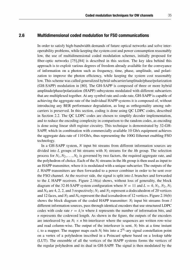
Coded modulation techniques for OW channels 35
2.6 Multidimensional coded modulation for FSO communications
In order to satisfy high-bandwidth demands of future optical networks and solve inter-operability problems, while keeping the system cost and power consumption reasonablylow, the use of multidimensional coded modulation schemes, initially proposed forfiber-optic networks [75],[84] is described in this section. The key idea behind thisapproach is to exploit various degrees of freedom already available for the conveyanceof information on a photon such as frequency, time, phase, amplitude, and polari-zation to improve the photon efficiency, while keeping the system cost reasonablylow. This scheme was called generalized hybrid subcarrier/amplitude/phase/polarization(GH-SAPP) modulation in [80]. The GH-SAPP is composed of three or more hybridamplitude/phase/polarization (HAPP) subsystems modulated with different subcarriersthat are multiplexed together. At any symbol rate and code rate, GH-SAPP is capable ofachieving the aggregate rate of the individual HAPP systems it is composed of, withoutintroducing any BER performance degradation, as long as orthogonality among sub-carriers is preserved. In this section, coding is done using QC LDPC codes, describedin Section 2.2. The QC LDPC codes are chosen to simplify decoder implementation,and to reduce the encoding complexity in comparison to the random codes, as encodingis done using linear shift register circuitry. This technique is demonstrated by 32-GH-SAPP, which in combination with commercially available 10 Gb/s equipment achievesthe aggregate data rate of 110 Gb/s, thus representing the 100G Ethernet enabling FSOtechnology.
In a GH-SAPP system, N input bit streams from different information sources aredivided into L groups of bit streams with Nl streams for the lth group. The selectionprocess for N1, N2, . . . , NL is governed by two factors, the required aggregate rate, andthe polyhedron of choice. Each of the Nl streams in the lth group is then used as input toan HAPP transmitter, where it is modulated with a unique subcarrier. The outputs of theL HAPP transmitters are then forwarded to a power combiner in order to be sent overthe FSO channel. At the receiver side, the signal is split into L branches and forwardedto the L HAPP receivers. Figure 2.16(a) shows, without loss of generality, the blockdiagram of the 32-H-SAPP system configuration where N = 11 and L = 4; N1, N2, N3
and N4 are 4, 2, 2, and 3 respectively; N1 and N2 represent a dodecahedron of 20 verticesand 12 faces, and N3 and N4 represent the dual icosahedron of 12 vertices. Figure 2.16(b)shows the block diagram of the coded HAPP transmitter: Nl input bit streams from ldifferent information sources, pass through identical encoders that use structured LDPCcodes with code rate r = k/n where k represents the number of information bits, andn represents the codeword length. As shown in the figure, the outputs of the encodersare interleaved by an Nl × n bit-interleaver where the sequences are written row-wiseand read column-wise. The output of the interleaver is sent, Nl bits at a time instanti, to a mapper. The mapper maps each Nl bits into a 2Nl -ary signal constellation pointon a vertex of a polyhedron inscribed in a Poincaré sphere based on a lookup table(LUT). The ensemble of all the vertices of the HAPP systems forms the vertices ofthe regular polyhedron and its dual in GH-SAPP. The signal is then modulated by the
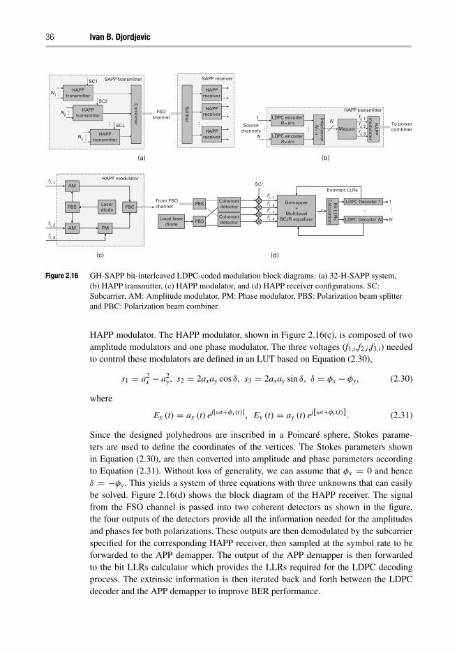
36 Ivan B. Djordjevic
HAPPtransmitter
HAPPtransmitter
HAPPtransmitter
SC1
…N1
SC2
…N2
… SCL
…NL
Co
mb
iner
Sp
litter
HAPPreceiver
HAPPreceiver
HAPPreceiver
…
FSOchannel
SAPP transmitter SAPP receiver
LDPC encoderR = k/n
LDPC encoderR = k/n
…
Sourcechannels
1
NIn
terleaverN
× n… Mapper
HA
PP
mo
du
lator
To powercombiner
fi, 1fi, 2fi, 3
N
(c)
(a) (b)
(d)
PBS
AM
AM PM
PBCLaserdiode
HAPP modulator
HAPP transmitter
fi, 1
fi, 2
fi, 3
Demapper+
MultilevelBCJR equalizer
Bit LLR
sC
alculatio
n
LDPC Decoder 1 1
NLDPC Decoder N
… …
Extrinsic LLRsf ’
Coherentdetector
Coherentdetector
PBS
PBS
SCl
From FSOchannel
Local laserdiode
i, 1
f ’i, 2f ’i, 3f ’i, 4
Figure 2.16 GH-SAPP bit-interleaved LDPC-coded modulation block diagrams: (a) 32-H-SAPP system,(b) HAPP transmitter, (c) HAPP modulator, and (d) HAPP receiver configurations. SC:Subcarrier, AM: Amplitude modulator, PM: Phase modulator, PBS: Polarization beam splitterand PBC: Polarization beam combiner.
HAPP modulator. The HAPP modulator, shown in Figure 2.16(c), is composed of twoamplitude modulators and one phase modulator. The three voltages (f1,i,f2,i,f3,i) neededto control these modulators are defined in an LUT based on Equation (2.30),
s1 = a2x − a2
y , s2 = 2axay cos δ, s3 = 2axay sin δ, δ = φx − φy, (2.30)
where
Ex (t) = ax (t) ej[ωt+φx(t)], Ey (t) = ay (t) ej[ωt+φy(t)]. (2.31)
Since the designed polyhedrons are inscribed in a Poincaré sphere, Stokes parame-ters are used to define the coordinates of the vertices. The Stokes parameters shownin Equation (2.30), are then converted into amplitude and phase parameters accordingto Equation (2.31). Without loss of generality, we can assume that φx = 0 and henceδ = −φy. This yields a system of three equations with three unknowns that can easilybe solved. Figure 2.16(d) shows the block diagram of the HAPP receiver. The signalfrom the FSO channel is passed into two coherent detectors as shown in the figure,the four outputs of the detectors provide all the information needed for the amplitudesand phases for both polarizations. These outputs are then demodulated by the subcarrierspecified for the corresponding HAPP receiver, then sampled at the symbol rate to beforwarded to the APP demapper. The output of the APP demapper is then forwardedto the bit LLRs calculator which provides the LLRs required for the LDPC decodingprocess. The extrinsic information is then iterated back and forth between the LDPCdecoder and the APP demapper to improve BER performance.
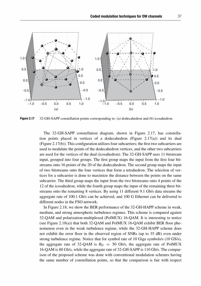
Coded modulation techniques for OW channels 37
−1.0 −0.5 0.0 0.5 1.0 −1.0 −0.5 0.0
(a) (b)
0.5 1.0−1.0
−0.5
0.0
0.5
1.0
−1.0
−0.5
0.0
0.5
1.0
−1.0
−0.5
0.0
0.5
1.0
−1.0
−0.5
0.0
0.5
1.0
Figure 2.17 32-GH-SAPP constellation points corresponding to: (a) dodecahedron and (b) icosahedron.
The 32-GH-SAPP constellation diagram, shown in Figure 2.17, has constella-tion points placed in vertices of a dodecahedron (Figure 2.17(a)) and its dual(Figure 2.17(b)). This configuration utilizes four subcarriers; the first two subcarriers areused to modulate the points of the dodecahedron vertices, and the other two subcarriersare used for the vertices of the dual (icosahedron). The 32-GH-SAPP uses 11-bitstreaminput, grouped into four groups. The first group maps the input from the first four bit-streams onto 16 points of the 20 of the dodecahedron. The second group maps the inputof two bitstreams onto the four vertices that form a tetrahedron. The selection of ver-tices for a subcarrier is done to maximize the distance between the points on the samesubcarrier. The third group maps the input from the two bitstreams onto 4 points of the12 of the icosahedron, while the fourth group maps the input of the remaining three bit-streams onto the remaining 8 vertices. By using 11 different 9.1 Gb/s data streams theaggregate rate of 100.1 Gb/s can be achieved, and 100 G Ethernet can be delivered todifferent nodes in the FSO network.
In Figure 2.18, we show the BER performance of the 32-GH-HAPP scheme in weak,medium, and strong atmospheric turbulence regimes. This scheme is compared against32-QAM and polarization-multiplexed (PolMUX) 16-QAM. It is interesting to notice(see Figure 2.18(a)) that both 32-QAM and PolMUX 16-QAM exhibit BER floor phe-nomenon even in the weak turbulence regime, while the 32-GH-HAPP scheme doesnot exhibit the error floor in the observed region of SNRs (up to 35 dB) even understrong turbulence regime. Notice that for symbol rate of 10 Giga symbols/s (10 GS/s),the aggregate rate of 32-QAM is RD = 50 Gb/s, the aggregate rate of PolMUX16-QAM is 80 Gb/s, while the aggregate rate of 32-GH-SAPP is 110 Gb/s. The compar-ison of the proposed scheme was done with conventional modulation schemes havingthe same number of constellation points, so that the comparison is fair with respect
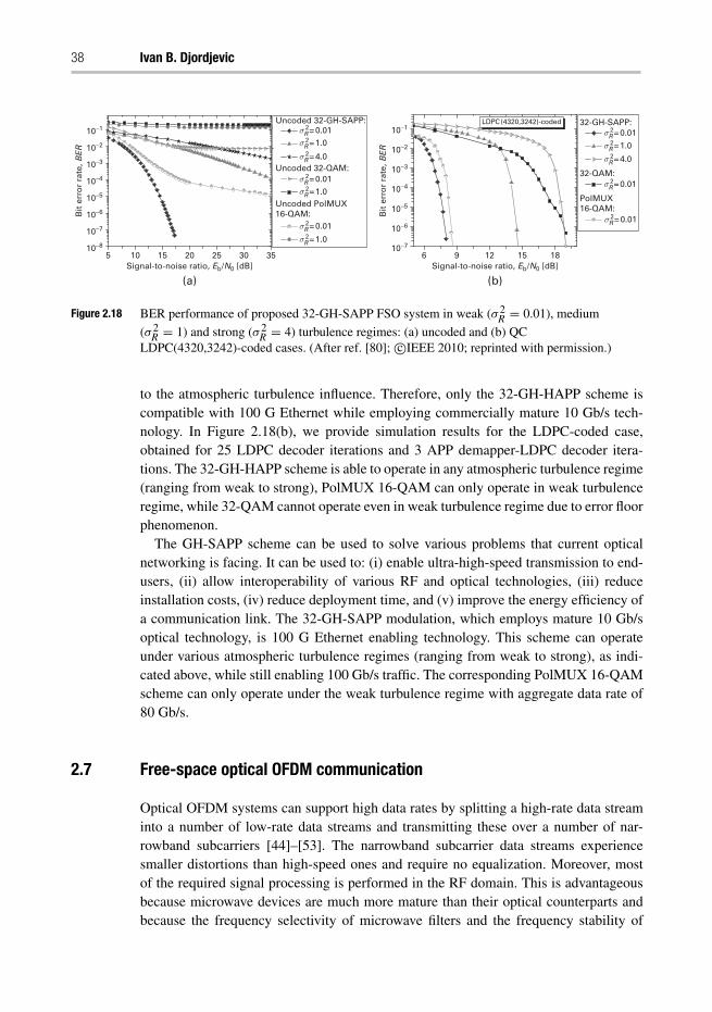
38 Ivan B. Djordjevic
5 10 15 20 25 30 35
10−1
10−2
10−3
10−4
10−5
10−6
10−7
10−1
10−2
10−3
10−4
10−5
10−6
10−710−8
Bit
err
or
rate
, BE
R
Bit
err
or
rate
, BE
R
Signal-to-noise ratio, Eb/N0 [dB] Signal-to-noise ratio, Eb/N0 [dB]6 9 12
(b)(a)
15 18
LDPC (4320,3242)-codedUncoded 32-GH-SAPP:
Uncoded 32-QAM:
Uncoded PolMUX16-QAM:
σR = 0.012
σR = 1.02
σR = 4.02
σR = 0.012
σR = 1.02
σR = 0.012
σR = 1.02
32-GH-SAPP:σR = 0.012
σR = 1.02
σR = 4.02
32-QAM:σR = 0.012
PolMUX16-QAM:
σR = 0.012
Figure 2.18 BER performance of proposed 32-GH-SAPP FSO system in weak (σ 2R = 0.01), medium
(σ 2R = 1) and strong (σ 2
R = 4) turbulence regimes: (a) uncoded and (b) QCLDPC(4320,3242)-coded cases. (After ref. [80]; c©IEEE 2010; reprinted with permission.)
to the atmospheric turbulence influence. Therefore, only the 32-GH-HAPP scheme iscompatible with 100 G Ethernet while employing commercially mature 10 Gb/s tech-nology. In Figure 2.18(b), we provide simulation results for the LDPC-coded case,obtained for 25 LDPC decoder iterations and 3 APP demapper-LDPC decoder itera-tions. The 32-GH-HAPP scheme is able to operate in any atmospheric turbulence regime(ranging from weak to strong), PolMUX 16-QAM can only operate in weak turbulenceregime, while 32-QAM cannot operate even in weak turbulence regime due to error floorphenomenon.
The GH-SAPP scheme can be used to solve various problems that current opticalnetworking is facing. It can be used to: (i) enable ultra-high-speed transmission to end-users, (ii) allow interoperability of various RF and optical technologies, (iii) reduceinstallation costs, (iv) reduce deployment time, and (v) improve the energy efficiency ofa communication link. The 32-GH-SAPP modulation, which employs mature 10 Gb/soptical technology, is 100 G Ethernet enabling technology. This scheme can operateunder various atmospheric turbulence regimes (ranging from weak to strong), as indi-cated above, while still enabling 100 Gb/s traffic. The corresponding PolMUX 16-QAMscheme can only operate under the weak turbulence regime with aggregate data rate of80 Gb/s.
2.7 Free-space optical OFDM communication
Optical OFDM systems can support high data rates by splitting a high-rate data streaminto a number of low-rate data streams and transmitting these over a number of nar-rowband subcarriers [44]–[53]. The narrowband subcarrier data streams experiencesmaller distortions than high-speed ones and require no equalization. Moreover, mostof the required signal processing is performed in the RF domain. This is advantageousbecause microwave devices are much more mature than their optical counterparts andbecause the frequency selectivity of microwave filters and the frequency stability of
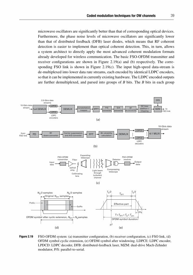
Coded modulation techniques for OW channels 39
microwave oscillators are significantly better than that of corresponding optical devices.Furthermore, the phase noise levels of microwave oscillators are significantly lowerthan that of distributed feedback (DFB) laser diodes, which means that RF coherentdetection is easier to implement than optical coherent detection. This, in turn, allowsa system architect to directly apply the most advanced coherent modulation formatsalready developed for wireless communication. The basic FSO-OFDM transmitter andreceiver configurations are shown in Figure 2.19(a) and (b) respectively. The corre-sponding FSO link is shown in Figure 2.19(c). The input high-speed data-stream isde-multiplexed into lower data rate streams, each encoded by identical LDPC encoders,so that it can be implemented in currently existing hardware. The LDPC encoded outputsare further demultiplexed, and parsed into groups of B bits. The B bits in each group
Constellationmapper IFFT P/S
converterD/A
converterRF
up-converter MZM
DFB
toFSO link
DC biasaddition +Clipping
DEMUX
2.5-Gb/s datastreams
LDPCE
LDPCE
LDPCencoders
… …1x4 DEMUX
10-Gb/s datastream
(a)
LDPCdecoders
PDfromFSO link
RFdown-converter
Carrier suppressionand A/D converter FFT Bit reliability
calculation DEMUX …LDPCD
LDPCD
… 4:1 MUX
10-Gb/s datastream
(b)
Light beamthroughturbulentchannel
Inputdata
Outputdata
FSO-OFDMtransmitter
opticalamp.
Expandingtelescope
DetectorFiber
Collimatinglens
Compressingtelescope
FSO-OFDMreceiver
(c)
(d) (e)
Original NFFT samples
Suffix
Prefix
NG/2 samples NG/2 samples
OFDM symbol after cyclic extension, NFFT + NGsamples
TFFT
TG/2 TG/2
Effective part
T = TFFT + TG + Twin
OFDM symbol duration
kT
Twin
Figure 2.19 FSO-OFDM system: (a) transmitter configuration, (b) receiver configuration, (c) FSO link, (d)OFDM symbol cyclic extension, (e) OFDM symbol after windowing. LDPCE: LDPC encoder,LPDCD: LDPC decoder, DFB: distributed-feedback laser, MZM: dual-drive Mach-Zehndermodulator, P/S: parallel-to-serial.
40 Ivan B. Djordjevic
(frame) are subdivided into K subgroups with the ith subgroup containing bi bits. The bi
bits from the ith subgroup are mapped into a complex-valued signal from a 2bi-point sig-nal constellation such as QAM. The complex-valued signal points from K subchannelsare considered to be the values of the discrete Fourier transform (DFT) of a multicarrierOFDM signal. Therefore, the symbol length (the time between two consecutive OFDMsymbols) in an OFDM system is T = KTs, where Ts is the symbol-interval length in anequivalent single-carrier system.
The transmitted OFDM signal can be written as
s (t) = sOFDM (t)+ D, (2.32)
where D is DC bias and
sOFDM (t) = Re
⎧⎨⎩
∞∑k=−∞
w (t − kT)NFFT/2−1∑
i=−NFFT/2
Xi,k · ej2π iTFFT
·(t−kT)ej2π fRFt
⎫⎬⎭ , (2.33)
which is defined for kT − TG/2 − Twin ≤ t ≤ kT + TFFT + TG/2 + Twin. In theabove expression Xi,k denotes the kth OFDM symbol in the ith subcarrier, w(t) is thewindow function, and fRF is the RF carrier frequency. The duration of the OFDM symbolis denoted by T , while TFFT is the FFT sequence duration, TG is the guard intervalduration (the duration of cyclic extension), and Twin is the length of the windowinginterval.
The details of the resulting OFDM symbol are shown in Figure 2.19(d)–(e). Thesymbols are generated as follows. NQAM(= K) consecutive input QAM symbols arezero-padded to obtain NFFT(= 2m, m > 1) input samples for inverse fast Fourier trans-form (IFFT), then NG samples are inserted to create the guard interval TG and finally theOFDM symbol is multiplied by the window function (raised cosine function is used in[47], but the Kaiser, Blackman–Harris and other window functions are also applicable).The purpose of the cyclic extension is to preserve the orthogonality among subcarri-ers when the neighboring OFDM symbols partially overlap, and the purpose of thewindowing is to reduce the out-of-band spectrum. The cyclic extension, illustrated inFigure 2.19(d), is performed by repeating the last NG/2 samples of the FFT frame (ofduration TFFT with NFFT samples) as the prefix, and repeating the first NG/2 samples(out of NFFT) as the suffix. After a D/A conversion and RF up-conversion, we convertthe RF signal to the optical domain using one of two options: (i) for symbol rates upto 10 Gsymbols/s the OFDM signal directly modulates the DFB laser, and (ii) for sym-bol rates above 10 Gsymbols/s the OFDM signal drives the dual-drive Mach-Zehndermodulator (MZM). The DC component (D in Eq. (2.32)) is inserted to enable inco-herent recovery of the QAM symbols. In the remainder of this section, three differentOFDM schemes are described. The first scheme is based on intensity modulation, andshall be referred to as the “biased-OFDM” (B-OFDM) scheme. Because bipolar sig-nals cannot be transmitted over an IM/DD link, it is assumed that the bias componentD is sufficiently large so that when added to sOFDM(t) the resulting sum is non nega-tive. The main disadvantage of the B-OFDM scheme is the poor power efficiency. Toimprove the power efficiency we describe two alternative schemes [45]. The first of
Coded modulation techniques for OW channels 41
these, which we shall refer to as the “clipped-OFDM” (C-OFDM) scheme, is based onsingle-side band (SSB) transmission, with clipping of the negative portion of the OFDMsignal after bias addition. The bias is varied to find the optimum one for fixed opticallaunched power. It was found that the optimum case is one in which ∼50% of the totalelectrical signal energy before clipping is allocated for transmission of a carrier. Toconvert the signal from double-side band (DSB) to SSB, we have two options: (i) touse Hilbert transformation of the in-phase signal as the quadrature signal in electricaldomain, and (ii) to perform DSB to SSB transformation by an optical filter. The secondpower-efficient scheme, which we shall refer to as the “unclipped-OFDM” (U-OFDM)scheme, is based on SSB transmission employing LiNbO3 MZM. To avoid distortiondue to clipping, the information-bearing signal is transmitted by modulating the elec-trical field (instead of intensity modulation employed in the B-OFDM and C-OFDMschemes) so that the negative part of the OFDM signal is transmitted to the photode-tector. Distortion introduced by the photodetector, caused by squaring, is successfullyeliminated by proper filtering, and the recovered signal distortion is insignificant. Noticethat U-OFDM is less power efficient than C-OFDM because the negative portion ofthe OFDM signal is transmitted and then discarded. For U-OFDM the detector non-linearity is compensated by post-detection filters that reject (potentially useful) signalenergy and compromise power efficiency. Despite this drawback we find that U-OFDMis still significantly more power efficient than B-OFDM. Note that the DC bias shiftsthe average of the C-OFDM signal towards positive values, while in the case of B-OFDM a much larger bias is needed to completely eliminate the negative portion of thesignal.
The point-to-point FSO system considered here, shown in Figure 2.19(c), consistsof an FSO-OFDM transmitter, propagation medium and an FSO-OFDM receiver. Themodulated beam is projected toward the receiver using the expanding telescope. Atthe receiver, an optical system collects the light, and focuses it onto a detector, whichdelivers an electrical signal proportional to the incoming optical power. The receivercommonly employs the transimpedance design, which is a good compromise betweennoise and bandwidth. A PIN photodiode plus preamplifier or an avalanche photodi-ode are typically used as optical detectors. During propagation through the air, theoptical beam experiences amplitude and phase variations caused by scattering, refrac-tion caused by atmospheric turbulence, absorption, and building sway. The photodiodeoutput current can be written as
i (t) = RPD |a (t) sOFDM (t)+ a (t)D|2
= RPD
[|a (t) sOFDM (t)|2 + |a (t)D|2 + 2Re
{a (t) sOFDM (t) a∗ (t)D
}], (2.34)
where |a(t)|2 denotes the intensity fluctuation due to atmospheric turbulence, and RPD
denotes the photodiode responsivity.After RF down-conversion, the A/D conversion and cyclic extension removal, the
transmitted signal is demodulated by the FFT algorithm. The soft outputs of the FFTdemodulator are used to estimate the bit reliabilities that are fed to four identical LDPC
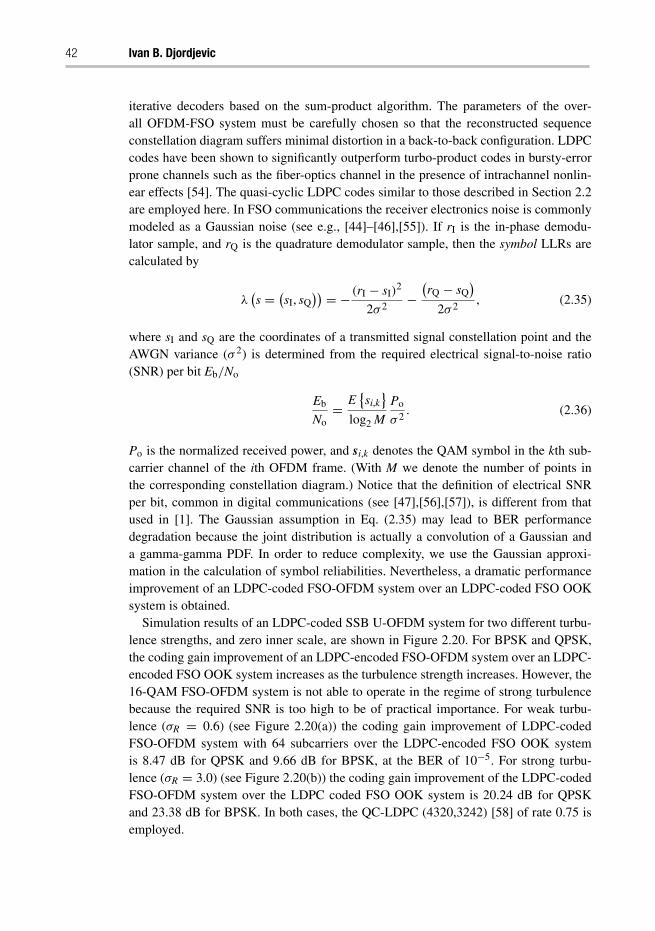
42 Ivan B. Djordjevic
iterative decoders based on the sum-product algorithm. The parameters of the over-all OFDM-FSO system must be carefully chosen so that the reconstructed sequenceconstellation diagram suffers minimal distortion in a back-to-back configuration. LDPCcodes have been shown to significantly outperform turbo-product codes in bursty-errorprone channels such as the fiber-optics channel in the presence of intrachannel nonlin-ear effects [54]. The quasi-cyclic LDPC codes similar to those described in Section 2.2are employed here. In FSO communications the receiver electronics noise is commonlymodeled as a Gaussian noise (see e.g., [44]–[46],[55]). If rI is the in-phase demodu-lator sample, and rQ is the quadrature demodulator sample, then the symbol LLRs arecalculated by
λ(s = (
sI, sQ)) = − (rI − sI)
2
2σ 2−
(rQ − sQ
)2σ 2
, (2.35)
where sI and sQ are the coordinates of a transmitted signal constellation point and theAWGN variance (σ 2) is determined from the required electrical signal-to-noise ratio(SNR) per bit Eb/No
Eb
No= E
{si,k
}log2 M
Po
σ 2. (2.36)
Po is the normalized received power, and si,k denotes the QAM symbol in the kth sub-carrier channel of the ith OFDM frame. (With M we denote the number of points inthe corresponding constellation diagram.) Notice that the definition of electrical SNRper bit, common in digital communications (see [47],[56],[57]), is different from thatused in [1]. The Gaussian assumption in Eq. (2.35) may lead to BER performancedegradation because the joint distribution is actually a convolution of a Gaussian anda gamma-gamma PDF. In order to reduce complexity, we use the Gaussian approxi-mation in the calculation of symbol reliabilities. Nevertheless, a dramatic performanceimprovement of an LDPC-coded FSO-OFDM system over an LDPC-coded FSO OOKsystem is obtained.
Simulation results of an LDPC-coded SSB U-OFDM system for two different turbu-lence strengths, and zero inner scale, are shown in Figure 2.20. For BPSK and QPSK,the coding gain improvement of an LDPC-encoded FSO-OFDM system over an LDPC-encoded FSO OOK system increases as the turbulence strength increases. However, the16-QAM FSO-OFDM system is not able to operate in the regime of strong turbulencebecause the required SNR is too high to be of practical importance. For weak turbu-lence (σR = 0.6) (see Figure 2.20(a)) the coding gain improvement of LDPC-codedFSO-OFDM system with 64 subcarriers over the LDPC-encoded FSO OOK systemis 8.47 dB for QPSK and 9.66 dB for BPSK, at the BER of 10−5. For strong turbu-lence (σR = 3.0) (see Figure 2.20(b)) the coding gain improvement of the LDPC-codedFSO-OFDM system over the LDPC coded FSO OOK system is 20.24 dB for QPSKand 23.38 dB for BPSK. In both cases, the QC-LDPC (4320,3242) [58] of rate 0.75 isemployed.
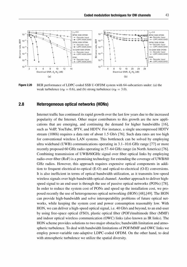
Coded modulation techniques for OW channels 43
2 4 6 8 10 12
(a) (b)
14
10−1
10−2
10−3
10−4
10−5
10−6
Bit
err
or
rate
, BE
R
10−1
10−2
10−3
10−4
10−5
10−6
Bit
err
or
rate
, BE
R
Electrical SNR, Eb/N0 [dB] Electrical SNR, Eb/N0 [dB]
BPSK SSB OFDM:Decoder inputLDPC(4320,3242)
QPSK SSB OFDM:Decoder inputLDPC(4320,3242)
16-QAM SSB OFDM:Decoder inputLDPC(4320,3242)
OOK:Decoder inputLDPC (4320,3242)
BPSK SSB OFDM:Decoder inputLDPC (4320,3242)
QPSK SSB OFDM:Decoder inputLDPC (4320,3242)
16-QAM SSB OFDM:Decoder inputLDPC (4320,3242)
OOK:Decoder inputLDPC (4320,3242)
4 8 12 16 20 24 28
Figure 2.20 BER performance of LDPC-coded SSB U-OFDM system with 64-subcarriers under: (a) theweak turbulence (σR = 0.6), and (b) strong turbulence (σR = 3.0).
2.8 Heterogeneous optical networks (HONs)
Internet traffic has continued its rapid growth over the last few years due to the increasedpopularity of the Internet. Other major contributors to this growth are the new appli-cations that are emerging, and continuing the demand for higher bandwidths [16],such as VoIP, YouTube, IPTV, and HDTV. For instance, a single uncompressed HDTVstream (1080i) requires a data rate of about 1.5 Gb/s [76]. Such data rates are too highfor conventional wireless LAN systems. This bottleneck can be solved by employingultra wideband (UWB) communications operating in 3.1–10.6 GHz range [77] or morerecently proposed 60 GHz radio operating in 57–64 GHz range (in North America) [76].Combining transmission of UWB/60GHz signal over fiber optical links by employingradio-over-fiber (RoF) is a promising technology for extending the coverage of UWB/60GHz radios. However, this approach requires expensive optical components in addi-tion to frequent electrical-to-optical (E-O) and optical-to-electrical (O-E) conversions.It is also inefficient in terms of optical bandwidth utilization, as it transmits low-speedwireless signals over high-bandwidth optical channel. Another approach to deliver high-speed signal to an end-user is through the use of passive optical networks (PONs) [78].In order to reduce the system cost of PONs and speed up the installation cost, we pro-posed recently the use of heterogeneous optical networking (HON) [48],[49]. The HONcan provide high-bandwidth and solve interoperability problems of future optical net-works, while keeping the system cost and power consumption reasonably low. WithHON, we can deliver a high-speed optical signal, i.e. 40 Gb/s and beyond, to an end-userby using free-space optical (FSO), plastic optical fiber (POF)/multimode fiber (MMF)and indoor optical wireless communication (OWC) links (also known as IR links). TheHON scheme provides solutions to two major obstacles; bandwidth limitation and atmo-spheric turbulence. To deal with bandwidth limitations of POF/MMF and OWC links weemploy power-variable rate-adaptive LDPC-coded OFDM. On the other hand, to dealwith atmospheric turbulence we utilize the spatial diversity.
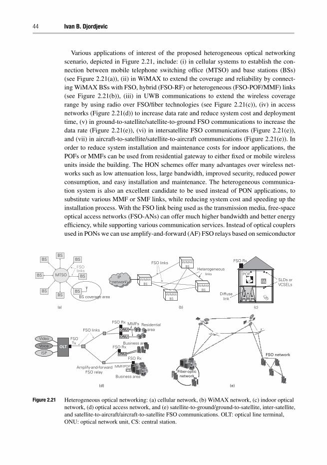
44 Ivan B. Djordjevic
Various applications of interest of the proposed heterogeneous optical networkingscenario, depicted in Figure 2.21, include: (i) in cellular systems to establish the con-nection between mobile telephone switching office (MTSO) and base stations (BSs)(see Figure 2.21(a)), (ii) in WiMAX to extend the coverage and reliability by connect-ing WiMAX BSs with FSO, hybrid (FSO-RF) or heterogeneous (FSO-POF/MMF) links(see Figure 2.21(b)), (iii) in UWB communications to extend the wireless coveragerange by using radio over FSO/fiber technologies (see Figure 2.21(c)), (iv) in accessnetworks (Figure 2.21(d)) to increase data rate and reduce system cost and deploymenttime, (v) in ground-to-satellite/satellite-to-ground FSO communications to increase thedata rate (Figure 2.21(e)), (vi) in intersatellite FSO communications (Figure 2.21(e)),and (vii) in aircraft-to-satellite/satellite-to-aircraft communications (Figure 2.21(e)). Inorder to reduce system installation and maintenance costs for indoor applications, thePOFs or MMFs can be used from residential gateway to either fixed or mobile wirelessunits inside the building. The HON schemes offer many advantages over wireless net-works such as low attenuation loss, large bandwidth, improved security, reduced powerconsumption, and easy installation and maintenance. The heterogeneous communica-tion system is also an excellent candidate to be used instead of PON applications, tosubstitute various MMF or SMF links, while reducing system cost and speeding up theinstallation process. With the FSO link being used as the transmission media, free-spaceoptical access networks (FSO-ANs) can offer much higher bandwidth and better energyefficiency, while supporting various communication services. Instead of optical couplersused in PONs we can use amplify-and-forward (AF) FSO relays based on semiconductor
BS
MTSO BS
BS
BS
BSBS
(a)
BS
BS
FSOlinks
BS coverage area
WiMAXBS
(b)
IPnetwork
FSO links
WiMAXBS
WiMAXBS
WiMAXBS
Heterogeneouslinks
FSO Rx
POFSLDs orVCSELs
Diffuselink
(c)
Video
Voice
ISP
OLT
ONU
ONU
Amplify-and-forwardFSO relay
ONU
CS
Business area
FSO links
MMF/POF
FSO Rx
FSOTx
MMFsFSO Rx
FSO Rx
Residentialarea
Business area
FSO network
(e)(d)
Fiber-opticnetwork
Figure 2.21 Heterogeneous optical networking: (a) cellular network, (b) WiMAX network, (c) indoor opticalnetwork, (d) optical access network, and (e) satellite-to-ground/ground-to-satellite, inter-satellite,and satellite-to-aircraft/aircraft-to-satellite FSO communications. OLT: optical line terminal,ONU: optical network unit, CS: central station.
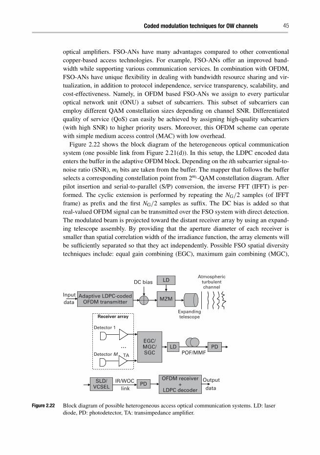
Coded modulation techniques for OW channels 45
optical amplifiers. FSO-ANs have many advantages compared to other conventionalcopper-based access technologies. For example, FSO-ANs offer an improved band-width while supporting various communication services. In combination with OFDM,FSO-ANs have unique flexibility in dealing with bandwidth resource sharing and vir-tualization, in addition to protocol independence, service transparency, scalability, andcost-effectiveness. Namely, in OFDM based FSO-ANs we assign to every particularoptical network unit (ONU) a subset of subcarriers. This subset of subcarriers canemploy different QAM constellation sizes depending on channel SNR. Differentiatedquality of service (QoS) can easily be achieved by assigning high-quality subcarriers(with high SNR) to higher priority users. Moreover, this OFDM scheme can operatewith simple medium access control (MAC) with low overhead.
Figure 2.22 shows the block diagram of the heterogeneous optical communicationsystem (one possible link from Figure 2.21(d)). In this setup, the LDPC encoded dataenters the buffer in the adaptive OFDM block. Depending on the ith subcarrier signal-to-noise ratio (SNR), mi bits are taken from the buffer. The mapper that follows the bufferselects a corresponding constellation point from 2mi -QAM constellation diagram. Afterpilot insertion and serial-to-parallel (S/P) conversion, the inverse FFT (IFFT) is per-formed. The cyclic extension is performed by repeating the NG/2 samples (of IFFTframe) as prefix and the first NG/2 samples as suffix. The DC bias is added so thatreal-valued OFDM signal can be transmitted over the FSO system with direct detection.The modulated beam is projected toward the distant receiver array by using an expand-ing telescope assembly. By providing that the aperture diameter of each receiver issmaller than spatial correlation width of the irradiance function, the array elements willbe sufficiently separated so that they act independently. Possible FSO spatial diversitytechniques include: equal gain combining (EGC), maximum gain combining (MGC),
Adaptive LDPC-codedOFDM transmitter
MZMAdaptive LDPC-coded
OFDM transmitter MZMInputdata
LDDC bias
Expandingtelescope
Detector 1
TA
Receiver array
Detector M
…EGC/MGC/SGC
LDPOF/MMF
PD
OFDM receiver+
LDPC decoder
Output
dataSLD/
VCSELIR/WOC
linkPD
Atmosphericturbulentchannel
Figure 2.22 Block diagram of possible heterogeneous access optical communication systems. LD: laserdiode, PD: photodetector, TA: transimpedance amplifier.
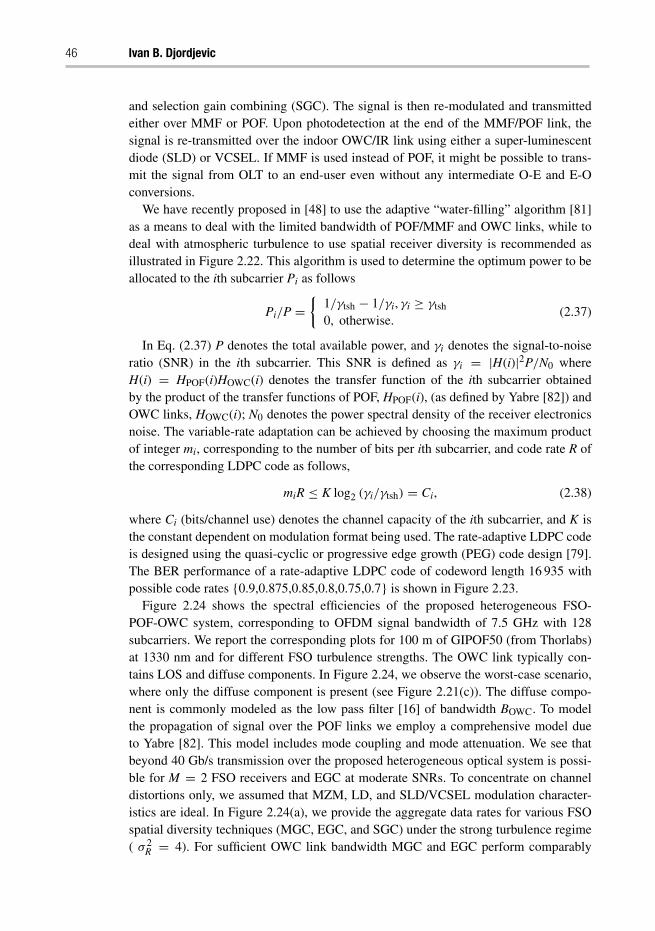
46 Ivan B. Djordjevic
and selection gain combining (SGC). The signal is then re-modulated and transmittedeither over MMF or POF. Upon photodetection at the end of the MMF/POF link, thesignal is re-transmitted over the indoor OWC/IR link using either a super-luminescentdiode (SLD) or VCSEL. If MMF is used instead of POF, it might be possible to trans-mit the signal from OLT to an end-user even without any intermediate O-E and E-Oconversions.
We have recently proposed in [48] to use the adaptive “water-filling” algorithm [81]as a means to deal with the limited bandwidth of POF/MMF and OWC links, while todeal with atmospheric turbulence to use spatial receiver diversity is recommended asillustrated in Figure 2.22. This algorithm is used to determine the optimum power to beallocated to the ith subcarrier Pi as follows
Pi/P ={
1/γtsh − 1/γi, γi ≥ γtsh
0, otherwise.(2.37)
In Eq. (2.37) P denotes the total available power, and γi denotes the signal-to-noiseratio (SNR) in the ith subcarrier. This SNR is defined as γi = |H(i)|2P/N0 whereH(i) = HPOF(i)HOWC(i) denotes the transfer function of the ith subcarrier obtainedby the product of the transfer functions of POF, HPOF(i), (as defined by Yabre [82]) andOWC links, HOWC(i); N0 denotes the power spectral density of the receiver electronicsnoise. The variable-rate adaptation can be achieved by choosing the maximum productof integer mi, corresponding to the number of bits per ith subcarrier, and code rate R ofthe corresponding LDPC code as follows,
miR ≤ K log2 (γi/γtsh) = Ci, (2.38)
where Ci (bits/channel use) denotes the channel capacity of the ith subcarrier, and K isthe constant dependent on modulation format being used. The rate-adaptive LDPC codeis designed using the quasi-cyclic or progressive edge growth (PEG) code design [79].The BER performance of a rate-adaptive LDPC code of codeword length 16 935 withpossible code rates {0.9,0.875,0.85,0.8,0.75,0.7} is shown in Figure 2.23.
Figure 2.24 shows the spectral efficiencies of the proposed heterogeneous FSO-POF-OWC system, corresponding to OFDM signal bandwidth of 7.5 GHz with 128subcarriers. We report the corresponding plots for 100 m of GIPOF50 (from Thorlabs)at 1330 nm and for different FSO turbulence strengths. The OWC link typically con-tains LOS and diffuse components. In Figure 2.24, we observe the worst-case scenario,where only the diffuse component is present (see Figure 2.21(c)). The diffuse compo-nent is commonly modeled as the low pass filter [16] of bandwidth BOWC. To modelthe propagation of signal over the POF links we employ a comprehensive model dueto Yabre [82]. This model includes mode coupling and mode attenuation. We see thatbeyond 40 Gb/s transmission over the proposed heterogeneous optical system is possi-ble for M = 2 FSO receivers and EGC at moderate SNRs. To concentrate on channeldistortions only, we assumed that MZM, LD, and SLD/VCSEL modulation character-istics are ideal. In Figure 2.24(a), we provide the aggregate data rates for various FSOspatial diversity techniques (MGC, EGC, and SGC) under the strong turbulence regime( σ 2
R = 4). For sufficient OWC link bandwidth MGC and EGC perform comparably
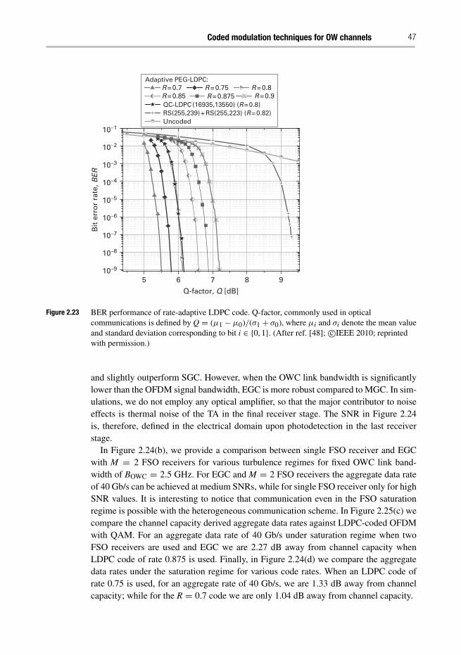
Coded modulation techniques for OW channels 47
5 6 7 8 9
10−1
10−2
10−3
10−4
10−5
10−6
10−7
10−8
10−9
Bit
err
or
rate
, BE
R
Q-factor, Q [dB]
Adaptive PEG-LDPC: R = 0.7 R = 0.75 R = 0.8 R = 0.85 R = 0.875 R = 0.9QC-LDPC (16935,13550) (R = 0.8)RS(255,239) + RS(255,223) (R = 0.82)Uncoded
Figure 2.23 BER performance of rate-adaptive LDPC code. Q-factor, commonly used in opticalcommunications is defined by Q = (μ1 −μ0)/(σ1 + σ0), where μi and σi denote the mean valueand standard deviation corresponding to bit i ∈ {0, 1}. (After ref. [48]; c©IEEE 2010; reprintedwith permission.)
and slightly outperform SGC. However, when the OWC link bandwidth is significantlylower than the OFDM signal bandwidth, EGC is more robust compared to MGC. In sim-ulations, we do not employ any optical amplifier, so that the major contributor to noiseeffects is thermal noise of the TA in the final receiver stage. The SNR in Figure 2.24is, therefore, defined in the electrical domain upon photodetection in the last receiverstage.
In Figure 2.24(b), we provide a comparison between single FSO receiver and EGCwith M = 2 FSO receivers for various turbulence regimes for fixed OWC link band-width of BOWC = 2.5 GHz. For EGC and M = 2 FSO receivers the aggregate data rateof 40 Gb/s can be achieved at medium SNRs, while for single FSO receiver only for highSNR values. It is interesting to notice that communication even in the FSO saturationregime is possible with the heterogeneous communication scheme. In Figure 2.25(c) wecompare the channel capacity derived aggregate data rates against LDPC-coded OFDMwith QAM. For an aggregate data rate of 40 Gb/s under saturation regime when twoFSO receivers are used and EGC we are 2.27 dB away from channel capacity whenLDPC code of rate 0.875 is used. Finally, in Figure 2.24(d) we compare the aggregatedata rates under the saturation regime for various code rates. When an LDPC code ofrate 0.75 is used, for an aggregate rate of 40 Gb/s, we are 1.33 dB away from channelcapacity; while for the R = 0.7 code we are only 1.04 dB away from channel capacity.
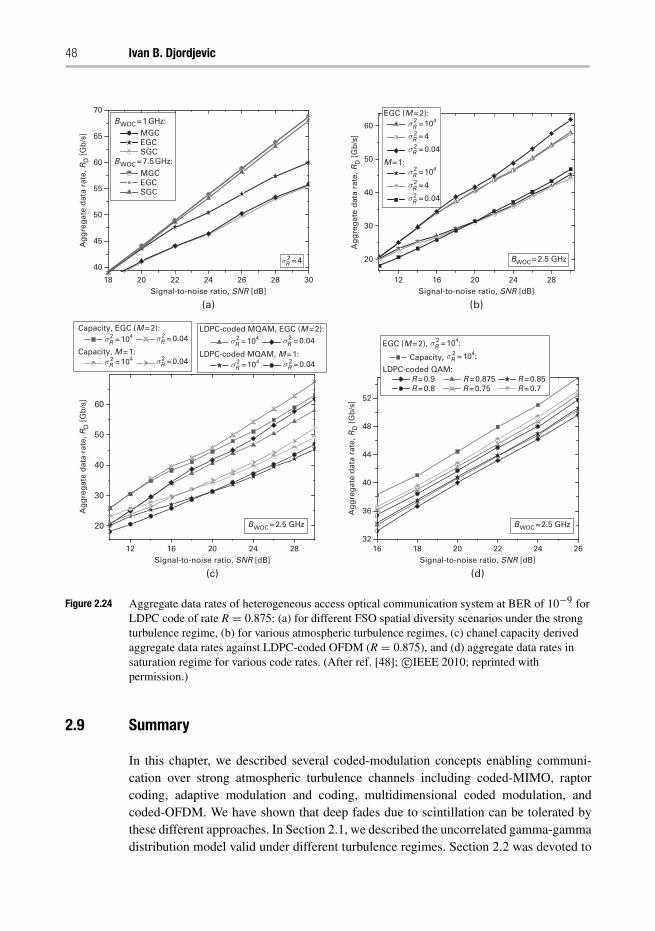
48 Ivan B. Djordjevic
40
45
50
55
60
65
70
Ag
gre
gat
e d
ata
rate
, RD
[G
b/s
]A
gg
reg
ate
dat
a ra
te, R
D [
Gb
/s]
Ag
gre
gat
e d
ata
rate
, RD
[G
b/s
]A
gg
reg
ate
dat
a ra
te, R
D [
Gb
/s]
Signal-to-noise ratio, SNR [dB] Signal-to-noise ratio, SNR [dB]
B WOC = 1 GHz:
B WOC = 7.5 GHz:
MGCEGCSGC
MGCEGCSGC
20
30
40
50
60
BWOC = 2.5 GHz
(a) (b)
20
30
40
50
60
18 20 22 24 26
Signal-to-noise ratio, SNR [dB]
(d)
1816 20 22 24 26
28 30 12 16 20 24 28
Signal-to-noise ratio, SNR [dB]
(c)
12 16 20 24 2832
36
40
44
48
52
σR = 42
EGC (M = 2):
M = 1:
σR = 1042
σR = 42
σR = 0.042
σR = 1042
σR = 42
σR = 0.042
B WOC = 2.5 GHz B WOC = 2.5 GHz
Capacity, EGC (M = 2):
Capacity, M = 1:
σR = 1042
σR = 1042
σR = 0.042LDPC-coded MQAM, EGC (M = 2):
LDPC-coded MQAM, M = 1:
σR = 1042EGC (M = 2),
Capacity,
LDPC-coded QAM:R = 0.9
R = 0.7R = 0.85
R = 0.75R = 0.875
R = 0.8
σR = 104:2
σR = 104:2
σR = 0.042
σR = 1042 σR = 0.042σR = 0.042
Figure 2.24 Aggregate data rates of heterogeneous access optical communication system at BER of 10−9 forLDPC code of rate R = 0.875: (a) for different FSO spatial diversity scenarios under the strongturbulence regime, (b) for various atmospheric turbulence regimes, (c) chanel capacity derivedaggregate data rates against LDPC-coded OFDM (R = 0.875), and (d) aggregate data rates insaturation regime for various code rates. (After ref. [48]; c©IEEE 2010; reprinted withpermission.)
2.9 Summary
In this chapter, we described several coded-modulation concepts enabling communi-cation over strong atmospheric turbulence channels including coded-MIMO, raptorcoding, adaptive modulation and coding, multidimensional coded modulation, andcoded-OFDM. We have shown that deep fades due to scintillation can be tolerated bythese different approaches. In Section 2.1, we described the uncorrelated gamma-gammadistribution model valid under different turbulence regimes. Section 2.2 was devoted to
Coded modulation techniques for OW channels 49
different codes on graphs suitable for use in FSO communications. In Section 2.3, wedescribed coded-MIMO, and have shown that the repetition MIMO can be used to dealwith scintillation. In Section 2.4, we described the use of raptor codes as a means ofenabling the communication over temporal correlated FSO channels. Section 2.5 wasdevoted to adaptive modulation and coding. Two AMC schemes were described: AMCwith RF feedback and a hybrid FSO-RF AMC scheme. Both schemes enable communi-cation under strong atmospheric turbulence. The possibility of using multidimensionalcoded modulation schemes to enable ultra-high-speed optical communication was dis-cussed in Section 2.6. In Section 2.7, we have shown that deep fades due to atmosphericturbulence can be tolerated by using the coded-OFDM in combination with interleaving.In Section 2.8, we discussed the possibility of implementation of heterogeneous opticalnetworks, composed of various optical links (SMF, MMF, POF, and FSO links).
Acknowledgments
This chapter is supported in part by the NSF under Grants CCF-0952711 and ECCS-0725405.
References
[1] L. C. Andrews and R. L. Philips, Laser Beam Propagation Through Random Media. SPIEOptical Engineering Press, 1998.
[2] H. Willebrand, B.S. Ghuman, Free-Space Optics: Enabling Optical Connectivity in Today’sNetworks. Sams Publishing, 2002.
[3] A. Ishimaru, Wave Propagation and Scattering in Random Media. Academic, 1978, vol.1–2.
[4] L. C. Andrews, R. L. Phillips, and C. Y. Hopen, Laser Beam Scintillation with Applications.SPIE Press, 2001.
[5] S. Karp, R. Gagliardi, S. E. Moran, and L. B. Stotts, Optical Channels. Plenum, 1988.[6] S. M. Flatté, C. Bracher, and G.-Y. Wang, “Probability-density functions of irradiance for
waves in atmospheric turbulence calculated by numerical simulation,” J. Opt. Soc. Am. A,vol. 11, pp. 2080–2092, 1994.
[7] L. C. Andrews and R. L. Phillips, “I-K distribution as a universal propagation model of laserbeams in atmospheric turbulence,” J. Opt. Soc. Am., vol. 2, pp. 160–163, 1985.
[8] L. C. Andrews and R. L. Phillips, “Mathematical genesis of the I-K distribution for randomoptical fields,” J. Opt. Soc. Am., vol. 3, pp. 1912–1919, 1986.
[9] J. H. Churnside and R. J. Hill, “Probability density of irradiance scintillations for strongpath-integrated refractive turbulence,” J. Opt. Soc. Am. A, vol. 4, pp. 727–733, 1987.
[10] R. J. Hill and R. G. Frehlich, “Probability distribution of irradiance for the onset of strongscintillation,” J. Opt. Soc. Am. A, vol. 14, pp. 1530–1540, 1997.
[11] J. H. Churnside and R. G. Frehlich, “Experimental evaluation of log-normally modulatedRician and IK models of optical scintillation in the atmosphere,” J. Opt. Soc. Am. A, vol. 6,pp. 1760–1766, 1989.
50 Ivan B. Djordjevic
[12] M. A. Al-Habash, L.C. Andrews, and R. L. Phillips, “Mathematical model for the irradianceprobability density function of a laser beam propagating through turbulent media,” Opt.Eng., vol. 40, pp. 1554–1562, 2001.
[13] X. Zhu, and J. M. Kahn, “Free-space optical communication through atmospheric turbu-lence channels,” IEEE Trans. Commun., vol. 50, pp. 1293–1300, 2002.
[14] S. G. Wilson, M. Brandt-Pearce, Q. Cao, and J.J.H. Leveque, III, “Free-space optical MIMOtransmission with Q-ary PPM,” IEEE Trans. Comm., vol. 53, pp. 1402–1412, Aug. 2005.
[15] S. G. Wilson, M. Brandt-Pearce, Q. Cao, and M. Baedke, “Optical repetition MIMO trans-mission with multipulse PPM,” IEEE Sel. Areas Comm., vol. 23, pp. 1901–1910, Sept.2005.
[16] W. Shieh and I. Djordjevic, OFDM for Optical Communications. Elsevier, 2009.[17] I. B. Djordjevic, W. Ryan, and B. Vasic, Coding for Optical Channels. Springer, 2010.[18] I. B. Djordjevic, L. L. Minkov, and H. G. Batshon, “Mitigation of linear and nonlinear
impairments in high-speed optical networks by using LDPC-coded turbo equalization,”IEEE J. Sel. Areas Comm. Optical Comm. and Netw., vol. 26, pp. 73–83, 2008.
[19] I. B. Djordjevic, S. Sankaranarayanan , S. K. Chilappagari, and B. Vasic, “Low-densityparity-check codes for 40 Gb/s optical transmission systems,” IEEE/LEOS J. Sel. Top.Quantum Electron., vol. 12, no. 4, pp. 555–562, July/Aug. 2006.
[20] I. B. Djordjevic, O. Milenkovic, and B. Vasic, “Generalized low-density parity-check codesfor optical communication systems,” IEEE/OSA J. Lightwave Technol., vol. 23, pp. 1939–1946, May 2005.
[21] B. Vasic, I. B. Djordjevic, and R. Kostuk, “Low-density parity check codes and itera-tive decoding for long haul optical communication systems,” IEEE/OSA J. LightwaveTechnology, vol. 21, pp. 438–446, Feb. 2003.
[22] I. B. Djordjevic et al., “Projective plane iteratively decodable block codes for WDM high-speed long-haul transmission systems”, IEEE/OSA J. Lightwave Technol., vol. 22, pp. 695–702, Mar. 2004.
[23] O. Milenkovic, I. B. Djordjevic, and B. Vasic, “Block-circulant low-density parity-checkcodes for optical communication systems,” IEEE/LEOS J. Sel. Top. Quantum Electron.,vol. 10, pp. 294–299, Mar./Apr. 2004.
[24] B. Vasic and I. B. Djordjevic, “Low-density parity check codes for long haul opticalcommunications systems,” IEEE Photon. Technol. Lett., vol. 14, pp. 1208–1210, Aug. 2002.
[25] T. Mizuochi et al., “Forward error correction based on block turbo code with 3-bit softdecision for 10 Gb/s optical communication systems,” IEEE J. Sel. Top. Quantum Electron.,vol. 10, pp. 376–386, 2004.
[26] T. Mizuochi et al., “Next generation FEC for optical transmission systems,” in Proc. Opt.Fib. Comm. Conf. (OFC 2003), vol. 2, pp. 527–528, 2003.
[27] R. M. Tanner, “A recursive approach to low complexity codes,” IEEE Trans. Inform. Theory,vol. IT-27, pp. 533–547, Sept. 1981.
[28] M. P. C. Fossorier, “Quasi-cyclic low-density parity-check codes from circulant permutationmatrices,” IEEE Trans. Inform. Theory, vol. 50, pp. 1788–1793, 2004.
[29] I. B. Djordjevic, L. Xu, T. Wang, and M. Cvijetic, “Large girth low-density parity-check codes for long-haul high-speed optical communications,” in Proc. OFC/NFOEC,(IEEE/OSA, San Diego, CA, 2008), Paper no. JWA53.
[30] H. Xiao-Yu, E. Eleftheriou, D.-M. Arnold, and A. Dholakia, “Efficient implementations ofthe sum-product algorithm for decoding of LDPC codes,” in Proc. IEEE Globecom, vol. 2,Nov. 2001, pp. 1036–1036E.
Coded modulation techniques for OW channels 51
[31] R. G. Gallager, Low Density Parity Check Codes. MIT Press, 1963.[32] D. J. C. MacKay, “Good error correcting codes based on very sparse matrices,” IEEE Trans.
Inform. Theory, vol. 45, pp. 399–431, 1999.[33] K. Simon and V.A Vilnrotter, “Alamouti-type space-time coding for free-space optical com-
munication with direct detection,” IEEE Trans. Wireless Comm., vol. 4, pp. 35–39, Jan.2005.
[34] I. B. Djordjevic, B. Vasic, and M.A. Neifeld, “Multilevel coding in free-space optical MIMOtransmission with Q-ary PPM over the atmospheric turbulence channel,” IEEE Photon.Tehnol. Lett., vol. 18, no. 14, pp. 1491–1493, July 15, 2006.
[35] N. Cvijetic, S.G. Wilson, and M. Brandt-Pearce, “Receiver optimization in turbulent free-space optical MIMO channels with APDs and Q-ary PPM,” IEEE Photon. Tehnol. Lett.,vol. 19, no. 2, pp. 1491–1493, Jan. 15, 2007.
[36] V. Tarokh, H. Jafarkani, and A. R. Calderbank, “Space-time block codes from orthogonaldesigns,” IEEE Trans. Inform. Theory, vol. 45, no. 5, pp. 1456–1467, Jul. 1999.
[37] S. M. Alamouti, “A simple transmit diversity technique for wireless communications,” IEEEJ. Sel. Areas Commun., vol. 16, no. 8, pp. 1451–1458, Oct. 1998.
[38] I. B. Djordjevic, S. Denic, J. Anguita, B. Vasic, and M. A. Neifeld, “LDPC-Coded MIMOOptical Communication over the Atmospheric Turbulence Channel,” IEEE/OSA J. Light-wave Technol., vol. 26, no. 5, pp. 478–487, March 1, 2008.
[39] S. Denic, I. B. Djordjevic, J. Anguita, B. Vasic, and M. A. Neifeld, “Information theoreticlimits for free-space optical channels with and without memory,” IEEE/OSA J. LightwaveTechnol., vol. 26, no.19, pp. 3376–3384, October 1, 2008.
[40] S. ten Brink, “Designing iterative decoding schemes with the extrinsic information transferchart,” AEÜ Int. J. Electron. Comm., vol. 54, pp. 389–398, Dec. 2000.
[41] G. J. Foschini, “Layered space-time architecture for wireless communication in a fadingenvironment when using multi-element antennas,” Bell Labs Tech. J., vol. 1, no. 2, pp. 41–59, 1996.
[42] I. Anderson, Combinatorial Designs and Tournaments. Oxford University Press, 1997.[43] I. B. Djordjevic, “LDPC-coded MIMO optical communication over the atmospheric turbu-
lence channel using Q-ary pulse-position modulation,” Opt. Express, vol. 15, no. 16, pp.10026–10032, 2007.
[44] I. B. Djordjevic, B. Vasic, and M. A. Neifeld, “LDPC coded orthogonal frequency divisionmultiplexing over the atmospheric turbulence channel,” in Proc. CLEO/QELS 2006, May21–26, 2006, Long Beach, California, Paper no. CMDD5. (Invited Paper.)
[45] I. B. Djordjevic, B. Vasic, and M. A. Neifeld, “LDPC coded OFDM over the atmosphericturbulence channel,” Opt. Express, vol. 15, pp. 6332–6346, 2007.
[46] I. B. Djordjevic, B. Vasic, and M. A. Neifeld, “LDPC-coded OFDM for optical communi-cation systems with direct detection,” IEEE/LEOS J. Sel. Top. Quantum Electron., vol. 13,pp. 1446–1454, 2007.
[47] R. Prasad, OFDM for Wireless Communications Systems. Artech House, 2004.[48] I. B. Djordjevic and H. G. Batshon, “LDPC-coded OFDM for heterogeneous access optical
networks,” IEEE Photon. J., vol. 2, no. 4, pp. 611–619, Aug. 2010.[49] I. B. Djordjevic, “Coded-OFDM in hybrid optical networks,” IET Optoelectronics, vol. 4,
no. 1, pp. 17–28, Feb. 2010.[50] I. B. Djordjevic, “LDPC-coded optical communication over the atmospheric turbulence
channel,” in Proc. 41st Asilomar Conference on Signals, Systems, and Computers, Nov.4–7, 2007, pp. 1903–1909, 2007. (Invited Paper.)
52 Ivan B. Djordjevic
[51] W. Shieh and C. Athaudage, “Coherent optical frequency division multiplexing,” Electron.Lett., vol. 42, pp. 587–589, 2006.
[52] A. J. Lowery, L. Du, and J. Armstrong, “Orthogonal frequency division multiplexing foradaptive dispersion compensation in long haul WDM systems,” in Proc. OFC PostdeadlinePapers, Paper no. PDP39, Mar. 2006.
[53] S. L. Jansen, I. Morita, N. Takeda, and H. Tanaka, “20-Gb/s OFDM transmission over 4,160-km SSMF enabled by RF-pilot tone phase compensation,” in Proc. OFC/ NFOEC 2007Postdeadline Papers, Paper no. PDP15, March 25–29, 2007, Anaheim, CA, USA.
[54] I. B. Djordjevic, M. Arabaci, and L. L. Minkov, “Next generation FEC for high-capacitycommunication in optical transport networks,” IEEE/OSA J. Lightwave Technol., vol. 27,no. 16, pp. 3518–3530, August 15, 2009.
[55] J. A. Anguita, I. B. Djordjevic, M. A. Neifeld, and B. V. Vasic, “Shannon capacities anderror-correction codes for optical atmospheric turbulent channels,” OSA J. Opt. Networking,vol. 4, pp. 586-601, 2005.
[56] J. G. Proakis, Digital Communications. McGraw Hill, 2001.[57] A. Goldsmith, Wireless Communications. Cambridge University Press, 2005.[58] O. Milenkovic, I. B. Djordjevic, and B. Vasic, “Block-circulant low-density parity-check
codes for optical communication systems,” IEEE J. Sel. Top. Quantum Electron., vol. 10,pp. 294–299, 2004.
[59] N. Levinson, “The Wiener RMS error criterion in filter design and prediction,” J. Math.Phys., vol. 25, pp. 261–278, 1947.
[60] J. Durbin, “Efficient estimation of parameters in moving-average models,” Biometrica, vol.46, pp. 306–316, 1959.
[61] A. T. A Wood and G. Chan, “Simulation of stationary Gaussian processes in [0,1]d,” J.Comp. Graph. Stat., vol. 3, 409–432, 1994.
[62] I. B. Djordjevic, “Coded-OFDM in hybrid optical networks,” IET Optoelectronics, acceptedfor publication.
[63] I. B. Djordjevic, L. Xu, and T. Wang, “Beyond 100 Gb/s optical transmission based onpolarization multiplexed coded-OFDM with coherent detection,” IEEE J. Sel. Areas Comm.,Optical Comm. and Netw., vol. 27, no. 3, Apr. 2009.
[64] J. A. Anguita, M. A. Neifeld, B. Hildner, B. Vasic, “Rateless coding on experimental tem-porally correlated FSO channels,” IEEE/OSA J. Lightwave Technol., vol. 28, no. 7, pp.990–1002, 2010.
[65] M. Luby, “LT codes,” Proc. IEEE Symposium on Foundations of Computer Science(FOCS02), 43, 2002.
[66] A. Shokrollahi, “Raptor codes,” IEEE Inf. Theory, vol. 52, pp. 2551–2567, June 2006.[67] D. J. C. MacKay, “Fountain codes,” IEE Proc. Commun., vol. 152, pp. 1062–1068, Dec.
2005.[68] A. Goldsmith, Wireless Communications. Cambridge University Press, 2005.[69] I. B. Djordjevic, “Adaptive modulation and coding for communication over the atmospheric
turbulence channels,” IEEE Photonics Society Summer Topicals 2009, 20–22 July 2009,Newport Beach, California, Paper no. TuD3. 3.
[70] I. B. Djordjevic and G. T. Djordjevic, “On the communication over strong atmospheric tur-bulence channels by adaptive modulation and coding,” Optics Express, vol. 17, no. 20, pp.18250-18262, 28 September 2009.
[71] I. B. Djordjevic, “Adaptive modulation and coding for free-space optical channels,”IEEE/OSA J. Opt. Commun. Netw., vol. 2, no. 5, pp. 221–229, May 2010.
Coded modulation techniques for OW channels 53
[72] G. Ungerboeck, “Channel coding with multilevel/phase signals,” IEEE Trans. Inform.Theory, vol. 28, pp. 55–67, Jan. 1982.
[73] G. D. Forney, Jr., “Coset codes – Part I: introduction and geometrical classification,” IEEETrans. Inform. Theory, vol. 34, pp. 1123–1151, Sept. 1988.
[74] A. A. Farid, and S. Hranilovic, “Upper and lower bounds on the capacity of wireless opticalintensity channels,” in Proc. ISIT 2007, pp. 2416–2420, Nice, France, June 24–June 29,2007.
[75] H. G. Batshon and I. B. Djordjevic, “Beyond 240 Gb/s per wavelength optical transmissionusing coded hybrid subcarrier/amplitude/phase/polarization modulation,” IEEE Photon.Technol. Lett., vol. 22, pp. 299–301, March 1, 2010.
[76] A. Stöhr, et al., “60 GHz radio-over-fiber technologies for broadband wireless services,”OSA J. Opt. Netw., vol. 8, pp. 471–487, May 2009.
[77] M. Ghavami, L. B. Michael, and R. Kohno, Ultra Wideband Signals and Systems inCommunication Engineering. John Wiley & Sons, 2007.
[78] C. F. Lam, Passive Optical Networks: Principles and Practice. Amsterdam: Else-vier/Academic Press, 2007.
[79] X.-Y. Hu, E. Eleftheriou, and D. M. Arnold, “Regular and irregular progressive edge-growthTanner graphs,” IEEE Trans. Inform. Theory, vol. 51, no. 1, pp. 386–398, Jan. 2005.
[80] I. B. Djordjevic and H. G. Batshon, “Generalized hybrid subcarrier/amplitude/phase/polarization LDPC-coded modulation based FSO networking,” in Proc. 12th Interna-tional Conference on Transparent Optical Networks (ICTON 2010), June 27–July 1, 2010,Munich, Germany, Paper no. Th.B3.4.
[81] T. M. Cover and J. A. Thomas, Elements of Information Theory. John Wiley and Sons, 1991.[82] G. Yabre, “Theoretical investigation on the dispersion of graded-index polymer optical
fibers,” J. Lightwave Technol., vol. 18, pp. 869–877, 2000.[83] B. A. Khawaja, I. Djordjevic and M. J. Cryan, “A millimeter wave phase shifter using a
wireless hybrid mode locked laser,” in Proc. OFC/NFOEC 2009, Paper No. OTuM5, SanDiego, CA, March 22–26, 2009.
[84] H. G. Batshon, I. B. Djordjevic, and T. Schmidt, “Ultra high speed optical transmissionusing subcarrier-multiplexed four-dimensional LDPC-coded modulation,” Opt. Express,vol. 18, no. 19, pp. 20546–20551, 13 September 2010.
3 Wireless optical CDMAcommunication systemsJawad A. Salehi, Babak M. Ghaffari, and Mehdi D. Matinfar
3.1 Introduction
Amidst revolutionary communication technologies of recent decades such as opticalfiber and wireless systems other forms of communication technologies are popping upin order to complete or complement the ever-increasing and insatiable need for com-munications links in today’s society. Among many such niche technologies opticalwireless communication technology, in particular, is begining to enjoy a wide rangeof applications and attention from many industries for short-range interchip applica-tions to interplanetary space applications. Furthermore, optical wireless systems haveattracted even further considerable growth in research and development since they canbe appropriate alternatives for wireless or fiber-optic communication systems in somespecific applications. Indoor wireless LANs, atmospheric optical links, and submarineoptical wireless systems have grown in importance where lightwave communications ispreferred to radio communications. This preference in various applications can be orig-inated from security requirements, radio interference avoidance, no need for reservingfrequency bands and cost of development [1]–[9].
In this chapter we study and analyze a particular and advanced form of optical wire-less communication systems namely optical code-division multiple-access (OCDMA)in the context of wireless optical systems. As wireless optical communication systemsget more mature and become viable for multi-user communication systems, advancedmultiple-access techniques become more important and attractive in such systems.Among all multiple-access techniques in optical domain, OCDMA is of utmost interestbecause of its flexibility, ease of implementation, no need for synchronization amongmany users, and soft traffic handling capability.
Intensity modulation/direct detection (IM/DD) schemes are widely used in wirelessoptical applications. The interest in using IM/DD schemes stems from the fact that theycan be easily implemented in transmitter and receiver sides. For instance, in opticalwireless indoor systems design a portion of a wireless OCDMA transmitter and receiverbased on IM/DD can be established easily using existing and off-the-shelf technology.On the other hand it is shown that in the optical scatter channels it is more efficientto employ incoherent optical modulations [1]. In these cases system structure can be
Advanced Optical Wireless Communication Systems, ed. Shlomi Arnon, John R. Barry, George K.Karagiannidis, Robert Schober, and Murat Uysal. Published by Cambridge University Press.c© Cambridge University Press 2012.
Wireless optical CDMA communication systems 55
designed based on on–off keying (OOK) or pulse position modulations (PPM) family[2]. Optical orthogonal codes (OOC), that have been introduced for use in OCDMAsystems are binary unipolar codes that have been shown to be optimum in OCDMAsystems by means of limiting the multiple-access interference (MAI) noise [10]–[13].By employing OOC in the OCDMA systems, each user transmits its corresponding databits on a sparse sequence of optical pulses which constitute its dedicated code. Sucha pulsing scheme allows users to communicate simultaneously on the shared channelwithout the requirement to be synchronized among each other. On the other hand in thiscase the maximum allowable peak power of optical pulses can be greater than ordinarysystems due to multiple pulse OOC structure. This feature is effective in optical wirelesssystems where the peak power is limited due to the eye safety conditions.
In this chapter we study deployment of OCDMA communication systems in bothindoor and outdoor (free-space optical link) environments. In applications where elec-tromagnetic interference is to be avoided, optical networks are preferred to radionetworks. The networks inside passenger planes and hospitals are categorized into suchgroup applications. Intra-satellite networks for small scientific spacecrafts is anotherexample that follows this rule too. Employing infrared communications as the intra-satellite network not only prevents electromagnetic interference but also reduces thevolume and the weight of the spacecraft. This point is critical since there are severalhundreds of wire bundles and connectors, and about one half are dedicated to data trans-mission [14]. Usually there are several transmit/receive nodes in these networks thatneed moderate bit rate. Employing a multiple-access technique in this case in orderto support communications in the shared physical channel is necessary. OCDMA isan excellent choice since the implementation of the receiver is simple and all opticaldevices operate on the same wavelength and there is no need to synchronize variousnodes.
Free-space optical (FSO) links are extremely important in many applications espe-cially when installation of fiber between various nodes is expensive or is not feasible forvarious reasons. In fact an FSO link can be part of a bigger optical network that is usingOCDMA as the multiple-access technique. We study and investigate the performanceof an OCDMA FSO link. In our analysis we consider a realistic model that has beenimplemented recently. We use 1550 nm wavelength in order to integrate FSO link withhigh-speed fiber optic network. At this wavelength, EDFA is a good choice to use as thepost- and (or) pre-amplifier. However in the case that the amplifier gain is high enough,employing high power post-amplifier (booster) can be more efficient than pre-amplifiersince post-amplifier only amplifies the signal but not the noise as the pre-amplifier does.
In what follows we study OCDMA principles along with the structure of OOC andfollow up with the introduction of two receiver structures for wireless OCDMA systems.
3.2 OCDMA system description
In OCDMA systems each user transmits its corresponding data bits by its correspond-ing code. The codes in optical systems may be constructed in different domains such as
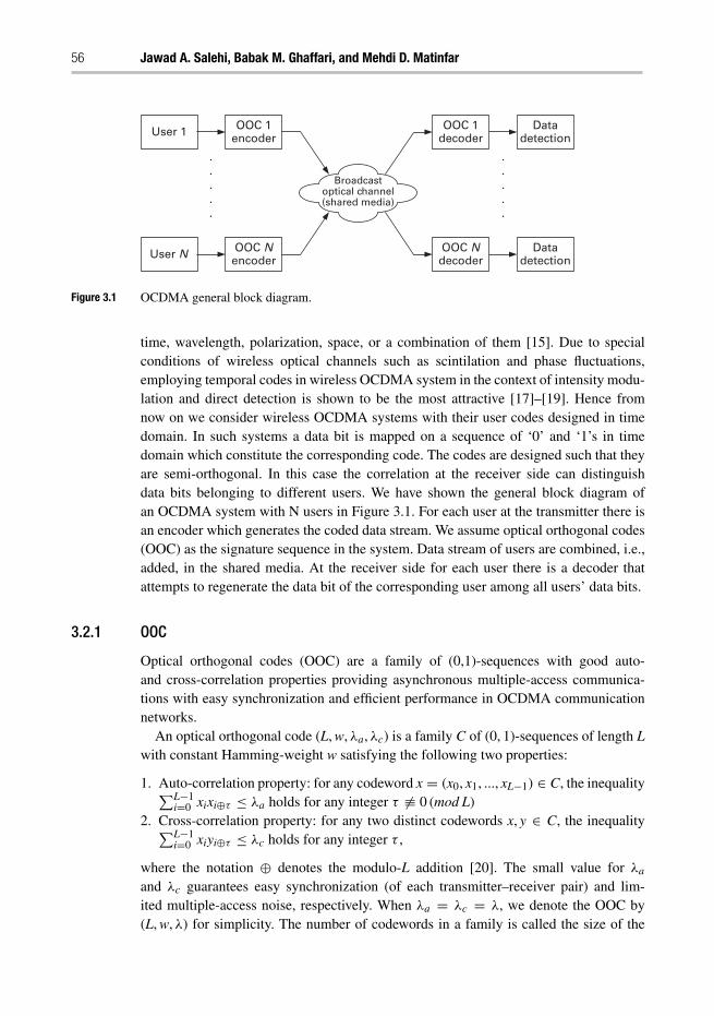
56 Jawad A. Salehi, Babak M. Ghaffari, and Mehdi D. Matinfar
User N
User 1 OOC 1encoder
OOC 1decoder
Datadetection
Datadetection
Broadcastoptical channel(shared media)
OOC Nencoder
OOC Ndecoder
Figure 3.1 OCDMA general block diagram.
time, wavelength, polarization, space, or a combination of them [15]. Due to specialconditions of wireless optical channels such as scintilation and phase fluctuations,employing temporal codes in wireless OCDMA system in the context of intensity modu-lation and direct detection is shown to be the most attractive [17]–[19]. Hence fromnow on we consider wireless OCDMA systems with their user codes designed in timedomain. In such systems a data bit is mapped on a sequence of ‘0’ and ‘1’s in timedomain which constitute the corresponding code. The codes are designed such that theyare semi-orthogonal. In this case the correlation at the receiver side can distinguishdata bits belonging to different users. We have shown the general block diagram ofan OCDMA system with N users in Figure 3.1. For each user at the transmitter there isan encoder which generates the coded data stream. We assume optical orthogonal codes(OOC) as the signature sequence in the system. Data stream of users are combined, i.e.,added, in the shared media. At the receiver side for each user there is a decoder thatattempts to regenerate the data bit of the corresponding user among all users’ data bits.
3.2.1 OOC
Optical orthogonal codes (OOC) are a family of (0,1)-sequences with good auto-and cross-correlation properties providing asynchronous multiple-access communica-tions with easy synchronization and efficient performance in OCDMA communicationnetworks.
An optical orthogonal code (L, w, λa, λc) is a family C of (0, 1)-sequences of length Lwith constant Hamming-weight w satisfying the following two properties:
1. Auto-correlation property: for any codeword x = (x0, x1, ..., xL−1) ∈ C, the inequality∑L−1i=0 xixi⊕τ ≤ λa holds for any integer τ �≡ 0 (mod L)
2. Cross-correlation property: for any two distinct codewords x, y ∈ C, the inequality∑L−1i=0 xiyi⊕τ ≤ λc holds for any integer τ ,
where the notation ⊕ denotes the modulo-L addition [20]. The small value for λa
and λc guarantees easy synchronization (of each transmitter–receiver pair) and lim-ited multiple-access noise, respectively. When λa = λc = λ, we denote the OOC by(L, w, λ) for simplicity. The number of codewords in a family is called the size of the
Wireless optical CDMA communication systems 57
optical orthogonal code. From a practical point of view, a code with large size is desired[11]. To find the best possible codes, we need to determine an upper bound on the sizeof an OOC family with the given parameters. Let �(L, w, λa, λc) be the largest pos-sible size of an (L, w, λa, λc)-OOC. It is easy to show that if w(w − 1) > λa(L − 1)then �(L, w, λa, λc) = 0 and if w2 > λcL then �(L, w, λa, λc) ≤ 1 [21]. However,based on the Johnson bound for constant-weight error-correcting codes [22], we havethe following bound [20],
�(L, w, λ) ≤⌊
1
w
⌊L− 1
w− 1
⌊L− 2
w− 2
⌊...
⌊L− λ+ 1
w− λ+ 1
⌊L− λ
w− λ
⌋⌋...
⌋⌋⌋⌋(3.1)
where the notation �� denotes the integer floor function. Also, it is clear from thedefinition that �(L, w, λa, λc) ≤ �(L, w, λ) where λ = max { λa , λc }[20].
From the mutual interference point of view, the most desirable on–off signaturesequences are OOCs with λc = 1. However, when we look at the system with a smallnumber of users interacting on each other’s OOCs λc = 1 is not necessarily the optimumcase. The main reason being that there is a trade-off between the code weight, w and λc.Larger λc allows more interference between users but on the other hand allows havinglarger code weight which by itself increases the coding gain hence decreasing the totalinterference. Briefly, the number of users in the network, receiver structure, and targetbit error rate define the optimum values of OOC parameters [12].
In what follows we study two main structures for OCDMA receiver and investigatetheir characteristics in an optical channel.
3.2.2 Correlator structure
The simplest structure for an OCDMA receiver, namely, correlator includes a matchedfilter, corresponding to its code pattern, and an integrate and dump circuit. We haveshown the structure of a OCDMA transmitter including encoder, and the correlatorreceiver in Figure 3.2. In this block diagram the decoder is matched to the correspondingcode generated by the encoder. In fiber-optic CDMA systems the matched filter can beimplemented by fiber tapped-delay lines at the receiver side. Delay lines in each branchserve to compensate for the corresponding delays induced at the encoder which consti-tute the corresponding OOC. The properly delayed replicas add to construct the outputcorrelator which is then fed to the photodetector, integrate, dump, and thresholder elec-tronic circuit. In Figure 3.2 the white pulses at the input of the desired decoder are thereceived signal from undesired users. The major advantage of the correlator structureis that the limiting high-speed chip time decoding operation is done passively and opti-cally. On the other hand in digital electronic implementation, delays can be generated byemploying flip flops. If we assume the sampling rate per chip equal to ns, nsL flip flopsare sufficient to construct the matched filter of the corresponding OOC code [18]. If wedenote the code length, the weight and the chip duration by L, w, and Tc respectively, andif the positions of the pulsed mark chips corresponding to the code sequence is c1,c2,. . . ,and cw, then the optical matched filter (passive optical tapped-delay line) consists of wfiber delay lines each of which make a delay equal to (L − c1)Tc, (L − c2)Tc,. . . , and
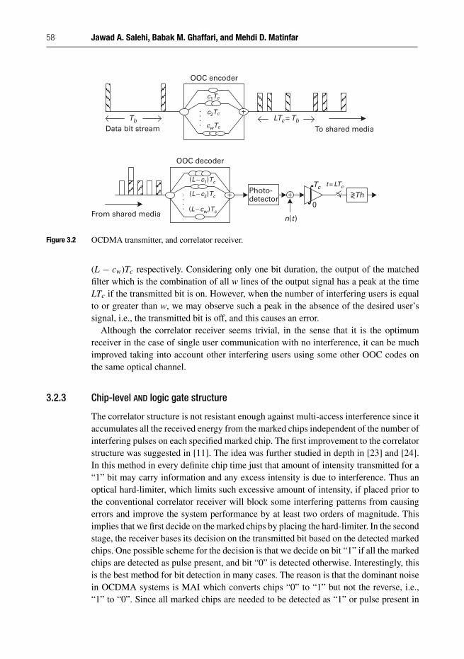
58 Jawad A. Salehi, Babak M. Ghaffari, and Mehdi D. Matinfar
OOC encoder
To shared media
Photo-detector
OOC decoder
LTc = Tb
∫
c1Tc
c2Tc
cwTc
Tb
Tc t = LTc
n(t )
0
(L − c1)Tc
(L − c2)Tc
(L − cw )TcFrom shared media
Data bit stream
><Th
Figure 3.2 OCDMA transmitter, and correlator receiver.
(L − cw)Tc respectively. Considering only one bit duration, the output of the matchedfilter which is the combination of all w lines of the output signal has a peak at the timeLTc if the transmitted bit is on. However, when the number of interfering users is equalto or greater than w, we may observe such a peak in the absence of the desired user’ssignal, i.e., the transmitted bit is off, and this causes an error.
Although the correlator receiver seems trivial, in the sense that it is the optimumreceiver in the case of single user communication with no interference, it can be muchimproved taking into account other interfering users using some other OOC codes onthe same optical channel.
3.2.3 Chip-level AND logic gate structure
The correlator structure is not resistant enough against multi-access interference since itaccumulates all the received energy from the marked chips independent of the number ofinterfering pulses on each specified marked chip. The first improvement to the correlatorstructure was suggested in [11]. The idea was further studied in depth in [23] and [24].In this method in every definite chip time just that amount of intensity transmitted for a“1” bit may carry information and any excess intensity is due to interference. Thus anoptical hard-limiter, which limits such excessive amount of intensity, if placed prior tothe conventional correlator receiver will block some interfering patterns from causingerrors and improve the system performance by at least two orders of magnitude. Thisimplies that we first decide on the marked chips by placing the hard-limiter. In the secondstage, the receiver bases its decision on the transmitted bit based on the detected markedchips. One possible scheme for the decision is that we decide on bit “1” if all the markedchips are detected as pulse present, and bit “0” is detected otherwise. Interestingly, thisis the best method for bit detection in many cases. The reason is that the dominant noisein OCDMA systems is MAI which converts chips “0” to “1” but not the reverse, i.e.,“1” to “0”. Since all marked chips are needed to be detected as “1” or pulse present in
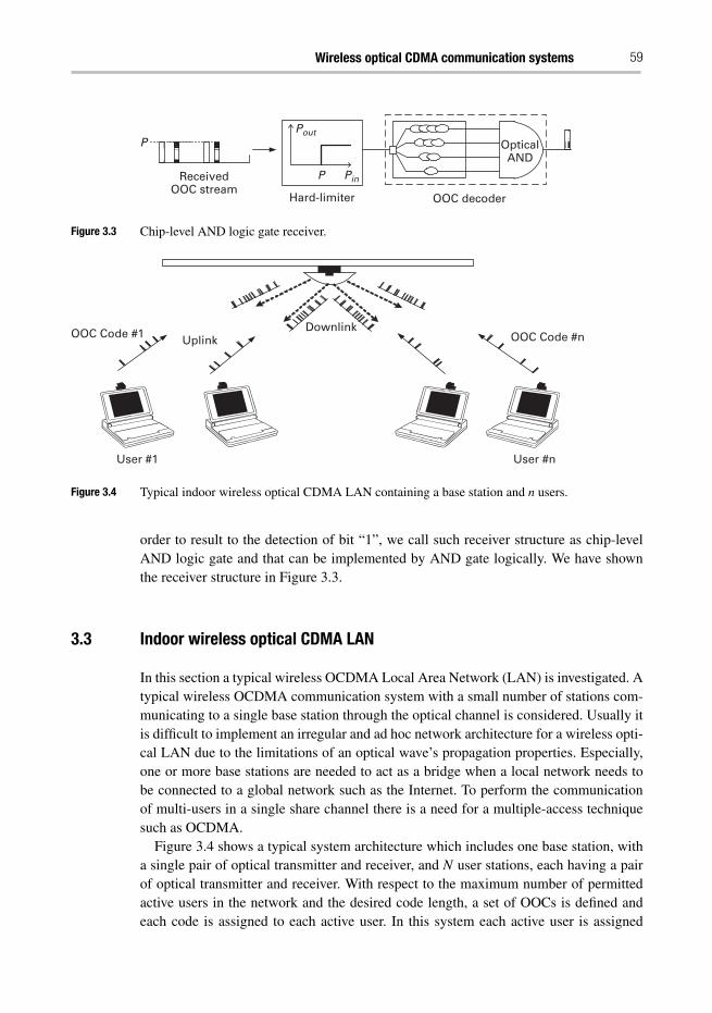
Wireless optical CDMA communication systems 59
ReceivedOOC stream
PPout
P Pin
Hard-limiter OOC decoder
OpticalAND
Figure 3.3 Chip-level AND logic gate receiver.
DownlinkUplinkOOC Code #1 OOC Code #n
User #1 User #n
Figure 3.4 Typical indoor wireless optical CDMA LAN containing a base station and n users.
order to result to the detection of bit “1”, we call such receiver structure as chip-levelAND logic gate and that can be implemented by AND gate logically. We have shownthe receiver structure in Figure 3.3.
3.3 Indoor wireless optical CDMA LAN
In this section a typical wireless OCDMA Local Area Network (LAN) is investigated. Atypical wireless OCDMA communication system with a small number of stations com-municating to a single base station through the optical channel is considered. Usually itis difficult to implement an irregular and ad hoc network architecture for a wireless opti-cal LAN due to the limitations of an optical wave’s propagation properties. Especially,one or more base stations are needed to act as a bridge when a local network needs tobe connected to a global network such as the Internet. To perform the communicationof multi-users in a single share channel there is a need for a multiple-access techniquesuch as OCDMA.
Figure 3.4 shows a typical system architecture which includes one base station, witha single pair of optical transmitter and receiver, and N user stations, each having a pairof optical transmitter and receiver. With respect to the maximum number of permittedactive users in the network and the desired code length, a set of OOCs is defined andeach code is assigned to each active user. In this system each active user is assigned
60 Jawad A. Salehi, Babak M. Ghaffari, and Mehdi D. Matinfar
a signature sequence from a set of OOC which is specified by (L, w, λa, λc). Allactive users send their data bits asynchronously on the common channel. Therefore,the received signal is comprised of the analog summation of all users’ optical intensitytransmitted signals. Hence, the received signal can be written as follows,
Y (t) =N∑
k=1
y(k) (t − τk) (3.2)
where, y(k)(t) is the received signal due to the kth user and τk indicates its delay timewith respect to the base station reference clock and can be written as follows,
y(k) (t) =∞∑
i=−∞
L∑j=1
u(k)i c(k)j PTc (t − iTb − jTc) (3.3)
where{
u(k)i
}i
is the bit stream of user k,{
c(k)j
}L
j=1denotes the kth OOC code pattern,
and PTc (t) is the pulse function with a duration equal to Tc.In the design of any wireless CDMA communication network the near-far problem
needs to be addressed [26]. The near-far problem in wireless OCDMA LAN requiresspecific algorithms to mitigate its effect such as the use of a proper automatic gaincontrol (AGC) circuit. Hence, in this section it is assumed the existence of power con-trol algorithms. Therefore we can safely ignore the near-far problem such that all usershave equal power in the uplink channel. In what follows we discuss the transmitter andtwo viable and relevant receiver structures for a wireless OCDMA system. Further wediscuss the pros and cons of such transmitter and receiver structures in the context oftheir digital design and their implementation. Finally their performance is obtained anddiscussed.
3.3.1 Wireless OCDMA transmitter
In an OCDMA network, using OOC, the network’s active users transmit their cor-responding data bits asynchronously. But at the receiver side prior to detecting databits it is first essential to obtain bit-level synchronization between the correspondingtransmitter–receiver pair. OOC coding takes place in the physical layer. So by addingsome redundant bits, namely training sequence, to information data bits prior to coding,the receiver will be able to synchronize its code with its corresponding transmitted codeusing the knowledge of the training bits pattern.
3.3.2 Wireless OCDMA receiver
In the design of the receiver and its implementation more complexity is encounteredwhen compared to the transmitter especially in the synchronization module. Similar toradio CDMA systems, synchronization in OCDMA receivers precedes the data detectionblock and it is applied in two stages namely acquisition and tracking. In a typical syn-chronization process prior to tracking state, the received data is first passed through the
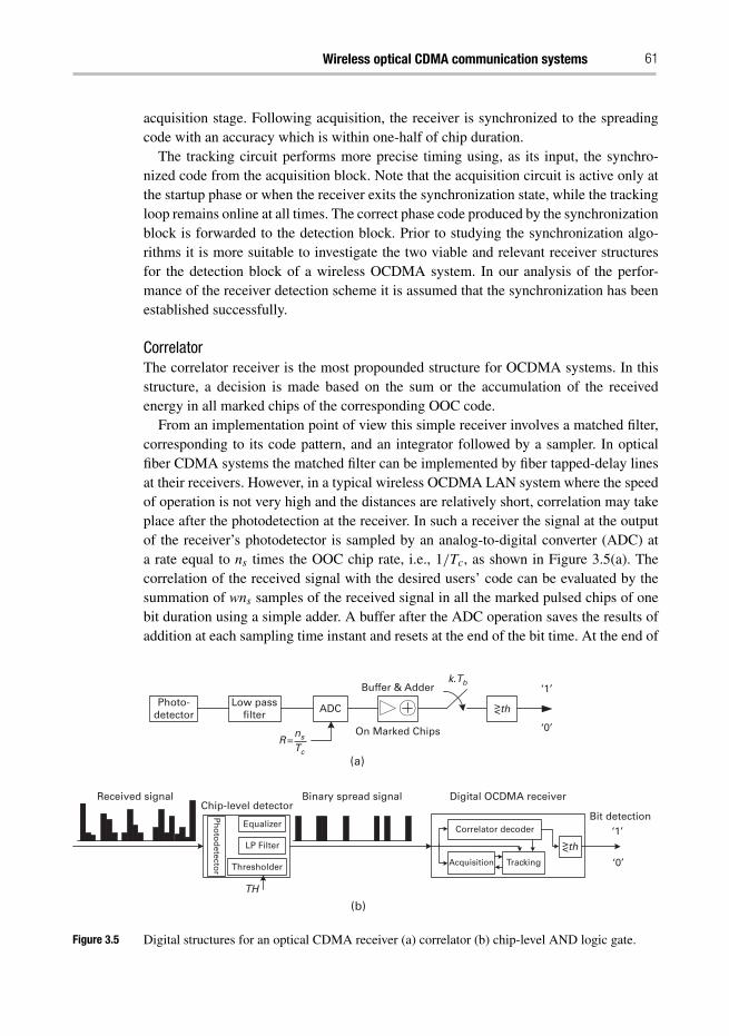
Wireless optical CDMA communication systems 61
acquisition stage. Following acquisition, the receiver is synchronized to the spreadingcode with an accuracy which is within one-half of chip duration.
The tracking circuit performs more precise timing using, as its input, the synchro-nized code from the acquisition block. Note that the acquisition circuit is active only atthe startup phase or when the receiver exits the synchronization state, while the trackingloop remains online at all times. The correct phase code produced by the synchronizationblock is forwarded to the detection block. Prior to studying the synchronization algo-rithms it is more suitable to investigate the two viable and relevant receiver structuresfor the detection block of a wireless OCDMA system. In our analysis of the perfor-mance of the receiver detection scheme it is assumed that the synchronization has beenestablished successfully.
CorrelatorThe correlator receiver is the most propounded structure for OCDMA systems. In thisstructure, a decision is made based on the sum or the accumulation of the receivedenergy in all marked chips of the corresponding OOC code.
From an implementation point of view this simple receiver involves a matched filter,corresponding to its code pattern, and an integrator followed by a sampler. In opticalfiber CDMA systems the matched filter can be implemented by fiber tapped-delay linesat their receivers. However, in a typical wireless OCDMA LAN system where the speedof operation is not very high and the distances are relatively short, correlation may takeplace after the photodetection at the receiver. In such a receiver the signal at the outputof the receiver’s photodetector is sampled by an analog-to-digital converter (ADC) ata rate equal to ns times the OOC chip rate, i.e., 1/Tc, as shown in Figure 3.5(a). Thecorrelation of the received signal with the desired users’ code can be evaluated by thesummation of wns samples of the received signal in all the marked pulsed chips of onebit duration using a simple adder. A buffer after the ADC operation saves the results ofaddition at each sampling time instant and resets at the end of the bit time. At the end of
(a)
(b)
Photo-detector
Low passfilter
ADC
Buffer & Adderk.Tb
‘1’
‘1’
‘0’
‘0’
On Marked Chipsns
Tc
><th
><th
Received signalChip-level detector
Binary spread signal Digital OCDMA receiver
Bit detectionPh
oto
detecto
r
Equalizer
LP Filter
Thresholder
TH
Correlator decoder
Acquisition Tracking
R =
Figure 3.5 Digital structures for an optical CDMA receiver (a) correlator (b) chip-level AND logic gate.
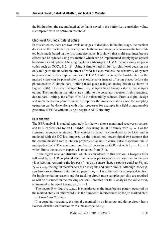
62 Jawad A. Salehi, Babak M. Ghaffari, and Mehdi D. Matinfar
the bit duration, the accumulated value that is saved in the buffer, i.e., correlation value,is compared with an optimum threshold.
Chip-level AND logic gate structureIn this structure, there are two levels or stages of decision. In the first stage, the receiverdecides on the marked chips, one by one. In the second stage, a decision on the transmit-ted bit is made based on the first stage decisions. It is shown that multi-user interferenceeffects can be reduced using this method which can be implemented simply by an opticalhard-limiter and optical AND logic gate in a fiber-optic CDMA receiver using unipolarcodes such as OOCs, [12, 19]. Using a simple hard-limiter for chip-level decision notonly mitigates the undesirable effect of MAI but also reduces the sensitivity of systemto power control. In a typical wireless OCDMA LAN receiver, the hard-limiter on themarked chips can be placed after the photodetector instead of being placed before thephotodetector. A simple hard-limiting takes place using an analog circuit as shown inFigure 3.5(b). Thus, each sample from wns samples has a binary value at the sampleroutput. The remaining operations are similar to the correlator receiver. In this structure,due to hard-limiting, the effect of MAI is substantially reduced. From a digital designand implementation point of view, it simplifies the implementation since the samplingoperation can be done along with other processes for example in a field programmablegate array (FPGA) without using a separate ADC circuitry.
BER analysisThe BER analysis is studied separately for the two above-mentioned receiver structuresand BER expressions for an OCDMA LAN using an OOC family with λc = 1 as thesignature sequence is studied. The wireless channel is considered to be LOS and ismodeled with the DC loss imposed on the transmitted power signal (we assume thatthe communication rate is chosen properly so as not to cause pulse dispersion due tomultipath effect). The maximum number of codes in an OOC set with λa = λc = 1which limits the network capacity is obtained from (3.1).
In the digital receiver structure which is considered in this section, a lowpass filterfollowed by an ADC is placed after the receiver photodetector, as described in the pre-vious section. Assuming the lowpass filter as a square shape response equal to PTf (t),Tf = Tc/ns, the digital receiver acts as an integrate and dump circuit. Although, for chip-synchronous multi-user interference pattern, ns = 1 is sufficient for a proper detection,for implementation reasons and for tracking circuit more samples per chip are requiredas will be discussed in the tracking section. Hereafter, for BER analysis the value for ns
is assumed to be equal to one, i.e., ns = 1.The vector �α = (α1,α2, ...,αw) is considered as the interference pattern occurred on
the marked chips. In other word αj is the number of interferences on the jth marked chip.a. Correlator StructureIn a correlator structure, the signal generated by an integrate and dump circuit has a
Poisson distribution function with a mean equal to md,
md(l) = [(wd + l)γs + wγb]Tc (3.4)
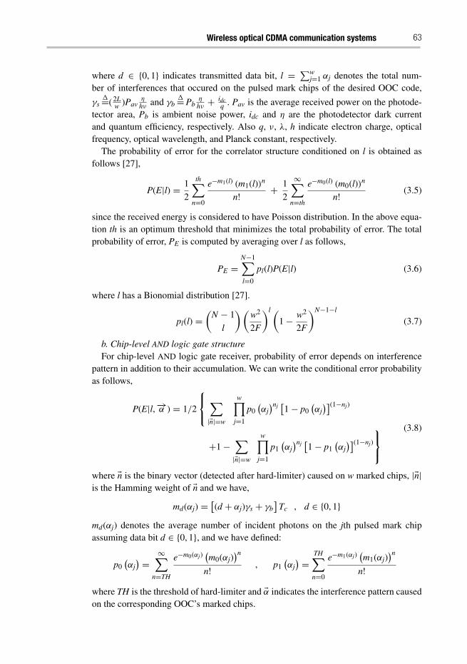
Wireless optical CDMA communication systems 63
where d ∈ {0, 1} indicates transmitted data bit, l = ∑wj=1 αj denotes the total num-
ber of interferences that occured on the pulsed mark chips of the desired OOC code,
γs�=( 2L
w )Pavηhν and γb
�=Pbηhν + idc
q . Pav is the average received power on the photode-tector area, Pb is ambient noise power, idc and η are the photodetector dark currentand quantum efficiency, respectively. Also q, ν, λ, h indicate electron charge, opticalfrequency, optical wavelength, and Planck constant, respectively.
The probability of error for the correlator structure conditioned on l is obtained asfollows [27],
P(E|l) = 1
2
th∑n=0
e−m1(l) (m1(l))n
n! + 1
2
∞∑n=th
e−m0(l) (m0(l))n
n! (3.5)
since the received energy is considered to have Poisson distribution. In the above equa-tion th is an optimum threshold that minimizes the total probability of error. The totalprobability of error, PE is computed by averaging over l as follows,
PE =N−1∑l=0
pl(l)P(E|l) (3.6)
where l has a Bionomial distribution [27].
pl(l) =(
N − 1
l
)(w2
2F
)l (1− w2
2F
)N−1−l
(3.7)
b. Chip-level AND logic gate structureFor chip-level AND logic gate receiver, probability of error depends on interference
pattern in addition to their accumulation. We can write the conditional error probabilityas follows,
P(E|l,−→α ) = 1/2
⎧⎨⎩
∑|�n|=w
w∏j=1
p0(αj)nj
[1− p0
(αj)](1−nj)
+1−∑|�n|=w
w∏j=1
p1(αj)nj
[1− p1
(αj)](1−nj)
⎫⎬⎭
(3.8)
where �n is the binary vector (detected after hard-limiter) caused on w marked chips, |�n|is the Hamming weight of �n and we have,
md(αj) =[(d + αj)γs + γb
]Tc , d ∈ {0, 1}
md(αj) denotes the average number of incident photons on the jth pulsed mark chipassuming data bit d ∈ {0, 1}, and we have defined:
p0(αj) = ∞∑
n=TH
e−m0(αj)(m0(αj)
)n
n! , p1(αj) = TH∑
n=0
e−m1(αj)(m1(αj)
)n
n!where TH is the threshold of hard-limiter and �α indicates the interference pattern causedon the corresponding OOC’s marked chips.
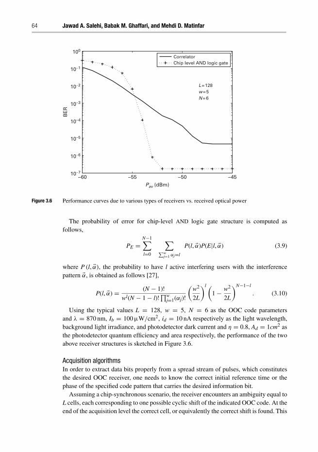
64 Jawad A. Salehi, Babak M. Ghaffari, and Mehdi D. Matinfar
−60 −55 −50 −45
100
10−1
10−2
10−3
10−4
10−5
10−6
10−7
Pav (dBm)
BE
R
L = 128w = 5N = 6
CorrelatorChip level AND logic gate
Figure 3.6 Performance curves due to various types of receivers vs. received optical power
The probability of error for chip-level AND logic gate structure is computed asfollows,
PE =N−1∑l=0
∑∑w
j=1 αj=l
P(l, �α)P(E|l, �α) (3.9)
where P (l, �α), the probability to have l active interfering users with the interferencepattern �α, is obtained as follows [27],
P(l, �α) = (N − 1)!wl(N − 1− l)!∏w
j=1(αj)!(
w2
2L
)l (1− w2
2L
)N−1−l
. (3.10)
Using the typical values L = 128, w = 5, N = 6 as the OOC code parametersand λ = 870 nm, Ib = 100 μW/cm2, id = 10 nA respectively as the light wavelength,background light irradiance, and photodetector dark current and η = 0.8, Ad = 1cm2 asthe photodetector quantum efficiency and area respectively, the performance of the twoabove receiver structures is sketched in Figure 3.6.
Acquisition algorithmsIn order to extract data bits properly from a spread stream of pulses, which constitutesthe desired OOC receiver, one needs to know the correct initial reference time or thephase of the specified code pattern that carries the desired information bit.
Assuming a chip-synchronous scenario, the receiver encounters an ambiguity equal toL cells, each corresponding to one possible cyclic shift of the indicated OOC code. At theend of the acquisition level the correct cell, or equivalently the correct shift is found. This
Wireless optical CDMA communication systems 65
can be obtained for example by using training bits which are inserted at the beginningof each frame. Some algorithms are suggested to be used in acquisition state. For eachalgorithm, a different number of training bits is required to meet acquisition with aprobability near 1. It is evident that the less training bits required the more efficient thealgorithm in use will be. In the following, three recently suggested algorithms for OOCbased OCDMA are presented.
a. Simple serial-search methodIn this approach, one cell is randomly selected and it is assumed to be the correct cell.
A correlation between the received data and the selected code over a bit time duration(dwell time) is obtained and the outcome is compared with an optimum threshold. If theoutput of the correlation is greater than the optimum threshold, then the first randomlyselected cell is the correct cell [28]. Otherwise, the next cell is examined. By next cell itis implied a chip-sized rotation replica of the initial cell or phase of the specified code.So by continuing this algorithm and in maximum L stages the correct cell is obtained inthe ideal case. This method is relatively slow but its implementation in ultra-fast fiberoptic systems is viable.
b. Multiple-shift methodTo reduce the average time of acquisition, the multiple-shift method was proposed
recently [29]. In this method L cells are divided into Q groups each containing M cells.In the first stage of the algorithm, all M cells of group 1 are examined simultaneously.If the output of the correlation is greater than a predetermined optimum threshold thenit will proceed to the second stage, otherwise it will proceed to examine cells whichbelong to group 2. In continuing this process and from [29] in maximum Q steps thetrue group is obtained. In the second stage the M possible cells will be examined one byone similar to the simple serial-search method. So in the ideal case the corrected cell canbe found in maximum Q+M stages. So acquisition time is reduced considerably whencompared to the simple serial search method from maximum L stages to 2
√L stages.
c. Matched filter methodAssume a matched filter containing w delay lines. Each, delay line value is propor-
tional to the position of pulsed chips corresponding to its respective OOC. When trainingbits enter the matched filter then the output signal is a periodic training pulse with awidth equal to Tc and a period equal to Tb. This implies that in one bit duration the peakcorrelation of the incident signal and code pattern can be observed without any knowl-edge of the correct initial time reference. As an example the digital implementation ofa matched filter is depicted for an OOC stream with w = 3 in Figure 3.7. Consideringthis idea, matched filtering automatically searches all the L cells within one bit dura-tion instead of L bits duration as in the simple serial-search method. This method isextremely fast and can be easily implemented in wireless OCDMA systems that havebeen implemented in digital electronics.
Tracking circuitThe tracking circuit performs two key operations in a typical OCDMA receiver. In gen-eral, the received code from acquisition block has an ambiguity in phase or initial timereference which is less than Tc/2. The first task of the tracking circuit is to minimize this
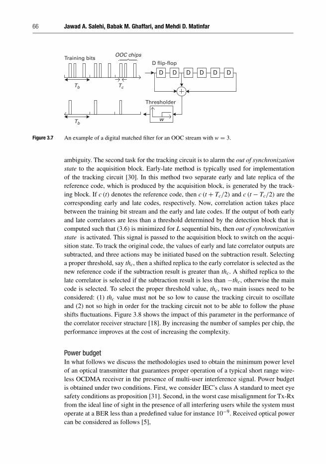
66 Jawad A. Salehi, Babak M. Ghaffari, and Mehdi D. Matinfar
Training bitsOOC chips
D flip-flop
D D D D D D
Thresholder
w
Tb Tc
Tb
Figure 3.7 An example of a digital matched filter for an OOC stream with w = 3.
ambiguity. The second task for the tracking circuit is to alarm the out of synchronizationstate to the acquisition block. Early-late method is typically used for implementationof the tracking circuit [30]. In this method two separate early and late replica of thereference code, which is produced by the acquisition block, is generated by the track-ing block. If c (t) denotes the reference code, then c (t + Tc/2) and c (t − Tc/2) are thecorresponding early and late codes, respectively. Now, correlation action takes placebetween the training bit stream and the early and late codes. If the output of both earlyand late correlators are less than a threshold determined by the detection block that iscomputed such that (3.6) is minimized for L sequential bits, then out of synchronizationstate is activated. This signal is passed to the acquisition block to switch on the acqui-sition state. To track the original code, the values of early and late correlator outputs aresubtracted, and three actions may be initiated based on the subtraction result. Selectinga proper threshold, say thc, then a shifted replica to the early correlator is selected as thenew reference code if the subtraction result is greater than thc. A shifted replica to thelate correlator is selected if the subtraction result is less than −thc, otherwise the maincode is selected. To select the proper threshold value, thc, two main issues need to beconsidered: (1) thc value must not be so low to cause the tracking circuit to oscillateand (2) not so high in order for the tracking circuit not to be able to follow the phaseshifts fluctuations. Figure 3.8 shows the impact of this parameter in the performance ofthe correlator receiver structure [18]. By increasing the number of samples per chip, theperformance improves at the cost of increasing the complexity.
Power budgetIn what follows we discuss the methodologies used to obtain the minimum power levelof an optical transmitter that guarantees proper operation of a typical short range wire-less OCDMA receiver in the presence of multi-user interference signal. Power budgetis obtained under two conditions. First, we consider IEC’s class A standard to meet eyesafety conditions as proposition [31]. Second, in the worst case misalignment for Tx-Rxfrom the ideal line of sight in the presence of all interfering users while the system mustoperate at a BER less than a predefined value for instance 10−9. Received optical powercan be considered as follows [5],
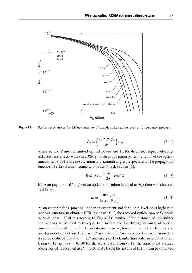
Wireless optical CDMA communication systems 67
−55−60 −50 −45
Err
or
pro
bab
ility
ns = 3
ns = 4
ns = 5
ns = 8
ns = 16
Analog case (ns = infinity)
L = 128w = 5N = 4
100
10−5
10−10
10−15
10−20
Pav (dBm)
Figure 3.8 Performance curves for different number of samples taken at the receiver for detection process.
Pr =(
PtR (θ ,φ)
d2
)Aeff (3.11)
where Pt and d are transmitted optical power and Tx-Rx distance, respectively; Aeff
indicates lens effective area and R(θ ,ϕ) is the propagation pattern function of the opticaltransmitter; θ and ϕ are the elevation and azimuth angles, respectively. The propagationfunction of a Lambertian source with order m is defined as [5],
R (θ ,φ) = m+ 1
2πcosm θ . (3.12)
If the propagation half-angle of an optical transmitter is equal to θ1/2 then m is obtainedas follows,
m = ln (1/2)
ln(cos θ1/2
) . (3.13)
As an example for a practical indoor environment and for a chip-level AND logic gatereceiver structure to obtain a BER less than 10−7, the received optical power Pr needsto be at least −52 dBm referring to Figure 3.6 results. If the distance of transmitterand receiver is assumed to be equal to 3 meters and the divergence angle of opticaltransmitter θ = 30◦, then for the worst-case scenario, transmitter–receiver distance andmisalignment are obtained to be d = 3 m and θ = 30◦ respectively. For such parametersit can be deduced that θ1/2 = 15◦ and using (3.13) Lambertian order m is equal to 20.Using (3.12) R(θ ,ϕ) = 0.188 for the worst case. From (3.11) the transmitted averagepower per bit is obtained as Pt = 3.01 mW. Using the results of [31], it can be observed
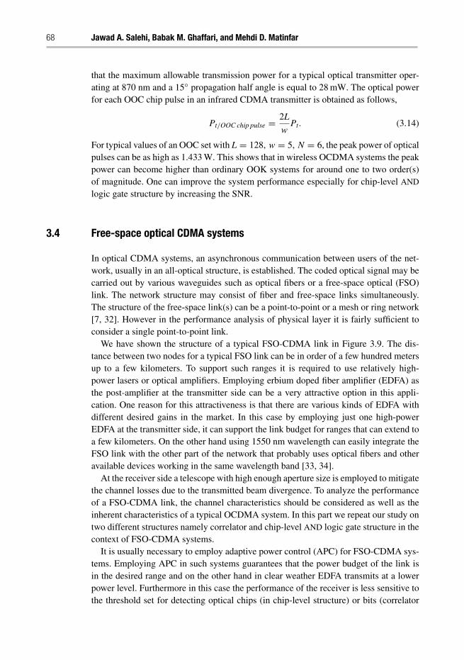
68 Jawad A. Salehi, Babak M. Ghaffari, and Mehdi D. Matinfar
that the maximum allowable transmission power for a typical optical transmitter oper-ating at 870 nm and a 15◦ propagation half angle is equal to 28 mW. The optical powerfor each OOC chip pulse in an infrared CDMA transmitter is obtained as follows,
Pt/OOC chip pulse = 2L
wPt. (3.14)
For typical values of an OOC set with L = 128, w = 5, N = 6, the peak power of opticalpulses can be as high as 1.433 W. This shows that in wireless OCDMA systems the peakpower can become higher than ordinary OOK systems for around one to two order(s)of magnitude. One can improve the system performance especially for chip-level AND
logic gate structure by increasing the SNR.
3.4 Free-space optical CDMA systems
In optical CDMA systems, an asynchronous communication between users of the net-work, usually in an all-optical structure, is established. The coded optical signal may becarried out by various waveguides such as optical fibers or a free-space optical (FSO)link. The network structure may consist of fiber and free-space links simultaneously.The structure of the free-space link(s) can be a point-to-point or a mesh or ring network[7, 32]. However in the performance analysis of physical layer it is fairly sufficient toconsider a single point-to-point link.
We have shown the structure of a typical FSO-CDMA link in Figure 3.9. The dis-tance between two nodes for a typical FSO link can be in order of a few hundred metersup to a few kilometers. To support such ranges it is required to use relatively high-power lasers or optical amplifiers. Employing erbium doped fiber amplifier (EDFA) asthe post-amplifier at the transmitter side can be a very attractive option in this appli-cation. One reason for this attractiveness is that there are various kinds of EDFA withdifferent desired gains in the market. In this case by employing just one high-powerEDFA at the transmitter side, it can support the link budget for ranges that can extend toa few kilometers. On the other hand using 1550 nm wavelength can easily integrate theFSO link with the other part of the network that probably uses optical fibers and otheravailable devices working in the same wavelength band [33, 34].
At the receiver side a telescope with high enough aperture size is employed to mitigatethe channel losses due to the transmitted beam divergence. To analyze the performanceof a FSO-CDMA link, the channel characteristics should be considered as well as theinherent characteristics of a typical OCDMA system. In this part we repeat our study ontwo different structures namely correlator and chip-level AND logic gate structure in thecontext of FSO-CDMA systems.
It is usually necessary to employ adaptive power control (APC) for FSO-CDMA sys-tems. Employing APC in such systems guarantees that the power budget of the link isin the desired range and on the other hand in clear weather EDFA transmits at a lowerpower level. Furthermore in this case the performance of the receiver is less sensitive tothe threshold set for detecting optical chips (in chip-level structure) or bits (correlator
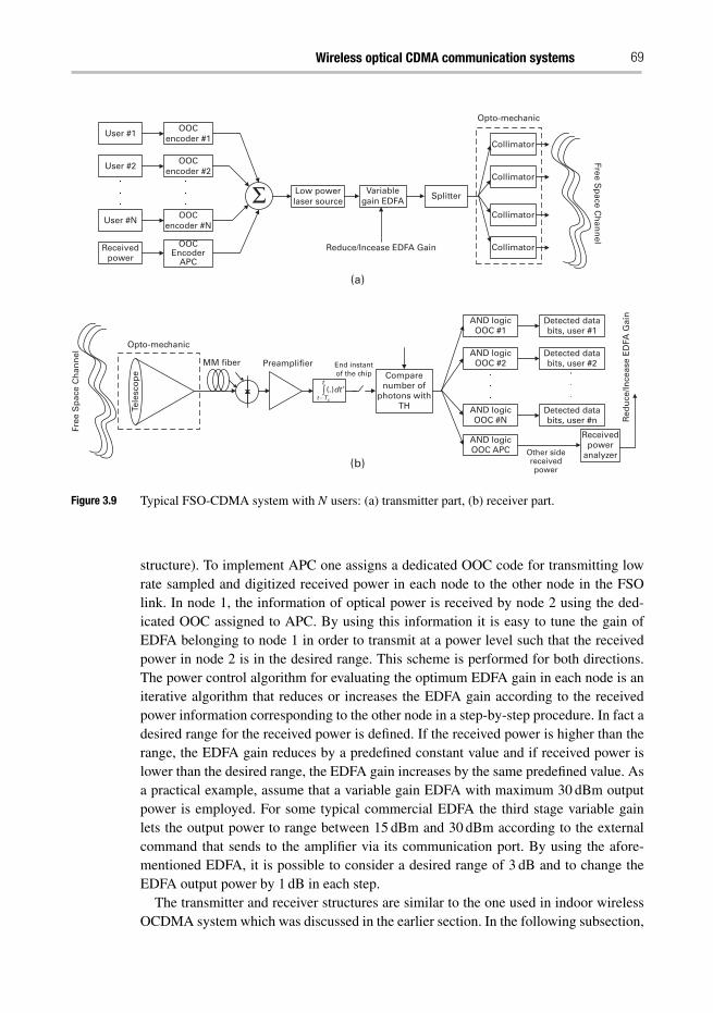
Wireless optical CDMA communication systems 69
User #1
User #2
User #N
Receivedpower
OOCencoder #N
OOCEncoder
APC
OOCencoder #1
OOCencoder #2
Low powerlaser source
Variablegain EDFA
Splitter
Collimator
Collimator
Free Sp
ace Ch
ann
el
Collimator
CollimatorReduce/Incease EDFA Gain
(a)
Σ
∫
(b)
Opto-mechanic
Tele
sco
pe
Free
Sp
ace
Ch
ann
el
MM fiber Preamplifier End instantof the chip Compare
number ofphotons with
TH
AND logicOOC #1
AND logicOOC #2
AND logicOOC #N
AND logicOOC APC Other side
receivedpower
Receivedpower
analyzer
Detected databits, user #1
Detected databits, user #2
Detected databits, user #n R
edu
ce/In
ceas
e E
DFA
Gai
n
(.)dt’t
Opto-mechanic
Figure 3.9 Typical FSO-CDMA system with N users: (a) transmitter part, (b) receiver part.
structure). To implement APC one assigns a dedicated OOC code for transmitting lowrate sampled and digitized received power in each node to the other node in the FSOlink. In node 1, the information of optical power is received by node 2 using the ded-icated OOC assigned to APC. By using this information it is easy to tune the gain ofEDFA belonging to node 1 in order to transmit at a power level such that the receivedpower in node 2 is in the desired range. This scheme is performed for both directions.The power control algorithm for evaluating the optimum EDFA gain in each node is aniterative algorithm that reduces or increases the EDFA gain according to the receivedpower information corresponding to the other node in a step-by-step procedure. In fact adesired range for the received power is defined. If the received power is higher than therange, the EDFA gain reduces by a predefined constant value and if received power islower than the desired range, the EDFA gain increases by the same predefined value. Asa practical example, assume that a variable gain EDFA with maximum 30 dBm outputpower is employed. For some typical commercial EDFA the third stage variable gainlets the output power to range between 15 dBm and 30 dBm according to the externalcommand that sends to the amplifier via its communication port. By using the afore-mentioned EDFA, it is possible to consider a desired range of 3 dB and to change theEDFA output power by 1 dB in each step.
The transmitter and receiver structures are similar to the one used in indoor wirelessOCDMA system which was discussed in the earlier section. In the following subsection,
70 Jawad A. Salehi, Babak M. Ghaffari, and Mehdi D. Matinfar
performances of these receiver structures in the context of FSO-CDMA system are stud-ied. Analytical solutions to the error probability for various channel models using PINphotodetector are obtained. In the following analysis, the effects of atmospheric turbu-lence, ambient light, thermal noise, and multi-user interference are considered in thecontext of the semi-classical photon counting approach. For the sake of mathematicalsimplicity, the Gaussian approximation is used for performance evaluation.
3.4.1 BER analysis
The following analysis is based on semi classical photon counting where the photoncount statistics is obtained separately in each stage. As it is shown in Figure 3.9, weplace an optical amplifier in the FSO system which is not necessarily present in indoorwireless optical CDMA systems. High-power EDFA amplifier along with a low-powerlaser source, e.g., with Pt,1 = 0dBm output power, act as a high-power laser sourceat the transmitter side. Similar to indoor wireless OCDMA system OOK signalling isemployed.
Low-power laser sourceThe photon count in one chip duration due to low power laser is indicated by n1 whichis assumed to have a Poisson distribution. The mean photon counts of low-power laserpulses representing zero and one are respectively, mt,0,c = 0 and mt,1,c = Pt,1Tc/hυ.Where Pt,1, Tc, h, and υ are the peaked output power of the low-power laser source, chipduration, Planck’s constant and optical frequency, respectively. Therefore, the momentgenerating function (MGF) corresponding to the photon count of low-power laser outputwith Poisson distribution is as follows,
φt,d,c (z) = exp[1− mt,d,c (1− z)
]. (3.15)
Optical amplifierThe dominant noise source in optical amplifiers is ASE (Amplified Spontaneous Emis-sion). By assuming G, K = nsp (G− 1), and M as the gain, the noise factor, and thenumber of spontaneous modes, respectively, the optical amplifier output photon count,denoted by n2, is obtained as a Laguerre distribution with parameters
(mt,d,cG, K, M
)[35]. Hence, the MGF corresponding to the photon count of optical amplifier output isobtained as follows,
φEDFA,t,d,c (z) = 1
[1+ K (1− z)]M × φt,d,c
(1− G (1− z)
1+ K (1− z)
). (3.16)
FSO channel modelAtmospheric channel can be simply modeled as an attenuator with random attenu-ation coefficient. Channel attenuation can be expressed as the multiplication of twoparameters: one a deterministic parameter and another a random variable. FSO chan-nel attenuation is caused by both molecular absorption and aerosol scattering which
Wireless optical CDMA communication systems 71
randomly affects the light intensity traversing through the channel. The deterministicpart can be written as follows [1],
a = A
π(θL0
2
)2e−βL0 . (3.17)
In the above equation L0 and β are the link distance and atmospheric extinction coef-ficient, A and θ are the telescope area and transmitted beam divergence in radians,respectively. The random attenuation of the channel is induced by the random varia-tions of the channel refractive index which can be modeled as a log normal distributione2x in which x is a normal random variable. The random term is assumed to be normal-ized such that E
[e2x
] = 1. So, the mean and the variance of the normal random variablex are considered as −σ 2
x and σ 2x , respectively. Hence, if we assume that the channel
attenuation is deterministic, i.e., condition on known x, the MGF of the photon countdue to the channel output, denoted by n3, can be written as follows,
φs,d,c (z|x) = φEDFA,t,d,c
[1− ae2x (1− z)
]. (3.18)
Furthermore the ambient light can also be modeled as an additive independent photoncount with Poisson distribution. So, the MGF due to the total photon count coupled intothe multi-mode fiber is obtained as follows,
φr,d,c|x (z) = φs,d,c (z|x) φa,c (z) : φa,c (z) = exp[1− ma,c (1− z)
](3.19)
where ma,c in the above equation indicates the mean photon count of the ambient lightin one chip duration and it is obtained as follows,
ma,c = W (λ)A�FOV�λTc
hυ(3.20)
where �FOV is the receiver field of view (FOV) in steradian, �λ is the optical filterbandwidth, and W (λ) is the spectral radiance function, defined as the power radiated atwavelength per cycle of bandwidth in a unit solid angle per unit of source area.
Photodetector modelThe photodetoctor is modeled as an attenuator with attenuation coefficient equal to itsquantum efficiency indicated by η. So, the MGF corresponding to the photo electroncount at the photodetector output is obtained as follows,
φPD,d,c (z|x) = φr,d,c [1− η (1− z) |x] . (3.21)
As it was mentioned earlier, the Gaussian approximation is employed for the BER anal-ysis. The BER analysis is studied hereafter for two different receiver structures, namely,simple correlator and chip-level AND logic gate.
3.4.2 Correlator receiver structure
Usually, the coherence time of fading in FSO links is on the order of several millisec-onds [1], while usual bit durations are less than several microseconds; therefore, we can
72 Jawad A. Salehi, Babak M. Ghaffari, and Mehdi D. Matinfar
assume that the fading is constant during a bit period. Considering the structure of thecorrelator receiver, independence of counts for different chip intervals, and the fact thatthe fading is approximately constant during a bit period, mean and the variance of thedecision variable for transmitting bit “1” and “0” can be written as follows,
md =w∑
i=1
m(i)r,d,c , σ 2
d =w∑
i=1
σ 2i,r,d,c ; d = 0, 1 (3.22)
where{
m(i)r,d,c
}w
i=1and
{σ 2
i,r,d,c
}w
i=1are the means and variances corresponding to w
marked chips. Assuming l active interfering users, in the desired user’s marked chips,the decision variable mean md,l and variance σ 2
d,l are obtained as follows,
md,l = (d × w+ l)× mPD,d,c + w× mdc,c
σ 2d,l = (d × w+ l)× σ 2
PD,d,c + w× mdc,c + σ 2th d = 0, 1
(3.23)
where, mPD,d,c, σ 2PD,d,c are the mean and variance of the phoelectrons in one chip dura-
tion; mdc,c, σ 2th are the variance of the photodetector dark current per chip and thermal
noise photoelectron count, respectively [36],
mdc,c = idTc
q, σ 2
th =2KbTrTc
RLq2(3.24)
where, Kb, Tr, and RL are Boltzman constant, receiver equivalent temperature, and theresistance of the receiver load. Also, id, Tc, and q are the photodetector dark current,chip time, and the electron charge, respectively. Using the aforementioned mathematicalmodel in each stage, the mean and variance of the photoelectron count in one chipduration is obtained as follows,
mPD,d,c = ηma,c +(M × K + mt,d,c × G
)× ηae2x
σ 2PD,d,c = ηma,c +M × K × ηae2x
(1+ ηae2x × K
)+mt,d,c × G× ηae2x
(1+ 2ηae2x × K
).
(3.25)
Finally, using Gaussian approximation, the BER of the simple correlator receiverstructure is obtained as follows,
PE (x) =1
2
N−1∑l=0
(N − 1
l
)(w2
2L
)l (1− w2
2L
)N−1−l [Q
(m1,l − th
σ1,l
)+ Q
(th− m0,l
σ0,l
)], (3.26)
where th in the above equation is the optimum threshold for the correlator that minimizesthe total error probability; Q (u) is the normalized Gaussian function defined as Q (u) =(
1/√
2π) ∫∞
u e(−v2/2
)dv. Note that the above expression evaluates the conditional error
probability given the fading coefficient x. Hence the total error probability is obtainedby averaging PE (x) over the fading coefficient x as follows,
PE =∫ ∞
−∞PE (x) fX (x) dx (3.27)
Wireless optical CDMA communication systems 73
where fX (x) is the pdf of the fading coefficient defined as follows,
fX(x) = 1√2πσx
e− (x+σ2
x )2
2σ2x .
3.4.3 Chip level AND logic gate
The conditional error probability given the turbulence coefficient x can be evaluatedsimilar to the approach used in indoor wireless OCDMA section. The conditionalerror probability given the interference number, the interference pattern, and the fadingcoefficient is obtained as follows,
P(E|l,−→α , x) = 12
[∑|�n|=w
∏wj=1 p0
(αj, x
)nj(1− p0
(αj, x
))(1−nj)
+1−∑|�n|=w
∏wj=1 p1
(αj, x
)nj(1− p1
(αj, x
))(1−nj)] (3.28)
where �n is the binary vector (detected after hard-limiter) caused on w marked chips, |�n|is the hamming weight of �n, p0
(αj, x
)and p1
(αj, x
)are the chip level error probabilities
on the jth chip for transmitting bit ‘0’ and bit ‘1’, while �α and x are the known interfer-ence pattern and the fading coefficient on that chip duration, respectively. Assuming thephotoelectron counts in the jth chip to be Gaussian, the error probabilities p0
(αj, x
)and
p1(αj, x
)are obtained as follows,
p0(αj, x
) = Q
(TH − m0,j
σ0,j
), p1
(αj, x
) = Q
(m1,j − TH
σ1,j
)(3.29)
withmd,j =
(d + αj
)× mPD,d,c + ma,c
σ 2d,j =
(d + αj
)× σ 2PD,d,c + ma,c + σ 2
th, d = 0, 1
where TH is the optimum threshold for chip level detection and is obtained to minimizethe total error probability. The total error probability is obtained by averaging the errorprobability P
(E|l,αj, x
)over the number of interfering users l, the interference pattern{
αj}w
j=1 and the turbulence coefficient x as follows,
PE =∫ ∞
−∞
⎡⎢⎣N−1∑
l=0
∑∑w
j=1 αj=l
P(l, �α)P(E|l, �α, x)
⎤⎥⎦ fX (x) dx (3.30)
where P (l, �α), the probability to have l active interfering users with the interferencepattern �α, is obtained as follows,
P(l, �α) = (N − 1)!wl(N − 1− l)!∏w
j=1(αj)!(
w2
2L
)l (1− w2
2L
)N−1−l
. (3.31)
As an example, consider FSO link with parameters listed in Table 3.1. Performancesof the aforementioned receiver structures are evaluated using the above representedexpressions for the error probabilities. The result for σ 2
x = 0.01 and σ 2x = 0.03 as
the fading variance is shown in Figure 3.10. In a communication system the variance
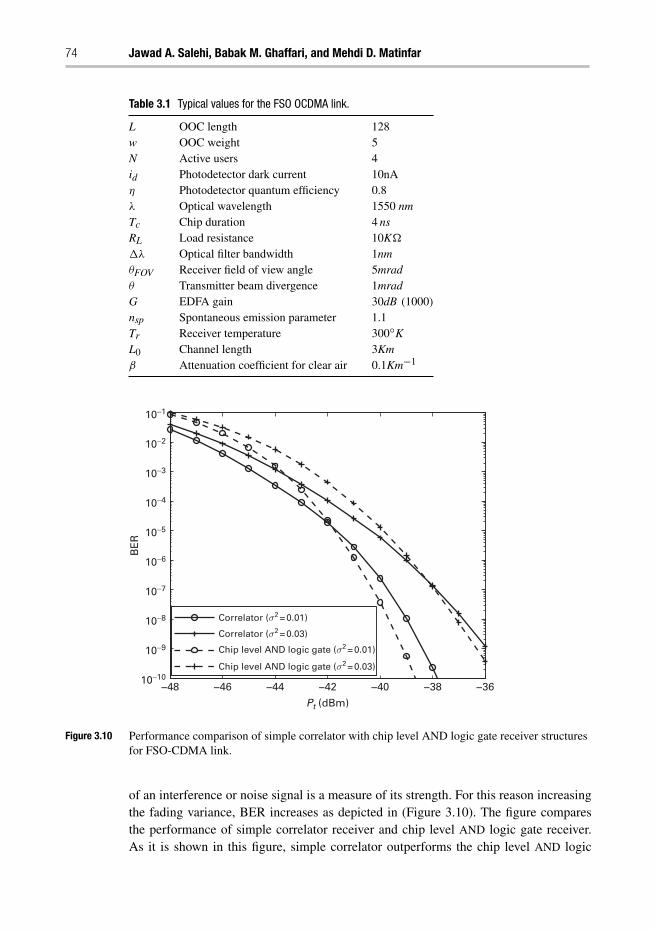
74 Jawad A. Salehi, Babak M. Ghaffari, and Mehdi D. Matinfar
Table 3.1 Typical values for the FSO OCDMA link.
L OOC length 128w OOC weight 5N Active users 4id Photodetector dark current 10nAη Photodetector quantum efficiency 0.8λ Optical wavelength 1550 nmTc Chip duration 4 nsRL Load resistance 10K�
�λ Optical filter bandwidth 1nmθFOV Receiver field of view angle 5mradθ Transmitter beam divergence 1mradG EDFA gain 30dB (1000)nsp Spontaneous emission parameter 1.1Tr Receiver temperature 300◦KL0 Channel length 3Kmβ Attenuation coefficient for clear air 0.1Km−1
−48 −46 −44 −42 −40 −38 −36
BE
R
Correlator (σ 2 = 0.01)
Correlator (σ 2 = 0.03)
Chip level AND logic gate (σ 2 = 0.01)
Chip level AND logic gate (σ 2 = 0.03)
10−1
10−2
10−3
10−4
10−5
10−6
10−7
10−8
10−9
10−10
Pt (dBm)
Figure 3.10 Performance comparison of simple correlator with chip level AND logic gate receiver structuresfor FSO-CDMA link.
of an interference or noise signal is a measure of its strength. For this reason increasingthe fading variance, BER increases as depicted in (Figure 3.10). The figure comparesthe performance of simple correlator receiver and chip level AND logic gate receiver.As it is shown in this figure, simple correlator outperforms the chip level AND logic
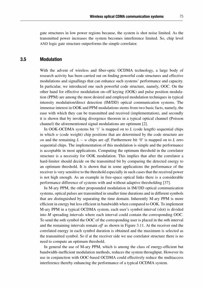
Wireless optical CDMA communication systems 75
gate structures in low power regions because, the system is shot noise limited. As thetransmitted power increases the system becomes interference limited. So, chip levelAND logic gate structure outperforms the simple correlator.
3.5 Modulation
With the advent of wireless and fiber-optic OCDMA technology, a large body ofresearch activity has been carried out on finding powerful code structures and effectivemodulations and signallings that can enhance such systems’ performance and capacity.In particular, we introduced one such powerful code structure, namely, OOC. On theother hand for effective modulation on–off keying (OOK) and pulse position modula-tion (PPM) are among the most desired and employed modulation techniques in typicalintensity modulation/direct detection (IM/DD) optical communication systems. Theimmense interest in OOK and PPM modulations stems from two basic facts, namely, theease with which they can be transmitted and received (implementation), and secondlyit is shown that by invoking divergence theorem in a typical optical channel (Poissonchannel) the aforementioned signal modulations are optimum [2].
In OOK-OCDMA systems bit ‘1’ is mapped on to L (code length) sequential chipsin which w (code weight) chip positions that are determined by the code structure areon and the remaining L − w chips are off. Furthermore bit ‘0’ is mapped on to L zerosequential chips. The implementation of this modulation is simple and the performanceis acceptable in most applications. Computing the optimum threshold in the correlatorstructure is a necessity for OOK modulation. This implies that after the correlator ahard-limiter should decide on the transmitted bit by comparing the detected energy toan optimum threshold. It is shown that in some applications the performance of thereceiver is very sensitive to the threshold especially in such cases that the received poweris not high enough. As an example in free-space optical links there is a considerableperformance difference of systems with and without adaptive thresholding [37].
In M-ary PPM, the other propounded modulation in IM/ DD optical communicationsystems, optical pulses are transmitted in smaller time durations and in different symbolsthat are distinguished by separating the time domain. Inherently M-ary PPM is moreefficient in energy but less efficient in bandwidth when compared to OOK. To implementM-ary PPM in a typical OCDMA system, each user’s symbol interval (slot) is dividedinto M spreading intervals where each interval could contain the corresponding OOC.To send the mth symbol the OOC of the corresponding user is placed in the mth intervaland the remaining intervals remain off as shown in Figure 3.11. At the receiver end thecorrelated energy in each symbol duration is obtained and the maximum is selected asthe transmitted symbol. So if at the receiver side we use correlator structure there is noneed to compute an optimum threshold.
In general the use of M-ary PPM, which is among the class of energy-efficient butbandwidth-inefficient modulation methods, reduces the system throughput. However itsuse in conjunction with OOC-based OCDMA could effectively reduce the multiaccessinterference thereby enhancing the performance of a typical OCDMA system.
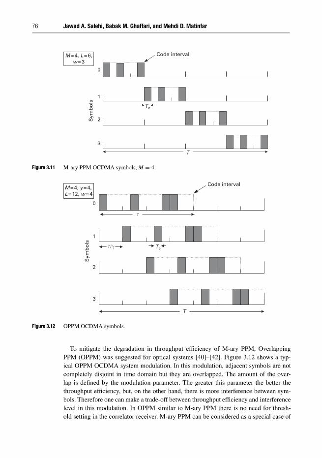
76 Jawad A. Salehi, Babak M. Ghaffari, and Mehdi D. Matinfar
Code interval
Sym
bo
ls
0
2
1
3
Tc
T
M = 4, L = 6,w = 3
Figure 3.11 M-ary PPM OCDMA symbols, M = 4.
Code interval
Tc
τ
τ/γ
T
0
2
1
3
Sym
bo
ls
M = 4, y = 4,L = 12, w = 4
Figure 3.12 OPPM OCDMA symbols.
To mitigate the degradation in throughput efficiency of M-ary PPM, OverlappingPPM (OPPM) was suggested for optical systems [40]–[42]. Figure 3.12 shows a typ-ical OPPM OCDMA system modulation. In this modulation, adjacent symbols are notcompletely disjoint in time domain but they are overlapped. The amount of the over-lap is defined by the modulation parameter. The greater this parameter the better thethroughput efficiency, but, on the other hand, there is more interference between sym-bols. Therefore one can make a trade-off between throughput efficiency and interferencelevel in this modulation. In OPPM similar to M-ary PPM there is no need for thresh-old setting in the correlator receiver. M-ary PPM can be considered as a special case of
Wireless optical CDMA communication systems 77
OPPM if we set the modulation parameter to unity. Here if we consider an OOC codewith length L and given laser pulse duration Tc, PPM multiplicity M, and index of over-lap γ , we divide a spreading interval of duration τ = LTc into γ smaller subintervalswith width τ/γ and define OPPM modulator unit delay as LTc/γ . In a single OPPMframe each spreading interval is located at a unit delay with respect to the previous one.Thus adjacent spreading intervals have (1-1/γ )τ seconds overlap and since there are intotal M symbols, an OPPM frame length equals in seconds:
T = (M − 1)τ
γ+ τ = (M − 1+ γ )
L
γTc. (3.32)
Note that in order to fit unit delay properly in the symbol interval, the followingconstraint should be met
τ
γ= integer× Tc or
L
γ= integer. (3.33)
One should note that M-arry PPM is a special case of M-ary OPPM signalling in whichthe index of overlap, γ , equals 1 that means that there is no overlap between the adjacentspreading intervals. As shown in Figure 3.12, to send the mth symbol we place the OOCof the desired user in the mth spreading interval and make all remaining chips off in thecorresponding frame of information. Considering ni as the number of collected photonsin the ith spreading interval, the receiver detects the mth symbol if for all i, 0 ≤ i ≤ M−1and i �= m we have nm > ni .
Studying the performance of OPPM in OCDMA systems will lead us to differentresults than typical optical systems. It can be shown that using OPPM in OOC-basedOCDMA systems improves the performance in both throughput and energy efficiency.To explain the reason intuitively we can say that OOC codes are typically sparse.Therefore they allow us to overlap the codes without increasing the inter-symbol inter-ference by much. Furthermore it is shown that by choosing proper parameters for themodulation, OPPM outperforms OOK and M-ary PPM [43].
To compare the performance of the three mentioned modulations in OCDMA systemsit is sufficient to consider the case of interference limited (high enough SNR) and thechip-level AND logic gate receiver structure.
3.5.1 Performance analysis
An upper bound on the error probability of the above-mentioned modulations inOCDMA systems using OOC codes and chip-level AND logic gate as the receiver struc-ture is obtained. For the performance evaluation we only consider MAI noise in orderto obtain the limits or the floor on the performance for different modulation OOC-basedOCDMA systems.
For a system with N users where each user is assigned an OOC with code weight w,code length L, and cross-correlation coefficient λ = 1 the probability of error for OOKmodulation can be found as follows [12],
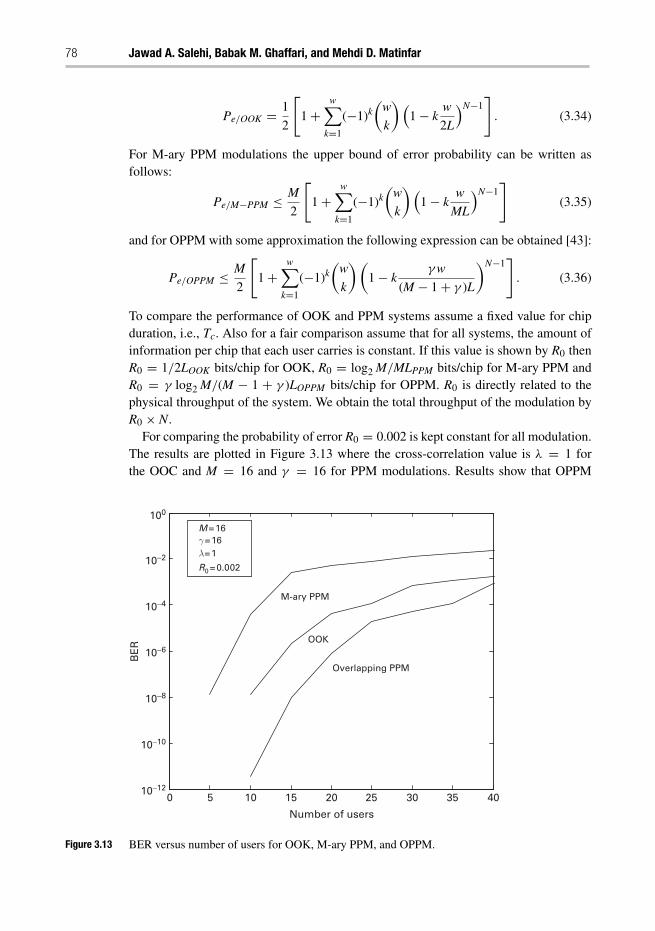
78 Jawad A. Salehi, Babak M. Ghaffari, and Mehdi D. Matinfar
Pe/OOK = 1
2
[1+
w∑k=1
(−1)k(
w
k
)(1− k
w
2L
)N−1]
. (3.34)
For M-ary PPM modulations the upper bound of error probability can be written asfollows:
Pe/M−PPM ≤ M
2
[1+
w∑k=1
(−1)k(
w
k
)(1− k
w
ML
)N−1]
(3.35)
and for OPPM with some approximation the following expression can be obtained [43]:
Pe/OPPM ≤ M
2
[1+
w∑k=1
(−1)k(
w
k
)(1− k
γw
(M − 1+ γ )L
)N−1]
. (3.36)
To compare the performance of OOK and PPM systems assume a fixed value for chipduration, i.e., Tc. Also for a fair comparison assume that for all systems, the amount ofinformation per chip that each user carries is constant. If this value is shown by R0 thenR0 = 1/2LOOK bits/chip for OOK, R0 = log2 M/MLPPM bits/chip for M-ary PPM andR0 = γ log2 M/(M − 1 + γ )LOPPM bits/chip for OPPM. R0 is directly related to thephysical throughput of the system. We obtain the total throughput of the modulation byR0 × N.
For comparing the probability of error R0 = 0.002 is kept constant for all modulation.The results are plotted in Figure 3.13 where the cross-correlation value is λ = 1 forthe OOC and M = 16 and γ = 16 for PPM modulations. Results show that OPPM
100
10−2
10−4
10−6
10−8
10−10
10−120 5 10 15 20
Number of users
25 30 35 40
BE
R
Overlapping PPM
OOK
M-ary PPM
M = 16γ = 16λ = 1
R0 = 0.002
Figure 3.13 BER versus number of users for OOK, M-ary PPM, and OPPM.
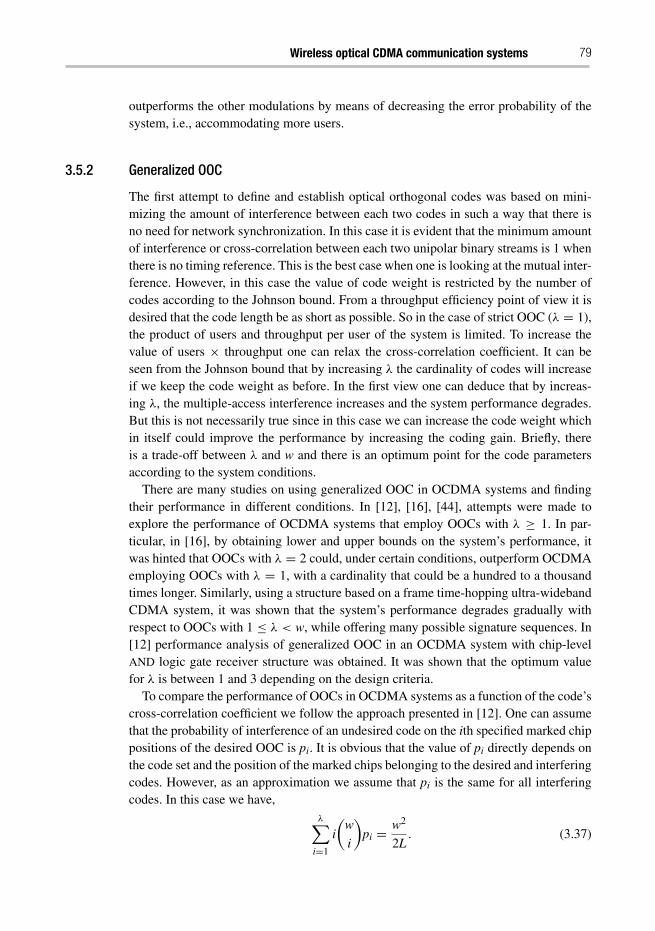
Wireless optical CDMA communication systems 79
outperforms the other modulations by means of decreasing the error probability of thesystem, i.e., accommodating more users.
3.5.2 Generalized OOC
The first attempt to define and establish optical orthogonal codes was based on mini-mizing the amount of interference between each two codes in such a way that there isno need for network synchronization. In this case it is evident that the minimum amountof interference or cross-correlation between each two unipolar binary streams is 1 whenthere is no timing reference. This is the best case when one is looking at the mutual inter-ference. However, in this case the value of code weight is restricted by the number ofcodes according to the Johnson bound. From a throughput efficiency point of view it isdesired that the code length be as short as possible. So in the case of strict OOC (λ = 1),the product of users and throughput per user of the system is limited. To increase thevalue of users × throughput one can relax the cross-correlation coefficient. It can beseen from the Johnson bound that by increasing λ the cardinality of codes will increaseif we keep the code weight as before. In the first view one can deduce that by increas-ing λ, the multiple-access interference increases and the system performance degrades.But this is not necessarily true since in this case we can increase the code weight whichin itself could improve the performance by increasing the coding gain. Briefly, thereis a trade-off between λ and w and there is an optimum point for the code parametersaccording to the system conditions.
There are many studies on using generalized OOC in OCDMA systems and findingtheir performance in different conditions. In [12], [16], [44], attempts were made toexplore the performance of OCDMA systems that employ OOCs with λ ≥ 1. In par-ticular, in [16], by obtaining lower and upper bounds on the system’s performance, itwas hinted that OOCs with λ = 2 could, under certain conditions, outperform OCDMAemploying OOCs with λ = 1, with a cardinality that could be a hundred to a thousandtimes longer. Similarly, using a structure based on a frame time-hopping ultra-widebandCDMA system, it was shown that the system’s performance degrades gradually withrespect to OOCs with 1 ≤ λ < w, while offering many possible signature sequences. In[12] performance analysis of generalized OOC in an OCDMA system with chip-levelAND logic gate receiver structure was obtained. It was shown that the optimum valuefor λ is between 1 and 3 depending on the design criteria.
To compare the performance of OOCs in OCDMA systems as a function of the code’scross-correlation coefficient we follow the approach presented in [12]. One can assumethat the probability of interference of an undesired code on the ith specified marked chippositions of the desired OOC is pi. It is obvious that the value of pi directly depends onthe code set and the position of the marked chips belonging to the desired and interferingcodes. However, as an approximation we assume that pi is the same for all interferingcodes. In this case we have,
λ∑i=1
i
(w
i
)pi = w2
2L. (3.37)
80 Jawad A. Salehi, Babak M. Ghaffari, and Mehdi D. Matinfar
The probability of error caused by MAI is obtained as follows,
Pe = 1
2Pr (error|1)+ 1
2Pr (error|0) . (3.38)
Neglecting shot noise the first term on the right-hand side of the above equation is equalto zero. However an error occurs by MAI noise only when the transmitted bit is 0. If weshow the number of interference on the ith marked chip of the desired OOC by αi thenthe probability of error is as follows [12],
Pe = 1
2Pr (error|0) = 1
2Pr (α1 > 0, α2 > 0, ...., αw > 0)
= 1− Pr (α1 = 0 or α2 = 0 or .... or αw = 0 )
= 1+w∑
k=1
(−1)k(
w
k
)Pr (α1 = α2 = .... = αk = 0) . (3.39)
The λ events that are related to p1, p2, ..., and pλ are disjoint. Furthermore all N − 1interfering users are independent and hence we can write:
Pr (α1 = α2 = .... = αk = 0) =[
1+λ∑
l=1
(−1)l(
k
l
)ρl
]N−1
(3.40)
where ρl is defined as:
ρl = Pr (α1 = α2 = .... = αl = 1 | one interfering user)
= pl +(
w− l
1
)pl+1 + ...+
(w− l
λ− l
)pλ =
λ∑i=l
(w− l
i− l
)pi. (3.41)
Substituting (3.41) in (3.40) and using (3.39) we can rewrite (3.38) as follows:
Pe = 1
2
⎧⎨⎩1+
w∑k=1
(−1)k(
w
k
)[1+
λ∑l=1
λ∑i=l
(−1)l(
k
l
)(w− l
i− l
)pi
]N−1⎫⎬⎭ . (3.42)
However, it is shown that if OOC codes are chosen such that pk = 0 for 1 ≤ k ≤ λ− 1and thus only pλ �= 0, we obtain an upper bound on the performance of such an OCDMAsystem with generalized OOCs.
To analyze the effect of cross-correlation of codes on the system performance weobtain the maximum achievable throughput of the system versus number of users in thecase which the bit error rate does not exceed a predefined value, e.g., 10−9. The goalis to find the minimum value for the code length, assuming a fixed value for numberof users by finding the optimum value for cross-correlation and code weight using theJohnson bound. The results have been sketched in Figure 3.14 where it can be seen thatthe optimum value for λ varies between 2 and 3. It is noteworthy that for λ > 1 weconsider the worst case, i.e., pk = 0 for 1 ≤ k ≤ λ − 1 and pλ = w2/2Lλ
(wλ
). Such
codes may not necessarily exist but from a mathematical point of view it gives an upperbound on the performance of all possible and existing codes.
Wireless optical CDMA communication systems 81
Number of users
5 10 15 20 25 30 35 40 45 50
0.02
0.04
0.1
0.08
0.06
0.12
00
Max
imu
m a
chie
vab
le t
hro
ug
hp
ut
λ = 2
λ = 1
λ = 3
λ = 4
Figure 3.14 Maximum achievable throughput vs. number of users for OCDMA chip-level AND logic gatereceiver.
3.6 Experimental prototypes
3.6.1 Indoor wireless optical CDMA LAN
We have shown the implemented block diagram of wireless OCDMA indoor prototypein Figure 3.15 [19]. In the transmitter side we have used dual port memory in whichthe training bits and matched pattern are put in the header section. Data bit stream iswritten in the remaining section of the memory while to generate the whole frame,including data bits and header, data is read from the first to last cell of memory. Therelation between the speed of the read and write clocks is equal to the relation of thetotal length of frame to the payload part of frame. The corresponding OOC is loaded ina shift register. The chip rate clock feeds the shift register. The output of the shift registeris combined with the output of the memory through an AND gate. This structure simplygenerates the coded bits.
The outcome of the digital part of the transmitter feeds the analog part of the trans-mitter that includes fast transistors as the driver prior to the LEDs operating in infraredwavelength (here 870 nm).
In the receiver part we have used PIN photodiode following by a three-stage amplifiercircuit. The gains of the three stages are computed such that they support the nomi-nal parameters of the system. In the implemented indoor system we have designed theanalog circuit in the receiver such that it supports the distance range of transmitter and
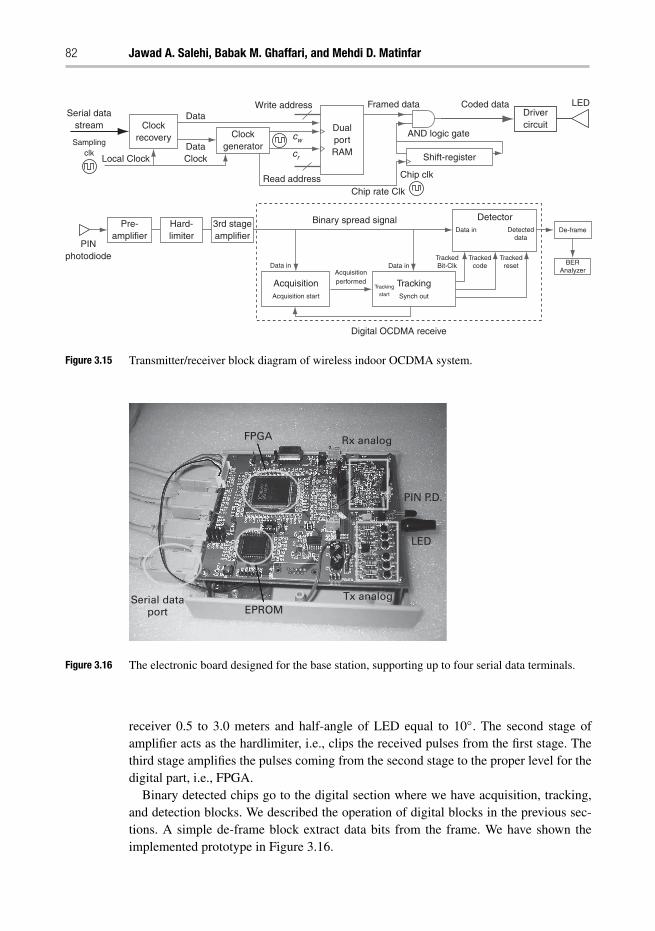
82 Jawad A. Salehi, Babak M. Ghaffari, and Mehdi D. Matinfar
Serial datastream
Samplingclk
Clockrecovery Clock
generatorDataClockLocal Clock
DataWrite address Framed data Coded data
Drivercircuit
LED
AND logic gate
Shift-register
Chip clk
Chip rate ClkRead address
Data in Data in
Data in Detecteddata
De-frame
BERAnalyzer
AcquisitionAcquisition start
Acquisitionperformed
Trackingstart
TrackingSynch out
Detector
Trackedreset
TrackedBit-Clk
Digital OCDMA receive
Trackedcode
Binary spread signal3rd stageamplifier
Hard-limiter
Pre-amplifier
PINphotodiode
DualportRAM
cw
cr
Figure 3.15 Transmitter/receiver block diagram of wireless indoor OCDMA system.
FPGA Rx analog
PIN P.D.
LED
Tx analogEPROM
Serial dataport
Figure 3.16 The electronic board designed for the base station, supporting up to four serial data terminals.
receiver 0.5 to 3.0 meters and half-angle of LED equal to 10◦. The second stage ofamplifier acts as the hardlimiter, i.e., clips the received pulses from the first stage. Thethird stage amplifies the pulses coming from the second stage to the proper level for thedigital part, i.e., FPGA.
Binary detected chips go to the digital section where we have acquisition, tracking,and detection blocks. We described the operation of digital blocks in the previous sec-tions. A simple de-frame block extract data bits from the frame. We have shown theimplemented prototype in Figure 3.16.
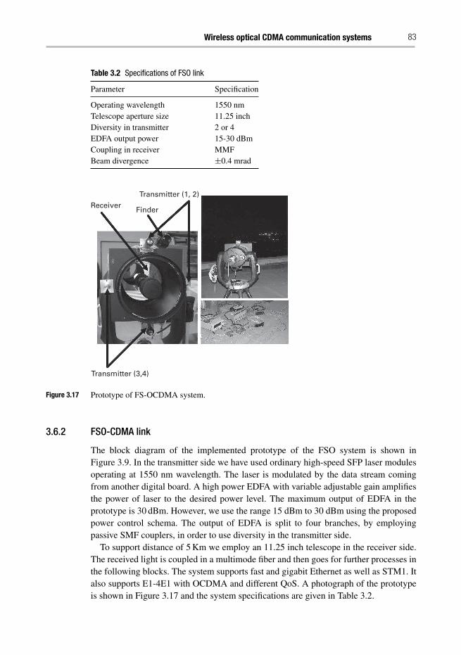
Wireless optical CDMA communication systems 83
Table 3.2 Specifications of FSO link
Parameter Specification
Operating wavelength 1550 nmTelescope aperture size 11.25 inchDiversity in transmitter 2 or 4EDFA output power 15-30 dBmCoupling in receiver MMFBeam divergence ±0.4 mrad
Transmitter (1, 2)
Transmitter (3,4)
FinderReceiver
Figure 3.17 Prototype of FS-OCDMA system.
3.6.2 FSO-CDMA link
The block diagram of the implemented prototype of the FSO system is shown inFigure 3.9. In the transmitter side we have used ordinary high-speed SFP laser modulesoperating at 1550 nm wavelength. The laser is modulated by the data stream comingfrom another digital board. A high power EDFA with variable adjustable gain amplifiesthe power of laser to the desired power level. The maximum output of EDFA in theprototype is 30 dBm. However, we use the range 15 dBm to 30 dBm using the proposedpower control schema. The output of EDFA is split to four branches, by employingpassive SMF couplers, in order to use diversity in the transmitter side.
To support distance of 5 Km we employ an 11.25 inch telescope in the receiver side.The received light is coupled in a multimode fiber and then goes for further processes inthe following blocks. The system supports fast and gigabit Ethernet as well as STM1. Italso supports E1-4E1 with OCDMA and different QoS. A photograph of the prototypeis shown in Figure 3.17 and the system specifications are given in Table 3.2.
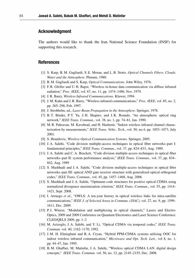
84 Jawad A. Salehi, Babak M. Ghaffari, and Mehdi D. Matinfar
Acknowledgment
The authors would like to thank the Iran National Science Foundation (INSF) forsupporting this research.
References
[1] S. Karp, R. M. Gagliardi, S. E. Moran, and L. B. Stotts, Optical Channels Fibers, Clouds,Water and the Atmosphere. Plenum, 1980.
[2] R. M. Gagliardi and S. Karp, Optical Communications. John Wiley, 1976.[3] F. R. Gfeller and U. H. Bapst, “Wireless in-house data communication via diffuse infrared
radiation,” Proc. IEEE, vol. 67, no. 11, pp. 1474–1486, Nov. 1979.[4] J. R. Barry, Wireless Infrared Communications. Kluwer, 1994.[5] J. M. Kahn and J. R. Barry, “Wireless infrared communications,” Proc. IEEE, vol. 85, no. 2,
pp. 265–298, Feb. 1997.[6] J. Strohbehn, ed., Laser Beam Propagation in the Atmosphere. Springer, 1978.[7] B. T. Binder, P. T. Yu, J. H. Shapiro, and J. K. Bounds, “An atmospheric optical ring
network,” IEEE Trans. Commun., vol. 38, no. 1, pp. 74–81, Jan. 1990.[8] M. R. Pakravan, M. Kavehrad, and H. Hashemi, “Indoor wireless infrared channel charac-
terization by measurements,” IEEE Trans. Vehic. Tech., vol. 50, no.4, pp. 1053–1073, July2001.
[9] S. Hranilovic, Wireless Optical Communication Systems. Springer, 2005.[10] J. A. Salehi, “Code division multiple-access techniques in optical fiber networks–part I:
fundamental principles,” IEEE Trans. Commun., vol. 37, pp. 824–833, Aug. 1989.[11] J. A. Salehi and C. A. Brackett, “Code division multiple-access techniques in optical fiber
networks–part II: system performance analysis,” IEEE Trans. Commun., vol. 37, pp. 834–842, Aug. 1989
[12] S. Mashhadi and J. A. Salehi, “Code division multiple-access techniques in optical fibernetworks–part III: optical AND gate receiver structure with generalized optical orthogonalcodes,” IEEE Trans. Commun., vol. 45, pp. 1457–1468, Aug. 2006.
[13] S. Mashhadi and J. A. Salehi, “Optimum code structures for positive optical CDMA usingnormalized divergence maximization criterion,” IEEE Trans. Commun., vol. 55, pp. 1414–1421, Sept. 2008.
[14] I. Arruego et al., “OWLS: A ten-year history in optical wireless links for intra-satellitecommunications,” IEEE J. of Selected Areas in Commun. (JSAC), vol. 27, no. 9, pp. 1599–1611, Dec. 2009.
[15] P. J. Winzer, “Modulation and multiplexing in optical channels,” Lasers and Electro-Optics, 2009 and 2009 Conference on Quantum Electronics and Laser Science Conference.CLEO/QELS 2009, pp. 1–2
[16] M. Azizoglo, J. A. Salehi, and Y. Li, “Optical CDMA via temporal codes,” IEEE Trans.Commun. vol. 40, 1162–1170, 1992.
[17] J. M. H. Elmirghani and R. A. Cryan, “Hybrid PPM-CDMA systems utilising OOC forindoor wireless infrared communication,” Microwave and Opt. Tech. Lett., vol 8, no. 1,pp. 44–47, Jan. 1995.
[18] B. M. Ghaffari, M. Matinfar, J. A. Salehi, “Wireless optical CDMA LAN: digital designconcepts,” IEEE Trans. Commun. vol. 56, no. 12, pp. 2145–2155, Dec. 2008.
Wireless optical CDMA communication systems 85
[19] B. M. Ghaffari, M. D. Matinfar, and J. A. Salehi, “Wireless optical CDMA LAN: digitalimplementation analysis,” IEEE J. of Selected Areas in Commun. (JSAC), vol. 27, no. 9,pp.1676–1686, Dec. 2009.
[20] F. R. K. Chung, J. A. Salehi, and V. K. Wei, “Optical orthogonal codes: design, analysis, andapplications,” IEEE Trans. Inf. Theory vol. 35, no. 3, pp. 595–604, May 1989.
[21] H. Chung and P. Vijay Kumar, “Optical orthogonal codes – new bounds and an optimalconstruction,” IEEE Trans. Inf. Theory, vol. 36, no. 4, pp. 866–873 Jul. 1990.
[22] S. M. Johnson, “A new upper bound for error-correcting codes,” IRE Trans. Inf. Theory, vol.IT-8, pp. 203–207, 1962.
[23] H. M. Shalaby, “Chip level detection in optical code division multiple access,” J. LightwaveTechnol., vol. 16, pp. 1077–1087, Jun. 1998.
[24] T. Ohtsuki, “Performance analysis of direct-detection optical asynchronous CDMA systemswith double optical hard-limiters,” J. Lightwave Technol., vol. 15, no. 3, pp. 452–457, Mar.1997.
[25] U. N. Griner and S. Arnon, “Multiuser diffuse indoor wireless infrared communicationusing equalized synchronous CDMA,” IEEE Trans. Commun., vol. 54, pp. 1654–1662,Sep. 2006.
[26] A. Aminzadeh-Gohari and M. R. Pakravan, “Analysis of power control for indoor wire-less infrared CDMA communication,” in Proceedings of the 25th IEEE Performance,Computing, and Communications Conference (IPCCC) (IEEE, 2006), pp. 297–302.
[27] S. Zahedi and J. A. Salehi, “Analytical comparison of various fiber-optic CDMA receiverstructures,” J. Lightwave Technol., vol. 18, no. 12, pp. 1718–1727, Dec. 2000.
[28] A. Keshavarizan and J. A. Salehi, “Optical orthogonal code acquisition in fiber-optic CDMAsystems via the simple serial-search method,” IEEE Trans. Commun., vol. 50, no. 3,pp. 473–483, Mar. 2002.
[29] A. Keshavarizan and J. A. Salehi, “Multiple-shift code acquisition of optical orthogonalcodes in optical CDMA systems,” IEEE Trans. Commun., vol. 53, no. 4, pp. 687–697,Apr. 2005.
[30] R. L. Peterson, D. E. Borth, and R. E. Ziemer, Introduction to Spread Spectrum Communi-cations. Prentice-Hall, 1995.
[31] Int. Electrotech. Commission, CEI/IEC 825-1: Safety of Laser Products, 1993. J. D.Rancourt, Optical Thin Film. Macmillan, 1987.
[32] R. M. Gagliardi, “Pulse-coded multiple access in space optical communications,” IEEEJSAC, vol. 13, no. 3, pp. 603–608, 1995.
[33] T. H. Carbonneau and D. R. Wisely, “Opportunities and challenges for optical wireless; thecompetitive advantage of free space telecommunications links in today’s crowded market-place,” in Proc. SPIE Wireless Technologies and Systems: Millimeter-Wave and Optical,vol. 3232, pp. 119–128, Jan. 1998.
[34] P. F. Szajowski, G. Nykolak, J. J. Auborn, H. M. Presby, and G. E. Tourgee, “High poweroptical amplifiers enable 1550 nm terrestrial freespace optical data-link operating at 10Gbs,” in Proc. MILCOM ’99, vol. 1, pp. 687–689, 1999.
[35] T. Li and M. C. Teich, “Photon point process for traveling-wave laser amplifiers,” IEEE J.Quantum Electron., vol. 29, no. 9, pp. 2568–2578 Sep. 1993.
[36] M. Razavi and J. H. Shapiro, “Wireless optical communications via diversity reception andoptical preamplification,” IEEE Trans. Wireless Commun., vol. 4, no. 3, pp. 975–983, 2005.
[37] M. Jazayerifar and J. A. Salehi, “Atmospheric optical CDMA communication systems viaoptical orthogonal codes,” IEEE Trans. Commun. vol. 54, no. 9, pp. 1614–1623 Sept. 2006.
86 Jawad A. Salehi, Babak M. Ghaffari, and Mehdi D. Matinfar
[38] B. Hamzeh and M. Kavehrad, “OCDMA-coded free-space optical for wireless optical-meshnetworks,” IEEE Trans. Commun., no. 12, pp. 2165–2174, Dec. 2004.
[39] T. Ohtsuki, “Performance analysis of atmospheric optical PPM systems,” J. LightwaveTechnol., vol. 21, no. 2, pp. 406–411, Feb.
[40] G. M. Lee and G. W. Schroeder, “Optical PPM with multiple positions per pulse-width,”IEEE Trans. Commun., vol. COM-25, pp. 360–364, Mar. 1977.
[41] C. N. Georghiades, “Modulation and coding for throughput-efficient optical systems,” IEEEInform. Theory, vol. 40, pp 1313–1326, Sept. 1994.
[42] H. M. H. Shalaby, “Maximum achievable throughputs for uncoded OPPM and MPPM inoptical direct-detection channels,” J. Lightwave Technol. vol. 13, no. 11, pp. 2121–2128,Nov. 1995.
[43] H. M. H. Shalaby, “Direct detection optical overlapping PPM-CDMA communication sys-tems with double optical hardlimiters,” J. Lightwave Technol. vol. 17, pp. 1158–1165, July1999.
[44] J. J. Chen and G. Yang, “CDMA fiber-optic systems with optical hard limiters,” J. LightwaveTechnol., vol. 19, no. 7, pp. 950–958, Jul. 2001.
[45] A. R. Forouzan, J. A. Salehi, and M. Nasiri-Kenari, “Frame time-hopping fiber-opticcode-division multiple access using generalized optical orthogonal codes,” IEEE Trans.Commun., vol. 50, no. 12, pp. 1971–1982, Dec. 2002.
4 Pointing error statisticsShlomi Arnon
Optical wireless communication transceivers use in many cases very narrow laser beamdivergence and very narrow field of view receiver telescope. The laser transmitter usesnarrow laser beam divergence in order to minimize the transmitter power while thereceiver uses very narrow field of view telescope in order to reduce background radi-ation noise [1–7]. As a result the pointing between the transmitter and the receiver iscomplicated and in order to establish optical communication between two transceivers,the line of sight of their optics must be aligned during the entire communication time.Optical acquisition and tracking system is used to keep line of sight of the transceivers.However, from time to time due to electronic noise, and mechanical vibration (e.g. windin an urban system [2, 3] or jitter of antenna of a satellite [8, 9]) error in pointing direc-tion occurs. In the following we present a simple model that describes the effect of thestatistic of the pointing error on the performance of the communication system.
We assume that the orthogonal direction of error pointing angle models are basedon a normal distribution [1]. In that case the elevation pointing error angle is normallydistributed with a probability density
f (θV ) = 1√2πσV
exp
(− θ2
V
2σ 2V
), (4.1)
where σv and θv are elevation pointing standard deviation and elevation pointingrespectively.
The azimuth pointing error angle is normally distributed with probability density
f (θH) = 1√2πσH
exp
(− θH
2
2σ 2H
), (4.2)
where σH and θH are azimuth pointing standard deviation and azimuth pointing angle,respectively.
The radial pointing error angle is the root square sum of the azimuth and elevationangles
θ =√θ2
V + θ2H . (4.3)
Advanced Optical Wireless Communication Systems, ed. Shlomi Arnon, John R. Barry, George K.Karagiannidis, Robert Schober, and Murat Uysal. Published by Cambridge University Press.c© Cambridge University Press 2012.
88 Shlomi Arnon
Based on symmetry we can assume that
σV = σH = σ. (4.4)
We assume that the azimuth and elevation processesare independent and identi-cally distributed so the radial pointing error angle model is Rayleigh distributed withprobability density
f (θ) = θ
σ 2exp
(− θ2
2σ 2
). (4.5)
Now, we derive a model that relates the transmitted optical signal from the transmitterto the receiver. The distance between the transmitter and the receiver satellite is z meters.The instantaneous received power as a function of pointing direction error angle θ is
PR (θ) = PTηTηR
(λ
4πz
)2
GTGR exp(−GT · θ2) (4.6)
where ηR, ηT , and GR =(
πDRλ
)2and GT =
(2πWλ
)2are the optical efficiencies and
the telescope gain of the receiver and the transmitter respectively. And where DR isthe receiver aperture diameter, W is Gaussian rms width at the transmitter aperture, thewavelength of the laser transmitter is λ, and PT is the optical laser transmitter power.
The received signal is given by
μ (θ) = R · PR (θ) . (4.7)
The signal-to-noise ratio (SNR) model is
SNR =∞∫
0
μ (θ)
σf (θ) · dθ , (4.8)
where σn is the noise variance variance. The receiver is assumed to include an opticaldetector in direct detection mode. In such systems the instantaneous error probability isgiven by
BER (θ) ≈ 1
2
(erfc
(μ (θ)√2 (2σn)
)), (4.9)
where the complementary error function is given by
erfc(x) = 1− 2√π
x∫0
exp(−y2
)dy. (4.10)
The average bit error probability is given
BER =∞∫
0
BER (θ) · f (θ) · dθ . (4.11)
Pointing error statistics 89
References
[1] Arnon., S. Rotman, and N. S Kopeika, “The performance limitations of free space opticalcommunication satellite networks due to vibrations – digital case,” Optical Engineering,vol. 36, no. 11, pp. 3148–3157, (Nov. 1997).
[2] S. Arnon, “The effects of atmospheric turbulence and building sway on optical wirelesscommunication systems,” Optics Letters, Vol. 28, no. 2, pp. 129–131 (Jan. 2003).
[3] D. Kedar and S. Arnon, “Urban optical wireless communication network: The mainchallenges and possible solutions,” IEEE Optical Communications Supplement to IEEECommunications Magazine, pp. S1–S7, (May 2004).
[4] S. Arnon and N. S Kopeika, “Adaptive optical transmitter and receiver for space com-munication through clouds,” Applied Optics, vol. 36, no. 9, pp. 1987–1993, (March1997).
[5] S. Arnon and N. S. Kopeika, “The performance limitations of free space optical commu-nication satellite networks due to vibrations – analog case,” Optical Engineering, vol. 36,no.1, pp.175–182, (Jan. 1997).
[6] S. Arnon and N. S Kopeika, “Probing and monitoring aerosol and atmospheric cloud via anelectro-optic oscillator,” Applied Optics, vol. 35, no. 27, pp. 5427–5434, (Sep. 1996).
[7] S. Arnon and N. S Kopeika, “Free space optical communication: analysis of spatial widen-ing of optical pulses for propagation through clouds,” Optical Engineering, vol. 34, no. 2,pp. 511–515, (Feb. 1995).
[8] S. Arnon and N. S Kopeika, “Laser satellite communication networks-vibration effects andpossible solutions,” Proceedings of the IEEE, vol. 85, no. 10, pp. 1646–1661, (Oct 1997).
[9] S Arnon, S. Rotman, and N. S Kopeika, “Beam-width and transmitter power adaptive totracking system performance for free space optical communication,” Applied Optics, vol.36, no 24, pp. 6095–6101, (Aug. 1997).
5 Equalization and Markov chainsin cloud channelMohsen Kavehrad
Abstract: Free-space optical (FSO) communications is a practical solution for creat-ing a three-dimensional global broadband communications grid, offering bandwidthsfar beyond those possible in Radio Frequency (RF) range. However, attributes ofatmospheric turbulence and obscurants such as clouds impose perennial limitations onavailability and reliability of optical links. To design and evaluate optimum transmissiontechniques that operate under realistic atmospheric conditions, a good understanding ofthe channel behavior is necessary.
In some prior works, the Monte Carlo ray tracing (MCRT) algorithm has been used toanalyze the channel behavior. This task is quite numerically intensive. The focus of thischapter is on investigating the possibility of simplifying this task by a direct extractionof state transition matrices associated with standard Markov modeling from the MCRTcomputer simulations programs. We show that by tracing a photon’s trajectory in spacevia a Markov chain model, the angular distribution can be calculated by simple matrixmultiplications. We also demonstrate that the new approach produces results that areclose to those obtained by MCRT and other known methods. Furthermore, consider-ing the fact that angular, spatial, and temporal distributions of energy are interrelated,mixing time of Monte Carlo Markov chain (MCMC) for different types of aerosols iscalculated based on eigen-analysis of the state transition matrix and possibility of com-munications in scattering media is investigated. We also consider in this chapter signalprocessing techniques for airborne FSO wireless communications through clouds. TheFSO channel is known to be accompanied by multi-scattering, which causes severe inter-symbol interference in digital transmissions at high data rates. The chapter investigatesthe feasibility of digital signal processing schemes applied to FSO communications. Byhaving a channel shortening equalizer (CSE) or time equalization (TEQ) at the transmit-ter and a Viterbi equalizer at the receiver, reliable communication at low-to-mid leveloptical thickness values is shown to be feasible. We also suggest how existing TEQalgorithms can be modified to fit into TEQ-in-transmitter configurations. Performance isevaluated in average bit error rate (BER), and compared with conventional equalizationtechniques.
Advanced Optical Wireless Communication Systems, ed. Shlomi Arnon, John R. Barry, George K.Karagiannidis, Robert Schober, and Murat Uysal. Published by Cambridge University Press.c© Cambridge University Press 2012.
Equalization and Markov chains in cloud channel 91
Key words – angular dispersion, channel modeling, Markov chain, Monte Carlo raytracing, multi-scattering, second largest eigen modulus (SLEM), channel-shortening,Viterbi algorithm,
5.1 Introduction
Free-space optical (FSO) communications is the only practical solution for creating abroadband three-dimensional global communications grid among ground and airbornenodes, due to its ease of deployment, enormous available bandwidth, possibility of band-width reuse, and inherent security at physical layer, as laser beams are normally spatiallyconfined and cannot be tapped [1, 2]. In ideal free-space, the total loss due to absorp-tion and scattering is virtually zero. This is because of the spatial confinement of laserbeams. However, atmospheric obscurants such as fog, haze, smoke, dust, and cloudsturn the propagation environment into a multiple scattering medium and hence introducelaser pulse broadening in space and time. Moreover, even in clear weather, turbulencedue to refractive index fluctuations in layers of atmosphere causes wavefront distortion,introducing both random phase and intensity fluctuations across the transmitted lightbeam [3, 4]. In presence of multi-scattering, both availability and capacity of opticallink degrade, significantly.
Turbulent air creates small-scale fluctuations of the refractive index along a wave-form propagation path causing random amplitude, phase, and angle-of-arrival variationsknown as “turbulence.”
Turbulence distorts an optical beam cross-section spatially, causing random beamdancing, phase-front distortion, etc., in imaging. These spatial adverse effects contributeto image blurring. In transmissions or communications using simple Intensity Modula-tion/Direct Detection, turbulence lends itself approximately to a multiplicative Lognor-mal fading coefficient (flat fading) – known as scintillation which is a temporal effect.Where there is moisture, turbulent air can create an upward motion of moist air particlesand this is a prerequisite in formation of clouds. Once a cloud is formed, light beamphotons traveling through along a propagation path are scattered due to Mie scattering.Received optical power loss associated with light beam passing through clouds, for themost part, is a loss to scattering rather than absorption, in parts of the infrared range.
The focus of this section is on deleterious effects of multi-scatterings and aerosols.Turbulence-induced effects are not further discussed in this work, as sufficient linkpower budget and diversity can overcome this shortfall [3].
In some applications, transmit power is limited, in order to observe eye and skin safetyregulations and on the other hand, sensitivity of optical receivers is affected by the shotnoise caused by background light [5]. Hence, link budget management becomes verycritical and challenging. Furthermore, multi-path delay spreading limits the achievablebit rates [5]. In digital FSO communications, one is usually interested in the peak powerof received waveform in order to distinguish the signal from steady background radiation[6, 7]. In a receiver unequipped with appropriate countermeasure techniques, overlap-ping of pulse tails on adjacent symbol intervals introduces intersymbol-interference
92 Mohsen Kavehrad
(ISI), and thus limits the achievable bit rate. As a result, the receiver should have a smallfield-of-view (FOV) and has to resort to line-of-sight (LOS) photons, known as ballistic,and/or near LOS (snake) photons which are highly forward scattered. However, if due tothickness and/or particle density of obscurants, a light pulse enters the diffusion regime,spatial distribution approaches a normal distribution and angular distribution becomesisotropic [8]. In this case, a receiver of small FOV may fail to maintain the desired linkmargin.
To answer the fundamental question of optical communications feasibility in pres-ence of clouds, one has to accurately model atmospheric optical channel and estimateparameters such as angular, spatial, and temporal dispersions.
As a collimated laser beam propagates through clouds, it spreads and after travelingsome distance, it reaches a steady state of being defocused and diffused. The rate of con-vergence to this steady state determines feasibility of communications through variousclouds of different optical thickness values. Optical thickness τ is the average number ofscatterings over a given length of cloud whose value is a number with no physical unit. Itis defined by multiplying the scattering coefficient (km−1), βsca, of cloud by the physicalcloud length, L, in kilometer. We will elaborate on this issue more, in Section 5.2.
So far, Monte-Carlo ray tracing (MCRT) has been used to calculate the channelparameters [ 6, 9, and 10– 12]. This method requires a high computational capacity anda long execution time. In [8], authors find spatial and angular distribution by a statisticalapproach. However, their results are limited to the first two moments of multiple scatter-ing. Finding angular distribution is of great importance in computer graphics, as well.In [13], a single-scatter impulse response is defined and then the result is generalizedto multiple scattering via convolution. Since this impulse response is three dimensional,the convolution process is quite cumbersome. In this work, angular distribution evolu-tion of a laser beam in a multiple scattering medium is characterized by extracting thecorresponding simplified Markov chain information from the MCRT algorithm. By cal-culating the state transition matrix, one can find the probability distribution function ofscattering angle after any number of scatterings. We show that the Markov chain modelproduces values that are close to MCRT results and other proposed analytical methods,yet need much less time to produce the results. Since angular, spatial, and temporal dis-tributions of received power are inter-related, useful information can be extracted fromangular distribution about the behavior of the entire system. The remainder of this chap-ter is organized as follows. In Section 5.2, channel propagation modeling is reviewed.Section 5.3 details our modeling results and eigen-analyses of the state transition matrixfor the cloud channel. This is followed by an investigation of advance digital signalprocessing techniques, in particular, channel shortening algorithms as apply to cloudchannel models. Finally Section 5.5 presents a summary and concludes the chapter.
5.2 Channel propagation modeling
When propagating through clouds or fog, a laser beam interacts with medium particles,which are mostly water droplets of sizes comparable to the optical wavelength values.Hence, we need Mie theory to explain these interactions. This theory is the application
Equalization and Markov chains in cloud channel 93
of Maxwell’s equation to the problem of a homogeneous sphere radiated by a plane wavefrom a single direction [14]. Knowing the particle size distribution of the medium, onecan determine absorption, extinction, and scattering coefficients as well as phase func-tion, using this theory. Assuming that particles are homogeneously distributed in space,distance between two successive scatters turns out to be an exponential random variablewith a mean value of Dave = 1
βscawhere βsca is the scattering coefficient. Furthermore,
absorption, extinction, and scattering coefficients are related as: βsca + βabs = βext,where βabs and βext are absorption and extinction coefficients, respectively. Addition-ally, the ratio of the scattered energy to the total energy is determined by single scatteralbedo, � = βsca/βext.
According to Mie theory, one can define the scatter direction via a three-dimensionalprobability distribution function (PDF) known as the Phase Function. In other words,Phase Function is the PDF of the solid angle � = (θ ,φ) [14–16]. For example, in [15]we find that:
∫Over 4π
P(θ )d� =π∫
0
2π∫0
P(θ ) sin(θ )dθdϕ = 4π (5.1)
and where P(θ ) in Eq. (5.1) is referred to as the (un-normalized) scattering phasefunction in the literature.
Figure 5.1 demonstrates the scattering phase function for different types of clouds.These functions are obtained by substituting the modified gamma distribution for radiusdensity of cloud particles in equations extracted from Mie theory for the poly-dispersedphase function [14, 17]. It is clear from this figure that all these phase functions arehighly peaked in the forward direction. Actually, since the azimuth scattering angle, ϕ,is uniformly distributed in [0, 2π ], the Phase Function can be plotted only against thepolar scattering angle, θ . Scattering phase function can also be interpreted as the PDFof cos(θ ) [9, 16].
In order to find suitable probabilities to inject into a Monte Carlo model, one needsthe probability density function of θ , not the plotted scattering phase functions. Thenormalized phase function, as generally used in the literature, is normalized so that itsintegration over all possible scatter angles (4π steradians) is unity, thus qualifying it tobe a PDF. With no ϕ dependence of P(θ ), the integration over ϕ simply contributes afactor of 2π. This leads to the normalization definition for P(θ ) of:
2π ·∫ π
0
P(θ )
4π· sin(θ )dθ =
∫ π
0P(θ ) · sin(θ )
2· dθ = 1.
Thus, the PDF of θ can be extracted from the normalized phase function and beexpressed as:
f (θ ) = P(θ ) · sin(θ )
2. (5.2)
Unfortunately, expressing the phase function versus θ has caused a great deal of confu-sion in the published literature [18, 19]. More specifically, several authors have mistaken
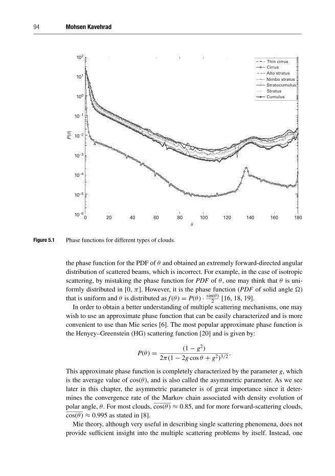
94 Mohsen Kavehrad
102
101
100
10−1
10−2
10−3
P (θ
)
10−4
10−5
10−60 20 40 60 80 100 120 140 160
Thin cirrusCirrusAlto stratusNimbo stratusStratocumulus
CumulusStratus
180θ
Figure 5.1 Phase functions for different types of clouds.
the phase function for the PDF of θ and obtained an extremely forward-directed angulardistribution of scattered beams, which is incorrect. For example, in the case of isotropicscattering, by mistaking the phase function for PDF of θ , one may think that θ is uni-formly distributed in [0, π]. However, it is the phase function (PDF of solid angle �)that is uniform and θ is distributed as f (θ ) = P(θ ) · sin(θ )
2 [16, 18, 19].In order to obtain a better understanding of multiple scattering mechanisms, one may
wish to use an approximate phase function that can be easily characterized and is moreconvenient to use than Mie series [6]. The most popular approximate phase function isthe Henyey–Greenstein (HG) scattering function [20] and is given by:
P(θ ) = (1− g2)
2π(1− 2g cos θ + g2)3/2.
This approximate phase function is completely characterized by the parameter g, whichis the average value of cos(θ ), and is also called the asymmetric parameter. As we seelater in this chapter, the asymmetric parameter is of great importance since it deter-mines the convergence rate of the Markov chain associated with density evolution ofpolar angle, θ . For most clouds, cos(θ ) ≈ 0.85, and for more forward-scattering clouds,cos(θ ) ≈ 0.995 as stated in [8].
Mie theory, although very useful in describing single scattering phenomena, does notprovide sufficient insight into the multiple scattering problems by itself. Instead, one
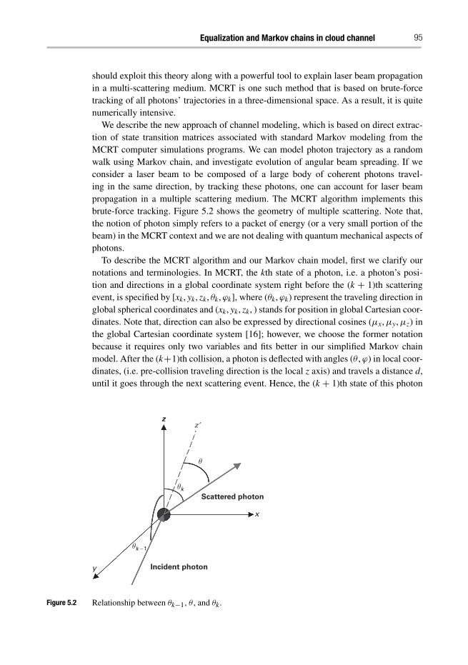
Equalization and Markov chains in cloud channel 95
should exploit this theory along with a powerful tool to explain laser beam propagationin a multi-scattering medium. MCRT is one such method that is based on brute-forcetracking of all photons’ trajectories in a three-dimensional space. As a result, it is quitenumerically intensive.
We describe the new approach of channel modeling, which is based on direct extrac-tion of state transition matrices associated with standard Markov modeling from theMCRT computer simulations programs. We can model photon trajectory as a randomwalk using Markov chain, and investigate evolution of angular beam spreading. If weconsider a laser beam to be composed of a large body of coherent photons travel-ing in the same direction, by tracking these photons, one can account for laser beampropagation in a multiple scattering medium. The MCRT algorithm implements thisbrute-force tracking. Figure 5.2 shows the geometry of multiple scattering. Note that,the notion of photon simply refers to a packet of energy (or a very small portion of thebeam) in the MCRT context and we are not dealing with quantum mechanical aspects ofphotons.
To describe the MCRT algorithm and our Markov chain model, first we clarify ournotations and terminologies. In MCRT, the kth state of a photon, i.e. a photon’s posi-tion and directions in a global coordinate system right before the (k + 1)th scatteringevent, is specified by [xk, yk, zk, θk,ϕk], where (θk,ϕk) represent the traveling direction inglobal spherical coordinates and (xk, yk, zk, ) stands for position in global Cartesian coor-dinates. Note that, direction can also be expressed by directional cosines (μx,μy,μz) inthe global Cartesian coordinate system [16]; however, we choose the former notationbecause it requires only two variables and fits better in our simplified Markov chainmodel. After the (k+1)th collision, a photon is deflected with angles (θ ,ϕ) in local coor-dinates, (i.e. pre-collision traveling direction is the local z axis) and travels a distance d,until it goes through the next scattering event. Hence, the (k + 1)th state of this photon
z
θ
θk
θk − 1
x
y
Scattered photon
Incident photon
z’
Figure 5.2 Relationship between θk−1, θ , and θk.
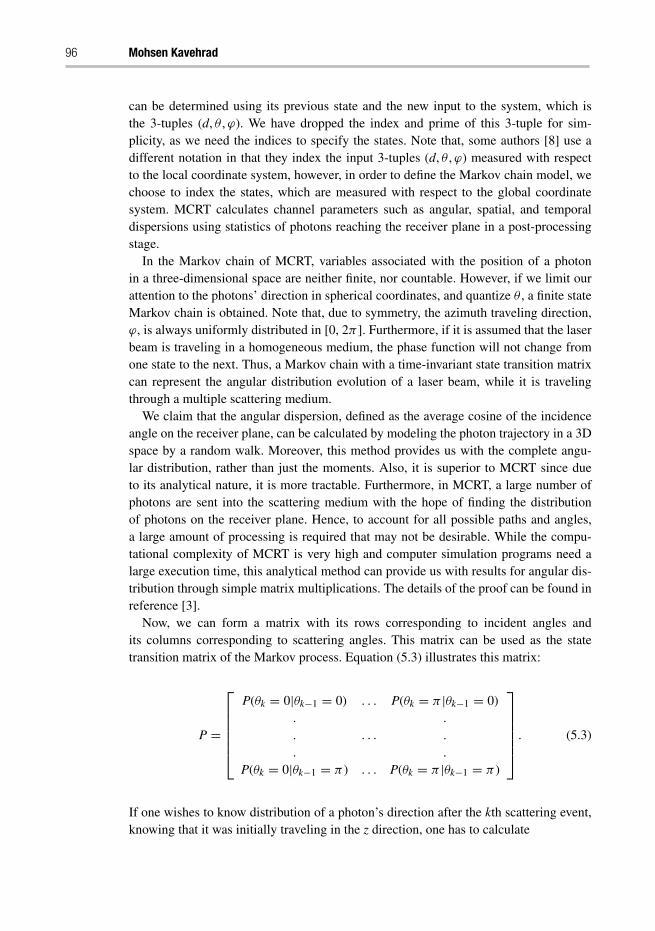
96 Mohsen Kavehrad
can be determined using its previous state and the new input to the system, which isthe 3-tuples (d, θ ,ϕ). We have dropped the index and prime of this 3-tuple for sim-plicity, as we need the indices to specify the states. Note that, some authors [8] use adifferent notation in that they index the input 3-tuples (d, θ ,ϕ) measured with respectto the local coordinate system, however, in order to define the Markov chain model, wechoose to index the states, which are measured with respect to the global coordinatesystem. MCRT calculates channel parameters such as angular, spatial, and temporaldispersions using statistics of photons reaching the receiver plane in a post-processingstage.
In the Markov chain of MCRT, variables associated with the position of a photonin a three-dimensional space are neither finite, nor countable. However, if we limit ourattention to the photons’ direction in spherical coordinates, and quantize θ , a finite stateMarkov chain is obtained. Note that, due to symmetry, the azimuth traveling direction,ϕ, is always uniformly distributed in [0, 2π ]. Furthermore, if it is assumed that the laserbeam is traveling in a homogeneous medium, the phase function will not change fromone state to the next. Thus, a Markov chain with a time-invariant state transition matrixcan represent the angular distribution evolution of a laser beam, while it is travelingthrough a multiple scattering medium.
We claim that the angular dispersion, defined as the average cosine of the incidenceangle on the receiver plane, can be calculated by modeling the photon trajectory in a 3Dspace by a random walk. Moreover, this method provides us with the complete angu-lar distribution, rather than just the moments. Also, it is superior to MCRT since dueto its analytical nature, it is more tractable. Furthermore, in MCRT, a large number ofphotons are sent into the scattering medium with the hope of finding the distributionof photons on the receiver plane. Hence, to account for all possible paths and angles,a large amount of processing is required that may not be desirable. While the compu-tational complexity of MCRT is very high and computer simulation programs need alarge execution time, this analytical method can provide us with results for angular dis-tribution through simple matrix multiplications. The details of the proof can be found inreference [3].
Now, we can form a matrix with its rows corresponding to incident angles andits columns corresponding to scattering angles. This matrix can be used as the statetransition matrix of the Markov process. Equation (5.3) illustrates this matrix:
P =
⎡⎢⎢⎢⎢⎢⎣
P(θk = 0|θk−1 = 0) . . . P(θk = π |θk−1 = 0)...
. . .
.
.
.P(θk = 0|θk−1 = π ) . . . P(θk = π |θk−1 = π )
⎤⎥⎥⎥⎥⎥⎦ . (5.3)
If one wishes to know distribution of a photon’s direction after the kth scattering event,knowing that it was initially traveling in the z direction, one has to calculate
Equalization and Markov chains in cloud channel 97
Pk(θ ) = (PK)T
⎡⎢⎢⎢⎢⎢⎢⎢⎣
10...0
⎤⎥⎥⎥⎥⎥⎥⎥⎦
. (5.4)
The first row of the state transition matrix is P(θ ) sin(θ )/2. Hence, we can find the phasefunction resulting from k scattering events from the first row of the kth power of thestate transition matrix, simply by taking out the sin(θ )/2 factor.
Figure 5.3 shows the state transition matrix for cumulus cloud at a wavelength of1.55 μm. We have calculated the state transition matrix with a resolution of π/300. Inother words, P is a 300 × 300 matrix. We observed that by increasing the resolution toπ/1000, our simulation results do not change. The forward scattering property of cumu-lus cloud is clear from this picture. That is, the state transition matrix is very close to anidentity matrix. Figure 5.4 shows P15 which clarifies transition probabilities at an opti-cal thickness value of 15. Here, the value 15 is chosen since for this value, there are lessline-of-sight (LOS) photons, and most of the photons that may reach the receiver havegone through multiple scatterings. From Figure 5.4, one can see that after 15 scatteringevents, the phase surface is very close to the shape of sin(θ )/2. This corresponds to anisotropic scattering.
0.1
0.08
0.06
0.04
0.02
150
100
50
0 0
50
100
150
Pro
babi
lity
dens
ity fu
nctio
n
0
θk − 1θk
Figure 5.3 State transition matrix of cumulus clouds at a wavelength = 1.55 μm.
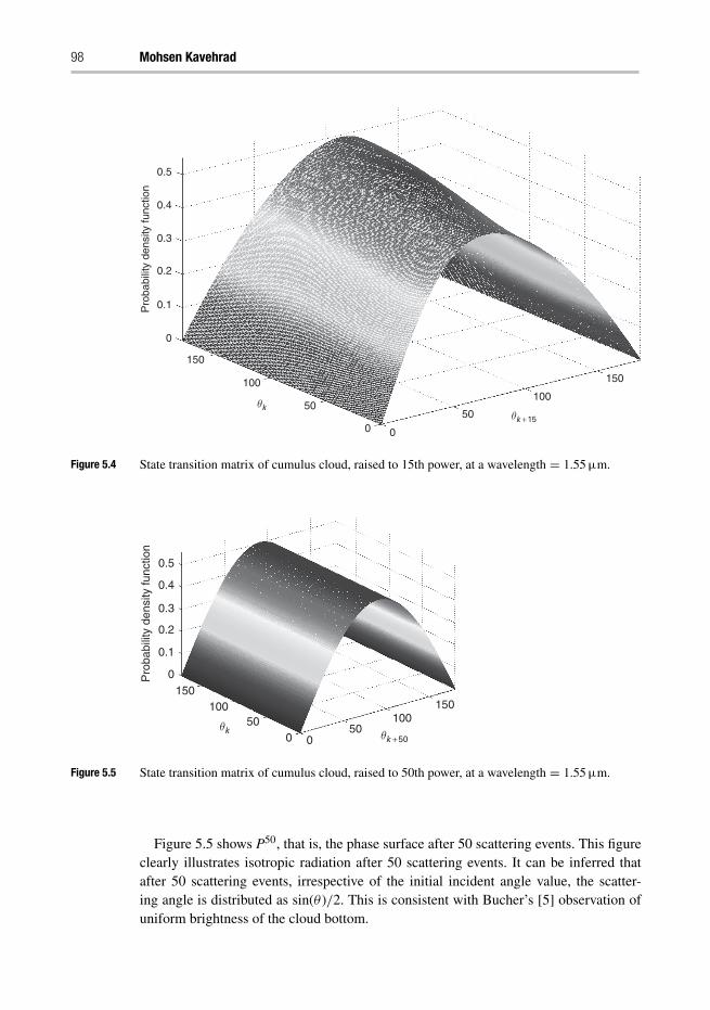
98 Mohsen Kavehrad
0.5
0.4
0.3
0.2
0.1
0
150
100
50
0 0
50
100
150
θk + 15
θk
Pro
babi
lity
dens
ity fu
nctio
n
Figure 5.4 State transition matrix of cumulus cloud, raised to 15th power, at a wavelength = 1.55 μm.
0.5
0.4
0.3
0.2
0.1
0Pro
babi
lity
dens
ity fu
nctio
n
150100
500
θk 0
50100
150
θk + 50
Figure 5.5 State transition matrix of cumulus cloud, raised to 50th power, at a wavelength = 1.55 μm.
Figure 5.5 shows P50, that is, the phase surface after 50 scattering events. This figureclearly illustrates isotropic radiation after 50 scattering events. It can be inferred thatafter 50 scattering events, irrespective of the initial incident angle value, the scatter-ing angle is distributed as sin(θ )/2. This is consistent with Bucher’s [5] observation ofuniform brightness of the cloud bottom.
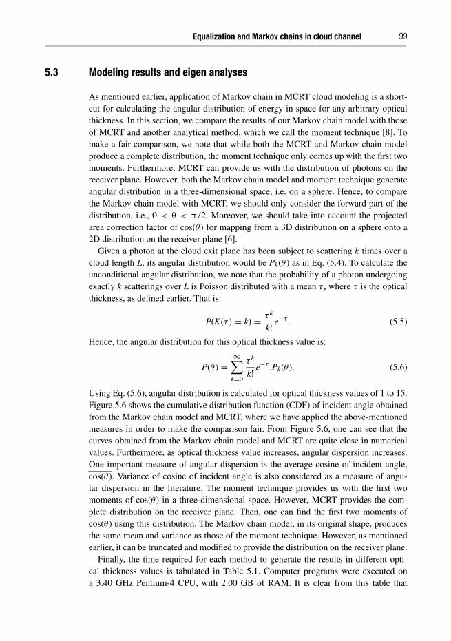
Equalization and Markov chains in cloud channel 99
5.3 Modeling results and eigen analyses
As mentioned earlier, application of Markov chain in MCRT cloud modeling is a short-cut for calculating the angular distribution of energy in space for any arbitrary opticalthickness. In this section, we compare the results of our Markov chain model with thoseof MCRT and another analytical method, which we call the moment technique [8]. Tomake a fair comparison, we note that while both the MCRT and Markov chain modelproduce a complete distribution, the moment technique only comes up with the first twomoments. Furthermore, MCRT can provide us with the distribution of photons on thereceiver plane. However, both the Markov chain model and moment technique generateangular distribution in a three-dimensional space, i.e. on a sphere. Hence, to comparethe Markov chain model with MCRT, we should only consider the forward part of thedistribution, i.e., 0 < θ < π/2. Moreover, we should take into account the projectedarea correction factor of cos(θ ) for mapping from a 3D distribution on a sphere onto a2D distribution on the receiver plane [6].
Given a photon at the cloud exit plane has been subject to scattering k times over acloud length L, its angular distribution would be Pk(θ ) as in Eq. (5.4). To calculate theunconditional angular distribution, we note that the probability of a photon undergoingexactly k scatterings over L is Poisson distributed with a mean τ , where τ is the opticalthickness, as defined earlier. That is:
P(K(τ ) = k) = τ k
k! e−τ . (5.5)
Hence, the angular distribution for this optical thickness value is:
P(θ ) =∞∑
k=0
τ k
k! e−τ .Pk(θ ). (5.6)
Using Eq. (5.6), angular distribution is calculated for optical thickness values of 1 to 15.Figure 5.6 shows the cumulative distribution function (CDF) of incident angle obtainedfrom the Markov chain model and MCRT, where we have applied the above-mentionedmeasures in order to make the comparison fair. From Figure 5.6, one can see that thecurves obtained from the Markov chain model and MCRT are quite close in numericalvalues. Furthermore, as optical thickness value increases, angular dispersion increases.One important measure of angular dispersion is the average cosine of incident angle,cos(θ ). Variance of cosine of incident angle is also considered as a measure of angu-lar dispersion in the literature. The moment technique provides us with the first twomoments of cos(θ ) in a three-dimensional space. However, MCRT provides the com-plete distribution on the receiver plane. Then, one can find the first two moments ofcos(θ ) using this distribution. The Markov chain model, in its original shape, producesthe same mean and variance as those of the moment technique. However, as mentionedearlier, it can be truncated and modified to provide the distribution on the receiver plane.
Finally, the time required for each method to generate the results in different opti-cal thickness values is tabulated in Table 5.1. Computer programs were executed ona 3.40 GHz Pentium-4 CPU, with 2.00 GB of RAM. It is clear from this table that
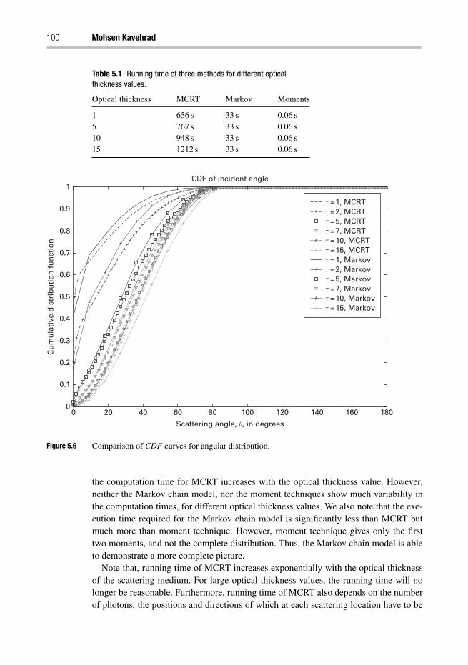
100 Mohsen Kavehrad
Table 5.1 Running time of three methods for different opticalthickness values.
Optical thickness MCRT Markov Moments
1 656 s 33 s 0.06 s5 767 s 33 s 0.06 s10 948 s 33 s 0.06 s15 1212 s 33 s 0.06 s
60402000
0.1
0.2
0.3
0.4
0.5
0.6
0.7
0.8
0.9
1
80
Scattering angle, θ, in degrees
CDF of incident angle
Cu
mu
lati
ve d
istr
ibu
tio
n f
un
ctio
n
100 120 140 160
τ =1, MCRTτ =2, MCRTτ =5, MCRTτ =7, MCRTτ =10, MCRTτ =15, MCRTτ =1, Markovτ =2, Markovτ =5, Markovτ =7, Markovτ =10, Markovτ =15, Markov
180
Figure 5.6 Comparison of CDF curves for angular distribution.
the computation time for MCRT increases with the optical thickness value. However,neither the Markov chain model, nor the moment techniques show much variability inthe computation times, for different optical thickness values. We also note that the exe-cution time required for the Markov chain model is significantly less than MCRT butmuch more than moment technique. However, moment technique gives only the firsttwo moments, and not the complete distribution. Thus, the Markov chain model is ableto demonstrate a more complete picture.
Note that, running time of MCRT increases exponentially with the optical thicknessof the scattering medium. For large optical thickness values, the running time will nolonger be reasonable. Furthermore, running time of MCRT also depends on the numberof photons, the positions and directions of which at each scattering location have to be
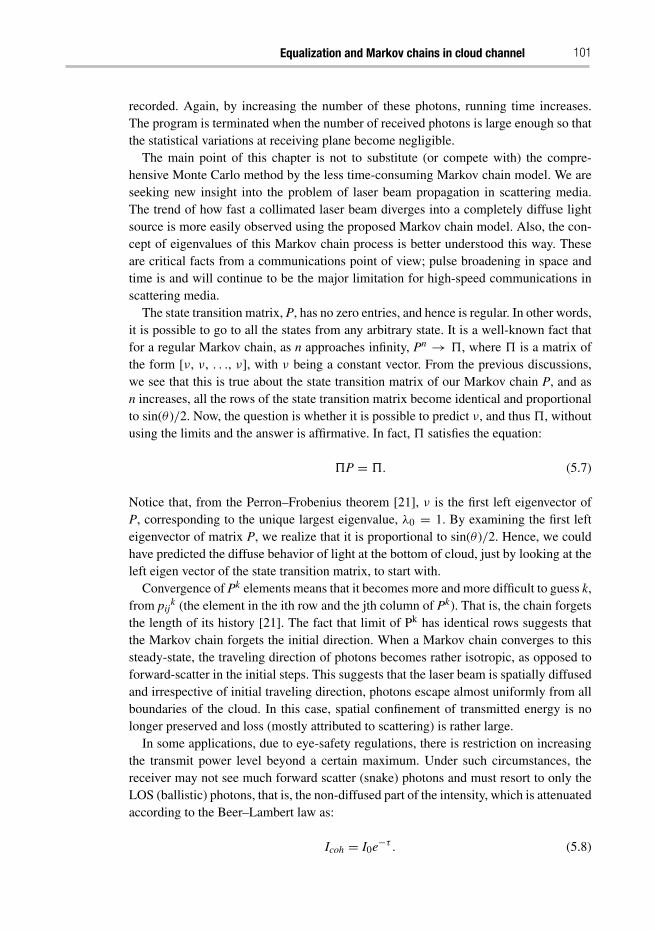
Equalization and Markov chains in cloud channel 101
recorded. Again, by increasing the number of these photons, running time increases.The program is terminated when the number of received photons is large enough so thatthe statistical variations at receiving plane become negligible.
The main point of this chapter is not to substitute (or compete with) the compre-hensive Monte Carlo method by the less time-consuming Markov chain model. We areseeking new insight into the problem of laser beam propagation in scattering media.The trend of how fast a collimated laser beam diverges into a completely diffuse lightsource is more easily observed using the proposed Markov chain model. Also, the con-cept of eigenvalues of this Markov chain process is better understood this way. Theseare critical facts from a communications point of view; pulse broadening in space andtime is and will continue to be the major limitation for high-speed communications inscattering media.
The state transition matrix, P, has no zero entries, and hence is regular. In other words,it is possible to go to all the states from any arbitrary state. It is a well-known fact thatfor a regular Markov chain, as n approaches infinity, Pn → �, where � is a matrix ofthe form [ν, ν, . . ., ν], with ν being a constant vector. From the previous discussions,we see that this is true about the state transition matrix of our Markov chain P, and asn increases, all the rows of the state transition matrix become identical and proportionalto sin(θ )/2. Now, the question is whether it is possible to predict ν, and thus �, withoutusing the limits and the answer is affirmative. In fact, � satisfies the equation:
�P = �. (5.7)
Notice that, from the Perron–Frobenius theorem [21], ν is the first left eigenvector ofP, corresponding to the unique largest eigenvalue, λ0 = 1. By examining the first lefteigenvector of matrix P, we realize that it is proportional to sin(θ )/2. Hence, we couldhave predicted the diffuse behavior of light at the bottom of cloud, just by looking at theleft eigen vector of the state transition matrix, to start with.
Convergence of Pk elements means that it becomes more and more difficult to guess k,from pij
k (the element in the ith row and the jth column of Pk). That is, the chain forgetsthe length of its history [21]. The fact that limit of Pk has identical rows suggests thatthe Markov chain forgets the initial direction. When a Markov chain converges to thissteady-state, the traveling direction of photons becomes rather isotropic, as opposed toforward-scatter in the initial steps. This suggests that the laser beam is spatially diffusedand irrespective of initial traveling direction, photons escape almost uniformly from allboundaries of the cloud. In this case, spatial confinement of transmitted energy is nolonger preserved and loss (mostly attributed to scattering) is rather large.
In some applications, due to eye-safety regulations, there is restriction on increasingthe transmit power level beyond a certain maximum. Under such circumstances, thereceiver may not see much forward scatter (snake) photons and must resort to only theLOS (ballistic) photons, that is, the non-diffused part of the intensity, which is attenuatedaccording to the Beer–Lambert law as:
Icoh = I0e−τ . (5.8)
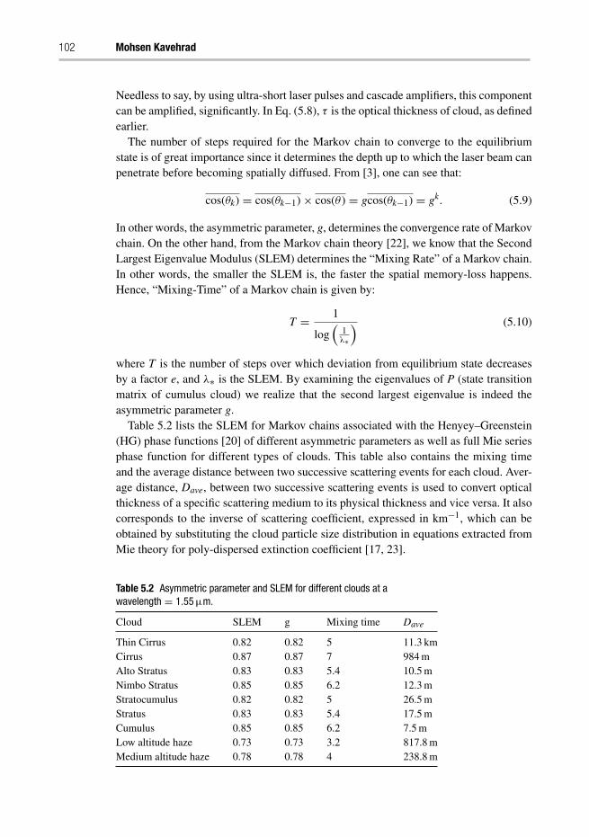
102 Mohsen Kavehrad
Needless to say, by using ultra-short laser pulses and cascade amplifiers, this componentcan be amplified, significantly. In Eq. (5.8), τ is the optical thickness of cloud, as definedearlier.
The number of steps required for the Markov chain to converge to the equilibriumstate is of great importance since it determines the depth up to which the laser beam canpenetrate before becoming spatially diffused. From [3], one can see that:
cos(θk) = cos(θk−1)× cos(θ ) = gcos(θk−1) = gk. (5.9)
In other words, the asymmetric parameter, g, determines the convergence rate of Markovchain. On the other hand, from the Markov chain theory [22], we know that the SecondLargest Eigenvalue Modulus (SLEM) determines the “Mixing Rate” of a Markov chain.In other words, the smaller the SLEM is, the faster the spatial memory-loss happens.Hence, “Mixing-Time” of a Markov chain is given by:
T = 1
log(
1λ∗
) (5.10)
where T is the number of steps over which deviation from equilibrium state decreasesby a factor e, and λ∗ is the SLEM. By examining the eigenvalues of P (state transitionmatrix of cumulus cloud) we realize that the second largest eigenvalue is indeed theasymmetric parameter g.
Table 5.2 lists the SLEM for Markov chains associated with the Henyey–Greenstein(HG) phase functions [20] of different asymmetric parameters as well as full Mie seriesphase function for different types of clouds. This table also contains the mixing timeand the average distance between two successive scattering events for each cloud. Aver-age distance, Dave, between two successive scattering events is used to convert opticalthickness of a specific scattering medium to its physical thickness and vice versa. It alsocorresponds to the inverse of scattering coefficient, expressed in km−1, which can beobtained by substituting the cloud particle size distribution in equations extracted fromMie theory for poly-dispersed extinction coefficient [17, 23].
Table 5.2 Asymmetric parameter and SLEM for different clouds at awavelength = 1.55 μm.
Cloud SLEM g Mixing time Dave
Thin Cirrus 0.82 0.82 5 11.3 kmCirrus 0.87 0.87 7 984 mAlto Stratus 0.83 0.83 5.4 10.5 mNimbo Stratus 0.85 0.85 6.2 12.3 mStratocumulus 0.82 0.82 5 26.5 mStratus 0.83 0.83 5.4 17.5 mCumulus 0.85 0.85 6.2 7.5 mLow altitude haze 0.73 0.73 3.2 817.8 mMedium altitude haze 0.78 0.78 4 238.8 m
Equalization and Markov chains in cloud channel 103
From Table 5.2 we see that the second largest eigenvalue is equal to g for all of thesephase functions. That is why asymmetric parameter is important in calculating themoments of multiple scattering and channel parameters [6, 8]. Since angular, spatial,and temporal distributions of energy are interrelated, isotropic angular distribution sug-gests that spatial distribution in transverse coordinates (x and y directions) is Gaussian.Furthermore, spatial memory-loss of Markov chain associated with angular distribu-tion after several scattering events implies that the entire Monte Carlo Markov chain(MCMC) has converged to the equilibrium state. This suggests that the pulse is so broad-ened in space and time that use of equalization on the pulse might be difficult, unlessthere is no constraint on the optical transmitted peak power level.
Examining the parameters of Table 5.2, we realize that mixing time is rather shortfor clouds and haze and a large link margin is necessary, in order to have reliablecommunications through clouds of optical thickness values much larger than 10 to 15.However, this rather small optical thickness value may translate into a long physicalthickness for clouds such as thin Cirrus due to the long average distance between twosuccessive scatterings for these clouds [17]. Note that, all the results presented in thischapter assume a homogeneous body of clouds. In reality, as a waveform moves throughclouds, the dynamics are far more rapidly varying. Hence, the predictions in this sectionare on the conservative side.
5.4 Equalization related issues
A cloudy or foggy optical channel is usually characterized by severe intersymbol inter-ference (ISI) at high data rates, due to multi-scattering. In Section 5.3, we investigatedthe feasibility of high data rate FSO transmission through a cloud channel. Results sug-gest that beyond a certain cloud thickness, pulses are broadened in space and timeto the extent that use of equalization to counter intersymbol interference (ISI) mightbe difficult. In this section, we will try to examine the level of challenge and seekways of countering the severe channel ISI by various equalization techniques. The sub-ject has been of research interest for some time now [24–29]. As it should be clear,unlike RF communications where spectrum is costly and scarce, the availability of widebandwidth light beams enable reliable wireless communications at very high data rateswith enhanced security via direct beams. One way to enhance the link performance inISI is through linear minimum mean-squared error (LMMSE) equalization or throughdecision-feedback equalization (DFE).
In this section, as an alternative, we propose an FSO system for through-cloud com-munications consisting of a channel shortening equalizer (CSE) [30–32] followed bya Viterbi equalizer [33]. Time-domain equalization (TEQ) was originally proposed toreduce the length of the discrete channel impulse response (CIR) in channels suchas digital subscriber loop (DSL) or cable. In FSO through clouds, in the same sense,use of TEQ can be justified in the context of heavy scattering dispersion. The ensuingMaximum-likelihood sequential detection (MLSD) scheme is known to be the optimalequalization algorithm, compared with linear minimum mean-squared error (LMMSE)
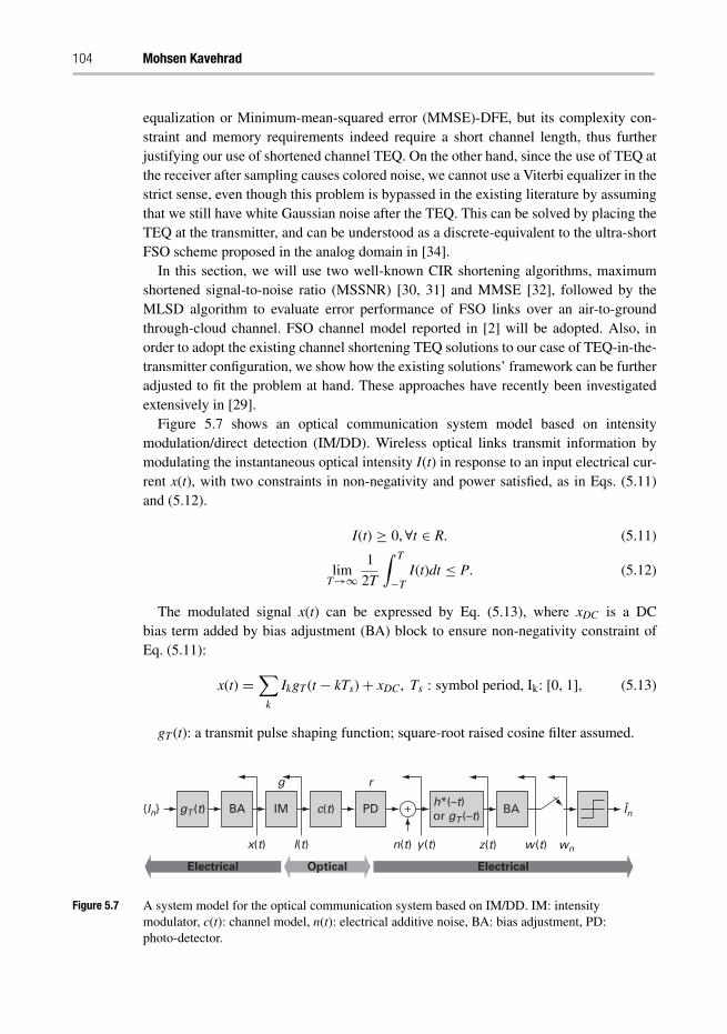
104 Mohsen Kavehrad
equalization or Minimum-mean-squared error (MMSE)-DFE, but its complexity con-straint and memory requirements indeed require a short channel length, thus furtherjustifying our use of shortened channel TEQ. On the other hand, since the use of TEQ atthe receiver after sampling causes colored noise, we cannot use a Viterbi equalizer in thestrict sense, even though this problem is bypassed in the existing literature by assumingthat we still have white Gaussian noise after the TEQ. This can be solved by placing theTEQ at the transmitter, and can be understood as a discrete-equivalent to the ultra-shortFSO scheme proposed in the analog domain in [34].
In this section, we will use two well-known CIR shortening algorithms, maximumshortened signal-to-noise ratio (MSSNR) [30, 31] and MMSE [32], followed by theMLSD algorithm to evaluate error performance of FSO links over an air-to-groundthrough-cloud channel. FSO channel model reported in [2] will be adopted. Also, inorder to adopt the existing channel shortening TEQ solutions to our case of TEQ-in-the-transmitter configuration, we show how the existing solutions’ framework can be furtheradjusted to fit the problem at hand. These approaches have recently been investigatedextensively in [29].
Figure 5.7 shows an optical communication system model based on intensitymodulation/direct detection (IM/DD). Wireless optical links transmit information bymodulating the instantaneous optical intensity I(t) in response to an input electrical cur-rent x(t), with two constraints in non-negativity and power satisfied, as in Eqs. (5.11)and (5.12).
I(t) ≥ 0, ∀t ∈ R. (5.11)
limT→∞
1
2T
∫ T
−TI(t)dt ≤ P. (5.12)
The modulated signal x(t) can be expressed by Eq. (5.13), where xDC is a DCbias term added by bias adjustment (BA) block to ensure non-negativity constraint ofEq. (5.11):
x(t) =∑
k
IkgT (t − kTs)+ xDC, Ts : symbol period, Ik: [0, 1], (5.13)
gT (t): a transmit pulse shaping function; square-root raised cosine filter assumed.
Electrical Optical Electrical
h*(–t)or gT (–t)
BA
x(t) n(t) y(t) z(t) w(t) wnI(t)
gT (t){In} ÎnIM PD BAc(t)
r
+
g
Figure 5.7 A system model for the optical communication system based on IM/DD. IM: intensitymodulator, c(t): channel model, n(t): electrical additive noise, BA: bias adjustment, PD:photo-detector.
Equalization and Markov chains in cloud channel 105
Denoting the optical gain of electrical-optical conversion by g, the optical intensitymodulated signal can be represented by Eq. (5.14):
I(t) = gx(t). (5.14)
Referring to the impulse response due to multi-scattering by c(t), the received signal atthe receiver front end after photo-detection can be represented by a baseband electricalmodel as in Eq. (5.15). In our notations, for simplicity, we will assume rg = 1.
y(t) = rI(t)⊗ c(t)+ n(t) = r g x(t)⊗ c(t)+ n(t),
r: photo-detector sensitivity, [A · m2/W], n(t): AWGN.(5.15)
Finally, using a receive filter gR(t) = gT (t), y(t) is filtered to z(t) = y(t) ⊗ gR(t). Thez(t) can be mathematically derived in further detail as in Eq. (5.16), using definitionsof Eqs. (5.17), (5.18), and (5.19). Alternatively, the equivalent discrete-time impulseresponse can be expressed by Eq. (5.20), yielding Eq. (5.21).
z(t) = y(t)⊗ gR(t) = [x(t)⊗ c(t)+ n(t)]⊗ gR(t) =∑
k
Ikf (t − kTs)+ α xDC + v(t).
(5.16)
f (t) = gT (t)⊗ c(t)⊗ gR(t). (5.17)
α =∫
(c(t)⊗ gR(t)) dt. (5.18)
v(t) = n(t)⊗ gR(t). (5.19)
fk = f (t −�)∣∣t=kTs
, � : synchronization delay. (5.20)
zn =∑
k
Ikfn−k + α xDC + vn. (5.21)
Most of the existing DSP techniques such as equalization depend on the autocorre-lation property of transmitted symbols. In case of an OOK modulation which does notsatisfy Eq. (5.22), one good way is to adjust the DC at the receiver.
E(InIm) ={
0, n �= mσ 2
I , n = m
}, In, Im: transmit symbols. (5.22)
At the receiver, the BA block can first work on Eq. (5.21) to remove the DC term α xDC.Furthermore, assuming a frame-by-frame transmission of frame length FR (>> L), andthe finite-length discrete-time channel fk, k = 0 . . . L, one can further adjust the DClevel. In Eq. (5.23), the transmit symbol constellation is changed from [0, 1] to [1/2,−1/2]. However, for some portions of the received frame,
∑m2m1
fkIavg is time-varying.Thus, the frame structure needs a preamble longer than L + 1 and a post-amble longerthan L. One point to note is that Iavg in Eq. (5.23) was used as a part of the detectionscheme with channel state information at the receiver (CSIR) assumed, whereas the DCterm xDC in Eq. (5.16) was used to ensure non-negativity condition at the transmitter.
un =m2∑
k=m1
fkIn−k −m2∑
k=m1
fkIavg + vn =m2∑
k=m1
fk(In−k − Iavg)+ vn =m2∑
k=m1
fkDn−k + vn
(5.23)
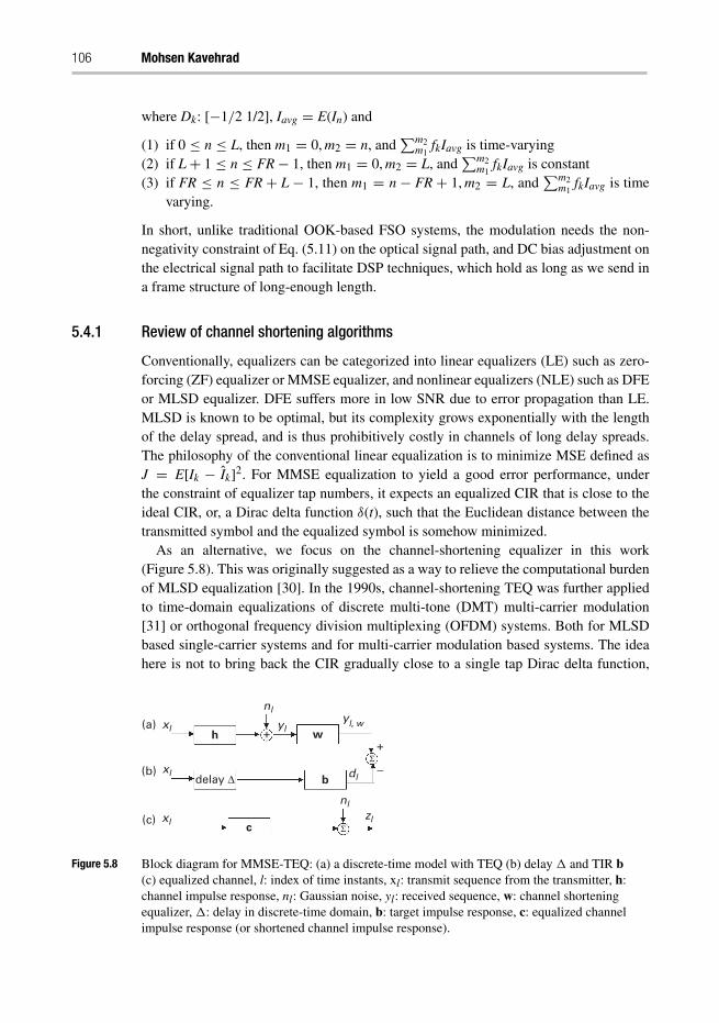
106 Mohsen Kavehrad
where Dk: [−1/2 1/2], Iavg = E(In) and
(1) if 0 ≤ n ≤ L, then m1 = 0, m2 = n, and∑m2
m1fkIavg is time-varying
(2) if L+ 1 ≤ n ≤ FR− 1, then m1 = 0, m2 = L, and∑m2
m1fkIavg is constant
(3) if FR ≤ n ≤ FR + L − 1, then m1 = n − FR + 1, m2 = L, and∑m2
m1fkIavg is time
varying.
In short, unlike traditional OOK-based FSO systems, the modulation needs the non-negativity constraint of Eq. (5.11) on the optical signal path, and DC bias adjustment onthe electrical signal path to facilitate DSP techniques, which hold as long as we send ina frame structure of long-enough length.
5.4.1 Review of channel shortening algorithms
Conventionally, equalizers can be categorized into linear equalizers (LE) such as zero-forcing (ZF) equalizer or MMSE equalizer, and nonlinear equalizers (NLE) such as DFEor MLSD equalizer. DFE suffers more in low SNR due to error propagation than LE.MLSD is known to be optimal, but its complexity grows exponentially with the lengthof the delay spread, and is thus prohibitively costly in channels of long delay spreads.The philosophy of the conventional linear equalization is to minimize MSE defined asJ = E[Ik − Ik]2. For MMSE equalization to yield a good error performance, underthe constraint of equalizer tap numbers, it expects an equalized CIR that is close to theideal CIR, or, a Dirac delta function δ(t), such that the Euclidean distance between thetransmitted symbol and the equalized symbol is somehow minimized.
As an alternative, we focus on the channel-shortening equalizer in this work(Figure 5.8). This was originally suggested as a way to relieve the computational burdenof MLSD equalization [30]. In the 1990s, channel-shortening TEQ was further appliedto time-domain equalizations of discrete multi-tone (DMT) multi-carrier modulation[31] or orthogonal frequency division multiplexing (OFDM) systems. Both for MLSDbased single-carrier systems and for multi-carrier modulation based systems. The ideahere is not to bring back the CIR gradually close to a single tap Dirac delta function,
(a)
delay Δ
xl
nl
nl
yl, wyl
dl
zl
xl
xl
(b)
(c)c
h w+
+
Σ
Σ
−b
Figure 5.8 Block diagram for MMSE-TEQ: (a) a discrete-time model with TEQ (b) delay � and TIR b(c) equalized channel, l: index of time instants, xl: transmit sequence from the transmitter, h:channel impulse response, nl: Gaussian noise, yl: received sequence, w: channel shorteningequalizer, �: delay in discrete-time domain, b: target impulse response, c: equalized channelimpulse response (or shortened channel impulse response).
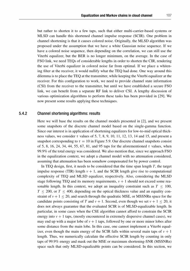
Equalization and Markov chains in cloud channel 107
but rather to shorten it to a few taps, such that either multi-carrier-based systems orMLSD can handle this shortened channel impulse response (SCIR). One problem inchannel shortening is that it causes colored noise. Originally, the MLSD algorithm wasproposed under the assumption that we have a white Gaussian noise sequence. If wehave a colored noise sequence, then depending on the correlation, we can still use theViterbi equalizer, but the BER is no longer minimum, on the average. In the case ofFSO link, we need TEQs of considerable lengths in order to shorten the CIR, renderingthe use of Viterbi equalizer in colored noise far from optimal. If we place a whiten-ing filter at the receiver, it would nullify what the TEQ had done. One way around thisdilemma is to place the TEQ at the transmitter, while keeping the Viterbi equalizer at thereceiver. For this configuration to work, we need to provide channel state information(CSI) from the receiver to the transmitter, but until we have established a secure FSOlink, we can benefit from a separate RF link to deliver CSI. A lengthy discussion ofvarious optimization algorithms to perform these tasks has been provided in [29]. Wenow present some results applying these techniques.
5.4.2 Channel shortening algorithms: results
Here we will base the results on the channel models presented in [2], and we presentsome snapshots of the discrete channel model based on the single-gamma function.Since our interest is in application of shortening equalizers for low-to-mid optical thick-ness values, we consider τ values of 5, 7, 8, 9, 10, 11, 12, 13, 14 and 15, and present asnapshot corresponding to τ = 10 in Figure 5.9. Our discrete channel snapshots consistof 5, 8, 16, 24, 34, 44, 55, 67, 81, and 95 taps for the aforementioned τ values, when99.9% of the total energy was considered. We also mention that, since we approach FSOin the equalization context, we adopt a channel model with no attenuation considered,assuming that attenuation has been somehow compensated for by power control.
In TEQ design, first, it needs to be considered that the time span length T , the targetimpulse response (TIR) length v + 1, and the SCIR length give rise to computationalcomplexity of TEQ and MLSD equalizer, respectively. Also, considering the MLSDstage following TEQ and its memory requirements, v + 1 should not exceed some rea-sonable length. In this context, we adopt an inequality constraint such as T ≤ 100,T ≤ 200, or T ≤ 400, depending on the optical thickness value and an equality con-straint of v+ 1 ≤ 20, and search through the quadratic MSE, or MSSNRn space for thecandidate points consisting of T and v + 1. Second, even though we set v + 1 ≤ 20, itdoes not always guarantee that the evaluated SCIR is of MLSD-equalizable length. Inparticular, in some cases when the CSE algorithm cannot afford to constrain the SCIRenergy into v+ 1 taps, (mostly encountered in extremely dispersive channel cases), wemay end up with a major lobe of v+ 1 taps, followed by one or more minor lobes aftersome distance from the main lobe. In this case, one cannot implement a Viterbi equal-izer, even though the main energy of the SCIR falls within several main taps of v + 1length. Thus, we numerically calculate the effective SCIR length by counting in onlytaps of 99.9% energy and mask out the MSE or maximum shortening-SNR (MSSNRn)space such that only MLSD-equalizable points can be considered. In this section, we
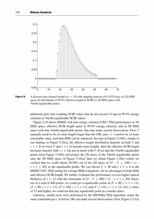
108 Mohsen Kavehrad
10 20 30 40 50 60 700–0.05
0
0.05
0.1
0.15
0.2
0.25
0.3
Figure 5.9 A discrete-time channel model at τ = 10 with sampling interval of 0.18751 nsec (a) 3D MSEspace (b) distribution of 99.9% effective length of SCIR (c) 3D MSE space withViterbi-equalizable points.
arbitrarily pick only resulting SCIR values that do not exceed 14 taps in 99.9% energycriterion as Viterbi-equalizable SCIR values.
Figure 5.10 shows MMSE with unit energy criterion (UEC) TEQ performance in 3DMSE space, effective SCIR length space in 99.9% energy criterion, and in 3D MSEspace with only Viterbi-equalizable points. One may make several observations. First, Tnaturally needs to be of some length longer than the CIR, and v+ 1 need to be of somereasonable value, such that MSE can be enhanced. Second, in Figure 5.10(b), similar toour findings in Figure 5.10(a), the effective length distribution depends on both T andv + 1. If we have T and v + 1 of beyond some lengths, then the effective SCIR lengthincreases linearly with v+ 1, but not as much with T . If we take the Viterbi-equalizablepoints from Figure 5.10(b) and project the 2D space of the Viterbi-equalizable pointsonto the 3D MSE space of Figure 5.10(a), then we obtain Figure 5.10(c) where weverified that we could obtain 38.50% out of the 2D space of {T : T ≤ 100} ∩ {v :v + 1 ≤ 20}, as the equalizable points. We can choose T = 80 and v + 1 = 6 as theMMSE-UEC-TEQ setting for average BER evaluations, for its advantages in both MSEand effective SCIR length. We further evaluated the performance at even higher opticalthickness of τ = 12 with the constraints of {T : T ≤ 200} ∩ {v : v + 1 ≤ 20} where,out of a total of 400 points, we could get 4 equalizable points at (T = 80, v+ 1 = 11),(T = 90, v+ 1 = 11), (T = 100, v+ 1 = 11), and (T = 110, v+ 1 = 11). For τ valuesof 13 and higher, we could not find any equalizable point in a similar space.
Likewise, similar tests were performed by the MSSNRn-TEQ algorithm, under thesame constraints per τ as before. We can make several observations. First, Figure 5.11(a)
Equalization and Markov chains in cloud channel 109
Length of TIR
5 10 15 20
20 20
100
100
120
80
80
60
60
40
40Eff
ecti
ve le
ng
th o
f S
CIR
Length of TEQ
510 15
20
20
−20
10080
−80 60
−6040
−40
Length of TIR
MS
E w
ith
eff
len
con
sid
ered
[d
B]
Length of TEQ
Length of TIR
5 10 15 10080
−80 6040
−40
−60 20
20
−20
Length of TEQ
MS
E [
dB
]
(a) (b)
(c)
Figure 5.10 MMSE-UEC TEQ, τ = 10, SNR = 30 dB, T ≤ 100, ν + 1 ≤ 20. (a) 3D SSNR space(b) Distribution of 99.9% effective length of SCIR (c) 3D SSNRn space withViterbi-equalizable points.
shows that the 3D SSNRn space shows dependence on both T and v + 1. Second,Figure 5.11(a) shows that, to some extent, complexity in terms of T and v + 1 areexchangeable, although the TEQ’s complexity is linear with T whereas the Viterbi equal-ization’s complexity grows exponentially with v+ 1 in true sense. However, in so far aswe employ TEQ of enough length and aim at SCIR of beyond a certain length, MSSNRspace shows a flat response. Third, Figure 5.11(b) shows that in so far as T and v+1 arelarger than some values, SCIR’s effective length grows linearly with v+ 1 as expected,but almost independent of T . Fourth, Figure 5.11(c) shows that out of the total of 200points, we obtained 50.3% Viterbi-equalizable points. We chose T = 100 and v+1 = 15as the point for BER evaluation.
At even more dispersive channel with τ = 15, out of a total space of 400 points in{T : T ≤ 200}∩ {v : v+1 ≤ 20}, we could obtain 67 equalizable points confined within{T : 105 ≤ T ≤ 200} ∩ {v : 8 ≤ v + 1 ≤ 14}. At τ = 20, however, out of 400 pointsin {T : T ≤ 400} ∩ {v : v + 1 ≤ 20}, we could not find any equalizable point by theMSSNRn algorithm. To summarize, we can make several observations by consideringFigure 5.10 and Figure 5.11. We can use both MMSE-UEC and the MSSNRn algorithms
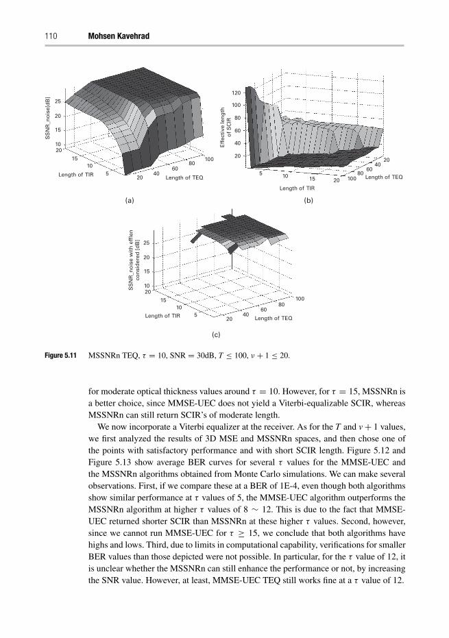
110 Mohsen Kavehrad
(a) (b)
(c)
Length of TIR
Length of TEQ
Eff
ecti
ve le
ng
tho
f S
CIR
5 10 15
40
40
60
60
80
80
100
100
120
2020
20
Length of TEQLength of TIR
SS
NR
_no
ise
wit
h e
ffle
nco
nsi
der
ed [
dB
]
510
10
15
15
6080
100
40
20
20
20
25
Length of TEQLength of TIR 5
10
10
15
15
20
6080
100
4020
20
25
SS
NR
_no
ise[
dB
]
Figure 5.11 MSSNRn TEQ, τ = 10, SNR = 30dB, T ≤ 100, ν + 1 ≤ 20.
for moderate optical thickness values around τ = 10. However, for τ = 15, MSSNRn isa better choice, since MMSE-UEC does not yield a Viterbi-equalizable SCIR, whereasMSSNRn can still return SCIR’s of moderate length.
We now incorporate a Viterbi equalizer at the receiver. As for the T and v+ 1 values,we first analyzed the results of 3D MSE and MSSNRn spaces, and then chose one ofthe points with satisfactory performance and with short SCIR length. Figure 5.12 andFigure 5.13 show average BER curves for several τ values for the MMSE-UEC andthe MSSNRn algorithms obtained from Monte Carlo simulations. We can make severalobservations. First, if we compare these at a BER of 1E-4, even though both algorithmsshow similar performance at τ values of 5, the MMSE-UEC algorithm outperforms theMSSNRn algorithm at higher τ values of 8 ∼ 12. This is due to the fact that MMSE-UEC returned shorter SCIR than MSSNRn at these higher τ values. Second, however,since we cannot run MMSE-UEC for τ ≥ 15, we conclude that both algorithms havehighs and lows. Third, due to limits in computational capability, verifications for smallerBER values than those depicted were not possible. In particular, for the τ value of 12, itis unclear whether the MSSNRn can still enhance the performance or not, by increasingthe SNR value. However, at least, MMSE-UEC TEQ still works fine at a τ value of 12.
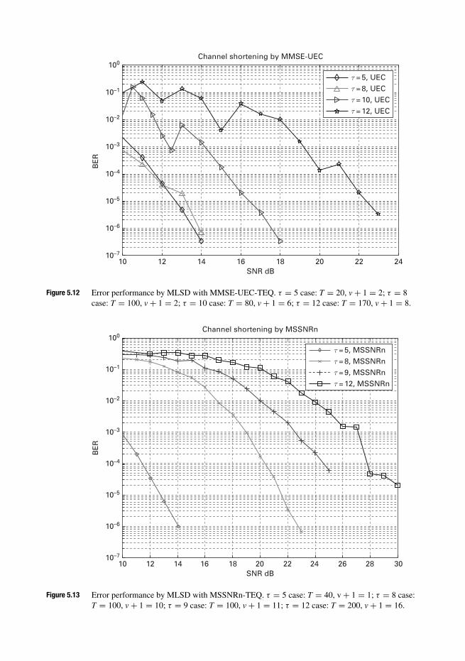
1010–7
10–6
10–5
10–4
BE
R
10–3
10–2
10–1
100
12 14 16SNR dB
Channel shortening by MMSE-UEC
18 20 22 24
τ = 5, UECτ = 8, UECτ = 10, UECτ = 12, UEC
Figure 5.12 Error performance by MLSD with MMSE-UEC-TEQ. τ = 5 case: T = 20, v+ 1 = 2; τ = 8case: T = 100, v+ 1 = 2; τ = 10 case: T = 80, v+ 1 = 6; τ = 12 case: T = 170, v+ 1 = 8.
1010–7
10–6
10–5
10–4
BE
R
10–3
10–2
10–1
100
12 14 16SNR dB
Channel shortening by MSSNRn
18 20 22 24 26 28 30
τ = 5, MSSNRnτ = 8, MSSNRnτ = 9, MSSNRnτ = 12, MSSNRn
Figure 5.13 Error performance by MLSD with MSSNRn-TEQ. τ = 5 case: T = 40, v+ 1 = 1; τ = 8 case:T = 100, v+ 1 = 10; τ = 9 case: T = 100, v+ 1 = 11; τ = 12 case: T = 200, v+ 1 = 16.
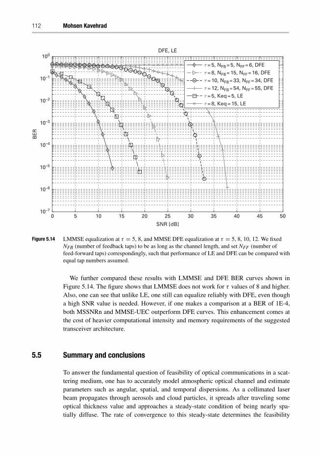
112 Mohsen Kavehrad
0 5 10 15 20 25
SNR [dB]
30 35 40 45 5010–7
10–6
10–5
10–4
BE
R
10–3
10–2
10–1
100DFE, LE
τ = 5, NFB= 5, NFF= 6, DFEτ = 8, NFB= 15, NFF= 16, DFEτ = 10, NFB= 33, NFF= 34, DFEτ = 12, NFB= 54, NFF= 55, DFEτ = 5, Keq = 5, LEτ = 8, Keq = 15, LE
Figure 5.14 LMMSE equalization at τ = 5, 8, and MMSE DFE equalization at τ = 5, 8, 10, 12. We fixedNFB (number of feedback taps) to be as long as the channel length, and set NFF (number offeed-forward taps) correspondingly, such that performance of LE and DFE can be compared withequal tap numbers assumed.
We further compared these results with LMMSE and DFE BER curves shown inFigure 5.14. The figure shows that LMMSE does not work for τ values of 8 and higher.Also, one can see that unlike LE, one still can equalize reliably with DFE, even thougha high SNR value is needed. However, if one makes a comparison at a BER of 1E-4,both MSSNRn and MMSE-UEC outperform DFE curves. This enhancement comes atthe cost of heavier computational intensity and memory requirements of the suggestedtransceiver architecture.
5.5 Summary and conclusions
To answer the fundamental question of feasibility of optical communications in a scat-tering medium, one has to accurately model atmospheric optical channel and estimateparameters such as angular, spatial, and temporal dispersions. As a collimated laserbeam propagates through aerosols and cloud particles, it spreads after traveling someoptical thickness value and approaches a steady-state condition of being nearly spa-tially diffuse. The rate of convergence to this steady-state determines the feasibility
Equalization and Markov chains in cloud channel 113
of communications through various types of clouds and aerosols with different opticalthickness values. Average distance between two successive scattering events is used toconvert optical thickness of a specific scattering medium into its physical thickness andvice versa.
By directly applying the Markov chain model to angular distribution evolution ofa laser beam in a scattering medium, and considering the fact that angular, spatial,and temporal distributions of energy are inter-related, the mixing rate of Monte-CarloMarkov Chain (MCMC) is found for different types of scattering media. Mixing time isintroduced as the number of steps over which deviation from equilibrium state decreasesby a factor e. This indicates the rate by which the energy distribution approaches beingspatially isotropic.
Examining parameters of Table 5.2, we realize that mixing time is rather short forclouds and haze. That is, when coherent light is traveling through clouds, its spatialcoherence rapidly degrades. However, it may take a much larger cloud length valuefor the coherence bandwidth of the medium to vanish. In the latter case, optical pulsesbroaden extensively in time and restoring them by signal processing might be difficult.
In this chapter, we also investigated the feasibility of applying TEQ combined withMLSD equalizer as a way to countermeasure severe channel ISI encountered in through-clouds FSO channels. We investigated the channel-shortening characteristics of twoTEQ designs, in terms of SSNRn and MSE versus TEQ length and TIR length. We alsoprovided end-to-end mathematical formulations showing feasibility of electrical equal-ization on the FSO link. By Monte Carlo simulations, we conclude that, for low-to-midrange optical thickness values, the suggested DSP techniques can work relatively wellto enhance BER performance. However, for mid-to-high range of optical thickness, wecannot rely solely on the TEQ, since the SCIR length distribution itself relies more onTIR length than on TEQ length.
Acknowledgment
A DARPA Grant sponsored by the US Air Force Research Laboratory/Wright-PattersonAFB Contract-FA8650-04-C-7114 and another DARPA Grant sponsored by the sameunder the Contract-FA8650-08-C-7850 and the Pennsylvania State University CICTRhave supported this research. The author of this book chapter is grateful and acknowl-edges the contributions of his former PhD Students whose dissertations have allcontributed to creating the knowledge embedded in this chapter. In particular worksof Drs. B. Hamzeh, S. Lee, B. Wu, Z. Hajjarian and J. Fadlullah are acknowledged withutmost respect.
References
[1] M. Kavehrad and B. Hamzeh, “Laser communication system using wavelet-based multi-rate signaling,” Proceedings of IEEE MILCOM, vol. 1, pp. 398–403, Monterey-California,November 2004.
114 Mohsen Kavehrad
[2] Z. Hajjarian, “MIMO optical communications and imaging through turbulent cloudyatmosphere,” PhD dissertation, Pennsylvania State University, September 2009.
[3] Z. Hajjarian, M. Kavehrad, and J. Fadlullah, “Analysis of wireless optical communicationsfeasibility in presence of clouds using Markov chains,” IEEE J. Sel. Areas Commun., vol.27, no. 9, December 2009.
[4] L. C. Andrews and R. L. Phillips, Laser Beam Propagation through Random Media, SPIEPress, second edition, 2005.
[5] E. A. Bucher and R. M. Lerner, “Experiments on light pulse communication and propa-gation through atmospheric clouds,” Appl. Opt. vol. 12, no. 10, pp. 2401–2414, October1973.
[6] E. A. Bucher, “Computer simulation of light pulse propagation for communication throughthick clouds,” Appl. Opt., vol. 12, no. 10, pp. 2391–2400. October 1973.
[7] N. S. Kopeika and J. Bordogna, “Background noise in optical communication systems,”Proc. IEEE, vol. 58, no. 10, pp. 1571–1577, October 1970.
[8] R. F. Lutomirski, A. P. Ciervo, and G. J. Hall, “Moments of multiple scattering,” Appl. Opt.,vol. 34, no. 30, 7125–7136, October 1995.
[9] G. N. Plass and G. W. Kattawar, “Monte Carlo calculations of light scattering from clouds,”Appl. Opt., vol. 7, no. 3, pp. 415–419, March 1968.
[10] H. M. Gupta, “Space-time response of a cloud communication channel to an optical signal,”Opt. Quantum Electron., vol. 12, no. 6, pp 499–509, November 1980.
[11] S. Arnon, D. Sadot, and N. S. Kopeika, “Simple mathematical models for temporal, spa-tial, angular characteristics of light propagating through the atmosphere for space opticalcommunication: Monte Carlo simulations,” J. Mod. Opt., vol. 41, pp. 1955–1972, October1994.
[12] S. Arnon and N. S. Kopeika, “Free space optical communication: analysis of spatial widen-ing of optical pulses for propagation through clouds,” Opt. Eng., vol. 34, pp. 511–516,Febuary 1995.
[13] K. Riley, D. Ebert, M. Kraus, J. Tessendorf, and C. Hansen, “Efficient rendering ofatmospheric phenomena,” Proceedings of Eurographics Symposium on Rendering 2004,pp. 375–386, June 2004.
[14] F. G. Smith, The Infrared & Electro-optical Systems Handbook: Atmospheric Propagatingof Radiation, Vol. 2, SPIE PRESS, 1993.
[15] D. Deirmendjian, “Scattering and polarization properties of water clouds and hazes in thevisible and infrared,” Appl. Opt. vol. 3, no. 2, pp 187–196, February 1964.
[16] A. Sawetprawichkul, P. Hsu and K. Mitra, “Parallel computing of three-dimensional MonteCarlo simulation of transient radiative transfer in participating media,” American Instituteof Aeronautics and Astronautics, 8th AIAA/ASME Joint Thermophysics and Heat TransferConference, St. Louis, Missouri, June 2002.
[17] B. Y. Hamzeh, Multi-rate wireless optical communications in cloud obscured channels,Ph.D. Thesis, Pennsylvania State University, December 2005.
[18] T. Binzoni, T. S. Leung, A. H. Gandjbakhche, D. Rüfenacht, and D. T. Delpy, “The use ofthe Henyey-Greenstein phase function in Monte Carlo simulations in biomedical optics,”Phys. Med. Biol., vol. 51, no. 17, pp. N313–N322, Sepember 2006 .
[19] T. Binzoni, T. S. Leung, A. H. Gandjbakhche, D. Rüfenacht, D. T. Delpy, “Comment on‘The use of the Henyey-Greenstein phase function in Monte Carlo simulations in biomedicaloptics’,” Phys. Med. Biol., vol. 51, no. 22, pp. L39–L41(1), November 2006.
[20] L. Henyey and J. Greenstein, “Diffuse radiation in the galaxy,” Astrophys. Journal, vol. 93,pp. 70–83, 1941.
Equalization and Markov chains in cloud channel 115
[21] E. Behrends, Introduction to Markov Chains with Special Emphasis on Rapid Mixing,Friedrick Vieweg & Son, 2001.
[22] S. Boyd, P Diaconis, and L. Xiao, “Fastest mixing Markov chain on a graph,” SIAM Review,vol. 46, no. 4, pp. 667–689, December 2004.
[23] B. Wu, “Free-space optical communications through the scattering medium: analysis ofsignal characteristics,” Ph.D. Thesis, Pennsylvania State University, December 2007.
[24] M. Kavehrad, “A countermeasure to improve outage performance of interference-limitedmicrowave radio links,” Can. Elect. Comput. Eng. J., vol. 16, no. 1, pp. 13–18, January1991.
[25] M. Kavehrad, B. Y. Hamzeh, “Laser communication system using wavelet-based multi-ratesignaling,” Proceedings of IEEE MILCOM, Monterey California, November 2004.
[26] X. Zhu and J. M. Kahn, “Free-space optical communication through atmospheric turbulencechannels,” IEEE Trans. Comm., vol. 50, no. 8, pp. 1293–1300, August 2002.
[27] J. M. Kahn and X. Zhu, “Performance bounds for coded free-space optical communicationsthrough atmospheric turbulence channels,” IEEE Trans. Comm., vol. 51, no. 8, pp. 1233–1239, August 2003.
[28] H. Wu and M. Kavehrad, “Availability evaluation of ground-to-air hybrid FSO/RF links,”Int. J. Wireless Inf. Networks, vol. 14, no. 1, March 2007.
[29] S. Lee and M. Kavehrad, “Free-space optical communications with channel shortening filterand viterbi equalizer,” Int. J. Wireless Inf. Networks, vol. 16, no. 4, December 2009.
[30] P. J. W. Melsa, R. C. Younce, and C. E. Rohrs, “Impulse response shortening for discretemultitone transceivers,” IEEE Trans Comm, vol. 44, no. 12, pp. 1662–1672, December1996.
[31] R. Schur, J. Speidel, and R. Angerbauer, “Reduction of guard interval by impulse compres-sion for DMT modulation on twisted pair cables,” Proc. IEEE Global Telecom. Conf., vol. 3,pp. 1632–1636, 2000.
[32] M. V. Bladel and M. Moenceclay, “Time-domain equalization for multicarrier communica-tions,” Proc. IEEE Global Telecom. Conf., pp. 167–170, 1995.
[33] Forney, G., Jr., “Maximum-likelihood sequence estimation of digital sequences in the pres-ence of intersymbol interference,” IEEE Trans. Inform. Theory, vol. 18, no. 3, pp. 363–378,May 1972..
[34] B. Hamzeh and M. Kavehrad, “Multi-rate RZ Communications for Dispersive WirelessOptical Channels,” Proceedings of SPIE Defense and Security Conference, Orlando –Florida, April 2006.
6 Multiple-input multiple-outputtechniques for indoor optical wirelesscommunicationsSteve Hranilovic
The popular adage, “a picture is worth a thousand words” suggests that it is ofteneasier to convey a large amount of information in parallel by way of an image ratherthan by serial transmission of words. Indeed, this is the underlying inspiration for anew class of indoor optical wireless (OW) channels. In these channels data are con-veyed by coordinating the transmission of a series of transmitters and receivers. Socalled, multiple-input multiple-output (MIMO) OW systems employ a number of opticalsources as transmitters and a collection of photodiodes as receivers. The arrange-ment of emitters and detectors varies depending on application and implementationtechnology.
The use of MIMO techniques in radio channels is a long-standing topic of interest.It has been shown that by increasing the number of antennae in a radio system that adiversity gain can be achieved, i.e., an improvement in the reliability of the system canbe had. Alternatively, it has been demonstrated that multiple transmitting and receivingantennae can be used to provide a boost in rate, i.e. a multiplexing gain. In fact, a formaltrade-off between diversity and multiplexing gain in MIMO radio channels has beenestablished [1].
The OW MIMO systems discussed in this chapter differ fundamentally from earlierwork on radio channels. In particular, only indoor OW channels are considered here andare free of multipath fading. In addition, the signalling constraints imposed by intensity-modulated/direct-detection (IM/DD) systems limits the direct application of theory fromradio channels. Nonetheless, MIMO techniques have been applied to OW channels toyield improvements in reliability and to improve data rates. This chapter starts with abrief overview of the characteristics of indoor OW MIMO systems. Given that the appli-cation and available gains depend on channel architecture, the balance of the chapterconsiders the use of MIMO techniques in three main OW channel topologies: diffuse,spot-diffusing and point-to-point.
Advanced Optical Wireless Communication Systems, ed. Shlomi Arnon, John R. Barry, George K.Karagiannidis, Robert Schober, and Murat Uysal. Published by Cambridge University Press.c© Cambridge University Press 2012.
Optical multiple-input multiple-output systems 117
6.1 Indoor OW MIMO channel characteristics
6.1.1 Channel fundamentals
Optical wireless systems use optoelectronic components to convert signals frombaseband to transmission wavelengths. Lasers and light-emitting diodes (LEDs) aretypically used to convert an electrical current signal to a time-varying optical intensity.The transmitted signal of interest is an optical intensity which is the normalized powerin units of Watts per steradian. The receiver accepts emissions inside of its field-of-view(FOV) and outputs a current proportional to the impinging optical power. These typesof channels are termed intensity modulated/direct-detection (IM/DD) and are found in avast majority of OW systems.
The quantity of interest at the transmitter is the instantaneous intensity, I(t). Dataare imposed on the instantaneous emitted optical power x(t) which is the integrationof I(t) over the solid angle of the transmitter. At the receiver, a current y(t) is outputin proportion to the power on the detector surface. The received power is simply theintegration of the irradiance, in Watts per area, over the detector surface.
The IM/DD channel imposes two primary constraints on all emitted signals. Sincex(t) represents a power it must be nonnegative, i.e.,
x(t) ≥ 0. (6.1)
International bodies impose safety limits on the permissible peak and average opticalpower to ensure skin and eye-safety. For modulated laser sources faster than 55 kHz,in most cases the average optical power constraint dominates the peak constraint [2]. Acareful study of the eye-safety of many commercial OW devices can be found in [3]. Asa result, a limit on the average emitted optical power must also be imposed for safetyreasons, i.e.,
limu→∞
1
2u
∫ u
−ux(t) dt ≤ P (6.2)
where P is eye-safety limitation of average optical power. These channel constraintsmust be considered in all signalling design for IM/DD OW systems.
The dominant source of noise in indoor OW systems is due to ambient lighting fromfluorescent and incandescent sources. These devices produce emissions into the infraredwhich are quite detrimental to OW communications [4]. Fluorescent sources are modu-lated at tens to hundreds of kilohertz and have significant powers in the near-infraredband [5]. In addition, rooms with windows may allow sunlight to enter and furthercorrupt OW signalling. A conventional assumption is that the ambient light is of highintensity. This induces a Poisson shot noise with a large mean, which is well modeledby a Gaussian distribution [6]. As a result, in most indoor OW communication studiesthe noise is modeled as white, signal-independent, and Gaussian distributed [5].
6.1.2 Multiple transmitters
In indoor OW MIMO configurations, the arrangement of optical emitters into a singletransmitter is an important feature. A straightforward method is to use a series of discrete
118 Steve Hranilovic
emitters to produce a time-varying optical intensity distribution in space. There aremany options for this role including the use of vertical-cavity surface emitted lasers(VCSELs). In the area of optical interconnect, a 540-element array with 1080 VCSELswas built with a data rate of over 200 Mbps per pixel [7]. Specifically for OW com-munications, an array of integrated transceivers was constructed with a data rate of155 Mbps per element using specially designed LEDs bonded directly to underlyingCMOS drivers [8]. Recent studies have even investigated the integration of radio andoptical transceivers together [9]. A nice overview of challenges in OW transceiver designcan be found in [10].
If a large number of elements are required in close proximity, a spatial-light modula-tor (SLM) can be employed. In general terms, an SLM is able to produce a time-varyingoptical intensity image. An example of such a device is a liquid-crystal display whichcan have millions of emitters, however, each can be addressed at rates on the orderof 100 Hz. Recent, micro-electrical-mechanical systems (MEMS) known as digitalmicro-mirror devices (DMD) integrate arrays of turnable mirrors with appropriate driveelectronics. Commercially available DMD devices used in high-definition displays andprojection equipment is capable of high-resolution output at switching periods as smallas 8-16 μsec [11, DLP R© HDTV].
6.1.3 Receiver architectures
A key disadvantage of single-element OW receivers is that they are unable to rejectmultipath or ambient light interference. All signals in the FOV of a single element OWreceiver are integrated over the surface of the detector. This is a key disadvantage ofusing such a receiver arrangement, however, single element receivers are inexpensive toimplement.
Multiple element receivers have the advantage of sampling the spatial profile of thereceived optical intensity and rejecting portions which are corrupted by large amountsof interference. There are several options to implement such a receiver. One possibilityis to use a series of discrete receivers and their optics and to orient them in differentdirections. These architectures are termed angle diversity receivers [12, 13]. Progress inthis type of receiver is limited due to their large size and weight which is not appropriatefor mobile devices. A more popular architecture is the use of a single imaging opticalelement (perhaps a lens) and an integrated array of receivers. These receivers are termedimaging receivers [14]. This architecture is significantly more compact than angle diver-sity receivers and permits the implementation of high-speed integrated transceivers [8].Qualitatively, the lens does the operation of providing angular separation in the spatialfield while the imaging array measures the intensity at each spatial point. Recent OWMIMO receivers have been constructed at rates of 5 Gbps with seven elements operatingin the infrared band [15]. The high-speed imaging receiver is built in commercial CMOStechnologies while the bonded photodetector array was produced in an InGaAs technol-ogy. In [16] an interesting multi-element receiver is presented which combines imageacquisition and communications. In this way the same device can be used for imaging
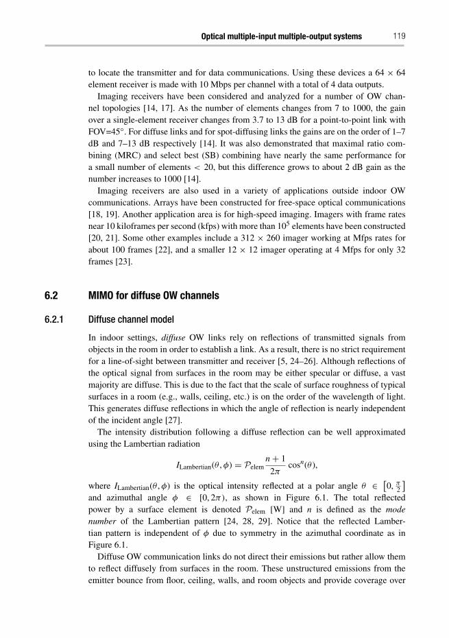
Optical multiple-input multiple-output systems 119
to locate the transmitter and for data communications. Using these devices a 64 × 64element receiver is made with 10 Mbps per channel with a total of 4 data outputs.
Imaging receivers have been considered and analyzed for a number of OW chan-nel topologies [14, 17]. As the number of elements changes from 7 to 1000, the gainover a single-element receiver changes from 3.7 to 13 dB for a point-to-point link withFOV=45◦. For diffuse links and for spot-diffusing links the gains are on the order of 1–7dB and 7–13 dB respectively [14]. It was also demonstrated that maximal ratio com-bining (MRC) and select best (SB) combining have nearly the same performance fora small number of elements < 20, but this difference grows to about 2 dB gain as thenumber increases to 1000 [14].
Imaging receivers are also used in a variety of applications outside indoor OWcommunications. Arrays have been constructed for free-space optical communications[18, 19]. Another application area is for high-speed imaging. Imagers with frame ratesnear 10 kiloframes per second (kfps) with more than 105 elements have been constructed[20, 21]. Some other examples include a 312 × 260 imager working at Mfps rates forabout 100 frames [22], and a smaller 12 × 12 imager operating at 4 Mfps for only 32frames [23].
6.2 MIMO for diffuse OW channels
6.2.1 Diffuse channel model
In indoor settings, diffuse OW links rely on reflections of transmitted signals fromobjects in the room in order to establish a link. As a result, there is no strict requirementfor a line-of-sight between transmitter and receiver [5, 24–26]. Although reflections ofthe optical signal from surfaces in the room may be either specular or diffuse, a vastmajority are diffuse. This is due to the fact that the scale of surface roughness of typicalsurfaces in a room (e.g., walls, ceiling, etc.) is on the order of the wavelength of light.This generates diffuse reflections in which the angle of reflection is nearly independentof the incident angle [27].
The intensity distribution following a diffuse reflection can be well approximatedusing the Lambertian radiation
ILambertian(θ ,φ) = Pelemn+ 1
2πcosn(θ ),
where ILambertian(θ ,φ) is the optical intensity reflected at a polar angle θ ∈ [0, π
2
]and azimuthal angle φ ∈ [0, 2π), as shown in Figure 6.1. The total reflectedpower by a surface element is denoted Pelem [W] and n is defined as the modenumber of the Lambertian pattern [24, 28, 29]. Notice that the reflected Lamber-tian pattern is independent of φ due to symmetry in the azimuthal coordinate as inFigure 6.1.
Diffuse OW communication links do not direct their emissions but rather allow themto reflect diffusely from surfaces in the room. These unstructured emissions from theemitter bounce from floor, ceiling, walls, and room objects and provide coverage over
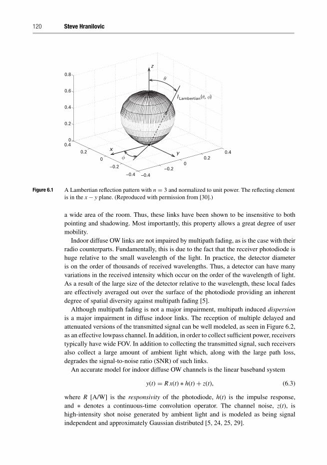
120 Steve Hranilovic
−0.2−0.4−0.4
−0.2
00
0.20.40.2
0.40
0.2
0.4
0.6
0.8θ
φx
y
z
I Lambertian(θ, φ)
Figure 6.1 A Lambertian reflection pattern with n = 3 and normalized to unit power. The reflecting elementis in the x− y plane. (Reproduced with permission from [30].)
a wide area of the room. Thus, these links have been shown to be insensitive to bothpointing and shadowing. Most importantly, this property allows a great degree of usermobility.
Indoor diffuse OW links are not impaired by multipath fading, as is the case with theirradio counterparts. Fundamentally, this is due to the fact that the receiver photodiode ishuge relative to the small wavelength of the light. In practice, the detector diameteris on the order of thousands of received wavelengths. Thus, a detector can have manyvariations in the received intensity which occur on the order of the wavelength of light.As a result of the large size of the detector relative to the wavelength, these local fadesare effectively averaged out over the surface of the photodiode providing an inherentdegree of spatial diversity against multipath fading [5].
Although multipath fading is not a major impairment, multipath induced dispersionis a major impairment in diffuse indoor links. The reception of multiple delayed andattenuated versions of the transmitted signal can be well modeled, as seen in Figure 6.2,as an effective lowpass channel. In addition, in order to collect sufficient power, receiverstypically have wide FOV. In addition to collecting the transmitted signal, such receiversalso collect a large amount of ambient light which, along with the large path loss,degrades the signal-to-noise ratio (SNR) of such links.
An accurate model for indoor diffuse OW channels is the linear baseband system
y(t) = R x(t) ∗ h(t)+ z(t), (6.3)
where R [A/W] is the responsivity of the photodiode, h(t) is the impulse response,and ∗ denotes a continuous-time convolution operator. The channel noise, z(t), ishigh-intensity shot noise generated by ambient light and is modeled as being signalindependent and approximately Gaussian distributed [5, 24, 25, 29].
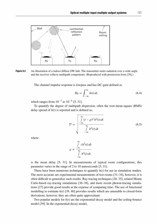
Optical multiple-input multiple-output systems 121
Rx
Roomceiling
Rx Tx
Wall Lambertianreflectionpattern
Figure 6.2 An illustration of a indoor diffuse OW link. The transmitter emits radiation over a wide angleand the receiver collects multipath components. (Reproduced with permission from [30].)
The channel impulse response is lowpass and has DC-gain defined as
H0 =∫ ∞
−∞h(t) dt, (6.4)
which ranges from 10−7 to 10−5 [5, 31].To quantify the degree of multipath dispersion, often the root-mean-square (RMS)
delay spread of h(t) is reported and is defined as,
D =
√√√√√√√√∞∫−∞
(t − �)2 h2(t) dt
∞∫−∞
h2(t) dt
(6.5)
where
� =
∞∫−∞
t h2(t) dt
∞∫−∞
h2(t) dt
is the mean delay [5, 31]. In measurements of typical room configurations, thisparameter varies in the range of 2 to 10 nanoseconds [5, 31].
There have been numerous techniques to quantify h(t) for use in simulation studies.The most accurate are experimental measurements of test rooms [31–34], however, it isoften difficult to generalize such results. Ray-tracing techniques [28, 35], related MonteCarlo-based ray-tracing simulations [36–38], and more recent photon-tracing simula-tions [27] provide good results at the expense of computing time. The use of functionalmodelling to estimate h(t) [39, 40] provides results which are amenable to closed-formderivations, however, they are often quite approximate.
Two popular models for h(t) are the exponential-decay model and the ceiling-bouncemodel [39]. In the exponential-decay model,
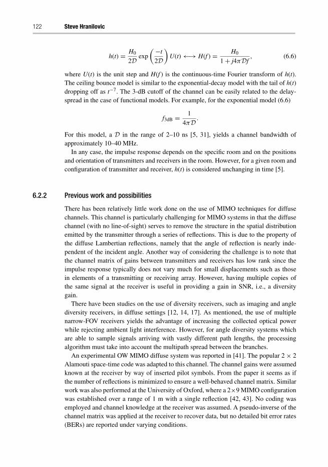
122 Steve Hranilovic
h(t) = H0
2D exp
(−t
2D)
U(t) ←→ H(f ) = H0
1+ j4πDf, (6.6)
where U(t) is the unit step and H(f ) is the continuous-time Fourier transform of h(t).The ceiling bounce model is similar to the exponential-decay model with the tail of h(t)dropping off as t−7. The 3-dB cutoff of the channel can be easily related to the delay-spread in the case of functional models. For example, for the exponential model (6.6)
f3dB = 1
4πD .
For this model, a D in the range of 2–10 ns [5, 31], yields a channel bandwidth ofapproximately 10–40 MHz.
In any case, the impulse response depends on the specific room and on the positionsand orientation of transmitters and receivers in the room. However, for a given room andconfiguration of transmitter and receiver, h(t) is considered unchanging in time [5].
6.2.2 Previous work and possibilities
There has been relatively little work done on the use of MIMO techniques for diffusechannels. This channel is particularly challenging for MIMO systems in that the diffusechannel (with no line-of-sight) serves to remove the structure in the spatial distributionemitted by the transmitter through a series of reflections. This is due to the property ofthe diffuse Lambertian reflections, namely that the angle of reflection is nearly inde-pendent of the incident angle. Another way of considering the challenge is to note thatthe channel matrix of gains between transmitters and receivers has low rank since theimpulse response typically does not vary much for small displacements such as thosein elements of a transmitting or receiving array. However, having multiple copies ofthe same signal at the receiver is useful in providing a gain in SNR, i.e., a diversitygain.
There have been studies on the use of diversity receivers, such as imaging and anglediversity receivers, in diffuse settings [12, 14, 17]. As mentioned, the use of multiplenarrow-FOV receivers yields the advantage of increasing the collected optical powerwhile rejecting ambient light interference. However, for angle diversity systems whichare able to sample signals arriving with vastly different path lengths, the processingalgorithm must take into account the multipath spread between the branches.
An experimental OW MIMO diffuse system was reported in [41]. The popular 2× 2Alamouti space-time code was adapted to this channel. The channel gains were assumedknown at the receiver by way of inserted pilot symbols. From the paper it seems as ifthe number of reflections is minimized to ensure a well-behaved channel matrix. Similarwork was also performed at the University of Oxford, where a 2×9 MIMO configurationwas established over a range of 1 m with a single reflection [42, 43]. No coding wasemployed and channel knowledge at the receiver was assumed. A pseudo-inverse of thechannel matrix was applied at the receiver to recover data, but no detailed bit error rates(BERs) are reported under varying conditions.
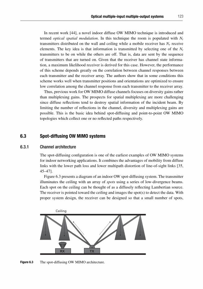
Optical multiple-input multiple-output systems 123
In recent work [44], a novel indoor diffuse OW MIMO technique is introduced andtermed optical spatial modulation. In this technique the room is populated with Nt
transmitters distributed on the wall and ceiling while a mobile receiver has Nr receiveelements. The key idea is that information is transmitted by selecting one of the Nt
transmitters to be on while the others are off. That is, data are sent by the sequenceof transmitters that are turned on. Given that the receiver has channel state informa-tion, a maximum likelihood receiver is derived for this case. However, the performanceof this scheme depends greatly on the correlation between channel responses betweeneach transmitter and the receiver array. The authors show that in some conditions thisscheme works well when transmitter positions and orientations are optimized to ensurelow correlation among the channel response from each transmitter to the receiver array.
Thus, previous work for OW MIMO diffuse channels focuses on diversity gains ratherthan multiplexing gains. The prospects for spatial multiplexing are more challengingsince diffuse reflections tend to destroy spatial information of the incident beam. Bylimiting the number of reflections in the channel, diversity and multiplexing gains arepossible. This is the basic idea behind spot-diffusing and point-to-point OW MIMOtopologies which collect one or no reflected paths respectively.
6.3 Spot-diffusing OW MIMO systems
6.3.1 Channel architecture
The spot-diffusing configuration is one of the earliest examples of OW MIMO systemsfor indoor networking applications. It combines the advantages of mobility from diffuselinks with the lower path loss and lower multipath distortion of line-of-sight links [35,45–47].
Figure 6.3 presents a diagram of an indoor OW spot-diffusing system. The transmitterilluminates the ceiling with an array of spots using a series of low-divergence beams.Each spot on the ceiling can be thought of as a diffusely reflecting Lambertian source.The receiver is pointed toward the ceiling and images the spot(s) to detect the data. Withproper system design, the receiver can be designed so that a small number of spots,
Ceiling
RX TX
Figure 6.3 The spot-diffusing OW MIMO architecture.
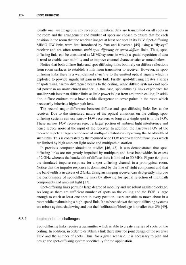
124 Steve Hranilovic
ideally one, are imaged in any reception. Identical data are transmitted on all spots inthe room and the arrangement and number of spots are chosen to ensure that for eachposition in the room that the receiver images at least one spot in its FOV. Spot-diffusingMIMO OW links were first introduced by Yun and Kavehrad [45] using a “fly-eye”receiver and are often termed multi-spot diffusing or quasi-diffuse links. Thus, spot-diffusing links can be considered as MIMO systems in which a spatial repetition of datais used to enable user mobility and to improve channel characteristics as noted below.
Notice that both diffuse links and spot-diffusing links both rely on diffuse reflectionsfrom room surfaces to establish a link from transmitter to receiver. However, in spot-diffusing links there is a well-defined structure to the emitted optical signals which isexploited to provide significant gain in the link. Firstly, spot-diffusing creates a seriesof spots using narrow divergence beams to the ceiling, while diffuse systems emit opti-cal power in an unstructured manner. In this case, spot-diffusing links experience farsmaller path loss than diffuse links as little power is lost from emitter to ceiling. In addi-tion, diffuse emitters must have a wide divergence to cover points in the room whichnecessarily inherits a higher path loss.
The second major difference between diffuse and spot-diffusing links lies at thereceiver. Due to the structured nature of the optical emissions on the ceiling, spot-diffusing systems can use narrow FOV receivers so long as a single spot is in the FOV.These narrow FOV receivers reject a larger portion of ambient light interference andhence reduce noise at the input of the receiver. In addition, the narrower FOV of thereceiver rejects a large component of multipath distortion improving the bandwidth ofsuch links. This is contrasted by the required wide FOV receivers for diffuse links whichare limited by high ambient light noise and multipath distortion.
In previous computer simulation studies [46, 48], it was demonstrated that spot-diffusing links are not greatly impaired by multipath and have bandwidths in excessof 2 GHz whereas the bandwidth of diffuse links is limited to 50 MHz. Figure 6.4 plotsthe simulated impulse response for a spot diffusing channel in a prototypical room.Notice that the impulse response is dominated by the line-of-sight component and thatthe bandwidth is in excess of 2 GHz. Using an imaging receiver can also greatly improvethe performance of spot-diffusing links by allowing for spatial rejection of multipathcomponents and ambient light [17].
Spot-diffusing links permit a large degree of mobility and are robust against blockage.As long as there are sufficient number of spots on the ceiling and the FOV is largeenough to catch at least one spot in every position, users are able to move about in aroom while maintaining a high-speed link. It has been shown that spot-diffusing systemsare robust against shadowing and that the likelihood of blockage is smaller than 2% [49].
6.3.2 Implementation challenges
Spot-diffusing links require a transmitter which is able to create a series of spots on theceiling. In addition, in order to establish a link there must be joint design of the receiverFOV and the number of spots. Thus, for a given scenario, it is necessary to plan anddesign the spot-diffusing system specifically for the application.
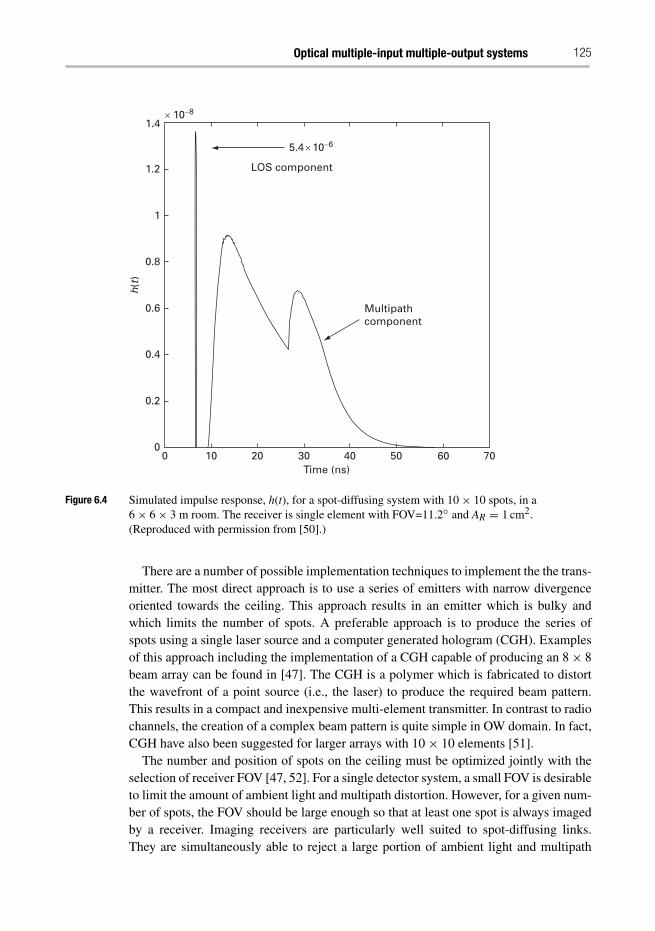
Optical multiple-input multiple-output systems 125
1.4× 10⁻⁸
5.4 × 10⁻⁶
1.2
1
0.8
h(t
)
0.6
0.4
0.2
00 10 20 30 40
Time (ns)
Multipathcomponent
LOS component
50 60 70
Figure 6.4 Simulated impulse response, h(t), for a spot-diffusing system with 10× 10 spots, in a6× 6× 3 m room. The receiver is single element with FOV=11.2◦ and AR = 1 cm2.(Reproduced with permission from [50].)
There are a number of possible implementation techniques to implement the the trans-mitter. The most direct approach is to use a series of emitters with narrow divergenceoriented towards the ceiling. This approach results in an emitter which is bulky andwhich limits the number of spots. A preferable approach is to produce the series ofspots using a single laser source and a computer generated hologram (CGH). Examplesof this approach including the implementation of a CGH capable of producing an 8× 8beam array can be found in [47]. The CGH is a polymer which is fabricated to distortthe wavefront of a point source (i.e., the laser) to produce the required beam pattern.This results in a compact and inexpensive multi-element transmitter. In contrast to radiochannels, the creation of a complex beam pattern is quite simple in OW domain. In fact,CGH have also been suggested for larger arrays with 10× 10 elements [51].
The number and position of spots on the ceiling must be optimized jointly with theselection of receiver FOV [47, 52]. For a single detector system, a small FOV is desirableto limit the amount of ambient light and multipath distortion. However, for a given num-ber of spots, the FOV should be large enough so that at least one spot is always imagedby a receiver. Imaging receivers are particularly well suited to spot-diffusing links.They are simultaneously able to reject a large portion of ambient light and multipath
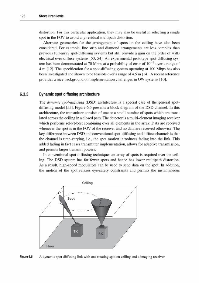
126 Steve Hranilovic
distortion. For this particular application, they may also be useful in selecting a singlespot in the FOV to avoid any residual multipath distortion.
Alternate geometries for the arrangement of spots on the ceiling have also beenconsidered. For example, line strip and diamond arrangements are less complex thanprevious full-array spot-diffusing systems but still provide a gain on the order of 4 dBelectrical over diffuse systems [53, 54]. An experimental prototype spot-diffusing sys-tem has been demonstrated at 70 Mbps at a probability of error of 10−9 over a range of4 m [12]. The specification for a spot-diffusing system operating at 100 Mbps has alsobeen investigated and shown to be feasible over a range of 4.5 m [14]. A recent referenceprovides a nice background on implementation challenges in OW systems [10].
6.3.3 Dynamic spot diffusing architecture
The dynamic spot-diffusing (DSD) architecture is a special case of the general spot-diffusing model [55]. Figure 6.5 presents a block diagram of the DSD channel. In thisarchitecture, the transmitter consists of one or a small number of spots which are trans-lated across the ceiling in a closed path. The detector is a multi-element imaging receiverwhich performs select-best combining over all elements in the array. Data are receivedwhenever the spot is in the FOV of the receiver and no data are received otherwise. Thekey difference between DSD and conventional spot-diffusing and diffuse channels is thatthe channel is time-varying, i.e., the spot motion introduces fading into the link. Thisadded fading in fact eases transmitter implementation, allows for adaptive transmission,and permits larger transmit powers.
In conventional spot-diffusing techniques an array of spots is required over the ceil-ing. The DSD system has far fewer spots and hence has lower multipath distortion.As a result, high-speed modulators can be used to send data on the spot. In addition,the motion of the spot relaxes eye-safety constraints and permits the instantaneous
Spot
Ceiling
RX TX
Floor
Spot
Figure 6.5 A dynamic spot-diffusing link with one rotating spot on ceiling and a imaging receiver.
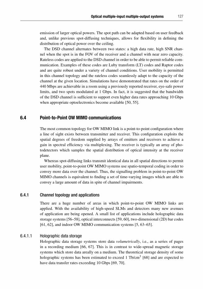
Optical multiple-input multiple-output systems 127
emission of larger optical powers. The spot path can be adapted based on user feedbackand, unlike previous spot-diffusing techniques, allows for flexibility in defining thedistribution of optical power over the ceiling.
The DSD channel alternates between two states: a high data rate, high SNR chan-nel when the spot is in the FOV of the receiver and a channel with near zero capacity.Rateless codes are applied to the DSD channel in order to be able to permit reliable com-munication. Examples of these codes are Luby transform (LT) codes and Raptor codesand are quite robust under a variety of channel conditions. User mobility is permittedin this channel topology and the rateless codes seamlessly adapt to the capacity of thechannel at the given location. Simulations have demonstrated that rates on the order of440 Mbps are achievable in a room using a previously reported receiver, eye-safe powerlimits, and two spots modulated at 1 Gbps. In fact, it is suggested that the bandwidthof the DSD channel is sufficient to support even higher data rates approaching 10 Gbpswhen appropriate optoelectronics become available [50, 55].
6.4 Point-to-Point OW MIMO communications
The most common topology for OW MIMO link is a point-to-point configuration wherea line of sight exists between transmitter and receiver. This configuration exploits thespatial degrees of freedom supplied by arrays of emitters and receivers to achieve again in spectral efficiency via multiplexing. The receiver is typically an array of pho-todetectors which samples the spatial distribution of optical intensity at the receiverplane.
Whereas spot-diffusing links transmit identical data in all spatial directions to permituser mobility, point-to-point OW MIMO systems use spatio-temporal coding in order toconvey more data over the channel. Thus, the signalling problem in point-to-point OWMIMO channels is equivalent to finding a set of time-varying images which are able toconvey a large amount of data in spite of channel impairments.
6.4.1 Channel topology and applications
There are a huge number of areas in which point-to-point OW MIMO links areapplied. With the availability of high-speed SLMs and detectors many new avenuesof application are being opened. A small list of applications include holographic datastorage systems [56–58], optical interconnects [59, 60], two-dimensional (2D) bar codes[61, 62], and indoor OW MIMO communication systems [5, 63–65].
6.4.1.1 Holographic data storageHolographic data storage systems store data volumetrically, i.e., as a series of pagesin a recording medium [66, 67]. This is in contrast to wide-spread magnetic storagesystems which store data areally on a medium. The theoretical storage density of someholographic systems has been estimated to exceed 1 Tb/cm3 [68] and are expected tohave data transfer rates exceeding 10 Gbps [69, 70].
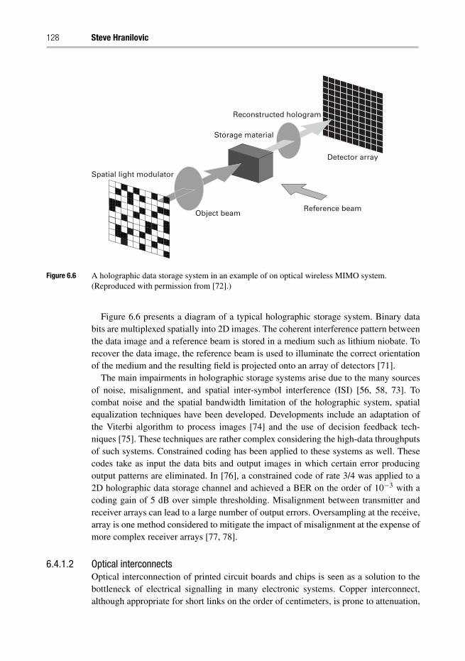
128 Steve Hranilovic
Detector array
Storage material
Spatial light modulator
Object beamReference beam
Reconstructed hologram
Figure 6.6 A holographic data storage system in an example of on optical wireless MIMO system.(Reproduced with permission from [72].)
Figure 6.6 presents a diagram of a typical holographic storage system. Binary databits are multiplexed spatially into 2D images. The coherent interference pattern betweenthe data image and a reference beam is stored in a medium such as lithium niobate. Torecover the data image, the reference beam is used to illuminate the correct orientationof the medium and the resulting field is projected onto an array of detectors [71].
The main impairments in holographic storage systems arise due to the many sourcesof noise, misalignment, and spatial inter-symbol interference (ISI) [56, 58, 73]. Tocombat noise and the spatial bandwidth limitation of the holographic system, spatialequalization techniques have been developed. Developments include an adaptation ofthe Viterbi algorithm to process images [74] and the use of decision feedback tech-niques [75]. These techniques are rather complex considering the high-data throughputsof such systems. Constrained coding has been applied to these systems as well. Thesecodes take as input the data bits and output images in which certain error producingoutput patterns are eliminated. In [76], a constrained code of rate 3/4 was applied to a2D holographic data storage channel and achieved a BER on the order of 10−3 with acoding gain of 5 dB over simple thresholding. Misalignment between transmitter andreceiver arrays can lead to a large number of output errors. Oversampling at the receive,array is one method considered to mitigate the impact of misalignment at the expense ofmore complex receiver arrays [77, 78].
6.4.1.2 Optical interconnectsOptical interconnection of printed circuit boards and chips is seen as a solution to thebottleneck of electrical signalling in many electronic systems. Copper interconnect,although appropriate for short links on the order of centimeters, is prone to attenuation,
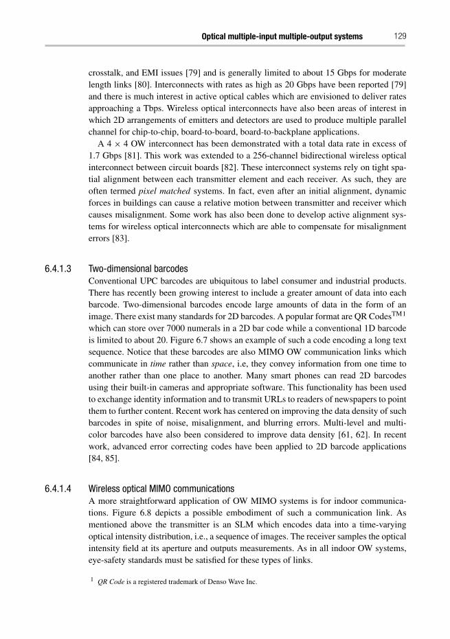
Optical multiple-input multiple-output systems 129
crosstalk, and EMI issues [79] and is generally limited to about 15 Gbps for moderatelength links [80]. Interconnects with rates as high as 20 Gbps have been reported [79]and there is much interest in active optical cables which are envisioned to deliver ratesapproaching a Tbps. Wireless optical interconnects have also been areas of interest inwhich 2D arrangements of emitters and detectors are used to produce multiple parallelchannel for chip-to-chip, board-to-board, board-to-backplane applications.
A 4 × 4 OW interconnect has been demonstrated with a total data rate in excess of1.7 Gbps [81]. This work was extended to a 256-channel bidirectional wireless opticalinterconnect between circuit boards [82]. These interconnect systems rely on tight spa-tial alignment between each transmitter element and each receiver. As such, they areoften termed pixel matched systems. In fact, even after an initial alignment, dynamicforces in buildings can cause a relative motion between transmitter and receiver whichcauses misalignment. Some work has also been done to develop active alignment sys-tems for wireless optical interconnects which are able to compensate for misalignmenterrors [83].
6.4.1.3 Two-dimensional barcodesConventional UPC barcodes are ubiquitous to label consumer and industrial products.There has recently been growing interest to include a greater amount of data into eachbarcode. Two-dimensional barcodes encode large amounts of data in the form of animage. There exist many standards for 2D barcodes. A popular format are QR CodesTM1
which can store over 7000 numerals in a 2D bar code while a conventional 1D barcodeis limited to about 20. Figure 6.7 shows an example of such a code encoding a long textsequence. Notice that these barcodes are also MIMO OW communication links whichcommunicate in time rather than space, i.e, they convey information from one time toanother rather than one place to another. Many smart phones can read 2D barcodesusing their built-in cameras and appropriate software. This functionality has been usedto exchange identity information and to transmit URLs to readers of newspapers to pointthem to further content. Recent work has centered on improving the data density of suchbarcodes in spite of noise, misalignment, and blurring errors. Multi-level and multi-color barcodes have also been considered to improve data density [61, 62]. In recentwork, advanced error correcting codes have been applied to 2D barcode applications[84, 85].
6.4.1.4 Wireless optical MIMO communicationsA more straightforward application of OW MIMO systems is for indoor communica-tions. Figure 6.8 depicts a possible embodiment of such a communication link. Asmentioned above the transmitter is an SLM which encodes data into a time-varyingoptical intensity distribution, i.e., a sequence of images. The receiver samples the opticalintensity field at its aperture and outputs measurements. As in all indoor OW systems,eye-safety standards must be satisfied for these types of links.
1 QR Code is a registered trademark of Denso Wave Inc.
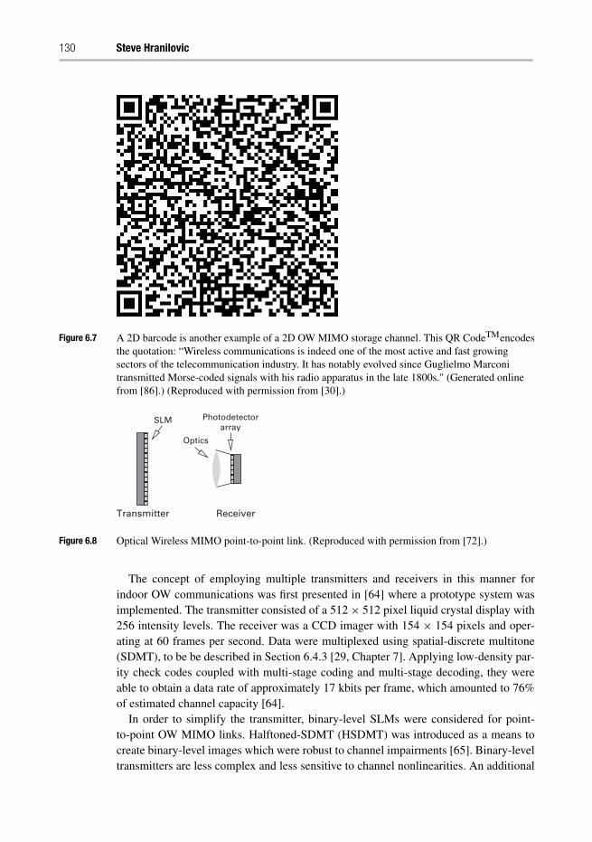
130 Steve Hranilovic
Figure 6.7 A 2D barcode is another example of a 2D OW MIMO storage channel. This QR CodeTMencodesthe quotation: “Wireless communications is indeed one of the most active and fast growingsectors of the telecommunication industry. It has notably evolved since Guglielmo Marconitransmitted Morse-coded signals with his radio apparatus in the late 1800s." (Generated onlinefrom [86].) (Reproduced with permission from [30].)
Optics
Photodetectorarray
SLM
Transmitter Receiver
Figure 6.8 Optical Wireless MIMO point-to-point link. (Reproduced with permission from [72].)
The concept of employing multiple transmitters and receivers in this manner forindoor OW communications was first presented in [64] where a prototype system wasimplemented. The transmitter consisted of a 512× 512 pixel liquid crystal display with256 intensity levels. The receiver was a CCD imager with 154 × 154 pixels and oper-ating at 60 frames per second. Data were multiplexed using spatial-discrete multitone(SDMT), to be be described in Section 6.4.3 [29, Chapter 7]. Applying low-density par-ity check codes coupled with multi-stage coding and multi-stage decoding, they wereable to obtain a data rate of approximately 17 kbits per frame, which amounted to 76%of estimated channel capacity [64].
In order to simplify the transmitter, binary-level SLMs were considered for point-to-point OW MIMO links. Halftoned-SDMT (HSDMT) was introduced as a means tocreate binary-level images which were robust to channel impairments [65]. Binary-leveltransmitters are less complex and less sensitive to channel nonlinearities. An additional
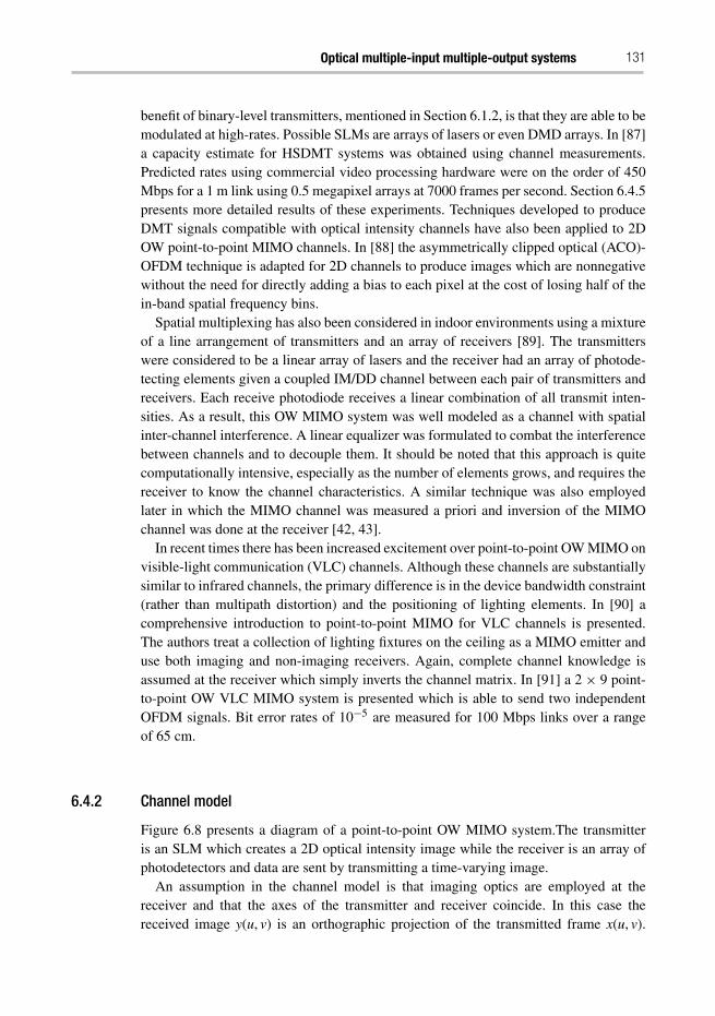
Optical multiple-input multiple-output systems 131
benefit of binary-level transmitters, mentioned in Section 6.1.2, is that they are able to bemodulated at high-rates. Possible SLMs are arrays of lasers or even DMD arrays. In [87]a capacity estimate for HSDMT systems was obtained using channel measurements.Predicted rates using commercial video processing hardware were on the order of 450Mbps for a 1 m link using 0.5 megapixel arrays at 7000 frames per second. Section 6.4.5presents more detailed results of these experiments. Techniques developed to produceDMT signals compatible with optical intensity channels have also been applied to 2DOW point-to-point MIMO channels. In [88] the asymmetrically clipped optical (ACO)-OFDM technique is adapted for 2D channels to produce images which are nonnegativewithout the need for directly adding a bias to each pixel at the cost of losing half of thein-band spatial frequency bins.
Spatial multiplexing has also been considered in indoor environments using a mixtureof a line arrangement of transmitters and an array of receivers [89]. The transmitterswere considered to be a linear array of lasers and the receiver had an array of photode-tecting elements given a coupled IM/DD channel between each pair of transmitters andreceivers. Each receive photodiode receives a linear combination of all transmit inten-sities. As a result, this OW MIMO system was well modeled as a channel with spatialinter-channel interference. A linear equalizer was formulated to combat the interferencebetween channels and to decouple them. It should be noted that this approach is quitecomputationally intensive, especially as the number of elements grows, and requires thereceiver to know the channel characteristics. A similar technique was also employedlater in which the MIMO channel was measured a priori and inversion of the MIMOchannel was done at the receiver [42, 43].
In recent times there has been increased excitement over point-to-point OW MIMO onvisible-light communication (VLC) channels. Although these channels are substantiallysimilar to infrared channels, the primary difference is in the device bandwidth constraint(rather than multipath distortion) and the positioning of lighting elements. In [90] acomprehensive introduction to point-to-point MIMO for VLC channels is presented.The authors treat a collection of lighting fixtures on the ceiling as a MIMO emitter anduse both imaging and non-imaging receivers. Again, complete channel knowledge isassumed at the receiver which simply inverts the channel matrix. In [91] a 2 × 9 point-to-point OW VLC MIMO system is presented which is able to send two independentOFDM signals. Bit error rates of 10−5 are measured for 100 Mbps links over a rangeof 65 cm.
6.4.2 Channel model
Figure 6.8 presents a diagram of a point-to-point OW MIMO system.The transmitteris an SLM which creates a 2D optical intensity image while the receiver is an array ofphotodetectors and data are sent by transmitting a time-varying image.
An assumption in the channel model is that imaging optics are employed at thereceiver and that the axes of the transmitter and receiver coincide. In this case thereceived image y(u, v) is an orthographic projection of the transmitted frame x(u, v).
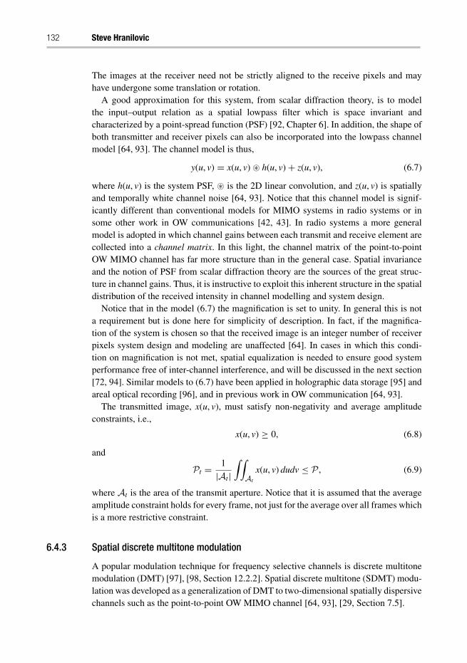
132 Steve Hranilovic
The images at the receiver need not be strictly aligned to the receive pixels and mayhave undergone some translation or rotation.
A good approximation for this system, from scalar diffraction theory, is to modelthe input–output relation as a spatial lowpass filter which is space invariant andcharacterized by a point-spread function (PSF) [92, Chapter 6]. In addition, the shape ofboth transmitter and receiver pixels can also be incorporated into the lowpass channelmodel [64, 93]. The channel model is thus,
y(u, v) = x(u, v) � h(u, v)+ z(u, v), (6.7)
where h(u, v) is the system PSF, � is the 2D linear convolution, and z(u, v) is spatiallyand temporally white channel noise [64, 93]. Notice that this channel model is signif-icantly different than conventional models for MIMO systems in radio systems or insome other work in OW communications [42, 43]. In radio systems a more generalmodel is adopted in which channel gains between each transmit and receive element arecollected into a channel matrix. In this light, the channel matrix of the point-to-pointOW MIMO channel has far more structure than in the general case. Spatial invarianceand the notion of PSF from scalar diffraction theory are the sources of the great struc-ture in channel gains. Thus, it is instructive to exploit this inherent structure in the spatialdistribution of the received intensity in channel modelling and system design.
Notice that in the model (6.7) the magnification is set to unity. In general this is nota requirement but is done here for simplicity of description. In fact, if the magnifica-tion of the system is chosen so that the received image is an integer number of receiverpixels system design and modeling are unaffected [64]. In cases in which this condi-tion on magnification is not met, spatial equalization is needed to ensure good systemperformance free of inter-channel interference, and will be discussed in the next section[72, 94]. Similar models to (6.7) have been applied in holographic data storage [95] andareal optical recording [96], and in previous work in OW communication [64, 93].
The transmitted image, x(u, v), must satisfy non-negativity and average amplitudeconstraints, i.e.,
x(u, v) ≥ 0, (6.8)
and
Pt = 1
|At|∫∫
At
x(u, v) dudv ≤ P , (6.9)
where At is the area of the transmit aperture. Notice that it is assumed that the averageamplitude constraint holds for every frame, not just for the average over all frames whichis a more restrictive constraint.
6.4.3 Spatial discrete multitone modulation
A popular modulation technique for frequency selective channels is discrete multitonemodulation (DMT) [97], [98, Section 12.2.2]. Spatial discrete multitone (SDMT) modu-lation was developed as a generalization of DMT to two-dimensional spatially dispersivechannels such as the point-to-point OW MIMO channel [64, 93], [29, Section 7.5].
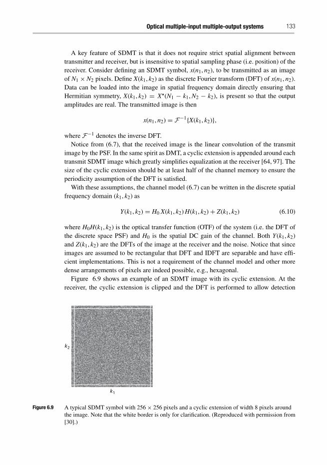
Optical multiple-input multiple-output systems 133
A key feature of SDMT is that it does not require strict spatial alignment betweentransmitter and receiver, but is insensitive to spatial sampling phase (i.e. position) of thereceiver. Consider defining an SDMT symbol, x(n1, n2), to be transmitted as an imageof N1 ×N2 pixels. Define X(k1, k2) as the discrete Fourier transform (DFT) of x(n1, n2).Data can be loaded into the image in spatial frequency domain directly ensuring thatHermitian symmetry, X(k1, k2) = X�(N1 − k1, N2 − k2), is present so that the outputamplitudes are real. The transmitted image is then
x(n1, n2) = F−1{X(k1, k2)},
where F−1 denotes the inverse DFT.Notice from (6.7), that the received image is the linear convolution of the transmit
image by the PSF. In the same spirit as DMT, a cyclic extension is appended around eachtransmit SDMT image which greatly simplifies equalization at the receiver [64, 97]. Thesize of the cyclic extension should be at least half of the channel memory to ensure theperiodicity assumption of the DFT is satisfied.
With these assumptions, the channel model (6.7) can be written in the discrete spatialfrequency domain (k1, k2) as
Y(k1, k2) = H0 X(k1, k2) H(k1, k2)+ Z(k1, k2) (6.10)
where H0H(k1, k2) is the optical transfer function (OTF) of the system (i.e. the DFT ofthe discrete space PSF) and H0 is the spatial DC gain of the channel. Both Y(k1, k2)and Z(k1, k2) are the DFTs of the image at the receiver and the noise. Notice that sinceimages are assumed to be rectangular that DFT and IDFT are separable and have effi-cient implementations. This is not a requirement of the channel model and other moredense arrangements of pixels are indeed possible, e.g., hexagonal.
Figure 6.9 shows an example of an SDMT image with its cyclic extension. At thereceiver, the cyclic extension is clipped and the DFT is performed to allow detection
k 2
k 1
Figure 6.9 A typical SDMT symbol with 256× 256 pixels and a cyclic extension of width 8 pixels aroundthe image. Note that the white border is only for clarification. (Reproduced with permission from[30].)
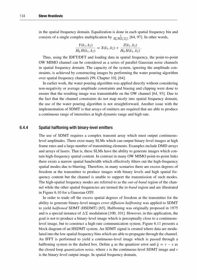
134 Steve Hranilovic
in the spatial frequency domain. Equalization is done in each spatial frequency bin andconsists of a single complex multiplication by 1
H0 H(k1,k2) [64, 97]. In other words,
Y(k1, k2)
H0 H(k1, k2)= X(k1, k2)+ Z(k1, k2)
H0 H(k1, k2).
Thus, using the IDFT/DFT and loading data in spatial frequency, the point-to-pointOW MIMO channel can be considered as a series of parallel Gaussian noise channelsin spatial frequency domain. The capacity of the system, ignoring the amplitude con-straints, is achieved by constructing images by performing the water pouring algorithmover spatial frequency channels [99, Chapter 10], [64].
In earlier work, the water pouring algorithm was applied directly without consideringnon-negativity or average amplitude constraints and biasing and clipping were done toensure that the resulting image was transmittable on the OW channel [64, 93]. Due tothe fact that the channel constraints do not map nicely into spatial frequency domain,the use of the water pouring algorithm is not straightforward. Another issue with theimplementation of SDMT is that arrays of emitters are required that are able to producea continuous range of intensities at high dynamic range and high rate.
6.4.4 Spatial halftoning with binary-level emitters
The use of SDMT requires a complex transmit array which must output continuous-level amplitudes. There exist many SLMs which can output binary-level images at highframe rates and a large number of transmitting elements. Examples include DMD arraysand arrays of lasers. That is, these SLMs have the ability to generate images which con-tain high-frequency spatial content. In contrast in many OW MIMO point-to-point linksthere exists a narrow spatial bandwidth which effectively filters out the high-frequencyspatial modes due to blurring. Therefore, in many scenarios there are excess degrees offreedom at the transmitter to produce images with binary levels and high spatial fre-quency content but the channel is unable to support the transmission of such modes.The high-spatial frequency modes are referred to as the out-of-band region of the chan-nel while the other spatial frequencies are termed the in-band region and are illustratedin Figure 6.10 for a Gaussian OTF.
In order to trade off the excess spatial degrees of freedom at the transmitter for theability to generate binary-level images error diffusion halftoning was applied to SDMTto yield halftoned SDMT (HSDMT) [65]. Halftoning was originally proposed in 1975and is a special instance of �� modulation [100, 101]. However, in this application, thegoal is not to produce a binary-level image which is perceptually close to a continuous-level image, but to construct a high-rate communication system. Figure 6.11 presents ablock diagram of an HSDMT system. An SDMT signal is created where data are modu-lated into the low spatial frequency bins which are able to propagate through the channel.An IFFT is performed to yield a continuous-level image which is passed through ahalftoning system in the dashed box. Define q as the quantizer error and q = v − x asthe closed loop quantization noise, where x is the continuous-level SDMT image and vis the binary-level output image. In spatial frequency domain,
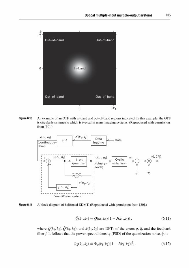
Optical multiple-input multiple-output systems 135
In−band
Out−of−band Out−of−band
Out−of−band Out−of−band
0
0
→k 1
→k 2
Figure 6.10 An example of an OTF with in-band and out-of-band regions indicated. In this example, the OTFis circularly symmetric which is typical in many imaging systems. (Reproduced with permissionfrom [30].)
1−bitquantizer
Cyclicextension
Dataloading
+
+
Error diffusion system
Data(continuous−level)
(binary−level)
+1
{0, 2 t }
t
±1
−1x(n1, n2) X (k 1, k 2)
υ (n1, n2)
j (n1, n2)q (n1, n2)
ω (n1, n2)
Figure 6.11 A block diagram of halftoned-SDMT. (Reproduced with permission from [30].)
Q(k1, k2) = Q(k1, k2) [1− J(k1, k2)] , (6.11)
where Q(k1, k2), Q(k1, k2), and J(k1, k2) are DFTs of the errors q, q, and the feedbackfilter j. It follows that the power spectral density (PSD) of the quantization noise, q, is
�q(k1, k2) = �q(k1, k2) |1− J(k1, k2)|2, (6.12)
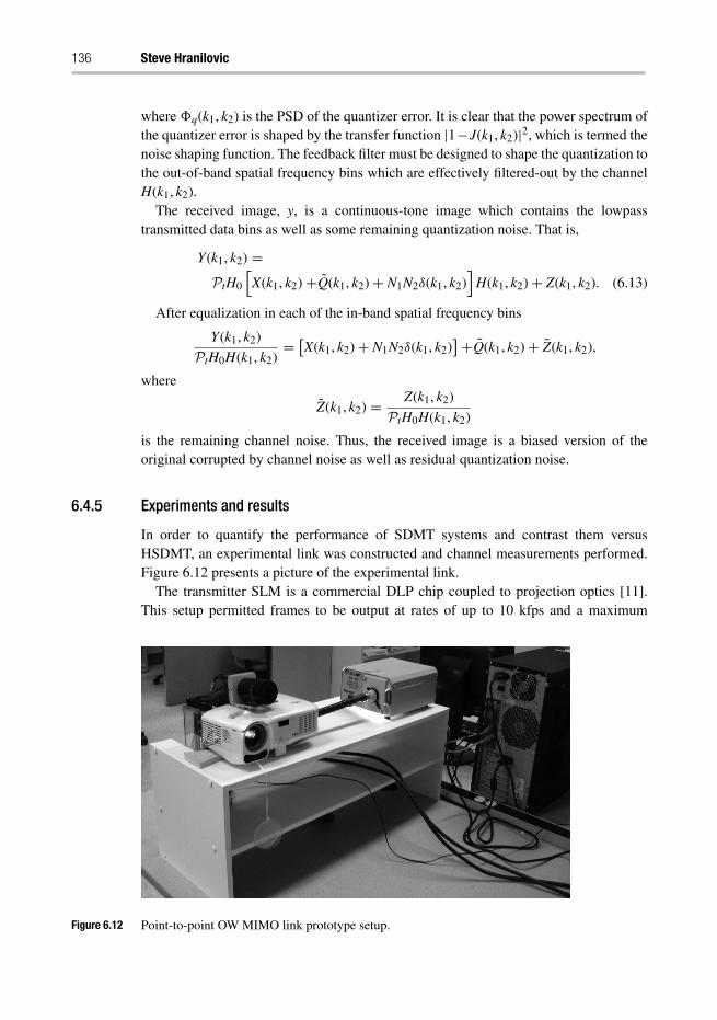
136 Steve Hranilovic
where �q(k1, k2) is the PSD of the quantizer error. It is clear that the power spectrum ofthe quantizer error is shaped by the transfer function |1−J(k1, k2)|2, which is termed thenoise shaping function. The feedback filter must be designed to shape the quantization tothe out-of-band spatial frequency bins which are effectively filtered-out by the channelH(k1, k2).
The received image, y, is a continuous-tone image which contains the lowpasstransmitted data bins as well as some remaining quantization noise. That is,
Y(k1, k2) =PtH0
[X(k1, k2)+Q(k1, k2)+ N1N2δ(k1, k2)
]H(k1, k2)+ Z(k1, k2). (6.13)
After equalization in each of the in-band spatial frequency bins
Y(k1, k2)
PtH0H(k1, k2)= [
X(k1, k2)+ N1N2δ(k1, k2)]+Q(k1, k2)+ Z(k1, k2),
where
Z(k1, k2) = Z(k1, k2)
PtH0H(k1, k2)
is the remaining channel noise. Thus, the received image is a biased version of theoriginal corrupted by channel noise as well as residual quantization noise.
6.4.5 Experiments and results
In order to quantify the performance of SDMT systems and contrast them versusHSDMT, an experimental link was constructed and channel measurements performed.Figure 6.12 presents a picture of the experimental link.
The transmitter SLM is a commercial DLP chip coupled to projection optics [11].This setup permitted frames to be output at rates of up to 10 kfps and a maximum
Figure 6.12 Point-to-point OW MIMO link prototype setup.
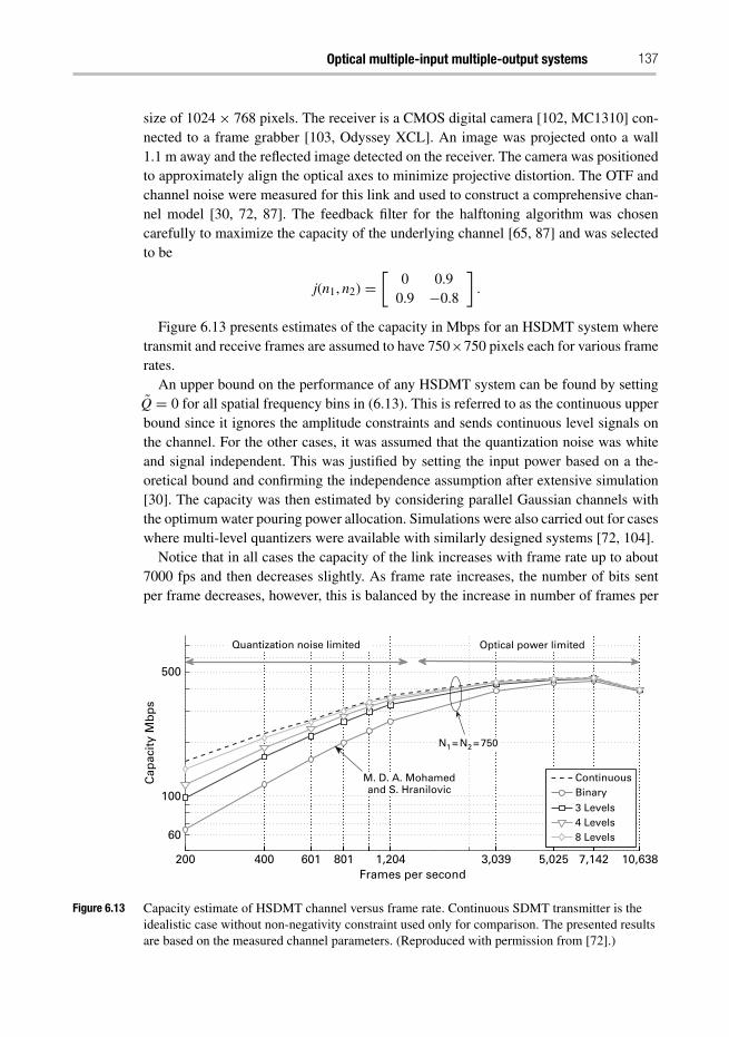
Optical multiple-input multiple-output systems 137
size of 1024× 768 pixels. The receiver is a CMOS digital camera [102, MC1310] con-nected to a frame grabber [103, Odyssey XCL]. An image was projected onto a wall1.1 m away and the reflected image detected on the receiver. The camera was positionedto approximately align the optical axes to minimize projective distortion. The OTF andchannel noise were measured for this link and used to construct a comprehensive chan-nel model [30, 72, 87]. The feedback filter for the halftoning algorithm was chosencarefully to maximize the capacity of the underlying channel [65, 87] and was selectedto be
j(n1, n2) =[
0 0.90.9 −0.8
].
Figure 6.13 presents estimates of the capacity in Mbps for an HSDMT system wheretransmit and receive frames are assumed to have 750×750 pixels each for various framerates.
An upper bound on the performance of any HSDMT system can be found by settingQ = 0 for all spatial frequency bins in (6.13). This is referred to as the continuous upperbound since it ignores the amplitude constraints and sends continuous level signals onthe channel. For the other cases, it was assumed that the quantization noise was whiteand signal independent. This was justified by setting the input power based on a the-oretical bound and confirming the independence assumption after extensive simulation[30]. The capacity was then estimated by considering parallel Gaussian channels withthe optimum water pouring power allocation. Simulations were also carried out for caseswhere multi-level quantizers were available with similarly designed systems [72, 104].
Notice that in all cases the capacity of the link increases with frame rate up to about7000 fps and then decreases slightly. As frame rate increases, the number of bits sentper frame decreases, however, this is balanced by the increase in number of frames per
ContinuousBinary3 Levels4 Levels8 Levels
200 400 601 801 1,204 3,039 5,025 7,142 10,638
60
100
500
Frames per second
Cap
acit
y M
bp
s
N1 = N2 = 750
Quantization noise limited Optical power limited
M. D. A. Mohamedand S. Hranilovic
Figure 6.13 Capacity estimate of HSDMT channel versus frame rate. Continuous SDMT transmitter is theidealistic case without non-negativity constraint used only for comparison. The presented resultsare based on the measured channel parameters. (Reproduced with permission from [72].)
138 Steve Hranilovic
second. Asymptotically, in the case of white noise these two effects should be perfectlybalanced, however, it is apparent that the noise in the experimental link was not white.Notice also that at low fps, there is a large discrepancy between the capacity availableusing the idealistic continuous model and the halftoned schemes. In this range of frame-rates the channel is termed quantization noise limited since the water pouring spectrumis dominated by the quantization noise introduced by halftoning. Notice also that in thisregime quantizers with multiple levels are useful in approaching the continuous boundon capacity [72, 104]. At higher frame rates, the channel is termed optical power limitedsince the dominant source of noise is due to ambient light. In this regime, even binarysignalling can approach the continuous bound. Therefore, using binary-level halftoningwith high frame rate provides high data rates. In a first trial experiment using no coding,we have been able to achieve rates of 250 Mbps with binary halftoning with 768× 1024frames over a distance of 0.55 m in the presence of a significant magnification error of0.89 using techniques presented in [94].
6.5 Future directions
The use of multiple transmitters and receivers in indoor OW channels has been shownto improve data rates and reliability in a wide variety of applications. A diversity gaincan be had simply by using a receiver with multiple elements. The key feature of such areceiver, be it angle diversity or imaging, is that it is able to spatially sample the receivedoptical intensity image. This permits the use of combining techniques to improve thereceived SNR. In addition, in many point-to-point links, a multiplexing gain in the rateis available by exploiting spatial degrees of freedom. Although the channel has dis-persion, the spatial dispersion is well structured and nicely represented by a linear spacemodel. The key feature in these systems is that the multi-element transmitter can imposestructure on the spatial distribution of power. Similarly, a multi-element receiver is ableto provide a gain, either in SNR or in rate, by exploiting any underlying structure inthe received optical intensity distribution. This is useful in cases where multiple or evensingle emitters are available.
There is a plethora of exciting future applications for MIMO techniques in OW sys-tems. Among the applications are visible light communication (VLC) channels. Suchchannels are quickly becoming of commercial interest due to their use of illuminationdevices for a dual role as communication systems. The white phosphorescent LEDs typ-ically used in such VLC applications have very limited bandwidth, at most 20 MHz.The use of MIMO techniques to improve the spectral efficiency of such links is cur-rently a topic of intense interest in the community. Many VLC applications are naturallyMIMO problems since each illumination device is composed of numerous white LEDemitters. In addition, white LEDs are currently used in backlighting applications forLCD displays and their use for communications has yet to be deeply investigated.In automotive applications, arrays of white LEDs and receivers are envisioned forcar-to-car communications primarily for collision avoidance and navigation applications.Another interesting avenue of study for indoor OW MIMO is in the area of areal storage
Optical multiple-input multiple-output systems 139
and bar codes. These storage channels can be simply viewed as a communications sys-tem in time. There are many applications for such 2D storage and transmission channelswhich would benefit from further study.
Ongoing challenges in the implementation of high-speed optical transmit arrays andintegrated imaging receivers are vital directions of research required in order to allowsystem designers to reap the rewards of MIMO techniques. Although progress hasbeen made in developing integrated emitters and holographic-based filtering techniques,added work is required to implement such systems. Encouragingly, there is much workin the development of high-speed detector arrays and circuitry which are packaged in acompact form factor.
Certainly, there are many hurdles to overcome in the implementation of OW MIMOsystems. However, the potential gains in SNR and rate are exciting and justify redoubledefforts to make such approaches widespread. Regardless of the application, the use ofMIMO OW techniques improves system performance to such a degree that indeed withOW MIMO techniques “a picture can be worth far more than a thousand words”!
References
[1] L. Zheng and D. N. C. Tse, “Diversity and multiplexing: A fundamental tradeoff inmultiple-antenna channels,” IEEE Transactions on Information Theory, vol. 49, no. 5, pp.1073–1096, May 2003.
[2] IEC 60825-1, Safety of Laser Products - Part 1: Equipment Classification, Requirements,and User’s Guide, International Electrotechnical Commission (IEC), 2001, edition 1.2.
[3] A. C. Boucouvalas, “IEC 825-1 eye safety classification of some consumer electronic prod-ucts,” in Proceedings of the IEE Colloquium on Optical Free Space Communication Links,IEE Savoy Place, London, 19 Feb. 1996, pp. 13/1–13/6.
[4] T.-S. Chu and M. Gans, “High speed infrared local wireless communication,” IEEECommunications Magazine, vol. 25, no. 8, pp. 4–10, Aug. 1987.
[5] J. M. Kahn and J. R. Barry, “Wireless infrared communications,” Proceedings of the IEEE,vol. 85, no. 2, pp. 263–298, Feb. 1997.
[6] W. Hubbard, “The approximation of a Poisson distribution by a Gaussian distribution,”Proceedings of the IEEE, vol. 58, no. 9, pp. 1374–1375, Sept. 1970.
[7] M. B. Venditti, E. Laprise, J. Faucher et al., “Design and test of an optoelectronic-VLSIchip with 540-element receiver-transmitter arrays using differential optical signaling,”IEEE Journal of Selected Topics in Quantum Electronics, vol. 9, no. 2, pp. 361–379,Mar./Apr. 2003.
[8] D. C. O’Brien, G. E. Faulkner, E. B. Zyambo et al., “Integrated transceivers for opti-cal wireless communications,” IEEE Journal of Selected Topics in Quantum Electronics,vol. 11, no. 1, pp. 173–183, Jan./Feb. 2005.
[9] A. Boryssenko, J. Liao, J. Zeng, V. Joyner, and Z. R. Huang, “Studies on RF-opticaldual mode wireless communication modules,” in 2009 IEEE International MicrowaveSymposium, June 7-12, 2009, pp. 805–808.
[10] D. O’Brien, H. L. Minh, G. Faulkner et al., “High data-rate infra-red optical wireless com-munications: Implementation challenges,” in 2010 IEEE Globecom Workshop on OpticalWireless Communications, pp. 1047–1051, Dec. 2010.
140 Steve Hranilovic
[11] Texas Instruments Incorporated, Digital Light Processing. URL: www.dlp.com.[12] J. B. Carruthers and J. M. Kahn, “Angle diversity for nondirected wireless infrared com-
munication,” IEEE Transactions on Communications, vol. 48, no. 6, pp. 960–969, June2000.
[13] A. Tavares, R. Valadas, R. L. Aguiar, and A. O. Duarte, “Angle diversity and rate-adaptivetransmission for indoor wireless optical communications,” IEEE Communications Maga-zine, pp. 64–73, Mar. 2003.
[14] J. M. Kahn, R. You, P. Djahani et al., “Imaging diversity receivers for high-speed infraredwireless communcation,” IEEE Communations Magazine, pp. 88–94, Dec. 1998.
[15] J. Zeng, V. Joyner, J. Liao, S. Deng, and Z. Huang, “A 5Gb/s 7-channel current-mode imag-ing receiver front-end for free-space optical MIMO,” in Proc. IEEE Midwest Symposiumon Circuits and Systems (MWSCAS), Aug. 2009, pp. 148–151.
[16] K. Kagawa, J. Ohta, and J. Tanida, “Dynamic reconfiguration of differential pixel out-put for CMOS imager dedicated to WDM-SDM indoor optical wireless LAN,” IEEEPhotonics Technology Letters, vol. 48, no. 18, pp. 1308–10, Sept. 2009.
[17] P. Djahani and J. M. Kahn, “Analysis of infrared wireless links employing multibeam trans-mitters and imaging diversity receivers,” IEEE Transactions on Communications, vol. 48,no. 12, pp. 2077–2088, Dec. 2000.
[18] B. S. Leibowitz, B. E. Boser, and K. S. J. Pister, “CMOS smart pixel for free-space opticalcommunication,” in Proceedings of the SPIE, vol. 4306, Jan. 2001, pp. 308–318.
[19] D. C. O’Brien, G. E. Gaulkner, K. Jim et al., “High-speed integrated transceivers foroptical wireless,” IEEE Communications Magazine, vol. 41, no. 3, pp. 58 – 62, 2003.
[20] S. Kleinfelder, S. Lim, X. Liu, and A. El Gamal, “A 10000 frames/s CMOS digitalpixel sensor,” IEEE Journal of Solid-State Circuits, vol. 36, no. 12, pp. 2049–2059, Dec.2001.
[21] S. Kleinfelder, S. Lim, X. Liu, and A. E. Gamal, “A 10 kframe/s 0.18 μm CMOS digitalpixel sensor with pixel-level memory,” in Proceedings of the IEEE International Solid-State Circuits Conference, San Francisco, CA, USA, 4-8 Feb. 2001, pp. 88–89.
[22] T. Etoh, D. Poggemann, G. Kreider et al., “An image sensor which captures 100 consecu-tive frames at 1000000 frames/s,” IEEE Transactions on Electron Devices, vol. 50, no. 1,pp. 144–151, Jan. 2003.
[23] S. Kleinfelder, Y. Chen, K. Kwiatkowski, and A. Shah, “High-speed CMOS image sensorcircuits with in situ frame storage,” IEEE Transactions on Nuclear Science, vol. 51, no. 4,pp. 1648–1656, Aug. 2004.
[24] F. Gfeller and U. Bapst, “Wireless in-house data communication via diffuse infraredradiation,” Proceedings of the IEEE, vol. 67, no. 11, pp. 1474–1486, Nov. 1979.
[25] J. M. Kahn, J. R. Barry, M. D. Audeh, J. B. Carruthers, W. J. Krause, and G. W. Marsh,“Non-directed infrared links for high-capacity wireless LANs,” IEEE Personal Communi-cations, vol. 1, no. 2, pp. 12–25, 1994.
[26] M. Kotzin and A. van den Heuvel, “A duplex infra-red system for in-building communi-cations,” in Proceedings of the 36th IEEE Vehicular Technology Conference, vol. 36, May1986, pp. 179–185.
[27] H.-S. Lee, “A photon modeling method for the characterization of indoor optical wirelesscommunication,” Progress In Electromagnetics Research, PIER 92, pp. 121–136, 2009.
[28] J. R. Barry, J. M. Kahn, W. J. Krause, E. A. Lee, and D. G. Messerschmitt, “Simulationof multipath impulse response for indoor wireless optical channels,” IEEE Journal onSelected Areas in Communications, vol. 11, no. 3, pp. 367–379, Apr. 1993.
Optical multiple-input multiple-output systems 141
[29] S. Hranilovic, Wireless Optical Communication Systems. Springer, 2004.[30] M. D. A. Mohamed, “Modulation and detection in wireless optical channels using tem-
poral and spatial degrees of freedom,” Ph.D. dissertation, Department of Electrical andComputer Engineering, McMaster University, 2010.
[31] J. M. Kahn, W. J. Krause, and J. B. Carruthers, “Experimental characterization of non-directed indoor infrared channels,” IEEE Transactions on Communications, vol. 43, no.234, pp. 1613–1623, Feb./Mar./Apr. 1995.
[32] H. Hashemi, G. Yun, M. Kavehrad, F. Behbahani, and P. A. Galko, “Indoor propa-gation measurements at infrared frequencies for wireless local area networks applica-tions,” IEEE Transactions on Vehicular Technology, vol. 43, no. 3, pp. 562–576, Aug.1994.
[33] H. Hashemi, G. Yun, M. Kavehrad, and F. Behbahani, “Frequency response measure-ments of the wireless indoor channel at infrared frequencies,” in Proceedings of the IEEEInternational Conference on Communications, vol. 3, May 1994, pp. 1511–1515.
[34] M. R. Pakravan and M. Kavehrad, “Indoor wireless infrared channel characterization bymeasurements,” IEEE Transactions on Vehicular Technology, vol. 50, no. 4, pp. 1053–1073, July 2001.
[35] Y. A. Alqudah and M. Kavehrad, “MIMO characterization of indoor wireless opticallink using a diffuse-transmission configuration,” IEEE Transactions on Communications,vol. 51, no. 9, pp. 1554–1560, Sept. 2003.
[36] F. J. López-Hernández, R. Pérez-Jiménez, and A. Santamaría, “Ray-tracing algorithms forfast calculation of the channel impulse response on diffuse IR wireless indoor channels,”Optical Engineering, vol. 39, no. 10, pp. 2775–2780, 2000.
[37] O. González, S. Rodriguez, R. Pérez-Jiménez, B. R. Mendoza, and A. Ayala, “Error anal-ysis of the simulated impulse response on indoor wireless optical channels using a MonteCarlo-based ray-tracing algorithm,” IEEE Transactions on Communications, vol. 53, no. 1,pp. 124–130, Jan. 2005.
[38] Y. Cocheril and R. Vauzelle, “A new ray-tracing based wave propagation model includingrough surfaces scattering,” Progress In Electromagnetics Research, PIER 75, pp. 357–381,2007.
[39] J. B. Carruthers and J. M. Kahn, “Modeling of nondirected wireless infrared channels,”IEEE Transactions on Communications, vol. 45, no. 10, pp. 1260–1268, Oct. 1997.
[40] V. Jungnickel, V. Pohl, S. Nönnig, and C. von Helmolt, “A physical model of the wirelessinfrared communication channel,” IEEE Journal on Selected Areas in Communications,vol. 20, no. 3, pp. 631–640, Apr. 2002.
[41] M. Garfield, C. Liang, T. P. Kurzweg, and K. R. Dandekar, “MIMO space-time coding fordiffuse optical communication,” Microwave and Optical Technology Letters, vol. 48, no. 6,pp. 1108–1110, June 2006.
[42] D. O’Brien, “Multi-input multi-output (MIMO) indoor optical wireless communications,”in 43rd Asilomar Conference on Signals, Systems and Computers, Nov. 1–4, 2009, pp.1636–1639.
[43] D. O’Brien, “Optical multi-input multi-output systems for short-range free-space datatransmission,” in 7th Conference on Communication Systems, Networks and Digital SignalProcessing (CSNDSP 2010), Jul. 21–23, 2010, pp. 566–570.
[44] R. Mesleh, R. Mehmood, H. Elgala, and H. Haas, “Indoor MIMO optical wirelesscommunication using spatial modulation,” in Proc. 2010 International Conference onCommunications, May 23–27, 2010.
142 Steve Hranilovic
[45] G. Yun and M. Kavehrad, “Spot-diffusing and fly-eye receivers for indoor infrared wire-less communications,” In Proc. of IEEE International Conference on Selected Topics inWireless Communications, pp. 262–265, 1992.
[46] S. T. Jivkova, B. A. Hristov, and M. Kavehrad, “Power-efficient multispot-diffuse multiple-input-multiple-output approach to broad-band optical wireless communications,” IEEETransactions on Vehicular Technology, vol. 53, no. 3, pp. 882–889, May 2004.
[47] S. T. Jivkova and M. Kavehrad, “Multispot diffusing configuration for wireless infraredaccess,” IEEE Transactions on Communications, vol. 48, no. 6, pp. 970–978, June2000.
[48] S. Jivkova and M. Kavehrad, “Receiver designs and channel characterization for multi-spothigh-bit-rate wireless infrared communications,” IEEE Transactions on Communications,vol. 49, no. 12, pp. 2145–2153, Dec. 2001.
[49] S. Jivkova and M. Kavehrad, “Shadowing and blockage in indoor optical wireless commu-nications,” In IEEE Proceedings Global Telecommunications Conference, pp. 3269–3273,2003.
[50] F. Khozeimeh, “Dynamic spot diffusing channel – a novel configuration for indoor opti-cal wireless communications,” Master’s thesis, Department of Electrical and ComputerEngineering, McMaster University, 2006.
[51] M. Kavehrad and S. Jivkova, “Indoor broadband optical wireless communications: opti-cal subsystems design and their impact on channel characteristics,” IEEE WirelessCommunications Magazine, pp. 30–35, Apr. 2003.
[52] S. Jivkova and M. Kavehrad, “Multi-spot diffusing configuration for wireless infraredaccess: Joint optimization of multi-beam transmitter and angle diversity receiver,” InProc. Conference Optical Wireless Communications II, SPIE., vol. 3850, pp. 72–77, Sept.1999.
[53] A. G. Al-Ghamdi and J. M. H. Elmirghani, “Line strip spot-diffusing transmitter con-figuration for optical wireless systems influenced by background noise and multipathdispersion,” IEEE Transactions Communications, vol. 52, no. 1, pp. 37–45, Jan. 2004.
[54] A. G. Al-Ghamdi and J. M. H. Elmirghani, “Multiple spot diffusing geometries forindoor optical wireless communication systems,” International Journal of CommunicationSystems, vol. 16, pp. 909–922, 2003.
[55] F. Khozeimeh and S. Hranilovic, “Dynamic spot diffusing configuration for indoor opticalwireless access,” IEEE Transactions on Communications, vol. 57, no. 6, pp. 1765–1775,June 2009.
[56] R. M. Shelby, J. Hoffnagle, G. W. Burr et al., “Pixel-matched holographic data storagewith megabit pages,” Optics Letters, vol. 22, no. 19, pp. 1509–1511, October 1997.
[57] G. W. Burr, J. Ashley, H. Coufal et al., “Modulation coding for pixel-matched holographicdata storage,” Optics Letters, vol. 22, no. 9, pp. 639–641, May 1997.
[58] S. Nabavi and B. V. K. V. Kumar, “Detection methods for holographic data storage,” inProceedings of the IEEE Optical Data Storage, Montreal, QC, Canada, April 2006, pp.156–158.
[59] D. V. Plant and A. G. Kirk, “Optical interconnects at the chip and board level: Challengesand solutions,” Proceedings of the IEEE, vol. 88, no. 6, pp. 806–818, 2000.
[60] J. Bristow, J. Lehman, M. Hibbs-Brenner, and Y. Liu, “Applying optical interconnectsto electronic systems: Promise vs. practicality,” Proceedings of the Fourth InternationalConference on Massively Parallel Processing Using Optical Interconnections., pp. 54–59,22–24 June 1997.
Optical multiple-input multiple-output systems 143
[61] R. Villn, S. Voloshynvskiy, O. Koval, and T. Pun, “Multilevel 2-D bar codes: Towards highcapacity storage modules for multimedia security and management,” IEEE Transactionson Information Forensics and Security, vol. 1, no. 4, pp. 405–420, Dec. 2006.
[62] W. Claycomb and D. Shin, “Using a two dimensional colorized barcode solution forauthentication in pervasive computing,” in Proceeding of IEEE ACS/ IEEE InternationalConference on Pervasive Services, Lyon, France, June 26–29 2006, pp. 173–180.
[63] D. C. O’Brien, S.Quasem, S. Zikic, and G. E. Faulkner, “Multiple input multiple outputsystems for optical wireless: Challenges and possibilities,” Proceeding of SPIE, vol. 6304,2006.
[64] S. Hranilovic and F. R. Kschischang, “A pixelated MIMO wireless optical communicationsystem,” IEEE Journal of Selected Topics in Quantum Electronics, vol. 12, no. 4, pp. 859–874, July/Aug. 2006.
[65] M. D. A. Mohamed and S. Hranilovic, “Two-dimensional binary half-toned optical inten-sity channels,” IET Communications, vol. 2, no. 1, pp. 11–17, January 2008.
[66] H. Coufal, “Holographic data storage or reliability; a status report,” in Optical DataStorage Topical Meeting, 1997. ODS. Conference Digest, 7–9 Apr. 1997, pp. 46–47.
[67] “InPhase Technologies,” www.inphase-technologies.com, 2007.[68] J. F. Heanue, M. Bashaw, and L. Hesselink, “Volume holographic storage and retreival of
digital data,” Science, vol. 265, no. 5173, pp. 749–752, Aug. 1994.[69] S. S. Orlov, W. Phillips, E. Bjornson, L. Hesselink, and R. Okas, “10 gigabit/second sus-
tained optical data transfer rate from a holographic disk digital data storage system,”Presented at the OSA Annual Meeting 2000, Paper MK3., 2000.
[70] S. S. Orlov, “Volume holographic data storage,” Communications of the ACM, vol. 43,no. 11, pp. 46–54, 2000.
[71] J. Ashley, M. Bernal, G. W. Burr et al., “Holographic data storage,” IBM Journal ofResearch and Development, vol. 44, no. 3, pp. 341–368, May 2000.
[72] A. Dabbo, “Design of wireless optical MIMO links,” Master’s thesis, Department ofElectrical and Computer Engineering, McMaster University, 2009.
[73] E. Bisaillon, D. F. Brosseau, T. Yamamato et al., “Free-space optical link with spatialredundancy for misalignment tolerance,” IEEE Photonic Technology Letters, vol. 14, no. 4,pp. 859–874, 2002.
[74] J. F. Heanue, K. Gurkan, and L. Hesselink, “Signal detection for page-access optical mem-ories with inter-symbol interference,” Journal of Applied Optics, vol. 35, no. 14, pp.2431–2438, 10 May 1996.
[75] J. K. Nelson, A. C. Singer, and U. Madhow, “Multi-directional decision feedback for 2Dequalization,” Proceedings of IEEE International Conference on Acoustics, Speech, andSignal Processing., vol. 4, pp. iv (921–924), 17–21 May 2004.
[76] C. Y. Chen and T. D. Chiueh, “A low-complexity high-performance modulation code forholographic data storage,” in 14th IEEE International Conference on Electronics, Circuitsand Systems, 11–14 December 2007, pp. 788–791.
[77] M. Ayres, A. Hoskins, and K. Curtis, “Image oversampling for page-oriented optical datastorage ,” Applied Optics, vol. 45, no. 11, pp. 2459 – 2464, 10 Apr. 2006.
[78] H. Ohtoh and M. Yamamoto, “Data position detection analysis for 1.X time oversampledimage in holographic data storage,” in Conference on Lasers and Electro-Optics, PacificRim, 26–31 August 2007, pp. 1–2.
[79] D. A. B. Miller, “Rationale and challenges for optical interconnects to electronic chips,”Proceedings of IEEE, vol. 88, no. 6, pp. 728–749, June 2000.
144 Steve Hranilovic
[80] D. Lammers, “Intel prepares for optical-interconnect future,” EE Times, 3 August 2004.[81] D. V. Plant, B. Robertson, H. S. Hinton et al., “4 × 4 vertical-cavity surface-emitting
laser (VCSEL) and metal–semiconductor–metal (MSM) optical backplane demonstratorsystem,” Applied Optics, vol. 35, no. 32, pp. 6365–6368, 1996.
[82] D. V. Plant, M. B. Venditti, E. Laprise et al., “256-channel bidirectional optical inter-connect using VCSELs and photodiodes on CMOS,” Journal of Lightwave Technology,vol. 19, no. 8, pp. 1093–1103, Aug. 2001.
[83] M. Naruse, S. Yamamoto, and M. Ishikawa, “Real-time active alignment demonstration forfree-space optical interconnections,” IEEE Photonic Technology Letters, vol. 13, no. 11,pp. 1257–1259, Nov. 2001.
[84] S. Lyons, “Two-dimensional barcodes for mobile phones,” Master’s thesis, Department ofElectrical and Computer Engineering, University of Toronto, 2009.
[85] S. Lyons and F. Kschischang, “Two-dimensional barcodes for mobile phones,” in 25thBiennial Symposium on Communication, May 12–14, 2010, pp. 344–347.
[86] www.terryburton.co.uk/barcodewriter/generator/, (last accessed: Sept. 12, 2010).[87] M. D. A. Mohamed, A.Dabbo, and S. Hranilovic, “MIMO optical wireless channel using
halftoning,” in IEEE International Conference on Communications ICC, Beijing, China,May 2008, pp. 1306–1364.
[88] M. R. H. Mondal, K. Panta, and J. Armstrong, “Performance of two dimensional asym-metrically clipped optical OFDM,” in 2010 IEEE Globecom Workshop on Optical WirelessCommunications, pp. 995–999, Dec. 2010.
[89] D. Takase and T. Ohtsuki, “Spatial multiplexing in optical wireless MIMO com-munications over indoor enviroment,” The Institute of Electronic, Information, andCommunication Engineers (IEICE) Transactions, vol. E89-B, no. 4, pp. 1364–1371,Apr. 2006.
[90] L. Zeng, D. C. O’Brien, H. L. Minh et al., “High data rate multiple input multiple output(MIMO) optical wireless communications using white LED lighting,” IEEE Journal onSelected Areas in Communications, vol. 27, no. 9, pp. 1654–1662, Dec. 2009.
[91] A. H. Azhar, T.-A. Tran, and D. O’Brien, “Demonstration of high-speed data transmissionusing MIMO-OFDM visible light communications,” in 2010 IEEE Globecom Workshopon Optical Wireless Communications, pp. 1052–1054, Dec. 2010.
[92] J. Goodman, Introduction to Fourier Optics, 2nd edn. McGraw-Hill, 1996.[93] S. Hranilovic and F. R. Kschischang, “Short-range wireless optical communication
using pixelated transmitters and imaging receivers,” in Proceedings of the IEEE Inter-national Conference on Communications, vol. 2, Paris, France, 20–24 June 2004,pp. 891–895.
[94] A. Dabbo and S. Hranilovic, “Receiver design for wireless optical MIMO channels withmagnification,” in Proceedings of the 10th International Conference on Telecommunica-tions, ConTEL 2009, Zagreb, Croatia, 8–10 June 2009, pp. 51–58.
[95] S. Nabavi and B. V. K. V. Kumar, “Detection methods for holographic data storage,” inProceedings of the IEEE Optical Data Storage Topical Meeting, Montreal, QC, Canada,23–26 Apr. 2006, pp. 156–158.
[96] P. H. Siegel, “Information-theoretic limits of two-dimensional optical recording channels,”in Proceedings of the IEEE Optical Data Storage Topical Meeting, Montreal, QC, Canada,23–26 Apr. 2006, pp. 165– 167.
[97] A. Peled and A. Ruiz, “Frequency domain data transmission using reduced computa-tional complexity algorithms,” in Proceedings of the IEEE International Conference on
Optical multiple-input multiple-output systems 145
Acoustics, Speech, and Signal Processing, vol. 5, Denver, CO, USA, 9–11 Apr. 1980,pp. 964–967.
[98] J. G. Proakis, Digital Communications, 4th edn. McGraw-Hill, 2001.[99] T. M. Cover and J. A. Thomas, Elements of Information Theory. John Wiley & Sons, 1991.
[100] R. W. Floyd and L. Steinberg, “An adaptive algorithm for spatial gray scale,” in SIDSymposium Digest, Society for Information Display, 1975, pp. 36–37.
[101] D. Anastassiou, “Error diffusion coding for A/D conversion,” IEEE Transactions onCircuits and Systems, vol. 36, no. 9, pp. 1175–1186, Sept. 1989.
[102] Mikrotron GmbH. URL: www.mikrotron.de.[103] Matrox Imaging. URL: www.matrox.com.[104] A. Dabbo and S. Hranilovic, “Multilevel error diffusion for wireless optical MIMO chan-
nels,” in Proceedings of the 24th Biennial Symposium on Communications, Kingston, ON,Canada, 24–26 June 2008, pp. 208–211.
7 Channel capacityAmos Lapidoth, Stefan M. Moser, and Michèle Wigger
7.1 Introduction and channel models
Optical communications take place at high frequencies at which it is sometimes difficultto modulate the phase and frequency of the transmitted signal. Instead, some optical sys-tems modulate the intensity of the signal. Such systems are consequently fundamentallydifferent from standard (e.g., mobile) wireless systems. For example, the channel inputcannot be negative because it corresponds to the instantaneous light intensity. Also, sincethe light intensity, and thus the input, is proportional to the instantaneous optical power,the average-power constraints apply linearly to the input and not, as is usual in standardradio communications, to its square.
In this chapter we focus on communication systems that employ pulse amplitudemodulation (PAM), which in the case of optical communication is called pulse inten-sity modulation. In such systems the transmitter modulates the information bits ontocontinuous-time pulses of duration T , and the receiver preprocesses the incomingcontinuous-time signal by integrating it over nonoverlapping intervals of length T . Suchcontinuous-time systems can be modeled as discrete-time channels where the (discrete)time k input and output correspond to the integrals of the continuous-time transmit-ted and received signals (i.e., optical intensities) from kT to (k+ 1)T . Note that for suchdiscrete-time systems, the achieved data rate is not measured in bits (or nats) per second,but in bits (or nats) per channel use.
We discuss three different discrete-time, pulse intensity modulated, optical channelmodels: the discrete-time Poisson channel, the free-space optical intensity channel, andthe optical intensity channel with input-dependent Gaussian noise.
7.1.1 Discrete-time Poisson channel
In the continuous-time Poisson channel, the channel output is the sum of two indepen-dent stochastic processes. Conditional on the input, the first is a conditional Poissonprocess – also known as a doubly stochastic Poisson process – whose rate functionis equal to the input. The second is a homogeneous Poisson process that accounts forspurious counts resulting from background radiation and receiver noise. If we employ
Advanced Optical Wireless Communication Systems, ed. Shlomi Arnon, John R. Barry, George K.Karagiannidis, Robert Schober, and Murat Uysal. Published by Cambridge University Press.c© Cambridge University Press 2012.
Channel capacity 147
pulse intensity modulation where the input is constant over length-T time intervals ofthe form [kT , (k + 1)T) for integers k, then the number of counts registered in the inter-vals {[kT , (k+1)T)} form a sufficient statistic for guessing the input waveform based onthe channel output. This leads to the discrete-time Poisson channel.
In the discrete-time Poisson channel, we model the input as a nonnegative sequence{xk}, where xk corresponds to the integral of the continuous-time input over the interval[kT , (k + 1)T). Thus, since we envision pulse intensity modulation, xk is the product ofT by the instantaneous power of the transmitted signal during the interval [kT , (k+1)T).The output is a sequence {Yk}, where Yk denotes the number of counts registered duringthe interval [kT , (k+1)T). We assume that, conditional on the transmitted waveform, Yk
has a Poisson distribution of mean xk + λ, where λ is the expected number of spuriouscounts during the interval [kT , (k + 1)T). We sometimes refer to λ as dark current. Thediscrete-time Poisson channel is thus a memoryless discrete-time channel whose outputY takes value in the set of nonnegative integers Z
+0 and whose input X takes value in the
set of nonnegative real numbers R+0 . Conditional on the nonnegative input x, the output
is Poisson with mean x+ λ:
W(y|x) = e−(x+λ) (x+ λ)y
y! , y ∈ Z+0 , x ∈ R
+0 . (7.1)
For safety reasons and practical implementation considerations, the optical averagepower and the maximal instantaneous power must be constrained. We therefore imposethe constraints
E[X] ≤ E , (7.2)
Pr [X > A] = 0, (7.3)
for some fixed parameters E , A > 0, and refer to E as the allowed average power andto A as the allowed peak power.1 Note again that the average-power constraint is on theexpectation of the channel input and not on its square.
We denote the ratio of the allowed average power to the allowed peak power by α,
α � EA , (7.4)
where 0 < α ≤ 1. Note that for α = 1 the average-power constraint is inactive inthe sense that it has no influence on the system and is automatically satisfied wheneverthe peak-power constraint is satisfied. Thus, α = 1 corresponds to the case with onlya peak-power constraint. Similarly, α � 1 corresponds to a stringent average-powerconstraint and only a mild peak-power constraint.
In our discussion of capacity, we shall pay particular attention to the low-powerasymptotic regime. Since the input power of the discrete-time Poisson channel
1 A peak-power constraint A and an average-power constraint E in the discrete-time model correspond toa peak-power constraint A/T and an average-power constraint E/T in the corresponding continuous-timemodel. Also, “power in the continuous-time model” refers to the “average number of photons emitted persecond.” To express this in energy per second we must multiply by the energy of each photon �ω, whereω (in radians per second) is the transmitter’s frequency. We can also divide by the detector’s quantumefficiency, if it is not 1.
148 Amos Lapidoth, Stefan M. Moser, and Michèle Wigger
corresponds to the product of the light intensity and the pulse duration in the continuous-time model, the low-power regime where E ↓ 0 or A ↓ 0 can come about in twodifferent ways: either from the continuous-time scenario with pulses of very short dura-tion T � 1,2 or from a continuous-time scenario with fixed pulse duration and very lowtransmit power. In the former case the number of spurious counts in each (short) pulseinterval is also very small, so the dark current λ is also very small, whereas in the latterscenario the number of spurious counts does not decrease with the power. In the sameway, the high-power regime, which will also be of interest to us, can come about fromtwo different scenarios depending on whether the pulse duration is held fixed or not.
7.1.2 Free-space optical intensity channel
In our second model we account for three sources of noise: thermal noise of the post-detection circuitry following the photo detection, which is well-modeled by a Gaussiandistribution; relative-intensity noise, which models random intensity fluctuations inher-ent to low-cost laser sources and which can also be assumed to be Gaussian [13]; andshot noise caused by the ambient light. The shot noise has an appreciable impact onlyat large intensities where its distribution tends to be Gaussian and in a first approxi-mation can be assumed to be independent of the signal. At low intensity the thermalnoise is the limiting factor. The sum of these three noise sources can be well-modeledby independent and memoryless additive Gaussian noise,
Y = x+ Z, (7.5)
where Y denotes the channel output; where x denotes the channel input, which isproportional to the optical intensity and therefore cannot be negative,
x ∈ R+0 ; (7.6)
and where the additive noise is zero-mean Gaussian with variance σ 2. It is important tonote that, unlike the input, the output Y may be negative since the noise introduced atthe receiver can be negative. The input is again constrained in both its average power(7.2) and its peak power (7.3), with α denoting the average-to-peak power ratio (7.4).
This model is sometimes used to describe optical communication through air and istherefore known as the free-space optical intensity channel. Another name is opticaldirect-detection channel with Gaussian post-detection noise. See [13], [16] for moredetails.
For a channel model that also accounts for the random components of the ambientlight and for the effects caused by an optical pre-amplifier at the receiver, see [18]and [17].
2 This corresponds to the wide-band regime where by “wide-band” we mean that the communication band-width, i.e., the reciprocal of the pulse duration T , is large enough so that ηPT/�ω � 1, but this bandwidthis still much smaller than the optical center frequency ω. Once the bandwidth becomes comparable to theoptical center frequency, photon-flux is no longer proportional to input power, and therefore our channelmodel becomes inadequate.
Channel capacity 149
7.1.3 Optical intensity channel with input-dependent Gaussian noise
In our third model we still assume that the signal at the receiver is impaired by additiveGaussian noise, however, we now assume that the variance of the noise depends on thechannel input. Thereby we try to better reflect the implicit dependence of the randomdistortion in an optical channel on the signal itself. This model thus combines some ofthe features of the previous two models: the assumption of Gaussian noise of the free-space optical intensity channel and the double-stochastic (signal-dependent) nature ofthe discrete-time Poisson channel.
The model is called the optical intensity channel with input-dependent Gaussiannoise, and its conditional channel law is
W(y|x) = 1√2π (σ 2 + x)
e− (y−x)2
2(σ2+x) , y ∈ R, x ≥ 0. (7.7)
Thus, the channel is described by
Y = x+√xZ1 + Z0, (7.8)
where Y denotes the channel output, x ≥ 0 denotes the channel input, Z0 is a zero-mean, variance-σ 2 Gaussian random variable describing the input-independent noise,and Z1 is a zero-mean, unit-variance Gaussian random variable describing the input-dependent noise. Here Z0 and Z1 are independent. Note that there is no loss in generalityin assuming that Z1 is of unit variance. In fact, by appropriately scaling the channel inputand output, every channel of the form (7.8) can be transformed into a channel where theinput-dependent noise part has unit variance.
As before, we consider both an average-power constraint (7.2) and a peak-powerconstraint (7.3), and we denote the average-to-peak power ratio by α (7.4).
7.1.4 Channel capacity
Loosely speaking, the capacity of a channel is the highest rate at which one can com-municate reliably over the channel. For all rates below channel capacity it is possibleto achieve arbitrarily small probability of error by using channel codes of sufficientlylarge block-length, whereas for all rates above capacity this is impossible. The channelcapacity thus describes the quality of the channel and provides an important benchmarkfor practical systems. For discrete-time channels, the capacity is typically measured innats per channel use.
The capacity depends on the channel model and on the given input constraints.We denote the capacity with allowed peak power A and allowed average power E byC(A, E). Shannon proved [29] that
C(A, E) = supQ
I(Q, W), (7.9)
150 Amos Lapidoth, Stefan M. Moser, and Michèle Wigger
where I(Q, W) = I(X; Y) denotes the mutual information [4] between the input X andthe output Y of a channel of law W(·|·) when the input X is distributed according to Q;and where the supremum is over all probability distributions Q that satisfy the giveninput constraints. For our channel models the supremum is thus over all probabilitydistributions Q on R
+0 that satisfy the constraints (7.2) and (7.3).
When only an average-power constraint is imposed, capacity is denoted by C(E) andis given as in (7.9), but where the supremum is taken over all laws Q on X ≥ 0 satisfying(7.2) only.
Unfortunately, it is analytically and numerically very difficult to evaluate (7.9). Weshall therefore only present upper and lower bounds on channel capacity and asymptoticexpansions.
To distinguish between the capacities of the three considered channel models we add asubscript to the capacity indicating the channel. Thus, the capacity of the free-space opti-cal intensity channel under a peak-power constraint A and an average-power constraintE is denoted by CFreeSpace(A, E), and the capacity of this channel under only an average-power constraint by CFreeSpace(E). Similarly, the capacities of the optical intensitychannel with input-dependent Gaussian noise under an average- and a peak-power con-straint and under only an average-power constraint are denoted by CDepNoise(A, E) andCDepNoise(E), respectively.
For the discrete-time Poisson channel we make the dependence of the capacity on thedark current λ explicit by writing CPoisson(λ,A, E) in the case of both an average- anda peak-power constraint, and CPoisson(λ, E) in the case of an average-power constraintonly.
Note that in the following the logarithmic function log(·) stands for the natural loga-rithmic function, and all results are expressed in the unit of nats. To display the resultsin bits, all expressions have to be divided by log 2.
7.2 Capacity results
For each of the above channels the capacity can be computed numerically using theKarush–Kuhn–Tucker conditions [11] and the fact that the capacity-achieving input dis-tributions are discrete with a finite number of mass points [27], [3]. However, an analyticexpression for the capacity with general peak- and average-power constraints seems outof reach.
Our main results in this chapter are analytic expressions for the asymptotic behaviorof the channel capacity in the asymptotic high-power regime where both the average-power and the peak-power constraints are very large and in the asymptotic low-powerregime where at least one of the power constraints is very small. In the asymptotichigh-power regime our goal is to determine the capacity up to a gap that tends to 0as the powers tend to infinity, and in the asymptotic low-power regime our goal isto determine the capacity up to a gap that tends to zero faster than capacity. We alsopresent bounds on the capacity for arbitrary (nonasymptotic) average- and peak-powerconstraints.
Channel capacity 151
7.2.1 Discrete-time Poisson channel
While the capacity of the discrete-time Poisson channel is unknown, the capacity ofthe continuous-time Poisson channel where the input signal is not restricted to be pulseintensity modulated has been derived exactly: the case with a peak-power constraintonly was solved by Kabanov [15]; the more general case of peak- and average-powerconstraints was treated by Davis [6]; Wyner [32] found the reliability function of thechannel; Frey [10], [9] studied the capacity of the continuous-time Poisson channelunder an L-norm constraint; and Shamai and Lapidoth [28] investigated the capacityunder spectral constraints. The capacity of (single- or multiple-antenna) Poisson fadingchannels has been studied, e.g., in [2], [12].
In the following subsections we present results on the asymptotic high- and low-power capacity of the discrete-time Poisson channel. In the high-power regime, wepresent results on the scenario with both an average- and a peak-power constraint; on thescenario with only a peak-power constraint; and on the scenario with only an average-power constraint. In the scenario with both average-power and peak-power constraintsthe two constraints are assumed to grow proportionally, i.e., with a constant average-to-peak power ratio α (see (7.4)). For all three scenarios the precise asymptotic high-powercapacity is known when the dark current is held fixed (i.e., when it does not tend toinfinity with the power). When the dark current grows proportionally with the power,then only the case where no peak-power constraint is imposed has been studied. Forthis setup upper and lower bounds on the asymptotic high-power capacity have beenproposed, but they do not coincide.
The asymptotic low-power capacity is discussed for a scenario where the dark currentλ is fixed and positive, and for a scenario where it tends to 0 proportionally to theaverage-power constraint E , i.e., with a constant ratio
c � λ
E . (7.10)
Both scenarios are examined with a fixed peak-power constraint (i.e., the peak-powerconstraint does not tend to 0) or without peak-power constraint.
7.2.1.1 High-power resultsBefore presenting the theorem, we define for given α ∈ (
0, 13
)the parameter ν∗ as the
unique solution to the equation
α = 1
2ν− e−ν√
ν√πerf
(√ν) . (7.11)
Here erf (·) denotes the error function defined as
erf (ξ) � 2√π
∫ ξ
0e−t2 dt, ∀ ξ ∈ R. (7.12)
Note that the function ν �→ 12ν − e−ν√
ν√πerf(
√ν)
is monotonically decreasing in [0,∞)
and tends to 13 for ν ↓ 0 and to 0 for ν ↑ ∞. Hence, for α ∈ (
0, 13
)a solution always
exists and is unique.
152 Amos Lapidoth, Stefan M. Moser, and Michèle Wigger
TH E O R E M 7.1 (Constant dark current, [21]) If the channel is peak-power constrainedto A and average-power constrained to E = αA for some α ∈ (
0, 13
), then
CPoisson(λ,A,αA) = 1
2log
(2Aπe
)− (1− α)ν∗ − log(1− 2αν∗)+ oA(1), (7.13)
where oA(1) is a term that tends to 0 as the power A tends to infinity and where ν∗ isthe unique solution to (7.11).
If the channel is peak-power constrained to A and average-power constrained toE = αA for some α ∈ [ 1
3 , 1], or if the channel is only peak-power constrained to A
(which corresponds to α = 1), then
CPoisson(λ,A,αA) = 1
2log
(2Aπe
)+ oA(1). (7.14)
If the channel is only average-power constrained to E , then
CPoisson(λ, E) = 1
2log E + oE (1). (7.15)
The high-power asymptotes (7.13), (7.14), and (7.15) do not depend on the dark cur-rent λ. Also, for α ≥ 1
3 the asymptote (7.14) does not depend on the average-to-peakpower ratio α. Thus, in the high-power asymptote, the average-power constraint is notactive if E ≥ A
3 .Notice that asymptotes (7.14) and (7.15) coincide with the high-power capacity-
asymptotes of the classical additive white Gaussian noise (AWGN) channel when itsnoise variance σ 2 = 1 and when its channel input is either peak-power constrained toA, i.e., 0 ≤ X2 ≤ A, or average-power constrained to E , i.e., E[X2] ≤ E .3
Comparing (7.13) and (7.14) we observe that if in addition to a peak-power con-straint A also an average-power constraint E = αA is imposed, for α ∈ (
0, 13
), then the
asymptotic high-power capacity is reduced by (1 − α)ν∗ + log(1 − 2αν∗). Similarly,comparing (7.14) and (7.15), we notice that if instead of a (stronger) peak-power con-straint A a (weaker) average-power constraint E = A is imposed, then the high-powercapacity is increased by 1
2 log(πe2
).
A different high-power asymptote was investigated by Brady and Verdú in [1]. Theyfocused on the special case with only an average-power constraint and studied theasymptotic behavior of capacity when the dark current grows proportionally with theaverage-power constraint.
TH E O R E M 7.2 (Dark current proportional to E , [1]) If only the average power isconstrained to E and the dark current λ grows proportionally with E , i.e., λ = cE forsome c > 0, then the following two bounds hold: given ε > 0 there exists an Eε suchthat for all E > Eε the capacity is bounded by
3 Recall that for the classical AWGN channel the standard input-power constraints act on the square of theinput X2, and not directly on the input X.
Channel capacity 153
CPoisson(λ = cE , E) ≥ 1
2log
( E2π
)− 1
2log(1+ c)− ε, (7.16)
CPoisson(λ = cE , E) ≤ 1
2log
( E2π
)+ log
(1√c
(1+ 1
Eε
)+√c
)
+ 1+ log
(3
2
)+ ε. (7.17)
7.2.1.2 Low-power resultsThe first low-power result treats the case where the dark current λ is fixed and positive.
TH E O R E M 7.3 (Constant nonzero dark current, [23]) If a peak-power constraint Aand an average-power constraint E are imposed, then for fixed dark current λ > 0:
limE↓0
CPoisson(λ, E ,A)
E =(
1+ λ
A)
log
(1+ A
λ
)− 1. (7.18)
If only an average-power constraint E is imposed, then for fixed dark current λ > 0:
limE↓0
CPoisson(λ, E)
E log log( 1E) ≥ 1
2, (7.19)
limE↓0
CPoisson(λ, E)
E log log( 1E) ≤ 2. (7.20)
When only an average-power constraint E is imposed, then our upper and lowerbounds on the asymptotic low-power capacity are not tight, but only exhibit similarbehavior.
Both (7.18) and (7.19) can be achieved with on–off signalling. In the case of (7.18),the “on” signal is equal to A; while in the case of (7.19), the “on” signal tends to infinityas a constant times log
( 1E).
For constant (nonzero) dark current λ, the asymptotic low-power capacity dependsheavily on the peak-power constraint A. In particular, it is linear in the average-power constraint E in the presence of a peak-power constraint, and it is proportionalto E log log
( 1E)
in its absence.The second low-power result treats the case where the dark current is proportional to
the average-power constraint E , and thus tends to 0 with E ↓ 0.
TH E O R E M 7.4 (Dark current proportional to E , [23]) If a peak-power constraintA and an average-power constraint E are imposed, then for a dark-current λ that isproportional4 to E , i.e., λ = cE for some real number c ≥ 0:
limE↓0
CPoisson(λ = cE , E ,A)
E log( 1E) = 1. (7.21)
The result also holds in the absence of a peak-power constraint.
4 Note that this includes the case of zero dark current λ = 0.
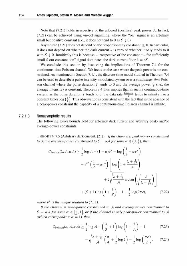
154 Amos Lapidoth, Stefan M. Moser, and Michèle Wigger
Note that (7.21) holds irrespective of the allowed (positive) peak power A. In fact,(7.21) can be achieved using on–off signalling, where the “on” signal is an arbitrarysmall but positive constant (i.e., it does not tend to 0 as E ↓ 0).
Asymptote (7.21) does not depend on the proportionality constant c ≥ 0. In particular,it does not depend on whether the dark current λ is zero or whether it only tends to 0with E ↓ 0. Intuitively this is because – irrespective of the constant c – for sufficientlysmall E our constant “on” signal dominates the dark-current floor λ = cE .
We conclude this section by discussing the implications of Theorem 7.4 for thecontinuous-time Poisson channel. We focus on the case where the peak power is not con-strained. As mentioned in Section 7.1.1, the discrete-time model studied in Theorem 7.4can be used to describe a pulse intensity modulated system over a continuous-time Pois-son channel where the pulse duration T tends to 0 and the average power E
T (i.e., theaverage intensity) is constant. Theorem 7.4 thus implies that in such a continuous-timesystem, as the pulse duration T tends to 0, the data rate CPoisson
T tends to infinity like aconstant times log
( 1T
). This observation is consistent with the fact that in the absence of
a peak-power constraint the capacity of a continuous-time Poisson channel is infinite.
7.2.1.3 Nonasymptotic resultsThe following lower bounds hold for arbitrary dark current and arbitrary peak- and/oraverage-power constraints.
TH E O R E M 7.5 (Arbitrary dark current, [21]) If the channel is peak-power constrainedto A and average-power constrained to E = αA for some α ∈ (
0, 13
), then
CPoisson(λ,A,αA) ≥ 1
2logA− (1− α)ν∗ − log
(1
2− αν∗
)
− eν∗(
1
2− αν∗
)⎡⎣log
(1+ λ+ 1
12
A
)
+ 2
√λ+ 1
12
A arctan
(√A
λ+ 112
)⎤⎦+ (E + 1) log
(1+ 1
E)− 1− 1
2log(2πe), (7.22)
where ν∗ is the unique solution to (7.11).If the channel is peak-power constrained to A and average-power constrained to
E = αA for some α ∈ [ 13 , 1
], or if the channel is only peak-power constrained to A
(which corresponds to α = 1), then
CPoisson(λ,A,αA) ≥ 1
2logA+
(A3+ 1
)log
(1+ 3
A)− 1 (7.23)
−√λ+ 1
12
A(π
4+ 1
2log 2
)− 1
2log
(πe
2
). (7.24)
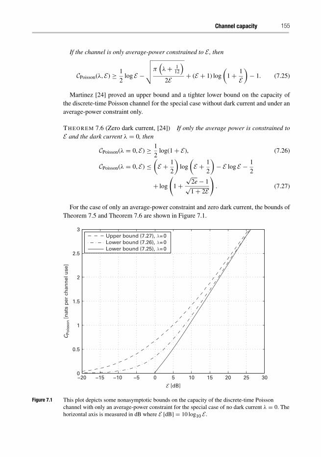
Channel capacity 155
If the channel is only average-power constrained to E , then
CPoisson(λ, E) ≥ 1
2log E −
√√√√π(λ+ 1
12
)2E + (E + 1) log
(1+ 1
E)− 1. (7.25)
Martinez [24] proved an upper bound and a tighter lower bound on the capacity ofthe discrete-time Poisson channel for the special case without dark current and under anaverage-power constraint only.
TH E O R E M 7.6 (Zero dark current, [24]) If only the average power is constrained toE and the dark current λ = 0, then
CPoisson(λ = 0, E) ≥ 1
2log(1+ E), (7.26)
CPoisson(λ = 0, E) ≤(E + 1
2
)log
(E + 1
2
)− E log E − 1
2
+ log
(1+
√2e− 1√1+ 2E
). (7.27)
For the case of only an average-power constraint and zero dark current, the bounds ofTheorem 7.5 and Theorem 7.6 are shown in Figure 7.1.
−20 −15 −10 −5 0 5 10 15 20 25 300
0.5
1
1.5
2
2.5
3
CP
ois
son [
nat
s p
er c
han
nel
use
]
Upper bound (7.27), λ = 0Lower bound (7.26), λ = 0Lower bound (7.25), λ = 0
Figure 7.1 This plot depicts some nonasymptotic bounds on the capacity of the discrete-time Poissonchannel with only an average-power constraint for the special case of no dark current λ = 0. Thehorizontal axis is measured in dB where E [dB] = 10 log10 E .
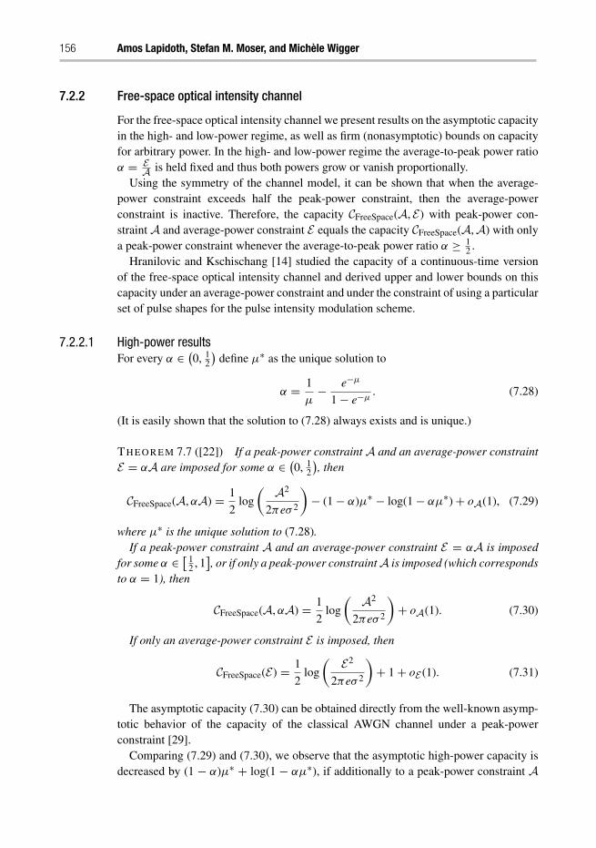
156 Amos Lapidoth, Stefan M. Moser, and Michèle Wigger
7.2.2 Free-space optical intensity channel
For the free-space optical intensity channel we present results on the asymptotic capacityin the high- and low-power regime, as well as firm (nonasymptotic) bounds on capacityfor arbitrary power. In the high- and low-power regime the average-to-peak power ratioα = E
A is held fixed and thus both powers grow or vanish proportionally.Using the symmetry of the channel model, it can be shown that when the average-
power constraint exceeds half the peak-power constraint, then the average-powerconstraint is inactive. Therefore, the capacity CFreeSpace(A, E) with peak-power con-straint A and average-power constraint E equals the capacity CFreeSpace(A,A) with onlya peak-power constraint whenever the average-to-peak power ratio α ≥ 1
2 .Hranilovic and Kschischang [14] studied the capacity of a continuous-time version
of the free-space optical intensity channel and derived upper and lower bounds on thiscapacity under an average-power constraint and under the constraint of using a particularset of pulse shapes for the pulse intensity modulation scheme.
7.2.2.1 High-power resultsFor every α ∈ (
0, 12
)define μ∗ as the unique solution to
α = 1
μ− e−μ
1− e−μ. (7.28)
(It is easily shown that the solution to (7.28) always exists and is unique.)
TH E O R E M 7.7 ([22]) If a peak-power constraint A and an average-power constraintE = αA are imposed for some α ∈ (
0, 12
), then
CFreeSpace(A,αA) = 1
2log
( A2
2πeσ 2
)− (1− α)μ∗ − log(1− αμ∗)+ oA(1), (7.29)
where μ∗ is the unique solution to (7.28).If a peak-power constraint A and an average-power constraint E = αA is imposed
for some α ∈ [ 12 , 1
], or if only a peak-power constraint A is imposed (which corresponds
to α = 1), then
CFreeSpace(A,αA) = 1
2log
( A2
2πeσ 2
)+ oA(1). (7.30)
If only an average-power constraint E is imposed, then
CFreeSpace(E) = 1
2log
( E2
2πeσ 2
)+ 1+ oE (1). (7.31)
The asymptotic capacity (7.30) can be obtained directly from the well-known asymp-totic behavior of the capacity of the classical AWGN channel under a peak-powerconstraint [29].
Comparing (7.29) and (7.30), we observe that the asymptotic high-power capacity isdecreased by (1 − α)μ∗ + log(1 − αμ∗), if additionally to a peak-power constraint A
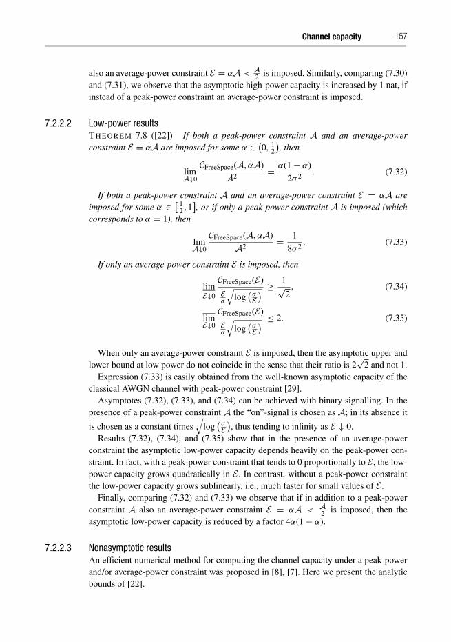
Channel capacity 157
also an average-power constraint E = αA < A2 is imposed. Similarly, comparing (7.30)
and (7.31), we observe that the asymptotic high-power capacity is increased by 1 nat, ifinstead of a peak-power constraint an average-power constraint is imposed.
7.2.2.2 Low-power resultsTH E O R E M 7.8 ([22]) If both a peak-power constraint A and an average-powerconstraint E = αA are imposed for some α ∈ (
0, 12
), then
limA↓0
CFreeSpace(A,αA)
A2= α(1− α)
2σ 2. (7.32)
If both a peak-power constraint A and an average-power constraint E = αA areimposed for some α ∈ [ 1
2 , 1], or if only a peak-power constraint A is imposed (which
corresponds to α = 1), then
limA↓0
CFreeSpace(A,αA)
A2= 1
8σ 2. (7.33)
If only an average-power constraint E is imposed, then
limE↓0
CFreeSpace(E)
Eσ
√log
(σE) ≥ 1√
2, (7.34)
limE↓0
CFreeSpace(E)
Eσ
√log
(σE) ≤ 2. (7.35)
When only an average-power constraint E is imposed, then the asymptotic upper andlower bound at low power do not coincide in the sense that their ratio is 2
√2 and not 1.
Expression (7.33) is easily obtained from the well-known asymptotic capacity of theclassical AWGN channel with peak-power constraint [29].
Asymptotes (7.32), (7.33), and (7.34) can be achieved with binary signalling. In thepresence of a peak-power constraint A the “on”-signal is chosen as A; in its absence it
is chosen as a constant times√
log(σE), thus tending to infinity as E ↓ 0.
Results (7.32), (7.34), and (7.35) show that in the presence of an average-powerconstraint the asymptotic low-power capacity depends heavily on the peak-power con-straint. In fact, with a peak-power constraint that tends to 0 proportionally to E , the low-power capacity grows quadratically in E . In contrast, without a peak-power constraintthe low-power capacity grows sublinearly, i.e., much faster for small values of E .
Finally, comparing (7.32) and (7.33) we observe that if in addition to a peak-powerconstraint A also an average-power constraint E = αA < A
2 is imposed, then theasymptotic low-power capacity is reduced by a factor 4α(1− α).
7.2.2.3 Nonasymptotic resultsAn efficient numerical method for computing the channel capacity under a peak-powerand/or average-power constraint was proposed in [8], [7]. Here we present the analyticbounds of [22].
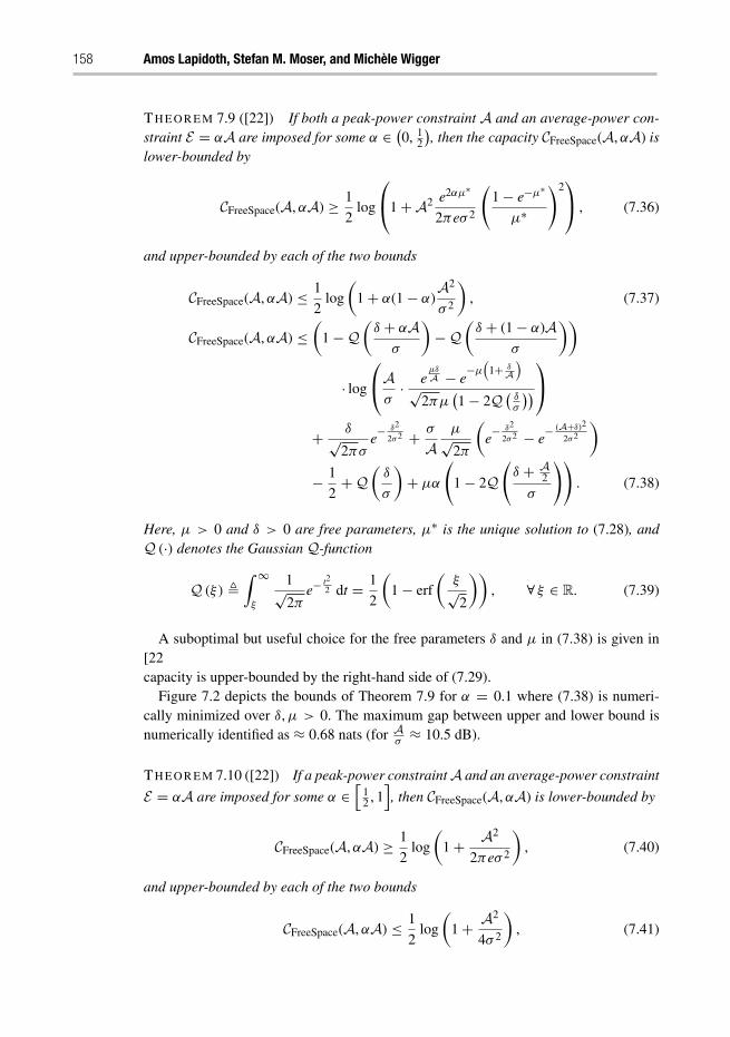
158 Amos Lapidoth, Stefan M. Moser, and Michèle Wigger
TH E O R E M 7.9 ([22]) If both a peak-power constraint A and an average-power con-straint E = αA are imposed for some α ∈ (
0, 12
), then the capacity CFreeSpace(A,αA) is
lower-bounded by
CFreeSpace(A,αA) ≥ 1
2log
⎛⎝1+A2 e2αμ∗
2πeσ 2
(1− e−μ∗
μ∗
)2⎞⎠ , (7.36)
and upper-bounded by each of the two bounds
CFreeSpace(A,αA) ≤ 1
2log
(1+ α(1− α)
A2
σ 2
), (7.37)
CFreeSpace(A,αA) ≤(
1−Q(δ + αA
σ
)−Q
(δ + (1− α)A
σ
))
· log
⎛⎝A
σ· e
μδA − e
−μ(
1+ δA
)√
2πμ(1− 2Q (
δσ
))⎞⎠
+ δ√2πσ
e− δ2
2σ2 + σ
Aμ√2π
(e− δ2
2σ2 − e− (A+δ)2
2σ2
)
− 1
2+Q
(δ
σ
)+ μα
(1− 2Q
(δ + A
2
σ
)). (7.38)
Here, μ > 0 and δ > 0 are free parameters, μ∗ is the unique solution to (7.28), andQ (·) denotes the Gaussian Q-function
Q (ξ) �∫ ∞
ξ
1√2π
e−t22 dt = 1
2
(1− erf
(ξ√2
)), ∀ ξ ∈ R. (7.39)
A suboptimal but useful choice for the free parameters δ and μ in (7.38) is given in[22, Eqs. (14) and (15)]. This choice suffices to prove that the asymptotic high-powercapacity is upper-bounded by the right-hand side of (7.29).
Figure 7.2 depicts the bounds of Theorem 7.9 for α = 0.1 where (7.38) is numeri-cally minimized over δ,μ > 0. The maximum gap between upper and lower bound isnumerically identified as ≈ 0.68 nats (for A
σ≈ 10.5 dB).
TH E O R E M 7.10 ([22]) If a peak-power constraint A and an average-power constraint
E = αA are imposed for some α ∈[
12 , 1
], then CFreeSpace(A,αA) is lower-bounded by
CFreeSpace(A,αA) ≥ 1
2log
(1+ A2
2πeσ 2
), (7.40)
and upper-bounded by each of the two bounds
CFreeSpace(A,αA) ≤ 1
2log
(1+ A2
4σ 2
), (7.41)

Channel capacity 159
−10 −5 0 5 10 15 20 250
0.5
1
1.5
2
2.5
3
σ [dB]
CFr
eeS
pac
e [n
ats
per
ch
ann
el u
se]
Upper bound (7.37), α = 0.1Upper bound (7.38), α = 0.1Lower bound (7.36), α = 0.1
Figure 7.2 Bounds of Theorem 7.9 for α = 0.1.
CFreeSpace(A,αA) ≤(
1− 2Q(δ + A
2
σ
))log
(A+ 2δ
σ√
2π(1− 2Q (
δσ
)))
− 1
2+Q
(δ
σ
)+ δ√
2πσe− δ2
2σ2 , (7.42)
where δ > 0 is a free parameter.
A suboptimal but useful choice for the free parameter δ > 0 in (7.42) is given in[22, Eq. (21)]. This choice suffices to prove that the asymptotic high-power capacity isupper-bounded by the right-hand side of (7.30).
Figure 7.3 depicts the bounds of Theorem 7.10, where upper bound (7.42) is numer-ically minimized over δ > 0. The maximum gap between upper and lower bound isnumerically identified as ≈ 0.50 nats (for A
σ≈ 6.4 dB).
TH E O R E M 7.11 ([22]) If only an average-power constraint E is imposed, then thecapacity CFreeSpace(E) is lower-bounded by
CFreeSpace(E) ≥ 1
2log
(1+ E2e
2πσ 2
), (7.43)
and upper-bounded by each of the bounds
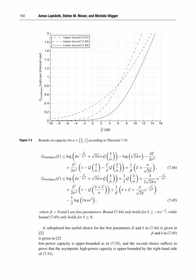
160 Amos Lapidoth, Stefan M. Moser, and Michèle Wigger
−10 −8 −6 −4 −2 0 2 4 6 8 10 12 14 160
0.2
0.4
0.6
0.8
1
1.2
1.4
1.6
1.8
2
Lower bound (7.40)
Upper bound (7.41)Upper bound (7.42)
CFr
eeS
pac
e [n
ats
per
ch
ann
el u
se]
σ [dB]
Figure 7.3 Bounds on capacity for α ∈ [ 12 , 1
]according to Theorem 7.10.
CFreeSpace(E) ≤ log
(βe− δ2
2σ2 +√2πσQ(δ
σ
))− log
(√2πσ
)− δE
2σ 2
+ δ2
2σ 2
(1−Q
(δ
σ
)− E
δQ
(δ
σ
))+ 1
β
(E + σ√
2π
), (7.44)
CFreeSpace(E) ≤ log
(βe− δ2
2σ2 +√2πσQ(δ
σ
))+ 1
2Q
(δ
σ
)+ δ
2√
2πσe− δ2
2σ2
+ δ2
2σ 2
(1−Q
(δ + Eσ
))+ 1
β
(δ + E + σ√
2πe− δ2
2σ2
)
− 1
2log
(2πeσ 2
), (7.45)
where β > 0 and δ are free parameters. Bound (7.44) only holds for δ ≤ −σe− 12 , while
bound (7.45) only holds for δ ≥ 0.
A suboptimal but useful choice for the free parameters β and δ in (7.44) is given in[22, Eqs. (29) and (30)] and a suboptimal choice for the free parameters β and δ in (7.45)is given in [22, Eqs. (31) and (32)]. The first choice suffices to prove that the asymptoticlow-power capacity is upper-bounded as in (7.35), and the second choice suffices toprove that the asymptotic high-power capacity is upper-bounded by the right-hand sideof (7.31).
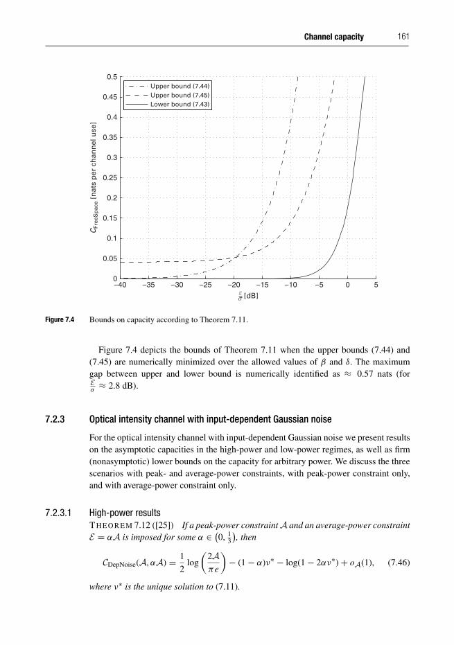
Channel capacity 161
−40 −35 −30 −25 −20 −15 −10 −5 0 50
0.05
0.1
0.15
0.2
0.25
0.3
0.35
0.4
0.45
0.5
Lower bound (7.43)
Upper bound (7.44)Upper bound (7.45)
CFr
eeS
pac
e [n
ats
per
ch
ann
el u
se]
εσ [dB]
Figure 7.4 Bounds on capacity according to Theorem 7.11.
Figure 7.4 depicts the bounds of Theorem 7.11 when the upper bounds (7.44) and(7.45) are numerically minimized over the allowed values of β and δ. The maximumgap between upper and lower bound is numerically identified as ≈ 0.57 nats (forEσ≈ 2.8 dB).
7.2.3 Optical intensity channel with input-dependent Gaussian noise
For the optical intensity channel with input-dependent Gaussian noise we present resultson the asymptotic capacities in the high-power and low-power regimes, as well as firm(nonasymptotic) lower bounds on the capacity for arbitrary power. We discuss the threescenarios with peak- and average-power constraints, with peak-power constraint only,and with average-power constraint only.
7.2.3.1 High-power resultsTH E O R E M 7.12 ([25]) If a peak-power constraint A and an average-power constraintE = αA is imposed for some α ∈ (
0, 13
), then
CDepNoise(A,αA) = 1
2log
(2Aπe
)− (1− α)ν∗ − log(1− 2αν∗)+ oA(1), (7.46)
where ν∗ is the unique solution to (7.11).
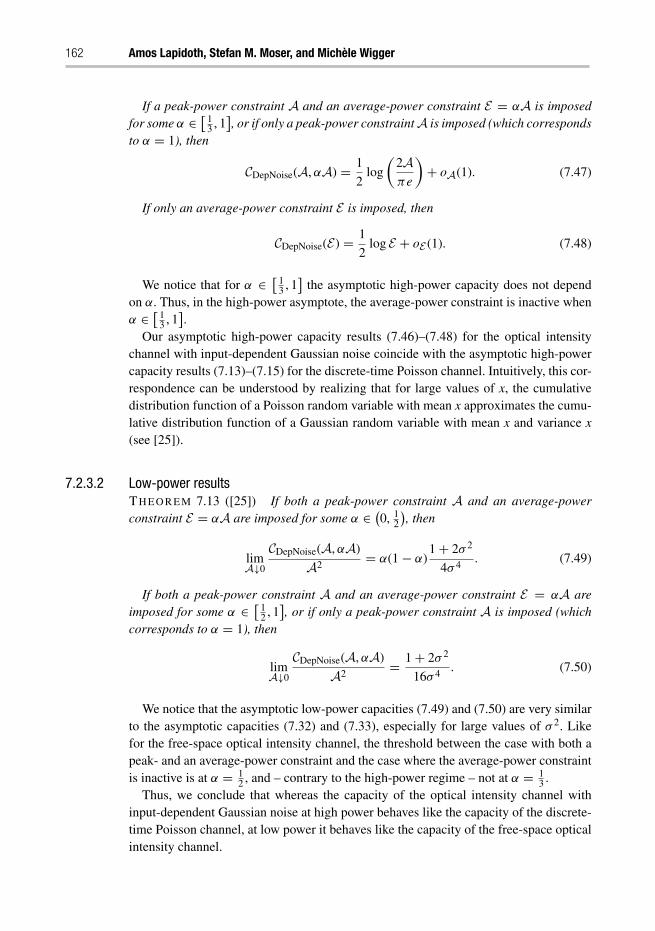
162 Amos Lapidoth, Stefan M. Moser, and Michèle Wigger
If a peak-power constraint A and an average-power constraint E = αA is imposedfor some α ∈ [ 1
3 , 1], or if only a peak-power constraint A is imposed (which corresponds
to α = 1), then
CDepNoise(A,αA) = 1
2log
(2Aπe
)+ oA(1). (7.47)
If only an average-power constraint E is imposed, then
CDepNoise(E) = 1
2log E + oE (1). (7.48)
We notice that for α ∈ [ 13 , 1
]the asymptotic high-power capacity does not depend
on α. Thus, in the high-power asymptote, the average-power constraint is inactive whenα ∈ [ 1
3 , 1].
Our asymptotic high-power capacity results (7.46)–(7.48) for the optical intensitychannel with input-dependent Gaussian noise coincide with the asymptotic high-powercapacity results (7.13)–(7.15) for the discrete-time Poisson channel. Intuitively, this cor-respondence can be understood by realizing that for large values of x, the cumulativedistribution function of a Poisson random variable with mean x approximates the cumu-lative distribution function of a Gaussian random variable with mean x and variance x(see [25]).
7.2.3.2 Low-power resultsTH E O R E M 7.13 ([25]) If both a peak-power constraint A and an average-powerconstraint E = αA are imposed for some α ∈ (
0, 12
), then
limA↓0
CDepNoise(A,αA)
A2= α(1− α)
1+ 2σ 2
4σ 4. (7.49)
If both a peak-power constraint A and an average-power constraint E = αA areimposed for some α ∈ [ 1
2 , 1], or if only a peak-power constraint A is imposed (which
corresponds to α = 1), then
limA↓0
CDepNoise(A,αA)
A2= 1+ 2σ 2
16σ 4. (7.50)
We notice that the asymptotic low-power capacities (7.49) and (7.50) are very similarto the asymptotic capacities (7.32) and (7.33), especially for large values of σ 2. Likefor the free-space optical intensity channel, the threshold between the case with both apeak- and an average-power constraint and the case where the average-power constraintis inactive is at α = 1
2 , and – contrary to the high-power regime – not at α = 13 .
Thus, we conclude that whereas the capacity of the optical intensity channel withinput-dependent Gaussian noise at high power behaves like the capacity of the discrete-time Poisson channel, at low power it behaves like the capacity of the free-space opticalintensity channel.
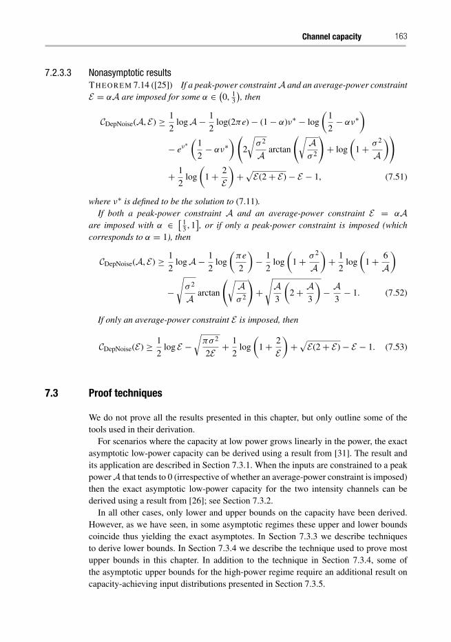
Channel capacity 163
7.2.3.3 Nonasymptotic resultsTH E O R E M 7.14 ([25]) If a peak-power constraint A and an average-power constraintE = αA are imposed for some α ∈ (
0, 13
), then
CDepNoise(A, E) ≥ 1
2logA− 1
2log(2πe)− (1− α)ν∗ − log
(1
2− αν∗
)
− eν∗(
1
2− αν∗
)(2
√σ 2
A arctan
(√Aσ 2
)+ log
(1+ σ 2
A))
+ 1
2log
(1+ 2
E)+√
E(2+ E)− E − 1, (7.51)
where ν∗ is defined to be the solution to (7.11).If both a peak-power constraint A and an average-power constraint E = αA
are imposed with α ∈ [ 13 , 1
], or if only a peak-power constraint is imposed (which
corresponds to α = 1), then
CDepNoise(A, E) ≥ 1
2logA− 1
2log
(πe
2
)− 1
2log
(1+ σ 2
A)+ 1
2log
(1+ 6
A)
−√σ 2
A arctan
(√Aσ 2
)+
√A3
(2+ A
3
)− A
3− 1. (7.52)
If only an average-power constraint E is imposed, then
CDepNoise(E) ≥ 1
2log E −
√πσ 2
2E + 1
2log
(1+ 2
E)+√
E(2+ E)− E − 1. (7.53)
7.3 Proof techniques
We do not prove all the results presented in this chapter, but only outline some of thetools used in their derivation.
For scenarios where the capacity at low power grows linearly in the power, the exactasymptotic low-power capacity can be derived using a result from [31]. The result andits application are described in Section 7.3.1. When the inputs are constrained to a peakpower A that tends to 0 (irrespective of whether an average-power constraint is imposed)then the exact asymptotic low-power capacity for the two intensity channels can bederived using a result from [26]; see Section 7.3.2.
In all other cases, only lower and upper bounds on the capacity have been derived.However, as we have seen, in some asymptotic regimes these upper and lower boundscoincide thus yielding the exact asymptotes. In Section 7.3.3 we describe techniquesto derive lower bounds. In Section 7.3.4 we describe the technique used to prove mostupper bounds in this chapter. In addition to the technique in Section 7.3.4, some ofthe asymptotic upper bounds for the high-power regime require an additional result oncapacity-achieving input distributions presented in Section 7.3.5.
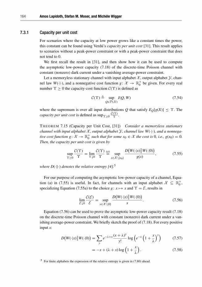
164 Amos Lapidoth, Stefan M. Moser, and Michèle Wigger
7.3.1 Capacity per unit cost
For scenarios where the capacity at low power grows like a constant times the power,this constant can be found using Verdú’s capacity per unit cost [31]. This result appliesto scenarios without a peak-power constraint or with a peak-power constraint that doesnot tend to 0.
We first recall the result in [31], and then show how it can be used to computethe asymptotic low-power capacity (7.18) of the discrete-time Poisson channel withconstant (nonzero) dark current under a vanishing average-power constraint.
Let a memoryless stationary channel with input alphabet X , output alphabet Y , chan-nel law W(·|·), and a nonnegative cost function g : X → R
+0 be given. For every real
number ϒ ≥ 0 the capacity-cost function C(ϒ) is defined as
C(ϒ) � supQ∈P(X )
I(Q, W) (7.54)
where the supremum is over all input distributions Q that satisfy EQ[g(X)] ≤ ϒ . Thecapacity per unit cost is defined as supϒ≥0
C(ϒ)ϒ
.
TH E O R E M 7.15 (Capacity per Unit Cost, [31]) Consider a memoryless stationarychannel with input alphabet X , output alphabet Y , channel law W(·|·), and a nonnega-tive cost function g : X → R
+0 such that for some x0 ∈ X the cost is 0, i.e., g(x0) = 0.
Then, the capacity per unit cost is given by
supϒ≥0
C(ϒ)
ϒ= lim
ϒ↓0
C(ϒ)
ϒ
(a)= supx∈X \{x0}
D(W(·|x)
∥∥W(·|0))
g(x), (7.55)
where D(·‖·) denotes the relative entropy [4].5
For our purpose of computing the asymptotic low-power capacity of a channel, Equa-tion (a) in (7.55) is useful. In fact, for channels with an input alphabet X ⊆ R
+0 ,
specializing Equation (7.55a) to the choice g : x �→ x and ϒ = E , results in
limE↓0
C(E)
E = supx∈X \{0}
D(W(·|x)
∥∥W(·|0))
x. (7.56)
Equation (7.56) can be used to prove the asymptotic low-power capacity result (7.18)on the discrete-time Poisson channel with constant (nonzero) dark current under a van-ishing average-power constraint. We briefly sketch the proof of (7.18). For every positiveinput x:
D(W(·|x)
∥∥W(·|0)) =∑
y
e−λ+x (x+ λ)y
y! log(
e−x(
1+ x
λ
)y)(7.57)
= −x+ (λ+ x) log(
1+ x
λ
). (7.58)
5 For finite alphabets the expression of the relative entropy is given in (7.80) ahead.
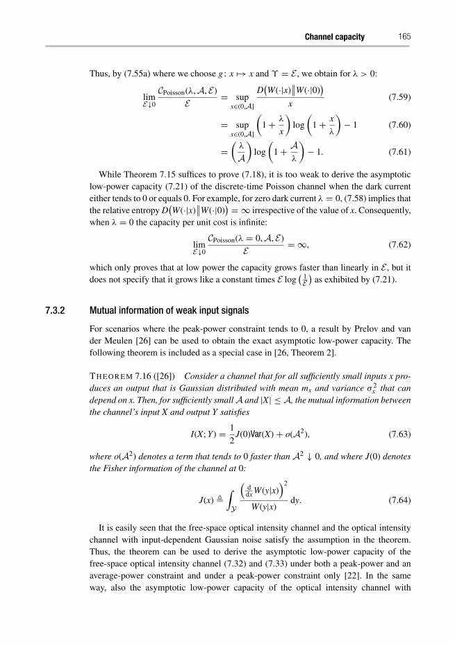
Channel capacity 165
Thus, by (7.55a) where we choose g : x �→ x and ϒ = E , we obtain for λ > 0:
limE↓0
CPoisson(λ,A, E)
E = supx∈(0,A]
D(W(·|x)
∥∥W(·|0))
x(7.59)
= supx∈(0,A]
(1+ λ
x
)log
(1+ x
λ
)− 1 (7.60)
=(λ
A)
log
(1+ A
λ
)− 1. (7.61)
While Theorem 7.15 suffices to prove (7.18), it is too weak to derive the asymptoticlow-power capacity (7.21) of the discrete-time Poisson channel when the dark currenteither tends to 0 or equals 0. For example, for zero dark current λ = 0, (7.58) implies thatthe relative entropy D
(W(·|x)
∥∥W(·|0)) = ∞ irrespective of the value of x. Consequently,
when λ = 0 the capacity per unit cost is infinite:
limE↓0
CPoisson(λ = 0,A, E)
E = ∞, (7.62)
which only proves that at low power the capacity grows faster than linearly in E , but itdoes not specify that it grows like a constant times E log
( 1E)
as exhibited by (7.21).
7.3.2 Mutual information of weak input signals
For scenarios where the peak-power constraint tends to 0, a result by Prelov and vander Meulen [26] can be used to obtain the exact asymptotic low-power capacity. Thefollowing theorem is included as a special case in [26, Theorem 2].
TH E O R E M 7.16 ([26]) Consider a channel that for all sufficiently small inputs x pro-duces an output that is Gaussian distributed with mean mx and variance σ 2
x that candepend on x. Then, for sufficiently small A and |X| ≤ A, the mutual information betweenthe channel’s input X and output Y satisfies
I(X; Y) = 1
2J(0)Var(X)+ o(A2), (7.63)
where o(A2) denotes a term that tends to 0 faster than A2 ↓ 0, and where J(0) denotesthe Fisher information of the channel at 0:
J(x) �∫Y
(ddx W(y|x)
)2
W(y|x)dy. (7.64)
It is easily seen that the free-space optical intensity channel and the optical intensitychannel with input-dependent Gaussian noise satisfy the assumption in the theorem.Thus, the theorem can be used to derive the asymptotic low-power capacity of thefree-space optical intensity channel (7.32) and (7.33) under both a peak-power and anaverage-power constraint and under a peak-power constraint only [22]. In the sameway, also the asymptotic low-power capacity of the optical intensity channel with
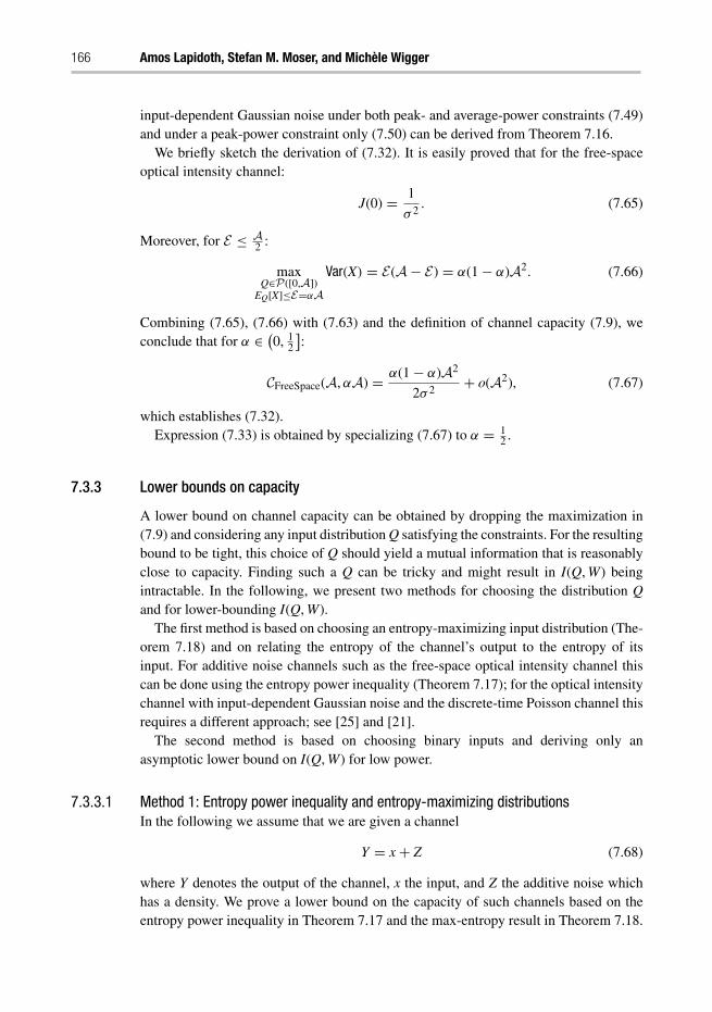
166 Amos Lapidoth, Stefan M. Moser, and Michèle Wigger
input-dependent Gaussian noise under both peak- and average-power constraints (7.49)and under a peak-power constraint only (7.50) can be derived from Theorem 7.16.
We briefly sketch the derivation of (7.32). It is easily proved that for the free-spaceoptical intensity channel:
J(0) = 1
σ 2. (7.65)
Moreover, for E ≤ A2 :
maxQ∈P([0,A])
EQ[X]≤E=αAVar(X) = E(A− E) = α(1− α)A2. (7.66)
Combining (7.65), (7.66) with (7.63) and the definition of channel capacity (7.9), weconclude that for α ∈ (
0, 12
]:
CFreeSpace(A,αA) = α(1− α)A2
2σ 2+ o(A2), (7.67)
which establishes (7.32).Expression (7.33) is obtained by specializing (7.67) to α = 1
2 .
7.3.3 Lower bounds on capacity
A lower bound on channel capacity can be obtained by dropping the maximization in(7.9) and considering any input distribution Q satisfying the constraints. For the resultingbound to be tight, this choice of Q should yield a mutual information that is reasonablyclose to capacity. Finding such a Q can be tricky and might result in I(Q, W) beingintractable. In the following, we present two methods for choosing the distribution Qand for lower-bounding I(Q, W).
The first method is based on choosing an entropy-maximizing input distribution (The-orem 7.18) and on relating the entropy of the channel’s output to the entropy of itsinput. For additive noise channels such as the free-space optical intensity channel thiscan be done using the entropy power inequality (Theorem 7.17); for the optical intensitychannel with input-dependent Gaussian noise and the discrete-time Poisson channel thisrequires a different approach; see [25] and [21].
The second method is based on choosing binary inputs and deriving only anasymptotic lower bound on I(Q, W) for low power.
7.3.3.1 Method 1: Entropy power inequality and entropy-maximizing distributionsIn the following we assume that we are given a channel
Y = x+ Z (7.68)
where Y denotes the output of the channel, x the input, and Z the additive noise whichhas a density. We prove a lower bound on the capacity of such channels based on theentropy power inequality in Theorem 7.17 and the max-entropy result in Theorem 7.18.
Channel capacity 167
TH E O R E M 7.17 (Entropy power inequality, [4]) If X and Z are independent randomvariables with densities, then
e2h(X+Z) ≥ e2h(X) + e2h(Z). (7.69)
TH E O R E M 7.18 (Max-entropy theorem, [4]) Let an alphabet X ⊆ R, a nonnegativeinteger m, a set of m functions {ri : X → R}mi=1, and m values {ai ∈ R}mi=1 be given, andconsider the optimization problem
supQ∈P(X )
h(X) (7.70)
subject to
EQ[ri(X)] = ai, i ∈ {1, . . . , m}. (7.71)
If there exist real numbers κ0, . . . , κm such that the distributionQ with density
Q′(x) � eκ0+∑m
i=1 κiri(x), x ∈ X , (7.72)
satisfies constraints (7.71) when Q is replaced byQ, thenQ is the unique distribution onX subject to (7.71) that achieves the supremum in (7.70).
Using the entropy power inequality, a lower bound on the capacity of additive noisechannels as in (7.68) is obtained by noting that for any input X that has a density wehave
C ≥ I(X; Y) (7.73)
= h(Y)− h(Y|X) (7.74)
= h(X + Z)− h(Z) (7.75)
≥ 1
2log
(e2h(X) + e2h(Z)
)− h(Z). (7.76)
Obviously, the lower bound is made tightest if the density of X is chosen so as to maxi-mize the differential entropy under the given constraints. For many interesting scenariosthe desired density can be found using the max-entropy result in Theorem 7.18.
This method was used to derive the lower bounds on the capacity of the free-spaceoptical intensity channel both in the asymptotic high-power regime as well as in thenonasymptotic regime.
We quickly sketch how this method is used to prove lower bound (7.36). ByTheorem 7.18 the density that maximizes differential entropy under a nonnegativityconstraint, a peak constraint A, and an average constraint E = αA ≤ 1
2A is given by6
Q′(x) = 1
A · μ∗
1− e−μ∗e−
μ∗xA , 0 ≤ x ≤ A, (7.77)
6 Using the symmetry of the channel and the uniqueness of the capacity-achieving input distribution [3] it iseasily proved that for the free-space optical intensity channel and E ≤ 1
2A the average-power constraint isalways active.
168 Amos Lapidoth, Stefan M. Moser, and Michèle Wigger
where μ∗ is the unique solution to (7.28). We also note that since the noise of the free-space optical intensity channel is Gaussian with variance σ 2:
1
2log
(e2h(X) + e2h(Z)
)− h(Z) = 1
2log
(1+ e2h(X)
2πeσ 2
). (7.78)
Evaluating the right-hand side of (7.78) for an input X that has density (7.77) andcombining the result with (7.76) yields the desired lower bound (7.36).
7.3.3.2 Method 2: Binary inputs and asymptotic lower boundIt is well known that the capacity-achieving input distribution for our channels is discreteand that for sufficiently low power the number of mass points is two [27], [3]. Thus,good lower bounds for the channel capacity at low power can be obtained by evaluatingthe mutual information I(X; Y) for binary inputs. Unfortunately, for most such binaryinputs an analytic expression for the mutual information I(X; Y) seems infeasible evenin the asymptotic regime of low power. We therefore propose to lower-bound the mutualinformation and only derive the low-power asymptote of the lower bound.
This method was used to prove: the lower bound on the asymptotic low-powercapacity of the discrete-time Poisson channel with constant dark current (7.19); theachievability of the asymptotic low-power capacity of the discrete-time Poisson channelwith vanishing dark current (7.21); and the lower bound on the asymptotic low-powercapacity of the free-space optical intensity channel (7.34). The exact derivations aretedious; for details see [23] and [22].
7.3.4 Duality-based upper bounds on capacity
We present an approach from [19], [20] for deriving upper bounds on the channel capac-ity. The approach is explained here for discrete memoryless channels W(·|·) with finiteinput and output alphabets X and Y . The generalization to continuous alphabets withinput constraints is relatively straightforward.7
In [5] a dual expression for the channel capacity of discrete memoryless channels in(7.9) was presented:
C = minR∈P(Y)
maxx∈X
D(W(·|x)
∥∥R(·)), (7.79)
where D(·‖·) denotes relative entropy [4]
D(W(·|x)
∥∥R(·)) =∑y∈Y
W(y|x) log
(W(y|x)
R(y)
). (7.80)
This dual expression allows us to easily obtain upper bounds on the channel capacity. Infact, every choice of a distribution R(·) on the output Y leads to such an upper bound:
C ≤ maxx∈X
D(W(·|x)
∥∥R(·)). (7.81)
7 There are some mathematical technicalities that must be addressed, but they do not change the fundamentalidea.
Channel capacity 169
However, for every choice of the distribution R(·) a generally tighter upper bound oncapacity can be derived. In fact, by considering the identity [30]∑
x∈XQ(x)D
(W(·|x)
∥∥R(·)) = I(Q, W)+ D((QW)(·)∥∥R(·)) (7.82)
and by noting that relative entropy is nonnegative [4], we have
I(Q, W) ≤∑x∈X
Q(x)D(W(·|x)
∥∥R(·)), R ∈ P(Y). (7.83)
This leads to the following upper bound on capacity [19], [20]. For every choice of adistribution R(·) on the channel output alphabet
C ≤ EQ∗[D(W(·|X)
∥∥R(·))] , (7.84)
where Q∗ denotes a capacity-achieving input distribution, i.e., a distribution thatachieves the maximum in (7.9). It is important to note that R(·) in (7.84) can be anydistribution on the output alphabet: it need not be an output distribution that is inducedby some input distribution.
Two problems make the evaluation of the right-hand side of (7.84) difficult. Firstly,evaluating D
(W(·|x)
∥∥R(·)) analytically is generally difficult; and secondly, the right-hand side of (7.84) involves an expectation over the capacity-achieving input distributionQ∗ which in general is not known.8 So in order for the bound to be useful, a good butrelatively simple distribution R(·) has to be found for which the expectation in (7.84)over Q∗ can be computed or reasonably upper-bounded (without knowing Q∗). Often theexpectation with respect to Q∗ can be computed/bounded by using some of the knownproperties of Q∗ like, e.g., that it satisfies the input constraints or that it escapes toinfinity (see Section 7.3.5), or by using Jensen’s inequality [4] which states that forevery concave function f (·):
E[f (X)] ≤ f (E(X)) . (7.85)
Most of the upper bounds presented in this chapter have been proved using this tech-nique. Typically, in these proofs the output distribution R(·) was chosen depending onsome parameters that can be optimized at a later stage. Thus, a family of output distri-butions was chosen and a particular choice was singled out only after the evaluation of(7.84). This way one can even make the choice of R(·) depend on the channel parameterssuch as the allowed peak and average powers.9
7.3.5 Input distributions that escape to infinity
As we have seen, the capacity with peak power A and average power E = αA of manychannels of interest can be expressed at high input powers as
C(A,αA) = � logA+ χ + oA(1), (7.86)
8 If it were known, then capacity could be (at least numerically) computed directly, and no bounding wouldbe necessary.
9 Note, however, that by definition R(·) must not depend on the channel input x.
170 Amos Lapidoth, Stefan M. Moser, and Michèle Wigger
where the correction term oA(1) tends to zero as A tends to infinity. The constant � issometimes called the pre-log and is given by
� = limA↑∞
C(A,αA)
logA . (7.87)
For example, the pre-log in (7.29) is10 1 and the pre-logs in (7.13) and (7.46) are 12 . To
compute � and χ the notion of input distributions that escape to infinity can be useful.For many channels of interest the asymptotic capacity or even the pre-log can only
be achieved if the input distributions escape to infinity. Loosely speaking this meansthat the probabilities that they assign to any fixed ball tend to zero as the allowed powertends to infinity. We next define this concept more formally and explain how it can beused to compute � and χ . (For an example, see [18].)
The definition and the statements in this section are valid for general channels; theyare not restricted to optical channels. We will only assume that the input and outputalphabets X and Y of some channel are separable metric spaces and that for any setB ⊂ Y the mapping x �→ W(B|x) from X to [0, 1] is Borel measurable. We thenconsider a general cost function g : X → [0,∞) which is assumed measurable.11 Inthis setting, the capacity-cost function with an average- and a peak-cost constraint isdefined as
DE FI N I T I O N 7.1 Given a channel W(·|·) over the input alphabet X and the outputalphabet Y and given some nonnegative cost function g : X → R
+0 , we define the
capacity-cost function C :([infx∈X g(x),∞]
)2 → R+0 by
C(A, E) � supQ(·)
I(Q, W), A, E ≥ infx∈X
g(x) (7.88)
where the supremum is over all input distributions Q(·) that satisfy
Q({x ∈ X : g(x) > A}) = 0 (7.89)
and
EQ[g(X)] ≤ E . (7.90)
The following results also hold in the absence of a peak-power constraint. For brevitywe omit the explicit statements for this case.
DE FI N I T I O N 7.2 Fixing the ratio of available average-to-peak cost α � EA , we say
that a family of input distributions {QA,E (·)}A≥infxg(x)α
,E=αA on X parameterized by Aand E escapes to infinity if for any fixed A0 > 0
limA↑∞
QA,αA({x ∈ X : g(x) ≤ A0}
) = 0. (7.91)
10 Note the A2 in the logarithm that will multiply the factor 12 in front of the logarithm by 2.
11 For an intuitive understanding of the following definitions and some of their consequences, it is best tofocus on the example of the channel models shown in Section 7.1 where the channel inputs are nonnegativereal numbers and where the cost function g(·) is g(x) = x, ∀ x ≥ 0.
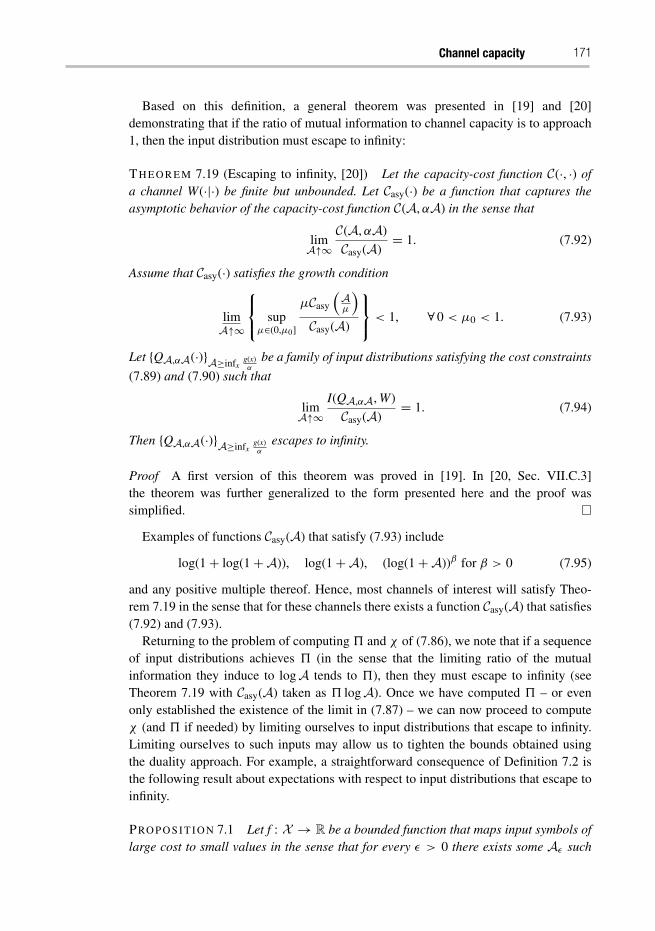
Channel capacity 171
Based on this definition, a general theorem was presented in [19] and [20]demonstrating that if the ratio of mutual information to channel capacity is to approach1, then the input distribution must escape to infinity:
TH E O R E M 7.19 (Escaping to infinity, [20]) Let the capacity-cost function C(·, ·) ofa channel W(·|·) be finite but unbounded. Let Casy(·) be a function that captures theasymptotic behavior of the capacity-cost function C(A,αA) in the sense that
limA↑∞
C(A,αA)
Casy(A)= 1. (7.92)
Assume that Casy(·) satisfies the growth condition
limA↑∞
⎧⎨⎩ sup
μ∈(0,μ0]
μCasy
(Aμ
)Casy(A)
⎫⎬⎭ < 1, ∀ 0 < μ0 < 1. (7.93)
Let {QA,αA(·)}A≥infxg(x)α
be a family of input distributions satisfying the cost constraints
(7.89) and (7.90) such that
limA↑∞
I(QA,αA, W)
Casy(A)= 1. (7.94)
Then {QA,αA(·)}A≥infxg(x)α
escapes to infinity.
Proof A first version of this theorem was proved in [19]. In [20, Sec. VII.C.3]the theorem was further generalized to the form presented here and the proof wassimplified.
Examples of functions Casy(A) that satisfy (7.93) include
log(1+ log(1+A)), log(1+A), (log(1+A))β for β > 0 (7.95)
and any positive multiple thereof. Hence, most channels of interest will satisfy Theo-rem 7.19 in the sense that for these channels there exists a function Casy(A) that satisfies(7.92) and (7.93).
Returning to the problem of computing � and χ of (7.86), we note that if a sequenceof input distributions achieves � (in the sense that the limiting ratio of the mutualinformation they induce to logA tends to �), then they must escape to infinity (seeTheorem 7.19 with Casy(A) taken as � logA). Once we have computed � – or evenonly established the existence of the limit in (7.87) – we can now proceed to computeχ (and � if needed) by limiting ourselves to input distributions that escape to infinity.Limiting ourselves to such inputs may allow us to tighten the bounds obtained usingthe duality approach. For example, a straightforward consequence of Definition 7.2 isthe following result about expectations with respect to input distributions that escape toinfinity.
PRO P O S I T I O N 7.1 Let f : X → R be a bounded function that maps input symbols oflarge cost to small values in the sense that for every ε > 0 there exists some Aε such
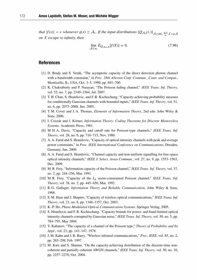
172 Amos Lapidoth, Stefan M. Moser, and Michèle Wigger
that |f (x)| < ε whenever g(x) ≥ Aε . If the input distributions {QA,E (·)}A≥infxg(x)α
,E=αAon X escape to infinity, then
limA↑∞
EQA,αA [f (X)] = 0. (7.96)
References
[1] D. Brady and S. Verdú, “The asymptotic capacity of the direct detection photon channelwith a bandwidth constraint,” in Proc. 28th Allerton Conf. Commun., Contr. and Comput.,Monticello, IL, USA, Oct. 3–5, 1990, pp. 691–700.
[2] K. Chakraborty and P. Narayan, “The Poisson fading channel,” IEEE Trans. Inf. Theory,vol. 53, no. 7, pp. 2349–2364, Jul. 2007.
[3] T. H. Chan, S. Hranilovic, and F. R. Kschischang, “Capacity-achieving probability measurefor conditionally Gaussian channels with bounded inputs,” IEEE Trans. Inf. Theory, vol. 51,no. 6, pp. 2073–2088, Jun. 2005.
[4] T. M. Cover and J. A. Thomas, Elements of Information Theory, 2nd edn. John Wiley &Sons, 2006.
[5] I. Csiszár and J. Körner, Information Theory: Coding Theorems for Discrete MemorylessSystems. Academic Press, 1981.
[6] M. H. A. Davis, “Capacity and cutoff rate for Poisson-type channels,” IEEE Trans. Inf.Theory, vol. 26, no. 6, pp. 710–715, Nov. 1980.
[7] A. A. Farid and S. Hranilovic, “Capacity of optical intensity channels with peak and averagepower constraints,” in Proc. IEEE International Conference on Communications, Dresden,Germany, Jun. 2009.
[8] A. A. Farid and S. Hranilovic, “Channel capacity and non-uniform signalling for free-spaceoptical intensity channels,” IEEE J. Select. Areas Commun., vol. 27, no. 9, pp. 1553–1563,Dec. 2009.
[9] M. R. Frey, “Information capacity of the Poisson channel,” IEEE Trans. Inf. Theory, vol. 37,no. 2, pp. 244–256, Mar. 1991.
[10] M. R. Frey, “Capacity of the Lp norm-constrained Poisson channel,” IEEE Trans. Inf.Theory, vol. 38, no. 2, pp. 445–450, Mar. 1992.
[11] R. G. Gallager, Information Theory and Reliable Communication. John Wiley & Sons,1968.
[12] S. M. Haas and J. Shapiro, “Capacity of wireless optical communications,” IEEE Trans. Inf.Theory, vol. 21, no. 8, pp. 1346–1357, Oct. 2003.
[13] K.-P. Ho, Phase-Modulated Optical Communication Systems. Springer Verlag, 2005.[14] S. Hranilovic and F. R. Kschischang, “Capacity bounds for power- and band-limited optical
intensity channels corrupted by Gaussian noise,” IEEE Trans. Inf. Theory, vol. 50, no. 5, pp.784–795, May 2004.
[15] Y. Kabanov, “The capacity of a channel of the Poisson type,” Theory of Probability and ItsAppl., vol. 23, pp. 143–147, 1978.
[16] J. M. Kahn and J. R. Barry, “Wireless infrared communications,” Proc. IEEE, vol. 85, no. 2,pp. 265–298, Feb. 1997.
[17] M. Katz and S. Shamai, “On the capacity-achieving distribution of the discrete-time non-coherent and partially coherent AWGN channels,” IEEE Trans. Inf. Theory, vol. 50, no. 10,pp. 2257–2270, Oct. 2004.
Channel capacity 173
[18] A. Lapidoth, “On phase noise channels at high SNR,” in Proc. IEEE Inf. Theory Workshop,Bangalore, India, Oct. 20–25, 2002, pp. 1–4.
[19] A. Lapidoth and S. M. Moser, “Capacity bounds via duality with applications to multiple-antenna systems on flat fading channels,” IEEE Trans. Inf. Theory, vol. 49, no. 10, pp.2426–2467, Oct. 2003.
[20] A. Lapidoth and S. M. Moser, “The fading number of single-input multiple-output fadingchannels with memory,” IEEE Trans. Inf. Theory, vol. 52, no. 2, pp. 437–453, Feb. 2006.
[21] A. Lapidoth and S. M. Moser, “On the capacity of the discrete-time Poisson channel,” IEEETrans. Inf. Theory, vol. 55, no. 1, pp. 303–322, Jan. 2009.
[22] A. Lapidoth, S. M. Moser, and M. A. Wigger, “On the capacity of free-space opticalintensity channels,” IEEE Trans. Inf. Theory, vol. 55, no. 10, pp. 4449–4461, Oct. 2009.
[23] A. Lapidoth, J. H. Shapiro, V. Venkatesan, and L. Wang, “The Poisson channel at low inputpowers,” in Proc. 25th IEEE Conv. El. & Electr. Eng. in Israel, Eilat, Israel, Dec. 3–5, 2008.
[24] A. Martinez, “Spectral efficiency of optical direct detection,” J. Opt. Soc. Am. B, vol. 24,no. 4, pp. 739–749, Apr. 2007.
[25] S. M. Moser, “Capacity results of an optical intensity channel with input-dependentGaussian noise,” IEEE Trans. Inf. Theory, vol. 58, no. 1, Jan. 2012.
[26] V. V. Prelov and E. C. van der Meulen, “An asymptotic expression for the information andcapacity of a multidimensional channel with weak input signals,” IEEE Trans. Inf. Theory,vol. 39, no. 5, pp. 1728–1735, Sept. 1993.
[27] S. Shamai (Shitz), “Capacity of a pulse amplitude modulated direct detection photon chan-nel,” in Proc. IEE, vol. 137, pt. I (Communications, Speech and Vision), no. 6, Dec. 1990,pp. 424–430.
[28] S. Shamai (Shitz) and A. Lapidoth, “Bounds on the capacity of a spectrally constrainedPoisson channel,” IEEE Trans. Inf. Theory, vol. 39, no. 1, pp. 19–29, Jan. 1993.
[29] C. E. Shannon, “A mathematical theory of communication,” Bell System Techn. J., vol. 27,pp. 379–423 and 623–656, Jul. and Oct. 1948.
[30] F. Topsøe, “An information theoretical identity and a problem involving capacity,” StudiaSci. Math. Hungar., vol. 2, pp. 291–292, 1967.
[31] S. Verdú, “On channel capacity per unit cost,” IEEE Trans. Inf. Theory, vol. 36, no. 5, pp.1019–1030, Sept. 1990.
[32] A. D. Wyner, “Capacity and error exponent for the direct detection photon channel – part Iand II,” IEEE Trans. Inf. Theory, vol. 34, no. 6, pp. 1462–1471, Nov. 1988.


Part III
Unique channels

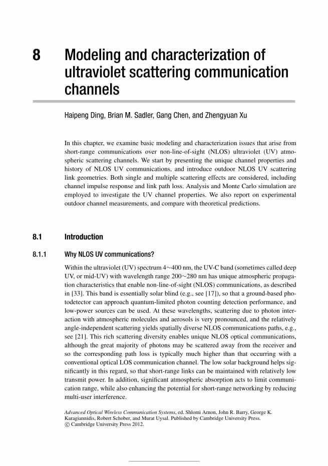
8 Modeling and characterization ofultraviolet scattering communicationchannelsHaipeng Ding, Brian M. Sadler, Gang Chen, and Zhengyuan Xu
In this chapter, we examine basic modeling and characterization issues that arise fromshort-range communications over non-line-of-sight (NLOS) ultraviolet (UV) atmo-spheric scattering channels. We start by presenting the unique channel properties andhistory of NLOS UV communications, and introduce outdoor NLOS UV scatteringlink geometries. Both single and multiple scattering effects are considered, includingchannel impulse response and link path loss. Analysis and Monte Carlo simulation areemployed to investigate the UV channel properties. We also report on experimentaloutdoor channel measurements, and compare with theoretical predictions.
8.1 Introduction
8.1.1 Why NLOS UV communications?
Within the ultraviolet (UV) spectrum 4∼400 nm, the UV-C band (sometimes called deepUV, or mid-UV) with wavelength range 200∼280 nm has unique atmospheric propaga-tion characteristics that enable non-line-of-sight (NLOS) communications, as describedin [33]. This band is essentially solar blind (e.g., see [17]), so that a ground-based pho-todetector can approach quantum-limited photon counting detection performance, andlow-power sources can be used. At these wavelengths, scattering due to photon inter-action with atmospheric molecules and aerosols is very pronounced, and the relativelyangle-independent scattering yields spatially diverse NLOS communications paths, e.g.,see [21]. This rich scattering diversity enables unique NLOS optical communications,although the great majority of photons may be scattered away from the receiver andso the corresponding path loss is typically much higher than that occurring with aconventional optical LOS communication channel. The low solar background helps sig-nificantly in this regard, so that short-range links can be maintained with relatively lowtransmit power. In addition, significant atmospheric absorption acts to limit communi-cation range, while also enhancing the potential for short-range networking by reducingmulti-user interference.
Advanced Optical Wireless Communication Systems, ed. Shlomi Arnon, John R. Barry, George K.Karagiannidis, Robert Schober, and Murat Uysal. Published by Cambridge University Press.c© Cambridge University Press 2012.
178 Haipeng Ding, Brian M. Sadler, Gang Chen, and Zhengyuan Xu
For eye and skin safety, the International Commission on Non-Ionizing Radiation Pro-tection [1] and the International Electrotechnical Commission [2] govern UV exposurepower limits. In the deep UV region, the minimum allowable continuous exposureoccurs at 270 nm at a level as low as 3 mJ per cm2 per second, while increasing to100 mJ at 200 nm and 3.4 mJ at 280 nm. So, while solar background radiation is verylow, human sensitivity is correspondingly high, and this is an important consideration insystem design.
Thus, for conditions in which low-power consumption, NLOS operability, and secu-rity are essential, while range and bandwidth requirements are modest, UV technologyprovides an interesting alternative to conventional approaches such as radio, and sofor example may find broad-ranging applications in data communication on the move,surveillance sensor networks, homeland security, unattended ground sensor (UGS) net-works, and small unit communications in urban terrain environments described in [29].
8.1.2 History of NLOS UV communications
Early studies of NLOS UV communications date to the 1960s. An early experimentallong-range link employed a high-power xenon flashtube UV source with shortest wave-length of 280 nm, and a photomultiplier tube (PMT) receiver [30]. A transmit–receiveseparation of 26 km was demonstrated, with an equivalent NLOS path length of 40 km.A NLOS UV system based on an isotropic radiating mercury arc lamp with a modulationrate of 40 kHz was also demonstrated by Fishburne et al. [12], and later Puschell andBayse [20] reported an improved UV local area network test-bed spanning a kilometerrange based on a collimated mercury-xenon lamp increasing the modulation rate up to400 kHz at an effective wavelength of 265 nm. A UV laser communication system at 266nm that radiated short pulses at high peak power was also reported by Charles et al. [4],although the modulation rate was only 600 Hz. During this early period of NLOS exper-imentation, Reilly and Warde [22] developed an elegant theoretical channel responsemodel to describe the temporal characteristics of scattered radiation in 200∼300 nm.Later Luettgen et al. [18] extended the model to examine scattering-induced angularsignal distribution and path losses.
The early UV NLOS systems were limited to employing rather bulky, power-hungry,bandwidth-limited flashtube/lamp/laser UV sources. Semiconductor UV optical sourcesoffer the potential of low cost, small size, low power, high reliability, and high band-width. State-of-the-art device technology has enabled miniaturized UV light-emittingdiodes (LEDs), for example as reported in Bai et al. [3] and Shen et al. [28]. TheseLEDs are no bigger than one square millimeter, offer a series of wavelengths in the deepUV region, typically consume electrical power of 150 mW, and radiate optical power of0.5 mW. Consequently, the arrival of this new generation of UV sources has inspired newstudies of LED-based UV systems, with applications including sensing and short-rangecommunications.
Shaw et al. [21–27] report on experiments using a 24-element LED array at 274 nm,producing 40 mW optical power. They used a relatively large transmit divergence angleof about 50o. A NLOS link was configured by setting transmitter (Tx) and receiver (Rx)pointing angles equal to 90◦ (vertical pointing). At the receiver, a Perkin Elmer PMT
Ultraviolet scattering communication channel 179
(MP-1921) was combined with a solar blind filter to achieve an overall rejection ratioexceeding 1010 in the visible through infrared bands. This system was shown to reliablydeliver a data rate of 2.4kbps using 4-PPM with transmitter and receiver separation of11 m (or 200 bps at 100 m). Kedar and Arnon [16] introduced a NLOS optical wirelesssensor network based on UV multiple backscattering. A mathematical model for theoptical received signal power was developed using the bistatic lidar equation approach.The model was then applied to evaluate the viability and limitations of the inter-nodelink, and predict the communication performance. Their analysis is valuable for designand study of miniature operational sensor networks.
8.1.3 The communication medium: atmosphere
The atmosphere can be viewed as a complex composition of molecules and aerosols,such as gases, water vapor, pollutants, and other chemical particles. These atmosphericparticles interact with the radiation fields generated by an emitter, and cause the sig-nal power losses and wavefront distortion. These interactions are generally classifiedas scattering and absorption. From a photon propagation point of view, scatteringimplies a redirection of the angle of propagation, whereas absorption means the pho-ton is annihilated. The magnitude of the atmospheric interaction varies considerablywith meteorological conditions, generally becoming stronger as the optical wavelengthapproaches the cross-sectional dimension of the atmospheric particles (which explainsthe strong scattering observed in the UV spectrum). Scattering is generally modeledthrough Rayleigh and Mie theory, as a function of the wavelength and particle size,e.g., [14]. Both of these are included in the models described in the following. Scatter-ing enables NLOS communications, although the great majority of photons are eitherabsorbed or scattered away from the intended detector yielding large path loss.
Atmospheric turbulence due to random non-homogeneity in the atmosphere willcause local changes in the refractive index, that induces distortion in the optical wave-front. This effect is well known in coherent line-of-sight laser communications, where adistorted wavefront arriving at the detector can limit communications rates or receivedsignal quality. Here, we consider NLOS communications due to scattering over rela-tively short range, and ignore turbulence effects. We consider coherent scattering, whereenergy lost from the primary field is redistributed to a scatter field which has the samewavelength as the primary. Absorption considers all other interactions (true absorption,incoherent scattering, etc.) in which “absorbed”energy is lost to the total radiation field(primary and coherently scattered radiation).
8.1.4 The NLOS UV scattering channel
The NLOS UV channel involves both molecular scattering and absorption, and aerosolscattering and absorption. We ignore atmospheric turbulence and focus on relativelyshort-range propagation where turbulence typically plays a very small role. For NLOSUV communications, scattering serves as the vehicle for information exchange betweenthe transmitter and receiver. The scattered light that reaches the receiver depends on thelink geometry and the optical properties of the atmosphere, as described next.
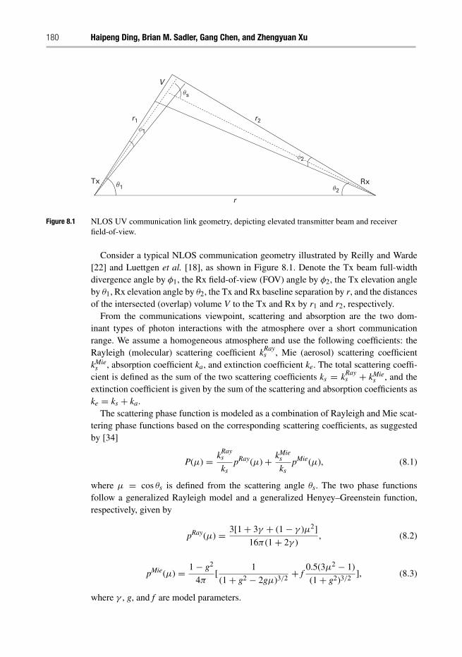
180 Haipeng Ding, Brian M. Sadler, Gang Chen, and Zhengyuan Xu
RxTx
V
r2r1
r
θs
θ1 θ2
φ1
φ2
Figure 8.1 NLOS UV communication link geometry, depicting elevated transmitter beam and receiverfield-of-view.
Consider a typical NLOS communication geometry illustrated by Reilly and Warde[22] and Luettgen et al. [18], as shown in Figure 8.1. Denote the Tx beam full-widthdivergence angle by φ1, the Rx field-of-view (FOV) angle by φ2, the Tx elevation angleby θ1, Rx elevation angle by θ2, the Tx and Rx baseline separation by r, and the distancesof the intersected (overlap) volume V to the Tx and Rx by r1 and r2, respectively.
From the communications viewpoint, scattering and absorption are the two dom-inant types of photon interactions with the atmosphere over a short communicationrange. We assume a homogeneous atmosphere and use the following coefficients: theRayleigh (molecular) scattering coefficient kRay
s , Mie (aerosol) scattering coefficientkMie
s , absorption coefficient ka, and extinction coefficient ke. The total scattering coeffi-cient is defined as the sum of the two scattering coefficients ks = kRay
s + kMies , and the
extinction coefficient is given by the sum of the scattering and absorption coefficients aske = ks + ka.
The scattering phase function is modeled as a combination of Rayleigh and Mie scat-tering phase functions based on the corresponding scattering coefficients, as suggestedby [34]
P(μ) = kRays
kspRay(μ)+ kMie
s
kspMie(μ), (8.1)
where μ = cos θs is defined from the scattering angle θs. The two phase functionsfollow a generalized Rayleigh model and a generalized Henyey–Greenstein function,respectively, given by
pRay(μ) = 3[1+ 3γ + (1− γ )μ2]
16π(1+ 2γ ), (8.2)
pMie(μ) = 1− g2
4π[
1
(1+ g2 − 2gμ)3/2+ f
0.5(3μ2 − 1)
(1+ g2)3/2], (8.3)
where γ , g, and f are model parameters.
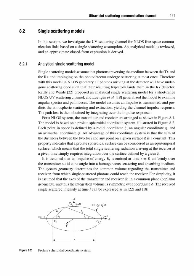
Ultraviolet scattering communication channel 181
8.2 Single scattering models
In this section, we investigate the UV scattering channel for NLOS free-space commu-nication links based on a single scattering assumption. An analytical model is reviewed,and an approximate closed-form expression is derived.
8.2.1 Analytical single scattering model
Single scattering models assume that photons traversing the medium between the Tx andthe Rx and impinging on the photodetector undergo scattering at most once. Thereforewith this model in NLOS geometry all photons arriving at the detector will have under-gone scattering once such that their resulting trajectory lands them in the Rx detector.Reilly and Warde [22] proposed an analytical single scattering model for a short-rangeNLOS UV scattering channel, and Luettgen et al. [18] generalized the model to examineangular spectra and path losses. The model assumes an impulse is transmitted, and pre-dicts the atmospheric scattering and extinction, yielding the channel impulse response.The path loss is then obtained by integrating over the impulse response.
For a NLOS system, the transmitter and receiver are arranged as shown in Figure 8.1.The model is based on a prolate spheroidal coordinate system, illustrated in Figure 8.2.Each point in space is defined by a radial coordinate ξ , an angular coordinate η, andan azimuthal coordinate φ. An advantage of this coordinate system is that the sum ofthe distances between the two foci and any point on a given surface ξ is a constant. Thisproperty indicates that a prolate spheroidal surface can be considered as an equitemporalsurface, which means that the total single scattering radiation arriving at the receiver ata given time simply requires integration over the surface defined by a given ξ .
It is assumed that an impulse of energy Et is emitted at time t = 0 uniformly overthe transmitter solid cone angle into a homogeneous scattering and absorbing medium.The system geometry determines the common volume regarding the transmitter andreceiver, from which single-scattered photons could reach the receiver. For simplicity, itis assumed that the axes of the transmitter and receiver lie in a common plane (coplanargeometry), and thus the integration volume is symmetric over coordinate φ. The receivedsingle scattered intensity at time t can be expressed as in [22] and [18]
r
z
y
η = −1 η = 1
η = 0θs ξ = (r2 + r2)/r
θ2θ1
x
F1
r1 r2
F2
Figure 8.2 Prolate spheroidal coordinate system.
182 Haipeng Ding, Brian M. Sadler, Gang Chen, and Zhengyuan Xu
h(t) = EtArckse−kect
2π�tr2×
∫ η2(ct/r)
η1(ct/r)
2G[φ(ct/r, η)]p(θs)
(ct/r)2 − η2dη, (8.4)
where the function G[·] is defined in the cited works.With reference to Figure 8.1, the parameters and functions are defined as follows. Let
�t be the solid angle of the Tx cone, r the Tx–Rx baseline separation, and r1 and r2
the distances of the common volume to the Tx and Rx, respectively. Define φ1 and φ2
as the Tx beam angle and Rx FOV, and θ1 and θ2 as the Tx and Rx focal angles (inter-changeable with elevation angles in this context) between each axis and the horizontalaxis. The elevation angles are also referred to as pointing or apex angles; perhaps apexis the better term in NLOS scenarios. ke, ks, ka are the atmosphere coefficients, θs is thescattering angle, Ar is the area of the receiving aperture, and p(θs) the scattering phasefunction.
8.2.2 Approximate single scattering path loss model
The impulse response model in (8.4) does not lead to a tractable closed form and sorequires numerical analysis. We can obtain a closed-form approximation for h(t) thatis amenable to incorporation into communications performance analysis, as follows.The derivation assumes that the geometry is such that the intersecting cones are small.Following the geometry and parameters defined above, the energy at the Rx scatteredfrom the differential volume dV in V can be modeled as [33]
δEr = EtksP(μ)ArδV cos(ζ )e−ke(r1+r2)
�tr21r2
2
, (8.5)
where ζ is the angle between the Rx axis and a vector from the Rx to the commonvolume, and phase function P(μ) is given by (8.1). The total energy at the receiver canbe found by integrating over the common volume using the prolate spheroidal coor-dinate system, but this requires numerical evaluation. To obtain a tractable analyticalexpression, we assume that the common volume is small so that ζ ≈ 0, and use thisto simplify h(t) and the resulting expression for the total received energy. Note that�t = 2π (1− cos φ1
2 ), r1 = r sin θ2/ sin θs, r2 = r sin θ1/ sin θs, and θs = θ1 + θ2. Now,we can approximate the total received energy as
Er ≈EtksP(μ)ArV sin4 θs exp[− ker
sin θs(sin θ1 + sin θ2)]
2πr4 sin2 θ1 sin2 θ2(1− cos φ12 )
. (8.6)
Define the path loss as the energy ratio L = EtEr
. Here L depends on the commonvolume V that in turn depends on the shape of the intersection. For a small overlapvolume, V can be well approximated by a frustum1 of the right cone of volume V =13π(D2
1h1 − D22h2), where h1 = r1 + r2
φ22 and D1 = h1
φ12 are the height and the radius
of the bottom surface of the large cone, and h1 = r1 − r2φ22 and D2 = h2
φ12 for the
smaller cone. Both cones share a common apex at the Tx location. Substituting r1, r2,
1 The frustum is the portion lying between two parallel planes.
Ultraviolet scattering communication channel 183
and θs into V and the corresponding result into Eq. (8.6), we obtain the following pathloss expression
L ≈ 96r sin θ1 sin2 θ2(1− cos φ12 ) exp[ ker(sin θ1+sin θ2)
sin θs]
ksP(μ)Arφ21φ2 sin θs(12 sin2 θ2 + φ2
2 sin2 θ1). (8.7)
This provides L as an explicit function of the system and geometric parameters, andis easily applied to link analysis for a particular choice of the atmospheric parameters.However, this model only provides high fidelity path loss approximations when the com-mon volume is small, which limits its applicability for geometries with longer baselinerange or large common volume overlap such as can occur with wide optical field ofview.
8.3 Multiple scattering models
Next we remove the single scattering assumption, and describe models that allow mul-tiple scattering. Generally, higher atmospheric particle density and longer propagationrange lead to a higher probability of multiple scattering, and atmospheric particles canbe quite abundant and reactive to UV photons. Thus, in some cases, a multiple scatteringmodel can lead to more accurate channel prediction, and the model enables separationand study with respect to the scattering order effect.
As we will show, multiple scattering interactions of photons with the atmosphericconstituents result in additional pulse broadening beyond that due to single scatter-ing, i.e., there is increased channel delay spread. The additional pulse spreading occursbecause, with multiple scattering, both longer and shorter path lengths are now possible.The pulse spreading limits the channel bandwidth available for communications due tothe introduction of inter-symbol interference (ISI). Accounting for multiple scatteringalso enables more accurate prediction of path loss. With multiple scattering there aremore opportunities for photons to successfully transit from the Tx to the Rx, so that thepredicted path loss under the multiple scattering model is generally less than that fromthe corresponding single scattering path loss model. These channel characteristics are afunction of transmitter–receiver geometry, including transmitter beam width, elevationangles, range, and receiver FOV. While these are crucial for UV NLOS communicationssystem performance analysis, there is no simple closed-form multi-scattering NLOS UVchannel model. In this section, first we review a Monte Carlo numerical technique toobtain both the impulse response and the corresponding path loss, and then we consideran analytical solution for the path loss.
8.3.1 Numerical Monte Carlo multiple scattering channel model
The method described here computes the impulse response due to multiple scatteringvia Monte Carlo (MC) simulation of each photon’s arrival probability along with theassociated propagation delay to the Rx. Path loss can then be easily obtained from thearea under the impulse response curve as illustrated by [8].
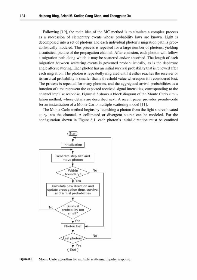
184 Haipeng Ding, Brian M. Sadler, Gang Chen, and Zhengyuan Xu
Following [19], the main idea of the MC method is to simulate a complex processas a succession of elementary events whose probability laws are known. Light isdecomposed into a set of photons and each individual photon’s migration path is prob-abilistically modeled. This process is repeated for a large number of photons, yieldinga statistical picture of the propagation channel. After emission, each photon will followa migration path along which it may be scattered and/or absorbed. The length of eachmigration between scattering events is governed probabilistically, as is the departureangle after scattering. Each photon has an initial survival probability that is renewed aftereach migration. The photon is repeatedly migrated until it either reaches the receiver orits survival probability is smaller than a threshold value whereupon it is considered lost.The process is repeated for many photons, and the aggregated arrival probabilities as afunction of time represent the expected received signal intensities, corresponding to thechannel impulse response. Figure 8.3 shows a block diagram of the Monte Carlo simu-lation method, whose details are described next. A recent paper provides pseudo-codefor an instantiation of a Monte-Carlo multiple scattering model [11].
The Monte Carlo method begins by launching a photon from the light source locatedat r0 into the channel. A collimated or divergent source can be modeled. For theconfiguration shown in Figure 8.1, each photon’s initial direction must be confined
Start
Initialization
Generate step size andmove photon
Withinboundary?
Calculate new direction andupdate propagation time, survival
and arrival probabilities
Survivalprobability too
small?
Photon lost
Last photon?
End
Yes
Yes
No
No
Yes
No
Figure 8.3 Monte Carlo algorithm for multiple scattering impulse response.
Ultraviolet scattering communication channel 185
within the full beam angle φ1 with solid angle 2π(1− cos φ12 ). We place the light source
in the coordinate system such that the beam axis has a zenith angle (π/2 − θ1) andazimuth angle 0◦. Let the initial direction of an individual photon with respect to thezenith angle be θini, and with respect to the azimuth angle be ψini. Then, the initialdirection from the beam axis is
U = θini − (π/2− θ1).
For a uniformly distributed light source, the initial angles are generated to satisfy
cos U = 1− ξ (θ)(1− cosφ1
2),
ψini = 2πξ (ψ), (8.8)
where ξ (θ ) and ξ (ψ) are independent standard uniform random variables (uniformbetween zero and one).
The photon trajectory is then simulated by successive migration paths among differentscattering centers. After each interaction between a photon and a scattering center, thephoton’s propagation is assumed to follow the law of single scattering until it reachesthe next scattering center or arrives at the receiver. Following this theory, the distancebetween scattering interactions is given by the random variable
�s = − ln ξ (s)
ks, (8.9)
where ξ (s) is a standard uniform random variable.An individual photon’s spatial migration path can be uniquely described by five vari-
ables: three spatial coordinates for the position and two direction angles θ and ψ . Thephoton’s spatial position can be represented with three Cartesian coordinates and themigration direction can be described with three direction cosines from the two direc-tion angles. The direction cosines are specified by taking the cosines of the anglesthat the photon’s direction makes with each of the x, y, and z axes, respectively.As an example, the initial direction cosines are specified by μini
x = cosψini sin θini,μini
y = sinψini sin θini, and μiniz = cos θini. For a photon located at (xi, yi, zi) travelling a
distance �s in the direction (μix, μi
y,μiz), its coordinates are updated in the 3-dimensional
geometry by
xi+1 = xi + μix�s,
yi+1 = yi + μiy�s,
zi+1 = zi + μiz�s. (8.10)
The new migration direction is governed by the normalized phase function thatdescribes the angular intensity of scattered light. When applied to a single photon, thisdescribes the scattered direction (the scattering angle). The deviation from the currentdirection is determined from a standard uniform random variable ξ (μ) and the phasefunction by [31]
ξ (μ) = 2π∫ μ1
−1P(μ)dμ. (8.11)
186 Haipeng Ding, Brian M. Sadler, Gang Chen, and Zhengyuan Xu
Here, μ1 = cos θ , where θ is the angle of the new photon path with respect to the currentdirection. A numerical solution for θ can be obtained from Eq. (8.11). Note that becausethere is no azimuth dependence in the phase function, the azimuth angle ψ is then setas a uniformly distributed random variable between 0 and 2π , and so this step providesboth angles θ and ψ .
The next step is to compute the direction cosines in the absolute Cartesian coordinatesystem previously described. If a photon is scattered at angles (θ ,ψ) offset from theincoming direction with direction cosines (μi
x, μiy, μi
z), then the new direction cosinesare easily calculated via
μi+1x = sin θ√
1− (μiz)
2(μi
xμiz cosψ − μi
y sinψ)+ μix cos θ ,
μi+1y = sin θ√
1− (μiz)
2(μi
yμiz cosψ + μi
x sinψ)+ μiy cos θ ,
μi+1z = − sin θ cosψ
√1− (μi
z)2 + μi
z cos θ . (8.12)
Each photon is assigned a survival probability, initialized to one when first emitted bythe source. The probability that the photon arrives at the receiver within its FOV after nscattering steps is given by
p1n =∫�n
P(cos θ )d�, (8.13)
where �n is the solid angle along the scattered direction that can be seen by the receiveraperture of area Ar, and P(·) is the phase function defined earlier. The probability thatthe photon cannot be seen by the receiver (i.e., it moves out of the receiver FOV) is thus(1− p1n).
Between scattering interactions, the photon is modeled to move with a random stepsize, and along this path we next consider energy loss between two consecutive scatter-ing centers. The photon location changes from the (n − 1)th scattering center locationrn−1 to the nth scattering center location rn according to the direction cosine and coordi-nate updates described above. Between these scattering centers, the propagation distance|rn−rn−1| is given by the random variable �s in Eq. (8.9). Along this path between scat-terers, the photon undergoes an energy loss of e−ka|rn−rn−1|, which is a function of ka.Impinging upon the nth scattering center, the photon’s survival probability is reduceddue to this energy loss and so is updated according to
wn = (1− p1n)e−ka|rn−rn−1|wn−1. (8.14)
After the nth scattering interaction, the probability that the photon successfully arrivesat the receiver is given by
Pn = wnp1np2n, (8.15)
where p2n represents the propagation loss of the photon from the nth scattering centerto the receiver
Ultraviolet scattering communication channel 187
p2n = e−ke|rn−r′|, (8.16)
r′ is the location vector of the receiver, and ke is employed to model the path loss.To calculate the channel impulse response, it is necessary to find the propagation time
(i.e., relative time delay) of each photon, in addition to its probability of arrival at thedetector. This is easily found from the photon migration path, and is given by dn/c,where dn is the accumulated propagation distance dn = ∑n
j=1 |rj − rj−1| and c is thespeed of light. For example, suppose a photon undergoes N scattering interactions. Then,associated with this photon are a set of probabilities (P1, . . ., PN), and a correspondingset of propagation times between each pair of scatterers. The Monte Carlo procedureis carried out for a large number of photons (e.g., M = 106 or more). To display theexpected impulse response, the probabilities are superimposed. If we denote each photonenergy by Ep, then the probabilities versus time represent the channel response due to Mphotons. The curve is normalized by EPM to obtain the impulse response correspondingto a transmitted pulse with energy equal to one joule.
8.3.2 Analytical multiple scattering path loss model
Following the same physical scattering law as the Monte Carlo technique, Ding et al.[9] proposed a stochastic analytical method to theoretically derive the nth order scatteredsignal energy collected by the detector. The model considers all photons to be stochasti-cally scattered and/or absorbed by the atmospheric particles, and involves probabilisticmodeling of the photon direction, distance, energy loss, and receiver capture for a spec-ified scattering order. In order to obtain the nth order scattered signal at the receiver,we trace the migration route of a single photon through the medium, similar to [13].The migration distance and scattering angles follow probability distribution functions(PDFs) that are determined by Beer’s law and the phase function, respectively. The PDFof the migration distance r is given by
fr(r) = kse−ksr. (8.17)
The zenith scattering angle under combined Rayleigh and Mie scattering has thefollowing PDF
fθ (θ ) = kRays
ksf Rayθ (θ )+ kMie
s
ksf Mieθ (θ ), (8.18)
where f Rayθ (θ ) and f Mie
θ (θ ) are the phase functions, and θ takes values in [0,π]. Weconsider a uniform distribution between 0 and 2π for azimuth scattering angle φ becausethere is no azimuth dependence in the phase function (symmetry is assumed). Thus, theazimuth scattering angle PDF is simply
fφ(φ) = 1
2π, φ ∈ [0, 2π ]. (8.19)
Assume a photon from a UV emitter is uniformly emitted at initial direction angles θ0
and φ0 within the beam divergence, and migrates a distance r0 before the first scat-tering occurs. The solid angle within the beam can thus be modeled as a uniform
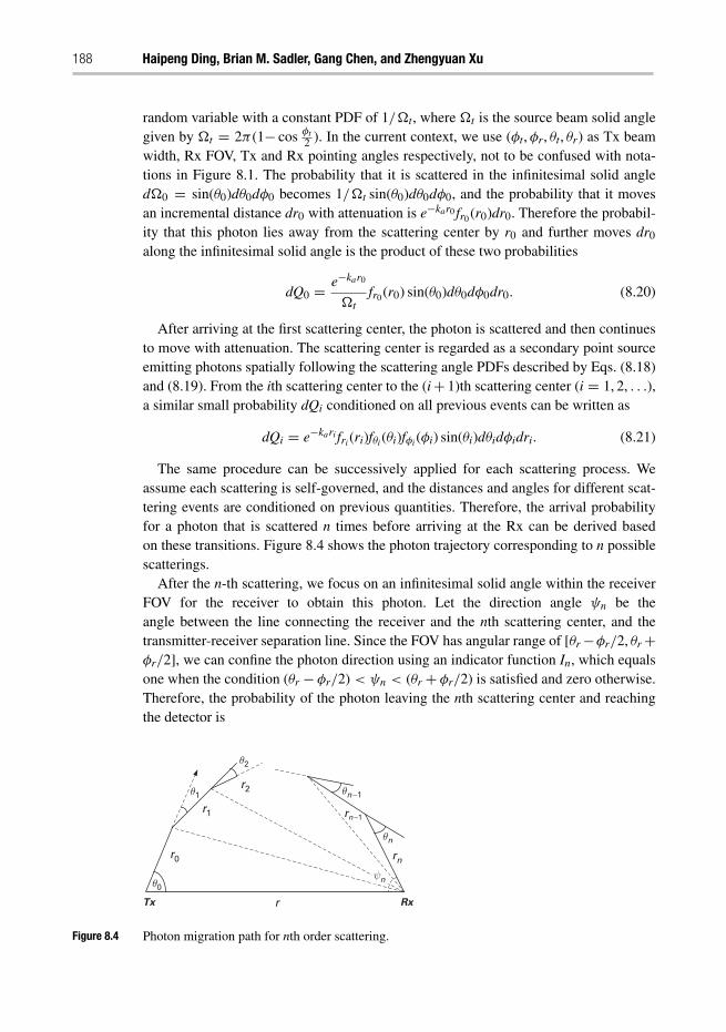
188 Haipeng Ding, Brian M. Sadler, Gang Chen, and Zhengyuan Xu
random variable with a constant PDF of 1/�t, where �t is the source beam solid anglegiven by �t = 2π(1− cos φt
2 ). In the current context, we use (φt,φr, θt, θr) as Tx beamwidth, Rx FOV, Tx and Rx pointing angles respectively, not to be confused with nota-tions in Figure 8.1. The probability that it is scattered in the infinitesimal solid angled�0 = sin(θ0)dθ0dφ0 becomes 1/�t sin(θ0)dθ0dφ0, and the probability that it movesan incremental distance dr0 with attenuation is e−kar0 fr0 (r0)dr0. Therefore the probabil-ity that this photon lies away from the scattering center by r0 and further moves dr0
along the infinitesimal solid angle is the product of these two probabilities
dQ0 = e−kar0
�tfr0 (r0) sin(θ0)dθ0dφ0dr0. (8.20)
After arriving at the first scattering center, the photon is scattered and then continuesto move with attenuation. The scattering center is regarded as a secondary point sourceemitting photons spatially following the scattering angle PDFs described by Eqs. (8.18)and (8.19). From the ith scattering center to the (i+ 1)th scattering center (i = 1, 2, . . .),a similar small probability dQi conditioned on all previous events can be written as
dQi = e−kari fri (ri)fθi (θi)fφi (φi) sin(θi)dθidφidri. (8.21)
The same procedure can be successively applied for each scattering process. Weassume each scattering is self-governed, and the distances and angles for different scat-tering events are conditioned on previous quantities. Therefore, the arrival probabilityfor a photon that is scattered n times before arriving at the Rx can be derived basedon these transitions. Figure 8.4 shows the photon trajectory corresponding to n possiblescatterings.
After the n-th scattering, we focus on an infinitesimal solid angle within the receiverFOV for the receiver to obtain this photon. Let the direction angle ψn be theangle between the line connecting the receiver and the nth scattering center, and thetransmitter-receiver separation line. Since the FOV has angular range of [θr−φr/2, θr+φr/2], we can confine the photon direction using an indicator function In, which equalsone when the condition (θr − φr/2) < ψn < (θr + φr/2) is satisfied and zero otherwise.Therefore, the probability of the photon leaving the nth scattering center and reachingthe detector is
Tx Rxr
r1
r0
r2
rn
θ1
θ0
θ2
θn
θn −1
rn −1
ψn
Figure 8.4 Photon migration path for nth order scattering.
Ultraviolet scattering communication channel 189
dQn = Ine−kern fθn (θn)fφn(φn) sin(θn)dθndφn. (8.22)
The photon arrival probability after n scatterings is denoted Pn, given by
Pn =∫ ∫
· · ·∫
dQ0 × dQ1 · · · × dQn. (8.23)
If the UV source emits a pulse with energy Et, then the received total energy up to nscatterings is
Er,n =n∑
i=1
Er(i) = Et
n∑i=1
Pi, (8.24)
and the corresponding path loss can be expressed as
PLn = Et
Er,n= 1∑n
i=1 Pi. (8.25)
We typically express the path loss in decibels, given by 10 log10(PLn). As n goes to∞, the energy represents the total possible over all scattering orders. Later we willconsider some specific cases. Sometimes single scattering dominates, while for somecases scattering up to about 4th-order can make a meaningful contribution.
8.4 NLOS UV channel measurement systems
To validate the channel models, we have experimentally measured both impulseresponse and path loss, employing a UV pulsed-laser for impulse response and UVLEDs for path loss, respectively. In this section we briefly describe the measurementsystems. In the next section we compare channel models and experimental data.
8.4.1 LED path loss measurements
Chen et al. [5, 6] describe a solar blind UV path loss experimental test-bed at 260 nmwavelength. As shown in Figure 8.5, the transmitter employed a signal generator to feeda current driver circuit that powered an array of seven ball-lens UV LEDs. The driv-ing current for each LED was 30 mA, yielding an average radiated optical power of0.3 mW. Using a beam profiler, the beam divergence angle was measured to be 17◦.At the receiver, a solar blind filter was mounted on top of the circular sensing windowof a Perkin-Elmer PMT module MP1922. The PMT’s output current was fed to a highbandwidth preamplifier, whose output was further sent to a photon counter for photondetection. The LEDs, PMT, and filter were attached to Tx and Rx angular control mod-ules, respectively. Each module utilized two perpendicular rotation stages to achieve aprecise angular control up to 360◦ in the azimuth and zenith directions. Experimentsreported below have focused on scenarios where the Tx beam axis and Rx FOV axiswere coplanar, and only Tx and Rx apex angles were adjusted. The Rx filter had full-width half maximum (FWHM) bandwidth of 15 nm. The filter in-band transmissionwas 8% and visible-band transmission was below 10−10. The PMT sensing window had
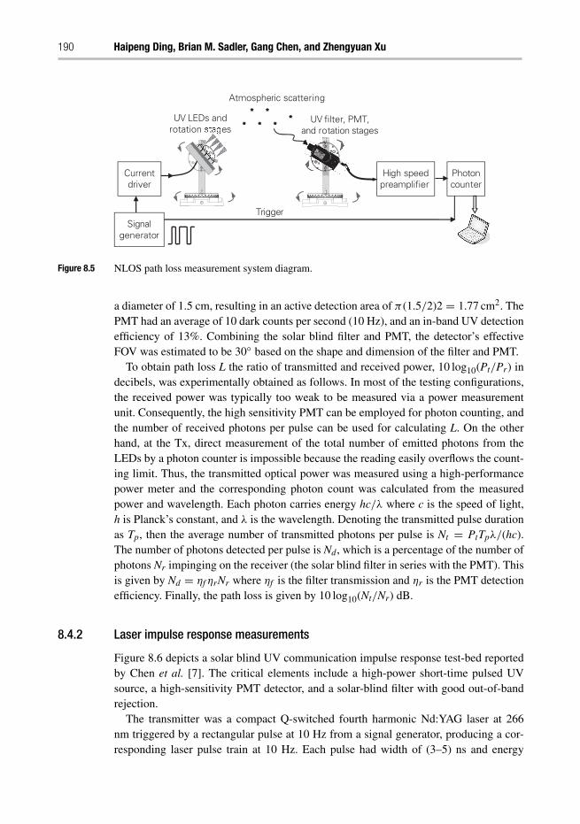
190 Haipeng Ding, Brian M. Sadler, Gang Chen, and Zhengyuan Xu
Signalgenerator
Currentdriver
UV LEDs androtation es
High speedpreamplifier
UV filter, PMT, and rotation stages
Photoncounter
Trigger
Atmospheric scattering
Figure 8.5 NLOS path loss measurement system diagram.
a diameter of 1.5 cm, resulting in an active detection area of π(1.5/2)2 = 1.77 cm2. ThePMT had an average of 10 dark counts per second (10 Hz), and an in-band UV detectionefficiency of 13%. Combining the solar blind filter and PMT, the detector’s effectiveFOV was estimated to be 30◦ based on the shape and dimension of the filter and PMT.
To obtain path loss L the ratio of transmitted and received power, 10 log10(Pt/Pr) indecibels, was experimentally obtained as follows. In most of the testing configurations,the received power was typically too weak to be measured via a power measurementunit. Consequently, the high sensitivity PMT can be employed for photon counting, andthe number of received photons per pulse can be used for calculating L. On the otherhand, at the Tx, direct measurement of the total number of emitted photons from theLEDs by a photon counter is impossible because the reading easily overflows the count-ing limit. Thus, the transmitted optical power was measured using a high-performancepower meter and the corresponding photon count was calculated from the measuredpower and wavelength. Each photon carries energy hc/λ where c is the speed of light,h is Planck’s constant, and λ is the wavelength. Denoting the transmitted pulse durationas Tp, then the average number of transmitted photons per pulse is Nt = PtTpλ/(hc).The number of photons detected per pulse is Nd, which is a percentage of the number ofphotons Nr impinging on the receiver (the solar blind filter in series with the PMT). Thisis given by Nd = ηf ηrNr where ηf is the filter transmission and ηr is the PMT detectionefficiency. Finally, the path loss is given by 10 log10(Nt/Nr) dB.
8.4.2 Laser impulse response measurements
Figure 8.6 depicts a solar blind UV communication impulse response test-bed reportedby Chen et al. [7]. The critical elements include a high-power short-time pulsed UVsource, a high-sensitivity PMT detector, and a solar-blind filter with good out-of-bandrejection.
The transmitter was a compact Q-switched fourth harmonic Nd:YAG laser at 266nm triggered by a rectangular pulse at 10 Hz from a signal generator, producing a cor-responding laser pulse train at 10 Hz. Each pulse had width of (3–5) ns and energy
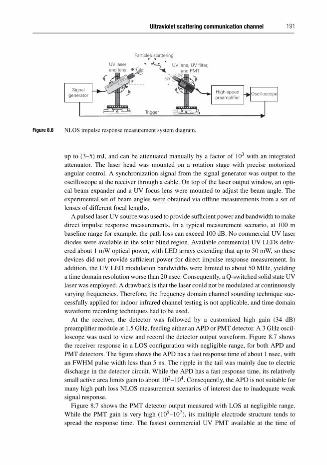
Ultraviolet scattering communication channel 191
Signalgenerator
UV laserand lens
Q-switched laser
Particles scattering
UV lens, UV filter,and PMT
High-speedpreamplifier
Oscilloscope
Trigger
θ1θ2
Φ1Φ2
Figure 8.6 NLOS impulse response measurement system diagram.
up to (3–5) mJ, and can be attenuated manually by a factor of 103 with an integratedattenuator. The laser head was mounted on a rotation stage with precise motorizedangular control. A synchronization signal from the signal generator was output to theoscilloscope at the receiver through a cable. On top of the laser output window, an opti-cal beam expander and a UV focus lens were mounted to adjust the beam angle. Theexperimental set of beam angles were obtained via offline measurements from a set oflenses of different focal lengths.
A pulsed laser UV source was used to provide sufficient power and bandwidth to makedirect impulse response measurements. In a typical measurement scenario, at 100 mbaseline range for example, the path loss can exceed 100 dB. No commercial UV laserdiodes were available in the solar blind region. Available commercial UV LEDs deliv-ered about 1 mW optical power, with LED arrays extending that up to 50 mW, so thesedevices did not provide sufficient power for direct impulse response measurement. Inaddition, the UV LED modulation bandwidths were limited to about 50 MHz, yieldinga time domain resolution worse than 20 nsec. Consequently, a Q-switched solid state UVlaser was employed. A drawback is that the laser could not be modulated at continuouslyvarying frequencies. Therefore, the frequency domain channel sounding technique suc-cessfully applied for indoor infrared channel testing is not applicable, and time domainwaveform recording techniques had to be used.
At the receiver, the detector was followed by a customized high gain (34 dB)preamplifier module at 1.5 GHz, feeding either an APD or PMT detector. A 3 GHz oscil-loscope was used to view and record the detector output waveform. Figure 8.7 showsthe receiver response in a LOS configuration with negligible range, for both APD andPMT detectors. The figure shows the APD has a fast response time of about 1 nsec, withan FWHM pulse width less than 5 ns. The ripple in the tail was mainly due to electricdischarge in the detector circuit. While the APD has a fast response time, its relativelysmall active area limits gain to about 102–104. Consequently, the APD is not suitable formany high path loss NLOS measurement scenarios of interest due to inadequate weaksignal response.
Figure 8.7 shows the PMT detector output measured with LOS at negligible range.While the PMT gain is very high (105–107), its multiple electrode structure tends tospread the response time. The fastest commercial UV PMT available at the time of
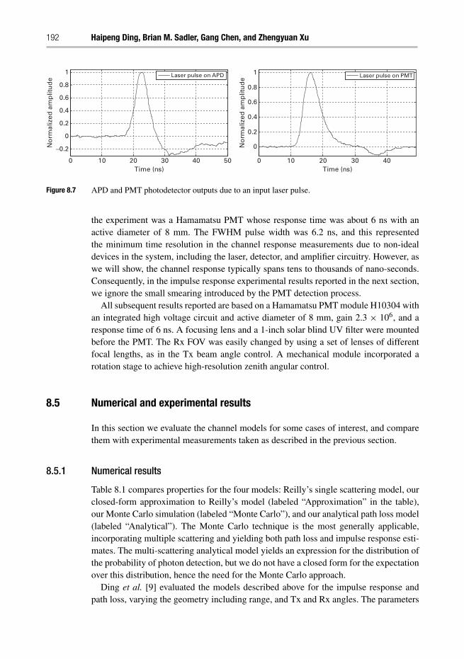
192 Haipeng Ding, Brian M. Sadler, Gang Chen, and Zhengyuan Xu
0 10 20 30 40 50
−0.2
0
0.2
0.4
0.6
0.8
1
Time (ns)
No
rmal
ized
am
plit
ud
e
Laser pulse on APD
0 10 20 30 40
0
0.2
0.4
0.6
0.8
1
Time (ns)
No
rmal
ized
am
plit
ud
e
Laser pulse on PMT
Figure 8.7 APD and PMT photodetector outputs due to an input laser pulse.
the experiment was a Hamamatsu PMT whose response time was about 6 ns with anactive diameter of 8 mm. The FWHM pulse width was 6.2 ns, and this representedthe minimum time resolution in the channel response measurements due to non-idealdevices in the system, including the laser, detector, and amplifier circuitry. However, aswe will show, the channel response typically spans tens to thousands of nano-seconds.Consequently, in the impulse response experimental results reported in the next section,we ignore the small smearing introduced by the PMT detection process.
All subsequent results reported are based on a Hamamatsu PMT module H10304 withan integrated high voltage circuit and active diameter of 8 mm, gain 2.3 × 10⁶, and aresponse time of 6 ns. A focusing lens and a 1-inch solar blind UV filter were mountedbefore the PMT. The Rx FOV was easily changed by using a set of lenses of differentfocal lengths, as in the Tx beam angle control. A mechanical module incorporated arotation stage to achieve high-resolution zenith angular control.
8.5 Numerical and experimental results
In this section we evaluate the channel models for some cases of interest, and comparethem with experimental measurements taken as described in the previous section.
8.5.1 Numerical results
Table 8.1 compares properties for the four models: Reilly’s single scattering model, ourclosed-form approximation to Reilly’s model (labeled “Approximation” in the table),our Monte Carlo simulation (labeled “Monte Carlo”), and our analytical path loss model(labeled “Analytical”). The Monte Carlo technique is the most generally applicable,incorporating multiple scattering and yielding both path loss and impulse response esti-mates. The multi-scattering analytical model yields an expression for the distribution ofthe probability of photon detection, but we do not have a closed form for the expectationover this distribution, hence the need for the Monte Carlo approach.
Ding et al. [9] evaluated the models described above for the impulse response andpath loss, varying the geometry including range, and Tx and Rx angles. The parameters
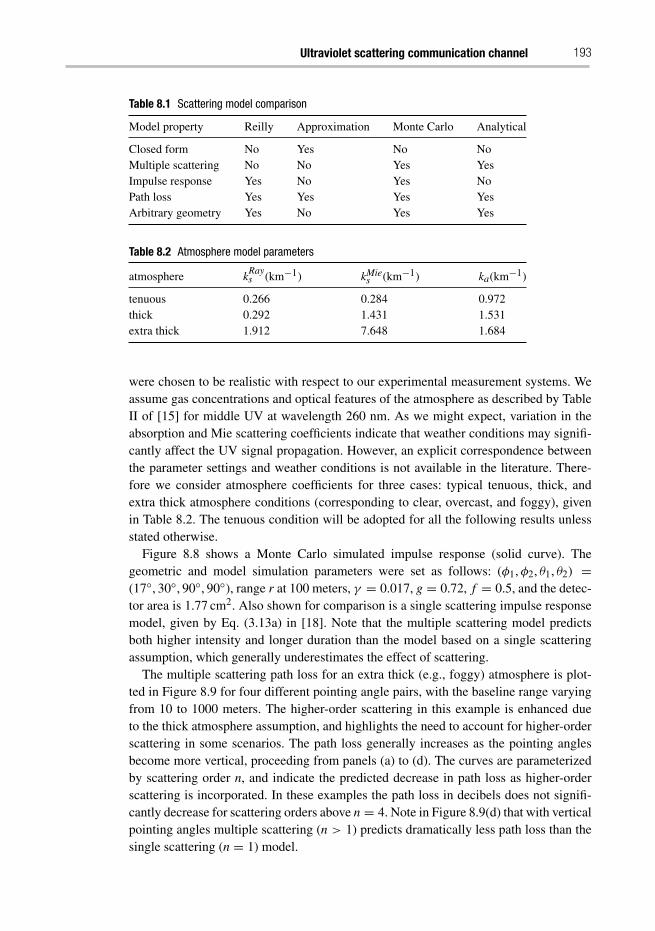
Ultraviolet scattering communication channel 193
Table 8.1 Scattering model comparison
Model property Reilly Approximation Monte Carlo Analytical
Closed form No Yes No NoMultiple scattering No No Yes YesImpulse response Yes No Yes NoPath loss Yes Yes Yes YesArbitrary geometry Yes No Yes Yes
Table 8.2 Atmosphere model parameters
atmosphere kRays (km−1) kMie
s (km−1) ka(km−1)
tenuous 0.266 0.284 0.972thick 0.292 1.431 1.531extra thick 1.912 7.648 1.684
were chosen to be realistic with respect to our experimental measurement systems. Weassume gas concentrations and optical features of the atmosphere as described by TableII of [15] for middle UV at wavelength 260 nm. As we might expect, variation in theabsorption and Mie scattering coefficients indicate that weather conditions may signifi-cantly affect the UV signal propagation. However, an explicit correspondence betweenthe parameter settings and weather conditions is not available in the literature. There-fore we consider atmosphere coefficients for three cases: typical tenuous, thick, andextra thick atmosphere conditions (corresponding to clear, overcast, and foggy), givenin Table 8.2. The tenuous condition will be adopted for all the following results unlessstated otherwise.
Figure 8.8 shows a Monte Carlo simulated impulse response (solid curve). Thegeometric and model simulation parameters were set as follows: (φ1,φ2, θ1, θ2) =(17◦, 30◦, 90◦, 90◦), range r at 100 meters, γ = 0.017, g = 0.72, f = 0.5, and the detec-tor area is 1.77 cm2. Also shown for comparison is a single scattering impulse responsemodel, given by Eq. (3.13a) in [18]. Note that the multiple scattering model predictsboth higher intensity and longer duration than the model based on a single scatteringassumption, which generally underestimates the effect of scattering.
The multiple scattering path loss for an extra thick (e.g., foggy) atmosphere is plot-ted in Figure 8.9 for four different pointing angle pairs, with the baseline range varyingfrom 10 to 1000 meters. The higher-order scattering in this example is enhanced dueto the thick atmosphere assumption, and highlights the need to account for higher-orderscattering in some scenarios. The path loss generally increases as the pointing anglesbecome more vertical, proceeding from panels (a) to (d). The curves are parameterizedby scattering order n, and indicate the predicted decrease in path loss as higher-orderscattering is incorporated. In these examples the path loss in decibels does not signifi-cantly decrease for scattering orders above n = 4. Note in Figure 8.9(d) that with verticalpointing angles multiple scattering (n > 1) predicts dramatically less path loss than thesingle scattering (n = 1) model.
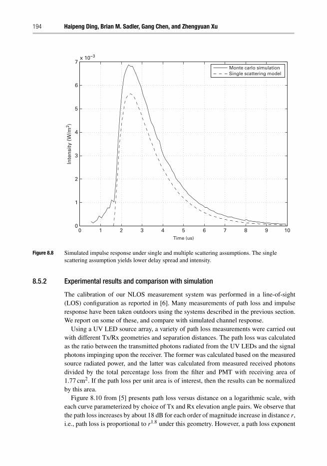
194 Haipeng Ding, Brian M. Sadler, Gang Chen, and Zhengyuan Xu
0 1 2 3 4 5 6 7 8 9 100
1
2
3
4
5
6
7x 10⁻³
Time (us)
Inte
nsi
ty (
W/m
2 )Monte carlo simulationSingle scattering model
Figure 8.8 Simulated impulse response under single and multiple scattering assumptions. The singlescattering assumption yields lower delay spread and intensity.
8.5.2 Experimental results and comparison with simulation
The calibration of our NLOS measurement system was performed in a line-of-sight(LOS) configuration as reported in [6]. Many measurements of path loss and impulseresponse have been taken outdoors using the systems described in the previous section.We report on some of these, and compare with simulated channel response.
Using a UV LED source array, a variety of path loss measurements were carried outwith different Tx/Rx geometries and separation distances. The path loss was calculatedas the ratio between the transmitted photons radiated from the UV LEDs and the signalphotons impinging upon the receiver. The former was calculated based on the measuredsource radiated power, and the latter was calculated from measured received photonsdivided by the total percentage loss from the filter and PMT with receiving area of1.77 cm2. If the path loss per unit area is of interest, then the results can be normalizedby this area.
Figure 8.10 from [5] presents path loss versus distance on a logarithmic scale, witheach curve parameterized by choice of Tx and Rx elevation angle pairs. We observe thatthe path loss increases by about 18 dB for each order of magnitude increase in distance r,i.e., path loss is proportional to r1.8 under this geometry. However, a path loss exponent
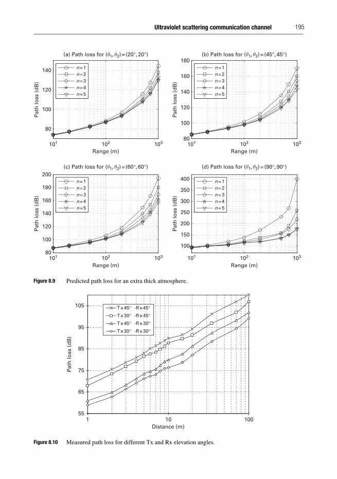
Ultraviolet scattering communication channel 195
101 102 103 101 102 103
101 102 103101 102 103
80
100
120
140
(a) Path loss for (θ1, θ2) = (20°, 20°)
(c) Path loss for (θ1, θ2) = (60°, 60°) (d) Path loss for (θ1, θ2) = (90°, 90°)
(b) Path loss for (θ1, θ2) = (45°, 45°)
Range (m)
Pat
h lo
ss (
dB
)
n = 1n = 2n = 3n = 4n = 5
80
100
120
140
160
180
Range (m)
Pat
h lo
ss (
dB
)
80
100
120
140
160
180
200
Range (m)
Pat
h lo
ss (
dB
)
100
150
200
250
300
350
400
Range (m)
Pat
h lo
ss (
dB
)
n = 1n = 2n = 3n = 4n = 5
n = 1n = 2n = 3n = 4n = 5
n = 1n = 2n = 3n = 4n = 5
Figure 8.9 Predicted path loss for an extra thick atmosphere.
55
65
75
85
95
105
100101
Pat
h lo
ss (
dB
)
Distance (m)
T x 45° -R x 45°T x 30° -R x 45°T x 45° -R x 30°T x 30° -R x 30°
Figure 8.10 Measured path loss for different Tx and Rx elevation angles.
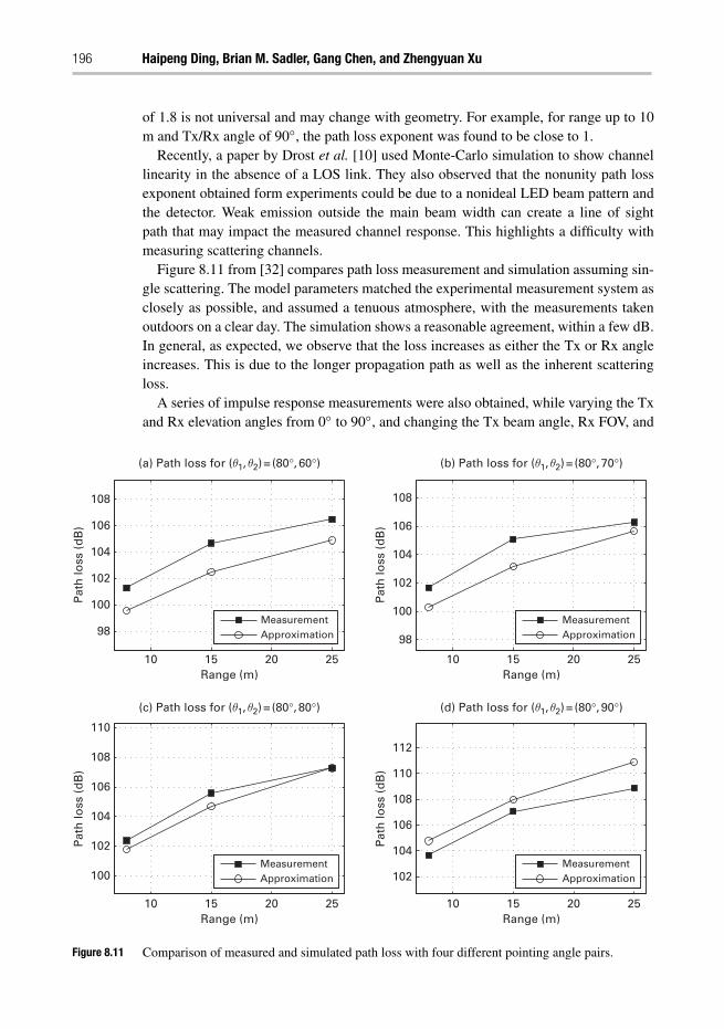
196 Haipeng Ding, Brian M. Sadler, Gang Chen, and Zhengyuan Xu
of 1.8 is not universal and may change with geometry. For example, for range up to 10m and Tx/Rx angle of 90◦, the path loss exponent was found to be close to 1.
Recently, a paper by Drost et al. [10] used Monte-Carlo simulation to show channellinearity in the absence of a LOS link. They also observed that the nonunity path lossexponent obtained form experiments could be due to a nonideal LED beam pattern andthe detector. Weak emission outside the main beam width can create a line of sightpath that may impact the measured channel response. This highlights a difficulty withmeasuring scattering channels.
Figure 8.11 from [32] compares path loss measurement and simulation assuming sin-gle scattering. The model parameters matched the experimental measurement system asclosely as possible, and assumed a tenuous atmosphere, with the measurements takenoutdoors on a clear day. The simulation shows a reasonable agreement, within a few dB.In general, as expected, we observe that the loss increases as either the Tx or Rx angleincreases. This is due to the longer propagation path as well as the inherent scatteringloss.
A series of impulse response measurements were also obtained, while varying the Txand Rx elevation angles from 0◦ to 90◦, and changing the Tx beam angle, Rx FOV, and
10 15 20 25
98
100
102
104
106
108
Range (m)
Pat
h lo
ss (
dB
)
98
100
102
104
106
108
Pat
h lo
ss (
dB
)
MeasurementApproximation
10 15 20 25Range (m)
10 15 20 25Range (m)
10 15 20 25Range (m)
100
102
104
106
108
110
Pat
h lo
ss (
dB
)
102
104
106
108
110
112
Pat
h lo
ss (
dB
)
(a) Path loss for (θ1, θ2) = (80°, 60°) (b) Path loss for (θ1, θ2) = (80°, 70°)
(c) Path loss for (θ1, θ2) = (80°, 80°) (d) Path loss for (θ1, θ2) = (80°, 90°)
MeasurementApproximation
MeasurementApproximation
MeasurementApproximation
Figure 8.11 Comparison of measured and simulated path loss with four different pointing angle pairs.
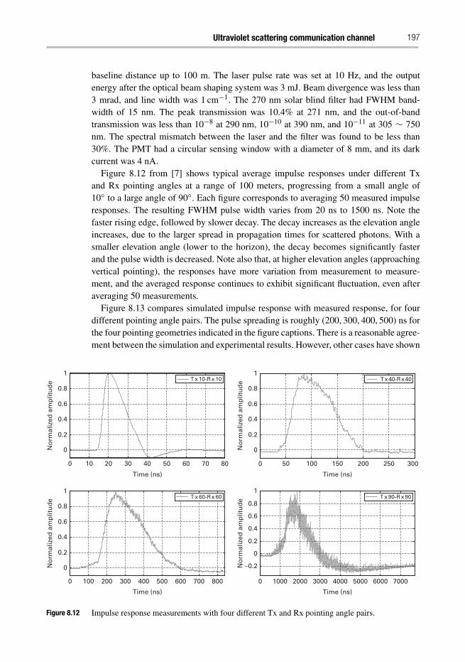
Ultraviolet scattering communication channel 197
baseline distance up to 100 m. The laser pulse rate was set at 10 Hz, and the outputenergy after the optical beam shaping system was 3 mJ. Beam divergence was less than3 mrad, and line width was 1 cm−1. The 270 nm solar blind filter had FWHM band-width of 15 nm. The peak transmission was 10.4% at 271 nm, and the out-of-bandtransmission was less than 10−8 at 290 nm, 10−10 at 390 nm, and 10−11 at 305 ∼ 750nm. The spectral mismatch between the laser and the filter was found to be less than30%. The PMT had a circular sensing window with a diameter of 8 mm, and its darkcurrent was 4 nA.
Figure 8.12 from [7] shows typical average impulse responses under different Txand Rx pointing angles at a range of 100 meters, progressing from a small angle of10◦ to a large angle of 90◦. Each figure corresponds to averaging 50 measured impulseresponses. The resulting FWHM pulse width varies from 20 ns to 1500 ns. Note thefaster rising edge, followed by slower decay. The decay increases as the elevation angleincreases, due to the larger spread in propagation times for scattered photons. With asmaller elevation angle (lower to the horizon), the decay becomes significantly fasterand the pulse width is decreased. Note also that, at higher elevation angles (approachingvertical pointing), the responses have more variation from measurement to measure-ment, and the averaged response continues to exhibit significant fluctuation, even afteraveraging 50 measurements.
Figure 8.13 compares simulated impulse response with measured response, for fourdifferent pointing angle pairs. The pulse spreading is roughly (200, 300, 400, 500) ns forthe four pointing geometries indicated in the figure captions. There is a reasonable agree-ment between the simulation and experimental results. However, other cases have shown
0 10 20 30 40 50 60 70 80
0
0.2
0.4
0.6
0.8
1
Time (ns)
No
rmal
ized
am
plit
ud
e
0
0.2
0.4
0.6
0.8
1
No
rmal
ized
am
plit
ud
eT x 10-R x 10
0 50 100 150 200 250 300
Time (ns)
0 100 200 300 400 500 600 700 800
0
0.2
0.4
0.6
0.8
1
Time (ns)
No
rmal
ized
am
plit
ud
e
0 1000 2000 3000 4000 5000 6000 7000
−0.2
0
0.2
0.4
0.6
0.8
1
Time (ns)
No
rmal
ized
am
plit
ud
e
T x 40-R x 40
T x 60-R x 60 T x 90-R x 90
Figure 8.12 Impulse response measurements with four different Tx and Rx pointing angle pairs.
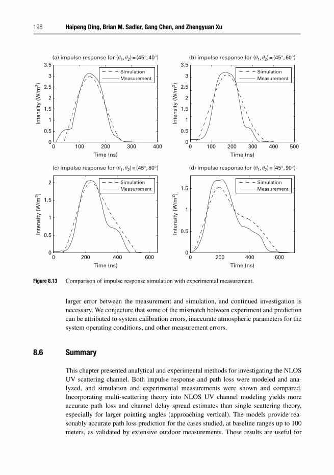
198 Haipeng Ding, Brian M. Sadler, Gang Chen, and Zhengyuan Xu
0 100 200 300 4000
0.5
1
1.5
2
2.5
3
3.5
Time (ns)
Inte
nsi
ty (
W/m
2 )In
ten
sity
(W
/m2 )
0
0.5
1
1.5
2
2.5
3
3.5
Inte
nsi
ty (
W/m
2 )In
ten
sity
(W
/m2 )
0 100 200 300 400 500
Time (ns)
0 200 400 6000
0.5
1
1.5
2
Time (ns)
0 200 400 6000
0.5
1
1.5
Time (ns)
SimulationMeasurement
(a) impulse response for (θ1, θ2) = (45°, 40°) (b) impulse response for (θ1, θ2) = (45°, 60°)
(d) impulse response for (θ1, θ2) = (45°, 90°)(c) impulse response for (θ1, θ2) = (45°, 80°)
SimulationMeasurement
SimulationMeasurement
SimulationMeasurement
Figure 8.13 Comparison of impulse response simulation with experimental measurement.
larger error between the measurement and simulation, and continued investigation isnecessary. We conjecture that some of the mismatch between experiment and predictioncan be attributed to system calibration errors, inaccurate atmospheric parameters for thesystem operating conditions, and other measurement errors.
8.6 Summary
This chapter presented analytical and experimental methods for investigating the NLOSUV scattering channel. Both impulse response and path loss were modeled and ana-lyzed, and simulation and experimental measurements were shown and compared.Incorporating multi-scattering theory into NLOS UV channel modeling yields moreaccurate path loss and channel delay spread estimates than single scattering theory,especially for larger pointing angles (approaching vertical). The models provide rea-sonably accurate path loss prediction for the cases studied, at baseline ranges up to 100meters, as validated by extensive outdoor measurements. These results are useful for
Ultraviolet scattering communication channel 199
system design and communications link performance analysis. Topics of further interestinclude developing an analytical impulse response model, developing a stochastic pathloss model, analyzing non-coplanar propagation geometry, study of multi-user channelsand multi-sensor cases, and modeling turbulence effects at longer ranges.
References
[1] International Commission on Non-Ionizing Radiation Protection (ICNIRP): Guidelines onlimits of exposure to ultraviolet radiation of wavelengths between 180nm and 400nm (inco-herent optical radiation), 2004, initially published in Health Physics 49:331–340, 1985;amended in Health Physics 56:971–972, 1989; reconfirmed by ICNIRP in Health Physics71:978, 1996; republished in Health Physics 87(2):171–186.
[2] International Electrotechnical Commission (IEC), IEC 60825-12: Safety of laser products –part 12: Safety of free space optical communication systems used for transmission ofinformation, 2005.
[3] Bai, X., Mcintosh, D., Liu, H., and Campbell, J. C. Ultraviolet single photon detection withGeiger-mode 4H-SiC avalanche photodiodes, IEEE Photon. Technol. Lett., 19(22), 1822–1824, 2007.
[4] Charles, B., Hughes, B., Erickson, A., Wilkins, J., and Teppo, E. An ultraviolet laser basedcommunication system for short range tactical applications, Proc. of SPIE, 2115, 79–86,1994.
[5] Chen, G., Abou-Galala, F., Xu, Z., and Sadler, B. M. Experimental evaluation of LED-basedsolar blind NLOS communication links, Optics Express, 16(19), 15059–15068, 2008.
[6] Chen, G., Xu, Z., Ding, H., and Sadler, B. M. Path loss modeling and performance trade-off study for short-range non-line-of-sight ultraviolet communications, Opt. Express, 17(5),3929–3940, 2009.
[7] Chen, G., Xu, Z., and Sadler, B. M. Experimental demonstration of ultraviolet pulse broad-ening in short-range non-line-of-sight communication channels, Opt. Express, 18(10),10500–10509, 2010.
[8] Ding, H., Chen, G., Majumdar, A. K., Sadler, B. M., and Xu, Z. Modeling of non-line-of-sight ultraviolet scattering channels for communication, IEEE J. Sel. Topics Comm., 27(9),1535–1544, 2009.
[9] Ding, H., Xu, Z., and Sadler, B. M. A path loss model for non-line-of-sight ultraviolet mul-tiple scattering channels, EURASIP Journal on Wireless Communications and Networking:Special Issue on Optical Wireless Communications and Networking, 2010(598572), 1–12,2010.
[10] Drost, R. J., Moore, T. J., and Sadler, B. M. Monte-Carlo-based multiple-scattering channelmodeling for non-line-of-sight ultraviolet communications, Proc. SPIE, 8038, 803802-1–803802-9, April 2011.
[11] Drost, R. J., Moore, T. J., and Sadler, B. M. UV communications channel modeling incor-porating multiple scattering interactions, JOSA A, 28(4), 686–695, 2011.
[12] Fishburne, E. S., Neer, M. E., and Sandri, G. Voice communication via scattered ultravioletradiation. Final report of Aeronautical Research Associates of Princeton, Inc., NJ, 1976.
[13] Gillespie, D. T. Stochastic-analytic approach to the calculation of multiply scattered lidarreturns, J. Opt. Soc. Am. A., 2(8), 1307–1324, 1985.
[14] Ishimaru, A. Wave Propagation and Scattering in Random Media. Academic Press, 1978.
200 Haipeng Ding, Brian M. Sadler, Gang Chen, and Zhengyuan Xu
[15] Junge, D. M. Non-line-of-sight electro-optic laser communications in the middle ultraviolet,M.S Thesis. Naval Postgraduate School, Monterey, MA, 1977.
[16] Kedar, D. and Arnon, S. Non-line-of-sight optical wireless sensor network operating inmultiscattering channel, App. Optics, 45(33), 8454–8461, 2006.
[17] Koller, L. R. Ultraviolet Radiation. 2nd edn., John Wiley & Sons, 1965.[18] Luettgen, M. R., Shapiro, J. H., and Reilly, D. M. Non-line-of-sight single-scatter propaga-
tion model, J. Opt. Soc. Am., 8(12), 1964–1972, 1991.[19] Mobley, C. D. Light and Water: Radiative Transfer in Natural Waters. Academic Press,
1994.[20] Puschell, J. J. and Bayse, R. High data rate ultraviolet communication systems for the
tactical battlefield, Proc. Tactical Communications Conf., 1, 253–267, 1990.[21] Reilly, D. M., Moriarty, D. T., and Maynard, J. A. Unique properties of solar blind ultraviolet
communication systems for unattended ground sensor networks, Proc. of SPIE, 5611, 244–254, 2004.
[22] Reilly, D. M. and Warde, C. Temporal characteristics of single-scatter radiation, J. Opt. Soc.Am., 69(3), 464–470, 1979.
[23] Shaw, G. A., Fitzgerald, J., Nischan, M. L., and Boettcher, P. W. Collaborative sensing testbed and experiments, Proc. of SPIE, 5101, 27–38, 2000.
[24] Shaw, G. A., and Nischan, M. L. Short-range NLOS ultraviolet communication testbed andmeasurements, Proc. of SPIE, 4396, 31–40, 2001.
[25] Shaw, G. A., Nischan, M. L., Iyengar, M. A., Kaushik, S., and Griffin, M. K. NLOS UVcommunication for distributed sensor systems, Proc. of SPIE, 4126, 83–96, 2000.
[26] Shaw, G. A., Siegel, A. M., Model, J., and Greisokh, D. Recent progress in short-rangeultraviolet communication, Proc. of SPIE, 5796, 214–225, 2005.
[27] Shaw, G. A., Siegel, A. M., and Model, J. Extending the range and performance of non-line-of-sight ultraviolet communication links, Proc. of SPIE., 6231, 62310C.1–62310C.12,2006.
[28] Shen, S. C, Zhang, Y., Yoo, D. et al. Performance of deep ultraviolet GaN avalanchephotodiodes grown by MOCVD, IEEE Photon. Technol. Lett., 19(21), 1744–1746, 2007.
[29] Stotts, L. B. and Bryski, D. D. Unattended ground sensor related technologies: an Armyperspective, Proc. of SPIE, 4743, 1–9, 2002.
[30] Sunstein, D. E. A scatter communications link at ultraviolet frequencies, B.S Thesis. MIT,1968.
[31] Witt, A. N. Multiple scattering in reflection nebulae I: A Monte Carlo approach, Astrophys.J. Suppl. Ser., 35, 1–6, 1977.
[32] Xu, Z., Ding, H., Sadler, B. M., and Chen, G. Analytical performance study of solarblind non-line-of-sight ultraviolet short-range communication links, Opt. Lett., 33(16),1860–1862, 2008.
[33] Xu, Z. and Sadler, B. M. Ultraviolet communications: potential and state-of-the-art, IEEECommun. Mag., 46(5), 67–73, 2008.
[34] Zachor, A. S. Aureole radiance field about a source in a scattering—absorbing medium,Appl. Opt., 17(12), 1911–1922, 1978.
9 Free-space optical communicationsunderwaterBrandon Cochenour and Linda Mullen
Wireless optical communications underwater is enjoying a renewed interest fromresearchers due to the wide advances in laser sources and receivers, digital commu-nications, and signal processing. Underwater free space optics (uFSO) fulfills severalniche applications for wireless communications in ocean waters. While RF communi-cations have become ubiquitous in our everyday lives above water, the RF portion ofthe electromagnetic spectrum exhibits high attenuation in seawater. Acoustics on theother hand have long enjoyed success for detection and communication underwater,given their ability to propagate long distances underwater (>km). However, for high-speed data transfer (>Mbps), acoustics are at a disadvantage, as it is well known thatacoustic energy exhibits increasing attenuation with increasing frequency. Supported byenormous growth in the telecommunications industry over the past few decades, opti-cal techniques are garnering serious consideration for underwater communications dueto the high data rates they may provide. Additionally, as we will learn, the blue/greenportion of the visible spectrum exhibits minimal absorption in seawater. Still, scatteringof light by organic and inorganic particulates in ocean water can cause significant spa-tial and temporal dispersion, which may have a measurable impact on link range andavailable bandwidth.
This chapter serves as both an introduction to the field of light propagation under-water, as well as a survey of current literature pertaining to uFSO. We begin with asimple examination of a link budget equation. Next, we present an introduction of oceanoptics in order to gain an appreciation for the challenges involved with implement-ing free-space optical links underwater. We then discuss state-of-the-art theoretical andexperimental methods for predicting beam propagation in seawater. Finally, we presentsome common uFSO link types, and discuss the system-level design issues associatedwith each.
9.1 Introduction: towards a link equation
The goal of any communications receiver, optical or otherwise, is to maximize thesignal-to-noise (SNR) before decisions on bits are made. In optical communications, the
Advanced Optical Wireless Communication Systems, ed. Shlomi Arnon, John R. Barry, George K.Karagiannidis, Robert Schober, and Murat Uysal. Published by Cambridge University Press.c© Cambridge University Press 2012.
202 Brandon Cochenour and Linda Mullen
SNR is directly proportional to the optical power that is detected by the photoreceiver.While the exact expression will vary depending on the link geometry and type, let usassume that the transmitter and receiver are positioned in a line-of-sight configuration,where the receiver is accurately aligned with the beam axis. The received power in thiscase may be modeled by,
PR(t, r, z) = PT (t)DTLW (t, r, z)DR (9.1)
where PR(t, r, z) is the received power as a function of time (t), lateral displacementfrom the beam axis (r), and range (z); PT (t) is the transmitted power, DT representsthe aperture and divergence of the optical source, and DR represents the photoreceiveraperture and field of view. The most important term, LW (t, r, z), is the channel lossterm. Wrapped up in this single term are decades worth of experimental and theoreticalresearch that has aimed to characterize the spatial and temporal characteristics of lightpropagation in seawater.
We might ask ourselves, “what exactly do we mean by channel loss?”. It may beconvenient to describe “loss” in terms of dispersion, in both space and time. With spatialdispersion, we mean that the initial laser source distribution (collimated) has spreadout in space due to either natural divergence, or most likely, scattering by particles inthe water. Certainly, this means that fewer photons are incident on the photoreceiverand hence, a lower SNR. With temporal dispersion, we refer to a loss of modulationdepth, or contrast, of the information signal placed upon the optical carrier. Temporaldispersion underwater is result of spatial dispersion. In other words, a photon that hasbeen multiply scattered accumulates a path difference relative to a photon that has notbeen altered by scattering. As such, spatial dispersion can limit the maximum signallingbandwidth available in the uFSO channel.
While the end result of uFSO channel loss may be similar to that of other wirelessoptical channels (i.e. – reduced range, bandwidth, reliability, etc.), the processes bywhich they occur can be markedly different. In order to gain appreciation for this fact,in the next section we introduce some basic fundamentals in ocean optics. This willserve as a foundation for understanding how different ocean environments influence thechannel loss term.
9.2 Introduction to ocean optics
In this section, we aim to gain further insight into the complex and dynamic nature ofthe free space underwater optical channel. The biological and chemical processes thattake place in seawater produce a metaphorical “soup” of particles, both organic andinorganic.
Typically, we are concerned with “optically significant” particles, i.e. ones that con-tribute to a measurable change to the optical properties of ocean water. These propertiescan be segregated into two broad areas: inherent or apparent. Inherent optical prop-erties (IOPs) are those that are dependent only upon the medium. Examples includethe absorption and scattering coefficients, as well as the index of refraction. Apparent
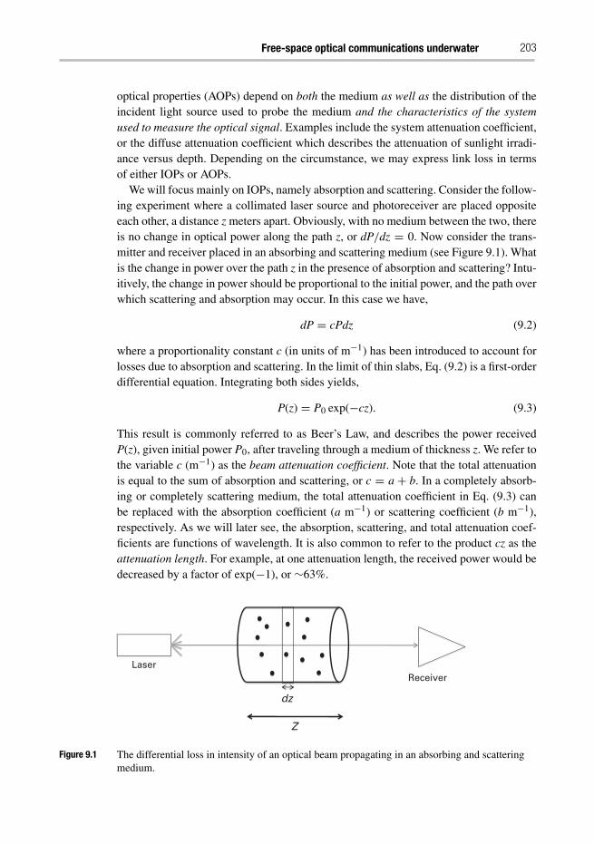
Free-space optical communications underwater 203
optical properties (AOPs) depend on both the medium as well as the distribution of theincident light source used to probe the medium and the characteristics of the systemused to measure the optical signal. Examples include the system attenuation coefficient,or the diffuse attenuation coefficient which describes the attenuation of sunlight irradi-ance versus depth. Depending on the circumstance, we may express link loss in termsof either IOPs or AOPs.
We will focus mainly on IOPs, namely absorption and scattering. Consider the follow-ing experiment where a collimated laser source and photoreceiver are placed oppositeeach other, a distance z meters apart. Obviously, with no medium between the two, thereis no change in optical power along the path z, or dP/dz = 0. Now consider the trans-mitter and receiver placed in an absorbing and scattering medium (see Figure 9.1). Whatis the change in power over the path z in the presence of absorption and scattering? Intu-itively, the change in power should be proportional to the initial power, and the path overwhich scattering and absorption may occur. In this case we have,
dP = cPdz (9.2)
where a proportionality constant c (in units of m−1) has been introduced to account forlosses due to absorption and scattering. In the limit of thin slabs, Eq. (9.2) is a first-orderdifferential equation. Integrating both sides yields,
P(z) = P0 exp(−cz). (9.3)
This result is commonly referred to as Beer’s Law, and describes the power receivedP(z), given initial power P0, after traveling through a medium of thickness z. We refer tothe variable c (m−1) as the beam attenuation coefficient. Note that the total attenuationis equal to the sum of absorption and scattering, or c = a + b. In a completely absorb-ing or completely scattering medium, the total attenuation coefficient in Eq. (9.3) canbe replaced with the absorption coefficient (a m−1) or scattering coefficient (b m−1),respectively. As we will later see, the absorption, scattering, and total attenuation coef-ficients are functions of wavelength. It is also common to refer to the product cz as theattenuation length. For example, at one attenuation length, the received power would bedecreased by a factor of exp(−1), or ∼63%.
LaserReceiver
Z
dz
Figure 9.1 The differential loss in intensity of an optical beam propagating in an absorbing and scatteringmedium.
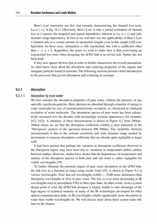
204 Brandon Cochenour and Linda Mullen
Beer’s Law represents our first step towards characterizing the channel loss term,LW (t, r, z), in Eq. (9.1). Obviously, Beer’s Law is only a partial estimation of channelloss as it ignores the temporal and spatial dependency inherent in LW (t, r, z) and onlyincludes range dependency. In fact as we will later see, the applicability of Beer’s Lawis limited only to a certain amount of attenuation lengths even in this simple LOS con-figuration. In these cases, attenuation is still exponential, but with a coefficient otherthan c = a + b. Regardless, the point we wish to make here is that overcoming anexponential loss term when designing the uFSO link is no trivial task. Nature has notbeen kind.
It may now appear obvious that in order to further characterize the overall attenuation,we must know more about the absorption and scattering properties of the organic andinorganic particles found in seawater. The following sections present a brief introductionto the processes that govern absorption and scattering in seawater.
9.2.1 Absorption
9.2.1.1 Absorption by pure waterWe first consider the absorption properties of pure water, without the presence of anyoptically significant particles. Here, photons are absorbed through a transfer of energy towater molecules by way of ionization/electronic excitation, or vibrational or rotationalexcitation of water molecules. The absorption spectra of pure water has been exhaus-tively measured over the decades with increasingly accurate apparatuses (for example,[47], [43]). A summary of these measurements is shown in Figure 9.2 from 300nm–700nm where we see that the absorption coefficient exhibits a clear minimum in the“blue/green” portion of the spectrum between 400–500nm. The variability betweenmeasurements is due to the extreme sensitivity and wide dynamic range needed byinstruments to measure absorption coefficients that are already quite negligible to beginwith.
It had been posited that perhaps the variation in absorption coefficient observed inthe blue/green region may have been due to variations in temperature and/or salinitybetween studies. However, studies have shown that the dependence on temperature andsalinity of the absorption spectra of both pure and salt water is rather negligible forvisible wavelengths [39].
To further illustrate the potential impact of pure water absorption on the uFSO link,the link loss as a function of range using results from [43], is shown in Figure 9.3 atvarious wavelengths. Note that red wavelengths exhibit > 25dB more attenuation thanblue/green wavelengths at 10 m in pure water. The loss is even more devastating at IRwavelengths used in atmospheric FSO or fiber optic links. In other words, from a systemdesign point of view, the uFSO link designer is largely unable to take advantage of thehigh degree of technical maturity of many of the IR technologies developed for otheroptical communication links, as IR wavelengths exhibit significantly more absorption inwater than visible wavelengths do. We will discuss more about these system trade-offslater in the chapter.
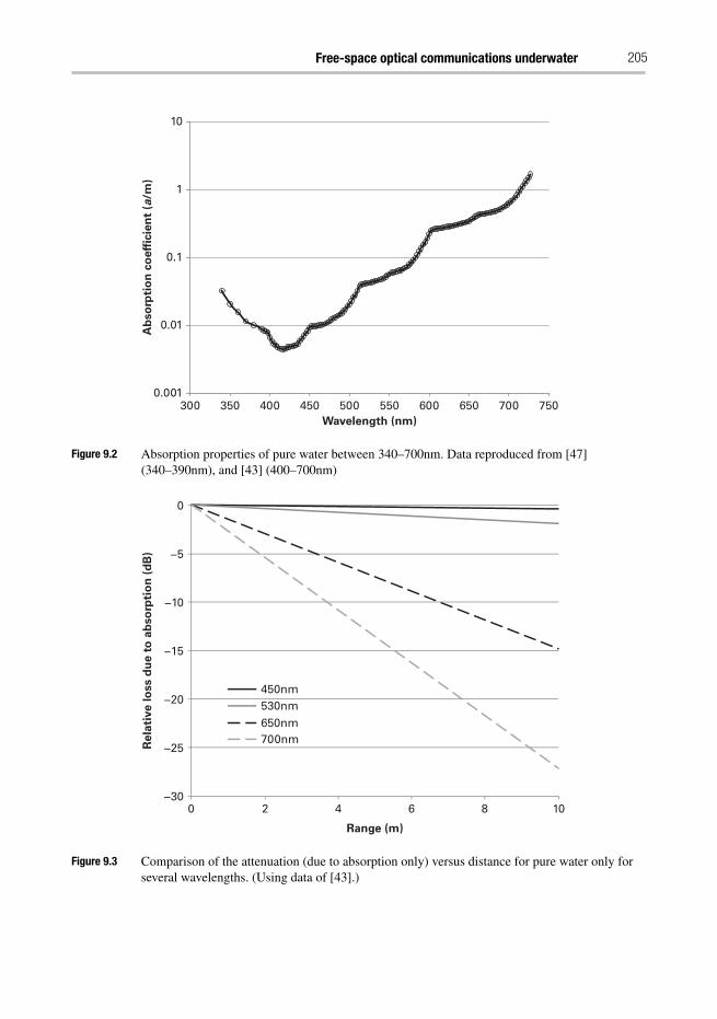
Free-space optical communications underwater 205
0.001
0.01
0.1
1
10
300 350 400 450 500 550 600 650 700 750Wavelength (nm)
Ab
so
rpti
on
co
eff
icie
nt
(a/m
)
Figure 9.2 Absorption properties of pure water between 340–700nm. Data reproduced from [47](340–390nm), and [43] (400–700nm)
−30
−25
−20
−15
−10
−5
0
0 2 4 6 8 10
Rela
tive lo
ss d
ue t
o a
bso
rpti
on
(d
B)
Range (m)
450nm530nm650nm700nm
Figure 9.3 Comparison of the attenuation (due to absorption only) versus distance for pure water only forseveral wavelengths. (Using data of [43].)
206 Brandon Cochenour and Linda Mullen
9.2.1.2 Absorption by colored dissolved organic matterColored dissolved organic matter (CDOM) (also known as yellow substance orgelbstoff) is the result of dead or decaying organisms and cells. Absorption due toCDOM is high in the UV and blue, and typically falls off exponentially with wave-length (see for example, [26]). As we will later see, this tends to shift the wavelength ofminimum absorption from the blue into the green.
9.2.1.3 Absorption by phytoplanktonThe word “phytoplankton” is derived from Greek words that translate literally to “wan-dering plant.” As its name suggests, phytoplankton produce energy via photosynthesis,and therefore it is often found near the water surface where sunlight is abundant.As such, phytoplankton plays a significant role in the absorption of light in the sea.Chlorophyll-a is a main “ingredient” in the phytoplankton photosynthesis process, andtends to exhibit strong absorption to UV, blue, and red wavelengths ([33], [44]). (Forthe non-specialist, this is precisely the reason that the leaves of trees, which also containcholorophyll-a, appear green).
While beyond the scope of this discussion, the impact of chlorophyll-a on the absorp-tion coefficient in seawater depends on the amount of pigment contained within aphytoplankton species as well as the concentration of phytoplankton in the water. Addi-tionally, concentration and species can be depth dependent. Suffice to say, the windowof minimum absorption at blue wavelengths for pure water observed in Figure 9.2, tendsto shift towards green wavelengths in waters containing phytoplankton.
9.2.2 Scattering
Scattering is the process whereby a photon’s path is altered by interaction with amolecule or particle. Mobley [33] separates scattering into three broad regimes:
1. Molecular scattering (<<λ): Scattering caused by local molecule density fluctua-tions. For example, local concentrations of sea salts in pure seawater.
2. Scattering by “large” particles (>λ): Particles typically 10 times λ are consid-ered “large” particles. These are the organic and inorganic particles that typicallydominate the scattering properties of seawater.
3. Turbulent scattering (>>λ): Temperature, pressure, or salinity changes that causesignificant changes in the index of refraction.
9.2.2.1 Molecular scatteringScattering by pure water arises from the random nature of molecular motion. Scatteringby pure seawater is similar, though with the included contribution of various salt ionsfound in seawater. The scattering coefficient for pure water and pure seawater is foundin Figure 9.4 [34]. The slight increase in pure seawater is due to the extra contributionfrom salt ions. However, in relation to the absorption coefficient, Figure 9.4 shows thatscattering of pure water contributes minimally to the overall attenuation. As such, wewill focus our discussion on the scattering caused by large particles.
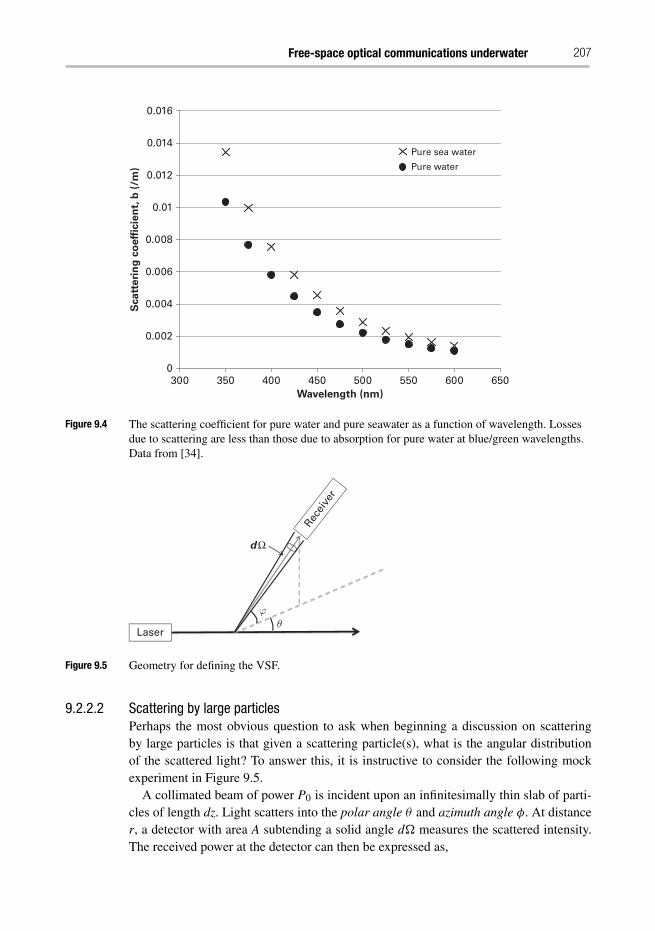
Free-space optical communications underwater 207
0
0.002
0.004
0.006
0.008
0.01
0.012
0.014
0.016
300 350 400 450 500 550 600 650Wavelength (nm)
Scatt
eri
ng
co
eff
icie
nt,
b (
/m)
Pure sea water
Pure water
Figure 9.4 The scattering coefficient for pure water and pure seawater as a function of wavelength. Lossesdue to scattering are less than those due to absorption for pure water at blue/green wavelengths.Data from [34].
Laser
ϕθ
Rece
iver
d Ω
Figure 9.5 Geometry for defining the VSF.
9.2.2.2 Scattering by large particlesPerhaps the most obvious question to ask when beginning a discussion on scatteringby large particles is that given a scattering particle(s), what is the angular distributionof the scattered light? To answer this, it is instructive to consider the following mockexperiment in Figure 9.5.
A collimated beam of power P0 is incident upon an infinitesimally thin slab of parti-cles of length dz. Light scatters into the polar angle θ and azimuth angle φ. At distancer, a detector with area A subtending a solid angle d� measures the scattered intensity.The received power at the detector can then be expressed as,
208 Brandon Cochenour and Linda Mullen
PS (θ ,φ) = P0β(θ ,φ)dzd� (9.3)
where we have introduced a term β(θ ,φ) that describes the angular distribution of light.Rearranging terms,
β(θ ,φ) = PS (θ ,φ)
P0dzd�(9.4)
Note that the received scattered differential intensity is dI(θ ,φ) = PS (θ ,φ) /d�(W sr−1). Also, if the incident power illuminates an area on the slab dA, then the inci-dent irradiance is E = P0/dA (W m−2). If we consider the incident beam illuminatesan infinitesimal volume dV = dzdA, then Eq. (9.4) can be re-written as,
β(θ ,φ) = dI(θ ,φ)
EdV(9.5)
Thus, the physical meaning of β(θ ,φ) is the scattered intensity (in direction (θ ,φ))per unit incident irradiance per unit volume. Therefore, β(θ ,φ) is often referred to asthe volume scattering function (VSF) and has the units m−1 sr−1. Integrating the VSFover all 4π steradians is analogous to determining the “strength” of scattering over allangles.
b =∫φ
∫θ
β(θ ,φ) sin θ dθd φ = 2π
π∫0
β(θ ) sin θd θ (9.6)
We refer to b as the scattering coefficient (in units of m−1). Note that the last step inEq. (9.6) arises due to the fact that we have assumed a spatially homogenous medium,and that the VSF is symmetric in the azimuthal direction. If we take the VSF (angu-lar distribution of scattered light) and normalize it by the scattering coefficient, b, wehave
p(θ ) = β(θ )
b(9.7)
which is commonly referred to as the phase function. A warning to the reader, despite itsname, the phase function has nothing to do with any phase. Rather, it borrows its namefrom astronomy, where it is used to describe how solar fluxes are reflected versus angle.Other popular names for the phase function include scattering diagram or scatteringindicatrix.
One may ask what physical meaning the phase function would have, given that we’vealready described the distribution of scattered intensity with the VSF. While the exer-cise is left to the reader, integrating Eq. (9.7) from θ : 0 → π results in unity, which isthe requirement for a probability distribution. As we will see later, probability distribu-tions are useful in analytical and numerical modeling techniques for simulating opticalpropagation underwater.
9.2.2.3 Phase functions of natural watersIn the 1960s and 1970s, a great deal of work was performed at Scripps Insti-tute of Oceanography in San Diego, CA aimed at characterizing the visibility of
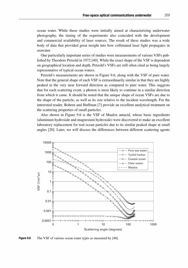
Free-space optical communications underwater 209
ocean water. While these studies were initially aimed at characterizing underwaterphotography, the timing of the experiments also coincided with the developmentand commercial availability of laser sources. The result of these studies was a widebody of data that provided great insight into how collimated laser light propagates inseawater.
One particularly important series of studies were measurements of various VSFs pub-lished by Theodore Petzold in 1972 [40]. While the exact shape of the VSF is dependenton geographical location and depth, Petzold’s VSFs are still often cited as being largelyrepresentative of typical ocean waters.
Petzold’s measurements are shown in Figure 9.6, along with the VSF of pure water.Note that the general shape of each VSF is extraordinarily similar in that they are highlypeaked in the very near forward direction as compared to pure water. This suggeststhat for each scattering event, a photon is most likely to continue in a similar directionfrom which it came. It should be noted that the unique shape of ocean VSFs are due tothe shape of the particle, as well as its size relative to the incident wavelength. For theinterested reader, Bohren and Huffman [7] provide an excellent analytical treatment onthe scattering properties of small particles.
Also shown in Figure 9.6 is the VSF of Maalox antacid, whose basic ingredients(aluminum hydroxide and magnesium hydroxide) were discovered to make an excellentlaboratory replacement for real ocean particles due to its similar peaked shape at smallangles [20]. Later, we will discuss the differences between different scattering agents
0.0001
0.001
0.01
0.1
1
10
100
1000
10000
0 1 10 100 1000
Scattering angle (degrees)
Pure sea water
Turbid harbor
Coastal ocean
Clear ocean
Maalox
VS
F (1
/m*s
r)
Figure 9.6 The VSF of various ocean water types as measured by [40].
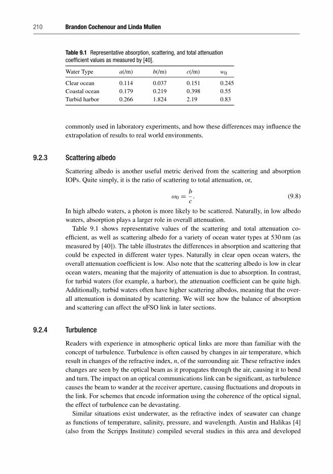
210 Brandon Cochenour and Linda Mullen
Table 9.1 Representative absorption, scattering, and total attenuationcoefficient values as measured by [40].
Water Type a(/m) b(/m) c(/m) w0
Clear ocean 0.114 0.037 0.151 0.245Coastal ocean 0.179 0.219 0.398 0.55Turbid harbor 0.266 1.824 2.19 0.83
commonly used in laboratory experiments, and how these differences may influence theextrapolation of results to real world environments.
9.2.3 Scattering albedo
Scattering albedo is another useful metric derived from the scattering and absorptionIOPs. Quite simply, it is the ratio of scattering to total attenuation, or,
ω0 = b
c. (9.8)
In high albedo waters, a photon is more likely to be scattered. Naturally, in low albedowaters, absorption plays a larger role in overall attenuation.
Table 9.1 shows representative values of the scattering and total attenuation co-efficient, as well as scattering albedo for a variety of ocean water types at 530 nm (asmeasured by [40]). The table illustrates the differences in absorption and scattering thatcould be expected in different water types. Naturally in clear open ocean waters, theoverall attenuation coefficient is low. Also note that the scattering albedo is low in clearocean waters, meaning that the majority of attenuation is due to absorption. In contrast,for turbid waters (for example, a harbor), the attenuation coefficient can be quite high.Additionally, turbid waters often have higher scattering albedos, meaning that the over-all attenuation is dominated by scattering. We will see how the balance of absorptionand scattering can affect the uFSO link in later sections.
9.2.4 Turbulence
Readers with experience in atmospheric optical links are more than familiar with theconcept of turbulence. Turbulence is often caused by changes in air temperature, whichresult in changes of the refractive index, n, of the surrounding air. These refractive indexchanges are seen by the optical beam as it propagates through the air, causing it to bendand turn. The impact on an optical communications link can be significant, as turbulencecauses the beam to wander at the receiver aperture, causing fluctuations and dropouts inthe link. For schemes that encode information using the coherence of the optical signal,the effect of turbulence can be devastating.
Similar situations exist underwater, as the refractive index of seawater can changeas functions of temperature, salinity, pressure, and wavelength. Austin and Halikas [4](also from the Scripps Institute) compiled several studies in this area and developed
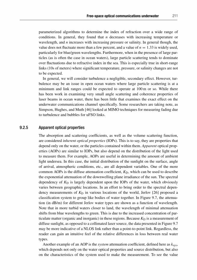
Free-space optical communications underwater 211
parameterized algorithms to determine the index of refraction over a wide range ofconditions. In general, they found that n decreases with increasing temperature orwavelength, and n increases with increasing pressure or salinity. In general though, thevalue does not fluctuate more than a few percent, and a value of n = 1.33 is widely used,particularly for blue/green wavelengths. Furthermore, when in the presence of large par-ticles (as is often the case in ocean waters), large particle scattering tends to dominateover fluctuations due to refractive index in the sea. This is especially true in short-rangelinks (10s of meters) where significant temperature, pressure, or salinity changes are notto be expected.
In general, we will consider turbulence a negligible, secondary effect. However, tur-bulence may be an issue in open ocean waters where large particle scattering is at aminimum and link ranges could be expected to operate at 100 m or so. While therehas been work in examining very small angle scattering and coherence properties oflaser beams in ocean water, there has been little that examines the exact effect on theunderwater communications channel specifically. Some researchers are taking note, asSimpson, Hughes, and Muth [46] looked at MIMO techniques for measuring fading dueto turbulence and bubbles for uFSO links.
9.2.5 Apparent optical properties
The absorption and scattering coefficients, as well as the volume scattering function,are considered inherent optical properties (IOPs). This is to say, they are properties thatdepend only on the water, or the particles contained within them. Apparent optical prop-erties (AOPs) are similar to IOPs, but also depend on the distribution of the light usedto measure them. For example, AOPs are useful in determining the amount of ambientlight undersea. In this case, the initial distribution of the sunlight on the surface, angleof arrival, atmospheric conditions, etc., are all dependent variables. One of the morecommon AOPs is the diffuse attenuation coefficient, KD, which can be used to describethe exponential attenuation of the downwelling plane irradiance of the sun. The spectraldependency of KD is largely dependent upon the IOPs of the water, which obviouslyvaries between geographic locations. In an effort to bring order to the spectral depen-dency measurements of KD in various locations of the world, Jerlov [26] proposed aclassification system to group like bodies of water together. In Figure 9.7, the attenua-tion (in dB/m) for different Jerlov water types are shown as a function of wavelength.Note that in more turbid waters closer to land, the wavelength of minimal attenuationshifts from blue wavelengths to green. This is due to the increased concentration of par-ticulate matter (organic and inorganic) in these regions. Because KD is a measurement ofdiffuse sunlight, as opposed to a collimated laser source, the data presented in Figure 9.7may be more indicative of a NLOS link rather than a point-to-point link. Regardless, thereader can gain an intuitive feel of the relative differences in loss between real watertypes.
Another example of an AOP is the system attenuation coefficient, defined here as ksys,which depends not only on the water optical properties and source distribution, but alsoon the characteristics of the system used to make the measurement. To see the value
212 Brandon Cochenour and Linda Mullen
0
2
4
6
8
10
12
14
16
18
300 350 400 450 500 550 600 650 700Wavelength (nm)
Att
en
uati
on
(d
B/m
)
Open ocean
Coastal ocean
Turbid harbor
Figure 9.7 Approximate loss in dB/meter for various ocean waters as defined by Jerlov (data adaptedfrom [26]).
of ksys, let us consider the line-of-sight configuration. We have seen that using the totalattenuation coefficient, c = a+b, in Beer’s Law can accurately describe the line-of-sightscenario (i.e. Eq. (9.2)). This model for channel loss is predicated upon any photon thatis absorbed or scattered does not contribute to the received optical power at the photore-ciever. However, now consider a scenario where there is significantly more scatteringevents. Here, multiple scattering causes photons that were once “lost” to scatter backinto the receiver aperture and field of view. In this case, the photoreceiver collects morelight than predicted by the attenuation coefficient. Additionally, we might consider theeffect of increasing the receiver aperture and field of view. This would certainly increasethe collection of scattered light.
The point is that modeling optical power loss by the attenuation coefficient, c, isonly valid if we assume that only non-scattered light is collected. If scattered light iscollected (due to either significantly turbid waters, a change in system parameters, orboth), then another term must be used to describe attenuation. This “other” term is ksys,and it provides us with the ability to modify Beer’s Law as given in Eq. (9.2) to accountfor both properties of the water (multiple scattering, ratio of scattering to absorption,etc.) as well as the properties of the system (receiver aperture, field of view, sourcedivergence, etc.).
Free-space optical communications underwater 213
9.2.6 Relating AOPs to IOPs
It should be clear now that it is important for the link designer to take into account boththe environment as well as the system design when determining how to predict uFSOchannel loss. Said another way, while the IOPs may be used to characterize the waterand its constituents, it is an AOP that is often measured by the system. Understandingthis relationship is crucial.
We now formalize the above discussion, following the notation of [10]. We begin bymodifying Eq. (9.2) as,
P(z) = P0 exp(−ksysz) where ksys = a+ (1− η)b (9.9)
where we have introduced a scattering factor 0 ≤ η ≤ 1 that is used to account for thecollection of multiply scattered light. Observe that a high scattering factor effectivelyscales down the scattering coefficient. Intuitively, this makes sense since the collectionof scattered photons would have the net effect of reducing the attenuation due to scat-tering. A scattering factor of unity physically means that we have collected all light thathas been scattered. In this case, the received power will be attenuated by the absorptioncoefficient. A scattering factor of 0 physically means that we have collected none of thescattered light. In this case, Eq. (9.9) reduces to Eq. (9.2), since ksys = c. As we will seein later sections, neither Eq. (9.2) nor Eq. (9.9) can fully describe the attenuation for allranges or water types. More often, we find that attenuation is exponential by c in low orminimal scattering regimes, and by ksys in multiple scattering regimes.
9.3 Channel characterization: theory
In the previous section, we learned about some of the physical properties of ocean water,and gained insight into their potential impact to the uFSO link. We saw that while IOPscan be used to characterize the water, the exponential attenuation given by Beer’s Lawusing the beam attenuation coefficient may only provide a first-order understanding ofthe ocean channel. In reality, we must consider physical subtleties like multiple scatter-ing, or the balance between the degree of absorption and scattering, as well as systemsubtleties such as aperture, field of view, pointing and tracking, etc.
It should be clear at this point then, that in order to more accurately model uFSOlinks, we should simply find a way to express the spatial and temporal characteristicsof a propagated laser beam at all points in space. Once this is known, one can accu-rately predict both the expected received intensity, as well as the maximum bandwidthavailable, at all points in the underwater channel.
On the surface, this seems like a simple task. After all, based on our previous discus-sions in the last section, we have the ability to accurately measure absorption, scattering,and phase functions of seawater. In reality however, arriving at a complete spatial andtemporal description of the light field at all points in space is easier said than done. Forexample, while we may be able to describe the probability distribution of scattering ver-sus angle of a single photon interacting with a single particle, how do we extrapolate this
214 Brandon Cochenour and Linda Mullen
to millions of photons interacting with millions of particles, altering their paths manytimes over the length of propagation?
The starting point for many theoretical descriptions is the Radiative Transfer Equation(RTE),[
1
ν
∂
∂t+ �n · ∇
]I (t, �r, �n) = −cI (t, �r, �n)+
∫4π
β(�r, �n, �n′)I (t, �r, �n) d�n′ +E (t, �r, �n) (9.10)
where ν is the speed of light, c is the beam attenuation coefficient, t is time, �n is thedirection vector, �r is the position vector, and ∇ is the divergence operator with respectto position �r. I is the radiance, β is the VSF, and E is the source radiance.
Simply stated, the RTE is a formulation in energy conservation: the change in inten-sity over a differential length (l.h.s.) is equal to the extinction losses (absorption andscattering) over that path, plus the contribution of any scattered intensity from otherplaces in space (r.h.s.). The first term on the right, the one that describes extinction lossesover a differential length, is simply Beer’s Law. The second term on the right-hand sidehowever, represents all the possible contributions of scattered intensity from all otherpoints in space. This term is far less simple. In any case, we see the RTE is a complexintegro-differential equation of several variables, and finding tractable solutions is notrivial task. In this section, we introduce some of the common theoretical methods usedto describe the intensity distribution in space, as well as the temporal dispersion.
9.3.1 Numerical methods
Numerical methods, such as Monte Carlo simulations, are perhaps the most intuitive.Numerical methods essentially “mimic” the real world by individually tracking pho-tons through the scattering medium. Armed with information such as the absorption andscattering coefficients, as well as the phase function, a Monte Carlo computer program“marches” photons through a medium, and “counts” those that arrive at a particularlocation. Naturally, these techniques can also account for source aperture and diver-gence, receiver aperture and field of view, and can also keep track of the polarizationof individual photons. Numerical methods are most intuitive to understand, since wephysically “keep track” of the pathways and histories of individual photons. Naturally,knowing the precise location of every photon allows us to determine the spatial distri-bution of light. Additionally, because we know the path each photon travels, we cancalculate the time it takes each photon to arrive at a point in space. Comparing thesetime differences that arise due to different scattering paths allows us to calculate thetemporal dispersion (i.e. pulse spread, or channel bandwidth).
Of course, numerical techniques are also the most computationally time consuming,as millions (or billions) of photons may be needed in order to accurately simulate areal-world application. Of course, this downside continues to become less of an issue asfaster computers with more processing power become available.
While many Monte Carlo models describing photon transport in seawater have beenreported (e.g. [29]), we wish to highlight a few new studies that were performed par-ticularly with the uFSO channel in mind. Hanson and Radic [24] presented a Monte
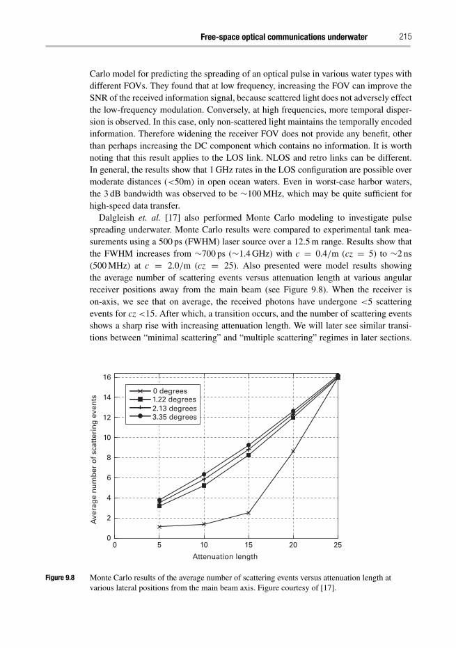
Free-space optical communications underwater 215
Carlo model for predicting the spreading of an optical pulse in various water types withdifferent FOVs. They found that at low frequency, increasing the FOV can improve theSNR of the received information signal, because scattered light does not adversely effectthe low-frequency modulation. Conversely, at high frequencies, more temporal disper-sion is observed. In this case, only non-scattered light maintains the temporally encodedinformation. Therefore widening the receiver FOV does not provide any benefit, otherthan perhaps increasing the DC component which contains no information. It is worthnoting that this result applies to the LOS link. NLOS and retro links can be different.In general, the results show that 1 GHz rates in the LOS configuration are possible overmoderate distances (<50m) in open ocean waters. Even in worst-case harbor waters,the 3 dB bandwidth was observed to be ∼100 MHz, which may be quite sufficient forhigh-speed data transfer.
Dalgleish et. al. [17] also performed Monte Carlo modeling to investigate pulsespreading underwater. Monte Carlo results were compared to experimental tank mea-surements using a 500 ps (FWHM) laser source over a 12.5 m range. Results show thatthe FWHM increases from ∼700 ps (∼1.4 GHz) with c = 0.4/m (cz = 5) to ∼2 ns(500 MHz) at c = 2.0/m (cz = 25). Also presented were model results showingthe average number of scattering events versus attenuation length at various angularreceiver positions away from the main beam (see Figure 9.8). When the receiver ison-axis, we see that on average, the received photons have undergone <5 scatteringevents for cz <15. After which, a transition occurs, and the number of scattering eventsshows a sharp rise with increasing attenuation length. We will later see similar transi-tions between “minimal scattering” and “multiple scattering” regimes in later sections.
00
2
4
6
8
10
12
14
16
5 10
Attenuation length
Ave
rag
e n
um
ber
of
scat
teri
ng
eve
nts
15 20 25
0 degrees1.22 degrees 2.13 degrees 3.35 degrees
Figure 9.8 Monte Carlo results of the average number of scattering events versus attenuation length atvarious lateral positions from the main beam axis. Figure courtesy of [17].
216 Brandon Cochenour and Linda Mullen
For off-axis receiver positions, the average number of scattering events appears to growsomewhat linearly with attenuation length.
9.3.2 Analytical methods
Analytical methods are sometimes preferred over numerical techniques because they aremore flexible, and are often less computationally intensive. The drawback to analyticalmethods are that they are often complex, less intuitive, and in some cases, do not yieldtractable solutions without some simplifying assumptions. In this section, we discusssome of these methods.
9.3.2.1 Small-angle approximationThe small-angle approximation (SAA) is a popular simplification of the RTE. Whilethe SAA has its origins in neutron scattering theory, its application to describing photontransport in ocean waters was made popular by a series of papers by H. G. Wells [51–52]. As its name suggests, the SAA assumes that scattering events are confined to nearforward angles to the beam axis. In this case, we can assume that cos(θ ) = 1 andsin(θ ) = tan(θ ) = θ , where θ is the angle off axis. This assumption is only valid whenthe VSF is peaked at forward angles. Fortunately, we have seen that this is preciselythe case for ocean waters. Also note that this effectively assumes that scattered photonstravel the same distance as non-scattered photons. This inherently means that the SAAignores time-dispersion.
Wells derives the beam-spread function (BSF) as f (θ , z), where θ is the angle off axisand z is the range. Wells showed the convenience of representing f (θ , z) as its 2D Fouriertransform F(ψ , z), where
f (θ , z) = 2π
∞∫0
F(ψ , z)J0 (2πθψ)ψdψ
F(ψ , z) = 2π
θmax∫0
f (θ , z)J0 (2πθψ)θdθ
(9.11)
where J0 is a zeroth-order Bessel function and θmax is the maximum angle of scatteringas defined by the SAA. Equation (9.11) represent a Hankel transform, which simplifiesthe 2D Fourier transform by taking advantage of radial symmetry. Wells derived theBSF in the spatial frequency domain as,
F(ψ , z) = exp
⎡⎣−cz+
z∫0
S
(ψ
r
z
)dr
⎤⎦ (9.12)
where S(ψ) is the Hankel transform of the VSF, β(θ ). Knowledge of the VSF allows fortransform to S(ψ). Integration of S(ψ) in Eq. (9.12) provides F(ψ , z), and transform ofF(ψ , z) in Eq. (9.11) provides f (θ , z), the desired BSF.
Free-space optical communications underwater 217
Wells suggested a cone of θmax = 10◦ for the small-angle limit, though the exactθmax can vary depending on the shape of the VSF and geometry to which the SAA isapplied. Zege et al. [54] showed that the SAA provides good results in regions wherex/z < 1, where x is the lateral distance from the beam axis and z is range. This limit onthe region of applicability is to be expected given our assumption that scattering eventsare confined to near forward angles.
9.3.2.2 Vector radiative transfer modelingJaruwatanadilok [25] approached the problem of predicting temporal dispersion byusing vector radiative transfer theory. This theory takes into account both the spatialand temporal dispersion, as well as modeling how the polarization changes duringpropagation. The impulse response for both polarization components was modeled inwater with c = 0.305/m at 30 m and 50 m. Results show that at both ranges, the co-polarized component is significantly more peaked than the cross-polarized component.This should make intuitive sense, as the co-polarized component is that which shouldnot have undergone multiple scattering, and hence retains a high temporal resolution.On the other hand, multiple scattering would stand to alter the orientation of the polar-ization vector. As such, the cross-polarized component should contain mostly light thathas been multiply scattered, and this multiple scattering will result in a spread of theimpulse response. The effect of FOV on BER was also studied. Results supported thefindings of Hanson and Radic [24], as they showed a diminishing improvement in BERwhen increasing FOV at high data rates. It was observed however that at short range, onedoes stand to benefit from increasing the FOV, even at high frequency. This is becauseat short range, there is less multiple scattering. However, as range increases, so does thedegree of multiple scattering. In this regime, the benefit of a wider FOV decreases.
9.3.2.3 Other analytical techniquesWe have previously seen that a common simplification in analytical models is to applythe small-angle approximation, and assume that all scattering events occur within verynear forward angles. This effectively ignores any time dispersion, since we essentiallypresume that all photons travel approximately the same path length through the medium.Of course, time dispersion is ignored only due to the mathematical convenience of thefirst-order assumption, cos(θ ) = 1 and sin(θ ) = tan(θ ) = θ . However, by consideringhigher-order effects, temporal dispersion can be included. To do this, one attempts todescribe the spatial dispersion and variation in photon transit time statistically.
Approaches may vary. Stotts [48] presents a simple statistical approach that appliesthe scattering statistics of electron scattering theory to that of photons undergoing scat-tering by large particles. In this way, he was able to calculate the average path lengthdifference a scattered photon has relative to a non-scattered photon. Using the speed oflight, the average pulse spreading can be given by,
�t = R
ν
{0.30
bRθ2
[(1+ 9
4bRθ2
)1.5
− 1
]− 1
}. (9.13)
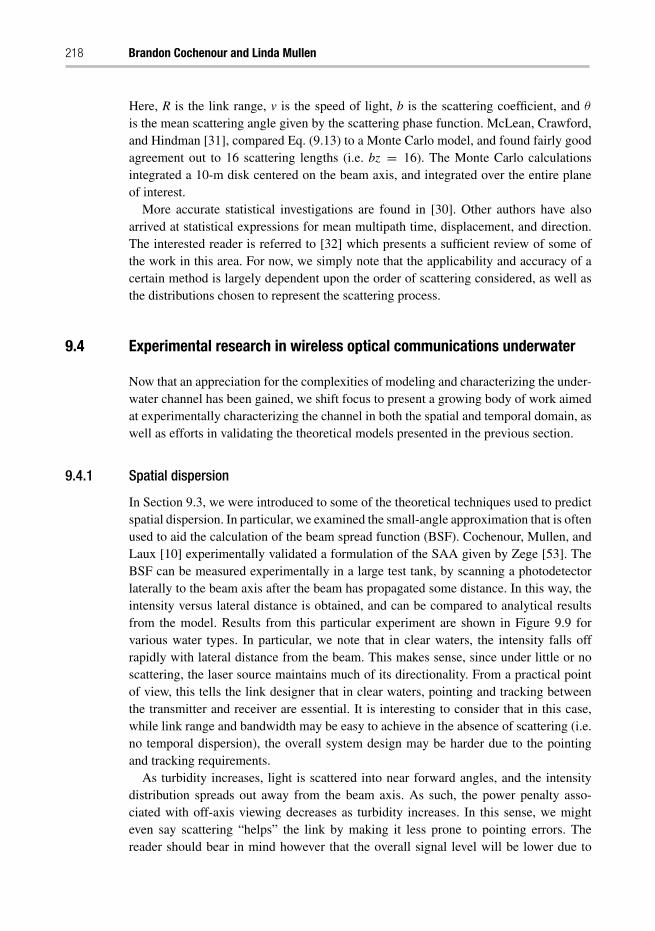
218 Brandon Cochenour and Linda Mullen
Here, R is the link range, v is the speed of light, b is the scattering coefficient, and θ
is the mean scattering angle given by the scattering phase function. McLean, Crawford,and Hindman [31], compared Eq. (9.13) to a Monte Carlo model, and found fairly goodagreement out to 16 scattering lengths (i.e. bz = 16). The Monte Carlo calculationsintegrated a 10-m disk centered on the beam axis, and integrated over the entire planeof interest.
More accurate statistical investigations are found in [30]. Other authors have alsoarrived at statistical expressions for mean multipath time, displacement, and direction.The interested reader is referred to [32] which presents a sufficient review of some ofthe work in this area. For now, we simply note that the applicability and accuracy of acertain method is largely dependent upon the order of scattering considered, as well asthe distributions chosen to represent the scattering process.
9.4 Experimental research in wireless optical communications underwater
Now that an appreciation for the complexities of modeling and characterizing the under-water channel has been gained, we shift focus to present a growing body of work aimedat experimentally characterizing the channel in both the spatial and temporal domain, aswell as efforts in validating the theoretical models presented in the previous section.
9.4.1 Spatial dispersion
In Section 9.3, we were introduced to some of the theoretical techniques used to predictspatial dispersion. In particular, we examined the small-angle approximation that is oftenused to aid the calculation of the beam spread function (BSF). Cochenour, Mullen, andLaux [10] experimentally validated a formulation of the SAA given by Zege [53]. TheBSF can be measured experimentally in a large test tank, by scanning a photodetectorlaterally to the beam axis after the beam has propagated some distance. In this way, theintensity versus lateral distance is obtained, and can be compared to analytical resultsfrom the model. Results from this particular experiment are shown in Figure 9.9 forvarious water types. In particular, we note that in clear waters, the intensity falls offrapidly with lateral distance from the beam. This makes sense, since under little or noscattering, the laser source maintains much of its directionality. From a practical pointof view, this tells the link designer that in clear waters, pointing and tracking betweenthe transmitter and receiver are essential. It is interesting to consider that in this case,while link range and bandwidth may be easy to achieve in the absence of scattering (i.e.no temporal dispersion), the overall system design may be harder due to the pointingand tracking requirements.
As turbidity increases, light is scattered into near forward angles, and the intensitydistribution spreads out away from the beam axis. As such, the power penalty asso-ciated with off-axis viewing decreases as turbidity increases. In this sense, we mighteven say scattering “helps” the link by making it less prone to pointing errors. Thereader should bear in mind however that the overall signal level will be lower due to
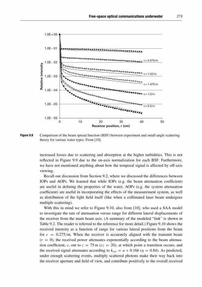
Free-space optical communications underwater 219
1.0E − 06
1.0E − 05
1.0E − 04
1.0E − 03
1.0E − 02
1.0E − 01
1.0E + 00
0 10 20 30 40 50Receiver position, r (cm)
Re
lati
ve
in
ten
sit
y
c = 2.675/m
c = 1.92/m
c = 1.475/m
c = 1.0/m
c = 0.5/m
Figure 9.9 Comparison of the beam spread function (BSF) between experiment and small-angle scatteringtheory for various water types. From [10].
increased losses due to scattering and absorption at the higher turbidities. This is notreflected in Figure 9.9 due to the on-axis normalization for each BSF. Furthermore,we have not mentioned anything about how the temporal signal is affected by off-axisviewing.
Recall our discussion from Section 9.2, where we discussed the differences betweenIOPs and AOPs. We learned that while IOPs (e.g. the beam attenuation coefficient)are useful in defining the properties of the water, AOPs (e.g. the system attenuationcoefficient) are useful in incorporating the effects of the measurement system, as wellas distribution of the light field itself (like when a collimated laser beam undergoesmultiple scattering).
With this in mind we refer to Figure 9.10, also from [10], who used a SAA modelto investigate the rate of attenuation versus range for different lateral displacements ofthe receiver from the main beam axis. (A summary of the modeled “link” is shown inTable 9.2. The reader is referred to the reference for more detail.) Figure 9.10 shows thereceived intensity as a function of range for various lateral positions from the beamfor c = 0.275/m. When the receiver is accurately aligned with the transmit beam(r = 0), the received power attenuates exponentially according to the beam attenua-tion coefficient, c, out to z = 75 m (cz = 20), at which point a transition occurs, andthe received signal attenuates according to ksys = a + 0.16b (η = 0.84). As predicted,under enough scattering events, multiply scattered photons make their way back intothe receiver aperture and field of view, and contribute positively to the overall received
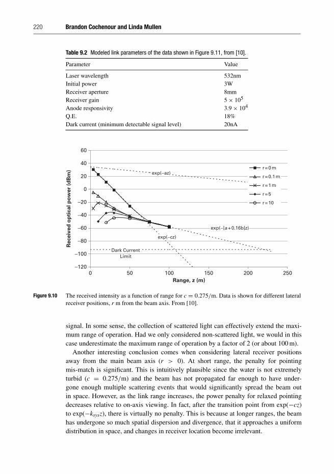
220 Brandon Cochenour and Linda Mullen
Table 9.2 Modeled link parameters of the data shown in Figure 9.11, from [10].
Parameter Value
Laser wavelength 532nmInitial power 3WReceiver aperture 8mmReceiver gain 5× 10⁵
Anode responsivity 3.9× 10⁴
Q.E. 18%Dark current (minimum detectable signal level) 20nA
−120
−100
−80
−60
−40
−20
0
20
40
60
0 50 100 150 200 250Range, z (m)
Re
ce
ive
d o
pti
ca
l p
ow
er
(dB
m) r = 0 m
r = 0.1 m
r = 1 m
r = 5
r = 10
exp(−az)
exp(−cz)
Dark CurrentLimit
exp(−[a + 0.16b]z)
Figure 9.10 The received intensity as a function of range for c = 0.275/m. Data is shown for different lateralreceiver positions, r m from the beam axis. From [10].
signal. In some sense, the collection of scattered light can effectively extend the maxi-mum range of operation. Had we only considered non-scattered light, we would in thiscase underestimate the maximum range of operation by a factor of 2 (or about 100 m).
Another interesting conclusion comes when considering lateral receiver positionsaway from the main beam axis (r > 0). At short range, the penalty for pointingmis-match is significant. This is intuitively plausible since the water is not extremelyturbid (c = 0.275/m) and the beam has not propagated far enough to have under-gone enough multiple scattering events that would significantly spread the beam outin space. However, as the link range increases, the power penalty for relaxed pointingdecreases relative to on-axis viewing. In fact, after the transition point from exp(−cz)to exp(−ksysz), there is virtually no penalty. This is because at longer ranges, the beamhas undergone so much spatial dispersion and divergence, that it approaches a uniformdistribution in space, and changes in receiver location become irrelevant.
Free-space optical communications underwater 221
9.4.1.1 Characterizing ksys and the c–ksys transitionThe reader may be wondering if it is possible that, given some properties of the water,one may predict at what range the attenuation will transition between c and ksys, aswell as what value ksys will take on. In essence, we would ideally like to parameterizeksys based upon all of the variables that influence the rate of attenuation. These wouldinclude both the water optical properties (absorption and scattering coefficients, VSF,etc.) as well as system parameters (receiver aperture, FOV, beam radius, divergence,etc.). This parameterization however is no trivial task due to the number of variablesinvolved [13]. However, some experimental work has gone into examining the impactof a subset of variables. Cochenour, Mullen, and Muth [12] experimentally showed thedependence of albedo and on overall attenuation versus attenuation length, as well aspolarization. In this light, it may be more convenient to represent Eq. (9.9) in terms ofthe scattering albedo. Rearranging terms results in,
P(cz) = P0 exp(−[1− ηω0]cz). (9.14)
Here we see that the natural logarithm of the received power versus attenuation lengthdecays with a slope m = 1− ηω0. When the scattering factor η = 0 (no scattered lightcollected), Eq. (9.14) reduces to Eq. (9.2). As η → 1, the received signal is dominatedby multiply scattered light, and reduces to,
P(cz) = P0 exp(−[1− ω0]cz). (9.15)
Because ω0 = b/c ≤ 1, the received power in Eq. (9.15) decays slower versus atten-uation length than the non-scattered regime in Eq. (9.14). Intuitively, this makes sensesince the collection of multiply scattered light in effect increases the optical power seenat the receiver. Finally, note that in the single scattering regime (η = 0) P0 is equal tothe initial transmitted power. However in the multiple scattering regime (η → 1), P0 isapproximately equal to the received power immediately before transition.
Equations (9.14) and (9.15) describe the rate of attenuation in the single scattering andmultiple scattering regimes. We now ask whether or not we can predict at what attenu-ation length this transition might occur. To do this, we borrow analysis from Lerner andSummers [29], who via Monte Carlo model, found that light remains relatively confinedto the original axis of propagation for distances less than a diffusion length, where adiffusion length is defined as,
LD = Lsca
1− 〈cos θ〉 . (9.16)
The scattering length is given as Lsca = b−1, and the term 〈cos θ〉 is the average cosineof the scattering angle,
〈cos θ〉 = 0.5
π∫0
ρ (θ) cos θ sin θ dθ , (9.17)
where ρ (θ) is the scattering phase function. When the VSF is highly peaked, as is thecase for ocean waters (see e.g. Figure 9.7), then the average cosine is high – typically 0.9
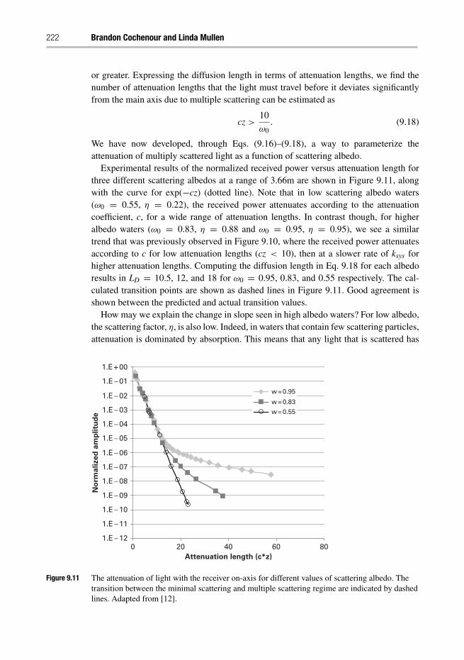
222 Brandon Cochenour and Linda Mullen
or greater. Expressing the diffusion length in terms of attenuation lengths, we find thenumber of attenuation lengths that the light must travel before it deviates significantlyfrom the main axis due to multiple scattering can be estimated as
cz >10
ω0. (9.18)
We have now developed, through Eqs. (9.16)–(9.18), a way to parameterize theattenuation of multiply scattered light as a function of scattering albedo.
Experimental results of the normalized received power versus attenuation length forthree different scattering albedos at a range of 3.66m are shown in Figure 9.11, alongwith the curve for exp(−cz) (dotted line). Note that in low scattering albedo waters(ω0 = 0.55, η = 0.22), the received power attenuates according to the attenuationcoefficient, c, for a wide range of attenuation lengths. In contrast though, for higheralbedo waters (ω0 = 0.83, η = 0.88 and ω0 = 0.95, η = 0.95), we see a similartrend that was previously observed in Figure 9.10, where the received power attenuatesaccording to c for low attenuation lengths (cz < 10), then at a slower rate of ksys forhigher attenuation lengths. Computing the diffusion length in Eq. 9.18 for each albedoresults in LD = 10.5, 12, and 18 for ω0 = 0.95, 0.83, and 0.55 respectively. The cal-culated transition points are shown as dashed lines in Figure 9.11. Good agreement isshown between the predicted and actual transition values.
How may we explain the change in slope seen in high albedo waters? For low albedo,the scattering factor, η, is also low. Indeed, in waters that contain few scattering particles,attenuation is dominated by absorption. This means that any light that is scattered has
1.E − 12
1.E − 11
1.E − 10
1.E − 09
1.E − 08
1.E − 07
1.E − 06
1.E − 05
1.E − 04
1.E − 03
1.E − 02
1.E − 01
1.E + 00
0 20 40 60 80Attenuation length (c*z)
No
rma
lize
d a
mp
litu
de
w = 0.95
w = 0.83
w = 0.55
Figure 9.11 The attenuation of light with the receiver on-axis for different values of scattering albedo. Thetransition between the minimal scattering and multiple scattering regime are indicated by dashedlines. Adapted from [12].
Free-space optical communications underwater 223
a higher probability of being absorbed, and therefore the chance of multiply scatteredlight scattering back into the receiver aperture and FOV is low. As such, we expect atten-uation by exp(−cz), even at higher turbidities, because there is little or no contributionof multiply scattered light. Conversely, in high albedo waters (such as a turbid harbor),an increasing η was observed. In this scenario, multiple scattering is quite likely, andthe contribution of multiply scattered light at the receiver causes the received powerto attenuate more slowly. We see then that albedo effectively “regulates” the degree ofmultiple scattering. In other words, it is important for the uFSO link designer to considernot only what the absorption and scattering coefficients are (in order to determine theattenuation coefficient, c = a+b), but also what the relative contributions of absorptionand scattering are (ω0 = b/c).
We have seen in the previous two sections how in some sense, multiple scatteringand spatial dispersion may actually help maintain the uFSO link under a wider rangeof environments and scenarios. This point has not been lost by other researchers, whohave looked at comparing the performance of different types of links under the sameenvironmental scenarios (see for example, [3]).
In summary, we have presented some experimental work that has attempted to vali-date spatial dispersion models, and examined the impact of multiple scattering on therate of attenuation with range and/or attenuation length. We find that in cases of multiplescattering, collecting scattered light can be useful, however only if it has not scatteredso much that the information encoded on it begins to degrade. In the next section, wefinally address this point, and present current work aimed at characterizing the temporaldispersion seen underwater.
9.4.2 Temporal dispersion
9.4.2.1 Methods for measuring temporal dispersionWe previously mentioned that one approach for characterizing the time-dependent prop-erties of light propagation in water is to measure the temporal spread of a short pulseafter it travels through water [17]. This information could then be converted to a fre-quency response via the Fourier transform. The disadvantage of this approach is that itrequires a large receiver bandwidth and a correspondingly short integration time, whichlimits the detection sensitivity. Another option is to use a continuous wave source thatis intensity modulated at a range of frequencies and measure the change in modulationdepth at each frequency after the signal propagates through water. This technique hasthe advantage of very narrow receiver bandwidths and long integration times, whichdrastically improves the detection sensitivity.
The challenge of the intensity modulation approach lies in identifying componentsrequired for high time resolution measurements with sufficient sensitivity to overcomethe exponential loss of light in water. On the transmitter end, a high-power source isneeded in the blue-green wavelength region that can be modulated at rates exceeding100 MHz. Although electro-optic modulators have been used in the past to externallymodulate high-power continuous wave green sources ([35], [8], [9]), they are limitedto frequencies < 100 MHz due to the capacitance of the modulator crystal. Blue laser
224 Brandon Cochenour and Linda Mullen
diodes are beginning to appear commercially with bandwidths of a few hundred MHz,albeit a lower output power (10s mW).
Hanson and Radic [24] reported on a system using an infrared laser diode that wasexternally modulated by a waveguide electro-optic modulator and amplified by a fiberamplifier before being frequency doubled to 532 nm. Although this source is capable ofgenerating modulated green light at rates up to 20 GHz, the optical power was limitedto less than 10 mW. Still, 1 GHz transmission was observed over a 2 m water pipe thatsimulated coastal ocean waters with 36 dB of attenuation. It was unclear however howthe confinement of the narrow water pipe affected multiple scattering dynamics.
On the receiver end, there is a trade-off between aperture and bandwidth. A largeactive area is desired to optimize the collection of scattered light, but large active areasusually translate into poor time response due to large RC time constants. Although pho-tomultiplier tubes (PMTs) are frequently used due to their high gain and large area,the fastest PMTs are limited to approximately 350 MHz with an 8 mm active area.Avalanche photodiodes (APDs) are another good choice due to their high speed andgain, but the active area is limited to <1 mm at speeds approaching 1 GHz.
An alternative approach has been presented by Mullen et. al [37, 38], which is set upcapable of measuring the transmission of light modulated at frequencies up to 1 GHzin simulated ocean water up to 55 attenuation lengths. The setup is based on the useof a mode-locked laser and a custom, modified PMT for high-speed applications (thebandwidth of this device (−3 dB) is approximately 1 GHz.). The use of a mode-lockedlaser allows us to take advantage of the frequency content inherent to a train of mode-locked pulses. These frequency components are also generated simultaneously, so thereis no need to vary the modulation frequency of the source. Furthermore, since mode-locked lasers are capable of high average optical powers, this source is an ideal candidatefor use in measuring the frequency response of light propagating in water. The frequencycontent of the received mode-locked signal is examined on a spectrum analyzer. Theaverage DC component is measured with a multimeter. The AC and DC components canthen be used to compute a modulation depth (MD), which is equivalent to measuring afrequency response of the underwater channel.
9.4.2.2 Effect of VSF on temporal dispersionThe characteristics (size, shape, composition) of the scattering particles can have sig-nificant impact on the way light propagates. Mullen et. al. [38] examined this issue bylooking at the differences between a variety of experimental scattering agents used tosimulate oceanic particles in the laboratory environment, and considered how the VSFof each influences the temporal dispersion. The scattering agents are: Maalox, magne-sium hydroxide (Mg(OH)2) and aluminum hydroxide (Al(OH)3), as well as a coursegrade of Arizona Test Dust (ATD).
Graphs showing the MD (i.e. frequency response) as a function of attenuationlength are included in Figure 9.12 for three different modulation frequencies (0.1 GHz,0.5 GHz, and 1.0 GHz). It is evident that for cz < 10, the results for all five scatter-ing agents are the same: the MD remains constant for all three modulation frequencies.However, for cz > 10, the MD began to decrease with increasing attenuation length.
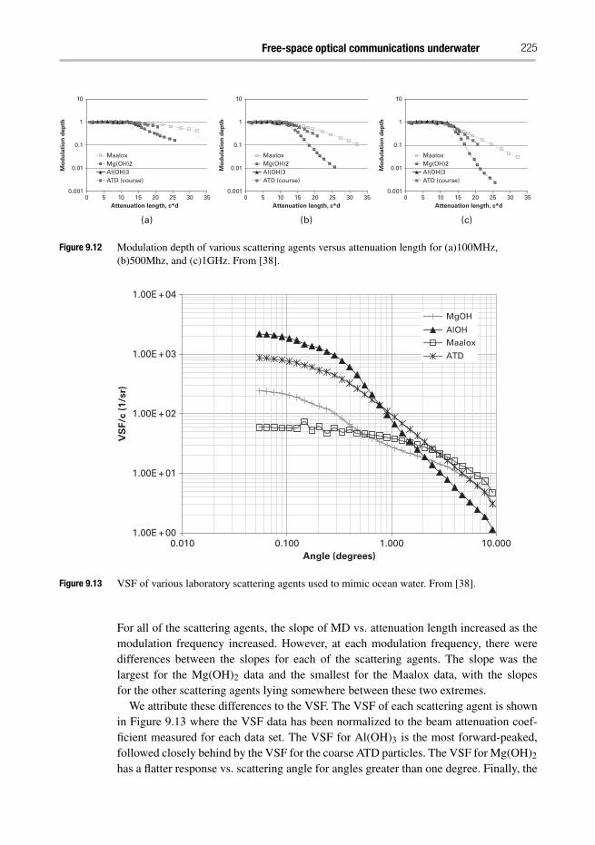
Free-space optical communications underwater 225
0.001
0.01
0.1
1
10
0 5 10 15 20 25
(a) (b) (c)
30 35Attenuation length, c*d
Mo
du
lati
on
dep
th
MaaloxMg(OH)2Al(OH)3ATD (course)
0 5 10 15 20 25 30 35Attenuation length, c*d
0.001
0.01
0.1
1
10
Mo
du
lati
on
dep
th
0 5 10 15 20 25 30 35Attenuation length, c*d
0.001
0.01
0.1
1
10
Mo
du
lati
on
dep
th
MaaloxMg(OH)2Al(OH)3ATD (course)
MaaloxMg(OH)2Al(OH)3ATD (course)
Figure 9.12 Modulation depth of various scattering agents versus attenuation length for (a)100MHz,(b)500Mhz, and (c)1GHz. From [38].
1.00E + 00
1.00E + 01
1.00E + 02
1.00E + 03
1.00E + 04
0.010 0.100 1.000 10.000Angle (degrees)
VS
F/c
(1/s
r)
MgOH
AlOH
Maalox
ATD
Figure 9.13 VSF of various laboratory scattering agents used to mimic ocean water. From [38].
For all of the scattering agents, the slope of MD vs. attenuation length increased as themodulation frequency increased. However, at each modulation frequency, there weredifferences between the slopes for each of the scattering agents. The slope was thelargest for the Mg(OH)2 data and the smallest for the Maalox data, with the slopesfor the other scattering agents lying somewhere between these two extremes.
We attribute these differences to the VSF. The VSF of each scattering agent is shownin Figure 9.13 where the VSF data has been normalized to the beam attenuation coef-ficient measured for each data set. The VSF for Al(OH)3 is the most forward-peaked,followed closely behind by the VSF for the coarse ATD particles. The VSF for Mg(OH)2
has a flatter response vs. scattering angle for angles greater than one degree. Finally, the
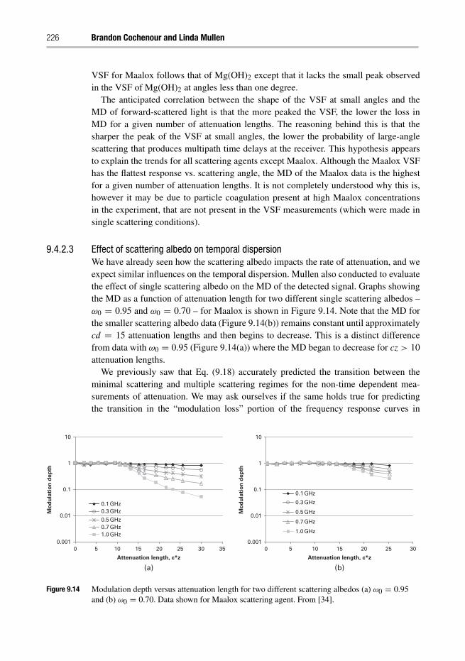
226 Brandon Cochenour and Linda Mullen
VSF for Maalox follows that of Mg(OH)2 except that it lacks the small peak observedin the VSF of Mg(OH)2 at angles less than one degree.
The anticipated correlation between the shape of the VSF at small angles and theMD of forward-scattered light is that the more peaked the VSF, the lower the loss inMD for a given number of attenuation lengths. The reasoning behind this is that thesharper the peak of the VSF at small angles, the lower the probability of large-anglescattering that produces multipath time delays at the receiver. This hypothesis appearsto explain the trends for all scattering agents except Maalox. Although the Maalox VSFhas the flattest response vs. scattering angle, the MD of the Maalox data is the highestfor a given number of attenuation lengths. It is not completely understood why this is,however it may be due to particle coagulation present at high Maalox concentrationsin the experiment, that are not present in the VSF measurements (which were made insingle scattering conditions).
9.4.2.3 Effect of scattering albedo on temporal dispersionWe have already seen how the scattering albedo impacts the rate of attenuation, and weexpect similar influences on the temporal dispersion. Mullen also conducted to evaluatethe effect of single scattering albedo on the MD of the detected signal. Graphs showingthe MD as a function of attenuation length for two different single scattering albedos –ω0 = 0.95 and ω0 = 0.70 – for Maalox is shown in Figure 9.14. Note that the MD forthe smaller scattering albedo data (Figure 9.14(b)) remains constant until approximatelycd = 15 attenuation lengths and then begins to decrease. This is a distinct differencefrom data with ω0 = 0.95 (Figure 9.14(a)) where the MD began to decrease for cz > 10attenuation lengths.
We previously saw that Eq. (9.18) accurately predicted the transition between theminimal scattering and multiple scattering regimes for the non-time dependent mea-surements of attenuation. We may ask ourselves if the same holds true for predictingthe transition in the “modulation loss” portion of the frequency response curves in
0.001
0.01
0.1
1
10
0 5 10 15 20 25
(a) (b)
30 35
Attenuation length, c*z
Mo
du
lati
on
dep
th
0.1 GHz0.3 GHz0.5 GHz0.7 GHz1.0 GHz
0.001
0.01
0.1
1
10
0 5 10 15 20 25 30
Attenuation length, c*z
Mo
du
lati
on
dep
th
0.1 GHz
0.3 GHz
0.5 GHz
0.7 GHz
1.0 GHz
Figure 9.14 Modulation depth versus attenuation length for two different scattering albedos (a) ω0 = 0.95and (b) ω0 = 0.70. Data shown for Maalox scattering agent. From [34].
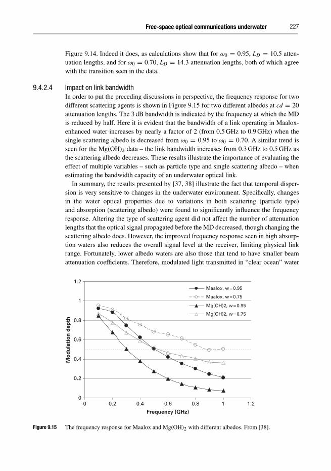
Free-space optical communications underwater 227
Figure 9.14. Indeed it does, as calculations show that for ω0 = 0.95, LD = 10.5 atten-uation lengths, and for ω0 = 0.70, LD = 14.3 attenuation lengths, both of which agreewith the transition seen in the data.
9.4.2.4 Impact on link bandwidthIn order to put the preceding discussions in perspective, the frequency response for twodifferent scattering agents is shown in Figure 9.15 for two different albedos at cd = 20attenuation lengths. The 3 dB bandwidth is indicated by the frequency at which the MDis reduced by half. Here it is evident that the bandwidth of a link operating in Maalox-enhanced water increases by nearly a factor of 2 (from 0.5 GHz to 0.9 GHz) when thesingle scattering albedo is decreased from ω0 = 0.95 to ω0 = 0.70. A similar trend isseen for the Mg(OH)2 data – the link bandwidth increases from 0.3 GHz to 0.5 GHz asthe scattering albedo decreases. These results illustrate the importance of evaluating theeffect of multiple variables – such as particle type and single scattering albedo – whenestimating the bandwidth capacity of an underwater optical link.
In summary, the results presented by [37, 38] illustrate the fact that temporal disper-sion is very sensitive to changes in the underwater environment. Specifically, changesin the water optical properties due to variations in both scattering (particle type)and absorption (scattering albedo) were found to significantly influence the frequencyresponse. Altering the type of scattering agent did not affect the number of attenuationlengths that the optical signal propagated before the MD decreased, though changing thescattering albedo does. However, the improved frequency response seen in high absorp-tion waters also reduces the overall signal level at the receiver, limiting physical linkrange. Fortunately, lower albedo waters are also those that tend to have smaller beamattenuation coefficients. Therefore, modulated light transmitted in “clear ocean” water
0
0.2
0.4
0.6
0.8
1
1.2
0 0.2 0.4 0.6 0.8 1 1.2
Frequency (GHz)
Mo
du
lati
on
dep
th
Maalox, w = 0.95
Maalox, w = 0.75
Mg(OH)2, w = 0.95
Mg(OH)2, w = 0.75
Figure 9.15 The frequency response for Maalox and Mg(OH)2 with different albedos. From [38].
228 Brandon Cochenour and Linda Mullen
(ω0 = 0.247, c = 0.151 m) can propagate a longer physical range than in “turbidharbor” water (ω0 = 0.833, 2.19 m) for the same number of attenuation lengths beforethe modulation depth is reduced.
Once the transition between MD = 1 and MD < 1 is reached, the type of scatteringparticle appears to have the largest effect on the propagation of modulated light in water.Specifically, the decay rate of the MD with increasing attenuation length is dependent onthe VSF of the scattering particle. To date, there have been no experimental comparisonsof the frequency response between various ocean water types (for example, Jerlov watertypes). Such an investigation would be largely beneficial.
9.5 System design for uFSO links
As the physics of the underwater channel become more clearly understood, researchersare beginning to look at “system-level” issues and testing uFSO links in real oceanenvironments. Now that we have discussed some of the theoretical and experimentalefforts underway to describe the ocean channel, we shift focus in this section to discusssome of the system trade-offs that should be considered by the uFSO link designer, aswell as review some related applications by researchers in this area.
9.5.1 Transceiver components
Due to the near ubiquitous presence of fiber optics in today’s world, transceiver compo-nents in the IR are relatively mature. Atmospheric FSO links have taken advantage thata certain degree of technological maturity already exists for the wavelengths of interest.However, this cannot always be said for the blue/green portion of the spectrum whereuFSO links will operate.
A comparison of transmitter technology is summarized in Table 9.3. While solid-state lasers (often frequency doubled Nd:YAG) offers the highest output powers, LED([45], [50], [18], [19]) and laser diode sources ([14], [28], [6]) in the blue/green arealso gaining popularity due to their small size and flexibility compared to the large sizeof a solid-state laser. It should be noted that fiber and fiber amplified lasers representan exciting new area in this field, as they have the potential to provide high powers,flexible modulation schemes, and low size and weight requirements ([41]). LED andlaser diode sources are best suited for small platforms like underwater sensor nodes,where size and power consumption must be minimized. Solid-state and some fiber lasersare more suited for large platforms (such as a vehicle) where size and efficiency areless of a concern and can be traded off for higher laser output powers. Indeed, the“holy grail” of transmitters is a small, high-efficiency, high-power source that wouldallow for closing links at long ranges or high turbidities. However, until such a sourcearrives, it is necessary to make trade-offs depending on the particular platform and/orapplication.
On the receiver end, PIN-photodiodes may be attractive due to their fast response(>1 GHz) and generally low cost. However photomultipler tubes (PMTs) and avalanche
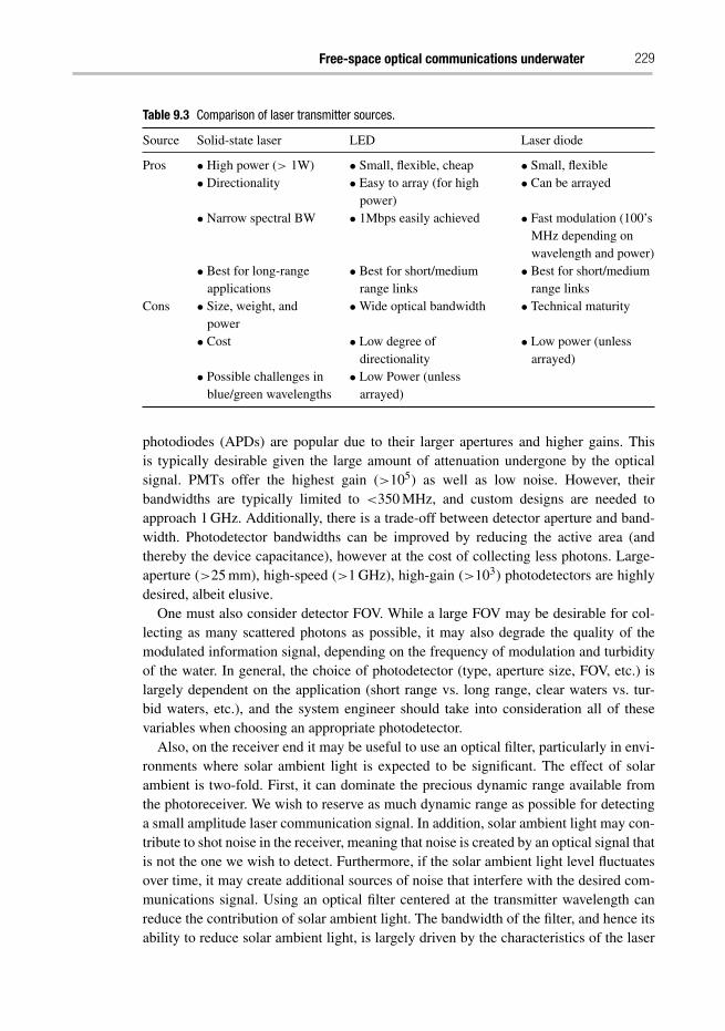
Free-space optical communications underwater 229
Table 9.3 Comparison of laser transmitter sources.
Source Solid-state laser LED Laser diode
Pros • High power (> 1W) • Small, flexible, cheap • Small, flexible• Directionality • Easy to array (for high
power)• Can be arrayed
• Narrow spectral BW • 1Mbps easily achieved • Fast modulation (100’sMHz depending onwavelength and power)
• Best for long-rangeapplications
• Best for short/mediumrange links
• Best for short/mediumrange links
Cons • Size, weight, andpower
•Wide optical bandwidth • Technical maturity
• Cost • Low degree ofdirectionality
• Low power (unlessarrayed)
• Possible challenges inblue/green wavelengths
• Low Power (unlessarrayed)
photodiodes (APDs) are popular due to their larger apertures and higher gains. Thisis typically desirable given the large amount of attenuation undergone by the opticalsignal. PMTs offer the highest gain (>105) as well as low noise. However, theirbandwidths are typically limited to <350 MHz, and custom designs are needed toapproach 1 GHz. Additionally, there is a trade-off between detector aperture and band-width. Photodetector bandwidths can be improved by reducing the active area (andthereby the device capacitance), however at the cost of collecting less photons. Large-aperture (>25 mm), high-speed (>1 GHz), high-gain (>103) photodetectors are highlydesired, albeit elusive.
One must also consider detector FOV. While a large FOV may be desirable for col-lecting as many scattered photons as possible, it may also degrade the quality of themodulated information signal, depending on the frequency of modulation and turbidityof the water. In general, the choice of photodetector (type, aperture size, FOV, etc.) islargely dependent on the application (short range vs. long range, clear waters vs. tur-bid waters, etc.), and the system engineer should take into consideration all of thesevariables when choosing an appropriate photodetector.
Also, on the receiver end it may be useful to use an optical filter, particularly in envi-ronments where solar ambient light is expected to be significant. The effect of solarambient is two-fold. First, it can dominate the precious dynamic range available fromthe photoreceiver. We wish to reserve as much dynamic range as possible for detectinga small amplitude laser communication signal. In addition, solar ambient light may con-tribute to shot noise in the receiver, meaning that noise is created by an optical signal thatis not the one we wish to detect. Furthermore, if the solar ambient light level fluctuatesover time, it may create additional sources of noise that interfere with the desired com-munications signal. Using an optical filter centered at the transmitter wavelength canreduce the contribution of solar ambient light. The bandwidth of the filter, and hence itsability to reduce solar ambient light, is largely driven by the characteristics of the laser
230 Brandon Cochenour and Linda Mullen
source. For solid state (and most fiber) lasers, the bandwidth of the optical carrier canoften be <1 nm. For LED sources, the bandwidth may be 10s of nm. Narrow opticalfilter bandwidths may reduce the field of view (depending on the implementation) andmay be expensive depending upon the aperture size. These are all trade-offs that mustbe considered.
9.5.2 Modulation and coding schemes
A related issue to our discussion on laser sources and receivers is the choice of modu-lation scheme. In general, there are two options. One is to use a pulsed laser (typicallysolid-state, or fiber-amplified), and to implement a modulation scheme like pulse posi-tion modulation (PPM). This is a popular choice for long-range links, or links thattraverse the air–water interface (for instance, from an aircraft to a submarine). In thisscenario, we are interested in putting as much peak power into the water as possible inorder to combat attenuations. As such, pulsed lasers are an ideal source for this. Thereis a bandwidth trade-off however, as in order to achieve higher peak power pulses, thelaser repetition rate often must be reduced, meaning pulses enter the water at a slowerrate. This may be offset by using a higher-order PPM encoding, however overall datarate is usually not preserved. As such, the trade-off between link range (or peak power)and data rate still exists. Furthermore, high peak power lasers may be rather large andpower hungry, and are therefore not well suited for applications such as sensor nodesor unmanned vehicles. While baseband schemes like PPM are ideal for long-range/highpeak power applications due to the inherent nature of pulsed laser action, short-rangelinks using lower power devices, like LEDs, may also implement some flavor of base-band modulation. The motivation in this case is to minimize power consumption perbit by limiting LED on-time, yet still providing sufficient information bandwidth.(cf., [50], [19])
The other alternative is to use a bandpass modulation scheme like M-PSK or QAM[8, 9]. Because of the continuous wave nature of these modulation formats, the peakpower available is often lower than solid-state pulsed laser sources, which may leadto shorter range of operation (or conversely, restrict operation to clearer waters). How-ever, higher data rates may be achieved relative to PPM. A further benefit of bandpassmodulation schemes may appear in real environments where noises around DC may besignificant (for instance, a low-frequency solar ambient fluctuation). Bandpass systemsare also beneficial in full-duplex LOS links operating at the same wavelength, or in retro-reflector links [16]. In turbid LOS links, a receiver must be able to discriminate anothertransmitter’s signal from the backscatter caused by its own transmitter’s signal. In retrolinks, the receiver must discriminate the modulated retro return from the backscatter ofthe non-modulated interrogator. It has been shown that in underwater laser imaging sys-tems, using intensity modulation can reduce the impact of backscattered light. Due to thedistributed nature of backscattered light along the beam path, backscatter has a lowpassresponse [35]. By using high-frequency modulation, the incoming information signal(centered at high frequency) can be separated from a “washed out” backscatter (locatednear DC). There are practical downsides to bandpass modulation schemes, depending
Free-space optical communications underwater 231
on the laser source chosen. For example, in order to modulate a high-power CW source(>1 W), large power-hungry external electro-optic modulators must be used. Further-more, these bulk devices limit carrier frequencies to <100 MHz. Lower power sourceslike LEDs or laser diodes may be used to achieve some of the above benefits, howeverdue to the CW nature of laser transmission, may be less power efficient than a basebandscheme. As always, trade-offs exist.
While there have been few published studies comparing the two flavors of modulationside by side, unpublished work from SA Photonics (San Francisco, CA) has demon-strated both QPSK and PPM modulation schemes via a custom semi-conductor/fiberamplified laser in laboratory test tank environments. The laser wavelength was 532 nm,and had an output power of 1–3 W depending on the modulation scheme used. AnAPD was used at the receiver. 50 Mbps QPSK data (140 MHz RF carrier) was trans-mitted error free (<10−7) over 13.2 attenuation lengths. 15 Mbps was demonstratederror free over ∼21 attenuation lengths using an 8-PPM modulation format. Notethat the higher peak power of the PPM pulses allowed for the error-free range to beextended an additional∼8 attenuation lengths, albeit at the cost of a reduced informationbandwidth.
New studies are looking at error control coding for the underwater channel. Usingforward error correction (FEC) allows link operation at lower SNRs due to the errorcorrecting features of the coding. Cox et. al. [14], presented a 3.66m uFSO link thatimplemented (255,129) Reed–Solomon coding. The transmitter was an 80 mW laserdiode at 405 nm, and an amplified photodiode was used at the receiver. The link used anon–off keying (OOK) modulation format at 500 kbps. They showed that for a BER of10−4, a 2.5 dB EB/N0 improvement could be gained by using FEC. In their laboratoryexperiment, the FEC link could achieve the same BER as an uncoded link even thoughthe attenuation coefficient was 1/4 larger. Everett [21] has shown coding gains of 6.8 dBto 9.5 dB EB/N0 using state-of-the-art Turbo Codes with rates ranging from r = 1/2 tor = 1/6. The same work also showed a coding gain of 7.7 dB to 9.2 dB EB/N0 usingLDPC codes with code rates varying from r = 1/2 to r = 1/4. All improvements arerelative to an uncoded system with a BER of 10−4. An 80 mW laser diode at 405 nmwas used at the transmitter, with a PMT used at the receiver.
9.5.3 Examples of uFSO links
9.5.3.1 Line-of-sight (LOS) linksThe simplest uFSO link geometry is the direct point-to-point link (Figure 9.16(a)).In this case, each transmitter/receiver pair must maintain accurate line-of-sight (LOS)between them. For static links where the transmitter and receiver are not expected tomove relative to each other, this link is fairly easy to implement. An example of such alink is two sensor nodes, fixed to the bottom of the seafloor. For mobile platforms, suchas communication between autonomous underwater vehicles (AUVs), sophisticatedpointing-and-tracking (PAT) technologies must be implemented in order to maintainthe maximum amount of optical power density incident upon the optical receiver. We
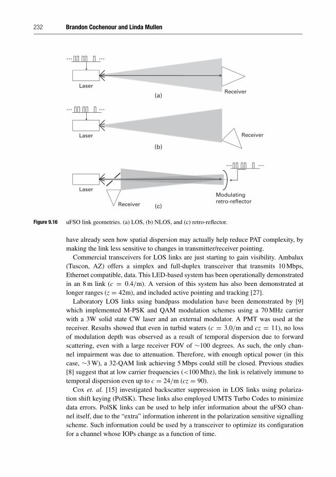
232 Brandon Cochenour and Linda Mullen
LaserReceiver
Laser Receiver
……
……
……
Laser
Receiver
Modulatingretro-reflector
(a)
(b)
(c)
Figure 9.16 uFSO link geometries. (a) LOS, (b) NLOS, and (c) retro-reflector.
have already seen how spatial dispersion may actually help reduce PAT complexity, bymaking the link less sensitive to changes in transmitter/receiver pointing.
Commercial transceivers for LOS links are just starting to gain visibility. Ambalux(Tuscon, AZ) offers a simplex and full-duplex transceiver that transmits 10 Mbps,Ethernet compatible, data. This LED-based system has been operationally demonstratedin an 8 m link (c = 0.4/m). A version of this system has also been demonstrated atlonger ranges (z = 42m), and included active pointing and tracking [27].
Laboratory LOS links using bandpass modulation have been demonstrated by [9]which implemented M-PSK and QAM modulation schemes using a 70 MHz carrierwith a 3W solid state CW laser and an external modulator. A PMT was used at thereceiver. Results showed that even in turbid waters (c = 3.0/m and cz = 11), no lossof modulation depth was observed as a result of temporal dispersion due to forwardscattering, even with a large receiver FOV of ∼100 degrees. As such, the only chan-nel impairment was due to attenuation. Therefore, with enough optical power (in thiscase, ∼3 W), a 32-QAM link achieving 5 Mbps could still be closed. Previous studies[8] suggest that at low carrier frequencies (<100 Mhz), the link is relatively immune totemporal dispersion even up to c = 24/m (cz = 90).
Cox et. al. [15] investigated backscatter suppression in LOS links using polariza-tion shift keying (PolSK). These links also employed UMTS Turbo Codes to minimizedata errors. PolSK links can be used to help infer information about the uFSO chan-nel itself, due to the “extra” information inherent in the polarization sensitive signallingscheme. Such information could be used by a transceiver to optimize its configurationfor a channel whose IOPs change as a function of time.
Free-space optical communications underwater 233
9.5.3.2 Non-line-of-sight (NLOS) linksNLOS links are also of interest due to a decreased dependence on pointing and tracking(Figure 9.16(b)). In clear waters, NLOS links are achieved by either intentionallydiverging the transmit beam, or by using arrays of high divergence sources (like LEDs).In turbid waters, it is possible that spatial dispersion of a collimated laser source due toscattering may have the same effect, though this is not often considered in analysis.
Researchers at Woods Hole Oceanographic Institute have begun to investigate NLOStransceivers for the application of AUV data mining. Farr et. al. [22] have performedlink budget analysis of NLOS geometries (as well as variations of point-to-point links).While their analysis includes attenuation by the attenuation coefficient, it does not con-sider spatial dispersion and multiple scattering, and as such is expected to be valid onlyin clearer waters. Indeed, this is likely to be the case in the open ocean application tar-geted in their work. It was found that one disadvantage of the NLOS link is the increaseof laser power necessary due to the intentional divergence of the transmit beam. In aclear water scenario, analysis showed that a LOS link could achieve 10 Mbps at 100 mwith 6 mW of transmit power. However for the NLOS link, a 50-fold increase in transmitpower is needed to achieve the same data rates at similar range due to use of a broadertransmit beam. That said, laser diodes of 300 mW (or arrays of LEDs totaling the samepower) are available in the blue/green, making such a trade-off reasonable. However, inturbid waters, the increase in transmit power is expected to increase exponentially withattenuation coefficient in order to maintain the same data rate or link range. Indeed,follow-on NLOS experiments by [42] showed 5 Mbps at 200 m in clear waters withc = 0.025/m. However operation in turbid waters (c = 1.25/m) necessitated a reduc-tion in both data rate (1 Mbps) and range (30 m). While trade-off studies were performedin [22], exact details on the experimental system, other than the transmitter operatingat 470 nm, are hard to come by (i.e. choice of transmitter/receiver, transmitter power,receiver gain, etc.).
Penguin Automated Systems (Ontario, CAN) has developed a NLOS transceiverfor tele-robotic operations consisting of 100s of LEDs in a spherical configuration toachieve a 120 degree transmitter field of view. Field tests with this system demonstratedvideo transfer at 1.5 Mbps at 15 m in turbid lake water [5]. The exact water clarity wasnot reported, nor has any details regarding the transceiver hardware.
Finally, a unique method of NLOS communications has been proposed by Arnonand Kedar [2, 3]. In this geometry, the transmitted signal is reflected off the air–waterinterface. Naturally, under normal circumstances the LOS geometry will outperform the“reflective” NLOS link. However the real power in this unique reflective geometry liesin its ability to mitigate obstructions between transceiver nodes.
9.5.3.3 Retro-reflector linksIn the links described above, light that is modulated with information is transmitted toa remote optical receiver. In a retro-reflector link, the laser and receiver are situated onone end of the link where there is sufficient power and payload capacity. On the otherend of the link is a small passive optical retro-reflector that is coupled to an optical mod-ulator (Figure 9.16(c)). When the laser interrogates a modulated retro-reflector (MRR),
234 Brandon Cochenour and Linda Mullen
the light is encoded with information and reflected back towards the source where theco-located receiver recovers the information signal. Retro-reflector links are ideal forbottom dwelling sensor nodes, where maximizing battery life is essential to prolongingthe lifetime of the sensor. Replacing power-hungry items like lasers and photoreceiverelectronics for small, efficient retro-reflectors is an attractive proposal to the underwatercommunications link designer.
MRR links can be seriously limited by backscatter, similar to the issue previouslydiscussed in full-duplex links. Mullen et. al. [36] investigated the use of polariza-tion discrimination to suppress the backscatter signal. This approach relies on thefact that backscattered light tends to retain its original polarization state. However,the polarization state of the light at the retro end can be intentionally rotated sothat it is opposite to that of the backscattered light. The receiver polarizer is ori-ented to accept the retro-reflected light while simultaneously rejecting the backscatteredlight. Laboratory experimental results showed that the addition of polarization-sensitivecomponents increased the useful range of the MRR link by at least two attenuationlengths.
The challenge now lies in developing an MRR device that can support modulationspeeds on the order of > 1 Mbps. While semiconductor multiple quantum well modu-lators are typically used for atmospheric links in the IR, similar devices are difficult tofabricate in the blue/green. Until this technology becomes more mature, micro-electro-mechanical (MEMS) modulators appear to be the technology of choice. While thesemodulators have lower bandwidths than the semiconductor modulators, they have theadvantage of operating at any wavelength. Two different MEMS approaches have beenstudied. The first implements a Fabry–Perot cavity with two partially reflective alu-minum mirrors; one fixed on a glass substrate and the other on a flexible silicon nitridebridge. The Fabry–Perot cavity is designed such that when interrogated with blue/greenlight, an applied voltage to the silicon nitride membrane will result in modulation.This approach was recently tested in a laboratory test tank by [16]. The transceiverused a small, compact, 20 mW solid state laser and a PMT receiver. QPSK modula-tion was implemented at the retro. Error free transmission (<10−4) at 500 kbps wasobserved up to 5 attenuation lengths, and extended to 6.47 attenuation lengths usingrate r = 1/2. Reed Solomon forward error control coding. 1 Mbps was achievedout to 2.77 attenuation lengths, which could be extended to 3.76 attenuation lengthswith FEC.
In the second MEMS approach, a MEMS fabricated mirror was used as one of thefaces of a corner cube. By deflecting the mirror down using electrostatic actuation theretro-reflectivity of the corner cube could be spoiled, thus modulating the light. ThisMEMS structure was capable of bandwidths exceeding 100 kHz [55].
9.5.3.4 NetworkingNetworking underwater is an up and coming area of study. With the advent of AUVs,ROVs, and other underwater robots, ocean exploration is poised to grow rapidly in thefuture. A popular targeted application for underwater communication networks is datamining of scientific sensor nodes. Typically, physical retrieval of the nodes is undesirable
Free-space optical communications underwater 235
(or in some locations, impossible). In order to limit the frequency of costly physicalretrievals, the nodes must either have large memories, complex data processing, or lowsampling rates; none of which is particularly desirable. Acoustics could be used as amethod of wireless data transfer between the node and, say, an AUV. However due tothe slow data rates and high latency associated with acoustics, extra burden is placed onboth the sensor node and the AUV.
Researchers are now considering optics as an alternative due to the higher bandwidthsthey support. On the sensor side, sampling frequency can increase now that higher datarates are supported between the sensor and the AUV. On the AUV side, mission time isreduced as less time is spent visiting each node since data transfer time is significantlydecreased (as compared to acoustics).
As a step towards autonomous data mining, a series of tests have been reported by [23]using the human operated vehicle Alvin. In these tests, a compact, real-time, system wasdeveloped to eventually fit on a small unmanned vehicle (a similar system is reportedin [42]). Results in clear water (c = 0.05/m) show error free detection at 1 Mbps out to100 m. This study also showed full-duplex communications with the ROV Nereus. Real-time video transfer from the ROV shows the potential for enabling real-time controlof underwater vehicles in addition to data transfer from the vehicle to a controllingplatform.
Researchers at MIT have developed prototype sensor nodes and AUVs in orderto demonstrate the potential of wireless data collection underwater (cf. [49, 50]).These studies have used a blend of both acoustics and optics in order to accomplishautonomous data collection. By using a blend of acoustics and optics, the systemdesigner can tailor the transceiver based on the expected mission. For example, it isanticipated the acoustics can be used for location of sensor nodes at long range. Thislow bandwidth information can be used to guide the vehicle within range of the opti-cal link. Once close enough, the optical link will be used for high-speed data transfer.Should the optical link be broken, or the vehicle move out of range, the acoustic linkcan still be used to transmit data, albeit at a slower rate. In addition, the low bandwidthacoustic link can be used for network activities such as medium access and node dis-covery. These items can occur in the background during a UUV mission, leaving theoptics only for the high-speed data transfer at mid to close range. The most recent ver-sion of the optical transceiver has been shown to operate a 2.28 Mbps over 50 m in clearpool tests [19]. The transmitter is an array of 470 nm LEDs, resulting with a total out-put of 10 W. An APD is used as the photoreceiver. While yet reported, the FPGA-basedhardware can support several different modulation schemes, providing a software radioapproach to underwater communications. Previous versions of the optical transceiverhave been used for wireless underwater robot control in a clear pool 13.7m × 7.3m indimension [18].
A slightly different application is considered by [1], opting for an all-optical approachto networking. Here, the authors considered small sensor nodes oriented in a star-liketopology, where several nodes all transmit information to a larger “cluster head” node.The cluster node must implement some method of medium access control (MAC) inorder to handle contention between its “slave” nodes. Unlike RF protocols, which can
236 Brandon Cochenour and Linda Mullen
attempt to, “sense” the medium to determine whether or not another node is transmitting,the directional nature of FSO communications makes it largely impossible to know ifa nearby slave node is attempting communication with the master node. As such, itis the job of the master node to (1) determine which nodes are trying to send data,and (2) adaptively regulate the medium between those nodes in order to avoid datastream collisions. The custom protocol developed also runs adaptively, meaning that itcan handle slave nodes that move in and out of the master node’s range. Such a capabilitywould be highly desired, for instance, in an underwater network with swarms of AUVs.
9.6 Summary
Presented in this chapter is the unique and quickly growing area of wireless opticalcommunications underwater. The underwater channel is a complex environment thathas many challenges not seen in other FSO links. Researchers are currently employ-ing both theoretical and experimental tools to characterize the spatial dispersion (beamspreading) seen underwater due to scattering.
In our discussion of spatial dispersion, we find that for attenuation lengths less than adiffusion length (as given by Lerner and Summers in Eq. (9.18)), the only effect of thewater on the optical signal is an exponential reduction in power, as given by the attenu-ation coefficient. Furthermore, the channel appears to support frequencies up to 1 GHz(and possibly beyond). We can broadly assume then that in this “minimally scattered”regime, that the only “loss” is due to the exponential attenuation given by the IOPs.Theoretical modeling has shown that in this regime, performance may also be sensitiveto changes in system parameters like FOV.
Beyond a diffusion length however, both spatial and temporal dispersion begins tohave a more marked effect. We have denoted this as the “multiple scattering” regime.Here, the rate of attenuation is given by ksys, due to the contribution of scattered light.While it may be beneficial that the intensity decreases at a slower rate in this regime,we have also seen that the frequency response supported by the water begins to decay aswell. This rate of decay is largely influenced by the shape of the VSF. While it has yetto be developed, we foresee a similar “ksys” term for describing the rate of modulationloss versus attenuation length or range. Regardless, it should be obvious that in themultiple scattering regime, the “loss term” can be dependent on different variables andin different ways than the minimally scattered regime.
The point we wish to make here is that while experiment and modeling are begin-ning to help the link designer understand how both the environment and system impactsthe link, we have barely scratched the surface in achieving an exhaustive parameteri-zation of all possible regimes. Furthermore, characterizations will most certainly varyfor different links (LOS, NLOS, retro, etc..). Continued investigation remains a signifi-cant, non-trivial task both in experiment and simulation. Regardless, we see that as thephysics of propagation is becoming better understood, “real-world” systems will alsoimprove in terms of technical maturity.
Free-space optical communications underwater 237
References
[1] Agrawal, N., Davis, C. C., Milner, S. D. Free space optical sensor networking for underwatersensing appications. Intelligent Sensors, Sensor Networks, and Information Processing(ISSNIP), 5th International Conference on, 475–480, 2009.
[2] Arnon, S and Kedar, D. Non-line-of-sight underwater optical wireless communicationnetwork. Journal of the Optical Society of America A, 26 (3), 530–539, 2009.
[3] Arnon, S. Underwater optical wireless communication network. Optical Engineering,49(1), 2010.
[4] Austin, R. and Halikas, G. The Index of Refraction in Seawater, Scripps Institution ofOceanography Visibility Laboratory, 1976.
[5] Baiden, G., Bissiri, Y. High bandwidth optical networking for underwater untetheredtelerobotic operation. IEEE Proc. OCEANS 07 Conf., 1–9, 2007.
[6] Bartolini, L., De Dominicis, L., Ferri de Collibus, M. et al. Experimental evidence of signal-optical noise interferencelike effect in underwater amplitude-modulated laser optical radarsystems. Optics Letters 33, 2584–2586, 2008.
[7] Bohren, C. F. and Huffman, D. R. Absorption and Scattering of Light by Small Particles.Wiley, 1998.
[8] Cochenour, B. M., Curran, T., Mullen, L. J., Laux, A. E. Effects of multiple scattering onthe implementation of an underwater wireless optical communications link. IEEE Proc.OCEANS 06 Conf., 1–6, 2006.
[9] Cochenour, B. M., Mullen, L. J., Laux, A. E. Phase coherent digital communications forwireless optical links in turbid underwater environments. IEEE Proc. OCEANS 07 Conf.,1–5, 2007.
[10] Cochenour, B. M., Mullen, L. J., Laux, A. E. Characterization of the beam-spread func-tion for underwater wireless optical communications Links. IEEE Journal of OceanicEngineering. 33 (4) 513–521, 2008.
[11] Cochenour, B. M., Mullen, L. J., Rabinovich, W. S., Mahon, R. Underwater optical commu-nications with a modulating retro-reflector. Proc. SPIE, 7317, 2009.
[12] Cochenour, B. M., Mullen, L. J., Muth, J. F. Effect of scattering albedo on attenuation andpolarization of light underwater. Optics Letters, 35 (12), 2088–2090, 2010.
[13] Concannon, B. M. and Davis, J. P Results of a Monte Carlo investigation of the diffuseattenuation coefficient. Applied Optics, 38(24), 5104–5107, 1999.
[14] Cox, W. C. A 1Mbps underwater communication system using a 405nm laser diode andphotomultiplier tube, M.S. thesis, North Carolina State University, Raleigh NC, 2007.
[15] Cox, W. C., Hughes, B. L., Muth, J. F. A polarization shift keying system for underwateroptical communications. IEEE Proc. OCEANS 09 Conf., 1–4, 2009.
[16] Cox, W. C., Gray, K. F., Simpson, J. A. et al. A MEMS Blue/Green Retroreflecting Modu-lation for Underwater Optical Communication. IEEE Proc. OCEANS 10 Conf. Acceptedpaper, 2010.
[17] Dalgleish, F. R., Caimi, F. M., Vuorenkoski, A. K. et al. Efficient laser pulse dispersioncodes for turbid undersea imaging and communications applications. Proc. SPIE, vol. 7678,2010.
[18] Doniec, M., Vasilescu, I., Detweiller, C. et al. AquaOptical: A lightweight device forhigh-rate long-range underwater point-to-point communication. Marine Technical SocietyJournal, 44(4), 55–65, 2010.
238 Brandon Cochenour and Linda Mullen
[19] Doniec, M., Rus, D. BiDirectional optical communication with AquaOptical II. Interna-tional Conference on Communication Systems (ICCS). Accepted paper, 2010.
[20] Duntley, S. Underwater Lighting by Submerged Lasers and Incandescent Sources. ScrippsInstitution of Oceanography Visibility Laboratory, ch. 7, 1971.
[21] Everett, J. S. Forward-error correction coding for underwater free-space optical communi-cation. M. S. thesis, North Carolina State University, Raleigh, North Carolina, 2009.
[22] Farr, N., Chave, A., Freitag, L. et al. Optical modem technology for seafloor observatories.IEEE Proc. OCEANS 05 Conf., 1, 928–934, 2006.
[23] Farr, N., Bowen, A., Ware, J., Pontbriand, C., Tivey, M. An integrated, underwateroptical/acoustic communications system. IEEE Proc. OCEANS 10 Conf., 1–6, 2010.
[24] Hanson, R., and Radic, S. High bandwidth underwater optical communication, AppliedOptics 47, 277–283, 2008.
[25] Jaruwatanadilok, S. Underwater wireless optical communication channel modeling and per-formance evaluation using vector radiative transfer theory. IEEE Journal on Selected Areasin Communications 26 (9) 1620–1627, 2008.
[26] Jerlov, N.G. Marine Optics, 1st edn. Elsevier Science, 1976.[27] Lacovara, P. Fiber optic interconnect technology SBIR phase II final report: Test. Defense
Technical Information Center, Alexandria, VA, 2006.[28] Lacovara, P. High-bandwidth underwater communications. Marine Technology Society
Journal. 42 (1), 93–102, 2008.[29] Lerner, R. M., and Summers, J. D. Monte Carlo description of time-and space-resolved
multiple forward scatter in natural water. Applied Optics, 21 861–869, 1982.[30] Lutomirski, R. F., Ciervo, A. P., Hall, G. J. Moments of multiple scattering. Applied Optics
34(30), 7125–7136, 1995.[31] McLean, J. W., Crawford, D. R., Hindman, C. L. Limits of small angle scattering theory.
Applied Optics 26 (11), 2053–2054, 1987.[32] McLean, J. W., Freeman, J. D., Walker, R. E. Beam spread function with time dispersion.
Applied Optics 37(21), 4701–4711, 1998.[33] Mobley, C. Light and Water. Academic Press/Elsevier Science, 1994.[34] Morel, A. Optical properties of pure water and pure sea water. In: Optical Aspects of
Oceanography, N. Jerlov and E.S. Nielson, eds., 1–23, Academic Press.[35] Mullen, L.J., Laux, A.E., Cochenour et al. Demodulation techniques for the amplitude
modulated laser imager. Applied Optics, 46, 7374–7383, 2007.[36] Mullen, L., Cochenour, B., Rabinovich, W., Mahon, R., Muth, J. Backscatter suppression
for underwater modulating retroreflector links using polarization discrimination. AppliedOptics, 48 (2), 328–337, 2009.
[37] Mullen, L. J., Laux, A. E., Cochenour, B. M. Propagation of modulated light in water: impli-cations for imaging and communications systems. Applied Optics 48 (14), 2607–2612,2009.
[38] Mullen, L., Alley, D., Cochenour, B. Investigation of the effect of scattering agent andscattering abedo on modulated light propagation in water. Applied Optics 50 (10), 1396–1404, 2011.
[39] Pegau, W. S., Gray, D., Zaneveld, J. R. V Absorption and attenuation of visible and near-infrared light in water: dependence on temperature and salinity. Applied Optics 36 (24)6035–6046, 1997.
[40] Petzold, T. J. Volume Scattering Functions for Selected Ocean Waters. Scripps Institution ofOceanography Visibility Laboratory, 1972.
Free-space optical communications underwater 239
[41] Polynkin, P., Roussev, R., Fejer, M. M., Peyghambarian, N., Moloney, J. Laser transmit-ter for undersea communications using third-harmonic generation of fiber-laser system at1.5 μm. IEEE Photonics Technology Letters, 19 (17), 1328–1330, 2007.
[42] Pontbriand, C., Farr, N., Ware, J., Preisig, J., Popenoe, H. Diffuse, high bandwidth opticalcommunications. IEEE Proc. OCEANS 08 Conf. 1–4, 2008.
[43] Pope, R. M., and Fry, E. S. Absorption spectrum (380–700nm) of pure water. II. Integratingcavity measurements. Applied Optics, 36 (33), 8710–8723, 1997.
[44] Prieur, L. and Sathyendranath, S. An optical classification of coastal and oceanic watersbased on the specific spectral absorption curves of phytoplankton pigments, dissolvedorganic matter, and other particulate materials. Limnology and Oceanography, 26(4),671–689, 1981.
[45] Simpson, J. A. A 1Mbps underwater communications system using LEDs and photodiodeswith signal processing capability. M.S. thesis, North Carolina State University, Raleigh,NC, 2007.
[46] Simpson, J. A., Hughes, B. L., Muth, F. A spatial diversity system to measure optical fadingin an underwater communications channel. Proc IEEE OCEANS 09 Conf., 1–6, 2009.
[47] Sogandares, F. M., and Fry, E. S. Absorption spectrum (340–640 nm) of pure water. I.Photothermal measurements. Applied Optics, 36 (33), 8699–8709, 1997.
[48] Stotts, L. B. Closed form expression for optical pulse broadening in multiple-scatteringmedia. Applied Optics 17 (4), 504–505, 1978.
[49] Vasilescu, I., Kotay, K., Rus, D., Dunbabin, M., Corke, P. Data collection, storage, andretrieval with an underwater sensor network. ACM Proc. 3rd International Conference onEmbedded Networked Sensor Systems (SenSys), 154–165, 2005.
[50] Vasilescu, I. Using light underwater: devices, algorithms and systems for maritime per-sistent surveillance, PhD thesis, Massachusetts Institute of Technology, Cambridge MA,2009.
[51] Wells, W. H. Loss of resolution in water as a result of multiple small-angle scattering.Journal of the Optical Society of America, 59 (6), 686–691, 1969.
[52] Wells, W. H. Theory of small angle scattering. In: Optics of the Sea. AGARD Lect..Brussels, Belgium: NATO, vol. 61, ch. 3.3, 1973.
[53] Zege, E. P, Ivanov, A.P., Katsev, I. L. Image Transfer Through a Scattering Medium.Springer-Verlag, 1991.
[54] Zege, E. P., Katsev, I. L., Prikhach, A. S., Ludbrook, G. D., Bruscaglioni, P. Analyticalcomputer modeling of the ocean lidar performance, SPIE Proceedings, 5059 189–199,2002.
[55] Ziph-Schatzberg, L., Bifano, T., Cornelissen, S., Stewart, J., Bleier, Z. Deformable MEMSmirrors in secure optical communications system. Proc. SPIE, 7318, 2009.
10 The optical wireless channelRoger Green and Mark Leeson
10.1 Introduction
Infrared (IR) indoor optical wireless (OW) potentially combines the high bandwidthavailability of optical communications with the mobility found in radio frequency (RF)wireless communication systems. So although IR is currently overshadowed by a mul-titude of home and office RF wireless networking schemes, it has significant potentialwhen bandwidth demand is high. Compared to an RF system, OW offers the advanta-geous opportunity for high-speed medium- to short-range communications operatingwithin a virtually unlimited and unregulated bandwidth spectrum using lower-costcomponents. Furthermore, OW systems may be securely deployed with immunity toadjacent communication cell interference because the signal radiation cannot penetrateopaque barriers such as walls. Low transceiver costs, coupled with rapid deploymentand compatibility with the existing optical fiber communication systems mean that OWis an attractive alternative when fiber deployment is difficult [1], [2]. Moreover, band-width congestion in the RF domain has led to the installation of optical hotspots inpublic buildings and application-specific OW hotspots can be integrated into futureoffice designs [3]. Optical wireless communication has attracted considerable attentionfrom the academic community. From its short-distance, low-speed origins [4], OW hasbecome a viable addition to communication systems with promising prospects, havingpassed the 155 Mbps indoor landmark during the 1990s [5]. In recent years, techniquessuch as multispot diffusion (MSD) [6], angular diversity [7], and rate adaptive modula-tion [8] have been adopted as will be discussed later in this chapter. Furthermore, theconventional RF community has now accepted that optical wireless is part of the elec-tromagnetic communication spectrum thanks to work by the Wireless World ResearchForum [9] and the continual work of the commercial Infrared Data Association (IrDA)[10]. Current diverse application requirements suggest that the future communicationframework will benefit from a combined RF and optical infrastructure [11]. Neverthe-less, the technology is not without its drawbacks compared to RF techniques. A basestation needs to be situated in every room and the signal is susceptible to the intenseambient background light from the sun, incandescent and fluorescent lights. Thus, thefirst sections of the chapter provide a brief overview of the system configurations,
Advanced Optical Wireless Communication Systems, ed. Shlomi Arnon, John R. Barry, George K.Karagiannidis, Robert Schober, and Murat Uysal. Published by Cambridge University Press.c© Cambridge University Press 2012.
The optical wireless channel 241
sources, detectors, and filters used for OW followed by consideration of bit error rate(BER) performance in typical indoor scenarios.
10.2 System configurations
Indoor OW network topologies are classified according to the degree of directionalityof the transmitter and the receiver, and on the existence of a direct path between them.Based on these factors, optical wireless links are classified as: directed, non-directed,or hybrid. Depending on the existence of a direct path between the transmitter andthe receiver, wireless IR links can be classified as line-of-sight (LOS) or non line-of-sight (non-LOS) [12]. Directed links do not suffer from multipath distortion. They alsoimprove power efficiency because, in the case of the transmitter, the emitted energyis concentrated into a narrow beam (which results in more power per unit area at thetransmitter). In the case of the receiver, the detector can incorporate a directive opticalelement of high gain (which increases its sensitivity). A narrow emission beam trans-mitter and a narrow field of view (FOV) receiver allow the transmitted optical power tobe reduced (for a given distance). This improves the power budget of the system as wellas eye safety. LOS links improve power efficiency and minimize multipath distortion.Non-LOS links, on the other hand, increase link robustness as they base their opera-tion on the use of reflective surfaces, which allow the system to operate even whenobstacles exist between the transmitter and the receiver. This means that alignmentbetween the transmitter and the receiver is not necessarily required. The main disadvan-tage of the LOS configuration is the possibility of blocking from persons and objectsand the fact that it sometimes requires careful alignment of the transmitter and thereceiver.
Taking into account the individual characteristics of the directed and of the LOS linksit is not difficult to realize that the configuration that provides better power efficiencyand minimum multipath distortion is directed-LOS. The main drawbacks of this con-figuration are its limited coverage and its susceptibility to blocking. A special case ofthis configuration is the tracking system, which benefits from the advantages offeredby directed-LOS links, but provides a wide coverage at the same time. Unfortunately,mechanical tracking systems are expensive and increase system complexity. Otheroptions developed to minimize multipath dispersion and to optimize power consumptioninclude the use of quasi-diffuse transmitters and angle diversity receivers [13].
A potentially attractive configuration is the non-directed non-LOS or diffuse link. Inthis topology, careful alignment between the transmitter and the receiver is not requiredbecause the FOV of the receiver and the emission beam of the transmitter are wide.This, and the fact that this configuration makes use of the reflective properties of ceil-ings and walls to distribute the energy as uniformly as possible in a close environment,implies that this topology also provides maximum coverage and mobility. Furthermore,this configuration presents the advantage of being able to operate even when personsand objects are blocking the direct path between the transmitter and the receiver. Themain disadvantage of the diffuse configuration is that it presents maximum multipath
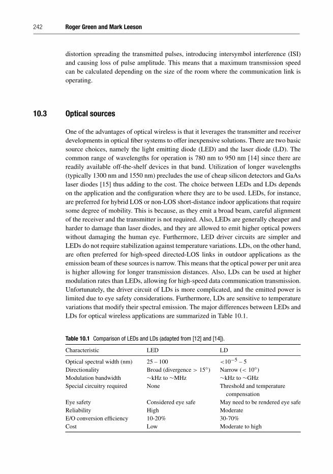
242 Roger Green and Mark Leeson
distortion spreading the transmitted pulses, introducing intersymbol interference (ISI)and causing loss of pulse amplitude. This means that a maximum transmission speedcan be calculated depending on the size of the room where the communication link isoperating.
10.3 Optical sources
One of the advantages of optical wireless is that it leverages the transmitter and receiverdevelopments in optical fiber systems to offer inexpensive solutions. There are two basicsource choices, namely the light emitting diode (LED) and the laser diode (LD). Thecommon range of wavelengths for operation is 780 nm to 950 nm [14] since there arereadily available off-the-shelf devices in that band. Utilization of longer wavelengths(typically 1300 nm and 1550 nm) precludes the use of cheap silicon detectors and GaAslaser diodes [15] thus adding to the cost. The choice between LEDs and LDs dependson the application and the configuration where they are to be used. LEDs, for instance,are preferred for hybrid LOS or non-LOS short-distance indoor applications that requiresome degree of mobility. This is because, as they emit a broad beam, careful alignmentof the receiver and the transmitter is not required. Also, LEDs are generally cheaper andharder to damage than laser diodes, and they are allowed to emit higher optical powerswithout damaging the human eye. Furthermore, LED driver circuits are simpler andLEDs do not require stabilization against temperature variations. LDs, on the other hand,are often preferred for high-speed directed-LOS links in outdoor applications as theemission beam of these sources is narrow. This means that the optical power per unit areais higher allowing for longer transmission distances. Also, LDs can be used at highermodulation rates than LEDs, allowing for high-speed data communication transmission.Unfortunately, the driver circuit of LDs is more complicated, and the emitted power islimited due to eye safety considerations. Furthermore, LDs are sensitive to temperaturevariations that modify their spectral emission. The major differences between LEDs andLDs for optical wireless applications are summarized in Table 10.1.
Table 10.1 Comparison of LEDs and LDs (adapted from [12] and [14]).
Characteristic LED LD
Optical spectral width (nm) 25 – 100 <10−5 – 5Directionality Broad (divergence > 15◦) Narrow (< 10◦)Modulation bandwidth ∼kHz to ∼MHz ∼kHz to ∼GHzSpecial circuitry required None Threshold and temperature
compensationEye safety Considered eye safe May need to be rendered eye safeReliability High ModerateE/O conversion efficiency 10-20% 30-70%Cost Low Moderate to high
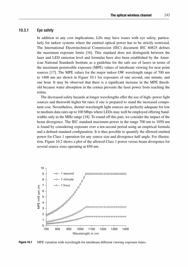
The optical wireless channel 243
10.3.1 Eye safety
In addition to any cost implications, LDs may have issues with eye safety, particu-larly for indoor systems where the emitted optical power has to be strictly restricted.The International Electrotechnical Commission (IEC) document IEC 60825 definesthe maximum exposure limits [16]. This standard does not distinguish between thelaser and LED emission level and formulas have also been established by the Amer-ican National Standards Institute as a guideline for the safe use of lasers in terms ofthe maximum permissible exposure (MPE) values of intrabeam viewing for near pointsources [17]. The MPE values for the major indoor OW wavelength range of 700 nmto 1400 nm are shown in Figure 10.1 for exposures of one second, one minute, andone hour. It may be observed that there is a significant increase in the MPE thresh-old because water absorption in the cornea prevents the laser power from reaching theretina.
The decreased safety hazards at longer wavelengths offer the use of high- power lightsources and therewith higher bit rates if one is prepared to stand the increased compo-nent cost. Nevertheless, shorter-wavelength light sources are perfectly adequate for lowto medium data rates up to 100 Mbps where LEDs may well be employed offering band-widths only in the MHz range [18]. To round off this part, we consider the impact of thebeam divergence. The IEC standard maximum power in the range 700 nm to 1050 nmis found by considering exposure over a ten-second period using an empirical formulaand a defined standard configuration. It is thus possible to quantify the allowed emittedpower for Class 1 operation for any source size and divergence half angle. For illustra-tion, Figure 10.2 shows a plot of the allowed Class 1 power versus beam divergence forseveral source sizes operating at 850 nm.
7000
1
2
3
4
5
6
7
8
9
10
800 900
1 second
1 minute
1 hour
MP
E m
W p
er c
m
1000Wavelength in nm
1100 1200 1300 1400
Figure 10.1 MPE variation with wavelength for intrabeam different viewing exposure times.
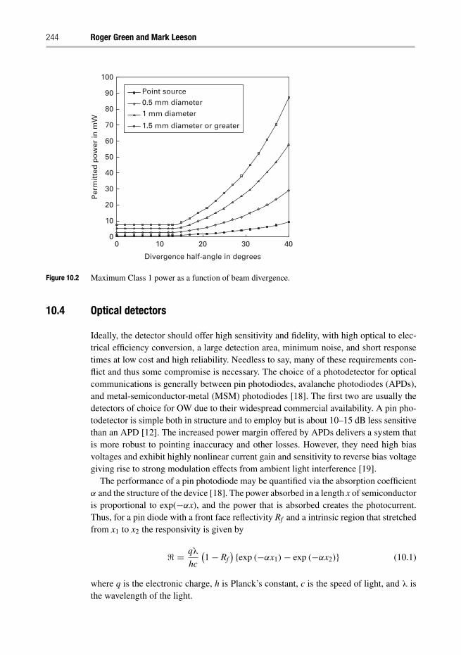
244 Roger Green and Mark Leeson
00
10
20
30
40
50
60
70
80
90
100
10
Point source0.5 mm diameter1 mm diameter
1.5 mm diameter or greater
20
Divergence half-angle in degrees
Per
mit
ted
po
wer
in m
W
30 40
Figure 10.2 Maximum Class 1 power as a function of beam divergence.
10.4 Optical detectors
Ideally, the detector should offer high sensitivity and fidelity, with high optical to elec-trical efficiency conversion, a large detection area, minimum noise, and short responsetimes at low cost and high reliability. Needless to say, many of these requirements con-flict and thus some compromise is necessary. The choice of a photodetector for opticalcommunications is generally between pin photodiodes, avalanche photodiodes (APDs),and metal-semiconductor-metal (MSM) photodiodes [18]. The first two are usually thedetectors of choice for OW due to their widespread commercial availability. A pin pho-todetector is simple both in structure and to employ but is about 10–15 dB less sensitivethan an APD [12]. The increased power margin offered by APDs delivers a system thatis more robust to pointing inaccuracy and other losses. However, they need high biasvoltages and exhibit highly nonlinear current gain and sensitivity to reverse bias voltagegiving rise to strong modulation effects from ambient light interference [19].
The performance of a pin photodiode may be quantified via the absorption coefficientα and the structure of the device [18]. The power absorbed in a length x of semiconductoris proportional to exp(−αx), and the power that is absorbed creates the photocurrent.Thus, for a pin diode with a front face reflectivity Rf and a intrinsic region that stretchedfrom x1 to x2 the responsivity is given by
& = qλ
hc
(1− Rf
) {exp (−αx1)− exp (−αx2)} (10.1)
where q is the electronic charge, h is Planck’s constant, c is the speed of light, and λ isthe wavelength of the light.
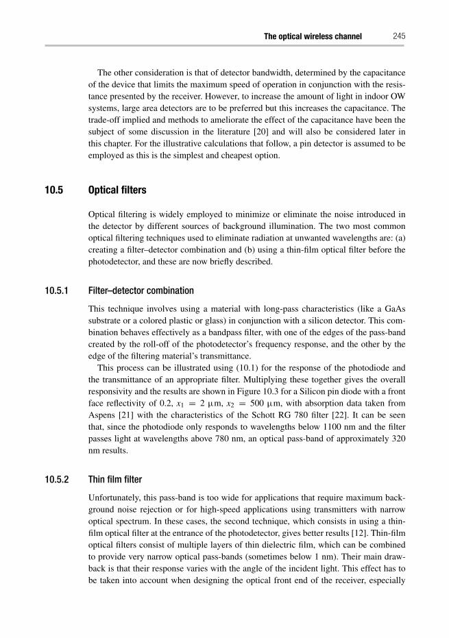
The optical wireless channel 245
The other consideration is that of detector bandwidth, determined by the capacitanceof the device that limits the maximum speed of operation in conjunction with the resis-tance presented by the receiver. However, to increase the amount of light in indoor OWsystems, large area detectors are to be preferred but this increases the capacitance. Thetrade-off implied and methods to ameliorate the effect of the capacitance have been thesubject of some discussion in the literature [20] and will also be considered later inthis chapter. For the illustrative calculations that follow, a pin detector is assumed to beemployed as this is the simplest and cheapest option.
10.5 Optical filters
Optical filtering is widely employed to minimize or eliminate the noise introduced inthe detector by different sources of background illumination. The two most commonoptical filtering techniques used to eliminate radiation at unwanted wavelengths are: (a)creating a filter–detector combination and (b) using a thin-film optical filter before thephotodetector, and these are now briefly described.
10.5.1 Filter–detector combination
This technique involves using a material with long-pass characteristics (like a GaAssubstrate or a colored plastic or glass) in conjunction with a silicon detector. This com-bination behaves effectively as a bandpass filter, with one of the edges of the pass-bandcreated by the roll-off of the photodetector’s frequency response, and the other by theedge of the filtering material’s transmittance.
This process can be illustrated using (10.1) for the response of the photodiode andthe transmittance of an appropriate filter. Multiplying these together gives the overallresponsivity and the results are shown in Figure 10.3 for a Silicon pin diode with a frontface reflectivity of 0.2, x1 = 2 μm, x2 = 500 μm, with absorption data taken fromAspens [21] with the characteristics of the Schott RG 780 filter [22]. It can be seenthat, since the photodiode only responds to wavelengths below 1100 nm and the filterpasses light at wavelengths above 780 nm, an optical pass-band of approximately 320nm results.
10.5.2 Thin film filter
Unfortunately, this pass-band is too wide for applications that require maximum back-ground noise rejection or for high-speed applications using transmitters with narrowoptical spectrum. In these cases, the second technique, which consists in using a thin-film optical filter at the entrance of the photodetector, gives better results [12]. Thin-filmoptical filters consist of multiple layers of thin dielectric film, which can be combinedto provide very narrow optical pass-bands (sometimes below 1 nm). Their main draw-back is that their response varies with the angle of the incident light. This effect has tobe taken into account when designing the optical front end of the receiver, especially
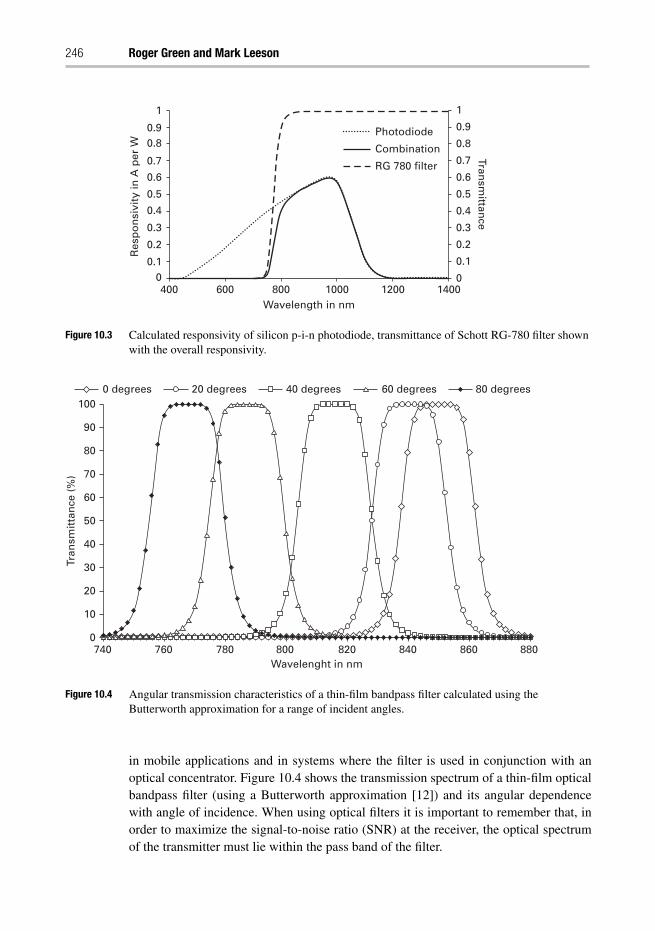
246 Roger Green and Mark Leeson
400
Res
po
nsi
vity
in A
per
W
00.1
0.2
0.3
0.4
0.5
0.6
0.7
0.80.9
1
0
0.1
0.2
0.3
0.4
0.5
0.6
0.7
0.8
0.9
1
600 800Wavelength in nm
1000 1200
Photodiode
Combination
RG 780 filter
1400
Transm
ittance
Figure 10.3 Calculated responsivity of silicon p-i-n photodiode, transmittance of Schott RG-780 filter shownwith the overall responsivity.
0 degrees 20 degrees 40 degrees 60 degrees 80 degrees
0740 760 780 800
Wavelenght in nm
Tran
smit
tan
ce (
%)
820 840 860 880
10
20
30
40
50
60
70
80
90
100
Figure 10.4 Angular transmission characteristics of a thin-film bandpass filter calculated using theButterworth approximation for a range of incident angles.
in mobile applications and in systems where the filter is used in conjunction with anoptical concentrator. Figure 10.4 shows the transmission spectrum of a thin-film opticalbandpass filter (using a Butterworth approximation [12]) and its angular dependencewith angle of incidence. When using optical filters it is important to remember that, inorder to maximize the signal-to-noise ratio (SNR) at the receiver, the optical spectrumof the transmitter must lie within the pass band of the filter.
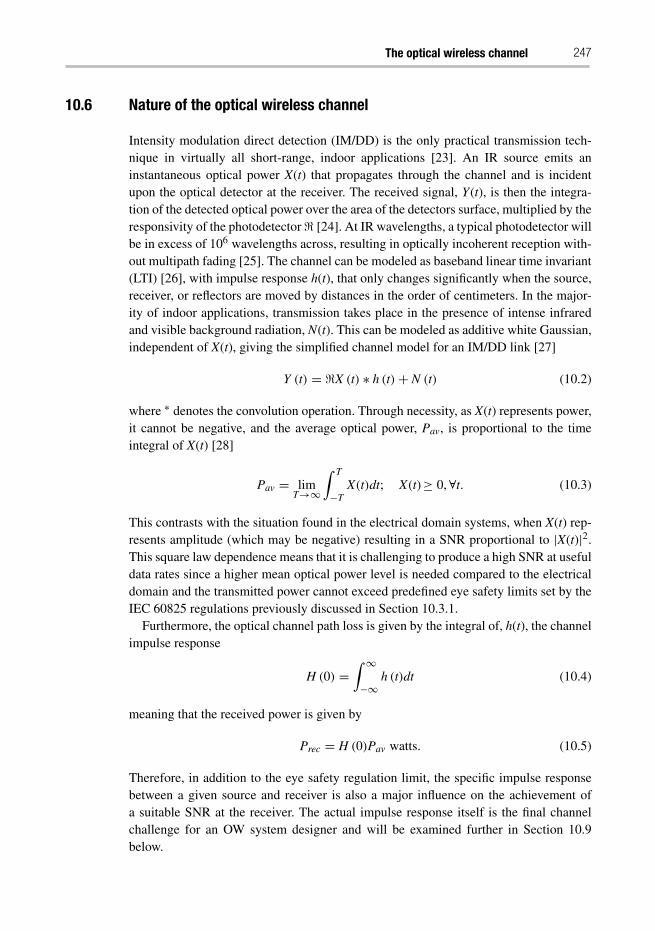
The optical wireless channel 247
10.6 Nature of the optical wireless channel
Intensity modulation direct detection (IM/DD) is the only practical transmission tech-nique in virtually all short-range, indoor applications [23]. An IR source emits aninstantaneous optical power X(t) that propagates through the channel and is incidentupon the optical detector at the receiver. The received signal, Y(t), is then the integra-tion of the detected optical power over the area of the detectors surface, multiplied by theresponsivity of the photodetector& [24]. At IR wavelengths, a typical photodetector willbe in excess of 106 wavelengths across, resulting in optically incoherent reception with-out multipath fading [25]. The channel can be modeled as baseband linear time invariant(LTI) [26], with impulse response h(t), that only changes significantly when the source,receiver, or reflectors are moved by distances in the order of centimeters. In the major-ity of indoor applications, transmission takes place in the presence of intense infraredand visible background radiation, N(t). This can be modeled as additive white Gaussian,independent of X(t), giving the simplified channel model for an IM/DD link [27]
Y (t) = &X (t) ∗ h (t)+ N (t) (10.2)
where ∗ denotes the convolution operation. Through necessity, as X(t) represents power,it cannot be negative, and the average optical power, Pav, is proportional to the timeintegral of X(t) [28]
Pav = limT→∞
∫ T
−TX(t)dt; X(t)≥ 0, ∀t. (10.3)
This contrasts with the situation found in the electrical domain systems, when X(t) rep-resents amplitude (which may be negative) resulting in a SNR proportional to |X(t)|2.This square law dependence means that it is challenging to produce a high SNR at usefuldata rates since a higher mean optical power level is needed compared to the electricaldomain and the transmitted power cannot exceed predefined eye safety limits set by theIEC 60825 regulations previously discussed in Section 10.3.1.
Furthermore, the optical channel path loss is given by the integral of, h(t), the channelimpulse response
H (0) =∫ ∞
−∞h (t)dt (10.4)
meaning that the received power is given by
Prec = H (0)Pav watts. (10.5)
Therefore, in addition to the eye safety regulation limit, the specific impulse responsebetween a given source and receiver is also a major influence on the achievement ofa suitable SNR at the receiver. The actual impulse response itself is the final channelchallenge for an OW system designer and will be examined further in Section 10.9below.
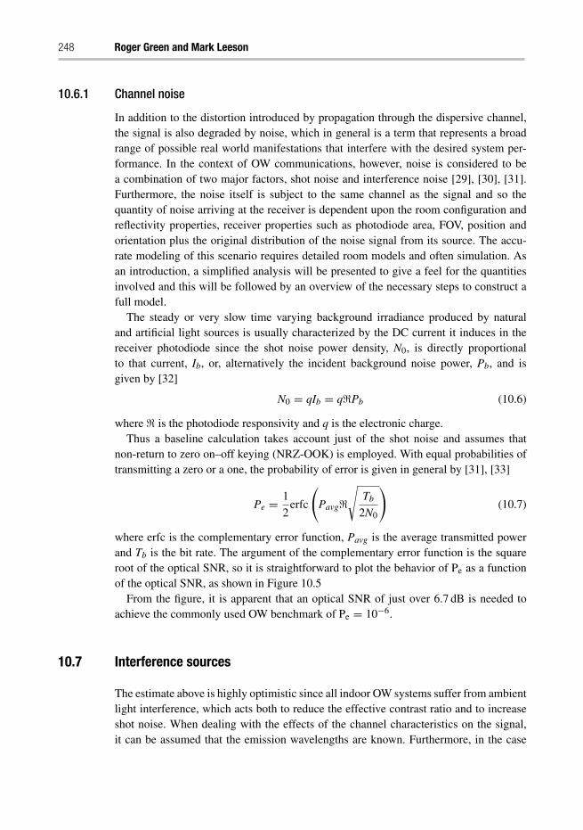
248 Roger Green and Mark Leeson
10.6.1 Channel noise
In addition to the distortion introduced by propagation through the dispersive channel,the signal is also degraded by noise, which in general is a term that represents a broadrange of possible real world manifestations that interfere with the desired system per-formance. In the context of OW communications, however, noise is considered to bea combination of two major factors, shot noise and interference noise [29], [30], [31].Furthermore, the noise itself is subject to the same channel as the signal and so thequantity of noise arriving at the receiver is dependent upon the room configuration andreflectivity properties, receiver properties such as photodiode area, FOV, position andorientation plus the original distribution of the noise signal from its source. The accu-rate modeling of this scenario requires detailed room models and often simulation. Asan introduction, a simplified analysis will be presented to give a feel for the quantitiesinvolved and this will be followed by an overview of the necessary steps to construct afull model.
The steady or very slow time varying background irradiance produced by naturaland artificial light sources is usually characterized by the DC current it induces in thereceiver photodiode since the shot noise power density, N0, is directly proportionalto that current, Ib, or, alternatively the incident background noise power, Pb, and isgiven by [32]
N0 = qIb = q&Pb (10.6)
where & is the photodiode responsivity and q is the electronic charge.Thus a baseline calculation takes account just of the shot noise and assumes that
non-return to zero on–off keying (NRZ-OOK) is employed. With equal probabilities oftransmitting a zero or a one, the probability of error is given in general by [31], [33]
Pe = 1
2erfc
(Pavg&
√Tb
2N0
)(10.7)
where erfc is the complementary error function, Pavg is the average transmitted powerand Tb is the bit rate. The argument of the complementary error function is the squareroot of the optical SNR, so it is straightforward to plot the behavior of Pe as a functionof the optical SNR, as shown in Figure 10.5
From the figure, it is apparent that an optical SNR of just over 6.7 dB is needed toachieve the commonly used OW benchmark of Pe = 10−6.
10.7 Interference sources
The estimate above is highly optimistic since all indoor OW systems suffer from ambientlight interference, which acts both to reduce the effective contrast ratio and to increaseshot noise. When dealing with the effects of the channel characteristics on the signal,it can be assumed that the emission wavelengths are known. Furthermore, in the case
The optical wireless channel 249
010–8
10–6
10–4
Pe
10–2
100
1 2 3 4Optical SNR in dB
5 6 7 8
Figure 10.5 General dependence of Pe on optical SNR for an idealized OW channel.
of infrared communications, signals will occupy a fairly narrow band operating at thetypical center wavelengths of 780 nm, 870 nm, or 970 nm [29] implying that a givensource power is contained within a known range of radiation wavelengths that is wellmatched with photodiode responsivities. It is more common to find such infrared devicescharacterized by their radiometric properties [34] whereas illumination light sourcesare normally characterized by their interaction with the human eye (their photometricproperties) or their electrical properties [35].
10.7.1 Sunlight
The effects of the sun on OW links have been apparent since the beginning of work in thearea [4] and without filtering, daylight can overpower OW IR links [29]. For modelingpurposes, the sun is a relatively broadband source of approximately constant spectraldensity over the bandwidth of an OW receiver. It thus induces a constant shot noiseelement in the receiver that can be some hundreds of μA or more [32].
10.7.2 Artificial sources
A 60 W light source does not emit all its power at the wavelengths of interest to opti-cal wireless communications. All illumination light sources, including the sun, emitradiation to varying degree within a silicon photodiode responsivity range. Commonlyemployed daylight filters with a cut off wavelength < 780 nm remove some of the back-ground radiation but above that wavelength, the light sources still induce a backgroundphotocurrent [29]. The effects of background illumination have most commonly beenincluded in the modeling of indoor OW by way of practical measurements such as thosein [36], [37] and [38]. Each of the measurement sets in these publications was carried out
250 Roger Green and Mark Leeson
in a different environment using different receivers with different properties so althoughthey give very good approximations or expectations of the level of received backgroundnoise power that, is present, their results are not totally comparable.
The work by Moreira et al. [31] and [32] has provided through measurement, anaccurate but nevertheless general model for interference from three types of light bulb:incandescent lamps, fluorescent lamps with conventional ballasts, and fluorescent lampswith electronic ballasts. Each model is based upon the measurements from a wide-ranging collection of lamps from many manufacturers. The resultant Fourier seriesformulation can be used to represent to a good approximation the level of interference agiven type of lamp will produce.
10.7.2.1 Incandescent lampsIncandescent, or Tungsten filament lamps are set to become less common under thenew European Parliament and Council Directive 2005/32/EC [39], under which theyare to disappear for energy usage reasons. Nevertheless, they are still very common inoffices and homes so continue to contribute to the noise in current indoor optical wirelesssystems. The interference signal for incandescent lamps may be represented as [32]:
iincand(t) = IB
F1A1
∞∑k=1
ak cos (200πkt + φk) (10.8)
The magnitude factors, ak, and the phase factors, φk, of the 100 Hz harmonics weredetermined empirically in [36] and the first 10 are significant. The multiplying factorcontains IB, the level of the background radiation, F1, the filter attenuation factor andA1, which relates the interference amplitude to IB [31], [32].
10.7.2.2 Fluorescent lamps driven by conventional ballastsOffices commonly contain fluorescent lamps driven by conventional ballasts and thesehave interference effects up to around 2 kHz. The interfering signal can be described by
ifluor(t) = IB
F2A2
∞∑k=1
[bk cos (100π {2k − 1} t + φk)+ ck cos (100π {2k} t + ζk)]
(10.9)
The phase factors, φk and ζk may again be taken from [36] with the first 20 being sig-nificant, and F2 and A2 are the corresponding values for this interferer. The magnitudes,bk and ck, are those of the odd and even Fourier harmonics.
10.7.2.3 Fluorescent lamps driven by electronic ballastsIn recent years, fluorescent lamps driven by electronic ballasts (sometimes known ashigh-frequency fluorescent lamps) have developed and are likely to become the domi-nant type in future since this is the technology employed by energy saving lights [39].Unfortunately, they are a worst case scenario for indoor optical wireless communicationsystems for two reasons. First, they exhibit settling times following initial switch on
The optical wireless channel 251
when the output radiation spectrum shifts from one dominated by the infrared emissionto visible light after approximately six minutes [29]. This is commonly observed withenergy saving bulbs that appear initially dim to the human eye, and is of particular rele-vance in residential settings where users move between rooms tuning lights on and off.Here, we follow [40] and assume that the bulbs are in their settled state whilst notingthat incorporating the effects of bulb switch on would form an interesting topic for futurework. The second problem is that the harmonic components of their interference extendto several MHz. The interference signal can be modeled as the sum of two components(low and high frequency) thus:
ielec (t) = ilow (t)+ ihigh (t) (10.10)
where, similar to Equation (10.9)
ilow(t) = IB
F3A3
∞∑k=1
[bk cos (100π{2k − 1}t + φk)+ ck cos (100π {2k} t + ζk)]
(10.11)
ihigh(t) = IB
F4A4
∞∑k=1
dk cos(2π fhighkt + θk
). (10.12)
The parameters in (10.11) above are those for conventional fluorescent lamps with theappropriate filter and conversion factors; values for dk and θk may be taken from [36]with 22 harmonics making significant contributions and fhigh equal to 37.5 kHz [32].
10.8 Impact of interference on BER
The work in [31] and [32] also provides the basis for calculations of the effect of ambientinterference on the BER. Inclusion of the artificial background sources may be achievedby recognizing that they are periodic and integrating the BER expression over the period.This approach modifies (BER) to give [31]
Pe = 1
Ti
∫ Ti
0
[1
2erfc
(Pavg&Tb − vi (t)√
2N0Tb
)+ 1
4
{1+ erf
(−Pavg&Tb − vi (t)√2N0Tb
)}]dt.
(10.13)
The period of the integral Ti is the period of the interference signal and vi(t) is the energyof the interference within the period of a pulse
vi (t) =∫ t+T
tiint (t) dt (10.14)
where iint(t) is the appropriate expression for the type of periodic interferer. When theonly source of noise is the shot element from the signal itself, the SNR is
SNRmax = Pavg&q
(10.15)
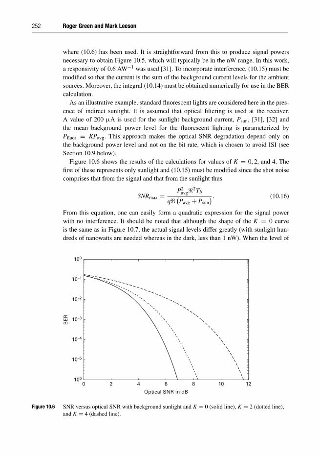
252 Roger Green and Mark Leeson
where (10.6) has been used. It is straightforward from this to produce signal powersnecessary to obtain Figure 10.5, which will typically be in the nW range. In this work,a responsivity of 0.6 AW−1 was used [31]. To incorporate interference, (10.15) must bemodified so that the current is the sum of the background current levels for the ambientsources. Moreover, the integral (10.14) must be obtained numerically for use in the BERcalculation.
As an illustrative example, standard fluorescent lights are considered here in the pres-ence of indirect sunlight. It is assumed that optical filtering is used at the receiver.A value of 200 μA is used for the sunlight background current, Psun, [31], [32] andthe mean background power level for the fluorescent lighting is parameterized byPfluor = KPavg. This approach makes the optical SNR degradation depend only onthe background power level and not on the bit rate, which is chosen to avoid ISI (seeSection 10.9 below).
Figure 10.6 shows the results of the calculations for values of K = 0, 2, and 4. Thefirst of these represents only sunlight and (10.15) must be modified since the shot noisecomprises that from the signal and that from the sunlight thus
SNRmax =P2
avg&2Tb
q& (Pavg + Psun
) . (10.16)
From this equation, one can easily form a quadratic expression for the signal powerwith no interference. It should be noted that although the shape of the K = 0 curveis the same as in Figure 10.7, the actual signal levels differ greatly (with sunlight hun-dreds of nanowatts are needed whereas in the dark, less than 1 nW). When the level of
0 2 4 6
Optical SNR in dB
8 10 12
10–4
10–5
BE
R
10–2
10–3
10–1
100
106
Figure 10.6 SNR versus optical SNR with background sunlight and K = 0 (solid line), K = 2 (dotted line),and K = 4 (dashed line).
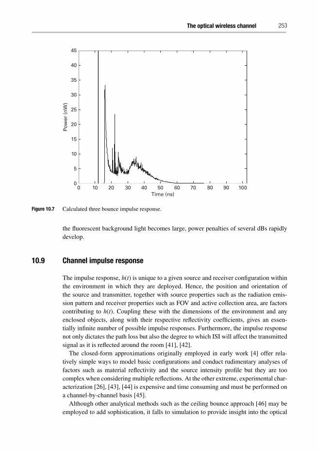
The optical wireless channel 253
45
40
35
30
25
20
15
Pow
er (
nW
)
10
5
00 10 20 30 40 50 60
Time (ns)70 80 90 100
Figure 10.7 Calculated three bounce impulse response.
the fluorescent background light becomes large, power penalties of several dBs rapidlydevelop.
10.9 Channel impulse response
The impulse response, h(t) is unique to a given source and receiver configuration withinthe environment in which they are deployed. Hence, the position and orientation ofthe source and transmitter, together with source properties such as the radiation emis-sion pattern and receiver properties such as FOV and active collection area, are factorscontributing to h(t). Coupling these with the dimensions of the environment and anyenclosed objects, along with their respective reflectivity coefficients, gives an essen-tially infinite number of possible impulse responses. Furthermore, the impulse responsenot only dictates the path loss but also the degree to which ISI will affect the transmittedsignal as it is reflected around the room [41], [42].
The closed-form approximations originally employed in early work [4] offer rela-tively simple ways to model basic configurations and conduct rudimentary analyses offactors such as material reflectivity and the source intensity profile but they are toocomplex when considering multiple reflections. At the other extreme, experimental char-acterization [26], [43], [44] is expensive and time consuming and must be performed ona channel-by-channel basis [45].
Although other analytical methods such as the ceiling bounce approach [46] may beemployed to add sophistication, it falls to simulation to provide insight into the optical
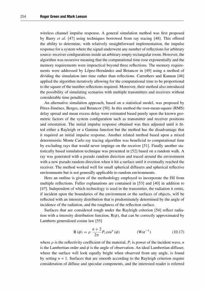
254 Roger Green and Mark Leeson
wireless channel impulse response. A general simulation method was first proposedby Barry et al. [47] using techniques borrowed from ray tracing [48]. This offeredthe ability to determine, with relatively straightforward implementation, the impulseresponse for a system where the signal underwent any number of reflections for arbitrarysource–receiver configurations inside an arbitrary empty rectangular room. However, thealgorithm was recursive meaning that the computational time rose exponentially and thememory requirements were impractical beyond three reflections. The memory require-ments were addressed by López-Hernández and Betancor in [49] using a method ofdividing the simulation into time rather than reflections. Carruthers and Kannan [46]applied the algorithm iteratively allowing for the computational time to be proportionalto the square of the number reflections required. Moreover, their method also introducedthe possibility of simulating scenarios with multiple transmitters and receivers withoutconsiderable time penalties.
An alternative simulation approach, based on a statistical model, was proposed byPérez-Jiménez, Berges, and Betancor [50]. In this method the root-mean-square (RMS)delay spread and mean excess delay were estimated based purely upon the known geo-metric factors of the system configuration such as transmitter and receiver positionsand orientation. The initial impulse response obtained was then adjusted until it fit-ted either a Rayleigh or a Gamma function but the method has the disadvantage thatit required an initial impulse response. Another related method based upon a mixeddeterministic Monte Carlo ray tracing algorithm was beneficial to computational timeby excluding rays that would never impinge on the receiver [51]. Finally another sta-tistically based simulation technique was presented in [52] based on a random walk. Aray was generated with a pseudo random direction and traced around the environmentwith a new pseudo random direction when it hit a surface until it eventually reached thereceiver. The method worked well for small spherical diffusers and spherical reflectiveenvironments but is not generally applicable to random environments.
Here an outline is given of the methodology employed to incorporate the ISI frommultiple reflections. Fuller explanations are contained in [53] and [40] in addition to[47]. Independent of which technology is used in the transmitter, the radiation it emits,if incident upon the boundaries of the environment or the surfaces of objects, will bereflected with an intensity distribution that is predominately determined by the angle ofincidence of the radiation, and the roughness of the reflection surface.
Surfaces that are considered rough under the Rayleigh criterion [54] reflect radia-tion with a intensity distribution function, R(φ), that can be correctly approximated byLamberts generalized cosine law [55]
R (φ) = ρn+ 2
2πPi cosn (φ) (Wsr−1) (10.17)
where ρ is the reflectivity coefficient of the material, Pi is power of the incident wave, nis the Lambertian order and φ is the angle of observation. An ideal Lambertian diffuser,where the surface will look equally bright when observed from any angle, is foundby setting n = 1. Surfaces that are smooth according to the Rayleigh criterion requireconsideration of diffuse and specular components, and the interested reader is referred
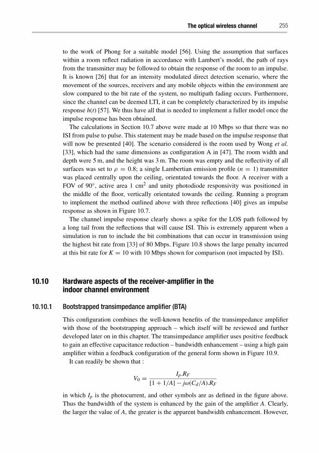
The optical wireless channel 255
to the work of Phong for a suitable model [56]. Using the assumption that surfaceswithin a room reflect radiation in accordance with Lambert’s model, the path of raysfrom the transmitter may be followed to obtain the response of the room to an impulse.It is known [26] that for an intensity modulated direct detection scenario, where themovement of the sources, receivers and any mobile objects within the environment areslow compared to the bit rate of the system, no multipath fading occurs. Furthermore,since the channel can be deemed LTI, it can be completely characterized by its impulseresponse h(t) [57]. We thus have all that is needed to implement a fuller model once theimpulse response has been obtained.
The calculations in Section 10.7 above were made at 10 Mbps so that there was noISI from pulse to pulse. This statement may be made based on the impulse response thatwill now be presented [40]. The scenario considered is the room used by Wong et al.[33], which had the same dimensions as configuration A in [47]. The room width anddepth were 5 m, and the height was 3 m. The room was empty and the reflectivity of allsurfaces was set to ρ = 0.8; a single Lambertian emission profile (n = 1) transmitterwas placed centrally upon the ceiling, orientated towards the floor. A receiver with aFOV of 90◦, active area 1 cm2 and unity photodiode responsivity was positioned inthe middle of the floor, vertically orientated towards the ceiling. Running a programto implement the method outlined above with three reflections [40] gives an impulseresponse as shown in Figure 10.7.
The channel impulse response clearly shows a spike for the LOS path followed bya long tail from the reflections that will cause ISI. This is extremely apparent when asimulation is run to include the bit combinations that can occur in transmission usingthe highest bit rate from [33] of 80 Mbps. Figure 10.8 shows the large penalty incurredat this bit rate for K = 10 with 10 Mbps shown for comparison (not impacted by ISI).
10.10 Hardware aspects of the receiver-amplifier in theindoor channel environment
10.10.1 Bootstrapped transimpedance amplifier (BTA)
This configuration combines the well-known benefits of the transimpedance amplifierwith those of the bootstrapping approach – which itself will be reviewed and furtherdeveloped later on in this chapter. The transimpedance amplifier uses positive feedbackto gain an effective capacitance reduction – bandwidth enhancement – using a high gainamplifier within a feedback configuration of the general form shown in Figure 10.9.
It can readily be shown that :
V0 = Ip.RF
[1+ 1/A]− jω(Cd/A).RF
in which Ip is the photocurrent, and other symbols are as defined in the figure above.Thus the bandwidth of the system is enhanced by the gain of the amplifier A. Clearly,the larger the value of A, the greater is the apparent bandwidth enhancement. However,
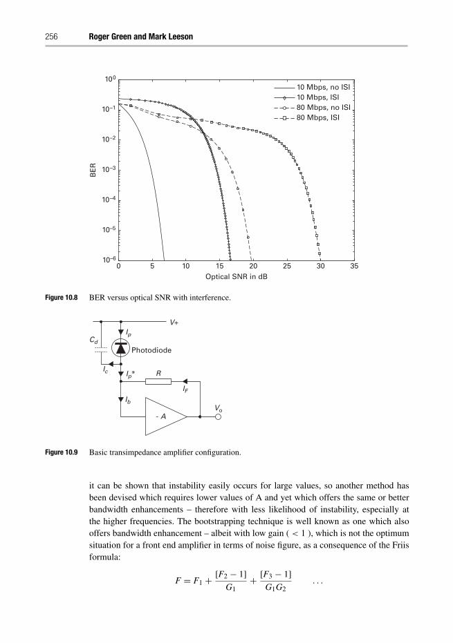
256 Roger Green and Mark Leeson
0 5 10 15Optical SNR in dB
20 25
10 Mbps, no ISI10 Mbps, ISI80 Mbps, no ISI80 Mbps, ISI
30 35
10–4
10–5
BE
R
10–2
10–3
10–1
100
10–6
Figure 10.8 BER versus optical SNR with interference.
Photodiode
R
V+Ip
Ic
Ib
IF
- AVo
Ip*
Cd
Figure 10.9 Basic transimpedance amplifier configuration.
it can be shown that instability easily occurs for large values, so another method hasbeen devised which requires lower values of A and yet which offers the same or betterbandwidth enhancements – therefore with less likelihood of instability, especially atthe higher frequencies. The bootstrapping technique is well known as one which alsooffers bandwidth enhancement – albeit with low gain ( < 1 ), which is not the optimumsituation for a front end amplifier in terms of noise figure, as a consequence of the Friisformula:
F = F1 + [F2 − 1]
G1+ [F3 − 1]
G1G2. . .
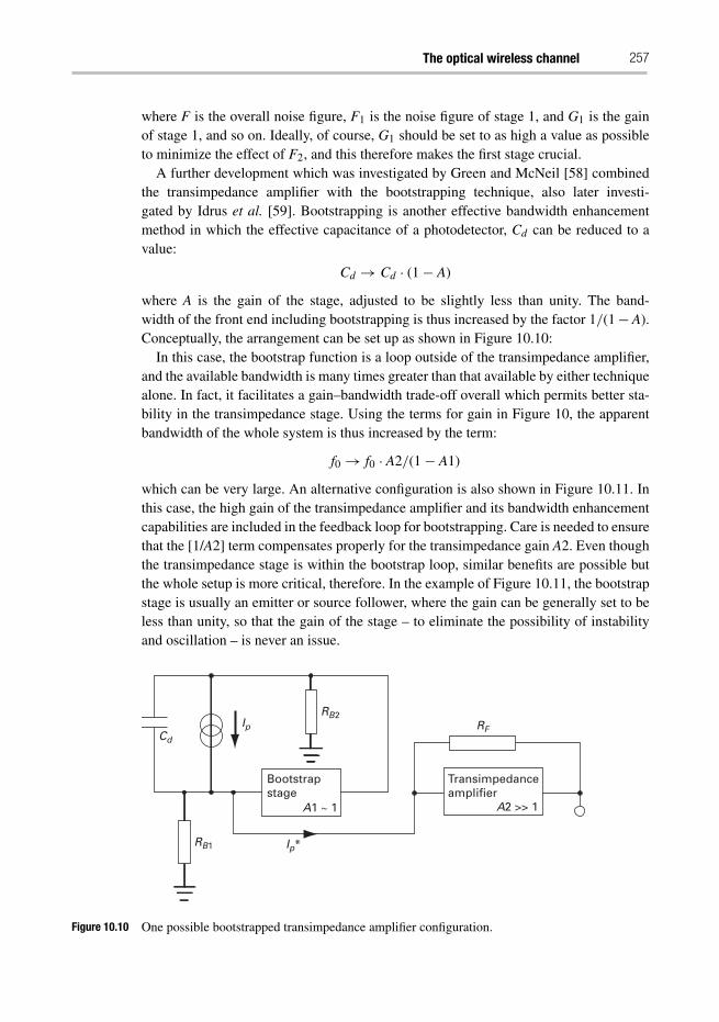
The optical wireless channel 257
where F is the overall noise figure, F1 is the noise figure of stage 1, and G1 is the gainof stage 1, and so on. Ideally, of course, G1 should be set to as high a value as possibleto minimize the effect of F2, and this therefore makes the first stage crucial.
A further development which was investigated by Green and McNeil [58] combinedthe transimpedance amplifier with the bootstrapping technique, also later investi-gated by Idrus et al. [59]. Bootstrapping is another effective bandwidth enhancementmethod in which the effective capacitance of a photodetector, Cd can be reduced to avalue:
Cd → Cd · (1− A)
where A is the gain of the stage, adjusted to be slightly less than unity. The band-width of the front end including bootstrapping is thus increased by the factor 1/(1− A).Conceptually, the arrangement can be set up as shown in Figure 10.10:
In this case, the bootstrap function is a loop outside of the transimpedance amplifier,and the available bandwidth is many times greater than that available by either techniquealone. In fact, it facilitates a gain–bandwidth trade-off overall which permits better sta-bility in the transimpedance stage. Using the terms for gain in Figure 10, the apparentbandwidth of the whole system is thus increased by the term:
f0 → f0 · A2/(1− A1)
which can be very large. An alternative configuration is also shown in Figure 10.11. Inthis case, the high gain of the transimpedance amplifier and its bandwidth enhancementcapabilities are included in the feedback loop for bootstrapping. Care is needed to ensurethat the [1/A2] term compensates properly for the transimpedance gain A2. Even thoughthe transimpedance stage is within the bootstrap loop, similar benefits are possible butthe whole setup is more critical, therefore. In the example of Figure 10.11, the bootstrapstage is usually an emitter or source follower, where the gain can be generally set to beless than unity, so that the gain of the stage – to eliminate the possibility of instabilityand oscillation – is never an issue.
Cd
IpRB2
RF
RB1 Ip*
Transimpedanceamplifier
A2 >> 1
Bootstrapstage
A1 ~ 1
Figure 10.10 One possible bootstrapped transimpedance amplifier configuration.
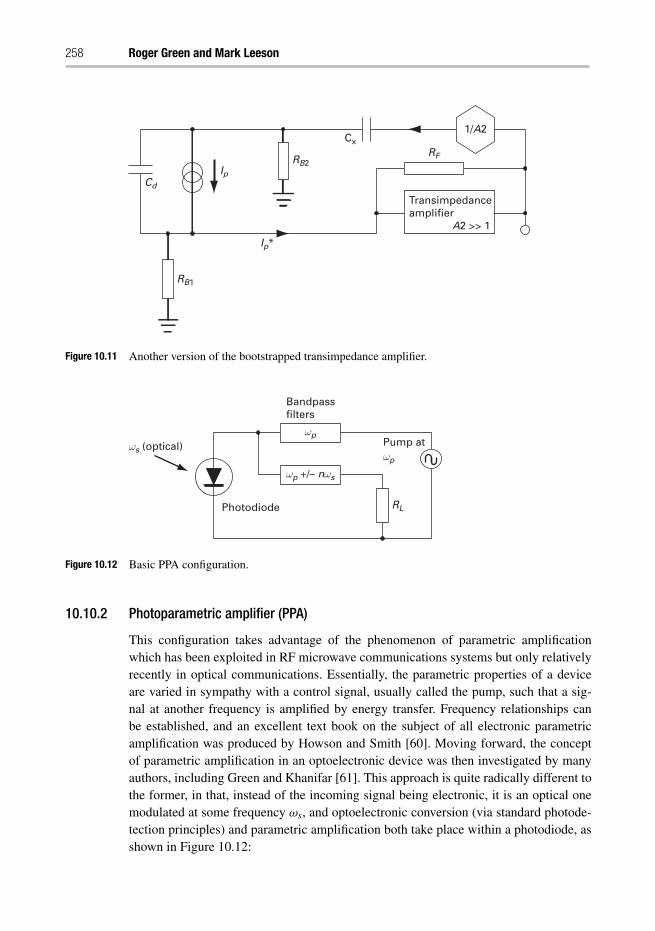
258 Roger Green and Mark Leeson
Cd
IpRB2
RF
RB1
Cx
Ip*
Transimpedanceamplifier
1/A2
A2 >> 1
Figure 10.11 Another version of the bootstrapped transimpedance amplifier.
Bandpassfilters
Photodiode
ωs (optical) Pump atωp
RL
ωp
ωp +/– nωs
Figure 10.12 Basic PPA configuration.
10.10.2 Photoparametric amplifier (PPA)
This configuration takes advantage of the phenomenon of parametric amplificationwhich has been exploited in RF microwave communications systems but only relativelyrecently in optical communications. Essentially, the parametric properties of a deviceare varied in sympathy with a control signal, usually called the pump, such that a sig-nal at another frequency is amplified by energy transfer. Frequency relationships canbe established, and an excellent text book on the subject of all electronic parametricamplification was produced by Howson and Smith [60]. Moving forward, the conceptof parametric amplification in an optoelectronic device was then investigated by manyauthors, including Green and Khanifar [61]. This approach is quite radically different tothe former, in that, instead of the incoming signal being electronic, it is an optical onemodulated at some frequency ωs, and optoelectronic conversion (via standard photode-tection principles) and parametric amplification both take place within a photodiode, asshown in Figure 10.12:
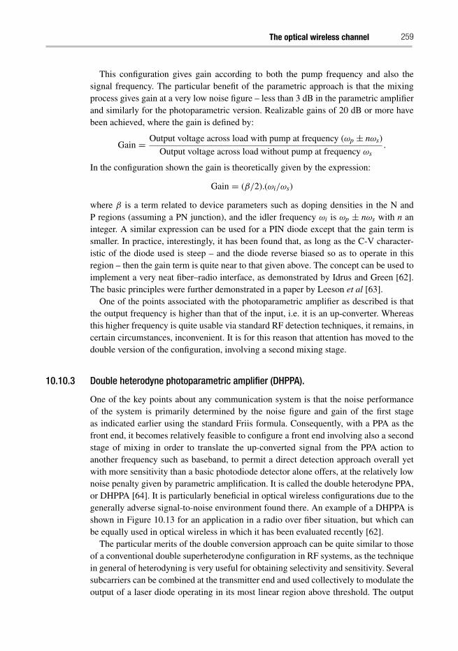
The optical wireless channel 259
This configuration gives gain according to both the pump frequency and also thesignal frequency. The particular benefit of the parametric approach is that the mixingprocess gives gain at a very low noise figure – less than 3 dB in the parametric amplifierand similarly for the photoparametric version. Realizable gains of 20 dB or more havebeen achieved, where the gain is defined by:
Gain = Output voltage across load with pump at frequency (ωp ± nωs)
Output voltage across load without pump at frequency ωs.
In the configuration shown the gain is theoretically given by the expression:
Gain = (β/2).(ωi/ωs)
where β is a term related to device parameters such as doping densities in the N andP regions (assuming a PN junction), and the idler frequency ωi is ωp ± nωs with n aninteger. A similar expression can be used for a PIN diode except that the gain term issmaller. In practice, interestingly, it has been found that, as long as the C-V character-istic of the diode used is steep – and the diode reverse biased so as to operate in thisregion – then the gain term is quite near to that given above. The concept can be used toimplement a very neat fiber–radio interface, as demonstrated by Idrus and Green [62].The basic principles were further demonstrated in a paper by Leeson et al [63].
One of the points associated with the photoparametric amplifier as described is thatthe output frequency is higher than that of the input, i.e. it is an up-converter. Whereasthis higher frequency is quite usable via standard RF detection techniques, it remains, incertain circumstances, inconvenient. It is for this reason that attention has moved to thedouble version of the configuration, involving a second mixing stage.
10.10.3 Double heterodyne photoparametric amplifier (DHPPA).
One of the key points about any communication system is that the noise performanceof the system is primarily determined by the noise figure and gain of the first stageas indicated earlier using the standard Friis formula. Consequently, with a PPA as thefront end, it becomes relatively feasible to configure a front end involving also a secondstage of mixing in order to translate the up-converted signal from the PPA action toanother frequency such as baseband, to permit a direct detection approach overall yetwith more sensitivity than a basic photodiode detector alone offers, at the relatively lownoise penalty given by parametric amplification. It is called the double heterodyne PPA,or DHPPA [64]. It is particularly beneficial in optical wireless configurations due to thegenerally adverse signal-to-noise environment found there. An example of a DHPPA isshown in Figure 10.13 for an application in a radio over fiber situation, but which canbe equally used in optical wireless in which it has been evaluated recently [62].
The particular merits of the double conversion approach can be quite similar to thoseof a conventional double superheterodyne configuration in RF systems, as the techniquein general of heterodyning is very useful for obtaining selectivity and sensitivity. Severalsubcarriers can be combined at the transmitter end and used collectively to modulate theoutput of a laser diode operating in its most linear region above threshold. The output
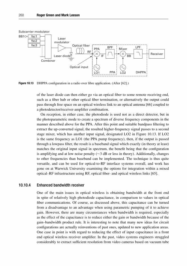
260 Roger Green and Mark Leeson
Subcarrier modulator
Lasermodulator
Laser diode
Combiner
Optical fiber
RFPPA BPF Mixer LPF
BB
DHPPALO2
ReceiverIF
LO1 PPA
Optical input
BB1 fsc1fsc2fsc3
Figure 10.13 DHPPA configuration in a radio over fibre application. (After [62].)
of the laser diode can then either go via an optical fiber to some remote receiving end,such as a fiber hub or other optical fiber termination, or alternatively the output couldpass through free space on an optical wireless link to an optical antenna [66] coupled toa photodetector/receiver-amplifier combination.
On reception, in either case, the photodiode is used not as a direct detector, but inthe photoparametric mode to create a spectrum of diverse frequency components in themanner described above for the PPA. After this point and suitable bandpass filtering toextract the up-converted signal, the resulted higher-frequency signal passes to a secondstage mixer, which has another input signal, designated LO2 in Figure 10.13. If LO2is the same frequency as LO1 (the PPA pump frequency), then, if the output is passedthrough a lowpass filter, the result is a baseband signal which exactly (in theory at least)matches the original input signal in spectrum, the benefit being that the configurationis amplifying and at low noise penalty (∼3 dB or less in theory). Additionally, changesto other frequencies than baseband can be implemented. The technique is thus quiteversatile, and can be used for optical-to-RF interface systems overall, and work hasgone on at Warwick University examining the options for integration within a mixedoptical–RF infrastructure using RF, optical fiber- and optical wireless links [65].
10.10.4 Enhanced bandwidth receiver
One of the main issues in optical wireless is obtaining bandwidth at the front endin spite of relatively high photodiode capacitance, in comparison to values in opticalfiber communications. Of course, as discussed above, this capacitance can be turnedfrom a disadvantage to an advantage when using parametric pumping of it to achievegain. However, there are many circumstances when bandwidth is required, especiallyas the effect of the capacitance is to reduce either the gain or bandwidth because of thegain–bandwidth product rule. It is interesting to note that many new ideas for circuitconfigurations are actually reinventions of past ones, updated to new application areas.One case in point is with regard to reducing the effect of input capacitance in a frontend optical wireless receiver amplifier. In the past, video systems engineers struggledconsiderably to extract sufficient resolution from video cameras based on vacuum tube
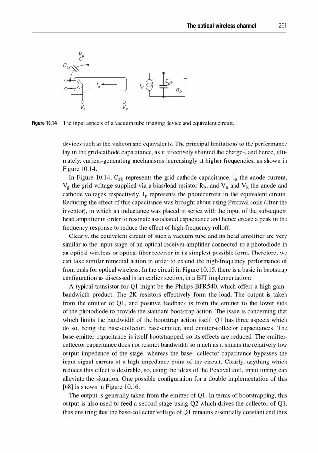
The optical wireless channel 261
Vk
la lp
Cgk
Cgk
Vg
Va
Rb
Figure 10.14 The input aspects of a vacuum tube imaging device and equivalent circuit.
devices such as the vidicon and equivalents. The principal limitations to the performancelay in the grid-cathode capacitance, as it effectively shunted the charge-, and hence, ulti-mately, current-generating mechanisms increasingly at higher frequencies, as shown inFigure 10.14.
In Figure 10.14, Cgk represents the grid-cathode capacitance, Ia the anode current,Vg the grid voltage supplied via a bias/load resistor Rb, and Va and Vk the anode andcathode voltages respectively. Ip represents the photocurrent in the equivalent circuit.Reducing the effect of this capacitance was brought about using Percival coils (after theinventor), in which an inductance was placed in series with the input of the subsequenthead amplifier in order to resonate associated capacitance and hence create a peak in thefrequency response to reduce the effect of high-frequency rolloff.
Clearly, the equivalent circuit of such a vacuum tube and its head amplifier are verysimilar to the input stage of an optical receiver-amplifier connected to a photodiode inan optical wireless or optical fiber receiver in its simplest possible form. Therefore, wecan take similar remedial action in order to extend the high-frequency performance offront ends for optical wireless. In the circuit in Figure 10.15, there is a basic in bootstrapconfiguration as discussed in an earlier section, in a BJT implementation:
A typical transistor for Q1 might be the Philips BFR540, which offers a high gain–bandwidth product. The 2K resistors effectively form the load. The output is takenfrom the emitter of Q1, and positive feedback is from the emitter to the lower sideof the photodiode to provide the standard bootstrap action. The issue is concerning thatwhich limits the bandwidth of the bootstrap action itself: Q1 has three aspects whichdo so, being the base-collector, base-emitter, and emitter-collector capacitances. Thebase-emitter capacitance is itself bootstrapped, so its effects are reduced. The emitter-collector capacitance does not restrict bandwidth so much as it shunts the relatively lowoutput impedance of the stage, whereas the base- collector capacitance bypasses theinput signal current at a high impedance point of the circuit. Clearly, anything whichreduces this effect is desirable, so, using the ideas of the Percival coil, input tuning canalleviate the situation. One possible configuration for a double implementation of this[68] is shown in Figure 10.16.
The output is generally taken from the emitter of Q1. In terms of bootstrapping, thisoutput is also used to feed a second stage using Q2 which drives the collector of Q1,thus ensuring that the base-collector voltage of Q1 remains essentially constant and thus
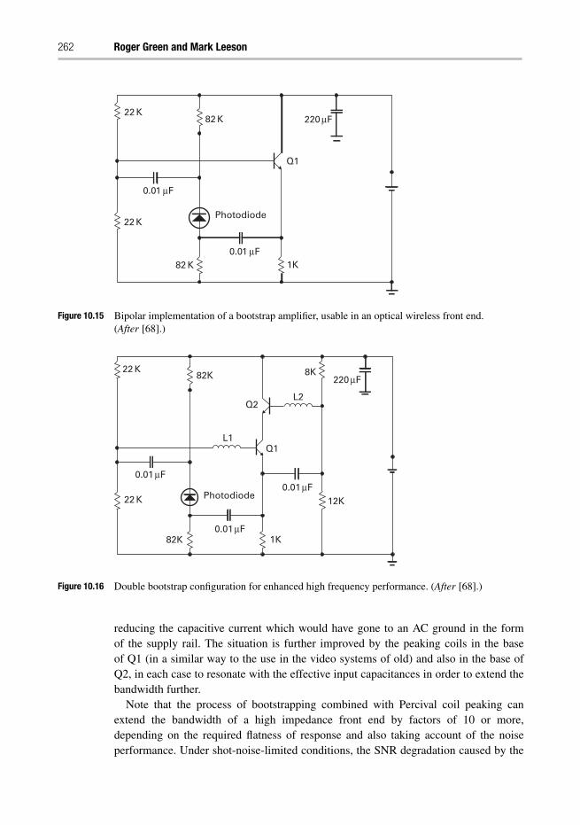
262 Roger Green and Mark Leeson
22 K82 K 220 μF
Q1
0.01 μF
22 K
1K82 K0.01 μF
Photodiode
Figure 10.15 Bipolar implementation of a bootstrap amplifier, usable in an optical wireless front end.(After [68].)
22 K
22 K
82K
82K
8K
12K
1K
Q2
Q1
L2
L1
220 μF
0.01 μF
0.01 μF
0.01 μFPhotodiode
Figure 10.16 Double bootstrap configuration for enhanced high frequency performance. (After [68].)
reducing the capacitive current which would have gone to an AC ground in the formof the supply rail. The situation is further improved by the peaking coils in the baseof Q1 (in a similar way to the use in the video systems of old) and also in the base ofQ2, in each case to resonate with the effective input capacitances in order to extend thebandwidth further.
Note that the process of bootstrapping combined with Percival coil peaking canextend the bandwidth of a high impedance front end by factors of 10 or more,depending on the required flatness of response and also taking account of the noiseperformance. Under shot-noise-limited conditions, the SNR degradation caused by the
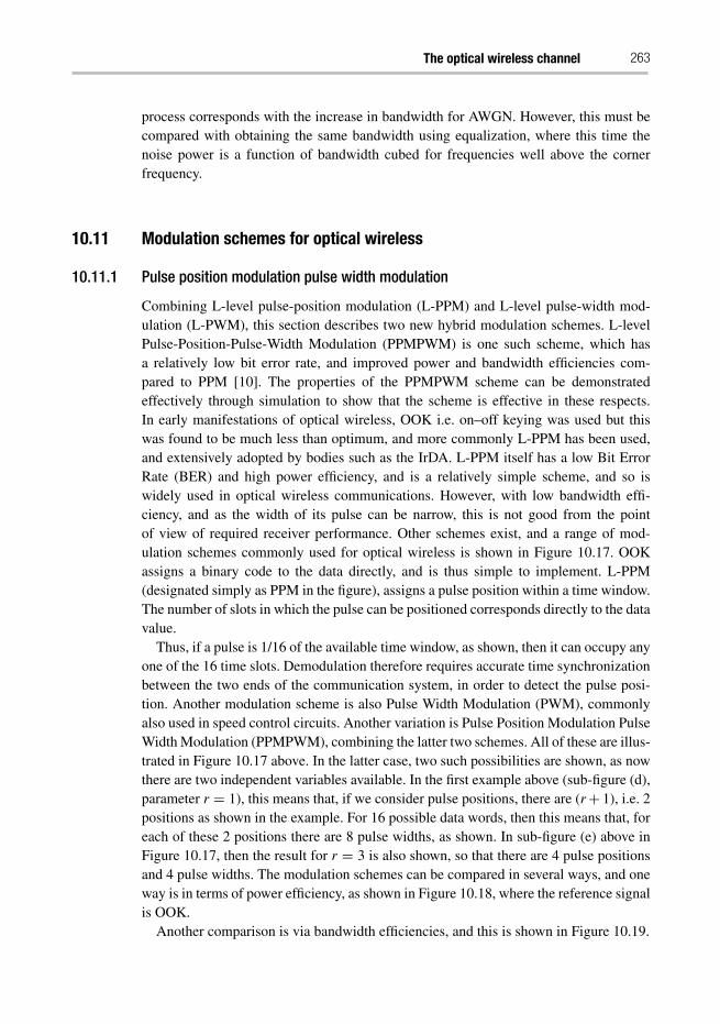
The optical wireless channel 263
process corresponds with the increase in bandwidth for AWGN. However, this must becompared with obtaining the same bandwidth using equalization, where this time thenoise power is a function of bandwidth cubed for frequencies well above the cornerfrequency.
10.11 Modulation schemes for optical wireless
10.11.1 Pulse position modulation pulse width modulation
Combining L-level pulse-position modulation (L-PPM) and L-level pulse-width mod-ulation (L-PWM), this section describes two new hybrid modulation schemes. L-levelPulse-Position-Pulse-Width Modulation (PPMPWM) is one such scheme, which hasa relatively low bit error rate, and improved power and bandwidth efficiencies com-pared to PPM [10]. The properties of the PPMPWM scheme can be demonstratedeffectively through simulation to show that the scheme is effective in these respects.In early manifestations of optical wireless, OOK i.e. on–off keying was used but thiswas found to be much less than optimum, and more commonly L-PPM has been used,and extensively adopted by bodies such as the IrDA. L-PPM itself has a low Bit ErrorRate (BER) and high power efficiency, and is a relatively simple scheme, and so iswidely used in optical wireless communications. However, with low bandwidth effi-ciency, and as the width of its pulse can be narrow, this is not good from the pointof view of required receiver performance. Other schemes exist, and a range of mod-ulation schemes commonly used for optical wireless is shown in Figure 10.17. OOKassigns a binary code to the data directly, and is thus simple to implement. L-PPM(designated simply as PPM in the figure), assigns a pulse position within a time window.The number of slots in which the pulse can be positioned corresponds directly to the datavalue.
Thus, if a pulse is 1/16 of the available time window, as shown, then it can occupy anyone of the 16 time slots. Demodulation therefore requires accurate time synchronizationbetween the two ends of the communication system, in order to detect the pulse posi-tion. Another modulation scheme is also Pulse Width Modulation (PWM), commonlyalso used in speed control circuits. Another variation is Pulse Position Modulation PulseWidth Modulation (PPMPWM), combining the latter two schemes. All of these are illus-trated in Figure 10.17 above. In the latter case, two such possibilities are shown, as nowthere are two independent variables available. In the first example above (sub-figure (d),parameter r = 1), this means that, if we consider pulse positions, there are (r+ 1), i.e. 2positions as shown in the example. For 16 possible data words, then this means that, foreach of these 2 positions there are 8 pulse widths, as shown. In sub-figure (e) above inFigure 10.17, then the result for r = 3 is also shown, so that there are 4 pulse positionsand 4 pulse widths. The modulation schemes can be compared in several ways, and oneway is in terms of power efficiency, as shown in Figure 10.18, where the reference signalis OOK.
Another comparison is via bandwidth efficiencies, and this is shown in Figure 10.19.
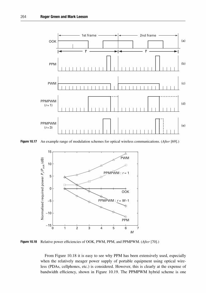
264 Roger Green and Mark Leeson
1st frame
OOK
T T
PPM
PWM
PPMPWM(r = 1)
PPMPWM(r = 3)
2nd frame
(a)
(b)
(c)
(d)
(e)
Figure 10.17 An example range of modulation schemes for optical wireless communications. (After [69].)
0−15
−10
−5
0
5
10
15
1
No
rmal
ised
req
uir
ed p
ow
er P
r/P
oo
k (d
B)
2 3 4 5 6 7M
PPM
PWM
OOK
PPMPWM : r = M –1
PPMPWM : r = 1
Figure 10.18 Relative power efficiencies of OOK, PWM, PPM, and PPMPWM. (After [70].)
From Figure 10.18 it is easy to see why PPM has been extensively used, especiallywhen the relatively meager power supply of portable equipment using optical wire-less (PDAs, cellphones, etc.) is considered. However, this is clearly at the expense ofbandwidth efficiency, shown in Figure 10.19. The PPMPWM hybrid scheme is one
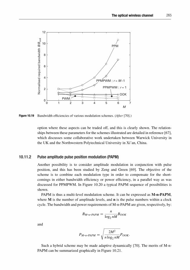
The optical wireless channel 265
00
2
4
6
8
10
12
1
No
rmal
ised
req
uir
ed b
and
wid
th B
/Bo
ok
2 3 4 5 6 7M
PWMOOK
PPMPWM : r = 1
PPMPWM : r = M –1
PPM
Figure 10.19 Bandwidth efficiencies of various modulation schemes. (After [70].)
option where these aspects can be traded off, and this is clearly shown. The relation-ships between these parameters for the schemes illustrated are detailed in reference [67],which discusses some collaborative work undertaken between Warwick University inthe UK and the Northwestern Polytechnical University in Xi’an, China.
10.11.2 Pulse amplitude pulse position modulation (PAPM)
Another possibility is to consider amplitude modulation in conjunction with pulseposition, and this has been studied by Zeng and Green [69]. The objective of thescheme is to combine each modulation type in order to compensate for the short-comings in either bandwidth efficiency or power efficiency, in a parallel way as wasdiscussed for PPMPWM. In Figure 10.20 a typical PAPM sequence of possibilities isshown.
PAPM is thus a multi-level modulation scheme. It can be expressed as M-n-PAPM,where M is the number of amplitude levels, and n is the pulse numbers within a clockcycle. The bandwidth and power requirements of M-n-PAPM are given, respectively, by:
BM-n-PAPM = n
log2 nMBOOK
and
PM-n-PAPM =√
2M2
n log2 nMPOOK .
Such a hybrid scheme may be made adaptive dynamically [70]. The merits of M-n-PAPM can be summarized graphically in Figure 10.21.
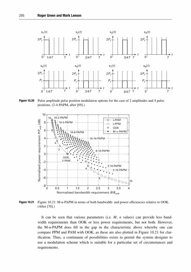
266 Roger Green and Mark Leeson
s1(t )
2Pt
0t
T1/4T 0t
T2/4T
2Pt
s2(t )
0t
T3/4T
2Pt
s3(t )
0t
T
2Pt
s4(t )
0t
T1/4T
2Pt
Pt
s5(t )
0t
T2/4T
2Pt
Pt
s6(t )
0t
T3/4T
2Pt
Pt
s7(t )
0t
T
2Pt
Pt
s8(t )
Figure 10.20 Pulse amplitude pulse position modulation options for the case of 2 amplitudes and 4 pulsepositions. (2-4-PAPM, after [69].)
L-PAML-PPMOOKM-n-PAPM
1016 16-2-PAPM
16-3-PAPM
16-8-PAPM
16-16-PAPM
8-16-PAPM
3-16-PAPM2-16-PAPM
8
4
3
OOK,2-PAM
4
8
8
6
4
2
0
0 0.5 1 1.5 2Normalised bandwidth requirement B/Book
No
rmal
ised
po
wer
req
uir
emen
t P
/Po
ok
(dB
)
2.5 3 3.5 4
16
−2
−4
−6
−8
Figure 10.21 Figure 10.21: M-n-PAPM in terms of both bandwidth- and power efficiencies relative to OOK.(After [70].)
It can be seen that various parameters (i.e. M, n values) can provide less band-width requirements than OOK or less power requirements, but not both. However,the M-n-PAPM does fill in the gap in the characteristic above whereby one cancompare PPM and PAM with OOK, as these are also plotted in Figure 10.21 for clar-ification. Thus, a continuum of possibilities exists to permit the system designer touse a modulation scheme which is suitable for a particular set of circumstances andrequirements.
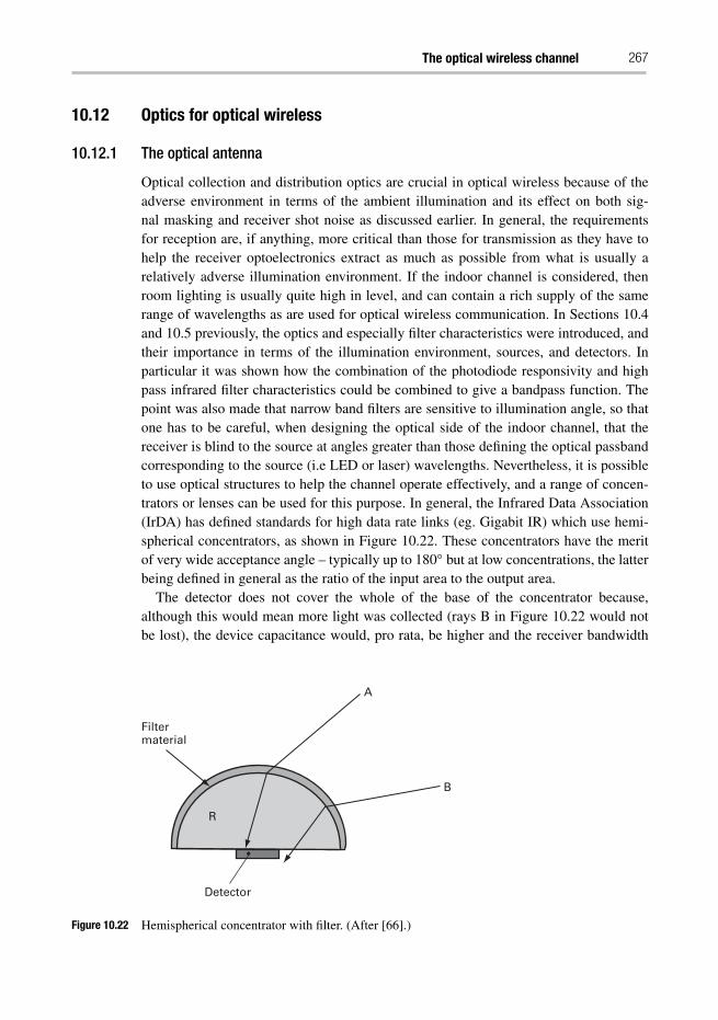
The optical wireless channel 267
10.12 Optics for optical wireless
10.12.1 The optical antenna
Optical collection and distribution optics are crucial in optical wireless because of theadverse environment in terms of the ambient illumination and its effect on both sig-nal masking and receiver shot noise as discussed earlier. In general, the requirementsfor reception are, if anything, more critical than those for transmission as they have tohelp the receiver optoelectronics extract as much as possible from what is usually arelatively adverse illumination environment. If the indoor channel is considered, thenroom lighting is usually quite high in level, and can contain a rich supply of the samerange of wavelengths as are used for optical wireless communication. In Sections 10.4and 10.5 previously, the optics and especially filter characteristics were introduced, andtheir importance in terms of the illumination environment, sources, and detectors. Inparticular it was shown how the combination of the photodiode responsivity and highpass infrared filter characteristics could be combined to give a bandpass function. Thepoint was also made that narrow band filters are sensitive to illumination angle, so thatone has to be careful, when designing the optical side of the indoor channel, that thereceiver is blind to the source at angles greater than those defining the optical passbandcorresponding to the source (i.e LED or laser) wavelengths. Nevertheless, it is possibleto use optical structures to help the channel operate effectively, and a range of concen-trators or lenses can be used for this purpose. In general, the Infrared Data Association(IrDA) has defined standards for high data rate links (eg. Gigabit IR) which use hemi-spherical concentrators, as shown in Figure 10.22. These concentrators have the meritof very wide acceptance angle – typically up to 180◦ but at low concentrations, the latterbeing defined in general as the ratio of the input area to the output area.
The detector does not cover the whole of the base of the concentrator because,although this would mean more light was collected (rays B in Figure 10.22 would notbe lost), the device capacitance would, pro rata, be higher and the receiver bandwidth
Filtermaterial
R
A
B
Detector
Figure 10.22 Hemispherical concentrator with filter. (After [66].)
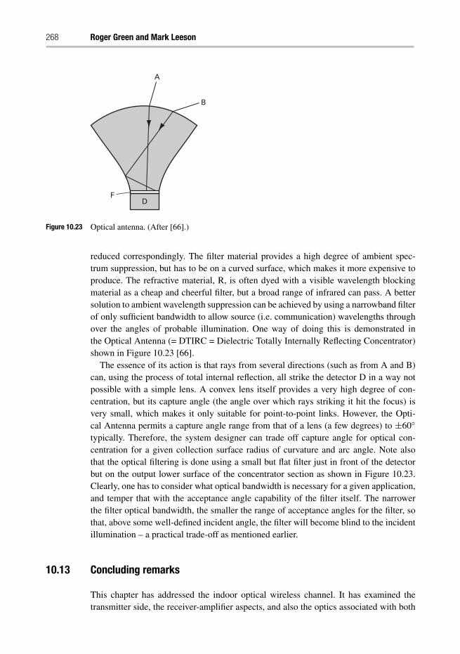
268 Roger Green and Mark Leeson
A
B
DF
Figure 10.23 Optical antenna. (After [66].)
reduced correspondingly. The filter material provides a high degree of ambient spec-trum suppression, but has to be on a curved surface, which makes it more expensive toproduce. The refractive material, R, is often dyed with a visible wavelength blockingmaterial as a cheap and cheerful filter, but a broad range of infrared can pass. A bettersolution to ambient wavelength suppression can be achieved by using a narrowband filterof only sufficient bandwidth to allow source (i.e. communication) wavelengths throughover the angles of probable illumination. One way of doing this is demonstrated inthe Optical Antenna (= DTIRC = Dielectric Totally Internally Reflecting Concentrator)shown in Figure 10.23 [66].
The essence of its action is that rays from several directions (such as from A and B)can, using the process of total internal reflection, all strike the detector D in a way notpossible with a simple lens. A convex lens itself provides a very high degree of con-centration, but its capture angle (the angle over which rays striking it hit the focus) isvery small, which makes it only suitable for point-to-point links. However, the Opti-cal Antenna permits a capture angle range from that of a lens (a few degrees) to ±60◦typically. Therefore, the system designer can trade off capture angle for optical con-centration for a given collection surface radius of curvature and arc angle. Note alsothat the optical filtering is done using a small but flat filter just in front of the detectorbut on the output lower surface of the concentrator section as shown in Figure 10.23.Clearly, one has to consider what optical bandwidth is necessary for a given application,and temper that with the acceptance angle capability of the filter itself. The narrowerthe filter optical bandwidth, the smaller the range of acceptance angles for the filter, sothat, above some well-defined incident angle, the filter will become blind to the incidentillumination – a practical trade-off as mentioned earlier.
10.13 Concluding remarks
This chapter has addressed the indoor optical wireless channel. It has examined thetransmitter side, the receiver-amplifier aspects, and also the optics associated with both
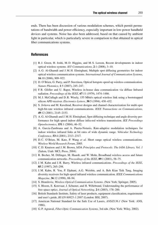
The optical wireless channel 269
ends. There has been discussion of various modulation schemes, which permit permu-tations of bandwidth and power efficiency, especially important in low-power handhelddevices and systems. Noise has also been addressed, based on that caused by ambientlight in particular, which is particularly severe in comparison to that obtained in opticalfiber communications systems.
References
[1] R. J. Green, H. Joshi, M. D. Higgins, and M. S. Leeson, Recent developments in indooroptical wireless systems. IET Communications, 2:1 (2008), 3–10.
[2] A. G. Al-Ghamdi and J. M. H. Elmirghani, Multiple spot diffusing geometries for indooroptical wireless communication systems. International Journal of Communication Systems,16:10 (2006), 909–922.
[3] D. O’Brien, G. Parry, and P. Stavrinou, Optical hotspots speed up wireless communication.Nature Photonics, 1:5 (2007), 245–247.
[4] F. R. Gfeller and U. Bapst, Wireless in-house data communication via diffuse Infraredradiation. Proceedings of the IEEE, 67:11 (1979), 1474–1486.
[5] M. J. McCullagh and D. R. Wisely, 155 Mbit/s optical wireless link using a bootstrappedsilicon APD receiver. Electronics Letters, 30:5 (1994), 430–432.
[6] S. Jivkova and M. Kavehrad, Receiver designs and channel characterization for multi-spothigh-bit-rate wireless infrared communications. IEEE Transactions on Communications,49:12 (2001), 2145–2153.
[7] A. G. Al-Ghamdi and J. M. H. Elmirghani, Spot diffusing technique and angle diversity per-formance for high speed indoor diffuse infra-red wireless transmission. IEE ProceedingsOptoelectronics, 151:1 (2004), 46–52.
[8] A. Garcia-Zambrana and A. Puerta-Notario, Rate-adaptive modulation techniques forindoor wireless infrared links at bit rates of wide dynamic range. Vehicular TechnologyConference, 53:4 (2001), 2313–2317.
[9] D. C. O’Brien, M. Katz, P. Wang et al. Short range optical wireless communications.Wireless World Research Forum, 2005.
[10] C. D. Knutson and J. M. Brown, IrDA Principles and Protocols: The IrDA Library, Vol. 1(Salem, Utah: MCL Press, 2004).
[11] R. Becher, M. Dillinger, M. Haardt, and W. Mohr, Broadband wireless access and futurecommunication networks. Proceedings of the IEEE, 89:1 (2001), 58–75.
[12] J. M. Kahn and J. R. Barry, Wireless infrared communications. Proceedings of the IEEE,85:2 (1997), 265–298.
[13] J. M. Kahn, R. You, P. Djahani, A.G. Weisbin, and A. Beh Kian Teik Tang, Imagingdiversity receivers for high-speed infrared wireless communication. IEEE CommunicationsMagazine, 36:12 (1998), 88–94.
[14] S. Hranilovic, Wireless Optical Communication Systems. (New York: Springer, 2005).[15] S. Bloom, E. Korevaar, J. Schuster, and H. Willebrand, Understanding the performance of
free-space optics. Journal of Optical Networking, 2:6 (2003), 178–200.[16] British Standards Institute, Safety of laser products, equipment classification, requirements
and user’s guide, BS EN 60825-1:2007 (London: BSI, 2007).[17] American National Standard for the Safe Use of Lasers, ANS/Z136.1 (New York: ANS,
1986).[18] G. P. Agrawal, Fiber-Optic Communication Systems, 3rd edn. (New York: Wiley, 2002).
270 Roger Green and Mark Leeson
[19] N. P. Schmitt, T. Pistner, C. Vassipoulis et al., Diffuse wireless optical link for aircraft intra-cabin passenger communication. Communications Systems, Networks and Digital SignalProcessing Conference, 5 (2006), 625-628.
[20] D. Heatley, D. R. Wisely, and P. Cochrane, Optical wireless: The story so far. IEEECommunications Magazine, 36:12 (1998), 72–82.
[21] D. E. Aspnes, Properties of silicon. In Emis Datareviews Series, vol. 4. (London: INSPEC,Institution of Electrical Engineers, 1988), pp. 59–80.
[22] www.schott.com[23] J. G. Proakis, Wiley Encyclopedia of Telecommunications (Hoboken, N.J: Wiley, 2003).[24] J. B. Carruthers and J. M. Kahn, Multiple-subcarrier modulation for nondirected wireless
infrared communication. IEEE Journal on Selected Areas in Communications, 14:3 (1996),538–546.
[25] D. C. M. Lee, J. M. Kahn, and M. D. Audeh, Trellis-coded pulse-position modulation forindoor wireless infrared communications. IEEE Transactions on Communications, 45:9(1997), 1080–1087.
[26] J. M. Kahn, W. J. Krause, and J. B. Carruthers, Experimental characterization of nondi-rected indoor infrared channels. IEEE Transactions on Communications, 43:2-4 (1995),1613–1623.
[27] Z. Ghassemlooy and A. R. Hayes, Digital pulse interval modulation for IR communica-tion systems – a review. International Journal of Communication Systems, 13:7-8 (2000),519–536.
[28] K. Park, Convolutional coded pulse-position modulation on wireless infrared link. IEEProceedings Optoelectronics, 148:4 (2001), 199–203.
[29] A. C. Boucouvalas, Indoor ambient light noise and its effect on wireless optical links. IEEProceedings Optoelectronics, 143:6 (1996), 334–338.
[30] R. Narasimhan, M. D. Audeh, and J. M. Kahn, Effect of electronic-ballast fluorescentlighting on wireless infrared links. IEE Proceedings Optoelectronics, 143:6 (1996),347–354.
[31] A. J. C. Moreira, R. T. Valadas, and A. M. de Oliveira Duarte, Performance of infrared trans-mission systems under ambient light interference. IEE Proceedings Optoelectronics, 143:6(1996) 339–346.
[32] A. J. C. Moreira, R. T. Valadas, and A. M. de Oliveira Duarte, Characterisation and mod-elling of artificial light interference in optical wireless communication systems. IEEEInternational Symposium on Personal, Indoor and Mobile Radio Communications. 6:1(1995), 326–331.
[33] K. K. Wong, T. O’Farrell, and M. Kiatweerasakul, The performance of optical wirelessook, 2-ppm and spread spectrum under the effects of multipath dispersion and artifi-cial light interference. International Journal of Communication Systems, 13:7–8 (2000),551–576.
[34] F. E. Nicodemus, Radiance. American Journal of Physics, 31:5 (1963), 368–377.[35] J. R. Meyer-Arendt, Radiometry and photometry: Units and conversion factors. Applied
Optics, 7:10 (1968), 2081–2084.[36] A. J. C. Moreira, R. T. Valadas, and A. M. de Oliveira Duarte, Optical interference produced
by artificial light. Wireless Networks, 3:2 (1997), 131–140.[37] R. T. Valadas, A. R. Tavares, and A. M. de Oliveira Duarte, Angle diversity to combat the
ambient noise in indoor optical wireless communication systems. International Journal ofWireless Information Networks, 4:4 (1997), 275–288.
The optical wireless channel 271
[38] A. G. Al-Ghamdi and J. M. H. Elmirghani, Optimization of a triangular PFDR antenna in afully diffuse OW system influenced by background noise and multipath propagation. IEEETransactions on Communications, 51:12 (2003), 2103–2114.
[39] European Union, Directive 2005/32/EC of the European Union. Official Journal of theEuropean Union, 48: L191 (2005), 29–58.
[40] M. D. Higgins, Genetic algorithm optimization methods applied to the indoor optical wire-less communications channel, PhD Thesis, University of Warwick (2009) [wrap.warwick.ac.uk/2757/].
[41] V. Jungnickel, V. Pohl, S. Nonnig, and C. von Helmolt, A physical model of the wirelessinfrared communication channel. IEEE Journal on Selected Areas in Communications, 20:3(2002), 631–640.
[42] M. R. Pakravan and M. Kavehrad, Design considerations for broadband indoor infraredwireless communication systems. International Journal of Wireless Information Networks,2:4 (1995), 223–238.
[43] H. Hashemi, G. Yun, M. Kavehrad, F. Behbahani, and P. A. Galko, Indoor propagationmeasurements at infrared frequencies for wireless local area networks applications. IEEETransactions on Vehicular Technology, 43:3 (1994), 562–576.
[44] M. R. Pakravan and M. Kavehrad, Indoor wireless infrared channel characterization bymeasurements. IEEE Transactions on Vehicular Technology, 50:4 (2001), 1053–1073.
[45] C. R. Lomba, R. T. Valadas, and A. M. de Oliveira Duarte, Efficient simulation of theimpulse response of the indoor wireless optical channel. International Journal of Com-munication Systems, 13:7-8 (2000), 537–549.
[46] J. B. Carruthers and P. Kannan, Iterative site-based modeling for wireless Infrared channels.IEEE Transactions on Antennas and Propagation, 50:5 (2002), 759–765.
[47] J. R. Barry, J. M. Kahn, W. J. Krause, E. A. Lee, and D. G. Messerschmitt, Simulation ofmultipath impulse response for indoor wireless optical channels, IEEE Journal on SelectedAreas in Communications, 11:3 (1993), 367–379.
[48] C. M. Goral, K. E. Torrance, D. P. Greenberg, and B. Battaile, Modeling the interactionof light between diffuse surfaces. Proceedings of the Annual Conference on ComputerGraphics and Interactive Techniques, 11 (1984), 213–222.
[49] F. J. López-Hernández and M. J. Betancor, Dustin: algorithm for calculation of impulseresponse on IR wireless indoor channels. Electronics Letters, 33:21 (1997), 1804–1806.
[50] R. Pérez-Jiménez, J. Berges, and M. J. Betancor, Statistical model for the impulse responseon infrared indoor diffuse channels. Electronics Letters, 33:15 (1997), 1298–1300.
[51] F. J. López-Hernández, R. P’erez-Jiménez, and A. Santamaría, Ray-tracing algorithms forfast calculation of the channel impulse response on diffuse IR wireless indoor channels.Journal of Optical Engineering, 39:10 (2000), 2775–2780.
[52] V. Pohl, V. Jungnickel, and C. von Helmolt, Integrating-sphere diffuser for wireless infraredcommunication. IEE Proceedings Optoelectronics, 147:4 (2000), 281–285.
[53] M. D. Higgins, R. J. Green, and M. S. Leeson, A genetic algorithm method for opticalwireless channel control. Journal of Lightwave Technology, 27:6 (2009), 760–772.
[54] C. R. Lomba, R. T. Valadas, and A. M. de Oliveira Duarte, Experimental characterizationand modeling of the reflection of infrared signals on indoor surfaces. IEE ProceedingsOptoelectronics, 145:3 (1998), 191–197.
[55] E. Uiga, Optoelectronics (London : Prentice Hall, 1995).[56] B. T. Phong, Illumination for computer generated pictures. Communications of the ACM,
18:6 (1975), 311–317.
272 Roger Green and Mark Leeson
[57] S. S. Haykin and B. V. Veen, Signals and Systems (New York: Wiley, 2003).[58] R. J. Green and M. G. McNeill, The bootstrap transimpedance amplifier – a new configura-
tion, IEE Proc. on Circuits & Systems, 136:2, (1989), 57–61.[59] S. M. Idrus, N. Ngajikin, N. N. N. A. Malik, and S. I. A. Aziz, Performance analysis of boot-
strap transimpedance amplifier for large windows optical wireless receiver, InternationalRF and Microwave Conference Proceedings, (2006), pp. 416–420.
[60] D. P. Howson and R. B. Smith, Parametric Amplifiers, (London: McGraw-Hill, 1970).[61] R. J. Green and A. Khanifar, Photoparametric amplifier/converter in subcarrier-multiplexed
lightwave communications systems, Proceedings of the IEEE International MicrowaveSymposium MTT-S, Alberquerque, New Mexico, (1992).
[62] S. M. Idrus and R. J. Green, Photoparametric up-converter for millimeter-wave fibre-radiosystem, Int. IrDA/IEE/IEEE Seminar, Warwick University, (2003), pp. 11–16.
[63] M. S. Leeson, R. J. Green, and M. D. Higgins, Photoparametric amplifier frequency convert-ers. Proceedings of ICTON 08, session We.D4.1, Athens, (2008), pp. 197–200. (invited).
[64] S. M. Idrus, Theoretical and practical performance of a photoparametric optical wirelessreceiver, Ph.D. thesis, University of Warwick, (2004).
[65] H. Alhaghagi, R. J. Green, and E. L. Hines, Double heterodyne photoparametric amplifica-tion techniques for optical wireless communications and sensing applications, Proceedingsof ICTON 2010, (2010), Munich.
[66] R. Ramirez-Iniguez and R. J. Green, Optical antenna design for indoor optical wireless com-munication systems, Special Issue of the International Journal of Communication Systems –Indoor Wireless Communication Systems and Networks, 18, (2005), 229–245.
[67] F. Yangyu, B. Bo, R. J. Green, PPMPWM: a new modulation format for wireless opticalcommunications, Proceedings of ICTON 2010, (2010), Munich.
[68] R. J. Green, H. Joshi, M. D. Higgins, and M. S. Leeson, Bandwidth extension in opticalwireless receiver-amplifiers, Proceedings of ICTON 08, session We.D4.2, (2008), pp. 201–204, Athens.
[69] Y. Zeng, R. J. Green, and M. S. Leeson, Multiple pulse amplitude and position modula-tion for the optical wireless channel, Proceedings of ICTON 08, session We.C4.4, (2008),pp. 193–196, Athens.
[70] Y. Zeng, Adaptive modulation schemes for optical wireless communication systems, Ph.D.thesis, University of Warwick, (2010).
11 Hybrid RF/FSO communicationsNick Letzepis and Albert Guillén i Fàbregas
11.1 Introduction
In free-space optical (FSO) communication an optical carrier is employed to con-vey information wirelessly. FSO systems have the potential to provide fiber-like datarates with the advantages of quick deployment times, high security, and no frequencyregulations. Unfortunately such links are highly susceptible to atmospheric effects. Scin-tillation induced by atmospheric turbulence causes random fluctuations in the receivedirradiance of the optical laser beam [1]. Numerous studies have shown that performancedegradation caused by scintillation can be significantly reduced through the use ofmultiple-lasers and multiple-apertures, creating the well-known multiple-input multiple-output (MIMO) channel (see e.g. [2], [3], [4], [5], [6], [7], [8], [9], [10]). However, it isthe large attenuating effects of cloud and fog that pose the most formidable challenge.Extreme low-visibility fog can cause signal attenuation on the order of hundreds of deci-bels per kilometer [11]. One method to improve the reliability in these circumstances isto introduce a radio frequency (RF) link to create a hybrid FSO/RF communication sys-tem [12], [13], [14], [15], [16], [11]. When the FSO link is blocked by cloud or fog, theRF link maintains reliable communications, albeit at a reduced data rate. Typically a mil-limeter wavelength carrier is selected for the RF link to achieve data rates comparableto that of the FSO link. At these wavelengths, the RF link is also subject to atmosphericeffects, including rain and scintillation [17], [18], [19], [20], [21], but less affected byfog. The two channels are therefore complementary: the FSO signal is severely attenu-ated by fog, whereas the RF signal is not; and the RF signal is severely attenuated byrain, whereas the FSO is not. Both, however, are affected by scintillation.
Most works on the hybrid channel [12], [13], [14], [16], [11] consider the RF and FSOlinks as separate channels, i.e. the channels do not aid each other to compensate signallevel fluctuations. In these works, the main purpose of the RF link is to act as a backupwhen the FSO link is down. In [15] a hybrid channel coding scheme is proposed thatcombines both FSO and RF channels and adapts the code rate to the channel conditions.Multilevel coding schemes have also been proposed in [22] for the hybrid channel.
Lacking so far in the literature on hybrid FSO/RF channels is the development of asuitable channel model and its theoretical analysis to determine the fundamental limits
Advanced Optical Wireless Communication Systems, ed. Shlomi Arnon, John R. Barry, George K.Karagiannidis, Robert Schober, and Murat Uysal. Published by Cambridge University Press.c© Cambridge University Press 2012.
274 Nick Letzepis and Albert Guillén i Fàbregas
of communication. This is the central motivation of this chapter. We propose a channelmodel for hybrid FSO/RF communications based on the well-known parallel chan-nel [23], that takes into account the differences in signalling rate, and the atmosphericfading effects present in both the FSO and RF links. These fading effects are slowcompared to typical data rates, and as such, each channel is based on a block-fadingchannel model. Previously in [2], [3], using a block-fading channel model, we exam-ined the outage probability of the multiple-input multiple-output (MIMO) FSO channelunder the assumption of pulse position modulation (PPM) for several well-known scin-tillation distributions, i.e. lognormal, exponential, gamma-gamma, lognormal-Rice, andI-K distributed scintillation [1]. In particular, we examined the outage exponent [24],[25], which describes the slope of the outage probability curve in the asymptotic highpower regime. In this chapter, we extend this analysis to include an RF link to cre-ate a hybrid FSO/RF channel. The message to be transmitted is encoded into parallelFSO and RF bit streams which are sent across the FSO and RF channels simultane-ously. We examine the case when perfect CSI is known at the receiver only (CSIRcase), then we consider the case when CSI is also known at the transmitter (CSITcase), and power allocation is employed to reduce the outage probability subject topower constraints. When CSI is not available at the transmitter, we derive the outageexponents of the hybrid channels for general scintillation distributions in each of thechannels. On the other hand, when CSI is available at the transmitter, we derive theoptimal power allocation algorithm subject to both (individual) peak and (total) averagepower constraints. For FSO channels with fixed equiprobable input distributions, theoptimal solution involves non-convex optimization, which has prohibitive complexityfor implementation in practical systems. To remedy this, in [26], we proposed a lowcomplexity, suboptimal solution. In this chapter we consider an alternative approach.Rather than enforcing equiprobable signalling, we consider two alternative signallingstrategies: time-sharing; and signalling with the optimal input distribution. For thesestrategies, the power allocation problem becomes convex, and hence yields a tractablesolution. Moreover, we further calculate the outage exponents with CSIT, showing thatfor any finite peak-to-average power ratios, the exponent is given by the same expo-nent as the no-CSIT case. However, the larger the peak-power constraints are, the morereliable transmission becomes, eventually removing outages altogether.
The remainder of this chapter is organized as follows. In Section 11.2 we presentour channel model and assumptions. Section 11.3 reviews the required information-theoretic preliminaries. Section 11.4 presents our main results for the CSIR-only casewhile Section 11.5 discusses power allocation and outage exponents for the CSIT case.Section 11.6 draws final concluding remarks. Proofs of our results can be found in theappendices.
In this chapter random variables and their realizations are denoted by upper and lowercase letters respectively, e.g. if X is denotes a random variable, then a random sampledrawn (or realisation) from X is denoted by x. The probability density and cumulativedistribution of the random variable X is denoted by fX and FX respectively. Conditionaldensities are denoted by fY|X(y|x), and where necessary, to highlight their importance,we explicitly list certain parameters of a density following a semicolon, e.g. the density
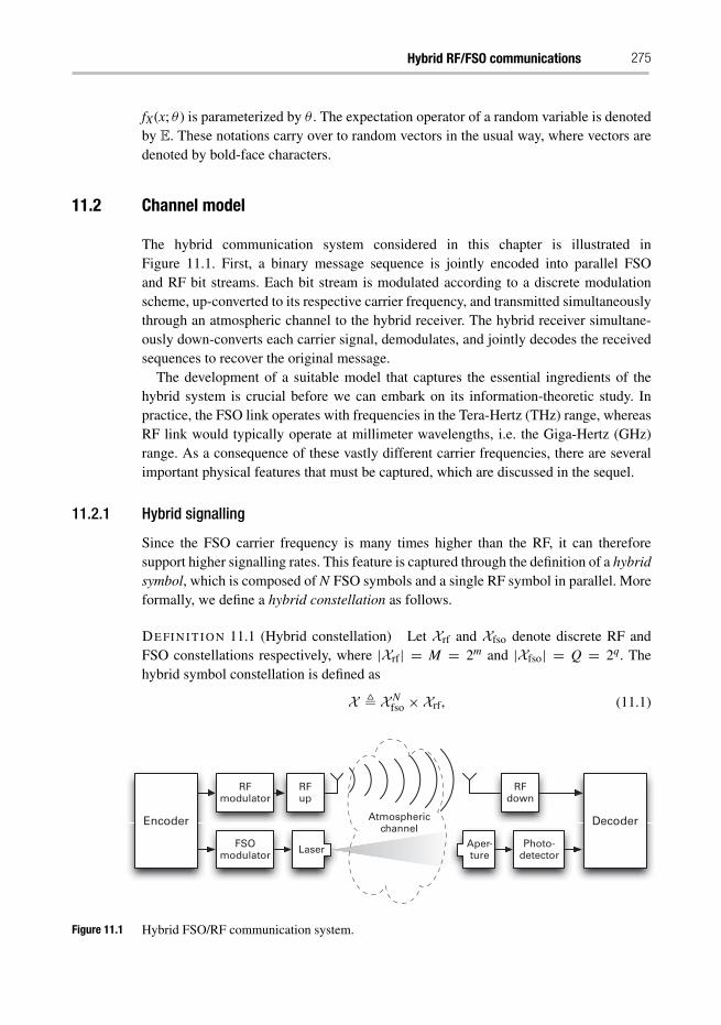
Hybrid RF/FSO communications 275
fX(x; θ ) is parameterized by θ . The expectation operator of a random variable is denotedby E. These notations carry over to random vectors in the usual way, where vectors aredenoted by bold-face characters.
11.2 Channel model
The hybrid communication system considered in this chapter is illustrated inFigure 11.1. First, a binary message sequence is jointly encoded into parallel FSOand RF bit streams. Each bit stream is modulated according to a discrete modulationscheme, up-converted to its respective carrier frequency, and transmitted simultaneouslythrough an atmospheric channel to the hybrid receiver. The hybrid receiver simultane-ously down-converts each carrier signal, demodulates, and jointly decodes the receivedsequences to recover the original message.
The development of a suitable model that captures the essential ingredients of thehybrid system is crucial before we can embark on its information-theoretic study. Inpractice, the FSO link operates with frequencies in the Tera-Hertz (THz) range, whereasRF link would typically operate at millimeter wavelengths, i.e. the Giga-Hertz (GHz)range. As a consequence of these vastly different carrier frequencies, there are severalimportant physical features that must be captured, which are discussed in the sequel.
11.2.1 Hybrid signalling
Since the FSO carrier frequency is many times higher than the RF, it can thereforesupport higher signalling rates. This feature is captured through the definition of a hybridsymbol, which is composed of N FSO symbols and a single RF symbol in parallel. Moreformally, we define a hybrid constellation as follows.
DE FI N I T I O N 11.1 (Hybrid constellation) Let Xrf and Xfso denote discrete RF andFSO constellations respectively, where |Xrf| = M = 2m and |Xfso| = Q = 2q. Thehybrid symbol constellation is defined as
X � XNfso × Xrf, (11.1)
Encoder
FSOmodulator
RFmodulator
RFup
Laser
Atmosphericchannel
RFdown
Photo-detector
Decoder
Aper-ture
Figure 11.1 Hybrid FSO/RF communication system.
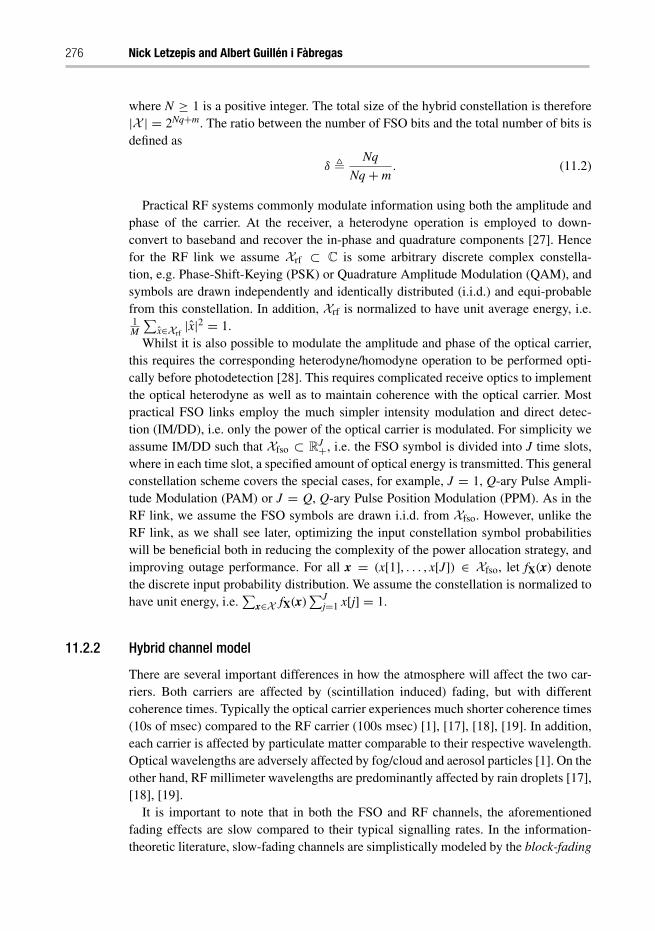
276 Nick Letzepis and Albert Guillén i Fàbregas
where N ≥ 1 is a positive integer. The total size of the hybrid constellation is therefore|X | = 2Nq+m. The ratio between the number of FSO bits and the total number of bits isdefined as
δ � Nq
Nq+ m. (11.2)
Practical RF systems commonly modulate information using both the amplitude andphase of the carrier. At the receiver, a heterodyne operation is employed to down-convert to baseband and recover the in-phase and quadrature components [27]. Hencefor the RF link we assume Xrf ⊂ C is some arbitrary discrete complex constella-tion, e.g. Phase-Shift-Keying (PSK) or Quadrature Amplitude Modulation (QAM), andsymbols are drawn independently and identically distributed (i.i.d.) and equi-probablefrom this constellation. In addition, Xrf is normalized to have unit average energy, i.e.1M
∑x∈Xrf
|x|2 = 1.Whilst it is also possible to modulate the amplitude and phase of the optical carrier,
this requires the corresponding heterodyne/homodyne operation to be performed opti-cally before photodetection [28]. This requires complicated receive optics to implementthe optical heterodyne as well as to maintain coherence with the optical carrier. Mostpractical FSO links employ the much simpler intensity modulation and direct detec-tion (IM/DD), i.e. only the power of the optical carrier is modulated. For simplicity weassume IM/DD such that Xfso ⊂ R
J+, i.e. the FSO symbol is divided into J time slots,where in each time slot, a specified amount of optical energy is transmitted. This generalconstellation scheme covers the special cases, for example, J = 1, Q-ary Pulse Ampli-tude Modulation (PAM) or J = Q, Q-ary Pulse Position Modulation (PPM). As in theRF link, we assume the FSO symbols are drawn i.i.d. from Xfso. However, unlike theRF link, as we shall see later, optimizing the input constellation symbol probabilitieswill be beneficial both in reducing the complexity of the power allocation strategy, andimproving outage performance. For all x = (x[1], . . . , x[J]) ∈ Xfso, let fX(x) denotethe discrete input probability distribution. We assume the constellation is normalized tohave unit energy, i.e.
∑x∈X fX(x)
∑Jj=1 x[j] = 1.
11.2.2 Hybrid channel model
There are several important differences in how the atmosphere will affect the two car-riers. Both carriers are affected by (scintillation induced) fading, but with differentcoherence times. Typically the optical carrier experiences much shorter coherence times(10s of msec) compared to the RF carrier (100s msec) [1], [17], [18], [19]. In addition,each carrier is affected by particulate matter comparable to their respective wavelength.Optical wavelengths are adversely affected by fog/cloud and aerosol particles [1]. On theother hand, RF millimeter wavelengths are predominantly affected by rain droplets [17],[18], [19].
It is important to note that in both the FSO and RF channels, the aforementionedfading effects are slow compared to their typical signalling rates. In the information-theoretic literature, slow-fading channels are simplistically modeled by the block-fading
Hybrid RF/FSO communications 277
K
FSO
RF
L
A
B21
21 43
Hybrid codeword
Figure 11.2 Hybrid codeword.
channel [29], [30]. In this setting, the transmitted codeword is divided into a finitenumber of blocks each consisting of an equal number of channel uses (or symbols). Thesymbols within a block experience the same fading realization, which is drawn i.i.d.from block to block. Given the slow-varying nature of scintillation, the block-fadingmodel is appropriate for both FSO and RF channels, i.e. we model the overall hybridchannel as a parallel block-fading channel. However, within this framework, we muststill model the difference in coherence time between the two channels. To capture thisimportant effect, as shown in Figure 11.2, we assume the FSO and RF components ofthe hybrid codeword experiences A and B i.i.d. fading realizations respectively. Typi-cally A ≥ B, since the fading on the FSO link is usually faster than that of the RF link.We assume the FSO component of K hybrid symbols are affected by the same FSOfading realization. Similarly the RF component of L hybrid symbols is affected by thesame RF fading realization. Note that since the total number of hybrid symbols mustbe consistent between the two channels, then we have the requirement AK = BL. Withthese assumptions, we write the parallel FSO and RF block-fading channels as follows.
For the FSO link, we write the received optical irradiance signal as
ra[k, n] = ρhapa
Nxa[k, n]+ λ, (11.3)
where: ra[k, n] = (ra[k, n, 1], . . . , ra[k, n, J]) ∈ RJ+ denotes a J vector representing the
received optical energy in each of the J time slots of FSO symbol n = 1, . . . , N of hybridsymbol k = 1, . . . , K in block a = 1, . . . , A; xa[k, n] = (xa[k, n, 1], . . . , xa[k, n, J])∈Xfso
denotes the nth transmitted FSO symbol vector of hybrid symbol k in block a; ρ modelslong-term fading effects; ha > 0 denotes the fading in block a due to scintillation,assumed to be drawn i.i.d. from some arbitrary density fH(h) with nonnegative support;pa denotes the power allocated to block a, and λ ≥ 0 models background irradia-tion/dark current (assumed to be constant). In (11.3) the 1/N factor ensures the FSOand RF components of the hybrid symbol have the same energy.
For the RF channel we similarly write the lth received symbol of block b as
yb[l] =√ρhbpbxb[l]+ σ zb[l], (11.4)
for l = 1, . . . , L and b = 1, . . . , B, where: xb[l] ∈ Xrf denotes the transmitted symbol; ρmodels long-term fading effects; hb > 0 denotes the scintillation of block b, drawn from
278 Nick Letzepis and Albert Guillén i Fàbregas
some arbitrary density fH(h) with nonnegative support; pb denotes the power allocated toblock b; zb[l] ∼ NC(0, 1) models zero mean, unit variance complex additive Gaussianwhite noise (AWGN); and σ 2 denotes the RF noise power. We assume ha and hb areindependent. Note that, as opposed to what happens in the RF channel, in the FSOchannel, the received signal scales with pa rather than
√pa.
The parameters 0 < ρ, ρ < 1 in (11.3) and (11.4) model differences in the relativestrengths of the two parallel channels, e.g. it reflects long-term fading effects due to rain,fog, or cloud as well as other parameters such as aperture/antenna gains and propagationloss. When ρ > ρ, the FSO channel is much stronger than the RF, e.g. modelling theeffects of severe rain attenuation. On the other hand, if ρ < ρ, then the RF channel isstronger than the FSO channel, e.g. modelling the effects of severe fog/cloud attenua-tion. Although in practice ρ and ρ are randomly varying with time (and are also mostlikely correlated random variables), we assume they remain unchanged over many code-word time intervals and therefore are fixed constants. Under this assumption, as we shallsee later, these parameters will not affect the asymptotic outage analysis that is to follow.
11.2.3 Channel state information and power adaptation
In wireless optical communications, efficient power adaptation not only extends the bat-tery lifetime in portable applications, but also reduces stress on the semiconductor laserdevice, extending its lifetime as well. However, in order to adapt the power, we firstrequire knowledge of the fading at the transmitter, commonly referred to as the channelstate information (CSI). Since the fading is slow, the CSI can be estimated at the receiverand conveyed to the transmitter via a feedback link.
In this chapter, we consider two channel state information (CSI) scenarios. First wewill assume only the receiver has perfect CSI and the transmitter allocates power uni-formly across all blocks (CSIR case). Then we will consider the case where perfect CSIis also known at the transmitter (CSIT case), i.e. the transmitter has perfect knowledge ofh1, . . . , hA and h1, . . . , hB. The transmitter then performs power allocation to reduce theoutage probability subject to power constraints. It is important to note that this assump-tion is impossible in practice, as the transmitter will only have access to past estimates ofthe fading (causal CSI), which may also contain imperfections due to estimation errorsat the receiver (imperfect CSI) [31], [32]. Nevertheless, the assumption of perfect CSIat the transmitter serves as an important performance benchmark for practical systems.
The transmit power for both channels is ultimately drawn from the same powerresource. As such, we assume the long-term average power consumed by the hybridsystem is constrained according to
E[〈p〉]+ E
[〈p〉] ≤ Pav, (11.5)
where 〈p〉 = 1A
∑Aa=1 pa and 〈p〉 = 1
B
∑Bb=1 pb. Practical communication systems have
limitations on the short-term power that can be transmitted. Since the FSO and RF linkswill realistically have different short-term (or peak) power limitations, we assume eachis subject to its own individual short-term power constraint, i.e.
Hybrid RF/FSO communications 279
〈p〉 ≤ αfsoPav and 〈p〉 ≤ αrfPav, (11.6)
where αfso and αrf denote the peak-to-average power ratios (PAPRs) for the FSO andRF channels respectively.
11.2.4 Photodetection models
The FSO channel model (11.3) only describes the received optical energy in each of the Jtime slots of an FSO symbol interval. In order to jointly decode the FSO and RF signals,the optical signal must be converted to an electrical one via photodetection. However, thephotodetection process itself introduces many additional noise effects uncommon in RFsystems. In the optical communications literature, a plethora of photodetection modelshave been considered, each dependent on certain photodetector device and channelmodel assumptions. For a detailed review and comparison of these models the inter-ested reader is referred to [28], [33], [34]. As we shall see later, whilst the photodetectionmodel may affect the power adaptation scheme, it does not affect the asymptotic slope ofthe outage probability curve (i.e. the outage exponent). However, for the sake of compar-ison, in the following we summarize some of the commonly employed photodetectionmodels that will be considered in this chapter.
In this section, for ease of exposition and brevity of notation, we drop indices a, k, nin (11.3) and consider non-fading FSO channels of the form
r = γ x+ λ, (11.7)
where r = (r[1], . . . , r[J]) and x = (x[1], . . . , x[J]) ∈ Xfso and γ denotes the transmittedoptical power. Conversion back to (11.3) is straightforward by letting γ = ρhapa/N andreplacing the appropriate indices a, k, n.
Given the received irradiance vector r, the photodetector converts it into an electricalsignal vector y = (y[1], . . . , y[J]). In this chapter, we will mostly be concerned withthe channel from the transmitted signal vector x to the photodetector output vector y. Inparticular, we consider channels for which the transition probability can be written as
fY|X(y|x; γ , λ) =J∏
j=1
fY|X(y[j]|x[j]; γ , λ). (11.8)
Note that we have made explicit the dependence of the channel transition probabilitieson the transmitted optical power γ and background irradiation λ. This will be usefullater on, when fading is introduced.
Under ideal photodetection, thermal noise is negligible and the photodetected electri-cal signal represents discrete photon counts. The photon count over a given time intervalis a Poisson random variable whose rate is proportional to the average irradiance overthe time interval [28]. Let y[j] denote the photodetector output induced by the receivedoptical energy r[j] as given by (11.7). For the ideal photodetection case, the conditionaldensity of y[j] is the discrete Poisson distribution given by
fY|X(y[j]|x[j]; γ , λ) = (γ x[j]+ λ)y[j]
y[j]! e−(γ x[j]+λ) (11.9)
280 Nick Letzepis and Albert Guillén i Fàbregas
for i = 1, . . . , Q. This is the well-known Poisson channel, used in a number of works onFSO communications (see e.g. [10], [7], [35]).
As the average irradiance increases due to increased background irradiation or highoptical signal power, these statistics can be well approximated by Gaussian statis-tics [36], [37]. In Appendix A we show that the Kullback–Leibler divergence [23]between the Poisson distribution and a Gaussian distribution with the same meanand variance approaches zero as the mean increases. This implies that, provided λ issufficiently large, y[j] ∼ N (γ x[j]+ λ, γ x[j]+ λ). Hence we may approximate (11.9) as
fY|X(y[j]|x[j]; γ , λ) ≈ 1√2π (γ x[j]+ λ)
exp
(− (y[j]− (γ x[j]+ λ))2
2(γ x[j]+ λ)
). (11.10)
In addition to background irradiation (and/or dark current), the photodetected signalwill also be corrupted by thermal noise. We assume this noise source is AWGN with zeromean and variance σ 2. Thus the overall received electrical signal will be the convolutionof (11.9) with the Gaussian thermal noise density. For large enough λ, where we mayuse the approximation (11.10), then we have
fY|X(y[j]|x[j]; γ , λ, σ 2) ≈ 1√2π(γ x[j]+ λ+ σ 2)
exp
(− (y[j]− (γ x[j]+ λ))2
2(γ x[j]+ λ+ σ 2)
).
(11.11)
It is important to note that (11.10) and (11.11) are signal-dependent Gaussian noisechannels, i.e. the noise variance is dependent on the value of x[j]. Moreover (11.11)implies we may write the photodetected channel model as
y[j] = γ x[j]+ λ+√γ x[j]+ λ+ σ 2z[j], (11.12)
where z[j] ∼ N (0, 1). In addition, we may ignore the constant background irradiationcontribution to the mean signal level, firstly because it can be removed straightfor-wardly by receiver electronics, and secondly it does not affect the input–output mutualinformation of the channel [23]. Hence we have
y[j] ≈ γ x[j]+√γ x[j]+ λ+ σ 2z[j]. (11.13)
When λ+ σ 2 � γ then the signal-dependent contribution to the noise variance can beconsidered negligible and we arrive at the signal-independent Gaussian noise model, i.e.
y[j] ≈ γ x[j]+√λ+ σ 2z[j]. (11.14)
Many works on FSO communications have employed the signal-independent photode-tection model, see e.g. [38], [39], [40], [41], [4], [42].
Comparing (11.13) and (11.14) with the received RF electrical signal model (11.4)we see an important difference: the received FSO photodetected signal is proportionalto the optical power, whereas the received RF signal is proportional to the square rootof the transmitted RF power. As we shall see later, this difference in power scaling willhave significant repercussions on the optimal power allocation strategy.
Hybrid RF/FSO communications 281
11.3 Information-theoretic preliminaries
11.3.1 Mutual information
Consider a particular transmitted hybrid codeword consisting of A and B FSO and RFblocks respectively, with vector power allocations p = (p1, . . . , pA) and p= (p1, . . . , pB).The FSO and RF components of the transmitted codeword experience vector chan-nel realizations h = (h1, . . . , hA) and h = (h1, . . . , hB), respectively. In the limitas K, L → ∞, the largest achievable rate supported by the hybrid channel is theinput–output mutual information [23]
Itot(p, p, h, h) = N
A
A∑a=1
IXfso (haρpa/N, λ, σ 2)+ 1
B
B∑b=1
IXrf (hbρpb, σ 2), (11.15)
in bits per hybrid channel symbol, where
IX (θ ) = E
[log2
fY|X(Y|X; θ )
fY(Y; θ )
](11.16)
denotes the input–output mutual information of the vector input channel with constella-tion X , parameterized by the vector θ . Note that the achievable rate (11.15) implicitlyassumes joint encoding and decoding across FSO and RF channels.
11.3.1.1 FSO channel mutual informationFor the FSO channel, as discussed in Section 11.2.4, the transition probabilitiesfY|X(Y|X; θ ) in (11.16) depend on the actual photodetection model. For the Poissonmodel (11.9), assuming the input vector symbols are drawn from Xfso using densityfX, we have
IPoissonXfso
(γ , λ) = −E
⎡⎣log2
⎛⎝ ∑
x′∈Xfso
fX(x′)e∑J
j=1 Yj log
(λ+γ x′jλ+γXj
)−γ (x′j−Xj)
⎞⎠⎤⎦ , (11.17)
where the expectation is over the dependent random vectors (X1, . . . , XJ) and(Y1, . . . , YJ). For the case when thermal noise and background irradiation are large, thesignal-independent noise model (11.14) is valid. Thus,
IawgnXfso
(γ 2
λ+ σ 2
)= −E
⎡⎣log2
⎛⎝ ∑
x′∈Xfso
fX(x′)e−∑J
j=1γ 2
λ+σ (Xj−x′j)2+2 γ√λ+σ2
(Xj−x′j)Zj
⎞⎠⎤⎦ ,
(11.18)
where Zj ∼ N (0, 1). Figure 11.3(a) compares the mutual information of the Poissonchannel (11.17) with that of the signal-independent Gaussian noise channel (11.18)(with σ 2 = 0, i.e. zero thermal noise) for on–off keying (OOK) with equi-probablesymbols. We see that both sets of curves have similar shape. The Gaussian approxima-tion tends to underestimate the mutual information at low powers and over-estimates forhigh powers.
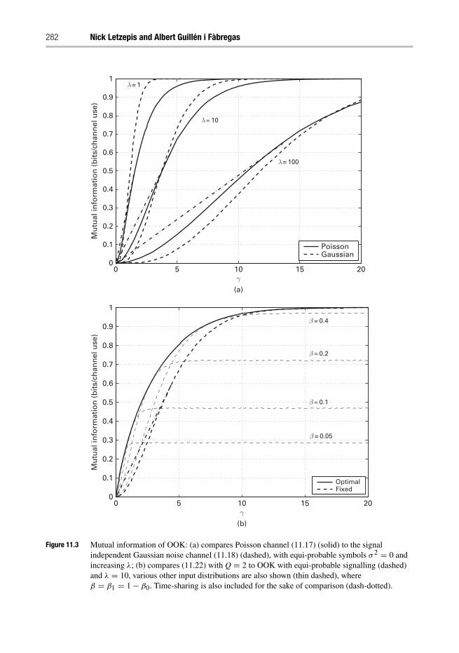
282 Nick Letzepis and Albert Guillén i Fàbregas
PoissonGaussian
OptimalFixed
0
0.1
0.2
0.3
0.4
0.5
0.6
0.7
0.8
0.9
1
0 5 10 15 200
0.1
0.2
0.3
0.4
0.5
0.6
0.7
0.8
0.9
1
γ
Mu
tual
info
rmat
ion
(b
its/
chan
nel
use
)M
utu
al in
form
atio
n (
bit
s/ch
ann
el u
se)
β = 0.4
λ = 100
λ = 1
λ = 10
β = 0.2
β = 0.1
β = 0.05
(b)
0 5 10 15 20γ
(a)
Figure 11.3 Mutual information of OOK: (a) compares Poisson channel (11.17) (solid) to the signalindependent Gaussian noise channel (11.18) (dashed), with equi-probable symbols σ 2 = 0 andincreasing λ; (b) compares (11.22) with Q = 2 to OOK with equi-probable signalling (dashed)and λ = 10, various other input distributions are also shown (thin dashed), whereβ = β1 = 1− β0. Time-sharing is also included for the sake of comparison (dash-dotted).
Hybrid RF/FSO communications 283
11.3.1.2 FSO channel, time-sharing mutual informationOn closer inspection of Figure 11.3(a) we see that both sets of curves are not concavewith γ . Moreover, we see that the curves are convex until a certain threshold power, atwhich point they become concave. This suggests equi-probable signalling is suboptimal,since, in the convex region, a higher achievable rate is possible via timesharing. Morespecifically, if the mutual information for equi-probable inputs is convex between 0 ≤γ < γts we can employ time-sharing between points (0, 0) and (γts, IXfso (γts, λ)), i.e.when γ < γts we transmit using a peak power of γts, but only for a fraction of γ /γts
of the block interval and zero power for the remaining 1 − γ /γts fraction. Hence theaverage power of the block is γ , and the resulting achievable rate is therefore given by
ItsXfso
(γ , λ) ={
IXfso (γts, λ) γγts
γ < γts
IXfso (γ , λ) otherwise.(11.19)
The threshold γts is the point at which the tangent to the curve IXfso (γ , λ) passes throughthe origin. Hence γts is the solution to
IXfso (γ , λ) = γφXfso (γ , λ), γ > 0, (11.20)
where
φX (γ , λ) � ∂
∂γIXfso (γ , λ) (11.21)
is the derivative of the mutual information with respect to γ .1 Note that γts is depen-dent on Xfso and the background irradiation λ. Threshold values for some examplemodulation schemes are listed in Table 11.1.
Figure 11.3(a) also compares with the resulting time-sharing scheme (dash-dottedline) using the parameters from Table 11.1. As we observe, some improvement ispossible, especially for low γ .
For signal-independent Gaussian channels, φX (γ , λ) is the minimum mean-squarederror (MMSE) [43]. Whereas for Poisson channels it is a certain function of theMMSE [44], and we provide further details for its computation in Appendix B.
11.3.1.3 FSO channel, optimal PAM mutual informationWhilst time-sharing obtains a higher achievable rate than fixed equi-probable signalling,the periods of zero power transmission represent an inefficient use of the block interval.
Table 11.1 Time-sharing thresholds for the Poisson channel,[γts, IXfso
(γts, λ)], where γts is measured in Decibels.
λ (dB) OOK 2PPM 4PPM
0 [1.80,0.49] [3.16,0.52] [3.76,1.09]10 [6.50,0.60] [6.18,0.62] [8.48,1.29]20 [11.33,0.65] [12.80,0.66] [13.38,1.38]
1 Note that if IXfso(γ , λ) is concave, the only solution to (11.20) is γ = 0
284 Nick Letzepis and Albert Guillén i Fàbregas
Time-sharing is in fact a naive way of changing the input distribution from the channel’sperspective.2 For example, if equi-probable OOK is employed, in the time-sharing inter-val, γ < γts, from the channel’s perspective the probability of a pulse being input to thechannel is reduced from 1
2 to γ2γts
. It turns out we can obtain an even higher achiev-able rate by optimizing the input distribution. In particular, for a fixed number of PAMmass points, we find the mass point locations and their probabilities that maximizes themutual information subject to an average (block) power constraint, i.e. for Q-ary PAM,let μ0, . . . ,μQ−1 and β0, . . . ,βQ−1 denote the mass point locations and their associatedprobabilities, then
IoptXPAM
(γ , λ) =
⎧⎪⎪⎪⎪⎨⎪⎪⎪⎪⎩
Maximize: IXPAM(μ, β, λ)
Subject to:∑Q−1
q=0 μqβq ≤ γ∑Q−1q=0 μq = 1
0 ≤ βq ≤ 1, q = 0, . . . , Q− 1,
(11.22)
where, e.g. for the Poisson channel,
IXPAM(μ, β, λ) = −Q−1∑q=0
βq log2 βq
−Q−1∑q=0
βqEY|X=μq
⎡⎣log2
⎛⎝1+
∑j �=q
βj
βq
(λ+ μj
λ+ μq
)Y
e−(μj−μq)
⎞⎠⎤⎦ .
(11.23)
Note that a peak power constraint may also be considered in (11.22). Indeed, forbandwidth constrained Poisson channels with average and peak power constraints,the capacity-achieving input distribution is proven to be discrete, i.e. a PAM schemewhereby the mutual information is maximized over the mass point locations and theirassociated probabilities [45]. When there is no peak power constraint, the optimal inputdistribution has only been conjectured to be discrete [45]. For high photon counts it hasbeen shown to be approximately exponential [46].
The solid line in Figure 11.3(b) shows the mutual information IoptXOOK
(γ , λ) in compar-ison to equi-probable OOK as shown by the dot-dashed curve. From this figure, we seeoptimizing over the input distribution not only results in a larger acheivable rate (for thesame average power), but it also results in a concave mutual information curve. As weobserve, optimizing the input distribution yields significant gains also when comparedto time-sharing.
11.3.1.4 RF channel mutual informationFor the RF channel (11.4) with power γ and noise variance σ 2, the mutual informationis [47]
2 That is, picking a symbol interval from the entire block uniformly at random.
Hybrid RF/FSO communications 285
IawgnXrf
(γ
σ 2
)= −E
⎡⎣log2
⎛⎝ ∑
x′∈Xrf
fX(x′)e−γ
σ2 |X−x′|2−2√
γ
σ2 &{(X−x′)Z∗}⎞⎠⎤⎦ , (11.24)
where the expectation is over the independent random variables X and Z ∼ NC(0, 1).From (11.18) and (11.24) we see that for signal-independent Gaussian channels, themutual information need only be parameterized by a certain ratio of the various channelparameters. For the RF channel it is the signal-to-noise ratio (SNR), i.e. γ
σ 2 . However, it
is important to note that for the FSO case, as a consequence of (11.14), γ 2
λ+σ 2 is not theSNR, since it is proportional to the optical power squared.
11.3.2 Outage probability
Suppose the hybrid system is required to operate at a target rate of R bits per hybridchannel symbol. Since A and B are finite, and Itot is a function of h, h, which are real-izations of the fading random variables, then Itot is also a random variable.3 Moreover,there is a non-zero probability that Itot < R, i.e. the channel cannot support the desiredtarget rate. Such events are referred to as outages, and the probability that they occur,
Pout(Pav, R) � Pr{
Itot(p, p, h, h) < R}
, (11.25)
is called the outage probability. Note that we have written Pout as a function of theaverage power constraint Pav as well as the target rate total R. The information outageprobability lower bounds the codeword error probability of any coding scheme [29],[30] and has been shown to be the fundamental limit of block-fading channels [49].In particular, there exist coding schemes of sufficiently large block length whose errorprobability is arbitrarily close to the outage probability; conversely, the error probabilityof any sufficiently long code is lower-bounded by the outage probability. In order tosimplify the expressions that will follow, we define the rate of the underlying binarycode as
Rc = R
Nq+ m. (11.26)
11.3.3 Outage exponent
Analytical computation of the outage probability (11.25) requires a closed-form expres-sion of the distribution of the instantaneous input–output mutual information (11.15).Such a task is intractable in general, and the usual approach is to numerically computethe outage probability via Monte Carlo simulations. Whilst this approach is simple toimplement, at low outage probability values, it requires lengthy simulations to countenough outage events for a reliable estimate. In addition, it reveals little insight as tohow various channel model and system design parameters affect the outage performance
3 The channel is therefore not information stable and the channel capacity in the strict Shannon sense iszero [48].
286 Nick Letzepis and Albert Guillén i Fàbregas
of the system. Towards this end, we study the outage exponent, which is substantiallysimpler to compute analyically. The outage exponent is defined as
d(k) � limPav→∞
− log Pout(Pav, R)
(log Pav)k, (11.27)
where k = 1, 2. In simple terms, the outage exponent describes the slope of the outageprobability curve (when plotted on a log-log scale) in the high power regime. The largerthe outage exponent, the faster the outage probability will decrease with increasingpower. Note that by including the integer k, (11.27) is more general than the outageexponent normally defined in RF systems [24], [25]. This modified definition is requiredto allow for scintillation cases where the resulting outage probability curve will not con-verge to a constant slope when plotted on a log-log scale, but does when plotted on alog-log2 scale (most notably under weak turbulence conditions where the scintillation islog-normal distributed [2]).
Clearly, the outage exponent will depend on the distribution of the fading coeffi-cients. Rather than assuming a specific distribution, we characterize the fading via thecomponent channel’s single block transmission outage exponent, defined as
d(i)fso � lim
γ→∞−log Pr{Ifso(hγ ) < Rfso}
(log γ )i(11.28)
d(j)rf � lim
γ→∞−log Pr{Irf(hγ ) < Rrf}
(log γ )j, (11.29)
for given component channel rate constraints 0 < Rfso < Nq and 0 < Rrf < m, wherei, j ∈ {1, 2}. We see that (11.28) and (11.29) imply
FH
(c
γ
).= e−d(i)
fso(log γ )i, FH
(c
γ
).= e−d(j)
rf (log γ )j, (11.30)
where c > 0 is some arbitrary constant (which in this case is the inverse of the mutualinformation function). In other words, (11.28) and (11.29) each define a family of scintil-lation distributions whose left-sided tail behaves like (11.30). In Table 11.2 we list somesingle block transmission outage exponents (derived in [2]) for some typical scintillationdistributions [1].4
Note that the exponents derived in [2] defined the outage exponent in terms ofthe received electrical SNR. In this chapter, we define the FSO exponent in terms ofthe transmitted optical power. This results in a factor of 2 in the exponents listed inTable 11.2 compared to those given in [2].
4 Note that if MIMO FSO with transmit repetition and equal gain combining is employed, then the exponentslisted in Table 11.2 are simply multiplied by NtNr , where Nt and Nr denote the number of lasers andapertures respectively [2].
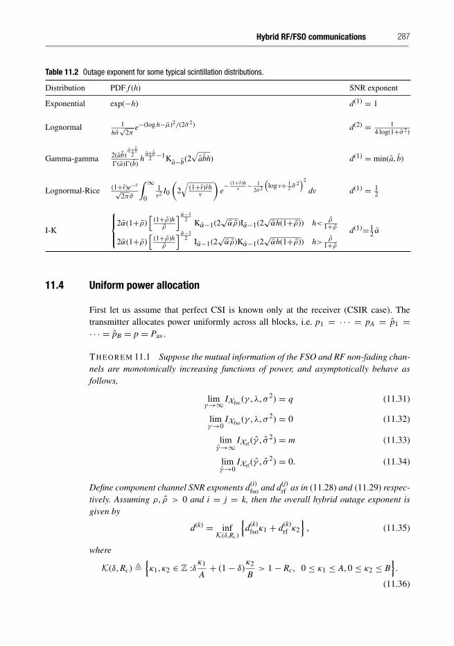
Hybrid RF/FSO communications 287
Table 11.2 Outage exponent for some typical scintillation distributions.
Distribution PDF f (h) SNR exponent
Exponential exp(−h) d(1) = 1
Lognormal 1hσ√
2πe−(log h−μ)2/(2σ 2) d(2) = 1
4 log(1+σ 2)
Gamma-gamma 2(ab)a+b
2
�(a)�(b)h
a+b2 −1Ka−b(2
√abh) d(1) = min(a, b)
Lognormal-Rice (1+r)e−r√2πσ
∫ ∞0
1v2 I0
(2√
(1+r)rhv
)e− (1+r)h
v − 12σ2
(log v+ 1
2 σ2)2
dv d(1) = 12
I-K
⎧⎪⎨⎪⎩
2α(1+ρ)[
(1+ρ)hρ
] α−12 Kα−1(2
√αρ)Iα−1(2
√αh(1+ρ)) h< ρ
1+ρ2α(1+ρ)
[(1+ρ)h
ρ
] α−12 Iα−1(2
√αρ)Kα−1(2
√αh(1+ρ)) h> ρ
1+ρd(1)= 1
2 α
11.4 Uniform power allocation
First let us assume that perfect CSI is known only at the receiver (CSIR case). Thetransmitter allocates power uniformly across all blocks, i.e. p1 = · · · = pA = p1 =· · · = pB = p = Pav.
TH E O R E M 11.1 Suppose the mutual information of the FSO and RF non-fading chan-nels are monotonically increasing functions of power, and asymptotically behave asfollows,
limγ→∞ IXfso (γ , λ, σ 2) = q (11.31)
limγ→0
IXfso (γ , λ, σ 2) = 0 (11.32)
limγ→∞
IXrf (γ , σ 2) = m (11.33)
limγ→0
IXrf (γ , σ 2) = 0. (11.34)
Define component channel SNR exponents d(i)fso and d(j)
rf as in (11.28) and (11.29) respec-tively. Assuming ρ, ρ > 0 and i = j = k, then the overall hybrid outage exponent isgiven by
d(k) = infK(δ,Rc)
{d(k)
fsoκ1 + d(k)rf κ2
}, (11.35)
where
K(δ, Rc) �{κ1, κ2 ∈ Z :δ
κ1
A+ (1− δ)
κ2
B> 1− Rc, 0 ≤ κ1 ≤ A, 0 ≤ κ2 ≤ B
}.
(11.36)
288 Nick Letzepis and Albert Guillén i Fàbregas
The generality of conditions (11.31) to (11.34) imply that the theorem is applicable toall of the photodetection models discussed in Section 11.2.4 and most practical discretemodulation schemes of interest. However, it should be noted that the time-sharing andoptimal PAM signalling strategies described in Section 11.3.1 cannot be applied as theyrequire knowledge of the CSI at the transmitter.
From Theorem 11.1, we see that the overall outage exponent depends on Rc, δ,A, B and the individual exponents d(k)
fso and d(k)rf in a non-trivial way. However, if
one considers (κ1, κ2, d(k)) as a three-dimensional space, we see that the overall out-age exponent is dominated by the end points (A(1 − Rc)/δ, 0, d(k)
fsoA(1 − Rc)/δ) and
(0, B(1−Rc)/(1− δ), d(k)rf B(1−Rc)/(1− δ)) of the line of intersection between the planes
defined by d(k) = κ1d(k)fso + κ2d(k)
rf and δ κ1A + (1− δ) κ2
B = 1− Rc. Thus we find, as a ruleof thumb, if
d(k)fso
d(k)rf
<B
A
δ
1− δ= B
A
Nq
m, (11.37)
then the scintillation on the FSO channel will dominate the overall hybrid exponent (andvice versa).
Although in general, the solution to (11.35) can be straightforwardly determinednumerically, it is difficult to obtain insight as to how the various system parameters influ-ence the overall SNR exponent. However, for the most basic and interesting scenario,A = B = 1, the solution to (11.35) reduces to a simple intuitive form.
CO RO L L A RY 11.1 Suppose A = B = 1. The solution to (11.35) is divided into twocases as follows.
(1) If δ ≤ 12 , then
d(k) =
⎧⎪⎪⎨⎪⎪⎩
d(k)fso + d(k)
rf 0 < Rc ≤ δ
d(k)rf δ < Rc ≤ 1− δ
min(d(k)fso, d(k)
rf ) 1− δ < Rc < 1.
(11.38)
(2) If δ ≥ 12 , then
d(k) =
⎧⎪⎪⎨⎪⎪⎩
d(k)fso + d(k)
rf 0 < Rc ≤ 1− δ
d(k)fso 1− δ < Rc ≤ δ
min(d(k)fso, d(k)
rf ) δ < Rc < 1.
(11.39)
From Corollary 11.1 we can see directly how the hybrid system parameters will affectthe asymptotic slope of the outage probability curve for the single block transmissioncase. In particular, we see that the asymptotic slope is affected by the SNR exponentof the individual component channels (which is in turn dependent on the scintillationdistribution), the size of the FSO/RF signal set constellation, and the overall binary coderate of the system. In most practical systems, δ ≥ 1
2 , i.e. in a hybrid symbol period,the number of transmitted FSO bits will be greater than the number of RF transmitted
Hybrid RF/FSO communications 289
bits. From (11.39), we see that the highest diversity is achieved if the binary code rateRc is set to be less than 1 − δ = m/(m + nq), i.e. the total information rate is less thanthe maximum information rate of the stand-alone RF channel. If 1 − δ < Rc ≤ δ, theexponent is the same as a single FSO link, i.e. the additional coding over an RF linkwill not improve the asymptotic slope of the outage probability curve. For high binarycode rates, δ < Rc < 1, the asymptotic performance is dominated by the worst ofthe two exponents. Note that code rates above δ are not achievable with a stand-aloneFSO link.
Although we have concentrated on the single block case, given the short coherencetime of the optical channel compared to the RF channel, the cases of A = 2, 3 and B = 1are also of practical interest and are readily evaluated from Theorem 11.1. In particular,these provide significant outage exponent improvements for lower rates, compared tothe single block case. This is illustrated in Figure 11.4, which plots the hybrid outageexponent with, d(k)
fso = 2, d(k)rf = 1 and δ = 0.8 for a: A = 1, B = 1 system (dash-dotted
line); A = 3, B = 1 system (solid line); and a stand-alone FSO link with three blocks,5
i.e. A = 3, B = 0 (dashed line). By coding over more FSO blocks, vast improvementsin the outage exponent can be seen, particularly as the code rate decreases. In addition,we see that the A = 3, B = 1 exponent exceeds that of the stand-alone FSO system byd(k)
rf for most code rates.
TH E O R E M 11.2 Define component channel outage exponents d(i)fso and d(j)
rf asin (11.28) and (11.29) respectively. Suppose i > j then the outage exponent is
d(i) = d(i)fso
(1+
⌊A
δ(δ − Rc)
⌋)0 < Rc ≤ δ (11.40)
d(j) = d(j)rf
(1+
⌊B
1− δ(1− Rc))
⌋)δ < R < 1. (11.41)
Otherwise, if i < j then the outage exponent is
d(j) = d(j)rf
(1+
⌊B
1− δ(1− δ − Rc)
⌋)0 < Rc ≤ 1− δ. (11.42)
d(i) = d(i)fso
(1+
⌊A
δ(1− Rc)
⌋)1− δ < Rc < 1 (11.43)
Theorem 11.2 shows how the overall performance of the hybrid channel will beaffected when one of the component channels has an asymptotic outage probability thatdecays with power much faster than the other. In particular, we see that the overall outageexponent will be dominated by the worst of the two component channel outage expo-nents unless the binary code rate is below a certain threshold dependent on the ratio ofFSO bits to total transmitted bits (δ). Note that the exponents in Theorems 11.1 and 11.2are related to how outage-approaching codes should be designed. In particular, they area form of the Singleton bound on the blockwise Hamming distance [49], [50], [51], [25].
5 Note that for the stand-alone FSO system with A blocks, the exponent is given by d(k) = d(k)fso(1+ �A(1−
Rc/δ)�) for 0 < Rc < δ, since we have defined Rc with respect to the hybrid system.
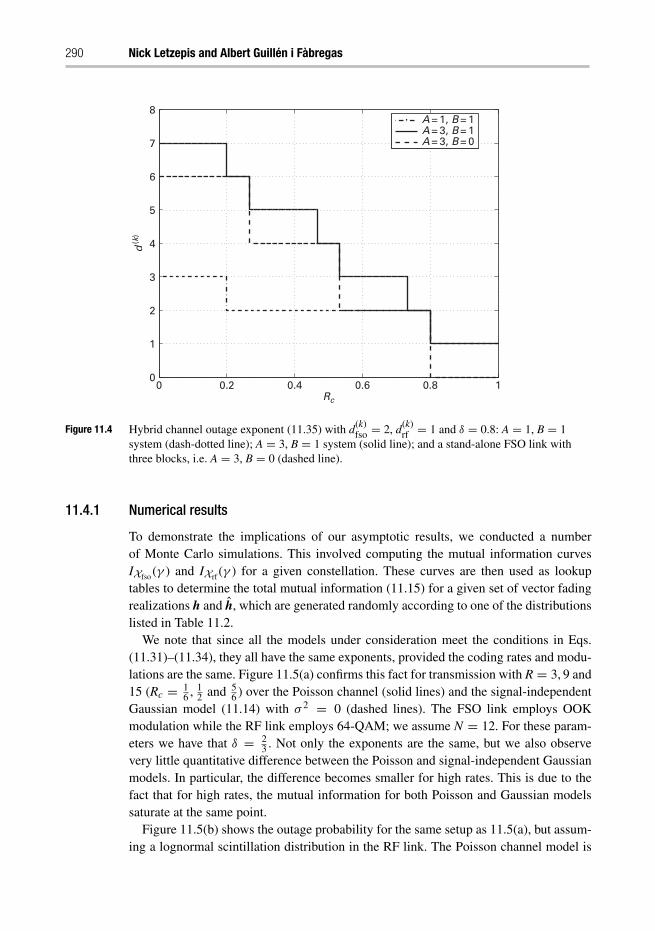
290 Nick Letzepis and Albert Guillén i Fàbregas
0 0.2 0.4 0.6 0.8 10
1
2
3
4
5
6
7
8
Rc
d (k
)
A = 1, B = 1A = 3, B = 1A = 3, B = 0
Figure 11.4 Hybrid channel outage exponent (11.35) with d(k)fso = 2, d(k)
rf = 1 and δ = 0.8: A = 1, B = 1system (dash-dotted line); A = 3, B = 1 system (solid line); and a stand-alone FSO link withthree blocks, i.e. A = 3, B = 0 (dashed line).
11.4.1 Numerical results
To demonstrate the implications of our asymptotic results, we conducted a numberof Monte Carlo simulations. This involved computing the mutual information curvesIXfso (γ ) and IXrf (γ ) for a given constellation. These curves are then used as lookuptables to determine the total mutual information (11.15) for a given set of vector fadingrealizations h and h, which are generated randomly according to one of the distributionslisted in Table 11.2.
We note that since all the models under consideration meet the conditions in Eqs.(11.31)–(11.34), they all have the same exponents, provided the coding rates and modu-lations are the same. Figure 11.5(a) confirms this fact for transmission with R = 3, 9 and15 (Rc = 1
6 , 12 and 5
6 ) over the Poisson channel (solid lines) and the signal-independentGaussian model (11.14) with σ 2 = 0 (dashed lines). The FSO link employs OOKmodulation while the RF link employs 64-QAM; we assume N = 12. For these param-eters we have that δ = 2
3 . Not only the exponents are the same, but we also observevery little quantitative difference between the Poisson and signal-independent Gaussianmodels. In particular, the difference becomes smaller for high rates. This is due to thefact that for high rates, the mutual information for both Poisson and Gaussian modelssaturate at the same point.
Figure 11.5(b) shows the outage probability for the same setup as 11.5(a), but assum-ing a lognormal scintillation distribution in the RF link. The Poisson channel model is
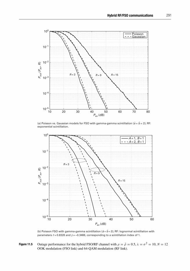
Hybrid RF/FSO communications 291
10 20 30 40 50 60 70 80
100
10–1
10–2
10–3
10–4
10–5
Pav (dB)
Po
ut (
Pav
, R )
PoissonGaussian
R = 15R = 9R = 3
(a) Poisson vs. Gaussian models for FSO with gamma-gamma scintillation (a = b = 2); RF:exponential scintillation.
¯¯
100
10–1
10–2
10–3
10–4
10–5
Pav (dB)
Po
ut (
Pav
, R )
10 20 30 40 50 60
A = 1, B = 1A = 2, B = 1
R = 3
R = 9
R = 15
(b) Poisson FSO with gamma-gamma scintillation (a = b = 2); RF: lognormal scintillation withparameters σ = 0.8326 and μ = −0.3466, corresponding to a scintillation index of 1.
¯ ¯¯¯
Figure 11.5 Outage performance for the hybrid FSO/RF channel with ρ = ρ = 0.5, λ = σ 2 = 10, N = 12OOK modulation (FSO link) and 64-QAM modulation (RF link).
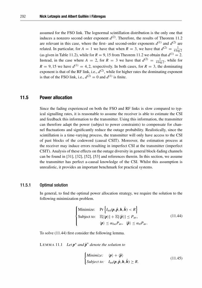
292 Nick Letzepis and Albert Guillén i Fàbregas
assumed for the FSO link. The lognormal scintillation distribution is the only one thatinduces a nonzero second order exponent d(2). Therefore, the results of Theorem 11.2are relevant in this case, where the first- and second-order exponents d(1) and d(2) arerelated. In particular, for A = 1 we have that when R = 3, we have that d(2) = 1
4 log 2
(as given in Table 11.2), while for R = 9, 15 from Theorem 11.2 we obtain that d(1) = 2.Instead, in the case where A = 2, for R = 3 we have that d(2) = 1
4 log 2 , while for
R = 9, 15 we have d(1) = 4, 2, respectively. In both cases, for R = 3, the dominatingexponent is that of the RF link, i.e., d(2), while for higher rates the dominating exponentis that of the FSO link, i.e., d(2) = 0 and d(1) is finite.
11.5 Power allocation
Since the fading experienced on both the FSO and RF links is slow compared to typ-ical signalling rates, it is reasonable to assume the receiver is able to estimate the CSIand feedback this information to the transmitter. Using this information, the transmittercan therefore adapt the power (subject to power constraints) to compensate for chan-nel fluctuations and significantly reduce the outage probability. Realistically, since thescintillation is a time-varying process, the transmitter will only have access to the CSIof past blocks of the codeword (causal CSIT). Moreover, the estimation process atthe receiver may induce errors resulting in imperfect CSI at the transmitter (imperfectCSIT). Analysis of these effects on the outage diversity in general block-fading channelscan be found in [31], [32], [52], [53] and references therein. In this section, we assumethe transmitter has perfect a-causal knowledge of the CSI. Whilst this assumption isunrealistic, it provides an important benchmark for practical systems.
11.5.1 Optimal solution
In general, to find the optimal power allocation strategy, we require the solution to thefollowing minimization problem.
⎧⎪⎪⎨⎪⎪⎩
Minimize: Pr{
Itot(p, p, h, h) < R}
Subject to: E[〈p〉]+ E[〈p〉] ≤ Pav,
〈p〉 ≤ αfsoPav, 〈p〉 ≤ αrfPav.
(11.44)
To solve (11.44) first consider the following lemma.
LE M M A 11.1 Let p∗ and p∗ denote the solution to
{Minimize: 〈p〉 + 〈p〉Subject to: Itot(p, p, h, h) ≥ R.
(11.45)
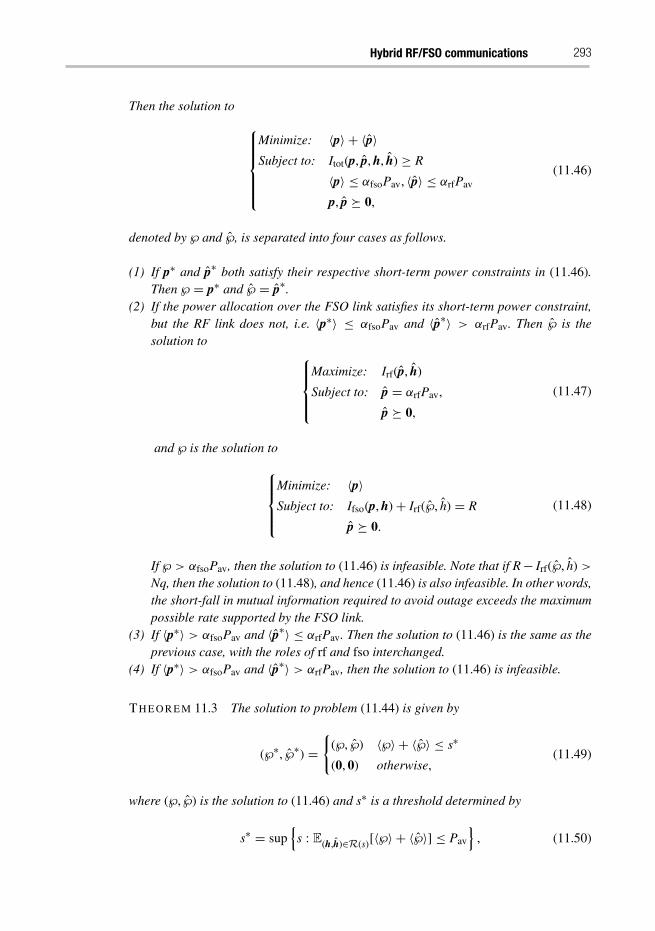
Hybrid RF/FSO communications 293
Then the solution to
⎧⎪⎪⎪⎪⎨⎪⎪⎪⎪⎩
Minimize: 〈p〉 + 〈p〉Subject to: Itot(p, p, h, h) ≥ R
〈p〉 ≤ αfsoPav, 〈p〉 ≤ αrfPav
p, p ' 0,
(11.46)
denoted by ℘ and ℘, is separated into four cases as follows.
(1) If p∗ and p∗ both satisfy their respective short-term power constraints in (11.46).Then ℘ = p∗ and ℘ = p∗.
(2) If the power allocation over the FSO link satisfies its short-term power constraint,but the RF link does not, i.e. 〈p∗〉 ≤ αfsoPav and 〈p∗〉 > αrfPav. Then ℘ is thesolution to ⎧⎪⎪⎨
⎪⎪⎩Maximize: Irf(p, h)
Subject to: p = αrfPav,
p ' 0,
(11.47)
and ℘ is the solution to
⎧⎪⎪⎨⎪⎪⎩
Minimize: 〈p〉Subject to: Ifso(p, h)+ Irf(℘, h) = R
p ' 0.
(11.48)
If ℘ > αfsoPav, then the solution to (11.46) is infeasible. Note that if R− Irf(℘, h) >Nq, then the solution to (11.48), and hence (11.46) is also infeasible. In other words,the short-fall in mutual information required to avoid outage exceeds the maximumpossible rate supported by the FSO link.
(3) If 〈p∗〉 > αfsoPav and 〈p∗〉 ≤ αrfPav. Then the solution to (11.46) is the same as theprevious case, with the roles of rf and fso interchanged.
(4) If 〈p∗〉 > αfsoPav and 〈p∗〉 > αrfPav, then the solution to (11.46) is infeasible.
TH E O R E M 11.3 The solution to problem (11.44) is given by
(℘∗, ℘∗) ={
(℘, ℘) 〈℘〉 + 〈℘〉 ≤ s∗
(0, 0) otherwise,(11.49)
where (℘, ℘) is the solution to (11.46) and s∗ is a threshold determined by
s∗ = sup{
s : E(h,h)∈R(s)[〈℘〉 + 〈℘〉] ≤ Pav
}, (11.50)
294 Nick Letzepis and Albert Guillén i Fàbregas
where
R(s) �{
(h, h) ∈ RA+B : 〈℘〉 + 〈℘〉 ≤ s
}. (11.51)
Proof The proof follows similar arguments to those described in [54], [55]. Essen-tially, (11.46) gives the minimum set of power allocations that satisfy the short-termpower constraints such that total mutual information is greater than the rate require-ment. The inclusion of threshold s∗ ensures that the long-term power constraint is alsosatisfied. The larger s∗ is, the smaller the outage probability will be. Since the solution(℘, ℘) from (11.46) gives the minimum sum power to satisfy the rate constraint, then thissolution also gives the maximum s∗, which in turn minimizes the outage probability.
We see that in general, the solution to (11.44) requires the solution to (11.46), whichwe have further decomposed into a number of smaller optimization sub-problems inLemma 11.1. Ultimately a tractable solution to the overall problem is only possible ifthese smaller sub-problems are convex. In this case, these sub-problems are solvablevia the Karush–Kahn–Tucker (KKT) conditions [56]. However, this is only possibleif and only if the input–output mutual information of each component channel is aconcave function of the input power. In this case, the KKT conditions yield a solu-tion that is expressed as a function of the derivative of the mutual information withrespect to the input power [57], [54], which is equal to the minimum mean-squarederror (MMSE) for the signal-independent Gaussian noise model [43]. Whilst this isthe case for the RF channel, as discussed in Section 11.3.1, the mutual information ofthe FSO channel is not concave in general. Moreover, to enforce concavity, we musteither employ time-sharing or optimize the FSO input distribution. Alternatively, wemay consider suboptimal power allocation. For example, in [26] a suboptimal schemewas proposed for the signal-independent Gaussian photodetection model (11.14) withan equi-probable signalling, by replacing the resulting non-convex problem (11.46) witha convex one. It was then proven that this suboptimal strategy still achieves the optimaloutage diversity. However, in this section, we only consider optimal power allocationand therefore assume either time-sharing or optimal PAM signalling is employed toensure a concave mutual information function.
11.5.2 Asymptotic Analysis
The asymptotic outage performance of optimal power allocation for discrete-inputblock-fading AWGN channels was analyzed by Nguyen et al. in [54], [58]. In partic-ular, from [54, Prop. 3], if the PAPRs αfso and αrf are finite, then the SNR exponentwill be the same as the CSIR case given in Theorems 11.1 and 11.2. When there areno PAPR constraints then the SNR exponent of the optimal power allocation strategyis [58, Th. 1]
d(1)csit =
⎧⎨⎩∞ d(1)
csir > 1d(1)
csir
1−d(1)csir
d(1)csir < 1,
(11.52)
where d(1)csir is the SNR exponent for the CSIR case.
Hybrid RF/FSO communications 295
The implications of (11.52) are described as follows. When d(1)csit = ∞, then the outage
probability curve will be vertical at a certain threshold of average power, i.e. the hybridsystem is able to maintain a constant level of instantaneous input–output mutual infor-mation. The threshold at which this occurs is referred to as the delay-limited capacityof the system [59]. Note that if d(1)
csir = 1 in (11.52) then d(1)csit = ∞, however, the outage
curve will not show a vertical behaviour, nor will it converge to a constant slope whenplotted on a log-log scale [54]. When the PAPRs are finite, the short-term power con-straints introduce an error floor with a slope equal to the CSIR case. The height of theerror floor is dependent on αfso and αrf [54].
11.5.3 Numerical results
To demonstrate the benefits of power allocation and its asymptotic behavior, we simu-lated the optimal power allocation strategies with OOK and gamma-gamma scintillationwith parameters a = b = 2 for the FSO link and 64-QAM and exponential scintil-lation for the RF link. In our simulations, we have chosen the following parametersρ = ρ = 0.5, A = B = 1 and N = 12.
Figure 11.6(a) shows the outage probability with and without power allocation, forseveral values of the peak-to-average power ratio α = αfso = αrf = 5, 10, 15, and20 dB and R = 9. Optimal OOK signalling is assumed for power allocation (solidlines) while equiprobable OOK is used for uniform power allocation (dashed line).Note also that, as predicted by Eq. (11.52), since d(1)
csir = 2, the outage curve withoutpeak power restrictions will show a vertical behavior. This can be seen in the figure(thick solid curve), for Pav > 24 dB outages are completely removed. Remark first theorder of magnitude of the gains. We see that there is a power saving of more than 20dB compared to uniform power allocation to achieve 10−5 outage probability. Whenpeak power constraints are introduced, as expected, we see that an error floor is intro-duced with the same slope as the CSIR case. The floor shifts down in probability as thepeak-to-average power ratio increases.
Figure 11.6(b) shows the outage probability for a fixed peak-to-average power ratioα = 15 dB and R = 3, 9, and 15. The figure compares uniform power allocation andoptimal power allocation for time-sharing OOK and optimal OOK. For R = 3, weobserve nearly 4 dB difference between the optimal scheme and time-sharing. Remarkthat this difference becomes smaller for higher rates, eventually disappearing. This isdue to the fact that the operating point is exactly in a region where the optimal mutualinformation and the time-sharing one are nearly the same.
11.6 Conclusions and summary
We proposed a simple hybrid FSO/RF channel model based on parallel block fadingchannels. This hybrid model takes into account differences in signalling rates and fadingeffects typically experienced by the component channels involved. Under this frame-work, we examined the information-theoretic limits of the hybrid channel. In particular,
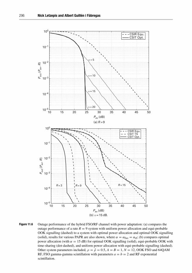
296 Nick Letzepis and Albert Guillén i Fàbregas
CSIR Equ.CSIT TSCSIT Opt.
(b) α = 15 dB.
100
10–1
10–2
10–3
10–4
10–5
Po
ut (
Pav
, R )
15 20 25 30 35 40 45 5010
Pav (dB)
R = 3 R = 9 R = 15
15 20 25 30 35 40 45 50
CSIR Equ.CSIT Opt.
(a) R = 9
100
10–1
10–2
10–3
10–4
10–5
Po
ut (
Pav
, R )
10
Pav (dB)
α = 15
α = 10
α = 5
α = 20
Figure 11.6 Outage performance of the hybrid FSO/RF channel with power adaptation: (a) compares theoutage performance of a rate R = 9 system with uniform power allocation and equi-probableOOK signalling (dashed) to a system with optimal power allocation and optimal OOK signalling(solid), results for various PAPR are also shown, where α = αfso = αrf; (b) compares optimalpower allocation (with α = 15 dB) for optimal OOK signalling (solid), equi-probable OOK withtime-sharing (dot-dashed), and uniform power allocation with equi-probable signalling (dashed).Other system parameters included, ρ = ρ = 0.5, A = B = 1, N = 12, OOK FSO and 64QAMRF, FSO gamma-gamma scintillation with parameters a = b = 2 and RF exponentialscintillation.
Hybrid RF/FSO communications 297
we studied the outage performance in the asymptotic high-power regime by analyz-ing the outage exponent. When CSI is only available at the receiver, in the generalcase, the exponent is not available in closed form. Instead, we derived simple expres-sions from which it can be computed numerically. These outage exponents are relatedto how optimal codes should be designed, and therefore are useful for practical codedesign. When CSI is also available at the transmitter, we derived the optimal powerallocation scheme that minimizes the outage probability subject to peak and averagepower constraints. Our results indicate that significant power savings (on the order oftens of dBs) are achievable using optimal power allocation compared to uniform powerallocation.
Appendix A Kullback–Leibler divergence between Poissonand Gaussian distributions
TH E O R E M 11.4 Let p(x) =∑∞k=0
&k
k! e−&δ(x− k) denote the continuous domain con-
version of the discrete Poisson distribution with mean &. Let q(x) = 1√2π&
e− 12& (x−&)2
be a Gaussian density with mean and variance &. Then
1
12&−1− 5
24&−2−O
(&−3
)≤ D (p||q) ≤ + 1
12&−1+ 33
24&−2+O
(&−3
)(11.53)
Proof The proof follows by first considering [23]
D(p||q) = −H(p)−∫ ∞
−∞p(x) log q(x) dx, (11.54)
where H(p) is the entropy of a Poisson random variable with mean &, which can bebounded as follows [60]
−33
24&−2 −O
(&−3
)≤ H(p)− 1
2log(2πe&)+ 1
12&−1 ≤ 5
24&−2 +O
(&−3
).
Using properties of the mean and variance of a Poisson random variable, it isstraightforward to show the cross-entropy term,
−∫ ∞
∞p(x) log q(x) dx =
∞∑k=0
&k
k! e−&[
1
2log 2π&− (k −&)2
2&
]= 1
2log(2πe&).
(11.55)
The proof of (11.53) then follows.
Appendix B Derivative of the mutual information for discrete-inputPoisson channels
TH E O R E M 11.5 ([44]) Let IX (γ , λ) denote the input–output mutual information ofthe discrete-input Poisson channel (11.7) in bits per channel use. Then
298 Nick Letzepis and Albert Guillén i Fàbregas
∂
∂γIX (γ , λ) =
J∑j=1
E
[xj log2
(γ xj + λ
E[γ xj + λ|y]
)], (11.56)
where E[γ xj + λ|y] is the conditional mean estimate.
LE M M A 11.2 The conditional mean estimate in (11.56) is given by
E[γ x+ λ|y] = ∑
x∈X(γ x+ λ)
⎛⎜⎜⎝1+
∑x′∈Xx′ �=x
Pr{x′}Pr{x}
J∏j=1
(1+ γ
λx′j
1+ γλ
xj
)yj
e−γ (x′j−xj)
⎞⎟⎟⎠−1
(11.57)
Proof
E[γ x+ λ|y] = ∑
x∈X(γ x+ λ)Pr{x|y} (11.58)
=∑x∈X
(γ x+ λ)Pr{y|x}Pr{x}∑
x′∈X Pr{y|x′}Pr{x′} (11.59)
=∑x∈X
γ x+ λ
1+∑x′∈Xx′ �=x
Pr{y|x′}Pr{x′}Pr{y|x}Pr{x}
(11.60)
=∑x∈X
(γ x+ λ)
⎛⎜⎜⎝1+
∑x′∈Xx′ �=x
Pr{x′}Pr{x}
Q∏i=1
(1+ γ
λx′j
1+ γλ
xj
)yj
e−γ (x′j−xj)
⎞⎟⎟⎠−1
(11.61)
TH E O R E M 11.6 For the special case of Q-ary PPM with equi-likely input symbols,
∂
∂γIXPPM(γ , λ) = log2 Q−IXPPM (γ , λ)−E log2
⎛⎝1+
Q∑q=2
(1+ γ
λ
)yq−y1−1
⎞⎠ . (11.62)
Proof From Lemma 11.2 we have
E[γ xi + λ|y] = Q∑
q=1
γ eq,i + λ∑Qj=1
(1+ γ
λ
)yj−yq(11.63)
=⎛⎝ Q∑
j=1
(1+ γ
λ
)yj−yi
⎞⎠−1 ⎛
⎝γ + λ
Q∑q=1
(1+ γ
λ
)yq−yi
⎞⎠ . (11.64)
Hybrid RF/FSO communications 299
Due to the symmetry of PPM, we need only consider x = e1 was transmitted. Hencecombining (11.64) and (11.56) we have
∂
∂γIXPPM(γ , λ) = E
[log2
(γ + λ
E[γ x1 + λ|y]
)]
= E log2
⎛⎝ Q∑
j=1
(1+ γ
λ
)yj−y1
⎞⎠− E log2
⎛⎝ γ
γ + λ+ λ
γ + λ
Q∑q=1
(1+ γ
λ
)yq−y1
⎞⎠
= log2 Q− IXPPM(γ , λ)− E log2
⎛⎝ γ
γ + λ+ λ
γ + λ
Q∑q=1
(1+ γ
λ
)yq−y1
⎞⎠
= log2 Q− IXPPM(γ , λ)+ log2
(1+ γ
λ
)− E log2
⎛⎝1+ γ
λ+
Q∑q=2
(1+ γ
λ
)yq−y1
⎞⎠
= log2 Q− IXPPM(γ , λ)− E log2
⎛⎝1+
Q∑q=2
(1+ γ
λ
)yq−y1−1
⎞⎠ . (11.65)
Acknowledgments
This work was supported by the Sir Ross and Sir Keith Smith Fund, Cisco Systems, theAustralian Research Council under RN0459498, DP0558861, DP088160, and the RoyalSociety under International Travel Grants 2009/R2 and 2009/R4.
References
[1] L. C. Andrews and R. L. Phillips, Laser Beam Propagation through Random Media, SPIEPress, 2nd edition, 2005.
[2] N. Letzepis and A. Guillén i Fàbregas, “Outage probability of the Gaussian MIMO free-space optical channel with PPM,” IEEE Trans. Commun., vol. 57, no. 12, pp. 3682–3690,Dec. 2009.
[3] N. Letzepis and A. Guillén i Fàbregas, “Outage probability of the free-space optical channelwith doubly stochastic scintillation,” IEEE Trans. Commun., vol. 57, no. 10, pp. 2899–2902,Oct. 2009.
[4] N. Letzepis, I. Holland, and W. Cowley, “The Gaussian free space optical MIMO channelwith Q-ary pulse position modulation,” IEEE Trans. Wireless Commun., vol. 7, no. 5, May2008.
[5] N. Cvijetic, S. G. Wilson, and M. Brandt-Pearce, “Performance bounds for free-space opticalMIMO systems with APD receivers in atmospheric turbulence,” IEEE J. Select. Areas.Commun., vol. 26, no. 3, pp. 3–12, April 2008.
300 Nick Letzepis and Albert Guillén i Fàbregas
[6] S. M. Navidpour, M. Uysal, and M. Kavehrad, “BER performance of free-space opti-cal transmission with spatial diversity,” IEEE Trans. Wireless Commun., vol. 6, no. 8,pp. 2813–2819, August 2007.
[7] S. G. Wilson, M. Brandt-Pearce, Q. Cao, and J. H. Leveque, “Free-space optical MIMOtransmission with Q-ary PPM,” IEEE Trans. Commun., vol. 53, no. 8, pp. 1402–1412,Aug. 2005.
[8] K. Chakraborty, “Capacity of the MIMO optical fading channel,” in Proc. IEEE Int. Symp.Inform. Theory, Adelaide, Sept. 2005, pp. 530–534.
[9] E. J. Lee and V. W. S. Chan, “Part 1: optical communication over the clear turbulent atmo-spheric channel using diversity,” J. Select. Areas Commun., vol. 22, no. 9, pp. 1896–1906,Nov. 2005.
[10] S. M. Haas and J. H. Shapiro, “Capacity of wireless optical communications,” IEEE J.Select. Areas Commun., vol. 21, no. 8, pp. 1346–1356, Oct. 2003.
[11] F. Nadeem, B. Flecker, E. Leitgeb, M. S. Awan, and T. Javornik, “Comparing the fog effectson hybrid network using optical wireless and GHz links,” in Proc. Int. Symp. Commun. Sys.,Networks and Digital Signal proc., Jun. 2008, pp. 278–282.
[12] H. Wu, B. Hamzeh, and M. Kavehrad, “Achieving carrier class availability of FSO link viacomplementary RF link,” in Proc. 38th Asilomar Conf. Signals, Systems and Computers,Oct. 2004.
[13] Z. Jia, F. Ao, and Q. Zhu, “BER performance of the hybrid FSO/RF attenuation system,” inInt. Symp. Anten., Prop. & EM Theory, Sep. 2006.
[14] T. Kamalakis, I. Neokosmidis, A. Tsipouras, S. Pantazis, and I. Andrikopolous, “Hybridfree space optical/millimeter wave outdoor links for broadband wireless access networks,”in Proc. Int. Symp. Personal, Indoor and Mobile Radio Commun., Aug. 2007.
[15] S. Vangala and H. Pishro-Nik, “A highly reliable FSO/RF communication system usingefficient codes,” in Proc. IEEE Global Commun. Conf., 2007.
[16] H. Wu, B. Hamzeh, and M. Kavehrad, “Availability of airbourne hybrid FSO/RF links,” inProc. SPIE, 2005, vol. 5819.
[17] T. Moulsley and E. Vilar, “Experimental and theoretical statistics of microwave amplitudescintillations on satellite down-links,” IEEE Trans. Anten. Propag., vol. 30, no. 6, pp. 1099–1106, Jan. 1982.
[18] C. E. Mayer, B. E. Jaeger, R. K. Crane, and X. Wang, “Ka-band scintillations: measurementsand model predictions,” Proc. IEEE, vol. 85, no. 6, pp. 936–945, Jun. 1997.
[19] M. S. Alouini, S. A. Borgsmiller, and P. G. Steffes, “Channel characterization and modelingfor Ka-band very small aperture terminals,” Proc. IEEE, vol. 85, no. 6, pp. 981–997, Jun.1997.
[20] S. A. Khan, A. N. Tawfik, and C. J. Gibbins, “Short-term amplitude scintillations at 97 GHzon 6.5 km urban link,” Electron. Lett., vol. 36, no. 19, pp. 1654–1656, Aug. 2000.
[21] S. A. Khan, A. N. Tawfik, B. C. Gremont, and C. J. Gibbins, “Long-term amplitude scintil-lations at 97 GHz on 6.5 km urban link,” Electron. Lett., vol. 36, no. 16, pp. 1425–1426, Jul.2000.
[22] I. B. Djordjevic, B. Vasic, and M. A. Neifeld, “Power efficient LDPC-coded modulation forfree-space optical communication over the atmospheric turbulence channel,” in Proc. Conf.Optical Fiber Commun. and Nat. Fiber Optic Engineers Conf., Feb. 2007.
[23] T. M. Cover and J. A. Thomas, Elements of Information Theory, Wiley Series inTelecommunications, 1991.
[24] L. Zheng and D. Tse, “Diversity and multiplexing: A fundamental tradeoff in multipleantenna channels,” IEEE Trans. Inf. Theory, vol. 49, no. 5, May 2003.
Hybrid RF/FSO communications 301
[25] A. Guillén i Fàbregas and G. Caire, “Coded modulation in the block-fading channel: Codingtheorems and code construction,” IEEE Trans. Inf. Theory, vol. 52, no. 1, pp. 262–271,Jan. 2006.
[26] N. Letzepis, K. D. Nguyen, A. Guillén i Fàbregas, and W. G. Cowley, “Outage analysis ofthe hybrid free-space optical and radio-frequency channel,” IEEE J. Select. Areas Com-mun. (special issue on optical wireless communications), vol. 27, no. 9, pp. 1709–1719,Dec. 2009.
[27] J. Proakis, Digital Communications, McGraw-Hill, 1995.[28] R. M. Gagliardi and S. Karp, Optical communications, John Wiley & Sons, Inc., 1995.[29] L. H. Ozarow, S. Shamai, and A. D. Wyner, “Information theoretic considerations for
cellular mobile radio,” IEEE Trans. Veh. Technol., vol. 43, no. 2, pp. 359–378, May 1994.[30] E. Biglieri, J. Proakis, and S. Shamai, “Fading channels: information-theoretic and
communications aspects,” IEEE Trans. Inf. Theory, vol. 44, no. 6, pp. 2619–2692,Oct. 1998.
[31] A. T. Asyhari and A. Guillén i Fàbregas, “Nearest neighbour decoding in block-fadingchannels with imperfect CSIR,” in IEEE Inf. Theory Workshop, Taormina, Italy, 2009.
[32] K. D. Nguyen, N. Letzepis, A. Guillén i Fàbregas, and L. K. Rasmussen, “Outage diversityof MIMO block-fading channels with causal channel state information,” in IEEE Int. Symp.Inf. Theory, Austin, TX, USA, 2010.
[33] S. Dolinar, D. Divsalar, J. Hamkins, and F. Pollara, “Capacity of pulse-position modulation(PPM) on Gaussian and Webb channels,” JPL TMO Progress Report 42-142, Aug. 2000,URL: lasers.jpl.nasa.gov/PAPERS/OSA/142h.pdf.
[34] S. J. Dolinar, J. Hamkins, B. E. Moision, and V. A. Vilnrotter, Optical Modulation andCoding, chapter 4, John Wiley & Sons, Inc., 2006.
[35] K. Chakraborty, S. Dey, and M. Franceschetti, “Outage capacity of MIMO Poisson fadingchannels,” IEEE Trans. Inf. Theory, vol. 54, no. 11, pp. 4887–4907, Nov. 2008.
[36] E. J. Gumbel, “The limiting form of Poisson’s distribution,” Phys. Rev., vol. 60, p. 689,1941.
[37] E. Rodgers, “Probable error for Poisson distributions,” Phys. Rev., no. 57, pp. 735–737,April 1940.
[38] X. Zhu and J. M. Kahn, “Free-space optical communication through atmospheric turbulencechannels,” IEEE Trans. Commun., vol. 50, no. 8, pp. 1293–1300, Aug. 2002.
[39] X. Zhu and J. M. Kahn, “Mitigation of turbulence-induced scintillation noise in free-spaceoptical links using temporal-domain detection techniques,” IEEE Photon. Tech. Let., vol.15, no. 4, pp. 623–625, April 2003.
[40] M. Uysal, J. Li, and M. Yu, “Error rate performance analysis of coded free-space opti-cal links over gamma-gamma atmospheric turbulence channels,” IEEE Trans. WirelessCommun., vol. 5, no. 6, pp. 1229–1233, June 2006.
[41] H. G. Sandalidis and T. A. Tsiftsis, “Outage probability and ergodic capacity of free-space optical links over strong turbulence,” IET Electron. Lett., vol. 44, no. 1, pp. 46–47,Jan. 2008.
[42] B. He and R. Schober, “Bit-interleaved coded modulation for hybrid RF/FSO systems,”IEEE Trans. Commun., vol. 57, no. 12, pp. 3753–3763, Dec. 2009.
[43] D. Guo, S. Shamai, and S. Verdú, “Mutual information and minimum mean-square error inGaussian channels,” IEEE Trans. Inf. Theory, vol. 51, no. 4, pp. 1261–1282, Apr. 2005.
[44] D. Guo, S. Shamai, and S. Verdú, “Mutual information and conditional mean estimation inPoisson channels,” IEEE Trans. Inf. Theory, vol. 54, no. 5, pp. 1837–1849, May 2008.
302 Nick Letzepis and Albert Guillén i Fàbregas
[45] S. Shamai, “Capacity of a pulse amplitude modulated direct detection photon channel,” IEEProc., vol. 137, no. 6, pp. 424–430, 1990.
[46] J. P. Gordon, “Quantum effects in communication systems,” Proc. IRE, vol. 50, pp. 1898–1908, 1962.
[47] G. Ungerboeck, “Channel coding with multilevel signals,” IEEE Trans. Inf. Theory, vol. 28,Jan. 1988.
[48] S. Verdú and T. S. Han, “A general formula for channel capacity,” IEEE Trans. Inf. Theory,vol. 40, no. 4, pp. 1147–1157, Jul. 1994.
[49] E. Malkamaki and H. Leib, “Coded diversity on block-fading channels,” IEEE Trans. Inf.Theory, vol. 45, no. 2, pp. 771–781, March 1999.
[50] R. Knopp and P. Humblet, “On coding for block fading channels,” IEEE Trans. Inf. Theory,vol. 46, no. 1, pp. 1643–1646, July 1999.
[51] E. Malkamaki and H. Leib, “Evaluating the performance of convolutional codes over blockfading channels,” IEEE Trans. Inf. Theory, vol. 45, no. 5, pp. 1643–1646, Jul. 1999.
[52] T. T. Kim and G. Caire, “Diversity gains of power control with noisy CSIT in MIMOchannels,” IEEE Trans. Inf. Theory, vol. 55, no. 4, pp. 1618–1626, Apr. 2009.
[53] T. T. Kim, K. D. Nguyen, and A. Guillén i Fàbregas, “Coded modulation with mismatchedcsit over mimo block-fading channels,” IEEE Trans. Inf. Theory, vol. 56, no. 11, Nov. 2010.
[54] K. D. Nguyen, A. Guillén i Fàbregas, and L. K. Rasmusen, “Power allocation for block-fading channels with arbitrary input constellations,” IEEE Trans. Wireless Commun., vol. 8,no. 5, pp. 2514–2523, May 2009.
[55] G. Caire, G. Taricco, and E. Biglieri, “Optimum power control over fading channels,” IEEETrans. Inf. Theory, vol. 45, no. 5, pp. 1468–1489, July 1999.
[56] S. Boyd and L. Vandenberghe, Convex Optimization, Cambridge University Press, 2004.[57] A. Lozano, A. M. Tulino, and S. Verdú, “Optimum power allocation for parallel Gaussian
channels with arbitrary input distributions,” IEEE Trans. Inf. Theory, vol. 52, no. 7, pp.3033–3051, July 2006.
[58] K. D. Nguyen, A. Guillén i Fàbregas, and L. K. Rasmussen, “Outage exponents of block-fading channels with power allocation,” IEEE Trans. Inf. Theory, vol. 56, no. 5, pp. 2373–2381, May 2010.
[59] S. V. Hanly and D. N. C. Tse, “Multiaccess fading channels. II. delay-limited capacities,”IEEE Trans. Inf. Theory, vol. 44, no. 7, pp. 2816–2831, Nov. 1998.
[60] J. A. Adell, A. Lekuona, and Y. Yu, “Sharp bounds on the entropy of the Poisson law andrelated quantities,” IEEE Trans. Inf. Theory, vol. 56, no. 5, pp. 2299–2306, May 2010.

Part IV
Applications

12 Quantum key distributionRupert Ursin, Nathan Langford and Andreas Poppe
12.1 Motivation
The ability to guarantee security and privacy in communication are critical factors inencouraging people to accept and trust new tools and methods for today’s information-based society (e.g. in eCommerce or eHealth) and for future services (e.g. eGovernment,eVoting). Cybercrime already hinders these new possibilities by creating widespreadmistrust in these new services. Another problem is that a (perhaps unpublicized) break-through in mathematics or computer science could completely compromise currentstate-of-the-art encryption methods overnight, even those which are the basis of all exist-ing internet banking transactions. This is because the security of cutting-edge public-keycryptography (conventional cryptography) relies on the computational difficulty of cer-tain mathematical tasks, meaning that conventional cryptography alone can neitherprovide any evidence of eavesdropping nor guarantee strong security. The trend towardsfaster electronics provides the ability to handle longer keys, thus providing better secu-rity, but also increases the possibility to break keys. This also has another worryingeffect: even using today’s most advanced available security technology to protect dataduring communication with best practice and without making any mistakes, the ongoingimprovements in technology (which hence require longer key lengths to ensure security)mean that today’s transmitted data will not be secure for more than a few years. Thus,while encrypted data might be safe today, it can still be stored by the adversary now andthen broken later on once the future technology has caught up with today’s encryption.
Alternatively, modern quantum cryptography has created a new paradigm for crypto-graphic communication, which provides strong, long-term security and incontrovertibleevidence of any attempted eavesdropping which is based on theoretically and experi-mentally proven laws of nature. This technique, called quantum key distribution (QKD),generates a symmetrical classical bit string using the correlations of measurementson quantum systems and has already developed into a mature technology providingcommercial products capable of everyday use [1–3]. The main hurdle for quantum com-munication is that, with present fiber and detector technologies, terrestrial QKD links arelimited to distances of just over 100 km, well within reach of how far someone couldtravel in a short time to simply deliver the information in person. In the future, however,
Advanced Optical Wireless Communication Systems, ed. Shlomi Arnon, John R. Barry, George K.Karagiannidis, Robert Schober, and Murat Uysal. Published by Cambridge University Press.c© Cambridge University Press 2012.
306 Rupert Ursin, Nathan Langford and Andreas Poppe
it will be possible to extend the distances spanned by individual fiber-based QKD linksby using repeater nodes. These individual QKD links could then be combined to createlarger and more complex QKD networks which will allow many different combina-tions of users to be connected over the same infrastructure, as has been shown at therecent SECOQC and UQCC demonstrations [4, 5]. The economic benefits of such aninterlinking network approach to QKD will be most apparent in a typical metropolitanscenario, where many potential users are likely to be located in a relatively small area,each wanting to be able to communicate securely with many different partners.
To further extend the distance for quantum communication, these metropolitan areaswould have to be connected and an interesting possibility for achieving this is to useoptical free-space links between (moving) high-altitude platforms (HAPs; a repeaternode located high above the turbulent atmosphere, keeping a roughly stationary posi-tion over a metropolitan area). Some QKD systems already make use of free-space links[6–9], and experiments have been performed outside the protected environment of thelaboratory, under real-world conditions over distances up to 144 km [10–12], the dis-tance limited mainly by the available terrestrial test locations. Alternatively, in urbanareas, HAPs could be used to distribute secret keys over distances potentially morethan 500 km, far exceeding the feasible distances for today’s fiber technology. Systemsusing moving platforms, however, would have to tackle additional challenges to terres-trial demonstrations. Ultimately, a satellite-based quantum communication terminal ina medium-earth orbit (MEO) would even be able to distribute single photons betweencontinents [13–18] and this is also being published in the framework of progress reportsof proposals [19–21]. The pointing acquisition and tracking of the optical links requiredfor such a scenario are a well-developed technology in regular use in satellite missionslike OISETS (Japan) or TerraSarX (Germany) and ARTEMIS (ESA).
Using a combination of terrestrial, HAP, and satellite-based point-to-point links,global quantum communication is a feasible target for current state-of-the-art tech-nology. Extending quantum communication and QKD to a global scale would have asubstantial impact on communication technology of the future. Moreover, the idea ofperforming QKD from air- or space-based platforms has a particular appeal to organiza-tions which require highest possible security to protect and authenticate communicationover global distances. Given the long-term security of messages transmitted using keysdistributed by QKD, a global QKD system will be highly marketable.
12.2 Security considerations of QKD
Quantum key distribution has an important advantage over its conventional counterpartof public-key cryptography, namely that its security is based on fundamental laws ofquantum physics (e.g., the no-cloning theorem and the superposition principle) [1–3].The output of the QKD protocol for both communicating parties is a symmetrical (iden-tical) classical key which generally takes the form of a random bit string. Both partiessubsequently use the same key to e.g. encrypt data to secure transmission over conven-tional communication lines. If this key is used only once (a one-time-pad protocol) the
Quantum key distribution 307
combined procedure of QKD and one-time-pad encryption is proven to be information-theoretically secure (ITS): that is, without knowledge of the key, a ciphertext wouldprovide no more information about the content of the plaintext than randomly guess-ing. In other words, from an encrypted message the adversary could extract neither themessage nor even a fraction of the key, even with unlimited computational power.
Conventional (asymmetrical) public-key exchange depends on unverifiable assump-tions that the computational complexity of the mathematical techniques involved willdeny an eavesdropper the ability to learn the contents of encrypted messages. QKD,however, is based on the fact that any attempt to intercept and read out the encoded quan-tum information will either damage or destroy it, decreasing the correlations observedby the communicating parties. As a result, such an eavesdropping attempt introduceserrors in the QKD protocol and can thus be detected. Indeed, if initially strong corre-lations decrease to the point where they can be explained by classical laws, then thecommunicating parties can assume that their communication has been compromised insome way. If, on the other hand, they still observe correlations beyond the reach of clas-sical physics, then the laws of physics guarantee that they can extract a secret key whichwill be completely secure from all possible eavesdroppers, even those who might hypo-thetically have access to unlimited computational power and resources, now and into thefar future – even future quantum computers!
Quantum cryptography needs to be compared with the two different types of conven-tional cryptography: secret-key (also called symmetric) cryptography and public-key(asymmetric) cryptography, both of which can operate over arbitrary distances (astriking advantage of conventional key distribution). Secret-key cryptography (e.g.,Advanced Encryption Standard (AES)) typically uses short keys (approved sizes byNIST: 128, 192, and 256 bits) to encrypt nearly arbitrarily large messages for high-speedcommunication on the fly and with basically no additional latency. From time to time,these secret keys are then changed. Public-key cryptography, on the other hand, pro-vides both a widely used means to generate the secret keys for symmetric cryptography(e.g. Diffie–Hellman key exchange protocol), and the means to generate public keys toencrypt/decrypt messages directly (e.g. RSA, named after authors Rivest, Shamir, andAdleman). Such asymmetric cryptography is not widely used since it requires muchmore computational power than the symmetric version. By contrast, QKD provides themeans to generate secret keys with generation rates over short distances from kbit/s upto the recently achieved record values of Mbit/s, but dropping with distance to only afew bit/s for a 100 km QKD link distance. QKD is the slow-but-ITS analogue to theDiffie–Hellman protocol.
The keys distributed by QKD can now be used together with well-established methodsfrom conventional cryptography. The highest security (albeit with low rates) is achievedby using QKD keys in combination with secret key one-time-pad encryption, which isitself ITS. However, an economical way of achieving the usual high data rates whilestill increasing practical security beyond the currently deployed crypto systems, is toprovide frequently changing seed keys for non-ITS secret-key encryption (e.g. AES)using QKD key generation. By doing this, the duration of the seed key’s validity, whichare typically maintained for months, years, or forever according to current practice, can
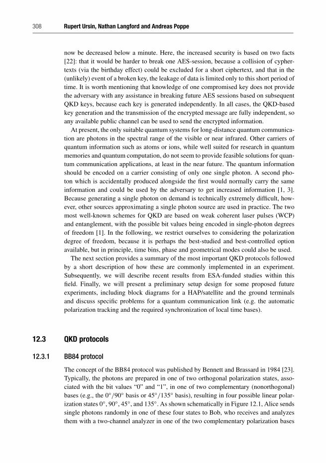
308 Rupert Ursin, Nathan Langford and Andreas Poppe
now be decreased below a minute. Here, the increased security is based on two facts[22]: that it would be harder to break one AES-session, because a collision of cypher-texts (via the birthday effect) could be excluded for a short ciphertext, and that in the(unlikely) event of a broken key, the leakage of data is limited only to this short period oftime. It is worth mentioning that knowledge of one compromised key does not providethe adversary with any assistance in breaking future AES sessions based on subsequentQKD keys, because each key is generated independently. In all cases, the QKD-basedkey generation and the transmission of the encrypted message are fully independent, soany available public channel can be used to send the encrypted information.
At present, the only suitable quantum systems for long-distance quantum communica-tion are photons in the spectral range of the visible or near infrared. Other carriers ofquantum information such as atoms or ions, while well suited for research in quantummemories and quantum computation, do not seem to provide feasible solutions for quan-tum communication applications, at least in the near future. The quantum informationshould be encoded on a carrier consisting of only one single photon. A second pho-ton which is accidentally produced alongside the first would normally carry the sameinformation and could be used by the adversary to get increased information [1, 3].Because generating a single photon on demand is technically extremely difficult, how-ever, other sources approximating a single photon source are used in practice. The twomost well-known schemes for QKD are based on weak coherent laser pulses (WCP)and entanglement, with the possible bit values being encoded in single-photon degreesof freedom [1]. In the following, we restrict ourselves to considering the polarizationdegree of freedom, because it is perhaps the best-studied and best-controlled optionavailable, but in principle, time bins, phase and geometrical modes could also be used.
The next section provides a summary of the most important QKD protocols followedby a short description of how these are commonly implemented in an experiment.Subsequently, we will describe recent results from ESA-funded studies within thisfield. Finally, we will present a preliminary setup design for some proposed futureexperiments, including block diagrams for a HAP/satellite and the ground terminalsand discuss specific problems for a quantum communication link (e.g. the automaticpolarization tracking and the required synchronization of local time bases).
12.3 QKD protocols
12.3.1 BB84 protocol
The concept of the BB84 protocol was published by Bennett and Brassard in 1984 [23].Typically, the photons are prepared in one of two orthogonal polarization states, asso-ciated with the bit values “0” and “1”, in one of two complementary (nonorthogonal)bases (e.g., the 0◦/90◦ basis or 45◦/135◦ basis), resulting in four possible linear polar-ization states 0◦, 90◦, 45◦, and 135◦. As shown schematically in Figure 12.1, Alice sendssingle photons randomly in one of these four states to Bob, who receives and analyzesthem with a two-channel analyzer in one of the two complementary polarization bases
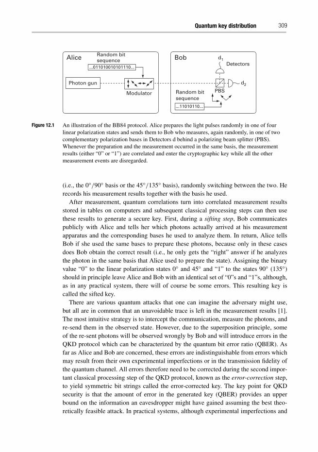
Quantum key distribution 309
Alice BobRandom bitsequence
Photon gun
Modulator PBSRandom bitsequence
...11010110...
...011010010101110...Detectors
d1
d2
Figure 12.1 An illustration of the BB84 protocol. Alice prepares the light pulses randomly in one of fourlinear polarization states and sends them to Bob who measures, again randomly, in one of twocomplementary polarization bases in Detectors d behind a polarizing beam splitter (PBS).Whenever the preparation and the measurement occurred in the same basis, the measurementresults (either “0” or “1”) are correlated and enter the cryptographic key while all the othermeasurement events are disregarded.
(i.e., the 0◦/90◦ basis or the 45◦/135◦ basis), randomly switching between the two. Herecords his measurement results together with the basis he used.
After measurement, quantum correlations turn into correlated measurement resultsstored in tables on computers and subsequent classical processing steps can then usethese results to generate a secure key. First, during a sifting step, Bob communicatespublicly with Alice and tells her which photons actually arrived at his measurementapparatus and the corresponding bases he used to analyze them. In return, Alice tellsBob if she used the same bases to prepare these photons, because only in these casesdoes Bob obtain the correct result (i.e., he only gets the “right” answer if he analyzesthe photon in the same basis that Alice used to prepare the state). Assigning the binaryvalue “0” to the linear polarization states 0◦ and 45◦ and “1” to the states 90◦ (135◦)should in principle leave Alice and Bob with an identical set of “0”s and “1”s, although,as in any practical system, there will of course be some errors. This resulting key iscalled the sifted key.
There are various quantum attacks that one can imagine the adversary might use,but all are in common that an unavoidable trace is left in the measurement results [1].The most intuitive strategy is to intercept the communication, measure the photons, andre-send them in the observed state. However, due to the superposition principle, someof the re-sent photons will be observed wrongly by Bob and will introduce errors in theQKD protocol which can be characterized by the quantum bit error ratio (QBER). Asfar as Alice and Bob are concerned, these errors are indistinguishable from errors whichmay result from their own experimental imperfections or in the transmission fidelity ofthe quantum channel. All errors therefore need to be corrected during the second impor-tant classical processing step of the QKD protocol, known as the error-correction step,to yield symmetric bit strings called the error-corrected key. The key point for QKDsecurity is that the amount of error in the generated key (QBER) provides an upperbound on the information an eavesdropper might have gained assuming the best theo-retically feasible attack. In practical systems, although experimental imperfections and
310 Rupert Ursin, Nathan Langford and Andreas Poppe
detector noise may also contribute to the QBER, it is important to assume that all errorsare caused by the adversary to maintain the strict security guarantees provided by thelaws of physics are not compromised by any additional assumptions about the exper-iment. The final classical data processing step is called privacy amplification, wherethe secure key is further refined (and reduced in size) to the extent that no informa-tion could have leaked away from that shared by the communicating parties. Assumingthat the QKD protocol is subjected to the best theoretically possible attacks, no securekey will be obtained from the privacy amplification step if the QBER exceeds a thresh-old of 11% – in such a situation, any resulting key could potentially be known to theadversary.
12.3.2 Decoy-state BB84 protocol
In practical realizations of the BB84 protocol, the photon source is usually not a (tech-nologically challenging) true single-photon source, e.g., based on quantum dots orvacancies in an optical crystal, but rather just an attenuated pulsed laser as commonlyused in telecom and laser industries [24, 25]. The pulses must therefore be attenuatedto a mean photon number smaller than one photon per pulse, but even then it is stillpossible that a pulse contains extra photons (due to the Poissonian statistics of the num-ber of photons in a given pulse) which would also be carrying the same externallyencoded quantum information (see Figure 12.1). Such multiphoton pulses enable aneavesdropper to mount a very powerful attack – the so-called photon number splittingattack (PNS attack) – where one of the extra photons in a multiphoton pulse is extractedand measured by the adversary [26].
An effective method to counteract this attack is to use decoy states – states of differ-ent mean photon numbers which are randomly sent in place of the actual signal states[27, 28]. The eavesdropper cannot distinguish between signal and decoy pulses and thuscannot act differently on them. After transmission, the measurement results are moni-tored by Alice and Bob to uncover the action of the adversary. Since the signal statesand the decoy states exhibit different photon-number statistics, any photon-number-dependent eavesdropping strategy (e.g., the PNS attack) will have different effects onthe signal and decoy states. Alice and Bob can now independently compute the trans-mission probability for signal and decoy states and detect, with high probability, anyphoton-number-dependent attack.
12.3.3 Entanglement-based BB84 protocol
The BB84 QKD schemes described above are both typical prepare-and-measureschemes, where Alice prepares one of several possible initial states and Bob selectsone of several possible measurement bases and gets a corresponding measurementresult. In the entanglement-based version of this protocol ([29] BBM92, illustrated inFigure 12.2), both Alice and Bob receive photons and carry out a similar measurementprocedure to Bob’s in the BB84-protocol. If the two photons are entangled, quantummeasurements in both 0◦/90◦ and 45◦/135◦ bases will then yield theoretically perfect
Quantum key distribution 311
DetectorsDetectors
EPR
Alice Source Bob
PBS PBSRandom bitsequence
Random bitsequence
12...00110101... ...11010110...
d1 d1
d2d2
Figure 12.2 A schematic of the entanglement based QKD protocol. A source generates entangled photonpairs, usually in the state |HH〉+|VV〉 (meaning the polarization of the photons emitted indifferent directions are known to be the same, but the individual state is unknown), which arethen sent to Alice and Bob. Both measure the incoming photons randomly in one of twocomplementary polarization bases in detectors d behind a polarizing beam splitter (PBS). Thecryptographic key consists of those results which are obtained from measurements in the samebasis. If the EPR source, which was first described by Einstein, Podolski, Rosen, emits a state|VH〉−|HV〉, as indicated in the figure, the ideal measurements are instead fully anticorrelatedand one receiver needs to invert the bits.
correlations whenever they choose the same measurement basis [30]. The source ofentangled photon pairs is located either as a third station in the middle [30] or perhaps,for practical reasons, at one of the two main stations [31].
Entangled photons have novel features not present in standard classical laser systems.One striking difference is that, individually, they have no well-specified polarization,but as soon as the first photon is measured, the behavior of the second photon dependson (is correlated to) the result of the measurement on the first photon. Clearly, non-entangled pairs of photons could be prepared in the four desired polarization states (e.g.,0◦0◦, 45◦45◦, 90◦90◦ or 135◦135◦), but if either photon is measured in the other basisfrom which it is not prepared (a choice made independently by Alice and Bob), themeasurement results would then be uncorrelated. Moreover, even if the source was itselfoperated by the adversary, no information of the quantum states, measurement resultsor key is left at the source in the hands of Eve, because this would be reflected in thequality of the observed quantum correlations.
Afterwards, the subsequent protocol steps are nearly identical with the BB84 protocol,the only difference being that the quantum correlations are between two measurementoutcomes rather than between a preparation and a measurement. Specifically, Alice andBob publicly communicate which photons they detected and the corresponding mea-surement bases, discarding events where only one photon is detected, as well as those inwhich the photons were both detected, but using different measurement bases. Becausea shared entangled state exhibits perfect polarization correlations, Alice’s and Bob’sresults should be perfectly correlated. Again, this key might contain errors from exper-imental imperfections or eavesdropping attacks, so an error correction protocol step isused to remove the differences and exactly specify the QBER. This error rate is impor-tant for the last processing step of privacy amplification, which cuts the length of thekey to the extent that the adversary loses all knowledge about the key.
312 Rupert Ursin, Nathan Langford and Andreas Poppe
12.4 Technical implementation of a free-space setup
This section describes the principal design issues for a free-space QKD apparatus (Sec-tion 12.4.1) and a specific design for a hybrid QKD link planned to be used in free-spaceexperiments to HAPs or even satellites (Section 12.4.2). The final Section (12.4.3)describes some results of the most recent free-space experiments.
12.4.1 Basic design considerations
There are two main possible ways to send photonic information over long distances –through optical fibers or free space. The different properties of these two media giverise to different design considerations when trying to implement QKD in the real world.Although we will focus primarily on the free-space implementation here, we will brieflytouch on some of these differences below. Some key practical issues for a practical QKDsystem are:
● Optimal transmission wavelength: Although photons are largely immune to mostforms of decoherence (e.g. the scrambling of polarization), they are quite suscepti-ble to loss, which can take many forms, such as absorption and scattering events.Effective loss can also be induced by effects such as mode distortion. For transmis-sion in optical fibers, the optimal wavelengths for minimizing absorption loss are inthe standard telecom band around 1550 nm (loss < 0.2 dB/km). In free space, on theother hand, transmission is more strongly affected by turbulence and scattering. How-ever, free-space communication is obviously vital for any possibility of satellite-basedcommunication.
● Single-photon detection: A detector capable of detecting the smallest possible bun-dle of light – a single photon – is a very sophisticated system made of the detectoritself and the electronics required to transfer the arrival of the photon to an electricalpulse (e.g. TTL, NIM) with a steep training edge carrying the timing information. Themost advanced single-photon detectors that can be used without specialist cryogenicequipment (an essential requirement for QKD applications) use avalanche photodi-odes (APDs) operated at voltages above breakdown and quenching electronics. Ofthese, the best currently available single-photon detectors are silicon APDs which aremainly sensitive to visible and very near-infrared wavelengths (typical efficiency of40–55%), with a design-dependent peak sensitivity for light from 550 nm to 680 nm(green to red for the human eye). Silicon APDs are therefore ideal for free-space com-munication in the red/near-infrared range, but absorption at these wavelengths in fiberis extremely high. For 1550 nm, Indium Gallium Arsenide (InGaAs) APDs providea feasible option for single-photon counting, but the operational parameters, such asquantum efficiency, dark-count rate and timing jitter are far worse than for SiliconAPDs.
● Signal tracking and beam capture: A laser pointing and tracking system is usedto set up and maintain a stable link between the terminals. To maintain the transmit-tance of the quantum channel using terminals moving relative to each other (or with
Quantum key distribution 313
changing atmospheric conditions between them), a closed-loop bi-directional corsageand fine pointing and tracking need to be implemented. To maximize this trans-mittance, the transmitter terminal should emit a diffraction-limited quantum signal.Likewise, for the receiver terminal, to limit the influence of stray light (causing anincreased QBER), the field of view (FOV) should be kept as small as possible. If weconsider as a worst case scenario, e.g., the movement in orbit of the ISS (orbit: 333× 348 km, inclination 51.6◦) relative to an optical ground station, the station willonly be visible (above a 10◦ elevation) for about 5 minutes. This implies a very fastrequired movement of the telescope of around 1 deg/s both in elevation and azimuth,while the static pointing and dynamic tracking accuracies need to be in the range ofup to ∼ ±1 arcsec. Several telescopes are available in Europe and other countries ingeodetic stations which have been designed to track GEO and also LEO satellites,with apertures of the order of 50 cm or larger. Besides these fixed optical ground sta-tions, transportable versions are also being developed in Germany (DLR) and Japan(NICT) for ad-hoc installations in the field and at various global locations.
● Polarization tracking and correction: In polarization-encoded quantum communi-cation using moving platforms, it is necessary to correct for any relative rotation ofthe polarization basis frame that the two terminals will experience as they move pasteach other. One conceivable solution might be to use a polarization-reference bea-con. Due to the extremely low power of the quantum signal channel, separate beaconlasers (well isolated from the signal wavelength) are required. A polarization analyzer(or polarimeter) could detect the state of polarization of the beacon laser and thisinformation could then be used in real time to compensate the polarization misalign-ment of the quantum channel. Alternatively, the polarization reference frame could beadjusted according to a precise computational prediction of the rotation angle fromaccurate knowledge of the platform’s trajectory and rotation.
12.4.2 Overall system design
After the review of critical design parameters mentioned above, we now explain themain quantum subunit of a basic system design – consisting of the sources and receiversrequired to obtain quantum correlations (see Figure 12.3). The source module compriseseither a weak laser source (Section 12.4.2.1) or an entangled photon source (12.4.2.2).The design of the optical antennas, beam pointing, acquisition and tracking does notdiffer from the design required from conventional optical communication techniquesand is not included here and can be found in other relevant chapters of this book. Somepropagation effects during transmission are revisited in Section 12.4.2.3 and the receiveris explained in Section 12.4.2.4. The timing synchronization to maintain a common timeframe is topic of Section 12.4.2.5.
As mentioned earlier, distributing provably secure keys for communication is possibleusing various techniques: namely, using weak coherent states (potentially with decoystates) or entanglement sources. In this section we give a brief overview on the possiblesource designs.
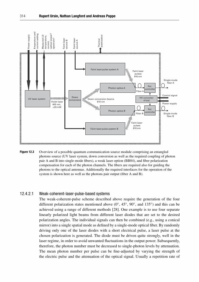
314 Rupert Ursin, Nathan Langford and Andreas Poppe
Pow
er s
up
ply
Em
per
atu
re a
nd
curr
ent
sett
ing
Mea
sure
d L
Dte
mp
erat
ure
,cu
rren
t,o
pti
cal p
ow
er?
spec
tru
m?
Fain
t la
ser
sou
rce
B
Fain
t la
ser
sou
rce
A
Th
erm
alst
abili
zati
on
Faint laserpulses810 nm
Single-modefiber A
Single-modefiber B
Fiber B
Fiber A
Pol.controller
HV converter4 fold
Pol.controllerPhoton optics A
Faint laser-pulse system A
Photon optics B
Faint laser-pulse system B
Down conversion beams810 nm
DownconversionUV laser system
Violet laser405 nm, >20 mW
Faint laserpulses810 nm
Control signal
Power supply
Figure 12.3 Overview of a possible quantum communication source module comprising an entangledphotons source (UV laser system, down conversion as well as the required coupling of photonpair A and B into single-mode fibers), a weak laser option (BB84), and fiber polarizationcompensation for each of the photon channels. The fibers are required also for guiding thephotons to the optical antennas. Additionally the required interfaces for the operation of thesystem is shown here as well as the photons pair output (fiber A and B).
12.4.2.1 Weak-coherent-laser-pulse-based systemsThe weak-coherent-pulse scheme described above require the generation of the fourdifferent polarization states mentioned above (0◦, 45◦, 90◦, and 135◦) and this can beachieved using a range of different methods [28]. One example is to use four separatelinearly polarized light beams from different laser diodes that are set to the desiredpolarization angles. The individual signals can then be combined (e.g., using a conicalmirror) into a single spatial mode as defined by a single-mode optical fiber. By randomlydriving only one of the laser diodes with a short electrical pulse, a laser pulse at thechosen polarization is generated. The diode must be driven quite strongly, well in thelaser regime, in order to avoid unwanted fluctuations in the output power. Subsequently,therefore, the photon number must be decreased to single-photon levels by attenuation.The mean photon number per pulse can be fine-adjusted by varying the strength ofthe electric pulse and the attenuation of the optical signal. Usually a repetition rate of
Quantum key distribution 315
singe-photon states of some MHz can be achieved, limited by the driving electronics ofthe laser diodes and the repetition rate of the detectors.
12.4.2.2 Entanglement-based systemsEntangled photon pairs are usually generated via spontaneous parametric down conver-sion (SPDC). An optical pump beam is incident on a birefringent crystal where nonlineareffects lead to the conversion of pump photons into pairs of correlated down-converted(i.e., lower-frequency) photons, usually called the signal and idler. Because of energyconservation, the sum of signal and idler energies equals the energy of a single pumpphoton, so the wavelengths of the down-converted photons are strongly anticorrelated.If the phase-matching conditions (momentum conservation) of the nonlinear crystal isfulfilled for the incident pump radiation and down-converted photons, constructive inter-ference over the full crystal length allows an emission of the down-converted photons.Depending on the type of nonlinear interaction in the crystal, the phase matching canbe designed to produce photon pairs with parallel polarization (type-I phase matching)or orthogonal polarization (type-II phase matching), allowing generation of quantumstates |VH〉−|HV〉 or |HH〉+|VV〉 for type-II or type-I, respectively. These two systemsare explained in more detail in the following.
One of the first schemes developed uses type-II SPDC in a BBO (β−BaB2O4: betabarium borate) crystal (a standard nonlinear optical crystal). An ultraviolet laser with apower of several mW is used to generate the signal and idler photons, which are emit-ted along separate cones that intersect along two straight lines [30, 31]. Photon pairsemitted along these lines are entangled in their polarization since it cannot be knownto which cone they belong without measuring their polarization. They can be describedby their quantum state |VH〉−|HV〉 as indicated in Figure 12.2. These photon pairs canbe collected with a single-mode optical fiber and used for entanglement-based QKDexperiments.
Another successful scheme for entangled-photon generation is the so-called polar-ization Sagnac interferometer [32]. This interferometric scheme uses a periodicallypoled (pp) type-I nonlinear crystal (e.g., ppKTP: periodically poled potassium titanylphosphate) and collinear quasi-phase matching to generate photon pairs with the samepolarization (|HH〉). The Sagnac loop is pumped in two directions and the |HH〉-polarized photon pairs in one direction are rotated to |VV〉. Combining both arms thengives the entangled quantum state |HH〉+|VV〉. Because of the high nonlinearity of suchperiodically poled crystals, the Sagnac source provides photon pair rates approximatelyten times higher than what is achievable with standard BBO-based sources. This iscritically important when a QKD experiment involves very high channel losses.
The entanglement based source is also included in Figure 12.3. The relative alignmentconstraints of the UV laser, the nonlinear crystal and the single mode fibers are severeand must be kept at high mechanical stability.
12.4.2.3 Polarization issues in the free-space channelSince in all of the QKD protocols described above the quantum state is encoded in thepolarization of a photon, relative rotations of the polarization reference frame cause bit
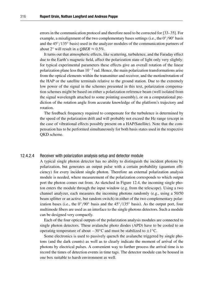
316 Rupert Ursin, Nathan Langford and Andreas Poppe
errors in the communication protocol and therefore need to be corrected for [33–35]. Forexample, a misalignment of the two complementary bases settings (i.e., the 0◦/90◦ basisand the 45◦/135◦ basis) used in the analyzer modules of the communication partners ofabout 2◦ will result in a QBER ≈ 0.5%.
It turns out that atmospheric effects, like scattering, turbulence, and the Faraday effectdue to the Earth’s magnetic field, affect the polarization state of light only very slightly:for typical experimental parameters these effects give an overall rotation of the linearpolarization plane less than 10−3 rad. Hence, the main polarization transformations arisefrom the optical elements within the transmitter and receiver, and the motion/rotation ofthe HAP or the satellite terminals relative to the ground station. Due to the extremelylow power of the signal in the schemes presented in this text, polarization compensa-tion schemes might be based on either a polarization reference beam (well isolated fromthe signal wavelength attached to some pointing assembly), or on a computational pre-diction of the rotation angle from accurate knowledge of the platform’s trajectory androtation.
The feedback frequency required to compensate for the turbulence is determined bythe speed of the polarization drift and will probably not exceed the Hz range (except inthe case of vibrational effects possibly present on a HAP/Satellite). Note that the com-pensation has to be performed simultaneously for both basis states used in the respectiveQKD scheme.
12.4.2.4 Receiver with polarization analysis setup and detector moduleA typical single photon detector has no ability to distinguish the incident photons bypolarization, but generates an output pulse with a certain probability (quantum effi-ciency) for every incident single photon. Therefore an external polarization analysismodule is needed, where measurement of the polarization corresponds to which outputport the photon comes out from. As sketched in Figure 12.4, the incoming single pho-ton enters the module through the input window (e.g. from the telescope). Using a twochannel analyzer, each measures the incoming photons randomly (e.g., using a 50/50beam splitter or an active, but random switch) in either of the two complementary polar-ization bases (i.e., the 0◦/90◦ basis and the 45◦/135◦ basis). As the output port, fourmultimode fibers are used as an interface to the single photons detectors. Such a modulecan be designed very compactly.
Each of the four optical outputs of the polarization analysis modules are connected tosingle photon detectors. These avalanche photo diodes (APD) have to be cooled to anoperating temperature of about −30◦C and must be stabilized to ±1◦C.
Some electronics is used to passively quench the avalanche triggered by single pho-tons (and the dark counts) as well as to clearly indicate the moment of arrival of thephotons by electrical pulses. A convenient way to further process the arrival time is torecord the times of detection events in time tags. The detector module can be housed inone box suitable to harsh environment as well.
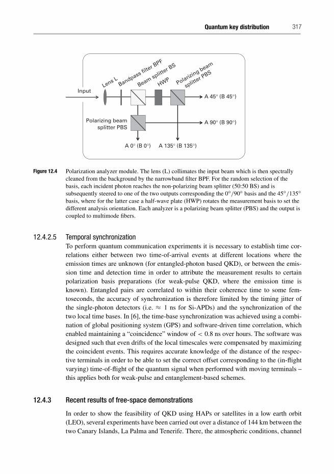
Quantum key distribution 317
Polarizing beamsplitter PBS
Polarizing beam
splitter P
BS
Lens LBandpass filt
er BPF
Beam splitter B
S
HWP
A 0° (B 0°)
A 90° (B 90°)
A 135° (B 135°)
A 45° (B 45°)Input
Figure 12.4 Polarization analyzer module. The lens (L) collimates the input beam which is then spectrallycleaned from the background by the narrowband filter BPF. For the random selection of thebasis, each incident photon reaches the non-polarizing beam splitter (50:50 BS) and issubsequently steered to one of the two outputs corresponding the 0◦/90◦ basis and the 45◦/135◦basis, where for the latter case a half-wave plate (HWP) rotates the measurement basis to set thedifferent analysis orientation. Each analyzer is a polarizing beam splitter (PBS) and the output iscoupled to multimode fibers.
12.4.2.5 Temporal synchronizationTo perform quantum communication experiments it is necessary to establish time cor-relations either between two time-of-arrival events at different locations where theemission times are unknown (for entangled-photon based QKD), or between the emis-sion time and detection time in order to attribute the measurement results to certainpolarization basis preparations (for weak-pulse QKD, where the emission time isknown). Entangled pairs are correlated to within their coherence time to some fem-toseconds, the accuracy of synchronization is therefore limited by the timing jitter ofthe single-photon detectors (i.e. ≈ 1 ns for Si-APDs) and the synchronization of thetwo local time bases. In [6], the time-base synchronization was achieved using a combi-nation of global positioning system (GPS) and software-driven time correlation, whichenabled maintaining a “coincidence” window of < 0.8 ns over hours. The software wasdesigned such that even drifts of the local timescales were compensated by maximizingthe coincident events. This requires accurate knowledge of the distance of the respec-tive terminals in order to be able to set the correct offset corresponding to the (in-flightvarying) time-of-flight of the quantum signal when performed with moving terminals –this applies both for weak-pulse and entanglement-based schemes.
12.4.3 Recent results of free-space demonstrations
In order to show the feasibility of QKD using HAPs or satellites in a low earth orbit(LEO), several experiments have been carried out over a distance of 144 km between thetwo Canary Islands, La Palma and Tenerife. There, the atmospheric conditions, channel
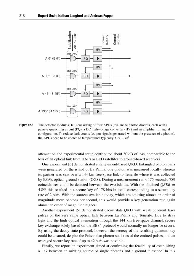
318 Rupert Ursin, Nathan Langford and Andreas Poppe
PQ
HVDet. APD
A 0° (B 0°)
PQ
HVDet. APD
A 90° (B 90°)
PQ
HVDet. APD
A 45° (B 45°)
PQ
HVDet. APD
A 135° (B 135°)
Det. APD
Det. APD
Det. APD
Det. APD
Sta
bili
zati
on
on
T =
–30
°
Pow
ersu
pp
ly
Co
ntr
ol
sig
nal
s
Figure 12.5 The detector module (Det.) consisting of four APDs (avalanche photon diodes), each with apassive quenching circuit (PQ), a DC high-voltage converter (HV) and an amplifier for signalconfiguration. To reduce dark counts (output signals generated without the presence of a photon),the APDs need to be cooled to temperatures typically T ≈ −30◦.
attenuation and experimental setup contributed about 30 dB of loss, comparable to theloss of an optical link from HAPs or LEO satellites to ground-based receivers.
One experiment [6] demonstrated entanglement-based QKD. Entangled photon pairswere generated on the island of La Palma, one photon was measured locally whereasits partner was sent over a 144 km free-space link to Tenerife where it was collectedby ESA’s optical ground station (OGS). During a measurement run of 75 seconds, 789coincidences could be detected between the two islands. With the obtained QBER =4.8% this resulted in a secure key of 178 bits in total, corresponding to a secure keyrate of 2 bit/s. With the sources available today, which are emitting almost an order ofmagnitude more photons per second, this would provide a key generation rate againalmost an order of magnitude higher.
Another experiment [5] demonstrated decoy state QKD with weak coherent laserpulses on the very same optical link between La Palma and Tenerife. Due to straylight and the high optical attenuation through the 144 km free-space channel, securekey exchange solely based on the BB84 protocol would normally no longer be secure.By using the decoy-state protocol, however, the secrecy of the resulting quantum keycould be ensured, despite the Poissonian photon statistics of the emitted pulses, and anaveraged secure key rate of up to 42 bit/s was possible.
Finally, we report an experiment aimed at confirming the feasibility of establishinga link between an orbiting source of single photons and a ground telescope. In this
Quantum key distribution 319
experiment, we simulated a quantum communication single-photon source on a satellite,and showed how the very dim signals could still be detected. Using a Japanese satellite(Ajisai) covered with retroflectors at about 1600 km of slant distance, we emulated thespace-based single-photon source by attenuating an outgoing pulsed laser such that onlyone single photon is reflected by the satellite back into the communication channel. Thisexperiment showed that it was possible to distinguish the received single photons fromthe background (mainly starlight in the FOV of the receiver) with sufficient SNR to beused for quantum communication protocols.
12.5 QKD networks
In Sections 12.1–12.3, we discussed only single point-to-point QKD links, where Aliceand Bob are connected by a quantum channel for single-photon signals and a classicalchannel for conventional communication: i.e., one particular Alice is always connectedto the same Bob. This is the concept used for almost all current QKD systems, bothcommercial, fiber-based systems and the experiments discussed in Section 12.4.3. Inthe following discussion, the names “Alice” and “Bob” refer to sender/receiver pairs foreach QKD link.
In the future, when one user wants to share information securely with a communica-tion partner, they will establish a connection via an intermediate QKD network. Uncon-ditional security over such a network will require special quantum repeater technology(currently under active development) [36], because standard optical amplification woulddestroy the fragile quantum correlations which provide both the communication mecha-nism and the security. Such quantum repeaters would enable a “truly quantum” network[37], allowing the distribution of genuine entanglement between far-separated com-munication partners, which they could then, for example, use to directly establish asecure communication key. Alternatively, even with existing technology, partners willbe able to share secret information over a network of individual QKD links combinedusing “trusted” repeater nodes [38, 39], where, as part of the information sharing pro-tocols (discussed in detail in Section 12.5.2 below), the secret information must beelectronically stored and protected inside the node. These nodes must be trusted byall users wishing to utilize the network. In the following we will focus on this scenarioof trusted-repeater networks.
The SECOQC QKD network has already demonstrated the possibility of combiningindependent point-to-point QKD links to form a trusted-repeater QKD network usingfiber-based QKD links [4]. Each QKD link has its own “Alice” and “Bob” and thesedevice pairs are never changed. The QKD devices at each node of the QKD network havebeen combined by node modules in that sense that the generated secure key is stored inkey stores. These key stores, which are independent of the underlying realization ofthe QKD links, are filled by secret keys distributed over each QKD link and used byapplications that request these keys.
In order to communicate beyond the limits of a local metropolitan network, however,users will need to establish a connection from the ground to a HAP or a satellite. Since
320 Rupert Ursin, Nathan Langford and Andreas Poppe
the partner will presumably not be on location there at the time, the flying object willserve as a trusted repeater. The underlying quantum architecture of HAPs and satellitesis different to fiber-based QKD networks, because one Alice on the flying object needsto communicate sequentially with many Bobs. If we assume there is only one Aliceon the flying object, she must select a specific Bob with high optical connectivity andhigh demand for a fresh key by steering the sender telescope to send her photons to thereceiver. Alice and Bob behave like a single link, her photons will be collected and thequantum measurements form a key, which will be saved in the corresponding key store.If Alice selects another Bob later on, the same procedure will be repeated. At the end,the various key stores for the selected Bobs will be used as appropriate. Despite this1:N architecture (one Alice to many Bobs), the principle at the layer of QKD links in abroader network (e.g., with the problems of synchronization to maintain a common timeframe, etc.) is no different from the already well-developed fiber-based QKD networkwhich has one central node and N independent links to the users.
In the following section, we consider the special case of entanglement-based QKDlinks for QKD networks. In Section 12.5.2, different “QKD transport” protocols willbe described to form a QKD network and finally we will discuss application scenariospermitting global QKD link connections in Section 12.5.3.
12.5.1 Entanglement based QKD links in QKD networks
In the special case where an entangled source on the flying object sends the photons ineach pair simultaneously to different ground locations, the two photons need to be mea-sured on arrival at nearly the same time. Depending on the different distance between thesource and the two receiver stations, the time of travel will vary marginally (e.g., a dif-ference in path length of 30 km causes one photon to arrive earlier by 10 μs). However,as discussed in Section 12.4.2.5, a common time frame with sub-nanosecond precisionneeds to be defined for Alice and Bob to match their clocks and to maintain correlations.
Although the source is high above Alice and Bob, such a system could be treated asa single QKD link, because the measured quantum correlations and further steps areequivalent to a QKD link based on, e.g., WCP operated over a direct quantum channel.The information exchanged during these subsequent classical protocol steps could besent over the Internet. This architecture helps to reduce the communication load to theflying object. Moreover, in contrast with the other QKD network architectures discussedbelow, the flying sender station containing the source which generates the entangledphoton pairs does not need to be trusted. The drawback is that the distance is limited tosimultaneous line of sight.
For longer distances (e.g., different continents), the same source of entangled photonpairs can instead be operated in the single-link mode, where one photon is measuredimmediately at the flying object, which acts as Alice for the QKD link, and the sec-ond photon is sent to Bob as usual. In this case, in order to span longer distances,the system loses its previous advantage of cutting out the middle station. Ultimately,such entanglement-based QKD links operated along highly asymmetrical path lengths
Quantum key distribution 321
are equivalent to a single QKD link based on, e.g., WCP. In the following parts of thissection, we will consider only this latter case.
12.5.2 QKD transport protocol
Whenever two users want to share a key with each other without line-of-sight connec-tion or a common fiber, they can achieve this by setting up two free-space quantumchannels to a common object. This could be a high tower or HAP for metropolitan areasor a satellite for global quantum communication. In all cases the common object actsas node in a QKD network. The node establishes separate keys with each user, fullyindependently, because unlike an entanglement-based QKD system, simultaneous keygeneration is not necessary at all. The keys will be saved in key stores and kept secreton both sides electronically in the QKD hardware ready for later use.
The starting point of the QKD transportation protocol is as follows [4]: two userssharing their own secure keys, K1 and K2, with the common node, want to use these keysfor a security application. As soon as the users send a request for a secure applicationto the node, different methods can be used to establish a common bit sequence, or evendirect communication over the node.
1. Direct communication: The first and most intuitive scenario is a direct communi-cation over this node. This is possible in principle, when the first user encrypts hismessage M using his key K1 with a bitwise XOR operation, (M ⊕ K1), to an ITS-secure one-time-pad encrypted cyphertext, which is then sent to the node. Inside thenode the received bit string, (M ⊕ K1), is decrypted, (M ⊕ K1) ⊕ K1 = M, and thesecret message is available in plain text. The message is then encrypted with the sec-ond key, (M⊕K2), and sent to the second user. He is the only one with the necessarykey, K2, to obtain again the original message, (M ⊕ K2) ⊕ K2 = M. This messagewas encrypted at all times during transmission, so provided the node is trusted, themessage is secure. The first disadvantage of this scheme is that the node must becapable of all higher-layer applications possible with secure keys. It sounds easy fora simple one-time-pad encryption at low data rates, but it can be extremely difficultin the case of an AES-encrypted video conference with ongoing seed-key exchange,when the node must be able to continuously decrypt/encrypt this high amount of data,paired with the difficulty of a satellite simultaneously communicating data with sev-eral concurrent users. Furthermore, another broad disadvantage for future customersis that the node would have not only the key, but also the message fully decrypted.This may still be acceptable if secure messages are communicated between branchesof one single company or institution, but would not be satisfactory if the service of“secure communication” were being offered by a communication provider, due tothe high resulting risk of legal dispute. How could a serious communication providerprove that no secret information present at their nodes was leaked to an outside partyeither accidentally or deliberately?
2. Secure bitstring: Instead of sending the main message, it turns out to be advanta-geous to send only a secret key KM . The first user would generate an additional secret
322 Rupert Ursin, Nathan Langford and Andreas Poppe
key only locally (e.g., using a quantum random number generator) and encrypt thisbit string using the key shared with the node, (KM ⊕ K1), for transmission to thenode. The node would again decrypt it, recovering a meaningless bit string, KM , andencrypt this bit string with the second secure key, (KM ⊕K2), for transmission to thesecond user. As a result, both users (and the node) share a random bit sequence KM .
3. XOR: This even simpler QKD transportation protocol minimizes the ground-to-satellite communication. After the node receives a key-distribution request, it thenencrypts the key from the first user, K1, with the one from the second user, K2, with abitwise XOR operation, (K1 ⊕ K2), and sends it to the second user. Only the seconduser can extract the secret key of the first user by another bitwise XOR operationwith the locally stored key, (K1 ⊕ K2)⊕ K2 = K1. Again, both users (and the node)share the same key, which is the QKD key of the first user with the node, K1.
All three concepts have the common feature that the node must be trusted to be robustagainst electronic, physical, or software hacking to extract secret keys or secure infor-mation. For security reasons, the communication of all possible applications using thesecret key should not be communicated over the same node, because the key from bothusers, K1 and K2, as well as the additional key, KM , was stored there and the secretinformation could be easily extracted with the knowledge of the ciphertext and the key.In the first protocol which uses direct communication, the QKD provider routinely pos-sesses the secret message M, but for the other two alternatives (using a secure bitstringor XOR procedure), a corrupt QKD network provider would need to actively searchfor the encrypted ciphertext ((M ⊕ KM) or (M ⊕ K1)) on the communication channelsfrom both users to get access. Using two alternative QKD network providers with thedelivered keys, KM1 and KM2, and building up a combined key, KM = (KM1 ⊕ KM2), toencrypt the secure data, (M ⊕ KM), a single corrupt QKD provider could not reveal thesecret message, M. Only two cooperating corrupt QKD network providers would makethe message M insecure.
As a result of QKD transportation protocols 2 and 3, both users share a commonkey without having a private QKD link. The system of trusted repeaters could easily beextended to more nodes in between. It is straightforward to show that all scenarios canbe scaled to a linear chain of more nodes in a larger QKD network.
For each secure bit exchanged between two users (as for KM in the second QKDprotocol) they need to invest one bit of information for each link K1 and K2. This lostoverhead the same bit length as the secret information is needed, because the additionalinformation is fully in the hands of the adversary. This is particularly evident for thethird method of QKD transport, because the result of the XOR combination of bothsecret keys is sent to one user and can therefore be considered to be public.
12.5.3 QKD networks via HAPs and satellites
Relay stations, similar to radio link systems at microwaves frequencies, clearly acces-sible at high altitudes would be needed to span longer distances between metropolitanareas by QKD links. Unfortunately, the atmosphere is very dense for optical wavelengths
Quantum key distribution 323
due to pollution and scattering (this same effect causes a blue sky and beautiful sunsets).Nevertheless, it is possible to reach objects such as HAPs (Section 12.5.3.1) and satel-lites (Section 12.5.3.2) with losses acceptable for QKD. Clearly, it is advantageous tocross the disturbing layer in the vertical direction to reach a ground station from a flyingnode (or vice versa) with minimal losses. This could be achieved if each metropolitanarea had its own HAP.
In the following we assume that QKD links could be technically realizable betweendifferent HAPs as well as between HAPs and satellites. This opens new interest-ing scenarios and applications for QKD networks with flying objects: the HAPs overmetropolitan areas could act as nodes and be connected by QKD links over a network ofHAPs (Section 12.5.3.3) for shorter distances, or again over satellites (Section 12.5.3.4)to achieve globally spanning QKD. To increase the secure key rate, more than one satel-lite could be used (Section 12.5.3.5). If intersatellite QKD connections are also feasible,a highly dynamic QKD network could perform superior interconnection over globaldistances. These scenarios will be outlined in detail below for the case of two users (forsimplicity), although it would of course also be possible to connect far more users withthe same infrastructure.
12.5.3.1 QKD links to a single HAPIn this first, most basic scenario one HAP establishes two QKD links with two users atline of sight. The HAP is stationary in the sense that it moves only slightly away from theexpected position, but bad weather conditions would decrease the practical availability.The schematic is shown in Figure 12.6(a). For simultaneous link connections, the HAPwould need two sending telescopes, but this is actually not necessarily required whenusing the concept of QKD networks described above. It is also possible for the HAP tohave only one telescope pointing alternately to both users, with the minor consequencethat the key stores would then be filled up sequentially.
To change the number of users at the ground, there is no need to change the hardwareof a HAP simultaneously, but only provide a new target point for the sending telescope.For the other users, the potential time slots available to them during operation would bedecreased, giving a correspondingly lower secure key rate. The number of offered timeslots and single photons could again be increased by an additional sender telescope,expanding the already installed capacity linearly.
12.5.3.2 QKD links to a single satelliteThis simple scenario is sketched in Figure 12.6(b). Whereas HAPs are stationary relativeto the ground, satellites are moving rather fast. Thereby high-rate QKD links with shorttimes to establish connections are needed, because the time a satellite could be used forkey exchange is less than 10 minutes before the receiver telescope would then have towait for the next opportunity to receive photons. Weather conditions and radiation fromthe Sun decreases the time of availability further.
In principle, the satellite serves as a node of a QKD network and stores the establishedkey in the key buffer. For the QKD transport protocol outlined in Section 12.5.2 the firstmethod of direct communication clearly would fail. Also the second, improved version
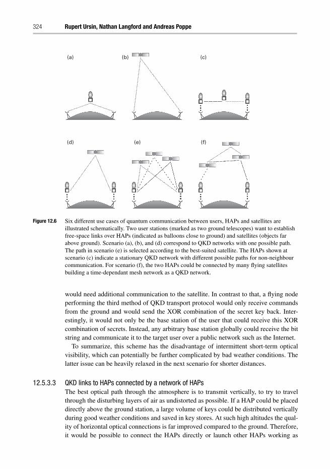
324 Rupert Ursin, Nathan Langford and Andreas Poppe
(c)(b)(a)
(d) (e) (f)
Figure 12.6 Six different use cases of quantum communication between users, HAPs and satellites areillustrated schematically. Two user stations (marked as two ground telescopes) want to establishfree-space links over HAPs (indicated as balloons close to ground) and satellites (objects farabove ground). Scenario (a), (b), and (d) correspond to QKD networks with one possible path.The path in scenario (e) is selected according to the best-suited satellite. The HAPs shown atscenario (c) indicate a stationary QKD network with different possible paths for non-neighbourcommunication. For scenario (f), the two HAPs could be connected by many flying satellitesbuilding a time-dependant mesh network as a QKD network.
would need additional communication to the satellite. In contrast to that, a flying nodeperforming the third method of QKD transport protocol would only receive commandsfrom the ground and would send the XOR combination of the secret key back. Inter-estingly, it would not only be the base station of the user that could receive this XORcombination of secrets. Instead, any arbitrary base station globally could receive the bitstring and communicate it to the target user over a public network such as the Internet.
To summarize, this scheme has the disadvantage of intermittent short-term opticalvisibility, which can potentially be further complicated by bad weather conditions. Thelatter issue can be heavily relaxed in the next scenario for shorter distances.
12.5.3.3 QKD links to HAPs connected by a network of HAPsThe best optical path through the atmosphere is to transmit vertically, to try to travelthrough the disturbing layers of air as undistorted as possible. If a HAP could be placeddirectly above the ground station, a large volume of keys could be distributed verticallyduring good weather conditions and saved in key stores. At such high altitudes the qual-ity of horizontal optical connections is far improved compared to the ground. Therefore,it would be possible to connect the HAPs directly or launch other HAPs working as
Quantum key distribution 325
relay stations as shown in Figure 12.6(c). This solution would work for a linear chain ofHAPs to span the required link distances and, moreover, it is also possible to arrange a 2-dimensional grid to cover the required area of a large country for long-distance quantumcommunication. Each HAP in the network would serve as a potential access node forusers. The routing in a simple 2-dimensional cell as a basic building block was alreadydemonstrated in the first fiber-based integrated QKD network experiment (SEQOQC).Thus, alternative paths can be used to avoid malfunctioning QKD links or damaged orproblematic HAPs. Multiple paths can also be used to enhance the accessible secure keyrate.
12.5.3.4 QKD links to HAPs connected by a single satelliteTo span even longer distances, too many HAP relay stations would be needed, and sucha scenario calls again for satellite-based key distribution. This scenario, sketched inFigure 12.6(d), is an extension of the one shown in Figure 12.6(b) using two HAPs asadditional relay stations.
The additional effort required to establish QKD link connections to satellites overHAPs would be worthwhile in order to relax constraints due to bad weather conditions.The altitude of a HAP is well above problematic fog and most opaque disturbing layersof clouds and greatly increases the availability of a QKD link connection, so the unrelia-bility of establishing a fresh key with the satellite is heavily reduced. Moreover, it wouldnormally be easy to fill the key stores of the QKD link between the ground and the HAP.If the satellite delivers a new secret key to the HAP when there is no visibility to theground due to bad weather, transport protocol 3 could be used to send the bit-sequenceof the XOR combination of both secret keys to the ground station using radio frequencytransmissions and it would still be possible to establish a key successfully. Even duringa longer period of limited visibility, such as during a rainy season in equatorial regions,this method is still usable if enough keys had been distributed with the HAP in advance.
12.5.3.5 QKD links to HAPs connected by many single satellitesAs outlined in Figure 12.6(e), it is possible to increase traffic over satellites by usingmore than one of them in parallel. At any given time, the optimal satellite can be chosento establish a secret key between the users. The more satellites available for this scenarioin different orbits, the more functionality of the connections that can be accessed.
12.5.3.6 QKD links to HAPs connected by a network of satellitesAgain, as in the last scenario, each HAP is able to establish a key to different satel-lites, with the relaxed requirement that different HAPs do not need to choose a commonsatellite. Additional intersatellite QKD connections could then connect satellites eitherdirectly, if the distance is not too large, or via other satellites in different orbits. Conse-quently, the HAPs establish a key with an arbitrary satellite (whichever is the closest)and the network of satellites is responsible for then connecting the HAPs and its users.
From a network perspective, the backbone network in such a situation would not behighly constant and stable as in fiber-based networks, but would change constantly overtime. As soon as two satellites would come close, they could establish new QKD linksleading to a highly flexible access to the network architecture.
326 Rupert Ursin, Nathan Langford and Andreas Poppe
References
[1] N. Gisin, G. Ribordy, W. Tittel, and H. Zbinden. Quantum cryptography. Rev. Mod. Phys.,74:145–195, 2002.
[2] M. Dusek, N. Lütkenhaus, and M. Hendrych. Chapter 5 quantum cryptography. volume 49of Progress in Optics, pages 381–454. Elsevier, 2006.
[3] V. Scarani, H. Bechmann-Pasquinucci, N. J. Cerf et al. The security of practical quantumkey distribution. Rev. Mod. Phys., 81(3):1301–1350, Sep 2009.
[4] M. Peev, C Pacher, R Alléaume et al. The secoqc quantum key distribution network inVienna. New J. Phys., 11(7):075001, 2009.
[5] M. Sasaki, M. Fujiwara, H. Ishizuka et al. Field test of quantum key distribution in the TokyoQKD Network. Opt. Express, 19:10387–10409, 2011.
[6] R. J. Hughes, J. E. Nordholt, D. Derkacs, and G. Peterson. Practical free-space quantum keydistribution over 10 km in daylight and at night. New J. Phys., 4:43, 2002.
[7] M. Aspelmeyer, H. R. Böhm, T. Gyatso et al. Long-distance free-space distribution ofquantum entanglement. Science, 301(5633):621–623, 2003.
[8] C-Z Peng, T Yang, X-H Bao, J Zhang et al. Experimental free-space distribution of entangledphoton pairs over a noisy ground atmosphere of 13km. Phys. Rev. Lett., 94:150501, 2005.
[9] R. Ursin, F. Tiefenbacher, T. Schmitt-Manderbach et al. Entanglement-based quantrumcommunication over 144 km. Nature Phys., 3:481–486, 2007.
[10] T. Schmitt-Manderbach, H. Weier, M. Fürst et al. Experimental demonstration of free-spacedecoy-state quantum key distribution over 144 km. Phys. Rev. Lett., 98(1):010504, Jan 2007.
[11] C. Erven, C. Couteau, R. Laflamme, and G. Weihs. Entangled quantum key distribution overtwo free-space optical links. Opt. Express, 16(21):16840–16853, Oct 2008.
[12] T. Scheidl, R. Ursin, A. Fedrizzi et al. Feasibility of 300 km quantum key distribution withentangled states. New J. Phys., 11(8):085002, 2009.
[13] J. G. Rarity, P. R. Tapster, P. M. Gorman, and P. Knight. Ground to satellite secure keyexchange using quantum cryptography. New J. Phys., 4:82, 2002.
[14] R. Kaltenbaek, M. Aspelmeyer, M. Pfennigbauer et al. Proof-of-concept experiments forquantum physics in space. In Proceedings of SPIE, 5161, pages 252–268, 2003.
[15] M. Aspelmeyer, T. Jennewein, M. Pfennigbauer, W. R. Leeb, and A. Zeilinger. Long-distance quantum communication with entangled photons using satellites. IEEE J. Sel. Top.Quantum Electronics, 9(6):1541–1551, 2003.
[16] M. Pfennigbauer, M. Aspelmeyer, W. Leeb et al. Satellite-based quantum communicationterminal employing state-of-the-art technology. J. Opt. Netw., 4:549–560, 2005.
[17] P. Villoresi, T. Jennewein, F. Tamburini et al. Experimental verification of the feasibility ofa quantum channel between space and earth. New J. Phys., 10(3):033038, 2008.
[18] R. Ursin, T. Jennewein, J. Kofler et al. Experiments with quantum entanglement in space.59th International Astronautical Congress (IAC) Proceedings A2.1.3, 2008.
[19] M. Toyoshima, T. Takahashi, K. Suzuki et al. Results from phase-1, phase-2 and phase-3kirari optical communication demonstration experiments with the nict optical ground sta-tion (koden). In 24th International Communications Satellite Systems Conference of AIAA,AIAA-2007-3228, Korea, 2007.
[20] J. Perdigues, B. Furch, C. de Matos et al. Quantum communication at ESA: Towards aspace experiment on the ISS. In Conference Proceedings IAC2007 Hydarabath, India, 2007.Accepted for publication in Acta Astronautica.
[21] N. Perlot, M. Knapek, D. Giggenbach et al. Results of the optical downlink experimentKIODO from OICETS satellite to optical ground station Oberpfaffenhofen (OGS-OP).
Quantum key distribution 327
In Conference on Laser Communication and Propagation, Proceedings of SPIE, 6457A,2007.
[22] R. Alléaume, J. Bouda, C. Branciard et al. Secoqc white paper on quantum key distri-bution and cryptography. arXiv:quant-ph/0701168v1, 2007. Quantum Physics (quant-ph);Cryptography and Security (cs.CR); Information Theory (cs.IT).
[23] C. H. Bennett and G. Brassard. Quantum cryptography: Public key distribution and coin toss-ing. Proceedings IEEE Int. Conf. on Computers, Systems and Signal Processing, Bangalore,India, IEEE, New York, pages 175–179, 1984.
[24] W.-Y. Hwang. Quantum key distribution with high loss: Toward global secure communica-tion. Phys. Rev. Lett., 91(5):057901, Aug 2003.
[25] X.-B. Wang. Beating the photon-number-splitting attack in practical quantum cryptography.Phys. Rev. Lett., 94(23):230503, Jun 2005.
[26] G. Brassard, N. Lütkenhaus, T. Mor, and B. C. Sanders. Limitations on practical quantumcryptography. Phys. Rev. Lett., 85(6):1330–1333, Aug 2000.
[27] H.-K. Lo, X. Ma, and K. Chen. Decoy state quantum key distribution. Phys. Rev. Lett.,94(23):230504, Jun 2005.
[28] C.-Z. Peng, J. Zhang, D. Yang et al. Experimental long-distance decoy-state quantum keydistribution based on polarization encoding. Phys. Rev. Lett., 98(1):010505, Jan 2007.
[29] C. H. Bennett, G. Brassard, and N. D. Mermin. Quantum cryptography without Bell’stheorem. Phys. Rev. Lett., 68(5):557–559, Feb 1992.
[30] T. Jennewein, C. Simon, G. Weihs, H. Weinfurter, and A. Zeilinger. Quantum cryptographywith entangled photons. Phys. Rev. Lett., 84(20):4729–4732, May 2000.
[31] A. Poppe, A. Fedrizzi, R. Ursin et al. Practical quantum key distribution with polarizationentangled photons. Opt. Express, 12(16):3865–3871, Aug 2004.
[32] A. Fedrizzi, T. Herbst, A. Poppe, T. Jennewein, and A. Zeilinger. A wavelength-tunablefiber-coupled source of narrowband entangled photons. Opt. Express, 15(23):15377–15386,Nov 2007.
[33] C. Bonato, M. Aspelmeyer, T. Jennewein et al. Influence of satellite motion on polarizationqubits in a space-earth quantum communication link. Opt. Express, 14(21):10050–10059,Oct 2006.
[34] C. Bonato, C. Pernechele, and P. Villoresi. Influence of all-reflective optical systems inthe transmission of polarization-encoded qubits. J. Optics A: Pure and Applied Optics,9(10):899, 2007.
[35] G. Anzolin, A. Gardelein, M. Jofre, G. Molina-Terriza, and M. W. Mitchell. Polarizationchange induced by a galvanometric optical scanner. J. Opt. Soc. Am. A, 27(9):1946–1952,Sep 2010.
[36] N. Sangouard, C. Simon, H. de Riedmatten, and N. Gisin. Quantum repeaters based onatomic ensembles and linear optics. arXiv:0906.2699v2, 2007. 52 pages, 34 figures, toappear in RMP.
[37] A. Acin, J. I. Cirac, and M. Lewenstein. Entanglement percolation in quantum networks.Nature Phys., 3:256–259, 2007.
[38] M. Dianati, R. Alléaume, and M. Gagnaire and X. Shen. Architecture and protocols of thefuture European quantum key distribution network. Security Comm. Netw., 1:57–74, 2008.
[39] R. Alléaume, F. Roueff, E. Diamanti, and N. Lütkenhaus. Topological optimization ofquantum key distribution networks. New J. Phys., 11(7):075002, 2009.
13 Optical modulating retro-reflectorsWilliam Rabinovich
13.1 Introduction
Free-space optical communication (FSO) offers many potential advantages. Theseinclude: high bandwidth, security, non-interference, and a large amount of availablespectrum. Many of these advantages are related to optics’ short wavelength relative toradio-frequency (RF) or microwave systems. At optical wavelengths even a small trans-mit aperture can produce highly directional beams, and optical receivers can focus lightdown to very small spots. To make use of this high optical antenna gain very good point-ing is required. Even a small telescope, with a 1 cm diameter, has a diffraction-limitedbeam divergence of less than 250 micro-radians in the near-infrared. Pointing with thisaccuracy is challenging, particularly if one or both ends of the link are in motion. ActiveFSO systems with high pointing accuracy are often large, heavy, and have high powerconsumption [1]. Such systems are also complex, which can lead to reliability issues.
Despite these challenges, direct FSO links – those with active terminals on both ends –have many good applications. There are, however, other applications in which the twoends of the link have different payload and power capabilities. Some examples include:unattended sensors, small unmanned aerial vehicles (UAVs), and small, tele-operatedrobots. For these applications a modulating retro-reflector (MRR) may be an appropriatesolution.
Optical MRRs couple passive retro-reflectors with electro-optic modulators toallow long-range, free-space optical communication with a laser, and pointing/acquisition/tracking system, required on only one end of the link. As shown inFigure 13.1, a conventional free-space optical communications terminal, the interroga-tor, is used on one end of the link to illuminate the MRR on the other end of the linkwith a continuous-wave beam. The MRR imposes a modulation on the interrogatingbeam and passively retro-reflects it back to the interrogator. The passive retro-reflectorwill generally have a large field of view over which incident light will be reflected backto its source, thus eliminating, or greatly reducing, pointing requirements on this end ofthe link. Despite this, the retro-reflected beam divergence can be very small, preservingthe desirable features of direct FSO such as security and non-interference.
Advanced Optical Wireless Communication Systems, ed. Shlomi Arnon, John R. Barry, George K.Karagiannidis, Robert Schober, and Murat Uysal. Published by Cambridge University Press.c© Cambridge University Press 2012.
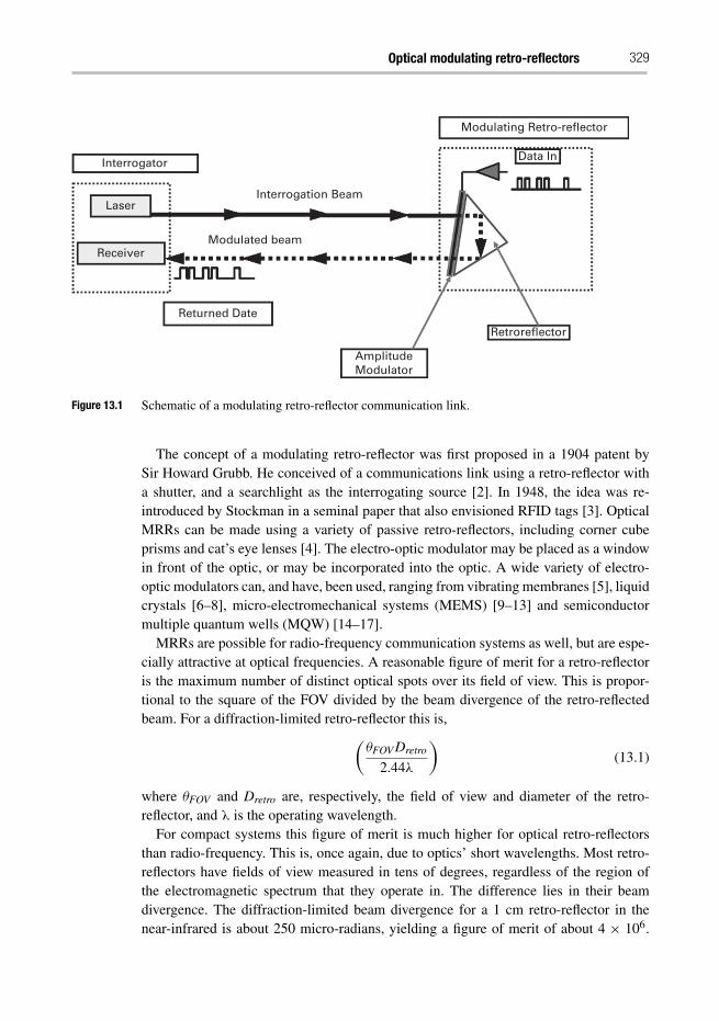
Optical modulating retro-reflectors 329
Interrogator
Laser
Receiver
Returned Date
Modulated beam
Interrogation Beam
AmplitudeModulator
Retroreflector
Data In
Modulating Retro-reflector
Figure 13.1 Schematic of a modulating retro-reflector communication link.
The concept of a modulating retro-reflector was first proposed in a 1904 patent bySir Howard Grubb. He conceived of a communications link using a retro-reflector witha shutter, and a searchlight as the interrogating source [2]. In 1948, the idea was re-introduced by Stockman in a seminal paper that also envisioned RFID tags [3]. OpticalMRRs can be made using a variety of passive retro-reflectors, including corner cubeprisms and cat’s eye lenses [4]. The electro-optic modulator may be placed as a windowin front of the optic, or may be incorporated into the optic. A wide variety of electro-optic modulators can, and have, been used, ranging from vibrating membranes [5], liquidcrystals [6–8], micro-electromechanical systems (MEMS) [9–13] and semiconductormultiple quantum wells (MQW) [14–17].
MRRs are possible for radio-frequency communication systems as well, but are espe-cially attractive at optical frequencies. A reasonable figure of merit for a retro-reflectoris the maximum number of distinct optical spots over its field of view. This is propor-tional to the square of the FOV divided by the beam divergence of the retro-reflectedbeam. For a diffraction-limited retro-reflector this is,(
θFOVDretro
2.44λ
)(13.1)
where θFOV and Dretro are, respectively, the field of view and diameter of the retro-reflector, and λ is the operating wavelength.
For compact systems this figure of merit is much higher for optical retro-reflectorsthan radio-frequency. This is, once again, due to optics’ short wavelengths. Most retro-reflectors have fields of view measured in tens of degrees, regardless of the region ofthe electromagnetic spectrum that they operate in. The difference lies in their beamdivergence. The diffraction-limited beam divergence for a 1 cm retro-reflector in thenear-infrared is about 250 micro-radians, yielding a figure of merit of about 4 × 10⁶.
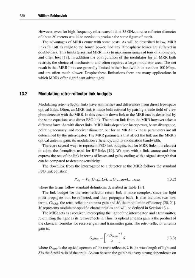
330 William Rabinovich
However, even for high-frequency microwave link at 35 GHz, a retro-reflector diameterof about 80 meters would be needed to produce the same figure of merit.
The advantages of MRRs come with some costs. As will be described below, MRRlinks fall off as range to the fourth power, and any atmospheric losses are suffered indouble-pass. This limits terrestrial MRR links to maximum ranges of tens of kilometers,and often less [18]. In addition the configuration of the modulator for an MRR bothrestricts the choice of mechanism, and often requires a large modulator area. The netresult is that MRR links are generally limited in their bandwidth to less than 100 Mbps,and are often much slower. Despite these limitations there are many applications inwhich MRRs offer significant advantages.
13.2 Modulating retro-reflector link budgets
Modulating retro-reflector links have similarities and differences from direct free-spaceoptical links. Often, an MRR link is made bidirectional by pairing a wide field of viewphotodetector with the MRR. In this case the down-link to the MRR can be described bythe same equations as a direct FSO link. The return link from the MRR however takes adifferent form. As with direct links, MRR links depend on laser power, beam divergence,pointing accuracy, and receiver diameter, but for an MRR link these parameters are alldetermined by the interrogator. The MRR parameters that affect the link are the MRR’soptical antenna gain, its modulation efficiency, and its modulation bandwidth.
There are several ways to represent FSO link budgets, but for MRR links it is clearestto adopt the formalism used for RF links [19]. We start with a link source and thenexpress the rest of the link in terms of losses and gains ending with a signal strength thatcan be compared to detector sensitivity.
The downlink from the interrogator to a detector at the MRR follows the standardFSO link equation
Psig = PlasGtxLtxLRLatmGrx−MRRLrx−MRR (13.2)
where the terms follow standard definitions described in Table 13.1.The link budget for the retro-reflector return link is more complex, since the light
must propagate out, be reflected, and then propagate back. It also includes two newterms, GMRR, the retro-reflector antenna gain and M, the modulation efficiency [20, 21].M represents modulator-specific characteristics and will be defined in Section 13.4.
The MRR acts as a receiver, intercepting the light of the interrogator, and a transmitter,re-emitting the light as its retro-reflects it. Thus its optical antenna gain is the product ofthe classical formulas for receiver gain and transmitter gain. The retro-reflector antennagain is,
GMRR =[πDretro
λ
]4
S (13.3)
where Dretro is the optical aperture of the retro-reflector, λ is the wavelength of light andS is the Strehl ratio of the optic. As can be seen the gain has a very strong dependence on
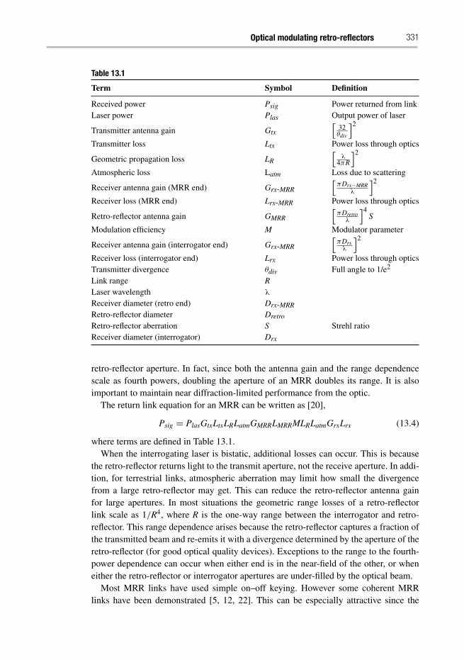
Optical modulating retro-reflectors 331
Table 13.1
Term Symbol Definition
Received power Psig Power returned from linkLaser power Plas Output power of laser
Transmitter antenna gain Gtx
[32θdiv
]2
Transmitter loss Ltx Power loss through optics
Geometric propagation loss LR
[λ
4πR
]2
Atmospheric loss Latm Loss due to scattering
Receiver antenna gain (MRR end) Grx-MRR
[πDrx−MRR
λ
]2
Receiver loss (MRR end) Lrx-MRR Power loss through optics
Retro-reflector antenna gain GMRR
[πDretro
λ
]4S
Modulation efficiency M Modulator parameter
Receiver antenna gain (interrogator end) Grx-MRR
[πDrx
λ
]2
Receiver loss (interrogator end) Lrx Power loss through opticsTransmitter divergence θdiv Full angle to 1/e2
Link range RLaser wavelength λ
Receiver diameter (retro end) Drx-MRRRetro-reflector diameter Dretro
Retro-reflector aberration S Strehl ratioReceiver diameter (interrogator) Drx
retro-reflector aperture. In fact, since both the antenna gain and the range dependencescale as fourth powers, doubling the aperture of an MRR doubles its range. It is alsoimportant to maintain near diffraction-limited performance from the optic.
The return link equation for an MRR can be written as [20],
Psig = PlasGtxLtxLRLatmGMRRLMRRMLRLatmGrxLrx (13.4)
where terms are defined in Table 13.1.When the interrogating laser is bistatic, additional losses can occur. This is because
the retro-reflector returns light to the transmit aperture, not the receive aperture. In addi-tion, for terrestrial links, atmospheric aberration may limit how small the divergencefrom a large retro-reflector may get. This can reduce the retro-reflector antenna gainfor large apertures. In most situations the geometric range losses of a retro-reflectorlink scale as 1/R4, where R is the one-way range between the interrogator and retro-reflector. This range dependence arises because the retro-reflector captures a fraction ofthe transmitted beam and re-emits it with a divergence determined by the aperture of theretro-reflector (for good optical quality devices). Exceptions to the range to the fourth-power dependence can occur when either end is in the near-field of the other, or wheneither the retro-reflector or interrogator apertures are under-filled by the optical beam.
Most MRR links have used simple on–off keying. However some coherent MRRlinks have been demonstrated [5, 12, 22]. This can be especially attractive since the
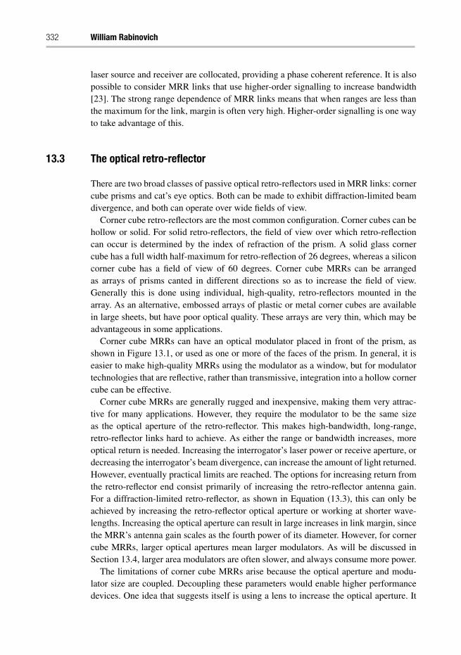
332 William Rabinovich
laser source and receiver are collocated, providing a phase coherent reference. It is alsopossible to consider MRR links that use higher-order signalling to increase bandwidth[23]. The strong range dependence of MRR links means that when ranges are less thanthe maximum for the link, margin is often very high. Higher-order signalling is one wayto take advantage of this.
13.3 The optical retro-reflector
There are two broad classes of passive optical retro-reflectors used in MRR links: cornercube prisms and cat’s eye optics. Both can be made to exhibit diffraction-limited beamdivergence, and both can operate over wide fields of view.
Corner cube retro-reflectors are the most common configuration. Corner cubes can behollow or solid. For solid retro-reflectors, the field of view over which retro-reflectioncan occur is determined by the index of refraction of the prism. A solid glass cornercube has a full width half-maximum for retro-reflection of 26 degrees, whereas a siliconcorner cube has a field of view of 60 degrees. Corner cube MRRs can be arrangedas arrays of prisms canted in different directions so as to increase the field of view.Generally this is done using individual, high-quality, retro-reflectors mounted in thearray. As an alternative, embossed arrays of plastic or metal corner cubes are availablein large sheets, but have poor optical quality. These arrays are very thin, which may beadvantageous in some applications.
Corner cube MRRs can have an optical modulator placed in front of the prism, asshown in Figure 13.1, or used as one or more of the faces of the prism. In general, it iseasier to make high-quality MRRs using the modulator as a window, but for modulatortechnologies that are reflective, rather than transmissive, integration into a hollow cornercube can be effective.
Corner cube MRRs are generally rugged and inexpensive, making them very attrac-tive for many applications. However, they require the modulator to be the same sizeas the optical aperture of the retro-reflector. This makes high-bandwidth, long-range,retro-reflector links hard to achieve. As either the range or bandwidth increases, moreoptical return is needed. Increasing the interrogator’s laser power or receive aperture, ordecreasing the interrogator’s beam divergence, can increase the amount of light returned.However, eventually practical limits are reached. The options for increasing return fromthe retro-reflector end consist primarily of increasing the retro-reflector antenna gain.For a diffraction-limited retro-reflector, as shown in Equation (13.3), this can only beachieved by increasing the retro-reflector optical aperture or working at shorter wave-lengths. Increasing the optical aperture can result in large increases in link margin, sincethe MRR’s antenna gain scales as the fourth power of its diameter. However, for cornercube MRRs, larger optical apertures mean larger modulators. As will be discussed inSection 13.4, larger area modulators are often slower, and always consume more power.
The limitations of corner cube MRRs arise because the optical aperture and modu-lator size are coupled. Decoupling these parameters would enable higher performancedevices. One idea that suggests itself is using a lens to increase the optical aperture. It
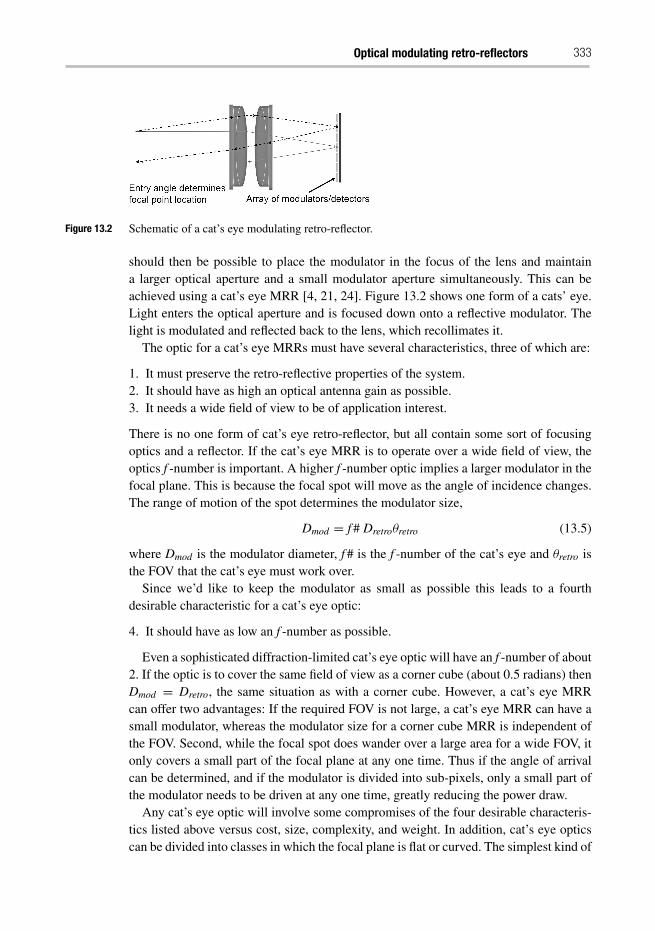
Optical modulating retro-reflectors 333
Figure 13.2 Schematic of a cat’s eye modulating retro-reflector.
should then be possible to place the modulator in the focus of the lens and maintaina larger optical aperture and a small modulator aperture simultaneously. This can beachieved using a cat’s eye MRR [4, 21, 24]. Figure 13.2 shows one form of a cats’ eye.Light enters the optical aperture and is focused down onto a reflective modulator. Thelight is modulated and reflected back to the lens, which recollimates it.
The optic for a cat’s eye MRRs must have several characteristics, three of which are:
1. It must preserve the retro-reflective properties of the system.2. It should have as high an optical antenna gain as possible.3. It needs a wide field of view to be of application interest.
There is no one form of cat’s eye retro-reflector, but all contain some sort of focusingoptics and a reflector. If the cat’s eye MRR is to operate over a wide field of view, theoptics f -number is important. A higher f -number optic implies a larger modulator in thefocal plane. This is because the focal spot will move as the angle of incidence changes.The range of motion of the spot determines the modulator size,
Dmod = f # Dretroθretro (13.5)
where Dmod is the modulator diameter, f # is the f -number of the cat’s eye and θretro isthe FOV that the cat’s eye must work over.
Since we’d like to keep the modulator as small as possible this leads to a fourthdesirable characteristic for a cat’s eye optic:
4. It should have as low an f -number as possible.
Even a sophisticated diffraction-limited cat’s eye optic will have an f -number of about2. If the optic is to cover the same field of view as a corner cube (about 0.5 radians) thenDmod = Dretro, the same situation as with a corner cube. However, a cat’s eye MRRcan offer two advantages: If the required FOV is not large, a cat’s eye MRR can have asmall modulator, whereas the modulator size for a corner cube MRR is independent ofthe FOV. Second, while the focal spot does wander over a large area for a wide FOV, itonly covers a small part of the focal plane at any one time. Thus if the angle of arrivalcan be determined, and if the modulator is divided into sub-pixels, only a small part ofthe modulator needs to be driven at any one time, greatly reducing the power draw.
Any cat’s eye optic will involve some compromises of the four desirable characteris-tics listed above versus cost, size, complexity, and weight. In addition, cat’s eye opticscan be divided into classes in which the focal plane is flat or curved. The simplest kind of
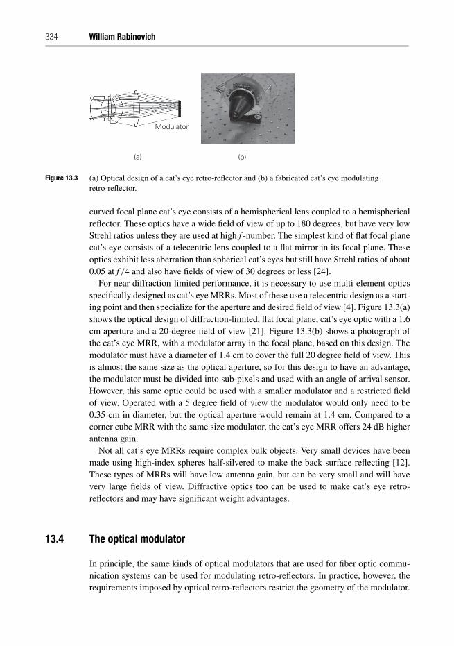
334 William Rabinovich
(a)
Modulator
(b)
Figure 13.3 (a) Optical design of a cat’s eye retro-reflector and (b) a fabricated cat’s eye modulatingretro-reflector.
curved focal plane cat’s eye consists of a hemispherical lens coupled to a hemisphericalreflector. These optics have a wide field of view of up to 180 degrees, but have very lowStrehl ratios unless they are used at high f -number. The simplest kind of flat focal planecat’s eye consists of a telecentric lens coupled to a flat mirror in its focal plane. Theseoptics exhibit less aberration than spherical cat’s eyes but still have Strehl ratios of about0.05 at f /4 and also have fields of view of 30 degrees or less [24].
For near diffraction-limited performance, it is necessary to use multi-element opticsspecifically designed as cat’s eye MRRs. Most of these use a telecentric design as a start-ing point and then specialize for the aperture and desired field of view [4]. Figure 13.3(a)shows the optical design of diffraction-limited, flat focal plane, cat’s eye optic with a 1.6cm aperture and a 20-degree field of view [21]. Figure 13.3(b) shows a photograph ofthe cat’s eye MRR, with a modulator array in the focal plane, based on this design. Themodulator must have a diameter of 1.4 cm to cover the full 20 degree field of view. Thisis almost the same size as the optical aperture, so for this design to have an advantage,the modulator must be divided into sub-pixels and used with an angle of arrival sensor.However, this same optic could be used with a smaller modulator and a restricted fieldof view. Operated with a 5 degree field of view the modulator would only need to be0.35 cm in diameter, but the optical aperture would remain at 1.4 cm. Compared to acorner cube MRR with the same size modulator, the cat’s eye MRR offers 24 dB higherantenna gain.
Not all cat’s eye MRRs require complex bulk objects. Very small devices have beenmade using high-index spheres half-silvered to make the back surface reflecting [12].These types of MRRs will have low antenna gain, but can be very small and will havevery large fields of view. Diffractive optics too can be used to make cat’s eye retro-reflectors and may have significant weight advantages.
13.4 The optical modulator
In principle, the same kinds of optical modulators that are used for fiber optic commu-nication systems can be used for modulating retro-reflectors. In practice, however, therequirements imposed by optical retro-reflectors restrict the geometry of the modulator.
Optical modulating retro-reflectors 335
As a result, optical modulators for MRRs generally have much lower bandwidth and/orextinction ratios than those for fiber optics. An optical modulator for an MRR must workfor light entering a large optical aperture, and over a wide range of angles. It must alsopreserve the retro-reflecting characteristics of the optic. This eliminates single-modewaveguide modulators, such as Lithium Niobate, which are too small to cover a cornercube or the focal plane of a cat’s eye MRR. Arrays of single-mode waveguides mightwork in a cat’s eye but the high fill factor required would be hard to achieve.
Most of the MRR systems demonstrated to date use large-area surface-normal modu-lators with thin active regions. These devices often have lower extinction ratios thanwaveguide devices. This is less of a problem for most MRR links than it would befor fiber telecommunications links. The lower bandwidth, larger area, detectors used infree-space optical links generally operate far from the shot-noise limit. As a result, thenoise in the optical receiver is generally dominated by that of the electronic pre-amplifiercircuit. Unlike quantum limited systems, in which the noise level increases as the opticalcontrast ratio decreases, the noise level in this case is independent of the optical contrastratio. The optical signal-to-noise ratio (OSNR) can then be defined as [20],
OSNR = POn − POff
Pnoise= Pret
e−αOn − e−αOff
Pnoise(13.6)
where POn is the optical power returned by the MRR when it is in its on-state, POff isthe power returned in the off-state, Pnoise is the noise equivalent power of the detector,Pret is the optical power returned by the MRR excluding losses in the modulator, αOn isthe double-pass absorption-length product of the modulator in its on-state, and αOff inits off-state. From Equation (13.6) it can be seen that maximizing the OSNR dependson both the optical contrast ratio and the optical transmission of the MQW. This can beseen more clearly by defining a figure of merit for the MQW, its modulation efficiency,
M = e−αOn − e−αOff = e−αOff · [CMQW − 1]
(13.7)
where M is the modulation efficiency and CMQW is the optical contrast ratio of themodulator. The OSNR of an MRR link is then simply PRetM.
While MRRs have been made with vibrating membranes [5] and gas-based Starkmodulators [25], the most common types of MRR modulators have been: liquid crystaldevices used in amplitude modulation mode, micro-electromechanical modulators usedeither as phase modulators or amplitude modulators, and multiple quantum well electro-absorption modulators.
All these systems are essentially capacitive in nature. While an MRR does not need toconsume power for transmission, it does consume power to change its modulation state.This capacitive power draw scales as
P = CV2f (13.8)
where P is the power, C is the device capacitance, V is the drive voltage, and f is themodulation frequency. Thus, across all these families of modulators, it is desirable tohave as low a capacitance and drive voltage as possible.
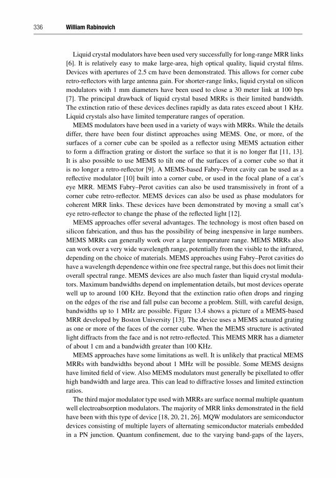
336 William Rabinovich
Liquid crystal modulators have been used very successfully for long-range MRR links[6]. It is relatively easy to make large-area, high optical quality, liquid crystal films.Devices with apertures of 2.5 cm have been demonstrated. This allows for corner cuberetro-reflectors with large antenna gain. For shorter-range links, liquid crystal on siliconmodulators with 1 mm diameters have been used to close a 30 meter link at 100 bps[7]. The principal drawback of liquid crystal based MRRs is their limited bandwidth.The extinction ratio of these devices declines rapidly as data rates exceed about 1 KHz.Liquid crystals also have limited temperature ranges of operation.
MEMS modulators have been used in a variety of ways with MRRs. While the detailsdiffer, there have been four distinct approaches using MEMS. One, or more, of thesurfaces of a corner cube can be spoiled as a reflector using MEMS actuation eitherto form a diffraction grating or distort the surface so that it is no longer flat [11, 13].It is also possible to use MEMS to tilt one of the surfaces of a corner cube so that itis no longer a retro-reflector [9]. A MEMS-based Fabry–Perot cavity can be used as areflective modulator [10] built into a corner cube, or used in the focal plane of a cat’seye MRR. MEMS Fabry–Perot cavities can also be used transmissively in front of acorner cube retro-reflector. MEMS devices can also be used as phase modulators forcoherent MRR links. These devices have been demonstrated by moving a small cat’seye retro-reflector to change the phase of the reflected light [12].
MEMS approaches offer several advantages. The technology is most often based onsilicon fabrication, and thus has the possibility of being inexpensive in large numbers.MEMS MRRs can generally work over a large temperature range. MEMS MRRs alsocan work over a very wide wavelength range, potentially from the visible to the infrared,depending on the choice of materials. MEMS approaches using Fabry–Perot cavities dohave a wavelength dependence within one free spectral range, but this does not limit theiroverall spectral range. MEMS devices are also much faster than liquid crystal modula-tors. Maximum bandwidths depend on implementation details, but most devices operatewell up to around 100 KHz. Beyond that the extinction ratio often drops and ringingon the edges of the rise and fall pulse can become a problem. Still, with careful design,bandwidths up to 1 MHz are possible. Figure 13.4 shows a picture of a MEMS-basedMRR developed by Boston University [13]. The device uses a MEMS actuated gratingas one or more of the faces of the corner cube. When the MEMS structure is activatedlight diffracts from the face and is not retro-reflected. This MEMS MRR has a diameterof about 1 cm and a bandwidth greater than 100 KHz.
MEMS approaches have some limitations as well. It is unlikely that practical MEMSMRRs with bandwidths beyond about 1 MHz will be possible. Some MEMS designshave limited field of view. Also MEMS modulators must generally be pixellated to offerhigh bandwidth and large area. This can lead to diffractive losses and limited extinctionratios.
The third major modulator type used with MRRs are surface normal multiple quantumwell electroabsorption modulators. The majority of MRR links demonstrated in the fieldhave been with this type of device [18, 20, 21, 26]. MQW modulators are semiconductordevices consisting of multiple layers of alternating semiconductor materials embeddedin a PN junction. Quantum confinement, due to the varying band-gaps of the layers,
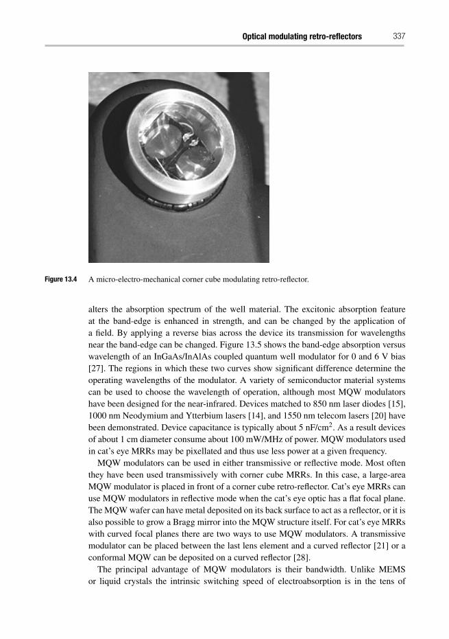
Optical modulating retro-reflectors 337
Figure 13.4 A micro-electro-mechanical corner cube modulating retro-reflector.
alters the absorption spectrum of the well material. The excitonic absorption featureat the band-edge is enhanced in strength, and can be changed by the application ofa field. By applying a reverse bias across the device its transmission for wavelengthsnear the band-edge can be changed. Figure 13.5 shows the band-edge absorption versuswavelength of an InGaAs/InAlAs coupled quantum well modulator for 0 and 6 V bias[27]. The regions in which these two curves show significant difference determine theoperating wavelengths of the modulator. A variety of semiconductor material systemscan be used to choose the wavelength of operation, although most MQW modulatorshave been designed for the near-infrared. Devices matched to 850 nm laser diodes [15],1000 nm Neodymium and Ytterbium lasers [14], and 1550 nm telecom lasers [20] havebeen demonstrated. Device capacitance is typically about 5 nF/cm2. As a result devicesof about 1 cm diameter consume about 100 mW/MHz of power. MQW modulators usedin cat’s eye MRRs may be pixellated and thus use less power at a given frequency.
MQW modulators can be used in either transmissive or reflective mode. Most oftenthey have been used transmissively with corner cube MRRs. In this case, a large-areaMQW modulator is placed in front of a corner cube retro-reflector. Cat’s eye MRRs canuse MQW modulators in reflective mode when the cat’s eye optic has a flat focal plane.The MQW wafer can have metal deposited on its back surface to act as a reflector, or it isalso possible to grow a Bragg mirror into the MQW structure itself. For cat’s eye MRRswith curved focal planes there are two ways to use MQW modulators. A transmissivemodulator can be placed between the last lens element and a curved reflector [21] or aconformal MQW can be deposited on a curved reflector [28].
The principal advantage of MQW modulators is their bandwidth. Unlike MEMSor liquid crystals the intrinsic switching speed of electroabsorption is in the tens of
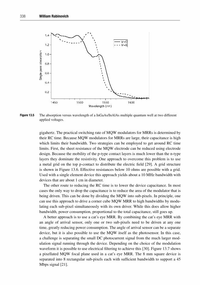
338 William Rabinovich
Figure 13.5 The absorption versus wavelength of a InGaAs/InAlAs multiple quantum well at two differentapplied voltages.
gigahertz. The practical switching rate of MQW modulators for MRRs is determined bytheir RC time. Because MQW modulators for MRRs are large, their capacitance is highwhich limits their bandwidth. Two strategies can be employed to get around RC timelimits. First, the sheet resistance of the MQW electrode can be reduced using electrodedesign. Because the mobility of the p-type contact layers is much lower than the n-typelayers they dominate the resistivity. One approach to overcome this problem is to usea metal grid on the top p-contact to distribute the electric field [29]. A grid structureis shown in Figure 13.6. Effective resistances below 10 ohms are possible with a grid.Used with a single element device this approach yields about a 10 MHz bandwidth withdevices that are about 1 cm in diameter.
The other route to reducing the RC time is to lower the device capacitance. In mostcases the only way to drop the capacitance is to reduce the area of the modulator that isbeing driven. This can be done by dividing the MQW into sub-pixels. In principle, onecan use this approach to drive a corner cube MQW MRR to high bandwidths by modu-lating each sub-pixel simultaneously with its own driver. While this does allow higherbandwidth, power consumption, proportional to the total capacitance, still goes up.
A better approach is to use a cat’s eye MRR. By combining the cat’s eye MRR withan angle of arrival sensor, only one or two sub-pixels need to be driven at any onetime, greatly reducing power consumption. The angle of arrival sensor can be a separatedevice, but it is also possible to use the MQW itself as the photosensor. In this case,a challenge is separating the small DC photocurrent signal from the much larger mod-ulation signal running through the device. Depending on the choice of the modulationwaveform it is possible to use electrical filtering to achieve this [30]. Figure 13.7 showsa pixellated MQW focal plane used in a cat’s eye MRR. The 8 mm square device isseparated into 8 rectangular sub-pixels each with sufficient bandwidth to support a 45Mbps signal [21].
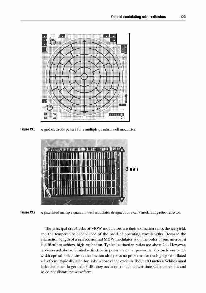
Optical modulating retro-reflectors 339
Figure 13.6 A grid electrode pattern for a multiple quantum well modulator.
Figure 13.7 A pixellated multiple quantum well modulator designed for a cat’s modulating retro-reflector.
The principal drawbacks of MQW modulators are their extinction ratio, device yield,and the temperature dependence of the band of operating wavelengths. Because theinteraction length of a surface normal MQW modulator is on the order of one micron, itis difficult to achieve high extinction. Typical extinction ratios are about 2:1. However,as discussed above, limited extinction imposes a smaller power penalty on lower band-width optical links. Limited extinction also poses no problems for the highly scintillatedwaveforms typically seen for links whose range exceeds about 100 meters. While signalfades are much larger than 3 dB, they occur on a much slower time scale than a bit, andso do not distort the waveform.
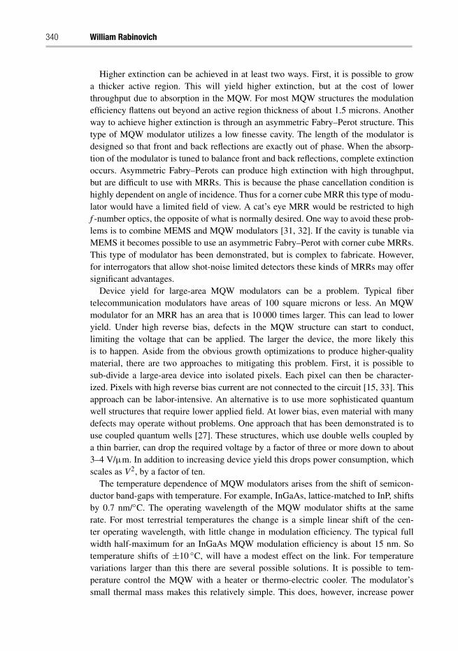
340 William Rabinovich
Higher extinction can be achieved in at least two ways. First, it is possible to growa thicker active region. This will yield higher extinction, but at the cost of lowerthroughput due to absorption in the MQW. For most MQW structures the modulationefficiency flattens out beyond an active region thickness of about 1.5 microns. Anotherway to achieve higher extinction is through an asymmetric Fabry–Perot structure. Thistype of MQW modulator utilizes a low finesse cavity. The length of the modulator isdesigned so that front and back reflections are exactly out of phase. When the absorp-tion of the modulator is tuned to balance front and back reflections, complete extinctionoccurs. Asymmetric Fabry–Perots can produce high extinction with high throughput,but are difficult to use with MRRs. This is because the phase cancellation condition ishighly dependent on angle of incidence. Thus for a corner cube MRR this type of modu-lator would have a limited field of view. A cat’s eye MRR would be restricted to highf -number optics, the opposite of what is normally desired. One way to avoid these prob-lems is to combine MEMS and MQW modulators [31, 32]. If the cavity is tunable viaMEMS it becomes possible to use an asymmetric Fabry–Perot with corner cube MRRs.This type of modulator has been demonstrated, but is complex to fabricate. However,for interrogators that allow shot-noise limited detectors these kinds of MRRs may offersignificant advantages.
Device yield for large-area MQW modulators can be a problem. Typical fibertelecommunication modulators have areas of 100 square microns or less. An MQWmodulator for an MRR has an area that is 10 000 times larger. This can lead to loweryield. Under high reverse bias, defects in the MQW structure can start to conduct,limiting the voltage that can be applied. The larger the device, the more likely thisis to happen. Aside from the obvious growth optimizations to produce higher-qualitymaterial, there are two approaches to mitigating this problem. First, it is possible tosub-divide a large-area device into isolated pixels. Each pixel can then be character-ized. Pixels with high reverse bias current are not connected to the circuit [15, 33]. Thisapproach can be labor-intensive. An alternative is to use more sophisticated quantumwell structures that require lower applied field. At lower bias, even material with manydefects may operate without problems. One approach that has been demonstrated is touse coupled quantum wells [27]. These structures, which use double wells coupled bya thin barrier, can drop the required voltage by a factor of three or more down to about3–4 V/μm. In addition to increasing device yield this drops power consumption, whichscales as V2, by a factor of ten.
The temperature dependence of MQW modulators arises from the shift of semicon-ductor band-gaps with temperature. For example, InGaAs, lattice-matched to InP, shiftsby 0.7 nm/◦C. The operating wavelength of the MQW modulator shifts at the samerate. For most terrestrial temperatures the change is a simple linear shift of the cen-ter operating wavelength, with little change in modulation efficiency. The typical fullwidth half-maximum for an InGaAs MQW modulation efficiency is about 15 nm. Sotemperature shifts of ±10 ◦C, will have a modest effect on the link. For temperaturevariations larger than this there are several possible solutions. It is possible to tem-perature control the MQW with a heater or thermo-electric cooler. The modulator’ssmall thermal mass makes this relatively simple. This does, however, increase power
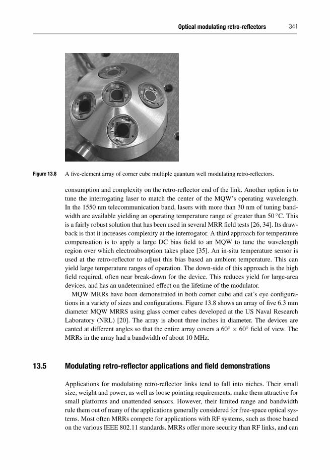
Optical modulating retro-reflectors 341
Figure 13.8 A five-element array of corner cube multiple quantum well modulating retro-reflectors.
consumption and complexity on the retro-reflector end of the link. Another option is totune the interrogating laser to match the center of the MQW’s operating wavelength.In the 1550 nm telecommunication band, lasers with more than 30 nm of tuning band-width are available yielding an operating temperature range of greater than 50 ◦C. Thisis a fairly robust solution that has been used in several MRR field tests [26, 34]. Its draw-back is that it increases complexity at the interrogator. A third approach for temperaturecompensation is to apply a large DC bias field to an MQW to tune the wavelengthregion over which electroabsorption takes place [35]. An in-situ temperature sensor isused at the retro-reflector to adjust this bias based an ambient temperature. This canyield large temperature ranges of operation. The down-side of this approach is the highfield required, often near break-down for the device. This reduces yield for large-areadevices, and has an undetermined effect on the lifetime of the modulator.
MQW MRRs have been demonstrated in both corner cube and cat’s eye configura-tions in a variety of sizes and configurations. Figure 13.8 shows an array of five 6.3 mmdiameter MQW MRRS using glass corner cubes developed at the US Naval ResearchLaboratory (NRL) [20]. The array is about three inches in diameter. The devices arecanted at different angles so that the entire array covers a 60◦ × 60◦ field of view. TheMRRs in the array had a bandwidth of about 10 MHz.
13.5 Modulating retro-reflector applications and field demonstrations
Applications for modulating retro-reflector links tend to fall into niches. Their smallsize, weight and power, as well as loose pointing requirements, make them attractive forsmall platforms and unattended sensors. However, their limited range and bandwidthrule them out of many of the applications generally considered for free-space optical sys-tems. Most often MRRs compete for applications with RF systems, such as those basedon the various IEEE 802.11 standards. MRRs offer more security than RF links, and can
342 William Rabinovich
also offer higher bandwidth at lower power at the sensor. Increasingly an advantage ofMRRs is their immunity to the problems of spectral congestion that have come to plaguesensor systems that use RF communication. As more and more high-bandwidth sensorsand platforms are used nearby each other, the available RF bandwidth has become ascarce commodity. Mutual interference is rarely a problem for retro-reflector systemsbecause of the high directionality of the beams, and the large spectrum availability inthe infrared.
MRR links face problems similar to direct FSO links, but with some important dif-ferences. Atmospheric effects due to scattering from rain, fog, and other obscurants,and optical scintillation due to turbulence, affect both MRR and direct FSO links. Infact, MRR links are more affected by the atmosphere because the link is double pass.In practice, however, this is offset by the fact that most MRR links are shorter rangethan direct FSO links. Thus the overall system challenge posed by loss of margin dueto weather is similar. Link drop-outs due to scintillation may be more severe for MRRlinks, however.
MRR links also face challenges of pointing and tracking, primarily on the interrogatorside of the link. MRR interrogators often use narrow beams to make up for the propaga-tion loss in the link. However, it is easier to acquire a retro-reflector than another FSOsystem. For acquisition in a direct FSO link, two narrow field of view systems must bepointed at each other. This creates a search problem that scales as the square of the num-ber of addressable points in the field of view of each system. A retro-reflector however isalways “pointed” at its interrogator as long as it falls within the very wide retro-reflectorfield of view. The search problem then scales linearly as the number of points in theinterrogators field of view. MRR links do face increased challenge in acquisition andtracking because they work at lower data rates. The typical signal power in an MRR linkis one to two orders of magnitude lower than for a high-bandwidth direct FSO link. Thismeans the acquisition sensor has much less power to work with.
FSO interrogators can be either monostatic or bistatic. The transmitter and receiveroptical axes are collinear in a monostatic interrogator, sharing an aperture. In a bistaticinterrogator, the transmitter and receiver apertures are side-by-side. This design choicehas unique ramifications for an MRR system with regard to transmit/receive isolationand minimum range.
All FSO systems must deal with the problem of transmit/receive isolation. In a typ-ical direct FSO link, the ratio of transmit to receive beam power is 30–40 dB. In anMRR link it is often 70–80 dB. Direct FSO links can use different transmit and receivewavelengths, allowing very good isolation. An MRR link does not have this option, asthe same laser is used for both transmit and receive. Isolation is most often achieved inMRR links using bistatic systems. This can be effective at long range, but has difficultiesat short range. A retro-reflector returns power exactly back to where it originated. In abistatic system, the power returns to the transmit aperture. If the range is long enoughthat the retro-reflected beam diameter covers both apertures, there is no problem, butwhen close most of the power may miss the receiver. This imposes a minimum range ofoperation for bistatic systems.
Optical modulating retro-reflectors 343
Monostatic transceivers pose their own set of challenges. Monostatic systems can bemade with beam splitters, using polarization to isolate transmit and receive, or with fibercirculators. These solutions have been demonstrated with some degree of success. Asimpler solution is to introduce the transmit beam into the optical path using an occlud-ing mirror contained within a larger receive aperture, or to pass the interrogating beamthrough a hole in a mirror in the receive path. However, these solutions limit the size ofthe transmit beam, and hence if the system is to stay eye-safe out of the aperture, theoutput power must be limited.
While many MRRs have been tested only in the laboratory, there have been somefield tests of complete MRR communication links, as well as some theoretical analyses[36]. Surface-to-surface links have been demonstrated with several different types ofMRRs. In 1995, Honeywell demonstrated a coherent MRR link at 10.6 microns using adeformable membrane MRR [5]. The link was at a low rate, a few kilohertz, and usedto transmit voice data from rooftop to rooftop at ranges up to 24 km.
In 2005, the US Naval Research Laboratory demonstrated a multiple quantum wellMRR link from the shore to a boat on the Chesapeake Bay using the MRR array shown inFigure 13.8 [20]. These devices were 6.3 mm diameter InGaAs/InAlAs MQWs designedto work in the telecom band at 1550 nm. Data rates up to 5 Mbps were demonstrated outto a range of 2 km using an interrogator with a four-inch receive aperture and a 1.5 Wattlaser. This interrogator had no tracking and was manually aimed at the boat. Scintillationindices for these links varied from about 0.3 to 0.6. These levels are lower than what onewould find for a link near the ground because optical turbulence is generally lower overwater. A higher data rate version of this link was demonstrated in 2007. Cat’s eye MRRs,with a pixellated MQW focal plane were used at a range of 7 km to close a 45 MbpsMRR link from shore to ship [21].
In 2008 a ship-to-ship MRR link was demonstrated by NRL as part of the US Navy’sTrident Warrior exercise [26]. A five-element corner cube MQW MRR array similar toFigure 13.8, but this time using 1 cm diameter devices, was combined with a 2 MbpsEthernet modem to demonstrate video and file transfer at ranges up to 4.5 km betweentwo US Navy vessels underway in the Pacific Ocean. The interrogator, used for this linkcould auto-track on the retro-reflected return using a quad cell sensor that could driveboth internal fast steering mirrors and an external gimbal [37].
Also in 2008, a joint experiment of the University of Maryland’s Laboratory forPhysical Sciences and NRL, demonstrated an MQW MRR link from one side of theChesapeake Bay to the other, a distance of 16 km [18]. This link used up to three 1.6 cmdiameter cat’s eye MRRs and sent data at 2 Mbps using an Ethernet protocol. Both filesand video were transmitted. Though this data was taken at the same place as the 2005Chesapeake Bay experiment, the much longer range resulted in scintillation indices thatvaried between 0.2 and 2. This experiment also showed that scintillation could be mit-igated by aperture averaging. By comparing the return of one, two, and three MRRs inan array, it was shown that the scintillation index was inversely proportional to the num-ber of retro-reflectors. The use of multiple MRRs for aperture averaging must, however,take into account coherent interference effects [38].
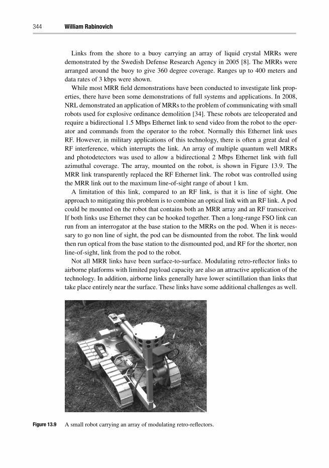
344 William Rabinovich
Links from the shore to a buoy carrying an array of liquid crystal MRRs weredemonstrated by the Swedish Defense Research Agency in 2005 [8]. The MRRs werearranged around the buoy to give 360 degree coverage. Ranges up to 400 meters anddata rates of 3 kbps were shown.
While most MRR field demonstrations have been conducted to investigate link prop-erties, there have been some demonstrations of full systems and applications. In 2008,NRL demonstrated an application of MRRs to the problem of communicating with smallrobots used for explosive ordinance demolition [34]. These robots are teleoperated andrequire a bidirectional 1.5 Mbps Ethernet link to send video from the robot to the oper-ator and commands from the operator to the robot. Normally this Ethernet link usesRF. However, in military applications of this technology, there is often a great deal ofRF interference, which interrupts the link. An array of multiple quantum well MRRsand photodetectors was used to allow a bidirectional 2 Mbps Ethernet link with fullazimuthal coverage. The array, mounted on the robot, is shown in Figure 13.9. TheMRR link transparently replaced the RF Ethernet link. The robot was controlled usingthe MRR link out to the maximum line-of-sight range of about 1 km.
A limitation of this link, compared to an RF link, is that it is line of sight. Oneapproach to mitigating this problem is to combine an optical link with an RF link. A podcould be mounted on the robot that contains both an MRR array and an RF transceiver.If both links use Ethernet they can be hooked together. Then a long-range FSO link canrun from an interrogator at the base station to the MRRs on the pod. When it is neces-sary to go non line of sight, the pod can be dismounted from the robot. The link wouldthen run optical from the base station to the dismounted pod, and RF for the shorter, nonline-of-sight, link from the pod to the robot.
Not all MRR links have been surface-to-surface. Modulating retro-reflector links toairborne platforms with limited payload capacity are also an attractive application of thetechnology. In addition, airborne links generally have lower scintillation than links thattake place entirely near the surface. These links have some additional challenges as well.
Figure 13.9 A small robot carrying an array of modulating retro-reflectors.
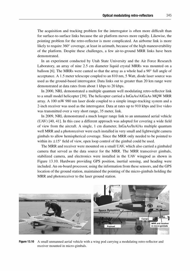
Optical modulating retro-reflectors 345
The acquisition and tracking problem for the interrogator is often more difficult thanfor surface-to-surface links because the air platform moves more rapidly. Likewise, thepointing problem for the retro-reflector is more complicated. An airborne link is morelikely to require 360◦ coverage, at least in azimuth, because of the high maneuverabilityof the platform. Despite these challenges, a few air-to-ground MRR links have beendemonstrated.
In an experiment conducted by Utah State University and the Air Force ResearchLaboratory, an array of nine 2.5 cm diameter liquid crystal MRRs was mounted on aballoon [6]. The MRRs were canted so that the array as a whole had a 90◦ full angle ofacceptance. A 1.5 meter telescope coupled to an 810 nm, 5 Watt, diode laser source wasused as the ground-based interrogator. Data links out to greater than 20 km range weredemonstrated at data rates from about 1 kbps to 20 kbps.
In 2000, NRL demonstrated a multiple quantum well modulating retro-reflector linkto a small model helicopter [39]. The helicopter carried a InGaAs/AlGaAs MQW MRRarray. A 100 mW 980 nm laser diode coupled to a simple image-tracking system and a2-inch receiver was used as the interrogator. Data at rates up to 910 kbps and live videowas transmitted over a very short range, 35 meter, link.
In 2009, NRL demonstrated a much longer range link to an unmanned aerial vehicle(UAV) [40, 41]. In this case a different approach was adopted for covering a wide fieldof view from the aircraft. A single, 1 cm diameter, InGaAs/InAlAs multiple quantumwell MRR and a photoreceiver were each installed in very small and lightweight cameragimbals to allow hemispherical coverage. Since the MRR only needed to be pointed towithin its ±15◦ field of view, open loop control of the gimbal could be used.
The MRR and receiver were mounted on a small UAV, which also carried a gimbaledcamera that served as the data source for the MRR. The MRR transceiver gimbals,stabilized camera, and electronics were installed in the UAV wingpod as shown inFigure 13.10. Hardware providing GPS position, inertial sensing, and heading wereincluded. An on-board processor, using the information from these sensors, and the GPSlocation of the ground station, maintained the pointing of the micro-gimbals holding theMRR and photoreceiver to the laser ground station.
Figure 13.10 A small unmanned aerial vehicle with a wing pod carrying a modulating retro-reflector andreceiver mounted in micro-gimbals.
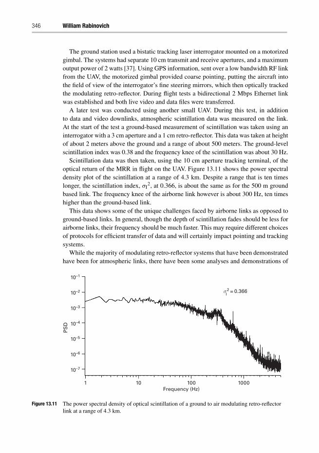
346 William Rabinovich
The ground station used a bistatic tracking laser interrogator mounted on a motorizedgimbal. The systems had separate 10 cm transmit and receive apertures, and a maximumoutput power of 2 watts [37]. Using GPS information, sent over a low bandwidth RF linkfrom the UAV, the motorized gimbal provided coarse pointing, putting the aircraft intothe field of view of the interrogator’s fine steering mirrors, which then optically trackedthe modulating retro-reflector. During flight tests a bidirectional 2 Mbps Ethernet linkwas established and both live video and data files were transferred.
A later test was conducted using another small UAV. During this test, in additionto data and video downlinks, atmospheric scintillation data was measured on the link.At the start of the test a ground-based measurement of scintillation was taken using aninterrogator with a 3 cm aperture and a 1 cm retro-reflector. This data was taken at heightof about 2 meters above the ground and a range of about 500 meters. The ground-levelscintillation index was 0.38 and the frequency knee of the scintillation was about 30 Hz.
Scintillation data was then taken, using the 10 cm aperture tracking terminal, of theoptical return of the MRR in flight on the UAV. Figure 13.11 shows the power spectraldensity plot of the scintillation at a range of 4.3 km. Despite a range that is ten timeslonger, the scintillation index, σI
2, at 0.366, is about the same as for the 500 m groundbased link. The frequency knee of the airborne link however is about 300 Hz, ten timeshigher than the ground-based link.
This data shows some of the unique challenges faced by airborne links as opposed toground-based links. In general, though the depth of scintillation fades should be less forairborne links, their frequency should be much faster. This may require different choicesof protocols for efficient transfer of data and will certainly impact pointing and trackingsystems.
While the majority of modulating retro-reflector systems that have been demonstratedhave been for atmospheric links, there have been some analyses and demonstrations of
PS
D
Frequency (Hz)1
10–7
10–6
10–5
10–4
10–3
10–2
10–1
σ 2 = 0.366
10 100 1000
I
Figure 13.11 The power spectral density of optical scintillation of a ground to air modulating retro-reflectorlink at a range of 4.3 km.
Optical modulating retro-reflectors 347
underwater MRR links [42, 43]. Like atmospheric MRRs, underwater MRRs are appli-cable to small platforms or unattended sensors. MRR links still provide the advantagesof loose pointing tolerances on the retro-reflector end of the link. Despite the fact thatunderwater propagation produces a much wider beam profile than diffraction-limitedatmospheric propagation, underwater links still need to be aimed to within a fraction of adegree to maximize their link range. Propagation losses are very different for underwaterlinks. The 1/R4 link dependence of retro-reflector links is dominated by the exponen-tial losses due to scattering and absorption. Underwater MRRs have more limitationson their modulator types. There is a relatively small window in the blue/green portionof the optical spectrum in which light propagates with low loss. While MEMS and liq-uid crystal devices can be designed to work in the blue/green, the most commonly usedsemiconductor materials cannot. Materials such as InGaN, which have a wide bandgap,are being investigated and may be used for blue/green MQW modulators in the future.However, these materials are not mature enough for use now. Underwater MRR linksmust be very short due to the high propagation losses. It is unlikely that link rangesmore than 100 meters will be possible, even in the cleanest of water. Within this rangehowever lie several useful applications, such as data transfer at megabit per second rateswithout the need to make a physical connection.
13.6 Conclusion
Modulating retro-reflectors have a unique niche in the world of free-space optical links.They share characteristics with direct FSO links and RF links. Like direct FSO links theyare secure and do not suffer from frequency allocation issues. Like RF links their band-widths tend to be below 100 MHz and they have loose pointing requirements (on oneend at least). MRR links are unique in the low power consumption of the retro-reflectingtransceiver, but also in their limited range due to the 1/R4 range dependence.
Modulating retro-reflectors, like direct free-space optical links in general, are still insearch of the applications that will lead to wide deployment of systems. This is likelyto occur as more and more high bandwidth sensors and communication links are usedin the field. Increasing frequency congestion and the demand for even higher bandwidthleads naturally to optical systems as an answer. Retro-reflecting links will be part of thatanswer.
References
[1] L. Stotts, B. Stadler, G. Lee, “Free space optical communications: coming of age,”Proceedings of the SPIE – The International Society for Optical Engineering 5550,W1–W15 (2008).
[2] H. Grubb, “Improvement in and means for signaling and indicating position of objects,” UKPatent #21,856, GB190321856, issued October 6, 1904.
[3] H. Stockman, “Communication by means of reflected power,” Proceedings of the I.R.E., 36(10) pp. 1196–1204 (1948).
348 William Rabinovich
[4] M. L. Biermann, W. S. Rabinovich, R. Mahon, G. C. Gilbreath, “Design and analysis of adiffraction-limited cat’s-eye retroreflector,” Opt. Eng., 41(7) pp. 1655–1660, (2002).
[5] G. O. Olsen, H. W. Mocker, N. A. Demma, J. B. Ross, “Coherent CO2 laser communicationsystem with modulable retroreflectors,” Appl. Optics, 34 (12) pp. 2033–2044 (1995).
[6] C. M. Swenson, C. A. Steed, I. A. A. DeLaRue, R. Q. Fugate, “Low power FLC-based retro-modulator communications system,” Proceedings of the SPIE – The International Societyfor Optical Engineering, 2990 pp. 296–310 (1997).
[7] D. C. O’Brien, J. J. Liu, G. E. Faulkner et al., “Design and implementation of optical wirelesscommunications with optically powered smart dust motes,” IEEE J. Sel. Area Comm., 27 (9)pp. 1646-1653 (2009).
[8] F. Kullander, P. Sakari, L. Sjöqvist, J. Ögren, “System trials with modulated retro-reflectiveoptical communication,” Proceedings of the SPIE – The International Society for OpticalEngineering, 5986 pp. 12-1–12-2 (2005).
[9] D. Pedersen, O. Solgaard, “Free space communication link using a grating light modulator,”Sensor Actuat. A-Phys., 83 (1–3) pp. 6–10 (2000).
[10] C. P. Lao, K. W. Goossen, “Optical microelectromechanical system array for free-spaceretrocommunication,” IEEE Photonic Tech. Lett., 16 (9) pp. 2045–2047 (2005).
[11] T. K. Chan, J. E. Ford, “Retroreflecting optical modulator using an MEMS deformablemicromirror array,” IEEE J. Lightwave Technol., 24 (1) pp. 516–525 (2006).
[12] C. Jenkins, J. G. Brown, L. Li, W. Johnstone, D. Uttamchandani, “MEMS retro-phase-modulator for free-space coherent optical communications,” IEEE J. Sel. Top. Quant.Electron., 13 (2) pp. 330–335 (2007)
[13] L. Ziph-Schatzberg, T. Bifano, S. Cornelissen, “Secure optical communication system uti-lizing deformable MEMS mirrors,” Proceedings of the SPIE – The International Society forOptical Engineering, 7209, C1–C15 (2009)
[14] I. J. Fritz, T. M. Brennan, B. E. Hammons et al., “Low-voltage vertical-cavity transmissionmodulator for 1.06 μm”, Appl. Phys. Lett., 63 (4) pp. 494–6 (1993)
[15] G. C. Gilbreath, W. S. Rabinovich, R. Mahon et al., “Large aperture quantum well shut-ters for fast retroreflected optical data links in free space,” Proceedings of the SPIE – TheInternational Society for Optical Engineering, 3707 pp. 666–672, (1999)
[16] W. S. Rabinovich, G. C. Gilbreath, P.G. Goetz et al., “InGaAs multiple quantum well modu-lating retro-reflector for free space optical communications,” Proceedings of the SPIE – TheInternational Society for Optical Engineering, 4489 pp. 190–201 (2001).
[17] S. Junique, D. Agren, Q. Wang et al., “Modulating retro-reflector for free-space opticalcommunication,” IEEE Photonic Tech. Lett., 18 pp. 85–87 (2006).
[18] M. Plett, W. S. Rabinovich, R. Mahon et al., “Free-space optical communication link across16 km over the Chesapeake Bay to a modulated retro-reflector-array,” Opt. Eng. 47, 045001(2008).
[19] S. G. Lambert and W. Casey, Laser Communication in Space, (Boston, Artech House, 1995).[20] W. S. Rabinovich, R. Mahon, H. R. Burris et al., “Free-space optical communications link at
1550 nm using multiple quantum well modulating retro-reflectors in a marine environment”,Opt. Eng., 44 pp. 056001 1–12 (2005).
[21] W. S. Rabinovich, P. G. Goetz, R. Mahon et al., “45-Mbit/s cat’s eye modulating retroreflec-tors,” Opt. Eng., 46 pp.104001 1–8, (2007).
[22] P. G. Goetz, R. Mahon, L. Swingen, J. L. Witkowsky, W. S. Rabinovich, “Coherent modulat-ing retroreflector system,” Proceedings of the SPIE – The International Society for OpticalEngineering 5550 pp. 115–121 (2004).
Optical modulating retro-reflectors 349
[23] P. G. Goetz, E. E. Funk, R. Mahon, W. S. Rabinovich, S. C. Binari, “Quadrature amplitudemodulation in modulating retroreflector system,” Electron. Lett., 39 pp. 1463–1464 (2003).
[24] W. S. Rabinovich, R. Mahon, P. G. Goetz, E. Waluschka, “A cat’s eye multiple quantum-wellmodulating retro-reflector”, IEEE Photonic Tech. Lett., 15 pp. 461–463 March 2003.
[25] M. B. Klein, R. H. Sipman, “Large aperture Stark modulated retroreflector at 10.8 μm,”J. Appl. Phys., 51 pp. 6101–6104, (1980).
[26] W. S. Rabinovich, C. I. Moore, H. R. Burris et al., “Free space optical communicationsresearch at the US Naval Research Laboratory,” Proceedings of the SPIE – The InternationalSociety for Optical Engineering, 7585 pp. 02-1–02-15, (2010).
[27] T. H. Stievater, W. S. Rabinovich, P. G. Goetz, , R. Mahon, S. C. Binari “A surface-normalcoupled-quantum-well modulator at 1.55 μm,” IEEE Photon. Tech. Lett. 16 pp. 2036–2038(2004).
[28] K. Sayyah, A. Narayanan, D. Persechini, P. Brewer, “Conformal pixellated MQW modula-tor structure for modulating retroreflector applications,” IEEE Photonic Tech. Lett., 17 pp.1854–1856, (2005).
[29] P. G. Goetz, W. S. Rabinovich, S. C. Binari, J. A. Mittereder, “High-performance chirpedelectrode design for cat’s eye retro-reflector modulators,” IEEE Photonic Tech. Lett., 18 pp.2278–2280 (2006).
[30] D. Klotzkin, P. G. Goetz, W. S. Rabinovich et al., “Integrated angle-of-arrival sensing andsimultaneous bidirectional communication using a cat’s eye modulating retroreflector,”Conference on Lasers and Electro-optics, article#5225567 (2009).
[31] W. S. Rabinovich, T. H. Stievater, N. A. Papanicolaou, D. S. Katzer, P. G. Goetz, “Demon-stration of a microelectromechanical tunable asymmetric Fabry-Perot quantum well modu-lator”, Appl. Phys. Lett., 83 pp. 1923–1925 (2003).
[32] T. H. Stievater, D. Park, M. W. Pruessner, “A microelectromechanically tunable asymmet-ric Fabry-Perot quantum well modulator at 1.55 μm”, Opt. Exp., 16 pp. 16766–16773(2008).
[33] K. W. Goossen, D. W. Prather, “Fabrication and, yield of large-area quantum-well modula-tors”, IEEE Photonic Tech. Lett., 19 pp. 2054–2056 (2007).
[34] W. S. Rabinovich, J. Murphy, M. Ferraro, R. Mahon, “Free-space optical data link to a smallrobot using modulating retroreflectors,” Proceedings of the SPIE – The International Societyfor Optical Engineering, 7464 pp. 08-1–08-9 (2009).
[35] D. Varshneya, L. Jeffers, “Temperature compensated dynamic optical tag modulator systemand method,” US Patent #7603041, October 13, 2009.
[36] S. Arnon and D. Kedar, “Sensing and communication trade-offs in picosatellite formationflying missions,” JOSA A, 26 pp. 2128–2133 (2009).
[37] E. Saint Georges, “Evaluation of cone tracking for free-space optical communicationwith a retro-modulator,” Proceedings of the SPIE – The International Society for OpticalEngineering 7464 pp. 70903–70903 (2009).
[38] R. Mahon, W. S. Rabinovich, M. Plett, et al., “Interference effects and aperture averaging inretroreflected light,” Opt. Eng., 47 pp. 046002-1–046002-9 (2008).
[39] G. C. Gilbreath, W. S. Rabinovich, T. J. Meehan et al., “Large-aperture multiple quan-tum well modulating retroreflector for free-space optical data transfer on unmanned aerialvehicles,” Opt. Eng., 40 pp. 1348–1356 (2001).
[40] P. G. Goetz, W. S. Rabinovich, R. Mahon, “Modulating retro-reflector lasercom systems atthe Naval Research Laboratory” (invited), Proc. MILCOM 2010, pp. 2302–2307, November2010.

350 William Rabinovich
[41] P. G. Goetz, J. L. Murphy, M. R. Suite, “Lasercom for small unmanned aerial systems usinga modulating retro-reflector,” MILCOM 2010 Classified Session, November 1, 2010.
[42] L. Mullen, B. Cochenour, W. Rabinovich, R. Mahon, J. Muth, “Backscatter suppression forunderwater modulating retroreflector links using polarization discrimination”, Appl. Opt.,48 pp. 328–337 (2009).
[43] S. Arnon, “Underwater optical wireless communication network,” Opt. Eng., 49 pp. 015001–015007 (2010).
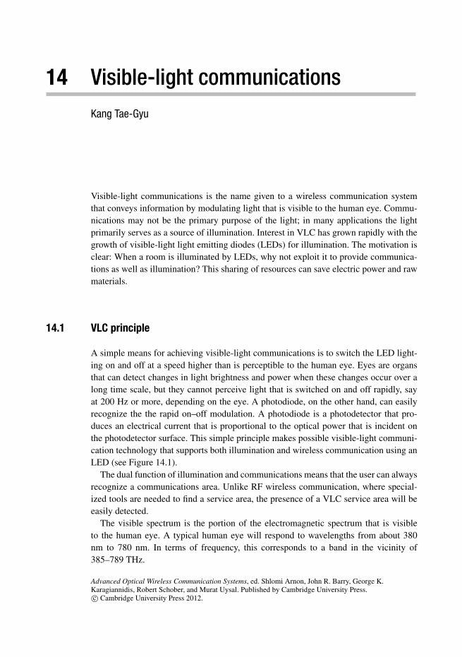
14 Visible-light communicationsKang Tae-Gyu
Visible-light communications is the name given to a wireless communication systemthat conveys information by modulating light that is visible to the human eye. Commu-nications may not be the primary purpose of the light; in many applications the lightprimarily serves as a source of illumination. Interest in VLC has grown rapidly with thegrowth of visible-light light emitting diodes (LEDs) for illumination. The motivation isclear: When a room is illuminated by LEDs, why not exploit it to provide communica-tions as well as illumination? This sharing of resources can save electric power and rawmaterials.
14.1 VLC principle
A simple means for achieving visible-light communications is to switch the LED light-ing on and off at a speed higher than is perceptible to the human eye. Eyes are organsthat can detect changes in light brightness and power when these changes occur over along time scale, but they cannot perceive light that is switched on and off rapidly, sayat 200 Hz or more, depending on the eye. A photodiode, on the other hand, can easilyrecognize the the rapid on–off modulation. A photodiode is a photodetector that pro-duces an electrical current that is proportional to the optical power that is incident onthe photodetector surface. This simple principle makes possible visible-light communi-cation technology that supports both illumination and wireless communication using anLED (see Figure 14.1).
The dual function of illumination and communications means that the user can alwaysrecognize a communications area. Unlike RF wireless communication, where special-ized tools are needed to find a service area, the presence of a VLC service area will beeasily detected.
The visible spectrum is the portion of the electromagnetic spectrum that is visibleto the human eye. A typical human eye will respond to wavelengths from about 380nm to 780 nm. In terms of frequency, this corresponds to a band in the vicinity of385–789 THz.
Advanced Optical Wireless Communication Systems, ed. Shlomi Arnon, John R. Barry, George K.Karagiannidis, Robert Schober, and Murat Uysal. Published by Cambridge University Press.c© Cambridge University Press 2012.
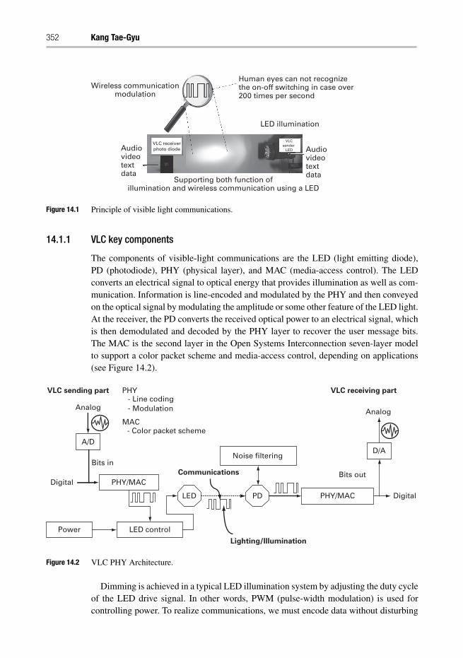
352 Kang Tae-Gyu
Human eyes can not recognizethe on-off switching in case over200 times per second
Wireless communicationmodulation
Audiovideotextdata
Audiovideotextdata
LED illumination
VLC receiverphoto diode
VLCsender
LED
Supporting both function ofillumination and wireless communication using a LED
Figure 14.1 Principle of visible light communications.
14.1.1 VLC key components
The components of visible-light communications are the LED (light emitting diode),PD (photodiode), PHY (physical layer), and MAC (media-access control). The LEDconverts an electrical signal to optical energy that provides illumination as well as com-munication. Information is line-encoded and modulated by the PHY and then conveyedon the optical signal by modulating the amplitude or some other feature of the LED light.At the receiver, the PD converts the received optical power to an electrical signal, whichis then demodulated and decoded by the PHY layer to recover the user message bits.The MAC is the second layer in the Open Systems Interconnection seven-layer modelto support a color packet scheme and media-access control, depending on applications(see Figure 14.2).
PHY
MAC
VLC sending part VLC receiving part
Communications
Lighting/Illumination
- Line coding
- Color packet scheme
Analog Analog
A/DD/A
Bits in
Bits outPHY/MAC
PHY/MAC
LED controlPower
Digital
Digital
Noise filtering
PDLED
- Modulation
Figure 14.2 VLC PHY Architecture.
Dimming is achieved in a typical LED illumination system by adjusting the duty cycleof the LED drive signal. In other words, PWM (pulse-width modulation) is used forcontrolling power. To realize communications, we must encode data without disturbing
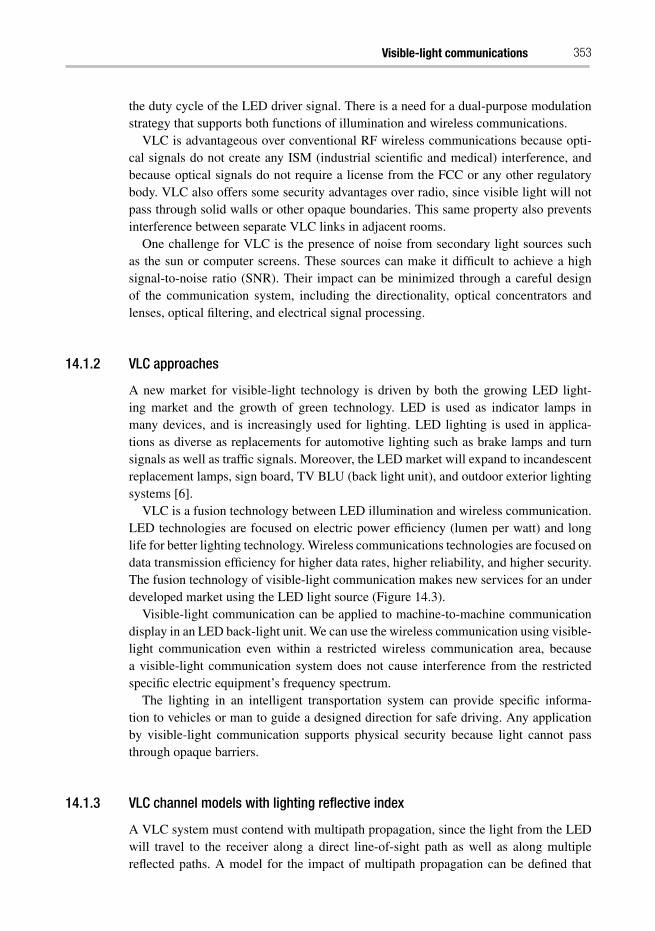
Visible-light communications 353
the duty cycle of the LED driver signal. There is a need for a dual-purpose modulationstrategy that supports both functions of illumination and wireless communications.
VLC is advantageous over conventional RF wireless communications because opti-cal signals do not create any ISM (industrial scientific and medical) interference, andbecause optical signals do not require a license from the FCC or any other regulatorybody. VLC also offers some security advantages over radio, since visible light will notpass through solid walls or other opaque boundaries. This same property also preventsinterference between separate VLC links in adjacent rooms.
One challenge for VLC is the presence of noise from secondary light sources suchas the sun or computer screens. These sources can make it difficult to achieve a highsignal-to-noise ratio (SNR). Their impact can be minimized through a careful designof the communication system, including the directionality, optical concentrators andlenses, optical filtering, and electrical signal processing.
14.1.2 VLC approaches
A new market for visible-light technology is driven by both the growing LED light-ing market and the growth of green technology. LED is used as indicator lamps inmany devices, and is increasingly used for lighting. LED lighting is used in applica-tions as diverse as replacements for automotive lighting such as brake lamps and turnsignals as well as traffic signals. Moreover, the LED market will expand to incandescentreplacement lamps, sign board, TV BLU (back light unit), and outdoor exterior lightingsystems [6].
VLC is a fusion technology between LED illumination and wireless communication.LED technologies are focused on electric power efficiency (lumen per watt) and longlife for better lighting technology. Wireless communications technologies are focused ondata transmission efficiency for higher data rates, higher reliability, and higher security.The fusion technology of visible-light communication makes new services for an underdeveloped market using the LED light source (Figure 14.3).
Visible-light communication can be applied to machine-to-machine communicationdisplay in an LED back-light unit. We can use the wireless communication using visible-light communication even within a restricted wireless communication area, becausea visible-light communication system does not cause interference from the restrictedspecific electric equipment’s frequency spectrum.
The lighting in an intelligent transportation system can provide specific informa-tion to vehicles or man to guide a designed direction for safe driving. Any applicationby visible-light communication supports physical security because light cannot passthrough opaque barriers.
14.1.3 VLC channel models with lighting reflective index
A VLC system must contend with multipath propagation, since the light from the LEDwill travel to the receiver along a direct line-of-sight path as well as along multiplereflected paths. A model for the impact of multipath propagation can be defined that
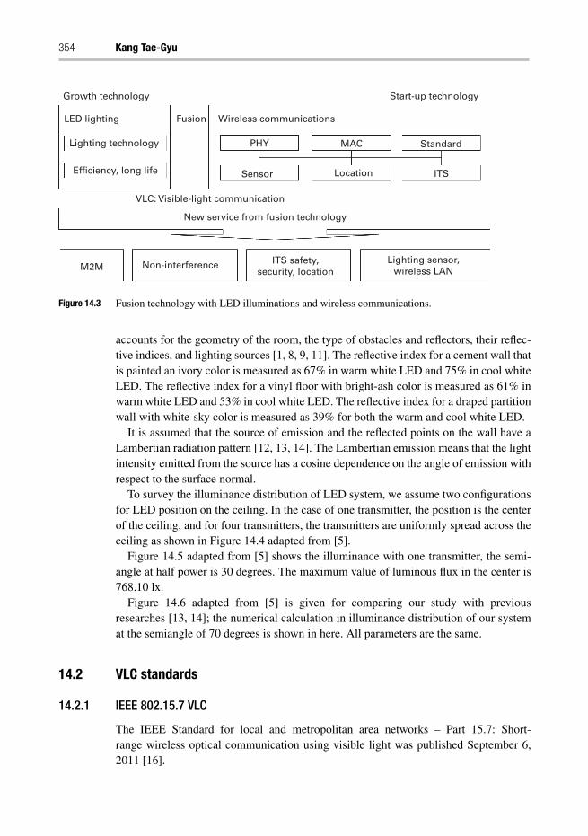
354 Kang Tae-Gyu
Growth technology
LED lighting Fusion Wireless communications
Start-up technology
StandardMACPHY
Sensor
VLC: Visible-light communication
New service from fusion technology
Location ITS
Lighting technology
Efficiency, long life
M2M Non-interference ITS safety,security, location
Lighting sensor,wireless LAN
Figure 14.3 Fusion technology with LED illuminations and wireless communications.
accounts for the geometry of the room, the type of obstacles and reflectors, their reflec-tive indices, and lighting sources [1, 8, 9, 11]. The reflective index for a cement wall thatis painted an ivory color is measured as 67% in warm white LED and 75% in cool whiteLED. The reflective index for a vinyl floor with bright-ash color is measured as 61% inwarm white LED and 53% in cool white LED. The reflective index for a draped partitionwall with white-sky color is measured as 39% for both the warm and cool white LED.
It is assumed that the source of emission and the reflected points on the wall have aLambertian radiation pattern [12, 13, 14]. The Lambertian emission means that the lightintensity emitted from the source has a cosine dependence on the angle of emission withrespect to the surface normal.
To survey the illuminance distribution of LED system, we assume two configurationsfor LED position on the ceiling. In the case of one transmitter, the position is the centerof the ceiling, and for four transmitters, the transmitters are uniformly spread across theceiling as shown in Figure 14.4 adapted from [5].
Figure 14.5 adapted from [5] shows the illuminance with one transmitter, the semi-angle at half power is 30 degrees. The maximum value of luminous flux in the center is768.10 lx.
Figure 14.6 adapted from [5] is given for comparing our study with previousresearches [13, 14]; the numerical calculation in illuminance distribution of our systemat the semiangle of 70 degrees is shown in here. All parameters are the same.
14.2 VLC standards
14.2.1 IEEE 802.15.7 VLC
The IEEE Standard for local and metropolitan area networks – Part 15.7: Short-range wireless optical communication using visible light was published September 6,2011 [16].
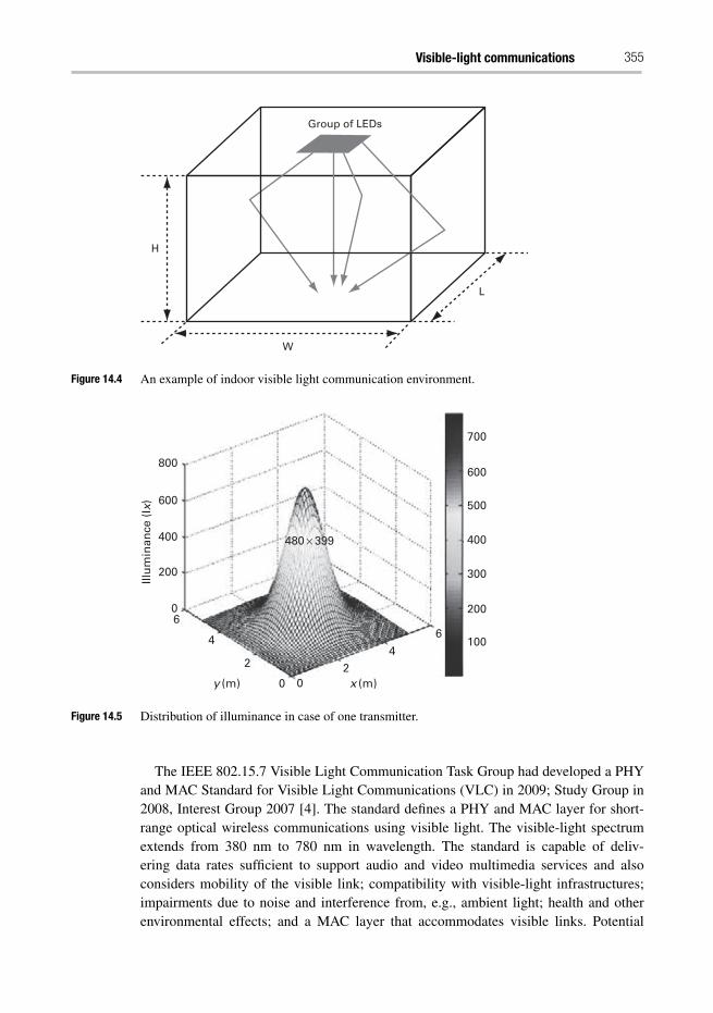
Visible-light communications 355
Group of LEDs
L
W
H
Figure 14.4 An example of indoor visible light communication environment.
700
600
500
400
300
200
1004
480 × 399
6
20 x (m)y (m) 0
2
4
60
200
400
600
800
Illu
min
ance
(Ix
)
Figure 14.5 Distribution of illuminance in case of one transmitter.
The IEEE 802.15.7 Visible Light Communication Task Group had developed a PHYand MAC Standard for Visible Light Communications (VLC) in 2009; Study Group in2008, Interest Group 2007 [4]. The standard defines a PHY and MAC layer for short-range optical wireless communications using visible light. The visible-light spectrumextends from 380 nm to 780 nm in wavelength. The standard is capable of deliv-ering data rates sufficient to support audio and video multimedia services and alsoconsiders mobility of the visible link; compatibility with visible-light infrastructures;impairments due to noise and interference from, e.g., ambient light; health and otherenvironmental effects; and a MAC layer that accommodates visible links. Potential
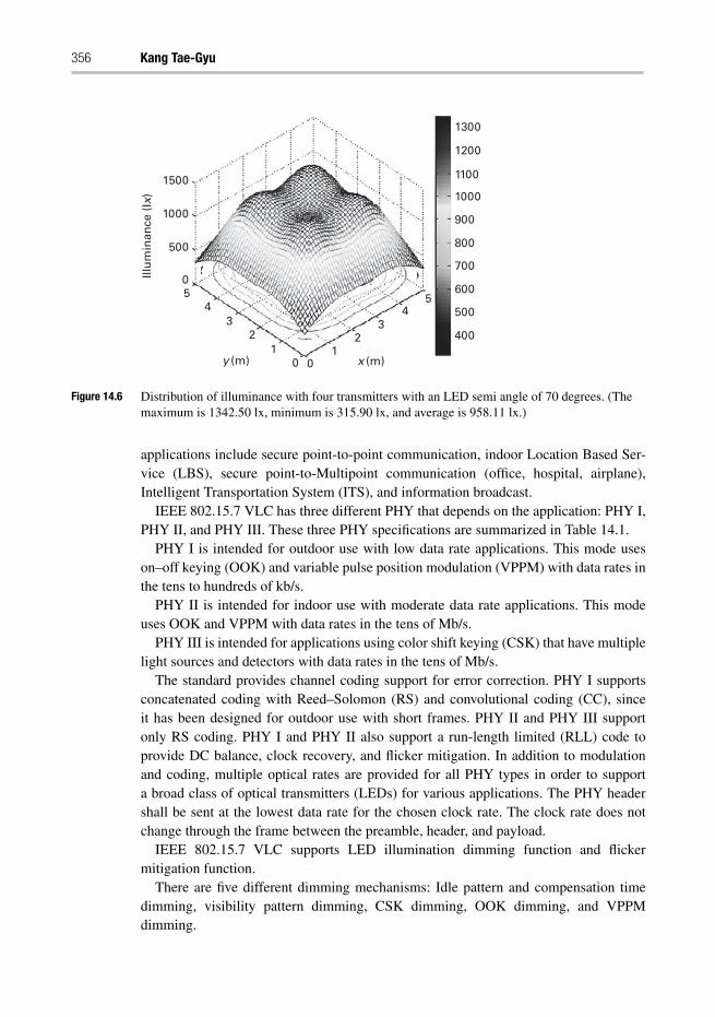
356 Kang Tae-Gyu
1300
1200
1100
1000
900
800
700
600
500
400
00y (m) x (m)1
23
450
500
1000
1500
Illu
min
ance
(Ix
)
12
34
5
Figure 14.6 Distribution of illuminance with four transmitters with an LED semi angle of 70 degrees. (Themaximum is 1342.50 lx, minimum is 315.90 lx, and average is 958.11 lx.)
applications include secure point-to-point communication, indoor Location Based Ser-vice (LBS), secure point-to-Multipoint communication (office, hospital, airplane),Intelligent Transportation System (ITS), and information broadcast.
IEEE 802.15.7 VLC has three different PHY that depends on the application: PHY I,PHY II, and PHY III. These three PHY specifications are summarized in Table 14.1.
PHY I is intended for outdoor use with low data rate applications. This mode useson–off keying (OOK) and variable pulse position modulation (VPPM) with data rates inthe tens to hundreds of kb/s.
PHY II is intended for indoor use with moderate data rate applications. This modeuses OOK and VPPM with data rates in the tens of Mb/s.
PHY III is intended for applications using color shift keying (CSK) that have multiplelight sources and detectors with data rates in the tens of Mb/s.
The standard provides channel coding support for error correction. PHY I supportsconcatenated coding with Reed–Solomon (RS) and convolutional coding (CC), sinceit has been designed for outdoor use with short frames. PHY II and PHY III supportonly RS coding. PHY I and PHY II also support a run-length limited (RLL) code toprovide DC balance, clock recovery, and flicker mitigation. In addition to modulationand coding, multiple optical rates are provided for all PHY types in order to supporta broad class of optical transmitters (LEDs) for various applications. The PHY headershall be sent at the lowest data rate for the chosen clock rate. The clock rate does notchange through the frame between the preamble, header, and payload.
IEEE 802.15.7 VLC supports LED illumination dimming function and flickermitigation function.
There are five different dimming mechanisms: Idle pattern and compensation timedimming, visibility pattern dimming, CSK dimming, OOK dimming, and VPPMdimming.
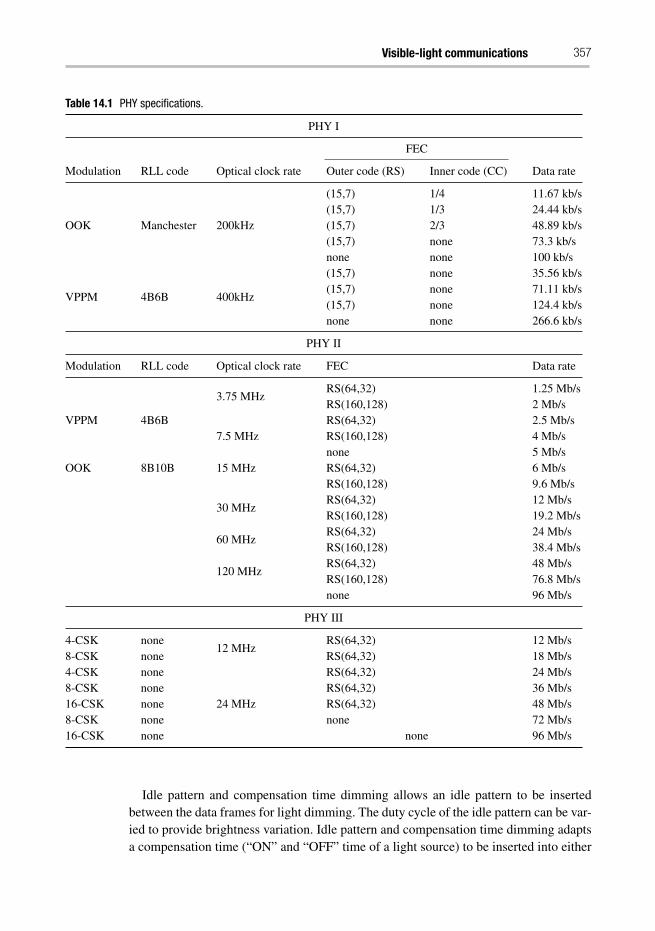
Visible-light communications 357
Table 14.1 PHY specifications.
PHY I
FEC
Modulation RLL code Optical clock rate Outer code (RS) Inner code (CC) Data rate
OOK Manchester 200kHz
(15,7) 1/4 11.67 kb/s(15,7) 1/3 24.44 kb/s(15,7) 2/3 48.89 kb/s(15,7) none 73.3 kb/snone none 100 kb/s
VPPM 4B6B 400kHz
(15,7) none 35.56 kb/s(15,7) none 71.11 kb/s(15,7) none 124.4 kb/snone none 266.6 kb/s
PHY II
Modulation RLL code Optical clock rate FEC Data rate
VPPM 4B6B
3.75 MHzRS(64,32) 1.25 Mb/sRS(160,128) 2 Mb/s
7.5 MHzRS(64,32) 2.5 Mb/sRS(160,128) 4 Mb/snone 5 Mb/s
OOK 8B10B 15 MHz RS(64,32) 6 Mb/sRS(160,128) 9.6 Mb/s
30 MHzRS(64,32) 12 Mb/sRS(160,128) 19.2 Mb/s
60 MHzRS(64,32) 24 Mb/sRS(160,128) 38.4 Mb/s
120 MHzRS(64,32) 48 Mb/sRS(160,128) 76.8 Mb/snone 96 Mb/s
PHY III
4-CSK none12 MHz
RS(64,32) 12 Mb/s8-CSK none RS(64,32) 18 Mb/s4-CSK none
24 MHz
RS(64,32) 24 Mb/s8-CSK none RS(64,32) 36 Mb/s16-CSK none RS(64,32) 48 Mb/s8-CSK none none 72 Mb/s16-CSK none none 96 Mb/s
Idle pattern and compensation time dimming allows an idle pattern to be insertedbetween the data frames for light dimming. The duty cycle of the idle pattern can be var-ied to provide brightness variation. Idle pattern and compensation time dimming adaptsa compensation time (“ON” and “OFF” time of a light source) to be inserted into either
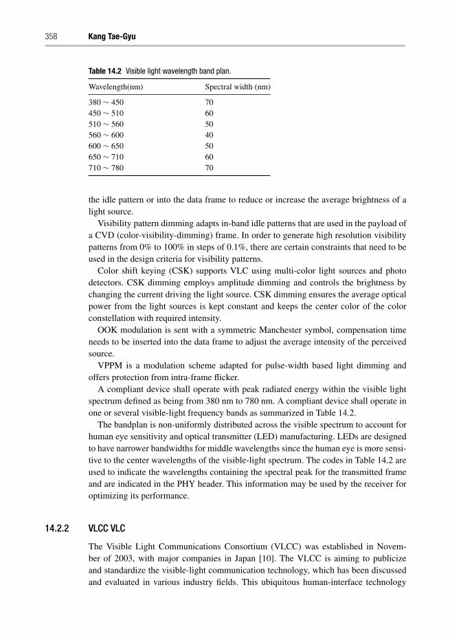
358 Kang Tae-Gyu
Table 14.2 Visible light wavelength band plan.
Wavelength(nm) Spectral width (nm)
380 ∼ 450 70450 ∼ 510 60510 ∼ 560 50560 ∼ 600 40600 ∼ 650 50650 ∼ 710 60710 ∼ 780 70
the idle pattern or into the data frame to reduce or increase the average brightness of alight source.
Visibility pattern dimming adapts in-band idle patterns that are used in the payload ofa CVD (color-visibility-dimming) frame. In order to generate high resolution visibilitypatterns from 0% to 100% in steps of 0.1%, there are certain constraints that need to beused in the design criteria for visibility patterns.
Color shift keying (CSK) supports VLC using multi-color light sources and photodetectors. CSK dimming employs amplitude dimming and controls the brightness bychanging the current driving the light source. CSK dimming ensures the average opticalpower from the light sources is kept constant and keeps the center color of the colorconstellation with required intensity.
OOK modulation is sent with a symmetric Manchester symbol, compensation timeneeds to be inserted into the data frame to adjust the average intensity of the perceivedsource.
VPPM is a modulation scheme adapted for pulse-width based light dimming andoffers protection from intra-frame flicker.
A compliant device shall operate with peak radiated energy within the visible lightspectrum defined as being from 380 nm to 780 nm. A compliant device shall operate inone or several visible-light frequency bands as summarized in Table 14.2.
The bandplan is non-uniformly distributed across the visible spectrum to account forhuman eye sensitivity and optical transmitter (LED) manufacturing. LEDs are designedto have narrower bandwidths for middle wavelengths since the human eye is more sensi-tive to the center wavelengths of the visible-light spectrum. The codes in Table 14.2 areused to indicate the wavelengths containing the spectral peak for the transmitted frameand are indicated in the PHY header. This information may be used by the receiver foroptimizing its performance.
14.2.2 VLCC VLC
The Visible Light Communications Consortium (VLCC) was established in Novem-ber of 2003, with major companies in Japan [10]. The VLCC is aiming to publicizeand standardize the visible-light communication technology, which has been discussedand evaluated in various industry fields. This ubiquitous human-interface technology
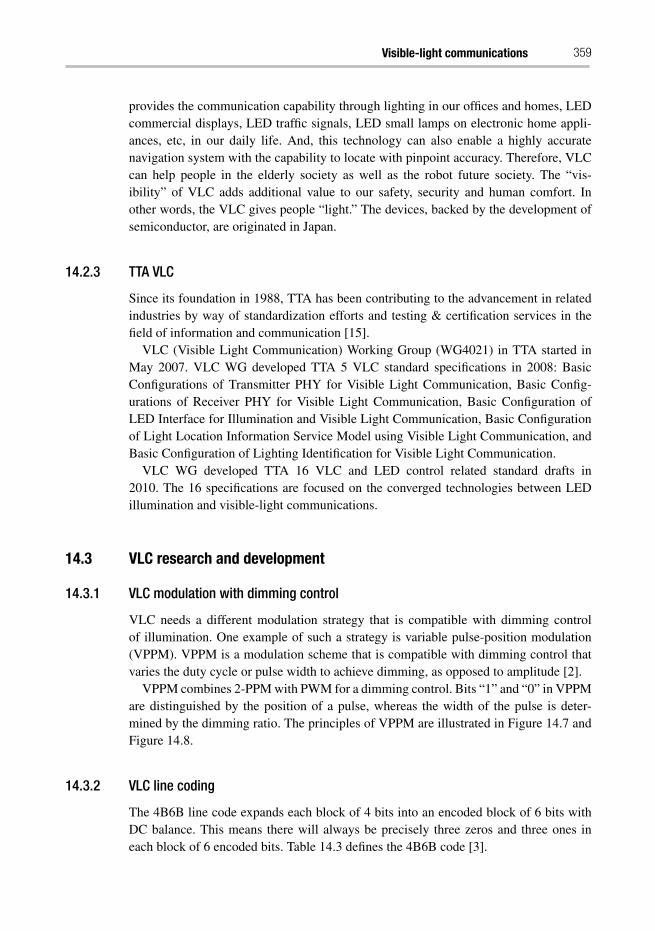
Visible-light communications 359
provides the communication capability through lighting in our offices and homes, LEDcommercial displays, LED traffic signals, LED small lamps on electronic home appli-ances, etc, in our daily life. And, this technology can also enable a highly accuratenavigation system with the capability to locate with pinpoint accuracy. Therefore, VLCcan help people in the elderly society as well as the robot future society. The “vis-ibility” of VLC adds additional value to our safety, security and human comfort. Inother words, the VLC gives people “light.” The devices, backed by the development ofsemiconductor, are originated in Japan.
14.2.3 TTA VLC
Since its foundation in 1988, TTA has been contributing to the advancement in relatedindustries by way of standardization efforts and testing & certification services in thefield of information and communication [15].
VLC (Visible Light Communication) Working Group (WG4021) in TTA started inMay 2007. VLC WG developed TTA 5 VLC standard specifications in 2008: BasicConfigurations of Transmitter PHY for Visible Light Communication, Basic Config-urations of Receiver PHY for Visible Light Communication, Basic Configuration ofLED Interface for Illumination and Visible Light Communication, Basic Configurationof Light Location Information Service Model using Visible Light Communication, andBasic Configuration of Lighting Identification for Visible Light Communication.
VLC WG developed TTA 16 VLC and LED control related standard drafts in2010. The 16 specifications are focused on the converged technologies between LEDillumination and visible-light communications.
14.3 VLC research and development
14.3.1 VLC modulation with dimming control
VLC needs a different modulation strategy that is compatible with dimming controlof illumination. One example of such a strategy is variable pulse-position modulation(VPPM). VPPM is a modulation scheme that is compatible with dimming control thatvaries the duty cycle or pulse width to achieve dimming, as opposed to amplitude [2].
VPPM combines 2-PPM with PWM for a dimming control. Bits “1” and “0” in VPPMare distinguished by the position of a pulse, whereas the width of the pulse is deter-mined by the dimming ratio. The principles of VPPM are illustrated in Figure 14.7 andFigure 14.8.
14.3.2 VLC line coding
The 4B6B line code expands each block of 4 bits into an encoded block of 6 bits withDC balance. This means there will always be precisely three zeros and three ones ineach block of 6 encoded bits. Table 14.3 defines the 4B6B code [3].
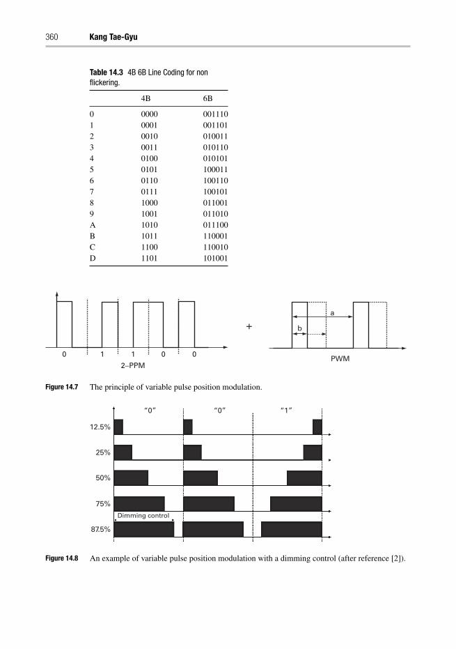
360 Kang Tae-Gyu
Table 14.3 4B 6B Line Coding for nonflickering.
4B 6B
0 0000 0011101 0001 0011012 0010 0100113 0011 0101104 0100 0101015 0101 1000116 0110 1001107 0111 1001018 1000 0110019 1001 011010A 1010 011100B 1011 110001C 1100 110010D 1101 101001
0 0 0
+
2−PPMPWM
a
b
1 1
Figure 14.7 The principle of variable pulse position modulation.
12.5%
“0” “0” “1”
25%
50%
75%
Dimming control
87.5%
Figure 14.8 An example of variable pulse position modulation with a dimming control (after reference [2]).
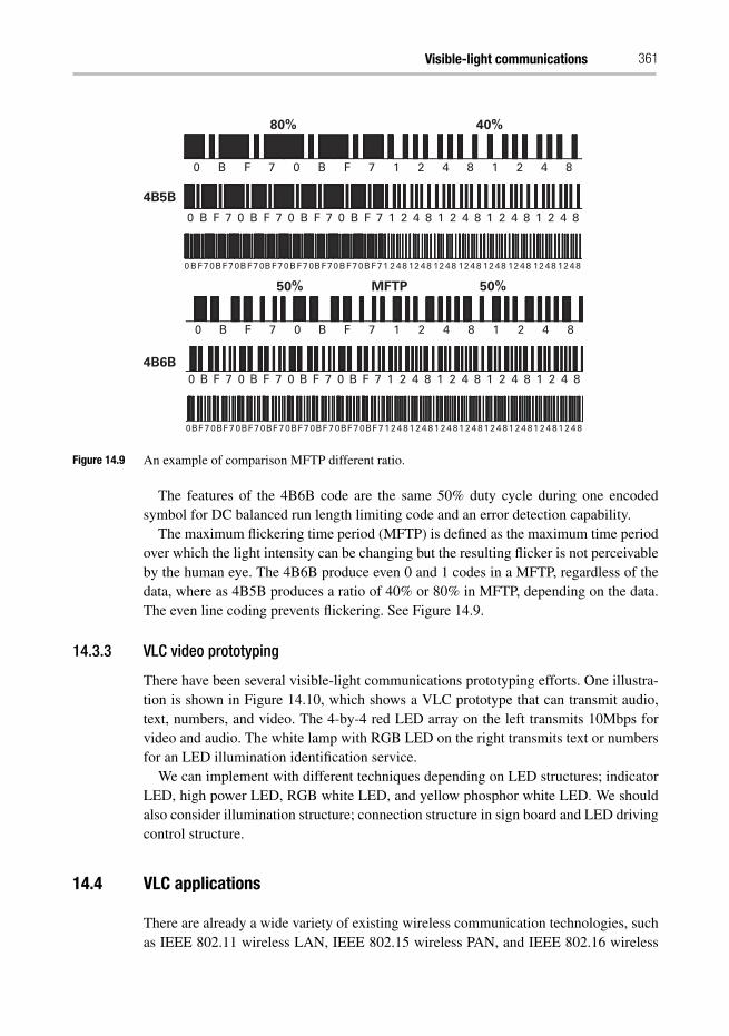
Visible-light communications 361
0 B F 7 B F 7 1 2 4 8 1 2 4 80
0 B F 7 B F 7 1 2 4 8 1 2 4 80
0 B F 7 0
0BF 7 0BF 7 0BF 7 0BF 7 0BF 7 0BF 7 0BF 7 0BF 7 1
0BF70BF70BF70BF70BF70BF70BF70BF71
2 4 8 2 4 81 2 4 81 2 4 81 2 4 81 2 4 81 2 4 81 2 4 81
2 48 2 481 2 481 2 481 2 481 2 481 2 481 2 481
B F 7 0 B F 7 0 B F 7 1 2 4 8 1 2 4 8 1 2 4 8 1 2 4 8
0 B F 7 0 B F 7 0 B F 7 0 B F 7 1 2 4 8 1 2 4 8 1 2 4 8 1 2 4 8
4B5B
MFTP
80% 40%
50%50%
4B6B
Figure 14.9 An example of comparison MFTP different ratio.
The features of the 4B6B code are the same 50% duty cycle during one encodedsymbol for DC balanced run length limiting code and an error detection capability.
The maximum flickering time period (MFTP) is defined as the maximum time periodover which the light intensity can be changing but the resulting flicker is not perceivableby the human eye. The 4B6B produce even 0 and 1 codes in a MFTP, regardless of thedata, where as 4B5B produces a ratio of 40% or 80% in MFTP, depending on the data.The even line coding prevents flickering. See Figure 14.9.
14.3.3 VLC video prototyping
There have been several visible-light communications prototyping efforts. One illustra-tion is shown in Figure 14.10, which shows a VLC prototype that can transmit audio,text, numbers, and video. The 4-by-4 red LED array on the left transmits 10Mbps forvideo and audio. The white lamp with RGB LED on the right transmits text or numbersfor an LED illumination identification service.
We can implement with different techniques depending on LED structures; indicatorLED, high power LED, RGB white LED, and yellow phosphor white LED. We shouldalso consider illumination structure; connection structure in sign board and LED drivingcontrol structure.
14.4 VLC applications
There are already a wide variety of existing wireless communication technologies, suchas IEEE 802.11 wireless LAN, IEEE 802.15 wireless PAN, and IEEE 802.16 wireless
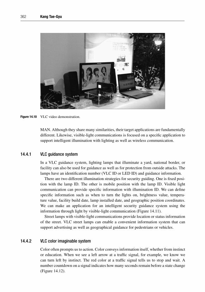
362 Kang Tae-Gyu
Figure 14.10 VLC video demonstration.
MAN. Although they share many similarities, their target applications are fundamentallydifferent. Likewise, visible-light communications is focused on a specific application tosupport intelligent illumination with lighting as well as wireless communication.
14.4.1 VLC guidance system
In a VLC guidance system, lighting lamps that illuminate a yard, national border, orfacility can also be used for guidance as well as for protection from outside attacks. Thelamps have an identification number (VLC ID or LED ID) and guidance information.
There are two different illumination strategies for security guiding. One is fixed posi-tion with the lamp ID. The other is mobile position with the lamp ID. Visible lightcommunication can provide specific information with illumination ID. We can definespecific information such as when to turn the lights on, brightness value, tempera-ture value, facility build date, lamp installed date, and geographic position coordinates.We can make an application for an intelligent security guidance system using theinformation through light by visible-light communication (Figure 14.11).
Street lamps with visible-light communications provide location or status informationof the street. VLC street lamps can enable a convenient information system that cansupport advertising as well as geographical guidance for pedestrians or vehicles.
14.4.2 VLC color imaginable system
Color often prompts us to action. Color conveys information itself, whether from instinctor education. When we see a left arrow at a traffic signal, for example, we know wecan turn left by instinct. The red color at a traffic signal tells us to stop and wait. Anumber countdown on a signal indicates how many seconds remain before a state change(Figure 14.12).
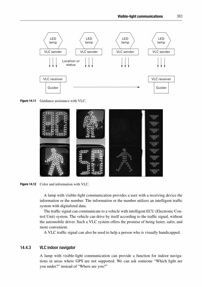
Visible-light communications 363
LEDlamp
LEDlamp
LEDlamp
LEDlamp
VLC senderVLC senderVLC sender
Location orstatus
VLC sender
VLC receiver VLC receiver
Guider Guider
Figure 14.11 Guidance assistance with VLC.
Figure 14.12 Color and information with VLC.
A lamp with visible-light communication provides a user with a receiving device theinformation or the number. The information or the number utilizes an intelligent trafficsystem with digitalized data.
The traffic signal can communicate to a vehicle with intelligent ECU (Electronic Con-trol Unit) system. The vehicle can drive by itself according to the traffic signal, withoutthe automobile driver. Such a VLC system offers the promise of being faster, safer, andmore convenient.
A VLC traffic signal can also be used to help a person who is visually handicapped.
14.4.3 VLC indoor navigator
A lamp with visible-light communication can provide a function for indoor naviga-tions in areas where GPS are not supported. We can ask someone “Which light areyou under?” instead of “Where are you?”
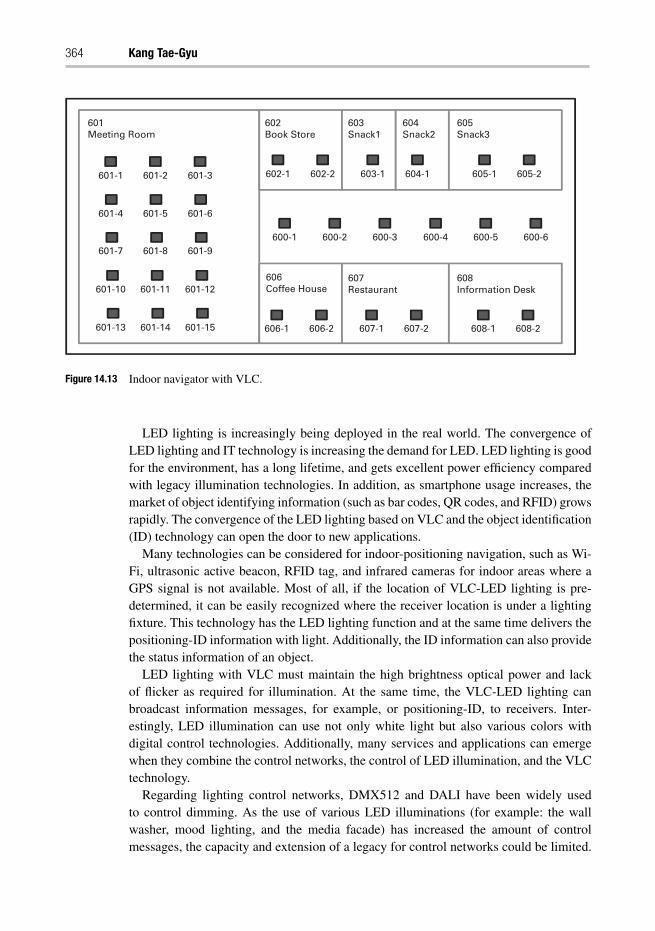
364 Kang Tae-Gyu
601Meeting Room
602Book Store
603Snack1
604Snack2
605Snack3
606Coffee House
607Restaurant
608Information Desk
601-1 601-2 601-3
601-4 601-5 601-6
601-7 601-8 601-9
601-10 601-11 601-12
601-13 601-14 601-15
602-1 602-2 603-1 604-1 605-1 605-2
606-1 606-2 607-1 607-2 608-1 608-2
600-1 600-2 600-3 600-4 600-5 600-6
Figure 14.13 Indoor navigator with VLC.
LED lighting is increasingly being deployed in the real world. The convergence ofLED lighting and IT technology is increasing the demand for LED. LED lighting is goodfor the environment, has a long lifetime, and gets excellent power efficiency comparedwith legacy illumination technologies. In addition, as smartphone usage increases, themarket of object identifying information (such as bar codes, QR codes, and RFID) growsrapidly. The convergence of the LED lighting based on VLC and the object identification(ID) technology can open the door to new applications.
Many technologies can be considered for indoor-positioning navigation, such as Wi-Fi, ultrasonic active beacon, RFID tag, and infrared cameras for indoor areas where aGPS signal is not available. Most of all, if the location of VLC-LED lighting is pre-determined, it can be easily recognized where the receiver location is under a lightingfixture. This technology has the LED lighting function and at the same time delivers thepositioning-ID information with light. Additionally, the ID information can also providethe status information of an object.
LED lighting with VLC must maintain the high brightness optical power and lackof flicker as required for illumination. At the same time, the VLC-LED lighting canbroadcast information messages, for example, or positioning-ID, to receivers. Inter-estingly, LED illumination can use not only white light but also various colors withdigital control technologies. Additionally, many services and applications can emergewhen they combine the control networks, the control of LED illumination, and the VLCtechnology.
Regarding lighting control networks, DMX512 and DALI have been widely usedto control dimming. As the use of various LED illuminations (for example: the wallwasher, mood lighting, and the media facade) has increased the amount of controlmessages, the capacity and extension of a legacy for control networks could be limited.
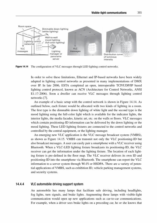
Visible-light communications 365
Room spaceDimmable down lighting(white lighting)
VLCmessages
VLCmessagesLighting
manager orpanorama
server
Distribution curveof luminousintensity
Wall-to-wallmood lighting(full-color lighting)Lighting control
networks
Figure 14.14 The configuration of VLC messages through LED lighting control networks.
In order to solve these limitations, Ethernet and IP-based networks have been widelyadapted in lighting control networks as presented in many implementations of DMXover IP. In late 2006, ESTA completed an open, interoperable TCP/UDP/IP basedlighting control protocol, known as ACN (Architecture for Control Networks, ANSIE1.17-2006). Soon a dweller can receive VLC messages through lighting controlnetworks [7].
An example of a basic setup with the control network is shown in Figure 14.14. Asoutlined below, each fixture would be allocated with two kinds of lighting in a room.The first type is the dimmable down lighting of white light and the second type is themood lighting using the full-color light which is available for the indicator lights, theinterior lights, the media facades, kinetic art, etc. on the walls or floors. VLC messageswhich contain positioning-ID information can be delivered by the down lighting or themood lighting. These LED lighting fixtures are connected to the control networks andcontrolled by the central equipment, or the lighting manager.
An emerging new VLC application is the VLC message broadcast system (VMBS),as shown as Figure 14.15. VMBS can transmit not only the VLC positioning-ID butalso broadcast messages. A user can easily pair a smartphone with a VLC receiver usingBluetooth. When a VLC-LED lighting fixture broadcasts its positioning-ID, the VLCreceiver can get the information under the lighting fixture. The location of each light-ing fixture is pre-defined in the floor map. The VLC receiver delivers its own ID andpositioning-ID into the smartphone via Bluetooth. The smartphone can report the VLCinformation to a server system through Wi-Fi or HSDPA. There are a variety of poten-tial applications of VMBS, such as exhibition ID, vehicle parking management systems,and security systems.
14.4.4 VLC automobile driving support system
An automobile has many lamps that facilitate safe driving, including headlights,fog lights, turn signals, and brake lights. Augmenting these lamps with visible-lightcommunication would open up new applications such as car-to-car communications.For example, when a driver sees brake lights on a preceding car, he or she knows that
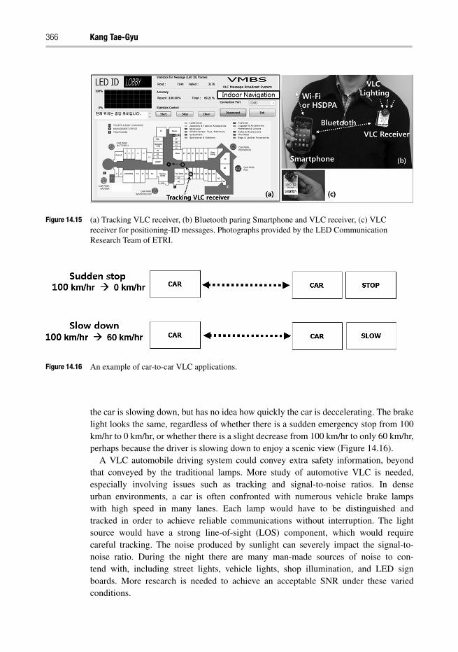
366 Kang Tae-Gyu
Figure 14.15 (a) Tracking VLC receiver, (b) Bluetooth paring Smartphone and VLC receiver, (c) VLCreceiver for positioning-ID messages. Photographs provided by the LED CommunicationResearch Team of ETRI.
Figure 14.16 An example of car-to-car VLC applications.
the car is slowing down, but has no idea how quickly the car is deccelerating. The brakelight looks the same, regardless of whether there is a sudden emergency stop from 100km/hr to 0 km/hr, or whether there is a slight decrease from 100 km/hr to only 60 km/hr,perhaps because the driver is slowing down to enjoy a scenic view (Figure 14.16).
A VLC automobile driving system could convey extra safety information, beyondthat conveyed by the traditional lamps. More study of automotive VLC is needed,especially involving issues such as tracking and signal-to-noise ratios. In denseurban environments, a car is often confronted with numerous vehicle brake lampswith high speed in many lanes. Each lamp would have to be distinguished andtracked in order to achieve reliable communications without interruption. The lightsource would have a strong line-of-sight (LOS) component, which would requirecareful tracking. The noise produced by sunlight can severely impact the signal-to-noise ratio. During the night there are many man-made sources of noise to con-tend with, including street lights, vehicle lights, shop illumination, and LED signboards. More research is needed to achieve an acceptable SNR under these variedconditions.
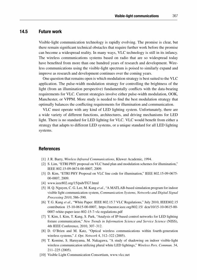
Visible-light communications 367
14.5 Future work
Visible-light communication technology is rapidly evolving. The promise is clear, butthere remain significant technical obstacles that require further work before the promisecan become a widespread reality. In many ways, VLC technology is still in its infancy.The wireless communications systems based on radio that are so widespread todayhave benefited from more than one hundred years of research and development. Wire-less communications using the visible-light spectrum is poised to similarly expand andimprove as research and development continues over the coming years.
One question that remains open is which modulation strategy is best suited to the VLCapplication. The pulse-width modulation strategy for controlling the brightness of thelight (from an illumination perspective) fundamentally conflicts with the data-bearingrequirements for VLC. Current strategies involve either pulse-width modulation, OOK,Manchester, or VPPM. More study is needed to find the best modulation strategy thatoptimally balances the conflicting requirements for illumination and communication.
VLC must operate with any kind of LED lighting system. Unfortunately, there area wide variety of different functions, architectures, and driving mechanisms for LEDlight. There is no standard for LED lighting for VLC. VLC would benefit from either astrategy that adapts to different LED systems, or a unique standard for all LED lightingsystems.
References
[1] J. R. Barry, Wireless Infrared Communications, Kluwer Academic, 1994.[2] S. Lim, “ETRI PHY proposal on VLC band plan and modulation schemes for illumination,”
IEEE 802.15-09-0674-00-0007, 2009.[3] D. Kim, “ETRI PHY Proposal on VLC line code for illumination,” IEEE 802.15-09-0675-
00-0007, 2009.[4] www.ieee802.org/15/pub/TG7.html[5] H. Q. Nguyen, C. G. Lee, M. Kang et al., “A MATLAB-based simulation program for indoor
visible light communication system, Communication Systems, Networks and Digital SignalProcessing 2010, 586–590.
[6] T. G. Kang et al., “White Paper: IEEE 802.15.7 VLC Regulations,” July 2010, IEEE802.15contribution 15-10-0615-00-0007, https://mentor.ieee.org/802.15/ dcn/10/15-10-0615-00-0007-white-paper-ieee-802-15-7-vlc-regulations.pdf
[7] Y. Kim, I. Kim, T. Kang, S. Park, “Analysis of IP-based control networks for LED lightingfixture communication,” New Trends in Information Science and Service Science (NISS),4th IEEE Conference, 2010, 307–312.
[8] D. O’Brien and M. Katz, “Optical wireless communications within fourth-generationwireless systems,” J. Opt. Network 4, 312–322 (2005).
[9] T. Komine, S. Haruyama, M. Nakagawa, “A study of shadowing on indoor visible-lightwireless communication utilizing plural white LED lightings,” Wireless Pers. Commun. 34,211–225 (2005).
[10] Visible Light Communication Consortium, www.vlcc.net
368 Kang Tae-Gyu
[11] D. C. O’Brien et al., Short-range optical wireless communications, Wireless WorldResearch Forum, 2007.
[12] J. M. Kahn and J. R. Barry, “Wireless infrared communications,” Proc. IEEE 85 (2),265–298 (1997).
[13] T. Komine and M. Nakagawa “Fundamental analysis for visible light communicationsystem using LED light,” IEEE Trans. Consum. Electron. 50, 100–107 (2004).
[14] T. Komine and M. Nakagawa, “Performance evaluation of visible-light wireless commu-nication system using white LED lighting,” Proceedings of the Ninth IEEE Symposium onComputers and Communications, 258–263 (2004).
[15] www.tta.or.kr/English/[16] IEEE Std. 802.15.7-2011, “IEEE Standard for local and metropolitan area networks – part
15.7: Short-range wireless optical communication using visible light,” 2011.
15 Optical wireless in sensor networksDominic C. O’Brien and Sashigaran Sivathasan
15.1 Introduction
Wireless sensor networks have been an active area of research for the past few decades[1, 2]. The availability of low-power radio communications, microprocessors, and sen-sors at low cost has led to highly capable sensor “motes” that can be connected inwireless networks (see for instance [3]). Environmental monitoring [2], monitoring ofstructures [4, 5], industrial process control [6], and mechanical systems [7] have allused wireless sensor networks, and such deployments are likely to become much morewidespread. The next generation of appliances and objects will be part of the Internet ofThings [8], and these will be connected wirelessly to each other and to an informationinfrastructure. Reduction in carbon emissions will require a smart electrical grid [9] thatallows for local generation of power and control of its use within the home at the appli-ance level. This will in turn require large numbers of sensors and actuators which willboth monitor and control generators and appliances.
In the field of healthcare the ageing population will lead to greater demands onresources, and home monitoring of patients has the potential to prolong life and qualityof life whilst reducing demands on resources. Body area networks of sensors are beingpursued as means to collect data to allow this [10].
A major challenge for sensor networks is that of prolonging sensor node lifetime,which is usually limited by battery capacity. An ideal sensor node would scavenge allthe energy required from its environment, and therefore have an “infinite” operatinglife, barring failure. There are many schemes to do this, including vibration, air, solar,and radio frequency (RF) energy harvesting [11, 12]. However, most commercial sensormotes require external batteries, which limit the life of the node.
Energy is consumed for sensing, processing and communications, and the balance ofthe energy demands of each of these is complex to determine. However, communica-tions using RF wireless forms a significant proportion of overall consumption in mostsensor nodes. This is due to the almost isotropic “broadcast” nature of the RF chan-nel, which leads to high path loss, and network architectures that require significantenergy to be expended on route discovery [13]. In addition the carrier-based RF trans-mission requires relatively complex and power-hungry transmitter and receiver stages.
Advanced Optical Wireless Communication Systems, ed. Shlomi Arnon, John R. Barry, George K.Karagiannidis, Robert Schober, and Murat Uysal. Published by Cambridge University Press.c© Cambridge University Press 2012.
370 Dominic C. O’Brien and Sashigaran Sivathasan
Careful management can reduce the need to communicate, by local processing of sensordata and communicating only when action is required, but communications still requiressignificant energy.
Point-to-point free-space optical (FSO) links have been successfully used betweenbuildings [14], ships [15], aircraft [16], earth and space [17], and from air-to-ground[18]. Free-space optical communications typically uses highly directed channels, andthese can have low path loss. In addition simple baseband modulation such as on–off-keying can be used, leading to low-complexity transmitter and receiver circuitry that canhave low power consumption. The lenses and mirrors that shape the transmitted beamand capture received radiation in these links can have high gain but be physically smalldue to the small wavelength of the transmitted radiation.
There are therefore potential advantages in using such links for communicationsbetween sensors, but substantial technical challenges to be overcome. Some form ofpointing and tracking is required for these links to ensure that the beam of light froma transmitter hits the required receiver, which might be placed anywhere within thecoverage area. For most FSO links the terminals are fixed, so manual pointing isused when they are installed. Gimbal-based pointing and tracking are used in typi-cal mobile systems. An alternative is to arrange multiple transmitters and receiversthat each have a small field of view in such a way as to cover the much largerrequired field of view. Such an angle diversity configuration has been demonstratedin [19, 20]. A larger-scale network of atmospheric sensors that use optical communica-tions is proposed in [21, 22]. A Scottish research consortium on “speckled computing”has been investigating various aspects of connection between small computing nodesor specks, including beam-steering [23, 24] and the power consumption of free spacecommunication [25].
There has also been work on underwater sensor networks [26–30] and on topologycontrol of free-space sensor networks [31]. Most of this work considers line-of-sightoptical links, but diffuse networks have been proposed [29, 32]. In these ultra violetwavelengths in the solar blind region of the optical spectrum are used, and atmosphericscattering creates a non-line-of-sight (NLOS) channel to create a scattering channel,albeit at the cost of reduced range compared with a line of sight situation.
Retro-reflecting data links [33] (and see Chapter 13) simplify the design of suchsystems considerably. In this case light from a transmitting terminal propagates to thereceiving terminal, which contains a retro-reflector. Light that strikes the retro-reflectoris returned to the transmitter terminal by the action of the retro-reflector, creating thebi-directional optical paths required for communication. Information can be transmit-ted on the downlink path by modulating the source, and on the uplink by modulatingthe retro-reflector. This removes the need for a source and tracking at the retro-reflectorend of the link. In addition the “natural” architecture becomes that of a complex termi-nal or base station that can direct beams of light to simple sensor nodes equipped withretro-reflectors and communicate with them.
This has the potential advantages of a simplified architecture, in that a central nodecommunicates with all other nodes, and that the sensor nodes can potentially have lowpower consumption and complexity. However, a line of sight between nodes is required.
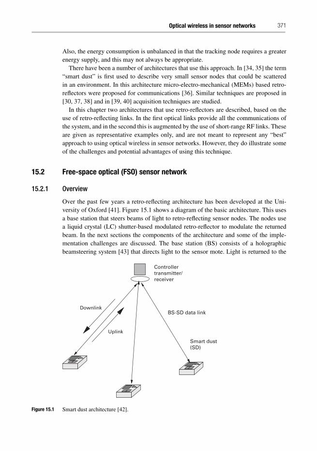
Optical wireless in sensor networks 371
Also, the energy consumption is unbalanced in that the tracking node requires a greaterenergy supply, and this may not always be appropriate.
There have been a number of architectures that use this approach. In [34, 35] the term“smart dust” is first used to describe very small sensor nodes that could be scatteredin an environment. In this architecture micro-electro-mechanical (MEMs) based retro-reflectors were proposed for communications [36]. Similar techniques are proposed in[30, 37, 38] and in [39, 40] acquisition techniques are studied.
In this chapter two architectures that use retro-reflectors are described, based on theuse of retro-reflecting links. In the first optical links provide all the communications ofthe system, and in the second this is augmented by the use of short-range RF links. Theseare given as representative examples only, and are not meant to represent any “best”approach to using optical wireless in sensor networks. However, they do illustrate someof the challenges and potential advantages of using this technique.
15.2 Free-space optical (FSO) sensor network
15.2.1 Overview
Over the past few years a retro-reflecting architecture has been developed at the Uni-versity of Oxford [41]. Figure 15.1 shows a diagram of the basic architecture. This usesa base station that steers beams of light to retro-reflecting sensor nodes. The nodes usea liquid crystal (LC) shutter-based modulated retro-reflector to modulate the returnedbeam. In the next sections the components of the architecture and some of the imple-mentation challenges are discussed. The base station (BS) consists of a holographicbeamsteering system [43] that directs light to the sensor mote. Light is returned to the
Controllertransmitter/receiver
Smart dust(SD)
BS-SD data linkDownlink
Uplink
Figure 15.1 Smart dust architecture [42].
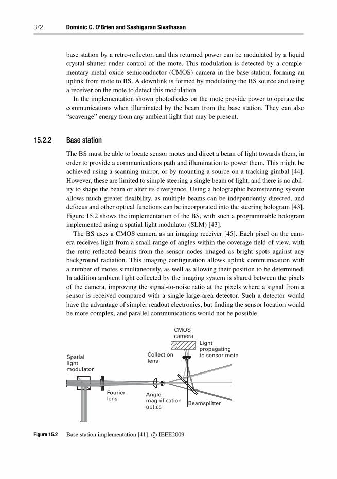
372 Dominic C. O’Brien and Sashigaran Sivathasan
base station by a retro-reflector, and this returned power can be modulated by a liquidcrystal shutter under control of the mote. This modulation is detected by a comple-mentary metal oxide semiconductor (CMOS) camera in the base station, forming anuplink from mote to BS. A downlink is formed by modulating the BS source and usinga receiver on the mote to detect this modulation.
In the implementation shown photodiodes on the mote provide power to operate thecommunications when illuminated by the beam from the base station. They can also“scavenge” energy from any ambient light that may be present.
15.2.2 Base station
The BS must be able to locate sensor motes and direct a beam of light towards them, inorder to provide a communications path and illumination to power them. This might beachieved using a scanning mirror, or by mounting a source on a tracking gimbal [44].However, these are limited to simple steering a single beam of light, and there is no abil-ity to shape the beam or alter its divergence. Using a holographic beamsteering systemallows much greater flexibility, as multiple beams can be independently directed, anddefocus and other optical functions can be incorporated into the steering hologram [43].Figure 15.2 shows the implementation of the BS, with such a programmable hologramimplemented using a spatial light modulator (SLM) [43].
The BS uses a CMOS camera as an imaging receiver [45]. Each pixel on the cam-era receives light from a small range of angles within the coverage field of view, withthe retro-reflected beams from the sensor nodes imaged as bright spots against anybackground radiation. This imaging configuration allows uplink communication witha number of motes simultaneously, as well as allowing their position to be determined.In addition ambient light collected by the imaging system is shared between the pixelsof the camera, improving the signal-to-noise ratio at the pixels where a signal from asensor is received compared with a single large-area detector. Such a detector wouldhave the advantage of simpler readout electronics, but finding the sensor location wouldbe more complex, and parallel communications would not be possible.
Spatiallightmodulator
Fourierlens
Anglemagnificationoptics
CMOScamera
Collectionlens
Beamsplitter
Lightpropagatingto sensor mote
Figure 15.2 Base station implementation [41]. c© IEEE2009.
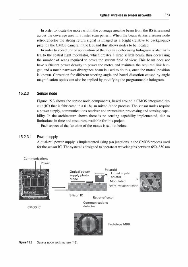
Optical wireless in sensor networks 373
In order to locate the motes within the coverage area the beam from the BS is scannedacross the coverage area in a raster scan pattern. When the beam strikes a sensor noderetro-reflector the strong return signal is imaged as a bright (relative to background)pixel on the CMOS camera in the BS, and this allows nodes to be located.
In order to speed up the acquisition of the motes a defocusing hologram is also writ-ten to the spatial light modulator, which creates a large search beam, thus decreasingthe number of scans required to cover the system field of view. This beam does nothave sufficient power density to power the motes and maintain the required link bud-get, and a much narrower divergence beam is used to do this, once the motes’ positionis known. Correction for different steering angle and barrel distortion caused by anglemagnification optics can also be applied by modifying the programmable hologram.
15.2.3 Sensor node
Figure 15.3 shows the sensor node components, based around a CMOS integrated cir-cuit (IC) that is fabricated in a 0.18 μm mixed-mode process. The sensor nodes requirea power supply, communications receiver and transmitter, processing and sensing capa-bility. In the architecture shown there is no sensing capability implemented, due tolimitations in time and resources available for this project.
Each aspect of the function of the motes is set out below.
15.2.3.1 Power supplyA dual-rail power supply is implemented using p-n junctions in the CMOS process usedfor the sensor IC. The system is designed to operate at wavelengths between 650–850 nm
CommunicationsPower
Optical powersupply photodiode
PolaroidLiquid crystalshutter
Modulated
Retro-reflector (MRR)
Silicon IC
CMOS IC
Retro-reflector
Communicationsdetector
Prototype MRR
Figure 15.3 Sensor node architecture [42].
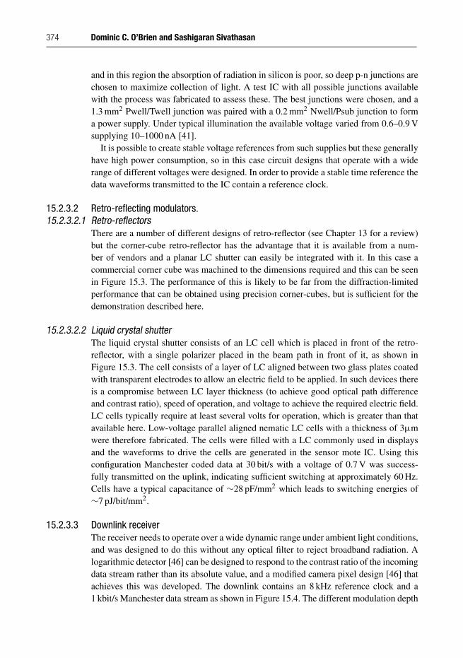
374 Dominic C. O’Brien and Sashigaran Sivathasan
and in this region the absorption of radiation in silicon is poor, so deep p-n junctions arechosen to maximize collection of light. A test IC with all possible junctions availablewith the process was fabricated to assess these. The best junctions were chosen, and a1.3 mm2 Pwell/Twell junction was paired with a 0.2 mm2 Nwell/Psub junction to forma power supply. Under typical illumination the available voltage varied from 0.6–0.9 Vsupplying 10–1000 nA [41].
It is possible to create stable voltage references from such supplies but these generallyhave high power consumption, so in this case circuit designs that operate with a widerange of different voltages were designed. In order to provide a stable time reference thedata waveforms transmitted to the IC contain a reference clock.
15.2.3.2 Retro-reflecting modulators.15.2.3.2.1 Retro-reflectors
There are a number of different designs of retro-reflector (see Chapter 13 for a review)but the corner-cube retro-reflector has the advantage that it is available from a num-ber of vendors and a planar LC shutter can easily be integrated with it. In this case acommercial corner cube was machined to the dimensions required and this can be seenin Figure 15.3. The performance of this is likely to be far from the diffraction-limitedperformance that can be obtained using precision corner-cubes, but is sufficient for thedemonstration described here.
15.2.3.2.2 Liquid crystal shutterThe liquid crystal shutter consists of an LC cell which is placed in front of the retro-reflector, with a single polarizer placed in the beam path in front of it, as shown inFigure 15.3. The cell consists of a layer of LC aligned between two glass plates coatedwith transparent electrodes to allow an electric field to be applied. In such devices thereis a compromise between LC layer thickness (to achieve good optical path differenceand contrast ratio), speed of operation, and voltage to achieve the required electric field.LC cells typically require at least several volts for operation, which is greater than thatavailable here. Low-voltage parallel aligned nematic LC cells with a thickness of 3μmwere therefore fabricated. The cells were filled with a LC commonly used in displaysand the waveforms to drive the cells are generated in the sensor mote IC. Using thisconfiguration Manchester coded data at 30 bit/s with a voltage of 0.7 V was success-fully transmitted on the uplink, indicating sufficient switching at approximately 60 Hz.Cells have a typical capacitance of ∼28 pF/mm2 which leads to switching energies of∼7 pJ/bit/mm2.
15.2.3.3 Downlink receiverThe receiver needs to operate over a wide dynamic range under ambient light conditions,and was designed to do this without any optical filter to reject broadband radiation. Alogarithmic detector [46] can be designed to respond to the contrast ratio of the incomingdata stream rather than its absolute value, and a modified camera pixel design [46] thatachieves this was developed. The downlink contains an 8 kHz reference clock and a1 kbit/s Manchester data stream as shown in Figure 15.4. The different modulation depth
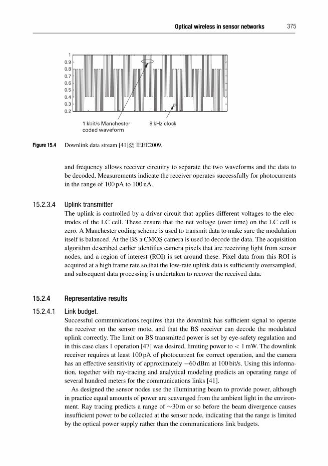
Optical wireless in sensor networks 375
0.2
0.30.4
0.50.60.7
0.80.9
1
1 kbit/s Manchestercoded waveform
8 kHz clock
Figure 15.4 Downlink data stream [41] c© IEEE2009.
and frequency allows receiver circuitry to separate the two waveforms and the data tobe decoded. Measurements indicate the receiver operates successfully for photocurrentsin the range of 100 pA to 100 nA.
15.2.3.4 Uplink transmitterThe uplink is controlled by a driver circuit that applies different voltages to the elec-trodes of the LC cell. These ensure that the net voltage (over time) on the LC cell iszero. A Manchester coding scheme is used to transmit data to make sure the modulationitself is balanced. At the BS a CMOS camera is used to decode the data. The acquisitionalgorithm described earlier identifies camera pixels that are receiving light from sensornodes, and a region of interest (ROI) is set around these. Pixel data from this ROI isacquired at a high frame rate so that the low-rate uplink data is sufficiently oversampled,and subsequent data processing is undertaken to recover the received data.
15.2.4 Representative results
15.2.4.1 Link budget.Successful communications requires that the downlink has sufficient signal to operatethe receiver on the sensor mote, and that the BS receiver can decode the modulateduplink correctly. The limit on BS transmitted power is set by eye-safety regulation andin this case class 1 operation [47] was desired, limiting power to < 1 mW. The downlinkreceiver requires at least 100 pA of photocurrent for correct operation, and the camerahas an effective sensitivity of approximately −60 dBm at 100 bit/s. Using this informa-tion, together with ray-tracing and analytical modeling predicts an operating range ofseveral hundred meters for the communications links [41].
As designed the sensor nodes use the illuminating beam to provide power, althoughin practice equal amounts of power are scavenged from the ambient light in the environ-ment. Ray tracing predicts a range of ∼30 m or so before the beam divergence causesinsufficient power to be collected at the sensor node, indicating that the range is limitedby the optical power supply rather than the communications link budgets.
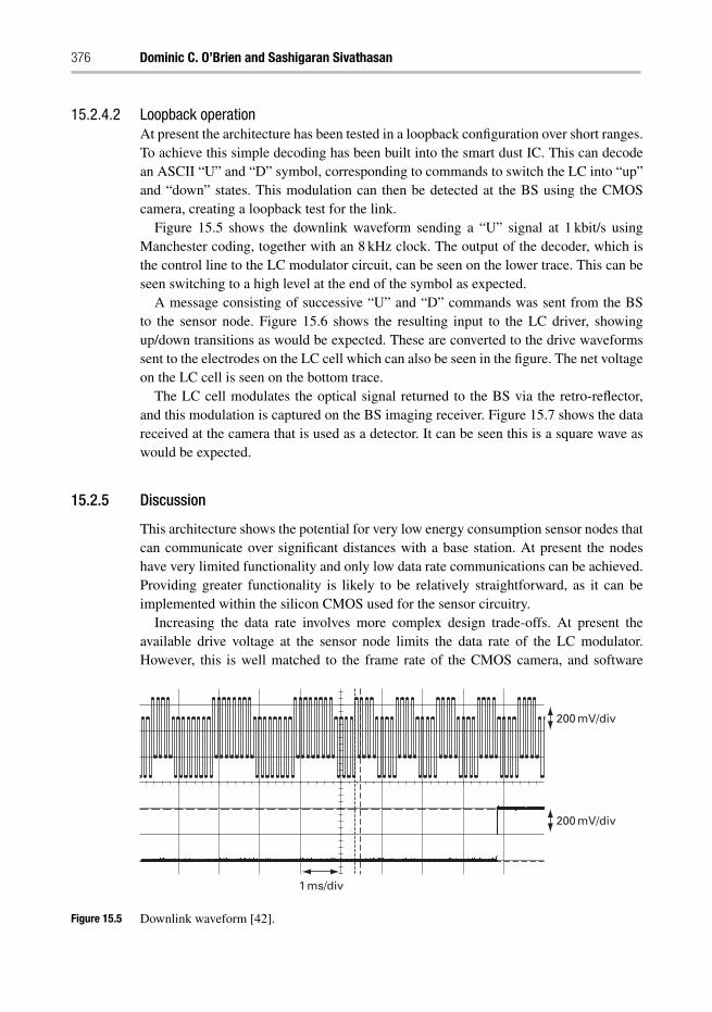
376 Dominic C. O’Brien and Sashigaran Sivathasan
15.2.4.2 Loopback operationAt present the architecture has been tested in a loopback configuration over short ranges.To achieve this simple decoding has been built into the smart dust IC. This can decodean ASCII “U” and “D” symbol, corresponding to commands to switch the LC into “up”and “down” states. This modulation can then be detected at the BS using the CMOScamera, creating a loopback test for the link.
Figure 15.5 shows the downlink waveform sending a “U” signal at 1 kbit/s usingManchester coding, together with an 8 kHz clock. The output of the decoder, which isthe control line to the LC modulator circuit, can be seen on the lower trace. This can beseen switching to a high level at the end of the symbol as expected.
A message consisting of successive “U” and “D” commands was sent from the BSto the sensor node. Figure 15.6 shows the resulting input to the LC driver, showingup/down transitions as would be expected. These are converted to the drive waveformssent to the electrodes on the LC cell which can also be seen in the figure. The net voltageon the LC cell is seen on the bottom trace.
The LC cell modulates the optical signal returned to the BS via the retro-reflector,and this modulation is captured on the BS imaging receiver. Figure 15.7 shows the datareceived at the camera that is used as a detector. It can be seen this is a square wave aswould be expected.
15.2.5 Discussion
This architecture shows the potential for very low energy consumption sensor nodes thatcan communicate over significant distances with a base station. At present the nodeshave very limited functionality and only low data rate communications can be achieved.Providing greater functionality is likely to be relatively straightforward, as it can beimplemented within the silicon CMOS used for the sensor circuitry.
Increasing the data rate involves more complex design trade-offs. At present theavailable drive voltage at the sensor node limits the data rate of the LC modulator.However, this is well matched to the frame rate of the CMOS camera, and software
1 ms/div
200 mV/div
200 mV/div
Figure 15.5 Downlink waveform [42].
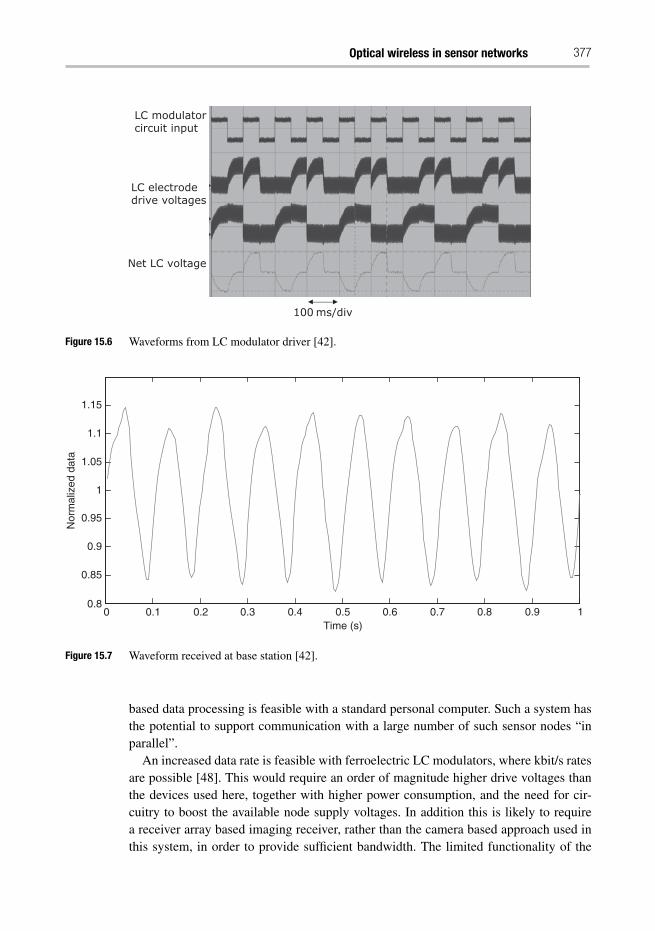
Optical wireless in sensor networks 377
Figure 15.6 Waveforms from LC modulator driver [42].
0 0.1 0.2 0.3 0.4 0.5 0.6 0.7 0.8 0.9 10.8
0.85
0.9
0.95
1
1.05
1.1
1.15
Time (s)
Nor
mal
ized
dat
a
Figure 15.7 Waveform received at base station [42].
based data processing is feasible with a standard personal computer. Such a system hasthe potential to support communication with a large number of such sensor nodes “inparallel”.
An increased data rate is feasible with ferroelectric LC modulators, where kbit/s ratesare possible [48]. This would require an order of magnitude higher drive voltages thanthe devices used here, together with higher power consumption, and the need for cir-cuitry to boost the available node supply voltages. In addition this is likely to requirea receiver array based imaging receiver, rather than the camera based approach used inthis system, in order to provide sufficient bandwidth. The limited functionality of the
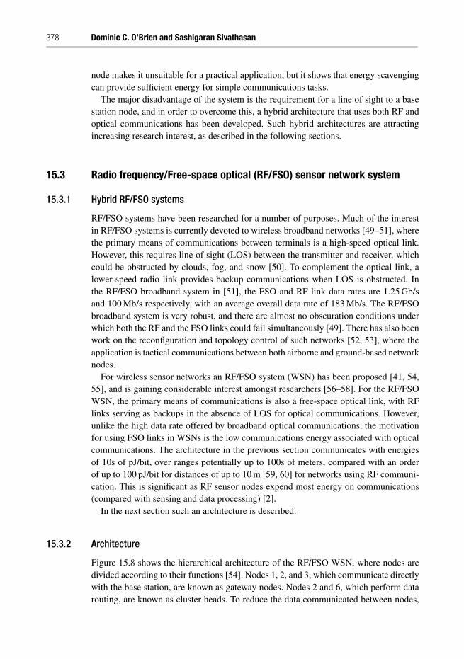
378 Dominic C. O’Brien and Sashigaran Sivathasan
node makes it unsuitable for a practical application, but it shows that energy scavengingcan provide sufficient energy for simple communications tasks.
The major disadvantage of the system is the requirement for a line of sight to a basestation node, and in order to overcome this, a hybrid architecture that uses both RF andoptical communications has been developed. Such hybrid architectures are attractingincreasing research interest, as described in the following sections.
15.3 Radio frequency/Free-space optical (RF/FSO) sensor network system
15.3.1 Hybrid RF/FSO systems
RF/FSO systems have been researched for a number of purposes. Much of the interestin RF/FSO systems is currently devoted to wireless broadband networks [49–51], wherethe primary means of communications between terminals is a high-speed optical link.However, this requires line of sight (LOS) between the transmitter and receiver, whichcould be obstructed by clouds, fog, and snow [50]. To complement the optical link, alower-speed radio link provides backup communications when LOS is obstructed. Inthe RF/FSO broadband system in [51], the FSO and RF link data rates are 1.25 Gb/sand 100 Mb/s respectively, with an average overall data rate of 183 Mb/s. The RF/FSObroadband system is very robust, and there are almost no obscuration conditions underwhich both the RF and the FSO links could fail simultaneously [49]. There has also beenwork on the reconfiguration and topology control of such networks [52, 53], where theapplication is tactical communications between both airborne and ground-based networknodes.
For wireless sensor networks an RF/FSO system (WSN) has been proposed [41, 54,55], and is gaining considerable interest amongst researchers [56–58]. For the RF/FSOWSN, the primary means of communications is also a free-space optical link, with RFlinks serving as backups in the absence of LOS for optical communications. However,unlike the high data rate offered by broadband optical communications, the motivationfor using FSO links in WSNs is the low communications energy associated with opticalcommunications. The architecture in the previous section communicates with energiesof 10s of pJ/bit, over ranges potentially up to 100s of meters, compared with an orderof up to 100 pJ/bit for distances of up to 10 m [59, 60] for networks using RF communi-cation. This is significant as RF sensor nodes expend most energy on communications(compared with sensing and data processing) [2].
In the next section such an architecture is described.
15.3.2 Architecture
Figure 15.8 shows the hierarchical architecture of the RF/FSO WSN, where nodes aredivided according to their functions [54]. Nodes 1, 2, and 3, which communicate directlywith the base station, are known as gateway nodes. Nodes 2 and 6, which perform datarouting, are known as cluster heads. To reduce the data communicated between nodes,
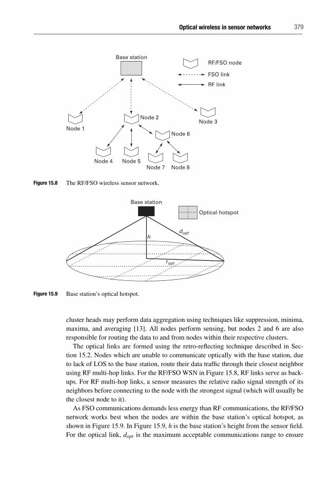
Optical wireless in sensor networks 379
Base station
Node 1
Node 2
Node 6
Node 3
RF/FSO node
FSO link
RF link
Node 8Node 7Node 5Node 4
Figure 15.8 The RF/FSO wireless sensor network.
Base station
Optical hotspot
hdopt
ropt
Figure 15.9 Base station’s optical hotspot.
cluster heads may perform data aggregation using techniques like suppression, minima,maxima, and averaging [13]. All nodes perform sensing, but nodes 2 and 6 are alsoresponsible for routing the data to and from nodes within their respective clusters.
The optical links are formed using the retro-reflecting technique described in Sec-tion 15.2. Nodes which are unable to communicate optically with the base station, dueto lack of LOS to the base station, route their data traffic through their closest neighborusing RF multi-hop links. For the RF/FSO WSN in Figure 15.8, RF links serve as back-ups. For RF multi-hop links, a sensor measures the relative radio signal strength of itsneighbors before connecting to the node with the strongest signal (which will usually bethe closest node to it).
As FSO communications demands less energy than RF communications, the RF/FSOnetwork works best when the nodes are within the base station’s optical hotspot, asshown in Figure 15.9. In Figure 15.9, h is the base station’s height from the sensor field.For the optical link, dopt is the maximum acceptable communications range to ensure
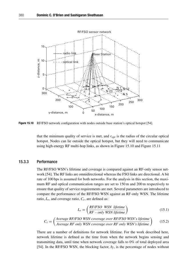
380 Dominic C. O’Brien and Sashigaran Sivathasan
RF/FSO sensor network
15
radio link
optical link
N 23N 1 N 12
N 5
10
5
0
300
200
100
050
x-distance, my-distance, m
z-d
ista
nce
, m
100150
200250
300
Base Station
Figure 15.10 RF/FSO network configuration with nodes outside base station’s optical hotspot [54].
that the minimum quality of service is met, and ropt is the radius of the circular opticalhotspot. Nodes can lie outside the optical hotspot, but they will need to communicateusing high-energy RF multi-hop links, as shown in Figure 15.10 and Figure 15.11
15.3.3 Performance
The RF/FSO WSN’s lifetime and coverage is compared against an RF-only sensor net-work [54]. The RF links are omnidirectional whereas the FSO links are directional. A bitrate of 100 bps is assumed for both networks. For the analysis in this section, the maxi-mum RF and optical communication ranges are set to 150 m and 200 m respectively toensure that quality of service requirements are met. Several parameters are introduced tocompare the performance of the RF/FSO WSN against an RF-only WSN. The lifetimeratio, Lr, and coverage ratio, Cr, are defined as:
Lr =(
RF/FSO WSN lifetime
RF – only WSN lifetime
)(15.1)
Cr =(
Average RF/FSO WSN coverage over RF/FSO WSN’s lifetime
Average RF only WSN coverage over RF only WSN’s lifetime
)(15.2)
There are a number of definitions for network lifetime. For the work described here,network lifetime is defined as the time from when the network begins sensing andtransmitting data, until time when network coverage falls to 0% of total deployed area[54]. In the RF/FSO WSN, the blocking factor, bf , is the percentage of nodes without
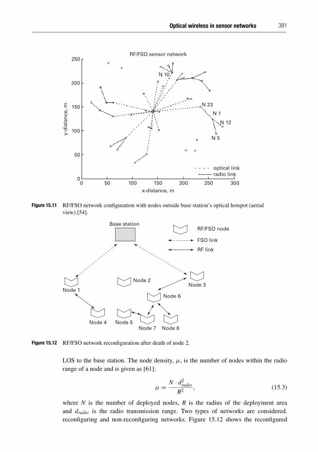
Optical wireless in sensor networks 381
250RF/FSO sensor network
200
150
100
50
00 50 100 150
x-distance, m
y-d
ista
nce
, m
200 250
optical link
N 23
N 10
N 1
N 12
N 5
radio link
300
Figure 15.11 RF/FSO network configuration with nodes outside base station’s optical hotspot (aerialview) [54].
Base station
Node 1
Node 2
Node 6
Node 3
RF/FSO node
FSO link
RF link
Node 8Node 7Node 5Node 4
Figure 15.12 RF/FSO network reconfiguration after death of node 2.
LOS to the base station. The node density, μ, is the number of nodes within the radiorange of a node and is given as [61]:
μ = N · d2radio
R2, (15.3)
where N is the number of deployed nodes, R is the radius of the deployment areaand dradio is the radio transmission range. Two types of networks are considered.reconfiguring and non-reconfiguring networks. Figure 15.12 shows the reconfigured
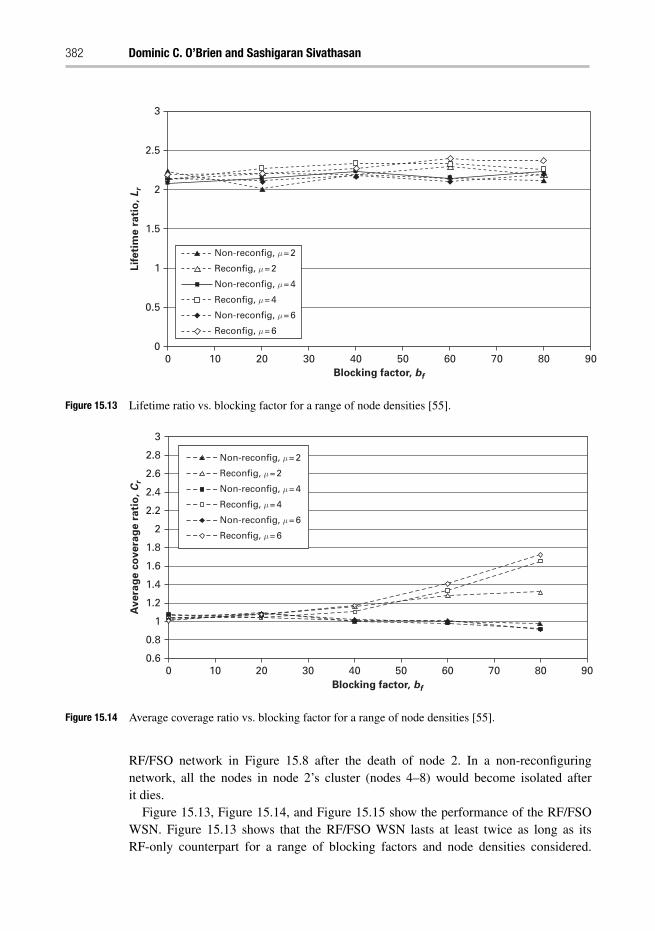
382 Dominic C. O’Brien and Sashigaran Sivathasan
3
2.5
2
1.5
1
0.5
00 10 20 30 5040 60 70 80 90
Blocking factor, bf
Lif
eti
me r
ati
o,
Lr
Non-reconfig, μ = 4
Reconfig, μ = 6
Reconfig, μ = 4
Non-reconfig, μ = 2
Reconfig, μ = 2
Non-reconfig, μ = 6
Figure 15.13 Lifetime ratio vs. blocking factor for a range of node densities [55].
Non-reconfig, μ = 4
Reconfig, μ = 6
Reconfig, μ = 4
Non-reconfig, μ = 2
Reconfig, μ = 2
Non-reconfig, μ = 6
0 10 20 30 40 50Blocking factor, bf
60 70 80 90
3
2.8
2.6
2.4
2.2
2
1.8
1.6
1.4
1.2
1
0.8
0.6
Avera
ge c
overa
ge r
ati
o,
Cr
Figure 15.14 Average coverage ratio vs. blocking factor for a range of node densities [55].
RF/FSO network in Figure 15.8 after the death of node 2. In a non-reconfiguringnetwork, all the nodes in node 2’s cluster (nodes 4–8) would become isolated afterit dies.
Figure 15.13, Figure 15.14, and Figure 15.15 show the performance of the RF/FSOWSN. Figure 15.13 shows that the RF/FSO WSN lasts at least twice as long as itsRF-only counterpart for a range of blocking factors and node densities considered.
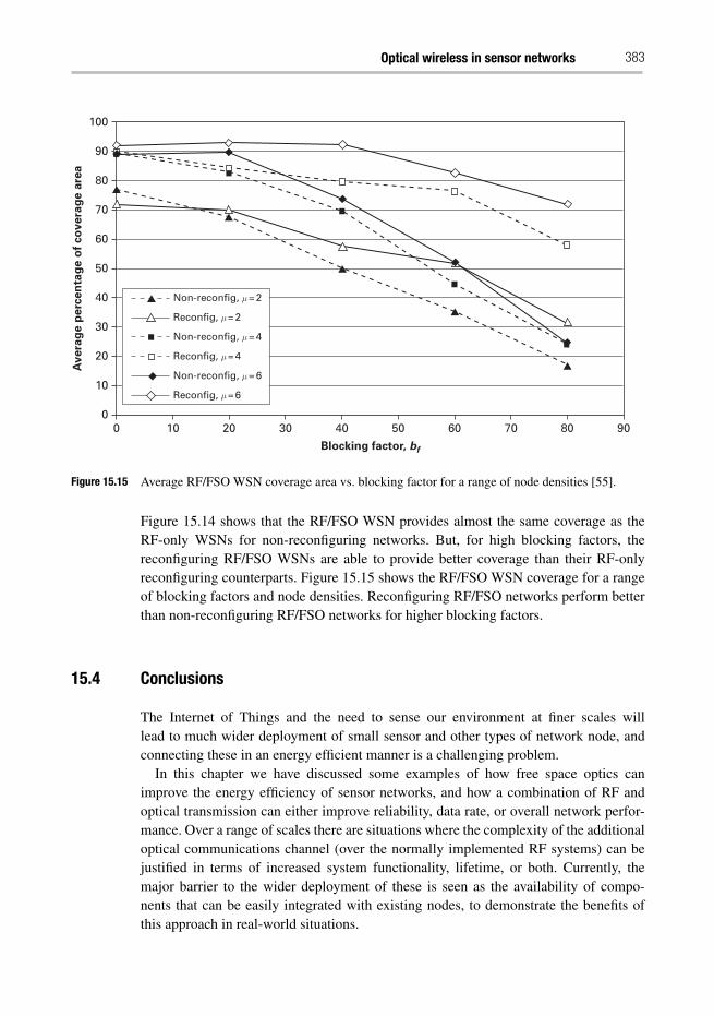
Optical wireless in sensor networks 383
100
90
80
70
60
50
40
30
20
10
00 10 20 30 40 50
Blocking factor, bf
60 70 80 90
Avera
ge p
erc
en
tag
e o
f co
vera
ge a
rea
Non-reconfig, μ = 4
Reconfig, μ = 6
Reconfig, μ = 4
Non-reconfig, μ = 2
Reconfig, μ = 2
Non-reconfig, μ = 6
Figure 15.15 Average RF/FSO WSN coverage area vs. blocking factor for a range of node densities [55].
Figure 15.14 shows that the RF/FSO WSN provides almost the same coverage as theRF-only WSNs for non-reconfiguring networks. But, for high blocking factors, thereconfiguring RF/FSO WSNs are able to provide better coverage than their RF-onlyreconfiguring counterparts. Figure 15.15 shows the RF/FSO WSN coverage for a rangeof blocking factors and node densities. Reconfiguring RF/FSO networks perform betterthan non-reconfiguring RF/FSO networks for higher blocking factors.
15.4 Conclusions
The Internet of Things and the need to sense our environment at finer scales willlead to much wider deployment of small sensor and other types of network node, andconnecting these in an energy efficient manner is a challenging problem.
In this chapter we have discussed some examples of how free space optics canimprove the energy efficiency of sensor networks, and how a combination of RF andoptical transmission can either improve reliability, data rate, or overall network perfor-mance. Over a range of scales there are situations where the complexity of the additionaloptical communications channel (over the normally implemented RF systems) can bejustified in terms of increased system functionality, lifetime, or both. Currently, themajor barrier to the wider deployment of these is seen as the availability of compo-nents that can be easily integrated with existing nodes, to demonstrate the benefits ofthis approach in real-world situations.
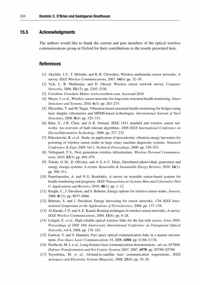
384 Dominic C. O’Brien and Sashigaran Sivathasan
15.5 Acknowledgments
The authors would like to thank the current and past members of the optical wirelesscommunications group at Oxford for their contributions to the results presented here.
References
[1] Akyildiz, I. F., T. Melodia, and K. R. Chowdury, Wireless multimedia sensor networks: Asurvey. IEEE Wireless Communications, 2007. 14(6): pp. 32–39.
[2] Yick, J., B. Mukherjee, and D. Ghosal, Wireless sensor network survey. ComputerNetworks, 2008. 52(12): pp. 2292–2330.
[3] Crossbow. Crossbow Motes: www.crossbow.com. Accessed 2010.[4] Meyer, J. et al., Wireless sensor networks for long-term structural health monitoring. Smart
Structures and Systems, 2010. 6(3): pp. 263–275.[5] Miyashita, T. and M. Nagai, Vibiration-based structural health monitoring for bridges using
laser doppler vibrometers and MEMS-based technologies. International Journal of SteelStructures, 2008. 8(4): pp. 325–331.
[6] Kher, S., J. R. Chen, and A. K. Somani, IEEE 1451 standard and wireless sensor net-works: An overview of fault tolerant algorithms. 2006 IEEE International Conference onElectro/Information Technology, 2006: pp. 227–232
[7] Pekoslawski, B. et al., Study on application of piezoelectric vibration energy harvesters forpowering of wireless sensor nodes in large rotary machine diagnostic systems. NanotechConference & Expo 2009, Vol 1, Technical Proceedings, 2009: pp. 530–533.
[8] Toftegaard, T. S., Next generation wireless infrastructure. Wireless Personal Communica-tions, 2010. 53(3): pp. 465–479.
[9] Toledo, O. M., D. Oliveira, and A. S. A. C. Diniz, Distributed photovoltaic generation andenergy storage systems: A review. Renewable & Sustainable Energy Reviews, 2010. 14(1):pp. 506–511.
[10] Pantelopoulos, A. and N. G. Bourbakis, A survey on wearable sensor-based systems forhealth monitoring and prognosis. IEEE Transactions on Systems Man and Cybernetics PartC–Applications and Reviews, 2010. 40(1): pp. 1–12.
[11] Knight, C., J. Davidson, and S. Behrens, Energy options for wireless sensor nodes. Sensors,2008. 8(12): pp. 8037–8066.
[12] Behrens, S. and J. Davidson, Energy harvesting for sensor networks. 17th IEEE Inter-national Symposium on the Applications of Ferroelectrics, 2008: pp. 137–138.
[13] Al-Karaki, J. N. and A. E. Kamal, Routing techniques in wireless sensor networks: A survey.IEEE Wireless Communications, 2004. 11(6): pp. 6–28.
[14] Leitgeb, E. et al., High reliable optical wireless links for the last mile access. Icton 2008:Proceedings of 2008 10th Anniversary International Conference on Transparent OpticalNetworks, vol 4, 2008: pp. 178–183.
[15] Gadwal, V. and S. Hammel, Free space optical communication links in a marine environ-ment. Free-Space Laser Communications VI, 2006. 6304: pp. U166–U176.
[16] Northcott, M. J. et al., Long distance laser communications demonstration – art. no. 65780S.Defense Transformation and Net-Centric Systems 2007, 2007. 6578: pp. S5780–S5780.
[17] Toyoshima, M. et al., Ground-to-satellite laser communication experiments. IEEEAerospace and Electronic Systems Magazine, 2008. 23(8): pp. 10–18.
Optical wireless in sensor networks 385
[18] Harris, A. and T. A. Giuma, Minimization of acquisition time in a wavelength diversifiedFSO link between mobile platforms – art. no. 655108. Atmospheric Propagation IV, 2007.6551: pp. 55108–55108.
[19] Agrawal, N., S. D. Milner, and C. C. Davis. Free space optical sensor network for short-range applications. Free-Space Laser Communications X. 2010. San Diego, California,USA: SPIE.
[20] Ghosh, A. K. et al. Free-space optics based sensor network design using angle-diversityphotodiode arrays. Free-Space Laser Communications X. 2010. San Diego, California,USA: SPIE.
[21] Kedar, D. and S. Arnon, Second-generation laser firefly clusters: improved scheme fordistributed sensing in the atmosphere. Applied Optics, 2005. 44(6): pp. 984–992.
[22] Kedar, D. and S. Arnon, Laser “firefly” clustering; a new concept in atmospheric probing.IEEE Photonics Technology Letters, 2003. 15(11): pp. 1672–1674.
[23] Reardon, C. et al., Optical beam-steering for wireless sensor networks. 2009 IEEE LeosAnnual Meeting Conference Proceedings, vols. 1and 2, 2009: pp. 583–584.
[24] Reardon, C. et al., Integrated polymer microprisms for free space optical beam deflecting.Optics Express, 2009. 17(5): pp. 3424–3428.
[25] Mathews, J., M. Barnes, and D. K. Arvind, Low power free space optical communication inwireless sensor networks. Proceedings of the 2009 12th Euromicro Conference on DigitalSystem Design, Architectures, Methods and Tools, 2009: pp. 849–856
[26] Srinivasan, B. and V. Rodoplu, Energy-efficient joint source-channel coding for opticalwireless underwater networks. 2007 Oceans, vols 1–5, 2007: pp. 725–729
[27] Liu, L. B., S. L. Zhou, and J. H. Cui, Prospects and problems of wireless communication forunderwater sensor networks. Wireless Communications & Mobile Computing, 2008. 8(8):pp. 977–994.
[28] Anguita, D., D. Brizzolara, and G. Parodi, Building an underwater wireless sensor networkbased on optical communication: Research challenges and current results. 2009 3rd Inter-national Conference on Sensor Technologies and Applications (Sensorcomm 2009), 2009:pp. 476–479
[29] Kedar, D. and S. Arnon, Subsea ultraviolet solar-blind broadband free-space optics commu-nication. Optical Engineering, 2009. 48(4).
[30] Arnon, S., Underwater optical wireless communication network. Optical Engineering,2010. 49(1).
[31] Llorca, J. et al., Reconfigurable optical wireless sensor networks. Optics in AtmosphericPropagation and Adaptive Systems VI, 2004. 5237: pp. 136–146.
[32] Kedar, D. and S. Arnon, An ultraviolet optical wireless sensor network in multi-scatteringchannels. Information Optics, 2006. 860: pp. 436–445
[33] Rabinovich, W. S., et al., InGaAs multiple quantum well modulating retro-reflector for freespace optical communications. Free-Space Laser Communication and Laser Imaging, 2002.4489: pp. 190–201
[34] Kahn, J. M., R. H. Katz, and K. S. Pister. Next century challenges: mobile networking for“Smart Dust”. 1999: Dept. of Electr. Eng. & Comput. Sci., California University BerkeleyCA USA.
[35] Warneke, B., B. Atwood, and K. S. J. Pister. Smart dust mote forerunners. 2001: Dept. ofElectr. Eng. & Comput. Sci. California University Berkeley CA USA.
[36] Lixia, Z., K. S. J. Pister, and J. M. Kahn. Assembled corner-cube retroreflector quadruplet.Technical Digest. 2002. Robotics & Autom: Dept. of Electr. Eng. & Comput. Sci. CaliforniaUniversity Berkeley CA USA.
386 Dominic C. O’Brien and Sashigaran Sivathasan
[37] Teramoto, S. and T. Ohtsuki, Optical wireless sensor network system using corner cuberetroreflectors (CCRs). Globecom ’04: IEEE Global Telecommunications Conference,vols 1–6, 2004: pp. 1035–1039.
[38] Moon, G. B., C. G. Park, and J. G. Lee, Optical Communication Method using CCR.2008 International Conference on Control, Automation and Systems, vols 1–4, 2008:pp. 642–646
[39] Arnon, S., Swarm of sensor acquisition and identification using optical wireless communi-cation. Free Space Laser Communications IV, 2004. 5550: pp. 436-442
[40] Arnon, S., Network of sensors: acquisition probability. Journal of the Optical Society ofAmerica a-Optics Image Science and Vision, 2007. 24(9): pp. 2758–2765.
[41] O’Brien, D. C. et al., Design and implementation of optical wireless communications withoptically powered smart dust motes. IEEE Journal on Selected Areas in Communications,2009. 27(9): pp. 1646–1653.
[42] O’Brien, D. C. et al. Energy scavenging sensors for ultra-low power sensor networks. Free-Space Laser Communications X. 2010. San Diego, California, USA: SPIE.
[43] Vachiramon P., G. E. Faulkner, and D. C. Obrien, A DC balancing algorithm for FLCOSbinary phase holograms. Optics Letters, 2007. 32(22): pp. 3275–3277.
[44] Cap, G. A., H. H. Refai, and J. J. J. Sluss. FSO tracking and auto-alignment transceiver sys-tem. Unmanned/Unattended Sensors and Sensor Networks V. 2008. Cardiff, Wales, UnitedKingdom: SPIE.
[45] Yun, G. and M. Kavehrad. Spot-diffusing and fly-eye receivers for indoor infrared wire-less communications. Conference Proceedings, 1992 IEEE International Conference onSelected Topics in Wireless Communications. 1992.
[46] Delbrück, T. and C. A. Mead, Analog VLSI phototransduction by continuous-time, adaptive,logarithmic photoreceptor circuits, in Vision Chips: Implementing Vision Algorithms withAnalog VLSI Circuits, C. Koch and H. Li, editors. 1995, IEEE Computer Society Press.pp. 139–161.
[47] IEC 60825-1. Safety of laser products part 1. 2007: British Standards Institution.[48] O’Brien, D. C. et al. Robust data transmission at high data rates using liquid crystal spatial
light modulators. Spatial Light Modulators and Integrated Optoelectronic Arrays. 1999:Optical Society of America.
[49] Kim, I. I. and E. Korevaar, Availability of free space optics (FSO) and hybrid FSO/RFsystems. Optical Wireless Communications IV, 2001. 4530: pp. 84–95.
[50] Desai, A. and S. Milner, Autonomous reconfiguration in free-space optical sensor networks.IEEE Journal on Selected Areas in Communications, 2005. 23(8): pp. 1556–1563.
[51] Gibson, S.M. et al., Coordinate measurement in 2-D and 3-D geometries usingfrequency scanning interferometry. Optics and Lasers in Engineering, 2005. 43(7):pp. 815–831.
[52] Llorca, J., S. D. Milner, and C. C. Davis. Molecular inspired models for prediction and con-trol of directional FSO/RF wireless networks. Free-Space Laser Communications X. 2010.San Diego, California, USA: SPIE.
[53] Milner, S. D., J. Llorca, and C. C. Davis, Autonomous reconfiguration and control indirectional mobile ad hoc networks. IEEE Circuits and Systems Magazine, 2009. 9(2):pp. 10–26.
[54] Sivathasan, S., Hybrid radio frequency/free space optical communications for energy-efficient wireless sensor networks, Doctor of Philosophy (DPhil) Thesis, 2008, Universityof Oxford.
Optical wireless in sensor networks 387
[55] Sivathasan, S. and D. O’Brien, Radio frequency/free space optical and radio frequency-onlywireless sensor networks: a comparative study of performance. IETE Journal of Research,2010. 56(1): pp. 52–61.
[56] Deng, S. L. et al., Wireless connections of sensor network using RF and free space opticallinks – art. no. 677307. Next-Generation Communication and Sensor Networks 2007, 2007.6773: pp. 77307–77307.
[57] Chonggang, W. et al. ISNOW: Integrated sensor networks with optical and wireless commu-nications. Optical Fiber Communication (OFC), collocated National Fiber Optic EngineersConference, 2010 Conference (OFC/NFOEC) 2010.
[58] Nadeem, F. et al., Comparing the life time of terrestrial wireless sensor networks byemploying hybrid FSO/RF and only RF access networks. ICWMC: 2009 Fifth InternationalConference on Wireless and Mobile Communications, 2009: pp. 134–139.
[59] Heinzelman, W. R., A. Chandrakasan, and H. Balakrishnan. Energy-efficient communica-tion protocol for wireless microsensor networks. System Sciences, 2000. Proceedings of the33rd Annual Hawaii International Conference, 2000.
[60] Lindsey, S. and C. S. Raghavendra, PEGASIS: Power-efficient GAthering in sensorinformation systems. 2002 IEEE Aerospace Conference Proceedings, vols 1–7, 2002.pp. 1125–1130
[61] Akyildiz, I. F. et al., Wireless sensor networks: a survey. Computer Networks, 2002. 38(4):pp. 393–422.

Index
Figures and tables are indicated in bold typeface.
absorption, 203, 203, 204–6, 210adaptive power control, 68–69. see also optical
orthogonal codesalbedo, 222, 226–28, 226, 227AMC. see hybrid RF/FSO wireless networksamplifier
double heterodyne photoparametric, 259–60, 260photoparametric, 258–59, 258trans-impedance, 19, 255–57, 256, 257, 258, 262
angle diversity receiver, 118AOP. see apparent optical propertiesAPC. see adaptive power controlapplications
optical code-division multiple-access wirelessnetwork, 81–83, 82, 83
optical modulating retro-reflectors, 341–47, 344,345, 346, 353, 361–67, 362, 363, 364, 365, 366
automobile driving application, 365–66, 366
barcodes, 129, 130BB84 protocol, 308–10, 309Beer’s Law, 203–4, 203, 212, 214. see also channel
lossBER analysis
channel shortening equalizer, 111, 112free-space optical wireless networks, 70–71free-space orthogonal frequency division
multiplexing wireless networks, 43in FSO links, 74generalized hybrid
subcarrier/amplitude/phase/polarizationmodulation, 37–38, 38
heterogeneous optical networks, 47, 48infrared optical wireless networks, 251–53, 256multiple-input multiple-output, 23–25, 24, 25, 26optical code-division multiple-access wireless
network, 62–64, 67, 70–71pulse amplitude modulation, 22–23time equalizer, 109
biased-OFDM scheme, 40B-OFDM. see biased-OFDM scheme
cat’s eye retro-reflector, 333–34, 333, 334channel inversion, 30–31, 30channel loss, 212. see also Beer’s Lawchannel modeling, 12–13channel shortening equalizer, 90, 106–12, 111, 112channel state information, 278–79. see also
transmitterCIDS. see cyclic-invarient difference setclipped OFDM scheme, 41clouds
and free-space optical wireless networks, 90–113,93, 95, 97, 98
RF frequency in, 273codes on graphs, 13–19. see also modulationC-OFDM. see clipped OFDM schemecommunication
line-of-sight, 11, 231–32non-line-of-sight, 177–99, 232, 233, 241–42
conventional cryptography, 306–8corner cube retro-reflectors, 332,
337, 341cryptography
conventional, 306–8modern quantum, 305–6, 312–25
CSE. see channel shortening equalizerCSI. see channel state informationcyclic-invarient difference set, 16
decision-feedback equalization, 103decoy-state BB84 protocol, 310deep fades, 38–43DFE. see decision-feedback equalizationdiffuse link, 241–42diffuse system design, 119–23, 121discrete-time wireless networks
free-space optical intensity, 148, 156–61, 159,160, 161
optical intensity with Gaussian noise, 149,161–63
performance, 149–63, 163–72Poisson, 146–48, 151–55, 155
Index 389
double heterodyne photoparametric amplifier,259–60, 260
eigen analysis, 102–3encryption. see cryptographyentanglement-based BB84 protocol, 310–11, 311entanglement-based QKD links, 320–21error, pointing, 87–88eye safety, 178, 243, 243
fountain code, 26free-space optical wireless networks
atmospheric effects in, 273cryptography, 305–25modulation, 11–49, 39OCDMA system, 68–75, 69and optical modulating retro-reflectors, 342system design, 104, 354turbulence, 11–49, 90–113
free-space orthogonal frequency divisionmultiplexing wireless networks, 38–43, 39, 43
FSO. see free-space optical wireless networks
Gaussian noise, 149, 161–63, 279–80, 282. see alsointerference
generalized hybridsubcarrier/amplitude/phase/polarizationmodulation, 35–38, 36, 37, 38
GH-SAPP. see generalized hybridsubcarrier/amplitude/phase/polarizationmoduilation
Gray mapping rule, 21, 24, 25
HAPP. see generalized hybridsubcarrier/amplitude/phase/polarizationmoduilation
heterogeneous optical networks, 12, 43–48, 44, 45,47, 48
high altitude platforms, 322–25, 324HONs. see heterogeneous optical networkshybrid RF/FSO sensor network, 378–83, 379, 380,
381, 382, 383hybrid RF/FSO wireless networks
modulation, 12, 29–34, 30performance, 290–95, 291system design, 275–80, 275, 277theory of, 281–90, 282, 283, 287, 290
imaging receiver, 118–19IM/DD. see intensity modulation with direct
detectionindoor optical wireless networks
fundamentals, 117modulation, 123, 138receiver, 118–19system design, 119–38, 135, 136
transmitter, 117–18, 132–38, 146–48infrared optical wireless networks
eye safety, 243, 243interference, 248–51, 249modulation, 263–66, 264, 265optical sources in, 242, 242, 267–68, 267performance, 251–53, 252, 253receiver, 255–63, 256, 257, 258, 260, 261, 262system design, 241–42, 244–47
intensity modulation with direct detection, 11, 91,247
interference. see also Gaussian noise; scattering;turbulence
and free-space optical wireless networks, 11–49infrared optical wireless networks, 248–51, 249optical code-division multiple-access wireless
network, 73–75, 74underwater free-space optical wireless networks,
202–3, 203, 205, 207, 209, 210, 212
laser diode, 242, 242, 243LD. see laser diodeLDPC codes, 14–19, 14, 24, 25, 26, 35LED. see light emitting diodelight emitting diode, 242, 242, 243, 352–58, 354linear minimum mean-squared error equalization,
103line-of-sight communication, 11, 231–32LOS. see line-of-sight communicationLT code. see Luby-transform codeLuby-transform code, 26–29
Markov chain model, 90–91, 95–103Maximum-likelihood sequential detection
equalization, 103MCRT. see Monte Carlo ray tracing modelMEMS. see micro-electrical mechanical modulatormicro-electrical mechanical modulator, 336, 337Mie theory, 92–103, 93MIMO. see multiple-input multiple-outputminimum-mean-squared error, 106min-sum-with-correction-term algorithm, 17–19, 17MLMD. see multiple lasers - multiple detectorsMLSD. see Maximum-likelihood sequential
detection equalizationmodern quantum cryptography
and conventional cryptography, 306–8limits, 305–6networking, 319–25system design, 312–19, 314, 317, 318
modulation. see also codes on graphs;multiple-input multiple-output
hybrid RF/FSO wireless networks, 12, 29–34, 30indoor optical wireless networks, 123, 138infrared optical wireless networks, 263–66intensity, 11, 91, 247
390 Index
multidimensional coded, 12, 35–38on-off keying, 75, 77optical modulating retro-reflectors, 334–41, 338,
339, 359–61, 360optical orthogonal codes, 75–82pulse amplitude, 21–25, 21, 24, 25, 76, 265–66,
266pulse position, 25–26, 75–78, 230–31, 263–65,
264underwater free-space optical wireless networks,
230–31moment technique model, 99–103, 100Monte Carlo ray tracing model
integration, 29and Markov chain, 90–91, 95–103, 95performance, 99–103, 100ultraviolet optical wireless networks, 183–87,
184, 192–94, 194underwater, 214–16, 215
MQW. see surface normal multiple quantum wellelectroabsorption modulators
MRR. see optical modulating retro-reflectors;retro-reflector communication
multidimensional coded modulation, 12, 35–38multiple lasers - multiple detectors, 19, 26multiple-input multiple-output, 11, 19–26, 20,
116–38, 128. see also modulationmulti-scatterings, 97, 98
networkingmodern quantum cryptography, 319–25underwater free-space optical wireless networks,
234–36NLOS. see non-line-of-sight communicationnon-line-of-sight communication, 177–99, 232, 233,
241–42. see also optical modulatingretro-reflectors
OCDMA. see optical code-division multiple-accesswireless network
OFDM. see free-space orthogonal frequencydivision multiplexing wireless networks
on-off keying modulation, 75, 77, 264, 266, 282, 283OOC. see optical orthogonal codesOOK. see on-off keying modulationOPPM. see overlapping pulse position modulationoptical code-division multiple-access wireless
networkapplications, 81–83, 82, 83BER analysis, 62–64, 70–71, 78interference, 73–75, 74modulation, 75–77, 76performance, 77–81receiver, 57–59, 60–62, 61, 64–66, 64, 66, 67,
71–73
system design, 55–57, 56, 58, 59–60, 59, 68–70,69
transmitter, 60, 66–68optical modulating retro-reflectors. see also
non-line-of-sight communicationapplications, 341–47, 344, 345, 346, 353, 361–67,
362, 363, 364, 365, 366modulation, 334–41, 338, 339, 359–61, 360system design, 232, 233–34, 329–34, 329, 333,
334, 370optical orthogonal codes, 56–57, 66, 75–82, 79–81,
81. see also adaptive power controloptical wireless networks
optical sources in, 242, 242optics in, 267–68
optical wireless sensor networksmodulation, 374performance, 380–83, 381, 382, 383receiver, 374–75system design, 371–74, 371, 372, 373, 374,
375–78, 376, 377, 379, 380transmitter, 375
orthogonal frequency division multiplexing, 12outage exponent, 285–87, 287, 290, 296outage probability, 285overlapping pulse position modulation, 76–77, 76
PAM. see pulse amplitude modulationpassive optical networks, 43performance
discrete-time wireless networks, 149–63, 163–72hybrid RF/FSO wireless networks, 290–95, 291infrared optical wireless networks, 251–53, 252,
253Monte Carlo ray tracing model, 99–103, 100optical code-division multiple-access wireless
network, 77–81optical wireless sensor networks, 380–83, 381,
382, 383ultraviolet optical wireless networks, 192–99, 192
Phase Function. see Mie theoryphotodetection model, 279–80photoparametric amplifier, 258–59, 258phytoplankton, 206point-to-point system design, 131–36, 135, 136, 370Poisson channel, 146–48, 151–55, 155, 279–80,
282, 283PONS. see passive optical networksPPM. see pulse position modulationprotocol
modern quantum cryptography, 308–11QKD transport, 321–22
prototypes. see applicationspublic-key cryptography. see conventional
cryptography

Index 391
pulse amplitude modulation, 21–25, 21, 24, 25, 76,265–66, 266. see also pulse intensitymodulation
pulse intensity modulation, 146–71. see also pulseamplitude modulation
pulse position modulation, 25–26, 75–78, 230–31,263–65, 264
punctured code, 26
QAM. see Quadrature Amplitude-ModulationQC LCPC. see quasi-cyclic binary LDPC codesQKD. see quantum key distributionQuadrature Amplitude-Modulation, 22quantum key distribution, 305–25
Radiative Transfer Equation, 214radio frequency technology
bandwidth, 103and fiber-optics, 43incompatibilities, 11and infrared optical wireless networks, 240and optical modulating retro-reflectors, 341–42sensors in, 369underwater, 201
Raptor code, 12, 26–29, 27, 29rate-less code, 26receiver
indoor optical wireless networks, 118–19infrared optical wireless networks, 255–63, 256,
257, 258, 260–63, 260, 261, 262optical code-division multiple-access wireless
network, 57–59, 60–62, 61, 64–66, 64, 66, 67,71–73
with polarization analyzer module forcryptography, 316–17, 317
and Viterbi equalizer, 107–12, 108repeaters, 319–20retro-reflectors. see optical modulating
retro-reflectorsRF. see radio frequency technologyRoF. see radio frequency technologyRTE. see Radiative Transfer Equation
SAA. see small-angle approximationsatellites, 322–25scattering. see also interference
albedo, 210atmospheric, 179in cloud channel, 90–113ULTRAVIOLET OPTICAL WIRELESS
NETWORKS, 179–89, 180, 181, 184, 188underwater, 203, 203, 206–13, 207, 209, 210
scintillation, 12–13, 273, 276–77, 346SDMT. see spatial discrete multitone modulation
transmitterSecond Largest Eigenvalue Modulus, 102–3, 102
secret-key cryptography. see conventionalcryptography
security guidance systems, 362signal-to-noise
infrared optical wireless networks, 249, 252underwater free-space optical wireless networks,
201–2SLEM. see Second Largest Eigenvalue Modulussmall-angle approximation, 216–20, 220smart dust, 371, 371SNR. see signal-to-noisespatial discrete multitone modulation transmitter,
132–38, 133, 135, 137spatial dispersion. see water dispersionspot-diffusing system design, 123–27, 125, 126,
127–38surface normal multiple quantum well
electroabsorption modulators, 336–41, 338,339, 341
system designdiffuse, 119–23, 121free-space optical, 104, 354hybrid RF/FSO wireless networks, 275–80, 275,
277indoor optical wireless networks, 119–38, 135,
136infrared optical wireless networks, 241–42modern quantum cryptography, 312–19, 314, 317,
318optical code-division multiple-access wireless
network, 55–57, 56, 58, 59–60, 59, 68–70, 69optical modulating retro-reflectors, 329–34, 329,
333, 334optical wireless sensor networks, 371–74, 371,
372, 373, 375–78, 375, 376, 377, 379, 380point-to-point, 131–36, 135, 136, 370spot-diffusing, 123–27, 125, 126, 127–38ultraviolet optical wireless networks, 189–92,
190, 191underwater free-space optical wireless networks,
228–30, 229, 231–34, 232visible-light wireless networks, 351–54, 352, 354
TA. see trans-impedance amplifierTanner graph, 14, 27temporal dispersion. see water dispersionTEQ. see time equalizertime equalizer, 90, 103–4, 106, 109TPC. see turbo-product codestrans-impedance amplifier, 19, 255–57, 256, 257,
258, 262transmitter. see also channel state information
and channel shortening equalizer, 90, 106–12indoor optical wireless networks, 117–18,
132–38, 146–48
392 Index
optical code-division multiple-access wirelessnetwork, 60, 66–68
optical wireless sensor networks, 375pointing errors, 87–88spatial discrete multitone modulation, 132–38,
133, 135, 137and time equalizer, 90, 103–4, 106, 109underwater free-space optical wireless networks,
228–29truncated channel inversion, 30, 31turbo product codes, 13turbulence. see also interference
and free-space optical wireless networks, 90–113in FSO wireless networks, 11–49underwater, 210
uFSO. see underwater free-space optical wirelessnetworks
ultra wideband communications, 43ultraviolet optical wireless networks
eye safety, 178history of, 177–78inteference, 179–89performance, 192–99, 192system design, 189–92, 190, 191
unclipped OFDM scheme, 41underwater free-space optical wireless networks
history of, 201–2
interference, 202–3, 203, 205, 207, 209, 210, 212modulation, 230–31networking, 234–36optical modulating retro-reflectors, 347system design, 228–30, 229, 232theory of, 213–28, 215, 219, 220, 222, 225, 227
U-OFDM. see unclipped OFDM schemeUV. see ultraviolet optical wireless networksUWB. see ultra wideband communications
variable rate variable power adaptation, 31–34, 33,34, 43–47, 47
variable spreading factor, 224–26, 225vector radiative transfer modeling, 217. see also
water dispersionVisible Light Communications Consortium, 358–59visible-light wireless networks
applications, 361–67, 362, 363, 364, 365, 366modulation, 359–61, 360standards, 354–59system design, 351–54, 352, 354
Viterbi equalizer, 107–12, 108VLC. see visible-light wireless networksVSF. see variable spreading factor
water dispersion, 218–28, 219, 220, 222, 225, 226,227. see also vector radiative transfer modeling
water optical properties, 211–13


