ONE-SIZE OR TAILOR-MADE PERFORMANCE RATIOS FOR RANKING

HEDGE FUNDS?

Martin Eling, Simone Farinelli, Damiano Rossello, Luisa Tibiletti∗

May 20, 2008

Abstract: Eling and Schuhmacher (2007) compared the Sharpe ratio with other performance

measures and found virtually identical rank ordering using hedge fund data. They conclude

that the choice of performance measure has no critical influence on fund evaluation and that

the Sharpe ratio is generally adequate for analyzing hedge funds. In this note, we ask whether

this is also true for performance ratios capable of being tailored to investment style as pre-

sented by Farinelli et al. (2008). Specifically, we deal with the Sortino-Satchell, Farinelli-

Tibiletti, and Rachev ratios. Empirical experiments illustrate that if the ratios are tailored to a

moderate investment style, they lead to rankings not too dissimilar to those found with the

Sharpe ratio. An explanation of this finding is provided by showing that a high percentage of

the return distributions are elliptical. But when the Rachev and Farinelli-Tibiletti ratios are

used to describe aggressive investment styles rank correlations with the Sharpe ratio shrink

drastically.

JEL Classification: D81, G10, G11, G23, G29

Keywords: Asset management, Performance measurement, Hedge funds, Sharpe ratio, Tailor-

made performance ratios, Rank correlation

1. Introduction

Whether the Sharpe ratio is an appropriate performance index for ranking financial products

remains a controversial question among both academics and practitioners. The academic criti-

cisms of the ratio are well known: although a trade-off ratio based on mean and variance is

fully compatible with normally distributed returns (or, in general, with elliptical returns), it

∗ Martin Eling (martin.eling@unisg.ch), Institute of Insurance Economics, University of St. Gallen, Switzer-

land. Simone Farinelli (simone.farinelli@ubs.com), Credit and Country Risk Control, UBS, Zurich, Switzer-land. Damiano Rossello (rossello@unict.it), Department of Economics and Quantitative Methods, University of Catania, Italy. Corresponding Author: Luisa Tibiletti (luisa.tibiletti@unito.it), Department of Statistics and Mathematics, University of Torino, Italy.

2

may lead to incorrect evaluations when returns exhibit heavy tails (see, e.g., Leland, 1999;

Bernardo and Ledoit, 2000). During the last two decades, many alternative ratios have been

proposed in the literature (see, e.g., Biglova et al., 2004; Menn et al., 2005; Gregoriou et al.,

2005). Nevertheless, more sophisticated tools require more information for proper implemen-

tation, and this is not without cost, both in time and effort. Thus, a crucial question faced by

many practitioners is to quantify the difference in results between sophisticated decision aid

systems and the classical Sharpe ratio.

A first attempt to answer this question has been carried out by Eling and Schuhmacher (2007)

using hedge fund data. They show that the rank correlations between a set of different per-

formance ratios based on downside risk measures and the Sharpe ratio are virtually equal to 1,

leading to the apparent conclusion that the Sharpe ratio is an appropriate performance meas-

ure for hedge funds.

Nevertheless, the above-mentioned research does not take into account the class of tailor-

made ratios, as considered in Farinelli et al. (2008). These measures are especially relevant for

investors in hedge funds (i.e., sophisticated investors, such as pension funds and endowments;

see Agarwal and Naik, 2004) that might seek a different risk profile compared to, for exam-

ple, investors in mutual funds. Fitting a performance measure to investor preferences is ex-

actly what tailor-made performance ratios accomplish.

The aim of the present work is to go a step further than previous research and study possible

mismatching between the Sharpe ratio and tailor-made ratios. Specifically, we focus on the

families of Sortino-Satchell (see Sortino and Satchell, 2001), Farinelli-Tibiletti (see Farinelli

and Tibiletti, 2003, 2008), and Rachev ratios (see Biglova et al., 2004). Parameters in these

ratios allow flexibility in the choice of which sector of the return distribution is focused on

and create ratios tailored to the financial products under consideration and/or the investor risk

profile.

Our empirical analysis partially confirms Eling and Schuhmacher’s (2007) results. When the

tailor-made ratios describe moderate investment styles and the quantitative analysis concerns

the entire return distribution (as in the case of the ratios analyzed in Eling and Schuhmacher,

2007), rankings are not too dissimilar to those established with the Sharpe ratio. However, as

the parameters move to extreme values, making the ratios tailored to more aggressive invest-

3

ment styles, discrepancies with the Sharpe ratio ranking can be observed. As expected, the

most discordant results are achieved for aggressive Rachev ratios, where only extreme tail

events are taken under consideration.

In this note we also address another question that has been the subject of some debate: Why

do such different “moderate” ratios, based on upside and downside variability, produce rank-

ings so similar to those attained with the Sharpe ratio? A possible answer to this question can

be found in an analysis of the empirical return distributions. In fact, by fitting real fund re-

turns with statistical distributions, we observe that 80% of the analyzed funds display an ellip-

tical return distribution, evidence that may explain why the first two moments are able to cap-

ture the most significant distribution features, and why the Sharpe ratio is a satisfactory in-

strument for ranking hedge funds.

The remainder of this paper is organized as follows. Section 2 provides an overview of the

tailor-made performance ratios. The empirical investigation is presented in Section 3. In Sec-

tion 4, fitting tests are carried out to check ellipticity of return distributions. We conclude in

Section 5.

2. Tailor-made Performance Ratios

The challenge in ranking financial prospects is to choose a ratio that is not only able to dis-

cover the best return/risk tradeoff but also matches the investor goals and/or the investment

style of the financial products under consideration. The use of tailor-made performance ratios

just seems to hit the target (see Farinelli and Tibiletti, 2008; Menn et al., 2005; Farinelli et al.,

2007). In the following we will deal with the one-size Sharpe ratio and tailor-made perform-

ance ratios belonging to the following three families: the Sortino-Satchell, the Farinelli-

Tibiletti, and the Rachev ratios. We first define these various ratios as they will be used

throughout this paper.

The classical Sharpe ratio can be calculated as (see Sharpe, 1966):

( ) ( )( )

; fSharpe f

f

E r rr r

r rσ

−Φ =

−, (1)

where σ denotes the standard deviation and fr is the free-risk monthly interest rate. Using

the standard deviation as a measure of risk means that upside and downside deviations to the

benchmark are equally weighted. Therefore, this ratio is a good match for investors with a

4

moderate investment style whose main concern is controlling the stability of returns around

the benchmark. Its use may is questionable, however, if the investment style is more aggres-

sive and focused on the tradeoff between large favorable/unfavorable deviations from the

benchmark.

The Sortino-Satchell ratio is defined as:

( ) ( )( )

1;− −

−Φ =

−

fSortino Satchell f q

qf

E r rr r

E r r, (2)

with 0q > . This ratio substitutes the standard deviation as a measure of risk with the left par-

tial moment of order q; therefore, the only penalizing volatility is the “harmful” one below the

benchmark. The original Sortino-Satchell ratio (see Sortino and Satchell, 2001) is defined for

q = 2, then the ratio has been extended to 1q ≥ (see Biglova et al., 2004; Rachev et al., 2007)

and, more recently, to 0q > (see Farinelli et al., 2007, 2008). How to choose q will be dis-

cussed below.

The Farinelli-Tibiletti ratio (see Farinelli and Tibiletti, 2003, 2008; Menn et al., 2005, pp.

208–209) can be calculated as:

( )( )

( )

1

1, , ;

pp

f

Farinelli Tibiletti f qq

f

E r rr p q r

E r r

+

− −

− Φ = −

, (3)

and , 0p q > . If p = q = 1, the index reduces to the so-called Omega index introduced in

Keating and Shadwick (2002).

The parameters p and q can be balanced to match the agent’s attitude toward the conse-

quences of overperforming or underperforming. It is known (see Fishburn, 1977) that the

higher p and q, the higher the agent’s preference for (in the case of expected gains, parameter

p) or dislike of (in the case of expected losses, parameter q) extreme events. If the agent’s

main concern is that it might miss the target, without particular regard to by how much, then a

small value (i.e., 0 1< <q ) for the left order is appropriate. However, if small deviations be-

low the benchmark are relatively harmless compared to large deviations (catastrophic events),

then a large value (i.e., q>1) for the left order is recommended. The right order p is chosen

analogously and should capture the relative appreciation for outcomes above the benchmark.

5

Instead of measuring over- and underperformance with respect to the benchmark, Rachev ra-

tios (see Biglova et al., 2004) draw attention to extreme events. The ratio is defined as fol-

lows:

( )( )( )

%

%

, , ;f f f

Rachev f

f f f

E r r r r VaR r rr r

E r r r r VaR r r

α

β

α β − − ≥ − Φ = − − ≥ −

, (4)

with ( ), 0,1α β ∈ and ( ) ( ){ }: infcVaR x z P x z c= − ≤ > interpreted as the smallest value to be

added to the random profit and loss x to avoid negative results with probability at least 1 c− .

Formula (4) is related to the expected shortfall ( )%ES ( )c cx E x x VaR x = − ≤ − also known

as tail conditional expectation or Conditional VaR (CVaR) (see Acerbi and Tasche, 2002): it

measures the expected value of profit and loss, given that the VaR has been exceeded. By

changing the sign in the ES, the Rachev ratio can be interpreted as the ratio of the expected

tail return above a certain level, i.e., the %VaRα divided by the expected tail loss below a cer-

tain level, i.e., the %VaRβ . In other words, this ratio awards extreme returns adjusted for ex-

treme losses. The STARR ratio (also called CVaR ratio, see Favre and Galeano, 2002; Martin,

Rachev, and Siboulet, 2003) is a special case of the Rachev ratio. For example, STARR(5%)

= Rachev ratio with (α, β): = (1, 0.05). We analyze the Rachev ratio for different parameters

α and β ; the lower they are, the more the focus is concentrated on the extreme tails.

In conclusion, by properly balancing parameters p, q, α , and β , we can tailor the ratios to

investor style and/or capture different features of the financial products under consideration.

As the parameters tend toward the extreme, the correspondent ratios shift to describe a more

“extreme” investment style. Specifically, if our goal is to focus on extreme events at the tails

(high stakes/huge losses), thus needing an aggressive ratio, parameters p and q in the

Farinelli-Tibiletti ratios are fixed at high values, whereas parameters α and β in the Rachev

ratios are fixed at low values (see Rachev et al., 2007 for a definition of aggressive measures

of risk).

3. Empirical Analysis

3.1. Data and Methodology

We consider hedge fund data provided by the Center for International Securities and Deriva-

tives Markets (CISDM). We decided not to employ the hedge fund data that Eling and

6

Schuhmacher (2007) used in their analysis because the CISDM database is larger and its use

more widespread (e.g., the CISDM database has been the subject of many academic studies;

see Edwards and Caglayan, 2001; Kouwenberg, 2003; Capocci and Hübner, 2004; Ding and

Shawky, 2007).

The database contains 4,048 hedge funds reporting monthly returns, net of fees, for the time

period of January 1996 to December 2005. Table 1 contains descriptive statistics on the return

distributions of the hedge funds. The table gives mean, median, standard deviation, minimum,

and maximum of the first four moments of the return distribution (mean value, standard de-

viation, skewness, and excess kurtosis). For example, the standard deviation in Row 3 means

that across the 4,048 funds, the standard deviation has a mean of 4.37% (second column in

Row 3) with a standard deviation of 4.32% (fourth column in Row 3). On the basis of the Jar-

que-Bera test, the assumption of normally distributed hedge fund returns must be rejected for

37.67% (43.60%) of the funds at the 1% (5%) significance level.

Fund Mean Median Standard deviation Minimum Maximum

Mean value (%) 0.97 0.86 1.48 -18.96 19.58

Standard deviation (%) 4.37 3.01 4.32 0.03 49.50

Skewness 0.01 0.00 1.15 -9.21 6.23

Excess kurtosis 2.45 0.91 6.13 -4.71 95.00

Table 1: Descriptive statistics for 4,048 hedge fund return distributions

Like other hedge fund databases, the CISDM database suffers from survivorship and backfill-

ing bias. We calculated survivorship bias as the difference in fund returns between all funds

and the surviving funds. This bias is 0.08 percentage points per month—a value comparable

to those found in literature (see, e.g., Ackermann, McEnally, and Ravenscraft, 1999; Liang,

2000). We also calculated estimators for the backfilling bias by stepwise deleting the first 12,

24, 36, 48, and 60 months of returns (see Brown, Goetzmann, and Ibbotson, 1999; Fung and

Hsieh, 2000; Capocci and Hübner, 2004). The monthly return of the portfolio that invests in

all hedge funds is 0.97%. Eliminating the first 12 (24, 36, 48, 60) months of returns reduces

the return about 0.28% (0.37%, 0.25%, 0.34%, 0.31%). These values are also comparable to

values found in the literature (see, e.g., Fung and Hsieh, 2000). Considering only the surviv-

ing or only the dead funds as well as eliminating the first months of the returns does not influ-

ence our main results.

7

The findings reported in the following section were generated by first using the measures pre-

sented in Section 2 to determine hedge fund performance. To produce results comparable to

those of Eling and Schuhmacher (2007), we chose a minimal acceptable return equal to the

risk-free monthly interest rate (rf) of 0.35%. Next, for each performance measure, the funds

were ranked on the basis of the measured values. Finally, the rank correlations between the

performance measures were calculated. This research design is of high relevance, as the per-

formance of funds is regularly ranked on basis of risk-adjusted performance measures in order

to benchmark the success of the fund compared with that of other funds and to serve as the

basis for investment decisions.

A large number of different parameter combinations were included in the analysis: For the

Sortino-Satchell ratio, the parameter q is varied between 0.01 and 10. For the Farinelli-

Tibiletti ratio, the parameters p and q are both varied between 0.01 and 10. For the Rachev

ratio, the parameters α and β are varied between 0.1% and 90%.

3.2. Findings

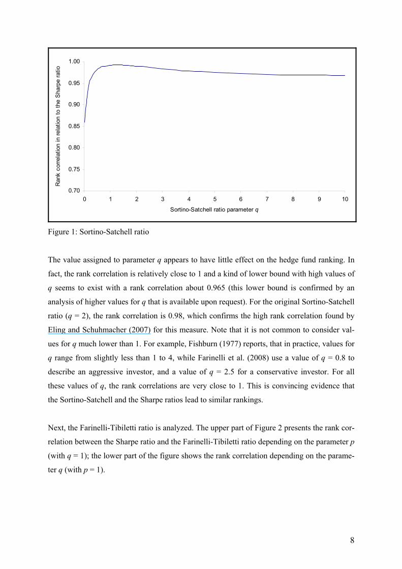
We first analyze the Sortino-Satchell ratio. Figure 1 presents the rank correlation between the

ranking resulting from the Sharpe ratio and that of the Sortino-Satchell ratio for different pa-

rameters q.

8

0.70

0.75

0.80

0.85

0.90

0.95

1.00

0 1 2 3 4 5 6 7 8 9 10

Sortino-Satchell ratio parameter q

Ran

k co

rrela

tion

in re

latio

n to

the

Sha

rpe

ratio

Figure 1: Sortino-Satchell ratio

The value assigned to parameter q appears to have little effect on the hedge fund ranking. In

fact, the rank correlation is relatively close to 1 and a kind of lower bound with high values of

q seems to exist with a rank correlation about 0.965 (this lower bound is confirmed by an

analysis of higher values for q that is available upon request). For the original Sortino-Satchell

ratio (q = 2), the rank correlation is 0.98, which confirms the high rank correlation found by

Eling and Schuhmacher (2007) for this measure. Note that it is not common to consider val-

ues for q much lower than 1. For example, Fishburn (1977) reports, that in practice, values for

q range from slightly less than 1 to 4, while Farinelli et al. (2008) use a value of q = 0.8 to

describe an aggressive investor, and a value of q = 2.5 for a conservative investor. For all

these values of q, the rank correlations are very close to 1. This is convincing evidence that

the Sortino-Satchell and the Sharpe ratios lead to similar rankings.

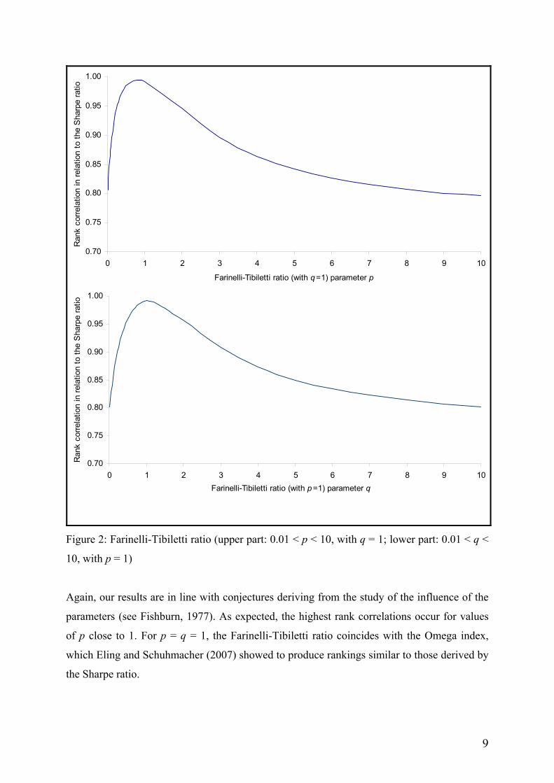
Next, the Farinelli-Tibiletti ratio is analyzed. The upper part of Figure 2 presents the rank cor-

relation between the Sharpe ratio and the Farinelli-Tibiletti ratio depending on the parameter p

(with q = 1); the lower part of the figure shows the rank correlation depending on the parame-

ter q (with p = 1).

9

0.70

0.75

0.80

0.85

0.90

0.95

1.00

0 1 2 3 4 5 6 7 8 9 10

Farinelli-Tibiletti ratio (with q=1) parameter p

Ran

k co

rrela

tion

in re

latio

n to

the

Sha

rpe

ratio

0.70

0.75

0.80

0.85

0.90

0.95

1.00

0 1 2 3 4 5 6 7 8 9 10Farinelli-Tibiletti ratio (with p=1) parameter q

Ran

k co

rrela

tion

in re

latio

n to

the

Sha

rpe

ratio

Figure 2: Farinelli-Tibiletti ratio (upper part: 0.01 < p < 10, with q = 1; lower part: 0.01 < q <

10, with p = 1)

Again, our results are in line with conjectures deriving from the study of the influence of the

parameters (see Fishburn, 1977). As expected, the highest rank correlations occur for values

of p close to 1. For p = q = 1, the Farinelli-Tibiletti ratio coincides with the Omega index,

which Eling and Schuhmacher (2007) showed to produce rankings similar to those derived by

the Sharpe ratio.

10

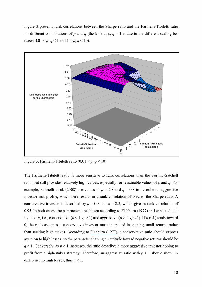
Figure 3 presents rank correlations between the Sharpe ratio and the Farinelli-Tibiletti ratio

for different combinations of p and q (the kink at p, q = 1 is due to the different scaling be-

tween 0.01 < p, q < 1 and 1 < p, q < 10).

0.01

0.1

0.2

0.3

0.4

0.5

0.6

0.7

0.8

0.9 1 2 3 4 5 6 7 8 9

100.

01

0.2 0.

4 0.6 0.

8

13

57

9

0.00

0.10

0.20

0.30

0.40

0.50

0.60

0.70

0.80

0.90

1.00

Rank correlation in relation to the Sharpe ratio

Farinelli-Tibiletti ratio parameter p

Farinelli-Tibiletti ratio parameter q

Figure 3: Farinelli-Tibiletti ratio (0.01 < p, q < 10)

The Farinelli-Tibiletti ratio is more sensitive to rank correlations than the Sortino-Satchell

ratio, but still provides relatively high values, especially for reasonable values of p and q. For

example, Farinelli et al. (2008) use values of p = 2.8 and q = 0.8 to describe an aggressive

investor risk profile, which here results in a rank correlation of 0.92 to the Sharpe ratio. A

conservative investor is described by p = 0.8 and q = 2.5, which gives a rank correlation of

0.95. In both cases, the parameters are chosen according to Fishburn (1977) and expected util-

ity theory, i.e., conservative (p < 1, q > 1) and aggressive (p > 1, q < 1). If p (<1) tends toward

0, the ratio assumes a conservative investor most interested in gaining small returns rather

than seeking high stakes. According to Fishburn (1977), a conservative ratio should express

aversion to high losses, so the parameter shaping an attitude toward negative returns should be

q > 1. Conversely, as p > 1 increases, the ratio describes a more aggressive investor hoping to

profit from a high-stakes strategy. Therefore, an aggressive ratio with p > 1 should show in-

difference to high losses, thus q < 1.

11

However, the Farinelli-Tibiletti ratio is a flexible tool that can be used in various ways. The

parameters can be chosen so that the ratio can be read as the tradeoff between moderate

gain/moderate risk or between high stakes/huge losses. In such a case, p and q go hand in

hand , i.e., p < 1 goes with q < 1, and p > 1 goes with q > 1. The ratio can then be interpreted

as the price of one unit of return for one unit of loss, where returns and losses are weighted by

p and q. As the ratio moves to extreme investment styles, rank correlations with the moderate

Sharpe ratio decrease. This is most evident for p and q close to 10, where the rank correlation

falls to 0.59. It is worth noting that this occurs in correspondence with the case where the ratio

detects the tradeoff between high stakes/huge losses.

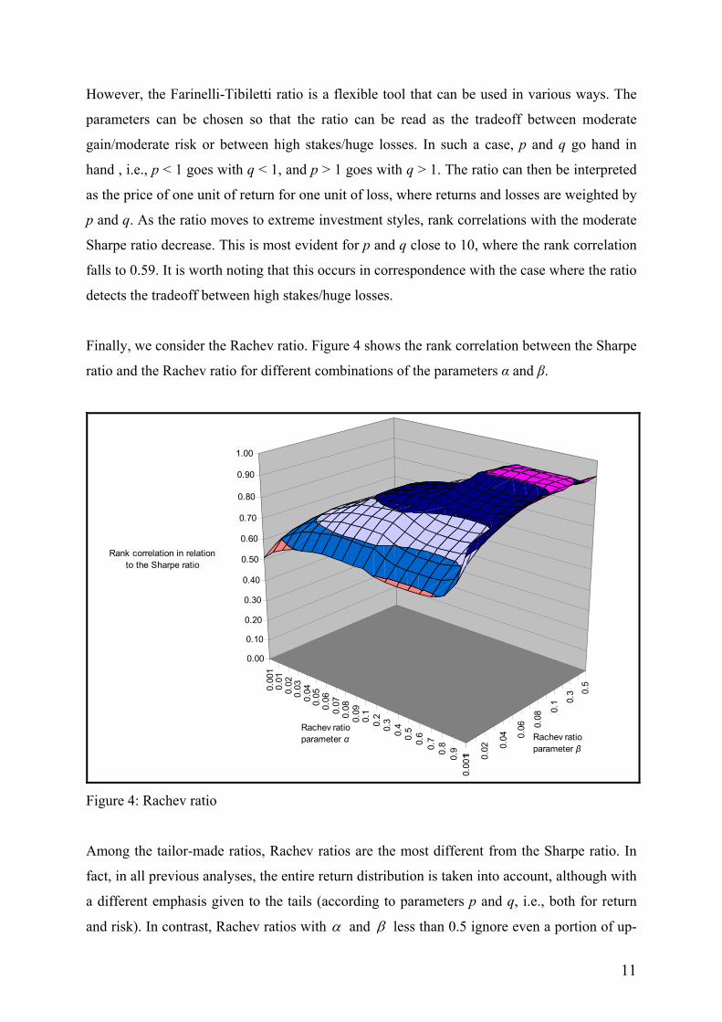
Finally, we consider the Rachev ratio. Figure 4 shows the rank correlation between the Sharpe

ratio and the Rachev ratio for different combinations of the parameters α and β.

0.00

10.

010.

020.

030.

040.

050.

060.

070.

080.

090.

10.

20.

30.

40.

50.

60.

70.

80.

9 10.

001 0.

02 0.04 0.

06 0.08

0.1 0.

3 0.5

0.00

0.10

0.20

0.30

0.40

0.50

0.60

0.70

0.80

0.90

1.00

Rank correlation in relation to the Sharpe ratio

Rachev ratio parameter α Rachev ratio

parameter β

Figure 4: Rachev ratio

Among the tailor-made ratios, Rachev ratios are the most different from the Sharpe ratio. In

fact, in all previous analyses, the entire return distribution is taken into account, although with

a different emphasis given to the tails (according to parameters p and q, i.e., both for return

and risk). In contrast, Rachev ratios with α and β less than 0.5 ignore even a portion of up-

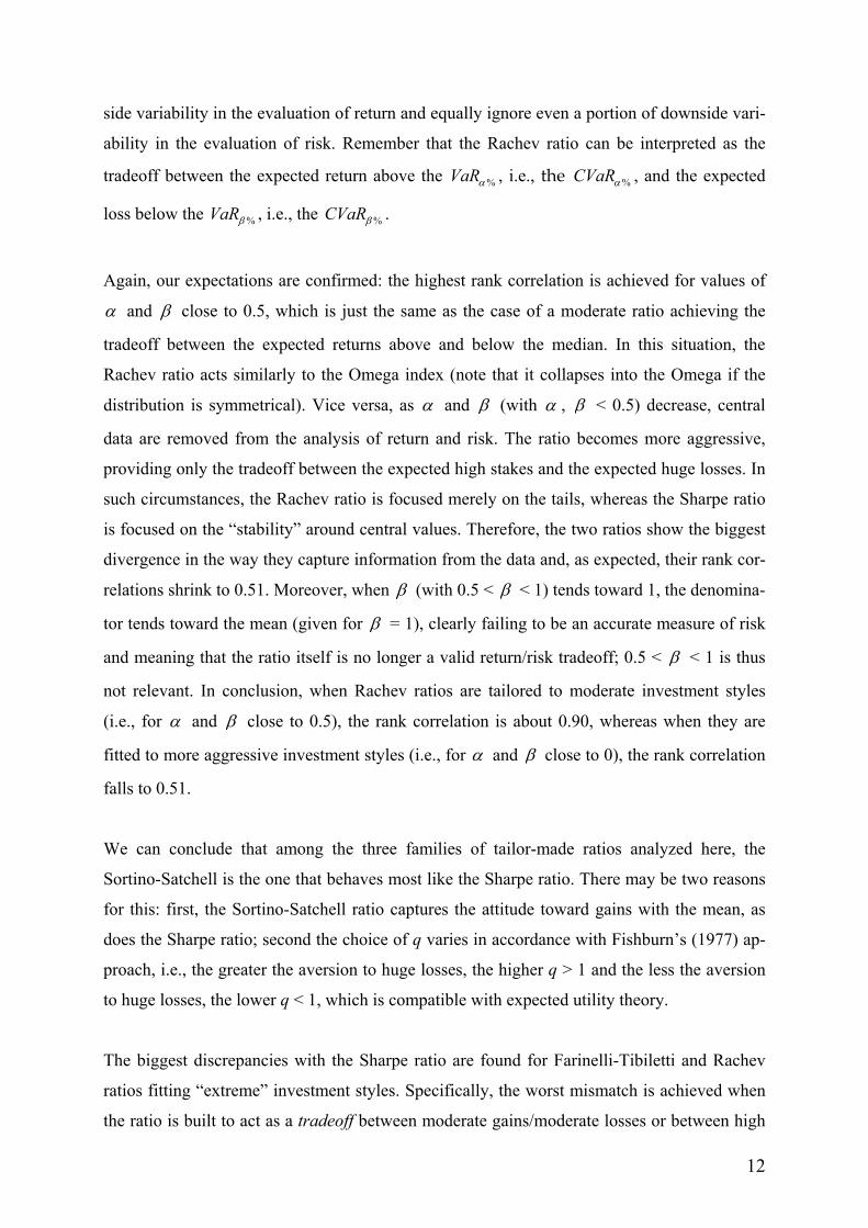
12

side variability in the evaluation of return and equally ignore even a portion of downside vari-

ability in the evaluation of risk. Remember that the Rachev ratio can be interpreted as the

tradeoff between the expected return above the %VaRα , i.e., the %CVaRα , and the expected

loss below the %VaRβ , i.e., the %CVaRβ .

Again, our expectations are confirmed: the highest rank correlation is achieved for values of

α and β close to 0.5, which is just the same as the case of a moderate ratio achieving the

tradeoff between the expected returns above and below the median. In this situation, the

Rachev ratio acts similarly to the Omega index (note that it collapses into the Omega if the

distribution is symmetrical). Vice versa, as α and β (with α , β < 0.5) decrease, central

data are removed from the analysis of return and risk. The ratio becomes more aggressive,

providing only the tradeoff between the expected high stakes and the expected huge losses. In

such circumstances, the Rachev ratio is focused merely on the tails, whereas the Sharpe ratio

is focused on the “stability” around central values. Therefore, the two ratios show the biggest

divergence in the way they capture information from the data and, as expected, their rank cor-

relations shrink to 0.51. Moreover, when β (with 0.5 < β < 1) tends toward 1, the denomina-

tor tends toward the mean (given for β = 1), clearly failing to be an accurate measure of risk

and meaning that the ratio itself is no longer a valid return/risk tradeoff; 0.5 < β < 1 is thus

not relevant. In conclusion, when Rachev ratios are tailored to moderate investment styles

(i.e., for α and β close to 0.5), the rank correlation is about 0.90, whereas when they are

fitted to more aggressive investment styles (i.e., for α and β close to 0), the rank correlation

falls to 0.51.

We can conclude that among the three families of tailor-made ratios analyzed here, the

Sortino-Satchell is the one that behaves most like the Sharpe ratio. There may be two reasons

for this: first, the Sortino-Satchell ratio captures the attitude toward gains with the mean, as

does the Sharpe ratio; second the choice of q varies in accordance with Fishburn’s (1977) ap-

proach, i.e., the greater the aversion to huge losses, the higher q > 1 and the less the aversion

to huge losses, the lower q < 1, which is compatible with expected utility theory.

The biggest discrepancies with the Sharpe ratio are found for Farinelli-Tibiletti and Rachev

ratios fitting “extreme” investment styles. Specifically, the worst mismatch is achieved when

the ratio is built to act as a tradeoff between moderate gains/moderate losses or between high

13

stakes/huge losses, so that the parameter regulating aversion to huge losses no longer follows

the Fishburn (1977) paradigm. Since by definition, the Rachev ratio is the tradeoff between

gains and losses, its largest discrepancy from the Sharpe ratio occurs when it is set up for the

most aggressive investor style, that is, small α and β . In this case, the rank correlation be-

tween the two measures falls as low as 0.51.

4. Tests on Return Distributions

Previous investigations confirm the results of Eling and Schuhmacher (2007) for “moderate”

ratios describing a nonaggressive investment style. Those results seem to be swimming

against the current stream of literature, which generally finds that the Sharpe ratio is not the

right tool for ranking hedge funds (see Perello, 2007). To provide an explanation, we check

whether the empirical returns can be said to be elliptically distributed. When this is the case,

rankings are known to be compatible with mean-variance analysis (see Owen and Rabino-

vitch, 1983) and the Sharpe ratio would be appropriate.

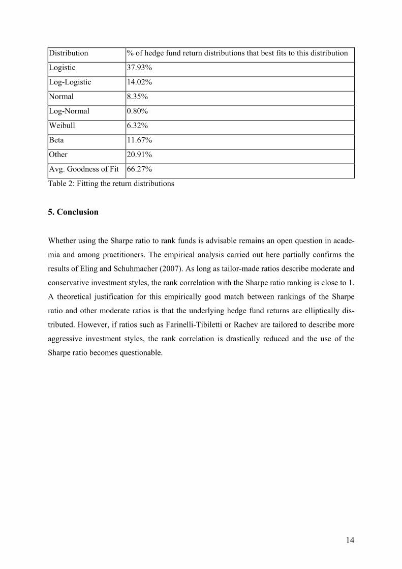
A number of fit tests are carried out to model the empirical distributions using the distribu-

tion-fitting software BestFit. Via a chi-square goodness-of-fit test, this program estimates

which one of 22 given statistical distributions best fits the empirical return distribution. Re-

sults for the 4,048 hedge funds are collected in Table 2: Most of the analyzed funds have el-

liptical distributed returns. The distribution that best fits the empirical distribution is in most

cases a logistic or a log-logistic distribution. Thus, one reason the ranking of the Sharpe ratio

is consistent with the ranking of the other measures might be because the returns of most

funds are elliptical distributed.

14

Distribution % of hedge fund return distributions that best fits to this distribution

Logistic 37.93%

Log-Logistic 14.02%

Normal 8.35%

Log-Normal 0.80%

Weibull 6.32%

Beta 11.67%

Other 20.91%

Avg. Goodness of Fit 66.27%

Table 2: Fitting the return distributions

5. Conclusion

Whether using the Sharpe ratio to rank funds is advisable remains an open question in acade-

mia and among practitioners. The empirical analysis carried out here partially confirms the

results of Eling and Schuhmacher (2007). As long as tailor-made ratios describe moderate and

conservative investment styles, the rank correlation with the Sharpe ratio ranking is close to 1.

A theoretical justification for this empirically good match between rankings of the Sharpe

ratio and other moderate ratios is that the underlying hedge fund returns are elliptically dis-

tributed. However, if ratios such as Farinelli-Tibiletti or Rachev are tailored to describe more

aggressive investment styles, the rank correlation is drastically reduced and the use of the

Sharpe ratio becomes questionable.

15

References

1. Acerbi, C., Tasche, D., 2002. On the Coherence of Expected Shortfall. Journal of Banking

& Finance 26, 1487–1503.

2. Ackermann, C., McEnally, R., Ravenscraft, D., 1999. The Performance of Hedge Funds:

Risk, Return, and Incentives. Journal of Finance 54, 833–874.

3. Agarwal, V., Naik, N.Y., 2004. Risk and Portfolio Decisions Involving Hedge Funds. Re-

view of Financial Studies 17, 63–98.

4. Bernardo, A., Ledoit, O., 2000. Gain, Loss and Asset Pricing. Journal of Political Econ-

omy 108, 144–172.

5. Biglova, A., Ortobelli, S., Rachev, S. T., Stoyanov, S., 2004. Different Approaches to Risk

Estimation in Portfolio Theory. Journal of Portfolio Management 31, 103–112.

6. Brown, S. J., Goetzmann, W. N., Ibbotson, R. G., 1999. Offshore Hedge Funds: Survival

and Performance 1989–1995. Journal of Business 72, 91–117.

7. Capocci, D., Hübner, G., 2004. Analysis of Hedge Fund Performance. Journal of Empiri-

cal Finance 11, 55–89.

8. Ding, B., Shawky, H. A., 2007. The Performance of Hedge Fund Strategies and the

Asymmetry of Return Distributions. European Financial Management 13, 309–331.

9. Edwards, F., Caglayan, M., 2001. Hedge Fund Performance and Manager Skill. Journal of

Futures Markets 21, 1003–1028.

10. Eling, M., Schuhmacher, F., 2007. Does the Choice of Performance Measure Influence the

Evaluation of Hedge Funds? Journal of Banking & Finance 31, 2632–2647.

11. Farinelli, S., Ferreira, M., Rossello, D., Thoeny, M., Tibiletti, L., 2007. Optimal Asset

Allocation Aid System: From “One-Size” vs “Tailor-Made” Performance Ratio. European

Journal of Operational Research, forthcoming.

12. Farinelli, S., Ferreira, M., Rossello, D., Thoeny, M., Tibiletti, L., 2008. Beyond Sharpe

Ratio: Optimal Asset Allocation Using Different Performance Ratios. Journal of Banking

& Finance, forthcoming.

13. Farinelli, S., Tibiletti, L., 2003. Sharpe Thinking with Asymmetrical Preferences, Techni-

cal Report presented at European Bond Commission; Winter Meeting; Frankfurt.

14. Farinelli, S., Tibiletti, L., 2008. Sharpe Thinking in Asset Ranking with One-Sided Meas-

ures. European Journal of Operational Research 185, 1542–1547.

15. Favre, L., Galeano, J. A., 2002. Mean-Modified Value at Risk Optimization with Hedge

Funds. Journal of Alternative Investments 5, 21–25.

16

16. Fishburn, P.C., 1977. Mean-Risk Analysis with Risk Associated with Below-Target Re-

turns. American Economic Review 66, 116–126.

17. Fung, W., Hsieh, D. A., 2000. Performance Characteristics of Hedge Funds and Commod-

ity Funds: Natural vs. Spurious Biases. Journal of Financial and Quantitative Analysis 35,

291–307.

18. Gregoriou, G. N., Sedzro, K., Zhu, J., 2005. Hedge Fund Performance Appraisal Using

Data Envelopment Analysis. European Journal of Operational Research 164, 555–571.

19. Keating, C., Shadwick, W., 2002. A Universal Performance Measure. Journal of Per-

formance Measurement 6(3), 59–84.

20. Kouwenberg, R., 2003. Do Hedge Funds Add Value to a Passive Portfolio? Journal of

Asset Management 3, 361–382.

21. Leland, H. E., 1999. Beyond Mean-Variance: Performance Measurement in a Non-

Symmetrical World. Financial Analysts Journal 55, 27–36.

22. Liang, B., 2000. Hedge Funds: The Living and the Dead. Journal of Financial and Quan-

titative Analysis 35, 309–326.

23. Martin, D., Rachev, S. T., Siboulet, F., 2003. Phi-Alpha Optimal Portfolios and Extreme

Risk Management. Wilmott Magazine of Finance November, 70–83.

24. Menn, C., Fabozzi, F. J., Rachev, S. T., 2005. Fat-Tailed and Skewed Asset Return Distri-

butions: Implications for Risk Management, Portfolio Selection, and Option Pricing. John

Wiley & Sons: Hoboken, NJ.

25. Owen, J., Rabinovitch, R., 1983. On the Class of Elliptical Distributions and Their Appli-

cation to the Theory of Portfolio Choice. Journal of Finance 38, 745–752.

26. Perello, J., 2007, Downside Risk Analysis Applied to the Hedge Funds Universe, Physica

A 383, 480–496.

27. Rachev, S. T., Ortobelli, S., Stoyanov, S., Fabozzi, F., Biglova, A., 2007. Desirable Prop-

erties of an Ideal Risk Measure in Portfolio Theory. International Journal of Theoretical

and Applied Finance, forthcoming.

28. Sharpe, W. F., 1966. Mutual Fund Performance. Journal of Business 39, 119–138.

29. Sortino, F. A., Satchell, S., 2001. Managing Downside Risk in Financial Markets. Butter-

worth Heinemann: Oxford.