On the use of Hamiltonian and maximized Hamiltonian in nondifferentiable control theory

JOURNAL OF OPTIMIZATION THEORY AND APPLICATIONS: Vol. 46, No. 4, AUGUST 1985

On the Use of Hamiltonian and Maximized Hamiltonian

in Nondifferentiable Control Theory ~

G. F E I C H T I N G E R 2 A N D R. F. H A R T L 3

Dedicated to G. Leitmann

Abstract. In optimal control problems involving nondifferentiable functions of the state variable, the adjoint differential inclusion can be formulated by either use of the Hamittonian or the maximized Hamiltonian. In this paper, we solve a production-employment model in which the latter approach must be utilized, since the former does not enable one to determine the optimal policy.

Key Words. Optimal control, envelope theorem, differential inclusions, nondifferentiable functions, production-employment model.

I. Introduction

In standard optimal control theory, the well-known envelope theorem states that the partial derivatives of the Hamiltonian H and the maximized Hamiltonian H ° = m a x ~ H with respect to the state are the same; i.e., Hx = H i (e.g., see Refs. 1-2). This result is always used when proving sufficiency theorems of Mangasarian type (see Refs. 2-5).

I f the problem is generalized to allow for nondifferentiable but locally Lipschitz functions of the state variable, then the adjoint relation as a part of the necessary conditions can be stated as -,~ ~ OxH or - ~ ~ OxH ° (e.g., see Refs. 6-7). In Ref. 7, it was shown that the usual Mangasarian-type sufficiency conditions also hold for problems involving nondifferentiable functions, if the adjoint differential inclusion relationship - ~ c OxH ° is used.

The authors gratefully acknowledge useful remarks by S. J~rgensen, J. Levine, A. Luhmer, and P. Michel.

2 Professor, Institute for Econometrics and Operations Research, Technical University, Vienna, ~ustria.

3 Assistant Professor, Institute for Econometrics and Operations Research, Technical Univer- sity, Vienna, Austria.

493 0022-3239/85/0800,.0493504.50/0 @) 1985 Plenum Publishing Corporation

494 JOTA: VOL. 46, NO. 4, AUGUST 1985

Only under additional assumptions can this relation be replaced by the more convenient one - }t c OxH.

In this paper, we show that the use of the latter relation can mean a loss of information by solving a model of optimal production and employment in which OxH ° contains only one number, while OxH is a whole interval, which does not enable one to determine the optimal policy.

2. Control Problems Involving Nondifferentiable Functions

Consider the following optimization problem:

or e x p ( - r t ) F(x, u, t) dt+exp(-rT) S(x( T))-~max, (1)

subject to

:~=g(x, u, t), x(0) = x0, u(t )c f l , (2)

where x(t)~R" denotes the absolutely continuous state trajectory and u(t) ~ f~ C R" denotes the measurable control functions. Assume the functions F : ~ " x ~ " xR--> ~ and g :R" x R " xl/~-> R" to be locally Lipschitz in x and continuous in u and t, and assume S : ~" -~ R to be locally Lipschitz.

Let us define the Hamiltonian H and the maximized Hamiltonian H ° (in current-value terms) as

H(x, u, t, A) = F(x, u, t)+ Ag(x, u, t), (3)

H°(x, t, A) = m a x H(x, u, t, A). (4)

Then, the following theorem gives the necessary optimality conditions for the above problem.

Theorem 2.1. Let (u(t) , x(t)) be an optimal pair for the problem: max (1), subject to (2). Then, there exists an absolutely continuous adjoint function A ~ ~" such that almost everywhere the following conditions hold:

H(x(t) , u(t), t, A(t)) = H°(x(t), t, A (t)), (5)

rA( t ) -A( t ) cOxH°(x ( t ) , t, A(t)), (6)

;t ( T) ~ OxS(x( T) ). (7)

The symbol 0~ denotes the generalized gradient with respect to x. Note that at is a subset of R". For definitions and a summary of properties of locally Lipschitz functions and generalized gradients, the reader is referred to Clarke (Refs. 6-10).

JOTA: VOL. 46, NO. 4, AUGUST 1985 495

For the purposes of application, the following formulation seems to be more convenient than Theorem 2.1.

Corollary 2.1. In Theorem 2.1, the differential inclusion relationship (6) can be replaced by

rA(t) - ,((t) 60xH(x( t ) , u(t), t, A (t)). (8)

The proofs of Theorem 2.1 and Corollary 2.1 are straightforward transformations of the results in Refs. 6, 7, or 8 to current-value formulation and are therefore omitted. If the maximization of H w.r.t, u is unique then (8) immediately follows from (6), because of OxH ° C OxH.

For the problem (1)-(2), we can also obtain the usual sufficiency conditons of Mangasarian and Arrow-Kurz type.

Theorem 2.2. Let (u(t) , x(t)) be a feasible solution of the problem (1)-(2), and let A(t) be such that the maximum principle conditions (5)-(7) are satisfied. Then, (u(t), x(t)) is an optimal pair provided that H°(x, t, A) is concave in x for every fixed t and A, and that S is concave.

Bearing in mind the envelope theorem of standard optimal control theory, i.e.,

OH/ox = oH°/ox,

it could be expected that in Theorem 2.2 the adjoint differential inclusion relationship (6) can be replaced by (8). The following corollary shows that this is possible in some cases.

Corollary 2.2. Relation (6) can be replaced by (8) in Theorem 2.2 if either H is separable, in the sense that

H(x, u, t ,A)= Hl(x, t,A)+ H2(u, t,A), (9)

or if H is regular, in the sense that the one-sided directional derivative of H equals its support function; i.e., if for every y ~ ~",

lira [H(x + ey, u, t, A) - H(x, u, t, X)]/E = max{~'y]~" c OxH(x, u, t, A )}. (10) E~,O

The proofs of Theorem 2.2 and Corollary 2.2 can be found in Ref. 7. For the definition of regularity, see also Clarke (Ref. 9).

In general, i.e., if neither (9) nor (10) is satisfied, then OxH C dxH ° need not hold and (6) cannot be replaced by (8) in Theorem 2.2. On the other hand, this replacement is always possible as far as the necessary conditions are concerned, but some information might get lost when using (8) rather than (6), and this may suggest the selection of a suboptimal solution.


In the next section, we shall present an economic model in which the original equation (6) has to be used, since 0xt-1 ° contains only one number, whereas OxH is a whole interval. The presentation is preceded by the following two remarks.

Remark 2.1. If the horizon time is infinite, i.e., T = ~ and S = 0 in the objective functional (1), then the necessary conditions of Theorem 2.1 and Corollary 2.1 remain valid, except for the transversality condition (7) which has no counterpart here. The sufficiency conditions of Theorem 2.2 and Corollary 2.2 remain valid if (7) is replaced by

!ira exp( - rt) A ( t)[~2(t) - x( t)] --> 0, (11)

with ~ denoting any other feasible state trajectory. For the proof of the necessary conditions for T = m, a similar continuity

argument as in Ref. 11, p. 316 can be used. A transversality condition similar to (11) can be shown to be necessary for optimality only under additional growth conditions imposed on the state equation (Ref. 12). The generali- zation of the sufficiency theorems of Ref. 7 to the infinite-horizon case is straightforward.

Remark 2.2. In the literature, the concavity of H ° and the adjoint relation (6) is sometimes combined in the form

H(~, a, t, A ) - H ( x ( t ) , u ( t ) , t, a ) - < - A ( t ) [ Y , - x ( t ) ] ,

for all admissible ~, ~ and every to[0, T]. See Leitmann (Refs. 13-16).

3. A Dynamic Optimization Problem of Production and Employment

We consider a profit-maximizing firm which is faced with the following intertemporal maximization problem:

max e x p ( - r t ) [ p r l ( p ) - c ( f ( x ) ) - wx - k ( u ) - d)(Tq(p) - f ( x ) ) ] dt p ,u ,w 0

+ exp(- rT ) S x ( T ) ,

subject to

ic= u-cr(w)x, x(0) = Xo-> 0,

p ~ O , W~W,

(12)

(13)

(14)


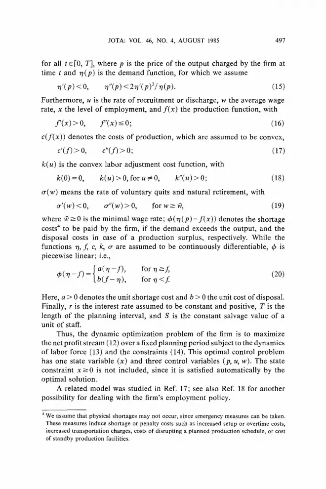
for all t ~ [0, T], where p is the price of the output charged by the firm at time t and r/(p) is the demand function, for which we assume

r/ '(p) < 0, rf'(p)<2rf(p)2/rl(p). (15)

Furthermore, u is the rate of recruitment or discharge, w the average wage rate, x the level of employment, and f (x) the production function, with

/ ' ( x ) > 0, f ' ( x ) - 0 ; (16)

c(f(x)) denotes the costs of production, which are assumed to be convex,

c'(f) > O, c"(f) > 0; (17)

k(u) is the convex labor adjustment cost function, with

k (0 )= 0 , k(u)>O, foru#O, k"(u) > 0; (18)

o-(w) means the rate of voluntary quits and natural retirement, with

cr'(w) <0 , cr"(w) > 0, for w_> #, (19)

where ~-> 0 is the minimal wage rate; ~b ( r / (p ) - f (x ) ) denotes the shortage c o s t s 4 tO be paid by the firm, if the demand exceeds the output, and the disposal costs in case of a production surplus, respectively. While the functions ~7, f, c, k, cr are assumed to be continuously differentiable, ~b is piecewise linear; i.e.,

j~ a ( r / - f ) , for ~7 - f ~f~ (20)

Lb(f-,7), for n<f.

Here, a > 0 denotes the unit shortage cost and b > 0 the unit cost of disposal. Finally, r is the interest rate assumed to be constant and positive, T is the length of the planning interval, and S is the constant salvage value of a unit of staff.

Thus, the dynamic optimization problem of the firm is to maximize the net profit stream (12) over a fixed planning period subject to the dynamics of labor force (13) and the constraints (14). This optimal control problem has one state variable (x) and three" control variables (p, u, w). The state constraint x-> 0 is not included, since it is satisfied automatically by the optimal solution.

A related model was studied in Ref. 17; see also Ref. 18 for another possibility for dealing with the firm's employment policy.

4 We assume that physical shortages may not occur, since emergency measures can be taken. These measures induce shortage or penalty costs such as increased setup or overtime costs, increased transportation charges, costs of disrupting a planned production schedule, or cost of standby production facilities.


4. Necessary Optimality Conditions

The current-value Hamiltonian for the above model is given by

H = p~q(p) - c ( f ( x ) ) - wx - k ( u ) - c h ( ~ ( p ) - f ( x ) ) + A[u - o-(w)x], (21)

with A denoting the current-value shadow price. In order to maximize H w.r.t, p, we consider three cases:

Case L ~ ( p ) > f ( x ) (excess demand).

Case IL V(P) = f ( x ) (demand is met by production).

Case I IL ~7(P) < f ( x ) (production surplus).

In Case I, we have

4)( v - f ) = a( *? - f ) .

Therefore, the necessary condition for an optimal p > 0, i.e., Hp = 0, yields P = Pa, defined by

P,~ + ~7(Pa)/ ~f(P,,) = a. (22)

On the other hand, in Case III, we have

qS(r / - f ) = -b(~7 - f ) ,

and Hp = 0 implies that p = Pb, where Pb is given by

Pb + n ( P b ) / n ' (Pb) = - b . (23)

Assumption (15) implies that p + rt/*l' is a strictly monotonic increasing function of p (see also Ref. 19):

( d / d p ) [ p + ~7/~7'] = 2 - rt~"/~7'2 > 0. (24)

Thus, the solutions of (22) and (23) are unique provided they exist (see also the first part of Fig. 1). The existence of pa and Pb can be guaranteed by assuming that

~9(0)/r/'(0) < -b , l i m [ p + ~ ( p ) / ~ ' ( p ) ] > a . (25) p~-oO

Otherwise, p, = oc and /or Pb = 0. To simplify the analysis, we assume (25). This implies the existence of threshold values x, and xb such that

f ( x , ) = rl(p,,) , f (Xb ) = "q(Pb). (26)

In Case I , f (x ) < ~ (p~) implies x < x~, whereas in Case III, f rornf(x) > r/(Pb), we obtain x > xh.


+rl P ~'

/

pa ~ p

-b

q f

p Pb P~ P p xa xb x

~ p Xa ×b 9 x

Fig. 1. Graphical derivation of the optimal price policy.

If the optimal price is not equal to p~ or Pb, we must have Case II, i.e.,

r/(p) = f ( x ) , (27)

and x ~ - < x - < xb. The implicit relation (27) can be solved as p =p (x ) , with

p ' ( x ) = f ' ( x ) / r f ( p ) < 0, (28)

and p(x,~) =p , , p(xb) =Pb.

Summing up, we have obtained the following optimal pricing policy:

Region L p = p,~, for x < x,. Region II. p = p ( x ) , for xo <- x <- Xb.


Region I lL P = Pb, for x > x b. This policy is derived graphically in Fig. 1.

The Hamiltonian maximizing conditions w.r.t, u and w,

H~ =0, Hw<-O, Hw(w- ~) =0,

yield

A = k ' (u ) , (29)

A = -1/o- ' (w), if A > -1 /o- ' (# ) , (30a)

w = @, if A <- -1/ tr ' (@). (30b)

The transversality condition is given by

A(T) = S x ( x ( T ) ) = S. (31)

In order to obtain the adjoint relation (6), we observe that, in Cases I and III, we have

O(a(•(p,,) - f ( x ) ) / O x = - a f t ( x )

and

O ¢ ( r l ( p a ) - f ( x ) ) / O x = b f ' (x ) ,

respectively. Furthermore, in these cases (O/Ox)prl(p) vanishes. In Case II, from (27) we have

0 6 ( n ( p ( x ) ) - f ( x ) ) / o x = O.

On the other hand, from (28) we deduce that

(O/ O x ) [ p ( x ) ~ ( p ( x ) )] = (',7 + p~l')p'(x) = (p + rl/ r f ) f ' .

Therefore, (6) becomes

( - a f t , in Case I, (32a)

A=,~(r+o)+c'f'+w~-f'(p+n/n'), in Case IX, (32b)

[_bf , in Case III. (32c)

Note that u and w, given by (29) and (30), do not depend on x. If we would compute the adjoint relation according to (8), rather than

(6), we would again obtain (32a) and (32c) in Cases I and III, whereas in Case II (32b) has to be replaced by

} t~[ ( r+o ' )A + c ' f ' + w - a f ' , ( r+cr)A + c ' f ' + w + bf']. (33)

It is important to note that using H rather than H ° in the adjoint relation implies a loss of information, since (32b) provides a unique value for )[, while (33) yields an interval containing this value.


5. Derivation of the Optimal Policy

In order to analyze the behavior of the optimal solution in the state- costate phase plane, (29) and (30) can be solved as u = u()t) and w = w(A), with

u'(A) = 1/k"(u) > 0, (34)

~ 0, for A < -1/o~'(v?), (35a)

w'(A)=(-o-(w)/,~o-' "(w)>O, f o r a > - 1 / o - ' ( ~ ) . (35b)

We are now prepared to analyze an optimal solution described by (13) and (32) in the (x, A) phase plane. Using (28), (34), (35), we obtain

O2/Ox = -o-(w) < 0, (36)

02/02t = u'(h ) - o-'(w)w'(lt )x > 0, (37)

f -aft ' , , ( in Case I, (38a)

O~/Ox=c"f '2+c'f" - f " p + - f ' p ' ( x ) 2 - - - ~ ] , i nCase I I , (38b)

bf", in Case III, (38c)

O~/02t = r+~+[2t~'(w)+l]w'(; t ) = r + o-> O. (39)

In order to determine the sign of O~/Ox we note that

c'--a } C'- (p + "17/rf) = - (1 / f ' ) [ ( r + o-)A + w],

c '+b

whenever }t = 0. Since all other terms in (38) are nonnegative, we obtain O),/Ox > 0 along the Jt = 0 isocline (at least in the region A-> 0). The two isoclines are sketched in Fig. 2. The 2 = 0 locus emanates from the origin and is upward sloping. On the other hand, the ~ =0 locus decreases (at least for A >-0), has a positive value of A for x = 0 [see (32a)], and ties below the abscissa in Region III [see (32c)]. Furthermore, for x = x, and x = Xb, the ,'~ = 0 curve has kinks. Thus, the two isoclines have a point of intersection in the first quadrant. This equilibrium is a saddle point.

There exist two cases for the stationary point (~, i ) : Case A. If a is large, then (£, i ) is contained in Region II (see Fig. 2A). Case B. I f a is small, then (~, i ) lies in Region I (see Fig. 2B). Let us consider Case A first. Figure 2A shows that, for a large initial

level of employment, Xo > xb, it is not optimal to charge a price p < Pb. This implies a production surplus, f = r /> 0, which gradually decreases. On the


-1 d(m) l

[A]

k 7

> * I i ' q T / ~ j . . .x=o

P P , ~ i./<' • I /

• . i r l : f

d ( ~ - i - " - "

! / / ,, ,x=0 [B] ~ . ', , . .

Fig. 2.

"X.. =0 t x x I . /

• / 4 " f n < f

.r~>- f

i ,

o / t - D / - - ",- - -- t ,.' I t l q=f \ ! "'-

'X ! ¢ , , / / - , ', . ..> Xa )< "'-, X b X

P=Pb

rl<f

W>W

>:..-

Xa Xa -, X b ~ X

Optimal solution in the state-costate phase plane.

other hand, if x0<x~, an excess demand occurs, ~ 7 - f > 0 . For T large enough, the trajectory eventually enters Region II, where it is optimal to charge the market clearing price; i.e., ~7 = f For infinite-time horizon, x approaches the stationary level ~ asymptotically (see the stable path in Fig. 2A). In Fig. 2A, we have also sketched two trajectories for T < to and S = 0.

The analysis of Case B can be carried out in a similar way (see Fig. 2B). It turns out that the qualitative behavior of the solution paths is the same as in Case A. Since the shortage costs are small, the tong-run optimal policy implies an excess in demand.

To characterize Cases A and B, we first consider a large value of a, which implies Case A. Note that xa-~ 0, as a-~ oo. The stationary level lies in Region II and does not depend on a. I f a decreases, then x~ increases and eventually reaches 2. Figure 2 shows that the stationary employment


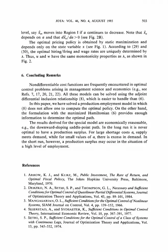
level, say ~ , moves into Region I if a continues to decrease. Note that ~ depends on a and that d:~/da > 0 (see Fig. 2B).

The optimal pricing policy is obtained by static maximization and depends only on the state variable x (see Fig. 1). According to (29) and (30), the optimal hiring/firing and wage rates are uniquely determined by A. Thus, u and w have the same monotonicity properties as A, as shown in Fig. 2.

6. Concluding Remarks

Nondifferentiable cost functions are frequently encountered in optimal control problems arising in management science and economics (e.g., see Refs. 7, 17, 20, 21, 22). All these models can be solved using the adjoint differential inclusion relationship (8), which is easier to handle than (6).

In this paper, we have solved a production-employment model in which (8) does not allow one to compute the optimal policy. On the other hand, the formulation with the maximized Hamiltonian (6) provides enough information to determine the optimal path.

The results derived for the special model are economically reasonable, e.g., the downward-sloping saddle-point path. In the long run it is never optimal to have a production surplus. For large shortage costs a, supply meets demand, while for small values of a, there is excess in demand. In the short run, however, a production surplus may occur in the situation of a high level of employment.

References

l. ARROW, K. J., and KURZ, M., Public Investment, The Rate of Return, and Optimal Fiscal Policcy, The Johns Hopkins University Press, Baltimore, Maryland, 1970.

2. DERZKO, N. A., SETHI, S. P., and THOMPSON, G. L., Necessary and Sufficient Conditions for Optimal Control of Quasilinear Partial Differential Systems, Journal of Optimization Theory and Applications, Vol. 43, pp. 8%101, 1984.

3. MANGASARIAN, O. L., Sufficient Conditions for the Optimal Control of Nonlinear Systems, SIAM Journal on Control, Vol. 4, pp. 13%152, 1966.

4. SEIERSTAD, A., and SYDSAETER, K., Sufficient Conditions in Optimal Control Theory, International Economic Review, Vol. 18, pp. 367-391, 1977.

5. SETHI, S. P., Sufficient Conditions for the Optimal Control of a Class of Systems with Continuous Lags, Journal of Optimization Theory and Applications, Vol. 13, pp. 545-552, 1974.


6. CLARKE, F. H., Optimal Control and the True Hamiltonian, SIAM Review, Vol. 21, pp. 157-166, 1979.

7. HARTL, R. F., and SETHI, S. P., Optimal Control Problems with Differential Inclusions: Sufficiency Conditions and an Application to a Production-Inventory Model, Optimal Control Applications and Methods, Vol. 5, pp. 289-307, 1984.

8. CLARKE, F. H., The Maximum Principle under Minimal Hypotheses, SIAM Journal on Control and Optimization, Vol. 14, pp. 1078-1091, 1976.

9. CLARKE, F. H., Generalized Gradients of Lipschitz Functionals, Advances in Mathematics, Vol. 40, pp. 52-67, 1981.

10. CLARKE, F. H., Optimization and Nonsmooth Analysis, Wiley, New York, New York / 1983.

11. LEE, E. B., and MARKUS, L., Foundations of Optimal Control Theory, Wiley, New York, New York, 1967.

12. AUBIN, J. P., and CLARKE, F. H., Shadow Prices and Duality for a Class of Optimal Control Problems, SIAM Journal on Control and Optimization, Vol. 17, pp. 567-586, 1979.

13. LEITMANN, G., and STALFORD, H., A Sufficiency Theorem for Optimal Control, Journal of Optimization Theory and Applications, Vol. 8, pp. 169-174, 1971.

14. LEITMANN, G. Einfiihrung in die Theorie Optimaler Steuerung und der Differen- tialspiele: Line Geometrische DarstelIung, Oldenbourg, Miinchen, Germany, 1974.

15. LEITMANN, G., The Calculus of Variations and Optimal Control, Plenum Press, New York, New York, 1981.

16. BLAGODATSKIKH, V. I., Sufficiency Conditions for Optimality in Problems with State Constraints, Applied Mathematics and Optimization, Vol. 7, pp. 149-157, 1981.

17. FEICHTINGER, G., and LUPTACIK, M., OptimaI Employment and Wage Policies of a Monopolistic Firm, Journal of Optimization Theory and Application (to appear).

18. LEBAN, R., and LESOURNE, J., The Firm's Investment and Employment Policy through a Business Cycle, European Economic Review, Vol. 13, pp. 43-80, 1980.

19. PHELPS, E. S., and WINTER, S. G., JR., Optimal Price Policy under Atomistic Competition, Microeconomic Foundations of Employment and Inflation Theory, Edited by E. S. Phelps et al., Macmillan, New York, New York, pp. 309-337, 1970.

20. FEICHTINGER, G., and HARTL, R., Optimal Pricing and Production in an Inventory Model, European Journal of Operations Research, Vol. 19, pp. 45-56, 1985.

21. McMASTERS, A. W., Optimal Control in Deterministic Inventory Models, US Naval Postgraduate School, Monterey, California, Report No. NPS- 55MG0031A, 1970.

20. LIEBER, Z., An Extension to Modigliani and Hohn" s Planning Horizon Results, Management Science, Vol. 20, pp. 319-330, 1973.

Documents

On the use of Hamiltonian and maximized Hamiltonian in nondifferentiable control theory