Embed Size (px)
Citation preview
Discrete time Hamiltonian spin systems
Robert McLachlan∗1, Klas Modin†2, and Olivier Verdier‡3
1 Institute of Fundamental Sciences, Massey University, New Zealand2 Mathematical Sciences, Chalmers University of Technology, Sweden
3 Department of Mathematics and Statistics, University of Umea, Sweden
2014-02-19
We construct generating functions for symplectic maps on products of 2-spheres and use them to construct symplectic integrators for classical spinsystems. They are the minimal possible such generating function and useno Lagrange multipliers or canonical variables. In the single spin case, theresulting spherical midpoint method is given by W −w = X( W+w
|W+w|), where
X(w) = w × ∇H(w), H being the generating function. We establish thebasic properties of the method and describe its relationship to collective sym-plectic integrators for spin systems based on the Hopf map. We introduce anumerical integrator for Riemannian manifolds called the Riemannian mid-point method and determine its properties with respect to isometries andRiemannian submersions and the conditions under which the spherical andRiemannian midpoint methods coincide.
Keywords: classical spin dynamics, Heisenberg spin chain, Landau-Lifshitzequation, symplectic integrator, midpoint method, generating function, rigidbody, discrete mechanics, discrete Moser-Veselov algorithm, collective inte-grator, Hopf map
MSC 2010: 37M15, 70H06, 70H08, 53Z05, 65L06
1. Introduction
Discrete time mechanics is studied for many reasons. (i) It has an immediate impact incomputational physics, where symplectic integrators are in widespread use and in manysituations are overwhelmingly superior to standard numerical integration [26]. (ii) As a
∗[email protected]†[email protected]‡[email protected]
1
arX
iv:1
402.
3334
v2 [
mat
h-ph
] 1
8 Fe
b 20
14
generalisation of continuous mechanics, discrete geometric mechanics is in principle moreinvolved: the nature of symmetries, integrals, and other geometric concepts is importantto understand both in its own right and for its impact on numerical simulations [9]. (iii)Discretisation leads to interesting physics models, for example the extensively-studiedChirikov standard map [5]. (iv) Discrete models can also be directly relevant to intrin-sically discrete situations, such as waves in crystal lattices. Here, the appearance of newphenomena, not persisting at small or vanishing lattice spacing, is well known [13]. (v)The field of discrete integrability is undergoing rapid evolution, with many new examples,approaches, and connections to other branches of mathematics, e.g., special functionsand representation theory [15]. (vi) A strand of research in physics, pioneered notably byLee [18], develops the idea that time is fundamentally discrete, and it is the continuummodels that are the approximation. (vii) Discrete models can contain “more informa-tion and more symmetry than the corresponding differential equations” [19]; this alsooccurs in discrete integrability [15]. While the present study is phrased in the languageof numerical integration, we wish to keep this range of applications in mind.
Symplectic integrators for general Hamiltonians are closely related to the classicalcanonical generating functions defined on symplectic vector spaces (or in local canonicalcoordinates). Generating functions are a tool of vital importance in mechanics, and arealso used for perturbation theory, construction of orbits, of normal forms, in bifurcationtheory, and elsewhere. They have retained their importance in the era of sympecticgeometry and topology, being used to construct Lagrangian submanifolds and to countperiodic orbits [35, 34]. Although there are different types of generating function, all ofthem are restricted to cotangent bundle phase spaces.
In this paper we construct generating functions (or, equivalently, symplectic integra-tors) for symplectic maps of the phase space (S2)n equipped with the symplectic formgiven by the sum of the Euclidean area on each sphere. This is the phase space for thewide range of classical spin systems [16], i.e., systems of the form
wi = wi ×∂H
∂wi, wi ∈ S2 ⊂ R3, i = 1, . . . , n, H : R3n → R,
such as the reduced free rigid body
w = w × I−1w, w ∈ S2 ⊂ R3,
and the classical Heisenberg spin chain of micromagnetics
wi = wi × (wi+1 +wi−1), w0 = wn, wi ∈ S2 ⊂ R3.
Other examples include the motion of massless particles in a divergence-free vector fieldon the sphere (for example, test particles in a global weather simulation), the motion of npoint vortices in a ideal incompressible fluid on the sphere, and the set of Lie–Poissonsystems on so(3)∗.
Apart from its abundance in physics, there are a number of reasons for focusing on thephase space (S2)n. It is the most fundamental example of a symplectic manifold that isnot a vector space, not a cotangent bundle, does not have a global coordinate chart or
2
a cover with one, and is not exact (that is, the symplectic form is not exact). Next tocotangent bundles, the two main types of symplectic manifolds are coadjoint orbits ofLie–Poisson manifolds, and Kahler manifolds; (S2)n is the simplest example of both ofthese.
Techniques to construct symplectic integrators for general Hamiltonian systems on asymplectic manifold M that is not a vector space are known in the following cases:
1. If M = T ∗Q is the cotangent bundle of a submanifold Q ⊂ Rn determined bylevel sets of m functions c1, . . . , cm, then the family of RATTLE methods can beused [12]. More generally, if M is a transverse submanifold of R2n defined bycoisotropic constraints, then geometric RATTLE methods can be used [25].
2. If M ⊂ g∗ is a coadjoint orbit (symplectic leaf) of the dual of a Lie algebra gcorresponding to a Lie group G, RATTLE methods can again be used: first extendthe symplectic system on M to a Poisson system on g∗, then “unreduce” to asymplectic system on T ∗G, then embed G in a vector space and use strategy 1above [9, §VII.5]. One can also use Lie group integrators for the unreduced systemon T ∗G [4, 21]. The discrete Lagrangian method, pioneered in this context byMoser and Veselov [28], yields equivalent classes of methods. The approach is verygeneral, containing a number of choices, especially those of the embedding andthe discrete Lagrangian. For certain choices, in some cases, such as the free rigidbody, the resulting discrete equations are completely integrable; this observationhas been extensively developed [7].
3. If M ⊂ g∗ is a coadjoint orbit and g∗ has a symplectic realisation on R2n obtainedthrough a momentum map associated with a Hamiltonian action of G on R2n,then symplectic Runge–Kutta methods for collective Hamiltonian systems (cf. [20])sometimes descends to symplectic methods on M (so far, the cases sl(2)∗, su(n)∗,so(n)∗, and sp(n)∗ have been worked out). This approach leads to collective sym-plectic integrators [24].
Let us review the listed approaches 1–3 for the case M = S2.The first approach is not applicable, since S2 is not a cotangent bundle.The second approach is possible, since S2 is a coadjoint orbit of su(2)∗ ' R3. SU(2)
can be embedded as a 3–sphere in R4 using unit quaternions, which leads to methodsthat use 10 variables, in the case of RATTLE (8 dynamical variables plus 2 Lagrangemultipliers), and 8 variables, in the case of Lie group integrators. Both of these methodsare complicated; the first due to constraints and the second due to the exponential mapand the need to solve nonlinear equations in auxiliary variables.
The third approach is investigated in [23]. It relies on a quadratic momentum mapπ : T ∗R2 → su(2)∗ and integration of the system corresponding to the collective Hamil-tonian H ◦ π using a symplectic Runge–Kutta method. This yields relatively simpleintegrators using 4 variables. They rely on an auxiliary structure (the suspension toT ∗R2 and the Poisson property of π) and requires solving nonlinear equations in auxil-iary variables; although simple, they do not fully respect the simplicity of S2.
3
In our approach, we still use the extra structure of the standard Euclidean embeddingof S2 in R3 and the standard Euclidean structure of R3, with the motivation that itinduces the symplectic structure on S2 and it seems to be the simplest way to workwith S2 concretely. The four ‘classical’ generating functions, that treat the position andmomentum differently, do not seem to be relevant given the symmetry of S2. Instead,we focus on the Poincare generating function [31, vol. III, §319]
J(W −w) = ∇H(W +w
2
), J =
(0 I−I 0
),
which is equivariant with respect to the full affine group and which corresponds to theclassical midpoint method when interpreted as a symplectic integrator. The classicalmidpoint method on vector spaces is known to conserve quadratic invariants [6], andhence automatically induces a map on S2 when applied to spin systems. However, ithas long been known not to be symplectic [2]. Another variant, namely evaluating thevector field at the geodesic midpoint on the sphere, is also not symplectic. Our mainresult is that a variant that we call the spherical midpoint method, given by
W i −wi =W i +wi
|W i +wi|× ∂H
∂wi
( W 1 +w1
|W 1 +w1|, . . . ,
W n +wn
|W n +wn|
), wi,W i ∈ S2 ⊂ R3,
is symplectic.In § 3 we provide a direct proof of the symplecticity of this method and establish a
number of its other properties, notably full equivariance with respect to the symmetrygroup O(3). The method turns out to be related to the collective symplectic integratorconstructed in [23, 24]; this provides in § 4 a second construction and a second proof ofsymplecticity.
The classical midpoint method evaluates the vector field at the midpoint of a straightline joining the start and ending points. This suggests a generalization to Riemannianmanifolds, and a Riemannian midpoint method, that appears to be new. We introducethis method in §5 and establish some of its basic properties, including equivariance withrespect to the isometry group of the manifold and natural behaviour with respect toRiemannian submersions. The application to S2 is particularly appealing because thegeodesics are associated with the same metric that induces the symplectic structure.Perhaps counterintuitively, the Riemannian midpoint method for the standard Rieman-nian structure on S2 is not symplectic, but the Riemannian structure of the Poissonmap π given does induce a non-standard metric on R3 for which the Riemannian mid-point method is symplectic and coincides with the spherical midpoint method. Thisprovides a third way to view the method.
In §6 we provide a series of detailed examples of the spherical midpoint method appliedto various spin systems.
We use the following notation. X(M) denotes the space of smooth vector fields on amanifold M . If M is a Poisson manifold, and H ∈ C∞(M) is a smooth function on M ,then the corresponding Hamiltonian vector field is denoted XH . The Euclidean lengthof a vector w ∈ Rd is denoted |w|. If w ∈ R3n ' (R3)n, then wi denotes the i:thcomponent in R3.
4
2. Main result
Definition 2.1. The classical midpoint method for discrete time approximation ofthe ordinary differential equation w = X(w), X ∈ X(Rd), is the mapping w 7→ Wdefined by
W −w = hX(W +w
2
), (1)
where h > 0 is the time-step length.
Definition 2.2. The sphere S2 is the standard Euclidean unit sphere in R3 equippedwith symplectic form given by the Euclidean area. (S2)n is the symplectic manifoldgiven by the direct product of n copies of S2 equipped with the direct sum symplecticstructure.
Define a projection map ρ by
ρ(w) =( w1
|w1|, . . . ,
wn
|wn|
).
Our paper is devoted to the following novel method.
Definition 2.3. The spherical midpoint method for ξ ∈ X((S2)n
)is the numerical
integratorΦ(hξ) : (S2)n → (S2)n, (2)
obtained by applying the classical midpoint method (1) to the vector field given by
X(w) := ξ(ρ(w)). (3)
This indeed gives an integrator on (S2)n, since the classical midpoint method preservesquadratic invariants, and the vector field (3) is tangent to the spheres (which are thelevel sets of quadratic functions on R3n).
We now give the main result of the paper.
Theorem 2.4. The spherical midpoint method (2) fulfils the following properties:
1. it is second order accurate;
2. it is equivariant with respect to(SO(3)
)nacting on (S2)n, i.e.,
ψg−1 ◦ Φ(hξ) ◦ ψg = Φ(hψ∗gξ), ∀ g = (g1, . . . , gn) ∈(SO(3)
)n,
where ψg is the action map;
3. it is symplectic if ξ is Hamiltonian;
4. it preserves arbitrary linear symmetries, arbitrary linear integrals, and single-spinhomogeneous quadratic integrals w>i Awi;
5. it is self-adjoint and preserves arbitrary linear time-reversing symmetries;
5
6. it is linearly stable: for the harmonic oscillator w = λw × a, the method yields arotation about the unit vector a by an angle cos−1(1− 1
2(λh)2) and hence is stablefor 0 ≤ λh < 2.
The claims 1–2 and 4–6 are proved in this section. Claim 3, about symplecticity,is proved in § 3. (In addition, the results in § 4 and § 5 provide a separate proof ofsymplecticity, more geometric in nature.)
Proofs.
1. Follows since the midpoint method is of order 2, and since a solution to w = X(w)with X given by (3) is also a solution to w = ξ(w).
2. Follows since the map ρ is equivariant with respect to(SO(3)
)n, and since
(SO(3)
)nis a subgroup of the affine group on R3n and the classical midpoint method is affineequivariant.
4–5. Direct calculations show that X has the same properties in the given cases as theoriginal vector field ξ, and the classical midpoint method is known to preservethese properties.
6. The projection ρ renders the equations for the method nonlinear, even for thislinear test equation; it is clear that the solution is a rotation about a by someangle; this yields a nonlinear equation for the angle with the given solution.
Remark 2.5. Note that the unconditional linear stability of the classical midpointmethod is lost for the spherical midpoint method; the method’s response to the harmonicoscillator is identical to that of the leapfrog (Stormer–Verlet) method.
2.1. Interpretation as Lie–Poisson integrator
R3n is a Lie–Poisson manifold with Poisson bracket
{F,G}(w) =
n∑k=1
(∂F (w)
∂wk× ∂G(w)
∂wk
)·wk. (4)
This is the canonical Lie–Poisson structure of (so(3)∗)n, or (su(2)∗)n, obtained by iden-tifying so(3)∗ ' R3, or su(2)∗ ' R3. For details, see [22, § 10.7] or [23].
The Hamiltonian vector field associated with a Hamiltonian function H : R3n → R isgiven by
XH(w) =n∑k=1
wk ×∂H(w)
∂wk. (5)
Its flow, exp(XH), preserves the Lie–Poisson structure, i.e.,
{F ◦ exp(XH), G ◦ exp(XH)} = {F,G} ◦ exp(XH), ∀F,G ∈ C∞(R3n).
6
The flow exp(XH) also preserves the coadjoint orbits [22, § 14], given by
S2λ1 × · · · × S
2λn ⊂ R3n, λ = (λ1, . . . , λn) ∈ (R+)n,
where S2λ denotes the 2–sphere in R3 of radius λ. A Lie–Poisson integrator for XH
is an integrator that, like the exact flow, preserves the Lie–Poisson structure and thecoadjoint orbits.
Define Γ: R3n ×R3n → R3n by
Γ(w,W
)7−→
(√|w1||W 1|(w1 +W 1)
|w1 +W 1|, . . . ,
√|wn||W n|(wn +W n)
|wn +W n|
)Definition 2.6. The extended spherical midpoint method for X ∈ X(R3n) is thenumerical integrator defined by
W −w = hX(Γ(w,W )
). (6)
IfX(w) ∈ Tw(S2)n for allw ∈ (S2)n, then the extended spherical midpoint method (6)coincides with the spherical midpoint method (2). We therefore have the following resultas a consequence of Theorem 2.4.
Corollary 2.7. The extended spherical midpoint method (6) fulfils the following prop-erties:
1. it is second order accurate;
2. it is equivariant with respect to(SO(3)
)nacting diagonally on (R3)n ' R3d.
3. it is a Lie–Poisson integrator for Hamiltonian vector fields XH ∈ X(R3n);
4. it preserves arbitrary linear symmetries, arbitrary linear integrals, and single-spinhomogeneous quadratic integrals w>i Awi, where A ∈ R3×3;
5. it is self-adjoint and preserves arbitrary linear time-reversing symmetries;
Proof.
1. First notice that
Γ(w,W ) =w +W
2+O(|W −w|) (7)
We plug (7) into (6) and use that X is smooth to obtain
W −w = hX(w +W
2
)+ hO(|W −w|).
We use (6) again to obtain
W −w = hX(w +W
2
)+ h2O
(∣∣X(Γ(w,W ))∣∣).
7
Since Γ(w,W ) is bounded for fixed w, we get W = W + O(h2), where W isthe solution obtained by the classical midpoint method (1) on R3n. The methoddefined by (6) is therefore at least first order accurate. Second order accuracyfollows since the method is symmetric.
2. Follows since Γ is equivariant with respect to (SO(3))n.
3. A Hamiltonian vector field XH is always tangent to the spheres (since it preservesthe coadjoint orbits). Furthermore, when restricted to a coadjoint orbit it is sym-plectic. The result now follows from Theorem 2.4.
4–5. Same proof as in Theorem 2.4.
Definition 2.8. The ray through a point w ∈ R3n is the subset
{(λ1w1, . . . , λnwn);λ ∈ Rn+}.
The set of all rays is in one-to-one relation with (S2)n. Note that the vector field Xdefined by (3) is constant on rays. The following result, essential throughout the re-mainder of the paper, shows that the property of being constant on rays is passed onfrom Hamiltonian functions to Hamiltonian vector fields.
Lemma 2.9. If a Hamiltonian function H on R3n is constant on rays, then so is itsHamiltonian vector field XH .
Proof. It is enough to consider n = 1, as the general case proceeds the same way. H isconstant on rays, so for λ > 0, we have
H(λw) = H(w).
Differentiating with respect to w yields
λ∇H(λw) = ∇H(w)
The Hamiltonian vector field at λw is
XH(λw) = λw ×∇H(λw)
= w ×∇H(w)
= XH(w),
which proves the result.
3. Proof of symplecticity
Lemma 3.1. Let ξ be a Hamiltonian vector field in X((S2)n). Then there exists afunction H ∈ C∞((R3\{0})n), constant on rays, such that ξ ◦ ρ = XH .
8
Proof. Denote by F ∈ C∞((S2)n) the Hamiltonian function for ξ and let H := F ◦ ρ.Then XH coincides with ξ when restricted to (S2)n, since H coincides with F whenrestricted to (S2)n and (S2)n is a coadjoint orbit of R3n. The result now follows fromLemma 2.9.
Proof of Theorem 2.4. Let H ∈ C∞(R3n) be a Hamiltonian function constant on rays.From Lemma 2.9, its Hamiltonian vector field XH is constant on rays. In addition, XH istangent to the coadjoint orbits, which are the level sets of the quadratics |x1|2, . . . , |xn|2,so the classical midpoint method applied to XH preserves the coadjoint orbits. Wewill show that it is also a Poisson map with respect to the Poisson bracket (4). AnyPoisson bracket on a manifold M is associated with a Poisson bivector K, a sec-tion of Λ2(T ∗M), such that {F,G}(w) = K(w)(dF (w), dG(w)). To establish thata map ϕ : w 7→ W is Poisson is equivalent to showing that K is preserved, i.e., thatK(W )(Σ,Λ) = K(w)(σ, λ) for all covectors Σ,Λ ∈ T ∗WM , where σ = ϕ∗Σ and λ = ϕ∗Λ.
First we determine how the classical midpoint method (1) acts on covectors when ap-plied to a system w = X(w). Let w := (w+W )/2 and w := W −w. Differentiating (1)with respect to w gives that tangent vectors u ∈ TwR3n and U ∈ TWR3n at W obeyU − u = 1
2hDX(w)(u + U) and therefore U = (I − 12hDX(w))−1(I + 1
2hDX(w))u.
Therefore, the covectors σ and Σ obey σ =((I − 1
2hDX(w))−1(I + 12hDX(w))
)>Σ or,
in terms of σ := Σ− σ and σ := 12(σ + Σ),
σ = −hDX(w)>σ.
In the Lie–Poisson case (4), K(w) is linear in w and so linearity in all three argumentsgives
K(W )(Σ,Λ)−K(w)(σ, λ) =
K(w)(σ, λ) +K(w)(σ, λ) +K(w)(σ, λ) +K(w)(σ, λ).
The last three terms are all O(h) and hence sum to 0 by consistency of the method;explicitly, their summing to zero is the condition that w be an infinitesimal Poissonautomorphism, which, by w = hX(w), it is. For the Poisson structure (4), K(w)(σ, λ) =∑n
i=1 det([xi, σi, λi]). This leaves
K(w)(σ, λ) =n∑i=1
det([wi, σi, λi])
= h3n∑i=1
det([X(w)i, (−DX(w)>σ)i, (−DX(w)>λ)i])
= 0
because X(w)i, (−DX(w)>σ)i, and (−DX(w)>λ)i are all orthogonal to xi: X(w)i,because it is tangent to the 2-sphere, and (−DX(w)>σ)i and (−DX(w)>λ)i, because〈wi, (−DX(w)>σ)i〉 = −〈(DX(w)w)i, σi〉, which is zero because X is constant on rays.
9
Thus, the classical midpoint method applied to XH is Poisson and preserves the sym-plectic leaves, thus it is symplectic on them. The spherical midpoint method for ξ is theclassical midpoint method applied to ξ ◦ ρ, which, from Lemma 3.1, is equal to XH forsome Hamiltonian H constant on rays. This establishes the result.
4. Connection to collective integrators
In this section we show the connection between the extended spherical midpoint methodon R3n and the classical midpoint method on R4n. The two methods are coupled throughthe concept of collective integrators, as developed in [23, 24], and through the conceptof intertwining, as we now review.
Let M and N be two manifolds, and consider a differentiable map f : N → M . Wesay that f intertwines X ∈ X(M) and Y ∈ X(N) if X ◦ f = Tf ◦ Y . (Some authorsprefer to say that X and Y are f -related.) Likewise, we say that f intertwines a functionΦ: M →M and a function Ψ: N → N if
Φ ◦ f = f ◦Ψ.
Throughout this section we use the notion of quaternions, as it makes the calculationsmore transparent. The field of quaternions is denoted H. We use the convention thatfunctions taking values to a field inherit the field operations and properties. In particular,product sets Cn and Hn are fields by componentwise operations. For instance, if z =(z1, z2) ∈ C2, then
z3 = (z31 , z32). (8)
All operations are defined in the same manner.
4.1. Intertwining by the double covering map
We first consider intertwining in the double covering case. We define the double coveringmap
$ : Cn → Cn, z 7→ z2 (9)
following the convention in (8). We use the notation C∗ := C\{0} and Cn∗ := (C∗)
n.
Lemma 4.1. Let X,Y ∈ X(Cn∗ ) and let Φ denote the classical midpoint method (1)
on Cn. Assume that:
1. X(λz) = X(z) for all λ ∈ Rn+, i.e., X is constant on rays.
2. Y is tangent to the tori in Cn∗ , i.e., Y (z)/z is imaginary for all z ∈ Cn
∗ .
3. $ intertwines X and Y
Then $ intertwines Φ(hX) and Φ(hY ).
10
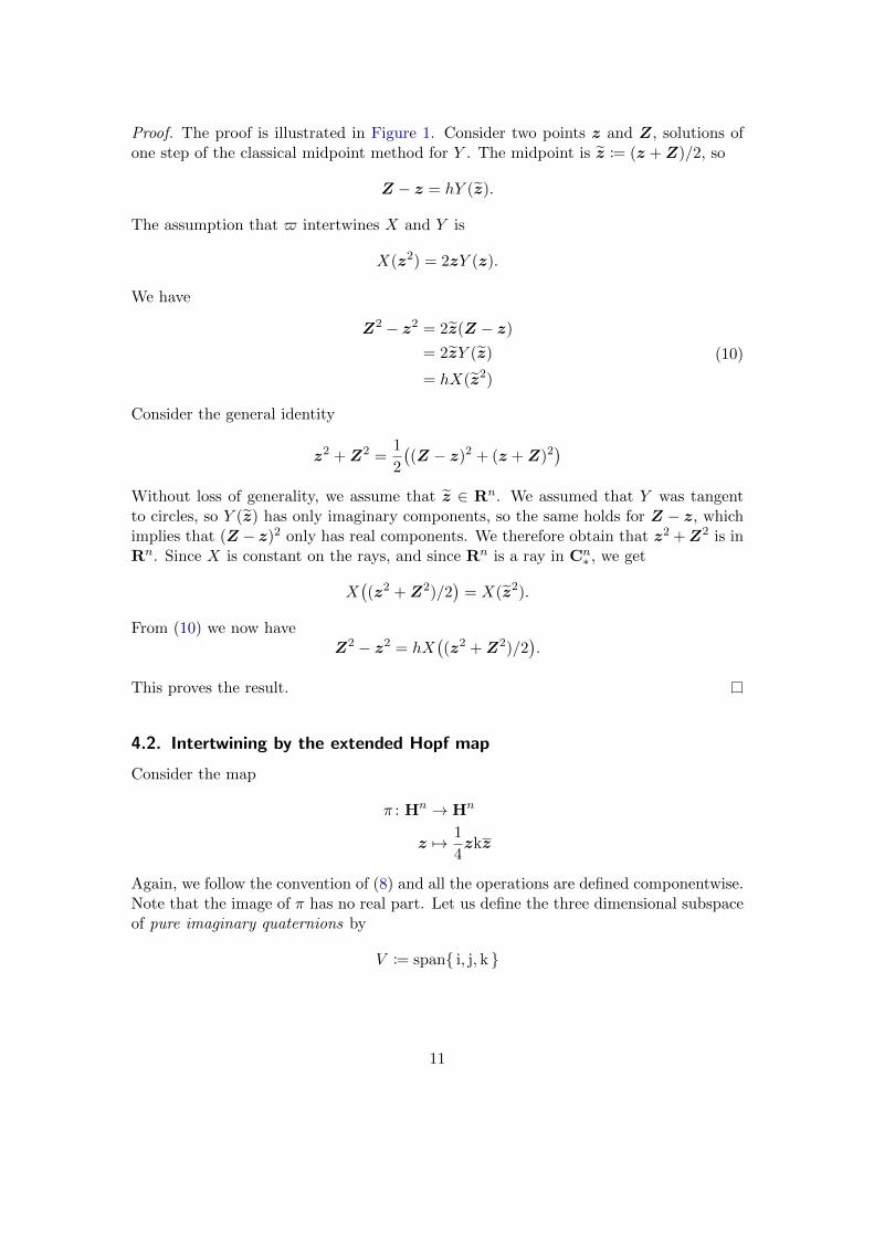
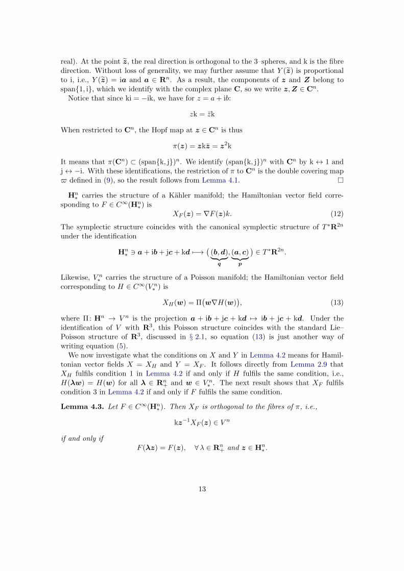
Proof. The proof is illustrated in Figure 1. Consider two points z and Z, solutions ofone step of the classical midpoint method for Y . The midpoint is z := (z +Z)/2, so
Z − z = hY (z).
The assumption that $ intertwines X and Y is
X(z2) = 2zY (z).
We have
Z2 − z2 = 2z(Z − z)
= 2zY (z)
= hX(z2)
(10)
Consider the general identity
z2 +Z2 =1
2
((Z − z)2 + (z +Z)2
)Without loss of generality, we assume that z ∈ Rn. We assumed that Y was tangentto circles, so Y (z) has only imaginary components, so the same holds for Z − z, whichimplies that (Z − z)2 only has real components. We therefore obtain that z2 +Z2 is inRn. Since X is constant on the rays, and since Rn is a ray in Cn
∗ , we get
X((z2 +Z2)/2
)= X(z2).
From (10) we now haveZ2 − z2 = hX
((z2 +Z2)/2
).
This proves the result.
4.2. Intertwining by the extended Hopf map
Consider the map
π : Hn → Hn
z 7→ 1
4zkz
Again, we follow the convention of (8) and all the operations are defined componentwise.Note that the image of π has no real part. Let us define the three dimensional subspaceof pure imaginary quaternions by
V := span{ i, j, k }
11
z
Z
z
z2
Z2
z2z2
s
Figure 1: An illustration of Lemma 4.1. The midpoint z maps to the same ray as the
midpoint z2 := (z2 +Z2)/2.
If we identify V with R3, we can regard π as a map
π : Hn → R3n. (11)
When n = 1 this is the extended Hopf map, essential in the construction of collectiveLie–Poisson integrators on R3 [23].V n is naturally endowed with the Lie–Poisson structure (4), inherited from R3n. We
use the notation V∗ := V \{0} and V n∗ := (V∗)
n.
Lemma 4.2. Let X ∈ X(V n∗ ) and Y ∈ X(Hn
∗ ), and let Φ and Ψ denote the classicalmidpoint methods on V n and Hn respectively. Assume that:
1. X(λw) = X(w) for all λ ∈ Rn+ and w ∈ V n
∗ .
2. Y is tangent to 3-spheres, i.e., z−1Y (z) ∈ V n for all z ∈ Hn∗ .
3. Y is orthogonal to the fibres of π, i.e. kz−1Y (z) ∈ V n for all z ∈ Hn∗ .
4. π intertwines X and Y .
Then π intertwines Φ(hX) and Ψ(hY ).
Proof. Consider z and Z, solution of the classical midpoint method in Hn for Y . Themidpoint is denoted by
z :=z +Z
2.
Since the classical midpoint method is equivariant with respect to affine transformations,we may, without loss of generality, assume that z is real (i.e., all its components are
12
real). At the point z, the real direction is orthogonal to the 3–spheres, and k is the fibredirection. Without loss of generality, we may further assume that Y (z) is proportionalto i, i.e., Y (z) = ia and a ∈ Rn. As a result, the components of z and Z belong tospan{1, i}, which we identify with the complex plane C, so we write z,Z ∈ Cn.
Notice that since ki = −ik, we have for z = a+ ib:
zk = zk
When restricted to Cn, the Hopf map at z ∈ Cn is thus
π(z) = zkz = z2k
It means that π(Cn) ⊂ (span{k, j})n. We identify (span{k, j})n with Cn by k ↔ 1 andj↔ −i. With these identifications, the restriction of π to Cn is the double covering map$ defined in (9), so the result follows from Lemma 4.1.
Hn∗ carries the structure of a Kahler manifold; the Hamiltonian vector field corre-
sponding to F ∈ C∞(Hn∗ ) is
XF (z) = ∇F (z)k. (12)
The symplectic structure coincides with the canonical symplectic structure of T ∗R2n
under the identification
Hn∗ 3 a+ ib+ jc+ kd 7−→
((b,d)︸ ︷︷ ︸
q
, (a, c)︸ ︷︷ ︸p
)∈ T ∗R2n.
Likewise, V n∗ carries the structure of a Poisson manifold; the Hamiltonian vector field
corresponding to H ∈ C∞(V n∗ ) is
XH(w) = Π(w∇H(w)
), (13)
where Π: Hn → V n is the projection a + ib + jc + kd 7→ ib + jc + kd. Under theidentification of V with R3, this Poisson structure coincides with the standard Lie–Poisson structure of R3, discussed in § 2.1, so equation (13) is just another way ofwriting equation (5).
We now investigate what the conditions on X and Y in Lemma 4.2 means for Hamil-tonian vector fields X = XH and Y = XF . It follows directly from Lemma 2.9 thatXH fulfils condition 1 in Lemma 4.2 if and only if H fulfils the same condition, i.e.,H(λw) = H(w) for all λ ∈ Rn
+ and w ∈ V n∗ . The next result shows that XF fulfils
condition 3 in Lemma 4.2 if and only if F fulfils the same condition.
Lemma 4.3. Let F ∈ C∞(Hn∗ ). Then XF is orthogonal to the fibres of π, i.e.,
kz−1XF (z) ∈ V n
if and only ifF (λz) = F (z), ∀λ ∈ Rn
+ and z ∈ Hn∗ .
13
Proof. From (12) it follows that XF (z) is orthogonal to the fibres if and only if
kz−1∇F (z)k ∈ V n.
This is equivalent to
z−1∇F (z) ∈ V n,
which means that z−1∇F (z) is pure imaginary, so ∇F (z) is tangential to the spheres.Since this is true for any z ∈ Hn
∗ , it means that F (λz) = F (z) for λ ∈ Rn+.
Given H ∈ C∞(V n∗ ) we can construct symplectic integrators on V n
∗ in two ways:(i) the classical midpoint method on Hn
∗ for the vector field XH◦π descends to a Lie–Poisson integrator on V n
∗ (this is what we call a collective symplectic integrator), (ii) theextended spherical midpoint method (6). In general the two methods are different, butthey coincide for ray-constant Hamiltonian vector fields.
Proposition 4.4. Let H ∈ C∞(V n∗ ) be constant on rays, let Φ denote the classical
midpoint method on V n∗ , and let Ψ denote the classical midpoint methods on Hn
∗ . Thenthe extended Hopf map π intertwines Φ(XH) and Ψ(XH◦π). That is, the map on V n
∗induced by Ψ(XH◦π) coincides with Φ(XH).
Proof. Appealing to Lemma 2.9, the vector field XH is constant on rays. If H(λw) =H(w) for all λ ∈ Rn
+, then H ◦π fulfils the same property, since π is homogeneous, thatis:
π(λz) = λ2π(z), λ ∈ Rn+.
We can therefore use Lemma 4.3 to obtain that XH◦π is orthogonal to the fibres.The Hopf map is a Poisson map [23], so
Tzπ ·XH◦π(z) = XH(π(z)), z ∈ H,
which means that π intertwines XH and XH◦π. The result now follows from Lemma 4.2,since Φ(XH) coincides with the classical midpoint method applied to XH .
Remark 4.5. Proposition 4.4 provides an independent proof of symplecticity of thespherical midpoint method, since collective integrators are symplectic [23].
Remark 4.6. Usually, collective integrators can not be defined solely in terms of V n∗ :
they must be implemented on Hn∗ . Proposition 4.4 shows that in the case of constant
ray Hamiltonians, the induced map can be defined directly on V n∗ .
14
5. Riemannian midpoint methods
In this section we describe the relation between the spherical midpoint method (6) andcollective symplectic integrators from a different viewpoint: as an interplay between Rie-mannian and symplectic geometry. More precisely, we construct a method on V n
∗ , stem-ming from a non-Euclidean metric, that coincides with the spherical midpoint methodfor Hamiltonian functions that are constant on rays. The relation between these twomethods is established through the classical midpoint method on Hn
∗ . Before workingthis out in § 5.1, we develop a theory of midpoint methods on Riemannian and Kahlermanifolds. This theory sheds light on the underlying geometry of the spherical midpointmethod, and provides an outlook for generalisations.
Given a Riemannian manifold (M, g), let [0, 1] 3 t 7→ γg(t;w,W ) ∈ M denote thegeodesic curve between w and W . Given a vector field X ∈ X(M), the Riemannianmidpoint method on M is the integrator Φg(hX) : w 7→W defined by
d
dt
∣∣∣t=1/2
γg(t;w,W ) = hX(γg(1/2,w,W )
). (14)
If M = Rd and g is the Euclidean metric, then (14) coincides with the definition of theclassical midpoint method (1).
Riemannian midpoint methods transform naturally under change of coordinates:
Proposition 5.1. Let M and N be two diffeomorphic manifolds, let ψ : N → M be adiffeomorphism, and let g be a Riemannian metric on M . Then
ψ−1 ◦ Φg(hX) ◦ ψ = Φψ∗g(hψ∗X).
Proof. The result follows from the definition (14) of Φg and standard change of coordi-nate formulas in differential geometry.
A consequence of Proposition 5.1 is that Riemannian midpoint methods are equivari-ant with respect to isometric group actions:
Proposition 5.2. Let (M, g) be a Riemannian manifold, and let G be a Lie groupacting isometrically on M . Then the Riemannian midpoint method Φg is equivariantwith respect to G, i.e.,
ψg−1 ◦ Φg(hX) ◦ ψg = Φg(hψ∗gX)
where ψg : M →M denotes the action map of g ∈ G.
Proof. The result follows from Proposition 5.1 and ψ∗gg = g (the action is isometric).
We will now discuss a generalised version of Proposition 5.1, where M and N are nolonger diffeomorphic.
Let π : N → M be a submersion from N to another manifold M (π is smooth andits Jacobian matrix Tzπ : TzN → Tπ(z)M is surjective at every z ∈ N .) π induces a
15
vertical distribution V by Vz = {v ∈ TzN ;Tzπ · v = 0}. By construction, the verticaldistribution is integrable, and the fibre through z ∈ N is given by π−1({π(z)}). If (N, h)is Riemannian, then the orthogonal complement with respect to h is called the horizontaldistribution and denoted H. Typically, the horizontal distribution is not integrable. TheRiemannian metric h is called descending (with respect to the submersion π) if thereexists a Riemannian metric g on M such that for all z ∈ N
hz(u,v) = gπ(z)(Tzπ · u, Tzπ · v), ∀u,v ∈ Hz.
The map π between the Riemannian manifolds (N, h) and (M, g) is then called a Rieman-nian submersion. For details on the geometry of Riemannian submersions, see [8, 27].
A vector field Y ∈ X(N) is called horizontal if Y (z) ∈ Hz for all z ∈ N . Y is calleddescending if there exists a vector field X ∈ X(M) such that π intertwines X and Y ,i.e., Tzπ · Y (z) = X(π(z)).
Proposition 5.3. Let (M, g) and (N, h) be Riemannian manifolds and π : N → M aRiemannian submersion. Let Y ∈ X(N) be horizontal, let X ∈ X(M), and assume thatπ intertwines X and Y . Then π intertwines the Riemannian midpoint method Φg(hX)and the Riemannian midpoint method Φh(hY ), i.e.,
π(Φh(hY )(z)
)= Φg(hX)(π(z)).
Proof. Let z and Z fulfil (14). Let w = π(z) and W = π(Z). We need to show thatW = Φg(hX)(w).
The geodesic γh(t; z,Z) is horizontal at t = 1/2. It is therefore horizontal at alltimes [10]. Since horizontal geodesics on N maps to geodesics on M , we have thatπ(γh(t; z,Z)) = γg(t;w,W ). By applying Tπ to (14) we obtain
Tγh(1/2,z,Z)π ·d
dt
∣∣∣t=1/2
γh(t; z,Z) = Tγh(1/2,z,Z)π · hY (γh(1/2; z,Z))
⇓d
dt
∣∣∣t=1/2
π(γh(t; z,Z)
)= hTγh(1/2,z,Z)π · Y (γh(1/2; z,Z))
⇓d
dt
∣∣∣t=1/2
π(γh(t; z,Z)
)= hX
(π(γh(1/2; z,Z))
)⇓
d
dt
∣∣∣t=1/2
γg(t;w,W ) = hX(γg(1/2;w,W )
).
Thus, W fulfils the equation defining Φg(hX), which proves the result.
Next, assume (N, h, ω) is a Kahler manifold such that the Riemannian metric h andthe symplectic form ω descend. (ω descends if it induces a Poisson structure on the spaceof fibres [36].) Thus, π is both a Riemannian submersion and a Poisson submersion.
16
Lemma 5.4. Let (N, h, ω) be a Kahler manifold such that h and ω are descending withrespect to a submersion π : N →M . Let H ∈ C∞(M) be a Hamiltonian. Then XH◦π ishorizontal if and only if ∇H (gradient of H with respect to the metric on M) is tangentto the symplectic leaves of M .
Proof. Let J : TN → TN be the complex structure associated with the Kahler structure.From general properties of Kahler manifolds we have
h(u,v) = ω(u, Jv) (15)
ω(u,v) = h(Ju,v)
h(Ju, Jv) = h(u,v)
XH◦π = J−1∇(H ◦ π) (16)
where ∇ is the gradient with respect to h. By definition, the vector field XH◦π ishorizontal if and only if
h(XH◦π,v) = 0, ∀v ∈ V. (17)
By (15)–(16) we also have
h(XH◦π,v) = h(J−1∇(H ◦ π),v)
= h(∇(H ◦ π), Jv)
= ω(v,∇(H ◦ π)).
(18)
Combining (17) and (18), XH◦π is horizontal if and only if
ω(v,∇(H ◦ π)) = 0, ∀v ∈ V.
Expressed in words, XH◦π is horizontal if and only if ∇(H ◦π) belongs to the symplecticcomplement of V. The symplectic complement of V is integrable and its integral man-ifolds project to the symplectic leaves of N [36]. Thus, Tπ ◦ ∇(H ◦ π) is tangential tothe symplectic leaves. Since the metric h is descending, the gradients on M and N arerelated by
Tπ ◦ ∇(H ◦ π) = ∇H.
This proves the assertion.
By combining Proposition 5.3 with Lemma 5.4 we obtain the following result.
Proposition 5.5. Let M and (N, h, ω) be as in Lemma 5.4. Let H ∈ C∞(M) fulfil thecondition in Lemma 5.4, i.e., ∇H is tangent to the symplectic leaves. Let Φg and Φh
denote the Riemannian midpoint methods on M and N respectively. Then:
1. If Φh(XH◦π) is symplectic, then Φg(XH) is a Poisson map.
2. If Φh(XH◦π) preserves the pre-image of the symplectic leaves, then Φg(XH) pre-serves the symplectic leaves.
17
3. If G is a Lie group that acts on M and N , and Φh and π are equivariant withrespect to G, then Φg is equivariant with respect to G.
Proof. Let Φh and Φg be the Riemannian midpoint methods on M and N respectively.By Lemma 5.4, XH◦π is horizontal, since ∇H is tangential to the symplectic leaves. Thevector field XH◦π is thus descending (it descends to XH since π is a Poisson submersion)and horizontal. By Proposition 5.3, π then intertwines Φg(XH) and Φh(XH◦π).
Proof of (1): Since π is a Poisson map and Φh(XH◦π) is a symplectic map, Φg(XH) isa Poisson map.
Proof of (2): Since Φh(XH◦π) preserves the integral submanifolds of the symplecticcomplement of V, and since these submanifolds project to the symplectic leaves, it followsfrom the π intertwining property that Φg(XH) preserves the symplectic leaves.
Proof of (3): Let X ∈ X(M). Let Y ∈ X(N) be horizontal and descending to X. Letg ∈ G Then g ·X ◦π = g ·Tπ ◦X = Tπg ·X, since π is equivariant. Thus, g ·Y descendsto g ·X. Next, using Proposition 5.3
Φg(g ·X) ◦ π = π ◦ Φh(g · Y ) = π ◦ g−1 · Φh(Y ) · g = g−1 · Φg(X) · g ◦ π.
This proves the results since π is a submersion.
5.1. Riemannian structure of the spherical midpoint method
Our objective is to show that the spherical midpoint method (6) on V n∗ , for Hamiltonian
vector fields XH ∈ X(V n∗ ) with H of the form in Lemma 5.4, is a Riemannian midpoint
method with respect to a non-Euclidean Riemannian metric, related to the classicalmidpoint method on Hn
∗ by a Riemannian submersion in the sense of Proposition 5.3.Recall that the extended Hopf map (11) is a submersion π : Hn
∗ → V n∗ that is a Poisson
map with respect to the Kahler structure on Hn∗ and the Poisson structure on V n
∗ (asdescribed in § 4). Let gR3 denote the Euclidean metric on R3.
Lemma 5.6. The Kahler metric on Hn∗ is descending with respect to the extended Hopf
map π : Hn∗ → V n
∗ . The corresponding Riemannian metric on V n∗ is
gV n∗ w
(u,v
):=
n∑i=1
1
|xi|gR3(ui,vi). (19)
Proof. Each fibre π−1({w}) ⊂ Hn∗ is the orbit of an action of the group U(1)n on Hn
∗ .This action is isometric with respect to the Kahler metric. That is, if gHn
∗ denotes theKahler metric and Lθ denotes the action map, then L∗θgHn
∗ = gHn∗ . It follows from [27,
Proposition 4.3] that gHn∗ is descending. Direct calculations verify that the corresponding
metric on V n∗ is given by (19).
As a specialisation of Proposition 5.3 to the case M = V n∗ and N = Hn
∗ , we obtaina relation between the Riemannian midpoint method on V n
∗ and Hn∗ (notice that the
Riemannian midpoint method on Hn∗ is the classical midpoint methods since gHn
∗ is theEuclidean metric).
18
Proposition 5.7. Let Y ∈ X(Hn∗ ) be a horizontal vector fields, let X ∈ X(V n
∗ ), andassume the the extended Hopf map π intertwines X and Y . Then π intertwines theRiemannian midpoint methods ΦgV n∗
(hX) and ΦgHn∗(hY ).
As a specialisation of Lemma 5.4 to the case M = V n∗ and N = Hn
∗ , we obtain ageometric formulation of Lemma 4.3.
Lemma 5.8. Let H ∈ C∞(V n∗ ). Then XH◦π is horizontal if and only if H is constant
on the rays. In particular, XH◦ρ◦π is horizontal for any H ∈ C∞((S2)n).
Proof. The symplectic leaves of V n∗ are the coadjoint orbits of (so(3)∗)n. These consists
ofS2r1 × · · · × S
2rn = {(w1, . . . ,wn) ∈ V n
∗ ; |wk| = rk}, (20)
for arbitrary rk ∈ R+. Let ∇ denote the gradient on V n∗ with respect to gV n
∗ . It followsfrom Lemma 5.4 that XH◦π is horizontal if and only if ∇H is tangent to (20). From (19)and the direct product structure of V n
∗ , we see that gV n∗ (u,v) = 0 for any u tangent to
(20) if and only if v is tangent to the rays (Definition 2.8). Let Rρ(w) ⊂ V n∗ denote the
ray through w. The condition for XH◦π to be horizontal is therefore
gV n∗ w
(∇H(w),v) = 0, ∀v ∈ TwRρ(w)
m〈dH(w),v〉 = 0, ∀v ∈ TwRρ(w),
which implies that H must be constant on the rays.
As a specialisation of Proposition 5.5 to the case M = V n∗ and N = Hn
∗ , we obtainthat the Riemannian midpoint method ΦgV n∗
on V n∗ is a Poisson integrator.
Proposition 5.9. The Riemannian midpoint method ΦgV n∗on V n
∗ , applied to Hamilto-nian vector fields, is a Poisson integrator.
The final result in this section connects the spherical midpoint method (6) and theRiemannian midpoint method ΦgV n∗
. The two methods are different, but they coincidefor ray-constant Hamiltonian vector fields, as a consequence of Proposition 4.4 andProposition 5.7.
Proposition 5.10. Let Ψ denote the spherical midpoint method (6) on V n∗ and ΦgV n∗
the Riemannian midpoint method with respect to gV n∗ . Let H ∈ C∞(V n
∗ ) be constant onrays. Then Ψ(hXH) = ΦgV n∗
(hXH).
Remark 5.11. Proposition 5.9 and Proposition 5.10 provide an independent proof thatthe spherical midpoint method is symplectic.
Remark 5.12. It is remarkable that the non-Euclidean induced metric gV n∗ has become
redundant in the case when H is constant on rays; the Riemannian midpoint methodΦgV n∗
(XH) can be expressed solely in terms of the classical midpoint method on V n∗ .
19
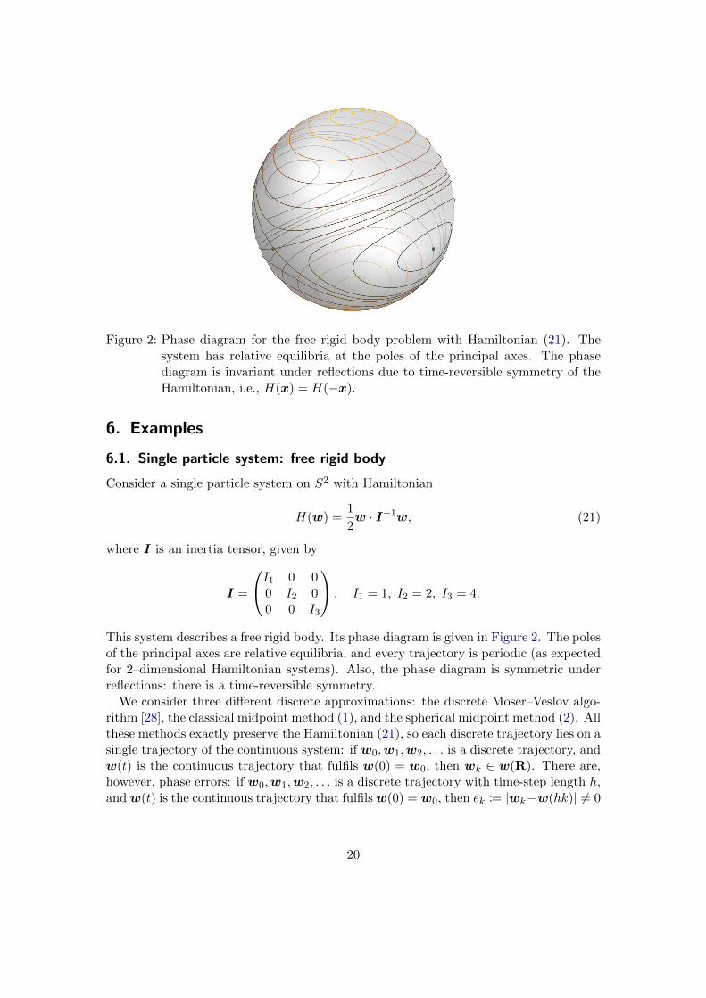
Figure 2: Phase diagram for the free rigid body problem with Hamiltonian (21). Thesystem has relative equilibria at the poles of the principal axes. The phasediagram is invariant under reflections due to time-reversible symmetry of theHamiltonian, i.e., H(x) = H(−x).
6. Examples
6.1. Single particle system: free rigid body
Consider a single particle system on S2 with Hamiltonian
H(w) =1
2w · I−1w, (21)
where I is an inertia tensor, given by
I =
I1 0 00 I2 00 0 I3
, I1 = 1, I2 = 2, I3 = 4.
This system describes a free rigid body. Its phase diagram is given in Figure 2. The polesof the principal axes are relative equilibria, and every trajectory is periodic (as expectedfor 2–dimensional Hamiltonian systems). Also, the phase diagram is symmetric underreflections: there is a time-reversible symmetry.
We consider three different discrete approximations: the discrete Moser–Veslov algo-rithm [28], the classical midpoint method (1), and the spherical midpoint method (2). Allthese methods exactly preserve the Hamiltonian (21), so each discrete trajectory lies on asingle trajectory of the continuous system: if w0,w1,w2, . . . is a discrete trajectory, andw(t) is the continuous trajectory that fulfils w(0) = w0, then wk ∈ w(R). There are,however, phase errors: if w0,w1,w2, . . . is a discrete trajectory with time-step length h,andw(t) is the continuous trajectory that fulfilsw(0) = w0, then ek := |wk−w(hk)| 6= 0
20
2−9 2−7 2−5 2−3 2−1
100
10−2
10−4
10−6
10−8
Time-step length h
Maxim
um
error Moser–Veselov
Classical midpoint
Spherical midpoint
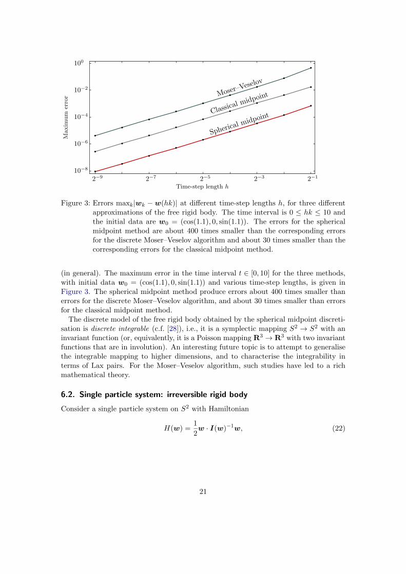
Figure 3: Errors maxk|wk −w(hk)| at different time-step lengths h, for three differentapproximations of the free rigid body. The time interval is 0 ≤ hk ≤ 10 andthe initial data are w0 = (cos(1.1), 0, sin(1.1)). The errors for the sphericalmidpoint method are about 400 times smaller than the corresponding errorsfor the discrete Moser–Veselov algorithm and about 30 times smaller than thecorresponding errors for the classical midpoint method.
(in general). The maximum error in the time interval t ∈ [0, 10] for the three methods,with initial data w0 = (cos(1.1), 0, sin(1.1)) and various time-step lengths, is given inFigure 3. The spherical midpoint method produce errors about 400 times smaller thanerrors for the discrete Moser–Veselov algorithm, and about 30 times smaller than errorsfor the classical midpoint method.
The discrete model of the free rigid body obtained by the spherical midpoint discreti-sation is discrete integrable (c.f. [28]), i.e., it is a symplectic mapping S2 → S2 with aninvariant function (or, equivalently, it is a Poisson mapping R3 → R3 with two invariantfunctions that are in involution). An interesting future topic is to attempt to generalisethe integrable mapping to higher dimensions, and to characterise the integrability interms of Lax pairs. For the Moser–Veselov algorithm, such studies have led to a richmathematical theory.
6.2. Single particle system: irreversible rigid body
Consider a single particle system on S2 with Hamiltonian
H(w) =1
2w · I(w)−1w, (22)
21

where I(w) is an irreversible inertia tensor, given by
I(w) =
I1
1+σw10 0
0 I21+σw2
0
0 0 I31+σw3
, I1 = 1, I2 = 2, I3 = 4, σ =2
3.
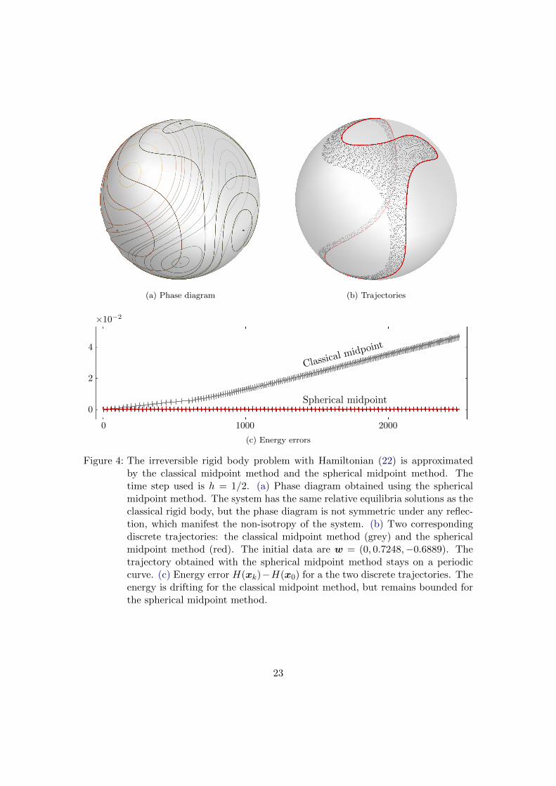
This system describes an irreversible rigid body with fixed unitary total angular mo-mentum. It is irreversible in the sense that the moments of inertia about the principalaxes depend on the rotation direction, i.e., the moments for clockwise and anti-clockwiserotations are different. A phase diagram is given in Figure 4(a). Like the free rigid body,the poles of the principal axes are relative equilibria, and every trajectory is periodic.Contrary to the free rigid body, the phase diagram is not symmetric under reflections,i.e., there is no time-reversible symmetry.
We consider two different discrete approximations: the classical midpoint method (1)and the spherical midpoint method (2). Locally the two methods are akin (they areboth second order accurate), but they exhibit distinct global properties: trajectories lieon periodic curves for the spherical midpoint method but not for the classical midpointmethod, see Figure 4(b). Also, the deviation in the Hamiltonian (22) along discretetrajectories remains bounded for the spherical midpoint method, but is drifting for theclassical midpoint method, see Figure 4(c).
Periodicity of phase trajectories and near conservation of energy, as displayed for thespherical midpoint method, suggests the presence of a first integral, a modified Hamil-tonian, that is exactly preserved. The existence of such a modified Hamiltonian hingeson symplecticity, as established through the theory of backward error analysis [9].
The example in this section illustrates the advantage of the spherical midpoint method,over the classical midpoint method, for approximating Hamiltonian dynamics on S2. Ingeneral, one can expect that spherical midpoint discretisations of continuous integrablesystems on (S2)n remain almost integrable in the sense of Kolmogorov–Arnold–Mosertheory for symplectic maps, as developed by Shang [33].
6.3. Single particle system: forced rigid body, development of chaos
Consider the time dependent Hamiltonian on S2 given by
H(w, t) =1
2w · I−1w + ε sin(t)w3, w = (w1, w2, w3), (23)
where I is an inertia tensor, given by
I =
I1 0 00 I2 00 0 I3
, I1 = 1, I2 = 4/3, I3 = 2.
This system describes a forced rigid body with periodic loading with period 2π. At ε = 0the system is integrable, but it becomes non-integrable as ε increases. We discretise thesystem using the spherical midpoint method with time-step length 2π/N , N = 20. A
22
(a) Phase diagram (b) Trajectories
0 1000 2000
4
2
0
×10−2
Classical midpoint
Spherical midpoint
(c) Energy errors
Figure 4: The irreversible rigid body problem with Hamiltonian (22) is approximatedby the classical midpoint method and the spherical midpoint method. Thetime step used is h = 1/2. (a) Phase diagram obtained using the sphericalmidpoint method. The system has the same relative equilibria solutions as theclassical rigid body, but the phase diagram is not symmetric under any reflec-tion, which manifest the non-isotropy of the system. (b) Two correspondingdiscrete trajectories: the classical midpoint method (grey) and the sphericalmidpoint method (red). The initial data are w = (0, 0.7248,−0.6889). Thetrajectory obtained with the spherical midpoint method stays on a periodiccurve. (c) Energy error H(xk)−H(x0) for a the two discrete trajectories. Theenergy is drifting for the classical midpoint method, but remains bounded forthe spherical midpoint method.
23

Figure 5: Poincare section of the forced rigid body system with Hamiltonian (23), ap-proximated by the spherical midpoint method. Left: ε = 0.01. Right: ε = 0.07.Notice the development of chaos near the unstable equilibria points.
Poincare section is obtain by sampling the system every N :th step; the result for variousinitial data and choices of ε is shown in Figure 5. Notice the development of chaoticbehaviour near the unstable equilibria points.
The example in this section illustrates that the spherical midpoint method, beingsymplectic, behaves as expected in the transition from integrable to chaotic dynamics.
6.4. 4–particle system: point vortex dynamics on the sphere
Point vortices constitute special solutions of Euler’s fluid equations on two-dimensionalmanifolds; see the survey by Aref [1] and references therein. Consider the codimensionzero submanifold of (S2)n given by
(S2)n∗ := {w ∈ (S2)n;wi 6= wj , 1 ≤ i < j ≤ n}.
Point vortex systems on the sphere, first studied by Bogomolov [3], are Hamiltonian sys-tems on (S2)n∗ that provide approximate models for atmosphere dynamics with localisedareas of high vorticity, such as cyclones on Earth and vortex streets [11] on Jupiter. Inabsence of rotational forces, the Hamiltonian function is given by
H(w) = − 1
4π
∑i<j
κiκj ln(2− 2wi ·wj),
where the constants κi are the vortex strengths. The cases n = 1, 2, 3 are integrable [14,32], but the case n = 4 is non-integrable. Characterisation and stability of relativeequilibria have been studied extensively; see [17] and references therein.
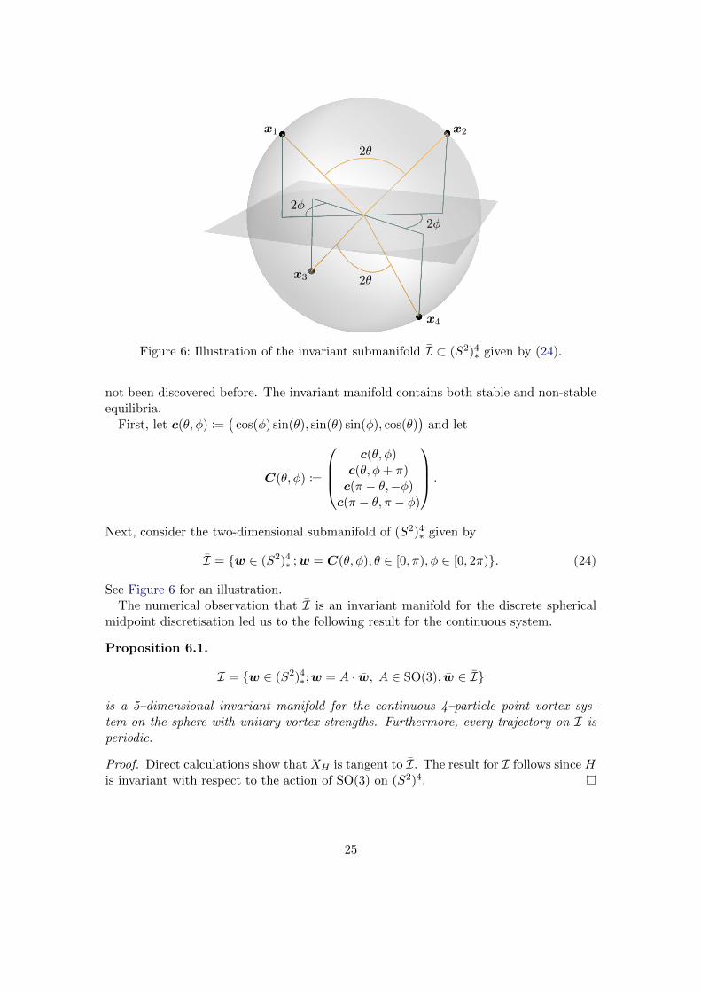
In this example, we study the case n = 4 and κi = 1 by using the time-discreteapproximation provided by the spherical midpoint method (2). Our study reveals a non-trivial 4-dimensional invariant manifold of periodic solutions, that, to our knowledge, has
24
2θ
2θ
2φ
2φ
x1 x2
x3
x4
Figure 6: Illustration of the invariant submanifold I ⊂ (S2)4∗ given by (24).
not been discovered before. The invariant manifold contains both stable and non-stableequilibria.
First, let c(θ, φ) :=(
cos(φ) sin(θ), sin(θ) sin(φ), cos(θ))
and let
C(θ, φ) :=
c(θ, φ)
c(θ, φ+ π)c(π − θ,−φ)c(π − θ, π − φ)
.
Next, consider the two-dimensional submanifold of (S2)4∗ given by
I = {w ∈ (S2)4∗ ;w = C(θ, φ), θ ∈ [0, π), φ ∈ [0, 2π)}. (24)
See Figure 6 for an illustration.The numerical observation that I is an invariant manifold for the discrete spherical
midpoint discretisation led us to the following result for the continuous system.
Proposition 6.1.
I = {w ∈ (S2)4∗;w = A · w, A ∈ SO(3), w ∈ I}
is a 5–dimensional invariant manifold for the continuous 4–particle point vortex sys-tem on the sphere with unitary vortex strengths. Furthermore, every trajectory on I isperiodic.
Proof. Direct calculations show that XH is tangent to I. The result for I follows since His invariant with respect to the action of SO(3) on (S2)4.
25
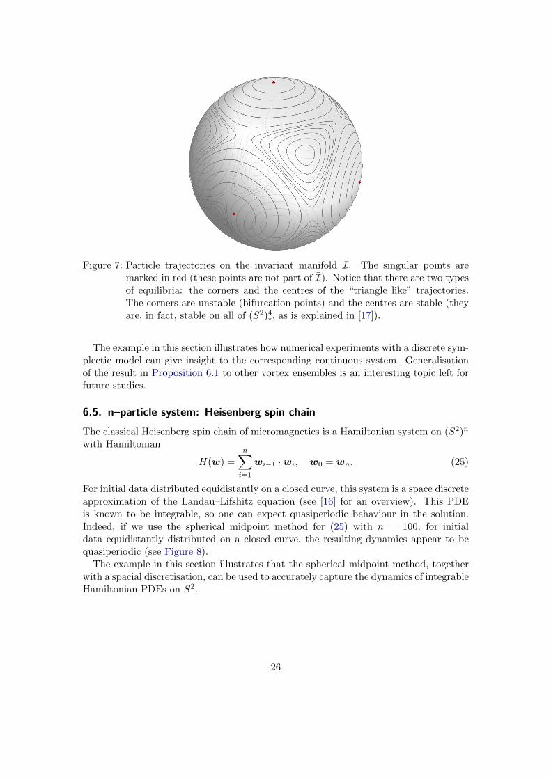
Figure 7: Particle trajectories on the invariant manifold I. The singular points aremarked in red (these points are not part of I). Notice that there are two typesof equilibria: the corners and the centres of the “triangle like” trajectories.The corners are unstable (bifurcation points) and the centres are stable (theyare, in fact, stable on all of (S2)4∗, as is explained in [17]).
The example in this section illustrates how numerical experiments with a discrete sym-plectic model can give insight to the corresponding continuous system. Generalisationof the result in Proposition 6.1 to other vortex ensembles is an interesting topic left forfuture studies.
6.5. n–particle system: Heisenberg spin chain
The classical Heisenberg spin chain of micromagnetics is a Hamiltonian system on (S2)n
with Hamiltonian
H(w) =
n∑i=1
wi−1 ·wi, w0 = wn. (25)
For initial data distributed equidistantly on a closed curve, this system is a space discreteapproximation of the Landau–Lifshitz equation (see [16] for an overview). This PDEis known to be integrable, so one can expect quasiperiodic behaviour in the solution.Indeed, if we use the spherical midpoint method for (25) with n = 100, for initialdata equidistantly distributed on a closed curve, the resulting dynamics appear to bequasiperiodic (see Figure 8).
The example in this section illustrates that the spherical midpoint method, togetherwith a spacial discretisation, can be used to accurately capture the dynamics of integrableHamiltonian PDEs on S2.
26
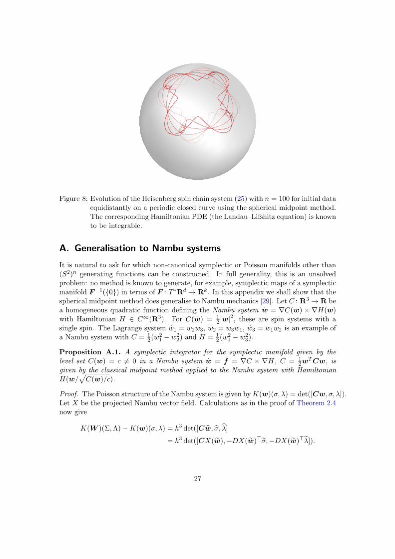
Figure 8: Evolution of the Heisenberg spin chain system (25) with n = 100 for initial dataequidistantly on a periodic closed curve using the spherical midpoint method.The corresponding Hamiltonian PDE (the Landau–Lifshitz equation) is knownto be integrable.
A. Generalisation to Nambu systems
It is natural to ask for which non-canonical symplectic or Poisson manifolds other than(S2)n generating functions can be constructed. In full generality, this is an unsolvedproblem: no method is known to generate, for example, symplectic maps of a symplecticmanifold F−1({0}) in terms of F : T ∗Rd → Rk. In this appendix we shall show that thespherical midpoint method does generalise to Nambu mechanics [29]. Let C : R3 → R bea homogeneous quadratic function defining the Nambu system w = ∇C(w) × ∇H(w)with Hamiltonian H ∈ C∞(R3). For C(w) = 1
2 |w|2, these are spin systems with a
single spin. The Lagrange system w1 = w2w3, w2 = w3w1, w3 = w1w2 is an example ofa Nambu system with C = 1
2(w21 − w2
2) and H = 12(w2
1 − w23).
Proposition A.1. A symplectic integrator for the symplectic manifold given by thelevel set C(w) = c 6= 0 in a Nambu system w = f = ∇C × ∇H, C = 1
2wTCw, is
given by the classical midpoint method applied to the Nambu system with HamiltonianH(w/
√C(w)/c).
Proof. The Poisson structure of the Nambu system is given byK(w)(σ, λ) = det([Cw, σ, λ]).Let X be the projected Nambu vector field. Calculations as in the proof of Theorem 2.4now give
K(W )(Σ,Λ)−K(w)(σ, λ) = h3 det([Cw, σ, λ]
= h3 det([CX(w),−DX(w)>σ,−DX(w)>λ]).
27
As before, all three arguments are orthogonal to w: CX(w), because X(w) is tan-gent to the level set C(w) = c, whose normal at w is Cw, and −DX(w)>σ because〈−DX(w)>σ, w〉 = 〈σ,−DX(w)w〉, and because w 7→ H(w/
√C(w)/c) is homogenous
on rays, X is constant on rays.
Note that if H is also a homogeneous quadratic (as in the Lagrange system), then themethod preserves C and H and generates an integrable map. The Nambu systems inProposition A.1 are all 3-dimensional Lie–Poisson systems. There are 9 inequivalent fam-ilies of real irreducible 3-dimensional Lie algebras [30]. Five of them have homogeneousquadratic Casimirs and are covered by Proposition A.1: in the notation of [30], they areA3,1 (C = w2
1, Heisenberg Lie algebra) A3,4 (C = w1w2, e(1, 1)); A3,6 (C = w21 + w2
2,e(2)); A3,8 (C = w2
2 + w1w3, su(1, 1), sl(2)); A3,9 (C = w21 + w2
2 + w23, su(2), so(3)).
A large set of Lie–Poisson systems is obtained by direct products of the duals of theseLie algebras. Such a structure was already mentioned by Nambu in his original paper,noting the application to spin systems. The spherical midpoint method applies to thesesystems; it generates symplectic maps in neighbourhoods of symplectic leaves with c 6= 0.
References
[1] H. Aref, Point vortex dynamics: a classical mathematics playground, J. Math. Phys.48 (2007), 065401, 23.
[2] M. A. Austin, P. Krishnaprasad, and L.-S. Wang, Almost Poisson integration ofrigid body systems, Journal of Computational Physics 107 (1993), 105–117.
[3] V. Bogomolov, Dynamics of vorticity at a sphere, Fluid Dynamics 12 (1977), 863–870.
[4] P. Channell and J. Scovel, Integrators for Lie–Poisson dynamical systems, PhysicaD: Nonlinear Phenomena 50 (1991), 80 – 88.
[5] B. Chirikov and D. Shepelyansky, Chirikov standard map, Scholarpedia 3 (2008),3550.
[6] G. Cooper, Stability of runge–kutta methods for trajectory problems, IMA J. Nu-mer. Anal. 7 (1987), 1–13.
[7] P. Deift, L.-C. Li, and C. Tomei, Loop groups, discrete versions of some classicalintegrable systems, and rank 2 extensions, vol. 100, AMS, 1992.
[8] R. H. Escobales, Jr., Riemannian submersions with totally geodesic fibers, J. Dif-ferential Geom. 10 (1975), 253–276.
[9] E. Hairer, C. Lubich, and G. Wanner, Geometric Numerical Integration, Springer-Verlag, Berlin, 2006.
28
[10] R. Hermann, A sufficient condition that a mapping of Riemannian manifolds be afibre bundle, Proc. Amer. Math. Soc. 11 (1960), 236–242.
[11] T. Humphreys and P. S. Marcus, Vortex street dynamics: The selection mechanismfor the areas and locations of jupiter’s vortices, Journal of the Atmospheric Sciences64 (2007), 1318–1333.
[12] L. Jay, Symplectic partitioned Runge-Kutta methods for constrained Hamiltoniansystems, SIAM J. Numer. Anal. 33 (1996), 368–387.
[13] K. Kaneko and K. Kaneko, Theory and applications of coupled map lattices, vol.159, Wiley Chichester, 1993.
[14] R. Kidambi and P. K. Newton, Motion of three point vortices on a sphere, PhysicaD: Nonlinear Phenomena 116 (1998), 143 – 175.
[15] Y. Kosmann-Schwarzbach, B. Grammaticos, and T. Tamizhmani, Discrete inte-grable systems, Springer, 2004.
[16] M. Lakshmanan, The fascinating world of the landau–lifshitz–gilbert equation: anoverview, Philosophical Transactions of the Royal Society A: Mathematical, Physicaland Engineering Sciences 369 (2011), 1280–1300.
[17] F. Laurent-Polz, J. Montaldi, and M. Roberts, Point vortices on the sphere: stabilityof symmetric relative equilibria, J. Geom. Mech. 3 (2011), 439–486.
[18] T. Lee, Can time be a discrete dynamical variable?, Physics Letters B 122 (1983),217 – 220.
[19] T. Lee, Difference equations and conservation laws, Journal of Statistical Physics46 (1987), 843–860.
[20] J. Marsden and A. Weinstein, Coadjoint orbits, vortices, and Clebsch variables forincompressible fluids, Phys. D 7 (1983), 305–323.
[21] J. E. Marsden, S. Pekarsky, and S. Shkoller, Discrete Euler-Poincare and Lie–Poisson equations, Nonlinearity 12 (1999), 1647–1662.
[22] J. E. Marsden and T. S. Ratiu, Introduction to Mechanics and Symmetry, Springer-Verlag, New York, 1999.
[23] R. McLachlan, K. Modin, and O. Verdier, Collective Lie–Poisson integrators on R3,2013, http://arxiv.org/abs/1307.2387.
[24] R. I. McLachlan, K. Modin, and O. Verdier, Collective Symplectic Integrators,arxiv.org/abs/1308.6620, 2013.
[25] R. I. McLachlan, K. Modin, O. Verdier, and M. Wilkins, Geometric generalisationsof Shake and Rattle, Found. Comput. Math. (2013), doi:10.1007/s10208-013-9163-y.
29
[26] R. I. McLachlan and G. R. W. Quispel, Geometric integrators for odes, Journal ofPhysics A: Mathematical and General 39 (2006), 5251.
[27] K. Modin, Generalised Hunter–Saxton equations, optimal information transport,and factorisation of diffeomorphisms, accepted in J. Geom. Anal. (2013).
[28] J. Moser and A. P. Veselov, Discrete versions of some classical integrable systemsand factorization of matrix polynomials, Comm. Math. Phys. 139 (1991), 217–243.
[29] Y. Nambu, Generalized hamiltonian dynamics, Physical Review D 7 (1973), 2405–2412.
[30] J. Patera, R. Sharp, P. Winternitz, and H. Zassenhaus, Invariants of real low di-mension lie algebras, Journal of Mathematical Physics 17 (1976), 986.
[31] H. Poincare, Les Methodes Nouvelles de la Mecanique Celeste, Gauthier–Villars,Paris, transl. in New Methods of Celestial Mechanics, Daniel Goroff, ed. (AIP Press,1993), 1892.
[32] T. Sakajo, The motion of three point vortices on a sphere, Japan Journal of Indus-trial and Applied Mathematics 16 (1999), 321–347.
[33] Z. Shang, KAM theorem of symplectic algorithms for Hamiltonian systems, Numer.Math. 83 (1999), 477–496.
[34] C. Viterbo, Generating functions, symplectic geometry, and applications, Proceed-ings of the International Congress of Mathematicians, vol. 1, p. 2, 1994.
[35] A. Weinstein, Symplectic geometry, Bull. Amer. Math. Soc. (N.S.) 5 (1981), 1–13.
[36] A. Weinstein, The local structure of Poisson manifolds, J. Differential Geom. 18(1983), 523–557.
30


