Embed Size (px)
Citation preview
On the Minimum Many-Valued
Modal Logic over a Finite
Residuated Lattice
FELIX BOU, FRANCESC ESTEVA and LLUIS GODO, Institutd’Investigacio en Intel.ligencia Artificial, IIIA - CSIC, Campus UAB,Bellaterra 08193, Spain. E-mail: [email protected]; [email protected];[email protected]
RICARDO OSCAR RODRIGUEZ, Dpto. de Computacion, Fac.Ciencias Exactas y Naturales, Universidad de Buenos Aires, 1428Buenos Aires, Argentina. E-mail: [email protected]
Abstract
This article deals with many-valued modal logics, based only on the necessity operator, over a
residuated lattice. We focus on three basic classes, according to the accessibility relation, of Kripkeframes: the full class of frames evaluated in the residuated lattice (and so defining the minimum
modal logic), the ones only evaluated in the idempotent elements and the ones evaluated in 0 and
1. We show how to expand an axiomatization, with canonical truth-constants in the language, of afinite residuated lattice into one of the modal logic, for each one of the three basic classes of Kripke
frames. We also provide axiomatizations for the case of a finite MV chain but this time without
canonical truth-constants in the language.
Keywords: many-valued modal logic, modal logic, many-valued logic, fuzzy logic, substructural logic.
1 Introduction
The basic idea of this article is to systematically investigate modal extensions ofmany-valued logics. Many-valued modal logics, under different forms and contexts,have appeared in the literature for different reasoning modeling purposes. For in-stance, Fitting introduces in [22, 23] a modal logic over logics valued on finite Heytingalgebras, and provides a nice justification for studying such modal systems for dealingwith opinions of experts with a dominance relation among them. But many papersoffer technical contributions but without practical motivations. Although we will alsomainly focus on developing a theoretical and general framework, let us say somethingabout specific problems where the necessity of combining modal and many-valued se-mantics seems to be important. Our starting point is that the framework of classicallogic is not enough to reason with vague concepts or with modal notions like belief,uncertainty, knowledge, obligations, time, etc. Residuated fuzzy (or many-valued)logics (in the sense of Hajek in [30]) appear as a suitable logical framework to for-malise reasoning under vagueness, while a variety of modal logics address the logicalformalization to reason about different modal notions as the ones mentioned above.Therefore, if one is interested in a logical account of both vagueness and some kind
1Journal of Logic and Computation, pp. 1–53 0000 c© Oxford University Press
arX
iv:0
811.
2107
v2 [
mat
h.L
O]
2 O
ct 2
009
2 On the Minimum Many-Valued Modal Logic over a Finite Residuated Lattice
of modalities, one is led to study systems of many-valued or fuzzy modal logic.A clear example of this are Fuzzy Description Logics (see e.g. [46] for an overview)
which, as in the classical case, can be viewed both as fragments of t-norm fuzzypredicate logics (see e.g. Hajek’s paper [31]) and as fuzzy (multi) modal logics. Otherexamples include generalizations of belief logics to deal with non-classical/fuzzy events[36, 29] or preliminary ideas on similarity-based fuzzy logics [27].
Having in mind these motivations, our main research goal at large is a systematicstudy of many-valued modal logics and their application, including the setting of fuzzydescription logics. Although there is a rich literature about both modal [11, 4, 5] andmany-valued logics [30, 13, 28], in our opinion there is no such systematic approach.This article may be seen as a first modest step in that direction, indeed, we restrictourselves to investigate minimum many-valued modal logics for the necessity operator� defined on top of logics of finite residuated lattices.
It is certainly true that several many-valued modal logics have been previouslyconsidered in the literature; but in most cases, with the two exceptions later cited,they are logics (we highlight [35, 30, 39] among them) that site at the top part of thehierarchy of modal logics, e.g., the modality is S5-like. In other words, they cannotbe considered as the many-valued counterpart of the minimum classical modal logicK. Since in our opinion any systematic study of many-valued modal logics must start,like in the classical modal case, by characterizing the corresponding minimum many-valued modal logic we consider that this problem is the first question that someonewho wants to study many-valued modal logics must answer. This is the reason whythe present article is focused on characterizing the minimum many-valued modal logic.This does not mean that the authors do not consider important to study the fullhierarchy of many-valued modal logics extending the minimum one, it is simply thatthis systematic study is left for future research.
Let us fix a residuated lattice A. The intended meaning of its universe A is the setof truth values. Thus, the classical modal logic framework corresponds to the casethat A is the Boolean algebra of two elements. Due to technical reasons sometimes itwill be convenient to add canonical constants to the residuated lattice A. By addingcanonical constants we mean to add one constant for every element in A in such away that these constants are semantically interpreted by its canonical interpretation.The residuated lattice obtained by adding these canonical constants will be denotedby Ac.
The intuition behind the minimum many-valued modal logic over A (and analo-gously over Ac) is that it has to be induced by the biggest class of Kripke frames.Therefore, the minimum logic must be semantically defined by using Kripke frameswhere the accessibility relation takes values in A. Thus, the accessibility relation inthese Kripke frames is also many-valued. In other words, the accessibility relationmay take values outside {0, 1}, and hence we cannot assume that it is a subset ofA×A.
As far as the authors are aware the only two cases in the literature that deal witha minimum modal logic over a residuated lattice A, and hence with many-valuedaccessibility relations, are the ones respectively introduced in [22] and [10, 47]. Thefirst one studies the case that A is a finite Heyting algebra (but adding canonicalconstants) and the second one studies the standard Godel algebra (which is also aHeyting algebra). One particular feature about these two cases is that the normality
On the Minimum Many-Valued Modal Logic over a Finite Residuated Lattice 3
axiom
�(ϕ→ ψ)→ (�ϕ→ �ψ) (K)
is valid in the minimum modal logic. However, there are a lot of residuated latticeswhere the normality axiom (K) is not valid in the minimum modal logic, e.g., finiteMV chains. Thus, whenever (K) is not valid there is no axiomatization in the literatureof the minimum modal logic. Even more, if (K) fails it is not so clear what could bea good candidate for an axiomatization.
The present article solves the problem of finding the minimum (local) modal logic,based only on the necessity operator �, for two cases: for finite residuated latticeswith canonical constants and for finite MV chains without adding canonical constants.For these two cases we show how to expand an axiomatization for the logic of theresiduated lattice A into one of the minimum modal logic over A. Thus, we assumein this article that we already know how to axiomatize the non-modal logic.
Besides the minimum (local) many-valued modal logic (i.e., the logic given byall Kripke frames) in this article we also consider the (local) many-valued modallogic given by two other classes of frames. These two other classes are the class ofcrisp frames where the accessibility relation takes values in {0, 1}, and the class ofidempotent frames where the accessibility relation takes values in the set of idempotentelements of A. For every finite residuated lattice with canonical constants we alsoaxiomatize in this article the logic given by idempotent frames, but for the logicgiven by crisp frames we have only succeeded when Ac has a unique coatom. Ourinterest on the class of crisp frames is due to its obvious connection with the classicalsetting, and the interest on idempotent frames is based on the tight connection withthe normality axiom (K) that will be shown later in the article.
In this article we stress that the non-modal logics considered are the ones definedover a particular residuated lattice and not over a class of residuated lattices1 Thereason to do so is a methodological one since a lot of our results are based on the roleof canonical constants, which can only be considered in the framework of non-modallogics defined using only one residuated lattice. On the other hand, the restriction tofinite residuate lattices is used in order to be sure that the non-modal logic is finitary.
It is worth pointing out that in this article logics are always (in the non-modal and inthe modal setting) considered as consequence relations invariant under substitutions.So, the reader must understand in this article “completeness” as a synonym of what itis sometimes called “strong completeness”. That is, we are talking about completenesseven for infinite sets of assumptions. For the same reason we use the expression localand global modal logic, and not the terminology of “local and global consequencerelations” which is more common in the modal tradition.
Structure and contents of the article. Section 2 contains the non-modal prelim-inaries; the definition of residuated lattice is stated and it is said what is the logicassociated with a residuated lattice. For certain modal aspects it will be convenientto add canonical constants to the residuated lattice, and so in Section 2.2 we alsoconsider the non-modal logic with canonical constants.
1 It is common in the non-modal literature to consider equational classes of residuated lattices. However, this
assumption does not seem reasonable to be done in the many-valued setting. For instance, in [8, p. 181] it is shown
an example of two classes of residuated lattices generating the same equational class, but having different minimum
many-valued modal logics.
4 On the Minimum Many-Valued Modal Logic over a Finite Residuated Lattice
In Section 3 we firstly introduce the Kripke semantics on the many-valued setting(with and without canonical constants). We notice that for the sake of simplicityin this article we only deal with the necessity modality �. The Kripke semantics isdefined by
V (�ϕ,w) =∧{R(w,w′)→ V (ϕ,w′) : w′ ∈W},
and it is meaningful for the case that A is lattice complete. Although there areseveral possibilities to generalize the classical Kripke semantics to the many-valuedrealm we justify in Remark 3.5 why we think that this semantics is the most naturalone; indeed, under this definition it holds that the semantics of the modal formula �pcorresponds to the first-order many-valued semantics of the formula ∀y(Rxy → Py).Then, the three basic classes of Kripke frames considered in this article (the full classof Kripke frames, idempotent Kripke frames and crisp Kripke frames) are introduced.In Section 3.1 the validity of some formulas, in the three basic classes of Kripke frames,is discussed. Among the validity results Corollary 3.13 is the more remarkable one.It says that the normality axiom (K) is valid iff all elements in the residuated latticeare idempotent (i.e., A is a Heyting algebras). In particular this result shows a tightconnection between (K) and the class of idempotent frames. Besides the three basicclasses of Kripke frames, we also introduce in this section another class (the class ofBoolean Kripke frames) which is tightly connected to the class of crisp Kripke frames(see Theorem 3.16). Next, Section 3.2 introduces the local and the global many-valuedmodal logic defined by a class of Kripke frames. In this Section 3.2 we discuss several(meta)rules whose role is crucial in the modal setting, we show how to reduce themodal logic to the non-modal one (see Theorem 3.26) and we study the relationshipbetween crisp and Boolean Kripke frames. In Section 3.3 we sum up the previousknown results about the minimum many-valued modal logics. This state of the art islocate there, and not at the beginning of the article, in order to be able to state thealready known results inside the notational framework introduced in this article.
Section 4 considers modal logics for the case that A is a finite residuated latticeand there are canonical constants. Firstly, in Section 4.1 we state several resultsillustrating the benefits of having canonical constants (these results work even for nonfinite residuated lattices). From these results it is clear that the presence of canonicalconstants simplifies proofs (but we must be really careful because some properties,like the Local Deduction Theorem, can be destroyed by adding canonical constants).Moreover, we also think that the presence of canonical constants helps to understandproofs. For example, the completeness proofs in Section 4 help to understand andclarify why the proofs in Section 5 work; that is, it is easier to understand the proofsin Section 5 after understanding the ones with canonical constants. In Sections 4.2,4.3 and 4.4 we show, for the classes of Kripke frames and idempotent frames, how toexpand an axiomatization of the non-modal logic of A with canonical constants intoone of the local many-valued modal logic over A with canonical constants. In thecase of crisp frames we only know how to do this expansion in case that A is a finiteresiduated lattice with a unique coatom. The proofs of these completeness results arebased on the canonical frame construction. For the global many-valued modal logicwe only know how to axiomatize the case of crisp frames.
In Section 5 we adapt the ideas from the previous section to the case that A isa finite MV chain and there are no canonical constants in the language. The trickis to realize that for finite MV chains we can somehow internalize the elements of
On the Minimum Many-Valued Modal Logic over a Finite Residuated Lattice 5
the lattice using strongly characterizing formulas (see Remark 4.5). For the case ofa finite MV chain we give axiomatizations of the local many-valued modal logic foreach one of the basic classes of Kripke frames (in this case idempotent frames coincidewith crisp ones). As in the previous section we have only succeed to axiomatize theglobal logic in the case of crisp frames. Although the logics defined by crisp framesover a finite MV chain were already axiomatized by Hansoul and Teheux in [39]we have included them in this article because the proofs here given are different, andbecause we think that these new proofs are more intuitive.
In Section 6 we state what in our opinion are the main left open problems in thisresearch field.
This article also contains two appendixes. Appendix A contains several remarksabout the non-modal logics. Most of the results given in this appendix are wellknown in the literature. One exception is Theorem A.14. This new result provides amethod to expand an axiomatization of the non-modal logic of A into one of the non-modal logic with canonical constants. Finally, Appendix B explains the non-modalcompanion framework as a simple method to discard the validity of some modalformulas (including the normality axiom).
Notation. Let us briefly explain the main conventions about notation that we as-sume in this article. Of course, in all these conventions sometimes subscripts andsuperscripts will be used. Algebras will be denoted by A,B, . . .; their universes byA,B, . . .; and their elements by a, b, . . .. For the particular case of the algebra offormulas we will use Fm, while the set of formulas will be denoted by Fm. Theformulas, generated by variables p, q, r, . . ., will be denoted by ϕ,ψ, γ, . . .; and sets offormulas by Γ,∆, . . .. In an algebraic disguise formulas are sometimes called terms;whenever we follow this approach x, y, . . . will denote term variables, t, u, . . . will de-note terms and tA, uA, . . . will denote its interpretation in an algebra. The set ofhomomorphisms from algebra A into B is abbreviated to Hom(A,B). OperatorsH,S,P and PU refer to the closure of a class of algebras under, respectively, homo-morphic images, subalgebras, direct products and ultraproducts. And operators Qand V denote, respectively, the quasivariety and the variety generated by a class ofalgebras. Finally, we remark that while f(x) denotes, as usual, the image under amap f of an element x in the domain, we will use f [X] to denote the image set underthe same map of a subset X of the domain.
Acknowledgements. The collaborative work between the authors of this articlewas made possible by several research grants: CyT-UBA X484, research CONICETprogram PIP 5541, AT Consolider CSD2007-0022, LOMOREVI Eurocores ProjectFP006/FFI2008-03126-E/FILO, MULOG2 TIN2007-68005-C04-01 of the Spanish Min-istry of Education and Science, including feder funds of the European Union, and2009SGR-1433/1434 of the Catalan Government. The authors also wish to thank theanonymous referees for their helpful comments.
2 Non-modal preliminares
All algebras considered in this article are residuated lattices. By definition residuatedlattices are algebras given in the propositional (algebraic) language 〈∧,∨,�,→, 1, 0〉 ofarity (2, 2, 2, 2, 0, 0). In the future sections we will often refer to this language (perhaps
6 On the Minimum Many-Valued Modal Logic over a Finite Residuated Lattice
expanded with constants) simply as the non-modal language. We will consider theconnectives ¬ and ↔ as they are usually defined: ¬ϕ := ϕ → 0 and ϕ ↔ ψ :=(ϕ → ψ) � (ψ → ϕ). Other abbreviations (where m ∈ ω) are ϕ ⊕ ψ := ¬(¬ϕ �¬ψ), ϕm := ϕ� m. . . �ϕ and m.ϕ := ϕ⊕ m. . . ⊕ϕ. By definition an algebra A =〈∧,∨,�,→, 1, 0〉 is a residuated lattice if and only if the reduct 〈A,∧,∨, 1, 0〉 is abounded lattice with maximum 1 and minimum 0 (its order is denoted by 6), thereduct 〈A,�, 1〉 is a commutative monoid, and the fusion operation � (sometimesalso called the intensional conjunction or strong conjunction) is residuated, with →being its residuum; that is, for all a, b, c ∈ A,
a� b 6 c ⇐⇒ b 6 a→ c. (2.1)
In the literature these lattices are also well known under other names: e.g., integral,commutative residuated monoids and FLew-algebras [40, 41, 49]. It is worth pointingout that the class of residuated lattices RL is a variety. Among its subvarieties are theones widely studied in the context of fuzzy logics and of substructural logics. Someinteresting subvarieties, which will appear later on, are: HA, the subvariety of Heytingalgebras, obtained from RL by adding idempotency of fusion x � x ≈ x; MTL, thesubvariety of RL obtained by adding the prelinearity condition (x→ y)∨(y → x) ≈ 1;BL, the subvariety of MTL obtained by adding the divisibility condition x � (x →y) ≈ x∧y; MV, the subvariety of BL obtained by making the negation involutive (i.e.,¬¬x ≈ x); Π, the variety of product algebras, which is the subvariety of BL obtainedby adding the cancellative property ¬¬x→ ((x→ (x�y))→ (y�¬¬y)) ≈ 1; and thevariety G of Godel or Dummett algebras, obtained from BL by adding idempotencyof fusion x� x ≈ x. The main sources of information concerning these varieties (andrelated ones) are [13, 19, 25, 28, 30, 40, 49].
For modal purposes later we will require completeness in the residuated lattices.This completeness is the common lattice-theoretic property stating that all supremaand infima (even of infinite subsets of the domain) exist. It is well known that completeresiduated lattices satisfy the law
x�∨yi ≈
∨(x� yi) (2.2)
In the non complete case the previous law also holds as far as we assume that thecorresponding suprema exists. A remarkable consequence is that joins of idempotentelements are idempotent. Other facts obtained from (2.2) are
x→ (∧yi) ≈
∧(x→ yi) (2.3)
(∨xi)→ y ≈
∧(xi → y) (2.4)
However, the next two laws
x→ (∨yi) ≈
∨(x→ yi) (2.5)
(∧xi)→ y ≈
∨(xi → y) (2.6)
are false in general. Indeed, the class of complete residuated lattices satisfying (2.5)and (2.6) is precisely the class of complete MTL algebras (see [40]).
On the Minimum Many-Valued Modal Logic over a Finite Residuated Lattice 7
We notice that all finite lattices satisfy the completeness condition. Other exam-ples of complete residuated lattices are standard BL-algebras. These are exactly theBL algebras over the real unit interval [0, 1] (with the usual order), which are alsocharacterized as the residuated lattices having a continuous t-norm as the � operator.We remind that the three basic examples are:
• Lukasiewicz: x� y := max{0, x+ y − 1} and x→ y := min{1, 1− x+ y}.• Godel: x� y := x ∧ y and x→ y := 1 if x 6 y and 0 if y < x.• Product: x� y := x · y and x→ y := 1 if x 6 y and y
x if y < x.
We will denote these algebras respectively by [0,1] L, [0,1]G and [0,1]Π. Finally, wepoint out that for every n > 2 the set { m
n−1 : m ∈ {0, . . . , n− 1}} is the support of asubalgebra of [0,1] L. This algebra is the only, up to isomorphism, MV chain with nelements, and we will denote it by Ln.
2.1 The (non-modal) logic of a residuated lattice
For every residuated lattice A, there is a natural way to associate a logic. Followingmodern algebraic logic literature in this article we consider a logic as a consequencerelation closed under substitutions. The main idea behind its definition is that forfinitary deductions we are essentially capturing the quasivariety generated by A. Thelogic associated with A will be denoted by Λ(A), and is obtained by putting, for allsets Γ ∪ {ϕ} of formulas,
Γ `A ϕ ⇐⇒ ∀h ∈ Hom(Fm,A), if h[Γ ] ⊆ {1} then h(ϕ) = 1. (2.7)
Our aim in this article is to explain how to expand an axiomatization of the non-modal logic Λ(A) into one for the modal logic (that we will later introduce). Hence,throughout this article we assume that we have an axiomatization of Λ(A). In otherwords, our concerns are not focused on the non-modal part. However, the readerinterested in the non-modal logic Λ(A) can take a look at Appendix A.1, where thereis a summary of known results about this logic together with several references toalready known axiomatizations for certain cases (which include finite and standardBL algebras).
2.2 Adding canonical constants to the non-modal logic
Next we are going to consider the expansion of the logic Λ(A) with a constant forevery truth value (i.e., element of A) such that each one of these constants will beinterpreted as the corresponding truth value. In the rest of this section we explainthe details of this approach.
For every residuated lattice A we consider its expanded language by constants asthe expansion of the algebraic language of residuated lattices obtained by adding anew constant a for every element a ∈ A. The canonical expansion Ac (cf. [18]) of Ais the algebra in this very expanded language whose reduct is A and such that theinterpretation of a in Ac is canonical in the sense that it is a. We remind that thelanguage for residuated lattices already have constants 0 and 1 (without an overline),and so indeed it would have been enough to introduce only new constants for the
8 On the Minimum Many-Valued Modal Logic over a Finite Residuated Lattice
elements a ∈ A \ {0, 1}. The logic associated with Ac will be denoted by Λ(Ac), andis obtained by putting, for all sets Γ ∪ {ϕ} of formulas (possibly including constantsfrom {a : a ∈ A}),
Γ `Ac ϕ ⇐⇒ ∀h ∈ Hom(Fm,Ac), if h[Γ ] ⊆ {1} then h(ϕ) = 1. (2.8)
This logic is introduced following the same pattern that is used for Λ(A), and henceΛ(Ac) is clearly a conservative expansion of Λ(A). Analogously to the case with-out canonical constants, the purpose of this article is to explain how to expand anaxiomatization of Λ(Ac) into one of the corresponding modal logic with canonicalconstants. Hence, throughout this article we assume that there is a fixed axiomatiza-tion of Λ(Ac).
In Appendix A.2 the reader can find several remarks about the logics `Ac . Inparticular, for finite residuated lattices with a unique coatom it is given (see Corol-lary A.16) a method to convert an axiomatization of Λ(A) into one of Λ(Ac), whichin opinion of the authors is a new result in the literature.
3 Introducing the minimum modal logic over A
This section is devoted to introduce the definition of the minimum modal logic as-sociated with a residuated lattice A (or Ac), and to state several properties aboutthis logic. In this definition it will be required that A is complete. Our interest ison minimum logics (i.e., logics given by the full class of frames, and so not by re-flexive, transitive, . . . ones) because we think that this is the first step in the way tounderstand the full landscape of modal logics over a residuated lattice A (or Ac).
Definition 3.1The modal language is the expansion of the non-modal one (see Section 2) by a newunary connective: the necessity operator �. a
Thus, the modal language contains the propositional language generated by theset V ar of propositional variables together with the connectives ∧,∨,�,→, 1, 0 and�. Depending whether we have or not the canonical constants in the non-modalbasis, these constants will be included or not in the modal language. As usual inthe classical setting, for every n ∈ ω we consider �n as an abbreviation for � n. . . �.The modal depth of a modal formula is defined as the number of nested necessityoperators. Thus, non-modal formulas are exactly those formulas with modal depth 0.Every � occurrence also has associated a modal degree, which is defined as the modaldepth of the subformula preceded by this � occurrence. For example, the formula�(p→ �q)→ (�p→ �q) has modal depth 2, and the modal degree of each one of �occurrences is, from left to right, 1, 0, 0 and 0.
Definition 3.2An A-valued Kripke frame (or simply a Kripke frame) is a pair F = 〈W,R〉 whereW is a non empty set (whose elements are called worlds) and R is a binary relationvalued in A (i.e., R : W ×W −→ A) called accessibility relation. The Kripke frame issaid to be crisp or classical2 in case that the range of R is included in {0, 1}, and it is
2 In this article we prefer to use the word “crisp” rather than “classical”. The reason to avoid this meaning of
“classical” is because we prefer to use “classical” to mean that A is the Boolean algebra 2 with two elements.
On the Minimum Many-Valued Modal Logic over a Finite Residuated Lattice 9
idempotent if the range of R is included in the set of idempotent elements of A (i.e.,R[W ×W ] ⊆ {a ∈ A : a� a = a}). The classes of Kripke frames, crisp Kripke framesand idempotent Kripke frames will be denoted, respectively, by Fr(A), CFr(A) andIFr(A) (or simply Fr, CFr and IFr if there is no ambiguity). aDefinition 3.3An A-valued Kripke model (or simply a Kripke model) is a 3-tuple M = 〈W,R, V 〉where 〈W,R〉 is an A-valued Kripke frame and V is a map, called valuation, assigningto each variable in V ar and each world inW an element of A (i.e., V : V ar×W −→ A).In such a case we say that M is based on the Kripke frame 〈W,R〉. a
From now on we assume throughout the article that the residuated lattice A iscomplete, i.e., all suprema and infima exist. If M = 〈W,R, V 〉 is a Kripke model,the map V can be uniquely extended to a map, also denoted by V , assigning to eachmodal formula and each world in W an element of A (i.e., V : Fm × W −→ A)satisfying that:
• V is an algebraic homomorphism, in its first component, for the connectives∧,∨,�,→, 1 and 0,• if the modal language contains canonical constants a’s, then V (a,w) = a.
• V (�ϕ,w) =∧{R(w,w′)→ V (ϕ,w′) : w′ ∈W}.
We emphasize that lattice completeness3 is what allow us to be sure that we cancompute the value of formulas with �. Although the original map and its extensionare different mappings there is no problem, since one is an extension of the other, touse the same notation V for both.
Remark 3.4 (Classical Setting)For the case that A is the Boolean algebra of two elements all previous definitionscorrespond to the standard terminology in the field of classical modal logic (cf. [11,4, 5]), and hence this approach can be understood as a generalization of the classicalmodal case. As far as the authors know the first one to talk about this way ofextending the valuation V into the many-valued modal realm was Fitting in [22]. aRemark 3.5 (The corresponding first-order fragment)In the classical setting it is well known [4, Section 2.4] that the semantics of the modallanguage can be seen as a fragment of first order classical logic (where propositionalvariables are seen as predicates): every modal formula expresses the same than itscorresponding first order translation (which has one free variable), e.g., �p expressesthe same than ∀y(Rxy → Py). This translation is often called in the literature thestandard translation. It is worth pointing out that this very translation also preservesthe meaning when the modal formula is considered under the many-valued modalsemantics, and the first order formula is considered under the first order many-valuedsemantics. In other words, the above way to extend V from variables to modalformulas is the only way to do it as far as we want that the standard translationpreserves meaning in the many-valued setting. Of course, the previous standardtranslation is not the only one that does the job in the classical setting (e.g., we could
3 Another possibility not explored in this article would be to consider arbitrary residuated lattices and to restrict
modal valuations to “safe” ones in the sense that the infima needed to compute � do exist (cf. [30]).
10 On the Minimum Many-Valued Modal Logic over a Finite Residuated Lattice
wp = 0.5q = 0
0.5
w0
w1
pi = 0
0.5w0
p = 0q = 0.5
w1
p = 1q = 0
w2
p = 0q = 0.9
0.6
0.5 1
0.1
0.3
Model 1 Model 2 Model 3
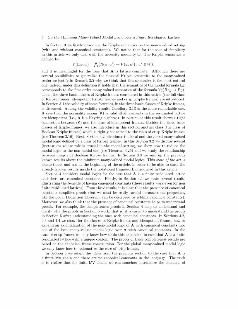
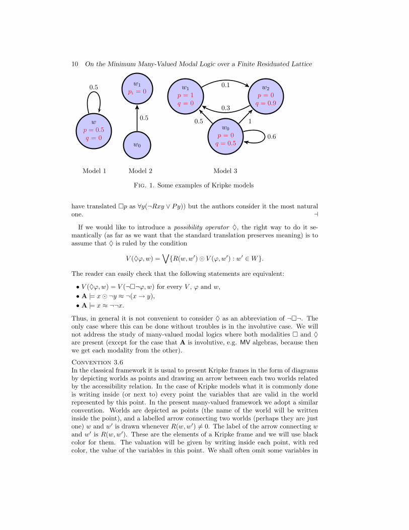
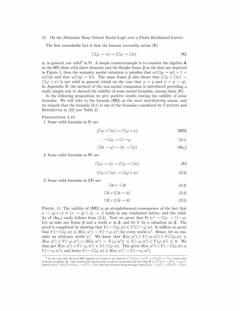
Fig. 1. Some examples of Kripke models
have translated �p as ∀y(¬Rxy ∨ Py)) but the authors consider it the most naturalone. a
If we would like to introduce a possibility operator ♦, the right way to do it se-mantically (as far as we want that the standard translation preserves meaning) is toassume that ♦ is ruled by the condition
V (♦ϕ,w) =∨{R(w,w′)� V (ϕ,w′) : w′ ∈W}.
The reader can easily check that the following statements are equivalent:
• V (♦ϕ,w) = V (¬�¬ϕ,w) for every V , ϕ and w,• A |= x� ¬y ≈ ¬(x→ y),• A |= x ≈ ¬¬x.
Thus, in general it is not convenient to consider ♦ as an abbreviation of ¬�¬. Theonly case where this can be done without troubles is in the involutive case. We willnot address the study of many-valued modal logics where both modalities � and ♦are present (except for the case that A is involutive, e.g. MV algebras, because thenwe get each modality from the other).
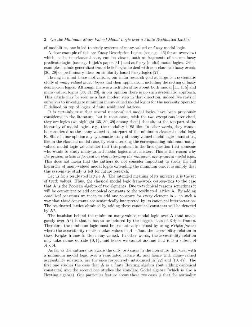
Convention 3.6In the classical framework it is usual to present Kripke frames in the form of diagramsby depicting worlds as points and drawing an arrow between each two worlds relatedby the accessibility relation. In the case of Kripke models what it is commonly doneis writing inside (or next to) every point the variables that are valid in the worldrepresented by this point. In the present many-valued framework we adopt a similarconvention. Worlds are depicted as points (the name of the world will be writteninside the point), and a labelled arrow connecting two worlds (perhaps they are justone) w and w′ is drawn whenever R(w,w′) 6= 0. The label of the arrow connecting wand w′ is R(w,w′). These are the elements of a Kripke frame and we will use blackcolor for them. The valuation will be given by writing inside each point, with redcolor, the value of the variables in this point. We shall often omit some variables in
On the Minimum Many-Valued Modal Logic over a Finite Residuated Lattice 11
the description under the agreement that all variables not explicitely written havevalue 1. The reader can find the diagrams of several Kripke models in Figure 1. a
3.1 Some remarks about validity
Definition 3.7We write M, w |=1 ϕ or simply w |=1 ϕ, and say that w validates ϕ, wheneverV (ϕ,w) = 1. And we write M |=1 ϕ whenever w |=1 ϕ for every w ∈W ; then, we sayϕ is valid in M. If F is a frame, we say that ϕ is valid in the frame F when ϕ is validin any Kripke model based on F. We write it F |=1 ϕ for short. And if K is a class offrames then we write K |=1 ϕ to mean that ϕ is valid in all frames in this class. a
Similarly to |=1 we could have introduced the relation |=+ of being positively validrequiring that the valuation does not get the value 0 (i.e., it gets a positive value).In the classical modal setting there is a natural notion of satisfiability that is dualto validity, but in the many-valued modal setting we must be really careful (even inthe involutive case) about this dual notion. Dually to the previous two notions wecan define the notions of a formula being satisfied or positively satisfied in a Kripkemodel or frame. If the negation of A is involutive then it obviously holds that
• ϕ is valid in a model M iff ¬ϕ is not positively satisfied in M,• ϕ is positively valid in a model M iff ¬ϕ is not satisfied in M.
Hence, the dual of validity, even in the involutive case, is not satisfiability; the dualis positive satisfiability. In the classical modal setting it really holds that the dual ofvalidity is satisfiability, but this is only because in this particular case satisfiabilitycoincides with positive satisfiability. And of course, without an involutive negationthere is no connection between the previous notions.
Definition 3.8A semantic modal valuation4 is a map v from the set of modal formulas into A (i.e.,v : Fm −→ A) such that v = V (•, w) for some Kripke model M = 〈W,R, V 〉 andsome world w in W . Sometimes, if there is no ambiguity, we will use the same namew to denote V (•, w). aRemark 3.9 (Properties on semantic modal valuations)It is clear that semantic modal valuations are homomorphisms for all non-modalconnectives, i.e., for ∧,∨,�,→, 1 and 0 (and the canonical constants when theyare in the language); but this is not the case for �. Thus, for every non-modalformula ϕ(p1, . . . , pn) and every semantic modal valuation v it holds that v(ϕ) =ϕA(v(p1), . . . , v(pn)). Another property that is clearly true is that if Fr |=1 ϕ, thenv(ϕ) = 1 for every semantic modal valuation v. a
Next, and as a first approximation to modal logics, we discuss the validity of someformula schemata in the classes Fr ⊇ IFr ⊇ CFr. Although they are indeed formulaschema we will simply use the word “formula” (the reader must think that ϕ,ψ, . . .are somehow metavariables) for the rest of the article.
4 We prefer to keep the adjective “semantic” because it is suggesting that these valuations are arising from Kripke
models. We use this word to emphasize the difference between these semantic modal valuations and the points of
the canonical models defined in Sections 4 and 5: these points may be seen as “syntactic” modal valuations.
12 On the Minimum Many-Valued Modal Logic over a Finite Residuated Lattice
The first remarkable fact is that the famous normality axiom (K)
�(ϕ→ ψ)→ (�ϕ→ �ψ) (K)
is, in general, not valid5 in Fr. A simple counterexample is to consider the algebra Aas the MV chain with three elements and the Kripke frame F as the first one depictedin Figure 1; then the semantic modal valuation w satisfies that w(�(p → q)) = 1 =w(�p) and that w(�q) = 0.5. The same frame F also shows that (�ϕ � �ψ) →�(ϕ � ψ) is not valid in general (think on the case that ϕ = p and ψ = p → q).In Appendix B, the method of the non-modal companion is introduced providing areally simple way to discard the validity of some modal formulas, among them (K).
In the following proposition we give positive results stating the validity of someformulas. We will refer to the formula (MD) as the meet distributivity axiom, andwe remark that the formula (3.1) is one of the formulas considered by Caicedo andRodrıguez in [10] (see Table 2).
Proposition 3.101. Some valid formulas in Fr are
(�ϕ ∧�ψ)↔ �(ϕ ∧ ψ) (MD)
¬¬�ϕ→ �¬¬ϕ. (3.1)
�(a→ ϕ)↔ (a→ �ϕ) (Axa)
2. Some valid formulas in IFr are
�(ϕ→ ψ)→ (�ϕ→ �ψ) (K)
(�ϕ��ψ)→ �(ϕ� ψ) (3.2)
3. Some valid formulas in CFr are�0 ∨ ¬�0 (3.3)
�a ∨ (�a↔ a) (3.4)
�0 ∨ (�a↔ a) (3.5)
Proof. 1): The validity of (MD) is an straightforward consequence of the fact thatx → (y ∧ z) ≈ (x → y) ∧ (x → z) holds in any residuated lattice, and the valid-ity of (Axa) easily follows from (2.3). Next we prove that Fr |=1 ¬¬�ϕ → �¬¬ϕ.Let us take any frame F and a world w in F, and let V be a valuation on F. Theproof is completed by showing that V (¬¬�ϕ,w) 6 V (�¬¬ϕ,w). It suffices to provethat V (¬¬�ϕ,w) 6 R(w,w′) → V (¬¬ϕ,w′) for every world w′. Hence, let su con-sider an arbitrary world w′. We know that R(w,w′) � V (¬ϕ,w′) � V (�ϕ,w) 6R(w,w′) � V (¬ϕ,w′) � (R(w,w′) → V (ϕ,w′)) 6 V (¬ϕ,w′) � V (ϕ,w′) 6 0. Wethus get R(w,w′) � V (¬ϕ,w′) 6 V (¬�ϕ,w). This gives R(w,w′) � V (¬¬�ϕ,w) 6V (¬¬ϕ,w′); and hence V (¬¬�ϕ,w) 6 R(w,w′)→ V (¬¬ϕ,w′).
5 In the case that A is an MTL algebra it is easy to see that Fr |=1 �((ϕ → ψ)2) → (�(ϕ2) → �ψ), where this
formula resembles (K). The reason why this formula is valid is essentially the fact that A |= (x2∧(x→ y)2)→ y ≈ 1.
Indeed, Fr |=1 (�(ϕ2)∧�((ϕ→ ψ)2))→ �ψ; this last formula being stronger than �((ϕ→ ψ)2)→ (�(ϕ2)→ �ψ).
On the Minimum Many-Valued Modal Logic over a Finite Residuated Lattice 13
2): We only give the proof for the case of the normality axiom. The proof is aconsequence of the validity of the quasi-equation
x ≈ x� x ⇒ (x→ (y → z))� (x→ y) 6 x→ z
in all residuated lattices. To see IFr |=1 (K) take any frame F and a world w in F, andlet V be a valuation on F. Then, for every world w′ it holds that V (�(ϕ→ ψ), w)�V (�ϕ,w) 6 (R(w,w′) → V (ϕ → ψ,w′)) � (R(w,w′) → V (ϕ,w′)) 6 R(w,w′) →V (ψ,w′). Thus, V (�(ϕ → ψ), w) � V (�ϕ,w) 6
∧{R(w,w′) → V (ψ,w′) : w′ ∈W} = V (�ψ,w). Hence, V (�(ϕ→ ψ)→ (�ϕ→ �ψ), w) = 1.
3): The validity of the first two formulas follows from the fact that for every valua-tion V in a crisp frame and every world w in this frame it holds that V (�a,w) ∈ {a, 1}.Next we prove that CFr |=1 �0 ∨ (�a ↔ a). Let us take any valuation V in a crispKripke frame and a world w in this frame such that V (�0, w) 6= 1. It is enough toprove that V (a,w) = V (�a,w). Since V (�0, w) 6= 1 we get that there is a world w′
such that 1 6= R(w,w′)→ V (0, w′). As the frame is crisp we have that R(w,w′) = 1.Therefore, V (a,w) = a = 1→ a =
∨{R(w,w′′) : w′′ ∈ W} → a =∧{R(w,w′′)→ a :
w′′ ∈W} = V (�a,w).
Before the previous proposition we saw that the formulas in the second item arenot in general valid in Fr. Analogously, the reader can easily check that the formulasin the third item are in general not valid in IFr (cf. Proposition 3.14). In the nextproposition we use the notion of (infinitely) distributive element a ∈ A defined asthose elements satisfying that
∧{a ∨ x : x ∈ X} ≈ a ∨
∧X (3.6)
for every set X ⊆ A. It is obvious that if A is finite then the previous definition canbe relaxed to the case that X = {x1, x2}. It is interesting to point out that if A is afinite algebra, then
• all Boolean elements6 are distributive,• all coatoms of A are distributive7.
The first statement is a consequence of the fact that p ∨ ¬p `RL (p ∨ (q ∧ r)) ↔((p ∨ q) ∧ (p ∨ r)). Here `RL refers to the non-modal logic associated with the classof all residuated lattices (see [25]). And the second one follows from the fact that ifa is a coatom, then the only possibility that (3.6) fails is when a = a ∨ (x1 ∧ x2) and1 = (a∨x1)∧(a∨x2); which is a contradiction with the fact that p∨q, p∨r `RL p∨(q∧r).In the proofs of these two statements it has been crucial the fact that `RL admitsproofs by cases. Hence, in particular we know that Proposition 3.11 holds when a isa coatom of a finite A.
6 We remind the reader that the set of Boolean elements is the set of a’s such that there is some b ∈ A satisfying
that a∨ b = 1 and a∧ b = 0. In the setting of residuated lattices it is well known that the set of Boolean elements is
exactly {a ∈ A : a∨¬a = 1}. Another characterization of this set is given by {a ∈ A : a→ b = ¬a∨ b for every b ∈A}. Indeed, using the fact that `RL admits proofs by cases it is easy to see that for every non-modal formula ϕ(p, ~q),
it holds that
– ϕA(p, ~q) = 1 for any residuated lattice A and any assignation such that pA ∈ {0, 1}, iff
– ϕA(p, ~q) = 1 for any residuated lattice A and any assignation such that pA is a Boolean element.
7 This is somehow suggesting the “picture” that the upper part of a residuated lattice is distributive in the
previous sense.
14 On the Minimum Many-Valued Modal Logic over a Finite Residuated Lattice
Proposition 3.11Let a be a distributive element of A. Then,
�(a ∨ ϕ)→ (a ∨�ϕ). (3.7)
is valid in CFr.
Proof. This is easily proved from the fact that a is a distributive element.
Next we consider the problem of definability for the main classes of frames con-sidered in this article. First of all we prove that the class IFr of idempotent framesis modally definable by the normality axiom (K). Indeed, the formula (3.2) and theformula (�ϕ � �ϕ) → �(ϕ � ϕ) are also defining the same class IFr. We stress thefact that none of the formulas in Proposition 3.12 is using canonical constants.
Proposition 3.12IFr = {F : F |=1 �(p→ q)→ (�p→ �q)} = {F : F |=1 (�p��q)→ �(p� q)} = {F :F |=1 (�p��p)→ �(p� p)}.
Proof. The inclusion of IFr in the other three classes follow from Proposition 3.10.The rest of inclusions can be proved using the same idea, and so we will prove only oneof them, namely that {F : F |=1 (�p��p)→ �(p� p)} ⊆ IFr. Hence, let us considera Kripke frame F = 〈W,R〉 and let us assume that there is an element a ∈ A suchthat a� a < a and a = R(w,w′) for certain worlds w,w′. We define a valuation V bythe conditions: (i)V (p, w′) = a, and (ii)V (p, w′′) = 1 for every world w′′ 6= w′. Then,V (�p, w) = 1 and V (�(p�p), w) 6 a→ a�a 6= 1. Therefore, (�p��p)→ �(p�p)is not valid in F.
Corollary 3.13• Axiom (K) is valid in Fr iff A is a Heyting algebra iff Fr = IFr.• {ϕ ∈ Fm : Fr |=1 ϕ} = {ϕ ∈ Fm : IFr |=1 ϕ} iff Fr = IFr.
Proof. It is obvious that A is a Heyting algebra iff Fr = IFr. Then, by the previousproposition we obtain this corollary.
Next we address the issue whether the class CFr of crisp Kripke frames is charac-terized by the set of its valid modal formulas. In general the answer is negative dueto a result proved in [10]: over the standard Godel algebra8, the valid modal for-mulas (without canonical constants) in IFr are exactly the valid ones in CFr. Hence,in general it may happen that IFr 6= CFr while both classes share the same validformulas. Although we have not got a characterization of the algebras A such that{ϕ ∈ Fm : IFr |=1 ϕ} = {ϕ ∈ Fm : CFr |=1 ϕ} we can state some necessary condi-tions. The last item also gives us a characterization in a particular case.
Proposition 3.141. IFr |=1 �0 ∨ ¬�0 iff A |= x ≈ x� x⇒ ¬x ∨ ¬¬x ≈ 1.2. If {ϕ ∈ Fm : IFr |=1 ϕ} = {ϕ ∈ Fm : CFr |=1 ϕ}, then A |= x ≈ x � x ⇒¬x ∨ ¬¬x ≈ 1.
3. If there are canonical constants in the language and 1 is join irreducible, then{ϕ ∈ Fm : IFr |=1 ϕ} = {ϕ ∈ Fm : CFr |=1 ϕ} iff IFr = CFr.
8A moment of reflection shows that this also holds for finite Godel chains.
On the Minimum Many-Valued Modal Logic over a Finite Residuated Lattice 15
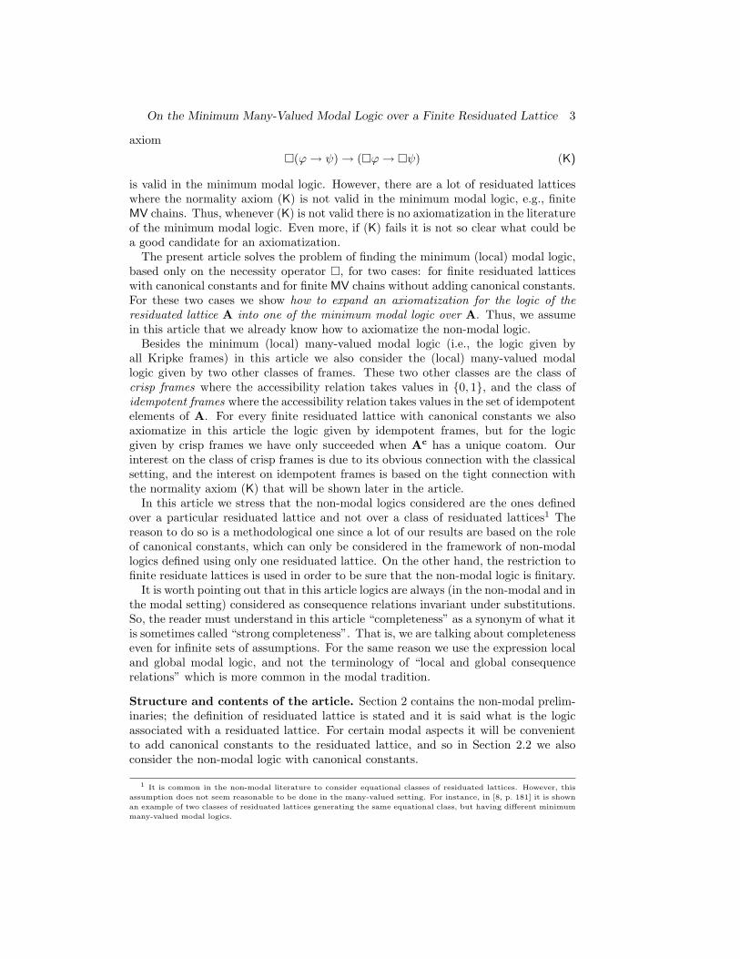
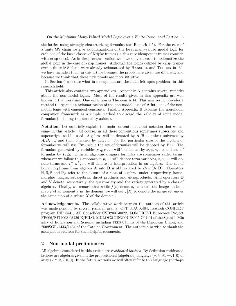
� 0 a b c d 10 0 0 0 0 0 0a 0 a a a a ab 0 a a a b bc 0 a a c c cd 0 a b c d d1 0 a b c d 1
→ 0 a b c d 10 1 1 1 1 1 1a 0 1 1 1 1 1b 0 c 1 1 1 1c 0 b b 1 1 1d 0 a b c 1 11 0 a b c d 1
wp = a
c
An interesting MTL chain A Kripke Model
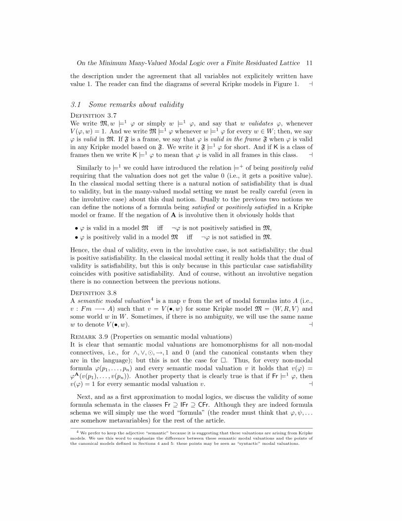
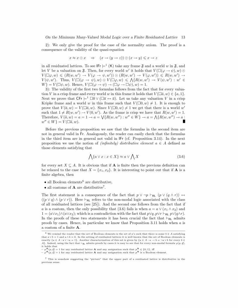
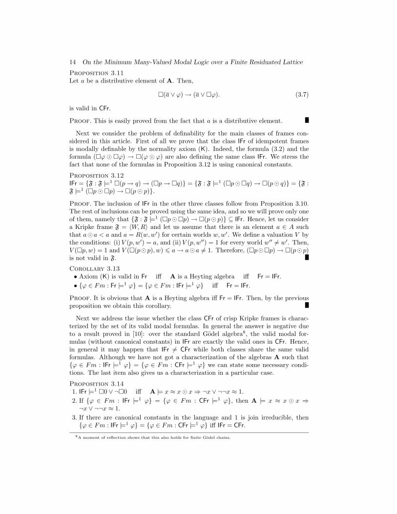
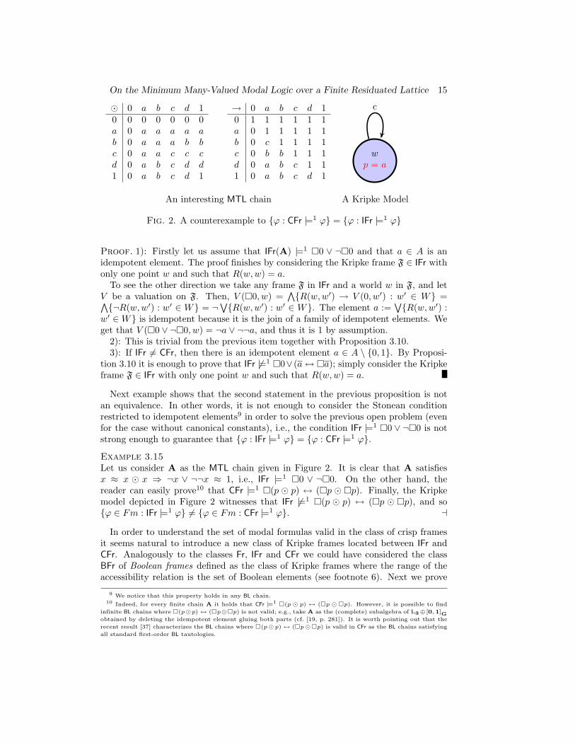
Fig. 2. A counterexample to {ϕ : CFr |=1 ϕ} = {ϕ : IFr |=1 ϕ}
Proof. 1): Firstly let us assume that IFr(A) |=1 �0 ∨ ¬�0 and that a ∈ A is anidempotent element. The proof finishes by considering the Kripke frame F ∈ IFr withonly one point w and such that R(w,w) = a.
To see the other direction we take any frame F in IFr and a world w in F, and letV be a valuation on F. Then, V (�0, w) =
∧{R(w,w′) → V (0, w′) : w′ ∈ W} =∧{¬R(w,w′) : w′ ∈ W} = ¬∨{R(w,w′) : w′ ∈ W}. The element a :=∨{R(w,w′) :
w′ ∈W} is idempotent because it is the join of a family of idempotent elements. Weget that V (�0 ∨ ¬�0, w) = ¬a ∨ ¬¬a, and thus it is 1 by assumption.
2): This is trivial from the previous item together with Proposition 3.10.3): If IFr 6= CFr, then there is an idempotent element a ∈ A \ {0, 1}. By Proposi-
tion 3.10 it is enough to prove that IFr 6|=1 �0∨ (a↔ �a); simply consider the Kripkeframe F ∈ IFr with only one point w and such that R(w,w) = a.
Next example shows that the second statement in the previous proposition is notan equivalence. In other words, it is not enough to consider the Stonean conditionrestricted to idempotent elements9 in order to solve the previous open problem (evenfor the case without canonical constants), i.e., the condition IFr |=1 �0 ∨ ¬�0 is notstrong enough to guarantee that {ϕ : IFr |=1 ϕ} = {ϕ : CFr |=1 ϕ}.Example 3.15Let us consider A as the MTL chain given in Figure 2. It is clear that A satisfiesx ≈ x � x ⇒ ¬x ∨ ¬¬x ≈ 1, i.e., IFr |=1 �0 ∨ ¬�0. On the other hand, thereader can easily prove10 that CFr |=1 �(p � p) ↔ (�p � �p). Finally, the Kripkemodel depicted in Figure 2 witnesses that IFr 6|=1 �(p � p) ↔ (�p � �p), and so{ϕ ∈ Fm : IFr |=1 ϕ} 6= {ϕ ∈ Fm : CFr |=1 ϕ}. a
In order to understand the set of modal formulas valid in the class of crisp framesit seems natural to introduce a new class of Kripke frames located between IFr andCFr. Analogously to the classes Fr, IFr and CFr we could have considered the classBFr of Boolean frames defined as the class of Kripke frames where the range of theaccessibility relation is the set of Boolean elements (see footnote 6). Next we prove
9 We notice that this property holds in any BL chain.10 Indeed, for every finite chain A it holds that CFr |=1 �(p � p) ↔ (�p � �p). However, it is possible to find
infinite BL chains where �(p�p)↔ (�p��p) is not valid; e.g., take A as the (complete) subalgebra of L3⊕ [0, 1]Gobtained by deleting the idempotent element gluing both parts (cf. [19, p. 281]). It is worth pointing out that the
recent result [37] characterizes the BL chains where �(p� p)↔ (�p��p) is valid in CFr as the BL chains satisfying
all standard first-order BL tautologies.
16 On the Minimum Many-Valued Modal Logic over a Finite Residuated Lattice
that the class BFr has the same valid formulas than the class CFr (even when canonicalconstants are allowed), and we also show that this new class BFr is always modallydefinable, using the formulas in Proposition 3.11, when there are canonical constantsin the language. It is worth pointing out that if 1 is join irreducible then BFr = CFr,and hence without canonical constants in the language in general it is not possibleto characterize BFr using modal formulas since the same counterexample cited above(and based on Godel chains) applies here.
Theorem 3.16Let A be a finite residuated lattice. Then, BFr and CFr have the same valid modalformulas (even allowing canonical constants in the language).
Proof. First of all we remark that by the finiteness assumption we know that A ∼=∏i<n A/θi where the only Boolean elements of A/θi are {0, 1}. This is a consequence
of the characterization of directly indecomposable residuated lattices stated in [43,Proposition 1.5].
Since CFr ⊆ BFr it suffices to prove that all modal formulas valid in CFr are alsovalid in BFr. The proof is based on a method that converts a Boolean Kripke modelover A into a family of n crisp Kripke models A. Let us assume that 〈W,R, V 〉 isa Boolean Kripke model. Then, for every i < n we consider the crisp Kripke model〈Wi, Ri, Vi〉 defined by
• Wi = W ,• Ri(w,w′) is (i) 1A if R(w,w′) ∈ 1/θ1, and (ii) 0A if R(w,w′) ∈ 0/θ1,• Vi(p, w) = V (p, w).
The previous Kripke models are well defined because since R(w,w′) is a Booleanelement we know that for every i < n, either R(w,w′) ∈ 1/θ1 or R(w,w′) ∈ 0/θ1.By construction of these Kripke models it is straightforward to check that for everymodal formula ϕ (perhaps including canonical constants), every world w ∈ W andevery i < n it holds that
πi(V (ϕ,w)) = πi(Vi(ϕ,w)),
where πi is the i-th projection. Therefore, V (ϕ,w) = 〈πi(Vi(ϕ,w)) : i < n〉 for everymodal formula ϕ and every world w ∈ W . Using this fact it is obvious all modalformulas valid in CFr are also valid in BFr.
Proposition 3.17Let A be a finite residuated lattice, and let F be a frame. The following statementsare equivalent.
1. F is a Boolean frame,2. F |=1 {�(a ∨ p)→ (a ∨�p) : a is a distributive element of A},3. F |=1 {�(k ∨ p)→ (k ∨�p) : k is a coatom of A}.
Proof. 1⇒ 2): This follows from Theorem 3.16 together with Proposition 3.11.2⇒ 3): This is trivial since we know that all coatoms are distributive elements.3⇒ 1): Let us assume that there is an element a ∈ A such that a is not a Boolean
element and a = R(w,w′) for certain worlds w,w′. Hence, a∨¬a 6= 1, and so a∨¬a 6 k
On the Minimum Many-Valued Modal Logic over a Finite Residuated Lattice 17
for certain coatom k. We define a valuation V by the conditions: (i)V (p, w′) = 0, and(ii)V (p, w′′) = 1 for every world w′′ 6= w′. Then, V (�(k ∨ p), w) = a → (k ∨ 0) = 1and V (k ∨�p, w) = k ∨ (a→ 0) = k. Therefore, �(k ∨ p)→ (k ∨�p) is not valid inF, which is a contradiction.
It is worth pointing out that Proposition B.4 (and Corollary B.5) gives us anothermethod to get valid formulas. We have left this result in Appendix B because althoughthis proposition is formulated without appealing to the non-modal companion we canunderstand this result as explaining why for some modal formulas the non-modalcompanion method is enough to discard its validity. To finish this section we prove asimilar result to Proposition B.4, but this time validity is restricted to a particularlyinteresting subclass of Kripke models, the class of modally witnessed models.
A Kripke model 〈W,R, V 〉 is modally witnessed11 when for every modal formula ϕand every world w, there is a world w′ (called the witness) such that
V (�ϕ,w) = R(w,w′)→ V (ϕ,w′).
It is obvious that this notion is the relaxed version of the witnessed first-order struc-tures considered by Hajek in [32, 33] when replacing first order formulas with modal(propositional) ones. In case we restrict our attention to valid formulas in all modallywitnessed Kripke models then we can get a similar result to Proposition B.4 withoutthe requirement saying that ε is expanding.
Proposition 3.18Let δ(p1, . . . , pn) and ε(p) be two non-modal formulas such that δ is non decreas-ing over Ac in any of its arguments. And let ϕ1, . . . , ϕn, ϕ be non-modal formulas.If `Ac δ(r → ϕ1, . . . , r → ϕn) → ε(r → ϕ) being r a variable not appearing in{ϕ1, . . . , ϕn, ϕ}, then δ(�ϕ1, . . . ,�ϕn) → ε(�ϕ) is valid in all modally witnessedKripke models.
Proof. Take any modally witnessed Kripke model 〈W,R, V 〉 and a world w in W .We consider w′ as the witness for V (�ϕ,w), i.e., V (�ϕ,w) = R(w,w′) → V (ϕ,w′).Then, V (δ(�ϕ1, . . . ,�ϕn), w) = δAc
(V (�ϕ1, w), . . . , V (�ϕn, w)) 6 δAc
(R(w,w′) →V (ϕ1, w
′), . . . , R(w,w′)→ V (ϕn, w′)) 6 εAc
(R(w,w′)→ V (ϕ,w′)) = εAc
(V (�ϕ,w))= V (ε(�ϕ), w).
3.2 The local and global modal logics
Now it is time to introduce the minimum modal logic we want to study in the presentarticle. Our main interest is in the class Fr of all frames, but in order to be as generalas possible the definitions are given for an arbitrary class K of frames. Thus, thisdefinition also defines the modal logic associated with the other two basic classes ofKripke frames.
Definition 3.19In the following we assume A to be a given residuated lattice. Let K be a subclassof its Kripke frames. The set {ϕ ∈ Fm : K |=1 ϕ} will be denoted by Λ(K,A). In
11 We point out that in general finite Kripke models are not modally witnessed; but when A is a chain then all
finite Krikpe models are modally witnessed. In the case that A is a chain it is worth pointing out a result of Hajek
[31, Theorem 4] showing that there is a tight connection, as far as we only consider the modal language, between
modally witnessed models and finite models.
18 On the Minimum Many-Valued Modal Logic over a Finite Residuated Lattice
case there are canonical constants we will use the notation Λ(K,Ac) to stress theirpresence. The local (many-valued) modal logic Λ(l,K,A) is the logic obtained bydefining, for all sets Γ ∪ {ϕ} of modal formulas (without canonical constants),
• Γ `Λ(l,K,A) ϕ iff12
• for every semantic modal valuation v arising from a Kripke frame in K, if v[Γ ] ⊆{1} then v(ϕ) = 1.
We will also use the notations Λ(l,K) or `lK(A). And for the analogous definition, butincluding canonical constants, we will use the notation Λ(l,K,Ac) or `lK(Ac). On theother hand, the global (many-valued) modal logic Λ(g,K,A) is the logic defined by
• Γ `Λ(g,K,A) ϕ iff• for every Kripke model M arising from a Kripke frame in K, if M |=1 γ for everyγ ∈ Γ , then M |=1 ϕ.
For the sake of simplicity we will write it simply Λ(g,K) or `gK(A). If we follow thesame definition scheme, but allowing canonical constants in the language, then wewill use the notation Λ(g,K,Ac) or `gK(Ac). a
By definition it is obvious that both logics, the local and the global, share the sameset of theorems, namely Λ(K,A). Another obvious consequence of the definition isthat Λ(l,K,A) 6 Λ(g,K,A), these two logics being conservative expansions of Λ(A).These last two sentences are also true with canonical constants in the language.
Remark 3.20 (Global vs. Local)The main advantadge of the local modal logic is that in most common cases wecan prove completeness using the canonical frame method (see Theorem 4.11). Onthe other hand, the global modal logic has other benefits. The first one is thatΛ(g,K,A) and Λ(g,K,Ac) are always algebraizable in the Abstract Algebraic Logicframework (see [16, 24]). This is an easy consequence of the general theory usingthat ϕ → ψ `gK �ϕ → �ψ together with the fact that the non-modal logics Λ(A)and Λ(Ac) are algebraizable with equivalence formulas {p → q, q → p}. Therefore,we can give an algebraic semantics (and hence, a truth functional semantics) for theglobal modal logic. Another benefit is that Λ(g,Fr,A) is the fragment (given by thestandard translation) of the first order logic associated with A. Thus, we can transferknown results from first order logics to global modal logics. a
In our opinion the developing of a many-valued modal logics hierarchy (addingproperties like reflexivity, transitivity, etc. and following the same ideas than in theclassical setting) cannot be successfully undertaken until we know how to axioma-tize (whenever they are axiomatizable) the minimum modal logics Λ(l,Fr,A) andΛ(g,Fr,A). What axioms and rules must be added to an axiomatization of Λ(A) toget an axiomatization of Λ(l,Fr,A)? And for Λ(g,Fr,A)? Of course a first step to
12 In the classical modal literature, it is not common to introduce the definition of the local modal logic using
the notion of semantic modal valuation; alternative equivalent definitions are usually provided. However, we feel
that this definition based on semantic modal valuations has the advantage of making more clear how to reduce the
local modal logic to the non-modal logic (cf. Theorem 3.26). Comparing this definition of the local modal logic
with the definition (2.7) of the non-modal logic it is obvious that in order to find this reduction one has to be able
to characterize the semantic modal valuations as the non-modal homomorphisms that are sending a certain set of
axioms to 1 (cf. Lemma 3.25, Theorem 4.11, etc).
On the Minimum Many-Valued Modal Logic over a Finite Residuated Lattice 19
answer this question is to know how to obtain the set Λ(Fr,A) from an axiomatizationof Λ(A).
This problem remains open in this general formulation (see Section 6 for a moredetailed discussion). But in Sections 4 and 5 we solve some instances of the problem.We point out that, as far as the authors are aware, the results in these two sectionspresent the first known axiomatizations for local many-valued modal logics wherenormality axiom (K) fails.
First of all, we consider the problem of comparing the many-valued modal logicsgiven by the main three classes of frames considered.
Proposition 3.211. Λ(g,Fr,A) = Λ(g, IFr,A) iff Λ(g,Fr,Ac) = Λ(g, IFr,Ac) iff Fr = IFr.2. Λ(l,Fr,A) = Λ(l, IFr,A) iff Λ(l,Fr,Ac) = Λ(l, IFr,Ac) iff Fr = IFr.3. Λ(g, IFr,Ac) = Λ(g,CFr,Ac) iff IFr = CFr.4. Λ(l, IFr,Ac) = Λ(l,CFr,Ac) iff IFr = CFr.
Proof. The first two statements are a consequence of Corollary 3.13. Let us provethe last two. If CFr 6= IFr, then there is an idempotent element a ∈ A \ {0, 1}.The proof finishes by noticing that �a `lCFr(Ac) �0 (and so �a `gCFr(Ac) �0) while�a 6`gIFr(Ac) �0 (and so �a 6`lIFr(Ac) �0).
We notice that in previous proposition it remains open to characterize when Λ(g, IFr,A) =Λ(g,CFr,A) or when Λ(l, IFr,A) = Λ(l,CFr,A). Using Theorem 3.26 it is easy toprove that this open question reduces to characterize the A’s such that Λ(IFr,A) =Λ(CFr,A), but this other question is also open.
There are five (meta)rules that play a remarkable role in the modal setting. Theserules are13
(N) ϕ ` �ϕ (Mon) ϕ→ ψ ` �ϕ→ �ψ
γ ` ϕ(Pref) �γ ` �ϕ
Γ ` ϕ(Pref∗) �Γ ` �ϕ
r → Γ ` r → ϕ(OrdPres∗) �Γ ` �ϕ
where r is a variable not appearing in Γ ∪ {ϕ}. These five rules will be respectivelycalled Necessity, Monotonicity, Prefixing, Infinitary Prefixing and Infinitary OrderPreserving. We notice that the rule (OrdPres∗) is not closed under substitutions;substitutions may destroy the requirement concerning the variable r.
Proposition 3.22Let K be a class of Kripke frames.
1. Λ(g,K,Ac) is closed under (N), that is, ϕ `gK(Ac) �ϕ.
2. Λ(g,K,Ac) is closed under (Mon), that is, ϕ→ ψ `gK(Ac) �ϕ→ �ψ.
3. Λ(l,K,Ac) is closed under (OrdPres∗), that is, if r is a variable not appearing in theset Γ ∪ {ϕ} of formulas and {r → γ : γ ∈ Γ} `lK(Ac) r → ϕ, then �Γ `lK(Ac) �ϕ.
13 As expected we use �Γ and r → Γ to denote, respectively, the sets {�γ : γ ∈ Γ} and {r → γ : γ ∈ Γ}.
20 On the Minimum Many-Valued Modal Logic over a Finite Residuated Lattice
4. If K ⊆ CFr then both Λ(g,K,Ac) and Λ(l,K,Ac) are closed under (Pref∗).5. If K ⊆ IFr and Λ(l,K,Ac) satifies the Local Deduction Theorem, then Λ(l,K,Ac)
is closed under (Pref). That is, if γ `lK(Ac) ϕ, then �γ `lK(Ac) �ϕ.
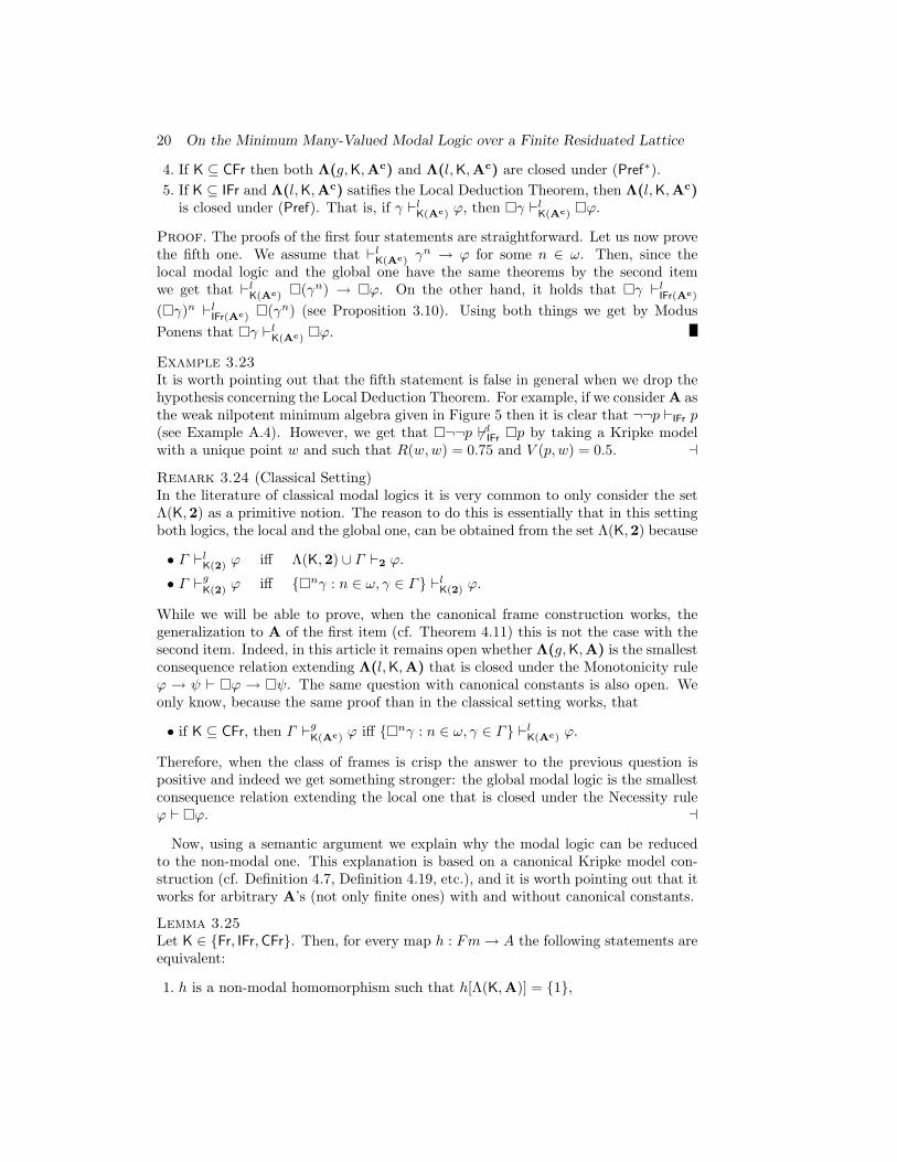
Proof. The proofs of the first four statements are straightforward. Let us now provethe fifth one. We assume that `lK(Ac) γ
n → ϕ for some n ∈ ω. Then, since thelocal modal logic and the global one have the same theorems by the second itemwe get that `lK(Ac) �(γn) → �ϕ. On the other hand, it holds that �γ `lIFr(Ac)
(�γ)n `lIFr(Ac) �(γn) (see Proposition 3.10). Using both things we get by ModusPonens that �γ `lK(Ac) �ϕ.
Example 3.23It is worth pointing out that the fifth statement is false in general when we drop thehypothesis concerning the Local Deduction Theorem. For example, if we consider A asthe weak nilpotent minimum algebra given in Figure 5 then it is clear that ¬¬p `IFr p(see Example A.4). However, we get that �¬¬p 6`lIFr �p by taking a Kripke modelwith a unique point w and such that R(w,w) = 0.75 and V (p, w) = 0.5. aRemark 3.24 (Classical Setting)In the literature of classical modal logics it is very common to only consider the setΛ(K,2) as a primitive notion. The reason to do this is essentially that in this settingboth logics, the local and the global one, can be obtained from the set Λ(K,2) because
• Γ `lK(2) ϕ iff Λ(K,2) ∪ Γ `2 ϕ.
• Γ `gK(2) ϕ iff {�nγ : n ∈ ω, γ ∈ Γ} `lK(2) ϕ.
While we will be able to prove, when the canonical frame construction works, thegeneralization to A of the first item (cf. Theorem 4.11) this is not the case with thesecond item. Indeed, in this article it remains open whether Λ(g,K,A) is the smallestconsequence relation extending Λ(l,K,A) that is closed under the Monotonicity ruleϕ → ψ ` �ϕ → �ψ. The same question with canonical constants is also open. Weonly know, because the same proof than in the classical setting works, that
• if K ⊆ CFr, then Γ `gK(Ac) ϕ iff {�nγ : n ∈ ω, γ ∈ Γ} `lK(Ac) ϕ.
Therefore, when the class of frames is crisp the answer to the previous question ispositive and indeed we get something stronger: the global modal logic is the smallestconsequence relation extending the local one that is closed under the Necessity ruleϕ ` �ϕ. a
Now, using a semantic argument we explain why the modal logic can be reducedto the non-modal one. This explanation is based on a canonical Kripke model con-struction (cf. Definition 4.7, Definition 4.19, etc.), and it is worth pointing out that itworks for arbitrary A’s (not only finite ones) with and without canonical constants.
Lemma 3.25Let K ∈ {Fr, IFr,CFr}. Then, for every map h : Fm→ A the following statements areequivalent:
1. h is a non-modal homomorphism such that h[Λ(K,A)] = {1},
On the Minimum Many-Valued Modal Logic over a Finite Residuated Lattice 21
2. h is a semantic modal valuation arising from a Kripke frame in K.
The same equivalence also holds when we replace A with Ac.
Proof. We will only prove the case without canonical constants, since the other oneis analogous replacing A with Ac. The only non-trivial direction is the downwardsone. In order to prove this we are going to define a canonical Kripke model belongingto the class K. First of all we define the set B as (i)A if K = Fr, (ii) {a ∈ A : a = a�a}if K = IFr, and (iii) {0, 1} if K = CFr. It is obvious that in all three cases the set Bis closed under arbitrary joins. Next we define the Kripke model 〈Wcan, Rcan, Vcan〉given by
• the set Wcan is the set of semantic modal valuations v arising from frames in K,• the accessibility relation Rcan(v1, v2) is defined as the largest element in B below∧{v1(�ϕ)→ v2(ϕ) : ϕ ∈ Fm},• the evaluation map is defined by Vcan(p, v) := v(p) for every variable p.
By definition this Kripke model belongs to K. To finish the proof it is enough to provethat Vcan(ϕ, v) = v(ϕ) for every modal formula ϕ and every v ∈Wcan. By inductionit suffices to prove that
∧{Rcan(v, v′)→ v′(ϕ) : v′ ∈Wcan} = v(�ϕ) for every modalformula ϕ and every v ∈Wcan.
The inequality∧{Rcan(v, v′) → v′(ϕ) : v′ ∈ Wcan} > v(�ϕ) trivially follows from
the definition of the accessibility relation Rcan.Let us now try to prove the other inequality. Since v ∈ Wcan we know that there
is a Kripke model 〈W,R, V 〉 in K and a world w ∈ W such that v = V (•, w). Itis obvious that all worlds w′ ∈ W can be seen as members of Wcan, and using thatR(w,w′) 6
∧{w(�ψ) → w′(ψ) : ψ ∈ Fm} it follows that R(w,w′) 6 Rcan(w,w′).Thus, v(�ϕ) = w(�ϕ) =
∧{R(w,w′) → w′(ϕ) : w′ ∈ W} > ∧{Rcan(w,w′) →w′(ϕ) : w′ ∈ W} > ∧{Rcan(w, v′) → v′(ϕ) : v′ ∈ Wcan} =
∧{Rcan(v, v′) → v′(ϕ) :v′ ∈Wcan}, which finishes the proof.
Theorem 3.26Let K ∈ {Fr, IFr,CFr}. Then, for every set Γ ∪ {ϕ} it holds that
Γ `lK(A) ϕ iff Γ ∪ Λ(K,A) `A ϕ.
Analogously it holds that
Γ `lK(Ac) ϕ iff Γ ∪ Λ(K,Ac) `Ac ϕ.
Proof. This trivially follows from the previous lemma together with our definitionof the local modal logic.
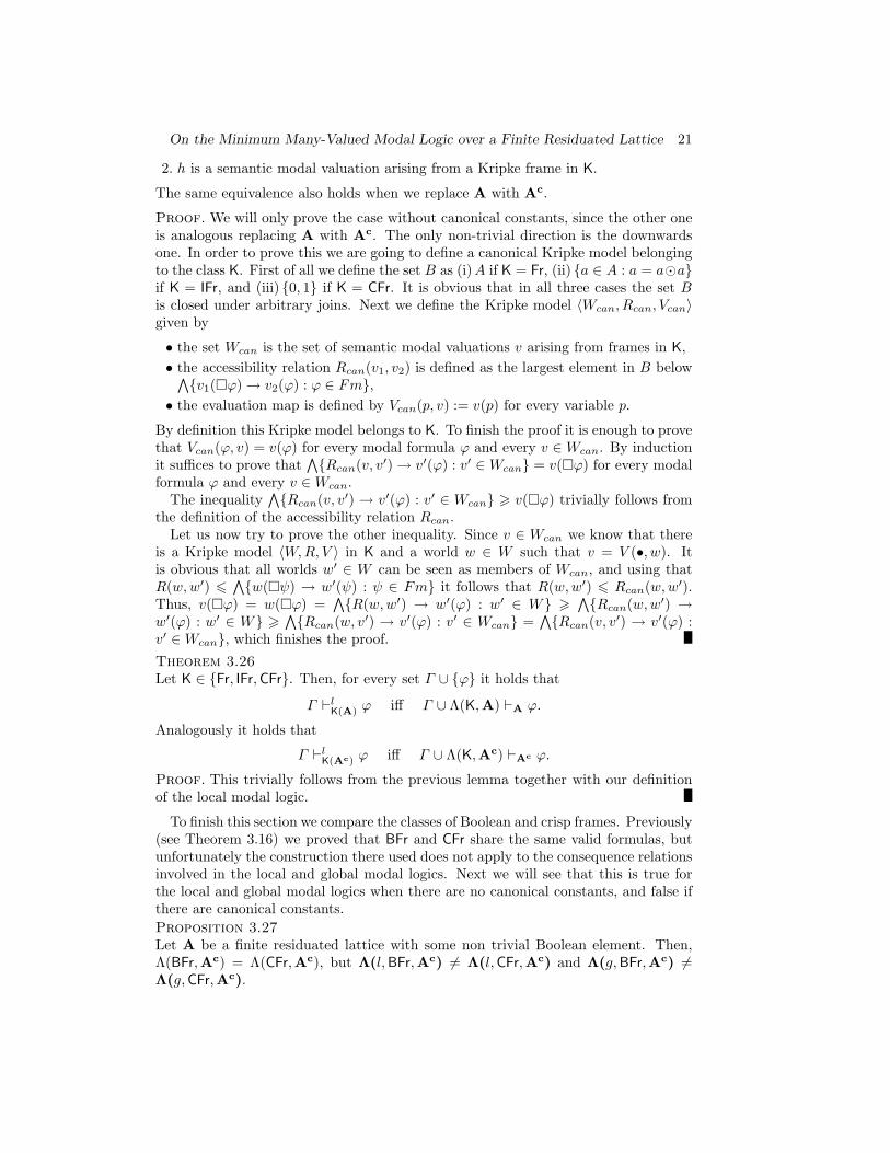
To finish this section we compare the classes of Boolean and crisp frames. Previously(see Theorem 3.16) we proved that BFr and CFr share the same valid formulas, butunfortunately the construction there used does not apply to the consequence relationsinvolved in the local and global modal logics. Next we will see that this is true forthe local and global modal logics when there are no canonical constants, and false ifthere are canonical constants.Proposition 3.27Let A be a finite residuated lattice with some non trivial Boolean element. Then,Λ(BFr,Ac) = Λ(CFr,Ac), but Λ(l,BFr,Ac) 6= Λ(l,CFr,Ac) and Λ(g,BFr,Ac) 6=Λ(g,CFr,Ac).
22 On the Minimum Many-Valued Modal Logic over a Finite Residuated Lattice
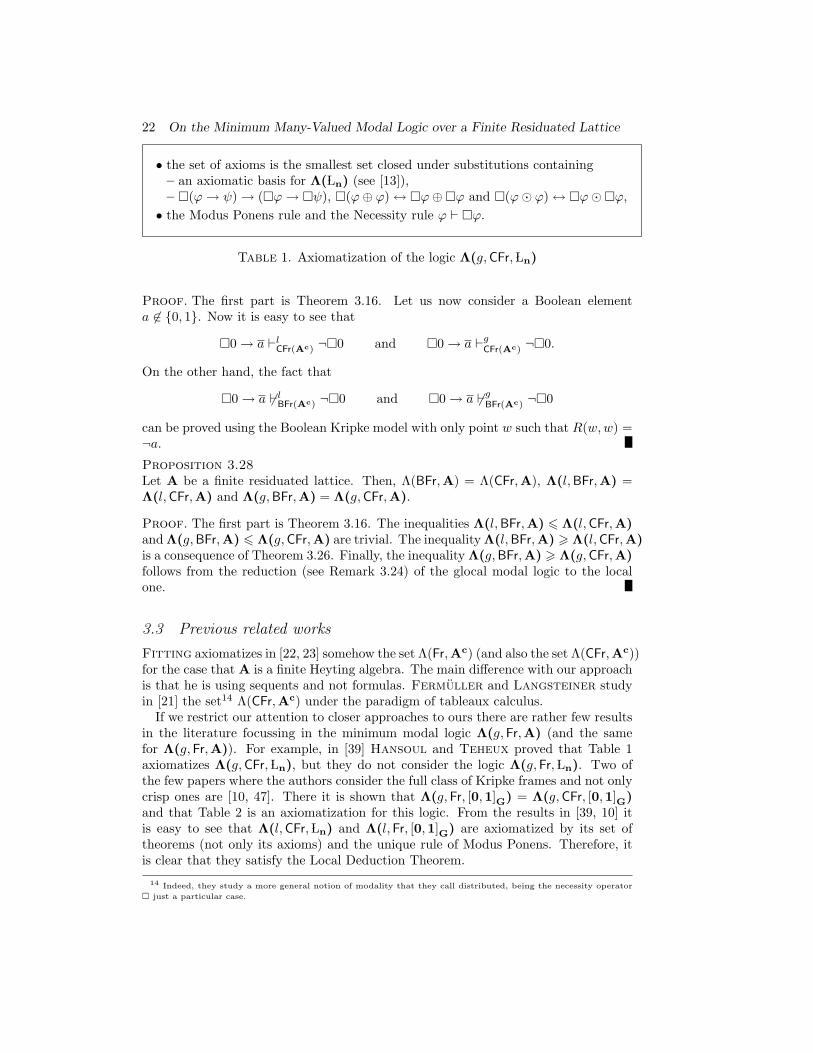
• the set of axioms is the smallest set closed under substitutions containing– an axiomatic basis for Λ( Ln) (see [13]),– �(ϕ→ ψ)→ (�ϕ→ �ψ), �(ϕ⊕ ϕ)↔ �ϕ⊕�ϕ and �(ϕ� ϕ)↔ �ϕ��ϕ,• the Modus Ponens rule and the Necessity rule ϕ ` �ϕ.
Table 1. Axiomatization of the logic Λ(g,CFr, Ln)
Proof. The first part is Theorem 3.16. Let us now consider a Boolean elementa 6∈ {0, 1}. Now it is easy to see that
�0→ a `lCFr(Ac) ¬�0 and �0→ a `gCFr(Ac) ¬�0.
On the other hand, the fact that
�0→ a 6`lBFr(Ac) ¬�0 and �0→ a 6`gBFr(Ac) ¬�0
can be proved using the Boolean Kripke model with only point w such that R(w,w) =¬a.
Proposition 3.28Let A be a finite residuated lattice. Then, Λ(BFr,A) = Λ(CFr,A), Λ(l,BFr,A) =Λ(l,CFr,A) and Λ(g,BFr,A) = Λ(g,CFr,A).
Proof. The first part is Theorem 3.16. The inequalities Λ(l,BFr,A) 6 Λ(l,CFr,A)and Λ(g,BFr,A) 6 Λ(g,CFr,A) are trivial. The inequality Λ(l,BFr,A) > Λ(l,CFr,A)is a consequence of Theorem 3.26. Finally, the inequality Λ(g,BFr,A) > Λ(g,CFr,A)follows from the reduction (see Remark 3.24) of the glocal modal logic to the localone.
3.3 Previous related works
Fitting axiomatizes in [22, 23] somehow the set Λ(Fr,Ac) (and also the set Λ(CFr,Ac))for the case that A is a finite Heyting algebra. The main difference with our approachis that he is using sequents and not formulas. Fermuller and Langsteiner studyin [21] the set14 Λ(CFr,Ac) under the paradigm of tableaux calculus.
If we restrict our attention to closer approaches to ours there are rather few resultsin the literature focussing in the minimum modal logic Λ(g,Fr,A) (and the samefor Λ(g,Fr,A)). For example, in [39] Hansoul and Teheux proved that Table 1axiomatizes Λ(g,CFr, Ln), but they do not consider the logic Λ(g,Fr, Ln). Two ofthe few papers where the authors consider the full class of Kripke frames and not onlycrisp ones are [10, 47]. There it is shown that Λ(g,Fr, [0,1]G) = Λ(g,CFr, [0,1]G)and that Table 2 is an axiomatization for this logic. From the results in [39, 10] itis easy to see that Λ(l,CFr, Ln) and Λ(l,Fr, [0,1]G) are axiomatized by its set oftheorems (not only its axioms) and the unique rule of Modus Ponens. Therefore, itis clear that they satisfy the Local Deduction Theorem.
14 Indeed, they study a more general notion of modality that they call distributed, being the necessity operator
� just a particular case.
On the Minimum Many-Valued Modal Logic over a Finite Residuated Lattice 23
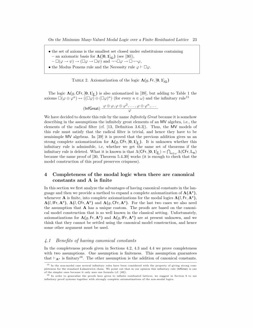
• the set of axioms is the smallest set closed under substituions containing– an axiomatic basis for Λ([0,1]G) (see [30]),– �(ϕ→ ψ)→ (�ϕ→ �ψ) and ¬¬�ϕ→ �¬¬ϕ,• the Modus Ponens rule and the Necessity rule ϕ ` �ϕ.
Table 2. Axiomatization of the logic Λ(g,Fr, [0,1]G)
The logic Λ(g,CFr, [0,1] L) is also axiomatized in [39], but adding to Table 1 theaxioms �(ϕ⊕ ϕn)↔ ((�ϕ)⊕ (�ϕ)n) (for every n ∈ ω) and the infinitary rule15
ϕ⊕ ϕ,ϕ⊕ ϕ2, . . . , ϕ⊕ ϕn, . . .(InfGreat) ϕ
We have decided to denote this rule by the name Infinitely Great because it is somehowdescribing in the assumptions the infinitely great elements of an MV algebra, i.e., theelements of the radical filter (cf. [13, Definition 3.6.3]). Thus, the MV models ofthis rule must satisfy that the radical filter is trivial, and hence they have to besemisimple MV algebras. In [39] it is proved that the previous addition gives us anstrong complete axiomatization for Λ(g,CFr, [0,1] L). It is unknown whether thisinfinitary rule is admissible, i.e, whether we get the same set of theorems if theinfinitary rule is deleted. What it is known is that Λ(CFr, [0,1] L) =
⋂n∈ω Λ(CFr, Ln)
because the same proof of [30, Theorem 5.4.30] works (it is enough to check that themodel construction of this proof preserves crispness).
4 Completeness of the modal logic when there are canonicalconstants and A is finite
In this section we first analyze the advantages of having canonical constants in the lan-guage and then we provide a method to expand a complete axiomatization of Λ(Ac),whenever A is finite, into complete axiomatizations for the modal logics Λ(l,Fr,Ac),Λ(l, IFr,Ac), Λ(l,CFr,Ac) and Λ(g,CFr,Ac). For the last two cases we also needthe assumption that A has a unique coatom. The proofs are based on the canoni-cal model construction that is so well known in the classical setting. Unfortunately,axiomatizations for Λ(g,Fr,Ac) and Λ(g, IFr,Ac) are at present unknown, and wethink that they cannot be settled using the canonical model construction, and hencesome other argument must be used.
4.1 Benefits of having canonical constants
In the completeness proofs given in Sections 4.2, 4.3 and 4.4 we prove completenesswith two assumptions. One assumption is finiteness. This assumption guaranteesthat `Ac is finitary16. The other assumption is the addition of canonical constants.
15 In the non-modal case several infinitary rules have been considered with the property of giving strong com-
pleteness for the standard Lukasiewicz chain. We point out that in our opinion this infinitary rule (InfGreat) is one
of the simpler ones because it only uses one formula (cf. [48]).16 In order to generalize the proofs here given to infinite residuated lattices, we suggest in Section 6 to use
infinitary proof systems together with strongly complete axiomatizations of the non-modal logics.
24 On the Minimum Many-Valued Modal Logic over a Finite Residuated Lattice
The addition of canonical constants, except for the Lukasiewicz case (see Remark 4.5and Section 5), seems really hard to overtake.
Of course, the main obvious benefit of having canonical constants in the languageis the increasing of expressive power because canonical constants allow us to expresscertain rules inside our formal language. For example, for every finite X ⊆ A the rule
((a1 → ϕ1)� . . .� (an → ϕn))→ (a→ ϕ) for every a1, . . . , an, a ∈ X(�ϕ1 � . . .��ϕn)→ �ϕ
is valid (cf. Corollary B.5) in the global consequence associated with any frame suchthat R only takes values inside X (i.e., R : W ×W −→ X). This rule gives us a wayto somehow rewrite Corollary B.5 using a rule that is closed under substitutions.
However, there are other benefits of having canonical constants that are more hid-den. Next we illustrate with two propositions17 the difference between having or notcanonical constants in the language. These propositions suggest that in the presenceof canonical constants the behaviour of a semantic modal valuation v is somehow de-termined by the set v−1[{1}] of formulas. This yields a different behaviour in modallogics, depending whether there are canonical constants or not, since by definition thelocal modal logic only takes into account those semantic modal valuations that sendthe involved formulas to 1.
We remark that the main advantage of the second representation in the next propo-sition is that the set {v2(ϕ) : ϕ ∈ Fm, v1(�ϕ) = 1} is closed under finite meets.
Proposition 4.1Let us assume that the canonical constants are in the modal language. If a ∈ A,and v1 and v2 are two semantic modal valuations, then the following statements areequivalent:
• a 6 ∧{v1(�ϕ)→ v2(ϕ) : ϕ ∈ Fm},• a 6 ∧{v2(ϕ) : ϕ ∈ Fm, v1(�ϕ) = 1}.
Proof. One direction is trivial. To prove the other, let us assume that a 6∧{v2(ϕ) :
ϕ ∈ Fm, v1(�ϕ) = 1} and let us consider a modal formula ϕ. We are left with thetask of checking that a 6 v1(�ϕ) → v2(ϕ). If we prove that v1(�ϕ) 6 a → v2(ϕ),the assertion follows. The proof is finished by showing18 that for every b ∈ A, ifb 6 v1(�ϕ) then b 6 a → v2(ϕ). For every b ∈ A, if b 6 v1(�ϕ) then 1 = b →v1(�ϕ) = v1(b → �ϕ) = v1(�(b → ϕ)); hence a 6 v2(b → ϕ) = b → v2(ϕ); and sob 6 a→ v2(ϕ).
Example 4.2It is not difficult to find counterexamples to the previous proposition in case that wedo not have canonical constants. For instance, let us consider the semantic modal
17 Another example of this different behaviour between having or not canonical constants can be obtained com-
paring the results in Section 4.3 with Lemma 5.10.18 This way of conducting the proof could seem tricky since we can simply consider b := v1(�ϕ) (this can be
done because we added one canonical constant for every element in A). However, the advantage of following this
tricky approach is that it also works as far as we only have canonical constants for a subset C satisfying for every
a ∈ A the condition a = sup{c ∈ C : c 6 a} = inf{c ∈ C : a 6 c}. This condition guarantees that the following
three statements are equivalent: (i) a 6 b, (ii) for every c ∈ C, if c 6 a then c 6 b, and (iii) for every c ∈ C, if b 6 cthen a 6 c. When we say that the proof also works for a subset C satisfying the previous condition we mean that
it is enough to replace “b ∈ A” with “b ∈ C” in the present proof to get a proof for the case that there are only
canonical constants for elements in C. In all future proofs we will also consider the same tricky way in order to be
as general as possible. It is worth pointing out that if A is the real unit interval [0, 1] then a subset C satisfying
this condition is the subset of its rational numbers.
On the Minimum Many-Valued Modal Logic over a Finite Residuated Lattice 25
valuations w0 and w1 given in the second diagram of Figure 1 over the MV chain L3 ofthree values (cf. [39, Lemma 5.4]). It is obvious that w1(ϕ) ∈ {0, 1} for every modalformula ϕ without canonical constants. Thus,
• 1 66 w0(�0)→ w1(0), while• 1 6 {w1(ϕ) : ϕ ∈ Fm,w0(�ϕ) = 1}. a
Proposition 4.3Let us assume that the canonical constants are in the modal language. If v1 and v2are two semantic modal valuations, then the following statements are equivalent:
• v1 = v2 (i.e., for every modal formula ϕ, it holds that v1(ϕ) = v2(ϕ)),• {ϕ ∈ Fm : v1(ϕ) = 1} = {ϕ ∈ Fm : v2(ϕ) = 1}.
Proof. For the non trivial implication, let us assume that {ϕ ∈ Fm : v1(ϕ) = 1} ={ϕ ∈ Fm : v2(ϕ) = 1} and let us consider a modal formula ϕ. We are left withthe task of checking that v1(ϕ) = v2(ϕ). By symmetry it is enough to prove thatv1(ϕ) 6 v2(ϕ). If we prove that for every b ∈ A, if b 6 v1(ϕ) then b 6 v2(ϕ),then the assertion follows. Let b be an element of A such that b 6 v1(ϕ). Then,1 = b→ v1(ϕ) = v1(b→ ϕ). This clearly forces 1 = v2(b→ ϕ) = b→ v2(ϕ). We thusget b 6 v2(ϕ).
Example 4.4Again it is easy to find counterexamples when there are no canonical constants. Forinstance, using that in non-modal interpretations over the standard Godel algebra[0,1]G the set of non-modal formulas evaluated to 1 depends only on the relativeordering (see [3, Remark 2.6] for details) it is easy to find a counterexample for[0,1]G. aRemark 4.5 ((Strongly) Characterizing formulas)A particular case where Proposition 4.3 holds even without canonical constants is thecase that A is a subalgebra of [0,1] L (i.e., A is a simple MV algebra). The reason whythis holds is that for every rational number α ∈ [0, 1] there is a non-modal formulaηα(p), from now on called the characterizing formula of the interval [α, 1], with onlyone variable such that for every a ∈ A, it holds that
ηAα (a) = 1 iff a ∈ [α, 1]. (4.1)
The existence of these formulas is an easy consequence of McNaughton’s Theorem(see [13, Theorem 9.1.5]). How can we use these formulas to prove Proposition 4.3?It suffices to realize19 that for every semantic modal valuation v over A and everymodal formula ϕ, it holds that v(ϕ) =
∨{α ∈ [0, 1] ∩ Q : α 6 v(ϕ)} =∨{α ∈
[0, 1] ∩ Q : ηAα (v(ϕ)) = 1} =
∨{α ∈ [0, 1] ∩ Q : v(ηα(ϕ)) = 1} =∨{α ∈ [0, 1] ∩ Q :
ηα(ϕ) ∈ v−1[{1}]}.In case that A is a finite subalgebra of [0,1] L (i.e., A is Ln for some n ∈ ω),
then every interval [α, 1], with α a rational number, also has a strongly characterizingformula ηα(p) in the sense that besides (4.1) it also holds that
A |= ηα(p) ∨ ¬ηα(p) ≈ 1. (4.2)
19 This idea was somehow noticed by Hansoul and Teheux in [39, Proposition 5.5].
26 On the Minimum Many-Valued Modal Logic over a Finite Residuated Lattice
• the set of axioms is the smallest set closed under substitutions containing– the axiomatic basis for Λ(Ac),– �1, (�ϕ ∧�ψ)→ �(ϕ ∧ ψ) and �(a→ ϕ)↔ (a→ �ϕ),• the rules of a basis for Λ(Ac) and the Monotonicity rule ϕ→ ψ ` �ϕ→ �ψ.
Table 3. Axiomatization of the set Λ(Fr,Ac) when A is finite
This last condition is simply saying that for every a ∈ A, it holds that ηAα (a) ∈ {0, 1}.
In other words, ηα(p) is a strongly characterizing formula of the interval [α, 1] iff ηAα
is the characteristic function of the interval [α, 1]. Of course, by continuity reasonsthere are no strongly characterizing formulas for the case [0,1] L. A weaker propertythan (4.2) but one that can be accomplished for the case [0,1] L is that the unarymap ηA
α is non decreasing. a
4.2 Completeness of Λ(l, Fr, Ac) when A is finite
The aim of this section is to prove that the axiomatization given in Table 3 is charac-terizing the set Λ(Fr,Ac) in case that A is finite. From this result we will be able togive an axiomatization for Λ(l,Fr,Ac). Throughout the rest of Section 4 we assumethat we have fixed an axiomatic (axioms and rules) basis for Λ(Ac). Indeed, therules in Table 3 include the axioms and rules of this axiomatic basis for Λ(Ac). It isobvious that all axioms and rules given in this table are sound (even in case that Ais infinite).
Definition 4.6 (cf. Table 3)A (many-valued) modal logic set over a residuated lattice Ac is any set L of modalformulas closed under substitutions such that
• L contains an axiomatic basis for Λ(Ac),• L contains the formulas of the form �1, (�ϕ∧�ψ)→ �(ϕ∧ψ) and �(a→ ϕ)↔
(a→ �ϕ),• L is closed under the rules of a basis for Λ(Ac),• L is closed under the rule (Mon).
L is said to be consistent in case that L is not the set of all formulas. aBy definition it is obvious that modal logic sets are closed under intersections.
Hence, there is a minimum modal logic set. The minimum modal logic set is exactlythe set described in Table 3. It is also clear that modal logic sets are closed under`Ac . From now on whenever we refer to `Ac (i.e., Λ(Ac)) we are considering allsubformulas starting with a � as propositional variables. Thus, by (2.8) it holds thatΓ `Ac ϕ iff for every non-modal homomorphism h from the algebra of modal formulasinto Ac, if h[Γ ] ⊆ {1} then h(ϕ) = 1. Using the closure under `Ac it is obvious thatL is closed under Modus Ponens, and also that L is consistent iff 0 6∈ L.Definition 4.7The canonical Kripke model Mc
can(L) associated with a consistent modal logic set Lis the Kripke model 〈W c
can, Rccan, V
ccan〉 where
On the Minimum Many-Valued Modal Logic over a Finite Residuated Lattice 27
• the set W ccan is the set20 of non-modal homomorphisms v : Fm −→ Ac (we point
out the language of the algebra of formulas includes the necessity modality) suchthat v[L] = {1},• the accessibility relation Rccan is defined by
Rccan(v1, v2) :=∧{v1(�ϕ)→ v2(ϕ) : ϕ ∈ Fm},
• the evaluation map is defined by V ccan(p, v) := v(p) for every variable p. a
In the previous definition the superscript refers to the fact that there are canonicalconstants. We notice that it is the consistency of L what implies that the set W c
can
just defined is non empty. This is so because 0 6∈ L, and hence L 6`Ac 0, what givesa non-modal homomorphism h from the set of modal formulas into Ac such thath[L] = {1}.
By the same argument that was given for Proposition 4.1 we can prove thatRccan(v1, v2) =
∧{v2(ϕ) : ϕ ∈ Fm, v1(�ϕ) = 1}. Using that this last set is closedunder finite meets we get that, since A is finite,
Rccan(v1, v2) = min{v2(ϕ) : ϕ ∈ Fm, v1(�ϕ) = 1}. (4.3)
The proof of the following Truth Lemma could be simplified using this last equality,but we prefer to avoid its use in order to give a proof that can be adopted in the nextsection where we do not have canonical constants in the language. We also remarkthat the intuition behind the first claim inside the proof of Truth Lemma is given bythe rule (OrdPres∗) where the new variable r is instantiated by every element of theresiduated lattice.
Lemma 4.8 (Truth Lemma)Let L be a consistent modal logic set over a finite residuated lattice Ac. The canonicalKripke model Mc
can(L) satisfies V ccan(ϕ, v) = v(ϕ) for every formula ϕ and every worldv.
Proof. The proof is done by induction on the formula. The only non trivial case iswhen this formula starts with a �. Let v be a world of the canonical Kripke model.We have to prove that V ccan(�ϕ, v) = v(�ϕ) under the induction hypothesis thatV ccan(ϕ, v′) = v′(ϕ) for every world v′. Hence, it suffices to prove that
∧{Rccan(v, v′)→ v′(ϕ) : v′ ∈W c
can} = v(�ϕ).
The fact that the inequality > holds is a trivial consequence of the definition of theaccessibility relation Rccan. In order to check the other inequality we will prove thatfor every a ∈ A, if a 6
∧{Rccan(v, v′) → v′(ϕ) : v′ ∈ W ccan} then a 6 v(�ϕ). Thus,
let us consider an element a such that a 6∧{Rccan(v, v′) → v′(ϕ) : v′ ∈ W c
can}, i.e.,Rccan(v, v′) 6 a→ v′(ϕ) for every world v′.
20 Another way to present the points of the canonical model is to define the elements of Wccan as the sets Σ of
modal formulas (including canonical constants) that are closed under `Ac and such that for every modal formula ϕ
there is a unique element a ∈ A such that a↔ ϕ ∈ Σ. It is clear that there is a 1-to-1 correspondence h 7−→ h−1[{1}between both presentations of points in the canonical model. The advantage of the presentation we have taken is
that it trivially generalizes to the case that there are no canonical constants in the language.
28 On the Minimum Many-Valued Modal Logic over a Finite Residuated Lattice
Claim 4.9For every element b ∈ A, it holds that
L ∪ {b→ (d→ ψ) : ψ ∈ Fm, d ∈ A, d 6 v(�ψ)} `AC b→ (a→ ϕ).
Proof of Claim. To prove this claim we take a non-modal homomorphism h thatsends all hypothesis to 1. Hence, for every formula ψ and every element d ∈ A,if d 6 v(�ψ) then d 6 b → h(ψ). That is, for every formula ψ, it holds thatv(�ψ) 6 b→ h(ψ). Hence, b 6
∧{v(�ψ)→ h(ψ) : ψ ∈ Fm}. Using that h is a pointof the canonical Kripke model, we get from the previous inequality that b 6 Rccan(v, h).By the assumed property of the element a it follows that b 6 a → h(ϕ). Hence,h(b→ (a→ ϕ)) = 1. q.e.d. (Claim)
Claim 4.10There is an m ∈ ω, formulas ψ1, . . . , ψm and elements d1, . . . , dm such that di 6v(�ψi) for every i ∈ {1, . . . ,m} and
L `Ac (∧
16i6m(di → ψi))→ (a→ ϕ).
Proof of Claim. Using that A is finite, and so `Ac is finitary, it is obvious by theprevious claim that for every b ∈ A there is an mb ∈ ω, formulas ψb1, . . . , ψ
bmb
and ele-ments db1, . . . , d
bmb
such that (i) dbi 6 v(�ψbi ) for every i ∈ {1, . . . ,mb}, and (ii) L∪{b→(dbi → ψbi ) : 1 6 i 6 mb} `AC b → (a → ϕ). Let us assume that A = {b1, . . . , bn}.Considering the finite sequence ψb11 , . . . , ψ
b1mb1
, ψb21 , . . . , ψb2mb2
, . . . , ψbn1 , . . . , ψbn
mbnof for-
mulas, and the finite sequence db11 , . . . , db1mb1
, db21 , . . . , db2mb2
, . . . , dbn1 , . . . , dbn
mbnof ele-
ments we get that there is an m ∈ ω, formulas ψ1, . . . , ψm and elements d1, . . . , dmsuch that (i) di 6 v(�ψi) for every i ∈ {1, . . . ,m}, and (ii) for every element b ∈ A itholds that
L ∪ {b→ (di → ψi) : 1 6 i 6 m} `AC b→ (a→ ϕ).
Now we prove that these formulas and elements satisfy the desired property statedin the claim. To prove this we consider a non-modal homomorphism h such thath[L] = {1}. The fact that h((
∧16i6m(di → ψi)) → (a → ϕ)) = 1 follows from the
property (ii) taking b as h(∧
16i6m(di → ψi)). q.e.d. (Claim)Using21 that L is closed under `Ac , we get that ((d1 → ψ1) ∧ . . . ∧ (dm → ψm))→
(a→ ϕ) belongs to L. Therefore, �((d1 → ψ1) ∧ . . . ∧ (dm → ψm))→ �(a→ ϕ) ∈ Lby the Monotonicity rule. Thus, (�(d1 → ψ1)∧ . . .∧�(dm → ψm))→ �(a→ ϕ) ∈ Lby the meet distributivity axiom. And so, by the fact that L is a modal logic set weget that ((d1 → �ψ1) ∧ . . . ∧ (dm → �ψm))→ (a→ �ϕ) belongs to L. Finally, usingthat v(((d1 → �ψ1)∧ . . .∧ (dm → �ψm))→ (a→ �ϕ)) = 1→ (a→ v(�ϕ)) and thatv[L] = {1} we obtain that a→ v(�ϕ) = 1, i.e., a 6 v(�ϕ). This finishes the proof.
Now we can easily prove that the set Λ(Fr,Ac) is the one axiomatized in Table 3,and also give a presentation of Λ(l,Fr,Ac). We point out that we do not know ifΛ(g,Fr,Ac) is precisely the consequence relation given by Table 3.
21 It is worth pointing out that up to now we have only used in this proof the definition of Rccan. In other words,
we have not used any of the properties encapsulated in the fact that L is a modal logic set. This will allow us to use
the same proof until the previous second claim for the case that we do not have canonical constants in the language
(see the proof of Lemma 5.6).
On the Minimum Many-Valued Modal Logic over a Finite Residuated Lattice 29
Theorem 4.11 (Axiomatization of Λ(l,Fr,Ac))Let L be the smallest modal logic set over a finite residuated lattice Ac. Then,
1. v is a semantic modal valuation iff v is a point of Mccan(L).
2. Γ `lFr(Ac) ϕ iff L ∪ Γ `Ac ϕ, for every set Γ ∪ {ϕ} of formulas.
3. L = Λ(Fr,Ac).4. Λ(l,Fr,Ac) is axiomatized by (i) L as a set of axioms, and (ii) the rules of the basis
for Λ(Ac).
Proof. 1): This first statement is a trivial consequence of the Truth Lemma.2): It is clear that we have the following chain of equivalences
• L ∪ Γ `Ac ϕ, iff• for every non-modal homomorphism h : Fm −→ Ac, if h[L] = {1} and h[Γ ] ⊆ {1}
then h(ϕ) = 1, iff• for every v ∈W c
can, if v[Γ ] ⊆ {1} then v(ϕ) = 1, iff• for every semantic modal valuation v, if v[Γ ] ⊆ {1} then v(ϕ) = 1, iff• Γ `lFr(Ac) ϕ.
3): This is a consequence of the previous item.4): This is again a consequence of the second item.
4.3 Completeness of Λ(l, IFr, Ac) when A is finite
The purpose of this section is to prove that Λ(IFr,Ac), whenever A is a finite residu-ated lattice, is the smallest modal logic set over Ac that contains at least one of thefollowing three kinds of formula (schema)
�(ϕ→ ψ)→ (�ϕ→ �ψ) (�ϕ��ψ)→ �(ϕ� ψ) (�ϕ��ϕ)→ �(ϕ� ϕ)
We remark that the first formula is (K) and that in Proposition 3.12 we proved thateach of them characterizes IFr. We will see that if any of these three formulas is ina modal logic set then all of them also belong to it. We will start studying the caseof the last of these formulas (it seems the weakest one), and later we will show theconnection between the three formulas.
Lemma 4.12Let L be the smallest modal logic set over a finite residuated lattice Ac containing(�ϕ��ϕ)→ �(ϕ� ϕ). Then, the frame of Mc
can(L) is an idempotent frame.
Proof. Let a be Rccan(v1, v2) for some points v1 and v2 of the canonical Kripke model.By (4.3) we know that there is a formula ϕ such that v1(�ϕ) = 1 and v2(ϕ) = a.Then, v1(�ϕ � �ϕ) = 1 � 1 = 1. Using that (�ϕ � �ϕ) → �(ϕ � ϕ) ∈ L weget that 1 = v1(�(ϕ � ϕ)). On the other hand, by the Truth Lemma we knowthat v1(�(ϕ � ϕ)) 6 Rccan(v1, v2) → (v2(ϕ) � v2(ϕ)) = a → (a � a). Therefore,1 6 a→ (a� a), i.e., a = a� a.
Theorem 4.13 (Axiomatization of Λ(l, IFr,Ac))Let L be the smallest modal logic set over a finite residuated lattice Ac containing(�ϕ��ϕ)→ �(ϕ� ϕ). Then,
30 On the Minimum Many-Valued Modal Logic over a Finite Residuated Lattice
1. v is a semantic modal valuation arising from an idempotent frame iff v is a pointof Mc
can(L).2. Γ `lIFr(Ac) ϕ iff L ∪ Γ `Ac ϕ, for every set Γ ∪ {ϕ} of formulas.
3. L = Λ(IFr,Ac).4. Λ(l, IFr,Ac) is axiomatized by (i) L as a set of axioms, and (ii) the rules of a basis
for Λ(Ac).
Proof. The proof is analogous to the one given for Theorem 4.11 (but now usingLemma 4.12).
Corollary 4.14Let L be a modal logic set over a finite residuated lattice Ac. Then,
1. �(ϕ→ ψ)→ (�ϕ→ �ψ) ∈ L, iff2. (�ϕ��ψ)→ �(ϕ� ψ) ∈ L, iff3. (�ϕ��ϕ)→ �(ϕ� ϕ) ∈ L.
Proof. 1 ⇒ 2): Applying two times the axiom (K) to the fact that ϕ → (ψ →(ϕ � ψ)) ∈ L we get that �ϕ → (�ψ → �(ϕ � ψ)) ∈ L. Therefore, (�ϕ � �ψ) →�(ϕ� ψ) ∈ L.
2⇒ 3): This is trivial.3⇒ 1): Let L′ be the smallest modal logic set containing (�ϕ��ϕ)→ �(ϕ�ϕ). It
suffices to prove that �(ϕ→ ψ)→ (�ϕ→ �ψ) ∈ L′, but this is a trivial consequenceof L′ = Λ(IFr,Ac) (see Theorem 4.13) together with Proposition 3.10.
Remark 4.15 (Idempotent Canonical Kripke model)There is an alternative way to prove the results given in this Section 4.3. This othermethod consists on introducing an idempotent canonical Kripke model Mc
ican(L) as inDefinition 4.7 except for the accessibility relation where we take the largest idempo-tent below
∧{v1(�ϕ) → v2(ϕ) : ϕ ∈ Fm}. This idempotent always exists becauseidempotent elements are closed under arbitrary joins. Then, the same strategy thanin the proof of Lemma 4.8 allows us to conclude the Truth Lemma, but this timethe two intermediate claims are (i) for every idempotent element b ∈ A, it holds thatL ∪ {b → (d → ψ) : ψ ∈ Fm, d ∈ A, d 6 v(�ψ)} `AC b → (a → ϕ) , and (ii) thereis an m ∈ ω, formulas ψ1, . . . , ψm and elements d1, . . . , dm such that di 6 v(�ψi) forevery i ∈ {1, . . . ,m} and L `Ac ((d1 → ψ1) ∧ . . . ∧ (dm → ψm))n → (a → ϕ) wheren is the cardinal of A. We have not adopted this method in this section because itwas not necessary, but in the next section we will have to consider a similar methodin order to get completeness for the class of crisp frames. a
4.4 Completeness of Λ(l, CFr, Ac) and Λ(g, CFr, Ac) when A is finiteand has a unique coatom
We have been looking for an axiomatization of Λ(l,CFr,Ac) and Λ(g,CFr,Ac) incase that A is finite, but we have only succeeded when A has a unique coatom k. Inthis section we present the solution to this problem. The main difficulty to generalizeour proof to the general case is that we need a method to reduce the consequencerelation `Ac to its set of theorems, and we only know how to do it when there is a
On the Minimum Many-Valued Modal Logic over a Finite Residuated Lattice 31
• the set of axioms is the smallest set closed under substitutions containing– the axiomatic basis for Λ(Ac),– �1, (�ϕ∧�ψ)→ �(ϕ∧ ψ), �(a→ ϕ)↔ (a→ �ϕ) and �(k ∨ϕ)→ (k ∨�ϕ),• the rules are
– those of the basis for Λ(Ac),– the Monotonicity rule ϕ→ ψ ` �ϕ→ �ψ.
Table 4: Axiomatization of Λ(g,CFr,Ac) when A is finite and k is its unique coatom
unique coatom k. For this particular case we know that this can be done using thetrivial equivalence
γ1, . . . , γn `Ac ϕ iff `Ac (γ1 ∧ . . . ∧ γn)→ (ϕ ∨ k), (4.4)
For the rest of this section we assume that A has a unique coatom (i.e., penultimateelement) k. Under this assumption it is obvious that the only Boolean elementsin A are the trivial ones 0 and 1; so indeed BFr = CFr. We already know that�(k ∨ ϕ) → (k ∨ �ϕ) ∈ Λ(CFr,Ac). In this section we will prove that Λ(CFr,Ac) isprecisely the smallest modal logic set L such that �(k ∨ ϕ)→ (k ∨�ϕ) ∈ L.
Definition 4.16 (cf. Table 4)A crisp (many-valued) modal logic set over Ac (where k is its unique coatom) is anymodal logic set over Ac such that L contains the formulas of the form �(k ∨ ϕ) →(k ∨�ϕ).
Thus, the statement claimed above can be rewritten as saying that Λ(CFr,Ac) isthe smallest crisp modal logic set. A first idea to prove this statement is to show thatthe frame of Mc
can(L), where L is the smallest crisp modal logic set, is a crisp frame.Unfortunately this method does not work in general as the following propositionpoints out. It is worth stressing that, as a consequence of Theorem 4.22, we couldreplace in this proposition the set L with Λ(CFr,Ac).
Proposition 4.17Let A be the ordinal sum A1 ⊕A2 of two finite MTL chains such that A1 and A2
are non trivial (i.e., min{|A1|, |A2|} > 2). And let L be the smallest crisp modal logicset over Ac. Then, the frame of Mc
can(L) is not crisp.
Proof. Let us consider a ∈ A as the idempotent element separating the componentsA1 and A2. Since A1 and A2 are non trivial it is obvious that a 6∈ {0A, 1A}, and alsothat for every b ∈ A, a�b = a∧b. Let w0, w1 and w2 be the semantic modal valuationsgiven in Figure 3. Next we are going to see that these three valuations belong to thecorresponding canonical Kripke model (i.e., wi[L] = {1}) and that Rccan(w0, w2) = a.This is enough in order to conclude that Mc
can(L) is not crisp.In order to prove that Rccan(w0, w2) = a we have to check that a =
∧{w0(�ϕ) →w1(ϕ) : ϕ ∈ Fm}. This is trivial because a = R(w0, w2) 6
∧{w0(�ϕ)→ w2(ϕ) : ϕ ∈Fm} 6 w0(�p)→ w2(p) = 1→ a = a.
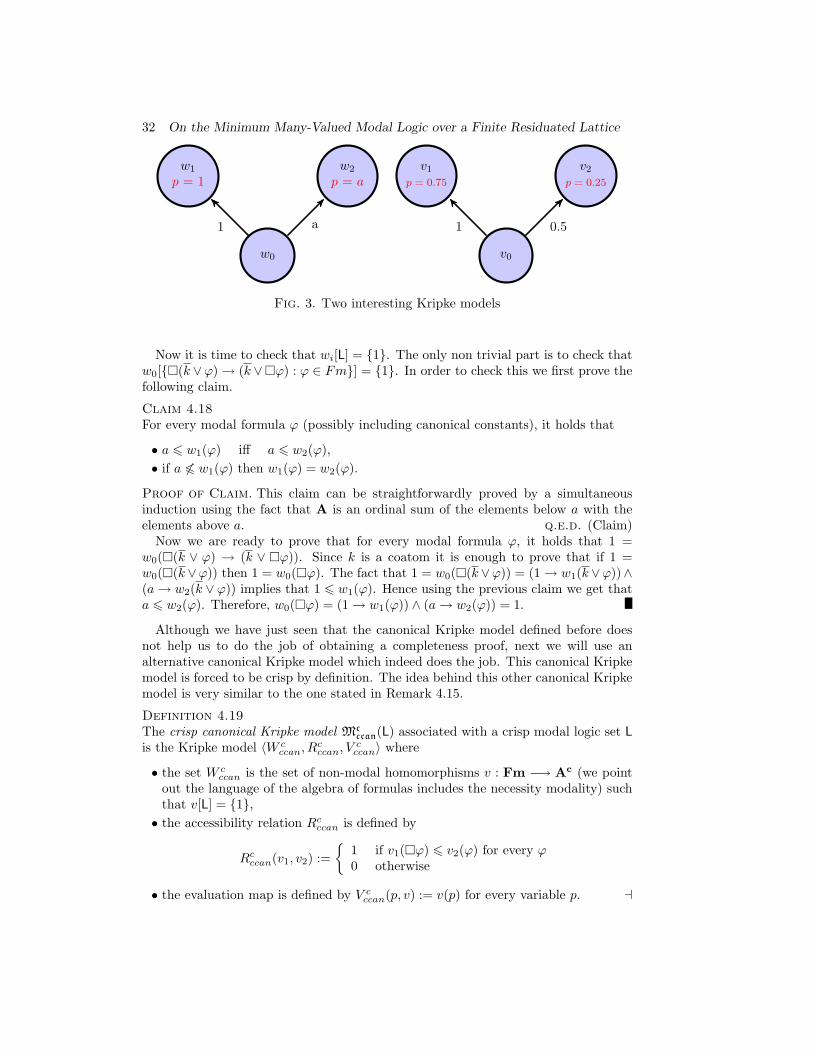
32 On the Minimum Many-Valued Modal Logic over a Finite Residuated Lattice
w0
w1
p = 1w2
p = a
1 a
v0
v1p = 0.75
v2p = 0.25
1 0.5
Fig. 3. Two interesting Kripke models
Now it is time to check that wi[L] = {1}. The only non trivial part is to check thatw0[{�(k ∨ϕ)→ (k ∨�ϕ) : ϕ ∈ Fm}] = {1}. In order to check this we first prove thefollowing claim.
Claim 4.18For every modal formula ϕ (possibly including canonical constants), it holds that
• a 6 w1(ϕ) iff a 6 w2(ϕ),• if a 66 w1(ϕ) then w1(ϕ) = w2(ϕ).
Proof of Claim. This claim can be straightforwardly proved by a simultaneousinduction using the fact that A is an ordinal sum of the elements below a with theelements above a. q.e.d. (Claim)
Now we are ready to prove that for every modal formula ϕ, it holds that 1 =w0(�(k ∨ ϕ) → (k ∨ �ϕ)). Since k is a coatom it is enough to prove that if 1 =w0(�(k∨ϕ)) then 1 = w0(�ϕ). The fact that 1 = w0(�(k∨ϕ)) = (1→ w1(k∨ϕ))∧(a→ w2(k ∨ ϕ)) implies that 1 6 w1(ϕ). Hence using the previous claim we get thata 6 w2(ϕ). Therefore, w0(�ϕ) = (1→ w1(ϕ)) ∧ (a→ w2(ϕ)) = 1.
Although we have just seen that the canonical Kripke model defined before doesnot help us to do the job of obtaining a completeness proof, next we will use analternative canonical Kripke model which indeed does the job. This canonical Kripkemodel is forced to be crisp by definition. The idea behind this other canonical Kripkemodel is very similar to the one stated in Remark 4.15.
Definition 4.19The crisp canonical Kripke model Mc
ccan(L) associated with a crisp modal logic set Lis the Kripke model 〈W c
ccan, Rcccan, V
cccan〉 where
• the set W cccan is the set of non-modal homomorphisms v : Fm −→ Ac (we point
out the language of the algebra of formulas includes the necessity modality) suchthat v[L] = {1},• the accessibility relation Rcccan is defined by
Rcccan(v1, v2) :={
1 if v1(�ϕ) 6 v2(ϕ) for every ϕ0 otherwise
• the evaluation map is defined by V cccan(p, v) := v(p) for every variable p. a
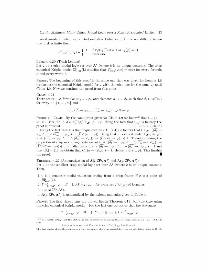
On the Minimum Many-Valued Modal Logic over a Finite Residuated Lattice 33
Analogously to what we pointed out after Definition 4.7 it is not difficult to seethat if A is finite then
Rcccan(v1, v2) ={
1 if ∀ϕ(v1(�ϕ) = 1⇒ v2(ϕ) = 1)0 otherwise
Lemma 4.20 (Truth Lemma)Let L be a crisp modal logic set over Ac (where k is its unique coatom). The crispcanonical Kripke model Mc
ccan(L) satisfies that V cccan(ϕ, v) = v(ϕ) for every formulaϕ and every world v.
Proof. The beginning of this proof is the same one that was given for Lemma 4.8(replacing the canonical Kripke model for L with the crisp one for the same L) untilClaim 4.9. Now we continue the proof from this point.
Claim 4.21There are m ∈ ω, formulas ψ1, . . . , ψm and elements d1, . . . , dm such that di 6 v(�ψi)for every i ∈ {1, . . . ,m} and
L ∪ {d1 → ψ1, . . . , dm → ψm} `Ac a→ ϕ.
Proof of Claim. By the same proof given for Claim 4.9 we know22 that L ∪ {d →ψ : ψ ∈ Fm, d ∈ A, d 6 v(�ψ)} `AC a → ϕ. Using the fact that `Ac is finitary theproof is finished. q.e.d. (Claim)
Using the fact that k is the unique coatom (cf. (4.4)) it follows that L `AC ((d1 →ψ1) ∧ . . . ∧ (dm → ψm)) → (k ∨ (a → ϕ)). Using that L is closed under `Ac , we getthat ((d1 → ψ1) ∧ . . . ∧ (dm → ψm)) → (k ∨ (a → ϕ)) ∈ L. Therefore, using theproperties of crisp modal logic sets we get that ((d1 → �ψ1)∧ . . .∧ (dm → �ψm))→(k ∨ (a→ �ϕ)) ∈ L. Finally, using that v((d1 → �ψ1) ∧ . . . ∧ (dm → �ψm)) = 1 andthat v[L] = {1} we obtain that k∨ (a→ v(�ϕ)) = 1. Hence, a 6 v(�ϕ). This finishesthe proof.
Theorem 4.22 (Axiomatization of Λ(l,CFr,Ac) and Λ(g,CFr,Ac))Let L be the smallest crisp modal logic set over Ac (where k is its unique coatom).Then,
1. v is a semantic modal valuation arising from a crisp frame iff v is a point ofMc
ccan(L).2. Γ `lCFr(Ac) ϕ iff L ∪ Γ `Ac ϕ, for every set Γ ∪ {ϕ} of formulas.
3. L = Λ(CFr,Ac).4. Λ(g,CFr,Ac) is axiomatized by the axioms and rules given in Table 4.
Proof. The first three items are proved like in Theorem 4.11 (but this time usingthe crisp canonical Kripke model). For the last one we notice that the statement
Γ `gCFr(Ac) ϕ iff {�nγ : n ∈ ω, γ ∈ Γ} `lCFr(Ac) ϕ
22 It is worth noting that this statement can be rewritten as saying that for every element b ∈ {0, 1}, it holds
that
L ∪ {b→ (d→ ψ) : ψ ∈ Fm, d ∈ A, d 6 v(�ψ)} `Ac b→ (a→ ϕ).
This last version shows the connection with crisp frames where the accessibility relation only takes values in {0, 1}.
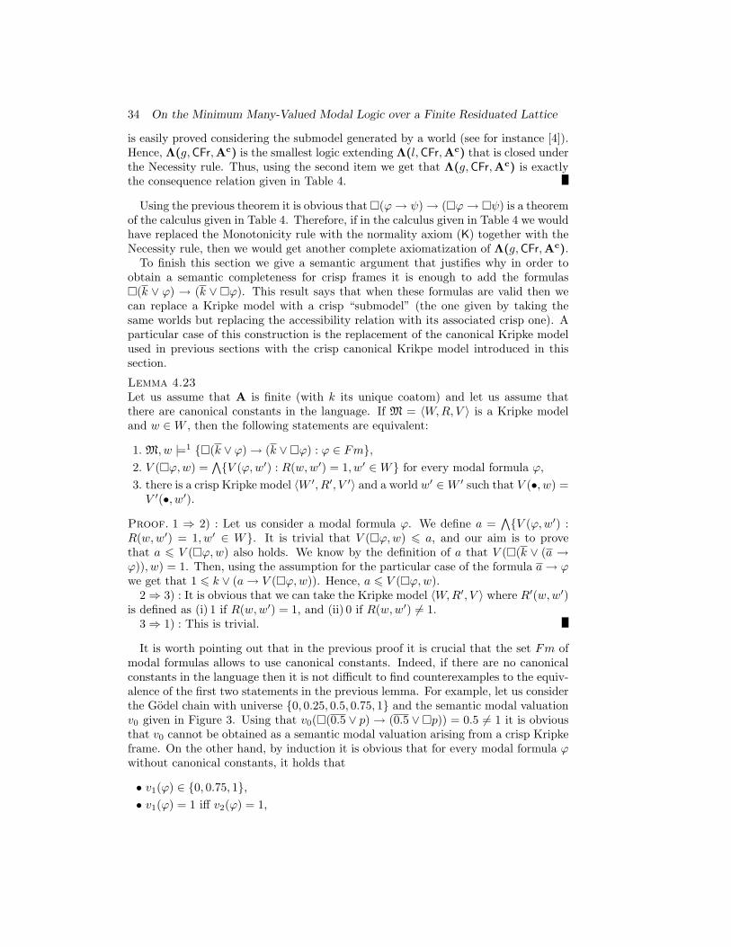
34 On the Minimum Many-Valued Modal Logic over a Finite Residuated Lattice
is easily proved considering the submodel generated by a world (see for instance [4]).Hence, Λ(g,CFr,Ac) is the smallest logic extending Λ(l,CFr,Ac) that is closed underthe Necessity rule. Thus, using the second item we get that Λ(g,CFr,Ac) is exactlythe consequence relation given in Table 4.
Using the previous theorem it is obvious that�(ϕ→ ψ)→ (�ϕ→ �ψ) is a theoremof the calculus given in Table 4. Therefore, if in the calculus given in Table 4 we wouldhave replaced the Monotonicity rule with the normality axiom (K) together with theNecessity rule, then we would get another complete axiomatization of Λ(g,CFr,Ac).
To finish this section we give a semantic argument that justifies why in order toobtain a semantic completeness for crisp frames it is enough to add the formulas�(k ∨ ϕ) → (k ∨ �ϕ). This result says that when these formulas are valid then wecan replace a Kripke model with a crisp “submodel” (the one given by taking thesame worlds but replacing the accessibility relation with its associated crisp one). Aparticular case of this construction is the replacement of the canonical Kripke modelused in previous sections with the crisp canonical Krikpe model introduced in thissection.
Lemma 4.23Let us assume that A is finite (with k its unique coatom) and let us assume thatthere are canonical constants in the language. If M = 〈W,R, V 〉 is a Kripke modeland w ∈W , then the following statements are equivalent:
1. M, w |=1 {�(k ∨ ϕ)→ (k ∨�ϕ) : ϕ ∈ Fm},2. V (�ϕ,w) =
∧{V (ϕ,w′) : R(w,w′) = 1, w′ ∈W} for every modal formula ϕ,3. there is a crisp Kripke model 〈W ′, R′, V ′〉 and a world w′ ∈W ′ such that V (•, w) =V ′(•, w′).
Proof. 1 ⇒ 2) : Let us consider a modal formula ϕ. We define a =∧{V (ϕ,w′) :
R(w,w′) = 1, w′ ∈ W}. It is trivial that V (�ϕ,w) 6 a, and our aim is to provethat a 6 V (�ϕ,w) also holds. We know by the definition of a that V (�(k ∨ (a →ϕ)), w) = 1. Then, using the assumption for the particular case of the formula a→ ϕwe get that 1 6 k ∨ (a→ V (�ϕ,w)). Hence, a 6 V (�ϕ,w).
2⇒ 3) : It is obvious that we can take the Kripke model 〈W,R′, V 〉 where R′(w,w′)is defined as (i) 1 if R(w,w′) = 1, and (ii) 0 if R(w,w′) 6= 1.
3⇒ 1) : This is trivial.
It is worth pointing out that in the previous proof it is crucial that the set Fm ofmodal formulas allows to use canonical constants. Indeed, if there are no canonicalconstants in the language then it is not difficult to find counterexamples to the equiv-alence of the first two statements in the previous lemma. For example, let us considerthe Godel chain with universe {0, 0.25, 0.5, 0.75, 1} and the semantic modal valuationv0 given in Figure 3. Using that v0(�(0.5 ∨ p) → (0.5 ∨�p)) = 0.5 6= 1 it is obviousthat v0 cannot be obtained as a semantic modal valuation arising from a crisp Kripkeframe. On the other hand, by induction it is obvious that for every modal formula ϕwithout canonical constants, it holds that
• v1(ϕ) ∈ {0, 0.75, 1},• v1(ϕ) = 1 iff v2(ϕ) = 1,
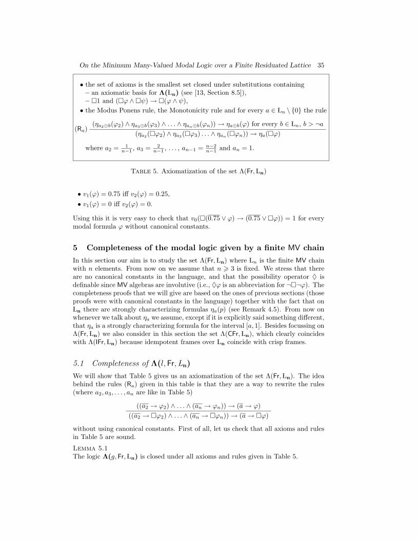
On the Minimum Many-Valued Modal Logic over a Finite Residuated Lattice 35
• the set of axioms is the smallest set closed under substitutions containing– an axiomatic basis for Λ( Ln) (see [13, Section 8.5]),– �1 and (�ϕ ∧�ψ)→ �(ϕ ∧ ψ),• the Modus Ponens rule, the Monotonicity rule and for every a ∈ Ln \ {0} the rule
(ηa2�b(ϕ2) ∧ ηa3�b(ϕ3) ∧ . . . ∧ ηan�b(ϕn))→ ηa�b(ϕ) for every b ∈ Ln, b > ¬a(Ra)
(ηa2(�ϕ2) ∧ ηa3(�ϕ3) . . . ∧ ηan(�ϕn))→ ηa(�ϕ)
where a2 = 1n−1 , a3 = 2
n−1 , . . . , an−1 = n−2n−1 and an = 1.
Table 5. Axiomatization of the set Λ(Fr, Ln)
• v1(ϕ) = 0.75 iff v2(ϕ) = 0.25,• v1(ϕ) = 0 iff v2(ϕ) = 0.
Using this it is very easy to check that v0(�(0.75 ∨ ϕ) → (0.75 ∨�ϕ)) = 1 for everymodal formula ϕ without canonical constants.
5 Completeness of the modal logic given by a finite MV chain
In this section our aim is to study the set Λ(Fr, Ln) where Ln is the finite MV chainwith n elements. From now on we assume that n > 3 is fixed. We stress that thereare no canonical constants in the language, and that the possibility operator ♦ isdefinable since MV algebras are involutive (i.e., ♦ϕ is an abbreviation for ¬�¬ϕ). Thecompleteness proofs that we will give are based on the ones of previous sections (thoseproofs were with canonical constants in the language) together with the fact that on Ln there are strongly characterizing formulas ηa(p) (see Remark 4.5). From now onwhenever we talk about ηa we assume, except if it is explicitly said something different,that ηa is a strongly characterizing formula for the interval [a, 1]. Besides focussing onΛ(Fr, Ln) we also consider in this section the set Λ(CFr, Ln), which clearly coincideswith Λ(IFr, Ln) because idempotent frames over Ln coincide with crisp frames.
5.1 Completeness of Λ(l, Fr, Ln)
We will show that Table 5 gives us an axiomatization of the set Λ(Fr, Ln). The ideabehind the rules (Ra) given in this table is that they are a way to rewrite the rules(where a2, a3, . . . , an are like in Table 5)
((a2 → ϕ2) ∧ . . . ∧ (an → ϕn))→ (a→ ϕ)((a2 → �ϕ2) ∧ . . . ∧ (an → �ϕn))→ (a→ �ϕ)
without using canonical constants. First of all, let us check that all axioms and rulesin Table 5 are sound.
Lemma 5.1The logic Λ(g,Fr, Ln) is closed under all axioms and rules given in Table 5.
36 On the Minimum Many-Valued Modal Logic over a Finite Residuated Lattice
Proof. It suffices to prove that it is closed under the rules (Ra). To see this, leta ∈ A and let V be a valuation from a Kripke model. We assume that V ((ηa2�b(ϕ2)∧ηa3�b(ϕ3) ∧ . . . ∧ ηan�b(ϕn))→ ηa�b(ϕ), w) = 1 for every world w and every b > ¬a.We have to prove that V ((ηa2(�ϕ2)∧ηa3(�ϕ3) . . .∧ηan
(�ϕn))→ ηa(�ϕ), w) = 1 foran arbitrary world w. Using that the formulas η are strongly characterizing it sufficesto prove that if V (ηai(�ϕi), w) = 1 for every i ∈ {2, . . . , n}, then V (ηa(�ϕ), w) = 1.That is, we have to prove that if ai 6 V (�ϕi, w) for every i ∈ {2, . . . , n}, thena 6 V (�ϕ,w). Hence, let us assume that ai 6 V (�ϕi, w) for every i ∈ {2, . . . , n}.We must prove that a 6 V (�ϕ,w), i.e., that a 6 R(w,w′) → V (ϕ,w′) for everyworld w′. Thus, we consider a world w′ and we define b := R(w,w′). If b 6 ¬a thenit is obvious that a 6 b → 0 6 R(w,w′) → V (ϕ,w′). Let us now consider the casethat b > ¬a. The fact that ai 6 V (�ϕi, w) tells us that ai � b 6 V (ϕi, w′) for everyi ∈ {2, . . . , n}. Therefore, V (ηai�b(ϕi), w
′) = 1 for every i ∈ {2, . . . , n}. Using theassumption about the upper part of the rule (Ra) we get that V (ηa�b(ϕ), w′) = 1.Thus, a 6 b→ V (ϕ,w′) = R(w,w′)→ V (ϕ,w′). This finishes the proof.
Before giving the proof based on the canonical model construction, as a matter ofexample next we analyze in detail the rules in Table 5 for the case of the MV chainwith three points.
Example 5.2 (Case of L3)For n = 3 the rules (Ra) considered are
(η0.5(ϕ2) ∧ η1(ϕ3))→ η0.5(ϕ)(R0.5)
(η0.5(�ϕ2) ∧ η1(�ϕ3))→ η0.5(�ϕ)
(η0(ϕ2) ∧ η0.5(ϕ3))→ η0.5(ϕ) (η0.5(ϕ2) ∧ η1(ϕ3))→ η1(ϕ)(R1)
(η0.5(�ϕ2) ∧ η1(�ϕ3))→ η1(�ϕ)
Using that η0(p) := 1, η0.5(p) := p ⊕ p and η1(p) := p � p, we get that the previousrules can be rewritten as
((ϕ2 ⊕ ϕ2) ∧ (ϕ3 � ϕ3))→ (ϕ⊕ ϕ)(R0.5)
((�ϕ2 ⊕�ϕ2) ∧ (�ϕ3 ��ϕ3))→ (�ϕ⊕�ϕ)
(1 ∧ (ϕ3 ⊕ ϕ3))→ (ϕ⊕ ϕ) ((ϕ2 ⊕ ϕ2) ∧ (ϕ3 � ϕ3))→ (ϕ� ϕ)(R1)
((�ϕ2 ⊕�ϕ2) ∧ (�ϕ3 ��ϕ3))→ (�ϕ��ϕ)
Some theorems that can be obtained using rule (R0.5) are
((�p⊕�p) ∧ (�q ��q))→ (�(p� q)⊕�(p� q))
((�p⊕�p) ∧ (�(q ⊕ q ⊕ (¬p� ¬p))��(q ⊕ q ⊕ (¬p� ¬p))))→ (�q ⊕�q)((�(q ⊕ ¬p)⊕�(q ⊕ ¬p)) ∧ (�p��p))→ (�q ⊕�q)((�1⊕�1) ∧ (�1��1))→ (�(p ∨ ¬p)⊕�(p ∨ ¬p)),
and some theorems using rule (R1) are
((�0⊕�0) ∧ (�1��1))→ (�(p ∨ ¬p)��(p ∨ ¬p))
((�(p� p)⊕�(p� p)) ∧ (�(p⊕ p)��(p⊕ p)))→ (�p��p)
On the Minimum Many-Valued Modal Logic over a Finite Residuated Lattice 37
((�p⊕�p) ∧ (�(p ∨ ¬p)��(p ∨ ¬p)))→ (�(p ∨ q ∨ ¬q)��(p ∨ q ∨ ¬q)).Using standard matrix arguments it is possible to prove that the rules (R0.5) and (R1)are independent of all the other axioms and rules in Table 5. For example, the matrix〈 L3 × L2,�, {(1, 1)}〉 where
�x :={
(0, 0), if π1(x) = 0 (i.e., x ∈ {(0, 0), (0, 1)})(1, 1), if π1(x) 6= 0
is a model of all axioms and rules except23 for (R0.5). And the matrix 〈 L3× L2,�′, {(1, 1)}〉where
�′x :={
(0.5, 1), if π1(x) 6= 1(1, 1), if π1(x) = 1 (i.e., x ∈ {(1, 0), (1, 1)})
is a model of all axioms and rules except24 for (R1). aDefinition 5.3 (cf. Table 5)A (many-valued) modal logic set over Ln is any set L of modal formulas closed undersubstitutions such that
• L contains an axiomatic basis for Λ( Ln) (see [13, Section 8.5]),• L contains the formulas of the form �1 and (�ϕ ∧�ψ)→ �(ϕ ∧ ψ),• L is closed under Modus Ponens and the Monotonicity rule,• for every a ∈ Ln \ {0}, L is closed under the rule (Ra). a
It is trivial that the minimum modal logic set exists, and it is exactly the setdescribed in Table 5. And it is obvious that all modal logic sets are closed under` Ln
. Next we show an slight generalization of the rule (Ra) that it is also preservedby modal logic sets.
Lemma 5.4Let L be a modal logic set over Ln. For every a1, . . . , am, a ∈ Ln it holds that L isclosed under the rule
(ηa1�b(ϕ1) ∧ . . . ∧ ηam�b(ϕm))→ ηa�b(ϕ) for every b ∈ Ln, b > ¬a(Ra1...ama )
(ηa1(�ϕ1) ∧ . . . ∧ ηam(�ϕm))→ ηa(�ϕ)
Proof. This is an straightforward consequence of the fact that for every a ∈ Ln itholds that ` Ln
ηa(ϕ1 ∧ ϕ2)↔ (ηa(ϕ1) ∧ ηa(ϕ2)), and so this formula belongs to L.
Definition 5.5The canonical Kripke model Mcan(L) associated with a modal logic set L over Ln isthe Kripke model 〈Wcan, Rcan, Vcan〉 defined as in Definition 4.7 except for the factthat now there are no canonical constants in the formulas. a
The proof of the following Truth Lemma follows the same pattern than the onegiven for Lemma 4.8. We also notice that at some intermediate steps of the proof weconsider the logic ` Lc
nwhere there are canonical constants.
23 Hint: To see that this matrix is not a model of (R0.5) it is enough to check that the first of the above stated
theorems derivable from (R0.5) is not valid in this matrix. A witness of this non validity is shown for instance taking
an evaluation where p and q are evaluated as (0.5, 0).24 Hint: To see that this matrix is not a model of (R1) we can consider the first of its stated theorems. This
theorem fails when we evaluate p as (0.5, 0).
38 On the Minimum Many-Valued Modal Logic over a Finite Residuated Lattice
Lemma 5.6 (Truth Lemma)Let L be a modal logic set over Ln. The canonical Kripke model Mcan(L) satisfiesthat Vcan(ϕ, v) = v(ϕ) for every formula ϕ and every world v.
Proof. The beginning of the this proof is the same one that was given for Lemma 4.8,except for the fact that now there are no canonical constants in the formulas, untilClaim 4.10 (see Footnote 21). Now we continue the proof from this point. It is worthpointing out that in the first of these claims we are considering the conservativeexpansion ` Lc
nwith canonical constants.
Claim 5.7There is an m ∈ ω, formulas ψ1, . . . , ψm and elements d1, . . . , dm such that di 6v(�ψi) for every i ∈ {1, . . . ,m} and
L ` Lc
n(∧
16i6m(di → ψi))→ (a→ ϕ).
Proof of Claim. This was proved inside Lemma 4.8. q.e.d. (Claim)
Claim 5.8For every b ∈ Ln, it holds that
L ` Ln(∧
16i6mηdi�b(ψi))→ ηa�b(ϕ).
Proof of Claim. Let b be an element of Ln. To prove this claim we take a non-modal homomorphism h such that h[L] = {1}. We have to prove that h((
∧16i6m ηdi�b(ψi))→
ηa�b(ϕ)) = 1. Since strongly characterizing formulas only take values in {0, 1} it isenough to prove that if h(ηd1�b(ψ1)) = . . . = h(ηdm�b(ψm)) = 1 then h(ηa�b(ϕ)) = 1.Hence, let us assume that h(ηdi�b(ψi)) = 1 for every i ∈ {1, . . . ,m}. Then, di � b 6h(ψi) for every i ∈ {1, . . . ,m}. Therefore, b 6 h((d1 → ψ1) ∧ . . . ∧ (dm → ψm)). Bythe previous claim we get that b 6 h(a→ ϕ), i.e., a�b 6 h(ϕ). Thus, h(ηa�b(ϕ)) = 1,and so this claim is proved. q.e.d. (Claim)Using that L is closed under ` Ln
, we get that for every b ∈ Ln, it holds that(∧
16i6m ηdi�b(ψi))→ ηa�b(ϕ) belongs to L. Therefore, (ηd1(�ψ1)∧. . .∧ηdm(�ψm))→
ηa(�ϕ) ∈ L by the rule (Rd1...dma ). Finally, using that v((ηd1(�ψ1)∧. . .∧ηdm
(�ψm))→ηa(�ϕ)) = 1 → v(ηa(�ϕ)) and that v[L] = {1} we obtain that v(ηa(�ϕ)) = 1, i.e.,a 6 v(�ϕ). This finishes the proof.
Theorem 5.9 (Axiomatization of Λ(l,Fr, Ln))Let L be the smallest modal logic set over Ln. Then,
1. v is a semantic modal valuation iff v is a point of Mcan(L).2. Γ `l
Fr( Ln)ϕ iff L ∪ Γ ` Ln
ϕ, for every set Γ ∪ {ϕ} of formulas.
3. L = Λ(Fr, Ln).4. Λ(l,Fr, Ln) is axiomatized by (i) L as a set of axioms, and (ii) Modus Ponens rule
as its unique rule.
Proof. These items are proved like in Theorem 4.11.
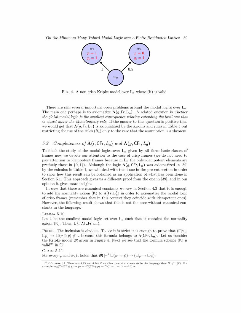
On the Minimum Many-Valued Modal Logic over a Finite Residuated Lattice 39
w0
w1
p = 1qi = 1
w2
p = 0qi = 1
1 0.5
Fig. 4. A non crisp Kripke model over Ln where (K) is valid
There are still several important open problems around the modal logics over Ln.The main one perhaps is to axiomatize Λ(g,Fr, Ln). A related question is whetherthe global modal logic is the smallest consequence relation extending the local one thatis closed under the Monotonicity rule. If the answer to this question is positive thenwe would get that Λ(g,Fr, Ln) is axiomatized by the axioms and rules in Table 5 butrestricting the use of the rules (Ra) only to the case that the assumption is a theorem.
5.2 Completeness of Λ(l, CFr, Ln) and Λ(g, CFr, Ln)
To finish the study of the modal logics over Ln given by all three basic classes offrames now we devote our attention to the case of crisp frames (we do not need topay attention to idempotent frames because in Ln the only idempotent elements areprecisely those in {0, 1}). Although the logic Λ(g,CFr, Ln) was axiomatized in [39]by the calculus in Table 1, we will deal with this issue in the present section in orderto show how this result can be obtained as an application of what has been done inSection 5.1. This approach gives us a different proof from the one in [39], and in ouropinion it gives more insight.
In case that there are canonical constants we saw in Section 4.3 that it is enoughto add the normality axiom (K) to Λ(Fr, Lc
n) in order to axiomatize the modal logicof crisp frames (remember that in this context they coincide with idempotent ones).However, the following result shows that this is not the case without canonical con-stants in the language.
Lemma 5.10Let L be the smallest modal logic set over Ln such that it contains the normalityaxiom (K). Then, L ( Λ(CFr, Ln).
Proof. The inclusion is obvious. To see it is strict it is enough to prove that (�p⊕�p) ↔ �(p ⊕ p) 6∈ L because this formula belongs to Λ(CFr, Ln). Let us considerthe Kripke model M given in Figure 4. Next we see that the formula scheme (K) isvalid25 in M.Claim 5.11For every ϕ and ψ, it holds that M |=1 �(ϕ→ ψ)→ (�ϕ→ �ψ).
25 Of course (cf. Theorems 4.13 and 4.14) if we allow canonical constants in the language then M 6|=1 (K). For
example, w0(�((0.5⊕ p)→ p)→ (�(0.5⊕ p)→ �p)) = 1→ (1→ 0.5) 6= 1.
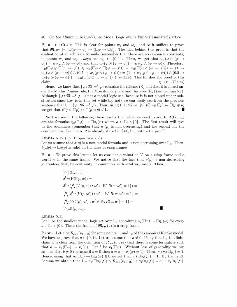
40 On the Minimum Many-Valued Modal Logic over a Finite Residuated Lattice
Proof of Claim. This is clear for points w1 and w2, and so it suffices to provethat M, w0 |=1 �(ϕ → ψ) → (�ϕ → �ψ). The idea behind this proof is that theevaluation of an arbitrary formula (remember that there are no canonical constants)in points w1 and w2 always belongs to {0, 1}. Thus, we get that w1(ϕ � (ϕ →ψ)) = w1(ϕ ∧ (ϕ → ψ)) and that w2(ϕ � (ϕ → ψ)) = w2(ϕ ∧ (ϕ → ψ)). Therefore,w0(�ϕ � �(ϕ → ψ)) 6 w0(�ϕ ∧ �(ϕ → ψ)) = w0(�(ϕ ∧ (ϕ → ψ))) = (1 →w1(ϕ ∧ (ϕ → ψ))) ∧ (0.5 → w2(ϕ ∧ (ϕ → ψ))) = (1 → w1(ϕ � (ϕ → ψ))) ∧ (0.5 →w2(ϕ� (ϕ → ψ))) = w0(�(ϕ� (ϕ → ψ))) 6 w0(�ψ). This finishes the proof of thisclaim. q.e.d. (Claim)
Hence, we know that {ϕ : M |=1 ϕ} contains the scheme (K) and that it is closed un-der the Modus Ponens rule, the Monotonicity rule and the rules (Ra) (see Lemma 5.1).Although {ϕ : M |=1 ϕ} is not a modal logic set (because it is not closed under sub-stitution since �q0 is in this set while �p not) we can easily see from the previoussentence that L ⊆ {ϕ : M |=1 ϕ}. Thus, using that M, w0 6|=1 (�p⊕�p)↔ �(p⊕ p)we get that (�p⊕�p)↔ �(p⊕ p) 6∈ L.
Next we see in the following three results that what we need to add to Λ(Fr, Ln)are the formulas ηa(�ϕ) → �ηa(ϕ) where a ∈ Ln \ {0}. The first result will giveus the soundness (remember that ηa(p) is non decreasing) and the second one thecompleteness. Lemma 5.12 is already stated in [39], but without a proof.
Lemma 5.12 ([39, Proposition 2.2])Let us assume that δ(p) is a non-modal formula and is non decreasing over Ln. Then,δ(�p)↔ �δ(p) is valid on the class of crisp frames.
Proof. To prove this lemma let us consider a valuation V on a crisp frame and aworld w in the same frame. We notice that the fact that δ(p) is non decreasingguarantees that, by continuity, it commutes with arbitrary meets. Then,
V (δ(�p), w) =
δLn(V (�p, w)) =
δ Ln(∧{V (p, w′) : w′ ∈W,R(w,w′) = 1}) =
∧{δ Ln(V (p, w′)) : w′ ∈W,R(w,w′) = 1} =
∧{V (δ(p), w′) : w′ ∈W,R(w,w′) = 1} =
V (�δ(p), w).
Lemma 5.13Let L be the smallest modal logic set over Ln containing ηa(�ϕ)→ �ηa(ϕ) for everya ∈ Ln \ {0}. Then, the frame of Mcan(L) is a crisp frame.
Proof. Let a be Rcan(v1, v2) for some points v1 and v2 of the canonical Kripke model.We have to prove that a ∈ {0, 1}. Let us assume that a 6= 0. Using that Ln is a finitechain it is clear from the definition of Rcan(v1, v2) that there is some formula ϕ suchthat a = v1(�ϕ) → v2(ϕ). Let b be v1(�ϕ). Without loss of generality we canassume that b 6= 0 (because if b = 0 then a = b→ v2(ϕ) = 1). Then, v1(ηb(�ϕ)) = 1.Hence, using that ηb(�ϕ) → �ηb(ϕ) ∈ L we get that v1(�ηb(ϕ)) = 1. By the TruthLemma we obtain that 1 = v1(�ηb(ϕ)) 6 Rcan(v1, v2)→ v2(ηb(ϕ)) = a→ v2(ηb(ϕ)).
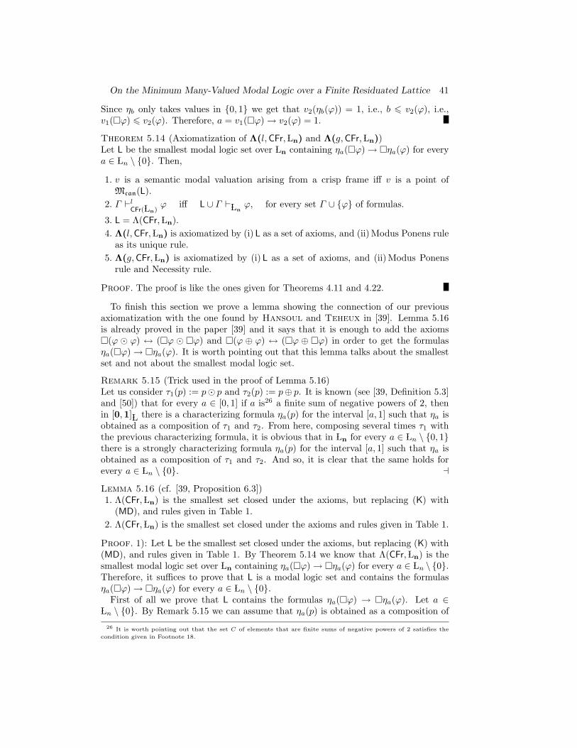
On the Minimum Many-Valued Modal Logic over a Finite Residuated Lattice 41
Since ηb only takes values in {0, 1} we get that v2(ηb(ϕ)) = 1, i.e., b 6 v2(ϕ), i.e.,v1(�ϕ) 6 v2(ϕ). Therefore, a = v1(�ϕ)→ v2(ϕ) = 1.
Theorem 5.14 (Axiomatization of Λ(l,CFr, Ln) and Λ(g,CFr, Ln))Let L be the smallest modal logic set over Ln containing ηa(�ϕ)→ �ηa(ϕ) for everya ∈ Ln \ {0}. Then,
1. v is a semantic modal valuation arising from a crisp frame iff v is a point ofMcan(L).
2. Γ `lCFr( Ln)
ϕ iff L ∪ Γ ` Lnϕ, for every set Γ ∪ {ϕ} of formulas.
3. L = Λ(CFr, Ln).4. Λ(l,CFr, Ln) is axiomatized by (i) L as a set of axioms, and (ii) Modus Ponens rule
as its unique rule.5. Λ(g,CFr, Ln) is axiomatized by (i) L as a set of axioms, and (ii) Modus Ponens
rule and Necessity rule.
Proof. The proof is like the ones given for Theorems 4.11 and 4.22.
To finish this section we prove a lemma showing the connection of our previousaxiomatization with the one found by Hansoul and Teheux in [39]. Lemma 5.16is already proved in the paper [39] and it says that it is enough to add the axioms�(ϕ � ϕ) ↔ (�ϕ � �ϕ) and �(ϕ ⊕ ϕ) ↔ (�ϕ ⊕ �ϕ) in order to get the formulasηa(�ϕ)→ �ηa(ϕ). It is worth pointing out that this lemma talks about the smallestset and not about the smallest modal logic set.
Remark 5.15 (Trick used in the proof of Lemma 5.16)Let us consider τ1(p) := p� p and τ2(p) := p⊕ p. It is known (see [39, Definition 5.3]and [50]) that for every a ∈ [0, 1] if a is26 a finite sum of negative powers of 2, thenin [0,1] L there is a characterizing formula ηa(p) for the interval [a, 1] such that ηa isobtained as a composition of τ1 and τ2. From here, composing several times τ1 withthe previous characterizing formula, it is obvious that in Ln for every a ∈ Ln \ {0, 1}there is a strongly characterizing formula ηa(p) for the interval [a, 1] such that ηa isobtained as a composition of τ1 and τ2. And so, it is clear that the same holds forevery a ∈ Ln \ {0}. aLemma 5.16 (cf. [39, Proposition 6.3])1. Λ(CFr, Ln) is the smallest set closed under the axioms, but replacing (K) with
(MD), and rules given in Table 1.2. Λ(CFr, Ln) is the smallest set closed under the axioms and rules given in Table 1.
Proof. 1): Let L be the smallest set closed under the axioms, but replacing (K) with(MD), and rules given in Table 1. By Theorem 5.14 we know that Λ(CFr, Ln) is thesmallest modal logic set over Ln containing ηa(�ϕ)→ �ηa(ϕ) for every a ∈ Ln \ {0}.Therefore, it suffices to prove that L is a modal logic set and contains the formulasηa(�ϕ)→ �ηa(ϕ) for every a ∈ Ln \ {0}.
First of all we prove that L contains the formulas ηa(�ϕ) → �ηa(ϕ). Let a ∈ Ln \ {0}. By Remark 5.15 we can assume that ηa(p) is obtained as a composition of
26 It is worth pointing out that the set C of elements that are finite sums of negative powers of 2 satisfies the
condition given in Footnote 18.
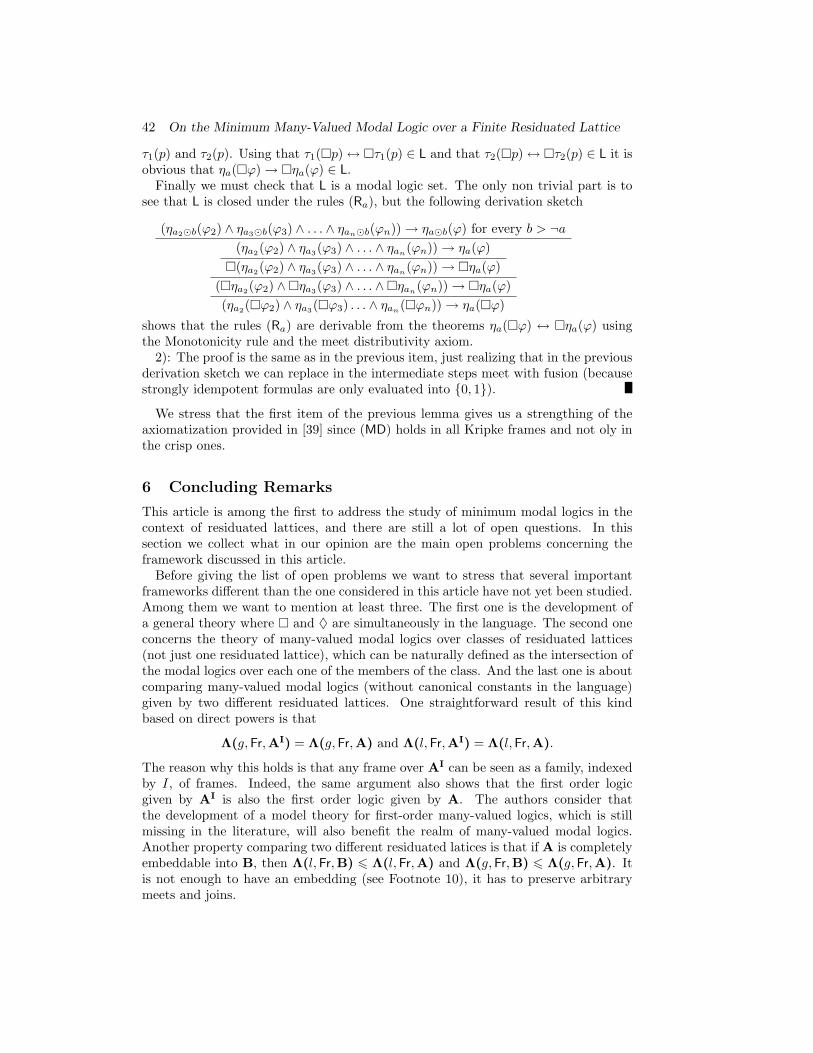
42 On the Minimum Many-Valued Modal Logic over a Finite Residuated Lattice
τ1(p) and τ2(p). Using that τ1(�p)↔ �τ1(p) ∈ L and that τ2(�p)↔ �τ2(p) ∈ L it isobvious that ηa(�ϕ)→ �ηa(ϕ) ∈ L.
Finally we must check that L is a modal logic set. The only non trivial part is tosee that L is closed under the rules (Ra), but the following derivation sketch
(ηa2�b(ϕ2) ∧ ηa3�b(ϕ3) ∧ . . . ∧ ηan�b(ϕn))→ ηa�b(ϕ) for every b > ¬a(ηa2(ϕ2) ∧ ηa3(ϕ3) ∧ . . . ∧ ηan(ϕn))→ ηa(ϕ)�(ηa2(ϕ2) ∧ ηa3(ϕ3) ∧ . . . ∧ ηan
(ϕn))→ �ηa(ϕ)(�ηa2(ϕ2) ∧�ηa3(ϕ3) ∧ . . . ∧�ηan
(ϕn))→ �ηa(ϕ)(ηa2(�ϕ2) ∧ ηa3(�ϕ3) . . . ∧ ηan
(�ϕn))→ ηa(�ϕ)
shows that the rules (Ra) are derivable from the theorems ηa(�ϕ) ↔ �ηa(ϕ) usingthe Monotonicity rule and the meet distributivity axiom.
2): The proof is the same as in the previous item, just realizing that in the previousderivation sketch we can replace in the intermediate steps meet with fusion (becausestrongly idempotent formulas are only evaluated into {0, 1}).
We stress that the first item of the previous lemma gives us a strengthing of theaxiomatization provided in [39] since (MD) holds in all Kripke frames and not oly inthe crisp ones.
6 Concluding Remarks
This article is among the first to address the study of minimum modal logics in thecontext of residuated lattices, and there are still a lot of open questions. In thissection we collect what in our opinion are the main open problems concerning theframework discussed in this article.
Before giving the list of open problems we want to stress that several importantframeworks different than the one considered in this article have not yet been studied.Among them we want to mention at least three. The first one is the development ofa general theory where � and ♦ are simultaneously in the language. The second oneconcerns the theory of many-valued modal logics over classes of residuated lattices(not just one residuated lattice), which can be naturally defined as the intersection ofthe modal logics over each one of the members of the class. And the last one is aboutcomparing many-valued modal logics (without canonical constants in the language)given by two different residuated lattices. One straightforward result of this kindbased on direct powers is that
Λ(g,Fr,AI) = Λ(g,Fr,A) and Λ(l,Fr,AI) = Λ(l,Fr,A).
The reason why this holds is that any frame over AI can be seen as a family, indexedby I, of frames. Indeed, the same argument also shows that the first order logicgiven by AI is also the first order logic given by A. The authors consider thatthe development of a model theory for first-order many-valued logics, which is stillmissing in the literature, will also benefit the realm of many-valued modal logics.Another property comparing two different residuated latices is that if A is completelyembeddable into B, then Λ(l,Fr,B) 6 Λ(l,Fr,A) and Λ(g,Fr,B) 6 Λ(g,Fr,A). Itis not enough to have an embedding (see Footnote 10), it has to preserve arbitrarymeets and joins.
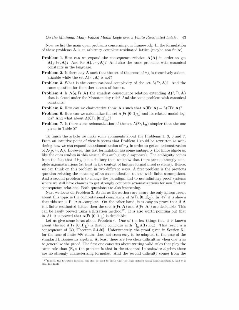
On the Minimum Many-Valued Modal Logic over a Finite Residuated Lattice 43
Now we list the main open problems concerning our framework. In the formulationof these problems A is an arbitrary complete residuated lattice (maybe non finite).
Problem 1. How can we expand the consequence relation Λ(A) in order to getΛ(g,Fr,A)? And for Λ(l,Fr,A)? And also the same problems with canonicalconstants in the language.
Problem 2. Is there any A such that the set of theorems of `A is recursively axiom-atizable while the set Λ(Fr,A) is not?
Problem 3. What is the computational complexity of the set Λ(Fr,A)? And thesame question for the other classes of frames.
Problem 4. Is Λ(g,Fr,A) the smallest consequence relation extending Λ(l,Fr,A)that is closed under the Monotonicity rule? And the same problem with canonicalconstants.
Problem 5. How can we characterize those A’s such that Λ(IFr,A) = Λ(CFr,A)?Problem 6. How can we axiomatize the set Λ(Fr, [0,1] L) and its related modal log-
ics? And what about Λ(CFr, [0,1] L)?Problem 7. Is there some axiomatization of the set Λ(Fr, Ln) simpler than the one
given in Table 5?
To finish the article we make some comments about the Problems 1, 3, 6 and 7.From an intuitive point of view it seems that Problem 1 could be rewritten as won-dering how we can expand an axiomatization of `A in order to get an axiomatizationof Λ(g,Fr,A). However, this last formulation has some ambiguity (for finite algebras,like the ones studies in this article, this ambiguity disappears). The ambiguity comesfrom the fact that if `A is not finitary then we know that there are no strongly com-plete axiomatizations (at least in the context of finitary formal proof systems). Hence,we can think on this problem in two different ways. A first problem is the previousquestion relaxing the meaning of an axiomatization to sets with finite assumptions.And a second problem is to change the paradigm and to use infinitary proof systemswhere we still have chances to get strongly complete axiomatizations for non finitaryconsequence relations. Both questions are also interesting.
Next we focus on Problem 3. As far as the authors are aware the only knwon resultabout this topic is the computational complexity of Λ(Fr, [0,1]G). In [47] it is shownthat this set is Pspace-complete. On the other hand, it is easy to prove that if Ais a finite residuated lattice then the sets Λ(Fr,A) and Λ(Fr,Ac) are decidable. Thiscan be easily proved using a filtration method27. It is also worth pointing out thatin [31] it is proved that Λ(Fr, [0,1] L) is decidable.
Let us give some ideas about Problem 6. One of the few things that it is knownabout the set Λ(Fr, [0,1] L) is that it coincides with
⋂n Λ(Fr, Ln). This result is a
consequence of [30, Theorem 5.4.30]. Unfortunately, the proof given in Section 5.1for the case of finite MV chains does not seem easy to be adapted to the case of thestandard Lukasiewicz algebra. At least there are two clear difficulties when one triesto generalize the proof. The first one concerns about writing valid rules that play thesame role than (Ra): the problem is that in the standard Lukasiewicz algebra thereare no strongly characterizing formulas. And the second difficulty comes from the
27Indeed, the filtration method can also be used to prove that the logic defined using simultaneously � and ♦ is
also decidable

44 On the Minimum Many-Valued Modal Logic over a Finite Residuated Lattice
fact that the non-modal logic is not finitary (this is used to get the first claim insidethe proof of Lemma 5.6).
At this moment it is not clear for us how to overcome the first difficulty. But aboutthe second one we think that one possible way is to use infinitary proof systems. Thismethod has been used in [39] to show an strong axiomatization of Λ(g,CFr, [0,1] L)(see Section 3.3), but even in the classical modal setting the method has been success-fully considered (see [44]). In our opinion the addition of infinitary rules may help toobtain a completeness proof based on a canonical model construction. Although inthe literature there are some reasons to believe that the canonical model constructionshould not help to settle the completeness for the case of the standard Lukasiewiczalgebra (see [26, 45]), these limitations may not apply to the case of using a canonicalmodel construction based on infinitary proof systems. We think, roughly speaking,that infinitary proof systems may help to overtake these limitations.
Finally, we focus on Problem 7 about the search of a more transparent axiomatiza-tion for Λ(Fr, Ln). That is, can we simplify the axiomatization given in Table 5? Theauthors can imagine at least two different strategies that may help to simplify theaxiomatization. A first one would be based on understanding better which non-modalformulas are always evaluated in [a, 1]∩ Ln for a certain value a ∈ Ln. We feel that theunderstanding28 of these non-modal formulas may help to solve this open questiondue to the connection with the rules29 (Ra). Next we illustrate this connection withan straightforward remark: if ϕ is always evaluated in [a, 1] and ηa is a (maybe notstrongly) characterizing formula of the interval [a, 1] then the formula ηa(�ϕ) belongsto Λ(Fr, Ln) (indeed it also belongs to Λ(Fr, [0,1] L)). For example, using a = 0.5 wecan get that �(p∨¬p)⊕�(p∨¬p) is a theorem. However, nowadays it is still unclearto the authors whether this research line could really help to simplify Table 5.
The other strategy is to visualize a many-valued accessibility relation R as a non-increasing sequence 〈Ra : a ∈ Ln \ {0}〉 of crisp accessibility relations. By beingnon-increasing we refer to the fact that if a 6 a′ then Ra′ ⊆ Ra. It is clear that everymany-valued accessibility relation R can be canonically represented in this way usingRa := {(w,w′) : R(w,w′) > a}; and on the other hand, every non-increasing sequence〈Ra : a ∈ Ln \ {0}〉 of crisp accessibility relations is canonically represented by themany-valued accessibility relation
R(w,w′) :={
min{a ∈ Ln \ {0} : (w,w′) ∈ Ra}, if (w,w′) ∈ ⋃aRa0, otherwise.
This suggests that Λ(Fr, Ln) has canonically associated a multi-modal {�a : a ∈ Ln \{0}} logic where each modality �a is semantically interpreted by the crisp acces-sibility relation Ra. The reason why this perspective could possibly help to simplifythe axiomatization in Table 5 is that for the case of crisp frames there are reallysimple axiomatizations of the many-valued modal logic over Ln due to Hansoul andTeheux (see Lemma 5.16). Indeed, some previous attempts to axiomatize Λ(Fr, Ln)done by some of the authors were based on this idea (see [8]).
28 This research has been started by one of the authors in the recent manuscript [7].29 We are mainly thinking in the informal version stated just before Lemma 5.1.
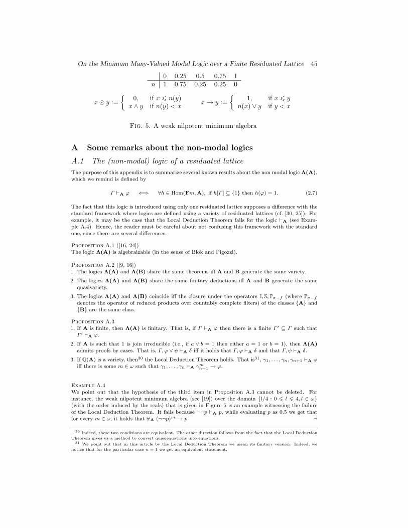
On the Minimum Many-Valued Modal Logic over a Finite Residuated Lattice 45
0 0.25 0.5 0.75 1n 1 0.75 0.25 0.25 0
x� y :={
0, if x 6 n(y)x ∧ y if n(y) < x
x→ y :={
1, if x 6 yn(x) ∨ y if y < x
Fig. 5. A weak nilpotent minimum algebra
A Some remarks about the non-modal logics
A.1 The (non-modal) logic of a residuated lattice
The purpose of this appendix is to summarize several known results about the non modal logic Λ(A),which we remind is defined by
Γ `A ϕ ⇐⇒ ∀h ∈ Hom(Fm,A), if h[Γ ] ⊆ {1} then h(ϕ) = 1. (2.7)
The fact that this logic is introduced using only one residuated lattice supposes a difference with the
standard framework where logics are defined using a variety of residuated lattices (cf. [30, 25]). Forexample, it may be the case that the Local Deduction Theorem fails for the logic `A (see Exam-
ple A.4). Hence, the reader must be careful about not confusing this framework with the standard
one, since there are several differences.
Proposition A.1 ([16, 24])
The logic Λ(A) is algebraizable (in the sense of Blok and Pigozzi).
Proposition A.2 ([9, 16])1. The logics Λ(A) and Λ(B) share the same theorems iff A and B generate the same variety.
2. The logics Λ(A) and Λ(B) share the same finitary deductions iff A and B generate the same
quasivariety.
3. The logics Λ(A) and Λ(B) coincide iff the closure under the operators I, S,Pσ−f (where Pσ−fdenotes the operator of reduced products over countably complete filters) of the classes {A} and{B} are the same class.
Proposition A.3
1. If A is finite, then Λ(A) is finitary. That is, if Γ `A ϕ then there is a finite Γ ′ ⊆ Γ such that
Γ ′ `A ϕ.
2. If A is such that 1 is join irreducible (i.e., if a ∨ b = 1 then either a = 1 or b = 1), then Λ(A)admits proofs by cases. That is, Γ, ϕ ∨ ψ `A δ iff it holds that Γ, ϕ `A δ and that Γ, ψ `A δ.
3. If Q(A) is a variety, then30 the Local Deduction Theorem holds. That is31, γ1, . . . , γn, γn+1 `A ϕ
iff there is some m ∈ ω such that γ1, . . . , γn `A γmn+1 → ϕ.
Example A.4We point out that the hypothesis of the third item in Proposition A.3 cannot be deleted. For
instance, the weak nilpotent minimum algebra (see [19]) over the domain {l/4 : 0 6 l 6 4, l ∈ ω}(with the order induced by the reals) that is given in Figure 5 is an example witnessing the failureof the Local Deduction Theorem. It fails because ¬¬p `A p, while evaluating p as 0.5 we get that
for every m ∈ ω, it holds that 6`A (¬¬p)m → p. a
30 Indeed, these two conditions are equivalent. The other direction follows from the fact that the Local Deduction
Theorem gives us a method to convert quasiequations into equations.31 We point out that in this article by the Local Deduction Theorem we mean its finitary version. Indeed, we
notice that for the particular case n = 1 we get an equivalent statement.
46 On the Minimum Many-Valued Modal Logic over a Finite Residuated Lattice
Remark A.5 (Modus Ponens as a unique rule)The third statement in the previous proposition says in particular that if Q(A) is a variety then
the finitary deductions of Λ(A) can be obtained using only one inference rule: Modus Ponens. The
previous example shows that in general it is not true that Λ(A) can be axiomatized using ModusPonens as a unique rule; maybe more rules have to be added. a
Is there some way to characterize those A’s such that Q(A) is a variety? Thanks to the congruence
extension property [25, Lemma 3.57] (it implies SH = HS) together with Jonsson’s Lemma [42] it is
obvious that32 Q(A) is a variety iff HPU (A) ⊆ Q(A). In the particular case that A is finite (cf. [51,Theorem 1.1.1]) we get that Q(A) is a variety iff H(A) ⊆ Q(A). Therefore, for every finite residuate
lattice A, if A is simple then Q(A) is a variety. Next we state other cases where we know for sure
that the generated quasivariety is a variety.
Proposition A.6Let A be a finite BL chain. Then, Q(A) is a variety. And Λ(A) can be axiomatized using Modus
Ponens as a unique rule.
Proof. It is enough to see that if F is a congruence filter then A/F is embeddable into A. The
reader can easily check that
i : A/F −→ A
x/F 7−→
1, if x ∈ Fx, if x 6∈ F
is well defined and it is an embedding. The reason why this map is well defined is because if a 6∈ F ,then a/F is a singleton.
Example A.7
The previous statement fails in the case of arbitrary BL chains. Let us consider for instance Aas the (simple) subalgebra of standard Lukasiewicz algebra [0,1] L with domain A = {x ∈ [0, 1] :
x is a rational number with denominator odd}. Then, p↔ ¬p `A q while for every m ∈ ω, it holdsthat 6`A (p↔ ¬p)m → q. a
A natural question that appears here is whether there are complete BL chains A such that thequasivariety generated by A is not a variety. In [18, Corollary 12] this question is negatively answered
for the case of standard BL algebras. Indeed, a similar proof can be used to answer the first question.
Proposition A.8 (cf. [18, Corollary 7])
Let A be a complete BL chain. Then, Q(A) is a variety, and so Λ(A) can be axiomatized usingModus Ponens as a unique rule.
Throughout this article we have assumed that we already know an axiomatization of Λ(A) inorder to see how to expand it for the modal logic. Unfortunately, in the literature there is no general
result stating how to axiomatize an arbitrary logic Λ(A). Nevertheless, it is worth pointing out that
for a lot of logics of the form Λ(A) we already know axiomatizations:• If A is a finite BL algebra, then Λ(A) has been axiomatized, among other logics, in [1, Theorem 5.1]
using as a rule only Modus Ponens. And the axiomatization has a finite number of axioms.
• If A is a standard BL algebra, then the finitary deductions33 of Λ(A) are axiomatized in [20](see also [38]). The axiomatization only uses one rule: Modus Ponens. And we notice that this
axiomatization has a finite number of axioms.
Remark A.9 (Recursive and finite axiomatizations)
Since it is known that the first order logic over any finite algebra is recursively axiomatizable [52, 2]
it is clear that Λ(A) is recursively axiomatizable for every finite residuated lattice A. It is worth
32 In the particular case that A is a BL chain, then [15, Theorem 3.8] is an strengthening of this fact. This theorem
states, with different terminology, that Q(A) is a variety iff every algebra in HPU (A) is partially embeddable into
A.33 We point out that if A is a standard BL algebra, then Λ(A) is finitary iff A is the standard Godel algebra
[0, 1]G (see [18, p. 603]).
On the Minimum Many-Valued Modal Logic over a Finite Residuated Lattice 47
pointing out that in general it is not true that for every finite residuated lattice A there is a finite34
axiomatization of Λ(A). In [17] there are counterexamples for finite Heyting algebras. However
it is known that if A is a finite subdirectly irreducible residuated lattice35 then Λ(A) is finitely
axiomatizable (see [6] together with [43, Proposition 1.11]). a
A.2 Adding canonical constants to the non-modal logic
In this appendix we analyze the non-modal logic Λ(Ac) obtained by adding canonical constants.
We remind that this logic is defined by the equivalence
Γ `Ac ϕ ⇐⇒ ∀h ∈ Hom(Fm,Ac), if h[Γ ] ⊆ {1} then h(ϕ) = 1. (2.8)
This logic is introduced following the same pattern that is used for Λ(A), and hence Λ(Ac) is clearly
a conservative expansion of Λ(A). Noticing this pattern it is not surprising that Proposition A.136,Proposition A.2 and the two first statements of Proposition A.3 also hold if we replace A and B
with Ac and Bc.
Unfortunately, the addition of canonical constants also has some undesired consequences, andso we must be really careful. These disadvantages are mainly caused by the fact that a `Λ(Ac) 0
whenever a ∈ A \ {1}. Among the properties that may fail are the Local Deduction Theorem andproofs by cases. If the set of idempotent elements of A is diferent than {0, 1}, then automatically
the Local Deduction Theorem fails for Λ(Ac). In particular we have that the addition of canonical
constants to (even finite) Godel algebras is destroying the Deduction Theorem. To avoid mistakes itis also worth pointing out that a consequence of the failure of the Local Deduction Theorem is that
these logics are not core fuzzy logics [14, 34] and hence we cannot apply the machinery developed
for core fuzzy logics as in [15].
Proposition A.10Each one of the following conditions implies the next one.
1. Λ(Ac) satisfies the Local Deduction Theorem.
2. Q(Ac) is a variety.
3. A is simple.
4. The set of idempotents elements of A is {0, 1}.In case A is finite all these conditions are equivalent.
Proof. 1 ⇒ 2): It is trivial because the Local Deduction Theorem gives us a way to convert
quasiequations into equations.
2 ⇒ 3): Let us assume that there is a non-trivial congruence filter F of A. Let a be an elementof F such that a 6= 1. Then, Ac satisfies the quasiequation a ≈ 1⇒ 0 ≈ 1 while the quotient Ac/F
does not satisfy this quasiequation. Therefore, Q(Ac) is not a variety.
3⇒ 4): It is trivial.4⇒ 1): Assume now that A is finite. Let n be the cardinal of A. Due to the assumption we know
that for every element a 6= 1 it holds that an = 0. Using this it is obvious that the Local DeductionTheorem holds.
As a consequence of this last proposition it is clear that if A is a finite and simple residuated
lattice then the logic Λ(Ac) can be axiomatized using Modus Ponens as a unique rule.
Proposition A.11
Λ(Ac) admits proofs by cases iff 1 is a join irreducible element of A.
34 Nevertheless, if one also accepts non Hilbert style axiomatizations then it is known [2] that all logics Λ(A)
defined by a finite algebra can be finitely presented.35 By [43, Proposition 1.4] this is equivalent to consider a finite residuated lattice with a unique coatom (i.e., a
maximum element strictly below 1).36 As a consequence of this algebraizability we know that, for all algebras in the quasivariety generated by Ac,
there is an isomorphism between its relative congruences and the set of “logical filters”. Indeed, for the algebra Ac
we know that these two sets have cardinal 2 due to the rules a `Ac 0 (when a ∈ A \ {1}).
48 On the Minimum Many-Valued Modal Logic over a Finite Residuated Lattice
Proof. This easily follows from the fact that if 1 = a ∨ b with a, b ∈ A \ {1}, then a `Ac 0 andb `Ac 0, while a ∨ b 6`Ac 0.
In the rest of this appendix we will explain a method to expand an axiomatization of Λ(A), when
A is finite, into one of Λ(Ac). This method is not universal, but it can be applied to quite a lot
of cases: the ones from Proposition A.11. As far as we know, this result about axiomatizing theconsequence relation (not only its theorems) obtained by adding canonical constants is new in the
literature (cf. [18]).
By the name book-keeping axioms we will refer as usual [30] to the equations
a ∗ b ≈ a ∗ b where a, b ∈ A and ∗ ∈ {∧,∨,�,→},
or to the formulas
(a ∗ b)↔ a ∗ b where a, b ∈ A and ∗ ∈ {∧,∨,�,→}.
The context will clarify whether we are thinking on equations or on formulas. Analogously, we will
refer to
Wa∈A(x↔ a) ≈ 1 or
Wa∈A(p↔ a)
as the witnessing axiom.
Lemma A.12Let A be a finite residuated lattice. The variety generated by Ac is axiomatized by the following
list of equations:• an equational presentation of A,
• the witnessing and book-keeping axioms.
Proof. It is obvious that the previous list of equations hold in Ac. Thus, it is enough to prove
that every algebra B (with the similarity type including the constants {a : a ∈ A}) that satisfies theprevious list of equations and that is subdirectly irreducible is a homomorphic image of Ac. Let us
consider B satisfying the previous properties. Then, it is obvious that the map
h : Ac −→ B
a 7−→ aB
is a homomorphism due to the book-keeping axioms. And it is onto thanks to the witnessing
axiom together with the fact that 1 is join irreducible in all subdirectly irreducible algebras (see [43,
Proposition 1.4]).
Remark A.13
We point out that in this proof we have seen that all subdirectly irreducible algebras in the varietygenerated by Ac are of the form Ac/F for a certain congruence filter F . This can also be obtained
as an easy consequence of Jonsson Lemma and the congruence extension property. a
Next we consider the problem of axiomatizing Q(Ac) for the particular case that there is a unique
coatom k. Although for this case it is possible to give an almost trivial proof of Theorem A.14 usingLemma A.12 together with the above displayed equivalence (where k is the unique coatom)
γ1, . . . , γn `Ac ϕ iff `Ac (γ1 ∧ . . . ∧ γn)→ (ϕ ∨ k), (4.4)
we have preferred to write down the following semantic proof since it could be easier to be generalizedin a future to the general case with more than one coatom.
Theorem A.14
Let A be a finite residuated lattice with a unique coatom k 6∈ {0, 1}. The quasivariety generated byAc is axiomatized by the following list of quasiequations:
• a quasiequational presentation of A,
• the witnessing and book-keeping axioms.
• k ∨ x ≈ 1⇒ x ≈ 1.
On the Minimum Many-Valued Modal Logic over a Finite Residuated Lattice 49
Proof. It is obvious that the previous list of quasiequations hold in Ac (we notice that the lastquasiequation is valid only because A has coatom k). Thus, it is enough to prove that every non
trivial algebra B (with the similarity type including the constants {a : a ∈ A}) that satisfies the
previous list of quasiequations is a subalgebra of a direct product of copies of Ac. Let us consider anon trivial B satisfying the list of quasiequations. By Lemma A.12 we know that B is in the variety
generated by Ac. And so, together with Remark A.13, it follows that B ⊆Q{Ac/Fi : i ∈ I} where
the Fi’s are congruence filters. By the last quasiequation in the list we know that kB 6= 1. Therefore,
{i ∈ I : Fi = {1}} 6= ∅. Let us consider the map
h : B −→ Q{Ac/Fi : i ∈ I, Fi = {1}}b 7−→ 〈πi(b) : i ∈ I, Fi = {1}〉
We remark that πi refers to the i-th projection. By definition it is obvious that h is a homomorphism.
The proof is completed (because Ac/{1} ∼= Ac) by showing that h is an embedding. If this doesnot hold, then the kernel of the map h is non trivial. So, there is an element b ∈ B \ {1} such that
h(b) = 1, i.e., for every i ∈ I, if Fi = {1} then πi(b) = 1. On the other hand, for every i ∈ I, if
Fi 6= {1} then k ∈ Fi, and hence πi(kB
) = 1. Therefore, for every i ∈ I, it holds that πi(kB∨ b) = 1.
Thus, kB ∨ b = 1 while b 6= 1. This contradicts the last quasiequation in the list.
We stress that in the previous theorem we cannot replace the last quasiequation with k∨0 ≈ 1⇒0 ≈ 1. The next example shows this.
Example A.15
Let us consider the Godel chain G3 with three elements, and let us denote its coatom by k and
its congruence filter {k, 1} by F . It is obvious that in Gc3/F ×Gc
3 fails the last quasiequation inTheorem A.14 (because k ∨ (0, 1) = 1 while (0, 1) 6= 1). On the other hand, Gc
3/F ×Gc3 satisfies all
quasiequations valid in G3, the witnessing and book-keeping axioms and the quasiequation k ∨ 0 ≈1⇒ 0 ≈ 1.
Next we state two trivial consequences of the previous results. We stress that the axiomatizationgiven in Corollary A.17 only uses one rule (Modus Ponens).
Corollary A.16
Let A be a finite residuated lattice with a unique coatom k 6∈ {0, 1}. The logic Λ(Ac) is axiomatizedby
• rules and axioms axiomatizing Λ(A),
• the witnessing and book-keeping axioms,
• the rule k ∨ p ` p.
Corollary A.17
Let A be a finite and simple residuated lattice. The logic Λ(Ac) is axiomatized by
• axioms axiomatizing Λ(A),
• the witnessing and book-keeping axioms,
• the Modus Ponens rule.
To finish the appendix we point out that it is an open problem to give, for every finite residuated
lattice A, a presentation of Q(Ac) (cf. Theorem A.14). In our opinion one of the difficulty to search
this axiomatization is the failure of proofs by cases (cf. Proposition A.11).
B The non-modal companion method
In this appendix we introduce the non-modal companion method, which provides a really simple
method to discard the validity of some modal formulas. This method does not work for all non valid
formulas (but it works for (K)), but when it works it gives us a very simple explanation why validityfails.
50 On the Minimum Many-Valued Modal Logic over a Finite Residuated Lattice
Definition B.1
We consider new variables r0, r1, r2, . . . The non-modal companion formula of a modal formula is
the non-modal formula that results from replacing every subformula of the form �ϕ with rn → ϕwhere n is the modal degree of this � occurrence. For example, the non-modal companion of
�(p → �q) → (�p → �q) is the formula (r1 → (p → (r0 → q))) → ((r0 → p) → (r0 → q)). The
non-modal companion of ϕ is denoted π(ϕ). a
Before next proposition we remind the reader that Λ(Ac) is a conservative expansion of Λ(A),
and so the statements in next proposition also apply to `A.
Proposition B.2
1. If Fr |=1 ϕ, then `Ac π(ϕ).
2. If IFr |=1 ϕ, then {rn ↔ (rn � rn) : n ∈ ω} `Ac π(ϕ).
3. If CFr |=1 ϕ, then37 `Ac s(π(ϕ)) where s is any substitution such that s[{rn : n ∈ ω}] ⊆ {0, 1}.
Proof. Let us prove the first statement. Let h be a homomorphism from the algebra of formulas
(including {rn : n ∈ ω} among its variables and also including canonical constants) into Ac. We
consider the Kripke model 〈N, R, V 〉 where
R(n, n′) =
h(rn), if n′ = n+ 1
0, otherwise.
and V (p, n) = h(p) for every variable p. A moment of reflection shows that for every modal formula
ϕ (without variables in {rn : n ∈ ω}) it holds that V (ϕ, 0) = h(π(ϕ)). Using that Fr |=1 ϕ we get
that h(π(ϕ)) = 1.The proofs of the other two statements are analogous since the same Kripke model construction
works for these classes of frames.
Example B.3
It is worth pointing out that the other direction is not true in general. For example, if A is an MTLalgebra and ϕ := �(p∨ q)↔ (�p∨�q) then `A π(ϕ). On the other hand, it is known that ϕ is not
valid in the class CFr(2) of crisp frames over the two element Boolean algebra (just consider a frame
with two different successors); and so for every residuated lattice A, it holds that CFr(A) 6|=1 ϕ(cf. [12]). a
In the case of the normality axiom (K) the non-modal companion gives a very simple explanationabout why in general this formula is not valid. Let us assume that Fr |=1 (K); then `A π(K) by
Proposition B.2, i.e., `A (r0 → (p → q)) → ((r0 → p) → (r0 → q)). Replacing p by a, q by a � aand r0 by a it clearly follows that a = a� a for every element a ∈ A. That is, we have just provedthat if Fr |=1 (K) then A is a Heyting algebra; and so we could have used the non-modal companion
to give an alternative proof of the first item in Corollary 3.13.
Although in Example B.3 we saw that the method of non-modal companions is in general notenough to characterize all non valid formulas next we state in Corollary B.5 a particular case where
it is indeed enough.
Proposition B.4
Let δ(p1, . . . , pn) and ε(p) be two non-modal formulas such that δ is non decreasing over Ac in anyof its arguments and ε is an expanding formula over Ac (i.e., `Ac p→ ε(p)). And let ϕ1, . . . , ϕn, ϕ
be non-modal formulas. If `Ac δ(r → ϕ1, . . . , r → ϕn)→ ε(r → ϕ), r being a variable not appearing
in {ϕ1, . . . , ϕn, ϕ}, then Fr |=1 δ(�ϕ1, . . . ,�ϕn)→ �ε(ϕ).
Proof. Take any frame F, a world w in F, and a valuation V on F. Then, for every world w′ it holds
37 If A has the property that 1 is join irreducible (e.g., subdirectly irreducible residuated lattices, chains, etc.)
then we can rewrite the conclusion as {rn ∨ ¬rn : n ∈ ω} `Ac π(ϕ).
On the Minimum Many-Valued Modal Logic over a Finite Residuated Lattice 51
that
V (δ(�ϕ1, . . . ,�ϕn), w) =
δAc(V (�ϕ1, w), . . . , V (�ϕn, w)) 6
δAc(R(w,w′)→ V (ϕ1, w
′), . . . , R(w,w′)→ V (ϕn, w′)) 6
εAc(R(w,w′)→ V (ϕ,w′)) =
εAc(R(w,w′))→ εA
c(V (ϕ,w′)) 6
R(w,w′)→ εAc(V (ϕ,w′)) =
R(w,w′)→ V (ε(ϕ), w′).
Therefore, V (δ(�ϕ1, . . . ,�ϕn), w) 6 V{R(w,w′)→ V (ε(ϕ), w′) : w′ ∈W}. Hence, V (δ(�ϕ1, . . . ,�ϕn), w) 6V (�ε(ϕ), w).
For the particular case that we apply the previous proposition to δ := p1 ∧ p2, ε := p and
ϕ := ϕ1 ∧ ϕ2 what we get is the validity of a particular case of (MD). Next we highlight anotherparticular case.
Corollary B.5
Let ϕ1, . . . , ϕn, ϕ be non-modal formulas. If `Ac ((r → ϕ1)� . . .� (r → ϕn))→ (r → ϕ), r being avariable not appearing in {ϕ1, . . . , ϕn, ϕ}, then Fr |=1 (�ϕ1 � . . .��ϕn)→ �ϕ.
Proof. This is a consequence of Proposition B.4; simply consider δ(p1, . . . , pn) := p1 � . . .� pn and
ε(p) := p.
To finish this appendix we point out that the notion of non-modal companion is also interestingfrom the point of view of the modal consequence relation (cf. Proposition B.2).
Proposition B.61. If Γ `l
Fr(Ac)ϕ, then π[Γ ] `Ac π(ϕ).
2. If Γ `lIFr(Ac)
ϕ, then {rn ↔ (rn � rn) : n ∈ ω}, π[Γ ] `Ac π(ϕ).
3. If Γ `lCFr(Ac)
ϕ, then s[π[Γ ]] `Ac s(π(ϕ)) where s is any substitution such that s[{rn : n ∈ ω}] ⊆{0, 1}.
Proof. The proof uses the same Kripke model given in Proposition B.2.
References
[1] P. Agliano and F. Montagna. Varieties of BL-algebras. I. General properties. Journal of Pure
and Applied Algebra, 181(2-3):105–129, 2003.
[2] M. Baaz, C. G. Fermuller, and R. Zach. Elimination of cuts in first-order finite-valued logics.
Journal of Information Processing and Cybernetics EIK, 29(6):333–355, 1994.
[3] M. Baaz, N. Preining, and R. Zach. First-order Godel logics. Annals of Pure and Applied Logic,
147(1-2):23–47, 2007.
[4] P. Blackburn, M. de Rijke, and Y. Venema. Modal logic. Number 53 in Cambridge Tracts inTheoretical Computer Science. Cambridge University Press, Cambridge, 2001.
[5] P. Blackburn, J. F. A. K. van Benthem, and F. Wolter, editors. Handbook of Modal Logic,Volume 3 (Studies in Logic and Practical Reasoning). Elsevier Science Inc., New York, NY,
USA, 2006.
[6] W. J. Blok and D. Pigozzi. A finite basis theorem for quasivarieties. Algebra Universalis,
22(1):1–13, 1986.
[7] F. Bou. Characterizing the generators of McNaughton functions evaluated in a lattice filter. In
Preparation, 2009.
[8] F. Bou, F. Esteva, and L. Godo. Exploring a syntactic notion of modal many-valued logics.Mathware and Soft Computing, 15(2):175–188, 2008.
52 On the Minimum Many-Valued Modal Logic over a Finite Residuated Lattice
[9] S. Burris and H. P. Sankappanavar. A course in Universal Algebra. The millennium edition,2000.
[10] X. Caicedo and R. O. Rodrıguez. Standard Godel modal logics. Studia Logica. To appear.
[11] A. Chagrov and M. Zakharyaschev. Modal Logic, volume 35 of Oxford Logic Guides. OxfordUniversity Press, 1997.
[12] A. Ciabattoni, G. Metcalfe, and F. Montagna. Adding modalities to MTL and its extensions.
Proceedings of the Linz Symposium 2005, 2005.
[13] R. Cignoli, I. M. L. D’Ottaviano, and D. Mundici. Algebraic foundations of many-valued rea-soning, volume 7 of Trends in Logic—Studia Logica Library. Kluwer Academic Publishers,
Dordrecht, 2000.
[14] P. Cintula. From fuzzy logic to fuzzy mathematics. Ph. D. thesis, Czech Technical University inPrague, 2004.
[15] P. Cintula, F. Esteva, J. Gispert, L. Godo, F. Montagna, and C. Noguera. Distinguished algebraic
semantics for t-norm based fuzzy logics: Methods and algebraic equivalencies. Annals of Pureand Applied Logic, 160(1):53–81, 2009.
[16] J. Czelakowski. Protoalgebraic logics, volume 10 of Trends in Logic—Studia Logica Library.
Kluwer Academic Publishers, Dordrecht, 2001.
[17] W. Dziobiak. Concerning axiomatizability of the quasivariety generated by a finite Heyting or
topological Boolean algebra. Studia Logica, 41(4):415–428 (1983), 1982.
[18] F. Esteva, J. Gispert, L. Godo, and C. Noguera. Adding truth-constants to logics of continuoust-norms: Axiomatization and completeness results. Fuzzy Sets and Systems, 158(6):597–618,
March 2007.
[19] F. Esteva and L. Godo. Monoidal t-norm based logic: towards a logic for left-continuous t-norms.Fuzzy Sets and Systems, 124:271–288, 2001.
[20] F. Esteva, L. Godo, and M. Montagna. Equational Characterization of the Subvarieties of BL
Generated by t-norm Algebras. Studia Logica, 76(2):161–200, 2004.
[21] C. G. Fermuller and H. Langsteiner. Tableaux for finite-valued logics with arbitrary distributionmodalities. In Automated reasoning with analytic tableaux and related methods (Oisterwijk,
1998), volume 1397 of Lecture Notes in Computer Science, pages 156–171. Springer, Berlin,
1998.
[22] M. Fitting. Many-valued modal logics. Fundamenta Informaticae, 15:235–254, 1992.
[23] M. Fitting. Many-valued modal logics, II. Fundamenta Informaticae, 17:55–73, 1992.
[24] J. M. Font, R. Jansana, and D. Pigozzi. A survey on abstract algebraic logic. Studia Logica,Special Issue on Abstract Algebraic Logic, Part II, 74(1–2):13–97, 2003. With an “Update” in
91 (2009), 125–130.
[25] N. Galatos, P. Jipsen, T. Kowalski, and H. Ono. Residuated Lattices: an algebraic glimpseat substructural logics, volume 151 of Studies in Logic and the Foundations of Mathematics.
Elsevier, Amsterdam, 2007.
[26] M. Gehrke and H. A. Priestley. Non-canonicity of MV-algebras. Houston Journal of Mathemat-
ics, 28(3):449–455, 2002.
[27] L. Godo and R. Rodrıguez. A fuzzy modal logic for similarity reasoning. In G. Chen, M. Ying,
and K.-Y. Cai, editors, Fuzzy Logic and Soft Computing, pages 33–48. Kluwer, 1999.
[28] S. Gottwald. A treatise on many-valued logics, volume 9 of Studies in Logic and Computation.Research Studies Press, Baldock, 2001.
[29] P. Hajek. Logics of knowing and believing. In U. Ratsch, M. M. Richter, and I.-O. Sta-
matescu, editors, Intelligence and artificial intelligence. An interdisciplinary debate, pages 96–108. Springer, 1998.
[30] P. Hajek. Metamathematics of fuzzy logic, volume 4 of Trends in Logic—Studia Logica Library.
Kluwer Academic Publishers, Dordrecht, 1998.
[31] P. Hajek. Making fuzzy description logic more general. Fuzzy Sets and Systems, 154(1):1–15,
2005.
[32] P. Hajek. On witnessed models in fuzzy logic. Mathematical Logic Quarterly, 53(1):66–77, 2007.
[33] P. Hajek. On witnessed models in fuzzy logic II. Mathematical Logic Quarterly, 53(6):610–615,2007.
On the Minimum Many-Valued Modal Logic over a Finite Residuated Lattice 53
[34] P. Hajek and P. Cintula. On theories and models in fuzzy predicate logics. The Journal ofSymbolic Logic, 71(3):863–880, 2006.
[35] P. Hajek and D. Harmancova. A many-valued modal logic. In Proceedings IPMU’96. Information
Processing and Management of Uncertainty in Knowledge-Based Systems, pages 1021–1024,
Granada, 1996. Universidad de Granada.
[36] P. Hajek, D. Harmancova, F. Esteva, P. Garcia, and L. Godo. On modal logics for qualitative
possibility in a fuzzy setting. In R. Lopez de Mantaras and D. Poole, editors, Proceedings of
the 10th Annual Conference on Uncertainty in Artificial Intelligence (UAI-94), pages 278–285,San Francisco, CA, 1994. Morgan Kaufmann.
[37] P. Hajek and F. Montagna. A note on the first-order logic of complete BL-chains. Mathematical
Logic Quarterly, 54(4):435–446, 2008.
[38] Z. Hanikova. A note on the complexity of propositional tautologies of individual t-algebras.Neural Network World, 12(5):453–460, 2002.
[39] G. Hansoul and B. Teheux. Completeness results for many-valued Lukasiewicz modal systems
and relational semantics, 2006. Available at http://arxiv.org/abs/math/0612542.
[40] U. Hohle. Commutative, residuated l-monoids. In U. Hohle and E. P. Klement, editors, Non-
classical logics and their applications to fuzzy subsets (Linz, 1992), volume 32 of Theory Decis.Lib. Ser. B Math. Statist. Methods, pages 53–106. Kluwer Acad. Publ., Dordrecht, 1995.
[41] P. Jipsen and C. Tsinakis. A survey of residuated lattices. In J. Martinez, editor, Ordered
Algebraic Structures, pages 19–56. Kluwer Academic Publishers, Dordrecht, 2002.
[42] B. Jonsson. Algebras whose congruence lattices are distributive. Mathematica Scandinavica,21:110–121, 1967.
[43] T. Kowalski and H. Ono. Residuated lattices: an algebraic glimpse at logics without contraction
(preliminary report). 2001.
[44] G. Renardel De Lavalette, B. Kooi, and R. Verbrugge. Strong completeness and limited canon-icity for PDL. Journal of Logic, Language and Information, 17(1):69–87, 2008.
[45] T. Litak and T. Kowalski. Completions of GBL-algebras: negative results. Algebra Universalis,
58(4):373–384, 2008.
[46] T. Lukasiewicz and U. Straccia. Managing uncertainty and vagueness in description logics forthe semantic web. Journal of Web Semantics, 6(4):291–308, 2008.
[47] G. Metcalfe and N. Olivetti. Proof systems for a Godel modal logic. In M. Giese and A. Waaler,
editors, Proceedings of TABLEAUX 2009, volume 5607 of LNAI. Springer, 2009.
[48] F. Montagna. Notes on strong completeness in Lukasiewicz, product and BL logics and in their
first-order extensions. In Algebraic and Proof-theoretic Aspects of Non-classical Logics, pages247–274, 2006.
[49] H. Ono. Substructural logics and residuated lattices - an introduction. In V. F. Hendricks and
J. Malinowski, editors, 50 Years of Studia Logica, volume 21 of Trends in Logic—Studia LogicaLibrary, pages 193–228. Dordrecht, 2003.
[50] P. Ostermann. Many-valued modal propositional calculi. Zeitschrift fur Mathematische Logik
und Grundlagen der Mathematik, 34(4):343–354, 1988.
[51] J. Pitkethly and B. Davey. Dualisability, volume 9 of Advances in Mathematics. Springer, NewYork, 2005. Unary algebras and beyond.
[52] S. Surma. An algorithm for axiomatizing every finite logic. Reports on Mathematical Logic,
3:57–61, 1974.
Received October 2008