On the extension of the minimum cost flow algorithm for phase unwrapping of multitemporal differential SAR interferograms

2374 IEEE TRANSACTIONS ON GEOSCIENCE AND REMOTE SENSING, VOL. 44, NO. 9, SEPTEMBER 2006

On the Extension of the Minimum Cost FlowAlgorithm for Phase Unwrapping of Multitemporal

Differential SAR InterferogramsAntonio Pepe and Riccardo Lanari, Senior Member, IEEE

Abstract—In this paper, an extension of the minimum cost flow(MCF) algorithm dealing with a sparse data grid, which allowsthe unwrapping of multitemporal differential synthetic apertureradar (SAR) interferograms for the generation of deformationtime series, is presented. The proposed approach exploits boththe spatial characteristics and the temporal relationships amongmultiple interferograms relevant to a properly chosen sequence.In particular, the presented solution involves two main steps: firstof all, for each arc connecting neighboring pixels on the inter-ferometric azimuth/range grid, the unwrapped phase gradientsare estimated via the MCF technique applied in the temporal/perpendicular baseline plane. Following this step, these estimatesare used as a starting point for the spatial-unwrapping operationimplemented again via the MCF approach but carried out in theazimuth/range plane. The presented results, achieved on simulatedand real European Remote Sensing satellite SAR data, confirm theeffectiveness of the extended MCF unwrapping algorithm.

Index Terms—Differential synthetic aperture radar interferom-etry (DInSAR), minimum cost flow (MCF), phase unwrapping(PhU).

I. INTRODUCTION

D IFFERENTIAL synthetic aperture radar interferometry(DInSAR) is a remote-sensing technique with impor-

tant applications in the investigation of several geophysicalprocesses due to its capability to produce spatially dense de-formation maps with centimeter to millimeter accuracy [1].While the DInSAR approach has been applied first to theanalysis of single deformation episodes [2]–[5], there is agrowing interest on extending this technique to the study ofthe temporal evolution of the detected displacements via thegeneration of deformation time series. To achieve this task, theinformation available from each interferometric data pair mustbe properly related to those included in the other acquisitionsvia the generation, and a subsequent combination [6]–[12], ofan appropriate sequence of DInSAR interferograms. In thiscontext, a critical task is represented by the phase unwrapping

Manuscript received August 17, 2005; revised December 16, 2005. Thiswork was supported in part by the Italian Space Agency and in part by theEuropean Union on Provision 3.16 under the project of the Campania RegionalCenter of Competence “Analysis and Monitoring of the Environmental Risk.”

A. Pepe is with the Dipartimento di Ingegneria Elettronica e delle Telecomu-nicazioni, Università di Napoli “Federico II,” Napoli 80125, Italy.

R. Lanari is with the Istituto per il Rilevamento Elettromagneticodell’Ambiente (IREA), National Research Council of Italy (CNR), Napoli80124, Italy (e-mail: [email protected]).

Digital Object Identifier 10.1109/TGRS.2006.873207

(PhU) operation, especially if we consider high temporal and/orspatial baseline DInSAR data pairs that are characterized bysignificant decorrelation phenomena [13].

In the SAR scenario, a rather popular PhU technique is basedon the solution of a minimum cost flow (MCF) network [14],and this approach has been subsequently changed in order todeal with sparse data [15]. In this case, the grid of the investi-gated samples is relevant to the coherent pixels of the DInSARinterferograms, while the Delaunay triangulation can be used todefine the neighboring points and the elementary cycles in theset of the identified coherent sparse pixels. The possibility toextend this approach to the three-dimensional case, in order tosimultaneously unwrap an interferometric sequence, has beenalready investigated in [16]. However, in this case, the problemcould not be formulated in terms of network MCF procedures.Accordingly, no computationally efficient codes are available,and therefore, the overall unwrapping process can be extremelytime consuming, particularly for long interferogram sequences.

In this paper, we propose an innovative unwrapping solution,shortly described first in [17], that, in addition to exploitingthe spatial characteristics of each DInSAR interferogram, alsoexploits the temporal relationships among a properly selectedinterferogram sequence, thus allowing to improve the perfor-mance of the original MCF technique [15].

The starting point of our approach, mostly oriented to de-formation time series generation, is the computation of twoDelaunay triangulations. The former is relevant to the SARdata acquisitions distribution in the so-called “temporal/perpendicular baseline” (T ×B⊥) plane and allows us to iden-tify the DInSAR interferogram sequence to be computed; thelatter is carried out in the azimuth/range (AZ ×RG) planeand involves the coherent pixels common to the interferogramswithin the sequence. The unwrapping operation of the overalldata set is then performed via a two-step processing procedure:first of all, we identify all the segments of the computed“spatial” triangles (i.e., the arcs connecting the coherent neigh-boring pixels in the AZ ×RG plane), and for each of these,we carry out a “temporal” PhU step by applying the MCFtechnique to the grid relevant to the T ×B⊥ plane. The secondstep uses, for each arc, the previously computed unwrappedphases as a starting point for the subsequent spatial-unwrappingoperation performed on each single interferogram. Again, thestandard MCF network-programming technique is applied, andin this case, we use the “costs” of the previous solutions (i.e.,achieved in the T ×B⊥ plane) to set the weights associated

0196-2892/$20.00 © 2006 IEEE

PEPE AND LANARI: PHASE UNWRAPPING OF MULTITEMPORAL DIFFERENTIAL SAR INTERFEROGRAMS 2375

Fig. 1. SAR data representation in the temporal/perpendicular baseline plane for the ERS SAR data analyzed in the following experiments (see Section IV).(a) SAR image distribution. (b) Delaunay triangulation. (c) Triangulation after removal of triangles with sides characterized by spatial and/or temporal baselinevalues exceeding the selected thresholds (corresponding in our experiments to 300 m and 1500 days, respectively).

with the single arcs involved in the spatial unwrapping. Overall,the basic rationale of the procedure is quite simple: to exploitthe temporal relationships among the computed multitemporalinterferograms to bootstrap the subsequent spatial-unwrappingoperation.

We remark that the presented approach is focused on multi-look interferograms. Moreover, the possibility of applying theMCF network-programming algorithm to both the temporal andspatial-unwrapping steps leads to a computationally efficientprocedure.

In order to validate the presented approach, we have carriedout a number of experiments on simulated and real SAR data,the latter involving 58 European Remote Sensing (ERS) satel-lite descending acquisitions relevant to the Abruzzi area (Italy),spanning the 1992–2002 time interval. The achieved resultsdemonstrate the effectiveness of the proposed PhU approach.

II. DINSAR INTERFEROGRAM GENERATION

Let us start our analysis by investigating the generationprocess of the interferograms needed for the algorithm imple-mentation discussed in the following sections. Accordingly, weconsider a set of N + 1 independent SAR images of the samearea, acquired at the ordered (t0, t1, . . . , tN ) times. We alsoassume that each image is coregistered with respect to a refer-ence one, with respect to which we may compute the temporal

and spatial (perpendicular) baseline components ti − tmaster,i = 0, . . . , N and b⊥i, i = 0, . . . , N , respectively, tmaster beingthe image reference time. Accordingly, each SAR image canbe represented by a point in the T ×B⊥ plane [see Fig. 1(a)],where we may also compute a Delaunay triangulation [seeFig. 1(b)]. Note that, in order to generate this triangulation, weneed to define a ratio between the perpendicular and temporalbaseline axis units. In our analysis, we assume that this ratio isequal to δT/δb⊥, wherein δT and δb⊥ represent the maximumallowed temporal and spatial baselines, respectively, whichhave been introduced in order to avoid the generation of inter-ferograms strongly corrupted by decorrelation phenomena [13].Note that the selection of the δT/δb⊥ factor is not a very criticalissue. Indeed, within a realistic range of variation of this ratio,say in the interval between one and five, the corresponding tri-angulation in the T ×B⊥ plane typically does not significantlychange, as shown in the analysis presented in the Appendix.Note also that each arc connecting two different points in theT ×B⊥ plane, say Pi ≡ (ti, b⊥i) and Pj ≡ (tj , b⊥j), identifiesa corresponding DInSAR data pair. Therefore, as a result ofthis triangulation, we finally identify a sequence of interfer-ograms for which ∆t = (∆t0,∆t1, . . . ,∆tM−1) and ∆b⊥ =(∆b⊥0,∆b⊥1, . . . ,∆b⊥M−1) represent the associated temporaland perpendicular baseline vectors, respectively, while M isthe overall number of interferograms. As a final issue, we havedefined for each arc of our triangulation (i.e., for each selected


interferometric data pair) a normalized length expressed asfollows:

Li,j =

√(ti − tjδT

)2

+(

b⊥i − b⊥j

δb⊥

)2

(1)

wherein δT and δb⊥ are our normalization factors.Despite our constraints on the maximum allowed baseline

extensions, we remark that the obtained triangulation mayinvolve arcs relevant to data pairs whose baselines exceed theassumed maxima, thus potentially leading to generate interfero-grams with strong decorrelations. To avoid these effects withoutlosing our triangulation representation, we may remove allthe triangles involving arcs with too-large baselines, as shownin Fig. 1(c). Equivalently, we may also remove the trianglescorresponding to interferograms including data pairs with largeDoppler centroid [18] differences; this is often the case forinterferograms involving ERS data acquired after 2000, i.e.,following the gyroscope failure events [19]. Note that thistriangle removal step may lead to discarding some acquisitionsand/or to the generation of more than one independent subsetof triangles, i.e., to a data representation consistent with the onedescribed in the DInSAR small baseline subset (SBAS) proce-dure [7]. Therefore, the compatibility between this data organi-zation and the one exploited in the SBAS technique is evident.

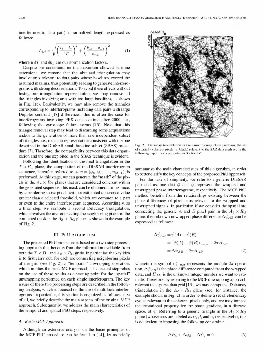
Following the identification of the final triangulation in theT ×B⊥ plane, the computation of the DInSAR interferogramsequence, hereafter referred to as ϕ = (ϕ0, ϕ1, . . . , ϕM−1), isperformed. At this stage, we can generate the “mask” of the pix-els in the AZ ×RG planes that are considered coherent withinthe generated sequence; this mask can be obtained, for instance,by considering those pixels with an estimated coherence valuegreater than a selected threshold, which are common to a partor even to the entire interferogram sequence. Accordingly, asa final step, we compute a second Delaunay triangulation,which involves the arcs connecting the neighboring pixels of thecomputed mask in the AZ ×RG plane, as shown in the exampleof Fig. 2.

III. PHU ALGORITHM

The presented PhU procedure is based on a two-step process-ing approach that benefits from the information available fromboth the T ×B⊥ and AZ ×RG grids. In particular, the key ideais to first carry out, for each arc connecting neighboring pixelsof the grid (see Fig. 2), a “temporal” unwrapping operation,which implies the basic MCF approach. The second step relieson the use of these results as a starting point for the “spatial”unwrapping performed on each single interferogram. The keyissues of these two processing steps are described in the follow-ing analysis, which is focused on the use of multilook interfer-ograms. In particular, this section is organized as follows: firstof all, we briefly describe the main aspects of the original MCFapproach. Subsequently, we address the main characteristics ofthe temporal and spatial PhU steps, respectively.

A. Basic MCF Approach

Although an extensive analysis on the basic principles ofthe MCF PhU procedure can be found in [14], let us briefly

Fig. 2. Delaunay triangulation in the azimuth/range plane involving the setof spatially coherent pixels (in black) relevant to the SAR data analyzed in thefollowing experiments presented in Section IV.

summarize the main characteristics of this algorithm, in orderto better clarify the key concepts of the proposed PhU approach.

For the sake of simplicity, we refer to a generic DInSARpair and assume that ϕ̃ and ψ̃ represent the wrapped andunwrapped phase interferograms, respectively. The MCF PhUmethod benefits from the relationships existing between thephase differences of pixel pairs relevant to the wrapped andunwrapped signals. In particular, if we consider the spatial arcconnecting the generic A and B pixel pair in the AZ ×RG

plane, the unknown unwrapped phase difference ∆ψ̃AB can beexpressed as follows:

∆ψ̃AB = ψ̃(A) − ψ̃(B)

= 〈ϕ̃(A) − ϕ̃(B)〉−π,π + 2πHAB

= ∆ϕ̃AB + 2πHAB (2)

wherein the symbol 〈·〉−π,π represents the modulo-2π opera-tion, ∆ϕ̃AB is the phase difference computed from the wrappeddata, and HAB is the unknown integer number we want to esti-mate. Therefore, by referring to the MCF unwrapping approachrelevant to a sparse data grid [15], we may compute a Delaunaytriangulation in the AZ ×RG plane (see, for instance, theexample shown in Fig. 2) in order to define a set of elementarycycles relevant to the coherent pixels only, and we may imposethe irrotational property for the phase gradient, in a discretespace, of ψ̃. Referring to a generic triangle in the AZ ×RG

plane (whose arcs are labeled as α, β, and γ, respectively), thisis equivalent to imposing the following constraint:

∆ψ̃α + ∆ψ̃β + ∆ψ̃γ = 0 (3)


which can be also expressed, by taking into account of (2),as follows:

Hα + Hβ + Hγ = −[∆ϕ̃α + ∆ϕ̃β + ∆ϕ̃γ

2π

]. (4)

At this stage, the PhU problem can be solved in a veryefficient way by recognizing that a network structure underlinesit and by searching for the network MCF solution [14]. This canbe carried out by choosing the weighted L1 norm for the errorcriterion, via the following minimization problem:

minHp

{NA−1∑p=0

wp · |Hp|}

(5)

subject to the constraints (4), wherein the min{·} symbol rep-resents the minimization operation, NA represents the overallnumber of arcs relevant to the Delaunay triangulation, andw = (w0, . . . , wp, . . . , wNA−1) sets the weights relevant to theweighted L1 norm.

B. Temporal Unwrapping

Let us start our discussion by reconsidering the spatial De-launay triangulation in the AZ ×RG plane (see, for example,the one in Fig. 2) and to assume that, for each given arc, δϕ =(δϕ0, δϕ1, . . . , δϕM−1) and δψ = (δψ0, δψ1, . . . , δψM−1) arethe (measured) wrapped and (unknown) unwrapped DInSARphase-gradient vectors of the DInSAR interferometric se-quence, respectively. Moreover, in order to facilitate theprocedure, we observe that a profitable model of the un-known unwrapped phase gradient vectors can be considered asfollows [6], [7]:

m(∆z,∆v) ≈ 4πλ

·(

∆b⊥r · sin(ϑ)

· ∆z + ∆t · ∆v

)(6)

wherein ∆z accounts for the error in the knowledge of thescene topography while ∆v accounts for the deformation ve-locity variations along the considered spatial arc. Moreover, rrepresents the sensor target distance, λ is the transmitted signalcentral wavelength, and ϑ is the incidence angle. Note that,because of the spatially correlated behavior of the atmosphericartifacts [6], we have assumed in (6) that they do not contributeto the model m(·). Since the wrapped phases differ from theunwrapped ones by 2π-integer multiples only, the DInSARunwrapped vector can be expressed as follows:

δψ = m + 〈δϕ− m〉−π,π + 2πK = δχ+ 2πK (7)

wherein K is the 2π-integer multiple vector and

δχ = m + 〈δϕ− m〉−π,π (8)

represents the phase component, for each considered arc, re-lated to the computed model m(·) and to the measured phasecontribution δϕ.

Note also that, for the sake of simplicity, the explicit depen-dence of m(·) on the ∆z and ∆v factors has been neglected in(7) and (8); this notation will be maintained hereafter.

At this stage, we can evaluate for each (∆z,∆v) pair theunknown vector K in (7) by applying the basic MCF technique(summarized in the previous section) to the T ×B⊥ grid.In particular, we search in this case for the solution of thefollowing minimization problem:

minkj

C =

M−1∑j=0

|kj | (9)

subject to the constraints

kα + kβ + kγ = −round

[δχα + δχβ + δχγ

2π

](10)

wherein kj is the jth element of the K vector in (7). Moreover,the round[·] symbol represents the operation of approximationto the nearest integer number, and, consistent with (3) and (4)in Section III-A, the constraints in (10) are expressed in termsof a generic triangle in the T ×B⊥ plane whose arcs have beenlabeled as α, β, and γ, respectively.

We remark that for each (∆z,∆v) pair, we will havea different solution, which is characterized by its overallnetwork cost

C =M−1∑j=0

|kj |. (11)

Accordingly, by exploring different values of the (∆z,∆v)pair and the corresponding model m in (6), we may finallyidentify the unknown vector

δψopt = δχopt + 2πKopt (12)

characterized by the “overall minimum” cost

Cmin =M−1∑j=0

∣∣∣koptj

∣∣∣ (13)

wherein δχopt and Kopt are the vectors (where koptjand

δχoptjare the jth components, respectively) defined in (7) and

(8) and evaluated in the minimum-cost condition. Accordingly,δψopt in (12) will represent our estimate of the unwrappedvector for the considered arc.

C. Spatial Unwrapping

With regard to this operation, it exploits the unwrappedDInSAR phase differences computed via the previous tem-poral PhU step [see (12)] as a starting point for the spatial-unwrapping operation. This second step is carried out onthe single interferograms through the application of the MCFunwrapping technique [15] summarized in Section III-A. More-over, in this case, we may use the minimum costs of thesolutions achieved in the T ×B⊥ plane, in order to set theweights wp [see (5)] associated to the single arcs. In particular,since the weights represent the confidence on the correctness ofthe achieved solution, we can reasonably assume that, for eachspatial arc, the smaller is the temporal network cost, the larger


Fig. 3. SAR products relevant to the investigated area and represented in theazimuth/range plane. (a) Multilook image. (b) Mask of the spatially coherentpixels (in black) defining the investigated spatial grid. (c) Corresponding spatialDelaunay triangulation. The latter is the same as that in Fig. 2 but it is repeatedfor the sake of completeness.

should be the weight applied within the minimization step[see (5)] involved in the spatial unwrapping. Accordingly, aninverse exponential relationship between the temporal networkcost and the corresponding spatial weight wp has been chosen

wp =

{2S

2Cmin, Cmin < ρ

1, Cmin ≥ ρ(14)

wherein 2S represents the maximum allowed weight, Cmin isthe minimum temporal cost defined in (13), with Cmin < S,and ρ is a threshold value that, based on experimental results,is typically set not greater than 5% of the total number ofinterferograms M .

Following the implementation of this spatial-unwrappingstep, which is carried out for each interferogram, the unwrappedphase can be easily retrieved via the integration of the computedspatial gradients.

IV. RESULTS

In order to investigate the performance of the proposedunwrapping approach, a number of experiments, involving bothreal and simulated data, were carried out. The considered realdata set is relevant to the Central Apennines (Abruzzi, Italy)area [see the multilook image shown in Fig. 3(a)], and iscomposed of 58 acquisitions collected by the ERS 1/2 sensorsbetween August 1992 and October 2002 (see Table I), whichare relevant to track 308 and frame 2755. The space/time datadistribution is the one depicted in Fig. 1(a), while the finaltriangulation is shown in Fig. 1(c); the latter has been obtainedby imposing a maximum spatial and temporal baseline valueof 300 m and 1500 days, respectively, and a Doppler centroidseparation, between the image pair, not larger than 1000 Hz.We further remark that, instead of imposing separate constraintson the maximum allowed spatial and temporal baselines, wecould alternatively consider an upper limit for the normalizedarc length defined in (1). Moreover, the value of the imposedconstraints could be also changed depending on the character-istics of the investigated zone. For instance, larger values couldbe considered in the presence of highly coherent areas, as in thecase of urbanized zones.

TABLE IERS 1/2 SAR DATA SET

Following the triangulation step shown in Fig. 1(c), we haveidentified the sequence of DInSAR interferograms to be gen-erated for implementing the proposed algorithm. In particular,we have computed 145 interferograms with four looks in therange direction and 20 looks in the azimuth one, having apixel spacing of about 90 × 90 m. Note that the number ofinterferograms generated from each SAR image is dependenton the result of the Delaunay triangulation within the T ×B⊥plane (see Fig. 1). In this case, it is evident that acquisitions


Fig. 4. Number of occurrences for each SAR image within the generatedinterferogram data set.

Fig. 5. Distribution of the temporal and spatial baselines relevant to thegenerated interferogram data set.

relevant to the triangulation boundaries are characterized byfewer arcs, i.e., are involved in a smaller number of interfer-ograms; obviously, this effect becomes less significant whenincreasing the number of SAR acquisitions. With regard to ourdata set, we present in Fig. 4 the plot showing the numberof appearances of each SAR image within the interferogramdata set. Note that only two acquisitions contribute to twointerferograms only. Moreover, we also present in Fig. 5 thedistribution of the temporal and spatial baselines obtainedby using our interferogram selection based on the Delaunaytriangulation. We remark that, within the limits we definedas maximum baselines, the interferogram distribution is ratheruniform, which is a relevant issue within the DInSAR scenarios.

Based on the computed interferograms, we have generatedthe coherence mask shown in Fig. 3(b), i.e., the mask of thepixels that are considered coherent in our sequence of multi-look interferograms. In our case, they have been selected byidentifying the pixels that have a coherence, estimated in a boxof four pixels in the range direction and 20 pixels in the azimuthone, greater than 0.35 in at least the 30% of the interferograms.Based on the mask shown in Fig. 3(b), the spatial triangulationhas been generated [see Fig. 3(c)]. We remark that the selectionof this Abruzzi test-site area is related to the difficulty in theunwrapping operation of the relevant interferograms caused

Fig. 6. Examples of the computed DInSAR interferograms and of the corre-sponding coherence maps. (a) and (d) have been computed from the ERS datapair acquired on July 15, 1997 and September 23, 1997, respectively (|∆b⊥| =39 m). (b) and (e) have been computed from the ERS data pair acquired onApril 6, 1999 and September 28, 1999, respectively (|∆b⊥| = 138 m). (c) and(f) have been computed from the ERS data pair acquired on October 28, 1997and January 11, 2000, respectively (|∆b⊥| = 207 m).

by the presence of strong decorrelation phenomena. To givean idea of these effects, we present in Fig. 6 a selection ofcomputed interferograms. It is evident that the impact of thedecorrelation effects can be very strong.

Before discussing in detail the results achieved on the con-sidered real SAR data, we prefer to start our analysis with somesimulations that represent controlled experiments, allowing adirect assessment of the algorithm performance. To this end,we have retained both the AZ ×RG and T ×B⊥ triangulationsshown in Figs. 1(c) and 3(c), respectively. Moreover, the sameinterferogram sequence generated for the real data set has beenproduced in the simulated experiments, but by exploiting thehigh-pass (HP) spatial components of a digital elevation model(DEM) of the area and by introducing a deformation parametricmodel. In particular, the jth interferogram of the simulatedDInSAR sequence, say ϕsj , has the following expression:

ϕsj =4πλ

·[

∆b⊥j

r · sin(ϑ)· h +

(∆tj · vel +

12· ∆t2j · acc

)]j = 0, . . . ,M − 1 (15)

wherein the first term represents the topographic phase con-tribution depending on the DEM height h, while the vel andacc factors are the velocity and acceleration model terms,respectively, the latter representing a significant deviation fromthe assumed model in (6). Moreover, in our experiments, wealso assumed that both the simulated deformation componentshad a Gaussian spatial shape, as shown in Fig. 7, wherein boththe masked and unmasked data are presented.

In order to investigate the algorithm performance on thesimulated data, we unwrapped the generated interferogram


Fig. 7. Maps relevant to the three components of the model presented in(15) and used to generated the simulated DInSAR interferograms. (a) and(d) Unmasked and masked topography maps, respectively (hmin = −327 m,hmax = 428 m). (b) and (e) Unmasked and masked velocity patterns, re-spectively (velmin = −2.83 cm/year, velmax = −0.07 cm/year). (c) and(f) Unmasked and masked acceleration patterns, respectively (accmin =−14.15 cm/year2, accmax = −0.06 cm/year2). Note that the position of theminima of the simulated velocity and acceleration patterns are relatively shiftedby 100 pixels in both directions.

sequence both via the original and the extended MCF tech-niques; obviously, the former has been independently appliedto each single interferogram. In the performed experiments, acomparison between the original and the unwrapped phasesis directly possible. As a result of our analysis, we presentin Fig. 8(a)–(c) the percentage, for each interferogram, ofcorrectly unwrapped pixels of the mask shown in Fig. 3(b),obtained by applying the original MCF technique and consider-ing on the horizontal axis the spatial and temporal baselinesand the normalized arc length, respectively. Moreover, theresults achieved via the extended MCF procedure are shown inFig. 8(d), where the horizontal axis is relevant to the normalizedarc length. The results presented in Fig. 8(a)–(c) clearly showthat, for the original MCF approach, an increase of the spatialand/or of the temporal baseline (thus, of the normalized arclength) may lead to significant degradations of the achievedreconstruction. On the contrary, the extended MCF approachguarantees a very good retrieval, as shown in Fig. 8(d). Withregard to the computational aspects, we remark that, on apersonal computer equipped with an AMD Athlon MP2600+processor, the basic MCF unwrapping procedure required about75 min for unwrapping the overall interferogram sequence,while the extended MCF algorithm needed about 225 min. Weremark that this computational increase is mostly related tothe evaluation of the model function m within the temporal-unwrapping step (see Section III-B). Indeed, this operation iscarried out via an exhaustive search, with a limited spacing, ofthe ∆z and ∆v factors within the intervals (−100, 100) m and(−5, 5) cm/year, respectively. Obviously, the availability of ana priori information on the ∆z and ∆v terms would lead to

Fig. 8. Percentage of the coherent pixels of each interferogram that havebeen correctly unwrapped. (a) Results obtained by applying the original MCFapproach with the horizontal axis relevant to the perpendicular baseline.(b) Same as (a) but with the horizontal axis relevant to the temporal baseline.(c) Same as (a) but with the horizontal axis relevant to the normalized arclength L defined in (1). (d) Results obtained by applying the extended MCFapproach with the horizontal axis relevant to the normalized arc length L.(e) Results obtained by applying the extended MCF approach but without themodel adjustment step; the horizontal axis is relevant to the normalized arclength L.

a significant computational improvement of the extended MCFPhU algorithm performance.

As a final test on our simulated data, we investigated thequality of the retrieved solution if the model adjustment step,relevant to m in (6), is not implemented. In this case, the


Fig. 9. Temporal coherence maps obtained from (a) the original and (b) theextended MCF unwrapping procedures, respectively.

required computing time reduced to about 80 min. However,the achieved results presented in Fig. 8(e) clearly show that thecomputational reduction is “paid” with a considerable degra-dation of the obtained unwrapped data with respect to thosegenerated through the extended MCF approach, with the lattershown in Fig. 8(d).

Let us now move to the real data analysis. In this case,the dimensions of the processed data set are the same as thesimulated signals, thus the computing requirements remainedpractically unchanged; on the contrary, we now had to define aquality index for our results. To achieve this task, we decided touse the SBAS algorithm [7] that, as previously stated, is fullycompatible with the presented data representation and allows usto generate DInSAR deformation time series from a sequenceof unwrapped multitemporal interferograms. In particular, weconsidered the following strategy: first of all, we applied theSBAS procedure to both the unwrapped sequences computedvia the original and the extended MCF algorithm; this allowedus to produce deformation time series for each pixel of the maskshown in Fig. 3(b). Subsequently, we used the computed timeseries (without any atmospheric filtering) and the estimatedtopographic errors to regenerate the original interferogramsreferred to as ϕ = (ϕ0, ϕ1, . . . , ϕM−1). At this stage, we useas quality index of the PhU retrieval the temporal coherencefactor defined for each pixel as follows:

γ =

∣∣∣∣∣M−1∑p=0

exp[j(ϕp − ϕp)

]∣∣∣∣∣M

, 0 ≤ γ ≤ 1. (16)

Note that for pixels where γ → 1, we expect that no unwrap-ping errors are present, since a nearly perfect retrieval of theoriginal phase has been obtained. On the other hand, low valuesof γ will correspond to poorly unwrapped data. Followingthe application of the SBAS algorithm to the two unwrappedDInSAR sequences, obtained through the original and theextended MCF techniques, respectively, we have evaluatedvia (16) the temporal coherence map for both data sets. Theachieved results are shown in Fig. 9(a) and (b), respectively. Theimprovement of the coherence obtained through the application

Fig. 10. Histograms of the temporal coherence maps. (a) The dashed lineis related to the results shown in Fig. 9(a), which are obtained via the basicMCF approach. The continuous line is relevant to those achieved by using theextended MCF approach, which are presented in Fig. 9(b). (b) Same plots as in(a) with the superimposed diamond plot relevant to the results of the extendedMCF approach implemented without 2π multiple corrections, i.e., by assumingKopt = 0 in (12).

of the extended PhU algorithm is evident, particularly in theareas in the lower left and upper right corners of the map.To emphasize the achieved gain, the histograms relevant tothese two results have been computed and superimposed inFig. 10(a); again, the obtained improvement is clear. In partic-ular, we remark that, in this case, we achieved an increase ofabout 60% with regard to the number of pixels with a temporalcoherence value greater than the selected threshold γ = 0.7,which is a typical value in DInSAR applications [20], [21].

As a final point, we have investigated the impact, on theunwrapping algorithm performance, of the Kopt vector com-ponent in (12). To this end, we have repeated the overallprocessing operation based on the extended MCF approach butassuming no 2π integer correction, i.e., with Kopt = 0. Thisimplies that, based on (12), we assumed δψopt = δχopt. Thehistogram of the computed new temporal coherence has beensuperimposed [see Fig. 10(b)] to those shown in Fig. 10(a). Thedegradation of the achieved results is remarkable with respect tothose of the overall extended MCF procedure. In particular, inthis case, we had a reduction of the number of coherent pixels,with γ ≥ 0.7, of about 30% with respect to the extended MCFresults. This clearly indicates the significant impact of the 2πinteger correction component within the proposed unwrappingprocedure.


Fig. 11. Delaunay triangulations in the temporal/perpendicular baseline planerelevant to the ERS SAR data analyzed in the experiments of Section IV.The triangulations are obtained by assuming that the ratio between theperpendicular and temporal baseline axis units is equal to δT/δb⊥, with(a) δT = 1500 days and δb⊥ = 300 m, (b) δT = 900 days and δb⊥ =300 m, and (c) δT = 300 days and δb⊥ = 300 m.

V. CONCLUSION

We have proposed a solution for extending the MCF PhUalgorithm dealing with a sparse data grid [15], to processmultitemporal DInSAR interferograms for the generation of de-formation time series. The approach involves the computationof a properly chosen interferogram sequence and is based on thecascade of two main steps, both involving the use of the basicMCF technique. In particular, we identify first the arcs connect-ing neighboring coherent pixels of the azimuth/range grid, andfor each of these, we estimate the unwrapped phase gradientsvia the MCF technique applied in the temporal/perpendicularbaseline plane. These results are used to bootstrap the subse-quent spatial-unwrapping operation carried out on each sin-gle interferogram via the conventional MCF approach. Thepresented results obtained on simulated and real data confirmthe effectiveness of the approach. Moreover, we underline thatthe proposed solution is naturally compatible with the SBASalgorithm for the generation of deformation time series. Theimplemented extension of the unwrapping procedure is basedon the application of the network-programming algorithm forboth the temporal- and spatial-unwrapping steps. Accordingly,the overall approach is computationally efficient.

As a final remark, we underline that the overall analysishas been focused on multilook interferograms. However, theextension of this technique to the unwrapping of full-resolutionDInSAR interferograms is under development. In this case,the noise phenomena affecting the single-look interferogramsbecome extremely relevant; moreover, at the variance of themultilook case, we cannot benefit from the availability ofan estimated coherence map generated via spatial averaging.Accordingly, an appropriate selection of temporally coherentpixels on the full-resolution interferograms is a crucial issue.We are presently investigating a solution based on the use ofboth multilook and single-look interferograms, which followsthe lines of the full-resolution SBAS approach presented in[22]; this analysis can be a topic for future discussions.

APPENDIX

Let us investigate, in the following, the impact of the differentselection of the δT/δb⊥ factor, which represents the ratiobetween the temporal and perpendicular baseline axis units,which is needed in order to generate the triangulation in theT ×B⊥ plane (see Section II). To achieve this task, we startedfrom the triangulation relevant to our experiments presentedin Section IV, where we have assumed δT = 1500 days andδb⊥ = 300 m. Subsequently, we maintained constant the valueof δb⊥ and considered the two additional cases relevant toδT = 900 days and δT = 300 days, respectively.

The results of the corresponding triangulations, presentedin Fig. 11(a)–(c), respectively, show a strong similarity. Morespecifically, we found that more than 60% of the arcs (thus,of the corresponding interferograms) are common to the threetriangulations. Accordingly, we may finally conclude that,within a realistic range of variation of the δT/δb⊥ ratio,the corresponding triangulations in the T ×B⊥ plane do notsignificantly change.

ACKNOWLEDGMENT

Precise satellite orbits were provided by the University ofDelft, The Netherlands. A Shuttle Radar Topography MissionDEM of the investigated zone has been used for the inter-ferogram generation. The European Space Agency providedthe ERS data relevant to the Abruzzi site through the CAT-1proposal N. 313. The authors would like to thank the reviewersfor their constructive remarks and suggestions.

REFERENCES

[1] A. K. Gabriel, R. M. Goldstein, and H. A. Zebker, “Mapping small ele-vation changes over large areas: Differential interferometry,” J. Geophys.Res., vol. 94, no. B7, pp. 9183–9191, Jul. 1989.

[2] D. Massonnet, M. Rossi, C. Carmona, F. Ardagna, G. Peltzer, K. Feigl,and T. Rabaute, “The displacement field of the Landers earthquakemapped by radar interferometry,” Nature, vol. 364, no. 6433, pp. 138–142, Jul. 1993.

[3] G. Peltzer and P. A. Rosen, “Surface displacement of the 17 Eurekavalley, California, earthquake observed by SAR interferometry,” Science,vol. 268, no. 5215, pp. 1333–1336, Jun. 1995.

[4] D. Massonnet, P. Briole, and A. Arnaud, “Deflation of Mount Etna mon-itored by spaceborne radar interferometry,” Nature, vol. 375, no. 6532,pp. 567–570, Jun. 1995.

[5] E. Rignot, “Fast recession of a west Antarctic glacier,” Science, vol. 281,no. 5376, pp. 549–551, Jul. 1998.


[6] A. Ferretti, C. Prati, and F. Rocca, “Nonlinear subsidence rate estima-tion using permanent scatterers in differential SAR interferometry,” IEEETrans. Geosci. Remote Sens., vol. 38, no. 5, pp. 2202–2212, Sep. 2000.

[7] P. Berardino, G. Fornaro, R. Lanari, and E. Sansosti, “A new algorithmfor surface deformation monitoring based on small baseline differentialSAR interferograms,” IEEE Trans. Geosci. Remote Sens., vol. 40, no. 11,pp. 2375–2383, Nov. 2002.

[8] O. Mora, J. J. Mallorquí, and A. Broquetas, “Linear and nonlinear terraindeformation maps from a reduced set of interferometric SAR images,”IEEE Trans. Geosci. Remote Sens., vol. 41, no. 10, pp. 2243–2253,Oct. 2003.

[9] S. Usai, “A least squares database approach for SAR interferometric data,”IEEE Trans. Geosci. Remote Sens., vol. 41, no. 4, pp. 753–760, Apr. 2003.

[10] C. Werner, U. Wegmuller, T. Strozzi, and A. Wiesmann, “Interferomet-ric point target analysis for deformation mapping,” in Proc. IGARSS,Toulouse, France, Jul. 2003, pp. 4362–4364.

[11] A. Hooper, H. Zebker, P. Segall, and B. Kampes, “A new methodfor measuring deformation on volcanoes and other natural terrains us-ing InSAR persistent scatterers,” Geophys. Res. Lett., vol. 31, no. 23,Dec. 2004, DOI: 10.1029/2004GL021737, CD-ROM.

[12] M. Crosetto, B. Crippa, and E. Biescas, “Early detection and in-depthanalysis of deformation phenomena by radar interferometry,” Eng. Geol.,vol. 79, no. 1/2, pp. 81–91, Jun. 2005.

[13] H. A. Zebker and J. Villasenor, “Decorrelation in interferometric radarechoes,” IEEE Trans. Geosci. Remote Sens., vol. 30, no. 5, pp. 950–959,Sep. 1992.

[14] M. Costantini, “A novel phase unwrapping method based on networkprogramming,” IEEE Trans. Geosci. Remote Sens., vol. 36, no. 3, pp. 813–821, May 1998.

[15] M. Costantini and P. A. Rosen, “A generalized phase unwrapping ap-proach for sparse data,” in Proc. IGARSS, Hamburg, Germany, Jun. 1999,pp. 267–269.

[16] M. Costantini, F. Malvarosa, F. Minati, L. Pietranera, and G. Milillo, “Athree-dimensional phase unwrapping algorithm for processing of multi-temporal SAR interferometric measurements,” in Proc. IGARSS, Toronto,ON, Canada, Jun. 2002, pp. 1741–1743.

[17] A. Pepe and R. Lanari, “A space-time minimum cost flow phase unwrap-ping algorithm for the generation of DInSAR deformation time-series,” inProc. IGARSS, Seoul, Korea, Jul. 2005, pp. 1979–1982.

[18] G. Franceschetti and R. Lanari, Synthetic Aperture Radar Processing.Boca Raton, FL: CRC, Mar. 1999.

[19] N. Miranda, B. Rosich, C. Santella, and M. Grion, “Review of the impactof ERS-2 piloting modes on the SAR Doppler stability,” in Proc. Fringe,Frascati, Italy, Dec. 2003, CD-ROM.

[20] R. Lanari, P. Lundgren, M. Manzo, and F. Casu, “Satellite radarinterferometry time series analysis of surface deformation for LosAngeles, California,”Geophys. Res. Lett., vol. 31, no. 23, Dec. 2004, DOI:10.1029/2004GL021294, CD-ROM.

[21] A. Borgia, P. Tizzani, G. Solaro, M. Manzo, F. Casu, G. Luongo,A. Pepe, P. Berardino, G. Fornaro, E. Sansosti, G. P. Ricciardi, N. Fusi,G. Di Donna, and R. Lanari, “Volcanic spreading of Vesuvius, a new par-adigm for interpreting its volcanic activity,” Geophys. Res. Lett., vol. 32,no. 3, Feb. 2005, DOI: 10.1029/2004GL022155, CD-ROM.

[22] R. Lanari, O. Mora, M. Manunta, J. J. Mallorquí, P. Berardino, andE. Sansosti, “A small baseline approach for investigating deformationson full resolution differential SAR interferograms,” IEEE Trans. Geosci.Remote Sens., vol. 42, no. 7, pp. 1377–1386, Jul. 2004.

Antonio Pepe was born in Salerno, Italy, in 1974. Hereceived the laurea degree in electronic engineeringfrom the University of Napoli “Federico II,” Naples,Italy, in 2000, with a thesis on the synthetic apertureradar (SAR) image processing. He is currently work-ing toward the Ph.D. degree at the same institution.

He joined the Istituto per il Rilevamento Elet-tromagnetico dell’Ambiente (IREA), Institute of theItalian National Research Council (CNR), Naples, in2002. Since 2003, he has been with the Departmentof Electronic and Telecommunication Engineering,

University of Napoli. In 2005, he was a Visiting Research at the Aerospace En-gineering and Engineering Mechanics, The University of Texas at Austin. Hisresearch interests concern the differential SAR interferometry applications forthe monitoring of surface displacements, such as those produced by subsidence,volcano activity, and earthquakes.

Riccardo Lanari (M’91–SM’01) was born in 1964.He received the degree in electronic engineering(summa cum laude) from the University of Napoli,“Federico II,” Naples, Italy, in 1989.

After graduation, he joined the Istituto di Ricercaper l’Elettromagnetismo e i Componenti Elletronici(IRECE), now the Istituto per il Rilevamento Elettro-magnetico dell’Ambiente (IREA), a Research Insti-tute of the Italian National Research Council (CNR),where he currently occupies the position of SeniorResearcher. He has been a Visiting Scientist at dif-

ferent foreign research institutes. He was a Research Fellow at the Instituteof Space and Astronautical Science, Japan in 1993; a Visiting Scientist at theGerman Aerospace Research Establishment (DLR), in 1991 and 1994, and atthe Jet Propulsion Laboratory, in 1997. He has lectured in several national andforeign universities and research centers and is currently a Lecturer of the SARmodule course of the International Master in Airborne Photogrammetry andRemote Sensing, offered by the Institute of Geomatics in Barcelona, Spain.He is the holder of two patents on SAR data-processing techniques. His mainresearch interests are in the synthetic aperture radar data-processing field aswell as in SAR interferometry techniques. On these fields, he has authored 40international journal papers, and, in 1999, he authored a book entitled SyntheticAperture Radar Processing (CRC Press, 1999).

Mr. Lanari received a NASA recognition for the development of theScanSAR processor used for the SRTM mission. He has been invited as Chair-man and Cochairman at several international conferences and as a member ofthe Technical Program Committee for the IGARSS’2000 symposia.

Documents

On the extension of the minimum cost flow algorithm for phase unwrapping of multitemporal differential SAR interferograms