arX

iv:c

ond-

mat

/030

4288

v2 [

cond

-mat

.sta

t-m

ech]

1 M

ar 2

004

On singular probability densities generated by extremal

dynamics

Guilherme J. M. Garcia∗ and Ronald Dickman†

Departamento de Fısica, Instituto de Ciencias Exatas

Universidade Federal de Minas Gerais, Caixa Postal 702

CEP 30123-970, Belo Horizonte - Minas Gerais, Brazil

(February 2, 2008)

Abstract

Extremal dynamics is the mechanism that drives the Bak-

Sneppen model into a (self-organized) critical state, marked by

a singular stationary probability density p(x). With the aim of

understanding of this phenomenon, we study the BS model and

several variants via mean-field theory and simulation. In all cases,

we find that p(x) is singular at one or more points, as a con-

sequence of extremal dynamics. Furthermore we show that the

extremal barrier xi always belongs to the ‘prohibited’ interval, in

which p(x) = 0. Our simulations indicate that the Bak-Sneppen

universality class is robust with regard to changes in the updating

rule: we find the same value for the exponent π for all variants.

Mean-field theory, which furnishes an exact description for the

model on a complete graph, reproduces the character of the prob-

ability distribution found in simulations. For the modified pro-

cesses mean-field theory takes the form of a functional equation

for p(x).

PACS: 05.65.+b, 02.30.Ks, 05.40.-a, 87.10.+e

keywords: extremal dynamics; Bak-Sneppen model; mean-field

theory; functional equations; universality

∗ Electronic address: gjmg@fisica.ufmg.br† Electronic address: dickman@fisica.ufmg.br

Corresponding author: Ronald Dickman

telephone: 55-31-3499-5665

FAX: 55-31-3499-5600

1

I. INTRODUCTION

The Bak-Sneppen (BS) model was proposed as a possible explanation ofmass extinctions observed in the fossil record [1], and was recently adapted tomodel experimental data on bacterial populations [2,3]. Independent of its bi-ological interpretation, the model has atracted much attention as a prototypeof self-organized criticality (SOC) under extremal dynamics [4,5]. The modelhas been studied through various approaches, including simulation [6–8], theo-retical analysis [9–11], probabilistic analysis (run time statistics) [12,13], renor-malization group [14,15], field theory [16] and mean-field theory [4,5,17]. Somevariants have been proposed, for example the anisotropic BS model [18,19]. Inthis paper, we study the consequences of extremal dynamics, using mean-fieldtheory and simulation. With this aim, we propose variants of the model andanalyse how varying the updating rule affects the stationary probability den-sity and the critical behaviour.

In the evolutionary interpretation of the BS model, each site i represents a“niche” occupied by a single species, and bears a real-valued variable xi repre-senting the “fitness” of this species. (In the present context “fitness” denotesa propensity to resist extinction: if xi > xj then species j goes extinct before i,so that xi may be termed a “barrier to extinction”.) At each step the site withthe smallest xi, and its nearest neighbors, are replaced with randomly chosenvalues. The replacement of the neighboring variables with new random valuesmay be interpreted as a sudden unpredictable change in fitness when a nearbyniche (which might have borne a predator, or a food source for the speciesin question), is suddenly colonized by a new species. Selection, at each step,of the global minimum of the {xi} (“extremal dynamics”) represents a highlynonlocal process, and would appear to require an external agent with completeinformation regarding the state of the system at each moment. Applicationsof the model in evolution studies are reviewed in [20].

In the original updating rule, neighbors are randomly affected by the ex-tinction of an interacting species. There is no a priori reason to expect thatevolution should obey this specific rule on a specific lattice. Thus, we ask:what happens if the extinction of the least adapted species favors (or pre-vents) the extinction of other species? Moreover, what is the signature ofextremal dynamics that can, in principle, allow us to recognize it in the realworld?

Due to extremal dynamics, the BS model exhibits scale invariance in thestationary state, in which several quantites display power-law behaviour [1].Simulations show that the stationary distribution of barriers follows a stepfunction, being zero (in the infinite-size limit) for x < x∗ ≃ 0.66702(8) [6].Relaxing the extremal condition leads to a smooth probability density andloss of scale invariance [4,5].

A striking feature of the BS model is that a simple updating rule leads to asingular stationary probability density p(x). An intriguing question thereforearises, as to how changes in the updating rule affect this density, an issue that

2

has not, to our knowledge, been investigated previously. In this work we exam-ine the consequences of rules in which one or more sites are updated accordingto x → x′ = f(x), instead of being replaced by a random number. (Heref maps the interval [0,1] to itself.) We find that this can provoke dramaticchanges in the stationary probability density. In the extremal dynamics limit,the variant models belong to the same universality class as the original. Wefind that the hallmarks of extremal dynamics are that i) the stationary prob-ability density is singular, and ii) with probability one, the extremal xi (i.e.,the next variable to be updated) belongs to the ‘prohibited’ region in whichp(x) = 0. Using a two-site mean-field approximation, we also find evidencethat nontrivial correlations are restricted to the prohibited region.

The balance of this paper is organized as follows. Section II introduces themodels, which are then analyzed using mean-field like approaches in Sec. III.In Sec. IV we present simulation results, and summarize our conclusions inSec. V.

II. MODELS

The Bak-Sneppen [1] model is a discrete-time Markov process on a d-dimensional lattice of Ld sites, with periodic boundaries. At each site wedefine a real-valued variable xi(0). Initially, these variables are independentlyassigned random values uniform on [0,1). At time 1, the site m bearing theminimum of all the numbers {xi(0)} is identified, and it, along with its 2d near-est neighbors, are given new random values, again drawn independently fromthe interval [0,1). (In the one dimensional case considered here this amountsto: xm(1) = η, xm+1(1) = η′, and xm−1(1) = η′′, where η, η′, and η′′ are inde-pendent and uniformly distributed on [0,1); for |j − m| > 1, xj(1) = xj(0).)At step 2 this process is repeated, with m representing the site with the globalminimum of the variables {xi(1)}, and so on. In the random neighbor versionof the model, the process is realized on a complete graph (all sites are con-sidered neighbors); two randomly selected sites are updated in addition to theminimum m.

We now define three modified Bak-Sneppen models, that differ from theoriginal only in the way that the barriers xi evolve. In one, the site M bearingthe maximum of the {xi} is replaced with a random number η and the twonearest neighbors are replaced with their own square roots: xM (t+1) = η and

xM±1(t + 1) =√

xM±1(t). We shall refer to this as the ‘radical’ variant. Inthe second variant, the site with the maximum value is replaced by its ownvalue squared, while its two nearest neighbors receive random numbers η andη′: xM(t + 1) = [xM(t)]2, xM+1(t + 1) = η, and xM−1(t + 1) = η′. This willbe called the ‘centered square’ version. Finally, we define a ‘peripheral square’variant, in which one of the nearest neighbors of M is squared, while M andits other neighbor are replaced with random numbers: xM ′(t + 1) = [xM ′(t)]2,xM(t + 1) = η and xM ′′(t + 1) = η′. (Here M ′ = M + σ and M ′′ = M − σ,

3

where σ is a random variable that assumes values of +1 and -1 with equalprobability.)

The motivation for studying these variants is twofold. First, the Bak-Sneppen model is notable for exhibiting a singular stationary probability den-sity, and it is of interest to examine the effect of changes in the dynamicalrule on this density and on the critical behavior. If we introduce a determin-istic function f(x) as part of the updating rule, it is desirable that f mapthe interval [0,1] to itself, making functions of the form f(x) = xα a naturalchoice. In this context we note that the variants feature what may be called‘migration’, that is, the systematic movement of certain variables xi withinthe interval [0, 1). In the radical variant the migration is from the populatedregion (smaller x) to the ‘excluded’ region (larger x), whereas in the squareversions migration occurs in the opposite direction.

Secondly, the variants admit interpretation as evolutionary processes. (Inthe modified models, we have for convenience defined the site with the maxi-mum variable as the most vulnerable, so that small xi now corresponds to highfitness.) In the radical variant, replacement of the least-fit species provokes areduction in the fitness of its neighbors, without leading to their immediateextinction. Thus, some memory of the fitness of the neighboring species isretained. The radical variant therefore seems a plausible modification of theoriginal model, in the biological context. In the peripheral square variant theextinction of the least-fit species provokes extinction of one neighbor, and in-creased fitness of the other. Finally, in the centered-square variant, xM → x2

M

represents an increase in the fitness of the least viable element of the system,while its neighbors go extinct.

III. MEAN-FIELD THEORY

A. Original Model

We develop mean-field approximations for the original and modified mod-els, along the lines of Refs. [4] and [5]. To begin, we relax the extremal conditionintroducing a flipping rate of Γe−βxi at site i, where Γ−1 is a characteristic time,irrelevant to stationary properties, and which we set equal to one (Γ = 1). Callthis regularized system the ‘finite-temperature’ model. The extremal dynamicsof the original model is recovered in the zero-temperature limit, β → ∞.

Consider the probability density p(x). In the finite-temperature version ofthe original model, p(x) satisfies

dp(x, t)

dt= −e−βxp(x, t) − 2

∫ 1

0e−βyp(x, y, t)dy + 3

∫ 1

0e−βyp(y, t)dy , (1)

where p(x, y, t) is the joint density for a pair of nearest-neighbor sites andp(y, t) is the one-site marginal density. Invoking the mean-field factorizationp(x, y) = p(x)p(y) (we suppress the time argument from here on), we find:

4

dp(x)

dt= −[e−βx + 2I(β)]p(x) + 3I(β) , (2)

where

I(β) ≡∫ 1

0e−βyp(y)dy , (3)

represents the overall flipping rate. Eq. (2) is a nonlinear equation for p, inwhich the density at x is coupled to p at all other arguments via I(β).

In the stationary state we have

p(x) =3I

2I + e−βx. (4)

Multiplying by e−βx and integrating over the range of x, we find

I(β) = (e2β/3 − 1)/[2eβ(1 − e−β/3)], (5)

and thus

pst(x) =3

2

1 − e−2β/3

1 − e−2β/3 + e−βx(eβ/3 − 1). (6)

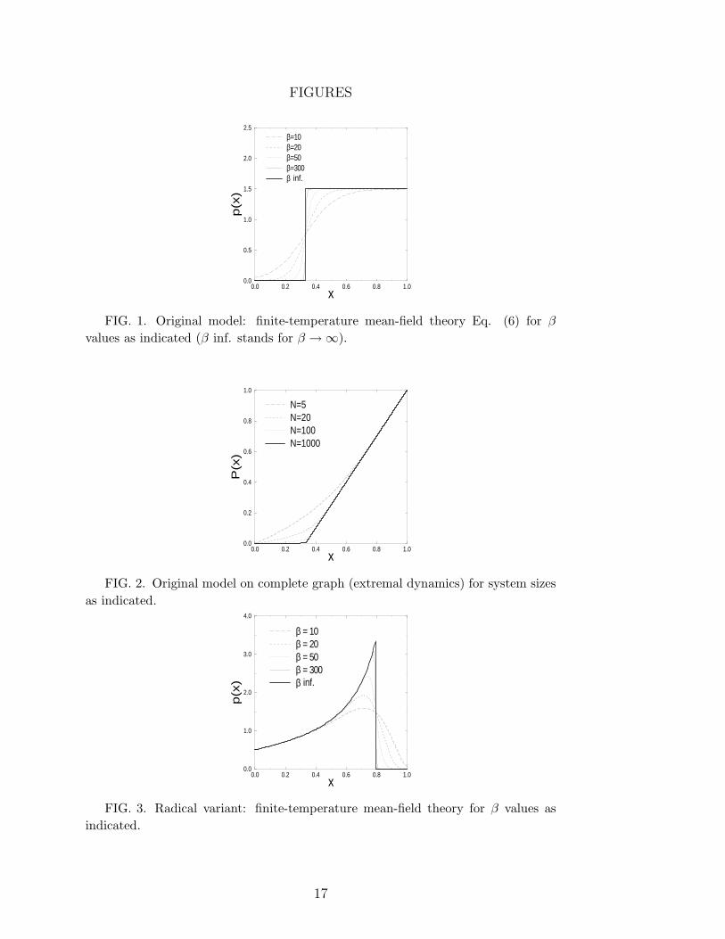
This solution is plotted for various β values in Fig. 1.In the limit β → ∞ the solution becomes a step function:

pst(x) =3

2Θ(x − 1/3)Θ(1 − x) . (7)

Thus the mean-field approach correctly predicts a step-function singularity forthe probability density, although it places the critical barrier at x∗ = 1/3,whereas it actually falls at 0.66702(8) [6]. On the other hand, the slightestrelaxation of the extremal condition destroys the singularity [5], since p(x) isa smooth function for β < ∞. The rate of convergence to the step-functionis generally exponential with β, away from the discontinuity. The curves forvarious β values exhibit an approximate crossing near x = 1/3. The derivativeat this point however diverges only linearly with β: (dpst/dx)x=1/3 ≃ 3β/8 forlarge β.

Using Eq. (2), we find, in the limit of large β, that the relaxation time fora small disturbance from the stationary solution grows ∼ eβ/3. (By ‘small’ wemean I(β) ≃ e−β/3/2.)

The following observation will prove useful in the discussion of the modifiedmodels. If we assume that, in the limit β → ∞, pst(x) is identically zero forx < x∗, and that pst ≥ C > 0 on some interval [x∗, a] (in other words, thedensity suffers a jump discontinuity at x∗), then I =

∫ 10 e−βyp(y)dy ∼ e−βx∗

and so e−βx/I ∼ e−β(x−x∗) → 0 for x > x∗. Then Eq. (4) reduces to the step-function expression, Eq. (7). Note however that limβ→∞ eβx∗

I(β) = 1/2 not3/2β, as would be found by naively inserting the limiting density, Eq.(7), inEq.(3). This means that the dominant contribution to I is due to the interval

5

[0, x∗], even in the limit β → ∞, which is readily seen if we write Eq.(6), forlarge β, as

pst(x) ≃ 3

2[Θ(x − x∗) + Θ(x∗ − x)eβ(x−x∗)] . (8)

In the limit β → ∞, sites with x < x∗ constitute a set of probability zero, butthe site m selected for extinction belongs to this set with probability one. Thisis a singular property of the Bak-Sneppen model in the infinite-size limit, asdiscussed in the next subsection. (The infinite-size limit is implicit in mean-field theory.)

Although in the modified models we are unable to find an analytical solu-tion for finite β, it is possible to integrate the mean-field equation numerically.Due to the factor eβx, for large β, a very small time step would be neededto avoid instability in the usual integration methods (e.g., Euler or Runge-Kutta). We circumvent this difficulty using a partial integration method [21].To apply this method to the MF equation for the original model, we write Eq.(2) in the form

dp(x, t)

dt= −f(t)p(x, t) + g(t) , (9)

where f(t) = e−βx + 2I(t) and g(t) = 3I(t). The formal solution is

p(x, t) = exp[−∫ t

0duf(u)]

{

p(x, 0) +∫ t

0dt′ exp

[

∫ t′

0dt′′f(t′′)

]

g(t′)

}

. (10)

For a small time interval ∆t, we find

p(x, ∆t) ≃ e−f(0)∆t

{

p(x, 0) + g(0)∫ ∆t

0dt′ef(0)t′

}

= e−f(0)∆tp(x, 0) +g(0)

f(0)(1 − e−f(0)∆t) . (11)

This relation can be iterated to find the evolution of p(x, t) from a given initialdistribution, which converges to the stationary density.

B. BS model on a finite complete graph

Mean-field theory is exact for the “random neighbor” model, which mayalso be thought of as the BS model on a complete graph, i.e., one in which allpairs of sites are neighbors. (When xm is updated, two of these neighbors arechosen at random for updating as well.) In this subsection we analyze the BSmodel with extremal dynamics on a complete graph of N sites.

Since sites are assigned independent random numbers, the xi are indepen-dent, identically distributed random variables drawn from the density p(x, t).Define the distribution function P (x, t) =

∫ x0 p(y, t)dy. The probability that

the next site to be updated, xm, lies between zero and x is:

6

Prob[xm ≤ x] = 1 − [1 − P (x)]N , (12)

i.e., one less the probability that the minimum is larger than x. The probabilitythat a randomly chosen neighbor has xi ≤ x is simply P (x), and the probabilitythat one of the updated sites receives a number ≤ x is x. At each step,therefore, the expected change in the number of sites with xi ≤ x is 3x −2P (x) − Prob[xm ≤ x], which implies

dP (x, t)

dt= −

{

1 − [1 − P (x)]N}

− 2P (x) + 3x . (13)

(Here we have taken the time unit to represent N updates.)Letting Q ≡ 1 − P , we have in the stationary state,

QN + 2Q − 3(1 − x) = 0. (14)

(Note that Q(0) = 1, Q(1) = 0, and dQ/dx ≤ 0.) Numerical solution (Fig.2) shows that for large N , PN(x) approaches a singular function that is zerofor x < 1/3, while for x > 1/3, P (x) = 3(x − 1/3)/2. It is straightforward toshow that for fixed x and N → ∞,

P (x) ≃

1 − (1 − 3x)1/N , x < 1/3

3x−12

+ 12[32(1 − x)]N , x > 1/3.

(15)

For x = 1/3 we have ln P ≃ − ln N + ln ln(N/2) (plus terms of lower order inN) as N → ∞. Of interest is the exponential convergence of P to its limitingform for x > 1/3, compared with algebraic convergence for x < 1/3. Note alsothat Prob[xm ≤ 1/3] ≃ 1 − 2/N , so that the minimum indeed belongs to theexcluded region with probability one, when N → ∞.

C. Pair approximation

The analysis of the finite-temperature model is readily extended to thepair level, in which one studies the evolution of the two-site joint probabilitydensity p(x, y). Our starting point is the following exact relation, obtainedusing the same reasoning that led to Eq. (1):

dp(x, y)

dt= −

(

e−βx + e−βy)

p(x, y) −∫ 1

0e−βu [p(x, y, u) + p(u, x, y)]du

+∫ 1

0

∫ 1

0

(

e−βu + e−βv)

p(u, v)dudv

+∫ 1

0

∫ 1

0[p(x, u, v) + p(v, u, y)] e−βvdudv . (16)

Now invoking the pair factorization,

p(x, y, u) ≃ p(x, y)p(y, u)

p(y), (17)

7

Eq. (16) becomes

dp(x, y)

dt= −

[

e−βx + e−βy + K(x) + K(y)]

p(x, y) + 2I

+∫ 1

0[p(x, u) + p(y, u)]K(u)du , (18)

with

K(x) = J(x)/p(x), (19)

J(x) =∫ 1

0p(x, u)e−βudu (20)

and

I =∫ 1

0p(x)e−βxdx =

∫ 1

0J(x)dx . (21)

To find the stationary solution numerically, we note that

p(x, y) =2I +

∫ 10 [p(x, u) + p(y, u)]K(u)du

e−βx + e−βy + K(x) + K(y). (22)

Starting from an arbitrary normalized density p0 (for example, uniform on[0, 1]× [0, 1]), we generate p1 by evaluating the r.h.s. of Eq. (22) using p0 andnormalizing the resulting expression. This procedure is then iterated until itconverges to the stationary density. We find that for large β, the stationarymarginal density approaches the step-function solution

p(x) =1

1 − x∗Θ(x − x∗)Θ(1 − x) (23)

with x∗ ≃ 0.47186, a considerable improvement over the site approximation. Inthis limit, the joint distribution is the product of two identical one-site distri-butions. Once again, the portion of the unit square that has probability zero isin fact responsable for all transitions. In the region D ≡ {(x, y)|0 < x, y < x∗},the two variables are correlated, as shown by the nonzero correlation coeffi-

cient ρ ≡ cov(x, y)/√

var(x)var(y). In the pair approximation, ρ ≃ 0.327 for

(x, y) ∈ D, as β → ∞.

D. Radical Variant

In the radical model, the probability density p(x) = pX(x) satisfies:

dpX(x)

dt= −eβxpX(x) − 2

∫ 1

0eβypX(x, y)dy +

∫ 1

0eβypX(y)dy

+ 2pX1/2(x)∫ 1

0eβypX(y)dy , (24)

8

where pX1/2(x) = 2xpX(x2). With the definition I(β) ≡ ∫ 10 eβyp(y)dy and the

mean-field assumption p(x, y) = p(x)p(y), Eq. (24) reduces to

dp(x)

dt= −eβxp(x) + I(β)[−2p(x) + 1 + 4xp(x2)] . (25)

Given the step-function form of the stationary density for the originalmodel, it is reasonable to expect that in this case as well, p(x) will have ajump discontinuity for β → ∞, and be zero for x > x∗. We can get someinsight into the nature of the density as β → ∞ by first observing that ifp(x) ≤ C < ∞ as x → 1, then I ∼ Ceβ/β for large β, and therefore e−βI → 0as β → ∞. This in fact holds unless p(x) has a δ-like contribution at x = 1,which is not expected since it is precisely the largest values of x that areremoved in the dynamics. Write the stationary solution to Eq. (25) as

p(x) =I[1 + 4xp(x2)]

1 + 2I, (26)

with I = e−βxI. This gives p(1) = 0 in the limit β → ∞. Similarly, supposingthat xp(x2) → 0 as x → 0, we have p(0) = 1/2 in this limit. A similar line ofreasoning can be used to show that dp/dx|x=1 = 0 in the β → ∞ limit.

The preceding discussion suggests that in the limit β → ∞, pst(x) is iden-

tically zero over some finite range [x∗, 1]. Assuming this to be so, we haveI ∼ eβx∗

and in the limit β → ∞ the stationary solution is given by thefunctional equation:

2p(x) − 4xp(x2) = 1 , (27)

for 0 ≤ x < x∗. Writing this as p(x) = 1/2 + 2xp(x2), we can iterate to findp(x2) = 1/2 + 2x2p(x4), p(x4) = 1/2 + 2x4p(x8), p(x8) = 1/2 + 2x8p(x16), etc.,which suggests the solution

p1(x) =1

2+ x + 2x3 + 4x7 + 8x15 + ... =

∞∑

i=0

2i−1x2i−1 . (28)

Substituting this ‘lacunary series’ in Eq.(27), one readily verifies that p1(x)is a solution. Similarly, rewriting Eq.(27) as p(x2) = −1/4x + p(x)/2x, onefinds p(x) = −1/4x1/2 + p(x1/2)/2x1/2, p(x1/2) = −1/4x1/4 + p(x1/4)/2x1/4,etc., leading to a second solution:

p2(x) = − 1

4x1/2− 1

8x3/4− 1

16x7/8− 1

32x15/16− ... = −

∞∑

i=1

2−(i+1)x−(1−2−i) .

(29)

We now search a solution of the form p(x) = Ap1(x)+Bp2(x); substitutingin Eq. (27), yields the condition A + B = 1. This linear combination musthowever be normalizable. The relevant integrals are:

9

∫ x∗

0p1(x)dx =

1

2

∞∑

n=0

x∗2n

=1

2(x∗ + x∗2 + x∗4 + x∗8 + ...) , (30)

∫ x∗

0p2(x)dx = −1

2

∞∑

n=1

x∗2−n

= −1

2(1 + x∗1/2 + x∗1/4 + x∗1/8 + ...) . (31)

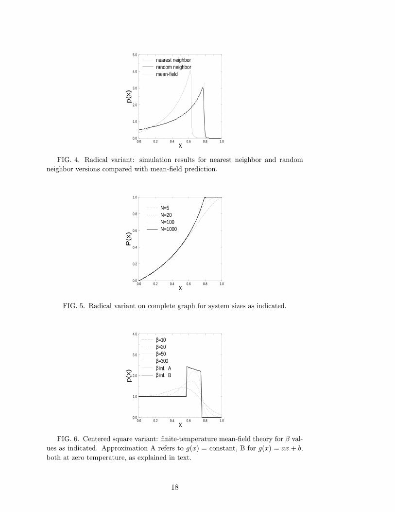
Since 0 < x∗ < 1, the first integral converges while the second diverges, so thatp2(x) is not normalizable, implying B = 0. A normalized, positive solutionis p(x) = p1(x) for x < x∗ = 0.793189 and p(x) = 0 for x > x∗. (x∗ isdetermined by normalization.) This solution, for infinite β, is plotted in Fig.3. Numerical integration of Eq. (25) through the method outlined in Sec.IIIA yields results consistent with this solution, as may again be seen in thefigure. Finally, simulation of the random-neighbor version of the model yieldsa stationary distribution consistent with this expression (see Fig. 4).

We will now analyze the radical model on a finite complete graph and showthat its probability density (equation 28) can be derived via a different path.Define the distribution function Q(x, t) =

∫ 1x p(y, t)dy. By the same reasoning

developed in section IIIB, the probability that xm, the next site to be updated,lies between x and 1 is

Prob[xm ≥ x] = 1 − [1 − Q(x)]N . (32)

The probability that a randomly chosen neighbor has xi ≥ x is Q(x), while theprobability that a neighbor receives a barrier ≥ x is Q(x2). The probabilitythat xm receives a new value between x and 1 is simply 1 − x. The expectedchange in the number of sites with xi ≥ x is (1− x) + 2Q(x2)− 2Q(x) − {1−[1 − Q(x)]N}, so that

dQ(x, t)

dt= (1 − x) + 2Q(x2) − 2Q(x) −

{

1 − [1 − Q(x)]N}

. (33)

In the sationary state, the definition P ≡ 1 − Q leads to

x + 2P (x2) − 2P (x) − P (x)N = 0 . (34)

(Note that P (0) = 0 and P (1) = 1). Since 0 ≤ P (x) < 1 for x < x∗,limN→∞ P (x)N = 0 and the probability density in an infinite system obeys thefunctional equation x + 2P (x2)− 2P (x) = 0. Using the iterative approach, wefind two solutions, one divergent (which is rejected), and the finite solution

P (x) =1

2

∞∑

n=0

x2n

, (35)

i.e., the integral of p1(x), Eq. (28). Normalization then demands that P = 1for x ≥ x∗.

Numerical solution of equation (33) (see Fig. 5) shows that, for large N ,PN(x) approaches the singular function described above. For fixed x > x∗1/2,and N → ∞, we find P (x) ≃ 1 − x1/N .

10

E. Centered Square Variant

The probability density in the finite-temperature version of the centeredsquare variant obeys:

dpX(x)

dt= −eβxpX(x) − 2

∫ 1

0eβypX(x, y)dy + 2

∫ 1

0eβypX(y)dy +

eβ√

x

2√

xpX(

√x) .

(36)

Mean-field factorization leads to

dp(x)

dt= −eβxp(x) − 2I(β)[p(x) − 1] +

eβ√

x

2√

xp(√

x) , (37)

with I(β) as defined in Sec. IIID. In the stationary state, we find

p(x) =2 + 1

2√

xp(√

x)eβ√

x/I

2 + eβx/I. (38)

The hypothesis that in the limit β → ∞ , the stationary density p(x) = 0 forx > x∗ implies I(β) ∼ eβx∗

. Therefore

limβ→∞

eβx

I=

{

0 if x < x∗

∞ if x > x∗ (39)

and

limβ→∞

eβ√

x

I=

{

0 if x < x∗2

∞ if x > x∗2 (40)

This, combined with Eq. (38), implies that p(x) = 1 for x ∈ [0, x∗2], andthat

p(x) = limβ→∞

[

1 +1

4√

x

eβ√

x

Ip(√

x)

]

for x ∈ [x∗2, x∗] (41)

The iterative process used in the preceding section is not useful here as it leadsto pathological solutions, due to the divergent ratio eβ

√x/I in this interval.

Observe that if, for x ∈ [x∗, x∗1/2], p(x) = g(x2)I/eβx, as β → ∞, with g(x2)finite, then p(x) = 1 + g(x)/4

√x for x ∈ [x∗2, x∗]. (Note that this means

that p(x) → 0 as β → ∞ for x in the interval [x∗, x∗1/2], consistent withthe hypothesis that p(x) → 0 for x > x∗.) The function g(x) is howeveryet to be determined. Attempting the simplest solution, g(x) = constant,we find a surprisingly reasonable result, as shown in Fig. 6. Next, allowingg(x) = ax + b, with a and b constant, yields excellent agreement with thenumerical integration of Eq. (37) as also shown in Fig. 6. We do not have anargument why g(x) should take this form.

11

The threshold x∗ can be determined in a simple way. Since the fractionof barriers in the interval [x∗, 1] is constant in the stationary state, the meannumber of barriers removed from this interval at each time step must equalthe mean number inserted. The probability that the maximum xM lies in[x∗, 1] is 1, while its random neighbors are certainly below x∗. Each updatedneighbor has a probability (1−x∗) of receiving a barrier in the interval [x∗, 1],while the maximum remains in [x∗, 1] with probability p1, the probability thatxM ∈ [x∗1/2, 1]. Thus, we have

1 = 2(1 − x∗) + p1 . (42)

This reasoning can be repeated for the intervals [x∗1/2, 1], [x∗1/4, 1], ...,leading to

p1 = 2(1 − x∗1/2) + p2 , (43)

p2 = 2(1 − x∗1/4) + p3 ... (44)

where pn is the probability that xM ∈ [x∗1/2n

, 1]. Substituting this result inequation (42), we find

1 = 2(1 − x∗) + 2(1 − x∗1/2) + 2(1 − x∗1/4) + 2(1 − x∗1/8) + ... , (45)

which provides x∗ = 0.761072. Finally, we note that normalization implies∫ x∗

x∗2 g(x)/4√

x dx = 1 − x∗ = 0.238928, providing a constraint on the functiong(x).

F. Peripheral Square Variant

We now apply the mean-field analysis to the peripheral square variant. Inthis case, the probability density satisfies:

dpX(x)

dt= −eβxpX(x) − 2

∫ 1

0eβypX(x, y)dy + 2

∫ 1

0eβypX(y)dy

+ pX2(x)∫ 1

0eβypX(y)dy , (46)

where pX2(x) = pX(x1/2)/2x1/2. Under the mean-field factorization this re-duces to

dp(x)

dt= −eβxp(x) + I(β)[−2p(x) + 2 +

1

2x1/2p(x1/2)] , (47)

with I(β) as given in Sec. IIIC. The hypothesis that, for β → ∞, the stationarydensity p(x) = 0 for x > x∗ implies I(β) ∼ eβx∗

, leading to the functionalequation:

p(x) − 1

4x1/2p(x1/2) = 1 (β → ∞) , (48)

12

for x < x∗.As in the centered-square variant, the iterative method does not yield a

useful solution, and we pursue a different approach. Let p(x) = f(x) on theinterval x∗2 ≤ x < x∗, where the function f(x) and the constant x∗ are yet tobe determined. Using Eq. (48), we find that

p(x) = 1 +f(x1/2)

4x1/2for x∗4 ≤ x < x∗2 , (49)

p(x) = 1 +1

4x1/2+

f(x1/4)

42x3/4for x∗8 ≤ x < x∗4 , (50)

p(x) = 1 +1

4x1/2+

1

42x3/4+

f(x1/8)

43x7/8for x∗16 ≤ x < x∗8 , etc. (51)

Thus we have found a family of solutions p(x) to Eq.(48), which is quite generalsince f(x) is still undetermined.

We now show that f(x) = 1 on the interval [x∗2, x∗). To begin, we notethat in the stationary state, Eq. (47) implies

(

eβx

I+ 2

)

p(x) = 2 +p(√

x)

2√

x. (52)

In particular, for x = 1 we have

(

eβ

I+

3

2

)

p(1) = 2 , (53)

so that if I ≃ Aeβx∗

, then p(1) ≃ 2Ae−β(1−x∗). It is readily seen that p(x) ≃2Ae−β(x−x∗) satisfies Eq. (52) for x∗ < x ≤ 1. The same equation then leadsto p(x) = 1 as β → ∞, for x∗2 < x < x∗. We may then develop the fullsolution using Eqs. (49) to (51); normalization implies x∗ = 1/2. The resultis the function p(x) plotted in Fig. 7, which is in good agreement with thedensity found via simulation of the random-neighbor model. This solution isdiscontinous at x∗, x∗2, x∗4,..., and exhibits an integrable divergence at x = 0.

The value of x∗ can be confirmed through the reasoning developed in pre-vious subsection for the peripheral square model, which in this case implies1 = 2(1 − x∗) so that x∗ = 1/2.

IV. NUMERICAL SIMULATION AND CRITICAL EXPONENTS

We now compare the mean-field theory predictions with simulation results.We estimate the probability density p(x) on the basis of a histogram of barrierfrequencies, dividing [0,1] into 100 subintervals. Histograms are accumulatedafter Nst time steps, as required for the system (a ring of N sites) to relaxto the stationary state. In order to improve statistics, we average over Nr

realizations.

13

The simulation results for the original BS model are shown in Fig. 8. Weobserve qualitative agreement between nearest-neighbor (NN) and random-neighbor (RN) versions. (The simulation parameters are: N = 1000, Nst =106, Nr = 103 (NN); N = 2000, Nst = 105, Nr = 103 (RN).) Here and in allother cases, the simulation result for the random neighbor model appears toconverge (as expected) to the mean-field prediction. In light of the discussionin Sec. IIIB, it is reasonable to regard the rounding of the step function as afinite-size effect.

Fig. 4 presents similar results for the radical variant. We notice that theNN and RN versions exhibit qualitatively similar probability densities, differingmainly in the value of the threshold x∗. (In this case we use Nst = 106 andNr = 103, with system sizes N = 1000 (NN) and 2000 (RN).)

Simulation results for the centered and peripheral square versions are shownin Fig. 9 and 10, resp.. For the centered square, the NN and RN, probabilitydensities are quite similar, differing mainly in the value of the threshold and inthe inclination of the central portion (Fig. 9). (The simulation parameters areN = 2000, Nst = 107, Nr = 500 (NN), N = 10000, Nst = 106, Nr = 103 (RN).)On the other hand, for the peripheral square version, the nearest-neighbor andrandom-neighbor densities are somewhat different, since the latter exhibitsvarious steps, while only one such step is evident in the former (see Fig. 10).Further study is needed to determine whether this is represents a qualitativedifference between the two formulations, or is instead due to finite size and/orfinite numerical resolution. (Note that for the square models we use largerlattices, which were necessary to observe clear singularities. The simulationparameters are: N = 1000, Nst = 106, Nr = 103 (NN), N = 50000, Nst = 107,Nr = 20 (RN).)

Several quantities are known to display power-law behaviour in the Bak-Sneppen model [1,6,18]. In particular, we studied the distribution PJ(r) thatsucessive updated sites are separated by a distance r. In the original model,PJ(r) ∼ r−π, with π = 3.23(2) [18]. (Figures in parentheses denote uncertain-ties.) We performed simulations of the modified models using 109 time stepson lattices of 2000 or more sites, yielding (see Fig. 11), π = 3.22(2) for theoriginal BS model; π = 3.27(2) for the radical variant; π = 3.25(2) and 3.24(2)for the centered and peripheral square variants, respectively. Thus we findstrong evidence that all of the variants introduced here belong to the sameuniversality class as the original model.

V. CONCLUSIONS

In order to understand the implications of extremal dynamics, we proposeseveral modified Bak-Sneppen models. Although different updating rules leadto completely different probability densities, they are always singular at oneor more points. The step-like singularities appear in the limiting densities,either as β → ∞ in the finite temperature model (on an infinite lattice), or asthe system size N → ∞, under extremal dynamics. Thus the double limit of

14

infinite size and zero temperature is required for the BS model or it variantsto generate a singular probability density.

A remarkable feature common to the original model and all the variantsconsidered, is that in the infinite-size limit, and under extremal dynamics, acertain interval D ⊂ [0, 1] has probability zero, and yet contains the extremalsite with probability one. If we regard the density of active sites, Prob[x ∈ D],as the order parameter ρ, then the BS model and its variants are seen to realizethe ‘SOC limit’ [4,5] ρ → 0+. Correlations between site variables xi, xj , ..., xn

are zero unless one or more of these values falls in D.Our conclusions regarding the form of the stationary densities are based

on mean-field analyses that are exact for the random-neighbor versions, as isverified numerically. We also present a pair approximation for the originalmodel. An important point is that mean-field theory captures the form of theprobability density correctly, as shown via simulations of the modified modelson a one-dimensional lattice. The latter suggest that the critical exponentsare independent of dynamics.

The Bak-Sneppen model appears to be a prototype for a large universalityclass, since countless variants, beyond those presented here, are possible. Weexpect any dynamics that respects the symmetry of the original model (that is,spatial isotropy), and that does not introduce new conserved quantities, to havethe same exponents as the original model. This is interesting, since the samecritical behavior may subsist, as it were, upon stationary distributions of verydifferent forms. Aside from its intrinsic interest, the question of universality isimportant for applications, since the precise form of the dynamics in a specificsetting (e.g., evolution) is generally unknown, and probably quite differentfrom that of the original model. Power laws and a singular stationary densityonly appear in the extremal dynamics limit, which may be difficult to realizein spatially extended natural systems.

ACKNOWLEDGMENTS

We thank CNPq and CAPES, Brazil, for finacial suport.

15

REFERENCES

[1] P. Bak, K. Sneppen, Phys. Rev. Lett. 71 (1993) 4083.[2] R. Donangelo, H. Fort, Phys. Rev. Lett. 89 (2002) 038101.[3] I. Bose, I. Chaudhuri, Int. J. Mod. Phys. C 12 (2001) 675.[4] R. Dickman, M.A. Munoz, A. Vespignani, S. Zapperi, Braz. J. Phys. 30

(2000) 27.[5] D. Head, Eur. Phys. J. B 17 (2000) 289.[6] P. Grassberger, Phys. Lett. A 200 (1995) 277.[7] P.D. Rios, M. Marsili, M. Vendruscolo, Phys. Rev. Lett. 80 (1998) 5746.[8] S. Boettcher, M. Paczuski, Phys. Rev. Lett. 84 (2000) 2267.[9] R. Meester, D. Znamenski, J. Stat. Phys. 109 (2002) 987.

[10] W. Li, X. Cai, Phys. Rev. E 62 (2000) 7743.[11] S.N. Dorogovtsev, J.F.F. Mendes, Y.G. Pogorelov, Phys. Rev. E 62 (2000)

295.[12] G. Caldarelli, M. Felici, A. Gabrielli, L. Pietronero, Phys. Rev. E 65 (2002)

046101.[13] M. Felici, G. Caldarelli, A. Gabrielli, L. Pietronero, Phys. Rev. Lett. 86

(2001) 1896.[14] M. Marsili, Europhys. Lett. 28 (1994) 385.[15] B. Mikeska, Phys. Rev. E 55 (1997) 3708.[16] M. Paczuski, S. Maslov, P. Bak, Europhys. Lett. 27 (1994) 97.[17] Y.M. Pismak, Phys. Rev. E 56 (1997) R1326.[18] D.A. Head, G.J. Rodgers, J. Phys. A 31 (1998) 3977.[19] S. Maslov, P. De Los Rios, M. Marsili, Y.-C. Zhang, Phys. Rev. E 58

(1998) 7141.[20] B. Drossel, Adv. Phys. 50 (2001) 209; e-print: cond-mat/0101409.[21] R. Dickman, Phys. Rev. E 65 (2002) 047701.

16

FIGURES

0.0 0.2 0.4 0.6 0.8 1.0x

0.0

0.5

1.0

1.5

2.0

2.5

p(x

)

β=10β=20β=50β=300β inf.

FIG. 1. Original model: finite-temperature mean-field theory Eq. (6) for β

values as indicated (β inf. stands for β → ∞).

0.0 0.2 0.4 0.6 0.8 1.0x

0.0

0.2

0.4

0.6

0.8

1.0

P(x

)

N=5N=20N=100N=1000

FIG. 2. Original model on complete graph (extremal dynamics) for system sizes

as indicated.

0.0 0.2 0.4 0.6 0.8 1.0x

0.0

1.0

2.0

3.0

4.0

p(x

)

β = 10β = 20β = 50β = 300β inf.

FIG. 3. Radical variant: finite-temperature mean-field theory for β values as

indicated.

17

0.0 0.2 0.4 0.6 0.8 1.0x

0.0

1.0

2.0

3.0

4.0

5.0

p(x

)

nearest neighborrandom neighbormean-field

FIG. 4. Radical variant: simulation results for nearest neighbor and random

neighbor versions compared with mean-field prediction.

0.0 0.2 0.4 0.6 0.8 1.0x

0.0

0.2

0.4

0.6

0.8

1.0

P(x

)

N=5N=20N=100N=1000

FIG. 5. Radical variant on complete graph for system sizes as indicated.

0.0 0.2 0.4 0.6 0.8 1.0x

0.0

1.0

2.0

3.0

4.0

p(x

)

β=10β=20β=50β=300ββ

inf. Ainf. B

FIG. 6. Centered square variant: finite-temperature mean-field theory for β val-

ues as indicated. Approximation A refers to g(x) = constant, B for g(x) = ax + b,

both at zero temperature, as explained in text.

18

0.0 0.2 0.4 0.6 0.8 1.0x

0.0

3.0

6.0

9.0

12.0

p(x

)

β = 10β = 20β = 50β = 300β inf.

FIG. 7. Peripheral square variant: finite-temperature mean-field theory for β

values as indicated.

0.0 0.2 0.4 0.6 0.8 1.0x

0.0

1.0

2.0

3.0

4.0

p(x

)

nearest neighborrandom neighbormean-field

FIG. 8. Original model: simulation results for NN and RN versions compared

with mean-field prediction.

0.0 0.2 0.4 0.6 0.8 1.0x

0.0

1.0

2.0

3.0

4.0

p(x

)

nearest neighborrandom neighbormean-field

FIG. 9. Centered square variant: simulation results for NN and RN versions

compared with mean-field prediction.

19

0.0 0.2 0.4 0.6 0.8 1.0x

0.0

3.0

6.0

9.0

12.0

p(x

)

nearest neighborrandom neighbormean-field

FIG. 10. Peripheral square variant: simulation results for NN and RN versions

compared with mean-field prediction.

100

101

102

103

r10

-5

10-3

10-1

101

103

105

107

109

Pj(r)

Original BS modelRadical variantCentered Square variantPeripheral Square variant

FIG. 11. Distribution PJ(r) of the distance r separating sucessive updated sites.

The curves have been shifted vertically to facilitate comparison.

20