On kernel smoothing for extremal quantile regression

Abdelaati Daouia(1), Laurent Gardes(2) & Stephane Girard(3,⋆)

(1) Institute of Statistics, Catholic University of Louvain, Belgium.Toulouse School of Economics, University of Toulouse, France.

(2) Universite de Strasbourg & CNRS, IRMA, UMR 7501, France.(3) INRIA Rhone-Alpes & LJK, team Mistis, Inovallee, 655, av. de l’Europe, Montbonnot,

38334 Saint-Ismier cedex, France.(⋆) Stephane.Girard@inria.fr (corresponding author)

Abstract

Nonparametric regression quantiles obtained by inverting a kernel estimator of the condi-tional distribution of the response are long established in statistics. Attention has been, however,restricted to ordinary quantiles staying away from the tails of the conditional distribution. Thepurpose of this paper is to extend their asymptotic theory far enough into the tails. We focuson extremal quantile regression estimators of a response variable given a vector of covariates inthe general setting, whether the conditional extreme-value index is positive, negative, or zero.Specifically, we elucidate their limit distributions when they are located in the range of the dataor near and even beyond the sample boundary, under technical conditions that link the speedof convergence of their (intermediate or extreme) order with the oscillations of the quantilefunction and a von-Mises property of the conditional distribution. A simulation experiment andan illustration on real data were presented. The real data are the American electric data wherethe estimation of conditional extremes is found to be of genuine interest.

Key words : Regression, extreme quantile, extreme-value index, kernel smoothing, von-Misescondition, asymptotic normality

1 Introduction

Quantile regression plays a fundamental role in various statistical applications. It complementsthe classical regression on the conditional mean by offering a more useful tool for examining howa vector of regressors X ∈ R

p influences the entire distribution of a response variable Y ∈ R.The nonparametric regression quantiles obtained by inverting a kernel estimator of the conditionaldistribution function are used widely in applied work and investigated extensively in theoreticalstatistics. See, for example [3, 28, 30, 31], among others. Attention has been, however, restrictedto conditional quantiles having a fixed order α ∈ (0, 1). In the following, the order α has to beunderstood as the conditional probability to be larger than the conditional quantile. In result, theavailable large sample theory does not apply sufficiently far in the tails.

There are many important applications in ecology, climatology, demography, biostatistics,econometrics, finance, insurance, to name a few, where extending that conventional asymptotictheory further into the tails of the conditional distribution is an especially welcome development.This translates into considering the order α = αn → 0 or αn → 1 as the sample size n goes toinfinity. Motivating examples include the study of extreme rainfall as a function of the geographicallocation [14], the estimation of factors of high risk in finance [32], the assessment of the optimalcost of the delivery activity of postal services [6], the analysis of survival at extreme durations [24],the edge estimation in image reconstruction [25], the accurate description of the upper tail of the

claim size distribution for reinsurers [2], the analysis of environmental time series with applica-tion to trend detection in ground-level ozone [29], the estimation of autoregressive models withasymmetric innovations [11], etc.

There have been several efforts to treat the asymptotics of extreme conditional quantile estima-tors in semi/parametric and other nonparametric regression models. For example, Chernozhukov [5]and Jureckova [23] considered the extreme quantiles in the linear regression model and derived theirasymptotic distributions under various distributions of errors. Other parametric models are pro-posed in [9, 29], where some extreme-value based techniques are extended to the point-processview of high-level exceedances. A semi-parametric approach to modeling trends in sample ex-tremes, based on local polynomial fitting of the Generalized extreme-value distribution, has beenintroduced in [8]. Hall and Tajvidi [20] suggested a nonparametric estimation of the temporaltrend when fitting parametric models to extreme values. Another semi-parametric method hasbeen developed in [1], where the regression is based on a Pareto-type conditional distribution ofthe response. Fully nonparametric estimators of extreme conditional quantiles have been discussedin [1, 4], where the former approach is based on the technique of local polynomial maximum likeli-hood estimation, while spline estimators are fitted in the latter by a maximum penalized likelihoodmethod. Recently, [13, 15] proposed, respectively, a moving-window based estimator for the tailindex and extreme quantiles of heavy-tailed conditional distributions, and they established theirasymptotic properties.

In the context of kernel-smoothing, the asymptotic theory for quantile regression in the tails isrelatively unexplored and still in full development. Daouia et al. [7] have extended the asymptoticsfurther into the tails in the particular setting of a heavy-tailed conditional distribution, while [16, 17]have analyzed the case αn = 1/n in the particular situation where the response Y given X = xis uniformly distributed. The purpose of this paper is to develop a unified asymptotic theory forthe kernel-smoothed conditional extremes in the general setting where the conditional distributioncan be short, light or heavy-tailed. We will focus on the αn → 0 case, which corresponds to theclass of large quantiles of the upper conditional tail. Similar considerations evidently apply tothe case αn → 1. Specifically, we first obtain the asymptotic normality of the extremal quantileregression under the ‘intermediate’ order condition nhpαn → ∞ where h = hn → 0 stands for thebandwidth involved in the kernel smoothing estimation. Next we extend the asymptotic normalityfar enough into the ‘most extreme’ order-βn regression quantiles with βn/αn → 0, thus providing aconditional analog of modern extreme-value results [19]. We also analyze kernel-smoothed Pickandstype estimators of the conditional extreme-value index as in the familiar nonregression case [10].

The paper is organized as follows. Section 2 contains the basic notations and assumptions. Sec-tion 3 states the main results. Section 4 presents some simulation evidence and practical guidelines.Section 5 provides a motivating example in production theory, and Section 6 collects the proofs.

2 The setting and assumptions

Let (Xi, Yi), i = 1, . . . , n, be independent copies of a random pair (X, Y ) ∈ Rp×R. The conditional

survival function (csf) of Y given X = x is denoted by F (y|x) = P(Y > y|X = x) and theprobability density function (pdf) of X is denoted by g. We address the problem of estimatingextreme conditional quantiles

q(αn|x) = F←(αn|x) = inf{t, F (t|x) ≤ αn},

where αn → 0 as n goes to infinity. In the following we denote by yF (x) = q(0|x) ∈ (−∞,∞]the endpoint of the conditional distribution of Y given X = x. The kernel estimator of F (y|x) is

2

defined for all (x, y) ∈ Rp × R by

ˆFn(y|x) =n

∑

i=1

Kh(x − Xi)I{Yi > y}/

n∑

i=1

Kh(x − Xi), (1)

where I{.} is the indicator function and h = hn is a nonrandom sequence such that h → 0 asn → ∞. We have also introduced Kh(t) = K(t/h)/hp where K is a pdf on R

p. In this context,h is called the window-width. Similarly, the kernel estimators of conditional quantiles q(α|x) are

defined via the generalized inverse of ˆFn(.|x):

qn(α|x) = ˆF←n (α|x) = inf{t, ˆFn(t|x) ≤ α}, (2)

for all α ∈ (0, 1). Many papers are dedicated to the asymptotic properties of this type of estimatorfor fixed α ∈ (0, 1): weak and strong consistency are proved respectively in [30] and [12], asymptoticnormality being established in [31, 28, 3]. In Theorem 1 below, the asymptotic distribution of (2)is investigated when estimating extreme quantiles, i.e when α = αn goes to 0 as the sample sizen goes to infinity. The asymptotic behavior of such estimators then depends on the nature of theconditional distribution tail. In this paper, we assume that the csf satisfies the following von-Misescondition, see for instance [19, equation (1.11.30)]:

(A.1) The function F (.|x) is twice differentiable and

limy↑yF (x)

F (y|x)F ′′(y|x)

(F ′)2(y|x)= γ(x) + 1,

where F ′(.|x) and F ′′(.|x) are respectively the first and the second derivatives of F (.|x).

Here, γ(.) is an unknown function of the covariate x referred to as the conditional extreme-valueindex. Let us consider, for all z ∈ R, the classical Kz function defined for all u ∈ R by

Kz(u) =

∫ u

1vz−1dv.

The associated inverse function is denoted by K−1z . Then, (A.1) implies that there exists a positive

auxiliary function a(.|x) such that,

limy↑yF (x)

F (y + t(x)a(y|x)|x)

F (y|x)=

1

K−1γ(x)(t(x))

, (3)

where t(x) ∈ R is such that 1 + t(x)γ(x) > 0. Besides, (3) implies in turn that the conditionaldistribution of Y given X = x is in the maximum domain of attraction (MDA) of the extreme-valuedistribution with shape parameter γ(x), see [19, Theorem 1.1.8] for a proof. The case γ(x) > 0corresponds to the Frechet MDA and F (.|x) is heavy-tailed while the case γ(x) = 0 corresponds tothe Gumbel MDA and F (.|x) is light-tailed. The case γ(x) < 0 represents most of the situationswhere F (.|x) is short-tailed, i.e F (.|x) has a finite endpoint yF (x), this is referred to as the WeibullMDA.The convergence (3) is also equivalent to

b(t, α|x) :=q(tα|x) − q(α|x)

a(q(α|x)|x)− Kγ(x)(1/t) → 0 (4)

for all t > 0 as α → 0, see [19, Theorem 1.1.6]. For all (x, x′) ∈ Rp × R

p, the Euclidean distancebetween x and x′ is denoted by d(x, x′). The following Lipschitz condition is introduced:

(A.2) There exists cg > 0 such that∣

∣g(x) − g(x′)∣

∣ ≤ cgd(x, x′).

The last assumption is standard in the kernel estimation framework.

(A.3) K is a bounded pdf on Rp, with support S included in the unit ball of R

p.

3

3 Main results

Let B(x, h) be the ball centered at x with radius h. The oscillations of the csf are controlled by

∆κ(x, α) := sup(x′,β)∈B(x,h)×[κα,α]

∣

∣

∣

∣

F (q(β|x)|x′)

β− 1

∣

∣

∣

∣

,

where (κ, α) ∈ (0, 1)2. Under assumption (A.1), F (.|x) is differentiable and the associated condi-tional density will be denoted in the sequel by f(.|x). We first establish the asymptotic normalityof qn(αn|x).

Theorem 1. Suppose (A.1), (A.2) and (A.3) hold. Let 0 < τJ < · · · < τ2 < τ1 ≤ 1 where J is apositive integer and x ∈ R

p such that g(x) > 0. If αn → 0 and there exists κ ∈ (0, τJ) such that

nhpαn → ∞, nhpαn(h ∨ ∆κ(x, αn))2 → 0,

then, the random vector

{

f(q(αn|x)|x)

√

nhpα−1n (qn(τjαn|x) − q(τjαn|x))

}

j=1,...,J

is asymptotically Gaussian, centered, with covariance matrix ‖K‖22/g(x)Σ(x) where Σj,j′(x) =

(τjτj′)−γ(x)τ−1

j∧j′ for (j, j′) ∈ {1, . . . , J}2.

Let us remark that, in the particular case where J = 1, τ1 = 1 and αn = α is fixed in (0, 1), wefind back the result of [3, Theorem 6.4]. Theorem 1 can be equivalently rewritten as

Corollary 1. Under the assumptions of Theorem 1, the random vector

{

√

nhpαnq(αn|x)

a(q(αn|x)|x)

(

qn(τjαn|x)

q(τjαn|x)− 1

)}

j=1,...,J

is asymptotically Gaussian, centered, with covariance matrix ‖K‖22/g(x)Σ(x) where Σj,j′(x) =

(τjτj′)−(γ(x)∧0)τ−1

j∧j′ for (j, j′) ∈ {1, . . . , J}2.

Moreover [19, Theorem 1.2.5] and [19, page 33] show that

limy↑yF (x)

a(y|x)

y= γ(x) ∨ 0. (5)

Under the assumptions of Theorem 1, and from (5), it follows that qn(τjαn|x)/q(τjαn|x)P−→ 1

when n → ∞ which can be read as a weak consistency result for the considered estimator. Besides,if γ(x) > 0, then collecting (5) and Corollary 1 shows that the random vector

{

√

nhpαn

(

qn(τjαn|x)

q(τjαn|x)− 1

)}

j=1,...,J

is asymptotically Gaussian, centered, with covariance matrix ‖K‖22γ

2(x)/g(x)Σ(x) where the co-efficients of the covariance matrix can be simplified Σj,j′(x) = τ−1

j∧j′ for (j, j′) ∈ {1, . . . , J}2. Ourresults thus build on and complement the analysis given by [7, Theorem 2] in the case γ(x) > 0.As pointed out in [7], the condition nhpαn → ∞ implies αn > logp(n)/n eventually. This condi-tion provides a lower bound on the order of the extreme conditional quantiles for the asymptoticnormality of kernel estimators to hold. We now propose a scheme to estimate extreme conditionalquantiles without this restriction. Let αn → 0 and βn/αn → 0 as n → ∞. Suppose one has γn(x)

4

and an(x) two estimators of γ(x) and a(q(αn|x)|x) respectively. Then, starting from the estima-tor qn(αn|x) of q(αn|x) defined in (2) and making use of (4), it is possible to build an estimatorqn(βn|x) of q(βn|x) which is an extreme conditional quantile of higher order than q(αn|x):

qn(βn|x) = qn(αn|x) + Kγn(x)(αn/βn)an(x). (6)

Let us consider, for all z ∈ R, the function defined for all u > 1 by

K ′z(u) =

∂Kz(u)

∂z=

∫ u

1vz−1 log(v)dv.

The following result provides a quantile regression analog of [19, Theorem 4.3.1].

Theorem 2. Suppose (A.1) holds and let αn → 0, βn/αn → 0. Let qn(αn|x) be the kernelestimator of q(αn|x) defined in (2). Let γn(x) and an(x) be two estimators of γ(x) and a(q(αn|x)|x)respectively such that

Λ−1n

(

γn(x) − γ(x),an(x)

a(q(αn|x)|x)− 1,

qn(αn|x) − q(αn|x)

a(q(αn|x)|x)

)td−→ ζ(x), (7)

where ζ(x) is a non-degenerate R3 random vector,

Λn log(αn/βn) → 0 and Λ−1n

b(βn/αn, αn|x)

K ′γ(x)(αn/βn)

→ 0

as n → ∞. Then,

Λ−1n

(

qn(βn|x) − q(βn|x)

a(q(αn|x)|x)K ′γ(x)(αn/βn)

)

d−→ c(x)tζ(x),

where c(x)t =(

1,−(γ(x) ∧ 0), (γ(x) ∧ 0)2)

.

As an illustration, for all r ∈ (0, 1), let us consider τj = rj−1, j = 1, . . . , J . The following estimatorsof γ(x) and a(q(αn|x)|x) are introduced

γRPn (x) =

1

log r

J−2∑

j=1

πj log

(

qn(τjαn|x) − qn(τj+1αn|x)

qn(τj+1αn|x) − qn(τj+2αn|x)

)

aRPn (x) =

1

KγRPn (x)(r)

J−2∑

j=1

πjrγRP

n (x)j(qn(τjαn|x) − qn(τj+1αn|x)),

where (πj) is a sequence of weights summing to one. Let us highlight that γRPn (x) is an adaptation

to the conditional case of the Refined Pickands estimator introduced in [10]. The joint asymptoticnormality of (γRP

n (x), aRPn (x), qn(αn|x)) is established in the next theorem.

Theorem 3. Suppose (A.1), (A.2) and (A.3) hold. Let x ∈ Rp such that g(x) > 0. If αn → 0

and there exists κ ∈ (0, τJ) such that

nhpαn → ∞, nhpαn

h ∨ ∆κ(x, αn) ∨J∨

j=1

b(τj , αn|x)

2

→ 0,

as n → ∞, then the random vector

√

nhpαn

(

γRP

n (x) − γ(x),aRP

n (x)

a(q(αn|x)|x)− 1,

qn(αn|x) − q(αn|x)

a(q(αn|x)|x)

)t

is asymptotically centered and Gaussian.

5

The asymptotic covariance matrix is denoted by S(x). It can be explicitly calculated from (27)in the proof of Theorem 3, but the result would be too complicated to be reported here. Asa consequence of the two above theorems, one obtains the asymptotic normality of the extremeconditional quantile estimator built on γRP

n (x) and aRPn (x):

qRPn (βn|x) := qn(αn|x) + KγRP

n (x)(αn/βn)aRPn (x).

Corollary 2. Suppose (A.1), (A.2) and (A.3) hold. Let x ∈ Rp such that g(x) > 0. If αn → 0,

βn/αn → 0 and there exists κ ∈ (0, τJ) such that

nhpαn

(log(αn/βn))2→ ∞, nhpαn

h ∨ ∆κ(x, αn) ∨J∨

j=1

b(τj , αn|x) ∨ b(βn/αn, αn|x)

K ′γ(x)(αn/βn)

2

→ 0,

as n → ∞, then√

nhpαn

(

qRP

n (βn|x) − q(βn|x)

a(q(αn|x)|x)K ′γ(x)(αn/βn)

)

is asymptotically Gaussian, centered with variance c(x)tS(x)c(x).

Finally, two particular cases of γRPn (x) may be considered. First, constant weights π1 = . . . πJ−2 =

1/(J − 2) yield

γRP,1n (x) =

1

(J − 2) log rlog

(

qn(τ1αn|x) − qn(τ2αn|x)

qn(τJ−1αn|x) − qn(τJαn|x)

)

.

Clearly, when J = 3, this estimator reduces the kernel Pickands estimator introduced and studiedin [7] in the situation where γ(x) > 0. Second, linear weights πj = 2j/((J − 1)(J − 2)) forj = 1, . . . , J − 2 give rise to a new estimator

γRP,2n (x) =

2

(J − 1)(J − 2) log r

J−2∑

j=1

log

(

qn(τjαn|x) − qn(τj+1αn|x)

qn(τJ−1αn|x) − qn(τJαn|x)

)

,

which can be read as the average of J − 1 estimators γRP,1n (x). These estimators are now compared

on finite sample situations.

4 Some simulation evidence

Subsection 4.1 provides Monte Carlo evidence that the extreme quantile function estimator qRP,1n (βn|x)

is efficient relative to the version qRP,2n (βn|x), whether γ(x) is positive, negative or zero, and out-

performs the estimator qn(βn|x) for heavy-tailed conditional distributions. Subsection 4.2 providesa comparison with the promising local smoothing approach introduced in [1] and [2, Section 7.5.2].Practical guidelines for selecting the bandwidth h and the order αn are suggested in Subsection 4.3.

4.1 Monte Carlo experiments

To evaluate finite-sample performance of the conditional extreme-value index and extreme quantileestimators described above we have undertaken some simulation experiments following the model

Yi = G(Xi) + σ(Xi)Ui, i = 1, . . . , n.

The local scale factor, σ(x) = (1 + x)/10, is linearly increasing in x, while the local locationparameter

G(x) =√

x(1 − x) sin

(

2π(1 + 2−7/5)

x + 2−7/5

)

6

has been introduced in [27, Section 17.5.1]. The design points Xi are generated following a standarduniform distribution. The Ui’s are independent and their conditional distribution given Xi = x ischosen to be standard Gaussian, Student tk(x), or Beta(ν(x), ν(x)), with

k(x) = [ν(x)] + 1, ν(x) =

{(

1

10+ sin(πx)

) (

11

10− 1

2exp{−64(x − 1/2)2}

)}−1

,

and [ν(x)] being the integer part of ν(x). Let us recall that the Gaussian distribution belongs tothe Gumbel MDA, i.e γ(x) = 0, the Student distribution tk(x) belongs to the Frechet MDA withγ(x) = 1/k(x) > 0 and the Beta distribution belongs to the Weibull MDA with γ(x) = −1/ν(x) < 0.

In all cases we have q(β|x) = G(x) + σ(x)F←U |X(β|x), for β ∈ (0, 1). All the experiments were

performed over 400 simulations for n = 200, and the kernel function K was chosen to be theTriweight kernel

K(t) =35

32(1 − t2)3I{−1 ≤ t ≤ 1}.

Monte Carlo experiments were first devoted to accuracy of the two conditional extreme-value indexestimators γRP,1

n (x) and γRP,2n (x). The measures of efficiency for each simulation used were the mean

squared error and the bias

MSE{γn(.)} =1

L

L∑

ℓ=1

{γn(xℓ) − γ(xℓ)}2 , Bias{γn(.)} =1

L

L∑

ℓ=1

{γn(xℓ) − γ(xℓ)}

for γn(x) = γRP,1n (x), γRP,2

n (x), with the xℓ’s being L = 100 points regularly distributed in [0, 1]. Toguarantee a fair comparison among the two estimation methods, we used for each estimator the pa-rameters (αn, h) minimizing its mean squared error, with αn ranging over A = {0.1, 0.15, 0.2, . . . , 0.95}and the bandwidth h ranging over a grid H of 50 points regularly distributed between hmin =max1≤i<n |X(i+1) − X(i)| and hmax = |X(n) − X(1)|/2, where X(1) ≤ · · · ≤ X(n) are the ordered ob-servations. The resulting values of MSE and bias are averaged on the 400 Monte Carlo replicationsand reported in Table 1 for J ∈ {3, 4, 5} and r ∈ {1/J, (J − 1)/J}.

r = 1/JMSE Bias

γRP,1n (x) γRP,2

n (x) γRP,1n (x) γRP,2

n (x)Gaussian

J=3 0.2026 0.2026 -0.2415 -0.2415J=4 0.1915 0.2018 -0.3270 -0.3501J=5 NaN NaN NaN NaNStudent

J=3 0.2882 0.2882 -0.2964 -0.2964J=4 0.3350 0.2837 -0.4167 -0.3480J=5 NaN NaN NaN NaNBeta

J=3 0.1157 0.1157 -0.0730 -0.0730J=4 0.0510 0.0597 -0.0811 -0.0750J=5 NaN NaN NaN NaN

r = (J − 1)/JMSE Bias

γRP,1n (x) γRP,2

n (x) γRP,1n (x) γRP,2

n (x)

0.7656 0.7656 -0.3213 -0.32130.6730 0.7960 -0.3455 -0.37470.7305 0.9128 -0.4104 -0.4107

1.1109 1.1109 -0.4497 -0.44970.9991 1.1997 -0.4384 -0.45971.1245 1.3331 -0.5715 -0.5872

0.6737 0.6737 -0.2591 -0.25910.5861 0.6891 -0.2338 -0.24320.6431 0.8167 -0.2185 -0.2757

Table 1: Performance of γRP,1

n (x) and γRP,2

n (x) – Results averaged on 400 simulations withn = 200. The results may not be available for r = 1/J and J = 5 since the numerator{qn(τjαn|x) − qn(τj+1αn|x)} and the denominator {qn(τJ−1αn|x) − qn(τJαn|x)} in the definitionsof both estimators might be null when n is not large enough.

It does appear that the results for r = 1/J are superior to those for r = (J − 1)/J , uniformlyin J . For these desirable results, it may be seen that the estimator γRP,1

n (x) performs better thanγRP,2

n (x) in the Gaussian error model, whereas the latter is superior to the former in the Student

7

error model. It may be also seen that there is no winner in the Beta error model in terms of bothMSE and bias.

Turning to the performance of the extreme conditional quantile estimators, we consider as abovethe two measures of performance

MSE{qn(βn|·)} =1

L

L∑

ℓ=1

{qn(βn|xℓ) − q(βn|xℓ)}2 , Bias{qn(βn|·)} =1

L

L∑

ℓ=1

{qn(βn|xℓ) − q(βn|xℓ)} ,

for qn(βn|x) = qn(βn|x), qRP,1n (βn|x), qRP,2

n (βn|x). The averaged MSE and bias of these threeestimators of q(βn|x), computed for βn ∈ {0.05, 0.01, 0.005}, J ∈ {3, 4} and r = 1/J , over 400Monte Carlo simulations are displayed in Table 2. Here also, we used for each estimator thesmoothing parameters (αn, h) minimizing its MSE over the grid of values A×H described above.When comparing the estimators qRP,1

n (βn|x) and qRP,2n (βn|x) themselves with qn(βn|x), the results

(both in terms of MSE and bias) indicate that qRP,2n (βn|x) is slightly less efficient than qRP,1

n (βn|x)in all cases, and that the latter is appreciably more efficient than qn(βn|x) only in the Student errormodel. It may be also noticed that qn(βn|x) is more efficient but not by much (especially whenJ = 3) in the Gaussian and Beta error models.

r = 1/J , βn = 0.05MSE Bias

qRP,1n (βn|x) qRP,2

n (βn|x) qn(βn|x) qRP,1n (βn|x) qRP,2

n (βn|x) qn(βn|x)Gaussian

J=3 0.0110 0.0110 0.0108 0.0001 0.0001 0.0063J=4 0.0591 0.0796 0.0108 0.1136 0.1131 0.0063Student

J=3 0.0307 0.0307 0.0771 -0.0134 -0.0134 0.0871J=4 0.0532 0.0743 0.0771 0.0792 0.0792 0.0871Beta

J=3 0.0091 0.0091 0.0022 0.0505 0.0505 0.0135J=4 0.0745 0.1002 0.0022 0.1746 0.1752 0.0135

r = 1/J , βn = 0.01MSE Bias

qRP,1n (βn|x) qRP,2

n (βn|x) qn(βn|x) qRP,1n (βn|x) qRP,2

n (βn|x) qn(βn|x)Gaussian

J=3 0.0265 0.0265 0.0161 -0.0776 -0.0776 -0.0360J=4 0.0693 0.0926 0.0161 0.1092 0.1225 -0.0360Student

J=3 0.1115 0.1115 0.6825 -0.0895 -0.0895 -0.0959J=4 0.1304 0.3992 0.6825 0.0018 0.1089 -0.0959Beta

J=3 0.0143 0.0143 0.0034 0.0523 0.0523 0.0212J=4 0.1038 0.1265 0.0034 0.1964 0.2064 0.0212

r = 1/J , βn = 0.005MSE Bias

qRP,1n (βn|x) qRP,2

n (βn|x) qn(βn|x) qRP,1n (βn|x) qRP,2

n (βn|x) qn(βn|x)Gaussian

J=3 0.0354 0.0354 0.0203 -0.0981 -0.0981 -0.0524J=4 0.0719 0.0932 0.0203 0.0982 0.1073 -0.0524Student

J=3 0.2919 0.2919 0.9782 -0.1623 -0.1623 -0.2605J=4 0.4569 0.9748 0.9782 -0.1920 0.0280 -0.2605Beta

J=3 0.0155 0.0155 0.0038 0.0536 0.0536 0.0239J=4 0.1130 0.1337 0.0038 0.1871 0.2111 0.0239

Table 2: Performance of qRP,1n (βn|x), qRP,2

n (βn|x) and qn(βn|x) with βn = 0.05 (top), βn = 0.01(middle) and βn = 0.005 (bottom) – Results averaged on 400 simulations with n = 200.

8

4.2 Benchmark nonparametric estimators of γ(x) and q(βn|x)

Alternative modern smoothing techniques were discussed in e.g. [2, Section 7.5]. For comparison,we focus on the prominent local polynomial maximum likelihood estimation. This contributionfits a generalized Pareto (GP) model to the exceedances Zx

i = Yj − ux given Yj > ux, for a highthreshold ux, where j denotes the original index of the ith exceedance. Let Nx be the number of allexceedances over ux and rearrange the indices of the explanatory variable such that Xi denotes thecovariate observation associated with exceedance Zx

i . If g(z; σ, γ) stands for the GP density, thenthe local polynomial maximum likelihood approach maximizes the kernel weighted log-likelihoodfunction

LNx(β1, β2) =1

Nx

Nx∑

i=1

log g

Zxi ;

p1∑

j=0

β1j(Xi − x)j ,

p2∑

j=0

β2j(Xi − x)j

Kh(Xi − x)

with respect to (β′1, β

′2) = (β10, · · · , β1p1 , β20, · · · , β2p2) to get the estimates σGP

n (x) = β10 and

γGPn (x) = β20 of the parameter functions σ(x) and γ(x) of the GP distribution fitted to the

exceedances over ux. Note that local polynomial fitting also provides estimates of the derivativesof σ(x) and γ(x) up to order p1 and p2, respectively. In order to not overload the estimationprocedure, we confine ourselves to p1 = p2 = 0. The Monte Carlo results for γGP

n (.) are reported inTable 3 (l-h.s). For each simulation, we used the parameters (h, u) that minimize the MSE{γGP

n (.)},with the bandwidth ranging over the grid H described above and the threshold ranging over theαth sample quantiles of Y , where α ∈ A. The estimator γGP

n has clearly smaller MSEs than theγRP

n estimators in the Gaussian and Student error models, but it seems to be less efficient in theBeta error model than both γRP,1

n and γRP,2n for J = 4 and r = 1/J . From a theoretical point of

view, it should be clear that the pointwise asymptotic normality of γGPn (x) is proved in [1] only

in case γ(x) > 0. Moreover, the proof is restricted to the setting where the design points Xi aredeterministic.

MSE{γGPn } Bias{γGP

n }Gaussian 0.1324 -0.2671Student 0.1310 -0.2238Beta 0.0675 -0.0221

βn = 0.05 βn = 0.01 βn = 0.005MSE Bias MSE Bias MSE Bias

Gaussian 0.0184 0.0974 0.0278 0.0952 0.0315 0.0861Student 0.1346 0.1526 0.6924 0.0895 1.0232 -0.0452Beta 0.0364 0.1578 0.0659 0.2067 0.0786 0.2242

Table 3: Performance of γGPn and qGP

n (βn|·) – Results averaged on 400 simulations with n = 200.

On the other hand, as suggested in [2, Section 7.5.2] and [1], the extreme conditional quantileq(βn|x) can be estimated by

qGPn (βn|x) := ux +

σGPn (x)

γGPn (x)

[

(

n⋆xhβn

kx

)−γGPn (x)

− 1

]

where n⋆xh is the number of observations in [x − h, x + h] and kx is the number of exceedances

receiving positive weight. Table 3 (r-h.s) reports the Monte Carlo estimates obtained by usingin each simulation the parameters (h, u) that minimize the MSE{qGP

n (βn|·)}, where h ∈ H and uranges over the αth sample quantiles of Y with α ∈ A. In all cases, the regression quantile (RQ)estimator qn(βn|·) do appear to be more efficient than qGP

n (βn|·). Compared with the qRPn (βn|·)

estimators (for J = 3 and r = 1/J), qGPn (βn|·) seems to be more efficient only in the Gaussian error

model for βn = 0.005 = 1/n, but not by much. A typical realization of the experiment in eachsimulated scenario is shown in Figure 1, where the smoothing parameters of each estimator werechosen in such a way to minimize its MSE. From a theoretical viewpoint, unlike our estimatorsqn(βn|x) and qRP

n (βn|x), the asymptotic distribution of qGPn (βn|x) is not elucidated yet.

9

0 0.1 0.2 0.3 0.4 0.5 0.6 0.7 0.8 0.9 1−0.8

−0.6

−0.4

−0.2

0

0.2

0.4

0.6

0.8

1

1.2

Xi

Yi

Conditional 0.995 quantiles (Gaussian noise)

True quantileRP estimate

RQ estimateGP estimate

0 0.1 0.2 0.3 0.4 0.5 0.6 0.7 0.8 0.9 1−2

0

2

4

6

8

10

Xi

Yi

Conditional 0.995 quantiles (Student noise)

True quantile

RP estimateRQ estimate

GP estimate

0 0.1 0.2 0.3 0.4 0.5 0.6 0.7 0.8 0.9 1−0.6

−0.4

−0.2

0

0.2

0.4

0.6

0.8

1

1.2

1.4

Xi

Yi

Conditional 0.995 quantiles (Beta noise)

True quantileRP estimate

RQ estimateGP estimate

Figure 1: Typical realizations for simulated samples of size n = 200. From left to right and fromtop to bottom, Y |X is Gaussian, Student, Beta. The true quantile function q(βn|·) in red withβn = 1/n. Its estimators qn(βn|·) in magenta, qRP,1

n (βn|·) ≡ qRP,2n (βn|·) in black with r = 1/J and

J = 3, and qGPn (βn|·) in green. The observations (Xi, Yi) are depicted as blue points.

4.3 Data-driven rules for selecting the parameters h and αn

The use of the ‘RQ’ estimator qn(βn|x) ≡ qn(βn|x; h), which relies on the inversion of ˆFn(·|·),requires only the choice of the bandwidth h in an interval H of lower and upper bounds givenrespectively by, say, hmin := max1≤i<n

(

X(i+1) − X(i)

)

and hmax :=(

X(n) − X(1)

)

/4. One way toselect this parameter is by employing the cross-validation criterion as in [7] to obtain

hcv = arg minh∈H

n∑

i=1

n∑

j=1

{

I(Yi ≥ Yj) − ˆFn,−i(Yj |Xi)}2

,

where ˆFn,−i(·|·) is the estimator ˆFn(·|·) computed from the sample {(Xj , Yj), 1 ≤ j ≤ n, j 6= i}.The empirical procedure of [33] could be used to get the alternative data-driven global bandwidth

hyj = hcv

(

βn(1 − βn)

φ(Φ−1(βn))2

)1/5

,

where φ and Φ stand respectively for the standard normal density and distribution functions.However, the use of the ‘RP’ estimators qRP,i

n (βn|x) and γRP,in (x), for i = 1, 2, requires in addition

the selection of an appropriate order αn. To simplify the discussion we set αn at k/n⋆xh, where

the integer k varies between 1 and n⋆xh − 1, for each h ∈ H. We also consider the value J = 3 for

which γRP,1n (x) ≡ γRP,2

n (x) := γRPn (x; h, k) and qRP,1

n (βn|x) ≡ qRP,2n (βn|x) := qRP

n (βn|x; h, k), withr = 1/J . An empirical way to decide what values of (h, k) should one use to compute the estimatesin practice could be the automatic ad hoc data driven-rule employed in [6]. The main idea is to

10

evaluate first the estimates, for each x in a chosen grid of values, and then to select the parameterswhere the variation of the results is the smallest. This can be achieved in two ways:

Selecting h and k separately.Step 1. Select a data-driven global bandwidth h, for example, hcv or hyj .Step 2. Evaluate qRP

n (βn|x; h, k) at k = 1, . . . , n⋆xh − 1. Then compute the standard deviation of

the estimates over a ‘window’ of (say [√

n⋆xh]) successive values of k. The value of k where this

standard deviation is minimal defines the desired parameter.The same considerations evidently apply to γRP

n (x) and to the ‘benchmark’ estimators γGPn (x) :=

γGPn (x; h, k) and qGP

n (βn|x) := qGPn (βn|x; h, k), defined in Subsection 4.2, with the covariate depen-

dent threshold being ux := Y x(n⋆

xh−k), and Y x

(1) ≤ · · · ≤ Y x(n⋆

xh) being the sequence of ascending order

statistics corresponding to the Yi’s such that |Xi − x| ≤ h.The main difficulty when employing such a separate choice of h and k is that both qRP

n (βn|x; hcv, k)and qGP

n (βn|x; hcv, k), respectively γRPn (x; hcv, k) and γGP

n (x; hcv, k), as functions of k may be sounstable that reasonable values of k (which would correspond to the true value of q(βn|x), re-spectively γ(x)) may be hidden in the graphs. In result, the estimators may exhibit considerablevolatility as functions of x itself.

A typical realization is shown in Figure 2 when the bandwidths hcv (left panels) and hyj (rightpanels) are used in Step 1. It may be seen that the method affords reasonable estimates in bothGaussian and Beta error models regarding the difficult curvature of the extreme quantile regressionand the very small sample size n = 200. However, it seems that the method fails in the case ofStudent noise, where the superiority of qRP

n (βn|·) over both qGPn (βn|·) and qn(βn|·), demonstrated

via the Monte Carlo study, is clearly sacrificed. This failure is probably due to the arbitrary choice(3, 1/3) of the parameters (J, r) in qRP

n (βn|·). It might also be seen that, apart from the studenterror model, the three estimators qRP

n (βn|·), qn(βn|·) and qGPn (βn|·) point toward similar results.

Selecting h and k simultaneously.Step 1. For each h ∈ H, proceed to Step 2 described in the separate parameters’ selection. Setthe value of k where the standard deviation is minimal to be kxh and calculate the correspondingestimate qRP

n (βn|x; h, kxh).Step 2. Compute the standard deviation of the estimates qRP

n (βn|x; h, kxh) over a window of (say10) successive values of h. Select the bandwidth where the standard deviation is minimal and thenevaluate the corresponding estimate.

In our simulations, we used a refined grid H of 50 points between min(hcv, hyj − hcv) andhyj + 2hcv. Any other limit bounds of H could of course be chosen near hcv below and near hyj

above. See Figure 3 for a typical realization in each simulated scenario. Here also the method isnot without disadvantage as can be seen from the case of Student noise, where good results requirea large sample size.

4.4 Concluding remarks

Monte Carlo evidence. The experiments indicate that qn(βn|x) is efficient relative to the modernsmoothing estimator qGP

n (βn|x) first introduced in [1, 2]. The simulations also indicate that theperformance of the alternative estimator qRP,1

n (βn|x) is quite remarkable in comparison with itsanalog qRP,2

n (βn|x), at least in terms of MSE. In comparison with qn(βn|x) and qGPn (βn|x), the

variability and the bias of both qRP,1n (βn|x) and qRP,2

n (βn|x) are quite respectable and it seemsthat the heavier is the conditional tail, the better the estimators qRP

n (βn|x) are. It should be alsoclear that qRP,1

n (βn|x) and qRP,2n (βn|x) can be improved appreciably by tuning the choice of the

parameters J and r.

Tuning parameters selection in practice. The simulations worked reasonably well for our ‘ad hoc’

11

0 0.1 0.2 0.3 0.4 0.5 0.6 0.7 0.8 0.9 1−1

−0.5

0

0.5

1

1.5

2Conditional 0.995 quantiles (Gaussian noise)

Xi

Yi

True quantileRP estimate

RQ estimateGP estimate

0 0.1 0.2 0.3 0.4 0.5 0.6 0.7 0.8 0.9 1−0.8

−0.6

−0.4

−0.2

0

0.2

0.4

0.6

0.8

1Conditional 0.995 quantiles (Gaussian noise)

Xi

Yi

True quantileRP estimate

RQ estimateGP estimate

0 0.1 0.2 0.3 0.4 0.5 0.6 0.7 0.8 0.9 1−1.5

−1

−0.5

0

0.5

1

1.5

2

2.5

3

3.5Conditional 0.995 quantiles (Student noise)

Xi

Yi

True quantileRP estimate

RQ estimateGP estimate

0 0.1 0.2 0.3 0.4 0.5 0.6 0.7 0.8 0.9 1−1.5

−1

−0.5

0

0.5

1

1.5

2

2.5

3

3.5Conditional 0.995 quantiles (Student noise)

Xi

Yi

True quantileRP estimate

RQ estimateGP estimate

0 0.1 0.2 0.3 0.4 0.5 0.6 0.7 0.8 0.9 1−0.5

0

0.5

1Conditional 0.995 quantiles (Beta noise)

Xi

Yi

True quantileRP estimate

RQ estimateGP estimate

0 0.1 0.2 0.3 0.4 0.5 0.6 0.7 0.8 0.9 1−0.6

−0.4

−0.2

0

0.2

0.4

0.6

0.8

1

1.2Conditional 0.995 quantiles (Gaussian noise)

Xi

Yi

True quantileRP estimate

RQ estimateGP estimate

Figure 2: Separate parameters’ selection using the same simulated samples as in Figure 1. Fromleft to right, the used bandwidth is hcv, hyj. From top to bottom, Y |X is Gaussian, Student,Beta. The true quantile function q(βn|·) in red with βn = 1/n. Its estimators qn(βn|·) in magenta,qRP,1n (βn|·) ≡ qRP,2

n (βn|·) in black with r = 1/J and J = 3, and qGPn (βn|·) in green. The observations

(Xi, Yi) are depicted as blue points.

selection methods except for the heavy-tailed case, corresponding to generally severe events. Asensible practice would be to verify whether the resulting ‘RP’, ‘GP’ and ‘RQ’ estimators pointtoward similar conclusions: the hard question of how to pick out the smoothing parameters (h, k)simultaneously in an optimal way might thus become less urgent. In contrast, if the estimators lookclearly different, this might diagnose a heavy-tailed conditional distribution with a great variabilityin severity: thereby our technique might be viewed as an exploratory tool, rather than as a methodfor final analysis. Doubtlessly, further work to define a concept of selecting appropriate values forthe crucial parameters (J, r) in the qRP

n (βn|x) estimators will yield new refinements.

The case of multiple covariates. We have discussed the asymptotic distributional properties of both

12

0 0.2 0.4 0.6 0.8 1−0.8

−0.6

−0.4

−0.2

0

0.2

0.4

0.6

0.8

1Conditional 0.995 quantiles (Gaussian noise)

Xi

Yi

True quantileRP estimateRQ estimateGP estimate

0 0.2 0.4 0.6 0.8 1−1.5

−1

−0.5

0

0.5

1

1.5

2

2.5Conditional 0.995 quantiles (Student noise)

Xi

Yi

True quantileRP estimateRQ estimateGP estimate

0 0.1 0.2 0.3 0.4 0.5 0.6 0.7 0.8 0.9 1−0.6

−0.4

−0.2

0

0.2

0.4

0.6

0.8Conditional 0.995 quantiles (Beta noise)

Xi

Yi

True quantileRP estimate

RQ estimateGP estimate

Figure 3: Simultaneous parameters’ selection using the same simulated samples as above. From leftto right and from top to bottom, Y |X is Gaussian, Student, Beta. The true quantile function q(βn|·)in red with βn = 1/n. Its estimators qn(βn|·) = qn(βn|·, hcv) in magenta, qRP,1

n (βn|·) ≡ qRP,2n (βn|·)

in black with (r, J) = (1/3, 3), and qGPn (βn|·) in green. The (Xi, Yi)’s are depicted as blue points.

estimators qn(βn|x) and qRPn (βn|x) in detail in Sections 2-3 for multiple regressors X ∈ R

p, but ourcontributions are probably only of a theoretical value in the case p > 1. Indeed, as in the ordinarysetting where the quantile order does not depend on the sample size, the kernel-smoothing methodsuffers from the ‘curse of dimensionality’. In our setting of extreme quantile regression, the curseis exacerbated by several degrees of magnitude and drastically increases in higher dimensions. Toovercome this vexing defect, one can use dimension reduction techniques such as ADE (AverageDerivative Estimator), see for instance [21]. Nevertheless, the theoretical properties of such methodsare not yet established in the extreme-value framework.

5 Data example

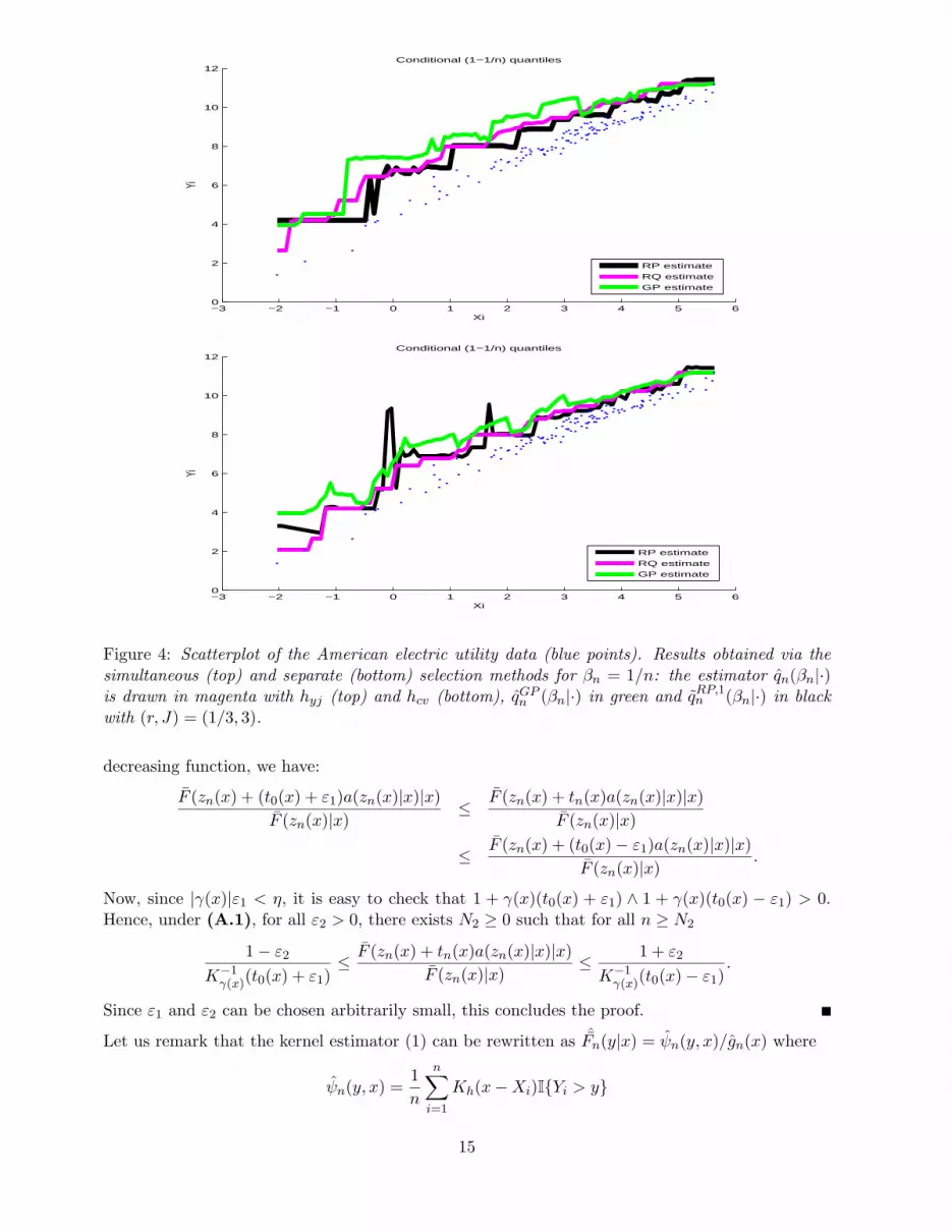
Data on 123 American electric utility companies were collected and the aim is to investigate theeconomic efficiency of these companies (see, e.g., [18]). A possible way to measure this efficiencyis by looking at the maximum level of produced goods which is attainable for a given level ofinputs-usage. From a statistical point of view, this problem translates into studying the upperboundary of the set of possible inputs X and outputs Y , the so-called cost/econometric frontierin production theory. Hendricks and Koenker [22] stated: “In the econometric literature on theestimation of production technologies, there has been considerable interest in estimating so calledfrontier production models that correspond closely to models for extreme quantiles of a stochasticproduction surface”. The present paper may be viewed as the first ‘purely’ nonparametric work toactually investigate theoretically the idea of Hendricks and Koenker.

For our illustration purposes, we used the measurements on the variable Y = log(Q), with Q

13

being the production output of a firm, and the variable X = log(C), with C being the total costinvolved in the production. Figure 4 shows the n = 123 observations, together with estimatedextreme conditional quantiles qn(βn|x), qGP

n (βn|x) and qRP,1n (βn|x) = qRP,2

n (βn|x) at r = 1/J withJ = 3. Given the small sample size, it was enough to use βn = 1/n in describing the conditionaldistribution tails. For selecting the window width h and the number k of extremes, we maintainedthe automatic empirical data-driven rules described above. It appears that the extreme conditionalquantile estimates are similar for both simultaneous (top) and separate (bottom) selection methods.Following their evolution, it may be seen that the American electric utility data do not correspond tothe situation hoped for by the practitioners of a heavily short-tailed production process. Indeed, onemay distinguish between two different behaviors of the extreme regression quantiles: They indicatea short-tailed conditional distribution for companies working at (transformed) input-factors largerthan, say, 2. In contrast, the tail distribution for the smallest companies with inputs Xi < 2 seemsto be moderately heavy. Therefore, the theoretical economic assumption that producers shouldoperate on the upper boundary of the joint support of (X, Y ) rather than on its interior is clearlynot fulfilled here, revealing a certain lack of production performance in this sector of activity. Theestimated graph of qRP,1

n (βn|x), qn(βn|x) or qGPn (βn|x) might be interpreted as the set of the most

efficient firms. It is then clear that the firms achieve significantly lesser output than that predictedby the extremal quantile frontiers. This indicates a relative economic inefficiency especially in thepopulation of the (sparse) smallest companies in terms of inputs.

6 Appendix: Proofs

6.1 Preliminary results

We begin with a homogeneous property of the quantile function.

Lemma 1. Suppose (A.1) holds. If αn → 0 as n → ∞, then,

limn→∞

q(ξαn|x)

q(αn|x)= ξ−(γ(x)∨0),

for all ξ > 0.

Proof. From (4), we have

q(ξαn|x)

q(αn|x)= 1 + Kγ(x)(1/ξ)

a(q(αn|x)|x)

q(αn|x)(1 + o(1))

and the conclusion follows using (5).

The following lemma states that the convergence in (3) is uniform.

Lemma 2. Under (A.1), if zn(x) ↑ yF (x) as n → ∞, then for all sequence of functions tn(x) suchthat tn(x) → t0(x) as n → ∞ where t0(x) is such that there exists η > 0 for which 1+γ(x)t0(x) ≥ ηthen,

limn→∞

F (zn(x) + tn(x)a(zn(x)|x)|x)

F (zn(x)|x)=

1

K−1γ(x)(t0(x))

.

Proof. Since tn(x) → t0(x) as n → ∞, for all ε1 > 0 such that |γ(x)|ε1 < η, there exists N1 ≥ 0such that for all n ≥ N1, t0(x) − ε1 ≤ tn(x) ≤ t0(x) + ε1. Since a(zn(x)|x) > 0 and F (.|x) is a

14

−3 −2 −1 0 1 2 3 4 5 60

2

4

6

8

10

12Conditional (1−1/n) quantiles

Xi

Yi

RP estimate

RQ estimateGP estimate

−3 −2 −1 0 1 2 3 4 5 60

2

4

6

8

10

12Conditional (1−1/n) quantiles

Xi

Yi

RP estimate

RQ estimateGP estimate

Figure 4: Scatterplot of the American electric utility data (blue points). Results obtained via thesimultaneous (top) and separate (bottom) selection methods for βn = 1/n: the estimator qn(βn|·)is drawn in magenta with hyj (top) and hcv (bottom), qGP

n (βn|·) in green and qRP,1n (βn|·) in black

with (r, J) = (1/3, 3).

decreasing function, we have:

F (zn(x) + (t0(x) + ε1)a(zn(x)|x)|x)

F (zn(x)|x)≤ F (zn(x) + tn(x)a(zn(x)|x)|x)

F (zn(x)|x)

≤ F (zn(x) + (t0(x) − ε1)a(zn(x)|x)|x)

F (zn(x)|x).

Now, since |γ(x)|ε1 < η, it is easy to check that 1 + γ(x)(t0(x) + ε1) ∧ 1 + γ(x)(t0(x) − ε1) > 0.Hence, under (A.1), for all ε2 > 0, there exists N2 ≥ 0 such that for all n ≥ N2

1 − ε2

K−1γ(x)(t0(x) + ε1)

≤ F (zn(x) + tn(x)a(zn(x)|x)|x)

F (zn(x)|x)≤ 1 + ε2

K−1γ(x)(t0(x) − ε1)

.

Since ε1 and ε2 can be chosen arbitrarily small, this concludes the proof.

Let us remark that the kernel estimator (1) can be rewritten as ˆFn(y|x) = ψn(y, x)/gn(x) where

ψn(y, x) =1

n

n∑

i=1

Kh(x − Xi)I{Yi > y}

15

is an estimator of ψ(y, x) = F (y|x)g(x) and gn(x) is the classical kernel estimator of the pdf g(x)defined by:

gn(x) =1

n

n∑

i=1

Kh(x − Xi).

Lemma 3 gives standard results on the kernel estimator (see [26] for a proof) whereas Lemma 4 isdedicated to the asymptotic properties of ψn(y, x).

Lemma 3. Suppose (A.2), (A.3) hold. If nhp → ∞, then, for all x ∈ Rp such that g(x) > 0,

(i) E(gn(x) − g(x)) = O(h),

(ii) var(gn(x)) =g(x)‖K‖2

2

nhp(1 + o(1)).

Therefore, under the assumptions of the above lemma, gn(x) converges to g(x) in probability.Let us introduce some further notations. In the following, yn(x) is a sequence such that yn(x) ↑yF (x) and yn,j(x) = yn(x)+Kγ(x)(1/τj)a(yn|x)(1+o(1)) for all j = 1, . . . , K. Recall that 0 < τJ <· · · < τ2 < τ1 ≤ 1. Moreover, the oscillations of the csf are controlled by

ωn(x) := maxj=1,...,J

supx′∈B(x,h)

∣

∣

∣

∣

F (yn,j(x)|x′)

F (yn,j(x)|x)− 1

∣

∣

∣

∣

.

Lemma 4. Suppose (A.1), (A.2) and (A.3) hold and let x ∈ Rp such that g(x) > 0. If ωn(x) → 0

and nhpF (yn(x)|x) → ∞ then,

(i) E(ψn(yn,j(x), x)) = ψ(yn,j(x), x) (1 + O(ωn(x)) + O(h)), for j = 1, . . . , J .

(ii) The random vector

{

√

nhpψ(yn(x), x)

(

ψn(yn,j(x), x) − E(ψn(yn,j(x), x))

ψ(yn,j(x), x)

)}

j=1,...,J

is asymptotically Gaussian, centered, with covariance matrix ‖K‖22V where Vj,j′ = τ−1

j∧j′ for

(j, j′) ∈ {1, . . . , J}2.

Proof. (i) Since the (Xi, Yi), i = 1, . . . , n are identically distributed, we have

E(ψn(yn,j(x), x)) =

∫

Rp

Kh(x − t)F (yn,j(x)|t)g(t)dt =

∫

SK(u)F (yn,j(x)|x − hu)g(x − hu)du,

under (A.3). Let us now consider

|E(ψn(yn,j(x), x))−ψ(yn,j(x), x)| ≤ F (yn,j(x)|x)

∫

SK(u)|g(x − hu) − g(x)|du (8)

+ F (yn,j(x)|x)

∫

SK(u)

∣

∣

∣

∣

F (yn,j(x)|x − hu)

F (yn,j(x)|x)−1

∣

∣

∣

∣

g(x−hu)du. (9)

Under (A.2), and since g(x) > 0, we have

(8) ≤ F (yn,j(x)|x)cgh

∫

Sd(u, 0)K(u)du = ψ(yn,j(x), x)O(h), (10)

16

and, in view of (10),

(9) ≤ F (yn,j(x)|x)ωn(x)

∫

SK(u)g(x − hu)du = F (yn,j(x)|x)ωn(x)g(x)(1 + o(1))

= ψ(yn,j(x), x)ωn(x)(1 + o(1)). (11)

Combining (10) and (11) concludes the first part of the proof.(ii) Let β 6= 0 in R

J , Λn(x) = (nhpψ(yn(x), x))−1/2, and consider the random variable

Ψn =J

∑

j=1

βj

(

ψn(yn,j(x), x) − E(ψn(yn,j(x), x))

Λn(x)ψ(yn,j(x), x)

)

=n

∑

i=1

1

nΛn(x)

J∑

j=1

βjKh(x − Xi)I{Yi ≥ yn,j(x)}ψ(yn,j(x), x)

− E

J∑

j=1

βjKh(x − Xi)I{Yi ≥ yn,j(x)}ψ(yn,j(x), x)

:=n

∑

i=1

Zi,n.

Clearly, {Zi,n, i = 1, . . . , n} is a set of centered, independent and identically distributed randomvariables with variance

var(Zi,n) =1

n2h2pΛ2n(x)

var

J∑

j=1

βjK

(

x − Xi

h

)

I{Yi ≥ yn,j(x)}ψ(yn,j(x), x)

=1

n2hpΛ2n(x)

βtBβ,

where B is the J × J covariance matrix with coefficients defined for (j, j′) ∈ {1, . . . , J}2 by

Bj,j′ =Aj,j′

ψ(yn,j(x), x)ψ(yn,j′(x), x),

Aj,j′ =1

hpcov

(

K

(

x − X

h

)

I{Y ≥ yn,j(x)}, K

(

x − X

h

)

I{Y ≥ yn,j′(x)})

= ‖K‖22E

(

1

hpQ

(

x − X

h

)

I{Y ≥ yn,j(x) ∨ yn,j′(x)})

− hpE(Kh(x − X)I{Y ≥ yn,j(x)})E(Kh(x − X)I{Y ≥ yn,j′(x)}),

with Q(.) := K2(.)/‖K‖22 also satisfying assumption (A.3). As a consequence, the three above

expectations are of the same nature. Thus, remarking that, for n large enough, yn,j(x)∨ yn,j′(x) =yn,j∨j′(x), part (i) of the proof implies

Aj,j′ = ‖K‖22ψ(yn,j∨j′(x), x) (1 + O(ωn(x)) + O(h))

− hpψ(yn,j(x), x)ψ(yn,j′(x), x) (1 + O(ωn(x)) + O(h))

leading to

Bj,j′ =‖K‖2

2

ψ(yn,j∧j′(x), x)(1 + O(ωn(x)) + O(h)) − hp (1 + O(ωn(x)) + O(h))

=‖K‖2

2

ψ(yn,j∧j′(x), x)(1 + o(1)),

since ψ(yn,j∧j′(x), x) → 0 as n → ∞. Now, from Lemma 2,

limn→∞

ψ(yn,j∧j′(x), x)

ψ(yn(x), x)=

1

K−1γ(x)(Kγ(x)(1/τj∧j′))

= τj∧j′

17

entailing

Bj,j′ =‖K‖2

2Vj,j′

ψ(yn(x), x)(1 + o(1)),

and therefore, var(Zi,n) ∼ ‖K‖22β

tV β/n, for all i = 1, . . . , n. As a preliminary conclusion, thevariance of Ψn converges to ‖K‖2

2βtV β. Consequently, Lyapounov criteria for the asymptotic

normality of sums of triangular arrays reduces to∑n

i=1 E |Zi,n|3 = nE |Z1,n|3 → 0. Remark thatZ1,n is a bounded random variable:

|Z1,n| ≤2‖K‖∞

∑Jj=1 |βj |

nΛn(x)hpψ(yn,J , x)=

2

τJ‖K‖∞

J∑

j=1

|βj |Λn(x)(1 + o(1))

and thus,

nE |Z1,n|3 ≤ 2

τJ‖K‖∞

J∑

j=1

n|βj |Λn(x)var(Z1,n)(1 + o(1))

=2

τJ‖K‖∞‖K‖2

2

J∑

j=1

|βj |βtV βΛn(x)(1 + o(1)) → 0

as n → ∞. As a conclusion, Ψn converges in distribution to a centered Gaussian random variablewith variance ‖K‖2

2βtV β for all β 6= 0 in R

p. The result is proved.

Let us now focus on the estimation of small tail probabilities F (yn(x)|x) when yn(x) ↑ yF (x)as n → ∞. The following result provides sufficient conditions for the asymptotic normality ofˆFn(yn(x)|x).

Proposition 1. Suppose (A.1), (A.2) and (A.3) hold and let x ∈ Rp such that g(x) > 0. If

nhpF (yn(x)|x) → ∞ and nhpF (yn(x)|x)(h ∨ ωn(x))2 → 0, then, the random vector

{

√

nhpF (yn(x)|x)

(

ˆFn(yn,j(x)|x)

F (yn,j(x)|x)− 1

)}

j=1,...,J

is asymptotically Gaussian, centered, with covariance matrix ‖K‖22/g(x)V where Vj,j′ = τ−1

j∧j′ for

(j, j′) ∈ {1, . . . , J}2.

Proof of Proposition 1. Keeping in mind the notations of Lemma 4, the following expansionholds

Λ−1n (x)

J∑

j=1

βj

(

ˆFn(yn,j(x)|x)

F (yn,j(x)|x)− 1

)

=T1,n + T2,n − T3,n

gn(x), (12)

where

T1,n = g(x)Λ−1n (x)

J∑

j=1

βj

(

ψn(yn,j(x), x) − E(ψn(yn,j(x), x))

ψ(yn,j(x), x)

)

T2,n = g(x)Λ−1n (x)

J∑

j=1

βj

(

E(ψn(yn,j(x), x)) − ψ(yn,j(x), x)

ψ(yn,j(x), x)

)

T3,n =

J∑

j=1

βj

Λ−1n (x) (gn(x) − g(x)) .

18

Let us highlight that assumptions nhpF (yn(x)|x)ω2n(x) → 0 and nhpF (yn(x)|x) → ∞ imply that

ωn(x) → 0 as n → ∞. Thus, from Lemma 4(ii), the random term T1,n can be rewritten as

T1,n = g(x)‖K‖2

√

βtV βξn, (13)

where ξn converges to a standard Gaussian random variable. The nonrandom term T2,n is controlledwith Lemma 4(i):

T2,n = O(Λ−1n (x)(h + ∆(yn(x), x)) = O

(

(nhpF (yn(x)|x))1/2(h ∨ ωn(x)))

= o(1). (14)

Finally, T3,n is a classical term in kernel density estimation, which can be bounded by Lemma 3:

T3,n = O(hΛ−1n (x)) + OP (Λ−1

n (x)(nhp)−1/2)

= O(

nhp+2F (yn(x)|x))1/2

+ OP (F (yn(x)|x))1/2 = oP (1). (15)

Collecting (12)–(15), it follows that

gn(x)Λ−1n (x)

J∑

j=1

βj

(

ˆFn(yn,j(x)|x)

F (yn,j(x)|x)− 1

)

= g(x)‖K‖2

√

βtV βξn + oP (1).

Finally, gn(x)P−→ g(x) yields

√

nhpF (yn(x)|x)J

∑

j=1

βj

(

ˆFn(yn,j(x)|x)

F (yn,j(x)|x)− 1

)

= ‖K‖2

√

βtV β

g(x)ξn + oP (1)

and the result is proved.

The last lemma establishes that Kγn(x)(rn) inherits from the convergence properties of γn(x).

Lemma 5. Suppose ξ(γ)n (x) := Λ−1

n (γn(x) − γ(x)) = OP(1), where Λn → 0. Let rn ≥ 1 or rn ≤ 1such that Λn log(rn) → 0. Then,

Λ−1n

(

Kγn(x)(rn) − Kγ(x)(rn)

K ′γ(x)(rn)

)

= ξ(γ)n (x)(1 + oP(1)).

Proof. Since γn(x)P−→ γ(x), a first order Taylor expansion yields

Kγn(x)(rn) = Kγ(x)(rn) + Λnξ(γ)n (x)K ′

γn(x)(rn),

where γn(x) = γ(x) + ΘnΛnξ(γ)n (x) with Θn ∈ (0, 1). As a consequence

Λ−1n

(

Kγn(x)(rn) − Kγ(x)(rn)

K ′γ(x)(rn)

)

= ξ(γ)n (x)

K ′γn(x)(rn)

K ′γ(x)(rn)

= ξ(γ)n (x)

(

1 +

∫ rn

1 (sγn(x)−γ(x) − 1)sγ(x)−1 log(s)ds∫ rn

1 sγ(x)−1 log(s)ds

)

.

Suppose for instance rn ≥ 1. The assumptions yield (log rn)(γn(x) − γ(x))P−→ 0 and thus, for n

large enough, with high probability,

sups∈[1,rn]

|(sγn(x)−γ(x) − 1)| ≤ 2(log rn)|γn(x) − γ(x)| = oP(1).

As a conclusion,

Λ−1n

(

Kγn(x)(rn) − Kγ(x)(rn)

K ′γ(x)(rn)

)

= ξ(γ)(x)(1 + oP(1))

and the result is proved. The case rn ≤ 1 is easily deduced since Kγ(x)(1/rn) = −K−γ(x)(rn) andK ′

γ(x)(1/rn) = K ′−γ(x)(rn).

19

6.2 Proofs of main results

Proof of Theorem 1. Let us introduce vn = (nhpα−1n )1/2, σn(x) = (vnf(q(αn|x)|x))−1 and, for

all j = 1, . . . , J ,

Wn,j(x) = vn

(

ˆFn(q(τjαn|x) + σn(x)zj |x) − F (q(τjαn|x) + σn(x)zj |x))

an,j(x) = vn

(

τjαn − F (q(αn,j |x) + σn(x)zj |x))

and zj ∈ R. We examine the asymptotic behavior of J-variate function defined by

Φn(z1, . . . , zJ) = P

J⋂

j=1

{

σ−1n (x)(qn(τjαn|x) − q(τjαn|x)) ≤ zj

}

= P

J⋂

j=1

{Wn,j(x) ≤ an,j(x)}

.

Let us first focus on the nonrandom term an,j(x). For each j ∈ {1, . . . , J} there exists θn,j ∈ (0, 1)such that

an,j(x) = vnσn(x)zjf(qn,j(x)|x) = zjf(qn,j(x)|x)

f(q(αn|x)|x),

where

qn,j(x) = q(τjαn|x) + θn,jσn(x)zj

= q(τjαn|x) + θn,jzj

τj(nhpαn)−1/2 τjαn

f(q(τjαn|x)|x)

f(q(τjαn|x)|x)

f(q(αn|x)|x)

= q(τjαn|x) + θn,jzjτγ(x)j (nhpαn)−1/2 τjαn

f(q(τjαn|x)|x)(1 + o(1)),

since y 7→ f(q(y|x)|x) is regularly varying at 0 with index γ(x) + 1, see [19, Corollary 1.1.10,eq. 1.1.33]. Now, in view of [19, Theorem 1.2.6] and [19, Remark 1.2.7], a possible choice of theauxiliary function is

a(t|x) =F (t|x)

f(t|x)(1 + o(1)), (16)

leading to

qn,j(x) = q(τjαn|x) + θn,jzjτγ(x)j (nhpαn)−1/2a(q(τjαn|x)|x)(1 + o(1)).

Applying Lemma 2 with zn(x) = q(τjαn|x), tn(x) = θn,jzjτγ(x)j (nhpαn)−1/2(1+o(1)) and t0(x) = 0

yieldsF (qn,j(x)|x)

τjαn→ K−1

γ(x)(0) = 1

as n → ∞. Recalling that y 7→ f(q(y|x)|x) is regularly varying, we have

f(qn,j(x)|x)

f(q(αn|x)|x)→ τ

γ(x)+1j

as n → ∞ and therefore

an,j(x) = zjτγ(x)+1j (1 + o(1)), j = 1, . . . , J. (17)

Let us now turn to the random term Wn,j(x). Let us define zn,j(x) = q(τjαn|x) + σn(x)zj forj = 1, . . . , J , yn(x) = q(αn|x), and consider the expansion

zn,j(x) − yn(x)

a(yn(x)|x)=

q(τjαn|x) − q(αn|x)

a(q(αn|x)|x)+

σn(x)zj

a(q(αn|x)|x).

20

From (4), we have

limn→∞

q(τjαn|x) − q(αn|x)

a(q(αn|x)|x)= Kγ(x)(1/τj),

and

limn→∞

σn(x)zj

a(q(αn|x)|x)= 0,

leading to zn,j(x) = yn(x) + Kγ(x)(1/τj)a(yn(x)|x)(1 + o(1)). Introducing βn,j(x) = F (yn,j(x)|x),the oscillation ωn(x) can be rewritten as

ωn(x) = maxj=1,...,J

supx′∈B(x,h)

∣

∣

∣

∣

F (q(βn,j(x)|x)|x′)

βn,j(x)− 1

∣

∣

∣

∣

.

For all κ ∈ (0, τJ) and j = 1, . . . , J , we eventually have zn,j(x) ∈ [yn(x), zn(x)] where zn(x) :=yn(x) + Kγ(x)(2/κ)a(yn(x)|x) and thus βn,j(x) ∈ [F (zn(x)|x), αn] eventually. Now, Lemma 2 im-plies that F (zn(x)|x)/αn → κ/2 as n → ∞ and thus, for n large enough, βn,j(x) ∈ [καn, αn].Consequently, ωn(x) ≤ ∆κ(αn, x). Applying Proposition 1 and Lemma 2 yields

Wn,j(x) =F (zn,j(x)|x)

αnξn,j = τjξn,j(1 + o(1))

where ξn = (ξn,1, . . . , ξn,j)t converges to a centered Gaussian random vector with covariance matrix

‖K‖22/g(x)V . Taking into account of (17), the results follows.

Proof of Corollary 1. Let us remark that, from (16),{

f(q(αn|x)|x)

√

nhpα−1n (qn(τjαn|x) − q(τjαn|x))

}

j=1,...,J

=

{

q(αn|x)f(q(αn|x)|x)

αn

q(τjαn|x)

q(αn|x)

√

nhpαn

(

qn(τjαn|x)

q(τjαn|x)− 1

)}

j=1,...,J

=

{

q(αn|x)

a(q(αn|x)|x)

q(τjαn|x)

q(αn|x)

√

nhpαn

(

qn(τjαn|x)

q(τjαn|x)− 1

)}

j=1,...,J

(1 + o(1))

=

{

q(αn|x)

a(q(αn|x)|x)τ−(γ(x)∨0)j

√

nhpαn

(

qn(τjαn|x)

q(τjαn|x)− 1

)}

j=1,...,J

(1 + o(1)),

in view of Lemma 1. The result follows from Theorem 1.

Proof of Theorem 2. By definition,

qn(βn|x) = qn(αn|x) + (Kγ(x)(αn/βn) + b(βn/αn, αn))a(q(αn|x)|x)

and thus, the following expansion can be easily established:

Λ−1n

(

qn(βn|x) − q(βn|x)

a(q(αn|x)|x)K ′γ(x)(αn/βn)

)

= Λ−1n

(

qn(αn|x) − q(αn|x)

a(q(αn|x)|x)K ′γ(x)(αn/βn)

)

+ Λ−1n

(

Kγn(x)(αn/βn) − Kγ(x)(αn/βn)

K ′γ(x)(αn/βn)

)

an(x)

a(q(αn|x)|x)

+ Λ−1n

Kγ(x)(αn/βn)

K ′γ(x)(αn/βn)

(

an(x)

a(q(αn|x)|x)− 1

)

+ Λ−1n

b(βn/αn, αn)

K ′γ(x)(αn/βn)

=: Tn,1 + Tn,2 + Tn,3 + Tn,4.

21

Introducing

(ξ(γ)n (x), ξ(a)

n (x), ξ(q)n (x)) := Λ−1

n

(

γn(x) − γ(x),an(x)

a(q(αn|x)|x)− 1,

qn(αn|x) − q(αn|x)

a(q(αn|x)|x)

)

,

from and remarking that, when u → ∞,

K ′z(u) = (1 + o(1))

∣

∣

∣

∣

∣

∣

∣

1z2 if z < 0,log2(u)

2 if z = 0,uz log(u)

z if z > 0,

(18)

the first term can be rewritten as

Tn,1 =ξ(q)n (x)

K ′γ(x)(αn/βn)

= (γ(x) ∧ 0)2ξ(q)n (x)(1 + oP(1)). (19)

Second, Λn → 0 and (7) entail an(x)/a(q(αn|x)|x)P−→ 1 and thus

Tn,2 = Λ−1n

(

Kγn(x)(αn/βn) − Kγ(x)(αn/βn)

K ′γ(x)(αn/βn)

)

(1 + oP(1)) = ξ(γ)n (x)(1 + oP(1)), (20)

from Lemma 5. From (7), (18), and in view of

Kz(u) = (1 + o(1))

∣

∣

∣

∣

∣

∣

−1z if z < 0,

log(u) if z = 0,uz

z if z > 0.

the third term can be rewritten as

Tn,3 = ξ(a)n (x)

Kγ(x)(αn/βn)

K ′γ(x)(αn/βn)

= −(γ(x) ∧ 0)ξ(a)n (x)(1 + oP(1)). (21)

Finally, Tn,4 = oP(1) by assumption and the conclusion follows from (7), (19), (20) and (21).

Proof of Theorem 3. The proof consists in deriving asymptotic expansions for the three con-sidered random variables. i) Let us first introduce

γn,j(x) =1

log rlog

(

qn(τjαn|x) − qn(τj+1αn|x)

qn(τj+1αn|x) − qn(τj+2αn|x)

)

(22)

such that γRPn (x) =

∑J−2j=1 πjγn,j(x). From Theorem 1 and in view of (4), we have, for all j =

1, . . . , J ,

qn(τjαn|x) = q(αn|x) + a(q(αn|x)|x)(Kγ(x)(1/τj) + b(τj , αn|x)) + σn(x)ξj,n,

with σ−1n (x) = f(q(αn|x)|x)

√

nhpα−1n and where the random vector ξn = (ξj,n)j=1,...,J is asymptot-

ically Gaussian, centered, with covariance matrix ‖K‖22/g(x)Σ(x). Introducing

ηn(x) := maxj=1,...,J

|b(τj , αn|x)|

εn := σn(x)/a(q(αn|x)|x) = (nhpαn)−1/2(1 + o(1)),

22

see [19], it follows that

qn(τjαn|x) − qn(τj+1αn|x)

a(q(αn|x)|x)= εn(ξj,n − ξj+1,n)

+ Kγ(x)(1/τj) − Kγ(x)(1/τj+1) + b(τj , αn|x) − b(τj+1, αn|x)

= εn(ξj,n − ξj+1,n) + Kγ(x)(r)r−γ(x)j + O(ηn(x)). (23)

Replacing in (22), we obtain

(log r)γn,j(x) = log

(

εn(ξj,n − ξj+1,n) + Kγ(x)(r)r−γ(x)j + O(ηn(x))

εn(ξj+1,n − ξj+2,n) + Kγ(x)(r)r−γ(x)(j+1) + O(ηn(x))

)

,

or equivalently,

(log r)(γn,j(x) − γ(x)) = log

(

1 +εn(ξj,n − ξj+1,n)rγ(x)j

Kγ(x)(r)+ O(ηn(x))

)

− log

(

1 +εn(ξj+1,n − ξj+2,n)rγ(x)(j+1)

Kγ(x)(r)+ O(ηn(x))

)

A first order Taylor expansion yields

(log r)ε−1n (γn,j(x)− γ(x)) =

rγ(x)j

Kγ(x)(r)

(

ξj,n − (1 + rγ(x))ξj+1,n + rγ(x)ξj+2,n

)

+ O(ε−1n ηn(x)) + oP(1)

and thus, under the assumption (nhpαn)1/2ηn(x) → 0 as n → ∞,

√

nhpαn(γRPn (x)−γ(x)) =

1

(log r)Kγ(x)(r)

J−2∑

j=1

πjrγ(x)j

(

ξj,n − (1 + rγ(x))ξj+1,n + rγ(x)ξj+2,n

)

+oP(1).

Defining for the sake of simplicity π−1 = π0 = πJ−1 = πJ = 0, β(γ)0 = 1

log r , β(γ)1 = −1+r−γ(x)

log(r) and

β(γ)2 = r−γ(x)

log(r) , we end up with

ξ(γ)n (x) :=

√

nhpαn(γRPn (x) − γ(x))

=1

Kγ(x)(r)

J∑

j=1

rγ(x)j(

β(γ)0 πj + β

(γ)1 πj−1 + β

(γ)2 πj−2

)

ξj,n + oP(1). (24)

ii) Second, let us now consider

an,j(x) =rγRP

n (x)j(qn(τjαn|x) − qn(τj+1αn|x))

KγRPn (x)(r)

such that an(x) =∑J−2

j=1 πjan,j(x). From (23), it follows that, for all j = 1, . . . , J ,

an,j(x)

a(q(αn|x)|x)=

rγRPn (x)j

KγRPn (x)(r)

(

εn(ξj,n − ξj+1,n) + Kγ(x)(r)r−γ(x)j + O(ηn(x))

)

.

Remarking that γRPn (x) = γ(x) + (nhpαn)−1/2ξ

(γ)n (x), Lemma 5 yields

an,j(x)

a(q(αn|x)|x)=

1 + rγ(x)j

Kγ(x)(r)εn(ξj,n − ξj+1,n) + O(ηn(x))

1 +K′

γ(x)(r)

Kγ(x)(r)(nhpαn)−1/2ξ

(γ)n (x)(1 + oP(1))

exp(

ξ(γ)n (x)j log(r)(nhpαn)−1/2

)

.

23

A first order Taylor expansion thus gives

√

nhpαn

(

an,j(x)

a(q(αn|x)|x)− 1

)

= ξ(γ)n (x)

(

j log(r) −K ′

γ(x)(r)

Kγ(x)(r)

)

+rγ(x)j

Kγ(x)(r)(ξj,n − ξj+1,n)

+ O(

√

nhpαnηn(x))

+ oP(1).

Recalling that π−1 = π0 = πJ−1 = πJ = 0 and introducing

E(π) =∑J

j=1 jπj , β(a)1 = −r−γ(x) − (r−γ(x) + 1)

(

E(π) − K′

γ(x)(r)

log(r)Kγ(x)(r)

)

,

β(a)0 = 1 + E(π) − K′

γ(x)(r)

log(r)Kγ(x)(r), β

(a)2 = r−γ(x)

(

E(π) − K′

γ(x)(r)

log(r)Kγ(x)(r)

)

it follows that

ξ(a)n (x) :=

√

nhpαn

(

an(x)

a(q(αn|x)|x)− 1

)

=

(

E(π) log(r) −K ′

γ(x)(r)

Kγ(x)(r)

)

ξ(γ)(x)n +

1

Kγ(x)(r)

J∑

j=1

rγ(x)j(πj − r−γ(x)πj−1)ξj,n + oP(1)

=1

Kγ(x)(r)

J∑

j=1

rγ(x)j(

β(a)0 πj + β

(a)1 πj−1 + β

(a)2 πj−2

)

ξj,n + oP(1) (25)

in view of (24). iii) Third, Corollary 1 states that

ξ1,n =

√nhpαn

a(q(αn|x)|x)(qn(αn|x) − q(αn|x)) (26)

is asymptotically Gaussian. Finally, collecting (24), (25) and (26),

(ξ(γ)n (x), ξ(a)

n (x), ξ1,n)t =1

Kγ(x)(r)A(x)ξn + oP(1),

where A(x) is the 3 × J matrix defined by

A1,j(x) = rγ(x)j(

β(γ)0 πj + β

(γ)1 πj−1 + β

(γ)2 πj−2

)

A2,j(x) = rγ(x)j(

β(a)0 πj + β

(a)1 πj−1 + β

(a)2 πj−2

)

A3,j(x) = Kγ(x)(r)I{j = 1},

for all j = 1, . . . , J . It is thus clear that the random vector (ξ(γ)n (x), ξ

(a)n (x), ξ1,n)t converges in

distribution to a centered Gaussian random vector with covariance matrix

‖K‖22

g(x)K2γ(x)(r)

A(x)Σ(x)At(x) =: S(x). (27)

Acknowledgements. The authors thank the Editor and both anonymous Associate Editor andreviewer for their valuable feedback on this paper.

24

References

[1] Beirlant, J., and Goegebeur, Y. (2004). Local polynomial maximum likelihood estimation forPareto-type distributions. Journal of Multivariate Analysis, 89, 97–118.

[2] Beirlant, J., Goegebeur, Y., Segers, J., and Teugels J. (2004). Statistics of extremes: Theoryand applications, Wiley.

[3] Berlinet, A., Gannoun, A. and Matzner-Lober, E. (2001). Asymptotic normality of convergentestimates of conditional quantiles. Statistics, 35, 139–169.

[4] Chavez-Demoulin, V., and Davison, A.C. (2005). Generalized additive modelling of sampleextremes. Journal of the Royal Statistical Society, series C, 54, 207–222.

[5] Chernozhukov, V. (2005). Extremal quantile regression, The Annals of Statistics, 33(2), 806–839.

[6] Daouia, A., Florens, J-P. and Simar, L. (2010). Frontier estimation and extreme value theory.Bernoulli, 16, 1039–1063.

[7] Daouia, A., Gardes, L., Girard, S. and Lekina, A. (2011). Kernel estimators of extreme levelcurves. Test, 20, 311–333.

[8] Davison, A.C., and Ramesh, N.I. (2000). Local likelihood smoothing of sample extremes. Journal

of the Royal Statistical Society, series B, 62, 191–208.

[9] Davison, A.C., and Smith, R.L (1990). Models for exceedances over high thresholds. Journal of

the Royal Statistical Society, series B, 52, 393–442.

[10] Drees, H. (1995). Refined Pickands estimators of the extreme value index. The Annals ofStatistics, 23, 2059-2080.

[11] Feigin, P.D., and Resnick, S.I. (1997). Linear programming estimators and bootstrapping forheavy tailed phenomena. Advances in Applied Probability, 29, 759–805.

[12] Gannoun, A. (1990). Estimation non parametrique de la mediane conditionnelle,medianogramme et methode du noyau. Publications de l’Institut de Statistique de l’Universite

de Paris, XXXXVI, 11–22.

[13] Gardes, L., and Girard, S. (2008). A moving window approach for nonparametric estimationof the conditional tail index. Journal of Multivariate Analysis, 99, 2368–2388.

[14] Gardes, L., and Girard, S. (2010). Conditional extremes from heavy-tailed distributions: Anapplication to the estimation of extreme rainfall return levels. Extremes, 13, 177–204.

[15] Gardes, L., Girard, S., and Lekina, A. (2010). Functional nonparametric estimation of condi-tional extreme quantiles. Journal of Multivariate Analysis, 101, 419–433.

[16] Girard, S., and Jacob, P. (2008). Frontier estimation via kernel regression on high power-transformed data. Journal of Multivariate Analysis, 99, 403–420.

[17] Girard, S., and Menneteau, L. (2005). Central limit theorems for smoothed extreme valueestimates of Poisson point processes boundaries. Journal of Statistical Planning and Inference,135, 433–460.

[18] Greene, W.H. (1990). A gamma-distributed stochastic frontier model. Journal of Econometrics,46, 141–163.

25

[19] de Haan, L., and Ferreira, A. Extreme value theory: An introduction, Springer Series in Oper-ations Research and Financial Engineering, Springer, 2006.

[20] Hall, P., and Tajvidi, N. (2000). Nonparametric analysis of temporal trend when fitting para-metric models to extreme-value data. Statistical Science, 15, 153–167.

[21] Hardle, W., and Stoker, T. (1999). Investigating smooth multiple regression by the method ofaverage derivatives. Journal of the American Statistical Association, 84, 986–995.

[22] Hendricks, W. and Koenker, R. (1992). Hierarchical spline models for conditional quantilesand the demand for electricity. Journal of the American Statistical Association, 87, 58–68.

[23] Jureckova, J. (2007). Remark on extreme regression quantile. Sankhya, 69, Part 1, 87–100.

[24] Koenker, R. and Geling, O. (2001). Reappraising medfly longevity: A quantile regressionsurvival analysis. Journal of American Statistical Association, 96, 458–468.

[25] Park, B.U. (2001). On nonparametric estimation of data edges. Journal of the Korean Statis-tical Society, 30, 265–280.

[26] Parzen, E. (1962). On estimation of a probability density function and mode. Annals of Math-ematical Statistics, 33, 1065–1076.

[27] Ruppert, D., Wand, M., and R.J. Carroll (2003). Semiparametric Regression. Cambridge U.Press.

[28] Samanta, T. (1989). Non-parametric estimation of conditional quantiles. Statistics and Prob-ability Letters, 7, 407–412.

[29] Smith, R.L. (1989). Extreme value analysis of environmental time series: An application totrend detection in ground-level ozone (with discussion). Statistical Science, 4, 367–393.

[30] Stone, C.J. (1977). Consistent nonparametric regression (with discussion). The Annals ofStatistics, 5, 595–645.

[31] Stute, W. (1986). Conditional empirical processes. The Annals of Statistics, 14, 638–647.

[32] Tsay, R.S. (2002). Analysis of financial time series. Wiley, New York.

[33] Yu, K. and M.C. Jones (1998). Local linear quantile regression. Journal of American StatisticalAssociation, 93, 228–237.

26