Occurrence of Naked Singularities in Higher Dimensional Dust Collapse

IOSR Journal of Mathematics (IOSR-JM)

e-ISSN: 2278-5728, p-ISSN: 2319-765X. Volume 10, Issue 5 Ver. V (Sep-Oct. 2014), PP 78-88 www.iosrjournals.org

www.iosrjournals.org 78 | Page

Occurrence of Naked Singularities in Higher Dimensional Dust

Collapse

Kishor D. Patil1 & Manisha S. Patil

2

1Department of Mathematics, B. D. College of Engineering, Sewagram, Wardha, (M.S.) India 2 Department of Mathematics, B. D. College of Engineering, Sewagram, Wardha, (M.S.) India

Abstract: We consider here the gravitational collapse of a inhomogeneous dust cloud described by Tolman-

bondi models. We find that the end state of the collapse is either a black hole or a naked singularity, depending

on the parameters of initial density distribution. Collapse ends into a black hole if the dimensionless quantity

𝜓 is greater than −22.18033 and ends into a naked singularity if 𝜓 ≤ −22.18033. We find the occurrence

of naked singularity in higher dimensional case. We proposed the concept of ‘trapped range’ of initial data in

the different higher dimensional space-times. We show that ‘trapped range’ of initial data increases with the

increase in dimensions of the space-times.

Keywords: Dust collapse, naked singularity, dust collapse, cosmic censorship.

I. Introduction Cosmic Censorship Conjecture is still an outstanding open problem and possesses a prime position in

the study of general relativity. Whereas no proof for this hypothesis is known, many counter examples have

been studied. It is clearly important to investigate specific dynamical collapse scenarios within the frame work

of gravitational theory for the final state of collapse. Such a study will be of great help in establishing whether or

not this hypothesis is correct. An important class of collapse scenarios available in this connection is the

dynamical evolution of a spherically symmetric cloud of pressure less dust.

Dust collapse has been studied by many researchers, perhaps the first being the work of Oppenheimer

and Snyder [1], which demonstrated that the collapse of a homogeneous spherical dust object ends in a black

hole. This leads to a view, reflected by the Cosmic Censorship Hypothesis that spherical collapse will always

ends in a black hole. However, such a view does not seem to be supported by a detailed analysis of spherical collapse. Departures from Oppenheimer- Snyder model come in the form of introducing inhomogeneities in the

initial distribution of matter [2, 3], and also in the form of changing the equation of state. It has been shown by

various authors [4-10] that the introduction of inhomogeneities in the matter distribution can give rise to the

occurrence of a naked singularity at the centre in the spherical gravitational collapse. However, the final fate of

collapse of an inhomogeneous distribution of matter with a general equation of state is largely unknown. An

important sub case which could be examined in this context is spherically symmetric but inhomogeneous

distribution of dust which collapses under the force of gravity. The general solutions to Einstein equations for

this case have been given by the Tolman-Bondi space-times [2, 3] and it has been demonstrated that naked

singularities can occur as the end state of such a collapse [4, 6, 7, 10-12]. In particular, it was pointed out in [6,

10] that the collapse ends in a naked singularity or a black hole depending on whether or not a certain algebraic

equation involving the metric functions and their derivatives has positive real roots. In order to be able to

ascertain the astrophysical implications of such a result, it is necessary to translate the condition for the existence of positive real roots into the actual constraints on the initial density distribution in the cloud. An

interesting problem that arises is the effect that higher dimensions can have on the formation of naked

singularity.

It is relevant to note here that the role of initial density distribution in dust collapse was earlier

considered by Christodoulou [4] and Newman [5]; however their discussion was restricted by the assumption of

evenness of density and metric functions. A classical statement in Hawking and Ellis [13] asserts that the

boundary of a trapped region is an apparent horizon. It is known that an apparent horizon forms in the region of

a sufficiently strong gravitational field. An apparent horizon seems to play an important role in deciding the

nature of the singularity. Much literature on apparent horizon has been appeared so far [14, 15, 16-18]. It is

believed that the formation of the central singularity earlier than the apparent horizon is a necessary condition

for a singularity to be naked. A singularity cannot be naked if it occurs after the formation of apparent horizon. Jhingan et. al.[19] has shown that the absence of apparent horizon formation prior to the central singularity does

not necessarily imply nakedness.

Recently Saraykar and Joshi showed that naked singularities in dynamical gravitational collapse of

inhomogeneous dust to be stable but non-generic [20]. Sil and Chatterjee [21] studied dust collapse in five

dimensional space-time. By considering a self-similar Tolman type model in higher dimensional space-time

Occurrence Of Naked Singularities In Higher Dimensional Dust Collapse


they showed the occurrence of a naked shell focusing singularity which may develop into a strong curvature

singularity.

In this chapter we consider the nature and structure of singularities arising in a non-self similar dust collapse in 5D. We show that the central singularity of collapse may indeed be a naked one depending on the

conditions of initial density distribution. In section 2 we describe five dimensional Tolman-bondi dust model

and showed the existence of a naked singularity. In section 3 we generalized this result to (N+2)-dimensional

space-times. Tolman-bondi model is the simplest solution to the Einstein equation and admits both a naked

singularity as well as a black hole depending on the nature of the initial data. In section 4 we discuss the

dynamics of an apparent horizon in higher dimensional space-times. We end this paper with concluding remarks

as a last section.

II. Dust Collapse In Five Dimensional Tolman Type Model To facilitate the discussion we give a brief summary of the higher dimensional Tolman-Bondi solution.

Let us consider the metric for 5D space-time with spherical symmetry [21].

ds2 = −dt2 +R ′ 2

1 + M dr2 + R2(dθ1

2 + sin2θ1dθ22 + sin2θ1sin2θ2dθ3

2) (1)

Where M(r) is an arbitrary function of commoving coordinate r, satisfying M > 1. R(t, r) is the

physical radius at a time t of the shell labeled by r, in the sense that 4πR2(r, t) is the proper area of the shell at time t. A prime denotes the partial derivative with respect to r.

The energy momentum tensor is given by

Tij = ςδt i δt

j (2)

Where

ς t, r =3F′

2R3R ′ , (3)

The function R r, t is the solution of

R 2 =F(r)

R2 + M(r) , (4)

Where an over dot denotes partial derivative with respect to t. The functions F(r) and M(r) are arbitrary, and

result from the integration of the field equations.

For simplicity we consider here only the marginally bound case M(r) = 0.

Here we are discussing gravitational collapse, for that we require R t, r < 0. Hence we get

R =− F

R . (5)

After integrating and using scaling freedom R r; 0 = r we get

R2 = r2 − 2 F. (6)

According to (6) the area radius of the shell r shrinks to zero at the time tc (r) given by

tc r =r2

2 F . (7)

The Kretschmann scalar is given by

K =A F′ 2

R6R ′ 2 −B FF′

R7R ′ +C F2

R8 , (8)

From above equation at t = tc (r), the Kretschmann scalar and energy density both diverge, indicating the

presence of scalar polynomial curvature singularity [13]. The time and radial coordinates are respectively in the

ranges −∞ < t < tc (r) and 0 ≤ r < ∞.

It has been shown that [5] shell crossing singularities (characterized by R′ = 0 and R > 0) are

gravitationally weak and hence such singularities need not be considered seriously. We therefore consider only

the shell focusing singularity. We thus assume R′ > 0 in the following discussion. We shall restrict ourselves to

the study of future directed radial null geodesics. In order to check whether the singularity is naked, we examine

the null geodesic equations for the tangent vectors Ka = dxa dk , where k is an affine parameter along the

geodesics. For radial null geodesics, these are

Kt =dt

dk=

P

R , (9)

Kr =dr

dk=

Kt

R ′ =P

RR ′ (10)

Where the function P(t, r) satisfies the differential equation dP

dk+ P2

R ′

R ′ R−

R

R2 −1

R2 = 0 (11)

Let u = rα α > 1 , then dR

du=

1

αrα−1 R

dt

dr+ R′



From equation (1) we see that, for outgoing radial null geodesics, dt dr = R′ , hence with the help of equation

(5) above equation becomes dR

du=

R ′

αrα−1 1 −

F

R =

R ′

αrα−1 1 −

Λ

X = U(X, u), (12)

Where

Λ = F

u , X =

R

u (13)

It is clear that R = 0, u = 0 is a singular point of equation (12). If there are outgoing radial null geodesics

terminating at this point then at the singularity, we have dR du > 0 for X > Λ i.e. R > F. Thus boundary of

the trapped surface i.e. apparent horizon is given by R = F. Using this relation we find from equation (6) that

tah r =r2

2 F−

F

2= tc r −

F

2

Where tah r denotes the time at which apparent horizon forms.

Since F(r) is strictly positive for r > 0, with F(r) = 0 at r = 0, we have tah r < tc (r) for r > 0 and

tah 0 = tc (0). Thus all other points on the singularity curve, except the point r = 0 are covered by the apparent horizon. We therefore consider the singularity of collapse at r = 0 i.e. the central singularity. We now find

conditions on the initial data so that the central singularity of collapse is naked.

If the outgoing null geodesics are to terminate in the past at the singularity at r = 0, which occurs at

time t = tc at which tc ,0 = 0 , then along these geodesics we have R → 0 as r → 0. After simplifying

differential equation (12), we see that the right hand side of this equation is of the form 0/0 in the limit of

approach to the singularity (R = 0, u = 0). The point R = 0, u = 0 in the (R, u) plane is thus a singularity of the

differential equation (12).

By using equation (6) one can write

R′ =RF′

4F+ 1 −

rF′

4F

r

F (14)

=ηXrα−1

4+

4−η

4

1

rα−1X (15)

Where η = rF′ F .

The initial state of the spherically symmetric dust cloud is described in terms of the density and

velocity profiles specified at an initial epoch of time from which collapse commences. We denote by ρ r =ς(r, 0) , the density distribution of the cloud at the starting epoch of collapse.

From equation (6.3) we get

F r = ρ(r)r3dr (16)

We assume that the density ρ r can be expanded (16) in a power series about the central density ρ0

ρ r = ρ0 + ρ1r +ρ2 r2

2!+

ρ3 r3

3!+ ⋯ +

ρn rn

n!+............., (17)

Where ρ0 > 0 and ρn stands for the nth derivative of ρ at r = 0.

Then F becomes

F r = F0r4 + F1r5 + F2r6 +.............., (18)

Where

Fn =2

3

ρn

n!(n+4) , n = 0, 1, 2,........ (19)

Also η appearing in equation (15) is given by

η =rF′

F=

n+4 Fn rn +4∞0

Fn rn +4∞0

(20)

Since we are interested in the behavior of η near the centre, we can simplify this further to get

η r = 4 + η1r + η2r2 + η3r3 +............., (21) Where

η1 =F1

F0 , η2 =

2F2

F0−

F12

F02 , η3 =

3F3

F0−

3F1F2

F02 +

F13

F03 , (22)

If all the derivatives ρn of the density vanish for n ≤ q − 1 , and the qth derivative is the first non-vanishing

derivative, then Tηq, the qth term in the expression for η is

Tηq

= qFq

F0 rq , (23)

Here q takes the values 1, 2 etc. and Tη0 = 4 .

In this case we can write η r as

η r = 4 +qFq

F0rq + O(rq+1), (24)

Substituting the value of 4 − η from equation (24) keeping only the terms up to the order rq and substituting in

equation (15) to get

R′ =ηX

4rα−1 −

qFq rq

4F0rα−1X , (25)



With the help of equation (25), equation (12) becomes dR

du=

1

α 1 −

Λ

X

ηX

4−

ϕ

X = U(X, u) , (26)

Where

ϕ =qFq rq

4F0r2 α−1 , (27)

Let us consider the limit X0 of the tangent X along the null geodesic terminating at the singularity at R = 0, u =

0. Using L’Hospital’s rule we get

X0 = limR→0u→0

R

u = lim

R→0u→0

dR

du = lim

R→0u→0

U X, u = U X0 , 0 , (28)

The necessary condition that the null geodesic emanates from the central singularity is the existence of the

positive real root X0 of the equation,

V X0 = 0 , (29) Where

V X = U X, 0 − X (30)

=1

α 1 −

Λ0

X

η0X

4−

ϕ0

X − X, (31)

q = 2 α − 1 ⟹ α = 1 +q

2 , ϕ0 =

qFq

4F0 (32)

Λ = F rα

Λ0 = 0 , q < 2

= F0 , q = 2 (33)

= ∞ , q > 2

X02 =

−F1

2F0=

−2ρ1

5ρ0 , (34)

1

2 1 −

F0

X0 X0 −

F2

2F0 X0 = X0

2X03

F03 2 +

2X02

F0+

F2 X0

F05 2 −

F2

F02 = 0

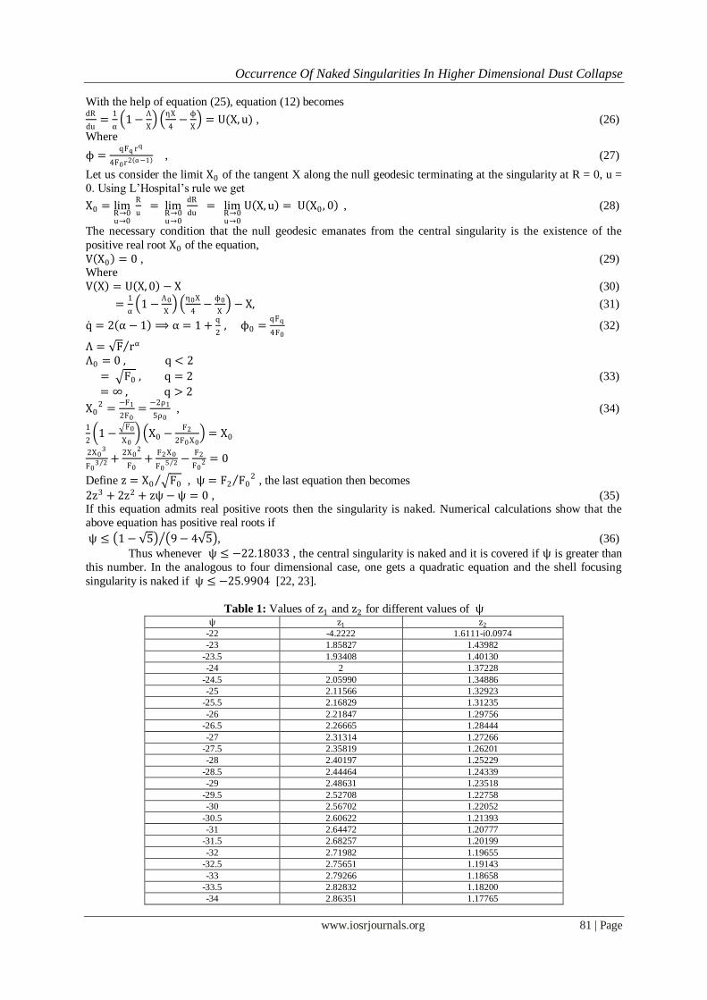
Define z = X0 F0 , ψ = F2 F02 , the last equation then becomes

2z3 + 2z2 + zψ − ψ = 0 , (35) If this equation admits real positive roots then the singularity is naked. Numerical calculations show that the

above equation has positive real roots if

ψ ≤ 1 − 5 9 − 4 5 , (36)

Thus whenever ψ ≤ −22.18033 , the central singularity is naked and it is covered if ψ is greater than

this number. In the analogous to four dimensional case, one gets a quadratic equation and the shell focusing

singularity is naked if ψ ≤ −25.9904 [22, 23].

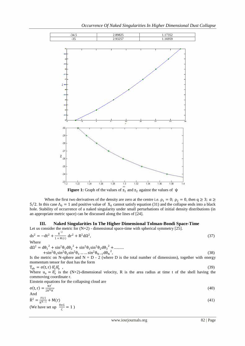
Table 1: Values of z1 and z2 for different values of ψ ψ z1 z2

-22 -4.2222 1.6111-i0.0974

-23 1.85827 1.43982

-23.5 1.93408 1.40130

-24 2 1.37228

-24.5 2.05990 1.34886

-25 2.11566 1.32923

-25.5 2.16829 1.31235

-26 2.21847 1.29756

-26.5 2.26665 1.28444

-27 2.31314 1.27266

-27.5 2.35819 1.26201

-28 2.40197 1.25229

-28.5 2.44464 1.24339

-29 2.48631 1.23518

-29.5 2.52708 1.22758

-30 2.56702 1.22052

-30.5 2.60622 1.21393

-31 2.64472 1.20777

-31.5 2.68257 1.20199

-32 2.71982 1.19655

-32.5 2.75651 1.19143

-33 2.79266 1.18658

-33.5 2.82832 1.18200

-34 2.86351 1.17765



-34.5 2.89825 1.17352

-35 2.93257 1.16959

Figure 1: Graph of the values of z1 and z2 against the values of ψ

When the first two derivatives of the density are zero at the centre i.e. ρ1 = 0; ρ2 = 0, then q ≥ 3; α ≥5 2 . In this case Λ0 = 1 and positive value of X0 cannot satisfy equation (31) and the collapse ends into a black

hole. Stability of occurrence of a naked singularity under small perturbations of initial density distributions (in

an appropriate metric space) can be discussed along the lines of [24].

III. Naked Singularities In The Higher Dimensional Tolman-Bondi Space-Time

Let us consider the metric for (N+2) - dimensional space-time with spherical symmetry [25].

ds2 = −dt2 +R ′ 2

1 + M (r) dr2 + R2dΩ2, (37)

Where

dΩ2 = dθ12 + sin2θ1dθ2

2 + sin2θ1sin2θ2dθ32 +..........

+sin2θ1sin2θ2sin2θ3 …… sin2θN−1dθN2, (38)

Is the metric on N-sphere and N = D - 2 (where D is the total number of dimensions), together with energy

momentum tensor for dust has the form

Tab = ς t, r δat δb

t , (39)

Where ua = δat is the (N+2)-dimensional velocity, R is the area radius at time t of the shell having the

commoving coordinate r.

Einstein equations for the collapsing cloud are

ς t, r =NF′

2RN R ′ (40)

And

R 2 =F r

RN−1 + M(r) (41)

(We have set up 8πG

C= 1 )



Here the over dot and prime denote partial derivatives with respect to t and r, respectively. The quantity

F(r) arises as a free function from the integration of the Einstein equations and can be interpreted physically as

the total mass of the collapsing cloud with in a coordinate radius r. M(r) is another free function of r and is

called the energy function. Since in the present discussion we stick with gravitational collapse, we take R (t, r) <0.

For physical reasons, one assumes that energy density ς t, r is non-negative everywhere. The epoch

R=0 denotes a physical singularity where the spherical shell of a matter collapses to zero radius and where the

density ς t, r blows up to infinity. Time t = ts r corresponds to the value R = 0 where the area of the shell of

matter at a constant value of coordinate r vanishes. The singularity curve t = ts r corresponds to the time when

the matter shells meet the physical singularity.

This specifies the ranges of the co-ordinates for the metric (37):

0 ≤ r < ∞, −∞ < t < ts r Simplicity, we consider the marginally bound case M(r) = 0.

Equation (41) yields

R 2 =F(r)

RN−1

In the collapsing case,

R =− F

R N −1 2 (42)

Integrating equation (42) we get

R N+1 2 = r N+1 2 − N+1

2 Ft , (43)

Where we have used the freedom in the scaling of the commoving coordinate r to set up R(0, r) = r at the

starting epoch of the collapse so that the physical area radius R increases monotonically in r, and with R′ = 1

there are no shell crossing on the initial surface.

Our interest is restricted only to the central shell focusing singularity at R = 0,

r = 0 which is a gravitationally strong singularity, unlike to the shell crossing ones which are weak and through

which the space-time may sometimes be extended [26].

It follows from Eq.(40) that the function F(r) becomes fixed once the initial density distribution ς 0, r = ρ r

is given, i.e.,

F r =2

N ρ r rN dr , (44)

We assume that initial density profile ρ r has the series of expansion [22, 23].

ρ r = ρ0 + ρ1r +ρ2 r2

2!+

ρ3 r3

3!+ ⋯ +

ρn rn

n! (45)

Near the centre r = 0, which can be substituted in Equation (44) to yield

F r = F0rN+1 + F1rN+2 + F2rN+3 +........., (46) Where

Fn = 2

N

ρn

n! N+1+n , (47)

And ρn is the nth derivative of density and n takes integral values 0, 1, 2, 3, ............We note that the first non-

vanishing derivative in the series expansion (45) should be negative, as we will consider only those density

functions which decreases as one move away from the centre.

As ts(r) gives the time at which area radius R becomes zero it follows from Equation (43) that

ts r = 2

N+1

r N +1 2

F , (48)

The Kretschmann scalar K = Rabcd Rabcd for the metric (37) is given by

K =AF′ 2

R2N R ′ 2 +BF F′

R2N +1R ′ +CF2

R2N +2 , (49)

Where A, B, C are some constants. It is seen from Equation (40) and (49) that the energy density and

Kretschmann scalar both diverge at the shell labeled r indicating the presence of a scalar polynomial curvature

singularity at r.

The outgoing radial null geodesic of Equation (37) are given by dt

dr= R′ , (50)

Let u = rα α > 1 . Then dR

du=

1

αrα−1 R

dt

dr+ R′ , (51)

By virtue of Equations (42) and (50), the above Equation leads to dR

du=

R ′

αrα−1 1 −

F

R N −1 2

=R ′

αrα−1 1 −

Λ

XN−1 = U X, u , (52)



Where

Λ =F

uN−1 , X =R

u , (53)

It is clear that R =0, u =0 is a singular point of Equation (52). If there are outgoing radial null geodesics

terminating in the past at the singularity with a definite tangent, then at the singularity we have positive dR du .

Hence apparent horizon for (N =2) dimensional space-time is given by R = F1 N−1 . In order to check whether

the singularity is naked, we examine the null geodesic equations for the tangent vector Ka = dxa dk , where k

is an affine parameter along the geodesics.

The radial null geodesics of the space-time (37) are given by

Kt =dt

dk=

P

R , (54)

Kr =dr

dk=

Kt

R ′ =P

RR ′ , (55)

Where the function P(t, r) satisfies the differential equation dP

dk+ P2

R ′

R ′ R−

R

R2 −1

R2 = 0. (56)

Differentiation of Equation (45) yields

R′ =Xηrα−1

N +1+

N+1−η

N+1

1

X N −1 2 r α−1 N−1 2 , (57)

Where η = rF ′ F

Since we are interested in the behavior of the η near the center, we can simplify η further to get

η r = N + 1 + η1r + η2r2 + η3r3 +............., (58) Where

η1 =F1

F0 , η2 =

2F2

F0−

F12

F02 , η3 =

3F3

F0−

3F1F2

F0+

F13

F03 etc. (59)

If all the derivatives ρn of the density vanish for n ≤ q − 1 , and the qth derivative is the first non-vanishing

derivative, then, the Tηq, the qth term in the expansion for η, is

Tηq

=qFq rq

F0, (60)

Here q takes the values 1, 2, 3 etc. in this case, we can write η r as

η r = N + 1 +qFq rq

F0rq + O(rq+1) , (61)

We use expression N + 1 − η from Equation (61) keeping only terms up to the order q and substitute in Equation (57) to yield

R′ = r α−1 ηX

N+1−

qFq

N+1 F0X N−1 2 r α−1 N +1 2 rq , (62)

We substitute the above expression for R′ in Equation (52) to get

dR

du=

1

α 1 −

Λ

X N−1 ηX

N+1−

ϕ

X N−1 2 = U(X, u), (63)

Where

ϕ =qFq

N+1 F0r α−1 N +1 2 rq , (64)

Let us consider the limit X0 of the tangent X along the null geodesic terminating at the singularity at R =0, u =0.

X0 = limR→0u→0

R

u = lim

R→0u→0

dR

du = lim

R→0u→0

U X, u , (65)

If a real and positive value of X0 satisfies the above equation then the singularity could be naked. If the

singularity is naked, some α exists such that at least one finite positive value of X0 exists which solves the algebraic equation

V X0 = 0 (66)

Where

V X = U X, 0 − X

=1

α 1 −

Λ0

X N−1 η0X

N+1−

ϕ

X N−1 2 − X , (67)

Where

Λ0 = limr→0

Λ , η0 = limr→0

η

Note that this root equation method picks up only the geodesics behaving as

X = R rα = Constant.

There might be possibility of the existence of geodesics which have different behaviors than are assumed. To

find such geodesics, we must solve the null geodesic equation [27-31].

The constant α can be determined by the requirement that ϕ0, the limiting value of ϕ as r → 0, should not be

equal to zero or infinity. This yields



q = α − 1 N + 1 2 ,

i.e., α =2q

N+1+ 1 , (68)

This implies

ϕ =qFq

N+1 F0 , (69)

Using Equation (48), the limiting value of the function Λ is found to be

Λ0 = 0 , q < N + 1 N − 1

= F0 , q = N + 1 N − 1 (70)

= ∞ , q > N + 1 N − 1

We note that q is the order of the first non-vanishing derivative of density. Since Λ0 takes different values for

different choices of q, the nature of the roots depends on the first non-vanishing derivative of density at the

centre.

So we analyze the various cases in N + 2 -dimensional space-times one by one. (A) First consider N =3 (i.e., 5D). We shall consider various cases of density profile in this space-time.

Case (i): ρ1 ≠ 0 in this case, q = 1 , α = 3 2 ,

Since, α =2q

N+1+ 1 ,

= 2(1)

3+1+ 1

= 3

2

And from Equation (69)

ϕ0 =qFq

N+1 F0=

F1

4F0

Λ0 = 0, ϕ0 =F1

4F0 , η0 = 4

Hence Equation (67) reduces to

V X0 = U X0 , 0 − X0

0 = 1

α 1 −

Λ0

X0 N−1

η0X0

(N+1)−

ϕ

X0 N −1 2 − X0

= 1

32 1 − 0

4X0

3+1−

F14F0

X0 3−1 2 − X0

= 2

3 X0 −

F1

4F0 x0 − X0

This gives

X02 =

−F1

2F0=

−2ρ1

5ρ0 , (71)

Because of the assumption that the density decreases away from the centre, ρ1 < 0 and so X0 will be positive and thus the singularity is naked.

Case (ii): ρ1 = 0, ρ2 ≠ 0 in this case, q = 2, α = 2 , Λ0 = F0 , ϕ0 =F2

2F0 .

Since, α =2q

N+1+ 1 ,

= 2(2)

3+1+ 1

= 4

2+ 1

= 2

And from Equation (69)

ϕ0 =qFq

N+1 F0=

2F2

4F0=

F2

2F0

Equation (67) then leads to 2X0

3

F03 2 +

2X02

F0+

F2 X0

F05 2 −

F2

F02 = 0 , (72)

Define z = X0 F0 , ψ = F2 F02 ,then equation (72) becomes

2z3 + 2z2 + zψ − ψ = 0 , (73) Numerical calculations show that the above equation has positive real roots if

ψ ≤ 1 − 5 9 − 4 5 , i.e., ψ ≤ −22.18033 (74)

Thus whenever ψ ≤ −22.18033 , the central singularity is naked, and it is covered if ψ is greater than this

number.

Case (iii): ρ1 = 0, ρ2 = 0, ρ3 ≠ 0 (i.e.q ≥ 3). In this case α ≥ 5 2 , Λ0 = ∞, and Equation (67) does not have

positive real roots and hence collapse ends into a black hole.



Case (iv): ρ1 = ρ2 = ρ3 = 0, ρ4 ≠ 0. In this case q = 4, α = 3, Λ0 = ∞. So positive values of X0 cannot

satisfy Equation (67) for the roots, hence the singularities are covered.

(B) Next consider N = 4 (i.e., space-time where the dimensions are equal to 6).

Case (i): ρ1 ≠ 0 in this case, q = 1, , Λ0 = 0, .

α =2q

N+1+ 1

=2(1)

4+1+ 1

= 7

5

ϕ0 =F1

(N+1)F0

=F1

4+1 F0

= F1

5F0

Hence Equation (67) gives

X0 = −F1

3F0

2 5

, (75)

Since F1 is negative, X0 will be positive and hence the singularity is naked.

Case (ii): ρ1 = 0, ρ2 ≠ 0. In this case q = 2, Λ0 = ∞, and hence Equation (67) does not have real positive

roots.

Case (iii): ρ1 = ρ2 = 0, ρ3 ≠ 0. In this case q = 3, and it can be seen from Equation (70) that Λ0 = ∞.

Hence Equation (67) cannot be satisfied for any positive value of X0. Therefore the collapse ends with a black

hole.

Case (iv): ρ1 = ρ2 = ρ3 = 0, ρ4 ≠ 0. In this case q = 4 and hence Λ0 = ∞. Hence by same reasoning

explained in case (iii), the singularity is covered.

(C) Next consider N ≥ 5 (i.e., space-time where the dimensions are greater than or equal to 7).

Case (i): ρ1 ≠ 0 in this case, q = 1,

α =2q

N+1+ 1

=2(1)

5+1+ 1

= 4

3

Hence, α =(N+3)

(N+1)

ϕ0 =F1

(N+1)F0

=F1

5+1 F0

= F1

6F0

And Λ0 = 0 . Hence Equation (67) gives

X0 = −F1

4F0

1 3

X0 = −F1

4F0

2 (N+1)

, (76)

Since F1 is negative, X0 will be positive and hence the singularity is naked.

Case (ii): ρ1 = 0, ρ2 ≠ 0. In this case q = 2, Λ0 = ∞, and hence Equation (67) does not have real positive

roots.

Case (iii): ρ1 = ρ2 = 0, ρ3 ≠ 0. In this case q = 3, and it can be seen from Equation (70) that Λ0 = ∞. Hence

Equation (67) cannot be satisfied for any positive value of X0. Therefore the collapse ends with a black hole.

Case (iv): ρ1 = ρ2 = ρ3 = 0, ρ4 ≠ 0. In this case q = 4 and hence Λ0 = ∞. Hence by same reasoning

explained in case (iii), the singularity is covered.

Thus, from conditions (B) and (C) , in all space-time where the dimensions are greater than or equal to 6,

singularity is naked only for the models where ρ1 < 0.

IV. Apparent Horizon And Trapped Surfaces The commoving time is given by

ts r = 2

N+1

r(N +1) 2

F , (77)



Physically, ts r the commoving time at which the shell of matter labelled by r becomes singular. As

the density increases unboundedly, trapped surfaces have to form with in the collapsing cloud. The outermost boundary of these trapped surfaces is known as apparent horizon.

In (N+2)-dimensional space-time, it follows from Equation

R =− F(r)

R N −1 2 ,

The apparent horizon is given by

R tah r , r = F1 N−1 , (78)

Where, tah r is the time at which apparent horizon forms.

Inserting value of R from equation (78) into Equation

R N+1 2 = r N+1 2 − N+1

2 Ft ,

We get,

tah r = 2

N+1

r N +1 2

F−

2

N+1F1 N−1 , (79)

Equation (79) determines the behavior of the apparent horizon in the vicinity of the central singularity in (N+2)-

dimensional space-time.

First, we consider the class of TBL models which are generally non-self-similar, but which can be

reduced to self similar under certain conditions. In the case of four dimensional space-time this type of solution

has been studied in [10,32, 33]. The mass function in general (N+2)-dimensional space-time for this class of

model is given by

F r = λ r r N−1 , λ 0 = λ0 > 0 (Finite). (80)

It should be noted that the space-time becomes self-similar when one keeps λ r = const. With the

choice of the above mass function, it can be seen that the density of the space-time is inversely proportional to

t2 and hence is finite on the initial epoch t = ti < 0 [34].

Inserting above mass function F r into Equation (79), we obtain

tah r = 2

N+1

1

λ− λ1 N−1 r , (81)

Since λ 0 ≠ 0, it can be observed that ts 0 . Hence, it follows that the point

r = 0, t = 0 corresponds to the central singularity on the hyper surface t = 0, where the energy density becomes

infinite. Since in these classes of models the central singularity occurs at t = 0, we can write

tah r = tah r − ts 0 = 2

N+1

1

λ− λ1 N−1 r , (82)

From the above equation, it is clear ts 0 < tah r if 1

λ− λ1 N−1 > 0 , (83)

Which in turn reduces to

λ N+1 2 N−1 < 1 , (84)

Hence the central singularity forms earlier than the apparent horizon if

λ0 N+1 2 N−1

< 1 , (85)

i.e. if λ0 < 1 (86)

Thus, in any (N+2)-dimensional space-time, if λ0 < 1, then the central shell focusing singularity could

be naked (locally naked). It has been shown in [4] that the shell focusing singularity occurring at r > 0, 𝑅 = 0

is totally space like; therefore, we discuss the central singularity only. The four-dimensional case of this type of

model has been discussed in [26] and it has been shown that, the gravitational collapse would end in a naked

singularity if

λ0 ≤ 0.1809 , (87)

While for λ0 > 0.1809, the collapse leads to a black hole. Thus, from Equations (86) and (87), one may argue

that there is a range of λ0 i.e.

0.1809 < λ0 < 1, (88)

In which the central singularity forms earlier than the apparent horizon but it is not naked. We shall call

this range a ‘trapped range’ because it is a range of initial data in which the central singularity remains trapped

though it forms earlier than the apparent horizon. This is possible because even though there is no apparent

horizon and event horizon might well exists and an event horizon may clothe the singularities even if the

apparent horizon does not appear on the spatial slice considered, in case of five dimensional space-time, it has

been shown in [34] that the gravitational collapse ends in an naked singularity if λ0 ≤ 0.0901, while it leads to a

black hole if λ0 > 0.0901. Thus, in the 5D case, the ‘trapped range’ of initial data is given by 0.0901 < λ0 <1.

Using the critical values of λ0 for the different higher dimensional space-times ‘trapped ranges’ of

initial data for different higher dimensional space-time had been calculated [34]. It is shown that as the



dimensions of the space-time increases, trapped ranges of initial data also increases at the same time naked

singularity ranges of initial data decreases.

Further, [35] if there is delay in the formation of the apparent horizon would increase the possibility of

the naked singularity in the collapse. Hence if interval tah r − t s 0 decreases, it leads to decrease in the

naked singularity spectrum. It is also been shown that the time interval tah r − t s 0 for λ = 0.01 and 0.001

in the different higher dimensional space-times decreases with the increase in dimensions of the space-times.

V. Concluding Remarks We have generalized the earlier work to a higher dimensional Tolman-Bondi space-times and found

that naked singularities do arise for a different critical value.

It is interesting to note that in 5D case the leading two derivatives decide the nature of the singularity

while in 4D case leading three derivatives of density at the centre play the role of deciding the nature of the

singularity. For the space-times where the dimensions is 6D only the first derivative of density plays this role

and similarly, for the dimension greater than or equal to 7, only first derivative decide the nature of singularity.

It means for 6D or greater than 6D, only first derivative decide the nature of singularity. As the dimensions of

the space-time increases, we require to calculate less number of derivatives of the density at the centre which

decide the nature of the singularity.

Considering analytic initial data, in case of collapse of a dust cloud, demands analyticity of the density

function then we have the initial density ρ r containing only even powers of r, ρ r = ρ0 + ρ2r2 +ρ4r4 +................. Since ρ1 first derivative of density at the centre is absent in above equations there could not

be a naked singularity in space-times where the dimensions are greater than or equal to 6. Thus for D ≥ 6 the CCH holds if the analytic density function is chosen as an initial data.

In [19] it was shown that formation of the central singularity earlier than the apparent horizon is not

necessary and sufficient condition for nakedness. We have generalized this result to higher dimensional space-

times. It is found that if same type of initial data is applied to all higher dimensional space-times, then the time

interval tah r − t s 0 decreases with the decrease in the naked singularity spectrum in the collapse.

References [1]. J. R. Oppenheimer and H. Snyder, On continued gravitational contraction, Phys. Rev. D 56, 0455 (1939).

[2]. R. C. Tolman, Effect of inhomogeneity on cosmological models, Proc. Natl. Acad. Sci. USA 20, 169 (1934).

[3]. H. Bondi, Spherically symmetric models in general relativity, Mon. Not.Roy. Astro. Soc. 107, 410 (1947).

[4]. D. Christodoulou, Commun. Math. Phys. 93, 171 (1984).

[5]. R. P. A. C. Newman, Strength of naked singularities in Tolman-Bondi space-times, Class. Quantum. Grav. 3, 527 (1986).

[6]. P. S. Joshi and I. H. Dwivedi, Naked singularities in spherically symmetric inhomogeneous Tolman-Bondi dust collapse, Phys. Rev.

D 47, 5357 (1993).

[7]. D. M. Eardley and L. Smarr, Phys. Rev., D 19, 2239 (1979).

[8]. A. Ori and T. Piran, Phys. Rev. D 42, 1068 (1990).

[9]. B. Waugh and K. Lake, Phys. Rev. D 38, 1315 (1988).

[10]. I. H. Dwivedi and P. S. Joshi, Class. Quantum. Grav. 9, L39 (1992).

[11]. Nestor Ortiz, arXiv: gr-qc/1204.4481v2, (2012).

[12]. Ujjal Debnath and Subenoy Chakraborty, arXiv: gr-qc/0212061v2, (2003).

[13]. S.W. Hawking and G.F.R. Ellis, The Large Scale Structure of Space-time, Cambridge University Press, Cambridge, (1973).

[14]. R. Goswami and P. S. Joshi, Phys. Rev. D 69, 027502 (2004).

[15]. Asit Banerjee, Ujjal Debnath and S. Chakraborty, ‘Naked singularities in higher- dimensional gravitational collapse’, Int. J. Mod.

Phys. D 12, No.7, 1255 (2003).

[16]. A. Banerjee, A. Sil and S. Chatterjee, The Astrophysical journal, 422, 681-687 (1994).

[17]. Ujjal Debnath, Subenoy Chakraborty and John D. Barrow, Gen. Relativ. Gravit. 36, No. 2231 (2004).

[18]. Ujjal Debnath and Subenoy Chakraborty, Gen. Relativ. Gravit. Vol. 36, No.6, 1243 (2004).

[19]. Sanjay Jhingan, P. S. Joshi and T. P. Singh, Class. Quantum. Gravit. 13, 3057-3067 (1996).

[20]. Ravindra V. Saraykar and Pankaj S. Joshi, arXiv: gr-qc/1207.3469v1, (2012).

[21]. A. Sil and S. Chatterjee, Gen. Relativ. Gravit. 26, 999 (1994).

[22]. T. P. Singh and P. S. Joshi, Class. Quantum. Gravit. 13, 559 (1996).

[23]. S. Jhingan and P. S. Joshi, Ann. Israel Phys. Soc. 13, 357 (1998).

[24]. S. H. Ghate, R. V. Saraykar and K. D. Patil, Pramana- J. Phys. 53, 253-269 (1999).

[25]. T. Harada, H. Iguchi and K. Nakao, Prog. Of Theor. Phys. 107, 449 (2002).

[26]. R. P. A. C. Newman, Class. Quantum. Gravit. 17, 4959 (2000).

[27]. Umpei Miyamoto, Hideki Maeda and Tomohiro Harada, gr-qc/0411100 (2004).

[28]. Hideaki Kudoh, T. Harada and H. Iguchi, Phys. Rev. D 62, 104016 (2000).

[29]. Filipe C. Mena, Brien C. Nolan and Reza Tavakol, Phys. Rev. D 70, 084030 (2004).

[30]. T. P. Singh and Cenalo Vaz, Phys. Rev. D 61, 124005 (2000).

[31]. Sergio M. C. V. Goncalves, Sanjay Jhingan and Giulio Magli, Phys. Rev. D 65, 064011 (2002).

[32]. P. S. Joshi and T. P. Singh , Gen. Relativ. Gravit. 27, 921 (1995).

[33]. P. S. Joshi and T. P. Singh, Phys. Rev. D 51, 6778 (1995).

[34]. S. G. Ghosh and A. Beeshram, Phys. Rev., D 64, 124005 (2001).

[35]. P. S. Joshi, N. Dadhich and R. Maartens, Phys. Rev. D 65, 101501 (2002).

Documents

Occurrence of Naked Singularities in Higher Dimensional Dust Collapse