The Astrophysical Journal, 751:127 (8pp), 2012 June 1 doi:10.1088/0004-637X/751/2/127C© 2012. The American Astronomical Society. All rights reserved. Printed in the U.S.A.

OBSERVATIONAL CONSTRAINTS ON THE MOLECULAR GAS CONTENT IN NEARBYSTARBURST DWARF GALAXIES∗

Kristen B. W. McQuinn1, Evan D. Skillman1, Julianne J. Dalcanton2, Andrew E. Dolphin3, John M. Cannon4,Jon Holtzman5, Daniel R. Weisz2, and Benjamin F. Williams2

1 Department of Astronomy, School of Physics and Astronomy, 116 Church Street, S.E., University of Minnesota,Minneapolis, MN 55455, USA; kmcquinn@astro.umn.edu

2 Department of Astronomy, Box 351580, University of Washington, Seattle, WA 98195, USA3 Raytheon Company, 1151 E. Hermans Road, Tucson, AZ 85756, USA

4 Department of Physics and Astronomy, Macalester College, 1600 Grand Avenue, Saint Paul, MN 55105, USA5 Department of Astronomy, New Mexico State University, Box 30001, Department 4500, 1320 Frenger Street, Las Cruces, NM 88003, USA

Received 2012 February 6; accepted 2012 March 30; published 2012 May 15

ABSTRACT

Using star formation histories derived from optically resolved stellar populations in 19 nearby starburst dwarfgalaxies observed with the Hubble Space Telescope, we measure the stellar mass surface densities of starsnewly formed in the bursts. By assuming a star formation efficiency (SFE), we then calculate the inferred gassurface densities present at the onset of the starbursts. Assuming an SFE of 1%, as is often assumed in normalstar-forming galaxies, and assuming that the gas was purely atomic, translates to very high H i surface densities(∼102–103 M� pc−2), which are much higher than have been observed in dwarf galaxies. This implies either highervalues of SFE in these dwarf starburst galaxies or the presence of significant amounts of H2 in dwarfs (or both).Raising the assumed SFEs to 10% or greater (in line with observations of more massive starbursts associated withmerging galaxies), still results in H i surface densities higher than observed in 10 galaxies. Thus, these observationsappear to require that a significant fraction of the gas in these dwarf starbursts galaxies was in the molecular format the onset of the bursts. Our results imply molecular gas column densities in the range 1019–1021 cm−2 for thesample. In the galaxies where CO observations have been made, these densities correspond to values of the CO−H2conversion factor (XCO) in the range >(3–80) × 1020 cm−2 (K km s−1)−1, or up to 40× greater than Galactic XCOvalues.

Key words: galaxies: dwarf – galaxies: evolution – galaxies: starburst

Online-only material: color figure

1. INTRODUCTION

Star formation rates (SFRs) are known to correlate with thesurface density of cold gas. This correlation, commonly referredto as the Kennicutt–Schmidt law, was seen using star formation(SF) and gas tracers integrated on galaxy scales (Schmidt1959; Kennicutt 1989, 1998b). The direct correlation of SFand molecular gas has been seen on sub-galactic spatial scalesas well, using maps of atomic and molecular gas (e.g., Martin& Kennicutt 2001; Wong & Blitz 2002; Bigiel et al. 2008;Rahman et al. 2012). However, the variables and conditionsthat govern when and how much gas is converted into starsremain unclear (e.g., Tan 2000; Martin & Kennicutt 2001; Wong& Blitz 2002; Leroy et al. 2008 and references therein). Inaddition, the role atomic H i gas plays in driving the SFR isalso poorly understood, particularly in dwarf and low surfacebrightness galaxies which lack significant CO detections thattrace molecular gas (e.g., Taylor et al. 1998; O’Neil et al. 2003;Leroy et al. 2005 and references therein).

While most studies approach this analysis based on the currentSFRs and gas surface densities, studies of optically resolvedstellar populations can provide a longer temporal baseline byprobing the SF as a function of time (i.e., SFR(t)). Using HubbleSpace Telescope (HST) observations, McQuinn et al. (2010a,2010b) reconstructed the star formation histories (SFHs) of

∗ Based on observations made with the NASA/ESA Hubble Space Telescope,obtained from the Data Archive at the Space Telescope Science Institute,which is operated by the Association of Universities for Research inAstronomy, Inc., under NASA contract NAS 5-26555.

19 nearby, starburst dwarf galaxies. These temporally resolvedSFHs enable a calculation of the total stellar mass of stars newlyformed in these systems over the duration of the burst events(i.e., a few 100 Myr). As the stellar mass was formed from thegas reservoirs of the galaxies, this calculation provides a way toestimate the gas surface densities present when the star-formingepisode began.

One way to quantify the amount of gas that is converted intostars is through the star formation efficiency (SFE) parameter,which estimates the fraction of gas that is converted into starsin a given area during a fiducial time period. The SFE definedin this way is dimensionless and based on the direct connectionbetween gas and the stars formed from the gas. Models of SF,based on different SF laws and SF thresholds, assume differentSFEs in their calculations, or conversely, predict SFEs given aset of inputs (e.g., Tan 2000; Parmentier & Fritze 2009; Coteet al. 2012). Measurements of the SFE are problematic, as themeasurements of the gas being converted into stars and of thestars produced from that gas cannot be made simultaneously. Inpractice, observations of SFEs usually assume typical observedgas surface densities or gas surface densities in the vicinity ofrecent SF.

SFEs have been studied in a variety of galaxy types andenvironments including, in order of increasing SFRs, dwarfgalaxies (Bigiel et al. 2008), normal disk galaxies (Kennicutt1998b; Bigiel et al. 2008; Rahman et al. 2012), luminousinfrared galaxies (Young et al. 1986; Solomon & Sage 1988;Sanders et al. 1991), and massive starburst galaxies (Kennicutt1998b). The SFE values range from ∼1% to values approaching

1

The Astrophysical Journal, 751:127 (8pp), 2012 June 1 McQuinn et al.

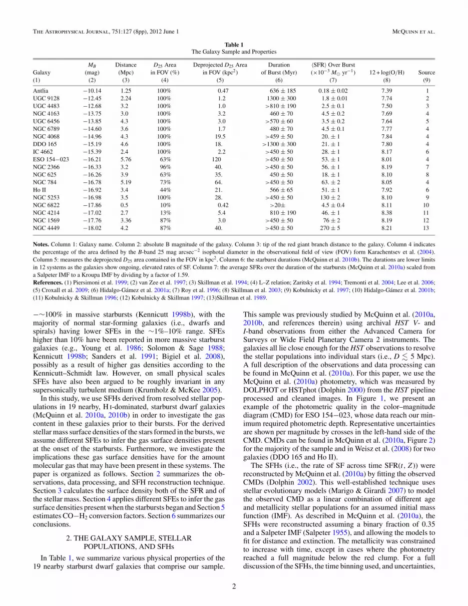
Table 1The Galaxy Sample and Properties

MB Distance D25 Area Deprojected D25 Area Duration 〈SFR〉 Over BurstGalaxy (mag) (Mpc) in FOV (%) in FOV (kpc2) of Burst (Myr) (×10−3 M� yr−1) 12 + log(O/H) Source(1) (2) (3) (4) (5) (6) (7) (8) (9)

Antlia −10.14 1.25 100% 0.47 636 ± 185 0.18 ± 0.02 7.39 1UGC 9128 −12.45 2.24 100% 1.2 1300 ± 300 1.8 ± 0.01 7.74 2UGC 4483 −12.68 3.2 100% 1.0 >810 ± 190 2.5 ± 0.1 7.50 3NGC 4163 −13.75 3.0 100% 3.2 460 ± 70 4.5 ± 0.2 7.69 4UGC 6456 −13.85 4.3 100% 3.0 >570 ± 60 3.5 ± 0.2 7.64 5NGC 6789 −14.60 3.6 100% 1.7 480 ± 70 4.5 ± 0.1 7.77 4NGC 4068 −14.96 4.3 100% 19.5 >459 ± 50 20. ± 1 7.84 4DDO 165 −15.19 4.6 100% 18. >1300 ± 300 21. ± 1 7.80 4IC 4662 −15.39 2.4 100% 2.2 >450 ± 50 28. ± 1 8.17 6ESO 154−023 −16.21 5.76 63% 120 >450 ± 50 53. ± 1 8.01 4NGC 2366 −16.33 3.2 96% 40. >450 ± 50 56. ± 1 8.19 7NGC 625 −16.26 3.9 63% 35. 450 ± 50 18. ± 1 8.10 8NGC 784 −16.78 5.19 73% 64. >450 ± 50 63. ± 2 8.05 4Ho II −16.92 3.4 44% 21. 566 ± 65 51. ± 1 7.92 6NGC 5253 −16.98 3.5 100% 28. >450 ± 50 130 ± 2 8.10 9NGC 6822 −17.86 0.5 10% 0.42 >20± 4.5 ± 0.4 8.11 10NGC 4214 −17.02 2.7 13% 5.4 810 ± 190 46. ± 1 8.38 11NGC 1569 −17.76 3.36 87% 3.0 >450 ± 50 76 ± 2 8.19 12NGC 4449 −18.02 4.2 87% 40. >450 ± 50 270 ± 5 8.21 13

Notes. Column 1: Galaxy name. Column 2: absolute B magnitude of the galaxy. Column 3: tip of the red giant branch distance to the galaxy. Column 4 indicatesthe percentage of the area defined by the B-band 25 mag arcsec−2 isophotal diameter in the observational field of view (FOV) form Karachentsev et al. (2004).Column 5: measures the deprojected D25 area contained in the FOV in kpc2. Column 6: the starburst durations (McQuinn et al. 2010b). The durations are lower limitsin 12 systems as the galaxies show ongoing, elevated rates of SF. Column 7: the average SFRs over the duration of the starbursts (McQuinn et al. 2010a) scaled froma Salpeter IMF to a Kroupa IMF by dividing by a factor of 1.59.References. (1) Piersimoni et al. 1999; (2) van Zee et al. 1997; (3) Skillman et al. 1994; (4) L–Z relation; Zaritsky et al. 1994; Tremonti et al. 2004; Lee et al. 2006;(5) Croxall et al. 2009; (6) Hidalgo-Gamez et al. 2001a; (7) Roy et al. 1996; (8) Skillman et al. 2003; (9) Kobulnicky et al. 1997; (10) Hidalgo-Gamez et al. 2001b;(11) Kobulnicky & Skillman 1996; (12) Kobulnicky & Skillman 1997; (13)Skillman et al. 1989.

−∼100% in massive starbursts (Kennicutt 1998b), with themajority of normal star-forming galaxies (i.e., dwarfs andspirals) having lower SFEs in the ∼1%–10% range. SFEshigher than 10% have been reported in more massive starburstgalaxies (e.g., Young et al. 1986; Solomon & Sage 1988;Kennicutt 1998b; Sanders et al. 1991; Bigiel et al. 2008),possibly as a result of higher gas densities according to theKennicutt–Schmidt law. However, on small physical scalesSFEs have also been argued to be roughly invariant in anysupersonically turbulent medium (Krumholz & McKee 2005).

In this study, we use SFHs derived from resolved stellar pop-ulations in 19 nearby, H i-dominated, starburst dwarf galaxies(McQuinn et al. 2010a, 2010b) in order to investigate the gascontent in these galaxies prior to their bursts. For the derivedstellar mass surface densities of the stars formed in the bursts, weassume different SFEs to infer the gas surface densities presentat the onset of the starbursts. Furthermore, we investigate theimplications these gas surface densities have for the amountmolecular gas that may have been present in these systems. Thepaper is organized as follows. Section 2 summarizes the ob-servations, data processing, and SFH reconstruction technique.Section 3 calculates the surface density both of the SFR and ofthe stellar mass. Section 4 applies different SFEs to infer the gassurface densities present when the starbursts began and Section 5estimates CO−H2 conversion factors. Section 6 summarizes ourconclusions.

2. THE GALAXY SAMPLE, STELLARPOPULATIONS, AND SFHs

In Table 1, we summarize various physical properties of the19 nearby starburst dwarf galaxies that comprise our sample.

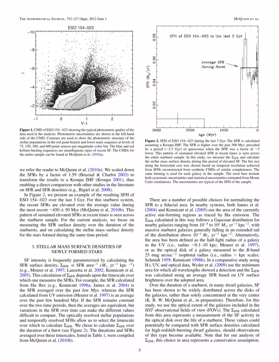
This sample was previously studied by McQuinn et al. (2010a,2010b, and references therein) using archival HST V- andI-band observations from either the Advanced Camera forSurveys or Wide Field Planetary Camera 2 instruments. Thegalaxies all lie close enough for the HST observations to resolvethe stellar populations into individual stars (i.e., D � 5 Mpc).A full description of the observations and data processing canbe found in McQuinn et al. (2010a). For this paper, we use theMcQuinn et al. (2010a) photometry, which was measured byDOLPHOT or HSTphot (Dolphin 2000) from the HST pipelineprocessed and cleaned images. In Figure 1, we present anexample of the photometric quality in the color–magnitudediagram (CMD) for ESO 154−023, whose data reach our min-imum required photometric depth. Representative uncertaintiesare shown per magnitude by crosses in the left-hand side of theCMD. CMDs can be found in McQuinn et al. (2010a, Figure 2)for the majority of the sample and in Weisz et al. (2008) for twogalaxies (DDO 165 and Ho II).

The SFHs (i.e., the rate of SF across time SFR(t, Z)) werereconstructed by McQuinn et al. (2010a) by fitting the observedCMDs (Dolphin 2002). This well-established technique usesstellar evolutionary models (Marigo & Girardi 2007) to modelthe observed CMD as a linear combination of different ageand metallicity stellar populations for an assumed initial massfunction (IMF). As described in McQuinn et al. (2010a), theSFHs were reconstructed assuming a binary fraction of 0.35and a Salpeter IMF (Salpeter 1955), and allowing the models tofit for distance and extinction. The metallicity was constrainedto increase with time, except in cases where the photometryreached a full magnitude below the red clump. For a fulldiscussion of the SFHs, the time binning used, and uncertainties,

2

The Astrophysical Journal, 751:127 (8pp), 2012 June 1 McQuinn et al.

ESO 154−023

−1 0 1 2V−I

−2

−4

−6

−8

−10

I

Figure 1. CMD of ESO 154−023 showing the typical photometric quality of thedata used in the analysis. Photometric uncertainties are shown in the left-handside of the CMD. Contours are used to show the photometric structure of thestellar populations in the red giant branch and lower main sequence at levels of75, 150, 300, and 600 point sources per magnitude–color bin. The blue and redhelium burning sequences are unambiguous signs of recent SF. The CMDs forthe entire sample can be found in McQuinn et al. (2010a).

we refer the reader to McQuinn et al. (2010a). We scaled downthe SFRs by a factor of 1.59 (Bruzual & Charlot 2003) totransform the results to a Kroupa IMF (Kroupa 2001), thusenabling a direct comparison with other studies in the literatureon SFR and SFR densities (e.g., Bigiel et al. 2008).

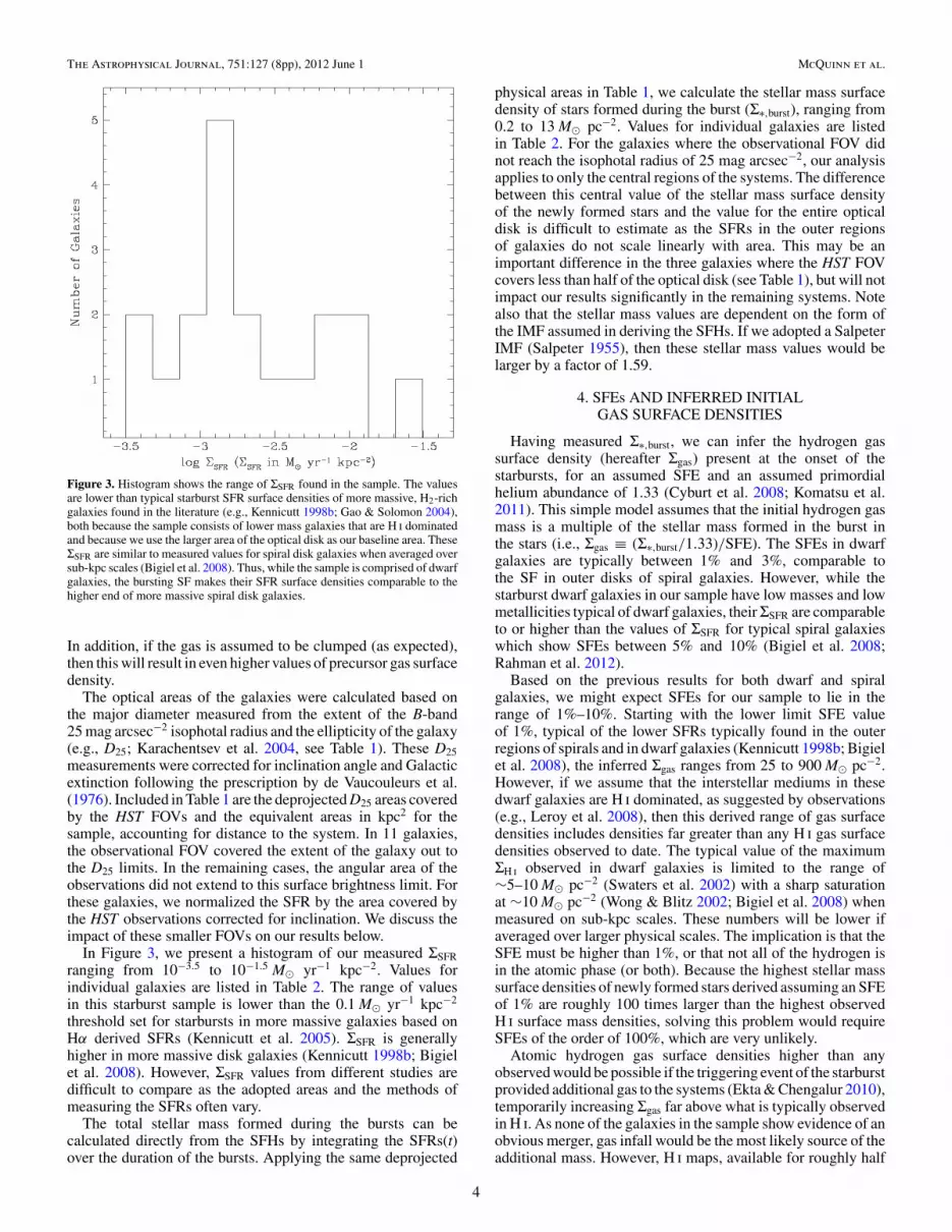
In Figure 2, we present an example of the resulting SFH ofESO 154−023 over the last 3 Gyr. For this starburst system,the recent SFRs are elevated over the average value duringthe most recent ∼450 ± 50 Myr (McQuinn et al. 2010b). Thispattern of sustained elevated SFRs at recent times is seen acrossthe starburst sample. For the current analysis, we focus onmeasuring the SFR surface density over the duration of thestarbursts, and on calculating the stellar mass surface densityfor the stars formed during the same time period.

3. STELLAR MASS SURFACE DENSITIES OFNEWLY FORMED STARS

SF intensity is frequently parameterized by calculating theSFR surface density, ΣSFR ≡ SFR area−1 (M� yr−1 kpc −2)(e.g., Meurer et al. 1997; Lanzetta et al. 2002; Kennicutt et al.2005). This calculation of ΣSFR depends upon the timescale overwhich one measures the SFRs. For example, the SFR calculatedfrom Hα flux (e.g., Kennicutt 1998a; James et al. 2004) isthe SFR averaged over the past few Myr, whereas the SFRcalculated from UV emission (Meurer et al. 1997) is an averageover the past few hundred Myr. If the SFR remains constantover the two time periods, then the averages are equivalent, butvariations in the SFR over time can make the different valuesdifficult to compare. The optically resolved stellar populationsand temporally resolved SFHs allow us to select the timescaleover which to calculate ΣSFR. We chose to calculate ΣSFR overthe duration of a burst (see Figure 2). The durations and SFRsaveraged over these timescales, listed in Table 1, were compiledfrom McQuinn et al. (2010b).

Figure 2. SFH of ESO 154−023 during the last 3 Gyr. The SFR is calculatedassuming a Kroupa IMF. The SFR is higher over the past 500 Myr, precededby a period (∼2.5 Gyr) of quiescence when the SFR was a factor of ∼5lower. This pattern of sustained elevated SFR at recent times is seen acrossthe entire starburst sample. In this study, we measure the ΣSFR and calculatethe stellar mass surface density during this period of elevated SF. The bin sizealong the horizontal axis was chosen based on temporal resolution achievedfrom SFHs reconstructed from synthetic CMDs of similar completeness. Thesame binning is used for each galaxy in the sample. The error bars includeboth systematic uncertainties and statistical uncertainties estimated from MonteCarlo simulations. The uncertainties are typical of the SFH of the sample.

There are a number of possible choices for normalizing theSFR to a fiducial area. In nearby systems, both James et al.(2004) and Kennicutt et al. (2005) use the area of the currentlyactive star-forming regions as traced by Hα emission. TheΣSFR calculated in this way follows a Gaussian distribution fornearby galaxies ranging from 10−4 to 102 M� yr−1 kpc−2, withmassive starburst galaxies generally falling in an extended tailof the distribution above 10−1 M� yr−1 kpc−2. Alternatively,the area has been defined as the half-light radius of a galaxyin the UV (i.e., radius ∼0.1–10 kpc; Meurer et al. 1997),or as the optical disk of a galaxy measured to the B-band25 mag arcsec−2 isophotal radius (i.e., radius ∼ kpc scales;Schmidt 1959; Kennicutt 1998b). In a comparative study usingH i, UV, and optical data, Wyder et al. (2009) use the minimumarea for which all wavelengths showed a detection and the ΣSFRwas calculated using an average SFR based on UV surfacebrightness over the adopted area.

Over the duration of a starburst, in many dwarf galaxies, SFhas been shown to be widely distributed across the disks ofthe galaxies, rather than solely concentrated at the very center(K. B. W. McQuinn et al., in preparation). Therefore, for thisstudy, we use the optical extent of the galaxies included in theHST observational fields of view (FOVs). The ΣSFR calculatedfrom this area represents a measurement of the SF activity inthe optical disk over the life of a starburst. These values couldpotentially be compared with SFR surface densities calculatedfor high-redshift-bursting dwarf galaxies, should observationsof this type become available. Note that for our analysis ofΣSFR, this choice in area represents a conservative assumption.

3

The Astrophysical Journal, 751:127 (8pp), 2012 June 1 McQuinn et al.

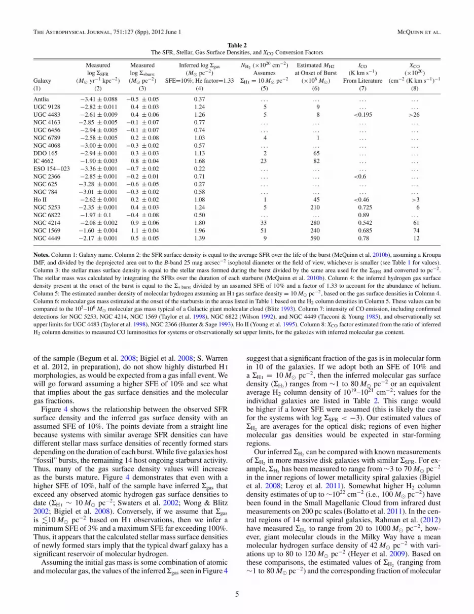
Figure 3. Histogram shows the range of ΣSFR found in the sample. The valuesare lower than typical starburst SFR surface densities of more massive, H2-richgalaxies found in the literature (e.g., Kennicutt 1998b; Gao & Solomon 2004),both because the sample consists of lower mass galaxies that are H i dominatedand because we use the larger area of the optical disk as our baseline area. TheseΣSFR are similar to measured values for spiral disk galaxies when averaged oversub-kpc scales (Bigiel et al. 2008). Thus, while the sample is comprised of dwarfgalaxies, the bursting SF makes their SFR surface densities comparable to thehigher end of more massive spiral disk galaxies.

In addition, if the gas is assumed to be clumped (as expected),then this will result in even higher values of precursor gas surfacedensity.

The optical areas of the galaxies were calculated based onthe major diameter measured from the extent of the B-band25 mag arcsec−2 isophotal radius and the ellipticity of the galaxy(e.g., D25; Karachentsev et al. 2004, see Table 1). These D25measurements were corrected for inclination angle and Galacticextinction following the prescription by de Vaucouleurs et al.(1976). Included in Table 1 are the deprojected D25 areas coveredby the HST FOVs and the equivalent areas in kpc2 for thesample, accounting for distance to the system. In 11 galaxies,the observational FOV covered the extent of the galaxy out tothe D25 limits. In the remaining cases, the angular area of theobservations did not extend to this surface brightness limit. Forthese galaxies, we normalized the SFR by the area covered bythe HST observations corrected for inclination. We discuss theimpact of these smaller FOVs on our results below.

In Figure 3, we present a histogram of our measured ΣSFRranging from 10−3.5 to 10−1.5 M� yr−1 kpc−2. Values forindividual galaxies are listed in Table 2. The range of valuesin this starburst sample is lower than the 0.1 M� yr−1 kpc−2

threshold set for starbursts in more massive galaxies based onHα derived SFRs (Kennicutt et al. 2005). ΣSFR is generallyhigher in more massive disk galaxies (Kennicutt 1998b; Bigielet al. 2008). However, ΣSFR values from different studies aredifficult to compare as the adopted areas and the methods ofmeasuring the SFRs often vary.

The total stellar mass formed during the bursts can becalculated directly from the SFHs by integrating the SFRs(t)over the duration of the bursts. Applying the same deprojected

physical areas in Table 1, we calculate the stellar mass surfacedensity of stars formed during the burst (Σ∗,burst), ranging from0.2 to 13 M� pc−2. Values for individual galaxies are listedin Table 2. For the galaxies where the observational FOV didnot reach the isophotal radius of 25 mag arcsec−2, our analysisapplies to only the central regions of the systems. The differencebetween this central value of the stellar mass surface densityof the newly formed stars and the value for the entire opticaldisk is difficult to estimate as the SFRs in the outer regionsof galaxies do not scale linearly with area. This may be animportant difference in the three galaxies where the HST FOVcovers less than half of the optical disk (see Table 1), but will notimpact our results significantly in the remaining systems. Notealso that the stellar mass values are dependent on the form ofthe IMF assumed in deriving the SFHs. If we adopted a SalpeterIMF (Salpeter 1955), then these stellar mass values would belarger by a factor of 1.59.

4. SFEs AND INFERRED INITIALGAS SURFACE DENSITIES

Having measured Σ∗,burst, we can infer the hydrogen gassurface density (hereafter Σgas) present at the onset of thestarbursts, for an assumed SFE and an assumed primordialhelium abundance of 1.33 (Cyburt et al. 2008; Komatsu et al.2011). This simple model assumes that the initial hydrogen gasmass is a multiple of the stellar mass formed in the burst inthe stars (i.e., Σgas ≡ (Σ∗,burst/1.33)/SFE). The SFEs in dwarfgalaxies are typically between 1% and 3%, comparable tothe SF in outer disks of spiral galaxies. However, while thestarburst dwarf galaxies in our sample have low masses and lowmetallicities typical of dwarf galaxies, their ΣSFR are comparableto or higher than the values of ΣSFR for typical spiral galaxieswhich show SFEs between 5% and 10% (Bigiel et al. 2008;Rahman et al. 2012).

Based on the previous results for both dwarf and spiralgalaxies, we might expect SFEs for our sample to lie in therange of 1%–10%. Starting with the lower limit SFE valueof 1%, typical of the lower SFRs typically found in the outerregions of spirals and in dwarf galaxies (Kennicutt 1998b; Bigielet al. 2008), the inferred Σgas ranges from 25 to 900 M� pc−2.However, if we assume that the interstellar mediums in thesedwarf galaxies are H i dominated, as suggested by observations(e.g., Leroy et al. 2008), then this derived range of gas surfacedensities includes densities far greater than any H i gas surfacedensities observed to date. The typical value of the maximumΣH i observed in dwarf galaxies is limited to the range of∼5–10 M� pc−2 (Swaters et al. 2002) with a sharp saturationat ∼10 M� pc−2 (Wong & Blitz 2002; Bigiel et al. 2008) whenmeasured on sub-kpc scales. These numbers will be lower ifaveraged over larger physical scales. The implication is that theSFE must be higher than 1%, or that not all of the hydrogen isin the atomic phase (or both). Because the highest stellar masssurface densities of newly formed stars derived assuming an SFEof 1% are roughly 100 times larger than the highest observedH i surface mass densities, solving this problem would requireSFEs of the order of 100%, which are very unlikely.

Atomic hydrogen gas surface densities higher than anyobserved would be possible if the triggering event of the starburstprovided additional gas to the systems (Ekta & Chengalur 2010),temporarily increasing Σgas far above what is typically observedin H i. As none of the galaxies in the sample show evidence of anobvious merger, gas infall would be the most likely source of theadditional mass. However, H i maps, available for roughly half

4

The Astrophysical Journal, 751:127 (8pp), 2012 June 1 McQuinn et al.

Table 2The SFR, Stellar, Gas Surface Densities, and XCO Conversion Factors

Measured Measured Inferred log Σgas NH2 (×1020 cm−2) Estimated MH2 ICO XCO

log ΣSFR log Σ∗burst (M� pc−2) Assumes at Onset of Burst (K km s−1) (×1020)Galaxy (M� yr−1 kpc−2) (M� pc−2) SFE=10%; He factor=1.33 ΣH i = 10 M� pc−2 (×106 M�) From Literature (cm−2 (K km s−1)−1

(1) (2) (3) (4) (5) (6) (7) (8)

Antlia −3.41 ± 0.088 −0.5 ± 0.05 0.37 . . . . . . . . . . . .

UGC 9128 −2.82 ± 0.011 0.4 ± 0.03 1.24 5 9 . . . . . .

UGC 4483 −2.61 ± 0.009 0.4 ± 0.06 1.26 5 8 <0.195 >26NGC 4163 −2.85 ± 0.005 −0.1 ± 0.07 0.77 . . . . . . . . . . . .

UGC 6456 −2.94 ± 0.005 −0.1 ± 0.07 0.74 . . . . . . . . . . . .

NGC 6789 −2.58 ± 0.005 0.2 ± 0.08 1.03 4 1 . . . . . .

NGC 4068 −3.00 ± 0.001 −0.3 ± 0.02 0.57 . . . . . . . . . . . .

DDO 165 −2.94 ± 0.001 0.3 ± 0.03 1.13 2 65 . . . . . .

IC 4662 −1.90 ± 0.003 0.8 ± 0.04 1.68 23 82 . . . . . .

ESO 154−023 −3.36 ± 0.001 −0.7 ± 0.02 0.22 . . . . . . . . . . . .

NGC 2366 −2.85 ± 0.001 −0.2 ± 0.01 0.71 . . . . . . <0.6 . . .

NGC 625 −3.28 ± 0.001 −0.6 ± 0.05 0.27 . . . . . . . . . . . .

NGC 784 −3.01 ± 0.001 −0.3 ± 0.02 0.58 . . . . . . . . . . . .

Ho II −2.62 ± 0.001 0.2 ± 0.02 1.08 1 45 <0.46 >3NGC 5253 −2.35 ± 0.001 0.4 ± 0.03 1.24 5 210 0.725 6NGC 6822 −1.97 ± 0.1 −0.4 ± 0.08 0.50 . . . . . . 0.89 . . .

NGC 4214 −2.08 ± 0.002 0.9 ± 0.06 1.80 33 280 0.542 61NGC 1569 −1.60 ± 0.004 1.1 ± 0.04 1.96 51 240 0.685 74NGC 4449 −2.17 ± 0.001 0.5 ± 0.05 1.39 9 590 0.78 12

Notes. Column 1: Galaxy name. Column 2: the SFR surface density is equal to the average SFR over the life of the burst (McQuinn et al. 2010b), assuming a KroupaIMF, and divided by the deprojected area out to the B-band 25 mag arcsec−2 isophotal diameter or the field of view, whichever is smaller (see Table 1 for values).Column 3: the stellar mass surface density is equal to the stellar mass formed during the burst divided by the same area used for the ΣSFR and converted to pc−2.The stellar mass was calculated by integrating the SFRs over the duration of each starburst (McQuinn et al. 2010b). Column 4: the inferred hydrogen gas surfacedensity present at the onset of the burst is equal to the Σ∗ burst divided by an assumed SFE of 10% and a factor of 1.33 to account for the abundance of helium.Column 5: The estimated number density of molecular hydrogen assuming an H i gas surface density = 10 M� pc−2, based on the gas surface densities in Column 4.Column 6: molecular gas mass estimated at the onset of the starbursts in the areas listed in Table 1 based on the H2 column densities in Column 5. These values can becompared to the 105–106 M� molecular gas mass typical of a Galactic giant molecular cloud (Blitz 1993). Column 7: intensity of CO emission, including confirmeddetections for NGC 5253, NGC 4214, NGC 1569 (Taylor et al. 1998), NGC 6822 (Wilson 1992), and NGC 4449 (Tacconi & Young 1985), and observationally setupper limits for UGC 4483 (Taylor et al. 1998), NGC 2366 (Hunter & Sage 1993), Ho II (Young et al. 1995). Column 8: XCO factor estimated from the ratio of inferredH2 column densities to measured CO luminosities for systems or observationally set upper limits, for the galaxies with inferred molecular gas content.

of the sample (Begum et al. 2008; Bigiel et al. 2008; S. Warrenet al. 2012, in preparation), do not show highly disturbed H imorphologies, as would be expected from a gas infall event. Wewill go forward assuming a higher SFE of 10% and see whatthat implies about the gas surface densities and the moleculargas fractions.

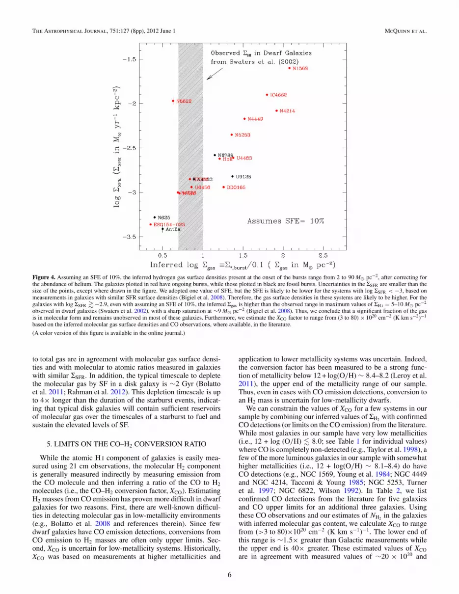
Figure 4 shows the relationship between the observed SFRsurface density and the inferred gas surface density with anassumed SFE of 10%. The points deviate from a straight linebecause systems with similar average SFR densities can havedifferent stellar mass surface densities of recently formed starsdepending on the duration of each burst. While five galaxies host“fossil” bursts, the remaining 14 host ongoing starburst activity.Thus, many of the gas surface density values will increaseas the bursts mature. Figure 4 demonstrates that even with ahigher SFE of 10%, half of the sample have inferred Σgas thatexceed any observed atomic hydrogen gas surface densities todate (ΣH i ∼ 10 M� pc−2; Swaters et al. 2002; Wong & Blitz2002; Bigiel et al. 2008). Conversely, if we assume that Σgasis �10 M� pc−2 based on H i observations, then we infer aminimum SFE of 3% and a maximum SFE far exceeding 100%.Thus, it appears that the calculated stellar mass surface densitiesof newly formed stars imply that the typical dwarf galaxy has asignificant reservoir of molecular hydrogen.

Assuming the initial gas mass is some combination of atomicand molecular gas, the values of the inferred Σgas seen in Figure 4

suggest that a significant fraction of the gas is in molecular formin 10 of the galaxies. If we adopt both an SFE of 10% anda ΣH i = 10 M� pc−2, then the inferred molecular gas surfacedensity (ΣH2 ) ranges from ∼1 to 80 M� pc−2 or an equivalentaverage H2 column density of 1019–1021 cm−2; values for theindividual galaxies are listed in Table 2. This range wouldbe higher if a lower SFE were assumed (this is likely the casefor the systems with log ΣSFR < −3). Our estimated values ofΣH2 are averages for the optical disk; regions of even highermolecular gas densities would be expected in star-formingregions.

Our inferred ΣH2 can be compared with known measurementsof ΣH2 in more massive disk galaxies with similar ΣSFR. For ex-ample, ΣH2 has been measured to range from ∼3 to 70 M� pc−2

in the inner regions of lower metallicity spiral galaxies (Bigielet al. 2008; Leroy et al. 2011). Somewhat higher H2 columndensity estimates of up to ∼1022 cm−2 (i.e., 100 M� pc−2) havebeen found in the Small Magellanic Cloud from infrared dustmeasurements on 200 pc scales (Bolatto et al. 2011). In the cen-tral regions of 14 normal spiral galaxies, Rahman et al. (2012)have measured ΣH2 to range from 20 to 1000 M� pc−2, how-ever, giant molecular clouds in the Milky Way have a meanmolecular hydrogen surface density of 42 M� pc−2 with vari-ations up to 80 to 120 M� pc−2 (Heyer et al. 2009). Based onthese comparisons, the estimated values of ΣH2 (ranging from∼1 to 80 M� pc−2) and the corresponding fraction of molecular

5

The Astrophysical Journal, 751:127 (8pp), 2012 June 1 McQuinn et al.

Figure 4. Assuming an SFE of 10%, the inferred hydrogen gas surface densities present at the onset of the bursts range from 2 to 90 M� pc−2, after correcting forthe abundance of helium. The galaxies plotted in red have ongoing bursts, while those plotted in black are fossil bursts. Uncertainties in the ΣSFR are smaller than thesize of the points, except where drawn in the figure. We adopted one value of SFE, but the SFE is likely to be lower for the systems with log ΣSFR < −3, based onmeasurements in galaxies with similar SFR surface densities (Bigiel et al. 2008). Therefore, the gas surface densities in these systems are likely to be higher. For thegalaxies with log ΣSFR � −2.9, even with assuming an SFE of 10%, the inferred Σgas is higher than the observed range in maximum values of ΣH i = 5–10 M� pc−2

observed in dwarf galaxies (Swaters et al. 2002), with a sharp saturation at ∼9 M� pc−2 (Bigiel et al. 2008). Thus, we conclude that a significant fraction of the gasis in molecular form and remains unobserved in most of these galaxies. Furthermore, we estimate the XCO factor to range from (3 to 80) × 1020 cm−2 (K km s−2)−1

based on the inferred molecular gas surface densities and CO observations, where available, in the literature.

(A color version of this figure is available in the online journal.)

to total gas are in agreement with molecular gas surface densi-ties and with molecular to atomic ratios measured in galaxieswith similar ΣSFR. In addition, the typical timescale to depletethe molecular gas by SF in a disk galaxy is ∼2 Gyr (Bolattoet al. 2011; Rahman et al. 2012). This depletion timescale is upto 4× longer than the duration of the starburst events, indicat-ing that typical disk galaxies will contain sufficient reservoirsof molecular gas over the timescales of a starburst to fuel andsustain the elevated levels of SF.

5. LIMITS ON THE CO–H2 CONVERSION RATIO

While the atomic H i component of galaxies is easily mea-sured using 21 cm observations, the molecular H2 componentis generally measured indirectly by measuring emission fromthe CO molecule and then inferring a ratio of the CO to H2molecules (i.e., the CO–H2 conversion factor, XCO). EstimatingH2 masses from CO emission has proven more difficult in dwarfgalaxies for two reasons. First, there are well-known difficul-ties in detecting molecular gas in low-metallicity environments(e.g., Bolatto et al. 2008 and references therein). Since fewdwarf galaxies have CO emission detections, conversions fromCO emission to H2 masses are often only upper limits. Sec-ond, XCO is uncertain for low-metallicity systems. Historically,XCO was based on measurements at higher metallicities and

application to lower metallicity systems was uncertain. Indeed,the conversion factor has been measured to be a strong func-tion of metallicity below 12 + log(O/H) ∼ 8.4–8.2 (Leroy et al.2011), the upper end of the metallicity range of our sample.Thus, even in cases with CO emission detections, conversion toan H2 mass is uncertain for low-metallicity dwarfs.

We can constrain the values of XCO for a few systems in oursample by combining our inferred values of ΣH2 with confirmedCO detections (or limits on the CO emission) from the literature.While most galaxies in our sample have very low metallicities(i.e., 12 + log (O/H) � 8.0; see Table 1 for individual values)where CO is completely non-detected (e.g., Taylor et al. 1998), afew of the more luminous galaxies in our sample with somewhathigher metallicities (i.e., 12 + log(O/H) ∼ 8.1–8.4) do haveCO detections (e.g., NGC 1569, Young et al. 1984; NGC 4449and NGC 4214, Tacconi & Young 1985; NGC 5253, Turneret al. 1997; NGC 6822, Wilson 1992). In Table 2, we listconfirmed CO detections from the literature for five galaxiesand CO upper limits for an additional three galaxies. Usingthese CO observations and our estimates of NH2 in the galaxieswith inferred molecular gas content, we calculate XCO to rangefrom (>3 to 80)×1020 cm−2 (K km s−1)−1. The lower end ofthis range is ∼1.5× greater than Galactic measurements whilethe upper end is 40× greater. These estimated values of XCOare in agreement with measured values of ∼20 × 1020 and

6

The Astrophysical Journal, 751:127 (8pp), 2012 June 1 McQuinn et al.

∼45 × 1020 cm−2 (K km s−1)−1 found for two dwarf galaxiesin the Local Group from infrared dust emission (Leroy et al.2011) and the lower limit of 10× Galactic XCO values placedon a low-metallicity (12 + [O/H] ∼ 7.67) Local Group dwarfgalaxy DDO 154 (Komugi et al. 2011).

Since nearby, metal poor, dwarf galaxies are often consideredthe prototypes of more massive galaxies at high redshift, it isalso interesting to compare our estimated XCO values to measure-ments in low-metallicity systems at high redshift. In a sample ofstar-forming galaxies in the mass range 1010–1011 M�, one totwo orders of magnitude more massive than any of the galaxiesin our sample, Genzel et al. (2012) found the CO luminosity tomolecular gas mass conversion factors to be ∼2.5–14× Galacticvalues in a metallicity range of 12 + [O/H] ∼ 8.1–8.4, withhigher values expected in lower mass galaxies. For comparison,for the lower mass galaxies in our sample which span the rangein metallicities from 12+[O/H] ∼ 7.4–8.4 (see Table 1), ourestimated XCO factors include values up to 40× greater thanGalactic XCO values.

6. CONCLUSIONS

We have used optical imaging of resolved stellar populationsobtained from the HST data archive to measure the SFRs andstellar mass surface densities of stars formed during starburstevents in a sample of 19 nearby starburst dwarf galaxies. TheSFR surface densities of these dwarf galaxies are comparable tothe higher end of SFR surface densities of more massive spiralgalaxies while still having low metallicities typical of dwarfsystems.

By assuming different SFEs, the stellar mass surface densitieswere used to infer gas surface densities present at the onset ofthe bursts. Using an SFE of 1% and assuming Σgas ∼ ΣH i, allinferred gas surface densities are greater than the observed rangeof H i gas surface densities in dwarf galaxies of �10 M� pc−2

(Swaters et al. 2002; Wong & Blitz 2002; Bigiel et al. 2008).Using a higher SFE of 10%, half of the inferred gas surfacedensities are still higher than the observed range of ΣH i byfactors of nine.

The simplest explanation appears to be that a significantfraction of the gas is in molecular form but remains unobservedin most of these galaxies due to their low metallicities. Indeed,the elevated levels of recent SF are an unambiguous sign thatour sample of galaxies has hosted significant reservoirs of coldmolecular gas. In this low-metallicity regime, the H2 massescan be significant, even for very low CO luminosities. Thus,the lack of CO detections in our sample is not inconsistent withtheir having significant reservoirs of molecular gas. Coupledwith limits on CO emission from the literature, the inferredmolecular gas surface densities suggest XCO factors of up to 40×greater than Galactic measurements in these low-metallicity andlow-mass galaxies.

Support for this work was provided by NASA through aROSES grant (No. NNX10AD57G). E.D.S. is grateful forpartial support from the University of Minnesota. The authorsthank the anonymous referee for helpful and constructivecomments. K.B.W.M. gratefully acknowledges Matthew, Cole,and Carling for their support. This research made use of NASA’sAstrophysical Data System and the NASA/IPAC ExtragalacticDatabase (NED) which is operated by the Jet PropulsionLaboratory, California Institute of Technology, under contractwith the National Aeronautics and Space Administration.

Facility: HST

REFERENCES

Begum, A., Chengalur, J. N., Karachentsev, I. D., Sharina, M. E., & Kaisin,S. S. 2008, MNRAS, 386, 1667

Bigiel, F., Leroy, A., Walter, F., et al. 2008, AJ, 136, 2846Blitz, L. 1993, in Protostars and Planets III, ed. E. H. Levy & J. I. Lunine

(Tucson, AZ: Univ. Arizona Press), 125Bolatto, A. D., Leroy, A. K., Jameson, K., et al. 2011, ApJ, 741, 12Bolatto, A. D., Leroy, A. K., Rosolowsky, E., Walter, F., & Blitz, L. 2008, ApJ,

686, 948Bruzual, G., & Charlot, S. 2003, MNRAS, 344, 1000Cote, B., Martel, H., Drissen, L., & Robert, C. 2012, MNRAS, 421, 847Croxall, K. V., van Zee, L., Lee, H., et al. 2009, ApJ, 705, 723Cyburt, R. H., Fields, B. D., & Olive, K. A. 2008, J. Cosmol. Astropart. Phys.,

JCAP11(2008)012de Vaucouleurs, G., de Vaucouleurs, A., & Corwin, J. R. 1976, Second Reference

Catalogue of Bright Galaxies (Austin, TX: Univ. Texas Press), 0Dolphin, A. E. 2000, PASP, 112, 1383Dolphin, A. E. 2002, MNRAS, 332, 91Ekta, B., & Chengalur, J. N. 2010, MNRAS, 403, 295Gao, Y., & Solomon, P. M. 2004, ApJ, 606, 271Genzel, R., Tacconi, L. J., Combes, F., et al. 2012, ApJ, 746, 69Heyer, M., Krawczyk, C., Duval, J., & Jackson, J. M. 2009, ApJ, 699, 1092Hidalgo-Gamez, A. M., Masegosa, J., & Olofsson, K. 2001a, A&A, 369,

797Hidalgo-Gamez, A. M., Olofsson, K., & Masegosa, J. 2001b, A&A, 367, 388Hunter, D. A., & Sage, L. 1993, PASP, 105, 374James, P. A., Shane, N. S., Beckman, J. E., et al. 2004, A&A, 414, 23Karachentsev, I. D., Karachentseva, V. E., Huchtmeier, W. K., & Makarov, D. I.

2004, AJ, 127, 2031Kennicutt, R. C., Jr. 1989, ApJ, 344, 685Kennicutt, R. C., Jr. 1998a, ARA&A, 36, 189Kennicutt, R. C., Jr. 1998b, ApJ, 498, 541Kennicutt, R. C., Jr., Lee, J. C., Funes, J. G., Sakai, S., & Akiyama, S. 2005,

in Starbursts from 30 Doradus to Lyman Break Galaxies, ed. R. De Gris &R. M. Gonzalez Delgado (Astrophysics & Space Science Library, Vol. 329;The Netherlands: Springer), 187

Kobulnicky, H. A., & Skillman, E. D. 1996, ApJ, 471, 211Kobulnicky, H. A., & Skillman, E. D. 1997, ApJ, 489, 636Kobulnicky, H. A., Skillman, E. D., Roy, J.-R., Walsh, J. R., & Rosa, M. R.

1997, ApJ, 477, 679Komatsu, E., Smith, K. M., Dunkley, J., et al. 2011, ApJS, 192, 18Komugi, S., Yasui, C., Kobayashi, N., et al. 2011, PASJ, 63, L1Kroupa, P. 2001, MNRAS, 322, 231Krumholz, M. R., & McKee, C. F. 2005, ApJ, 630, 250Lanzetta, K. M., Yahata, N., Pascarelle, S., Chen, H.-W., & Fernandez-Soto, A.

2002, ApJ, 570, 492Lee, H., Skillman, E. D., & Venn, K. A. 2006, ApJ, 642, 813Leroy, A., Bolatto, A. D., Simon, J. D., & Blitz, L. 2005, ApJ, 625, 763Leroy, A. K., Bolatto, A., Gordon, K., et al. 2011, ApJ, 737, 12Leroy, A. K., Walter, F., Brinks, E., et al. 2008, AJ, 136, 2782Marigo, P., & Girardi, L. 2007, A&A, 469, 239Martin, C. L., & Kennicutt, R. C., Jr. 2001, ApJ, 555, 301McQuinn, K. B. W., Skillman, E. D., Cannon, J. M., et al. 2010a, ApJ, 721, 297McQuinn, K. B. W., Skillman, E. D., Cannon, J. M., et al. 2010b, ApJ, 724, 49Meurer, G. R., Heckman, T. M., Lehnert, M. D., Leitherer, C., & Lowenthal, J.

1997, AJ, 114, 54O’Neil, K., Schinnerer, E., & Hofner, P. 2003, ApJ, 588, 230Parmentier, G., & Fritze, U. 2009, ApJ, 690, 1112Piersimoni, A. M., Bono, G., Castellani, M., et al. 1999, A&A, 352, L63Rahman, N., Bolatto, A. D., Xue, R., et al. 2012, ApJ, 745, 183Roy, J.-R., Belley, J., Dutil, Y., & Martin, P. 1996, ApJ, 460, 284Salpeter, E. E. 1955, ApJ, 121, 161Sanders, D. B., Scoville, N. Z., & Soifer, B. T. 1991, ApJ, 370, 158Schmidt, M. 1959, ApJ, 129, 243Skillman, E. D., Cote, S., & Miller, B. W. 2003, AJ, 125, 610Skillman, E. D., Kennicutt, R. C., & Hodge, P. W. 1989, ApJ, 347, 875Skillman, E. D., Televich, R. J., Kennicutt, R. C., Jr, Garnett, D. R., & Terlevich,

E. 1994, ApJ, 431, 172Solomon, P. M., & Sage, L. J. 1988, ApJ, 334, 613Swaters, R. A., van Albada, T. S., van der Hulst, J. M., & Sancisi, R. 2002, A&A,

390, 829Tacconi, L. J., & Young, J. S. 1985, ApJ, 290, 602Tan, J. C. 2000, ApJ, 536, 173Taylor, C. L., Kobulnicky, H. A., & Skillman, E. D. 1998, AJ, 116, 2746Tremonti, C. A., Heckman, T. M., Kauffmann, G., et al. 2004, ApJ, 613, 898Turner, J. L., Beck, S. C., & Hurt, R. L. 1997, ApJ, 474, L11

7

The Astrophysical Journal, 751:127 (8pp), 2012 June 1 McQuinn et al.

van Zee, L., Haynes, M. P., & Salzer, J. J. 1997, AJ, 114, 2479Weisz, D. R., Skillman, E. D., Cannon, J. M., et al. 2008, ApJ, 689, 160Wilson, C. D. 1992, ApJ, 391, 144Wong, T., & Blitz, L. 2002, ApJ, 569, 157Wyder, T. K., Martin, D. C., Barlow, T. A., et al. 2009, ApJ, 696, 1834

Young, J. S., Gallagher, J. S., & Hunter, D. A. 1984, ApJ, 276, 476Young, J. S., Schloerb, F. P., Kenney, J. D., & Lord, S. D. 1986, ApJ, 304,

443Young, J. S., Xie, S., Tacconi, L., et al. 1995, ApJS, 98, 219Zaritsky, D., Kennicutt, R. C., Jr., & Huchra, J. P. 1994, ApJ, 420, 87

8