arX

iv:g

r-qc

/000

6081

v1 2

2 Ju

n 20

00

J. Math. Phys.35, 4184 (1994)

Null cone evolution of axisymmetric vacuum spacetimes

R. Gomez, P. Papadopoulos and J. WinicourDepartment of Physics and Astronomy, University of Pittsburgh, Pittsburgh, PA 15260

Abstract

We present the details of an algorithm for the global evolution of asymptot-

ically flat, axisymmetric spacetimes, based upon a characteristic initial value

formulation using null cones as evolution hypersurfaces. We identify a new

static solution of the vacuum field equations which provides an important

test bed for characteristic evolution codes. We also show how linearized solu-

tions of the Bondi equations can be generated by solutions of the scalar wave

equation, thus providing a complete set of test beds in the weak field regime.

These tools are used to establish that the algorithm is second order accurate

and stable, subject to a Courant-Friedrichs-Lewy condition. In addition, the

numerical versions of the Bondi mass and news function, calculated at scri

on a compactified grid, are shown to satisfy the Bondi mass loss equation

to second order accuracy. This verifies that numerical evolution preserves

the Bianchi identities. Results of numerical evolution confirm the theorem

of Christodoulou and Klainerman that in vacuum, weak initial data evolve

to a flat spacetime. For the class of asymptotically flat, axisymmetric vac-

uum spacetimes, for which no nonsingular analytic solutions are known, the

algorithm provides highly accurate solutions throughout the regime in which

neither caustics nor horizons form.

Typeset using REVTEX

1

I. INTRODUCTION

The physical basis of a new algorithm for the evolution of spacetimes has been pro-posed. [1] This algorithm is based upon the characteristic initial value problem for generalrelativity, using light cones as the evolution hypersurfaces, rather than the spacelike folia-tion used in traditional approaches based upon the Cauchy problem. The intimate use ofcharacteristics has particular advantages for the description of gravitational radiation andblack hole formation. [2–4]. The first attempt to carry out numerical evolution based uponthis algorithm was only successful in a region outside some sufficiently large worldtube. Nearthe vertex of the null cone, instabilities arose which destroyed the accuracy of the code. Theunderlying cause of this instability was too complicated to analyze in the context of generalrelativity, especially since the numerical analysis of the characteristic initial value problemhad not yet been carried out even for the simplest linear axisymmetric systems.

This warranted an investigation of the basic computational properties of the evolutionof the flat space scalar wave equation using a null cone initial value formulation [5]. It wasfound that near the vertex of the cone the Courant-Friedrichs-Lewy (CFL) condition placesa stricter limit on the time step than for the case of Cauchy evolution. This insight madepossible the development of an extremely efficient marching algorithm for evolving the dataon the initial cone by stepping it out from the vertex of the next cone to null infinity (scri)along each angular ray direction. This marching algorithm is based upon a simple identitysatisfied by the values of the scalar field at the corners of a parallelogram formed by fournull rays. The result was a stable, calibrated, second order accurate global algorithm ona compactified grid. Furthermore, scri played the role of a perfect absorbing boundary sothat no radiation was reflected back into the system. This algorithm offers a powerful newapproach to generic wave type systems. The basic idea is applicable to any of the hyperbolicsystems occurring in physics.

In this paper, we apply the algorithm to the evolution of asymptotically flat, (twist-free)axisymmetric spacetimes. In a Bondi null coordinate system the metric takes the form [6]

ds2 = (V

re2β − U2r2e2γ)du2 + 2e2βdudr + 2Ur2e2γdudθ

−r2(e2γdθ2 + e−2γ sin2 θdφ2). (1)

The vacuum field equations then decompose into the three hypersurface equations

β,r =1

2r (γ,r)

2 (2)

[r4 e2(γ−β)U,r],r = 2r2[r2(β

r2),rθ −

(sin2 θ γ),rθ

sin2 θ+ 2 γ,r γ,θ)] (3)

V,r = −1

4r4e2(γ−β)(U,r)

2 +(r4 sin θU),rθ

2r2 sin θ

+e2(β−γ)[1 −(sin θβ,θ),θ

sin θ+ γ,θθ + 3 cot θγ,θ − (β,θ)

2 − 2γ,θ(γ,θ − β,θ)] (4)

2

and one evolution equation

4r(rγ),ur = [2rγ,rV − r2(2γ,θ U + sin θ(U

sin θ),θ)],r − 2r2 (γ,rU sin θ),θ

sin θ

+1

2r4e2(γ−β)(U,r)

2 + 2e2(β−γ)[(β,θ)2 + sin θ(

β,θ

sin θ),θ]. (5)

The initial data consists of γ, which is unconstrained except by smoothness conditions.Because γ represents a spin-2 field, it must be O(sin2 θ) near the axis and consist of l ≥ 2spin-2 multipoles.

Here we are interested in the global application of this system when the null hypersur-faces are null cones, although the approach also goes through without major change if thenull hypersurfaces emanate from a finite world tube. We require that the null cones havenonsingular vertices which trace out a geodesic worldline r = 0. For the quadrupole terms,this implies the boundary conditions γ = O(r2), β = O(r4), U = O(r) and V = r + O(r3).For higher multipoles, the smoothness conditions can be worked out by referring back tolocal Minkowski coordinates [7]. As a consequence, O(rn) terms in γ can contain multipoleswith 2 ≤ l ≤ n. Any satisfactory computational algorithm must meet the challenge ofpreserving these smoothness conditions.

In Sec. II, we analyze the linearized version of these equations and show how theirsolutions may be obtained locally from solutions of the scalar wave equation. This providesan important means of constructing linearized solutions in a null cone gauge for the purposeof code calibration. It also reveals essential changes in the grid structure necessary inadapting the null parallelogram algorithm for the wave equation to linearized gravity.

This also solves the major computational problems for the nonlinear case. In Sec. III,we show how the linearized algorithm can be extended to this case. In Sec. IV, we discussthe major finite difference techniques necessary for second order accuracy. In Sec. V, wepresent a study of the stability and accuracy of an evolution code based upon this algorithm.New exact and linearized solutions are introduced to establish second order convergence. Inaddition, a global check on accuracy is carried out using Bondi’s formula relating mass lossto the time integral of the square of the news function.

II. THE LINEARIZED BONDI EQUATIONS

In the linearized limit β = 0 and V = r. The equations (2)-(5) reduce to one hypersurfaceequation and one evolution equation for the surviving field variables γ and U ,

(r4U,r),r = −2r2(sin2 θ γ),rθ

sin2 θ(6)

4r(rγ),ur = [2r2γ,r − r2 sin θ(U

sin θ),θ],r. (7)

Physical considerations suggest that these equations be related to the wave equation. Ifthis relationship were sufficiently simple, then the scalar wave algorithm could be used as aguide in formulating an algorithm for evolving γ. A scheme for generating solutions to the

3

linearized Bondi equations in terms of solutions to the wave equation has been presentedpreviously [6]. However, in that scheme, the relationship of the scalar wave to γ is non-localin the angular directions and is not useful for this purpose.

We now formulate an alternative scheme in terms of spin-weight 0 quantities α and Z,related to γ (spin-weight 2) and U (spin-weight 1) by [8]

γ = ð2α = sin θ∂θ(

1

sin θ∂θα) (8)

U = ðZ = ∂θZ. (9)

Then the linearized equations are equivalent to

(r4Z,r),r = −2r2(2 − L2)α,r, (10)

and

E := 2(rα),ur − r−1(r2α,r − r2Z/2),r = 0, (11)

where L2 = −(1/ sin θ)∂θ(sin θ∂θ) is the θ-part of the angular momentum operator. Now letΦ be a solution of the flat space scalar wave equation,

r2 Φ = 2(rΦ),ur − (rΦ),rr + r−1L2Φ = 0, (12)

and set

r2α,r = (r2Φ),r (13)

and

r2Z,r = 2(L2 − 2)Φ. (14)

Then

E = r2 Φ + 2(Φ + α),u − 2r−2(r2Φ),r + Z, (15)

and

E,r = r−2(r32 Φ),r (16)

Equation (10) is satisfied as a result of (13) and (14)and the wave equation (12) impliesE,r = 0. If Φ is smooth and O(r2) at the origin, this implies E = 0, so that the linearizedequations are satisfied. The condition that Φ = O(r2) eliminates fields with only monopoleand dipole dependence so that it does not restrict the generality of the spin-weight 2 functionγ obtained through (8).

Thus for any linearized axisymmetric gravitational wave in the null cone gauge, γ maybe related to a scalar wave by (8) and (13). The CFL condition for convergence of afinite difference algorithm requires that the numerical domain of dependence be larger thanthe physical domain of dependence. Because the relationship between Φ and γ is local with

4

respect to the null rays on the cone, their domains of dependence coincide. This suggests thata stable and convergent evolution algorithm for the gravitational field may be modeled uponthe scalar wave algorithm. This turns out to be the case although some subtle distinctionsarise, as described below.

An evolution algorithm for scalar waves has been formulated in terms of an integralidentity for the values of the field at the corners of a null parallelogram lying on the (u, r)plane [5]. The wave equation with source, 2Φ = S, can be reexpressed in the form

2(2)ψ = −

L2ψ

r2+ rS, (17)

where ψ = rΦ and 2(2) is the 2-dimensional wave operator intrinsic to the (u, r) plane.

Integration over the null parallelogram as depicted in Fig. 1 then leads to the integralequation

ψQ = ψP + ψS − ψR +1

2

∫

A

dudr[−L2ψ

r2+ rS], (18)

where P , Q, R and S are the corners and A the area of the parallelogram.This identity gives rise to an explicit marching algorithm for evolution. Let the null

parallelogram span null cones at adjacent grid values u0 and u0 + ∆u, as shown in Fig. 1,for some θ and φ. If ψ has been determined on the entire u0 cone and on the u0 + ∆u coneradially outward from the origin to the point P , then (18) determines ψ at the next pointQ in terms of an integral over A. This procedure can then be repeated to determine ψ atthe next radially outward point T in Fig. 1. After completing this radial march to scri, thefield ψ is then evaluated on the next null cone at u0 + 2∆u, beginning at the vertex wheresmoothness gives the start up condition that ψ = 0. The resulting evolution algorithm isa 2-level scheme which reflects, in a natural way, the distinction between characteristic andCauchy evolution, i.e. that the time derivative of the field is not part of the characteristicinitial data.

The CFL condition on the numerical domain of dependence is a necessary conditionfor convergence of a numerical algorithm. For the grid point at (u, r, θ), there are threecritical grid points, (u−∆u, r + ∆r, θ) and (u−∆u, r−∆r, θ ±∆θ), which must lie insideits past physical light cone. These gives rise to the inequalities ∆u < 2∆r and ∆u <−∆r + (∆r2 + r2∆θ2)1/2. At large r, the second inequality becomes ∆u < r∆θ and thelimitations on the time step are essentially the same as for a Cauchy evolution algorithm.However, near the vertex of the cone, the second inequality gives a stricter condition

∆u < K∆r∆θ2, (19)

where K is a number of order 1 whose exact value depends upon the start up details atthe vertex. For the scalar wave equation, these stability limits were confirmed by numericalexperimentation and it was found [5] that K ≈ 4.

The linearized gravitational evolution equation (7) can be recast into a form similar to(17),

2(2)ψ = H, (20)

5

where now ψ = rγ and H only contains hypersurface terms. This allows use of the nullparallelogram algorithm to evolve γ by the same marching scheme as in the scalar case. Theadditional feature here is that U must be simultaneously marched out the null cone usingthe hypersurface equation (6). For the scalar wave equation (17), the angular momentumbarrier is represented by the term L2ψ/r2, which is determined from ψ by a double angularderivative. In the linearized gravitational evolution equation (7), the analogous term is[r2 sin θ(U/ sin θ),θ],r, which is determined from U by a single angular derivative. In turn,the hypersurface equation (6) relates U to γ by a single angular derivative. Physically,this has the same net effect of producing an angular momentum barrier depending uponthe second angular derivative, as in the scalar case. However, the nontrivial mathematicaldistinction between the two cases leads to nontrivial difference in their natural grid structuresfor a numerical algorithm. In particular, the grid for U must be staggered between the gridpoints for γ. These and other details of the marching algorithm will be given in Sec. IV,where we discuss the nonlinear case.

The use of scalar waves to generate solutions of the linearized Bondi equations providesan important tool for testing evolution algorithms in the linear regime. Monopole solutionsmay be represented in the form Φ = [F (u+2r)−F (u)]/r and axisymmetric multipoles maybe built up by applying the z-translation operator

∂z = cos θ(∂r − ∂u) − r−1 sin θ∂θ (21)

to these solutions. Then γ may be obtained via (8). For the calibration measurements inSec. V, we use the solutions

Φ = (∂z)ℓ[u(u+ 2r)]−1, (22)

obtained by applying (∂z)ℓ to the fundamental Lorentz invariant solution 1/(xαxα). This

solution is well behaved above the singular light cone u = 0.

III. THE NONLINEAR ALGORITHM

The nonlinear evolution equation (5) can also be recast in the form of (20) in terms ofψ = rγ, for an appropriate choice of 2-dimensional wave operator 2

(2). In this case, the(u, r) submanifold is not flat so that it would not be appropriate to base 2

(2) upon a flatmetric. Indeed, such a choice would lead to an improper domain of dependence and couldnot be used as the basis for a stable algorithm. It would seem more natural to use the 2

(2)

operator of the metric induced in the (u, r) submanifold by the 4-dimensional metric (1).Here we pursue an alternative choice based upon the line element

dσ2 = 2l(µnν) = e2βdu[V

rdu+ 2dr], (23)

where lµ = u,µ is the normal to the outgoing null cones and nµ is the other null vector normalto the spheres of constant r. Although this choice is not unique and other possibilities deserveexploration, it leads to the simplest H-terms when reexpressing (5) in the form (20). Becausethe domain of dependence of dσ2 contains the domain of dependence of the induced metric

6

of the (u, r) submanifold, this approach does not lead to convergence problems associatedwith the CFL condition.

The wave operator associated with (23) is

2(2)ψ = e−2β[2ψ,ru − (

V

rψ,r),r] (24)

and the nonlinear evolution equation (5) becomes

2(2)ψ = e−2βH, (25)

where

H = −(V

r),rγ −

1

r[r2(γ,θU +

1

2sin θ(

U

sin θ),θ)],r

−r(γ,rU sin θ),θ

sin θ+

1

4r3e2(γ−β)(U,r)

2

+1

re2(β−γ)[(β,θ)

2 + sin θ(β,θ

sin θ),θ]. (26)

Because all 2-dimensional wave operators are conformally flat, with conformal weight −2,the surface integral of (25) over a null parallelogram gives an integral equation analogous to(18),

ψQ = ψP + ψS − ψR +1

2

∫

A

du drH. (27)

This allows the evolution of γ by the same basic marching algorithm as described in Sec. IIfor the scalar wave and linearized wave cases. The additional modifications are that β, U ,and V must be simultaneously marched out the null cone using the nonlinear hypersurfaceequations (2)-(4). Because of the hierarchal structure of these equations, γ, β, U , and Vmay be marched in that order without any matrix inversions or other implicit operations.The basic computational cell and finite difference constructions are described in the nextsection.

Near the origin, the metric approaches the Minkowski metric so that the stability of thenonlinear algorithm in this region should be subject to the same Courant limit as for thelinearized equations. Near scri, the gravitational variables have the asymptotic form

γ = K + r−1c +O(r−2) (28)

β = H +O(r−2) (29)

U = L+O(r−1) (30)

V = r2 (L sin θ),θ

sin θ

+ re2(H−K)[

1 + 2(H,θ sin θ),θ

sin θ+

(K,θ sin3 θ),θ

sin3 θ+ 4(H,θ)

2 − 4H,θK,θ − 2(K,θ)2]

− 2e2HM +O(r−1), (31)

where M corresponds to Bondi’s mass aspect. In a standard Bondi frame at scri K, H ,and L all vanish, but not in null cone coordinates adapted to a Minkowski frame at the

7

origin. This dependence can lead to drastic behavior of the u-coordinate at large distances.In a numerical study of spherically symmetric, self-gravitating scalar radiation fields [2],H → ∞ as a horizon is formed and an infinite redshift develops between central observersand observers at scri. In that case, a consideration of the domains of dependence indicatesthat the step size ∆u for stable evolution must approach zero as the horizon is formed. Thedivergence of the outgoing null cone equals e−2β/r. If β → ∞ at a finite value of r then acaustic will in general form. When this occurs, a single null cone coordinate system cannotcover the entire exterior region of the spacetime.

In the more general case being considered here, it is also possible for the u-direction tobecome spacelike at large distances, corresponding to the coefficient of du2 in (1) becomingnegative. (The u = constant hypersurfaces, of course, must remain null.) As discussed inSec. V, this does not affect the stability of the algorithm. The algorithm is also valid whenthe vertex of the null cone is replaced by an inner boundary consisting of a timelike or nullworldtube, so that it may also be applied to other versions of the characteristic initial valueproblem [9].

IV. FINITE DIFFERENCE TECHNIQUES

The numerical grid is based upon the outgoing null cones, using the compactified radialcoordinate x = r/(1 + r) and the angular coordinate y = − cos θ. Thus points at scri areincluded in the grid at x = 1.

In order to improve numerical accuracy at the grid boundaries, the code is written interms of the variables ψ = rγ = rγ/ sin2 θ, β, S = (V − r)/r2 and U = U/ sin θ. For a purequadrupole mode, γ has constant angular dependence.

To develop a discrete evolution algorithm, we work with two sets of spatial grid points,both of which have the constant spacing ∆x = 1/Nx and ∆y = 1/Ny. The first grid isdefined by (un, xi, yj) = (n∆u, i∆x, j∆y). The second grid is shifted (staggered) in boththe x and y variables and is thus defined by (un, xi+ 1

2

, yj+ 1

2

) = (n∆u, (i+ 12)∆x, (j + 1

2)∆y).

Note that the staggered grid extends beyond the physical boundary x = 1. This peculiarityis successfully exploited for a smooth calculation of the metric at scri. The time step isvariable and is limited by the largest possible value that would satisfy the CFL conditionover the entire grid.

A staggerered grid is not necessary for the scalar wave equation but its introductionfor the gravitational case is dictated by a detailed von Neumann stability analysis of thelinearized equations. Accordingly, γ, β and S reside on the (xi, yj) grid while U is placed onthe (xi+ 1

2

, yj+ 1

2

) grid. We denote values of a field F at the site (n, i, j) by F nij = F (un, xi, yj).

We use centered second order differences for derivatives at points not on the edges of thegrid, e.g. for an arbitrary field F

F,y|i,j=

1

2∆y(Fi,j+1 − Fi,j−1) (32)

To calculate derivatives of the field at the edges of the grid, we use backward and forwardsecond-order differences, e.g at the y = ±1 edges of the grid, where j = ±Ny

F,y|i,±Ny

= ∓1

2∆y(−Fi,±Ny∓2 + 4Fi,±Ny∓1 − 3Fi,±Ny

) (33)

8

A. The Hypersurface Equations

In terms of the numerical variables γ, β, S and U , and expressed in the coordinates xand y used in the code, the hypersurface equations (2)-(4) are

β,x = Hβ (34)

(x4

(1 − x)2e2((1−y2)γ−β)U,x),x = 2

x2

(1 − x)2HU (35)

x2S,x +2x

1 − xS = HS, (36)

where the source terms Hβ, HU and HS are given by

Hβ =1

2x(1 − x)(1 − y2)2 (γ,x)

2 (37)

HU = β,xy −2

x(1 − x)β,y + 4yγ,x + (1 − y2)[2γ,x((1 − y2)γ,y − 2yγ) − γ,xy] (38)

HS = −1 − xy[4

1 − xU + xU,x] +

1

2(1 − y2)x[

4

1 − xU,y + xU,xy]

−1

4x4(U,x)

2(1 − y2)e2((1−y2)γ)−β − e2(β−(1−y2)γ){−1 − 12γ − 2yβ,y

+(1 − y2)[10γ + 8yγ,y + 8γ2 + 4yγβ,y + β,yy + (β,y)2

−(1 − y2)2(8γ2 + 2γ,yβ,y + γ,yy + 8yγγ,y) + 2(1 − y2)3(γ,y)2}. (39)

Note that Eq. (34) has just one radial derivative, and can be evaluated at the points (n, i−12, j). We can discretize it as follows

βi,j = βi−1,j + (Hβ)i− 1

2,j ∆x. (40)

Equation (35), which contains a second radial derivative, is evaluated at the points(n, i−1, j). Near the origin, where U = O(x), it becomes a singular differential equation. Inorder to integrate it to second order accuracy it is necessary to apply numerical regularizationto the derivatives on the left hand side. Noting that ∂/∂x = 4x3∂/∂x4, Eq. (35) becomes

2x(1 − x)[x4Ux],x4 + x2[1 − (1 − x)(β,x − (1 − y2)γ,x)]U,x

= e2(β−(1−y2)γ)(1 − x)HU . (41)

Using the identity

x4i− 1

2

− x4i−1− 1

2

= 2∆xxi−1(x2i− 1

2

+ x2i−1− 1

2

), (42)

we can discretize (41) as

(1 − xi−1)

(x2i− 1

2

+ x2i−1− 1

2

)[x4

i− 1

2

(Ui,j − Ui−1,j) − x4i−1− 1

2

(Ui−1,j − Ui−2,j)]

+1

2x2

i−1∆x[1 − (1 − xi−1)(βi,j − βi−2,j − (1 − y2j )(γi,j − γi−2,j))

1

∆x](Ui,j − Ui−2,j)

= (∆x)2(1 − xi−1) (HU)i−1,j. (43)

9

The above is a 3-point formula, and it can not be applied at the points at xi = ∆x,however we know the asymptotic behavior of U at the origin, and we can use it to constructa starting algorithm for these points. We approximate the Bondi equations for γ and U bythe leading two terms in a power series,

γ = ar2 + br3

U = 4y(ar +1

3br2), (44)

Expanding γ,u to the same order, we obtain for the rate of change of a and b

a,u =6

5b

b,u = 0. (45)

By fitting a least square polynomial to γ/r2 near the origin, we can read off the coefficientsa and b and evaluate U on the next hypersurface. This approximation is consistent with theglobal second order accuracy of the algorithm.

As with Eq. (34), Eq. (36) can be approximated at sites (n, i− 12, j) as follows

x2i− 1

2

1

∆x(Si,j − Si−1,j) +

xi− 1

2

1 − xi− 1

2

(Si,j + Si−1,j)

= (HS)i− 1

2,j. (46)

B. The Evolution Equation

In practice, the corners of the null parallelogram, P , Q, R and S, cannot be chosen to lieexactly on the grid because the velocity of light in terms of the compactified coordinate x isnot constant even in flat space. Numerical experimentation suggests that a stable algorithmwith high accuracy results from the choice made in Fig. 1. The essential feature of thisplacement of the parallelogram with respect to a coordinate cell is that the sides formedby incoming rays intersect adjacent u-hypersurfaces at equal but opposite x-displacementsfrom the neighboring grid points. Solution for the null geodesics of the metric (23) to secondorder accuracy then gives for the coordinates of the vertices

xi−1 − xP = xR − xi−1

= ∆u(1 − xi−1)2[1 + ri−1(S

n+1i−2 + Sn

i )/2]/4

xi − xQ = xS − xi

= ∆u(1 − xi)2[1 + ri(S

n+1i−1 + Sn

i+1)/2]/4. (47)

The elementary computational cell consists of the lattice points (n, i, j) and (n, i ± 1, j)on the “old” hypersurface and the points (n + 1, i − 2, j), (n + 1, i − 1, j) and (n + 1, i, j)on the “new” hypersurface (and their nearest neighbors in the angular direction). Themarching algorithm computes the value of the fields at the point (n + 1, i, j) in terms oftheir predetermined values at the other points in the cell.

10

The values of ψ at the vertices of the parallelogram are approximated to second orderaccuracy by linear interpolation between grid points. Furthermore, cancellations arise be-tween these four interpolations so that the evolution equation (27) is satisfied to fourth orderaccuracy, provided the integral can be calculated to that accuracy. This is accomplished byapproximating the integrand by its value at the center of the parallelogram. To second orderaccuracy, this gives

∫

A

du drH = Hc

∫

A

du dr =1

2∆u (rQ − rP + rS − rR)Hc, (48)

where the centered value Hc can be obtained by averaging between appropriate points inthe cell. Thus the discretized version of (27) is given by

ψn+1i = F(ψn+1

i−1 , ψn+1i−2 , ψ

ni+1, ψ

ni , ψ

ni−1)

+1

2∆u (rQ − rP + rS − rR)Hc (49)

where F is a linear function of ψ and the j index has been suppressed.Consequently, it is possible to move through the interior of the lattice, computing ψn+1

i

explicitly by an orderly radial march. This is achieved by starting at the origin at timeun+1. Field values vanish there. Next, proceed outward one radial step using the boundaryconditions (discussed below). Then step outward to the next interior radial point using (49),iterating this process throughout the interior and for all angles. This updates all field valuesstretching to scri along the new null cone at un+1, thus completing one evolutionary timestep.

The above scheme is sufficient for accurate evolution in a neighborhood of the origin.Global evolution, including the points at x = 1, requires careful manipulation of (49) toavoid problems from the fact that ψ ∼ rK at scri. Thus the direct use of this formula isnot possible for the point at scri, while points near scri would suffer serious loss of accuracy.We renormalize (49) in the following way. First, we introduce the quantity φ = ψ(1 − x).Near scri φ has the desired finite behavior, while near the origin it leaves unchanged theconstant coefficient form of the evolution equation, thus preserving the stability properties.With this substitution and with the use of (48), the evolution equation (27) becomes

φQ =1

4∆u xQHc +

(1 − xQ)

(1 − xP )(φP −

1

4∆u xPHc)

+(1 − xQ)

(1 − xS)(φS +

1

4∆u xSHc) −

(1 − xQ)

(1 − xR)(ψR +

1

4∆u xRHc) (50)

Now all terms have finite asymptotic value. The coefficient (1−xQ)/(1−xS) has 0/0 behaviorat scri but approaches the limit 1. Further refinement is possible with the use of the explicitsecond order approximation for the characteristics (47) which leads to the approximation

(1 − xQ)

(1 − xS)= 1 + 2

δ

1 − δ(51)

where

11

δ =1

4∆u(1 + xi(S

n+1i−1 + Sn

i+1)/2) (52)

The final result is that the equation (50) propagates φ radially outward one cell with anerror of fourth order in grid size. This is valid for all interior points and the point at scri.The error in each cell compounds to a third order error on each null cone and a second orderglobal error after evolving for a given physical time. Second order global accuracy is indeedconfirmed by the convergence tests described in Sec. V.

We mentioned that a modified form of the basic grid cell Eq. (47) is used at the origin.This is necessary since the incoming characteristic through the points P and R can not becentered at x = 0. The corners of the modified cell are given by

xP = 0

xR =1

2∆u

x1 − xQ = xS − x1 =1

4∆u(1 − xi)

2. (53)

Only the linear terms of H are kept while evolving the first point, i.e. for x1 = ∆x. Thisreduces equation (27) to

ψQ = ψS − ψR −1

4

∫

A

du dr1

r(r2U,y),r. (54)

Using the expansion (44) for U near the origin, the integral simplifies further to

∫

A

du dr(3 a r+12

5b r2). (55)

The integrand is now evaluated to second order accuracy at un+ 1

2 = un + ∆u2

using

an+ 1

2 = an +6

5bn

∆u

2

and bn+ 1

2 = bn. Keeping higher order terms would not improve the global convergence rateof the code.

V. CODE TESTS

A. Testbeds

As we have shown in Sec. II, linearized solutions of the Bondi equations can be generatedby solutions of the scalar wave equation, thus supplying a complete set of test beds for thevery weak regime. For the nonlinear case, exact boost and rotation symmetric solutions [10]of the Bondi initial hypersurface equations have also been found [11]. They have been usedto check the radial integrations leading from γ to β, U and V but they do not provide atest of the evolution algorithm. However, in the course of this work, we have found that

12

one of these initial data sets is in fact preserved under time evolution and is an exact staticsolution of the nonlinear vacuum equations.

This solution provides an important test bed for null cone evolution codes. Except forspherically symmetric cases, it is the only known solution of Einstein’s equation which canbe expressed explicitly in null cone coordinates with no singularity at the vertex. It has theform

2 eγ = 1 + Σ

e2β =(1 + Σ)2

4Σ

U = −a2ρ

√

r2 − ρ2

r Σ

V =r (2 a2ρ2 − a2 r2 + 1)

Σ(56)

where ρ = r sin θ, Σ =√

1 + a2ρ2 and a is a free scale parameter. It is remarkable thatthe null data γ is time independent under evolution, as can be verified by inserting theabove expressions in (5). Because this solution is static, as well as boost and rotationsymmetric, the commutator between the boost and time translation symmetries impliesthat it has an additional translation symmetry in the boost direction. Thus the solutionfalls into several overlapping and widely studied classes, including the static cylindricallysymmetric spacetimes and the Weyl static axisymmetric spacetimes. However, this solution,which we call SIMPLE, has not previously been singled out, apparently because it cannoteasily be identified in the traditional coordinates used for studying static solutions. Becauseof its cylindrical symmetry, it is clear that this solution is not asymptotically flat but itcan be used to construct an asymptotically flat, nonsingular solution by smoothly pastingasymptotically flat null data to it outside some radius R. The resulting solution will bestatic and given by (56) in the domain of dependence interior to R. Numerical solutionsgenerated by this technique are used in the code calibration tests presented below.

In addition, global energy conservation provides an important test bed. The Bondi massloss formula is not one of the equations used in the evolution algorithm but follows fromthose equations as a consequence of a global integration of the Bianchi identities.

B. Convergence and Stability

We have tested the algorithm to be second order accurate and stable, subject to the CFLcondition, throughout the regime in which caustics and horizons do not form. In Sec. II, weshowed how the the linearized Bondi equations may be reduced to the scalar wave equationby local operations. For very weak data, the nonlinear equations approximate the linearequations so that we would expect the global stability of the nonlinear algorithm to berelated to the CFL condition for the scalar wave algorithm. Near the origin, stability checksshow that the time step is limited by (19) with K = 8, which is twice the limit found forthe scalar wave algorithm. This factor of two apparently arises from the use of a staggeredgrid in the gravitational case, which effectively doubles the value of r at which the mainalgorithm takes over from the start up algorithm at the origin. This gives some reassurancethat the scalar wave algorithm has been optimally adapted to the Bondi equations.

13

By construction, the u-direction is timelike at the origin where it coincides with theworldline traced out by the vertex of the outgoing null cone. But even for weak fields, the u-direction becomes spacelike at large distances along a typical outgoing ray. This can be seenfrom the metric coefficient guu = (V/r)e2β −U2r2e2γ which at large r becomes dominated bythe the asymptotic behavior U = L+O(1/r). Geometrically, this reflects the property thatscri is itself a null hypersurface so that all internal directions are spacelike, except for the nullgenerator. For a flat space time, the u-direction picked out at the origin corresponds to thenull direction at scri but it becomes asymptotically spacelike under the slightest deviationfrom spherical symmetry.

By choosing initial data of very small amplitude (|γ| ≈ 10−9), we have performed conver-gence tests of the numerical solutions against the solutions of the linearized equations. Thelinearized solutions (22) were given as initial data at u = 0 and we compared the numericallyevolved solutions to the linearized solutions at a central time of u = 0.5. We observed thatfor the low angular momentum solutions (ℓ =2, 3, 4) the code is superaccurate, i.e. the solu-tions converge to the exact result at a rate faster than second order in the grid size. This isto be expected since for these solutions the hatted variables used in the code exhibit angulardependence that is at most quadratic in y, so that the second order accurate y-derivativesare calculated exactly. The error, as measured by the L2 norm, of a numerical solution withhigher harmonics (ℓ = 6) is graphed in Fig. 2. The slope of the graph gives a convergencerate of 2.04± 0.01 with respect to grid size. This result is insensitive to the particular normused, i.e. we also verified second order convergence in the L1 and L∞ norms.

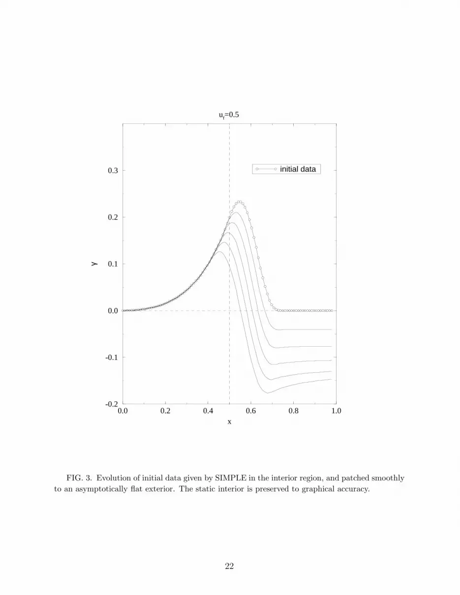
Second order convergence has also been checked against the exact static solution SIM-PLE. Since this solution is not asymptotically flat, we match the initial data smoothly toasymptotically flat data for a nonstatic exterior. Consideration of the domain of dependenceimplies that the matching boundary propagates along an ingoing null hypersurface. Thus,we can obtain a reliable measure of how accurately the evolution preserves the static inte-rior, provided we restrict the calculation of the error norm to a region not yet influenced bythe exterior nonstatic data. We matched one such static solution in the interior (x ≤ 0.5)to smooth exterior data with compact support. We calculated the L∞ norm for the regionx ≤ 0.4 at time u=0.25, and considered the dependence of the error on the grid size. Thepreservation of the static interior to graphical accuracy is shown in Fig. 3, while the secondorder convergence of the error is demonstrated in Fig. 4. In addition, for a wide variety ofinitial data having unknown analytic solution, we have verified that the numerical solutionconverges to second order in the sense of Cauchy convergence.

Stability of the code in the low to medium amplitude regime has been verified experimen-tally by running arbitrary initial data until it radiates away to scri. At higher amplitudes,it is expected that physical singularities will arise, but we have not yet explored this regime.Figure 5 shows a sequence of time slices of the numerical evolution of some arbitrary initialdata of compact support. Note the rich angular structure that arises at u ≈ 0.25 and thendissipates. At u ≈ 1.5 the amplitude of the field is sufficiently small so that it appears tobe zero in the figure. It continues to decay at later times.

14

C. Energy Conservation

The Bondi mass loss formula relates the gravitational radiation power to the square ofthe news function. It follows from the equations used in the algorithm as a consequenceof a global integration of the Bianchi identities. Thus it not only furnishes a valuable toolfor physical interpretation but it also provides a very important calibration of numericalaccuracy and consistency.

Historically, numerical calculations of the Bondi mass MB have been frustrated by tech-nical difficulties arising from the necessity to pick off nonleading terms in an asymptoticexpansion about infinity. For example, the mass aspect M must be picked off in the theasymptotic expansion (31) for V . This is similar to the experimental task of determining themass of an object by measuring its far field. In the non-radiative case it can be accomplishedby measuring gravity gradients, but otherwise this approach can be swamped by radiationfields. In the computational problem, further complications arise from gauge terms whichdominate asymptotically even over the radiation terms. We have recently developed a secondorder accurate algorithm for calculating the Bondi mass [12]. It avoids the above problemsthrough the use of Penrose compactification and the introduction of renormalized variablesin which Bondi’s mass aspect appears as the leading asymptotic term. The Bondi massalgorithm depends only upon fields on a single null hypersurface. It has been incorporatedinto the present evolution code to calculate the mass at any given retarded time.

In the present formalism, the news function N is given by [1]

2 e2HN = 2 c,u +(sin θ c2 L),θ

sin θ c+ e−2Kω sin θ

[

(e2Hω),θ

sin θ ω2

]

,θ

. (57)

Here ω is the conformal factor relating the asymptotic 2-geometry to the unit sphere geom-etry of a Bondi frame, i.e.

e2Kdθ2 + sin2 θe−2Kdφ2 = ω−2(dθ2B + sin2 θB dφ

2B), (58)

where θB and φB = φ are Bondi spherical coordinates. Calculation of ω complicates thecalculation of the news function. The simplest approach is to set y = − cos θ and yB =− cos θB. Then

ω2 =dyB

dy, (59)

where

yB = tanh

[∫ y

0

dy

1 − y2e2K

]

. (60)

This gives

ω =2 eK

(1 + y)e∆ + (1 − y)e−∆(61)

where

15

∆ =

∫ y

0

dye2K − 1

1 − y2. (62)

In order to prepare this integral in an explicitly regular form for computation we introducean auxiliary parameter α and rewrite (62) as the double integral

∆ = 2

∫ y

0

dy

∫ 1

0

dα e2αKK, (63)

where K = K/(1− y2) is regular at the poles. It is then straightforward to obtain a secondorder accurate finite difference formula for the news function.

The Bondi formula for energy conservation between central times u0 and u takes theform C =0, where

C = MB(u) −MB(u0) +1

2

∫ 1

−1

dy

∫ u

u0

du e2Hω−1N2. (64)

Figure 6 graphs C relative to the initial mass MB(u0) for a numerical evolution of thepolynomial data

γ = λ[(x− x1)(x− x2)(y

2 − y20)]

6

[(x1 − x2)y0]12 (65)

with compact support in the domain (x1 ≤ x ≤ x2) × (−y0 ≤ y ≤ y0) and amplitudeparameter λ. For the graph, we have chosen λ = 0.3, x1 = 0.1, x2 = 0.5 and y0 = 0.5, andevolved the numerical solution up to u = 0.01, on a grid of 512 radial × 128 angular points.The bulk of the error occurs in the calculation of the Bondi mass, whose accuracy is moresensitive to grid size than the accuracy of either the news function or the evolution code.Most of this error may be removed by using Richardson extrapolation to take advantageof the known second order accuracy of the Bondi mass. For example, if Fn(xi) is a secondorder accurate finite difference approximation to the function f(x) on a grid of n points,then (4Fn − Fn/2)/3 approximates f to third order and in fact to fourth order if odd ordersare absent in the approximation. This absence of odd orders indeed holds for the Bondimass because all derivatives, interpolations and integrals are centered. Thus, introductionof subgrids obtained by subsampling, leads to a fourth order expression for MB, with thecorresponding relative error in energy conservation also graphed in Fig. 6. In this way, energyconservation is attained to 0.4% accuracy. Note that only a single evolution on a fixed gridis necessary here because Richardson extrapolation is applied when calculating the Bondimass. For the purposes of the graph, we have done this for each time that C is plotted, butto check energy conservation, it suffices to do it only at the initial and final times. Figure 6serves as a rewarding testament to the virtues of a code with known convergence rates.

VI. CONCLUSION

We have constructed a second order accurate evolution algorithm for the null cone initialvalue problem for axisymmetric vacuum spacetimes. Energy conservation is maintained to

16

second order accuracy. Extensive tests of the algorithm establish that it is globally valid inthe regime where horizons and caustics do not develop. This generates a large complement ofhighly accurate numerical solutions for the class of asymptotically flat, axisymmetric vacuumspacetimes, for which no analytic solutions are known. All results of numerical evolutionsin this regime are consistent with the theorem of Christodoulou and Klainerman [13] thatweak initial data evolve asymptotically to Minkowski space at late time. The code is nowbeing tested in the strong field regime for application to the study of black hole formation.

ACKNOWLEDGMENTS

We benefited from research support from the National Science Foundation under NSFGrant PHY92-08349 and from computer time made available by the Pittsburgh Supercom-puting Center.

APPENDIX:

We sketch here the von Neumann stability analysis of the algorithm for the linearizedBondi equations. The analysis is based up freezing the explicit functions of r and y thatappear in the equations, so that it is only valid locally for grid sizes satisfying ∆r << r and∆y << 1. However, as is usually the case, the results are quite indicative of the stability ofthe actual global behavior of the code.

Starting with the hatted code variables introduced in Sec. IV and setting Γ = r2U andG = rγ, the linearized Bondi equations (6) and (7) take the form

r2Γ,rr − 2Γ = 2[4y − (1 − y2)∂y](rG,r −G) (A1)

and

2G,ur −G,rr = −(1/2r)Γ,ry. (A2)

Freezing the explicit factors of r and y at r = R and y = Y , introducing the Fourier modesG = esueikreily (with real k and l) and setting Γ = AG, these equations imply

A = 2(1 − ikR)[4Y − (1 − Y 2)il]/(2 +R2k2) (A3)

and

4is = −2k + Al/R. (A4)

For stable modes, Re(s) ≥ 0. This requires that the lIm(A) ≤ 0 which will be satisfied unlessY kl < 0. In the latter case, unstable solutions exist to the PDE’s obtained by freezing thecoefficients in the linearized equations (A1) and (A2). The linearized equations themselvesdo not have unstable modes but they arise in the frozen coefficient formalism from droppingthe boundary condition of spherical topology on the y-dependence. For a global solution,G should not have periodic dependence on y but instead be decomposed into spin-weight2 harmonics, in which case instabilities would not arise in the above analysis. Thus these

17

unstable modes of the frozen PDE are artificial and should be discarded by requiring Y kl ≥ 0when analyzing the stability of the corresponding FDE.

Consider now the FDE obtained by puttingG on the grid points rI and Γ on the staggeredpoints rI+1/2, while using the same angular grid yJ and time grid uN . Let P , Q, R and Sbe the corner points of the null parallelogram algorithm, placed so that P and Q are atlevel N + 1, R and S are at level N , and so that the line PR is centered about rI andQS is centered about rI+1. For simplicity, we display the analysis at the equator whereY = 0. Then, using linear interpolation and centered derivatives and integrals, the nullparallelogram algorithm for the frozen version of the linearized equations leads to the FDE’s

(R/∆r)2(ΓI+3/2 − 2ΓI+1/2 + ΓI−1/2) − (ΓI+3/2 + ΓI−1/2)

= −δy[2(R/∆r)(GI+1 −GI) − (GI+1 +GI)] (A5)

(all at the same time level) and

GN+1I+1 −GN+1

I −GNI+1 +GN

I

+ (∆u/4∆r)(−GN+1I+1 + 2GN+1

I −GN+1I−1 −GN

I+2 + 2GNI+1 −GN

I )

= −(∆u/8R)δy(ΓN+1I+1/2 − ΓN+1

I−1/2 + ΓNI+3/2 − ΓN

I+1/2), (A6)

where δy represents a centered first derivative. Again setting Γ = AG and introducing thediscretized Fourier mode G = esN∆ueikI∆reilJ∆y, we have δy = i sin(l∆y)/∆y and (A5) and(A6) reduce to

A[(R/∆r)2(1 − cosα) + cosα] = −L[(2R/∆r) sin(α/2) + i cos(α/2)] (A7)

and

es∆u = −eiα(C∗ − AD)/(C −AD), (A8)

where L = sin(l∆y)/∆y, α = k∆r, C = ieiα/2 sin(α/2) + (∆u/4∆r)(1 − cosα) and D =(L∆u/8R) sin(α/2). The stability condition that Re(s) ≤ 0 then reduces to Re[CD(A −A∗)] ≥ 0 which is equivalent to 1 + cosα[1 − (∆r/R)2] ≥ 0. Thus this stability condition isautomatically satisfied and poses no constraint on the algorithm.

The corresponding analysis at the poles Y = ±1 again leads to (A8), where now

A[(R/∆r)2(1 − cosα) + cosα] = −4Y [2i(R/∆r) sin(α/2) − cos(α/2)]. (A9)

The stability condition Re[CD(A− A∗)] ≥ 0 is satisfied provided Y kl ≥ 0, which rules outthe artificially unstable solutions of the frozen PDE discussed above.

As a result, local stability analysis places no constraints on the algorithm. This may seemsurprising because not even the analogue of a CFL condition on the time step arises but itcan be understood in the following vein. The local structure of the code is implicit, since itinvolves 3 points at the upper time level. Implicit algorithms do not necessarily lead to a CFLcondition. However, the algorithm is globally explicit in the way that evolution proceeds byan outward radial march from the origin. It is this feature that necessitates a CFL conditionin order to make the numerical and physical domains of dependence consistent.

18

REFERENCES

[1] R. Isaacson, J. Welling, and J. Winicour, J. Math. Phys. 24, 1824 (1983).[2] R. Gomez and J. Winicour, J. Math. Phys. 33, 1445 (1992).[3] R. Gomez and J. Winicour, Phys. Rev. D 45, 2776 (1992).[4] R. Gomez and J. Winicour, in Approaches to Numerical Relativity, edited by R.

d’Inverno (Cambridge University Press, Cambridge, 1992).[5] R. Gomez, R. Isaacson, and J. Winicour, J. Comp. Phys. 98, 11 (1992).[6] M. van der Burg, H. Bondi, and A. Metzner, Proc. R. Soc. London Ser. A 269, 21

(1962).[7] R. Penrose and W. Rindler, Spinors and Space-Time, Vol. 1 (Cambridge University

Press, Cambridge, 1984).[8] E. Newman and R. Penrose, Proc. R. Soc. London Ser. A 305, 175 (1968).[9] R. d’Inverno and J. Smallwood, Phys. Rev. D 22, 1223 (1980).

[10] J. Bicak and B. G. Schmidt, Phys. Rev. D 40, 1827 (1989).[11] J. Bicak, P. Reilly, and J. Winicour, Gen. Rel. Grav. 20, 171 (1988).[12] R. Gomez, P. Reilly, J. Winicour, and R. A. Isaacson, Phys. Rev. D 47, 3292 (1993).[13] D. Christodoulou and S. Klainerman, The Global Nonlinear Stability of the Minkowski

Space (Princeton University Press, Princeton, 1993).

19

FIGURES

u

uxi-1

xi

u

R

P

n+1

n

S

Q

T

x

x i+1

FIG. 1. Line segments drawn at forty-five degrees represent radial characteristics. Their in-

tersection defines the fundamental null parallelogram PQRS shown superimposed upon the com-

putational cell, which consists of the points marked by circles and their nearest neighbors in the

angular direction.

20

-2.2 -2.0 -1.8 -1.6 -1.4 -1.2log10(∆x)

-14.5

-14.0

-13.5

-13.0

-12.5

log 10

(||L

2||)

FIG. 2. The error, as measured by the L2 norm, of a numerical solution with higher harmonics

(ℓ = 6). The computation is made on grids of size Nx equal to 24, 48, 72, 96 and 120, while keeping

Nx = 3Ny.

21

0.0 0.2 0.4 0.6 0.8 1.0x

-0.2

-0.1

0.0

0.1

0.2

0.3

γ

uf=0.5

initial data

FIG. 3. Evolution of initial data given by SIMPLE in the interior region, and patched smoothly

to an asymptotically flat exterior. The static interior is preserved to graphical accuracy.

22

-2.6 -2.4 -2.2 -2.0 -1.8 -1.6log10(∆x)

-7.5

-7.0

-6.5

-6.0

-5.5

log 10

(max

|G-g

|)

FIG. 4. The error in the evolution of the initial data of Fig. 3 up to u = 0.25, as measured

by the L∞ norm. The error is computed on grids of size Ny equal to 16, 24, 32, 48 and 64,

while keeping Nx = 3Ny. The convergence rate is 1.92, in good agreement with the theoretically

expectation of second order accuracy.

23

u=0.0000

(a)

00.2

0.40.6

0.81 -1

-0.6-0.2

0.20.6

1

-0.005

0

0.005

u=0.5330

(c)

00.2

0.40.6

0.81 -1

-0.6-0.2

0.20.6

1

-0.005

0

0.005

u=1.0660

(e)

00.2

0.40.6

0.81 -1

-0.6-0.2

0.20.6

1

-0.005

0

0.005

u=0.2665

(b)

00.2

0.40.6

0.81 -1

-0.6-0.2

0.20.6

1

-0.005

0

0.005

u=0.7995

(d)

00.2

0.40.6

0.81 -1

-0.6-0.2

0.20.6

1

-0.005

0

0.005

u=1.4657

(f)

00.2

0.40.6

0.81 -1

-0.6-0.2

0.20.6

1

-0.005

0

0.005

FIG. 5. A sequence of time slices of the numerical evolution of initial data of compact support.

Note all the angular structure that arises at about u = 0.25, which later decays. At u ≈ 1.5 the

amplitude of the field has decayed below those values which can be observed in the figure.

24

0.000 0.002 0.004 0.006 0.008 0.010u

-0.020

-0.010

0.000

0.010

C/M

B(u

0)

Richardson extrap.

128 ang. x 512 rad.

FIG. 6. Graph of the relative error in C calculated up to u = 0.01 for a numerical evolution of

the data (65), on a grid of 512 radial × 128 angular points. The circles show the error as calculated

from the computed values of the mass, while the squares show the error after using Richardson

extrapolation, based on the known convergence rate of the algorithm.

25