Notes - M4 Algebra - Section 2 Mathematics - BMAT - Physics

https://bit.ly/pmt-edu-cc https://bit.ly/pmt-cc

BioMedical Admissions Test (BMAT)

Section 2: Mathematics Topic M4: Algebra

https://bit.ly/pmt-cchttps://bit.ly/pmt-cchttps://bit.ly/pmt-edu

This work by PMT Education is licensed under CC BY-NC-ND 4.0


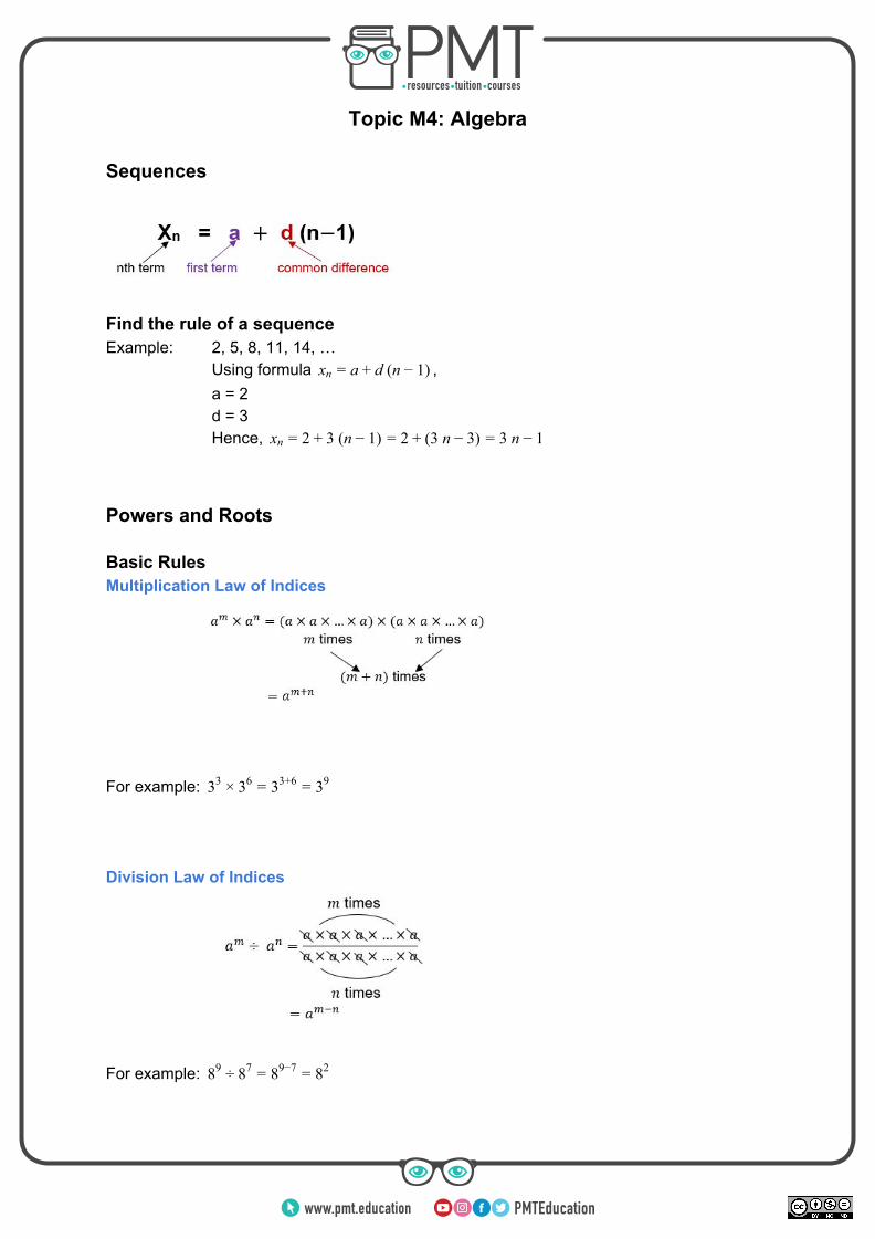
Topic M4: Algebra Sequences

Find the rule of a sequence Example: 2, 5, 8, 11, 14, …

Using formula , (n )xn = a + d − 1 a = 2 d = 3 Hence, (n )xn = 2 + 3 − 1 3 n )= 2 + ( − 3 n= 3 − 1

Powers and Roots Basic Rules Multiplication Law of Indices

For example: 33 × 36 = 33+6 = 39 Division Law of Indices

For example: 89 ÷ 87 = 89−7 = 82



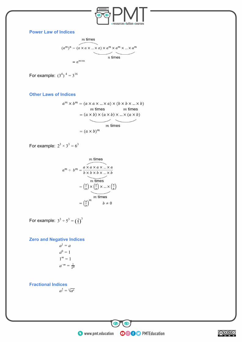
Power Law of Indices

For example: 3 ) ( 4 4 = 316 Other Laws of Indices

For example: 23 × 33 = 63

For example: 33 ÷ 53 = ( 53)3

Zero and Negative Indices

a1 = a a0 = 1 1m = 1 a−m = 1

am Fractional Indices

axy = √y ax



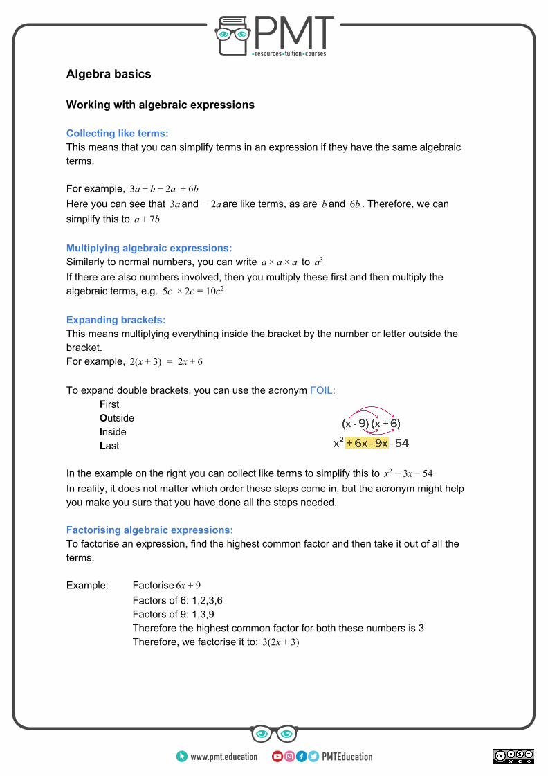
Algebra basics Working with algebraic expressions Collecting like terms: This means that you can simplify terms in an expression if they have the same algebraic terms. For example, a a b3 + b − 2 + 6 Here you can see that and are like terms, as are and . Therefore, we cana3 a− 2 b b6 simplify this to ba + 7 Multiplying algebraic expressions: Similarly to normal numbers, you can write to a × a × a a3 If there are also numbers involved, then you multiply these first and then multiply the algebraic terms, e.g. c c 0c5 × 2 = 1 2 Expanding brackets: This means multiplying everything inside the bracket by the number or letter outside the bracket. For example, (x ) 2x2 + 3 = + 6 To expand double brackets, you can use the acronym FOIL:

F irst Outside Inside Last

In the example on the right you can collect like terms to simplify this to x 4x2 − 3 − 5 In reality, it does not matter which order these steps come in, but the acronym might help you make you sure that you have done all the steps needed. Factorising algebraic expressions: To factorise an expression, find the highest common factor and then take it out of all the terms. Example: Factorise x6 + 9

Factors of 6: 1,2,3,6 Factors of 9: 1,3,9 Therefore the highest common factor for both these numbers is 3 Therefore, we factorise it to: (2x )3 + 3



Example: Solve x x4 2 = 7 x x4 2 = 7 x x4 2 − 7 = 0 here we can see that the common factor is x (4x )x − 7 = 0

or x = 0 x4 − 7 = 0 Hence, or x = 0 x = 1 4

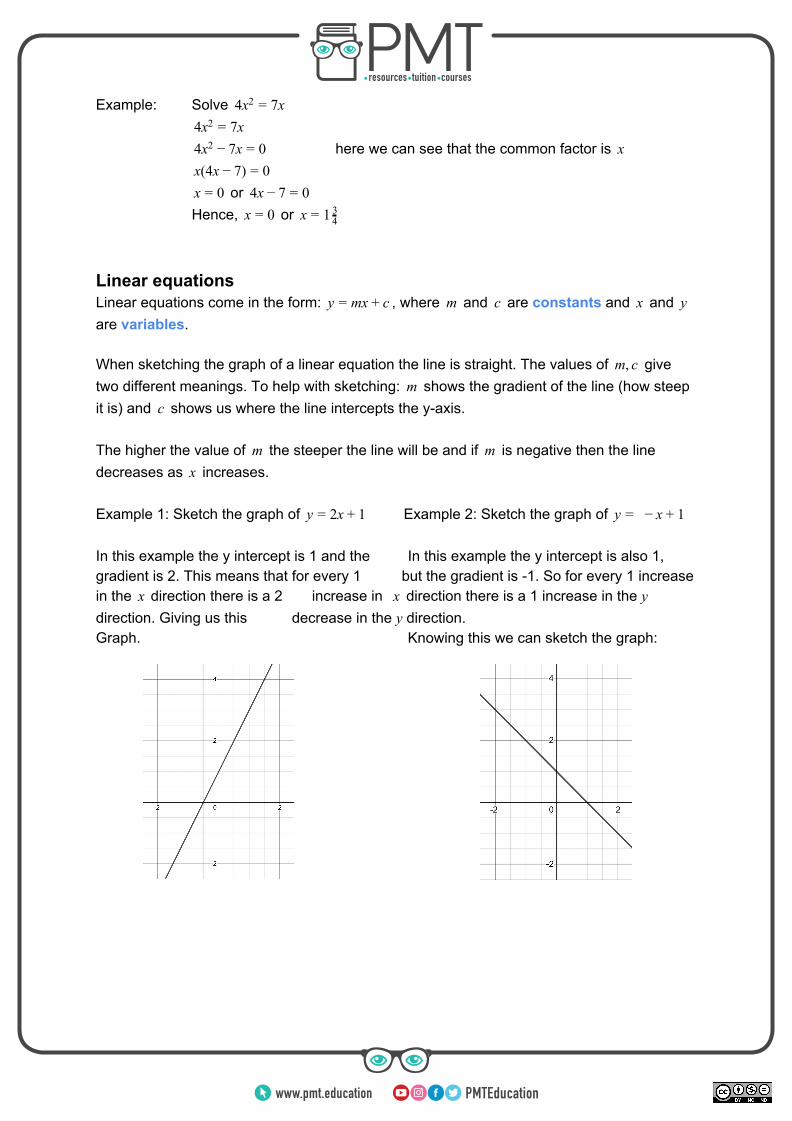
3 Linear equations Linear equations come in the form: , where and are constants and and xy = m + c m c x y are variables. When sketching the graph of a linear equation the line is straight. The values of give,m c two different meanings. To help with sketching: shows the gradient of the line (how steepm it is) and shows us where the line intercepts the y-axis.c The higher the value of the steeper the line will be and if is negative then the linem m decreases as increases.x Example 1: Sketch the graph of xy = 2 + 1 Example 2: Sketch the graph of y = − x + 1 In this example the y intercept is 1 and the In this example the y intercept is also 1, gradient is 2. This means that for every 1 but the gradient is -1. So for every 1 increase in the direction there is a 2 x increase in direction there is a 1 increase in the yx direction. Giving us this decrease in the y direction. Graph. Knowing this we can sketch the graph:



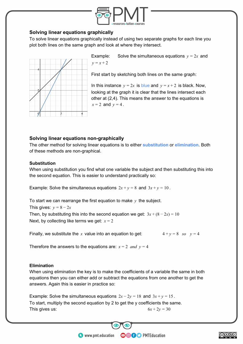
Solving linear equations graphically To solve linear equations graphically instead of using two separate graphs for each line you plot both lines on the same graph and look at where they intersect.

Example: Solve the simultaneous equations andxy = 2 y = x + 2

First start by sketching both lines on the same graph:

In this instance is blue and is black. Now,xy = 2 y = x + 2 looking at the graph it is clear that the lines intersect each other at (2,4). This means the answer to the equations is

and .x = 2 y = 4

Solving linear equations non-graphically The other method for solving linear equations is to either substitution or elimination. Both of these methods are non-graphical. Substitution When using substitution you find what one variable the subject and then substituting this into the second equation. This is easier to understand practically so: Example: Solve the simultaneous equations and .x2 + y = 8 x 03 + y = 1 To start we can rearrange the first equation to make the subject.y This gives: xy = 8 − 2 Then, by substituting this into the second equation we get: x 8 x) 03 + ( − 2 = 1 Next, by collecting like terms we get: x = 2 Finally, we substitute the value into an equation to get:x so4 + y = 8 y = 4 Therefore the answers to the equations are: and yx = 2 = 4 Elimination When using elimination the key is to make the coefficients of a variable the same in both equations then you can either add or subtract the equations from one another to get the answers. Again this is easier in practice so: Example: Solve the simultaneous equations and .x y 82 − 2 = 1 x 53 + y = 1 To start, multiply the second equation by 2 to get the y coefficients the same. This gives us: x y 06 + 2 = 3



Next we add the first equation to the second: x x 8 02 + 6 = 1 + 3Collecting like terms gives: x 88 = 4 Then solving to get gives:x x = 6 Finally, we substitute the value into an equation to get:x 2 y 8 so y1 − 2 = 1 = − 3 Quadratic Equations Factorising quadratic equations Factorisation is the process of expressing a quadratic expression, such as as abx x2 + + c product of two linear expressions. It is essentially the opposite of expanding brackets. Remember, when factorising, we are trying to get the quadratic expression in the form: x )(x )( + a + b = 0

If the quadratic equation is in the form of , then we are trying to find two numbersxx2 + a + b that multiply together to give and that add together to make . Here are some workeda b examples to demonstrate this. Example: x 2x2 + 7 + 1 = 0

(two numbers that have a product of 12 and a sum of 7)2 3 3 × 4 = 1 + 4 = 7 Therefore x )(x )( + 3 + 4 = 0 x + 3 = 0 x + 4 = 0

or x = − 3 x = − 4 Example: Solve .x x 32 2 + − = 0

x x 32 2 + + = 0 2x )(x ) 0( + 3 − 1 = x 02 + 3 = x − 1 = 0

or x = − 23 x = 1

Example: Solve .2x

x−5 = 3x−4

2xx−5 = 3

x−4 (Multiply both sides by 3(2x) to remove the denominators) (x ) x(x )3 − 5 = 2 − 4 x 5 x x3 − 1 = 2 2 − 8 x 1x 52 2 − 1 + 1 = 0 x )(2x )( − 3 − 5 = 0

or x = 3 x = 2 21



Common algebraic formulae:

1. the difference of two squaresa )(a )a2 − b2 = ( + b − b 2. ab = a )a2 + 2 + b2 ( + b 2 3. aba2 − 2 + b2 = (a )− b 2

Example: Difference of two squares

x )(x ) 12( + 2 − 2 = 2x2 − 4 = 1 here we are using equation 1

6x2 = 1 or x = 4 x = − 4

The quadratic equation

x x , a = then xa 2 + b + c = 0 / 0 = 2a−b±√b −4ac2

Example: Solve .x x2 2 − 8 + 5 = 0

x x2 2 − 8 + 5 = 0

x = 2(2)−(−8)±√(−8) −4(2)(5)2

x = 48±√24

x = 2 ± 4√4×6

x = 2 ± 42√6

x = 2 ± 2√6

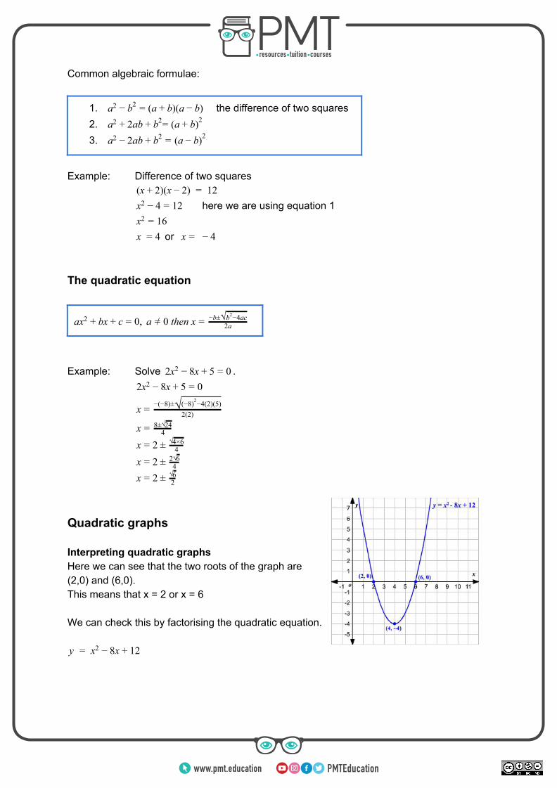
Quadratic graphs Interpreting quadratic graphs Here we can see that the two roots of the graph are (2,0) and (6,0). This means that x = 2 or x = 6 We can check this by factorising the quadratic equation.

x x 2y = 2 − 8 + 1



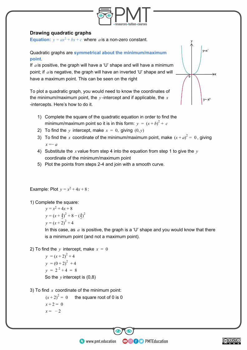
Drawing quadratic graphs Equation: where is a non-zero constant.x xy = a 2 + b + c a Quadratic graphs are symmetrical about the minimum/maximum point. If is positive, the graph will have a ‘U’ shape and will have a minimuma point; if is negative, the graph will have an inverted ‘U’ shape and willa have a maximum point. This can be seen on the right To plot a quadratic graph, you would need to know the coordinates of the minimum/maximum point, the -intercept and if applicable, the y x-intercepts. Here’s how to do it.

1) Complete the square of the quadratic equation in order to find the minimum/maximum point so it is in this form: (x ) cy = + b 2 +

2) To find the intercept, make giving y 0,x = 0, )( y 3) To find the coordinate of the minimum/maximum point, make , givingx x ) 0( + a 2 =

−x = a 4) Substitute the value from step 4 into the equation from step 1 to give the x y

coordinate of the minimum/maximum point 5) Plot the points from steps 2-4 and join with a smooth curve.

Example: Plot :xy = x2 + 4 + 8 1) Complete the square:

xy = x2 + 4 + 8 x ) )y = ( + 2

4 2 + 8 − ( 24 2

x )y = ( + 2 2 + 4 In this case, as is positive, the graph is a ‘U’ shape and you would know that therea is a minimum point (and not a maximum point).

2) To find the intercept, make y 0x =

x )y = ( + 2 2 + 4 0 ) y = ( + 2 2 + 4 2 8y = 2 + 4 =

So the intercept is (0,8)y 3) To find coordinate of the minimum point:x

x ) 0( + 2 2 = the square root of 0 is 0 0x + 2 =

x = − 2



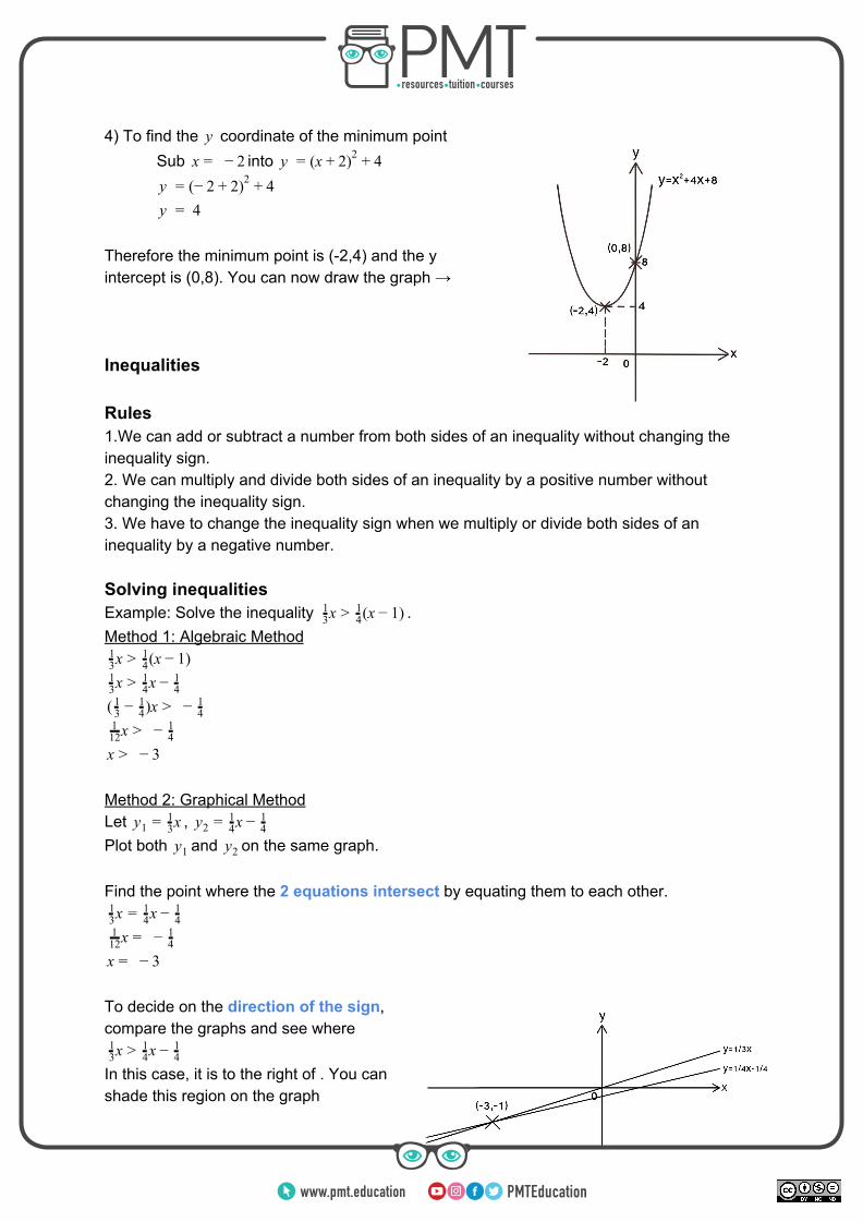
4) To find the coordinate of the minimum pointy

Sub into x = − 2 x )y = ( + 2 2 + 4 − )y = ( 2 + 2 2 + 4 4y =

Therefore the minimum point is (-2,4) and the y intercept is (0,8). You can now draw the graph → Inequalities Rules 1.We can add or subtract a number from both sides of an inequality without changing the inequality sign. 2. We can multiply and divide both sides of an inequality by a positive number without changing the inequality sign. 3. We have to change the inequality sign when we multiply or divide both sides of an inequality by a negative number. Solving inequalities Example: Solve the inequality .x (x )3

1 > 41 − 1

Method 1: Algebraic Method x (x )3

1 > 41 − 1

x x31 > 4

1 − 41

)x( 31 − 4

1 > − 41

x112 > − 4

1 x > − 3 Method 2: Graphical Method Let , xy1 = 3

1 xy2 = 41 − 4

1 Plot both and on the same graph.y1 y2 Find the point where the 2 equations intersect by equating them to each other.

x31 x= 4

1 − 41

x112 = − 4

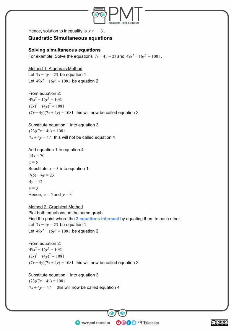
1 x = − 3 To decide on the direction of the sign, compare the graphs and see where

x x31 > 4

1 − 41

In this case, it is to the right of . You can shade this region on the graph



Hence, solution to inequality is .x > − 3

Quadratic Simultaneous equations Solving simultaneous equations For example: Solve the equations and .x y 37 − 4 = 2 9x 6y 0814 2 − 1 2 = 1 Method 1: Algebraic Method Let be equation 1x y 37 − 4 = 2 Let be equation 2.9x 6y 0814 2 − 1 2 = 1 From equation 2:

9x 6y 0814 2 − 1 2 = 1 081(7x)2 − (4y)2 = 1

this will now be called equation 37x y)(7x y) 081( − 4 + 4 = 1 Substitute equation 1 into equation 3. 23)(7x y) 081( + 4 = 1

this will not be called equation 4x y 77 + 4 = 4 Add equation 1 to equation 4:

4x 01 = 7 x = 5 Substitute into equation 1: x = 5

(5) y 37 − 4 = 2 y 24 = 1

y = 3 Hence, and x = 5 y = 3 Method 2: Graphical Method Plot both equations on the same graph. Find the point where the 2 equations intersect by equating them to each other. Let be equation 1.x y 37 − 4 = 2 Let be equation 2.9x 6y 0814 2 − 1 2 = 1 From equation 2:

9x 6y 0814 2 − 1 2 = 1 081(7x)2 − (4y)2 = 1

this will now be called equation 37x y)(7x y) 081( − 4 + 4 = 1 Substitute equation 1 into equation 3. 23)(7x y) 081( + 4 = 1 x y 77 + 4 = 4 this will now be called equation 4



Add equation 1 to equation 4: 4x 01 = 7

x = 5 Substitute into equation 1: x = 5

(5) y 37 − 4 = 2 y 24 = 1

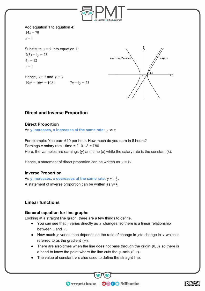
y = 3 Hence, and x = 5 y = 3

9x 6y 0814 2 − 1 2 = 1 x y 37 − 4 = 2 Direct and Inverse Proportion Direct Proportion As y increases, x increases at the same rate: ∝ xy For example: You earn £10 per hour. How much do you earn in 8 hours? Earnings = salary rate time = £10 8 = £80× × Here, the variables are earnings (y) and time (x) while the salary rate is the constant (k). Hence, a statement of direct proportion can be written as xy = k Inverse Proportion As y increases, x decreases at the same rate: y ∝ .x

1 A statement of inverse proportion can be written as y= .x

k Linear functions General equation for line graphs Looking at a straight line graph, there are a few things to define.

● You can see that varies directly as changes, so there is a linear relationshipy x between and .x y

● How much varies then depends on the ratio of change in to change in which isy y x referred to as the gradient .m)(

● There are also times when the line does not pass through the origin so there is0, )( 0 a need to know the point where the line cuts the -axis .y 0, )( c

● The value of constant is also used to define the straight line.c



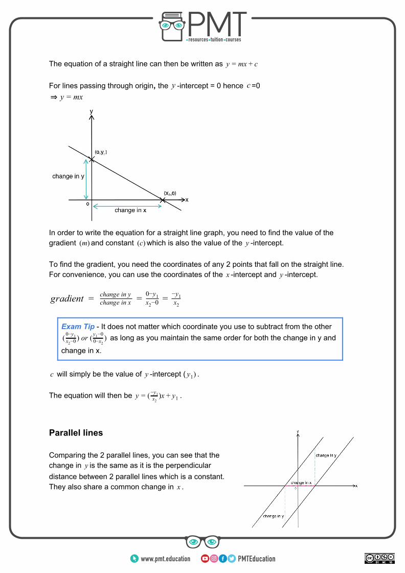
The equation of a straight line can then be written as xy = m + c For lines passing through origin, the -intercept = 0 hence =0 y c ⇒ x y = m

In order to write the equation for a straight line graph, you need to find the value of the gradient and constant which is also the value of the -intercept.m)( c)( y To find the gradient, you need the coordinates of any 2 points that fall on the straight line. For convenience, you can use the coordinates of the -intercept and -intercept.x y

radient g = change in x change in y = x −02

0−y1 = x2

−y1

Exam Tip - It does not matter which coordinate you use to subtract from the other as long as you maintain the same order for both the change in y and) or ( )( x −02

0−y10−x2

y −01

change in x.

will simply be the value of -intercept ( .c y )y1

The equation will then be .)xy = ( x2

−y1 + y1

Parallel lines Comparing the 2 parallel lines, you can see that the change in is the same as it is the perpendiculary distance between 2 parallel lines which is a constant. They also share a common change in .x



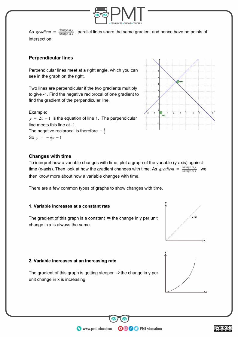
As , parallel lines share the same gradient and hence have no points ofradient g = change in x change in y

intersection. Perpendicular lines Perpendicular lines meet at a right angle, which you can see in the graph on the right. Two lines are perpendicular if the two gradients multiply to give -1. Find the negative reciprocal of one gradient to find the gradient of the perpendicular line. Example:

is the equation of line 1. The perpendicular 2x y = − 1 line meets this line at -1. The negative reciprocal is therefore − 2

1 So x y = − 2

1 − 1 Changes with time To interpret how a variable changes with time, plot a graph of the variable (y-axis) against time (x-axis). Then look at how the gradient changes with time. As , weradient g = change in x

change in y then know more about how a variable changes with time. There are a few common types of graphs to show changes with time. 1. Variable increases at a constant rate The gradient of this graph is a constant the change in y per unit⇒ change in x is always the same. 2. Variable increases at an increasing rate The gradient of this graph is getting steeper the change in y per⇒ unit change in x is increasing.





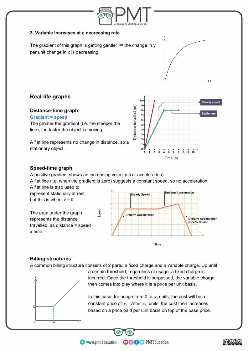
3. Variable increases at a decreasing rate The gradient of this graph is getting gentler the change in y⇒ per unit change in x is decreasing. Real-life graphs Distance-time graph Gradient = speed The greater the gradient (i.e. the steeper the line), the faster the object is moving. A flat line represents no change in distance, so a stationary object. Speed-time graph A positive gradient shows an increasing velocity (i.e. acceleration). A flat line (i.e. when the gradient is zero) suggests a constant speed, so no acceleration. A flat line is also used to represent stationary at rest, but this is when v = 0 The area under the graph represents the distance travelled, as distance = speed x time Billing structures A common billing structure consists of 2 parts: a fixed charge and a variable charge. Up until

a certain threshold, regardless of usage, a fixed charge is incurred. Once the threshold is surpassed, the variable charge then comes into play where it is a price per unit basis. In this case, for usage from 0 to units, the cost will be ax1 constant price of . After units, the cost then increasesy1 x1 based on a price paid per unit basis on top of the base price.



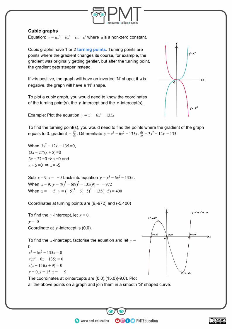
Cubic graphs Equation: where is a non-zero constant.x x xy = a 3 + b 2 + c + d a Cubic graphs have 1 or 2 turning points. Turning points are points where the gradient changes its course, for example, the gradient was originally getting gentler, but after the turning point, the gradient gets steeper instead. If is positive, the graph will have an inverted ‘N’ shape; if isa a negative, the graph will have a ‘N’ shape. To plot a cubic graph, you would need to know the coordinates of the turning point(s), the -intercept and the -intercept(s).y x Example: Plot the equation x 35xy = x3 − 6 2 − 1 To find the turning point(s), you would need to find the points where the gradient of the graph equals to 0. gradient . Differentiate .= dx

dy x 35xy = x3 − 6 2 − 1 2x 35dxdy = 3x2 − 1 − 1

When =0,2x 353x2 − 1 − 1

=03x 7)(x )( − 2 + 5 =0 =9 andx 73 − 2 ⇒ x

=0 = -5x + 5 ⇒ x Sub back into equation .,x = 9 x = − 5 x 35xy = x3 − 6 2 − 1 When , y 9) (9) 35(9) 72x = 9 = ( 3 − 6 2 − 1 = − 9 When , y − ) (− ) 35(− ) 00x = − 5 = ( 5 3 − 6 5 2 − 1 5 = 4 Coordinates at turning points are (9,-972) and (-5,400) To find the -intercept, let .y x = 0

0y = Coordinate at -intercept is (0,0).y To find the -intercept, factorise the equation and let x y =0.

x 35xx3 − 6 2 − 1 = 0 (x x 35)x 2 − 6 − 1 = 0 (x 5)(x )x − 1 + 9 = 0

, 5,x = 0 x = 1 x = − 9 The coordinates at x-intercepts are (0,0),(15,0)(-9,0). Plot all the above points on a graph and join them in a smooth ‘S’ shaped curve.





Exponential graphs Equation: where is a non-zero constant.y = kx k For exponential graphs, as approaches infinity, willx − y approach 0; the intercept will always have a magnitudey − of 1 because anything to the power of 0 is 1. Reciprocal graphs Equation: where is a non-zero constant.y = x

a a For reciprocal graphs, as approaches infinity, x − / + yapproaches 0; as approaches 0, approaches (+ )x / − y

infinity.+ )( / −



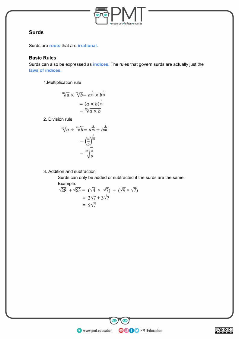
Surds Surds are roots that are irrational. Basic Rules Surds can also be expressed as indices. The rules that govern surds are actually just the laws of indices.

1.Multiplication rule

2. Division rule

3. Addition and subtraction Surds can only be added or subtracted if the surds are the same. Example:

( ) ( ) √28 + √63 = √4 × √7 + √9 × √7 = 2√7 + 3√7 = 5√7


Documents

Notes - M4 Algebra - Section 2 Mathematics - BMAT - Physics