1

Nonlinear energy harvesting

F. Cottone1, L. Gammaitoni1,2*, H. Vocca2

1 N.i.P.S. Laboratory, Dipartimento di Fisica, Università degli Studi di Perugia - 06100

Perugia, Italy. 2 INFN Sezione di Perugia, Via A. Pascoli, 1 – 06100 Perugia, Italy *To whom correspondence should be addressed. Email: luca.gammaitoni@pg.infn.it

Ambient energy harvesting has been in recent years the recurring object of a

number of research efforts aimed at providing an autonomous solution to the

powering of small-scale electronic mobile devices1-3. Among the different solutions,

vibration energy harvesting4-7 has played a major role due to the almost universal

presence of mechanical vibrations: from ground shaking to human movements,

from ambient sound to thermal noise. Standard approaches are mainly based on

resonant linear oscillators that are acted on by ambient vibrations. Here we

propose a new method based on the exploitation of the dynamical features of

stochastic nonlinear oscillators. Such a method is shown to outperform standard

linear oscillators and to overcome some of the most severe limitations of present

approaches, like narrow bandwidth, need for continuous frequency tuning and low

efficiency. We demonstrate the superior performances of this method by applying

it to piezoelectric energy harvesting from ambient vibration. Experimental results

from a toy-model oscillator are described in terms of nonlinear stochastic

dynamics. We prove that the method proposed here is quite general in principle

and could be applied to a wide class of nonlinear oscillators and different energy

conversion principles. There are also potentials for realizing micro/nano-scale

power generators8.

Ambient vibrations come in a vast variety of forms from sources as diverse as wind

induced movements, seismic noise and cars motion. Present working solutions for

vibration-to-electricity conversion are based on oscillating mechanical elements that

convert kinetic energy via capacitive, inductive or piezoelectric methods9-11.

Mechanical oscillators are usually designed to be resonantly tuned to the ambient

2

dominant frequency. However, in the vast majority of cases the ambient vibrations have

their energy distributed over a wide spectrum of frequencies, with significant

predominance of low frequency components and frequency tuning is not always

possible due to geometrical/dynamical constraints11-14.

To overcome these difficulties we propose a different approach based on the

exploitation of the properties of non-resonant oscillators. Specifically we demonstrate

that a bistable oscillator, under proper operating conditions15, can provide better

performances compared to a linear oscillator in terms of the energy extracted from a

generic wide spectrum vibration. In order to do so, we realized a toy-model oscillator

made by a piezoelectric inverted pendulum (See Supplementary Fig. 1) where on top of

the pendulum mass it has been added a small magnet (tip magnet). The effect of ground

vibration force is reproduced by applying a properly designed magnetic excitation on

two small magnets attached near the base of the pendulum. Under the action of the

excitation the pendulum oscillates, alternatively bending the piezoelectric beam and

thus generating a measurable voltage signal. The dynamics of the inverted pendulum tip

can be controlled with the introduction of an external magnet conveniently placed at a

certain distance Δ and with polarities opposed to those of the tip magnet. The external

magnet introduces a force dependent from the distance Δ between the two magnets that

opposes the elastic restoring force of the bended beam and, as a result, the inverted

pendulum dynamics can show two different types of dynamics. When the external

magnet is far away, the inverted pendulum behaves like a linear oscillator whose

dynamics is resonant with a resonance frequency determined by the system parameters.

This situation accounts well for the usual operating condition of traditional piezoelectric

vibration-to-electric energy converters6. On the other hand, when Δ is small enough two

new equilibrium positions appear. The random vibration makes the pendulum swing in

a more complex way with small oscillations around each of the two equilibrium

positions and large excursions from one to the other.

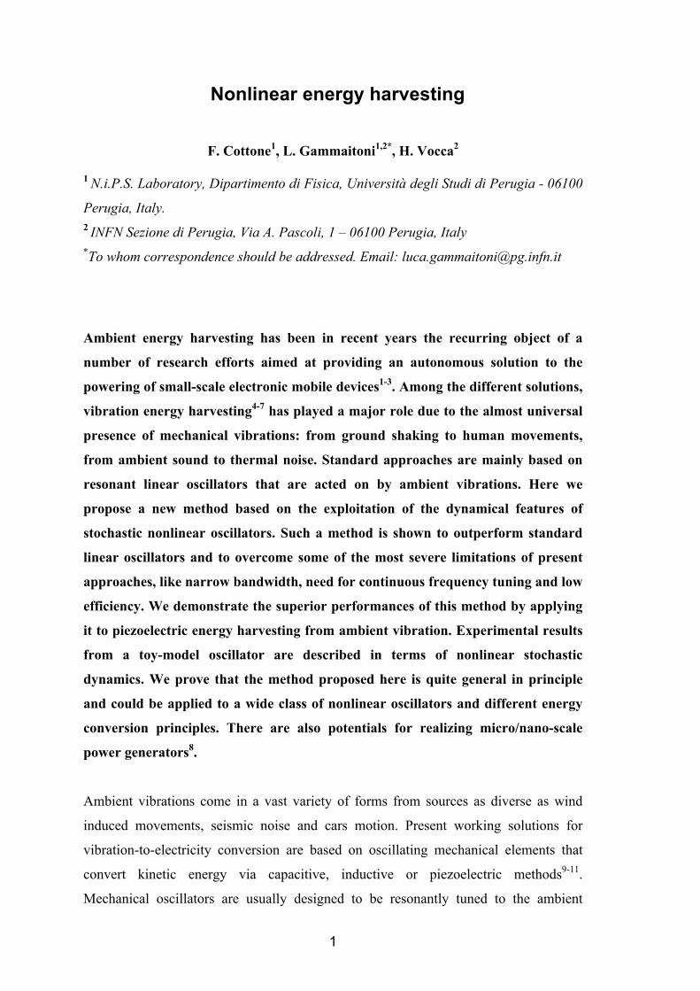
In order to quantify the energy produced by the piezoelectric oscillator we computed

the power dissipated in a purely resistive load, by measuring the voltage drop V over a

resistive load RL7, under the influence of a random vibration with Gaussian distribution

(with zero mean and standard deviation σ) and exponential autocorrelation function

(with correlation time τ). In Fig. 1 (upper) we show the average electrical power

<V2>/RL as a function of Δ for three different values of the noise standard deviation σ.

In all the cases the power increases rapidly from the linear case (large Δ) up to a

3

maximum value and then decreases when the magnets become closer and closer. A

qualitatively similar behaviour is observed (Fig. 1, lower) if we plot the pendulum rms

position xrms, as a function of Δ. In order to quantitatively account for the experiments

we developed a dynamical description of the inverted pendulum based on the following

equation of motion:

€

m˙ ̇ x = − ′ U (x) − γ˙ x −KvV (t) +σξ(t) . The first term on the right hand

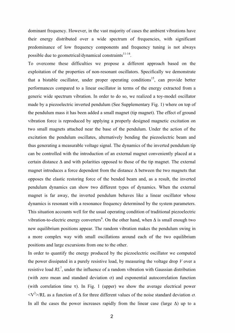
side accounts for the conservative force, where U(x) is the potential energy of the

pendulum16 shown in Fig.2:

€

U(x) = Kx 2 + (ax 2 + bΔ2)−3 2 + cΔ2 with a,b,c representing

constants related to the physical parameters of the pendulum17,18 (See Supplementary

Fig. 1). The second term

€

−γ˙ x , accounts for the energy dissipation due to the bending

and

€

−KvV (t) accounts for energy transferred to the electric load R with coupling

equation

€

˙ V = Kc ˙ x −V RC . C and Kc are respectively the capacitance and the coupling

constant of the piezoelectric sample. Finally,

€

σξ(t) accounts for the vibration force that

drives the pendulum.

€

ξ(t) represents a stochastic process with the same statistical

properties of the magnetic excitation. In Fig. 1 we plot with continuous line the

computed power <V2>/R (upper) and the rms value of x(t) (lower) as obtained by the

numerical solution of the equation of motion. All the parameters have been measured

from the experimental apparatus and introduced into the equation. As it is apparent the

agreement between the experimental data and the model is rather good.

In fig. 1 we can easily identify three different regimes: 1) Large Δ,

(i.e..

€

Δ >> Δ c =α b with

€

α = 3a 2K( )1 5). The dynamics is characterized by quasi-

linear oscillations around the single minimum located at zero displacement, in

correspondence with the vertical position of the pendulum. This condition accounts for

the usual performances of a linear piezoelectric generator. 2) Small Δ (

€

Δ << Δ c ), the

potential energy is bistable with a very pronounced barrier between the two wells. In

this condition and for a given amount of noise, the pendulm swing is almost exclusively

confined within one well and the dynamics is characterized once again by quasi-linear

oscillations around the minimum of the confining well. 3) In between there is a range of

distances Δ where the xrms (and the Vrms as well) reaches a maximum value. In this

condition the pendulum dynamics is highly nonlinear and the swing reaches its largest

amplitude with noise assisted jumps between the two wells. As it is well evident in fig.

1, the maximum values of the output power exceed by a factor that ranges between 4

and 6 the value obtainable when the magnet is far away. This indicates a potential gain

for power harvesting between 400% and 600% compared to the standard linear

4

oscillators, depending on the noise intensity and on the other physical features of the

pendulum. Two others important features are apparent: a) the maximum position shifts

toward larger Δ when the noise intensity increases. b) In the low Δ regime, the rms

reaches a plateau that is smaller than the plateau reached by the rms in the large Δ

regime.

Both features can be explained as follows. When

€

Δ >> Δ c the potential U(x) shows a

single minimum with librational frequency given by

€

ω02 = ′ ′ U (0) /m = 2k − 3ab−5 / 2 Δ5( ) m . The xrms value here can be estimated in the linear

oscillator approximation19 as proportional to

€

σ ω0 . On decreasing Δ,

€

ω0 decreases and

thus the xrms value increases. When

€

Δ = Δ c the potential develops two distinct minima

located at

€

x± = ± α 2 − bΔ2( )1 a . The pendulum swings now between the two minima

and the rms increases proportional to

€

x±. With decreasing Δ the potential barrier height

ΔU grows proportional to

€

Δ−3 and becomes so large that the jump probability becomes

negligible. The pendulum swing is thus permanently confined within one well. Such a

trapping condition happens at smaller values of Δ (i.e. larger barrier) for larger noise.

This explains the observed shift of the maximum position toward smaller Δ as observed

in a). Inside one well the dynamics is almost linear with small oscillations around the

potential local minima (x+ or x-) and

€

xrms ∝σ ω± with

€

ω±2 = ′ ′ U (x±) m . Being

€

ω± >ω0

it follows

€

rmsΔ→0 < rmsΔ→+∞ , as observed in b).

The increase in the rms value observed for the inverted pendulum is not a peculiar

feature of this specific system or potential. Instead it appears to be a quite general

feature of bistable dynamical systems in the presence of noise. To support this

statement we focussed our attention on the dynamics of the so-called Duffing

oscillator20, extensively studied in the presence of noise both in the classical21 and in the

quantum domain22. The potential

€

Uq (x) = −a 2 x 2 + b 4 x 4 is bistable when

€

a > 0 with

€

x± = ± a b and

€

ΔUq = a2 4b. The equation of motion:

€

m˙ ̇ x = −Uq′(x) − γ q ˙ x +σ qξ(t) is

in analogy with the pendulum case. The role of Δ, is played here by the parameter a.

The behaviour of xrms is qualitatively similar to the one shown by the pendulum (See

Supplementary Fig. 2), i.e. three distinct regimes can be identified: 1) a << 0. The

potential is monostable and the dynamics is characterized by quasi-linear oscillations

around the minimum located at x =0. 2) a >> 0. The potential is bistable with a very

pronounced barrier between the two wells. The dynamics is mainly trapped inside one

5

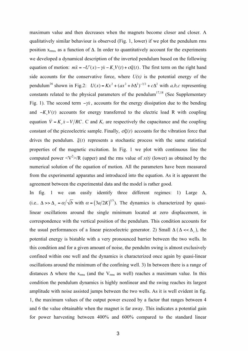
minimum. 3) In between there is a range of values of a where xrms reaches a maximum

and the dynamics is characterized by frequent jumps between the two wells. In Fig. 3

we present the xrms as a function of a and the noise variance σ2. The contour plot view

in the figure inset shows the evolution of the maximum xrms. The solid line is a

theoretical prediction obtained with the following argument. The rms evolution in

regime 3, can be roughly modelled as governed by to two main contributions: i) the

raising, mainly due to the growth of the separation between the two minima

€

x±; ii) the

drop, mainly due to the decrease in the jump probability measured by the crossing

probability, proportional23 to

€

exp −ΔUq σ 2τ( ), caused by the increase of the potential

barrier height

€

ΔUq . For the sake of identifying the dependence of the maximum

position we computed the root of the equation

€

d(xrms) da = d da x+ ⋅ exp −ΔUq σ 2τ( )( ) = 0 obtaining that xrms reaches a maximum

when

€

a = amax = bσ 2τ for a given noise intensity.

Finally we would like to stress the fact that the results obtained can led to a significant

increase in energy harvesting performances also in the small scale domain, where the

dynamical features discussed here can be applied without changes also to micro24,25 and

nanomechanical resonators26. Energy generators based on nanoscale linear oscillators

have been proposed8 and noise driven dynamics are considered as a promising

option27,28.

6

References

1. Paradiso, J., A., Starner, T. Energy Scavenging for Mobile and Wireless Electronics, IEEE Pervasive Computing, Vol. 4, No. 1, February 2005, pp. 18-27.

2. Roundy, S., Wright, P.K., Rabaey, J.M. Energy Scavenging for Wireless Sensor Networks, 2003 Kluwer Academic Publishers, Boston MA.

3. Byrne, R., Diamond, D. Chemo/bio-sensor networks, Nature Materials 5, 421 - 424 (01 Jun 2006).

4. Meninger, S. et al. Vibration-to-Electric Energy Conversion, IEEE Trans. Very Large Scale Integration (VLSI) Systems, vol. 9, no. 1, 2001, pp. 64–76.

5. Mitcheson, P., D., et al. Architectures for Vibration-Driven Micropower Generators, J. Microelectromechanical Systems, vol. 13, no. 3, 2004, pp. 429–440.

6. Roundy, S., Wright, P., K. A piezoelectric vibration based generator for wireless electronics, Smart Mater. Struct. 13 (2004) 1131–1142.

7. Shu,Y.C., Lien, I.C., Analysis of power output for piezoelectric energy harvesting systems, Smart Mater. Struct. 15 (2006) 1499-1512

8. Wang, Z.L., Song, J. Piezoelectric nanogenerators based on zinc oxide nanowire arrays, Science, 2006 Apr 14;312(5771):242-6.

9. von Buren, T., Troster, G. Design and optimization of a linear vibration-driven electromagnetic micro-power generator, Sensors and Actuators A-Physical 135 (2): 765-775 APR 15 2007.

10. Ottman, G.,K., Hofmann, H., F., Bhatt, A.,C., Lesieutre, G.,A., Adaptive Piezoelectric Energy Harvesting Circuit for Wireless Remote Power Supply, IEEE Trans. On Power Electronics, V. 17, No. 5, 669, SEPT 2002.

11. Anton, S.,R., Sodano, H.,A. A review of power harvesting using piezoelectric materials (2003-2006), Smart Materials & Structures 16 (3): R1-R21 JUN 2007.

12. Wang, S., Lam, K.,H., Sun, C.,L. et al., Energy harvesting with piezoelectric drum transducer, Appl. Phys. Lett. 90 (11): Art. No. 113506 MAR 12 2007.

13. Roundy, S. On the effectiveness of vibration-based energy harvesting, Journal of Intell. Mat. and Struct. 16 (10): 809-823 OCT 2005.

14. Beeby, S. P., Tudor M. J., White, N.M. Energy harvesting vibration sources for microsystems applications, Meas. Sci. Technol. 17 (2006) R175–R195.

15. The technology based on the exploitation of bistable oscillators as power generators has been named wisepower technology.

16. Kraftmakher, Y. Magnetic field of a dipole and the dipole–dipole interaction Eur. J. Phys., 2007, 28, 409–414.

17. Lefeuvre, E., et al. A comparison between several vibration-powered generators for standalone systems. Sensors and Actuators A: Physical, 2006, 126, 405-416.

18. Shu, Y. C. & Lien, I. C. Efficiency of energy conversion for a piezoelectric power harvesting system J. Micromech. Microeng., 2006, 16, 2429-2438.

7

19. Gitterman, M., Classical harmonic oscillator with multiplicative noise, Physica A 352 (2005) 309-334.

20. Duffing, G. Erzwungene Schwingungen bei Vernderlicher Eigengrequenz, Braunschweig, 1918, p. 134.

21. Rahman, M. Stationary solution for the color-driven Duffing oscillator PHYS. REV. E 53 (6): 6547-6550 Part B, JUN 1996.

22. Dittrich, T. Oelshlagel, B., Hanggi, P. Driven tunneling with dissipation, Europhysics Letters 22 (1): 5-10 APR 1 1993.

23. Hanggi, P., Talkner, P., Borkovec, M. Reaction-Rate Theory - 50 Years After Kramers, 1990 Rev. Mod. Phys. 62 (2): 251-341.

24. Fang, H.,B., Liu, J.,Q., Xu, Z.,Y., et al. Fabrication and performance of MEMS-based piezoelectric power generator for vibration energy harvesting, Microel. Journal 37 (11): 1280-1284 Sp. Iss. SI NOV 2006.

25. Choi, W.J., Jeon, Y., Jeong, J.H. et al. Energy harvesting MEMS device based on thin film piezoelectric cantilevers, Journal of Electroceramics 17 (2-4): 543-548 DEC 2006.

26. Aldridge, J.S., Cleland, A.N. Noise-enabled precision measurements of a duffing nanomechanical resonator, Phys. Rew. Lett. 94 (15): Art. No. 156403 APR 22 2005.

27. Gammaitoni, L., Bulsara, A.R. Noise Activated Nonlinear Dynamical Sensors (NANDS), Phys. Rev. Lett. 2002, 88, 230601, 2002.

28. Almog, R., Zaitsev, S., Shtempluck, O., Buks, E. Noise squeezing in a nanomechanical Duffing resonator, Phys. Rew. Lett. 98 (7): Art. No. 078103 FEB 16 2007.

Acknowledgements Useful discussions with P. Amico, I. Neri and F. Marchesoni are gratefully acknowledged. Correspondence and requests for materials should be addressed to L.G. (luca.gammaitoni@pg.infn.it).

8

Figure 1 Figure 1 | Piezoelectric oscillator mean electric power (upper panel) and position xrms (lower panel) as a function of Δ for three different values of the noise standard deviation σ . The symbols correspond to experimental values measured from the apparatus described in Supplementary Fig.1. The piezoelectric material used in the pendulum is Lead Zirconate Titanate. The continuous curves have been obtained from the numerical solution of the stochastic differential equation described in the text. Both in the experiment and in the numerical solution, the stochastic force has the same statistical properties: Gaussian distribution, with zero mean and standard deviation σ, exponentially auto-correlated with correlation time τ = 0.1 s. Every data point is obtained from averaging the rms values of ten time series sampled at a frequency of 1 KHz for 200 s. The rms is computed after zero averaging the time series. The expected relative error in the numerical solution is within 10%.

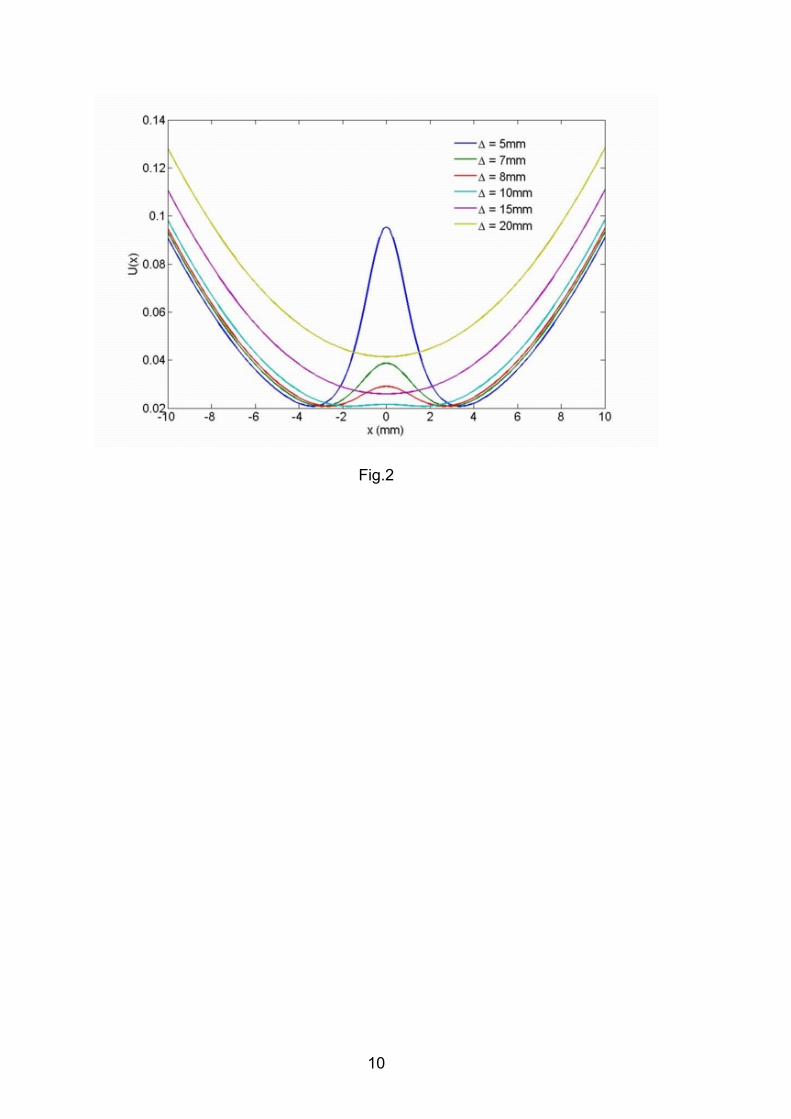
Figure 2 Figure 2 | Inverted pendulum potential function U(x). Five different plots of the potential function

€

U(x) = Kx 2 + (ax 2 + bΔ2)−3 2 + cΔ2 corresponding to five different values of the parameter Δ, representing the distance between the external magnet and the tip magnet (See Supplementary Fig.1) are shown (vertical scale in J). The constants

€

K,a,b,c are related to the pendulum parameters through:

€

K = Keff 2 with

€

Keff effective

elastic constant;

€

a = µ0M2 2πd( )

−2 / 3d2 with

€

µ0 the permeability constant,

€

M = 0.051 Am2, the effective magnetic moment and

€

d = 2.97 a geometrical parameter related to the distance between the measurement point and the pendulum length;

€

b = a d2 and

€

c = K d2 . On decreasing Δ the potential changes from monostable to bistable. The distance between the two minima located in

€

x± increases when Δ decreases, while the barrier height increases.

Figure 3 Figure 3 | Root mean squared (rms) values of the Duffing oscillator position xrms as a function of a and the noise variance σ2. The values plotted here have been obtained from the numerical solution of the stochastic differential equation described in the text. The rms is computed after zero averaging the x(t). In the inset: the contour plot view of xrms. Superimposed on the plot there is a continuous line representing the theoretical prediction for the maximum: i.e. xrms has a maximum when

€

a = bσ 2τ . The expected relative error in the numerical solution is within 10%.

9

Fig. 1

10

Fig.2

11

Fig.3

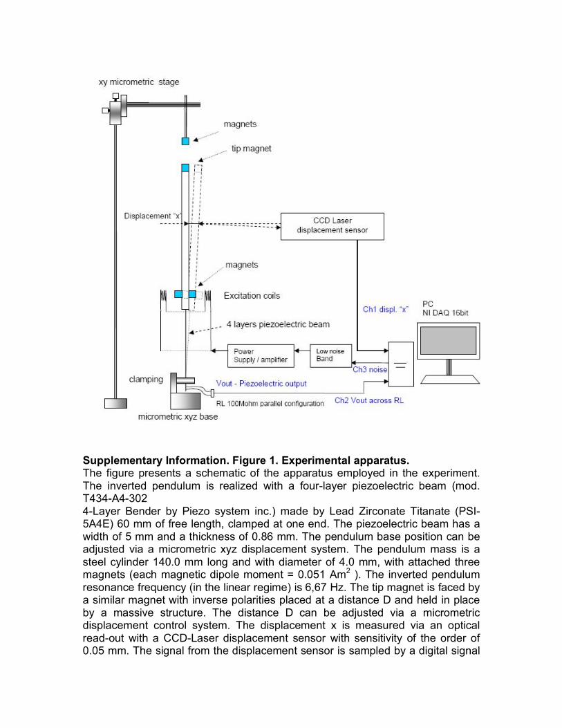
Supplementary Information. Figure 1. Experimental apparatus. The figure presents a schematic of the apparatus employed in the experiment. The inverted pendulum is realized with a four-layer piezoelectric beam (mod. T434-A4-302 4-Layer Bender by Piezo system inc.) made by Lead Zirconate Titanate (PSI-5A4E) 60 mm of free length, clamped at one end. The piezoelectric beam has a width of 5 mm and a thickness of 0.86 mm. The pendulum base position can be adjusted via a micrometric xyz displacement system. The pendulum mass is a steel cylinder 140.0 mm long and with diameter of 4.0 mm, with attached three magnets (each magnetic dipole moment = 0.051 Am2 ). The inverted pendulum resonance frequency (in the linear regime) is 6,67 Hz. The tip magnet is faced by a similar magnet with inverse polarities placed at a distance D and held in place by a massive structure. The distance D can be adjusted via a micrometric displacement control system. The displacement x is measured via an optical read-out with a CCD-Laser displacement sensor with sensitivity of the order of 0.05 mm. The signal from the displacement sensor is sampled by a digital signal

processing board (DSPB) controlled by a personal computer with sampling frequency 1KHz. The voltage signal from the piezo is measured through a load resistor RL placed in parallel with piezoelectric output voltage terminals and sampled by the DSPB. The digitalized signals are stored in the computer memory for post-processing elaboration. The DSPB is employed also to drive a current generator that produces, through a couple of coils, the magnetic excitation that mimic the ground vibration. The signal generated by the DSPB is filtered and conditioned in order to reproduce the desired statistical properties. The actual magnitude of the standard deviation of the vibrational force applied in the three cases is s= 3 10-4 N, 6 10-4 N, 12 10-4 N. The load resistance is R=RL = 100 MOhm and the piezo capacitance C=112 nF. The effective mass is m=0.0155 kg. The damping constant is γ=0.016 Hz.

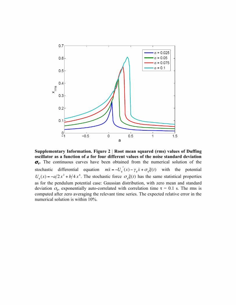
Supplementary Information. Figure 2 | Root mean squared (rms) values of Duffing oscillator as a function of a for four different values of the noise standard deviation σq. The continuous curves have been obtained from the numerical solution of the stochastic differential equation

!

m˙ ̇ x = "Uq#(x) " $ q

˙ x +% q&(t) with the potential

!

Uq (x) = "a 2 x2

+ b 4 x4 . The stochastic force

!

" q#(t) has the same statistical properties as for the pendulum potential case: Gaussian distribution, with zero mean and standard deviation σq, exponentially auto-correlated with correlation time τ = 0.1 s. The rms is computed after zero averaging the relevant time series. The expected relative error in the numerical solution is within 10%.