Nondeterministic Extended Finitely Recursive Process

Discrete Event Dynamic Systems: Theory and Applications, 7, 243–274 (1997)c© 1997 Kluwer Academic Publishers. Manufactured in The Netherlands.

A Nondeterministic Extension over FinitelyRecursive Process Model

SUPRATIK BOSE [email protected] for Artificial Intelligence and Robotics, Bangalore 560001 INDIA

SIDDHARTHA MUKHOPADHYAY* AND AMIT PATRA** smukh,[email protected] of Electrical Engineering, I.I.T. Kharagpur, W.B., 721302 INDIA

Received June 2, 1995; Revised August 5, 1996; Accepted December 17, 1996

Abstract. This paper extends the Finitely Recursive Process framework introduced by Inan and Varaiya for mod-elling Discrete Event Systems to encompass nondeterministic processes. Nondeterminism has been captured as aset of possible ‘deterministic futures’ instead of using the standard ‘failure’ model of Communicating SequentialProcesses. In the beginning a general structure of finitely recursive process space is provided with some importantmodifications. Next, the nondeterministic process space has been introduced as a special case of the generalalgebraic process space. A collection of operators has been defined over this nondeterministic process spacethat enables its characterisation in a finitely recursive manner. Finally, the advantages and disadvantages of theproposed model vis-a-vis other nondeterministic models of discrete event systems are discussed.

Keywords: Discrete Event Systems, Process Algebra Models, Finitely Recursive Processes, Nondeterminism.

1. Introduction.

In the last decade, research in the area of discrete event systems (DES) has led to thedevelopment of a large number of modelling frameworks that capture different logical andqualitative aspects of a DES. These may be categorised broadly into two types: state-based models and process algebra models. Typical examples for the first type are FiniteState Machines (FSM), (Ramadge and Wonham 89) , Petri Nets (PN) (Murata 89) , TimedTransition Model (TTM) (Ostroff90), State Charts (SC) (Harel 87) etc. On the other hand,research in programming language theory, during the seventies and the eighties, has ledto the development of algebraic process models, which capture the language behaviour ofcommunicating and concurrent processes. Notable among them are the CommunicatingSequential Processes (CSP) of Hoare (1985) and the Calculus of Communicating Systems(CCS) of Milner (1989). A comprehensive study on the process models can be found in(Hennessy 88). Recently, Inan and Varaiya (1988) have proposed a similar framework,known as the Finitely Recursive Process (FRP) model. This is a deterministic frameworkand we shall refer to it as the Deterministic FRP (DFRP). It is a generalisation of thedeterministic CSP (DCSP), where, a set of process operators is provided that may be used

* This work has been partially supported by University Grants Commission’s Young Teachers’ Career Devel-opment Award to Dr. S.Mukhopadhyay** Corresponding author. Tel. ++91-3222-55224-4619

244 BOSE, MUKHOPADHYAY AND PATRA

to build complex processes from simple ones. Recursive characterisation of the processesand the existence and uniqueness conditions of solutions of recursive equations are alsogiven. Subsequently Inan and Varaiya (1989) introduced a general algebra for logicalmodels of DES.

The process algebraic formalisms, such as CSP, CCS and DFRP, provide a compositionaland structured ”high level” description of the event dynamics than do the state based models,such as FSM or PN. Thus, these models have the advantage that they can express thebehaviour of a DES in a more compact way. While analysis of properties for arbitraryprocesses is difficult in these models and several problems are undecidable (Cieslak andVaraiya 90), there exist subclasses where such problems are solvable or at least decidable.Due to the ”high level” description, modelling of complex systems is often more manageablein process based frameworks than in graphical or state based paradigms, where the numberof states in a simple problem can easily exceed thousands. However, at present, the processalgebraic models lack solutions to various problems of control and observation that exist forstate-based models. Moreover, as in FSM, PN or TTM, extensions and tools are required tomodel features of time, numerical information, nondeterminism etc., in the process basedmodels.

Nondeterminism is an important concept of DES models. Sometimes a system has arange of possible behaviour, but the environment or the ‘user’ may not have the ability toinfluence, or even observe the selection between the alternative courses of behaviour. In acausal universe, where every physical system is necessarily deterministic, nondeterministicmodels arise either from a deliberate decision to ignore the factors that influence thisselection, or from the part of the dynamics that is not visible from the given vantage pointof the user. Thus, nondeterminism is necessary in maintaining a high level of abstraction indescription of the behaviour of physical processes. Naturally, a nondeterministic processmay have a number of possible deterministic implementations.

The state based models such as FSM, SC, TTM etc., incorporate nondeterminism by mak-ing the transition relation nondeterministic. In PN it may be achieved via a non-injectivelabelling of the transitions (Murata 89) . Recently, Heymann (1990) and Shayman-Kumar(1995) have characterised nondeterministic state machines in terms the so called ‘Trajec-tory Models’ (TM). They have also introduced the concept of ‘Prioritized Synchronization’(PS). This characterisation is more distinguishing than the traditional failure model andserves as a language congruence for DES in presence of PS. In CCS, nondeterminism arisesout of hidden transitions. In CSP, nondeterminism is described in terms of the externallyobservable behaviour of a process to engage in an event or ”refuse” it. A nondeterministicCSP (NCSP) is therefore characterised merely in terms of its traces and refusals, withoutregard for its internal state, giving rise to the so called ”failure”-based model. In contrast,here we argue that the underlying deterministic dynamics of a process is often, at leastpartially known, by say, the designer of the process. The system, however, while in action,may only be partially observable to an observer and/or supervisor. However, since theunderlying deterministic model is atleast available to some extent, one can use this knowl-edge in addition to external observations, to create an ‘observed’ nondeterministic modelof the system for practical use. This model approximates the original deterministic systemas closely as possible, since it utilises all available information, losing only the minimum

A NONDETERMINISTIC EXTENSION 245

amount that is unavoidable due to under-observation. This kind of reasoning leads us to a”possible future” based model of nondeterministic FRP (NFRP). Interestingly, it turns outthat, in case of a constant alphabet, treatment of nondeterminism in NCSP and NFRP areequivalent. But in case of a variable alphabet, given an extent of lack of observation, anNFRP in general results in less uncertainty, than what it would have been had a ”failure”type characterisation been used. This is similar to the case of TM. This similarity arisesbecause both approaches consider that the nondeterministic system model arises from anunderlying deterministic one, through some event concealment mechanism. Several otherconcepts such as those ofε-closure and concurrency with PS find their parallels in the NFRPframework, as we shall point out at various points in the paper.

The contributions of this paper and its organisation are as follows.a) The mathematical background is described in section 2. Though this section follows

Inan and Varaiya (1989) closely, some important generalisations are introduced in orderto present the nondeterministic process space as a special case of the general algebra ofDES models presented there. These include the concept of a ‘weakly spontaneous family’of functions, a generalised concept of mutually recursive family of functions and finally ageneralised equivalent condition for mutually recursive processes.

b) The nondeterministic process space has been introduced in section 3 as a special caseof general marked process space. As already mentioned, the representation is different fromthat of standard ‘failure’ model of NCSP.

c) In section 4, a substantial collection of process operators has been defined over thenondeterministic process space and their properties are discussed. In section 5, theseoperators have been shown to form a weakly spontaneous mutually recursive family offunctions and they have been used to give a finitely recursive characterisation over thenondeterministic process space.

d) A single track guideway and a fault diagnostic session of a chemical process aremodelled in section 6 to show the usefulness of the framework. A concluding discussioncovering assessment and comparison of the model with other nondeterministic models aswell as scopes for future work are presented in section 7.

2. Mathematical Background

This section is presented for completeness as well as for easy reference by the reader. Itclosely follows (Inan and Varaiya 89). However some important generalisations have beenmade to the concepts introduced there.

Definition 1 (Basic Objects:) Let Σ be a fixed finite collection of events.Σ∗ is the set ofall finite length strings formed with elements ofΣ, including the null string<>. It is alsocalled the set oftraces. L ⊆ Σ∗ is called alanguageover Σ and it is prefix closed ifsˆt ∈ L⇒ s ∈ L. C(Σ∗) denotes the family of prefix closed languages overΣ.

By marking is implied an assignment of values to a set of mathematical objects, associatedwith a process, after some event has taken place. This in turn determines the immediatefuture of the process. Each such assignment is called amark .


Definition 2 (Marking:) LetM be a set of marks andψ be a fixed family of functions fromΣ∗ toM such thatµ ∈ ψ ∧ s ∈ Σ∗ ⇒ µ/s ∈ ψ whereµ/s(t) := µ(sˆt), for all t ∈ Σ∗.

Definition 3 (Marked Process and Embedding Set:)A marked processis a tuplew =(tr w, µw) where,tr w ∈ C(Σ∗), µw : tr w →M is the marking function that determinesthe mark afters. The underlying global set of processes, also called anembedding set, isdenoted asWΣ,M,ψ (often simply asW ) and is defined as the cartesian productC(Σ∗)×ψ.µw(s) is themarking of the traces.

Definition 4 (Post-Process:)A processw, after executing a strings, behaves as itspost-process‘w afters’, denoted byw/s. It is formally defined astr w/s := t ∈ Σ∗ | sˆt ∈ tr w andµ (w/s)(t) := µw/s(t) = µw(sˆt).

At any point during its evolution, a process exercises a choice of events from a set ofalternatives. This is captured by the choice function stated below.

Definition 5 (Choice Function:) Given fori = 1, · · · , k, wi ∈W,σi ∈ Σ, and an initialmarkm ∈ M , a new processw, denoted asw = (σ1 → w1 | · · · | σk → wk)m is definedas follows.tr w := <> ∪

⋃ki=1< σi > ˆs | s ∈ tr wi. Also

µw(<>) := m; µw(< σi > ˆs) := µwi(s).

Processes unfold their traces like a tree. Thus any process first exercises its choice ofevents from those that are possible ( i.e., events included in traces of length 1) and thenbehaves as the corresponding post-process.

Property 1 (One Step Expansion :) For anyw ∈ W , if tr w 6= <> one can havew = (σ1 → w/ < σ1 >| · · · | σk → w/ < σk >)µw(<>) where< σi >| i = 1, · · · , k = s ∈ tr w | #s = 1. Here #s denotes the length ofs.

To relate the elements of the embedding setW , apartial order ¹onW is introduced. Thecomplete definition of¹may be made for specific cases appropriately. Also a sequence ofprojection operators↑ n : W →W | n = 0, 1, · · · is defined with the implied meaningthatw ↑ (n+ 1) is a process that has the same dynamics (trace and mark) asw for stringsupto lengthn + 1. Beyond thatw ↑ (n + 1) may differ fromw. Obviouslyw ↑ (n + 1)is a better approximation ofw compared tow ↑ n. The exact definition of↑ n is againmade appropriately for specific cases.

Definition 6 (Embedding Space:) Anembedding spaceis a triple(W,¹, ↑ n), whereW = WΣ,M,ψ is an embedding set,¹ is a partial order and↑ n : W →W | n = 0, 1, · · ·is a family of projections mappingW into itself, satisfying following properties:1) (w ↑ 0) ↑ n = w ↑ 0, ∀n ≥ 0. In a sense the↑ n operator is ‘causal’ on the indexingsequence.2) µw(<>) = µv(<>)⇒ w ↑ 0 = v ↑ 0.3) If w = (σ1 → w/ < σ1 >| · · · | σk → w/ < σk >)µw(<>) thenw ↑ n = (σ1 → w/ < σ1 >↑ (n− 1) | · · · | σk → w/ < σk >↑ (n− 1))µw(<>) . Herew ↑ n is the image ofw under↑ n. If tr w := <> then∀n > 0, we require (unlike in


(Inan and Varaiya 89) , wherew ↑ n := w ↑ 0, in such cases ) thatw ↑ n be defined asHALTµw(<>), where, form ∈M ,HALTm is the process havingtr HALTm := <>,µHALTm(<>) := m.4) If wi is a chain, (that is∀ i wi ¹ wi+1) then there exists a least upper bound (l. u. b)of wi in W . Thus (W,¹) is a complete partial order.5) If wi converges tow then< σ >∈ tr w ⇔ ∃l | ∀ i ≥ l, < σ >∈ tr wi. Alsowi/ < σ > ¹ wi+1/ < σ > andwi/ < σ > converges tow/ < σ >.6) If wi is a chain converging tow, u1, · · · , uk are processes inW , σ, σ1, · · · , σn aredistinct events,m is a mark, v := (σ → w | σ1 → u1 | · · · | σk → uk)m, and for i =1, · · · , k, vi := (σ → wi | σ1 → u1 | · · · | σk → uk)m, then,vi is a chain converging tov. Thus choice function preserves ordering of processes.7) w ↑ nn≥0 is a chain converging tow.8) If wii≥0 is a chain converging tow then∀n wi ↑ ni≥0 is a chain converging tow ↑ n.

Remark 1 In condition (3) above we have made a change in the definition ofw ↑ n whenn > 0 andtr w = <>, from the one that is given in (Inan and Varaiya 89) . Intuitively,since the informationtr w = <> is available, the reasonable approximationw ↑ n ofw for n > 0 should be a ‘do-nothing’HALTm process. It can be easily checked thatthis modification doesn’t affect any result in (Inan and Varaiya 89) . If we retained the olddefinition i.e.,tr w = <> ⇒ ∀n > 0, w ↑ n = w ↑ 0, then we encounter difficulties asshown while describing the process operators for our nondeterministic process space.

Fact 1 If ↑: W →W satisfies(w ↑ 0) ↑ 0 = w ↑ 0 and condition (2) of definition 6, thenthere exists a unique collection of maps,↑ n, n ≥ 0, satisfying (1) to (3) of definition 6.Also (w ↑ n) ↑ m = w ↑ min(m,n). For a proof of this, see (Inan and Varaiya 89) .

Definition 7 (Marked Process Space:)A (marked)process spaceΠ = (Π,¹, ↑ n) isany subset of(W,¹, ↑ n) that is closed with respect to the following operations.(a) P ∈ Π⇒ ∀n ≥ 0 P ↑ n ∈ Π,(b) P ∈ Π⇒ ∀s ∈ tr P, P/s ∈ Π,(c) if Pii≥0 is a chain converging toP such that∀i ≥ 0, Pi ∈ Π, thenP ∈ Π and(d) if ∀i = 1, · · · , k ≥ 0, R,P1, · · · , Pk ∈ Π andR/ < σi >↑ 0 = Pi ↑ 0 andR =(σ1 → R/ < σ1 >| · · · | σk → R/ < σk >)µR(<>) thenP := (σ1 → P1 | · · · | σk →Pk)µR(<>) is in Π.

In general a processP is an infinite object because of its infinite set of trajectories. Forthe purpose of computation it is necessary to have afinitedescription of processes of at leastsome restricted process space. The basic idea is to use recursion in a way analogous to themethod of differential or difference equation for describing infinite set of trajectories. Forrecursion to be well-defined, certain properties of functions used in recursive descriptionsare necessary. These are defined below.

Property 2 (Function Properties:) Given a process space(Π,¹, ↑ n), a process op-eratorf : Π→ Π is said to be :


continuous: if for every chainPii≥0,f(Pi)i≥0 is also a chain and∪f(Pi) = f(∪Pi).(Note thatP1 ¹ P2 ⇒ P1∪P2 = P2 andP2 ¹ P1 ⇒ P1∪P2 = P1, otherwise∪ betweenprocesses is not well defined).

nondestructive (ndes): if ∀P ∈ Π, ∀n, f(P ) ↑ n = f(P ↑ n) ↑ n.

constructive (con): if ∀P ∈ Π, ∀n, f(P ) ↑ n+ 1 = f(P ↑ n) ↑ n+ 1.

It is intuitively clear thatf is conif the (n+1)st event off(P ) is determined by then thevent inP . Also con impliesndes. If f has several arguments, these definitions apply toeach argument with others kept fixed.

Fact 2 The properties of continuity, nondestructiveness and constructiveness are preservedunder function composition. Furthermore, iff1 is conandf2 is ndes, then bothf1 f2 andf2 f1 arecon.

It is easy to see that the post-process functionP → P/s is usually destructive (notndes)unlesss =<>. Also from conditions of definition 6 it is easy to see (a) thechoicefunctionshould be continuous andcon; (b) every projection operator↑ n is continuous andndesand(c) the post-process is a continuous partial function in the sense that ifP1 ¹ P2 ¹ · · · is achain converging toP , ands ∈ tr P , then there is an integerl such thatPl/s ¹ Pl+1/s ¹ · · ·is a chain converging toP/s.

Having defined the above properties of process functions, the following theorem is nowstated to specify the conditions for unique solution of recursive equations defined on pro-cesses.

Theorem 1 LetΠ be a process space and consider the recursive equation

P = F(P,U) (1)

whereF = (F1, · · · , Fn), a (vector) function fromΠn×Πk toΠn andU = (U1, · · · , Uk) ∈Πk are given along with a set of consistent initial conditions:

Pi ↑ 0 = Z0i = Fi(Z01, · · · , Z0n,U) ↑ 0. (2)

(c1) existence:If eachFi is continuous and ndes inP, then the processZ = ∪kZk is well defined, whereZ0 := (Z01 · · ·Z0n) and Zk+1 := F(Zk,U), k ≥ 0.AlsoZ is the minimal solution to equations ( 1, 2), i.e., for any otherP = (P1 · · · , Pn)satisfying the above equations,Zi ¹ Pi, ∀i = 1 · · ·n. Moreover this minimal solution iscontinuous, con and ndes inUi accordingly, asF is continuous, con and ndes inUi.(c2) uniqueness:If F is constructively guarded, i.e., there do not exist indicesi1 · · · , im,im = i1 such thatFik is not con inPik+1 , 1 ≤ k < m− 1, then the above equations havea unique solution.

Proof: See (Inan and Varaiya 89). 2

The above theorem describes conditions under which a recursive process description hasa well-defined and perhaps unique solution. It turns out that as these recursive expressionsare expanded along the traces, new post-process expressions are generated. It is therefore


necessary to know whether these postprocesses can be described using function composi-tions on process operators and whether such function compositions are closed with respectto some family of functions. Below we develop a framework for specifying a family of func-tions in afinite and recursive way. The basic idea is to start with some primitive functionsand combine them by repeated algebraic operations to produce a larger family. Throughoutour discussion we fix a process spaceΠ = (Π,¹, ↑ n). AlsoΠ ↑ 0 = P ↑ 0 | P ∈ Π.

Definition 8 (Constant Functions:) Given a process spaceΠ, letCΠ be a set of functionsc : Πn → Π which isequinumerousto Π ↑ 0, that is, there exists a bijectionr : Π ↑0 → CΠ such that, for every uniqueP ↑ 0 in Π ↑ 0 for someP ∈ Π, there is a uniquefunctionc ∈ CΠ with r(P ↑ 0) = c andr−1(c) = P ↑ 0. CΠ is called the set ofconstantfunctions of Π.

For everyc ∈ CΠ, for anyn ≥ 0 and∀P = (P1, · · · , Pn) ∈ Πn, c(P) := r−1(c).

Definition 9 (Projection Functions:) For any n > 0, the set ofprojection functions,namelyProj(n), is the set of functionsProji | 1 ≤ i ≤ n, Proji : Πn → Π such thatfor anyP ∈ Πn, Proji(P) := Pi.

It is to be noted that the constant functions and the projection functions can be defined overany process spaceΠ, irrespective of what other operators one may define overΠ. Howeverother than the above ‘trivial’ functions one needs more complex operators for achieving gooddescribing power and language complexity. To indicate the desirable properties of suchclasses of operators which will facilitate recursive descriptions, the following definitionsare introduced.

LetG be a set of functions such that everyg ∈ G is a functiong : Πk → Π of arity k forsomek. The following definitions and theorems relate to recursive process characterisationwith functions selected fromG.

Definition 10 (Spontaneous Family:)G is said to be aspontaneous familyof functionsif everyg ∈ G is a spontaneousfunction, i.e.,g is continuous, ndes and if it is ak − aryfunction then∀(P1, · · · , Pk) ∈ Πk,

g(P1 ↑ 0, · · · , Pk ↑ 0) = (g(P1 ↑ 0, · · · , Pk ↑ 0)) ↑ 0.

G is said to be aweakly spontaneous familyof functions if everyg ∈ G is weaklyspontaneous, i.e., continuous and ndes.

Definition 11 Let G be the set of functions that can be formed recursively with elementsofG through function composition (denoted by the symbol ‘’) as described below.(a) Id ∈ G whereId is the identity map onΠ.(b)G ⊆ G(c) If f1, · · · , fk are inG andg ∈ G so thatg is ak − ary function, theng (f1, · · · , fk)is in G and has an aritym = m1 + · · · + mk wheremi is the arity offi. Finally(g (f1, · · · , fk))(P1, · · · , Pm) := g(f1(P1 · · · , Pm1), · · · , fk(P(m−mk)+1 · · · , Pm)).


Definition 12 (Mutually Recursive (MR) Family:) G is said to be aMutually RecursiveFamily of functions if for anyk − ary functiong ∈ G, (P1, · · · , Pk) ∈ Πk, < σ >∈tr (g(P1, · · · , Pk)) there exists somem′ − ary functiong′ in G such that

(g(P1, · · · , Pk))/ < σ >= g′(P ′1, · · · , P ′m′)

where for eachj, 1 ≤ j ≤ m′, ∃i, 1 ≤ i ≤ k with P ′j = Pi orP ′j = Pi/ < σ >.

Definition 13 (Ωn(G,Π):) Once we have a family of functionsG, for somen > 0, onecan define inductively the infinite class of functionsΩn(G,Π) (or simplyΩn if G and Πare understood ) as follows:(a)CΠ ⊆ Ωn(G,Π).(b) Proj(n) ⊆ Ωn(G,Π).(c) f1, · · · , fk ∈ Ωn(G,Π) andg ∈ G such thatg has an arityk impliesg (f1, · · · , fk) ∈Ωn(G,Π).

Fact 3 Ωn(G,Π) is (weakly) spontaneous ifG is (weakly) spontaneous.

Definition 14 (Mutually Recursive Processes:)A finite setP1, · · · , Pn is called a fam-ily of Mutually Recursive Processes (MRP)with respect toΩn(G,Π) if ∀ j,Pj , s ∈ tr PjPj/s = f(P1, · · · , Pn) for somef ∈ Ωn(G,Π).

The next theorem states the necessary and sufficient condition under which a process canbe considered to be mutually recursive with respect to a family of functions.

Theorem 2 Leteither (a)Gbe a mutually recursive spontaneous (MRS) family of functionsor (b)G be a mutually recursive weakly spontaneous (MRWS) family of functions such thatfor the embedding space(W,¹, ↑ n) in question, the projection operator↑ 0 is a constantfunction i.e., for anyw1, w2 in W , w1 ↑ 0 = w2 ↑ 0.

ThenP1, · · · , Pn is a family of MRP w.r.tΩn(G,Π) iff P = (P1, · · · , Pn) is the uniquesolution of the recursive equation with consistent initial condition,

(X1, · · · , Xn) = X = F(X), X ↑0 := P ↑0 (3)

whereF : Πn → Πn and each componentFi of F is guarded, that is

Fi(X) = (σi1 → fi1(X) | · · · | σiki → fiki (X))mi (4)

with eachfij ∈ Ωn(G,Π) andmi is a suitable mark.

Though the proof will follow similar reasoning as the one in (Inan and Varaiya 89) , wehave presented it in detail in the appendix because of two reasons: (a) we have generalisedthe concept of an MR family of functions. (b) We have relaxed the requirement onG byallowing it to be just an MRWS family instead of an MRS family under the condition that↑ 0 is a ‘constant’ function. Necessity of the above changes will be clear while definingthe process operators of our nondeterministic process space.


Definition 15 (Finitely Recursive Processes:)A processY ∈ Π is said to be aFinitelyRecursive Process (FRP)with respect toΩn(G,Π) if it can be represented asP = F(P),Y = g(P) whereP = (P1, · · · , Pn), F is of the form ( 4) andg ∈ Ωn(G,Π). (F, g) is saidto be arealisation of the processP .

Definition 16 (Algebraic Process Space:)The collection of all possible FRPs w.r.tΩn(G,Π)for arbitrary n is called thealgebraic process spaceand is denoted asA(Ω(G,Π)).

Fact 4 Because of MR-ness of functions ofΩ(G,Π), A(Ω(G,Π)) is closed under post-process operation, i.e., ifY ∈ A(Ω(G,Π)) with realisation(F, g) for somen, then for anys ∈ tr Y , Y/s can be represented asY/s = gs(P) for somegs ∈ A(Ω(G,Π)).

In this section we have presented the general ideas relating processes, operators andrecursive descriptions without instantiating the exact nature of the marking functions or theoperators. This we do next.

3. The Nondeterministic Process Space

In this section we define the specific embedding space and the marked process space ofconcern here. The definition of a nondeterministic mark is an extension on the deterministicmark defined in (Inan and Varaiya 88). There any deterministic processP has been defined as3-tupleP = (trP, αP, τP ) satisfying certain axioms. The settrP ⊆ Σ∗ is the set oftracesof P , αP : trP → 2Σ is thealphabetfunction, andτP : trP → 0, 1 is the terminationfunction whereτP (s) = 1 represents successful termination ofP after generation of theevent sequences in P . The axioms that are satisfied by any deterministic processP are(i) <>∈ trP andsˆt ∈ trP ⇒ s ∈ trP . (ii) sˆ < σ >∈ trP ⇒ σ ∈ αP (s). (iii)(τP (s) = 1∧ sˆt ∈ trP )⇒ t =<>. ΠD denotes the set of deterministic processes. Herea mark after a strings consists of a set of triples of the form (α, τ, f ) whereαandτ determinealphabet and termination afters in the usual sense of deterministic processes andf is theset of events that will be blocked. Thus each (α, τ, f ) is a possible deterministic ‘future’.A nondeterministic mark is represented as a set of deterministic marks,one of which getschosen in a nondeterministic fashion. If a particular future is chosen, then the correspondingα is the instantaneous alphabet of the process,f is the collection of events that can be blockedby the processin that ‘future’ andτ =1 implies that the process terminates successfullyinthat ‘future’. As mentioned earlier, nondeterminism essentially arises due to low resolutionof modelling or observation. Thus the process may engage in unmodelled or unobservedactions between modelled or observed events and arrive at new marks (‘futures’). Sincewe are interested in describing the modelled behaviour of the system, after every modelledevent we collect the set of deterministic marks that may be arrived at via possible internal(hidden) actions to make the nondeterministic mark or ‘future’. It is to be noted that inthe deterministic case, (that is in DFRP) since the blocking functionf is computable fromthe trace and the alphabet function, it is not included explicitly. It is however necessary toinclude it in the mark in the case of a nondeterministic process, since, depending upon themark chosen (by some internal unmodelled action), an event may either take place or maybe blocked and it is not possible to compute the chosen mark from the trace. We feel that


this characterisation of nondeterminism is appropriate since nondeterminism essentiallyarises due to ‘hiding’ or ‘undermodelling’ of events of a deterministic dynamics. It shouldalso be noted that the above definition cannot be treated as a special case of ‘CanonicalNondeterministic Embedding Space’ (W) defined in (Inan and Varaiya 89) mainly for tworeasons. Firstly divergence has not been treated in this work. In this sense, the present workis similar to the original Nondeterministic Communicating Sequential Processes (With-OutDivergence) (NCSP(WOD)) of (Brookes, Hoare and Roscoe 84) . Secondly, definitionof W in (Inan and Varaiya 89) basically generalises ‘refusal’ based postulates of CSP aswell as NCSP(WOD). Instead of refusals we have adopted a framework based on‘possiblefuture’. A detailed comparison between NCSP(WOD) and the nondeterministic processspaceΠN presented here, will be given in a later section. Below we provide the formaldescriptions of the related concepts.

Definition 17 (Basic Objects:) Let Σ be a fixed finite collection of events. LetMD be aset of‘deterministic’ marks andMN be the family of nonempty subsets ofMD. That isMN = 2MD\φ and it denotes the collection ofnondeterministic marks. LetψN be a fixedfamily of (set-valued) functions fromΣ∗ toMN such thatµ ∈ ψN ∧ s ∈ Σ∗ ⇒ µ/s ∈ ψNwhereµ/s(t) := µ(sˆt), for all t ∈ Σ∗. WΣ,MN ,ψN (or simplyWN ) denotes the suitablenondeterministic embedding setand it is defined asWN := C(Σ∗)× ψN .

In WN we first define two types ofnondeterministic ‘constant’ processes,namely,CHAOS andHALTm for somem ∈MN .

Definition 18 (The Constant Nondeterministic Processes):CHAOS is the maximally nondeterministic process ofWN defined astr CHAOS := Σ∗, ∀s ∈ Σ∗, µCHAOS(s) := MN .Also, for somem ∈MN ,HALTm is the ’do-nothing’ process defined astr HALTm := <>. µHALTm(<>) := m.

Next we define the projection operators.

Definition 19 (Nondeterministic Projection Operators↑N n | n ≥ 0:) .For anyw ∈WN , w ↑N 0 := CHAOS.For n > 0 if tr P = <> thenw ↑N n := HALTµw<>. Otherwisew ↑N n := (σ1 → w/ < σ1 >↑N (n − 1) | · · · | σk → w/ < σk >↑N (n − 1))µw(<>)

wherew = (σ1 → w/ < σ1 >| · · · | σk → w/ < σk >)µw(<>).

The partial order is defined next. This is useful in comparing the degrees of nondeter-minism of two processes.

Definition 20 (Nondeterministic Partial Order ¹N :) The partial order¹N overWN isdefined as :w1 ¹N w2 iff tr w2 ⊆ tr w1 and∀s ∈ tr w2, µw2(s) ⊆ µw1(s).

In other wordsw1 ¹N w2 implies thatw1 is less deterministic (or more nondeterministic)thanw2. This leads to the straightforward definition of the limit of a chainwi ¹N wi+1 asfollows.

limwii≥0 = w wheretr w := ∩itr wi, and∀s ∈ tr w, µw(s) := ∩iµwi(s).


Finally we have to specify the marking axioms that will define a suitable (marked) non-deterministic process space.

Definition 21 (Marking Axioms:) The marking axioms of our required process space are:(a) MD = (α, τ, f) ∈ (2Σ × 0, 1 × 2Σ) | f ⊆ α ∧ (τ = 1 ⇒ f = α). AlsoMN = 2MD\φ.(b) For any processP in our required process space,∀s ∈ tr P(∃(α, τ, f) ∈ µP (s) | (τ = 0 ∧ σ ∈ (α− f)))⇔ sˆ < σ >∈ tr P .

Let ΠN be a subset ofWN that satisfies the above marking axioms.

Fact 5 It can be verified that (a)(WΣ,MN ,ψN ,¹N , ↑N n) satisfies conditions of def-inition 6 and thus is a suitablenondeterministic embedding spaceand (b)ΠN satisfiesthe conditions of definition 7 and thus,(ΠN ,¹N , ↑N n) is a suitablenondeterministicprocess space.

It should also be noted that the 2nd marking axiom poses some restriction on the choiceof m ∈ MN for whichHALTm is a valid element ofΠN . Only for thosem ∈ MN suchthat for all triples inm, α = f ,HALTm is a valid process. This is becausetr HALTm isdefined to be a null set.

Remark 2 (Comparison with Deterministic Processes:)Naturally, a deterministic pro-cess is a special case of a nondeterministic process. Formally, anyP ∈ ΠD can be expressedas a special nondeterministic processF(P ) ∈ P, by the transformation ruleF , defined asfollows.• trF(P ) := tr P .• ∀s ∈ trF(P ), µF(P )(s) := (αP (s), τP (s), αP (s)− σ | sˆ < σ >∈ tr P).Thus∀s ∈ trF(P ), µF(P )(s) is a singleton (contains a single future) since it is actuallydeterministic.

The partial order on deterministic processes¹D is defined in (Inan and Varaiya 88) asP1 ¹D P2 if tr P1 ⊆ tr P2 and∀s ∈ tr P1, αP1(s) = αP2(s) andτP1(s) = τP2(s).However,P1 ¹D P2 does not imply thatF(P2) ¹N F(P1) even thoughtrF(P2) ⊇trF(P1). This is because,¹D relates single ‘future’s of two deterministic processes (aftera common string), which have the sameα andτ components and may differ only in set ofevents they block. Its nondeterministic counterpart¹N , on the other hand, essentially testswhether (after a common string) all the ‘futures’ of one process is included in another ornot.

The projection operator on deterministic processes (denoted as↑D n and defined in (Inanand Varaiya 88)) ‘truncates’ a deterministic process upto string lengthn. By comparisonwe find that↑D n on a deterministic processP and its nondeterministic counterpart↑N nonF(P ) behave identically upto a string lengthn− 1. We also have:•tr (P ↑D n) := s ∈ trP | #s ≤ n = s ∈ tr (F(P ) ↑N n) | #s ≤ n.•∀s ∈ tr P | #s ≤ n− 1, µF(P ↑D n)(s) = µ(F(P ) ↑N n)(s).

In this section we have completely defined the nondeterministic process space. It has alsobeen shown how deterministic processes can be treated as a special case of nondeterministicprocesses.


4. Process Operators

In this section we present a variety of process operators which will be used later to give arecursive characterisation ofΠN .

The Event Concealment Operator generates a possibly (more) nondeterministic processfrom a (non-)deterministic process through concealment of events.

Definition 22 (The Event Concealment Operator (ECO) :) GivenP ∈ ΠN andC ⊆Σ, P\C is defined in terms of a hiding operator↓C : Σ∗ → (Σ− C)∗ defined as below:• <>↓C :=<> andsˆ < σ >↓C := (s ↓C if σ ∈ C) or (s ↓C ˆ < σ > if σ ∈/C)• tr P\C := s ↓C | s ∈ tr P and

µ(P\C)(t) :=⋃

s∈tr P | s↓C=t

((α− C), τ, (f − C)) | (α, τ, f) ∈ µP (s)

ECO is valid, (i.e. P\C ∈ ΠN ) continuous butdestructivein nature. (P\C1)\C2 =(P\C1 ∪ C2).

For a nondeterministic process, often the choice mechanism of an event is concealed or,internal. In such a case the choice is called nondeterministic in the sense that the choicecannot be seen or influenced.

Definition 23 (The Nondeterministic Choice Operator (NCO):) Given processesP1 andP2, the processP = P1 u P2 is defined as:• tr P := tr P1 ∪ tr P2.• µP (s) := (µP1(s) if s ∈ tr P1− tr P2) ∨ (µP2(s) if s ∈ tr P2− tr P1) ∨ (µP1(s)∪µP2(s) if s ∈ tr P1 ∩ tr P2).

TheNCO is valid, continuous and ndes.ECO distributes overNCO, i.e.,(P1 u P2)\C= (P1\C) u (P2\C).

The deterministic version of choice is also well defined here.

Definition 24 (The Deterministic Choice Operator (DCO):) Given processesP1, · · · ,Pn in ΠN , distinct eventsσ1 · · ·σn and a consistent markm ∈ 22Σ×0,1×2Σ\φ, such that,m = (α, 0, f) is a singleton,f ⊆ α andσi | i = 1, · · · , n = (α − f), the processP ,denoted byP = (σ1 → P1 | · · · | σn → · · ·Pn)m is defined as:tr P := <> ∪

⋃ni=1< σi > ˆs | s ∈ tr Pi.

µP (<>) := m; µP (< σi > ˆs) := µPi(s).

As expected, the definition is similar to the one in the deterministic case of FRP. The choiceoperator is valid, continuous and con. Note that the initial mark of aDCO is a singleton,indicating that the initial event can be chosen deterministically by the environment.

TheECO distributes overDCO according to the following law. LetP = (σ1 → P1 | · · · | σm → · · ·Pm)(α,0,f) andC ⊆ Σ. Then


P\C =

(P1\C) u · · · u (Pm\C) uHALT(α−C,0,f−C) if α− f ⊆ C(σi1 → Pi1\C | · · · | σir → · · ·Pir\C)(α−C,0,f−C) u (Pj1\C) u · · · u (Pjk\C)if σi1 · · ·σir = (α− f)− C and σj1 · · ·σjk = (α− f) ∩ C

Next we define the sequential and parallel composition operators for processes.

Definition 25 (The Sequential Composition Operator (SCO):) Given two processesP1

andP2, the processP = P1;P2 is defined as:• tr P := s ∈ tr P1 | ∃(α, 0, f) ∈ µP1(s) ∪ s = rˆt | r ∈ tr P1 ∧ ∃(α, 1, α) ∈µP1(r) ∧ t ∈ tr P2.• µP (s) := Ms

1 ∪Ms2 where

Ms1 := ((α, 0, f) ∈ µP1(s) if s ∈ tr P1) or (φ otherwise). It is actually the collection

of marks ofP1 afters provided the event sequences has taken place inP1.Ms

2 := (⋃r,t µP2(t) | s = rˆt ∧ r ∈ tr P1 ∧ ∃(α, 1, α) ∈ µP1(r) ∧ t ∈ tr P2) or

(φ otherwise). It is the collection of marks ofP2 after t, whens = rˆt, P1 has terminatedafter r and inP2 the sequencet has taken place.

A consequence of nondeterminism here is that after generating a prefix ofs, namelyr,the processP1 may terminate and remaining part ofs gets generated inP2 otherwiseP1

itself may continue to generate the full strings.The sequential composition operator is used to achieve modularity of description. It also

brings about extra descriptive power and attendant complexities such as unboundedness ofprocess descriptions. TheSCO is valid, continuous and ndes. Moreover,ECO distributesoverSCO, i.e.,(P1;P2)\C = (P1\C); (P2\C).

Definition 26 (The Asynchronous Concurrency Operator (ACO):) Given P1, P2 ∈ΠN P1‖AP2 is defined, in terms of an asynchronous interleaving operatorIA of stringsfrom two processesP1 andP2, given below:• <> IA (<>,<>).• s IA (t1, t2) ⇔ s IA (t2, t1).• if s IA (t1, t2), ti ∈ tr Pi thentiˆ < σ >∈ tr Pi ⇒ sˆ < σ > IA (tiˆ < σ >, tj) i, j = 1, 2 i 6= j.Following thisP1‖AP2 is defined as:• tr (P1‖AP2) := s ∈ Σ∗ | s IA (t1, t2); ti ∈ tr Pi

µ(P1‖AP2)(s) :=⋃

t1,t2|s IA (t1,t2)

(µP1(t1) ∪ µP2(t2)).

The ACO is valid, continuous and ndes. It has similarity with the shuffle operatordefined on two FSM with disjoint alphabets. However here alphabets of two processesneed not be disjoint. Events even with identical names take place sequentially and withoutsynchronization. AlsoECO distributes overACO, i.e.,(P1‖AP2)\C = (P1\C)‖A(P2\C).

Example 1 A few examples ofDCO,NCO, SCO,ACO, andECO are given below.P0 = (a→ HALT(,1,) | b→ HALT(,0,))(a,b,0,).P1 = P0 uHALT(c,0,c).


P2 = (a→ HALT(b,0,b) | c→ HALT(,0,))(a,c,0,).P3 = (d→ HALT(,1,))(d,0,) uHALT(,1,).P3;P1 = P1 u ((d→ P1)(d,0,)).Let P = P1‖AP2. ThenµP (<>) = µP1(<>) ∪ µP2(<>). Also P/ < a > =(P1/ < a > ‖AP2)u(P2/ < a > ‖AP1),P/ = (P1/ ‖AP2) andP/ < c > =(P2/ < c > ‖AP1).Finally P1\a = (b→ HALT(,0,))(b,0,) uHALT(c,0,c),(,1,).

The parallel composition operator (PCO) captures concurrent behaviour of two nonde-terministic processes. This is a natural extension over its deterministic counterpart definedin (Inan and Varaiya 88). We give a formal definition below.

Definition 27 (The Parallel Composition Operator (PCO):) To begin with, we first de-fine an operatorIs, that interleaves two given strings with synchronisation, recursively asfollows:a) <> Is (<>,<>)b) s Is (t1, t2)⇔ s Is (t2, t1)c) If s Is (t1, t2), t1 ∈ tr P1, t2 ∈ tr P2 then(i) sˆ < σ > Is (tiˆ < σ >, tj); i, j = 1, 2; i 6= j if tiˆ < σ >∈ tr Pi and∃(α, τ, f) ∈ µPj(tj) such thatσ ∈/α, and(ii) sˆ < σ > Is (t1ˆ < σ >, t2ˆ < σ >) if tiˆ < σ >∈ tr Pi; i = 1, 2.

Here s Is (t1, t2) implies that there existat leastone pair (t1, t2) and sequences ofdeterministic marks along(t1, t2) which give rise tos in the same way as in deterministicprocesses.

Given the processesP1 andP2 we now define the PCOP := P1‖P2. Firstly,• tr P := s ∈ Σ∗ | s Is (t1, t2), ti ∈ tr Pi, i = 1, 2.In the nondeterministic case, all possible futures of all possiblet1, t2, such thats Is (t1, t2),are considered while constructingµP (s).• µP (<>) := (α1 ∪ α2, τ, f1 ∪ f2) | ∃((αk, τk, fk) ∈ µPk(<>), k = 1, 2) andτ = 1⇔ ((τ1 = τ2 = 1) ∨ (τi = 1 ∧ αj ⊆ αi; i, j = 1, 2; i 6= j))• Finally, ∀ t1, t2 | (ti ∈ tr Pi; i = 1, 2; s Is (t1, t2)) if sˆ < σ >∈ tr P thenµP (sˆ < σ >) := A1 ∪ A2 where

A1 :=⋃

t1ˆ<σ>,t2ˆ<σ>|sˆ<σ> Is (t1ˆ<σ>,t2ˆ<σ>)

A1(s, t1ˆ < σ >, t2ˆ < σ >)

A1(s, t1ˆ < σ >, t2ˆ < σ >) := (α1 ∪ α2, τ, f1 ∪ f2) | ∃((αk, τk, fk) ∈ µPk(tkˆ <σ >), k = 1, 2) andτ = 1⇔ ((τ1 = τ2 = 1) ∨ (τi = 1 ∧ αj ⊆ αi; i, j = 1, 2; i 6=j)).

A2 :=⋃

tiˆ<σ>,tj |sˆ<σ> Is (tiˆ<σ>,tj);i,j=1,2; i6=jA2(s, tiˆ < σ >, tj)

A2(s, tiˆ < σ >, tj) := (αi∪αj , τ, fi∪fj) | ∃(αi, τi, fi) ∈ µPi(tiˆ < σ >), (αj , τj , fj) ∈µPj(tj), σ ∈/αj andτ = 1⇔ ((τi = τj = 1) ∨(τi = 1 ∧ αj ⊆ αi) ∨ (τj = 1 ∧ αi ⊆ αj)).


ThePCO is valid, continuous and ndes. However, unlike the deterministic case,P‖P 6=P . Also(P1‖P2)\C = (P1\C)‖(P2\C) if ∀si ∈ tr Pi, (αi, τi, fi) ∈ µPi(si),α1 ∩ α2 ∩ Cis empty. In case this condition is not satisfied,(P1‖P2)\C can be computed after obtaining(if possible) a finite state characterisation (in terms of post process expressions) ofP1‖P2

and then applyingECO on it.

Remark 3 The following example shows that if we allow as in (Inan and Varaiya 89), thatfor tr P = <>, P ↑N n = CHAOS, ∀n, then the parallel composition fails to bendes. LetP4 = (a→ HALT(,1,))(a,0,) andP5 = (a→ (b→ HALT(,1,))(b,0,))(a,0,).SoP4‖P5 = (a → (b → HALT(,1,))(b,0,))(a,0,). According to (Inanand Varaiya 89), we haveP4 ↑N 2 = (a→ CHAOS)(a,0,).P5 ↑N 2 = (a→ (b→ CHAOS)(b,0,))(a,0,).(P4‖P5) ↑N 2 = (a→ (b→ CHAOS)(b,0,),)(a,0,).(P4 ↑N 2‖P5 ↑N 2) = (a→ (CHAOS‖(b→ CHAOS)(b,0,)))(a,0,).

In (P4 ↑N 2‖P5 ↑N 2) and hence in(P4 ↑N 2‖P5 ↑N 2) ↑N 2, the second event can beanyσ ∈ Σ. But this is not the case in(P4‖P5) ↑N 2, where the only possible second eventis b. Clearly thereforePCO is not ndes as(P4 ↑N 2‖P5 ↑N 2) ↑N 2 6= (P4‖P5) ↑N 2under this definition. However, if we apply our modified definition 6 thenP4 ↑N 2 = P4

andPCO is ndes.

Remark 4 In Shayman and Kumar (1995) it has been mentioned that the key differencebetween prioritised synchronisation (PS) andPCO of CSP is that inPS, although aprocess cannot block events which are outside its priority sets, it may be able to executethese events and whenever possible will execute them synchronously when they occur inother processes. The distinction holds good for thePCO defined in FRP (Inan Varaiya 88)as well as thePCO defined here. Further comparison is however difficult as the presentdefinition ofPCO deals with a variable event set and termination whereasPS is definedin a fixed alphabet scenario.

The next two operators have mainly been introduced to ensure a closure property called‘mutual recursiveness’ of the process operators, as will be seen later.

Definition 28 (The Local Deletion Operator (LDO):) GivenP ∈ ΠN andσ ∈ Σ suchthat∃(α, τ, f) ∈ µP (<>) with σ ∈/α, theLDO P−σ is defined as follows:• <>∈ tr P−σ.•µP−σ(<>) := (α, τ, f) ∈ µP (<>) | σ ∈/α.• < σ′ >∈ tr P−σ ⇔ ∃(α, 0, f) ∈ µP−σ(<>) | σ′ ∈ (α− f)• µP−σ(< σ′ >) = µP (< σ′ >)• (s ∈ tr P−σ | #s ≥ 1)⇒ (sˆ < σ′ >∈ tr P−σ ⇔ sˆ < σ′ >∈ tr P ).• µP−σ(sˆ < σ′ >) = µP (sˆ < σ′ >)∀(α, τ, f) ∈ µP (<>), σ ∈/α,⇒ P−σ = P.∀(α, τ, f) ∈ µP (<>), σ ∈ α,⇒ P−σ is undefined.


TheLDO deletes the deterministic ‘futures’ containingσ in the alphabet component,from its initial mark so that, from that process, at the initial stageσ can neither take placenor can it be blocked. This operator is valid, continuous and ndes.

Example 2 ( Example ofPCO:) Consider the processP = P1‖P2. It can be checkedeasily thattrP = <>,< a >,,< c >,< b, a >,< b, c >,< c, a >,< c, b >.AlsoP/ <>= P ; µP (<>) = (a, b, c, 0, ), (a, c, 0, c).P/ < a >= ((P1/ < a >)‖(P2/ < a >)) u (P−a1 ‖(P2/ < a >));µP (< a >) = (b, 0, b), (b, c, 0, b, c).P/ = ((P1/ )‖P2); µP () = (a, c, 0, ).P/ < c >= (P−c1 ‖(P2/ < c >)); µP (< c >) = (a, b, 0, ).P/ < b, a >= ((P1/ )‖(P2/ < a >)); µP (< b, a >) = (b, 0, b).P/ < b, c >= ((P1/ )‖(P2/ < c >)); µP (< b, c >) = (, 0, ).P/ < c, a >= ((P−c1 / < a >)‖(P2/ < c >)); µP (< c, a >) = (, 1, ).P/ < c, b >= ((P−c1 / )‖(P2/ < c >)); µP (< c >) = (, 0, ).

Definition 29 (The Local Non-termination Operator (LNO):) GivenP ∈ ΠN such that∃(α, 0, f) ∈ µP (<>), P [τ=0] is defined as follows:• trP [τ=0] := trP .• µP [τ=0](<>) := µP (<>)− (α, 1, α) | (α, 1, α) ∈ µP (<>).• µP [τ=0](s) := µP (s), ∀s 6=<>.

TheLNO removes the possibility of the process terminating successfully at the very startwithout generating any observable event. However deadlock or unsuccessful terminationremains a possibility. The operator is valid, continuous and ndes.

Next we define the alphabet change operators that are useful for easy introduction ofblocking as well as for pruning certain branches of the traces beginning with certain events.

Definition 30 (The local Change Operator (LCO):) GivenP ∈ ΠN , andB,C ⊆ Σ, P [−B+C]

is defined as follows:• <>∈ tr P [−B+C].• < σ >∈ tr P [−B+C] ⇔< σ >∈ tr P ∧ σ ∈/ B.• (s ∈ tr P [−B+C] ∧#s ≥ 1)⇒ (sˆ < σ >∈ tr P [−B+C] ⇔ sˆ < σ >∈ tr P ).• µP [−B+C](<>) := (α−B) ∪ C, τ, (f −B) ∪ C) | (α, τ, f) ∈ µP (<>).• µP [−B+C](s) := µP (s) ∀s 6=<>.

TheLCO is valid, continuous and ndes.

Definition 31 (The Global Change Operator (GCO):) GivenP ∈ ΠN , andB,C ⊆Σ, P [[−B+C]] is defined as follows:• <>∈ tr P [[−B+C]].• (s ∈ tr P [[−B+C]])⇒ (sˆ < σ >∈ tr P [[−B+C]] ⇔ (sˆ < σ >∈ tr P ∧ σ ∈/ B)).• µP [[−B+C]](s) := (α−B) ∪ C, τ, (f −B) ∪ C) | (α, τ, f) ∈ µP (s).


TheGCO is valid, continuous and ndes. Both theLCO andGCO are natural extensionsover similar operators defined for FRP.

For our convenience, from now on we will have two types of LCOs and GCOs:LCO[−B]or P [−B] (meaningP [−B+Φ]) andLCO[+C] or P [+C] (meaningP [−Φ+C]) and similarlyGCO[[−B]] andGCO[[+C]].

Example 3 The following examples show the use ofLNO, LDO, LCO andGCO.P−a1 = HALT(c,0,c).

(P [τ=0]3 );P1 = (d→ P1)(d,0)).

P[−a+d]0 = (b→ HALT(,0,))(b,d,0,d).P

[[+b]]3 = (d→ HALT(b,1,b))(b,d,0,b) uHALT(b,1,b).

Distribution Laws: The following laws describe distribution of the unary operators oversome of the binary ones.(i) NCO:(a) (P1 u P2)[[−B+C]] = P

[[−B+C]]1 u P [[−B+C]]

2 . (b) (P1 u P2)[−B+C] = P[−B+C]1 u

P[−B+C]2 .

(c) (P1 u P2)[τ=0] = P[τ=0]1 u P [τ=0]

2 if P [τ=0]i is defined for bothi = 1, 2. If P [τ=0]

i is

not defined then the r.h.s will beP [τ=0]j wherej = 1, 2, j 6= i.

(d) (P1 u P2)−σ = P−σ1 u P−σ2 if P−σi is defined for bothi = 1, 2. If P−σi is

not defined then the r.h.s will bePi u P−σj wherej = 1, 2, j 6= i.(ii) SCO:(a) (P1;P2)[[−B+C]] = P

[[−B+C]]1 ;P [[−B+C]]

2 . (b) (P1;P2)[−B+C] = (P [τ=0][−B+C]1 ;P2

if P [τ=0]1 is defined)u (P [−B+C]

2 if ∃(α, 1, α) ∈ µP1(<>)).(c)(P1;P2)[τ=0] = (P [τ=0]

1 ;P2 if P [τ=0]1 is defined)u (P [τ=0]

2 if ∃(α, 1, α) ∈ µP1(<>)).(c)(P1;P2)−σ = (P [τ=0]−σ

1 ;P2 if P [τ=0]1 is defined)u (P−σ2 if ∃(α, 1, α) ∈ µP1(<>

)).(iii) ACO andPCO: OverACO,GCO[[−B+C]] distributes. OverPCO onlyGCO[[−B]]distributes when every ‘future’ ofP1 andP2 has a zero termination. Other local operatorsdo not in general distribute over these two operators.

Having introduced the nondeterministic process space and the process operators, we arenow ready to deal with their recursive characterisation.

5. Recursive Characterisation

In this section, we establish the main property of mutual recursiveness, necessary for arecursive characterisation of nondeterministic processes using the operators defined in theprevious section.

First we define the family of functionsGN which we show to be MRWS (refer to defini-tions 10 and 12).


Definition 32 LetGN be the set of functions defined as :GN := NCO,SCO,PCO,ACO,LNO,LDOσ, LCO[−B+C], GCO[[−B+C]],HALTm | σ ∈ Σ, B, C ⊆ Σ,m ∈MN such that for any(α, τ, f) ∈ m, α = f.

Theorem 3 GN is an MRWS family of functions.

Proof: It can be easily verified that everyg ∈ GN is continuous and nondestructive.However many of them do not satisfy the third requirement of spontaneity. For ex-ampleLDOσ does not satisfy this requirement as(CHAOS)−σ 6= CHAOS, forσ ∈ Σ. The same holds forLNO,LCO[−B + C], GCO[−B + C] also. HoweverCHAOS‖CHAOS = CHAOS. ThusGN is a weakly spontaneous. Now we show theirmutual recursiveness as follows.•HALTm : It is trivially MR.•NCO : (P1 u P2)/ < σ >= (P1/ < σ > if < σ >∈ tr P1 − tr P2) ∧ (P2/ < σ >if < σ >∈ tr P2 − tr P1) ∧ (P1/ < σ > uP2/ < σ > if < σ >∈ tr P1 ∩ tr P2).•SCO : (P1;P2)/ < σ >= ((P1/ < σ >)[τ=0];P2, if (P1/ < σ >)[τ=0] is defined)u (P2, if P1/ < σ > is defined and∃(α, 1, α) ∈ µ(P1/ < σ >)(<>)).u (P2/ < σ >, if ∃(α, 1, α) ∈ µP1(<>) ∧ P2/ < σ > is defined).•PCO : (P1‖P2)/ < σ >=(P1/ < σ > ‖P−σ2 if < σ >∈ tr P1 ∧ ∃(α, τ, f) ∈ µP2(<>) | σ ∈/α)u(P2/ < σ > ‖P−σ1 if < σ >∈ tr P2 ∧ ∃(α, τ, f) ∈ µP1(<>) | σ ∈/α)u(P1/ < σ > ‖P2/ < σ > if < σ >∈ tr P1 ∩ tr P2).•ACO : (P1‖AP2)/ < σ >=(P1/ < σ > ‖AP2 if < σ >∈ tr P1) u (P2/ < σ > ‖AP1if < σ >∈ tr P2).•LCO : P [−B+C]/ < σ >= (P/ < σ >)•GCO : P [[−B+C]]/ < σ >= (P/ < σ >)[[−B+C]]

•LNO : P [τ=0]/ < σ >= (P/ < σ >)•LDO : P−σ

// < σ >= (P/ < σ >).This completes the theorem. 2

Given a recursive process description,P = F (P ), the processP = P\C for some eventsetC will be a nondeterministic process. However, it is not known whether the processPadmits a similar recursive process description, and if it does, under what conditions.

Definition 33 CΠN := CHAOS.CHAOS(P) := CHAOS.Note that the same namehas been used for both the function and the process.

By theorem 3 we see that it is possible to construct an MRWS family of recursive functionsΩn(GN ,ΠN ) usingCΠN ,Proj(n) andGN . Since the 2nd assumption of theorem 2 is satis-fied, it is also possible to build thenondeterministicalgebraic process spaceA(Ω(GN ,ΠN ))of all possible nondeterministic FRP (NFRP) with respect toΩn(GN ,ΠN ) for somen.

Note thatECO cannot be included inGN as it is destructive in nature. From the above,one can also see that theLDO and theLNO need to be included inGN to ensure mutualrecursiveness.

In this section the conditions, under which a collection of mutually recursive processdescriptions admits a unique solution, have been described. It has also been shown that


the operators defined in the previous section form a consistent family in terms of mutualrecursion.

6. Examples

Example 4 Consider the following modified version of the example taken from (Ramadgeand Wonham 89).

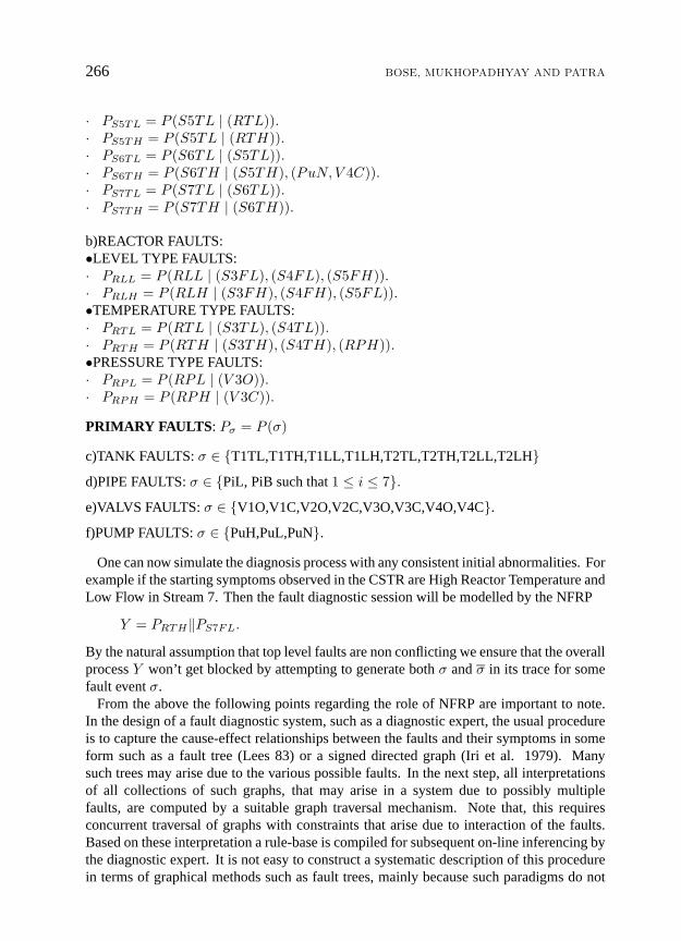
Two loop-lines, A-J1-· · ·-J7-A (L1) and B-J1-· · ·-J7-B (L2) share a common single oneway track from J1 to J7. The track consists of six sections (S1 to S6) separated by fivejunctions (J2 to J6) which are equipped by stoplights (*) and detectors (!). Simultaneously,two vehicles,V 1 andV 2, traverse the loops L1 and L2 respectively in the directions shownin Fig 1. VehicleV 1 (resp.V 2) loads material from A (resp. B) if it is empty and enters thecommon track. In the common track, after reaching J4 (resp. J5) it may either continue itsjourney directly and enter into S3 (resp. S5) or it may take a left (resp. right) turn, arriveat C (resp. D), unloads material, comes back to J3 (resp. J5) and then continue its journeyforward. The movement of vehicleV i from sectionSj toSj+1, j = 1, · · · , 5 is representedby eventσij,j+1. Rest of the event symbols are self explanatory. The overall dynamics isexpressed as the following deterministic processPlant. However since each deterministicprocess is a special case of a nondeterministic process, here we expressPlant as an NFRP.

Plant = V 1A1‖V 2

B1.

V 1A1 = (check1 → V 1

A2)(check1,0,).V 1A2 = (empty1 → V 1

A3 | non empty1 → V 1A4)(empty1,non empty1,0,).

V 1A3 = (load1 → V 1

A4)(load1,0,). V 1A4 = (start1 → V 1

A5)(start1,0,).V 1A5 = (arrive1

J1 → V 1J1)(arrive1

J1,0,). V 1J1 = (enter1

S1 → V 1S1)(enter1

S1,0,).V 1S1 = (σ1

1,2 → V 1S2)(σ1

1,2,0,).

V 1S2 = (σ1

2,3 → V 1S3 | turn1 →W 1

1 ;V 1S2

[−turn1])(σ12,3,turn

1,0,).

V 1S3 = (σ1

3,4 → V 1S4)(σ1

3,4,0,). V 1S4 = (σ1

4,5 → V 1S5)(σ1

4,5,0,).

V 1S5 = (σ1

5,6 → V 1S6)(σ1

5,6,0,).

V 1S6 = (arrive1

7 → V 1J7)(arrive17,0,). V 1

J7 = (return1A → V 1

A1)(return1A,0,).

W 11 = (arrive1

C →W 12 )(arrive1

C,0,). W 1

2 = (unload1C →W 1

3 )(unload1C,0,).

W 13 = (return1

J3 → HALT(,1,))(return1J3,0,).

The processV 2B1 can be constructed in an identical way with suitable changes in process and

event symbols (like changing the superscript 1 to 2, subscript A to B and C to D,return1J3

to return2J5). However it should be noted that, the eventturn2, (followed by the process

W 21 ;V 2

S4[−turn2]

) now takes place as a possible choice inV 2S4, instead ofV 2

S2.In the above plant, for the junctions not equipped with detectors, junction crossing events

are unobservable. The observable behaviour of the plant will become important in thecontext of controller synthesis under partial observation. For example, one may try toconstruct a supervisor, based on the event information supplied by the detectors, which will


control the stop lights in such a way that the two vehicles never ply in the same section of theguideway simultaneously. For the given plant, the observed behaviour, obtained by hidingthe unobservable events, is naturally a nondeterministic process. In general, the conditionsunder which a nondeterministic process, obtained by hiding of an NFRP, can be expressedagain as another NFRP, are not known, let alone the construction of a supervisor. Only inthe context of FSM this problem is well studied (Lin and Wonham 88, Cieslak et al. 88).However, in this example we can use the distribution laws ofECO over different operatorsand obtain an NFRP. It is described below.

The set of unobservable events isΣuo = σi1,2, σi2,3, σi4,5, σi5,6, turni | i = 1, 2. The ob-served behaviour of the plant is described by the nondeterministic processOP =Plant\Σuo.Now OP = (V 1

A1‖V 2B1)\Σuo = (V 1

A1\Σuo)‖(V 2B1\Σuo). The processV 1

A1\Σuo = P 1A1 is

described as follows.P 1A1 = (check1 → P 1

A2)(check1,0,).P 1A2 = (empty1 → P 1

A3 | non empty1 → P 1A4)(empty1,non empty1,0,).

P 1A3 = (load1 → P 1

A4)(load1,0,). P 1A4 = (start1 → P 1

A5)(start1,0,).P 1A5 = (arrive1

J1 → P 1J1)(arrive1

J1,0,).

P 1J1 = (enter1

S1 → HALT(,0,)uP 1S123u(W 1; (HALT(,0,)uP 1

S123)))(enter1S1,0,)

.

P 1S123 = (σ1

3,4 → P 1S456 uHALT(,0,))(σ1

3,4,0,).

P 1S456 = (arrive1

7 → P 1J7)(arrive17,0,)

. P 1J7 = (return1

A → P 1A1)(return1

A,0,).

W 11 = (arrive1

C →W 12 )(arrive1

C,0,). W 1

2 = (unload1C →W 1

3 )(unload1C,0,).

W 13 = (return1

J3 → HALT(,1,))(return1J3,0,)

.

Similarly the processV 1B1\Σuo =P 1

B1 can also be written as an NFRP. Based onPlant andOP , one can construct the supervisor. In this particular case it has been possible to obtaina recursive description of theobserved behaviourof Plant, namelyOP . This, however,may not be possible in general.

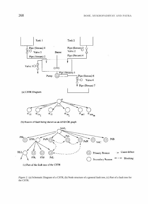
Example 5 In this example we model the fault diagnosis process of a Continuously StirredTank Reactor (CSTR) system (Rich and Venkatasubramaniam 87) whose schematic diagramis given in Fig 2. Here we are interested in modelling the sequences of observations madeby a fault diagnoser in response to logical sequences of process related queries which maybe made interactively with a human operator or automatically through process sensors. Thediagnoser starts the query upon receiving some symptoms of abnormality reported to itmanually or automatically. The observations of additional symptoms acquired from thesystem, on-line or off-line, in response to queries, lead the diagnosis process along a faulttree which eventually arrives at one or more root causes, termed as primary faults here.The ‘fault tree’ is a standard representation for possible search paths during diagnosis.Here each node of the tree is labeled with an abnormality symptom. A ‘parent’ node isconnected to a number of ‘child’ nodes in the tree, provided the symptoms labelling the‘child’ nodes are causes for that of the parent node. There are three types of nodes in afault tree: ‘And’, ‘Or’ and‘Mixed’ nodes. Occurrence of symptoms ofall the child nodestogether are necessary to cause the symptom associated with an‘And’ type parent node.Similarly, occurrence of symptoms ofany child node is a sufficient cause for that of an‘Or’ type parent node.‘Mixed’ nodes are those parent nodes where abnormality symptomsare caused byanyone of the different groups ofandchildren. In a diagnostic session, the


diagnoser starts from a given node, indicating the abnormality initially reported to it andmakes a query for symptoms of all its child processes. The children corresponding to thesymptoms obtained in response to the query that are causes for the abnormality representedby the parent node are ‘marked’. The query process repeats from the ‘marked’ children.The tree is traversed in a ‘breadth-first’ fashion.

As described above, the fault tree captures the knowledge about the effects of variousfaults that can occur in the system, as a tree of cause-effect relationships. Thus, it is astaticdescription which is to be utilized by the fault diagnosis procedure in arriving at a decisionregarding which fault(s) might have taken place. Depending on the observed symptoms,only a small fraction of the fault tree is to be dynamically searched in a given situation. Inthis example, we show how to capture both the static and dynamic aspects of fault diagnosisin the form of NFRPs. Thus, information encoded in a fault tree can be compactly andelegantly captured by NFRPs and the fault diagnosis procedure can be modelled by suitableparallel composition with appropriate synchronization and blocking, of these elementaryprocesses depending on the observed fault symptoms.• Since the diagnosis may start from any reported symptom, the query and the observationsequences beginning from each node are modelled as a process.•Observation of symptoms in response to a query is modelled as an event similarly named.• From a child node, if no abnormality symptom is observed in response to a query, a ‘Halt’process is substituted to stop further investigation from that node.•Once a particular level of the tree is searched, a synchronisation eventλ takes place in themodel, in all the marked nodes. Then the query process from the marked children nodescommences.• Finally, the search terminates at a set of leaf nodes, indicating the primary faults that havetaken place.

Each fault ‘event’ is described in the formatvariable-name variable-condition. In manycases we have complementaryvariable-conditionslike ‘high’ (H) and ‘low’(L) or ‘open’(O)or ‘closed’(C). We call these event pairs as complementary event pairs and if one event ofsuch a pair is symbolically denoted byσ then the other is calledσ. It is sometimes possiblethat an event has more than one complementary event. In that case if the event isσ, thenon-singleton complementary set is denoted asσ∗.• For each primary fault nodeσ we define a processPσ = P (σ), where, ifσ has acomplementary event then,

P (σ) := (σ → HALT(σ,1,σ))(σ,0,).

else if it has a complementary event setσ∗ then

P (σ) := (σ → HALT(σ∗,1,σ∗))(σ,0,).

else if it does not have any complementary event then

P (σ) := (σ → HALT(,1,))(σ,0,).

A diagnosis session stops successfully after identifying the primary fault processesPσ.Blocking of complementary events indicates that in the fault diagnosis session, which


proceeds after taking a snapshot of the physical conditions indicated by different sensors,we do not get contradictory information about the occurrence of a fault. Note that, here wedo not consider the temporal behaviour of processes where some physical faulty conditionand its complementary condition can be observed at differenttimes.

• For each secondary node having node structure as shown in Fig 6.2(a), we define theprocessPσ = P (σ | (σ11 · · ·σ1n1) · · · (σmσ1 · · ·σmσnmσ )) as follows:

Pσ := (σ → (λ→ (‖mσk=1((‖nkj=1Pσkj ) uHALTµk))[τ=0])[[−σ+σ]]µλ )µλ,σ

where

µk := (α, 1, α) | α ⊆ σk1 · · ·σknk, α 6= φ.

µλ := (λ, 0, ).

µλ, σ := (λ, σ, 0, λ).

If σ has a complementary set of events, namelyσ∗, thenGCO[[−σ + σ]] will bereplaced byGCO[[−σ∗+σ∗]]. If a secondary fault event (secondary node) does not have acomplementary fault event one should naturally do away with theGCO in the correspondingprocess description.

In the above, arrival at a secondary nodeσ, (start ofPσ) signifies a query. A positiveobservation is denoted by the occurrence of the eventσ after which the processPσ waits forthe next level query of its children. This takes place upon the occurrence of the synchronisa-tion eventλwhich denotes that queries at all the secondary nodes of that level of the tree arecompleted. Assuming that there aremσ possible (or) groups ofandchildren, one or moreof these groups may be the causes. If the k-th group (denoted by‖nkj=1Pσkj ) is not a cause,thenHALTµk is substituted. Hereµk represents the fact that k-th group of‘and’ childrenis not a cause forσ, because some nonempty subset of the fault setσk1 · · ·σknk hasfailed to take place. TheLNO captures the fact that among the possiblemσ (or groups)causes, at least one (group) must have actually taken place. TheGCO[[−σ + σ]]reflects the fact that in the search subsequent to the occurrence ofσ, not onlyσ will notbeencountered inPσ but it will also be blocked in the environment. The same is true formultiple complementary events.

Before describing the fault diagnosis mechanism as a process, we describe the list offaults (events/nodes).• STREAM FAULTS : S-i-j-k where i∈ 1 · · · 7, j ∈ F (Flow), T (Temperature), andk ∈ H (high), L (low). S-i-j-H and S-i-j-L are complementary events.• REACTOR FAULTS : R-i-j where i∈ L (Level), T (Temperature), P (Pressure), andj ∈ H (high), L(low). R-i-H and R-i-L are complementary events.• TANK FAULTS : T-i-j-k where i ∈ 1,2, j ∈ L (Level), T (Temperature), and k∈H (high), L (low). T-i-j-H and T-i-j-L are complementary events.• VALVE FAULTS : V-i-j where i ∈ 1 · · · 4, j ∈ O (Open), C (Closed). V-i-O and


V-i-C are complementary events.• PIPE FAULTS : P-i-j where i∈ 1 · · · 7, j ∈ L (Leak), B (Block). There is howeverno complementary event pair here.• PUMP FAULTS : PuH (pump high), PuL (pump low ) and PuN (pump normal). Out ofthese three events we consider any two events form a complementary event set for the third.Thus if σ is PuH thenσ∗ consists ofPuN,PuL. Also in the primary fault structureP (PuH), the marking ofHALT will be (PuN,PuL, 1, PuN,PuL) and similarlyfor P (PuL) andP (PuN).

Now we proceed to give the NFRP description of the fault tree. Since the structure ofprocesses modelling primary and secondary faults has been explained before in detail theseare not elaborated here. The reader will note that most of the nodes (processes) are of pure‘or’ type except those corresponding to the processesPS6FL, PS6FH andPS6TH . All theSTREAM and REACTOR faults are secondary faults and all the VALVE, TANK, PIPE andPUMP faults are primary faults. It should be noted that the choice of fault events is onlyintended to capture the logical structure in a realistic case. Obviously many other faultscould be included if an application demands.

SECONDARY FAULTS : Pσ = P (σ | (σ11 · · ·σ1n1) · · · (σmσ1 · · ·σmσnmσ ))a)STREAM FAULTS:•FLOW TYPE FAULTS:· PS1FL = P (S1FL | (T1LL), (P1L), (P1B), (V 1C)).· PS1FH = P (S1FH | (T1LH), (V 1O)).· PS2FL = P (S2FL | (T2LL), (P2L), (P2B), (V 2C)).· PS2FH = P (S2FH | (T2LH), (V 2O)).· PS3FL = P (S3FL | (S1FL), (P3L), (P3B)).· PS3FH = P (S3FH | (S1FH)).· PS4FL = P (S4FL | (S2FL), (P4L), (P4B)).· PS4FH = P (S4FH | (S2FH)).· PS5FL = P (S5FL | (RLL), (PuL), (P5L), (P5B)).· PS5FH = P (S5FH | (RLH), (PuH)).· PS6FL = P (S6FL | (PuL), (PuN, S5FL), (P6L), (P6B), (PuN, V 4C)).· PS6FH = P (S6FH | (PuN, S5FH), (PuH), (PuN, V 4O)).· PS7FL = P (S7FL | (S6FL), (V 4C), (P7L), (P7B)).· PS7FH = P (S7FH | (S6FH)).

•TEMPERATURE TYPE FAULTS:· PS1TL = P (S1TL | (T1TL)).· PS1TH = P (S1TH | (T1TH)).· PS2Tl = P (S2TL | (T2TL)).· PS2TH = P (S2TH | (T2TH)).· PS3TL = P (S3TL | (S1TL)).· PS3TH = P (S3TH | (S1TH)).· PS4TL = P (S4TL | (S2TL)).· PS4TH = P (S2TH | (S2TH)).


· PS5TL = P (S5TL | (RTL)).· PS5TH = P (S5TL | (RTH)).· PS6TL = P (S6TL | (S5TL)).· PS6TH = P (S6TH | (S5TH), (PuN, V 4C)).· PS7TL = P (S7TL | (S6TL)).· PS7TH = P (S7TH | (S6TH)).

b)REACTOR FAULTS:•LEVEL TYPE FAULTS:· PRLL = P (RLL | (S3FL), (S4FL), (S5FH)).· PRLH = P (RLH | (S3FH), (S4FH), (S5FL)).•TEMPERATURE TYPE FAULTS:· PRTL = P (RTL | (S3TL), (S4TL)).· PRTH = P (RTH | (S3TH), (S4TH), (RPH)).•PRESSURE TYPE FAULTS:· PRPL = P (RPL | (V 3O)).· PRPH = P (RPH | (V 3C)).

PRIMARY FAULTS : Pσ = P (σ)

c)TANK FAULTS: σ ∈ T1TL,T1TH,T1LL,T1LH,T2TL,T2TH,T2LL,T2LHd)PIPE FAULTS:σ ∈ PiL, PiB such that1 ≤ i ≤ 7.e)VALVS FAULTS: σ ∈ V1O,V1C,V2O,V2C,V3O,V3C,V4O,V4C.f)PUMP FAULTS:σ ∈ PuH,PuL,PuN.

One can now simulate the diagnosis process with any consistent initial abnormalities. Forexample if the starting symptoms observed in the CSTR are High Reactor Temperature andLow Flow in Stream 7. Then the fault diagnostic session will be modelled by the NFRP

Y = PRTH‖PS7FL.

By the natural assumption that top level faults are non conflicting we ensure that the overallprocessY won’t get blocked by attempting to generate bothσ andσ in its trace for somefault eventσ.

From the above the following points regarding the role of NFRP are important to note.In the design of a fault diagnostic system, such as a diagnostic expert, the usual procedureis to capture the cause-effect relationships between the faults and their symptoms in someform such as a fault tree (Lees 83) or a signed directed graph (Iri et al. 1979). Manysuch trees may arise due to the various possible faults. In the next step, all interpretationsof all collections of such graphs, that may arise in a system due to possibly multiplefaults, are computed by a suitable graph traversal mechanism. Note that, this requiresconcurrent traversal of graphs with constraints that arise due to interaction of the faults.Based on these interpretation a rule-base is compiled for subsequent on-line inferencing bythe diagnostic expert. It is not easy to construct a systematic description of this procedurein terms of graphical methods such as fault trees, mainly because such paradigms do not


support structures for systematic composition of individual graphs. Constructing productgraphs has the problem of a combinatorial explosion. Moreover the nondeterminism is notexplicit in these models. The NFRP, on the other hand provides a modular, unified andcompact description for computing the interpretation. It explicitly supports description ofevent sequences, concurrency with synchronization and nondeterminism. It is therefore animportant tool in describing the concurrent execution of individual fault diagnosis processesat a higher level. In an implementation, such a description may be used to govern theexecution of elementary fault diagnosis processes or equivalently govern the traversal ofthe individual fault tree to generate the overall sequence of fault symptoms, leading to theprimary reasons (faults).

Figure 1. Two Loop lines with a shared single track guideway.

7. Assessment and Conclusion

In this section we make a critical assessment of the proposed nondeterministic extensionand compare it with other well known nondeterministic frameworks such as CSP and CCS.

Advantages and Disadvantages:The major disadvantages of the NFRP framework are (i) complexity of operator definitions

because of variable alphabet and (ii) undecidability of analysis results (Cieslak and Varaiya90). The complexity of operator definitions is however unavoidable and would show upin any other framework that attempts to deal with features such as concurrency, modularsequencing etc., in the face of nondeterminism. Similarly, undecidability is also inevitable in


Figure 2. (a) Schematic Diagram of a CSTR, (b) Node structure of a general fault tree, (c) Part of a fault tree forthe CSTR.


such a powerful framework. Solution to this problem lies in identifying bounded subclasseswhere analysis will be possible. In the nondeterministic setting, this is still an open problem.

Among the advantages we have the following. (i) This is the first attempt of introducingnondeterminism in a variable alphabet situation which itself leads to modelling advantagesover the constant alphabet case ofCSP . (ii) It provides a much needed platform overwhich problems of observation (Ozveren and Willsky 90), control under partial observation(Lin and Wonham 88) etc., can be formulated. (iii) Because of mutual recursiveness of theoperators, the model can be simulated in a computer. (iv) Finally it has a rich languagegenerating power. For example, as shown in the appendix, any context free language (CFL)can be modelled by this framework.

Comparison with CSP:

The CSP has often been used for describing semantics of programming languages, net-work protocols etc. It is also the evolutionary predecessor of FRP. For this reason wecompare the formalisms of NFRP and NCSP in some detail below.

Although the DFRP has its origin in DCSP, an important extension introduced there is theconcept of a variable alphabet. The nondeterministic process framework proposesd here,naturally, is an extension over its corresponding CSP counterpart, namely NondeterministicCSP (NCSP).

In NCSP, nondeterminism has been treated in terms of the set of refusals of a process. Arefusal of a process is a collection of events, which when offered by the environment to theprocess, may be refused by the latter. In NCSP, nondeterminism arises from the fact that, at atime, a process may have mutiple refusal possibilities. The set of all possible refusals (whichis actually a family of sets of events) captures the immediate nondeterministic behaviour ofthe process. Subset of a refusal is also considered as a separate refusal and these refusalsare used to represent the dynamics of a process. It is as if the description of the processhas been arrived at by conducting experiments (like offering a collection of events to theprocess) and observing itsexternalbehaviour.

On the other hand, the NFRP framework takes a view point ofinternal behaviour. It isas if, the deterministic process model were known, and by some concealment operation, anondeterministic model has been arrived at. Here, a collection of ‘possible deterministicfutures’, characterised by corresponding alphabet, termination and blocking behaviour havebeen clubbed together to represent a ‘nondeterministic future’.

Thus given any nondeterministic mark of any NFRP, one can construct the immediateone length strings of events that are possible in the process at that stage. This is howevernot possible in NCSP, where information about both the refusals and trace is necessary todetermine the one length strings. This is because, by definition, any subset of a refusal isalso a refusal, and hence, an individual refusal may not qualify as a ‘possible deterministicfuture’.

Some of the other differences between NCSP and NFRP are the following.

• The NFRP has a variable alphabet, while the NCSP has a constant alphabet.


• In NFRP divergence has not been treated explicitly as in NCSP. In NFRP, a divergedprocess is just a process with maximal nondeterminism.

An important consequence of theinternal versusexternalviewpoints adopted in NFRPand NCSP respectively is the fact that, given the deterministic futures, a failure can becomputed but not vice versa. Also, there may be several different NFRPs for which thefailure sets are identical. A similar fact has been demonstrated for Trajectory Models byHeymann (1990). In this sense, the NFRP is more distinguishing than the NCSP, which isnatural, given the knowledge of the internal dynamics for NFRP. Several operators, such astheNCO, thePCO and theDCO have similar effects in both formalisms but for some,such as theECO, the effects are not similar.

Finally we make the following qualitative remarks regarding advantages and disadvan-tages of NFRP vis-a-vis CSP. The advantages include the following.

(+) The variable alphabet of NFRP usually offers advantage over the fixed alphabet of theNCSP.

(+) Another advantage over NCSP is that, due to the deterministic future approach,one gets the least possible degree of nondeterminism under the given event observationconstraints. Construction of an observer based on such a description is therefore likely toyield better resolution.

However the above advantages have been achieved at the cost of simplicity and elegancethat is inherent in a ‘constant alphabet’ NCSP. The disadvantages of this model are asfollows.

(−) The operators of the NFRP model are more complicated compared to their NCSPcounterpart in order to take care of the variable alphabet, while preserving the sense of theoperators. As a result, implementation of NFRP operators will be complex and postprocesscomputation will be computationally expensive.

(−) The ‘general choice’ operator in NCSP, allows the environment to choose an eventin a process only at the very first action. But a corresponding concept is difficult in case ofNFRP because of the use of variable alphabet and ‘possible futures’ in the model, insteadof constant alphabet and ‘refusals’. It is difficult even if the alphabet components of thedifferent ‘future’s are identical at the first instant. In absence of this,ACO of NFRP andits counterpart in NCSP do not carry completely identical meaning.

Comparison with CCS:CCS is another process algebra formalism to capture discrete event dynamics. While

there are some basic similarities with CSP, the CCS differs appreciably from CSP in itstreatment of operators, nondeterminism and recursive description. Relations between CCSand CSP have been discussed at length in both (Hoare 85) and (Milner 89 ). Here we brieflymention a few features in which NFRP is different from that of CCS.

The CCS framework has been used for studying different kinds of equivalences amongprocess algebra models of concurrent nondeterministic systems. Here nondeterminism isintroduced by a special symbolτ (different from the ‘termination component’ of determin-istic ‘futures’ of our NFRP model) which corresponds to the occurrence of a hidden event.In this respect it is similar to NFRP in the sense that both formalisms consider that non-determinism arises out of event concealment from deterministic dynamics. Unlike CSP orNFRP, in CCS, these hidden events are not ignored and they can be used, even for ‘guarding’


recursive equations involving process expressions. This implies the assumption that one isaware of the event concealment phenomenon, which is represented by the eventτ , wheneverit occurs. Different kinds of process equivalences are defined, which differ from each otherin their treatment regarding the hidden events. For example, ”strong equivalence” considersτ as an event and differentiates between the processesP and(τ → P ). On the other hand,‘weak’ or ‘observation equivalence’ ignoresτ completely. In NFRP, however, concealedevents are ignored, as in weak equivalence, and the only equivalence between processesdefined is that of ‘equality’ (P1 ¹N P2 and vice-versa). ‘Trace equivalence’ (identical setof observed strings) can also be defined in both models. But ‘trace equivalence’, cannotdistinguish between models having identical traces but with different deadlocking proper-ties. The ‘failure equivalence’ can be compared between the two models, only under therestriction of constant alphabet. It is however difficult, if not impossible, to define ‘weakbisimulation’ in NCSP and in NFRP as these frameworks are not distinguishing enough.ThePCO of NFRP and corresponding ‘conjunction’ operator of CCS can not be compareddirectly. The latter does not have any ‘blocking’ property, which is a major difference. Onthe other hand, besides synchronization and interleaving it includes aspects of hiding, sinceconcurrent transitionsa anda give rise to aτ , which, in turn, may cause nondeterminism.On the whole, the major differences of NFRP with CCS evolve from a variable alphabet,the absence of blocking and the hidden transitionτ . These differences perhaps stem fromthe fact that the CCS was motivated by a need for analysis of concurrent process semanticsand did not envisage applications such as control and supervision of DES.

This work has presented a formalism for capturing nondeterministic behaviour of DES ingeneral and FRP model in particular. Nondeterminism is often unavoidable in hierarchicalsupervision, where low level deterministic descriptions may become nondeterministic dueto deliberate undermodelling or lack of observation. Together with the FRP model thepresent work forms a uniform process algebraic approach for modelling untimed logicaldiscrete event systems. However problems related to control and observation remain to beworked out.

Appendix

Proof of Theorem 2:(→) LetP1, · · · , Pn be a family of MRP w.r.tΩn(G,Π). By one step expansion formula,each processPi can be expressed asPi = (σi1 → Pi/ < σi1 >| · · · | σiki → Pi/ < σiki >)µPi(<>). By definition 14each processPi/ < σij > can be expressed asfij (P) for somefij ∈ Ωn(G,Π). ThusPi = (σi1 → fi1(P) | · · · | σiki → fiki (P))mi , wheremi = µPi(<>). Now weconstruct the collection of recursive equationsX = F(X), X ↑0 := P ↑0, where eachcomponentFi of F is obtained from the corresponding one step post-process expression ofPi given above, i.e.,

Xi = Fi(X) := (σi1 → fi1(X) | · · · | σiki → fiki (X))mi .

It is obvious that eachFi is guarded, continuous andndes. To see thatX ↑0 = P ↑0 isconsistent, all we have to show that for anyi, Pi ↑ 0 = (Fi(P ↑ 0)) ↑ 0. If the assumption


(b) of the theorem is satisfied, then by ‘constancy’ of↑ 0 function, the above consistencyrequirement is trivially satisfied. On the other hand suppose (a) is satisfied, i.e.,↑ 0 is notnecessarily ‘constant’ butG is an MRS family. Also by fact 3, each function inΩn(G,Π)is spontaneous. Then note thatPi ↑ 0 = (σi1 → fi1(P) | · · · | σiki → fiki (P))mi ↑ 0= (σi1 → fi1(P) ↑ 0 | · · · | σiki → fiki (P) ↑ 0)mi ↑ 0(asFi is ndes)= (σi1 → fi1(P ↑ 0) ↑ 0 | · · · | σiki → fiki (P ↑ 0) ↑ 0)mi ↑ 0(as eachfij is ndes)= (σi1 → fi1(P ↑ 0) | · · · | σiki → fiki (P ↑ 0))mi ↑ 0(as eachfij is spontaneous)= (Fi(P ↑ 0)) ↑ 0.

Clearly conditions of theorem 1 is satisfied by the above collection of recursive equationsand (P1, · · · , Pn) is the unique solution.

(←) Conversely supposeP is the unique solution of equations (3) and (4). For anyarbitraryPi in P, one can show MR-ness using induction on the length ofs ∈ tr Pi.

The basis case is trivially true asPi/ <> = Proji(P). Assume that, for somes ∈ tr Pi,Pi/s = f(P) for somef ∈ Ωn(G,Π). ThenPi/(sˆ < σ >) = (Pi/s)/ < σ >= (f(P))/ < σ >. We claim that there existsf ′ ∈Ωn(G,Π) such that(f(P))/ < σ >= (f ′(P)). This proves our result forPi/(sˆ < σ >)and the rest follows by induction.

All we need now is to prove the claim made above and for this, we again use inductionon the number of steps in definition 13 needed to constructf ∈ Ωn(G,Π).• If f ∈ CΠ, i.e.,f(P) = P ↑ 0 for someP ∈ Π thentr f(P) 6= <> implies that forany< σ >∈ tr f(P), (f(P))/ < σ > = (P ↑ 0)/ < σ >. Now using condition (3) ofdefinition 6 we have the following. IfP ↑ 0 = (σ1 → (P ↑ 0)/ < σ1 >| · · · | σk → (P ↑0)/ < σk >)m with m = µ (P ↑ 0)(<>), then(P ↑ 0) ↑ 1 = (σ1 → ((P ↑ 0)/ < σ1 >) ↑ 0 | · · · | σk → ((P ↑ 0)/ < σk >) ↑ 0)m.However by (1) of definition 6(P ↑ 0) ↑ 1 = (P ↑ 0). Comparing one can concludethat for any< σ >∈ tr (P ↑ 0), (P ↑ 0)/ < σ >= ((P ↑ 0)/ < σ >) ↑ 0.Since the process in the right hand side belongs toΠ ↑ 0, one can findc′ ∈ CΠ suchthat c′ = r(((P ↑ 0)/ < σ >) ↑ 0). Thus (f(P))/ < σ >= (f ′(P)) for somef ′ = c′ ∈ CΠ ⊆ Ωn(G,Π).

• If f ∈ Proj(n), i.e.,f(P) = Pi for somei, then by equation 4f(P)/ < σ >= Pi/ < σ >= fij (P) for somefij ∈ Ωn(G,Π) asσ = σij for somej.

• Finally suppose the claim is true for somef1, · · · , fk in Ωn(G,Π) and letf = g (f1, · · · , fk) for somek − ary functiong ∈ G. Nowf(P)/ < σ >= (g(f1(P), · · · , fk(P)))/ < σ >. The MRness ofG guarantees existenceof g′ ∈ G such thatg(f1(P), · · · , fk(P))/ < σ >= g′(P ′1, · · · , P ′m′), where for eachj, 1 ≤ j ≤ m′ ∃i, 1 ≤i ≤ k with P ′j = fi(P) orP ′j = fi(P)/ < σ >. By induction hypotheses anyfi(P)/ <σ > can be expressed asf ′i(P) for somef ′i ∈ Ωn(G,Π). For eachj, 1 ≤ j ≤ m′ let hj bethe element ofΩn(G,Π) such thathj = fi if P ′j = fi(P) orhj = f ′i if P ′j = fi(P)/ < σ >.


Next we constructf ′ ∈ Ωn(G,Π) such thatf ′(P) = g′(h1(P), · · · , hm′(P)), using thefollowing recursive transformationG as follows.f ′ = G(g′, h1, · · · , hm′) :=

g′ (h1, · · · , hm′) if g′ ∈ Gg (G(g1, h1, · · · , hm1), · · · ,G(gk, hm′−mk+1, · · · , hm′)) otherwise

whereg′ = g (g1, · · · , gk) is in G, g ∈ G, gj ∈ G, gj has an aritymj andm′ = m1 +· · ·+mk. Note that, if, for somej, gj = Id, then,mj = 1 andG(gj , hmr ) := hmr wheremr = m1 + · · ·+ mj−1 + 1. Clearly f ′ ∈ Ωn(G,Π) and (f(P))/ < σ > = (f ′(P)).This completes our proof. 2

NFRP modelling of CFL:Given any Context Free LanguageL without ε (denoted here the null string<> ), we canconstruct an NFRPPL ∈ A(ΠN ,Ωn(Γ)) for some finiten such thattr PL = L and∀s ∈ L,PL/s ¹ HALT(,1,), as follows.

By Chomsky Normal Form, any suchL can be generated by a grammarGL whoseproduction rules are of the formA → BC or A → a whereA,B,C are nonterminalsanda ∈ Σ. We formulatePL to emulate the operation ofGL. For every nonterminalA aprocessPA is created.• If A→ BC ∈ GL thenPA = PB ;PC .• If A→ a ∈ GL thenPA = (a→ HALT(,1,))(a,0,).• If A → BC | a ∈ GL thenPA = (PB ;PC) u ((a→ HALT(,1,))(a,0,)).If, in GL the set of nonterminals beV = S,A1, · · · , An and the set of terminals beT = a1, · · · , an then we get a vector recursive equationX = F(X,U) whereX = (PS , PA1 , · · · , PAn) andU = ((ai → HALT(,1,))(ai,0,)) 1 ≤ i ≤ m).By the structure of a valid CFGGL there cannot be an unguarded loop of recursive definitionsamong the nonterminals of the grammar. HenceF must satisfy conditions of theorem 1and there is a unique solution process that mimicsGL. Y = PS will generate the requiredlanguage.

Acknowledgments

The first author would like to thank Prof. M.Vidyasagar, Director, CAIR, INDIA, for allthe support provided during the revision of this paper.

References

Brookes S.D., Hoare C.A.R., and Roscoe A.W., A Theory of Communicating Sequential Processes.J. ACM,31(3):560–599, July 1984.

Cieslak R.A., Desclaux C., Fawaz A.S., and VaraiyaP.P., Supervisory Control of Discrete Event Processes withPartial Observations.IEEE Trans. Auto. Control, 33(3):249–260, March 1988.

Cieslak R.A. and Varaiya P.P., Undecidability Results for Deterministic Communicating Sequential Processes.IEEE Trans. Auto. Control, 35(9):1032–1039, September 1990.


Harel D., Statecharts: A Visual Formalism for Complex Systems.Science of Computer Programming, 8:231–274,1987.

Hennessy M.,Algebraic Theory of Processes. M.I.T Press, Cambridge, Ma, 1988.Heymann M., Concurrency and discrete event control.IEEE Control Systems Magazine, 10(4):103–112, 1990.Hoare C.A.R.,Communicating Sequential Processes. Prentice Hall India, New Delhi, 1985.Inan K. and Varaiya P.P., Finitely Recursive Process Models for Discrete Event Systems.IEEE Trans. Auto.

Control, 33(7):626–639, July 1988.Inan K. and Varaiya P.P., Algebras of Discrete Event Models.Proc. IEEE, Special Issue on Discrete Event

Dynamic Systems, 77(1):24–38, January 1989.Iri M., Aoki K., Oshima E., and Matsuyama H., An Algorithm for Diagnosis of System Failures in the Chemical

Processes.Computers and Chemical Engineering, 3:489–493, 1979.Lees F.P., Process Computer Alarm and Disturbance Analysis: Review of the State of the Art.Computers and

Chemical Engineering, 7(6):669–694, 1983.Lin F. and Wonham W.M.,. On Observability of Discrete Event Systems.Information Sciences, 44:173–198,

1988.Milner R., Communication and Concurrency. Prentice Hall International, U.K., 1989.Murata T., Petri Nets: Properties, Analysis and Applications.Proc. IEEE, 77(4):541–580, April 1989.Ostroff J.S. and Wonham W.M., A Framework for Real-Time Discrete Event Control.IEEE Trans. Auto. Control,

35(4):386–397, April 1990.Ozveren C.M., and Willsky A.S.,. Observability of Discrete Event Dynamic Systems.IEEE Trans. Auto. Control,

35(7):797–806, July 1990.Ramadge P.J.G., and Wonham W.M., The Control of Discrete Event Systems.Proc. IEEE, Special Issue on

Discrete Event Dynamic Systems, 77(1):81–98, January 1989.Rich S.H. and Venkatasubramaniam V., A Model Based Expert System for Fault Diagnosis.Computers and

Chemical Engineering, 11(2):111–122, February 1987.Shayman M. and Kumar R., Supervisory control of nondeterministic systems with driven events via prioritized

synchronization and trajectory models.SIAM J. of Control and Optimization, 33(2):469–497, March 1995.

Documents

Nondeterministic Extended Finitely Recursive Process