Nondeterministic automatic complexity ofalmost square-free and strongly cube-free words

Kayleigh K. HydeBjørn Kjos-Hanssen

1 University of Hawai‘i at Manoa, Honolulu, HI 96822, USA,bjoernkh@hawaii.edu, http://math.hawaii.edu/wordpress/bjoern/

2 University of Hawai‘i at Manoa, Honolulu, HI 96822, USA,kkhyde@hawaii.edu,

http://math.hawaii.edu/wordpress/graduate-alumni/kkhyde/

Abstract. Shallit and Wang studied deterministic automatic complex-ity of words. They showed that the automatic Hausdorff dimension I(t)of the infinite Thue word satisfies 1/3 ≤ I(t) ≤ 2/3. We improve thatresult by showing that I(t) ≥ 1/2. For nondeterministic automatic com-plexity we show I(t) = 1/2. We prove that such complexity AN of aword x of length n satisfies AN (x) ≤ b(n) := bn/2c+ 1. This enables usto define the complexity deficiency D(x) = b(n)−AN (x). If x is square-free then D(x) = 0. If x almost square-free in the sense of Fraenkel andSimpson, or if x is a strongly cube-free binary word such as the infiniteThue word, then D(x) ≤ 1. On the other hand, there is no constantupper bound on D for strongly cube-free words in a ternary alphabet,nor for cube-free words in a binary alphabet.The decision problem whether D(x) ≥ d for given x, d belongs to NP∩E.

1 Introduction

The Kolmogorov complexity of a finite word w is roughly speaking the lengthof the shortest description w∗ of w in a fixed formal language. The descriptionw∗ can be thought of as an optimally compressed version of w. Motivated bythe non-computability of Kolmogorov complexity, Shallit and Wang studied adeterministic finite automaton analogue.

Definition 1 (Shallit and Wang [3]) The automatic complexity of a finitebinary string x = x1 . . . xn is the least number AD(x) of states of a deterministicfinite automaton M such that x is the only string of length n in the languageaccepted by M .

This complexity notion has two minor deficiencies:

1. Most of the relevant automata end up having a “dead state” whose solepurpose is to absorb any irrelevant or unacceptable transitions.

2. The complexity of a string can be changed by reversing it. For instance,

AD(011100) = 4 < 5 = AD(001110).

2

If we replace deterministic finite automata by nondeterministic ones, these defi-ciencies disappear. The NFA complexity turns out to have other pleasant prop-erties, such as a sharp computable upper bound.

Technical ideas and results. In this paper we develop some of the propertiesof NFA complexity. As a corollary we get a strengthening of a result of Shallit andWang on the complexity of the infinite Thue word t. Moreover, viewed throughan NFA lens we can, in a sense, characterize exactly the complexity of t. A maintechnical idea is to extend Shallit and Wang’s Theorem 9 which said that notonly do squares, cubes and higher powers of a word have low complexity, but aword completely free of such powers must conversely have high complexity. Theway we strengthen their results is by considering a variation on square-freenessand cube-freeness, strong cube-freeness. This notion also goes by the names ofirreducibility and overlap-freeness in the combinatorial literature. We also takeup an idea from Shallit and Wang’s Theorem 8 and use it to show that the naturaldecision problem associated with NFA complexity is in E = DTIME(2O(n)). Thisresult is a theoretical complement to the practical fact that the NFA complexitycan be computed reasonably fast; to see it in action, for strings of length up to23 one can view automaton witnesses and check complexity using the followingURL format

http://math.hawaii.edu/wordpress/bjoern/complexity-of-110101101/

and check one’s comprehension by playing a Complexity Guessing Game at

http:

//math.hawaii.edu/wordpress/bjoern/software/web/complexity-guessing-game/

Let us now define our central notion and get started on developing its properties.

Definition 2 The nondeterministic automatic complexity AN (w) of a word w isthe minimum number of states of an NFA M , having no ε-transitions, acceptingw such that there is only one accepting path in M of length |w|.The minimum complexity AN (w) = 1 is only achieved by words of the form an

where a is a single letter.

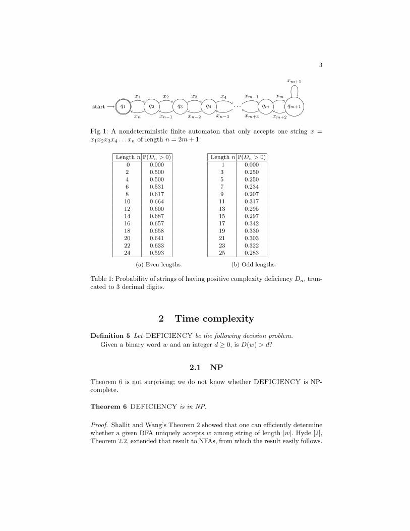
Theorem 3 (Hyde [2]) The nondeterministic automatic complexity AN (x) ofa string x of length n satisfies

AN (x) ≤ b(n) := bn/2c+ 1.

Proof (Proof sketch.). If x has odd length, it suffices to carefully consider theautomaton in Figure 1. If x has even length, a slightly modified automaton canbe used.

Definition 4 The complexity deficiency of a word x of length n is

Dn(x) = D(x) = b(n)−AN (x).

The notion of deficiency is motivated by the experimental observation that abouthalf of all strings have deficiency 0; see Table 1.

3

q1start q2 q3 q4 . . . qm qm+1

x1 x2 x3 x4 xm−1 xm

xm+1

xm+2xm+3xn−3xn−2xn−1xn

Fig. 1: A nondeterministic finite automaton that only accepts one string x =x1x2x3x4 . . . xn of length n = 2m+ 1.

Length n P(Dn > 0)

0 0.0002 0.5004 0.5006 0.5318 0.61710 0.66412 0.60014 0.68716 0.65718 0.65820 0.64122 0.63324 0.593

(a) Even lengths.

Length n P(Dn > 0)

1 0.0003 0.2505 0.2507 0.2349 0.20711 0.31713 0.29515 0.29717 0.34219 0.33021 0.30323 0.32225 0.283

(b) Odd lengths.

Table 1: Probability of strings of having positive complexity deficiency Dn, trun-cated to 3 decimal digits.

2 Time complexity

Definition 5 Let DEFICIENCY be the following decision problem.

Given a binary word w and an integer d ≥ 0, is D(w) > d?

2.1 NP

Theorem 6 is not surprising; we do not know whether DEFICIENCY is NP-complete.

Theorem 6 DEFICIENCY is in NP.

Proof. Shallit and Wang’s Theorem 2 showed that one can efficiently determinewhether a given DFA uniquely accepts w among string of length |w|. Hyde [2],Theorem 2.2, extended that result to NFAs, from which the result easily follows.

4

2.2 E

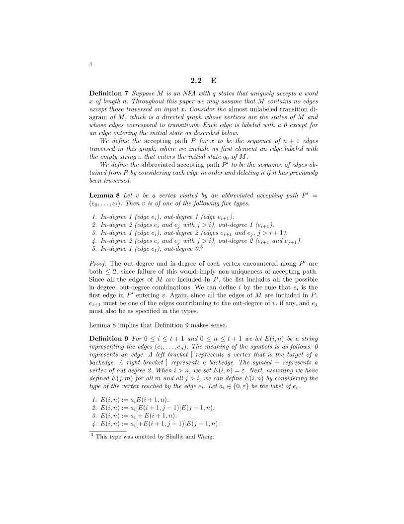
Definition 7 Suppose M is an NFA with q states that uniquely accepts a wordx of length n. Throughout this paper we may assume that M contains no edgesexcept those traversed on input x. Consider the almost unlabeled transition di-agram of M , which is a directed graph whose vertices are the states of M andwhose edges correspond to transitions. Each edge is labeled with a 0 except foran edge entering the initial state as described below.

We define the accepting path P for x to be the sequence of n + 1 edgestraversed in this graph, where we include as first element an edge labeled withthe empty string ε that enters the initial state q0 of M .

We define the abbreviated accepting path P ′ to be the sequence of edges ob-tained from P by considering each edge in order and deleting it if it has previouslybeen traversed.

Lemma 8 Let v be a vertex visited by an abbreviated accepting path P ′ =(e0, . . . , et). Then v is of one of the following five types.

1. In-degree 1 (edge ei), out-degree 1 (edge ei+1).2. In-degree 2 (edges ei and ej with j > i), out-degree 1 (ei+1).3. In-degree 1 (edge ei), out-degree 2 (edges ei+1 and ej, j > i+ 1).4. In-degree 2 (edges ei and ej with j > i), out-degree 2 (ei+1 and ej+1).5. In-degree 1 (edge et), out-degree 0.3

Proof. The out-degree and in-degree of each vertex encountered along P ′ areboth ≤ 2, since failure of this would imply non-uniqueness of accepting path.Since all the edges of M are included in P , the list includes all the possiblein-degree, out-degree combinations. We can define i by the rule that ei is thefirst edge in P ′ entering v. Again, since all the edges of M are included in P ,ei+1 must be one of the edges contributing to the out-degree of v, if any, and ejmust also be as specified in the types.

Lemma 8 implies that Definition 9 makes sense.

Definition 9 For 0 ≤ i ≤ t + 1 and 0 ≤ n ≤ t + 1 we let E(i, n) be a stringrepresenting the edges (ei, . . . , en). The meaning of the symbols is as follows: 0represents an edge. A left bracket [ represents a vertex that is the target of abackedge. A right bracket ] represents a backedge. The symbol + represents avertex of out-degree 2. When i > n, we set E(i, n) = ε. Next, assuming we havedefined E(j,m) for all m and all j > i, we can define E(i, n) by considering thetype of the vertex reached by the edge ei. Let ai ∈ {0, ε} be the label of ei.

1. E(i, n) := aiE(i+ 1, n).2. E(i, n) := ai[E(i+ 1, j − 1)]E(j + 1, n).3. E(i, n) := ai + E(i+ 1, n).4. E(i, n) := ai[+E(i+ 1, j − 1)]E(j + 1, n).

3 This type was omitted by Shallit and Wang.

5

5. E(i, n) := aiE(i+ 1, n).

Lemma 10 The abbreviated accepting path P ′ can be reconstructed from E(0, t).

Lemma 11

|E(a, b)| ≤ 2(b− a+ 1).

Theorem 12 DEFICIENCY is in E.

Proof. Let w be a word of a length n, and let d ≥ 0. To determine whetherD(w) > d, we must determine whether there exists an NFA M with at mostbn2 c − d states which accepts w, and accepts no other word of length n. Sincethere are prima facie more than single-exponentially many automata to consider,we consider instead codes E(0, t) as in Definition 9. By Lemma 10 we can recoverthe abbreviated accepting path P ′ and hence M from such a code. The numberof edges t is bounded by the string length n, so by Lemma 11

|E(0, t)| ≤ 2(t+ 1) ≤ 2(n+ 1);

since there are four symbols this gives

42(n+1) = O(16n)

many codes to consider. Finally, to check whether a given M accepts uniquelytakes only polynomially many steps, as in Theorem 6.

Remark 13 The bound 16n counts many automata that are not uniquely ac-cepting; the actual number may be closer to 3n based on computational evidence.

3 Powers and complexity

In this section we shall exhibit infinite words all of whose prefixes have complexitydeficiency bounded by 1. We say that such a word has a hereditary deficiencybound of 1.

3.1 Square-free words

Lemma 14 Let a and b be strings in an arbitrary alphabet with ab = ba. Thenthere is a string c and integers k and ` such that a = ck and b = c`.

We will use the following simple strengthening from DFAs to NFAs of a factused in Shallit and Wang’s Theorem 9 [3].

Theorem 15 If an NFA M uniquely accepts w of length n, and visits a state pas many as k + 1 times, where k ≥ 2, during its computation on input w, thenw contains a kth power.

6

Proof. Let w = w0w1 · · ·wkwk+1 where wi is the portion of w read betweenvisits number i and i+ 1 to the state p. Since one bit must be read in one unitof automaton time, |wi| ≥ 1 for each 1 ≤ i ≤ k (w0 and/or wk+1 may be emptysince the initial and/or final state of M may be p). For any permutation π on1, . . . , k, M accepts w0wπ(1) · · ·wπ(k)wk+1. Let 1 ≤ j ≤ k be such that wj hasminimal length and let wj = w1 · · ·wj−1wj+1 · · ·wk. Then M also accepts

w0wjwjwk+1 and w0wjwjwk+1.

By uniqueness,w0wjwjwk+1 = w = w0wjwjwk+1

and sowjwj = wjwj

By Lemma 14, wj and wj are both powers of a string c. Since |wj | ≥ (k−1)|wj |,wjwj is at least a kth power of c, so w contains a kth power of c.

We next strengthen a particular case of Shallit and Wang’s Theorem 9 to NFAs.

Theorem 16 A square-free word has deficiency 0.

Corollary 17 There exists an infinite word of hereditary deficiency 0.

Proof. There is an infinite square-free word over the alphabet {0, 1, 2} as shownby Thue [5][6]. The result follows from Theorem 16.

3.2 Cube-free words

Definition 18 For a word u, let first(u) and last(u) denote the first and lastletters of u, respectively. A weak cube is a word of the form uufirst(u) (orequivalently, last(u)uu). A word w is strongly cube-free if it does not containany weak cubes.

Theorem 19 (Shelton and Soni [4]) The set of all numbers that occur aslengths of squares within strongly cube-free binary words is equal to

{2a : a ≥ 1} ∪ {3 · 2a : a ≥ 1}.

Lemma 20 If a cube www contains another cube xxx then either |x| = |w|, orxxfirst(x) is contained in the first two consecutive occurrences of w, or last(x)xxis contained in the last two occurrences of w.

Theorem 21 The deficiency of cube-free binary words is unbounded.

Proof. Given k, we shall find a cube-free word x with D(x) ≥ k. Pick a number nsuch that 2n ≥ 2k+1. By Theorem 19, there is a strongly cube-free binary wordthat contains a square of length 2n+1; equivalently, there is a strongly cube-freesquare of length 2n+1. Thus, we may choose w of length ` = 2n such that ww

7

is strongly cube-free. Let x = www where w is the proper prefix of w of length|w| − 1. By Lemma 20, x is cube-free. The complexity of x is at most |w| as wecan just make one loop of length w, with code (Theorem 12)

[w1 . . . w`−1]w`.

And so

D(x) ≥ b|x|/2 + 1c − |w| ≥ |x|/2− |w| = 3|w| − 1

2− |w|

= |w|/2− 1/2 ≥ k.

3.3 Strongly cube-free words

Theorem 22 (Thue [5][6]) The infinite Thue word

t = t0t1 . . . = 0110 1001 1001 0110 . . .

given by

b =∑

bi2i, bi ∈ {0, 1} =⇒ tb =

∑bi mod 2,

is strongly cube-free.

Lemma 23 For each k ≥ 1 there is a sequence x1,k, . . . , xk,k of positive integerssuch that

k∑i=1

aixi,k = 2

k∑i=1

xi,k =⇒ a1 = · · · = ak = 2

Let tj denote bit j of the infinite Thue word. Then we can ensure that

1. xi,k + 1 < xi+1,k and2. txi,k

6= txi+1,kfor each 1 ≤ i < k.

Theorem 24 For an alphabet of size three, the complexity deficiency of stronglycube-free words is unbounded.

Proof. Let d ≥ 1. We will show that there is a word w of deficiency D(w) ≥ d.Let k = 2d − 1. For each 1 ≤ i ≤ k let xi = xk+1−i,k where the xj,k are as inLemma 23. Note that since xi,k + 1 < xi+1,k, we have xi > xi+1 + 1. Let

w =

(2

x1−1∏i=1

ti

)2

tx1

(2

x2−1∏i=1

ti

)2

tx2

(2

x3−1∏i=1

ti

)2

· · · txk−1

(2

xk−1∏i=1

ti

)2

= λ1tx1λ2 · · · txk−1

λk

where λi = (2τi)2, τi =

∏xi−1j=1 tj , and where ti is the ith bit of the infinite Thue

word on {0, 1}, which is strongly cube-free (Theorem 22). Let M be the NFAwith code (Theorem 12)

[+0x1−1]0[+0x2−1]0 · · · 0 ∗ [+0xk−1]

8

(where ∗ indicates the accept state). Let X =∑ki=1 xi. Then M has k − 1 +X

many edges but only q = X many states; and w has length

n = k − 1 + 2X = 2(d− 1) + 2X

giving n/2 + 1 = d+X.Suppose v is a word accepted by M . Then M on input v goes through each

loop of length xi some number of times ai ≥ 0, where

k − 1 +

k∑i=1

aixi = |v|.

If additionally |v| = |w|, then by Lemma 23 we have a1 = a2 = · · · = ak, andhence v = w. Thus

D(w) ≥ bn/2 + 1c − q = d+X −X = d.

We omit the proof that w is strongly cube-free in this version of the paper.

Definition 2 yields the following lemma.

Lemma 25 Let (q0, q1, . . .) be the sequence of states visited by an NFA M givenan input word w. For any t, t1, t2, and ri, si with

(p1, r1, . . . , rt−2, p2) = (qt1 , . . . , qt1+t)

and(p1, s1, . . . , st−2, p2) = (qt2 , . . . , qt2+t),

we have ri = si for each i.

Note that in Lemma 25, it may very well be that t1 6= t2.

Theorem 26 Strongly cube-free binary words have deficiency bound 1.

Proof. Suppose w is a word satisfying D(w) ≥ 2 and consider the sequence ofstates visited in a witnessing computation. As in the proof of Theorem 32, eitherthere is a state that is visited four times, and hence there is a cube in w, or thereare three state cubes (states that are visited three times each), and hence thereare three squares in w. By Theorem 19, a strongly cube-free binary word canonly contain squares of length 2a, 3 · 2a, and hence can only contain powers ui

where |u| is of the form 2a, 3 · 2a, and i ≤ 2.In particular, the length of one of the squares in the three state cubes must

divide the length of another. So if these two state cubes are disjoint then theshorter one repeated can replace one occurrence of the longer one, contradictingLemma 25.

So suppose we have two state cubes, at states p1 and p2, that overlap. Atp1 then we read consecutive words ab that are powers a = ui, b = uj of a wordu, and since there are no cubes in w it must be that i = j = 1 and so actually

9

a = b. And at p2 we have words c, d that are powers of a word v and again theexponents are 1 and c = d.

The overlap means that in one of the two excursions of the same lengthstarting and ending at p1, we visit p2. By uniqueness of the accepting path wethen visit p2 in both of these excursions. If we suppose the state cubes are chosento be of minimal length then we only visit p2 once in each excursion. If we writea = rs where r is the word read when going from p1 to p2, and s is the wordgoing from p2 to p1, then c = sr and w contains rsrsr. In particular, w containsa weak cube.

Definition 27 For an infinite word u define the deterministic automatic Haus-dorff dimension of u by

I(u) = lim infu prefix of u

AD(u)/|u|.

and the deterministic automatic packing dimension of u by4

S(u) = lim supu prefix of u

AD(u)/|u|.

For nondeterministic complexity, in light of Theorem 3 it is natural to make thefollowing definition.

Definition 28 Define the nondeterministic automatic Hausdorff dimension ofu by

IN (u) = lim infu prefix of u

AN (u)

|u|/2and define SN analogously.

Theorem 29 (Shallit and Wang’s Theorem 18) 13 ≤ I(t) ≤ 2

3 .

Here we strengthen Theorem 29.

Theorem 30 I(t) ≥ 12 . Moreover IN (t) = SN (t) = 1.

Proof. This follows from the observation that the proof of Theorem 26 appliesequally for deterministic complexity.

3.4 Almost square-free words

Definition 31 (Fraenkel and Simpson [1]) A word all of whose containedsquares belong to {00, 11, 0101} is called almost square-free.

Theorem 32 A word that is almost square-free has a deficiency bound of 1.

4 There is some connection with Hausdorff dimension and packing dimension. Forinstance, if the effective Hausdorff dimension of an infinite word x is positive thenso is its automatic Hausdorff dimension, by a Kolmogorov complexity calculation inShallit and Wang’s Theorem 9.

10

Corollary 33 There is an infinite binary word having hereditary deficiencybound of 1.

Proof. We have two distinct proofs. On the one hand, Fraenkel and Simpson [1]show there is an infinite almost square-free binary word, and the result followsfrom Theorem 32. On the other hand, the infinite Thue word is strongly cube-free(Theorem 22) and the result follows from Theorem 26.

Conjecture 34 There is an infinite binary word having hereditary deficiency 0.

We have some numerical evidence for Conjecture 34, for instance there are 108strings of length 18 with this property.

11

References

1. Aviezri S. Fraenkel and R. Jamie Simpson. How many squares must a binary se-quence contain? Electron. J. Combin., 2:Research Paper 2, approx. 9 pp. (elec-tronic), 1995.

2. Kayleigh Hyde. Nondeterministic finite state complexity. Master’s thesis, Universityof Hawaii at Manoa, U.S.A., 2013.

3. Jeffrey Shallit and Ming-Wei Wang. Automatic complexity of strings. J. Autom.Lang. Comb., 6(4):537–554, 2001. 2nd Workshop on Descriptional Complexity ofAutomata, Grammars and Related Structures (London, ON, 2000).

4. R. O. Shelton and R. P. Soni. Chains and fixing blocks in irreducible binary se-quences. Discrete Math., 54(1):93–99, 1985.

5. A. Thue. Uber unendliche zeichenreihen. Norske Vid. Skrifter I Mat.-Nat. Kl.,Christiania, 7:1–22, 1906.

6. A. Thue. Uber die gegenseitige lage gleicher teile gewisser zeichenreihen. NorskeVid. Skrifter I Mat.-Nat. Kl., Christiania, 1:1–67, 1912.