arX

iv:m

ath/

0408

259v

1 [

mat

h.SP

] 1

9 A

ug 2

004

NONCOMMUTATIVE PERRON-FROBENIUS-RUELLE

THEOREM, TWO WEIGHT HILBERT TRANSFORM, AND

ALMOST PERIODICITY

A. VOLBERG, P. YUDITSKII

Abstract. We consider the Jacobi matrix generated by a balanced measureof hyperbolic polynomial map. The conjecture of Bellissard says that thismatrix should have an extremely strong periodicity property. We show howthis conjecture is related to a certain noncommutative version of Bowen–Ruelletheory, and how the two weight Hilbert transform naturally appears in thiscontext.

1. Introduction and Main results

Let f be an expanding polynomial with real Julia set J(f), deg f = N . We recallthat J(f) is a nonempty compact set of points which do not go to infinity underforward iterations of f . Under the normalization

f−1 : [−ξ, ξ]→ [−ξ, ξ]such a polynomial is well defined by position of its critical values

ti = f(ci) : f ′(ci) = 0, ci > cj for i > j.Expanding, or hyperbolic polynomials are those, for which

ci /∈ J(f), ∀i .The term “expanding” is deserved because for expanding polynomials one has thefollowing inequality

(1) ∃Q > 1, |(fn)′(x)| ≥ cQn, ∀x ∈ J(f) .

Here and in everything that follows fn means n-th iteration of f , fn = f f ....f .We will always use letter T for polynomial fn, degT = Nn. We will always use

letter d for this degree, d = Nn.We will say that f is sufficiently hyperbolic if

∀i dist(f(ci), J(f)) ≥ A ,with a sufficiently large A.

Let us mention that for f with a real Julia set one has |f(ci)| > ξ since allsolutions of f(x) = ±ξ should be real.

Partially supported by NSF grant DMS-0200713, the grant for IAS and the Austrian ScienceFound FWF, project number: P16390–N04.

AMS subject classification codes: 42B20, 42C15, 42A50, 47B35, 47B38.

1

2 A. VOLBERG, P. YUDITSKII

We recall now Perron-Frobenius-Ruelle (PFR) theorem in a form convenient forus. Let φ be a Hol(α) function on J(f). We define the Perron-Frobenius-Ruelle(PFR) operator

Lφ = Lφ,f : C(J(f))→ C(J(f))

as follows

Lφψ(x) :=∑

λ:f(λ)=x

eφ(λ)ψ(λ) .

PFR theorem states that if ρ denotes the spectral radius of this operator then

ρ−nLnφψ(x)→ h(x)

∫

ψ(y)dν(y) ,

where h is the unique eigenvector of Lφ with eigenvalue ρ, ν is is the unique eigen-vector of L∗φ with eigenvalue ρ. Moreover, h is Holder continuous if φ is Holdercontinuous.

Let us emphasize that the requirement on f is just to be expanding (hyperbolic).We reformulate this result now. Or, rather we will formulate its essential part

in a different form. In fact, it turns out that at the heart of this result lies thefollowing theorem. See [6], for example.

Theorem 1.1. Let f be hyperbolic. Let φ ∈ Holα(J(f)), ψ ∈ Holα(J(f)), thenthere exist C <∞, q ∈ (0, 1), γ > 0 (all depending only on α) such that

(2)∣

∣

∣

Lnφψ(x1)

Lnφ1(x1)

−Ln

φψ(x2)

Lnφ1(x2)

∣

∣

∣ ≤ C qn|x1 − x2|γ .

Consider the operator Gφ = Gφ,f acting on probability measures on J(f) by theformula

Gφµ =L∗φµ‖L∗φµ‖

=L∗φµ〈1,L∗φµ〉

.

Then (2) means

(3) |〈ψ,Gnφδx1〉 − 〈ψ,Gn

φδx2〉| ≤ C qn|x1 − x2|γ .

This is for any test function ψ ∈ Holα(J(f)), under assumption that φ ∈ Holα(J(f)).In what follows φ will have the following form

φ := −t log |f ′| , t ∈ R .

Example. When t = 0 we have that Gnδx is a sum of delta measures with charges1/d = 1/Nn located at all T -preimages of x. We would like to understand the PFRtheorem as a consequence of a certain fact of noncommutative nature. Sometimesthis is indeed so, we can prove this. We would like to prove this noncommutativefact always, for all hyperbolic dynamics, but we can manage only a weaker estimate.

To explain what noncommutative proposition we have in mind, let us noticethat there is a natural operator for which Gn

φδx is a spectral measure. This is justJacobi matrix built by this probability measure. Let us recall that to built theJacobi matrix by a probability measure dµ(λ) with support on the real line, onejust orthogonalizes polynomials with respect to this measure, and Jacobi matrixis the matrix of multiplication by independent variable λ written in the basis oforthonormal polynomials.

PERRON-FROBENIUS-RUELLE THEOREM AND TWO WEIGHT HILBERT TRANSFORM 3

So let T = fn, deg T = d = Nn, J(x) = JT (x) be a Jacobi matrix built bymeasure

µx = Gnφ,fδx = Gφ,T δx ,

where φ = −t log |f ′| (as always in what follows).We already explained that J(x) is canonically defined. Another way to define

J(x) : Cd → Cd is to write

〈(z − J(x)−1e0, e0〉 =∫

dµx(λ)

z − λ = σ

d∑

k=1

eφ(λk)

z − λk,

where λ1(x), ...., λd(x) are all T -preimages of x .We can consider J(x) as a result of applying PFR operator to 1×1 matrix x. We

want to prove the following claim, which deserves to be called a noncommutativePerron-Frobenius-Ruelle (PFR) theorem.

(4) ‖J(x1)− J(x2)‖ ≤ C qn|x1 − x2|γ .We cannot prove (4) for all hyperbolic f and all φ. But here are our main results.

Theorem 1.2. Let f be hyperbolic. Let x1, x2 ∈ J(f). Let T = fn, we buildJ(x) = JT (x) using φ = −t log |f ′| , 0 ≤ t ≤ 2. Then there exists C such thatindependently of n

(5) ‖J(x1)− J(x2)‖ ≤ C|x1 − x2| .Theorem 1.3. Let f be sufficiently hyperbolic. Let x1, x2 ∈ J(f). Let T = fn, webuild J(x) = JT (x) using φ = 0. Then there exists c < 1 such that independentlyof n

(6) ‖J(x1)− J(x2)‖ ≤ cn|x1 − x2| .

Acknowledgements. The authors are grateful to Michael Shapiro, Fedja Nazarovand Sergei Treil for valuable discussions. The first author acknowledge with deepgratitude the grant from IAS that allowed to use the stimulating atmosphere of thisinstitution.

2. PFR theorem from noncommutative PFR theorem

This uniform closeness of operators quite easily imply the type of weak close-ness of Theorem 1.1, (2) or (3). We just use the fact that measures in, say, (3),are spectral measures of J(xi), and we use the Jackson-Bernstein type theoremto approximate the Holder continuous function ψ by functions holopmorphic innarrowing neighborhoods of J(f) with the speed ετ , where ε is the width of aneighborhood, and τ depends on α in Holder property of ψ. This is very standard,and it shows that really PFR theorem can be considered as a consequence of anoncommutative claim—(4).

3. Faybusovich–Gehktman flow

Let J(x) = JT (x), T = fn, and we think now that n is large but fixed, and weare heading towards the proof of Theorem 1.2 with constant independent of n. If wethink that x is the time, then the flow of Jacobi matrices J(x) of size d×d (d = Nn)can be treated alike the Toda flow. But unlike the Toda flow, the spectrum sp(J(x))

4 A. VOLBERG, P. YUDITSKII

is not time independent, that is, it is not x-independent. This brings a modificationto the equation of Toda flow. Such modifications were considered by Faybusovichand Gehktman in [9], we grateful to M. Shapiro who indicated this to us. Let ()·

denote the differentiation with respect to “time” x. We write J instead of J(x) forbrevity. Recall that in the standard basis e0, e1, ...., ed−1 of C

d the matrix of J isthree diagonal. Recall that sp(J) is always equal λ1(x), ...., λd(x) (all T -preimagesof x). If g is a continuous function on this spectrum, we know what is g(J) byfunctional calculus of self-adjoint operators. We need one more definition. Givenx we consider the orthonormal polynomials P0(λ;x) = 1, P1(λ;x), ..., Pd−1(λ;x)of degrees 0, 1, ..., d − 1 correspondingly. They are orthonormal with respect tomeasure

dµx(λ) := σ

d∑

k=1

eφ(λk(x)δλk(x) ,

where from now on always φ = −t log |f ′|, 1/σ =∑d

k=1 eφ(λk(x).

Theorem 3.1. Our J(x) satisfies the nonlinear ODE

(7) J · = F (J) + [G, J ] ,

where F (J) is a function of a self-adjoint operator J = J(x) with function F :=(T ′)−1 on sp(J). Operator G is skew self-adjoint, and its matrix in the standardbasis has upper triangular part G− equal to

(8) G− = (DF (J) +1

2φ′(J)F (J))− .

Finally operator D is given by the formula

(9) 〈D∗ek, em〉 := σ

d∑

k=1

eφ(λk(x)P ′k(λi(x))Pm(λi(x)) .

The form of D will allow to prove

Theorem 3.2.

(10) [J,D] = I − c · 〈·, F−1e0〉ed−1 .

And therefore

(11) [J,DF ]e = Fe, ∀e orthogonal to e0 .

In Toda flow F = 0 and G− = R(J)− for a certain function R. Here we are in amore complicated situation, but let us observe

(12) ‖F (J)‖ ≤ Cqn, q < 1 .

In fact, just use (1). Then if x ∈ J(f) we have sp(J) ⊂ J(f) and (1) impliesautomatically the latter inequality (12). If x is not on J(f), but is separated fromthe critical values of T , inequality (1) also holds on T -preimages of x, and this setis exactly sp(J).

It is very good that F (J) is small as in (12) because to prove Theorem 1.2 it ishence enough to prove

Theorem 3.3.

(13) ‖[G, J ]‖ ≤ C ,

PERRON-FROBENIUS-RUELLE THEOREM AND TWO WEIGHT HILBERT TRANSFORM 5

where C is independent of n. Then automatically

(14) ‖J ·‖ ≤ C′ .

Remark. We cannot prove that G is uniformly bounded, moreover this looks tobe false.

4. Uniform boundedness of the commutator

We postpone the explanation of Theorem 3.1. Now we will take it for granted,and we prove Theorem 3.3, which of course immediately gives the first main result—Theorem 1.2.

Let

H := DF (J) +1

2φ′(J)F (J) .

Let us adopt the following convention. If we write

A = B + small ,

we always mean that the small term is at most Cqn, with q < 1 in norm.Then, for every x

[G, J ] = three diaginal + small ,

just see (7), (12).This means that to prove the uniform boundedness of the commutator is the

same as to prove the uniform boundedness of its matrix elements in the standardbasis. Moreover, it is enough to prove the uniform boundedness of “three diagonal”elements only:

|〈[G, J ]em, em−1〉|, |〈[G, J ]em, em〉|, |〈[G, J ]em−1, em〉| .Moreover the skew symmetry of G implies that [G, J ] is self-adjoint, so only thefirst and the second type of elements should be checked.

Recall that the upper triangular parts coincide:

G− = H− .

Let us denote the diagonal elements of J by a0 = a0(x), ..., ad−1 = ad−1(x), and letbelow diagonal elements be b1 = b1(x), ..., bd−1 = bd−1(x).

Let us write the following equalities (G+ is the lower triangular part of skewsymmetric G)

〈[G, J ]em, em−1〉 = 〈[G−, J ]em, em−1〉+ 〈[G+, J ]em, em−1〉 = 〈[G−, J ]em, em−1〉 .In fact using only the lower triangular property of G+ we see that G+Jem ∈span(em, ...) and so is orthogonal to em−1. Also, G+em ∈ span(em+1, ...) and so isorthogonal to Jem−1.

Now we conclude that

〈[G, J ]em, em−1〉 = 〈[H−, J ]em, em−1〉 = 〈[H, J ]em, em−1〉−〈[H0, J ]em, em−1〉 − 〈[H+, J ]em, em−1〉 ,

where H+ is the lower triangular part of H = DF +φ′(J)F , and H0 is its diagonalpart (that may exist because nobody said that H is skew symmetric). We claimthat this means

(15) 〈[G, J ]em, em−1〉 = −〈[H0, J ]em, em−1〉+ small .

6 A. VOLBERG, P. YUDITSKII

In fact, the last term 〈[H+, J ]em, em−1〉 equals zero–we checked this for any lowertriangular matrix. On the other hand, the term 〈[H, J ]em, em−1〉 is equal to 〈[DF+φ′(J)F (J), J ]em, em−1〉 = 〈[DF, J ]em, em−1〉 = −〈Fem, em−1〉. The last equalityfollows from (11). So this term is small in our sense, and (15) is proved.

We can now use

Jem = bmem−1 + amem + bm+1em+1

to plug it into (15) and get it rewritten

(16) 〈[G, J ]em, em−1〉 = bm〈Hem, em〉 − bm−1〈Hem−1, em−1〉+ small .

We can also calculate 〈[G, J ]em, em〉.(17) 〈[G, J ]em, em〉 = 2bm+1〈Hem, em+1〉 − 2bm〈Hem−1, em〉+ small .

In fact, skew symmetry ofG implies 〈[G, J ]em, em〉 = 2〈[G−, J ]em, em〉 = 2〈[H−, J ]em, em〉.Again replace H− by H −H0 −H+. Then

〈[G, J ]em, em〉 = 2〈[H, J ]em, em〉−2〈[H0, J ]em, em〉−2〈[H+, J ]em, em〉 =: 2A−2B−2C .

Obviously B = 0. To see that A = small let us use (10): [J,D]Fe = Fe − c ·〈Fe, F−1e0〉ed−1. In other words [J,DF ]em = Fem−c·〈em, e0〉d−1. But we saw that[H, J ] = [DF, J ]. Therefore A = 〈[H, J ]em, em〉 = small for any m = 0, 1, ..., d− 1.We are left to see what is C.

C = 〈H+Jem, em〉 − 〈H+em, Jem〉 =

〈H+(bmem−1 + amem + bm+1em+1), em〉− 〈H+em, bmem−1 + amem + bm+1em+1〉 =

bm〈H+em−1, em〉 − bm+1〈H+em, em+1〉 .In both expressions here one can replace H+ by H without changing these scalarproducts. So (17) is proved.

From (16) and (17) it follows that the estimate of the norm of the commutator[G, J ] follows from the estimate of operator H = DF (J) + 1

2φ′(J)F (J).

If we can prove the uniform boundedness of H , we can prove, therefore, Theorem3.3 and, thus Theorem 1.2.

5. The uniform boundedness of H = DF (J) + 12φ

′(J)F (J). Two weight

Hilbert transform

To prove the uniform boundedness of H we need to understand D better. To dothis we will write H in a different basis, and we will see that DF becomes a twoweight Hilbert transform (almost). Then we use our knowledge of the boundednessof two weight Hilbert transform. This will prove the uniform boundedness of H ,and, as a result, will prove Theorem 3.3 and Theorem 1.2.

We already introduced polynomials orthonormal with respect to µx. Now con-sider the following matrices:

(18) P =

P0(λ1) ... P0(λd)...

...Pd−1(λ1) ... Pd−1(λd)

.

PERRON-FROBENIUS-RUELLE THEOREM AND TWO WEIGHT HILBERT TRANSFORM 7

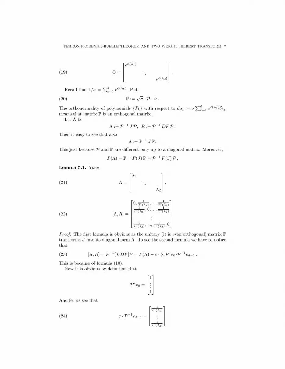
(19) Φ =

eφ(λ1)

. . .

eφ(λd)

.

Recall that 1/σ =∑d

k=1 eφ(λk). Put

(20) P :=√σ · P · Φ .

The orthonormality of polynomials Pk with respect to dµx = σ∑d

k=1 eφ(λk)δλk

means that matrix P is an orthogonal matrix.Let Λ be

Λ := P−1 J P , R := P−1DF P .Then it easy to see that also

Λ := P−1 J P .

This just because P and P are different only up to a diagonal matrix. Moreover,

F (Λ) = P−1 F (J) P = P−1 F (J)P .

Lemma 5.1. Then

(21) Λ =

λ1

. . .

λd

.

(22) [Λ, R] =

0, 1T ′(λ1)

, ..., 1T ′(λ1)

1T ′(λ2) , 0, ...,

1T ′(λ2)

...1

T ′(λd) , ...,1

T ′(λd) , 0

Proof. The first formula is obvious as the unitary (it is even orthogonal) matrix P

transforms J into its diagonal form Λ. To see the second formula we have to noticethat

(23) [Λ, R] = P−1[J,DF ]P = F (Λ)− c · 〈·,P∗e0〉P−1ed−1 .

This is because of formula (10).Now it is obvious by definition that

P∗e0 =

1...1

And let us see that

(24) c · P−1ed−1 =

1T ′(λ1)

...1

T ′(λd)

8 A. VOLBERG, P. YUDITSKII

This and (23) will finish the lemma. To prove (24) let us notice that denoting

c · P−1ed−1 =

v1...vd

we obtain from (23) and the form of P∗e0 that

[Λ, R] = F (Λ)−

v1, ..., v1...

vd, ..., vd

But Λ is diagonal, and so the diagonal of the LHS vanishes. But this gives us vi =i-th diagonal element of F (Λ), which is 1

T ′(λi). So (24) is proved, and lemma is

shown.

Recall that

R := P−1DF P .Lemma 5.2. The matrix elements of R are as follows

rij =1

T ′(λi)

1

λi − λj, if i 6= j .

rii =1

2

T ′′(λi)

(T ′(λi))2.

Proof. The non-diagonal terms can be immediately read from (22) of the previouslemma. On the other hand

R∗

1...1

= 0 .

In fact,

R∗

1...1

= P∗FD∗(P∗)−1

1...1

,

But we know that

(P∗)−1

1...1

= e0,

and D∗e0 = 0 (from (3.2)). So our first equality is proved. It means that the sumof column elements of R is zero for every column. We knew all elements of R exceptthe diagonal ones, but this sum property gives us the diagonal elements too. An

easy residue theorem application gives the formula rii = 12

T ′′(λi)

(T ′(λi))2.

Let

K := P−1DFP .

Compare this with R = P−1DFP . As P and P are almost the same matrices—thedifference is in diagonal factor we get

PERRON-FROBENIUS-RUELLE THEOREM AND TWO WEIGHT HILBERT TRANSFORM 9

Theorem 5.3.

(25) K = diag

(

e−φ(λi)/2

T′(λi)

)

12

T”(λ1)

T ′ (λi), ..., 1

λ1−λd

...1

λ1−λd, ..., 1

2T”(λi)

T ′ (λd)

diag(eφ(λi)/2)

And matrix H is unitary equivalent to

(26) diag

(

e−φ(λi)/2

T′(λi)

)

12 (log |T ′ |+ φ)′(λi), ...,

1λ1−λd

. . .1

λ1−λd, ..., 1

2 (log |T ′|+ φ)′(λd)

diag(eφ(λi)/2)

In particular, having in mind that φ = −t log |T ′| we get that matrix H is unitaryequivalent to(27)

H = Ht = diag

(

1

|T′(λi)|1− t2

)

1−t2 (log |T ′|)′(λi), ...,

1λ1−λd

. . .1

λ1−λd, ..., 1−t

2 (log |T ′|)′(λd)

diag

(

1

T′(λi)| t2

)

Proof. The first relation (25) follows from Lemma 5.2 and from formula (20) thatrelates P and P via a multiplication on a diagonal matrix. But P−1HP = K +12P−1φ′(J)F (J)P = K + 1

2F (Λ)φ′(Λ), and (26) follows.

We are ready to prove the uniform boundedness of H .

Theorem 5.4. Let f be a hyperbolic polynomial of degree N with real Julia setJ(f). Let T = fn, deg T = d = Nn. Let λ1, ..., λd be all T -preimages ofx ∈ J(f). Matrix Ht is uniformly bounded independently of n, x, and t, 0 ≤ t ≤ 2.Therefore, so is matrix H.

We already saw that the proof of this theorem finishes the proof of Theorem 3.3,and thus, of our first main result, Theorem 1.2.

Proof. The diagonal part H0 := 1−t2 diag(log |T′|)′(λi)) is bounded uniformly in n

and x ∈ J(f) just by Koebe distortion theorem, it is a standard fact dependingonly on hyperbolicity of f . (Notice that for t = 1 this matrix vanishes!) Let usconsider now the “out-of-diagonal” part

B = Bt = Ht −H0t .

Consider the counting measure on λ1, ..., λd: dn = dnx =∑d

k=1 δλk. Now we can

notice easily that B∗ is unitary equivalent to the following integral operator

g ∈ L2(dn)→ |T ′(x)|− t2

∫

1

x− y|T ′(y)| t2|T ′(y)| g(y) dn(y) ∈ L2(dn) .

Changing variable f := g · |T ′|1− t2 and changing measure dν(y) := dn(y)

|T ′(y)|2−t we

come to a unitary equivalent operator

f ∈ L2(dν)→ |T ′(x)|− t2

∫

1

x− y f(y) dν(y) ∈ L2(dn) .

Put

dκ := |T ′(x)|−t dn(x) .

10 A. VOLBERG, P. YUDITSKII

The norm of B is equal to the norm of the two weight Hilbert transform

Hνf :=

∫

y 6=x

1

x− y f(y) dν(y) : L2(ν)→ L2(κ) .

The story of two weighted problems in Harmonic analysis is beyond the scope ofthis work. We will just choose the result convenient for our narrow purpose here.A paper [14] looks like specially written for the occasion. However, the readerwho wants to familiarize her/himself with two weighted estimates is referred to[16] and to the vast literature cited there. We just make two remarks. First one isthat the two weight estimates for operators with positive kernels is more or less wellunderstood due to the works of Eric Sawyer (many of them are cited in [16]). On theother hand the singular kernel two weight estimates are not completely understoodeven for the simplest singular kernels (like the Hilbert transform). There is onlyone kernel–the dyadic singular kernel corresponding to the Martingale transform,where the technique of Bellman function gives a full criterion of boundedness. See[13]. There is no “classical” approach to this so far. And if kernel becomes justslightly more complicated than the dyadic one (for example the Hilbert transform)there is no real understanding. (The criterion of Cotlar-Sadosky [7] is very nicebut its language seems to be not applicable here.) Some criterion which “seemsto be” the right one is considered in the last two chapters of [16]. There are somecounterexamples to other “right criteria” in [12].

But we have to find a certain applicable and easily verifiable sufficient conditionof two weight boundedness of the Hilbert transform. The question is very intimatelyrelated to a so-called problem of Sarason: describe when the product of two Toeplitzoperators is bounded. Dechao Zheng found a wonderful sufficient condition in [8].It was then adopted in [14] to two weight Hilbert transform. One of the mainresults of [14] will be applied here—it is perfect for our goals.

Let us introduce notations. The symbol 〈f〉I will denote the usual averaging1|I|

∫

I f dx, where I is an interval on a real line. The symbol PIf denotes the

Poisson averaging, namely, 1π

∫

R

|I|(x−c)2+|I|2 f(x) dx, where c is the center of I. In

other words it is the value of the Poisson extension of f at the point c+ i · |I| ∈ C+.We prove Theorem 5.4 if we prove the following result.

Theorem 5.5. The norm of

Hν : L2(ν)→ L2(κ)

is uniformly bounded in n, x, and t, 0 ≤ t ≤ 2.

Proof. To prove it we need the following result

Lemma 5.6. Let udx, vdx be two positive measures on the line. Let g(t) = |t|1+ε,with ε > 0. If for every interval I we have

(28) PIg(u) · PIg(v) ≤ Cwith C <∞ independent of I, then the two weight Hilbert transform

Hudx : L2(udx)→ L2(vdx)

is bounded, and its norm depends only on C <∞ and ε > 0.

PERRON-FROBENIUS-RUELLE THEOREM AND TWO WEIGHT HILBERT TRANSFORM 11

Remark. The reader may wonder why we need the gauge function g here? Itturns out that PIu · PIv ≤ C is not sufficient for the boundedness of the Hilberttransform in general. See [11], or [12].

Let us reduce Theorem 5.5 to this lemma.We will to this in two stages. Our first goal will be to prove the following weaker

version of (28):

(29) 〈g(u)〉I〈g(v)〉I ≤ C .

Let us replace

d ν(y) =dn(y)

|T ′(y)|2−t

by u(y)dy, where

(30) u(y) :=

d∑

i=1

1

|T ′(y)|1−tχIi

(y) ,

where Ii is the i-th preimage of [−ξ, ξ] under T (left to right).Similarly replace

d κ(x) =dn(x)

|T ′(x)|tby vdx, where

(31) v(x) :=

d∑

i=1

1

|T ′(x)|t−1χIi

(x) ,

Lemma 5.7. The norm of Hudx : L2(udx) → L2(vdx) bounds the norm of Hdν :L2(dν)→ L2(dκ).

Proof. Intervals Ii are separated as their “centers”:

dist(Ii, Ij) ≍ |λi − λj | .

The constants of equivalence depend only on hyperbolicity. Every test functionf ∈ L2(ν), f = (f1, ..., fd) can be replaced by F :=

∑

fiχi, and clearly

‖f‖L2(ν) ≍ ‖F‖L2(udx)

as

|Ii| ≍1

|T ′(λi)|.

Now we prove the following

Lemma 5.8. Let g(t) = |t|1+ε. Let u, v be as in (30), (31). Then

supI〈g(u)〉I〈g(v)〉I <∞ .

12 A. VOLBERG, P. YUDITSKII

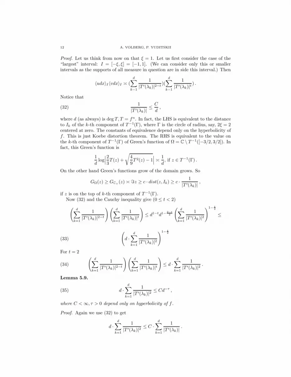
Proof. Let us think from now on that ξ = 1. Let us first consider the case of the“largest” interval: I = [−ξ, ξ] = [−1, 1]. (We can consider only this or smallerintervals as the supports of all measure in question are in side this interval.) Then

〈udx〉I〈vdx〉I ≍ (

d∑

k−1

1

|T ′(λk)|2−t)(

d∑

k−1

1

|T ′(λk)|t ) .

Notice that

(32)1

|T ′(λk)| ≤C

d,

where d (as always) is deg T, T = fn. In fact, the LHS is equivalent to the distanceto Ik of the k-th component of T−1(Γ), where Γ is the circle of radius, say, 2ξ = 2centered at zero. The constants of equivalence depend only on the hyperbolicity off . This is just Koebe distortion theorem. The RHS is equivalent to the value onthe k-th component of T−1(Γ) of Green’s function of Ω = C \ T−1([−3/2, 3/2]). Infact, this Green’s function is

1

dlog∣

∣

∣

2

3T (z) +

√

4

9T 2(z)− 1

∣

∣

∣ ≍ 1

d, if z ∈ T−1(Γ) .

On the other hand Green’s functions grow of the domain grows. So

GΩ(z) ≥ GC+(z) ≍ ℑz ≥ c · dist(z, Ik) ≥ c · 1

|T ′(λk)| ,

if z is on the top of k-th component of T−1(Γ).Now (32) and the Cauchy inequality give (0 ≤ t < 2)

(

d∑

k=1

1

|T ′(λk)|2−t

)(

d∑

k=1

1

|T ′(λk)|t

)

≤ d1−td1− 2−t2

(

d∑

k=1

1

|T ′(λk)|2

)1− t2

≤

(33)

(

d ·d∑

k=1

1

|T ′(λk)|2

)1− t2

For t = 2

(34)

(

d∑

k=1

1

|T ′(λk)|2−t

)(

d∑

k=1

1

|T ′(λk)|t

)

≤ d ·d∑

k=1

1

|T ′(λk)|2 .

Lemma 5.9.

(35) d ·d∑

k=1

1

|T ′(λk)|2 ≤ Cd−τ ,

where C <∞, τ > 0 depend only on hyperbolicity of f .

Proof. Again we use (32) to get

d ·d∑

k=1

1

|T ′(λk)|2 ≤ C ·d∑

k=1

1

|T ′(λk)| .

PERRON-FROBENIUS-RUELLE THEOREM AND TWO WEIGHT HILBERT TRANSFORM 13

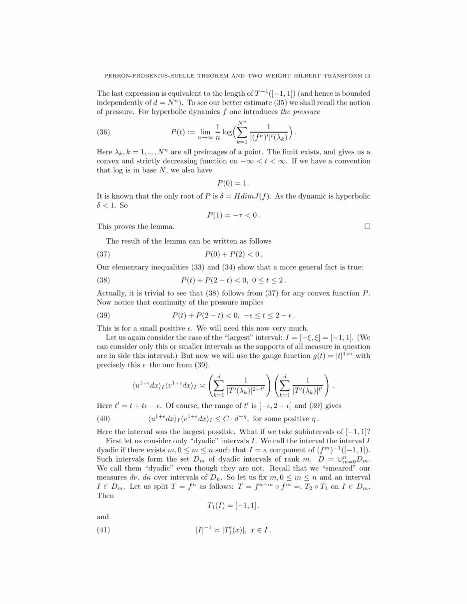
The last expression is equivalent to the length of T−1([−1, 1]) (and hence is boundedindependently of d = Nn). To see our better estimate (35) we shall recall the notionof pressure. For hyperbolic dynamics f one introduces the pressure

(36) P (t) := limn→∞

1

nlog(

Nn

∑

k=1

1

|(fn)′|t(λk)

)

.

Here λk, k = 1, ..., Nn are all preimages of a point. The limit exists, and gives us aconvex and strictly decreasing function on −∞ < t < ∞. If we have a conventionthat log is in base N , we also have

P (0) = 1 .

It is known that the only root of P is δ = HdimJ(f). As the dynamic is hyperbolicδ < 1. So

P (1) = −τ < 0 .

This proves the lemma.

The result of the lemma can be written as follows

(37) P (0) + P (2) < 0 .

Our elementary inequalities (33) and (34) show that a more general fact is true:

(38) P (t) + P (2− t) < 0, 0 ≤ t ≤ 2 .

Actually, it is trivial to see that (38) follows from (37) for any convex function P .Now notice that continuity of the pressure implies

(39) P (t) + P (2− t) < 0, −ǫ ≤ t ≤ 2 + ǫ .

This is for a small positive ǫ. We will need this now very much.Let us again consider the case of the “largest” interval: I = [−ξ, ξ] = [−1, 1]. (We

can consider only this or smaller intervals as the supports of all measure in questionare in side this interval.) But now we will use the gauge function g(t) = |t|1+ǫ withprecisely this ǫ–the one from (39).

〈u1+ǫdx〉I〈v1+ǫdx〉I ≍(

d∑

k=1

1

|T ′(λk)|2−t′

)(

d∑

k=1

1

|T ′(λk)|t′)

.

Here t′ = t+ tǫ− ǫ. Of course, the range of t′ is [−ǫ, 2 + ǫ] and (39) gives

(40) 〈u1+ǫdx〉I〈v1+ǫdx〉I ≤ C · d−η, for some positive η .

Here the interval was the largest possible. What if we take subintervals of [−1, 1]?First let us consider only “dyadic” intervals I. We call the interval the interval I

dyadic if there exists m, 0 ≤ m ≤ n such that I = a component of (fm)−1([−1, 1]).Such intervals form the set Dm of dyadic intervals of rank m. D = ∪n

m=0Dm.We call them “dyadic” even though they are not. Recall that we “smeared” ourmeasures dν, dκ over intervals of Dn. So let us fix m, 0 ≤ m ≤ n and an intervalI ∈ Dm. Let us split T = fn as follows: T = fn−m fm =: T2 T1 on I ∈ Dm.Then

T1(I) = [−1, 1] ,

and

(41) |I|−1 ≍ |T ′1(x)|, x ∈ I .

14 A. VOLBERG, P. YUDITSKII

We want to estimate

〈u1+ǫdx〉I〈v1+ǫdx〉I ≍1

|I|

(

∑

i:λi∈I

1

|T ′(λi)|2−t′

)

1

|I|

(

∑

i:λi∈I

1

|T ′(λk)|t′)

.

Let µjNn−m

j=1 be fn−m preimages of x. Notice that

∀i : λi ∈ I ∃j T1λi = µj .

Call d2 = Nn−m. The expression we want to estimate is, by chain rule, and (41)bounded by

c ·

d2∑

j=1

1

|T ′2(µj)|2−t′

·

d2∑

j=1

1

|T ′2(µj)|t′

.

But this is bounded by C · d−η2 by (39). This is obtained by exactly the same

reasoning as we get (40). Only d2 replaces d. So far we proved (40) only for all“dyadic” intervals. Let Jn(f) := ∪i∈Dn

I. If for any interval I0 ⊂ [−1, 1] such thatI0 ∩ Jn(f) 6= ∅ we would have that there exists a “dyadic” interval of comparablelength that contains I0 ∩ Jn(f), then (40) for I = I0 would follow from (40) for“dyadic” intervals. For usual dyadic intervals this is of course false. It is obviousthat one cannot always find the dyadic interval of comparable length containing agiven interval. But in our situation this is true.

Lemma 5.10. Let I0 ⊂ [−1, 1] such that I0 ∩Jn(f) 6= ∅. Let I denote the smallestinterval from D containing I0 ∩ Jn(f). Then

(42) |I0| ≥ c · |I| ,where c > 0 depends only on hyperbolicity of f .

Proof. Along with dyadic intervals D1 we have the collection of gap intervals G1

between them. Preimages of intervals of G1 give gaps Gk, k = 2, ..., n. Take ourI0. Let J be a gap interval inside it. If there is none then I0 ∩ Jn(f) coincideswith one interval of Dn. And (42) holds. So let J ⊂ I0 of the smallest generationk = 1, ..., n. J ∈ Gk. Then it lies in a dyadic interval I ∈ Dk−1. Let us prove that

(43) I0 ∩ Jn(f) ⊂ I ,Interval I has one or two neighbors of generation k − 1 or smaller generation m <k − 1. If (43) is false then I0 should intersect one of these neighbors. But then itshould contain the gap of generation ℓ ≤ k − 1. This contradicts the choice of J .So (43) holds.

One of the branches of f−(k−1) maps [−1, 1] onto I. Call this branch gk−1.Moreover, univalently

gk−1 : U → UI ,

where U is an open topological disc containing [−1, 1], and I ⊂ UI . Also gk−1 mapsa gap L ∈ G1 onto J . Now Koebe distortion theorem implies

(44)|J ||I| ≥ c ·

|L||[−1, 1]| ≥ c1 > 0 .

Here c, c1 depend only on f , not on n. Obviously (44) implies (42). Lemma 5.10 isproved.

PERRON-FROBENIUS-RUELLE THEOREM AND TWO WEIGHT HILBERT TRANSFORM 15

Together with (40) for dyadic intervals (already shown) it gives (40) for all in-tervals. This proves (29). This is almost the proof of Lemma 5.8.

But to finish the proof of this lemma we need to pass from (29), which we havejust proved to (28).

To do that we need still a couple of lemmas. First notations. Let

t′ = t+ ǫt− ǫ, 0 ≤ t ≤ 2 .

τ0 := τ0(t, ǫ) = −[P (t′) + P (2− t′)] .Lemma 5.11. Let “dyadic” interval I belong to Dk. Then

(45) 〈u1+ǫdx〉I〈v1+ǫdx〉I ≍ N−τ0(n−k) .

Proof.

(46) 〈u1+ǫdx〉I〈v1+ǫdx〉I ≍

Nn−k

∑

j=1

1

|T ′(λj)|2−t′

Nn−k

∑

j=1

1

|T ′(λj)|t′

.

On the other hand, the hyperbolicity of dynamics f standardly implies morethan the existence of the limit in (36). The more is actually known. Namely,

(47)∑

λ:fnλ=x

1

|(fn)′|t(λ) ≍ e−P (t)n ,

where the constants of comparison do not depend on n or x ∈ J(f).Now (46) and (47) give us (45), and the lemma is proved.

Lemma 5.12. Let Im ∈ Dm be a “dyadic” interval. Let Im+1 be its “dyadicsubinterval of Dm+1. Then

(48)

∫

Im

u1+ǫ dx ≥ (1 + δ)

∫

Im+1

u1+ǫ dx ,

where δ > 0 is independent of m.

Proof. Let us denote Im+1 by L, and let K be another interval from Dm+1 lyinginside Im. Then using repeatedly the estimates from below and from above inLemma 5.11 we get

∫

Im

u1+ǫ dx ≤ C ·N−τ0(n−m)|Im|1

〈v1+ǫ〉Im

≤

C ·N−τ0(n−m)|Im|21

∫

Imv1+ǫ

≤ C ·N−τ0(n−m)|Im|21

∫

K v1+ǫ≤

C ·N−τ0(n−m)|Im||Im||K|

〈u1+ǫ〉K〈u1+ǫ〉K〈v1+ǫ〉K

≤

C · |Im|2

|K|2∫

K

u1+ǫ dx ≤ C∫

K

u1+ǫ dx .

Of course we used in the last line that the lengths of an interval of Dm and its“son” from Dm+1 are comparable. Let us rewrite the previous inequality as follows

∫

K

u1+ǫ dx ≥ 1

C

∫

Im

u1+ǫ dx .

16 A. VOLBERG, P. YUDITSKII

Then∫

Im

u1+ǫ dx ≥ 1

C

∫

Im

u1+ǫ dx+

∫

L

u1+ǫ dx .

Lemma 5.12 follows.

Lemma 5.13. Let I ∈ Dk then

(49) PIv1+ǫ ≤ C ·N−τ0(n−k) 1

〈u1+ǫ〉I.

Proof. Let us denote I := I0 ⊂ I1 ⊂ I2 ⊂ .... ⊂ Ik = [−1, 1] the nest of “dyadic”intervals so that Ij ∈ Dk−j , j = 0, 1, ..., k. Then

PIv1+ǫ ≤ C

k∑

j=0

|I||Ij |〈v1+ǫ〉Ij

.

Using Lemma 5.11 we can continue

PIv1+ǫ ≤ C

k∑

j=0

|I||Ij |

N−τ0(n−(k−j))

〈u1+ǫ〉Ij

.

Now using Lemma 5.12 we rewrite this

PIv1+ǫ ≤ C

k∑

j=0

|I| N−τ0(n−(k−j))

(1 + δ)j∫

Iu1+ǫ dx

.

And this is exactly (49). Lemma is proved.

To finish the proof of Lemma 5.8 we apply the previous lemma to v and to uand write

PIu1+ǫPIv

1+ǫ ≤ C N−2τ0(n−k)

〈u1+ǫ〉I〈v1+ǫ〉I.

We are left to use the estimate from below part of Lemma 5.11 to get

PIu1+ǫPIv

1+ǫ ≤ C ·N−2τ0(n−k), ∀ I ∈ Dk .

In Lemma 5.8 one needs this same estimate but for every subinterval I of [−1, 1].Fix such an interval. Consider first the case: there exists ℓ ∈ Jn(f) such thatI ∩ ℓ 6= ∅. Such an I can be “big” or small”. Big means C · I contains an intervalof ℓ. Otherwise, I is “small” and then it intersects only one ℓ ∈ Dn and

|II ≤ |ℓ| .In the latter case, we use the fact that u is constant on ℓ to write

PIu1+ǫ ≤ C〈u1+ǫ〉I + Pℓu

1+ǫ .

And the same for v.But using again the fact that u is constant on ℓ to write

PIu1+ǫ ≤ A〈u1+ǫ〉ℓ +BPℓu

1+ǫ ≤ CPℓu1+ǫ .

And the same for v.So in this case PIu

1+ǫPIv1+ǫ ≤ CPℓu

1+ǫPℓv1+ǫ, and this has been proved to be

universally bounded (depending only on hyperbolicity) for ℓ ∈ D.

PERRON-FROBENIUS-RUELLE THEOREM AND TWO WEIGHT HILBERT TRANSFORM 17

Now suppose that I is “big”. Let J be a “dyadic” interval (that is J ∈ D :=∪n

k=0Dk) of maximal length contained in C · I. It is easy to see from Lemma 5.10that

|J | ≥ a · |I| a > 0 .

Here a is independent of I. Then Harnack inequality and this previous relationshipshow that

(50) PIu1+ǫPIv

1+ǫ ≤ C ·N−2τ0(n−k), ∀ I ∈ Dk

for such an I too.Finally, if I∩Jn(f) = ∅ we can find the smallest interval L such that L∩Jn(f) 6= ∅

and I ⊂ L. Notice that u = v = 0 on L except the endpoint(s). Therefore,

PIu1+ǫ ≤ CPLu

1+ǫ, PIv1+ǫ ≤ CPLv

1+ǫ .

But for the interval L (50) has just been proved. Therefore it holds for I too.

Lemma 5.8 is completely proved.

In its turn, it prove Theorem 5.5.

Our first main result–Theorem 1.2–is completely proved.

Our second main result–Theorem 1.3–can be found in [15] or below.

6. Sufficiently large hyperbolicity and contractivity of

noncommutative PFR map for φ = 0. Almost periodicity.

Here we will discuss Theorem 1.3 proved in [15]. Moreover, we will explain thatnot only

‖J(x1)− J(x2)‖ ≤ cn |x1 − x2| , c < 1 ,

but that also there is an operator analog of this fact

‖J (J1)− J (J2)‖ ≤ cn |J1 − J2| , c < 1 .

But there will be restrictions. First of all φ = 0 only (so t = 0 only). Secondly,unlike the previous sections, where it was not very important that f is a polynomial,here this will be very much used. And thirdly at last, not just hyperbolicity, butonly sufficiently large hyperbolicity allows us to prove this contractivity.

We do not know whether it is true in general. Or for other t’s, φ’s.A Jacobi matrix J : l2(Z)→ l2(Z) is called almost periodic if the family

S−kJSkk∈Z,

where S is the shift operator, S|k〉 = |k + 1〉, is a precompact in the operatortopology.

Example. Let G be a compact abelian group, p(α), q(α) be continuous functions onG, p(α) ≥ 0. Then J(α) with the coefficient sequences p(α+ kµ)k, q(α+ kµ)k,µ ∈ G, is almost periodic.

18 A. VOLBERG, P. YUDITSKII

Let us show that in fact this is a general form of almost periodic Jacobi matrices.For a given almost periodic J define the metric on Z by

ρJ (k) := ||S−kJSk − J ||.Evidently ρJ (k +m) ≤ ρJ(k) + ρJ(m). Then J = J(0), where G = IJ , IJ is thecloser of Z with respect to ρJ , and µ = 1 ∈ IJ .

Recall that for a given system of integers dk∞k=1 one can define the set of dadic numbers as

(51) I = lim←−Z/d1...dkZ,that is α ∈ I means that α is a sequence α0, α1, α2, ... such that

αk ∈ Z/d1...dk+1Z and αk|mod d1...dk = αk−1.

In particular, if p is a prime number and dk = p we get the ring of p–adic integers,I = Zp.

In [15] we built a certain machine that allows to construct almost periodic Jacobimatrices with singularly continuous spectrum such that IJ = I.

The key element of the construction is the following

Theorem 6.1. Let J be a Jacobi matrix with the spectrum on [−1, 1]. Then the

following Renormalization Equation has a solution J = J(ǫ, J) = J(ǫ, J ;T ) withthe spectrum on T−1([−1, 1]):

(52) V ∗ǫ (z − J)−1Vǫ = (T (z)− J)−1T ′(z)/d,

where Vǫ|k〉 = |ǫ+ dk〉, 0 ≤ ǫ ≤ d− 1. Moreover, if mini |ti| ≥ 10 then

||J(ǫ, J1)− J(ǫ, J2)|| ≤ c||J1 − J2||.with an absolute constant c < 1 (does not depend of T either ).

Let us point out the following two properties of the function J(ǫ, J ;T ). First, due

to the commutant relation VǫS = SdVǫ one gets J(ǫ, S−mJSm) = S−dmJ(ǫ, J)Sdm.Second, the chain rule holds

J(ǫ0, J(ǫ1, J ;T2);T1) = J(ǫ0 + ǫ1d1, J ;T2 T1),

where di = deg Ti, 0 ≤ ǫi ≤ di+1.Next steps are quite simple. For given d1, d2..., let us chose polynomials T1, T2...,

degTk = dk with sufficiently large critical values. For a fixed sequence ǫ0, ǫ1...,0 ≤ ǫk ≤ dk+1, define Jm = J(ǫ0 + ǫ1d1 + ...+ ǫm−1d1...dm−1, J ;Tm ... T2 T1).

Then J = limm→∞ Jm exists and does not depend of J . Moreover,

∀j, ||J − S−d1...dljJSd1...dlj || ≤ Acl, A > 0.

That is ρJ defines on Z the standard p–adic topology in this case.Notice that for the case T1 = T2 = ... = Tm =: T , T = fn, d1 = ... = Nn =: d

we just get

(53) ∀j, ||J − S−dljJSdlj || ≤ Acl, A > 0 .

This proves that J is a limit periodic matrix (so, in particular) it is almost periodic.This provides the bridge between Lipschitz or (better) contractivity property of ournoncommutative PFR operator and the question of almost periodicity of a wideclass of Jacobi matrix generated by hyperbolic dynamical systems.

19

References

[1] J. Avron, B. Simon, Singular continuous spectrum for a class of almost periodic Jacobi

matrices Bull. AMS 6 (1982), 81–85.[2] M. F. Barnsley, J. S. Geronimo, A. N. Harrington, Almost periodic Jacobi matrices associated

with Julia sets for polynomials, Comm. Math. Phys. 99 (1985), no. 3, 303–317.[3] J. Bellissard, J. Geronimo, A. Volberg and P. Yuditskii, Are they are limit periodic?, Pro-

ceedings of the International Conference on Complex Analysis and Dynamical Systems II, aconference in honor of Professor Lawrence Zalcman’s 60th birthday, to appear.

[4] J. Bellisard, D. Bessis, P. Moussa, Chaotic states of almost periodic Schrodinger operators,Phys. Rev. Lett. 49 (1982), no. 10, 701–704.

[5] J. Bellisard, B. Simon, Cantor spectrum for almost Mathieu equation J. Funct. Anal., 48

(1982), no. 3, 408–419.[6] R. Bowen, Equilibrium States and the Ergodic Theory of Anosov Diffeomorphisms Lecture

Notes in Mathematics, v. 470, Springer-Verlag, Berlin-Heidelberg-New York, 1975.[7] M. Cotlar, C. Sadosky, Characterization of two measures satisfying the Riesz inequality for

the Hilbert transform in L2, Acta Cient. Venezolana 30 (1979), no. 4, 346-348.[8] D. Zheng, Distribution function inequality and the boundedness of the product of Toeplitz

operators, J. Funct. Anal.,[9] L. Faybusovich, M. Gehktman, Poisson brackets on rational functions and multi-Hamiltonian

structure for integrable lattices, Phys. Lett. A 272 (2000), no. 4, 236–244.[10] J. Herndon, Limit perodicity of sequences defined by certain recurrence relations; and Julia

sets, Ph.D. thesis, Georgia Institute of Technology, 1985.[11] F. Nazarov, A counterexample to a problem of Sarason, Preprint, Mich. State Univ., 2000,

pp. 1-10.[12] F. Nazarov, A. Volberg, Bellman function, two weight Hilbert transform and imbedding for

the model space Kθ. J. d’Analyse Math., v. 87, 2002, 385-412, volume in the memory of TomWolff.

[13] F. Nazarov, S. Treil, A. Volberg, Bellman function and two-weight inequality for the martin-

gale transform, J.of Amer. Math. Soc., v. 12 (1999), no. 4.[14] S. Treil, A. Volberg, D. Zheng, Hilbert transform, Toeplitz operators and Hankel operators,

and invariant A∞ weights, Revista Mat. Iberoamericana, 13, (1997), no. 2, 319–360.[15] F. Peherstorfer, A. Volberg, P. Yuditskii, Limit periodic Jacobi matrices with prescribed p-

adic hull and a singular continuous spectrum, Preprint, 2004.[16] A. Volberg, Calderon-Zygmund capacities and operators on nonhomogeneous spaces, CBMS

Lectures, AMS, v. 100, 2003, pp. 1–167.

Address:

Alexander VolbergDepartment of MathematicsMichigan State UniversityEast Lansing, Michigan 48824, USAvolberg@math.msu.eduandSchool of MathematicsInstitute for Advanced StudyPrinceton, NJ. 08540

Address:

Peter YuditskiiInstitute for AnalysisJohannes Kepler UniversityLinz, Austria A4040